geometric algebra in linear algebra and geometry - pozo, sobczyk
DESCRIPTION
Geometric Algebra in Linear Algebra and GeometryTRANSCRIPT
Acta Applicandae Mathematicae 71: 207–244, 2002.© 2002 Kluwer Academic Publishers. Printed in the Netherlands.
207
Geometric Algebra in Linear Algebra andGeometry
JOSÉ MARÍA POZO1 and GARRET SOBCZYK2
1Departament de Física Fonamental, Universitat de Barcelona, Diagonal 647, E-08028 Barcelona,Spain. e-mail: [email protected] de Fisica y Matematicas, Universidad de las Américas-Puebla, Mexico,72820 Cholula, México. e-mail: [email protected]
(Received: 18 February 2000; in final form: 17 July 2001)
Abstract. This article explores the use of geometric algebra in linear and multilinear algebra, andin affine, projective and conformal geometries. Our principal objective is to show how the richalgebraic tools of geometric algebra are fully compatible with and augment the more traditionaltools of matrix algebra. The novel concept of an h-twistor makes possible a simple new proof of thestriking relationship between conformal transformations in a pseudo-Euclidean space to isometriesin a pseudo-Euclidean space of two higher dimensions. The utility of the h-twistor concept, which isa generalization of the idea of a Penrose twistor to a pseudo-Euclidean space of arbitrary signature,is amply demonstrated in a new treatment of the Schwarzian derivative.
Mathematics Subject Classifications (2000): 15A09, 15A66, 15A75, 17Bxx, 41A10, 51A05,51A45.
Key words: affine geometry, Clifford algebra, conformal group, Euclidean geometry, geometricalgebra, Grassmann algebra, horosphere, Lie algebra, linear algebra, Möbius transformation, non-Euclidean geometry, null cone, projective geometry, spectral decomposition, Schwarzian derivative,twistor.
1. Introduction
Almost 125 years after the discovery of ‘geometric algebra’ by William KingdonClifford in 1878, the discipline still languishes off the centerstage of mathematics.Whereas Clifford’s geometric algebra has gained currency among an increasingnumber scientists in different ‘special interest’ groups, the authors of the presentwork contend that geometric algebra should be known by all mathematicians andother scientists for what it really is – the natural algebraic completion of the realnumber system to include the concept of direction. Whereas, evidently, most math-ematicians and other scientists are either unfamiliar with or reject this point ofview, we will try to prevail by showing that Clifford algebra really has alreadybeen universally recognized in the guise of linear algebra. Since linear algebra isfully compatible with Clifford algebra, it follows that in learning linear algebra,every scientist has really learned Clifford algebra but is generally unaware of this
208 JOSE MARIA POZO AND GARRET SOBCZYK
fact! What is lacking in the standard treatments of linear algebra is the recognitionof the natural graded structure of linear algebra and, therefore, the geometric in-terpretation that goes along with the definition of geometric algebra. As has beenoften repeated by Hestenes and others, geometric algebra should be seen as a greatunifier of the geometric ideas of mathematics (Hestenes, 1991).
The purpose of the present article is to develop the ideas of geometric algebraalongside the more traditional tools of linear algebra by taking full advantage oftheir fully compatible structures. There are many advantages to such an approach.First, everybody knows matrix algebra, but not everybody is aware that exactly thesame algebraic rules apply to the multivectors in a geometric algebra. Because ofthis fact, it is natural to consider matrices whose elements are taken from a geomet-ric algebra. At the same time, by developing geometric algebra in such a way thatany problem can be easily changed into an equivalent problem in matrix algebra,it becomes possible to utilize the powerful and extensive computer software thathas been developed for working with matrices. Whereas CLICAL has proven itselfto be a powerful computer aid in checking tedious Clifford algebra calculations,it lacks symbolic capabilities (Lounesto, 1994). Geometric algebra offers not onlya comprehensive geometric interpretation but also a whole new set of algebraictools for dealing with problems in linear algebra. We show that matrices, whichare rectangular blocks of numbers, represent geometric numbers in a rather specialspinor basis of a geometric algebra with neutral signature.
This work consists of four main sections. This introductory section lays downthe rational for this article and gives a brief summary of its main ideas and content.Section 2 is primarily concerned with the development of the basic ideas of linearand multilinear algebra on an n-dimensional real vector space we call the nullspace, since we are assuming that all vectors in N are null vectors (the squareof each vector is zero). Taking all linear combinations of sums of products ofvectors in N generates the 2n-dimensional associative Grassmann algebra G(N ).This stucture is sufficiently rich to efficiently develop many of the basic notions oflinear algebra, such as the matrix of a linear operator and the theory of determinantsand their properties.
Recently, there has been much interest in the application of geometric algebrato affine, projective and other non-Euclidean geometries (Maks, 1989; Hestenes,1991; Hestenes and Ziegler, 1991; Porteous, 1995; Havel, 1995). These non-Euclidean models offer new computational tools for doing pseudo-Euclidean andaffine geometry using geometric algebra. Section 3 undertakes a systematic studyof some of these models, and shows how the tools of geometric algebra make itpossible to move freely between them, bringing a unification to the subject thatis otherwise impossible. One of the key ideas is to define the meet and join op-erations on equivalence classes of blades of a geometric algebra which representsubspaces. Since a nonzero r-blade characterizes only the direction of a subspace,the magnitude of the blade is unimportant. Basic formulas for incidence relation-ships between points, lines, planes, and higher-dimensional objects are compactly
GEOMETRIC ALGEBRA IN LINEAR ALGEBRA AND GEOMETRY 209
formulated. Examples of calculations are given in the affine plane which are justplain fun!
Section 4 explores the deep relationships which exist between projective geom-etry and the conformal group. The conformal geometry of a pseudo-Euclideanspace can be linearized by considering the horosphere in a pseudo-Euclidean spaceof two dimensions higher. The introduction of the novel concept of an h-twistormakes possible a simple new proof of the striking relationship between conformaltransformations in a pseudo-Euclidean space to isometries in a pseudo-Euclideanspace of two higher dimensions. The concept of an h-twistor greatly simplifiescalculations and is in many ways a generalization of the successful spinor/twistorformalisms to pseudo-Euclidean spaces of arbitrary signatures. The utility of theh-twistor concept is amply demonstrated in a new derivation of the Schwarzianderivative (Davis, 1974, p. 46; Nehari, 1952, p. 199).
2. Geometric Algebra and Matrices
Let N be an n-dimensional vector space over a given field K , and let
{e} = ( e1 e2 . . . en ) (1)
be a basis of N . In this work we only consider real (K = R) or complex (K = C)vector spaces although other fields could be chosen. By interpreting each of thevectors in {e} to be the column vectors of the standard basis of the identity matrixid(n) of the n× n matrix algebra M(K) over the field K , we are free to make theidentification {e} = id(n). We wish to emphasize that we are interpreting the basisvectors ei to be elements of the 1× n row matrix (1), and not the elements of a set.Thus, in what follows, we are assumming and often will apply the rules of matrixmultiplication when dealing with the (generalized) row vector of basis vectors {e}.
Now let N be the dual vector space of 1-forms over the the field K , and let {e}be the dual basis of N with respect to the basis {e} of N . If we now interpret eachof the vectors in {e} to be the row vectors of the standard basis of the identity matrixid(n) of the n × n matrix algebra M(K), we can again make the identification{e} = id(n). Because we wish to be able to interpret the elements of {e} as rowvectors, we will always write the vectors in {e} in the column vector form
{e} =
e1
e2...
en
. (2)
We also assume that the column vector {e} obeys all the rules of matrix additionand multiplication of a n× 1 column vector.
210 JOSE MARIA POZO AND GARRET SOBCZYK
In terms of these bases, any vector or point x ∈ N can be written
x = {e}x{e} = ( e1 e2 . . . en )
x1
x2...
xn
=
n∑i=1
xiei (3)
for xi ∈ R, where
x{e} =
x1
x2...
xn
are the column vector of components of the vector x with respect to the basis {e}.Since vectors in N are represented by column vectors, and vectors y ∈ N by
row vectors, we define the operation of transpose of the vector x by
xt = ({e}x{e})t = xt{e}{e} = ( x1 x2 . . . xn )
e1
e2...
en
. (4)
In the case of the complex field K = C, we have
x∗{e} = ( x1 x2 . . . xn ) =
x1
x2...
xn
t
. (5)
The transpose and Hermitian transpose operations allows us to move between thereciprocal vector spaces N and N . Clearly the operation of Hermitian transposereduces to the ordinary transpose for real vectors.
We now wish to weld together the structures of the matrix algebra M(K) andthe geometric algebras generated by the vectors in the dual null spaces N and N .Following Doran et al. (1993), we first consider the Grassmann algebra G(N ),generated by taking all linear combinations of sums and products of the elementsin the vector space N = span{e} subject to the condition that for each x ∈ N ,x2 = xx = 0. It follows that
(x + y)2 = x2 + xy + yx + y2 = xy + yx = 0 (6)
or xy = −yx for all x, y in the null space N . The geometric algebra G(N )generated by a null space N is called the Grassmann or exterior algebra for thenull space N .
As follows from (6), the Grassmann exterior product a1a2 . . . ak of k vectors inN is antisymmetric over the interchange of any two of its vectors;
a1 . . . ai . . . aj . . . ak = −a1 . . . aj . . . ai . . . ak
GEOMETRIC ALGEBRA IN LINEAR ALGEBRA AND GEOMETRY 211
so that the exterior product of null vectors is equivalent to the outer product ofthose vectors:
a1a2 . . . ak = a1 ∧ a2 ∧ · · · ∧ ak.The 2n-dimensional standard basis SB{e} of G(N ), is generated by taking all
products of the vectors in the standard basis {e} to get
SB{e} = {1; e1, . . . , en; e12, . . . , e(n−1)n; . . . ; e1...k, . . . , e(n−k+1)...n; . . . ; e12...n}= {{e0}, {e1}, {e2}, . . . , {en}}, (7)
where
{ek} := ( e1...k . . . e(n−k+1)...n )
is the(n
k
)-dimensional standard basis of k-vectors
ej1j2...jk ≡ ej1ej2 . . . ejkfor the
(n
k
)sets of indices 1 � j1 < j2 < · · · < jk � n. In particular, it is assumed
{e0} = (1) and {e1} = {e}. The unique component of {en} is the pseudoscalaror volume element I := e12...n. With respect to the standard basis SB(e) anymultivector X ∈ G(N ) can be expressed in the matrix form
X = SB{e}X{SB} (8)
where X{SB} is the column vector of components
X{SB} =
x{0}x{e}x{e2}...
x{en}
.
Just as we used the tranpose operation (4) to move from the the null spaceN = span{e} to the dual null space N , we can extend the definition of the transposeto enable us to move from the Grassmann algebra G(N ), to the Grassmann algebraG(N ) of the reciprocal null space N . Since multivectors in G(N ) are representedby column vectors, and multivectors Y ∈ G(N ) by row vectors, we define thetranspose Xt ∈ G(N ) by
Xt = (SB{e}X{SB})t = Xt{SB}SB{e}, (9)
where Xt{SB} is the row vector of components
Xt{SB} =(xt{0} xt{e} xt{e2} . . . x
t{en}).
The Hermitian transpose is similarly defined when we are dealing with complexmultivectors.
212 JOSE MARIA POZO AND GARRET SOBCZYK
The dual basis of multivectors SB{e} for G(N ) are arranged in a column andare defined by
SB{e} = (SB{e})t =
{1}{e}{e2}...
{en}
,
where
{ek} := ek...1
...
en...n−k+1
(10)
is the(n
k
)-dimensional basis of dual k-vectors defined by
ej1j2...jk ≡ ej1ej2 . . . ejkfor the
(n
k
)sets of indices n � j1 > j2 > · · · > jk � 1.
The dual space N of the space N , and more generally the dual Grassmannalgebra G(N ) of the Grassmann algebra G(N ), are defined to satisfy the usualproperties of the mathematical dual space. What Doran et al. (1993) observedwas that these same properties can be faithfully expressed in a larger neutral geo-metric algebra Gn,n (a fomal definition is given below) containing both of theseGrassmann algebras as subalgebras, by replacing the duality conditions with corre-sponding reciprocal conditions. We accomplish all this by assuming the additionalproperties
e2i = 0 = e2
i , eiej = −ej ei,eiej = −ejei (for i �= j), and eiej = −ejei, (11)
together with the reciprocal relations
ei · ej = δi,j = ej · ei (12)
for all i, j = 1, 2, . . . , n. With this definition, the Grassmann algebra G(N ) of thedual space N becomes the natural reciprocal of the Grassmann algebra G(N ).These relations imply that the reciprocal k-vectors and k-forms of Grassmannalgebras G(N ) and G(N ) satisfy the reciprocal relations
{ek} · {ek} = id
((n
k
)×(n
k
)).
The neutral pseudo-Euclidean space Rn,n is defined as the linear space which
contains both the null spaces N and N . Thus,
Rn,n = N ⊕N = {x + y | x ∈ N , y ∈ N }.
GEOMETRIC ALGEBRA IN LINEAR ALGEBRA AND GEOMETRY 213
Likewise, the 22n-dimensional associative geometric algebra Gn,n is defined to bethe geometric algebra that contains both the Grassmann algebras G(N ) and G(N ).We write
Gn,n = G(N )⊗ G(N ) = gen{e1, . . . , en, e1, . . . , en}, (13)
subjected to the relationships (11) and (12).A simple example will serve to show the interplay between the well-known ma-
trix multiplication and the geometric product in the super matrix algebra M(Gn,n).Recalling the basic geometric product of two vectors x, y,
xy = x · y + x ∧ y, (14)
we apply the same product to the row and column basis vectors {e} and {e}, andsimultaneously employ matrix multiplication, to get the expressions
{e}{e} = {e} · {e} + {e} ∧ {e}
= id(n× n)+
e1 ∧ e1 e1 ∧ e2 . . . e1 ∧ ene2 ∧ e1 e2 ∧ e2 . . . e2 ∧ en. . . . . . . . . . . .
. . . . . . . . . . . .
en ∧ e1 en ∧ e2 . . . en ∧ en
,
where id(n×n) is the n×n identity matrix, computed by taking all inner productsei · ej between the basis vectors of {e} and {e}. Similarly,
{e}{e} = {e} · {e} + {e} ∧ {e} =n∑i=1
ei · ei +n∑i=1
ei ∧ ei = n+n∑i=1
ei ∧ ei,
giving the useful formulas
{e} · {e} = n and {e} ∧ {e} =n∑i=1
ei ∧ ei. (15)
Because of the metrical structure induced by the reciprocal relationships (12),we can express the components x{e} of the vector x ∈ N (3) in the form
x{e} =
x1
x2...
xn
=
e1 · xe2 · x...
en · x
= {e} · x.
Similarly, the components of the reciprocal vector xt ∈ N can be found from
xt{e} = ( x1 x2 . . . xn ) = xt · ( e1 e2 . . . en ) . (16)
We call Gn,n the universal geometric algebra of order 22n. When n is countablyinfinite, we call G = G∞,∞ the universal geometric algebra. The universal algebra
214 JOSE MARIA POZO AND GARRET SOBCZYK
G contains all of the algebras Gn,n as proper subalgebras. In Doran et al. (1993),Gn,n is called the mother algebra.
2.1. NONDEGENERATE GEOMETRIC ALGEBRAS
The standard bases {e} and {e} of the reciprocal null spaces N and N , taken to-gether, are said to make up a Witt basis of null vectors (Ablamowicz and Salingaros,1985) of the neutral pseudo-Euclidean space R
n,n. From the Witt basis, we canconstruct the standard orthonormal basis of R
n,n {σ, η} of Gn,n,
σi = ei + 12ei, ηi = ei − 1
2ei, (17)
for i = 1, 2, . . . , n. Using the defining relationships (12) of the reciprocal frames{e} and {e}, we find that these basis vectors satisfy
σ 2i = 1, η2
i = −1, ηiσj = −σjηi, ∀i, j = 1, . . . , n,
σiσj = −σjσi, ηiηj = −ηjηi, ∀i �= j.
The basis {σ } spans a real Euclidean vector space Rn and generates the geomet-
ric subalgebra Gn,0, whereas {η} spans an anti-Euclidean space R0,n and generates
the geometric subalgebra G0,n. The standard bases (7) of these geometric algebrasnaturally take the forms SB{σ } and SB{η}, so that a general multivector X ∈ Gn,0can be written X = SB{σ }XSB and, similarly for X ∈ Gn,0. We can now expressthe geometric algebra Gn,n as the product of these geometric subalgebras
Gn,n = Gn,0 ⊗ G0,n = gen{σ1, . . . , σn, η1, . . . , ηn}, (18)
again only as linear spaces, but not as algebras.Notice that when we write down the relationship (17), we have given up the
possibility of interpreting the vectors in {e} and {e} as column and row vectors,respectively. When working in the nondegenerate geometric algebras Gn,n, Gn,0 orG0,n, we use the operation of reversal. The reversal of any vector x ∈ Gn,n is definedby x† := x, and for the k-vector Ak = a1 ∧ a2 ∧ · · · ∧ ak ,
A†k := ak ∧ ak−1 ∧ · · · ∧ a1 = (−1)k(k−1)/2Ak.
2.2. SPINOR BASIS
One nice application of the above formalism is that it allows us to simply expressa natural isomorphism that exists between the neutral geometric algebra Gn,n and
GEOMETRIC ALGEBRA IN LINEAR ALGEBRA AND GEOMETRY 215
the algebra of all real 2n × 2n matrices MR(2n). To express this isomorphism, wefirst define 2n mutually commuting idempotents
ui(±) = 12(1± σiηi) (19)
for i = 1, 2, . . . , n.We can now define 2n mutually annihiliating primitive idempotents for the
algebra Gn,n,
usigns =∏signs
ui(sign si), (20)
where signs is a particular sequence of n ±signs, and sign si is the ith sign in thesequence. For example,
u+++···+ =n∏i=1
ui(+) and u−−−···− =n∏i=1
ui(−).
The primitive idempotents satisfy the following basic properties:∑2n
signs usigns = 1,σiu+++···+ = u+···+−i+···+σi ,usign1
usign2= δsign1sign2
usign1, where δsign1 sign2
= 0,except when sign1 = sign2 for which δsign1 sign2
= 1.
The above properties are easily verified.In contrast to the standard basis SB{e} of the neutral geometric algebra Gn,n, the
spinor basis of Gn,n is defined to be the 2n × 2n multivectors in the matrix
SNB(n, n) = SB{σ }tu+++···+SB{σ }. (21)
The simplest example is the spinor basis for the geometric algebra G1,1. The 21
primitive idempotents for this geometric algebra are u± = 12 (1± ση). Using (21),
the spinor basis SNB(1, 1) is found to be
SB(σ )tu+SB(σ ) =(
1σ
)u+ ( 1 σ ) =
(u+ σu−σu+ u−
).
The significance of the position of each multivector in the spinor basis, i.e. itsmatrix representation corresponds to 1 in the same position (with zeros everywhereelse).
In terms of the spinor basis, any 2n × 2n matrix A represents the correspondingelement A ∈ Gn,n given by
A = SB{σ }u+++···+ASB{σ }t .The matrix A associated with the multivector A ∈ Gn,n is denoted by A = [A].This association constitutes an algebra isomorphism, since [A + B] = [A] + [B]and [AB] = [A][B]. Noting that
u+···+SB{σ }tSB{σ }u+···+ = u+···+id(2n × 2n),
216 JOSE MARIA POZO AND GARRET SOBCZYK
it easily follows that
AB = SB{σ }u+···+[A]SB{σ }t SB{σ }u+···+[B]SB{σ }t= SB{σ }u+···+[A][B]SB{σ }t . (22)
We will use the spinor basis SNB(1, 1) for studying conformal transformationin Section 4.
2.3. SYMMETRIC AND HERMITIAN INNER PRODUCTS
Until now we have only considered real geometric algebras and their correspondingreal matrices. Any pseudoscalar of the geometric algebra Gn,n will always havea positive square and will anticommute with the vectors in R
n,n. If we insistedon dealing only with real geometric algebras, we might consider working in thegeometric algebra Gn,n+1 where the pseudoscalar element i has the desired propertythat i2 = −1 and is in the center of the algebra (commutes with all multivectors). Acomplex vector x+iy in Gn,n+1 consists of the real vector part x and a pseudovectoror (2n)-blade part iy.
Instead, we choose to directly complexify the geometric algebra Gn,n to get thecomplex geometric algebra G2n(C) (Sobczyk, 1996). Whereas this algebra is iso-morphic to Gn,n+1, it is somewhat easier to work with than the former. A complexvector z ∈ C
2n has the form z = x + iy where x, y ∈ R2n. The imaginary unit i,
where i2 = −1, is defined to commute with all elements in the geometric algebraG2n(C).
Consider an orthonormal basis {σ } ∈ C2n: σi · σj = δij . The complexified null
space N (C) and its reciprocal null space N (C) are the subspaces spanned by thecomplex null vectors
ej = 12 (σj + iσn+j ) and ej = σj − iσn+j
for j = 1, 2, . . . , n. This definition is consistent with (17) if we consider ηj =iσn+j . Thus, a null vector x ∈ N (C) has the form x = {e}x{e} for xi ∈ C.
Previously we have defined the transposition (4). This operation can be extendedto complex vectors in two different ways. The first way is a linear extension. Weuse the term transposition for the linear extension, so that definition (4) is still validwhen xi ∈ C. The second extension is antilinear and is equivalent to Hermitianconjugation: x∗ ≡ x∗{e}{e}. Both operations, Hermitian conjugation and transposi-
tion, take us from the complex null space N (C) to the dual null space N (C), andif the components of x are all real, both reduce to the real transposition. Appliedto the components x{e}, x∗{e} is the usual Hermitian transpose of the column vectorx{e},
x∗{e} = ( x1 x2 . . . xn ) =
x1
x2...
xn
t
. (23)

GEOMETRIC ALGEBRA IN LINEAR ALGEBRA AND GEOMETRY 217
We now define the symmetric inner product (x, y), and the Hermitian innerproduct 〈x, y〉, on N (C). For all x, y ∈ N (C), the two products are defined,respectively, by using transposition and Hermitian conjugation:
(x, y) := xt · y = xt{e}y{e} and 〈x, y〉 := x∗ · y = x∗{e}y{e}. (24)
The Hermitian inner product will be used in the next subsection.
2.4. LINEAR TRANSFORMATIONS
Let N⊕N ′ and N⊕N′be (n+n′)-dimensional reciprocal null spaces in R
n+n′,n+n′
with the dual bases {e}∪{e′} and {e}∪{e′}. Let f : N → N ′ be a linear transforma-tion from the null space N into the null space N ′. In light of the previous section,we can consider the null spaces N and N ′ to be over the real or complex numbers.Let
Hom(N ,N ′) = {f : N → N ′ | f is a linear transformation}denote the linear space of all homomorphisms from N to N ′, with the usual opera-tion of addition of transformations. Of course, only when N = N ′ is the operationof multiplication (composition) defined.
Given an operator f ∈ Hom(N ,N ′), y′ = f (x) ≡ f x, the matrix F of f withrespect to the bases {e} and {e′} is defined by
f {e} ≡ (f e1 . . . f en) = (e′1 . . . e′n′)F = {e′}F . (25)
Of course, the matrix F = (fij ) is defined by its n′ × n components fij = ei ·f (ej ) ∈ C for i = 1, 2, . . . , n′ and j = 1, 2, . . . , n. It follows that f (ej ) =∑n′i=1 e
′ifij . By dotting both sides of the above equation on the left by {e′}, we find
the explicit expression
F = {e′} · {e′}F = {e′} · f {e}.Equation (15) can be used to define the bivector F of the linear operator f . It
is defined by F = f {e} ∧ {e′} and satisfies the property that f x = F · x for allx ∈ N . The bivector of a linear operator makes possible a new theory of linearoperators, and is particularly useful in defining the general linear group as a Liegroup of bivectors with the commutator product (Fulton and Harris, 1991; Bayroand Sobczyk, 2001, p. 32).
Given the Hermitian inner product (24), the transpose (or Hermitian transpose(23)) f ∗: N ′ → N of the mapping f : N → N ′ is defined by the requirement thatfor all x ∈ N and y′ ∈ N ′,
〈x, f ∗(y′)〉 = 〈f (x), y′〉 ⇔ F ∗ ≡ {e} · f ∗{e′} = [f {e}]∗ · {e′}.Likewise, we can define the transpose relative to the symmetric inner product
(x, f t (y′)) = (f (x), y′) ⇔ F t ≡ {e} · f t {e′} = [f {e}]t · {e′}.
218 JOSE MARIA POZO AND GARRET SOBCZYK
2.5. OUTERMORPHISM AND GENERALIZED TRACES
A linear transformation f naturally extends multilinearly to act on k-blades,
f (x ∧ y ∧ · · · ∧ z) ≡ f (x) ∧ f (y) ∧ · · · ∧ f (z) ∀x, y, . . . , z ∈ N ,
and where f (1) ≡ 1. Thus extended, f : G(N ) → G(N ′) is called the outermor-phism of the linear transformation f : N → N ′, since it preserves the structure ofthe outer product:
f (A ∧ B + C ∧D) = f (A) ∧ f (B)+ f (C) ∧ f (D)∀A,B,C,D ∈ G(N ).
Geometrically, the outermorphism f maps directed areas into directed areas, andmore generally, directed k-vectors into directed k-vectors.
A linear transformation from N into itself is called an endomorphism. Let
End(N ) = {f : N → N | f is a linear operator}denote the algebra of all endomorphisms on N . The operations of addition andcomposition of linear operators is well defined for endomorphisms.
The determinant det f of the endomorphism f is defined to be the eigenvalueof the pseudoscalar element I = e12...n:
f (I ) = det f I ⇔ det f = f (I ) · I .Thus, det f is the factor by which volume is scaled by f . The trace of f is definedby tr f := f {e} · {e}. Given the outermorphism of f , we define the generalizedtraces of f by
trif := f {ei} · {ei}.
Particular cases are tr0 f = f (1) · 1 = 1 and tr1 f = tr f . The generalized trace ofdegree n coincides with the determinant: tr
nf = f (I ) · I = det f .
A second basis {a} of N is related to the standard basis {e} by the applicationof some endomorphism a
{a} = a{e} = {e}A = ( e1 e2 . . . en )A, (26)
where A is called the matrix of transition from the basis {e} to the basis {a}. Takingthe outer product
∧ni=1{a} of the basis vectors {a}, we get
n∧i=1
{a} ≡ a1 ∧ a2 ∧ · · · ∧ an = a(e1 ∧ e2 ∧ · · · ∧ en) = det aI. (27)
We see from (27) that the determinant of the matrix of transition, det A ≡ det a,between two bases cannot be zero.
GEOMETRIC ALGEBRA IN LINEAR ALGEBRA AND GEOMETRY 219
We can now easily construct a dual or reciprocal basis {a} for the basis {a}:
ai = (−1)i+1 (a1 ∧ · · · ∧ i∗ ∧ · · · ∧ an) · Idet a
, (28)
where i∗ means that ai is omitted from the product. More compactly, using ourmatrix notation,
{a} = a({e} · I ) · Ia(I ) · I .
Checking, we find that
{a} · {a} = [a({e} · I ) · I ] · {a}a(I ) · I = [a(I · {e})∧ a{e}] · I
a(I ) · I= [a((I · {e})∧ {e})] · I
a(I ) · I = a(I ({e} · {e})) · Ia(I ) · I
= {e} · {e} = id.
We have actually found the inverse of the transition matrix A, given by A−1 ={a} · {e} (Bayro and Sobczyk, 2001, p. 25).
2.6. CHARACTERISTIC POLYNOMIAL
The characteristic polynomial of f : N → N is defined by
ϕf (λ) = det(λ− f ) = (λ− f )(I ) · I .The well-known Caley–Hamilton theorem, which says that every linear operatorsatisfies its characteristic equation, is a consequence of the identity
f [x ∧ {en−1}] · {en−1} = (x ∧ {en−1}) · {en−1} det f = x det f. (29)
When the left side of this identity is expanded, we get
f [x ∧ {en−1}] · {en−1}
=n∑i=1
(−1)i+1f {en−i} · {en−i}f i(x)
=n∑i=1
(−1)i+1trn−iff i(x). (30)
Expressed in terms of the generalized traces of f , the characteristic polynomial is
ϕf (λ) = (λ− f )(e12...n) · en...21 =n∑i=0
(−1)if {ei} · {ei}λn−i .

220 JOSE MARIA POZO AND GARRET SOBCZYK
Thus, from (29) and (30), we have ϕf (f ) = 0, i.e. f satisfies its characteristicpolynomial.
Equation (29) can also be used to derive a formula for the inverse of f . We get
x = f −1(y) = (y ∧ f {en−1}) · {en−1}det f
.
The minimal polynomial ψf (λ) of f is the polynomial of least degree that hasthe property that ψf (f ) = 0. Taken over the complex numbers C, we can expressϕf and ψf in the factored form
ϕf (λ) =r∏i=1
(λ− λi)ni and ψf (λ) =r∏i=1
(λ− λi)mi ,
where 1 � mi � ni � n for i = 1, 2, . . . , r, and the roots λi are all distinct.The minimal polynomial uniquely determines, up to an ordering of the idem-
potents, the following spectral decomposition theorem of the linear operator f(Sobczyk, 2001).
THEOREM 1. If f has the minimal polynomial ψ(λ), then a set of commutingmutually annihilating idempotents and corresponding nilpotents {(pi, qi) | i =1, . . . , r} can be found such that f =∑r
i=1(λi + qi)pi , where rank(pi) = ni, andthe of nilpotency index(qi) = mi , for i = 1, 2, . . . , r. Furthermore, when mi = 1,qi = 0.
Clearly, the operator f is diagonalizable if and only if it has the spectral form
f =r∑i=1
λipi.
The spectral decomposition theorem has many different uses and applies equallywell to a linear operator or a geometric number (Sobczyk, 1993, pp. 357–364,1997a, 1997b). For example, we can immediately define a generalized inverse ofthe operator f by
f inv =∑λi �=0
1
λi
(pi − qi
λi+ · · · +
(−qiλi
)mi−1)
satisfying the conditions ff inv = f invf =∑λi �=0 pi (Rao and Mitra, 1971, p. 20).
3. Geometric Algebra and Non-Euclidean Geometry
Leonardo da Vinci (1452–1519) was one of the first to consider the problems ofprojective geometry. However, projective geometry was not formally developed
GEOMETRIC ALGEBRA IN LINEAR ALGEBRA AND GEOMETRY 221
until the work ‘Traité des propriés projectives des figure’ of the French mathe-matician Poncelet (1788–1867), published in 1822. The extraordinary generalityand simplicity of projective geometry led the English mathematician Cayley toexclaim: ‘Projective geometry is all of geometry’ (Young, 1930).
Let Rn+1 be an (n+1)-dimensional Euclidean space and let Gn+1,0 be the corre-
sponding geometric algebra. The directions or rays of nonzero vectors in Rn+1 are
identified with the points of the n-dimensional projective plane (n (Hestenes andZiegler, 1991). More precisely, we write(n ≡ R
n+1/R∗, where R∗ = R−{0}. We
thus identify points, lines, planes, and higher-dimensional k-planes in (n with 1,2, 3, and (k + 1)-dimensional subspaces Sr of R
n+1, where k � n. To effectivelyapply the tools of geometric algebra, we need to introduce the new basic operationsof meet and join (Bayro and Sobczyk, 2001, p. 27).
3.1. THE MEET AND JOIN OPERATIONS
The meet and join operations of projective geometry are most easily defined interms of the intersection and direct sum of the subspaces which name the objectsin (n. On the other hand, each r-dimensional subspace Ar can be described bya nonzero r-blade Ar ∈ G(Rn+1). We say that an r-blade Ar represents, or is arepresentant of an r-subspace Ar of R
n+1 if and only if
Ar = {x ∈ Rn+1 | x ∧ Ar = 0}. (31)
We denote the equivalence class of all nonzero r-blades Ar ∈ G(Rn+1) whichdefine the subspace Ar by
{Ar}ray := {tAr | t ∈ R, t �= 0}. (32)
Evidently, every r-blade in {Ar}ray is a representant of the subspace Ar . With thesedefinitions, the problem of finding the meet and join is reduced to a problem ingeometric algebra of finding the corresponding meet and join of the (r + 1)- and(s + 1)-blades in the geometric algebra G(Rn+1) which represent these subspaces.
Let Ar , Bs and Ct be nonzero blades representing the three subspaces Ar , Bs
and C t , respectively. We say that
DEFINITION 1. The t-blade Ct = Ar ∩Bs is the meet of Ar and Bs if there existsa complementary (r − t)-blade Ac and a complementary (s − t)-blade Bc with theproperty that Ar = Ac ∧ Ct , Bs = Ct ∧ Bc, and Ac ∧ Bc �= 0.
It is important to note that the t-blade Ct ∈ {Ct}ray is not unique and is definedonly up to a nonzero scalar factor, which we choose at our own convenience. Theexistence of the t-blade Ct (and the corresponding complementary blades Ac andBc) is an expression of the basic relationships that exists between subspaces.
DEFINITION 1. 1. The (r + s − t)-blade D = Ar ∪Bs , called the join of Ar andBs is defined by D = Ar ∪ Bs = Ar ∧ Bc.
222 JOSE MARIA POZO AND GARRET SOBCZYK
Alternatively, since the joinAr∪Bs is defined only up to a nonzero scalar factor,we could equally well defineD byD = Ac∧Bs . We use the symbols ∩ intersectionand ∪ direct sum from set theory to mark this unusual state of affairs. The problemof ‘meet’ and ‘join’ has thus been solved by finding the direct sum and intersectionof linear subspaces and their (r + s − t)-blade and t-blade representants.
Note that it is only in the special case when Ar ∩ Bs = 0 that the join can beconsidered to reduce to the outer product, i.e.
Ar ∩ Bs = 0 ⇔ Ar ∪ Bs = Ar ∧ Bs.However, after the join IAr∪Bs ≡ Ar ∪Bs has been found, it can be used to find themeet Ar ∩ Bs ,
Ar ∩ Bs = Ar · [Bs · IAr∪Bs ] = [IAr∪Bs · Ar ] · Bs. (33)
While the positive definite metric of Rn+1 is irrelevant to the definition of the meet
and join of subspaces, formula (33) holds only in Rn+1.
A slightly modified version of this formula will hold in any nondegeneratepseudo-Euclidean space R
p,q , where p + q = n + 1. In this case, after we havefound the join IAr∪Bs , which is a (r + k)-blade, we find a reciprocal (r + k)-bladeIAr∪Bs with the property that IAr∪Bs · IAr∪Bs �= 0. The meet Ar ∩ Bs may then bedefined by
Ar ∩ Bs = Ar · [Bs · IAr∪Bs ] = [IAr∪Bs · Ar ] · Bs. (34)
3.2. AFFINE AND PROJECTIVE GEOMETRIES
We have seen in the previous section how the meet and join of the n-dimensionalprojective space (n can be defined in an (n + 1)-dimensional Euclidean spaceRn+1. There is a very close connection between affine and projective geometries.
A projective space can be considered to be an affine space with idealized pointsat infinity (Young, 1930). Since all the formulas for meet and join remain validin the pseudo-Euclidean space R
p,q , subject only to (34), we will define the n =(p + q)-dimensional affine plane Ae(R
p,q) of the null vector e = 12 (σ + η) in the
larger pseudo-Euclidean space Rp+1,q+1 = R
p,q ⊕ R1,1, where R
1,1 = span{σ, η}for σ 2 = 1 = −η2. Whereas, effectively, we are only extending the Euclideanspace R
p,q by the null vector e, it is advantageous to work in the geometric algebraGp+1,q+1 of the nondegenerate pseudo-Euclidean space R
p+1,q+1.The affine plane Ap,q
e := Ae(Rp,q) is defined by
Ae(Rp,q) = {xh = x + e | x ∈ R
p,q} ⊂ Rp+1,q+1, (35)
for the null vector e ∈ R1,1. The affine plane Ae(R
p,q) has the nice property thatx2h = x2 for all xh ∈ Ae(R
p,q), thus preserving the metric structure of Rp,q . By
GEOMETRIC ALGEBRA IN LINEAR ALGEBRA AND GEOMETRY 223
employing the reciprocal null vector e = σ −η with the property that e · e = 1, wecan restate definition (35) of Ae(R
p,q) in the form
Ae(Rp,q) = {y | y ∈ R
p+1,q+1, y · e = 1 and y · e = 0} ⊂ Rp+1,q+1.
This form of the definition is interesting because it brings us closer to the definitionof the n = (p + q)-dimensional projective plane.
We summarize here the important properties of the reciprocal null vectors e =12(σ + η) and e = σ − η that will be needed later, and their relationship to thehyperbolic unit bivector u := ση.
e2 = e2 = 0, e · e = 1, u = e ∧ e = σ ∧ ν, u2 = 1. (36)
The projective n-plane (n can be defined to be the set of all points of the affineplane Ae(R
p,q), taken together with idealized points at infinity. Each point xh ∈Ae(R
p,q) is called a homogeneous representant of the corresponding point in (n
because it satisfies the property that xh · e = 1. To bring these different viewpointscloser together, points in the affine plane Ae(R
p,q) will also be represented by raysin the space
Arayse (Rp,q)= {{y}ray | y ∈ R
p+1,q+1, y · e = 0, y · e �= 0}⊂ R
p+1,q+1. (37)
The set of rays Arayse (Rp,q) gives another definition of the affine n-plane, because
each ray {y}ray ∈ Arayse (Rp,q) determines the unique homogeneous point
yh = y
y · e ∈ Ae(Rp,q).
Conversely, each point y ∈ Ae(Rp,q) determines a unique ray {y}ray in A
rayse (Rp,q).
Thus, the affine plane of homogeneous points Ae(Rp,q) is equivalent to the affine
plane of rays Arayse (Rp,q).
Suppose that we are given k-points ah1 , ah2 , . . . , a
hk ∈ Ae(R
p,q)where each ahi =ai + e for ai ∈ R
p,q . Taking the outer product or join of these points gives theprojective (k − 1)-plane Ah ∈ (n. Expanding the outer product gives
Ah = ah1 ∧ ah2 ∧ · · · ∧ ahk = ah1 ∧ (ah2 − ah1 ) ∧ ah3 ∧ · · · ∧ ahk= ah1 ∧ (ah2 − ah1 ) ∧ (ah3 − ah2 ) ∧ ah4 ∧ · · · ∧ ahk = · · ·= ah1 ∧ (a2 − a1) ∧ (a3 − a2) ∧ · · · ∧ (ak − ak−1),
or
Ah = ah1 ∧ ah2 ∧ · · · ∧ ahk = a1 ∧ a2 ∧ · · · ∧ ak ++ e ∧ (a2 − a1) ∧ (a3 − a2) ∧ · · · ∧ (ak − ak−1). (38)
224 JOSE MARIA POZO AND GARRET SOBCZYK
Whereas (38) represents a (k − 1)-plane in (n, it also belongs to the affine(p, q)-plane A
p,qe , and thus contains important metrical information. Dotting this
equation with e, we find that
e ·Ah = e · (ah1 ∧ ah2 ∧ · · · ∧ ahk )= (a2 − a1) ∧ (a3 − a2) ∧ · · · ∧ (ak − ak−1).
This result motivates the following
DEFINITION 1.1.1. The directed content of the (k− 1)-simplex Ah = ah1 ∧ ah2 ∧· · · ∧ ahk in the affine (p, q)-plane is given by
e ·Ah(k − 1)! =
e · (ah1 ∧ ah2 ∧ · · · ∧ ahk )(k − 1)!
= (a2 − a1) ∧ (a3 − a2) ∧ · · · ∧ (ak − ak−1)
(k − 1)! .
3.3. EXAMPLES
Many incidence relations can be expressed in the affine plane Ae(Rp,q) which are
also valid in the projective plane (n (Bayro and Sobczyk, 2001, p. 263). A fewexamples are provided below.
Given 4 coplanar points ah, bh, ch, dh ∈ Ae(R2). The join and meet of the lines
ah∧ bh and ch∧ dh are given, respectively, by (ah∧ bh)∪ (ch∧ dh) = ah∧ bh∧ ch,and using (34)
(ah ∧ bh) ∩ (ch ∧ dh) = [I · (ah ∧ bh)] · (ch ∧ dh),where I = σ2∧ σ1∧ e. Carrying out the calculations for the meet and join, we findthat
(ah ∧ bh) ∪ (ch ∧ dh) = det{ah, bh, ch}I = det{a, b}I, (39)
where I = σ1 ∧ σ2 ∧ e, and
(ah ∧ bh) ∩ (ch ∧ dh) = det{c − d, b − c}ah + det{c − d, c − a}bh. (40)
Note that the meet (40) is not, in general, a homogeneous point. Normaliz-ing (40), we find the homogeneous point ph ∈ Ae(R
2)
ph = det{c − d, b − c}ah + det{c − d, c − a}bhdet{c − d, b − a} ,
which is the intersection of the lines ah ∧ bh and ch ∧ dh, see Figure 1. The meetcan also be solved for directly in the affine plane by noting that
ph = αpah + (1− αp)bh = βpch + (1− βp)dh
GEOMETRIC ALGEBRA IN LINEAR ALGEBRA AND GEOMETRY 225
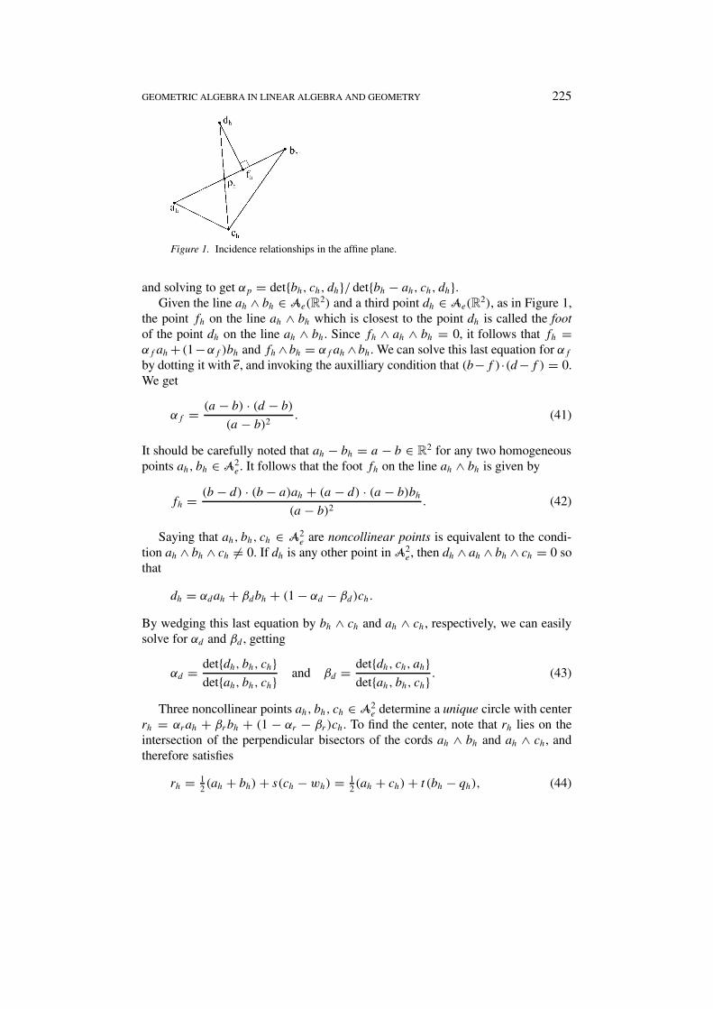
Figure 1. Incidence relationships in the affine plane.
and solving to get αp = det{bh, ch, dh}/ det{bh − ah, ch, dh}.Given the line ah ∧ bh ∈ Ae(R
2) and a third point dh ∈ Ae(R2), as in Figure 1,
the point fh on the line ah ∧ bh which is closest to the point dh is called the footof the point dh on the line ah ∧ bh. Since fh ∧ ah ∧ bh = 0, it follows that fh =αf ah+ (1−αf )bh and fh∧bh = αf ah∧bh. We can solve this last equation for αfby dotting it with e, and invoking the auxilliary condition that (b−f )·(d−f ) = 0.We get
αf = (a − b) · (d − b)(a − b)2 . (41)
It should be carefully noted that ah − bh = a − b ∈ R2 for any two homogeneous
points ah, bh ∈ A2e . It follows that the foot fh on the line ah ∧ bh is given by
fh = (b − d) · (b − a)ah + (a − d) · (a − b)bh(a − b)2 . (42)
Saying that ah, bh, ch ∈ A2e are noncollinear points is equivalent to the condi-
tion ah ∧ bh ∧ ch �= 0. If dh is any other point in A2e , then dh ∧ ah ∧ bh ∧ ch = 0 so
that
dh = αdah + βdbh + (1− αd − βd)ch.By wedging this last equation by bh ∧ ch and ah ∧ ch, respectively, we can easilysolve for αd and βd , getting
αd = det{dh, bh, ch}det{ah, bh, ch} and βd = det{dh, ch, ah}
det{ah, bh, ch} . (43)
Three noncollinear points ah, bh, ch ∈ A2e determine a unique circle with center
rh = αrah + βrbh + (1 − αr − βr)ch. To find the center, note that rh lies on theintersection of the perpendicular bisectors of the cords ah ∧ bh and ah ∧ ch, andtherefore satisfies
rh = 12 (ah + bh)+ s(ch − wh) = 1
2(ah + ch)+ t (bh − qh), (44)
226 JOSE MARIA POZO AND GARRET SOBCZYK
where
wh = fwah + (1− fw)bh and qh = fqah + (1− fq)chare the feet (42) of ch and bh along the lines ah ∧ bh and ah ∧ ch, respectively, for
fw = (a − b) · (c − b)(a − b)2 and fq = (c − a) · (b − a)
(c − a)2 .
From (44), it follows that
(fws − fqt)ah + [t + (1− fw)s − 12 ]bh + [ 12 − (1− fq)t − s]ch ≡ 0,
which gives
s = fq
2fq(1− fw)+ 2fwand t = fw
2fq(1− fw)+ 2fw.
After simplification, the center rh is found to be
rh = [fq + fw − 2fbfw]ah + fwbh + fbch2[fq + fw − fbfw] . (45)
Another theorem of interest is Simpson’s theorem for the circle. We have assem-bled all of the tools necessary for a proof of this venerable theorem in the affineplane Ae(R
2), but we will not prove it here (Bayro and Sobczyk, 2001, p. 39).Simpson’s theorem has also been proven in the nonlinear horosphere (Li et al.,2000), but the proof is not trivial. It remains to be seen if there are any real ad-vantages to proving such theorems on the horosphere and not in the simpler affineplane. The issue at hand is how to best represent problems in distance geometry(Dress and Havel, 1993).
Hestenes and Zigler have also given a proof of Desargues theorem in the pro-jective plane (2 (Hestenes and Ziegler, 1991), by using its representation in theEuclidean space R
3. A proof of Desargues theorem can also be given in the affineplane of rays A
rayse (Rp,q), (Bayro and Sobczyk, 2001, p. 37). The importance of
such proofs is that even though geometric algebra is endowed with a metric, thereis no reason why we cannot use the tools of Euclidean space to give a proof of thismetric independent result. Indeed, as has been emphasized by Hestenes and others(Barnabei et al., 1985), all the results of linear algebra can be supplied with sucha projective interpretation.
4. Conformal Geometry
The conformal geometry of a pseudo-Euclidean space can be linearized by con-sidering the horosphere in a pseudo-Euclidean space of two dimensions higher.Because it is so easy to introduce extra orthogonal anticommuting vectors into ageometric algebra, without altering the structure of the geometric algebra in any
GEOMETRIC ALGEBRA IN LINEAR ALGEBRA AND GEOMETRY 227
other way, the framework of geometric algebra offers a unification to the subjectthat is impossible in other formalisms. The horosphere has recently attracted theattention of many workers, see for example (Dress and Havel, 1993; Porteous,1995; Havel, 1995).
The horosphere and null cone are formally introduced in Subsections 4.1 and 4.2.In Subsection 4.3, the concept of an h-twistor is introduced which will greatly sim-plify computations. An h-twistor is a generalization of the Penrose twistor concept.In Subsection 4.4, we give a simple proof, using only basic concepts from differ-ential geometry developed in (Hestenes and Sobczyk, 1984), of an intriging resultthat relates conformal transformations in a pseudo-Euclidean space to isometriesin a pseudo-Euclidean space of two higher dimensions. The original proof of thisstriking relationship was given by Haantjes (1937). In Subsection 4.5, we showthat for any dimension greater than two, that any isometry on the null cone can beextended to all of the pseudo-Euclidean space.
In Subsections 4.6 and 4.7, we show the beautiful relationships that exists be-tween Mobius transformations (linear fractional transformations) and their 2 × 2matrix representation over a suitable geometric algebra. In a final subsection, weexplore how all of the formalism developed in the previous sections can be utilizedin the characterization of conformal transformations of the pseudo-Euclidean spaceRp,q . We develop the theory in a novel way which suggests a nontrivial general-
ization of the theory of two-component spinors and 4-component twistors. Recallthat a conformal transformation preserves angles between tangent vectors at eachpoint (Lounesto and Springer, 1989; Porteous, 1995). The utility of the h-twistorconcept is amply demonstrated in a new derivation of the Schwarzian derivative.
We begin by defining the horosphere Hp,qe in R
p+1,q+1 by moving up from theaffine plane Ap,q
e := Ae(Rp,q).
4.1. THE HOROSPHERE
Let Gp+1,q+1 = gen(Rp+1,q+1) be the geometric algebra of Rp+1,q+1, and recall
the definition (35) of the affine plane Ap,qe := Ae(R
p,q) ⊂ Rp+1,q+1. Any point
y ∈ Rp+1,q+1 can be written in the form y = x + αe + βe, where x ∈ R
p,q andα, β ∈ R.
The horosphere Hp,qe is most directly defined by
Hp,qe := {xc = xh + βe | xh ∈ Ap,q
e and x2c = 0}. (46)
With the help of (36), the condition that
x2c = (xh + βe)2 = x2 + 2β = 0
gives us immediately that β := −x2/2. Thus each point xc ∈ Hp,qe has the form
xc = xh − x2h
2e = x + e − x
2
2e = 1
2xhexh. (47)
228 JOSE MARIA POZO AND GARRET SOBCZYK
The last equality on the right follows from
12xhexh = 1
2 [(xh · e)xh + (xh ∧ e)xh] = xh − 12x
2he.
Just as xh ∈ Ap,qe is called the homogeneous representant of x ∈ R
p,q , thepoint xc is called the conformal representant of both the points xh ∈ Ap,q
e andx ∈ R
p,q . The set of all conformal representants Hp,q := c(Rp,q) is called thehorosphere. The horosphere Hp,q is a nonlinear model of both the affine planeAp,qe and the pseudo-Euclidean space R
p,q . The horosphere Hn for the Euclideanspace R
n was first introduced by F. A. Wachter, a student of Gauss (Havel, 1995),and has been recently finding many diverse applications (Bayro and Sobczyk, 2001,Chapters 1, 4, 6).
Defining the bivector Kx := e ∧ xc = e ∧ xh, it is easy to get back xh by thesimple projection,
xh = e ·Kx (48)
and to x ∈ Rp,q , by
x = u · (u ∧ xc) = e · (e ∧ xh), (49)
using the bivector u defined in (36).The set of all null vectors y ∈ R
p+1,q+1 make up the null cone
N := {y ∈ Rp+1,q+1 | y2 = 0}.
The subset of N containing all the representants y ∈ {xc}ray for any x ∈ Rp,q is
defined to be the set
N0 = {y ∈ N | y · e �= 0} =⋃x∈Rp,q
{xc}ray,
and is called the restricted null cone. The conformal representant of a null ray {z}ray
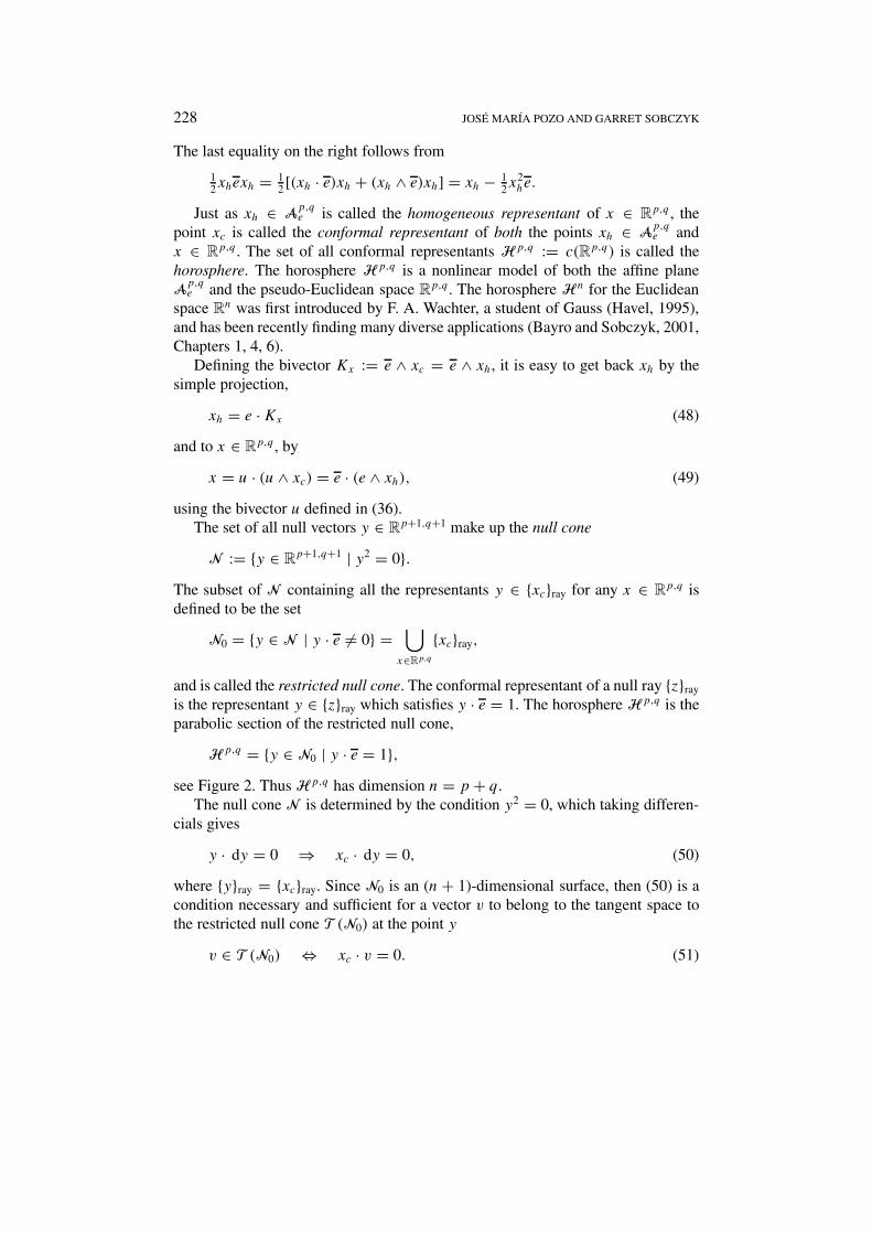
is the representant y ∈ {z}ray which satisfies y · e = 1. The horosphere Hp,q is theparabolic section of the restricted null cone,
Hp,q = {y ∈ N0 | y · e = 1},see Figure 2. Thus Hp,q has dimension n = p + q.
The null cone N is determined by the condition y2 = 0, which taking differen-cials gives
y · dy = 0 ⇒ xc · dy = 0, (50)
where {y}ray = {xc}ray. Since N0 is an (n + 1)-dimensional surface, then (50) is acondition necessary and sufficient for a vector v to belong to the tangent space tothe restricted null cone T (N0) at the point y
v ∈ T (N0) ⇔ xc · v = 0. (51)
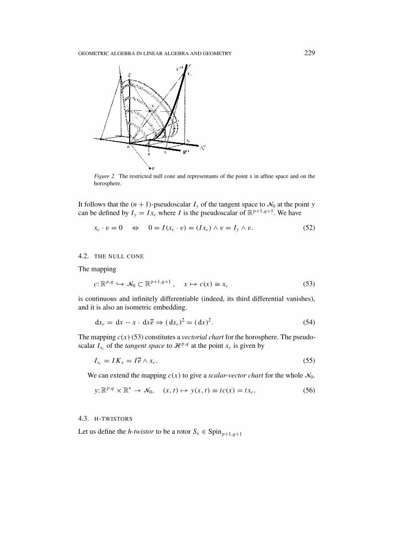
GEOMETRIC ALGEBRA IN LINEAR ALGEBRA AND GEOMETRY 229
Figure 2. The restricted null cone and representants of the point x in affine space and on thehorosphere.
It follows that the (n+ 1)-pseudoscalar Iy of the tangent space to N0 at the point ycan be defined by Iy = Ixc where I is the pseudoscalar of R
p+1,q+1. We have
xc · v = 0 ⇔ 0 = I (xc · v) = (Ixc) ∧ v = Iy ∧ v. (52)
4.2. THE NULL CONE
The mapping
c: Rp,q ↪→ N0 ⊂ R
p+1,q+1 , x !→ c(x) ≡ xc (53)
is continuous and infinitely differentiable (indeed, its third differential vanishes),and it is also an isometric embedding.
dxc = dx − x · dxe⇒ ( dxc)2 = ( dx)2. (54)
The mapping c(x) (53) constitutes a vectorial chart for the horosphere. The pseudo-scalar Ixc of the tangent space to Hp,q at the point xc is given by
Ixc = IKx = Ie ∧ xc. (55)
We can extend the mapping c(x) to give a scalar-vector chart for the whole N0.
y: Rp,q × R
∗ → N0, (x, t) !→ y(x, t) ≡ tc(x) = txc. (56)
4.3. H-TWISTORS
Let us define the h-twistor to be a rotor Sx ∈ Spinp+1,q+1
230 JOSE MARIA POZO AND GARRET SOBCZYK
Sx := 1+ 12xe = exp( 1
2xe). (57)
Noting that SxS†x = 1, we define its angular velocity by
4S := 2S†x dSx = dxe or equivalently 4S(a) = ae ∀a ∈ R
p,q . (58)
Later, in Section 4.7, we more carefully define an h-twistor to be an equivalenceclass of two ‘twistor’ components from Gp,q , that have many twistor-like proper-ties.
The reason for these definitions are found in their properties. The point xc isgenerated from 0c = e by
xc = SxeS†x , (59)
and the tangent space to the horosphere at the point xc is generated from dx ∈ Rp,q
by
dxc = dSxeS†x + Sxe dS†
x = Sx(4S · e)S†x = Sx dxS†
x (60)
or, equivalently, in terms of the argument of the differential
dxc(a) = SxaS†x ∀a ∈ R
p,q.
It also keeps unchanged the ‘point at infinity’ e = SxeS†x .
The motivation for the term ‘h-twistor’ is that it generates both points and tan-gent vectors on the horosphere from the corresponding objects in R
p,q . We call theh-twistor (60) ‘nonrotational’ because tangent vectors coincide with the differen-tial of points. More generally, the h-twistor Tx := SxRx , with Rx ∈ Spin(Rp,q)generates
xc = TxeT †x = SxeS†
x and dxc(RxaR†x) = TxaT †
x .
The angular velocity 4T of the more general h-twistor Tx is easily calculated
4T := 2T †x dTx = R†
x4SRx +4R = R†x dxRxe +4R. (61)
The analogy with Penrose twistors is, of course, not complete. We will have moreto say about this later.
4.4. CONFORMAL TRANSFORMATIONS AND ISOMETRIES
In this subsection we show that every conformal transformation in Rp,q corre-
sponds to two isometries on the null cone N0 in Rp+1,q+1.
DEFINITION 1. A conformal transformation in Rp,q is any twicely differentiable
mapping between two connected open subsets U and V ,
f :U −→ V, x −→ x′ = f (x)such that the metric changes by only a conformal factor
(df (x))2 = λ(x)(dx)2, λ(x) �= 0.
GEOMETRIC ALGEBRA IN LINEAR ALGEBRA AND GEOMETRY 231
If p �= q then λ(x) > 0. In the case p = q, there exists the posibility thatλ(x) < 0, when the conformal transformations belong to two disjoint subsets. Wewill only consider the case when λ(x) > 0.
Recall that N0 can be coordinized by the vector-scalar chart (56). Using theh-twistor (57), (59) and (60), we obtain the expressions
y = SxteS†x and dy = dtxc + t dxc = dtSxeS
†x + tSx dxS†
x . (62)
It easily follows that
(dy)2 = t2(dxc)2 = t2(dx)2. (63)
DEFINITION 1. 1. An isometry F on N0 is any twicely differentiable mappingbetween two connected open subsets U0 and V0 in the relative topology of N0,
F :U0 −→ V0, y !−→ y′ = F(y)which satisfies (dF(y))2 = (dy)2.
Using the scalar-vector chart y(x, t) = txc, any mapping in N0 can be expressedin the form
y′ = F(y) = t ′x′c = φ(x, t)f (x, t)c,where t ′ = φ(x, t) and x′c = f (x, t)c are defined implicitly by F . Using (63), weobtain the result that y′ = F(y) is an isometry if and only if
(dy′)2 = (dy)2 ⇔ t ′2(dx′)2 = t2(dx)2 ⇔ (df (x, t))2 = t2
φ(x, t)2(dx)2.
Since f (x, t), x ∈ Rp,q (nondegenerate metric), and the right-hand side of this
equation does not contain dt , it follows that f (x, t) = f (x) is independent of t . Itthen follows that φ(x) := φ(x, t)/t is also independent of t . Thus, we can expressany isometry y′ = F(y) in the form y′ = tφ(x)f (x)c, where f (x)c ∈ N0 is theconformal representant of f (x) ∈ R
p,q . This implies that y′ = F(y) is an isometryiff
y′ = tφ(x)f (x)c and (df (x))2 = (φ(x))−2(dx)2.
Therefore, f (x) is a conformal transformation with
λ(x) = φ(x)−2 > 0↔ φ(x) = ± 1√λ(x)
.
4.5. ISOMETRIES IN N0
In this section we show that for any dimension greater than 2 any isometry in N0 isthe restriction of an isometry in R
p+1,q+1. The inverse of the statement is obvious.
232 JOSE MARIA POZO AND GARRET SOBCZYK
From the definition of an isometry, (dF(x))2 = (dy)2. Since dF(y) and dy arevectors in R
p+1,q+1, dF(y) can be obtained as the result of applying a field oforthogonal transformations to dy,
dF(y) = R(y) dyR(y)∗−1 (64)
expressed here through a field of versors
R(y) ∈ Pinp+1,q+1 ≡ {X = a1a2 . . . an ∈ Gp+1,q+1 | a2i = ±1}.
Note that R(y)∗−1 = ±R(y)†, where R∗ and R† denote the main involution and thereversion respectively. Thus, the result that we must prove is that R(y) is constant,i.e. independent of the point y. This shall guarantee that F(y) is a global rigidisometry.
The fact that the tangent space T (N0) has dimension n + 1 and a metricallydegenerate null direction xc is sufficient to guarantee that the image of dF(y)defines a unique orthogonal transformation in R
p+1,q+1, which determines (up to asign) the versor R(y).
Previously, we found that any isometry F(y) = tφ(x)f (x)c in N0 is linear inthe scalar coordinate t . Taking the exterior derivative, we get
dF(y) = dt
tF (y)+ t d(φ(x)f (x)c) = dt
tF (y)+ t d
(φ(x)Sf (x)eS
†f (x)
)and using (64) and (62), we also have
R(y) dyR(y)∗−1 = dt
tR(y)yR(y)∗−1 + tR(y)Sx dxS†
xR(y)∗−1.
It follows that
R(y)Sx dxS†xR(y)
∗−1 = d(φ(x)Sf (x)eS†f (x))
and F(y) = R(y)yR(y)∗−1, so that R(y) is independent of t . We have now shownthat any isometry in N0 satisfies
dF(y) = R(x) dyR(x)∗−1 and F(y) = R(x)yR(x)∗−1, (65)
where R(x) ∈ Pinp+1,q+1 is solely a function of x ∈ Rp,q . It remains to be shown
that R(x) = R is also independent of x so that F(y) = RyR∗−1 is a globalorthogonal transformation in N0 ⊂ R
p+1,q+1.We now slightly generalize the definition of the h-twistor to apply to the rotor
Rx := R(x) ∈ Pinp+1,q+1. Letting Tx := RxSx , we can rewrite (65) in the form
dF(y) = Tx(t dx + dte)Tx∗−1 and F(y) = TxteTx∗−1. (66)
Analogous to (58) and (61), we define the three bivector valued forms:
4R := 2R−1x dRx, 40 := S†
x4RSx and 4T := 2T −1x dTx. (67)
GEOMETRIC ALGEBRA IN LINEAR ALGEBRA AND GEOMETRY 233
From the definition of Tx , we obtain the relation 4T = 40 +4S .In order to prove that Rx is constant, let us first impose the integrability con-
dition that the second exterior differential d dF must vanish. Note that in thecalculations below we are taking into account both the antisymmetry of exteriorforms as well as the noncommutativity of multivectors. Using (65), we find
0 = d dF = d(Rx dyR∗−1x ) = dRx dyR∗−1
x − Rx dy dR∗−1x
= 12Rx(4R dy + dy4R)R
∗−1x ⇒ 4R · dy = 0.
Using (62), this is equivalent to
4R · dy = (S†x4RSx) · (S†
x dySx) = 40 · (t dx + dte) = 0. (68)
Since R(x) and Sx are independent of t , then 40 does not contain dt . Thus,Equation (68) can be separated into two parts:
40 · (t dx + dte) = t40 · dx + dt40 · e = 0⇒{40 · dx = 0,40 · e = 0.
(69)
From 40 · e = 0, it follows that the bivector-valued form 40 can be written as
40(x, a) = v(x, a) ∧ e + B(x, a),where v(x, a) is a vector in R
p,q , and B(x, a) is a bivector in the geometric algebraG2p,q of R
p,q .Imposing the first equation in (69) we get
40(a) · b −40(b) · a = 0
⇒{v(a) · b − v(b) · a = 0,B(a) · b − B(b) · a = 0
⇒ B(a) · (b ∧ c) = B(b) · (a ∧ c)⇒ B(a) = 0 ∀a ∈ Rp,q
⇒ 40(a) = v(a) ∧ e. (70)
The second integrability condition is found by taking the exterior derivative of4R = 2R−1
x dRx to find
d4R = 2 dRx−1 dRx = 2 dR−1
x RxRx−1 dRx = − 1
24R4R. (71)
But (70) implies 4R4R = Sx4040S†x = 0, from which it follows that d4R = 0.
Next, we write this as an equation in 40, getting
0 = d4R = d(Sx40S†x) = Sx(d40 +4S ×40)S
†x
⇔ d40 +4S ×40 = 0.
With the help of (70) and (58), we now split this equation into its three multivectorparts:
d40 +4S ×40 = dv e + v ∧ dx + v · dx e ∧ e = 0
⇒
dv = 0,v ∧ dx = 0,v · dx = 0.
(72)
234 JOSE MARIA POZO AND GARRET SOBCZYK
The bivector part
v ∧ dx = 0 ⇔ v(a) ∧ b = v(b) ∧ adifferentiates drastically between the dimension d = 2, and for the dimensionsd > 2. When d > 2, we can wedge this last expression with the vector a ∈ R
p,q
to infer
v(a) ∧ b ∧ a = 0 ∀b ∈ Rp,q ⇒ v(a) ∧ a = 0
⇒ v(a) = ρa, ρ ∈ R,
from which follows the desired result
ρa ∧ b = ρb ∧ a ⇒ ρ = 0⇒ v = 0⇒ 40 = 0.
Therefore R(x) is constant,
4R = 0⇒ dR(x) = 0⇒ R(y) = R = constant.
Thus, F(y) is a global orthogonal transformation in Rp+1,q+1,
F(y) = RyR∗−1, R ∈ Pinp+1,q+1. (73)
Since the group of isometries in N0 is a double covering of the group of con-formal transformations Conp,q in R
p,q , and the group Pinp+1,q+1 is a double cov-ering of the group of orthogonal transformations O(p + 1, q + 1), it follows thatPinp+1,q+1 is a four-fold covering of Conp,q .
The case of d = 2 will be treated after introducing the matrix representation ofnext section.
4.6. MATRIX REPRESENTATION
The algebra Gp+1,q+1 is isomorphic to Gp,q ⊗G1,1. This isomorphism can be spec-ified by means of the so-called conformal split (Hestenes, 1991). Evidently, oncethis isomorphism of algebras is established, we can use the matrix representationintroduced in Subsection 2.2 for SNB1,1, taking into account that the 2 × 2 ma-trices are defined over the module Gp,q . This identification makes possible a veryelegant treatment of the so-called Vahlen matrices (Lounesto, 1997; Maks, 1989;Cnops, 1996; Porteous, 1995).
The conformal split does not identify the algebra Gp,q appearing in the isomor-phism Gp,q ⊗ G1,1 directly with Gp,q := gen{Rp,q}. Instead, the conformal splitidentifies Gp,q with a subalgebra of Gp+1,q+1 generated by a subset of trivectors:Gp,q := gen{Rp,qu}, where u = σν is the unit bivector orthogonal to R
p,q , asintroduced in (36) and Subsection 4.1. This subalgebra has the property that itcommutes with G1,1 = gen{σ, ν} so that Gp+1,q+1 = Gp,q ⊗G1,1. The multivectorsbelonging to the subalgebra Gp,q are characterized by
A ∈ Gp,q ⇔ A = A+ + uA−, A+ ∈ G+p,q and A− ∈ G−p,q,
GEOMETRIC ALGEBRA IN LINEAR ALGEBRA AND GEOMETRY 235
where A+ and A− are, respectively, the even and odd multivectors parts of themultivector A = A++A− ∈ Gp,q . Thus, we have a direct correspondence betweenthe multivector A ∈ Gp,q and the multivector A ≡ A+ + A− ∈ Gp,q .
Recall that the idempotents u± = 12(1 ± u) of the algebra G1,1, first defined
in (20), satisfy the properties given in Subsection 2.2:
u+ + u− = 1, u+ − u− = u,u+u− = 0 = u−u+, σu+ = u−σ,
and
u = e ∧ e, u+ = 12ee, u− = 1
2ee,
ue = e = −eu, eu = e = −ue, σu+ = e, 2σu− = e.The representation of G1,1, introduced in Subsection 2.2 using the spinor basis,
enables us to write any multivector G ∈ Gp+1,q+1 = Gp,q ⊗ G1,1 in the form
G = ( 1 σ ) u+(
A BC D
)(1σ
),
where the entries of the 2× 2 matrix are in Gp,q . Noting that
u+A = u+(A+ + uA−) = u+(A+ + A−) = u+A,makes it possible to work directly with the proper subalgebra Gp,q , instead ofhaving to deal with the extra complexity introduced by using the subalgebra Gp,q .
It follows that each multivector G ∈ Gp+1,q+1 can be written in the form
G = ( 1 σ ) u+[G](
1σ
)= Au+ + Bu+σ + C∗u−σ +D∗u−, (74)
where
[G] ≡(A B
C D
)for A,B,C,D ∈ Gp,q .
The matrix [G] denotes the matrix corresponding to the multivector G, and as aconsequence of the general argument given in (22), we have the algebra isomor-phism
[G1 +G2] = [G1] + [G2] and [G1G2] = [G1][G2],for all G1,G2 ∈ Gp+1,q+1. This result is an example of the unusual fact that amatrix representation is sometimes possible even when the module of componentsGp,q does not commute with the subalgebra G1,1. Note, also, the relationships
u+[G] = [u+G] =(A B
0 0
)and [G]u+ = [Gu+] =
(A 0C 0
).
236 JOSE MARIA POZO AND GARRET SOBCZYK
The operation of reversion of multivectors translates into the following trans-pose-like matrix operation:
if [G] =(A B
C D
)then [G]† := [G†] =
(D B
C A
),
where A = A∗† is the Clifford conjugation.
4.7. h-TWISTORS AND MOBIUS TRANSFORMATIONS
As seen in Section 4.3, the point xc ∈ Hp,q can be written in the form (59),xc = SxeS†
x . More generally, in Subsection 4.5, we saw that any conformal trans-formation F(xc) must be of the form
sTxeT†x = F(xc) = φ(x)f (x)c = φ(x)Sf (x)eS†
f (x), (75)
where s := TxTx = ±1.Using the matrix representation of the previous section, for a general multivec-
tor G ∈ Gp+1,q+1, we find that
[GeG†] =(A B
C D
)(0 01 0
)(D B
C A
)
=(B
D
)(D B ) , (76)
where
[e] =(
0 01 0
), [G] ≡
(A B
C D
), [G]† =
(D B
C A
).
The relationship (76) suggests defining the conformal h-twistor of the multi-vector G ∈ Gp+1,q+1 to be [G]c :=
(B
D
), which may also be identified with the
multivector Gc := Ge = Bu+ + D∗e. The conjugate of the conformal h-twistoris then naturally defined by [G]†c := (D B ). Conformal h-twistors give us apowerful tool for manipulating the conformal representant and conformal transfor-mations much more efficiently. For example, since xc is generated by the conformalh-twistor [Sx]c, it follows that
[xc] = [Sx]c[Sx]†c =(x
1
)(1 − x) =
(x −x2
1 −x).
Two conformal h-twistors [G1]c and [G2]c will be said to be equivalent if theygenerate the same multivector, i.e., if
[G1]c[G1]†c = [G2]c[G2]†c .
GEOMETRIC ALGEBRA IN LINEAR ALGEBRA AND GEOMETRY 237
This is equivalent to the condition G1eG†1 = G2eG
†2. Two conformal h-twistors
[G1]c and [G2]c will be said to be projectively equivalent if they generate the samedirection, i.e., if
[G1]c[G1]†c = ρ[G2]c[G2]†c with ρ ∈ R∗.
This is equivalent to the condition {G1eG†1}ray = {G2eG
†2}ray.
A sufficient condition for two spinor to be projectively equivalent is the follow-ing:
If ∃H ∈ Gp,q such that HH ∈ R and [G2]c = [G1]cH,then [G2]c[G2]†c = HH [G1]c[G1]†c . (77)
Moreover, it is not difficult to show that if any component A,B,C orD of the twoconformal h-twistors
(A
B
)and
(C
D
)is invertible, then this condition is necessary and
sufficient.We can now write the conformal transformation (75) in its spinorial form
[F(xc)] = φ(x)[Sf (x)]c[Sf (x)]†c = s[Tx]c[Tx]†c,from which it follows that [Tx]c and [Sf (x)]c are projectively equivalent spinors.Since the bottom component of [Sf (x)]c =
(f (x)
1
)is trivially invertible, the two
spinors are equivalent by (77). Letting [Tx]c =(M
N
), it follows that(
M
N
)=(f (x)
1
)H ⇒ H = N and f (x) = MN−1, (78)
and also that φ(x) = sNN .The beautiful linear fractional expression for the conformal transformation f (x),
f (x) = (Ax + B)(Cx +D)−1 (79)
and
φ(x) = s(Cx +D)(D − xC)is a direct consequence of (78). Since Tx = RSx for the constant versor (73),R ∈ Pinp+1,q+1, its spinorial form is given by
[Tx]c = [R][Sx]c =(A B
C D
)(x
1
)=(Ax + BCx +D
)=(M
N
),
where
[R] =(A B
C D
), for constants A,B,C,D ∈ Gp,q .
The linear fractional expression (79) extends to any dimension and signature thewell-known Mobius transformations in the complex plane. The components A, B,C, D of [R] are, of course, subject to the condition that R ∈ Pinp+1,q+1.
238 JOSE MARIA POZO AND GARRET SOBCZYK
Although more difficult to manipulate, our conformal h-twistors are a gener-alization to any dimension and any signature of the familiar 2-component spinorsover the complex numbers, and the 4-component twistors. Penrose’s twistor the-ory (Penrose and MacCallum, 1972) has been discussed in the framework of Clif-ford algebra by a number of authors, for example see (Ablamowicz and Salingaros,1985; Ablamowicz and Fauser, 2000, pp. 75–92). In the language of spinors, anynull vector y ∈ N is the null pole of a conformal h-twistor, [y] = [G]c[G]†c .Also, two h-twistors will define the same null pole if they differ only by a phase,[G2]c = [G1]cH , where HH = 1. To complete the analogy, note that each confor-mal h-twistor also defines a null flag, i.e. a null bivector, tangent to the null cone N .It easily follows from the expressions (59) and (60) that
xc dxc = Sxe dxS†x ⇒ [xc dxc] = [Sx]c dx[Sx]†c.
Finally, any h-twistor differing only by a rotor H ∈ Spinp,q will give the same nullpole but with a different null flag, the null flag rotated by the rotor H :[Sx]cH dxH [Sx]†c .
4.8. THE RELATIVE MATRIX REPRESENTATION
In the two preceding subsections, we have introduced and used a matrix represen-tation of Gp+1,q+1, based on the isomorphism Gp+1,q+1 ∼ Gp,q ⊗G1,1. This matrixrepresentation depends only upon the choice of a fixed spin basis in G1,1, but noton any basis of Gp,q . We can introduce an alternative relative matrix representationrelative to a choosen nonnull direction a ∈ R
pq , by a slight modification of theformer (74), namely,
G = ( 1 σa−1 ) u+[G]′(
1aσ
), (80)
so that
[G]′ =(
1 00 a
)[G]
(1 00 a−1
).
Evidently, this relative representation has the disadvantage of depending on thedirection a that is chosen. However, it has the important advantage that the parityof G ∈ Gp+1,q+1 is the same as the parity of the components A,B,C,D ∈ Gp,q ,where
[G]′ =(A B
C D
).
Moreover, it is more directly related to complex numbers and to the 4-componenttwistors of Penrose and MacCallum (1972). This relative representation will enableus to relate isometries onN0 for d = 2 with analytic and antianalytic functions overthe complex numbers C or over the dual numbers D.
GEOMETRIC ALGEBRA IN LINEAR ALGEBRA AND GEOMETRY 239
The vectorial representation of points is most directly related to the complexrepresentation of points via the paravector representant of x relative to a, de-fined by
zx := xa−1 ⇔ x = zxa. (81)
Whereas this definition is valid in any dimension, we only consider here the di-mension d = p + q = 2. The set of relative paravectors, in this case, is the evensubalgebra:
{zx | x ∈ Rp,q} = G0
p,q ⊕ G2p,q = G+p,q for p + q = 2.
Depending on the signature, the square of the pseudoscalar I ∈ Gp,q can beeither negative (I 2 = −1) or positive (I 2 = 1). It follows that the algebra G+p,q isisomorphic to either the complex numbers C or to the dual numbers
G+2,0 & G+0,2 & C or G+1,1 & D.
The two vectors {a, Ia} ∈ Rp,q constitutes an orthonormal basis. Relative to this
basis, the vector x and its paravector zx have the coordinate forms
x = x1a + x2Ia and zx = x1 + x2I, (82)
where x1, x2 ∈ R.For example, the relative matrix representation of the conformal representant
xc is
[xc]′ =(zx −zxzx1 −zx
)a.
The relative matrix representation of the reversion of (80) is
[G]′† := [G†]′ = a−1
(D −B−C A
)a.
Conformal h-twistors can also be defined for the relative matrix representation inthe obvious way:
[G]′c :=(B
D
)and [G]′c† := (D − B),
and satisfy [GeG†]′ = [G]′c[G]′c†a.
4.9. CONFORMAL TRANSFORMATIONS IN DIMENSION 2
Before restricting ourselves in Subsection 4.5 to dimensions d > 2, we found theexpression (70) 40 = v(a)e, from which we derived the conditions (72). The ex-pression for v can be derived from the versor T ∈ Pinp+1,q+1 which generates (67)4T = 40 +4S .
240 JOSE MARIA POZO AND GARRET SOBCZYK
Expressing the bivector (58) 4S = dxe in terms of the relative paravectors (81)zx = xa−1, we get 4S = dzxae. From definition (67) of 4T , we find
dT = 12T4T = 1
2T (40 +4S) = 12T (ve + dzxae),
where the parity of T ∈ Pinp+1,q+1 is even or odd. Let us define
G :={T , if T is even,aT , if T is odd,
(83)
so that G is always even, and for which it is also true that dG = 12G4T .
Using the relative matrix representation introduced earlier, we have
[G]′ ≡(A B
C D
)and [4T ]′ =
(0 2 dzx−av 0
),
where A,B,C,D ∈ G+p,q . Note that since the matrix representation (80) is definedin terms of constant vectors, the differential will commute with the representation[dG]′ = d[G]′. It follows that(
dA dBdC dD
)=(A B
C D
)(0 dzx− 1
2av 0
).
We can split this matrix into two columns, getting(dAdC
)= −1
2av
(B
D
)and
(dBdD
)=(A
C
)dzx. (84)
Equation (84) implies that, considered as functions over G+p,q (isomorphic to C
or to D), the two components B and D are analytic, since their differentials areproportional to dzx . Therefore, the derivatives of these analytic functions are(
B ′D′
)=(A
C
), where B ′ := dB
dzx.
This implies, in turn, that the components A and C are also analytic(A
C
)=(B ′D′
)and
(A′C ′
)= −1
2
av
dzx
(B
D
). (85)
An immediate consequence of the above equations is that the 1-form av is propor-tional to dzx , so that 40 takes the form
av = g(zx) dzx ⇒ 40 = a−1eg(zx) dzx, (86)
where g(zx) is also an analytic function over G+p,q .Taking into account the change of representation of the conformal h-twistor
[G]c to [G]′c, formula (78) for the spinor [T ]′c =(M
N
)becomes f (x) = MN−1a.
Defining the function
f: G+p,q → G+p,q , zx !→ f(zx) := zf (x) = f (x)a−1,
GEOMETRIC ALGEBRA IN LINEAR ALGEBRA AND GEOMETRY 241
we obtain f(zx) = MN−1.We must now consider the two cases when T in (83) is either odd or even. If T
is even then
T = G ⇒(M
N
)=(B
D
)⇒ f(zx) = BD−1.
If T is odd then
T = a−1G ⇒(M
N
)= a−1
(B
D
)⇒ f(zx) = a−1BD−1a.
The function h(zx) defined by
h(zx) :={
f(zx), if T is even,af(zx)a−1 = f(zx), if T is odd,
has the property that, regardless of whether T is even or odd,
h(zx) = BD−1 ⇒ B = h(zx)D. (87)
Since B and D are analytic, it follows that h(zx) is also analytic. In the case thatT is even, it generates the analytic transformation f(zx) = h(zx) in G+p,q . On theother hand, in the case that T is odd, it generates the anti-analytic transformationf(zx) = h(zx).
Using (87) and (85), we can express [G]′ in terms of h(zx),
[G]′ =(A B
C D
)=((hD)′ hD
D′ D
). (88)
The fact that G is in Spinp,q can be used to find an explicit expression for D interms of h(zx). Using that GG† = ±1,
[GG†]′ =(A B
C D
)(D −B−C A
)=(AD − BC 0
0 AD − BC),
it follows that det[G]′ ≡ AD − BC = ±1. From (85) and (87), it directly followsthat
±1 = AD − BC = 2(B ′D − BD′) = 2D2(BD−1)′ = D2h′
so that formally we have
D = ±(±h′)−1/2 = ± 1√±h′ (89)
which, in general, represents four solutions.For the complex case C & G+2,0 & G+0,2, where I 2 = −1, the four solutions
of (89) are given as usual by
D = k√h′, where k = ±1,±I. (90)
242 JOSE MARIA POZO AND GARRET SOBCZYK
The inverse and square roots of the dual number h′ ∈ D & G+1,1 in (89), where I 2 =1, are not always well defined. The inverse of a dual number zx = x1 + x2I ∈ D isgiven by
z−1x =
1
zx= z†
x
x21 − x2
2
= x1 − x2I
x21 − x2
2
,
so will only exist when x1 �= ±x2. It can be shown that the dual number±h′ (exceptin the degenerate case when h′h′† = 0) has exactly one of the four hyperbolic Eulerforms (Sobczyk, 1995),
±h′ ={ ±ρ exp(Iφ),±ρI exp(Iφ),
where ρ = √|h′h′†| and φ is the hyperbolic angle defined by ±h′. Only in the casewhen the sign of±h′ can be chosen such that ±h′ = ρ exp(Iφ), will±h′ have fourwell-defined square roots in D. For this case we have
D = k√±h′ =k√ρ
exp(−1
2Iφ), where k = ±1,±I. (91)
Once we have found D, we also have A, B and C (88)
B = kh√h′, A = k (h
′)2 − 12hh
′′
(h′)3/2, C = −k h′′
2(h′)3/2,
but it is not, in general, possible to solve for the transformation h(zx) which cor-responds to a given 40 = a−1eg(zx) dzx . However, we can find g(zx) in termsof the function h(zx): From (85) and (86), we obtain the second-order differentialequation for the conformal h-twistor of G,(
B ′′D′′
)= − 1
2g(zx)
(B
D
). (92)
From (92) and (90) or (91), we have
g(zx) = −2D′′
D= h
′′′
h′− 3
2
(h′′
h′
)2
.
It is recognized that g(zx) is the Schwarzian derivative of h(zx), which vanisheswhenever h(zx) is a Möbius transformation. There are many possibilities for thefurther study of the Schwarzian derivative and its generalizations (Kobayashi andWada, 2000).
Acknowledgements
José Pozo acknowledges the support of the Spanish Ministry of Education (MEC),grant AP96-52209390, the project PB96-0384, and the Catalan Physics Society(IEC). Garret Sobczyk gratefully acknowledges the support of INIP of the Univer-sidad de Las Americas-Puebla, and CIMAT-Guanajuato during his Sabbatical, inthe Fall of 1999.
GEOMETRIC ALGEBRA IN LINEAR ALGEBRA AND GEOMETRY 243
References
Ablamowicz, R. and Salingaros, N. (1985) On the relationship between twistors and Cliffordalgebras, Lett. Math. Phys. 9, 149–155.
Ablamowicz, A. and Fauser, B. (eds) (2000) Clifford Algebras and their Applications in Mathemati-cal Physics, Birkhäuser, Boston.
Barnabei, M., Brini, A. and Rota, G. C. (1985) On the exterior calculus of invariant theory, J. Algebra96, 120–160.
Bayro Corrochano, E. and Sobczyk, G. (eds) (2001) Geometric Algebra with Applications in Scienceand Engineering, Birkhäuser, Boston.
Cnops, J. (1996) Vahlen matrices for non-definite metrics, In: R. Ablamowicz, P. Lounesto andJ. M. Parra (eds), Clifford Algebras with Numeric and Symbolic Computations, Birkhäuser,Boston.
Davis, P. J. (1974) The Schwarz Function and its Applications, Math. Assoc. Amer.Doran, C., Hestenes, D., Sommen, F. and Van Acker, N. (1993) Lie groups as spin groups, J. Math.
Phys. 34, 3642–3669.Dress, A. W. M. and Havel, T. F. (1993) Distance geometry and geometric algebra, Found. Phys.
23(10), 1357–1374.Fulton, W. and Harris, J. (1991) Representation Theory: A First Course, Springer-Verlag.Havel, T. (1995) Geometric algebra and Mobius sphere geometry as a basis for Euclidean invari-
ant theory, In: N. L. White (ed.), Invariant Methods in Discrete and Computational Geometry,Kluwer Acad. Publ., Dordrecht, pp. 245–256.
Haantjes, J. (1937) Conformal representations of an n-dimensional Euclidean space with a non-definite fundamental form on itself, Proc. Ned. Akad. Wet. (Math.) 40, 700–705.
Hestenes, D. (1991) The design of linear algebra and geometry, Acta Appl. Math. 23, 65–93.Hestenes, D. and Sobczyk, G. (1984) Clifford Algebra to Geometric Calculus: A Unified Language
for Mathematics and Physics, D. Reidel, Dordrecht.Hestenes, D. and Ziegler, R. (1991) Projective geometry with Clifford algebra, Acta Appl. Math. 23,
25–63.Kobayashi, O. and Wada, M. (2000) The Schwarzian and Möbius transformations in higher dimen-
sions, 5th International Clifford Algebra Conference, Ixtapa 1999, In: J. Ryan and W. Sprösig(eds), Clifford Algebras and their Applications in Mathematical Physics, Vol. 2, Birkhäuser,Boston.
Li, H., Hestenes, D. and Rockwood, A. Generalized Homogeneous Coordinates for ComputationalGeometry, to be published.
Lounesto, P. (1994) CLICAL software paquet and user manual, Helsinki Univ. Technol. Mathemat-ics, Research Report A248.
Lounesto, P. (1997) Clifford Algebras and Spinors, Cambridge Univ. Press, Cambridge.Lounesto, P. and Springer, P. (1989) Mobius transformations and Clifford algebras of Euclidean
and anti-Euclidean spaces, In: J. Lawrynowicz (ed.), Deformations of Mathematical Structures,Kluwer Acad. Publ., Dordrecht, pp. 79–90.
Maks, J. G. (1989) Modulo (1,1) periodicity of Clifford algebras and generalized Mobius transfor-mations, Technical Univ. Delft (Dissertation).
Nehari, Z. (1952) Conformal Mapping, McGraw-Hill, New York.Penrose, R. and MacCallum, M. A. H. (1972) Twistor theory: An approach to quantization of fields
and space-time, Phys. Rep. 6C, 241–316.Porteous, I. R. (1995) Clifford Algebras and the Classical Groups, Cambridge Univ. Press.Rao, C. R. and Mitra, S. K. (1971) Generalized Inverse of Matrices and its Applications, Wiley, New
York.

244 JOSE MARIA POZO AND GARRET SOBCZYK
Sobczyk, G. (1993) Jordan form in associative algebras, In: F. Brackx (ed.), Clifford Algebras andtheir Applications in Mathematical Physics, Proc. Third Internat. Clifford Workshop, KluwerAcad. Publ., Dordrecht, pp. 33–41.
Sobczyk, G. (1995) The hyperbolic number plane, College Math. J. 26(4), 268–280.Sobczyk, G. (1996) Structure of factor algebras and Clifford algebra, Linear Algebra Appl. 241–243,
803–810.Sobczyk, G. (1997a) The generalized spectral decomposition of a linear operator, College Math. J.
28(1), 27–38.Sobczyk, G. (1997b) Spectral integral domains in the classroom, Aportaciones Mat. Comun. 20,
169–188.Sobczyk, G. (2001) The missing spectral basis in algebra and number theory, Amer. Math. Monthly
108(4), 336–346.Young, J. W., (1930) Projective Geometry, The Open Court Publ. Co., Chicago.