geomechanics-reservoir modeling by displacement
TRANSCRIPT

Geomechanics-Reservoir Modeling by
Displacement Discontinuity-Finite Element
Method
by
Shunde Yin
A thesis
presented to the University of Waterloo
in fulfillment of the
thesis requirement for the degree of
Doctor of Philosophy
in
Civil Engineering
Waterloo, Ontario, Canada, 2008
©Shunde Yin 2008

ii
I hereby declare that I am the sole author of this thesis. This is a true copy of the thesis, including any required final revisions, as accepted by my examiners.
I understand that my thesis may be made electronically available to the public.

iii
Abstract
There are two big challenges which restrict the extensive application of fully coupled
geomechanics-reservoir modeling. The first challenge is computational effort. Consider a 3-D
simulation combining pressure and heat diffusion, elastoplastic mechanical response, and
saturation changes; each node has at least 5 degrees of freedom, each leading to a separate
equation. Furthermore, regions of large p, T and σ′ gradients require small-scale discretization
for accurate solutions, greatly increasing the number of equations. When the rock mass
surrounding the reservoir region is included, it is represented by many elements or nodes.
These factors mean that accurate analysis of realistic 3-D problems is challenging, and will so
remain as we seek to solve larger and larger coupled problems involving nonlinear responses.
To overcome the first challenge, the displacement discontinuity method is introduced
wherein a large-scale 3-D case is divided into a reservoir region where Δp, ΔT and non-linear
effects are critical and analyzed using FEM, and an outside region in which the reservoir is
encased where Δp and ΔT effects are inconsequential and the rock may be treated as elastic,
analyzed with a 3D displacement discontinuity formulation. This scheme leads to a
tremendous reduction in the degrees of freedom, yet allows for reasonably rigorous
incorporation of the reactions of the surrounding rock.
The second challenge arises from some forms of numerical instability. There are
actually two types of sharp gradients implied in the transient advection-diffusion problem: one
is caused by the high Peclet numbers, the other by the sharp gradient which appears during the
small time steps due to the transient solution. The way to eliminate the spurious oscillations is
different when the sharp gradients are induced by the transient evolution than when they are

iv
produced by the advective terms, and existing literature focuses mainly on eliminating the
spurious spatial temperature oscillations caused by advection-dominated flow.
To overcome the second challenge, numerical instability sources are addressed by
introducing a new stabilized finite element method, the subgrid scale/gradient subgrid scale
(SGS/GSGS) method.

v
Acknowledgments I am indebted to my supervisors Professor Leo Rothenburg and Professor Maurice B.
Dusseault for their patience, guidance, and financial support during my study at the University
of Waterloo.
I am also grateful for all the suggestions from the committee members, Professor Andre Unger,
Professor Mark Knight, Professor Cascante Giovanni, Professor Weichao Xie, Professor
Antonin Settari, Professor Leo Rothenburg, and Professor Maurice B. Dusseault.

vi
Table of Contents
Nomenclature………….……………...………………………………….……………….…..viii
Chapter 1 Introduction……..……………...…………………………………………………….1
1.1 Geomechanics and Petroleum Engineering ………………….…………………………1
1.2 Coupled Processes in Geomechanics…………………….…………………………..…5
1.3 Goals of the Thesis…………..……………...…………………………………………10
Chapter 2 Poromechanics on Fully Coupled Geomechanics-Reservoir Modeling……...…….12
2.1 Poroelasticity.………………..……………...…………………………………………12
2.2 Multiphase poroelasticity…..……………...………...…………………………………14
2.3 Thermoporoelasticity………..……………...………………………………….………16
2.4 Multiphase thermoporoelasticity…………...………………………………….………18
Chapter 3 Finite Element Formulation and Stabilized FEM Scheme………….………………21
3.1 FEM for poroelasticity ……………………...…………………………………………22
3.2 FEM for multiphase poroelasticity………...……..……………………………………23
3.3 FEM for thermoporoelasticity……………...…………………………….……………27
3.4 FEM for multiphase thermoporoelasticity..……………………………………………28
3.5 Stabilized finite element methods…………...…………………………………………32
3.6 Iterative GMRES solver……………………..…………………………………………47
Chapter 4 Displacement Discontinuity Analysis and Hybrid DDFEM Model …………….…51
4.1 Displacement Discontinuity Method…………..………………………………………51
4.2 Link between DD and FE element……………..………………………………………53
4.3 DDFEM Model………………………………...………………………………………55
4.4 Nonisothermal DDFEM Model…………………...……………...……………………57

vii
Chapter 5 Models Verifications…………………………...………………………...…………62
5.1 One dimensional consolidation……………………...…………………………………62
5.2 Mandel-Cryer effects……………...………………...…………………………………65
5.3 Partially saturated elastic consolidation…………...…...………………………………67
5.4 Thermal consolidation…………...………………...……………………………..……70
5.5 Partially saturated thermal consolidation………......……………………………..……72
5.6 Underground Excavation………...………………...……………………………..……77
5.7 Geertsma’s solution……....……...………………...……………………………..……80
5.8 Rothenburg’s solution…....……...…….…………...……………………………..……83
Chapter 6 Numerical Experiments…...…….…………...………………………………...……91
6.1 Subsidence in a half space……...………………...…..…………………………..……91
6.2 Noordbergum effects…....……...………………...…..…………………………..……96
6.3 Pressure drawdown and stresses changes………...…..………………………………100
6.4 Hot water flooding and ground surface uplift….....…..……………………..…..……105
Chapter 7 Conclusions and Recommendations………...…..…………………………...……124
7.1 Conclusions………………………………………...…..………………………..……124
7.2 Recommendations…………………..……………...…..………………………..……125
Bibliography……………..………………………………...…..………………………..……126

viii
Nomenclature
Subscripts: f = fluids, g = gas, m=rock matrix, n = non wetting phase, o = oil, p = fluid pressure, s = solids, T = temperature, w = water/wetting phase
B strain matrix relating strain and displacement (m-1)
Cr bulk compressibility of the reservoir (Pa−1)
Co bulk compressibility of the surrounding strata (Pa−1)
Cm compressibility of solid matrix (Pa−1)
Cf compressibility of the fluid (Pa−1)
c π specific heat of material π (J kg−1 K−1)
D elastic stiffness matrix relating stress and strain (Pa)
Di displacement discontinuity of component i (m)
DK Damkӧhler number (–)
E Young’s modulus (Pa)
f external force or flow/heat source/sink vector
G Lamé elastic constant (Pa)
h reservoir thickness (m)
finite element size (m)
k absolute permeability tensor (m2)
k absolute permeability (m2)
k r π relative permeability of phase π (–)
K bulk modulus of the material (Pa)
K π bulk modulus of material (Pa−1)

ix
N shape functions for the finite element (–)
Pe Peclet number (–)
p average pressure (Pa)
P atm atmospheric pressure (Pa)
P b bubbling pressure(Pa)
P c capillary pressure (Pa)
P π pressure of phase π (Pa)
Pcgw the capillary pressure between the gas and water phases (Pa)
Pcow the capillary pressure between the oil and the water phases (Pa)
Pcgo the capillary pressure between the gas and oil phases (Pa)
Q production rate (m3/s)
S π saturation of phase π
t time(s)
T temperature (K)
u displacement vector of solid matrix (m)
convective velocity vector (m s−1)
u convective velocity (m s−1)
v π velocity vector of phase π (m s−1)
Greek letters
α Biot's constant (–)
β reservoir-fluid coupling coefficient
β π thermal expansion coefficient of phase π (K−1)
Δt time step (s)

x
Δp pressure drawdown (Pa)
θ time integration coefficient (–)
κ the diffusion coefficient (m2 s-1)
λ Lamé elastic constant (Pa)
λ T thermal conductivity of solid (W m-1 K-1)
χ reservoir-overburden coupling coefficient (–)
μ π viscosity of phase π (Pa⋅s)
ν Poisson’s ratio (–)
νr Poisson’s ratio for the reservoir (–)
νo Poisson’s ratio for reservoir surrounding strata (–)
ρ π density of phase π (kg m−3)
σ total stress, Pa σ′ effective stress, Pa
τ stabilized finite element parameter (–)
φ dependent variable in advection-diffusion-reaction equation
ϕ porosity of porous media (–)

1
Chapter 1 Introduction
1.1 Geomechanics and Petroleum Engineering
Petroleum reservoir engineering involves at least four disciplines: geology, transport,
thermodynamics and geomechanics. The latter has suffered benign neglect for decades, but
large-scale development of viscous oils, high-porosity offshore reservoirs, HPHT cases, and
fractured carbonates with severe stress sensitivity are raising awareness that geomechanics is a
vital aspect of reservoir management. Because 60% of the world’s liquid fossil fuel is in the
form of viscous oil in weak sandstones (IEA 2005), geomechanics analysis has become an
indispensable consideration in oil field development from oil exploration to production and
monitoring, and the role of geomechanics will still increase sharply in decades to come
(Dusseault et al. 2007).
1.1.1 Massive Compaction and Subsidence in Production
In petroleum engineering, large-scale reservoir compaction due to oil and gas withdrawal can
lead to surface damage (Wilmington oil field, California; Lago de Maracaibo, Venezuela;
Niigata, Japan; Ravenna, Italy), casing damage, and even well failure (Bruno 1992). While
reservoir compaction itself has been widely recognized as an additional driving mechanism for
increasing oil and gas recovery, its side effects are undesirable. The most obvious one is
surface or seafloor settlement, which may create environmental problems and cause damage to
oil field structures and seabed pipelines. The North Sea offshore oil field Ekofisk, developed in
the early 1970’s, experienced massive subsidence (4.3 m by 1988) so that all five platforms
had to be raised in 1988-1990 at a cost of US$485,000,000, and fully redeveloped with two

2
new platforms replacing the original five in the late 1990’s at an additional cost in excess of
US$3,000,000,000. Currently, reservoir compaction at Ekofisk appears to be ~12 m, and sea
floor subsidence has passed 10 m. Knowing the relationship between the fluid withdrawal and
the ground surface movement by appropriate geomechanical modeling, we can mitigate the
losses by taking the prevention measures like water injection or CO2 injection, maintaining the
pressure inside the reservoir.
1.1.2 Extensive Casing Shear and Well Damage
A problem associated with massive subsidence and compaction is extensive casing damage.
Reservoir compaction and associated bedding plane slip and overburden shear have induced
damage to hundreds of wells in oil and gas fields throughout the world. Well casing damage
can be caused by compaction in the reservoir or by overburden formation faulting and bedding
plane slip. Casing damage types can include compression and buckling, shearing deformations,
and tensile parting. Compression and buckling damage is most often found within compaction
zones near perforations, while shear damage is most often found within the overburden and at
the top of compacting or dilating formations. Shearing damage in overburden and at top of the
producing interval has been noted in Gulf of Mexico, North Sea, California, and Southeast
Asia. Knowing the stresses distribution, especially the shear concentration zones, we can
reduce losses by avoiding placing wells through those zones.
1.1.3 Cap-Rock Integrity Maintenance in CO2– Enhanced Oil Recovery
As much of the easy-to-produce oil has already been recovered from oil fields, producers have
attempted tertiary, or enhanced oil recovery (EOR), techniques that offer prospects for
ultimately producing 30 to 60 percent, or more, of the reservoir’s original oil in place. CO2-
EOR is one of those attracting the most market interest. Basically, CO2-EOR is the injection of

3
CO2 into depleted oil reservoirs to recover additional oil beyond what would have been
recovered by conventional drilling. Currently, there is increasing interest in injecting CO2 from
industrial plants into either depleted reservoirs or aquifers for large-scale sequestration, thereby
reducing greenhouse gas emissions. Safety studies for such storage of CO2 are extremely
important since they need to consider the evolution of natural systems over timeframes
considerably in excess of those considered in ordinary industrial or engineering projects. And
the key to the success of long-term CO2 storage in depleted oil or gas fields is the hydraulic
integrity of both the cap-rock and the wellbores that penetrate it. During injection, the pore
pressure increase induces reservoir expansion, which results in shear stresses at the reservoir
and cap-rock boundary. Local pressure increase in a fault plane during injection may reactivate
faults within the reservoir or in those bounding the reservoir as well. Also, high injection
pressures combined with low injection fluid temperatures can induce hydraulic fracturing
which can affect the cap-rock. Analysis of these phenomena demands geomechanical
modeling. Once the state of pressure and stresses was determined by the geomechanical model,
safe injection pressures can be stipulated to achieve the maximum injectivity as well as
maintaining the integrity of the cap-rock, and therefore achieving the best benefits.
1.1.4 Sand Production in Cold Heavy Oil Production
As oil producers’ attention turned to heavy oil, cold heavy oil production with sands (CHOPS)
has become a major recovery technique in primary production. In the process of CHOPS,
continuous production of sand can improve the recovery of heavy oil from the reservoir by a
factor of 4-10. With the initiation of sand production from well, the confining stress on the oil
sands drops and the strength of oil sands thus declines as well. These result in yield and
dilation, and also make the sands more ductile, susceptible to continuous extrusion, and more

4
easily entrained in flowing slurry (Dusseault 1993). Continuous sand production generates a
growing zone of high permeability around the wellbore via the creation of a system of
wormholes. As the oil production rate is substantially related to the sand production, it’s
meaningful to incorporate the geomechanical model to analyze the sand fluidization and
production and to predict the increased permeability, and finally to estimate the performance of
the reservoir production.
1.1.5 Shear Dilation in Thermally Enhanced Recovery
After primary production has reached the economic limit, oil producers turn to thermally
enhanced recovery. Steam assisted gravity drainage (SAGD) is an important thermal recovery
technique that has been applied extensively in the heavy oil and bitumen reservoirs in Canada
and has been generally successful, particularly in the very viscous Athabasca oil sands
deposits. These deeply buried oil sands usually have a very densely interlocked structure but
little cementation; once the oil sands are disturbed, the sands grains will easily rotate and
translate. This will increase the porosity substantially, and the associated permeability
enhancement could be perhaps a factor of 3-4. The bulk volume increase in this process is
called dilation. In SAGD process, when hot, high-pressured steam is injected into the oil
sands, the effective stresses are greatly reduced, and this results in the reduction of oil sands
strength and stiffness, which leads to the shear failure of the oil sands. Dilation increases
significantly at shear failure, therefore SAGD projects should induce oil sands failure for
optimal geomechanical performance. Knowing the oil sands stresses and strength properties,
based on the geomechanical analysis, the injection pressures that lead to the shear failure can
be obtained. This is meaningful in maximizing the enhancement of the thermal recovery
process.

5
1.2 Coupled Processes in Petroleum Geomechanics
Different scenarios of the geomechanics effects in petroleum engineering have forced us to
incorporate geomechanics factor into petroleum engineering analyses, leading to coupled
geomechanics-reservoir modeling of the stress, pressure and temperature changes in one
framework. As pointed out by Dusseault (2003), coupling in geomechanics arises in various
natural and man-made systems, but seems ubiquitous in petroleum geomechanics because of
large changes in pressures, temperatures, stresses, rates and even chemistry.
1.2.1 Early Mathematical Solutions to Solid-Fluid Coupling Problems
Solid-to-fluid coupling problems involve the process in which a change in applied stress on the
solid produces a change in fluid pressure, and meanwhile the change in fluid pressure produces
a change in the volume of the solid, which is also called coupled deformation-flow problems.
The earliest theory addressing the fluid-solid coupling is the consolidation theory by Terzaghi
in 1923 (Terzaghi 1923). He is recognized for introducing the important concept of effective
stress, which for soils is well approximated to be the difference between the applied stress and
pore pressure. Terzaghi’s theory was based on his one-dimensional laboratory experiments.
Biot (1941) established the general theory of three-dimensional consolidation, which was later
called the theory of poroelasticity (Geertsma 1966). Biot showed that Terzaghi’s one-
dimensional consolidation theory is a special case of his three dimensional theory. Biot
subsequently (Biot 1955, 1956a, 1956b, 1962, 1973) extended the poroelastic theory to wave
propagation, anisotropic and nonlinear materials. McNamee and Gibson (1960) used Biot’s
theory to obtain analytical solutions for consolidation of a half space due to a strip or circular
load. Geertsma (1966) applied Biot’s theory to subsidence problems in petroleum engineering.
Haimson and Fairhurst (1969) applied Biot’s theory to hydraulic fracturing problems. Verruijt

6
(1969) applied Biot’s theory to groundwater hydrology. Rice and Cleary (1976) reformulated
Biot’s theory and applied it to geophysical problems. Zimmerman (1991) defined a new set of
compressibilities and consititutive equations based on poroelasticity theory which are widely
used in petroleum engineering. Detournay and Cheng (1993) also applied Biot’s theory to
borehole problems and hydraulic fracture problems. Rothenburg et al. (1994) developed an
analytical poroelastic solution for transient fluid flow into a well considering the overburden
effects, based on Biot’s theory. Later on, Biot’s equations were extended to multiphase flow
and for non-isothermal problems (Tortike and Farouq Ali 1987; Lewis and Schrefer 1998; Li
and Zienkiewicz 1992; Coussy 1995; Charlez 1995; Pao and Lewis 2002).
1.2.2 Fully Coupled Geomechanics-Reservoir Modeling
The Theory of Poroelasticity was initially applied in petroleum engineering mainly to
understand subsidence, estimate stress, and predict production. With the development of
computer techniques, numerical models started to be used more widely than analytical
solutions. Most commonly in the petroleum industry, “one-way coupling” or “partial coupling”
between the reservoir simulation and the geomechanics model was used, but this can lead to
substantial misestimates because in standard simulators it is implicitly assumed that Δp = -Δσ′,
so that stress redistribution effects on fluid flow due to the reaction of the elastic surrounding
rocks are not accounted for. From a petroleum geomechanics perspective, however, Δσ′
affects the pore volume, leading to influx or outflow, which means that the p and T solutions
given by the reservoir simulator must be “corrected” or “coupled” with the stress changes.
“Two-way full coupling” between the reservoir simulation and geomechanics model is an
improvement. The fully coupled geomechanics-reservoir models mainly fall in two categories:
iteratively coupled and tightly coupled schemes (Settari and Walters 2001, Dean et al. 2003).

7
Iteratively fully coupled models can be found in (Settari and Mourtis 1994 and 2001,
Fung et al. 1994, Chin et al. 2002, Minkoff et al. 2003, Wan and Wang 2003, Gai et al. 2003).
Tightly (fully) coupled models have also been described (Tortike and Farouq Ali 1992,
Li and Zienkiewicz 1992, Prevost 1997, Lewis and Schrefler 1998, Gutierrez and Lewis 1998,
Chin et al. 1998, Osorio et al. 1999, Pao and Lewis 2001, Wan 2002, Dean et al. 2003)
1.2.3 Challenges in Ever-Larger Discretized Reservoir Outer Domain
In an analytical solution presented by Rothenburg et al. (1994) for transient two-dimensional
radial flow of a compressible fluid into a line well, it is shown that the stiffness of the
overburden is an essential coupling element which must be taken into account, e.g. in Figure
1.1, the stresses redistribution is significantly dependent on the stiffness of the reservoir
surroundings. Settari (2002) and Osorio et al. (1999) also suggest that the domain should
include overburdens, sideburdens and underburdens for a better representation of the changing
reservoir boundary conditions, e.g. in Figure 1.2, a larger outer domain was included, and a
better prediction was obtained. Hettema et al. (2002) show that depletion-induced subsidence
modeling requires incorporating the surrounding strata mechanical response, as well.

8
Figure 1.1. Profiles of stresses changes corresponding to different reservoir surroundings (After Rothenburg et al. 1994)
In mining simulations, there is an active and efficient computing technique, the
displacement discontinuity method, which is an indirect boundary element method for solving
problems in solid mechanics. This method is especially useful for simulating large scale
mining (Salomon et al. 1963) activity tabular ore bodies (which extend at most a few meters in
one direction and hundreds or thousands of meters in the other two). It is also usually used for
analyzing other geomechanical cases involving displacements along faults or joints, and in
fracture mechanics. An advantage of the displacement discontinuity method for problems in
geomechanics, like any boundary method, is that the boundary conditions at infinity are
automatically satisfied. Hence, full domain discretization and stipulation of boundary
conditions on non-infinite boundaries can be avoided.
-1
-0.9
-0.8
-0.7
-0.6
-0.5
-0.4
-0.3
-0.2
-0.1
0
-40000 -20000 0 20000 40000 60000 80000
x distance (ft)
norm
aliz
ed v
ertic
al d
ispl
acem
ent a
t sur
no underburden
underburden
under and sideburden
Figure 1.2. Boundary effects on the precision of the reservoir performance prediction (After Settari 2002)
Inspired by the similarities between a tabular ore body and the typical tabular reservoir
in an oil field, comparing the shape and size of a reservoir to the whole domain, we may

9
consider applying this highly efficient method to the area outside the reservoir, and the
reservoir may be considered as a fault in a half space (Rothenburg et al. 1994; Charlez 1997).
Therefore, we can use the displacement discontinuity method to replace the boundary element
method, and to some extent address this challenge. Actually, based on this thought, some
rapidly executable models have been built to perform high-precision deformation monitoring
and inversion for reservoir processes (e.g. Dusseault and Rothenburg, 2002).
1.2.4 Challenges in Convection Issues in Thermal Reservoir Simulation
Thermal oil recovery processes involve high pressures and temperatures, leading to large
volume changes and induced stresses. To identify these deformation and stresses, we need to
address the challenges in thermal reservoir simulations. Challenges in the thermal reservoir
simulation mainly arise from some forms of numerical instability when solved by finite
element methods. One is the instability in the temperature field under thermal-advection-
dominant circumstances, and the other is the instability in early time steps in the unsteady
advection-diffusion problems. As pointed out by Idelsohn et al. (1996), there are actually two
types of sharp gradients implied in the transient advection-diffusion problem: one is caused by
the high Peclet numbers, the other by the sharp gradient which appears during the small time
steps due to the transient solution. This sharp gradient, analogous to a shock front in a fluid
mechanics problem, disappears after a few time steps if the problem is diffusion-dominated,
but remains as the solution approaches the stationary state if the problem is advection-
dominated. The way to eliminate the spurious oscillations is different when the sharp gradients
are induced by the transient evolution than when they are produced by the advective terms, and
existing literature focuses mainly on eliminating the spurious spatial temperature oscillations
caused by advection-dominated flow.

10
It’s well known that the standard Galerkin finite element method presents global
spurious oscillations in advection-dominated problems. Different stabilized finite element
methods have been proposed to tackle the advection-term-induced numerical oscillations.
Streamline-upwind/Petrov-Galerkin (SUPG) (Brooks and Hughes 1982) and Galerkin/least-
squares (GLS) (Hughes et al. 1989) are most popular ones. These methods stabilize the
solution by adding perturbation terms to the variational formulation and tuning the stabilization
parameters in those terms. These perturbations are proportional to the gradient of the standard
interpolation functions. The dimensionless Peclet number gives an accurate measure of the
magnitude of the perturbation to be incorporated.
However, when it comes to transient problems, additional difficulties arise associated
with the occurrence of local oscillations normally associated with sharp transient loads (Wood
and Lewis 1975). To overcome this difficulty, Tezduyar and Park (1986) introduce a concept
that employs two types of perturbation terms, one for the advection factor and the other for the
transient factor. Similarly, Idelsohn et al. (1996) introduce another type of perturbation term to
specifically incorporate the transient terms, in addition to the perturbation terms mentioned
above. Nevertheless, both these methods are difficult in implementation for ordinary
researchers in engineering.
Recently, Harari (2004) introduced the concept of semidiscrete formulation in time
integration and incorporated a novel stabilized method, the subgrid scale/gradient subgrid scale
method (SGS/GSGS), in order to solve the transient advection-diffusion-reaction problem.
This approach includes the advection term and transient term naturally in a concise way by
transforming the transient advection-diffusion-reaction problem into a steady advection-
diffusion-reaction problem, which reduces the difficulty in implementation substantially. To
take advantage of this approach, we can consider our transient advection-diffusion problem as

11
a special case of the transient advection-diffusion-reaction problem, and finally address this
challenge.
1.3 Goals of the Thesis
In this work, we will consider in a full-field domain the solution of the single-phase and the
multiphase (water, oil and gas) flow equations in deformable porous media. We attempt to
exploit the advantage of the displacement discontinuity method in solving the problems in
infinite and semi-infinite domains, combined with finite element methods for its excellence in
solving the flow-deformation systems, to present an improved method for the joint simulation
of the reservoir and the surroundings. We will use an iterative coupling technique to deal with
these two calculations. The attraction of this method lies in the computational ease in coupling
a basic FEM reservoir deformation-flow simulator with a basic displacement discontinuity
simulator.
To overcome spurious spatial temperature oscillations in the convection-dominated
thermal advection-diffusion problem, we place the transient problem into an advection-
diffusion-reaction problem framework, which is then efficiently addressed by a stabilized finite
element approach, the subgrid scale/gradient subgrid scale (SGS/GSGS).
In the following chapters, mathematical fundamentals for the fully coupled
geomechanics-reservoir simulation are reviewed in Chapter 2; the corresponding FEM
formulations are given in Chapter 3, where the stabilized FEM scheme is introduced in detail
as well; the displacement discontinuity method is introduced in Chapter 4, and links with the
FEM are analyzed, leading to the hybrid DDFEM models; verifications are given in Chapter 5;
numerical examples are given in Chapter 6; and, conclusions and recommendations are made
in Chapter 7.

12
Chapter 2 Poromechanics in Fully Coupled
Geomechanics-Reservoir Modeling
Poromechanics is a term apparently coined by Younane Abousleiman, Alex Cheng, Emmanuel
Detournay, Jean-Francois Thimus and Olivier Coussy, at the first Biot Conference on the
Mechanics of Porous Media in 1998, referring to the study of porous materials whose
mechanical behaviour is significantly influenced by the pore fluid. Poromechanics is then
relevant to disciplines as varied as petroleum geomechanics, geophysics, geotechnics,
biomechanics, physical chemistry, agricultural engineering or materials science, as well as new
frontiers related to various thermo/hydro/chemo/mechanical couplings (Coussy 2004).
Poromechanics provides the theoretical and mathematical basis for the fully coupled
geomechanics-reservoir modeling in the following chapters. For example, the theory of
poroelasticity is the basis for the simulation and prediction of reservoir compaction and the
induced surface subsidence.
2.1 Theory of Poroelasticity
The term poroelasticity was apparently first coined by Geertsma (1966), in reference to to
Biot’s (1941) theory of three-dimensional consolidation. The earliest theory to account for the
influence of pore fluid on the quasi-static deformation of soils was developed by Terzaghi
(1923) who proposed a model of one-dimensional consolidation, which was shown by Biot to
be a special case of his theory. Later, Biot (1941) generalized the theory to the three-
dimensional case. Biot's consolidation equations (used for the subsidence problem for

13
example) consist of equilibrium equations for an element of the solid frame, stress-strain
relations for the solid skeleton, and a continuity equation for the pore fluid.
Whereas Biot's original theory assumes linear behavior for the solid matrix, it may
easily be generalized to complex models dealing with nonlinear problems and thermal effects
(Small et al. 1976, Coussy 1989, Lewis and Schrefer 1998).
Based on Biot’s theory of poroelasticity and Darcy’s law (Biot 1941), with a
compressible fluid flowing through a saturated porous medium, the governing equations for the
problem of oil flow in deforming reservoir rock can be described as (the body force is
ignored):
2 ( ) div (1 ) 0λ∇ + + ∇ − − ∇ =m
KG G pK
u u (2.1)
T 2
2
1 - 1(1 ) div i D i 0(3 )
φ φμ
⎛ ⎞− + + − + ∇ =⎜ ⎟⎜ ⎟
⎝ ⎠t t
m m f m
K kp pK K K K
u (2.2)
where G and λ are Lamé constants. k is the permeability of the porous medium, μ is the
viscosity of the fluid, u and p denote the displacement of the porous medium and the pore
pressure respectively, the subscript t denotes time derivative, φ is the porosity of the porous
medium (for simplicity assumed constant hereafter), K, Kf and Km are the bulk modulus of the
skeleton, fluid and matrix, respectively. Furthermore, [1, 1, 1, 0, 0, 0]T =i , and D is the elastic
stiffness matrix expressed using Young’s modulus E and Poisson’s ratio ν:

14
⎥⎥⎥⎥⎥⎥⎥⎥⎥⎥⎥⎥⎥⎥
⎦
⎤
⎢⎢⎢⎢⎢⎢⎢⎢⎢⎢⎢⎢⎢⎢
⎣
⎡
−−
−−
−−
−−
−−
−−
−+−
=
)1(22100000
0)1(2
210000
00)1(2
21000
000111
0001
11
00011
1
)21)(1()1(
vv
vv
vv
vv
vv
vv
vv
vv
vv
vvvED (2.3).
2.2 Multiphase Poroelasticity
To mathematically describe multiphase fluid flow through a deformable porous medium, it is
necessary to determine functional expressions that best define the relationship among the
hydraulic properties of the porous medium, i.e. saturation, relative permeability and capillary
pressure. The capillary pressure relationship is required to couple phase pressure, and relative
permeability values are required to evaluate phase velocity. The porous medium voids are
assumed to be filled with water, gas and oil, and thus the sum of their saturations will be unity,
i.e.
1+ + =o w gS S S (2.4)
where Sπ is the saturation of the fluid phase π, with o,w and g representing oil, water and gas
phases, respectively. When more than one fluid exists in a porous medium, the pressure exerted
by the fluids may be evaluated using the effective average pore pressure, p , which is
calculated from
o o w w g gp = S P + S P +S P (2.5)

15
The water pressure Pw, gas pressure Pg and oil pressure Po are related through the capillary
pressure, and the three capillary terms are defined as
cow o w o wP (S ,S )= P - P (2.6)
cgo g o g oP (S ,S )= P - P (2.7)
cgw g w g wP (S ,S )= P - P (2.8)
where Pcgw is the capillary pressure between the gas and water phases, Pcow is the capillary
pressure between the oil and the water phases and Pcgo is the capillary pressure between the gas
and oil phases. In general, for a multiphase system, the saturation of any of the three phases is a
function of three capillary pressure relationships, i.e. oil-water, gas-oil and gas-water,
respectively,
p cgw cow cgoS = f(P ,P ,P ) (2.9)
The gas-water capillary pressure, expressed in terms of the other two capillary pressures, yields
the following:
cgo cgw cowP = P - P (2.10)
and we can rewrite the equation as
( , )π = cgw cowS f P P (2.11)
In a multiphase flow model for a porous medium, the simultaneous flow of the fluid
phases: water, oil, and gas,, depends primarily on the pressure gradient, the gravitational force
and the capillary pressures between the multiphase fluids. The fluid pressures and the
displacement values are used as the primary dependent variables.
A general equilibrium equation, incorporating the concept of effective stress, can be
written as follows:

16
2 ( ) div (1 ) 0λ∇ + + ∇ − − ∇ =m
KG G pK
u u (2.12)
A general form of continuity equation for each flowing phase π, incorporating the
Darcy’s Law, can be expressed as follows:
( )
( )
T T TT
21 0
3 3 3
π π π ππ π
π π π
ππ π π
π
ρ ρρ φμ
ε φρ ρ
⎡ ⎤ ⎛ ⎞∂−∇ ∇ + + ⎜ ⎟⎢ ⎥ ∂⎣ ⎦ ⎝ ⎠
⎡ ⎤⎛ ⎞⎛ ⎞ ∂ − ∂⎢ ⎥+ − + + − + =⎜ ⎟⎜ ⎟ ⎜ ⎟∂ ∂⎢ ⎥⎝ ⎠ ⎝ ⎠⎣ ⎦
T r
m m m m
kk SP ghB t B
S c p QB K t K K tK
i D i D i Dii(2.13)
where Qπ represents external sinks and sources, k is the absolute permeability, krπ is the relative
permeability, and Bπ is the formation volume factor.
Equations 2.12 and 2.13 represent a set of highly nonlinear partial differential equations
for three-phase flow coupled with the consolidation behavior occurring in a deformable
petroleum reservoir. The major non-linearities, i.e. the phase saturation Sπ, relative
permeability krπ, and the formation volume factor Bπ, are strongly dependent on the primary
unknowns and therefore should be updated at appropriate time intervals.
2.3 Thermoporoelasticity
In many cases it is necessary to take into account the effects of heat flow together with fluid
flow through porous media. For example, this allows for the investigation of land subsidence in
connection with geothermal energy production for a given geothermal system. Analyses of this
type can also be applied to the design of hydraulic fracturing stimulation of oil reservoirs and
for more accurate interpretation of well tests when thermal effects are taken into account. For

17
example, Aktan and Farouq Ali (1978) studied the thermal stresses induced by hot water
injection using thermoelastic stress-strain relationships.
Thermoporoelasticity extends the theory of thermoelasticity to porous continua. This
extension is achieved by considering an underlying thermoelastic skeleton. The dissipation
related to the skeleton is zero and there are no internal variables. The constitutive equations
reduce to state equations. Their operational formulation needs an explicit expression for the
skeleton-free energy. This expression is not restricted by any particular constraint and the
determination of the thermoporoelastic properties involved by the state equations is finally left
to experiments.
For the compressible fluid flowing through the saturated non-isothermal deformable
porous medium, in the form of displacements, pressure and temperature as unknowns, the
governing equations can be described as( the body force is ignored):
s2 ( ) div (1 ) 0λ β∇ + + ∇ − − ∇ − ∇ =
m
KG G p K TK
u u (2.14)
Tt 2
2 T
1 - 1(1 ) div(3 )
(1 ) 09
tm m f m
sf s t
s
K pK K K K
k p TK
φ φ
βφβ φ βμ
⎛ ⎞− + + − +⎜ ⎟⎜ ⎟
⎝ ⎠⎛ ⎞
∇ − + − + =⎜ ⎟⎝ ⎠
u i D i
i D i (2.15)
( ) 2
(1 )
(1 ) (1 ) 0
ρρφ φ
φ ρ φρ φ ρ β φρ β λ
⎛ ⎞− + +⎜ ⎟⎜ ⎟
⎝ ⎠
− + − − − + ∇ =
f fs st
s f
s s f f s s s f f f t T
ccT pK K
c c T c T c T T (2.16)
where λT is the thermal conductivity matrix of the porous media, T is the temperature, ρscs is
the heat capacity of the solid phase, ρfcf is the heat capacity of the fluid phase, βs is the thermal
expansion coefficient of the matrix, and βf is the thermal expansion coefficient of the fluid.

18
2.4 Multiphase Thermoporoelasiticty
In many processes the porous space in the porous material becomes filled by several fluids so
that the porous material is said to be unsaturated with regard to the reference fluid of principal
concern. In most cases two fluids coexist within the porous space, for instance oil and water in
petroleum engineering. The unsaturated context introduces new thermo/hydro/mechanical
couplings mainly associated with the surface tension or the energy related to each fluid-fluid or
fluid-solid interface. Under non-isothermal circumstances, multiphase thermoporoelasticity
(Coussy 1995, Charlez 1995) is a powerful tool addressing situations with strong coupling
between heat flow, multiphase fluid flow, and the deforming porous media.
Based on the theory of thermoporoelasticity for multiphase flow through a deformable
reservoir in a non-isothermal state, a general equilibrium equation incorporating the concept of
effective stress can be written as follows (for simplicity, two immiscible wetting and non-
wetting phases are considered here, and body force is ignored as well):
0)1(div)(2s =∇−∇−−∇++∇ TKp
KKGG
m
βλ uu (2.17)
where G and λ are the Lamé elastic constants, u, p and T denote displacement, pore pressure
and temperature respectively, and p = SnPn + SwPw where Sn, Sw, Pn, and Pw are the saturation
and pore pressure with respect to non-wetting and wetting phases respectively. βs is the
thermal expansion coefficient of the skeleton, whereas K and Km are bulk moduli for the
skeleton and matrix (mineral), respectively. In this version of the general equilibrium
equation, issues such as non-isotropic elastic properties or non-linearities are not addressed

19
explicitly, but could be handled through writing a more general tensorial statement, or using
iterative solutions.
Equations representing mass conservation and energy conservation are expressed below
(Tortike 1995, Pao et al. 2001).
The general form of the continuity equation for the wetting phase, incorporating
Darcy’s Law, can be expressed as follows:
( ) 01)(
)(
1)(
=∂∂
⎥⎥⎦
⎤
⎢⎢⎣
⎡⎟⎟⎠
⎞⎜⎜⎝
⎛∂∂
+−−∂∂
⎪⎭
⎪⎬⎫
⎪⎩
⎪⎨⎧
−⎟⎟⎠
⎞⎜⎜⎝
⎛ −−+
∂∂
+∂
∂
⎥⎥⎦
⎤
⎢⎢⎣
⎡
∂∂
+⎟⎟⎠
⎞⎜⎜⎝
⎛∂∂
−−⎟⎟⎠
⎞⎜⎜⎝
⎛ −+
∂∂
⎥⎥⎦
⎤
⎢⎢⎣
⎡
∂∂
−⎟⎟⎠
⎞⎜⎜⎝
⎛∂∂
+⎟⎟⎠
⎞⎜⎜⎝
⎛∂∂
−+⎟⎟⎠
⎞⎜⎜⎝
⎛ −+⎥
⎦
⎤⎢⎣
⎡∇∇
tT
BTS
BS
TS
PPKB
SB
tBS
tP
PS
BPS
PPSKB
S
tP
PS
BBPS
PS
PPSKB
SP
Bkk
wws
w
wwwn
mw
w
w
w
wn
c
w
wc
wwnn
mw
w
w
c
w
wwww
c
wwnw
mw
ww
ww
rwT
φβφαφαφ
εαφφα
φφφαμ
(2.18)
where α is Biot’s coefficient, which relates the bulk modulus of the skeleton and matrix as
follows:
1α = −m
KK
(2.19)
Next, the general form of the continuity equation for the non-wetting phase,
incorporating Darcy’s Law, can be expressed as follows:
( ) 01)(
)(
1)(
=∂∂
⎥⎥⎦
⎤
⎢⎢⎣
⎡⎟⎟⎠
⎞⎜⎜⎝
⎛∂∂
+−−∂∂
⎭⎬⎫
⎩⎨⎧
−⎟⎟⎠
⎞⎜⎜⎝
⎛ −−+
∂∂
+∂
∂⎥⎦
⎤⎢⎣
⎡
∂∂
+⎟⎟⎠
⎞⎜⎜⎝
⎛∂∂
−+⎟⎟⎠
⎞⎜⎜⎝
⎛ −+
∂∂
⎥⎦
⎤⎢⎣
⎡
∂∂
−⎟⎟⎠
⎞⎜⎜⎝
⎛∂∂
+⎟⎟⎠
⎞⎜⎜⎝
⎛∂∂
−−⎟⎟⎠
⎞⎜⎜⎝
⎛ −+⎥
⎦
⎤⎢⎣
⎡∇∇
tT
BTS
BS
TS
PPKB
SB
tBS
tP
PS
BPS
PPSKB
S
tP
PS
BBPS
PS
PPSKB
SP
Bkk
nns
n
nwwn
mn
n
n
n
nw
c
w
nc
wwnw
mn
n
n
c
w
nnnn
c
wwnn
mn
nn
nn
rnT
φβφαφαφ
εαφφα
φφφαμ
(2.20)
Finally, the general form of the energy balance equation, including thermal convection
and thermal conduction terms, can be expressed as follows:

20
[ ] ( )
( )
( )
[ 1 ( )
] [ 1 ( )
] [
TT w w w n n n
s w w ws w n w w w w w
s c w c
w w s w nn n s n n w n n
c s c n
w w ow w n n w w w w n n n n
c c
w w
T c c T
S ST c S P P S c cK P K P
S P Sc T c S P P S cP t K P KS S Pc c S c T S c TP P t
c
λ ρ ρ
ρ ρφ φ φρ
ρ ρφρ φ φ
φρ φρ φ ρ β φ ρ β
φ ρ
∇ ∇ + + ∇
⎛ ⎞∂ ∂+ − + − + −⎜ ⎟∂ ∂⎝ ⎠
⎛ ⎞∂ ∂ ∂+ + − − − +⎜ ⎟∂ ∂ ∂⎝ ⎠
∂ ∂ ∂+ − + − −
∂ ∂ ∂
+
v v
( )
( ) ( )
] [ 1
1 1 ( ) ] 0
w wn n s s w w w n n n
s ws s s s n w h
s
S S TT c T c S c S cT T t
S Tc T c P P T QK T t
φ ρ φ ρ φρ φρ
ρφ ρ β φ
∂ ∂ ∂− + − + +
∂ ∂ ∂∂ ∂
− − − − − + =∂ ∂
(2.21)
In the above equations, φ is porosity, k is the porous medium permeability, krπ is the
relative permeability with respect to phase π (π = w, n for wetting and non wetting phases
respectively), μπ is viscosity, qπ represents external sinks and sources, Bπ is the formation
volume factor, Kπ is bulk modulus, λT is the porous medium thermal conductivity, c is the
specific heat capacity, ρπ is the density, Q is external sink or source, and vπ is the velocity.
Details about relative permeability, capillary pressure and saturations relationships can be
found elsewhere (Aziz and Settari 1979).

21
Chapter 3 Finite Element Formulation and Stabilized FEM Scheme
In traditional reservoir simulation, in order to solve the differential system, the finite difference
method (FDM) is the most commonly used technique because the finite difference method is
simple and easy to implement. Finite difference methods are conceptually straightforward. The
fundamental concepts are readily understood and do not generally require advanced training in
applied mathematics. Moreover, due to their extensive history, they boast a firm theoretical
foundation. In addition, most sophisticated commercial reservoir simulators are based on finite
difference methods. Classic monographs on the application of finite difference theory to
petroleum reservoir engineering can be seen in publications by Aziz and Settari (1979) and
Peaceman (1977).
The finite element method (FEM) appears to have been introduced into petroleum
reservoir engineering literature via the classic paper of Price et al. (1968) and FEM approaches
have shown great potential. The methods were later applied to two-phase flow waterflooding
problems (Douglas et al. 1969, McMichael and Thomas 1973, Settari et al. 1977). Whereas
finite element methods have been considered noncompetitive with finite difference methods in
computational efficiency, it is advocated that finite element methods are capable of achieving
solutions with higher accuracy and solving coupled problems including multi-physical
processes (Zienkiewicz and Heinrich 1978, Huyakorn and Pinder 1983, Zienkiewicz and
Taylor 1991). With the development of more advanced computer facilities including computer

22
clusters, finite element methods are experiencing more applications in petroleum reservoir
engineering.
Nowadays, the finite element method (FEM) is becoming more and more popular in
implementing fully coupled geomechanics-reservoir simulation (Chin et al. 1998; Gutierrez
and Lewis 1998; Dean et al. 2003; Wan et al. 2003; Yin et al. 2006, 2007, 2008).
3.1 FEM for Poroelasticity
Due to the complexity of the coupled set of partial differential equations, most of the analytical
solutions of Biot’s model are limited to specialized load and boundary conditions (McNamee et
al. 1960a, 1960b; Cleary 1977; Rudnicki 1981). Numerical techniques can be applied to more
complex situations, and Sandhu et al. (1969) first applied the finite element method to
poroelasticity. Over the years, numerous refinements and extensions have been made
(Gambolati et al. 1973, 2001; Zienkiewicz 1976; Reed 1984; Lewis et al.1986, 1991, 1998;
Borja 1986; Li et al. 1992; Gutierrez et al. 1994, Sukirman et al. 1993; Pao et al. 2001, 2002).
The Galerkin finite element method is chosen here to approximate the governing
equations (Zienkiewicz and Taylor 1991, Smith et al. 1999). The final form of the FEM
solution to the poroelastic equations is as follows:
u
T p
0 00
− ⎧ ⎫⎧ ⎫⎡ ⎤ ⎧ ⎫ ⎡ ⎤+ =⎨ ⎬ ⎨ ⎬ ⎨ ⎬⎢ ⎥ ⎢ ⎥
⎣ ⎦ ⎩ ⎭ ⎣ ⎦ ⎩ ⎭ ⎩ ⎭
t
t
uM C u fpH p C S f (3.1)
where M, H, S and C are the elastic stiffness, the flow stiffness, the flow capacity and coupling
matrices, respectively.

23
⎧ ⎫⎨ ⎬⎩ ⎭
up
and ⎧ ⎫⎨ ⎬⎩ ⎭
t
t
up
are the vectors of unknown variables u and p and corresponding time
derivatives. u
p
⎧ ⎫⎨ ⎬⎩ ⎭
ff
is the vector for the nodal loads and flow sources.
The explicit expressions of the above matrices are as follows.
T d= ∫ VM B DBV
(3.2)
T( )( ) dμ
= ∇ ∇∫ p pk VH N N
V (3.3)
T T2
1 - 1 d(3 )
φ φ⎡ ⎤= + −⎢ ⎥
⎣ ⎦∫ p pV
s w m
VK K K
S N i D i N (3.4)
T T- d
3⎛ ⎞
= ⎜ ⎟⎝ ⎠
∫ p pVm
VKiC B i N B D N (3.5)
To integrate the above equations with respect to time there are many methods available,
but the generalized trapezoidal method (θ method) is adopted here and then the equations
become:
01T T
01
( 1) ( 1)( 1)
θ θ θ θθ θ
− − − − ⎧ ⎫⎧ ⎫⎧ ⎫⎡ ⎤ ⎡ ⎤= +⎨ ⎬ ⎨ ⎬ ⎨ ⎬⎢ ⎥ ⎢ ⎥+ Δ + − Δ Δ⎣ ⎦ ⎣ ⎦⎩ ⎭ ⎩ ⎭ ⎩ ⎭
u
pt t tuuM C M C fppC S H C S H f (3.6)
3.2 FEM for Multiphase Poroelasticity
Simulation of petroleum recovery or groundwater contamination in subsurface systems by
nonaqueous phase liquids, such as petroleum hydrocarbons and immiscible industrial
chemicals, requires a solution of the multiphase flow equations for deforming porous media. In
this section, the governing equations describing the displacement of matrix and two phase fluid

24
pressures are coupled and the nonlinear partial differential equations are solved by the finite
element method.
The final form of the FE solution to the coupled multiphase poroelastic equations can
be expressed as follows:
0 0 00 00 0
⎧ ⎫− −⎡ ⎤ ⎧ ⎫ ⎡ ⎤ ⎧ ⎫⎪ ⎪⎪ ⎪ ⎪ ⎪⎢ ⎥ ⎢ ⎥+ =⎨ ⎬ ⎨ ⎬ ⎨ ⎬⎢ ⎥ ⎢ ⎥
⎪ ⎪ ⎪ ⎪ ⎪ ⎪⎢ ⎥ ⎢ ⎥⎣ ⎦ ⎩ ⎭ ⎣ ⎦ ⎩ ⎭ ⎩ ⎭
usw sn t
www w ws ww wn wt
nnn n ns nw nn nt
M C C u u fH p C R C p f
H p C C R p f (3.7)
where [u, pw, pn]Tand [ut, pwt, pnt]T are the vectors of unknown variables u, pw and pn and
corresponding time derivatives. [fu, fw, fn]T is the vector for the nodal loads, flow source of the
wetting phase and flow source of the non-wetting phase. The explicit expressions of the above
matrices are as follows.
T d= ∫ VM B DBV
(3.8)
T T - ( ) d3
⎛ ⎞ ⎛ ⎞= + −⎜ ⎟ ⎜ ⎟
⎝ ⎠ ⎝ ⎠∫ w
sw w n wVm c
dSS P P VK dPiC B i B D N (3.9)
T T - ( ) d3
⎛ ⎞ ⎛ ⎞= − −⎜ ⎟ ⎜ ⎟
⎝ ⎠ ⎝ ⎠∫ w
sa n n wVm c
dSS P P VK dPiC B i B D N (3.10)
T( ) ( ) dρ
μ= ∇ ∇∫ w rw
ww pw w
k k VB
H N NV (3.11)
TT - d
3ρ ⎛ ⎞
= ⎜ ⎟⎝ ⎠
∫ w wws V
w m
S VB K
i DC N i B (3.12)

25
T T2
1
1- 1 ( ) d(3 )
φρ φ ρ φρ
ρ φ
⎡ ⎛ ⎞ ⎛ ⎞= − + +⎢ ⎜ ⎟ ⎜ ⎟
⎢ ⎝ ⎠ ⎝ ⎠⎣⎤⎛ ⎞ ⎛ ⎞
+ − + − ⎥⎜ ⎟ ⎜ ⎟⎥⎝ ⎠ ⎝ ⎠ ⎦
∫ w w w ww w w w
w c w w w wV
w w ww n w
w m m c
dS S d dSB dP B dP dP B
S dSS P P VB K K dP
R N
i D i N(3.13)
T T2
1 1 ( ) d(3 )
φρ
ρ φ
⎡= ⎢
⎣⎤⎛ ⎞ ⎛ ⎞−
+ − − − ⎥⎜ ⎟ ⎜ ⎟⎥⎝ ⎠ ⎝ ⎠ ⎦
∫ w ww n
w cV
w w wn n w
w m m c
dSB dP
S dSS P P VB K K dP
C N
i D i N(3.14)
TT d
3ρ ⎛ ⎞
= −⎜ ⎟⎝ ⎠
∫ n nns V
n m
S VB K
i DC N i B (3.15)
T T2
1 1 ( ) d(3 )
φρ
ρ φ
⎡= ⎢
⎣⎤⎛ ⎞ ⎛ ⎞−
+ − + − ⎥⎜ ⎟ ⎜ ⎟⎥⎝ ⎠ ⎝ ⎠ ⎦
∫ n wnw
n cV
n n ww n w
n m m c
dSB dP
S dSS P P VB K K dP
C N
i D i N (3.16)
T T2
1
1 1 ( ) d(3 )
φρ φ ρ φρ
ρ φ
⎡ ⎛ ⎞ ⎛ ⎞= − + +⎢ ⎜ ⎟ ⎜ ⎟
⎢ ⎝ ⎠ ⎝ ⎠⎣⎤⎛ ⎞ ⎛ ⎞−
+ − − − ⎥⎜ ⎟ ⎜ ⎟⎥⎝ ⎠ ⎝ ⎠ ⎦
∫ n w n nnn n n
n c n n n nV
n n wn n w
n m m c
dS S d dSB dP B dP dP B
S dSS P P VB K K dP
R N
i D i N (3.17)
T( ) ( ) dρμ
= ∇ ∇∫ n rnnn p
n n
k k VB
H N NV (3.18)
To integrate the above equations with respect to time, we use the θ method, and then
the equations become:

26
1
1
1
0
0
0
( 1) (1 ) (1 )( 1)
( 1)
θ θ θθ
θ
θ θ θθ
θ
− −⎡ ⎤ ⎧ ⎫⎪ ⎪⎢ ⎥+ Δ =⎨ ⎬⎢ ⎥⎪ ⎪⎢ ⎥Δ +⎣ ⎦ ⎩ ⎭
⎧ ⎫− − −⎡ ⎤ ⎧ ⎫⎪ ⎪⎪ ⎪⎢ ⎥+ − Δ + Δ⎨ ⎬ ⎨ ⎬⎢ ⎥
⎪ ⎪ ⎪ ⎪⎢ ⎥− Δ + Δ⎣ ⎦ ⎩ ⎭ ⎩ ⎭
sw sn
ws ww ww wn w
ns nw nn nn n
usw sn
wws ww wn w
ans nw nn nn n
Ct
t
t tt t
M C uC R H C pC C H R p
M C C u fC R H C p fC C H R p f
(3.19)
This is a nonlinear equation system because those coefficients which contain capillary
pressure, relative permeability and saturations are dependent on the primary unknowns;there
are at least three approaches to deal with this. The first is the simple iteration method, i.e. using
the value in the last time step to evaluate the coefficient in the current time step. The second
approach is the direct iteration method, also called the fixed-point method. By this approach,
within each time step, the values of unknowns in the last iteration are used to evaluate the
coefficients in the current iteration, and convergence is achieved when the error between two
successive iterations becomes less than the tolerance. The third method is the well known
Newton-Raphson method, which is similar to the second method, but with more rapid
convergence. For convenience, the direct iteration is used in the following simulation.
The major parametric non-linearities, i.e. the phase saturation Sπ, relative permeability
krπ, and formation volume factor Bπ, are updated at each time step. Pore pressures are
evaluated at each node of an element, and then the average pressure is obtained, representing
the entire element. The difference of the average pressures of the wetting phase and the non-
wetting phase leads to the capillary pressure of the element, and thus leads to an update of the
saturations of each phase within the element based on the saturation-capillary pressure curve.
Finally, the updated relative permeability of each phase within the element is obtained based
on the relative permeability-saturation curve. Then the updated parametric non-linearities are
brought forward to the next time step.

27
3.3 FEM for Thermoporoelasiticty
Lewis (1985) used FE simulation to study thermal recovery processes and heat losses problems
to surrounding strata. Aboustit et al. (1985) used a general variational principle to investigate
thermo-elastic consolidation problems, and Vaziri (1992) also presented a fully coupled
thermo-hydro-mechanical FE model.
The final form of the FE solution to the thermoporoelastic equations can be expressed
as follows:
T
0 0 00 00 0 0
⎧ ⎫− −⎡ ⎤ ⎧ ⎫ ⎡ ⎤ ⎧ ⎫⎪ ⎪⎪ ⎪ ⎪ ⎪⎢ ⎥ ⎢ ⎥+ − =⎨ ⎬ ⎨ ⎬ ⎨ ⎬⎢ ⎥ ⎢ ⎥
⎪ ⎪ ⎪ ⎪ ⎪ ⎪⎢ ⎥ ⎢ ⎥⎣ ⎦ ⎩ ⎭ ⎣ ⎦ ⎩ ⎭ ⎩ ⎭
usw sT t
pww sw ww wT t
TTT Tw TT t
M C C u u fH p C R C p f
H T C R T f (3.20)
where [u, p, T]Tand [ut, pt, Tt] T are the vectors of unknown variables and corresponding time
derivatives. [fu, fp, fT] T is the vector for the nodal loads, flow sources and heat sources. The
explicit expressions of the above matrices are as follows.
T d= ∫ VM B DBV
(3.21)
T( )( ) dμ
= ∇ ∇∫wwk VH N N
V (3.22)
T T2
1 1 d(3 )
φ φ⎡ ⎤−= + −⎢ ⎥
⎢ ⎥⎣ ⎦∫w w V
m f m
VK K K
R N i D i N (3.23)
T T- d3
⎛ ⎞= ⎜ ⎟
⎝ ⎠∫sw V
m
VKiC B i N B D N (3.24)
T d
3β
= ∫ ssT V
VC B Di N (3.25)

28
T T(1 ) d9βφ β φβ
⎡ ⎤= − + +⎢ ⎥
⎣ ⎦∫ s
wT s fVm
VK
C N i D i N (3.26)
f Ts(1 ) dρρφ φ
⎡ ⎤= − +⎢ ⎥
⎢ ⎥⎣ ⎦∫ fs
Tw Vm f
cc T VK K
C N N N (3.27)
T( )( ) dTT T VVλ= ∇ ∇∫H N N (3.28)
Ts f
(1 )
(1 ) d
φ ρ φρ
φ ρ β φρ β
⎡= − +⎣
⎤− − − ⎦
∫TT s s f fV
s s f f
c c
c T C T V
R
N N N (3.29)
To integrate the above equations with respect to time, the θ method is adopted and then
the equations become:
1
1
1
0
0
0
0
( 1) (1 ) (1 )( 1)
0 ( 1)
θ θ θθ
θ
θ θ θθ
θ
− −⎡ ⎤ ⎧ ⎫⎪ ⎪⎢ ⎥+ Δ − =⎨ ⎬⎢ ⎥⎪ ⎪⎢ ⎥Δ +⎣ ⎦ ⎩ ⎭
⎧ ⎫− − −⎡ ⎤ ⎧ ⎫⎪ ⎪⎪ ⎪⎢ ⎥+ − Δ − + Δ⎨ ⎬ ⎨ ⎬⎢ ⎥
⎪ ⎪ ⎪ ⎪⎢ ⎥− Δ + Δ⎣ ⎦ ⎩ ⎭ ⎩ ⎭
sw sTTsw ww ww wT
Tw TT TT
usw sT
T psw ww ww wT
TTw TT TT
tt
t tt t
M C C uC R H C p
C H R T
M C C u fC R H C p f
C H R T f
(3.30)
3.4 FEM for Multiphase Thermoporoelasiticty
Shrefler et al. (1993) and Pao et al. (2001) extended the problem to multiphase
thermoporoelasticity. By this method, for the above equations, the final matrix form of the
solution after FE discretisation is expressed as follows:

29
0 0 00 0 00 0 0
0 0 0 0
0
− − −⎡ ⎤ ⎧ ⎫⎢ ⎥ ⎪ ⎪
⎪ ⎪⎢ ⎥ ⎨ ⎬⎢ ⎥ ⎪ ⎪⎢ ⎥ ⎪ ⎪⎩ ⎭⎣ ⎦⎧ ⎫⎡ ⎤ ⎧ ⎫⎪ ⎪⎢ ⎥ ⎪ ⎪
⎪ ⎪ ⎪ ⎪⎢ ⎥+ =⎨ ⎬ ⎨ ⎬⎢ ⎥ ⎪ ⎪ ⎪ ⎪⎢ ⎥ ⎪ ⎪ ⎪ ⎪⎣ ⎦ ⎩ ⎭ ⎩ ⎭
sw sn sT
ww w
nn n
TT
ut
wws ww wn wT wt
nns nw nn nT nt
TTw Tn TT t
M C C C uH p
H pH T
u fC R C C p fC C R C p f
C C R T f
(3.21)
where [u, Pw, Pn, T] T and [ut, Pwt, Pnt, Tt] T are the vectors of unknown variables and
corresponding time derivatives. [f u, f w, f n, f T] T is the vector for the nodal loads, the flow
source of the wetting phase, the flow source of the non-wetting phase, and the heat source. The
explicit expressions of the above matrices are as follows.
T d= ∫ VM B DBV
(3.22)
T T - ( ) d3
⎛ ⎞⎛ ⎞= + −⎜ ⎟⎜ ⎟
⎝ ⎠⎝ ⎠∫ w
sw w n wVm c
dSS P P VK dPiC B i B D N (3.23)
T T - ( ) d3
⎛ ⎞⎛ ⎞= − −⎜ ⎟⎜ ⎟
⎝ ⎠⎝ ⎠∫ w
sn n n wVm c
dSS P P VK dPiC B i B D N (3.24)
T T T - ( ) d3 3
β⎧ ⎫⎛ ⎞⎛ ⎞⎪ ⎪= − +⎨ ⎬⎜ ⎟⎜ ⎟⎪ ⎪⎝ ⎠⎝ ⎠⎩ ⎭
∫ w ssT w nV
m
dSP P VK dTiC B i B D B Di N (3.25)
T( ) ( ) drww w V
w w
k VBμ
= ∇ ∇∫kH N N (3.26)
TT d
3⎛ ⎞
= −⎜ ⎟⎝ ⎠
∫ wws V
w m
S VB K
i DC N i B (3.27)

30
T Tw2
m m
1
1 1 ( ) d(3 )
φ φ
φ
⎡ ⎛ ⎞= − +⎢ ⎜ ⎟
⎢ ⎝ ⎠⎣⎤⎛ ⎞⎛ ⎞−
+ − + − ⎥⎜ ⎟⎜ ⎟⎥⎝ ⎠⎝ ⎠⎦
∫ www w
w c w wV
w wn w
w c
dS dSB dP dP B
S dSS P P VB K K dP
R N
i Di N (3.28)
T T2
m m
1 1 ( ) d(3 )
φ φ⎡ ⎤⎛ ⎞⎛ ⎞−= + − − −⎢ ⎥⎜ ⎟⎜ ⎟
⎝ ⎠⎝ ⎠⎣ ⎦∫ w w w
wn n n wVw c w c
dS S dSS P P VB dP B K K dP
C N i Di N (3.29)
T
m
T T2
m m
1 119
1 1 ( ) d(3 )
βφ φ
φ φ
⎡ ⎛ ⎞ ⎛ ⎞= − − −⎢ ⎜ ⎟ ⎜ ⎟
⎢ ⎝ ⎠⎝ ⎠⎣⎤⎧ ⎫⎛ ⎞−⎪ ⎪+ − − − ⎥⎨ ⎬⎜ ⎟
⎪ ⎪ ⎥⎝ ⎠⎩ ⎭ ⎦
∫ s wwT w
w wV
w wn w
w w
SdSdT B B K
S dSP P VB B K K dT
C N i Di
i Di N (3.30)
TT d
3⎛ ⎞
= −⎜ ⎟⎝ ⎠
∫ nns V
n m
S VB K
i DC N i B (3.31)
T T2
m m
1 1 ( ) d(3 )
φ φ⎡ ⎤⎛ ⎞⎛ ⎞−= + − + −⎢ ⎥⎜ ⎟⎜ ⎟
⎝ ⎠⎝ ⎠⎣ ⎦∫ w n w
nw w n wVn c n c
dS S dSS P P VB dP B K K dP
C N i Di N (3.32)
T
m
T T2
m m
1 119
1 1 ( ) d(3 )
βφ φ
φ φ
⎡ ⎛ ⎞ ⎛ ⎞= − − −⎢ ⎜ ⎟ ⎜ ⎟
⎢ ⎝ ⎠⎝ ⎠⎣⎤⎧ ⎫⎛ ⎞−⎪ ⎪+ − − − ⎥⎨ ⎬⎜ ⎟
⎪ ⎪ ⎥⎝ ⎠⎩ ⎭ ⎦
∫ s nnT n
n nV
n wn w
n n
SdSdT B B K
S dSP P VB B K K dT
C N i Di
i Di N (3.33)
T T2
1
1- 1 ( ) d(3 )
φ φ
φ
⎡ ⎛ ⎞= − +⎢ ⎜ ⎟
⎝ ⎠⎣⎤⎛ ⎞⎛ ⎞
+ − − − ⎥⎜ ⎟⎜ ⎟⎝ ⎠⎝ ⎠⎦
∫ wnn nV
n c n n
n wn n w
n m m c
dS dSB dP dP B
S dSS P P VB K K dP
R N
i Di N (3.34)

31
T( ) ( ) dμ
= ∇ ∇∫ rnnn V
n n
k VBkH N N (3.35)
( )m
T
1-( )
d
φ ρ
φ ρ φρ φρ
⎡ ⎛ ⎞= + −⎢ ⎜ ⎟
⎝ ⎠⎣⎤
+ − + ⎥⎦
∫ s s wTw w n wV
c
w w w w ww w n n
w c c
c dSS P PK dP
S c dS dSc c T VK dP dP
C N
N (3.36)
( )m
T
1-( )
d
φ ρ
φ ρ φρ φρ
⎡ ⎛ ⎞= − −⎢ ⎜ ⎟
⎝ ⎠⎣⎤
+ + − ⎥⎦
∫ s s wTn n n wV
c
n n n w ww w n n
n c c
c dSS P PK dP
S c dS dSc c T VK dP dP
C N
N (3.37)
( )
( ) ( ) T
m
1
11 ( ) d
φ ρ β φ ρ β φρ
φρ φ ρ φ ρ φ ρ
φ ρφ ρ β
⎡= − − +⎢⎣
− + − + +
− ⎤− − − − ⎥
⎦
∫ wTT w w w w n n n n w wV
wn n s s w w w n n n
s s ws s s n w
dSS c T S c T c TdT
dSc T c S c S cdT
c dSc T P P VK dT
R N
N
(3.38)
T T
w
n
( ) ( )
d
λ ρμ
ρμ
⎡ ⎛= ∇ ∇ +⎢ ⎜
⎝⎣⎤⎞
+ ∇ ⎥⎟⎠ ⎦
∫ rwTT T w w w w ,iV
rnn n n w ,i
k kS c P
k kS c P V
H N N N
N (3.39)
To integrate the above equations with respect to time, the linear interpolation in time
using finite differences methods (θ method) is used, and then the equations can be written as:

32
1
1
1
10
( 1) (1 ) (1 ) (1 )( 1)
θ θ θ θθ
θθ
θ θ θ θθ
− − − ⎧ ⎫⎡ ⎤ Δ⎧ ⎫⎪ ⎪⎢ ⎥ ⎪ ⎪+ Δ Δ⎪ ⎪ ⎪ ⎪⎢ ⎥ = +⎨ ⎬ ⎨ ⎬⎢ ⎥+ Δ Δ⎪ ⎪ ⎪ ⎪⎢ ⎥ ⎪ ⎪ ⎪ ⎪+ Δ Δ⎩ ⎭⎣ ⎦ ⎩ ⎭
− − − −+ − Δ
usw sn sT
wws ww ww wn wT w
nns nw nn nn nT n
TTw Tn TT TT
sw sn sT
ws ww ww wn wT
ns nw
tt t
t tt t
t
M C C C u fC R H C C p fC C R H C p f
C C R H T f
M C C CC R H C CC C R
0
0
0
0
( 1)0 ( 1)
θθ
⎡ ⎤⎢ ⎥⎢ ⎥⎢ ⎥+ − Δ⎢ ⎥+ − Δ⎣ ⎦⎧ ⎫⎪ ⎪⎪ ⎪⎨ ⎬⎪ ⎪⎪ ⎪⎩ ⎭
nn nn nT
Tw Tn TT TT
w
n
tt
H CC C R H
uppT
(3.40)
where [u1, Pw1, Pn1, T1] T and [u0, Pw0, Pn0, T1] T represent the solution at the current and the
last time step respectively.
3.5 Stabilized FE methods
Standard FE approximations are based upon the Galerkin formulation of the method of
weighted residuals. This formulation has proven eminently successful in application to
problems in solid/structural mechanics and in other situations, such as heat conduction,
governed by diffusion-type equations. The reason for this success is that, when applied to
problems governed by self-adjoint elliptic or parabolic partial differential equations, the
Galerkin FE method leads to symmetric stiffness matrices. In this case the difference between
the FE solution and the exact solution is minimized with respect to the energy norm (e.g.
Strang and Fix 1973).
The success of the Galerkin finite element method in solid/structural mechanics and
heat conduction problems is not replicated successfully in the case of fluid flow simulations,

33
especially with regard to modeling convection-dominated transport phenomena. The main
difficulty is due to the presence of convection operators in the formulation of flow problems
based on kinematical descriptions other than Lagrangian. Convection operators are in fact non-
symmetric and thus the best approximation property in the energy norm of the Galerkin
method, which is the basis for success in symmetric cases, is lost when convection dominates
the transport process (Donea and Huerta 2003).
The energy conservation equation mentioned above essentially is a transient advection-
diffusion equation. When the equation is diffusion-dominated, the traditional Galerkin FE
mentioned above is adequate to handle it. However, in advection-dominated cases, application
of FEM usually leads to spurious oscillations.
These features are in common with central-difference-type finite difference methods. In
the finite difference field, upstream weighting has been employed which successfully mitigates
the oscillations but may also severely degrade accuracy due to excessive numerical diffusion
(Hughes 1979).
Solving the steady-state advection-diffusion problem by FE methods has been
extensively studied, and many stabilized method such as streamline upwind Petrov-Galerkin
(SUPG) method, Galerkin/least-squares (GLS) method have provided a major break through in
FE modeling of flow problems. Basically, these methods stabilize the numerical scheme by
adding an additional stabilizing term to the original Galerkin formulation. The magnitude of
the stabilization parameters in the additional term can be determined by the dimensionless
Peclet number (Pe) which is an important parameter relating the rate of advection of a flux to
its rate of diffusion. When it comes to the unsteady advection-diffusion problem, additional
numerical oscillations take place at the small time steps, making the problem much more
complicated.

34
In time-dependent advection-diffusion equations, after the approximation by the FE
method, a mass matrix containing the time derivative terms is formed. If the mass matrix were
diagonal (or diagonalized), one could consider the use of explicit techniques for integrating the
system in time, whereas the consistent mass (non-diagonal) matrix essentially demands the use
of implicit methods. The relative speed and simplicity of explicit methods has led to the
sometimes compromising and always ad hoc concept of ‘mass lumping’ wherein the mass
matrix is converted to a diagonal form. Mass lumping is known to add significant numerical
diffusion. If mass lumping is employed, the FE method accuracy can be severely compromised,
although the FEM solution to the advection-diffusion equation can be much more accurate than
solutions generated via conventional finite difference methods (Gresho et al. 1978). Therefore,
the mass lumping technique is not an ideal technique in FE modeling of the advection-
diffusion flow problems.
Next, the performance of different FE methods in dealing with the transient advection-
diffusion problem will be discussed through some examples.
First let us observe the performance of the traditional Galerkin finite element method.
Consider a 1-D problem seeking numerical solution for the equation:
, , , 0
(0, ) 1, ( ,0) 0t x xxu
t x
ϕ ϕ κϕ
ϕ ϕ
+ − =
= = (3.41)
where u is the convective velocity and κ is the diffusion coefficient. While φ can refer to
temperature, concentration, saturation, etc. in different physical processes and industries, we
can specifically consider it temperature hereafter. We use 100 equal size linear elements for
spatial discretization between x = 0 and x = 5, where it is adiabatic at x = 5, and use the
generalized trapezoidal method (or θ method) in direct time-integration scheme.

35
We assume κ = 1, and u = 60, noting that the spurious oscillations appear at small time
steps and disappear at later larger time steps (see Figure 3.1).
In multidimensional cases, suppose a 2-D problem seeking the numerical solution for
the equation:
( ), 0
(0,0, ) 1, ( , ,0) 0t
t x y
ϕ ϕ κ ϕ
ϕ ϕ
+ ⋅ − ⋅ =
= =
u ∇ ∇ ∇ (3.42)
where u is the convective velocity vector and κ is the diffusion coefficient. We assume κ = 1,
u = 60 at direction of (cos45º, sin 45º). We can find phenomena similar (see Figure 3.2) to
those observed in the 1-D case.
t=0.0001
-0.2
-0.1
0
0.1
0.2
0.3
0.4
0.5
0.6
0.7
0.8
0.9
1
0 0.5 1 1.5 2
x
φ
t=0.0002
-0.1
0
0.1
0.2
0.3
0.4
0.5
0.6
0.7
0.8
0.9
1
0 0.5 1 1.5 2x
φ
t=0.001
-0.1
0
0.1
0.2
0.3
0.4
0.5
0.6
0.7
0.8
0.9
1
0 0.5 1 1.5 2
x
φ
t=0.01
0
0.1
0.2
0.3
0.4
0.5
0.6
0.7
0.8
0.9
1
0 0.5 1 1.5 2
x
φ
Num
Ana

36
Figure 3.1. 1D advection-diffusion problem solved by classic Galerkin method
0 0.51 1.5
20
0.5
1
1.52
-0.2-0.1
00.1
0.2
0.3
0.4
0.5
0.6
0.7
0.8
0.9
1
φ
x
y
t=0.0001
0 0.51 1.5
20
0.5
1
1.52
-0.1
0
0.1
0.2
0.3
0.4
0.5
0.6
0.7
0.8
0.9
1
φ
x
y
t=0.0002
0 0.51 1.5
20
0.5
1
1.52
-0.1
0
0.1
0.2
0.3
0.4
0.5
0.6
0.7
0.8
0.9
1
φ
x
y
t=0.001
0 0.51 1.5
20
0.5
1
1.52
0
0.1
0.2
0.3
0.4
0.5
0.6
0.7
0.8
0.9
1
φ
x
y
t=0.01
Figure 3.2. 2D advection-diffusion problem solved by classic Galerkin method
In the following, different stabilized finite element methods such as SUPG, GLS, and
SGS/GSGS methods are applied and the results are analyzed respectively, in the expectation of
producing oscillation-free solutions.
3.5.1. Streamline upwind Petrov-Galerkin (SUPG) method
The streamline upwind Petrov-Galerkin method (SUPG) is one of the streamline diffusion
algorithms in which the weighting functions are modified in an unsymmetrical way in the
upwind direction, with the additional function proportional to the gradient of the weighting
function.

37
The introduction of the SUPG scheme was originally inspired by the upstream
weighting technique used in the finite difference method (FDM) in order to elimination
numerical oscillations. Initially, it was also named as upstream weighted finite element,
upwind finite element or Petrov-Galerkin finite element method. Now it has become a standard
technique for solving steady sate advection-diffusion problems. However, when it comes to
transient problems, additional difficulties arise, associated with the occurrence of local
oscillations normally associated with sharp transient loads (Wood and Lewis 1975).
As to the problem expressed as equation (3.41), we consider a partition of the spatial
domain Ω in nel elements Ωe of size h. Let S h be the associated finite element solution space
and V h be the weighting space. The weak form of the semi-discrete temporal integration
method is defined as follows: find h hϕ ∈ S such that for all h hw ∈V :
( ) ( )el
, , , , adv , , ,1
d d 0n
h h h h h h h h h ht x x x t x xx
ew w u w w u
εΩ Ωϕ ϕ κϕ Ω τ ϕ ϕ κϕ Ω
=
+ + + + − =∑∫ ∫ L (3.43)
where
adv , .h hxw v w= ⋅L (3.44)
In the above, the first term is the Galerkin contribution, and the second term is the
SUPG stabilization term. The stabilization parameter τ is defined as follows:
,2
hu
ατ = (3.45)
where
1(Pe) coth(Pe) , Pe = .Pe 2
uhακ
= − (3.46)
In equation (3.46), Pe is the Peclet number. The Peclet number is a dimensionless
number which expresses the ratio of convective to diffusive transport; it is a measure of the
relative importance of advection to diffusion. The higher the Peclet number, the more

38
important is advection. It is equivalent to the product of the Reynolds number with the Prandtl
number in the case of thermal diffusion.
The numerical solution of the SUPG method is shown in Figure 3.1. We can find that
the oscillations at small time steps persist (see Figure 3.3).
In the 2-D case, the oscillations at small time steps persist, as well (see Figure 3.4).
t=0.0001
-0.3
-0.2
-0.1
0
0.1
0.2
0.3
0.4
0.5
0.6
0.7
0.8
0.9
1
0 0.5 1 1.5 2
x
φ
t=0.0002
-0.1
0
0.1
0.2
0.3
0.4
0.5
0.6
0.7
0.8
0.9
1
0 0.5 1 1.5 2x
φ
t=0.001
-0.1
0
0.1
0.2
0.3
0.4
0.5
0.6
0.7
0.8
0.9
1
0 0.5 1 1.5 2
x
φ
t=0.01
0
0.1
0.2
0.3
0.4
0.5
0.6
0.7
0.8
0.9
1
0 0.5 1 1.5 2
x
φ
Num
Ana
Figure 3.3. 1D advection-diffusion problem solved by SUPG method

39
0 0.51 1.5
20
0.6
1.2
1.8
-0.3-0.2-0.1
00.1
0.20.30.40.5
0.60.7
0.8
0.91
φ
x
y
t=0.0001
0 0.51 1.5
20
0.5
1
1.52
-0.1
0
0.1
0.2
0.3
0.4
0.5
0.6
0.7
0.8
0.9
1
φ
x
y
t=0.0002
0 0.51 1.5
20
0.5
1
1.52
-0.1
0
0.1
0.2
0.3
0.4
0.5
0.6
0.7
0.8
0.9
1
φ
x
y
t=0.001
0 0.51 1.5
20
0.5
1
1.52
0
0.1
0.2
0.3
0.4
0.5
0.6
0.7
0.8
0.9
1
φ
x
y
t=0.01
Figure 3.4. 2D advection-diffusion problem solved by SUPG method
3.5.2. Galerkin/least-squares (GLS) method
Similar to the SUPG method based on perturbing the original velocity test function of the
Galerkin method with a term proportional to the gradient of the test function, the
Galerkin/least-squares (GLS) method is developed by appending residuals of the Euler-
Lagrange equation in least-squares form to the standard Galerkin formulation (Hughes et al.
1989).
Focusing on the problem expressed as equation (3.41), we consider a partition of the
spatial domain Ω in nel elements Ωe of size h. Let S h be the associated finite element solution

40
space and V h be the weighting space. The weak form of the semi-discrete temporal integration
method is defined as follows: find h hϕ ∈ S such that for all h hw ∈V :
( ) ( )el
, , , , GLS , , ,1
d d 0n
h h h h h h h h h ht x x x t x xx
ew w u w w u
εΩ Ωϕ ϕ κϕ Ω τ ϕ ϕ κϕ Ω
=
+ + + + − =∑∫ ∫ L (3.46)
where
GLS , , .h h hx xxw v w wκ= ⋅ − ⋅L (3.47)
In the above, the first term is the standard Galerkin term, and the second term is the
GLS stabilizing term. The stabilizing parameter τ is chosen (from Shakib and Hughes 1991)
as follows:
12 2 2 2
2
2 2 49 ,ut h h
κτ−
⎛ ⎞⎛ ⎞ ⎛ ⎞ ⎛ ⎞= + +⎜ ⎟⎜ ⎟ ⎜ ⎟ ⎜ ⎟⎜ ⎟Δ⎝ ⎠ ⎝ ⎠ ⎝ ⎠⎝ ⎠ (3.48)
where Δt is the time step.
The numerical solution of the GLS method is shown in Figure 3.5. We find that the
oscillations at small time steps persist.
In the 2-D case, the oscillations at small time steps persist as well (see Figure 3.6).
Note that the performance of the SUPG method and the GLS method is very close, but
neither of them can circumvent the oscillation phenomenon at small time steps.

41
t=0.0001
-0.3
-0.2
-0.1
0
0.1
0.2
0.3
0.4
0.5
0.6
0.7
0.8
0.9
1
0 0.5 1 1.5 2
x
φ
t=0.0002
-0.1
0
0.1
0.2
0.3
0.4
0.5
0.6
0.7
0.8
0.9
1
0 0.5 1 1.5 2x
φ
t=0.001
-0.1
0
0.1
0.2
0.3
0.4
0.5
0.6
0.7
0.8
0.9
1
0 0.5 1 1.5 2
x
φ
t=0.01
0
0.1
0.2
0.3
0.4
0.5
0.6
0.7
0.8
0.9
1
0 0.5 1 1.5 2
x
φNum
Ana
Figure 3.5. 1D advection-diffusion problem solved by GLS method
0 0.51 1.5
20
0.5
1
1.52
-0.2-0.1
00.1
0.2
0.3
0.4
0.5
0.6
0.7
0.8
0.9
1
φ
x
y
t=0.0001
0 0.51 1.5
20
0.5
1
1.52
-0.1
0
0.1
0.2
0.3
0.4
0.5
0.6
0.7
0.8
0.9
1
φ
x
y
t=0.0002

42
0 0.51 1.5
20
0.5
1
1.52
-0.1
0
0.1
0.2
0.3
0.4
0.5
0.6
0.7
0.8
0.9
1
φ
x
y
t=0.001
0 0.51 1.5
20
0.5
1
1.52
0
0.1
0.2
0.3
0.4
0.5
0.6
0.7
0.8
0.9
1
φ
x
y
t=0.01
Figure 3.6. 2D advection-diffusion problem solved by GLS method
3.5.3. Subgrid scale/gradient subgrid scale (SGS/GSGS) method
From these studies we conclude that SUPG and GLS methods can not circumvent the spurious
oscillations that arise in numerical transient advection-diffusion problems. This indicates that
the determination of parameters in the stabilization method must take into account a time-
dependent factor, and that the transition between the advection-dominant situation, the
diffusion-dominant situation and the small-time-dominant situation must be natural. Harari
(2005) gives a solution that can incorporate the time-dependent factor naturally into the
determination of the stabilizing parameters. He suggests that one may transform the transient
term into the reaction term by discretizing the time first, instead of the conventional method of
first discretizing the spatial domain. For example, a transient diffusion problem can thus be
converted to a steady diffusion-reaction problem. This suggested the conversion of the
transient advection-diffusion problem to a steady advection-diffusion-reaction problem.
After the transient diffusion-convection problem is converted to a steady diffusion-
convection-reaction problem, then the latter can be addressed by the subgrid scale/gradient
subgrid scale (SGS/GSGS) method (Hauke and Doweidar 2006). The SGS/GSGS method

43
combines two types of stabilization integrals and presents appealing traits for solving
accurately the steady diffusion-convection-reaction equation. For instance, it is nodally exact
for one-dimensional solutions and any combination of dimensionless parameters, for multi-
dimensional solutions it has superior local stability properties than other stabilized methods,
and for linear elements the advective-diffusive limit recovers the SUPG method.
For a steady diffusion-convection-reaction equation such as
( ) 0 ,,
u s ing on
ϕ κ ϕ ϕϕ
⋅ − ⋅ − = Ω
= Γ
∇ ∇ ∇ (3.49)
where u is the velocity field, κ is the diffusion coefficient which is not less than zero, and s is
the source parameter where s > 0 for production and s < 0 for dissipation or absorption. The
function g is the Dirichlet datum on the boundary. Of particular interest for this problem are the
advective-diffusive-reactive operator and its adjoint, which are, respectively,
( )( )
,
.
u s
u s
ϕ ϕ κ ϕ ϕ
ϕ ϕ κ ϕ ϕ∗
= ⋅ − ⋅ −
= − ⋅ − ⋅ −
L
L
∇ ∇ ∇
∇ ∇ ∇ (3.50)
Now apply the combined SGS/GSGS method. Consider a mesh formed by nel non-
overlapping elements Ωe, so that 1eln e
e=Ω = Ω∪ . Let S h be the associated finite element solution
space and V h be the weighting space. The integral form of stabilized finite element method is
defined as follows: find h hϕ ∈ S such that for all h hw ∈V :
( )( )
( )
*00
1
*11
10,
el
e
el
e
h h h h h h
nh e h
en
h e h
e
w u w w s d
w d
w d
ϕ κ ϕ ϕ
τ ϕ
τ ϕ
Ω
Ω=
Ω=
⋅∇ + ∇ ⋅ ∇ − Ω
+ − Ω
+ ∇ − ⋅ ∇ Ω =
∫
∑∫
∑∫
L L
L L
(3.51)
where the stabilization parameters are defined as

44
12
00
32
11 3
2
sinh( )2 ,cosh( ) cosh( ) sinh( )
336
3 cosh( ) ( 3 )sinh( ),
2cosh( ) 2cosh( ) sinh( )
e KK
K
e KK
K
K K K
K
D Peh Du Pe D Pe
Dh DuD Pe
D D D PePe D Pe
τγ
τ
γ
γ
−⎛ ⎞
= − +⎜ ⎟− + +⎝ ⎠
⎧= − − +⎨⎩
⎫⎡ ⎤+ − + ⎪⎣ ⎦+ ⎬− + + ⎪⎭
(3.52)
in which
( )
/ 2 ,/ ,
2 .K
K
Pe uh Peclet numberD sh u Damk hler number
D Pe
κ
γ α
==
= − +
ö (3.53)
For the transient advection-diffusion equation (3.41), in terms of the Rothe method
(Harari 2005), we discretize it in time first. The generalized trapezoidal method (θ method) is
adopted for time-integration.
( ) ( ), , , ,
1 1 1( 1) (1 ) (1 )x xx x xx
n n n n n ntu t tu tθ ϕ θ κ ϕ ϕ θ ϕ θ κϕ ϕ+ + +Δ − Δ − − = − − Δ + − Δ + , (3.54)
where the superscripts n and n+1 represent the evaluation at nth and n+1th time step,
respectively.
Now the link between the semi-discretized equation (3.54) and the equation (3.49) can
be seen to be as follows:
.(3.49) ~ .(3.41).(3.49) ~ .(3.41).(3.49) ~ 1 .(3.41)
in Eq t in Equ in Eq tu in Eqs in Eq in Eq
κ γ κγ
ΔΔ
−, (3.55)
and the stabilizing parameters can be calculated according to equation (3.52), the following
procedures can just follow the equation (3.51) to incorporate the stabilizing terms. Now the
transient advection-diffusion problem as been converted to a steady advection-diffusion-
reaction problem framework, while the time factor is taken into account naturally for

45
determining the stabilizing parameters, and the transition between the advection-dominant,
diffusion-dominant, and small time steps-dominant situations is determined naturally through
the stabilizing parameters as well.
The numerical solution of the SGS/GSGS method is shown in Figure 3.7; the spurious
oscillations at small time are circumvented successfully. To compare the accuracy of the
SGS/GSGS method, a comparison of the results with the analytical solution is also provided
(see Figure 3.7). The analytical solution (Carslaw and Jaeger 1959) for the specific problem is
as follows:
/1/ 2 1/ 2
12 2( ) 2( )
uxx ut x uterfc e erfct t
κϕκ κ
⎡ ⎤− += +⎢ ⎥
⎣ ⎦ (3.56)
It is interesting that at the larger timesteps (e.g. t = 0.01), the SUPG method and GLS
method (see Figures 3.3 and 3.5) have much less numerical dispersion than the SGS/GSGS
method (see Figures 3.7). This is the price paid for getting a smooth solution.
In the 2-D case, the spurious oscillations at small time steps are also circumvented
successfully (see Figure 3.8).
t=0.0001
0
0.1
0.2
0.3
0.4
0.5
0.6
0.7
0.8
0.9
1
0 0.5 1 1.5 2
x
φ
Num
Ana
t=0.0002
0
0.1
0.2
0.3
0.4
0.5
0.6
0.7
0.8
0.9
1
0 0.5 1 1.5 2
x
φ
Num
Ana

46
t=0.001
0
0.1
0.2
0.3
0.4
0.5
0.6
0.7
0.8
0.9
1
0 0.5 1 1.5 2
x
φ
Num
Ana
t=0.01
0
0.1
0.2
0.3
0.4
0.5
0.6
0.7
0.8
0.9
1
0 0.5 1 1.5 2
x
φ
Num
Ana
Figure3.7. 1D advection-diffusion problem solved by SGS/GSGS method
0 0.51 1.5
20
0.5
1
1.52
-0.2-0.1
00.1
0.2
0.3
0.4
0.5
0.6
0.7
0.8
0.9
1
φ
x
y
t=0.0001
0 0.51 1.5
20
0.5
1
1.52
-0.1
0
0.1
0.2
0.3
0.4
0.5
0.6
0.7
0.8
0.9
1
φ
x
y
t=0.0002
0 0.51 1.5
20
0.5
1
1.52
-0.1
0
0.1
0.2
0.3
0.4
0.5
0.6
0.7
0.8
0.9
1
φ
x
y
t=0.001
0 0.51 1.5
20
0.5
1
1.52
0
0.1
0.2
0.3
0.4
0.5
0.6
0.7
0.8
0.9
1
φ
x
y
t=0.01
Figure 3.8. 2D advection-diffusion problem solved by SGS/GSGS method

47
Comparing our energy conservation equation (2.21) after first time discretization, we
can find the following links to equation (3.49) to calculate the stabilization parameters for our
problem:
( )
( )
( )
( ) ( )
( )
,2
1
1 1 ( ).
w w w n n n
T
w ww w w w n n n n w w n n s s
w w w n n n
s ww w w n n n s s s s n w
s
w w w n n n
c v c v h
S SS c S c c c c TT T
c v c v t
SS c S c c T c P P TK T
c v c v t
ρ ρα
λ
φ ρ β φ ρ β φ ρ φ ρ φ ρσ
ρ ρ
ρφρ φρ φ ρ β φ
ρ ρ
+←
∂ ∂⎛ ⎞− − + − −⎜ ⎟∂ ∂⎝ ⎠←+ Δ
∂+ − − + − −
∂+
+ Δ
(3.57)
After the stabilizing parameters are determined by equation (3.52), and procedure is
just to follow equation (3.51) to append the stabilizing terms.
3.6 Iterative GMRES solver
The Generalized Minimum Residual Method (GMRES) is developed by Saad and Schultz
(1986) for solving large sparse nonsymmetric linear systems.
The GMRES algorithm uses the Arnoldi process (Arnoldi 1951) to construct
orthonormal basis vectors of the Krylov subspace, and is guaranteed not to break down even
for problems with indefinite symmetric parts (unless the algorithm has converged anyway).
The Arnoldi process uses all the previous orthonormal basis vectors to calculate the next vector
at each iteration. The algorithm is arranged such that only one matrix vector multiplication is
required per iteration, compared to the two matrix vector multiplications required for most
other iterative solvers such as the Bi-Conjugate Gradient and Bi-CGSTAB algorithms which
also converge for non-symmetric matrices.
The standard non-restarted GMRES algorithm is shown below.

48
For a system of equations
Ax b=
1. Start:
Choose x0 and a dimension m of the Krylov subspaces.
2. Arnoldi process:
Compute 0 0r b Ax= − ,
0rβ = .
Set 1 0 /rυ β=
For j = 1, 2, …m
( , ), 1, 2,...,ij j ih A i jυ υ= = ,
11
j
j j ij ii
A hω υ υ+=
= − ∑ ,
1, 1j j jh ω+ += ,
1 1 1,/j j j jhυ ω+ + +=
3. Form the approximate solution:
Compute 0m m mx x V y= + , where
ym minimizes 1m m mH y eβ− , and
1 [1,0,...,0]Te =
In the above, mH is the upper Hessenberg matrix consisting of the components hij. The
minimization of the term 1m m mH y eβ− to find the vector ym is a least-squares problem, and can
be achieved by factorizing the mH matrix into QkRk using plane rotations.

49
The dimension, m, is chosen so that the approximate solution xm is sufficiently accurate,
but small enough so as not to be prohibitive in terms of storage required. If after m iterations
the approximate solution has not converged then it is possible to restart the algorithm using the
current estimate of x as the new initial guess. This method is denoted by GMRES(m).
The GMRES(m) algorithm is shown below.
For a system of equations
Ax b=
1. Start:
Choose x0 and a dimension m of the Krylov subspaces (Saad 1996).
2. Arnoldi process:
Compute 0 0r b Ax= − ,
0rβ = .
Set 1 0 /rυ β=
For j = 1, 2, …m
( , ), 1, 2,...,ij j ih A i jυ υ= = ,
11
j
j j ij ii
A hω υ υ+=
= − ∑ ,
1, 1j j jh ω+ += ,
1 1 1,/j j j jhυ ω+ + +=
3. Form the approximate solution:
Compute 0m m mx x V y= + , where
ym minimizes 1m m mH y eβ− , and

50
1 [1,0,...,0]Te =
4. Restart:
If converged then stop, otherwise set 0 mx x= , and GOTO 2.
Traditionally, computer programs have been based on the assembly techniques. For
static equilibrium problems, all the element stiffness matrices would be assembled to form a
general system matrix. Then the linear algebraic system would be solved, typically by some
form of Gaussian elimination, a strategy demanding huge storage requirements when the
problem size becomes large.
Element-by-element (EBE) strategies can reduce the storage requirements substantially.
In this process, the product can be carried out element by element without even assembling the
general system stiffness matrix. The basic idea is to convert calculation of the vector product of
a global matrix into that of the vector product of a group of element stiffness matrices. During
computation in the EBE strategy, the global stiffness matrix and global force vector will not be
integrated. All the computation occurs at the element level.
The element by element (EBE) strategy was first introduced and applied in the finite
element analysis of heat conduction problems by Hughes et al. (1983). Later on in 1987,
Hughes implemented the EBE method on a parallel system (Hughes et al. 1987).

51
Chapter 4 Displacement Discontinuity Analysis
and Hybrid DDFEM Model
It is well known that the finite element method (FEM) is the most developed for solving
nonlinear problems and multi-field problems involving many different types of equations,
whereas the boundary element method (BEM) has the advantage of reducing the dimension of
the problem by one as only the boundaries are discretized. The ideal approach would be to
combine both methods to form a hybrid method. The BEM handles the open regions and linear
solution while the FEM handles the nonlinear regions and locations of multi-field problems.
For example, as to the problem of fully coupled gemechanics-reservoir simulation considering
the strata surrounding the reservoir, we can use FEM to handle the reservoir area while using
BEM to account for the strata surrounding the reservoir.
4.1 Displacement Discontinuity Method
The displacement discontinuity method is a boundary element method designed to solve
problems in solid mechanics involving bodies containing thin, slit-like openings or cracks.
Physically, one may imagine a displacement discontinuity as a crack whose opposing surfaces
have been displaced relative to one another. The displacement discontinuity method is based
on the notion that one can make a discrete approximation to a continuous distribution of
displacement discontinuities along a crack, finding numerical solutions to distributed loading
problems for an elastic half-space. That is, we divide the crack into a series of N elements and
take the displacement discontinuity to be constant over each one. Knowing the analytical

52
solution for a single, constant elemental displacement discontinuity, we find a numerical
solution to the problem by summing the effects of all N elements (Crouch and Starfield 1983).
In mining problems, the displacement discontinuity has been defined as the relative
displacement between the roof and floor of a small area of a seam-like deposit. Similarly, for
the behavior of a producing petroleum reservoir, the displacement discontinuity components
can be defined as the relative displacement components between the top and bottom of a small
area of a tabular reservoir.
Consider a displacement discontinuity as a plane crack with a normal in the x3
direction; its two faces can be distinguished by specifying one in the positive side (x3= 0+) and
the other is in the negative side (x3= 0-). In crossing from one side to the other, the
displacements undergo a specified change in value Di = (D1, D2, D3) given by
( ) ( ) ( )( ) ( ) ( )( ) ( ) ( )+−
+−
+−
−=
−=
−=
0,x,xu0,x,xu0,x,xD
0,x,xu0,x,xu0,x,xD
0,x,xu0,x,xu0,x,xD
213213213
212212212
211211211
(4.1)
The general form solution for a displacement discontinuity element can be expressed
as(Crouch et al. 1983; Salamon et al.1963):
( ) ( ) 1 1,2 3 1,13 3 2,12 3,1 3 1,132 1 1 2u v x x v xφ φ φ φ φ⎡ ⎤ ⎡ ⎤= − − − − − +⎣ ⎦ ⎣ ⎦ (4.2)
( ) ( ) 2 2,3 3 2,22 3 1,12 3,2 3 3,232 1 1 2u v x x v xφ φ φ φ φ⎡ ⎤ ⎡ ⎤= − − − − − +⎣ ⎦ ⎣ ⎦ (4.3)
( ) ( ) ( ) 3 3,3 3 3,33 1,1 3 1,13 2,2 3 2,232 1 1 2 1 2u v x v x v xφ φ φ φ φ φ⎡ ⎤ ⎡ ⎤ ⎡ ⎤= − − + − − − − −⎣ ⎦ ⎣ ⎦ ⎣ ⎦ (4.4)
( ) 11 1,13 3 1,111 2,23 3 2,112 3,33 3,22 3 3,1132 2 2 1 2G x v x v xσ φ φ φ φ φ φ φ⎡ ⎤ ⎡ ⎤ ⎡ ⎤= − + − + + − −⎣ ⎦ ⎣ ⎦ ⎣ ⎦ (4.5)
( ) 22 1,13 3 1,122 2,23 3 2,222 3,33 3,11 3 3,2232 2 2 1 2G v x x v xσ φ φ φ φ φ φ φ⎡ ⎤ ⎡ ⎤ ⎡ ⎤= − + − + + − −⎣ ⎦ ⎣ ⎦ ⎣ ⎦ (4.6)
33 3 1,133 3 2,233 2,33 3 2,3332G x x xσ φ φ φ φ⎡ ⎤= − − + −⎣ ⎦ (4.7)

53
( ) ( ) ( ) 12 1,23 3 1,112 2,13 3 2,122 3,12 3 3,1232 1 1 1 2G v x v x v xσ φ φ φ φ φ φ⎡ ⎤ ⎡ ⎤ ⎡ ⎤= − − + − − − − +⎣ ⎦ ⎣ ⎦ ⎣ ⎦ (4.8)
23 1,12 3 1,123 2,23 2,11 3 2,223 3 3,1232G v x v x xσ φ φ φ φ φ φ⎡ ⎤ ⎡ ⎤= − − + + − −⎣ ⎦ ⎣ ⎦ (4.9)
13 1,33 1,22 3 1,113 2,12 3 2,123 3 3,1332G v x v x xσ φ φ φ φ φ φ⎡ ⎤ ⎡ ⎤= + − + − − −⎣ ⎦ ⎣ ⎦ (4.10)
where ( )3,2,1,,,, ,,, =lkjjklijkiji φφφ , are the derivatives of the kernel function
( ) ( ) ( ) ( )[ ] ηξηξπ
φ ddxxxDv
xxx ii
2/123
22
21321 18
1,,−
ℜ
+−+−−
= ∫∫ (4.11)
in which ℜ is the area of the element, Di (i = 1, 2, 3) are the displacement discontinuities, (x1,
x2, x3) is the coordinate system originated at the element, and ( , , 0ξ η ) are the coordinates of
the loading point. For the most common constant displacement discontinuity element, the
displacement discontinuities can be taken out of the integration formula. The last equation is in
terms of the basic kernel function
( ) ( ) ( )1/ 22 2 2
1 2 3 1 2 3, ,I x x x x x x d dξ η ξ η−
ℜ
⎡ ⎤= − + − +⎣ ⎦∫∫ (4.12)
which depends on the geometry of the element. The kernel functions were derived for the
rectangular element by Salamon (1963).
4.2 Link between DD and FE element
The relationship between the DD element and the FE element is shown in Figure 4.1. From
experience in mining problems, the interface shear stress is of lower order of importance
compared to the normal stresses, and is always ignored. Therefore, in the present reservoir
problem, we provide only the continuity of vertical displacements and do not match other
components.
An exchange of information between the reservoir model and the DD model is
necessary. The information that the FEM model provides is the deformation of the reservoir,

54
which is then converted into a displacement discontinuity provided to the DD model; the
information that the DD model provides is the stress state of the reservoir, which is then
converted into overburden loads provided to the FEM model.
Figure 4.1. Sketch of relationship between Finite Element and Displacement Discontinuity Element
Finite Element Discretization (Brick Element)
x
y z
Top Surface
Bottom Surface
y
x
z
Normal DD
Shear DD
Rectangular DD Element
Top Surface
Bottom Surface

55
The process of coupling between the reservoir model and the DD model is repeated until
convergence is achieved.
4.3 DDFEM Model
In this section, we combine a FEM method for the reservoir with a DD formulation for the
surrounding strata, to address the compaction-induced surface subsidence problem numerically
in a half-space domain. It should be noted that, although the displacement discontinuity method
itself can not deal with the sideburden, this problem could be overcome when it is coupled with
the FE reservoir model. Meanwhile, the underburden is to be dealt with in a similar way to the
overburden; however, for simplification, it is not taken into account separately in this
formulation.
We use the iteration method to implement data exchange between the DD and FEM
models; the procedure is as follows (shown in Figure 4.2):
1. Start with the FEM (reservoir) model to calculate the displacement and pressure
under prescribed external loads and fluid discharge conditions within a specified time period.
2. Convert displacements obtained from the FEM model into the displacement
discontinuity which is needed to apply to the DD elements defining surrounding strata.
3. Execute the DD model, from which the local stresses can be computed.
4. Apply the induced stresses calculated from the DD model, along with the difference
between the stresses in FEM and DDM, into the external loadings to be applied to the FEM
model in the next iteration. The purpose of doing this is to make sure the stresses retain
continuity.
( 1) ( ) ( ) ( )33( )k k k k
vq q σ σ+ = + − (4.13)

56
where k denotes the number of iteration, ( )33
kσ is the vertical stress calculated from DD model
in last step, ( )kvσ is the vertical total stress calculated from the FE model by
( ) ' ( ) ( )k k kv v pσ σ= − (4.14)
where ' ( )kvσ is the effective stress(sign convention: compression as negative in FE model), p is
the pore water pressure.
Based on our experience, to accelerate the convergence, we introduce a constant, χ , to
multiply the stress difference between the two models
( 1) ( ) ( ) ( )33( )k k k k
vq q c σ σ+ = + − (4.15)
And the formulation for χ is recommended as
r
r o
EE E
χ =+
(4.16)
where Er represents the Elastic modulus of the reservoir, and Eo represents the Elastic modulus
of the surroundings.
n = 0
k = 0
FE Model u, p
DD Model σ
Update Overburden
Convergence
k = k + 1
tn >=tmax
Yes No
No
Yes
Stop
k >=kmax
n = n + 1
Update DD
No
Yes

57
Figure 4.2. Flowchart of the iteration calculation between DD and FEM Model
5. The first iteration in the first time step ends, and this iteration is now repeated until
the difference of the displacement discontinuity between successive iterations is less than the
error tolerance. (There is also a criterion for maximum number of iterations.)
6. Now, the first time step is complete, and we return to step (1) above to undertake the
second time step, repeating the process until the desired time is reached. Intermediate stresses
and displacements are stored for examination of time-dependent, diffusion-controlled factors.
(Note that temperature effects can be included easily.)
4.4 Non-isothermal DDFEM Model
Conventional thermal reservoir simulation does not account rigorously for ΔT, Δp and
Δσ′ in surrounding strata. For example, heat losses are addressed with empirical coefficients
determined from thermal conductivity data and closed-form or semi-analytical heat flux
calculations. Temperature distributions in bounding strata are usually calculated separately,
often with a one-dimensional thermal conduction model.
To address these limitations, we developed the “three zones” concept (Dusseault et al.
2007). Besides the reservoir zone, we appropriately define a volume adjacent to and
surrounding the reservoir zone. In this zone we will account for heat and fluid diffusion, and
refer to this as the T-p influence zone (See Figure 4.3). Trial and error leads quickly to a
reasonable estimate for the size of this T-p influence zone. Thus, we partition a 3D problem
into three zones: the reservoir zone, the T-p influence zone and the surrounding strata zone.

58
Figure 4.3. Schematic for the “Three zones” concept
For the reservoir and T-p influence zones, we discretize into FEM “bricks”, then
account for the existence of the surrounding domain through the nodal reactions of the DD
surface elements placed on the outside of the FEM model. Providing the T-p zone dimensions
are chosen realistically, heat flux and pressure diffusion are dealt with naturally and rigorously,
and p- and T-induced ΔV around the reservoir is accounted for as well.
In the coupled DDFEM approach, DD elements bound the FEM domain, providing the
realistic mixed stress-displacement boundary that accounts for the reservoir surroundings. This
means that we need to execute flow and stress calculations only within the FEM-discretized
reservoir and T-p influence zones. The displacement discontinuity components can be viewed
as the relative displacement components between the top and bottom of the T-p influence zone
around a tabular reservoir. The correspondence between the DD element and the FE element is
shown in Figure 4.4, where it is indicated that a DD element of an area corresponding to the
surface area of the subjacent FEM isoparametric brick is defined. Of course, in this simple
cartoon, only one FEM brick is shown; in reality, there are many layers of elements between
the upper and lower surfaces where the DD elements are found.

59
Figure 4.4. Sketch of relationship between finite elements and DD elements
The coupling is developed as follows: FEM provides DDM with σ, ε, used for
updating and to satisfy continuity; then, DDM provides FEM with boundary reactions, used to
update the boundary load vector. The flow chart of the iteration process is shown in Figure
4.5.
NoYes No
Yes
tn ≥ tmax
n = 0
k = 0
Convergence?
k = k + 1
Yes No
n = n + 1
Update DD
FEM Modelu, p,T
STOP
Update overburden
k ≥ kmax
DD Modelσij
NoYes No
Yes
tn ≥ tmax
n = 0
k = 0
Convergence?
k = k + 1
Yes No
n = n + 1
Update DD
FEM Modelu, p,T
n = 0n = 0
k = 0k = 0
Convergence?
k = k + 1k = k + 1
Yes No
n = n + 1n = n + 1
Update DDUpdate DDUpdate DD
FEM Modelu, p,Tu, p,T
STOP
Update overburden
k ≥ kmax
DD Modelσij
DD Modelσijσij
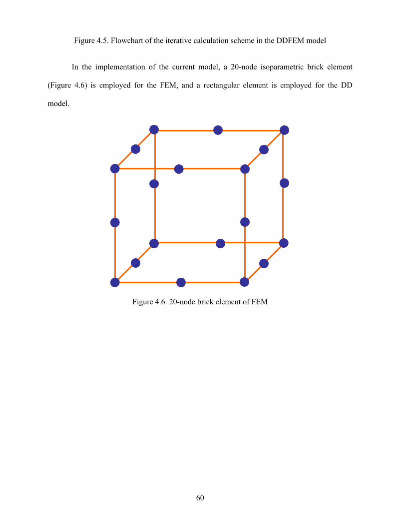
60
Figure 4.5. Flowchart of the iterative calculation scheme in the DDFEM model
In the implementation of the current model, a 20-node isoparametric brick element
(Figure 4.6) is employed for the FEM, and a rectangular element is employed for the DD
model.
Figure 4.6. 20-node brick element of FEM

61
Chapter 5 Model Verification
Numerical models mentioned in the previous chapters, including the finite element models and
boundary element models, are verified in this chapter.
5.1 One Dimensional Consolidation
Consider a one-dimensional consolidation case (Figure 5.1). Isoparametric 20-node brick
elements are employed, and the domain is discretized into 4 elements with 56 nodes. The
material properties used are as follows.
Figure 5.1. One-dimensional Consolidation Model
Young’s modulus E 1 MPa
Poisson’s ratio ν 0.3
Hydraulic conductivity k/μ 100 M m4/N·s

62
Initial porosity φ 0.28
Fluid bulk modulus Kf 100 MPa
Boundary conditions and initial conditions are as follows: an external surface load of q
= 0.10 MPa was applied at the top surface of the model, the fluid is allowed to drain through
both the top and the bottom surfaces, and no-lateral-strain is imposed on horizontal
displacements. The following figures (5.2, 5.3) and table (5.1) compares initial and final
values from the FEM model (after 50 iterations) and the closed-form poroelastic solutions (in
solid lines); high precisions are reported for purposes of comparison only.
Vertical Displacement vs. Depth Development with Time
-7.50E-01-7.25E-01-7.00E-01-6.75E-01-6.50E-01-6.25E-01-6.00E-01-5.75E-01-5.50E-01-5.25E-01-5.00E-01-4.75E-01-4.50E-01-4.25E-01-4.00E-01-3.75E-01-3.50E-01-3.25E-01-3.00E-01-2.75E-01-2.50E-01-2.25E-01-2.00E-01-1.75E-01-1.50E-01-1.25E-01-1.00E-01-7.50E-02-5.00E-02-2.50E-020.00E+00
0 1.25 2.5 3.75 5 6.25 7.5 8.75 10
Depth(m)Dis
p(m
)
1
2
3
4
5
8
13
19
50
Figure 5.2. Deformation evolution

63
Pressure Profile(Mpa) Development with Time
0.00E+004.20E-038.40E-031.26E-021.68E-022.10E-022.52E-022.94E-023.36E-023.78E-024.20E-024.62E-025.04E-025.46E-025.88E-026.30E-026.72E-027.14E-027.56E-027.98E-028.40E-028.82E-029.24E-029.66E-021.01E-011.05E-01
0 2.5 5 7.5 10
1
3
5
7
10
20
30
40
50
Figure 5.3. Pressure evolution
Table 5.1 Comparison between the solution from FEM and analytical solution
Parameter FEM Solution Analytical Solution
Initial pressure 0.09962456 MPa 0.0996245 MPa
Initial displacement 0.27894361×10⁻³ m 0.2789429×10⁻³ m
Final pressure 0.000224 MPa 0 (at t = ∞)
Final displacement 0.7418612 m 0.74285 m

64
5.2 Mandel’s Problem
Mandel’s problem has been used as a benchmark problem for testing the validity of the
numerical codes of poroelasticity (Christian et al. 1970; Cheng et al. 1988). Mandel’s problem
involves an infinitely long rectangular specimen sandwiched at the top and the bottom by two
rigid frictionless and impermeable plates. The lateral sides are free from normal and shear
stress, and pore pressure (See Figure 5.4).
Figure 5.4. Mandel’s Problem geometry
At += 0t a force of 2F per unit thickness of the specimen is applied at the top and
bottom. As predicted by the Skempton effect (Skempton 1954), a uniform pressure rise will be
generated inside the specimen. As time goes on, pore pressure near the side boundaries will
dissipate due to the drainage. Later the pressure depletion region will propagate into the center
of the specimen. Fluid drainage will finally stop once the initial pressure rise totally vanishes

65
over the entire domain. The analytical solution for the pore pressure is given as (Mandel 1953;
Abousleiman et al. 1996):
( )22
1/expcoscos
cossinsin
3)1(2
actaa
vFBp ii
i
i iii
iu βββ
ββββ
−⎟⎠⎞
⎜⎝⎛ −
−+
= ∑∞
= (5.1)
where iβ satisfies
iu
i vvv ββ
−−
=1tan (5.2)
To simulate this problem by our 3D FEM model, we set the dimensions of the
specimen and material properties as follows: 100ma = , 10mb = , 81.0 10 NF = × , 0 0.0Pap = ,
81.0 10 PaE = × , 2.0=v , 0.1=α , 141.0 10 PafK = × , 141.0 10 PamK = × , 2.0=φ , 0.1Dk = ,
1.0cPfμ = .
Figure 5.5 shows the comparison of the numerical and analytical results for pore
pressure at different time. The non-monotonic pore pressure response under the centre of the
strip (first rising, then falling), known as the Mandel-Cryer effect (Cryer 1963), can be
observed. This is because the initial presence of the pore pressure adds to the apparent
compressive stiffness of the specimen, and the specimen becomes more compliant near the side
with the reduction of the pore pressure. By the compatibility requirement, there is a load
transfer of compressive total stress towards the effectively stiffer (as-yet undrained) center
region. This transferring works as a pore pressure generation mechanism such that the pressure
in the centre region continues to rise after its initial creation (Abousleiman et al. 1996). As
mentioned, this is a strain and stiffness effect, and can only be addressed by methods that
afford correct coupling of displacements and pressures. The faithful replication by the FEM
model is part of the demonstration of verification.

66
Mandel's Problem Pore Pressure Distribution Along X axis
0.00
0.10
0.20
0.30
0.40
0.50
0.60
-1 -0.8 -0.6 -0.4 -0.2 0 0.2 0.4 0.6 0.8 1
x
Nor
mal
ized
Por
e Pr
essu
re FEM_t=1.0E4s FEM_t=1.0E5sFEM_t=5.0E5s FEM_t=8.0E5sFEM_t=1.0E6s AnalyticalAnalytical AnalyticalAnalytical Analytical
Figure 5.5. Mandel’s Problem pore pressure distribution along the x-axis (normalized pore pressure = ap/F)
5.3 Partially Saturated Elastic Consolidation
In order to correctly illustrate the governing equations and constitutive relationships upon
which the numerical model is based, the numerical model is validated through a partially
saturated elastic consolidation problem initially solved by Dakshanamurthy and Fredlund
(1981), and later on by Schrefler et al. (1995), Lewis et al. (1998), and Rahman et al. (1999).
Geometry and FE discretization are shown in Figure 5.6.
The soil column was assumed to be unsaturated with an initial water saturation of 0.52.
The initial pore water pressure boundary was -280 kPa. The boundary condition is as follows:
the lateral surface and bottom surface are not supposed to move horizontally and vertically
respectively, and are not permeable to both fluids. The prescribed pressure at the top surface is,
Pw = -420kPa, Pa = Patm. The following data were assumed: Column height L = 1.0m, E =

67
6000 kPa, Kf = 2 × 10⁶ kPa, Km= 1.4 × 10⁶ kPa, ν = 0.4, k = 4.6 × 10⁻¹² m2, μw = 1.0cP, μa =
0.018cP, Pb = 225.0kPa, λ = 3.0, Swc = 0.3966, ϕ = 0.3.
Figure 5.6. Partially Saturated Elastic Consolidation Model
Figures representing the final results are as follows: Figure 5.7 shows the vertical
displacements for selected points in consolidation process; and, Figure 5.8 shows the pore
water pressure distribution throughout the soil layer at different time steps. The model
describes the behavior of partially saturated soil systems under environmental changes and the
results agree well with the results obtained by previous researchers (Lewis et al. 1998, Rahman
et al. 1999).

68
-3.0
-2.5
-2.0
-1.5
-1.0
-0.5
0.0
0.01 0.1 1 10 100
Time (days)
Vert
ical
dis
plac
emen
t (m
)/100
0
1.00m
0.50m
0.07m
Figure 5.7. Vertical displacement profile
-430
-410
-390
-370
-350
-330
-310
-290
-270
-250
0 0.2 0.4 0.6 0.8 1Height(m)
Wat
er P
ress
ure(
kPa)
0.01days
0.10days
0.30days
0.50days
2.00days
100.0days
Figure 5.8. Pore pressure profile

69
5.4 Thermal Consolidation
We now do verification through a thermo-elastic one-dimensional consolidation problem
solved previously by Aboustit et al. (1985). Geometry and FE discretization are shown in
Figure 5.9.
A column of linear elastic material is subjected to a unit surface pressure (q = 1.0 kPa)
and a constant surface temperature T = 50oC. The following data were assumed: Column
height L = 7m, E = 6000kPa, Kf = Km = 1012kPa, v = 0.4, ϕ = 0.5, ρfcf = 0.0, k/μ = 4×10⁻⁶m4 kN-
1 s-1, λT = 0.2 kCal m-1 s-1 ºC-1, βs = 0.9×10⁻⁶ ºC-1, βf = 0.63×10⁻⁵ ºC-1, ρscs = 40kCal m-3 ºC-1.
Only the top of the column is permeable.
Figure 5.9. One-dimensional Consolidation Model
The Figures that represent the final results are as follows: Figure 5.10 shows the temperature
change with time, Figure 5.11 shows the pressure change with time, and Figure 5.12 shows the
displacement change with time. All of these curves have a good agreement with the results
presented by Aboustit (1985) and Lewis (1998).

70
05
101520253035404550
0.1 1 10 100 1000 10000
Time (s)
Tem
pera
ture
(ºC
)
05
101520253035404550
0.1 1 10 100 1000 10000
Time (s)
Tem
pera
ture
(ºC
)
Figure 5.10. Temperature (oC) vs. time (s) at mid column node
00.10.20.30.40.50.60.70.80.9
11.1
0.01 0.1 1 10 100 1000
Time (s)
Pres
sure
(kPa
)
00.10.20.30.40.50.60.70.80.9
11.1
0.01 0.1 1 10 100 1000
Time (s)
Pres
sure
(kPa
)
Figure 5.11. Pressure vs. time at mid column node

71
-5.0E-04
-4.0E-04
-3.0E-04
-2.0E-04
-1.0E-04
0.0E+000.01 0.1 1 10 100 1000 10000
Time (s)
Dis
plac
emen
t (m
)
-5.0E-04
-4.0E-04
-3.0E-04
-2.0E-04
-1.0E-04
0.0E+000.01 0.1 1 10 100 1000 10000
Time (s)
Dis
plac
emen
t (m
)
Figure 5.12. Deformation (m) vs. time (s) at top surface
5.5 Partially Saturated Thermal Consolidation
This verification deals with a thermoelastic consolidation of partially saturated clay for which
previous solutions are known (Dakshanamurthy and Frelund 1981, Schrefler et al.1995). In
the former, a constant permeability and thermal properties case was studied; in the latter, the
problem was solved for the relationships between relative permeabilities of water and air, using
the Sw - capillary pressure relationship of Brooks and Corey (1966).
A 100 mm layer of partially saturated clay (Sw = 0.89), initially in a state of
equilibrium, is subjected to a sudden environmental change. A surface temperature jump of 15
K and a capillary pressure jump of 140 kPa cause simultaneous heat and mass transfer
(corresponding to a drying process caused by warm dry-air flux). Parameters are E = 60×103
kPa, v = 0.4, φ = 0.5, Km = 1.4×10⁶ kPa, Kw = 1.0×10⁶ kPa, k = 10.0 D, µw = 1 cP, µair = 1 cP,

72
ρs = 1.8×10³ kg/m3, ρw = 1.0×10³ kg/m3, ρair = 1.22 kg/m3, B0w =1.0, and air is considered to
be an ideal gas. Also, βs = 1.0×10⁻⁶ K-1, βw = 0.63×10⁻⁵ K-1, cs = 30.0 kCal/kg-K, cw = 50.0
kCal/kg-K, cair = 0.0, and the thermal conductivity λT = 0.4574 cal/m-s-K. The relationships in
Brooks & Corey’s formulation for relative permeabilities of water and gas, as well as for Sw-
capillary pressure, were assumed as follows:
(2 3 ) /c crw ek S λ λ+= (5.3)
( ) ( )c c(2 λ )/λ2rg e ek 1 S 1 S += − − (5.4)
c1 /λc b eP P S −= (5.5)
w wce
wc
S SS
1 S−
=−
(5.6)
Here, Se is effective saturation, bubble-point pressure Pb = 316.6 kPa, irreversible saturation
Swc = 0.2114, and the constant λc = 0.80, which corresponds to the given saturation-capillary
pressure values for consolidation in Dakshanamurthy et al.’s case. The initial conditions were:
T = 283.15 K, Pg = 102 kPa, Pw = -280 kPa.
The boundary conditions were the following: for the lateral surface, qT = 0, qw = 0, qg =
0, uh = 0; for the top surface, T = 298.15 K, Pg = 102 kPa, Pw = -420 kPa; and, for the bottom
surface, qT = 0, qw = 0, qg = 0, and uv = 0.
Figures 5.13 to 5.15 show the temperature, water pressure, and air pressure during
consolidation calculated by our FEM model (shown in colored lines) and along with the results
by Dakshanamurthy et al. (1981) (shown in black lines) for comparison. It can be seen that
results obtained by our FEM model largely agree well with those obtained by Dakshanamurthy
et al., which were calculated through separate analytical equations. It should be noted that the
time needed for pressure dissipation in our results is longer than that by Dakshanamurthy et al.

73
because they used a constant relative permeability value, and based on the given relative
permeability curve and capillary curve, the water saturation profile during consolidation is
shown in Figure 5.16. Furthermore, because the equilibrium equation is not considered in the
Dakshanamurthy et al.’ case, pore air pressure buildup is observed. This is not the case when
the equilibrium equation is coupled, because the total stress should remain constant as no
external load is enforced on the clay. Based on the given modulus, the vertical deformation
profile is shown in Figure 5.17.
Temperature(K)
Dep
th( c
m)
284 286 288 290 292 294 296 2980
2
4
6
8
10
8.89hrs
17.7hrs
35.6h
rs
71.1
hrs
142.
2hr
s
854
hrs
Temperature(K)
Dep
th( c
m)
284 286 288 290 2
Temperature(K)
Dep
th( c
m)
284 286 288 290 292 294 296 2980
2
4
6
8
10
8.89hrs
17.7hrs
35.6h
rs
71.1
hrs
142.
2hr
s
854
hrs
Figure5.13. Profile of temperature during consolidation

74
Pore water pressure (kPa)
Dep
th(c
m)
-420-400-380-360-340-320-300-2800
2
4
6
8
10
4.44 hrs
8.89 hrs
17.7 hrs
35.6hrs
71.1
hrs
142.
2hr
s
284
hrs
569
hrs
854
hrs
Figure 5.14. Profile of water pressure during consolidation
Pore air pressure (kPa)
Dep
th(c
m)
3042546678901020
2
4
6
8
10
4.44hrs
8.89 hrs
17.7 hrs
35.6hrs
71.1
hrs
142.
2hr
s
284
hrs
569
hrs
854
hrs

75
Figure 5.15. Profile of air pressure during consolidation
Water saturation
Dep
th(c
m)
0.740.790.840.890
2
4
6
8
10
4.44 hrs
8.89 hrs
17.7hrs
71.1
hrs
142.
2hr
s28
4hr
s56
9hr
s
854
hrs
Figure 5.16. Profile of water saturation during consolidation

76
Vertical displacement (m)
Dep
th(c
m)
-0.000125-0.000100-0.000075-0.000050-0.0000250.0000000
2
4
6
8
10
4.44 hrs
8.89 hrs
17.7
hrs
71.1
hrs
142.2hrs
569 hrs854 hrs
Figure 5.17. Profile of vertical displacement during consolidation
5.6 Underground excavation
To verify the DD model based on rectangular elements with a constant displacement
discontinuity variation, we use the 3-D boundary element model (BEM) (Figure 5.18) to
compute a sample problem, and compare the results from it with those from the DD model.
3D DDM
• Domain: Semi-Infinite.
• 20.0m 20.0m 2.0m× × Excavation and the ground surface.
• 30m deep underground.
• mDDz 1= is prescribed on the excavation.
• 1GPa, 0.333E v= = .
• Discretized with rectangular elements.

77
• 2025(= 2599 ×× ) elements.
3D BEM
DD elements representing the excavation
Boundary elements on the ground surface and excavation surfaces
DD elements representing the excavation
Boundary elements on the ground surface and excavation surfaces
Figure 5.18. 3-D Semi-infinite domain excavation problem solved by DDM and BEM
• Domain: Semi-Infinite.
• 20.0m 20.0m 2.0m× × Excavation and the ground surface.
• 30m deep underground.
• 0.5427m, 0.4573mZ ZU U= − = are prescribed on top and bottom surface,
respectively.
• Traction free surface is prescribed.
• 1.0GPa, 0.333E v= = .
• Discretized with 4-node rectangular elements.
• 1199 nodes (plus 121 interior nodes).
• 1166 elements.

78
Figure 5.19 shows the vertically induced stress calculated from DDM and BEM; Figure 5.20
shows surface subsidence calculated from DDM and BEM. These results show the satisfactory
accuracy of the DD method.
Stress ZZ along X axis on the top surface of an excavation at depth of 30m (discretized with 1166 elements)
-0.200-0.180-0.160-0.140-0.120-0.100-0.080-0.060-0.040-0.0200.0000.0200.0400.0600.0800.1000.1200.1400.1600.1800.2000.220
-22 -20 -18 -16 -14 -12 -10 -8 -6 -4 -2 0 2 4 6 8 10 12 14 16 18 20 22
X (m)
Stre
ss (M
Pa)
DDM(0.5m above the top surface)
BEM (0.5m above the top surface)
Figure 5.19 Vertically induced stress calculated from DDM and BEM

79
Subsidence bowl (due to excavation of 20X20X2 at 30m depth)
-0.2
-0.18
-0.16
-0.14
-0.12
-0.1
-0.08
-0.06
-0.04
-0.02
0-55 -50 -45 -40 -35 -30 -25 -20 -15 -10 -5 0 5 10 15 20 25 30 35 40 45 50 55
Distance from center in X axis direction(m)
disp
lace
men
t(m)
BEMDD
Figure 5.20. Surface subsidence calculated from DDM and BEM
5.7 Geertsma’s Solution
To verify the DDFEM model, we consider a m4m20m20 ×× reservoir at depth of 300m (in
reality, it could be much deeper) with the following basic parameters (see Figure 5.21):
41 10 kPaE = × , v = 0.3, ϕ = 0.28, 61 10 kPafK = × , kPaK m6101×= , k = 1.0D, µ = 1.0cP.

80
Figure 5.21. Mesh of the reservoir FEM model
Convergence of DD
-0.184
-0.182
-0.18
-0.178
-0.176
-0.174
-0.172
-0.17
-0.168
-0.166
0 5 10 15 20 25 30 35 40
Iterat io ns
Figure 5.22. Convergence of the Displacement Discontinuity
The reservoir has an impermeable boundary, and is supposed to be under a production
rate Q = 0.5m3/min with uniform pumping. The purpose of this is to obtain a uniform pressure
decline inside the reservoir. The advantage is that we can substitute the uniform pressure into
Geertsma’s analytical solution later on. In the present problem, the time step is set as Δt =
120minutes.
In the FEM mesh, the domain is discretized into 50 elements, 360 nodes; in DDM
mesh, the domain is discretized into 25 DD elements.

81
Convergence is shown in Figure 5.22, continuity of stress is demonstrated by the
consistency of the stresses from both the FEM model and DD model (Figure 5.23), and the
subsidence profile at different time steps is shown in Figure 5.24.
We select Geertsma’s solution in particular case, which is close to our case. We will
compare the result of the FEM-DDM model with Geertsma’s analytical solution in the
following: Geertsma (1966) came up with the analytical solution to the subsidence caused by
Vertical stress profile
-27
-24
-21
-18
-15
-12
-9
-6
-3
00 2 4 6 8 10 12 14 16 18 20
X( m)
FEM
DDM
Figure 5.23. Continuity of stresses

82
Displacement profile(m)
-0.12
-0.1
-0.08
-0.06
-0.04
-0.02
00 5 10 15 20
X(m)Di
spla
cem
ent(m
) 12345
Figure 5.24. Subsidence profile at different times
a uniform pressure decline in a fluid saturated reservoir as follows: for 0=r and a pΔ which is
constant throughout the reservoir, the vertical displacement can be expressed as:
( )1 1 3
2 2 22 2 2 22 2
(0, )2
3 4 ( 1)( 1) 2 (3 4 )1 ( 1)1 ( 1) 1 ( 1)
mz
c hu z
v C ZC Z CZ v pC ZC Z C Z
ε
= −
⎡ ⎤− +−⎢ ⎥− + + − + Δ⎢ ⎥
⎡ ⎤+ +⎢ ⎡ ⎤ ⎡ ⎤ ⎥+ − + + ⎣ ⎦⎣ ⎦ ⎣ ⎦⎣ ⎦
(5.7)
where Z = z/c, C = c/R and 1−=ε for z > c, and 1+=ε for z < c, respectively. Thus the elastic
surface subsidence above the centre of a disc-shaped depleted reservoir amounts to
( ) ⎟⎟⎠
⎞⎜⎜⎝
⎛
+−Δ−−=
211)1(20,0
CCphcvu mz (5.8)

83
The calculation based on the DDFEM model and Geertsma’s solution is done by computer and
by spreadsheet respectively. The comparison is shown in Table 5.2. The result from this hybrid
method shows high consistency with that by Geertsma (1966).
Table 5.2 Comparison between the Geertsma’s Solution and DDFEM model
subsidence at the centre
Time E(kPa) v Thick(h) ~Radius(m) Depth(m) Drawdown(kPa) Ratio(D/R) Geertsma(m) DDFEM(m) Rel. Err.
2hrs 10000 0.3 4 11.283 300 -314.103 26.586808 -9.23E-05 -9.30E-05 0.68%
4hrs 10000 0.3 4 11.283 300 -635.232 26.586808 -1.87E-04 -1.86E-04 -0.35%
6hrs 10000 0.3 4 11.283 300 -957.137 26.586808 -2.81E-04 -2.79E-04 -0.77%
8hrs 10000 0.3 4 11.283 300 -1278.716 26.586808 -3.76E-04 -3.72E-04 -0.97%
5.8 Rothenburg’s Solution
Another verification of the DDFEM model is through the comparison with Rothenburg et al.’s
analytical solution. It has been more and more recognized that the stiffness of the interbeds is
an essential coupling element which must be taken into account. In a semi-analytical solution
to single phase flow into a single well in an infinite reservoir developed by Rothenburg et al.
(see Rothenburg et al. 1994; Charlez 1997), coupling of reservoir deformation with overburden
effects is achieved through stress-strain (σ-ε) coupling to pressure changes, referred to by some
as stress-deformation analysis. Coupling is introduced through two dimensionless coefficients,
χ and β, which address relative stiffness and relative thickness issues between the extremes of
“infinitely soft” (fluid) or “infinitely stiff” (totally rigid) conditions for the overburden strata.
2
1 211 1 4
or r
o r o
C hC R
ννχν ν
−+=
− − (5.9)

84
2
2
13 3
1( )3 3
r r
r
m r rf
r
C
C CC
α νφ νβ
α να φφ φ ν
−+
=−
+ − ++
(5.10)
Here, Cr and Co are the bulk compressibility of the reservoir and surrounding strata
respectively, Cm is the compressibility of solid matrix, Cf is the compressibility of the fluid, νr
and νo are the Poisson’s ratios for the reservoir and surrounding strata respectively, and φ is the
porosity. Also, h and R are the thickness and radius of the circular reservoir.
The coefficient χ expresses the ratio of the stiffness (Cr/Co) of the reservoir and
overburden and the aspect ratio (h/R) of the reservoir. For thin reservoirs (h/R → 0) and
extremely soft overburden (Co >> Cr), χ ≈ 0, the solution is decoupled, and pressure changes
are governed only by the oedometric compressibility (one-dimensional compression with no
lateral strain), and the compaction induces no redistribution in the vertical stress, σv. In
contrast, for thick reservoirs and extremely “rigid” interbeds (Co << Cr), χ >> 1, no compaction
occurs in the case of a single well because of perfect stress arching (the overburden is so rigid
that it accommodates all stress changes without deformation). These χ limits are decoupled
cases that are not attained in practice; any oilfield subjected to drawdown will evidence some
compaction, and interbeds always have some stiffness, usually within a factor of 0.5 to 2 of the
reservoir itself.
β, unlike χ, depends only on the reservoir properties; it describes the ratio of the
reservoir rock matrix compressibility (Cr) to the bulk compressibility of the reservoir-fluid
system (a combination of Cf, Cm and Cr). When Cf << Cr, β ≈ 1, and stress redistribution
effects are the most pronounced. When Cf is very large, for example when the pore fluid
contains large amounts of compressible gas, β ≈ 0, and stress redistribution effects are
negligible. For highly compressible fluids (e.g. gas reservoirs), the pressure term becomes

85
dominant in the diffusion equation compared with the compaction term, which re-decouples
the solution.
For a pressure drawdown problem in a poroelastic reservoir subjected to pumping, the
problem is formulated in a poroelastic context so that the solution fully accounts for stress
redistribution effects around the well, as well as for the effects of stress changes on fluid flow.
Note that this has nothing to do with any non-linearity in the system; it is merely the elastic
overburden response to reservoir volume changes caused by the pressure changes. The
poroelastic, fluid-saturated reservoir is considered to be planar and surrounded by an
impermeable elastic material of infinite extent. The governing equation for fluid pressure was
derived using a general elastic axisymmetric approach while assuring compatibility of
displacement and stresses at the interface between the reservoir and the surrounding material.
The resulting second-order integro-differential equation is solved using the Hankel transform,
so that the given solution for pressure change due to a flow rate Q is as follows:
02
201 exp d
2 11
w
w
rJrQ ktP
kh c r
ξμ ξ ξχξπ μ φ ξβ
χξ
∞
⎛ ⎞⎛ ⎞⎛ ⎞⎜ ⎟⎜ ⎟⎜ ⎟ ⎝ ⎠⎜ ⎟⎜ ⎟Δ = − − −
⎜ ⎟⎜ ⎟−⎜ ⎟⎜ ⎟+⎝ ⎠⎝ ⎠
∫ (5.11)
where k is permeability, μ is the viscosity, rw is the well radius, ξ is a transformed variable for
the Hankel transform, and J0 is the Bessel function of the first kind, zeroth order.
5.8.1 Reservoir Scale Problem
In this section, we attempt to investigate the problem of the vertical stress changes as a result
of pressure depletion which has been solved by Rothenburg solution (Rothenburg et al. 1994).
The model is still based on basically the same parameters of the reservoir we used in last
section’s verification, except that we change the stiffness of the overburden, in order to show

86
that changes in effective stress (leading to compaction) are strongly related to a relative
stiffness Rχ . Firstly, we need to defined a relative stiffness χR as follows,
2
1 211 1 4
or rR
o r o r r
vC v hC v v R R
χχ −+= =
− − (5.4)
The correspondence between the stiffness of the overburden and the relative stiffness is as
follows:
Figure 5.25. Change in effective stress with reservoir depletion (After Rothenburg et al. 1994)
χR 0.0 0.2 0.5 1.0 2.0 6.0
Eo(kPa) 0.0 27,640 69,110 138,220 276,430 829,300

87
Changes in effective stress as a result of reservoir depletion
0
0.2
0.4
0.6
0.8
1
0 0.5 1Distance from reservoir centrer
Cha
nge
in e
ffect
ive
stre
ss
X=0 X=0.2 X=0.5X=1 X=2 X=6
Figure 5.26. Change in effective stress with reservoir depletion
The comparison between the numerical results (Figure 5.26) and analytical results (Figure
5.25) shows good agreement in the centre of the reservoir. Some gap between the two results in
edge of the reservoir is due to the shape effects (analytical model is in an axisymmetric shape,
numerical model is in 3D brick shape), but the tendency of curves is consistent.
5.8.2 Single Producing Well
Based on the above analytical solution, an interesting phenomenon about a single producing
well, which is similar to Mandel-Cryer effect, can be observed. This can be observed only
when coupled reservoir and surroundings are correctly considered in simulation.

88
In this section, we want to investigate this problem using the numerical model. We
consider a m4m21m21 ×× reservoir at depth of 300m with the following basic parameters
(see Figure 5.27): 41 10 kPaE = × , v = 0.3, ϕ = 0.28, 61 10 kPafK = × , 61 10 kPamK = × , k =
1.0D, µ = 1.0 cP.
Producing wellProducing well
Figure 5.27. Geometry and mesh of the reservoir model
The reservoir is subjected to a zero pressure boundary, and is supposed to be under a
production rate Q = 0.5m3/min (i.e. 720 m3/day) from a single well at the center of the
reservoir.
In the FEM mesh, the domain is discretized into 72 elements, 497 nodes; in the DDM
mesh, the domain is discretized into 36 DD elements.

89
- 12 0 0
- 10 0 0
- 8 0 0
- 6 0 0
- 4 0 0
- 2 0 0
0
2 0 00 3 .5 7 10 .5 14 17.5 2 1
X(m)
Pres
sure
(kPa
)
1min2 min3 min10 min2 0 min3 0 min6 0 min
Figure 5.28. Pressure changes at different time
- 2 50
- 2 0 0
- 150
- 10 0
- 50
0
50
10 00 10 2 0 3 0 4 0 50 6 0
Time(minutes)
Pres
sure
(kPa
)
Figure 5.29. Pressure evolution in a node adjacent to the producing well

90
In Figures 5.28 and 5.29, the non-monotonic pore pressure response adjacent to the
centre of the strip (first rising, then falling), similar to the Mandel-Cryer effect, is observed.
This is because the initial sharp removal of the fluid from the single well at the centre of the
reservoir considerably softens the center reservoir region. By the compatibility requirement,
there is a load transfer of compressive total stress towards the effectively stiffer region adjacent
to the center. This transferring works as a pore pressure generation mechanism such that the
pressure in the region adjacent to the centre rises for a while before its dissipation later on. The
faithful replication by the DDFEM model is part of the demonstration of verification.

91
Chapter 6 Numerical Experiments
Based on the models described in the previous chapters, some numerical experiments are
conducted in analyzing the petroleum reservoir compaction/expansion, ground surface
subsidence/heave, pressure drawdown/buildup, stress changes, and temperature distributions in
some scenarios.
6.1 Ground subsidence in a half-space
In this example, we want to look into the computational efficiency of the DDFEM method. It
only took 2 minutes for the program to finish the problem. However, when the finite element
method alone is employed to solve the problem, the outer boundary of the domain must be
extended reasonably far from the reservoir, and it needs to be meshed inside the entire domain
(Figure 6.1).
We consider a 25m 25m 4m× × reservoir at depth of 300m with the following basic
parameters (see Figure 6.1): 42.0 10 kPaE = × , v = 0.25, ϕ = 0.30, 61 10 kPafK = × ,
81 10 kPamK = × , k = 1.0D, µ = 22.0cP.
The parameter for the surrounding rock is as follows: 52.0 10 kPaE = × , v = 0.25.
The reservoir has an impermeable boundary, and is supposed to be under a production
rate Q = 720.0m3/day with uniform pumping. The time step is set as Δt = 0.1 days. We want to
predict the subsidence with time.

92
Firstly we use the DDFEM model to solve this problem. In the FEM mesh, the domain
is discretized into 50 elements, 360 nodes; in DDM mesh, the domain is discretized into 25 DD
elements.
Ground surface
Reservoir
Ground surface
Reservoir
Figure 6.1. Fine finite element discretization of the reservoir and surroundings
It only took 2 minutes for the program to finish the problem. The ground surface
subsidence evolution curves produced by DDFEM model along the diagonal direction are
shown in Figure 6.2. The lateral ground surface movement curves produced by DDFEM model
along the diagonal direction are shown in Figure 6.3. It should be noted that we did not put the

93
complete solution provided by the DDFEM model into these two figures. They are
approaching to zero with distance from the center.
However, when the finite element method is employed to solve the problem, the outer
boundary of the domain must be extended to be reasonably far from the reservoir, and it needs
to be meshed inside the entire domain.
When we still use 5×5×2 finite elements accounting for the reservoir domain, there are
totally 35×35×14 finite elements for the reservoir and its surroundings (Figure 6.1). The
reservoir is in layers 5 and 6 in the vertical direction, and from gridblocks 16 to 20 in the
horizontal directions. The sideburden, underburden and overburden are obtained by extending
75m, 40m and 300m from the side, bottom and top of the reservoir, respectively, discretized
uniformly in each zone. To solve the same problem, the full finite element model took 241
minutes, which is 120 times as long as the DDFEM model.
The ground surface subsidence evolution curves produced by FEM model along the
diagonal direction are shown in Figure 6.2. The lateral ground surface movement curves
produced by FEM model along the diagonal direction are shown in Figure 6.3.
This shows that the DDFEM model is excellent in computing efficiency compared to
the full FEM model.

94
-1.6E-02
-1.4E-02
-1.2E-02
-1.0E-02
-8.0E-03
-6.0E-03
-4.0E-03
-2.0E-03
0.0E+00-250 -150 -50 50 150 250
r (m)
Z(m
)
t = 0.1 days @DDFEMt = 0.2 days @DDFEMt = 0.3 days @DDFEMt = 0.4 days @DDFEMt = 0.5 days @DDFEMt = 0.1 days @FEMt = 0.2 days @FEMt = 0.3 days @FEMt = 0.4 days @FEMt = 0.5 days @FEM
Figure 6.2. Comparison of ground surface subsidence profiles predicted by DDFEM model and FEM model

95
-2.0E-03
-1.5E-03
-1.0E-03
-5.0E-04
0.0E+00
5.0E-04
1.0E-03
1.5E-03
2.0E-03
-250 -150 -50 50 150 250
r (m)
u x(m
)
t = 0.1 days @DDFEMt = 0.2 days @DDFEMt = 0.3 days @DDFEMt = 0.4 days @DDFEMt = 0.5 days @DDFEMt = 0.1 days @FEMt = 0.2 days @FEMt = 0.3 days @FEMt = 0.4 days @FEMt = 0.5 days @FEM
Figure 6.3. Comparison of lateral ground surface movements predicted by DDFEM model and FEM model

96
We can see the significant differences between the outcomes of the two models from
Figures 6.2 and 6.3. It was calculated that the subsidence ‘volume’ taken place at the ground
surface produced by the DDFEM model and FEM model are close. Obviously, the limited
reservoir outer domain included in the FEM model caused the inaccuracy and even led to
wrong “predictions”. However if the outer domain of the FEM model is extremely large to
account for the right predictions, the computing efforts will be accordingly huge.
6.2 Noordbergum effects
In this section, we will revisit Theis’ solution as well as the aforementioned Rothenburg et al.’s
analytical solution (referred to as RBD model later on) and the numerical DDFEM model to
investigate the effects of the stiffness of the surroundings on the pressure drawdown in a
poroelastic reservoir due to pumping.
The Theis solution gives the pressure drawdown within a pumping reservoir at a radial
distance, r, and at time, t, as
2
4 4Q c rp Ei
kh ktμ μ φ
π⎛ ⎞
Δ = − −⎜ ⎟⎝ ⎠
(6.1)
where Q is the pumping rate at the reservoir center, k is the permeability, μ is viscosity, φ is
porosity, c is the compressibility of the reservoir, h is the thickness of the reservoir, and Ei is
the exponential integral function.
It may be useful here to note that the Theis solution (Theis 1935) and all other
subsequent well behavior solutions have been derived with the implicit assumption that the

97
overburden strata are infinitely soft; therefore, these solutions cannot accommodate stress
redistribution effects, so there is no coupling within them.
Suppose a reservoir of dimensions 1000 m × 1000 m × 20 m with a pumping well at the
center extracting 1000 m3/day. The pressure at the lateral boundaries is maintained the same as
that at the initial state. The bottom of the reservoir is fixed both vertically and horizontally, the
four sides are fixed horizontally, and the top is free to move. Physical parameters of the
reservoir are set as follows. Er = 9.0×10² MPa, νr = 0.3, φ = 0.25, Kf = 2.25×10³ MPa, Km =
1.0×10⁴ MPa, k = 58.633 D, μ = 1.0 cP. The physical parameters of the reservoir surroundings
are: Eo = 9.0×10³ MPa, νo = 0.3. Finite element discretization of the reservoir zone is as shown
in Figure 6.4.
Using the DDFEM model and RBD model respectively, we investigated the pressure
drawdown at a distance of 250 m from the well; Figures 6.5 and 6.6 show the pressure
drawdown curve at times of 0.0025 days and 0.005 days respectively. The pressure drawdown
curve obtained through Theis’s solution for identical parameters is displayed in Figure 6.7.
The short time scales here are deliberately chosen to clearly show the Noordbergum
effect (Verruijt 1969), which describes the increase of pore pressure at some distance away
from the pumping well in a reservoir or aquifer, while usually a monotonic pressure
drawdown is expected in this case if only Theis-type equations are used. Indeed, in comparing
Figures 6.5 and 6.6 to Figure 6.7, we can clearly see the Noordbergum effects in the fully
coupled model DDFEM and RBD, but not in the Theis-type solution results.
Next we investigate the complete overburden effects on pressure drawdown. Keeping
the basic parameters above unchanged, we only change the stiffness of the reservoir
surroundings from Eo = 9.0×10³ MPa to Eo = 1.8×10⁴ MPa (a doubling of the overburden
stiffness). Figure 6.8 shows the results from these two cases, and we note that the

98
Noordbergum effect is more pronounced with a stiffer surrounding rock, and the pressure is
also higher.
Figure 6.4. FEM mesh for a 1000m ×1000m × 20m reservoir.
Pressure drawdown till T=0.0025days
-0.00019-0.00018-0.00017-0.00016-0.00015-0.00014-0.00013-0.00012-0.00011-0.0001
-0.00009-0.00008-0.00007-0.00006-0.00005-0.00004-0.00003-0.00002-0.00001
00.00001
0 0.00025 0.0005 0.00075 0.001 0.00125 0.0015 0.00175 0.002 0.00225 0.0025
Time.days
Pres
sure
.MPa
DDFEM @ R=250 RBD @ R=250
Figure 6.5. Pressure drawdown till 0.0025days solved by RBD model and DDFEM model.

99
Pressure drawdown till T=0.005days
-0.00039-0.00037-0.00035-0.00033-0.00031-0.00029-0.00027-0.00025-0.00023-0.00021-0.00019-0.00017-0.00015-0.00013-0.00011-0.00009-0.00007-0.00005-0.00003-0.000010.00001
0 0.0005 0.001 0.0015 0.002 0.0025 0.003 0.0035 0.004 0.0045 0.005
Time.daysPr
essu
re.M
Pa
DDFEM @ R=250 RBD @ R=250
Figure 6.6. Pressure drawdown till 0.005days solved by RBD model and DDFEM model
Pressure drawdown till T=0.0025days
-0.00012
-0.00011
-0.0001
-0.00009
-0.00008
-0.00007
-0.00006
-0.00005
-0.00004
-0.00003
-0.00002
-0.00001
0
0.000010 0.00025 0.0005 0.00075 0.001 0.00125 0.0015 0.00175 0.002 0.00225 0.0025
Time.days
Pres
sure
.MPa
Theis @ R=250
Figure 6.7. Pressure drawdown till 0.0025days obtained by Theis’ solution

100
Pressure drawdown till T=0.0025days
-0.00019-0.00018-0.00017-0.00016-0.00015-0.00014-0.00013-0.00012-0.00011-0.0001
-0.00009-0.00008-0.00007-0.00006-0.00005-0.00004-0.00003-0.00002-0.00001
00.000010.00002
0 0.00025 0.0005 0.00075 0.001 0.00125 0.0015 0.00175 0.002 0.00225 0.0025
Time.daysPr
essu
re.M
Pa
Softer surrounding Stiffer surrounding
Figure 6.8. Comparison of pressure drawdown with a softer and stiffer reservoir surrounding solved by DDFEM
6.3 Pressure drawdown and stresses changes
In this case, two-phase flow is considered in a production-induced compaction/subsidence
problem to study overburden effects on pressure and saturation over time. Assume a 20 m × 20
m × 4 m reservoir at z = 300 m with E = 6.0×10³ kPa, v = 0.4, ϕ = 0.3, Km = 1.4×10⁶ kPa, k =
1.0D, µw = 1.0 cP, µoil = 1.0 cP. Formation volume factor Bo = Bw = 1.0. The relative
permeability-saturation function and capillary pressure-saturation function are taken after
Brook’s formula (Brooks and Corey 1966) with Pb = 16 kPa, λc = 3.0, Swc = 0.25. The
reservoir is subjected to a single production well in the center with the initial condition: Soil =
0.70, Poil = 11.8378 kPa, and Pw = -27.6216 kPa.
First, we assume E = 12.0×10³ kPa and v = 0.4 for the reservoir surroundings. Pressure
and saturation changes at the center of the reservoir calculated by the DDFEM model are

101
shown in Figures 6.9 and 6.10, and curves obtained by a FEM model without considering
reservoir surroundings are also shown to highlight the significant effects on pressure and
saturation change during depletion. Figure 6.11 shows subsidence (Δz) at different times; Δz at
x = ± 300m is still significant compared to the center, showing that the discretized domain has
to be large to obtain a local accurate solution. With the DDFEM model, this is handled
naturally.
-2.0-1.8-1.6-1.4-1.2-1.0-0.8-0.6-0.4-0.20.0
0 1 2 3 4 5 6Time(days)
Oil
Pre
ssur
e (M
pa)
DDFEM
FEM
Figure 6.9. Poil vs Time with/without overburden (E = 12 MPa)

102
0.50
0.55
0.60
0.65
0.70
0 1 2 3 4 5 6Time(days)
Oil
Satu
ratio
n
DDFEM
FEM
Figure 6.10. Soil vs Time with/without overburden (E = 12 MPa)
-7.0E-04
-6.0E-04
-5.0E-04
-4.0E-04
-3.0E-04
-2.0E-04
-1.0E-04
0.0E+00-350 -300 -250 -200 -150 -100 -50 0 50 100 150 200 250 300 350
X(m)
Subs
iden
ce(m
)
T=1dayT=2daysT=4days
Figure 6.11. Subsidence profile with overburden (E = 12 MPa)

103
Second, we change the stiffness of the reservoir surroundings to E = 60.0×10³ kPa and
v = 0.4. Pressure and saturation changes calculated by our model are shown in Figures 6.12
and 6.13, curves obtained without considering the surroundings are still included for
comparison. Clearly, a stiffer overburden corresponds to a larger pressure drawdown and oil
saturation decrease.
Figure 6.14 shows slower subsidence, compared with Figure 6.11, thus stiffer
overburden retards compaction appearance.
-3.5
-3.0
-2.5
-2.0
-1.5
-1.0
-0.5
0.00 1 2 3 4 5 6
Time(days)
Oil
Pre
ssur
e (M
pa)
DDFEM
FEM
Figure 6.12. Poil vs Time with/without overburden (E = 60 MPa)

104
0.50
0.55
0.60
0.65
0.70
0 1 2 3 4 5 6Time(days)
Oil
Satu
ratio
n
DDFEM
FEM
Figure 6.13. Soil vs Time with/without overburden (E = 60 MPa)
-7.0E-04
-6.0E-04
-5.0E-04
-4.0E-04
-3.0E-04
-2.0E-04
-1.0E-04
0.0E+00-350 -300 -250 -200 -150 -100 -50 0 50 100 150 200 250 300 350
X(m)
Subs
iden
ce(m
)
T=1dayT=2daysT=4days

105
Figure 6.14. Subsidence profile at different time with overburden (E = 60 MPa)
6.4 Hot water flooding and ground surface uplift
In this example, we deal with a simple hot water injection problem. Suppose a 240 m × 240 m
× 20 m reservoir, 300 m deep, with E = 5.0×10⁵ kPa, v = 0.3, φ = 0.35, Km= 1.4×10⁸ kPa, k =
1.0 D, µw = 1 cP, µ0oil = 22.0 cP, ρs = 2.5×10³ kg/m3, ρw = 1.0×10³ kg/m3, ρo = 1.0×10³ kg/m3 ,
Bo0 =1.0, Bw
0 = 1.0, βs = 2.0×10⁻⁶ K-1, βw = 1.0×10⁻⁵ K-1, βo = 1.0×10⁻⁵ K-1, cs = 0.4 kJ/kg-K , cw
= 3.0 kJ /kg-K, coil = 2.0 kJ/kg-K, and λT = 2.3 J/m-s-K. Suppose a coordinate system where
the top and bottom of the reservoir are normal to the z axis, and the sides are all vertical and
normal to the X-Y plane.
Extending 12 m from the outer reservoir boundary in vertical directions is assumed to
be the T-p influence zone. In this zone, the following properties apply: E = 5.0×10⁵ kPa, v =
0.30, φ = 0.30, k = 1.0 mD, µw = 1.0 cP, βs = 2.0×10⁻⁶ K-1, ρs = 2.5×10³ kg/m3, cs = 0.4 kJ/kg-K,
and λT = 2.3 J/m-s-K. The remaining elastic part representing surrounding strata has E =
2.0×10⁶ kPa and v = 0.3.
We use a number of empirical formulae to specify certain types of behavior. The
relative permeability-saturation functions are simply defined as:
21.0 (1.0 )rw wk S= − − (6.2)
( )21.0ro wk S= − (6.3)
The capillary pressure curve is given as:
⎟⎠⎞
⎜⎝⎛ −
=S'
S'10.016lnPc (6.4)
orwc
wcw
SS1SSS−−
−=' (6.5)

106
The units of Pc in (28) are MPa, and Swc = 0.10 and Sor = 0.20 are assumed as residual
water and oil saturation limits.
Initially, the average p = 0.0 kPa and T = 303.15 K; then, water at 573.15 K is centrally
injected at a rate of 800 m3/day, and a mixture of oil and water is produced at a rate of 80
m3/day from each of the four corners of the reservoir zone. The outer boundary of the T-p
influence zone is a no heat or mass flux boundary, therefore we are “over-injecting” by 480
m3/day. The reservoir pressure should rise, generating expansion and an increase in the vertical
total stress on the reservoir. A few typical results are presented here.
Figure 6.15 shows the water pressure increase across the middle layer of the reservoir
at 30 days and 100 days respectively due to hot water injection. Figure 6.16 shows the oil
pressure increase across the middle layer of the reservoir at 30 days and 100 days respectively
due to hot water injection.
Figure 6.17 shows the vertical strain across the middle layer of the reservoir at 30 days
and 100 days respectively. Figure 6.18 shows the X-direction strain across the middle layer of
the reservoir at 30 days and 100 days respectively. Figure 6.19 shows the Y-direction strain
across the middle layer of the reservoir at 30 days and 100 days respectively.
Figure 6.20 shows the vertical effective stress change across the middle layer of the
reservoir at 30 days and 100 days respectively. Figure 6.21 shows the X-direction effective
stress change across the middle layer of the reservoir at 30 days and 100 days respectively.
Figure 6.22 shows the Y-direction effective stress change across the middle layer of the
reservoir at 30 days and 100 days respectively.
Figure 6.23 shows the vertical total stress change across the middle layer of the
reservoir at 30 days and 100 days respectively. Figure 6.24 shows the X-direction total stress
change across the middle layer of the reservoir at 30 days and 100 days respectively. Figure

107
6.25 shows the Y-direction total stress change across the middle layer of the reservoir at 30
days and 100 days respectively.
Figure 6.26 shows the vertical displacement across the top of the reservoir at 30 days
and 100 days respectively. Figure 6.27 shows the ground surface uplift at 30 days. Figure 6.31
show the ground surface uplift at 100 days. Figure 6.32 shows the X-direction displacement
on the ground surface at 30 days and 100 days respectively. Figure 6.33 shows the Y-direction
displacement on the ground surface at 30 days and 100 days respectively. We can see that
within the range of several times the reservoir area, the displacements are still significant.
Figure 6.27 shows the temperature across the reservoir at 30 days and 100 days
respectively, showing advection-dominated features. Figure 6.28 shows the temperature above
the central well at 30 days and 100 days respectively, showing a clear diffusion-dominated
process. Both the ΔT within the reservoir and the ΔT above and below the reservoir contribute
to volume changes and therefore to stress changes everywhere in the system.
Figure 6.29 show the saturation of water across the reservoir at 30 days and 100 days
respectively.
Figure 6.15. Water pressure contour across the reservoir at 30 days and 100 days

108
Figure 6.16. Oil pressure contour across the reservoir at 30 days and 100 days
Figure 6.17. Contour of vertical strain across the reservoir at 30 days and 100 days

109
Figure 6.18. Contour of X-direction strain across the reservoir at 30 days and 100 days
Figure 6.19. Contour of Y-direction strain across the reservoir at 30 days and 100 days

110
Figure 6.20. Contour of effective vertical stress decrease across the reservoir at 30 days and 100 days
Figure 6.21. Contour of X-direction effective stress increase across the reservoir at 30 days and 100 days

111
Figure 6.22. Contour of Y-direction effective stress increase across the reservoir at 30 days and 100 days
Figure 6.23. Contour of total vertical stress increase across the reservoir at 30 days and 100 days
Figure 6.24. Contour of X-direction total stress increase across the reservoir at 30 days and 100 days

112
Figure 6.25. Contour of Y-direction total stress increase across the reservoir at 30 days and 100 days
Figure 6.26. Vertical displacements across the top of reservoir at 30 days and at 100 days

113
Figure 6.27. Temperature contour across the middle of reservoir at 30 days and 100 days
Figure 6.28. Temperature contour in the T-p influence zone above the reservoir at 30 days and 100 days

114
Figure 6.29. Saturation of water across the middle of the reservoir at 30 days and 100 days
Figure 6.30. Ground surface uplift at 30 days
Figure 6.31. Ground surface uplift at 100 days

115
Figure 6.32. X-direction displacement on the ground surface at 30 days and 100 days

116
Figure 6.33. Y-direction displacement on the ground surface at 30 days and 100 days

117
To see the overburden effects more clearly in the thermal process, we change the
Young’s modulus of the surrounding zone from 2.0×10⁶ kPa to 1.0×10⁶ kPa, while keeping all
the other conditions unchanged. With the softer surrounding strata, we get the results described
in the net set of figures.
Figure 6.34 shows the oil pressure and the water pressure increase across the middle
layer of the reservoir at 30 days respectively. Compared with results shown in Figure 6.15 with
stiffer surrounding strata, the water pressure becomes smaller with current softer surrounding
strata.
Figure 6.35 shows the vertical total stress and X-direction total stress changes
respectively across the middle layer of the reservoir at 30 days. Compared with results shown
in Figure 6.23 with stiffer surrounding strata, the vertical total stress increase gets a bit smaller
in the area adjacent to the injecting well while in the remaining area it gets much larger with
current softer surrounding strata. Compared with results shown in Figure 6.24 with stiffer
surrounding strata, the X-direction total stress increase gets larger across the reservoir area
with current softer surrounding strata.
Figure 6.36 shows the vertical effective stress and X-direction effective stress changes
respectively across the middle layer of the reservoir at 30 days. Compared with results shown
in Figure 6.20 with stiffer surrounding strata, the vertical effective stress decrease gets larger in
magnitude with current softer surrounding strata. Compared with results shown in Figure 6.21
with stiffer surrounding strata, the X-direction effective stress decrease gets larger in
magnitude as well with current softer surrounding strata.
Figure 6.37 shows the vertical strain and X-direction strain respectively across the
middle layer of the reservoir at 30 days. Compared with results shown in Figure 6.17 with
stiffer surrounding strata, the vertical strain gets larger with current softer surrounding strata.

118
Compared with results shown in Figure 6.18 with stiffer surrounding strata, the X-direction
strain increase gets larger in magnitude when X approaches the boundary value, and the strain
decrease gets larger in magnitude as well in the remaining area with current softer surrounding
strata.
Figure 6.38 shows the temperature in the T-p influence zone and the temperature across
the reservoir at 30 days respectively. Compared with results shown in Figure 6.28 with stiffer
surrounding strata, the temperature in the T-p influence zone increases a little bit; this is
insignificant, and again results show a diffusion-dominated process. Compared with results
shown in Figure 6.27 with stiffer surrounding strata, it shows no difference between these two
cases. This clearly indicates that these specific thermal transfer processes are advection-
dominated due to the same prescribed flow rate boundary condition. The evolution of the oil
pressure difference between two points 4 m and 8 m away from the reservoir center with stiffer
and softer surrounding strata also shows overlap (Figure 6.39), which indirectly reflects the
same prescribed flow velocity.
Figure 6.40 shows the vertical displacement across the top of the reservoir at 30 days.
Compared with results shown in Figure 6.26 with stiffer surrounding strata, the vertical
displacement across the top of the reservoir gets larger with the softer surrounding strata.
Figure 6.41 shows the ground surface uplift at 30 days. Compared with results shown in
Figures 6.30 with stiffer surrounding strata, the ground surface uplift gets larger with softer
surrounding strata.
Figure 6.42 shows the horizontal movement of the ground surface at 30 days.
Compared with results shown in Figures 6.32 and 6.33 with stiffer surrounding strata, both the
displacements in X-direction and the displacements in Y-direction get larger in the magnitude
with the softer surrounding strata.

119
From the above, we can find that, with the softer surrounding strata, the reservoir has
less resistance to its expansion due to the hot water injection, and this leads to larger vertical
and horizontal displacements at the ground surface. The process of pressure buildup is slowed
down compared to the situation with the stiffer surrounding strata. The total stresses across the
reservoir are getting smaller compared to the situation with the stiffer surrounding strata, while
changes in effective stresses are not so significant. The temperatures across the reservoir and in
the T-p influence zone seem uninfluenced. This is because, in the reservoir zone where thermal
convection is dominant, the velocity of the fluids flow is comparable due to the constant rates
of injection and production boundary condition in this specific problem, while in the T-p
influence zone where thermal conduction is dominant, the major influence factor thermal
conductivity coefficient is constant by nature.
Overall, the reservoir surrounding effect is an essential element to be considered in the
thermal reservoir modeling because it has impact on pressure and temperature changes in the
reservoir zone and displacements and stresses changes in the whole domain.
Figure 6.34. Oil pressure and water pressure at 30 days with softer surrounding strata

120
Figure 6.35. Vertical total stress and X-direction total stress at 30 days with softer surrounding
strata
Figure 6.36. Vertical effective stress and X-direction effective stress at 30 days with softer
surrounding strata
Figure 6.37. Vertical strain and X-direction strain at 30 days with softer surrounding strata

121
Figure 6.38. Temperature contour in the T-p influence zone above the reservoir and temperature contour across the reservoir at 30 days with softer surrounding strata
0.00
0.01
0.02
0.03
0.04
0.05
0.06
0.07
0 5 10 15 20Time (days)
Pre
ssur
e di
ffere
nce
(MP
a
delta Pw @stiffer surrounding
delta Pw @softer surrounding

122
Figure 6.39. Oil pressure gradient evolution with stiffer and softer surrounding strata
Figure 6.40. Vertical displacements across the top of reservoir at 30 days with softer
surrounding strata
Figure 6.41. Ground surface uplift at 30 days with softer surrounding strata

123
Figure 6.42. X-direction displacement and Y-direction displacement on the ground surface at
30 days with softer surrounding strata

124
Chapter 7 Conclusions and Recommendations
7.1 Conclusions
In this work, a hybrid method that combines the advantages of both FEM and DD models is
presented to develop a coupled numerical simulation of a compacting reservoir within a semi-
infinite or infinite domain. Some of these advantages are:
1. It has advantages over analytical methods which are restricted to simple geometries,
linear elastic rock behavior in the reservoir, uniform drawdown, etc.
2. It has advantages over the FEM method alone which must introduce proximal
boundaries (not a true half-space) and leads to a much larger number of degrees of freedom for
the discretization of the surrounding strata.
3. It has the advantage over the DD method alone, which cannot account for the flow-
deformation coupling within the reservoir zone.
4. It has the advantage of higher accuracy with a reduced number of degrees of freedom
through considering the reservoir compaction as one part of the problem, and its influence on
the surrounding impermeable half-space domain as the second part of the problem. This seems
to be a relatively natural way of addressing a large number of realistic problems.
Finally, through comparison with other methods and analytical solutions, we have
shown that the DDFEM method leads to correct solutions.
The key contribution of current work can be concluded as follows:

125
1. It introduced a boundary element method (BEM), the displacement discontinuity
method (DD), into the 3-D fully coupled geomechanics-reservoir modeling, considering
reservoir surrounding effects.
2. It contributes to stabilized finite element method (FEM), so that the subgrid
scale/gradient subgrid scale method (SGS/GSGS) canbe naturally introduced into thermal
reservoir simulations in petroleum geomechanics while overcoming the numerical oscillations
at small steps.
7.2 Recommendations
Possible future work or issues for further study are as follows:
1. Extend the current linear geomechanics constitutive model to a moe complex level
involving elastoplasticity, and even visoelastoplasicity.
2. Take into account the dependence of permeability and porosity on pressure, stresses
and temperature.
3. Incorporate the petroleum rock physics model, leading to an integrated fully coupled
geomechanics-seismic modeling, which is meaningful for seismic monitoring analysis and
interpretation, especially in time-lapse seismic monitoring.
4. Extend the current isothermal and nonisothermal black oil model to multiphase and
multicomponent model.

126
Bibliography
Abousleiman, Y., Cheng, A.H.-D., Cui, L., Detournay, E. and Roegiers, J.-C. (1996), Mandel's problem revisited. Geotechnique. 46: 187-195.
Aboustit, B.L., Advani, S.H. and Lee, J.K. (1985). Variational principles and finite element simulations for thermo-elastic consolidation. International Journal for Numerical and Analytical Methods in Geomechanis. 9: 49-69.
Aktan, T. and Farouq Ali, S.M. (1978). Finite element analysis of temperature and thermal stresses induced by hot water injection. Society of Petroleum Engineers Journal. 18: 457-69.
Allen, M.B. and Furtado, F. (1997). Computational methods for porous-media flows. Chapter 6, Advances in Fluid Mechanics: Fluid Transport in Porous Media, ed. by J.P. du Plessis, Computational Mechanics Publications, Southampton, UK. p. 255-302.
Allen, D. R. (1968). Physical changes of reservoir properties caused by subsidence and repressurizing operations, Wilmington field, California. Journal of Petroleum Technology. 20: 23-29.
Alvarado, V. (2005). Scaling behavior of a convection-dispersion process in hierarchical networks. Physical Review E. 71, 036304.
Arnoldi, W. (1951). The principle of minimized iterations in the solution of the matrix eigenvalue problem. Quart. Appl. Math. 9: 17-29.
Aziz, K. and Settari, A. (1979). Petroleum Reservoir Simulation, Elsevier Applied Science Publishers, London and New York.
Barends, F.B.J., Carbognin, L., Gambolati, G. and Steedman, R.S. (Eds.). (2005). Proc. of the 7th International Symposium on Land Subsidence (SISOLS 2005). Land Subsidence - Special Volume: Multi-disciplinary Assessment of Subsidence Phenomena in the Ravenna Area. Shangai, China.
Bear, J. and Bachmat, Y. (1990). Introduction to Modeling Phenomena of Transport in Porous Media. Kluwer Academic Publishers, Dordrecht, The Netherlands.
Bilak, R., Rothenburg, L. and Dusseault, M.B. (1991). Use of surface displacements to monitor EOR projects. Proc. 5th International UNITAR Conf. on Heavy Crude and Tar Sands, Caracas, Venezuela.

127
Biot, M. A. (1941). General theory of three-dimensional consolidation. Journal of Applied Physics. 12:155-164.
Biot, M. A.(1955). Theory of elasticity and consolidation for a porous anisotropic solid. Journal of Applied Physics. 26: 182-185.
Biot, M. A. (1956a). General solutions of the equations of elasticity and consolidation for a porous material. Journal of Applied Physics. 27:91-96.
Biot, M. A. (1956b). Theory of deformation of a porous viscoelastic anisotropic solid. Journal of Applied Physics. 27:452-469.
Biot, M. A. (1962). Mechanics of deformation and acoustic propagation in porous media. Journal of Applied Physics. 33:1482-1498.
Biot, M. A. (1973). Nonlinear and semilinear rheology of porous solids. Journal of Geophysical Research. 78:4924-4937.
Borja, R.I. (1986). Finite element formulation for transient pore pressure dissipation: a variational approach. International Journal of Solids and Structures. 22:1201-1211.
Brooks, A.N. and Hughes, T.J.R. (1982). Streamline upwind/Petrov-Galerkin formulations for convection dominated flows with particular emphasis on the incompressible Navier-Stokes equations. Computer Methods in Applied Mechanics and Engineering. 32:199–259.
Brooks, R.H. and Corey, A.T. (1966). Properties of porous media affecting fluid flow. Journal of the Irrigation and Drainage Division, American Society of Civil Engineers. 92(IR2):61-88.
Bruno, M.S. (1992). Subsidence-induced well failure. SPE Drilling Engineering. 7: 148-152. Carslaw, H.S. and Jaeger, J.C. (1959). Conduction of Heat in Solids, 2nd edn., Oxford University Press.
Chalaturnyk, R.J., Wagg, B.T. and Dusseault, M.B. (1992). The mechanism of solids production in unconsolidated heavy-oil reservoirs. SPE Formation Damage Control Symposium, 26-27 February 1992, Lafayette, Louisiana. SPE 23780.
Charlez, P.A. (1995). The well and thermoporoelasticity. Mechanics of Porous Media, ed. PA Charlez, Balkema, Rotterdam.
Charlez, P.A. (1997). Rock Mechanics, Petroleum Applications, 2, Edition Technip, Paris, France.
Charlez, P.A., Bathellier, E., Tan, C., Francois, O. (1999). Understanding the present day in-situ state of stress in the Cusiana Field – Colombia. SPE/ISRM Rock Mechanics in Petroleum Engineering, 8-Trondheim, Norway, 10 July, 1999. SPE 47208-MS.

128
Chen, H. Y. (1995). Coupled fluid flow and geomechanics in reservoir study 1. thoery and governing equations. In the SPE Annual Technical Conference and Exhibition, Dallas, Texas, October 22-25 1995. SPE 30752.
Chen, Z. and Ewing, R.E. (1997). Comparison of various formulations of three-phase flow in porous media. Journal of Computational Physics. 132:362–373.
Cheng, A. H.-D. and Detournay, E. (1988). A direct boundary element method for plain strain poroelasticity. International Journal for Numerical and Analytical Methods in Geomechanics. 12:551-572.
Cheng, H.H. and Dusseault, M.B. (2002). Continuum damage theories and petroleum geomechanics. SPE/ISRM Rock Mechanics Conference, Irving, Texas. SPE 78198.
Chin, L. Y. and Boade, R. R. (1990). Full-field, 3-D finite element subsidence model for Ekofisk. In 3rd North Sea Chalk Symposium, Copenhagen, June 11-12 1990.
Chin, L. Y., Raghavan, R. and Thomas, L. K. (1998). Fully-coupled geomechanics and fluid-flow analysis of wells with stress-dependent permeability. In the 1998 SPE International Conference and Exhibition, Beijing, China, November 2-6 1998.
Chin, L.Y., Thomas, L.K., Sylte, J.E. and Pierson, R.G. (2002). Iterative coupled analysis of geomechanics and fluid flow for rock compaction in reservoir simulation. Oil and Gas Science and Technology. 57:485-497.
Christian, J.T. and Bochmer, J.W. (1970). Plain strain consolidation by finite elements. Journal of the Soil Mechanics and Foundations Division, ASCE. 96: 1435-1457.
Cleary, M.P. (1977). Fundamental solutions for fluid saturated porous solid. International Journal of Solids and Structures. 13: 785-806.
Collins, P.M., Carlson, M.R., Walters, D.A. and Settari, A. (2002). Geomechanical and Thermal Reservoir Simulation Demonstrates SAGD Enhancement Due to Shear Dilation. Proc SPE/ISRM Rock Mechanics Conf., Irving TX, SPE/ISRM #78237, 7 p.
Collins, P.M. (2007). Geomechanical Effects on the SAGD Process, SPE Reservoir Evaluation & Engineering, V10N4, August, SPE 97905-PA.
Coussy, O. (1989). A general theory of thermoporoelastoplasticity for saturated porous materials. Transport in Porous Media. 4: 281-293.
Coussy, O. (1995). Mechanics of porous continua. Wiley, New York.
Coussy, O. (2004). Poromechanics. John Wiley & Sons, New York.
Crouch, S.L. and Starfield, A.M. (1983). Boundary Element Methods in Solid Mechanics. Allen and Unwin, London.

129
Cryer,C.W.(1963). A comparison of three dimensional consolidation theories of Biot and Terzaghi. Quarterly Journal of Mechanics and Applied Mathematics. 16: 401-412.
Dakshanamurthy, V. and Fredlund, D. G. (1981). Mathematical Model for Predicting Moisture Flow in an Unsaturated Soil under Hydraulic and Temperature Gradients. Water Resources Research. 17:714-722.
Dean, R. H., Gai, X., Stone, C. M. and Minkof, S. E. (2003). A comparison of techniques for coupling porous flow and geomechanics. In the SPE Reservoir Simulation Symposium, Houston, Texas, February 3-5 2003. SPE 79709.
Detournay, E. and Cheng, A.H.-D. (1993). Fundamentals of Poroelasticity, volume II. Pergaman Press, Dordrecht, The Netherlands.
Donea, J. and Huerta, A. (2003). Finite Element Methods for Flow Problems. John Wiley & Sons. Chichester, England.
Douglas, J., Dupont, T. and Rachford, H.H. (1969). The application of variational methods to waterflooding probems. Journal of Canadian Petroleum Technology. 8: 79-85.
Douglas, J., Furtado, F. and Pereira, F. (1997). On the numerical simulation of waterflooding of heterogeneous petroleum reservoirs. Computational Geosciences. 1: 155-190.
Dullien, F.A.L. (1979). Porous Media: Fluid transport and Pore Structure. Academic Press, New York.
Dusseault, M.B. and Rothenburg, L. (1988). Shear dilatancy and permeability enhancement in oil sands. Proceedings of the 4th UNITAR Conference Heavy Crude and Tar Sands. Edmonton, Canada.
Dusseault, M.B. (1993). Cold production and enhanced oil recovery. Journal of Canadian Petroleum Technology. 32:16-18.
Dusseault, M.B., Wang, Y. and Simmons, J.V. (1998). Induced stresses near a fire flood front. AOSTRA Journal of Research. 4: 153-170.
Dusseault, M.B. (1999). Petroleum geomechanics: excursions into coupled behavior. Journal of Canadian Petroleum Technology. 38: 10-14.
Dusseault, M.B., Bruno, M.S. and Barrera, J. (2001). Casing shear: causes, cases, cures. SPE Drilling & Completion. 16: 98-107.
Dusseault, M.B. and Rothenburg, L.(2002). Deformation analysis for reservoir management. In Oil & Gas Science and Technology - Revue de l’Institut Français du Pétrole. 57:539-554.
Dusseault, M.B., Rothenburg, L. and Bachu, S. (2002). Sequestration of CO2 in salt caverns. In: Proceedings of the Canadian international petrol conference (CD-ROM). Calgary, Alberta. Paper 2002-237.

130
Dusseault, M.B. (2003). Coupled processes and petroleum geomechanics. Proceedings of Geoproc 2003, International Conference on Coupled THMC Processes in Porous Media, Stockholm, Sweden. p. 44-57.
Dusseault, M.B. (2005). Advanced Rock Mechanics. Course notes. University of Waterloo.
Dusseault, M.B., Yin, S., Rothenburg, L. and Han, H. (2007). Seismic monitoring and geomechanics simulation. The Leading Edge. 26: 610-620.
Dusseault, M.B. (2007). Monitoring and modeling in coupled geomechanics processes. Proc. 8th Canadian International Petroleum Conference (CIPC), Calgary, Canada. Paper 2007-028, 10 p.
Dusseault, M.B. (2008). Coupling geomechanics and transport in petroleum engineering. First Southern Hemisphere International Rock Mechanics Symposium (SHIRMS), Perth, Australia, 20p.
Elsworth, D. (1986). A boundary element-finite element procedure for porous and fractured media flow. International Journal of Numerical and Analytical Methods in Geomechanics. 10:569-584.
Ewing, R.E. (1983). The mathematics of reservoir simulations. Frontiers in Applied Mathematics 1, SIAM, Philadelphia.
Fielding, E. J., Blom, R. G. and Goldstein, R. M. (1998). Rapid subsidence over oil fields measured by SAR interferometry. Geophysical Research Letters. 25:3215-3218.
Fjaer, E., Holt, R. M., Horsrud, P., Raaen, A.M. and Rasmus, R. (2008). Petroleum Related Rock Mechanics. Elsevier.
Fokker, P. A. (2002). Subsidence prediction and inversion of subsidence data. SPE paper 78227.
Franklin, J.A. and Dusseault, M.B. (1989). Rock Engineering. McGraw-. Hill, New York.
Fredrich, J. T., Arguello, J. G., Thorne, B. J., Wawersik, W. R., Deitrick, G. L., de Rouffignac, E. P., Myer, L. R. and Bruno, M. S. Three-dimensional geomechanical simulation of reservoir compaction and implications for well failures in the Belridge diatomite. In the 1996 SPE Annual Technical Conference and Exhibition, pages 195-210, Denver, Colorado, October 6-9 1996. SPE 36698.
Fredrich, J. T., Arguello, J. G., Deitrick, G. L. and de Rouffignac, E. P. (2000). Geomechanical modeling of reservoir compaction, surface subsidence, and casing damage at the Belridge diatomite field. SPE Reservoir Evaluation and Engineering. 3:348-359.
Fung, L. S. K., Buchanan, L. and Wan, R. G. (1994). Coupled geomechanical-thermal simulation for deforming heavy-oil reservoirs. Journal of Canadian Petroleum Technology. 33:22-28.

131
Gai, X., Dean, R. H., Wheeler, M. F. and Liu, R. Coupled geomechanical and reservoir modeling on parallel computers. In the SPE Reservoir Simulation Symposium, Houston, Texas, February 3-5 2003. SPE 79700.
Ghaboussi, J. and Wilson, E. L. (1973). Flow of compressible fluid in porous elastic media. International Journal for Numerical Methods in Engineering. 5:419-442.
Gambolati, G. and Freeze, R.A. (1973). Mathematical simulation of the subsidence of Venice. I. Theory. Water Resources Research. 9: 721-733.
Gambolati, G., Sartoretto, F., Rinaldo, A. and Ricceri, G. (1987). A boundary element solution to land subsidence above 3-D gas/oil reservoirs. International Journal for Numerical and Analytical Methods in Geomechanics. 11: 489-502.
Gambolati, G., Ferronato, M., Teatini, P., Deidda, R. and Lecca, G. (2001). Finite element analysis of land subsidence above depleted reservoirs with pore pressure gradient and total stress formulations. International Journal for Numerical and Analytical Methods in Geomechanics 25, 307-327
Geertsma, J.(1966). Problems of rock mechanics in petroleum production engineering. In Proceedings of the First Congress of International Society of Rock Mechanics, Lisbon 1, p.585-594.
Geertsma, J. (1973). Land subsidence above compacting oil and gas reservoirs. Journal of Petroleum Technology. 25:734-744.
Ghassemi, A. and Roegiers, J.-C. (1996). A three-dimensional poroelastic hydraulic fracture simulator using the displacement discontinuity method. Proc. Second North American Rock Mechanics Symposium. 1:982–987.
Gresho, P. M., Lee, R. L.and Sani, R. (1978). Advection-dominated flows with emphasis on the consequences of mass lumping. In: Gallager, R.H., Zienkiewicz, O.C., Oden, J.T., Morandi Cecchi, M. and Taylor, C. (eds.): Finite Elements in Fluids. Chichester: Wiley. 3:335-351.
Gutierrez, M. and Hansteen, H.(1994). Fully coupled analysis of reservoir compaction and subsidence. In Proceedings of the European Petroleum Conference. 2:339-347.
Gutierrez, M. and Lewis, R. W. The role of geomechanics in reservoir simulation. In the 1998 SPE/ISRM Eurock Conference, Trondheim, July 8-10 1998. SPE/ISRM 47392.
Han, G. and Dusseault, M.B. (2003). Description of fluid flow around a wellbore with stress-dependent porosity and permeability. Journal of Petroleum Science and Engineering. 40:1-16.
Han, H. and Dusseault, M.B. and Xu, B. (2006). Simulations of tectonic deformation and large area casing shear mechanisms”, ARMA/USRMS 06-1004, The 41st US Symposium on Rock Mechanics, Golden, Colorado.

132
Hansen, K. S., Prats, M. and Chan, C. K. Modeling of reservoir compaction and surface subsidence at south Belridge. In The 1993 SPE Western Regional Meeting, Anchorage AK, May 26-28 1993. SPE 26074.
Harari, I. (2005). Stability of semidiscrete formulations for parabolic problems at small time steps. Computer Methods in Applied Mechanics and Engineering. 193:1491–1516.
Harari, I. and Hauke, G. (2007). Semidiscrete formulations for transient transport at small time steps. International Journal for Numerical Methods in Fluids. 54: 731–743.
Hauke, G. and Doweidar, M.H. (2006). Fourier analysis of semi-discrete and space-time stabilized methods for the advective-diffusive-reactive equation: III. SGS/GSGS. Computer Methods in Applied Mechanics and Engineering. 195: 6158–6176.
Hawkes, C. McLellan, P., Zimmer, U. and Bachu, S. (2005). Geomechanical factors affecting geological storage of CO2 in depleted oil and gas reservoirs. Canadian Journal of Petroleum Technology. 44: 52-61.
Heinrich, J.C. and Pepper, D.W. (1999). Intermediate Finite Element Method : Fluid Flow and Heat Transfer Applications. Taylor & Francis. Philadelphia.
Hettema, M., Papamichos, E. and Schutjens, P. (2002). Subsidence delay: field observations and analysis. Oil and Gas Science and Technology. 57: 443-458.
Hughes, T.J.R. (1979). Finite Element Methods for Convection Dominated Flows. ASME. New York.
Hughes, T.J.R., Levit, J. and Winget, J. (1983). Implicit, unconditionality stable, element-by-element algorithms for heat conduction analysis. Journal of Engineering Mechanics. 109: 576–585.
Hughes, T.J.R., Ferencz, R.M. and Hallquist, J.O. (1987). Large-scale vectorized implicit calculations in solid mechanics on a CRAY X-MP/48 utilizing EBE preconditioned conjugate gradients. Computer Methods in Applied Mechanics and Engineering. 61: 215-248.
Hughes, T.J.R., Franca, L.P. and Hulbert, G. (1989). A new finite element formulation for computational fluid dynamics: VIII. The Galerkin/least-squares method for advective-diffusive equations. Computational methods in applied mechanics and engineering. 73:173-189.
Huyakorn, P.S. and Pinder, G.F. (1983). Computational Methods in Subsurface Flow. Academic Press. New York.
Idelson, S.R., Heinrich, J.C. and Onate, E. (1996). Petrov-Galerkin methods for the transient advective-diffusive equation with sharp gradients. International Journal for Numerical Methods in Engineering. 39: 1455-1473.
Jaeger, J. C. and Cook, N. (1979). Fundamentals for rock mechanics. Chapman and Hall, London.

133
Jensen, T.B., Sharma, M.P., Harris, H.G. and Whitman, D.L. (1992). Numerical investigations of steam and hot-water flooding in fractured porous media. SPE/DOE Enhanced Oil Recovery Symposium, 22-24 April 1992, Tulsa, Oklahoma.
Jing, L. and Hudson, J.A. (2002). Numerical methods in rock mechanics. International Journal of Rock Mechanics and Mining Sciences. 39: 409-427.
Jing, L. (2003). A review of techniques, advances and outstanding issues in numerical modelling for rock mechanics and rock engineering. International Journal of Rock Mechanics and Mining Sciences. 44: 283-353.
Juanes, R. and Patzek, T. W. (2004). Multiscale-stabilized finite element methods for miscible and immiscible flow in porous media, Journal of Hydraulic Research, Special Issue: Bridging the gap between measurement and modeling in heterogeneous media. 42:131-140.
Koutsabeloulis, N. C. and Hope, S. A. (1998). Coupled stress/fluid/thermal multi-phase reservoir simulation studies incorporating rock mechanics. In SPE/ISRM Eurock'98, Trondheim, Norway, July 5-10 1998. SPE/ISRM 47393.
Laloui, L., Cekerevac, C. and François, B. (2005). Constitutive modelling of the thermo-plastic behaviour of soils. European Journal of Civil Engineering. 9:635-650.
Lewis, R.W., Morgan, K. and Roberts, P.M. (1985). Finite element simulation of thermal recovery processes and heat losses to surrounding strata. 3rd European Meeting on Improved Oil Recovery, Rome, p. 305-315.
Lewis, R.W. and Sukirman, Y. (1994). Finite element modelling for simulating the surface subsidence above a compacting hydrocarbon reservoir. International Journal for Numerical and Analytical Methods in Geomechanics. 18:619-639.
Lewis, R.W. and Schrefler, B.A. (1998).The finite element method in the static and dynamic deformation and consolidation of porous media, John Wiley, New York.
Lewis, R.W., Makurat, A. and Pao, W.K.S. (2003). Numerical modeling of seabed subsidence and reservoir compaction of North Sea oil fields. Hydrogeology Journal. 11: 142-161.
Lewis, R.W., Schrefler, B.A. and Rahman, N.A. (1998). A finite element analysis of multiphase immiscible flow in deforming porous media for subsurface systems. Communications in Numerical Methods in Engineering 14. No.2, 135-149.
Lewis, R.W., Schrefler, B.A. and Simoni, L. (1991). Coupling versus uncoupling in soil consolidation. International Journal for Numerical and Analytical Methods in Geomechanics. 15: 533-548.
Lewis, R.W., Majorana, C.E. and Schrefler, B.A. (1986). A coupled finite element model for the consolidation of non-isothermal elastoplastic porous media. Transport in Porous Media. 1: 155-178.

134
Lewis, R.W. and Schrefler, B.A. (1978). Fully coupled consolidation model of the subsidence of Venice. Water Resources Research. 14: 223-229.
Li, P. and Chalturnyk, R.J. (2006). Coupled Reservoir Geomechanical Simulations for the SAGD Process. Journal of Canadian Petroleum Technology. 45: 33-40.
Li, X.K. and Zienkiewicz, O.C. (1992). Multiphase flow in deforming porous media and finite element solutions. Computers and Structures. 45: 211-227
Liu, R. (2004). Discontinuous Galerkin for Mechanics. PhD thesis, The University of Texas at Austin, Austin, Texas.
Mandel, J. (1953). Consolidation des sols (étude mathématique). Géotechnique. 3: 287-299.
McLellan, P.J. and Wang, Y. (1994). Predicting the Effects of Pore Pressure Penetration on the Extent of Wellbore Instability: Application of a Versatile Poro-Elastoplastic Model, SPE/ISRM 28053, EUROCK 94 - Rock Mechanics in Petroleum Engineering, A Joint SPE/ISRM Meeting, The Hague, Netherlands, August 1994.
McLellan, P.J. (1999). In-Situ stresses and their application to coalbed methane extraction and CO2 Sequestration. Presentation given at the Canadian Coalbed Methane Forum Technical Conference, Calgary, Alberta, September 22, 1999.
McMichael, C.L. and Thomas, G.W. (1973). Reservoir simulation by Galerkin’s method. Society of Petroleum Engineers Journal. 13:125-138.
McNamee, J. and Gibson, R.E. (1960a). Displacement functions and linear transforms applied to diffusion through porous media. Quarterly Journal of Mechanics and Applied Mathematics. 13: 98-111.
McNamee, J. and Gibson, R.E. (1960b). Plane strain and axially symmetric problems of the consolidation of a semi-infinite clay stratum. Quarterly Journal of Mechanics and Applied Mathematics. 13: 210-227.
Mindlin, R.D. and Cheng, D.H. (1950). Thermoelastic stress in the semi-infinite solid. Journal of Applied Physics. 21: 931-933.
Minkof, S., Stone, C. M., Arguello, J. G., Bryant, S., Eaton, J., Peszynska, M. and Wheeler, M. F. (1999). Staggered in time coupling of reservoir flow simulation and geomechanical deformation: Step 1 - one-way coupling. In the 1999 SPE Reservoir Simulation Symposium, Houston, Texas, 1999. SPE 51920.
Osorio, J. G., Chen, H. Y. and Teufel, L. W. (1999). Numerical simulation of the impact of flow-induced geomechanics response on the productivity of stress-sensitive reservoirs. In the SPE Reservoir Simulation Symposium, Houston, Texas, February 14-17 1999. SPE 51929.

135
Papanastasiou, P. and Zervos ,A. (2005). Applications of computational geomechanics in petroleum engineering. 5th GRACM International Congress on Computational Mechanics, Limassol.
Pao, W.K.S. and Lewis R.W. (2002). Three-dimensional finite element simulation of three-phase flow in a deforming fissured reservoir. Computer Methods in Applied Mechanics and Engineering. 191: 2631-2659.
Pao, W.K.S., Lewis R.W.,and Masters, I. (2001). A fully coupled hydro-thermo-poro-mechanical model for black oil reservoir simulation. International Journal for Numerical and Analytical Methods in Geomechanics. 25: 1229-1256.
Peaceman, D.W. (1977). Fundamentals of Numerical Reservoir Simulation. Elsevier, Amsterdam.
Piri, M. and Blunt, M.J. (2005). Three-dimensional mixed-wet random pore-scale network modeling of two- and three-phase flow in porous media. I. Model description. Physical Review E. 71, 026301
Prevost, J.H. (1995). DYNAFLOW: A nonlinear transient finite element analysis program. Technical report, Dept. of Civil Eng. and Op. Research, Princeton University, Princeton, NJ.
Prevost, J. H. (1997). Partitioned solution procedure for simultaneous integration of coupled-field problems. Communications in Numerical Methods in Engineering. 13: 239-247.
Price, H.S., Cavendish, J.C. and Varga, R.A. (1968). Numerical methods of higher order accuracy for diffusion convection equations. Society of Petroleum Engineers Journal. 8: 293-303.
Pruess, K. (2005). Numerical studies of fluid leakage from a geologic disposal reservoir for CO2 show self-limiting feedback between fluid flow and heat transfer, Geophys. Res. Lett., 32, L14404.
Rahman, N.A. and Lewis, R.W. (1999). Finite element modeling of multiphase immiscible flow in deforming porous media for subsurface systems. Computers and Geotechnics. 24: 41-63.
Reed, M.B. (1984). An investigation of numerical error in the analysis of consolidation by finite elements. International Journal for Numerical and Analytical Methods in Geomechanics. 8: 243-257.
Rice, J. R. and Cleary, M. P. (1976). Some basic stress diffusion solutions for fluid-saturated elastic porous media with compressible constituents. Reviews of Geophysics and Space Physics. 14: 227-241.
Roegiers, J.-C. (1995). Recent rock mechanics developments in the petroleum industry. In Daemen, J.J.K., and Schultz, R.A., eds., 35th U.S. rock mechanics symposium proceedings: A.A. Balkema, Rotterdam, p. 17-29.

136
Rothenburg, L., Frayne, M.A. and Mraz, D.Z. (1993). Application of two and three dimensional numerical models for intact salt rock. Proceedings of the International Congress on Mine Design, Aug 23-26 1993, Kingston, Canada. p609.
Rothenburg, L., Bratli, R.K. and Dusseault, M.B. (1994). A poroelastic solution for transient fluid flow into a well. PMRI Publications, University of Waterloo, Canada.
Rothenburg, L., Obah, A. and Baruni, S.EI (1995) Horizontal ground movements due to water extraction and formation of earth fissures. IAHS (International Association of Hydrological Sciences), n234: 239-249.
Rothenburg, L. and Bruno, M.S. (1997). Micromechanical modeling of sand production and arching effects around a cavity. Int. J. Rock Mech. & Min. Sci.. 34 (3-4), Paper #068.
Rothenburg, L., Dusseault, M.B. and Mraz, D.Z. (2002). Steady-state creep of salt in mines follows a power-law exponent of 3.0, based on a reanalysis of published data and mine simulation. In: Cristescu ND, Hardy Jr RR, Simionescu RO, editors. In: Proceedings of the fifth Conference on mechanical behavior on salt. Bucharest, Romania; Balkema, Lisse, the Netherlands.
Rothenburg, L. (2006). Numerical Methods in Geomechanics. Course notes. University of Waterloo.
Rudnicki, J.W. (1981). On fundamental solutions for a fluid saturated porous solid by M.P. Cleary. International Journal of Solids and Structures. 17: 855-857.
Rutqvist, J., Börgesson, L., Chijimatsu, M., Kobayashi, A., Jing, L., Nguyen, T.S., Noorishad, J. and Tsang, C.F. (2001). Thermohydro-mechanics of partially saturated geological media: governing equations and formulation of four finite element models. Int J Rock Mech Min Sci . 38: 105–127.
Saad, Y. and Schultz, M. (1986). GMRES: A Generalized Minimal Residual Algorithm for Solving Nonsymmetric Linear Systems. SIAM J. Sci. Statist. Comput. 7:856-869.
Saad, Y. (1996). Iterative Methods for Sparse Linear Systems. PWS Publishing Co, Boston, MA.
Salamon, M.D.G. (1963). Elastic analysis of displacements and stresses induced by the mining of seam or reef deposits, Part I, Journal of the South African Institute of Mining and Metallurgy. 64: 128-149.
Sandhu, R.S. and Wilson, E.L. (1969). Finite element analysis of seepage in elastic medium. Journal of the Engineering Mechanics Division, ASCE. 95: 641-651.
Sandhu, R.S. (1983). Finite Element Analysis of Subsidence due to Fluid Withdrawal. DOE, Bartlesville Energy Technology Cent (CONF-821199). p.97-107.

137
Sayers, C.M. and Schutjens, P.M.T.M. (2007). An introduction to reservoir geomechanics. The Leading Edge. 26: 597-601.
Schrefler, B.A., Zhan, X. and Simoni, L. (1995). A coupled model for water flow, airflow and heat flow in deformable porous media: International Journal of Numerical Methods for Heat and Fluid Flow. 5: 531-547.
Schrefler, B.A., Lewis, R.W. and Norris, V.A. (1977). A case study of the surface subsidence of the Polesine area. International Journal for Numerical and Analytical Methods in Geomechanics. 1: 377-386.
Schrefler, B.A., Matteazzi, R., Gawin, D. and Wang, X. (2000). Two parallel computing methods for coupled thermo-hydro-mechanical problems. Computer-Aided Civil and Infrastructure Engineering. 15: 176-188.
Schutjens P.M.T.M., Hanssen T.H., Hettema M.H.H., Merour J., de Bree P., Coremans J.W.A. and Helliesen G. (2004). Compaction-induced porosity/permeability reduction in sandstone reservoirs: Data and model for elasticity-dominated deformation. SPE Reservoir Evaluation and Engineering. 7: 202–216.
Settari, A. Price, H.S. and Dupont, T. (1977). Development and application of variational methods for simulation of miscible displacement in porous media. Society of Petroleum Engineers Journal. 17:228-246.
Settari, A. and Mourits, F. M. (1994). Coupling of geomechanics and reservoir simulation models. In Siriwardane and Zeman, editors, Comp. Methods and Advances in Geomech., Balkema, Rotterdam. p. 2151-2158.
Settari, A. and Mourits, F.M. (1998). A Coupled reservoir and geomechanical simulation system. SPE 50939, SPE Reservoir Simulation Symposium, San Antonio, TX.
Settari, A. and Walters, D.A. (2001). Advances in coupled geomechanical and reservoir modelling with applications to reservoir compaction. SPE paper 74142. SPE J., Sep. 2001, 334-342.
Settari, A. (2002). Reservoir compaction. Journal of Petroleum Technology. 54: 62-69
Segall. P. (1992). Induced stresses due to fluid extraction from axisymetric reservoirs. Pure and Applied Geophysics. 139: 535-560.
Selvadurai, A.P.S. Mechanics of Poroelastic Media. Dordrecht: Kluwer Academic Publishers. 1996.
Shakib, F and Hughes, T.J.R. (1991). A new finite element formulation for computational fluid dynamics: IX. Fourier analysis of space-time Glerkin/least-squares algorithms. Computational methods in applied mechanics and engineering. 87:35-58.

138
Shao, J.F., Henry, J.P., Skoczylaz, F. and Shahrour, I. (1993). Study of massive water injection by thermoporomechanical coupling model. Computers & Geotechnics. 15:105-121
Sharma, A., Chen, H.-Y. and Teufel, L. W. (1998). Flow-induced stress distribution in a multi-rate and multi-well reservoir. SPE Rocky Mountain Regional/Low-Permeability Reservoirs Symposium, Denver, Colorado. SPE 39914-MS.
Skempton, A.W. (1954). The pore pressure coefficients A and B. Geotechnique. 4: 143-147.
Small, J. C., Booker, J. R. and Davis, E. H. (1976). Elastoplastic consolidation of soil. International Journal of Solids and Structures. 12:431-448.
Smith, I.M., Griffiths, D.V. (1999). Programming the Finite Element Method, 3Edn. John Wiley & Sons, Chichester.
Stone, T. W., Xian, C., Fang, Z., Manalac, E., Marsden, R. and Fuller, J. (2003). Coupled geomechanical simulation of stress dependent reservoirs. In the SPE Reservoir Simulation Symposium, Houston, Texas. SPE 79697.
Strang, G. and Fix, G. (1973). An Analysis of the Finite Element Method. Prentice-Hall. New Jersey.
Sukirman, Y, and Lewis, R.W. (1993). A finite element solution of a fully coupled implicit formulation for reservoir simulation. International Journal for Numerical and Analytical Methods in Geomechanics. 17: 677-698.
Sulak, R. M., Thomas, L. K. and Boade, R. R. (1991). 3D reservoir simulation of Ekofisk compaction drive. Journal of Petroleum Technology. 43: 1272-1278.
Suzuki, I. and Morita, N. (2004). Subsidence and horizontal earth surface movement during reservoir depletion for 3D Reservoirs with 3D earth surface. SPE 89960.
Terzaghi, K. (1923). Die Berechnung der Durchlässigkeitsziffer des Tones aus dem Verlauf der Hydrodynamischen Spannungsercheinungen. Sitz. Akad. Wissen. Wien, Math. Naturwiss. Kl., Part IIa. 132:125–128.
Terzaghi, K. (1943). Theoretical Soil Mechanics. Wiley, New York.
Tezduyar, T.E. and Park, Y.J. (1986). Discontinuity capturing finite element formulations for nonlinear convection-diffusion-reactions. Computational Methods in Applied Mechanics and Engineering. 59:307-325.
Theis, C.V. (1935). The relation between the lowering of the piezometric surface and the rate and duration of discharge of a well using ground water storage. Trans Amer Geophys . 16: 519-524.

139
Thomas, L.K., Chin, L.Y., Pierson, R.E. and Sylte, J.E. (2002). Coupled geomechanics and reservoir simulation. Proc. Annual Technical Conference and Exhibition, San Antonio, Texas. SPE 77723.
Tortike, W. S. and Farouq Ali, S. M. A framework for multiphase nonisothermal fluid flow in a deforming heavy oil reservoir. In the SPE Reservoir Simulation Symposium, San Antonio, February 1-4 1987. SPE 16030.
Tortike, W. S. and Farouq Ali, S. M. Reservoir simulation integrated with geomechanics. In Proc. CIM Annual Tech. Conf., pages 39-1-39-20, Calgary, Canada, June 7-10, 1992.
Towler, B.F. and Killough, J.E. (1982). Comparison of preconditioners for the conjugate gradient method in reservoir simulation. SPE Reservoir Simulation Symposium, 31 January-3 Feburary 1982, New Orleans, Louisiana.
Towler, B.F. and Griffith, D.B. (1986). Well Tests in a Complex Sandstone Reservoir. SPE Annual Technical Conference and Exhibition, 5-8 October 1986, New Orleans, Louisiana.
Tran, D., Settari, A. and Nghiem, L. (2004). New iterative coupling between a reservoir simulator and a geomechanics module. SPE Journal. 9: 362-369.
Tsang, C.F., Stephansson, O. and Hudson, J. (2000). A discussion of THM processes associated with nuclear waste repositories. International Journal of Rock Mechanics and Mining Sciences, 37: 397–402.
Vaziri, H.H. and Britto, A.M. (1992). Theory and application of a fully coupled thermal-hydromechanical finite-element model. SPE 25306.
Verruijt, A. (1969). Elastic storage of aquifers. In R. De Wiest, editor, Flow through Porous Media. New York, Academic Press.
Wan, J. (2002). Stabilized Finite Element Methods for Coupled Geomechanics and Multiphase Flow. Ph.D. thesis, Stanford University.
Wan, J., Durlofsky, L. J., Hughes, T. J. R. and Aziz, K. (2003). Stabilized finite element methods for coupled geomechanics-reservoir flow simulations. SPE Reservoir Simulation Symposium, Houston, Texas, February 3-5. SPE 79694.
Wan, R.G. and Wang, J. (2004). Modelling of sand production and wormhole propagation in an oil saturated sand pack using stabilized finite element methods. Journal of Canadian Petroleum Technology. 43: 45-52.
Wang, H.F. (2000). Theory of Linear Poroelasticity with Applications to Geomechanics and Hydrogeology. Princeton University Press.
Wang, Y. and Dusseault, M.B. (2003). A coupled conductive - convective thermoporoelastic solution and implications for wellbore stability. Journal of Petroleum Science and Engineering. 38:187-198.

140
Wheeler, M.F., Arbogast, T., Bryant, S., Eaton, J., Lu, Q., Peszynska, M. and Yotov, I. (1999). A Parallel Multiblock / Multidomain Approach for Reservoir Simulation. SPE Reservoir Simulation Symposium, 14-17 February 1999, Houston, Texas.
White, W. A. and Morton, R. A. (1997). Wetland losses related to fault movement and hydrocarbon production, southeasten Texas coast. Journal of Coasted Research. 13:1305-1320. Wong, R.C.K. (2003). Strain-induced anisotropy in fabric and hydraulic parameters of oil sand in triaxial compression. Canadian Geotechnical Journal. 40: 489–500.
Wood, W.L. and Lewis, R.W. (1975). A comparison of time marching schemes for the transient heat conduction equation. International Journal of Numerical Methods in Engineering. 9: 679-689.
Yin, S., Dusseault, M.B. and Rothenburg, L. (2008). Thermal reservoir modelling in petroleum geomechanics. International Journal for Numerical and Analytical Methods in Geomechanics.
Yin, S., Rothenburg, L. and Dusseault, M.B. (2007). Analyzing production-induced subsidence using coupled displacement discontinuity and finite element methods. Computer Modeling in Engineering & Sciences. 19: 111-120.
Yin, S., Dusseault, M.B. and Rothenburg, L. (2007). Coupled multiphase poroelastic analysis of reservoir depletion including surrounding strata. International Journal of Rock Mechanics and Mining Sciences. 44: 758-766.
Yin, S., Dusseault and M.B. and Rothenburg, L. (2007). Analytical and numerical analysis of pressure drawdown in a poroelastic reservoir with complete overburden effect considered. Advances in Water Resources. 30: 1160-1167.
Yin, S., Rothenburg, L. and Dusseault, M.B. (2006). 3D coupled displacement discontinuity method and finite element analysis of reservoir behavior during production in semi-infinite domain. Transport in Porous Media. 65:425-441.
Yuan, Y.-G. (1997). Simulation of Penny-Shaped Hydraulic Fracturing in Porous Media. PhD thesis. University of Oklahoma.
Zaman, M., Desai, C.S. and Selvadurai, A.P.S. 1992. Recent accomplishments and future trends in geomechanics in the 21st Century. Proc. of U.S.-Canada Workshop, sponsored by National Science Foundation, Norman, Oklahoma (USA).
Zeng, Z.-W., Roegiers, J.-C. and Grigg, R. B. (2004). Experimental Determination of Geomechanical and Petrophysical Properties of Jackfork Sandstone – A Tight Gas Formation. Paper ARMA/NARMS04-562, Proc. 6th North America Rock Mechanics Symposium, Houston, Texas, USA, June 5 – 9.
Zienkiewicz, O.C. (1976). The Finite Element Method, 3 Edn., McGraw-Hill, New York.

141
Zienkiewicz, O. C. and Heinrich, J.C. (1978). The finite element method and convection problems in fluid mechanics. In: Gallager, R.H., Zienkiewicz, O.C., Oden, J.T., Morandi Cecchi, M. and Taylor, C. (eds.): Finite Elements in Fluids. Chichester: Wiley. 3:1-22.
Zienkiewicz, O. C. and Taylor, R. L. (1991). The Finite Element Method, Fourth Edition, Vol. 2, Solid and Fluid Mechanics-Dynamics and Non-Linearity. McGraw-Hill International.
Zienkiewicz, O.C., Chan, A. H. C., Pastor, M., Schrefler, B. A. and Shiomi, T. (1999). Computational Geomechanics with special reference to earthquake engineering. John Wiley & Sons, New York.
Zimmerman, R.W. (1991). Compressibility of sandstones. Elsevier, Amsterdam.
Zoback, M.D. (2007). Reservoir Geomechanics. Cambridge University Press, Cambridge.