1

ANALYSIS OF THE INTERVERTEBRAL DISCS ADJACENT TO

INTERBODY FUSION USING A MULTIBODY AND FINITE ELEMENT

CO-SIMULATION

Nuno Miguel Barroso Monteiro

Instituto Superior Técnico

Av. Rovisco Pais, P-1049-001 Lisboa

nuno.barroso.monteiro@gmail.com

Abstract

This work describes a novel methodology for the dynamic and structural analysis of complex (bio)mechanical

systems that joins both multibody dynamics and finite element domains, in a synergetic way, through a co-simulation

procedure that takes benefit of the advantages of each numerical formulation. To accomplish this goal, a co-simulation

module is developed based on the gluing algorithm X-X, which is the key element responsible for the management of

the information flux between the two software packages (each using its own mathematical formulation and code). The

X-X algorithm uses for each co-simulated structure a pair of reference points whose kinematics are solved by the

multibody module and prescribed, as initial data, to the finite element counterpart. The finite element module, by its

turn, solves the structural problem imposed by the prescribed kinematics, calculates the resulting generalized loads

applied over the reference points and return these loads back to the multibody module that uses them to solve the

dynamic problem and to calculate new reference kinematics to prescribe to the finite element module in the next time

step. The proposed method is applied to study the spine (cervical and lumbar) dynamics in a pathologic situation, in

which an intersomatic fusion between one or more spine levels is simulated. Taking into account the proposed

simulation scenario, three major components are developed and included in the model: the spine multibody model

(being the cervical model an adaptation of the de Jager’s cervical model and the lumbar spine obtained from

measurements retrieved or/and adapted from the literature) that includes the rigid vertebrae, the facet joints’ and spinous

processes’ contacts, ligaments and the finite element models of the intervertebral discs and of the fixation plate. The

proposed model is simulated for flexion and extension movements in a forward dynamics perspective.

Keywords: Co-simulation, Multibody Systems, Finite Element, Spine, Intervertebral Disc, Fixation Plate, Forward

Dynamics.

1. Introduction

The vertebral column not only allows for a wide

range of movements, including lateral flexion, left and

right rotation and flexion of the torso, but it also

encloses and protects the spinal cord, supports the head,

and serves as a point of attachment for the ribs and the

muscles of the back. Adjacent vertebrae (from C2 to the

sacrum) are interconnected by intervertebral discs

(IVD), which are slightly movable joints that allow 6

degrees-of-freedom movements and absorb vertical

shocks [1]. Besides each disc grants a limited motion to

the motion segment, the set of the 23 intervertebral discs

provide the spine with great flexibility and motion.

The intervertebral disc is an inhomogeneous,

anisotropic, porous, nonlinearly viscoelastic structure [2,

3] that, simultaneously with the articular facets, has an

important role in the spine biomechanics, namely, in

transmitting loads (between 500 and 5600 N for normal

discs) between adjacent vertebral bodies [4,5], in

supporting and attenuate compression loads [3,6], as

well as, in the spine mobility [5].

In each disc it is possible to distinguish three

regions: a peripheral region, the annulus fibrosus,

consisting of quasi-concentric lamellae of fibrocartilage;

a soft and highly elastic posterocentral region, the

nucleus pulposus; and an upper and lower cartilage

(hyaline cartilage towards its vertebral surface and

fibrocartilage towards its discal surface), connecting the

annulus and nucleus to the vertebral core [7], the

endplates.

The most common fractures in the intervertebral disc

occur in the endplate and in the annulus, which tend to

appear with age or degeneration or due to an applied

load associated with a non-physiological motion. These

fractures translate in failure or in the appearance of

fissures, which determines the loss of integrity of the

annulus and through which the nucleus pulposus

material passes to the fibers of the annulus and to the

spinal canal. The process of degeneration often leads to

herniation, which occurs when the nuclear material is

emitted and compresses the medulla or nerve roots [8].

Notice that irreversible spinal coord injury becomes

very probable when the compression exceeds 31 of its

normal diameter [9]. Furthermore, the decreased height

tends to increase the loads exerted over the posterior

elements, namely the articular facets [10].

Intersomatic fusion is required when it is necessary

to reestablish the intervertebral disc function and

conservative treatment not produces the intended

results. This surgical procedure is characterized by the

union of two or more adjacent vertebrae through

replacement of the pathologic disc by an artificial

surrogate or a bone graft (autograft, from the own’s

2

patient bone, or allograft, bone from a donor different of

the receiver, of the same species), which provides a

substrate for reconstruction of the vertebral column by

bone fusion of the adjacent vertebrae [11]. This surgical

procedure, also known as intervertebral body fusion,

was firstly described by Robinson and Smith in 1955

[12] for the treatment of disc degeneration with nerve

root compression and its goal is to support the spine,

maintain correction and alleviate pain by diminishing

movement [13,14].

In a great number of cases, the stresses experienced

by these materials are high and, consequently, there is a

real danger of being expelled or crushed. To avoid and

prevent this from happening, fixation devices are

incorporated when an intersomatic fusion takes place.

Nonetheless, the fixation devices has some well known

disadvantages due to the Young modulus of their

materials, usually from titanium alloys (E = 115 GPa),

which are greater than that of the bone (E = 12 GPa, for

cortical bone). This result in a phenomenon

denominated of stress shielding and consists in a

diminished vertebral bone density due to a reduction of

the normal stress supported by the bone, which induces

a non-equilibrated activity of osteoblasts (responsible

for bone formation) and osteoclasts cells (responsible

for bone resorption). As such, to decide which type of

implant and the materials that compose the implant two

factors have to be taken into account: the implant’s

efficiency in stabilizing the region where it is inserted

by evaluating the region mobility, and the ability of the

implant to bypass and withstand the forces by

evaluating the stress distribution in the different parts of

the implant [15].

Despite this technique has been considered as a

common routine to re-establish the stability of the spine

in case of pathology, it has disadvantages, namely, on

the adjacent structures. There are several studies that

report increases in stress up to 96% in the adjacent

levels for all loading situations leading to accelerated

degeneration and spinal refusion with spine fusion [14],

and alterations on the motion segments adjacent to

interbody fusion (41% of the patients followed) being

necessary secondary operations in about 20% of the

patients followed [16]. Nonetheless, other studies

support that fusion and plating do not increase motion

or intradiscal pressure in adjacent levels [17]. As such,

to study the influence of an intersomatic fusion on

the adjacent IVDs, a co-simulation module has been

developed to link the multibody system dynamics

(MSD) with the finite element (FE) softwares.

The conjunction of the multibody system dynamics

and finite element is scarcely applied to analyze the

multibody dynamics of flexible bodies. Nonetheless, as

a consequence of new integration algorithms [18] and

the advent of computers, the future of these two

domains is to decrease the gap between them. Hence,

the relevance and importance of its employment has

increased, namely in applications to the railway

industry, for example in modelling a catenary

pantograph contact [19].

In spine biomechanics, these two computational

domains have been used independently and prove to be

a good choice when the goal is to obtain the kinematics

and loads that the spine carries (MSD), or the stress

distribution in each spine internal structure (FE). Having

the scientific community played an important role in

developing the spine models, which have evolved

greatly since in 1957 an analytic model to analyze the

spine was described [20], that allows simulating

realistically its behaviour for the most varied loading

situations in order to understand the load transfer and

the importance of each of its component to the spine

stability and function, as well as its response in

accidents and injuries [15,21,22,23,24]. However, the

combination between the two methods is barely applied,

and no studies in this area have been perceived of using

a real integration and simultaneous execution of the two

formulations. The studies that use both methods are

used to complement the information provided by each

one of the numeric methods by prescribing a load

history (from the MSD) to a specific interface of the

FEMs in isolated analyses [25,26,27].

In the current work, a co-simulation between the two

numerical methods is described, which benefits from the

advantages of each method to outcome and complement

the disadvantages of the other, establishing a real

synergetic link between the MSD and FE.

The objectives of this work are to develop an

efficient and robust method for the co-simulation

between the multibody system dynamics and finite

element formulations, allowing the flux information

management between the two domains, and assemble a

detailed and validated biomechanical model of the

cervical and lumbar spine regions, with the aim of

comparing the stress distribution in the intervertebral

discs before and after the intersomatic fusion, and also

the movement restriction of the spine. With this

purpose, a multibody model of the two spine regions

with a detailed vertebral geometry, and complex finite

element models of the intervertebral discs and their

surrogates, as well as, a FEM of a fixation plate are

developed.

2. Methods and Model

The computational methods and models described

hereafter are implemented and simulated in the

FORTRAN code/program APOLLO [28], which is a

general purpose MSD simulator that uses a multibody

formulation with natural, or fully-Cartesian, coordinates

to perform forward (or inverse) dynamic analyses. In

APOLLO, several modules are implemented and

improved, which include the ligaments, the contact pairs

and the six degree of freedom (DOF) bushing elements

[29]. The finite element models of the IVDs, their

surrogates and of the fixation plate are modeled using

the ABAQUS software package. The co-simulation

module core is incorporated into the APOLLO code

while the file management and linkage with ABAQUS

is developed in Python language.

2.1 The Spine Multibody Model

The spine regions developed in the current work are

a combination of an adaptation of the de Jager’s cervical

model and a lumbar model developed with dimensions

either retrieved from the literature or computed based

3

upon the literature values. The cervical (lumbar) spine

model consists of 9 (6) rigid bodies defining the head

and vertebrae C1-T1 (L1-S1), with 49 (35) ligaments,

and 23 (15) contacts comprising the articular facets and

the contact between the spinous processes. In order to

simplify the spine model, it is assumed that the spine is

symmetric relatively to the sagittal plan.

The geometry of the vertebrae is important in the

definition of a spine model, since it is to this bony

structure that ligaments and muscles attach [30]. As

such, a complex representation of the vertebra structure

allows assembling a complex spine model as long as the

soft tissue’s attachment points are known relatively to a

local reference frame. The posterior region of the

vertebral body is aligned with the z-axis of the local

reference frame, being the x-direction defined as a line

traversing the vertebral body from its posterior to

anterior region and the y-direction defined from its right

to its left side. This way a right-handed reference frame

is defined, whose origin is located at the posterior mid-

height of the vertebral body (Figure 1).

Figure 1 – Representation of the local reference frame associated to a given

vertebrae and spine level.

The global coordinates associated to each vertebrae

(or local reference frame) are adapted from the work of

Stokes et al. [31], Gangnet et al. [32], de Jager [33] and

Ferreira [29]. The first two studies are used to define the

initial positions and orientations of the lumbar spine

while the remainders are used to define the geometrical

representation of the cervical spine.

The inertial properties of each body level are

computed assuming that they can be lumped into the

origin of the respective local reference frame. These

body levels represent slices of a given region of the

body comprising all hard and soft tissues between two

consecutive intervertebral spaces (i.e., containing only

one vertebra).

For the cervical spine, these properties are retrieved

from Ferreira [29] which adapted the moments of inertia

reported by de Jager [33] through the theorem of parallel

axes. According to de Jager, the neck is considered a

solid cylinder with a total mass of 1.63 kg, which is

divided into seven segments whose heights correspond

to the displacement between adjacent local reference

frames.

On the other hand, the lumbar spine is considered to

be divided into five segments and the data used to

compute their inertial properties are retrieved from the

anthropometric model of the code SOM-LA [34]. The

inertial properties are computed by approximating each

level to a solid elliptical cylinder with mass M, height

Lz, radius Lx and Ly, respectively, using the following

equations (assuming that the local reference frame

origin coincides to the center of gravity):

22312

zyxxLL

MI (1)

22312

zxyyLL

MI (2)

22

4yxzz

LLM

I (3)

2.2 Co-Simulation Module

The conjunction between the MSD and FE has been

scarcely described and used as an alternative approach

to the dynamic analysis of mechanical systems.

However, the two methods can be used simultaneously

to overcome their disadvantages in a really synergetic

link, benefiting of the multibody dynamics formalisms

capacity to incorporate other disciplines [35]. The

multibody system models have a simpler geometry

relatively to the finite element models, since only the

points defining the elements geometry and involved in

joints or other structures are needed. Furthermore, the

material description for the finite element formulation is

far more complex than that of the multibody systems.

As such, the multibody formulation is faster and less

demanding on computational time than finite elements

formulation. On the other hand, the MSD define

precisely the global and local kinematics of a given

(bio)mechanical model. A major drawback of the

multibody formulation is that the elements are

considered as rigid bodies, which limits its capability to

analyze stresses. Consequently, if the goal is to

investigate the intrinsic mechanical behavior for a

specific set of elements considering the dynamics of the

global structure where they are incorporated, the two

methods can be merged in order to complement the

information from each other and diminish the

computational cost for a given analysis.

With the intention of performing a simultaneous

execution of the two computational domains (MSD and

FE), an independent co-simulation model (Figure 2) is

proposed and developed. This model allows linking the

two domains using pairs of reference points (RP),

through which a bidirectional flux of information is

established. Initially, this model [36,37] was used to link

the rigid vertebral bodies (MSD) to the flexible

intervertebral disc (FE) using only one pair of RP, as

illustrated in Figure 2. Presently, an improvement is

introduced to obtain a more complex and real

deformation of the flexible bodies, so more reference

points are used in the interface between the two

domains (namely, in the fixation plate model) [38,39].

The linkage module described herein is based on the

gluing algorithm denominated by the X-X method

(proposed by Wang et al. [18]) and consists in the

prescription of the RP kinematics (positions and

rotations) by the multibody system software (APOLLO)

to the finite element software (ABAQUS), which by its

turn returns the structural response of the flexible body

(forces and torques). The X-X method is one of the

gluing algorithm variants introduced by Wang, Ma and

Hulbert that can be used for static, dynamic and

multibody dynamic component models of a given

(bio)mechanical system, which is more convenient for

forward dynamic analysis in order to acknowledge the

4

load (T) necessary to apply to each subsystem for

producing a given motion characterized by (X).

In each co-simulation model there are only and

always two bodies, a constrained Master body and a

mobile Slave body, which are defined in the multibody

system model. The boundary, sharing common surfaces

with the two rigid bodies, has several pair of points, the

RP, which are used to define its deformation and are

denominated by Master or Slave point according to the

body that they belong.

Figure 2 – Co-simulation model.

Considering a pair of reference points of a given co-

simulation model, there is a Master point (P2) according

to which the input is given to the finite element software

(being constrained in all six DOF), and a Slave point

(P1) that drives the deformation of the model. In order to

define the motion of the finite element model, a total of

six degrees of freedom have to be prescribed (three

translational and three rotational values), according to

the Euler’s and, the subsequent, Chasles’s Theorem that

states that the most general movement of a body is a

rotation plus a translation.

Assuming the global coordinates of the master and

slave points (𝐫P2and 𝐫P1 respectively), the translational

values (Δ) given as input for ABAQUS are given by:

21 PP

T

ArrAΔ (4)

where AA is the transformation matrix of the master

body of the co-simulation model.

On the other hand, the rotational values (φ) are

obtained from the Euler parameters (e) [40]. The Euler

parameters are chosen since they allow determining

uniquely the rotations that define the body’s orientation

relatively to a given frame, conversely to the Euler or

Bryant angles. In order to compute the parameters’

values, a first evaluation for the value of e0 is performed

considering the trace of ABA (transformation matrix of

the slave body relatively to the master body):

4

1tr2

0

BAe

A (5)

If the value of e0 is zero, one of the remaining values

of the Euler parameters is necessarily non-zero and can

be determined using the diagonal entries of the

transformation matrix ABA:

3,2,1,,

4

212

ikitra

e BAik

i

A (6)

After finding the nonzero parameter, it is necessary

to use the non-diagonal entries to define the remaining

Euler parameters. In summary, the pathway to

determine these parameters is described and detailed in

the flowchart presented in Figure 3.

ABAQUS Manuals refer that the rotation values

given as input to ABAQUS/CAE are the rotations about

the axis of the global coordinate system, or of the axis

of another coordinate system associated with the

specific degrees of freedom. These rotations,

afterwards, are used to obtain the rotation value φ

presented in Eq. 7 and the respective axis of rotation h

defined in Eq. 8 (Figure 4).

Figure 3 – Fluxogram to define the Euler parameters values.

Figure 4 – Representation of a body rotation.

2

3

2

2

2

1 (7)

φh,

φh,

φh 3

3

2

2

1

1

(8)

Comparing this definition (Eq. 7 and Eq. 8) with the

Euler parameters (Eq. 5 and Eq. 6) and taking into

account the trigonometric properties, the following

relation can be inferred:

3,2,1,

sin

2

12cos

2sin

2cos

0

2

0

1

0

iee

ee

i

i

he

(9)

With the definition of the translational and rotational

values, corresponding to the degrees of freedom of a

given body, as well as the time increment between

consecutive analysis (velocities and angular velocities

are implicitly defined) its motion can be prescribed

completely.

The multibody integration method is characterized

by a multi-time step depending on the stability of the

integrator and the integrator convergence rate in a given

analysis. Moreover, the co-simulation module executes

a finite element analysis by each step analysis (predictor

and corrector) in the multibody integration method, an

efficiency procedure is of major importance in reducing

the real time analysis. In the current work, a method that

improves the co-simulation efficiency based on a linear

regression of the finite element data is described. This

method assumes that between each analysis step there is

a very small variation in the values prescribed to the

FEMs, due to the very small time steps. Hence, the

output values from the FEMs can be approximated

using a weighted linear interpolation or extrapolation of

the data in their vicinity.

In order to test the linkage between the two domains,

a simple multibody model is developed comprising two

rigid bodies and a flexible body defined in finite

elements (Figure 5). The finite element model of the

cylinder has a Young modulus E of 31,831 MPa and a

5

Poisson coefficient of zero. The Poisson coefficient is

zero in order to avoid deformation in the transversal

directions.

A B

Figure 5 – Global multibody test model assembled (A) and finite element

model of the cylinder (B).

This test model is subjected to different loading

situations (flexion, torsion, axial and transverse loading)

in order to evaluate the cylinder dynamic behavior,

namely its displacements and rotations, using the finite

element model and an equivalent multibody model.

Also, the maximum deformations are compared to the

value obtained from the mechanical theory assuming a

static situation. Notice that the upper surface of the

upper rigid body is constrained in all six DOF in the

tests performed and the loads are applied on the lower

body. To introduce the dynamical behavior in the

structure, the moments of inertia are determined for

each body. Comparing the several results, it can be seen

that the co-simulation proposed provide good results for

all loading situations, not exceeding the maximum error

the limit of 5%: 1.6% for displacements in axial

loading, 3.44% for rotations in torsion, 0.92% for

displacements in flexion, and 4.16% for moments in

transverse loading. On other hand, comparing these

results with that obtained with bushing elements, it can

be seen that for more complex loading situations

(flexion and transverse loading) the co-simulation

provide better results. Contrarily, the bushing elements

provide better results in the other load scenarios (torsion

and axial loading), nonetheless, the load error using

finite element models not exceeds 0.13%.

2.3 Ligaments and Contacts

Ligaments and facet joints have great importance on

the overall spine stability as they are able to absorb

energy during normal and traumatic situations [41].

Moreover, the ligaments are important in resisting

flexion rotation and posterior shear, while facets are

responsible for resisting large extension rotation and

anterior shear [42]. Ligaments work in their toe-in

region (when spine is under its physiological range of

motion), which is characterized by a relatively high

deformation in response to a small applied load,

conferring the spine with its neutral zone [43,44]. On the

other hand, the articular facets, like the intervertebral

disc, are the more important load bearing structures of

the spine [45] carrying about 18% of the total

compressive load on a given motion segment, reaching

to 33% depending upon the spine posture [3].

Ligaments are viscoelastic structures composed

mainly of collagen and elastin that connect two or more

bones together and are important in joint stabilization,

by limiting its possible movements, in maintaining the

correct bone and joint geometry [46], and in absorbing

energy during trauma [41], by developing strain and

stress in the ligament. Ligaments exhibit a characteristic

mechanical behavior comprising three distinct regions:

the toe-in region (small load determines a large deformation; the collagen fibers are straightened up),

the linear region (collagen fibers start to deform), and

the failure region (ligament stiffness starts to decrease).

Ligaments are modeled as nonlinear viscoelastic

structures, being their elastic behavior described using

the approach proposed in the knee model developed by

Wisman [47], while their viscous properties (namely the

hysteretic behavior) are modeled using a strain rate

dependent force component weighted by a coefficient C

when the ligament is in the loading phase cycle as

reported in van der Horst’s model [48]. Therefore,

considering that ligaments are structures that only

produce force when tensioned, the total force, FT,

exerted by a ligament is given by:

0

00

00

,

,

,

0

1

CF

F

FE

E

T (10)

where FE is the elastic force module, defined as:

B

B

B

BE

LK

LK

F

0

,

,

2

2

0

2

0

(11)

In the previous equation εB is the transition strain

value between the toe-in and the linear region, K is the

stiffness of the ligament (in Newton per meter), L0 is the

resting length of the ligament, ε is the ligament strain

(Eq. 12) for a given length (L) and 휀 is the

corresponding strain rate (Eq. 13):

0

0

L

LLε

(12)

0L

L

dt

dε

(13)

Figure 6 – Ligament model with N segments, with representation of the

force direction applied along the ligament.

The developed ligament model considers the use

multiple points in the definition of the ligament path, as

represented in Figure 6. This allows a more accurate

description of the force exerted along the ligament,

particularly in what refers the direction according to

which this force is applied. The position of these

viapoints is expressed in the local coordinates of the

rigid body to which they wrap around.

Considering a ligament defined by N segments, the

total force exerted when it is subjected to a tensile load

depends on its length and its lengthening velocity as a

whole. Therefore, the ligament total length (L) is given

by the sum of each segment length, i.e., the norm of the

6

difference between the position vectors of the two

points that define the segment:

N

iPP

N

i

i

iiLL

111

rr (14)

Likewise, the ligament total lengthening velocity (𝐿 ) is defined as the sum of the projection of the relative

velocity between the points that define each segment on

the unitary vector of the ligament segment, ui.

Analytically 𝐿 and ui are respectively defined as:

N

i

iT

PP

N

i

i

iiLL

111

urr (15)

ii

ii

PP

PPi

rr

rru

1

1 (16)

After obtaining the force module and the unitary

vectors of the ligament segments, these are applied to

compute the force exerted by the ligament in all of its

points. As it can be seen from Figure 6, for isolated

points (that only have the contribution of one segment)

the ligament force is given by Eq. 17, while for shared

points (that have the contribution of two segments) the

ligament force is given by Eq. 18. i

T

i F uF (17)

ii

T

i F uuF 1 (18)

In the current model, the force produced in the

failure region is considered constant and equal to the

maximum force exerted by the ligament in the linear

region. Notice that pretension (FPT) can be included into

the ligament by reevaluating its length (LPT) using:

0

0

00

02

KL

FL

KL

F

KL

FLL PTBPTBPTB

PT

(19)

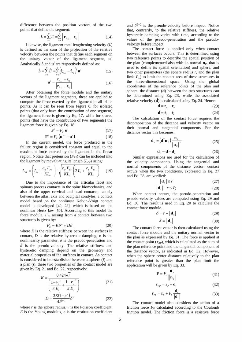
Due to the importance of the articular facet and

spinous process contacts in the spine biomechanics, and

also of the upper cervical and head contacts, namely

between the atlas, axis and occipital condyles, a contact

model based on the nonlinear Kelvin-Voigt contact

model is developed [49, 28], which is based on the

nonlinear Hertz law [50]. According to this model the

force module, FC, arising from a contact between two

structures is given by:

DKF n

C (20)

where K is the relative stiffness between the surfaces in

contact, D is the relative hysteretic damping, n is the

nonlinearity parameter, δ is the pseudo-penetration and

𝛿 is the pseudo-velocity. The relative stiffness and

hysteretic damping depend on the geometry and

material properties of the surfaces in contact. As contact

is considered to be established between a sphere (i) and

a plan (j), these two properties of the contact model are

given by Eq. 21 and Eq. 22, respectively:

j

j

i

i

EE

rK

22 11

424.0

(21)

neKD

)(

2

4

13

(22)

where r is the sphere radius, ν is the Poisson coefficient,

E is the Young modulus, e is the restitution coefficient

and 𝛿 (−) is the pseudo-velocity before impact. Notice

that, contrarily, to the relative stiffness, the relative

hysteretic damping varies with time, according to the values of the pseudo-penetration and the pseudo-

velocity before impact.

The contact force is applied only when contact

between the surfaces occurs. This is determined using

two reference points to describe the spatial position of

the plan (complemented also with its normal nP, that is

used to define its spatial orientation) and sphere, and

two other parameters (the sphere radius r, and the plan

limit PL) to limit the contact area of these structures in

the three-dimensional space. Using the global

coordinates of the reference points of the plan and

sphere, the distance (d) between the two structures can

be determined using Eq. 23, while the associated

relative velocity (𝐝 ) is calculated using Eq. 24. Hence:

PSrrd (23)

PSrrd (24)

The calculation of the contact force requires the

decomposition of the distance and velocity vector on

their normal and tangential components. For the

distance vector this becomes:

2

P

P

P

T

n

n

nndd (25)

ntddd (26)

Similar expressions are used for the calculation of

the velocity components. Using the tangential and

normal components of the distance vector, contact

occurs when the two conditions, expressed in Eq. 27

and Eq. 28, are verified:

rnd (27)

LtPr d (28)

When contact occurs, the pseudo-penetration and

pseudo-velocity values are computed using Eq. 29 and

Eq. 30. The result is used in Eq. 20 to calculate the

contact force module.

nr d (29)

nd (30)

The contact force vector is then calculated using the

contact force module and the unitary normal vector to

the plan as expressed by Eq. 31. The force is applied at

the contact point (rAP), which is calculated as the sum of

the plan reference point and the tangential component of

the distance vector, as indicated in Eq. 32. However,

when the sphere center distance relatively to the plan

reference point is greater than the plan limit the

application will be given by Eq. 33.

p

p

cF

n

nF (31)

tPAPdrr (32)

t

t

LPAPP

d

drr (33)

The contact model also considers the action of a

friction force FF calculated according to the Coulomb

friction model. The friction force is a resistive force

7

applied in the opposite direction of the tangential

component of the velocity vector, as:

t

t

cFF

d

dF

(34)

where μ is the friction coefficient and FC the contact

force calculated in Eq. 20.

The geometrical properties of the cervical ligaments in

the lower and upper cervical ligaments are retrieved

from the work of Ferreira [29], which adapted the points

of the de Jager’s cervical model [33]. In the lumbar

spine, on the other hand, the data is computed using

specific points in the vertebra as a reference (Figure 7)

[51,52,53,54]. These studies are used in both regions to

obtain the reference points and orientation of the

contacts between the articular facets and the spinous

processes. Notice that the upper cervical contacts

geometry is retrieved from the work of de Jager [33].

A B

C D

Figure 7 – Ligaments and contacts modelled in the multibody model of the

spine: A – Interspinous and supraspinous ligaments; B – Anterior and

posterior longitudinal ligaments; C – Capsular ligaments and ligamentum

flavum; D – Articular facets (orange) and spinous process (blue) contacts.

With respect to the material properties, the stiffness

and transition strains of the ligaments are retrieved from

the work of Yoganadan et al. [55] (cervical spine), and

from the work of Pintar et al. [56] and Chazal et al. [43]

(lumbar spine). Notice that the material properties for

the upper cervical ligaments are retrieved from the work

of Ferreira [29], which adopted the approximation of

van der Horst [48] and Meertens [57]. Moreover, the

damping coefficients are retrieved from van der Horst

[48] for the cervical spine and adopted for the lumbar

ligaments and from Meertens [57] for the transverse

ligament and tectorial membrane. The current spine

model exhibits pretension, which is introduced in the

ligaments (1.8 N and 3.0 N to the anterior and posterior

longitudinal ligament [58,59], respectively, and 18.0 N

[60] to the ligamentum flavum).

Relatively to the sphere-plan contacts, the relative

stiffness between contact pairs is retrieved from the

work of van der Horst [48] (K = 5862000 N/m), the

nonlinearity parameter is considered equal to 1.5, and

the restitution coefficient is retrieved from the work of

Burgin and Aspden [61] (e = 0.476). Regarding the

friction force, facet joints and spinous processes

contacts are considered to be frictionless and therefore,

in this work, the friction coefficient is set to zero.

2.4 The Finite Element Models of the

Intervertebral Disc and Fixation Plate

The intervertebral disc is the most critical

component in most of the finite element models of the

spine due to its complex macro and microstructure and,

consequently, its complex mechanical behaviour [62]. In

the current work, two intervertebral discs finite element

models for each region of the spine are developed. In

the cervical spine, the IVD developed correspond to the

C5-C6 and C6-C7, while, for the lumbar spine,

correspond to the L3-L4 and L4-L5. These

intervertebral joints present the intervertebral discs most

susceptible to injury as reported by Tanaka et al. [63],

which verified that a total of 75% of the patients

analyzed presented prolapsed discs at C5-C6 or C6-C7

spine levels, and by Panjabi et al. [3] and Battiè et al.

[64], which verified that the lumbar spine levels, L4-L5

and L5-S1, are the most susceptible since these levels

bear the highest loads and undergo the most motion in

the spine.

The IVDs are simulated as viscoelastic models

comprising the annulus, the quasi-incompressible

hydrostatic nucleus [65,66] and endplates, being

symmetric relatively to the sagittal plan. The annulus

matrix is reinforced by a network of collagen fibers

modelled as tension only rebar elements, accounting for

the radial variation in their inclination and stiffness.

The annulus fibrosus and nucleus pulposus geometry

is obtained using software developed for the purpose

and a cross-sectional image of the intervertebral disc.

Notice that the nucleus geometry is obtained from the

annulus geometry using the cross-sectional ratio

between the nucleus and annulus area (Yoganandan et

al. [45] for the cervical spine – 38 % and 58.2 % for the

C5-C6 and C6-C7 IVD, respectively; and the O’Connell

et al. [67] for the lumbar spine – 27.7 % for both lumbar

IVDs). Finally, the interpolated points are converted

from pixels to milimeters using two parametrization

measurements: the intervertebral disc mean width and

depth (retrieved from the work of Panjabi et al. [52, 68]).

On the other hand, the height of the intervertebral disc is

given by the mean height of the posterior and anterior

measurements made by Nissan and Gilad [51], and the

height retrieved from the work of de Jager [33], for the

lumbar and cervical spine, respectively. The nucleus

and annulus are modelled as viscoelastic materials,

whose values are adapted from the studies of Wang et

al. [69,70] for the lumbar spine, and Esat and Acar [27]

for the cervical spine.

The collagen fibers are modelled as rebar elements,

which are incorporated into surface sections (in order to

not introduce additional stiffness to the annulus ground

matrix besides that of the collagen fibers) that simulate

the laminate structure of the annulus. To define the

geometry of the rebar elements it is necessary to define

their cross-sectional area (A), their angle of inclination

and their spacing (s) between the fibers for each lamella,

whose values are derived from the experimental data of

Marchand and Ahmed [71]. The current intervertebral

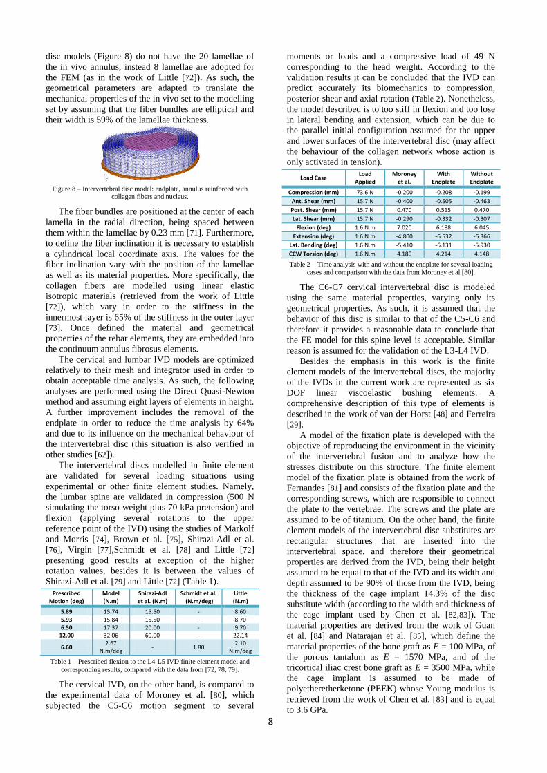
8

disc models (Figure 8) do not have the 20 lamellae of

the in vivo annulus, instead 8 lamellae are adopted for

the FEM (as in the work of Little [72]). As such, the

geometrical parameters are adapted to translate the

mechanical properties of the in vivo set to the modelling

set by assuming that the fiber bundles are elliptical and

their width is 59% of the lamellae thickness.

Figure 8 – Intervertebral disc model: endplate, annulus reinforced with

collagen fibers and nucleus.

The fiber bundles are positioned at the center of each

lamella in the radial direction, being spaced between

them within the lamellae by 0.23 mm [71]. Furthermore,

to define the fiber inclination it is necessary to establish

a cylindrical local coordinate axis. The values for the

fiber inclination vary with the position of the lamellae

as well as its material properties. More specifically, the

collagen fibers are modelled using linear elastic

isotropic materials (retrieved from the work of Little

[72]), which vary in order to the stiffness in the

innermost layer is 65% of the stiffness in the outer layer

[73]. Once defined the material and geometrical

properties of the rebar elements, they are embedded into

the continuum annulus fibrosus elements.

The cervical and lumbar IVD models are optimized

relatively to their mesh and integrator used in order to

obtain acceptable time analysis. As such, the following

analyses are performed using the Direct Quasi-Newton

method and assuming eight layers of elements in height.

A further improvement includes the removal of the

endplate in order to reduce the time analysis by 64%

and due to its influence on the mechanical behaviour of

the intervertebral disc (this situation is also verified in

other studies [62]).

The intervertebral discs modelled in finite element

are validated for several loading situations using

experimental or other finite element studies. Namely,

the lumbar spine are validated in compression (500 N

simulating the torso weight plus 70 kPa pretension) and

flexion (applying several rotations to the upper

reference point of the IVD) using the studies of Markolf

and Morris [74], Brown et al. [75], Shirazi-Adl et al.

[76], Virgin [77],Schmidt et al. [78] and Little [72]

presenting good results at exception of the higher

rotation values, besides it is between the values of

Shirazi-Adl et al. [79] and Little [72] (Table 1).

Prescribed Motion (deg)

Model (N.m)

Shirazi-Adl et al. (N.m)

Schmidt et al. (N.m/deg)

Little (N.m)

5.89 15.74 15.50 - 8.60 5.93 15.84 15.50 - 8.70 6.50 17.37 20.00 - 9.70

12.00 32.06 60.00 - 22.14

6.60 2.67

N.m/deg - 1.80

2.10 N.m/deg

Table 1 – Prescribed flexion to the L4-L5 IVD finite element model and

corresponding results, compared with the data from [72, 78, 79].

The cervical IVD, on the other hand, is compared to

the experimental data of Moroney et al. [80], which

subjected the C5-C6 motion segment to several

moments or loads and a compressive load of 49 N

corresponding to the head weight. According to the

validation results it can be concluded that the IVD can

predict accurately its biomechanics to compression,

posterior shear and axial rotation (Table 2). Nonetheless,

the model described is to too stiff in flexion and too lose

in lateral bending and extension, which can be due to

the parallel initial configuration assumed for the upper

and lower surfaces of the intervertebral disc (may affect

the behaviour of the collagen network whose action is

only activated in tension).

Load Case Load

Applied Moroney

et al. With

Endplate Without Endplate

Compression (mm) 73.6 N -0.200 -0.208 -0.199

Ant. Shear (mm) 15.7 N -0.400 -0.505 -0.463

Post. Shear (mm) 15.7 N 0.470 0.515 0.470

Lat. Shear (mm) 15.7 N -0.290 -0.332 -0.307

Flexion (deg) 1.6 N.m 7.020 6.188 6.045

Extension (deg) 1.6 N.m -4.800 -6.532 -6.366

Lat. Bending (deg) 1.6 N.m -5.410 -6.131 -5.930

CCW Torsion (deg) 1.6 N.m 4.180 4.214 4.148

Table 2 – Time analysis with and without the endplate for several loading

cases and comparison with the data from Moroney et al [80].

The C6-C7 cervical intervertebral disc is modeled

using the same material properties, varying only its

geometrical properties. As such, it is assumed that the

behavior of this disc is similar to that of the C5-C6 and

therefore it provides a reasonable data to conclude that

the FE model for this spine level is acceptable. Similar

reason is assumed for the validation of the L3-L4 IVD.

Besides the emphasis in this work is the finite

element models of the intervertebral discs, the majority

of the IVDs in the current work are represented as six

DOF linear viscoelastic bushing elements. A

comprehensive description of this type of elements is

described in the work of van der Horst [48] and Ferreira

[29].

A model of the fixation plate is developed with the

objective of reproducing the environment in the vicinity

of the intervertebral fusion and to analyze how the

stresses distribute on this structure. The finite element

model of the fixation plate is obtained from the work of

Fernandes [81] and consists of the fixation plate and the

corresponding screws, which are responsible to connect

the plate to the vertebrae. The screws and the plate are

assumed to be of titanium. On the other hand, the finite

element models of the intervertebral disc substitutes are

rectangular structures that are inserted into the

intervertebral space, and therefore their geometrical

properties are derived from the IVD, being their height

assumed to be equal to that of the IVD and its width and

depth assumed to be 90% of those from the IVD, being

the thickness of the cage implant 14.3% of the disc

substitute width (according to the width and thickness of

the cage implant used by Chen et al. [82,83]). The

material properties are derived from the work of Guan

et al. [84] and Natarajan et al. [85], which define the

material properties of the bone graft as E = 100 MPa, of

the porous tantalum as E = 1570 MPa, and of the

tricortical iliac crest bone graft as E = 3500 MPa, while

the cage implant is assumed to be made of

polyetheretherketone (PEEK) whose Young modulus is

retrieved from the work of Chen et al. [83] and is equal

to 3.6 GPa.

9

A B C

Figure 9 – Intervertebral disc (A), Fixation plate (B) and intervertebral disc

substitute (C) model.

In order to model the intervertebral discs, it is

necessary to define the respective reference points. The

reference points used in the definition of each element

are defined as the geometrical center of the lower and

upper endplate of a given IVD, which is assumed to be,

approximately, the geometrical center of the lower

vertebral body’s surface of a given vertebra and the

upper surface of the subsequent vertebra, respectively.

The initial translational and angular offsets are obtained

considering the initial configuration of the spine model.

Furthermore, the initial inclination is given in Bryant

angles for bushing elements, while it is given in Euler

angles for the co-simulation module.

The material properties of the cervical intervertebral

discs simulated using bushing elements are obtained

from Ferreira [29], which adapted the properties

reported by van der Horst [48]. On the other hand, for

the lumbar spine, the material properties are derived

from the studies of Markolf [86], Virgin [77], Hirsch and

Nachemson [87], Brown et al. [75] and Eberlein et al.

[88].

3. Results

The cervical and lumbar spine models described are

validated against values from several studies in order to

determine the capabilities of each one to the several

loading situations. The improved cervical spine model is

validated for extension and flexion with the

experimental data of Wheeldon et al. [89], Camacho et

al. [90] (Table 3), Nightingale et al. [91,92], and Goël et

al. [93]. The cervical spine model present a high

stiffness to flexion and a low stiffness to extension,

which translates to a good correlation of the model

values for extension at small loads and a good

correlation for flexion at relatively high loads. This is a

consequence of the constant stiffness properties of the

spinal structures that confer the spine with the same

resistance (disregarding the velocity dependent

component of their constitutive equations). Nonetheless,

the presence of the contacts between the spinous

processes is an improvement of the cervical spine model

limiting the extension movements to a maximum value.

Spine Level - 1.0 N.m 1.0 N.m

Model Camacho Model Camacho

C3-C2 (deg) -6.53 -5.53 4.55 5.03

C4-C3 (deg) -6.78 -4.38 4.45 5.13

C5-C4 (deg) -5.77 -3.61 4.49 5.82

C6-C5 (deg) -5.94 -4.58 4.81 5.09

C7-C6 (deg) -4.02 -3.55 4.77 3.73

Table 3 – Model rotations for the lower cervical spine levels for extension

and flexion, compared with the data from [90].

Moreover, the model of the lumbar spine is validated

for extension, flexion, lateral bending and axial rotation

using the experimental data of Eberlein et al. [88] (Table

4), which applied several moments at the top of the

vertebra L2 being the vertebra S1 fixed. The lumbar

spine presents a high stiffness to lateral bending and is

too loose for extension and flexion, producing

acceptable results for axial rotation.

Load Situation 4.0 N.m 8.0 N.m

Model Eberlein Model Eberlein

Extension (deg) -11.6 -9.6 -15.0 -13.9

Flexion (deg) 22.9 15.0 26.2 18.7

Lat. Bend. (deg) 3.6 16.1 8.5 21.1

Torsion (deg) -6.8 -4.7 -10.7 -7.5

Table 4 – Model rotations for the lumbar spine for several loading

situations, compared with the data from [88].

The validations of the functional spine units

involving the finite element models (for the cervical and

lumbar spine) exhibit a good correlation with the

experimental results [80,94] (Table 5), displaying a gain

of using the co-simulation between the domains of the

finite element models and the mulibody system

dynamics.

Load Situation C5-C6 L4-L5

Model Moroney Model Heuer

Flexion (deg) 3.26 5.55 6.86 7.14

Extension (deg) 5.28 3.52 3.60 4.92

Lat. Bending (deg) 10.66 4.71 5.43 6.12

Torsion (deg) 8.25 1.85 4.42 3.45

Table 5 – Model rotations for the C5-C6 and L4-L5 spine levels for several

loading situations, compared with the data from [80, 94].

In order to evaluate the influence of intersomatic

fusion in the adjacent levels, two common movements

of the spine are simulated before and after the chirurgic

procedure: the extension and flexion movements. The

movements are originated by applying a moment of 1.5

N.m to the head and during a time interval of 400 ms.

Independently of the type of movement, it can be

seen that intersomatic fusion reduces the movement in

the spine level subjected to this procedure almost

completely, more even if it is complemented with the

introduction of a fixation plate. More specifically, in

extension, the rotation is reduced by 96.38% when an

intervertebral disc surrogate is used and is further

limited by a factor of 98.51% with the fixation plate

(Figure 10). In flexion, the movement restriction

increases, being of 98.34% for the intervertebral disc

grafts and 99.41% with the inclusion of the titanium

plate.

Figure 10 – Intervertebral rotation for the lower cervical spine levels in

extension.

Furthermore, intersomatic fusion modifies the

biomechanics of the spine levels in the vicinity of the

fusioned area. Namely, it increases the rotational

movement on the cervical spine levels in order to

-0.14

-0.12

-0.1

-0.08

-0.06

-0.04

-0.02

0

T1 - C7 C7 - C6 C6 - C5 C5 - C4 C4 - C3 C3 - C2

Ro

tati

on

(rad

)

Normal

BGraft

BFplate

10

compensate the loss of movement in C7-C6;

nonetheless, the total motion of the cervical spine

decreases relatively to the normal spine. Notice that the

increase is not only verified in the adjacent levels, but

also in non-adjacent spine levels. The rotational increase

translates in higher stresses in the adjacent intervertebral

disc (from 3.58 MPa for the normal cervical spine to

3.99 MPa for the cervical spine with bone graft and

fixation plate), as can be seen in Figure 11 for flexion,

which in a long-term physiological load can degenerate

its structure. Similar observations for intersomatic

fusion are found in the work of Ivanov et al. [95] for the

lumbar spine. The fixation plate influence in these

studies is not significantly noticed, as such, further

analyses are necessary to determine its influence in the

spine biomechanics.

A B C

Figure 11 – Stress distribution in the C5-C6 intervertebral disc in flexion:

normal cervical spine (A), cervical spine with a bone graft (B), and

cervical spine with a bone graft and fixation plate (C).

Moreover, the single-level fusion not only affects

the intervertebral discs but also the facet joints in

extension. Namely, the load sharing by the facet joints

increases as a result of an increase in the movement

associated with each motion segment, which may affect

the integrity of this structure and originate additional

pathologies, as facet arthropathy. These results are in

agreement with the results of Guan et al. [84] for the

lumbar spine.

In the current work, several types of materials are

studied in the cervical and lumbar spine. In the cervical

spine, the bone graft is compared to the cancellous graft,

while in the lumbar spine, these two graft materials are

also compared to the porous tantalum graft. Observing

the results, it can be concluded that higher elastic

modulus translates in a higher restriction of the

movement in the fusioned level and a greater rotational

movement on the other spine levels (Figure 12).

Figure 12 – Intervertebral rotation for the lumbar spine levels in flexion

using several types of graft materials.

A B C

Figure 13 – Stress distribution in the C5-C6 intervertebral disc in extension: normal cervical spine (A), cervical spine with a bone graft (B),

and cervical spine with a cancellous graft (C).

The forces exerted over the facet joints also vary

with the type of material, being greater for the materials

that are responsible for a greater motion in the motion

segments near the one subjected to intersomatic fusion,

i.e., with higher elastic modulus. As a consequence, the

stresses induced in the adjacent intervertebral disc

structure are higher for the cervical spine with bone

graft (with a 14.51% increase) (Figure 13).

4. Conclusions and Future Developments

In the current work, a co-simulation module is

applied in the study of the dynamic stress distributions

on the IVD adjacent to the vertebral level that is

engaged with a bone graft and, simultaneously, on the

fixation plate that is placed along one cervical stage

during the surgical intervention of intervertebral fusion.

The combination of the two types of models (finite

element models and multibody models) allows

analyzing simultaneously, in an integrated way, the

kinematics and the stress distribution on the structures

of interest for any particular region of the vertebral

column. This is extremely important from the clinical

point of view as it will allow for the identification of the

regions of the spine that, for a given movement, present

the higher stresses and where the risk of injury is higher.

Furthermore, it can be used in the future to develop or

analyze different types of materials and geometrical

designs for the orthopaedic implants. Nonetheless an

effort has to be done to optimize the co-simulation

process in order to turn it faster and more efficient.

Additionally, there is a problem in the prescription of all

degrees of freedom to the finite element models, since

the convergence of the FE decreases. As such, a

processing step of the loads and moments retrieved from

the finite element models have to be created and

executed in order to satisfy the equilibrium equations.

In order to study the stress distribution on the discs

adjacent to a single-level intersomatic fusion, the

movements of the spine are analyzed before and after

the fusion with the bone graft and with or without the

fixation plate. These analyses require the development

and validation of the multibody models of the cervical

and lumbar spine regions, as well as the finite element

models of the IVD developed for the same spine

regions. Namely, the cervical IVD can predict

accurately its biomechanics to compression, posterior

shear and axial rotation, being too stiff in flexion and

too lose in lateral bending and extension. On the other

hand, the lumbar disc exhibits moments that are within

the values of Shirazi-Adl et al. [79] and Schmidt et al.

[78] for small rotations. The multibody models of the

spine regions present distinct results: the lumbar spine

cannot show good correlation with the data of Eberlein

et al. [88] for flexion and lateral bending, being capable

of predicting acceptably for axial rotation while the

cervical spine model present a high stiffness to flexion

and a low stiffness to extension, which translates to a

good correlation of the model values for extension at

small loads and a good correlation for flexion at

relatively high loads.

The single level intersomatic fusion determines

alterations in the biomechanics not only of the motion

segment it affects directly but also of the spine levels in

0

0.02

0.04

0.06

0.08

0.1

0.12

S1-L5 L5-L4 L4-L3 L3-L2 L2-L1

Ro

tati

on

(rad

)

Normal

CGraft

BGraft

TGraft

11

their vicinity. Namely, the motion of the level subjected

to fusion is highly restricted by using only an

intervertebral substitute or by complementing with the

inclusion of a fixation plate, while the adjacent levels

and the other spine levels near to the fusioned area

exhibit an increase in their rotational movement (higher

in the adjacent levels). The higher rotational movement

implies higher stresses in the intervertebral disc and an

increased load sharing by the facet joints. The higher

loads experienced by these structures, posteriorly to

fusion, may be responsible for their degeneration and,

consequently, to spine refusion as reported by other

researchers. Nonetheless, further analyses taking into

account different loads and longer time analysis are

necessary to reinforce these results.

Acknowledgements

The computational methodologies developed in the

scope of this work unfold under the objectives of the

FCT projects DACHOR – Multibody Dynamics and

Control of Hybrid Active Orthoses (MIT-Pt/BS-

HHMS/0042/2008) and PROPAFE - Design and

Development of a Patello-Femoral Prosthesis

(PTDC/EME-PME/67687/2006).

References

[1] Rouvière H., Anatomie Humaine – Descriptive et

Topographique: Tome II Tronc, Masson et Cie, 10th Edition,

1970.

[2] Ehlers W., Markert B., Karajan N., Acartürk A., A

Coupled FE Analysis of the Intervertebral Disc Based on a

Multiphasic TPM Formulation, in Proceedings of IUTAM

Symposium on Mechanics of Biological Tissue, Editors

Holzapfel G. A., Ogden R. W., Springer, pp. 373-386, 2005.

[3] White A. A., Panjabi M. M., Clinical Biomechanics of the

Spine, Lippincott Williams & Wilkins, 2nd Edition, 1970.

[4] Best B. A., Guilak F., Setton L. A., Zhu W., Saed-Nejad

F., Ratcliffe A., Weidenbaum M., Mow V. C., Compressive

Mechanical Properties of the Human Annulus Fibrosus and

Their Relationship to Biomechanical Composition, Spine, Vol.

19, No. 2, pp. 212-221, 1994.

[5] Costi J. J., Stokes I. A., Gardner-Morse M., Laible J. P.,

Scoffone H. M., Iatridis J. C., Direct Measurement of the

Intervertebral Disc Maximum Shear Strain in Six Degree of

Freedom: Motions that Place Disc Tissue at Risk of Injury,

Journal of Biomechanics, Vol. 40, pp. 2457-2466, 2007.

[6] Skaggs D. L., Weidenbaum M., Iatridis J. C., Ratcliffe A.,

Mow V. C., Regional Variation in Tensile Properties and

Biochemical Composition of the Lumbar Annulus Fibrosus,

Spine, Vol. 19, No. 12, pp. 1310-1319, 1994.

[7] Harris R. I., Macnab I., Structural Changes in the Lumbar

Intervertebral Disc: Their Relationship to Low Back Pain and

Sciatica, The Journal of Bone and Joint Surgery, Vol. 36B,

No. 2, pp. 304-322, 1954.

[8] Brown S. H. M., Gregory D. E., McGill S. M., Vertebral

Endplate Fractures as a Result of High Rate Pressure Loading

in the Nucleus of the Young Adult Porcine Spine, Journal of

Biomechanics, Vol. 41, pp. 122-127, 2008.

[9] Cusick J. F., Yoganandan N., Biomechanics of the

Cervical Spine 4: Major Injuries, Clinical Biomechanics, Vol.

17, pp. 1-20, 2002.

[10] Shirazi-Adl A., Finite Element Simulation of Changes in

the Fluid Content of Human Lumbar Discs: Mechanical and

Clinical Implications, Spine, Vol. 17, No. 2, pp. 206-212,

1992.

[11] Dvorak M., Pitzen T., Zhu O., Gordon J., Fisher C.,

Oxland T., Anterior Cervical Plate Fixation: A Biomechanical

Study to Evaluate the Effects of Plate Design, Endplate

Preparation, and Bone Mineral Density, Spine, Vol. 30, No.

3, pp. 294-301, 2005.

[12] Green P. W. B., Anterior Cervical Fusion: A Review of

33 Patients with Cervical Disc Degeneration, The Journal of

Bone and Joint Surgery, Vol. 59B, No. 2, pp. 236-240, 1977.

[13] Hilibrand A. S., Balasubramanian K., Eichenbaum M.,

Thinnes J. H., Daffner S., Berta S., Albert T. J., Vaccaro A.

R., Siegler S., The Effect of Anterior Cervical Fusion on Neck

Motion, Spine, Vol. 31, No. 15, pp. 1688-1692, 2006.

[14] Lopez-Espina C. G., Amirouche F., Havalad V.,

Multilevel Cervical Fusion and Its Effect on Disc

Degeneration and Osteophyte Formation, Spine, Vol. 31, No.

9, pp. 972-978, 2006.

[15] Skalli W., Robin S., Lavaste F., Dubousset J., A

Biomechanical Analysis of Short Segment Spinal Fixation

Using a Three-Dimensional Geometric and Mechanical

Model, Spine, Vol. 18, No. 5, pp. 536-545, 1993.

[16] Gillet P., The Fate of Adjacent Motion Segments after

Lumbar Fusion, Journal of Spinal Disorders and Techniques,

Vol. 16, No. 4, pp. 338-345, 2003.

[17] Rao R. D., Wang M., McGrady L. H., Perlewitz T. J.,

Dacid K. S., Does Anterior Plating of the Cervical Spine

Predispose to Adjacent Segment Changes?, Spine, Vol. 30,

No. 24, pp. 2788-2792, 2005.

[18] Wang J., Ma Z.-D., Hulbert G. M., A Gluing Algorithm

for Distributed Simulation of Multibody Systems, Nonlinear

Dynamics, Vol. 34, pp. 159-188, 2003.

[19] Rauter F. G., Pombo J., Ambrósio J., Pereira M.,

Multibody Modeling of Pantographs for Pantograph-Catenary

Interaction, in IUTAM Symposium On Multiscale Problems

in Multibody System Contacts, Editor Eberhard P., pp. 205-

226, Springer, 2007.

[20] Latham F., A Study in Body Ballistics: Seat Ejection, in

Proceedings of the Royal Society of London, Vol. 147, pp.

121-139, 1957.

[21] Dooris A. P., Goël V. K., Grosland N. M., Gilbertson L.

G., Wilder D. G., Load Sharing Between Anterior and

Posterior Elements in a Lumbar Motion Segment Implanted

with an Artificial Disc, Spine, Vol. 24, No. 6, pp. E122-E129,

2001.

[22] Goël V. K., Lim T.-H., Gwon J., Chen J.-Y.,

Winterbottom J. M., Park J. B., Weinstein N., Ahn J.-Y.,

Effects of Rigidity of an Internal Fixation Device: A

Comprehensive Biomechanical Investigation, Spine, Vol. 16,

No. 3, pp. S155-S161, 1991.

[23] Mizrahi J., Silva M. J., Keaveny T. M., Edwards W. T.,

Hayes W. C., Finite Element Stress Analysis of the Normal

and Osteoporotic Lumbar Vertebral Body, Spine, Vol. 18, No.

14, pp. 2088-2096, 1993.

[24] Tschirhart C. E., Finkelstein J. A., Whyne C. M.,

Biomechanics of Vertebral Level, Geometry, and

Transcortical Tumors in the Metastatic Spine, Journal of

Biomechanics, Vol. 40, pp. 46-54, 2007.

[25] Esat V., Acar M., A Multibody Human Spine Model for

Dynamic Analysis in Conjunction with the FE Analysis of

Spinal Parts, in Proceedings of 1st Annual Injury

Biomechanics Symposium, The Ohio State University, USA,

2005.

[26] Esat V., van Lopik D. W., Acar M., Combined Multi-

Body Dynamic and FE Models of Human Head and Neck, in

IUTAM Proceedings on Impact Biomechanics: from

Fundamental Insights to Application, Editor Gilchrist M. D.,

pp. 91-100, Springer, 2005.

[27] Esat V., Acar M., Viscoelastic Finite Element Analysis of

the Cervical Intervertebral Discs in Conjuction with a Multi-

Body Dynamic Model of the Human Head and Neck,

Proceedings of the Institution of Mechanical Engineers, Part

H: Journal of Engineering in Medicine, pp. 249-262, 2009.

12

[28] Silva M. T., Human Motion Analysis Using Multibody

Dynamics and Optimization Tools, PhD. Thesis Instituto

Superior Técnico – Technical University of Lisbon, Lisbon,

2003.

[29] Ferreira A., Multibody Model of the Cervical Spine and

Head for the Simulation of Traumatic and Degenerative

Disorders, M. Sc. Thesis Instituto Superior Técnico –

Technical University of Lisbon, Lisbon, 2008.

[30] van Lopik D. W., Acar M., Dynamic Verification of a

Multibody Computational Model of Human Head and Neck

for Frontal, Lateral and Rear Impacts, Proceedings of the

Institution of Mechanical Engineers, Part K: Journal of

Multibody Dynamics, Vol. 221, No. 2, pp. 199-217, 2007.

[31] Stokes I. A. F., Gardner-Morse M., Quantitative Anatomy

of the Lumbar Musculature, Journal of Biomechanics, Vol. 32,

pp. 311-316, 1999.

[32] Gangnet N., Dumas R., Pomero V., Mitulescu A., Skalli

W., Vital J.-M., Three-Dimensional Spinal and Pelvic

Alignment in an Asymptomatic Population, Spine, Vol. 31,

No. 15, pp. E507-E512, 2006.

[33] de Jager M., Mathematical Head-Neck Models for

Acceleration Impacts, Technische Universiteit Eindhoven –

University of Technology, Eindhoven, 2000.

[34] Laananen D., Computer Simulation of an Aircraft Seat

and Occupant in a Crash Environment – Program SOM-LA /

SOM-TA User Manual, DOT/FAA/CT-90/4, US Department

of Transportation, Federal Aviation Administration, 1991.

[35] Ambrósio J. A. C., Multibody Dynamics: Bridging for

Multidisciplinary Applications, in Mechanics of the 21st

Century, Editors Gutkowski W., Kowalewski, Springer, pp.

61-88, 2005.

[36] Monteiro N., Folgado J., Silva M., Melancia J., Analysis

of the Intervertebral Discs Using a Finite Element and

Multibody Dynamics Approach, 8th World Congress on

Computational Mechanics (WCCM8), 5th European Congress

on Computational Methods in Applied Sciences and

Engineering (ECCOMAS 2008), Venice, Italy, June 30 – July

5, 2008.

[37] Monteiro N., Folgado J., Silva M., Melancia J., Co-

Simulação de Sistemas Multicorpo com Modelos de Elementos

Finitos: Aplicação à Análise de Tensões nos Discos

Intervertebrais, 3º Congresso Nacional de Biomecânica,

Bragança, 2009.

[38] Monteiro N., Folgado J., Silva M., Melancia J., Dynamic

Stress Distribution on a Multilevel Cervical Fusion Using a

MSD/FE Co-Simulation Approach, Proceedings of Multibody

Dynamics 2009 An ECCOMAS Thematic Conference,

Warsaw, Poland, June 29 – July 2, 2009.

[39] Monteiro N., Folgado J., Silva M., Melancia J., A New

Approach to Analyze the Stress Distribution on a Multilevel

Cervical/Lumbar Intersomatic Fusion, Proceedings of

ESMC2009, 7th EUROMECH Solid Mechanics Conference,

Lisbon, Portugal, September 7 – 11 2009.

[40] Nikravesh P., Computer-Aided Analysis of Mechanical

Systems, Prentice-Hall, Englewood Cliffs, New Jersey, 1988.

[41] Panjabi M. M., Oxland T. R., Parks E. H., Quantitative

Anatomy of Cervical Spine Ligaments. Part I: Upper Cervical

Spine, Journal of Spinal Disorders and Techniques, Vol. 4, Nº

3, pp. 270-276, 1991.

[42] Sharma M., Langrana N. A., Rodriguez J., Role of

Ligaments and Facets in Lumbar Spinal Stability, Spine, Vol.

20, No. 8, pp. 887-900, 1995.

[43] Chazal J., Tanguy A., Bourges M., Gaurel G., Escande

G., Guillot M., Vanneuville G., Biomechanical Properties of

Spinal Ligaments and a Histological Study of the Supraspinal

Ligament in Traction, Journal of Biomechanics, Vol. 18, No.

3, pp. 167-176, 1985.

[44] Panjabi M. M., The Stabilizing System of the Spine – Part

II: Neutral Zone and Instability Hypothesis, Journal of Spinal

Disorders and Techniques, Vol. 5, pp. 390-396, 1992.

[45] Yoganandan N., Kumaresan S., Pintar F. A.,

Biomechanics of the Cervical Spine Part 2: Cervical Spine

Soft Tissue Responses and Biomechanical Modeling, Clinical

Biomechanics, Vol. 16, pp. 1-27, 2001.

[46] Martin R. B., Burr D. B., Sharkey N. A., Skeletal Tissue

Mechanics, Springer, United States of America, 2004.

[47] Wisman J., A Three-Dimensional Mathematical Model of

the Human Knee Joint, PhD. Thesis, Technische Hogenschool

Eindhoven, 1980.

[48] van der Horst M., Human Head Neck Response in

Frontal, Lateral and Rear End Impact Loading, Technisch

Universiteit Eindhoven – University of Technology,

Eindhoven, 2002.

[49] Ambrósio J. A., Silva M., Multibody Dynamics

Approaches for Biomechanical Modeling in Human Impact

Application, in IUTAM Proceedings on Impact Biomechanics:

From Fundamental Insights to Applications, Editor Gilchrist

M. D., Springer, pp. 61-80, 2005.

[50] Hertz H., On the Contact of Solids – On the Contact of

Rigid Elastic Solids and on Hardness, Miscellaneous Papers,

MacMillan and Co. Ltd., London, pp. 146-183, 1896.

[51] Nissan M., Gilad I., The Cervical and Lumbar Vertebrae

- An Anthropometric Model, Engineering in Medicine, Vol.

13, No. 3, pp. 111-114, 1984.

[52] Panjabi M. M., Duranceau J., Goel V., Oxland T., Takata

K., Cervical Human Vertebrae: Quantitative Three-

Dimensional Anatomy of the Middle and Lower Regions,

Spine, Vol. 16, No. 8, pp. 861-869, 1991.

[53] Panjabi M. M., Oxland T., Takata K., Goël V., Duranceau

J., Krag M., Articular Facets of the Human Spine:

Quantitative Three-Dimensional Anatomy, Spine, Vol. 18, No.

10, pp. 1298-1310, 1993.

[54] Xu R., Burgar A., Ebraheim N. A., Yeasting R. A., The

Quantitative Anatomy of the Laminas of the Spine, Spine, Vol.

24, No. 2, pp. 107-113, 1999.

[55] Yoganandan N., Kumaresan S., Pintar F. A., Geometrical

and Mechanical Properties of Human Cervical Spine

Ligaments, Journal of Biomechanical Engineering, Vol. 122,

pp. 623-629, 2000.

[56] Pintar F. A., Yoganandan N., Myers T., Elhagediab A.,

Sances A. Jr., Biomechanical Properties of Human Lumbar

Spine Ligaments, Journal of Biomechanics, Vol. 25, No. 11,,

pp. 1351-1356, 1992.

[57] Meertens W., Mathematical Modelling of the Upper

Cervical Spine with MADYMO, Final Thesis, Eindhoven

University of Technology, 1995.

[58] Hukins D. W. L., Kirby M. C., Sikoryn T. A., Aspden R.

M., Cox A. J., Comparison of Structure, Mechanical

Properties, and Functions of Lumbar Spinal Ligaments, Spine,

Vol. 15, No. 8, pp. 787-795, 1990.

[59] Tkaczuk H., Tensile Properties of Human Lumbar

Longitudinal Ligaments, Acta Orthopaedica Scandinava, Vol.

115 (Supplement), 1968.

[60] Nachemson A., Evans J., Some Mechanical Properties of

the Third Lumbar Inter-Laminar Ligament (Ligamentum

Flavum), Journal of Biomechanics, Vol. 1, No. 211, 1968.

[61] Burgin L. V., Aspden R. M., Impact Testing to Determine

the Mechanical Properties of Articular Cartilage in Isolation

and on Bone, Journal of Material Science: Materials in

Medicine, Vol. 19, pp. 703-711, 2008.

[62] Fagan M. J., Julian S., Siddall D. J., Mohsen A. M.,

Patient-Specific Spine Models. Part 1: Finite Element

Analysis of the Lumbar Intervertebral Disc – A Material

Sensitivity Study, Proceedings of Institution of Mechanical

Engineers, Part H: Journal of Engineering in Medicine, Vol.

216, pp. 299-314, 2002.

13

[63] Tanaka N., Fujimoto Y., An H. S., Ikuta Y., Yasuda M.,

The Anatomic Relation Among the Nerve Roots, Intervertebral

Foramina, and Intervertebral Disc of the Cervical Spine,

Spine, Vol. 25, No. 3, pp. 286-291, 2000.

[64] Battié M. C., Videman T., Parent E., Lumbar Disc

Degeneration: Epidemiology and Genetic Influences, Spine,

Vol. 29, No. 23, pp. 2679-2690, 2004.

[65] Bogduk N., Clinical Anatomy of the Lumbar Spine and

Sacrum, Churchill Livingstone, New York, 1997.

[66] Nachemson A., Lumbar Intradiscal Pressure:

Experimental Studies on Postmortem Material, Acta

Orthopaedica Scandinava, Vol. 43, pp. 9-104, 1960.

[67] O’Connell G., Vresilovic E., Elliott D., Comparison of

Animals Used in Disc Research to Human Lumbar Disc

Geometry, Spine, Vol. 32, No. 3, pp. 328-333, 2007.

[68] Panjabi M. M., Goel V., Oxland T., Takata K., Duranceau

J., Krag M., Prince M., Human Lumbar Vertebrae:

Quantitative Three-Dimensional Anatomy, Spine, Vol. 17, No.

3, pp. 299-306, 1992.

[69] Wang J. L., Parnianpour M., Shirazi-Adl A., Engin A. E.,

Li S., Patwardhan A., Development and Validation of a

Viscoelastic Finite Element Model of an L2-L3 Motion

Segment, Theoretical and Applied Fracture Mechanics, Vol.

28, pp. 81-93, 1997.

[70] Wang J. L., Parnianpour M., Shirazi-Adl A., Engin A. E.,

Viscoelastic Finite Element Analysis of a Lumbar Motion

Segment in Combined Compression and Sagittal Flexion,

Spine, Vol. 25, No. 3, pp. 310-318, 2000.

[71] Marchand F., Ahmed A., Investigation of the Laminate

Structure of Lumbar Disc Annulus Fibrosus, Spine, Vol. 15,

No. 5, pp. 402-410, 1990.

[72] Little J. P., Finite Element Modeling of Anular Lesions in

the Lumbar Intervertebral Disc, PhD. Thesis, Queensland

University of Technology, 2004.

[73] Eyre D., Muir H., Types I and II Collagens in

Intervertebral Disc: Interchanging Radial Distributions in

Annulus Fibrosus, Biochemistry Journal, Vol. 157, No. 1, pp.

267-270, 1976.

[74] Markolf K. L., Morris J. M., The Structural Components

of the Intervertebral Disc: A Study of their Contributions to

the Ability of the Disc to Withstand Compressive Forces,

Journal of Bone and Joint Surgery, Vol. 56, pp. 675-687,

1974.

[75] Brown T., Hanson R., Yorra A., Some Mechanical Tests

on the Lumbo-Sacral Spine with Particular Reference to the

Intervertebral Discs, Journal of Bone and Joint Surgery, Vol.

39A, pp.1135-1164, 1957.

[76] Shirazi-Adl A., Shrivastava S. C., Ahmed A. M., Stress

Analysis in the Lumbar Disc Body Unit in Compression,

Spine, Vol. 9, pp. 120-134, 1984.

[77] Virgin W., Experimental Investigations into Physical

Properties of Intervertebral Disc, Journal of Bone and Joint

Surgery, Vol. 33B, pp. 607, 1951.

[78] Schmidt T. A., An H. S., Lim T, Nowicki B. H.,

Haughton V. M., The Stiffness of Lumbar Spinal Motion

Segments with a High-Intensity Zone in the Anulus Fibrosus,

Spine, Vol. 23, No. 20, pp. 2167-2173, 1998.

[79] Shirazi-Adl A., Ahmed A. M., Shrivastava S. C., A Finite

Element Study of a Lumbar Motion Segment Subjected to Pure

Sagittal Plane Moments, Journal of Biomechanics, Vol. 19,

No. 4, pp. 331-350, 1986.

[80] Moroney S. P., Schultz A. B., Miller J. A. A., Andersson

G. B. J., Load-Displacement Properties of Lower Cervical

Spine Motion Segments, Journal of Biomechanics, Vol. 21, pp.

767-779, 1988.

[81] Fernandes P., Modelação e Análise da Fusão

Intersomática Cervical, M. Sc. Thesis Instituto Superior

Técnico – Technical University of Lisbon, Lisbon, Portugal,

2008.

[82] Chen J.-F., Wu C.-T., Lee S.-C., Lee S.-T., Use of a

Polymethylmethacrylate Cervical Cage in the Treatment of

Single-Level Cervical Disc Disease, Journal of Neurosurgery

Spine, Vol. 3, pp. 24-28, 2005.

[83] Chen J.-F., Lee S.-T., The Polymethyl Methacrylate

Cervical Cage for Treatment of Cervical Disc Disease. Part

III: Biomechanical Properties, Surgical Neurology, Vol. 66,

pp. 367-370, 2006.

[84] Guan Y., Yoganandan N., Maiman D. J., Pintar F. A.,

Internal and External Responses of Anterior Lumbar /

Lumbosacral Fusion: Nonlinear Finite Element Analysis,

Journal of Spinal Disorders and Techniques, Vol. 21, No. 4,

2008.

[85] Natarajan R. N., Chen B. H., An H. S., Andersson G. B.

J., Anterior Cervical Fusion: A Finite Element Model Study on

the Motion Segment Stability Including the Effect of

Osteoporosis, Spine, Vol. 25, No. 8, pp. 955-961, 2000.

[86] Markolf K. L., Stiffness and Damping Characteristics of

the Thoracic-Lumbar Spine, in Proceedings of Workshop on

Bioengineering Approaches to the Problems of the Spine,

NIH, September, 1970.

[87] Hirsch C., Nachemson A., A New Observation on the

Mechanical Behaviour of Lumbar Discs, Acta Orthopaedica

Scandinava, Vol. 23, pp. 254, 1954.

[88] Eberlein R., Holzapfel G. A., Fröhlich M., Multi-Segment

Finite Element Analysis of the Human Lumbar Spine

Including the Heterogeneity of the Annulus Fibrosus,

Computational Mechanics, Vol. 34, pp. 147-163, 2004.

[89] Wheeldon J. A., Pintar F. A., Knowles S., Yoganandan

N., Experimental Flexion/Extension Data Corridors for

Validation of Finite Element Models of the Young, Normal

Cervical Spine, Journal of Biomechanics, Vol. 39, pp. 375-

380, 2004.

[90] Camacho D. L., Nightingale R. W., Robinette J. J.,

Vanguri S. K., Coates D. J., Myers B. S., Experimental

Flexibility Measurements for the Development of a

Computational Head-Neck Model Validated for a Near-Vertex

Head Impact, Society of Automotive Engineers, Paper No.

973345, 1997.

[91] Nightingale R. W., Winkelstein B. A., Knaub K. E.,

Richardson W. J., Luck J. F., Myers B. S., Comparative

Strengths and Structural Properties of the Upper and Lower

Cervical Spine in Flexion and Extension, Journal of

Biomechanics, Vol. 35, pp. 725-732, 2002.

[92] Nightingale R. W., Chancey V. C., Ottaviano D., Luck J.

F., Tran L., Prange H., Myers B. S., Flexion and Extension

Structural Properties and Strengths for Male Cervical Spine

Segments, Journal of Biomechanics, Vol. 40, pp. 535-542,

2007.

[93] Goël V., Clark C., Gallaes K., King Liu Y., Moment-

Rotation Relationships of the Ligamentous Occipito-Axial

Complex, Journal of Biomechanics, Vol. 21, No. 8, pp. 673-

680, 1988.

[94] Heuer F., Schmidt H., Klezl Z., Claes L., Wike H.-J.,

Stepwise Reduction of Functional Spinal Structures Increase

Range of Motion and Change Lordosis Angle, Journal of

Biomechanics, Vol. 40, pp. 271-280, 2007.

[95] Ivanov A. A., Kiapour A., Ebraheim N. A., Goël V.,

Lumbar Fusion Leads to Increases in Angular Motion and

Stress Across Sacroiliac Joint, Spine, Vol. 34, No. 5, pp.

E162-E169, 2009.