geomagnetic survey and geomagnetic model research in china

Earth Planets Space, 58, 741–750, 2006

Geomagnetic survey and geomagnetic model research in China

Zuowen Gu1, Zhijia Zhan1, Jintian Gao1, Wei Han1, Zhenchang An1,2, Tongqi Yao1, and Bin Chen1

1Institute of Geophysics, China Earthquake Administration, Beijing 100081, China2Institute of Geology and Geophysics, Chinese Academy of Sciences, Beijing 100029, China

(Received February 21, 2005; Revised September 23, 2005; Accepted October 11, 2005; Online published June 2, 2006)

The geomagnetic survey at 135 stations in China were carried out in 2003. These stations are with betterenvironmental condition and small magnetic field gradient (<5 nT/m). In the field survey, the geomagneticdeclination D, the inclination I and the total intensity F were measured. Ashtech ProMark2 differential GPS(Global Positioning System) was used in measuring the azimuth, the longitude, the latitude and the elevation atthese stations. The accuracy of the azimuth is 0.1′. The geomagnetic survey data were reduced using the dataat geomagnetic observatories in China. The mean standard deviations of the geomagnetic reduced values are:<1.5 nT for F , <0.5′ for D and I . Using the geomagnetic data which include the data at 135 stations and 35observatories in China, and the data at 38 IGRF (International Geomagnetic Reference Field) calculation points inChina’s adjacent regions, the Taylor polynomial model and the spherical cap harmonic model were calculated forthe geomagnetic field in China. The truncation order of the Taylor polynomial model is 5, and its original pointis at 36.0◦N and 104.5◦E. Based on the geomagnetic anomalous values and using the method of spherical capharmonic (SCH) analysis , the SCH model of the geomagnetic anomalous field was derived. In the SCH model,the pole of the spherical cap is at 36.0◦N and 104.5◦E, and the half-angle is 30◦, the truncation order K = 8is determined according to the mean square deviation between the model calculation value and the observationvalue, the AIC (Akaike Information Criterion) and the distribution of geomagnetic field.Key words: Geomagnetic survey, geomagnetic model, Taylor polynomial model, spherical cap harmonic model,China.

1. IntroductionThe geomagnetic survey and the geomagnetic field model

are the foundation in geomagnetic research. The geomag-netic surveys were carried out in some regions of Chinasince the beginning of the 20th century (Chen, 1944; Chenand Liu, 1948). The geomagnetic surveys in the wholeChina were carried out once every 10 years on the averageduring 1950∼2000 (Tschu, 1979; An, 2001). In order tocompile China geomagnetic chart for 2005.0, the geomag-netic surveys in China were carried out during 2002∼2004.Modern equipments including GPS were used in geomag-netic survey. A lot of geomagnetic survey data with betteraccuracy and stability were obtained.

Geomagnetic field model is one of the important subjectsin the study of geomagnetism (Langel, 1987). Geomagneticfield model is divided into the global model and the regionalone. Beginning from 1968, the International Association ofGeomagnetism and Aeronomy (IAGA) provides the globalspherical harmonic models for each 5 years, i.e. the Inter-national Geomagnetic Reference Field (IGRF) and there isalready the 9th generation IGRF (IAGA, 1996, 2000, 2003).In the research on regional geomagnetic field model, differ-ent scientists have used various mathematical methods andhave obtained geomagnetic field models in various coun-tries and regions (Alldredge, 1987; Barton, 1988; Haines,

Copyright c© The Society of Geomagnetism and Earth, Planetary and Space Sci-ences (SGEPSS); The Seismological Society of Japan; The Volcanological Societyof Japan; The Geodetic Society of Japan; The Japanese Society for Planetary Sci-ences; TERRAPUB.

1990; Haines and Newitt, 1986; Newitt et al., 1996; Koteand Haok, 2000). In the research on geomagnetic fieldmodel in China, Chen (1948) first established the Taylorpolynomial model of geomagnetic field in Beipai region ofChongqing for 1946. Chinese scientists have studied the ge-omagnetic models by using the Taylor polynomial method,the rectangular harmonic analysis, the spline method andthe spherical cap harmonic analysis (An et al., 1991; Xia etal., 1988; Xu et al., 2003; Gu et al., 2004; Gao et al., 2005).The above-mentioned results have greatly promoted the de-velopment of the research on geomagnetic field model.

The geomagnetic survey in China in 2003 was brieflydescribed in the Section 2; the Section 3 gives the methodand result of Taylor polynomial analysis of geomagneticfield in China; the model of geomagnetic anomalous fieldin China is calculated based on the spherical cap harmonicmethod in the Section 4; finally the discussion and theconclusions are also given respectively in the Sections 5and 6.

2. Geomagnetic Survey in China in 2003In geomagnetic survey, G-856 magnetometer is used for

measuring the total intensity F of geomagnetic field, its res-olution is 0.1 nT and the accuracy is 0.5 nT. DI magne-tometer is used for measuring the declination D and incli-nation I , the resolution is 0.1′ and the accuracy is 0.2′. GPSis used for measuring the azimuth of the reference markso as to determine the geomagnetic declination, as well asto measure the longitude, the latitude and the elevation at

741

742 Z. GU et al.: GEOMAGNETIC SURVEY AND GEOMAGNETIC MODEL RESEARCH IN CHINA

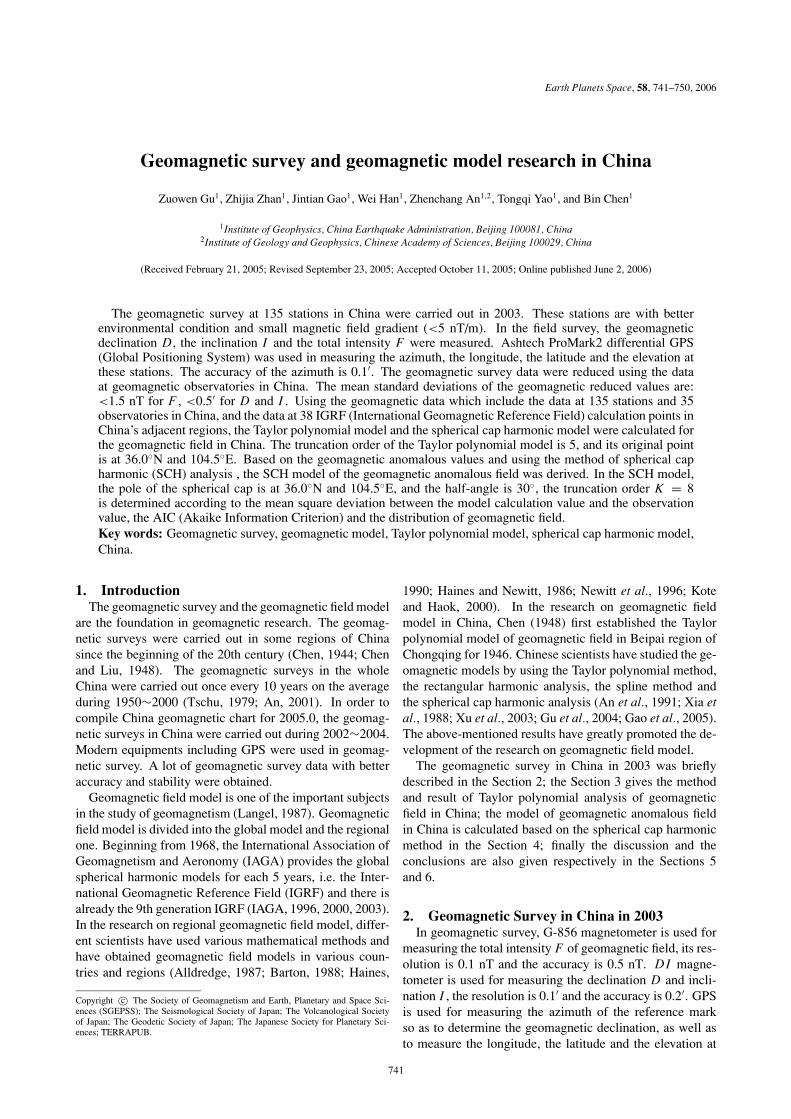
Fig. 1. Distribution of the geomagnetic stations and observatories in China.

the station (Newitt et al., 1996; Gu et al., 2006), its verti-cal locating accuracy is 10 mm + 1 ppm and the horizontallocating accuracy is 5 mm + 1 ppm. The magnetometersare calibrated before and after the survey in order to de-termine the differences between these magnetometers andthe standard one, and the differences were corrected in dataprocessing.

In China, the 135 geomagnetic stations (Fig. 1) were es-tablished in 2003. Each station was carefully selected. Theenvironmental condition around each station is good with-out any electromagnetic noise. The geomagnetic gradientaround each station is <5 nT/m: the range of the horizon-tal gradient is 0.4∼4.9 nT/m, and its average is 2.1 nT/m;the range of vertical gradient is 0.2∼4.9 nT/m, and its aver-age is 2.3 nT/m. The distance between the station and thereference mark is >200 m.

The survey at each station includes geomagnetic three-component and GPS observations. The sensor position ofG-856 magnetometer is ensured at the same position withthe coil position of DI magnetometer, the DI magnetome-ter is ensured at the same position with the centering posi-tion of GPS.

G-856 magnetometer is used to measure F simultane-ously with I . DI magnetometer is used to measure D andI with 8 group-data, including 4 group-data of positive andinverted telescope. Meanwhile, the azimuths of the refer-ence mark are measured by GPS before and after measuringD and I respectively.

GPS is used twice to measure the azimuths of the refer-ence mark at each station. The observation results of GPSshow that the distances between the station and the refer-ence mark are >200 m. The number of satellite received byGPS is 5∼10, the PDOP (Positioning Dilution of Precision)value is 1.7∼5.4. The data measured by GPS are processed

by using a notebook computer in field. The results show thatthe differences between two azimuths measured by GPS atvarious sites are 0.0′′∼5.9′′, the average is 1.6′′.

The geomagnetic data of field survey were reduced byusing the data at the observatories in China. The mean stan-dard deviations of geomagnetic reduced values are: <1.5nT for F ; <0.5′ for D and I . This shows that the geomag-netic survey data are reliable and accurate.

3. Taylor Polynomial Analysis of GeomagneticField in China

3.1 MethodTaylor polynomial model of geomagnetic field can be

expressed as:

F =N∑

n=0

n∑m=0

Anm(ϕ − ϕ0)n−m(λ − λ0)

m (1)

where Anm is the Taylor polynomial coefficient, N is thetruncation order of the Taylor polynomial, ϕ and λ arerespectively the longitude and the latitude at the station, ϕ0

and λ0 are respectively the longitude and the latitude at theoriginal point. F can represent any element of geomagneticfield.3.2 Result

According to the geomagnetic data, which include thedata at 135 stations and 35 observatories in China, andthe data at 38 IGRF calculation points in China’s adjacentregions, the Taylor polynomial model of the geomagneticfield in China for 2003 were calculated.

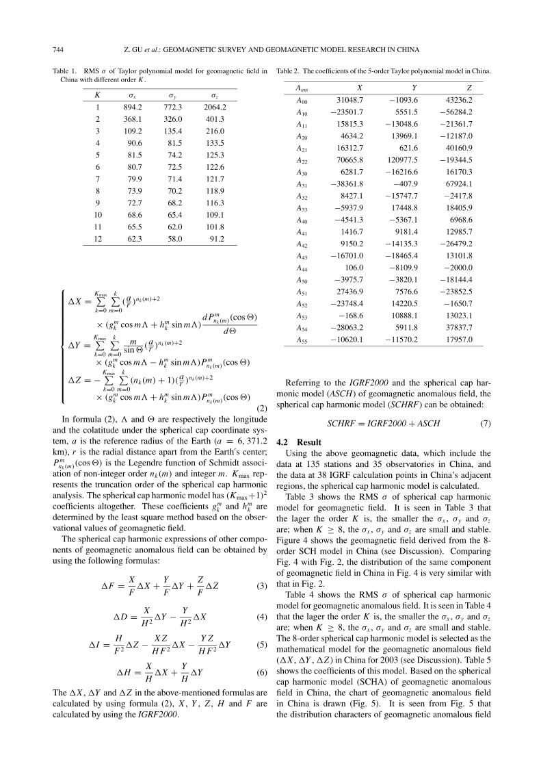
Table 1 shows the RMS (root mean square) σ of the Tay-lor polynomial model for geomagnetic field in China withdifferent order K . It is seen from Table 1 that when the or-der K increases, all of σx , σy and σz decrease; when K ≥ 5,

Z. GU et al.: GEOMAGNETIC SURVEY AND GEOMAGNETIC MODEL RESEARCH IN CHINA 743

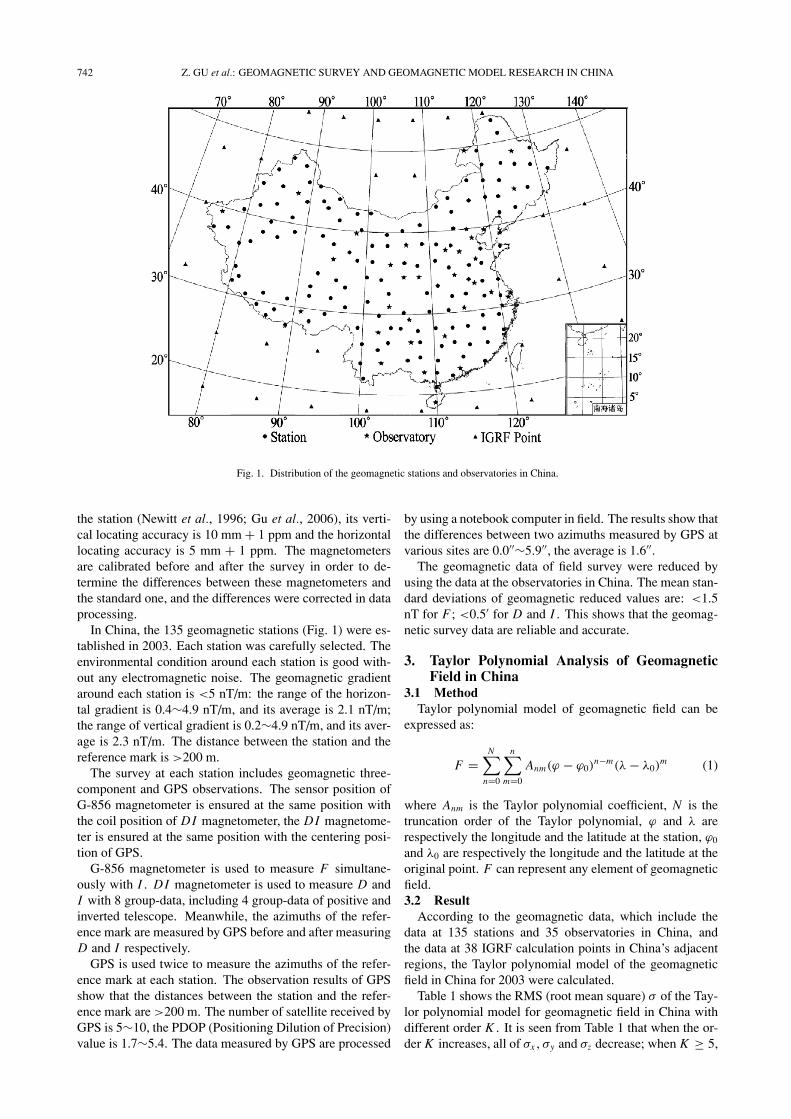
Fig. 2. Geomagnetic charts derived from the 5-order Taylor polynomial model in China. (a) D, � = 1◦; (b) I , � = 5◦; (c) F , � = 1,000 nT; (d) X ,� = 1,000 nT; (e) Y , � = 500 nT; (f) Z , � = 1,000 nT.

σx , σy and σz are small and stable. The 5-order Taylor poly-nomial model is taken as the geomagnetic field model inChina for 2003 (see Discussion). Table 2 shows the coeffi-cients of this model. Figure 2 shows the geomagnetic chartsderived from this model in China. The distribution charac-ters of various geomagnetic components can be seen fromFig. 2 that: the declination D and the east component Y arebasically distributed along the longitude; D decreases from8◦ in the west to −12◦ in the east; Y decreases from 2,000nT in the west to −4,000 nT in the east. The geomagnetictotal intensity F , the inclination I , the north component Xand the vertical component Z are basically distributed alongthe latitude; F increases from 43,000 nT in the south to59,000 nT in the north; X decreases from 38,000 nT in thesouth to 20,000 nT in the north; Z increases from 22,000

nT in the south to 54,000 nT in the north; I increases from30◦ in the south to 70◦ in the north.

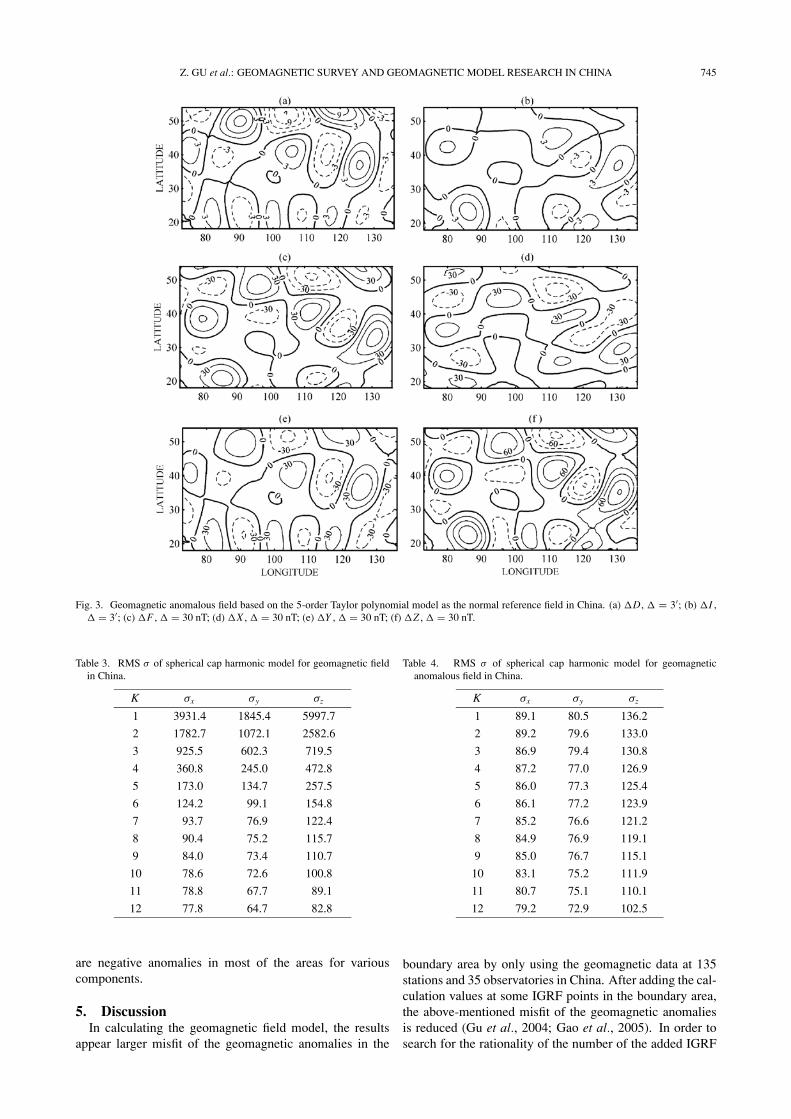
Figure 3 shows the distribution of the geomagneticanomalous field in China, the values of this anomalous fieldare the differences between the observed values and those ofthe 5-order Taylor polynomial model of geomagnetic fieldin China (CGRF). In Fig. 3, there are either positive or neg-ative geomagnetic anomalies in most regions of China, thedistribution is reasonable.

4. Spherical Cap Harmonic Analysis on the Geo-magnetic Field in China

4.1 MethodThe geomagnetic anomalous field (�X , �Y , �Z ) under

the spherical cap coordinate system can be expressed as:


Table 1. RMS σ of Taylor polynomial model for geomagnetic field inChina with different order K .

K σx σy σz

1 894.2 772.3 2064.2

2 368.1 326.0 401.3

3 109.2 135.4 216.0

4 90.6 81.5 133.5

5 81.5 74.2 125.3

6 80.7 72.5 122.6

7 79.9 71.4 121.7

8 73.9 70.2 118.9

9 72.7 68.2 116.3

10 68.6 65.4 109.1

11 65.5 62.0 101.8

12 62.3 58.0 91.2

⎧⎪⎪⎪⎪⎪⎪⎪⎪⎪⎪⎪⎪⎪⎪⎪⎨⎪⎪⎪⎪⎪⎪⎪⎪⎪⎪⎪⎪⎪⎪⎪⎩

�X =Kmax∑k=0

k∑m=0

(ar )nk (m)+2

× (gmk cos m� + hm

k sin m�)d Pm

nk (m)(cos �)

d�

�Y =Kmax∑k=0

k∑m=0

msin �

(ar )nk (m)+2

× (gmk cos m� − hm

k sin m�)Pmnk (m)(cos �)

�Z = −Kmax∑k=0

k∑m=0

(nk(m) + 1)(ar )nk (m)+2

× (gmk cos m� + hm

k sin m�)Pmnk (m)(cos �)

(2)In formula (2), � and � are respectively the longitude

and the colatitude under the spherical cap coordinate sys-tem, a is the reference radius of the Earth (a = 6, 371.2km), r is the radial distance apart from the Earth′s center;Pm

nk (m)(cos �) is the Legendre function of Schmidt associ-ation of non-integer order nk(m) and integer m. Kmax rep-resents the truncation order of the spherical cap harmonicanalysis. The spherical cap harmonic model has (Kmax+1)2

coefficients altogether. These coefficients gmk and hm

k aredetermined by the least square method based on the obser-vational values of geomagnetic field.

The spherical cap harmonic expressions of other compo-nents of geomagnetic anomalous field can be obtained byusing the following formulas:

�F = X

F�X + Y

F�Y + Z

F�Z (3)

�D = X

H 2�Y − Y

H 2�X (4)

�I = H

F2�Z − X Z

H F2�X − Y Z

H F2�Y (5)

�H = X

H�X + Y

H�Y (6)

The �X , �Y and �Z in the above-mentioned formulas arecalculated by using formula (2), X , Y , Z , H and F arecalculated by using the IGRF2000.

Table 2. The coefficients of the 5-order Taylor polynomial model in China.

Anm X Y Z

A00 31048.7 −1093.6 43236.2

A10 −23501.7 5551.5 −56284.2

A11 15815.3 −13048.6 −21361.7

A20 4634.2 13969.1 −12187.0

A21 16312.7 621.6 40160.9

A22 70665.8 120977.5 −19344.5

A30 6281.7 −16216.6 16170.3

A31 −38361.8 −407.9 67924.1

A32 8427.1 −15747.7 −2417.8

A33 −5937.9 17448.8 18405.9

A40 −4541.3 −5367.1 6968.6

A41 1416.7 9181.4 12985.7

A42 9150.2 −14135.3 −26479.2

A43 −16701.0 −18465.4 13101.8

A44 106.0 −8109.9 −2000.0

A50 −3975.7 −3820.1 −18144.4

A51 27436.9 7576.6 −23852.5

A52 −23748.4 14220.5 −1650.7

A53 −168.6 10888.1 13023.1

A54 −28063.2 5911.8 37837.7

A55 −10620.1 −11570.2 17957.0

Referring to the IGRF2000 and the spherical cap har-monic model (ASCH) of geomagnetic anomalous field, thespherical cap harmonic model (SCHRF) can be obtained:

SCHRF = IGRF2000 + ASCH (7)

4.2 ResultUsing the above geomagnetic data, which include the

data at 135 stations and 35 observatories in China, andthe data at 38 IGRF calculation points in China’s adjacentregions, the spherical cap harmonic model is calculated.

Table 3 shows the RMS σ of spherical cap harmonicmodel for geomagnetic field. It is seen in Table 3 thatthe lager the order K is, the smaller the σx , σy and σz

are; when K ≥ 8, the σx , σy and σz are small and stable.Figure 4 shows the geomagnetic field derived from the 8-order SCH model in China (see Discussion). ComparingFig. 4 with Fig. 2, the distribution of the same componentof geomagnetic field in China in Fig. 4 is very similar withthat in Fig. 2.

Table 4 shows the RMS σ of spherical cap harmonicmodel for geomagnetic anomalous field. It is seen in Table 4that the lager the order K is, the smaller the σx , σy and σz

are; when K ≥ 8, the σx , σy and σz are small and stable.The 8-order spherical cap harmonic model is selected as themathematical model for the geomagnetic anomalous field(�X , �Y , �Z ) in China for 2003 (see Discussion). Table 5shows the coefficients of this model. Based on the sphericalcap harmonic model (SCHA) of geomagnetic anomalousfield in China, the chart of geomagnetic anomalous fieldin China is drawn (Fig. 5). It is seen from Fig. 5 thatthe distribution characters of geomagnetic anomalous field


Fig. 3. Geomagnetic anomalous field based on the 5-order Taylor polynomial model as the normal reference field in China. (a) �D, � = 3′; (b) �I ,� = 3′; (c) �F , � = 30 nT; (d) �X , � = 30 nT; (e) �Y , � = 30 nT; (f) �Z , � = 30 nT.

Table 3. RMS σ of spherical cap harmonic model for geomagnetic fieldin China.

K σx σy σz

1 3931.4 1845.4 5997.7

2 1782.7 1072.1 2582.6

3 925.5 602.3 719.5

4 360.8 245.0 472.8

5 173.0 134.7 257.5

6 124.2 99.1 154.8

7 93.7 76.9 122.4

8 90.4 75.2 115.7

9 84.0 73.4 110.7

10 78.6 72.6 100.8

11 78.8 67.7 89.1

12 77.8 64.7 82.8

are negative anomalies in most of the areas for variouscomponents.

5. DiscussionIn calculating the geomagnetic field model, the results

appear larger misfit of the geomagnetic anomalies in the

Table 4. RMS σ of spherical cap harmonic model for geomagneticanomalous field in China.

K σx σy σz

1 89.1 80.5 136.2

2 89.2 79.6 133.0

3 86.9 79.4 130.8

4 87.2 77.0 126.9

5 86.0 77.3 125.4

6 86.1 77.2 123.9

7 85.2 76.6 121.2

8 84.9 76.9 119.1

9 85.0 76.7 115.1

10 83.1 75.2 111.9

11 80.7 75.1 110.1

12 79.2 72.9 102.5

boundary area by only using the geomagnetic data at 135stations and 35 observatories in China. After adding the cal-culation values at some IGRF points in the boundary area,the above-mentioned misfit of the geomagnetic anomaliesis reduced (Gu et al., 2004; Gao et al., 2005). In order tosearch for the rationality of the number of the added IGRF


Table 5. The coefficients of the 8-order spherical cap harmonic model of geomagnetic anomalous field in China.

K M gmk hm

k K M gmk hm

k

0 0 358.5 6 2 −49.2 62.6

1 0 −406.8 6 3 77.7 48.2

1 1 −104.7 63.2 6 4 −70.4 23.1

2 0 702.2 6 5 −23.2 27.0

2 1 255.1 −57.6 6 6 19.9 −9.4

2 2 −58.5 14.6 7 0 −82.3

3 0 −892.7 7 1 −61.8 16.8

3 1 −397.9 68.6 7 2 −1.4 −32.4

3 2 160.8 −37.4 7 3 −43.0 −12.8

3 3 −14.2 −45.7 7 4 47.2 −10.6

4 0 874.0 7 5 17.1 −27.3

4 1 414.9 −61.9 7 6 −8.6 9.5

4 2 −209.2 59.4 7 7 −0.3 5.8

4 3 56.0 82.9 8 0 13.5

4 4 −4.0 21.7 8 1 10.8 −4.2

5 0 −595.4 8 2 4.1 9.8

5 1 −318.2 50.8 8 3 10.6 −1.4

5 2 141.0 −73.7 8 4 −14.0 2.0

5 3 −83.8 −86.7 8 5 −5.8 11.2

5 4 49.4 −24.3 8 6 1.5 −6.8

5 5 17.8 −12.1 8 7 −2.4 1.4

6 0 289.3 8 8 3.4 −3.1

6 1 165.8 −35.0

points and the distribution, a model calculation is done forsome groups of selecting 28∼48 IGRF points and their ho-mogeneous distribution. The model calculation results fordifferent groups are analyzed and compared. The compre-hensive analysis and comparison show that the effects be-come the best when adding 38 IGRF points as shown inFig. 1. This shows that it is necessary and rational to addIGRF points appropriately.

Taylor polynomial model is a common one of geomag-netic field because it is convenient in calculation and ap-plication. In the research on geomagnetic field model inChina, Chinese scientists have studied the Taylor polyno-mial models in China (Chen, 1948; Xia et al., 1988; Xu etal., 2003). In these studies of the Taylor polynomial model,the truncation order K of the models was taken as K = 2(Chen, 1948), K = 3 (Xia et al., 1988) and K = 4 (Xu etal., 2003). The truncation order of the Taylor polynomialmodel is taken as K = 5 in this paper. The larger the Kis, the higher the space resolution is, and the smaller themean square deviation between the model calculation valueand the observation value is. Therefore, the 5-order Tay-lor polynomial model in this paper can better describe thegeomagnetic field in China.

The spherical cap harmonic (SCH) analysis is an effec-tive method in the research on regional geomagnetic field.The calculation results show that SCH method can not onlydescribe the distribution of geomagnetic field in a largerange (such as the whole China or Asia), but can also de-scribe the distribution of geomagnetic field in a smallerrange as Beijing-Tianjin-Hebei region (Gu et al., 2004).

In order to compare the distribution of the geomagneticanomalous field in China derived from the Taylor polyno-mial model (Fig. 3) and the SCHA model (Fig. 5), we ana-lyze the similarity and the difference between Figs. 3 and 5.It is seen from Figs. 3 and 5 that the geomagnetic anomalouscharts basically have the similar shape for the same compo-nent. In Fig. 3, there are either positive or negative geomag-netic anomalies in most regions of China, the distribution isreasonable. In Fig. 5, the geomagnetic anomalous fields(such as �F , �Y and �Z etc.) in most regions of Chinaare negative, the distribution of geomagnetic anomaly is notequivalent. It shows that there is difference between theanomalous fields in Figs. 3 and 5. In fact, Fig. 5 is basedon IGRF as the normal reference field while Fig. 3 is basedon CGRF as the normal reference field. Taking IGRF asthe normal reference field, it can study the anomalous fieldwith a large scale; while taking CGRF as the normal refer-ence field, it can explore the anomalous field with a smallerscale.

One of the key problems in establishing the geomagneticfield model is to determine the truncation order K . Thelarger the K is, the higher the space resolution is, and thesmaller the mean square deviation between the model cal-culation value and the observation value is. However, whenK is large, the model calculation results are relatively un-stable. In order to reasonably determine K , K was respec-tively taken as 1∼12 for the spherical cap harmonic modelin model calculation. Figure 6(a) shows the decrease of σ

(RMS values) of the SCH model of the geomagnetic fieldwith different truncation order K . It is seen from Fig. 6(a)


Fig. 4. Geomagnetic field derived from the 8-order SCH model in China. (a) D, � = 1◦; (b) I , � = 5◦; (c) F , � = 1,000 nT; (d) X , � = 1,000 nT;(e) Y , � = 500 nT; (f) Z , � = 1,000 nT.

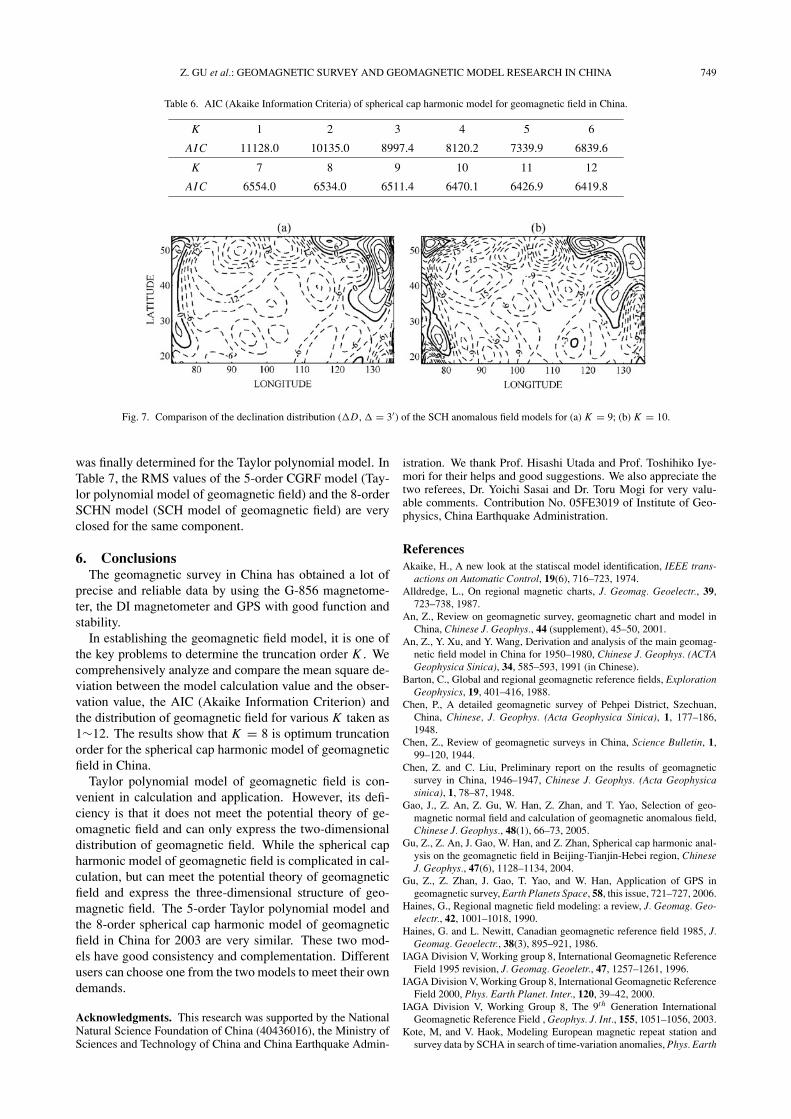
that when K ≥ 8, the σx , σy and σz are small and stable. Inorder to determine the truncation order K , we also calculateAIC (Akaike Information Criteria) (Akaike, 1974; Miura etal., 2000) for different truncation order K taken as 1–12 re-spectively. The AIC for each K is shown in Table 6 andFig. 6(b). Figure 6(b) shows that the AIC decreases whenK increases; when K ≥ 7, the AIC is nearly stable. Mean-while, we compare the distribution of the geomagnetic fieldand the anomalous field derived from the SCH models withK ≥ 8. As an example, Figs. 3(a) and 7 give the com-parison of the declination distribution of the SCH anoma-lous field models for K = 8 (Fig. 3(a)), K = 9 and 10(Fig. 7). The comparison results show that the distributionwith K = 8 is reasonable. However, the distribution withK ≥ 9 appears some misfit, the larger the K is, the largerthe misfit is. Therefore, K = 8 is finally taken as the trun-cation order of the SCH model. It is seen from Table 7 thatthe RMS values of the 8-order SCHN model (SCH model

Table 7. Comparison of σ (RMS) for various models in China for 2003.The 8-order SCHN is the 8-order SCH model of geomagnetic field, the8-order SCHA is the 8-order SCH model of geomagnetic anomalousfield, the 5-order CGRF is the 5-order Taylor polynomial model ofgeomagnetic field.

Model σx (nT) σy(nT) σz(nT)

8-order SCHN 90.4 75.2 115.7

8-order SCHA 84.9 76.9 119.1

5-order CGRF 81.5 74.2 125.3

of geomagnetic field) and the 8-order SCHA model (SCHmodel of geomagnetic anomalous field) are very closed forthe same component.

Similarly, K was respectively taken as 1∼12 for the Tay-lor polynomial model in model calculation. The results forvarious K (1∼12) were analyzed and compared, K = 5


Fig. 5. Geomagnetic anomalous field derived from the 8-order SCHA model in China. (a) �D, � = 3′; (b) �I , � = 3′; (c) �F , � = 30 nT; (d) �X ,� = 30 nT; (e) �Y , � = 30 nT; (f) �Z , � = 30 nT.

Fig. 6. (a) Decrease of σ (RMS values) of the SCH model of the geomagnetic field with different truncation orders K . (b) Decrease of AIC of the SCHmodel of the geomagnetic field with different truncation order K .


Table 6. AIC (Akaike Information Criteria) of spherical cap harmonic model for geomagnetic field in China.

K 1 2 3 4 5 6

AI C 11128.0 10135.0 8997.4 8120.2 7339.9 6839.6

K 7 8 9 10 11 12

AI C 6554.0 6534.0 6511.4 6470.1 6426.9 6419.8

Fig. 7. Comparison of the declination distribution (�D, � = 3′) of the SCH anomalous field models for (a) K = 9; (b) K = 10.

was finally determined for the Taylor polynomial model. InTable 7, the RMS values of the 5-order CGRF model (Tay-lor polynomial model of geomagnetic field) and the 8-orderSCHN model (SCH model of geomagnetic field) are veryclosed for the same component.

6. ConclusionsThe geomagnetic survey in China has obtained a lot of

precise and reliable data by using the G-856 magnetome-ter, the DI magnetometer and GPS with good function andstability.

In establishing the geomagnetic field model, it is one ofthe key problems to determine the truncation order K . Wecomprehensively analyze and compare the mean square de-viation between the model calculation value and the obser-vation value, the AIC (Akaike Information Criterion) andthe distribution of geomagnetic field for various K taken as1∼12. The results show that K = 8 is optimum truncationorder for the spherical cap harmonic model of geomagneticfield in China.

Taylor polynomial model of geomagnetic field is con-venient in calculation and application. However, its defi-ciency is that it does not meet the potential theory of ge-omagnetic field and can only express the two-dimensionaldistribution of geomagnetic field. While the spherical capharmonic model of geomagnetic field is complicated in cal-culation, but can meet the potential theory of geomagneticfield and express the three-dimensional structure of geo-magnetic field. The 5-order Taylor polynomial model andthe 8-order spherical cap harmonic model of geomagneticfield in China for 2003 are very similar. These two mod-els have good consistency and complementation. Differentusers can choose one from the two models to meet their owndemands.

Acknowledgments. This research was supported by the NationalNatural Science Foundation of China (40436016), the Ministry ofSciences and Technology of China and China Earthquake Admin-

istration. We thank Prof. Hisashi Utada and Prof. Toshihiko Iye-mori for their helps and good suggestions. We also appreciate thetwo referees, Dr. Yoichi Sasai and Dr. Toru Mogi for very valu-able comments. Contribution No. 05FE3019 of Institute of Geo-physics, China Earthquake Administration.

ReferencesAkaike, H., A new look at the statiscal model identification, IEEE trans-

actions on Automatic Control, 19(6), 716–723, 1974.Alldredge, L., On regional magnetic charts, J. Geomag. Geoelectr., 39,

723–738, 1987.An, Z., Review on geomagnetic survey, geomagnetic chart and model in

China, Chinese J. Geophys., 44 (supplement), 45–50, 2001.An, Z., Y. Xu, and Y. Wang, Derivation and analysis of the main geomag-

netic field model in China for 1950–1980, Chinese J. Geophys. (ACTAGeophysica Sinica), 34, 585–593, 1991 (in Chinese).

Barton, C., Global and regional geomagnetic reference fields, ExplorationGeophysics, 19, 401–416, 1988.

Chen, P., A detailed geomagnetic survey of Pehpei District, Szechuan,China, Chinese, J. Geophys. (Acta Geophysica Sinica), 1, 177–186,1948.

Chen, Z., Review of geomagnetic surveys in China, Science Bulletin, 1,99–120, 1944.

Chen, Z. and C. Liu, Preliminary report on the results of geomagneticsurvey in China, 1946–1947, Chinese J. Geophys. (Acta Geophysicasinica), 1, 78–87, 1948.

Gao, J., Z. An, Z. Gu, W. Han, Z. Zhan, and T. Yao, Selection of geo-magnetic normal field and calculation of geomagnetic anomalous field,Chinese J. Geophys., 48(1), 66–73, 2005.

Gu, Z., Z. An, J. Gao, W. Han, and Z. Zhan, Spherical cap harmonic anal-ysis on the geomagnetic field in Beijing-Tianjin-Hebei region, ChineseJ. Geophys., 47(6), 1128–1134, 2004.

Gu, Z., Z. Zhan, J. Gao, T. Yao, and W. Han, Application of GPS ingeomagnetic survey, Earth Planets Space, 58, this issue, 721–727, 2006.

Haines, G., Regional magnetic field modeling: a review, J. Geomag. Geo-electr., 42, 1001–1018, 1990.

Haines, G. and L. Newitt, Canadian geomagnetic reference field 1985, J.Geomag. Geoelectr., 38(3), 895–921, 1986.

IAGA Division V, Working group 8, International Geomagnetic ReferenceField 1995 revision, J. Geomag. Geoeletr., 47, 1257–1261, 1996.

IAGA Division V, Working Group 8, International Geomagnetic ReferenceField 2000, Phys. Earth Planet. Inter., 120, 39–42, 2000.

IAGA Division V, Working Group 8, The 9th Generation InternationalGeomagnetic Reference Field , Geophys. J. Int., 155, 1051–1056, 2003.

Kote, M, and V. Haok, Modeling European magnetic repeat station andsurvey data by SCHA in search of time-variation anomalies, Phys. Earth


Planet. Inter., 122(3–4), 205–220, 2000.Langel, L., Main field, in Geomagnetism, edited by J. A. Jacobs, Vol. 1,

pp. 249–512, Academic Press, London, 1987.Miura, S., S. Ueki, T. Sato, K. Tachibana, and H. Hamaguchi, Crustal

deformation associated with the 1998 seismo-volcanic crisis of IwateVolcano, Northeastern Japan, as observed by a dense GPS network,Earth Planets Space, 52, 1003–1008, 2000.

Haines, G., Regional magnetic field modeling: a review, J. Geomag. Geo-electr., 42, 1001–1018, 1990.

Newitt, L. B., C. E. Barton, and J. Bitterly, in Guide for Magnetic RepeatStation Surveys, 112 pp., International Association of Geomagnetismand Aeronomy, 1996.

Tschu, K., On some advancement of Chinese geomagnetism and aeronomyduring 1949–1979, Chinese J. Geophys. (Acta Gephysica sinica), 22,

326–335, 1979 (in Chinese).Xia, G., S. Zheng, L. Wu, F. Zhang, and H. Wei, The geomagnetic field

chart of China in 1980.0 and the mathematical model, Chinese J. Geo-phys. (Acta Geophysica Sinica), 31, 82–89, 1988 (in Chinese).

Xu, W., G. Xia, Z. An, G. Chen, F. Zhang, Y. Wang, Y. Tian, Z. Wei, S.Ma, and H. Chen, Magnetic survey and China GRF2000, Earth PlanetsSpace, 55, 215–217, 2003.

Z. Gu (e-mail: [email protected]), Z. Zhan, J. Gao (e-mail:[email protected]), W. Han (e-mail: [email protected]), Z. An,T. Yao (e-mail: [email protected]), and B. Chen (e-mail: cham-pion [email protected])

geomagnetic survey and geomagnetic model research in china

Documents