geological society of america special papers · geological society of america special papers 2012;...

Geological Society of America Special Papers

doi: 10.1130/2012.2492(01) 2012;492;1-22Geological Society of America Special Papers

G. Burch Fisher, Colin B. Amos, Bodo Bookhagen, Douglas W. Burbank and Vincent Godard processeshigh-spatial resolution Google Earth imagery in the study of earth surface Channel widths, landslides, faults, and beyond: The new world order of

Email alerting servicescite this article

to receive free e-mail alerts when new articleswww.gsapubs.org/cgi/alertsclick

SubscribeAmerica Special Papers

to subscribe to Geological Society ofwww.gsapubs.org/subscriptions/click

Permission request to contact GSAhttp://www.geosociety.org/pubs/copyrt.htm#gsaclick

viewpoint. Opinions presented in this publication do not reflect official positions of the Society.positions by scientists worldwide, regardless of their race, citizenship, gender, religion, or politicalarticle's full citation. GSA provides this and other forums for the presentation of diverse opinions and articles on their own or their organization's Web site providing the posting includes a reference to thescience. This file may not be posted to any Web site, but authors may post the abstracts only of their unlimited copies of items in GSA's journals for noncommercial use in classrooms to further education andto use a single figure, a single table, and/or a brief paragraph of text in subsequent works and to make

GSA,employment. Individual scientists are hereby granted permission, without fees or further requests to Copyright not claimed on content prepared wholly by U.S. government employees within scope of their

Notes

© 2012 Geological Society of America

on December 12, 2012specialpapers.gsapubs.orgDownloaded from

http://specialpapers.gsapubs.org/cgi/alerts

http://specialpapers.gsapubs.org/subscriptions/index.ac.dtl

http://www.geosociety.org/pubs/copyrt.htm#gsa

http://specialpapers.gsapubs.org/

1

The Geological Society of AmericaSpecial Paper 492

2012

Channel widths, landslides, faults, and beyond: The new world order of high-spatial resolution Google Earth imagery

in the study of earth surface processes

G. Burch Fisher*Department of Earth Science, University of California, Santa Barbara, California, USA

Colin B. AmosDepartment of Earth and Planetary Science, University of California, Berkeley, California, USA

Bodo BookhagenDepartment of Geography, University of California, Santa Barbara, California, USA

Douglas W. BurbankDepartment of Earth Science, University of California, Santa Barbara, California, USA

Vincent GodardCEREGE, CNRS-UMR6635, Aix-Marseille Université, Aix-en-Provence, France

ABSTRACT

The past decade has seen a rapid increase in the application of high-resolution imagery and geographic-based information systems across every segment of society from security intelligence to product marketing to scientifi c research. Google Earth has positioned itself at the forefront of this spatial information wave by providing free access to high-resolution imagery through a simple, user-friendly interface. Whereas Google Earth imagery has been widely exploited across the earth sciences for spatial visualization, education, and place-based searches, few studies have utilized the high-resolution imagery to yield quantitative insights about the processes and mechanisms acting at the earth’s surface. In this paper, we detail the benefi ts of the underlying high-resolution imagery available within Google Earth, review the limited published research to date, and utilize this imagery to quantitatively illuminate previously dif-fi cult and unresolved questions within the discipline of geomorphology involving: (1) channel-width variability and scaling relations in the tectonically active Hima-laya; (2) landslide characteristics related to large magnitude climatic and tectonic events in Haiti; and (3) identifi cation and quantifi cation of laterally offset geomor-phic features within eastern California. In each example, we compare analyses using

*[email protected]

Fisher, G.B., Amos, C.B., Bookhagen, B., Burbank, D.W., and Godard, V., 2012, Channel widths, landslides, faults, and beyond: The new world order of high-spatial resolution Google Earth imagery in the study of earth surface processes, in Whitmeyer, S.J., Bailey, J.E., De Paor, D.G., and Ornduff, T., eds., Google Earth and Virtual Visualizations in Geoscience Education and Research: Geological Society of America Special Paper 492, p. 1–22, doi:10.1130/2012.2492(01). For permission to copy, contact [email protected]. © 2012 The Geological Society of America. All rights reserved.



2 Fisher et al.

1. INTRODUCTION

Since the launch of Google Earth in 2005, millions of people have gained the ability to access and visualize spatial data in a historically unprecedented way. The ability to see and query the world with speed and simplicity across a broad range of spatial (and now temporal) scales was only a dream when proto–Google Earth creators Silicon Graphics (SGI) launched their “Space-to-Your-Face” demo in 1996 (M. Aubin, “Google Earth: From Space to Your Face...and Beyond,” http://mattiehead.wordpress.com/tag/google-earth/, accessed May 2012). A decade and a half later, Google Earth has brought geographical information systems to the masses with hundreds of millions of recreational users exploring both human and natural ecosystems across not just the earth, but the solar system. Despite the obvious utility of Google Earth’s extensive high-resolution imagery database, it has to date been largely regarded by the research community as purely for education and/or visualization purposes. The focus of this article is to demonstrate the utility of Google Earth and its high-resolution imagery as a powerful research tool to explore and quantify earth surface processes.

In this article, we begin by describing the background and underlying imagery that makes Google Earth such a powerful platform. We then discuss the limited published research to date and highlight three research examples that underscore the value of Google Earth imagery in solving problems whose solutions were previously inhibited by traditional techniques, fi nancial constraints, and/or inaccessible terrain. Lastly, we assess some of the current limitations with using Google Earth imagery for research purposes and highlight suitable future applications of high-resolution Google Earth imagery to quantitatively study the processes shaping both earth and planetary surfaces.

2. THE BEAUTY OF GOOGLE EARTH IMAGERY

Early on, Google Earth utilized freely available Landsat imagery (30-m resolution) (landsat.gsfc.nasa.gov/) with Shuttle Radar Topography Mission (SRTM) digital elevation models (30 m or 90 m resolution) (Farr et al., 2007). With the advent of high-resolution passive optical sensors and a commercial market for that imagery, however, Google Earth has been well placed to exploit such spatial information. Presently, Google Earth con-

tains a large range of true-color visible spectrum (400–700 nm wavelength) imagery derived from a mix of freely available pub-lic domain Landsat imagery, government orthophotos, and high-resolution commercial data sets available from DigitalGlobe™ (www.digitalglobe.com), GeoEye™ (www.geoeye.com), and SPOT™ (www.spot.com), with considerable investment in Geo-Eye™ coming directly from Google (Jones, 2008) (Fig. 1 and Table 1). The investment in high-resolution imagery has paid great dividends for Google with Google Earth now being used by millions of people around the world. Due to this popularity, earth scientists and especially geomorphologists now have access to imagery that in places reaches sub-meter resolution and costs nothing. This free access stands in stark contrast to the hundreds of dollars one would normally pay per scene (~100 km2) for high-resolution imagery, permitting large-scale, high-resolution studies that were previously diffi cult or impossible to achieve. Furthermore, Google has shown great commitment to constantly improving and expanding the imagery available in Google Earth, not only in terms of the spatial resolution of the imagery, but tem-porally as well. With the update to Google Earth 5 in early 2009, historical imagery became a key component of the platform, and now allows users to browse through past airphotos and archival satellite images of a given area to easily detect changes through time. Historical imagery along with an ever-expanding archive of high-resolution base imagery makes Google Earth a wonderful resource for the layperson, but also a powerful database and tool for researchers in the earth sciences.

In the following section we review the minimal literature to date that has utilized Google Earth as a primary data source and show three ways in which we have leveraged Google Earth imagery to: (1) improve on current understandings of how widths of river channels adjust and scale in tectonically active orogens; (2) document landslide triggering mechanisms and characteris-tics in Haiti; and (3) characterize and quantify previously uniden-tifi ed fault displacements in eastern California.

3. GOOGLE EARTH AS A PRIMARY DATA SOURCE

3.1. Past Work

Google Earth provides a palatable and expansive medium for visualizing, disseminating, and interacting with spatial data

freely available Google Earth imagery with standard imagery and techniques (e.g., Landsat, ASTER, lidar) to demonstrate the potential benefi ts of using high-spatial resolution Google Earth imagery over established methodologies. In addition, we dis-cuss the potential limitations and problems with using the imagery currently avail-able in Google Earth and propose favorable future applications, namely studies in remote terrains and those requiring high-resolution imagery across a large spatial extent, where purchasing such imagery in an academic environment would be cost-prohibitive. Whether as a supplement, for reconnaissance, or as the primary data set, high-resolution Google Earth imagery, when properly applied, holds great promise for quantitatively tackling previously unresolved problems in the study of earth sur-face processes.



Channel widths, landslides, faults, and beyond 3

Figure 1. Examples of four predominant types of imagery available in Google Earth from a viewing height of 1500 m. (A) High-resolution (~1 m) GeoEye™ imagery of a small island in the Maldives, Indian Ocean. (B) High-resolution (~1 m) Worldview™ imagery of a star dune from the Namib Desert. (C) High-resolution (~1–5 m) CNES/Spot™ imagery of a debris covered glacial terminus in the Bhutan Himalaya. (D) Lower-resolution (pan-sharpened to 15 m) Landsat 7 ETM+ image of an Amazonian tributary near Puerto Limón, Peru. North is to the top in all images.

TABLE 1. SOME OF THE MOST COMMONLY USED IMAGERY IN GOOGLE EARTH

regami rojaM noituloseR yregami fo epyT noitamrofni lanoitiddA redivorp yLandsat 7 ETM+ 30 m or 15 m

pan-sharpened Terra Metrics, Inc. NASA

www.truearth.com landsat.gsfc.nasa.gov

SPOT, FORMOSAT-2, KOMPSAT-2, Pleiades

moc.tops.www .A.S egamI topS m 8–5.0

Worldview-1, Worldview-2, Quickbird

moc.ebolglatigid.www .cnI ,ebolGlatigiD m 5.2–5.0

moc.eyeoeg.www .cnI ,eyEoeG m 2.3–5.0 SONOKI ,1-eyEoeG

Aerial Imagery (USA) 0.5–2 m U.S. Department of Agriculture; U.S. Geological Survey; Bluesky; Aerodata International Surveys; etc.

eros.usgs.gov www.fsa.usda.gov www.bluesky-world.com www.aerodata-surveys.com

naeco/moc.elgoog.htrae OCBEG ,AGN ,yvaN .S.U ,OIS ,AAON m 001> yrtemyhtab ekal dna naecO

Note: Google does not make public the specific type of imagery used in Google Earth, only the providers. Due to this, and the constant evolution of the platform, some of the imagery presented above may not actually be utilized in Google Earth, while other unlisted sources undoubtedly are. Additionally, the U.S. government limits the resolution of imagery made available to the public to 0.5 m despite the fact that GeoEye-1 has a maximum resolution of 0.41 m. NOAA—National Oceanic and Atmospheric Administration; SIO—Scripps Institute of Oceanography; NGA—National Geospatial Intelligence Agency; GEBCO—General Bathymetric Chart of the Oceans.



4 Fisher et al.

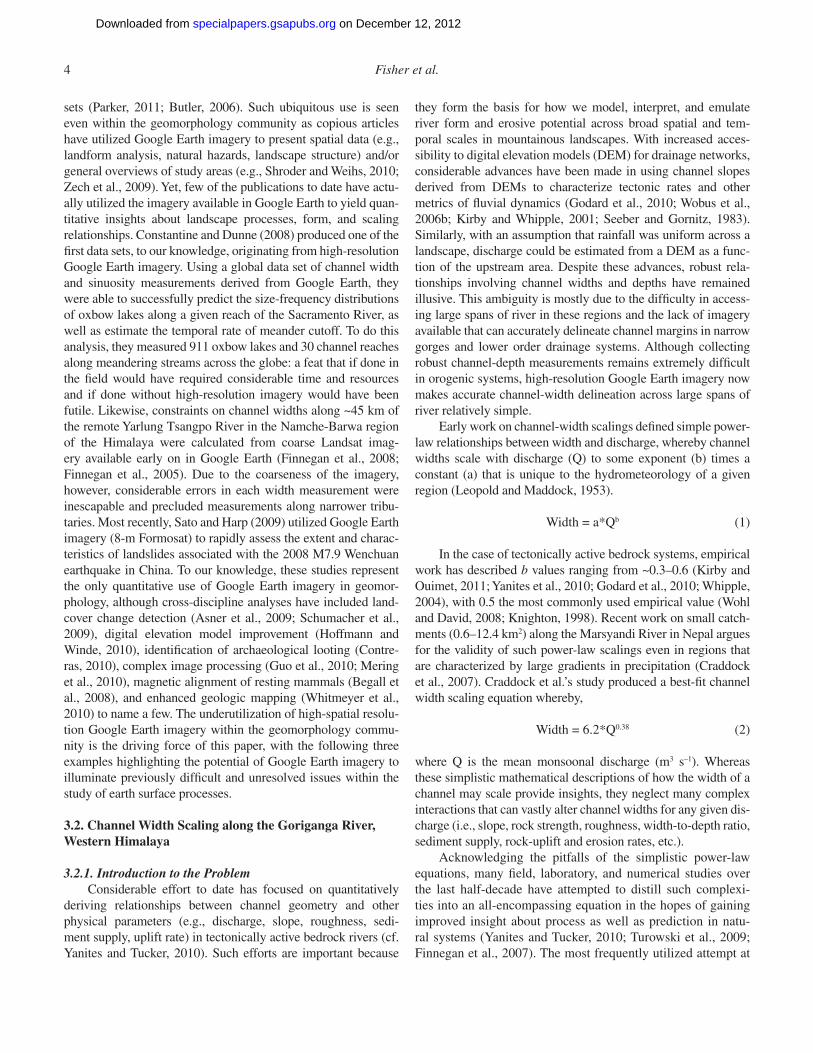
sets (Parker, 2011; Butler, 2006). Such ubiquitous use is seen even within the geomorphology community as copious articles have utilized Google Earth imagery to present spatial data (e.g., landform analysis, natural hazards, landscape structure) and/or general overviews of study areas (e.g., Shroder and Weihs, 2010; Zech et al., 2009). Yet, few of the publications to date have actu-ally utilized the imagery available in Google Earth to yield quan-titative insights about landscape processes, form, and scaling relationships. Constantine and Dunne (2008) produced one of the fi rst data sets, to our knowledge, originating from high-resolution Google Earth imagery. Using a global data set of channel width and sinuosity measurements derived from Google Earth, they were able to successfully predict the size-frequency distributions of oxbow lakes along a given reach of the Sacramento River, as well as estimate the temporal rate of meander cutoff. To do this analysis, they measured 911 oxbow lakes and 30 channel reaches along meandering streams across the globe: a feat that if done in the fi eld would have required considerable time and resources and if done without high-resolution imagery would have been futile. Likewise, constraints on channel widths along ~45 km of the remote Yarlung Tsangpo River in the Namche-Barwa region of the Himalaya were calculated from coarse Landsat imag-ery available early on in Google Earth (Finnegan et al., 2008; Finnegan et al., 2005). Due to the coarseness of the imagery, however, considerable errors in each width measurement were inescapable and precluded measurements along narrower tribu-taries. Most recently, Sato and Harp (2009) utilized Google Earth imagery (8-m Formosat) to rapidly assess the extent and charac-teristics of landslides associated with the 2008 M7.9 Wenchuan earthquake in China. To our knowledge, these studies represent the only quantitative use of Google Earth imagery in geomor-phology, although cross-discipline analyses have included land-cover change detection (Asner et al., 2009; Schumacher et al., 2009), digital elevation model improvement (Hoffmann and Winde, 2010), identifi cation of archaeological looting (Contre-ras, 2010), complex image processing (Guo et al., 2010; Mering et al., 2010), magnetic alignment of resting mammals (Begall et al., 2008), and enhanced geologic mapping (Whitmeyer et al., 2010) to name a few. The underutilization of high-spatial resolu-tion Google Earth imagery within the geomorphology commu-nity is the driving force of this paper, with the following three examples highlighting the potential of Google Earth imagery to illuminate previously diffi cult and unresolved issues within the study of earth surface processes.

3.2. Channel Width Scaling along the Goriganga River, Western Himalaya

3.2.1. Introduction to the ProblemConsiderable effort to date has focused on quantitatively

deriving relationships between channel geometry and other physical parameters (e.g., discharge, slope, roughness, sedi-ment supply, uplift rate) in tectonically active bedrock rivers (cf. Yanites and Tucker, 2010). Such efforts are important because

they form the basis for how we model, interpret, and emulate river form and erosive potential across broad spatial and tem-poral scales in mountainous landscapes. With increased acces-sibility to digital elevation models (DEM) for drainage networks, considerable advances have been made in using channel slopes derived from DEMs to characterize tectonic rates and other metrics of fl uvial dynamics (Godard et al., 2010; Wobus et al., 2006b; Kirby and Whipple, 2001; Seeber and Gornitz, 1983). Similarly, with an assumption that rainfall was uniform across a landscape, discharge could be estimated from a DEM as a func-tion of the upstream area. Despite these advances, robust rela-tionships involving channel widths and depths have remained illusive. This ambiguity is mostly due to the diffi culty in access-ing large spans of river in these regions and the lack of imagery available that can accurately delineate channel margins in narrow gorges and lower order drainage systems. Although collecting robust channel-depth measurements remains extremely diffi cult in orogenic systems, high-resolution Google Earth imagery now makes accurate channel-width delineation across large spans of river relatively simple.

Early work on channel-width scalings defi ned simple power-law relationships between width and discharge, whereby channel widths scale with discharge (Q) to some exponent (b) times a constant (a) that is unique to the hydrometeorology of a given region (Leopold and Maddock, 1953).

Width = a*Qb (1)

In the case of tectonically active bedrock systems, empirical work has described b values ranging from ~0.3–0.6 (Kirby and Ouimet, 2011; Yanites et al., 2010; Godard et al., 2010; Whipple, 2004), with 0.5 the most commonly used empirical value (Wohl and David, 2008; Knighton, 1998). Recent work on small catch-ments (0.6–12.4 km2) along the Marsyandi River in Nepal argues for the validity of such power-law scalings even in regions that are characterized by large gradients in precipitation (Craddock et al., 2007). Craddock et al.’s study produced a best-fi t channel width scaling equation whereby,

Width = 6.2*Q0.38 (2)

where Q is the mean monsoonal discharge (m3 s–1). Whereas these simplistic mathematical descriptions of how the width of a channel may scale provide insights, they neglect many complex interactions that can vastly alter channel widths for any given dis-charge (i.e., slope, rock strength, roughness, width-to-depth ratio, sediment supply, rock-uplift and erosion rates, etc.).

Acknowledging the pitfalls of the simplistic power-law equations, many fi eld, laboratory, and numerical studies over the last half-decade have attempted to distill such complexi-ties into an all-encompassing equation in the hopes of gaining improved insight about process as well as prediction in natu-ral systems (Yanites and Tucker, 2010; Turowski et al., 2009; Finnegan et al., 2007). The most frequently utilized attempt at




predicting channel widths following these tenets uses the Man-ning equation and principles of mass conservation to produce the following equation:

Width = [α(α+2)2/3]3/8Q3/8S–3/16n3/8 (3)

where α is the width-to-depth ratio, Q is discharge (m3 s–1), S is channel slope (m/m), and n is roughness as defi ned by Manning’s equation (Finnegan et al., 2005; Manning, 1891). Although Equation 3 takes a more thorough approach to predicting chan-nel widths, it is not without its pitfalls. For example, it is diffi -cult to estimate, much less measure, width-to-depth ratios with much reliability or accuracy over large spans of rivers in tec-tonically active areas. Whereas Finnegan et al. (2005) assumed a constant width to depth ratio along the ~45-km stretch of the Tsangpo River where the equation was validated, many fi eld observations in these environments attest to the wide ranging geometries observed in tectonically active orogens (Fisher et al., 2011; Whittaker et al., 2007; Duvall et al., 2004; Lavé and Avouac, 2001). Likewise, Manning’s roughness coeffi cient is not easily calculated where cyclical landsliding and damming can greatly alter channel bed properties over relatively short length and time scales (Korup and Montgomery, 2008; Korup, 2006; Bookhagen et al., 2005a). In addition, widths derived from the equations above are commonly key inputs for simple physics-based estimates of the geomorphic work performed on the bed of a channel by a given fl ow (e.g., shear stress, spe-cifi c stream power). Such proxies are then commonly used to assess a host of topics ranging from tectonic rates and structural boundaries to particle and wood stabilities along fl uvial pro-fi les (Attal et al., 2011; Fisher et al., 2010; Thiede et al., 2009; Finnegan et al., 2008; Stock and Montgomery, 1999; Whipple and Tucker, 1999; Bookhagen and Strecker, 2012). Although channel width is only one term in the equation, considerable deviation in the width values can greatly alter observations of spatial variations in erosion and subsequent interpretations.

Whereas power-law and more complex equations (Equa-tions 1–3) can provide fi rst-order estimates of channel widths based on digital topography and a set of assumptions, the dearth of high-resolution width data to date has precluded a proper com-parison between these scalings and real world data in tectonically active orogens. Copious work employing coarse satellite imagery to defi ne channel and fl oodplain widths has been well utilized in large-scale systems, such as Arctic rivers and even along higher order Himalayan streams (Korup and Montgomery, 2008; Smith and Pavelsky, 2008; Lavé and Avouac, 2001). Little is known, however, as to whether these approaches can provide accurate measurements in lower order, bedrock-dominated channel sys-tems as are typical of tectonically active orogens.

In the following analysis, we seek to illuminate both uncer-tainties in channel-width scalings and the utility of satellite imag-ery in tectonically active systems by comparing high-resolution Google Earth–derived channel widths along the Goriganga River in northwest India with those derived by freely available Landsat

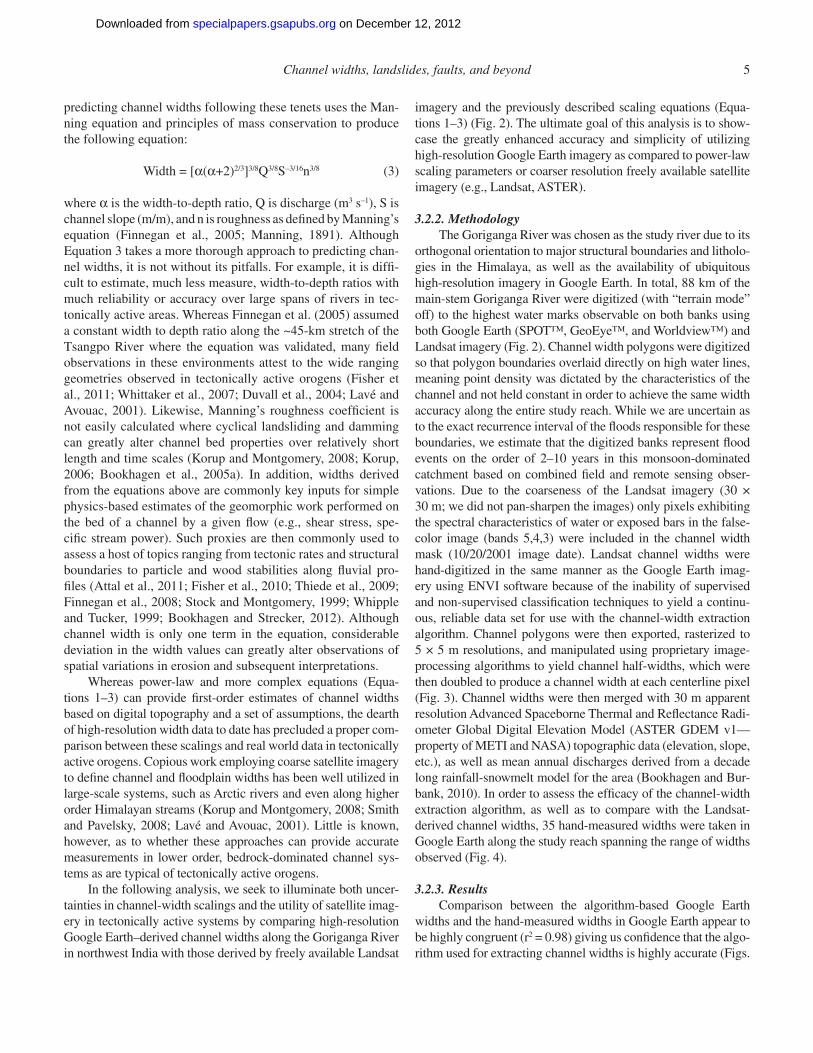
imagery and the previously described scaling equations (Equa-tions 1–3) (Fig. 2). The ultimate goal of this analysis is to show-case the greatly enhanced accuracy and simplicity of utilizing high-resolution Google Earth imagery as compared to power-law scaling parameters or coarser resolution freely available satellite imagery (e.g., Landsat, ASTER).

3.2.2. MethodologyThe Goriganga River was chosen as the study river due to its

orthogonal orientation to major structural boundaries and litholo-gies in the Himalaya, as well as the availability of ubiquitous high-resolution imagery in Google Earth. In total, 88 km of the main-stem Goriganga River were digitized (with “terrain mode” off) to the highest water marks observable on both banks using both Google Earth (SPOT™, GeoEye™, and Worldview™) and Landsat imagery (Fig. 2). Channel width polygons were digitized so that polygon boundaries overlaid directly on high water lines, meaning point density was dictated by the characteristics of the channel and not held constant in order to achieve the same width accuracy along the entire study reach. While we are uncertain as to the exact recurrence interval of the fl oods responsible for these boundaries, we estimate that the digitized banks represent fl ood events on the order of 2–10 years in this monsoon- dominated catchment based on combined fi eld and remote sensing obser-vations. Due to the coarseness of the Landsat imagery (30 × 30 m; we did not pan-sharpen the images) only pixels exhibiting the spectral characteristics of water or exposed bars in the false-color image (bands 5,4,3) were included in the channel width mask (10/20/2001 image date). Landsat channel widths were hand-digitized in the same manner as the Google Earth imag-ery using ENVI software because of the inability of supervised and non-supervised classifi cation techniques to yield a continu-ous, reliable data set for use with the channel-width extraction algorithm. Channel polygons were then exported, rasterized to 5 × 5 m resolutions, and manipulated using proprietary image-processing algorithms to yield channel half-widths, which were then doubled to produce a channel width at each centerline pixel (Fig. 3). Channel widths were then merged with 30 m apparent resolution Advanced Spaceborne Thermal and Refl ectance Radi-ometer Global Digital Elevation Model (ASTER GDEM v1—property of METI and NASA) topographic data (elevation, slope, etc.), as well as mean annual discharges derived from a decade long rainfall-snowmelt model for the area (Bookhagen and Bur-bank, 2010). In order to assess the effi cacy of the channel-width extraction algorithm, as well as to compare with the Landsat-derived channel widths, 35 hand-measured widths were taken in Google Earth along the study reach spanning the range of widths observed (Fig. 4).

3.2.3. ResultsComparison between the algorithm-based Google Earth

widths and the hand-measured widths in Google Earth appear to be highly congruent (r2 = 0.98) giving us confi dence that the algo-rithm used for extracting channel widths is highly accurate (Figs.



6 Fisher et al.

3 and 4B). Whereas we don’t have fi eld measurements against which to compare the hand measured widths, both previous fi eld research and other studies assessing the positional accuracy of Google Earth imagery argues for strong correlation between real world distances and those measured on Google Earth imagery (Constantine and Dunne, 2008; Potere, 2008).

A comparison between Landsat (30 × 30 m) and Google Earth–derived channel widths shows a continuous offset along the Goriganga River, whereby Landsat widths are consistently over-estimated along the study reach (mean and 1 standard deviation of 18.2 ± 7.4 m) (Fig. 4). When compared to the hand-measured widths from Google Earth, the importance of imagery resolution becomes readily apparent, with channel widths less than 1-pixel length nearly impossible to detect accurately (Fig. 4). With the high-resolution imagery in Google Earth, channel-width delinea-

tion appears to be dictated completely by the raster resolution (which in this case is 5 × 5 m) in these tectonically active systems where riparian vegetation is minimal. Theoretically, using a 1 × 1 m matrix with the ~1 m spatial-resolution GeoEye™ imagery could further improve the channel-width accuracy. For the sake of computational effi ciency and to encompass some of the error introduced by digitizing the channel widths, however, a conser-vative 5 m resolution was used. Nonetheless, the improvement over Landsat-based techniques is both striking and necessary to accurately assess channel geometries in tectonically active and/or lower order channel systems (<60 m wide or drainage areas less than ~3000 km2) where narrow, steep gorges are the norm, rather than the exception.

A closer look at the Google Earth channel-width data along the nearly 90-km-long study reach shows great variability in

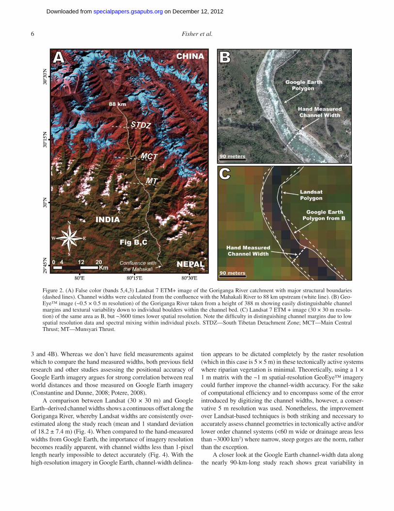
Figure 2. (A) False color (bands 5,4,3) Landsat 7 ETM+ image of the Goriganga River catchment with major structural boundaries (dashed lines). Channel widths were calculated from the confl uence with the Mahakali River to 88 km upstream (white line). (B) Geo-Eye™ image (~0.5 × 0.5 m resolution) of the Goriganga River taken from a height of 388 m showing easily distinguishable channel margins and textural variability down to individual boulders within the channel bed. (C) Landsat 7 ETM + image (30 × 30 m resolu-tion) of the same area as B, but ~3600 times lower spatial resolution. Note the diffi culty in distinguishing channel margins due to low spatial resolution data and spectral mixing within individual pixels. STDZ—South Tibetan Detachment Zone; MCT—Main Central Thrust; MT—Munsyari Thrust.




widths that is coincident with major Himalayan tectonic units (Fig. 4 and 5). This variability makes it impossible to fi t a sim-ple power-law scaling (e.g., Craddock et al., 2007) to the entire data set that even broadly mimics the large-scale variability in channel widths, much less any small-scale perturbations (Fig. 5). Although more complex scaling relationships (Finnegan et al., 2005) may do a slightly better job, these equations include many more unknowns that must be accounted for, which in remote locations are nearly impossible to accurately assess and com-monly vary greatly between sub-reaches of the river (e.g., width-to-depth ratios, roughness). The departure of these scaling laws from the actual channel widths derived using Google Earth imag-ery can be striking (Fig. 5). Both established power-law (Crad-dock et al., 2007) and mass-conservation equations (Finnegan et al., 2005) systematically under-predict the actual channel widths along the study reach, especially where the mass-conservation equation of Finnegan et al. (2005) is defi ned as a bedrock chan-

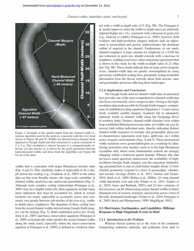
Figure 3. Example of the spatial output from the channel-width ex-traction algorithm used in the analysis, consistent with the river bend shown in Figure 2B and 2C. Widths are derived from a channel mask digitized in Google Earth and then rasterized to a pixel resolution of 5 × 5 m. This resolution is chosen because it is computationally ef-fi cient, yet also precise as is shown by the good agreement between hand-measured widths and those from the algorithm (see Figure 4B for all of the data).

nel with a width-to-depth ratio of 5 (Fig. 5B). The Finnegan et al. model improves when the width-to-depth ratios are arbitrarily adjusted higher (α = 21), consistent with a decrease in grain size (e.g., bedrock to cobble) (Finnegan et al., 2005); however, fi eld evidence and high-resolution imagery indicate such an adjust-ment is unwarranted and grossly underestimates the dominant caliber of material in the channel. Furthermore, in our study, channel roughness is kept constant for simplicity (n = 0.20) but any reduction in grain size should coincide with a decrease in roughness, yielding even lower values and poorer agreement than is shown in this study for the width-to-depth value of 21 (blue line: Fig. 5B). These results indicate that, in many active orogenic rivers, channel-width data are greatly oversimplifi ed by using previously established scaling laws, potentially losing invaluable information from the fl uvial network about both tectonic rates and geomorphic processes affecting these landscapes.

3.2.4. Implications and ConclusionsThe Google Earth–derived channel width data set presented

here provides one of the most comprehensive channel-width data sets from a tectonically active orogen to date. Owing to the high-resolution data made possible by Google Earth imagery, compari-sons of established scaling equations (Equations 1–3) and coarser freely available satellite imagery (Landsat) fail to adequately represent trends in channel width along the Goriganga River in northern India. Distinct channel-width domains exist within long-established Himalayan tectonic units, yet widths can vary by several folds within individual units, thereby indicating distinct channel-width responses to tectonic and geomorphic processes or characteristics (glaciation, rock types, uplift rate, etc.) within active orogenic environments (Figs. 4 and 5). These pronounced width variations serve geomorphologists as a roadmap by iden-tifying anomalous river reaches (such as in the high Himalayan crystalline unit) where some fundamental controls are strongly changing within a restricted spatial domain. Whereas this data set leaves many questions unanswered, the availability of high-resolution Google Earth imagery and the extraction methodol-ogy presented here is sure to yield future insights about: (1) how channel geometries respond to a host of geomorphic, climatic, and tectonic forcings (Fisher et al., 2011; Yanites and Tucker, 2010; Stark et al., 2009; Wobus et al., 2006a); (2) what channel width thresholds exist and why (Fisher et al., 2011; Yanites et al., 2010; Amos and Burbank, 2007); and (3) how estimates of fl uvial power can be refi ned using actual channel widths to better illuminate foci of erosion, transport, and incision across a host of fl uvially dominated landscapes (Fisher et al., 2010; Finnegan et al., 2005; Stock and Montgomery, 1999; Magilligan, 1992).

3.3. Hurricanes, Earthquakes, and Landslides: Hillslope Response to High-Magnitude Events in Haiti

3.3.1. Introduction to the ProblemWhereas fl uvial systems act as the veins of the continents

transporting sediment, nutrients, and pollutants from land to



8 Fisher et al.

sea (Milliman and Syvitski, 1992), mass wasting is the domi-nant mechanism by which particles enter the fl uvial network, especially in tectonically active regions. In moderate- to high-relief terrains, landsliding has been shown to play a critical role in landscape evolution through mass transfer related to variable tectonic rates (Clarke and Burbank, 2010, 2011; Densmore et al., 1997; Hovius et al., 1997; Burbank et al., 1996), climate pertur-bations (Galewsky et al., 2006; Bookhagen et al., 2005b; Gabet et al., 2004), anthropogenic effects (Lavé and Burbank, 2004), fi re regimes (Roering and Gerber, 2005; Pierce et al., 2004), and increased seismicity (Parker et al., 2011; Hovius et al., 2011; Dadson et al., 2004; Hovius et al., 2000). Alternatively, landslid-ing has been argued to retard regressive erosion by large rivers

along the Tibetan Plateau margin (Korup et al., 2010; Korup and Montgomery, 2008) as well as shield certain glaciers from enhanced melting related to climate change by providing a pro-tective surfi cial debris cover (Scherler et al., 2011a, 2011b; San-tamaria Tovar et al., 2008). Because landsliding is such a diverse and integral process in landscape evolution, it is imperative to be able to identify, delineate, and develop mechanistic explanations for landsliding across broad spatial and temporal scales. Most landslide analyses to date have suffered from having spatially limited, yet high-resolution aerial photo sets (Clarke and Bur-bank, 2010) or spatially extensive, yet low-resolution remotely sensed optical imagery (Korup et al., 2010). Furthermore, many of these studies have been further hindered by the lack of

Channel Width (m)

Deviatio

n fro

m H

and

Measu

red C

han

nel W

idth

(%)

0 15 30 45 60 75 90 105 120 135 150

y = 582x-1.07R = 0.76

y = 18320x-1.58R = 0.76

1 Pixel Error Envelopes

0

50

100

150

200

250

300Landsat ETM+Google Earth

C

Dev

iati

on

fro

m H

and

Mea

sure

d C

han

nel

Wid

th (

%)

Channel Width (m)

Hand Measured Width (m)

Cal

cula

ted

Wid

th (

m)

y = 1.05x

y = 0.96xR = 0.98

R = 0.57

0

20

40

60

80

100

120

140

160

0 20 40 60 80 100 120 140 160

1:1 line

Landsat ETM+Google Earth

B

0

50

100

150

200

250

300

350

400

450

500

0-2020-40

40-6060-80

80-100

100-120

120-140

140-160

n=4

n=10n=7

n=6 n=3 n=2n=2 n=1

[n=35]

0

0.5

1

1.5

2

2.5

3

3.5

0

20

40

60

80

100

Ch

ann

el W

idth

(m

)

Distance Upstream from Mahakali Confluence (km)

Elevatio

n (km

) or D

rainag

e Area (%

)

Landsat ETM+ (30x30m Resolution)

Google Earth (5x5m Resolution)

Goriganga River Profile

Drainage Area (max = 2230 km2)

0 10 20 30 40 50 60 70 80 900

20

40

60

80

100

120

140

MC

T

MT

ST

D

A LHS LHC HHC Tethy.

Figure 4. (A) Plot of channel width (after 5-km smoothing window) versus distance from the confl uence with the Mahakali River showing the general overestimation of channel widths derived from Landsat imagery in steep, narrow gorges within tectonically active regions. Longitudinal profi le and drainage area are plotted on alternate Y-axes for reference. (B) The percent deviation from hand-measured channel widths (see Fig. 2B, 2C, and Fig. 3) and fi t for both data sets (see inset). (C) Fits for the average values from B (dashed lines and red points for Landsat) and the 1-pixel error envelopes (shaded regions). Note the low error associated with Google Earth (Spot™, GeoEye™, and Worldview™ imagery) widths versus Landsat ETM + (which provides little information below 1 pixel and still has ~50% error at 45 m channel widths) as shown by low percent deviation as well as high correlation in the inset plot. STD—South Tibetan Detachment Zone; MCT—Main Central Thrust; MT—Munsyari Thrust; LHS—Lesser Himalayan Sedimentary; LHC—Lesser Himalayan Crystalline; HHC—High Himalayan Crystalline; Tethy—Tethyan Series.




temporal variability in imagery, constraining analyses and inter-pretations alike. Google Earth has, however, created a platform where resolution, spatial extent, and even temporal issues with imagery are greatly diminished, thereby allowing researchers to more thoroughly explore the mechanisms, characteristics, and linkages associated with landsliding across a range of environ-ments and triggering mechanisms.

In the following analysis we utilize high-resolution Google Earth imagery portraying the area around Port-au-Prince, Haiti, to illuminate landslide-triggering mechanisms and characteris-tics. Haiti provides a prime opportunity to present the utility of not only recent high-resolution Google Earth imagery, but also of the rich historical image archive available for the region. The 2008 hurricane season battered Haiti with four major storms producing nearly a meter of rain over less than a month-long period. These storms caused nearly 800 deaths and billions of U.S. dollars in damages (Carroll, 2001) (Fig. 6). On 12 Janu-ary 2010 Haiti experienced yet another major blow with a mag-nitude 7.0 earthquake located ~15 km west of the capital city of Port-au-Prince (Hayes et al., 2010) (Fig. 7). This event rep-resented the largest earthquake to strike the area in more than 200 years and led to deaths estimated in the tens of thousands

(Associated Press, “Report challenges Haiti earthquake death toll,” BBC News, retrieved 25 June 2011, http://www.bbc.co.uk/news/world-us-canada-13606720). Whereas these events are tragic, they present an unparalleled opportunity to compare and contrast the hillslope mass-wasting response to both high-mag-nitude climatic and seismic events. The goal of this analysis is, therefore, to gain improved insight about landslide triggers and characteristics, as well as to show the utility of Google Earth in such research ventures.

3.3.2. MethodologyThe study area was chosen due to its proximity to the epi-

center of the 12 January 2010 earthquake and the availability of clear, high-resolution imagery spanning both the pre- and post-2008 hurricane season, as well as imagery taken the day after the earthquake event clearly showing a large number of landslides (Fig. 7). Hurricane path and cumulative event rainfall data were obtained from the National Weather Service–National Hurricane Center (www.nhc.noaa.gov) and compared with the Tropical Rainfall Monitoring Mission (TRMM) 3B42 V6 data set for the area over the same time period (Fig. 6)(cf. Bookhagen, 2010; Huffman et al., 2007; Hong et al., 2006). Landslides were delin-

1

10

100

1000

10 100

Tethyan (n=393; b=1.4)HHC (n=597; b=-1.2)LHC (n=212; b=4.4)LHS (n=1312; b=-0.16)

TRMM + SWE - ET Mean Annual Discharge (m3 s-1)

Ch

ann

el W

idth

(m

)

W=20.6*Q0.23

R2 = 0.05

A

0 10 20 30 40 50 60 70 80 90

20

40

60

80

100

120

Ch

ann

el W

idth

(m

)

Distance Upstream from theMahakali Confluence (km)

LHS LHC HHC Tethy.

Finnegan - α = 5Finnegan - α = 21

W = 6.2*Q0.38

BW = 6.2*Q0.6

W = 6.2*Q0.3

W = 6.2*Q0.5

Google Earth Widths

W = 20.6*Q0.23

from A

(after Eqs. 1 & 2)

(after Eq. 3)

MC

T

MT

ST

D

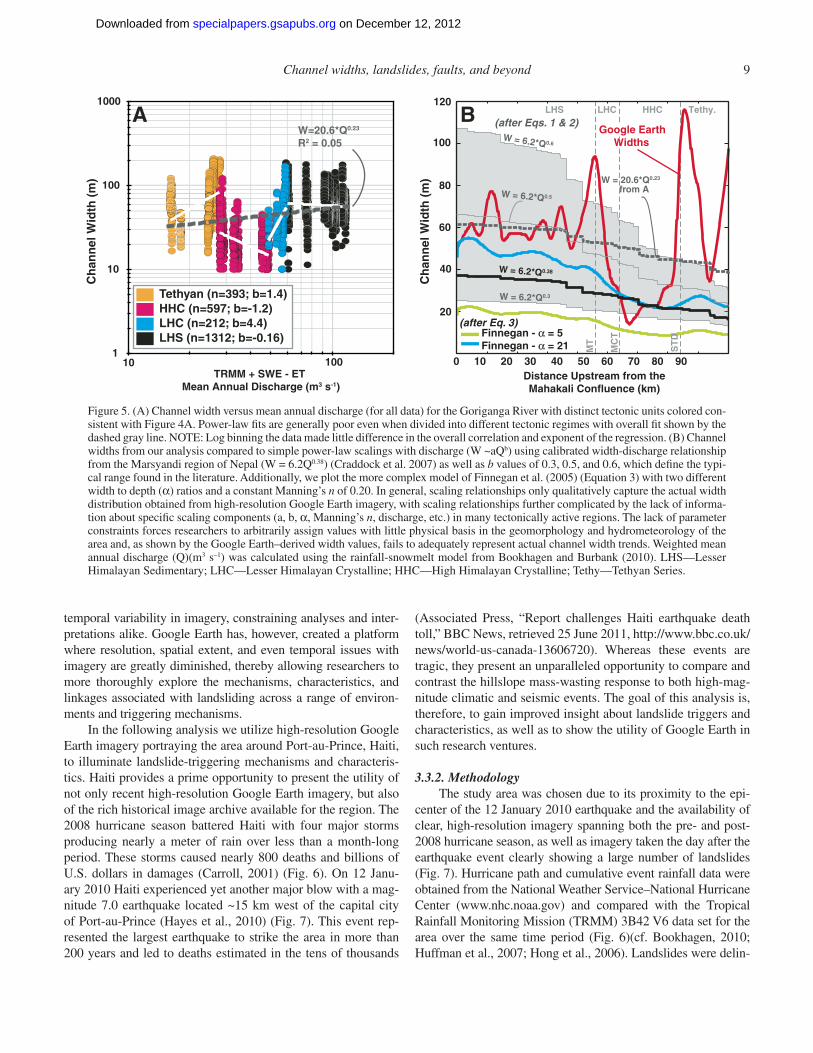
Figure 5. (A) Channel width versus mean annual discharge (for all data) for the Goriganga River with distinct tectonic units colored con-sistent with Figure 4A. Power-law fi ts are generally poor even when divided into different tectonic regimes with overall fi t shown by the dashed gray line. NOTE: Log binning the data made little difference in the overall correlation and exponent of the regression. (B) Channel widths from our analysis compared to simple power-law scalings with discharge (W ~aQb) using calibrated width-discharge relationship from the Marsyandi region of Nepal (W = 6.2Q0.38) (Craddock et al. 2007) as well as b values of 0.3, 0.5, and 0.6, which defi ne the typi-cal range found in the literature. Additionally, we plot the more complex model of Finnegan et al. (2005) (Equation 3) with two different width to depth (α) ratios and a constant Manning’s n of 0.20. In general, scaling relationships only qualitatively capture the actual width distribution obtained from high-resolution Google Earth imagery, with scaling relationships further complicated by the lack of informa-tion about specifi c scaling components (a, b, α, Manning’s n, discharge, etc.) in many tectonically active regions. The lack of parameter constraints forces researchers to arbitrarily assign values with little physical basis in the geomorphology and hydrometeorology of the area and, as shown by the Google Earth–derived width values, fails to adequately represent actual channel width trends. Weighted mean annual discharge (Q)(m3 s–1) was calculated using the rainfall-snowmelt model from Bookhagen and Burbank (2010). LHS—Lesser Himalayan Sedimentary; LHC—Lesser Himalayan Crystalline; HHC—High Himalayan Crystalline; Tethy—Tethyan Series.



10 Fisher et al.

eated and digitized (with “terrain mode” off) on three images in Google Earth (Fig. 7), then exported, and merged with the 30 m apparent resolution ASTER GDEM topographic data set to derive slope angles for the study area. Proper positional accu-racy between the study area and the ASTER GDEM was ensured using landscape features (e.g., hydrologic features, terrace edges), as large discrepancies will undoubtedly confound results. One potential reason for a close match in our region between the two is the availability of airborne lidar data postdating the earthquake which Google may use to orthorectify the imagery; however, this is mere speculation (cf. www.opentopography.org).

3.3.3. ResultsDespite ideal conditions (namely heavy deforestation and

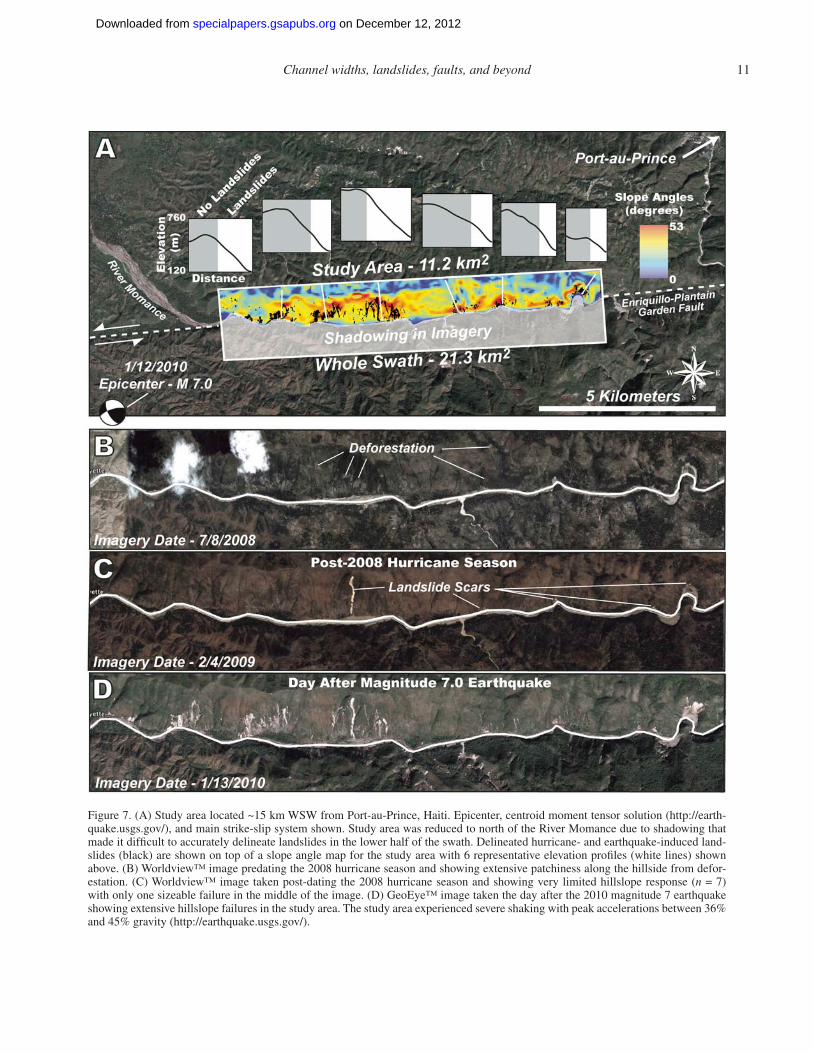
steep slopes) for landsliding in the study area leading up to the 2008 hurricane season, only 7 slides were delineated (Fig. 7). In contrast, the 2010 magnitude 7 earthquake produced 325 land-

slides in our study area ranging in area from 10 m2 to 27,000 m2 (Figs. 7A, 7C, and 8). Hillslopes are generally planar to slightly convex in the study area, with landslides predominately limited to the lower, steeper toe slopes (≥20 degrees) (Figs. 7 and 8). Analysis of magnitude-frequency plots for the earthquake-derived landslide data set produces a characteristic double-pareto distribution with a similar beta slope value (cf. Stark and Hovius, 2001) to previous studies, despite integrating only one event and having roughly an order of magnitude fewer mapped landslides (325 versus 1000s by Clarke and Burbank, 2010; Hovius et al., 1997)(Fig. 8B). The beta value is derived from the simple power-law function,

NL = kA−β (4)

where NL is the number of landslides for a given landslide

area A, k is a scaling coeffi cient, and β defi nes the slope of the magnitude-frequency relationship for the log-log linear segment

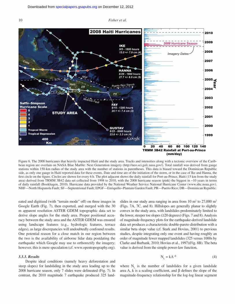
Figure 6. The 2008 hurricanes that heavily impacted Haiti and the study area. Tracks and intensities along with a tectonic overview of the Carib-bean region are overlain on NASA Blue Marble: Next Generation imagery (http://neo.sci.gsfc.nasa.gov/). Total rainfall was derived from gauge stations within 150-km radius of the study area with the number of stations in parentheses. This data is biased toward the Dominican Republic side, as only one gauge in Haiti reported data for these events. Date and time are of the initiation of the storm, or in the case of Ike and Hanna, the fi rst circle on the fi gure. Circles are shown for every 6 h. The plot adjacent shows the daily rainfall for Port-au-Prince, Haiti (15 km from the study area) derived from TRMM 3B42 data set collected from 1998 to 2010, with the 2008 hurricane season (pink) the biggest in ~10 years in terms of daily rainfall (Bookhagen, 2010). Hurricane data provided by the National Weather Service National Hurricane Center (www.nhc.noaa.gov). NHF—North Hispanola Fault; SF—Septentrional Fault; EPGF—Enriquillo–Plantain Garden Fault; PR—Puerto Rico; DR—Dominican Republic.




Figure 7. (A) Study area located ~15 km WSW from Port-au-Prince, Haiti. Epicenter, centroid moment tensor solution (http://earth-quake.usgs.gov/), and main strike-slip system shown. Study area was reduced to north of the River Momance due to shadowing that made it diffi cult to accurately delineate landslides in the lower half of the swath. Delineated hurricane- and earthquake-induced land-slides (black) are shown on top of a slope angle map for the study area with 6 representative elevation profi les (white lines) shown above. (B) Worldview™ image predating the 2008 hurricane season and showing extensive patchiness along the hillside from defor-estation. (C) Worldview™ image taken post-dating the 2008 hurricane season and showing very limited hillslope response (n = 7) with only one sizeable failure in the middle of the image. (D) GeoEye™ image taken the day after the 2010 magnitude 7 earthquake showing extensive hillslope failures in the study area. The study area experienced severe shaking with peak accelerations between 36% and 45% gravity (http://earthquake.usgs.gov/).



12 Fisher et al.

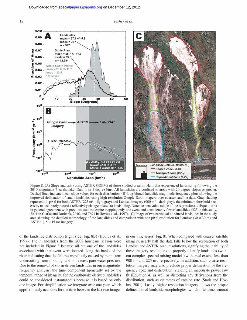
of the landslide distribution (right side: Fig. 8B) (Hovius et al., 1997). The 7 landslides from the 2008 hurricane season were not included in Figure 8 because all but one of the landslides associated with that event were located along the banks of the river, indicating that the failures were likely caused by main-stem undercutting from fl ooding, and not excess pore water pressure. Due to the removal of storm-driven landslides in our magnitude-frequency analysis, the time component (generally set by the temporal range of imagery) for the earthquake-derived landslides could be considered instantaneous because it is based on only one image. For simplifi cation we integrate over one year, which approximately accounts for the time between the last two images

in our time series (Fig. 8). When compared with coarser satellite imagery, nearly half the data falls below the resolution of both Landsat and ASTER pixel resolutions, signifying the inability of these imagery resolutions to properly identify landslides (with-out complex spectral mixing models) with areal extents less than 900 m2 and 225 m2, respectively. In addition, such coarse reso-lution imagery may also preclude proper delineation of the fre-quency apex and distribution, yielding an inaccurate power law fi t (Equation 4) as well as distorting any derivations from the distribution, such as estimates of erosion rate (Stark and Hov-ius, 2001). Lastly, higher-resolution imagery allows the proper delineation of landslide morphologies, which oftentimes cannot

Figure 8. (A) Slope analysis (using ASTER GDEM) of those studied areas in Haiti that experienced landsliding following the 2010 magnitude 7 earthquake. Data is in 1-degree bins. All landslides are confi ned to areas with 20 degree slopes or greater. Dashed lines indicate mean slope values for each distribution. (B) Log-binned landslide magnitude-frequency plots showing the improved delineation of small landslides using high-resolution Google Earth imagery over coarser satellite data. Gray shading represents 1-pixel for both ASTER (225 m2—light gray) and Landsat imagery (900 m2—dark gray), the minimum threshold nec-essary to accurately record a refl ectivity change related to landsliding. Note the beta value (slope of the regression) is (Equation 4) in general agreement with previous studies despite mapping only one event and considerably fewer landslides (325 in this study, 2211 in Clarke and Burbank, 2010, and 7691 in Hovius et al., 1997). (C) Image of two earthquake-induced landslides in the study area showing the detailed morphology of the landslides and comparison with one pixel resolution for Landsat (30 × 30 m) and ASTER (15 × 15 m) imagery.




be distinguished using coarser imagery and may considerably overestimate landslide area and sediment volumes in many steep terrains (Fig. 8C).

3.3.4. Implications and ConclusionsDespite hydrological evidence for intense rainfall during the

2008 hurricane season and heavy deforestation only one major failure occurred in the study area. Possible explanations for the lack of failures may include considerable overland fl ow due to steep slopes, lithologic and soil properties (i.e., clay rich), lack of a critical accumulation zone, localized orographic effects, and/or the low relative magnitude of the event (~10-year recurrence inter-val). The story is quite different following the 12 January 2010 earthquake where 325 landslides were observed. Previous work has proposed a topographic signature exists within tectonically active landscapes to distinguish between storm- and earthquake-derived landslide-dominated hillslopes (Meunier et al., 2008; Densmore and Hovius, 2000). In the Haiti study area, such sim-ple delineations are muddled. We know that the landslides were generated coseismically, yet many of them were triggered along the lower, steeper toe slopes, consistent with a storm-induced, hydrologic accumulation model (Fig. 7A). At the same time, hill-slopes are generally planar and inner gorges absent as would be predicted by a landscape dominated by earthquake-induced land-sliding (Densmore and Hovius, 2000). Whereas both earthquake and storm processes are clearly active in the study area, the ques-tion becomes at what time frame and with what frequency each is dominant (e.g., Wolman and Miller, 1960). The observed earth-quake event is the largest to strike the area in over two centuries, but during this same time interval, there have been numerous hur-ricane and storm events of greater magnitude than the 2008 hurri-cane season. We would expect those large storms to have caused considerable landsliding. One explanation for the lack of a land-slide response to the repeated storms is the mismatch of magni-tudes between the climatic and seismic events observed, whereby the heavily deforested hillslopes may already be adjusted to such climatic recurrence intervals. In all likelihood any climatic event of a similar magnitude post-dating the earthquake would exploit current earthquake-induced landslide scars, exacerbating the total volume of sediment removed from the hillslopes and providing the necessary transport mechanism to move the hillslope material into the fl uvial network (Hovius et al., 2000, 2011). Another pos-sible explanation as to why there is such a discrepancy between the hillslope response to the 2010 earthquake and 2008 hurri-canes in the study area is that of the rupture style (Meunier et al., 2008). Both remote sensing observations following the 2010 earthquake and our own reconnaissance in Google Earth noted fairly localized hillslope failures concentrated in the study area (van Westen and Gorum, 2010). The fi rst fault plane solutions to come out following the earthquake placed it as an oblique slip failure consistent with the preexisting Enriquillo–Plantain Gar-den Fault (EPGF). However, subsequent InSAR (Interferometric Synthetic Aperture Radar) analyses have hypothesized that the rupture may have occurred along a previously unmapped blind

thrust fault (hanging wall moved due south) that would daylight adjacent to and strike-parallel to the study area ridge (Hashimoto et al., 2011; Calais et al., 2010; Hayes et al., 2010). This geom-etry would then explain the relatively localized failures, where much of the energy was directly focused into the study area caus-ing signifi cant, localized failures on the south-facing hillslopes.

This study again underscores the complexities involved in deciphering processes and mechanisms that shape the surface of our earth. In the case of Haiti, Google Earth gives us an addi-tional tool with which to glimpse how the landscape responds to both climatic and tectonic perturbations of varying magnitudes. Obviously, detailed fi eld research would be needed to properly tackle the complex interactions actively shaping the landscape in this subtropical environment. Nonetheless, Google Earth imagery can provide an important starting point by making high- resolution imagery accessible, at both the temporal and spatial scales neces-sary to adequately undertake such questions. In this study, we have documented a time series of landsliding in Haiti using Google Earth high-resolution imagery that spans both high-magnitude climatic and tectonic events, providing valuable insights about the characteristics of landslides associated with these events, their potential mechanisms, and how high-resolution Google Earth imagery may benefi t similar studies in the future.

3.4. Fault Characterization in the Eastern California Shear Zone

3.4.1. Introduction to the ProblemThe eastern California shear zone and Walker Lane comprise

a distributed network of dextral strike-slip and normal faults east of the Sierra Nevada in California (Fig. 9). Together, this zone of active deformation accounts for roughly one quarter of the total Pacifi c–North American plate translation (Dokka and Tra-vis, 1990). An ever-expanding inventory of information on active faults within the eastern California shear zone and Walker Lane elucidates spatial and temporal patterns of strain along these structures. Comparison of these patterns with ongoing deforma-tion measured from space geodesy (e.g., Dixon et al., 2000) and seismicity (e.g., Unruh et al., 2003) provides a unique opportu-nity to investigate the dynamics and evolution of this intraconti-nental plate-boundary fault system.

Fault studies in the eastern California shear zone typically rely on measurements of displaced Quaternary landforms and geomorphic features such as river channels, terraces, or alluvial fans to defi ne patterns of fault displacement at a variety of spatial and temporal scales (e.g., Frankel et al., 2011). An intriguing out-come from this body of work is the apparent, twofold mismatch between the summed rates of dextral fault slip across the Mojave section of the eastern California shear zone (~6 ± 2 mm/yr, Oskin et al., 2008) and interseismic strain measured from GPS (~12 ± 2 mm/yr, Sauber et al., 1994). Individual structures within this zone, such as the Blackwater fault, also show pronounced rate discrepancies. There, dextral shear measured at decadal time scales from radar interferometry (up to ~7 mm/yr, Peltzer et al.,



14 Fisher et al.

2001) radically outpaces Quaternary-averaged rates of fault slip (~0.5 mm/yr, Oskin and Iriondo, 2004). Based on a lack of iden-tifi ed and described Quaternary offset landforms, comparatively little is known about how this dextral shear in the eastern Cali-fornia shear zone is transferred and partitioned onto structures north of the Garlock fault in the Indian Wells and Rose Valley areas (Fig. 9).

Here, we present new measurements of displaced Quater-nary landforms cut by the Little Lake fault and identifi ed using high-resolution Google Earth imagery. These images reveal a series of previously undescribed river terraces formed during the drainage of pluvial Owens Lake southward from Rose Valley into the Indian Wells Valley and China Lake basin (Fig. 9). Measured

lateral offsets of these features using Google Earth imagery com-pares favorably with measurements made from ground-based ter-restrial laser scanning (TLS) along the Little Lake fault as part of this study. This work demonstrates the utility of Google Earth for rapidly identifying and quantifying patterns of lateral fault displacement in actively deforming landscapes.

3.4.2. MethodologyNumerous studies utilize remotely sensed imagery in arid

regions for cataloging lateral offsets along strike-slip faults (e.g., Klinger et al., 2011) and for documenting the sense and style of displacement for under-characterized geologic structures (e.g., Phillips and Majkowski, 2011). Our study focuses on the western

Figure 9. (A) Regional tectonic map of the southeastern Sierra Nevada of California. Active fault traces are taken from Jennings (1994), with the exception of the Kern Canyon fault (Brossy et al., 2012). SNFF—Sierra Nevada frontal fault. (B) Google Earth image of Little Lake wash (shown by arrow in A) highlighting neotectonic and geomorphic features associated with the Little Lake fault. (C) Reconstructed offset along the Little Lake fault suggests between ~33 and 37 m of dextral displacement of terrace risers cut by the fault zone.




margin of the eastern California shear zone between the Sierra Nevada and the Coso Range (Fig. 9), along the northwestern continuation of interseismic dextral shearing observed from radar interferometry (Peltzer et al., 2001). Here, abundant Quaternary volcanic and geomorphic features provide markers for quantify-ing fault offset.

Along the Little Lake fault (Fig. 9), we used Google Earth imagery to identify a series of prominent river terraces cut by the fault immediately east of U.S. Highway 395 (Fig. 9B). These landforms are undescribed in the literature despite a well-known relative sequence of late-Pleistocene volcanism and fl u-vial downcutting driven by drainage of Owens Lake through the Little Lake area (Duffi eld and Smith, 1978). Images of the Little Lake wash collected from Google Earth were used to cre-ate a reconnaissance-level neotectonic map (Fig. 9B) and also to reconstruct the total dextral offset of this landform across the fault (Fig. 9C). These reconstructions are based on retro deforma-tion of the mapped image, sliced along the fault trace, in order to create a “best fi t” for the base of the terrace riser on either side of the fault. The riser base was chosen for these reconstruc-tions because it provides the best visual contrast in the imagery. In order to minimize errors in our reconstruction associated with image distortion, screen captures were collected with Google Earth’s “terrain” feature disengaged.

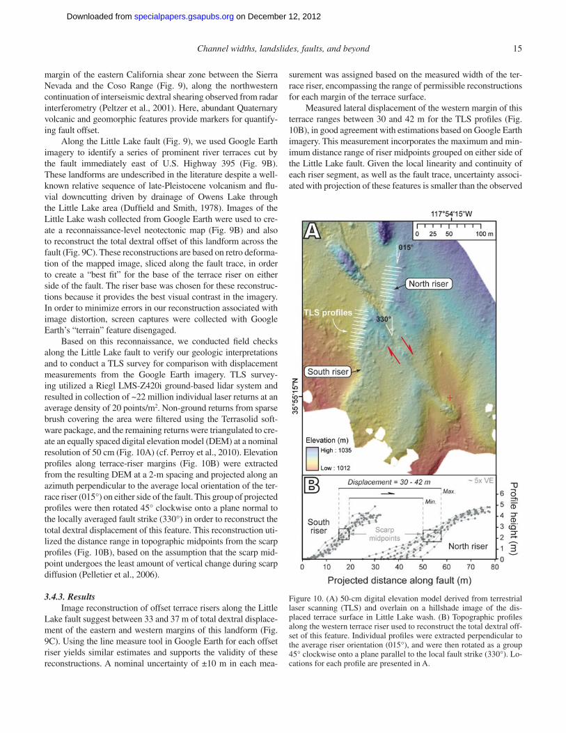
Based on this reconnaissance, we conducted fi eld checks along the Little Lake fault to verify our geologic interpretations and to conduct a TLS survey for comparison with displacement measurements from the Google Earth imagery. TLS survey-ing utilized a Riegl LMS-Z420i ground-based lidar system and resulted in collection of ~22 million individual laser returns at an average density of 20 points/m2. Non-ground returns from sparse brush covering the area were fi ltered using the Terrasolid soft-ware package, and the remaining returns were triangulated to cre-ate an equally spaced digital elevation model (DEM) at a nominal resolution of 50 cm (Fig. 10A) (cf. Perroy et al., 2010). Elevation profi les along terrace-riser margins (Fig. 10B) were extracted from the resulting DEM at a 2-m spacing and projected along an azimuth perpendicular to the average local orientation of the ter-race riser (015°) on either side of the fault. This group of projected profi les were then rotated 45° clockwise onto a plane normal to the locally averaged fault strike (330°) in order to reconstruct the total dextral displacement of this feature. This reconstruction uti-lized the distance range in topographic midpoints from the scarp profi les (Fig. 10B), based on the assumption that the scarp mid-point undergoes the least amount of vertical change during scarp diffusion (Pelletier et al., 2006).

3.4.3. ResultsImage reconstruction of offset terrace risers along the Little

Lake fault suggest between 33 and 37 m of total dextral displace-ment of the eastern and western margins of this landform (Fig. 9C). Using the line measure tool in Google Earth for each offset riser yields similar estimates and supports the validity of these reconstructions. A nominal uncertainty of ±10 m in each mea-

surement was assigned based on the measured width of the ter-race riser, encompassing the range of permissible reconstructions for each margin of the terrace surface.

Measured lateral displacement of the western margin of this terrace ranges between 30 and 42 m for the TLS profi les (Fig. 10B), in good agreement with estimations based on Google Earth imagery. This measurement incorporates the maximum and min-imum distance range of riser midpoints grouped on either side of the Little Lake fault. Given the local linearity and continuity of each riser segment, as well as the fault trace, uncertainty associ-ated with projection of these features is smaller than the observed

Figure 10. (A) 50-cm digital elevation model derived from terrestrial laser scanning (TLS) and overlain on a hillshade image of the dis-placed terrace surface in Little Lake wash. (B) Topographic profi les along the western terrace riser used to reconstruct the total dextral off-set of this feature. Individual profi les were extracted perpendicular to the average riser orientation (015°), and were then rotated as a group 45° clockwise onto a plane parallel to the local fault strike (330°). Lo-cations for each profi le are presented in A.



16 Fisher et al.

range of riser midpoints. We do note, however, a larger variation in profi le shape and midpoint location for the riser segment north of the fault, possibly due to either locally increased diffusion or a slight azimuth change to the north in this direction. To our know-ledge, this study presents the fi rst systematic comparison of fault offsets measured using Google Earth imagery and ground-based survey methods.

3.4.4. Implications and ConclusionsNew measurements of fault displacement for the Little Lake

fault add to our growing inventory of deformation patterns in the eastern California shear zone. Although the exact age of the offset terrace is yet unknown, several lines of evidence suggest a latest Pleistocene age for this feature. Specifi cally, this faulted terrace rests unconformably on a strath surface cut into the basalt of Red Hill (Fig. 9B), the youngest of several fl ows to spill through the Little Lake drainage (Duffi eld and Smith, 1978). 3He exposure ages measured using olivine phenocrysts from this fl ow (Cerling, 1990) suggest the timing of eruption and subsequent scouring during overfl ow from Owens Lake between ca. 57 and ca. 15 ka, respectively. This range in ages implies a dextral slip rate of at least ~0.5 mm/yr over this interval. We emphasize the prelimi-nary nature of this measurement and note that we are currently processing new 10Be exposure age measurements to bolster our slip-rate estimate. In any case, our appraisal is within the range of dextral slip-rates described along the Owens Valley fault to the north (Bacon and Pezzopane, 2007), which transfers strain across the Coso Range in a releasing step-over onto strike-slip faults in the Indian Wells Valley (Unruh et al., 2002) (Fig. 9A).

Our measurements of dextrally offset landforms in the east-ern California shear zone highlight the utility of Google Earth as a primary tool for quantifying the style and magnitude of displace-ment in actively deforming regions. Agreement between offset measurements from Google Earth imagery and measurements from ground-based, high-resolution survey methods indicates the quality of these displacement estimates and fi rmly extends the utility of this software and high-resolution imagery beyond that of a reconnaissance tool. Although these measurements are currently limited to lateral displacements, future integration of high-quality lidar terrane data (currently available for limited areas in Google Maps) will no doubt extend the range of possible measurements to dip-slip faults, providing a free and simple tool for quantifying and characterizing fault systems across the globe.

4. LIMITATIONS, PROBLEMS, AND POTENTIAL RESEARCH APPLICATIONS FOR GOOGLE EARTH IMAGERY

The previous three research examples have highlighted the utility of high-resolution Google Earth imagery as a potential research tool in geomorphology, as well as a few of the diverse research questions that can now be undertaken without regard for imagery cost or location. As with all good tools, however, a proper understanding of the limitations and pitfalls must be

acknowledged in order to properly apply it. Google Earth is no exception, and presently contains key limitations and potentially problematic situations that should guide suitable applications in the future.

4.1. Standard Sensor Issues

As with all remotely sensed data sets, inherent fl aws in imag-ery occur and are often the necessary byproduct of having an effi -cient, cost-effective single-satellite system. In the case of Google Earth imagery, extensive shadowing can often occur (especially in high-relief terrains) due to sensor view and/or solar incidence angles, depending on location and time of the day and year (Fig. 11). In the case of steep terrains, shadowing may completely obscure surface features (as was the case with the Haiti data set), rendering the high-resolution true-color imagery useless in those locations. Likewise, heavily vegetated regions will yield little insight about geomorphic processes and landforms (e.g., fault traces, tropical rivers, etc.), especially when compared to tools such as lidar (light detection and ranging) with which vegetation can be removed during data processing (e.g., Mackey and Roer-ing, 2011). In addition, the lack of access to longer wavelength bands (e.g., near, short, and longwave infrared, radar) from the sensors used in Google Earth imagery prevents compensation for shadowing using the spectral range of bands normally available in multi-spectral data sets.

4.2. The Google Black Box Problem

Despite the many benefi ts of the Google Earth imagery, it remains a black box. For example, very little is known about the algorithms being used to process, orthorectify, overlay, inter-polate, degrade, and display scenes, as these are proprietary to Google and no public documentation exists. In addition, little is known about the underlying digital elevation models used with respect to data sources, interpolation algorithms, and orthorec-tifi cation basemaps. It can safely be assumed that SRTM data make up a large part of the data set where it is available, but to what extent the new ASTER GDEM (Slater et al., 2011), national mapping agency, and regional lidar (cf. Perroy et al., 2010) data sets are incorporated is unknown. Furthermore, considerable uncertainty exists about the extent to which Google reprocesses or collects new elevation data, especially given the suggestion that elevation data sets available in Google Earth are superior to publicly available data sets in certain locations (Hoffmann and Winde, 2010). There does appear to be evidence for the incor-poration of lidar data in certain locations (namely urban areas); however, it is diffi cult to verify such assertions.

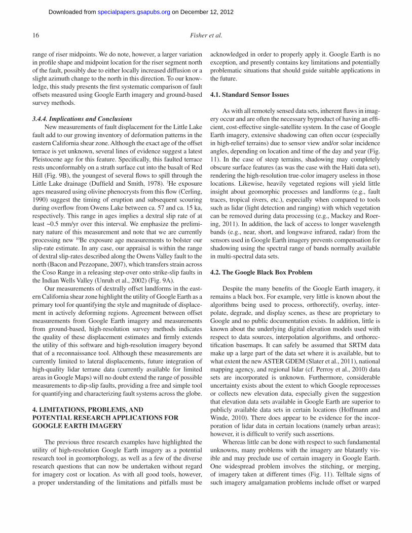
Whereas little can be done with respect to such fundamental unknowns, many problems with the imagery are blatantly vis-ible and may preclude use of certain imagery in Google Earth. One widespread problem involves the stitching, or merging, of imagery taken at different times (Fig. 11). Telltale signs of such imagery amalgamation problems include offset or warped




features along the seam of the image (broken roads, diverging waterfalls, etc.). A second major problem (especially in steep terrain) involves the unrealistic warping of imagery when using “terrain mode” in Google Earth. The spatially high-resolution optical images require nearly equally high-resolution digital elevation models, which are not readily available in most areas. The current image correction and orthorectifi cation procedures therefore rely on lower resolution digital elevation models that often result in artifacts in high relief areas (e.g., rivers that bank up onto mountainsides and roads that go off cliffs). Because of these artifacts, any digitizing should be done with the terrain mode off, using just the optical imagery. Other current problems include: (1) the lack of spatially and temporally ubiquitous high-resolution imagery, which may dictate the area and/or scope of a research project; (2) the arbitrary availability of certain imagery, whereby imagery may disappear (Fig. 11) due to updates, caus-ing a loss of access to imagery that may have been the foundation for previous measurements; and (3) the Google Earth user inter-face can be quite awkward for collecting and manipulating large amounts of data (i.e., digitizing, naming, displaying, organizing).

Lastly, the horizontal accuracy of the imagery may cause problems, especially when the digitized imagery and digital ele-vation models used for analyses are highly mismatched (Sato and Harp, 2009). While it is nearly impossible to assess the horizontal positional accuracy (georegistration) of the entire Google Earth imagery collection, previous work by Potere (2008) utilizing a global database of 436 control points spread across 109 cities found positional accuracy to be less than 50 m root-mean-squared error (RMSE) on the whole when compared with Landsat Geo-Cover. Satellite imagery accuracy (22.8 m RMSE) was found to have half the error of aerial imagery (41.3 m RMSE) in Google Earth and the same discrepancy was found between develop-ing (44.4 m RMSE) and developed (24.1 m RMSE) countries.

While Potere’s study (2008) is encouraging, there is no doubt that mountainous and remote regions will have greater complications with horizontal accuracy than urban areas with low relief, and in some cases the mismatch may require considerable work to properly align (Sato and Harp, 2009).

While these problems are not trivial, Google has been proac-tive in updating and improving the platform’s utility and accuracy, as well as the imagery within it. For example, historical imag-ery now archives most of the past imagery for a given location. Thus, imagery used in the past can usually be accessed even when new imagery comes online. Additionally, images displaying merging issues or warping commonly are fi xed with subsequent image releases (Fig. 11). Whereas proprietary algorithms and data management workfl ows will likely never be disclosed to the user community, many other limitations discussed above will surely continue to be improved as Google Earth expands both the user experience, content, and processing algorithms in future releases.

4.3. Suitable Research Applications

Google Earth imagery will never replace fi eldwork and/or independent processing of remote sensing data by the individual, especially without access to the algorithms employed by Google. However, for many researchers, access to high-resolution optical imagery is only feasible at small spatial scales due to cost, com-putational ability, and/or user knowledge. Additionally, many parts of the earth preclude fi eldwork due to remoteness and/or political confl icts. In these cases, Google Earth imagery provides a powerful data set that until recently was unavailable to the scientifi c community. Whereas Google Earth imagery has been widely underutilized to date, several key features, as utilized in section 3, may help to guide future quantitative applications in geomorphology and earth sciences alike.

Figure 11. Image of Victoria Falls on the border of Zimbabwe and Zambia illus-trating some of the potential problems with using Google Earth imagery (e.g., improper warping and stitching of imag-ery, shadowing due to sensor view angle and solar incidence, discrepancies in im-agery dates, etc.). Arrows point to tell-tale signs of problems due to imagery amalgamation, such as diverging water-falls, roads to nowhere, and abrupt cliff faces in the middle of the river. It should be noted that the imagery for this area was updated shortly after this fi gure was made, correcting all of these problems.



18 Fisher et al.

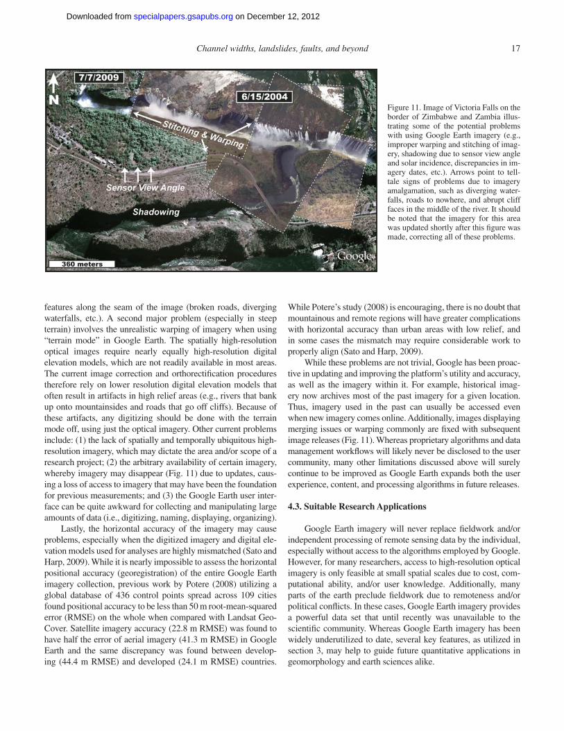
The fi rst of these features is the availability of historical imagery, which allows temporal as well as spatial change to be assessed and can supplement current research looking at land-use change, geomorphic change, event-scale impacts, etc. (Fig. 12). Second, Google has shown great commitment to providing rapid response imagery and support following large-scale natu-ral disasters. This commitment was most recently displayed with the 2011 Japan earthquake and tsunami, but has been a major campaign of Google’s since the inception of Google Earth (e.g., 2010 Haiti earthquake, 2004 Indian Ocean tsunami). Given this response, researchers now have access to both pre- and post-event imagery (one day to a few weeks) for rapid assessment

and analysis that spans the gamut of processes, landforms, and events. Third, the ease of use of the imagery, specifi cally, the complexities of image processing and orthorectifi cation are out of the control of the researcher. This absence can be both a bur-den and a benefi t, depending on the project and the user. One great example of the benefi t is shown with landslide imagery from New Zealand. In order to properly analyze aerial photos for landslides in Fjordland, New Zealand, Clarke and Burbank (2010) purchased and orthorectifi ed close to 60 aerial photos, an expensive and time-consuming endeavor. This imagery recently became freely available on Google Earth, saving both processing time and money, as well as increasing the spatial

Figure 12. Images (A) (GeoEye™ image taken 1 March 2003) and (B) (Worldview™ image taken on 2 February 2005) showing the power of Google Earth’s historical imagery for detecting change along a coastal area south of Banda Aceh, Sumatra, that was heavily impacted during the December 2004 Indian Ocean tsunami. (C) Image from Google Earth Mars of Shalbatana Vallis, a site argued to have direct evidence of lake strand-lines and deltaic features implying extensive water on the surface of Mars in the past (cf. Di Achille et al., 2009; Di Achille and Hynek, 2010; Head et al., 1999). Also note the variable morphology and terracing within many of the craters on the rim. (D) Image of Mercury from the MESSENGER mission showing the variation in surface texture and abundant tensional fault scarps due to crustal cooling. The fault scarp in the upper right hand corner is calculated by the Mercury Laser Altimeter to have a topographic relief of ~1.4 km (http://messenger.jhuapl.edu) (cf. Solomon, 2011).




area available for analysis due to lack of fi nancial constraints. Although some accuracy would likely be lost by not control-ling the orthorectifi cation process, preliminary comparison of several landslides in the area indicates minimal discrepancies between the two processes.

Google has not stopped at earth, but rather expanded the digital globe to other bodies in our solar system opening up new terrains for exploration and research (Fig. 12). Currently, digital globes for the moon and Mars are standard in Google Earth, with second-party digital globe imagery now available for Mercury (Appendix). Moreover, as imagery and topo-graphic data are acquired from across our solar system and beyond, the spatial information available in Google Earth will certainly expand along with the research possibilities. Although Google Earth imagery has many limitations, it provides one of the only feasible high-resolution spatial data sets currently available that allows user interaction for many remote areas and projects necessitating high-resolution imagery across large spatial extents (see also Bing Maps in ESRI ArcGIS). In cases where fi eld access is plausible, Google Earth imagery may act as supplemental tool to compare data sets through time and space. The most benefi cial aspect of high-resolution Google Earth imagery, however, may be the serendipitous discoveries and ideas generated from simply exploring the prolifi c imagery. The combination of curiosity-driven hypothesis creation and the ability to quantitatively test those hypotheses makes Google Earth imagery benefi cial, when properly applied, as a supple-ment, for reconnaissance, or as the primary data set across a wide range of studies in earth surface processes.

5. CONCLUSIONS

The utility of high-resolution imagery has permeated nearly every segment of society over the past decade, with Google Earth well-positioned at the forefront by providing freely available high-resolution imagery within a simple, user-friendly interface. Whereas Google Earth imagery has been widely exploited as a visualization and education tool across the earth sciences, few quantitative studies have utilized the high-resolution imagery freely available within Google Earth to yield insights about the processes and mechanisms acting upon the surface of the earth. In this paper, we have discussed the underlying high-resolution imagery within Google Earth and provided three research examples using this imagery as the primary datasource in order to demonstrate the benefi ts of the imagery over established methods, and to illuminate previously unresolved questions involving: (1) channel-width variability in the tectonically active Himalaya; (2) landslide characteris-tics related to large magnitude climatic and tectonic events in Haiti; and (3) distributed fault characteristics within the eastern California shear zone. Lastly, we have highlighted the poten-tial limitations and problems with using the imagery currently available in Google Earth and proposed favorable future appli-cations with respect to the study of earth surface processes.

APPENDIX. HELPFUL LINKS AND INFORMATION RELATED TO GOOGLE EARTH

Google Earth: http://www.google.com/earth/Google Earth Engine: http://www.google.org/earthengine/Google Fusion Tables: http://www.google.org/fusiontables/Google Earth Help Forum: http://www.google.com/support/forum

/p/earthGoogle Earth Development Team Blog: http://google-latlong.blogspot

.com/NASA Blue Marble: Next Generation KML fi le: http://ti.arc.nasa.gov

/tech/asr/intelligent-robotics/planetary/earth/Mercury Messenger Virtual Globe: http://messenger.jhuapl.edu/the

_mission/google.html

ACKNOWLEDGMENTS

This work was generously supported by a NASA Earth and Space Science Fellowship (NNX09AO24H) to G.B. Fisher and B. Bookhagen, NASA (NNX08AG05G) and NSF grants (EAR0819874) to D.W. Burbank and B. Bookhagen, an NSF Postdoctoral Research Fellowship (EAR0847990) to C.B. Amos, and a Marie Curie Fellowship to V. Godard (Geo-cycl-219662). Additional support from Google and Oxford Press to reduce the cost of attendance to the Google Earth Penrose Conference for G.B. Fisher is greatly appreciated and led to the formulation of this paper. Helpful reviews by Phillip Prince and Wes Lauer greatly improved an earlier version of this manuscript.

REFERENCES CITED

Amos, C.B., and Burbank, D.W., 2007, Channel width response to differen-tial uplift: Journal of Geophysical Research, v. 112, no. F02010, 11 p., doi:10.1029/2006JF000672.

Asner, G.P., Rudel, T.K., Aide, T.M., Defries, R., and Emerson, R.A., 2009, Con-temporary assessment of change in humid tropical forests: Conservation Biology, v. 23, p. 1386–1395, doi:10.1111/j.1523-1739.2009.01333.x.

Attal, M., Cowie, P.A., Whittaker, A.C., Hobley, D., Tucker, G.E., and Roberts, G.P., 2011, Testing fl uvial erosion models using the transient response of bedrock rivers to tectonic forcing in the Apennines, Italy: Journal of Geo-physical Research, v. 116, no. F02005, 17 p., doi:10.1029/2010JF001875.

Bacon, S.N., and Pezzopane, S.K., 2007, A 25,000-year record of earthquakes on the Owens Valley fault near Lone Pine, California: Implications for recurrence intervals, slip rates, and segmentation models: Geological Society of America Bulletin, v. 119, p. 823–847, doi:10.1130/B25879.1.

Begall, S., Cerveny, J., Neef, J., Vojtech, O., and Burda, H., 2008, Magnetic alignment in grazing and resting cattle and deer: Proceedings of the National Academy of Sciences of the United States of America, v. 105, p. 13451–13455, doi:10.1073/pnas.0803650105.

Bookhagen, B., 2010, Appearance of extreme monsoonal rainfall events and their impact on erosion in the Himalaya: Geomatics, Natural Hazards, and Risk, v. 1, p. 37–50, doi:10.1080/19475701003625737.

Bookhagen, B., and Burbank, D.W., 2010, Toward a complete Himalayan hydrological budget: Spatiotemporal distribution of snowmelt and rain-fall and their impact on river discharge: Journal of Geophysical Research, v. 115, no. F03019, 25 p., doi:10.1029/2009JF001426.

Bookhagen, B., and Strecker, M.R., 2012, Spatiotemporal trends in erosion rates across a pronounced rainfall gradient: Examples from the south-cen-tral Andes: Earth and Planetary Science Letters, v. 327-328, p. 97–110, doi:10.1016/j.epsl.2012.02.005.

Bookhagen, B., Thiede, R.C., and Strecker, M.R., 2005a, Late Quaternary intensifi ed monsoon phases control landscape evolution in the northwest Himalaya: Geology, v. 33, p. 149, doi:10.1130/G20982.1.



20 Fisher et al.

Bookhagen, B., Thiede, R.C., and Strecker, M.R., 2005b, Abnormal monsoon years and their control on erosion and sediment fl ux in the high, arid northwest Himalaya: Earth and Planetary Science Letters, v. 231, p. 131–146, doi:10.1016/j.epsl.2004.11.014.

Brossy, C.C., Kelson, K.I., Amos, C.B., Baldwin, J.N., Kozlowicz, B., Simpson, D., Ticci, M.G., Lutz, A.T., Kozaci, O., Streig, A., Turner, R., and Rose, R., 2012, Map of the late Quaternary active Kern Canyon and Brecken-ridge faults, Southern Sierra Nevada, California: Geosphere, doi:10.1130/GES00663.1.

Burbank, D., Leland, J., Fielding, E., Anderson, R., Brozovic, N., Reid, M., and Duncan, C., 1996, Bedrock incision, rock uplift and threshold hill-slopes in the northwestern Himalayas: Nature, v. 379, p. 505–510, doi:10.1038/379505a0.

Butler, D., 2006, Virtual globes: The web-wide world: Nature, v. 439, p. 776–778, doi:10.1038/439776a.

Calais, E., Freed, A., Mattioli, G., Amelung, F., Jónsson, S.F.J., Jansma, P., Hong, S.-H., Dixon, T., Prépetit, C.P., and Momplaisir, R., 2010, Transpressional rupture of an unmapped fault during the 2010 Haiti earth-quake: Nature Geoscience, v. 3, p. 794–799, doi:10.1038/ngeo992.

Carroll, R., 2008, We are going to disappear one day: The Guardian, 8 Novem-ber 2008 (retrieved 25 June 2011).

Cerling, T.E., 1990, Dating geomorphologic surfaces using cosmogenic He-3: Qua-ternary Research, v. 33, p. 148–156, doi:10.1016/0033-5894(90)90015-D.

Clarke, B.A., and Burbank, D.W., 2010, Bedrock fracturing, threshold hill-slopes, and limits to the magnitude of bedrock landslides: Earth and Plan-etary Science Letters, v. 297, p. 577–586, doi:10.1016/j.epsl.2010.07.011.

Clarke, B.A., and Burbank, D.W., 2011, Quantifying bedrock-fracture patterns within the shallow subsurface: Implications for rock-mass strength, bed-rock landslides, and erodibility: Journal of Geophysical Research–Earth Surface, v. 116, F04009, doi:10.1029/2011JF001987.

Constantine, J.A., and Dunne, T., 2008, Meander cutoff and the controls on the production of oxbow lakes: Geology, v. 36, p. 23–26, doi:10.1130/G24130A.1.

Contreras, D.A., 2010, Huaqueros and remote sensing imagery: assessing loot-ing damage in the Viru Valley, Peru: Antiquity, v. 84, p. 544–555.

Craddock, W.H., Burbank, D.W., Bookhagen, B., and Gabet, E.J., 2007, Bedrock channel geometry along an orographic rainfall gradient in the upper Marsyandi River valley in central Nepal: Journal of Geophysical Research, v. 112, no. F03007, 17 p., doi:10.1029/2006JF000589.

Dadson, S.J., Hovius, N., Chen, H., Dade, W.B., Lin, J.-C., Hsu, M.-L., Lin, C.-W., Horng, M.-J., Chen, T.-C., Milliman, J., and Stark, C.P., 2004, Earthquake-triggered increase in sediment delivery from an active moun-tain belt: Geology, v. 32, p. 733, doi:10.1130/G20639.1.

Densmore, A., and Hovius, N., 2000, Topographic fi ngerprints of bedrock landslides: Geology, v. 28, p. 371–374, doi:10.1130/0091-7613(2000)28<371:TFOBL>2.0.CO;2.

Densmore, A.L., Anderson, R.S., McAdoo, B.G., and Ellis, M.A., 1997, Hill-slope evolution by bedrock landslides: Science, v. 275, p. 369–372, doi:10.1126/science.275.5298.369.

Di Achille, G., and Hynek, B.M., 2010, Ancient ocean on Mars supported by global distribution of deltas and valleys: Nature Geoscience, v. 3, p. 459–463, doi:10.1038/ngeo891.

Di Achille, G., Hynek, B.M., and Searls, M.L., 2009, Positive identifi cation of lake strandlines in Shalbatana Vallis, Mars: Geophysical Research Let-ters, v. 36, no. L14201, 5 p., doi:10.1029/2009GL038854.

Dixon, T.H., Miller, M., Farina, F., Wang, H., and Johnson, D., 2000, Present-day motion of the Sierra Nevada block and some tectonic implications for the Basin and Range province, North American Cordillera: Tectonics, v. 19, p. 1–24, doi:10.1029/1998TC001088.

Dokka, R.K., and Travis, C.J., 1990, Role of the Eastern California shear zone in accommodating Pacifi c-North-American plate motion: Geo-physical Research Letters, v. 17, no. 9, p. 1323–1326, doi:10.1029/GL017i009p01323.

Duffi eld, W.A., and Smith, G.I., 1978, Pleistocene history of volcanism and Owens River near Little-Lake, California: Journal of Research of the U.S. Geological Survey, v. 6, no. 3, p. 395–408.

Duvall, A., Kirby, E., and Burbank, D., 2004, Tectonic and lithologic con-trols on bedrock channel profi les and processes in coastal Califor-nia: Journal of Geophysical Research, v. 109, no. F03002, 18 p., doi:10.1029/2003JF000086.

Farr, T.G., Rosen, P.A., Caro, E., Crippen, R., Duren, R., Hensley, S., Kobrick, M., Paller, M., Rodriguez, E., Roth, L., Seal, D., Shaffer, S., Shimada, J.,

Umland, J., Werner, M., Oskin, M., Burbank, D., and Alsdorf, D., 2007, The shuttle radar topography mission: Reviews of Geophysics, v. 45, Rg2004, doi:10.1029/2005rg000183.

Finnegan, N.J., Roe, G.H., Montgomery, D.R., and Hallet, B., 2005, Controls on the channel width of rivers: Implications for modeling fl uvial incision of bedrock: Geology, v. 33, p. 229–232, doi:10.1130/G21171.1.

Finnegan, N.J., Sklar, L.S., and Fuller, T.K., 2007, Interplay of sediment sup-ply, river incision, and channel morphology revealed by the transient evolution of an experimental bedrock channel: Journal of Geophysical Research, v. 112, no. F03S11, 17 p., doi:10.1029/2006JF000569.

Finnegan, N.J., Hallet, B., Montgomery, D.R., Zeitler, P.K., Stone, J.O., Anders, A.M., and Yuping, L., 2008, Coupling of rock uplift and river incision in the Namche Barwa-Gyala Peri massif, Tibet: Geological Society of America Bulletin, v. 120, p. 142–155, doi:10.1130/B26224.1.

Fisher, G.B., Magilligan, F.J., Kaste, J.M., and Nislow, K.H., 2010, Constrain-ing the timescales of sediment sequestration associated with large woody debris using cosmogenic 7Be: Journal of Geophysical Research, v. 115, no. F01013, 19 p., doi:10.1029/2009JF001352.

Fisher, G.B., Bookhagen, B., and Burbank, D.W., 2011, High-resolution channel widths and erosion along the entire Indus River: Eos (Transac-tions, American Geophysical Union), Fall Meeting Supplement, abstract EP23C-0762.

Frankel, K.L., Dolan, J.F., Owen, L.A., Ganev, P., and Finkel, R.C., 2011, Spa-tial and temporal constancy of seismic strain release along an evolving segment of the Pacifi c-North America plate boundary: Earth and Plan-etary Science Letters, v. 304, p. 565–576, doi:10.1016/j.epsl.2011.02.034.

Gabet, E., Burbank, D., Putkonen, J., Pratt-Sitaula, B., and Ojha, T.P., 2004, Rainfall thresholds for landsliding in the Himalayas of Nepal: Geomor-phology, v. 63, p. 131–143, doi:10.1016/j.geomorph.2004.03.011.

Galewsky, J., Stark, C.P., Dadson, S., Wu, C.-C., Sobel, A.H., and Horng, M.-J., 2006, Tropical cyclone triggering of sediment discharge in Taiwan: Journal of Geophysical Research, v. 111, p. F03014, doi:10.1029/2005JF000428.

Godard, V., Lavé, J., Carcaillet, J., Cattin, R., Bourlès, D., and Zhu, J., 2010, Spatial distribution of denudation in Eastern Tibet and regressive erosion of plateau margins: Tectonophysics, v. 491, p. 253–274, doi:10.1016/j.tecto.2009.10.026.

Guo, J., Liang, L., and Gong, P., 2010, Removing shadows from Google Earth images: International Journal of Remote Sensing, v. 31, p. 1379–1389, doi:10.1080/01431160903475316.

Hashimoto, M., Fukushima, Y., and Fukahata, Y., 2011, Fan-delta uplift and mountain subsidence during the Haiti 2010 earthquake: Nature Geosci-ence, v. 4, p. 255–259, doi:10.1038/ngeo1115.

Hayes, G.P., Briggs, R.W., Sladen, A., Fielding, E.J., Prentice, C., Hudnut, K., Mann, P., Taylor, F.W., Crone, A.J., Gold, R., Ito, T., and Simons, M., 2010, Complex rupture during the 12 January 2010 Haiti earthquake: Nature Geoscience, v. 3, p. 800–805, doi:10.1038/ngeo977.

Head, J., Hiesinger, H., Ivanov, M., Kreslavsky, M., Pratt, S., and Thomson, B., 1999, Possible ancient oceans on Mars: Evidence from Mars Orbiter Laser Altimeter data: Science, v. 286, p. 2134–2137, doi:10.1126/science.286.5447.2134.

Hoffmann, E., and Winde, F., 2010, Generating high-resolution digital elevation models for wetland research using Google Earth™ imagery—an example from South Africa: Water S.A., v. 36, p. 53–68.

Hong, Y., Adler, R., and Huffman, G., 2006, Evaluation of the potential of NASA multi-satellite precipitation analysis in global landslide haz-ard assessment: Geophysical Research Letters, v. 33, L22402, 5 p., doi:10.1029/2006GL028010.

Hovius, N., Stark, C., and Allen, P., 1997, Sediment fl ux from a moun-tain belt derived by landslide mapping: Geology, v. 25, p. 231–234, doi:10.1130/0091-7613(1997)025<0231:SFFAMB>2.3.CO;2.

Hovius, N., Stark, C., Chu, H., and Lin, J., 2000, Supply and removal of sedi-ment in a landslide-dominated mountain belt: Central Range, Taiwan: The Journal of Geology, v. 108, p. 73–89, doi:10.1086/314387.

Hovius, N., Meunier, P., Ching-Weei, L., Hongey, C., Yue-Gau, C., Dadson, S., Ming-Jame, H., and Lines, M., 2011, Prolonged seismically induced erosion and the mass balance of a large earthquake: Earth and Planetary Science Letters, v. 304, p. 347–355, doi:10.1016/j.epsl.2011.02.005.

Huffman, G.J., Bolvin, D.T., Nelkin, E.J., Wolff, D.B., Adler, R.F., Gu, G., Hong, Y., Bowman, K.P., and Stocker, E.F., 2007, The TRMM Multisatellite Pre-cipitation Analysis (TMPA): Quasi-Global, Multiyear, Combined-Sensor Precipitation Estimates at Fine Scales: Journal of Hydrometeorology, v. 8, p. 38–55, doi:10.1175/JHM560.1.




Jennings, C.W., 1994, Fault activity map of California and adjacent areas, Geo-logic Data Map 6: California Division of Mines and Geology, Sacramento.

Jones, K.C., 2008, Google Launches Mapping Satellite: InformationWeek.com, 8 September 2008 (retrieved 15 February 2011).

Kirby, E., and Ouimet, W., 2011, Tectonic geomorphology along the eastern margin of Tibet: insights into the pattern and processes of active deforma-tion adjacent to the Sichuan Basin, in Gloaguen, R., and Ratschbacher, L., eds., Growth and Collapse of the Tibetan Plateau: Geological Society of London Special Publication 353, p. 165–188, doi:10.1144/SP353.9.

Kirby, E., and Whipple, K., 2001, Quantifying differential rock-uplift rates via stream profi le analysis: Geology, v. 29, p. 415–418, doi:10.1130/0091-7613(2001)029<0415:QDRURV>2.0.CO;2.

Klinger, Y., Etchebes, M., Tapponnier, P., and Narteau, C., 2011, Characteristic slip for fi ve great earthquakes along the Fuyun fault in China: Nature Geoscience, v. 4, p. 389–392, doi:10.1038/ngeo1158.

Knighton, D.A., 1998, Fluvial forms and processes: Edward Arnold, London, 377 p.

Korup, O., 2006, Rock-slope failure and the river long profi le: Geology, v. 34, no. 1, p. 45–48, doi:10.1130/G21959.1.

Korup, O., Densmore, A.L., and Schlunegger, F., 2010, The role of land-slides in mountain range evolution: Geomorphology, v. 120, p. 77–90, doi:10.1016/j.geomorph.2009.09.017.

Korup, O., and Montgomery, D.R., 2008, Tibetan plateau river incision inhib-ited by glacial stabilization of the Tsangpo gorge: Nature, v. 455, p. 786–789, doi:10.1038/nature07322.

Lavé, J., and Avouac, J., 2001, Fluvial incision and tectonic uplift across the Himalayas of central Nepal: Journal of Geophysical Research—Solid Earth, v. 106, p. 26561–26591, doi:10.1029/2001JB000359.

Lavé, J., and Burbank, D.W., 2004, Denudation processes and rates in the Transverse Ranges, southern California: Erosional response of a transi-tional landscape to external and anthropogenic forcing: Journal of Geo-physical Research, v. 109, no. F01006, 31 p., doi:10.1029/2003JF000023.

Leopold, L., and T. Maddock, 1953, The hydraulic geometry of stream chan-nels and some physiographic implications: U.S. Geological Survey Pro-fessional Paper 252.

Mackey, B.H., and Roering, J.J., 2011, Sediment yield, spatial characteristics, and the long-term evolution of active earthfl ows determined from airborne LiDAR and historical aerial photographs, Eel River, California: Geological Society of America Bulletin, v. 123, p. 1560–1576, doi:10.1130/B30306.1.

Magilligan, F.J., 1992, Thresholds and the spatial variability of fl ood power dur-ing extreme fl oods: Geomorphology, v. 5, p. 373–390, doi:10.1016/0169-555X(92)90014-F.

Manning, R., 1891, On the fl ow of water in open channels and pipes: Institute of Civil Engineers of Ireland Transactions, v. 20, p. 161–207.

Mering, C., Baro, J., and Upegui, E., 2010, Retrieving urban areas on Google Earth images: application to towns of West Africa: International Journal of Remote Sensing, v. 31, p. 5867–5877, doi:10.1080/01431161.2010.512311.

Meunier, P., Hovius, N., and Haines, J.A., 2008, Topographic site effects and the location of earthquake induced landslides: Earth and Planetary Sci-ence Letters, v. 275, p. 221–232, doi:10.1016/j.epsl.2008.07.020.

Milliman, J., and Syvitski, J., 1992, Geomorphic tectonic control of sediment discharge to the ocean—The importance of small mountainous rivers: The Journal of Geology, v. 100, p. 525–544, doi:10.1086/629606.

Oskin, M., and Iriondo, A., 2004, Large-magnitude transient strain accumu-lation on the Blackwater fault, Eastern California shear zone: Geology, v. 32, p. 313–316, doi:10.1130/G20223.1.

Oskin, M., Perg, L., Shelef, E., Strane, M., Gurney, E., Singer, B., and Zhang, X., 2008, Elevated shear zone loading rate during an earthquake cluster in eastern California: Geology, v. 36, p. 507–510, doi:10.1130/G24814A.1.

Parker, J.D., 2011, Using Google Earth to teach the magnitude of deep time: Journal of College Science Teaching, v. 40, p. 23–27.

Parker, R.N., Densmore, A.L., Rosser, N.J., de Michele, M., Li, Y., Huang, R., Whadcoat, S., and Petley, D.N., 2011, Mass wasting triggered by the 2008 Wenchuan earthquake is greater than orogenic growth: Nature Geosci-ence, v. 4, p. 449–452, doi:10.1038/ngeo1154.

Pelletier, J.D., DeLong, S.B., Al-Suwaidi, A.H., Cline, M., Lewis, Y., Psillas, J.L., and Yanites, B., 2006, Evolution of the Bonneville shoreline scarp in west-central Utah: Comparison of scarp-analysis methods and impli-cations for the diffusion model of hillslope evolution: Geomorphology, v. 74, p. 257–270, doi:10.1016/j.geomorph.2005.08.008.

Peltzer, G., Crampe, F., Hensley, S., and Rosen, P., 2001, Transient strain accumulation and fault interaction in the Eastern California shear zone:

Geology, v. 29, p. 975–978, doi:10.1130/0091-7613(2001)029<0975:TSAAFI>2.0.CO;2.

Perroy, R.L., Bookhagen, B., Asner, G.P., and Chadwick, O.A., 2010, Compari-son of gully erosion estimates using airborne and ground-based LiDAR on Santa Cruz Island, California: Geomorphology, v. 118, p. 288–300, doi:10.1016/j.geomorph.2010.01.009.

Phillips, F.M., and Majkowski, L., 2011, The role of low-angle normal faulting in active tectonics of the northern Owens Valley, California: Lithosphere, v. 3, p. 22–36, doi:10.1130/L73.1.

Pierce, J.L., Meyer, G.A., and Jull, A.J.T., 2004, Fire-induced erosion and millennial-scale climate change in northern ponderosa pine forests: Nature, v. 432, p. 87–90, doi:10.1038/nature03058.

Potere, D., 2008, Horizontal Positional Accuracy of Google Earth’s High- Resolution Imagery Archive: Sensors (Basel, Switzerland), v. 8, p. 7973–7981, doi:10.3390/s8127973.

Roering, J.J., and Gerber, M., 2005, Fire and the evolution of steep, soil- mantled landscapes: Geology, v. 33, p. 349, doi:10.1130/G21260.1.

Santamaria Tovar, D., Shulmeister, J., and Davies, T.R., 2008, Evidence for a landslide origin of New Zealand’s Waiho Loop moraine: Nature Geosci-ence, v. 1, p. 524–526, doi:10.1038/ngeo249.

Sato, H.P., and Harp, E.L., 2009, Interpretation of earthquake-induced landslides triggered by the 12 May 2008, M7.9 Wenchuan earthquake in the Beichuan area, Sichuan Province, China using satellite imagery and Google Earth: Land-slides, v. 6, p. 153–159, doi:10.1007/s10346-009-0147-6.

Sauber, J., Thatcher, W., Solomon, S.C., and Lisowski, M., 1994, Geodetic slip rate for the eastern California shear zone and the recurrence time of Mojave Desert earthquakes: Nature, v. 367, p. 264–266, doi:10.1038/367264a0.

Schumacher, J., Luedeling, E., Gebauer, J., Saied, A., El-Siddig, K., and Buerk-ert, A., 2009, Spatial expansion and water requirements of urban agricul-ture in Khartoum, Sudan: Journal of Arid Environments, v. 73, p. 399–406, doi:10.1016/j.jaridenv.2008.12.005.

Scherler, D., Bookhagen, B., and Strecker, M.R., 2011a, Hillslope-glacier coupling: The interplay of topography and glacial dynamics in High Asia: Journal of Geophysical Research, v. 116, no. F02019, 21 p., doi:10.1029/2010JF001751.

Scherler, D., Bookhagen, B., and Strecker, M.R., 2011b, Spatially variable response of Himalayan glaciers to climate change affected by debris cover: Nature Geoscience, v. 4, p. 156–159, doi:10.1038/ngeo1068.

Seeber, L., and Gornitz, V., 1983, River profi les along the Himalayan Arc as indicators of active tectonics: Tectonophysics, v. 92, p. 335–367, doi:10.1016/0040-1951(83)90201-9.

Shroder, J.F.J., and Weihs, B.J., 2010, Geomorphology of the Lake Shewa Landslide Dam, Badakhshan, Afghanistan, Using Remote Sensing Data: Geografi ska Annaler, v. 92 A, p. 469–483.

Slater, J.A., Heady, B., Kroenung, G., Curtis, W., Haase, J., Hoegemann, D., Shockley, C., and Tracy, K., 2011, Global assessment of the new ASTER Global Digital Elevation Model: Photogrammetric Engineering and Remote Sensing, v. 77, p. 335–349.

Smith, L.C., and Pavelsky, T.M., 2008, Estimation of river discharge, propa-gation speed, and hydraulic geometry from space: Lena River, Siberia: Water Resources Research, v. 44, doi:10.1029/2007WR006133.

Solomon, S., 2011, A new look at the planet Mercury: Physics Today, v. 64, p. 50–55, doi:10.1063/1.3541945.

Stark, C.P., and Hovius, N., 2001, The characterization of landslide size distributions: Geophysical Research Letters, v. 28, p. 1091–1094, doi:10.1029/2000GL008527.

Stark, C.P., Foufoula-Georgiou, E., and Ganti, V., 2009, A nonlocal theory of sediment buffering and bedrock channel evolution: Journal of Geophysi-cal Research, v. 114, p. F01029, doi:10.1029/2008JF000981.

Stock, J.D., and Montgomery, D.R., 1999, Geologic constraints on bed-rock river incision using the stream power law: Journal of Geophysical Research. Solid Earth, v. 104, p. 4983–4993, doi:10.1029/98JB02139.

Thiede, R.C., Ehlers, T.A., Bookhagen, B., and Strecker, M.R., 2009, Ero-sional variability along the northwest Himalaya: Journal of Geophysical Research–Earth Surface, v. 114, F01015, 19 p., doi:10.1029/2008jf001010.

Turowski, J.M., Lague, D., and Hovius, N., 2009, Response of bedrock channel width to tectonic forcing: Insights from a numerical model, theoretical considerations, and comparison with fi eld data: Journal of Geophysical Research, v. 114, no. F03016, 16 p., doi:10.1029/2008JF001133.

Unruh, J., Humphrey, J., and Barron, A., 2003, Transtensional model for the Sierra Nevada frontal fault system, eastern California: Geology, v. 31, p. 327–330, doi:10.1130/0091-7613(2003)031<0327:TMFTSN>2.0.CO;2.



22 Fisher et al.

Unruh, J.R., Hauksson, E., Monastero, F.C., Twiss, R.J., and Lewis, J.C., 2002. Seismotectonics of the Coso Range-Indian Wells Valley region, Califor-nia: Transtensional deformation along the southeastern margin of the Sierran microplate, in Glazner, A.F., Walker, J.D., and Bartley, J.M., eds., Geologic Evolution of the Mojave Desert and Southwestern Basin and Range: Geological Society of America Memoir 195, p. 277–294.

van Westen, C., and Gorum, T., 2010, Preliminary results on earthquake trig-gered landslides for the Haiti earthquake (January 2010): Geophysical Research Abstracts, v. 12, p. EGU2010–EGU1153.

Whipple, K.X., 2004, Bedrock rivers and the geomorphology of active orogens: Annual Review of Earth and Planetary Sciences, v. 32, no. 1, p. 151–185, doi:10.1146/annurev.earth.32.101802.120356.

Whipple, K.X., and Tucker, G.E., 1999, Dynamics of the stream-power river inci-sion model: Implications for height limits of mountain ranges, landscape response timescales, and research needs: Journal of Geophysical Research, Solid Earth, v. 104, p. 17661–17674, doi:10.1029/1999JB900120.

Whitmeyer, S., Nicoletti, J., and De Paor, D., 2010, The digital revolution in geologic mapping: GSA Today, v. 20, p. 4–10, doi:10.1130/GSATG70A.1.

Whittaker, A.C., Cowie, P.A., Attal, M., Tucker, G.E., and Roberts, G.P., 2007, Bedrock channel adjustment to tectonic forcing: Implications for pre-dicting river incision rates: Geology, v. 35, no. 2, p. 103, doi:10.1130/G23106A.1.

Wobus, C.W., Tucker, G.E., and Anderson, R.S., 2006a, Self- formed bed-rock channels: Geophysical Research Letters, v. 33, no. L18408, 6 p., doi:10.1029/2006GL027182.

Wobus, C., Whipple, K., Kirby, E., Snyder, N., Johnson, J., Spyropolou, K., Crosby, B., and Sheehan, D., 2006b, Tectonics from topography: Procedures, promise and pitfalls, in Willett, S., Hovius, N., Bran-don, M., and Fisher, D., eds., Tectonics, Climate, and Landscape Evo-lution: Geological Society of America Special Paper 398, p. 55–74, doi:10.1130/2006.2398(04).

Wohl, E., and David, G.C.L., 2008, Consistency of scaling relations among bedrock and alluvial channels: Journal of Geophysical Research, v. 113, no. F04013, 16 p., doi:10.1029/2008JF000989.

Wolman, M.G., and Miller, J.P., 1960, Magnitude and frequency of forces in geomorphic processes: The Journal of Geology, v. 68, no. 1, p. 54–74.

Yanites, B.J., and Tucker, G.E., 2010, Controls and limits on bedrock channel geometry: Journal of Geophysical Research, v. 115, no. F04019, 17 p., doi:10.1029/2009JF001601.

Yanites, B.J., Tucker, G.E., Mueller, K.J., Chen, Y.G., Wilcox, T., Huang, S.Y., and Shi, K.W., 2010, Incision and channel morphology across active structures along the Peikang River, central Taiwan: Implications for the importance of channel width: Geological Society of America Bulletin, v. 122, no. 7–8, p. 1192–1208, doi:10.1130/B30035.1.

Zech, R., Zech, M., Kubik, P.W., Kharki, K., and Zech, W., 2009, Deglaciation and landscape history around Annapurna, Nepal, based on 10Be surface exposure dating: Quaternary Science Reviews, v. 28, no. 11–12, p. 1106–1118, doi:10.1016/j.quascirev.2008.11.013.

MANUSCRIPT ACCEPTED BY THE SOCIETY 16 APRIL 2012

Printed in the USA



geological society of america special papers · geological society of america special papers 2012;...

Documents