GEOLOGIC NOTE

A simple model of gasproduction from hydrofracturedhorizontal wells in shalesTad Patzek, Frank Male, and Michael Marder

ABSTRACT

Assessing the production potential of shale gas can be assisted byconstructing a simple, physics-based model for the productivity ofindividual wells. We adopt the simplest plausible physical model:one-dimensional pressure diffusion from a cuboid region with theeffective area of hydrofractures as base and the length of horizon-tal well as height. We formulate a nonlinear initial boundary valueproblem for transient flow of real gas that may sorb on the rockand solve it numerically. In principle, solutions of this problemdepend on several parameters, but in practice within a given gasfield, all but two can be fixed at typical values, providing a nearlyuniversal curve for which only the appropriate scales of time inproduction and cumulative production need to be determined foreach well. The scaling curve has the property that production ratedeclines as one over the square root of time until the well starts tobe pressure depleted, and later it declines exponentially. We showthat this simple model provides a surprisingly accurate descriptionof gas extraction from 8305 horizontal wells in the United States’oldest shale play, the Barnett Shale. Good agreement exists withthe scaling theory for 2133 horizontal wells in which productionstarted to decline exponentially in less than 10 yr. We provideupper and lower bounds on the time in production and originalgas in place.

Copyright ©2014. The American Association of Petroleum Geologists. All rights reserved.

Manuscript received July 16, 2012; provisional acceptance November 14, 2012; revised manuscriptreceived August 19, 2013; final acceptance March 24, 2014.DOI: 10.1306/03241412125

AUTHORS

Tad Patzek ∼ The University of Texas,Department of Petroleum & GeosystemsEngineering, Austin, Texas 78712;patzek@mail.utexas.edu

Tadeusz (Tad) W. Patzek is the Lois K. andRichard D. Folger Leadership Professor andChairman of the Petroleum and GeosystemsEngineering Department at The University ofTexas at Austin. He also holds the CockrellRegents Chair #11. Between 1990 and 2008,he was a professor of geoengineering at theUniversity of California, Berkeley. Prior tojoining Berkeley, he was a researcher atShell Development. Patzek’s researchinvolves mathematical and numericalmodeling of earth systems with emphasis onsubsurface fluid flow. He is working on thethermodynamics and ecology of humansurvival and energy supply for humanity. Heis also working on unconventional naturalgas and oil resources. Patzek is a coauthor ofover 200 papers and reports, and one book,and is currently writing five books.

Frank Male ∼ The University of Texas,Department of Physics, Austin, Texas 78712;fmale@chaos.utexas.edu

Frank Male received his bachelor’s degreesin physics and political science from KansasState University in 2009. He spent fivesummers at the Max Planck Institute forDynamics and Self-organization inGottingen, Germany, studyingcomputational microfluidics as a researchintern. Since 2010, Frank has been agraduate student in the Physics Departmentof the University of Texas at Austin.

Michael Marder ∼ The University of Texas,Department of Physics, Austin, Texas 78712;marder@chaos.utexas.edu

Michael Marder is a member of the Centerfor Nonlinear Dynamics, internationallyknown for its experiments on chaos andpattern formation, and for many yearsranked #1 in the nation by US News andWorld Report. He is involved in a widevariety of theoretical, numerical, andexperimental investigations, ranging fromstudies of plasticity and phasetransformations to experiments on sand

AAPG Bulletin, v. 98, no. 12 (December 2014), pp. 2507–2529 2507

NOMENCLATURESymbols and dimensions of key quantitiesSymbol SI dimensions Field dimensionsc–compressibility Pa−1 μ cipd–half-distance betweenhydrofractures

m ft

D–production decline coefficientk–permeability m2 darcyK–partitioning coefficientm–gas pseudopressure Pa s−1 psi2∕cpm–cumulative produced mass kg tonM–Original gas in place kg tonM–molecular weight kmol lbmolH–formation thickness m ftp–pressure Pa psiq–volumetric flow rate m3 s−1 bbl/dQ–volumetric cumulativeproduction

m3 bbl

R—universal gas constant J/kmol-K psi-ft3∕lb-molRF–recovery factorS–saturationt–time in production s month, yT–temperature K °F, °Cv–specific volume m3∕kg ft3∕lbmy–molar compositionZ–compressibility factorα–hydraulic diffusivity m2 s−1 ft2∕yκ–dimensionless constant for gasproduction in square root phaseK–dimensional constant for gasproduction in square root phase

kg∕ffiffis

pton∕

ffiffiffiffiffiffiffiffiffiffiffiffimonth

p

μ–gas viscosity Pa s cpρ–density kg m−3 lbm∕ft3

τ–time to interference s yϕ–porositySubscripts and SuperscriptsSymbol Meaninga adsorbedf (hydro)fractureg gasi initialL LangmuirST stock tank conditionsw waterwc connate water∼ dimensionless∧ specific0 reference or standard

conditions

ripples at the sea bottom. He specializes inthe mechanics of solids, particularly thefracture of brittle materials. He hasdeveloped numerical methods allowingfracture computations on the atomic scale tobe compared directly with laboratoryexperiments on a macroscopic scale. He isemploying these methods to study theproduction of natural gas fromhydrofractured shale. He has also publishedtwo textbooks, one a graduate text oncondensed matter physics, and the other anundergraduate text on research methods forscience.

ACKNOWLEDGEMENTS

This paper was supported by the ShellUniversity of Texas project “Physics ofHydrocarbon Recovery” with Patzek andMarder as co-PIs, and the Bureau ofEconomic Geology’s Sloan Foundationfunded project “The Role of Shale Gas in theU.S. Energy Transition: RecoverableResources, Production Rates, andImplications.” Thanks to John Browning forhelp estimating reserves, for his deepinsights into well performance in the BarnettShale, and selection of well-behaved groupsof wells. We thank D. Silin, S. Bhattacharaya,and R. Dombrowski for detailed commentson the manuscript. The gas production datawas extracted from the InformationHandling Service Cera database, licensed tothe Bureau of Economic Geology. M.M.acknowledges partial support from theNational Science Foundation CondensedMatter and Materials Theory program.Neither Shell, the Sloan Foundation, nor theNational Science Foundation endorse thefindings in this paper.

2508 Geologic Note

INTRODUCTION

The fast progress of hydraulic fracturing technologyhas led to the extraction of natural gas and oil fromtens of thousands of wells drilled into mudrock for-mations almost exclusively in the United States.However, a significant potential exists for drillinginto mudrock formations on all continents, (Birol,2012). The fracturing technology has generated con-siderable concern about environmental consequences(Osborn et al., 2011; Vidic et al., 2013), and aboutwhether hydrocarbon extraction from mudrocks willultimately be profitable (Hughes, 2013).

The cumulative gas obtained from the wellshydrofractured in mudrocks and their ultimate profit-ability depend upon how the hydrocarbon flow ratevaries over time. Large-scale use of hydraulic fractur-ing in mudrocks is relatively new, and therefore dataon the behavior of hydrofractured wells on the scaleof 10 yr or more are only now becoming available.

Our aim is to assemble the basic equations gov-erning flow of high-pressure gas in a porous mediumand assess whether gas transport in mudrock beds canadequately be described by a diffusion equation writ-ten and solved in one dimension. We believe this tobe the most appropriate setting, although the mostfamiliar reservoir flow laws result from flow prob-lems posed in two dimensions (Kelkar, 2008). Weaddress this question by comparing simple modelflow problems with data from a large subset of all16,533 vertical and horizontal wells in the Texas’Barnett Shale. The Barnett Shale is a Mississippianmudstone located in the Bend arch–Fort Worth Basin.

The power-law behavior of the flow is most com-patible with a one-dimensional (1-D) model.However, we will show that the rate at which the flowoccurs is incompatible with laboratory values of gasdiffusivity in shale. Therefore, the subsurface geom-etry created by hydrofracturing and reactivation ofmicrocracks, natural fractures, and faults is complex,as observed by Olson (2004), Gale et al. (2007), andGeiser et al. (2012), among others. Our understandingof the nature, creation, and evolution of hydrofrac-tured natural fracture systems is far from complete.

Recently, we presented the derivation of a simplemodel that appears to capture the essential features ofgas production from tight shale formations (Patzek

et al., 2013). Here, we expand on the conclusions ofthat work, particularly by exploring the experimentalfoundations more thoroughly. The structure of thispaper is as follows. After a brief discussion of themostly heuristic models of decline of well produc-tion, we present the conceptual structure of ourphysics-based model of gas production. The modelconstitutes the simplest description consistent withthe basic physics of gas extraction from horizontalfractured wells. The basic idea of the model had pre-viously been presented by Al-Ahmadi et al. (2010).Nobakht et al. (2012) found analytical approxima-tions they compared with numerical solutions and asmall number of field cases. In Patzek et al. (2013),we provided a detailed analysis showing that theexact solution of the recovery factor in this modelreduces to a nearly universal scaling curve that canbe tabulated for convenient comparison with fielddata. Here, we discuss properties of the dimensionlessrecovery factor and fit it to a mean horizontal well inthe Barnett, yielding effective rock permeability andhydrofracture area. Next we analyze a group of 66good (producing most of the time, not converted,and not refractured) horizontal wells in the BarnettShale that evidently were in transient flow for up to8 yr, and we describe a composite median well thatwe use to test the validity of our assumptions. Wealso analyze a group of 105 similarly defined goodvertical wells, and show that most wells in theBarnett Shale have been in 1-D (rectilinear) transientflow for up to 7 to 10 yr. Finally, we apply our modelto 8305 horizontal wells that have not been recom-pleted and generate distributions of their times toexponential decline of production rate caused bypressure interference, original gas in place, hydrofrac-ture area, and drainage area.

Brief History of Predictions of WellProduction

Attempts to quantify the rate of decline of oil andnatural gas production by a well are as old as reser-voir engineering. In 1944, J. J. Arps first published aseminal paper on several types of decline of well pro-duction: exponential, hyperbolic, harmonic, and geo-metric (Arps, 1945). In that paper, Arps reviewedalmost 30 yr of the prior history of empirical

PATZEK ET AL. 2509

predictions of future well production. Thirty-six yearslater, Fetkovich (1980) showed how the different wellflow equations listed by Arps arise from radial tran-sient flow.

Today, the literature discussing production fromoil, gas and water wells is enormous, and impossibleto summarize briefly. A Google search with “frac*”conducted on November 4, 2013, returned over 143million hits. Another Google Scholar search for anyof the keywords, gas, well, shale, and/or production,returned 156,000 research papers. Nevertheless, thelong and continuing tradition of using purely phe-nomenological models in this area means that puttingeffort into models based upon physical reasoning isworthwhile.

Jones (1942), also quoted by Arps, suggested forwells declining at variable rates an approximationwhereby the fractional decline-time relationship isgiven by a straight line in log–log coordinates:

ln  D = ln  D0 − m  ln  t (1)

in which D is the fractional decline coefficient offluid production rate, D0 is the initial value of thatcoefficient, t is time in production, and m is the slope;see Section 1 for nomenclature.

If a is an increment of the logarithm of volumet-ric production rate q over the nth  production timeincrement δt:

an = −�1qdqdt

δt�

n> 0; n = 0; 1; 2;… (2)

then the production decline coefficient D = 1∕a is aconstant for exponential decline; D is proportional toqb, 0 < b < 1, for hyperbolic decline; proportionalto q1 in harmonic decline; and D diminishes with timeat a constant fraction in geometric decline,

Dn =r−P

n0δti

an∕an−1(3)

in which r is the constant decline ratio, n = 0; 1; 2;…is the counter of the subsequent production time (withwell downtimes excluded) intervals δtn, months inthe current paper.

Upon integration, equation 1 gives:

q = q0  exp�−D0t1−m

1 − m

�; 0 ≤ m < 1 (4)

in which q0 is the initial production rate. If we set n =1 − m and define a characteristic interference time, τ,

τ =�D0

n

�−1∕n

(5)

we recover the stretched exponential equation ofValko and Lee (2010):

q = q0  exp�−�tτ

�n�

(6)

proposed to explain the expected rates of productiondecline for large groups of wells in the BarnettShale.

Arps (1945, p. 229) already stated that the vari-ous estimates of production decline are based on theassumption that future well behavior will be governedby whatever trend or mathematical relationship is ap-parent in its past performance:

“This assumption puts the extrapolation methodson a strictly empirical basis and it must be realizedthat this may make the results sometimes inferior tothe more exact volumetric methods.”

The volumetric methods mentioned by Arps arebased on geology, core analysis, wireline logging,and downhole well pressures.

Semi-analytic and numerical models of transientflow in vertical wells with vertical hydrofractureshave been developed for 50 yr under a variety ofassumptions. Most of the relevant papers have beendevoted to short- and intermediate-time well testing:pressure build up, well storage effects, and flow tests.The classical papers by Prats (1961), Russell andTruitt (1964), Wattenbarger and Ramey (1969),Gringarten and Henry (1974) should be mentionedin this context. A 1-D (rectilinear) transient flowanalysis was also applied to long-time productionfrom hydrofractured wells in ultra-low-permeabilityformations. Patzek (1992) analyzed performance ofover 1000 production and injection wells in the onemicrodarcy, naturally fractured South BelridgeDiatomite oil field in California, and demonstratedthe significant extensions of injection hydrofracturesand injector–producer linkages. Most wells remainedin purely transient flow for more than a decade.Wattenbarger et al. (1998) have calculated declinecurves for tight gas wells and concluded that

2510 Geologic Note

rectilinear flow may last for 10 or 20 yr. Kelkar(2008) in his Chapter 4 discusses 1-D (rectilinear)and two-dimensional (2-D) (radial) flow models, withan example drawn from the Barnett Shale. Similar tomany other authors, Kelkar focuses on flow from asemi-infinite region into a plane, avoiding interfer-ence effects that will be prominent in our analysis.

Nobakht and Clarkson (2011a) looked at tightgas wells and gas shale wells in 1-D (rectilinear) tran-sient flow and used production data to calculate theeffective formation permeability and fracture half-lengths. By effective permeability, we mean theenhanced permeability of the shales produced by thehydrofracturing process, which in the current paperwe will treat as spatially uniform. Nobakht andClarkson (2011a) have concluded that not accountingfor gas slippage in nanopores may lead to an underes-timated rock permeability and overestimate of size ofthe hydrofractures. However, their own calculationsshow a negligible impact of slip, well within the noisein the field data. In addition, Nobakht and Clarkson(2011b) accounted for variable fluid and rock proper-ties. They used numerical examples in which neitherthe flow rate nor flowing wellbore pressure were con-stant. The problem with this approach is that reservoirpressure is not well known in shales, and well flow-ing pressures are not reported accurately or not at allover multi-year time intervals (Lee and Sidle, 2010).Recently, Silin (2011), Silin and Kneafsey (2012)presented an elegant analytical solution of compress-ible gas flow with adsorption.

The physical model underlying time-dependent1-D flow was presented conceptually by Al-Ahmadiet al. (2010) and solved in approximate analytical aswell as in numerical fashion by Nobakht et al.(2012). This model, we maintain, is the simplestpossible starting point for analysis of hydrofracturedwells that is consistent with the physics of the extrac-tion process. Nevertheless, it has received relativelylittle attention, and appears to be regarded asadvanced.

Thus, we pursue three goals. The first is to presenta brief and largely conceptual review of the model wederived in Patzek et al. (2013). The second is to showhow the solution can be used to obtain upper and lowerbounds on gas production rates and recoverablereserves. The third is to perform a comprehensive

analysis of the oldest shale play in the United States,the Barnett Shale, and show that the model in factdescribes decline curves accurately. An accurate butpractically usable model of gas production from shalesis important because shale gas has pumped over $800billion into the United States economy in the last5 yr, whereas at the same time serious questions existabout the profitability and economic viability ofextraction (Patzek et al., 2013). Both decisions abouthow to invest in and regulate shale gas extraction needto be informed by accurate scientific assessment.

MODEL OF WELL PRODUCTION

Until relatively recently, mudrock formations werethought unsuitable for economic gas productionbecause the source rock has very low permeability,on the order of one nanodarcy (Vermylen, 2011).The hydrofracturing process raises the effective per-meability, as we will show in this paper, by one ortwo orders of magnitude. However, only those spatialregions in which fractures have been activated andpropped open are reasonable candidates for theenhanced permeability. Therefore, a physically rea-sonable starting point for the study of hydrofracturewells should consider pressure diffusion from a finiteregion, outside which diffusion vanishes, rather thanfrom an infinite or semi-infinite region, as for con-ventional wells (Kelkar, 2008; Dake, 1978).

Consider a single horizontal well, shown inFigure 1. Suppose that this well has N vertical trans-verse hydrofractures that are spaced uniformly alongits entire horizontal length. The exterior sides of thefirst and last hydrofracture drain the reservoir volumeexternal to the horizontal-well length, and this addi-tional production will also be accounted for.Essentially identical well schematics appear asfigure 2 in Al-Ahmadi et al. (2010) and figure 1 inNobakht et al. (2012).

If each hydrofracture plane in the well is sepa-rated by distance 2d from another fracture plane, eachtwo consecutive fractures will interfere with oneanother after a certain characteristic time, (Patzeket al., 2003). For pressure-dependent fluid and forma-tion properties, this characteristic time changes withthe pressure.

PATZEK ET AL. 2511

As shown in equation 28, the reference time topressure interference τ, or the interference time is

τ =d2

αiαi =

kφSgμgcg

����Initial reservoirp;T

(7)

Equation 25 defines the hydraulic diffusivity αi interms of the gas viscosity μg, compressibility cg, satu-ration Sg, the reservoir permeability k, and porosity ϕ.The interference times are shown in Figure 2 for atypical spacing of hydrofractures and typical reser-voir temperatures and pressures. Also see Table 1for typical values.

Note that τ in equation 7 is a constant definedat the initial average pressure p and temperature Tof the reservoir, and does not depend on the

instantaneous gas pressure that will vary in spaceand time as the reservoir is depleted.

In equation 28, we define the dimensionless time,t, as:

t ≡tτ

(8)

Let m be the cumulative gas production in units ofmass, and let M be the mass of the original gas inplace that is contained in the reservoir volumedrained by a single horizontal well. Our final resultfor the solution of the model takes a deceptively sim-ple form. We compute explicitly a dimensionlessrecovery factor, RF,

RFðt; y; T ; pi; pf Þ =m

M(9)

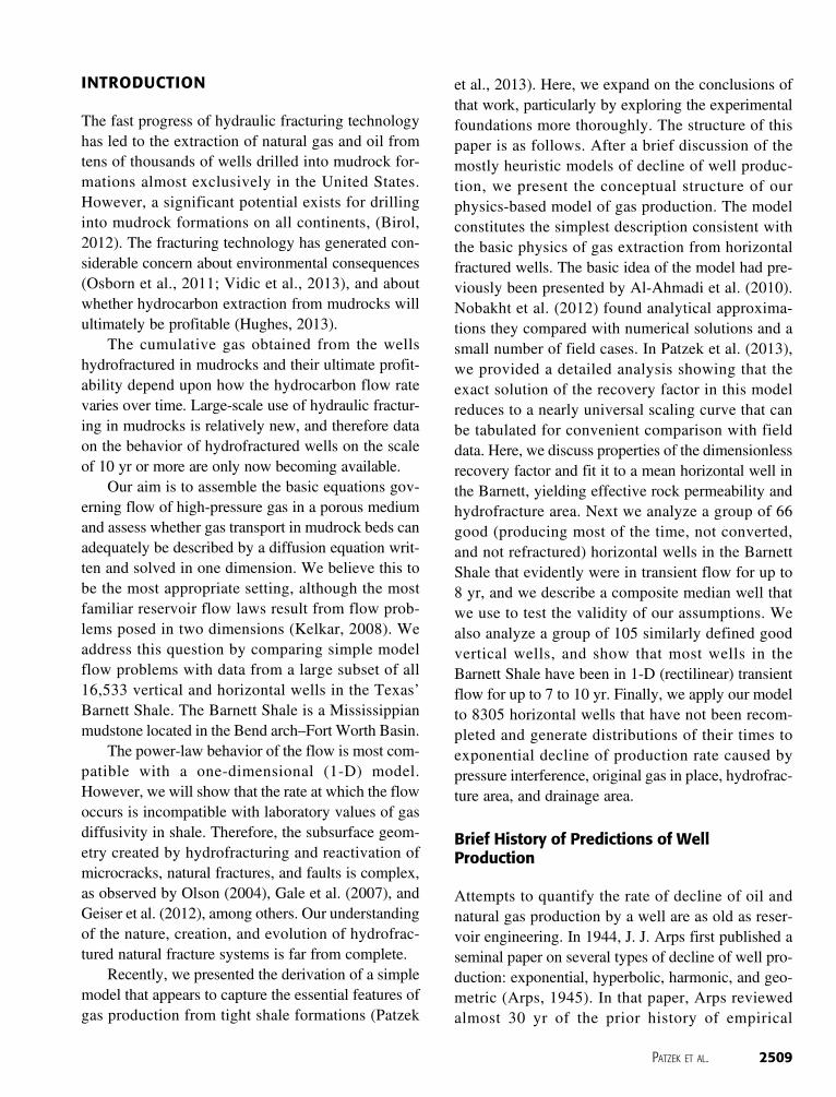
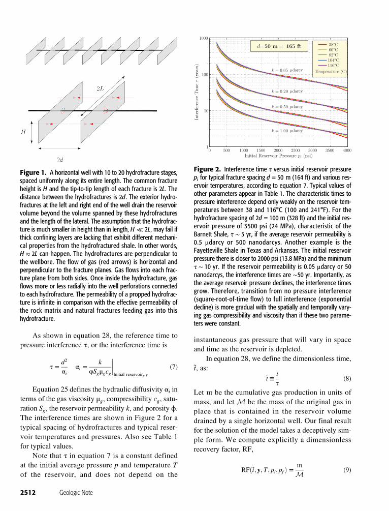
Figure 1. A horizontal well with 10 to 20 hydrofracture stages,spaced uniformly along its entire length. The common fractureheight is H and the tip-to-tip length of each fracture is 2L. Thedistance between the hydrofractures is 2d . The exterior hydro-fractures at the left and right end of the well drain the reservoirvolume beyond the volume spanned by these hydrofracturesand the length of the lateral. The assumption that the hydrofrac-ture is much smaller in height than in length, H ≪ 2L, may fail ifthick confining layers are lacking that exhibit different mechani-cal properties from the hydrofractured shale. In other words,H ≈ 2L can happen. The hydrofractures are perpendicular tothe wellbore. The flow of gas (red arrows) is horizontal andperpendicular to the fracture planes. Gas flows into each frac-ture plane from both sides. Once inside the hydrofracture, gasflows more or less radially into the well perforations connectedto each hydrofracture. The permeability of a propped hydrofrac-ture is infinite in comparison with the effective permeability ofthe rock matrix and natural fractures feeding gas into thishydrofracture.

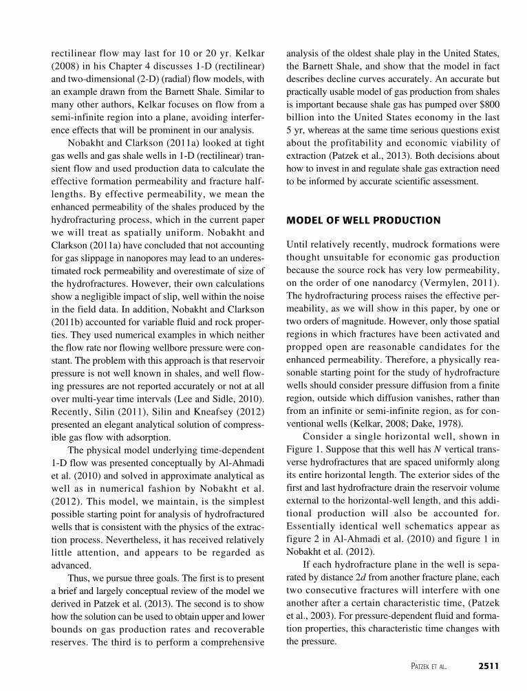
Figure 2. Interference time τ versus initial reservoir pressurepi for typical fracture spacing d = 50 m (164 ft) and various res-ervoir temperatures, according to equation 7. Typical values ofother parameters appear in Table 1. The characteristic times topressure interference depend only weakly on the reservoir tem-peratures between 38 and 116°C (100 and 241°F). For thehydrofracture spacing of 2d = 100 m (328 ft) and the initial res-ervoir pressure of 3500 psi (24 MPa), characteristic of theBarnett Shale, τ ∼ 5 yr, if the average reservoir permeability is0.5 μdarcy or 500 nanodarcys. Another example is theFayetteville Shale in Texas and Arkansas. The initial reservoirpressure there is closer to 2000 psi (13.8 MPa) and the minimumτ ∼ 10 yr. If the reservoir permeability is 0.05 μdarcy or 50nanodarcys, the interference times are ∼50 yr. Importantly, asthe average reservoir pressure declines, the interference timesgrow. Therefore, transition from no pressure interference(square-root-of-time flow) to full interference (exponentialdecline) is more gradual with the spatially and temporally vary-ing gas compressibility and viscosity than if these two parame-ters were constant.

2512 Geologic Note

that depends only on the dimensionless time, themolar composition of gas y, the reservoir temperatureT , the initial reservoir pressure pi, and the hydrofrac-ture pressure pf .

PROPERTIES OF RF�t; y; T ;pi;pf �

Our model of single-phase fluid (e.g., gas) productionfrom hydrofractured horizontal (and vertical) wells ispresented and solved exactly in Appendices 1–3.Here, we discuss features of the solution, and itsapplication to production data.

The recovery factor RF can be computed by solv-ing an initial boundary value problem. We illustratethe solution first by scaling it with various characteris-tic values and comparing to a median good horizontalwell in the Barnett Shale, Figure 3. This median well,defined in the next section, will produce 2.5 Bscf ofgas in 30 yr. Because pressure interference amongthe hydrofractures and gas compressibility have beenaccounted for in the model, this prediction is quiterealistic, barring a mechanical failure of the well.

Additional plots in dimensionless form appear inFigures 15 and 16.

The solution to the initial value problem dependsupon gas composition, the initial state of the reservoirðpi; TÞ, and the hydrofracture pressure pf , but is inde-pendent of the details of the well geometry, the diffu-sivity, or the original gas in place.

For practical purposes, we will divide well produc-tion data into two phases that correspond to particularfeatures of the recovery factor scaling curve. We willcall them the square root phase and interference phase.The first phase corresponds to wells sufficiently earlyin their production history so that flow from a reservoircell between two adjacent fractures has not yet begunto produce pressure depletion at the center of the cell.The second phase corresponds to wells for which thepressure depletion process has become visible.

The first phase is named for the fact that fordimensionless times t sufficiently less than 1, therecovery factor takes a particularly simple form:

RFðt; y; T ; pi; pf Þ = κðy; T ; pi; pf Þffiffit

p; for  t ≪ 1

(10)

Figure 3. The dimensionless rate recovery factor RF for themedian composite well in Figures 5–7. A non-unique translationinto a particular well geometry and reservoir parameters can bedone by assuming that the reservoir permeability (k) is0.4 μdarcy, the hydrofractures are 125 m (400 ft) apart, and thehorizontal well is 1220 m (4003 ft) long. The effective one-sidedarea of each hydrofracture is then 7000 m2 (75;350 ft2) and totalone-sided hydrofracture area is 70;000 m2(0.03 mi2). The bestmatch is obtained when the median well is time shifted by sub-tracting 1.5 months from its time in production. It seems that fort ≪ 0.1, real wells fall behind production from ideal wells.

Table 1. Typical Values of Key Parameters Used in theCalculations

Parameter SI units Field units

Rock porosity, ϕ 0.060* 0.060Rock permeability†, k 0.5 × 10−18 m2 0.5

microdarcyGas saturation, Sg 0.75 0.75Initial pressure, pi 24.1 MPa 3500 psiReservoir temperature, T 361 K 190°FGas‡ compressibility, cg;i 3.42 × 10−8 Pa−1 236 microsips

ð10−6 psi−1ÞGas viscosity, μg;i 2.13 × 10−5 Pa s 0.0213 cpGas compressibilityfactor, Zg;i

0.91 0.91

Fracture pressure, pf 3.44 MPa 500 psiFracture height, H 30 m 100 ftTip-to-tip fracturelength, 2L

213 m 700 ft

*In agreement with the average core determined porosity for the Barnett Shale.†The reservoir permeability is at most k = 0.5 μdarcy.‡In comparison with the large compressibility of gas, the compressibility of thepore space and connate water expansion are negligible. For example, the porespace compressibility might be cf = 3−50 microsips (the high-end compressibil-ity would be for an intensively fractured mudrock), water compressibility is cw =3 microsips, and gas compressibility is upwards of 230 microsips. Therefore, thetotal rock compressibility ct = cf + Swccw + Sgcg ≈ Sgcg .

PATZEK ET AL. 2513

Here, κ is a dimensionless constant. In general itdepends on the gas composition and temperature,the limiting reservoir pressures pi and pf and isobtained from detailed solution of equation 29 inAppendix 1. For the conditions of the Barnett Shale,we have used κ = 0.625, and it has a value of about0.6 for all reservoir conditions we have checked.

The second phase begins when depletion becauseof interference from two adjacent fractures causesmeasurable deviation from the square root growthof cumulative recovery. We have settled on the some-what arbitrary criterion that interference is visiblewhen the dimensionless time t reaches a value of0.64. For larger scaled times the growth in recoveryfactor slows, and it eventually reaches a plateauthat describes the maximum recovery possible for thegiven problem parameters. The way this slowing downoccurs depends in detail upon the thermodynamics ofgas expansion, the reservoir permeability, and the ini-tial and final pressures in the reservoir.

To first illustrate the use of equations 9 and 10suppose one has an estimate of the original gas inplace, M. The greatest uncertainty in M is likely

to be the effective area Af of the transverse hydrofrac-tures. After transients of the first few monthsof production have subsided, cumulative productiontakes the formK

ffiffit

p(for details see Appendix 1). Then

Mκffiffiffiffiffiffiffit∕τ

p= K

ffiffit

p(11)

⇒ τ =�MκK

�2

(12)

Thus, to estimate the interference time τ that sets thescale on which well production will begin to declineexponentially, measure K from the first year ofproduction, estimate M from the well geometry, usethe nominal value of κ = 0.625, and τ follows fromequation 12. Here, K is an empirical constant withdimension of gas mass divided by the square root oftime. The first 1–3 months in production should bediscounted.

The practical difficulty we face with gas produc-tion from the hydraulically fractured horizontal wellsis greater than this example indicates. Neither the totalmass of gas that ultimately will be extracted nor thetime scale for interference to begin is known with

6 21 36 51 67

12

28

43

58

Bosque

Clay

Comanche

Cooke

Dallas

Denton

EastlandEllis

Erath

Hamilton

Hill

Hood

Jack

Johnson

Montague

PaloParker

Somervell

Tarrant

Wise

N

Easting, km

Nor

thin

g, k

m

99.0 98.5 98.0 97.5 97.0 96.5

32.0

32.5

33.0

33.5

Latit

ude,

deg

rees

Nor

th

Longitude, degrees WestFigure 4. The Barnett wellscolored by the county inwhich they were drilled. Themap coordinates are degreesnorth and west. North isalong the y axis. Surface welllocations are from IHS Cera.

2514 Geologic Note

any precision. The original mass of gas in place isuncertain mainly because the effective hydrofracturelength 2L, and the number of active hydrofracturesare uncertain. The time to interference is uncertainbecause the hydrofracturing process greatly increasesthe effective permeability k of the rock in the vicinityof the well; laboratory values of k obtained from coresamples are on the order of nanodarcys (Vermylen,2011), whereas accounting for observed well produc-tion requires effective values of k approximately 100times greater. When wells are in the square root phase,τ and M can not be determined independently. Wheninterference begins, both interference time τ and origi-nal gas in placeM can be determined through carefulcomparison of cumulative production data with ourdimensionless recovery factor.

FIELD OBSERVATIONS FROM SELECTEDWELLS

To commence a discussion of field data, we turn to asample of 66 good horizontal wells. This sample com-prises 30 Denton County wells, 10 Johnson Countywells, 12 Tarrant County wells, and 14 Wise County

0 10 20 30 40 50 600

1

2

3

4

5

6

Cum

ulat

ive

prod

uctio

n, 1

09 scf

Horizontal wells in sample

Figure 5. The distribution of cumulative production from asample of 66 horizontal wells in the Barnett Shale, none refrac-tured. These wells had up to 8 yr in production. The continuousline is the composite median well (1.64 Bscf after 7 yr), and thetwo dotted lines are ±1 standard deviation (0.96 Bscf). The sixhighest producing wells with only 6.5 yr in production are out-liers, 2–3 standard deviations above the median.

0 1 2 3 4 5 6 7 80

0.5

1

1.5

2

2.5

3

3.5

4

Years on production

Pro

duct

ion

rate

, 106 s

cf/d

Figure 6. The production rates of gas from the sample inFigure 5, in millions of standard cubic feet per day, versus timein production. The gray area delineates the highest and lowestproduction rates each month. After the initial few months in pro-duction, the median well rate follows the dashed 1∕

ffiffit

pcurve.

Almost all of these 66 wells were in the square-root phase, pro-ducing in pure 1-D transient flow.

0 1 2 3 4 5 6 7 80

1

2

3

4

5

6

Years on production

Cum

ulat

ive

prod

uctio

n, 1

09 scf

Figure 7. The cumulative production of gas the well sample inFigure 5, in billions of standard cubic feet, versus time in produc-tion. The gray area delineates the highest and lowest cumulativeproduction from the sampled wells. After the initial few monthsin production, the median well production follows the dashedffiffit

pcurve. To catch up early with the square-root-of-time curve,

0.15 Bscf is added to the median well’s production after onemonth.

PATZEK ET AL. 2515

wells. Therefore, the sample consists of wells from thebest or core area of the Barnett Shale shown in Figure 4and characterized in Figure 5: Three 2003 wells, 182004 wells, and 45 2005 wells; thus, the sample wellshave up to 8 yr in production. No refracturing or pres-sure interference occurred in any of the wells. The pro-duction rates from the 66 wells are shown in Figure 6and their cumulative production in Figure 7.

Almost all Barnett wells are in the square rootphase, not just the median composite well. Themedian and mean of well production are close, butthe median curves are less noisy. We use the medianwell only for clarity, to fix ideas and to avoid gettingdistracted by excessive detail.

Suppose that the typical initial reservoir pressurein the Barnett is 3500 psi (24 MPa) and the horizontal

wells have 12 hydrofractures on the average, spacedevery 360 ft (110 m). By consulting Figures 2–7,one may conclude that the effective formationpermeability is no higher than 0.5 μd, or 500 nano-darcys, and the median well in the core area of theBarnett play is expected to produce 1.64 ± 0.96Bscf after about 7 yr in production. It also appearsthat the initial production in the sample wells issignificantly lower than the square-root-of time curve,because it is choked and/or water left after hydrofrac-turing fills the lower parts of all hydrofractures andimpedes production until this water is produced and/or evaporated by gas. This low performance relativeto an equivalent ideal gas well amounts to a productiondecrease of up to 50–150 million standard cubic feet ofgas over the first 1–3 months in production.

0 1 2 3 4 5 6 7 8 9 10 150

0.5

1

1.5

2

2.5

Years on production

Cum

ulat

ive

gas

prod

uced

, Bsc

f

Figure 8. Cumulative gas production versus time in production. Note that the x axis is nonlinear, because it is scaled in units of thesquare root of time in production. This well sample consists of 105 vertical wells; a few were converted and/or refractured, as indicatedby the abrupt changes of slope that can be treated through superposition. In these coordinates, most wells plot as straight lines for up to10 yr in production, indicating little or no interference among the vertically-spaced hydrofractures that are also vertical. Thus, one maysafely assume that almost no interference occurs among the formation layers and individual wells. The median well is plotted as thethick black line. Notice the initial production lag.

2516 Geologic Note

Well-by-Well Check of Model Quality

The production from vertical and horizontal wellsshown in Figures 8 and 9 follows 1-D transient flow.Flow superposition (breaks in the line slope) existsfor several vertical wells, as well as a hint of interfer-ence after up to 10 yr in production. The horizontalwells are mainly perfect examples of the square rootphase, except for a small subset showing evidenceof interference. Therefore, if the time in productionincreases four-fold, the cumulative gas production Qshould increase two-fold. Note that this predictiondoes not depend on any model parameters, butonly on the validity of the assumption of 1-Dtransient flow:

Qð24 monthsÞQð96 monthsÞ =

12

(13)

The results of this test are displayed in Figures 10and 11. The bottom line is that our model representsthe field quite well. The mean values of the cumula-tive production ratios are 0.45 and 0.43, respectively,for the sample of vertical and horizontal wells. Thesmall but curious downward bias of the horizontalwell data may be caused by several factors: The firstmonth in production is on average 15 days. In addi-tion, for the first 1–3 months, well production lags,is erratic, and it stabilizes only gradually. Patzek(1992) had to omit the first three months in produc-tion for the diatomite wells because they were pro-ducing the hydrofracture proppant and reservoirrock, and had to be cleaned. It appears that water leftbehind after hydrofracturing blocks lower parts of thehydrofractures and limits initial gas production untilthis water is produced and/or evaporated in situ.This is a real problem in all wells, because—as we

0 1 2 3 4 5 6 7 8 90

0.5

1

1.5

2

2.5

3

3.5

4

4.5

5

Years on production

Cum

ulat

ive

gas

prod

uced

, Bsc

f

Figure 9. Cumulative gas production versus the square root of time in production. This well sample consists of 66 horizontal wellsdescribed in Figure 5. In these coordinates, most wells plot as straight lines for up to 8 yr in production, indicating no interference amongadjacent vertical hydrofractures and among wells. One may conclude that the effective formation permeability is close to 0.5 μd, giventhe geometrical constraints on the hydrofracture size and actual production volumes of 1 to 5 bcf. Several of the top seven outlier wellsin Figure 5 have short interference times, caused perhaps by the closely-spaced hydrofractures and/or the effective rock permeabilityabove 1 μd. The median well is plotted as the thick black line. Notice the initial production lag.

PATZEK ET AL. 2517

show in (Patzek et al., 2013)—the emergence of thesquare-root phase is universal, and the downwarddeviations from this regime stem from the problemswith starting field wells properly.

Another interesting comparison is with thedeclines of most Barnett Shale wells grouped byValko and Lee (2010). In their Figure 4, these authorsshow the ratios of cumulative gas production after 2and 1 yr, 3 and 1 yr, respectively, for what they termmonth-groups of all vertical and all horizontal wells.Their ratios are stable, but not quite

ffiffiffi2

p= 1.41 andffiffiffi

3p

= 1.73 as required by our model. However, ifone discounts the first 3.5 months of production fromall wells, by putting

x =3.512

R2∕1 =

ffiffiffiffiffiffiffiffiffiffiffiffiffiffiffiffiffiffi�2 − x1 − x

�s= 1.55

R3∕1 =

ffiffiffiffiffiffiffiffiffiffiffiffiffiffiffiffiffiffi�3 − x1 − x

�s= 1.96

(14)

one recovers table 2 in Valko and Lee (2010). Here,R2∕1 and R3∕1 are the ratios of cumulative gas produc-tion after 2 and 3 yr, respectively, relative to that after1 yr. The same procedure can be applied to the wellsshown in Figures 10 and 11, and the model-predictedratio is 0.47.

FIELD OBSERVATIONS FROM COMPLETEBARNETT FIELD

We now set out to answer the following question:Can one extract enough information from existingnoisy field production data to estimate both the inter-ference time τ and the original gas in place M at thesame time? In the early stages of gas production,when t ≪ τ, the production rate declines purely as1∕

ffiffit

pand this cannot be done. Wells delivering a

small ultimate amount of gas at a relatively high ratecannot be distinguished from those in which lowerpermeability rock or a small number of hydrofrac-tures delivers ultimately larger quantities of gas at arelatively lower rate. Only the onset of interferencebetween adjacent hydrofractures makes it possible todisentangle the two scenarios.

We obtained data for 16,533 wells in the BarnettShale, and from them selected the 8807 horizontalwells that had operated continuously for 18 monthsor more, and had not been recompleted (the hydro-fracturing process was not repeated to increase pro-duction). We plot all these wells in Figure 12. Note

0 10 20 30 40 50 600

0.1

0.2

0.3

0.4

0.5

0.6

0.7

0.8

0.9

1

Wells sorted on cum production

Rat

io o

f cum

gas

afte

r 24

and

96

mon

ths

Production starts at t=0Production starts at t=3.5 months

Figure 11. A test of our model for a group of 66 horizontalwells with long production history and no refracturing to avoidconfusion. Each well is represented by a circle the area for whichis proportional to the cumulative gas production at 96 months.Note that production ratios are somewhat biased toward 0.4for most wells. This means that the long-term production issomewhat larger than the prediction of our model, or that a biasexists in the reporting of monthly production increments (socalled well allocation factors), or that the initial couple of monthsin production should be discounted.

0 20 40 60 80 1000

0.1

0.2

0.3

0.4

0.5

0.6

0.7

0.8

0.9

1

Wells sorted on cum production

Rat

io o

f cum

gas

afte

r 24

and

96

mon

ths

Production starts at t=0Production starts at t=3.5 months

Figure 10. A test of our model for a group of 105 vertical wellswith long production history. Each well is represented by a circlethe area of which is proportional to the cumulative gas produc-tion at 96 months. The low-performing vertical wells were some-times converted to horizontal wells and/or refractured, causingan increase of production and lowering the ratios plotted here.

2518 Geologic Note

the excellent agreement overall. As shown in Patzeket al. (2013) the wells in this plot fall into two basicgroups. Interference is sufficiently advanced in 2133wells that it can be detected with an average param-eter uncertainty of less than 20%. These wells havebegun to interfere. The remaining 6172 wells forwhich interference is not yet visible are still growingsimply as the square root of time.

Figure 13 provides four additional pieces ofinformation for all the wells. In the upper left panelwe provide a lower bound on the interference timeτ. This lower bound is obtained by noting that inter-ference becomes evident when t reaches 0.64, so ifinterference is not evident, the interference time τmust be at least 1.6 times larger than the current lifeof the well. From this estimate one obtains a lowerbound on the gas in place for each well, becauseequation 12 and the known value of K for each wellturns a lower bound on τ into a lower bound on M(upper right). The lower right panel displays an upper

Figure 12. Comparison of 8305 wells with scaling function.Data come from the Barnett Shale, scaled so as to fit ourscaling function (initial reservoir pressure of 3500 psi[24 MPa], hydrofracture pressure of 500 psi [3.4 MPa]).Burnt orange curves give scaled production of each well,and the black curve is the scaling function. Overall agreementis satisfactory.

Figure 13. Bounds on the interference time τ and the original mass of gas in place M for the wells from Figure 12.

PATZEK ET AL. 2519

bound on the original gas in place M obtained byusing the measured thickness of the mudstone sourcerock of each well, and the length of the well. From theupper bound on M one obtains through equation 12an upper bound on τ, shown in the lower left. Thisbound on τ is not very tight. A peak occurs at around30 yr, but a long tail stretches into the hundreds ofyears. We think it is impossible that wells will lastthis long before beginning to interfere, but they aresimply too young to provide evidence that interfer-ence will occur any sooner.

Finally, in Figure 14 we display informationabout each of the 2133 wells for which interferencecan be detected with some certainty. However, ratherthan directly reporting the original gas in place Mand the interference time τ, as done in Patzek et al.(2013), we rescale the presentation of the interferencetime τ using equation 7 to calculate the effectivespacing d between fracture planes. To do this we needthe value of αi, and for the purposes of this computa-tion we assume αi = 3 × 10−8 m2∕s, which corre-sponds to a permeability k of one nanodarcy andporosity of around 6%. The characteristic spacingcomes out to be around 2 m (6.6 ft); this is 10 timessmaller than the separation between fracture stages,but is on the order of spacing between natural

fractures. Equivalently, one could view the wells ascontaining fracture stages spaced by 20 m (65.6 ft),but with effective permeability 100 times larger, onthe order of 100 nanodarcys.

DISCUSSION

1. A simple universal model of pressure diffusionbetween absorbing boundaries provides surpris-ingly good agreement with all wells that can rea-sonably be analyzed in the Barnett Shale and inother shales, for example, Male et al. (2014). Thesimplicity of the model is particularly surprisingbecause the hydrofracturing process should beexpected to produce a complex fracture networkwith structure on many scales, as described forexample by Marrett (1996). Nevertheless, theexisting data are fit rather well by treating wellsas being in contact with a medium with uniformtransport properties.

2. Although we have not yet published the results ofmost of our calculations, we have checked themodel on thousands of wells in the MississippianFayetteville located in the Arkoma basin ofArkansas, the Jurassic Haynesville located in theTexas–Louisiana Salt Basin, and the MiddleDevonian Marcellus located in the Appalachian

Figure 14. Values of effectivefracture spacing d and gas inplace M for the 2133 for whichproduction bends over enoughto display interference. Errorbars indicate two standarduncertainties. To compute thespacing d , a nominal value ofα = 3 × 10−8 m2∕s is adopted.Note that the characteristicspacing comes out to be around2 m (6.6 ft). This spacing is muchsmaller than the separationbetween fracture stages, but iscomparable to spacing betweennatural fractures.

2520 Geologic Note

Basin. In all cases we were able to arrive at univer-sal scalings of all wells in given play; for theHaynesville shale, see Male et al. (2014).

3. Inserting characteristic values into equations 71

and 72, one deduces rock permeability k of 50nanodarcys for τ of 50 yr and 500 nanodarcysfor τ of 5 yr. These values of permeability are20–200 times larger than the characteristic valueof one nanodarcy found for shale core samples inlaboratory experiments. This enhanced permeabil-ity must result from the hydrofracturing process,which makes it all the more unexpected that asimple model accounts well for gas transport.The degree to which permeability on the length-scale of wells increases over permeability ofcentimeter-scale laboratory samples is identical tothe general pattern of permeability increase foundin large-scale versus small-scale studies of geologi-cal formations (Clauser, 1992). However, what weare describing is a man-made rather than purelynatural phenomenon; otherwise, the tens of billionsof dollars spent to inject water and proppant intohorizontal wells in shale would not be needed.

4. We provide upper and lower bounds on time tointerference and original gas in place for all thewells. The median lower bound on time to interfer-ence is 5 yr and the median upper bound is 100 yr.The bounds on gas in place are somewhat tighter;the lower bound for mean well is 1 Bscf, and theupper bound is 7 Bscf.

5. Given the available data, one cannot provide betterbounds on gas production, even in the BarnettShale with the longest history of production.Pessimists (Hughes, 2013) see only the lowerbounds, whereas optimists (Potential GasCommittee, 2013) look beyond the upper bounds.A rigorous economic analysis of the Barnett play,based on the model presented here, has been pub-lished elsewhere (Browning et al., 2013a, b, c;Gülen et al., 2013; Ikonnikova et al., 2013).

CONCLUSIONS

We have shown that for mostly single-phase gasflow in the Barnett Shale, the classical modelsof transient flow in hydrofractured wells (see, e.g.,Patzek, 1992), apply, at least during early production.Given the mystique surrounding gas (and oil) produc-tion from mudrock systems, this finding was

somewhat of a surprise. And then there were moresurprises. The main conclusions of this paper are asfollows.

1. We have formulated a complete 1-D modelof flow of natural gas that can sorb on therock. The result is a dimensionless, nonlinear dif-fusion equation of gas pseudopressure. We solvethis equation numerically using a fast implicitsolver. Our model can be applied to verticalwells, but here we are mostly interested in hori-zontal wells.

2. Cumulative gas production follows a nearly uni-versal function scaled by two parameters, inter-ference time τ and mass of gas in place M.For over 8000 wells in the Barnett Shale,selected simply because they were horizontalwells that had not been recompleted and hadover 18 months of production, agreement withthe scaling function is excellent.

3. We have shown that early (but not too early) inthe flow, this nonlinear pseudopressure equationleads to a square-root phase, during which gasproduction rate must decline as 1∕

ffiffit

pand cumu-

lative production must increase asffiffit

p.

4. Within the first 1–3 months from starting a fieldwell, gas production is substantially hamperedrelative to an equivalent ideal horizontalwell. The lower gas production in the fieldis most likely caused by fracturing water leftin the hydrofractures and blocking gas flow.We make slight adjustments (time-shifts, forexample) of field production to account for thisphenomenon.

5. When our dimensionless time, measured in unitsof 1/2 of the distance between hydrofracturessquared divided by the initial hydraulic diffusiv-ity of gas, approaches 0.64, gas flow starts todeviate measurably from the square-root phase,and enters the interference phase. As the dimen-sionless time passes 1, gas production rate beginsexponential decline. These production regimesare universal; all gas wells in the Barnett Shalethat were not recompleted in fact appear to fol-low them.

6. We have tested this model on over 8807 horizon-tal wells in the Barnett Shale with at least 18months of production. We found 2133 wells thathad entered the interference phase, and whereproduction had started to decline exponentially

PATZEK ET AL. 2521

in less than 10 yr. The remaining 6172 horizontalwells were in the square root phase.

7. In horizontal wells in the Barnett Shale gas flowsinto transverse vertical hydrofractures thatappear as parallel planes, but are likely complexsystems of multiscale, nested flow paths that in-fluence a non-negligible volume of reservoirrock around the fracture planes. This complexitymanifests itself as an apparent formation per-meability that is 1–2 orders of magnitude higherthan lab-measured shale permeabilities. Basedon our model, we can place both upper and lowerbounds on the effective permeability. Lowerbounds on τ imply upper bounds on the per-meability k, whereas upper bounds on τ implylower bounds on the permeability. Using the typ-ical values of Table 1, we find that τ of 5 yr cor-responds to k of 500 nanodarcys, 100 yrcorresponds to 25 nanodarcys, and 500 yr corre-sponds to 5 nanodarcys. Thus inspection ofFigure 13 shows that permeabilities are typicallybounded between 25 and 500 nanodarcys.

8. In vertical wells in the Barnett Shale, eachstacked vertical hydrofracture drains its ownreservoir interval and acts almost independentlyof other hydrofractures for 10 to 12 yr inproduction.

9. Our universal dimensionless solution istranslated into production of a compositemedian horizontal well in the core area of theBarnett. The best match of field data isachieved if this well is assumed to be 1220 m(4003 ft) long and nominally it has 10 hydro-fractures spaced every 125 m (410 ft). It isestablished that the rock permeability is closeto 400 nanodarcys, and that each fracture hasan effective one-sided area of 7000 squaremeters (75; 350 ft2). Thus, a typical total two-sided area of hydrofractures in a Barnett wellis 0.14 km2ð0.05 mi2Þ.

10. It appears that gas sorption is negligible in thecore area of the Barnett Shale (Browning et al.,2013b, c). However, our still unpublished mod-eling shows that gas desorption is important inother U.S. shale plays, for example, in theFayetteville and Woodford Shales, as discussedin Appendix 2.

11. The core-measured values of shale permeabilityat the length scale of millimeters cannotdescribe gas flow at the scale of tens or hundreds

of meters. At the latter scale, natural and inducedfracture systems dominate the flow. Becausebasic reservoir characterization of the BarnettShale depends mostly on core analysis(Montgomery et al., 2005), this flow wouldbe missed by the laboratory experimentsand the permeability would routinely beunderestimated.

12. Pressure interference explains the accelerateddecline of gas production at later times. Therefore,with the model we have studied, no need arises foran arbitrary switch from one type of empiricalextrapolation of production to another.

APPENDIX 1: ONE-DIMENSIONALTRANSIENT FLOW OF REAL GAS

Model Formulation

To arrive at the pressure diffusion equation, we assumethat only gas is flowing, and we perform the mass balance forthe gas:

The rate of flowof mass IN

across the boundary−

The rate of flowof mass OUT

across the boundary

=The rate of mass

ACCUMULATIONinside the boundary

(15)

The gas flows across the system boundary, that is, perpendicu-larly to a sufficiently smooth mathematical surface that separatesthe system from its surroundings. For this surface, let us choosea box with two walls of unit width and height (i.e., of unit flowarea), perpendicular to the flow in the x direction. These wallsare separated by Δx. Then, in the limit of Δx → 0, we obtain

−∂ðρgugÞ

∂x=∂½ðφSgρg + ð1 − φÞρa�

∂tkg gasm3s

(16)

wherein which ug is the Darcy (superficial) velocity of gas, Sg =1 − Swc is gas saturation (Swc being the connate water saturation),ρg is the free gas density, ρa is the adsorbed gas density(kg gas∕m3 solid), and ϕ is the rock porosity.

By applying Darcy’s law to the 1-D horizontal flow of gas,we can substitute

ug = −kμg

∂p∂x

(17)

in which p is the gas pressure, and obtain the following nonlinearpartial differential equation:

∂∂x

�kρgμg

∂p∂x

�≈ φSg

∂ρg∂p

∂p∂t

+ ð1 − φÞ ∂ρa∂ρg

∂ρg∂p

∂p∂t (18)

2522 Geologic Note

The absolute permeability of the rock is k, and μg is the viscosityof gas, and we have neglected the pore space compressibility:

cf =1φ

�∂φ∂p

�T=const

≈ 0 (19)

The gas density is related to its pressure and temperature throughan equation of state for real gases:

ρg =MgpZgRT

(20)

in which Zgðp;TÞ is the compressibility factor of gas, Mg is thepseudo molecular mass of gas, R = 8314.462, J/kmol-K is theuniversal gas constant, and T is a constant temperature ofthe reservoir.

The isothermal compressibility of gas is defined as:

cg =1ρg

�∂ρg∂p

�T=const

=1p−

1Zg

∂Zg

∂p(21)

We define Kaðp;TÞ as the differential equilibrium partitioningcoefficient of gas at constant temperature; see, for example, Cuiet al. (2009):

Ka =�∂ρa∂ρg

�T=const

(22)

By inserting equations 21 and 22 into equation 18, the generalnonlinear equation of transient, 1-D horizontal flow of gas isobtained:

∂∂x

�kρgμg

∂p∂x

�= ½φSg + ð1 − φÞKa�cpρg

∂p∂t

(23)

Note that only if

φSg is not much greater than ð1 − φÞKa (24)

desorption matters. For the Barnett Shale at or above 100 psi(0.7 MPa), this gas adsorption term is an order of magnitudesmaller than ϕSg, and gas adsorption can be neglected, seeAppendix 2.

Notice that the hydraulic diffusivity of a gas α stronglydepends on the gas pressure, because the gas viscosity μgðpÞ canvary three-fold and the gas compressibility cg ≈ 1∕p:

10−3

10−2

10−1

100

10−2

10−1

100

101

Numerical solutionMedian well

Figure 15. The dimensionless pseudopressure gradient,∂m∕∂x at the hydrofracture versus dimensionless time t. Thefracture pressure pf is 500 psi (3.4 MPa), and the initial reservoirpressure pi is 3500 psi (24 MPa). The scaled gas production fromthe composite median well in Figures 3 to 7 is superimposed onthe numerical solution. Notice that at very early times the actualproduction rate lags behind the theoretical one, because the left-behind hydrofracturing water blocks gas flow.

0 0.5 1 1.5 20

0.1

0.2

0.3

0.4

0.5

0.6

0.7

0.8

Dim

ensi

onle

ss R

ecov

ery

Fac

tor

Numerical solutionMedian well

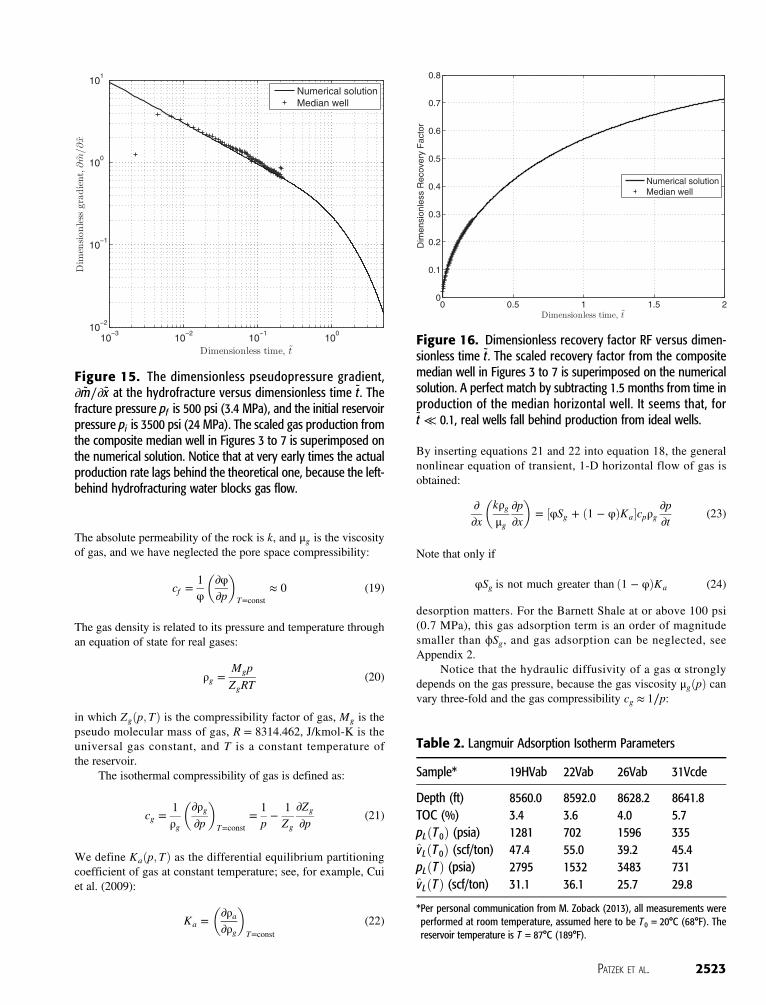
Figure 16. Dimensionless recovery factor RF versus dimen-sionless time t. The scaled recovery factor from the compositemedian well in Figures 3 to 7 is superimposed on the numericalsolution. A perfect match by subtracting 1.5 months from time inproduction of the median horizontal well. It seems that, fort ≪ 0.1, real wells fall behind production from ideal wells.

Table 2. Langmuir Adsorption Isotherm Parameters

Sample* 19HVab 22Vab 26Vab 31Vcde

Depth (ft) 8560.0 8592.0 8628.2 8641.8TOC (%) 3.4 3.6 4.0 5.7pLðT 0Þ (psia) 1281 702 1596 335vLðT 0Þ (scf/ton) 47.4 55.0 39.2 45.4pLðTÞ (psia) 2795 1532 3483 731vLðTÞ (scf/ton) 31.1 36.1 25.7 29.8

*Per personal communication from M. Zoback (2013), all measurements wereperformed at room temperature, assumed here to be T 0 = 20°C (68°F). Thereservoir temperature is T = 87°C (189°F).

PATZEK ET AL. 2523

αðpÞ = kφSgμgcg

(25)

In addition, both the rock porosity ϕ and the permeability k arefunctions of effective stress. In particular, the rock matrix per-meability may decrease by an order of magnitude when the porepressure is depleted (Vermylen, 2011). An example of typicalvariability of α is given in Appendix 3.

This nonlinear differential equation 23 is now be simplifiedby introducing the Kirchhoff integral transform of gas pressureafter Al-Hussainy et al. (1966), which in the present context isalso called the real gas pseudopressure:

mðpÞ = 2Z

p

p�

pdpμgZg

(26)

Here, p� is a reference pressure that will be set to a constant pres-sure in the hydrofractures. Appendix 3 contains the relevantphysical properties of natural gas and the calculation of thepseudopressure.

Next, to find the gas flowing into a fracture plane we replacethe pressure with the real gas pseudopressure in equation 26:

_m = 2HLk2Mg

RT∂m∂x

����0

(27)

A detailed solution of these equations is reported in Patzeket al. (2013) and its supplementary materials. Our primaryfinding is that the solutions take on universal (or nearly universal)

form once we define dimensionless time, distance, and pseudo-pressure by

t = t∕τ; τ =d2

αix = x∕d m =

12ð½cgp�μgZg∕p2Þimðx; tÞ

(28)

Here, the subscript i refers to the quantities at the initial reservoirpressure pi and temperature T . As shown in Figure 26, the factorðcgpÞi is close to unity.

The net result is the following dimensionless boundary-value problem: Consider the 1-D flow of gas into a transverse pla-nar hydrofracture of height H, length 2L, and separated by

0 500 1000 1500 2000 2500 3000 35000

5

10

15

20

25

30

35

40

45

50

19HVab

22Vab

26Vab

31Vcde

Pressure, psia

Ads

orbe

d na

tura

l gas

, scf

/ton

Figure 17. Langmuir adsorption isotherms with the parametersfrom Table 2. All data in this table were acquired at room temper-ature. Gas desorption increases nonlinearly as pressure decreases.The vertical line corresponds to the minimum hydrofracture pres-sure of 500 psia (3.4 MPa). As pressure decreases to respectiveLangmuir pressures (denoted by the vertical lines emanating fromeach isotherm), 50% of the maximum gas each sample couldadsorb will have been desorbed. Note that at 500 psia (3.4 MPa),roughly 50% of the maximum adsorbed gas will have desorbedin samples 31Vcde and 22Vab. For the remaining two samples, thispercent will have been higher, up to 80% for 26Vab.

0 500 1000 1500 2000 2500 3000 35000

5

10

15

20

25

30

35

40

45

50

19HVab

22Vab

26Vab

31Vcde

Pressure, psia

Ads

orbe

d na

tura

l gas

, scf

/ton

Figure 18. Langmuir adsorption isotherms with the parame-ters from Table 2 translated to the reservoir temperature of87°C (189°F). The correlations published in Lewis et al. (2004)were corrected and used. Note that at an elevated temperatureless gas adsorbs, but the Langmuir pressures become morefavorable.

0 500 1000 1500 2000 2500 3000 35000

0.005

0.01

0.015

0.02

0.025

0.03

0.035

0.04

0.045

0.05

Pressure, psia

(1−

φ)K

a

19HVab22Vab26Vab31Vcde

Figure 19. The differential gas adsorption for Langmuiradsorption isotherm at the reservoir temperature of 87°C(189°F). Note that ð1 − ϕÞKa ≪ ϕSg and gas adsorption doesnot matter for the Barnett Shale.

2524 Geologic Note

distance 2d from the next hydrofracture planes, as depicted inFigure 1. The scaled transport equation is

∂m∂t

=ααi∂2m∂x2

; mðx; t = 0Þ = miðxÞ mðx; tÞ = 0 for

x = 0 and ∂m∕∂x = 0 for x = 1 (29)

APPENDIX 2: SORPTION OF NATURAL GAS

Natural gas, which is 80–90% methane, adsorbs only on the surfa-ces of pores in kerogen filaments in a mudrock, and is in thermo-dynamic equilibrium with free gas in the pores. Langmuir (1918)developed a sorption isotherm to describe this type of equilibriumat a specific temperature:

va =vLp

p + pL

standard  cm3

g of bulk rock(30)

Here, va is the specific sorbed gas volume at stock tank conditions(ST) of 1 atm (0.1 MPa or 14.7 psi) at TST = 288.7 K (60°F or15.5°C); p is the pressure of free gas; vL is the specific volumeof sorbed gas at infinite pressure, or the Langmuir volume, alsoat standard conditions; pL is the pressure at which 1/2 of the maxi-mum sorbed gas is still adsorbed, or the Langmuir pressure.

The field units of specific sorbed-gas volume are standardcubic feet per short ton (scf/ton), and the conversion factor is

1scf

ton of bulk rock=

132

standard cm3

g of bulk rock(31)

0 500 1000 1500 2000 2500 30000

0.01

0.02

0.03

0.04

0.05

0.06

0.07

0.08

0.09

0.1

Pressure, psia

(1−

φ)K

a

N 1−16P 1−05HGBP 1−21L 1−14PH

Figure 20. In the cooler and shallower reservoirs with moreadsorbed gas, as is the case in the Fayetteville Shale, gas desorp-tion is more significant. As an example, the Langmuir volumesmeasured by Vermylen (2011) for the Barnett Shale sampleswere increased by 50%. For the GBP 1-21 sample, we assumedvLðT 0Þ = 86 scf∕ton and pLðT 0Þ = 718 psia (5.0 MPa), so thattheir values at the reservoir temperature would be 66 scf/tonand 800 psia (5.5 MPa), respectively, in agreement with table 1in Boulis et al. (2013). All other reservoir parameters were fromthe Fayetteville core measurements by Southwestern Energy,and the core temperatures were estimated from the geothermalgradient.

Figure 21. Gas-swollen Woodford cuttings bags: doubled plastic bags inside cloth bags. This is how the volume of gas evolved fromthe core can be measured. Image source: Breig (2010).

PATZEK ET AL. 2525

Core analysis is required to generate a Langmuir isotherm.However, generally only one Langmuir isotherm is necessary toadequately describe a gas shale within a field or subbasin. TheLangmuir volumes and pressures were measured by Vermylen(2011) on four Barnett core samples; see Table 2. The room tem-perature isotherms are plotted in Figure 17 and the elevated reser-voir temperature ones in Figure 18.

The adsorbed gas density at the reservoir temperature is

ρa = vaðp;TÞρgðpST ; TSTÞρb (32)

in which ρgðpST ;TSTÞ = 7.4 × 10−4 g∕cc (4.3 × 10−4 oz∕in:3) isthe stock tank gas density and ρb = 2.5 g∕cc (1.4 oz∕in:3) is themudrock bulk density (Vermylen, 2011). Consequently,

Ka =∂ρa∂ρg

= ρgðpST ;TSTÞρb∂vaðp; TÞ

∂p∂p∂ρg

=ρgðpST ;TSTÞρb

cgρgvLðTÞpLðTÞðpLðTÞ + pÞ2

(33)

From Figure 19 it is clear that for the reservoir pressures encoun-tered during gas production in the Barnett Shale, the termð1 − ϕÞKa is an order of magnitude smaller than ϕSg, and gasadsorption can be neglected. Note that in coal seams adsorbedmethane may be as high as 200–400 scf/ton (Dallegge andBarker, 2013).

Because our theory is universal, it applies to all gas shales,some of which may be strongly sorbing gas. In shallower and

cooler reservoirs with more adsorbed methane, gas desorptionmay be more important, see Figure 20. For example, assumingthat the Woodford and Fayetteville shales are similar, one canestimate the in situ gas content in the latter from the drilling cut-tings in the former, shown in Figure 21. The shape of Langmuirisotherm in Figure 22 is approximate, as pL is unknown, and vLis approximated with the total evolved-gas volume. With theseassumptions, gas desorption is important in the Woodford shaleand—by implication—the Fayetteville shale, as can be seen fromFigure 23.

APPENDIX 3: NATURAL GAS PROPERTIES

The composition of a sample of natural gas representative of thecore area in the Barnett Shale (compare Hill et al., 2007) is listedin Table 3. The measured gas viscosities and densities at 190°F(88°C), close to a typical reservoir temperature in the BarnettShale, are listed in Gonzalez et al. (1970), table III-9. To calculate

0 500 1000 1500 2000 2500 3000 3500 40000

20

40

60

80

100

120

8132 ft

8163 ft

Pressure, psia

Ads

orbe

d na

tura

l gas

, scf

/ton

Figure 22. Another example of the hypothetical gas adsorp-tion isotherms consistent with the drill cutting data published inBreig (2010). These drill cuttings, shown in Figure 21, wereacquired from the depth of roughly 2480 m (8136 ft). The calcu-lated reservoir pressure and temperature are 26.5 MPa (3850psia) and 80°C (176°F), respectively. Because the captured gasevolved from the cuttings, this gas volume is assumed adsorbedat reservoir conditions. Note that the amount of gas adsorbedin the Woodford shale is 3–4 times higher than that in theBarnett Shale, shown in Figure 18. Again, the adsorption iso-therm parameters were chosen to agree with table 1 in (Bouliset al., 2013).

0 500 1000 1500 2000 2500 3000 3500 40000

0.02

0.04

0.06

0.08

0.1

0.12

0.14

0.16

0.18

Pressure, psia

(1−

φ)K

a

8132 ft8163 ft

Figure 23. In the Woodford shale cuttings, the desorbed-gasvolume exceeds the free-gas volume at pressures below1500 psi (10.3 MPa). Data sources: Breig (2010), Boulis et al.(2013).

Table 3. Composition and Critical Properties of a Natural GasSample*

Component Mole % M kg/kmol T c K Pc bar

Methane 91.5 16.043 190.4 46.0Ethane 3.1 30.070 305.4 48.8Propane 1.4 44.094 369.8 42.5n-Butane 0.5 58.124 425.2 38.0iso-Butane 0.7 58.124 408.2 36.5CO2 1.7 44.010 304.1 73.8N2 0.6 28.013 126.2 34.0Pentanes 0.6 2.151 469.7 33.7

*Sample No. 3, page 31 in Gonzalez et al. (1970). The critical properties are fromPoling et al. (2001).

2526 Geologic Note

μgðp; TÞ and ρgðp;TÞ, we use a bilinear lookup table. Therefore, wehave also used table III-8, “Viscosity of Natural Gas Sample No. 3at 100, 130, and 160 deg F.” In addition, we wrote anequation-of-state-based pressure versus temperature (pressure-vol-ume-temperature) package to calculate thermodynamic propertiesof natural gas mixtures of arbitrary composition. This package andthe numerical approach will be discussed in a future paper.

From the measured data, one can calculate the gas compress-ibility factor directly from equation 20:

Zg =pMg

ρgRT(34)

in which Mg = 18.82 kg∕kmol is the pseudo molecular mass ofthe gas, ρg is the measured gas density, and T = 361 K (88°C or190°F) is the reservoir temperature. With the measured gas vis-cosity, μg, and the gas compressibility factor calculated fromequation 1, one can calculate the gas pseudopressure:

mðpÞ = 2Z

p

p�

pdpμgZg

(35)

Here, p� = pf = 500 psi is the anticipated pressure in thehydrofractures.

The result of numerical integration using the cumulativetrapezoid rule is shown in Figure 24.

The numerically integrated equation 35 is well approxi-mated as follows:

mðpÞ = 4590ðp − 500Þ3∕2 psi2

cp(36)

The inverse algebraic transformation,

pðmÞ = 500 + 0.0036  m2∕3psi (37)

is shown in Figure 25.

The experimental gas compressibility factor Zðp;TÞ can beapproximated with a parabola. The isothermal gas compressibil-ity is then obtained by differentiating equation 20:

cgðpÞ =1ρg

∂ρg∂p

=1p−

1Zg

∂Zg

∂p(38)

The result is plotted in Figure 26. If the rock permeability andporosity are held constant and gas adsorption is neglected, thehydraulic diffusivity of gas,

αðpÞ = kφSgμgðpÞcgðpÞ

m2

s(39)

increases with pseudopressure because of the gas viscosity, μðpÞ,and gas compressibility cðpÞ. This variability can be captured bycalculating the product μgðmÞcpðmÞ. The result is shown inFigure 27. The inverse of the product of μgðmÞcpðmÞ in s−1,

0 2 4 6 8 10

x 108

500

1000

1500

2000

2500

3000

3500

4000

Pseudopressure, psi2/cp

Pre

ssur

e, p

si

Numerical integrationFit of p(m)

Figure 25. The gas pressure versus its pseudopressure andthe algebraic fit of pðmÞ in equation 37.

500 1000 1500 2000 2500 3000 3500 40000

1

2

3

4

5

6

7

8

9

10x 10

8

Pressure, psi

Pse

udop

ress

ure,

psi

2 /cp

Numerical integrationFit of m(p)

Figure 24. The pseudopressure of gas mðpÞ, obtained bynumerical integration of equation 2 and the algebraic fit ofmðpÞ in equation 3.

500 1000 1500 2000 2500 3000 3500 4000−500

0

500

1000

1500

2000

2500

Pressure, psi

Gas

com

pres

sibi

lity,

μ s

ips

Figure 26. The gas compressibility in equation 38 versus pres-sure. The compressibility unit is 106∕psi or μ sips.

PATZEK ET AL. 2527

multiplied by 10−11 can be approximated as a function of pseudo-pressure m in Pa/s multiplied by 10−19 as

m 0 = m × 10−19  m  in Pa∕s1

μgðmÞcgðmÞ× 10−11 = a4m 04 + a3m 03 + a2m 02 + a1m 0

+ a0μgcg in s (40)

where a4 = −0.1110, a3 = 1.0528, a2 = −3.4362, a1 = 7.0012,and a0 = 2.6869.

REFERENCES CITED

Al-Ahmadi, H. A., A. M. Almarzooq, and R. A. Wattenbarger,2010, Application of linear flow analysis to shale gas wells:Field cases: SPE Unconventional Gas Conference,Pittsburgh, Pennsylvania, USA, February 23–25, SPEPaper 130370, 10 p.

Al-Hussainy, R., H. J. Ramey, and P. B. Crawford, 1966, Theflow of real gases through porous media: Journal ofPetroleum Technology, American Institute of Mining,Metallurgical and Petroleum Engineers PetroleumTransactions, 237, p. 624–636.

Arps, J. J., 1945, Analysis of decline curves: American Instituteof Mining, Metallurgical and Petroleum EngineersPetroleum Transactions, v. 160, p. 228–247.

Birol, F., 2012, Golden rules for a golden age of gas: Worldenergy outlook special report on unconventional gas:Report, International Energy Agency, accessed October 22,2014, www.worldenergyoutlook.org/media/weowebsite/2012/goldenrules/WEO2012_GoldenRulesReport.pdf.

Boulis, A., R. Jayakumar, and R. Rai, 2013, IPTC 17150:Application of wells spacing optimization workflow in

various shale gas resources: Lessons learned: InternationalPetroleum Technology Conference, Beijing, China, 13 p.

Breig, J., 2010, Gas shale: Adsorbed component assessment,Oklahoma Geological Survey, accessed October 22, 2014,www.ogs.ou.edu/MEETINGS/Presentations/Shales2010/Breig.pdf.

Browning, J., S. Ikonnikova, G. Gülen, and S. W. Tinker, 2013a,SPE 165585: Barnett Shale production outlook: SPEEconomics & Management, v. 5, no. 3, p. 89–104.

Browning, J., S. W. Tinker, S. Ikonnikova, G. Gülen, E. Potter,Q. Fu, S. Horvath, T. W. Patzek, F. Male, W. Fisher, F.Roberts, and K. Medlock III, 2013b, Barnett Shale Model-1: Barnett study determines full-field reserves, productionforecast: Oil & Gas Journal, v. 111, no. 8, p. 62, accessedOctober 22, 2014, www.ogj.com/articles/print/volume-111/issue-8/drilling-production/study-develops-decline-analysis-geologic.html.

Browning, J., S. W. Tinker, S. Ikonnikova, G. Gülen, E. Potter,Q. Fu, S. Horvath, T. W. Patzek, F. Male, W. Fisher, F.Roberts, and K. Medlock III, 2013c, Barnett Shale Model-2(Conclusion): Barnett study determines full-field reserves,production forecast: Oil & Gas Journal, v. 111, no. 9,accessed October 22, 2014, www.beg.utexas.edu/info/docs/OGJ_SFSGAS_pt2.pdf.

Clauser, C., 1992, Permeability of crystalline rocks: EOS, v. 73,no. 233, p. 237–238.

Cui, X., A. M. M. Bustin, and R. M. Bustin, 2009, Measurementsof gas permeability and diffusivity of tight reservoir rocks:Different approaches and their application: Geofluids, v. 9,p. 208–223, doi:10.1111/gfl.2009.9.issue-3.

Dake, L. P., 1978, Fundamantals of reservoir engineering, devel-opments in Petroleum Science: Amsterdam, Elsevier, 8 p.

Dallegge, T. A., and C. E. Barker, 2013, Coal-bed methane gas-in-place resource estimates using sorption isotherms andburial history reconstruction: An example from the FerronSandstone Member of the Marcos Shale, Utah, in Nationalcoal resource assessment: Geologic assessment of coal inthe Colorado Plateau: Arizona, New Mexico, and Utah,U.S. Geological Survey Professional Paper 1625-B: U.S.Geological Survey, accessed October 22, 2014, pubs.usgs.gov/pp/p1625b/.

Fetkovich, M., 1980, Decline curve analysis using type curves:SPE, v. 4629, p. 1065–1077.

Gale, J. F. W., R. M. Reed, and J. Holder, 2007, Natural fracturesin the Barnett Shale and their importance for hydraulic frac-ture treatments: AAPG Bulletin, v. 91, no. 4, p. 603–622,doi:10.1306/11010606061.

Geiser, P., A. Lacazette, and J. Vermilye, 2012, Beyond “dots in abox”: An empirical view of reservoir permeability withtomographic fracture imaging: First Break, v. 30, p. 63–69.

Gonzalez, M., B. E. Eakin, and A. L. Lee, 1970, Monographon API Research Project 65: Viscosity of Natural Gas:New York, American Petroleum Institute, 109 p.

Gringarten, A., and J. R. Henry, 1974, Unsteady-state pressuredistributions created by a well with a single infinite-conductivity vertical fracture: SPE Journal, v. 14, no. 4,p. 347–360.

Gülen, G., J. Browning, S. Ikonnikova, and T. S. W. Well, 2013,Economics across ten tiers in low and high Btu (British

0 0.5 1 1.5 2 2.5 3 3.5 42

4

6

8

10

12

14

Pseudo−pressure, m(p), Pa/s×10−19

(μg c

g)−1 , 1

/s×1

0−11

CalculatedPolynomial approx.

Figure 27. The product ðμgcgÞ−1 versus pseudopressure.Notice that α varies with pressure as this product. Therefore,over the expected range of reservoir pressures α varies almostseven-fold.

2528 Geologic Note

thermal unit) areas, Barnett Shale: Texas, Energy, v. 60,no. 10, p. 302–315, doi:10.1016/j.energy.2013.07.041.

Hill, R. J., D. M. Jarvie, J. Zumberge, M. Henry, and R. M.Pollastro, 2007, Oil and gas geochemistry and petroleumsystems of the Fort Worth Basin: AAPG Bulletin, v. 91,p. 445–473, doi:10.1306/11030606014.

Hughes, J. D., 2013, Energy: A reality check on the shale revolu-tion: Nature, v. 494, p. 307–308.

Ikonnikova, S., J. Browning, S. Horvath, and S. W. Tinker, 2013,Well recovery, drainage area, and future drillwell inventory:Empirical study of the Barnett Shale gas play: SPEReservoir Evaluation: Engineering, in press.

Jones, P. J., 1942, Estimating oil reserves from production-decline rates: Oil & Gas Journal, v. 40, p. 43.

Kelkar, M., 2008, Natural gas production engineering: Tulsa,Oklahoma, PennWell, 571 p.

Langmuir, I., 1918, Adsorption of gases on glass, mica, and plati-num, Journal of the American Chemical Society, v. 40,p. 1361, doi:10.1021/ja02242a004.

Lee, J., and R. Sidle, 2010, Gas-reserves estimation in resourceplays: SPE Economics &Management, v. 2, no. 2, p. 86–91.

Lewis, R., J. Williamson, W. Sawyer, and J. Frantz, 2004,New evaluation techniques for gas shale reservoirs:Schlumberger Reservoir Symposium, accessed November26, 2013, www.sipeshouston.com/presentations/pickens%20shale%20gas.pdf.

Male, F., A. Islam, T. W. Patzek, S. Ikonnikova, J. Browning, andM. P. Marder, 2014, SPE Paper 168993: Analysis of gasproduction from hydraulically fractured wells in theHaynesville Shale using scaling methods: SPEInternational, Resources Conference, The Woodlands,Texas, USA, April 1–3, 9 p.

Marrett, R., 1996, Aggregate properties of fracture populations:Journal of Structural Geology, v. 18, p. 169–178.

Montgomery, S. L., D. M. Jarvie, K. A. Bowker, and R. M.Pollastro, 2005, Mississippian Barnett Shale, Fort Worthbasin, north-central Texas: Gas-shale play with multi-trillion cubic foot potential: AAPG Bulletin, v. 89, no. 2,p. 155–175, doi:10.1306/09170404042.

Nobakht, M., and C. R. Clarkson, 2011a, Reservoirs exhibitinglinear flow: Constant pressure production: North AmericanUnconventional Gas Conference and Exhibition, TheWoodlands, Texas, June 14–16, 2011, SPE 143989, 15 p.

Nobakht, M., and C. R. Clarkson, 2011b, Analysis of productiondata in shale gas reservoirs: Rigorous corrections for fluidand flow properties: SPE Eastern Regional Meeting,Columbus, Ohio, USA, August 17–19, 2011, SPE 149404,19 p.

Nobakht, M., L. Mattar, S. Moghadam, and D. M. Anderson,2012, Simplified forecasting of tight/shale-gas productionin linear flow: Journal of Canadian Petroleum Technology,p. 476–486.

Olson, J. E., 2004, Predicting fracture swarms: The influence ofsubcritical crack growth and the crack-tip process zone onjoint spacing in rock: Geological Society, London, SpecialPublications, v. 231, no. 1, p. 73–88.

Osborn, S. G., A. Vengosh, N. R. Warner, and R. B. Jackson,2011, Methane contamination of drinking water

accompanying gas-well drilling and hydraulic fracturing:Proceedings of the National Academy of Sciences of theUnited States of America, v. 108, p. 8172–8176, doi:10.1073/pnas.1100682108.

Patzek, T. W., 1992, SPE 24040: Surveillance of South Belridgediatomite: Proceedings of the Western Regional SPEMeeting, Bakersfield, CA, accessed October 22, 2014, gaia.pge.utexas.edu/papers/2-SPE24040.pdf.

Patzek, T. W., D. B. Silin, S. M. Benson, and G. I. Barenblatt,2003, Non-vertical diffusion of gases in a horizontal reser-voir: Transport in Porous Media, v. 51, p. 141–156.

Patzek, T., F. Male, and M. Marder, 2013, Gas production in theBarnett Shale obeys a simple scaling theory: Proceedingsof the National Academy of Sciences, v. 110,p. 19,731–19,736, doi:10.1073/pnas.1313380110.

Poling, B. E., J. M. Prausnitz, and J. P. O’Connell, 2001,The properties of gases and liquids, 5th ed.: New York,McGraw-Hill, 768 p.

Potential Gas Committee, 2013, Report of the Potential GasCommittee: accessed December 31, 2012, Press Release,potentialgas.org/download/pgc-press-release-april-2013-slides.pdf.

Prats, M., 1961, Effect of vertical fractures on reservoir behavior:Incompressible fluid case: Society of Petroleum EngineersJournal, v. 1, p. 105–118.

Russell, D. G., and N. E. Truitt, 1964, Transient pressure behaviorin vertically fractured reservoirs: Journal of PetroleumTechnology, v. 16, no. 10, p. 1159–1170, doi:10.2118/967-PA.

Silin, D. B., 2011, Gas Shale: From nanometer observations towell modeling: Canadian Unconventional ResourcesConference, SPE, Alberta, Canada, CSUG/SPE 149489,20 p.

Silin, D. B., and T. J. Kneafsey, 2012, Gas shale: Nanometer-scale observations and well modeling: Journal of CanadianPetroleum Technology, v. 51, p. 475.

Valko, P. P., and J. W. Lee, 2010, A better way to forecast pro-duction from unconventional gas wells: Proceedings of theSPE Annual Technical Conference and Exhibition, Societyof Petroleum Engineers, Florence, Italy, September 19–22,SPE-134231, 16 p.

Vermylen, J. P., 2011, Geomechanical studies of the Barnettshale, Texas, USA: Ph.D. thesis, Stanford University, PaloAlto, California, accessed October 22, 2014, https://pangea.stanford.edu/departments/geophysics/dropbox/SRB/public/docs/theses/SRB_125_MAY11_Vermylen.pdf.

Vidic, R. D., S. L. Brantley, J. M. Vandenbossche, D.Yoxtheimer, and J. D. Abad, 2013, Impact of shale gasdevelopment on regional water quality: Science, v. 340,1235009, doi:10.1126/science.1235009.

Wattenbarger, R. A., and H. J. Ramey, 1969, Well test interpreta-tion of vertically fractured gas wells: Journal of PetroleumTechnology, v. 21, no. 5, p. 625–632, doi:10.2118/2155-PA.

Wattenbarger, R. A., A. H. El-Banbi, M. E. Villegas, and J. B.Maggard, 1998, Production analysis of linear flow into frac-tured tight gas wells, SPE Rocky Mountain Regional/Low-Permeability Reservoirs Symposium, Denver,Colorado, April 5–8, 1998, SPE 39931, 12 p.

PATZEK ET AL. 2529