geologic interpretations of seismic scattering and

Geologic interpretations of seismic scattering and

attenuation for the Cianten Caldera and the

surrounding area

by

Clarion Hadleigh Hess

Submitted to the Department of Earth, Atmospheric, and PlanetarySciences

in partial fulfillment of the requirements for the degree of

Master of Science in Geophysics

at the

MASSACHUSETTS INSTITUTE OF TECHNOLOGY

ARCHNV

Z 0 3201

June 2013

© Massachusetts Institute of Technology 2013. All rights reserved.

Author ................................................Department of Earth, Atmospheric, and Planetary Sciences

May 30, 2013

Certified by... ...... ..................................Professor Alison Malcolm

Atlantic Richfield Career Development Assistant Professor,Department of Earth, Atmospheric, and Planetary Sciences

Thesis Supervisor

Accepted by ...... ......................................Professor Robert D. van der Hilst

Schlumberger Professor of Earth Sciences,Head, Department of Earth, Atmospheric, and Planetary Sciences

Geologic interpretations of seismic scattering and

attenuation for the Cianten Caldera and the surrounding

area

by

Clarion Hadleigh Hess

Submitted to the Department of Earth, Atmospheric, and Planetary Scienceson May 30, 2013, in partial fulfillment of the

requirements for the degree ofMaster of Science in Geophysics

Abstract

The Cianten Caldera in Indonesia is immediately adjacent to the producing portionof the Awibengkok geothermal field. The Cianten Caldera contains rocks similarto those in the Awibengkok field, however, the Cianten Caldera is not capable ofproducing geothermal power on a commercial scale. The Cianten Caldera has beenmicroseismically monitored along with the producing Awibengkok field as injectionsand fracing in that field have occurred. This microseismic data is analyzed with MultiWindow Time Lapse Analysis (MWTLA) to find values for the scattering coefficient,go, and the seismic albedo, B0, of the Cianten Caldera. The scattering coefficientdescribes the amount of seismic energy that is attenuated due to the wave scatteringoff of heterogeneities and the seismic albedo is the ratio of the amount of scatteringto the total amount of attenuation that includes both scattering and intrinsic attenu-ation. This information has been combined with the geology of the Cianten Calderato define the interior features of the Cianten Caldera and which of these features arepreventing the Cianten Caldera from being a productive geothermal energy source.

Thesis Supervisor: Professor Alison MalcolmTitle: Atlantic Richfield Career Development Assistant Professor, Department ofEarth, Atmospheric, and Planetary Sciences

3

Acknowledgments

I would like to thank my advisor, Alison Malcolm, for all of her guidance during this

project and her assistance in revising this thesis. I would also like to thank Gabi Melo

for her help in the selection and quality control of the subset of data that was analyzed.

I would like to thank Chevron for the use of their microseismic data.

5

Contents

1 Introduction 13

1.1 Motivation. . . . . . . . . . . . . . . . . . . . . . . . . . . . . . . . . 13

1.2 Organization . . . . . . . . . . . . . . . . . . . . . . . . . . . . . . . 15

1.3 Geology . . . . . . . . . . . . . . . . . . . . . . . . . . . . . . . . . . 16

1.3.1 Regional Geology . . . . . . . . . . . . . . . . . . . . . . . . . 16

1.3.2 Local Geology . . . . . . . . . . . . . . . . . . . . . . . . . . . 18

1.3.3 Cianten Caldera. . . . . . . . . . . . . . . . . . . . . . . . . . 21

2 Data 27

2.1 Synthetic Acoustic Data . . . . . . . . . . . . . . . . . . . . . . . . . 27

2.2 Microseismic Data . . . . . . . . . . . . . . . . . . . . . . . . . . . . 30

3 Method 39

3.1 Theory . . . . . . . . . . . . . . . . . . . . . . . . . . . . . . . . . . . 39

3.2 Multiple W indow Time Lapse Analysis . . . . . . . . . . . . . . . . . 42

3.3 Applications of MW TLA . . . . . . . . . . . . . . . . . . . . . . . . . 44

4 Results 49



4.2.1 Cianten West to East Results . . . . . . . . . . . . . . . . . . 54

4.2.2 Cianten South to North Results . . . . . . . . . . . . . . . . . 61

7

5 Discussion 67



5.3 Future Work. . . . . . . . . . . . . . . . . . . . . . . . . . . . . . . . 74

8

List of Figures

The location of the Cianten Caldera . . . . . . . .

The structural geology of the Cianten Caldera and

The stratigraphy of Awibengkok . . . . . . . . . .

A geologic map of the Cianten Caldera . . . . . .

A facies model of the Cianten Caldera . . . . . .

Sources and Receivers for Acoustic Data . . . . .

Seismic Traces from Acoustic Data . . . . . . . .

Distribution of Sources and Receivers . . . . . . .

Sources and Receivers on the Geologic Map . . .

West-East Plane of Sources and Receivers . . . .

North-South Plane of Sources and Receivers . . .

North-South and West-East Planes of Sources and

Seismic Traces from Awibengkok . . . . . . . . .

. . . . . . . . . . .

Awibengkok at depth

1-1

1-2

1-3

1-4

1-5

2-1

2-2

2-3

2-4

2-5

2-6

2-7

2-8

3-1 Scattering Coefficient vs. Total Attenuation

g, for Synthetic Acoustic Data . . .

B, for Synthetic Acoustic Data . .

Counts for Synthetic Acoustic Data

Typical Microseismic Trace . . . . .

Spectrum of Microseismic Trace . .

g, for West-East Plane (East) . . .

4-7 g, for West-East Plane (North)

9

Receivers

17

19

22

23

25

. . . 28

. . . 29

. . . 31

. . . 32

. . . 34

. . . 35

. . . 36

. . . 37

4-1

4-2

4-3

4-4

4-5

4-6

45

. . . . . . . . . . . . . . . . . . 5 1

. . . . . . . . . . . . . . . . . . 5 2

. . . . . . . . . . . . . . . . . . 5 3

. . . . . . . . . . . . . . . . . . 5 5

. . . . . . . . . . . . . . . . . . 5 6

. . . . . . . . . . . . . . . . . . 5 8

59

4-8 B, for West-East Plane (North) . . . . . . . . . . . . . . . . . . . . . 60

4-9 Count for West-East Plane (North) . . . . . . . . . . . . . . . . . . . 62

4-10 g, for South-North Plane (North) . . . . . . . . . . . . . . . . . . . . 63

4-11 B0 for South-North Plane (North) . . . . . . . . . . . . . . . . . . . . 64

4-12 Count for South-North Plane (North) . . . . . . . . . . . . . . . . . . 66

5-1 B0 for Synthetic Acoustic Data . . . . . . . . . . . . . . . . . . . . . 70

10

List of Tables

3.1 Table of Previous MWTLA Results . . . . . . . . . . . . . . . . . . .

11

46

Chapter 1

Introduction

1.1 Motivation

Seismic observation is one of the few methods that can be used to observe material

properties within the Earth. The seismic signals carry valuable information about the

interior of the Earth since they are affected by variations in the medium that the wave

travels through, including variations in porosity, pore fluids, density, composition, and

chemical structure. Seismic observation can determine different geologic features in-

cluding the depth of particular rock layers, the shape of underground formations, and

the location and angle of faults. Seismic observation at the global scale can determine

larger scale physical properties including the general structure and composition of the

Earth's interior. The correct interpretation of seismic data depends on the accurate

knowledge of the geology and material properties along the path of the seismic signal.

Local variations in the material properties over a region are determined by analyzing

the variations of the seismic signal with multiple source to receiver paths.

This thesis investigates the Cianten Caldera in Indonesia using data from a mi-

croseismic array for the adjacent Awibengkok geothermal power plant provided by

the Chevron Corporation. This data is analyzed using Multiple Window Time Lapse

Analysis (MWTLA)[6] to determine the proportion of energy of the direct arrival of

the seismic signal lost due to either the scattering of the wave or the intrinsic ab-

sorption of the medium by measuring the scattering coefficient, go, and the seismic

13

albedo, BO, across the Cianten Caldera. The scattering coefficient is a measure of

how often a particular medium scatters a wave, changing its direction and amplitude.

The seismic albedo is the ratio of the amount of energy lost due to scattering to the

total amount of energy lost due to both scattering and intrinsic attenuation. [6] The

scattered energy is recoverable since this energy is redirected rather than lost when

the wave encounters a heterogeneity such as a change in density. [7] The energy from

scattered waves reaches the seismometer, but the scattered waves will have followed

longer paths than the direct arrival and will arrive later. The energy that is lost to

absorption is not recoverable by the seismometer since the energy has been converted

to heat as the wave moves through the medium. [7] These variables are related to

geologic features by assuming that the largest coherent scatterers that a seismic wave

encounters are fractures and that the absorption of energy happens most efficiently

when the medium is free to move as in a liquid. Knowing the extent to which energy

is absorbed or scattered implies the amount of fractures and liquid present in a certain

area.

The distributions of fractures and fluids are very important to the operation of a

commercial geothermal plant that relies on being able to extract enough hot water

from the ground to supply its customers with electricity. This hot water is brought

directly from the hot reservoir to the surface via a well, but the speed with which the

liquid can seep into the well is controlled by the availability of pathways for the water

to move from the pores within rocks of the reservoir to the well. A geothermal power

plant extracts hot water to spin its turbines. The hot water is depressurized to create

steam that spins a steam turbine. A generator converts this motion to electricity

by inducing a current with magnets. A commercial geothermal plant that needs to

supply a consistent amount of electricity must be able extract enough hot water at a

steady rate to keep its turbines spinning constantly or it will be unable to meet the

energy needs of its customers.

The Cianten Caldera is not suitable for commercial geothermal energy production

unlike the the neighboring Awibengkok geothermal system also known as Salak. [23]

The goal of this paper is to use MWTLA to examine the variations in the values

14

of the scattering coefficient and the seismic albedo within the Cianten Caldera and

compare it with those found in the Awibengkok field. The variations in the scattering

coefficient and the seismic albedo are then related to variations in the geology of the

Cianten Caldera itself. The insight provided by this examination creates a better

understanding of the geology of the Cianten Caldera and the manner in which the

geology affects the physical properties of the Cianten Caldera. These results are used

to investigate why the Cianten Caldera is not a commercial scale geothermal energy

source.

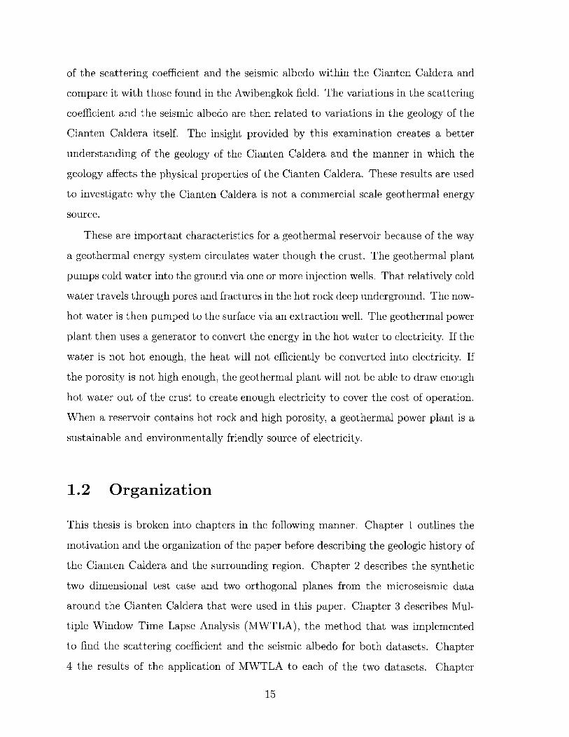
These are important characteristics for a geothermal reservoir because of the way

a geothermal energy system circulates water though the crust. The geothermal plant

pumps cold water into the ground via one or more injection wells. That relatively cold

water travels through pores and fractures in the hot rock deep underground. The now-

hot water is then pumped to the surface via an extraction well. The geothermal power

plant then uses a generator to convert the energy in the hot water to electricity. If the

water is not hot enough, the heat will not efficiently be converted into electricity. If

the porosity is not high enough, the geothermal plant will not be able to draw enough

hot water out of the crust to create enough electricity to cover the cost of operation.

When a reservoir contains hot rock and high porosity, a geothermal power plant is a

sustainable and environmentally friendly source of electricity.

1.2 Organization

This thesis is broken into chapters in the following manner. Chapter 1 outlines the

motivation and the organization of the paper before describing the geologic history of

the Cianten Caldera and the surrounding region. Chapter 2 describes the synthetic

two dimensional test case and two orthogonal planes from the microseismic data

around the Cianten Caldera that were used in this paper. Chapter 3 describes Mul-

tiple Window Time Lapse Analysis (MWTLA), the method that was implemented

to find the scattering coefficient and the seismic albedo for both datasets. Chapter

4 the results of the application of MWTLA to each of the two datasets. Chapter

15

5 discusses the possible implications of the results of MWTLA with respect to the

geologic setting of the Cianten Caldera.

1.3 Geology

This paper specifically examines microseismic events located within and surrounding

the Cianten Caldera. In order to show the geology that has shaped this area, the

following three sections will examine the geology within and surrounding the Cianten

Caldera on the scales of the tectonic region of the Sunda Arc subduction zone, the

local area that includes the Awibengkok geothermal system, and the extent of the

Cianten Caldera itself.

1.3.1 Regional Geology

The Cianten Caldera is directly to the west of the well-studied Awibengkok geother-

mal field, 60 km south of Jakarta, Indonesia on the island of Java as shown in Figure

1-1. Java is a part of the Sunda Arc, a 5,600 km chain of volcanic islands that lie

between China and Australia. The Sunda Arc is on the edge of the Eurasian tectonic

plate where the Eurasian plate meets the Australian plate. The collision of these two

oceanic plates forms the subduction zone where the Australian plate is subducted

underneath the Eurasian plate at the Sunda Trench. The Sunda Arc parallels the

subduction zone from the superior Eurasian plate.

The volcanic islands of the Sunda Arc are a direct result of this subduction.[18]

The process of subduction introduces water from the subducted plate to minerals

in the upper mantle and deep crust which chemically lowers the melting point of

those minerals until liquid melts form. In the case of a collision between two oceanic

tectonic plates, these resulting melts rise to form underwater volcanoes that grow and

eventually form islands given enough time.[8] This process forms volcanoes like those

of the Sunda Arc, including those that make up the islands of Java and Sumatra. [18]

As a result of the volcanic origins of the Sunda Arc, the seamounts and islands

of the Sunda Arc are composed of igneous rocks of various volcanic compositions

16

JVA

AW1BENGKOK Gnn

DARAJAT

Figure 1-1: A map of Indonesia (Figure 1-la) and western Java (Figure 1-1b). The

extent of the contract for the Awibengkok geothermal field is shown by the dotted

box on the left of Figure 1-1b. The Cianten Caldera is smaller than the Awibengkok

field and lies immediately to the west of Awibengkok. This image was taken from

Stimac et al., 2008.[23, p. 302]

17

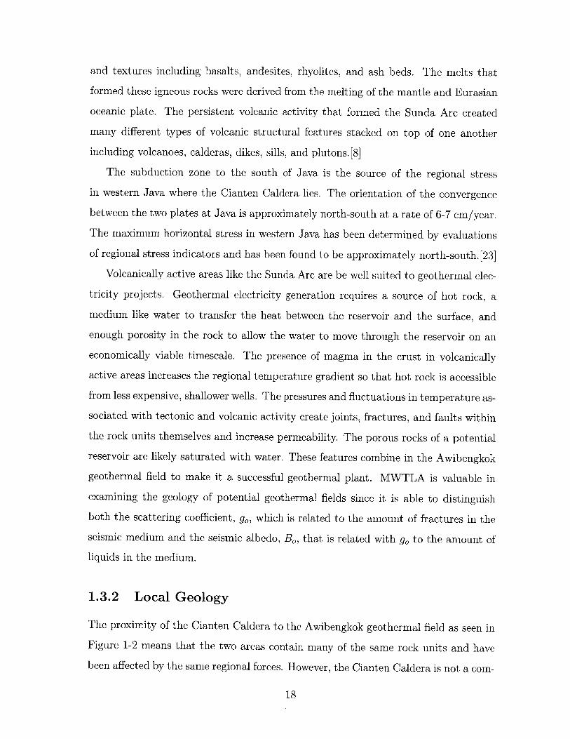
and textures including basalts, andesites, rhyolites, and ash beds. The melts that

formed these igneous rocks were derived from the melting of the mantle and Eurasian

oceanic plate. The persistent volcanic activity that formed the Sunda Arc created

many different types of volcanic structural features stacked on top of one another

including volcanoes, calderas, dikes, sills, and plutons.[8]

The subduction zone to the south of Java is the source of the regional stress

in western Java where the Cianten Caldera lies. The orientation of the convergence

between the two plates at Java is approximately north-south at a rate of 6-7 cm/year.

The maximum horizontal stress in western Java has been determined by evaluations

of regional stress indicators and has been found to be approximately north-south. [23]

Volcanically active areas like the Sunda Arc are be well suited to geothermal elec-

tricity projects. Geothermal electricity generation requires a source of hot rock, a

medium like water to transfer the heat between the reservoir and the surface, and

enough porosity in the rock to allow the water to move through the reservoir on an

economically viable timescale. The presence of magma in the crust in volcanically

active areas increases the regional temperature gradient so that hot rock is accessible

from less expensive, shallower wells. The pressures and fluctuations in temperature as-

sociated with tectonic and volcanic activity create joints, fractures, and faults within

the rock units themselves and increase permeability. The porous rocks of a potential

reservoir are likely saturated with water. These features combine in the Awibengkok

geothermal field to make it a successful geothermal plant. MWTLA is valuable in

examining the geology of potential geothermal fields since it is able to distinguish

both the scattering coefficient, go, which is related to the amount of fractures in the

seismic medium and the seismic albedo, BO, that is related with go to the amount of

liquids in the medium.

1.3.2 Local Geology

The proximity of the Cianten Caldera to the Awibengkok geothermal field as seen in

Figure 1-2 means that the two areas contain many of the same rock units and have

been affected by the same regional forces. However, the Cianten Caldera is not a com-

18

em ~Ii-

Figure 1-2: The geology of the Cianten Caldera and the Awibengkok geothermal fieldat the depth of the Rhyodacite Marker. The Cianten Caldera is the circular featureon the left. The productive Awibengkok field is the triangular outline in the centralthird of the figure. The Muara Fault hydrologically divides the two regions. Theimage was taken from Stimac et al., 2008.[23, p. 305]

19

mercially viable geothermal energy source. Awibengkok produces 377 MWe of elec-

tricity for the region from approximately 18 km 2 of proven geothermal reservoir.[23]

The Awibengkok field is geothermally productive because the temperature of the

rock in the reservoir ranges from 235'C to 310'C and the reservoir is naturally

fractured and saturated with water.[1] The field has been hydrofraced to increase

the porosity.[29] This temperature, porosity, and water content has allowed the Aw-

ibengkok field to reliably produce electricity since 1994.[23] The Cianten Caldera is

separated from the Awibengkok field by the Maura Fault. The Cianten Caldera has

a lower temperature which has caused many of the fractures in the Cianten Caldera

to be sealed by mineral precipitation. The Cianten Caldera and the Awibengkok

geothermal field have very different properties despite the fact that they are adjacent

to one another.

The stratigraphy of Awibengkok is shown in Figure 1-3. The oldest units at the

bottom of the stratigraphic column are marine sedimentary rocks that were formed

prior to volcanic activity when the oceanic floor was gradually collecting sediment.

These compacted sediments have less porosity, permeability, and hydrothermal al-

teration than the volcanic sequences above them. The units above these sediments

are igneous layers of andesitic and dacitic composition. The alternating composition

formed as the melt evolved over time due to crystal fractionation, crustal assimilation,

or magma mixing. Most of the Awibengkok reservoir is contained within the lower

andesite volcanic layer. [23] The reservoir has an impermeable smectite clay cap called

the Rhyodacite Marker that prevents water even under pressure from rising through

the stratigraphic column. This smectite clay cap of the geothermal reservoir is a com-

mon feature in volcanic geothermal fields that is formed by hydrothermal alteration

of the existing rocks at high temperatures. [23] Volcanic activity in the Awibengkok

area has created multiple intrusions that have disturbed the stratigraphic column.

These molten bodies thermally alter the layers they come into contact with, forming

contact aureoles. [1] These intrusions are the source of the heat that the Awibengkok

geothermal power plant uses to produce electricity. These intrusions also heat fluids

which rise until they are trapped at the smectite cap in the Awibengkok reservior. [23]

20

Without the cap, the fluids would be free to rise towards the surface and dissipate

the heat they contain. The cap forces these fluids to pool underground where they

are insulated and able to be retrieved by wells. As a result, the reservoir is can be a

profitable geothermal energy source.

The geology and structure of the Cianten Caldera and the Awibengkok field at the

Rhyodacite Marker is shown in Figure 1-2. The multiple faults in the Awibengkok

region generally trend in the north-northeast direction. Some of these north-northeast

faults that cut the Awibengkok geothermal field, including the Gagak Fault and

the Cibeureum Fault, are semi-permeable and have segmented the field into four

geochemically semi-independent cells. The Muara Fault is an impermeable fault, and

it geothermically isolates the Cianten Caldera from the Awibengkok field.[23] The

surface geologic map of the Awibengkok area is shown in Figure 1-4 and has similar

features. Figure 1-4 contains the full extent of both the active Awibengkok field to

the east and the Cianten Caldera on the west. This image is also shown in Figure

2-4 with the locations of the sources and receivers from the microseismic survey used

for analysis. The geology of the area is difficult to determine due to thick tropical

vegetation and sediments so there is some uncertainty in some of the details including

the extent of the Maura Fault.[23]

1.3.3 Cianten Caldera

A caldera is formed when a volcano collapses under its own weight after an eruption

empties the magma chamber underneath the volcano.[8] The Cianten Caldera is a

small caldera with a diameter of 4.5 km and an area of 16 km2 that erupted approxi-

mately 16 km 3 dense rock equivalent (DRE) of material prior to its collapse between

150,000 and 670,000 years ago.[24] The Cianten Caldera is outlined in Figure 1-2 by

the circular ring fault created during this collapse. Most of the exposed surface of

the Cianten Caldera visible in this figure is part of the Upper Rhyolite unit or the

alluvium. [23]

Figure 1-5 shows a facies model of the Cianten Caldera taken from Stimac et al.,

2008. This model is based on the limited outcrop available in the Cianten Caldera,

21

Jpper Rhyotite

Rhyodacite Marker

(a)1500-

1000-

500 -

## 01

I r

- 20M0

-4000-

-5000-

Aitme. Sndaloe, Tug

SntriWn

Ash Tuft

FIRST OCCURRENCE OF MIOCENEMARINE SEDIMENTARY ROCKS

Mad > Argilite

"CONTINUOUS"MARINESEDIMENTARYROCKS

Clastic Rocks - Marl

Figure 1-3: A stratigraphic column of the Awibengkok geothermal field. The oldest,deepest rock units are marine sediments. Above these sediments are alternatinglayers of andesitic, dacitic, and rhyolitic volcanic material. The layered stratigraphyis interrupted by younger intrusions that have thermally altered the rock surroundingthe intrusion. The Awibengkok geothermal reservior is in the Lower Andesite andis capped by a smectite clay layer at the Rhyodacite Marker. This figure was takenfrom Stimac et al., 2008.[23, p. 310]

22

I

RDM

i RDM1

4000

3000

2000

1000

E

.2

WON

lS0- 0-

Dacite andesitetufts andsediments

-1000

- 1500

Figure 1-4: A geologic map of the Awibengkok region. The Cianten Caldera is theorange circular structure on the west side of the map. The productive Awibengkokfield is the triangular shape. The Maura Fault is an impermeable fault that dividesthe two areas. This map was made by Stimac et al., 2009.[25]

23

local stratigraphy, and the structure of other small calderas. [24] The original extent

of the volcano that formed the Cianten Caldrea and the original, uneroded shape of

the caldera is visible in Figure 1-5.

The oldest rocks in this model are the basement of Miocence sedimentary rocks

that were in place prior to volcanic activity. Much of these sediments have been

altered after their deposition through contact metamorphism. The unit above these

sediments is composed of the volcanic rock that was erupted before the collapse that

formed the caldera. The unit of megabreccia and the caldera ash-flow tuff is from

after the caldera collapse. The top of this layer became the floor of the caldera after

the collapse. A lake formed in the caldera and collected the lacustrine deposits. The

fan and talus deposits also eroded into the lake. Eventually, the lake that filled the

caldera breeched the rim of the caldera and drained. The Cianten Caldera then began

to fill with debris and ejecta from other eruptions until the present day. [23]

The Cianten Caldera has been affected by both pre-caldera and post-caldera vol-

canism. There are many intrusions of different ages embedded in different layers of

the caldera. These intrusions thermally altered the rock they contacted. Most of

these intrusions predate the collapse of the caldera as small calderas rarely have sig-

nificant post-caldera volcanism. The last of these intrusions was likely a post-caldera

dome formed from the residual magma shortly after its collapse. [24]

Interest in the Cianten Caldera began when geophysical surveys at the borders

of the active Awibengkok field found the presence of a low resistivity layer in the

Cianten Caldera that could have been an extension of the low resistivity, anisotropic,

smectite clay layer that caps the active Awibengkok geothermal reservoir. Prior to

drilling, it was believed that the smectite clay layer could have originated from the

sediments in the lake that formed after the creation of the caldera. [23] A local high

gravity anomaly on the southeastern rim of the caldera was thought to indicate the

presence of shallower basement or an intrusion. [23]

After wells were drilled in the Cianten Caldera, it was found to not be suitable

for an expansion of the Awibengkok goethermal field. The Cianten Calera has sub-

commercial temperatures, numerous intrusions, and a shallow basement. [23] The low

24

orignal Cobpse Margin Original Edc

INa

Distance (km)

LiiUU

Recent Tuft

Lnher and FluilDqepoets

Fa and TaksDeposits

Deposits

Broodsu

Dcme

S Caldera Ash-FlowTLU

UPmo-CidersVolcanic: Rocks

UMioceneSedlrnunwry Rocks

M-cnq'

Figure 1-5: A facies model of the Cianten Caldera based on outcrop, local stratig-raphy, and the structure of other calderas of a similar size and tectonic setting. Itcontains a basement of marine Miocene sedimentary rocks overlain by pre-calderavolcanic rock. Above these rocks are post-caldera megabreccia and a caldera ash-flowtuff. The caldera's lacustrine deposits and the eroded fan and talus deposits filled inmuch of the caldera basin. Other deposits and recent tuffs fill the top of the section.Pre-caldera and post-caldera intrusions have cut and metamorphosed the layers theycontacted. This image was taken from Stimac et al., 2008.[23, p. 327]

25

resistivity layer in the Cianten Caldera was later confirmed to be a smectite clay layer

by rock cuttings obtained from drilling through this layer. [23] The smectite clay layer

is an anisotropic feature which affects seismic data. However, drilling also showed

that subsurface temperatures in the Cianten Caldera are much lower than in the

Awibengkok field and not of commercial value.[29]

The Cianten Caldera was thought to have the potential to be a commercial

geothermal field like the Awibengkok field immediately adjacent to it. However,

the temperatures in the Cianten Caldera are too low for this to be possible. The

knowledge gained by finding the distribution of the scattering coefficient and the

seismic albedo over the Cianten Caldera and across the Maura Fault from the appli-

cation of MWTLA to microseismic data should shed light on the interior structure of

the Cianten Caldera. A better understanding of the interior geology of the Cianten

Caldera would help explain the reasons why the Cianten Caldera has lower tem-

peratures and sealed fractures due to mineral precipitation that make the Cianten

Caldera not expected to be as geothermally productive as the adjacent Awibengkok

geothermal field.

The geology of the Cianten Caldera gave it the potential to be a good geothermal

candidate. Other calderas have been successful geothermal energy producers includ-

ing the Long Valley Caldera in California.[21] This caldera has been well studied

because it is seismically active and there was concern that it would become an active

volcano once more.[9] Seismic waveforms from this area have been processed with

MWTLA in order to find values for the scattering coefficient and the seismic albedo.

The results of this study are discussed in Section 3.3.

Hawaii is another volcanic area that has been considered for geothermal energy

production. The geology in the area has features that are similar to those of the

Awibengkok field that would make electricity generation possible including fractured

volcanic rock and a high geothermal gradient. The region has a high temperature

gradient due to the intrusions that are in the crust. [13] The results of the application

of MWTLA to this area is discussed in Section 3.3.

26

Chapter 2

Data

This chapter describes both the two dimensional synthetic acoustic dataset that was

created to test the MWTLA code and the Awibengkok microseismic dataset from the

Awibengkok geothermal field that are analyzed in this paper.

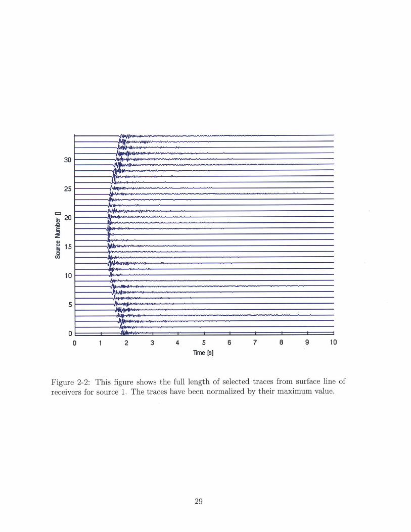
2.1 Synthetic Acoustic Data

A synthetic two dimensional, acoustic dataset was created in order to test the MWTLA

code before adding the complications of field data. The setup of the receivers for the

dataset can be seen in Figure 2-1. Each line of receivers contains 1024 receivers, and

each receiver has a seismic trace for each of the 9 sources. Synthetic traces were

created for three different cases by using moving the source locations to one quarter

of the full depth, one half of the full depth, and three quarters of the full depth.

Synthetic traces were created for three different velocity models that were generated

by adding zero mean Gaussian random noise with a correlation length of 0.05 km

to a background velocity of 3 km/s. To simulate intrinsic attenuation, an artificial

exponential decay was applied to all of the traces of e-a where a is a constant value

of 0.3 and r is the distance between the source and the receiver. Examples of the

traces that were used for the analysis of the acoustic case can be seen in Figure 2-2.

27

1 -

2 -

3 -

5-

6-

7-II I I I

0 1 2 3 4 5 6 7Distance [kin]

Figure 2-1: This figure shows the general distribution of the sources, shown in blue,and receivers, shown in red, for the synthetic acoustic dataset. There are two orthog-onal lines of 1024 receivers and nine sources in a three by three matrix.

28

30

25

5

20 - - o - - -- - - - ---- --- ---

0 1 2 3 4 5 6 7 8 9 10Time [s]

Figure 2-2: This figure shows the full length of selected traces from surface line ofreceivers for source 1. The traces have been normalized by their maximum value.

29

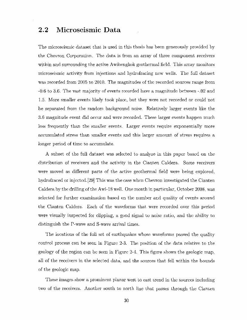
2.2 Microseismic Data

The microseismic dataset that is used in this thesis has been generously provided by

the Chevron Corporation. The data is from an array of three component receivers

within and surrounding the active Awibengkok geothermal field. This array monitors

microseismic activity from injections and hydrofracing new wells. The full dataset

was recorded from 2005 to 2010. The magnitudes of the recorded sources range from

-0.6 to 3.6. The vast majority of events recorded have a magnitude between -.02 and

1.5. More smaller events likely took place, but they were not recorded or could not

be separated from the random background noise. Relatively larger events like the

3.6 magnitude event did occur and were recorded. These larger events happen much

less frequently than the smaller events. Larger events require exponentially more

accumulated stress than smaller events and this larger amount of stress requires a

longer period of time to accumulate.

A subset of the full dataset was selected to analyze in this paper based on the

distribution of receivers and the activity in the Cianten Caldera. Some receivers

were moved as different parts of the active geothermal field were being explored,

hydrofraced or injected. [29] This was the case when Chevron investigated the Cianten

Caldera by the drilling of the Awi-18 well. One month in particular, October 2008, was

selected for further examination based on the number and quality of events around

the Cianten Caldera. Each of the waveforms that were recorded over this period

were visually inspected for clipping, a good signal to noise ratio, and the ability to

distinguish the P-wave and S-wave arrival times.

The locations of the full set of earthquakes whose waveforms passed the quality

control process can be seen in Figure 2-3. The position of the data relative to the

geology of the region can be seen in Figure 2-4. This figure shows the geologic map,

all of the receivers in the selected data, and the sources that fell within the bounds

of the geologic map.

These images show a prominent planar west to east trend in the sources including

two of the receivers. Another south to north line that passes through the Cianten

30

-21

A ~IE

A *

* ** A

*~A

A

T

N

0

2

4

LA A A A A

*

*

* *r ®

A

*0*

*

*

* 9246 9248 9250 9252 9254 9256Y [km]

9245- I

9240

T 0

N

4* Sources- Receivers

675 680X [km]

* *

675A*

*(*

* *

680X [km]

*

685

685

Figure 2-3: This figure shows the distribution of all of the sources and receivers fromOctober 2008 that passed the quality control measures.

31

9260F

9255F

*

92501

CM

F.. 0

- -c

E

x

(D

N C N M N NCD too O to0) 0) 0) 0) 0) 0)

[wNJ A

Figure 2-4: This figure shows the distribution of the sources and receivers on thegeologic map. There are a number of sources on both sides of the Maura fault whichseparates the Cianten Caldera from the active Awibengkok geothermal field. Onereceiver is located within the Cianten Caldera.

32

Caldera can be constructed using four receivers and a number of sources. We use

these two different planar trends for the two dimensional analysis made later in the

paper. The selected data for the west to east plane are shown in Figure 2-5. The

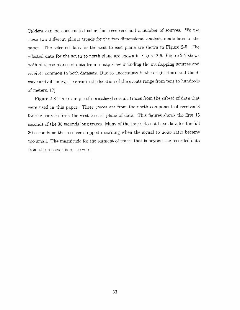
selected data for the south to north plane are shown in Figure 2-6. Figure 2-7 shows

both of these planes of data from a map view including the overlapping sources and

receiver common to both datasets. Due to uncertainty in the origin times and the S-

wave arrival times, the error in the location of the events range from tens to hundreds

of meters. [17]

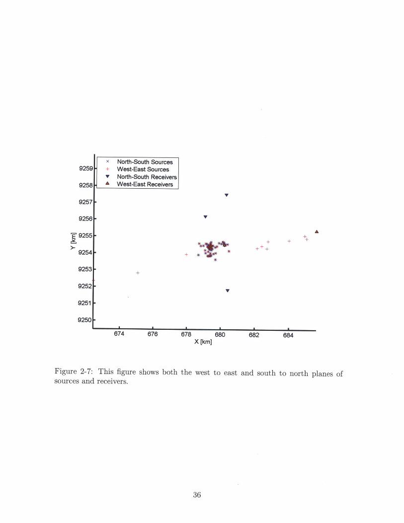
Figure 2-8 is an example of normalized seismic traces from the subset of data that

were used in this paper. These traces are from the north component of receiver 8

for the sources from the west to east plane of data. This figures shows the first 15

seconds of the 30 seconds long traces. Many of the traces do not have data for the full

30 seconds as the receiver stopped recording when the signal to noise ratio became

too small. The magnitude for the segment of traces that is beyond the recorded data

from the receiver is set to zero.

33

9265 F

-10-

9260-5

9255F 0* *

* N

5

9250F

-A

*

A

**

*

101

9245-

* SourcesA Receivers

675 680X [km]

685

15

675 680X [km]

685

Figure 2-5: This figure shows the selected plane of sources and receivers that runswest to east across the Cianten Caldera and the Awibengkok field.

34

A

92571-

A

** *

* * ***

* SourcesA Receivers

679 680X [km]

Figure 2-6: This figure shows the selected plane of sources and receivers that runssouth to north across the Cianten Caldera.

35

92561

92551

A A,a

9254

-1,

0

1

2

3

4

N

92531

**4*

*

*

9252

9252 9254Y [km]

9256

681

x North-South Sources+ West-East SourcesV North-South ReceiversA West-East Receivers

V

V

*

+

V

674 676 678X [km]

680

Figure 2-7: This figure shows both thesources and receivers.

west to east and south to north planes of

36

9259

9258

9257

9256-

9255,

9254-

9253-

9252

92511

9250

A

±++ +

+++

682 6840 9 0 a m a

60

50

40

EM

S300

20

10 7o" o

0 5 10 15Time [s]

Figure 2-8: This figure shows the first 15 seconds of the normalized traces from thenorth component of receiver 8 for the sources from the west to east plane of sources.The full traces are 30 seconds long, but a shorter section is shown here for detail.

37

I

Chapter 3

Method

This chapter details the theory behind the Multiple Window Time Lapse Analysis

(MWTLA) method developed by Fehler et. al. in their 1992 paper. Then this

chapter describes MWTLA and the process by which MWTLA is used to determine

the scattering coefficient, g0, and the seismic albedo, B0, from the seismic traces.

3.1 Theory

The direct arrival energy for a seismic signal decays faster than simple geometric

spreading can account for. This attenuation occurs either from waves scattering off

of heterogeneities in the medium or from intrinsic absorption of energy as heat because

of anelastic behavior in the medium. Scattering does not result in a loss of energy

as scattering simply causes a change in direction or a phase shift of a wave. Intrinsic

absorption does result in the wave losing energy when seismic energy is converted

into heat.[11]

The process of scattering requires that the scattered wave covers a greater distance

than the direct wave, so the scattered wave will arrive after the direct wave. Conse-

quently, the portion of the seismic trace that is immediately after the arrival time will

be dominated by the direct wave, and the coda of the seismic trace will be dominated

by the scattered waves. This property that separates the intrinsic attenuation of a

wave from the scattering of a wave is the basis of MWTLA.

39

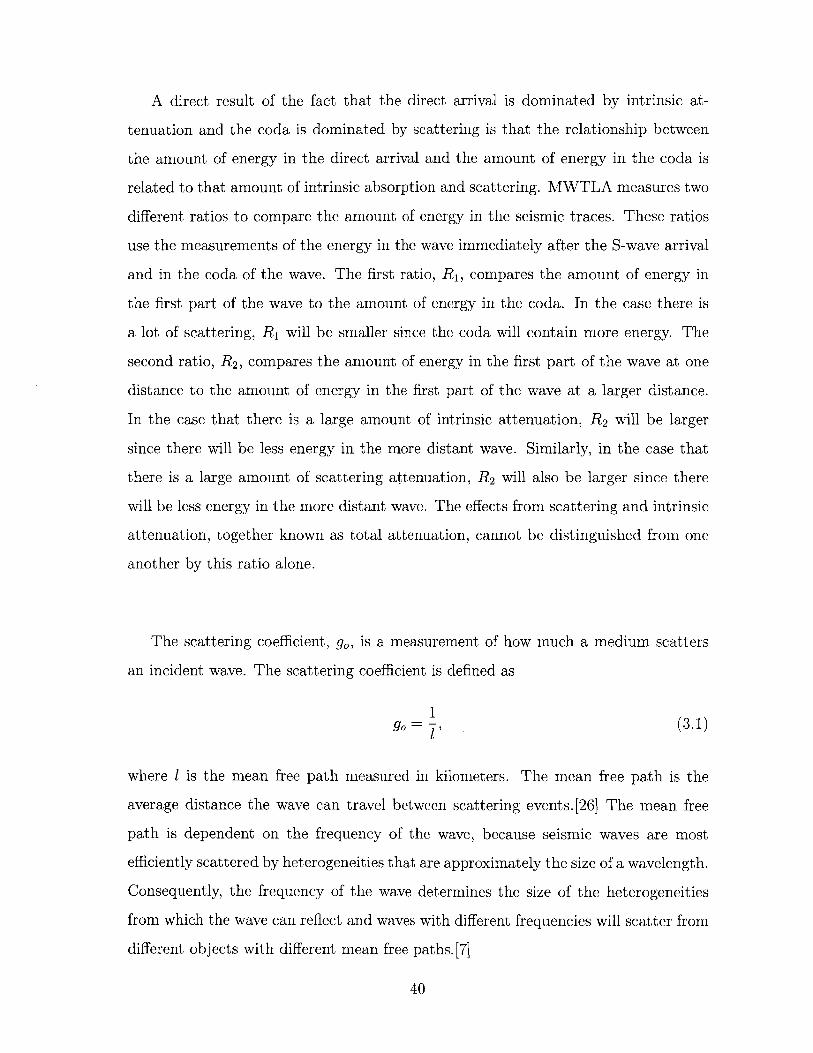
A direct result of the fact that the direct arrival is dominated by intrinsic at-

tenuation and the coda is dominated by scattering is that the relationship between

the amount of energy in the direct arrival and the amount of energy in the coda is

related to that amount of intrinsic absorption and scattering. MWTLA measures two

different ratios to compare the amount of energy in the seismic traces. These ratios

use the measurements of the energy in the wave immediately after the S-wave arrival

and in the coda of the wave. The first ratio, R1, compares the amount of energy in

the first part of the wave to the amount of energy in the coda. In the case there is

a lot of scattering, R1 will be smaller since the coda will contain more energy. The

second ratio, R2 , compares the amount of energy in the first part of the wave at one

distance to the amount of energy in the first part of the wave at a larger distance.

In the case that there is a large amount of intrinsic attenuation, R2 will be larger

since there will be less energy in the more distant wave. Similarly, in the case that

there is a large amount of scattering attenuation, R2 will also be larger since there

will be less energy in the more distant wave. The effects from scattering and intrinsic

attenuation, together known as total attenuation, cannot be distinguished from one

another by this ratio alone.

The scattering coefficient, go, is a measurement of how much a medium scatters

an incident wave. The scattering coefficient is defined as

go 1 (3.1)

where 1 is the mean free path measured in kilometers. The mean free path is the

average distance the wave can travel between scattering events.[26] The mean free

path is dependent on the frequency of the wave, because seismic waves are most

efficiently scattered by heterogeneities that are approximately the size of a wavelength.

Consequently, the frequency of the wave determines the size of the heterogeneities

from which the wave can reflect and waves with different frequencies will scatter from

different objects with different mean free paths. [7]

40

The scattering quality factor, Q, is related to the scattering coefficient, go, by

QS = w (3.2)g0V

and the intrinsic quality factor, Qj, is similarly related to the intrinsic absorption

coefficient, a, by

Q = , (3.3)aV'

where w is the frequency of the wave, and V is the seismic velocity of the wave in the

medium. [6]

The seismic albedo, Bo, is defined by

B = + = g (3.4)

where Qs is the scattering quality factor and Qj is the intrinsic quality factor. [6] The

inverse of the scattering quality factor and the inverse of the intrinsic attenuation

quality factor describe the amount of attenuation due to scattering and intrinsic

absorption respectively. Bo ranges in values from 0 to 1. When Bo approaches 0,

g approaches 0 km-1 and 1, the mean free path of the wave, approaches infinity.

The intrinsic attenuation of this wave is undetermined. When go is much larger

than 1 km-1, there is effectively no traveling wave as the medium dissipates the

energy in the wave almost immediately by converting it to heat or other forms of

intrinsic absorption. When Bo = 1, the medium exhibits perfect scattering with

no losses due to dissipation of the energy of the wave as heat.[26] Most materials

within the Earth fall somewhere between these two extreme cases. When Bo < 0.5,

intrinsic attenuation is the dominant mechanism, and when Bo > 0.5, scattering is

the dominant mechanism.[27]

The total attenuation, Qt, is

Qt- = IQj + Q;1 (3.5)

41

since the only two ways for the direct wave to lose energy are intrinsic attenuation

and scattering.

The scattering coefficient, go, and the intrinsic attenuation coefficient, a, are both

determine by the geology of the region. When there are more heterogeneities on the

scale of the wavelength of the wave and when these heterogeneities are closer together,

the scattering coefficient will increase. These heterogeneities could be fractures or

changes in the density or other properties of the medium the wave travels through.

Similarly, the intrinsic attenuation coefficient is related to how well the medium is

able to dissipate heat. Softer medium or the presence of water in the pores of the

rock will increase the amount of energy that is lost as heat as the wave passes through

it. The goal of this study is to relate these coefficients to the geology of the Cianten

Caldera and the surrounding area.

When scattering is the dominant attenuation mechanism, the region contains more

heterogeneities on the scale of the wavelength of the seismic wave such as fractures

or changes in composition. When intrinsic attenuation is the dominant attenuation

mechanism, the regions contains more attenuating features such as a higher water

content or softer rock that is better able to convert seismic energy to heat. Both

high values for scattering and attenuation are good for a geothermal reservoir. A

high scattering coefficient, especially in an area that is more homogeneous than a

volcano, could indicate large amounts of fractures that could be high permeability

pathways to move water through the reservoir and into the well on a timescale that

enables a geothermal plant to operate. A high attenuation coefficient could indicate

that the region is saturated with a large amount of water, potentially indicating a

larger porosity that would mean there is more water for the geothermal plant to use.

A larger porosity could also indicate a larger permeability.

3.2 Multiple Window Time Lapse Analysis

MWTLA is based on the radiative transfer theory. The first methods that addressed

the manner in which waves scatter were simple and included single scattering for

42

weakly scattering areas and diffusion for strongly scattering areas. Then the mul-

tiple scattering model allowed the calculation of scattering for a finite number of

scatterers. [6] The radiative transfer theory is a method used to calculate the response

of the intensity of a signal to passing through a medium that has an indefinite number

of scatterers. In this application, we assume that scatterers are isotropic scatterers ar-

ranged uniformly throughout the medium and that only body waves are recorded. [26]

The raw seismic traces should be corrected for source and site amplification factors

as well as geometric spreading prior to applying MWTLA.[6] The corrected seismic

traces can be used to calculate two values, R1 and R2 , directly from the seismic traces

by using the ratio of energy at different portions of a seismic wave.

As explained in Section 3.1, the portion of the seismic trace immediately after

the arrival time is dominated by the direct wave and the coda is dominated by the

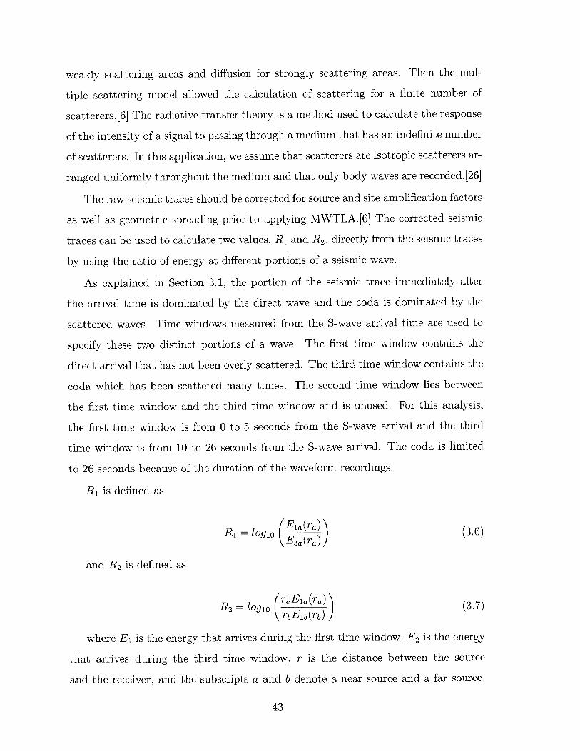
scattered waves. Time windows measured from the S-wave arrival time are used to

specify these two distinct portions of a wave. The first time window contains the

direct arrival that has not been overly scattered. The third time window contains the

coda which has been scattered many times. The second time window lies between

the first time window and the third time window and is unused. For this analysis,

the first time window is from 0 to 5 seconds from the S-wave arrival and the third

time window is from 10 to 26 seconds from the S-wave arrival. The coda is limited

to 26 seconds because of the duration of the waveform recordings.

R1 is defined as

(Eia(ra)R1 = logio i (3.6)

E 3a(ra)

and R 2 is defined as

(raE1a(ra)R 2 = ogio il(r) (3.7)

where E1 is the energy that arrives during the first time window, E2 is the energy

that arrives during the third time window, r is the distance between the source

and the receiver, and the subscripts a and b denote a near source and a far source,

43

respectively. [6] The energy is found by integrating the square of the trace over the

time window.

With these values for R1 and R 2 , the corresponding values of g, and B, can be

found using Figure 3-1. This paper uses an alternative method to find g, and B,

from R1 and R 2. A table of values was calculated by calculating the Green's function

from different values of B0, go, and r. The two dimensional, radiative transfer Green's

function, GF, that was used in this paper is

_ 1 / r2 N -3 cGF(t)= ( (1 - 2 )) exp (jC(c 2t 2 _r 2 ).5 ct - (3.8)

4,rDt c2t2 2D

where D is the diffusion coefficient, r is the distance between the source and the

receiver, c is the energy velocity of the medium, and t is the time.[19] Given B0 , go,

and r, the values for E1 and E 3 were calculated from the Green's function. The table

of values created by this method was then used to find B, and g, for values of r, E1 ,

and E 3 estimated from the data.

3.3 Applications of MWTLA

MWTLA has been successfully used to find measurements of scattering and intrinsic

attenuation in a number of different types of geologic regions. Table 3.1 summarizes

some of these results for regions that are volcanic like the Cianten Caldera and for

regions that are different from the Cianten Caldera. The values go and B0 that are

shown are for frequencies closest to 4 to 6 Hz, the frequencies that dominate the

Awibengkok dataset as shown in Figure 4-5. The papers listed in this table are

discussed in more detail below.

Fehler et al. 1992 developed MWTLA in order to be able to separate the ef-

fects of intrinsic attenuation and scattering. They examined three frequency bands

that ranged from 1 to 8 Hz for data from the Kanto-Tokai region of Japan and

found regional values for both the scattering coefficient and the intrinsic attenuation

coefficient.[6] Mayeda et al. 1992 applied MWTLA to three geologically different re-

44

0.05

0.04 "10 1 eE,(r)Ir:15Okm -

1.0

s -- 1.C3 0.0

C0.01

O

1..0

0.

B.- 0,1

11.5

81 -. 0, 1 1 P

._

0 0.01 0.02 0.03 O4 0.05

Total Attenuation Coefficient, g +

Figure 3-1: This figure shows the graphical relationship between R 1, R 2, go, andthe total attenuation coefficient. For specified values of R1 and R 2, the scatteringcoefficient, g,, and the total attenuation coefficient can be found. From these twonumbers, the seismic albedo, BO, can be obtained. This image was taken from Fehleret al., 1992.[6, p. 796]

45

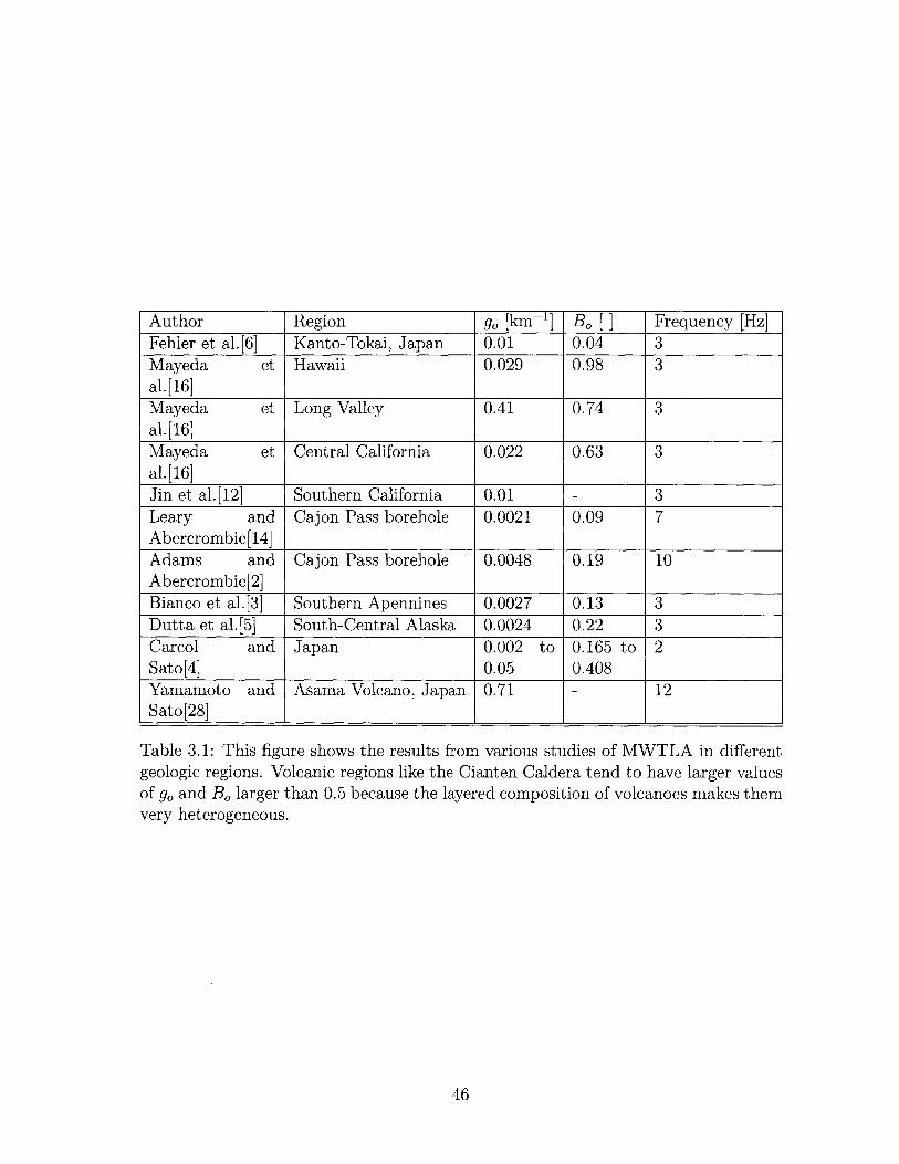
Author Region go [km- 1 ] BO [ ] Frequency [Hz]Fehler et al.[6] Kanto-Tokai, Japan 0.01 0.04 3Mayeda et Hawaii 0.029 0.98 3al. [16]Mayeda et Long Valley 0.41 0.74 3al.[16]Mayeda et Central California 0.022 0.63 3al. [16]Jin et al.[12] Southern California 0.01 - 3Leary and Cajon Pass borehole 0.0021 0.09 7Abercrombie[14]Adams and Cajon Pass borehole 0.0048 0.19 10Abercrombie[2]

Bianco et al.[3] Southern Apennines 0.0027 0.13 3Dutta et al.[5] South-Central Alaska 0.0024 0.22 3Carcol and Japan 0.002 to 0.165 to 2Sato[4] 0.05 0.408Yamamoto and Asama Volcano, Japan 0.71 - 12Sato[28]

Table 3.1: This figure shows the results from various studies of MWTLA in differentgeologic regions. Volcanic regions like the Cianten Caldera tend to have larger valuesof g, and BO larger than 0.5 because the layered composition of volcanoes makes themvery heterogeneous.

46

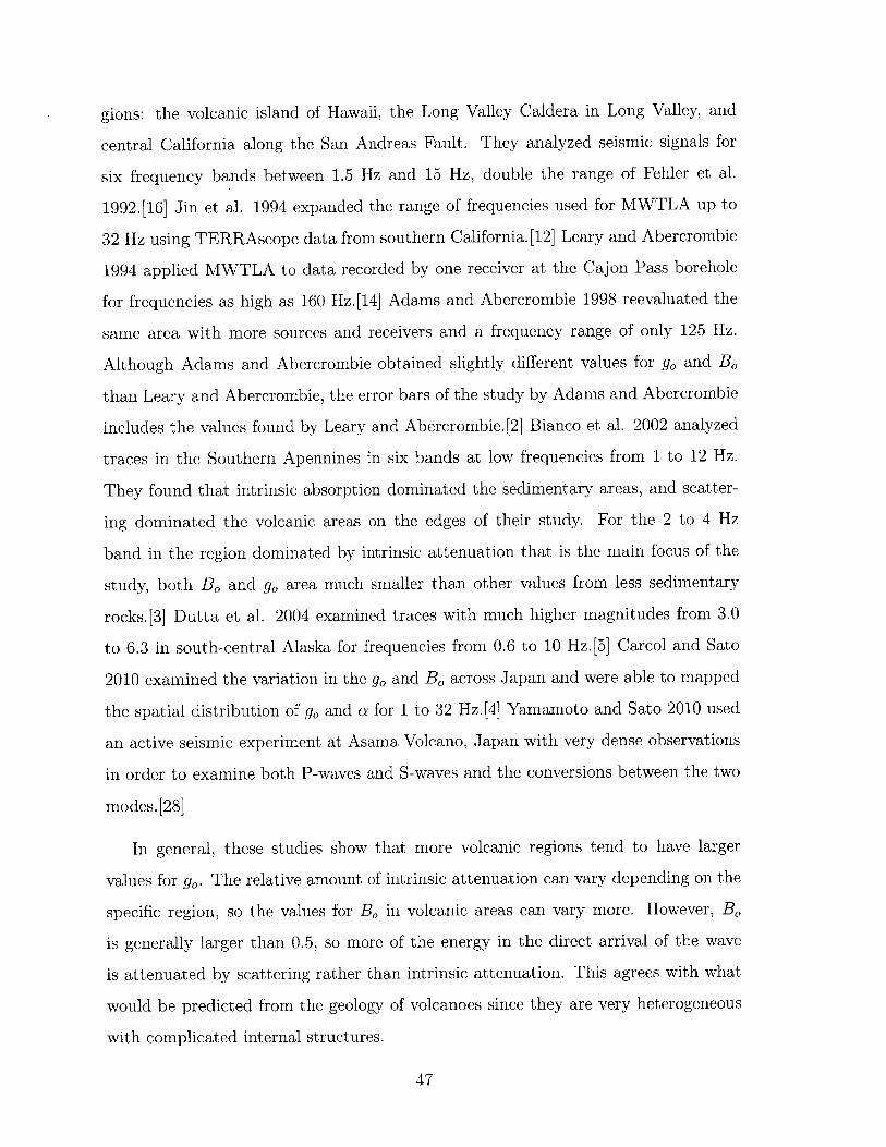
gions: the volcanic island of Hawaii, the Long Valley Caldera in Long Valley, and

central California along the San Andreas Fault. They analyzed seismic signals for

six frequency bands between 1.5 Hz and 15 Hz, double the range of Fehler et al.

1992.[16] Jin et al. 1994 expanded the range of frequencies used for MWTLA up to

32 Hz using TERRAscope data from southern California. [12] Leary and Abercrombie

1994 applied MWTLA to data recorded by one receiver at the Cajon Pass borehole

for frequencies as high as 160 Hz.[14] Adams and Abercrombie 1998 reevaluated the

same area with more sources and receivers and a frequency range of only 125 Hz.

Although Adams and Abercrombie obtained slightly different values for g, and B,

than Leary and Abercrombie, the error bars of the study by Adams and Abercrombie

includes the values found by Leary and Abercrombie.[2] Bianco et al. 2002 analyzed

traces in the Southern Apennines in six bands at low frequencies from 1 to 12 Hz.

They found that intrinsic absorption dominated the sedimentary areas, and scatter-

ing dominated the volcanic areas on the edges of their study. For the 2 to 4 Hz

band in the region dominated by intrinsic attenuation that is the main focus of the

study, both B, and g, area much smaller than other values from less sedimentary

rocks.[3] Dutta et al. 2004 examined traces with much higher magnitudes from 3.0

to 6.3 in south-central Alaska for frequencies from 0.6 to 10 Hz.[5] Carcol and Sato

2010 examined the variation in the g, and B0 across Japan and were able to mapped

the spatial distribution of g, and a for 1 to 32 Hz.[4] Yamamoto and Sato 2010 used

an active seismic experiment at Asama Volcano, Japan with very dense observations

in order to examine both P-waves and S-waves and the conversions between the two

modes. [28]

In general, these studies show that more volcanic regions tend to have larger

values for g,. The relative amount of intrinsic attenuation can vary depending on the

specific region, so the values for B0 in volcanic areas can vary more. However, B0

is generally larger than 0.5, so more of the energy in the direct arrival of the wave

is attenuated by scattering rather than intrinsic attenuation. This agrees with what

would be predicted from the geology of volcanoes since they are very heterogeneous

with complicated internal structures.

47

MWTLA has developed from only being able to give a regional estimate of the

scattering coefficient and the seismic albedo from S-waves. This method can now map

the changes in g, and B0 across a region given a dense enough distribution of sources

and receivers. It can also account for P-waves and mode conversions. The ability to

separate the intrinsic attenuation from the scattering attenuation is invaluable and

provides a new way to examine the interior of the Earth.

48

Chapter 4

Results

In this chapter, the results for the seismic albedo, B0, and the scattering coefficient,

go, are shown from applying two dimensional MWTLA first to a synthetic two di-

mensional acoustic dataset and then to two orthogonal planes of sources and receivers

from the Awibengkok microseismic dataset.

The figures that are used to convey the results for B0 and go are all created in

the same manner. The two dimensional plane of sources and receivers is broken into

cells. These cells were 0.05 km wide and 0.05 km deep for the synthetic acoustic data

and 0.1 km wide and 0.1 km high for the microseismic data. B0 and go are calculated

for each path joining a source and receiver pair. B0 and go are put into every cell on

the path between that source and receiver along with the length of the path in that

cell. Once all of the paths are calculated, the weighted averages of both Bo and go

are taken for each cell based on the path length in each cell. These weighted averages

for Bo and go are the values that are shown in each cell of the figures. This is similar

to the method that is used for traveltime tomography.[20, Ch. 5]


The locations of the sources and receivers used to construct the seismic traces used

for this case are described in Section 2.1. Figure 4-1, Figure 4-2, and Figure 4-3 were

created using a subset of this dataset including line of receivers close to the surface

49

and two pairs of sources approximately beneath the midpoint of the line of receivers.

One pair of sources is at 1.9 km deep and the other pair of sources is at 5.6 km deep.

Finding B0 and go requires sources at two different distances from the receiver, so the

resulting values for B0 and g, are interpreted as the value between the nearer source

and the receiver. The radiating pattern of lines from the shallow source is an artifact

the creation of the figure, since values are assigned to cells on the path between a

certain source and receiver pair.

Figure 4-1 shows the calculated values of g, for the synthetic acoustic dataset.

There is very little variation in the values of g, across this figure. The values of go

range from 1.6 km- to 2.0 km- 1 . The average value of g, is 1.77 km-1, which is close

to the expected value of g, estimated from the model of 1 km- 1.

Figure 4-2 shows the calculated values of B0 for the synthetic acoustic dataset.

The values of B0 range from 0.65 to 0.75 and vary little over this figure. This is

consistent with the constant artificial decay that was imposed on the waveforms. The

artificial decay that was applied to the waveforms as a substitute for the intrinsic

attenuation, a, was 0.3 km- 1 as described in Section 2.1. Assuming go is equal to the

estimated value of 1 km 1 , Equation 3.1 gives the expected value of B0 for the model

be approximately 0.77. This matches the average value of B0 in Figure 4-2 of 0.71.

Figure 4-3 shows the number of times a cell in the figure is on a path between a

source and receiver. Most of the cells far from the sources are in the figure are only

sampled once or twice. Cells with larger values are closer to the receivers where more

paths overlap.

These results for B0 and go are typical results for the synthetic acoustic dataset.

These values agree with the expected results, so only these this case is shown in detail.


The data used for this case is described in Section 2.2.

Figure 4-4 shows a typical trace from the microseismic dataset. This trace was

normalized by dividing by the maximum value of the absolute value of the trace.

50

2

0.2- 1.8

0.4- 1.6

0.6- 1.4

~0.8 -1.2

1.2- 0.8

0.61.4-

0.41.6-

0.21.8

3 3.5 4 4.5Distance [km]

Figure 4-1: This figure shows go for the synthetic acoustic data. The colorbar is inunits of inverse kilometers. The values for go across this figure range from 1.6 km- 1

to 2.0 km- 1 and are approximately uniform. The radiating pattern of lines from theshallow source is an artifact of the manner in which the figure was made. The averagevalue of g, is 1.77 km-1, which is close to the estimated value of 1 km-'.

51

0

0.70.2-

0.4- 0.6

0.6- - 0.5

0.8 -0.4

1.2- 0.3

1.4 0.2

1.6-0.1

1.8-

3 3.5 4 40Distance [km]

Figure 4-2: This figure shows B0 for the synthetic acoustic data. The colorbar isunitless, and B0 ranges from 0 to 1. The values for B0 across this figure range from0.65 to 0.75 and are approximately uniform. The radiating pattern of lines from theshallow source is an artifact of the manner in which the figure was made. The averagevalue of B0 is 0.71, which agrees with the expected value of 0.70.

52

U100

0.2~ 90

0.4- 80

0.6- 70

0.8 - 60

S 1 - 50

1.2 40

1.4- 30

1.6 20

101.8 -

3 3.5 4 4.50Distance [km]

Figure 4-3: This figure shows the number of times a path from a source to a receiverin the synthetic acoustic data traveled through any cell in the figure. Most of thecells far from the sources are in the figure are only sampled once or twice. Cells withlarger values tend to be along the path between a cluster of sources and a receiverand near the receivers in general.

53

This particular trace is the east component of receiver 8 from event 3271 located

at 675.1 km north, 9252.8 km east, and 1.7 km deep. Figure 4-5 shows the Fourier

transform of this trace. Other traces from this dataset have frequencies similar to the

frequencies seen in this trace.

The maximum value of Figure 4-5 occurs at 4.42 Hz, the strongest frequency of the

seismic trace in Figure 4-4. The full-width, half-height peak frequencies occur between

3.5 Hz and 6.5 Hz. The most prominent wavelengths of this seismic trace range from

539 m to 1 km, assuming an average background velocity of 3.5 km/s. The range of

wavelengths contained within the seismic trace are important because they show the

scale of a heterogeneity required to scatter the seismic wave. A heterogeneity much

larger than the wavelength will cause the wave to turn slowly rather than scatter.

A heterogeneity that is much smaller than the wavelength will alter the perceived

properties of the medium that the wave travels through. A heterogeneity that is

approximately the same size as the wavelength will cause the wave to scatter.[22, Ch.

3] Consequently, scattering should be the dominant mechanism of attenuation if the

heterogeneities are on the scale of the wavelength of the seismic traces, approximately

0.5 to 1 km.

4.2.1 Cianten West to East Results

MWTLA was applied to the waveforms from the west to east plane of sources and

receivers to find values for go and B. The results of this analysis are presented in

this section.

Figure 4-6 shows the values for g, that are derived from the north component of

the receivers on the west to east plane of sources and receivers. There is no discernible

pattern or trend in the variation in values of g. While there are a few scattered larger

values of g, that range up to 7.4 km 1 and smaller values as low as 0.2 km- 1, the

vast majority of the values in this figure are in the range of 0.5 to 1.2 km- 1. The

consistency of values across this figure shows that the values of go do not change

across the length of this section, especially since measured values for go range over

several orders of magnitude. In this figure, the average value of g, is 1.10 km 1 . This

54

1

0.8

0.2-

E0

(D-0.2-

: -0.4-

-0.6-

-0.8-

-1-0 5 10 15

Time [seconds]

Figure 4-4: This figure shows the first 15 seconds of a normalized seismic trace fromthe microseismic dataset. This is event 3271 as it was recorded on the east componentof receiver 8. This seismic trace is typical of the waveforms seen in this dataset.

55

801

70

60-

50-

40

30-

20-

10,

00 5 10 15 20 25 30 35 40

Frequency [Hz]

Figure 4-5: This figure shows the spectrum of the seismic trace in Figure 4-4. Themaximum frequency occurs at 4.42 Hz. The full-width, half-height peak frequenciesoccur between 3.5 Hz and 6.5 Hz, which corresponds to wavelengths of approximately0.5 to 1 km. This is consistent with the other waveforms for the microseismic dataset.Although there are contributions from frequencies outside of this range, the dominantlength scale at which these waveforms would scatter is approximately on the scale of0.5 to 1 km.

56

value is agrees with the value of g, of 1 km- 1 for volcanic rocks from Yamamoto and

Sato 2010.[28]

Figure 4-7 shows the values for g, that are derived from the east component of

the receivers on the west to east plane of sources and receivers. This figure closely

resembles Figure 4-6 in both the values of g, and the distribution of those values. The

values of g, in this figure range from 0.3 km- 1 to 7.1 km- 1 , with a mean value of 1.05

km-1. Both the east and the north transverse component of the receiver for g, on

the west to east plane give very similar calculated results. The transverse component

that is chosen also has very little affect on all of the other results for B0 and g, in

both the west to east plane and the south to north plane. The vertical component of

the receivers were not examined as we were dealing primarily with the S-wave. As a

result, only the figures for the north component will be shown from now on.

Figure 4-8 shows the values for B0 derived from the north component of the

receivers on the west to east plane of sources and receivers. Two distinct values

for B0 can be seen in this figure. The paths originating with the sources on the

eastern side of the figure have an average B0 value of approximately 0.8. The paths

originating with the sources on the western side of the figure have an average B0

value of approximately 0.6. The overlap between the two sides occurs in the cluster

of sources around 679 km. The Maura fault intersects this plane at the surface at

679.2 km, although the dip of the fault is unknown. The error in the location of these

events ranges from tens to hundreds of meters.[17] This uncertainty in the locations

of the sources could be consistent with the idea that the paths with different values

of B0 correspond to differences in the material on either side of the fault.

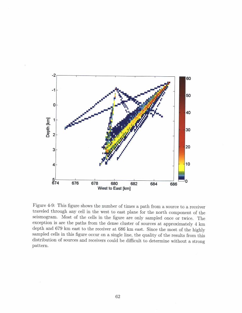
Figure 4-9 shows the number of times each cell is sampled in the west to east

plane of sources and receivers for the north component of the receivers on that plane.

Cells are sampled more often closest to the receivers where more source to receiver

paths overlap. Cells are also samples more often when they are on the path between

a dense cluster of sources and a receiver. The largest cluster of receivers in this figure

is the cluster around 679 km. Most of the cells in this figure are only sampled once

or twice, but a few are sampled as many as 61 times. Consequently, there is a large

57

-27

6

5

S2- 3

3- - 2

4- 1

5 ' ' 0674 676 678 680 682 684 686West to East [km]

Figure 4-6: This figure shows g, for the west to east plane for the east componentof the seismogram. The colorbar is in units of inverse kilometers. The values forgo across this figure are approximately constant and show no distinct pattern. Theaverage value of g0 in this figure is 1.10 km 1 .

58

-2 7

-l 6

0- 5

El 4

2- - 3

3- 2

4- 1

5 ' ' ' ' ' 0674 676 678 680 682 684 686

West to East [km]

Figure 4-7: This figure shows g, for the west to east plane for the north component ofthe seismogram. The colorbar is in units of inverse kilometers. Similar to Figure 4-6,the values for g, across this figure are approximately constant and show no distinctpattern. The average value of g, in this figure is 1.05 km- 1 . Since the results fromthe east and north components of the receiver are so similar here and in all of theremaining results, only the north component will be examined from now on.

59

-21 I0.8

-1

0.7

0 - - 0.

1 0.5

0.4

0.33-

0.2

4-0.1

5 '' ' 0674 676 678 680 682 684 686

West to East [km]

Figure 4-8: This figure shows B, for the west to east plane for the north componentof the seismogram. The colorbar is unitless, and B0 ranges from 0 to 1. Most valuesof B0 are near either 0.6 or 0.8. The larger values of B0 tend to be from sources onthe east side of the figure and the smaller values of B0 tend to be from the west sideof the figure with some overlap in the central cluster of sources. The difference maybe caused by differences in the attenuation coefficient on different sides of the Maurafault.

60

I

variation in the number of contributions to the value of B, or g, for any particular

cell.

The cells that are only sampled a few times will be strongly influenced by whichever

source to receiver paths happen to cross that cell. The addition of more paths and

especially more intersecting paths through each cell allows any single extreme value

that may be influenced by noise to be averaged out. This redundancy of data increases

the confidence of the results as opposed to being determined from a single source to

receiver waveform. The concentration of most of the multiply sampled cells into a

single line in this distribution of source and receiver paths would make it difficult to

draw conclusions from the distribution of g, and B0 without strong trends like the

trends found in this results from this dataset.

4.2.2 Cianten South to North Results

MWTLA was applied to the waveforms from the south to north plane of sources and

receivers to find values for g, and B,. The results of this analysis are presented in

this section.

Figure 4-10 shows the values for g, derived from the north component of the

receivers on the south to north plane of sources and receivers. The values of g, range

from 0.2 km- to 3.3 km- 1 , but most of the values for g, in this figure are closer to

the average value of 1.25 km- 1 . This value of g, is in agreement with the value of

g, of 1 km- 1 by Yamamoto and Sato 2010 for volcanic rocks.[28] The values for g,

across this figure are approximately constant and show no distinct pattern, especially

since measured values of g, range over several orders of magnitude. There is little

variation in g, across this section.

The average value for g, of 1.25 km-1 in Figure 4-10 for the south to north plane

is slightly higher than the average value for g, of 1.10 km 1 in Figure 4-7 for the west

to east plane. Note that the colorbar on Figure 4-10 is different from the colorbar on

Figure 4-7. The maximum of Figure 4-10 is 3.3 km' and the maximum of Figure

4-7 is 7.1 km-1, so specific colors do not correspond to the same values.

Figure 4-11 shows the values for B0 derived from the north component of the

61

-2 ' ' ' 60

-150

0-40

30

203-

4- 10

5 ' ' ' ' 0674 676 678 680 682 684 686

West to East [km]

Figure 4-9: This figure shows the number of times a path from a source to a receivertraveled through any cell in the west to east plane for the north component of theseismogram. Most of the cells in the figure are only sampled once or twice. Theexception is are the paths from the dense cluster of sources at approximately 4 kmdepth and 679 km east to the receiver at 686 km east. Since the most of the highlysampled cells in this figure occur on a single line, the quality of the results from thisdistribution of sources and receivers could be difficult to determine without a strongpattern.

62

U

-

UU

U

U

9251 9252 9253 9254 9255South to North [km]

9256 9257 9258

Figure 4-10: This figure shows g, for the north-south plane for the north component ofthe seismogram. The colorbar is in units of inverse kilometers and has a different rangethan the previous figures for g. The values for go across this figure are approximatelyconstant and show no distinct pattern. The average value of g, is 1.25 km-1 .

63

-2

-1

0-

1-

10

3

4-

3

2.5

2

1.5

1

0.5

0

M

-1

- - -- 1-

0.8-1-

% -0.7

0- 0.6

"E 0.4

0.33-

M? 0.2

0.1

5' 09251 9252 9253 9254 9255 9256 9257 9258

South to North [km]

Figure 4-11: This figure shows B0 for the north-south plane for the north componentof the seismogram. The colorbar is unitless, and B, ranges from 0 to 1. Most values ofB0 are near 0.65 or 0.8. The smaller values of B0 tend to be to either the northernmostreceiver or the southernmost receiver. The larger values of B0 tend to be from thecluster of sources to the middle receiver at 9256 km. This receiver is located withinthe Cianten Caldera. The Maura fault intersects this cross section at 9254.3 km.

receivers. The values for B0 in this figure range from 0.43 to 0.87. However, most

of the values are close to either 0.65 or 0.8. Most of the lower values of B0 are

found along the path between the cluster of sources around 9254 km and either the

southernmost receiver located at approximately 9252 km or northernmost receiver

located at approximately 9257 km. Most of the larger values of B0 are along the

paths from the cluster of sources to the middle receiver, located at approximately

9256 km. This middle receiver is the only receiver that is located within the Cianten

Caldera. The Maura fault intersects this cross section at 9254.3 km.

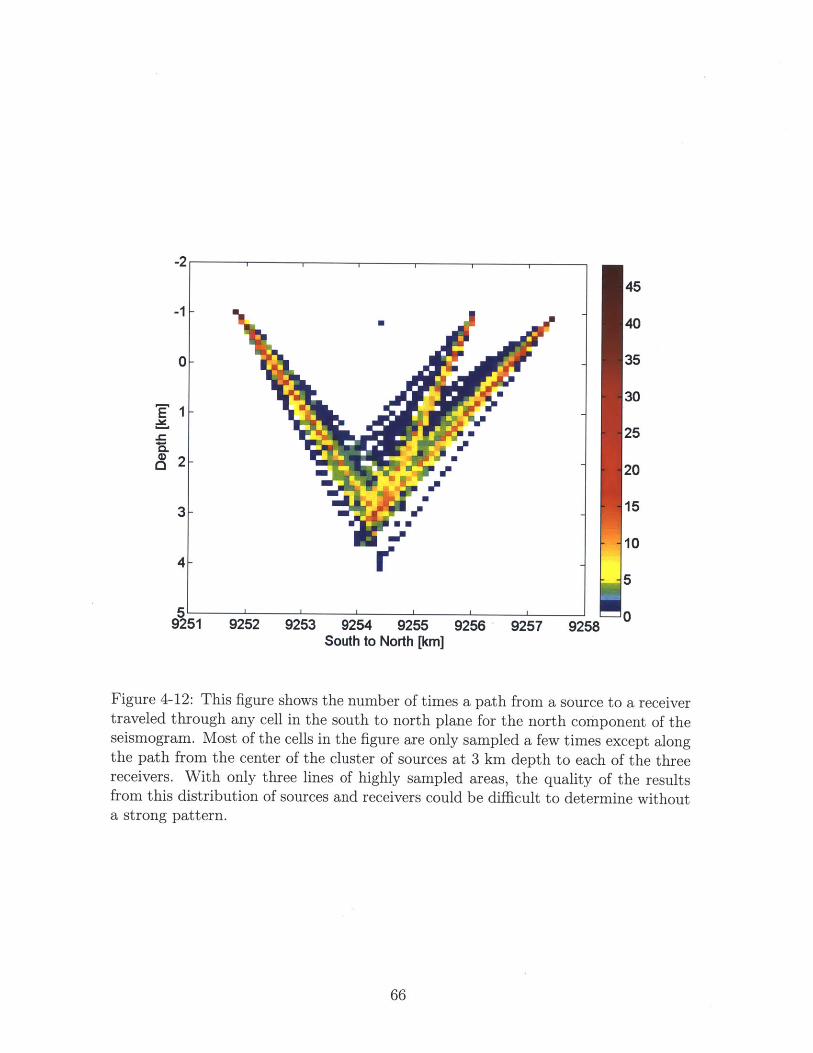
Figure 4-12 shows the number of times a path traveled through each cell in the

64

2

south to north plane of sources and receivers for the north component of the receivers

in that plane. Similarly to Figure 4-9, the cells that were sampled the largest number

of times are either near the receivers or between the largest cluster of sources and

each receiver. In this plane of sources and receivers, most of the sources lie in a

single cluster, so many of the paths between individual sources and receivers overlap.

However, most of the cells in the Figure 4-12 are sampled less than 3 times. With the

lack of intersecting paths in this distribution of source to receiver paths, it would be

difficult to draw conclusions from the distribution of g, and B, without strong trends

like the trends found in this results from this dataset.

65

9252 9253 9254 9255South to North [km]

45

40

35

30

25

20

15

10

5

92 156 92 157 92 158 i

Figure 4-12: This figure shows the number of times a path from a source to a receivertraveled through any cell in the south to north plane for the north component of theseismogram. Most of the cells in the figure are only sampled a few times except alongthe path from the center of the cluster of sources at 3 km depth to each of the threereceivers. With only three lines of highly sampled areas, the quality of the resultsfrom this distribution of sources and receivers could be difficult to determine withouta strong pattern.

66

-2

ET

.a:

1

2

E

I..-U

5192

' ' I ' I

51

-1-

0-

3-

4-

Chapter 5

Discussion

The implications of the results for the intrinsic attenuation coefficient, B,, and the

scattering coefficient, go, that are shown in Chapter 4 are examined in this chapter

for both the synthetic acoustic dataset and the Awibengkok microseismic dataset.

Potential areas for further investigation with the Aweibengkok dataset are also dis-

cussed.


The two dimensional synthetic acoustic dataset was created in order to test the

MWTLA code and explore some of the limitations of the process with a dataset

that did not have the complications and uncertainties associated with real seismic

signals. The synthetic waveforms were designed to have a value for intrinsic attenua-

tion, a, of 0.3 km-1 and estimated to have a value for the scattering coefficient, go, of

1 km- 1 . This gives the expected value of B, of 0.77. Figure 4-2 has an average value

of B, of 0.71, which is close to the expected value of 0.77. Figure 4-1 has an average

value of g, of 1.77 km-1, which is close to the expected value of 1 km- 1 . This is a

relatively small difference in g, considering that reasonable values for go range over

several orders of magnitude. The values for B0 and go calculated by MWTLA agree

with the expected results for the synthetic acoustic model.

The agreement of the results from the application of MWTLA to the synthetic

67

acoustic dataset with the values predicted based on the construction of the model gives

confidence in the MWTLA code and MWTLA itself. This agreement remains true

for the two other velocity models in the synthetic acoustic dataset. Other variations

on the specific setup in Figures 4-2, 4-1, and 4-3, were also examined where variables

such as the depths of sources, the numbers of sources, the distribution of receivers,

the number of receivers, and the density of receivers were changed within the dataset

as described in Section 2.1. Despite these changes, the general agreement between

the expected values and the calculated values did not change. These results support

the robustness of MWTLA.


Two dimensional MWTLA was used on the Awibengkok microseismic dataset to find

the distribution of values for B, and go. The north and east components of the

receivers both gave approximately the same image for the same variable. The shear

component that was chosen does not significantly alter the resulting figures. The

north component of the seismogram will be used for discussion in this section.

There are several significant geological features in the region of the microseismic

dataset that are described in detail in Section 1.3. The Cianten Caldera is a cylindrical

structure that is less than 5 km across and is separated from the active Awibengkok

goethermal field by the Maura fault. The Maura Fault is an impermeable fault that

trends north-northeast with an unknown dip between the Awibengkok field and the

Cianten Caldera. The fault crosses the west to east plane at 679.2 km and the south

to north plane at 9254.3 km. There are several sets of parallel faults and joints caused

by regional stresses from the nearby active subduction zone. The Rhyodacite Marker

is an anisotropic smectite clay layer that extends over both the Awibengkok field and

the Cianten Caldera. This is the impermeable cap of the Awibengkok geothermal

reservoir. Drilling has confirmed that temperatures are lower in the Cianten Caldera

and some of the fractures have been filled by precipitants. [23]

More subtle variables that affect the signal include anisotropy and attenuation.

68

Anisotropy is affected by strain, stress, temperature, pressure and volatile content. [15]

Intrinsic attenuation primarily comes from the motion of water within pores and

fractures in the rock. Intrinsic attenuation does happen within the rock itself, however

the movement of water is a much more efficient way to dissipate heat than the friction

caused by shear waves within a rock, so the majority of the energy lost to intrinsic

attenuation is lost in the presence of water. [20, Ch. 7] Scattering attenuation depends

on the frequency of the wave because waves are best scattered by heterogeneities on

the order of magnitude of their wavelength. Also, there is little difference between the

effect of scattering from relatively few heterogeneities with a high reflection coefficient

and scattering from many heterogeneities with low reflection coefficients.

Figure 4-5 showed that the peak frequencies found in the microseismic trace from

Figure 4-4 in the dataset range from 3.5 Hz to 6.5 Hz. The corresponding wavelengths

of these waves assuming a 3.5 km/s velocity is 539 m to 1 km. This is the size of the

heterogeneity needed to scatter this wave.

Figures 4-7 and 4-10 both show very small variation over the extent of the data.

There is also no discernible pattern or trend in either figure. Consequently, these

results show that the value for g, in the west to east plane and in the south to

north plane is approximately constant in that plane. Figure 4-7 has an average

value for g, of 1.05 km-1, so the mean free path, 1 is 0.95 km. Figure 4-10 has

an average value for g, of 1.25 km-1, so 1 is 0.8 km. These values for g, agree

with the values for go of 1 km- 1 from Yamamoto and Sato 2010.[28] The smaller

value for the mean free path for the south to north plane of sources and receivers

indicates that scatterers occur more frequently along the south to north plane than

the west to east plane. Scatterers can be faults or joints in the medium. In Figure 1-

4 shows several parallel, regularly spaced faults, especially through the Awibengkok

geothermal field. These faults extend from the surface through the Awibengkok

geothermal field and have sectioned the producing field into different regions that

have limited hydrological contact with one another.[23]. These faults that trend to

the northeast have a significant impact on the properties of the region that they

divide. The west to east plane of sources and receivers does not trend directly east to

69

000

C g CIn[unji qIoN oi 4tloS

[] CN[unji IP.oN oi I4nfoS

C4

,o

00

010

0

0

CN

o4 ON[uq] gyoN ol MinoS

[uDI] tpo

Figure 5-1: This figure shows a simplified geology map of the Awibenkok region in theupper left alongside both the figures for B0 for the Awibengkok microseismic dataset.The west to east cross section is located below the simplified geology map and thesouth to north cross section is located to the right of it. The colorbars are unitless.The figure in the lower left hand corner summarizes the results from both planes ina map view.

70

~cINj1<1 V

C

00

0

0

Co

L~u

*

pa.

i

0000

S0

40

00

0

oc

0040N

00

0

west. It trends east-northeast, so this plane of sources and receivers is more parallel

to these faults. Since they are more parallel, they will intersect one another less

frequently. If these faults are the primary cause of scattering for the seismic waves,

then the mean free path would also increase. This would result in a distribution of

g, that would depend primarily on the direction of the path between the source and

receiver since the value of 1 would primarily be determined by the spacing at that

angle between sets of regional faults. This angular dependence could be confirmed

by analyzing other planes of data or using three dimensional MWTLA with more

sources and receivers.

Figure 5-1 summarizes the results of applying MWTLA to the microseismic dataset.

The upper left corner is a simplified version of the geology including the Maura fault

and the extent of both the Cianten Caldera and the Awibengkok geothermal field.

The two black lines in the figure are the traces of the west to east cross section and

the south to north cross section. The figure below the map is Figure 4-8 which shows

the values of B0 on the west to east plane of sources and receivers. The figure to the

right of the map is Figure 4-11 that has been rotated 90 degrees and which shows the

values of B0 on the south to north plane of sources and receivers. The x axis and y

axis of the simplified geology map match the corresponding axis on the figures for B,.

The figure in the lower left corner shows a map view of the results for B0 for both

the west to east plane and the south to north plane stacked on top of one another.

The results for the west to east plane are in green. The lower values of B0 and higher

values of a in this figure are on the west side of the cluster of sources that lies at the

intersection of the two cross section lines. The higher values of B0 and lower values of

a are on the east. The results for the south to north plane are in red and yellow. The

red region has is in the Cianten Caldera and has high values for B0 and low values of

a. The yellow regions have lower values of B0 and higher values of a.

The colorbars for the figures for B0 are the same, but the values of B0 in the west

to east plane of sources and receivers cannot be directly compared to the values of

B0 for the south to north plane of sources and receivers. The changes in B0 between

the west to east plane and the south to north plane cannot be directly interpreted as

71

a change in the geology of the region. B depends on both the scattering coefficient,

g0 , and the intrinsic attenuation coefficient, a. The value of go in the west to east

plane is different from the value of go in the south to north plane, so the variation

in Bo is not directly related to a change in the geologic properties of the region. For

this reason, each plane of sources and receivers will be considered independently.

In Chapter 4, it was determined that both figures for Bo have two distinct values

for Bo.

The west to east plane appeared to be to have lower values of Bo of 0.6 on the

western side of the figure and higher values of 0.8 on the eastern side of the figure.

The place where these two values overlap is a cluster of sources that is divided by the

Maura fault at approximately 9254.3 km. The Maura fault is one of the largest faults

in the geologic map in Figure 1-4. The Maura fault is an impermeable fault that

water cannot pass, indicating that the fault itself has different physical properties

that the rest of the region. Since the value of go across the figure was determined to

be constant, the variation in BO must be due to a change in the intrinsic attenuation

coefficient. Since both of the receivers that fall on the west to east plane are to the east

of the fault, all of the waveforms from the western side of the figure on the other side

of the Maura fault must pass through the fault. The bimodal distribution of Bo values

could be explained by the Maura fault being a major source of intrinsic attenuation

due to either softer material that more readily dissipates heat or the presence of

an unusual amount of water. These results indicate that the Maura Fault could be

having a large effect on the distribution of the intrinsic attenuation coefficient.

The south to north plane of sources and receivers saw a general trend for B,

of lower values of 0.65 between the cluster of sources and the northernmost and

southernmost receivers. The paths between the cluster of sources and the middle

receiver at about 9256 km has higher values for Bo of 0.8. The northernmost and

southernmost receivers as can be seen in Figure 2-4 lie further to the east than the

middle receiver. The middle receiver also lies within the Cianten Caldera and since

the cluster of sources lies on the edge of the caldera, the path between the sources

and the receivers samples the caldera along the vast majority of the path. Since the

72

value of g, across the figure was determined to be constant, the increase in B0 in the

Cianten Caldera must be due to a decrease in the intrinsic attenuation coefficient.

The intrinsic attenuation coefficient is to a first order affected by the water content

as water more easily converts seismic energy to heat than rock. A smaller value for

the intrinsic attenuation coefficient could be caused by the presence of less water in

the rock. The lower values of B0 in this area agree with what is known about the

geology of the Cianten Caldera since the cooling of the hydrothermal system has

caused minerals to precipitate into existing fractures. This displaces the water that

was held in those fractures and reduced the overall amount of water in the region.

The relatively low rates of sampling indicated by Figures 4-9 and 4-12 show that

the value in each cell is often only supported by one source and receiver pairing. The

patterns that have resulted from the data that was analyzed is convincing, but the

results would be much more robust with a larger area of multiply sampled cells.

The values obtained for g, and B0 are similar to the values obtained by other

studies[28, 13, 16] in volcanic areas that are discussed in Section 3.3. In such a

heterogeneous environment as a volcano, scattering happens frequently and is the

dominant form of energy loss from the direct arrival. Values for g, are expected to

be relatively large due to the small mean free path. Previous studies have obtained

values for g, of the order of 10-2 to 100. Since scattering is the dominant form of

attenuation, values for B0 are expected to be larger than 0.5, however, specific values

do vary depending on the amount of intrinsic attenuation in the region. Previous

studies have found values of B0 that range from 0.7 to close to 1. The values for

g, and B0 that were obtained in this thesis agree with the expected values for this

region. The Cianten Caldera has a large enough value for g, of approximately 1 km-1

to be a good geothermal field, but the high value of B0 that means a low value of a

indicates that there may not be enough water for an active geothermal field due to the

low temperatures that have caused fractures to seal with mineral precipitants. These

observations agree with what is known of the geology of the region. The Cianten

Caldera would not make a good geothermal field.

The apparent continuation of the cap of the Awibengkok geothermal field to the

73

Cianten Caldera may not exist. The smectite clay layer found over the Cianten

Caldera may be from the caldera lake sediments rather than hydrothermal alteration

of ashes that forms the cap of the Awibengkok field. Alternatively, the cap could

be formed by hydrothermal alteration and the Cianten Caldera may have been cut

off from the Awibengkok field by the Maura fault and lost circulation of fresh hot

fluids from intrusions. If the Awibengkok field and the Cianten Caldera have never

been connected geothermally, then there is little likelihood that the Cianten Caldera

will ever be a viable option for geothermal energy without the formation of a new

intrusion. If the two regions were connected prior to the rupture of the Maura fault,

there is a chance that the impermeable barrier of the Maura fault could be broken

and hydrothermal activity eventually restored by a process like hydrofracing. Such an

endeavor on the scale that would be required may be beyond current technology and

the timescale of reheating the Cianten reservoir may be too long to be economically

viable. An extension of the smectite clay layer may in a direction different than the

Cianten Caldera may prove more fruitful to pursue.

5.3 Future Work

More information about the geologic characteristics of the Cianten Caldera and the

Awibenkok geothermal field could be extracted from the Awibengkok microseismic

dataset beyond the scope of what was investigated in this thesis. Further work with

MWTLA and the Awibengkok microseismic dataset could increase confidence in the

trends observed in the Cianten Caldera and the surrounding area, reveal other pat-

terns that are not observable within the limitations of this study, and extend the

geographic extent of the current results.

The amount of the data from the Awibengkok microseismic dataset that was

used in this analysis was limited. The vertical component of the receivers was not

examined. The dataset includes events from 2005 to 2010 distributed across the

entire Awibengkok geothermal field and the surrounding areas, but the events used

were limited to October 2008 when there was significant activity near the Cianten

74

Caldera. Utilizing more sources and receivers over a larger geographic area would

increase both the redundancy of the results and the extent of the region covered.

This would also allow the variables B, and g, to be monitored with respect to time

as the Awibengkok field has been developed.

The distribution of the sources and the receivers that were selected for analysis

in this thesis is well suited to a two dimensional application of MWTLA. However,

a three dimensional application of MWTLA would sample much more of the geology

and avoid any distortions caused by the projection of sources and receivers onto a

two dimensional plane. Due to the larger volume that affected by a three dimensional

analysis, more sources and receivers would be required in order to resolve the changes

in B, and g, over the Awibengkok region.

This particular study analyzed the broadband values of g, and B0 using the wave-

forms in their entirety. However, these variables can also be investigated with respect

to the frequency dependence of the waveforms by filtering the waveforms to specific

frequency bands. This type of analysis has been successfully conducted on different

types of regions as is discussed in Section 3.3.[6, 16, 12, 14, 2, 3, 5, 4, 28]

The simplification for MWTLA of isotropic, homogeneous scattering as described

in Section 3.2 is not likely to be accurate for the interior of the Earth. This is espe-

cially true in volcanic regions like the Cianten Caldera and the Awibengkok geother-

mal field, since the accumulation of layers of volcanic rock which forms volcanoes

results in strongly heterogeneous rocks. [16] Another distribution that includes hetero-

geneities may be more accurate. [10] The extra degrees of freedom added by removing

the homogeneous assumption would require more sources and receivers for the same

resolution in order to resolve heterogeneities.

75

Bibliography

[1] Jorge A. Acufna, James Stiamc, Lutfhie Sirad-Azwar, and Riza Glorius Pasikki.

Reservoir management at Awibengkok geothermal field, West Java, Indonesia.

Geothermics, 37(3):332-346, 2008.

[2] D.A. Adams and R.E. Abercrombie. Seismic attenuation above 10 Hz in southern

California from coda waves recorded in the Cajon Pass borehole. Journal of

Geophysical Research, 103(B10):24257 - 70, Oct. 1998.

[3] F. Bianco, E. Del Pezzo, M. Castellano, J. Ibanez, and F. Di Luccio. Separation

of intrinsic and scattering seismic attenuation in the Southern Apennine zone,

Italy. Geophysical Journal International, 150(1):10-22, 2002.

[4] Eduard Carcol and Haruo Sato. Spatial distribution of scattering loss and intrin-

sic absorption of short-period S waves in the lithosphere of Japan on the basis of

the Multiple Lapse Time Window Analysis of Hi-net data. Geophysical Journal

International, 180(1):268-290, 2010.

[5] U. Dutta, N. N. Biswas, D. A. Adams, and A. Papageorgiou. Analysis of S-Wave

Attenuation in South-Central Alaska. Bulletin of the Seismological Society of

America, 94(1):16-28, 2004.

[6] Michael Fehler, Mitsuyuki Hoshiba, Haruo Sato, and Kazushige Obara. Separa-

tion of scattering and intrinsic attenuation for the Kanto-Tokai region, Japan,

using measurements of S-wave energy versus hypocentral distance. Geophysical

Journal International, 108(3):787-800, 1992.

77

[7] A. Frankel and L. Wennerberg. Energy-flux model of seismic coda: separation

of scattering and intrinsic attenuation. Bulletin of the Seismological Society of

America, 77(4):1223 - 51, 1987.

[8] John P. Grotzinger and Thomas H. Jordan. Understanding Earth. W.H. Freeman

and Company, New York, Sixth edition, 2010.

[9] David P. Hill, Roy A. Bailey, and Alan S. Ryall. Active tectonic and magmatic

processes beneath Long Valley Caldera, eastern California: An overview. Journal

of Geophysical Research: Solid Earth, 90(B13):11111-11120, 1985.

[10] M. Hoshiba. Simulation of multiple-scattered coda wave excitation based on the

energy conservation law. Physics of the Earth and Planetary Interiors, 67(1-

2):123 - 36, 1991.

[11] Mitsuyuki Hoshiba. Separation of scattering attenuation and intrinsic absorp-

tion in Japan using the multiple lapse time window analysis of full seismogram

envelope. Journal of Geophysical Research, 98(9):15809-24, 1993.

[12] Anshu Jin, K. Mayeda, D. Adams, and K. Aki. Separation of intrinsic and

scattering attenuation in southern California using TERRAscope data. Journal

of Geophysical Research, 99(B9):17835 - 48, Sept. 1994.

[13] Jim Kauahikaua. Geophysical characteristics of the hydrothermal systems of

Kilauea volcano, Hawaii. Geothermics, 22(4):271 - 299, 1993.

[14] Peter Leary and Rachel Abercrombie. Frequency dependent crustal scattering

and absorption at 5-160 Hz from coda decay observed at 2.5 km depth. Geo-

physical Research Letters, 21(11):971-974, 1994.

[15] Maureen D. Long and Paul G. Silver. Shear Wave Splitting and Mantle

Anisotropy: Measurements, Interpretations, and New Directions. Surveys in

Geophysics, 30(4-5):407 - 461, 2009.

78

[16] K. Mayeda, S. Koyanagi, M. Hoshiba, K. Aki, and Y. Zeng. A comparative study

of scattering, intrinsic, and coda Q-1 for Hawaii, Long Valley, and central Cal-

ifornia between 1.5 and 15.0 Hz. Journal of Geophysical Research, 97(B5):6643

- 59, May 1992.

[17] Gabriela Melo, Alison Malcolm, Oleg Poliannikov, and Michael Fehler. Analysis

of location uncertainty for a microearthquake cluster: A case study. Society of

Exploration Geophysicists, 2012.

[18] K. R. Newcomb and W. R. McCann. Seismic History and Seismotectonics of the

Sunda Arc. Journal of Geophysical Research, 92(B1):421-439, 1987.

[19] J. C. J. Paasschens. Solution of the Time-dependent Boltzmann Equation. Phys.

Rev. E, 56:1135-1141, July 1997.

[20] Peter Shearer. Introduction to Seismology. Cambridge University Press, Cam-

bridge, Second edition, 2009.

[21] M. L. Sorey, C. D. Farrar, G. A. Marshall, and J. F. Howie. Effects of geothermal

development on deformation in the Long Valley Caldera, eastern California,

1985-1994. Journal of Geophysical Research: Solid Earth, 100(B7):12475-12486,

1995.

[22] Seth Stein and Michael Wysession. An Introduction to Seismology, Earthquakes,

and Earth Structure. Blackwell Pub., Malden, MA, 2003.

[23] James Stimac, Gregg Nordaddquist, Aquardi Suminar, and Lutfhie Sirad-Azwar.

An overview of the Awibengkok geothermal system, Indonesia. Geothermics,

37(3):300 - 331, 2008.

[24] Jim Stimac, Birean D. Sagala, and Mirzal Nur Ardhie. Geologic Map of the

Cianten Caldera, Indonesia.

[25] Jim Stimac, Birean D. Sagala, and Gregg Nordquist. Salak Awibengkok - West

Java: Geology and Structure Map of the Cianten Caldera, Indonesia. 2009.

79

[26] Ru-Shan Wu. Multiple scattering and energy transfer of seismic waves- Sepa-

ration of scattering effect from intrinsic attenuation. I. Theoretical modelling.

Geophysical Journal of the Royal Astronomical Society, 82(1):57 - 80, 1985.

[27] Ru-Shan Wu and Keiiti Aki. Multiple scattering and energy transfer of seismic

waves- Separation of scattering effect from intrinsic attenuation. II. Application

of the theory to Hindu Kush region. Pure and Applied Geophysics, 128(1-2):49-

80, 1988.

[28] Mare Yamamoto and Haruo Sato. Multiple scattering and mode conversion

revealed by an active seismic experiment at Asama volcano, Japan. Journal of

Geophysical Research.Solid Earth, 115(7), 2010.

[29] Keita Yoshioka, Riza Pasikki, Indra Suryata, and Ken Riedel. Hydraulic Stim-

ulation Techniques Applied to Injection Wells at the Salak Geothermal Field,

Indonesia. In SPE Western Regional Meeting 2009. Society of Petroleum Engi-

neers, Curran Associates Inc., 2009.

80

geologic interpretations of seismic scattering and

Documents