geography and realty prices: evidence from … and realty prices: evidence from international...
TRANSCRIPT

Geography and Realty Prices: Evidence from International Transaction-Level Data
Daisuke Miyakawa Chihiro Shimizu
and Iichiro Uesugi
March, 2016
Grant-in-Aid for Scientific Research(S) Real Estate Markets, Financial Crisis, and Economic Growth
: An Integrated Economic Approach
Working Paper Series No.52
HIT-REFINED PROJECT Institute of Economic Research, Hitotsubashi University
Naka 2-1, Kunitachi-city, Tokyo 186-8603, JAPAN Tel: +81-42-580-9145
E-mail: [email protected] http://www.ier.hit-u.ac.jp/hit-refined/
Geography and Realty Prices:
Evidence from International Transaction-Level Data*
Daisuke Miyakawa†
Hitotsubashi University, Graduate School of International Corporate Strategy
Chihiro Shimizu
National University of Singapore, Institute of Real Estate Studies
Iichiro Uesugi
Hitotsubashi University, Institute of Economic Research
March 2016
Abstract
In this paper, we examine the role of the international flow of capital in real estate prices by
quantifying the relation between investors’ geographical locations and the prices they pay for
their realty investments. Our data set contains more than 30,000 realty investment transactions
in Australia, Canada, France, Hong Kong, Japan, Netherlands, the United Kingdom, and the
United States. First, we find that foreign investors pay significantly higher prices than domestic
investors do even after taking a wide variety of controls into account. Second, this overpricing
becomes smaller as the buyers’ exposure to realty investments in the host countries becomes
higher. Third, in support of these results, the investment returns of foreign investors are
systematically lower than that of domestic investors. This negative excess return becomes
smaller as the buyers’ exposure to the host countries becomes higher. These results indicate that
the overpricing of foreign investors occurs when investors are less informed about the local
property market and lessens with the accumulation of investment experience.
Keywords: Realty Price; Transaction Data; Geographical Location; Fixed Effects
JEL classification: D83, F21, G12, R30
* This research was conducted as a part of the work of JSPS KAKEN Grant (S) 25220502. We thank Bob White, Jim Sempere, Yiqin Wang, Doug Murphy, Willem Vlaming, and Yogeeta Chatoredussy of RCA for kindly providing the data on international real estate transactions and for valuable comments. † Corresponding author: Associate Professor, Graduate School of International Corporate Strategy, Hitotsubashi University, 2-1-2 Hitotsubashi, Chiyoda-ku, Tokyo 101-8439 JAPAN. E-mail: [email protected]. Tel: +81342123101. Fax: +81342123020.

2
1. Introduction
Given that international realty investment is one of the major alternative investments, a
large body of literature has attempted to examine the impacts of the international money flow on
realty prices. The interaction between the international money flow and real estate markets becomes
more relevant in the age of the global saving glut in which a large influx of capital from emerging
economies lowers long-term interest rates and contributes to a run-up in asset prices (Bernanke
2005). Recently, many studies examine the argument that global imbalances in money flows have
contributed to a massive fluctuation in asset prices, above all, real estate prices. On the one hand,
Jordà et al. (2014) point out that a change in monetary policy in one country could play an important
role in generating a large fluctuation in realty prices in other countries through a change in the
international money flow. On the other hand, Favilukis et al. (2013) counter the presumption that the
change in the international monetary flow leads to a large fluctuation in local realty prices. In this
study, we examine this unsettled question by using a unique data set that accounts for a large number
of international property investment transactions.
Presumably, if the prices paid by foreign investors are systematically higher than domestic
investors, then the international money flow could create a demand shock in the local market. Given
that many pieces of anecdotal evidence suggest that foreign investors are the central cause of local
property booms,3 a considerable number of empirical studies examine the pricing implication of the
international money flow in the context of realty prices. However, the majority of these studies use
aggregated data (e.g., Aizenman and Jinjarak 2009; Favilukis 2013) and have yet to reach a decisive
conclusion on the relation between foreign realty investments and its prices. This is partly due to a
3 As one example of such a discussion, see http://www.news.com.au/finance/real-estate/buying/housing-affordability-are-foreign-investors-to-blame-for-australias-high-property-prices/news-story/710ba2cff1932f0fb3f81ce83a07946b.
3
lack of international transaction-level data on realty investment, although a limited number of
exceptions exist such as Badarinza and Ramadorai (2015). To date, our knowledge on the
characteristics of real estate transactions is not sufficiently clear on how the pricing patterns of
domestic real estate investors differ from those of foreign investors.
The aim of this study is to investigate the impact of geography, especially the impact of
crossing country borders, on the pricing patterns in real estate markets. We use the micro-level
information associated with each investment transaction instead of aggregate-level data. To be more
precise, we estimate the extent to which the prices that foreign investors pay for their realty
investments are different from those of domestic investors. The estimations control for property
characteristics (e.g., location, type, size, and age), and transaction characteristics (e.g., geographical
locations of buyers and sellers, and the type of buyers and sellers).
Furthermore, based on theoretical considerations, our empirical analysis examines the role
of the information accumulated by foreign investors in the real estate markets of host countries.
Specifically, following the studies that focus on other financial markets, we assume that the
information disadvantage of foreign investors gradually lessens over the course of their investment
experience. Focusing on stock markets, for example, Coval and Moskowitz (2001) empirically show
that the geographical distance between fund managers specializing in domestic corporate stocks and
the portfolio companies matter for the performance of the fund managers. Based on their estimation
results, they claim that the information advantage of fund managers that are geographically close to
the target domestic firms contributes to better investment performance. While Coval and Moskowitz
(2001) exclusively deal with the geographical distance between fund managers and domestic
companies, the discussion of home country bias in the extant literature implies that distance matters
more for the case of cross-border investments than for domestic investments. We further presume

4
that, in the case that the investors’ location is different from the host country, the abovementioned
“learning-by-investment” (e.g., Sorensen 2008, Gompers et al. 2008) might help them to acquire
information associated with the local real estate. Notably, given that the heterogeneity associated
with real estate is supposed to be much higher than that of other traditional investment objects (e.g.,
stocks and bonds), the research finds that the effect of accumulated cross-border investment
experience should effectively suppress the price difference between foreign and domestic investors.
This study is the first to explicitly examine both the difference between the pricing behaviors of
foreign and domestic investors in the context of the realty prices and the effect arising from firms’
previous cross-border investment experience.
Our findings are as follows. First, we find, that foreign investors pay substantially higher
prices than domestic investors do even after taking into account a wide variety of controls. Second,
this price difference becomes smaller as the buyers’ investment exposure to the host countries where
the properties in their portfolio are located becomes higher. Third, consistent with these results, the
investment returns of foreign investors are systematically lower than that of domestic investors. This
negative excess return becomes smaller as the buyers’ exposure to the host countries becomes higher.
These results indicate that the overpricing occurs especially when foreign investors are less informed
about the local realty markets.
The remainder of this study is organized as follows. In Section 2 we briefly survey the
related literature that provides the theoretical underpinnings of our empirical study. We explain the
data and our empirical framework in Section 3. In Section 4 we examine and discuss the empirical
results associated with the realty prices paid by foreign and domestic investors. Section 5 concludes
and presents future research questions.
5
2. Related Literature and Theoretical Underpinnings
In this section, we first provide a brief survey of the studies on the impacts of international
money flow on local realty prices. We then survey the literature that highlights the role of the
geographical location of investors in various security prices.
A considerable number of studies quantitatively examine the determinants of real estate
prices. Aizenman and Jinjarak (2009) use aggregate-level data on 43 countries from 1978 to 2008
and show that current account deficits, which are largely associated with the international money
flow to these countries, have positive impacts on the realty prices. Justiniano et al. (2014) also posit
that international money flows accounted for a sizable portion of the increase in US house prices
before the recent financial crisis of 2008. In contrast with the studies that emphasize the importance
of money flow on real estate prices, Favilukis et al. (2013) also use aggregate-level statistics and
insist that the impact of the international money flow on real estate market is limited. Ferrero (2014)
also focuses on the negative association between house prices and the current account in the United
States and in several other countries and states that several domestic factors such as credit and
preference shocks can explain this association. In sum, these studies have yet to reach a decisive
conclusion regarding the role of international money flows to the local realty market.
A number of studies use the micro-evidence on the determination of realty prices to focus
on the information asymmetry in real estate. Kurlat and Stroebel (2015), for example, use the data on
realty transactions for Los Angeles county in the United States and analyze the determinants of the
change in realty prices. They find that the physical characteristics of both the property itself and
nearby properties as well as the information asymmetry about these characteristics between insiders
(i.e., residents in the area) and outsiders determine realty prices. Based on the empirical evidence
that the increase in prices after investment is smaller when the share of informed sellers is higher and

6
the buyer is less informed; they conclude that information asymmetry is an important determinant of
realty prices. In a similar vein, Garmaise and Moskowitz (2004) use the realty transaction data in the
United States and find that the geographical distance between the buyers and the property becomes
shorter as the information asymmetry faced by the buyers becomes larger. They also show that the
median distance between the buyers and the property is short (i.e., 47km) and such a distance
becomes shorter as the dispersions of evaluated value and transaction prices become larger.
Furthermore, the latter becomes less apparent for older property. In sum, they show that the
geographical distance between the buyers and the property is an important characteristic associated
with information asymmetry. The difference between their study and the present study is that we
extend their discussion to international transactions. We presume that the theoretical predication in
these studies becomes more critical in the context of international transactions where information
asymmetry is more significant.
Somewhat in the same context, Badarinza and Ramadorai (2015), also feature the role of
the proximity between buyers and property in the context of the transmission of shocks. In their
study, they use detailed resident information in London and show that foreign residents transmit an
exogenous shock in their home country (i.e., outside of UK) to the realty prices in the host country.
This result indicates that the proximity between buyers and property affects the way of shocks in
buyer countries to transmit to host countries, thus drives realty transactions. The biggest difference
between their studies and the present study is that we use many pairs accounting for buyer countries
and the countries where the properties are so that we have greater heterogeneity to extract a more
detailed mechanism that affects realty transactions.
Literature already exists on this importance of geographical characteristics on investments
in other financial markets. First, Coval and Moskowitz (2001) show that the geographical distance
7
between the fund manager and the portfolio’s companies matter for performance. They find that the
abnormal return associated with the investment with a shorter distance is larger. Further, this pattern
is more apparent for the investments in companies in small towns where information asymmetry
matters more. The authors also find that the advantage of geographical proximity shows some
persistency. While such a result in Coval and Moskowitz (2001) specifically shows the advantage of
local investors, we could also presume that greater exposure to the distant companies allows fund
managers to learn, which Sorensen (2008) theoretically models and empirically studies in the context
of venture capital funds. Gompers et al. (2008) also study the importance of venture capital funds’
investment experience. Given these discussions, the present paper examines the advantage of local
investors and how such an advantage varies as the investment to distant properties accumulates.4
Another strand of studies, such as Autor et al. (2014), argue that an exogenous shock
induces price changes in nearby properties. They use the termination of rent control in Cambridge,
Boston, in 1995. Their natural experiment shows that the prices of the properties close to the
property facing the termination of rent control increase. This spillover indicates that overpricing for
other reasons, for example that of less informed investors, could exhibit a similar effect.
Given the abovementioned reasoning, we hypothesize that foreign investors pay
substantially higher prices (lower returns) than domestic investors, and this price difference becomes
smaller as the buyers’ exposure to realty investments in the host country increases. In order to
examine this hypothesis, we regress the property price on a wide variety of variables including the
investors’ geographical location and investment experience while controlling for a comprehensive
list of transaction-level and aggregate-level characteristics.
4 There are also many studies that measure proximity through various measures (see, e.g., Hochberg et al 2007; Patnum 2013; Shue 2013; Fracassi 2014; Leary and Roberts 2014; Serafinelli 2015).
8
3. Data and Method
3.1. Data overview
The data used for this study are transaction-level data for the period from 2005 to 2015.
We obtain the data from Real Capital Analytics Inc. (RCA), which is one of the most influential data
vendors specializing in real estate investments. The data in RCA reflects institutional investment
activities and cover relatively large investment transactions, which are at least one million USD. The
original data covers 71,000 realty transactions in Australia, Canada, France, Hong Kong, Japan,
Netherlands, the United Kingdom, and the United States. While the properties in a large number (i.e.,
1,223) of cities are recorded in the data, a large part of the data are concentrated in properties located
in the major cities in the eight countries: Amsterdam, Chicago, Kyoto, LA, London, New York,
Osaka, Paris, San Francisco, Sydney, Tokyo, Toronto, and Vancouver. In this sense, the data we use
is mainly for large investments in major cities.
The data contains various information associated with the investment transactions. The
first group of information covers the property included in the transaction: the price measured in USD,
the size of the property’s structure in square feet, and the size of the property’s land in acre measured
as the natural logarithms (LN_PriceUSD, LN_Sqft, and LN_land_area_nb). The data also contains
the age of each structure (Age) as well as its type. The latter information is stored as a categorical
variable accounting for apartment, development site, hotel, industrial, office, other, retail, and
seniors housing and care facilities. In the present study, we construct eight dummy variables for
these property types (Property type).
A wide variety of transaction-related information is also stored in the data set. This
information comprises the identification of the countries where the invested property is (Property
location country), buyer’s location (Buyer country), and the seller’s location (Seller country). In our
9
empirical analysis, we control for these characteristics by including eight dummy variables for
Property location country, and at most 102 dummy variables for Buyer country and Seller country,
respectively. By using these information, we also construct a large number of dummy variables for
the individual effects that pairs the property location and buyer country (Property Location-Buyer
Country). This pair-level individual effect can be used to control for, for example, the geographical
distance between the property’s location and the buyer’s location.5
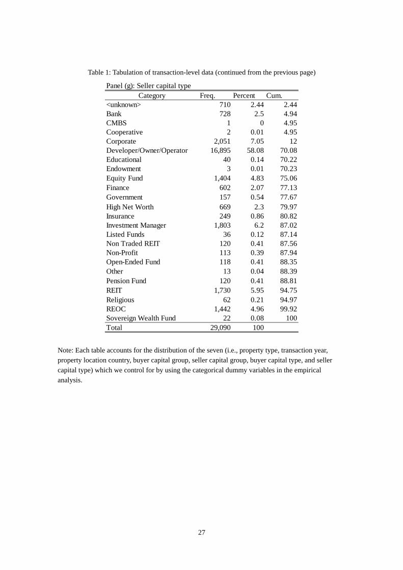
The data further contains the characteristics of the buyers and the sellers in two categorical
variables (Buyer/Seller capital group and Buyer/Seller capital type). The Buyer/Seller capital group
mainly denotes what kind of investment entity the buyer and seller are. The category comprises
equity, institutional, private, and public funds. Partly overlapping with this information, Buyer/Seller
capital type, on the other hand, accounts for the detailed characteristics of investment funds (e.g.,
corporate, developer/owner/operator, investment manager, or REIT). Because the capital group and
type of buyers and sellers are supposed to affect the transaction price, we construct dummy variables
for the relative bargaining power between buyer and seller or the difference in their funding
environments. Each panel of Table 1 tabulates the number of observations falling into each category.
We use the data on the location country associated with the property and the buyer to
construct a dummy variable that equals one if these two locations are different (dum_forbuyer) and
zero otherwise. We hypothesize that the higher information asymmetry in the case of
dum_forbuyer=1 leads to higher (lower) transaction prices (return) compared to the case of
dum_forbuyer=0 (i.e., domestic buyer). Then, in order to take into account the impact associated
with buyer’s investment experience, we construct the accumulated investment amount of the buyer
5 In the original data set, we have the information associated with the top three buyers and sellers. While this information is certainly important to characterize the transaction, we only use the information associated with the top buyer and seller because a large part of the data contain only one buyer and seller.

10
located in a country to a host country and construct the natural logarithms of the sum of accumulated
investment amount for all the buyers headquartered in the same country to each host country
(INVACC_unadj). This pairwise variable is measured at each monthly data point for the previous
month. Although we can compute this variable for each buyer, we choose to construct the variable at
the country level. This choice reflects our presumption that there is information sharing to some
extent among the buyers in one country (Badarinza and Ramadorai 2015). Since this variable
monotonically increases over the data periods, following Gompers et al. (2008), we standardize it to
construct a new variable INVACC by dividing it by the accumulated total sum of the investment
amount of all the buyers located in a country to all the host countries measured at each monthly data
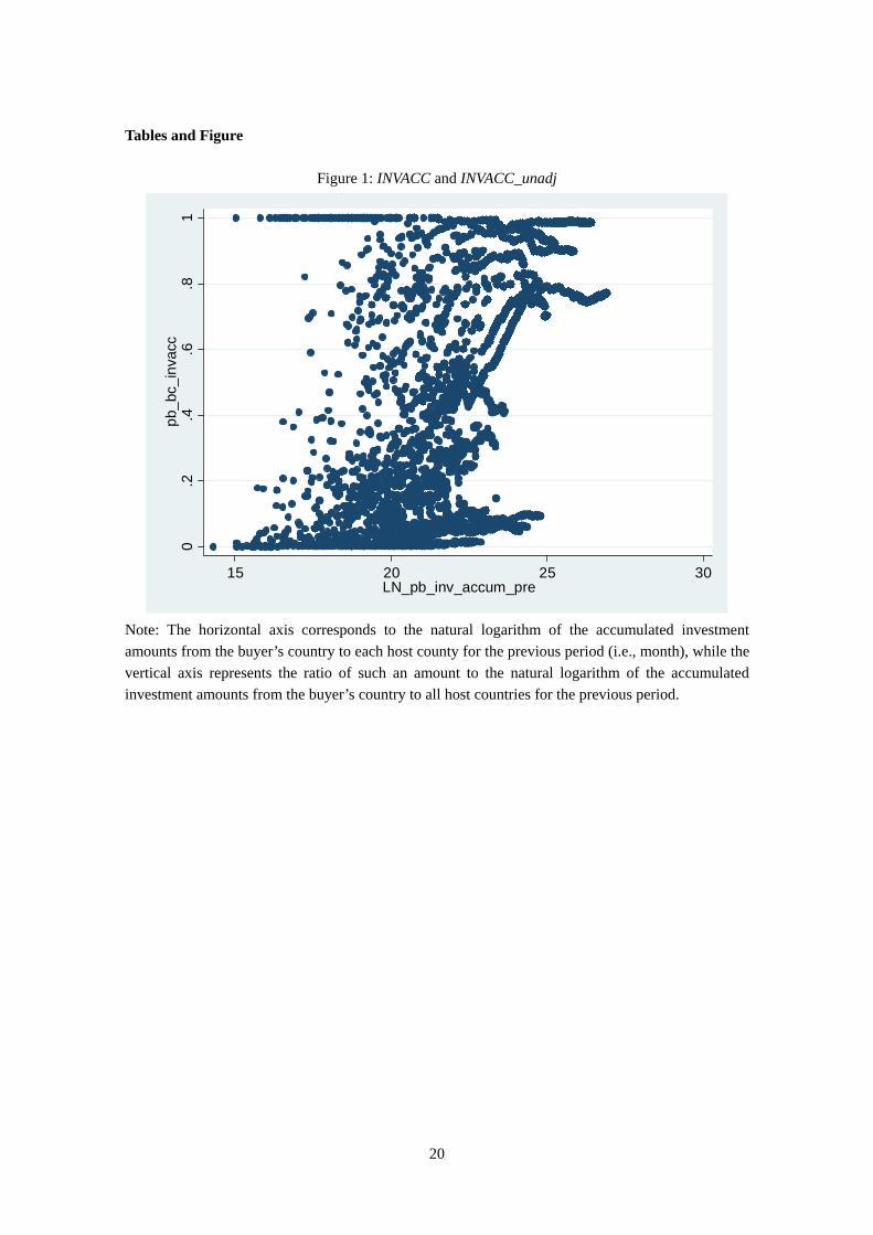
point for the previous month. Figure 1 depicts the scatter plot between these two variables, which
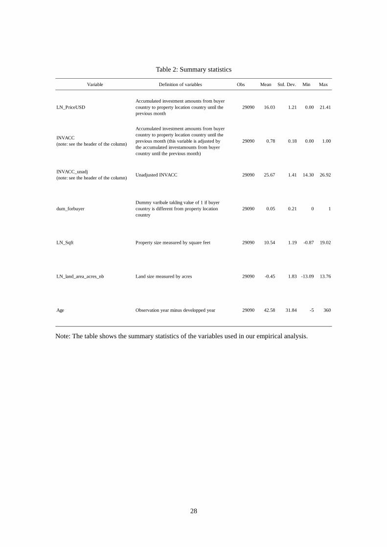
shows an apparent positive correlation. Table 2 lists the summary statistics for each variable. Note
that the number of observations reduces from the original 71,000 to less than 30,000 due to the lack
of information on some variables.
3.2. Empirical framework
Using our transaction-level data, we examine how the buyer’s characteristics (esp.,
dum_forbuyer, INVACC, and its interaction term) as well as other transaction-specific information
affect the transaction price through the following linear regression model:
_ , , , , _ , , ,
_ , , , 1
The left-hand variable accounts for the natural logarithm of the transaction price of property i in

11
country p that is sold by the seller in country s to the buyer in country b in time t (measured
monthly). This variable comprises property-level characteristics , which contains the property’s
size, age, and type. On the right-hand of the equation, _ , accounts for the dummy
variable that equals one if country p and b are different. The , , is the standardized
accumulated investment amounts from country b to country p in the month before t. We include the
interaction term _ , , , to test for the possibility that the impact
associated with _ , varies with the change in , , . The four variables
, , , account for the country-level fixed-effect for the property location, country-level
fixed-effect for the buyer location, location-level fixed-effect for the seller country, and the
time-level fixed effects, respectively.
As another main specification, we also estimate the following equation:
_ , , , , _ , , ,
_ , , , , 2
In this equation, we include an individual effect associated with the property location in
country p and the buyer location in country b ( , ), instead of the two separate individual effects
, . This specification omits . Technically speaking, we can still include this country-specific
individual effect for the seller location. Nonetheless, given that , fairly controls for the
location-related information, we omit in our specification.
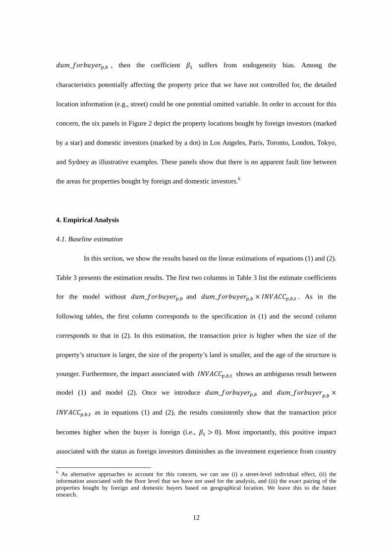
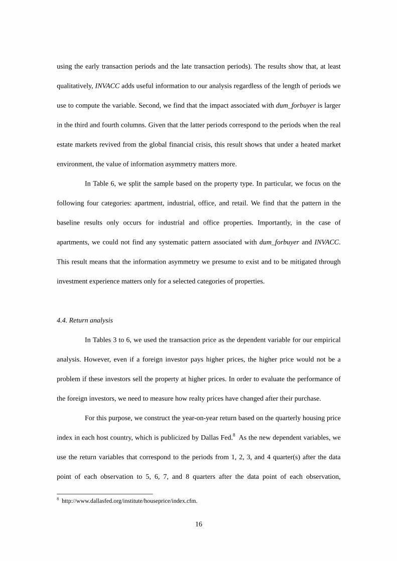
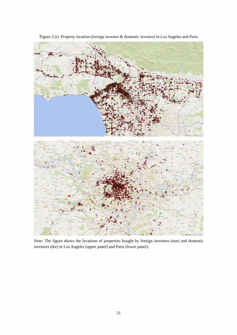
While we include a fair number of characteristics that affect the transaction price, there
could still be a concern about the existence of omitted variables. If, for example, we omit an
important property characteristic that affects _ , , , , and is correlated with
12
_ , , then the coefficient suffers from endogeneity bias. Among the
characteristics potentially affecting the property price that we have not controlled for, the detailed
location information (e.g., street) could be one potential omitted variable. In order to account for this
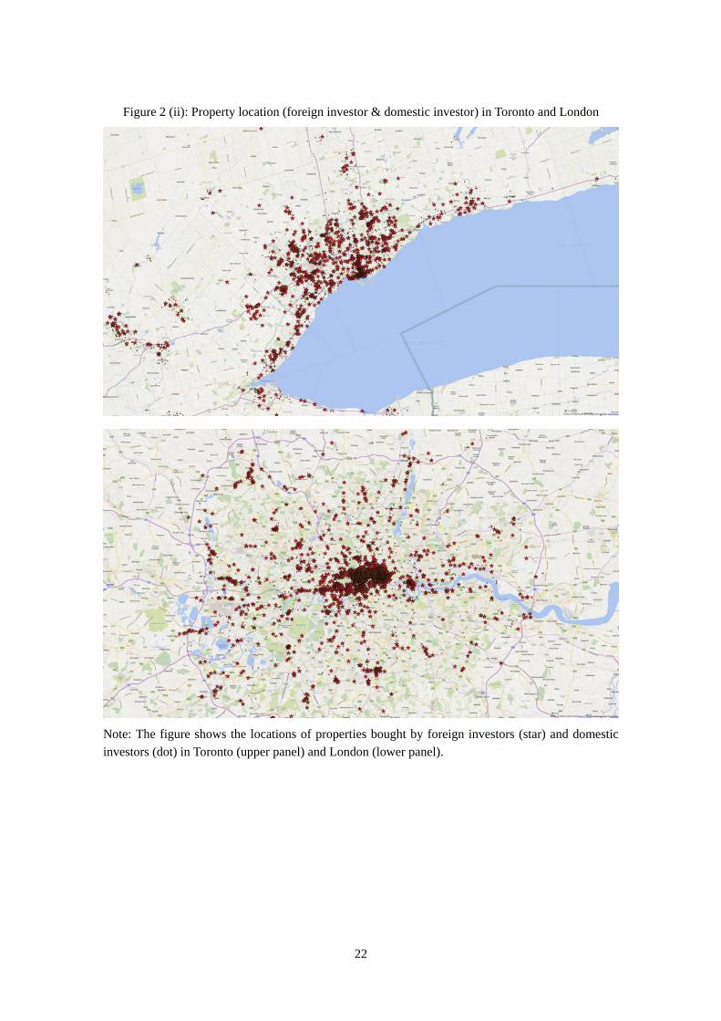
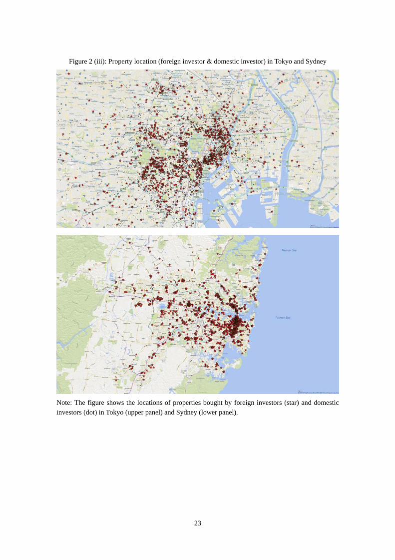
concern, the six panels in Figure 2 depict the property locations bought by foreign investors (marked
by a star) and domestic investors (marked by a dot) in Los Angeles, Paris, Toronto, London, Tokyo,
and Sydney as illustrative examples. These panels show that there is no apparent fault line between
the areas for properties bought by foreign and domestic investors.6
4. Empirical Analysis
4.1. Baseline estimation
In this section, we show the results based on the linear estimations of equations (1) and (2).
Table 3 presents the estimation results. The first two columns in Table 3 list the estimate coefficients
for the model without _ , and _ , , , . As in the
following tables, the first column corresponds to the specification in (1) and the second column
corresponds to that in (2). In this estimation, the transaction price is higher when the size of the
property’s structure is larger, the size of the property’s land is smaller, and the age of the structure is
younger. Furthermore, the impact associated with , , shows an ambiguous result between
model (1) and model (2). Once we introduce _ , and _ ,
, , as in equations (1) and (2), the results consistently show that the transaction price
becomes higher when the buyer is foreign (i.e., 0). Most importantly, this positive impact
associated with the status as foreign investors diminishes as the investment experience from country
6 As alternative approaches to account for this concern, we can use (i) a street-level individual effect, (ii) the information associated with the floor level that we have not used for the analysis, and (iii) the exact pairing of the properties bought by foreign and domestic buyers based on geographical location. We leave this to the future research.

13
b accumulates for country p (i.e., 0). These results are fairly robust for the two model
specifications of equations (1) and (2) and show that even after controlling for a comprehensive list
of information, foreign investors pay higher prices and the systematic change in such overpricing
over the course of the investment experience is observed.
The coefficient associated with the single term , , shows a positive sign that
indicates that a higher , , has an opposite effect for domestic buyers than for foreign
buyers. One source of this difference is the fact that we use the standardized variable for
, , . While we interpret this variable to represent investment experience for the case of
foreign buyers, it could also be a proxy for the precursor of a property bubble in the case of domestic
buyers. Because domestic buyers are already informed about domestic property, a larger exposure
means the property bubble is heating up the market.
Using the results in Table 3, we compute the economic impact associated with
, , . For example, the estimated coefficient associated with _ , (0.423 for
the equation (1)), , , (-0.817 for the equation (1)), and the standard deviation of the
variable (0.18) indicates that , , needs to change by almost three standard deviations
(0.54) to offset the impact associated with _ , (i.e., 0.423 and (-0.817)*0.54 =
-0.44118). These results show that the overpricing of foreign investors is not economically
negligible.
4.2. Additional independent variables and nonlinearity of INVACC
In this section, to control for endogneity bias, we add two more variables to our
estimation. First, we take into account the condition of the real estate market by adding the return
calculated by using the housing price index in each country p. This addition reflects our concern that

14
the positive correlation between the transaction price and INVACC is driven by the temporal price
trend in local markets in country p. Second, we add the investment flow from the countries other
than the buyer location county b to effectively control for demand from other countries. This
addition corresponds to our concern that the positive correlation between the transaction price and
INVACC is driven by the correlated (e.g., herding) behavior of the foreign investors who are locating
in multiple countries.
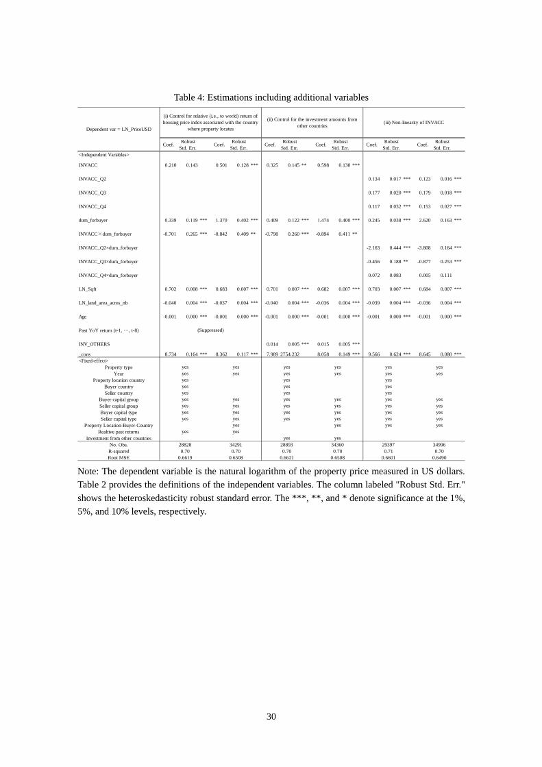
The first four columns in Table 4 show these additional estimation results. The first and
second columns correspond to equations (1) and (2) while controlling for the year-on-year return
based on the quarterly housing price index for each property location. We add the return variables
that correspond to the periods from 16, 15, 14, 13, 12, 11, 10, and 9 quarters prior to the data point of
each observation to the 8, 7, 6, 5, 4, 3, 2, 1 quarter(s) prior to the data point of each observation,
respectively. Thus, we add eight return variables to equations (1) and (2). The results are fairly
robust and consistent with those in the baseline estimation.
The third and fourth columns correspond to equations (1) and (2) while controlling for the
investment flows from other countries. For this estimation, we add the aggregated investment
amount other than that from the buyer location country b during the previous month to the data point
of each observation. While the newly added variable, which is supposed to account for the demand
pressure from other countries, shows a positive sign, the results associated with _ , ,
, , , and _ , , , are intact.
In the fifth and sixth columns of Table 4, we show that the estimation results for the
nonlinearity of INVACC. To be more precise, we construct four dummy variables (INVACC_Q1,
INVACC_Q2, INVACC_Q3, and INVACC_Q4) equal to one if INVACC falls in the first, second, third,
and fourth quantiles, respectively. Adding the last three dummy variables (i.e., INVACC_Q2,

15
INVACC_Q3, and INVACC_Q4) and their interaction terms with dum_forbuyer to the model, we
estimate the two models as in specifications (1) and (2). This modification of the model also
accounts for the concern about the high correlation between dum_forbuyer and INVACC in the
baseline estimation. Notably, the correlation coefficients between dum_forbuyer and (INVACC_Q1,
INVACC_Q2, INVACC_Q3, INVACC_Q4) are -0.5359, -0.0702, 0.097, and 0.5898, respectively.
First, in both columns, the coefficient associated with dum_forbuyer takes a positive value,
which is consistent with the baseline result. Furthermore, the coefficient associated with the
interaction terms between dum_forbuyer and INVACC_Q2 (-2.163 for (1)), and dum_forbuyer and
INVACC_Q3 (-0.456 for (1)) show negative signs. These results, especially the relative size of the
two coefficients, show that the contribution associated with the accumulated investment experience
matters especially in the stage where the INVACC is small. This is consistent with the presumption
that the additional information acquired through investment experience does not largely matter once
the foreign investors acquire enough information.7
4.3. Subsample analysis
In this subsection, we present whether the estimation results in Table 3 are affected by the
subsample analysis or not. First, we split the sample into two subsamples corresponding to the early
transaction periods (i.e., before 2011) and the late transaction periods (i.e., 2011 and onward). The
results in Table 5 show, first, that the qualitative features are consistent with those in Table 3.
Furthermore, given that the appropriateness of INVACC could potentially be affected by the length of
periods we use for its calculation, this exercise also checks the validity of INVACC computed by
7 We also conducted two robustness checks for the estimation results by using only the INVACC smaller than one to exclude the case where a country has exposure to properties in only one country. Then, we employ INVACC_unadj, which is the natural logarithm of the accumulated investment amounts instead of INVACC. Both the estimations provide consistent results with the baseline results.
16
using the early transaction periods and the late transaction periods). The results show that, at least
qualitatively, INVACC adds useful information to our analysis regardless of the length of periods we
use to compute the variable. Second, we find that the impact associated with dum_forbuyer is larger
in the third and fourth columns. Given that the latter periods correspond to the periods when the real
estate markets revived from the global financial crisis, this result shows that under a heated market
environment, the value of information asymmetry matters more.
In Table 6, we split the sample based on the property type. In particular, we focus on the
following four categories: apartment, industrial, office, and retail. We find that the pattern in the
baseline results only occurs for industrial and office properties. Importantly, in the case of
apartments, we could not find any systematic pattern associated with dum_forbuyer and INVACC.
This result means that the information asymmetry we presume to exist and to be mitigated through
investment experience matters only for a selected categories of properties.
4.4. Return analysis
In Tables 3 to 6, we used the transaction price as the dependent variable for our empirical
analysis. However, even if a foreign investor pays higher prices, the higher price would not be a
problem if these investors sell the property at higher prices. In order to evaluate the performance of
the foreign investors, we need to measure how realty prices have changed after their purchase.
For this purpose, we construct the year-on-year return based on the quarterly housing price
index in each host country, which is publicized by Dallas Fed.8 As the new dependent variables, we
use the return variables that correspond to the periods from 1, 2, 3, and 4 quarter(s) after the data
point of each observation to 5, 6, 7, and 8 quarters after the data point of each observation,
8 http://www.dallasfed.org/institute/houseprice/index.cfm.
17
respectively. In this sense, we use the return of the country-level housing price index to represent the
investment return for each observation. As the right-hand side variables, we use the same set of
independent variables as in equation (1).
Table 7 shows the results. First, as the baseline results indicate, the estimated coefficient
for dum_forbuyer shows a negative sign while that of the interaction term between dum_forbuyer
and INVACC is positive. This pattern is consistent with the implication we obtain from the baseline
estimation using the transaction price as the dependent variable. Second, the impact of these two
variables becomes larger as we use the return away from the investment periods. This impact means
that the obtained information through investment experience helps foreign investors to improve
long-term investment returns.
5. Conclusion
In this paper, we study how investors’ geographical locations are related to the prices they
pay for their realty investments. We use more than 30,000 observations that cover the realty
investment transactions in eight countries. Further, we control for a comprehensive list of property
and transaction characteristics. We find, first, that foreign investors pay substantially higher prices
than domestic investors even after taking into account the controls. Second, this price difference
becomes smaller as the buyers’ exposure to realty investments in the host countries becomes higher.
Third, consistent with these results, the investment returns of foreign investors are systematically
lower than that of domestic investors and this return difference becomes smaller as the buyers’
exposure experience becomes higher. These results show that the overpricing of foreign investors
exists when investors are less informed about local property markets and lessens with the
accumulation of investment experience.
18
Further, we highlight the potential avenues for future research. First, the present study does
not explicitly examine the spillover effect associated with the overpricing of foreign investors but
only studies the relation between the transaction price and the investors’ location. As we have
detailed information associated with the property address as well as the timing of each transaction,
we can study the spillover effect with a careful consideration for the causal identification. Second,
investors’ characteristics, which we mainly use as control variables in the present paper, could be
used to study, for example, the pricing behavior of specific investors after the financial crisis (e.g.,
hedge funds’ fire sale). Third, another important direction might be to examine investors’ choice over
multiple investment locations. We believe all of these potential extensions could provide further
insights for a better understanding of the pricing implication of international real estate transaction.

19
References Aizenman, J., and J. Yothin (2009) “Current account patterns and national real estate markets,”
Journal of Urban Economics 66(2): 75-89.
Autor, D., H. Palmer, J. Christopher, and P. A. Pathak (2014) “Housing Market Spillovers: Evidence
from the End of Rent Control in Cambridge, Massachusetts,” Journal of Political Economy 122
(3): 661-717.
Badarinza, C., and T. Ramadorai (2015) “Home Away From Home? Foreign Demand and London
House Prices” working paper.
Bernanke, B. (2005) “The Global Saving Glut and the U.S. Current Account Deficit,” Remarks at the
Homer Jones Lecture, St. Louis, MO.
Coval, J. D., and T. J. Moskowitz (2001) “The Geography of Investment: Informed Trading and
Asset Prices”, Journal of Political Economy 109 (4): 811-841.
Ferrero A. (2014) “House Price Booms, Current Account Deficits, and Low Interest Rates,” Journal
of Money, Credit, and Banking 47 (S1): 261-293.
Fracassi, C. (2014) “Corporate Finance Policies and Social Networks,” Working Paper.
Justiniano, A, G. Primiceri, and A. Tambalotti (2014) “The Effects of the Saving and Banking Glut
on the U.S. Economy,” Journal of International Economics 92 (S1): S52-S67.
Garmaise, M. J., and T. J. Moskowitz (2004) “Confronting Information Asymmetries: Evidence from
Real Estate Markets,” Review of Financial Studies 17 (2): 405-437.
Gompers P., Kovner, A., Lerner, J., and Scharfstein, D. (2008). “Venture Capital Investment Cycles:
The Impact of Public Markets.” Journal of Financial Economics 87 (1): 1-23.
Favilukis J., Kohn, D., Ludvigson, S, and S. V. Nieuwerburgh (2013) “International Capital Flows
and House Prices: Theory and Evidence,” in: Housing and the Financial Crisis, NBER,
Cambridge, MA. Chapter 8. 2013.
Hochberg, Y., A. Ljungqvist, and Y. Lu (2007) “Whom You Know Matters: Venture Capital
Networks and Investment Performance,” Journal of Finance 62 (1): 251-301.
Jordà, Ò, Schularick, M. and A. M. Taylor (2014) “Betting the House,” NBER Working Paper No.
20771.
Kurlat, P., and J. Stroebel (2015) “Testing for Information Asymmetries in Real Estate Markets,”
Review of Financial Studies 28 (8): 2429-2461.
Leary, M.T., and M. R. Roberts (2014) “Do Peer Firms Affect Corporate Financial Policy?” Journal
of Finance 69 (1): 139-178.
Patnum M. (2013) “Corporate Networks and Peer effects in Firm Policies,” Working Paper.
Serafinelli. M. (2015) “Good Firms, Worker Flows and Local Productivity” Working Paper.
Sorensen M. (2008) “Learning by Investing: Evidence from Venture Capital,” Working Paper.
Shue, K. (2013) “Executive Networks and Firm Policies: Evidence from the Random Assignment of
MBA Peers” Review of Financial Studies 26(6): 1401-1442.
20
Tables and Figure
Figure 1: INVACC and INVACC_unadj
Note: The horizontal axis corresponds to the natural logarithm of the accumulated investment
amounts from the buyer’s country to each host county for the previous period (i.e., month), while the
vertical axis represents the ratio of such an amount to the natural logarithm of the accumulated
investment amounts from the buyer’s country to all host countries for the previous period.
0.2
.4.6
.81
pb_
bc_
inva
cc
15 20 25 30LN_pb_inv_accum_pre
21
Figure 2 (i): Property location (foreign investor & domestic investor) in Los Angeles and Paris
Note: The figure shows the locations of properties bought by foreign investors (star) and domestic
investors (dot) in Los Angeles (upper panel) and Paris (lower panel).
22
Figure 2 (ii): Property location (foreign investor & domestic investor) in Toronto and London
Note: The figure shows the locations of properties bought by foreign investors (star) and domestic
investors (dot) in Toronto (upper panel) and London (lower panel).
23
Figure 2 (iii): Property location (foreign investor & domestic investor) in Tokyo and Sydney
Note: The figure shows the locations of properties bought by foreign investors (star) and domestic
investors (dot) in Tokyo (upper panel) and Sydney (lower panel).
24
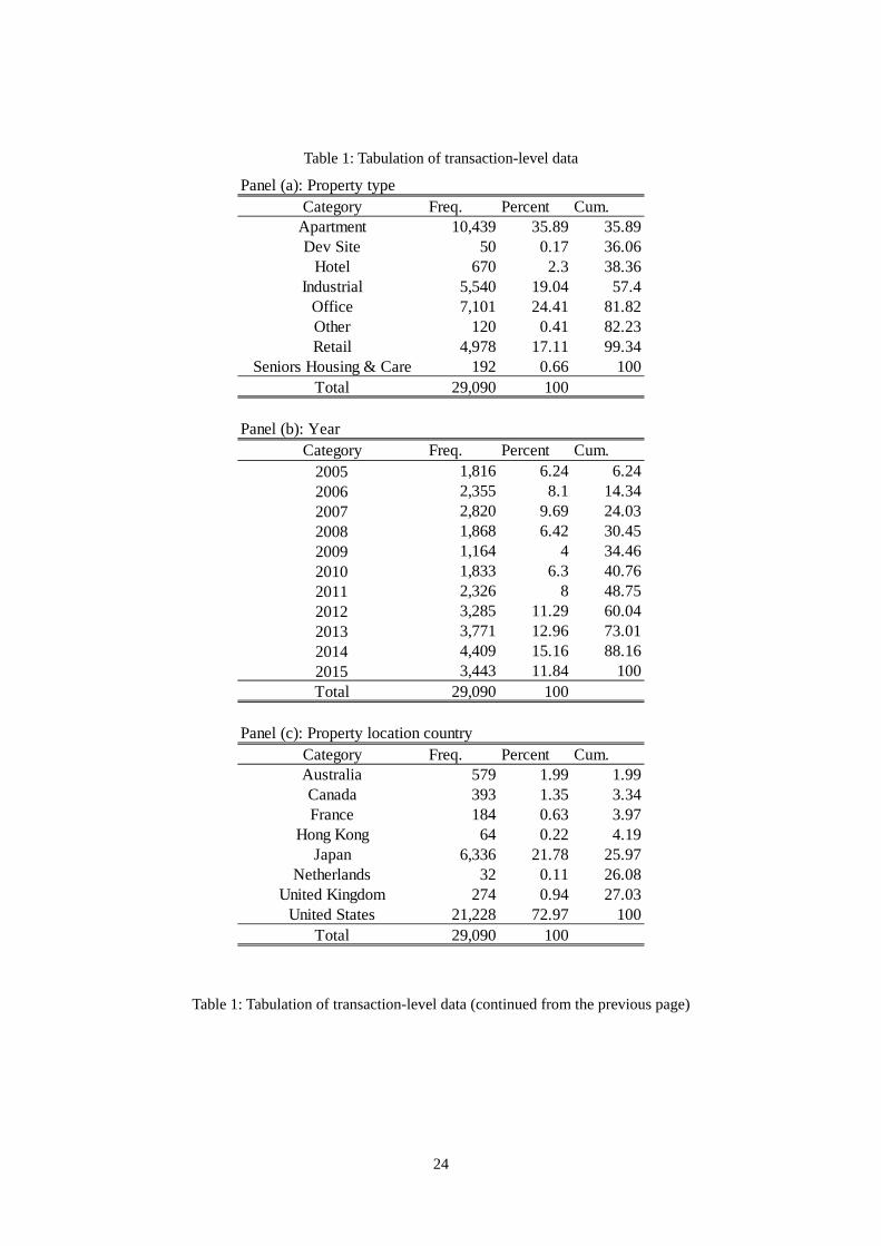
Table 1: Tabulation of transaction-level data
Table 1: Tabulation of transaction-level data (continued from the previous page)
Panel (a): Property typeCategory Freq. Percent Cum.
Apartment 10,439 35.89 35.89Dev Site 50 0.17 36.06
Hotel 670 2.3 38.36Industrial 5,540 19.04 57.4
Office 7,101 24.41 81.82Other 120 0.41 82.23Retail 4,978 17.11 99.34
Seniors Housing & Care 192 0.66 100Total 29,090 100
Panel (b): YearCategory Freq. Percent Cum.
2005 1,816 6.24 6.242006 2,355 8.1 14.342007 2,820 9.69 24.032008 1,868 6.42 30.452009 1,164 4 34.462010 1,833 6.3 40.762011 2,326 8 48.752012 3,285 11.29 60.042013 3,771 12.96 73.012014 4,409 15.16 88.162015 3,443 11.84 100Total 29,090 100
Panel (c): Property location countryCategory Freq. Percent Cum.Australia 579 1.99 1.99Canada 393 1.35 3.34France 184 0.63 3.97
Hong Kong 64 0.22 4.19Japan 6,336 21.78 25.97
Netherlands 32 0.11 26.08United Kingdom 274 0.94 27.03
United States 21,228 72.97 100Total 29,090 100

25
Panel (d): Buyer capital groupCategory Freq. Percent Cum.
<unknown> 533 1.83 1.83Equity Fund 1,612 5.54 7.37Institutional 2,293 7.88 15.26Private 17,787 61.14 76.4Public 4,842 16.64 93.05User/Other 2,023 6.95 100
Total 29,090 100
Panel (e): Seller capital groupCategory Freq. Percent Cum.
<unknown> 710 2.44 2.44CMBS 1 0 2.44Equity Fund 1,404 4.83 7.27Institutional 3,645 12.53 19.8Private 17,684 60.79 80.59Public 3,208 11.03 91.62User/Other 2,438 8.38 100Total 29,090 100
26
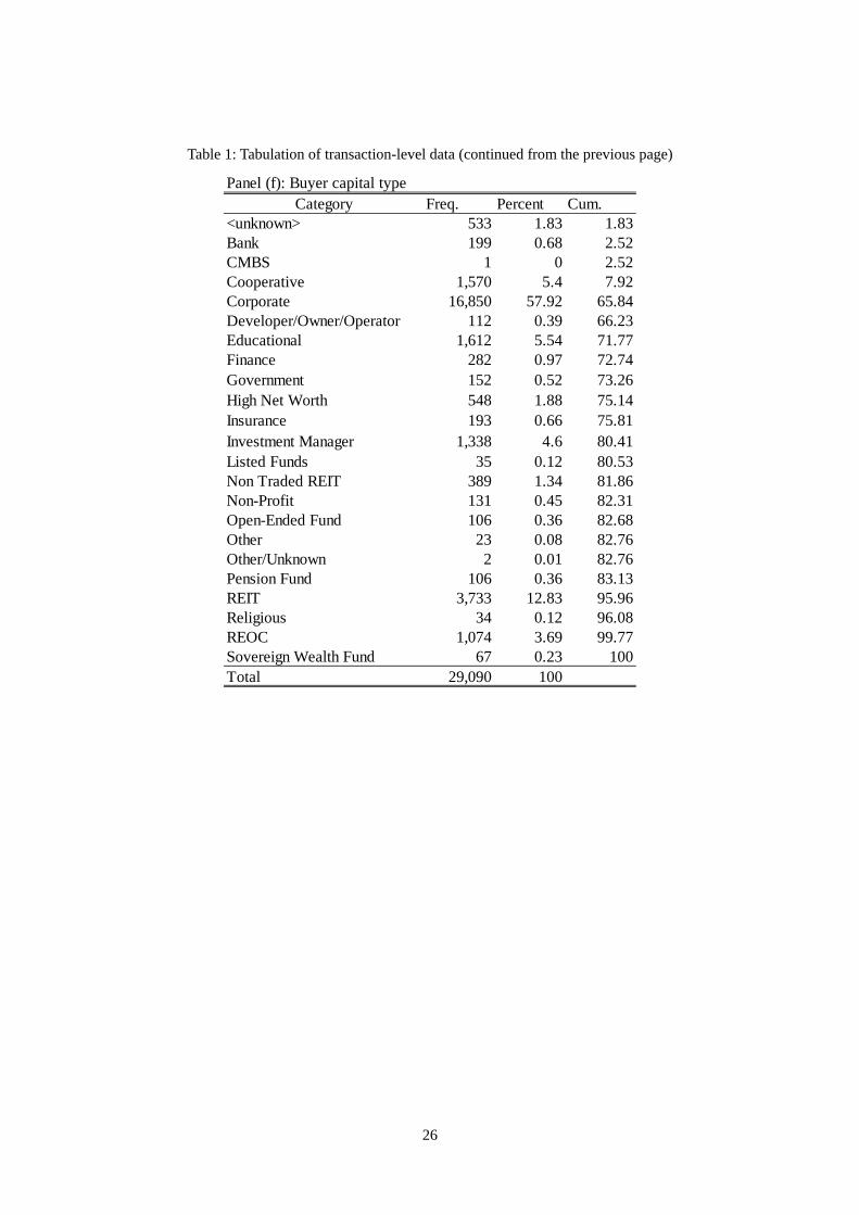
Table 1: Tabulation of transaction-level data (continued from the previous page)
Panel (f): Buyer capital typeCategory Freq. Percent Cum.
<unknown> 533 1.83 1.83Bank 199 0.68 2.52CMBS 1 0 2.52Cooperative 1,570 5.4 7.92Corporate 16,850 57.92 65.84Developer/Owner/Operator 112 0.39 66.23Educational 1,612 5.54 71.77Finance 282 0.97 72.74Government 152 0.52 73.26High Net Worth 548 1.88 75.14Insurance 193 0.66 75.81Investment Manager 1,338 4.6 80.41Listed Funds 35 0.12 80.53Non Traded REIT 389 1.34 81.86Non-Profit 131 0.45 82.31Open-Ended Fund 106 0.36 82.68Other 23 0.08 82.76Other/Unknown 2 0.01 82.76Pension Fund 106 0.36 83.13REIT 3,733 12.83 95.96Religious 34 0.12 96.08REOC 1,074 3.69 99.77Sovereign Wealth Fund 67 0.23 100Total 29,090 100
27
Table 1: Tabulation of transaction-level data (continued from the previous page)
Note: Each table accounts for the distribution of the seven (i.e., property type, transaction year,
property location country, buyer capital group, seller capital group, buyer capital type, and seller
capital type) which we control for by using the categorical dummy variables in the empirical
analysis.
Panel (g): Seller capital typeCategory Freq. Percent Cum.
<unknown> 710 2.44 2.44Bank 728 2.5 4.94CMBS 1 0 4.95Cooperative 2 0.01 4.95Corporate 2,051 7.05 12Developer/Owner/Operator 16,895 58.08 70.08Educational 40 0.14 70.22Endowment 3 0.01 70.23Equity Fund 1,404 4.83 75.06Finance 602 2.07 77.13Government 157 0.54 77.67High Net Worth 669 2.3 79.97Insurance 249 0.86 80.82Investment Manager 1,803 6.2 87.02Listed Funds 36 0.12 87.14Non Traded REIT 120 0.41 87.56Non-Profit 113 0.39 87.94Open-Ended Fund 118 0.41 88.35Other 13 0.04 88.39Pension Fund 120 0.41 88.81REIT 1,730 5.95 94.75Religious 62 0.21 94.97REOC 1,442 4.96 99.92Sovereign Wealth Fund 22 0.08 100Total 29,090 100
28
Table 2: Summary statistics
Note: The table shows the summary statistics of the variables used in our empirical analysis.
Variable Definition of variables Obs Mean Std. Dev. Min Max
LN_PriceUSDAccumulated investment amounts from buyercountry to property location country until theprevious month
29090 16.03 1.21 0.00 21.41
INVACC(note: see the header of the column)
Accumulated investment amounts from buyercountry to property location country until theprevious month (this variable is adjusted bythe accumulated investamounts from buyercountry until the previous month)
29090 0.78 0.18 0.00 1.00
INVACC_unadj(note: see the header of the column)
Unadjusted INVACC 29090 25.67 1.41 14.30 26.92
dum_forbuyerDummy varibale takling value of 1 if buyercountry is different from property locationcountry
29090 0.05 0.21 0 1
LN_Sqft Property size measured by square feet 29090 10.54 1.19 -0.87 19.02
LN_land_area_acres_nb Land size measured by acres 29090 -0.45 1.83 -13.09 13.76
Age Observation year minus developped year 29090 42.58 31.84 -5 360

29
Table 3: Baseline estimation
Note: The dependent variable is the natural logarithm of the property price measured in US dollars.
Table 2 provides the definitions of the independent variables. The column labeled "Robust Std. Err."
shows the heteroskedasticity robust standard error. The ***, **, and * denote significance at the 1%,
5%, and 10% levels, respectively.
Coef.Robust
Std. Err.Coef.
RobustStd. Err.
Coef.Robust
Std. Err.Coef.
RobustStd. Err.
<Independent Variables>
INVACC -0.183 0.047 *** 0.414 0.120 *** 0.315 0.143 ** 0.602 0.127 ***
dum_forbuyer 0.423 0.119 *** 1.586 0.393 ***
INVACC×dum_forbuyer -0.817 0.257 *** -0.971 0.404 **
LN_Sqft 0.702 0.007 *** 0.683 0.007 *** 0.702 0.007 *** 0.683 0.007 ***
LN_land_area_acres_nb -0.040 0.004 *** -0.036 0.004 *** -0.040 0.004 *** -0.036 0.004 ***
Age -0.001 0.000 *** -0.001 0.000 *** -0.001 0.000 *** -0.001 0.000 ***
_cons 9.661 0.154 *** 8.462 0.113 *** 8.627 0.162 *** 8.334 0.116 ***<Fixed-effect>
Property typeYear
Property location countryBuyer countrySeller country
Buyer capital groupSeller capital groupBuyer capital typeSeller capital type
Property Location-Buyer CountryNo. Obs.R-squaredRoot MSE
yes yes yes yesyes yes
0.6615 0.6507 0.6614 0.35060.70 0.70 0.70 0.70
yes yes
29090 34585 29090 34585yes yes
yes yes yes yesyes yes yes yesyes yesyes yesyes yes
yesyes yes yesyes yes yes yes
Dependent var = LN_PriceUSDBaseline estimation
30
Table 4: Estimations including additional variables
Note: The dependent variable is the natural logarithm of the property price measured in US dollars.
Table 2 provides the definitions of the independent variables. The column labeled "Robust Std. Err."
shows the heteroskedasticity robust standard error. The ***, **, and * denote significance at the 1%,
5%, and 10% levels, respectively.
Coef.Robust
Std. Err.Coef.
RobustStd. Err.
Coef.Robust
Std. Err.Coef.
RobustStd. Err.
Coef.Robust
Std. Err.Coef.
RobustStd. Err.
<Independent Variables>
INVACC 0.210 0.143 0.501 0.128 *** 0.325 0.145 ** 0.598 0.130 ***
INVACC_Q2 0.134 0.017 *** 0.123 0.016 ***
INVACC_Q3 0.177 0.020 *** 0.179 0.018 ***
INVACC_Q4 0.117 0.032 *** 0.153 0.027 ***
dum_forbuyer 0.339 0.119 *** 1.370 0.402 *** 0.409 0.122 *** 1.474 0.400 *** 0.245 0.038 *** 2.620 0.163 ***
INVACC×dum_forbuyer -0.701 0.265 *** -0.842 0.409 ** -0.798 0.260 *** -0.894 0.411 **
INVACC_Q2×dum_forbuyer -2.163 0.444 *** -3.808 0.164 ***
INVACC_Q3×dum_forbuyer -0.456 0.188 ** -0.877 0.253 ***
INVACC_Q4×dum_forbuyer 0.072 0.083 0.005 0.111
LN_Sqft 0.702 0.008 *** 0.683 0.007 *** 0.701 0.007 *** 0.682 0.007 *** 0.703 0.007 *** 0.684 0.007 ***
LN_land_area_acres_nb -0.040 0.004 *** -0.037 0.004 *** -0.040 0.004 *** -0.036 0.004 *** -0.039 0.004 *** -0.036 0.004 ***
Age -0.001 0.000 *** -0.001 0.000 *** -0.001 0.000 *** -0.001 0.000 *** -0.001 0.000 *** -0.001 0.000 ***
Past YoY return (t-1, …, t-8)
INV_OTHERS 0.014 0.005 *** 0.015 0.005 ***
_cons 8.734 0.164 *** 8.362 0.117 *** 7.989 2754.232 8.058 0.149 *** 9.566 0.624 *** 8.645 0.080 ***<Fixed-effect>
Property typeYear
Property location countryBuyer countrySeller country
Buyer capital groupSeller capital groupBuyer capital typeSeller capital type
Property Location-Buyer CountryRealtive past returns
Investment from other countriesNo. Obs.R-squaredRoot MSE
yes yes yes yesyes yes
Dependent var = LN_PriceUSD
(i) Control for relative (i.e., to world) return ofhousing price index associated with the country
where property locates
(ii) Control for the investment amounts fromother countries
yes yes yes yes
yes yes yesyes yes yes yes
yes yesyes yes
yes
0.70 0.70 0.70 0.700.6619 0.6508 0.6621 0.6508
yes28828 34291 28893 34360
yes
(Suppressed)
(iii) Non-linearity of INVACC
yes yesyes yesyes
yes yesyes
yes yes yes yesyes yes yes yes
yesyes yesyes yesyes yes
yesyesyes yes
0.6601 0.64900.71 0.70
yes yes
29397 34996

31
Table 5: Subperiod estimation
Note: The dependent variable is the natural logarithm of the property price measured in US dollars.
Table 2 provides the definitions of the independent variables. The column labeled "Robust Std. Err."
shows the heteroskedasticity robust standard error. The ***, **, and * denote significance at the 1%,
5%, and 10% levels, respectively.
Coef.Robust
Std. Err.Coef.
RobustStd. Err.
Coef.Robust
Std. Err.Coef.
RobustStd. Err.
<Independent Variables>
INVACC 0.354 0.181 ** 0.605 0.162 *** 1.758 0.432 *** 4.255 0.592 ***
dum_forbuyer 0.481 0.152 *** 1.232 0.254 *** 1.495 0.350 *** 4.916 0.460 ***
INVACC×dum_forbuyer -1.248 0.359 *** -1.467 0.678 ** -1.209 0.485 ** -4.369 0.965 ***
LN_Sqft 0.723 0.010 *** 0.694 0.009 *** 0.693 0.010 *** 0.679 0.009 ***
LN_land_area_acres_nb -0.040 0.007 *** -0.029 0.006 *** -0.040 0.005 *** -0.039 0.005 ***
Age -0.003 0.000 *** -0.002 0.000 *** 0.000 0.000 0.000 0.000
_cons 13.237 0.537 *** 8.114 0.139 *** 7.495 0.461 *** 5.914 0.437 ***<Fixed-effect>
Property typeYear
Property location countryBuyer countrySeller country
Buyer capital groupSeller capital groupBuyer capital typeSeller capital type
Property Location-Buyer CountryNo. Obs.R-squaredRoot MSE
0.70 0.690.6714 0.6683
17234 19946
yes yesyes yes
yes
yesyes yesyes yes
0.6244 0.6079
Year>=2011
yes yesyes yesyesyes
0.74 0.73
yes yesyes
11856 14639
yes yesyes yesyes yes
yesyesyes
Dependent var = LN_PriceUSDYear<2011
yes yesyes yes

32
Table 6: Estimation results for each property type
Note: The dependent variable is the natural logarithm of the property price measured in US dollars.
Table 2 provides the definitions of the independent variables. The column labeled "Robust Std. Err."
shows the heteroskedasticity robust standard error. The ***, **, and * denote significance at the 1%,
5%, and 10% levels, respectively.
Coef.Robust
Std. Err.Coef.
RobustStd. Err.
Coef.Robust
Std. Err.Coef.
RobustStd. Err.
<Independent Variables>
INVACC 0.030 0.318 0.507 0.212 ** 1.099 0.232 *** -0.356 0.642
dum_forbuyer 0.222 0.283 0.538 0.170 *** 0.938 0.195 *** 0.001 0.506
INVACC×dum_forbuyer -1.376 1.026 -4.120 0.737 *** -0.985 0.305 *** 0.425 0.996
LN_Sqft 0.692 0.019 *** 0.562 0.013 *** 0.853 0.010 *** 0.585 0.015 ***
LN_land_area_acres_nb 0.018 0.008 ** -0.016 0.007 ** -0.065 0.008 *** -0.033 0.009 ***
Age -0.005 0.000 *** 0.003 0.000 *** 0.000 0.000 0.000 0.000
_cons 9.394 0.554 *** 12.919 0.510 *** 6.733 0.271 *** 10.021 0.683 ***<Fixed-effect>
Property typeYear
Property location countryBuyer countrySeller country
Buyer capital groupSeller capital groupBuyer capital typeSeller capital type
Property Location-Buyer CountryNo. Obs.R-squaredRoot MSE
0.660.6986
yesyesyesyes
49780.77
0.6542
Retail
yesyesyesyesyes
yesyesyesyes
71010.60
0.6044
Office
yesyesyesyesyes
yesyesyesyes
5540
Industrial
yesyesyesyesyes
0.660.5640
10439
yesyes
yesyes
yesyes
yesyes
Dependent var = LN_PriceUSDApartment
yes

33
Table 7: Return estimation
Note: The dependent variable is the year-on-year return of the quarterly-level housing price index
associated with the country where the property is. For example, QTR_RETURN (+5quarter)
corresponds to the return of the housing price index from (a) the quarter that includes the month after
the month when each property is bought to (b) that of five quarters later (i.e., one year later). Table 2
provides the definitions of the independent variables. The column labeled "Robust Std. Err." shows
the heteroskedasticity robust standard error. The ***, **, and * denote significance at the 1%, 5%,
and 10% levels, respectively.
Coef.Robust
Std. Err.Coef.
RobustStd. Err.
Coef.Robust
Std. Err.Coef.
RobustStd. Err.
<Independent Variables>
INVACC -0.042 0.010 *** -0.095 0.009 *** -0.149 0.010 *** -0.191 0.012 ***
dum_forbuyer -0.032 0.008 *** -0.073 0.007 *** -0.113 0.008 *** -0.147 0.010 ***
INVACC×dum_forbuyer 0.033 0.014 ** 0.086 0.014 *** 0.144 0.015 *** 0.188 0.017 ***
LN_Sqft 0.000 0.000 *** 0.000 0.000 *** 0.000 0.000 ** 0.000 0.000 ***
LN_land_area_acres_nb 0.000 0.000 0.000 0.000 0.000 0.000 0.000 0.000
Age 0.000 0.000 0.000 0.000 0.000 0.000 0.000 0.000
Past YoY return (t-1, …, t-8)
_cons 0.107 0.009 *** 0.128 0.013 *** 0.097 0.015 *** 0.120 0.017 ***<Fixed-effect>
Property typeYear
Property location countryBuyer countrySeller country
Buyer capital groupSeller capital groupBuyer capital typeSeller capital type
Property Location-Buyer CountryNo. Obs.R-squaredRoot MSE
(Suppressed) (Suppressed)
0.810.0197
(Suppressed) (Suppressed)
yesyesyesyes
190430.80
0.0199
QTR_RETURN(+8quarter)
yesyesyesyesyes
yesyesyesyes
200730.81
0.0194
QTR_RETURN(+7quarter)
yesyesyesyesyes
yesyesyesyes
211840.80
0.0202
QTR_RETURN(+6quarter)
yesyesyesyesyes
yesyesyesyes
22241
QTR_RETURN(+5quarter)
yesyesyesyesyes
Dependent var =YoY return measured for quarter
frequency