geodesy by radio interferometry: effects of atmospheric modeling

Radio Science, Volume 20, Number 6, Pages 1593-1607, November-December 1985

Geodesy by radio interferometry: Effects of atmospheric modeling errors

on estimates of baseline length

J. L. Davis, • T. A. Herrinch 2 I. I. Shapiro, 2 A. E. E. Rollers, 3 and G. El•lered 4

(Received March 14, 1985; revised June 27, 1985; accepted June 27, 1985.)

Analysis of very long baseline interferometry data indicates that systematic errors in prior estimates of baseline length, of order 5 cm for • 8000-km baselines, were due primarily to mismodeling of the electrical path length of the troposphere and mesosphere ("atmospheric delay"). Here we discuss observational evidence for the existence of such errors in the previously used models for the atmospheric delay and develop a new "mapping" function for the elevation angle dependence of this delay. The delay predicted by this new mapping function differs from ray trace results by less than • 5 ram, at all elevations down to 5 ø elevation, and introduces errors into the estimates of baseline length of •< 1 cm, for the multistation intercontinental experiment analyzed here.

1. INTRODUCTION

A signal from a distant radio source received by an antenna located on the surface of the earth will have

been refracted by the terrestrial atmosphere. The corresponding delay introduced by the atmosphere depends on the refractive index along the actual path traveled by the received signal. For an atmosphere which is azimuthally symmetric about the receiving antenna, this delay depends only on the vertical profile of the atmosphere and the elevation angle of the radio source. The function which describes the de-

pendence upon elevation angle of the atmospheric delay has become known as the mapping function. This mapping function is used, along with some model for the zenith delay, to account for the atmospheric delay in models for the interferometric observables. Historically, analyses of very long baseline interferometry (VLBI) data for geodesy [e.g., Robert- son, 1975] have made use of the "Chao" mapping function and, more recently [Clark et al., 1985], of the "Marini" mapping function. The Chao mapping function [Chao, 1972] is based on ray tracing studies

XDepartment of Earth, Atmospheric, and Planetary Sciences, Massachusetts Institute of Technology, Cambridge.

2Harvard-Smithsonian Center for Astrophysics, Cambridge, Massachusetts.

3Haystack Observatory, Westford, Massachusetts. •Onsala Space Observatory, Chalmers University of Technol-

ogy, Sweden.

Copyright 1985 by the American Geophysical Union.

Paper number 5S0522. 0048-6604/85/005 S-0522508.00

in which refractivity profiles, averaged over all seasons and various sites, were used. This mapping function therefore contains no parametrization based on surface weather conditions at the site. However, for the refractivity profiles used, the mapping function describes the elevation angle behavior of the atmospheric delay to better than 1% for elevation angles above 1 ø. On the other hand, the Marini mapping function [Marini, 1972; J. W. Marini, unpublished manuscript, 1974] contains terms which depend on surface meteorological conditions, but it is based on approximations that degrade its accuracy below about 10 ø. Mapping functions other than these two have appeared in the literature [e.g., Hopfield, 1969; Saastamoinen, 1972; Black, 1978; Black and Eisner, 1984], but these other mapping functions have not undergone testing with VLBI data.

In the following, we review the manner in which the atmospheric delay is modeled, and the effects of these models on estimates of baseline length made from radio interferometric data. We present evidence of systematic errors in estimates of baseline length made from VLBI data, and we demonstrate that these errors are caused by the mismodeling of the atmosphere. Finally, we describe the development and testing of a new mapping function.

2. MODELING THE ATMOSPHERIC DELAY

The models for the interferometric observables of

group and phase delay, and of phase delay rate, must account for the atmospheric delay:

•a = •atm dS n(s) - fvac dS (1) 1593

1594 DAVIS ET AL.: ATMOSPHERIC DELAY IN VLB INTERFEROMETRY

where the first integral is evaluated along the path of a hypothetical ray originating from the direction of the radio source and passing through the atmosphere to a receiving antenna, and n(s) is the index of refraction at the point s along the path; the second integral is evaluated along the path the ray would take were the atmosphere replaced by vacuum. For simplicity, we have chosen units in which the speed of light is unity. (Delay will therefore be expressed in units of equivalent length.) The difference, r?-r?, for the two antennas i and j, of an interferometer gives the contribution of the atmosphere to the model of the interferometric delay. (Using the term "tropospheric delay" here would be inaccurate, since about 25% of the atmospheric delay occurs above the troposphere.)

We can find the point at which the integration in both parts of (1) is terminated at the earth by visual- izing the path of the (hypothetical) paraxial ray. This ray would strike the vertex of the paraboloid of the antenna normal to the surface of the antenna and be

reflected back along the axis. For a prime focus antenna, this paraxial ray would continue to travel until it enters the antenna feed at the focus. For a

Cassegrain focus antenna, the ray would be reflected once more at the subreflector and then enter the feed

located at or above the vertex along the axis. The path(s) after the initial reflection can be ignored in evaluating (1), because the delay is very nearly constant. The daily variation is usually less than 0.5 mm per 10 m of travel. (The largest diurnal variation in this delay, calculated from data taken by meteorological sensors located at the sites, was recorded for the Westford antenna site; the value was 0.8 mm per 10 m of travel and was associated with a rapid de- crease in the humidity.) A constant delay of any type at one of the sites is indistinguishable from a constant clock offset or instrumental delay for that site.

For most antennas, the vertex of the primary re- flector moves when pointing is changed; the size of the movement is usually a few meters. This movement can usually be ignored, with consequent negli- gible error, and a fixed reference point used in the evaluation of (1). For example, the intersection of axes of rotation of the Haystack antenna (one of the antennas used in VLBI experiments; see below) is located 4.3 m from the vertex along the axis of the parabola in a direction opposite to that of the prime focus. In this case, if we use the axis intersection as the fixed reference point for the evaluation of (1), the errors introduced will be equal to the neglected delay from vertex to the subreflector and back to the sec-

ondary focus (a total distance traveled of 25.2 m),

minus the erroneously added path from the vertex to the intersection. These paths should contribute less than • 1 mm amplitude of diurnal variation (due to diurnal variations of temperature and humidity) and less than 0.01 mm variation with antenna pointing angle.

Evaluation of the second integral on the right- hand side of (1) requires only knowledge of the source and antenna coordinates. However, evaluation of the first integral requires, as well, knowledge of the index of refraction in the neighborhood of the correct ray path, which is necessary in order to obtain the path itself via Fermat's principle [Born and Wolf, 1970]. Since in practice it is not possible to obtain this knowledge, one usually relies on models of the structure of the atmosphere. For example, one often assumes that the index of refraction of the at-

mosphere is constant from the surface of the earth up to an altitude H; for altitudes above H, the index of refraction is assumed to be unity, and the bending of the ray at the atmosphere/vacuum boundary is ignored. Then for a plane parallel model of the earth and the atmosphere, (1) reduces to

z a = csc e •oHdz (n o -- 1) (2) where e is the elevation angle of the radio source and no is the index of refraction at the surface of the earth.

It is possible to write (1) in a form which is moti- vated by the simple form of (2). Quite generally, we can write

•a = m(e, P) dz In(z)- 1] (3)

The function m(e, P), which is defined by (1) and (3), depends on the elevation angle e as well as on the parameter vector P, which is a parametrized repre- sentation of the behavior of the index of refraction in

the atmosphere. The number of elements (parameters) in P depends on the assumptions made about "regular" atmospheric structure. For example, if one assumes that no discernible atmospheric structure exists, then P will be an infinite-dimensional vector containing the index of refraction at all points. Since, as previously discussed, the refraction at all points is not known, this assumption would void (3) of any possible advantages. Instead, one usually makes some assumptions and approximations concerning the structure of the atmosphere and its effects on the ray path. A simple set of assumptions and approxi-

DAVIS ET AL.: ATMOSPHERIC DELAY IN VLB INTERFEROMETRY 1595

mations is, for example, that which led to the cose- cant law. In this case, the dependence of the function m on parameters P other than elevation is completely absent. (See below for a discussion of the assumptions used to develop the new mapping function.)

The integral in (3) is the atmospheric delay for a radio source at zenith. This integral will be denoted z•, the "zenith delay." Its dependence on atmospheric conditions directly above the antenna is discussed in the Appendix A. The function re(s, P) is known also as the "mapping function." For simplicity, the dependence on the parameters P will be suppressed, and we will write simply re(s).

Often separate mapping functions are used for the "wet" and "dry" components of the delay:

•. = •,• r%(s) + r•w rnw(S) (4)

where the subscript d on the zenith delays and mapping functions refers to "dry" and w to "wet." Such a form is used when, for instance, water vapor radiometer (WVR) data are used to estimate the "wet" component directly [Resch, 1984]. Then (4) is replaced by

12 a -- '17• ma(e) + Zwv. (5)

where rwwt is obtained from the WVR data. The user of such formulas, however, must be extremely careful to understand exactly what is meant by the terms "dry" and "wet," because the path the radio signal travels through the atmosphere is dependent on the contributions to the index of refraction from all at-

mospheric constituents. Furthermore, the so-called "dry" zenith delay also contains contributions from water vapor (see Appendix A).

3. SYSTEMATIC ERRORS IN ESTIMATES OF

BASELINE LENGTH

The manner in which estimates of baseline length are affected by errors in the mapping function used to model the atmospheric delay can be understood by first examining the approximate expression for the "geometric" term '•geom of the group delay model

•geom -- -- bø • -- -- (r2 sin e2 - r• sin e•) (6)

where b is the baseline vector (directed from site 1 to site 2), g is a unit vector in the direction of the source, ri is the distance from the center of the earth to the ith site, and ei is the elevation of the source at the ith site (i = 1, 2), and where the total group delay (of which 'rgeo m is but one term) is defined as the time of arrival of the signal at site 2 minus the time of arrival of the signal at site 1. (See Robertson [1975] for a

more complete discussion of the group delay model.) The feature of importance in (6) is the dependence of the group delay on the elevation of the source at each site. Any elevation-dependent error (such as a mapping function error) in the group delay model which correlates with the sine of the elevation will

corrupt the least squares adjustment of the radial component of the site position. An error Ar introduced into the estimate of the radial component of the position of either site introduces a corresponding error Ab in the estimate of the length of the baseline between the sites:

b Ab • • Ar (7)

2r e

where b is the baseline length and r e is the radius of the earth. The above equation is accurate to order (Ar)2/b.

Mapping function errors introduce systematic errors into the estimates of other parameters as well. In fact, all estimated parameters will be systemati- cally affected, although the magnitude with which the mapping function error manifests itself in the estimate of a particular parameter depends on the func- tional dependence of the group delay on that parameter. Thus one can expect systematic errors in estimates of source position, earth orientation, nutation, and any and all other estimated parameters; however, for illustration, this paper will confine itself to studying only errors in baseline length estimates.

Do we have evidence of mapping function errors, and, if so, how large are they? A useful method which can be used to indicate the presence and size of elevation-dependent systematic errors, such as mapping function errors, is the "elevation angle cutoff test." In this test, all baselines are estimated simultaneously using all the data available. (Of course, other parameters are estimated along with baselines, but here and in the following, as stated above, the discussion will be confined for illustration to the effects on the estimates of baseline length.) The baselines are then reestimated with the data limited to observations above some minimum elevation

angle. More estimates can be made with different elevation angle minima. If there are no elevation- dependent systematic errors, the mean of the differences between the corresponding baseline-length estimates should tend toward zero. Significant biases indicate mapping function errors. Figure 1 contains the results from such a test. Plotted are the differences in

baseline-length estimates for 5 ø and 15 ø minimum

1596 DAVIS ET AL.' ATMOSPHERIC DELAY IN VLB INTERFEROMETRY

1 2 3 4 5 6 7 8 9 10 Baseline length (1000 km)

Fig. 1. Difference in baseline length estimates for the 15ø-5 ø elevation angle cutoff test of the Marini mapping function. The error bars are the statistical standard deviations of the differences (see Appendix B). The straight line represents the effects of a change in the local vertical component of site position of 3 cm at each of the sites.

elevation angles. These differences are plotted against the length of the baseline. The error bars shown are the standard deviations of the differences, obtained from the statistical standard deviations of the indi-

vidual estimates. (It can be quite easily shown that the variances of the differences of the baseline-length estimates are the differences of the corresponding variances resulting from the two least squares solu- tions; see Appendix B.) The group delay data used to generate these differences are the entire yield of VLBI group delay data from the project MERIT short campaign of September and October 1980 [Robert- son and Carter, 1982], with the exception noted below. These data were processed as described by Clark et al. [1985]. The atmospheric delay was modeled by using the Marini formula, which requires surface weather data. The group delay data involving the site at Chilbolton, United Kingdom, were de- leted, since surface weather data were not available

for this site for some periods of the campaign. The phase delay rate data were not included.

From Figure 1 it can be seen that the differences in the estimates of baseline length seem to be nearly proportional to baseline length. Recalling (7), we can interpret these differences as due to corresponding differences in the estimates of radial positions of the individual sites, if these latter differences are nearly equal. For reference, Figure 1 contains a line representing the effect of a 3-cm radial difference at each site. (The sense of the radial difference is, from (7), such that the estimates of the radial positions from the 0 ø cutoff solution were greater than those from the 15 ø cutoff solution.) It can be seen that this nearly represents the actual situation. We thus conclude that the differences evident in Figure 1 are due to mapping function errors, on the assumption that there do not exist any other elevation angle- dependent errors of this magnitude.


4. THE NEW MAPPING FUNCTION

Marini [1972] showed that the continued fraction form of the mapping function

1 me) =

a

sin e + b sin • +

sin • + (8) sin • +...

where a, b, c,... are constants, can be used to approximate the elevation angle dependence of the atmospheric delay. Only two terms are used in the Marini mapping function (J. W. Marini, unpublished manuscript, 1974). Chao [1972] uses two terms as well, except he replaces the second sin e with tan e, thereby ensuring that m(90 ø) = 1. We have attempted to develop a mapping function for the "dry" or "hydrostatic" component of the atmosphere (see Appen- dix A) based on the Chao model, but with improved accuracy at low elevation angles. In order to achieve subcentimeter accuracy at 5 ø elevation, we have "continued the fraction" by adding one more term but keeping the tangent'

m(•) =

sin • +

tan e + • (9) sin e + c

The advantage of using this form is its simplicity, both in calculating the mapping function itself and in calculating partial derivatives of the mapping function with respect to the parameters to be estimated. The disadvantage of this form is that for higher elevation angles (20ø-60ø), tan e does not approach sin e quickly enough. As a result, one can expect 1- to 2-mm errors in representing the atmospheric delay with (9) for these elevations.

In order to determine the mapping function parameters a, b, and c, we performed ray trace analyses for various values of a limited number of atmospheric conditions. The ray trace algorithm we used was based on a spherically symmetric, layered atmosphere. The temperature profile was taken to have a linear dependence with height up to the tropopause, above which the temperature was assumed constant. The total pressure was assumed to result from hydrostatic equilibrium, and the relative humidity was assumed to be constant up to 11 km and zero above

that height. The acceleration due to gravity was assumed to be constant with height. This simple set of assumptions concerning the structure of the atmosphere allowed us to examine the dependence of the mapping function on variations about the nominal values of the following parameters: surface pressure, surface relative humidity, surface partial pressure of water vapor, temperature of the tropopause, and height of the tropopause. However, the sampling of parameter space was not done in a systematic manner due to the large number of ray trace analyses which this would entail. For example, if just three values for each parameter were used, there would be 35= 243 different combinations of parameters. In- stead, 57 analyses were performed, and there are resulting gaps in the sampling of the parameter space.

For each set of atmospheric conditions, then, we determined the ray trace values for the mapping function, in steps of 1 ø for elevations from 5 ø to 90 ø. We then used least squares to estimate a, b, and c. However, c could be fixed at some nominal value and not appreciably degrade the solution; the nominal value ultimately decided upon (see below) for c was taken to be the approximate average of the values for the first several ray traces performed. The mapping function form given in (9) was, for each set of atmospheric conditions, able to model the elevation angle dependence of the delay to within 3 mm for all elevation angles down to 5 ø, and with an rms deviation of less than 1.5 mm.

The ray trace analyses thus provided a set of estimates of each of the mapping function parameters, a and b, covering a variety of atmospheric conditions. We then represented a and b each as a linear function of the various atmospheric parameters that were varied and used least squares to determine the coef- ficients. Such a linear model fits the mapping function parameter a within 0.2% (corresponding to • 5 mm at 5 ø elevation) and the parameter b to within 0.5% (• 2 mm at 5 ø elevation) in all cases; the rms fit for a is 0.08% (• 2 mm at 5 ø elevation) and for b is 0.15% (•0.6 mm at 5 ø elevation). In particular, we have

a =0.001185 [1 + 0.6071 x 10-'•(Po

-0.1471 x 10-3eo

+0.3072 x 10-2(To- 20)

+0.1965 x 10-•(fi + 6.5)

-0.5645 x 10-2(ht- 11.231)]

- looo)

(10)


b = 0.00114411 + 0.1164 x 10-'•(Po- 1000)

+0.2795 x 10-3eo

+0.3109 x 10-2(To- 20)

+0.3038 x 10- •(• + 6.5)

-0.1217 x 10-X(ht - 11.231)] (11)

c = -0.0090 (12)

where Po is the total surface pressure in millibars, eo is the partial pressure of water vapor at the surface in millibars, To is the surface temperature in degrees Celsius,/• is the tropospheric temperature lapse rate in K km-x, and ht is the height of the tropopause in kilometers. This version of the "dry" mapping function has been dubbed CfA-2.2. The sensitivities of the

CfA-2.2 mapping function to changes in these atmospheric parameters are summarized in Table 1. For example, a 10-mbar change in the partial pressure of

TABLE 1. Sensitivities of the Path Delay From Model CfA-2.2 to Changes in Atmospheric Parameters for ALz½ n = 240 cm and

for Different Elevations e

P, T, e, /•, h,, cm/mbar cm/øC cm/mbar cm/(K/km) cm/km

15 ø -9.1 x 10 -4 -0.046 0.002 -0.29 0.082 10 ø -2.8 x 10 -3 -0.14 0.007 -0.88 0.25

5 ø -0.017 -0.75 0.053 -4.4 1.1

See text for explanation of model CfA-2.2. P, pressure- T, temperature; e, partial pressure of water vapor; ]•, temperature lapse rate; ht, height of tropopause.

water vapor produces a change of approximately 5 mm in the predicted delay at 5 ø elevation. (It is fortu- nate, in fact, that the mapping function is not very sensitive to the amount of water vapor in the atmosphere, since this quantity is spatially highly variable and not well predicted by surface measurements.) Figures 2 and 3 contain the differences between ray

40

30

• 2o

10

o

• 0 .,•

-10

CfA-2.2

Marini

Chao

I I I i i i I I I i

5 10 15 20 Elevation angle (deg)

Fig. 2. Differences from ray tracing of the new mapping function, the Chao mapping function, and the Marini mapping function for Po = 850 mbar and T O = 15øC. The partial pressure of water vapor, temperature lapse rate, and tropopause height are all at their nominal values of 0 mbar, -6.5 K/km, and 11.231 km, respectively. The corresponding value of the zenith delay is 1.935 m of equivalent length (6.5 ns).

DAVIS ET AL.' ATMOSPHERIC DELAY IN VLB INTERFEROMETRY 1599

40

30

20

10

0

-10

-20

Fig. 3.

Marini

Chao

C[A-2.2

5 lO

Same as Figure 2, except for Po

15 20 Elevation angle (deg)

= 1000 mbar and T o = -30øC. The corresponding value of the zenith delay is 2.277 m.

tracing and CfA-2.2 for the different atmospheric conditions indicated. These conditions, which represent the nominal conditions of humidity, lapse rate, and tropopause height, were chosen because they represent locations in the pressure-temperature plane near which no ray trace analyses were performed. Their agreement with ray tracing is therefore an in- dication of the robustness of the method used in the

plane of temperature and pressure. Also shown are the differences from ray tracing for the Chao and Marini models. These models are the most common-

ly used mapping functions in VLBI data analysis [Fanselow, 1983; Clark et al., 1985]. ,

The accuracy of the CfA-2.2 mapping function model seems higher near latitudes of 45øN, for which the nominal values of tropopause height and lapse rate used in CfA-2.2 are representative. For example, for conditions representative of a latitude of 30øN (h, = 16 km, /• =-4.7 K/km to -5.9 K/km), the difference between CfA-2.2 and ray trace values reaches • 4 cm at 5 ø elevation. Relatively large differ-

ences have also been noted for higher latitudes in the extreme of winter: For a latitude of 60øN (h, - 8 km, /• = -3.9 K/km), the differences from the ray trace values reach •2.5 cm at 5 ø. These (comparatively) large differences from the ray trace values seem to be due to the simultaneous departures from the nominal values of lapse rate and tropopause height. Although our choice of -6.5 K/km is the standard one for the lapse rate in the troposphere (U.S. Standard Atmo- sphere, 1976), it seems to be somewhat large (in magnitude) when one considers compilations of temperature profiles found, for example, in the work of Smith et al. [1963]. However, even with a better choice of nominal value, a site-dependent model of some type will have to be developed: lapse rate and tropopause height do not truly vary independently, since the temperature of the tropopause varies less than the surface temperature. Thus those climates with a very low tropopause height (high latitudes) can be expected to have correspondingly small (in magnitude) lapse rates. Those climates with a high


tropopause height (equatorial latitudes) will have correspondingly large (in magnitude) lapse rates.

The lack of dependence of the new mapping function on azimuth results directly from the assumption of azimuthal symmetry. Gardner [1977] expressed the index of refraction in (1) in cylindrical coordinates (with the z coordinate aligned along the local vertical) and expanded it in powers of horizontal distance from the z axis. He showed that the zeroth-

order term represents the spherically symmetric term. Thus our new mapping function represents this zeroth-order term. The first-order term in Gardner's

expansion arises from horizontal refractivity gradients; Gardner showed that this term can be as large as 5 cm at 10 ø elevation angle. However, this term has never been included in our VLBI data analysis because of the lack of a network of meteorological sensors in the near vicinity of our sites from which to determine the refractivity gradients. In principle, though, there is no reason that this gradient term could not be introduced into our atmospheric models; its utility would depend on (1) a dense enough network of meteorological sensors being in place around each site, (2) models for the gradient being developed that depend on the meteorological conditions at the site only (such as wind direction and speed), and possibly on climate and/or season, or (3) the ability to estimate accurately the gradient term being demonstrated for data from a network of distant (> 100 km) meteorological sensors such as exist at airports and other weather stations.

5. PROCESSING VLBI DATA WITH CfA-2.2

We have performed the elevation-angle-cutoff test on the CfA-2.2 mapping function. For this test, the Saastamoinen formula for the zenith delay [Saasta- moinen, 1972] was used to be consistent with the zenith delay values used for the Marini formula. The "wet" part of the delay (see Appendix A) was mapped by using (9)-(12) as well, even though this use introduces a small error which is, from (4), the "wet" delay multiplied by the difference between CfA-2.2 and the "true" wet mapping function. The values listed in Table 2 were used for tropopause height and lapse rate. These values are based on tables of mean temperature profiles near the 80th meridian west [Smith et al., 1963]. No attempt was made to obtain the exact profiles of temperature that prevailed at the sites, since for this elevation angle cutoff test we were attempting only to remove the gross effects of differences from the nominal values of

TABLE 2. Values for Tropopause Height h t and Temperature Lapse Rate fl Used in Elevation Angle Cutoff Test of CfA-2.2

Mapping Function

Site Geographic North ht,* •, Name Location Latitude km K/km

Onsala south Sweden 57 ø 10.5 - 5.7

Effelsberg West Germany 51 ø 9.6 - 5.7 Haystack east Massachusetts 43 ø 13.6 - 5.6 Owens Valley south California 37 ø 12.8 -5.6 Fort Davis southwest Texas 31 ø 13.4 -6.3

*Height of tropopause given as height above station for direct use in CfA-2.2 mapping function formula; see text.

/• and hr. The procedure used was first to obtain estimates of/• and ht at the latitudes of 30 ø, 40 ø, and 50 ø by fitting a linear function of height to the values given in the tables; possible variations of these parameters with longitude were ignored. The three estimates for each of the parameters/• and ht were then expressed via least squares as second-order poly- nomials in latitude. For each North American site, the latitude of the antenna was then substituted to

determine/• and ht. Each European site was treated as though it were 5 ø south of its true position to account approximately for the warmer climate at Eu- ropean longitudes in the choice of /• and hr. (The value of 5 ø was based upon visual inspection of world maps of tropopause height found by Bean et at. l- 1966].)

The results of this elevation angle cutoff test are shown in Figure 4. Any systematic trend that may be present in this figure is clearly much smaller than that seen in Figure 1. Table 3 allows us to compare the results from the two tests more quantitatively. The second column contains least squares estimates of the differences in the radial site positions which, from (7), would yield the baseline-length differences evident in Figure 1. The third column contains the same information, except for Figure 4. The fourth column contains the differences of the second two

columns. The numbers in this fourth column, then, represent the changes in the inferred differences of the radial position we obtained in performing the 15ø-5 ø elevation angle cutoff tests. It can be seen that for the sites at Haystack, Onsala, and Effelsberg, these changes were • 4 cm, over 10 times the changes at Ft. Davis and Owens Valley. This difference can be explained by the entries in the fifth column. This column contains the fraction of data obtained below

15 ø elevation at these sites. That these last two sites

had no data from these lower elevation angles


0 1 2 3 4 5 6 7 [5 9 10 Baseline length (1000 km)

Difference in baseline length estimates for the 15ø-5 ø elevation angle cutoff test of the CfA-2.2 mapping function. The error bars are the statistical standard deviations of the differences (see Appendix B).

-1

-2

-3

-4

-5

-6

-7

Fig. 4.

implies that there should be little difference between the results for either of these sites from using different mapping functions.

Further testing of the CfA-2.2 mapping function is

TABLE 3. Comparison of Elevation Angle Cutoff Tests

Fraction of

Site Ar, cm Ar, cm Difference, Data Below 15 ø Name (Marini) (CfA-2.2) cm Elevation

Onsala - 3.7 + 1.0 0.9 -4.6 10.4%

Effelsberg -4.9 ___ 1.3 -0.7 -4.2 7.7% Haystack - 3.9 _+ 0.8 0.1 -4.0 3.1% Owens Valley -1.0 _+ 0.3 -0.8 -0.2 0% Fort Davis - 1.4 _+ 0.5 - 1.1 -0.3 0%

The entries in the columns headed by Ar are the changes in the estimates of the local vertical positions of the sites corresponding to the baseline length differences from each of the elevation angle cutoff tests, shown in Figure 1 (Marini) and Figure 4 (CfA-2.2). The column labeled "difference" is the difference between the

changes in the radial estimates. The uncertainties for the values of Ar (CfA-2.2) are the same as for the values for Ar (Marini).

underway. Single-baseline experiments are now being carried out in which a large fraction of the observations from one site are obtained for elevation angles below 5 ø elevation, and for a very large fraction below 10 ø elevation, while observations from the other site remain at relatively high (> 10 ø) elevation angles. This procedure should enable us to isolate mapping function errors for the site at which the low elevation observations are taken, since we would be relatively insensitive to mapping function errors for the other site.

Plans are also being made to optimize the coef- ficients in (10)-(12) for site location, and to develop seasonal atmospheric structure parameters. For this purpose, radiosonde data obtained from the National Climatic Data Center for U.S. sites, and from various European centers, will be used. Simultaneously, an effort will be made to attempt to increase the accuracy of the mapping function at all elevation angles (but with emphasis at extending the mapping function for use at elevation angles below 5 ø ) and to in-


vestigate possible means for modeling of horizontal gradients.

6. SUMMARY

Errors in modeling the elevation angle dependence of the atmospheric delay can cause systematic errors in the estimated radial positions of the antenna sites. These radial errors will "map" into the estimates of baseline length by an amount approximately proportional to the baseline length. An elevation angle cutoff test performed with the Marini mapping function indicated that the errors in the estimates of base-

line length introduced by this mapping function were of the order of --, 5 cm for a baseline length of • 8000 km and that these errors display a systematic dependence on baseline length indicative of a mapping function error. A new mapping function has been developed which is based on ray-tracing through model atmospheres. Repetition of the elevation angle cutoff test with this new mapping function yields ap- parent errors in baseline-length estimates of •< 1 cm, with the differences showing little or no dependence on baseline length.

APPENDIX A: ZENITH DELAY FORMULAS

The purpose of this appendix is to derive an accurate expression for the zenith delay from the wet and dry refractivity formulas. We pay particular attention to the treatment of the wet/dry mixing ratio. We also obtain an estimate for the accuracy of the hydrostatic (i.e., "dry") delay formula, and derive an expression for the "wet" zenith delay which is consistent with the "dry" zenith delay formula. This "wet" delay formula makes use of the most recent expression for the wet refractivity and can be used to establish the relationship between the observables of instruments which measure the radiative emission of atmospheric water vapor (e.g., water vapor radiometers) and the line-of-sight delay due to water vapor.

Derivation of the zenith delay from the refractive index

The three-term formula for the total refractivity of moist air, as given by Thayer [ 1974], is

N = k• -• Z• -• + k2 -• Z•, • + k3 •¾ Z• • (A1) Here T is the temperature, Pd is the partial pres-

sure of the "dry" constituents ("dry" is defined below), Pw the partial pressure of water vapor, and

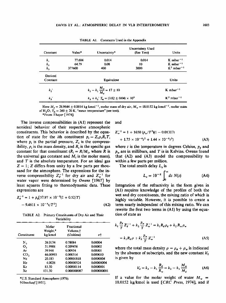
Z• -• and Z• • are the respective inverse compressibilities, with the subscripts having the same meaning as for the pressures. The symbol e is usually used in place of pw. Thayer's values for the constants k•, k2, and k3 are summarized in Table A1. The uncertainties of these values limit the accuracy with which the refractivity can be calculated to about 0.02%.

The first term in (A1) represents the effect of the induced dipole moment ("displacement polariza- tion") of the dry constituents. The second term represents the same effect for water vapor, whereas the third term represents the dipole orientation effects of the permanent dipole moment of the water molecule. None of the primary constituents of dry air (shown in Table A2) possesses a permanent dipole moment.

The values for k2 and k3 listed in Table A1 have been disputed by Hill et al. [1982]. They point out that Thayer's extrapolation of the value of k2 from its value at optical wavelengths ignores the effect of the rotational and vibrational resonances in the infrared

[Van Vleck, 1965]. Hill et al. calculate a theoretical value for k2 and k 3 and find kz = 98 + 1 K/mbar and k 3 = (3.583 + 0.003)x 105 K•/mbar. However, these results are so greatly in disagreement with pub- lished values of k2 and k3, which have been obtained by measurements in the microwave region [Bou- douris, 1963; Birnbaum and Chatterjee, 1952], that Hill recommends using the measured values instead of either his or Thayer's. Birnbaum and Chatterjee find k2 = 71.4 + 5.8 K/mbar and k 3 = (3.747 +0.029) x 105K•/mbar, while Boudouris finds

k: = 72 __+ 11 K mbar and k 3 = (3.75 __+ 0.03) x 105 K'/mbar. As a compromise, we keep Thayer's values for k• and k 3 (which differ from the experimental values by less than the uncertainties of the latter), but choose the (rounded) experimental uncertainties, as shown in Table A1. -

The grouping together of all the dry constituents into one refractivity term is possible because the relative mixing ratios of these gasses remain nearly constant in time and over the surface of the earth

[Glueckauf, 1951]. The eight main constituents of the dry atmosphere are listed in Table A2, along with their molar weight and fractional volume, and a standard deviation representing the variability of that constituent in the atmosphere. Using these numbers, we find the mean molar weight Md of dry air to be Md = 28.9644 + 0.0014 kg/kmol, where the standard deviation is an upper bound on the variability of Ma based on the values in Table A1 and on the assumption that these constituents vary independently.


TABLE A1. Constants Used in the Appendix

Constant Uncertainty Used

Value* Uncertainty* (See Text) Units

kx 77.604 0.014 0.014 K mbar- • k 2 64.79 0.08 10 K mbar- 1 k 3 377600 400 3000 K 2 mbar- •

Derived

Constant Equivalent Units

k 2' k 2 -k• M._•.• = 17 +_ 10 K mbar -x Ma

k 3' k 3 + k,_' T m = (3.82 +_ 0.04) x 105 K'- mbar -•

Here Ma = 28.9644 +_ 0.0014 kg kmol -•, molar mass of dry air' M,• = 18.0152 kg kmol -•, molar mass of H20' r m = 260 _+ 20 K, "mean temperature" (see text).

*From Thayer [1974].

The inverse compressibilities in (A1) represent the nonideal behavior of their respective atmospheric constituents. This behavior is described by the equation of state for the ith constituent Pi = Zip•R•T, where Pi is the partial pressure, Z• is the compressibility, p• is the mass density, and Ri is the specific gas constant for that constituent (Ri = R/M•, where R is the universal gas constant and Mi is the molar mass), and T is the absolute temperature. For an ideal gas Z = 1; Z differs from unity by a few parts per thou- sand for the atmosphere. The expressions for the inverse compressibility Z• -• for dry air and Z• • for water vapor were determined by Owens [1967] by least squares fitting to thermodynamic data. These expressions are

Z•-•= 1 + pd[57.97 x 10-8(1 + 0.52/T)

-9.4611 x 10-4t/T 2] (A2)

and

Z•, 1= 1 + 1650(pw/T3X 1 - 0.01317t

+ 1.75 x 10-'•t2 + 1.44 x 10-6t 3)

TABLE A2. Primary Constituents of Dry Air and Their Variability

Molar Fractional

Weight,* Volume, J' Constituent kg/kmol (Unitless)

N 2 28.0134 0.78084 0.00004 O •_ 31.9988 0.209476 0.00002 Ar 39.948 • 0.00934 0.00001

CO 2 44.00995 0.000314 0.000010 Ne 20.183 0.00001818 0.0000004

He 4.0026 0.00000524 0.(X)(X)(X)04

Kr 83.30 0.00000114 0.0000001

Xe • 131.30 0.000000087 0.000000001

*U.S. Standard Atmosphere (1976). t'Gleuckauf [1951].

(A3)

where t is the temperature in degrees Celsius, Pd and Pw are in millibars, and T is in Kelvins. Owens found that (^2) and (^3) model the compressibility to within a few parts per million.

The total zenith delay Lz is

© Lz -- 10- 6 dz N(z) (A4)

Integration of the refractivity in the form given in (^1) requires knowledge of the profiles of both the wet and dry constituents, the mixing ratio of which is highly variable. However, it is possible to create a term nearly independent of this mixing ratio. We can rewrite the first two terms in (A1) by using the equation of state as

Pd Pw

z; ' + -7' ' = + , Pw

= k•Rap + k2 -• ZT• • (A5) where the total mass density p - Pa + P,• is indicated by the absence of Subscripts, and the new constant k• is given by

R a M,•

k• = k2 - k, • = k2 - k, (A6) Ma

If a value for the molar weight of water M• = 18.0152 kg/kmol is used ICRC Press, 1974], and if


independent errors in kx, k2, and Md are assumed, then we find k• = (17 ___ 10) K mbar -x. By using (A5), we find the expression for the total refractivity to be

N = k,R.,p + k 2 -• Z•* + k3 '• Z,7,,* (A7) It is important to note that the first term in (A7) is dependent only on the total density and not on the wet/dry mixing ratio. This term can be integrated by applying the condition that hydrostatic equilibrium is satisfied:

dP - -p(z)g(z) (A8)

dz

where g(z) is the acceleration due to gravity at the vertical coordinate z, P(z) is the total pressure, and, as above, p(z) is the total mass density. Denoting the result of the integration of the first term in (A7) as L•, we find that

L, = [10-6k,Rdg,• •]Po (A9)

where Po is the total atmospheric pressure at the intersection of rotation axes of the radio antenna

(not the surface pressure, since the antenna is located some height above the ground; see text), and where gm is given by

©Clz •(z)•(z) (AlO)

o •z P(Z) By expanding g(z) to first order in z, it can be seen

that (A10) very nearly represents the acceleration due to gravity at the center of mass of the vertical column. The value of gm at this point is [Saastamoin- en, 1972]

g.• = 9.8062 m s-2(1 - 0.00265 cos 2it - 0.00031He)

(All)

where ,• is the geodetic site latitude and Hc is the height in kilometers of the center of mass of the vertical column of air. The quantity He and therefore gm is dependent upon the atmospheric total density profile, but Saastamoinen [19723 used his simple model atmosphere and "average" conditions to generate the expression

H• = 0.9H + 7.3 km (A12)

where H is the height in kilometers of the station

above the geoid. Saastamoinen claims that this expression is accurate to within 0.4 km for all latitudes and for all seasons. Substituting for He into (All) yields

gm= 9.784 m s-2(1 -0.00266 cos 2it- 0.00028H)

+ 0.001 rn s -2 = gO,,[f(j., H) + 0.0001] (A13)

where gO,, = 9.784 m s-2. Combining all the constants in (A9), along with their uncertainties (assumed uncorrelated), gives

Po L, - [(0.0022768 + 0.0000005) rn mbar-•] • (A14)

f(,•, H)

where a value of R = 8314.34 q-0.35 J kmol -x K -x has been used for the universal gas constant ICRC Press, 1974]. The uncertainty of the constant in (A14) takes into account the uncertainty of kx, the uncertainty in g,•, the uncertainty in R, and the variability of the dry mean molar mass. It does not include the effect due to nonequilibrium conditions. It is, in fact, difficult to assess this effect without actually inte- grating vertical profiles of vertical wind acceleration (which, in general, are not available); no attempt to assess this effect will be made here. Fleagle and Bus- inger [1980] state that only under extreme weather conditions (thunderstorm or heavy turbulence) do these vertical accelerations reach 1% of gravity, corresponding to an error in Lx of about 20 mm/1000 mbar. Exactly where the true uncertainty lies between these values of 0.5 and 20 mm/1000 mbar must be left to future investigation.

Because the uncertainty associated with L• in (A14) is so small, and because variability is associated with water vapor, Lx is usually (and inaccur- ately) termed the "dry delay." Something like the "hydrostatic delay" would be more descriptive, for in principle the uncertainty of the dry density at any point is no less than the uncertainty of the wet density, whereas the total density is very predictable.

The remaining two terms in the expression for the refractivity are wet terms

P]z -' Nw = + k 3 T2 j w The partial pressure of water is not by itself in equilibrium, and water vapor can remain relatively un- mixed, making the wet delay very unpredictable. Water vapor radiometers (WVR's) will, we hope, ob- viate this problem. However, there are large amounts of VLBI and other data for which no WVR calibra-

tion is available, and more such data are being con-


tinually generated. Thus there is still a need for models of the zenith wet delay. No attempt will be made to develop one here. All such models in current use [e.g., Chao, 1972; Berman 1976; Saastamoinen, 1972] use obsolete values for the refractivity constants ke and k3. However, these old values induce errors on the submillimeter level, much less than the inherent error in the prediction of the wet delay. On the other hand, these models also tend to be based on empirical models for the wet atmosphere, averaged over location and season. However, we be- lieve that site and season dependence of the atmospheric profile could cause seasonal and site- dependent biases in these wet models of up to 10- 20%, based on a comparison of expressions for "average" profiles reported throughout the literature.

Water vapor radiometers

A water vapor radiometer is a multichannel radiometer which uses the sky brightness temperature near the 22-GHz rotational absorption line of atmospheric water vapor to obtain an estimate of the integral of the wet refractivity in (A15). The WVR's now coming into use should have their "retrieval coef- ficients" [see Resch, 1984] "optimized" for site and seasonal dependence of the atmospheric profiles. For this optimization, one uses radiosonde estimates of the wet delay ALw to determine the retrieval coef- ficients ax and a2 defined in the equation

ALw = alf(WVR) + a2g(Po, To) (A16)

where f(WVR) is some function of the WVR observables, and g(Po, To) is some function of the surface temperature and pressure [Resch, 1983]. Both f(WVR) and g(Po, To) are determined by theory. By "radiosonde estimates of the wet delay" we mean that ALw is determined by numerical integration of the wet refractivity given in (A15) using radiosonde profiles of p• and T. In practice, most investigators use a one-term expression for the wet delay:

• •'• (A•7) AL,• = 10-6k• dz T•

where k• is the k 3 in (A15) modified for the effect of k•. This modification is made possible by using the mean value theorem to introduce a "mean temperature" via

• dz p• f P• (A18) -•= Tr,, dZ T' •

whence the (nearly)constant k• is given by

k• = k3 + k• Tm (A19)

Most investigators choose a constant value for Tm for all sites and seasons. For example, for Tm = 260 + 20 K, we find, assuming independent errors in k•

and k3, k• = (3.82 + 0.04)x 105 K 2 mbar -x. This approach is adequate, since the k• Tm term is only about 1% of k3, and based on seasonal temperature profiles, seasonal variations in k• Tm are one order of magnitude smaller, or <0.2 mm for a zenith delay. However, it is fairly common in the literature to use an incorrect value for k•. This usage arises from im- plicitly assuming that Md = M• in (A6), which actually changes the sign of k•. The value then found for k• is approximately 0.373, or about •2.5% smaller than the 0.382 number derived here. This (incorrect) value results in an underestimate by • 5 mm for a zenith wet path delay of • 20 cm.

APPENDIX B: COVARIANCE

OF DIFFERENCED PARAMETERS

In this appendix we derive the expression for the covariance matrix for the difference of two (different) least squares estimates of the same parameter vector. We assume that one of the estimates is based on a

subset of the data used to make the estimate of the

other. We begin by writing the linearized equation relating the observations to the parameters.

Yl = AlX -{- t•1 (B1)

where x is a vector of parameters to be estimated, is an unknown, Gaussian, zero-mean random vector

whose covariance matrix is Gy.•, and whose mean square is to be minimized, and where y• is a vector of observations. (The subscript y was chosen for the covariancc matrix of • to emphasize that it represents the experimental errors of the observations y•.) The least squares estimate :• of x based on y• is

•1 T -1 -1ATt%'.-1 (B2) -- [A1 Gy,1 All I •'•y,1 Yl

The covariance matrix G•,• of the parameter estimate ]•1 is

Gx, 1 = [A T - - 1 1 Gy,]A1] (B3)

Let us now consider the least squares estimate of •t given a set of observations Yt which are composed of the previous observations y x as well as a distinct set of observations

yt = (B4) Y2


We will assume that y• and Y2 are uncorrelated, so that

Gy•=E[y•y•r]=[G•,• 0 ] (B5) • , Gy,2

where E[ ] indicates expectation, and Gy,2 is the covariance matrix of e2, the observational errors associated with Y2. The least squares estimate i t based on y, is therefore given by

•t T - 1 - = [A, Gy,, At] •ArG -• t y,t Yt

_[Ar -• r -• -• r - Ara-• -- 2 Gy,2 2] (A1 Gy, 1 2 1Gy,1A 1 + A A •Y + Y2)

__ Gx t G•..• 1 q_ Gx t T -1 (B6) -- , , , A2Gy,2 Y2

where

and

A t = (B7) A2

r - • A2]- • (B8) Gx,t = [A•G•,•A• + A2Gy,2

The difference between the parameter estimates i• and it will be denoted Ai. The covariance matrix Gax of Ai is

G•x = E[Ai Air]

- E[((Gx t G•. • - l)i• + Gxt Ar- • transpose] -- , , , 2Gy,2 Y2) x

(B9)

where I is the identity matrix. Since yx and Y2 are uncorrelated, we have

E[ixy2 r] = E[y2 ix r] = 0 (B10)

and therefore

G,•x = (Gx,t G•,x x - l)Gx, x(Gff, xXGx,t- I)

+ Gx., A %.z A z Gx., (B where we have used the fact that a covariance matrix

is symmetric. Algebraic manipulation of (B 11) yields

Gax = Gx,, G•Gx,, + Gx, x -- 2Gx,,

+ Gx,Ar -• Gxt (B12) , 2 Gy,2 A2 ,

From (B3) and (B8) it can be seen that

A• Gy• A2 = C-' - C• (B13) •,t ,

Substitution of (B13) into (B12) and cancellation yield

Gax = G•,x - Gx,, (B14)

In terms of this paper, y x would be composed of the VLBI observations from elevations above the ele-

vation angle cutoff, while Y2 would be composed of observations from below this cutoff in elevation. The

vector ix is the least squares estimate of x resulting from the observations y x, while it results from using all the data (both yx and y2). From (B14) it can be seen that the covariance matrix of the difference be-

tween ix and it is the difference of their respective covariance matrices.

Acknowledgments. This work was supported by Air Force Geophysics Laboratory contract F19628-83-K-0031, NASA contract NAS5-27571, and NSF grants EAR-83-02221 and EAR-83- 06380.

REFERENCES

Bean, B. R., B. A. Cahoon, C. A. Samson, and G. D. Thayer, A World Atlas of Atmospheric Radio Refractivity, ESSA Monogr., vol. 1, U.S. Government Printing Office, Washington, D.C., 1966.

Berman, A. L., The prediction of zenith refraction from surface measurements of meteorological parameters, Rep. JPL TR 32- 1602, Calif. Inst. of Technol. Jet Propul. Lab., Pasadena, Calif., 1976.

Birnbaum, G., and S. K. Chatterjee, The dielectric constant of water vapor in the microwave region, J. Appl. Phys., 23, 220- 223, 1952.

Black, H. D., An easily implemented algorithm for the tropospheric range correction, J. Geophys. Res., 83, 1825-1828, 1978.

Black, H. D., and A. Eisner, Correcting satellite Doppler data for tropospheric effects, J. Geophys. Res., 89, 2616-2626, 1984.

Born, M., and E. Wolf, Principles of Optics. 4th ed., Pergamon, New York, 1970.

Boudouris, G., On the index of refraction of air, the absorption and dispersion of centimeter waves by gasses, J. Res. Natl. Bur. Stand., 67D, 631-684, 1963.

Chao, C. C., A model for tropospheric calibration from daily surface and radiosonde balloon measurements, Tech. Memo Calif. Inst. Technol. ,let Propul. Lab., 391-350, 17 pp., 1972.

Clark, T. A., et al., Precision geodesy using the MklII very-long- baseline interferometer system, IEEE Trans. Geosci. Remote $ens., GE-23, 438-449, 1985.

CRC Press, Handbook of Chemistry and Physics, 55th ed., pp. B-1 and F-223, Boca Raton, Fla., 1974.

Fanselow, J. L., Observation model and parameter partials for the JPL VLBL parameter estimation software "MASTERFIT- V1.0," JPL Publ., 83-39, 54 pp., 1983.

Fleagle, R. G., and J. A. Businger, An Introduction to Atmospheric Physics, pp. 15-16, Academic, Orlando, Fla., 1980.

Gardner, C. S., Correction of laser tracking data for the effects of horizontal refractivity gradients, Appl. Opt., 16, 2427-2432, 1977.

Glueckauf, E., The composition of the atmosphere, in Compendium of Meteorology, edited by T. F. Malone, pp. 3-10, American Meteorological Society, Boston, Mass., 1951.

Hill, R. J., R. S. Lawrence, and J. T. Priestly, Theoretical and calculational aspects of the radio refractive index of water vapor, Radio $ci., 17, 1251-1257, 1982.


Hopfield, H. S., Two-quartic tropospheric refractivity profile for correcting satellite data, d. Geophys. Res., 74(18), 4487-4499, 1969.

Marini, J. W., Correction of satellite tracking data for an arbitrary tropospheric profile, Radio Sci., 7, 223-231, 1972.

Owens, J. C., Optical refractive index of air: Dependence on pressure, temperature, and composition, Appl. Opt., 6, 51-58, 1967.

Resch, G. M., Inversion algorithm for water vapor radiometers operating at 20.7 and 31.4 GHz, JPL TDA Progr. Rep. 42-76, Calif. Inst. of Technol. Jet Propul. Lab., Pasadena, Calif., 1983.

Resch, G. M., Water vapor radiometry in geodetic applications, in Geodetic Refraction, edited by F. K. Brunner, Springer-Verlag, New York, 1984.

Robertson, D. S., Geodetic and astrometric measurement with very-long-baseline interferometry, Ph.D. thesis, 186 pp., Mass. Inst. of Technol., Cambridge, 1975.

Robertson, D. S., and W. E. Carter, Earth rotation information derived from MERIT and POLARIS observations, in High Pre- cision Earth Orientation and Earth-Moon Dynamics, edited by O. Calame, pp. 97-122, D. Reidel, Hingham, Mass., 1982.

Saastamoinen, J., Atmospheric correction for the troposphere and

stratosphere in radio ranging of satellites, in The Use of Arti- ficial Satellites for Geodesy, Geophys. Monogr. Ser., vol. 15, edited by S. W. Henriksen et al., pp. 247-251, AGU, Wash- ington, D.C., 1972.

Smith, O. E., W. M. McMurray, and H. L. Crutcher, Cross sec- tions of temperature, pressure, and density near the 80th meridian west, Rep. NASA TND-1641, 1963.

Thayer, G. D., An improved equation for the radio refractive index of air, Radio Sci., 9, 803-807, 1974.

Van Vleck, J. H., The Theory of Electric and Magnetic Suscep- tibilities, Oxford University Press, New York, 1965.

J. L. Davis, Department of Earth, Atmospheric, and Planetary Sciences, Massachusetts Institute of Technology, Cambridge, MA 02139.

G. Elgered, Onsala Space Observatory, Chalmers University of Technology, S-43900 Onsala, Sweden.

T. A. Herring and I. I. Shapiro, Harvard-Smithsonian Center for Astrophysics, Cambridge, MA 02138.

A. E. E. Rogers, Haystack Observatory, Westford, MA 01886.

geodesy by radio interferometry: effects of atmospheric modeling

Documents