GPlates: Building a Virtual Earth Through Deep TimeR. Dietmar Müller1,2 , John Cannon1 , Xiaodong Qin1 , Robin J. Watson3,4, Michael Gurnis5,Simon Williams1 , Tobias Pfaffelmoser6, Maria Seton1 , Samuel H. J. Russell1, andSabin Zahirovic1

1EarthByte Group, School of Geosciences, The University of Sydney, Sydney, NSW, Australia, 2Sydney Informatics Hub, TheUniversity of Sydney, Sydney, NSW, Australia, 3Geological Survey of Norway, Trondheim, Norway, 4Centre for EarthEvolution and Dynamics, Oslo, Norway, 5Seismological Laboratory, California Institute of Technology, Pasadena, CA, USA,6TNG Technology Consulting GmbH, Unterfoehring, Germany

Abstract GPlates is an open-source, cross-platform plate tectonic geographic information system,enabling the interactive manipulation of plate-tectonic reconstructions and the visualization of geodatathrough geological time. GPlates allows the building of topological plate models representing the mosaic ofevolving plate boundary networks through time, useful for computing plate velocity fields as surfaceboundary conditions for mantle convection models and for investigating physical and chemical exchanges ofmaterial between the surface and the deep Earth along tectonic plate boundaries. The ability of GPlates tovisualize subsurface 3-D scalar fields together with traditional geological surface data enables researchersto analyze their relationships through geological time in a common plate tectonic reference frame. Toachieve this, a hierarchical cube map framework is used for rendering reconstructed surface raster data tosupport the rendering of subsurface 3-D scalar fields using graphics-hardware-accelerated ray-tracingtechniques. GPlates enables the construction of plate deformation zones—regions combining extension,compression, and shearing that accommodate the relative motion between rigid blocks. Users can explorehow strain rates, stretching/shortening factors, and crustal thickness evolve through space and time andinteractively update the kinematics associated with deformation. Where data sets described by geometries(points, lines, or polygons) fall within deformation regions, the deformation can be applied to thesegeometries. Together, these tools allow users to build virtual Earth models that quantitatively describecontinental assembly, fragmentation and dispersal and are interoperable with many other mapping andmodeling tools, enabling applications in tectonics, geodynamics, basin evolution, orogenesis, deep Earthresource exploration, paleobiology, paleoceanography, and paleoclimate.

Plain Language Summary The GPlates virtual globe software provides the capability to reconstructgeodata attached to tectonic plates to develop and modify models that describe how the plates and theirboundaries have evolved through time. It allows users to deform plates and to visualize surface tectonics inthe context of convecting mantle structure and evolution by importing seismic tomography models oroutputs from geodynamic models. GPlates applications include tectonics, geodynamics, basin evolution,orogenesis, deep Earth resource exploration, paleobiology, paleoceanography, and paleoclimate. Thesoftware is enabling end-users in universities, government organizations, industry, and schools to explore theevolution of planet Earth on their desktop.

1. Introduction

Geographic information systems (GIS) form a core part of Earth Science, enabling the growing repositories ofdigital geodata to be integrated and visualized in a unified fashion. These systems cope with the wide varietyof spatial data types, each with their own properties and metadata. In order to make digital geospatial datasets suitable for exploring geological processes and events that have occurred on our planet over geologicaltime, one needs the ability to restore the geographic positions of all data into the distant past and then linkthem to models that simulate Earth’s long-term evolution. Plate tectonic reconstructions, which quantita-tively describe the motions of tectonic plates through time, are the framework used to determine thetemporal and spatial positions of these data. They rely on the integration of disparate data types to buildand test alternative plate tectonic models, at multiple scales, which can then be connected to geodynamicmodels of Earth’s internal structure, models of the evolution of surface topography, including erosion,sediment transport and deposition, and coupled ocean-atmosphere models to simulate Earth’s past

MÜLLER ET AL. 2243

Geochemistry, Geophysics, Geosystems

TECHNICALREPORTS:METHODS10.1029/2018GC007584

Key Points:• GPlates is an open-source plate

tectonic geographic informationsystem, enabling the interactivemanipulation of tectonicreconstructions

• GPlates enables the building oftopological plate models, includingplate deformation, and allows thevisualization of subsurface volumes

• GPlates applications includetectonics, geodynamics, basinevolution, orogenesis, resourceexploration, paleobiology, andpaleoclimate

Correspondence to:R. D. Müller,dietmar.muller@sydney.edu.au

Citation:Müller, R. D., Cannon, J., Qin, X., Watson,R. J., Gurnis, M., Williams, S., et al. (2018).GPlates: Building a virtual Earth throughdeep time. Geochemistry, Geophysics,Geosystems, 19, 2243–2261. https://doi.org/10.1029/2018GC007584

Received 30 MAR 2018Accepted 2 JUN 2018Accepted article online 21 JUN 2018Published online 12 JUL 2018

©2018. American Geophysical Union.All Rights Reserved.

climate and ocean circulation patterns. The GPlates software was conceived to play this role as a “platetectonic geographic information system (GIS)” in which plate tectonic models can be built and assessed,and geodata attached to an evolving mosaic of reconstructed tectonic plates via a standardized, platform-independent virtual globe software system that is interoperable with many other mapping, GIS, andmodeling software packages.

2. Development History

GPlates open source software development was initiated in 2003 at the University of Sydney’s School ofGeosciences. In 2004 the California Institute of Technology’s Seismolab started contributing code, and in2007 the Geological Survey of Norway’s Geodynamics Group joined the development process. In 2004 theAustralian Partnership for Advanced Computing started supporting the development of GPlates and of itsGML standard-based information model, the GPlates Markup Language (GPML), via a 3-year program. Thiswas followed in 2006 by an Australian Research Council Special e-Research Initiative 2-year grant, enablingthe implementation of the originally conceived idea to link GPlates to mantle convection software such asCitcomS to advance our understanding of the feedbacks between plate motions and the evolution of theEarth’s deep interior via subduction and mantle upwellings. This entailed the invention of an entirely newsemi-interactive workflow and associated data structures to construct “topological plate boundary models,”in which a continuous, closing mosaic of plate boundaries evolves through time (Gurnis et al., 2012). Thise-Research pilot project led to inclusion of GPlates development into the AuScope National CollaborativeResearch Infrastructure System (NCRIS) funding from 2007 to the present. Over this period the GPlatessoftware and its underlying information model evolved into a robust, platform-independent infrastructure(Boyden et al., 2011) which has been downloaded over 90,000 times between 2003 and 2018, with users in182 countries and regions, covering academia, government agencies, and industry (see http://www.gplates.org/download.html for up-to-date download statistics).

3. GPlates Functionality and Applications

In GPlates, users can build regional or global plate motion models, import their own data, and digitizefeatures. GPlates can handle paleomagnetic data, create and display virtual paleomagnetic poles, and deriveabsolute plate rotations from them. GPlates allows users to interactively investigate alternative fits of thecontinents, to test hypotheses of supercontinent formation and breakup through time, and to unravel theevolution of tectonically complex areas such as the Tethys, the Caribbean, and Southeast Asia. Numericaland color raster files and images in a variety of formats can be loaded (Figure 1), assigned to tectonic

Figure 1. Reconstruction of a selection of the GPlates sample data at 67 million years ago using the Müller, Seton, et al. (2016) plate motion model, including plateboundaries (thick black lines), absolute plate velocity fields (arrows colored by tectonic plate), and reconstructed present-day coastlines (brown). (a) Reconstructionwith reconstructed present-day topography (Amante & Eakins, 2009), oceanic fracture zones (Matthews et al., 2011), and seafloor isochrons (Müller, Seton, et al.,2016). (b) Reconstruction of the United Nations Educational, Scientific and Cultural Organization world geology with present-day mantle hotspots (red dots withwhite outlines).

10.1029/2018GC007584Geochemistry, Geophysics, Geosystems

MÜLLER ET AL. 2244

plates, age-coded, and reconstructed through geological time. The software also allows the exporting ofimage sequences for animations or for publication-quality figure generation as vector graphics files. Platesand plate boundaries through time can be visualized over time-dependent rasters, for example, mantletomography image stacks, which are provided in the GPlates sample data.

GPlates is also designed to enable the linking of plate tectonic models with mantle convection models (e.g.,Bower et al., 2015). The software allows the construction of time-dependent plate boundary topologies aswell as exporting plate polygons and velocity time sequences. Mantle convection model output imagescan be imported with plate tectonic reconstructions overlain. Plate topologies can also be used to studythe size distribution of plates through time (Mallard et al., 2016; Morra et al., 2013), while global plate velocityfields can be used to assess individual and global RMS plate speeds through time (e.g., Zahirovic et al., 2015).GPlates is interoperable with other GIS tools, including QGIS, ArcGIS, GeoMapApp, and others (i.e., it can readand write shapefiles), with reconstructed GPlates data that can be exported to be processed and plottedseamlessly using the open-source Generic Mapping Tools (GMT; Wessel & Smith, 1991; Wessel & Smith, 1998).

GPlates allows users to explore the evolution of the entire Earth system in accordance with past tectonic plateconfigurations (e.g., Matthews et al., 2016; Müller, Seton, et al., 2016) by combining GPlates with a variety ofresearch tools, data, and workflows. GPlates applications include deep Earth dynamics (e.g., Bower et al.,2013; Coltice et al., 2013; Flament et al., 2017; Shephard et al., 2012), global and regional dynamic surfacetopography (e.g., Barnett-Moore et al., 2017; Flament et al., 2015; Harrington et al., 2017; R. Müller et al., 2018;Rubey et al., 2017; Spasojevic & Gurnis, 2012), tectonics and continental margin reconstruction (e.g., Bruneet al., 2016; Williams et al., 2011; Zahirovic et al., 2015), evolution of continental stress fields (e.g., Dyksterhuis& Müller, 2017; Müller et al., 2012), evolution of river systems (Salles et al., 2017) and carbonate reefs(DiCaprio et al., 2010), long-term sea level change (e.g., Müller et al., 2008; Spasojevic & Gurnis, 2012), biologicalevolution (Lehtonen et al., 2017), the evolution of sedimentation in the ocean basins (Dutkiewicz et al., 2017),sedimentary basin kinematics (Heine et al., 2013; Pángaro & Ramos, 2012; Torsvik et al., 2009) and dynamicevolution (Yang et al., 2016; Zahirovic et al., 2016), mountain building processes (Cook et al., 2018), continentalarc evolution (Cao, Lee, et al., 2017), global paleogeography (Cao et al., 2018; Herold et al., 2008; Herold et al.,2014; Scotese & Schettino, 2017; van Hinsbergen et al., 2016; Wright et al., 2013), and the evolution of climateand vegetation (Henrot et al., 2017; Herold et al., 2011; Huber, 2012; O’Regan et al., 2011) and ocean circulation(Hague et al., 2012; Herold et al., 2012; Scher et al., 2015).

4. GPlates Information Model

The GPlates Geological Information Model (GPGIM) represents a formal specification of geological andgeophysical data in a time-varying plate tectonics context, used by the GPlates virtual-globe software (Qinet al., 2012). It provides a framework in which relevant types of geological data are attached to a commonplate tectonic reference frame, allowing the data to be reconstructed in a time-dependent spatiotemporalframework. The GPML, being an extension of the open standard Geography Markup Language (GML), is boththe modeling language for the GPGIM and an XML-based data format for the interoperable storage andexchange of data modeled by it. The GPlates software implements the GPGIM allowing researchers to query,visualize, reconstruct, and analyze a rich set of geological data including numerical raster data. The GPGIMhas recently been extended to support time-dependent georeferenced numerical raster data by wrappingGML primitives into the time-dependent framework of the GPGIM.

5. Vector Feature Geometries

All features in GPlates store their geometry in present-day coordinates so that different rotation models canbe used to reconstruct them backward in time. GPlates can reconstruct a variety of present-day vector geo-metries, including points, multipoints, polylines, and polygons. Although these geometries are reconstructedusing Euler rotations, their overall shape remains the same, and hence, they are often referred to as “rigid” or“static” geometries. When a new feature is digitized at a past geological time, the digitization tool reversereconstructs the digitized geometry forward in time to present day. This way when the newly created featureis reconstructed back to its digitization time, it will match the location of the original digitized geometry.These reconstructions use information stored inside a feature (in the form of feature properties) to determinehow to reconstruct the feature. Most features are simply reconstructed using a single plate identification

10.1029/2018GC007584Geochemistry, Geophysics, Geosystems

MÜLLER ET AL. 2245

number (Plate ID) that looks up a rotation model. Other features have more complex reconstructions, such asa mid-ocean ridge that uses two Plate IDs to calculate spreading between the neighboring plates.

6. Topological Lines and Plate Topologies

As each geometry can move independently in GPlates (using different Plate IDs), the user can select multiplepoint and/or polyline geometries to participate in an evolving topological line, where an evolving line featureis generated from the connections between points or intersections between lines. These topological lines,along with standard polylines, can be used to create a tectonic plate topology that persists and evolvesgeometrically through time. GPlates includes a continuously closed plate (CCP) algorithm, such that a platepolygon, with a finite set of plate margins, all with different Euler rotations, remains closed as a function oftime (Gurnis et al., 2012). A continuously closing plate is constructed with the rules of plate tectonics (Cox& Hart, 1986) in which a plate is represented at any moment in time by a closed polygon (Figure 1). Thedifficulty in creating such polygons is that the different segments of its boundary continuously change.Each segment potentially has a different Euler rotation. Euler rotations may only exist for a finite period oftime and some boundaries may disappear while others appear. The time intervals over which each of theseplate boundary processes occurs are typically different for each segment. For complete coverage of thesurface of the Earth with no gaps or overlaps, the plate margins and data that define them between adjacentplate boundaries must form a continuous boundary network.

When a new plate topology is created, the user typically selects which point, polyline, or topological linefeatures collectively become the boundary of the plate. As these choices are made, GPlates determines theintersection of a given (topological) line with its neighbors and then chooses the middle segment of threelines to participate in the plate topology. Where a line intersects with only one neighbor, it selects the longestsegment of the line. In this way, GPlates maintains the intended choice of which part of the line feature to usefor the boundary and which part is to be discarded. Once the boundary segments have all been identified, afull topological boundary is formed and the new closed plate polygon feature is added to the featurecollection. During each reconstruction time step, GPlates performs a few steps to execute the continuouslyclosing plate algorithm. First, all regular features (points, lines, static polygons, etc.) are reconstructed frompresent-day positions to new positions at the reconstruction age. Next, all topological features (topologicallines, continuously closing plates, deforming zones, etc.) are computed by processing their list of topologicalboundary sections. Each section on the list holds a reference to a regular feature (using a hexadecimalFeature ID string), and that reference is used to obtain the new reconstructed position. The coordinates ofthe current section are fetched from the reconstruction, after which the intersection relationships areprocessed. The coordinates for the previous and next neighbors are also extracted from the reconstruction,and these are tested against the coordinates for the current section. If there are intersections, GPlates splicesout the proper subset of coordinates and appends them to the closed plate polygon. To extend the lifespanof a plate topology, especially considering that individual plate boundary segments may change shape orcharacter (for example, a subduction zone feature being replaced by an orogenic belt following collision),GPlates allows plate boundaries to participate for a portion of the plate topology timeframe (for example,the subduction zone geometry disappears and the topology is rebuilt using an orogenic belt line feature thatappears in its place). In the case where individual boundaries do not have two intersections in order to closethe entirely topology, GPlates will apply “rubber banding” to close the topology by connecting the closestpoints from the “dangling” lines. However, a user can edit a topology and add line features using insertionpoints to address breaks in the plate topologies through time. In summary, an important functionality ofGPlates is the ability to interpolate plate and plate boundary reconstructions, that is, the relative or absolutepositions of any feature can be reconstructed for any user-chosen time.

7. GPlates Interoperability

One of the key design features of GPlates is the interoperability with a broad range of community andcommercial software packages. GPlates is most commonly identified as a deep-time GIS platform, whichmakes use of the open source Geospatial Data Abstraction Library (GDAL) to seamlessly convert nativeGPlates geometry files (GPML and GPMLZ) into other common formats, as well as converting betweena range of industry- and community-standard raster formats. GPlates can read and write the ubiquitous

10.1029/2018GC007584Geochemistry, Geophysics, Geosystems

MÜLLER ET AL. 2246

and commercially standard ESRI Shapefile format, either converting the entirety of the GPML file orexporting reconstructed snapshots at user-defined temporal intervals as Shapefiles. The Shapefiles canbe used directly with GIS platforms including ArcGIS, QGIS, GRASS, GeoMapApp, and many others.GPlates is also backward compatible with the PLATES formats (Gahagan, 1998), including the rotationparameters (ROT) and the present-day geometry files (DAT), while the Shapefile geometries and rotationscan be imported for use in the proprietary 4DPlates software (Clark et al., 2012), as well as the commercialPaleoGIS module for ArcGIS. Although many users generate cartographic material using interactive GISplatforms, GPlates is interoperable with the open source GMT (Wessel & Smith, 1991, 1998), which canbe used to visualize present-day and reconstructed vector (load/save OGR gmt and export GMT xy)and raster (NetCDF GRD/NC) data. By leveraging GDAL, GPlates can read a variety of raster formats thatare in the WGS84 geographic reference system (Erdas Imagine IMG, ER Mapper ERS, NetCDF GRD/NC,GeoTIFF), as well as nongeographic rasters that can be georeferenced internally using corner coordinatesor an affine spatial transformation (JPG, PNG, BMP, TIFF, and GIF). Numerical rasters can be colored usinga library of in-built color palettes or GMT-compatible palettes with the ability to also export the present-day or reconstructed numerical or color rasters. The rainbow color scale is our default because itmaximizes the effect of shading (artificial sun illumination, resulting in the addition of white or black)since the primary colors along the hexagonal color wheel are the most distant from the gray axis inthe rainbow color scale. Other color scales are preferable for other reasons but have very little dynamicrange for shading. Users can load their own color palettes in GPlates, and for rasters, 3-D volumes, andcrustal thickness visualization, there is a selection of color palettes available using the color schemes thatare perceptually linear. The user’s choice of palettes gets saved to project files, subsequently becominguser project defaults. For users who prefer to edit GPlates views in vector and raster graphics editingtools, snapshots can be exported in standard raster formats, as well as the more flexible layered scalablevector graphics format (SVG).

Beyond the deep-time GIS functionality, one of the key applications of GPlates is the interoperability with arange of numerical geodynamic modeling codes of plate tectonics and mantle convection. The first code tobe coupled to GPlates was the spherical version of the California Institute of Technology Convection in theMantle code, CitcomS (Zhong et al., 2000). The resolved plate topologies are used to calculate plate velocities,which are sampled using the CitcomS diamond-shaped mesh caps and exported as simple text ASCII (DAT,XY, etc.) or GPML files, and the geometry of subduction zones and their polarity through time is also exportedfrom GPlates. In addition to assimilating the subduction zone geometries and plate velocities, the age of theoceanic crust and the tectonothermal age of the continents are used to assimilate the thermal lithospherefrom the GPlates reconstructions into CitcomS (Bower et al., 2015). Similarly, the plate velocities can besampled from in-built functionality that generates a mesh for the TERRA mantle convection code (e.g.,Rubey et al., 2017; Shephard et al., 2012). More recently, GPlates reconstructions have been applied to theAdvanced Solver for Problems in Earth’s ConvecTion (ASPECT) mantle convection code with adaptive meshrefinement (e.g., Zhang & Li, 2017).

GPlates has also been applied to other workflows, including data mining through the export of coregistereddata (Landgrebe et al., 2013), and has been linked to a number of Web services, including the PaleobiologyDatabase (Peters & McClennen, 2016; https://paleobiodb.org) and the GPlates Web Portal (http://portal.gplates.org/; Müller, Qin, et al., 2016). More generally, the development of an open source GPlates Pythonlibrary, released as pyGPlates, has exposed GPlates functionality to a wide range of community Python auto-mation tools and interfaces, which has been applied to tectonics (Brune et al., 2016; Merdith et al., 2017), tothe deep carbon cycle (Brune et al., 2017; Müller & Dutkiewicz, 2018), and to paleobiogeography (Cao et al.,2018). This approach will enable users to generate their own interfaces between their data and workflowswith GPlates functionality and opens avenues for cloud-based processing and deeper GPlates integrationwith high performance computing workflows.

8. Raster Visualization

In addition to reconstructing regular geometries (points, lines, and polygons), GPlates supports interactivereconstruction of very large raster data sets. Raster data can be imported from a variety of color imageformats containing red green blue alpha (RGBA) color data (including JPEG and PNG, Figure 1), as well as

10.1029/2018GC007584Geochemistry, Geophysics, Geosystems

MÜLLER ET AL. 2247

numerical image formats containing floating-point and integer data (including NetCDF and GeoTIFF).Numerical raster data are visualized by selecting a color palette that is either built-in or loaded from a GMT(Wessel & Smith, 1998) regular CPT file.

To reconstruct regular geometries, features must first be partitioned into tectonic polygons and assignedtheir Plate IDs, after which the tectonic polygons are no longer required (since only the Plate IDs areneeded to look up rotations in the rotation model). On the other hand, to reconstruct raster data, boththe tectonic polygons and rotation model must always be present, and hence, the user reconstructs a ras-ter layer by connecting it to a polygon layer that is in turn implicitly connected to the default rotationlayer (unless overridden with an explicit connection). This is necessary because the graphics hardwareaccelerates the reconstruction process by combining both the partitioning and rotation steps into a singlerendering operation. It essentially does this by simultaneously extracting chunks of raster data, in theshape of the tectonic plates, from the unpartitioned raster (using a separate triangulation for each tec-tonic polygon) and rendering rotated versions of those plates (and the raster data along with them) intothe reconstructed arrangement. However, the extraction part is complicated by the fact that each rasterdata set can have its own georeferenced coordinate system and optional projection (such as LambertConic Conformal) that positions its raster data on the globe. Reconstruction is greatly simplified by usinga common georeferencing and projection for all raster data sets. GPlates achieves this by resampling allraster data into a cube map representation (Cannon et al., 2014) immediately prior to reconstruction.Rotated tectonic polygon rendering then references these cube map raster data instead of the originalgeoreferenced raster.

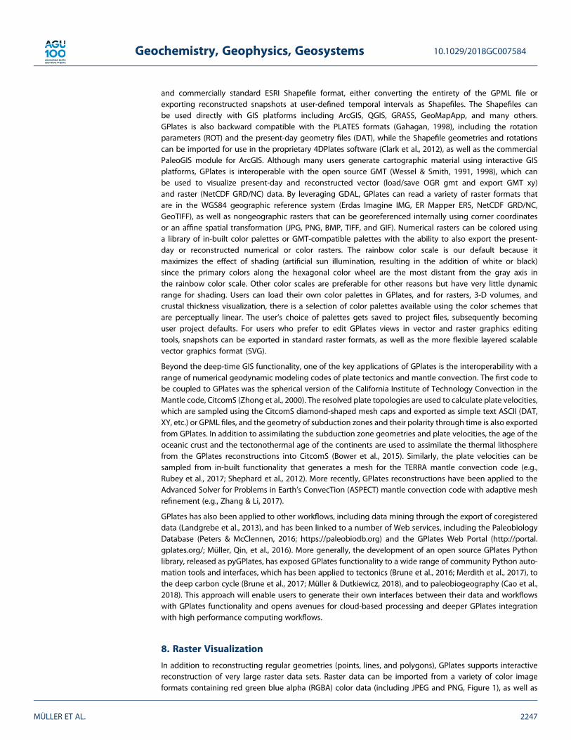
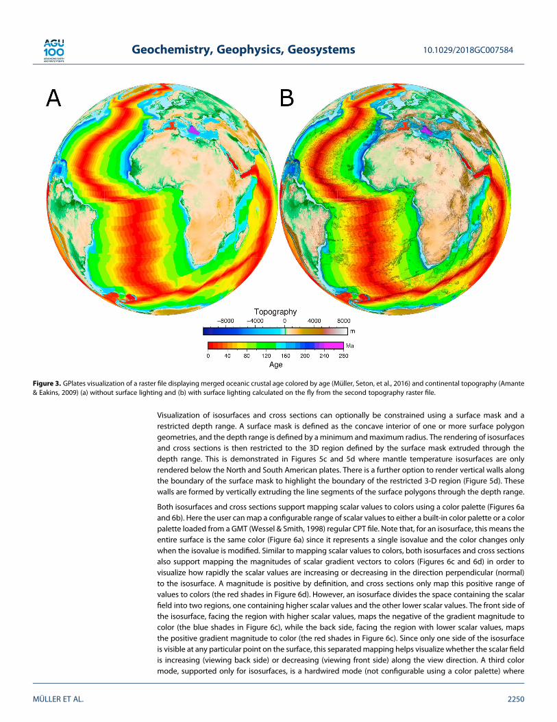
Since a raster can be arbitrarily large and may not fit into memory, the cube map structure is furtherenhanced with a multiresolution tile partitioning that significantly reduces the in-memory raster data to onlythose tiles that are currently visible and at the lowest resolution required. For example, when the view iszoomed in, only part of a reconstructed raster is visible but a higher resolution is required, whereas azoomed-out view sees more of the reconstructed raster but at a lower resolution. The cube map structurealso enables multiple rasters with different georeferencing to be combined once they have been resampledinto cube maps. An example is enhancing raster reconstruction with a present-day age grid that contains thetime of appearance of oceanic crust at each pixel location. Here both the age raster and the actual rasterbeing reconstructed are simultaneously accessed via their cube maps when rendering rotated tectonic poly-gons, during which a per-pixel age comparison determines whether to render each reconstructed rasterpixel, thus achieving a finer granularity than is possible with polygon-size tests (each tectonic polygon alsohas a time of appearance). Figure 2 shows how reconstructing a raster with an age grid removes the gapscaused by polygons following discrete isochrons. Another example of combining cube maps is surface reliefshading where a second raster is treated as an elevation map. Here surface lighting is not precomputed forthe first raster but calculated interactively from the second raster and modulated with the color from the firstraster. Figure 3 shows an oceanic age grid (colored by age) overlain on a topography raster (colored byelevation), but both with lighting determined by the topography raster.

In addition to visualizing rasters, GPlates can also interactively analyze reconstructed numerical rasters bycomputing statistics such as the mean and standard deviation within raster regions restricted to a user-specified distance from points, lines, and polygons. Alternatively, researchers can export reconstructednumerical raster data from GPlates for analysis in other software.

9. Volume Visualization

GPlates supports the interactive visualization of subsurface 3-D scalar fields, enabling them to beobserved together with traditional geological surface data in a common plate tectonic reference frame.For example, a user can visualize the output of geodynamic models in relation to their plate tectonic sur-face constraints. Scalar fields can be visualized either as isosurfaces or cross sections. Figure 4 shows theMIT-P08 (Li et al., 2008) tomographic model visualized both as an isosurface representation (Figure 4a)and color-coded on cross sections along tectonic plate boundaries (Figure 4b). An isosurface representsthe surface through the scalar field with a specific scalar value known as the isovalue. Isosurfaces are ren-dered by tracing a ray through the scalar field, at each screen pixel in the globe view, until the isosurfaceis found. To achieve this, a ray-tracing process is executed on the graphics hardware simultaneously for

10.1029/2018GC007584Geochemistry, Geophysics, Geosystems

MÜLLER ET AL. 2248

each pixel. This approach is particularly suited to modern graphics hardware because the rays (pixels) areindependent of each other and hence can be distributed in parallel across the thousands ofcomputational units in the Graphics Processing Unit (GPU). This enables real-time interactivity when theisosurface is rerendered each time the view changes or the user adjusts the isovalue. An intuitive 3-Dvisualization is achieved by evaluating a lighting model at each intersection point—resulting in specificshadow effects. Cross sections are surface lines extruded vertically (in the radial direction) to visualizethe 3-D scalar field along the resultant 2-D slices—based on a specific color palette. Any existingsurface geometries can be used as the source of these cross sections, such as the black tectonic plateboundaries in Figure 4b. Additionally, the existing canvas tools enable the user to interactivelymanipulate cross sections by moving, inserting, and deleting surface geometry vertices.

The rendering of isosurfaces and cross sections both have the common requirement that the graphics hard-ware must convert locations (within the 3-D scalar field) into scalar values. A cube map data structure waschosen for this purpose and is an extension of the cube map structure used for 2-D surface rasters withthe addition of depth layers in order to support subsurface 3-D scalar fields. A 3-D scalar field is created byimporting several 2-D rasters, each assigned to a different depth. During import, these 2-D georeferenceddepth rasters are resampled into a cube map partition that is similar to that used for a 2-D surface rasterexcept each partition in the cube map is a tile column, instead of a single tile, since it now has several tilesbelow it (one for each depth). This pregenerated cube map partitioning is then imported into a binary file(GPlates Scalar Field), referenced by a GPML file, such that future loads of the scalar field are fast. Duringisosurface or cross-section rendering, sampling the 3-D scalar field at an arbitrary 3-D location within the fieldthen involves projecting that location into a specific partition (tile column) of the cube map, to find its 2-Dcoordinates within any tile image below that partition (tile column), followed by interpolating between thetwo depth layer tiles in that tile column that surround the 3-D location in the depth dimension. All interpola-tions are performed by efficient texture lookups directly on the GPU.

Figure 2. GPlates reconstruction of a present-day global free air gravity raster (Sandwell et al., 2014) (a) using static polygons only and (b) using a combination ofstatic polygons and an age grid. Note that red color has been added to (a) purely to highlight the difference. The static plate polygons are based on discreteseafloor isochrons (Müller, Seton, et al., 2016), resulting in gaps in reconstructions whose ages do not correspond to a given isochron age, while using the associatedpresent-day age grid (Müller, Seton, et al., 2016) removes the gaps.

10.1029/2018GC007584Geochemistry, Geophysics, Geosystems

MÜLLER ET AL. 2249

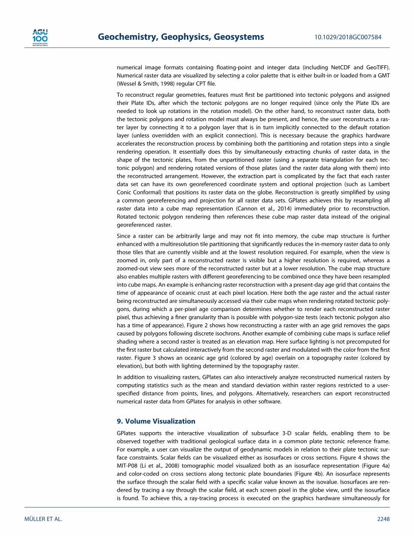
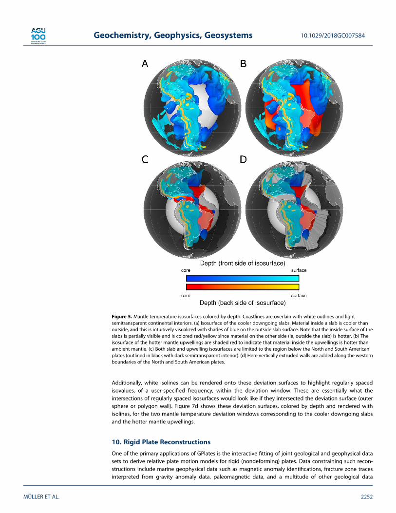
Visualization of isosurfaces and cross sections can optionally be constrained using a surface mask and arestricted depth range. A surface mask is defined as the concave interior of one or more surface polygongeometries, and the depth range is defined by aminimum andmaximum radius. The rendering of isosurfacesand cross sections is then restricted to the 3D region defined by the surface mask extruded through thedepth range. This is demonstrated in Figures 5c and 5d where mantle temperature isosurfaces are onlyrendered below the North and South American plates. There is a further option to render vertical walls alongthe boundary of the surface mask to highlight the boundary of the restricted 3-D region (Figure 5d). Thesewalls are formed by vertically extruding the line segments of the surface polygons through the depth range.

Both isosurfaces and cross sections support mapping scalar values to colors using a color palette (Figures 6aand 6b). Here the user canmap a configurable range of scalar values to either a built-in color palette or a colorpalette loaded from a GMT (Wessel & Smith, 1998) regular CPT file. Note that, for an isosurface, this means theentire surface is the same color (Figure 6a) since it represents a single isovalue and the color changes onlywhen the isovalue is modified. Similar to mapping scalar values to colors, both isosurfaces and cross sectionsalso support mapping the magnitudes of scalar gradient vectors to colors (Figures 6c and 6d) in order tovisualize how rapidly the scalar values are increasing or decreasing in the direction perpendicular (normal)to the isosurface. A magnitude is positive by definition, and cross sections only map this positive range ofvalues to colors (the red shades in Figure 6d). However, an isosurface divides the space containing the scalarfield into two regions, one containing higher scalar values and the other lower scalar values. The front side ofthe isosurface, facing the region with higher scalar values, maps the negative of the gradient magnitude tocolor (the blue shades in Figure 6c), while the back side, facing the region with lower scalar values, mapsthe positive gradient magnitude to color (the red shades in Figure 6c). Since only one side of the isosurfaceis visible at any particular point on the surface, this separatedmapping helps visualize whether the scalar fieldis increasing (viewing back side) or decreasing (viewing front side) along the view direction. A third colormode, supported only for isosurfaces, is a hardwired mode (not configurable using a color palette) where

Figure 3. GPlates visualization of a raster file displaying merged oceanic crustal age colored by age (Müller, Seton, et al., 2016) and continental topography (Amante& Eakins, 2009) (a) without surface lighting and (b) with surface lighting calculated on the fly from the second topography raster file.

10.1029/2018GC007584Geochemistry, Geophysics, Geosystems

MÜLLER ET AL. 2250

the color varies with depth as shown in Figure 5. Here the front side of the isosurface blends between blue atthe bottom (deepest) layer and cyan at the top (shallowest) layer, and the back side of the isosurface blendsbetween red at the bottom layer and yellow at the top layer. The use of blue and red shades on the front andback sides of an isosurface is intuitive for mantle temperature scalar fields (Figure 5) where downgoing slabsare shades of blue, to indicate material inside the slab is cooler than its surrounding, and mantle upwellingsare shades of red, to indicate material inside the upwelling is hotter than its surrounding.

An isosurface deviation window consists of a main isosurface and a deviation isosurface on either side of it.The two deviation isovalues are offset from the main isovalue by a user-adjustable constant such that thedeviation isosurfaces track the main isosurface as its isovalue is modified. The main isosurface is opaqueand white, whereas the two deviation isosurfaces are colored according to the user-selected color modeand are semitransparent by default so that the main isosurface is visible through them. The deviation windowessentially provides an alternative visualization of gradients along the main isosurface since locations withhigher gradients will result in larger distances between the main and deviation isosurfaces. A single deviationwindow consists of one main isosurface and its two deviation isosurfaces. A double deviation window is alsopossible and consists of two nonoverlapping deviation windows, with each window having a separately con-figurable main isovalue and deviation offset. This is useful for the mantle temperature example, shown againin Figure 7, where cooler downgoing slabs use a lower isovalue in the first window and hotter mantle upwel-lings use a higher isovalue in the second window. Since a deviation window is a 3-D region of space, enclosedby its two deviation isosurfaces (surrounding its main isosurface), it can be intersected by the 2-D outersphere (topmost depth layer) and by the 2-D vertically extruded polygon walls of the surface mask(Figure 7c). These intersections are 2D deviation surfaces that essentially close off the 3-D deviation windowregion. They can optionally be rendered using the same color mode as the isosurface, with the depth colormode also blending from green at the main isosurface to the usual blue and red shades at the deviationisosurfaces (which, at the outer sphere, are the topmost-depth blue and red shades of cyan and yellow).

Figure 4. MIT-P08 tomographic model (Li et al., 2008) overlain with coastlines in white and tectonic plate boundaries in black. The gray interior of the continents issemitransparent. (a) A seismic velocity anomaly isosurface colored by depth. (b) Vertically extruded cross sections are shown along tectonic plate boundaries.

10.1029/2018GC007584Geochemistry, Geophysics, Geosystems

MÜLLER ET AL. 2251

Additionally, white isolines can be rendered onto these deviation surfaces to highlight regularly spacedisovalues, of a user-specified frequency, within the deviation window. These are essentially what theintersections of regularly spaced isosurfaces would look like if they intersected the deviation surface (outersphere or polygon wall). Figure 7d shows these deviation surfaces, colored by depth and rendered withisolines, for the two mantle temperature deviation windows corresponding to the cooler downgoing slabsand the hotter mantle upwellings.

10. Rigid Plate Reconstructions

One of the primary applications of GPlates is the interactive fitting of joint geological and geophysical datasets to derive relative plate motion models for rigid (nondeforming) plates. Data constraining such recon-structions include marine geophysical data such as magnetic anomaly identifications, fracture zone tracesinterpreted from gravity anomaly data, paleomagnetic data, and a multitude of other geological data

Figure 5. Mantle temperature isosurfaces colored by depth. Coastlines are overlain with white outlines and lightsemitransparent continental interiors. (a) Isosurface of the cooler downgoing slabs. Material inside a slab is cooler thanoutside, and this is intuitively visualized with shades of blue on the outside slab surface. Note that the inside surface of theslabs is partially visible and is colored red/yellow since material on the other side (ie, outside the slab) is hotter. (b) Theisosurface of the hotter mantle upwellings are shaded red to indicate that material inside the upwellings is hotter thanambient mantle. (c) Both slab and upwelling isosurfaces are limited to the region below the North and South Americanplates (outlined in black with dark semitransparent interior). (d) Here vertically extruded walls are added along the westernboundaries of the North and South American plates.

10.1029/2018GC007584Geochemistry, Geophysics, Geosystems

MÜLLER ET AL. 2252

including terrain boundaries, faults, large igneous provinces, ophiolites, and other geological markers asdescribed in Müller, Seton, et al. (2016). Reconstructions of conjugate magnetic anomalies and fracturezone identifications can also be performed quantitatively in a least squares sense using Hellinger’s (1981)criterion of fit, via a canvas tool workflow. The computed best fit depends on providing conjugate pairs ofsegments of magnetic or fracture zone identifications (“picks”), which represent a common mid-oceanridge-segment or a common transform fault. One set of segments is considered fixed, and the other setmoves with respect to the fixed set. The fitting algorithm uses an initial user-provided rotation-poleestimate to rotate the moving picks toward the fixed picks. Picks from conjugate segment pairs are fittedto a great circle arc, and the deviations of picks from their great circles are used to generate a measure ofthe goodness of fit. The best fitting rotation pole is found either by a grid-search around the initialestimate or by a downhill-simplex minimization algorithm. The GPlates interface allows interactiveadjustment of magnetic or fracture zone pick locations, data segmentation, and fit parameters. Both two-plate and three-plate fitting can be performed. To maintain compatibility with legacy code, GPlates can

Figure 6. Mantle temperature isosurfaces and cross sections colored by (a and b) mantle temperature and(c and d) temperature gradient magnitude. Coastlines are overlain with white outlines and semitransparent interiors.(a) Visualization of two isosurfaces of downgoing slabs and mantle upwellings colored by temperature. Each isosurface is aconstant temperature and hence a constant color. (b) Cross sections of mantle temperature highlighting cooler (blue) slabsof oceanic crust subducting into the relatively hotter mantle (red/orange) underneath the North and South Americancontinents. (c) Visualization of two isosurfaces colored by temperature gradient magnitude. The shades of red indicate thatthe temperature is increasing along the view direction, such as traveling from outside to inside a hot mantle upwelling.The shades of blue indicate decreasing temperature, for instance as seen in the gradient from outside to inside a cool slab. Thedarker shades of red or blue indicate higher temperature gradients compared to the lighter shades. (d) Mantlecross sections colored by temperature gradient magnitude. The temperature gradient direction relative to an isosurface is notvisualized here, so only shades of red exist with darker shades indicating higher gradients.

10.1029/2018GC007584Geochemistry, Geophysics, Geosystems

MÜLLER ET AL. 2253

import magnetic picks and fit parameters from text files suitable for use with legacy FORTRAN programs(Kirkwood et al., 1999); picks can also be created and edited through the GPlates user interface. Theresulting best fit finite rotation pole is displayed on the GPlates globe together with its uncertainty ellipse,computed following Kirkwood et al. (1999).

The GPlates rotation engine allows for calculation of time-dependent position and velocity information ofan arbitrary point on any plate. Such information can be exported to various file formats through GPlates’export functionality. The Kinematics Tool provides an interactive way of accessing this information,visualizing latitude, longitude, and the relative or absolute plate motion velocity history of any point ofinterest, in both tabular and graphical form. Positional and velocity information are calculated at user-definedintervals; velocity calculation parameters (e.g., the time interval used in the velocity calculation) arealso user-adjustable.

Figure 7. Mantle temperature deviation windows colored by depth. Coastlines are overlain with white outlines and semi-transparent continental interiors. (a) Two isosurfaces of cooler downgoing slabs and hotter mantle upwellings withoutdeviation windows. (b) Isosurfaces with deviation windows added. Each constant-temperature main isosurface has its owntemperature offset (deviation). Each resultant deviation window has an opaque white isosurface surrounded by twosemitransparent deviation isosurfaces colored by depth. Note that the white isosurfaces are exposed at the surface. (c) Bothslab and upwelling deviation windows are limited to the region below the North and South American plates (outlined inblack with semitransparent interior). Note that the white isosurfaces are also exposed by the cut-out region. (d) Theexposed deviation windows are filled in with depth coloring and white isolines. The deviation windows at the outer spheresurface are semitransparent, whereas those along the sidewalls are opaque. Note that depth coloring blends from the usualred and blue shades at the deviation isosurfaces to green at the main (white) isosurfaces.

10.1029/2018GC007584Geochemistry, Geophysics, Geosystems

MÜLLER ET AL. 2254

11. Plate Deformation

GPlates deforming plate functionality allows users to define the spatial and temporal extent of diffuse plateboundaries and model the deformation of these regions through time (Gurnis et al., 2018). These are regionscombining extension, compression, and shearing that accommodate the relative motion between rigidblocks that follow the traditional concept of plate tectonics. Alternatively, GPlates can input a set of pointswithin a deformation region with rotations relative, for example, to its edge. These could be computedoutside of GPlates with a wide range of data not directly used inside of GPlates, such as paleomagneticrotations of small blocks, tectonic subsidence curves, or structure measures of finite strain, as commonly usedin regional reconstructions. Users can explore how strain rates, stretching/shortening factors, and crustalthickness evolve through space and time within deforming regions and interactively update the kinematicsassociated with deformation to investigate how these parameters are influenced by alternative platereconstruction scenarios. The geometries that define regions of deformation change over time in responseto the user-defined kinematics, and the consequences of these changes can be quantified and representedusing stretching/shortening factors. Together, the new tools form the basis for building reconstructions thatquantitatively describe the cycles of rifting, mountain building, and intracontinental shearing that accom-pany supercontinent assembly and dispersal.

The building blocks of a deforming plate reconstruction are points, lines, and polygons that define plateboundaries, the boundaries between deforming and rigid regions, and can partition the deformation withinthe regions of deformation. Each of these geometries can be assigned its own history of motion in the sameway as a plate. The GPlates user interface is designed to facilitate the process of defining both the extent ofdeforming regions and the motion history of each building block, as well as define subregions that have notexperienced deformation (i.e., behaved as rigid tectonic blocks). Defining a region of deformation follows thesame logic as creating plate topologies, with the additional option of adding features into the deformingregion that model deformation (such as rifts or orogens) or the absence of deformation (such as rigid ele-ments). The spatial extent of deforming meshes is mainly based on a variety of geological and geophysicalevidence—for example, models of crustal thickness, estimates of sediment thickness for extensional regions,and the topography and structure of mountain belts. GPlates allows the computation of time-dependentstretching or compression within deforming regions based on the kinematic motions of the surrounding(rigid) features. Although the rigid elements are reconstructed using their Plate ID, and hence, their velocitiesare simply derived from the Euler rotation, the velocities within the deforming mesh are interpolated basedon the deformation history of the topology. One can also compute finite strain and quantities related to finitestrain, like stretching factors. Here points are integrated forward in time for points within the deformingmeshwith an assumption made of an initial condition, like crustal thickness prior to a given phase of extension. Thestrain history is simple to modify within the GPlates interface, allowing multiple estimates of stretching factorbe determined for a single kinematic reconstruction based on alternative prerift scenarios. If the deformationwithin a region entirely arises from the rotations of the edges of the region, a simplification in the currentmodel is the absence of deformation partitioning within each margin so there is currently no distinctionbetween high extension factors expected in distal margin areas versus the more moderate amounts ofextension closer to the rift edge—instead, the displayed values represent average stretching factors for eachmargin segment that vary along strike.

As an example we show a deforming plate model for New Zealand (D. Müller et al., 2018), focusing on the last20 million years (Figure 8), based on a rigid plate model by Wood and Stagpoole (2007). The reconstructionprovides a representation of deformation including the individual relative motions of the blocks correspond-ing to the western North Island, East coast North Island, Marlborough, west coast South Island, and east coastSouth Island, including regions of extension and shortening, with oblique compression forming the SouthernAlps, the North Island’s eastern ranges, and the East Coast fold and thrust belt (Wood & Stagpoole, 2007).

12. Reconstructing Features Using Topologies

GPlates 2.0 introduces a reconstruction paradigm called “topological reconstruction” that involves usingplate boundary topologies (deforming and nondeforming) to partition features into tectonic plates andreconstruct features. Topological reconstruction is based on points since this greatly simplifies the implemen-tation. If the initial geometry is a polyline or polygon, then it is tessellated into closely spaced points that

10.1029/2018GC007584Geochemistry, Geophysics, Geosystems

MÜLLER ET AL. 2255

approximate its shape. Incremental topological reconstruction begins with the points of the initial geometry.A single time step involves independently attaching each point to the deforming or nondeforming topology(if any) whose boundary contains the point. Each point then moves to its new position, over an incrementaltime interval, as its temporarily assigned topology would at that location. For a nondeforming topology theincremental point movement is a rigid plate motion that simply uses the Plate ID of the topology to rotate thepoint. For a deforming topology this incremental point movement requires further locating the point withinthe nonuniform deformation field inside the topology, unless the point is contained within a rigid interiorblock in which case it is treated the same as regular nondeforming topologies. This deformation field isrepresented by a triangulation where each vertex in the triangulation has a Plate ID and hence a motiondefined by Euler rotations. Initially, the triangle containing the point is located along with the point’sinterpolation coordinates within that triangle. Then the three vertices of the triangle are rotated over theincremental time interval (using their Plate IDs), resulting in a new triangle with a distorted shape (ifthe three Plate IDs are not the same). Finally, the deformed point position is obtained by using theinterpolation coordinates to interpolate the new vertex positions of the triangle. There is also an option tointerpolate additional nearby vertices than just the three of the triangle containing the point to obtain asmoother deformation field. It is also possible that the point might not be contained by any topologies(deforming or non deforming), for example, when topologies do not have global coverage. In this case thepoint falls back to using its own Plate ID, as would have been the case if topological reconstruction wasswitched off.

After obtaining the new reconstructed point positions from the first time step, these positions are thenused as input to the next time step and the process is repeated until the desired reconstruction timeis reached resulting in the reconstructed points of the final geometry. Note that at each time step theset of topologies can change, since nondeforming plates can split and merge, and deforming networkscan appear and disappear when deformation begins and ends. As a result, each point can transition fromone topology to another, and this highlights the advantage of using topologies that have global cover-age. For example, when deformation ends in a region, its deforming topology will disappear and bereplaced by nondeforming plates that will then pick up the points and continue to reconstruct them

Figure 8. (a) Deforming meshes colored by strain rate covering the main regions that have undergone distributed deformation in New Zealand since 20 Ma, basedon a rigid plate model by Wood and Stagpoole (2007). (b) Stretching factor grids that display the lithospheric stretching/thickening factor as defined byLe Pichon and Sibuet (1981) with values from one to two expressing extension, while values less than one correspond to compression.

10.1029/2018GC007584Geochemistry, Geophysics, Geosystems

MÜLLER ET AL. 2256

appropriately (instead of falling back to using the Plate ID of the points feature). Note that a deformingtopology can be overlain on top of nondeforming topologies, in which case a point contained by bothwill only be influenced by the deforming topology. However, deforming topologies are typicallyembedded into a global nondeforming plate model such that they share common boundaries and hencedo not overlap.

Topological reconstruction also supports automatic lifetime detection, such as determining when each topo-logically reconstructed point of a gradually subducting seafloor isochron should disappear. This is in contrastto the usual method of reconstruction whereby a user-specified time of appearance and disappearance isrequired and must be manually updated whenever the tectonic plate arrangement changes. The lifetimedetection algorithm works by looking at a point’s convergent/divergent velocity when it transitions fromone plate to another. These transitions represent an opportunity for the point to appear at a divergent plateboundary (seafloor created at a mid-ocean ridge) or disappear at a convergent plate boundary(seafloor subducted).

13. Project Files

A GPlates session consists of the loaded data filenames and associated layers. Unlike previous versions,Glates2.0 saves and restores all layer information including layer order and visibility and all settings withineach layer such as color styles and color palette filenames. A GPlates session can be saved to a user-specifiedproject file and later restored from it when GPlates is reopened. The most recent sessions are also automati-cally saved internally as an extra convenience, allowing the user to restore from a list of recent sessions with-out having to save or load a project file. However, only a limited number of sessions are stored in this way,with new sessions overwriting old sessions. Project files do not have this limitation and also can be copiedto other computers. Hence, they are generally recommended over the recent-sessions list.

14. Plate Motion Models and Associated Data

The broad philosophy behind the GPlates project (GPROJ) is to provide open-source workflows and open-access data for the scientific community, and in this regard, the software is bundled with a comprehensiveset of sample data. The plate motion model (including rotation parameters and plate topologies) that isincluded with GPlates 2.0 and the recently released GPlates2.1, which includes a number of bug fixes andminor updates, spans the last 410 million years (Matthews et al., 2016), which is a modified and merged ver-sion of the pre-Pangea (Domeier & Torsvik, 2014) and post-Pangea (Müller, Seton, et al., 2016) plate recon-structions. It is important to note that GPlates is not tied to any given plate model. One of its strengths isthat it allows for easy comparison between different published plate models (e.g., Cao et al., 2018). A numberof GPlates-compatible plate models are available on the EarthByte Web site at https://www.earthbyte.org/global-plate-models and at https://www.earthbyte.org/paleomap-paleoatlas-for-gplates/, while the modelfrom Torsvik and Cocks (2016) is available at http://www.earthdynamics.org/earthhistory/. The most appro-priate model for any user will depend on the purpose of their research, for example, paleoenvironmentalor climate modeling versus geodynamic modeling, how far back in time a given model needs to go andwhether or not a given application requires a plate model with evolving topological plate boundaries ornot. To ensure that vector and raster data can be reconstructed in GPlates, the bundle includes a globalset of present-day polygons that allow GPlates to partition the Earth’s surface into tectonic elements by theirPlate ID and their age. These present-day polygons are referred to as “static polygons” as they do not changetheir shape through time but can be rotated and reconstructed using the Euler rotations loaded in GPlatesand enable the partitioning of data into tectonic plates and reconstruction of geospatial vector andraster data.

One of the most commonly used vector data sets represents the present-day global self-consistent hier-archical high-resolution shorelines (GSHHS; Wessel & Smith, 1996), which are partitioned into tectonicplates using static polygons. The reconstructed present-day coastlines are useful to help the user identifypresent-day features in deep-time plate reconstructions (Figure 1), but due to the nature of sea levelchange, paleo-shorelines are an additional geometric feature that can be plotted to better representthe paleogeographic reconstruction (Cao, Zahirovic, et al., 2017). Similarly, the supplied present-day 5°graticule grid marks can be reconstructed to provide a visual reference at reconstructions snapshots.

10.1029/2018GC007584Geochemistry, Geophysics, Geosystems

MÜLLER ET AL. 2257

Not all of the geographic features are partitioned in this way, with the best example representing present-day hotspots (Whittaker et al., 2015), which are separated into their Indo-Atlantic and Pacific domains(Figure 1b). For continental regions, the outline of present-day continental crust is supplied (Müller,Seton, et al., 2016), as well as the paleomagnetic virtual geomagnetic poles (VGP) for the major continen-tal blocks (Torsvik et al., 2008). The continent-ocean boundaries as the transition between continental andoceanic crust at passive margins are also included, as well as a number of data sets specific to the oceaniccrust including the mapped seafloor fabric (Matthews et al., 2011), seafloor age isochrons, and extinct andactive mid-oceanic ridges (Müller, Seton, et al., 2016; Figure 1a). The new functionality of GPROJ filesmeans that a single GPROJ file can be opened in GPlates, which then loads basic and commonly usedvector and raster layers (with their coloring and appropriate links encoded), which provides added flexibil-ity for users to use and expand their GPlates workspaces.

An extended set of common geophysical raster data sets are bundled in GPlates2.1, including the numer-ical NetCDF grid of seafloor age (Müller, Seton, et al., 2016), as well as the color rasters of elevation(Amante & Eakins, 2009; Figure 1a), free air gravity anomalies and vertical gravity gradients (Sandwell et al.,2014), Bouguer and isostatic gravity anomalies (Balmino et al., 2012), magnetic anomalies without direc-tional gridding from seafloor age models applied (Maus et al., 2009), crustal thickness (https://igppweb.ucsd.edu/~gabi/crust2.html), crustal strain (Kreemer et al., 2014), and UNESCO global geology (https://ccgm.org/en/home/164-carte-geologique-du-monde-a-l-echelle-de-135-000-000-9782917310243.html, Figure 1b).The present-day rasters can be partitioned and reconstructed using the static polygons, and theirreconstructed snapshots exported. Numerical rasters can be exported as reconstructed numerical or colorrasters, allowing such data sets to retain their flexibility. One common approach to expand the utility ofreconstructing rasters using the “static polygons” involves connecting the present-day seafloor agenumerical raster to another color raster layer (such as elevation), which enables the color raster pixelsto be masked by the seafloor age, and is especially useful when visualizing oceanic basin evolution.Time-dependent rasters, for instance of modeled paleo-bathymetry (Müller et al., 2008), lack the detailof present-day grids but add the dimension of time. These rasters are classified as “time-dependent” asthey represent a series of snapshots at different geological times, enabling GPlates to load the relevantglobal or regional raster field. However, time-dependent rasters are tied to a particular plate model.Other examples of time-dependent rasters include the output of geodynamic models of mantleconvection, with time-dependent rasters of dynamic topography or mantle temperature at depth.GPlates2.1 is bundled with a time-dependent raster of age-coded subducted slabs, represented by fastseismic velocities in tomographic models of the mantle. The bundled rasters use the global P wave modelof Li et al. (2008) and assume a constant vertical sinking rate of 3 and 1.2 cm/yr in the upper and lowermantles, respectively. This tomography model is also provided as a 3-D scalar field, but for the SoutheastAsia region in order to reduce the file size of the sample data. The sample data provide an overview ofwhat vector, raster, and scalar field data can be loaded by the user in GPlates, as well as how such dataare structured and stored in the file system. GPlates compatible data are available from https://www.earthbyte.org/gplates-2-0-software-and-data-sets.

15. Future Outlook

Future development of GPlates includes improvements to volume visualization, globe viewing, and sym-bology as well as the use of the Open Compute Language (OpenCL) to transform gridded data on the fly.Currently, only one data volume for a given reconstruction time can be imported, while in the future, thisfunctionality will be extended to handle time-dependent scalar fields, for instance allowing the importingof time-dependent mantle volume outputs from geodynamic models. Globe viewing will be extended toinclude camera tilts, and the symbology used to render points and lines will be extended to includeappropriate symbols for different plate boundaries and properties of point data (such as lithology sym-bols). Users will also be able to apply equations to rasters using OpenCL, for instance to convert seafloorage to depth. Future development will also include vertical rasters, for instance representing importedseismic cross sections, which may appear as “pop-ups” orthogonal to the globe surface, as well as variablealtitude rasters, that is, visualizing a global raster at altitudes above or below the surface of the Earth. Wewelcome input about improved functionality from the growing community of users via our “GPlates-discuss” mailing list (subscription here: https://mailman.sydney.edu.au/mailman/listinfo/gplates-discuss).

10.1029/2018GC007584Geochemistry, Geophysics, Geosystems

MÜLLER ET AL. 2258

ReferencesAmante, C., & Eakins, B. (2009). ETOPO1 1 arc-minute global relief model: Procedures, data sources and analysis. NOAA Technical

Memorandum NESDIS NGDC-24 (National Geophysical Data Center, NOAA). https://doi.org/10.7289/V5C8276MBalmino, G., Vales, N., Bonvalot, S., & Briais, A. (2012). Spherical harmonic modelling to ultra-high degree of Bouguer and isostatic anomalies.

Journal of Geodesy, 86(7), 499–520. https://doi.org/10.1007/s00190-011-0533-4Barnett-Moore, N., Hassan, R., Müller, R., Williams, S. E., & Flament, N. (2017). Dynamic topography and eustasy controlled the paleogeo-

graphic evolution of northern Africa since the mid-Cretaceous. Tectonics, 36, 929–944. https://doi.org/10.1002/2016TC004280Bower, D. J., Gurnis, M., & Flament, N. (2015). Assimilating lithosphere and slab history in 4-D Earth models. Physics of the Earth and Planetary

Interiors, 238, 8–22. https://doi.org/10.1016/j.pepi.2014.10.013Bower, D. J., Gurnis, M., & Seton, M. (2013). High bulk modulus structures in the lower mantle from dynamic Earth models with paleogeo-

graphy. Geochemistry, Geophysics, Geosystems, 14, 44–63. https://doi.org/10.1029/2012GC004267Boyden, J. A., Müller, R. D., Gurnis, M., Torsvik, T. H., Clark, J. A., Turner, M., et al. (2011). Next-generation plate-tectonic reconstructions using

GPlates. In G. R. Keller, & C. Baru (Eds.), Geoinformatics: Cyberinfrastructure for the solid Earth sciences (pp. 95–114). Cambridge: CambridgeUniversity Press. https://doi.org/10.1017/CBO9780511976308.008

Brune, S., Williams, S. E., Butterworth, N. P., & Müller, R. D. (2016). Abrupt plate accelerations shape rifted continental margins. Nature,536(7615), 201–204. https://doi.org/10.1038/nature18319

Brune, S., Williams, S. E., & Müller, R. D. (2017). Potential links between continental rifting, CO 2 degassing and climate change through time.Nature Geoscience, 10(12), 941. https://doi.org/10.1038/s41561-017-0003-6-946

Cannon, J., Lau, E., & Müller, R. (2014). Plate tectonic raster reconstruction in GPlates. Solid Earth, 5(2), 741. https://doi.org/10.5194/se-5-741-2014-755

Cao, W., Lee, C.-T. A., & Lackey, J. S. (2017). Episodic nature of continental arc activity since 750 Ma: A global compilation. Earth and PlanetaryScience Letters, 461, 85–95. https://doi.org/10.1016/j.epsl.2016.12.044

Cao, W., Williams, S., Flament, N., Zahirovic, S., Scotese, C., & Müller, R. D. (2018). Paleolatitudinal distribution of lithologic indicators of climatein a paleogeographic framework. Geological Magazine, 1–24. https://doi.org/10.17605/OSF.IO/H52D6

Cao, W., Zahirovic, S., Flament, N., Williams, S., Golonka, J., & Müller, R. D. (2017). Improving global paleogeography since the late Paleozoicusing paleobiology. Biogeosciences, 14(23), 5425–5439. https://doi.org/10.5194/bg-14-5425-2017

Clark, S. R., Skogseid, J., Stensby, V., Smethurst, M. A., Tarrou, C., Bruaset, A. M., & Thurmond, A. K. (2012). 4DPlates: On the fly visualization ofmultilayer geoscientific datasets in a plate tectonic environment. Computers & Geosciences, 45, 46–51. https://doi.org/10.1016/j.cageo.2012.03.015

Coltice, N., Seton, M., Rolf, T., Müller, R., & Tackley, P. J. (2013). Convergence of tectonic reconstructions and mantle convection models forsignificant fluctuations in seafloor spreading. Earth and Planetary Science Letters, 383, 92–100. https://doi.org/10.1016/j.epsl.2013.09.032

Cook, K. L., Hovius, N., Wittmann, H., Heimsath, A. M., & Lee, Y.-H. (2018). Causes of rapid uplift and exceptional topography of Gongga Shanon the eastern margin of the Tibetan Plateau. Earth and Planetary Science Letters, 481, 328–337. https://doi.org/10.1016/j.epsl.2017.10.043

Cox, A., & Hart, B. R. (1986). Plate tectonics: How it works (p. 400). Oxford: Blackwell Science Inc.DiCaprio, L., Müller, R. D., & Gurnis, M. (2010). A dynamic process for drowning carbonate reefs on the northeastern Australian margin.

Geology, 38(1), 11–14. https://doi.org/10.1130/G30217.1Domeier, M., & Torsvik, T. H. (2014). Plate tectonics in the late Paleozoic. Geoscience Frontiers, 5(3), 303–350. https://doi.org/10.1016/j.

gsf.2014.01.002Dutkiewicz, A., Müller, R., Wang, X., O’Callaghan, S., Cannon, J., & Wright, N. (2017). Predicting sediment thickness on vanished ocean crust

since 200 Ma. Geochemistry, Geophysics, Geosystems, 18, 4586–4603. https://doi.org/10.1002/2017GC007258Dyksterhuis, S., & Müller, R. D. (2017). Future intraplate stress and the longevity of carbon storage. Fuel, 200, 31–36. https://doi.org/10.1016/j.

fuel.2017.03.042Flament, N., Gurnis, M., Müller, R. D., Bower, D. J., & Husson, L. (2015). Influence of subduction history on South American topography. Earth

and Planetary Science Letters, 430, 9–18. https://doi.org/10.1016/j.epsl.2015.08.006Flament, N., Williams, S., Müller, R., Gurnis, M., & Bower, D. (2017). Origin and evolution of the deep thermochemical structure beneath

Eurasia. Nature Communications, 8, 14164. https://doi.org/10.1038/ncomms14164Gahagan, L. (1998). Plates4. 0: A user’s manual for the PLATES project’s interactive reconstruction software, Rep., pp. 39.Gurnis, M., Turner, M., Zahirovic, S., DiCaprio, L., Spasojević, S., Müller, R. D., et al. (2012). Plate tectonic reconstructions with continuously

closing plates. Computers and Geosciences, 38(1), 35–42. https://doi.org/10.1016/j.cageo.2011.04.014Gurnis, M., Yang, T., Cannon, J., Turner, M., Williams, S., Flament, N., & Müller, R. D. (2018). Global tectonic reconstructions with continuously

deforming and evolving rigid plates. Computers and Geosciences, 116, 32–41. https://doi.org/10.1016/j.cageo.2018.04.007Hague, A. M., Thomas, D. J., Huber, M., Korty, R., Woodard, S. C., & Jones, L. B. (2012). Convection of North Pacific deep water during the early

Cenozoic. Geology, 40(6), 527–530. https://doi.org/10.1130/G32886.1Harrington, L., Zahirovic, S., Flament, N., & Müller, R. D. (2017). The role of deep Earth dynamics in driving the flooding and emergence of New

Guinea since the Jurassic. Earth and Planetary Science Letters, 479, 273–283. https://doi.org/10.1016/j.epsl.2017.09.039Heine, C., Zoethout, J., & Müller, R. D. (2013). Kinematics of the South Atlantic rift. Solid Earth, 4(2), 215. https://doi.org/10.5194/se-4-215-

2013-253Hellinger, S. J. (1981). The uncertainties of finite rotations in plate tectonics. Journal of Geophysical Research, 86, 9312–9318. https://doi.org/

10.1029/JB086iB10p09312Henrot, A.-J., Utescher, T., Erdei, B., Dury, M., Hamon, N., Ramstein, G., et al. (2017). Middle Miocene climate and vegetation models and their

validation with proxy data. Palaeogeography, Palaeoclimatology, Palaeoecology, 467, 95–119. https://doi.org/10.1016/j.palaeo.2016.05.026Herold, N., Buzan, J., Seton, M., Goldner, A., Green, J., Müller, R., et al. (2014). A suite of early Eocene (~55 Ma) climate model boundary

conditions. Geoscientific Model Development, 7(5), 2077–2090. https://doi.org/10.5194/gmd-7-2077-2014Herold, N., Huber, M., & Müller, R. (2011). Modeling the Miocene climatic optimum. Part I: Land and atmosphere. Journal of Climate, 24(24),

6353–6372. https://doi.org/10.1175/2011JCLI4035.1Herold, N., Huber, M., Müller, R., & Seton, M. (2012). Modeling the Miocene climatic optimum: Ocean circulation. Paleoceanography, 27,

PA1209. https://doi.org/10.1029/2010PA002041Herold, N., Seton, M., Muller, R. D., You, Y., & Huber, M. (2008). Middle Miocene tectonic boundary conditions for use in climate models.

Geochemistry, Geophysics, Geosystems, 9, Q10009. https://doi.org/10.1029/2008GC002046Huber, M. (2012). Progress in greenhouse climate modeling. In L. C. Ivany & B. T. Huber (Eds.), Reconstructing Earth’s Deep-Time Climate – The

State of the Art in 2012. Boulder, CO: The Paleontological Society.

10.1029/2018GC007584Geochemistry, Geophysics, Geosystems

MÜLLER ET AL. 2259

AcknowledgmentsThis research was supported by theAuScope National CollaborativeResearch Infrastructure System (NCRIS)program and the Australian ResearchCouncil (ARC) ITRP grant IH130200012.M.S. was supported by ARC grantFT130101564 and R.J.W. by theResearch Council of Norway through itsCentres of Excellence funding scheme,project 223272. We thank Juraj Cirbusfor his contributions to the hellingerworkflow tool. GPlates software, docu-mentation, and tutorials are available athttps://www.gplates.org/, and a num-ber of published plate models areavailable at https://www.earthbyte.org/global-plate-models. We thank twoanonymous reviewers and the associateeditor who helped with improvingsome key aspects of the manuscript.

Kirkwood, B. H., Royer, J.-Y., Chang, T. C., & Gordon, R. G. (1999). Statistical tools for estimating and combining finite rotations and theiruncertainties. Geophysical Journal International, 137(2), 408–428.

Kreemer, C., Blewitt, G., & Klein, E. C. (2014). A geodetic plate motion and global strain rate model. Geochemistry, Geophysics, Geosystems, 15,3849–3889. https://doi.org/10.1002/2014GC005407

Landgrebe, T., Merdith, A., Dutkiewicz, A., & Müller, R. (2013). Relationships between palaeogeography and opal occurrence in Australia: Adata-mining approach. Computers & Geosciences, 56, 76–82. https://doi.org/10.1016/j.cageo.2013.02.002

Le Pichon, X., & Sibuet, J. C. (1981). Passive margins: A model of formation. Journal of Geophysical Research, 86, 3708–3720. https://doi.org/10.1029/JB086iB05p03708

Lehtonen, S., Silvestro, D., Karger, D. N., Scotese, C., Tuomisto, H., Kessler, M., et al. (2017). Environmentally driven extinction and opportu-nistic origination explain fern diversification patterns. Scientific Reports, 7(1), 4831. https://doi.org/10.1038/s41598-017-05263-7

Li, C., van der Hilst, R., Engdahl, E., & Burdick, S. (2008). A new global model for P wave speed variations in Earth’s mantle. Geochemistry,Geophysics, Geosystems, 9, Q05018. https://doi.org/10.1029/2007GC001806

Mallard, C., Coltice, N., Seton, M., Müller, R. D., & Tackley, P. J. (2016). Subduction controls the distribution and fragmentation of Earth’stectonic plates. Nature, 535(7610), 140–143. https://doi.org/10.1038/nature17992

Matthews, K. J., Maloney, K. T., Zahirovic, S., Williams, S. E., Seton, M., & Müller, R. D. (2016). Global plate boundary evolution and kinematicssince the late Paleozoic. Global and Planetary Change, 146, 226–250. https://doi.org/10.1016/j.gloplacha.2016.10.002

Matthews, K. J., Müller, R. D., Wessel, P., & Whittaker, J. M. (2011). The tectonic fabric of the ocean basins. Journal of Geophysical Research, 116,B12109. https://doi.org/10.1029/2011JB008413

Maus, S., Barckhausen, U., Berkenbosch, H., Bournas, N., Brozena, J., Childers, V., et al. (2009). EMAG2: A 2-arc min resolution Earth magneticanomaly grid compiled from satellite, airborne, and marine magnetic measurements. Geochemistry, Geophysics, Geosystems, 10, Q08005.https://doi.org/10.1029/2009GC002471

Merdith, A. S., Williams, S. E., Müller, R. D., & Collins, A. S. (2017). Kinematic constraints on the Rodinia to Gondwana transition. PrecambrianResearch, 299, 132–150. https://doi.org/10.1016/j.precamres.2017.07.013

Morra, G., Seton, M., Quevedo, L., & Müller, R. D. (2013). Organization of the tectonic plates in the last 200 Myr. Earth and Planetary ScienceLetters, 373, 93–101. https://doi.org/10.1016/j.epsl.2013.04.020

Müller, D., Russell, S., Zahirovic, S., Williams, S., & Williams, C. (2018). Modelling and visualising distributed crustal deformation of Australiaand Zealandia using GPlates 2.0. ASEG Extended Abstracts, 2018(1), 1–7. https://doi.org/10.1071/ASEG2018abT6_2A

Müller, R., Hassan, R., Gurnis, M., Flament, N., & Williams, S. (2018). Dynamic topography of passive continental margins and their hinterlandssince the Cretaceous. Gondwana Research, 53, 225–251. https://doi.org/10.1016/j.gr.2017.04.028

Müller, R. D., & Dutkiewicz, A. (2018). Oceanic crustal carbon cycle drives 26-million-year atmospheric carbon dioxide periodicities. ScienceAdvances, 4(2), eaaq0500. https://doi.org/10.1126/sciadv.aaq0500

Müller, R. D., Dyksterhuis, S., & Rey, P. (2012). Australian paleo-stress fields and tectonic reactivation over the past 100 Ma. Australian Journalof Earth Sciences, 59(1), 13–28. https://doi.org/10.1080/08120099.2011.605801

Müller, R. D., Qin, X., Sandwell, D. T., Dutkiewicz, A., Williams, S. E., Flament, N., et al. (2016). The GPlates portal: Cloud-based interactive 3Dvisualization of global geophysical and geological data in a Web browser. PLoS One, 11(3), e0150883. https://doi.org/10.1371/journal.pone.0150883

Müller, R. D., Sdrolias, M., Gaina, C., Steinberger, B., & Heine, C. (2008). Long-term sea-level fluctuations driven by ocean basin dynamics.Science, 319(5868), 1357–1362. https://doi.org/10.1126/science.1151540

Müller, R. D., Seton, M., Zahirovic, S., Williams, S. E., Matthews, K. J., Wright, N. M., et al. (2016). Ocean basin evolution and global-scale platereorganization events since Pangea breakup. Annual Review of Earth and Planetary Sciences, 44(1), 107–138. https://doi.org/10.1146/annurev-earth-060115-012211

O’Regan, M., Williams, C. J., Frey, K. E., & Jakobsson, M. (2011). A synthesis of the long-term paleoclimatic evolution of the Arctic.Oceanography, 24(3), 66–80. https://doi.org/10.5670/oceanog.2011.57

Pángaro, F., & Ramos, V. A. (2012). Paleozoic crustal blocks of onshore and offshore Central Argentina: New pieces of the southwesternGondwana collage and their role in the accretion of Patagonia and the evolution of Mesozoic South Atlantic sedimentary basins. Marineand Petroleum Geology, 37(1), 162–183. https://doi.org/10.1016/j.marpetgeo.2012.05.010

Peters, S. E., & McClennen, M. (2016). The Paleobiology database application programming interface. Paleobiology, 42(1), 1–17.Qin, X., Müller, R., Cannon, J., Landgrebe, T., Heine, C., Watson, R., & Turner, M. (2012). The GPlates Geological Information Model and markup

language. Geoscientific Instrumentation, Methods and Data Systems, 2(2), 365–428. https://doi.org/10.5194/gid-2-365-2012Rubey, M., Brune, S., Heine, C., Davies, D. R., Williams, S. E., & Müller, R. D. (2017). Global patterns in Earth’s dynamic topography since the

Jurassic: The role of subducted slabs. Solid Earth, 8(5), 899. https://doi.org/10.5194/se-8-899-2017–919Salles, T., Flament, N., & Müller, D. (2017). Influence of mantle flow on the drainage of eastern Australia since the Jurassic period.

Geochemistry, Geophysics, Geosystems, 18, 280–305. https://doi.org/10.1002/2016GC006617Sandwell, D. T., Müller, R. D., Smith, W. H., Garcia, E., & Francis, R. (2014). New global marine gravity model from CryoSat-2 and Jason-1 reveals

buried tectonic structure. Science, 346(6205), 65–67. https://doi.org/10.1126/science.1258213Scher, H. D., Whittaker, J. M., Williams, S. E., Latimer, J. C., Kordesch, W. E., & Delaney, M. L. (2015). Onset of Antarctic circumpolar current 30

million years ago as Tasmanian gateway aligned with westerlies. Nature, 523(7562), 580–583. https://doi.org/10.1038/nature14598Scotese, C., & Schettino, A. (2017). Late Permian-Early Jurassic paleogeography of western Tethys and the world. In Permo-Triassic

salt provinces of Europe, North Africa and the Atlantic margins (pp. 57–95). Amsterdam: Elsevier. https://doi.org/10.1016/B978-0-12-809417-4.00004-5

Shephard, G. E., Bunge, H.-P., Schuberth, B. S., Müller, R., Talsma, A., Moder, C., & Landgrebe, T. (2012). Testing absolute plate reference framesand the implications for the generation of geodynamic mantle heterogeneity structure. Earth and Planetary Science Letters, 317, 204–217.https://doi.org/10.1016/j.epsl.2011.11.027

Spasojevic, S., & Gurnis, M. (2012). Sea level and vertical motion of continents from dynamic earth models since the Late Cretaceous. AAPGBulletin, 96(11), 2037–2064. https://doi.org/10.1306/03261211121

Torsvik, T. H., & Cocks, L. R. M. (2016). Earth history and palaeogeography. Cambridge: Cambridge University Press.Torsvik, T. H., Muller, R. D., Van der Voo, R., Steinberger, B., & Gaina, C. (2008). Global plate motion frames: Toward a unified model. Reviews of

Geophysics, 46, G3004. https://doi.org/10.1029/2007RG000227Torsvik, T. H., Rousse, S., Labails, C., & Smethurst, M. A. (2009). A new scheme for the opening of the South Atlantic Ocean and the dissection

of an Aptian salt basin. Geophysical Journal International, 177(3), 1315–1333. https://doi.org/10.1111/j.1365-246X.2009.04137.xvan Hinsbergen, D. J., von der Heydt, A. S., Dijkstra, H. A., Abels, H. A., & Bijl, P. K. (2016). Reconstructing geographical boundary conditions for

palaeoclimate modelling during the Cenozoic. Climate of the Past, 12(8), 1635. https://doi.org/10.5194/cp-12-1635-2016-1644

10.1029/2018GC007584Geochemistry, Geophysics, Geosystems

MÜLLER ET AL. 2260

Wessel, P., & Smith, W. H. F. (1991). Free software helps map and display data. Eos, Transactions American Geophysical Union, 72(41), 441–446.https://doi.org/10.1029/90EO00319

Wessel, P., & Smith, W. H. F. (1996). A global, self-consistent, hierarchical, high-resolution shoreline database. Journal of Geophysical Research,101, 8741–8743. https://doi.org/10.1029/96JB00104

Wessel, P., & Smith, W. H. F. (1998). New, improved version of Generic Mapping Tools released. EOS Transactions, AGU, 79(47), 579. https://doi.org/10.1029/98EO00426

Whittaker, J., Afonso, J., Masterton, S., Müller, R., Wessel, P., Williams, S., & Seton, M. (2015). Long-term interaction between mid-ocean ridgesand mantle plumes. Nature Geoscience, 8(6), 479–483. https://doi.org/10.1038/ngeo2437

Williams, S. E., Whittaker, J. M., & Müller, R. D. (2011). Full-fit, palinspastic reconstruction of the conjugate Australian-Antarctic margins.Tectonics, 30, TC6012. https://doi.org/10.1029/2011TC002912

Wood, R., & Stagpoole, V. (2007). Validation of tectonic reconstructions by crustal volume balance: New Zealand through the Cenozoic.Geological Society of America Bulletin, 119(7–8), 933–943. https://doi.org/10.1130/B26018.1

Wright, N., Zahirovic, S., Müller, R., & Seton, M. (2013). Towards community-driven paleogeographic reconstructions: Integrating open-accesspaleogeographic and paleobiology data with plate tectonics. Biogeosciences, 10(3), 1529–1541. https://doi.org/10.5194/bg-10-1529-2013

Yang, T., Gurnis, M., & Zahirovic, S. (2016). Mantle-induced subsidence and compression in SE Asia since the early Miocene. GeophysicalResearch Letters, 43, 1901–1909. https://doi.org/10.1002/2016GL068050

Zahirovic, S., Flament, N., Müller, R. D., Seton, M., & Gurnis, M. (2016). Large fluctuations of shallow seas in low-lying Southeast Asia driven bymantle flow. Geochemistry, Geophysics, Geosystems, 17, 3589–3607. https://doi.org/10.1002/2016GC006434

Zahirovic, S., Müller, R. D., Seton, M., & Flament, N. (2015). Tectonic speed limits from plate kinematic reconstructions. Earth and PlanetaryScience Letters, 418, 40–52. https://doi.org/10.1016/j.epsl.2015.02.037

Zhang, N., & Li, Z.-X. (2017). Formation of mantle “lone plumes” in the global downwelling zone—A case for subduction-controlled plumegeneration beneath the South China Sea. Tectonophysics, 723, 1–13. https://doi.org/10.1016/j.tecto.2017.11.038

Zhong, S., Zuber, M., Moresi, L., & Gurnis, M. (2000). Role of temperature-dependent viscosity and surface plates in spherical shell models ofmantle convection. Journal of Geophysical Research, 105, 11,063–11,082. https://doi.org/10.1029/2000JB900003

10.1029/2018GC007584Geochemistry, Geophysics, Geosystems

MÜLLER ET AL. 2261