genomics assisted breeding and field-based high throughput
TRANSCRIPT
Jesse Poland Wheat Genetics Resource Center
Applied Wheat Genomics Innovation Lab
Kansas State University
June 18, 2014 1
DOE ARPA-E – Advanced Plant Phenotyping Workshop
Chicago, IL
June 18, 2014
Genomics Assisted Breeding
and
Field-Based High Throughput Phenotyping
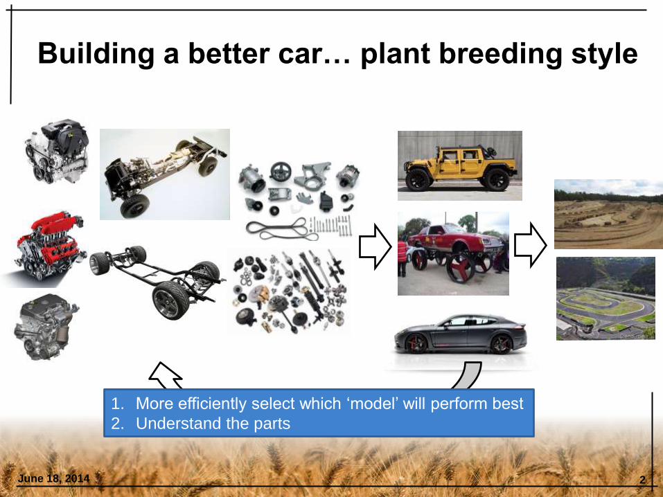
Building a better car… plant breeding style
June 18, 2014 2
1. More efficiently select which ‘model’ will perform best
2. Understand the parts
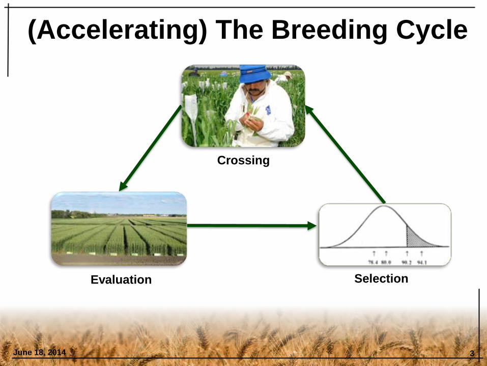
(Accelerating) The Breeding Cycle
June 18, 2014 3
Crossing
Evaluation Selection
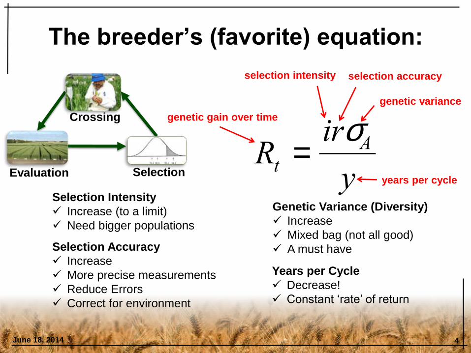
The breeder’s (favorite) equation:
June 18, 2014 4
Rt =irsA
y
genetic gain over time
years per cycle
selection intensity selection accuracy
genetic variance
Crossing
Evaluation Selection
Selection Intensity
Increase (to a limit)
Need bigger populations
Selection Accuracy
Increase
More precise measurements
Reduce Errors
Correct for environment
Genetic Variance (Diversity)
Increase
Mixed bag (not all good)
A must have
Years per Cycle
Decrease!
Constant ‘rate’ of return

Genomic Selection Prediction of total genetic value using dense genome-wide markers
Estimate Kinship (realized relationship) between breeding with markers
June 18, 2014 5
DNA
markers
Phenotypic
prediction
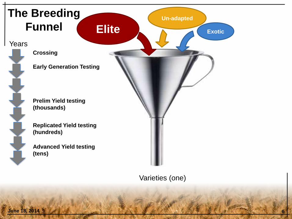
June 18, 2014 6
Early Generation Testing
Prelim Yield testing
(thousands)
Replicated Yield testing
(hundreds)
Advanced Yield testing
(tens)
Years
Varieties (one)
Crossing
Un-adapted
Exotic Elite
The Breeding
Funnel
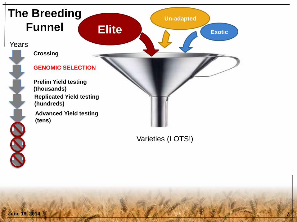
June 18, 2014 7
GENOMIC SELECTION
Prelim Yield testing
(thousands)
Replicated Yield testing
(hundreds)
Advanced Yield testing
(tens)
Years
Varieties (LOTS!)
Crossing
Un-adapted
Exotic Elite
The Breeding
Funnel

Genomic Selection Needed:
1) Training Population (genotypes + phenotypes)
2) Selection Candidates (genotypes)
June 18, 2014 8
Heffner, E.L., M.E. Sorrells, J.-L. Jannink. 2009. Genomic selection for crop improvement.
Crop Sci. 49:1-12. DOI: 10.2135/cropsci2008.08.0512
Inexpensive, high-density genotypes Accurate phenotypes
‘black box’ model
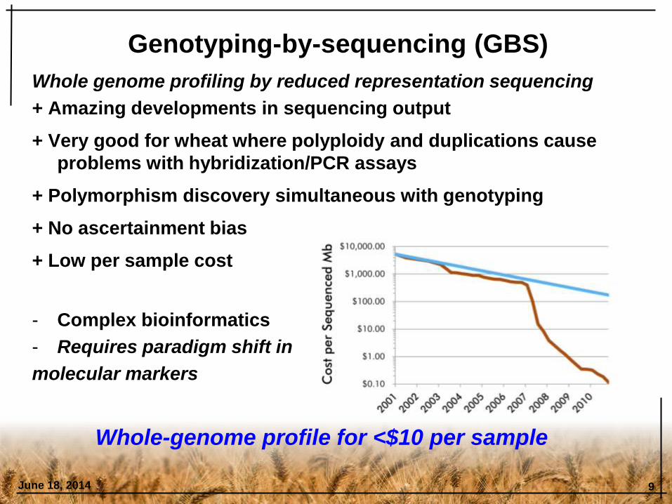
Whole genome profiling by reduced representation sequencing
+ Amazing developments in sequencing output
+ Very good for wheat where polyploidy and duplications cause
problems with hybridization/PCR assays
+ Polymorphism discovery simultaneous with genotyping
+ No ascertainment bias
+ Low per sample cost
- Complex bioinformatics
- Requires paradigm shift in
molecular markers
June 18, 2014 9
Genotyping-by-sequencing (GBS)
Whole-genome profile for <$10 per sample

Genotyping-by-sequencing (GBS)
“massively parallel sequencing”
- next-gen sequencing (Illumina)
“multiplex” = using DNA barcode
- unique DNA sequence synthesized on the
adapter
- pool 48-384 samples together
“reduced-representation”
- capture only the portion of the genome
flanking restriction sites
- methylation-sensitive restriction enzymes
- Target rare, low-copy sites in genome
- PstI (CTGCAG), MspI (CCGG)
10
“…massively parallel sequencing of multiplexed reduced-representation genomic libraries.”
CONFIDENTIAL. For Internal Use Only. © 2012 Life Technologies
Alexander Sartori, Alain Rico, Life Technologies GmbH, Frankfurter Str. 129 B, 22339 Darmstadt, Germany
ABSTRACT
We demonstrate a Genotyping by Sequencing (GBS)
workflow for plants using Ion PGM™ Sequencer. This
GBS approach aims at the discovery of high-density
molecular markers in crops required for better under-
standing of genetics of complex traits for breeding of
plants with large, complex genomes such as barley
(used in this study) and wheat. We also extrapolate the
results towards the use of the Ion Proton™ System.
INTRODUCTION
In this study the goal was to adapt an established GBS
protocol [1,2] towards Ion Semiconductor Sequencing.
Size and complexity of large plant genomes (barley:
5.5 Gb) are reduced by treatment of the gDNA with
species specific restr iction enzymes prior to library
construction. Subsequently only a certain population
of DNA fragments will be captured, sequenced and
analyzed. Libraries for 48 bar-coded and pooled barley
samples were prepared according to the scheme in
figure 1, where 2 libraries of 24 samples each were
made. Each library was sequenced with the 200 bp
chemistry on multiple Ion 318™ Chips for a total of 10
chips. This design was chosen in order to simulate the
throughput of a single Ion PI™ Chip, with the Ion
Proton™ System being the platform of choice once
available. Data were analyzed using the TASSEL
pipeline[3] for mapping and the discovery of novel
SNPs. SNPs were called according to the Fisher Exact
Test [4] (figure 2]. An in depth comparison of Ion PGM™
Sequencer with Illumina® HiSeq® data is ongoing.
BUSINESS IMPACT
GBS has a wide range of applications for breeding of
various crops and other culture plants and the breed-
ers are in the move to replace classical genotyping
methods towards NGS in order to enable the survey of
larger populations in less time. This harbors multi-
mill ion US$ business potential. The original workflow
was first demonstrated for Illumina® HiSeq® which
we can outperform with the Ion Proton™ System in
terms of speed and cost.
We received requests for this workflow from China,
India, South East Asia, Japan, Brazil, Europe and the
US, mainly regions with strong agriculture markets
and demographic projections that suggest improved
crop breeding.
RESULTS
The restriction of barley genomic DNA returned
approximately 500 k unique fragments of the desired
kind (see fig. 1). For library 1 we obtained 30 M reads
from 6 Ion 318™ Chips, for library 2 we sequenced 4
Ion 318™Chips for a total of 17 M reads. With 24
samples per library we gained 1.25 M reads per
FIGURE 1:
Principle of l ibrary construction:
A) suggests how genomic barley
DNA is targeted by the restr iction
enzymes MspI (frequent cutter)
PstI (rare cutter). For the desired
depth of sequencing information,
only fragments with two restr ict-
ion sites are ‘wanted’ subse-
quently. B) For their enrichment
two double stranded adapters are
ligated to the ends, each being
specific to each restriction site.
Also, one adapter pair contains
the DNA barcode sequences
required for sample multiplexing.
The common adapter was
designed as a Y-adapter to
prevent amplification of the more
common MspI-MspI fragments
and adapter-dimers formed by
self- l igation. C) Thus, in the first
PCR cycle only the lower strand
deals as template for primer
elongation. D) The final l ibrary
fragment is formed in the second
PCR cycle.
sample (on average) for l ibrary 1 and 0.7 M reads per sample for
l ibrary 2. For all 48 samples we discovered 13,640 SNPs in total.
Due to the higher sequence coverage (almost 2-fold) for l ibrary 1
the number of present SNPs was significantly higher than for
library 2 (figure 3). About 75% of all SNPs show a minor allele
frequency of <0,35, indicating 0clear heterocygotes (figure 4A) and
the low number of missing data in each library for the majority of
SNPs indicate good sequence coverage (figure 4B), despite the
varying levels for the two libraries. Inititial analysis suggests that
Ion PGM™-generated data are well comparable to Illumina®
HiSeq® -derived data and SNP concordance is very high (>0.995).
CONCLUSIONS
In this study we demonstrated the feasibility of SNP discovery in
barley through GBS on the Ion PGM™ Sequencer. The interrogation
of 48 samples on 10 Ion 318™ Chips was designed to simulate the
performance of a single Ion PI™ Chip experiment as the Ion Pro-
ton™ System will be the platform of choice for the crop breeding
community due to the required sample numbers.
When sequencing 48 samples on a Ion PI™ Chip the cost per
sample is below US$ 20, with using Ion PII™ Chips (by multiplexing
200+ samples) the cost would drop down below US$ 5 per sample,
which is about 3 times less than today on the Il lumina® HiSeq® .
In addition, our collaboration partners value the extremely short
workflow durations on Ion PGM™ and Ion Proton™ Systems comp-
ared to the competition and the expectation of further improved
performance announced for the near future.
REFERENCES
1. Poland et al., (2012) Development of High-Density Genetic Maps for
Barley and Wheat Using a Novel Two-Enzyme
Genotyping-by-Sequencing Approach. PLoS ONE 7(2): e32253.
doi:10.1371/journal.pone.0032253
2. Elshire et al. (2011) A Robust, Simple Genotyping-by-Sequencing (GBS)
Approach for High Diversity Species.
PLoS ONE ): e19379. doi:10.1371/journal.pone.0019379
3. http://www.maizegenetics.net/
4. http://en.wikipedia.org/wiki/Fisher's_exact_test
ACKNOWLEDGEMENTS
This project was carried out in collaboration with
Dr. Jesse Poland, United States Department of Agriculture, Agricultural
Research Service (USDA-ARS), at Kansas State University (KSU),
Manhattan, KS, USA and
Dr. Nils Stein, The Leibniz Institute of Plant Genetics and Crop Plant
Research (IPK), Gatersleben, Germany
We would like to thank Robert Greither at Life Tech Germany for his support.
For inquiries:
alexander.sartori@l ifetech.com
+49 173 3474 629
2012 Science and Technology Symposium P274
Plant Genotyping by Ion Sequencing
A
B
C
D
FIGURE 2:
For reference-independent SNP calling, a
population-based filtering approach was
used. A) Putative SNPs were identified by
internal alignment of sequence tags (1-3 bp
MM/64 bp tag). B) The number of individuals
in the population with each SNP allele were
tallied and a Fisher exact test was conducted
to test if the two alleles were independent.
Within an inbred line, alleles at a biallelic
SNP locus should be mutually exclusive.
Putative SNPs that failed the Fisher test (p-
value < 0.001) were considered biallelic SNPs
in the population and converted to SNP calls.
C) Based on presence/absence of the
different tags in the individuals across the
population, genotype scores were assigned.
FIGURE 4:
A) Minor allele frequencies (MAF) of
most SNPs are in the expected
range for heterozygous mutations
(>0.35)
B) Amount of missing data per SNP.
Low percentage of missing data for
the majority of SNPs indicate that
libraries had good sequence
coverage
A B
FIGURE 3:
Percentage of present SNPs per sample
and library (library 1 in blue; library 2 in
red). Due to higher sequence coverage of
library 1 the average SNP calls per
sample (85%) are significantly higher
than for library 2 samples (73%). The
total number of discovered SNPs across
all 48 samples was 13,640.
SN
Ps
pre
sen
t
Sample
Elshire, R. J., J. C. Glaubitz, Q. Sun, J. A. Poland, K. Kawamoto, E. S. Buckler and S. E. Mitchell (2011). "A Robust, Simple Genotyping-by-
Sequencing (GBS) Approach for High Diversity Species." PloS one 6(5): e19379.
June 18, 2014

GS: Prediction of wheat quality
June 18, 2014 11
CIMMYT elite breeding lines (n=1,138) Cycle 45 & 46 International Bread Wheat Screening Nursery (C45IBWSN)
- Genotyping-by-sequencing: 15,330 SNPs (imputed with MVN-EM) (rrBLUP)
Replicated yield tests
2009 & 2010
6 environments
One replication for quality testing
milling
dough rheology
baking tests
Best Linear Unbiased Estimate (BLUE)
Cross-validation (x100)
Training sets of n=134
Validation sets of n=30
Sarah Battenfield, KSU
Grain quality traits:
- thousand kernel weight
- milling yield
- mix time
- pup loaf volume
(= $$$)

June 18, 2014 12
GS: Prediction of wheat quality
TRAIT PREDICTION ACCURACY
(r)
Test Weight 0.725***
Grain Hardness 0.513***
Grain Protein 0.630***
Flour Protein 0.604***
Flour SDS 0.666***
Mixograph Mix Time 0.718***
Alveograph W 0.697***
Alveograph P/L 0.476***
Loaf Volume 0.638***
Sarah Battenfield, KSU
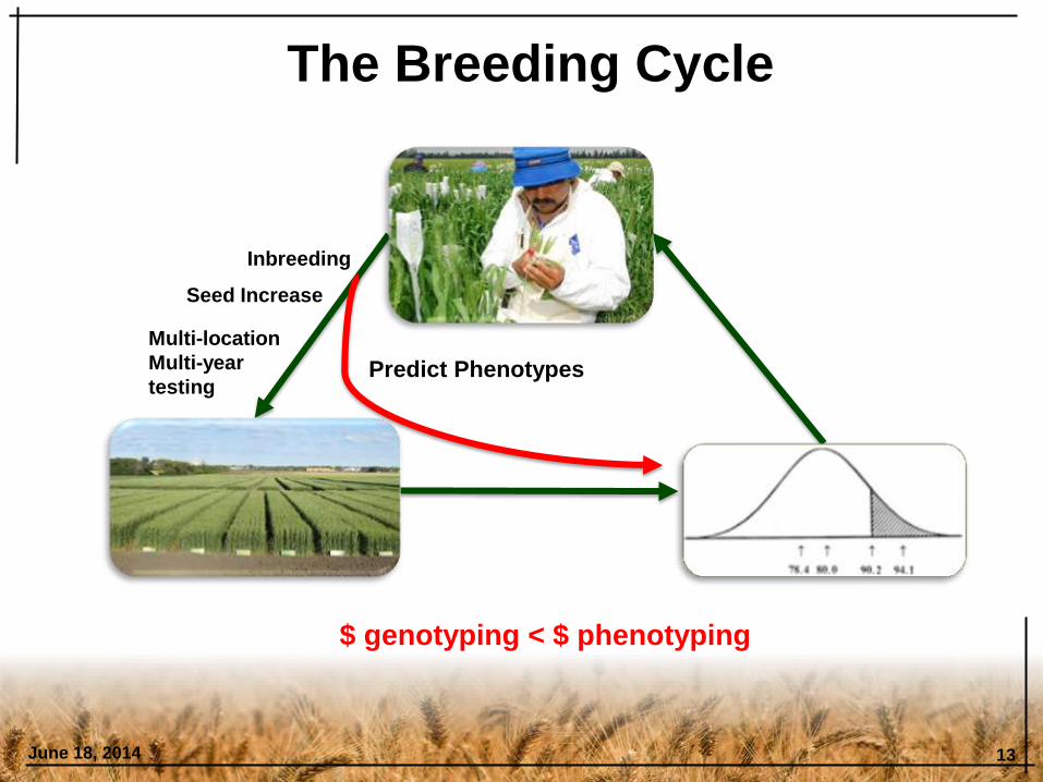
The Breeding Cycle
June 18, 2014 13
Predict Phenotypes
Inbreeding
Seed Increase
Multi-location
Multi-year
testing
$ genotyping < $ phenotyping
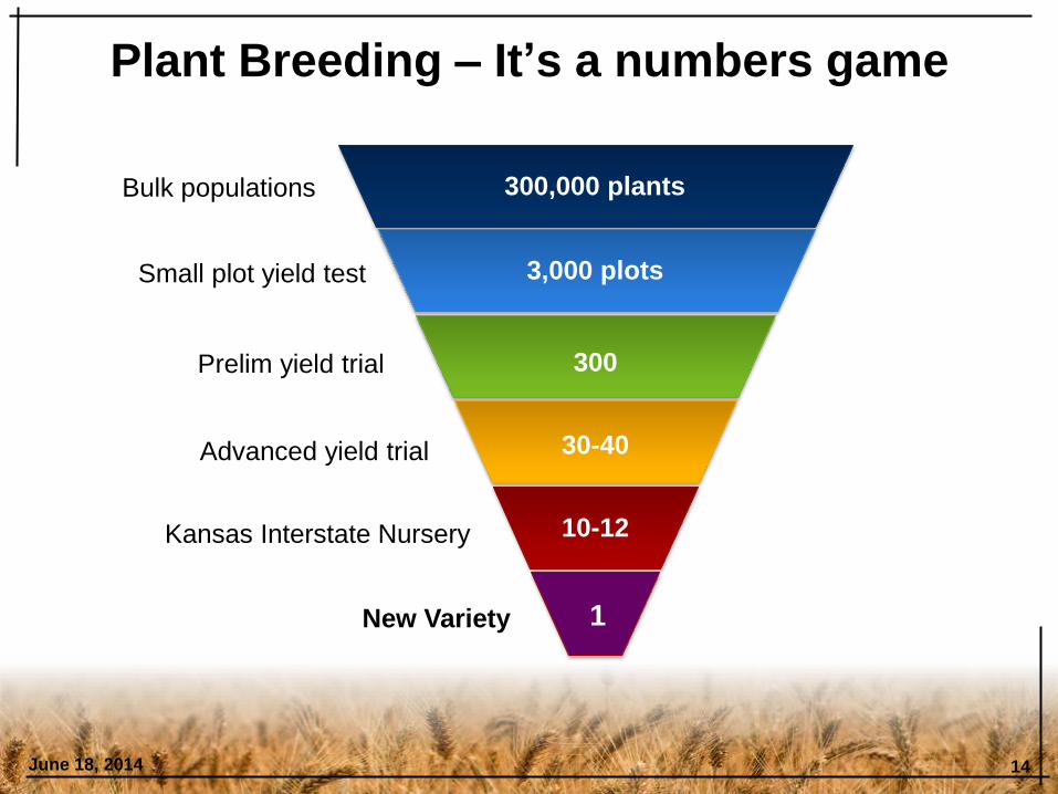
Plant Breeding – It’s a numbers game
June 18, 2014 14
Bulk populations
Small plot yield test
Prelim yield trial
Advanced yield trial
Kansas Interstate Nursery
300,000 plants
3,000 plots
300
30-40
10-12
New Variety 1

Increasing selection intensity = more to chose from
June 18, 2014 15

Phenotype
G2P: connecting genotype to phenotype
June 18, 2014 16
Genotype
24 25 26 27 28 29 30
50
100
150
200
250
300
350
Canopy Temperature (°C)
Yie
ld (
g m
-2) r = -0.71

The need for phenotypes:
1. more efficient selection (breeding)
2. understanding the parts (genetics)
June 18, 2014 17
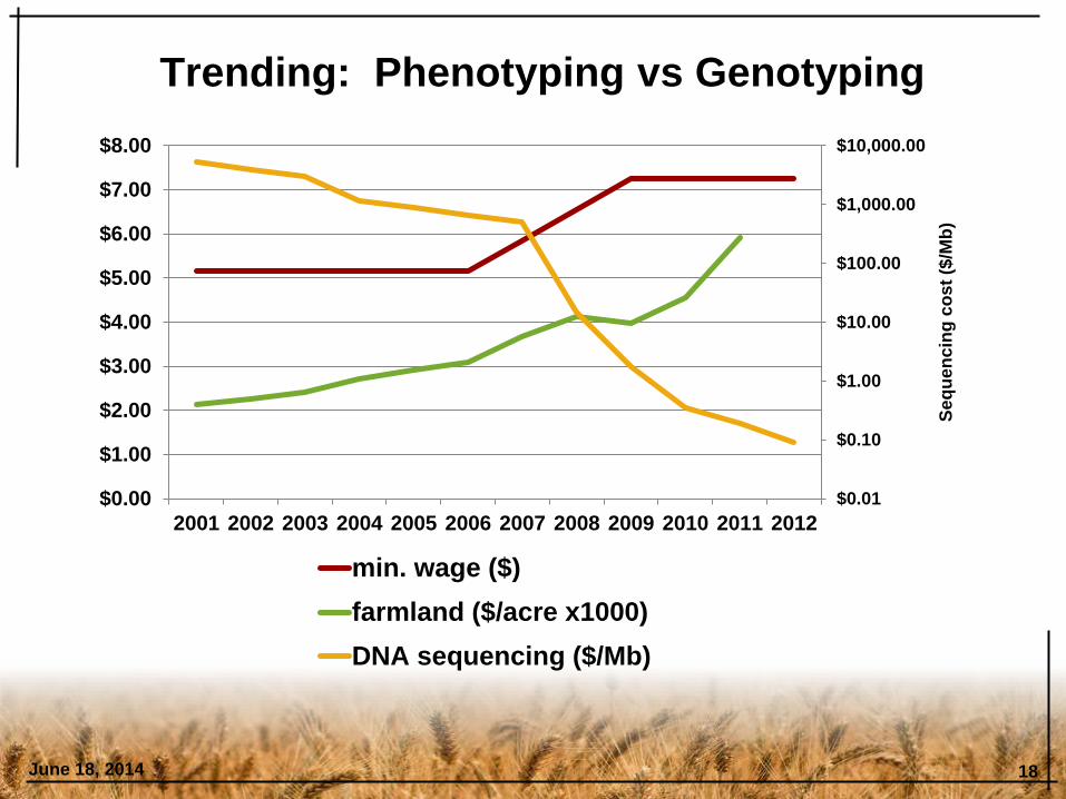
Trending: Phenotyping vs Genotyping
June 18, 2014 18
$0.01
$0.10
$1.00
$10.00
$100.00
$1,000.00
$10,000.00
$0.00
$1.00
$2.00
$3.00
$4.00
$5.00
$6.00
$7.00
$8.00
2001 2002 2003 2004 2005 2006 2007 2008 2009 2010 2011 2012
Se
qu
en
cin
g c
ost
($/M
b)
min. wage ($)
farmland ($/acre x1000)
DNA sequencing ($/Mb)
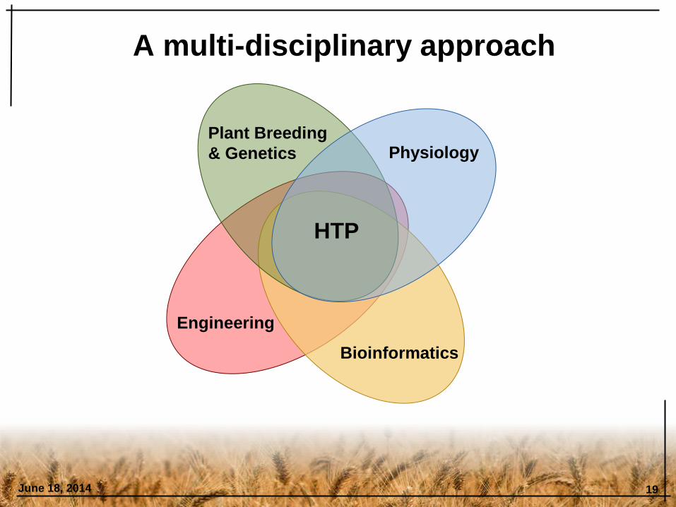
A multi-disciplinary approach
June 18, 2014 19
Plant Breeding
& Genetics Physiology
Engineering
Bioinformatics
HTP
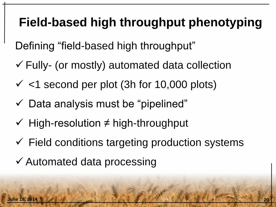
Field-based high throughput phenotyping
Defining “field-based high throughput”
Fully- (or mostly) automated data collection
<1 second per plot (3h for 10,000 plots)
Data analysis must be “pipelined”
High-resolution ≠ high-throughput
Field conditions targeting production systems
Automated data processing
June 18, 2014 20
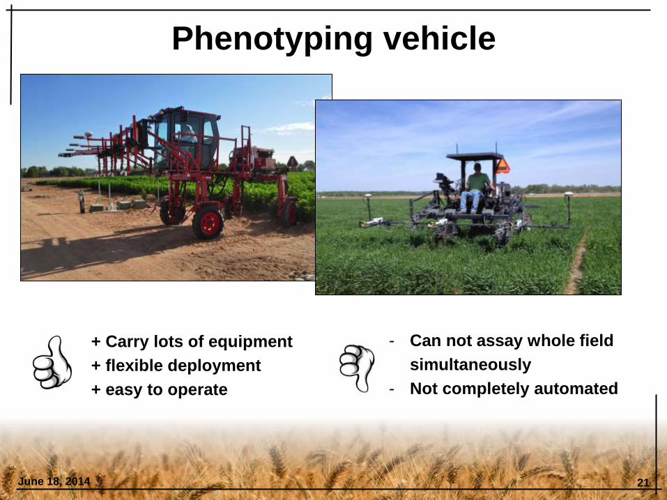
Phenotyping vehicle
June 18, 2014 21
- Can not assay whole field
simultaneously
- Not completely automated
+ Carry lots of equipment
+ flexible deployment
+ easy to operate
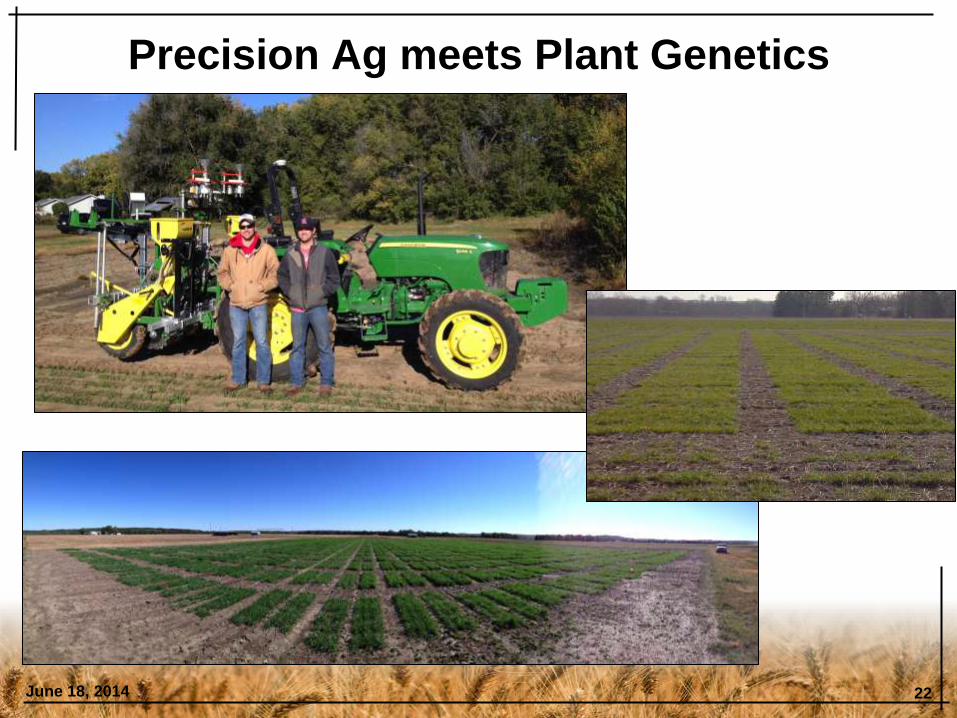
Precision Ag meets Plant Genetics
June 18, 2014 22

“Geo-referenced proximal sensing”
June 18, 2014 23
GPS Data logger
Sensors
Sensors
- GreenSeeker = NDVI
- IRT = canopy temperature
- SONAR = plant height
Physiologically define
proximal measurements
RTK-GPS
(cm level accuracy)
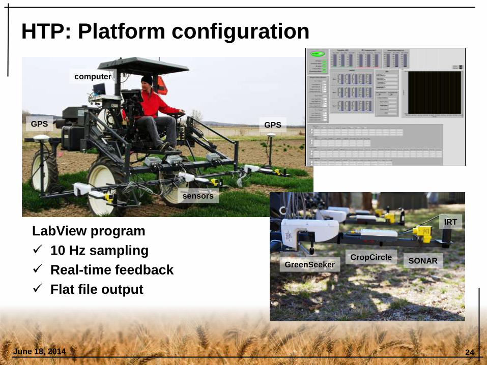
HTP: Platform configuration
June 18, 2014 24
GreenSeeker CropCircle SONAR
IRT
GPS GPS
sensors
computer
LabView program
10 Hz sampling
Real-time feedback
Flat file output

HTP: Multiple sensor orientation
June 18, 2014 25
-3908.040 -3908.035 -3908.030 -3908.025
9637.1
33
9637.1
34
9637
.135
963
7.1
36
96
37.1
37
96
37.1
38
9637.1
39
9637.1
40
-data$Right_Longitude
data
$R
ight_
La
titu
de
Right GPS
Left GPS
NDVI
0.1
0.3
0.5
0.7
0.9

NDVI – raw data
June 18, 2014 26
-96.6135 -96.6130 -96.6125
39
.12
84
39.1
28
63
9.1
288
39
.12
90
NDVI - 2012.05.10
Longitude (DD.dddd)
Latitu
de
(D
D.d
dd
d)

Assigning data
to field entries
June 18, 2014 27
-9636.82 -9636.80 -9636.78 -9636.76 -9636.74
390
7.7
039
07
.72
390
7.7
4
NDVI - 2012.05.10
Longitude
Latitu
de
-9636.800 -9636.804 -9636.808
3907
.720
3907
.722
3907
.724
NDVI - 2012.05.10
Longitude
Lat
itu
de
-9636.800 -9636.804 -9636.808
390
7.7
20
390
7.7
22
39
07
.724
NDVI - 2012.05.10
-data.2$long[!is.na(data.2$pass)]
data
.2$
lat[
!is.n
a(d
ata
.2$
pa
ss)]
-9636.800 -9636.804 -9636.808
3907
.720
3907
.722
3907
.724
NDVI - 2012.05.10
Longitude
Lat
itu
de
Raw data
Define plot
boundaries
Trim data
Assign to plots
June 18, 2014 28
-9636.82 -9636.80 -9636.78 -9636.76 -9636.74
390
7.7
039
07
.71
39
07.7
23
907
.73
390
7.7
4
NDVI - 2012.05.03
-data.1$long
-9636.82 -9636.80 -9636.78 -9636.76 -9636.74
39
07
.70
390
7.7
13
90
7.7
23
90
7.7
339
07
.74
NDVI - 2012.05.10
-data.2$long
-9636.82 -9636.80 -9636.78 -9636.76 -9636.74
39
07
.70
390
7.7
13
90
7.7
239
07
.73
39
07
.74
NDVI - 2012.05.15
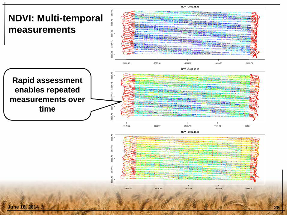
NDVI: Multi-temporal
measurements
Rapid assessment
enables repeated
measurements over
time

NDVI: Multi-temporal measurements
June 18, 2014 29
DATE
ND
VI
0.0
0.2
0.4
0.6
0.8
5/3/12 5/10/12 5/15/12 5/21/12
Advanced Yield Nursery
Identify dynamic
differences among
genotypes

June 18, 2014 30
X2013.05.31
−10 −5 0 5 10
●
●
●
●
●
●●
●●
●
●
●
●
●●
●
●
●
●
●●
●
●
●●
●
●
●●●●
●
●
●●
●●
●●●
●
● ●●
●
●
●
●●
●
●
●
●
●
●
●●
●●
●
●
●● ●
●
●
●
●●
●●
●●
●●
●
●●
●
●
●
●
●●
●
●
●
●
●
●
●●
●
●
●
●●
●
●
●
●●
●
●
●
●●
●
●
●
●
●
●●●●
●
●
●
●
●
●
●
●
●
●●
●
●
●
●
●●
●
●
●
●
●●
●
●
●●
●
●
● ●●
●
●
●
●●
●●
●●●
●
●● ●
●
●
●
●●
●
●
●
●
●
●
● ●
●●
●
●
●● ●
●
●
●●
● ●
●
●●
●
●●
●●
●
●●
●
●
●
●
●
●
●●
●
●
●
●●
●
●
●
● ●
●
●
●
●●●
●
●
●
●
●●● ●●
●
●
75 80 85 90 95
●
●
●
●
●
●●
●●
●
●
●
●
●●
●
●
●
●
●●
●
●
●●
●
●
● ●●
●
●
●
●●
●●
●●●
●
●● ●
●
●
●
●●
●
●
●
●
●
●
● ●
●●
●
●
●● ●
●
●
●
●●
● ●
● ●
●●
●
●●
●
●
●
●
●●
●
●
●
●
●
●
●●
●
●
●
●●
●
●
●
●●
●
●
●
●●
●
●
●
●
●
●●
●● ●
●
●
−1
0−
50
510
●
●
●
●
●
●●
●●
●
●
●
●
●●
●
●
●
●
●●
●
●
●●
●
●
● ●●●
●
●
●●
●●
●●●
●
●● ●
●
●
●
●●
●
●
●
●
●
●
●●
●●
●
●
●●●
●
●
●
●●
● ●
● ●
●●●
●●
●
●
●
●
●●
●
●
●
●
●
●
●●
●
●
●
●●
●
●
●
● ●
●
●
●
●●
●
●
●
●
●
●●●●●
●
●
−1
0−
50
510
0.84***(0.78,0.89)
X2013.06.06
●●
●●
●
●
●
●
●
●●
●
●●●
●
●
●●
●
●
●
●
●●
●
● ●
● ●
●
●●●
● ●
●
●●
●
●
●
●
●
●
●
●
●
●●
●● ●
●● ●
●●●
●●
●
●
●
●
●●
●
●
●●
●●
●●
●●
●
●●
●
●
●
●
●
●
● ●
●
●
●
●● ●●
●
● ●●
●
●
●
●
●
●
●
● ●
●●●
●●
●
●
●●
●●
●
●●
●
●
●
●●
●
●● ●
●
●
●●
●
●
●
●
●●
●
● ●
● ●
●
●●●
●●
●
●●
●
●
●
●
●
●
●
●
●
●●
●● ●
●● ●
●●●
●●
●
●
●
●
●
●●
●
●
● ●●
●●
●●
●
●
●
●
●●
●
●
●
●
●
●
●●
●
●
●
●● ●●
●
●● ●
●
●
●
●
●
●
●
●●
●●●
●●
●
●
●●
●●
●
●●
●
●
●
●●
●
●● ●
●
●
●●
●
●
●
●
●●
●
● ●
●●
●
●●●
●●
●
●●
●
●
●
●
●
●
●
●
●
●●
●● ●
●●●
●●●
●●●
●
●
●
●
●●
●
●
● ●●●●●●
●
●
●
●
●●
●
●
●
●
●
●
●●
●
●
●
●● ●●
●
● ●●
●
●
●
●
●
●
●
●●
●●●
●●
●
●
0.53***(0.65,0.4)
0.55***(0.67,0.42)
Height_Jesse
●●
●●
●
● ●●
●●
●●
●● ●
●
●●
●
●
● ●
●● ●●
●
●●
●
●
●
●●
●
●
●
●●
●●
●
●
●
●
●
●
●
●●
●
●
●
●
●●
●●●●●
●
●
●
●
●● ●
●
●
●●
●●
●
●●
●
●● ●
●
●
●
●
●
●
●
●
●●
●
●
●● ●
●● ●
●
●
●
● ●
●
●
●●
●
●●
●
●
●
●
70
75
80
85
90
95
10
0
●●
●●
●
● ●●
●●
●●
●● ●
●
●●
●
●
●●
●● ●●
●
● ●
●
●
●
●●
●
●
●
●●
●●
●
●
●
●
●
●
●
●●
●
●
●
●
●●
●●●●●
●
●
●
●
●●●
●
●
●●
●●
●
●●
●
●● ●
●
●
●
●
●
●
●
●
●●
●
●
●● ●
●●●
●
●
●
● ●
●
●
●●
●
●●
●
●
●
●
75
80
85
90
95
0.49***(0.61,0.35)
0.43***(0.56,0.29)
0.55***(0.42,0.66)
Height_Jon
●
●
●●●
●
●
●
●
●●
●
●
●●
●
●
●
●●
●
●
●
●●
●
●
●
●●
●
●
●
●●
●
●
●●
●●●●
●
●●
●
●
●
●●
●●
●●
●
●●
●●●
●
●●
●
●
●●
●
●●
●
●
●
●
●
●●
●
●
●●●
●●●
●●
●
●
●●
●
●●
●
●
●●
●
●
●
●●
●●
●
●
●
●
●●
●●●
●●
●●
−10 −5 0 5 10
0.47***(0.60,0.34)
0.41***(0.54,0.27)
70 75 80 85 90 95 100
0.36***(0.22,0.5)
0.56***(0.43,0.67)
80 85 90 95 100
80
85
90
95
100
Height_Jacob
Phenotyper: Increased accuracy
Plant Height w/ SONAR
- 40 varieties
- 3 reps
- 1.3m x 3m plots

HTP platforms of all shapes and sizes…
June 18, 2014 31

HTP: Imaging
June 18, 2014 32
GreenSeeker CropCircle SONAR
IRT
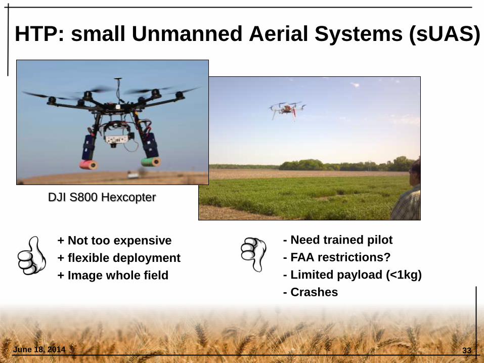
HTP: small Unmanned Aerial Systems (sUAS)
DJI S800 Hexcopter
- Need trained pilot
- FAA restrictions?
- Limited payload (<1kg)
- Crashes
+ Not too expensive
+ flexible deployment
+ Image whole field
June 18, 2014 33

• Ortho mosaic from multiple images
HTP: sUAS platform and 3D modeling
Camera positions
Common Points
June 18, 2014 34
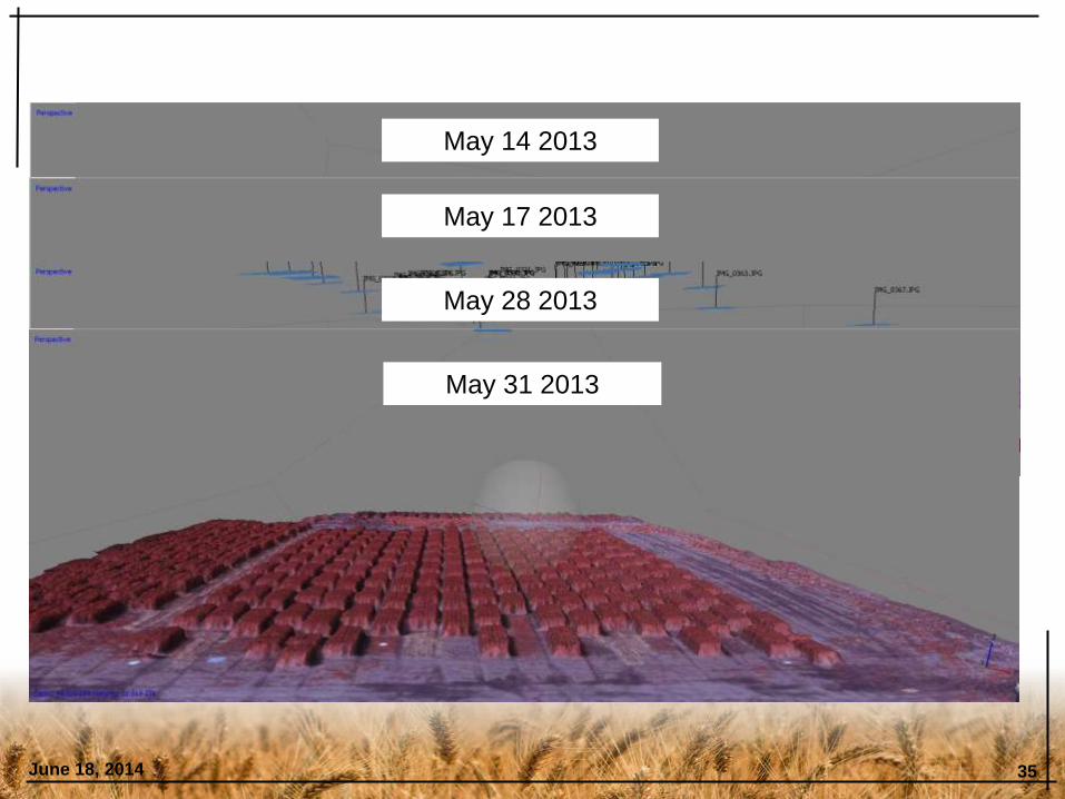
Time-Series 3D models for High-Throughput Phenotyping
May 14 2013
May 17 2013
May 28 2013
May 31 2013
June 18, 2014 35

Phenotype
G2P: connecting genotype to phenotype
June 18, 2014 36
Genotype
24 25 26 27 28 29 30
50
100
150
200
250
300
350
Canopy Temperature (°C)
Yie
ld (
g m
-2) r = -0.71

To make it work….
1. Start with the breeding program
- many failures in ‘genomic assisted breeding’
2. USER FRIENDLY!
- pragmatic triumphs
- short learning curve
3. Timely assessment under any conditions
June 18, 2014 37

HTP: The future is here…
Implementation of existing technology
Commercial and existing sensors
Imaging
Low-cost, modular ‘nodes’
June 18, 2014 38
How MultispeQ and PhotosynQ work
Figure 1: MultispeQ current design, with leaf clamp attached. Figure 2: a prototype version measuring
pulse modulated fluorescence of an arabidopsis leaf.
MultispeQ uses bluetooth to wirelessly send data to a user's cell phone to an Android app. The app
displays the results both in absolute terms and in comparison to previously collected data in the same
Research Project.
The data is then automatically synchronized with an online database where anyone can see and
analyze it. The website includes a variety of graphing analytical tools so most analysis can be
performed through the web interface itself, though the data is also downloadable as a standard text
(.csv) file.
Within the online database, users can organize data around research groups of any size and type: a
decentralized group of unaffiliated collaborators studying global climate change, or members of a single
organization (like a group of extension agents or graduate students) performing breeding trials.
MultispeQ measurements types
The PhotosynQ platform can be equipped a wide range of sensors. In the pilot project, we focus on
sensors and protocols that will be immediately useful for extension agents and breeders in the
developing world, as described in the following.
Plant chlorophyll content
Chlorophyll content is used in a variety of plants to identify plant stress and indicate the need for
additional fertilization. MultispeQ will estimate chlorophyll content using transmission spectroscopy.3
Dedicated commercial instruments are available which make similar measurements, but are expensive
(from $250 to $2,200 per unit), proprietary and lack the linked data stream of PhotosynQ. PhotosynQ
technology will be sufficiently distinct to avoid IP issues.
Soil health - biological activity
3 http://www.regional.org.au/au/asa/2012/precision-agriculture/7979_alim.htm

Interactive data collection and analysis
Dec 2, 2013 39
How MultispeQ and PhotosynQ work
Figure 1: MultispeQ current design, with leaf clamp attached. Figure 2: a prototype version measuring
pulse modulated fluorescence of an arabidopsis leaf.
MultispeQ uses bluetooth to wirelessly send data to a user's cell phone to an Android app. The app
displays the results both in absolute terms and in comparison to previously collected data in the same
Research Project.
The data is then automatically synchronized with an online database where anyone can see and
analyze it. The website includes a variety of graphing analytical tools so most analysis can be
performed through the web interface itself, though the data is also downloadable as a standard text
(.csv) file.
Within the online database, users can organize data around research groups of any size and type: a
decentralized group of unaffiliated collaborators studying global climate change, or members of a single
organization (like a group of extension agents or graduate students) performing breeding trials.
MultispeQ measurements types
The PhotosynQ platform can be equipped a wide range of sensors. In the pilot project, we focus on
sensors and protocols that will be immediately useful for extension agents and breeders in the
developing world, as described in the following.
Plant chlorophyll content
Chlorophyll content is used in a variety of plants to identify plant stress and indicate the need for
additional fertilization. MultispeQ will estimate chlorophyll content using transmission spectroscopy.3
Dedicated commercial instruments are available which make similar measurements, but are expensive
(from $250 to $2,200 per unit), proprietary and lack the linked data stream of PhotosynQ. PhotosynQ
technology will be sufficiently distinct to avoid IP issues.
Soil health - biological activity
3 http://www.regional.org.au/au/asa/2012/precision-agriculture/7979_alim.htm

June 18, 2014 40 40
Pedro Andrade-Sanchez ★
John Heun
Shuangye Wu
Josh Sharon ★
Ryan Steeves ★
Jared Crain ★
Sandra Dunckel
Trevor Rife
Daljit Singh
Narinder Singh
Traci Viinanen
Xu (Kevin) Wang
Lisa Borello
Erena Edae
Allan Fritz
Andy Auld
Shaun Winnie
Naiqian Zhang
Jed Barker ★
Spencer Kepley
Yong (Ike) Wei
Randy Price
Kevin Price
www.wheatgenetics.org
Ravi Singh
Susanne Dreisigacker
Matthew Reynolds
David Bonnett
Rick Ward
Jeffery White ★
Kelly Thorp ★
Andrew French ★
Mike Salvucci ★
Michael Gore ★
www.fieldphenomics.org
Steve Welch
Nan An★
Dale Schinstock
If we knew what it was we were doing, it
would not be called research, would it?
- Albert Einstein