genetic testing with primary prevention and moral hazard”genetic testing with primary prevention...

12-320

Research Group: Public Economics May 2012

“Genetic testing with primary prevention and moral hazard”

Philippe De Donder and David Bardey

Genetic testing with primary prevention and moralhazard1

David Bardey2 and Philippe De Donder3

May 11, 2012

1We thank Chiara Canta, Francesca Barigozzi and participants to seminars held at the Uni-versities of Toulouse, Cergy-Pontoise, ENS Cachan and at CESifo (Munich) for their comments.This research has been undertaken in part while the second author was visiting the Universityof Rosario. He thanks the University for its generous hospitality. We gratefully acknowledgethe �nancial support of the Fondation du Risque (Chaire Santé, Risque et Assurance, Allianz).The usual disclaimer applies.

2University of Rosario (Colombia) and Toulouse School of Economics (France). Email:[email protected]

3Toulouse School of Economics (GREMAQ-CNRS and IDEI), France. Email: [email protected]

Abstract

We develop a model where a genetic test reveals whether an individual has a low or highprobability of developing a disease. A costly prevention e¤ort allows high-risk agents todecrease this probability. Agents are not obliged to take the test, but must disclose itsresults to insurers, and taking the test is associated to a discrimination risk.

We study the individual decisions to take the test and to undertake the preventione¤ort as a function of the e¤ort cost and of its e¢ ciency. If e¤ort is observable byinsurers, agents undertake the test only if the e¤ort cost is neither too large nor toolow. If the e¤ort cost is not observable by insurers, moral hazard increases the valueof the test if the e¤ort cost is low. We o¤er several policy recommendations, from theoptimal breadth of the tests to policies to do away with the discrimination risk.

JEL Codes: D82, I18.Keywords: discrimination risk, informational value of test, personalized medecine.

1 Introduction

�Increasing the focus on prevention in our communities will help improve America�shealth, quality of life and prosperity. For example, seven out of 10 deaths amongAmericans each year are from chronic diseases (such as cancer and heart disease), andalmost one out of every two adults has at least one chronic illness, many of whichare preventable�. This statement by the US Centers for Disease Control and Preven-tion (CDC) reveals the crucial and increasing role played by prevention for health caresystems worldwide.

An important characteristic of prevention actions is that, while many individualsmay undertake prevention and thus incur its costs, the health and �nancial bene�tsgenerally only accrue to the individuals who are at risk of developing the disease orinjury. There is evidence that, for many important health risks, individuals di¤er sig-ni�cantly in how e¢ cient prevention is for them. For instance, the same CDC writethat �Several genetic disorders are associated with increased risk of premature heartattacks. A relatively common disorder is familial hypercholesterolemia, which causeshigh levels of "bad" cholesterol (low density lipoprotein, or LDL cholesterol) beginningat birth. One out of 500 people in the United States may inherit this condition. Earlydetection of this disorder can help reduce the burden of heart disease in the person withhypercholesterolemia as well as in their family members.�

This in turn means that sizeable welfare gains would be reaped if it were possibleto identify individual characteristics associated to a larger e¢ ciency of prevention. Oneway to uncover those characteristics is through genetic tests. The main thesis of Collins(2010) (as well as other books, such as Davies [2010]) is precisely that genetic testingis ever more reliable and allows not only to be better informed about individual healthrisks, but also to use this information to individually tailor prevention. Collins insiststhat improvement in the assessment of the risk of occurrence of a disease very oftenallows the individual to take preventive action in order to prevent this disease from oc-curring. �There are many diseases such as cystic �brosis or PKU, for which a particularbiochemical or DNA test result makes a very strong prediction about the likelihood ofillness, and interventions are available�(page 802). There is actually a whole range ofsuch prevention activities: �institution of drug therapies; (...) special diets; (...) surgeryor other options" (page 815). As Collins writes quoting a patient �I know early in mylife something I am substantially predisposed to. I now have the opportunity to adjustmy life to reduce those odds�(page 1070).

The objective of our paper is to try and assess the impact of o¤ering a (genetic)test to individuals on both the private health insurance market and on the welfare ofindividuals. More precisely, we aim at understanding under what circumstances such atest would be voluntarily taken by individuals, what the consequences of the availabilityof testing would be on the extent to which individuals undertake prevention e¤orts, and

1

whether such a test would increase individual welfare. The simple model we developto answer these questions has the main ingredients of Collins�s story. Agents di¤erin their risk to develop a disease, with two types (L and H) corresponding to twolevels of risk in the general population: a fraction � has the high probability pH ofdeveloping the disease while the remainder has the low probability pL < pH . Peopleare born uninformed about their individual risk level, but can undertake a (genetic orotherwise1) test in order to assess (without any error) whether they are of a low or hightype (in the former case, we talk about a negative test, versus a positive test in the lattercase). After the testing phase, agents decide whether to undertake a prevention e¤ort,at a cost, in order to decrease the probability of occurrence of the disease. That is, wemodel primary prevention (as opposed to secondary prevention, which does not a¤ectthe probability that the disease occurs, but decreases its severity).2 Collins (2010)provides many examples of both primary and secondary prevention (�discoveries areproviding powerful new insights into both treatment and prevention�, page 1084).

We assume that prevention is e¢ cient at reducing the risk of illness only if theindividual�s test is positive (i.e., if he is of a high type). One can give several examplesof tests/illnesses with such features, ranging from prophylactic mastectomy in case ofmutated BRCA1 gene, to �intense medical surveillance and removal of polyps (that)can be lifesaving for those at high risk�of colon cancer (page 1853). One reason whyprevention e¤ort may be e¢ cient only if an individual has a high type is that �it is acombination of the genes that you have inherited and the environment that you livein that determines the outcome. Hence the common saying, �genes load the gun, andenvironment pulls the trigger�(page 1098). For instance, �Participants in the lifestyleintervention group reduced their risk of developing full-blown diabetes by 58 percent.�(page 1313). For macular degeneration, �it became clear that almost 80 percent of therisk could be inferred from a combination of (...) two genetic risk factors, combinedwith just two environmental risk factors (smoking and obesity)�(page 1169). Anotherreason why e¤ort may be e¢ cient for high risk only is that it has to combine severalapproaches, including drug therapies: �In many instances, dietary modi�cation turnsout to be insu¢ cient (...) Thus drugs in the class known as statins have become themost widely prescribed in the developed world�(page 1313).

We assume perfect competition between pro�t-maximizing insurers, who observewhether individuals have taken the test, and the result of the test. On the other hand,insurers cannot force individuals to undertake the test, and/or the prevention e¤ort.This corresponds to the situation labeled �disclosure duty� by Barigozzi and Henriet(2011), and to the legal environment in New Zealand and the United Kingdom. Observe

1Alternatively, the �test�could be an exploration of family history, which Collins (2010, page 1084)indeed dubs a �free genetic test�.

2We thus do not cover the illnesses that are entirely driven by genetic conditions and/or for whichthere is no known prevention e¤ort (such as, for instance, Huntington desease).

2

that this regulation is simply an extension to genetic testing of the generic regulationfor insurance existing in most countries : when buying insurance (health or otherwise),buyers have to disclose the risk factors that they are aware of. For instance, healthinsurers may ask questions about the family history of the patient, and patients wholie or fail to disclose important elements may be penalized or even see their insurancecontract made void.

We also assume, in line with existing conditions, that genetic insurance (i.e., insur-ance against the risk of a positive test) is not available in the market. Taking the testthen corresponds to a lottery, since it means (under disclosure duty and with separat-ing insurance contracts) that the agent ends up with probability � with the contractdesigned for high types, and with probability 1 � � with the contract designed for thelow type, rather than with the contract designed for uninformed agents and based onthe average risk �pH + (1 � �)pL. In other words, taking the test means supporting adiscrimination risk. We already know from previous literature (Hirshleifer, 1971) that,in a classical von Neumann-Morgenstein expected utility framework, risk averse agentswill not undertake the test in the simple setting where the test does not allow to bettercalibrate prevention e¤orts.

We then add the possibility for the individuals to exert some primary preventione¤ort in order to decrease their probability of bad health from pH to the lower p1H .

3

The availability of a prevention strategy should give stronger incentives to undertakethe test. Whether individuals make the prevention e¤ort and thus decrease their riskis also of interest to the insurers. An open question is whether this prevention e¤ortis observable by insurers. Prevention is easily observable when it takes the form ofsurgery, or even drug therapy. It is much more di¢ cult to observe if it consists oflifestyle changes such as dietary modi�cations or exercise. We thus cover the two cases,treating �rst the situation where the prevention is observable, and then the case whereit is not observable by insurers. Throughout our analysis, we stress two dimensions ofthe prevention e¤ort: its cost for the agent, and its e¤ectiveness, i.e. the amount bywhich it reduces the risk of someone whose test is positive.4

We �rst study the benchmark situation where the e¤ort is observable, veri�able andcontractible by the insurers. Even in this simple situation, our results reveal that thevalue of information given by the test has an interesting relationship with the cost ofthe preventive actions. More precisely, we �rst point out that the genetic test generatesa valuable information only for intermediate levels of the prevention cost. When theprevention e¤ort cost is low, even uninformed people (who do not take the test) make

3See Barigozzi and Henriet (2011) for a comparison of legal environments in a setting with observablesecondary prevention.

4We assume that the prevention e¤ort is useless for an agent of type L. This assumption is madeto simplify the analysis �our results would carry through qualitatively to the case where prevention ise¤ective for type L as well, provided that the risk decreases more for type H than for type L.

3

the prevention e¤ort, although it is e¢ cient only with probability �. In such a case,the genetic test precisely allows to forego the e¤ort (and its cost) if the test is revealednegative. The value of the test, de�ned as the di¤erence in ex ante utility betweentaking the test or not, is then increasing with the e¤ort cost, and may become positiveif both the cost and e¢ ciency of e¤ort are not too low. For intermediate values of thee¤ort cost, agents undertake the prevention e¤ort only if they have a positive test.5 Thetest then allows them to undertake the prevention e¤ort, and the value of the test isdecreasing in the e¤ort cost. This value if positive provided that the e¤ort cost is nottoo large. Finally, when the e¤ort cost is large, even high type agents do not undertakethe e¤ort, and the value of the test is always negative since the only impact of takingthe test is to expose agents to the discrimination risk. As is intuitive, the value of thetest increases with the e¢ ciency of the prevention e¤ort.

We then turn to the case where e¤ort is not observable by insurers. Full insurancewould induce agents not to provide any e¤ort: we are facing a moral hazard problem,solved by insurers by under-providing insurance.6 A naïve intuition would suggestthat this under-provision, by reducing the utility level with e¤ort (compared to theperfect information case) is detrimental to the value of the test, whose only raisond�être is to provide information allowing to calibrate the prevention e¤ort to one�s owncircumstances. We show that this intuition does not hold in general. More precisely,this intuition is correct for the middle range of values of the e¤ort cost, where the e¤ortis undertaken only in the case of a (positive) test. But it does not hold when the e¤ortcost is low enough that prevention is undertaken both if uninformed or if tested positive.In that case, we show that the value of the test is actually larger with than withoutmoral hazard, because moral hazard degrades more the utility when the test is not taken(and e¤ort is undertaken) than when it is taken (and e¤ort undertaken only in the caseof a positive test). Roughly, this is true because insurers have to ration coverage moreto uninformed types than to high types in order to induce them to undertake the e¤ort.

Comparing further the cases with and without moral hazard, we obtain two mainresults. First, for a given e¢ ciency level of prevention, the interval of (intermediate)values of the e¤ort cost which are inducing agents to take the test (i.e., for which thevalue of the test is positive) moves to the left as we introduce moral hazard consider-ations. That is, quite counter intuitively, there exist combinations of e¤ort cost ande¢ ciency such that the genetic test is undertaken if and only if e¤ort is not observable

5This corresponds to the following two observations by Collins (2010): �Information about an ele-vated genetic risk may cause people to take actions they otherwise would have ignored� (page 1313),and �She was aware that she was following diet and exercise routines that she probably should haveadhered to anyway, but she found the additional genetic information helpful in inducing a greater senseof urgency to make these changes�(page 1461).

6For instance, Dave and Kaestner (2006) ��nd evidence that obtaining health insurance reducesprevention and increases unhealthy behaviors among elderly men.�

4

by insurers! Second, we �nd occurrences where the test is undertaken for lower val-ues of the e¢ ciency of e¤ort when this e¤ort is unobservable than when it is observedby insurers. Both results are due to the fact that the value of the test is larger withthan without moral hazard when the e¤ort cost is su¢ ciently low that even uninformedagents undertake the prevention e¤ort.

Finally, we assess the impact of the various ingredients of our model on ex ante(expected) utility or welfare. We start from the situation where there is no insurance,no genetic test and no prevention e¤ort available, and we measure the impact on welfareof allowing each of these three ingredients as a function of the prevention e¤ort cost.We also show that moral hazard is always detrimental to both the prevention e¤ortdecision and ex ante utility of agents. Observe that, in the light of the results presentedabove, this is not a foregone conclusion. For certain combinations of prevention e¤ortcost and e¢ ciency, the introduction of moral hazard considerations changes the testingand e¤ort decisions of agents. At �rst sight, such a change could then be bene�cial tothe prevention decision and generate a larger welfare for agents if moral hazard wereto induce agents to test while uninformed agents do not undertake the e¤ort. We showthat this situation never happens because, for moral hazard to induce the test, the e¤ortcost need to be low enough that uninformed agents do undertake prevention.

The welfare analysis allows us to make several policy recommendations. First, tar-geted genetic tests (tailored for a speci�c disease) are to be encouraged rather thana single, all encompassing test, since the value of the information may be positive forcertain health risks and negative for others. Second, our analysis provides no groundfor policies that would indiscriminately increase the prevention e¤orts by all agents (forcertain con�gurations of prevention e¢ ciency and costs, there is already too much e¤ortat equilibrium). Third, since the presence of a discrimination risk explains why there isless than optimal testing in our model, it is tempting to recommend that governmentsdo away with this risk. We study three possible ways to proceed and we show that twoof them actually decrease welfare! We recommend the creation of genetic insurance thatwould be made mandatory in order to take the genetic tests. We do not recommend twoalternative policies: the strict prohibition of the use of genetic information by insurers(which creates an adverse selection problem if agents are aware of their genetic riskwhen buying health insurance), and requiring proof of health insurance when takingthe tests (since it would blunt incentives to test and to make the e¤ort when sociallyoptimal). Finally, although moral hazard may have some welfare enhancing properties(when it decreases a prevention level that is socially too large), its overall impact onwelfare is always negative. We then call for the enlargement of the �disclosure duty�approach to the prevention e¤orts, as well.

5

Related literatureThis paper is part of a growing literature dealing with genetic testing and the value

of information. An implication of the seminal paper by Hirshleifer (1971) is that, ifhealth risk is exogenously determined (i.e., there is no prevention e¤ort available), thevalue of the information brought by the test is negative, because individuals are facedwith a discrimination risk. Doherty and Thistle (1996) have further shown that theprivate value of information is non-negative only if insurers cannot observe consumers�information status or if consumers can conceal their informational status.7 Severalpapers have extended this analysis to settings with prevention e¤orts.8 As pointed outin Ehrlich and Becker (1972), preventive actions can be primary or secondary.

Secondary prevention (or self-insurance) is analyzed in Barigozzi and Henriet (2011)and Crainich (2011). Barigozzi and Henriet (2011) compare several regulatory ap-proaches used in practice, from laissez-faire to the prohibition of tests. They show thatpolicyholders are better o¤ under a �disclosure duty� regulation, which is the one westudy in this paper and where policyholders cannot been forced by insurers to under-take the test, but are obliged to disclose its results when known. The superiority of thisregulation method is mainly due to the fact that it does not create any adverse selectionproblem for the insurers, while allowing to use the information provided by the test toself insure against the damage.9 Crainich (2011) points out that the consequences of reg-ulating the insurers�access to genetic information crucially depend on the nature of theequilibrium in the health insurance market �whether pooling or separating. Crainich(2011) also analyzes conditions to ensure that the genetic insurance market suggestedby Tabarrok (1994) induces the optimal level of secondary prevention. We come backto this important point in section 6.

Primary prevention is considered in Doherthy and Posey (1998) and Hoel and Iversen(2002). Both papers assume that policyholders are not required to inform insurers abouttheir test results and thus focus on the interplay between risk discrimination and adverseselection. Our framework is closer to Hoel and Iversen (2002). We share the assumptionthat only high risk people can reduce their health risk thanks to primary preventionactions, but we di¤er when they assume that uninformed policyholders never undertakepreventions while we explore all cases in our paper. Also, Hoel and Iversen (2002) allowfor both compulsory and voluntary (supplementary) health insurance.

The main di¤erence between this paper and all the articles which introduce pre-vention (primary or secondary) is that we assume that primary prevention (especially

7Rees and Apps (2006) study how redistributional policies can counteract the discrimination risk inorder to induce all buyers to supply their genetic information to the insurers.

8Another way to make testing more agreeable to individuals is to introduce a �repulsion from chance�component to their utility, as in Hoel et al. (2006).

9Hoy and Polborn (2000) and Strohmenger and Wambach (2000) also study the impact of genetictests on the health insurance market in the presence of adverse selection.

6

when it consists of lifestyle improvements such as exercising or eating healthy food) isnot observable by insurers, which gives rise to a moral hazard problem solve by providingpartial insurance coverage.10

2 Setting and notation

The economy is composed of a unitary mass of individuals. Each individual may be sickwith some probability, with sickness modeled as the occurrence of a monetary damageof amount d. Individuals belong to one of two groups according to their risk: a fraction� of individuals are of type H and have a high probability, p0H , of incurring the damage(with 0 < � < 1), while the remaining fraction 1 � � is of type L and has a lowerprobability, pL (with 0 < pL < p0H < 1). Therefore, the average risk in the society isgiven by p0U = �p

0H + (1� �)pL.

Individuals are not aware of the group they belong to (i.e., of their risk level) unlessthey take a genetic test.11 The test is assumed to be costless and perfect, in the sensethat it tells the individual who takes it with certainty whether he is of type L or H.12

After having taken this test or not, individuals choose whether to exert some preventione¤ort. Unlike Barigozzi and Henriet (2011), we consider primary prevention �i.e., ane¤ort which decreases the probability that the damage occurs, but does not decrease theamount of the damage. For simplicity reason, we assume that the prevention decisionis binary and that the e¤ort cost (normalized to zero if no e¤ort is undertaken) c ismeasured in utility terms rather than in money. The assumption of a utility cost �tsbetter the behavior modi�cation type of prevention e¤ort, which is also the type ofprevention that is the most di¢ cult to observe for insurers. We further assume thatprevention has no e¤ect for a low risk individual, while it decreases the risk of a highrisk individual to p1H , with pL � p1H < p0H . We capture the prevention e¢ ciency through� with � = p0H � p1H . The parameter � can take any value between zero (preventionhas no impact on risk, p1H = p0H) and �� = p0H � pL (prevention decreases the risk ofa type H agent to the level of a low risk agent, p1H = pL). The two characteristics ofthe prevention technology, its cost c and e¢ ciency �, will play an important role in ouranalysis.

10A recent exception is the paper by Filipova and Hoy (2009), which focuses on surveillance and moreprecisely on the moral hazard risk of over-consumption of surveillance when �nancial costs are absorbedby the insurance pool. Also, they concentrate on the consequences of information on prevention, whilewe endogenize both the prevention and testing decisions.11To shorten the text, we sometimes write that an individual is of type U when he is uninformed

about his own type and thus believes that he has type H with probability � and type L with probability1� �.12The cost of genetic tests decreases exponentially and is believed to cross the $1,000 mark within a

few years. See Collins(2011) and Davies (2010).

7

We now come to the description of the insurance market. We assume that thereis a competitive fringe of pro�t-maximizing insurers. Insurers o¤er contracts that arecomposed of a premium � to be paid before the risk realization, and of an indemnity (netof the premium) I paid to the individual once and if the risk has materialized. Contractscan of course be conditioned upon what the insurers observe. Contracts are o¤ered andbought after the individuals have obtained information from the test (provided theychose to take it), but before they exert any prevention e¤ort.

The timing of the model consists in four sequential stages: (1) insurers o¤er con-tracts, (2) agents decide whether to take the test or not, (3) they choose one insurancecontract (or remain uninsured), and (4) they then exert or not some prevention e¤ort.

In the rest of the paper, we compute and compare the equilibrium allocations de-pending upon what is observed by the insurers. Section 3 studies the simplest scenario,where the insurers observe both whether an individual has taken the test or not, theresult of the test, and whether the individual exerts a prevention e¤ort or not. E¤ortis both observable, veri�able and contractible, so that insurers are allowed to conditionthe contract they o¤er on both the test result (when one is taken) and the preventione¤ort. Section 4 assumes that e¤ort is not observable or contractible, so that insurersface a moral hazard problem. Section 5 studies the impact of introducing moral hazardon testing and prevention. Section 6 investigates the welfare characteristics of the equi-librium and discusses the role of the discrimination risk and how to move closer to the�rst best allocation. Section 7 concludes and presents policy recommendations.

3 Perfect information

In this section, insurers can observe all relevant information. This allows them tocondition the contracts they o¤er on whether a test has been taken, its results andwhether e¤ort is provided or not. We then start by describing the contracts o¤ered bythe insurers, and we then move to the individuals�decisions of whether to test and tomake a prevention e¤ort.

3.1 Contracts o¤ered by the insurers

With perfect information, insurance contracts can be conditioned on both the intrinsicrisk of the individual (low, high or average if the individual has not taken the test)and on whether the individual exerts e¤ort. By assumption, prevention has costs butno bene�t when the individual is revealed by the test to be of a low type, so thatthe contracts o¤ered to type L agents entail no prevention e¤ort. Competition forcesinsurers to o¤er actuarially fair contracts, so that individuals prefer full insurance atthese actuarially fair terms. Insurers may then o¤er at most �ve contracts.

8

One contract is destined to the low type agents (i.e., those who have taken a testwhose result has been negative, and who thus exert no e¤ort): the premium is denotedby �L and the indemnity (net of the premium) by IL. The zero-pro�tability constrainttogether with full coverage impose that

�L = pLd;

IL = (1� pL)d:

The expected utility of a low type agent buying this contract is then given by

UL = (1� pL)v(y � �L) + pLv(y � d+ IL)= v(y � pLd) � v(cL);

where v(:) is a classical von Neumann Morgenstein utility function (v0(:) > 0; v00(:) < 0)with y the individual�s exogenous income. We then denote by cL the consumption levelof a low type agent.

The second contract will be sold to the high type agent who is not exerting anye¤ort. The same analysis as above results in

�0H = p0Hd;

I0H = (1� p0H)d;

and in an individual�s utility of

U0H = (1� p0H)v(y � �0H) + p0Hv(y � d+ I0H)= v(y � p0Hd) � v(c0H);

where the superscript 0 indicates that the agent makes no e¤ort.The third contract is aimed at the high type agent who is exerting e¤ort. We then

obtain that

�1H = p1Hd;

I1H = (1� p1H)d;

with a resulting individual utility of

U1H = (1� p1H)v(y � �1H) + p1Hv(y � d+ I1H)� c= v(y � p1Hd)� c � v(c1H)� c;

where the superscript 1 indicates that the agent makes a prevention e¤ort. Observethat the two di¤erences between U1H and U0H are the lower risk (recall that p1H � p0H)and the utility cost of e¤ort c.

9

Insurers also devise contracts to be sold to agents who are not taking the test andnot exerting any e¤ort. The risk level of these agents is given by

p0U = �p0H + (1� �)pL;

so that they are o¤ered a contract with

�0U = p0Ud;

I0U = (1� p0U )d;

which results in an individual�s utility level of

U0U = (1� p0U )v(y � �0U ) + p0Uv(y � d+ I0U )= v(y � p0Ud) � v(c0U ):

Finally, the �fth contract is devised for the agent who is not taking the test but isexerting e¤ort. The risk of this agent is given by

p1U = �p1H + (1� �)pL;

so that he is o¤ered a contract with

�1U = p1Ud;

I1U = (1� p1U )d;

and a corresponding individual�s utility of

U1U = (1� p1U )v(y � �1U ) + p1Uv(y � d+ I1U )� c= v(y � p1Ud)� c � v(c1U )� c:

We now turn to the contract chosen by the agent, i.e. whether they take the testand perform some prevention. Agents �rst choose whether to test, observe the resultand then decide whether to exert e¤ort. We then proceed backwards, solving �rst forthe prevention decision before looking at the testing decision.

3.2 The choice of prevention

We �rst look at agents who have taken the test in the �rst stage of the game. Theseagents know with certainty (since the test is always correct) whether they are of typeL (negative test) or H (positive test). Agents of type L have no incentive to performthe e¤ort and so buy the contract (�L; IL) giving them a utility level of UL.13 Agents

13 It is straightforward that agents prefer to be fully insured at an actuarially fair rate rather than notbuying any contract and shouldering their risk alone (Mossin 1968).

10

of type H have the choice between two contracts (with and without e¤ort) and choosethe contract they prefer by comparing the utility level attained under the two contracts.Then, they buy the contract with e¤ort provided that

U1H > U0H

, v(c1H)� c > v(c0H), c < cmax � v(c1H)� v(c0H): (1)

Not surprisingly, this condition imposes an upperbound on the cost of e¤ort. Observethat, if this condition is satis�ed, then no insurance �rm will propose the no-e¤ortcontract (�0H ; I

0H) at equilibrium. If one �rm were to do so, then another �rm would

propose the e¤ort contract (�1H ; I1H � ") with " small, would attract the patronage of all

H type, and would make a strictly positive pro�t.We now look at agents who have decided not to take the test. These agents do

not know their true type, but only that they are of average type U . They choose thecontract specifying e¤ort o¤ered by insurers to type U if it gives them a higher utilitylevel than the same contract without prevention�i.e. if

U1U > U0U ;

, v(c1U )� c > v(c0U ), c < cmin � v(c1U )� v(c0U ): (2)

We can apply the same reasoning as above to show that, if it is individually optimalfor an individual who has not taken the test to make a protection e¤ort (resp., notto make an e¤ort), then only the corresponding contract (�1U ; I

1U ) (resp., the contract

(�0U ; I0U )) will be o¤ered at equilibrium by private �rms to this individual.

There are two reasons why cmin < cmax if � > 0. First, as the cost of e¤ort doesnot depend on the type, it is always e¤ective if type H, but not always e¤ective if typeU . Second, due to the higher actuarial premium paid by policyholders of type H, theyare characterized by a lower consumption, so that their marginal utility is higher. Theythus gain more than average type U from the lower premium made possible by theprevention e¤ort.

Finally, it is easy to see that, if condition (1) is not satis�ed, then no agent choosesto exert e¤ort at equilibrium, and our model boils down to a special case of Hoel et al.(2002).

We then have the following result:14

Result 1 Depending on the cost of prevention c, we are in one of the following threecases:14To simplify notation, we write cmin and cmax rather than cmin(�) and cmax(�).

11

a) c < cmin: all individuals who have chosen not to take the test buy a contractprescribing prevention e¤ort, as well as agents who have taken a test and discoveredthat they belong to the high risk type.

b) cmin < c < cmax: only individuals who have taken the test and who are of a highrisk type do buy a contract prescribing prevention.

c) c > cmax: no one buys a contract with prevention.

We now move to the �rst stage of the model, and assess under what circumstancesindividuals choose to make the test.

3.3 To test or not to test

The �rst stage decision of an individual �i.e. whether taking the test is worth its while,depends on the value of c, since it determines under what circumstances an individualmakes a prevention e¤ort. We cover in turn the three cases covered by Result 1: c > cmax(so that e¤ort is never undertaken), c < cmin (so that e¤ort is always undertaken, exceptif a test is taken and results in a low type), and �nally cmin < c < cmax (where thee¤ort is undertaken only in the case of a positive test).

In all cases, we de�ne as the value of the test, denoted by (c;�), the di¤erencebetween the utility the agent gets with and without taking the test (anticipating in bothcases the contract he will buy and whether he will make the prevention e¤ort). Recallthat the individual takes the test if and only if this value is positive.

3.3.1 No one undertakes prevention: c � cmaxResult 2 When c � cmax, (c;�) < 0, 8(c;�) so that the test is not taken.

Proof. In that case, we have

(c;�) = �U0H + (1� �)UL � U0U= �v(y � p0Hd) + (1� �)v(y � pLd)� v(y � p0Ud) < 0;

so that individuals do not test.This is the well known (Hirshleifer, 1971) result of the negative value of a genetic test

whose results are observable and contractible but which does not allow the individualto use the information to mitigate his risk. The intuition is that taking the test is likebuying a lottery, with a good outcome with probability 1� � and a bad outcome withprobability �. On the other hand, by not taking the test, the individual obtains a certainpayo¤ (since he is perfectly insured) at an actuarially fair rate. If the individual is riskaverse i.e. exhibits a concave utility function v(:) (in the expected utility framework),

12

he prefers the sure and actuarially fair payo¤ to the lottery. We call this drawback ofthe test the discrimination risk, in line with Barigozzi and Henriet (2011).

Observe that is independent of both the cost and e¤ectiveness of prevention, aslong as the cost c is larger than the threshold cmax. We then have that (c;�) � 0 < 0for c > cmax.

We now move to the case where e¤ort is undertaken even when the test is not taken.

3.3.2 Uninformed types undertake prevention: c � cminThe value of the test is given by

(c;�) = �U1H + (1� �)UL � U1U= �(v(y � p1Hd)� c) + (1� �)v(y � pLd)�

�v(y � p1Ud)� c

�= (1� �)c�

�v(y � p1Ud)�

��v(y � p1Hd) + (1� �)v(y � pLd)

��: (3)

The �rst term in (3) measures the gain from the test, which allows to forgo the preventione¤ort cost c if the test proves negative (i.e., with probability 1 � �) while the termsbetween brackets represent the drawback from taking the test (moving from a certainpayo¤ to a lottery with the same average payo¤, since e¤ort is undertaken even if thetest is not taken, but pays o¤ only if the agent has a high risk).

We are now in a position to state the following result:15

Result 3 When c � cmin, the value of the test, (c;�); is positive provided that theprevention e¤ort�s cost c and e¢ ciency � are large enough. Formally,a) there exists a unique value of �, denoted by ~�, such that 0 < ~� < �� and (cmin; ~�) =0;b) for all � � ~�, there exists a unique value of c; denoted by ~c1(�); such that 0 �~c1(�) � cmin and (~c1(�);�) = 0;c) (c;�) > 0 for all � > ~� and ~c1(�) < c < cmin;d) for all � � ~�, ~c1(�) decreases with �;e) ~c1( ��) = 0.

There are two main drivers behind this result. First, the value of the test increaseswith the cost of prevention e¤ort, c: although this may seem counter-intuitive, it is dueto the fact that the test allows to forgo making the e¤ort when its results are negative.Second, the value of the test also increases with the prevention e¢ ciency �: althoughthe expected monetary gain associated to a lower risk after prevention is the samewhether the test is taken or not, the marginal utility of money is larger when taking

15Most proofs are relegated to the Appendix. Throughout the paper, when varying �, we keep p0H�xed and we decrease p1H . In other words, we replace p

1H by p0H ��.

13

the test, since the gain occurs when the individual pays the large premium associatedto being of type H rather than the average premium when the test is not taken.

Hence, when the e¢ ciency of prevention is low, the value of the test remains negativefor all values of c � cmin: any gain from taking the test (in terms of foregone cost ofe¤ort if the test results are negative) is too low to compensate for the discriminationrisk entailed by the test. When � is large enough, becomes positive provided thatthe e¤ort cost is large enough. Formally, we identify both a threshold ~� on e¤orte¢ ciency and on cost, ~c1, above which the value of the test is positive. The thresholdcost decreases with prevention e¢ ciency: the value of the test increases with �, so thatit remains positive for lower values of c as � increases. When � reaches ��, the valueof the test is positive for all values of c � cmin.

We then move to the intermediate case, where e¤ort is undertaken if and only if thepolicyholder is of type H.

3.3.3 Only informed types undertake prevention: cmin < c < cmax

In such a case, the value of the test for a policyholder is given by

(c;�) = �U1H + (1� �)UL � U0U ;= �(v(y � p1Hd)� c) + (1� �)v(y � pLd)� v(y � p0Ud): (4)

In this case, taking the test allows to make the prevention e¤ort in case the test ispositive. Equation (4) then shows that the discrimination risk associated to testing ismitigated by the lower premium, thanks to prevention, when the test is positive. Itis then easy to see that the value of the test increases with prevention e¢ ciency �,but decreases with the cost of e¤ort c. This latter result is in stark contrast with theone obtained when even uninformed types undertake prevention, where taking the testallowed not to make the prevention e¤ort in case of a negative result.

We then obtain the following result.

Result 4 When cmin � c < cmax, the value of the test is positive provided that theprevention e¢ ciency � is large while the e¤ort cost c is small. Formally,a) for all � � ~� (as de�ned in Result 3), there exists a unique value of c; denoted by~c2(�); such that cmin � ~c2(�) < cmax and (~c2(�);�) = 0;b) (c;�) > 0 for all � > ~� and cmin < c < ~c2(�);c) for all � � ~�, ~c2(�) increases with �;d) ~c1( ~�) = ~c2( ~�) = cmin and cmin < ~c2( ��) < cmax.

The value of the test is positive provided that prevention is cost e¤ective (samethreshold ~� as in Result 3) and that the cost of e¤ort is low enough. As e¤ectiveness

14

increases, the threshold cost ~c2 below which the value of the test is positive increases,so that the test is undertaken for larger values of c.

Figure 1 provides a graphical illustration of the value of the test as a function ofprevention cost for four di¤erent values of the prevention e¢ ciency. Throughout thepaper, graphical illustrations are based on the following assumptions: v(c) =

pc, y = 5;

d = 3; � = 0:3; pL = 0:1, p0H = 0:6, so that �� = 0:5.

Insert Figure 1 around here

3.4 Testing and e¤ort at equilibrium

We now summarize our results so far in the following proposition.

Proposition 1 a) If the e¢ ciency of prevention is low enough (� � ~�), the test isnever chosen, whatever the prevention cost.

b) If the e¢ ciency of prevention is large enough (� > ~�), the test is chosen only ifthe prevention cost takes intermediate values: ~c1(�) � c � ~c2(�):

c) The set of values of the prevention cost compatible with agents taking the test in-creases with the prevention e¢ ciency.

We already know from Hirshleifer (1971) that the value of the test for agents isnegative in the absence of prevention e¤ort. Prevention may increase the value of thetest, because the test determines whether prevention has a bene�t or not. Hence, a largeenough e¢ ciency of prevention is a necessary condition for the test to be taken, as shownin part a) of Proposition 1. Part b) is less intuitive. Recall that if the prevention costis low (c < cmin), prevention is undertaken in the absence of test. The gain from takingthe test is then that it allows not to do a prevention e¤ort if the test is negative. Thetest then allows to save the prevention cost c (with probability 1��). If the preventioncost is too low, then this gain from taking the test is dominated by the discriminationrisk such that the value of the test remains negative. If the prevention cost is larger(cmin < c < cmax), agents undertake prevention only if they obtain a positive test.Taking the test is then a necessary condition to make the prevention e¤ort, and thegain from the test decreases with the cost of prevention. If this cost is too large, thevalue of the test remains also negative.

The following proposition states when prevention is undertaken as a function of itscost and e¢ ciency.

15

Proposition 2 a) If the e¢ ciency of prevention is low enough (� � ~�), then all agentsundertake prevention if its cost is low enough (c < cmin) while no one undertakes pre-vention otherwise (if c > cmin).

b) If the e¢ ciency of prevention is large enough (� > ~�), then everyone undertakesprevention if its cost is low enough (c < ~c1(�)), only people of type H undertake pre-vention if its cost is intermediate (~c1(�) � c � ~c2(�)) while no one makes a preventione¤ort otherwise (i.e., if c > ~c2(�)).

We illustrate the results of Propositions 1 and 2 on Figure 2, which depicts thethresholds ~c1 (in yellow), cmin (in blue), ~c2 (in green) and cmax (in purple) as functionsof �. With this numerical example, the value of ~� is 4%. The area between the curves~c2(�) and ~c1(�) represents the combinations of prevention cost and e¢ ciency for whichagents take the test, and where they make an e¤ort only if this test is positive. Outside ofthis region, no individual takes the test. Combinations of (c;�) located below the cminand ~c1(�) curves are such that everyone makes the prevention e¤ort, while combinationsabove the cmin and ~c2(�) curve are such that no prevention e¤ort is made.


We now move to the case where both the test and its results are observable andcontractible, but where the prevention e¤ort is not.

4 Unobserved prevention e¤ort

In that case, we have a moral hazard problem, since the desired prevention e¤ort has tobe induced by the insurer by adequately crafting the insurance contracts. We proceedas in section 3 and we �rst study the contracts proposed by the insurers before movingto the choice of prevention e¤ort and of testing by the agents.

4.1 Contracts o¤ered by the insurers

First, observe that contracts without prevention e¤ort are unchanged, compared tothe previous section. These are the contracts o¤ered to low-type (for whom making aprevention e¤ort is not worthwhile), (�L; IL), to the high type (�0H ; I

0H) and the average

type (�0U ; I0U ) who need not be induced to make an e¤ort.

Look now at the contract o¤ered to a high type who the insurer would like to induceto make an e¤ort, which we denote by (�1H ; I

1H). For a type H individual to make

16

an e¤ort, it must be the case that the following incentive compatibility (IC hereafter)constraint holds:

(1� p1H)v(b1H) + p1Hv(d1H)� c � (1� p0H)v(b1H) + p0Hv(d1H); (5)

where b1H and d1H denote the consumption level of a type H individual buying the(�1H ; I

1H) contract in case they are lucky and in case the damage occurs�i.e.,

b1H = y � �1H ;d1H = y � d+ I1H :

The IC constraint (5) states that the individual, when buying the contract (�1H ; I1H),

is at least as well o¤ making an e¤ort (the LHS of (5)) than pretending to make one(the RHS of (5)). It is straightforward to see that such a result cannot be attainedif the individual is provided with full coverage, since in that case consumption levelsare equalized across states of the world (b1H = d

1H), and the individual never makes an

e¤ort. As pointed out by Shavell (1979), in such a case, the only way for the insurerto induce e¤ort making is then to restrict the coverage o¤ered to the individual (thecompetition between insurers ensures that the contracts remain actuarially fair). Wedenote the contracts as

�1H = �Hp1Hd;

I1H = �H(1� p1H)d;

where �H is the (maximum) coverage rate o¤ered to individuals of type H in order toinduce them to make an e¤ort. The value of �H is implicitly obtained by solving theIC constraint (5) with equality. Restated in terms of c, we then obtain that

c = �(v(b1H)� v(d1H)): (6)

The IC constraint (6) equalizes, on its LHS, the cost of e¤ort with its bene�t on theRHS, given the contract o¤ered to a high type pretending to undertake prevention. Thisbene�t is the product of the e¢ ciency of the prevention e¤ort, �, with the utility gapbetween the two states of the world (sick or healthy) when making the e¤ort. We havethat b1H > d

1H : the insured is better o¤ if the damage does not occur, which gives him

the exact incentive needed to support the prevention e¤ort cost c.Observe that the same argument as in the previous section explains why the insurers

o¤er either the contract (�1H ; I1H) or the contract (�

0H ; I

0H) to individuals of type H,

depending upon which of the two contracts gives more utility to these buyers. In otherwords, competition among insurers ensures that only the utility-maximizing contract(given the observability constraints) is o¤ered to types H.

17

Insurers face a similar problem with the individuals who have not taken the test.The e¤ort-inducing contract o¤ered to them is (�1U ; I

1U ) with

�1U = �Up1Ud;

I1U = �U (1� p1U )d;

and with �U satisfying the following incentive compatibility constraint

c = ��(v(b1U )� v(d1U )); (7)

with

b1U = y � �1U ;d1U = y � d+ I1U ;

and b1U > d1U .

We obtain the following useful lemma.

Lemma 1 a) �U < �H < 1.b) �H and �U are decreasing in c: There exists a maximum value of c, denoted by �cH(respectively, �cU ) such that e¤ort by type H (resp., U) may be induced only if c � �cH(resp., c � �cU ). Moreover, �cU < �cH .

Observe that there are two e¤ects at play, both pushing towards a larger coveragerate for type H than for type U . First, the expected e¤ectiveness of the prevention e¤ortis larger for type H than for an average type, since for the latter there is a probability1�� that his e¤ort is actually worthless. Second, the utility gap between the good andbad states of the world is larger for type H than for type U for a given coverage level,because the insurance premium is larger for H than for U . Both e¤ects explain why itis necessary to underprovide insurance by a smaller amount for a type H than for anaverage type in order to induce them to undertake the costly prevention e¤ort.

The amount of coverage o¤ered to type i 2 fH;Ug equalizes his cost and bene�t ofprevention e¤ort, with the latter equal to the product of the e¢ ciency of prevention,�, by the utility di¤erence between good and bad states of the world when makingthe e¤ort (see equations (6) and (7)). As the cost of e¤ort increases, it is necessaryto increase this utility di¤erence, and hence to reduce the coverage �i o¤ered to anindividual of type i. At the limit, this coverage tends toward zero, determining themaximum value of the e¤ort cost, �ci, compatible with inducing prevention e¤ort for

18

type i. Intuitively, this maximum prevention cost �ci is lower for type U (when e¤ortworks with probability �) than for type H.16

Figure 3 illustrates Result 1 for our numerical example.


We now move to the prevention choice of agents.

4.2 The choice of prevention

An individual of type H chooses the contract inducing e¤ort (with the expected utilitydenoted by U1MH

H ) rather than the other one proposed to his type if

U1MHH > U0H

, (1� p1H)v(b1H) + p1Hv(d1H)� c > v(c0H), c < cMH

max � (1� p1H)v(b1H) + p1Hv(d1H)� v(c0H): (8)

Likewise, the condition under which it is optimal for an individual who has not takenthe test to exert some prevention e¤ort is

U1MHU > U0U ;

, (1� p1U )v(b1U ) + p1Uv(d1U )� c > v(c0U ), c < cMH

min � (1� p1U )v(b1U ) + p1Uv(d1U )� v(c0U ): (9)

The following result parallels Result 1.

Result 5 Uninformed agents undertake the e¤ort provided that c � cMHmin < min[cmin; �cL];

while type H agents exert the prevention e¤ort provided that c � cMHmax < min[cmax; �cH ].

The maximum values of the prevention cost inducing (uninformed or type H) agentsto make a prevention e¤ort decrease when this e¤ort is not observable by the insurers.The intuition for this result rests on the observation that contracts intended for e¤ort-making agents are actuarially fair both with and without moral hazard, and di¤er only inthe lower coverage rates o¤ered with moral hazard. It is well known (Mossin, 1968) that

16As for the bene�t of prevention, it need not increase with prevention e¢ ciency, because a larger valueof � decreases the utility gap between states of the world for a given coverage level (both consumptionlevels b1i and d

1i increase by the same amount with �, but the marginal utility is larger in the bad state

of the world �i.e., with d1i ). The non monotonic relationship between the prevention e¢ ciency � andthe level of coverage � in ex ante moral hazard model has already been pointed out in Bardey and Lesur(2005).

19

agents prefer full coverage when o¤ered actuarially fair terms. It then results that theintroduction of moral hazard degrades the utility obtained with the contract intendedfor e¤ort-making agents, decreasing the maximum values of the e¤ort cost compatiblewith making the e¤ort.

We now move to the value of the genetic test.

4.3 To test or not to test

The value of the test depends upon whether e¤ort is undertaken at equilibrium �i.e.,of how c compares with cMH

min and cMHmax . As in the previous section, we consider three

cases according to the value taken by the prevention cost.

4.3.1 No one undertakes prevention: c � cMHmax

It is easy to see that

Result 6 For c � cMHmax,

MH(c;�) = (c;�) = 0 < 0, 8(c;�) so that the test is nottaken.

Result 2 extends to the case with moral hazard, which is intuitive since we are backto the case where no prevention e¤ort is undertaken, so that there is complete insuranceat full coverage.

We now consider the case where even uninformed types make the prevention e¤ort.

4.3.2 Uninformed types undertake prevention: c � cMHmin

Individuals decide to take the test if

MH(c;�) = �U1MHH + (1� �)UL � U1MH

U > 0

, ��(1� p1H)v(b1H) + p1Hv(d1H)� c

�+ (1� �)v(cL)�

�(1� p1U )v(b1U ) + p1Uv(d1U )� c

�> 0:

We �rst discuss the following lemma.

Lemma 2 When c � cMHmin , we have that

a)@MH(c;�)

@c> 1� � if �! ��;

b) MH(0;�) = (0;�) for all �:

As in the situation without moral hazard, taking the test allows to save on the costof e¤ort in case the test is negative �i.e., with probability 1 � �. Additionally, withmoral hazard, insurers decrease their coverage to keep the incentive for policy holders

20

faced with a larger cost of e¤ort to exert this prevention e¤ort. This decreases both theutility of individuals who receive (with probability �) a positive test and of those whodo not take the test (and undertake prevention in all cases). The sign of the di¤erencebetween these two a¤ects is in general ambiguous, because types U and H di¤er bothin coverage (�U < �H) and in risk (p1H � p1U ). When � ! ��, the risks of both typesconverge when they undertake prevention, while the coverage rate remains lower fortype U than for type H (because prevention is e¤ective only with probability � for typeU). We then obtain that a larger e¤ort cost degrades more the utility of type U thanof type H, because there is a larger utility gap between states of the world for type U(formally, d1U < d

1H < c

1U = c

1H < b

1H < b

1U ), who then su¤ers more at the margin from

the decrease in coverage rate. This in turn increases the value of the test, compared tothe case where prevention is observable. Part b) of Lemma 2 is straightforward sincethe unobservability by insurers of the prevention e¤ort does not matter when this e¤ortis costless.

Finally, observe that the value of the test may not always increase in preventione¢ ciency, because the utility of an uniformed type may increase more with � than thatof a type H, due to the partial and endogenous coverage o¤ered by insurers to bothtypes in order to induce them to make the prevention e¤ort.


Result 7 When c � cMHmin , the value of the test is positive provided that the prevention

e¢ ciency � and the e¤ort cost c are large enough. Formally, assume that � is largeenough. We then have thata) there exists a (unique) value of c; denoted by ~cMH

1 (�); such that ~cMH1 (�) < cMH

min andMH(~cMH

1 (�);�) = 0. Moreover, ~cMH1 ( ��) = 0;

b) MH(c;�) < 0 for c < ~cMH1 (�) and MH(c;�) > 0 for c > ~cMH

1 (�):

This result is similar to the one obtained without moral hazard (Result 3): Lemma 2implies that the value of the test is larger with than without moral hazard when c � cMH

min

and � ! ��; so that we can identify a threshold e¤ort cost level above (respectively,below) which agents do (resp., do not) undertake the test.17 Observe that Result 7concentrates on large values of � while Result 3 is stronger and shows the existence of athreshold value of � above which the value of the test is positive for low enough valuesof c. The fact that, unlike in the perfect information case, the value of the test may notalways increase with � explains this weaker statement.

We now turn to the case where e¤ort is undertaken if and only if the policyholder�stype is high.

17We will compare the threshold costs with and without moral hazard in section 5.

21

4.3.3 Only informed types undertake prevention: cMHmin < c < c

MHmax

The value of the test for a policyholder is here given by

MH(c;�) = �U1MHH + (1� �)UL � U0U

= ��(1� p1H)v(b1H) + p1Hv(d1H)� c

�+ (1� �)v(cL)� v(c0U ):

The next lemma states how prevention cost and e¢ ciency a¤ect the value of thetest:

Lemma 3 For cMHmin < c < c

MHmax, we have that

a)@MH(c;�)

@�> 0;

b)@MH(c;�)

@c< 0:

With intermediate values of c, the prevention e¢ ciency � a¤ects the value of thetest only through its impact on the utility level attained by agents who obtain a positivetest (and thus make the prevention e¤ort). This impact is twofold. The direct impactof a larger e¢ ciency � lowers both the risk and premium, for a given coverage level �i,i = fU;Hg and thus increases the utility of this individual. The indirect impact of �takes place through variations in the coverage rate. If the coverage rate �i increaseswith �, this indirect impact reinforces the direct one. We show in the proof that, evenif the coverage rate decreases with �, the direct impact is larger than the indirect one,so that the value of the test always increases with � when cMH

min < c < cMHmax . The impact

of a higher prevention cost on the value of the test works similarly: the direct impactdecreases the utility of the individual with a positive test (who makes the preventione¤ort) for a given insurance contract, while the indirect impact of c on the insurancecontract is to decrease the coverage rate �H proposed by the insurer (see Lemma 1),further damaging the utility of this individual and thus the value of the test.

Observe that the sign of the impact of c and � on the value of the test is the sameas without moral hazard: the moral hazard e¤ects, through variations in the coveragerate �H , either reinforce the direct impact on the value of the test, in the case of c,or are swamped by the direct e¤ect, in the case of �. This is in stark contrast withthe previous section, where the fact that moral hazard a¤ects the insurance contractso¤ered to both types H and U (since they both undertake prevention and are o¤eredinsurance contracts with partial coverage) renders the sign of the impact of c and � onthe value of the test ambiguous in general.


22

Result 8 When cMHmin � c < cMH

max, the value of the test is positive provided that theprevention e¢ ciency � is large while the e¤ort cost c is small. Formally, assume that� is large enough. We then have thata) there exists a unique value of c; denoted by ~cMH

2 (�); such that cMHmin � ~cMH

2 (�) < cMHmax

and MH(~cMH2 (�);�) = 0. Moreover, cMH

min < ~cMH2 ( ��) < cMH

max;b) MH(c;�) > 0 for cMH

min < c < ~cMH2 (�);

c) ~cMH2 (�) increases with �:

This result is also similar to the one obtained without moral hazard (Result 4), withthe same caveat as explained after Result 7, due to the ambiguity of the impact ofprevention e¢ ciency on the value of the test when only type H makes the preventione¤ort.

We now take stock of what we have learned when prevention is not observable, andwe compare our results with the perfect information case.

5 The impact of introducing moral hazard on testing andprevention

We �rst summarize our results with unobservable prevention e¤ort in the followingpropositions. They follow closely Propositions 1 and 2 obtained in the absence of moralhazard.

Proposition 3 A su¢ cient condition for the test to be taken is that the e¢ ciencyof prevention is large enough and that the prevention cost takes intermediate values:~cMH1 (�) � c � ~cMH

2 (�): Moreover, the threshold ~cMH2 (�) increases with �.

The main di¤erence with Proposition 1 is due to the fact that, as we have underlinedin section 4.3.2, the value of the test need not always be increasing in the e¢ ciency ofprevention when the cost of prevention is low enough that even uninformed types takethe test. This prevents us from determining a speci�c prevention e¢ ciency thresholdabove which individuals take the test for speci�c values of prevention also. This alsoprevents us from assessing how the lowest prevention cost compatible with taking thetest varies with the prevention e¢ ciency. Except for these caveats, the main gist ofour results is not a¤ected by the introduction of moral hazard: the test is undertakenprovided that the prevention e¢ ciency is large enough, and that prevention costs takeintermediate values.

The following proposition states when preventions is undertaken as a function of itscost and e¢ ciency and parallels Proposition 2.

23

Proposition 4 a) If the e¢ ciency of prevention is large enough, then everyone under-takes prevention if its cost is low enough (c < ~cMH

1 (�)), only people of type H undertakeprevention if its cost is intermediate (~cMH

1 (�) � c � ~cMH2 (�)) while no one makes a

prevention e¤ort otherwise (i.e., if c > ~cMH2 (�)).

b) If the e¢ ciency of prevention is low enough that MH(c;�) < 0 8c, then all agentsundertake prevention if its cost is low enough (c < cMH

min ) while no one undertakes pre-vention otherwise (if c > cMH

min ).

The same caveats apply for Proposition 4 as for Proposition 3, compared to thesituation where prevention is observable.

Figure 4 provides a graphical illustration of the value of the test as a function ofprevention cost for �ve di¤erent values of the prevention e¢ ciency. It is based on thesame assumptions as those used to depict Figures 1 to 3, and is the equivalent, withmoral hazard, of Figure 1.


Each curve on Figure 4 shows the value of the test as a function of prevention costfor a given value of prevention e¢ ciency. All curves have the same shape, so we startby focusing on any curve �i.e., on any given e¢ ciency �. We observe that MH is �rstincreasing and convex in c: This complements nicely our analytical �nding of Lemma2 that the slope of MH is larger than 1 � � when � ! ��. The curve MH is then(as proved in Lemma 3) decreasing in c until it reaches 0 for c > cMH

max.18 Finally, a

striking characteristic of Figure 4 is that MH(cMHmin ;�) is increasing in �: although a

larger prevention e¢ ciency does not always increase the value of the test for all valuesof c such that even untested types undertake e¤ort, the maximum value of the test isindeed increasing with � in our numerical example.

We now look at the impact of the unobservability of the prevention e¤ort. We�rst assume that � is �xed, and look at how the testing and prevention decisionsare a¤ected by moral hazard as a function of the cost of prevention e¤ort, c. Weassume that � is close to ��, and that cMH

min < cmin < cMHmax < cmax (the case where

cMHmin < cMH

max < cmin < cmax can be treated similarly and does not bring any newinsight, so we leave it to the reader).

We then obtain the following proposition.

18A close examination of Figure 4 reveals that MH is indeed not always increasing in � whenc < cMH

min, as suggested in section 4.3.2: we obtain that MH increases with � for low values of c, and

then decreases with � for larger values of c < cMHmin.

24

Proposition 5 Assume that � is large enough (close but not equal to ��). Then(a) there exists a threshold cMH

min < c < cmin such that the value of the test is larger (resp.,lower) with than without moral hazard for all prevention costs below (resp., above) thisthreshold;(b) for ~cMH

1 (�) < c < min[~c1(�); ~cMH2 (�)], the value of the test if positive with moral

hazard but negative without: agents take the test if and only if there is moral hazard;(c) for max[~c1(�); ~cMH

2 (�)] < c < ~c2(�), the value of the test if positive without moralhazard but negative with: agents take the test if and only if there is no moral hazard;(d) the maximum value of the test is higher under moral hazard than without:

MH(cMHmin ;�) > (cmin;�):

We give the intuition for this proposition, starting with part (a). Recall that thevalue of the test is de�ned as the di¤erence between the expected utility of taking thetest and of remaining uninformed about one�s own risk. We know that the value of thetest is larger with than without moral hazard when the e¤ort cost is so low that evenuninformed agents undertake the prevention e¤ort (a direction consequence of Lemma2). The reason is that, moral hazard damages more the utility of the uninformed typethan that of type H, through a lower coverage.19 By contrast, the value of the testis lower with than without moral hazard when only type H undertakes the preventione¤ort (i.e., for intermediate values of the prevention cost). In that case, uninformedand low type agents receive the same contract (and thus utility level) with and withoutmoral hazard. The contract o¤ered to type H with moral hazard is degraded comparedto the situation without moral hazard because of the partial coverage o¤ered, hencelowering the value of the test. Since the value of the test is continuous in preventioncost whether prevention is observable or not, the intermediate value theorem impliesthat there exists a cost threshold below (resp., above) which the value of the test islarger (resp., lower) with than without moral hazard.

Part (b) shows that, for some values of the prevention cost low enough that evenuninformed agents undertake prevention, the value of the test is positive if and onlyif prevention is not observable. Recall that the value of the test is negative for verylow values of the prevention cost (since the discrimination risk trumps the gain fromforegoing the cheap prevention e¤ort if tested positive), whether prevention is observableor not. The result then obtains directly from the observation that the value of the testincreases faster with e¤ort cost with than without moral hazard (thanks to the increasein coverage rate of type H) when � is large enough. Similarly, part (c) establishes that,for larger values of the e¤ort cost (such that the value of the test is lower with than

19As we explain after Lemma 2, this is true for � large enough that the main di¤erence between thesetwo types of agents is the coverage rate they buy, rather than their riskiness.

25

without moral hazard), agents undertake the test at equilibrium if and only if there isno moral hazard.

Finally, we give the intuition for part (d). In both cases (with and without moralhazard), the value of the test is measured for the prevention cost that renders uninformedagents indi¤erent between making the e¤ort or not (anticipating the contract they obtainin each case). They also obtain the same contract in case of a negative test, or if theyremain uninformed and do not exert any prevention. We then obtain that the value ofthe test is larger with moral hazard if the di¤erence in utility levels between uninformedand type H agents is larger with moral hazard than without. We show that it is thecase when prevention e¢ ciency is close to its maximum, because, while the risks ofthe two types of agents converge in that case, the lower coverage o¤ered by insurers touninformed types (as opposed to type H) when prevention is not observable is especiallydetrimental to them.

With our numerical example, Proposition 5 holds for all values of �, as illustratedin Figure 5 for the case where � = 0:1 < �� = 0:5.


We now endogenize the decision to take the test and study the impact of introducingmoral hazard on the amount of prevention e¤ort at equilibrium.

Proposition 6 Introducing moral hazard considerations (weakly) decreases the fractionof the population exerting the prevention e¤ort.

To prove this proposition, observe �rst that, for values of (c;�) such that the test-ing decision is not a¤ected by moral hazard, the fraction of the population exerting theprevention e¤ort either remains constant or decreases. This is a straightforward conse-quence of the fact (see Result 5) that cMH

min < cmin and that cMHmax < cmax. We now show

that the same result holds if (c;�) is such that the introduction of moral hazard changesthe testing decision. Proposition 5 has shown that two situations may occur. The �rstone happens when (c;�) are such that the test is taken if and only if there is moralhazard. This case materializes when the e¤ort cost is low enough (c < ~c1(�) < cmin)that, without moral hazard, all individuals choose to remain uninformed and to un-dertake the prevention e¤ort. The decision to take the test when moral hazard existsthen induces low type agents not to exert the e¤ort, decreasing the prevention e¤ort(since c < ~cMH

2 (�) < cMHmax). We then obtain that introducing moral hazard decreases

the fraction of the population exerting the prevention e¤ort at equilibrium by a fac-tor 1 � �. A similar phenomenon appears when the e¤ort cost is large enough that

26

agents take the test if and only if there is no moral hazard. The cost is large enough(c > ~cMH

2 (�) > cMHmin ) that, with moral hazard, agents remain uninformed and do not

exert e¤ort while, without moral hazard, agents take the test and exert e¤ort if theyare of type H (since c < ~c2(�) < cmax). Hence, moral hazard also decreases preventione¤ort from a fraction � of the population to zero.

The analysis we have performed up to now in this section looks at the impact ofintroducing moral hazard for a given value of �. We now look at how this impact variesas a function of �. The value of the test is larger with than without moral hazard whenthe prevention cost is low enough that uninformed agents undertake the e¤ort. Thissuggests that making the test may be compatible with lower values of the preventione¢ ciency with than without moral hazard. Unfortunately, the larger value of the testwith moral hazard can only be proven for large values of �. Resorting to numericalsimulations, we obtain that the minimum value of � above which there exists an intervalof prevention cost values compatible with taking the test is lower (at 3.4%) with thanwithout moral hazard (where ~� = 4%). We then have that

Proposition 7 Introducing moral hazard considerations may induce individuals to un-dertake the genetic test for lower values of the prevention e¢ ciency �.

Up to now, we have concentrated on the value of the test, and on the testing andprevention decisions of agents. We now look at their welfare level.

6 Welfare analysis

In this section, we investigate the impact of the availability of (observable or not)prevention e¤ort, testing and insurance on the ex ante welfare of agents. We thencontrast these results with the �rst best allocation, and we discuss three ways to do awaywith the discrimination risk that is at the root of the non optimality of the equilibriumallocation studied here.

We start from the simplest case where prevention is not available, and we thenadd sequentially the availability of prevention and of testing in order to measure theirindividual impact on welfare. We illustrate our results with the help of Figures 6 and 7,which depict welfare (ex ante utility) as a function of the prevention cost c, for a givenvalue of �, under various scenarios.

Insert Figure 6

We start from the simplest situation where prevention is not available. In thatcase, whether the test is available or not plays no role: policyholders do not take the

27

test since it has only drawbacks, namely the discrimination risk. The ex ante utilitylevel is then v(c0U ) which is of course independent of c. This utility level correspondsto the horizontal line on Figure 6.20 We then introduce the possibility to exert e¤ortbut assume that the genetic test is not available. In that case, agents are uninformedabout their individual risk and exert e¤ort if and only if the e¤ort cost is lower than thethreshold cmin (see Result 1). Their ex ante utility is given by v(c1U ) � c for c < cmin,and v(c0U ) for c � cmin. We represent this utility level on Figure 6. The vertical distancebetween this utility level and the horizontal line (denoted by A on Figure 6) representsthe ex ante utility gain from the prevention technology. It obviously decreases linearly(at a rate of one) with the cost of e¤ort.

The next step consists in introducing the testing technology, assuming that theprevention e¤ort is observable and the prevention e¢ ciency � is large enough that thetest is worth taking for certain values of c. We know from Result 3 that the test istaken only if the e¤ort cost c is comprised between ~c1 and ~c2. For c < ~c1, agents remainuninformed and exert e¤ort, so that their utility remains v(c1U )� c, while if c > ~c2 theyalso remain uninformed but do not exert e¤ort, with a utility level of v(c0U ). For c inbetween ~c1 and ~c2, agents test and their ex ante utility is �(v(c1H)� c) + (1� �)v(cL),which decreases with c at a rate of � since the test enables those who, with probability�, are of a high type to make the prevention e¤ort at a cost c. Figure 6 depicts thevalue of the test as a function of the cost of prevention (vertical distance labeled B). Itis composed of the gain from the targeted e¤ort, minus the discrimination risk.

Before turning to the impact of moral hazard, we study the �rst best allocationin order to look for ways to improve upon the equilibrium allocation studied in thispaper.21

The �rst best allocation maximizes the expected welfare of the (ex ante identical)individuals. Given risk aversion, the �rst best allocation should perfectly ensure againstboth the risk of being of type H (or discrimination risk) and the health risk, and shouldthus give the same (ex post) consumption to all individuals.22 The test gives informationthat can be acted upon to reduce the health risk and is then prescribed to everyone.High type agents are all prescribed to do the prevention e¤ort provided that its costis not too large. From an ex ante perspective, if e¤ort is prescribed for types H, theaverage probability to incur the damage in the economy equals p1U and the individuals�expected utility is v(c1U ) � �c because of the probability � of being of type H and ofhaving to do the e¤ort. If type H agents are told not to make the e¤ort, all agents

20This level is larger than the expected ex ante utility in case no insurance exists, which is given byp0Uv(y � d) + (1� p0U )v(y).21The comparison between �rst best and equilibrium allocations under various assumptions is more

easily made assuming away moral hazard. Moreover, the introduction of moral hazard would not changesigni�cantly the arguments made here.22We assume that the e¤ort cost, being a utility cost, is not ensurable.

28

obtain ex ante a utility level of v(c0U ) based on the higher average risk p0U . So, the �rst

best solution entails e¤ort for all agents of type H if and only if

v(c1U )� �c � v(c0U )

, c <v(c1U )� v(c0U )

�=cmin�:

The welfare level attainable under the �rst best allocation is represented on Figure 6. Itcorresponds to v(c1U )� �c if c < cmin=� and to v(c0U ) otherwise. Its slope with respectto c equals the probability of having to make the e¤ort, which is � if the e¤ort cost islow enough, and zero otherwise.

The vertical distance C on Figure 6 represents the utility di¤erence between expectedwelfare levels attained at the �rst-best and at the equilibrium allocation studied in thispaper. The discrimination risk explains this di¤erence, through two channels. First, thediscrimination risk may bias the prevention decision of agents away from the �rst bestlevel, leading to too much prevention (if c < ~c1) or to too little of it (if ~c2 < c < cmin=�).Second, even when the prevention decisions are �rst best optimal (when ~c1 < c < ~c2),the discrimination risk by itself entails a decrease in the ex ante utility. It is thenvery tempting to infer as policy recommendation that the discrimination risk shouldbe banned in order to move us closer to the �rst best allocation. It is important toremain cautious in this area, since there are di¤erent ways for a planner to do awaywith the discrimination risk, and since these di¤erent ways have very di¤erent welfareimplications.

By far the best way to remove discrimination is to create a market selling insuranceagainst the discrimination risk. Testing would then be allowed only after having shownproof of subscription to this �genetic insurance�. In other words, it would be illegalto perform the genetic test without �rst purchasing this insurance. Tabarrok (1994)has shown that creating this insurance market would allow to decentralize the �rst bestallocation.23 To the best of our knowledge, no country has adopted such a policy, andno such insurance exists.

Another, much more travelled route to get rid of the discrimination risk consists inprohibiting insurers from asking the test results and from using this information. Thiscorresponds to the �strict prohibition� regulation studied by Barigozzi and Henriet(2011) and implemented in Austria, Belgium, Denmark, France, Germany, Israel, Italy,Norway and the US. Note that, in that case, nothing prevents individuals from taking thetest before buying insurance contracts, as assumed in our model. Even though insurersare prohibited from asking the test results, nothing prevents them from proposing menusof contracts that will be self selected by agents according to their (private) information

23Crainich (2011) analyzes conditions to ensure that the genetic insurance market suggested by Tabar-rok (1994) induces the optimal level of secondary prevention.

29

about their genetic risk. In other words, strict prohibition introduces adverse selectioninto the insurance market, and Barigozzi and Henriet (2011) show that this results intostrict prohibition being weakly dominated by the disclosure duty approach!

There is a third way to get rid of the discrimination risk, which is less demanding thanthe �rst one, since it does not entail the creation of a new insurance product coveringthis risk. As with Tabarrok (1994), agents would have to show proof of insurance beforetaking a test, but the insurance concerned is classical health insurance, rather than the(empirically non available) genetic insurance.24 In other words, agents would have totake the test (if they wish to) after having bought health insurance, and not before. Thiswould prevent insurers from distorting coverage rates in order to extract from agentstheir private information regarding their type, since this private information would notexist at the stage where agents buy health insurance contracts. Competition amonginsurers would then drive premia to their actuarially fair levels: insurers would o¤er acontract with the sure consumption level of c0U if the agent performs no prevention, andof c1U otherwise. Agents would decide about the prevention e¤ort after having tested(or not), as in the sequence studied above, and would then perform prevention providedthat its cost is low enough, and more precisely, that25

c < v(c1U )� v(c0U ) = cmin:

The expected welfare of agents is then v(c1U ) � c if c < cmin and v(c0U ) if c � cmin.This corresponds to the utility when the test is not available while e¤ort is, and is thusweakly dominated by the disclosure duty situation studied in the rest of the paper.The intuition is that the provision of a pooling insurance contract interferes with theprevention decision, leading to too much prevention if the e¤ort cost is lower than cmin,and to too little for larger values of this cost.

This comparison of three ways to get rid of discrimination risk shows that the onlyway to proceed to increase welfare consists in creating a new product, namely geneticinsurance, while making it mandatory for those who wish to take genetic tests. Theother ways to get rid of discrimination risk end up being detrimental for ex ante welfare,either because of adverse selection by insurers, or because the pooling of health insuranceinterferes with the incentives to do the prevention e¤ort.

We now turn to Figure 7, which depicts the impact of making the prevention e¤ortunobservable when the testing technology is available (but entails a discrimination risk).Lemma 4 in the Appendix shows that moral hazard reduces the two cost thresholdsbelow which, respectively, policyholders exert e¤ort if uninformed about their own risk

24A similar mechanism (although in a di¤erent context) can be found in Cochrane (1995).25Observe that agents are indi¤erent about testing or not, since the pay o¤ they obtain (either v(c1U )�c

or v(c0U )) depends only upon e¤ort and not upon their type.

30

level (cMHmin < cmin) and if they know their type to be H (cMH

max < cmax). Moreover, theex ante utility is lower with moral hazard, even when the testing decision is the samethan without moral hazard, because of the lower coverage implied by the unobservabilityof the prevention e¤ort. Figure 7 represents this welfare loss of moral hazard as thevertical distance D between the two curves.

Insert Figure 7

7 Conclusion

We have studied the situation where a costless genetic test perfectly informs an indi-vidual about his risk of developing a speci�c disease in the future. This informationallows the individual to better inform his decision to undertake a costly prevention ef-fort, which reduces his probability of incurring the health damage in the case the genetictest is positive. The drawback of the genetic test is that its results are used by insurersto price their insurance policies, so that agents undertaking the test are faced with adiscrimination risk. We �rst show that, when the prevention e¤ort is observable, thepros of the test are larger than its cons when the prevention e¢ ciency is large while itscost is neither too low nor too high. We then obtain that, when e¤ort is not observ-able by insurers, the private value of the genetic test is not always increasing with thee¢ ciency of prevention. Also, and contrary to the intuition, the value of the test mayactually be larger when e¤ort is not observable, so that the test may be taken for lowervalues of the prevention e¢ ciency than when prevention is observable.

What policy implications can we derive from this paper? Even when e¤ort is observ-able, there is too little testing since people choose to test only for intermediate values ofthe prevention e¤ort cost, while the �rst best allocation calls for testing for a larger setof values of this cost. The equilibrium prevention level can be too small or too large:while optimality calls for only type H to perform e¤ort, with a low prevention cost thereis actually too much prevention (all undertake the e¤ort) while with a large preventioncost there is too little of it (no one exerts the prevention e¤ort). This model then doesnot provide ground to recommend policies that would result in a general increase in pre-vention e¤orts by all. Pushing for more testing would not be advisable either, becauseof the utility cost (the discrimination risk) that is associated to taking the test.

Since this discrimination risk is at the root of the ine¢ ciencies exhibited by the equi-librium allocation (both because it decreases directly the utility of agents and becauseit biases their testing and prevention decisions away from the socially optimal levels),the main recommendation is to get rid of this risk. We have shown that, out of three

31

ways to proceed to make discrimination risk disappear, only one allows to decentralizethe �rst best allocation: completing the insurance markets by creating a �genetic insur-ance�against the risk of a positive test, and making this insurance mandatory in orderto test. The other two procedures studied actually result in a worse ex ante welfarelevel than the equilibrium allocation studied here: the �strict prohibition� regulationintroduces adverse selection into the problem, while requiring that agents buy health(as opposed to genetic) insurance before testing defeats the purpose of the test becauseit suppresses the agents�incentive to tailor their prevention decision to the test result.Our main recommendation is then to combat discrimination risk by making geneticinsurance mandatory, together with implementing the disclosure duty regulation on thetesting decision and results.

Moral hazard considerations further reduce ex ante welfare. This is true even thoughmoral hazard may actually induce agents to take the test, for certain con�gurations ofthe e¤ort cost and e¢ ciency parameters for which the test would not be taken withoutmoral hazard. Also, this happens even though taking the test allows to make the e¤ortonly if it is socially worthwhile. The reason is that moral hazard, by decreasing thecoverage rate o¤ered to those insurers want to induce to exert the prevention e¤ort,reduces more the utility of uninformed than of informed types. So, even if moral hazardmay have bene�cial e¤ects on both the testing and prevention decisions, its net impacton welfare is always negative. This calls for policy measures that would make preventione¤ort more easily observable by insurers. One prominent such measure would consistin enlarging the scope of disclosure duty to prevention decisions: insurees could not beobliged to perform such an e¤ort, but would be required to disclose truthfully whetherthey have stopped smoking or perform physical exercise regularly. In other words, oneconclusion of our work is that disclosure duty should be embraced not only for genetictests, but also for the prevention activities whose desirability they inform.

Another policy recommendation concerns the breadth of the tests, measured by thenumber of health problems a genetic test shows light on. There is a lot of talk andprojections about decoding the whole genome of individual human beings, allowing toscreen for as many potential risk issues as possible in a single, global test. As long asdiscrimination risks persist, such a global test has a lower value than the sum of narrowertests aiming at a single health issue at a time. Even if the value of the global test ispositive, it may include information on speci�c diseases for which the con�guration ofprevention cost and e¤ectiveness is such that agents would prefer not to be informedabout these speci�c risks. At the limit, the value of a global test may be negative, eventhough the value of several of its components is positive. We then advocate the issueof targeted rather than all encompassing tests, allowing the individuals to choose thetests whose value is positive.

32

References

[1] Bardey D. and R. Lesur, 2005, "Optimal health insurance contract: Is a deductibleuseful?," Economics Letters, vol. 87(3), p. 313-317.

[2] Barigozzi F. and D. Henriet [2011], "Genetic information: comparing alternativeregulatory approaches when prevention matters", Journal of Public Economic The-ory, 13(1), p. 23-46.

[3] Cochrane J.H, 1995, "Time-Consistent Health Insurance," Journal of PoliticalEconomy, vol. 103(3), p445-73.

[4] Collins F., 2010, The Language of Life: DNA and the Revolution in PersonalizedMedicine, kindle edition, HarperCollins Publishers.

[5] Crainich D., 2011, "Self-insurance with genetic testing tools", Working paper Lem.

[6] Dave D. and R. Kaestner, 2006, "Health Insurance and ex ante Moral Hazard:Evidence from Medicare", NBER Working Paper 12764.

[7] Davies K., 2010, The $1,000 genome, Free Press.

[8] Doherty N. and L. Posey 1998, "On the value of a checkup: adverse selection, moralhazard and the value of information", The Journal of Risk and Insurance, 65(2),p. 189-211.

[9] Doherty N. and P. Thistle 1996, "Adverse selection with endogenous informationin insurance market", Journal of Public Economics, 63, p. 83-102.

[10] Ehrlich I. and G. Becker 1972, "Market insurance, self-insurance and self-protection", Journal of Political Economy, 80, p. 623-648.

[11] Filipova L and M. Hoy, 2009, "Impact of genetic testing on surveillance and pre-vention", Working paper University of Guelph.

[12] Hirshleifer J. 1971, "The Private and Social Value of Information and the Rewardto Incentive Activity", The American Economic Review, 61, p. 561-74.

[13] Hoel M. and T. Iversen 2002, "Genetic testing when there is a mix of compulsoryand voluntary health insurance" Journal of Health Economics, 21(2), p. 253-270.

[14] Hoel M. and Iversen T, Nilssen T. and Vislie J., 2006, "Genetic testing in compet-itive insurance markets with repulsion from chance: A welfare analysis", Journalof Health Economics, 25, p. 847-860.

33

[15] Hoy M. 1989, "The value of screening mecanisms under alternative insurance pos-sibilities", Journal of Public Economics, 39, p. 177-206.

[16] Hoy M. and Polborn M., 2000, "The value of genetic information in the life insur-ance market", Journal of Public Economics, 78, p. 235-252.

[17] Mossin J., 1968, "Aspects of rational insurance purchasing," Journal of PoliticalEconomy, 76, p. 533�568.

[18] Rees R. and P. Apps, 2006, "Genetic testing, income distribution and insurancemarkets", Les Annales d�Economie et de Statistique, 83-84, p. 295-325.

[19] Shavell S., 1979, "On moral hazard and insurance," Quarterly Journal of Eco-nomics, vol 93, No 4, p. 541-562.

[20] Strohmenger R. and A. Wambach 2000, "Adverse selection and categorical discrim-ination in the health insurance markets: the e¤ects of genetic tests", Journal ofHealth Economics, 19(2), p. 197-218.

[21] Tabarrok, A. 1994, "Genetic testing: an economic and contractarian analysis",Journal of Health Economics, 13, p. 75-91.

8 Appendix

8.1 Proof of Result 3

a) First note that c1H � c0H = (p0H � p1H)d while c1U � c0U = �(p0H � p1H)d, so thatcmin = cmax = 0 if � = 0, and that (0; 0) < 0. We also know that @cmin=@� =�dv0(c1U ) > 0 (so that cmin > 0 if � > 0) which, together with @(c ;�)=@c > 0 and@(c;�)=@� > 0, implies that

d(cmin;�)

d�=@(cmin;�)

@c

@cmin@�

+@(cmin;�)

@�> 0:

Finally, we know that (0; ��) = 0 and that cmin > 0 when � = ��, which imply that(cmin; ��) > 0. The continuity of (c;�) in � together with the fact that (c;�) isstrictly increasing with � for any c implies, by the intermediate value theorem, thatthere exists a unique value 0 < � < ��, denoted by ~�, such that (cmin; ~�) = 0.b) By the same reasoning as above, we know that (cmin;�) > 0 for all � > ~�.The fact that @(c ;�)=@c > 0 and that (0;�) � 0 for all � > ~� imply, by theintermediate value theorem, that there exists a unique value of c; denoted by ~c1(�);such that 0 � ~c1(�) � cmin and (~c1(�);�) = 0;

34

c) Straightforward since @(c ;�)=@c > 0:d) We have by de�nition that (~c1(�);�) = 0 so that

d(~c1(�);�)

d�=@(~c1(�);�)

@~c1(�)

@~c1(�)

@�+@(~c1(�);�)

@�= 0:

Our claim then results from the fact that @(c ;�)=@c > 0 and that @(c ;�)=@� > 0for all c and �.e) Straightforward since (0; ��) = 0:

�


a) First, part a) of the proof of Result 3 has shown that (cmin;�) > 0 for all � > ~�.Second, Result 2 has shown that (cmax;�) < 0 for all �: The fact that @(c ;�)=@c =�� < 0 then implies, by the intermediate value theorem, that there exists a unique valueof c; denoted by ~c2(�); such that cmin � ~c2(�) < cmax and (~c2(�);�) = 0;b) Straightforward since @(c ;�)=@c = �� < 0:c) We have by de�nition that (~c2(�);�) = 0 so that

d(~c2(�);�)

d�=@(~c2(�);�)

@c

@~c2(�)

@�+@(~c2(�);�)

@�= 0:

Our claim then results from the fact that @(c ;�)=@c < 0 and that @(c ;�)=@� =�dv0(c1H) > 0 for all c and �.d) The fact that ~c1( ~�) = ~c2( ~�) = cmin comes from the de�nitions of ~�, ~c1(�) and ~c2(�).The fact that cmin < ~c1( ��) < cmax comes from the observation that (cmin; ��) > 0while (cmax; ��) < 0.

�

8.3 Proof of Lemma 1

a) �H and �U are respectively implicitly determined by

c = (p0H � p1H)(v(b1H)� v(d1H))

and,c = �(p0H � p1H)(v(b1U )� v(d1U )):

It is worth noticing that �U = �H in the special case � = 1 (since p1U = p1H). Then, let

us consider the following function

F (�U ; �) = �(p0H � p1H)(v(b1U )� v(d1U ))� c:

35

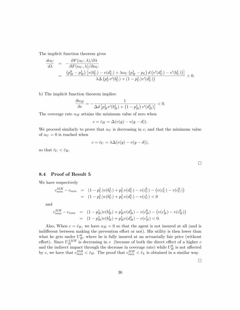
The implicit function theorem gives

d�Ud�

= � @F (�U ; �)=@�

@F (�U ; �)=@�U

=

�p0H � p1H

� �v(b1U )� v(d1U ) + ��U

�p1H � pL

�d�v0(d1U )� v0(b1U )

��p1Uv

0(b1U ) + (1� p1U )v0(d1U )� > 0:

b) The implicit function theorem implies:

@�H@c

= � 1

�d�p1Hv

0(b1H) +�1� p1H

�v0(d1H)

� < 0:The coverage rate �H attains the minimum value of zero when

c = �cH = �(v(y)� v(y � d)):

We proceed similarly to prove that �U is decreasing in c, and that the minimum valueof �U = 0 is reached when

c = �cU = ��(v(y)� v(y � d));

so that �cU < �cH .

�


We have respectively

cMHmin � cmin = (1� p1U )v(b1U ) + p1Uv(d1U )� v(c0U )�

�v(c1U )� v(c0U )

�= (1� p1U )v(b1U ) + p1Uv(d1U )� v(c1U ) < 0

and

cMHmax � cmax = (1� p1H)v(b1H) + p1Hv(d1H)� v(c0H)�

�v(c1H)� v(c0H)

�= (1� p1H)v(b1H) + p1Hv(d1H)� v(c1H) < 0:

Also, When c = �cH , we have �H = 0 so that the agent is not insured at all (and isindi¤erent between making the prevention e¤ort or not). His utility is then lower thanwhat he gets under U0H , where he is fully insured at an actuarially fair price (withoute¤ort). Since U1MH

H is decreasing in c (because of both the direct e¤ect of a higher cand the indirect impact through the decrease in coverage rate) while U0H is not a¤ectedby c, we have that cMH

max < �cH . The proof that cMHmin < �cL is obtained in a similar way.

�

36


a) We have that

@MH(c;�)

@c= 1� �

+�

�(1� p1H)p1Hd

@�H@c

�v0(d1H)� v0(b1H)

��p1U (1� p1U )d

@�U@c

�v0(d1U )� v0(b1U )

��:

We then have that@MH(c;�)

@c� @(c;�)

@c= 1� �

if and only if

�

"(1� p1H)p1H

�v0(d1H)� v0(b1H)

��p1Hv

0(b1H) + (1� p1H)v0(d1H)� # � " p1U (1� p1U ) �v0(d1U )� v0(b1U )�

��p1Uv

0(b1U ) + (1� p1U )v0(d1U )�# :

If �! ��, this condition simpli�es to

�2�

v0(d1H)� v0(b1H)pLv0(b1H) + (1� pL)v0(d1H)

��

v0(d1U )� v0(b1U )pLv0(b1U ) + (1� pL)v0(d1U )

�:

A su¢ cient condition is�pLv

0(b1U ) + (1� pL)v0(d1U )� �v0(d1H)� v0(b1H)

��pLv

0(b1H) + (1� pL)v0(d1H)� �v0(d1U )� v0(b1U )

�;

() v0(d1U )v0(b1H) � v0(b1U )v0(d1H);

which is true since d1U < d1H for �! ��.

The proof of part b) of the lemma is straightforward.

�


a) Start by assuming that � = ��. We know from Lemma 2 b) that

MH(0; ��) = (0; ��) = 0:

Part a) of Lemma 2 shows that

@MH(c; ��)

@c� (c; ��)

@c= 1� � for all c < cMH

min ;

37

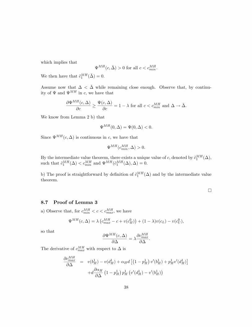
which implies thatMH(c; ��) > 0 for all c < cMH

min :

We then have that ~cMH1 ( ��) = 0:

Assume now that � < �� while remaining close enough. Observe that, by continu-ity of and MH in c, we have that

@MH(c;�)

@c� (c;�)

@c= 1� � for all c < cMH

min and �! ��:

We know from Lemma 2 b) that

MH(0;�) = (0;�) < 0:

Since MH(c;�) is continuous in c, we have that

MH(cMHmin ;�) > 0:

By the intermediate value theorem, there exists a unique value of c; denoted by ~cMH1 (�);

such that ~cMH1 (�) < cMH

min and MH(~cMH

1 (�);�) = 0.

b) The proof is straightforward by de�nition of ~cMH1 (�) and by the intermediate value

theorem.

�


a) Observe that, for cMHmin < c < c

MHmax, we have

MH(c;�) = ��cMHmax � c+ v(c0H)

�+ (1� �)v(cL)� v(c0U );

so that@MH(c;�)

@�= �

@cMHmax

@�:

The derivative of cMHmax with respect to � is

@cMHmax

@�= v(b1H)� v(d1H) + �Hd

��1� p1H

�v0(b1H) + p

1Hv

0(d1H)�

+d@�H@�

�1� p1H

�p1H�v0(d1H)� v0(b1H)

�38

If @�H=@� > 0, it is clear that @cMHmax=@� > 0. On the contrary, if @�H=@� < 0, the

sign is a priori ambiguous. We have

@cMHmax

@�= v(b1H)� v(d1H) + �Hdv0(b1H)

+�Hdp1H

�v0(d1H)� v0(b1H)

�+ d

@�H@�

�1� p1H

�p1H�v0(d1H)� v0(b1H)

�:

A su¢ cient condition to have @cMHmax=@� > 0 is then

�H +@�H@�

�1� p1H

�� 0:

Using the implicit function on the equation de�ning �H , we obtain

d�Hd�

=v(b1H)� v(d1H) + ��Hd

�v0(b1H)� v0(d1H)

��d�p1Hv

0(b1H) +�1� p1H

�v0(d1H)

� ;

whose denominator is always positive. Therefore, the previous su¢ cient condition be-comes

�H � � v(b1H)� v(d1H) + ��Hd

�v0(b1H)� v0(d1H)

��d�p1Hv

0(b1H) +�1� p1H

�v0(d1H)

� ! �1� p1H

�, �d�H

�p1Hv

0(b1H) +�1� p1H

�v0(d1H) +

�v0(b1H)� v0(d1H)

� �1� p1H

��

�v(b1H)� v(d1H)

� �1� p1H

�, �d�Hv

0(b1H) � ��v(b1H)� v(d1H)

� �1� p1H

�;

which is always true since the RHS is negative.b) The derivative of MH(c;�) with respect to c is

@MH(c;�)

@c= �

��1�

�1� p1H

�v0(b1H)

@�H@c

p1Hd+ p1Hv

0(d1H)@�H@c

�1� p1H

�d

�= �

�p1H�1� p1H

�d@�H@c

�v0(d1H)� v0(b1H)

�� 1�< 0:

�


a) Recall that, for cMHmin < c < c

MHmax, we have

MH(c; ��) = (1� �)v(cL) + ��(1� pL)v(b1H) + pLv(d1H)� c

�� v(c0U ):

39

Result 6 has shown that MH(cMHmax; ��) < 0:We now prove that

MH(cMHmin ;

��) > 0:Wehave

MH(cMHmin ; ��) = (1� �)

�v(cL)� v(c0U )

�(10)

+��pL�v(d1H)� v(d1U )

�+ (1� pL)

�v(b1H)� v(b1U )

��:

Note that the �rst term of (10) is positive. Moreover, using the mean value theorem,we obtain that

v(d1H)� v(d1U ) = v0($)d(1� pL) (�H � �U ) ;v(b1H)� v(b1U ) = v0(�)dpL (�U � �H) ;

with $ 2�d1H ; d

1U

�and � 2

�b1H ; b

1U

�. Therefore, the second term of (10) becomes

pL�v(d1H)� v(d1U )

�+ (1� pL)

�v(b1H)� v(b1U )

�= d(1� pL)pL (�H � �U )

�v0($)� v0(�)

�:

As �H > �U (Lemma 1) and $ < �, then the concavity of v(:) implies thatMH(cmin; ��) < 0:Moreover, Lemma 3 has shown that @MH(c;�)=@c < 0 for cMH

min < c < cMHmax. As

MH(c; ��) is continuous in c, the intermediate value theorem implies that there exist~cMH2 ( ��) 2]cMH

min ; cMHmax[ such that

MH(~c( ��); ��) = 0. By continuity of MH(c;�) in �,this threshold ~cMH

2 (�) also exists for value of � close enough to ��. Observe that, whenit exists, ~cMH

2 (�) < cMHmax since

MH(cMHmax;�) < 0 for all �. From now on, we consider

only values of � large enough that ~cMH2 (�) exists.

b) The claim is straightforward since @MH(c ;�)=@c < 0 by Lemma 3.c) We have by de�nition that MH(~cMH

2 (�);�) = 0 so that

dMH(~cMH2 (�);�)

d�=@MH(~cMH

2 (�);�)

@c

@~cMH2 (�)

@�+@MH(~cMH

2 (�);�)

@�= 0:

Our claim then results from the fact that @MH(c ;�)=@c < 0 and that @MH(c ;�)=@� >0 for all c and �.

�

8.9 Proof of Proposition 5

We �rst prove the following two lemmatas.

Lemma 4 We have (a) ~cMH1 (�) < ~c1(�) and (b) ~cMH

2 (�) < ~c2(�) when �! ��:

40

Proof. Result 3 has shown that ~c1(�) < cmin exists if � � ~� (de�ned asMH(cmin; ~�) = 0), with (c;�) < 0 for c < ~c1(�). Obviously, � ! �� > ~�, sothat ~c1(�) exists. Similarly, Result 7 shows that ~cMH

1 (�) exists for � ! ��, withMH(~cMH

1 (�);�) = 0. We then have that MH(c;�) > (c;�) for c < cMHmin (a con-

sequence of Lemma 2) implies that ~cMH1 (�) < ~c1(�):

Result 4 has shown that cmin < ~c2(�) < cmax exists if � � ~�, with (c;�) > 0for ~c1(�) < c < ~c2(�). Similarly, Result 8 shows that ~cMH

2 (�) < cMHmax exists for

� ! ��, with MH(c;�) > 0 for ~cMH1 (�) < c < ~cMH

2 (�). We then have thatMH(c;�) < (c;�) for any � when cMH

min < cmin < c < cMHmax (Lemma 5) implies

that ~cMH2 (�) < ~c2(�):

Lemma 5 MH(c;�) < (c;�) for any � when cMHmin < cmin < c < c

MHmax:

Proof. Recall that, when cmin < c < cMHmax, we have

MH(c;�) = ��(1� p1H)v(b1H) + p1Hv(d1H)� c

�+ (1� �)v(cL)� v(c0U );

(c;�) = ��v(c1H)� 1

�+ (1� �)v(cL)� v(c0U );

hence we obtain

(c;�)�MH(c;�) = ��v(c1H)� (1� p1H)v(b1H)� p1Hv(d1H)

�> 0:

We now prove Proposition 5Proof. (a) Recall that, when � is close enough to ��, we have that MH(0;�) =

(0;�) and that MH(c;�) > (c;�) for c < cMHmin (see Lemma 2 for both), which

implies that MH(cMHmin ;�) > (c

MHmin ;�). Lemma 5 shows that

MH(c;�) < (c;�)for cMH

min < cmin < c < cMHmax. By continuity of

MH(c;�) and (c;�) in c, the factthat @MH(c;�)=@c < 0 for cMH

min < c < cmin (see Lemma 3) and the intermediatevalue theorem, we then have that there exists a unique value of c, denoted by c, withcMHmin < c < cmin, and such that

MH(c;�) > (c;�) for c < c, MH(c;�) = (c;�)and MH(c;�) < (c;�) for c < c < cmax. As for the latter inequality, observe thatMH(c;�) = 0 < (c;�) for cMH

max � c < cmax, while MH(c;�) = (c;�) = 0 forc � cmax.(b) The proof of Lemma 4 shows that ~c1(�), ~cMH

1 (�) and ~cMH2 (�) exist when �! ��.

The claim follows from the observation that MH(c;�) > 0 for ~cMH1 (�) < c < ~cMH

2 (�)(Results 7 and 8) while (c;�) < 0 for for c < ~c1(�) (Result 3).(c) The proof of Lemma 4 shows that ~c1(�), ~c2(�) and ~cMH

2 (�) exist when � ! ��.The claim follows from the observation that MH(c;�) < 0 for c > ~cMH

2 (�) (Result 3)while (c;�) > 0 for ~c1(�) < c < ~c2(�) (Result 1 (b)).

41

(d) We know that (c;�) is maximized at c = cmin, and we now show that fromMH(cMH

min ;�) > (cmin;�) . We have that

MH(cMHmin ;�) = �

�(1� p1H)v(b1H) + p1Hv(d1H)� (1� p1U )v(b1U )� p1Uv(d1U )

�+ (1� �)

�v(cL)� v(c0U )

�;

(cmin;�) = ��v(c1H)� v(c1U )

�+ (1� �)

�v(cL)� v(c0U )

�;

so that

MH(cMHmin ;�) > (cmin;�)

, v(c1U )��(1� p1U )v(b1U )� p1Uv(d1U )

�> v(c1H)�

�(1� p1H)v(b1H) + p1Hv(d1H)

�:

If we assume that � = ��, the latter inequality becomes

(1� pL)�v(b1U )� v(b1H)

�< pL

�v(d1H)� v(d1U )

�(1� pL)

�b1U � b1H

�v0(�) < pL

�d1H � d1U

�v0(�); (11)

with � > �. Using

b1U � b1H = (�H � �U )pLd;b1U � b1H = (�H � �U )pLd;

the inequality (11) becomesv0(�) < v0(�);

which is true.

By continuity of MH(cMHmin ;�) and of (cmin;�) in�, we obtain that

MH(cMHmin ;�) >

(cmin;�) for �! ��.

42

Figure 1 : Value of test as a function of c for several values of

0.1 0.2 0.3 0.4c

0.02

0.04

0.06

Yc,D

Figure 2 : Value of c1 yellow, cmin blue, c2 green and cmax purple as a function of

0.1 0.2 0.3 0.4 0.5D

0.05

0.10

0.15

0.20

0.25

0.30

0.35

ctilda, cmin & cmax

Figure 3 : H and U U H as a function of c

0.05 0.10 0.15 0.20 0.25 0.30c

0.2

0.4

0.6

0.8

1.0

aU and aH

Figure 4 : Value of test with moral hazard as a function of c for several values of

0.1 0.2 0.3 0.4c

0.02

0.04

0.06

Y^MHc,D

2 NEW Figures 1 to 5 of Paper.nb

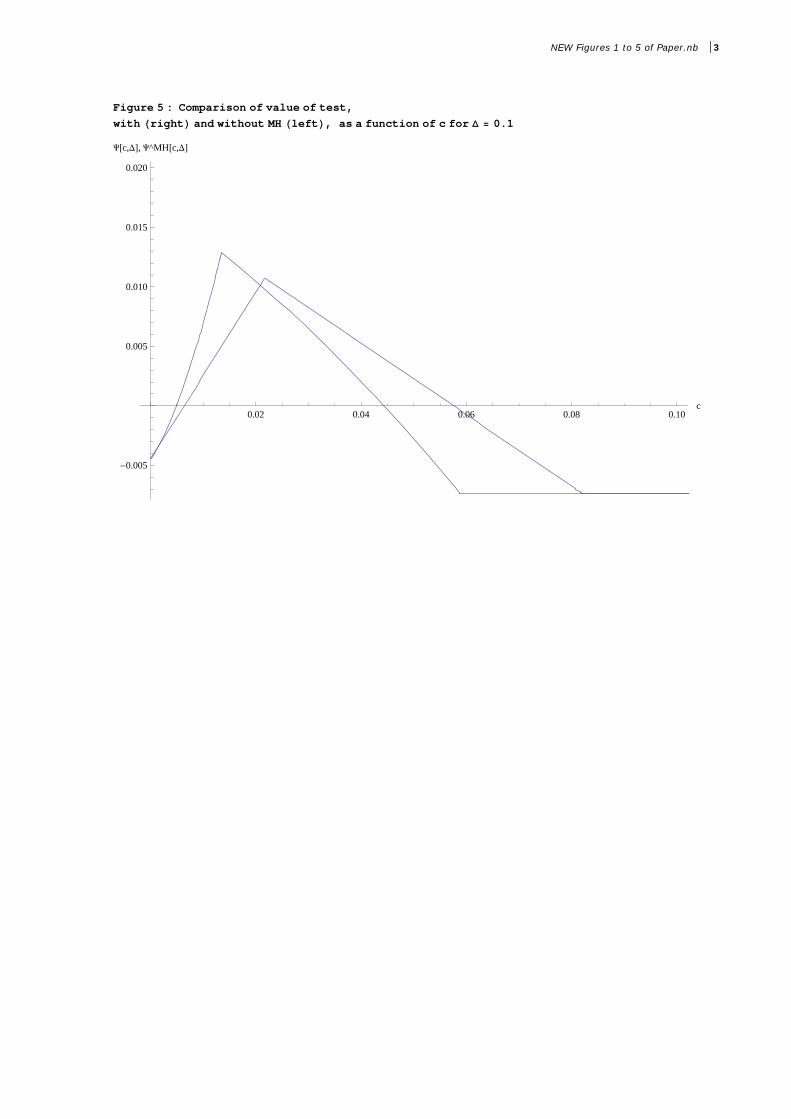
Figure 5 : Comparison of value of test,

with right and without MH left, as a function of c for 0.1

0.02 0.04 0.06 0.08 0.10c

-0.005

0.005

0.010

0.015

0.020

Yc,D, Y^MHc,D

NEW Figures 1 to 5 of Paper.nb 3

Figure 6 : Ex‐ante utility as a function of effort cost

Ex‐ante utility

A : Expected utility gain from

1

p y gprevention technology

B : Expected utility gain from genetictest

C E t d tilit i ith fi t b t 1uv c C : Expected utility gain with first best

allocation

First best allocationNo test effort by

AC

B

effort by all

Test, effort if H

0uv c

No prevention, no testB

0 cminc1c 2c

Figure 7 : Ex‐ante utility with and without moral hazard

Ex‐ante utility

D : Expected utility loss from moralhazard

With

Without Moral HazardD

WithMoral Hazard

Without Moral Hazard

0 c1MHc 1c 2c2

MHc

genetic testing with primary prevention and moral hazard”genetic testing with primary prevention...

Documents