genetic programming methodology - brad · pdf filegenetic programming methodology 31...

CHAPTER 4 Genetic Programming

Methodology

4.1 Introduction

Identification of approximation functions in the response surface methodology is

fundamental. The function identification problem is to find a functional model in

symbolic form that fits a set of experimental data.

In a conventional li near or nonlinear regression, the mathematical problem is

reduced to finding the coefficients for a prespecified function. In contrast, if the

search process works simultaneously on both the model specification problem

(structure of the approximation) and the problem of f itting coeff icients (tuning

parameters), the technique is called symbolic regression (Koza, 1992).

To obtain the best quali ty approximation, the formulation of the symbolic

regression problem should not specify the size or the structural complexity of the

model in advance. Instead, these features of the problem should emerge during the

problem-solving process, as part of the solution. With these premises, the search

space is clearly too vast for a blind random search. We need to search it in some

intelli gent and adaptive way.

Genetic programming methodology 31

Evolutionary algorithms (EA) are search techniques based on computer

implementations of some of the evolutionary mechanisms found in nature, such as

selection, crossover and mutation, in order to solve a problem. Structures do not just

happen, but rather evolve and simultaneously sample the search space. EAs are often

referred to as global optimization methods because they can effectively explore very

large solution spaces without being trapped by local minima. EAs are robust, global

and may be applied without problem-specific heuristics. This makes EAs well suited

to symbolic regression.

In structural optimization, Xie and Steven (1997) have developed a design

method called Evolutionary Structural Optimization (ESO). However, despite the

similarities of its name, this technique falls in a different category to EAs. The

concept is to gradually remove inefficient material (lightly stressed) from a structure

at the same time as it is being designed, so that the structure evolves to its optimum

shape.

EAs maintain a population of structures that evolve according to the rules of

natural selection and the sexual operators borrowed from natural genetics such as

reproduction or crossover. Each individual in the population receives a measure of

its fitness in the current environment, i.e. how good the individual is at competing

with the rest of the population. At each generation, a new population is created by

the process of selecting individuals according to their fitness and breeding them

together using the genetic operators. Figure 4.1 shows the evolution system for each

generation.


Genetic �

Search �

Fitness

Selection �

Reproduction Crossover �

Mutation

Figure 4.1 Genetic system using EAs

Two types of EAs are considered in this thesis, genetic algorithms and genetic

programming. The former is used in parameter optimization, while the latter evolves

the structure of the approximation model.

4.2 Genetic Algorithms

A genetic algorithm (Holland, 1975) is a machine learning technique modelled upon

the natural process of evolution. It uses a stochastic, directed and highly parallel

search based on principles of population genetics that artificially evolve solutions to

a given problem.

Genetic algorithms differ from conventional optimization techniques in that

they work on a whole population of individual objects of f inite length, typically

binary strings (chromosomes), that encode candidate solutions using a problem-

specific representation scheme. These strings are decoded and evaluated for their

fitness, which is a measure of how well each solution solves the problem objective.


GAs are problem-independent. To guide the search in highly nonlinear and

multidimensional spaces, GAs do not have any knowledge about the problem

domain, except the information provided by the fitness measure and the

representation scheme. In practice, GAs are efficient in searching for the optimum

solution.

The genetic algorithm attempts to find the best solution to the problem by

genetically breeding the population of individuals over a number of generations.

Following Darwin's principle of survival of the fittest, strings with higher fitness

values have a higher probabili ty of being selected for mating purposes to produce the

next generation of candidate solutions.

Selected individuals are reproduced through the application of genetic

operators. A string selected for mating is paired with another string and with a

certain probabili ty each pair of parents undergo crossover (sexual recombination)

and mutation. The strings that result from this process, the children, become

members of the next generation of candidate solutions.

In this thesis, a variant of the generational GAs is used in which almost the

whole population is replaced in each generation, except the elite (see Section 4.2.7),

as opposed to steady-state selection where only a few individuals are replaced in

each generation, usually a small number of the least fit individuals.

This process is repeated for many generations in order to artificially evolve a

population of strings that yield a very good solution to a given problem. Theoretical

work and practical applications of genetic algorithms (Goldberg, 1989) reveal that


these algorithms are robust and capable of eff iciently locating the regions of search

spaces that yield highly fit solutions to a nonlinear and multidimensional problem.

One important aspect of GAs is the balance between exploration and

exploitation. An eff icient algorithm uses two techniques, exploration to investigate

new and unknown areas in the search space, and exploitation to make use of the

knowledge gained by exploration to reach better positions in the search space.

Compared to classical search algorithms, random walk is good at exploration, but has

no exploitation. Hill climbing is good at exploitation, but has littl e exploration.

The main factors that make GA different from traditional methods of search

and optimization are:

1. GAs work with a coding of the design variables as opposed to the design

variables themselves;

2. GAs work with a population of points as opposed to a single point, thus reducing

the risk of getting stuck at local minima;

3. GAs require only the objective function value, not the derivatives. This aspect

makes GAs application problem-independent;

4. GAs are a family of probabili stic search methods, not deterministic, making the

search highly exploitative.

GAs have been widely applied in design optimization. Hajela (1992) and

Hajela and Lin (1992) have implemented genetic search methods in multicriteria

design optimization with a mix of continuous, integer and discrete design variables.

Dhingra and Lee (1994) have studied single and multiobjective structural


optimization with discrete-continuous variables. The problem of parameter

identification with GAs has been studied by Worden and Deacon (1996), Nair and

Mujumdar (1996) and Wright (1991).

Other work can be found in the papers by Le Riche and Haftka (1993), Kosigo

et al. (1994), Grierson (1995), Parmee (1998), Blachut (1997), Wright and Holden

(1998), Keane and Brown (1996),, Mahfouz et al. (1998), Weldali and Saka (1999).

The next sections will describe the main elements of a GA mechanism.

4.2.1 The representation scheme

In most GAs, finite-length binary-coded strings of ones and zeros are used to

describe the parameters for each solution. In a multiparameter optimization problem,

individual parameter codings are usually concatenated into a complete string (Figure

4.2).

1 0 �

1 1 0 �

0 �

1 1 0 �

1 0 �

1 0 �

1 1 1 1 0 �

1 1 1 1 1 0 �

0 �

1 1 0 �

1 0 �

x �i

� x �i

�+1 x �

i �+2

Figure 4.2 Binary representation of a design in a GA

To decode a string, substrings of specified length are extracted successively

and mapped to the desired interval in the corresponding solution space.

Let us assume that each variable xi, i=1...N is coded with a substring of length n

and that each position in the substring is defined by qij, j=1...n, where qij ∈ [0,1]. A

candidate solution to the problem is represented as a string of length n*N. To decode


a substring and map it to a particular interval in the solution space, the design

variable xi is defined as follows:

∑=

− =−

−+=

n

j

jijn

mini

maximin

ii Niqxx

xx

1

1 1,212

� (4.1)

For the 3 design variables example in Figure 4.2 defined in the interval

[-100,100] and represented by a 10-bit binary string, Table 4.1 shows the

corresponding mapping:

Table 4.1 Mapping of design variables

Binary string Real value

1 1011001101 40.176

2 0101111011 -25.904

3 1110011010 80.254

Real coded GAs have also been proposed for continuous variable optimization

problems (Golberg, 1990, Wright, 1991).

4.2.2 Fitness

The evolutionary process is driven by the fitness measure. The fitness assigns a

value to each fixed-length character string in the population. The nature of the

fitness varies with the problem.

For unconstrained maximization problems, the objective function can be used

for the formulation of the fitness function. The fitness function can be defined as the


inverse of the objective function or the difference between an upper limit value of the

objective function and the objective value for each individual.

For constrained optimal design problems, an exterior penalty function can be

adopted to transform a constrained optimization problem into an unconstrained one.

Penalty functions can be applied in the exterior or in the interior of the feasible

domain. With the exterior penalty function, constraints are applied only when they

are violated. Generally, this penalty is proportional to the square of a violation and

forces the design to move in the infeasible domain.

The choice of the fitness function is criti cal because this value is the basis for

the selection strategy, discussed later in this chapter. If a few members of the

population have a very high fitness in relation to the others, more fit individuals

would quickly dominate and result in premature convergence. Figure 4.3 compares

two fitness functions F = 1/f and F = fu-f, where fu is a selected upper limit value for

the fitness and f is a function to be minimised. Clearly, the latter example maintains

diversity, while the former would direct the search toward a local optimum.


1

2

3 � 4

3 �

4

2

1

(a) (b)

members

of

population

fi(a)

1 / fi

(b)fu - fI

(fu = fmin + fmax)

1 0.2 5 5

2 1 1 4.2

3 2 0.5 3.2

4 5 0.2 0.2

Figure 4.3 Definition of the fitness function for diversity

4.2.3 Selection scheme

The selection operator improves the average quality of the population by giving

individuals with higher fitness a higher probabili ty to undertake any genetic

operation. An important feature of the selection mechanism is its independence of

the representation scheme, as only the fitness is taken into account. The probabili stic

feature allocates to every individual a chance of being selected, allowing individuals

with poor fitness to be selected occasionally. This mechanism ensures that the


information carried out by unfit strings is not lost prematurely from the population.

The GA is not merely a hill -climbing algorithm due to this non-local behaviour.

The most popular of the stochastic selection strategies is fitness proportionate

selection, also called biased roulette wheel selection. It can be regarded as allocating

pie slices on a roulette wheel, with each slice proportional to a string's fitness.

Selection of a string to be a parent can then be viewed as a spin of the wheel, with

the winning slice being the one where the spin ends up. Although this is a random

procedure, the chance of a string to be selected is directly proportional to its fitness

and the least fit individuals will gradually be driven out of the population. For

example, if we generate a random number C between 0 and 1 and we get the value

0.61, string 3 in Figure 4.4 would be selected.

1 30.8 %

2 28.3 %

3

25.2 %

4 15.7 %

P 1 + P 2 < C < P 1 + P 2 + P 3

Fi Pi = Fi / ∑∑Fi

1 9.8 0.308

2 9 0.283

3 8 0.252

4 5 0.157

C = 0.61 ( 0 ≤ C < 1 at random )

Figure 4.4 Fitness proportionate method


A major drawback of f itness proportionate selection is that, for relatively small

populations, early in the search a small number of strings are much fitter than the

others and will quickly multiply. There is a high risk of premature convergence of

the population characterized by a too high exploitation of highly fit strings at the

expense of exploration of other regions of the search space.

A second selection strategy is called tournament selection (Goldberg and Deb,

1991). A subpopulation of individuals is chosen at random. The individual from this

subpopulation with the highest fitness wins the tournament. Generally, tournaments

are held between two individuals (binary tournament). However, this can be

generalised to an arbitrary group whose size is called the tournament size. This

algorithm can be implemented eff iciently as no sorting of the population is required.

More important, it guarantees diversity of the population. The most important

feature of this selection scheme is that it does not use the value of the fitness

function. It is only necessary to determine whether an individual is fitter than any

other or not.

Other selection schemes and their comparative analysis have been reviewed by

(Goldberg and Deb, 1991).

4.2.4 Crossover

The crossover operator is responsible for combining good information from two

strings and for testing new points in the search space. The two offsprings are

composed entirely of the genetic material from their two parents. By recombining

randomly certain effective parts of a character string, there is a good chance of


obtaining an even more fit string and making progress towards solving the

optimization problem.

Several ways of performing crossover can be used. The simplest but very

effective is the one-point crossover (Goldberg, 1989). Two individual strings are

selected at random from the population. Next, a crossover point is selected at

random along the string length, and two new strings are generated by exchanging the

substrings that come after the crossover point in both parents. The mechanism is

ill ustrated in Figure 4.5.

1 0 �

1 1 0 �

0 �

1 1 0 �

1

0 �

1 0 �

1 1 1 1 0 �

1 1

1 0 �

1 1 0 �

0 �

1 1 0 �

1 0 �

1 0 �

1 1

1 1 0 �

1 1 Parent 1 Offspring 1 �

Offspring 2 �

Parent 2

Figure 4.5 GA Crossover

A more general case is the multipoint crossover (De Jong, 1975) in which parts

of the information from the two parents are swapped among more string segments.

An example is the two-point crossover, where two crossover points are selected at

random and the substrings lying in between the points are swapped.

Uniform crossover (Syswerda, 1991) is the method of choice in this thesis.

Each bit of the offspring is created by copying the corresponding bit from one or the

other parent selected at random with equal probabili ty, as shown in Figure 4.6.

1 0

1 1 0

0

1 1 0

1

0

1 1 1 1 0

1 1 0

1

Parent 1

Offspring �

0

1 0

1 1 1 1 0

1 1 Parent 2

Figure 4.6 GA Uniform crossover


Uniform crossover has the advantage that the ordering of bits is entirely

irrelevant because there is no linkage between adjacent bits. Multipoint crossover

takes half of the material from each parent in alternation, while uniform crossover

decides independently which parent to choose. When the population has largely

converged, the exchange between two similar parents leads to a very similar

offspring. This is less likely to happen with uniform crossover particularly with

small population sizes, and so, gives more robust performance.

4.2.5 Mutation

Mutation prevents the population from premature convergence or from having

multiple copies of the same string. This feature refers to the phenomenon in which

the GA loses population diversity because an individual that does not represent the

global optimum becomes dominant. In such cases the algorithm would be unable to

explore the possibili ty of a better solution.

Mutation consists of the random alteration of a string with low probabili ty. It

is implemented by randomly selecting a string location and changing its value from 0

to 1 or vice versa, as shown in Figure 4.7.

1 0 �

1 1 0 �

0 �

1 1 0 �

1 1 0 �

0 �

1 Parent Offspring �

1 0 �

0 �

1 0 �

1

Figure 4.7 GA Mutation


4.2.6 Mathematical foundation

GA implicitly processes in parallel a large amount of useful information concerning

schemata (Holland, 1975). A schema is a set of points from the search space with

certain specified similarities. The schema is described by a string with a certain

alphabet (0 and 1 if the alphabet is binary) and a "don't care" symbol denoted by an

asterisk. For example, 1**0 represents the set of all 4-bit strings that begin with 1

and end with 0.

The GA creates individual strings in such a way that each schema can be

expected to be represented in proportion to the ratio of its schema fitness to the

average population fitness (Koza et al, 1999). The schema fitness is the average of

the fitness of all the points from the search space contained in the population and

contained in the schema. The average population fitness is the average of the fitness

of all the points from the search space contained in the population. The schema

theorem (Holland, 1975) explains that an individual's high fitness is due to the fact

that it contains good schemata. The optimum way to explore the search space is to

allocate reproductive trials to individuals in proportion to their fitness relative to the

rest of the population. In this way, good schemata receive exponentially increasing

number of trials in successive generations.

According to the building block hypothesis (Golberg, 1989), the power of GA

is in its abili ty to find good building blocks. These are schemata of short defining

lengths consisting of bits working well together that tend to lead to improved

performance when incorporated into an individual.


4.2.7 Implementation of the GA

In this thesis, GAs are used to find an initial guess which serves as input to a

gradient-based optimization algorithm (Madsen and Hegelund, 1991) in order to

obtain the tuning parameters a in (3.2) or (3.3) of the approximate model, combined

with a nonlinear regression algorithm. Generally, GAs work well even if the space

to be searched is large, not smooth or not well understood, or if the fitness function is

noisy and, in addition, when finding a good solution (not necessarily the exact global

optimum) is suff icient.

Figure 4.8 shows a flowchart of the implementation of the GA used in this

thesis. Assuming we have n tuning parameters encoded with l-bit strings, GA works

as follows:

1) Start with a randomly generated population of individuals of length n*l-bits.

2) Iteratively perform the following steps on the population:

a) calculate the fitness of each chromosome by least-squares,

b) sort the population,

c) create a new population:

i) In the reproduction stage a strategy must be adopted as to which strings

should die: either to kill t he individuals with fitness below the average or,

alternatively, to kill a small percentage of the individuals with the worst

fitness. The second approach is preferred in this thesis as it provides

more diversity.


ii ) Calculate the elite (De Jong, 1975) according to input parameter Pe,

which is an additional operator that transfers unchanged a relatively small

number of the fittest individuals to the next generation. Such individuals

can be lost if they are not selected to reproduce or if they are destroyed by

crossover or mutation. In this thesis, Pe=20% of the population has been

used.

iii ) Fill up the population with the surviving strings according to tournament

selection of size 2.

iv) Select a pair of individuals from the current population. The same string

can be selected more than once to become a parent. Recombine

substrings using the uniform crossover. Two new offsprings are inserted

into the new population.

v) With the probabili ty Pm taken as 0.01 in this thesis, mutate a randomly

selected string at a randomly selected point.

3) Check the termination criterion. If not satisfied, perform the next iteration.


START

Create randomly the initial population

�

KILLING Kill k

�% of strings

with the worst fitness

REPRODUCTION Fill up the population with surviving strings

SPAWNING Create new population

ELITE TRANSFER Put elite strings into the new population

CROSSOVER Put 2 offsprings into the new population

MUTATION Mutate one node within a string

More �

crossovers ? More

�

mutations ? �

Convergence ?

STOP

Yes Yes

Yes

Evaluate the fitness �

for each string

No �

No �

Figure 4.8 Flowchart of the GA

Each iteration of this process is called a generation. The entire set of

generations is called a run. At the end of the run, there are one or more highly fit

strings in the population. Generally, it is necessary to make multiple independent

runs of a GA to obtain a result that can be considered successful for a given problem.


In this thesis, GA only performs 1 run with 30 generations due to computing

time constraints and the fact that the solution is only used as a starting guess for the

gradient-based optimization technique.

A limitation in the application of GAs is the fixed-length representation

scheme and the need to encode the variables. These two aspects do not provide a

convenient way of representing general computational structures like a symbolic

regression model. In addition, GAs do not have dynamic variabili ty as they require

the string length to be defined in advance. To deal with this problem, Koza (1992)

implemented an extension of the genetic model of GAs with parse trees called

genetic programming.

4.3 Genetic Programming

Genetic Programming (GP) is a generalization and an extension of GAs. The same

description of GA given in Section 4.2 is applicable to GP, so only new concepts and

differences with respect to GAs will be discussed in this section.

GP combines a high-level symbolic representation with the search eff iciency of

the GA. Its basis is the same Darwinian concept of survival of the fittest. The

innovation of the GP is the use of more complex structures. While a GA uses a string

of numbers to represent the solution, the GP creates computer programs with a tree

structure. In the case of design optimization, a program represents an empirical

model to be used for approximation of response functions in the original

optimization problem.


These randomly generated programs are general and hierarchical, varying in

size and shape. GP's main goal is to solve a problem by searching highly fit computer

programs in the space of all possible programs that solve the problem. This aspect is

the key to finding near global solutions by keeping many solutions that may

potentially be close to minima (local or global). The creation of the initial population

is a blind random search of the space defined by the problem. In contrast to a GA, the

output of the GP is a program, whereas the output of a GA is a quantity.

The main advantages of using GP for symbolic regression are that the size and

shape of the approximation function do not need to be specified in advance and that

the problem specific knowledge can be included in the search process through the

use of the appropriate mathematical functions.

The term symbolic regression in genetic programming (Koza, 1992) stands for

the process of discovering both the functional form of the approximation and all of

its tuning parameters. Unfortunately, a weakness of GP is the diff iculty of f inding

the numerical constants due to their representation as tree nodes and the fact that the

genetic operators only affect the structure of the tree. Although GP can generate

constants, dividing for example one variable by itself, the process becomes very

ineff icient (Evett and Fernandez, 1998). For this reason, in this thesis the tuning

parameters are not modified by the evolutionary process but identified by a nonlinear

least-squares surface fitting using an optimization method.

The evolutionary process in GP proceeds in a similar way to standard GA. GP

starts with a population of randomly generated programs built from a library of

available mathematical functions. These trees are assigned a fitness value and evolve


by means of the genetic operators of selection, crossover and mutation following the

Darwinian principle of survival and reproduction of the fittest, similar to GAs.

GP has been applied to systems identification by Watson and Parmee (1996),

McKay et al. (1996) and Gray et al. (1996) among others. Other applications can be

in found in Kinnear (1994).

4.3.1 Representation scheme

The structures in GP are computer programs represented as expression trees. They

are hierarchical and can dynamically change the size and shape during the evolution

process. A typical program representing the expression (x1/x2+x3)2 is shown in

Figure 4.9.

SQ �

+

/ �

x �1 x �

2

x �3

�

Unary Node �

Binary Nodes

Terminal Nodes

Figure 4.9 Typical tree structure for

2

32

1

+ x

x

x

The programs are composed of nodes that are elements from a terminal set and

a functional set, as described in Table 4.2.


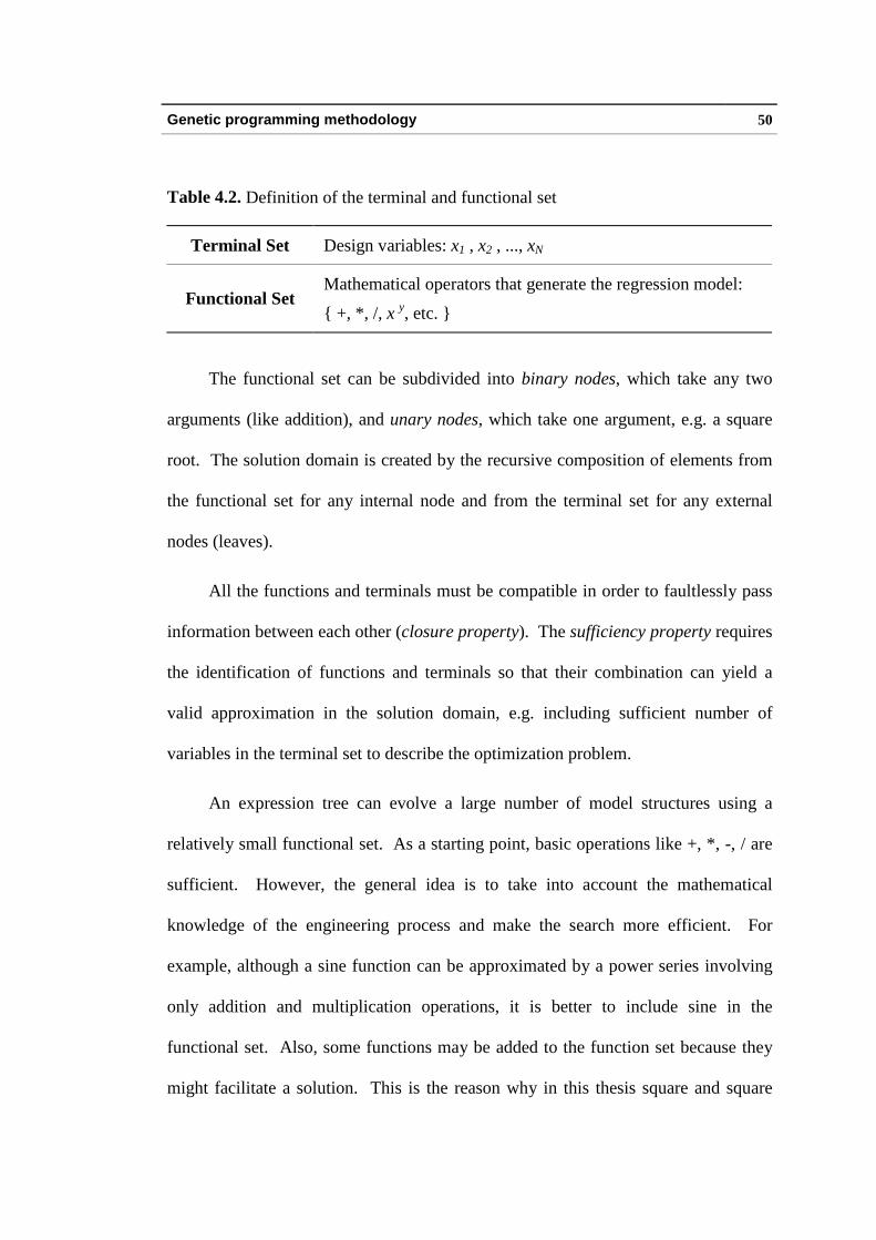
Table 4.2. Definition of the terminal and functional set

Terminal Set Design variables: x1 , x2 , ..., xN

Functional SetMathematical operators that generate the regression model:

{ +, *, /, x y, etc. }

The functional set can be subdivided into binary nodes, which take any two

arguments (li ke addition), and unary nodes, which take one argument, e.g. a square

root. The solution domain is created by the recursive composition of elements from

the functional set for any internal node and from the terminal set for any external

nodes (leaves).

All the functions and terminals must be compatible in order to faultlessly pass

information between each other (closure property). The sufficiency property requires

the identification of functions and terminals so that their combination can yield a

valid approximation in the solution domain, e.g. including suff icient number of

variables in the terminal set to describe the optimization problem.

An expression tree can evolve a large number of model structures using a

relatively small functional set. As a starting point, basic operations like +, *, -, / are

suff icient. However, the general idea is to take into account the mathematical

knowledge of the engineering process and make the search more eff icient. For

example, although a sine function can be approximated by a power series involving

only addition and multiplication operations, it is better to include sine in the

functional set. Also, some functions may be added to the function set because they

might facilit ate a solution. This is the reason why in this thesis square and square


root functions are included in the functional set, even though the same result could be

obtain with multiplication and power respectively at a more expensive computational

cost.

Table 4.3 summarizes mathematical operators that are useful for a large range

of problems. If the functional set contains irrelevant operators or if the terminal set

contains more variables than necessary to define the problem, GP will usually be

able to find a solution, although the performance of the search will be degraded.

Table 4.3 The functional set

Label Description Operation

+ Addition x1 + x2

- Subtraction x1 - x2

* Multiplication x1 × x2

/ Divisionx1 / x2

if x2 = 0 assign penalty

SQ Square 21x

SQRT Square root√x1

if x1 < 0 assign penalty

EXP Exponential 1xe

SIN Sine sin(x1)

COS Cosine cos(x1)

An important aspect of the functional set is the handling of mathematical

exceptions during fitness evaluation. Illegal mathematical operations like division by


zero or run-time overflow and underflow errors need to be removed in order to

obtain valid expressions. In this thesis, infeasible expression trees are assigned the

worst possible fitness in the population as a penalty.

The evolution of the programs is performed through the action of the genetic

operators and the evaluation of the fitness function.

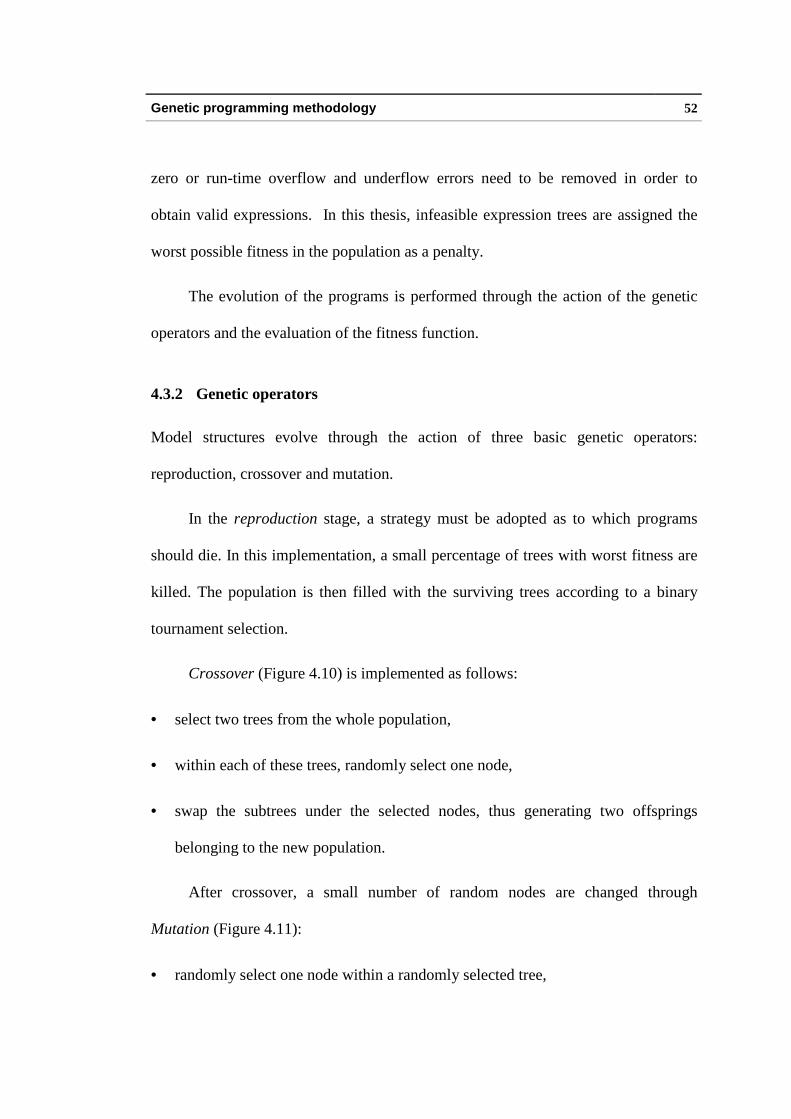
4.3.2 Genetic operators

Model structures evolve through the action of three basic genetic operators:

reproduction, crossover and mutation.

In the reproduction stage, a strategy must be adopted as to which programs

should die. In this implementation, a small percentage of trees with worst fitness are

kill ed. The population is then fill ed with the surviving trees according to a binary

tournament selection.

Crossover (Figure 4.10) is implemented as follows:

• select two trees from the whole population,

• within each of these trees, randomly select one node,

• swap the subtrees under the selected nodes, thus generating two offsprings

belonging to the new population.

After crossover, a small number of random nodes are changed through

Mutation (Figure 4.11):

• randomly select one node within a randomly selected tree,


• replace this node with another one from the same set (a function replaces a

function and a terminal replaces a terminal) except by itself,

An additional operator, elite transfer, is used to allow a relatively small number

of the fittest programs, called the elite, to be transferred unchanged to a next

generation, in order to keep the best solutions found so far. As a result, a new

population of trees of the same size as the original one is created, but it has a higher

average fitness value.

/ �

SQ �

+

*

x �1 SQ

�

x �2

/ �

x �2 SQ

�

x �1

SQ �

+

SQ �

x �1

x �2

+

*

x �1 SQ

�

x �2

SQ �

+

x �2 x �

1

x �2 SQ

�

x �1

Parent 1 Parent 2

Offspring 2 �

Offspring 1 �

Figure 4.10 GP Crossover


S Q

-

S Q x 2

x 1

S Q

*

S Q x 2

x 1

+ - / *

Figure 4.11 GP mutation

4.3.3 Fitness function

When selecting randomly a tree to perform any genetic operation, the tournament

selection method is used here. This method specifies the probabili ty of selection on

the basis of the fitness of the solution.

The fitness of a solution shall reflect:

(i) The quali ty of approximation of the experimental data by a current expression

represented by a tree.

(ii) The length of the tree in order to obtain more compact expressions.

In problems of empirical model building, the most obvious choice for the

estimation of the quali ty of the model is the sum of squares of the difference between

the simpli fied model output and the results of runs of the original model over some

chosen plan (design) of experiments.

Generally, there can be two sources of error: incorrect structure and inaccurate

tuning parameters. In order to separate these, the measure of quali ty Q(Si) is only

calculated for the tuned approximation, as described in Section 4.3.5.


In a dimensionless form this measure of quali ty of the solution can be

presented as follows:

( )( )

∑

∑

=

=

−

=P

p

p

P

p

pp

i

F

FF

SQ

1

2

1

2~

(4.2)

or as (3.3) with equal weights when derivatives are used.

If ( )iSQ is the measure of quali ty of the solution Si, uQ is an upper limit value

of the quali ty for all Nt members of the population, ntpi is the number of tuning

parameters contained in the solution Si and c is a coeff icient penalizing the excessive

length of the expression, the fitness function ( )iSΦ can be expressed in the following

form:

( ) ( ) 2* iiui ntpcSQQS −−=Φ → max (4.3)

Programs with greater fitness values ( )iSΦ have a greater chance of being

selected in a subsequent genetic action. Highly fit programs live and reproduce, and

less fit programs die.

In terms of computer implementation of the GP paradigm, it is more

convenient and more efficient to make the best value of the fitness 0, i.e to solve a

minimization problem. For this reason, the definition of the fitness used in the

computer program developed in this thesis is the following:


( ) ( ) 2* iii ntpcSQS +=Φ → min (4.4)

Another possible choice is the statistical concept of correlation, which

determines and quantifies whether a relationship between two data sets exists. This

definition was used for the identification of industrial processes (McKay et al. 1996).

To evaluate the goodness-of-fit, the standard root mean square (RMS) error

will be used in this thesis according to the following expression:

( )

P

FFP

p

pp∑=

−

= 1

2~

RMS(4.5)

4.3.4 Allocation of tuning parameters

Traditional implementations use GP to generate constants that are optimized by a

nonlinear regression algorithm. In this thesis, the algorithm implements two

different tasks. First, GP finds an appropriate symbolic model structure (without

constant creation). Second, an automatic procedure allocates tuning parameters

within the regression model in a symbolic form as shown in Figure 4.12, and

optimizes the symbolic parameters with a gradient-based optimization method

(Madsen and Hegelund, 1991).


SQ �

+

/ �

x �1 x �

2

x �3

�

SQ �

+

*

a �1 /

�

+

a �0

�

x �1 x �

2

*

a �2 x �

3 �

Figure 4.12 Symbolic allocation of parameters for

2

322

110

++ xa

x

xaa

This implementation has the advantages that the coefficients are optimized in

the whole range of a prespecified interval, and subsequently, the complexity of the

expression is reduced. In contrast, in Koza's implementation (1992), only a few

constants to be used as coeff icients were defined in the terminal set, leading to much

bigger expressions than that of the minimal solution.

The allocation of tuning parameters a to an individual tree follows basic

algebraic rules. Going through the tree downwards, tuning parameters are allocated

to a subtree depending on the type of the current node and the structure of the

subtree. The different cases are described as follows (according to Figure 4.13):


1. Current node is of type binary:

• Multiplication and division operations only require one tuning parameter, e.g.

( ) 21121~~

xxaFxxF ∗∗=⇒∗= a

• All other operations require two tuning parameters, e.g.

( )

( ) ( ) ( )221121

221121

^~

^~

~~

xaxaFxxF

xaxaFxxF

∗∗=⇒=

∗+∗=⇒+=

a

a

• When F~

is a combination of the previous two approaches, tuning parameters

are only applied to operations different from multiplication and division, e.g.

( ) ( ) ( )

( ) ( ) ( ) ( ) ( )4322114321

4232114321

^~

^~

~~

xxxaxaFxxxxF

xaxxaxFxxxxF

∗∗+∗=⇒∗+=

∗+∗∗=⇒+∗=

a

a

2. Current node is of type unary:

• Ignore

3. Current node is of type variable (terminal node):

• One tuning parameter is inserted, e.g.

( ) ( ) ( )2112

1~~

xaFxF ∗=⇒= a

4. Free parameter:

• One free parameter is added to the expression, e.g.

( ) ( ) 01111~~

axaFxaF +∗=⇒∗= aa


START

Check first node in the subtree

Variable node �

Unary node �

Check left node Check right node

Binary node

Insert tuning parameter !

Insert tuning parameter !

Yes

More nodes to check ?

"

Yes

No #

STOP

No #

Only * and / in subtree ?

$

Figure 4.13 Flowchart for the symbolic allocation of tuning parameters

4.3.5 Tuning of an approximation function

The representation of the tuning parameters is a binary multiparameter coding

mapped to the interval [-100, 100] with a 10-digit binary string, defining a precision

of 100 - (-100) / (210 - 1) = 0.196 for each tuning parameter.

The objective function is defined here as the sum of squares of the difference

between the simpli fied model output with the current guess, and the results of runs of

the original model over some chosen plan of experiments, as defined in (3.2) with

equal weights. If, in addition to the function values, the design sensitivity

information is available, function (3.3) should be minimised instead.


The main parameters controlli ng the GA are the population size and the

maximum number of generations to be run (termination criterion). The present

algorithm works with a population size of 30 individuals and a number of

generations of 30. These values are abnormally low as compared to

recommendations in the literature (Mahfouz, 1999). Generally, the greater the

number of populations and generations (hundreds, thousands or more) the higher the

probabili ty of f inding the global optimum. The only limitations here are the

execution time and the computing resources available. In the present case, GA is not

the main mechanism for finding the tuning parameters, this is why the values are

simply a compromise between low computing time and good quali ty of the initial

guess for the further gradient-based optimization.

4.3.6 Implementation of GP

In this thesis, GP has been used to find the structure of the approximation model that

will be used in the response surface methodology. The identification of the tuning

parameters is achieved by a gradient-based optimization method in conjunction with

the initial guess provided by the GA.

The termination criterion for the minimization problem (4.4) is that the fitness

of the best individual found in the actual generation has a small value, typically of

the order of 1.0E-19. In certain cases, if no individual in the population reaches a

successful fitness, the run can terminate after a prespecified maximum number of

generations. As usual no solution is 100% correct, there is a need for postprocessing

the output in order to get a better understanding of the process. The purpose is to get


rid of those terms in the expression that give a null or tiny contribution, for example

when the same value is added and subtracted. It is then suggested to run the problem

several times in order to identify, by comparison, the most likely components.

The two major control parameters in GP are the population size and the

maximum number of generations to be run when no individual reaches the

termination criterion. These two parameters depend on the difficulty of the problem

to be solved. Generally, populations of 500 or more trees give better chances of

finding a global optimum. For a small number of design variables, a starting

population of 100 has proven to be suff icient. The maximum number of generations

has been chosen as 1000.

Figure 4.14 shows a flowchart of the GP methodology. The algorithm works

as follows:


Read Input file

%

Random initial population &

Functions '

Terminals (

KILLING Kill k % of trees

)

with worst fitness *

REPRODUCTION Fill up the

'

population &

SPAWNING +

Create the new ,

population &

CROSSOVER ,

Put 2 offsprings into -

the new population .

ELITE /

Put -

elite 0 trees into the new population

.

MUTATION 1

Mutate one node 1

within a tree *

Convergence ? ,

Save individual +

with best fitness *

in the generation 2

START +

Allocate tuning 3

parameters &

Run GA for 4

initial guess

Parameter -

optimization 5

No 6More

1

crossovers ? 7 No 6 More

1

mutations ?

Yes 8

Yes

No 6

STOP +

Yes 8

Evaluate fitness /

for each tree

Figure 4.14 Flowchart of the GP methodology


1) Start with a randomly generated population of trees composed of elements from

the functional set and the terminal set. The root node of every tree must be

restricted to a function. If a terminal is chosen, that node is an endpoint of the

tree. To limit the complexity of the initial trees, an input parameter defines the

maximum depth of the tree. In subsequent generations, the length of the tree is

limited by the maximum allowed number of tuning parameters allocated in the

tree.

2) Iteratively perform the following steps on the population until the termination

criterion has been satisfied:

a) Calculate the fitness of each tree according to (4.4). Prior to fitness

evaluation, tuning parameters are allocated in the tree as described in Section

4.3.4. A GA finds the initial guess for the parameters that are then optimized

by a gradient-based algorithm (Madsen and Hegelund, 1991).

b) Sort the population according to the fitness.

c) Create a new population

i) In the reproduction stage kill a small percentage of the individuals with

the worst fitness.

ii ) Calculate the elite according to input parameter Pe taken as 20%.

iii ) Fill up the population with the surviving trees according to binary

tournament selection.

iv) Select a pair of individuals from the current population. The same tree

can be selected more than once to become a parent. Recombine subtrees


using the crossover operation. Two new offsprings are inserted into the

new population. Crossover takes place starting from the second node, not

the root, to avoid duplication of trees.

v) With probabili ty Pm taken as 0.01 in this thesis, mutate a randomly

selected tree at a randomly selected node.

3) Check the termination criterion. If not satisfied, perform the next iteration.

4.4 Conclusion

The theory behind GAs and GP has been reviewed. They are a relatively new form of

artificial intelli gence based on the ideas of Darwinian evolution and genetics. They

use a stochastic, directed and parallel search technique that makes them well suited

for global optimization.

GP is a generalization of a GA with high-level symbolic representation. A

common drawback of GP is the diff iculty to handle constants. Therefore, in this

thesis, the structure of the approximation function is evolved by the GP, while the

tuning parameters are optimized using a combination of a GA and a gradient-based

optimization method.

The definition of the fitness function has been modified from the standard

least-squares to accommodate derivatives, if available.

Applications of this methodology are described in Chapters 5 and 6.

Interim results of this section have been reported in Toropov and Alvarez

(1998a, 1998e, 1998f).

genetic programming methodology - brad · pdf filegenetic programming methodology 31...

Documents