genetic algorithms for neural network training on...

Genetic Algorithms forNeural Network Training

on TransputersBernhard Omer

May 24, 1995

Supervisor: Dr. Graham M. Megson

Department of Computing Science

University of Newcastle upon Tyne

Abstract

The use of both, genetic algorithms and artificial neural networks, wasoriginally motivated by the astonishing success of these concepts in theirbiological counterparts. Despite their totally different approaches, bothcan merely be seen as optimisation methods which are used in a wide rangeof applications, where traditional methods often prove to be unsatisfactory.

This project deals about how genetic methods can be used as train-ing strategies for neural networks and how they can be implemented on adistributed memory system. The main point of interest is, whether theyprovide a reasonable alternative to the mainstream backpropagation algo-rithm, because of their inherently wide scope for parallelism.

To answer this questions, both algorithms have been tested on a va-riety of – mainly high nonlinear – problems, using a backpropagation aswell as a serial and parallel genetic version for comparative performancemeasurements.

Moreover, a combined algorithm with both, genetic and backpropaga-tion features has been developed and found out to be better suited for adistributed memory system than the corresponding uncombined versions.

CONTENTS 1

Contents

1 Introduction 21.1 Motivation . . . . . . . . . . . . . . . . . . . . . . . . . . . . . . . 21.2 Principles of Neuronal Networks . . . . . . . . . . . . . . . . . . . 21.3 Principles of Genetic Algorithms . . . . . . . . . . . . . . . . . . . 31.4 About this Project . . . . . . . . . . . . . . . . . . . . . . . . . . 4

2 Neuronal Networks 42.1 Topology . . . . . . . . . . . . . . . . . . . . . . . . . . . . . . . . 42.2 Temporal Behaviour . . . . . . . . . . . . . . . . . . . . . . . . . 5

2.2.1 Cyclic Networks . . . . . . . . . . . . . . . . . . . . . . . . 52.2.2 Networks as Dynamic Systems . . . . . . . . . . . . . . . . 6

2.3 Common Network Types . . . . . . . . . . . . . . . . . . . . . . . 62.3.1 Feed Forward Networks . . . . . . . . . . . . . . . . . . . . 62.3.2 n-Layer Networks . . . . . . . . . . . . . . . . . . . . . . . 7

2.4 The Neurone . . . . . . . . . . . . . . . . . . . . . . . . . . . . . 72.4.1 The Propagation Function . . . . . . . . . . . . . . . . . . 72.4.2 The Nettoinput Functions . . . . . . . . . . . . . . . . . . 82.4.3 The Activation Function . . . . . . . . . . . . . . . . . . . 82.4.4 Common Neurone Types . . . . . . . . . . . . . . . . . . . 8

3 The Genetic Algorithm 93.1 Chromosome Strings . . . . . . . . . . . . . . . . . . . . . . . . . 93.2 The Individual . . . . . . . . . . . . . . . . . . . . . . . . . . . . 10

3.2.1 Genotype and Phenotype . . . . . . . . . . . . . . . . . . . 103.2.2 The Grey Code . . . . . . . . . . . . . . . . . . . . . . . . 103.2.3 Encoding Neuronal Networks . . . . . . . . . . . . . . . . 11

3.3 The Population . . . . . . . . . . . . . . . . . . . . . . . . . . . . 123.3.1 The Initial Population . . . . . . . . . . . . . . . . . . . . 123.3.2 Decimation . . . . . . . . . . . . . . . . . . . . . . . . . . 12

3.4 Fitness . . . . . . . . . . . . . . . . . . . . . . . . . . . . . . . . . 123.4.1 Linearity . . . . . . . . . . . . . . . . . . . . . . . . . . . . 123.4.2 Fitness and Error . . . . . . . . . . . . . . . . . . . . . . . 133.4.3 Error Function of a Neural Network . . . . . . . . . . . . . 13

3.5 Evolution . . . . . . . . . . . . . . . . . . . . . . . . . . . . . . . 133.5.1 Selection . . . . . . . . . . . . . . . . . . . . . . . . . . . . 143.5.2 Genetic Operators . . . . . . . . . . . . . . . . . . . . . . 15

4 Backpropagation 164.1 The Error Gradient . . . . . . . . . . . . . . . . . . . . . . . . . . 16

4.1.1 Online and Batch Learning . . . . . . . . . . . . . . . . . . 174.1.2 Learning with Impulse . . . . . . . . . . . . . . . . . . . . 17

CONTENTS 2

4.2 Evaluation and Backpropagation . . . . . . . . . . . . . . . . . . 174.2.1 The Network Function . . . . . . . . . . . . . . . . . . . . 184.2.2 Calculating the Error Gradient . . . . . . . . . . . . . . . 18

4.3 Backpropagation for a 2-Layer Network . . . . . . . . . . . . . . . 19

5 Parallelism 205.1 Performance Measures . . . . . . . . . . . . . . . . . . . . . . . . 20

5.1.1 Speedup and Efficiency . . . . . . . . . . . . . . . . . . . . 205.1.2 Amdahl’s Law . . . . . . . . . . . . . . . . . . . . . . . . . 20

5.2 Parallel Architectures . . . . . . . . . . . . . . . . . . . . . . . . . 205.2.1 Shared Memory Systems . . . . . . . . . . . . . . . . . . . 205.2.2 Distributed Memory Systems . . . . . . . . . . . . . . . . 215.2.3 Specialised Hardware . . . . . . . . . . . . . . . . . . . . . 21

5.3 The Parallel Genetic Algorithm . . . . . . . . . . . . . . . . . . . 215.3.1 Distribution of the Workload . . . . . . . . . . . . . . . . 215.3.2 The Computation/Communication Ratio . . . . . . . . . . 225.3.3 Finding a Topology . . . . . . . . . . . . . . . . . . . . . . 23

5.4 A Combined Algorithm . . . . . . . . . . . . . . . . . . . . . . . . 235.4.1 Data Conversion . . . . . . . . . . . . . . . . . . . . . . . 235.4.2 Genetic Backpropagation . . . . . . . . . . . . . . . . . . . 24

6 Implementations 256.1 Program Layout . . . . . . . . . . . . . . . . . . . . . . . . . . . . 25

6.1.1 Hardware . . . . . . . . . . . . . . . . . . . . . . . . . . . 256.1.2 Developing Software . . . . . . . . . . . . . . . . . . . . . 256.1.3 General Principles . . . . . . . . . . . . . . . . . . . . . . 25

6.2 Sample Problems . . . . . . . . . . . . . . . . . . . . . . . . . . . 266.2.1 N-M-N Encoder/Decoder . . . . . . . . . . . . . . . . . . . 266.2.2 1-Norm of a Vector . . . . . . . . . . . . . . . . . . . . . . 276.2.3 2×N Comparator . . . . . . . . . . . . . . . . . . . . . . . 27

6.3 Program Modules . . . . . . . . . . . . . . . . . . . . . . . . . . . 286.3.1 Parameter Handling and Initialisation . . . . . . . . . . . 296.3.2 Module: Definitions . . . . . . . . . . . . . . . . . . . . . . 306.3.3 Module: Sequential . . . . . . . . . . . . . . . . . . . . . . 306.3.4 Module: Parallel . . . . . . . . . . . . . . . . . . . . . . . 316.3.5 Module: Simulation . . . . . . . . . . . . . . . . . . . . . . 326.3.6 Module: Individual . . . . . . . . . . . . . . . . . . . . . . 326.3.7 Module: Standard Network . . . . . . . . . . . . . . . . . 336.3.8 Module: Genetic Algorithm . . . . . . . . . . . . . . . . . 346.3.9 Module: Backpropagation . . . . . . . . . . . . . . . . . . 356.3.10 Module: Genetic Backpropagation . . . . . . . . . . . . . . 366.3.11 Main Modules . . . . . . . . . . . . . . . . . . . . . . . . . 37

6.4 Example Session: Parallel XOR-Problem . . . . . . . . . . . . . . 37

CONTENTS 3

7 Performance 387.1 Efficiency of Parallelisation . . . . . . . . . . . . . . . . . . . . . . 387.2 The XOR-Problem . . . . . . . . . . . . . . . . . . . . . . . . . . 39

7.2.1 Backpropagation . . . . . . . . . . . . . . . . . . . . . . . 407.2.2 Genetic Algorithm . . . . . . . . . . . . . . . . . . . . . . 40

7.3 The 1-Norm Problem . . . . . . . . . . . . . . . . . . . . . . . . . 417.3.1 Backpropagation . . . . . . . . . . . . . . . . . . . . . . . 417.3.2 Genetic Backpropagation . . . . . . . . . . . . . . . . . . . 41

7.4 The Comparator Problem . . . . . . . . . . . . . . . . . . . . . . 427.4.1 Backpropagation . . . . . . . . . . . . . . . . . . . . . . . 427.4.2 Genetic Backpropagation . . . . . . . . . . . . . . . . . . . 43

7.5 Conclusion . . . . . . . . . . . . . . . . . . . . . . . . . . . . . . . 437.5.1 Parallelism . . . . . . . . . . . . . . . . . . . . . . . . . . . 447.5.2 Reliability . . . . . . . . . . . . . . . . . . . . . . . . . . . 447.5.3 Convergence Speed . . . . . . . . . . . . . . . . . . . . . . 457.5.4 Genetic Backpropagation . . . . . . . . . . . . . . . . . . . 45

A Makefile 46

B Source Code 48B.1 Problem Definitions . . . . . . . . . . . . . . . . . . . . . . . . . . 48

B.1.1 File: enc.c . . . . . . . . . . . . . . . . . . . . . . . . . . . 48B.1.2 File: cnt.c . . . . . . . . . . . . . . . . . . . . . . . . . . . 49B.1.3 File: cmp.c . . . . . . . . . . . . . . . . . . . . . . . . . . 50

B.2 Module: Definitions . . . . . . . . . . . . . . . . . . . . . . . . . . 52B.2.1 File: defs.h . . . . . . . . . . . . . . . . . . . . . . . . . . 52B.2.2 File: defs.c . . . . . . . . . . . . . . . . . . . . . . . . . . . 53

B.3 Module: Sequential . . . . . . . . . . . . . . . . . . . . . . . . . . 55B.3.1 File: seq.h . . . . . . . . . . . . . . . . . . . . . . . . . . . 55B.3.2 File: seq.c . . . . . . . . . . . . . . . . . . . . . . . . . . . 55

B.4 Module: Parallel . . . . . . . . . . . . . . . . . . . . . . . . . . . 57B.4.1 File: par.h . . . . . . . . . . . . . . . . . . . . . . . . . . . 57B.4.2 File: par.c . . . . . . . . . . . . . . . . . . . . . . . . . . . 57

B.5 Module: Simulation . . . . . . . . . . . . . . . . . . . . . . . . . . 61B.5.1 File: sim.h . . . . . . . . . . . . . . . . . . . . . . . . . . . 61B.5.2 File: sim.c . . . . . . . . . . . . . . . . . . . . . . . . . . . 61

B.6 Module: Individual . . . . . . . . . . . . . . . . . . . . . . . . . . 62B.6.1 File: ind.h . . . . . . . . . . . . . . . . . . . . . . . . . . . 62

B.7 Module: Standard Network . . . . . . . . . . . . . . . . . . . . . 64B.7.1 File: stdnet.h . . . . . . . . . . . . . . . . . . . . . . . . . 64B.7.2 File: stdnet.c . . . . . . . . . . . . . . . . . . . . . . . . . 65

B.8 Module: Genetic Algorithm . . . . . . . . . . . . . . . . . . . . . 70B.8.1 File: gen.h . . . . . . . . . . . . . . . . . . . . . . . . . . . 70

CONTENTS 4

B.8.2 File: gen.c . . . . . . . . . . . . . . . . . . . . . . . . . . . 72B.9 Module: Backpropagation . . . . . . . . . . . . . . . . . . . . . . 78

B.9.1 File: back.h . . . . . . . . . . . . . . . . . . . . . . . . . . 78B.9.2 File: back.c . . . . . . . . . . . . . . . . . . . . . . . . . . 79

B.10 Module: Genetic Backpropagation . . . . . . . . . . . . . . . . . . 84B.10.1 File: genback.h . . . . . . . . . . . . . . . . . . . . . . . . 84B.10.2 File: genback.c . . . . . . . . . . . . . . . . . . . . . . . . 85

B.11 Main Modules . . . . . . . . . . . . . . . . . . . . . . . . . . . . . 86B.11.1 File: mainseq.c . . . . . . . . . . . . . . . . . . . . . . . . 86B.11.2 File: mainpar.c . . . . . . . . . . . . . . . . . . . . . . . . 90B.11.3 File: mainback.c . . . . . . . . . . . . . . . . . . . . . . . 94

1 INTRODUCTION 5

1 Introduction

1.1 Motivation

Since the very first days of artificial intelligence (AI) in the forties and fifties ofour century, there have been two main approaches on how to model and simulateintelligent behaviour. While the symbolic approach, as favoured e.g. by AlanTuring, saw intelligence a process relating discrete concepts and predicates ac-cording to certain rules, the connectivistic approach, as supported by e.g. WarrenMcCulloch and Walter Pitts claimed that the connection and interaction of manysmall and simple units could show intelligent behaviour; a theory that is stronglyencouraged by the fact, that this concept has already shown itself extraordinarysuccessful; in the neural system of the human brain.

The evolutionary principle of mutation and surviving of the fittest, first for-mulated by Charles Darwin, has also proven to be obviously a rather successfulone. Despite of the discovery of the genetic encoding in DNA-strings and the cel-lular reproduction mechanism, it took rather long, until scientists like e.g. JohnHolland and Davis Goldberg took up the idea to use the same principle as anoptimisation algorithm in computers.

While both methods didn’t in fact come up to the high expectations thattheir biological counterparts might suggest, both have left behind their image ofrather academic research and play tools and are nowadays generally accepted andused in a wide range of applications, where traditional methods often prove tobe unsatisfactory.

1.2 Principles of Neuronal Networks

In the most general case, neural networks consist of an (often very high) number ofneurones, each of which has a number of inputs which are mapped via a relativelysimple function to its output. Networks differ in the way their neurones areinterconnected (topology), in the way the output of a neurone determined out ofits inputs (propagation function) and in their temporal behaviour (synchronous,asynchronous or continuous).

While the temporal behaviour is normally determined by the simulation hard-and software used and the topology remains very often unchanged, the propaga-tion function is associated with a set of variable parameters witch refer to therelative importance of the different inputs (weights) or to describe a threshold-value of the output (bias).

The most striking difference between neural networks and traditional pro-gramming is, that neural networks are in fact not programmed at all, but areable to “learn” by example, thus extracting and generalising features of a pre-sented training set and correlating them to the desired output. After a certaintraining period, the net should be able to produce the right output also for new

1 INTRODUCTION 6

input values, which are nor part of the training set.This learning process is accomplished by a training algorithm, which succes-

sively changes the parameters (i.e. the weights and the bias) of each neuroneuntil the desired result, typically expressed by the maximum distance betweenthe actual and the training output, is achieved. Those algorithms cant be subdi-vided into two major groups according to the data used to update the neuroneparameters. Local algorithms (e.g. Perceptron Learn Algorithm (PLA), Back-propagation) restrict themselves to the local data at the in- and outputs of eachneurone, while global methods (e.g. Simulated Annealing) also use overall data(e.g. statistical information).

The main application areas of neural networks are pattern recognition, pictureand speech processing, artificial intelligence and robotics. As a scientific concept;they also play a role in other disciplines as e.g. theoretical physics and chaostheory.

1.3 Principles of Genetic Algorithms

As neural networks, genetic algorithms also rely one a specific representation ofthe problem to solve, but instead of the rather restricting network-parameters,any representation which can be expressed as a fixed length string (genotype)over a finite (typically the binary) alphabet can be used. The interpretation (i.e.the phenotype) of a strings (genotype) is of no importance to the algorithm, nomatter whether they represent the design parameters of a jet, the strategy in acooperative game or, as for this project, the weights and biases of a neural net.

The genetic algorithm will generate a (generally very high) number of thosechromosome strings at random, each representing an individual in the initial (orparent) population, to which the evolutionary principles of selection and mutationare applied. For the selection mechanism, the user has to provide means todetermine the relative fitness of the individuals. This can be done by comparingtwo individuals and deciding which one is better (tournament selection, rankselection) or by providing an fitness or error function which allows to classify eachindividual in relation to the average fitness or error of the population (normalisedfitness). The algorithm will then favour individual with higher fitness (lowererror) to be selected to be propagated into the next generation. Typically, thisevaluation process consumes most of the execution time, no matter whether thefitness is determined by calculation or by experiment.

A new generation is then produced by applying genetic operators to the se-lected individuals. The basic operators are mutation, where one or more digitsof the chromosome string are changed, and crossover, where two strings are cutand crosswise recombined to form two new strings, which contain features ofboth parents. Other operators like reproduction (copy) or inversion (swapping ofsubstrings) are of minor importance.

The two steps of selection and propagation are repeated, until an individual

2 NEURONAL NETWORKS 7

matches the termination criterion. It is worth stressing the fact, that nothing hasto be known about the actual solution of the problem and not even sample solu-tions (as with neural networks) have to be given. However, the more knowledgeis put into the fitness function by making it more accurate and more “linear”(i.e. proportional to the actual distance to the solution string) the faster thealgorithm will converge.

This directed stochastic search makes genetic algorithms a very robust anduniversal tool for almost any optimisation problem which can be expressed in areasonably small set of parameters. Thus, they are e.g. often used in aero- andhydrodynamic design where, in lack of a practicable computer model, the fitnessis evaluated by experiment. More academic applications are found e.g. in gametheoretic simulations and artificial life.

1.4 About this Project

This project deals with the use of genetic algorithms for the training of neuralnetworks. While gradient descend methods, of which backpropagation is the mostpopular, can be very fast and, since they normally don’t need global data, are wellapt to run specialised hardware as neural chips, they also have certain drawbacks:They are “greedy” (i.e. only search in the momentarily best direction) which canlead to convergence problems with highly nonlinear problems, and they are hardto parallelize on a distributed memory system due to their high interdependencewhich raises communication costs.

Genetic algorithms, on the other hand, are very robust and explore the searchspace more uniformly. And, since every individual is evaluated independently,they are perfectly suited to run on a distributed memory machine like the 16-transputer-network, for which the parallel versions of the simulations have beenwritten.

This report should give a brief description of the genetic, backpropagation andcombined algorithms used and present their serial and parallel implementations,the usage of the corresponding programs, the statistical data, gathered from testruns and the overall conclusions that can be drawn from them.

2 Neuronal Networks

2.1 Topology

In the most general point of view, artificial neural networks can be seen as functionnetworks of a certain topology. A topology can be defined as a directed graphG, which consists of a set of nodes N (the Neurones) and a set of transitions T ,which represent directed connections between the nodes. A graph is called cyclic,if there exists a series of transitions which begins and end at the same node.


G = (N,T), N = {N1, N2, . . . Nn}, T ⊆ N2

Each Neurone Ni in the topology graph is associated with a state s(Ni) = si,which represents its current activation i.e. its output state Oi, while the vectorIi of the states of all nodes from which a transition leads to Ni is called the inputstate of Ni. The set of possible states S can be any real interval or any finiteset. If it happens to be S = {0, 1}, the network is called Boolean or logical. Thepropagation function fi of the neurone Ni associates the input state Ii with theoutput state Oi. If the Ii is of dimension 0, then fi and Oi are constant.

Ii = (x1, x2, . . . xk), Oi = si, fi : Sk → S

with xj = slj , k = |Mi|, lj ∈ Mi, Mi = {l | (Nl, Ni) ∈ T}

A set I of p Nodes are defined as the input nodes, the vector I of their statesis the input state or input vector of the network. (Normally it is also demandedthat I satisfies {A | (A,B) ∈ T} ∩ I = ∅.) A set O of q Nodes are defined asoutput nodes, their state vector O is the output vector of the network.

I = {X1, X2, . . . Xp}, Xi ∈ N, I = (s(X1), s(X2), . . . s(Xp))

O = {Y1, Y2, . . . Yq}, Yi ∈ N, O = (s(Y1), s(Y2), . . . s(Yp))

2.2 Temporal Behaviour

2.2.1 Cyclic Networks

The relation between the input and output can be described by a set of equations,where the input states I are known, and all other states are variable. If thenetwork graph is cyclic, there exists a least one series of transitions

〈(A,A1), (A1, A2), . . . (An, A)〉

which begins and end at the same node A. Thus, the equation for a, the state ofA, will contain a itself and may therefore have no solution.


2.2.2 Networks as Dynamic Systems

Cyclic networks are dynamic systems which must be described by their tem-poral behaviour, thus all states sk become a function of time sk(t) (or sk,t fordiscrete time). In the case S is a real interval, the propagation function fi(Ii)must be replaced by a corresponding temporal operator Fi(Ii). If the evalua-tion takes place in continuous time, Fi(Ii) would be a differential operator, ifdiscrete timesteps are assumed, Fi(Ii) would be a difference operator, using the∆-operator (∆xt = xt − xt−1) to refer to previous values of states. The dynamicbehaviour of the network could then be described by a set of differential or dif-ference equations with the following boundary conditions, of which the last oneis optional, depending whether the input is hold fixed during the simulation.

sk = sk(t), (∀k) sk(0) = s(0)k , (∀Xi ∈ I) si(t) = si

Another possibility of dealing with discrete time is the use of recursion, wherethe new states is calculated using the old states. The temporal operator Fi of aneurone can be defined as:

Fi(Ii) Oi,t = fi(Ii,t−1), with Ii,t = (x1,t, x2,t, . . . xk,t)

The description of the network would then result in a system in a recursiveformula.

2.3 Common Network Types

2.3.1 Feed Forward Networks

A network with the topology G = (N,T), the input nodes I and the output nodesO is called a feed forward network if it satisfies the following three conditions:

¬ cyclic (G), {A | (A,B) ∈ T} ∩ I = ∅, {B | (A,B) ∈ T} ∩O = ∅

Since the network is supposed to be acyclic, the output state is a directfunction of the input state. This network function f defines the functionality ofthe network.

O = f(I) with I ∈ Sp, O ∈ Sq, f : Sp → Sq


2.3.2 n-Layer Networks

A feed forward network with the topology G = (N,T), the input nodes I and theoutput nodes O is called a n-layer network if it satisfies the following conditions:

N =n⋂

k=0

Nk, Ni ∩Nj = ∅ ⇐⇒ i 6= j

T =n⋂

k=1

Tk, Ti ∩Tj = ∅ ⇐⇒ i 6= j

I = N0, O = Nn, Tk ⊆ Nk−1 ×Nk

Note that the input layer N0 is not counted as a real layer, since their propa-gation functions are merely constants set to the components of the input vector.

The partitions Tk can also be expressed my an adjacence matrix Mk which isdefined follows:

Nj = {Nj,i | 1 ≤ i ≤ |Nj|} s = |Nk−1|, t = |Nk|

Mk =

m(k)11 · · · m(k)

1t... . . . ...

m(k)s1 · · · m(k)

st

, m(k)ij =

{

0, (Nk,i, Nk,j) 6∈ Tk

1, (Nk,i, Nk,j) ∈ Tk

If (∀i, j) m(k)ij = 1, the layers Nk−1 and Nk are fully connected.

2.4 The Neurone

2.4.1 The Propagation Function

Since neural networks can merely be seen a function networks, neurone types areclassified by the type of their propagation function. The propagation function fk

of a neurone Nk is normally of the form

fk(x) = g(hk(x)), fk : Sn → S, hk : Sn → R, g : R → S, n = |Ik|

The function hk is called the netto input function of the neurone Nk, andmaps the input states onto a single real value. The function g is called activationfunction, is usually the same for all neurones and maps the real netto input backonto S.


2.4.2 The Nettoinput Functions

Since most learn algorithm train the network by iteratively changing the nettoinput functions of the neurones, they can be written as

hk = h(Pk) and hk(Ik) = h(Pk; Ik)

where Pk is a vector of function parameters, which is to be determined by thelearn algorithm. Normally, each input node X(k)

i of the neurone Nk is associatedwith a parameter w(k)

i called its weight. Often, there is an extra parameter, calledthreshold or bias.

A very common definition of the netto input, is a weighted sum (a dot product)to which the bias is added.

h(I) = h(P, I) = θ +n

∑

i=1xiwi with I = (x1, x2, . . . xn), P = (wi, w2, . . . wn; θ)

A convenient way to store the weights for n-layer networks is by replacing theadjacence matrix Mk by the weight matrix Wk, which contains the weights theinput nodes or 0 if there is no connection.

2.4.3 The Activation Function

The activation function g is normally a monotone, nonlinear function to rescalethe netto input to S, which is usually a limited interval. If supS = 1 andinf S = 0, then g uses binary logic, if supS = 1 and inf S = −1, then g usesbipolar logic.

The two most commonly used activation functions for binary logic are thestep- or Θ-function and the sigmoide function σc.

Θ(x) ={

0, x ≤ 01, x > 0 , σc(x) =

11 + e−cx

2.4.4 Common Neurone Types

In the following examples, B stands for the set {0, 1}, Z is the set of integernumbers and R the set of real numbers. All neurones are assumed to have ninputs. I ·W stands for

∑ni=1 xiwi.

3 THE GENETIC ALGORITHM 12

McCulloch-Pitts-Cells

S = B, P = (W ; θ), W ∈ Bn

h(P ; I) ={

I ·W − θ, (∀i) xi = 0 ∨ wi = 1 ≥ 00, (∃i) xi = 1 ∧ wi = 0 , g(x) = Θ(x)

Perceptron

S = R, P = (W ; θ), W ∈ Rn h(P ; I) = I ·W + θ, g(x) = Θ(x)

Standard Backpropagation Neurone This type of neurone is very oftenused with the backpropagation algorithm and also the main type for this project.No explicit θ is defined, however, the effect of the bias can be achieved by simplyadding an extra neurone to each layer with a constant propagation function of 0.

S = R, P = W, W ∈ Rn h(P ; I) = I ·W, g(x) = σc(x)

3 The Genetic Algorithm

3.1 Chromosome Strings

A Chromosome String is a fixed length string of a genetic alphabet A.

S = (d0, d1, . . . dn), S ∈ An, di ∈ A

The function len returns the length of a string, the operator ⊕ concatenatestwo strings.

S = (d0, d1, . . . dn) =⇒ lenS = n

A = (a1, a2, . . . an), B = (b1, b2, . . . bm) =⇒ A⊕B = (a1, a2, . . . an, b1, b2, . . . bm)

If A = {0, 1} then the Hamming distance H between two string of the samelength is define as

H(A,B) =n

∑

i=1|Ai −Bi| with lenA = lenB = n

From now on, we will assume that the genetic alphabet is always {0, 1}.


3.2 The Individual

3.2.1 Genotype and Phenotype

The genotype S of an individual I is its chromosome string, while its phenotypeP is the representation of the problem, the user originally wants to solve. Sincethe genetic algorithm operates only on the genotype, a function must be providedto translate P into S.

How this encoding is done, depends on the type of the problem parametersP and no fixed rules can be given. A encoding is optimal if the relation betweenthe fitness f(I) of a individual I is in a linear relation to the Hamming distancebetween S and Sopt, when Sopt represents the genotype of the optimal solution:

f(I) = −k H(S, Sopt) + c, k > 0

Since the Sopt in normally not known, the general strategy should be, thatsimilar phenotypes should also have a small Hamming distance between their cor-responding genotypes. Moreover, related groups of parameters should be encodedin subsequent substrings of the genotype.

3.2.2 The Grey Code

While Boolean parameters of the phenotype P can be directly encoded by map-ping them onto the chromosome string S, the encoding of integer and real valuesis not so straightforward.

Using binary numbers for the encoding of integers of the range [0, 2n − 1],leads to the problem, that the encoding of two successive numbers a and a + 1may have a Hamming distance up to n− 1.

max{H(binna, binn(a + 1)) | a ∈ Z2n−1} = H(binn(2n−1 − 1), binn(2n−1)) = n− 1

The Grey code encodes the successor a + 1 of an integer a by inverting onedigit of greyna, and is defined by the following conditions.

greyn : Z2n → Bn, a, b ∈ Z2n , Zk = {0, 1, . . . k − 1}

greyna = greynb ⇐⇒ a = b

grey10 = (0), greyn+1a = (0) ⊕ greyna

H(greyna, greyn(a + 1 mod 2n)) = 1


A real value x ∈ [a, b) can be mapped onto Z2n and then be Grey encodedas n-bit strings. The mapping function φ must be strictly monotonous and itsreturn values should be uniformly distributed. For already uniformly distributedparameters, φ should be defined as

φ : [a, b) → Z2n , φ(x) =⌊

2n x− ab− a

⌋

3.2.3 Encoding Neuronal Networks

If the genetic algorithm is to be used for the training of neural networks, thephenotype P is the set of network parameters which are to be optimised, namelythe set of the parameter vectors Pk of all neurones in N.

The main network type used in this project is a 2-layer network which isfully interconnected except for one extra neurone in the input and the hidden(the second) layer which has no inputs and is constantly set to 1. The otherneurones are either input or standard backpropagation neurones as described inSection 2.4.4.

Thus, the parameters of a n-m-o-network can be described by two real weightmatrices W (1) and W (2) of the dimensions (n + 1) ×m and (m + 1) × o. If wedecide to use Grey code with a precision of b bit, restrict the possible weightvalues to the interval [−w, w] and assume them to be uniformly distributed, thenthe encoding function enum for weights can be defined as

enum : [−w,w] → Bb, enum(x) = greyb φ(x)

with φ : [−w, w] → Z2b , φ(x) =⌊

(2b − 1)x + w2w

⌋

The encoding function enet for the whole network is very straightforward andsimply concatenates all parameters. The input weights of one neurone are en-coded together as one coherent substring.

enet : R(n+1)m ×R(m+1)o → Bl, l = b ((n + 1)m + (m + 1)o)

enet(W (1),W (2)) =m

⊕

j=1

n+1⊕

i=1enum(w(1)

ij ) ⊕o

⊕

k=1

m+1⊕

j=1enum(w(2)

ij )


3.3 The Population

The genetic algorithm doesn’t work on a single individual but on a whole popu-lation P of p individuals which undergoes an evolutionary process starting withthe initial Population P0.

3.3.1 The Initial Population

The simplest way to create P0, is by simply generating p random strings of lengthl. However, it is also possible to generate the phenotypes of the individual andthen translating them into their corresponding genotypes. If certain parameter-combinations of the phenotype tend to be more successful, this knowledge canbe used to improve the quality of P0 and lead to a faster convergence of thealgorithm. However this will cut down the probability of finding totally differentcombination which might perform even better.

3.3.2 Decimation

A better method of improving the quality of the initial population is decimation.A population P0 of the size pd is created at random of which the best (i.e. thefittest) p individuals are selected into P0. The factor d is called decimation factor.

3.4 Fitness

The fitness function f is used to direct the evolutionary process into a certaindirection. The genetic algorithm is in fact merely a method of approximatingthe global maximum of f in the search space of chromosome strings. The actualinterpretation of this search space (the phenotypes) is packed into f and doesn’tconcern the algorithm itself.

3.4.1 Linearity

As mentioned in Section 3.2.1, the optimal choice for f is in a linear relationto the Hamming distance Hopt to the optimal solution Sopt. In a more generaldefinition of linearity, problems are also refered to as linear, when the followingcondition applies.

H(A, Sopt) < H(B, Sopt) ⇒ f(A) > f(B), A,B ∈ Bl, f : Bl → R

Nonlinearities in f result in the slower convergence of the algorithm. Due toits stochastic nature, the algorithm will always eventually find a solution, but insome cases the number of necessary evaluations of f can be greater than 2l andthe performance is worse then in a simple systematic search of Bl.


3.4.2 Fitness and Error

In many cases, it is more natural to refer to the quality of an individual by itserror instead of its fitness and use the genetic algorithm to minimises the error.As this is the case with neural networks, we will occasionally replace the fitnessfunction f by the error function E.

3.4.3 Error Function of a Neural Network

A training set T of a neural network is a set of pairs of a sample input vectors I(k)

and its associated output vector O(k), which are called training patterns. If f isthe network function, then the error E of the network for the pattern (I(k), O(k))is defined as

Ek =12

q∑

i=1(O(k)

i −Oi)2 with O = f(I(k)), f : Sp → Sq

To use this definition for the genetic algorithm, the network (the phenotype)must be decoded from the chromosome string. The decoding function dnet isinverse function of enet as defined in Section 2.4.4. 1

To calculate an error for all patterns, a mean value of all Ek must be calcu-lated. If all patterns are of equal importance and a low sum of all errors is moreimportant than a small maximum error for each pattern, then the arithmeticmean of all Ek should be returned.

E =1t

t∑

j=1Ek(dnet(S)), t = |T|, S ∈ Tl

If the training set is very large and highly redundat, it is possibel to estimatethe error by evaluating only a subset of T which is changed for each generation.(This can be seen as the genetic eqivalent to the backpropagation online learningdescribed in Section 4.1.1.)

3.5 Evolution

The key part of the genetic algorithm if the evolutionary step of producing achild-population P′ out of a parent-population P and thereby generating newgenerations of the initial population P. This process consists of two main parts:selection and genetic transformation by applying genetic operators to the selectedindividuals.

1Since enet maps real numbers onto strings, its inverse can in fact only return the corre-sponding class of networks which are mapped onto the same string, but we will gently ignorethis subtlety and be content if any network of the class is returned.


3.5.1 Selection

The selection operator S selects an individual of the given population accordingto its fitness. The operator Sn selects a set of n individuals and is defined asfollows.

S0P = ∅, Sn+1P = {SP} ∪ SnP

In the following examples, P = {S1, S2, . . . Sp}, fk = f(Sk) and the functionrnd() returns a random number of the interval [0, 1).

Random Selection Since this method ignores fitness, it leads to a blind searchunless used in combination with another method.

SRD P = Sr, r = bp rnd()c

Roulette Wheel Selection This method selects a individual with a proba-bility directly proportional to its fitness. The disadvantage of this method is,that is strongly depends on the actual definition of f . A simple transformationf ′ = φ(f) with a strictly monotonously increasing function φ would result in adifferent distribution.

SRW P ={

S, S = SRD P ∧ f(S) > rnd()SRW P, otherwise

with f(S) =f(S)

∑pk=1 fk

Rank Selection This method avoids the disadvantage of the Roulette Wheelselection by selecting individuals according to their rank in the whole populationand thereby gaining a fixed distribution. In the case of a linear distribution witha uniform fraction of u, SRS is defined as

SRS = SRW [f ′], f ′(S) =(1− u)

p|{S′ ∈ P | f(S) ≥ f(S′)}|+ u

This selection mechanism is used in this project, but to avoid the calculation ofthe ranks, the following equivalent method is used. 2

2In fact, the method is only equivalent if f(A) = f(B) ⇐⇒ A = B. They are, however,totally equivalent, if the ranks are determined by sorting.


SRS P ={

SRD P, rnd() ≤ uSTS P, otherwise

Tournament Selection This method is often used in optimising game strate-gies, where two individuals play and the winner is selected. This method can beused even without knowing f .

STS P ={

A, f(A) ≥ f(B)B, f(A) < f(B) , A = SRD P, B = SRD P

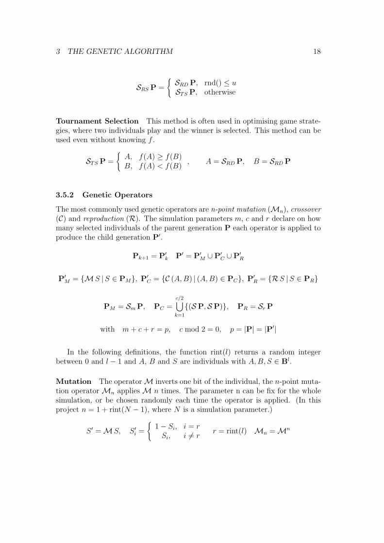
3.5.2 Genetic Operators

The most commonly used genetic operators are n-point mutation (Mn), crossover(C) and reproduction (R). The simulation parameters m, c and r declare on howmany selected individuals of the parent generation P each operator is applied toproduce the child generation P′.

Pk+1 = P′k P′ = P′

M ∪P′C ∪P′

R

P′M = {MS |S ∈ PM}, P′

C = {C (A,B) | (A,B) ∈ PC}, P′R = {RS |S ∈ PR}

PM = Sm P, PC =c/2⋃

k=1

{(S P,S P)}, PR = Sr P

with m + c + r = p, c mod 2 = 0, p = |P| = |P′|

In the following definitions, the function rint(l) returns a random integerbetween 0 and l − 1 and A, B and S are individuals with A,B, S ∈ Bl.

Mutation The operator M inverts one bit of the individual, the n-point muta-tion operator Mn applies M n times. The parameter n can be fix for the wholesimulation, or be chosen randomly each time the operator is applied. (In thisproject n = 1 + rint(N − 1), where N is a simulation parameter.)

S ′ = MS, S ′i ={

1− Si, i = rSi, i 6= r r = rint(l) Mn = Mn

4 BACKPROPAGATION 19

Crossover The operator C exchanges the chromosome strings of two individualsstarting from a random index.

(A′, B′) = C (A,B)

(∀ i < r) (A′i = Ai ∧ B′

i = Bi), (∀ i ≥ r) (A′i = Bi ∧ B′

i = Ai), r = rint(l)

Reproduction The operator R simply reproduces the individual.

S ′ = RS, S′ = S

4 Backpropagation

A very popular learn algorithm for feed forward networks with linear netto inputfunctions and differentiatabel activation functions is the backpropagation algo-rithm.

4.1 The Error Gradient

As in Section 3.4.3, the error function of the training pattern (I(k), O(k)) is onceagain defined as

Ek =12

q∑

i=1(O(k)

i −Oi)2 with O = f(I(k)), f : Rp → Rq

Since the network function f is itself a function of the network parameters Pand P is the set W of the weight vectors Wj of the n neurones, the error functionEk is also a function of W and a gradient can be defined as

∇Ek = ∇Ek(W1,W2, . . . Wn) =(

∂Ek

∂W1,∂Ek

∂W1, . . .

∂Ek

∂Wn

)

∂Ek

∂Wj=

(

∂Ek

∂wj1,

∂Ek

∂wj2, . . .

∂Ek

∂wjpj

)

, pj = dim Wj

The backpropagation algorithm is a gradient descent method and thus, theweights are updated with the negative gradient of the error function.


4.1.1 Online and Batch Learning

The weights can be updated immediately after ∆W is determined for a pattern.This is called online learning.

W(i+1) = W(i) + ∆W(i), ∆W(i) = −γ∇Ek(W(i))

Batch Learning updates the weights with the arithmetic mean of the cor-rections for all t patterns. This can lead to better results with small and veryheterogeneous learn sets.

∆W(i) = −γp

t∑

k=1

∇Ek(W(i))

The constant γ is called learn rate. A high value of γ leads to greater learnsteps at the cost of lower accuracy.

4.1.2 Learning with Impulse

In regions where the error function is very flat, the resulting gradient vector willbe very short and lead to very small learn steps. A solution to this problem is theintroduction of an impulse term which is added to the update ∆W and steadilybecomes greater if the direction of ∆W remains stable.

∆W(i) = −γ∇E(W(i)) + α∆W(i−1), α ∈ [0, 1)

The impulse constant α reflects the “acceleration” a point gets on descendingthe error function. If we assume ∇E as constant, the maximum accelerationfactor a is given by

a =∆W(∞)

∆W(0) =∞∑

i=0αi =

11− α

Fig. 1 shows a training process for the XOR-problem (Section 6.2.2) withα = 0 and α = 0.9.

4.2 Evaluation and Backpropagation

The main feature of backpropagation in comparison with other gradient descentmethods is, that, provided that all netto input functions are linear, the weightupdate ∆Wj of the neurone Nj can be found by using only local information, thusinformation passed through the incoming and outgoing transitions of the neurone.This process consists of the evaluation step, where the error is calculated and the


XOR Problem (Backpropagation)

alpha=0

alpha=0.9

err x 10-3

3gen x 100.00

20.00

40.00

60.00

80.00

100.00

120.00

0.00 1.00 2.00 3.00 4.00

Figure 1: Error Graph for the XOR Problem

backpropagation of the error in the inverse direction form the output back to theinput neurones.

4.2.1 The Network Function

Due to the linearity of the netto input function, the overall network functionf consists merely of additions, scalar multiplications and compositions of theactivation functions. The partial derivations are thus calculated as follows:

∂f1(x) + f2(x)∂x

=∂f1(x)

∂x+

∂f2(x)∂x

,∂k f(x)

∂x= k

∂f(x)∂x

∂f2 (f1(x))∂x

=∂f1(x)

∂x

[

∂f2(y)∂y

]

y=f1(x)

4.2.2 Calculating the Error Gradient

During the evaluation step, not only the value of the activation function g(x)but also the value of its derivation g′(x) is calculated for the netto input x. Ifg = σ1 = σ, the derivation has a very simple form.

σ(x) =1

1 + e−x ,∂σ(x)

∂x=

e−x

(1 + e−x)2 = σ(x)(1− σ(x))


Since Ek depends of the output vector O (calculated by the network functionf) and only indirectly on the weights, ∇Ek can be written as

∇Ek =∂Ek

∂W=

∂Ek

∂O∂O∂W

, O = f(I(k))

and∂Ek

∂Oi=

12

∂∂Oi

q∑

i=1(O(k)

i −Oi)2 = Oi −O(k)i = ∆Oi

To calculate the partial derivation for each element of the weight vector foreach node, the output nodes are set to ∆Oi and ∂O

∂W is calculated by successivelystepping backward in opposite direction of the transition in T and applying theabove listed derivation rules. Composition is handled by multiplying the storedouter derivation g′(x) onto the sum of the inner derivations δj received via the qinverted output transitions.

input δi, δ =∂Ek

∂x= g′(x)

q∑

j=1δj

Then, δ is propagated to the p input nodes by multiplying it with the corre-sponding weight wi. Then the weight is updated.

δ′i = wiδ, output δ′i, ∆wi = Iiδ

4.3 Backpropagation for a 2-Layer Network

As shown in Section 3.2.3, for standard backpropagation neurones (Section 2.4.4)the parameters of a n-m-o-network can be described by two real weight matricesW (1) and W (2) of the dimensions (n + 1) ×m and (m + 1) × o. Let the vectorsI, H and O refer to the states of the input, hidden and output neurones and I(p)

and O(p) to the actual training pattern. The weight updates ∆W (1) and ∆W (2)

without impulse can then be calculated as follows.

∆w(1)ij = −γ Iiδ

(1)j , ∆w(2)

jk = −γ Hjδ(2)k

δ(1)j = Hj(1−Hj)

o∑

k=1

w(2)jk δ(2)

k , δ(2)k = Ok(1−Ok) (Ok −O(p)

k )

5 PARALLELISM 23

5 Parallelism

The genetic as well as the backpropagation algorithm are both inherently paral-lel, in the first case due to the independent calculations of the fitness function, inthe latter, due to the local nature of the error propagation. However, parallelismis provided at totally different levels, which has great impact on possible paral-lel implementations on different architectures, especially on distributed memorysystems.

5.1 Performance Measures

5.1.1 Speedup and Efficiency

Let T0 be the execution time of the serial version of a problem and Tp the executiontime of the parallel version of the same problem to run on p processors. Thespeedup Sp, algorithmic speedup Sp and efficiency Ep are then given by

Sp =T0

Tp, Sp =

T1

TpEp =

Sp

p

Since the parallelisation of a problem normally involves a certain overhead forsynchronisation and/or communication, the efficiency is usually below 100

5.1.2 Amdahl’s Law

If a fraction s of the serial problem is inherently sequential and can not be par-allelised, the highest possible speedup is limited by Amdahl’s law.

Sp ≤T0

T ser + T par

p

=1

s + 1−sp

≤ 1s

with T0 = T ser + T par, T ser = sT0, T par = (1− s)T0

5.2 Parallel Architectures

5.2.1 Shared Memory Systems

A shared memory system consists of a number of processes with small localmemory (cache), with are connected to common (shared) memory modules viaa bus or a system of crossbar switches. All communication between processes ishandled via the shared memory. Synchronisation is needed to avoid simultaneouswriting access and to separate interdependent program parts.

5 PARALLELISM 24

5.2.2 Distributed Memory Systems

A distributed memory system consists of a higher number of independent pro-cessors with sufficiently big local main memory, which are interconnected viahardlinks, a bus or any other interconnection system. All communication must beexplicitly programmed, program data and initial parameters must be distributedand the results must be regathered.

Since the communication is significantly slower than in shared memory sys-tems, the computation/communication ratio of a problem must be sufficientlyhigh to allow an efficient parallel implementation.

5.2.3 Specialised Hardware

Specialised hardware as neural chips reflect the structure and the interdependen-cies of a certain algorithms in their design and thereby minimise any synchronisa-tion and communication overhead. They are therefore able to apply parallelismat very low level as e.g. at the update of a single neurone where the computa-tion/communication ratio is of the order O(1).

5.3 The Parallel Genetic Algorithm

This section describes the distributed memory version of a parallel genetic al-gorithm for the training of neural networks as it has been implemented for atransputer network of 16 T800’s.

5.3.1 Distribution of the Workload

The genetic algorithm consists of two main parts, the evaluation of the fitnessand the fitness based selection and generation of a child population. The fitnessevaluations for each individual are totally independent and can be thus be donein parallel with each processor holding his share of the global population.

The selections and the generation of a child population by genetic operatorsare also independent from each other, but there are three problems to exploitthis parallelism on a distributed memory system:

1. The selection must be based on the fitness data of the whole population.

2. The crossover operator works on individuals selected form the whole pop-ulation.

3. The selection is not necessarily equally distributed between the local pop-ulations on each processor and can unbalance the workload.

5 PARALLELISM 25

It is therefor necessary to collect the individuals with their associated errorsfrom all processors to one master processor, which performs those steps andredistributes the child population again in equal portions. 3

5.3.2 The Computation/Communication Ratio

For a n-m-o network with a training set of t patterns and an encoding in chro-mosome strings of the length l, the computation/communication ratio r is givenby

r =T comp

T comm =O(t((n + 1)m + (m + 1)o))

O(l)=

O(t(n + o)m)O((n + o)m)

= O(t)

The ratio between the (parallel) error calculation and the (serial) selection andgenetic operations is also of order (t). Since t is normally sufficiently high, thisshould allow an efficient parallel implementation. Fig. 2 gives the speedup graphfor the parallel implementation of the encoder/decoder problem (Section 6.2.1).

Speedup Graph (ENC/DEC, pop=1000)

8-3-8 E/D

16-4-16 E/D

32-5-32 E/D

speedup

procs0.00

2.00

4.00

6.00

8.00

10.00

12.00

0.00 5.00 10.00

Figure 2: Speedup for parallel ENC/DEC-problem

To further improve the computation/communication ratio, it is possible toperform the global selection not for every new generation, but only after a certain

3With very low crossover rates, very long chromosome strings and a simple and fast fitnessfunction, a more sophisticated distribution scheme with “communication on demand” mightbring some additional speedup.

5 PARALLELISM 26

number of local selections. This possibility is provided as an option in the parallelimplementation. However, due to the negative impact on global covergence, theuse of this method brings hardly any speedup.

5.3.3 Finding a Topology

The genetic algorithm involves only communications between master and slaves,which should be reflected in an appropriate topology of the transputer network.If each processor can be directly linked to n other processor, then the optimaltopology is an (n−1)-ary tree with the master as root. Since the used T800’s havefour hardlinks, a ternary tree was used. To avoid unnecessary idle times, also themaster works on his own local population. (In the parallel implementation forthis project even the same sourcecode is used for master and slaves.)

5.4 A Combined Algorithm

While, in opposite to backpropagation, the genetic algorithm allows very efficientparallel implementation on distributed memory system, its main disadvantage is,that, due to its stochastic nature, its superior robustness and reliability is oftenoutweighed by its slower convergence and thus longer calculation times, whichoften leaves backpropagation the better choice for squential network training.

These facts suggest the conclusion, that a combined algorithm which exploitsthe parallel nature and robustness of the genetic algorithm without sacrificingthe efficiency of backpropagation might perform better than each algorithm foritself.

5.4.1 Data Conversion

A hybrid genetic backpropagation algorithm will necessarily involve a conversionbetween the chromosome string and the matrix representation of a network asintroduced in Section 3.2.3. This brings up two encoding problems, for which areasonable compromise must be found.

Accuracy While backpropagation normally uses a hardware floating point rep-resentation with a length of 32 or even 64 bit per weight, the genetic algorithmnormally uses a representation just long enough to guarantee a sufficient diver-sity of the population. Thus, too short representations might cause small weightupdates to be ignored, while too long representations will lead to unnecessarylong chromosome string, which slow down the genetic features of the algorithmby increasing communication times.

Range The representations of numbers as grey encodes bitstrings is limited toa certain range. If this range is too small, gradient updates exceeding the limits

5 PARALLELISM 27

would be lost, if it is too large, this unnecessarily increases the searchspace forthe stochastic genetic search.

5.4.2 Genetic Backpropagation

The combined algorithm used in this project works, like the standard geneticalgorithm, on a population of string-encoded networks, but before the fitness iscalculated, the individual is decoded, undergoes a certain number b of backprop-agation steps and is encoded again. Then, the selection is performed and a newpopulation is generated.

Initialising the Population The initial population is not generated by ran-domising the chromosome strings but by randomising weight matrices which arethen encoded as strings. This allows the initial weights to be distributed in asmaller range than the used encoding interval and reduces the probability ofstarting backpropagation in a very flat region of the error function which wouldlead to very small gradients.

Backpropagation Parameters As introduced in Section 4.1, the main pa-rameters of the backpropagation algorithm are the learn rate γ and the impulserate α. Instead of fixing γ and α for all individuals as a simulation parameter,their values can also be optimised by the genetic algorithm by including theminto the chromosome string. The phenotype new P ′

k of the individual k is thendetermined by the phenotype Pk of the network (described by the weight matricesW (1)

k and W (2)k , see Section 3.2.3 for details) and the backpropagation parameters

γk and αk. The new encoding function e′net is the defined as

e′net : R(n+1)m ×R(m+1)o ×R×R → Bl, l = b ((n + 1)m + (m + 1)o + a + g)

e′net(W(1),W (2), γ, α) = enet(W (1),W (2))⊕ greyg φg(γ)⊕ greya φa(α)

The mapping functions φg and φa map the possible values of γ and α onto theinteger intervals {0, . . . 2g−1} and {0, . . . 2a−1}. For the implementation in thisproject, φg was chosen to be logarithmic and φa to be linear over the followingintervals:

φg : [0.02, 20] → Z256, φa : [0, 0.95] → Z256

6 IMPLEMENTATIONS 28

6 Implementations

This section describes the actual implementations of the introduced algorithmsin both, serial and parallel versions, as well as the sample problems they havebeen tested with.

6.1 Program Layout

6.1.1 Hardware

The serial versions of the programs are designed to run under any standard UNIXenvironment and were developed on an Encore Multimax 520 mainframe with 14NS32532 processors. For testing and performance measurements, also severalHewlett Packard Apollo workstations (Series 700 with 32 MB RAM) have beenused.

The target system for the parallel versions was a network of 16 T800 transput-ers, each equipped with floating point unit, 4 MB RAM and 4 free configurableserial hardlinks, using a Sun workstation as host.

6.1.2 Developing Software

All programs are written in ANSI C using only standard UNIX libraries andinclude files except for the parallel versions, which also use the Meiko ComputingSurface Network library CS-Tools with their according header files for transputerspecific functions. The following compilers have been used:

Target System CompilerMultimax GNU project C and C++ Compiler (v2 preliminary)HP Apollo HP-UX C compilerTransputer MEIKO c compiler driver

6.1.3 General Principles

The aim of this project was to explore and test genetic algorithms for the trainingof neural networks on a transputer network as a possible alternative to backpropa-gation. A task like this naturally involves permanent changes an enhancements inthe program as well as the testing of several algorithmic alternatives and wouldnormally result in a series of different program versions, which makes globalchanges and debugging very difficult and direct comparisons between programsoften impossible.

To avoid this problems, all simulation parameters, procedural alternatives andnew features were either added as options to the existing program or linked toit at an object code level, keeping the changes to the original code as minimalas possible. This requires a strict modularity of the code with well defined,


standardised interfaces. The class concept and the inheritance features of anobject oriented programming language like C++ would be perfectly suited tomeet with these requirements, however no C++ compiler was available for thetransputer system, so the modularity had to be reflected on an object code level,using header files for the declaration of global interface variables and procedures.

The definition of the training problems follows the same strategy. Since theproblem size is a variable in many performance measurements, the usage of ex-plicit training files including the definition of a certain network topology andthe corresponding training patterns would lead to many similar definition filesvarying in just one parameter (e.g. the number of input nodes) and new networkoptions might require numerous file updates.

In order to avoid this, all simulation parameters including network definitionsand problem sizes are passed to the programs as command line option and dif-ferent test problems are defined by a small C-file which can interpret its owncommand line options and then define the network topology and the training set.These definition files are linked to the rest of the program without requiring itsrecompilation.

6.2 Sample Problems

All sample problems deal with 2 layer networks of standard backpropagationneurones and use Boolean logic. Since the aim of this project lies mainly inquantitative comparisons, all problems are abstract, well defined and can beadapted for arbitrary problem sizes.

The variables n, m and o refer to the number of input, hidden and outputnodes of an n-m-o-layer network. p is the number of training patterns (I(k), O(k)).The problem parameters are set by upper-case command line options of the corre-sponding programs; if omitted, the standard values given in the right column areassumed. Only the problem specific options are given here; for general genetic,backpropagation, sequential and parallel options, please refer to the correspond-ing sections.

The program names of the sequential backpropagation version have the post-fix -back, the sequential and parallel versions of the genetic and the combinedalgorithm end in -seq and -par.

6.2.1 N-M-N Encoder/Decoder

Source: enc.c problem definition

Programs: encseq sequential genetic implementationencpar parallel genetic implementationencback sequential backpropagation implementation


Options: -Nn number of input and output nodes n = 3-Mm number of hidden nodes m = dldne

An n-m-n encode/decoder reproduces input unit vectors at the output byfinding a a compressed binary intermediate representation in the hidden layer.

p = n, I(k)i = O(k)

i = δjk

The encoder/decoder problem allows big networks to be trained by a relativelysmall training set since the number of training patters is equal to the number ofnodes.

6.2.2 1-Norm of a Vector

Source: cnt.c problem definition

Programs: cntseq sequential genetic implementationcntpar parallel genetic implementationcntback sequential backpropagation implementation

Options: -Nn number of input nodes n = 3-Mm number of hidden nodes m = n-Oo number of output nodes o = dldne

Counts all input nodes set to 1 and produces the number binary encoded atthe output. If the number of output nodes o is set to 1, then 1 will be produced,if an odd number of inputs is set to 1, and 0 will be produced otherwise. The1-norm can thus be seen as a generalisation of the n-parity problem. In thecase of 2 input and 1 output node, this results in the 2-parity or exclusive or(XOR) problem.

p = 2n, I(k) = binnk, I(k) = bino

n∑

i=1I(k)i

with (binbs)j =⌊ s2j−1

⌋

mod 1, j = 1, . . . b

The 1-norm and the n-parity problem have both highly nonlinear error func-tions and are therefor a good test for the robustness of the training algorithm.

6.2.3 2×N Comparator

Source: cmp.c problem definition


Programs: cmpseq sequential genetic implementationcmppar parallel genetic implementationcmpback sequential backpropagation implementation

Options: -NN length of one operand N = 3-Mm number of hidden nodes m = 1 +

⌊

N3

⌋

-Qq test for = if q 6= 0, else test for ≤ q = 0

Compares the binary encoded operands a and b and sets the output nodeaccording to the operator determined by q.

p = 22N , n = 2N, o = 1, I(k) = binnk, ak = k mod 2N , bk =⌊ s2N

⌋

O(k)1 =

{

1, ak ◦OP bk

0, otherwise ◦OP ={

≤, q = 0=, q 6= 0

The 2×N comparator is a relatively simple problem (at least for q = 0) whichvery large (p = 22N) and highly redundant training sets and is therefor a goodtest for online learning (Section 4.1.1) or error estimation (Section 3.4.3).

6.3 Program Modules

According to the modular programming concept, all executables are generatedby linking together separate specialised modules (object files). A module withoutobject file, thus merely containing definitions is called virtual. The following tablelists all modules and shows their hierarchic dependencies. The files problem.cand problem.o refer to the source and object file of the problem definition (e.g. toenc.c and enc.o). For a more detailed description, please refer to the Makefile.


Module File Source UsingDefinitions defs.o defs.c defs.hSequential seq.o seq.c seq.h defs.hParallel par.o par.c par.h defs.h CS-ToolsSimulation sim.o sim.c sim.h defs.hIndividual virtual ind.h defs.hStandard Net stdnet.o stdnet.c

stdnet.hdefs.h ind.h

Problem Def. problem.o problem.c defs.h ind.h stdnet.hGenetic Alg. gen.o gen.c gen.h defs.h ind.h gen.hBackpropagation back.o back.c back.h defs.h ind.hGen. Backprop. genback.o genback.c

genback.hdefs.h ind.h back.h

Main Sequential mainseq.o mainseq.c defs.h ind.h back.hseq.h gen.h genback.h

Main Parallel mainpar.o mainpar.c defs.h ind.h back.hpar.h gen.h genback.h

Main Backprop. mainback.c mainback.c defs.h ind.h back.hsim.h

6.3.1 Parameter Handling and Initialisation

Most modules require an initialisation to allocate arrays, to setup local variablesor hardware, or to process command line options passed to the program. For thispurpose, the following functions and variables are declared in the interface (i.e.the header file):

• char *ModOptStr(); returns a pointer to the option string of the module.

• char *ModUsage(); returns a pointer to the usage message of the module.

• int handleModOpt(char opt,char* arg); returns 0 if the option optwith the argument arg was successfully handled by the module.

• int initMod(); returns 0 if the Module has been successfully initialised.

• char ModParamStr[256]; is set by initMod() and contains a verbal de-scription of the module parameters.

Mod stands for the module names Seq, Par, Sim, Ind, Net (also declared inind.h for network initialisation), Std (declared in stdnet.h and implementedin the problem definition), Gen, Back and Out (defined by the main programsfor output handling). These routines are either called directly form the main


program or by the corresponding routines of the parent module reflecting theobject oriented concept of inheritance.

In the following module descriptions, only variables and functions directlyrelated to the implemented algorithms are mentioned. For auxiliary and systemor hardware specific functions, please refer to the source code.

6.3.2 Module: Definitions

Source: defs.h declarations of standard types and functionsdefc.c implementation

Programs: all

Options: none

Parent: none

This module contains commonly used constants, type declaration and auxil-iary functions for bit manipulation and random numbers.

6.3.3 Module: Sequential

Source: seq.h declarations of sequential featuresseq.c implementation

Programs: encseq sequential genetic ENC/DEC problemcntseq sequential genetic 1-norm problemcmpseq sequential genetic comparator

Options: -pp population size p=100-gNmax maximum number of generations Nmax = 100000-eEmax maximum error for success Emax = 0.01-ssrnd random seed value srnd = time

Parent: none

This module contains all functions, specific to the sequential execution of thegenetic and combined algorithm and is, like the module Simulation a mere place-holder, since no network functions or special initialisations have to be defined.

Variables and Functions

• int PopSize; population size p

• int MaxGen; maximum number Nmax of generations

• errtyp MaxErr; maximum error Emax for success

• int SeedRand; random seed value srnd


• int initSeq; initialises the sequential parameters

• void errorexit(char *msg); prints the error message msg and aborts theprogram

6.3.4 Module: Parallel

Source: defs.h declarations of parallel featuressefc.c implementation

Programs: encseq parallel genetic ENC/DEC problemcntseq parallel genetic 1-norm problemcmpseq parallel genetic comparator

Options: -pp population size p=100-gNmax maximum number of generations Nmax = 100000-eEmax maximum error for success Emax = 0.01-ssrnd random seed value srnd = time-tNtr global selection every Ntr generations Ntr = 1

Parent: none

This module contains all functions specific to the parallel execution of thegenetic and combined algorithm on the transputer network and uses the MeikoCS-Tools library.


• int Procs; number of processors (determined automatically)

• int ProcId; process Id (0 is master)

• int PopGlobal; global population size p

• int PopLocal; local population size ploc

• int MaxGen; maximum number Nmax of generations

• errtyp MaxErr; maximum error Emax for succes


• int Ntrans; global selection every Ntrans generations

• int initPar(); initialises parallel parameters and communication net-work and communicates the random seed values.

• void initNetwork(); network setup


• send and receive functions for network communication

• void errorexit(char *msg); prints the error mesage msg and aborts allprocesses

6.3.5 Module: Simulation

Source: defs.h declarations of sequential backpropagation featuressefc.c implementation

Programs: encback backpropagation ENC/DEC problemcntback backpropagation 1-norm problemcmpback backpropagation comparator

Options: -gNmax maximum number of iterations Nmax = 100000-eEmax maximum error for success Emax = 0.01-ssrnd random seed value srnd = time

Parent: none

This module is the backpropagation equivalent to the module Sequential andis also merely a placeholder.


• int MaxIter; maximum number Nmax of iterations

• errtyp MaxErr; maximum error Emax for success


• int initSim(); initialises parameters

6.3.6 Module: Individual

Source: ind.h declaration of individual and network features

Programs: all

Options: none

Parent: none

This virtual module contains variable and function declaration for the individ-ual definition in the genetic algorithm including network topology and trainingsets, which are also used for backpropagation. The actual implementation areleft to the derived modules. This allows to use the genetic programs for any kindof phenotypes.


The actual implementations for 2-layer neural networks is left to the derivedmodule Standard Net.

Declarations

• int CrBits; length l of one chromosome string in bits

• int Nin, Nhid, Nout; network topology for a 2-layer n-m-o-network

• float **TrainIn, **TrainOut; input and output patters I(k) and O(k)

of the training set T.

• int Ntrain; number of patterns t

• int Nback; number of backpropagation steps b for the combined genetic-backpropagation algorithm

• int NoTrain; number of training patters t′ used for error estimation (Sec-tion 3.4.3)

• float Estimate the initial information ratio rest, which is defined as rest =t′(n+o)

m(n+1)+o(m+1) and used to calculate t′.

• int initInd(); and int initNet(); initialise the individual or the net-work parameters

• errtyp calcerr(ind x); returns the error (i.e. the negative fitness) E(x)of the individual x.

• void printind(ind x); prints a description of the phenotype of x.

6.3.7 Module: Standard Network

Source: stdnet.h declarations for 2-layer n-m-o-networksstdnet.c implementation

Programs: all

Options: -BB number of bits B used for weight encoding B = 8-WW weights in interval [−W,W ] W = 10-Erest error estimation factor rest = 0-bb no. of backprop. steps for combined alg. b = 0

Parent: Individual

This module contains the implementation for 2-layer networks of the functionsdeclared in the module Individual. The actual topology, as well as the trainingset, is, however, determined by the problem definition via the “virtual” functionsinitStd and initTrain.


The individual options -B, -W, -E and -b are recognised by initInd andignored, when only the backpropagation initNet is called.


• int Nbits; number of bits B used for weight encoding

• float Width; range W for weights in interval [−W,W ]

• int initStd(); and void initTrain(); forward declarations for the ac-tual problem definition. The interface variables Nin, Nhid, Nout and Ntrainmust be set according to the problem.

• void initTrain(); forward declarations for the actual problem definition.The arrays TrainIn and TrainOut must be set to the training patters ofthe problem.

• various auxiliary constants, macros and functions for decoding chromosomestrings

6.3.8 Module: Genetic Algorithm

Source: gen.h declaration of the genetic algorithmgen.c implementation

Programs: encseq, cntseq, cmpseq sequential versionsencpar, cntpar, cmppar parallel versions

Options: -mpm percentage of mutations pm = 60%-nNm perform (1, . . . N)-point mutations Nm =

⌊

l50

⌋

+ 1-cpc percentage of reproduction (copies) pc = 0%-uu percentage of uniform selections u = 0%-dd decimation factor d = 0-hH size of internal hashtable H = 0

Parent: none

This modules contains the variables and functions for the genetic algorithm.The chromosome strings (type ind) are arrays of unsigned integers; all geneticoperators work on this representation by directly manipulating the bits.


• int Ncopy, Nmutate, Ncrossover the numbers r, m and c of individualson which to perform reproduction, mutation and crossover (Section 3.5.2)

• int Decimation; initial decimation factor d (Section 3.3.2)


• ind *Pop; array of the chromosome strings Sk of the population P.

• errtyp *Err; array of the errors E(Sk) of all individuals in P

• int initGen(int popsize,int popmem); initialises parameters and gen-erates P0 by randomising strings.

• void randomPop(int popsize); generates popsize random individuals.

• void mutate(ind x0,ind x1); perform n-point mutation on x0 where nis a random number in {1, . . . Nm}. The result is written to x1.

• void crossover(ind x0,ind y0,ind x1,ind y1); performs crossover ofx0 and y0; the results are written to x1 and y1.

• void copy(ind x0,ind x1); copies x0 onto x1.

• void calcerrors(int popsize); calculates the error of all individualsusing calcerr declared in the module Individual.

• void selection(int popsize); generates the next generation, using therank selection mechanism defined in Section 3.5.1.

6.3.9 Module: Backpropagation

Source: back.h declaration of the backpropagation algorithmback.c implementation

Programs: all

Options: -oO use online learning (0/1) O = 1-kγ learn rate γ = 1-aα impulse factor α = 0-ww range of initial weights [−w,w] w=1

Parent: none

This module contains the backpropagation algorithm as described in Sec-tion 4.3.


• float NetErr; residual Error E(W (1), W (2))

• float LearnRate; learn rate γ

• float Impulse; impulse constant α

• float InitWeight; initial weight range w


• float **Wih, **Who; weight matrices W (1) and W (2)

• float **Dih,**Dho; first order updates ∆W (1) and ∆W (2)

• float **DDih,**DDho; second order updates ∆2W (1) and ∆2W (2) (im-pulse term)

• int initBack(); initialise parameters and weights

• void randomNet(float w); randomise weights (interval [−w,w])

• float calcNetErr(); calculates the average network error per pattern(E(W (1),W (2))) and updates weights in case of online learning

• void updateNet(); updates weights in case of batch learning

• void printnet(); prints W (1) and W (2)

6.3.10 Module: Genetic Backpropagation

Source: back.h declarations for the combined algorithmback.c implementation

Programs: encseq, cntseq, cmpseq sequential versionsencpar, cntpar, cmppar parallel versions

Options: none

Parent: none

This module implements special function for the combined genetic backprop-agation algorithm (Section 5.4).


• void randomNetPop(int popsize,float w); randomises a network pop-ulation with initial weights in [−w, w].

• void gen2back(ind x); decoding function d′net

• void back2gen(ind x); encoding function e′net

• void backsteps(ind x,int n); performs n backpropagation steps on theindividual x.


6.3.11 Main Modules

Source: mainseq.c main program for the sequential genetic alg.mainpar.c main program for the parallel genetic alg.mainback.c main program for sequential backpropagation

Programs: encseq, cntseq, cmpseq sequential versions (mainseq.c)encpar, cntpar, cmppar parallel versions (mainpar.c)encback, cntback, cmpback backpropagation (mainback.c)

Options: -lL frequency of log-output automatic-fF log momentarily best network F = 0-iI show parameter info I = 1-rR show calculation statistics R = 1

Parent: none

These modules contain the main-procedures for all executables. They mainlyconsist of a loop which performs the genetic or backpropagation iterations andproduces log-output. The output options are the same for all three modules.

6.4 Example Session: Parallel XOR-Problem

The command

mrun xor.par

with the following configuration file xor.par

par processor 0 for 4 cntpar -N2 -O1 -p200 -b5 -e0.001-f1 -l2 networkis ternarytree endpar

starts a parallel simulation of the XOR-problem (1-norm with -N2 and -O1)on a ternary tree of 4 transputers, using the combined genetic backpropagationalgorithm with a population size of p = 200 (-p200) and 5 backpropagation stepsper generation (-b10). The simulation stops when the average error per patternof the best individual is lower than 0.001 (-e0.001).

Log output is produced every second generation (-l2) and the resulting net-work is printed (-f1):

Simulation Parameters:Network: 2 bit Counter (counts 1s in input) (4 patterns)

Topology 2-2-1, 3 Neurons, 88 bits (Weights 8)Weights in [-10.00, 10.00]5 backpropagation steps per generation

Simulation: Procs = 4, PopSize = 200, MaxGen = 10000, MaxErr = 0.0010

7 PERFORMANCE 41

RandomSeed = 802499780Genetic: Pcopy = 0 %, Pmutate(1..2 pt.) = 60 %, Pcrossover = 40 %

Selection 100 % linear, 0 % uniformBackprop.: Method: Batch, InitWeight = [ -1.000, 1.000]

Gen 1: t= 0, MinErr= 0.1242, AvgErr= 0.1335Gen 2: t= 1, MinErr= 0.1225, AvgErr= 0.1330Gen 4: t= 2, MinErr= 0.1193, AvgErr= 0.1335Gen 6: t= 3, MinErr= 0.1087, AvgErr= 0.1286Gen 8: t= 4, MinErr= 0.0890, AvgErr= 0.1252Gen 10: t= 5, MinErr= 0.0574, AvgErr= 0.1134Gen 12: t= 6, MinErr= 0.0202, AvgErr= 0.1022Gen 14: t= 7, MinErr= 0.0090, AvgErr= 0.0684Gen 16: t= 8, MinErr= 0.0040, AvgErr= 0.0378Gen 18: t= 9, MinErr= 0.0014, AvgErr= 0.0252Gen 20: t= 10, MinErr= 0.0012, AvgErr= 0.0195Gen 21: t= 11, MinErr= 0.0006, AvgErr= 0.0160

Statistic total per sec. time--------------------------------------------------------Generations: 21 1.909091 0.523810 sIndividuals global: 4200 381.818176 0.002619 sIndividuals local: 1050 95.454544 0.010476 sBackprop. steps: 21000 1909.090942 0.000524 sevaluated Patterns: 25200 2290.909180 0.436508 ms

(-8.75, 7.80,b:-3.18)( 3.88,-3.80,b:-1.53)( 9.69, 9.14,b:-5.14)

program succeeded.

7 Performance

This section contains performance measurements of various aspects of the imple-mented algorithms as well as the conclusions for their practical use. Of course,only a small fraction of all test runs can be presented; every example was chosento illustrate a different aspect of the relative performance of the algorithms used,and to highlight the advantages and disadvantages of every method.

7.1 Efficiency of Parallelisation

As shown in Section 5.3.2, the genetic algorithm provides a large scope for dis-tributes memory parallelism (see also Fig. 2).

7 PERFORMANCE 42

The following table gives the speedup Sp and the efficiency Ep as defined inSection 5.1.1 for three different network sizes of the genetic Encoder/Decoderproblem using three different population sizes. The ENC/DEC problem waschosen because the number of training patterns t is equal to the number of inputnodes n, which results in a computation/communication ratio r of order O(n).For all other problems, r is of order O(2n) which would soon lead to efficienciesof nearly 100% and make comparisons difficult for greater network sizes.

The simulations were executed in parallel on 4, 8 and 12 processors (encpar)and the optained performance was compared to the sequential version encseq ona single transputer.

Ep,Sp 8-3-8 ENC/DEC 16-4-16 ENC/DEC 32-5-32 ENC/DECpop. 100 1000 10000 100 1000 10000 100 1000 10000

S4 3.22 3.61 3.56 3.88 3.88 3.83 3.90 3.99 3.934E4 81% 90% 89% 97% 97% 96% 98% 100% 98%S8 2.61 5.91 6.00 5.30 7.05 7.21 6.88 7.76 7.668E8 33% 74% 75% 66% 88% 90% 86% 97% 96%S12 2.72 6.29 7.68 6.12 9.69 9.69 9.75 10.92 11.1312E12 23% 52% 64% 51% 81% 81% 81% 91% 93%

The efficiency increases with the problem size, due to larger training setsan therefore longer error calculations. It also increases with larger populationsizes which reduce the relative impact of the overhead involved for setting upthe connections. Higher numbers of processes reduce efficiency, which can beexplained by Amdahl’s Law (Section 5.1.2) and by the fact, that the overheadfor routing information between the master and the slaves increases with thenumber of transputers in the network. This explains the very high efficiency ofthe 4 transputer networks, because they require no routing at all.

7.2 The XOR-Problem

One of the most common test problems to evaluate the performance of networktraining algorithms is the XOR-problem. To allow algorithmic comparisons, onlythe sequential versions of the genetic (cntseq -N2 -O1) and the backpropagationalgorithm (cntback -N2 -O1) have been used. (Since the training set consistsonly of the 4 patterns ((0, 0), (0)), ((0, 1), (1)), ((1, 0), (1)) and ((1, 1), (0)), aparallel algorithm on a shared memory system would be of rather low efficiency,anyway.)

For the following measurements, the problem was considered to be solved,when the average error per pattern is less than 0.001. A program fails, after100000 backpropagation steps or 10000 generations.

7 PERFORMANCE 43

7.2.1 Backpropagation

Four series of 10 simulations varying in learn method (online or batch) and im-pulse factor (α = 0 or α = 0.9) have been started and produced the followingresults:

γ α method succeeded avg. iterations avg. time1 0 batch 8/10 5188.0 9.0 s1 0.9 batch 9/10 538.7 1.1 s1 0 online 6/10 1294.8 2.2 s1 0.9 online 7/10 138.0 0.3 s

This figures show the limitation of backpropagation or any other gradientdescend method: One quarter of the started simulations failed i.e. got trappedin a local minimum of the error functions. Also, the data illustrates the effects ofthe impulse term with speedups about 900%, the value of the acceleration factora (see Section 4.1.2). Online learning is about 4 times faster than batch learning,but leads to more than the double number of failures.

7.2.2 Genetic Algorithm

Six series of 10 simulations varying in the numbers of bits b used for the encod-ing of the weights have been started. The standard genetic parameters (60%mutation, 40% crossover, population size 100, linear rank selection) have beenused.

p succeeded avg. gen. avg. time4 10/10 20.7 2.5 s6 10/10 62.8 8.6 s8 10/10 51.7 6.7 s

10 10/10 40.4 5.8 s12 10/10 33.0 4.7 s

The most striking difference to backpropagation is, that all programs havesucceeded, which illustrates the robustness of the genetic method, while back-propagation normally converges faster if it converges at all.

The impact of b shows, that a more accurate error function normally leads tobetter convergence, except for very short encodings, where the element of randomsearch might outweigh this effect. Fig. 3 shows the error graph for two simulationswith b = 4 and b = 12.

7 PERFORMANCE 44

XOR Problem (Genetic Algorithm)

b=4 bit

b=12 bit

err x 10-3

gen0.00

20.00

40.00

60.00

80.00

100.00

0.00 5.00 10.00 15.00 20.00 25.00

Figure 3: Error Graph for the XOR Problem

7.3 The 1-Norm Problem

To compare the performance of the backpropagation and the combined algorithmon large and highly nonlinear problems, both algorithms were used to train anetwork for the 1-Norm of a 7-dimensional binary vector to an error of 0.001. 4runs of the sequential versions of both algorithms have been performed.


All 4 programs used online learning at a learn rate of 1. The impulse constants0 and 0.8 were used on two programs each. The simulations were started by thefollowing commands.

cntback -N7 -O1 -e0.001 -f1 -g250000 -o1cntback -N7 -O1 -e0.001 -f1 -g250000 -o1 -a0.8

Both simulations with α = 0.8 failed, while the other two programs succeededafter 55097 and 45974 iterations (11661 s and 9800 s)


The combined algorithm used a population size of 50 with 5 backpropagationsteps per generation and was started by the following command

cntseq -N7 -O1 -e0.001 -f1 -g1000 -p50 -b5

7 PERFORMANCE 45

All 4 programs succeeded after an average of 240 generations and an averagecomputation time of 18797.5 s. The following weight matrices W (1) and W (2)

were found by one of the programs:

W (1) =

10.00 9.06 −6.94 5.29 7.65 −5.22 −5.45 −7.339.61 −7.02 −8.75 −8.12 −7.49 −8.27 9.61 10.008.75 −7.33 −8.35 8.90 −7.25 −9.29 −4.90 9.61

−5.22 −8.98 −7.88 −8.90 −7.33 8.75 9.53 9.847.10 4.75 −7.41 7.57 −6.94 −6.71 −7.02 4.518.35 7.02 −9.29 −8.90 −9.92 −8.51 8.27 6.553.10 −10.00 −4.27 −2.94 −3.57 −3.73 2.86 9.45

W (2) =(

5.22 10.00 8.67 6.16 −6.16 −9.29 −10.00 −2.31)

Since the encoding range of the weights is by default defined as [−10, 10], theoccurrences of 10 and−10 indicate range overflows caused by the backpropagationsteps.

Considering that the parallel version at this problem size (t = 256) would runwith an efficiency of effectively 100%, the combined algorithm would definitelybe the better choice for this problem.

7.4 The Comparator Problem

The comparator problem with the operator ≤ is, in comparison with the n-parityproblem, very linear in the sense that its error function has no significant localminima. This property makes it a perfect choice for all gradient descend meth-ods like backpropagation and will illustrate the performance gains that can beoptained by adding backpropagation features to the standard genetic algorithm.


To get some reference values for comparisons, two series of 10 sequential back-propagation programs (online learning with γ = 1), one of which used learningwith impulse (α = 0.9), were started on single transputers. The test problemwas a 2 × 4-comparator with the operator ≤, the maximal error was 0.001. Allprograms succeeded and produced the following results (x refers to the arithmeticmen, ∆x to average deviation from x and x to the geometric mean of the samplesxi):

impulse iterations time

α N ∆N N T ∆T T0 55.9 9.0 55.3 10.2 s 1.8 s 10.1 s

0.9 235.4 318.0 138.1 53.9 s 72.6 s 31.6 s

7 PERFORMANCE 46


Six series of 10 programs have been started, the first using the standard geneticalgorithm with a population size p of 256, the other five using b = 1, 2, 4, 8 and16 backpropagation steps per generation with proportional reduced populationsizes of 256, 128, 64, 32 and 16. All simulations were run in their parallel versionson a 16 transputer ternary tree using the following configuration file:

parprocessor 0 for 16 cmppar -N4 -B12 -e0.001 -g100 -pp -bbnetworkis ternarytreeendpar

While all 10 programs with the standard genetic algorithm (b = 0) failed totrain the network to the goal of E ≤ 0.001 within 100 generations, all programsusing the combined algorithm succeeded.

backprop. steps pop. size generations time

b p N ∆N N T ∆T T1 256 19.9 5.4 19.3 143.3 s 38.9 s 138.9 s2 128 11.5 3.5 11.1 63.0 s 19.6 s 60.7 s4 64 4.9 1.0 4.8 22.6 s 4.3 s 22.2 s8 32 2.9 0.6 2.8 12.3 s 2.6 s 12.0 s16 16 2.0 0.0 2.0 8.1 s 0.3 s 8.1 s

Fig. 4 shows the average computation time T in relation to the number ofbackpropagation steps in the combined algorithm. The two horizontal lines indi-cate the average times of the serial backpropagation programs.

While for sequential implementations, the standard backpropagation algo-rithm would certainly be the better choice for this very problem, the exampleshows that a parallel implementation of the combined algorithm with a suffi-ciently high number of backpropagation steps can nevertheless lead to faster exe-cution times even if, as in this case, due to the high linearity of its error function,the problem is perfectly suited for a simple gradient descend method.

7.5 Conclusion

The given examples are only a small but representative selection of all test runsand measurements performed for this project, and illustrate the advantages anddisadvantages of genetic methods for the training of neuronal networks. Theoreticanalysis and the optained practical results suggest the following conclusions:

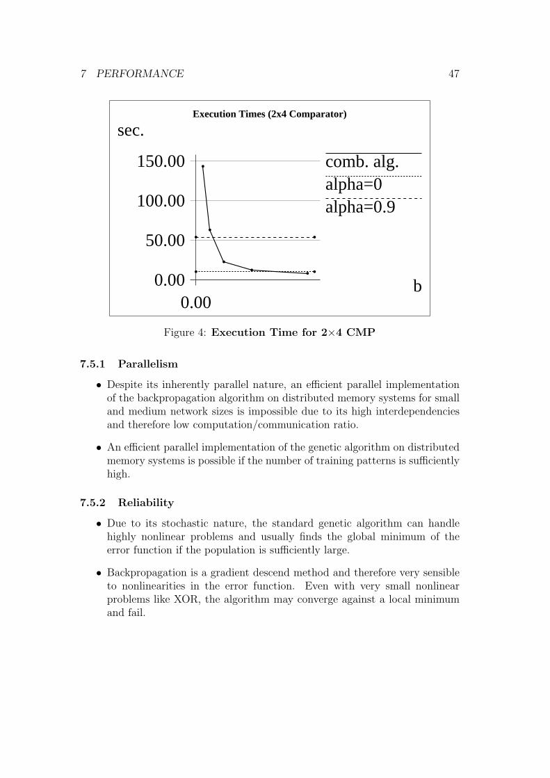
7 PERFORMANCE 47

Execution Times (2x4 Comparator)

comb. alg.alpha=0alpha=0.9

sec.

b0.00

50.00

100.00

150.00

0.00

Figure 4: Execution Time for 2×4 CMP

7.5.1 Parallelism

• Despite its inherently parallel nature, an efficient parallel implementationof the backpropagation algorithm on distributed memory systems for smalland medium network sizes is impossible due to its high interdependenciesand therefore low computation/communication ratio.

• An efficient parallel implementation of the genetic algorithm on distributedmemory systems is possible if the number of training patterns is sufficientlyhigh.

7.5.2 Reliability

• Due to its stochastic nature, the standard genetic algorithm can handlehighly nonlinear problems and usually finds the global minimum of theerror function if the population is sufficiently large.

• Backpropagation is a gradient descend method and therefore very sensibleto nonlinearities in the error function. Even with very small nonlinearproblems like XOR, the algorithm may converge against a local minimumand fail.

REFERENCES 48

7.5.3 Convergence Speed

• The necessary population size and number of generations for the standardgenetic algorithm dramatically increase with the problem size and renderthe method impracticable for bigger networks.

• Provided that the problem is sufficiently linear, the backpropagation algo-rithm normally converges reasonably fast. However, the actual speed de-pends very much on the simulation parameters γ and α and on the initialweight values.


• Unlike standard backpropagation, the combined genetic backpropagationalgorithm is relatively robust against nonlinearities, can dynamically adaptlearn and impulse rates and can efficiently be parallelised on distributedmemory systems.

• Unlike the standard genetic algorithm, the required population sizes andthe number of necessary generations are smaller, which allows the use ofthe combined algorithm for bigger networks and larger training sets.

References

[Rojas] Raul Rojas. 1993 Theorie der Neuralen Netze [Theory of Neural Nets]

[Gold] David E. Goldberg. 1989 Genetic Algorithms in Search, Optimization,and Machine Learning

[Davis] Lawrence Davis. 1991 Handbook of Genetic Algorithms

A MAKEFILE 49

A Makefile12 ## Transputers (Bowes)3 CC = mcc4 CCOPT = -c -O5 LNKOPT = -O -lm -lcs -lcsn6 STDLNKOPT = -O7 all: seq par back89 ## Multimax (Newton)10 #CC = gcc11 #CCOPT = -c -pedantic12 #LNKOPT = -lm13 #STDLNKOPT = -r -nostdlib14 #all: seq back1516 seq: encseq cntseq cmpseq1718 par: encpar cntpar cmppar1920 back: encback cntback cmpback2122 # executables2324 STDPAR = mainpar.o par.o gen.o back.o genback.o stdnet.o defs.o25 STDSEQ = mainseq.o seq.o gen.o back.o genback.o stdnet.o defs.o26 STDBACK = mainback.o sim.o back.o genback.o stdnet.o defs.o2728 stdpar.o: mainpar.o par.o gen.o back.o genback.o stdnet.o defs.o2930 stdseq.o: mainseq.o seq.o gen.o back.o genback.o stdnet.o defs.o3132 stdback.o: mainback.o sim.o back.o genback.o stdnet.o defs.o3334 encpar: enc.o stdpar.o35 $(CC) $(STDPAR) enc.o -o encpar $(LNKOPT)3637 encseq: enc.o stdseq.o38 $(CC) $(STDSEQ) enc.o -o encseq $(LNKOPT)3940 encback: enc.o stdback.o41 $(CC) $(STDBACK) enc.o -o encback $(LNKOPT)4243 cntpar: cnt.o stdpar.o44 $(CC) $(STDPAR) cnt.o -o cntpar $(LNKOPT)4546 cntseq: cnt.o stdseq.o47 $(CC) $(STDSEQ) cnt.o -o cntseq $(LNKOPT)4849 cntback: cnt.o stdback.o

A MAKEFILE 50

50 $(CC) $(STDBACK) cnt.o -o cntback $(LNKOPT)5152 cmppar: cmp.o stdpar.o53 $(CC) $(STDPAR) cmp.o -o cmppar $(LNKOPT)5455 cmpseq: cmp.o stdseq.o56 $(CC) $(STDSEQ) cmp.o -o cmpseq $(LNKOPT)5758 cmpback: cmp.o stdback.o59 $(CC) $(STDBACK) cmp.o -o cmpback $(LNKOPT)6061 # object files6263 mainpar.o: mainpar.c gen.h back.h genback.h par.h ind.h defs.h64 $(CC) mainpar.c -o mainpar.o $(CCOPT)6566 mainseq.o: mainseq.c gen.h back.h genback.h seq.h ind.h defs.h67 $(CC) mainseq.c -o mainseq.o $(CCOPT)6869 mainback.o: mainback.c back.h ind.h defs.h70 $(CC) mainback.c -o mainback.o $(CCOPT)7172 enc.o: enc.c stdnet.h ind.h defs.h73 $(CC) enc.c -o enc.o $(CCOPT)7475 cnt.o: cnt.c stdnet.h ind.h defs.h76 $(CC) cnt.c -o cnt.o $(CCOPT)7778 cmp.o: cmp.c stdnet.h ind.h defs.h79 $(CC) cmp.c -o cmp.o $(CCOPT)8081 gen.o: gen.c gen.h ind.h defs.h82 $(CC) gen.c -o gen.o $(CCOPT)8384 par.o: par.c par.h defs.h85 $(CC) par.c -o par.o $(CCOPT)8687 seq.o: seq.c seq.h defs.h88 $(CC) seq.c -o seq.o $(CCOPT)8990 sim.o: sim.c sim.h defs.h91 $(CC) sim.c -o sim.o $(CCOPT)9293 back.o: back.c back.h ind.h defs.h94 $(CC) back.c -o back.o $(CCOPT)9596 defs.o: defs.c defs.h97 $(CC) defs.c -o defs.o $(CCOPT)9899 stdnet.o: stdnet.c stdnet.h defs.h ind.h

100 $(CC) stdnet.c -o stdnet.o $(CCOPT)

B SOURCE CODE 51

101102 genback.o: genback.c genback.h back.h ind.h defs.h103 $(CC) genback.c -o genback.o $(CCOPT)104105 clear:106 rm -f *.o107 rm -f encpar encseq encback108 rm -f cntpar cntseq cntback109 rm -f cmppar cmpseq cmpback110

B Source Code

B.1 Problem Definitions

B.1.1 File: enc.c

12 /* Implementaion of the Encode/Decoder-Problem */34 #include "defs.h"5 #include "ind.h"6 #include "stdnet.h"78 /* Parameter Handling */910 #define DEFNIN AUTO11 #define DEFNHID AUTO1213 #define MAXIN 0x7fff14 #define MAXHID 151516 char *StdOptStr() {return "N:M:\0";}1718 char *StdUsage() {return19 "Network (N-M-N-ENC/DEC) Parameters:\n"20 "-N <no. of inputs/outputs>: 4\n"21 "-M <no. of hidden units>: auto (>= ld M)\n\0";}2223 /* set default values */2425 int Nin = DEFNIN; /* no. of inputs */26 int Nhid = DEFNHID; /* no. of hidden units */2728 int handleStdOpt(char opt,char* arg)29 {30 switch(opt)31 {32 case ’N’: return (Nin =getint(arg,1,MAXIN))<0;33 case ’M’: return (Nhid =getint(arg,1,MAXHID))<0;

B SOURCE CODE 52

34 default: return 1;35 };36 }3738 int initStd()39 {40 if(Nin==AUTO) Nin=4;41 Nout=Nin;42 if(Nhid==AUTO) Nhid=duallog(Nin);43 if(Nhid<duallog(Nin)) return 1;44 Ntrain=Nin;45 sprintf(StdName,"%d-%d-%d ENC/DEC",Nin,Nhid,Nout);46 return 0;47 }4849 void initTrain()50 {51 int p,i;5253 for(p=0;p<Ntrain;p++)54 for(i=0;i<Nin;i++)55 TrainIn[p][i]=TrainOut[p][i]= p==i ? 1.0 : 0.0;56 }

B.1.2 File: cnt.c

12 /* Implementation of 1-norm of a binary vector */3 /* out[]=sum(i,in[i]) mod 2^O */45 #include "defs.h"6 #include "ind.h"7 #include "stdnet.h"89 /* Parameter Handling */

1011 #define DEFNIN 312 #define DEFNHID AUTO13 #define DEFNOUT AUTO1415 #define MAXIN 3116 #define MAXHID 25517 #define MAXOUT 51819 char *StdOptStr() {return "N:M:O:\0";}2021 char *StdUsage() {return22 "Network (Counter):\n"23 "-N <no. of input units>: 3\n"24 "-M <no. of hidden units>: auto (M)\n"25 "-O <no. of output units>: auto (>= ld M)\n\0";}

B SOURCE CODE 53

2627 int Nin=DEFNIN;28 int Nhid=DEFNHID;29 int Nout=DEFNOUT;3031 const int grey2dec[16]={0,1,3,2,7,6,4,5,15,14,12,13,8,9,11,10};3233 int handleStdOpt(char opt,char* arg)34 {35 switch(opt)36 {37 case ’N’: return (Nin =getint(arg,1,MAXIN))<0;38 case ’M’: return (Nhid =getint(arg,1,MAXHID))<0;39 case ’O’: return (Nout =getint(arg,1,MAXOUT))<0;40 };41 return 1;42 }4344 int initStd()45 {46 if(Nhid==AUTO) Nhid=Nin;47 if(Nout==AUTO) Nout=duallog(Nin+1);48 Ntrain=1<<Nin;49 sprintf(StdName,"%d bit Counter (counts 1s in input)",Nin);50 return 0;51 }5253 void initTrain()54 {55 int p,z,i;5657 for(p=0;p<Ntrain;p++)58 {59 z=0;60 for(i=0;i<Nin;i++)61 z+=TrainIn[p][i]=(float) ((p>>i) & 1);62 for(i=0;i<Nout;i++)63 TrainOut[p][i]=(float) ((z>>i) & 1);64 };65 }66

B.1.3 File: cmp.c

12 /* Implementation of 2*N-bit Comperator */34 #include "defs.h"5 #include "ind.h"6 #include "stdnet.h"7

B SOURCE CODE 54

8 /* Parameter Handling */9

10 #define DEFNIN 311 #define DEFNHID AUTO1213 #define MAXIN 814 #define MAXHID 2551516 char *StdOptStr() {return "N:M:\0";}1718 char *StdUsage() {return19 "Network (2xN Comperator) Parameters:\n"20 "-N <no. of input units>: 3\n"21 "-M <no. of hidden units>: auto (M)\n"22 "-Q <train for = instead of =< ?> 0\n\0";}2324 int Nin=DEFNIN;25 int Nhid=DEFNHID;26 int Equality=0;2728 const int grey2dec[16]={0,1,3,2,7,6,4,5,15,14,12,13,8,9,11,10};29 const char EqualityStr[2][40]={"less or equal","equal"};30 const int stdNhid[17]={0,0,2,0,2,0,3,0,3,0,3,0,4,0,4,0,4};3132 int handleStdOpt(char opt,char* arg)33 {34 switch(opt)35 {36 case ’N’: return (Nin =getint(arg,1,MAXIN))<0;37 case ’M’: return (Nhid =getint(arg,1,MAXHID))<0;38 case ’Q’: return (Equality =getint(arg,0,1))<0;39 };40 return 1;41 }4243 int initStd()44 {45 Nin*=2;46 if(Nhid==AUTO) Nhid=stdNhid[Nin];47 Nout=1;48 Ntrain=1<<Nin;49 sprintf(StdName,"2x%d bit Comperator (%s)",50 Nin/2,EqualityStr[Equality]);51 return 0;52 }5354 void initTrain()55 {56 int p,i;57 unsigned l,a,b,m;58

B SOURCE CODE 55

59 l=Nin/2; m=(1<<l)-1;60 for(p=0;p<Ntrain;p++)61 {62 a=p&m; b=(p>>l)&m;63 for(i=0;i<Nin;i++)64 TrainIn[p][i]=(float) ((p>>i) & 1);65 TrainOut[p][0]=(float)( Equality ? (a==b) : (a<=b) );66 };67 }68

B.2 Module: Definitions

B.2.1 File: defs.h

12 /* Common Definitions */34 #ifndef DEFS_H5 #define DEFS_H 167 /* data types */89 #define errtyp float

10 #define byte unsigned char11 #define word unsigned int12 #define ind word*13 #define state int1415 /* data lengths */1617 #define INTLEN sizeof(int)18 #define ERRLEN sizeof(int)19 #define WORDLEN sizeof(unsigned int)20 #define INDLEN sizeof(ind)21 #define FLOATLEN sizeof(float)22 #define PNTLEN sizeof(void*)2324 /* maximum values */2526 #define MAXERROR 0x7fffffff27 #define MAXRANDOM 0x7fffffff2829 /* macros */3031 #define bitoffs(n) ((n) & 31)32 #define wordoffs(n) ((n) >> 5)33 #define getbit(x,i) ((x[wordoffs(i)]>>bitoffs(i))&1)34 #define min(x,y) ((x)<(y) ? (x) : (y))35 #define max(x,y) ((x)>(y) ? (x) : (y))36 #define getrand() random()

B SOURCE CODE 56

37 #define seedrand(s) srandom(s)38 #define gettime() time(0)3940 /* flags */4142 #define AUTO (-1)43 #define FAUTO (-65536.0*65536.0)44 #define NOENTRY (-1)45 #define UNDEF (-1)4647 /* procedures */4849 word getbits(ind x,int i,int n);50 word putbits(word w,ind x,int i,int n);51 int duallog(int n);52 int getint(char *s,int min,int max);53 int getfloat(float *y,char *s,float min,float max);54 int rounddec(int x);5556 #endif57

B.2.2 File: defs.c

12 /* Common Procedures */34 #include "defs.h"5 #include "par.h"67 /* isolate bitstring */89 word getbits(ind x,int i,int n)10 {11 byte *p;12 word *q;13 int j,k;14 word m;1516 j=bitoffs(i);17 k=wordoffs(i);18 m=(1 << n)-1;19 if(j<bitoffs(i+n))20 return (x[k] >> j) & m;21 else22 return ((x[k] >> j) | (x[k+1] << (32-j))) & m;23 }2425 word putbits(word w,ind x,int i,int n)26 {27 byte *p;

B SOURCE CODE 57

28 word *q;29 int j,k;30 word m;3132 j=bitoffs(i);33 k=wordoffs(i);34 m=((1 << n)-1);35 x[k]&= ~(m << j); x[k]|=(w << j);36 if(j>=bitoffs(i+n))37 {38 x[k+1]&= ~(m >> (32-j));39 x[k+1]|= (w >> (32-j));40 };41 }4243 /* dual logarithm, rounded up */4445 int duallog(int n)46 {47 int l;4849 for(l=0;(1<<l)<n;l++);50 return l;51 }5253 int getfloat(float *y,char *s,float min,float max)54 {55 float x;5657 if(!s) return 1;58 switch(s[0])59 {60 case 0: return 1;61 default: sscanf(s,"%f",&x);62 };63 if(x<min || x>max) return 1;64 *y=x;65 return 0;66 }6768 int getint(char *s,int min,int max)69 {70 int n;7172 if(!s) return -1;73 switch(s[0])74 {75 case ’+’: n=1; break;76 case ’-’: n=0; break;77 case 0: n=1; break;78 default: n=atoi(s);

B SOURCE CODE 58

79 };80 if(n<min || n>max) return(-1);81 return n;82 }8384 int rounddec(int x)85 {86 if(x<=1) return 1;87 if(x<=3) return 2;88 if(x<=7) return 5;89 return 10*rounddec((x+5)/10);90 }

B.3 Module: Sequential

B.3.1 File: seq.h

12 /* Declaration of Sequential Features */34 #ifndef SEQ_H5 #define SEQ_H 167 #include "defs.h"89 char *SeqOptStr();

10 char *SeqUsage();11 char SeqParamStr[256];1213 int PopSize; /* size of actual population */1415 int MaxGen; /* Maximum no. of generations */16 errtyp MaxErr; /* Maximum error for succes */1718 int SeedRand; /* random seed */1920 int handleSeqOpt(char opt,char* arg);21 int initSeq();2223 void errorexit(char *msg);2425 #endif

B.3.2 File: seq.c

12 /* Implementation of sequential features */34 #include "defs.h"5 #include "seq.h"6

B SOURCE CODE 59

7 /* Parameter Handling */89 #define DEFPOPSIZE 10010 #define DEFMAXGEN 1000011 #define DEFMAXERR 0.0112 #define DEFSEED AUTO1314 char *SeqOptStr() {return "p:g:e:s:\0";}1516 char *SeqUsage() {return17 "Simulation Parameters:\n"18 "-p <population size>: 100\n"19 "-g <max. no. of generations>: 10000\n"20 "-e <max. error for succes>: 0.01\n"21 "-s <random seed value>: time\n\0";}2223 /* set default values */2425 int PopSize =DEFPOPSIZE; /* size of actual population */26 int MaxGen =DEFMAXGEN; /* Maximum no. of generations */27 errtyp MaxErr =DEFMAXERR; /* Maximum error for succes */28 int SeedRand =DEFSEED; /* random seed */2930 int handleSeqOpt(char opt,char* arg)31 {32 switch(opt)33 {34 case ’p’: return (PopSize =getint(arg,2,1000000))<0;35 case ’g’: return (MaxGen =getint(arg,1,1000000000))<0;36 case ’e’: return getfloat(&MaxErr,arg,0,1000000);37 case ’s’: return (SeedRand =getint(arg,0,MAXRANDOM))<0;38 default: return 1;39 };40 }4142 void errorexit(char *msg)43 {44 printf(msg);45 exit(1);46 }4748 int initSeq()49 {50 if(SeedRand==AUTO) SeedRand=gettime();51 seedrand(SeedRand);5253 sprintf(SeqParamStr,54 "Simulation: serial, PopSize = %d, MaxGen = %d, "55 "MaxErr = %7.4f\n RandomSeed = %d\n",56 PopSize,MaxGen,MaxErr,SeedRand);57 return 0;

B SOURCE CODE 60

58 }

B.4 Module: Parallel

B.4.1 File: par.h

12 /* Declaration of Parallel Features */34 #ifndef PAR_H5 #define PAR_H 167 #include "defs.h"89 #define MAXPROCS 16

1011 char *ParOptStr();12 char *ParUsage();13 char ParParamStr[256];1415 int Procs; /* no. of processes */16 int ProcId; /* process Id */17 int LocalId; /* Local Id */1819 int PopGlobal; /* size of global population */20 int PopLocal; /* size of local population */2122 int MaxGen; /* Maximum no. of generations */23 errtyp MaxErr; /* Maximum error for succes */2425 int SeedRand; /* random seed */26 int Ntrans; /* frequency of data transfer */2728 void initNetwork();29 int handleParOpt(char opt,char* arg);30 int initPar();3132 void errorexit(char *msg);33 void send(int proc,void *p,int len);34 void recv(void *p,int len);35 int recvfrom(void *p,int len);36 void setvect(int n,void *p,int len);37 void sendvect(int proc,int n);38 void recvvect(int n);39 int recvvectfrom(int n);4041 #endif

B.4.2 File: par.c

1

B SOURCE CODE 61

2 /* Implementation of parallel features */34 #include <csn/csn.h>5 #include <csn/names.h>6 #include <csn/csnuio.h>78 #include "defs.h"9 #include "par.h"

1011 /* Parameter Handling */1213 #define DEFPOPSIZE 10014 #define DEFMAXGEN 1000015 #define DEFMAXERR 0.0116 #define DEFSEED AUTO17 #define DEFTRANS 11819 char *ParOptStr() {return "p:g:e:s:t:\0";}2021 char *ParUsage() {return22 "Simulation Parameters:\n"23 "-p <population size>: 100\n"24 "-g <max. no. of generations>: 10000\n"25 "-e <max. error for succes>: 0.01\n"26 "-s <random seed value>: time\n"27 "-t <frequency of data transfers> 1\n\0";}2829 /* set default values */3031 int PopGlobal =DEFPOPSIZE; /* size of actual population */32 int MaxGen =DEFMAXGEN; /* Maximum no. of generations */33 errtyp MaxErr =DEFMAXERR; /* Maximum error for succes */34 int SeedRand =DEFSEED; /* random seed */35 int Ntrans =DEFTRANS; /* frequency of data transfers */3637 /* Network variables */3839 Transport Tr;40 netid_t NetId[MAXPROCS];41 char Name[MAXPROCS][2];42 struct iovec Vector[CSN_MAX_IOVCNT];4344 int handleParOpt(char opt,char* arg)45 {46 switch(opt)47 {48 case ’p’: return (PopGlobal =getint(arg,2,1000000))<0;49 case ’g’: return (MaxGen =getint(arg,1,1000000000))<0;50 case ’e’: return getfloat(&MaxErr,arg,0,1000000);51 case ’s’: return (SeedRand =getint(arg,0,MAXRANDOM))<0;52 case ’t’: return (Ntrans =getint(arg,1,10000))<0;

B SOURCE CODE 62

53 default: return 1;54 };55 }5657 void errorexit(char *msg)58 {59 cs_abort(msg,-1);60 }6162 void send(int proc,void *p,int len)63 {64 if(csn_tx(Tr,0,NetId[proc],(char*)p,len)!=len)65 errorexit("send error\n");66 }6768 void recv(void *p,int len)69 {70 netid_t from;7172 if(csn_rx(Tr,&from,(char*)p,len)!=len)73 errorexit("receive error\n");74 }7576 int recvfrom(void *p,int len)77 {78 netid_t from;79 int i;8081 if(csn_rx(Tr,&from,(char*)p,len)!=len)82 errorexit("receive error\n");83 for(i=0;i<Procs;i++)84 if(i!=ProcId && NetId[i]==from) return i;85 errorexit("sender not found\n");86 return -1;87 }8889 void setvect(int n,void *p,int len)90 {91 if(n>=CSN_MAX_IOVCNT)92 errorexit("too many vectors\n");93 Vector[n].iov_base=(caddr_t)p;94 Vector[n].iov_len=len;95 }9697 void sendvect(int proc,int n)98 {99 csn_txv(Tr,0,NetId[proc],Vector,n);

100 }101102 void recvvect(int n)103 {

B SOURCE CODE 63

104 netid_t from;105106 csn_rxv(Tr,&from,Vector,n);107 }108109 int recvvectfrom(int n)110 {111 netid_t from;112 int i;113114 csn_rxv(Tr,&from,Vector,n);115 for(i=0;i<Procs;i++)116 if(i!=ProcId && NetId[i]==from) return i;117 errorexit("sender not found\n");118 return -1;119 }120121 void initNetwork()122 {123 csn_init();124 cs_getinfo(&Procs,&ProcId,&LocalId);125 }126127 int initPar()128 {129 int i,k,n,h;130 word *p;131 ind* pop;132133 if(csn_open(-1,&Tr)!=CSN_OK)134 errorexit("Can’t open transport.\n");135 for(i=0;i<Procs;i++)136 {137 Name[i][0]=’A’+i;138 Name[i][1]=0;139 };140 if(csn_registername(Tr,Name[ProcId])!=CSN_OK)141 errorexit("Can’t register name\n");142 for(i=0;i<Procs;i++)143 {144 if(i==ProcId)145 NetId[i]=CSN_NULL_ID;146 else147 if(csn_lookupname(&NetId[i],Name[i],1)!=CSN_OK)148 errorexit("Can’t find process name\n");149 };150 PopLocal=(PopGlobal-1)/Procs+1;151 PopGlobal=PopLocal*Procs;152 if(ProcId==0)153 {154 if(SeedRand==AUTO) SeedRand=gettime();

B SOURCE CODE 64

155 for(i=1;i<Procs;i++)156 send(i,&SeedRand,WORDLEN);157 } else {158 recv(&SeedRand,WORDLEN);159 SeedRand+=ProcId;160 };161 seedrand(SeedRand);162163 MaxGen=((MaxGen-1)/Ntrans+1)*Ntrans;164165 sprintf(ParParamStr,166 "Simulation: Procs = %d, PopSize = %d, MaxGen = %d, "167 "MaxErr = %7.4f\n RandomSeed = %d\n",168 Procs,PopGlobal,MaxGen,MaxErr,SeedRand);169 return 0;170 }

B.5 Module: Simulation

B.5.1 File: sim.h

1 /* Declarations of simulation features (backpropagation) */23 #ifndef SIM_H4 #define SIM_H 156 #include "defs.h"78 char *SimOptStr();9 char *SimUsage();

10 char SimParamStr[256];1112 float MaxErr; /* Maximum error for succes */13 int MaxIter; /* Maximum no. of iterations */14 int SeedRand; /* random seed */1516 int handleSimOpt(char opt,char* arg);17 int initSim();1819 #endif

B.5.2 File: sim.c

1 /* Declarations of simulation features (backpropagation) */23 #include "defs.h"4 #include "sim.h"56 /* Parameter Handling */78 #define DEFMAXITER 100000

B SOURCE CODE 65

9 #define DEFMAXERR 0.0110 #define DEFSEED AUTO1112 char *SimOptStr() {return "g:e:s:\0";}1314 char *SimUsage() {return15 "Simulation Parameters:\n"16 "-g <max. no. of iterations:>: 10000\n"17 "-e <max. error for succes>: 0.01\n"18 "-s <random seed value>: time\n\0";19 }2021 /* set default values */2223 int MaxIter =DEFMAXITER; /* Maximum no. of generations */24 float MaxErr =DEFMAXERR; /* Maximum error for succes */25 int SeedRand =DEFSEED; /* random seed */2627 int handleSimOpt(char opt,char* arg)28 {29 switch(opt)30 {31 case ’g’: return (MaxIter =getint(arg,1,1000000000))<0;32 case ’e’: return getfloat(&MaxErr,arg,0,1000000);33 case ’s’: return (SeedRand =getint(arg,0,MAXRANDOM))<0;34 default: return 1;35 };36 }3738 int initSim()39 {40 if(SeedRand==AUTO) SeedRand=gettime();41 seedrand(SeedRand);4243 sprintf(SimParamStr,44 "Simulation: MaxIter = %d, MaxErr = %7.4f, Seed = %d\n",45 MaxIter,MaxErr,SeedRand);46 return 0;47 }48

B.6 Module: Individual

B.6.1 File: ind.h

12 /* Declarations of individual-specific functions */34 #ifndef IND_H5 #define IND_H 16

B SOURCE CODE 66

7 #include "defs.h"89 int ptrain;1011 /* Genetic */1213 char *IndOptStr();14 char *IndUsage();15 char IndParamStr[256];1617 int CrBits; /* length of one chromosome in bits */18 int CrBytes; /* length of one chromosome in bytes */19 int CrWords; /* length of one chromosome in words */2021 int OffsTrain; /* Offset of error estimate */22 int NoTrain; /* No. of patterns of err. estim. */23 float Estimate; /* initial information ratio */2425 int handleIndOpt(char opt,char* arg);26 int initInd();2728 int GenCalcs;2930 errtyp calcerr(ind x);31 void printind(ind x);3233 /* Backpropagation */3435 char *NetOptStr();36 char *NetUsage();37 char NetParamStr[256];3839 int Nin; /* no. of inputs */40 int Nhid; /* no. of hidden units */41 int Nout; /* no. of outputs */4243 float **TrainIn; /* Training Set Input */44 float **TrainOut; /* Training Set Output */45 int Ntrain; /* no. of patterns */4647 int Nback; /* no. of backprop. steps for combined moethod */4849 int BackCalcs;5051 int handleNetOpt(char opt,char* arg);52 int initNet();5354 #endif

B SOURCE CODE 67

B.7 Module: Standard Network

B.7.1 File: stdnet.h

12 /* Declarations for standard 2 layer networks */34 #ifndef STDNET_H5 #define STDNET_H67 #include "defs.h"89 char *StdOptStr();

10 char *StdUsage();11 char StdName[80];1213 /* These and Nin,Nhid,Nout,Ntrain are to be defined */14 /* in initStd() */1516 int Nbits; /* bits for bias and weights (gen.alg.) */17 float Width; /* weights in [-Width,Width] */1819 int handleStdOpt(char opt,char* arg);20 int initStd();21 void initTrain();2223 /* Standard Decoding */2425 int OffW1,OffW2,IncW1,IncW2,OffLR,OffIM;26 float FGmult,FGadd;27 int FGmax;2829 float *grey2float;30 float *grey2lrate;31 float *grey2imp;32 word *int2grey;3334 int initDecoding();3536 #define Nlrate 837 #define Nimp 838 #define Llrate 0.0239 #define Hlrate 20.040 #define Limp 0.041 #define Himp 0.954243 #define decode(x,i,n) grey2float[getbits(x,i,n)]44 #define weight1(x,i,h) decode(x,IncW1*h+Nbits*i,Nbits)45 #define weight2(x,h,o) decode(x,OffW2+IncW2*o+Nbits*h,Nbits)46 #define bias1(x,h) weight1(x,Nin,h)47 #define bias2(x,o) weight2(x,Nhid,o)48 #define lrate(x) grey2lrate[getbits(x,OffLR,Nlrate)]

B SOURCE CODE 68

49 #define imp(x) grey2imp[getbits(x,OffIM,Nimp)]50 #define float2int(x) ((int)(x*FGmult+FGadd))5152 #define sigma(y) 1/(1+exp(-(y)))5354 #endif55

B.7.2 File: stdnet.c

12 /* Implementation of standard 2 layer networks */34 #include <math.h>56 #include "defs.h"7 #include "ind.h"8 #include "stdnet.h"9 #include "genback.h"

1011 char IndStdOptStr[40]="B:W:E:b:\0";12 char NetStdOptStr[40]="\0";1314 int Nbits =8;15 float Width =10.0;16 float Estimate =0;17 int Nback =0;1819 char *IndStdUsage=20 "-B <no. of bits for weights> 8\n"21 "-W <interval for weights [-W,W]>: 10\n"22 "-E <error estimation factor>: 0.0\n"23 "-b <no. of backprop. iterations>: 0\n\0";2425 char *NetStdUsage="\0";2627 char* IndOptStr()28 {29 strcat(IndStdOptStr,StdOptStr());30 return IndStdOptStr;31 }32 char* NetOptStr()33 {34 strcat(NetStdOptStr,StdOptStr());35 return NetStdOptStr;36 }37 char* IndUsage()38 {39 char *s;4041 s=(char*)malloc(512);

B SOURCE CODE 69

42 strcpy(s,StdUsage());43 strcat(s,IndStdUsage);44 return s;45 }46 char* NetUsage()47 {48 char *s;4950 s=(char*)malloc(512);51 strcpy(s,StdUsage());52 strcat(s,NetStdUsage);53 return s;54 }5556 int handleIndOpt(char opt,char* arg)57 {58 switch(opt)59 {60 case ’B’: return (Nbits =getint(arg,1,24))<0;61 case ’W’: return getfloat(&Width ,arg,0.01,100);62 case ’E’: return getfloat(&Estimate ,arg,0.1,100);63 case ’b’: return (Nback =getint(arg,0,100000))<0;64 };65 return handleStdOpt(opt,arg);66 }6768 int handleNetOpt(char opt,char* arg)69 {70 return handleStdOpt(opt,arg);71 }7273 float *grey2float= (float*)0;74 float *grey2lrate= (float*)0;75 float *grey2imp= (float*)0;76 word *int2grey= (word*)0;7778 float *Hidden=(float*)0;7980 float **TrainIn= (float**)0; /* Training Set Input */81 float **TrainOut= (float**)0; /* Training Set Output */8283 int OffW1,OffW2,IncW1,IncW2,OffLR,OffIM;8485 void intgrey(word *a,int n)86 {87 int i;88 int sum,bit,par;8990 for(i=0;i<n;i++)91 {92 bit=n>>1; sum=0; par=0;

B SOURCE CODE 70

93 while(bit)94 {95 if(bit&i) par=!par;96 if(par) sum|=bit;97 bit>>=1;98 };99 a[sum]=i;

100 };101 }102103 void greyfloat(float *a,int n,float l,float h)104 {105 int i;106 int sum,bit,par;107108 for(i=0;i<n;i++)109 {110 bit=n>>1; sum=0; par=0;111 while(bit)112 {113 if(bit&i) par=!par;114 if(par) sum|=bit;115 bit>>=1;116 };117 a[i]=(float)sum*(h-l)/(n-1)+l;118 };119 }120121 int getTrainSet()122 {123 int i,j,k;124 float *p,*q;125126 if(TrainIn) return 0;127 if(!(TrainIn=(float**)malloc(Ntrain*PNTLEN))) return 1;128 if(!(TrainOut=(float**)malloc(Ntrain*PNTLEN))) return 1;129 if(!(p=(float*)malloc((Nin+1)*Ntrain*FLOATLEN))) return 1;130 if(!(q=(float*)malloc(Nout*Ntrain*FLOATLEN))) return 1;131 for(i=0;i<Ntrain;i++)132 {133 TrainIn[i]=p; p+=(Nin+1);134 TrainOut[i]=q; q+=Nout;135 TrainIn[i][Nin]=1.0;136 };137 initTrain();138 for(i=0;i<4*Ntrain;i++)139 {140 j=getrand()%Ntrain; k=getrand()%Ntrain;141 p=TrainIn[k]; q=TrainOut[k];142 TrainIn[k]=TrainIn[j]; TrainOut[k]=TrainOut[j];143 TrainIn[j]=p; TrainOut[j]=q;

B SOURCE CODE 71

144 };145 return 0;146 }147148 int initDecoding()149 {150 int i;151152 OffW1=0;153 IncW1=(Nin+1)*Nbits;154 OffW2=IncW1*Nhid;155 IncW2=(Nhid+1)*Nbits;156 OffLR=CrBits-Nlrate-Nimp;157 OffIM=CrBits-Nimp;158 FGmax=(1<<Nbits)-1;159 FGmult=0.5*(float)FGmax/Width;160 FGadd=0.5*(float)FGmax+0.5;161 if(!(grey2float=(float*)malloc((1<<Nbits)*FLOATLEN))) return 1;162 greyfloat(grey2float,1<<Nbits,-Width,Width);163164 if(Nback)165 {166 if(int2grey) return 0;167 if(!(int2grey=(word*)malloc((1<<Nbits)*WORDLEN))) return 1;168 intgrey(int2grey,1<<Nbits);169 if(!(grey2lrate=(float*)malloc((1<<Nlrate)*FLOATLEN))) return 1;170 greyfloat(grey2lrate,1<<Nlrate,log(Llrate),log(Hlrate));171 for(i=0;i<(1<<Nlrate);i++) grey2lrate[i]=exp(grey2lrate[i]);172 if(!(grey2imp=(float*)malloc((1<<Nimp)*FLOATLEN))) return 1;173 greyfloat(grey2imp,1<<Nimp,Limp,Himp);174 };175 return 0;176 }177178 int initInd()179 {180 char s[80]="\0";181 char t[80]="\0";182183 initStd();184 if(!(Ntrain && Nin && Nhid && Nout)) return 1;185186 CrBits=(Nin+1)*Nbits*Nhid+(Nhid+1)*Nbits*Nout;187 if(Nback) CrBits+= Nlrate+Nimp;188 CrBytes=(CrBits-1)/8+1;189 CrWords=(CrBytes-1)/WORDLEN+1;190191 if(initDecoding()) return 1;192 if(getTrainSet()) return 1;193194 if(!(Hidden=(float*)malloc(Nhid*FLOATLEN))) return 1;

B SOURCE CODE 72

195196 NoTrain=Ntrain;197 OffsTrain=0;198199 if(Nback)200 sprintf(t,201 " %d backpropagation steps per generation\n",Nback);202 if(Estimate!=0.0)203 {204 NoTrain=(Estimate*((Nin+1)*Nhid+(Nhid+1)*Nout))/(Nin+Nout)+1;205 NoTrain=min(NoTrain,Ntrain);206 sprintf(s,207 "Estimation: Initial factor %4.1f, %d patterns (%d %%) used\n",208 Estimate,NoTrain,(NoTrain*100)/Ntrain);209 };210 sprintf(IndParamStr,211 "Network: %s (%d patterns)\n"212 " Topology %d-%d-%d, %d Neurons, %d bits (Weights %d)\n"213 " Weights in [%6.2f,%6.2f]\n%s%s",214 StdName,Ntrain,Nin,Nhid,Nout,Nhid+Nout,CrBits,Nbits,215 -Width,Width,t,s);216 return 0;217 }218219 errtyp calcerr(ind x)220 {221 int p,pp,i,j,k;222 float e,s,d;223224 if(Nback)225 backsteps(x,Nback);226 p=OffsTrain; e=0.0;227 for(pp=0;pp<NoTrain;pp++)228 {229 for(j=0;j<Nhid;j++)230 {231 s=0.0;232 for(i=0;i<Nin;i++)233 s+=weight1(x,i,j)*TrainIn[p][i];234 Hidden[j]=sigma(s+bias1(x,j));235 };236 for(k=0;k<Nout;k++)237 {238 s=0.0;239 for(j=0;j<Nhid;j++) s+=weight2(x,j,k)*Hidden[j];240 d=sigma(s+bias2(x,k))-TrainOut[p][k];241 e+=d*d;242 };243 p++; if(p>=Ntrain) p=0;244 };245 GenCalcs+=NoTrain;

B SOURCE CODE 73

246 return (0.5*e)/((float)NoTrain);247 }248249 void printind(ind x)250 {251 int i,j,k,c;252253 c=0;254 for(j=0;j<Nhid;j++)255 {256 if(c>70-6*Nin) { printf("\n"); c=0; };257 printf("(");258 for(i=0;i<Nin;i++) printf("%5.2f,",weight1(x,i,j));259 printf("b:%5.2f)",bias1(x,j));260 c+=9+6*Nin;261 };262 printf("\n"); c=0;263 for(k=0;k<Nout;k++)264 {265 if(c>70-6*Nhid) { printf("\n"); c=0; };266 printf("(");267 for(j=0;j<Nhid;j++) printf("%5.2f,",weight2(x,j,k));268 printf("b:%5.2f)",bias2(x,k));269 c+=9+6*Nhid;270 };271 printf("\n");272 }273274 /* Backpropagation */275276 int initNet()277 {278 int i,j;279 float *p,*q;280281 initStd();282 if(getTrainSet()) return 1;283 Nback=0;284285 sprintf(NetParamStr,286 "Network: %s\n"287 " Topology %d-%d-%d, %d Neurons, %d patterns\n",288 StdName,Nin,Nhid,Nout,Nhid+Nout,Ntrain);289 return 0;290 }

B.8 Module: Genetic Algorithm

B.8.1 File: gen.h

1

B SOURCE CODE 74

2 /* Declarations of general genetic algorithms */34 #ifndef GEN_H5 #define GEN_H 167 #include "defs.h"89 char *GenOptStr();

10 char *GenUsage();11 char GenParamStr[256];1213 /* CONSTANTS */1415 int Pcopy; /* % of indiv. to copy per gen. */16 int Pmutate; /* % of indiv. to mutate per gen.*/17 int Pcrossover; /* % of indiv. to crossover per gen. */1819 int Ncopy; /* no. of indiv. to copy per gen. */20 int Nmutate; /* no. of indiv. to mutate per gen.*/21 int Ncrossover; /* no. of indiv. to crossover per gen. */2223 int Decimation; /* initial decimation factor */24 float DecErrMin;25 float DecErrAvg;2627 int HashLen; /* lenth of hashkey 9n bits */28 int HashSize; /* size of hashtable */2930 /* Variables set by calcerr */3132 int Nunique; /* no. of different indiv. */33 int Nredundant; /* no. of redundant indiv. */34 int Nmismatch; /* no. of mismatches */3536 float ErrMin;37 float ErrAvg;38 int TopInd;3940 /* Arrays */4142 ind *Pop; /* Poulation */43 errtyp *Err; /* errorlist of Populaton */4445 /* Procedures */4647 int handleGenOpt(char opt,char* arg);48 int initGen(int popsize,int popmem);49 void randomPop(int popsize);5051 int hashfct(ind x);52 void clearerrtab();

B SOURCE CODE 75

5354 errtyp geterr(int n);55 void mutate(ind x0,ind x1);56 void crossover(ind x0,ind y0,ind x1,ind y1);57 void copy(ind x0,ind x1);58 void calcerrors(int popsize);59 void selection(int popsize);6061 #endif

B.8.2 File: gen.c

12 /* Implementation of general genetic algorithms */34 #include "defs.h"5 #include "gen.h"6 #include "ind.h"78 /* Parameter Handling */9

10 #define DEFMUTATE 6011 #define DEFNMUTATE AUTO12 #define DEFCOPY 013 #define DEFDECIMATION 014 #define DEFHASH AUTO1516 char *GenOptStr() {return "m:n:c:u:d:h:\0";}1718 char *GenUsage() {return19 "Genetic Parameters:\n"20 "-m <percentage of mutations>: 60\n"21 "-n <n for 1..n point mutations>: auto\n"22 "-c <percentage of copies>: 0\n"23 "-u <perc. of uniform selections>: 0\n"24 "-d <initial decimation factor>: 0\n"25 "-h <size of hashtable (0=off)>: auto\n\0";}2627 /* set default values */2829 int Pcopy =DEFCOPY; /* % of indiv. to copy per gen. */30 int Pmutate =DEFMUTATE; /* % of indiv. to mutate per gen.*/31 int Puniform =0; /* % of indiv. for uniform selection */32 int Nmutate =DEFNMUTATE; /* 1..Nmutate point mutations */33 int Decimation =DEFDECIMATION; /* initial decimation factor */34 int HashLen =DEFHASH; /* lenth of hashkey 9n bits */35 int HashSize =0; /* size of hashtable */36 int Nunique =UNDEF; /* no. of different indiv. */37 int Nredundant =UNDEF; /* no. of redundant indiv. */38 int Nmismatch =UNDEF; /* no. of mismatches */39

B SOURCE CODE 76

40 ind *OldPop; /* old population */41 int HashMask; /* HashSize-1 */42 int *HashTab;43 int Nuniform;4445 int handleGenOpt(char opt,char* arg)46 {47 switch(opt)48 {49 case ’m’: return (Pmutate =getint(arg,0,100))<0;50 case ’n’: return (Nmutate =getint(arg,1,1000))<0;51 case ’c’: return (Pcopy =getint(arg,0,100))<0;52 case ’u’: return (Puniform =getint(arg,0,100))<0;53 case ’d’: return (Decimation=getint(arg,0,100))<0;54 case ’h’: return (HashLen =getint(arg,0,16))<0;55 default: return 1;56 };57 }5859 int initGen(int popsize,int popmem)60 {61 int i,j,k,n,h,t;62 word *p;63 ind* pop;64 char s[128];65 errtyp e,m;6667 GenCalcs=0;68 Pcrossover=100-Pmutate-Pcopy;69 if(Pcrossover<0) return 1;70 Nuniform=Puniform*(MAXRANDOM/100);7172 if(HashLen==AUTO) HashLen=Pmutate>50 ? 0 : duallog(popsize)+1;73 if(HashLen)74 {75 if(popsize>(1<<HashLen)) return 1;76 HashSize=1 << HashLen;77 HashMask=HashSize-1;78 HashTab=(int*)malloc(HashSize*WORDLEN);79 };80 if(!(Pop=(ind*)malloc(popmem*INDLEN))) return 1;81 if(!(p=(word*)malloc(popmem*CrWords*WORDLEN))) return 1;82 for(i=0;i<popmem;i++) Pop[i]=p+i*CrWords;83 if(!(OldPop=(ind*)malloc(popmem*INDLEN))) return 1;84 if(!(p=(word*)malloc(popmem*CrWords*WORDLEN))) return 1;85 for(i=0;i<popmem;i++) OldPop[i]=p+i*CrWords;86 if(!(Err=(errtyp*)malloc(popmem*ERRLEN))) return 1;87 if(Decimation<=1) Decimation=0;88 if(Decimation)89 {90 h=HashLen; HashLen=0;

B SOURCE CODE 77

91 DecErrAvg=0; DecErrMin=MAXERROR;92 k=(popsize-1)/Decimation+1; n=0;93 while(n<popsize)94 {95 randomPop(popsize);96 calcerrors(popsize);97 if(DecErrMin>ErrMin) DecErrMin=ErrMin;98 DecErrAvg+=ErrAvg;99 for(i=0;i<k && n<popsize;i++)

100 {101 t=0;102 for(j=1;j<popsize;j++)103 if(Err[j]<Err[t]) t=j;104 copy(Pop[t],OldPop[n++]);105 Err[t]=MAXERROR;106 };107 };108 pop=Pop; Pop=OldPop; OldPop=pop;109 DecErrAvg/=Decimation;110 HashLen=h;111 } else {112 randomPop(popsize);113 };114 if(Nmutate==AUTO) Nmutate=CrBits/50+1;115116 s[0]=0;117 if(HashLen) sprintf(s,", HashSize = %d",HashSize);118 sprintf(GenParamStr,119 "Genetic: Pcopy = %d %%, Pmutate(1..%d pt.) = %d %%, "120 "Pcrossover = %d %%%s\n"121 " Selection %d %% linear, %d %% uniform\n",122 Pcopy,Nmutate,Pmutate,Pcrossover,s,100-Puniform,Puniform);123 if(Decimation)124 {125 sprintf(s,"Decimation: Factor = %d, PopSize = %d, "126 "MinErr=%6.2f, AvgErr=%6.2f\n",127 Decimation,popmem*Decimation,DecErrMin,DecErrAvg);128 strcat(GenParamStr,s);129 };130 return 0;131 }132133 void randomPop(int popsize)134 {135 int i,j;136 word m;137 byte *p;138139 p=(byte*)Pop[0];140 for(i=0;i<popsize*CrWords*WORDLEN;i++) p[i]=getrand() & 0xff;141 j=CrBits % (8*WORDLEN);

B SOURCE CODE 78

142 if(CrBits%(WORDLEN*8))143 {144 m=(1<<j)-1;145 for(i=0;i<popsize;i++)146 Pop[i][CrWords-1] &= m;147 };148 }149150 void clearerrtab()151 {152 int i;153154 for(i=0;i<HashSize;i++) HashTab[i]=NOENTRY;155 Nunique=Nredundant=Nmismatch=0;156 }157158 int hashfct(ind x)159 {160 int i;161 word w=0;162163 for(i=0;i<CrWords;i++) w+=x[i];164 w+=w>>HashLen;165 w+=w>>HashLen;166 w+=w>>HashLen;167 return (int)(w & HashMask);168 }169170 errtyp geterr(int n)171 {172 int i,j,h,k;173 word w;174 errtyp e;175176 h=hashfct(Pop[n]);177 mismatch:178 k=HashTab[h];179 if(k==NOENTRY)180 {181 e=Err[n]=calcerr(Pop[n]);182 HashTab[h]=n;183 Nunique++;184 return e;185 } else {186 for(i=0;i<CrWords;i++)187 if(Pop[n][i]!=Pop[k][i])188 {189 h=(h+1)&HashMask;190 Nmismatch++;191 goto mismatch;192 };

B SOURCE CODE 79

193 e=Err[n]=Err[k];194 Nredundant++;195 return e;196 };197 }198199 void mutate(ind x0,ind x1)200 {201 int i,k,m;202 for(i=0;i<CrWords;i++) x1[i]=x0[i];203 m=getrand()%Nmutate;204 for(i=0;i<=m;i++)205 {206 k=getrand()%CrBits;207 x1[wordoffs(k)]^=1<<bitoffs(k);208 };209 }210211 void crossover(ind x0,ind y0,ind x1,ind y1)212 {213 int n,i,k;214 word w,m,xx0,xx1,yy0,yy1;215216 n=getrand()%CrBits; n=67;217 k=wordoffs(n);218 for(i=0;i<k;i++)219 {220 x1[i]=y0[i]; y1[i]=x0[i];221 };222 m=(1<<bitoffs(n))-1;223224 xx0=m & (x0[k]); xx1=(~m) & (x0[k]);225 yy0=m & (y0[k]); yy1=(~m) & (y0[k]);226227 x1[k]=yy0|xx1;228 y1[k]=xx0|yy1;229230 for(i=k+1;i<CrWords;i++)231 {232 x1[i]=x0[i]; y1[i]=y0[i];233 };234235 }236237 void copy(ind x0,ind x1)238 {239 int i;240241 for(i=0;i<CrWords;i++) x1[i]=x0[i];242 }243

B SOURCE CODE 80

244 void calcerrors(int popsize)245 {246 int i;247 errtyp e,sum,min;248249 sum=0; min=MAXERROR;250 if(HashLen)251 {252 clearerrtab();253 for(i=0;i<popsize;i++)254 {255 e=geterr(i);256 sum+=e;257 if(e<min) { min=e; TopInd=i; };258 };259 } else {260 for(i=0;i<popsize;i++)261 {262 e=Err[i]=calcerr(Pop[i]);263 sum+=e;264 if(e<min) { min=e; TopInd=i; };265 };266 };267 ErrMin=(float)min;268 ErrAvg=((float)sum)/((float)popsize);269 }270271 ind selectind(int popsize)272 {273 int p,q,n;274275 if(getrand()>=Nuniform)276 {277 p=getrand()%popsize;278 q=getrand()%popsize;279 return (Err[p]<=Err[q]) ? OldPop[p] : OldPop[q];280 } else {281 return OldPop[getrand()%popsize];282 };283 }284285 void selection(int popsize)286 {287 int n,i,j;288 ind *p;289290 int ncopy,nmutate,ncrossover;291292 ncopy=(popsize*Pcopy)/100;293 nmutate=(popsize*Pmutate)/100;294 ncrossover=popsize-ncopy-nmutate;

B SOURCE CODE 81

295 if(ncopy==0)296 {297 ncopy=1;298 if(nmutate) nmutate--; else ncrossover--;299 }300 if(ncrossover&1) { ncrossover--; nmutate++; };301302 p=Pop; Pop=OldPop; OldPop=p; i=0;303 copy(OldPop[TopInd],Pop[i++]);304 for(j=1;j<ncopy;j++)305 copy(selectind(popsize),Pop[i++]);306 for(j=0;j<ncrossover;j+=2)307 crossover(selectind(popsize),selectind(popsize),Pop[i++],Pop[i++]);308 while(i<popsize)309 mutate(selectind(popsize),Pop[i++]);310 }311

B.9 Module: Backpropagation

B.9.1 File: back.h

12 /* Declarations of backpropagation algorithm */34 #ifndef BACK_H5 #define BACK_H 167 #include "defs.h"89 char *BackOptStr();

10 char *BackUsage();11 char BackParamStr[256];1213 float NetErr; /* residual Error */14 float LearnRate; /* learn rate */15 float Impulse; /* impulse constant */16 float InitWeight; /* initial weight range */1718 /* Arrays */1920 float **Wih; /* weight matrix input -> hidden */21 float **Who; /* weight matrix hidden -> output */22 float *Hid; /* hidden states */23 float *Out; /* output states */24 float *BiasHid; /* bias of hidden neurons */25 float *BiasOut; /* bias of output neurons */26 float **Dih,**Dho; /* Weight update (1st order) */27 float **DDih,**DDho; /* Weight update (2nd order) */2829 /* Procedures */

B SOURCE CODE 82

3031 int handleBackOpt(char opt,char* arg);32 int initBack();33 void randomNet(float w);34 float calcNetErr();35 void updateNet();36 void printnet();3738 #endif

B.9.2 File: back.c

12 /* Implementation of backpropagation algorithm */34 #include <math.h>56 #include "defs.h"7 #include "back.h"8 #include "ind.h"9

10 /* Parameter Handling */1112 #define DEFLEARNRATE 1.013 #define DEFIMPULSE 0.014 #define DEFINITWEIGHT 1.015 #define DEFONLINE 11617 char *BackOptStr() {return "o:w:k:a:\0";}1819 char *BackUsage() {return20 "Backpropagation Parameters:\n"21 "-o <use online learning ?>: 1\n"22 "-w <w for initial weights [-w,w]> 1.0\n"23 "-k <learn rate>: 1.0\n"24 "-a <impulse factor>: 0.0\n\0";}2526 /* set default values */2728 int Online =DEFONLINE; /* Use online learning */29 float LearnRate =DEFLEARNRATE; /* learn rate */30 float Impulse =DEFIMPULSE; /* impulse constant */31 float InitWeight=DEFINITWEIGHT; /* initial weight range */3233 /* others */3435 float *Dout; /* Delta update for output layer */3637 const char OnlineStr[2][10]={"Batch","Online"};3839 int handleBackOpt(char opt,char* arg)

B SOURCE CODE 83

40 {41 switch(opt)42 {43 case ’o’: return (Online =getint(arg,0,1))<0;44 case ’w’: return getfloat(&InitWeight,arg,0.0,1000.0);45 case ’k’: return getfloat(&LearnRate,arg,0.0,1000.0);46 case ’a’: return getfloat(&Impulse,arg,0.0,1000.0);47 default: return 1;48 };49 }5051 int initBack()52 {53 int i,j,k;54 float *p,*q,*pp,*qq;5556 BackCalcs=0;57 if(!(Hid=(float*)malloc((Nin+1)*FLOATLEN))) return 1;58 if(!(Out=(float*)malloc(Nout*FLOATLEN))) return 1;59 if(!(Dout=(float*)malloc(Nout*FLOATLEN))) return 1;60 if(!(Wih=(float**)malloc((Nin+1)*PNTLEN))) return 1;61 if(!(Who=(float**)malloc((Nhid+1)*PNTLEN))) return 1;62 if(!(Dih=(float**)malloc((Nin+1)*PNTLEN))) return 1;63 if(!(Dho=(float**)malloc((Nhid+1)*PNTLEN))) return 1;64 if(!(p=(float*)malloc((Nin+1)*Nhid*FLOATLEN))) return 1;65 if(!(q=(float*)malloc((Nhid+1)*Nout*FLOATLEN))) return 1;66 if(!(pp=(float*)malloc((Nin+1)*Nhid*FLOATLEN))) return 1;67 if(!(qq=(float*)malloc((Nhid+1)*Nout*FLOATLEN))) return 1;68 for(i=0;i<=Nin;i++)69 {70 Wih[i]=p; p+=Nhid;71 Dih[i]=pp; pp+=Nhid;72 for(j=0;j<Nhid;j++) Dih[i][j]=0.0;73 };74 BiasHid=Wih[Nin];75 for(j=0;j<=Nhid;j++)76 {77 Who[j]=q; q+=Nout;78 Dho[j]=qq; qq+=Nout;79 for(k=0;k<Nout;k++) Dho[j][k]=0.0;80 };81 randomNet(InitWeight);82 BiasOut=Who[Nhid];83 Hid[Nhid]=1.0;8485 if(Nback || Impulse!=0.0)86 {87 if(!(DDih=(float**)malloc((Nin+1)*PNTLEN))) return 1;88 if(!(DDho=(float**)malloc((Nhid+1)*PNTLEN))) return 1;89 if(!(p=(float*)malloc((Nin+1)*Nhid*FLOATLEN))) return 1;90 if(!(q=(float*)malloc((Nhid+1)*Nout*FLOATLEN))) return 1;

B SOURCE CODE 84

91 for(i=0;i<=Nin;i++) { DDih[i]=p; p+=Nhid; };92 for(j=0;j<=Nhid;j++) { DDho[j]=q; q+=Nout; };93 };94 if(Nback)95 sprintf(BackParamStr,96 "Backprop.: Method: %s, InitWeight = [%7.3f,%7.3f]\n",97 OnlineStr[Online],-InitWeight,+InitWeight);98 else99 sprintf(BackParamStr,

100 "Backprop.: Method: %s, LearnRate = %7.4f, Impulse = %7.4f\n"101 " InitWeight = [%7.3f,%7.3f]\n",102 OnlineStr[Online],LearnRate,Impulse,103 -InitWeight,+InitWeight);104 return 0;105 }106107 #define randweight() (((float)getrand()/(float)MAXRANDOM) \108 *2.0*w-w)109110 void randomNet(float w)111 {112 int i,j,k;113114 for(i=0;i<=Nin;i++)115 for(j=0;j<Nhid;j++) Wih[i][j]= randweight();116 for(j=0;j<=Nhid;j++)117 for(k=0;k<Nout;k++) Who[j][k]= randweight();118 }119120 #undef randweight121122 #define sigma(x) 1/(1+exp(-(x)))123124 float evaluate(float *in,float *out)125 {126 int i,j,k;127 float s,e,d;128129 for(j=0;j<Nhid;j++)130 {131 s=0.0;132 for(i=0;i<=Nin;i++) s+=in[i]*Wih[i][j];133 Hid[j]=sigma(s);134 };135 for(k=0;k<Nout;k++)136 {137 s=0.0;138 for(j=0;j<=Nhid;j++) s+=Hid[j]*Who[j][k];139 Out[k]=sigma(s);140 };141 e=0.0;

B SOURCE CODE 85

142 for(k=0;k<Nout;k++)143 {144 d=(out[k]-Out[k]);145 Dout[k]=d*Out[k]*(1-Out[k]);146 e+=d*d;147 };148 return 0.5*e;149 }150151 #undef sigma152153 #define swap(x,y) {pt=x; x=y; y=pt;}154155 float calcNetErr()156 {157 int i,j,k,p;158 float **pt;159 float *in,*out;160 float s;161 NetErr=0.0;162163 BackCalcs+=Ntrain;164 if(Online)165 {166 for(p=0;p<Ntrain;p++)167 {168 if(Impulse!=0) { swap(Dih,DDih); swap(Dho,DDho); };169 in=TrainIn[p]; out=TrainOut[p];170 NetErr+=evaluate(in,out);171 for(j=0;j<Nhid;j++)172 {173 s=0.0;174 for(k=0;k<Nout;k++) s+=Who[j][k]*Dout[k];175 s*=Hid[j]*(1-Hid[j]);176 if(Impulse!=0.0)177 for(i=0;i<=Nin;i++)178 Wih[i][j]+=Dih[i][j]=179 LearnRate*s*in[i]+Impulse*DDih[i][j];180 else181 for(i=0;i<=Nin;i++)182 Wih[i][j]+=LearnRate*s*in[i];183 };184 for(j=0;j<=Nhid;j++)185 {186 if(Impulse!=0.0)187 {188 for(k=0;k<Nout;k++)189 Who[j][k]+=Dho[j][k]=190 LearnRate*Dout[k]*Hid[j]+Impulse*DDho[j][k];191 } else {192 for(k=0;k<Nout;k++)

B SOURCE CODE 86

193 Who[j][k]+=LearnRate*Dout[k]*Hid[j];194 };195 };196 };197 NetErr/=Ntrain;198 return NetErr;199 } else {200 if(Impulse!=0) { swap(Dih,DDih); swap(Dho,DDho); };201202 for(i=0;i<=Nin;i++)203 for(j=0;j<Nhid;j++) Dih[i][j]=0.0;204 for(j=0;j<=Nhid;j++)205 for(k=0;k<Nout;k++) Dho[j][k]=0.0;206207 for(p=0;p<Ntrain;p++)208 {209 in=TrainIn[p]; out=TrainOut[p];210 NetErr+=evaluate(in,out);211 for(j=0;j<Nhid;j++)212 {213 s=0.0;214 for(k=0;k<Nout;k++) s+=Who[j][k]*Dout[k];215 s*=Hid[j]*(1-Hid[j]);216 for(i=0;i<=Nin;i++)217 Dih[i][j]+=s*in[i];218 };219 for(j=0;j<=Nhid;j++)220 for(k=0;k<Nout;k++)221 Dho[j][k]+=Dout[k]*Hid[j];222 };223 NetErr/=Ntrain;224 return NetErr;225 };226 }227228 #undef swap229230 void updateNet()231 {232 int i,j,k;233 float l;234235 if(!Online)236 {237 l=LearnRate/Ntrain;238 if(Impulse!=0.0)239 {240 for(i=0;i<=Nin;i++)241 for(j=0;j<Nhid;j++)242 {243 Dih[i][j]*=l;

B SOURCE CODE 87

244 Wih[i][j]+=Dih[i][j]+=Impulse*DDih[i][j];245 };246 for(j=0;j<=Nhid;j++)247 for(k=0;k<Nout;k++)248 {249 Dho[j][k]*=l;250 Who[j][k]+=Dho[j][k]+=Impulse*DDho[j][k];251 };252 } else {253 for(i=0;i<=Nin;i++)254 for(j=0;j<Nhid;j++) Wih[i][j]+=Dih[i][j]*=l;255 for(j=0;j<=Nhid;j++)256 for(k=0;k<Nout;k++) Who[j][k]+=Dho[j][k]*=l;257 };258 };259 }260261 void printnet()262 {263 int i,j,k,c;264265 c=0;266 for(j=0;j<Nhid;j++)267 {268 if(c>70-6*Nin) { printf("\n"); c=0; };269 printf("(");270 for(i=0;i<Nin;i++) printf("%5.2f,",Wih[i][j]);271 printf("b:%5.2f)",Wih[Nin][j]);272 c+=9+6*Nin;273 };274 printf("\n"); c=0;275 for(k=0;k<Nout;k++)276 {277 if(c>70-6*Nhid) { printf("\n"); c=0; };278 printf("(");279 for(j=0;j<Nhid;j++) printf("%5.2f,",Who[j][k]);280 printf("b:%5.2f)",Who[Nhid][k]);281 c+=9+6*Nhid;282 };283 printf("\n");284 }

B.10 Module: Genetic Backpropagation

B.10.1 File: genback.h

12 /* Definitions for Genetic Backpropagation */34 #ifndef GENBACK_H5 #define GENBACK_H 1

B SOURCE CODE 88

67 #include "defs.h"89 void randomNetPop(int popsize,float w);

10 void gen2back(ind x);11 void back2gen(ind x);12 void backsteps(ind x,int n);1314 #endif15

B.10.2 File: genback.c

12 /* Implementations for Genetric Backpropagation */34 #include "defs.h"5 #include "ind.h"6 #include "gen.h"7 #include "back.h"8 #include "stdnet.h"9 #include "genback.h"

1011 void randomNetPop(int popsize,float w)12 {13 int i;1415 for(i=0;i<popsize;i++)16 {17 randomNet(w);18 back2gen(Pop[i]);19 };20 }2122 void gen2back(ind x)23 {24 int i,j,k;25 for(i=0;i<=Nin;i++)26 for(j=0;j<Nhid;j++)27 { Wih[i][j]=weight1(x,i,j); DDih[i][j]=0.0; };28 for(j=0;j<=Nhid;j++)29 for(k=0;k<Nout;k++)30 { Who[j][k]=weight2(x,j,k); DDho[j][k]=0.0; };31 LearnRate=lrate(x);32 Impulse=imp(x);33 }3435 void back2gen(ind x)36 {37 int i,j,k;38 int w,m;

B SOURCE CODE 89

39 float s;4041 m=(1<<Nbits)-1;42 s=((1<<(Nbits-1))-1)/Width;43 for(i=0;i<=Nin;i++)44 for(j=0;j<Nhid;j++)45 {46 w=float2int(Wih[i][j]);47 if(w<0) w=0; else if(w>FGmax) w=FGmax;48 putbits(int2grey[w],x,IncW1*j+Nbits*i,Nbits);49 };50 for(j=0;j<=Nhid;j++)51 for(k=0;k<Nout;k++)52 {53 w=float2int(Who[j][k]);54 if(w<0) w=0; else if(w>FGmax) w=FGmax;55 putbits(int2grey[w],x,OffW2+IncW2*k+Nbits*j,Nbits);56 };57 }5859 void backsteps(ind x,int n)60 {61 int i;6263 gen2back(x);64 for(i=0;i<n;i++)65 {66 calcNetErr();67 updateNet();68 };69 back2gen(x);70 }71

B.11 Main Modules

B.11.1 File: mainseq.c

12 /* Main file sequential */34 #include "defs.h"5 #include "seq.h"6 #include "ind.h"7 #include "gen.h"8 #include "back.h"9 #include "genback.h"

1011 #define DEFLOG AUTO12 #define DEFFIRST 013 #define DEFINFO 1

B SOURCE CODE 90

14 #define DEFSTAT 11516 extern char *optarg;17 extern int optind;1819 char *OutOptStr() {return "l:f:i:r:\0";}2021 char *OutUsage() {return22 "Output Parameters:\n"23 "-l <frequency of log-output>: auto\n"24 "-f <show first indiv. (0/1)>: 0\n"25 "-i <show parameter info>: 1\n"26 "-r <show statistic (0/1/2)>: 1\n\0";}2728 /* set default values */2930 int OptLog =DEFLOG;31 int OptFirst =DEFFIRST;32 int OptInfo =DEFINFO;33 int OptStat =DEFSTAT;3435 int Gen; /* current generation */36 int StartTime;37 int EndTime;3839 #define SimTime() (gettime()-StartTime)4041 int Calcs;42 int DecCalcs;43 float CalcsPerGen;44 float Diversity;4546 int handleOutOpt(char opt,char* arg)47 {48 switch(opt)49 {50 case ’l’: OptLog =getint(arg,0,1000000000); return 0;51 case ’f’: OptFirst =getint(arg,0,2); return 0;52 case ’i’: OptInfo =getint(arg,0,1); return 0;53 case ’r’: OptStat =getint(arg,0,2); return 0;54 default: return 1;55 };56 }5758 int initOut()59 {60 StartTime=gettime();61 DecCalcs=PopSize*Decimation;62 Calcs=0;6364 if(OptLog==AUTO)

B SOURCE CODE 91

65 {66 if(MaxGen<=10)67 OptLog=1;68 else if(Ntrain)69 OptLog=rounddec(500000/((1+Nback)*70 ((1+Nin+Nout)*(1+Nhid)*NoTrain*PopSize)));71 else72 OptLog=rounddec(500000/((1+Nback)*73 ((1+Nin+Nout)*(1+Nhid)*Nin*PopSize)));74 };75 return 0;76 }7778 void printinfo()79 {80 printf("Simulation Parameters:\n%s%s%s%s\n",81 IndParamStr,SeqParamStr,GenParamStr,BackParamStr);82 }8384 void printlog()85 {86 printf("Gen%7d: t=%7d, MinErr=%8.4f, AvgErr=%8.4f",87 Gen,SimTime(),ErrMin,ErrAvg,ptrain);88 if(HashLen) printf(", Nuni=%6d, Nred=%6d, Nmis=%6d",89 Nunique,Nredundant,Nmismatch);90 printf("\n");91 if(OptFirst==2) printind(Pop[TopInd]);92 }9394 void printstat()95 {96 float t,g,i,b,p;97 t=SimTime(); if(t==0.0) t=1.0;98 g=Gen;99 i=g*PopSize;100 b=i*Nback;101 p= Nback ? GenCalcs+BackCalcs : GenCalcs;102 printf("\n"103 "Statistic total per sec. time\n"104 "--------------------------------------------------------\n"105 "Generations: %10.0f%12.6f%12.6f s\n"106 "Individuals: %10.0f%12.6f%12.6f s\n",107 g,g/t,t/g,i,i/t,t/i);108 if(Nback) printf(109 "Backprop. steps: %10.0f%12.6f%12.6f s\n",b,b/t,t/b);110 printf(111 "evaluated Patterns:%10.0f%12.6f%12.6f ms\n",p,p/t,1000*t/p);112 }113114 int main(int argc,char **argv)115 {

B SOURCE CODE 92

116 int opt,i,j,k;117 char optstr[128]="\0";118119 strcat(optstr,SeqOptStr());120 strcat(optstr,IndOptStr());121 strcat(optstr,GenOptStr());122 strcat(optstr,BackOptStr());123 strcat(optstr,OutOptStr());124125 while((opt=getopt(argc,argv,optstr)) != -1)126 {127 if( handleSeqOpt(opt,optarg) &&128 handleIndOpt(opt,optarg) &&129 handleGenOpt(opt,optarg) &&130 handleBackOpt(opt,optarg) &&131 handleOutOpt(opt,optarg) )132 {133 printf("%s\n%s\n%s\n%s\n%s",134 SeqUsage(),IndUsage(),GenUsage(),135 BackUsage(),OutUsage());136 exit(1);137 };138 };139140 if(initSeq()) errorexit("sequential init failed\n");141 if(initInd()) errorexit("individual init failed\n");142 if(initGen(PopSize,PopSize)) errorexit("genetic init failed\n");143 if(Nback && initBack()) errorexit("backpropagation init failed\n");144 if(initOut()) errorexit("output init failed\n");145146 if(Nback) randomNetPop(PopSize,InitWeight);147 if(OptInfo) printinfo();148149 for(Gen=1;Gen<=MaxGen;Gen++)150 {151 calcerrors(PopSize);152 Calcs+= HashLen ? Nunique : PopSize;153 if((OptLog && (Gen==1 || Gen%OptLog==0)) || (ErrMin<=MaxErr))154 printlog();155 if((ErrMin<=MaxErr) && (Ntrain==NoTrain))156 {157 CalcsPerGen=((float)Calcs)/((float)Gen);158 Diversity=100*CalcsPerGen/PopSize;159 if(OptStat) printstat();160 if(OptFirst==1) {printf("\n"); printind(Pop[TopInd]);};161 printf("\nprogram succeeded.\n");162 exit(0);163 };164 selection(PopSize);165166 if((Ntrain>NoTrain) && (ErrMin*NoTrain<=MaxErr*Ntrain))

B SOURCE CODE 93

167 NoTrain=min(Ntrain,NoTrain*2);168 OffsTrain++; if(OffsTrain>=Ntrain) OffsTrain=0;169 };170 if(OptStat==2) printstat();171 printf("\ntime out - program failed.\n");172 exit(0);173 }

B.11.2 File: mainpar.c

12 /* Main file parallel */34 #include <stdio.h>56 #include "defs.h"7 #include "par.h"8 #include "ind.h"9 #include "gen.h"

10 #include "back.h"11 #include "genback.h"1213 #define DEFLOG AUTO14 #define DEFFIRST 015 #define DEFINFO 116 #define DEFSTAT 11718 extern char *optarg;19 extern int optind;2021 char *OutOptStr() {return "l:f:i:r:\0";}2223 char *OutUsage() {return24 "Output Parameters:\n"25 "-l <frequency of log-output>: auto\n"26 "-f <show first indiv. (0/1)>: 0\n"27 "-i <show parameter info>: 1\n"28 "-r <show statistic (0/1/2)>: 1\n\0";}2930 /* set default values */3132 int OptLog =DEFLOG;33 int OptFirst =DEFFIRST;34 int OptInfo =DEFINFO;35 int OptStat =DEFSTAT;3637 int Gen; /* current generation */38 int StartTime;39 int EndTime;4041 #define SimTime() (gettime()-StartTime)

B SOURCE CODE 94

4243 int handleOutOpt(char opt,char* arg)44 {45 switch(opt)46 {47 case ’l’: OptLog =getint(arg,0,1000000000); return 0;48 case ’f’: OptFirst =getint(arg,0,2); return 0;49 case ’i’: OptInfo =getint(arg,0,1); return 0;50 case ’r’: OptStat =getint(arg,0,2); return 0;51 default: return 1;52 };53 }5455 int initOut()56 {57 StartTime=gettime();5859 if(OptLog==AUTO)60 {61 if(MaxGen<=10)62 OptLog=1;63 else if(Ntrain)64 OptLog=rounddec(500000/((1+Nback)*65 ((1+Nin+Nout)*(1+Nhid)*NoTrain*PopLocal)));66 else67 OptLog=rounddec(500000/((1+Nback)*68 ((1+Nin+Nout)*(1+Nhid)*Nin*PopLocal)));69 };70 if(OptLog%Ntrans) OptLog=(OptLog/Ntrans+1)*Ntrans;71 return 0;72 }7374 void printinfo()75 {76 printf("Simulation Parameters:\n%s%s%s%s\n",77 IndParamStr,ParParamStr,GenParamStr,BackParamStr);78 }7980 void printlog()81 {82 printf("Gen%7d: t=%7d, MinErr=%8.4f, AvgErr=%8.4f\n",83 Gen,SimTime(),ErrMin,ErrAvg,ptrain);84 if(OptFirst==2) printind(Pop[TopInd]);85 }8687 void printstat()88 {89 float t,g,i,l,b,p;90 t=SimTime(); if(t==0.0) t=1.0;91 g=Gen;92 i=g*PopGlobal;

B SOURCE CODE 95

93 l=g*PopLocal;94 b=i*Nback;95 p= Nback ? GenCalcs+BackCalcs : GenCalcs;96 printf("\n"97 "Statistic total per sec. time\n"98 "--------------------------------------------------------\n"99 "Generations: %10.0f%12.6f%12.6f s\n"

100 "Individuals global:%10.0f%12.6f%12.6f s\n"101 "Individuals local: %10.0f%12.6f%12.6f s\n",102 g,g/t,t/g,i,i/t,t/i,l,l/t,t/l);103 if(Nback) printf(104 "Backprop. steps: %10.0f%12.6f%12.6f s\n",b,b/t,t/b);105 printf(106 "evaluated Patterns:%10.0f%12.6f%12.6f ms\n",p,p/t,1000*t/p);107 }108109 int main(int argc,char **argv)110 {111 int opt,i,j,k,n;112 char optstr[128]="\0";113 errtyp locErrMin,locErrAvg;114 int locTopInd;115116 strcat(optstr,ParOptStr());117 strcat(optstr,IndOptStr());118 strcat(optstr,GenOptStr());119 strcat(optstr,BackOptStr());120 strcat(optstr,OutOptStr());121122 initNetwork();123124 while((opt=getopt(argc,argv,optstr)) != EOF)125 {126 if( handleParOpt(opt,optarg) &&127 handleIndOpt(opt,optarg) &&128 handleGenOpt(opt,optarg) &&129 handleBackOpt(opt,optarg) &&130 handleOutOpt(opt,optarg) )131 {132 if(ProcId==0) printf("%s\n%s\n%s\n%s\n%s",133 ParUsage(),IndUsage(),GenUsage(),134 BackUsage(),OutUsage());135 exit(1);136 };137 };138139 if(initPar()) errorexit("parallel init failed\n");140 if(initInd()) errorexit("individual init failed\n");141 if(initGen(PopLocal,ProcId==0 ? PopGlobal : PopLocal))142 errorexit("genetic init failed\n");143 if(Nback && initBack()) errorexit("backpropagation init failed\n");

B SOURCE CODE 96

144 if(initOut()) errorexit("output init failed\n");145146 if(Nback) randomNetPop(PopLocal,InitWeight);147 if(OptInfo && ProcId==0) printinfo();148149 setvect(0,Pop[0],PopLocal*CrWords*WORDLEN);150 setvect(1,&Err[0],PopLocal*ERRLEN);151 setvect(2,&ErrMin,FLOATLEN);152 setvect(3,&ErrAvg,FLOATLEN);153 setvect(4,&TopInd,WORDLEN);154155 for(Gen=1;Gen<=MaxGen;Gen++)156 {157 calcerrors(PopLocal);158 if(Gen%Ntrans)159 {160 selection(PopLocal);161 continue;162 };163 if(ProcId==0) /* Master */164 {165 for(i=1;i<Procs;i++)166 {167 k=PopLocal*i;168 setvect(0,Pop[k],PopLocal*CrWords*WORDLEN);169 setvect(1,&Err[k],PopLocal*ERRLEN);170 setvect(2,&locErrMin,FLOATLEN);171 setvect(3,&locErrAvg,FLOATLEN);172 setvect(4,&locTopInd,WORDLEN);173 n=recvvectfrom(5);174 if(ErrMin>locErrMin)175 {176 ErrMin=locErrMin;177 TopInd=locTopInd+k;178 };179 ErrAvg+=locErrAvg;180 };181 ErrAvg/=Procs;182 if(ErrMin<=MaxErr)183 {184 for(i=1;i<Procs;i++) send(i,&ErrMin,FLOATLEN);185 printlog();186 if(OptStat) printstat();187 if(OptFirst==1) {printf("\n"); printind(Pop[TopInd]);};188 printf("\nprogram succeeded.\n");189 exit(0);190 }191 if(OptLog && (Gen==1 || Gen%OptLog==0)) printlog();192 selection(PopGlobal);193 for(i=1;i<Procs;i++)194 {

B SOURCE CODE 97

195 k=PopLocal*i;196 send(i,&ErrMin,FLOATLEN);197 send(i,Pop[k],PopLocal*CrWords*WORDLEN);198 };199 }200 else /* Slaves */201 {202 sendvect(0,5);203 recv(&ErrMin,FLOATLEN);204 if(ErrMin<=MaxErr) exit(0);205 recv(Pop[0],PopLocal*CrWords*WORDLEN);206 };207208 if((Ntrain>NoTrain) && (ErrMin*NoTrain<=MaxErr*Ntrain))209 NoTrain=min(Ntrain,NoTrain*2);210 OffsTrain++; if(OffsTrain>=Ntrain) OffsTrain=0;211212 };213 if(ProcId==0)214 {215 if(OptStat==2) printstat();216 printf("\ntime out - program failed.\n");217 };218 exit(0);219 }

B.11.3 File: mainback.c

12 /* Main file backpropagation */34 #include "defs.h"5 #include "sim.h"6 #include "ind.h"7 #include "back.h"89 extern char *optarg;

10 extern int optind;1112 char *OutOptStr() {return "l:f:i:r:\0";}1314 char *OutUsage() {return15 "Output Parameters:\n"16 "-l <frequency of log-output>: auto\n"17 "-f <show weights (0/1/2)>: 0\n"18 "-i <show parameter info (0/1)>: 1\n"19 "-r <show statistic (0/1/2)>: 1\0\n";}2021 #define DEFLOG AUTO22 #define DEFFIRST 023 #define DEFINFO 1

B SOURCE CODE 98

24 #define DEFSTAT 12526 /* set default values */2728 int OptLog =DEFLOG;29 int OptFirst =DEFFIRST;30 int OptInfo =DEFINFO;31 int OptStat =DEFSTAT;3233 int Iter; /* current generation */34 int StartTime;35 int EndTime;3637 #define SimTime() (gettime()-StartTime)3839 int handleOutOpt(char opt,char* arg)40 {41 switch(opt)42 {43 case ’l’: OptLog =getint(arg,0,1000000000); return 0;44 case ’f’: OptFirst =getint(arg,0,2); return 0;45 case ’i’: OptInfo =getint(arg,0,1); return 0;46 case ’r’: OptStat =getint(arg,0,2); return 0;47 default: return 1;48 };49 }5051 int initOut()52 {53 StartTime=gettime();5455 if(OptLog==AUTO)56 {57 if(MaxIter<=10)58 OptLog=1;59 else60 OptLog=rounddec(500000/((1+Nin+Nout)*61 (1+Nhid)*Ntrain));62 };63 return 0;64 }6566 void errorexit(char *s)67 {68 printf("%s",s);69 exit(1);70 }7172 void printinfo()73 {74 printf("Simulation Parameters:\n%s%s%s\n",

B SOURCE CODE 99

75 SimParamStr,NetParamStr,BackParamStr);76 }7778 void printlog()79 {80 printf("Iter%7d: t=%7d, NetErr=%8.4f\n",Iter,SimTime(),NetErr);81 if(OptFirst==2) printnet();82 }8384 void printstat()85 {86 float t,i,e,u;8788 t=SimTime(); if(t==0.0) t=1.0;89 i=Iter;90 e=BackCalcs;91 u=e*((Nin+1)*Nhid+(Nhid+1)*Nout);92 printf("\n"93 "Statistic total per sec. time\n"94 "--------------------------------------------------------\n"95 "Iterations: %10.0f%12.5f%12.6f s\n"96 "evaluated Patterns:%10.0f%12.5f%12.6f ms\n"97 "updated Weights: %10.0f%12.0f%12.6f us\n",98 i,i/t,t/i,e,e/t,1000*t/e,u,u/t,1000000*t/u);99 }

100101 int main(int argc,char **argv)102 {103 int opt,i,j,k;104 char optstr[128]="\0";105106 strcat(optstr,SimOptStr());107 strcat(optstr,NetOptStr());108 strcat(optstr,BackOptStr());109 strcat(optstr,OutOptStr());110111 while((opt=getopt(argc,argv,optstr)) != -1)112 {113 if( handleSimOpt(opt,optarg) &&114 handleNetOpt(opt,optarg) &&115 handleBackOpt(opt,optarg) &&116 handleOutOpt(opt,optarg) )117 {118 printf("%s\n%s\n%s",119 SimUsage(),NetUsage(),BackUsage(),OutUsage());120 exit(1);121 };122 };123124 if(initSim()) errorexit("simulation init failed\n");125 if(initNet()) errorexit("individual init failed\n");

B SOURCE CODE 100

126 if(initBack()) errorexit("backpropagation init failed\n");127 if(initOut()) errorexit("output init failed\n");128 if(OptInfo) printinfo();129130 for(Iter=1;Iter<=MaxIter;Iter++)131 {132133 calcNetErr();134135 if(NetErr<=MaxErr)136 {137 printlog();138 if(OptStat) printstat();139 if(OptFirst==1) {printf("\n"); printnet();};140 printf("\nprogram succeeded.\n");141 exit(0);142 };143 if(Iter%OptLog==0 || Iter==1 || Iter==MaxIter) printlog();144 updateNet();145 };146 if(OptStat==2) printstat();147 printf("\ntime out - program failed.\n");148 exit(0);149 }

genetic algorithms for neural network training on...

Documents