generic guidance for tier 1 focus ground water...

1

Version: 2.2

Date: May 2014

Generic Guidance for Tier 1

FOCUS Ground Water Assessments

About this document

This document is based on the reports of the FOCUS Groundwater Scenarios workgroup

(finalised in 2000), the FOCUS Ground Water Work Group (finalised in 2009), the FOCUS

Work Group on Degradation Kinetics (finalised in 2006), the EFSA guidance on DegT50matrix

(finalised in 2014) and the EFSA PPR scientific opinion on FOCUS, 2009, assessment of

lower tiers (finalised in 2013). This document does not replace the official FOCUS reports

or EFSA documents. However, a need was identified to maintain the definition of the

FOCUS ground water scenarios and the guidance for their use in an up-to-date version

controlled document, as changes become necessary. That is the purpose of this document.

The previous versions of this document were entitled Generic Guidance for FOCUS

Groundwater Scenarios.

2

Summary of changes made since the FOCUS Groundwater

Scenarios Report (SANCO/321/2000 rev.2). New in Version 1.0

The only changes in this version compared with the original report are editorial ones.

The original report stands alone and is not replaced by the current document. Therefore, some

sections of the original report have not been repeated here, since they do not form part of the

definition of the FOCUS scenarios or provide specific guidance for their use.

Appendices B-E of the original report are not included in this document. They have been

separated to form four model parameterisation documents, which complement the present

document. The present document describes the underlying scenario definitions and their use,

whilst the model parameterisation documents describe how the scenarios have been

implemented in each of the simulation models.

New in Version 1.1

Several values in the crop interception table (Table 1.6) have been changed and some

footnotes to this table have been added. As a result, the page numbering in the report and

Table of Contents was changed.

New in Version 2.0

The content was changed to include the guidance pertinent to Tier 1 assessments in the

documents prepared by FOCUS Ground Water Work Group (SANCO/13144/2010) and the

FOCUS Work Group on Degradation Kinetics (SANCO/10058/2005, version 2.0). A change was

made to achieve consistency with the FOCUS Surface Water Scenarios workgroup

(SANCO/4802/2001/2001-rev 2) guidance. Via footnotes, information on evaluation practice

agreed between Member State competent authority experts, that attend EFSA PRAPeR

meetings has been added.

The title of this document was changed to indicate that this guidance applied only to Tier 1

scenarios.

New in Version 2.1

Wording on selecting pesticide input parameters has been updated to reflect the exponent for

moisture response that has to be used with FOCUS_MACROv5.5.3 and above. For

transparency changes from Version 2.0 are highlighted in yellow.

New in Version 2.2

3

Wording on selecting pesticide input parameters has been updated to reflect the EFSA

guidance (2014) and implementable recommendations of the EFSA PPR scientific opinion

(2013a) on FOCUS, 2009, assessment of lower tiers. For transparency changes from Version

2.0 are highlighted in yellow.

4

Table of CONTENTS EXECUTIVE SUMMARY

1. DEFINING THE SCENARIOS ..................................................................................... 10

1.1 Framework for the FOCUS ground water scenarios ............................................ 10

1.2 Weather and irrigation data for the FOCUS scenarios ......................................... 19

1.3 Soil and crop data ................................................................................................ 19

1.4 References .......................................................................................................... 21

2. PESTICIDE INPUT PARAMETER GUIDANCE ........................................................... 23

2.1 Summary of Main Recommendations .................................................................. 23

2.2 Introduction .......................................................................................................... 25

2.3 General guidance on parameter selection ........................................................... 26

2.4 Guidance on substance-specific input parameters .............................................. 29

2.5 References .......................................................................................................... 42

3. DEFINITION OF THE FOCUS SCENARIOS ............................................................... 47

3.1 Châteaudun ......................................................................................................... 47

3.2 Hamburg ............................................................................................................. 50

3.3 Jokioinen ............................................................................................................. 52

3.4 Kremsmünster ..................................................................................................... 54

3.5 Okehampton ........................................................................................................ 56

3.6 Piacenza .............................................................................................................. 58

3.7 Porto .................................................................................................................... 60

3.8 Sevilla .................................................................................................................. 62

3.9 Thiva ................................................................................................................... 64

3.10 Latitude and longitude of the FOCUS Scenario Locations ................................... 66

3.11 Reference ............................................................................................................ 66

5

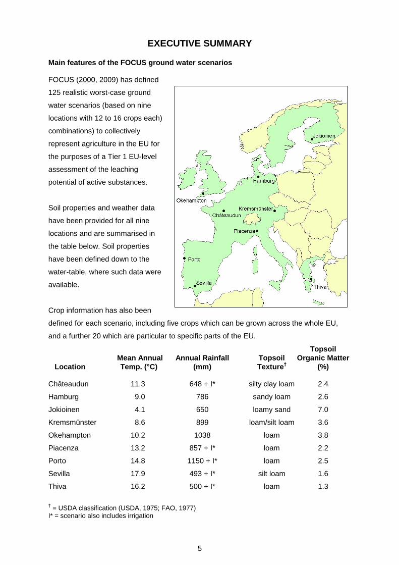
EXECUTIVE SUMMARY Main features of the FOCUS ground water scenarios

FOCUS (2000, 2009) has defined

125 realistic worst-case ground

water scenarios (based on nine

locations with 12 to 16 crops each)

combinations) to collectively

represent agriculture in the EU for

the purposes of a Tier 1 EU-level

assessment of the leaching

potential of active substances.

Soil properties and weather data

have been provided for all nine

locations and are summarised in

the table below. Soil properties

have been defined down to the

water-table, where such data were

available.

Crop information has also been

defined for each scenario, including five crops which can be grown across the whole EU,

and a further 20 which are particular to specific parts of the EU.

Topsoil

Mean Annual Annual Rainfall Topsoil Organic Matter

Location Temp. (°C) (mm) Texture† (%)

Châteaudun 11.3 648 + I* silty clay loam 2.4

Hamburg 9.0 786 sandy loam 2.6

Jokioinen 4.1 650 loamy sand 7.0

Kremsmünster 8.6 899 loam/silt loam 3.6

Okehampton 10.2 1038 loam 3.8

Piacenza 13.2 857 + I* loam 2.2

Porto 14.8 1150 + I* loam 2.5

Sevilla 17.9 493 + I* silt loam 1.6

Thiva 16.2 500 + I* loam 1.3

† = USDA classification (USDA, 1975; FAO, 1977)

I* = scenario also includes irrigation

6

The scenarios as defined do not mimic specific fields, and nor should they be viewed as

representative of the agriculture in the Member States where they are located.

The scenario definitions are simply lists of properties and characteristics which exist

independently of any simulation model. These scenario definitions have also been used to

produce sets of model input files. Input files corresponding to 125 scenarios have been

developed for use with the simulation models PEARL, PELMO and PRZM, while input files

for crops grown at a single location have also developed for the model MACRO. The models

all report concentrations at 1m depth for comparative purposes, but this does not represent

ground water. Results can also be produced for depths down to the water-table in cases

where the model is technically competent to do so and the soil data is available. The

weather data files developed for these models include irrigation in five of the locations, and

also include the option of making applications every year, every other year or every third

year.

How can the scenarios be used to assess leaching?

Defining scenarios and producing sets of model input files is not enough to ensure a

consistent scientific process for evaluating leaching potential in the EU. The user still has to

define substance-specific model inputs, and then has to run the models and summarise the

outputs. (In this report the term “substance” is used to describe active substances of plant

protection products and their metabolites in soil.) Each of these steps can result in

inconsistent approaches being adopted by different modellers, resulting in inconsistent

evaluations of leaching potential. The work groups have addressed these issues as follows:

Defining substance-specific model inputs

This document provides guidance on the selection of substance-specific input parameters.

This includes guidance on

default values and the substance-specific measurements which may supersede them

how to derive input values for a substance from its regulatory data package

selection of representative single input values from a range of measurements

the differing ways in which individual processes are parameterised in the four models,

and differences in units of measurement

Running the FOCUS scenarios in the simulation models

For each of the four models there is a “shell” which has been developed to simplify the

process of running the FOCUS scenarios.

7

Summarising the model outputs

In order to ensure the overall vulnerability of the scenarios, and to also ensure consistency,

a single method of post-processing the model outputs has been defined, and is built directly

into the model shells.

What benefits does this work deliver to the regulatory process?

The FOCUS ground water scenarios offer a way of evaluating leaching potential across the

EU. A consistent process has been defined which is based on best available science at the

time of last update.

The anticipated benefits include:

Increased consistency. The primary purpose of defining standard scenarios is to

increase the consistency with which industry and regulators evaluate leaching. The

standard scenarios, the guidance on substance-specific input parameters, the model

shells, and the standard way of post-processing model outputs should together help

greatly in achieving this.

Speed and simplicity. Simulation models are complex and are difficult to use

properly. Having standard scenarios means that the user has fewer inputs to specify,

and the guidance document simplifies the selection of these inputs. The model shells

also make the models easier to operate.

Ease of review. Using standard scenarios means that the reviewer can focus on

those relatively few inputs which are in the control of the user.

Common, agreed basis for assessment. The FOCUS scenarios provide Member

States a common basis on which to discuss leaching issues with substances at the

EU level. Registrants will also have greater confidence that their assessments have

been done on a basis which the regulators will find acceptable. Debate can then

focus on the substance-specific issues of greatest importance, rather than details of

the weather data or soil properties, for example.

Will the four models give differing results?

Three possible reasons for differences between the results of the models have been

identified and are listed below, together with the measures undertaken to minimise these

differences.

Different weather, soil and crop data. This source of variation has been largely

eliminated by the provision of standard scenarios.

Different ways of summarising the model output. The standard way of post-

processing model outputs, which is built into the model shells, should eliminate this.

8

Different process descriptions within the models. This is the one source of variation

between model results which has not been addressed, since harmonisation of the

models was beyond the scope of the work groups. Similarly, validation of the models

or of the process descriptions within the models was also beyond the scope of the

work groups.

One of the major activities of the FOCUS Ground Water Work Group (FOCUS, 2009) was

to harmonise the results of the models by agreeing to common descriptions of dispersion

length, crop transpiration, and runoff. The harmonisation effort was largely successful with

90 percent of the PEARL and PELMO values for the proposed scenarios within a factor of

three. As shown in FOCUS (2009), this agreement among models for the FOCUS (2009)

scenarios is considerably better than observed among the models for the FOCUS (2000)

scenarios. Given the current agreement among the models, the FOCUS (2009)

recommended that the ground water assessments might be performed with any of the

models (PEARL, PELMO, and PRZM) and there was no need to perform the assessments

with more than one model. However EFSA PPR (2013a) recommends that the PECgw

calculations for decision making should be based on more than one model. Applicants and

rapporteurs are advised that they should again provide simulations with PEARL and PELMO

or PRZM. Where a crop of interest is defined for Châteaudun, MACRO simulations need to

be run. (EFSA PPR, 2013a).

There are situations when the differences between the models can be useful, for example

there may be a fate process which is important for a particular substance which is not

represented in all the models, and this could guide model selection.

References

EFSA Panel on Plant Protection Products and their Residues (PPR) 2013a; Scientific

Opinion on the report of the FOCUS groundwater working group (FOCUS, 2009):

assessment of lower tiers. EFSA Journal 2013;11(2):3114. [29 pp.]

doi:10.2903/j.efsa.2013.3114. Available online: www.efsa.europa.eu/efsajournal

EFSA 2014 European Food Safety Authority. Guidance Document for evaluating laboratory

and field dissipation studies to obtain DegT50 values of active substances of plant

protection products and transformation products of these active substances in soil.

EFSA Journal 2014;12(5):3662, 38 pp., doi:10.2903/j.efsa.2014.3662 Available online:

www.efsa.europa.eu/efsajournal

FAO, 1977. Guidelines for soil profile description. Food and Agriculture Organization of the

United Nations, Rome. ISBN 92-5-100508-7.

http://www.efsa.europa.eu/efsajournal


9

FOCUS. 2009. Assessing Potential for Movement of Active Substances and their

Metabolites to Ground Water in the EU. Report of the FOCUS Ground Water Work

Group, EC Document Reference Sanco/13144/2010 version 1, 604 pp.

FOCUS. 2001. FOCUS Surface Water Scenarios in the EU Evaluation Process under

91/414/EEC. Report of the FOCUS Working Group on Surface Water Scenarios, EC

Document Reference SANCO/4802/2001-rev.2. 245 pp

FOCUS. 2000. FOCUS groundwater scenarios in the EU review of active substances.

Report of the FOCUS Groundwater Scenarios Workgroup, EC Document Reference

Sanco/321/2000 rev.2, 202pp.

USDA, 1975. Soil Taxonomy. A basic system of soil classification for making and

interpreting soil surveys. Agriculture Handbook no. 436. Soil Conservation Service,

USDA, Washington DC.

10

1. DEFINING THE SCENARIOS

1.1 Framework for the FOCUS ground water scenarios

1.1.1 Objectives

One objective of the two FOCUS work groups (FOCUS, 2000; 2009) addressing ground

water was to develop a set of standard scenarios which can be used to assess the potential

movement of crop protection products and their relevant metabolites to ground water as part

of the EU review process for active substances. In order to eliminate the impact of the

person performing these simulations as much as possible, one goal was to standardise

input parameters, calculation procedures, and interpretation and presentation of results. For

ease and uniformity in implementing these standard scenarios computer shells were

developed containing the standard scenarios and all of the associated crop, soil, and

weather information.

1.1.2 Principal Criteria

The following principles guided the selection and development of the leaching scenarios:

The number of locations should not exceed 10.

The combinations of crop, soil, climate, and agronomic conditions should be realistic.

The scenarios should describe an overall vulnerability approximating the 90th

percentile of all possible situations (this percentile is often referred to as a realistic

worst case).

The vulnerability should be split evenly between soil properties and weather.

The exact percentile for the soil properties and weather which will provide an overall

vulnerability of the 90th percentile cannot be determined precisely without extensive

simulations of the various combinations present in a specific region. After exploratory

statistical analysis, FOCUS (2000) decided that the overall 90th percentile could be best

approximated by using a 80th percentile value for soil and a 80

th percentile value for weather.

The 80th percentile for weather was determined by performing simulations using multi-year

weather data, while the 80th percentile soil was selected by expert judgement.

1.1.3 Selection of Locations

Locations were selected by an iterative procedure with the objective that they should:

represent major agricultural regions (as much as possible).

span the range of temperature and rainfall occurring in EU arable agriculture.

be distributed across the EU with no more than one scenario per Member State.

11

The selection process involved an initial proposal of about ten regions derived from

examining information from a number of sources (FAO climatic regions, recharge map of

Europe, temperature and rainfall tables, land use information, etc.). This proposal was

refined by dropping similar climatic regions and adding regions in climatic areas not covered

by the original proposal. Some of these added scenarios are not located in major

agricultural regions, but they represent areas with a significant percentage of arable

agriculture in the EU, albeit diffuse (Table 1.1). The end result was the selection of nine

locations (shown in Figure 1.1 and listed in Table 1.2).

The selected locations should also not be viewed as sites representative of agricultural in

the countries in which they are located. Instead the sites should be viewed collectively as

representative of agricultural areas in climatic zones with significant agriculture in the whole

EU.

Table 1.1. Arable agriculture in EU climate zones.

Precipitation

(mm)

Mean Annual

Temperature (°C)

Arable land *

(%)

Total Area *

(%)

Representative

Locations

601 to 800 5 to 12.5 31 19 Hamburg/Châteaudun 801 to 1000 5 to 12.5 18 13 Kremsmünster 1001 to 1400 5 to 12.5 15 12 Okehampton 601 to 800 >12.5 13 11 Sevilla/Thiva**

801 to 1000 >12.5 9 8 Piacenza < 600 >12.5 4 4 Sevilla/Thiva < 600 5 to 12.5 3 2 Châteaudun***

1001 to 1400 >12.5 3 3 Porto < 600 <5 1 11 Jokioinen

>1400 5 to 12.5 1 1 -- 1001 to 1400 <5 1 4 -- 601 to 800 <5 1 8 --

801 to 1000 <5 0 3 -- >1400 <5 0 0 -- >1400 >12.5 0 0 --

*Relative to the area of the European Union in 2000 plus Norway and Switzerland.

**Although these locations have less than 600 mm of precipitation, irrigation typically used at

these two locations brings the total amount of water to greater than 600 mm.

***Most areas in this climatic zone will be irrigated, raising the total amount of water to

greater than 600 mm. Therefore, Châteaudun can be considered representative of

agriculture in this climatic zone.

12

Figure 1.1. Location of the ground water scenarios.

The arable and total land area data in Table 1.1 is based on the work of Knoche et al., 1998.

Temperature and precipitation boundaries were determined based on weather data of about

5000 stations in Europe from Eurostat (1997) and agricultural use was based on information

from USGS et al. (1997). As a check, the same area data was also estimated using a

13

second approach based on the data of FAO (1994) and van de Velde (1994). Both of these

approaches resulted in very similar estimates.

Since the generation of Table 1.1, the number of countries in the EU has increased

significantly. Therefore FOCUS Ground Water Work Group (FOCUS, 2009) assessed

whether the FOCUS scenarios „covers‟ the agricultural area of new member states. A

scenario „covers‟ an area when it represents either the same properties or represents a

more vulnerable situation like higher rainfall amounts or lower organic carbon contents. The

spatial analysis shows that the current set of FOCUS leaching scenarios is applicable to

new member countries for the purpose of Tier 1 screening simulations.

1.1.4 Selection of Soils

The selection of the soil was based on the properties of all soils present in the specific

agricultural region represented by a location. Thus unrealistic combinations of climatic and

soil properties were avoided. The intent was to chose a soil that was significantly more

vulnerable than the median soil in the specific agricultural region, but not so extreme as to

represent an unrealistic worst case. Soils which did not drain to ground water were

excluded when possible, therefore no drainage assumptions were required in the scenario

definitions. This is a conservative assumption in terms of predicting leaching. Soil tillage

was also ignored. Vulnerability was defined with respect to chromatographic leaching (that

is, leaching is greater in low organic matter sandy soils than higher organic matter loams).

The selection of appropriate soils was performed by expert judgement, except for the

Okehampton location where SEISMIC, an environmental modelling data base for England

and Wales, was used to select a suitable soil (Hallett et al., 1995). Soil maps (NOAA, 1992;

Fraters, 1996) were used to obtain information on the average sand and clay fractions and

the organic matter in a region. Based on these average values, target values for soil texture

and organic matter were developed for each location to ensure that they were more

vulnerable than the average. In consultation with local experts, soils were selected which

met these target values (values for surface parameters are provided in Table 1.2). In some

cases special consideration was given to suitable soils at research locations where

measurements of soil properties were readily available (Châteaudun, Sevilla and Piacenza).

In a few cases the target values had to be re-examined during the process of picking

specific soils. The Hamburg scenario was based on the national German scenario. This

national scenario was based on a soil survey intended to locate a worst case leaching soil,

so the vulnerability associated with this soil significantly exceeds the target of an 80th

percentile soil (Kördel et al, 1989). FOCUS (2009) revised the organic matter content of the

Piacenza and Porto scenarios based on a spatial analysis of the climatic zones represented

by the Porto and Piacenza locations that indicated a change in the organic matter was

14

appropriate to make them fit the vulnerability concept. Detailed soil properties for all

scenarios as a function of depth are provided in Section 3.

Table 1.2. Overview of the locations for the ground water scenarios.

Topsoil

Mean Annual Annual Rainfall Topsoil Organic Matter

Location Temp. (°C) (mm) Texture† (%)

Châteaudun 11.3 648 + I* silty clay loam 2.4

Hamburg 9.0 786 sandy loam 2.6

Jokioinen 4.1 650 loamy sand 7.0

Kremsmünster 8.6 899 loam/silt loam 3.6

Okehampton 10.2 1038 loam 3.8

Piacenza 13.2 857 + I* loam 2.2

Porto 14.8 1150 + I* loam 2.5

Sevilla 17.9 493 + I* silt loam 1.6

Thiva 16.2 500 + I* loam 1.3

† = USDA classification (USDA, 1975; FAO, 1977)

I* = scenario also includes irrigation

1.1.5 Climatic Data

As part of the scenario selection process, targets for annual rainfall were also developed for

each site based on tables of annual rainfall (Heyer, 1984). These target values were used

by FOCUS (2000) to identify appropriate climatic data for a 20 year period. The resulting

average values for rainfall at each site are shown in Table 1.2. Five locations (Châteaudun,

Piacenza, Porto, Sevilla, and Thiva) were identified as having irrigation normally applied to

at least some crops in the region.

1.1.6 Macropore Flow

The question of macropore flow was discussed at length in FOCUS (2000) and they decided

to develop parameters for one scenario to be able to compare differences between

simulations with and without macropore flow to help demonstrate to Member States the

effect of macropore flow. The Châteaudun location was chosen for this scenario because

soils at this site are heavier than at most of the other sites and because experimental data

were available for calibrating soil parameters. The macropores in the profile at Châteaudun

are present to about 60 cm depth. Note that macropore flow is just one form of preferential

15

flow. Forms of preferential flow other than macropore flow are not considered by current

models and were not considered by the workgroup.

1.1.7 Crop Information

FOCUS (2000) decided to make the scenarios as realistic as possible by including most

major European crops (except rice which was excluded since scenarios for this crop are

being developed elsewhere and the regulatory models being used are not suitable for

predicting leaching under these flooded conditions). Crop parameters were obtained for five

crops grown in all nine locations and for a further 20 crops grown in at least one location

(Table 1.3). Sometimes parameters for a crop not typically grown in a specific area (for

example, sugar beets in Okehampton) were included because such crops might be grown in

similar soils and climates. Crops for each scenario were identified and cropping parameters

were developed with the help of local experts. Some crops not included in this table can be

simulated using these same parameters, e.g. pears map onto apples. On the other hand

some crops and land uses cannot be mapped onto the crops in Table 1.3, e.g. Christmas

trees, fallow land and rotational grassland.

The scenarios assume that the same crop is grown every year. For three of the crops

(cabbage, vegetable beans, and carrots) there are multiple crops grown per season at some

locations, with the standard practice for applications to be made to both crops. Some crops

(such as potatoes) are rarely grown year after year. Therefore, an option was added to

allow applications every year, every other year, or every third year. In order to conduct

comparable evaluations, the simulation period was extended to 40 and 60 years for

applications made every other year and every third year respectively (by repeating the 20

year weather dataset, with a date offset). The specification of applications to be made every

other year or every third year is also applicable to products for which annual applications are

excluded by a label restriction. Crop rotations are not explicitly simulated for reasons of

technical difficulty.

The use of various crops for each location necessitated the development of crop-specific

irrigation schedules for the five irrigated locations, namely Châteaudun, Piacenza, Porto,

Sevilla, and Thiva.

16

Table 1.3. Crops included in FOCUS scenarios by location.

Crop C H J K N P O S T

apples + + + + + + + + +

grass (+ alfalfa) + + + + + + + + +

potatoes + + + + + + + + +

sugar beets + + + + + + + + +

winter cereals + + + + + + + + +

beans (field) + + +

beans (vegetables) + +

bush berries +

cabbage + + + + + + +

carrots + + + + + +

citrus + + + +

cotton + +

linseed +

maize + + + + + + + +

oilseed rape (summer) + + +

oilseed rape (winter) + + + + + +

onions + + + + + +

peas (animals) + + + +

soybean +

spring cereals + + + + + +

strawberries + + + +

sunflower + +

tobacco + +

tomatoes + + + + +

vines + + + + + + +

C Châteaudun, H Hamburg, J Jokioinen, K Kremsmünster, N Okehampton, P Piacenza, O Porto, S Sevilla, T Thiva.

1.1.8 Information on Crop Protection Products and Metabolites

Information on the chemical properties of crop protection products and their metabolites,

application rates, and application timing are left to the user to provide. A more detailed

discussion appears in Section 2.4, including recommendations for selecting values of the

parameters required by the various models. Because the vulnerability of the scenarios is to

be reflected in the soil properties and climatic data rather than in the properties chosen for

the crop protection products and their metabolites, and because each simulation consists of

twenty repeat applications, mean or median values (using a geometric mean of the sample

population as the best estimate of the median of the whole population) are recommended

for these parameters.

1.1.9 Implementation of Scenarios

Models. The remit of the workgroup was to develop scenarios generally suitable for

evaluating potential movement to ground water. The intent was not to produce model-

specific scenarios but rather describe a set of conditions that can continue to be used as

existing models are improved and better models developed. However, simulating any of

17

these scenarios with an existing model also requires the selection of many model-specific

input parameters. Therefore, for uniform implementation of these standard scenarios,

computer shells were developed to generate the input files needed for the various computer

models. Such shells, which include all scenarios, were developed for three widely used

regulatory models (PELMO, PEARL, and PRZM). A shell for MACRO, another widely used

model (and the most widely used considering macropore flow), was developed for the

macropore flow scenario at Châteaudun. These shells also included post-processors to

calculate and report the annual concentrations used as a measure of the simulation results.

Simulation Period. As mentioned earlier, a simulation period of 20 years should normally be

used to evaluate potential movement to ground water. When applications are made only

every other year or every third year the simulation period should be increased to 40 and 60

years, respectively. In order to appropriately set soil moisture in the soil profile prior to the

simulation period and because residues may take more than one year to leach (especially

for persistent compounds with moderate adsorption to soil), a six year “warm-up” period has

been added to the start of the simulation period. Simulation results during the warm-up

period are ignored in the assessment of leaching potential.

Calculation of Annual Concentrations. The method for calculating the mean annual

concentration for a crop protection product or associated metabolites is the same for all

models. The mean annual concentration moving past a specified depth is the integral of the

solute flux over the year (total amount of active substance or metabolite moving past this

depth during the year) divided by the integral of the water flux over the year (total annual

water recharge). In years when the net recharge past the specified depth is zero or

negative, the annual mean concentration should be set to zero. All mean concentrations are

based on a calendar year. When applications are made every other year or every third

year, the mean concentrations for each of the 20 two or three year periods are determined

by averaging the annual concentrations in each two or three year period on a flux-weighted

basis.

In equation form, the average concentration past a specified depth is calculated as follows:

Ci = ( i, i+j Js ) / ( i, i+j Jw )

where Ci is the average (flux) concentration of substance at the specified depth

(mg/L) for the period starting on day i, Js the daily substance leaching flux

(mg/m2/day), Jw the daily soil water drainage (l/m2/day) and j the number of days

considered in the averaging period (365 or 366 days for a 20 year scenario; 730 or

731 for a 40 year scenario; 1095 or 1096 for a 60 year scenario).

18

For the Richard's equation based models (PEARL and MACRO), this average concentration

includes the negative terms due to upward flow of water and solute. Therefore, when

degradation is occurring below the specified depth, the upward movement can artificially

increase the calculated average solute concentration at the specified depth. In these cases,

the simulations should be conducted at the deepest depth which is technically feasible to

minimise this effect. Alternatively, PELMO or PRZM could be used.

Simulation Depth. All simulations have to be conducted to a sufficient depth in order to

achieve an accurate water balance. For capacity models such as PRZM and PELMO, this

means that simulations must be conducted at least to the maximum depth of the root zone.

For Richard‟s equations models such as PEARL and MACRO, the simulations should be

conducted to the hydrologic boundary. With respect to concentrations of active substances

and metabolites, the EU Uniform Principles (product authorisation decision making criteria)

refer to concentrations in ground water. However, a number of factors can make

simulations of chemical transport in subsoils difficult. These include lack of information on

subsoil properties, lack of information of chemical-specific properties of crop protection

products and their metabolites, model limitations, and sometimes fractured rock or other

substrates which cannot be properly simulated using existing models. Information on

degradation of active substance and metabolites in subsoils is especially important, since in

the absence of degradation the main change in concentration profiles is only the result of

dispersion. Therefore, all model shells report integrated fluxes of water and relevant

compounds at a depth of 1 m. Models may also report integrated fluxes at deeper depths

such as at the hydrologic boundary or water table, where technically appropriate. As more

information becomes available and improvements to models occur, the goal is to be able to

simulate actual concentrations in ground water. Soil properties below 1 m are included in

the soil property files for each scenario, along with the depth to ground water.

Model Output. The model shells rank the twenty mean annual concentrations from lowest to

highest. The average between the sixteenth and seventeenth value (fourth and fifth

highest) is used to represent the 80th percentile value associated with weather for the

specific simulation conditions (and the overall 90th percentile concentration considering the

vulnerability associated with both soil and weather). When applications are made every

other or every third year, the 20 concentrations for each two or three year period are ranked

and the average of the sixteenth and seventeenth values selected.

In addition to the concentration in water moving past 1 m, the outputs also include at a

minimum a listing of the input parameters and annual water and chemical balances for each

19

of the simulation years. Water balance information includes the annual totals of rainfall plus

irrigation, evapotranspiration, runoff, leaching below 1 m, and water storage to 1 m.

Chemical balances (for the active substance and/or relevant metabolites) include the annual

totals of the amount applied (or produced in the case of metabolites), runoff and erosion

losses, plant uptake, degradation, volatilisation losses, leaching below 1 m, and storage to

1 m. All variables may additionally be reported at a depth greater than 1 m, as discussed

previously.

1.2 Weather and irrigation data for the FOCUS scenarios

Section 2.2 of the original FOCUS Groundwater Scenarios report (FOCUS, 2000) still

stands as a description of how the weather data were derived and implemented, so

repeating it here is not necessary. Refinements made by FOCUS (2009) were the use of

FAO rather than MARS reference evapotranspiration and the evaporation from bare soil in

PELMO and PRZM (see Section 11.5 in FOCUS, 2009).

The current irrigation routines are described in Section 11.5.3 of FOCUS (2009). FOCUS

(2009) decided that irrigation schedules should be developed for individual crops in

Châteaudun, Piacenza, Porto, Seville, and Thiva. These irrigation schedules provide

irrigation from the time of planting until start of senescence and are generated using

irrigation routines in PEARL and PELMO, which apply irrigation once a week on a fixed day

to bring the root zone up to field capacity. However, irrigation was applied only if the

amount required exceeded 15 mm. Because of the minor differences remaining in the water

balance (primarily evapotranspiration), the irrigation routines for PEARL and PELMO predict

somewhat different amounts. However, using different irrigation routines tends to

compensate for evapotranspiration differences to provide closer estimates between the two

models for the amount of water moving below the root zone, which is the key water balance

parameter affecting leaching. The irrigation amounts generated by PELMO are used

directly in PRZM. While allowing PRZM to generate irrigation amounts is also possible, the

work group decided that this added a level of complexity that was not needed, given the

similarity of PELMO and PRZM.

1.3 Soil and crop data

Section 2.3 of FOCUS (2000) describes how the soil and crop data were derived and

implemented. Sections 11.3 and 11.5 of FOCUS (2009) describe refinements in this

information. All of this data is provided in the tables in Chapter 3 of this report, with the

exception of the crop interception data, which the user needs in order to adjust the

application rate correctly.

20

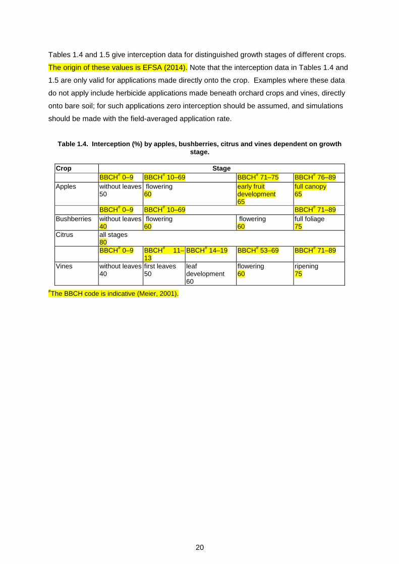
Tables 1.4 and 1.5 give interception data for distinguished growth stages of different crops.

The origin of these values is EFSA (2014). Note that the interception data in Tables 1.4 and

1.5 are only valid for applications made directly onto the crop. Examples where these data

do not apply include herbicide applications made beneath orchard crops and vines, directly

onto bare soil; for such applications zero interception should be assumed, and simulations

should be made with the field-averaged application rate.

Table 1.4. Interception (%) by apples, bushberries, citrus and vines dependent on growth

stage.

Crop Stage

BBCH# 0–9 BBCH

# 10–69 BBCH

# 71–75 BBCH

# 76–89

Apples without leaves 50

flowering 60

early fruit development 65

full canopy 65

BBCH# 0–9 BBCH

# 10–69 BBCH

# 71–89

Bushberries without leaves 40

flowering 60

flowering 60

full foliage 75

Citrus all stages 80

BBCH# 0–9 BBCH

# 11–

13 BBCH

# 14–19 BBCH

# 53–69 BBCH

# 71–89

Vines without leaves 40

first leaves 50

leaf development 60

flowering 60

ripening 75

#The BBCH code is indicative (Meier, 2001).

21

Table 1.5. Interception by other crops dependent on growth stage.

Crop Bare –

emergence

Leaf

development

Stem elongation Flowering Senescence

Ripening

BBCH#

0– 09 10–19 20–39 40–89 90–99

Beans (field + vegetable)

0 25 40 70 80

Cabbage 0 25 40 70 90

Carrots 0 25 60 80 80

Cotton 0 30 60 75 90

Grass##

0 40 60 90 90

Linseed 0 30 60 70 90

Maize 0 25 50 75 90

Oil seed rape (summer)

0 40 80 80 90

Oil seed rape (winter)

0 40 80 80 90

Onions 0 10 25 40 60

Peas 0 35 55 85 85

Potatoes 0 15 60 85 50

Soybean 0 35 55 85 65

Spring cereals 0 0 BBCH 20–29*

BBCH 30–39*

BBCH 40–69

BBCH 70–89

80

20 80 90 80

Strawberries 0 30 50 60 60

Sugar beets 0 20 70 (rosette) 90 90

Sunflower 0 20 50 75 90

Tobacco 0 50 70 90 90

Tomatoes 0 50 70 80 50

Winter cereals 0 0 BBCH 20–29*

BBCH 30–39*

BBCH 40–69

BBCH 70–89

80

20 80 90 80 # The BBCH code is indicative (Meier, 2001).

## A value of 90 is used for applications to established turf

* BBCH code of 20-29 for tillering and 30-39 for elongation

1.4 References






EUROSTAT. 1997. Geographic Information System of the Commission of the European

Communities (GISCO). Datenbanken: Climate EU (CT) und Administrative Regions Pan-

Europe (AR). Luxembourg.

FAO. 1977. Guidelines for soil profile description. Food and Agriculture Organization of the

United Nations, Rome. ISBN 92-5-100508-7.


22

FAO. 1994. The digital soil map of the world, notes version 3. United Nations.






Sanco/321/2000 rev.2, 202pp.

Fraters, D. 1996. Generalized Soil Map of Europe. Aggregation of the FAO-Unesco soil

units based on the characteristics determining the vulnerability to degradation

processes. Report no. 481505006, National Institute of Public Health and the

Environment (RIVM), Bilthoven.

Hallett, S.H., Thanigasalam, P., and Hollis, J.M.H. 1995. SEISMIC; A desktop information

system for assessing the fate and behaviour of pesticides in the environment.

Computers and Electronics in Agriculture, 13:227 - 242

Heyer, E. 1984. Witterung und Klima. Eine allgemeine Klimatologie. 7. Auflage, Leipzig.

Knoche, H., Klein, M., Lepper, P. Herrchen, M., Köhler, C. and U. Storm. 1998.

Entwicklung von Kriterien und Verfahren zum Vergleich und zur Übertragbarkeit

regionaler Umweltbedingungen innerhalb der EU-Mitgliedstaaten (Development of

criteria and methods for comparison and applicability of regional environmental

conditions within the EU member countries), Report No: 126 05 113, Berlin

Umweltbundesamt.

Kördel, W, Klöppel H and Hund, K. 1989. Physikalisch-chemische und biologische

Charakterisierung von Böden zur Nutzung in Versickerungsmodellen von

Pflanzenschutzmitteln. (Abschlussbericht. Fraunhofer-Institut für Umweltchemie und

Ökotoxikologie, D-5948 Schmallenberg-Grafschaft, 1989.

Meier, U (Ed.), 2001. Growth stages of mono- and dicotyledonous plants.: BBCH-

Monograph. Blackwell Wissenshafts-Verlag, Berlin, Germany, 158 pp

National Oceanic and Atmospheric Administration (NOAA). 1992. Global Ecosystem

Database Version 1.0. National Geophysical Data Center (NGDC), Boulder, Co., USA,

CD-ROM.

U.S. Geological Survey (USGS), University of Nebraska-Lincoln (UNL) and European

Commission's Joint Research Centre (JRC) (Hrsg.). 1997. 1-km resolution Global Land

Cover Characteristics Data Base. Sioux Falls.

USDA. 1975. Soil taxonomy. A basic system of soil classification for making and

interpreting soil surveys. Agriculture Handbook no. 436. Soil Conservation Service,

USDA, Washington DC.

van de Velde, R. J. 1994. The preparation of a European landuse database. RIVM report

712401001.

23

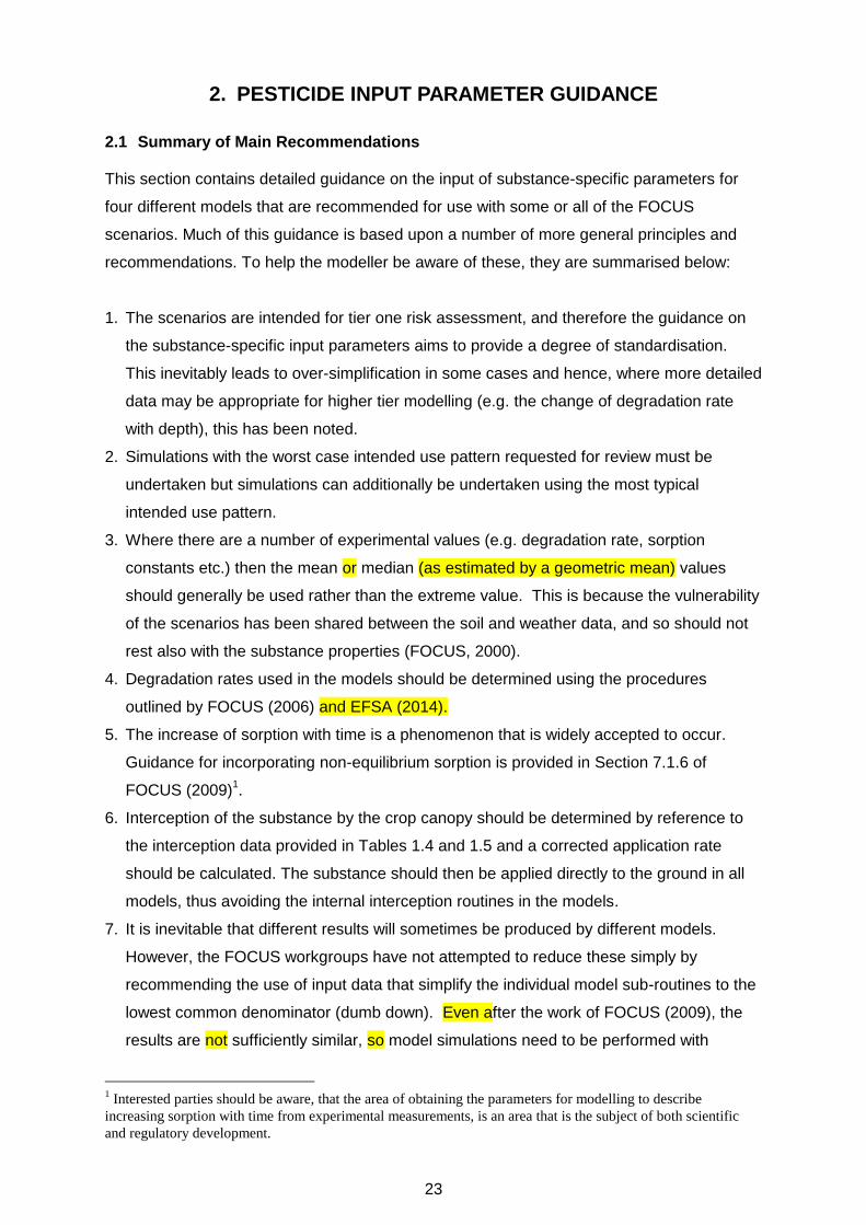
2. PESTICIDE INPUT PARAMETER GUIDANCE

2.1 Summary of Main Recommendations

This section contains detailed guidance on the input of substance-specific parameters for

four different models that are recommended for use with some or all of the FOCUS

scenarios. Much of this guidance is based upon a number of more general principles and

recommendations. To help the modeller be aware of these, they are summarised below:

1. The scenarios are intended for tier one risk assessment, and therefore the guidance on

the substance-specific input parameters aims to provide a degree of standardisation.

This inevitably leads to over-simplification in some cases and hence, where more detailed

data may be appropriate for higher tier modelling (e.g. the change of degradation rate

with depth), this has been noted.

2. Simulations with the worst case intended use pattern requested for review must be

undertaken but simulations can additionally be undertaken using the most typical

intended use pattern.

3. Where there are a number of experimental values (e.g. degradation rate, sorption

constants etc.) then the mean or median (as estimated by a geometric mean) values

should generally be used rather than the extreme value. This is because the vulnerability

of the scenarios has been shared between the soil and weather data, and so should not

rest also with the substance properties (FOCUS, 2000).

4. Degradation rates used in the models should be determined using the procedures

outlined by FOCUS (2006) and EFSA (2014).

5. The increase of sorption with time is a phenomenon that is widely accepted to occur.

Guidance for incorporating non-equilibrium sorption is provided in Section 7.1.6 of

FOCUS (2009)1.

6. Interception of the substance by the crop canopy should be determined by reference to

the interception data provided in Tables 1.4 and 1.5 and a corrected application rate

should be calculated. The substance should then be applied directly to the ground in all

models, thus avoiding the internal interception routines in the models.

7. It is inevitable that different results will sometimes be produced by different models.

However, the FOCUS workgroups have not attempted to reduce these simply by

recommending the use of input data that simplify the individual model sub-routines to the

lowest common denominator (dumb down). Even after the work of FOCUS (2009), the

results are not sufficiently similar, so model simulations need to be performed with

1 Interested parties should be aware, that the area of obtaining the parameters for modelling to describe

increasing sorption with time from experimental measurements, is an area that is the subject of both scientific

and regulatory development.

24

PEARL and PELMO or PRZM. Where a crop of interest is defined for Châteaudun

MACRO simulations need to be run. (EFSA PPR, 2013a).

25

2.2 Introduction

The scenarios developed by the FOCUS are aimed to assist the risk assessment required

for the review of active substances under Directive 91/414/EEC and Regulation (EC) No

1107/2009. A number of Member States (MS; Germany [Resseler et al., 1997], The

Netherlands [Brouwer et al., 1994], UK [Jarvis, 1997]) have already produced guidance for

modelling under their national plant protection product legislation and this has been taken

into account in the current document. Unsurprisingly MS have historically differing views

over the most appropriate input values for models. Therefore, our task is to provide clear

guidance to users on appropriate values to input into models for risk assessment under

Directive 91/414/EEC and Regulation (EC) No 1107/2009, at Tier 1, while still retaining the

support of the MS.

The aim of these scenarios is to be a first tier to the risk assessment and this does not

exclude the possibility of more detailed modelling at subsequent times. As a first tier, a high

degree of standardisation of the model inputs has been undertaken. For instance, the model

input values for the nine selected soils have been fixed and are not subject to user

variability. Similarly the crop, weather and much of the agricultural practice data have been

provided as set inputs. The modeller therefore has only to input various substance-specific

parameters in order to achieve consistent results for the substance of interest in the

scenarios provided.

Comparative modelling exercises have shown that the modeller can be a significant variable

in the range of output data obtained from the same available information for input (Brown et

al., 1996, Boesten, 2000). Therefore we consider it important to attempt to reduce still

further the amount of variation introduced. By necessity, individual users must provide their

own input values for their substance of interest. However, this provides the opportunity for

different users to input different substance-specific information into the models, even though

they have the same range of data available to them.

This chapter aims to provide further advice to users to help them select a representative

single input value from a range that may be available and to help less experienced users to

be aware of the most appropriate form of the data to use in particular models. It is important

in this context that the user recognises that the quality of the experimental data may vary

and this should be taken into account when selecting input parameters for modelling. The

guidance cannot be exhaustive in considering all substance-specific factors but it attempts

to highlight the major differences between models where it is likely to have a significant

effect on the results of the simulation. Note that this guidance is aimed specifically for Tier 1

FOCUS ground water scenarios and is not necessarily appropriate for the wider use of the

26

models. Any user is also advised to check their proposed input data prior to running the

model to ensure that the totality of the substance-specific input values results in a realistic

reflection of the general behaviour of the compound.

In developing these scenarios FOCUS has chosen to include three different models for all

scenarios and a further model for a macropore flow scenario. It is inevitable that some

differences in the outputs will occur between the differing models. To some extent this is a

strength of the project since differing models treat the varying transport and transformation

processes in different manners and hence for specific situations some models are likely to

account for substance behaviour better than others. It is not within the FOCUS remit to

validate the various model sub-routines nor is it our aim to reduce all the processes

simulated to the lowest common denominator with the intention of producing the same result

from all models. Therefore where models deal with processes such as volatilisation in

differing manners, this guidance does not attempt to artificially manipulate the

recommended input data with a view to reducing variability of the results. In these cases the

best guidance and sources of information are provided for each of the different processes.

In the majority of cases however, recommendations for standardised inputs are made (i.e.

when the same input parameter is required by different models but in differing units etc.).

Finally, these scenarios have been developed to provide realistic worst case situations for

the EU review process. The user should recognise that vulnerability is being covered by the

choice of soils and climates and, therefore, choices of extreme values of substance-specific

parameters would result in model predictions beyond the 90th percentile.

2.3 General guidance on parameter selection

Directive 91/414/ EEC and Regulation (EC) No 1107/2009 require that estimations of

PECgw are made for both the active substance and metabolites or transformation products.

(Levels triggering ground water assessment for metabolites are presented in

Sanco/221/2000-rev.10 25 February 2003). Historically most models and modellers have

principally addressed the leaching of the parent compound but routines are now available in

many models (including those used with the FOCUS scenarios) to directly assess the

mobility of metabolites if required. In order to use these routines it is necessary to have

information on either, the proportion of each metabolite formed (kinetically derived formation

fraction), or on the individual rate constants for the formation of each metabolite. If this

information is not available, a less sophisticated, but nonetheless valid, method is to

substitute the metabolite data for the parent compound in the model and adjust the

application rate to correspond to the amount of metabolite formed in the experimental

studies. This method may lead to underestimation of leaching concentrations, especially

27

when the parent is rather mobile and the user should be aware of this. In either situation the

guidance in this document applies equally to the parent or metabolite.

The ground water leaching scenarios have been provided for four models; PRZM (PRZM 3.0

Manual; Carsel et al., 1998), PELMO (Jene 1998), PEARL (Leistra et al, 2000), and

MACRO (Jarvis and Larsson, 1998). Each of these models requires the same general

information regarding the most important substance properties (e.g. degradation rate,

sorption). However, all input these data in slightly different ways. This section addresses

general information such as the broader availability of input data and the follow section

addresses specific parameters. Further information on the differences between earlier

versions of the models can be obtained from FOCUS (1995). However, the reader should be

aware that some significant changes may have occurred in more recent versions of the

models.

Regardless of the particular model, the amount of data available from which to select the

model input varies significantly from parameter to parameter. For a number of the input

parameters, such as diffusion coefficients, degradation rate correction factors for

temperature and moisture and transpiration stream concentration factor (TSCF), substance-

specific data is unlikely to be available or alternatively is unlikely to be more reliable than a

generic average. Default values for such parameters are recommended by FOCUS (2000,

2009).

For a further number of the input parameters, such as the physico-chemical properties, and

the management-related information, the values are generally straightforward to input into

the models. The physico-chemical property data are generally available as single values

from standard experiments conducted as part of the registration package. The management

related parameters can be obtained from the intended Good Agricultural Practice (GAP).

For the management related parameters the worst case supported must be used (i.e.

highest application rates, most vulnerable time for leaching etc.). In addition, the most

typical uses can also be simulated if significantly different.

For the remaining parameters, such as degradation rate, kinetic formation fraction of

metabolites, and soil sorption, a number of experimental values are generated as part of the

registration package. Determining which single value should be used as input for each

parameter is difficult and contentious since the relevant output data can vary significantly

depending on which of the range of possible values are used as input.

28

The environmental fate data requirement annexes to Directive 91/414/EEC (95/36/EC) and

data required for Regulation (EC) no 1107/2009 require that reliable degradation rate

endpoints are available from a minimum of four soils for the parent compound and three

soils for metabolites (laboratory studies initially and then, if necessary, field studies). (The

trigger levels for assessing metabolites are defined in the data requirements for Regulation

(EC) no 1107/2009 and in Sanco/221/2000-rev.10 25 February 2003.) Therefore FOCUS

(2000, 2006) recommends that where reliable endpoints for the parent compound are

available in a minimum of four different soils it is generally acceptable to use the geometric

mean of the degradation rates as input into the model. Similarly, FOCUS (2000, 2006)

recommends that where reliable endpoints for metabolites are available in a minimum of

three different soils it is generally acceptable to use the geometric mean of the degradation

rate as input into the model. EFSA (2014) also prescribes that a geometric mean value is

selected as input, except when degradation rate is correlated with soil properties such as

pH. FOCUS (2000, 2006) also provides for the exception when degradation rate is

correlated with soil properties. In situations where less than the required number of reliable

degradation rates from different soils can be derived further experimental data should be

generated (EFSA, 2014).

For the kinetic formation fractions of metabolites from their precursor/s FOCUS (2006)

recommends an arithmetic mean is used.

Reliable soil sorption results (KFoc, Koc or KFom, Kom) are also required in a minimum of four

soils for parent compound and in a minimum of three soils for metabolites that reach levels

defined in Sanco/221/2000-rev.10 25 February 2003 and/or the environmental fate data

requirement annexes to Directive 91/414/EEC and data required for Regulation (EC) No

1107/2009. Where these are all representative agricultural soils, EFSA (2014) prescribes

that the geometric mean value of the sorption constant normalised for organic carbon (KFoc,

Koc, Kom or KFom) be input to the models, unless the sorption is indicated to be pH-or other

soil property dependent. In situations where there are reliable results from less than the

required number of different agricultural soils then further experimental data should be

generated.

When characterising sorption behaviour of ionic compounds, the value will vary depending

on the pH and a geometric mean value is no longer appropriate. For some compounds,

both sorption and degradation are pH dependent. Under these conditions, use of linked

values of Koc and degradation rates is appropriate. Inputs should be selected with the aim

of obtaining a realistic rather than an extreme situation and the values used should be

justified in the report.

29

Though FOCUS (2000, 2009) recommended a first approach for compounds with pH

dependent sorption of running the scenarios with the soil pH defined for the specific FOCUS

scenarios (provided in the tables in Chapter 3), EFSA PPR (2013a) considered that this was

not appropriate. Therefore Tier 1 simulations for consideration of EU approval should select

adsorption values, chosen to represent a realistic worst case considering the pH of the soils

in the EU that are used for the production of the pertinent crop. Normally this pH would be

selected to minimise sorption; however, there are certain compounds for which lower

sorption results in faster degradation. In addition to choosing adsorption values that

represent a realistic worst case applicants might also provide simulations for all scenarios

selecting a contrasting adsorption value associated for a more best case, considering the

pH of the soils in the EU that are used for the production of the pertinent crop. Decision

makers would then get a view on the range of recharge concentrations that can result

depending on the average pH of the soils overlying a confined aquifer in a particular region.

As an example ,for a compound with a single ionisable functional group that follows a typical

S shaped relationship for adsorption with pH, such as a weak acid, two contrasting pH

values for which best and worst case adsorption estimates could be selected would be

associated with a pH of 5.0 and 7.5 respectively if the crop could grow in this range of soil

pH. If the pH relationship was more ∩ or U shaped, adsorption associated with an

intermediate pH as the best or worst case respectively could be justified. Using correct pH

maps and using soil column pH descriptions to parameterise scenarios in case of pH

dependent substance properties, was considered more important in assessments at the

national level rather than the EU level by the EFSA PPR panel (EFSA PPR, 2013a).

For all model inputs derived from the regulatory data package, only studies of acceptable

quality should be considered.

2.4 Guidance on substance-specific input parameters

2.4.1 Physico chemical parameters

Molecular Weight. In PELMO this can be used to estimate the Henry‟s law constant if

required. In PELMO and PEARL these data are also required to correct concentrations for

the differing molecular weights of parents and metabolites.

Solubility in Water. In PEARL this is required for the model (units: mg/L) to calculate the

Henry‟s law constant (this is only appropriate for non-ionised compounds). In PELMO this

can be used to determine the Henry‟s law constant if this value is not input directly (see

below).

30

Vapour Pressure. In PEARL this is required for the model (units: Pa) to subsequently

calculate the Henry‟s law constant. In PELMO this can be used to determine the Henry‟s law

constant if this value is not input directly (see below).

pKa-Value (if acid or base). The pKa value has an effect on the sorption of a compound at

different pH values (i.e. dissociated acidic molecules are more mobile than the uncharged

acid conjugates). When simulating the behaviour of compounds which dissociate, the user

should thoroughly describe which charge transfer is given by the pKa value (i.e. H2A HA-,

HA- A

2- etc.). PELMO and PEARL can account directly for the effect of changing

ionisation with pH. PELMO requires both the pKa value and the reference pH at which the

Koc was obtained in order to adjust the sorption for pH in the profile. PEARL requires both

the pKa value and the two extreme Kom values (one at very low pH and one at very high pH).

MACRO_DB also has a similar routine if this is used to parameterise MACRO.

FOCUS (2009) decided to make the pH-H2O values of the FOCUS groundwater scenarios

available electronically because most of the values provided for the soil profiles were pH-

H2O values (FOCUS, 2000). Models may now be used to describe the sorption of

substances showing pH dependent sorption, however the modelling report should

demonstrate that the adsorption values predicted by the model fit the experimental data.

Using an experimental adsorption value appropriate for the soil pH of the relevant FOCUS

scenario is not considered an acceptable method of including pH dependent sorption into

the FOCUS scenarios when used for applications to support EU level decision making. This

is because these scenarios cannot be considered to possess the FOCUS-defined

vulnerability as the FOCUS (2000) (as updated by FOCUS (2009)) scenario selection

procedure did not consider pH effects as a variable when defining 80th percentile soil column

descriptions. Defining scenario vulnerability using correct pH maps in case of pH dependent

sorption was considered more important in assessments at the national level rather than the

EU level by the EFSA PPR panel (EFSA PPR, 2013a).

When introducing a measured Koc-pH relationship into the FOCUS leaching models, the pH-

H2O measuring method must be consistent with that used for analysing the sorption

measurements. If the pH-H2O is not available for the soils from the adsorption studies, it

can be calculated as follows (A.M.A. van der Linden, personal communication, 2008):

pH-H2O = 0.820 pH-KCl + 1.69

pH-H2O = 0.953 pH-CaCl2 + 0.85

31

where pH-KCl is the pH measured in an aqueous solution of 1 mol/L of KCl and where pH-

CaCl2 is the pH measured in an aqueous solution of 0.01 mol/L of CaCl2.

Reference pH-Value at which Koc-Value was Determined. This is required for PELMO only

(see above).

Dimensionless Henry’s Law Constant. The Henry‟s law constant can be used as a direct

input in PRZM and PELMO (in PEARL the model calculates the value from input values of

water solubility and vapour pressure; see above). This value (H; in its dimensioned form of

Pa m³ mol-1

) should be available for the active substance as it is required as part of the

substance dossier for review under Directive 91/414/EEC and Regulation (EC) No

1107/2009. Care should be taken with the units of the Henry‟s law constant. In PRZM the

Henry‟s law constant value is dimensionless (this is also often stated as the air/water

partition coefficient, Kaw i.e. has no units due to concentrations in the gas and liquid phases

being expressed in the same units, usually mol/m³) but in PELMO the units are Pa m³ mol-1

(equivalent to J/mol). The conversion factor from Kaw (dimensionless) to H (Pa m³ mol-1

) is

as follows H = Kaw R T, where R is the universal gas constant (8.314 Pa m³ mol-1

K-1

) and T

is in K.

The Henry‟s law constant is used to calculate the volatility of the substance once in the soil.

MACRO does not include this parameter and is unable to simulate volatilisation of

substance, so this model may not be the most appropriate for compounds which possess

significant volatility.

If the soil degradation rate is a value derived from field studies (see below) it will incorporate

all relevant degradation/dissipation processes, including volatilisation. Therefore care should

be taken regarding the use of the Henry‟s law constant input. This is particularly important

for substances which show some volatility.

Diffusion Coefficient in Water. This is required for MACRO and PEARL only. The suggested

default value is 4.3 x 10-5

m²/day (Jury, 1983; PEARL units) which is equivalent to 5.0 x 10-

10 m²/sec (MACRO units). This is generally valid for molecules with a molecular mass of

200-250. If necessary, a more accurate estimate can be based on the molecular structure of

the molecule using methods as described by Reid & Sherwood (1966).

Gas Diffusion Coefficient. This is required for PELMO, PRZM and PEARL. The suggested

default value is 0.43 m²/day (Jury, 1983; PEARL units) which is equivalent to 4300 cm²/day

32

(PRZM units) and 0.050 cm²/sec (PELMO units). This is generally valid for molecules with a

molecular mass of 200-250. If necessary, a more accurate estimate can be based on the

molecular structure of the molecule using methods as described by Reid & Sherwood

(1966).

Molecular Enthalpy of Dissolution. This is required for PEARL. The suggested default value

is 27 kJ/mol.

Molecular Enthalpy of Vaporisation. This is required for PEARL and PRZM. The suggested

value is 95 kJ/mol (PEARL) which is equivalent to 22.7 kCal/mol (PRZM).

2.4.2 Degradation parameters of the active substance/metabolite

Degradation Rate or Half-Life in Bulk Topsoil at Reference Conditions. The guidance in

EFSA (2014) that also relies on FOCUS (2006) provides guidance for determining

degradation rates for both laboratory and field studies. With either type of data, the

degradation rates should be normalised to reference conditions. The procedure for

normalising laboratory data to reference conditions (moisture of 10kPa (pF2) and

temperature of 20°C) is provided later in this section. FOCUS (2006) provides the

procedure for normalising field data. EFSA (2014) recommends that the time step

normalisation procedure from FOCUS (2006) is used. When using field data, the

degradation must be parameterised in such a way as to avoid duplicating degradation

processes. Either laboratory degradation or field degradation or combined laboratory and

field degradation rates should be used following a consideration of the available data as

outlined in EFSA (2014). In addition the modeller should take into account the effect of this

decision on the parameterisation of the model. PEARL, PELMO, PRZM (PRZM 3.15+ only),

and MACRO all have the ability to operate using degradation rates normalised to reference

conditions.

Degradation of compound in soil may not be suitably described in all cases with single first

order kinetics models. In these cases non-equilibrium sorption approaches in FOCUS

models with linked sorption and degradation routines (see Section 7.1.6 of FOCUS, 2009 )

should be checked to see if they are capable of describing the behaviour of the compound

and therefore suitable for use in predicting leaching to ground water. Information on this

subject is also given in FOCUS (2006) (see especially Section 7.1.2.2.1 and Appendix 4).

Metabolism Scheme (if Necessary with Transformation Fractions (parent to metabolites).

PRZM, PELMO and PEARL are capable of directly simulating the behaviour of metabolites

through a transformation scheme within the model. To undertake this, the models require all

33

the same substance information for the metabolite as for the parent and, in addition, input is

required on the nature of the degradation pathway. MACRO is able to simulate parent plus

one metabolite, but a metabolite file must be created during a simulation with the parent

compound. This file can then be used as the input data for a subsequent simulation for the

metabolite.

PRZM and PEARL require information regarding the sequence of compound formation and

what fraction of the parent ultimately degrades to the metabolite (for PEARL and PRZM this

fraction is required for each parent-daughter pair). MACRO also requires information on the

fraction of the parent that degrades to the metabolite. PELMO requires the input of rate

constants for each degradation pathway (therefore if the parent degraded to two

metabolites, rate constants for the degradation of the parent to each of the compounds

would be required). Each of the two forms of data used by the different models is easily

converted to the other. Degradation rates of parent and metabolites are usually estimated

by a computer fitting program based on the percentages of each compound present at each

timepoint and a proposed (by the user) route of degradation. Further guidance on best

practice for these procedures is included in FOCUS (2006). FOCUS (2006) recommends

arithmetic mean kinetic formation fractions are derived from these estimates made by the

pertinent computer fitting program and associated pertinent compartment model, when this

is feasible. Guidance is also given in FOCUS (2006) on approaches, when robust kinetic

formation fractions made by the pertinent computer fitting program prove problematic.

Reference Temperature. Where laboratory data have been obtained in line with current EU

guidelines (95/36/EC), the reference temperature will be 20°C. Degradation rates obtained

at other temperatures should be corrected to this value before averaging (using the

procedures described later in this section) or being used directly in model simulations.

Reference Soil Moisture (gravimetric; volumetric; pressure head). Guidelines for laboratory

degradation studies require that these are undertaken at a moisture content of 40-50%

MWHC (maximum water holding capacity; SETAC, 1995) or matric potential of pF 2-2.5

(OECD 307, 2002). Additional data provided in study reports may include the actual

moisture content of the soil during the study as volumetric (% volume/volume), or as

gravimetric (% mass/mass). Other studies may define the reference soil moisture in terms

of; % field capacity (FC), or as other matric potential values such as kPa or Bar.

The availability of water within a soil profile, and therefore its effect on the rate of pesticide

degradation, depends on the texture of the soil. Heavier soils contain a larger percentage of

water before it becomes "available" than do lighter soils. For this reason studies are usually

34

undertaken at defined percentages of the MWHC or FC, or at defined matric potentials, to

attempt to ensure that experimental conditions are equivalent. However, by strict principles

of soil physics some of these values have no definition (and some have no consistent

definition), hence it is very difficult to relate them to each other directly. It is only via the

actual water contents associated with some of these terms that comparisons can be made

between values.

There is however, little advantage in simply using the actual water content from the

experimental study as input into the model, as the DT50 used is likely to be an average from

a number of soils. The solution to this problem is not straightforward but, since the concept

of matric potential is independent of soil type and can be related to volumetric water content,

a reference moisture content of 10kPa (pF2) must be used with the FOCUS scenarios. It is

further recommended that for the purposes of this guidance, this value be considered as

field capacity for PELMO and PRZM and in any study report where field capacity is specified

without any reference to the matric potential or actual moisture content.

This requires that a complex procedure is undertaken to normalise the DT50 values from all

laboratory studies before an average value (geometric mean) can be calculated.

(i) The moisture content of each soil must first be converted to a volumetric or gravimetric

value (The soil moisture correction is based on a ratio ( / REF ) and hence the actual water

content units are unimportant as long as they are consistent). If these values are not

available in the study report then Tables 2.1 and 2.2 provide guidance on conversion

methods based on average properties for the stated soil types (Wösten et al., 1998; PETE).

If more than one of the available methods of measurement is given in the study report then

it is recommended that the value that appears first in Table 2.1 be used for the conversion

process.

Note that the optimal data to use are the specific moisture content at which the experiment

was undertaken and the moisture content at 10kPa for the given soil as stated in the study

report. All conversions stated in Table 2.1 are approximations based on generic properties

of soil types and these could, on occasion, produce anomalous results. Therefore the user

should also consider any transformed water contents in comparison to the original study

data to ensure the derived data provide reasonable results.

35

Table 2.1. Generic methods for obtaining soil moisture contents for subsequent DT50

standardisation.

Units

provided

Required unit for soil moisture normalisation

%v/v (volumetric) % g/g dry weight (gravimetric)

Value used

in

experiment

Value at field

capacity

(10kPa)

Value used in

experiment

Value at field

capacity (10kPa)

% FC (assumed 10kPa)

Conversion to volumetric or gravimetric water content unnecessary since fraction

of FC can be input directly into Walker equation (i.e. = / REF)

% g/g (gravimetric)

As stated Use default gravimetric value at field capacity for texture type given in Table 2.2

% v/v (volumetric)

As stated

Use default volumetric value at field capacity for texture type given in Table5.2

kPa In reality the only values are likely to be 5 or 10kPa. 10kPa is the defined value of field capacity and therefore no correction is required. 5 kPa is slightly wetter than field capacity but the assumption is made that degradation rates do not change at water contents between field capacity and saturation therefore these values also do not need a moisture correction. Note: If water contents are given as fractions of 5 or 10 kPa then they can be treated in the same manner as fractions of field capacity

pF In reality, the only values are likely to be 2 or 2.5 (10 and 33kPa respectively). pF 2 (10 kPa) is the defined value of field capacity and therefore no correction is required.

For pF 2.5 (also given as 33kPa or 1/3 Bar) Use default gravimetric value at pF 2.5 for texture type given in Table 2.2

Use default gravimetric value at field capacity for texture type given in Table 2.2

Bar In reality the only values are likely to be 75% of 1/3 bar.

Use default gravimetric value for texture type at 1/3 Bar given in Table 2.2. Calculate % gravimetric at given % of 1/3 Bar


% MWHC (Maximum water holding capacity; assumed 1kPa, i.e. pF1)

Use default gravimetric value for texture type at MWHC given in Table 2.2. Calculate % gravimetric at given % of MWHC


36

Table 2.2 Default values for moisture contents for soils at field capacity, maximum water

holding capacity and 1/3 Bar (based on HYPRES [Wösten et al., 1998]; PETE)*.

USDA

classification

Proposed

UK/BBA

equivalent

classification

Volumetric

water

content at

10 kPa (field

capacity)

( v10) (%)

Gravimetric

water content

at 10 kPa

(field

capacity)

(W10) (%)

Gravimetric

water content

at 1/3 Bar (pF

2.5, 33kPa)

(W33)

(%)

Gravimetric

water content

at MWHC

(1kPa)

(%)

Sand Sand 17 12 7 24

Loamy sand Loamy sand 20 14 9 24

Sandy loam Sandy loam 27 19 15 27

Sandy clay loam

Sandy clay loam

31 22 18 28

Clay loam Clay loam 38 28 25 32

Loam Sandy silt loam

34 25 21 31

Silt loam 36 26 21 32

Silty clay loam Silty clay loam 40 30 27 34

Silt Silt loam 37 27 21 31

Sandy clay Sandy clay 40 35 31 41

Silty clay Silty clay 46 40 36 44

Clay Clay 50 48 43 53

* The PETE database gives average topsoil organic carbon content and undisturbed soil bulk density based on over 3000 UK soil profiles. The average of these bulk density values and those predicted by HYPRES (using mid-range sand, silt and clay percentage for the given soil classes) was used for the calculations. The pedotransfer functions from HYPRES were used to determine the soil water content at the given matric potentials based on bulk density, organic carbon content and particle size characteristics. It has been assumed that these data from undisturbed soil profiles provide an acceptable approximation to disturbed profile data which are generally stated in regulatory reports (water contents in disturbed soil profiles are likely to be higher and hence the generic data provided above would lead to more conservative [longer] standardisations of the DT50)

(ii) The water content at 10kPa (pF2) for the given soil is also determined. For the purposes

of FOCUS this can be considered equivalent to field capacity. If this information is not

provided it can be approximated as shown in Tables 2.1 and 2.2.

(iii) Once the moisture content data are converted to water contents (ensuring units are the

same), then the DT50 can be manually corrected to that at 10kPa (pF2) using the same

moisture dependent correction equation as used in the models. The correction factor is

expressed as (f ) = ( / REF)B (see relevant section of this guidance). Each DT50 is then

multiplied by this factor to obtain values normalised to 10kPa (pF2). In cases where the

water content of the experimental soil is calculated to be above field capacity then the DT50

should be considered to be the same as that at field capacity (i.e. no correction required)

(iv) The average DT50 (geometric mean or for large data sets median value) can then be

calculated from each individual value normalised to 10kPa.

37

PELMO and PRZM allow reference water contents to be input as % FC. Therefore, following

the normalisation procedure a value of 100% should be used. The default option in PEARL

implies that the degradation rate was measured at a matric potential of –10 kPa (-100 hPa).

It is also possible to specify the reference water content in kg/kg but this option is not used

for FOCUS. For further information the actual volumetric water content at 10kPa for each

scenario is provided in Table 2.3.

Table 2.3. Topsoil volumetric water contents of the FOCUS scenario locations at field

capacity (10kPa).

C H J K N P O S T 37.4 29.2 30.4 33.4 35.8 33.9 44.3 36.4 34.0

Recent versions of MACRO allow the degradation rate to be specified at a reference

moisture content of pF 1 or 2 (i.e.10kPa).

This results in an equivalent DT50 value being used as input for each scenario and each

model.

To provide some clarity to this normalisation procedure an example is given as follows. A

study is undertaken in 4 soils at 45% MWHC and 20°C and the results are shown below:

Soil Type

(USDA classification)

DT50 Gravimetric Water

Content at MWHC

Sandy loam 100 34

Sand 150 27

Clay loam 85 47

Silt 80 41

1. Since the gravimetric water content at MWHC is measured it is most appropriate to use

these soil specific values as the basis of the normalisation process. 45% MWHC (the

moisture content under study conditions) is therefore 15.3, 12.2, 21.2 and 18.5% g/g in

the sandy loam, sand, clay loam and silt soils respectively.

2. No data regarding the water content at 10kPa is provided and therefore the default data

from Tables 2.1 & 2.2 are used to obtain approximated values for these soil types i.e. 19,

12, 28, 26% g/g for the sandy loam, sand, clay loam and silt soils respectively.

3. Using the Walker equation, a correction factor (f ) for the degradation rate at 10 kPa can

be worked out as follows (f )= ( / REF)0.7

.

f = (15.3/19) 0.7

= 0.86 for the sandy loam soil

The default data suggest that the sandy soil is above field capacity therefore a value of 1

38

(i.e. no correction for moisture content) is used

f = (21.2/28) 0.7

= 0.82 for the clay loam soil

f = (18.5/26) 0.7

= 0.79 for the silt soil

4. Multiplying the DT50 values by the appropriate factors gives values of 86, 150, 70 and 63

days for the sandy loam, sand, clay loam and silt soils respectively at 10 kPa. The

geometric mean of these values is 87 days.

5. The input onto the relevant model would be a DT50 of 87 days at the field capacity

(10kPa, pF 2) of the soil.

Factors or Function for the Adjustment of Degradation rates in Different Depths. This

parameter can have a large effect on the amount of substance simulated to leach to ground

water and is required for all four models. Unfortunately experimental data are rarely

available and hence estimation methods are usually required. Consideration should be given

to whether degradation is predominantly chemical or microbial. If the substance degrades

solely (or predominantly) by chemical processes (i.e. hydrolysis) then the rate of

degradation does not need to change dramatically down the profile (unless degradation is

pH sensitive, in which case further consideration may be required). In this case the modeller

should provide a justified argument and proceed to more specific (Tier 2) modelling. The

scenarios provided by FOCUS have assumed that degradation is microbially mediated and

have provided default factors which should not be altered by the user unless specific

experimental data are available. The group considers that, in the light of current

understanding, the most appropriate factors by which to multiply the degradation rate with

depth (i.e. increase the half life) are as follows (Boesten and van der Pas, 2000; Di et al,

1998; Fomsgaard, 1995; Helweg, 1992; Jones and Norris, 1998; Koch et al, 1979; Kruger et

al, 1993 & 1997; Lavy et al, 1996; Smelt et al, 1978ab; Vaughan et al, 1999):

0-30 cm 1

30-60 cm 0.5

60-100 cm 0.3

>100 cm no degradation

Due to slightly varying horizon depths in the nine soils selected, there are some minor

adjustments to these values and these are provided with the soils data for the scenarios

(See Chapter 3).

This parameter is input into the models in two differing manners. MACRO and PRZM require

the degradation rates at each depth to be input directly (after the changes with depth have

been manually estimated – this is done automatically in the PRZM and MACRO shells

according to the specifications above). PEARL and PELMO require a factor to be input for

39

each depth, which is then used by the model to provide a degradation rate relative to that in

the topsoil.

If any modeller possesses degradation rate data at depths below 1 m which they intend to

use to increase the realism of a higher tier simulation, then they should be aware of a

potential anomaly that could occur in the results at 1m depth. For the Richards equation

based models (PEARL and MACRO) the average concentration at 1m includes the negative

terms due to upward movement of water and solute. Therefore, when degradation is

occurring below the specified depth, the upward movement can artificially inflate the solute

concentration. In these cases the simulations should be conducted at the deepest depth

which is technically feasible to minimise this effect. Alternatively, PELMO or PRZM could be

used.

Parameters Relating Degradation Rate to Soil Temperature. The four models require

different factors to relate degradation rate to soil temperature but all are related. The user

should ensure that equivalent values are used if any comparison of model outputs is

undertaken ( = = (ln Q10)/10).

The Q10 factor is required for PELMO and PRZM (versions 3.15+), and the recommended

default value is 2.58. The alpha factor (a) value is required for MACRO and the

recommended default value is 0.0948 K-1. These factors can also be derived from the

Arrhenius activation energy. PEARL uses the Arrhenius activation energy directly, for which

the recommended default value is 65.4 kJ mol-1

.

Parameter Relating Degradation to Soil Moisture. The B value is required for all four models

except the most recent releases of FOCUS_MACRO (FOCUS_MACROv5.5.3 and above)

and early versions of PRZM that predated the FOCUS tools. The B value is derived from

the Walker equation (f = ( / REF)B, Walker, 1974). The recommended default value is 0.7,

which is the geometric mean of a number of values found in the literature (Gottesbüren,

1991). In FOCUS_MACROv5.5.3 and above the MACRO „exponent for moisture response‟

should be set to 0.49 to simulate a comparable degradation rate soil moisture relationship to

that produced by the Walker equation with a B value of 0.7. Though FOCUS_MACROv5.5.3

and above simulations must use an exponent of 0.49, due to the moisture correction

equation implemented in MACRO 5.5.3 and above, laboratory degradation rates and when

possible field degradation rates, derived from the studies should always be normalised to

the reference soil moisture (pF2) using the Walker equation, with its B value of 0.7.

40

2.4.3 Sorption parameters

Koc-/Kom-value or KF-values in Different Depths. PEARL, PELMO, PRZM and MACRO now

all use the Freundlich adsorption coefficient (KF), however previous versions of PRZM use

the linear partition coefficient (Kd). The Freundlich adsorption coefficient is defined as x= KF

cref (c/cref)1/n

where x is the content of substance sorbed (mg/kg) and c is the concentration in

the liquid phase (mg/L). Cref is the reference concentration which is usually 1 mg/L.

In PRZM and PELMO the sorption coefficient (Kd or KF) can be set for each layer down the

profile or a single KFoc (the Freundlich sorption constant normalised for organic carbon

content) value can be given, with appropriate organic carbon contents down the profile and

the model will automatically correct the sorption with depth. PEARL has the same options,

but uses organic matter rather than organic carbon for input and hence Kom rather than Koc

(%OC = %OM/1.724; Koc = 1.724 * Kom). MACRO requires Kd to be set for each layer whilst

PEARL requires a single KFom value and organic matter content in each soil layer.

Exponent of the Freundlich Isotherm. The FOCUS models require the Freundlich

adsorption coefficient (see above), so the exponent of the isotherm (1/n, sometimes also

referred to as N) is also required and this is determined in each laboratory sorption

experiment. Where the results of a number of adsorption coefficient determinations are

averaged (geometric mean) to derive the single coefficient value to use as model input, the

arithmetic mean value of 1/n should be used as model input. When there is no data, a

default value of 0.9 should be used. If a linear relation for sorption has been determined the

value may be set to 12.

Non-Equilibrium Sorption Parameters. Results from non equilibrium sorption studies can be

used when data are available. Default values can be used when no data are available.

When using non-equilibrium sorption a corresponding DT50 must be used. Information on

the application of non-equilibrium sorption is provided in Section 7.1.6 in FOCUS (2009).

2 The origin of the last sentence in this paragraph is the FOCUS Surface Water Scenarios workgroup

report. Applicants should be aware that with the aim of harmonising regulatory exposure assessments, Member State fate and behaviour experts from the competent authorities have agreed the following as a practical way of applying „If a linear relation for sorption has been determined the value may be set to 1‟. They have interpreted this sentence to mean that where an applicant has chosen to carry out a batch adsorption experiment investigating only a single concentration (i.e. just screening experiments in the OECD 106 test guideline), that the applicant has started with the assumption (i.e. text from section 2.4.3 “has determined”) that a linear relation for sorption in that soil is reasonable, so a 1/n of 1 should be ascribed for that soil. In the situation where the available experiments investigated the relationship between soil solution concentration and sorption, but it was not possible to determine a reliable 1/n value, (i.e. text from section 2.4.3 “where there is no data”) the default value of 0.9 has been ascribed to the pertinent soils.

41

2.4.4 Crop related substance parameters

TSCF (Transpiration Stream Concentration Factor). This value is required for PEARL and

MACRO. Equations produced by Briggs et al. (1982) for non-ionic compounds provide a

relationship between TSCF and octanol:water partition coefficient with the maximum value

for TSCF given as 0.8. The recommended default value is 0 for all compounds. When a

reliable measured octanol:water partition coefficient for neutral pH is available, the equation:

TSCF = 0.784 exp{(-[log(Kow) - 1.78]2 / 2.44 )}

produced by Briggs et al. (1982) should be used to calculate the TSCF. (EFSA PPR, 2013b)

PRZM and PELMO require a plant uptake factor. The TSCF should be used for this value.

2.4.5 Management related substance parameters

Number of Applications. These should be from the GAP. Worst case options should be

used, but realistic values may be used for additional simulations.

Dosages (Application Rates). Worst case options should be used, but realistic values may

be used for additional simulations. For all models, the dose should be corrected for the

amount of crop interception occurring (see below). This means that the dose input into the

model should be that which actually reaches the soil according to experimental crop

interception data.

Note that 100% of the dose should be applied and not 99% as occurs in the US (i.e.

allowing 1% loss through drift).

Application Dates. These should be from the GAP. Worst case options should be used, but

realistic values may be used for additional simulations.

Incorporation Depth. The majority of applications in agriculture are likely to be to foliage or

the soil surface and the depth of incorporation is therefore unnecessary. However some

compounds may be incorporated and in such cases the label recommendation for

incorporation depth (usually ca. 20 cm) should be used as input

PELMO incorporates switches that determine whether application is to soil or to foliage. If

the soil method is used then an incorporation depth can be specified (if application is to the

soil surface the incorporation depth should be specified as 0).

PRZM works by specifying CAM values (Chemical Application Method) and associated

values such as depth . This allows for different soil distributions from a variety of application

42

methods (CAM 1 is application direct to soil, although a 4 cm incorporation depth is

automatically assumed, to account for surface roughness).

PEARL incorporates switches that determine whether application is to soil, to foliage,

incorporated or injected. If the incorporation option is used, an incorporation depth can be

specified.

MACRO cannot directly simulate soil incorporation of plant protection products. It requires a

plant protection product to be applied in a minimal amount of irrigation water (suggested 0.1

mm) to the soil surface. The user therefore needs to calculate the concentration of the

substance in the irrigation water such that it equals the application rate in kg/ha (from the

GAP).

For the purposes of the FOCUS scenarios all applications will be to soil (see below), either

incorporated or to the surface.

Factor Accounting for Interception by Crops. When application is made to bare soil

according to the GAP, crop interception is clearly not required. However, much of the

application is to plants and therefore, in practice, some interception will occur.

The methods to account for foliar interception in PELMO and PRZM are based on a simple

model of ground cover and that in MACRO and PEARL based on LAI. For reasons of

consistency, simplicity and accuracy, FOCUS (2000) recommends that the internal

interception routines in all models are disabled and the application rate is manually

corrected for interception. Experimental values of interception for all the crops have been

provided earlier in this report (Tables 1.4 and 1.5), based on Becker et al. (1999), van de

Zande et al. (1999), van Beinum & Beulke (2010) and Olesen & Jensen (2013). These

should be used to calculate the effective application rate to the soil. If the timing of the

substance application might be in one of two or more growth stage windows, then the worst

case interception assumption should be used.

2.5 References

Anon. 2009. Regulation (EC) No 1107/2007 Concerning the Placing of Plant Protection

Products on the Market. Official Journal of the European Union No L 309, 24.11.2009,

p1.

43

Anon. 2003. Sanco/221/2000-rev.10 25 February 2003. Draft Working Document. Guidance

Document On The Assessment Of The Relevance Of Metabolites In Groundwater Of

Substances Regulated Under Council Directive 91/414/EEC.

Anon. 1995. 95/36/EC. Fate and Behaviour sections of Annex II/III of 91/414/EEC. Official

Journal of the European Communities No L 172, 22.7.1995, p8.

Anon. 1991. 91/414/EEC. The Authorisation Directive. Official Journal of the European

Communities No L 230, 19.8.1991, p1.

Becker FA, Klein AW, Winkler R, Jung B, Bleiholder H, Schmider F. 1999. The degree of

ground coverage by arable crops as a help in estimating the amount of spray solution

intercepted by the plants. [Bodendeckungsgrade bei Flächenkulturen als Hilfsmittel zum

Abschätzen der Interzeption von Spritzflüssigkeiten]. Nachrichtenbl. Deut.

Pflanzenschutzd., 51 (9), 237-242.

Boesten, J.J.T.I. 2000. Modeller subjectivity in estimating pesticide parameters for leaching

models using the same laboratory data set. Agricultural Water Management 44:389-409.

Boesten JJTI & van der Pas LJT. 2000. Movement of water, bromide ion and the pesticides

ethoprophos and bentazone in a sandy soil: the Vredepeel data set. Agricultural Water

Management 44: 21-42.

Briggs, G.G., Bromilow, R.H. & Evans, A.A. 1982. Pestic Sci. 13:495-504.

Brouwer, W.W.M., Boesten, J.J.T.I., Linders, J.B.H.L. and van der Linden, A.M.A. 1994.

The behaviour of pesticides in soils: Dutch guidelines for laboratory studies and their

evaluation. Pesticide Outlook. October 1994 p23-28.

Brown, C.D., Baer, U., Günther, P., Trevisan, M. and Walker, A. 1996. Ring test with the

models LEACHP, PRZM-2 and VARLEACH: Variability between model users in

Prediction of Pesticide Leaching Using a Standard Data Set. Pestic Sci. 47:249-258.

Carsel, R.F., Imhoff, J.C., Hummel, P.R., Cheplick, J.M. and Donigian, A.S. 1998. PRZM-

3, A Model for Predicting Pesticide and Nitrogen Fate in the Crop Root and Unsaturated

Soil Zones: Users Manual for Release 3.0. National Exposure Research Laboratory,

Office of Research and Development, U.S. Environmental Protection Agency, Athens,

GA 30605-2720.

Di, H.J., Aylmore, A.G. and Kookana, R.S. 1998. Degradation rates of eight pesticides in

surface and subsurface soils under laboratory and field conditions. Soil Science,

163:404-411.

EFSA Panel on Plant Protection Products and their Residues (PPR) 2013a; Scientific


assessment of lower tiers. EFSA Journal 2013;11(2):3114. [29 pp.]

doi:10.2903/j.efsa.2013.3114. Available online: www.efsa.europa.eu/efsajournal

EFSA Panel on Plant Protection Products and their Residues (PPR) 2013b; Scientific



44

assessment of higher tiers. EFSA Journal 2013;11(6):3291. [25 pp.]

doi:10.2903/j.efsa.2013.3291 Available online: www.efsa.europa.eu/efsajournal









FOCUS. 2006. Guidance Document on Estimating Persistence and Degradation Kinetics

from Environmental Fate Studies on Pesticides in EU Registration. Report of the

FOCUS Work Group on Degradation Kinetics, EC Document Reference

Sanco/10058/2005 version 2.0, 434 pp.



Sanco/321/2000 rev.2, 202pp.

FOCUS. 1996. Soil Persistence Models and EU Registration. European Commission

Document 7617/VI/96

FOCUS. 1995. Leaching Models and EU registration. European Commission Document

4952/VI/95

Fomsgaard, I.S. 1995. Degradation of pesticides in subsurface soils, unsaturated zone - a

review of methods and results. Intern. J. Environ. Anal. Chem., 58:231-245.

Gottesbüren, B. 1991. Doctoral thesis. Konzeption, Entwicklung und Validierung des

wissenbasierten Herbizid-Beratungssystems HERBASYS.

Helweg, A. 1992. Degradation of pesticides in subsurface soil. Proceedings of

International Symposium on Environmental Aspects of Pesticide Microbiology, August

1992, Sigtuna, Sweden), pp 249-265.

Jarvis, T.D. 1997. Guidance document for applicants wishing to submit computer

simulation data to PSD to address the environmental fate of agricultural pesticides. UK

Registration Handbook Part Three/A3/Appendix 6.2.

Jarvis, N. and Larsson, M. 1998. The Macro Model (Version 4.1): Technical Description.

http://www.mv.slu.se/macro/doc/

Jene, B. 1998. PELMO 3.00, Manual Extension, SLFA Neustadt, Ecology Department,

Staatliche Lehr - und Forschungsanstalt für Landwirtschaft, Weinbau und Gartenbau,

Breitenweg 71, D-67435 Neustadt, Germany.

Jones, R. L., and F. A. Norris. 1998. Factors Affecting Degradation of Aldicarb and

Ethoprop. Journal of Nematology 30(1):45-55.


45

Jury, W.A., Spencer, W.F. and Farmer, W.F. 1983. J. Environ. Qual. 12:558-564

Koch W, Baumeister P, and Hurle K. 1979. Freiland- und Laborversuche zum zeitlichen

Verlauf des Abbaus einiger Herbizide in verschiedenen Boden und Bodentiefen. In H

Boerner et al. (ed.) Herbizide: Abschlussbericht zum Schwerpunktprogramm "Verhalten

und Nebenwirkungen von Herbiziden im Boden und in Kulturpflanzen", p. 72-77. Harald

Bolt, Boppard, Germany.

Kruger, E.L., Rice, P.J., Anhalt, J.C., Anderson, T.A. and Coats, J.R. 1997. Comparative

fates of atrazine and deethylatrazine in sterile and nonsterile soils. J. Environ. Qual.,

26:95-101.

Kruger, E.A., Somasundaram, L., Kanwar, R.S. and Coats, J.R. 1993. Persistence and

degradation of [14C]atrazine and [14C] deisopropylatrazine as affected by soil depth and

moisture conditions. Environmental Toxicology and Chemistry, 12:1959-1967.

Lavy, T.L., Mattice, J.D., Massey, J.H., Skulman, B.W., Sensemen, S.A., Gbur, E.E. Jr. and

Barrett, M.R. 1996. Long-term in situ leaching and degradation of six herbicides aged

in subsoils. J. Environ. Qual., 25:1268-1279.

Leistra, M., van der Linden, A.M.A., Boesten, J.J.T.I., Tiktak, A. and van den Berg, F. 2000.

PEARL model for pesticide behaviour and emissions in soil-plant systems. Description of

processes. Alterra report 13, RIVM report 711401009.

OECD. 2002. OECD Guideline for the Testing of Chemicals. Aerobic and Anaerobic

Transformation in Soil.

Olesen, M. H. Jensen P. K. 2013. Collection and evaluation of relevant information on crop

interception. Report by the Aarhus University,. Denmark, 67 pp. Available online:

www.efsa.europa.eu/en/supporting/pub/438e.htm

PETE. http:\\www.iacr.bbsrc.ac.uk/res/depts/bec/pete/tpete.html

Reid, R.S. and Sherwood, T.K. 1966. The Properties of gases and liquids. p550. McGraw-

Hill, London, 646 pp.

Resseler, H., Schäfer, H., Görlitz, G., Hermann, M., Hosang, J., Kloskowski, R., Marx, R.,

Sarafin, R., Stein, B. and Winkler, R. 1997. Recommendations for conducting

Simulation Calculations for the registration procedure. Nachrichtenbl. Deut.

Pflanzenschutzd. 49(12):305-309.

SETAC. 1995. Procedures for Assessing the Environmental Fate and Ecotoxicity of

Pesticides. Society of Environmental Toxicology and Chemistry. ISBN 90-5607-002-9.

Brussels, Belgium pp1-54.

Smelt JH, Leistra M, Houx NWH & Dekker A. 1978a. Conversion rates of aldicarb and its

oxidation products in soils. I. Aldicarb sulphone. Pesticide Science 9:279-285.

Smelt JH, Leistra M, Houx NWH & Dekker A. 1978b. Conversion rates of aldicarb and its

oxidation products in soils. I. Aldicarb sulphoxide. Pesticide Science 9:286-292.

46

Tiktak, A., van den Berg, F., Boesten, J.J.T.I., Leistra, M., van der Linden, A.M.A. and van

Kraalingen, D. 2000. Pesticide Emission at Regional and Local scales: Pearl version

1.1 User Manual. RIVM report 711401008, Alterra report 29.

JC van de Zande, HAJ Porskamp, HJ Holterman. 1999. Spray deposition in crop

protection. Environmental Planning Bureau Series No. 8, IMAG-DLO, Wageningen.

van Beinum, W. Beulke, S. 2010. Collection and evaluation of relevant information on crop

interception for the revision of the Guidance Document on Persistence in Soil. Report

FERA, Sand Hutton, UK, 41 pp. Available online:

www.efsa.europa.eu/en/supporting/pub/73e.htm

Vaughan, P.C., Verity, A.A., Mills, M.S., Hill, I.R., Newcombe, A.C. and Simmons, N.D.

1999. Degradation of the herbicide, acetochlor in surface and sub-surface soils under

field and laboratory conditions. Proceedings of the XI Symposium Pesticide Chemistry:

Human and Environmental Exposure to Xenobiotics, Editors: Del Re, A.A.M., Brown, C.,

Capri, E., Errera, G., Evans, S.P. and Trevisan, M., September 11-15th, 1999, pp 481-

490.

Walker, A. 1974. A simulation model for prediction of herbicide persistence. J. Environ.

Qual. 3:396-401.

Wösten, J.H.M., Lilly, A., Nemes, A. and Le Bas, C. 1998. Using existing soil data to derive

hydraulic parameters for simulation models in environmental studies and in land use

planning. Final Report on the European Union Funded project. Report 156. DLO-Staring

Centre, Wageningen.

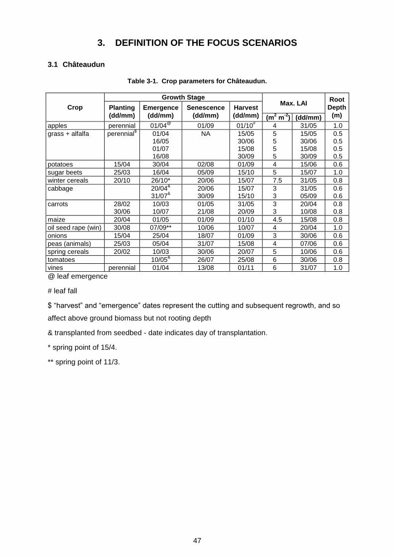
47

3. DEFINITION OF THE FOCUS SCENARIOS

3.1 Châteaudun

Table 3-1. Crop parameters for Châteaudun.

Crop

Growth Stage Max. LAI

Root

Depth

(m) Planting

(dd/mm)

Emergence

(dd/mm)

Senescence

(dd/mm)

Harvest

(dd/mm) (m2 m

-2) (dd/mm)

apples perennial 01/04@

01/09 01/10# 4 31/05 1.0

grass + alfalfa perennial$ 01/04

16/05 01/07 16/08

NA 15/05 30/06 15/08 30/09

5 5 5 5

15/05 30/06 15/08 30/09

0.5 0.5 0.5 0.5

potatoes 15/04 30/04 02/08 01/09 4 15/06 0.6

sugar beets 25/03 16/04 05/09 15/10 5 15/07 1.0

winter cereals 20/10 26/10* 20/06 15/07 7.5 31/05 0.8

cabbage 20/04&

31/07&

20/06 30/09

15/07 15/10

3 3

31/05 05/09

0.6 0.6

carrots 28/02 30/06

10/03 10/07

01/05 21/08

31/05 20/09

3 3

20/04 10/08

0.8 0.8

maize 20/04 01/05 01/09 01/10 4.5 15/08 0.8

oil seed rape (win) 30/08 07/09** 10/06 10/07 4 20/04 1.0

onions 15/04 25/04 18/07 01/09 3 30/06 0.6

peas (animals) 25/03 05/04 31/07 15/08 4 07/06 0.6

spring cereals 20/02 10/03 30/06 20/07 5 10/06 0.6

tomatoes 10/05& 26/07 25/08 6 30/06 0.8

vines perennial 01/04 13/08 01/11 6 31/07 1.0

@ leaf emergence

# leaf fall

$ “harvest” and “emergence” dates represent the cutting and subsequent regrowth, and so

affect above ground biomass but not rooting depth

& transplanted from seedbed - date indicates day of transplantation.

* spring point of 15/4.

** spring point of 11/3.

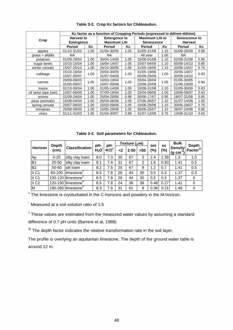
48

Table 3-2. Crop Kc factors for Châteaudun.

Crop

Kc factor as a function of Cropping Periods (expressed in dd/mm-dd/mm)

Harvest to

Emergence

Emergence to

Maximum LAI

Maximum LAI to

Senescence

Senescence to

Harvest

Period Kc Period Kc Period Kc Period Kc

apples 01/10-31/03 1.00 01/04-30/05 1.05 31/05-31/08 1.10 01/09-30/09 0.98

grass + alfalfa NA NA All year 1.00 NA

potatoes 01/09-29/04 1.00 30/04-14/06 1.05 15/06-01/08 1.10 02/08-31/08 0.90

sugar beets 15/10-15/04 1.00 16/04-14/07 1.05 15/07-04/09 1.10 05/09-14/10 0.85

winter cereals 15/07-25/10 1.00 26/10-30/05 1.05 31/05-19/06 1.10 20/06-14/07 0.70

cabbage 15/10-19/04 15/07-30/07

1.00 20/04-30/05 31/07-04/09

1.00 31/05-19/06 05/09-29/09

1.00 20/06-14/07 30/09-14/10

0.93

carrots 20/09-09/03 31/05-09/07

1.00 10/03-19/04 10/07-09/08

1.03 20/04-30/04 10/08-20/08

1.05 01/05-30/05 21/08-19/09

0.90

maize 01/10-30/04 1.00 01/05-14/08 1.05 15/08-31/08 1.10 01/09-30/09 0.83

oil seed rape (win) 10/07-06/09 1.00 07/09-19/04 1.00 20/04-09/06 1.00 10/06-09/07 0.93

onions 01/09-24/04 1.00 25/04-29/06 0.98 30/06-17/07 0.95 18/07-31/08 0.85

peas (animals) 15/08-04/04 1.00 05/04-06/06 1.05 07/06-30/07 1.10 31/07-14/08 1.05

spring cereals 20/07-09/03 1.00 10/03-09/06 1.05 10/06-29/06 1.10 30/06-19/07 0.70

tomatoes 25/08-09/05 1.00 10/05-29/06 1.05 30/06-25/07 1.10 26/07-24/08 0.85

vines 01/11-31/03 1.00 01/04-30/07 0.88 31/07-12/08 0.75 13/08-31/10 0.65

Table 3-3. Soil parameters for Châteaudun.

Horizon Depth

(cm) Classification

pH-

H2O*

pH-

KCl†

Texture ( m) om

(%)

oc

(%)

Bulk

Density

(g cm-3

)

Depth

Factor@

<2 2-50 >50

Ap 0-25 silty clay loam 8.0 7.3 30 67 3 2.4 1.39 1.3 1.0

B1 25-50 silty clay loam 8.1 7.4 31 67 2 1.6 0.93 1.41 0.5

B2 50-60 silt loam 8.2 7.5 25 67 8 1.2 0.7 1.41 0.5

II C1 60-100 limestone# 8.5 7.8 26 44 30 0.5 0.3 1.37 0.3

II C1 100-120 limestone# 8.5 7.8 26 44 30 0.5 0.3 1.37 0

II C2 120-190 limestone# 8.5 7.8 24 38 38 0.46 0.27 1.41 0

M 190-260 limestone# 8.3 7.6 31 61 8 0.36 0.21 1.49 0

# The limestone is cryoturbated in the C-horizons and powdery in the M-horizon.

* Measured at a soil solution ratio of 1:5

† These values are estimated from the measured water values by assuming a standard

difference of 0.7 pH units (Barrere et al, 1988)

@ The depth factor indicates the relative transformation rate in the soil layer.

The profile is overlying an aquitanian limestone. The depth of the ground water table is

around 12 m.

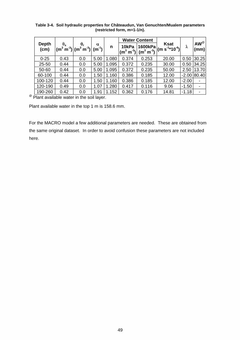
49

Table 3-4. Soil hydraulic properties for Châteaudun, Van Genuchten/Mualem parameters

(restricted form, m=1-1/n).

Depth

(cm) s

(m3 m

-3)

r

(m3 m

-3)

(m-1)

n

Water Content Ksat

(m s-1

*10-6)

AW

@

(mm) 10kPa

(m3 m

-3)

1600kPa

(m3 m

-3)

0-25 0.43 0.0 5.00 1.080 0.374 0.253 20.00 0.50 30.25

25-50 0.44 0.0 5.00 1.095 0.372 0.235 30.00 0.50 34.25

50-60 0.44 0.0 5.00 1.095 0.372 0.235 50.00 2.50 13.70

60-100 0.44 0.0 1.50 1.160 0.386 0.185 12.00 -2.00 80.40

100-120 0.44 0.0 1.50 1.160 0.386 0.185 12.00 -2.00 -

120-190 0.49 0.0 1.07 1.280 0.417 0.116 9.06 -1.50 -

190-260 0.42 0.0 1.91 1.152 0.362 0.176 14.81 -1.18 - @

Plant available water in the soil layer.

Plant available water in the top 1 m is 158.6 mm.

For the MACRO model a few additional parameters are needed. These are obtained from

the same original dataset. In order to avoid confusion these parameters are not included

here.

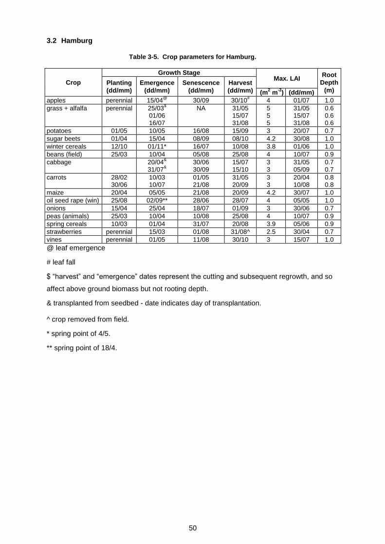
50

3.2 Hamburg

Table 3-5. Crop parameters for Hamburg.

Crop


Root

Depth

(m) Planting

(dd/mm)

Emergence

(dd/mm)

Senescence

(dd/mm)

Harvest

(dd/mm) (m2 m

-2) (dd/mm)


30/09 30/10# 4 01/07 1.0

grass + alfalfa perennial 25/03$

01/06 16/07

NA 31/05 15/07 31/08

5 5 5

31/05 15/07 31/08

0.6 0.6 0.6

potatoes 01/05 10/05 16/08 15/09 3 20/07 0.7

sugar beets 01/04 15/04 08/09 08/10 4.2 30/08 1.0

winter cereals 12/10 01/11* 16/07 10/08 3.8 01/06 1.0

beans (field) 25/03 10/04 05/08 25/08 4 10/07 0.9

cabbage 20/04&

31/07&

30/06 30/09

15/07 15/10

3 3

31/05 05/09

0.7 0.7

carrots 28/02 30/06

10/03 10/07

01/05 21/08

31/05 20/09

3 3

20/04 10/08

0.8 0.8

maize 20/04 05/05 21/08 20/09 4.2 30/07 1.0

oil seed rape (win) 25/08 02/09** 28/06 28/07 4 05/05 1.0

onions 15/04 25/04 18/07 01/09 3 30/06 0.7

peas (animals) 25/03 10/04 10/08 25/08 4 10/07 0.9

spring cereals 10/03 01/04 31/07 20/08 3.9 05/06 0.9

strawberries perennial 15/03 01/08 31/08^ 2.5 30/04 0.7

vines perennial 01/05 11/08 30/10 3 15/07 1.0

@ leaf emergence

# leaf fall


affect above ground biomass but not rooting depth.


^ crop removed from field.



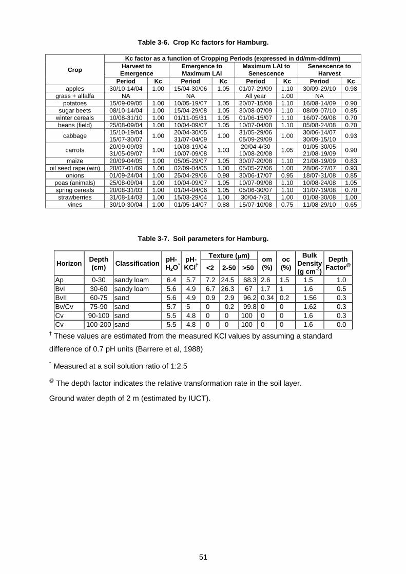
51

Table 3-6. Crop Kc factors for Hamburg.

Crop


Harvest to

Emergence

Emergence to

Maximum LAI

Maximum LAI to

Senescence

Senescence to

Harvest


apples 30/10-14/04 1.00 15/04-30/06 1.05 01/07-29/09 1.10 30/09-29/10 0.98


potatoes 15/09-09/05 1.00 10/05-19/07 1.05 20/07-15/08 1.10 16/08-14/09 0.90

sugar beets 08/10-14/04 1.00 15/04-29/08 1.05 30/08-07/09 1.10 08/09-07/10 0.85

winter cereals 10/08-31/10 1.00 01/11-05/31 1.05 01/06-15/07 1.10 16/07-09/08 0.70

beans (field) 25/08-09/04 1.00 10/04-09/07 1.05 10/07-04/08 1.10 05/08-24/08 0.70

cabbage 15/10-19/04 15/07-30/07

1.00 20/04-30/05 31/07-04/09

1.00 31/05-29/06 05/09-29/09

1.00 30/06-14/07 30/09-15/10

0.93

carrots 20/09-09/03 31/05-09/07

1.00 10/03-19/04 10/07-09/08

1.03 20/04-4/30

10/08-20/08 1.05

01/05-30/05 21/08-19/09

0.90

maize 20/09-04/05 1.00 05/05-29/07 1.05 30/07-20/08 1.10 21/08-19/09 0.83

oil seed rape (win) 28/07-01/09 1.00 02/09-04/05 1.00 05/05-27/06 1.00 28/06-27/07 0.93

onions 01/09-24/04 1.00 25/04-29/06 0.98 30/06-17/07 0.95 18/07-31/08 0.85

peas (animals) 25/08-09/04 1.00 10/04-09/07 1.05 10/07-09/08 1.10 10/08-24/08 1.05

spring cereals 20/08-31/03 1.00 01/04-04/06 1.05 05/06-30/07 1.10 31/07-19/08 0.70

strawberries 31/08-14/03 1.00 15/03-29/04 1.00 30/04-7/31 1.00 01/08-30/08 1.00

vines 30/10-30/04 1.00 01/05-14/07 0.88 15/07-10/08 0.75 11/08-29/10 0.65

Table 3-7. Soil parameters for Hamburg.

Horizon Depth

(cm) Classification

pH-

H2O*

pH-

KCl†

Texture ( m) om

(%)

oc

(%)

Bulk

Density

(g cm-3

)

Depth

Factor@

<2 2-50 >50

Ap 0-30 sandy loam 6.4 5.7 7.2 24.5 68.3 2.6 1.5 1.5 1.0

BvI 30-60 sandy loam 5.6 4.9 6.7 26.3 67 1.7 1 1.6 0.5

BvII 60-75 sand 5.6 4.9 0.9 2.9 96.2 0.34 0.2 1.56 0.3

Bv/Cv 75-90 sand 5.7 5 0 0.2 99.8 0 0 1.62 0.3

Cv 90-100 sand 5.5 4.8 0 0 100 0 0 1.6 0.3

Cv 100-200 sand 5.5 4.8 0 0 100 0 0 1.6 0.0 † These values are estimated from the measured KCl values by assuming a standard


* Measured at a soil solution ratio of 1:2.5


Ground water depth of 2 m (estimated by IUCT).

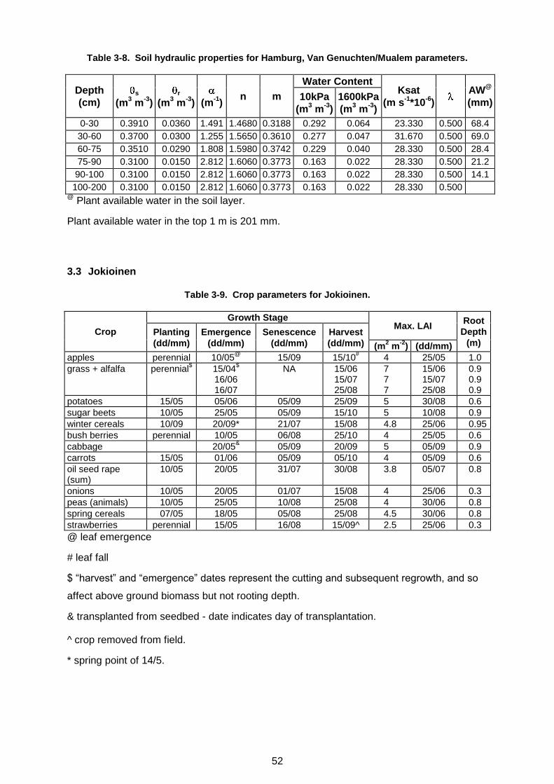
52

Table 3-8. Soil hydraulic properties for Hamburg, Van Genuchten/Mualem parameters.

Depth

(cm) s

(m3 m

-3)

r

(m3 m

-3)

(m-1)

n m

Water Content Ksat

(m s-1*10

-6)

AW

@

(mm) 10kPa

(m3 m

-3)

1600kPa

(m3 m

-3)

0-30 0.3910 0.0360 1.491 1.4680 0.3188 0.292 0.064 23.330 0.500 68.4

30-60 0.3700 0.0300 1.255 1.5650 0.3610 0.277 0.047 31.670 0.500 69.0

60-75 0.3510 0.0290 1.808 1.5980 0.3742 0.229 0.040 28.330 0.500 28.4

75-90 0.3100 0.0150 2.812 1.6060 0.3773 0.163 0.022 28.330 0.500 21.2

90-100 0.3100 0.0150 2.812 1.6060 0.3773 0.163 0.022 28.330 0.500 14.1

100-200 0.3100 0.0150 2.812 1.6060 0.3773 0.163 0.022 28.330 0.500 @


Plant available water in the top 1 m is 201 mm.

3.3 Jokioinen

Table 3-9. Crop parameters for Jokioinen.

Crop


Root

Depth

(m) Planting

(dd/mm)

Emergence

(dd/mm)

Senescence

(dd/mm)

Harvest

(dd/mm) (m2 m

-2) (dd/mm)


15/09 15/10# 4 25/05 1.0


$

16/06 16/07

NA 15/06 15/07 25/08

7 7 7

15/06 15/07 25/08

0.9 0.9 0.9

potatoes 15/05 05/06 05/09 25/09 5 30/08 0.6

sugar beets 10/05 25/05 05/09 15/10 5 10/08 0.9

winter cereals 10/09 20/09* 21/07 15/08 4.8 25/06 0.95

bush berries perennial 10/05 06/08 25/10 4 25/05 0.6

cabbage 20/05& 05/09 20/09 5 05/09 0.9

carrots 15/05 01/06 05/09 05/10 4 05/09 0.6

oil seed rape (sum)

10/05 20/05 31/07 30/08 3.8 05/07 0.8

onions 10/05 20/05 01/07 15/08 4 25/06 0.3

peas (animals) 10/05 25/05 10/08 25/08 4 30/06 0.8

spring cereals 07/05 18/05 05/08 25/08 4.5 30/06 0.8


@ leaf emergence

# leaf fall






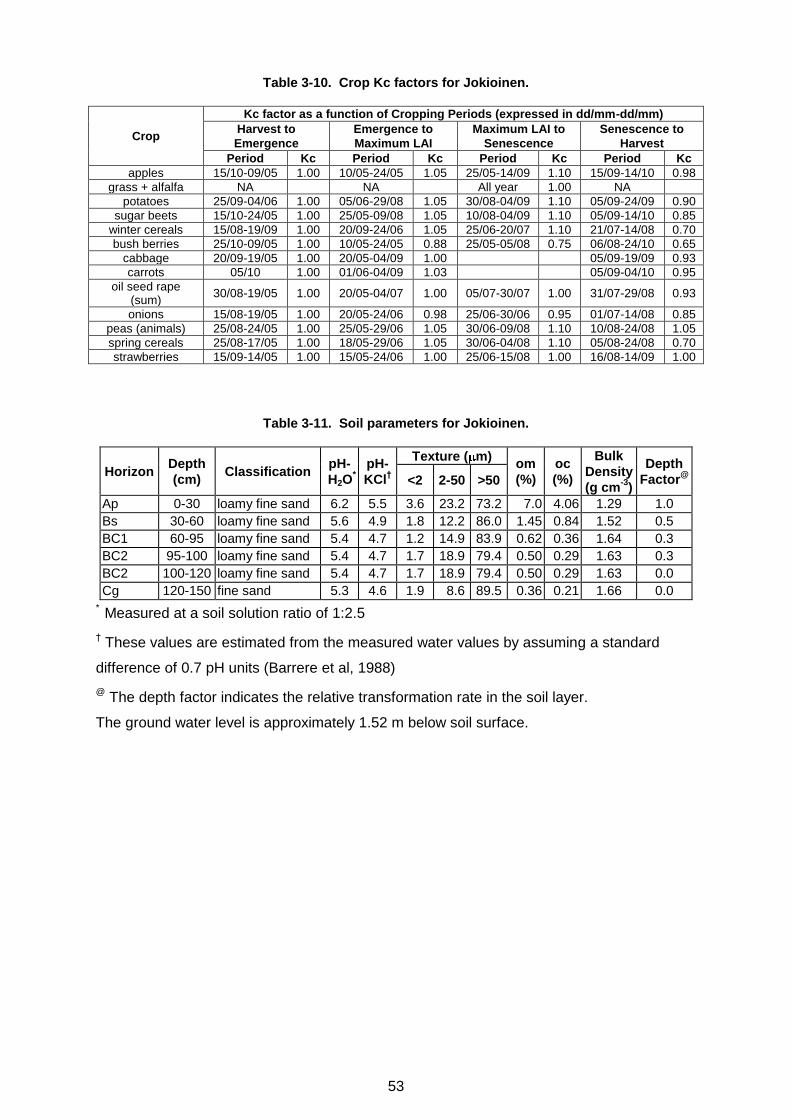
53

Table 3-10. Crop Kc factors for Jokioinen.

Crop


Harvest to

Emergence

Emergence to

Maximum LAI

Maximum LAI to

Senescence

Senescence to

Harvest


apples 15/10-09/05 1.00 10/05-24/05 1.05 25/05-14/09 1.10 15/09-14/10 0.98


potatoes 25/09-04/06 1.00 05/06-29/08 1.05 30/08-04/09 1.10 05/09-24/09 0.90

sugar beets 15/10-24/05 1.00 25/05-09/08 1.05 10/08-04/09 1.10 05/09-14/10 0.85

winter cereals 15/08-19/09 1.00 20/09-24/06 1.05 25/06-20/07 1.10 21/07-14/08 0.70

bush berries 25/10-09/05 1.00 10/05-24/05 0.88 25/05-05/08 0.75 06/08-24/10 0.65

cabbage 20/09-19/05 1.00 20/05-04/09 1.00 05/09-19/09 0.93

carrots 05/10 1.00 01/06-04/09 1.03 05/09-04/10 0.95

oil seed rape (sum)

30/08-19/05 1.00 20/05-04/07 1.00 05/07-30/07 1.00 31/07-29/08 0.93

onions 15/08-19/05 1.00 20/05-24/06 0.98 25/06-30/06 0.95 01/07-14/08 0.85

peas (animals) 25/08-24/05 1.00 25/05-29/06 1.05 30/06-09/08 1.10 10/08-24/08 1.05

spring cereals 25/08-17/05 1.00 18/05-29/06 1.05 30/06-04/08 1.10 05/08-24/08 0.70

strawberries 15/09-14/05 1.00 15/05-24/06 1.00 25/06-15/08 1.00 16/08-14/09 1.00

Table 3-11. Soil parameters for Jokioinen.

Horizon Depth

(cm) Classification

pH-

H2O*

pH-

KCl†

Texture ( m) om

(%)

oc

(%)

Bulk

Density

(g cm-3

)

Depth

Factor@

<2 2-50 >50

Ap 0-30 loamy fine sand 6.2 5.5 3.6 23.2 73.2 7.0 4.06 1.29 1.0

Bs 30-60 loamy fine sand 5.6 4.9 1.8 12.2 86.0 1.45 0.84 1.52 0.5

BC1 60-95 loamy fine sand 5.4 4.7 1.2 14.9 83.9 0.62 0.36 1.64 0.3



Cg 120-150 fine sand 5.3 4.6 1.9 8.6 89.5 0.36 0.21 1.66 0.0 *

Measured at a soil solution ratio of 1:2.5




The ground water level is approximately 1.52 m below soil surface.

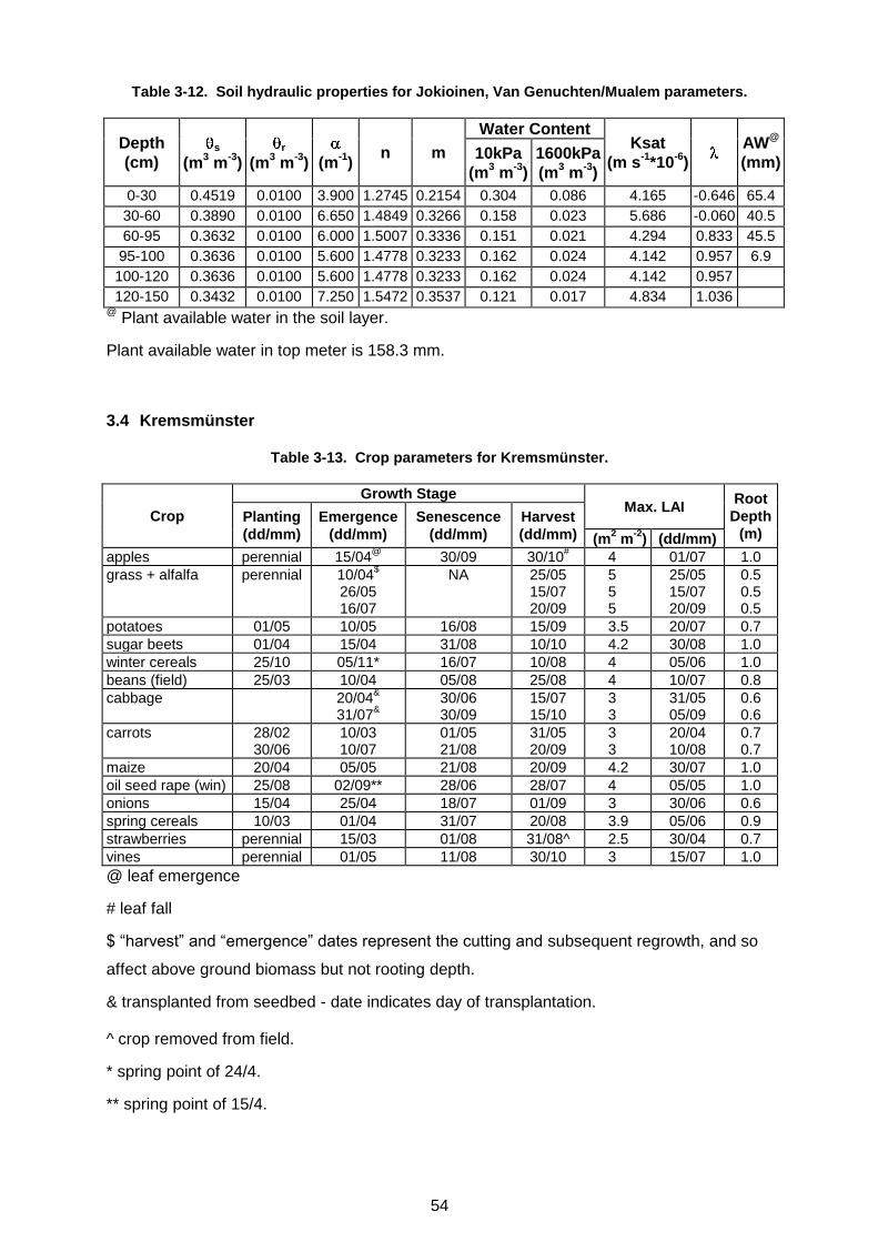
54

Table 3-12. Soil hydraulic properties for Jokioinen, Van Genuchten/Mualem parameters.

Depth

(cm) s

(m3 m

-3)

r

(m3 m

-3)

(m-1)

n m

Water Content Ksat

(m s-1*10

-6)

AW

@

(mm) 10kPa

(m3 m

-3)

1600kPa

(m3 m

-3)

0-30 0.4519 0.0100 3.900 1.2745 0.2154 0.304 0.086 4.165 -0.646 65.4

30-60 0.3890 0.0100 6.650 1.4849 0.3266 0.158 0.023 5.686 -0.060 40.5

60-95 0.3632 0.0100 6.000 1.5007 0.3336 0.151 0.021 4.294 0.833 45.5

95-100 0.3636 0.0100 5.600 1.4778 0.3233 0.162 0.024 4.142 0.957 6.9

100-120 0.3636 0.0100 5.600 1.4778 0.3233 0.162 0.024 4.142 0.957

120-150 0.3432 0.0100 7.250 1.5472 0.3537 0.121 0.017 4.834 1.036 @


Plant available water in top meter is 158.3 mm.

3.4 Kremsmünster

Table 3-13. Crop parameters for Kremsmünster.

Crop


Root

Depth

(m) Planting

(dd/mm)

Emergence

(dd/mm)

Senescence

(dd/mm)

Harvest

(dd/mm) (m2 m

-2) (dd/mm)


30/09 30/10# 4 01/07 1.0


26/05 16/07

NA 25/05 15/07 20/09

5 5 5

25/05 15/07 20/09

0.5 0.5 0.5

potatoes 01/05 10/05 16/08 15/09 3.5 20/07 0.7

sugar beets 01/04 15/04 31/08 10/10 4.2 30/08 1.0

winter cereals 25/10 05/11* 16/07 10/08 4 05/06 1.0

beans (field) 25/03 10/04 05/08 25/08 4 10/07 0.8

cabbage 20/04&

31/07&

30/06 30/09

15/07 15/10

3 3

31/05 05/09

0.6 0.6

carrots 28/02 30/06

10/03 10/07

01/05 21/08

31/05 20/09

3 3

20/04 10/08

0.7 0.7

maize 20/04 05/05 21/08 20/09 4.2 30/07 1.0

oil seed rape (win) 25/08 02/09** 28/06 28/07 4 05/05 1.0

onions 15/04 25/04 18/07 01/09 3 30/06 0.6

spring cereals 10/03 01/04 31/07 20/08 3.9 05/06 0.9


vines perennial 01/05 11/08 30/10 3 15/07 1.0

@ leaf emergence

# leaf fall







55

Table 3-14. Crop Kc factors for Kremsmünster.

Crop


Harvest to

Emergence

Emergence to

Maximum LAI

Maximum LAI to

Senescence

Senescence to

Harvest


apples 30/10-14/04 1.00 15/04-30/06 1.05 01/07-29/09 1.10 30/09-29/10 0.98


potatoes 15/09-09/05 1.00 10/05-19/07 1.05 20/07-15/08 1.10 16/08-14/09 0.90

sugar beets 10/10-14/04 1.00 15/04-29/08 1.05 30/08 1.10 31/08-09/10 0.85

winter cereals 10/08-04/11 1.00 05/11-04/06 1.05 05/06-15/07 1.10 16/07-09/08 0.70

beans (field) 25/08-09/04 1.00 10/04-09/07 1.05 10/07-04/08 1.10 05/08-24/08 0.70

cabbage 15/10-19/04 15/07-30/07

1.00 20/04-30/05 31/07-04/09

1.00 31/05-29/06 05/09-29/09

1.00 30/06-14/07 30/09-14/10

0.93

carrots 20/09-09/03 31/05-09/07

1.00 10/03-19/04 10/07-09/08

1.03 20/04-30/04 10/08-20/08

1.05 01/05-30/05 21/08-19/09

0.90

maize 20/09-04/05 1.00 05/05-29/07 1.05 30/07-20/08 1.10 21/08-19/09 0.83

oil seed rape (win) 28/07-01/09 1.00 02/09-04/05 1.00 05/05-27/06 1.00 28/06-27/07 0.93

onions 01/09-24/04 1.00 25/04-29/06 0.98 30/06-17/07 0.95 18/07-31/08 0.85

spring cereals 20/08-31/03 1.00 01/04-04/06 1.05 05/06-30/07 1.10 31/07-19/08 0.70

strawberries 31/08-14/03 1.00 15/03-29/04 1.00 30/04-31/07 1.00 01/08-30/08 1.00

vines 30/10-30/04 1.00 01/05-14/07 0.88 15/07-10/08 0.75 11/08-29/10 0.65

Table 3-15. Soil parameters for Kremsmünster.

Depth

(cm) Classification

pH-

H2O*

pH-

KCl†

Texture ( m) om

(%)

oc

(%)

Bulk

Density

(g cm-3

)

Depth

Factor@

<2 2-50 >50

0-30 loam/silt loam 7.7 7.0 14 50 36 3.6 2.1 1.41 1.0

30-50 loam/silt loam 7.0 6.3 25 50 25 1.0 0.6 1.42 0.5

50-60 loam/clay loam 7.1 6.4 27 44 29 0.5 0.3 1.43 0.5

60-100 loam/clay loam 7.1 6.4 27 44 29 0.5 0.3 1.43 0.3

100-200 loam/clay loam 7.1 6.4 27 44 29 0.5 0.3 1.43 0.0 † These values are estimated from the measured KCl values by assuming a standard




The depth of ground water is around 1.6 m, for apples and vines a deeper ground water

level has to be assumed. At a depth of approximately 3.3 m a rather impermeable layer is

present.

Layer below 1 m copied from 60 - 100 cm layer.

Layer 0 - 30 cm is Ap horizon, 30 - 100 cm is Bwg horizon.

56

Table 3-16. Soil hydraulic properties for Kremsmünster, Van Genuchten/Mualem parameters.

Depth

(cm) s

(m3 m

-3)

r

(m3 m

-3)

(m-1)

n m

Water Content Ksat

(m s-1*10

-6)

AW

@

(mm) 10kPa

(m3 m

-3)

1600kPa

(m3 m

-3)

0-30 0.4246 0.0100 2.440 1.2186 0.1794 0.334 0.123 1.769 -2.080 63.3

30-50 0.4446 0.0100 2.700 1.1659 0.1423 0.365 0.169 2.780 -2.404 39.2

50-60 0.4430 0.0100 3.080 1.1578 0.1363 0.361 0.173 2.459 -2.065 18.8

60-100 0.4430 0.0100 3.080 1.1578 0.1363 0.361 0.173 2.459 -2.065 75.2

100-200 0.4430 0.0100 3.080 1.1578 0.1363 0.361 0.173 2.459 -2.065 @

Plant available water in soil layer.


Layer 100 - 200 cm copied from layer 60 - 100 cm because of lacking information.

3.5 Okehampton

Table 3-17. Crop parameters for Okehampton.

Crop


Root

Depth

(m) Planting

(dd/mm)

Emergence

(dd/mm)

Senescence

(dd/mm)

Harvest

(dd/mm) (m2 m

-2) (dd/mm)


16/08 15/09# 2.5 15/06 1.0


16/05 16/07

NA 15/05 15/07 15/09

4.5 4.5 4.5

15/05 15/07 15/09

0.45 0.45 0.45

potatoes 15/04 30/04 02/08 01/09 4 15/07 0.6

sugar beets 10/04 25/04 15/09 25/10 3 30/08 0.8

winter cereals 07/10 17/10* 07/07 01/08 7.5 15/05 0.8

beans (field) 01/03 15/03 26/08 15/09 4 07/06 0.45

linseed 25/03 30/03 18/08 25/09 3 25/06 0.6

maize 07/05 25/05 18/08 07/10 7 15/07 0.8

oil seed rape (sum)

25/03 30/03 21/07 20/08 3 15/05 0.6

oil seed rape (win) 07/08 14/08** 21/06 21/07 4.5 30/04 0.85

peas (animals) 25/03 05/04 31/07 15/08 4.0 07/06 0.45

spring cereals 25/03 01/04 31/07 20/08 4.5 22/05 0.6

@ leaf emergence

# leaf fall





57

Table 3-18. Crop Kc factors for Okehampton.

Crop


Harvest to

Emergence

Emergence to

Maximum LAI

Maximum LAI to

Senescence

Senescence to

Harvest


apples 15/09-24/03 1.00 25/03-14/06 1.05 15/06-15/08 1.10 16/08-14/09 0.98


potatoes 01/09-29/04 1.00 30/04-14/07 1.05 15/07-01/08 1.10 02/08-31/08 0.90

sugar beets 25/10-24/04 1.00 25/04-29/08 1.05 30/08-14/09 1.10 15/09-24/10 0.85

winter cereals 01/08-16/10 1.00 17/10-14/05 1.05 15/05-06/07 1.10 07/07-31/07 0.70

beans (field) 15/09-14/03 1.00 15/03-06/06 1.05 07/06-25/08 1.10 26/08-14/09 0.70

linseed 25/0929/03 1.00 30/03-24/06 1.03 25/06-17/08 1.05 18/08-24/09 0.65

maize 07/10-24/05 1.00 25/05-14/07 1.05 15/07-17/08 1.10 18/08-06/10 0.83

oil seed rape (sum)

20/08-29/03 1.00 30/03-14/05 1.00 15/05-20/07 1.00 21/07-19/08 0.93

oil seed rape (win) 21/07-13/08 1.00 14/08-29/04 1.00 30/04-20/06 1.00 21/06-20/07 0.93

peas (animals) 15/08-04/04 1.00 05/04-06/06 1.05 07/06-30/07 1.10 31/07-14/08 1.05

spring cereals 20/08-31/03 1.00 01/04-21/05 1.05 22/05-30/07 1.10 31/07-19/08 0.70

Table 3-19. Soil parameters for Okehampton.

Horizon Depth

(cm) Classification

pH-

H2O*

pH-

KCl†

Texture ( m) om

(%)

oc

(%)

Bulk

Density

(g cm-3

)

Depth

Factor@

<2 2-50 >50

A 0-25 loam 5.8 5.1 18 43 39 3.8 2.2 1.28 1.0

Bw1 25-55 loam 6.3 5.6 17 41 42 1.2 0.7 1.34 0.5

BC 55-85 sandy loam 6.5 5.8 14 31 55 0.69 0.4 1.42 0.3

C 85-100 sandy loam 6.6 5.9 9 22 69 0.17 0.1 1.47 0.3

C 100-150 sandy loam 6.6 5.9 9 22 69 0.17 0.1 1.47 0.0 *





The depth of ground is about 20 m.

58

Table 3-20. Soil hydraulic properties for Okehampton, Van Genuchten/Mualem parameters.

Depth

(cm) s

(m3 m

-3)

r

(m3 m

-3)

(m-1)

n m

Water Content Ksat

(m s-1*10

-6)

AW

@

(mm) 10kPa

(m3 m

-3)

1600kPa

(m3 m

-3)

0-25 0.4664 0.0100 3.550 1.1891 0.1590 0.358 0.148 3.484 -2.581 52.5

25-55 0.4602 0.0100 3.640 1.2148 0.1768 0.340 0.125 4.887 -2.060 64.5

55-85 0.4320 0.0100 4.560 1.2526 0.2017 0.290 0.090 4.838 -1.527 60.0

85-100 0.4110 0.0100 5.620 1.3384 0.2528 0.228 0.050 4.449 -0.400 26.7

100-150 0.4110 0.0100 5.620 1.3384 0.2528 0.228 0.050 4.449 -0.400 @



3.6 Piacenza

Table 3-21. Crop parameters for Piacenza.

Crop


Root

Depth

(m) Planting

(dd/mm)

Emergence

(dd/mm)

Senescence

(dd/mm)

Harvest

(dd/mm) (m2 m

-2) (dd/mm)


02/09 01/11# 5 31/05 1.0


$

16/05 16/07

NA 15/05 15/07 20/09

4 4 4

15/05 15/07 20/09

0.8 0.8 0.8

potatoes 01/04 20/04 11/08 10/09 5 01/06 0.5

sugar beets 01/03 20/03 27/07 15/09 4 30/06 0.8

winter cereals 25/11 01/12* 01/06 01/07 7 10/05 1.0

citrus perennial evergreen NA NA 5 31/05 1.0

maize 30/04 15/05 30/09 30/10 5 31/07 1.0

oil seed rape (win) 30/09 05/10** 21/05 20/06 3.5 15/04 0.6

soybean 25/04 10/05 10/09 05/10 6.5 31/07 0.6

sunflower 01/04 20/04 26/08 20/09 4 20/06 1.0

tobacco 20/05& 25/09 05/10 4 20/07 1.0

tomatoes 10/05& 26/07 25/08 6 30/06 1.0

vines perennial 01/04 13/08 01/11 6 31/07 1.0

@ leaf emergence

# leaf fall






59

Table 3-22. Crop Kc factors for Piacenza.

Crop


Harvest to

Emergence

Emergence to

Maximum LAI

Maximum LAI to

Senescence

Senescence to

Harvest


apples 01/11-31/03 1.00 01/04-30/05 1.05 31/05-01/09 1.10 02/09-31/10 0.98


potatoes 10/09-19/04 1.00 20/04-31/05 1.05 01/06-10/08 1.10 11/08-09/09 0.90

sugar beets 15/09-19/03 1.00 20/03-29/06 1.05 30/06-26/07 1.10 27/07-14/09 0.85

winter cereals 01/07-30/11 1.00 01/12-09/05 1.05 10/05-31/05 1.10 01/06-30/06 0.70

citrus NA NA All year 0.60 NA

maize 30/10-14/05 1.00 15/05-30/07 1.05 31/07-29/09 1.10 30/09-29/10 0.83

oil seed rape (win) 20/06-04/10 1.00 05/10-14/04 1.00 15/04-20/05 1.00 21/05-19/06 0.93

soybean 05/10-09/05 1.00 10/05-30/07 1.03 31/07-09/09 1.05 10/09-04/10 0.75

sunflower 20/09-19/04 1.00 20/04-19/06 1.05 20/06-25/08 1.10 26/08-19/09 0.75

tobacco 05/10-19/05 1.00 20/05-19/07 1.00 20/07-24/09 1.00 25/09-04/10 0.93

tomatoes 25/08-09/05 1.00 10/05-29/06 1.05 30/06-25/07 1.10 26/07-24/08 0.85

vines 01/11-31/03 1.00 01/04-30/07 0.88 31/07-12/08 0.75 13/08-31/10 0.65

Table 3-23. Soil parameters for Piacenza.

Horizon Depth

(cm) Classification

pH-

H2O*

pH-

KCl†

Texture ( m) om

(%)

oc

(%)

Bulk

Density

(g cm-3

)

Depth

Factor@

<2 2-50 >50

Ap 0-30 loam 7 6.3 15 45 40 2.17 1.26 1.3 1.0

Ap 30-40 loam 7 6.3 15 45 40 2.17 1.26 1.3 0.5

Bw 40-60 silt loam 6.3 5.6 7 53 40 0.80 0.47 1.35 0.5

Bw 60-80 silt loam 6.3 5.6 7 53 40 0.80 0.47 1.35 0.3

2C 80-100 sand 6.4 5.7 0 0 100 0 0 1.45 0.3

2C 100-170 sand 6.4 5.7 0 0 100 0 0 1.45 0.0 *





The depth of ground water is 1.5 m (range 1.30-1.70 m).

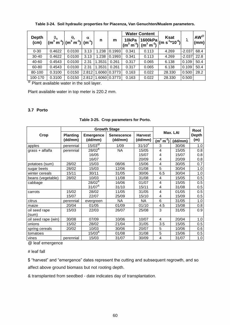
60

Table 3-24. Soil hydraulic properties for Piacenza, Van Genuchten/Mualem parameters.

Depth

(cm) s

(m3 m

-3)

r

(m3 m

-3)

(m-1)

n m

Water Content Ksat

(m s-1*10

-6)

AW

@

(mm) 10kPa

(m3 m

-3)

1600kPa

(m3 m

-3)

0-30 0.4622 0.0100 3.13 1.238 0.1993 0.341 0.113 4.269 -2.037 68.4

30-40 0.4622 0.0100 3.13 1.238 0.1993 0.341 0.113 4.269 -2.037 22.8

40-60 0.4543 0.0100 2.31 1.3531 0.261 0.317 0.065 6.138 0.109 50.4

60-80 0.4543 0.0100 2.31 1.3531 0.261 0.317 0.065 6.138 0.109 50.4

80-100 0.3100 0.0150 2.812 1.6060 0.3773 0.163 0.022 28.330 0.500 28.2

100-170 0.3100 0.0150 2.812 1.6060 0.3773 0.163 0.022 28.330 0.500 @



3.7 Porto

Table 3-25. Crop parameters for Porto.

Crop


Root

Depth

(m) Planting

(dd/mm)

Emergence

(dd/mm)

Senescence

(dd/mm)

Harvest

(dd/mm) (m2 m

-2) (dd/mm)


1/09 31/10# 3 30/06 1.0


16/05 16/07

NA 15/05 15/07 20/09

4 4 4

15/05 15/07 20/09

0.8 0.8 0.8

potatoes (sum) 28/02 15/03 08/06 15/06 4 30/05 0.7

sugar beets 28/02 15/03 12/06 01/08 5 30/04 1.0

winter cereals 15/11 30/11 31/05 30/06 6.5 30/04 1.0

beans (vegetable) 28/02 10/03 11/08 31/08 4 15/05 0.5

cabbage 28/02&

31/07&

16/06 31/10

01/07 15/11

4 4

15/05 31/08

0.5 0.5

carrots 15/02 15/07

28/02 22/07

11/05 25/09

31/05 15/10

4 4

01/05 15/09

0.5 0.5

citrus perennial evergreen NA NA 6 31/05 1.0

maize 20/04 01/05 01/09 01/10 4.5 15/08 0.8

oil seed rape (sum)

15/03 22/03 26/07 25/08 3 31/05 0.9

oil seed rape (win) 30/08 07/09 10/06 10/07 4 20/04 1.0

onions 15/02 28/02 21/04 31/05 3.5 15/05 0.5

spring cereals 20/02 10/03 30/06 20/07 5 10/06 0.6

tomatoes 15/03& 01/08 31/08 5 15/06 0.5

vines perennial 15/03 31/07 30/09 4 31/07 1.0

@ leaf emergence

# leaf fall




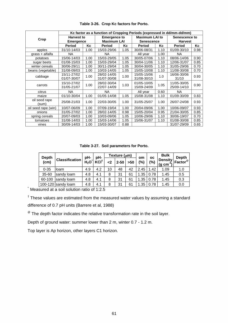
61

Table 3-26. Crop Kc factors for Porto.

Crop


Harvest to

Emergence

Emergence to

Maximum LAI

Maximum LAI to

Senescence

Senescence to

Harvest


apples 31/10-14/03 1.00 15/03-29/06 1.05 30/06-08/31 1.10 01/09-30/10 0.98


potatoes 15/06-14/03 1.00 15/03-29/05 1.05 30/05-07/06 1.10 08/06-14/06 0.90

sugar beets 01/08-15/03 1.00 15/03-29/04 1.05 30/04-11/06 1.10 12/06-31/07 0.85

winter cereals 30/06-29/11 1.00 30/11-29/04 1.05 30/04-30/05 1.10 31/05-29/06 0.70

beans (vegetable) 31/08-09/03 1.00 10/03-14/05 1.05 15/05-10/08 1.10 11/08-30/08 0.70

cabbage 15/11-27/02 01/07-30/07

1.00 28/02-14/05 31/07-30/08

1.00 15/05-15/06 31/08-30/10

1.0 16/06-30/06

31/10 0.93

carrots 15/10-27/02 31/05-21/07

1.00 28/02-30/04 22/07-14/09

1.03 01/05-10/05 15/09-24/09

1.05 11/05-30/05 25/09-14/10

0.90


maize 01/10-30/04 1.00 01/05-14/08 1.05 15/08-31/08 1.10 01/09-30/09 0.83

oil seed rape (sum)

25/08-21/03 1.00 22/03-30/05 1.00 31/05-25/07 1.00 26/07-24/08 0.93

oil seed rape (win) 10/07-06/09 1.00 07/09-19/04 1.00 20/04-09/06 1.00 10/06-09/07 0.93

onions 31/05-27/02 1.00 28/02-14/05 0.98 15/05-20/04 0.95 21/04-30/05 0.85

spring cereals 20/07-09/03 1.00 10/03-09/06 1.05 10/06-29/06 1.10 30/06-19/07 0.70

tomatoes 31/08-14/03 1.00 15/03-14/06 1.05 15/06-31/07 1.10 01/08-30/08 0.85

vines 30/09-14/03 1.00 15/03-30/07 0.88 31/07-29/09 0.65

Table 3-27. Soil parameters for Porto.

Depth

(cm) Classification

pH-

H2O*

pH-

KCl†

Texture ( m) om

(%)

oc

(%)

Bulk

Density

(g cm-3

)

Depth

Factor@

<2 2-50 >50

0-35 loam 4.9 4.2 10 48 42 2.45 1.42 1.09 1.0

35-60 sandy loam 4.8 4.1 8 31 61 1.35 0.78 1.45 0.5

60-100 sandy loam 4.8 4.1 8 31 61 1.35 0.78 1.45 0.3

100-120 sandy loam 4.8 4.1 8 31 61 1.35 0.78 1.45 0.0 *





Depth of ground water: summer lower than 2 m, winter 0.7 - 1.2 m.

Top layer is Ap horizon, other layers C1 horizon.

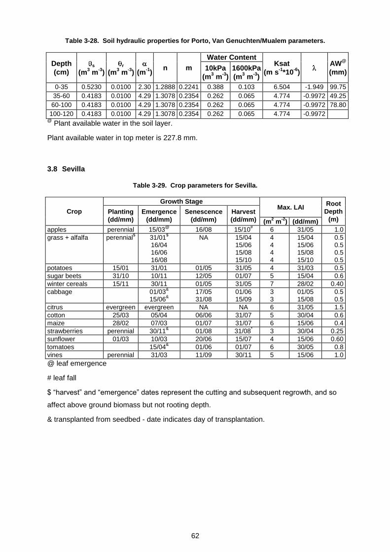
62

Table 3-28. Soil hydraulic properties for Porto, Van Genuchten/Mualem parameters.

Depth

(cm) s

(m3 m

-3)

r

(m3 m

-3)

(m-1)

n m

Water Content Ksat

(m s-1*10

-6)

AW

@

(mm) 10kPa

(m3 m

-3)

1600kPa

(m3 m

-3)

0-35 0.5230 0.0100 2.30 1.2888 0.2241 0.388 0.103 6.504 -1.949 99.75

35-60 0.4183 0.0100 4.29 1.3078 0.2354 0.262 0.065 4.774 -0.9972 49.25

60-100 0.4183 0.0100 4.29 1.3078 0.2354 0.262 0.065 4.774 -0.9972 78.80

100-120 0.4183 0.0100 4.29 1.3078 0.2354 0.262 0.065 4.774 -0.9972 @



3.8 Sevilla

Table 3-29. Crop parameters for Sevilla.

Crop


Root

Depth

(m) Planting

(dd/mm)

Emergence

(dd/mm)

Senescence

(dd/mm)

Harvest

(dd/mm) (m2 m

-2) (dd/mm)


16/08 15/10# 6 31/05 1.0


$

16/04 16/06 16/08

NA 15/04 15/06 15/08 15/10

4 4 4 4

15/04 15/06 15/08 15/10

0.5 0.5 0.5 0.5

potatoes 15/01 31/01 01/05 31/05 4 31/03 0.5

sugar beets 31/10 10/11 12/05 01/07 5 15/04 0.6

winter cereals 15/11 30/11 01/05 31/05 7 28/02 0.40

cabbage 01/03&

15/06&

17/05 31/08

01/06 15/09

3 3

01/05 15/08

0.5 0.5

citrus evergreen evergreen NA NA 6 31/05 1.5

cotton 25/03 05/04 06/06 31/07 5 30/04 0.6

maize 28/02 07/03 01/07 31/07 6 15/06 0.4

strawberries perennial 30/11& 01/08 31/08

* 3 30/04 0.25

sunflower 01/03 10/03 20/06 15/07 4 15/06 0.60

tomatoes 15/04& 01/06 01/07 6 30/05 0.8

vines perennial 31/03 11/09 30/11 5 15/06 1.0

@ leaf emergence

# leaf fall




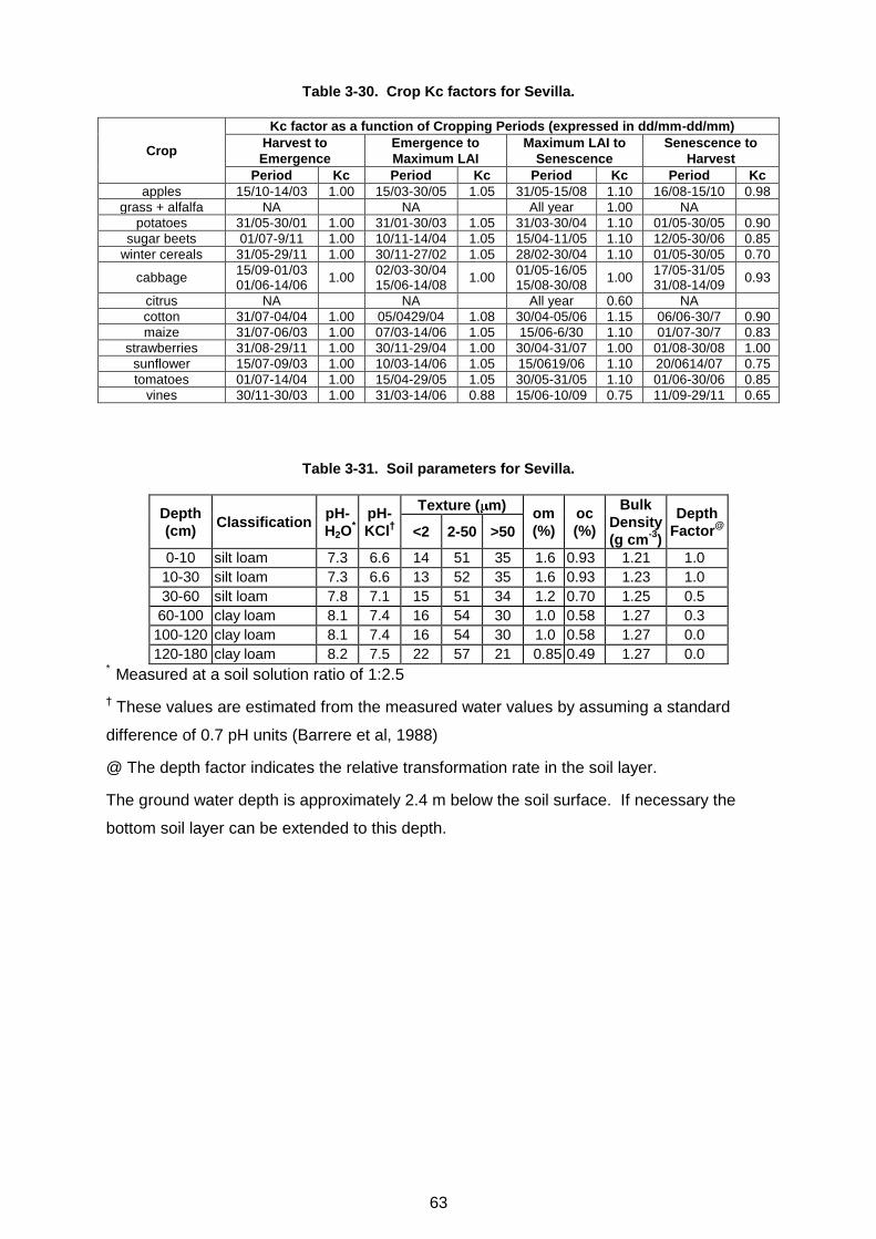
63

Table 3-30. Crop Kc factors for Sevilla.

Crop


Harvest to

Emergence

Emergence to

Maximum LAI

Maximum LAI to

Senescence

Senescence to

Harvest


apples 15/10-14/03 1.00 15/03-30/05 1.05 31/05-15/08 1.10 16/08-15/10 0.98


potatoes 31/05-30/01 1.00 31/01-30/03 1.05 31/03-30/04 1.10 01/05-30/05 0.90

sugar beets 01/07-9/11 1.00 10/11-14/04 1.05 15/04-11/05 1.10 12/05-30/06 0.85

winter cereals 31/05-29/11 1.00 30/11-27/02 1.05 28/02-30/04 1.10 01/05-30/05 0.70

cabbage 15/09-01/03 01/06-14/06

1.00 02/03-30/04 15/06-14/08

1.00 01/05-16/05 15/08-30/08

1.00 17/05-31/05 31/08-14/09

0.93


cotton 31/07-04/04 1.00 05/0429/04 1.08 30/04-05/06 1.15 06/06-30/7 0.90

maize 31/07-06/03 1.00 07/03-14/06 1.05 15/06-6/30 1.10 01/07-30/7 0.83

strawberries 31/08-29/11 1.00 30/11-29/04 1.00 30/04-31/07 1.00 01/08-30/08 1.00

sunflower 15/07-09/03 1.00 10/03-14/06 1.05 15/0619/06 1.10 20/0614/07 0.75

tomatoes 01/07-14/04 1.00 15/04-29/05 1.05 30/05-31/05 1.10 01/06-30/06 0.85

vines 30/11-30/03 1.00 31/03-14/06 0.88 15/06-10/09 0.75 11/09-29/11 0.65

Table 3-31. Soil parameters for Sevilla.

Depth

(cm) Classification

pH-

H2O*

pH-

KCl†

Texture ( m) om

(%)

oc

(%)

Bulk

Density

(g cm-3

)

Depth

Factor@

<2 2-50 >50

0-10 silt loam 7.3 6.6 14 51 35 1.6 0.93 1.21 1.0

10-30 silt loam 7.3 6.6 13 52 35 1.6 0.93 1.23 1.0

30-60 silt loam 7.8 7.1 15 51 34 1.2 0.70 1.25 0.5

60-100 clay loam 8.1 7.4 16 54 30 1.0 0.58 1.27 0.3

100-120 clay loam 8.1 7.4 16 54 30 1.0 0.58 1.27 0.0

120-180 clay loam 8.2 7.5 22 57 21 0.85 0.49 1.27 0.0 *





The ground water depth is approximately 2.4 m below the soil surface. If necessary the

bottom soil layer can be extended to this depth.

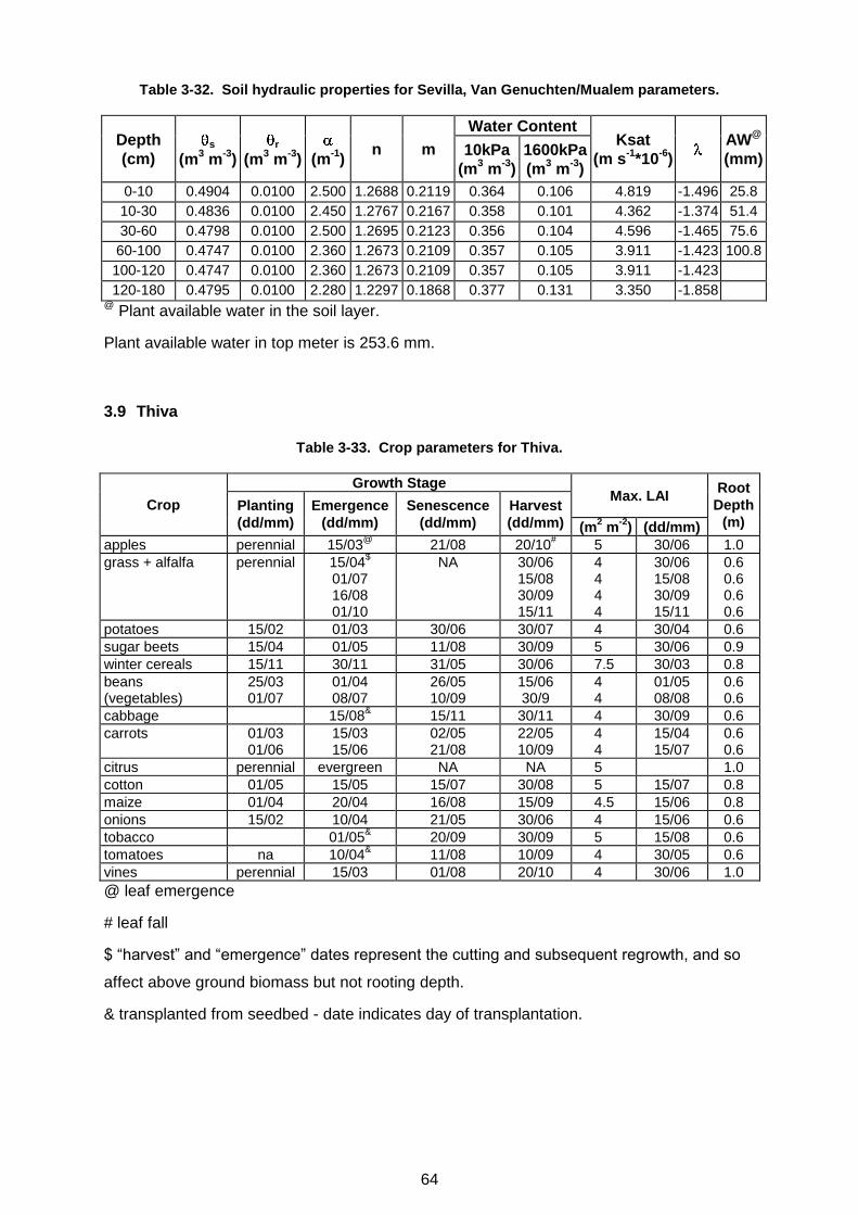
64

Table 3-32. Soil hydraulic properties for Sevilla, Van Genuchten/Mualem parameters.

Depth

(cm) s

(m3 m

-3)

r

(m3 m

-3)

(m-1)

n m

Water Content Ksat

(m s-1*10

-6)

AW

@

(mm) 10kPa

(m3 m

-3)

1600kPa

(m3 m

-3)

0-10 0.4904 0.0100 2.500 1.2688 0.2119 0.364 0.106 4.819 -1.496 25.8

10-30 0.4836 0.0100 2.450 1.2767 0.2167 0.358 0.101 4.362 -1.374 51.4

30-60 0.4798 0.0100 2.500 1.2695 0.2123 0.356 0.104 4.596 -1.465 75.6

60-100 0.4747 0.0100 2.360 1.2673 0.2109 0.357 0.105 3.911 -1.423 100.8

100-120 0.4747 0.0100 2.360 1.2673 0.2109 0.357 0.105 3.911 -1.423

120-180 0.4795 0.0100 2.280 1.2297 0.1868 0.377 0.131 3.350 -1.858 @



3.9 Thiva

Table 3-33. Crop parameters for Thiva.

Crop


Root

Depth

(m) Planting

(dd/mm)

Emergence

(dd/mm)

Senescence

(dd/mm)

Harvest

(dd/mm) (m2 m

-2) (dd/mm)


21/08 20/10# 5 30/06 1.0


01/07 16/08 01/10

NA 30/06 15/08 30/09 15/11

4 4 4 4

30/06 15/08 30/09 15/11

0.6 0.6 0.6 0.6

potatoes 15/02 01/03 30/06 30/07 4 30/04 0.6

sugar beets 15/04 01/05 11/08 30/09 5 30/06 0.9

winter cereals 15/11 30/11 31/05 30/06 7.5 30/03 0.8

beans (vegetables)

25/03 01/07

01/04 08/07

26/05 10/09

15/06 30/9

4 4

01/05 08/08

0.6 0.6

cabbage 15/08& 15/11 30/11 4 30/09 0.6

carrots 01/03 01/06

15/03 15/06

02/05 21/08

22/05 10/09

4 4

15/04 15/07

0.6 0.6

citrus perennial evergreen NA NA 5 1.0

cotton 01/05 15/05 15/07 30/08 5 15/07 0.8

maize 01/04 20/04 16/08 15/09 4.5 15/06 0.8

onions 15/02 10/04 21/05 30/06 4 15/06 0.6

tobacco 01/05& 20/09 30/09 5 15/08 0.6

tomatoes na 10/04& 11/08 10/09 4 30/05 0.6

vines perennial 15/03 01/08 20/10 4 30/06 1.0

@ leaf emergence

# leaf fall




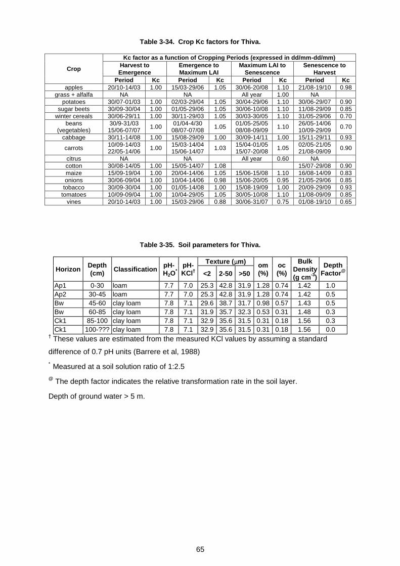
65

Table 3-34. Crop Kc factors for Thiva.

Crop


Harvest to

Emergence

Emergence to

Maximum LAI

Maximum LAI to

Senescence

Senescence to

Harvest


apples 20/10-14/03 1.00 15/03-29/06 1.05 30/06-20/08 1.10 21/08-19/10 0.98


potatoes 30/07-01/03 1.00 02/03-29/04 1.05 30/04-29/06 1.10 30/06-29/07 0.90

sugar beets 30/09-30/04 1.00 01/05-29/06 1.05 30/06-10/08 1.10 11/08-29/09 0.85

winter cereals 30/06-29/11 1.00 30/11-29/03 1.05 30/03-30/05 1.10 31/05-29/06 0.70

beans (vegetables)

30/9-31/03 15/06-07/07

1.00 01/04-4/30

08/07-07/08 1.05

01/05-25/05 08/08-09/09

1.10 26/05-14/06 10/09-29/09

0.70

cabbage 30/11-14/08 1.00 15/08-29/09 1.00 30/09-14/11 1.00 15/11-29/11 0.93

carrots 10/09-14/03 22/05-14/06

1.00 15/03-14/04 15/06-14/07

1.03 15/04-01/05 15/07-20/08

1.05 02/05-21/05 21/08-09/09

0.90


cotton 30/08-14/05 1.00 15/05-14/07 1.08 15/07-29/08 0.90

maize 15/09-19/04 1.00 20/04-14/06 1.05 15/06-15/08 1.10 16/08-14/09 0.83

onions 30/06-09/04 1.00 10/04-14/06 0.98 15/06-20/05 0.95 21/05-29/06 0.85

tobacco 30/09-30/04 1.00 01/05-14/08 1.00 15/08-19/09 1.00 20/09-29/09 0.93

tomatoes 10/09-09/04 1.00 10/04-29/05 1.05 30/05-10/08 1.10 11/08-09/09 0.85

vines 20/10-14/03 1.00 15/03-29/06 0.88 30/06-31/07 0.75 01/08-19/10 0.65

Table 3-35. Soil parameters for Thiva.

Horizon Depth

(cm) Classification

pH-

H2O*

pH-

KCl†

Texture ( m) om

(%)

oc

(%)

Bulk

Density

(g cm-3

)

Depth

Factor@

<2 2-50 >50

Ap1 0-30 loam 7.7 7.0 25.3 42.8 31.9 1.28 0.74 1.42 1.0

Ap2 30-45 loam 7.7 7.0 25.3 42.8 31.9 1.28 0.74 1.42 0.5

Bw 45-60 clay loam 7.8 7.1 29.6 38.7 31.7 0.98 0.57 1.43 0.5

Bw 60-85 clay loam 7.8 7.1 31.9 35.7 32.3 0.53 0.31 1.48 0.3

Ck1 85-100 clay loam 7.8 7.1 32.9 35.6 31.5 0.31 0.18 1.56 0.3

Ck1 100-??? clay loam 7.8 7.1 32.9 35.6 31.5 0.31 0.18 1.56 0.0 † These values are estimated from the measured KCl values by assuming a standard




Depth of ground water > 5 m.

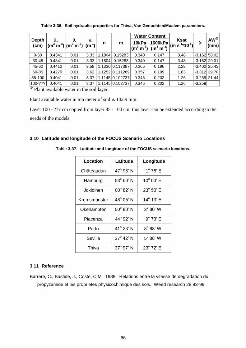
66

Table 3-36. Soil hydraulic properties for Thiva, Van Genuchten/Mualem parameters.

Depth

(cm) s

(m3 m

-3)

r

(m3 m

-3)

(m-1)

n m

Water Content Ksat

(m s-1*10

-6)

AW

@

(mm) 10kPa

(m3 m

-3)

1600kPa

(m3 m

-3)

0-30 0.4341 0.01 3.33 1.1804 0.15283 0.340 0.147 3.48 -3.162 58.02

30-45 0.4341 0.01 3.33 1.1804 0.15283 0.340 0.147 3.48 -3.162 29.01

45-60 0.4412 0.01 3.58 1.1330 0.117387 0.365 0.196 2.28 -3.402 25.43

60-85 0.4279 0.01 3.62 1.1252 0.111269 0.357 0.199 1.83 -3.312 39.70

85-100 0.4041 0.01 3.37 1.1145 0.102737 0.345 0.202 1.26 -3.259 21.44

100-??? 0.4041 0.01 3.37 1.1145 0.102737 0.345 0.202 1.26 -3.259 @


Plant available water in top meter of soil is 142.9 mm.

Layer 100 - ??? cm copied from layer 85 - 100 cm; this layer can be extended according to the

needs of the models.

3.10 Latitude and longitude of the FOCUS Scenario Locations

Table 3-37. Latitude and longitude of the FOCUS scenario locations.

Location Latitude Longitude

Châteaudun 47o 98‟ N 1

o 75‟ E

Hamburg 53o 63‟ N 10

o 00‟ E

Jokioinen 60o 82‟ N 23

o 50‟ E

Kremsmünster 48o 05‟ N 14

o 13‟ E

Okehampton 50o 80‟ N 3

o 80‟ W

Piacenza 44o 92‟ N 9

o 73‟ E

Porto 41o 23‟ N 8

o 68‟ W

Sevilla 37o 42‟ N 5

o 88‟ W

Thiva 37o 97‟ N 23

o 72‟ E

3.11 Reference

Barrere, C., Bastide, J., Coste, C.M. 1988. Relations entre la vitesse de degradation du

propyzamide et les proprietes physicochimique des sols. Weed research 28:93-99.

generic guidance for tier 1 focus ground water...

Documents