Generation of Tolerance Maps for Line Profile by Primitive T-Map Elements

by

Yifei He

A Thesis Presented in Partial Fulfillment

of the Requirements for the Degree

Master of Science

Approved April 2013 by the

Graduate Supervisory Committee:

Joseph Davidson, Chair

Jami Shah, Member

Marcus Herrmann, Member

ARIZONA STATE UNIVERSITY

May 2013

i

ABSTRACT

The objective of this research is to develop methods for generating the Tolerance-

Map for a line-profile that is specified by a designer to control the geometric profile

shape of a surface. After development, the aim is to find one that can be easily

implemented in computer software using existing libraries. Two methods were explored:

the parametric modeling method and the decomposed modeling method. The Tolerance-

Map (T-Map) is a hypothetical point-space, each point of which represents one geometric

variation of a feature in its tolerance-zone. T-Maps have been produced for most of the

tolerance classes that are used by designers, but, prior to the work of this project, the

method of construction required considerable intuitive input, rather than being based

primarily on automated computer tools. Tolerances on line-profiles are used to control

cross-sectional shapes of parts, such as every cross-section of a mildly twisted

compressor blade. Such tolerances constrain geometric manufacturing variations within a

specified two-dimensional tolerance-zone. A single profile tolerance may be used to

control position, orientation, and form of the cross-section. Four independent variables

capture all of the profile deviations: two independent translations in the plane of the

profile, one rotation in that plane, and the size-increment necessary to identify one of the

allowable parallel profiles. For the selected method of generation, the line profile is

decomposed into three types of segments, a primitive T-Map is produced for each

segment, and finally the T-Maps from all the segments are combined to obtain the T-Map

for the given profile. The types of segments are the (straight) line-segment, circular arc-

segment, and the freeform-curve segment. The primitive T-Maps are generated

ii

analytically, and, for freeform-curves, they are built approximately with the aid of the

computer. A deformation matrix is used to transform the primitive T-Maps to a single

coordinate system for the whole profile. The T-Map for the whole line profile is

generated by the Boolean intersection of the primitive T-Maps for the individual profile

segments. This computer-implemented method can generate T-Maps for open profiles,

closed ones, and those containing concave shapes.

iii

DEDICATION

To my parents

iv

ACKNOWLEDGMENTS

I would like to express my very great appreciation to my committee chair, Dr.

Davidson, for his patience, guidance, inspiration and support. Without his help, this work

would be too difficult to be accomplished.

I would like to thank Dr. Shah and Dr. Herrmann for their time serving as part of

my committee.

I would like to thank former student Samir Savaliya, Yadong Shen and Zihan

Zhang for their helpful information and willing to discuss my ideas.

I would like to thank former student Amir Mujezinović, Gaurav Ameta, Saurabh

Bhide and Patrick Clasen, who did preliminary work on the mathematical model with

geometric tolerances.

I am grate for financial support for this work provided by the National Science

Foundation Grant #CMMI-0969821.

v

TABLE OF CONTENTS

Page

LIST OF TABLES ................................................................................................................ viii

LIST OF FIGURES ................................................................................................................. ix

CHAPTER

1 INTRODUCTION ............................................................................................... 1

1.1 Background ............................................................................................. 1

1.2 Problem statement ................................................................................... 2

2 LITERATURE REVIEW .................................................................................... 4

2.1 Tolerance standard .................................................................................. 4

2.2 GD&T computer models ........................................................................ 5

2.3 The Tolerance Map ................................................................................. 7

3 T-MAP FOR LINE PROFILE TOLERANCE ................................................. 11

3.1 Profile specification and tolerance zone ............................................... 11

3.2 T-Map modeling of a line profile ......................................................... 12

4 PARAMETRIC MODELING METHOD ........................................................ 17

4.1 Parametric modeling method ................................................................ 17

4.2 The Invariant Point (Pole) of the Profile .............................................. 18

4.3 The base hypersection of the T-Map for the Middle-Sized Profile ..... 21

4.4 Smaller 3-D Hypersections of the T-Map ............................................ 27

5 DECOMPOSED MODELING METHOD ...................................................... 32

5.1 Decomposed modeling method ............................................................ 32

5.2 Slope conservation and 2-D modeling ................................................. 33

vi

CHAPTER Page

5.2.1 Slope conservation ..................................................................... 33

5.2.2 2-D modeling ............................................................................. 36

5.2.3 Slope conservation for curves ................................................... 38

5.3 3-D modeling of polygonal profile ....................................................... 41

5.3.1 First-order approximation for rotation deviation ...................... 42

5.3.2 3-D primitive model for straight line-segment ......................... 45

5.3.3 Uniformity of reference system ................................................. 48

5.4 Deformation of T-Map .......................................................................... 49

5.4.1 Space of mapping points ........................................................... 49

5.4.2 Orientation and origin location of the reference system ........... 50

5.4.3 Shear deformation ...................................................................... 52

5.5 Case study for polygonal profile........................................................... 59

5.6 3-D primitive model for Circular Arc Segment ................................... 66

5.7 3-D primitive Models for free curve element ....................................... 69

5.8 3-D model with size change and unequally disposed profile

tolerance… ............................................................................................ 73

5.8.1 Size change for line element ..................................................... 73

5.8.2 Size change for circular arc ....................................................... 76

5.8.3 Size change for free form curve ................................................ 78

5.8.4 Unequally disposed profile tolerance ........................................ 79

5.9 4-D model .............................................................................................. 80

5.10 Open profiles ......................................................................................... 80

vii

CHAPTER Page

5.11 T-Map under ISO Standard .................................................................. 82

5.12 Hypersections of the 4-D T-Maps ........................................................ 85

6 COMPUTER PROGRAMMING OF T-MAP CONSTRUCTION ................. 92

6.1 Requirements of programming ............................................................. 92

6.2 Programming environment and tools ................................................... 93

6.3 Class and functions ............................................................................... 94

6.4 Test of the class ..................................................................................... 97

7 CONCLUSION AND FUTURE WORK .......................................................... 98

6.1 Requirements of programming ............................................................. 98

6.2 Programming environment and tools ................................................... 99

REFERENCES ................................................................................................................... 100

Appendix

A OUTPUTS OF THE COMPUTER PROGRAM TESTING ..................... 104

viii

LIST OF TABLES

Table Page

4.1 Coordinates of contacts in Figure 4.5(a) and 4.5(b) ............................................. 23

4.2 Coordinates of contact points of size changed profile. ........................................ 28

5.1 Displacements between the origins and Shear matrix .......................................... 61

5.2 Displacements between the origins and Shear matrix for the profile with arc. ... 68

6.1 Variables of class LineProfileToTMAP ............................................................... 94

A.1 The 3-D models for the profile tolerance in Figure A.1 in different size change

values ................................................................................................................... 106

A.2 The 3-D models for the profile tolerance in Figure A.2 in different size change

values ................................................................................................................... 110

ix

LIST OF FIGURES

Figure Page

2.1 Standard tolerance classes ...................................................................................... 4

2.2 A feature control frame used to designate a line profile related to a reference

frame defined by feature A, B, and C. ................................................................... 5

2.3 T-Map for the size tolerance of a round bar (end plane) ....................................... 8

3.1 Square boss (external feature) with its shape controlled by the profile tolerance ŧ

=0.5mm relative to Datums A, B, and C.. ............................................................ 11

3.2(a) The MSP (dashed-lined square) in the (exaggerated) tolerance-zone that is

specified with the profile tolerance ŧ; five variational possibilities are labeled.. 14

3.2(b) One 2-D cross-section of the corresponding T-Map that is confined to all size

variations and displacements ex only in the x-direction.. .................................... 14

3.3 The central hypersection of the 4-D T-Map for a square line profile. This model

represents all the middle-sized squares in the tolerance-zone of Figure 3.2(a).. 15

3.4 The 4-D T-Map for the square tolerance-zone in Figure 3.2(a) and showing all

five basis-points ψ1,…,ψ5. For clarity of the graphics, the scale in the direction of

size (ψ1ψ 2) is exaggerated... ................................................................................. 16

4.1 Boss with its shape controlled by the profile tolerance ŧ = 0.2 mm relative to

Datums A, B, and C... ........................................................................................... 18

4.2 (a) The middle-sized profile (dashed-lined square) for a square profile in the

(exaggerated) tolerance-zone that is specified with the profile tolerance ŧ; five

variational possibilities are labeled, three with dotted lines... ............................. 19

x

Figure Page

4.2(b) The 3-D T-Map for all the middle-sized squares in the sharp-cornered tolerance-

zone of Figure 4.2(a). Taken from.. ..................................................................... 19

4.3(a) The middle-sized profile (dashed-lined rectangle) in the (exaggerated) tolerance-

zone that is specified with the profile tolerance ŧ, and two of its fully rotated

variational possibilities (dotted lines).. ................................................................. 20

4.3(b) The 3-D T-Map for all the middle-sized rectangles in the sharp-cornered

tolerance-zone of Figure 4.3(a). The two vertices at the front (with dots)

correspond to the two rotated profiles shown in Figure 4.3(a)............................ 20

4.4 Geometry parameters of the mid- size profile identified in the fixed coordinate

system... ................................................................................................................. 21

4.5 Selected displaced locations for the middle-sized profile (dashed-line) in the

(exaggerated) tolerance-zone that is specified with the profile tolerance ŧ =

0.2mm from Figure 4.1 (a) Constrained at three points of the boundary and

rotated counterclockwise. (b) Also constrained, but rotated clockwise... .......... 22

4.6 The 3-D T-Map for the middle-sized profile in Figure 4.1 in two different

orientations... ......................................................................................................... 23

4.7 Geometry representations of Equations in Table 4.1. Each equation is a surface

of T-Map model. The dark shadow presents the surfaces in frontward and the

light shadow present backward... ......................................................................... 26

4.8 Geometry parameters of the offset profile under the coordinate system….. ...... 28

4.9 Geometry parameters of the size-changed profile (increased by 0.05 mm).. ..... 31

xi

Figure Page

5.1 Boss with its shape controlled by the profile tolerance ŧ = 0.2 mm relative to

Datums A, B, and C. ............................................................................................. 34

5.2(a) Exaggerated tolerance-zone (between two solid-lined triangles) for a triangular

profile (dashed-lined triangle). Edges of outside boundaries is labeled in A, B, C,

and inside is in A’, B’, C’. Five spatial positions are also labeled... .................... 35

5.2(b) Corresponding 2-D T-Map that is only confined to translations......................... 35

5.3 One (bottom edge of triangle) of the decomposed line-segment, and its

exaggerated tolerance-zone. ψ12, ψA’, ψA are labeled... ........................................ 36

5.4 (a)(b)(c) are individual T-Maps for each portion of the triangular profile, and (d)

is the intersection of these three T-Map. The shaded areas are the acceptable

deviation regions of T-Maps... ............................................................................. 37

5.5 Boss with its shape controlled by the profile tolerance ŧ = 0.2 mm relative to

Datums A, B, and C... ........................................................................................... 38

5.6(a) Exaggerated tolerance-zone for rounded curve and its approximate polyline... . 39

5.6(b) Primitive model for polyline. (Intersection of models of line-segments, all

tangent to the tolerance circle).............................................................................. 40

5.6(c) Primitive model for curve... .................................................................................. 40

5.7 Boss with its shape controlled by the profile tolerance ŧ = 0.2 mm relative to

Datums A, B, and C... ........................................................................................... 42

5.8 Exaggerated tolerance-zone (between two solid-lined) for a line-segment (long

dashed). Extended line is in short dashed line and two limit positions of line-

segment are in dotted lines... ................................................................................ 43

xii

Figure Page

5.9 Exaggerated tolerance-zone (between two solid-lined) for a line-segment (long

dashed). Line-segment (dotted line) in limit rotation position for maximum

rotation deviation. ................................................................................................. 44

5.10 Exaggerated tolerance-zone (between the two solid-lines) for a line-segment

(dashed). ψ12, ψar, ψa and ψb are the positions (dotted line) for the line-segment

that floats inside the tolerance-zone... .................................................................. 45

5.11(a) 2-D T-Map (model is rescaled in direction θ). ψ12, ψar, ψa and ψb are points

corresponding to specific positions in Figure 5.10... ........................................... 47

5.11(b) A 3-D primitive model is got by extruding the 2-D model (shaded face) in x-

direction... .............................................................................................................. 47

5.12(a) A deviation position (dotted lines) of the mid-sized profile in the exaggerated

tolerance-zone... .................................................................................................... 49

5.12(b) Deformation result (dotted lines) by rotating around individual WCS origins. An

additional translation is required for each line-segment (dotted line) to help the

entire profile to keep its shape as in Figure 5.12(a)... .......................................... 49

5.13(a) Choose another axes x’ and y’ for the reference system... .................................. 51

5.13(b) Corresponding 2-D T-Map for Figure 5.13(a).. ................................................... 51

5.14 Mid-sized profile (ψ12, triangle in solid line) with two different reference

systems. ψar, ψa and ψb are the translated position from mid-sized profile... .... 53

5.15 Mid-sized profile (ψ12, triangle in solid line) with two different reference

systems. ψ12, ψa, ψb, ψ’12and ψ’a are the translated position from mid-sized

profile... ................................................................................................................. 56

xiii

Figure Page

5.16 Here the triangle is the mid-sized profile. Three WCS’s were created for each

line-segment. A temporary reference system for the whole profile is set on a

vertex of the triangle. O’x’y’ is the reference system whose origin locates at

invariant point... .................................................................................................... 59

5.17(a) 2-D T-Map sections for three line-segments (θ’=25θ) at their WCS O1x1y1,

O2x2y2 and O3x3y3. Use θ’ is to make sure the height of 3-D model for mid-sized

profile in θ axis is equal to half tolerance... ......................................................... 60

5.17(b) 3-D primitive model is got by extruding the left 2-D sections (shaded face) in x-

direction. Here only show the shape of model for bottom edge, and the other two

edges have the same shape... ................................................................................ 60

5.18(a) 3-D primitive model for left edge of triangle... .................................................... 62

5.18(b) 3-D primitive model for right edge of triangle... ................................................. 62

5.19 3-D primitive models for three edges of mid-sized triangle. Dotted lines are the

unsheared 2-D sections that are same as those in Figure 5.17(b), 5.18(a) and

5.18(b)... ................................................................................................................ 63

5.20 Intersection of primitive models. Shaded area is the intersection with plane Oexey

and it is same as the shape in Figure 5.2(b). Points for fully rotated locations lie

on two lines... ........................................................................................................ 65

5.21 The final 3-D T-Map. . Shaded area is the intersection with plane Oexey and it is

same as the shape in Figure 5.2(b)... .................................................................... 66

5.22(a) The tolerance-zone same as in Figure 5.6(a). The origin of WCS at the center of

the arc... ................................................................................................................. 67

xiv

Figure Page

5.22(b) 3-D primitive model for circular arc segment, the shaded section is same with

Figure 5.6(c)... ....................................................................................................... 67

5.23 Boss with its shape controlled by the profile tolerance ŧ = 0.2 mm relative to

Datums A, B, and C. A rounded corner is added to the right corner….... .......... 68

5.24 3-D T-Map model for the profile tolerance in Figure 5.23. The shaded area is the

section in exey plane... ........................................................................................... 69

5.25(a) The tolerance-zone, and sampling points... .......................................................... 70

5.25(b) Tangent direction and osculating circle at point P... ............................................ 70

5.26(a) The 2-D T-Map model of translation in x and y direction... ............................... 72

5.26(b) 3-D primitive sub-model for point P, the shaded section is same with Figure

5.26(a)... ................................................................................................................ 72

5.27 3-D T-Map model for the profile tolerance in Figure 5.23. The shaded area is the

section in exey plane. The curved faces are replaced by groups of small faces... 73

5.28 Exaggerated tolerance-zone (between two solid-lined triangles) for a triangular

profile (dashed-lined triangle) with a rounded corner in figure 5.23. The dot-line

is the offset profile for mid-sized profile... .......................................................... 74

5.29 Exaggerated tolerance-zone (between the two solid-lines) for a line-segment

(dashed). The dot-line is the location of the profile with zero translations and

rotation... ............................................................................................................... 74

5.30(a) 2-D T-Map section (model is rescaled in direction θ) for the tolerance-zone in

Figure 5.29... ......................................................................................................... 75

xv

Figure Page

5.30(b) 3-D T-Map from extruding the 2-D T-Map in Figure 5.30(a) along its normal

direction.. ............................................................................................................... 75

5.30(c) An example of 3-D primitive T-Map for the triangle profile with a size change as

shown in Figure 5.30(a)... ..................................................................................... 76

5.31(a) Exaggerated tolerance-zone for circular arc. Dash line is true profile and dot line

is the profile with size change... ........................................................................... 77

5.31(b) 2-D T-Map model (shaded area) for size- changed profile in 5.31(a)... ............. 77

5.32(a) The 2-D T-Map model of translation in x and y direction... ............................... 78

5.32(b) 3-D primitive sub-model for a sampling point, the shaded section is same with

Figure 5.32(a)... .................................................................................................... 78

5.33 Boss with its shape controlled by the profile tolerance ŧ = 0.2 mm relative to

Datums A, B, and C. A second value 0.15 is added. A rounded corner is added to

the right corner... ................................................................................................... 79

5.34 Exaggerated tolerance-zone (between two solid-lined triangles) for a triangular

profile (dashed-lined triangle) with a rounded corner in figure 5.33. The dash-

line is the true profile. The distance from true profile to inside boundary is

0.15.... .................................................................................................................... 80

5.35 The morphology of the 4-D T-Map as a function of size for the triangular line-

profile specified in Figure 5.1. The scale in the direction of size change is not

linear. One shape is shown for size decrease to illustrate the through-the-origin

symmetry in the direction of size... ...................................................................... 81

xvi

Figure Page

5.36 Exaggerated tolerance-zone (between two solid-lined triangles) for a triangular

profile (dashed-lined triangle). The corner of outside boundary is rounded.

Shaded area is the area that reduced from the tolerance zone under ASME

standard... .............................................................................................................. 83

3.57(a) The boundary of the “point” arc profile. “point” arc profile is located at O... .... 84

5.37(b) The 2-D T-Map of the “point” arc profile. The shaded area is the accept region

of the mapping point space... ................................................................................ 84

5.38 3-D T-Map model for mid-sized profile under the ISO standard.. ..................... 85

5.39(a) The 3-D primitives of the T-Map in the space with dimensions exθF at zero ey.

The shaded area is the 2-D section at the plane OθF........................................... 86

5.39(b) The 3-D primitives of the T-Map in the space with dimensions exθF at non-zero

ey. The shaded area is the 2-D section at the plane OθF.... ................................. 86

5.40 The 3-D primitives of the T-Map in the space with dimensions eyθF. The light

shaded area is the 2-D section at the plane Oeyθ. The dark one is the 2-D section

at the plane OθF. The extrude direction is 45 degree to axis F.... ....................... 87

5.41(a) The 3-D primitives of the T-Map in the space with dimensions exeyF at zero ex.

The model is a volume between two planes. The shaded area is the 2-D section

at the plane OeyF.... ............................................................................................... 88

5.41(b) The 3-D primitives of the T-Map in the space with dimensions exeyF non-zero ex.

The model is a volume between two planes. The shaded area is the 2-D section

at the plane OeyF.... ............................................................................................... 88

xvii

Figure Page

5.42 The 3-D primitives of the T-Map in the space with dimensions exeyF . The light

shaded area is the 2-D section at the plane OexF. The dark one is the 2-D section

at the plane OeyF.... ............................................................................................... 89

5.43 The 3-D primitives of the T-Map in the space with dimensions exeyF . The

shaded area is the 2-D section at the plane OexF.... ............................................. 91

6.1 Flowchart of function get_tmap and function build_tmap... ............................... 95

A.1 Boss with its shape controlled by the profile tolerance ŧ = 0.2 mm relative to

Datums A, B, and C.... ........................................................................................ 109

A.2 Boss with concave shape controlled by the profile tolerance ŧ = 0.2 mm relative

to Datums A, B, and C..... ................................................................................... 110

1

Chapter 1

INTRODUCTION

1.1 Background

Tolerances are specified by a designer to allow reasonable leeway by a

manufacturer for imperfections and inherent variability without compromising

performance. The object is to specify large enough tolerances so that manufacturing can

be inexpensive, yet not have the dimensional variations of parts adversely influence their

assembly and functionality. Two types of principles are used in industry for assigning

tolerances: conventional tolerancing and geometric tolerancing.

In conventional tolerancing, a tolerance specified a limiting range on a dimension,

and it applies limit to one degree of freedom to the target entity. But this method had

some serious drawback concerning controls on form and location [1]. So this tolerancing

method may fail to produce the desired part geometry within a high level of accuracy

when it is to be used for a complicated assembly. This often results in many rejected parts

and rework, and increases the cost of manufacturing. The modern and more rigorous

method of tolerancing, called geometric tolerancing, solves many of these problems, but

not all of them.

Geometric tolerancing refers to modern methods that are prescribed in the

ANSI/ASME Y14.5 Standard [2] and the ISO 1101 standards [3]. This thesis is based on

the ASME Standard, which will be introduced in section 2.1. The geometric tolerancing

method permits a designer to control several degrees of freedom for a target entity in its

tolerance-zone. The location of the tolerance-zone is defined with a basic dimension; and

its magnitude is determined by a tolerance to control a geometric variation, such as size,

2

position, or orientation. Additional geometric tolerances may also be specified on the

same feature to control more exact geometric form or orientation of a feature within its

larger size or position tolerance-zone. The ASME Standard gives a common language on

dimensioning and tolerancing, which is easily understood by professionals, and it is

widely used in the engineering design and manufacturing fields. Because of the

efficiency of GD&T in mass production, compared to conventional tolerancing, the

number of rejected manufactured parts is reduced, as well as the manufacturing cost.

However, the Standard is based on a collection of special cases and has little rigorous

mathematical basis, so it causes some inefficiency or ambiguity in communications

between design, manufacturing, and inspection. A mathematical model for tolerances has

the potential to eliminate errors and lower cost of manufacturing.

1.2 Problem statement

The tolerance-Map model, proposed by Davidson and Shah is one of the

mathematical models to represent geometric tolerances. A Tolerance-Map is a

hypothetical Euclidean volume of points, the shape, size, and internal subsets of which

represent all possible variations in size, position, form, and orientation of a target

feature.[4] In section 2.3, previous work done by several graduate students will be

introduced. A T-Map can represent the tolerance-zones for size, form, position and

orientation tolerances under the ASME Standard. The model can effectively represent the

interaction between tolerances types and the effects of datum precedence and sequence

that are important in tolerance accumulation. Of the six tolerance types built in the

standard, line profile tolerances have recently been modeled [33], and surface profiles

have not yet been modeled, either by T-Map, or by any other model.

3

The objective of this research is to develop methods for generating the Tolerance-

Map for line-profiles and to identify one that can be easily implemented in computer

software using existing libraries. In this thesis the T-Map is developed for any shape of

profile feature used in design, such as a polygon (combination of lines), a mixture of line

and arc segments, and those containing free-form curves. A profile combined from these

segments can be either open or closed. Two different modeling methods are developed in

this thesis for a given line profile and its specification: the parametric method and the

geometric decomposition method. It is the geometric decomposition method that is more

readily adaptable to computer automation. A remaining artifact from the project is the

computer programming code that may be used to build T-Maps for line-profiles.

4

Chapter 2

LITERATURE REVIEW

2.1 Tolerance standard

The ANSI/ASME Y14.5 Standard is used for specifying dimensions and

tolerances in order to ensure that the design requirements are interpreted unambiguously.

Geometric variations have been decomposed into specific types in the order of their

functional effect and assembling processes. Figure 2.1 gives the standard tolerance

classes. Each geometric tolerance is specified in the form of standard symbols (feature

control frame) on a drawing, as the example shown in Figure 2.2. All frames contain a

type symbol, and tolerance value, and optionally contain one or more datum reference

frames, and modifier symbols.

Figure 2.1: Standard tolerance classes

5

Figure 2.2: A feature control frame used to designate a line profile related to a reference frame

defined by feature A, B, and C.

2.2 GD&T computer models

Besides the T-Map model, several attempts have been proposed to represent

geometric tolerances described in the ASME Standard.

Parametric models use a set of explicit dimensions and constraints in the form of

parametric equations to create geometry in parametric computer-aided design (CAD).

These parametric equations can be solved to get one or more values for dependent

dimensions; tolerances are obtained by allowing variations on the dependent dimension

[5, 6, 7, 8]. Because equations are written and solved for vertex positions, the method is

only applicable in 2-D profiles and 3-D polyhedral parts. Parametric models have trouble

to deal with form tolerances, datum reference frames or directed datum-target relations.

Indirect parameterization models [9, 10] have been developed to decouple model

construction variables from variables for dimensioning and tolerancing.

Offset zone models represent a tolerance-zone as a Boolean subtraction of

maximal and minimal object volumes that are obtained by offsetting the object by

amounts equal to the tolerances on either side [11, 12, 13]. But the composite tolerance

zone, which is constructed from boundary surfaces of the part, cannot present each type

of variation separately, nor to study their interactions. Another problem is that some

tolerances in the ASME Standard, such as location, apply to axes or mid-planes of

6

toleranced features. Also, it does not include the effect from precedence of datum

reference frame (DRF).

Variational surfaces model uses the variational surfaces approach to calculate the

surface coefficients independently, in the way of changing the values of the model

variables according to the tolerance values [14, 15]. And positions of the vertices and

edges are computed from the surface variations. Form tolerances can be handled by using

higher-degree surfaces or surface triangulation. However, this model has some

topological problems, such as maintenance of tangency and incidence conditions among

vertices, edges and surfaces of a solid. And variational surfaces cannot model tolerances

applied to derived features such as axes or mid-planes, feature that are used widely in

practice and appear in the standard.

In kinematic models each tolerance class is represented by a combination of

kinematic joints [16]. The combinations are then used to estimate geometric variations

dependent on feature tolerances. This model is built upon prior work by Chase et al.[17]

of using transformation matrices to analyze tolerance stack-ups in mechanisms. The

developers of kinematic models have yet to show this approach can be extended to

combine the interaction of geometric variations with size dimensions.

The Degrees of freedom (DOF) model represents geometric tolerances in the form

of spatial degree of freedom. [18, 19] Several groups including ASME were

independently working on this model. Kramer [20] used symbolic reasoning to

demonstrate the determination of DOFs of parts in an assembly and to determine the

feasibility of the assembly.

7

In technologically and topologically related surfaces TTRS models, Clément et al.

[21, 22] used elementary surfaces (planes, cylinders, spheres, etc.) to model the six lower

kinematic pairs, identified by Reuleaux [23], with the complete constraint of a fixed rigid

body, as described by Hunt [24]. These are named the seven technologically and

topologically related surfaces (TTRS). 28 different geometric relationships are created

from the combination of TTRS, by using group theory and small displacement torsors.

The tolerance-zone for each tolerance related to a TTRS was represented as a

displacement torsor containing noninvariant rotations and translations. This model is a

part of the minimum system of datum reference frames required for each type of

geometric tolerance. But this model cannot distinguish between variations from form,

size and location. Also, datum precedence is not considered.

The vector space models created by Giordano et al.[25] represents tolerance-

zones with a point-space defined by a set of inequalities, and these inequalities are

expressed by the components of a deviation torsor and mapped to a corresponding

geometric deviation space. It has a similar concept to the Tolerance-Map, but the number

of independent parameters limits this model to represent a line or plane. An assembly is

modeled as one of two types of variations: clearances in joints between parts or

deviations between features. Using Minkowski sum of deviation spaces, the model can

represent the interaction of tolerances in an assembly of parts effectively. They have also

modeled projected tolerance-zones and material conditions of the tolerances.

2.3 The Tolerance Map

A T-Map is a hypothetical Euclidean point-space, the size and shape of which

reflects all variational possibilities for a target feature.[4] It is the range of points

8

resulting from a one-to-one mapping from all the variational possibilities of a feature,

within its tolerance-zone, to the Euclidean point-space. These variations are determined

by the tolerances specified to control size, position, orientation, and form of the feature.

Figure 2.3 shows the T-Map for the size dimension variation of a round bar. Every

possible plane in the allowable tolerance zone is represented by a point in the T-Map.

Thus, the T-Map represents the entire family of parts that are acceptable for the given

size tolerance.

(a) Section of Tolerance

zone

(b) Section of T-Map (c) T-Map model

Figure 2.3: T-Map for the size tolerance of a round bar (end plane) [4]

The number of degrees of freedom or the number of unique variations modeled

determines the dimension of the T-Map. For example, if ‘n’ types of variations of a

feature within the tolerance zone are considered, then the T-Map will be an n-

dimensional geometric entity. To model tolerance accumulation, T-Maps can be added

with Minkowski sums to model the composite quantitative effect of all tolerances on a

sequence of feature stock up.

9

T-Map models have been under development since 1998, and previous work has

been done by several researchers.

Mujezinović [26] developed T-Maps for size, form and orientation tolerances of

planar polyhedral and round faces. He used T-Maps for tolerance analysis for the stack-

up and tolerance allocation of an assembly of rectangular and cylindrical parts. He

demonstrated how T-Maps distinguished the effects of different datum sequencing on

parts with orientation tolerances. He has partially developed the stack-up for an assembly

of parts with an offset included.

Davidson and Shah [27] developed a T-Map for axes in accordance with a

position tolerance. This 4-D T-Map is built from 5 basis features, and it represents all

possible variations of the axis in the tolerance-zone. Davidson and Shah [28] also

developed the T-Map for a tab and slot features and demonstrated that T-Maps can be

used to represent tolerances on any part cross-section using methods of triangulation [29].

Bhide [30] expanded the T-Map for an axis of a cylindrical feature by mapping it

to variations due to position, orientation and form. The T-Map for a pin or a hole having

size, position and form tolerances as well as material modifiers was developed. This is a

5-D T-Map which represents 5 different variations along its axes. Bhide also gave the

difference in T-Maps for sequence of datums on a cylindrical hole, and evaluated the

interaction of tolerances in a pin-hole assembly.

Ameta [31] developed T-Maps for angled faces and for incident point-line feature

clusters. For angled faces, tolerances for size and angularity were included. He applied

the T-Maps to stack-ups of parts with angled faces, and the T-Map for the point-line

cluster to a picture frame assembly.

10

Clasen [32] developed T-Maps for runout and straightness tolerances and for a

line-plane cluster. He showed the T-Map circular and total runout specified on both

surfaces of revolution or on round faces, and the interaction of T-Map for size and form

tolerances with T-Map for runout. He demonstrated the usefulness of the T-Map for

circular runout in minimizing runout errors in assemblies. He constructed an accumulated

T-Map to demonstrate the increased variation of a part axis when the part has a runout

specification in reference to an imperfect datum axis. He also constructed the T-Map for

line-plane cluster, which is a pairing of two features: a plane and an axis at right angles to

it.

11

Chapter 3

T-MAP FOR LINE PROFILE TOLERANCE

In this chapter, the T-Map for line profile is introduced, including tolerance

specification, tolerance zone, and T-Map model. Content of this chapter is based on

Davidson and Shah’s research [33]. They created a method to generate the T-Maps for

line profiles, but the profile shapes were limited to square, rectangle and triangle, they

have not given a general method of modeling for arbitrarily shapes of line profiles.

Figure 3.1: Square boss (external feature) with its shape controlled by the profile tolerance ŧ

=0.5mm relative to Datums A, B, and C.

3.1 Profile specification and tolerance zone

The profile tolerance is used to control each cross-section of a surface that may

be formed by extruding a 2-D feature (curve). The specification of a profile tolerance

establishes a true (theoretical) line-element and tolerance zone at each cross-section of

the surface feature. The boundaries to the tolerance zone have similar geometric shape of

the true profile.

12

The specification for a simple profile is shown in Figure 3.1. The shape of the

rectangular boss is controlled by the profile tolerance ŧ =0.5mm relative to the Datums A,

B and C. This specification gives two square boundaries. The outside one is 0.25 mm

larger along every line normal to the surface, and the other is 0.25 mm smaller.

According to the ASME Standard [2], measured points on the manufactured surface at

every cross-section, which forms a line profile, must lie within the outer and inner

boundary lines at that cross-section. These kinds of line profiles are used to control the

shape of mildly twisted surfaces, such as those on compressor blades.

The tolerance specifications here define tolerance-zone boundaries that are

equally disposed about the true profile. But other tolerance (unilaterally outside,

unilaterally inside and unequal amounts inside and outside) specifications require the

boundaries to be unevenly disposed about the true profile.

When a profile tolerance is specified without any datum, it only controls form, but

when datums are specified with it, the profile tolerancing provides composite control of

form, orientation and location. The size variations of profiles are represented by using the

true profile and the allowable array of parallel curves to it. All curves have different

sizes, but they should reside in the tolerance zone.

3.2 T-Map modeling of a line profile

The basic idea of modeling T-Map for line profile is mapping variations of the

true profile within the tolerance zone. The variations in geometry represented are size

change, translational positions (both x and y in a plane), and angular orientation θ. Each

point in the T-Map will correspond to one of the profile variations. These four freedoms

for variation require a 4-D model.

13

Starting from a 2-D cross-section of the T-Map is an easy way to understand the

mapping of line profile. Let a be the half-side length of any allowable square in the

tolerance zone. The labels ψ1 and ψ2 designate the smallest and largest of these profile-

squares in Figure 3.2(a). In the T-Map, shown as in Figure 3.2(b), the points on the line

through ψ1 and ψ2 are mapping back to a set of non-rotated squares that have their centers

at O in Figure 3.2(a). The acceptable range of size within tolerance zone is from

, to , and this range corresponds to a line segment ψ1ψ2. Its midpoint

(labeled ψ12) corresponds to the middle-size profile. Then translate the middle-sized

profile (MSP) rightward by ŧ/2 to the limit of the tolerance (dotted square labeled ψ3 in

Figure 3.2(a)), and the basis-point of ψ3 is placed on another direction ex that is

orthogonal to axis a, as shown in Figure 3.2(b). There is linear relation between a (the

change of profile size) and ex (the profile displacement in x direction). When size

increases by some value ∆F, the allowable range of profile translation in a direction will

decrease by the same amount. So straight lines can be used to connect basis-points, such

as ψ1 and ψ3, and these lines form the boundaries of the 2-D cross-section of the T-Map.

Next, confine attention to the array of MSP, and this corresponds to a 3-D

hypersection of the 4-D T-Map at the size that equals to . The location of a variational

square is represented by components of displacement, ex, ey and θ. Basis-profile ψ4 is

chosen to be the profile of this set that has been translated upward ŧ /2 to the limit of the

zone (dotted square labeled ψ4 in Figure. 3.2(a)). The basis-profile ψ5 represents the

clockwise rotational displacement to the limit. For the condition that tolerances are two or

more orders of magnitude smaller than the corresponding dimensions, the linear relation

14

between rotation and translation has been proved by Davidson, Mujezinović and Shah

[4]. So the 3-D hypersection of the T-Map is an octahedron, as shown in Figure 3.3.

Figure 3.2(a): The MSP (dashed-lined square) in the (exaggerated) tolerance-zone that is

specified with the profile tolerance ŧ; five variational possibilities are labeled.

Figure 3.2 (b): One 2-D cross-section of the corresponding T-Map that is confined to all size

variations and displacements ex only in the x-direction.

15

Figure 3.3: The central hypersection of the 4-D T-Map for a square line profile. This model

represents all the middle-sized squares in the tolerance-zone of Figure 3.2(a).

Because the T-Map may be used for metric computations, the units along all axes

should be the same. The scale of the axis for angle θ is made . At the basis-point

ψ5 of T-Map, the limit of rotation variations is

(

)

The full 4-D T-Map for the square tolerance zone in Figure 3.2(a) is from the

combination of Figure 3.2(b) and Figure 3.3. The result is a double hyperpyramid in 4-D

that is depicted in Figure 3.4. The base for each single pyramid is the 3-D octahedron

from Figure 3.3, and every other section (two are shown) at right angles to the direction

of size is a smaller and geometrically similar octahedron.

16

Figure 3.4: The 4-D T-Map for the square tolerance-zone in Figure 3.2(a) and showing all five

basis-points ψ1,…,ψ5. For clarity of the graphics, the scale in the direction of size (ψ1ψ 2) is

exaggerated.

17

Chapter 4

PARAMETRIC MODELING METHOD

4.1 Parametric modeling method

The parametric modeling method is to get the extreme positions of a profile in the

extent of allowable variation, by moving the profile inside the tolerance zone. The profile

here can be the middle-sized profile of parts, or it can be of allowable larger or smaller

size. This method can be simulated by two laminas. One is fixed with tolerance zone, and

the other carries the displaced profile. Displacement of the moving the lamina can be

expressed by values of the small displacements , , and , and these small

displacements are three of the coordinates of one point in the T-Map space. So long as

the profile attached to the moving lamina lies within the fixed boundaries of the

tolerance-zone, the point identified with the corresponding coordinates lies inside the T-

Map. When this displaced profile touches these boundaries at one or more points, the

coordinates , , and identify a point on the T-Map boundary. The set of all boundary

points in the T-Map space gives a hypersection of T-Map in the specific size change ∆F

of profile.

To define and compute the positions analytically, both a fixed reference system

and a displaced reference system are required, the displaced one being attached to the

moving lamina. The fixed reference system is defined as a global fixed coordinate

system, and the boundaries of tolerance zone can be expressed by coordinates or

equations in this frame. The displaced reference system is bonded to the profile which

can move in tolerance zone. A homogeneous coordinate transformation matrix is

18

used to transform the coordinates in the displaced reference system to the fixed reference

system. When one or more points or segments of the displaced profile touch segments or

points of the tolerance-zone boundary, respectively; a point, line, or surface of the T-Map

boundary may be identified by using matrix [A] to relate each contacting pair of points.

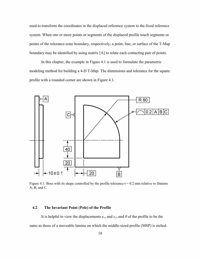
In this chapter, the example in Figure 4.1 is used to formulate the parametric

modeling method for building a 4-D T-Map. The dimensions and tolerance for the square

profile with a rounded corner are shown in Figure 4.1.

Figure 4.1: Boss with its shape controlled by the profile tolerance ŧ = 0.2 mm relative to Datums

A, B, and C.

4.2 The Invariant Point (Pole) of the Profile

It is helpful to view the displacements ex, and ey, and θ of the profile to be the

same as those of a moveable lamina on which the middle-sized profile (MSP) is etched.

19

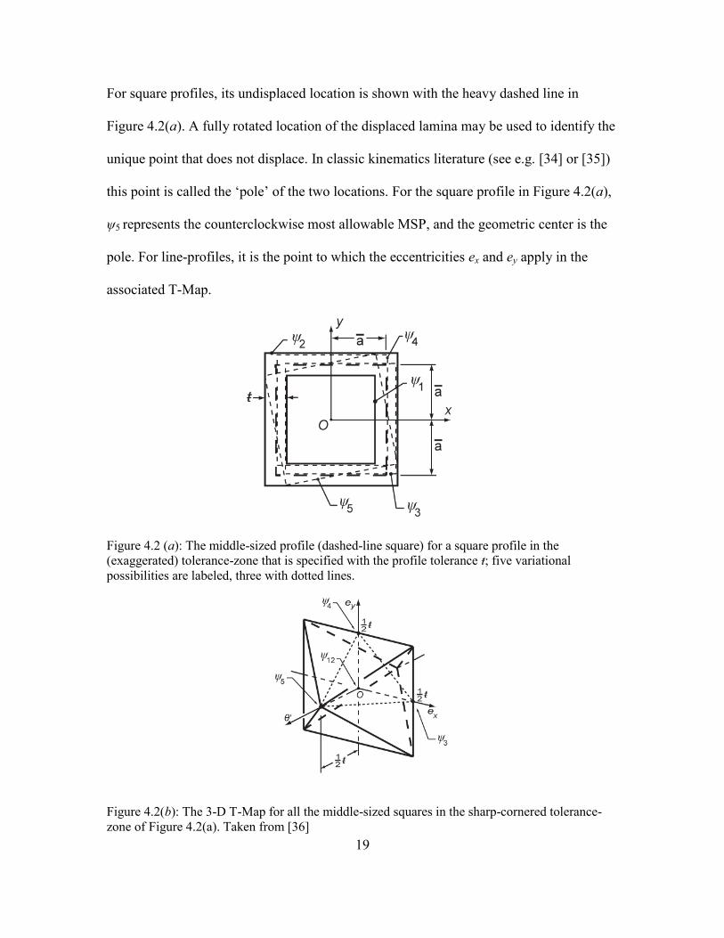
For square profiles, its undisplaced location is shown with the heavy dashed line in

Figure 4.2(a). A fully rotated location of the displaced lamina may be used to identify the

unique point that does not displace. In classic kinematics literature (see e.g. [34] or [35])

this point is called the ‘pole’ of the two locations. For the square profile in Figure 4.2(a),

ψ5 represents the counterclockwise most allowable MSP, and the geometric center is the

pole. For line-profiles, it is the point to which the eccentricities ex and ey apply in the

associated T-Map.

Figure 4.2 (a): The middle-sized profile (dashed-line square) for a square profile in the

(exaggerated) tolerance-zone that is specified with the profile tolerance ŧ; five variational

possibilities are labeled, three with dotted lines.

Figure 4.2(b): The 3-D T-Map for all the middle-sized squares in the sharp-cornered tolerance-

zone of Figure 4.2(a). Taken from [36]

20

For the square and rectangular profiles in Figure 4.2(a) and Figure 4.3(a), the pole

is at the geometric center O. However, for the rectangular profile, there is not one fully

rotated location of the lamina that is locked in place. Of the linear array of possibilities

shown in 4.3(b), we choose the one that is mid-way between the two dotted ones at the

limits. Note that, for both the square and rectangular profiles, the fully rotated lamina,

which is used in defining the pole and its associated origin of the required coordinate

system, corresponds to one of the two points in the T-Map where the θ′-axis pierces the

boundary. See Figure 4.2(b) and Figure 4.3(b).

Figure 4.3(a): The middle-sized profile (dashed-lined rectangle) in the (exaggerated) tolerance-

zone that is specified with the profile tolerance ŧ, and two of its fully rotated variational

possibilities (dotted lines)

Figure 4.3(b): The 3-D T-Map for all the middle-sized rectangles in the sharp-cornered

tolerance-zone of Figure 4.3(a). The two vertices at the front (with dots) correspond to the two

rotated profiles shown in Figure 4.3(a). Taken from [36]

21

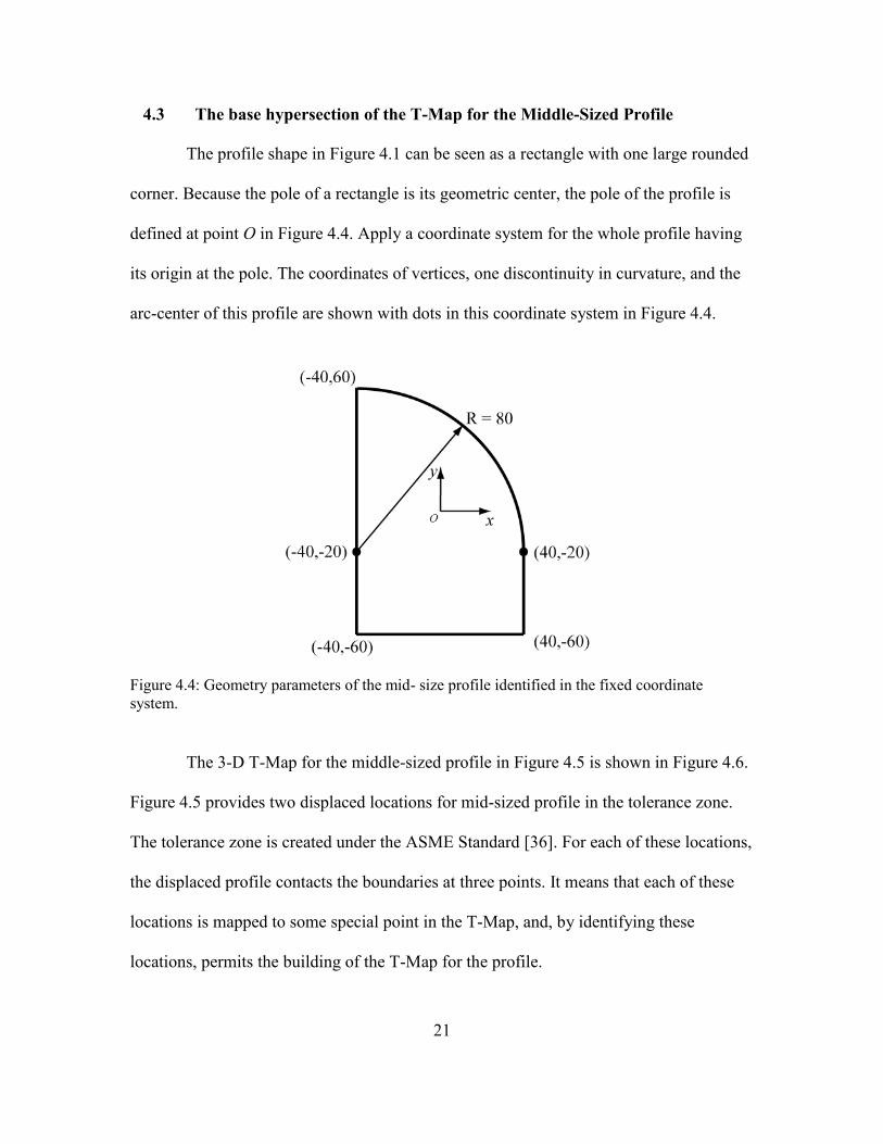
4.3 The base hypersection of the T-Map for the Middle-Sized Profile

The profile shape in Figure 4.1 can be seen as a rectangle with one large rounded

corner. Because the pole of a rectangle is its geometric center, the pole of the profile is

defined at point O in Figure 4.4. Apply a coordinate system for the whole profile having

its origin at the pole. The coordinates of vertices, one discontinuity in curvature, and the

arc-center of this profile are shown with dots in this coordinate system in Figure 4.4.

The 3-D T-Map for the middle-sized profile in Figure 4.5 is shown in Figure 4.6.

Figure 4.5 provides two displaced locations for mid-sized profile in the tolerance zone.

The tolerance zone is created under the ASME Standard [36]. For each of these locations,

the displaced profile contacts the boundaries at three points. It means that each of these

locations is mapped to some special point in the T-Map, and, by identifying these

locations, permits the building of the T-Map for the profile.

Figure 4.4: Geometry parameters of the mid- size profile identified in the fixed coordinate

system.

22

Figure 4.5: Selected displaced locations for the middle-sized profile (dashed-line) in the

(exaggerated) tolerance-zone that is specified with the profile tolerance ŧ = 0.2mm from Figure

4.1 (a) Constrained at three points of the boundary and rotated counterclockwise. (b) Also

constrained, but rotated clockwise.

The shape of T-Map in Figure 4.6 may be found analytically by using the

homogeneous coordinate transformation [A] that locates the displaced lamina (carrying

the dotted MSP in all parts of Fig 4.3) relative to the fixed (dashed) MSP; it transforms

homogeneous coordinates of points from the displaced frame to the fixed frame. From

any good book on robotics, e.g. [37],

[

] [

] (4.1)

23

where the small displacements ex, and ey, and θ locate the dotted frame relative to the

fixed one and the origins of both frames are at the geometric centers of the unrounded

rectangles. The second form of [A] in Equation 4.1 arises because angle θ is always very

small (<0.2/80 for the profile in Figure 4.1) and only first-order small quantities need to

be retained.

(a) (b)

Figure 4.6: The 3-D T-Map for the middle-sized profile in Figure 4.1 in two different

orientations.

Table 4.1 Coordinates of contacts in Figure 4.5(a) and 4.5(b)

Point

Coordinates (x, y), mm

Constraint equations In Displaced

Frame In Fixed Frame

E ( 40, yE ) (40 + t/2, 60 t/2 )

Fc ( xF, 60 ) (40 + t/2, 60 + t/2 )

Fcc ( 40, yF ) (40 + t/2, 60 t/2 )

G ( xG, 60 ) (40 t/2, 60 + t/2 )

Arc-center

(C) ( 40, 20 ) ( xHc, yHc ) ( )

( )

( )

24

Table 4.1 contains the coordinates of superimposed points in both the displaced

and fixed laminas; each row represents a constraint between the two laminas. For

instance, the third and fourth ones constrain the left and lower line-segments to touch

corners F and G, respectively, of the inner boundary (Figure 4.5(a)). The last row in the

table contains the coordinates of the arc-center corresponding to the contact of a point H

on the arc of the dotted MSP with the arc of the outer boundary (fixed) of the tolerance-

zone (Figure 4.5(a) and Figure 4.5(b)). The coordinates in Row 5 of Table 4.1 are related

by [xHc yHc 1]T = [A][– 40 – 20 1]

T. As a consequence of the contact at point H, the

displaced arc-center CH(xHc , yHc) lies on a circle of radius ŧ /2 = 0.1 mm and with the

fixed center C(x,y)=(– 40 , – 20), i.e.

( ) ( ) (

)

(4.1)

We now see that each of the contact constraints at points E, F, G, and H in Figure

4.5(a) and 4.5(b) may be formalized by relating the coordinates in one row of Table 4.1.

These formalizations, together with displaced arc-center CH, may be used to confirm all

the surfaces that form the right half of the boundary shown in Figure 4.6(a). For the

Rows 1 - 4 of Table 4.1, it is convenient to use the inverse of transformation [A], i.e.

[

] (4.2)

25

in which only first-order small quantities have been retained. Taken together, the matrix

equations are

[

]

[

] [

] (4.3)

The counterclockwise displacement in Figure 4.5(a) is constrained at points G and

also at point F with the coordinates in Row 3 of Table 4.1. From Equations 4.3, the

constraints at Fcc and G lead respectively to

{ ( ) ( )

( ) ( )

Similar for clockwise displacement which is constrained at point E and Fc

{ ( ) ( )

( ) ( )

For displaced arc-center HC

E Fc Fcc G C

E Fc Fcc G C

26

{

(4.4)

Combined with Equation 4.1, the constraints for contact at point H is created

( ) ( )

( )

To have consistent units (length) on all those axes of the T-Map, angle θ is multiplied by

a characteristic length, 40 mm, so θ′ = 40θ. This modified measure for angular

displacement appears in the rescaled constraint equations of Table 4.1.

Figure 4.7: Geometric representations of the equations in Table 4.1. Each equation defines a

surface of T-Map model. The dark shadow presents the surfaces on the front and the light

shadow present surfaces on the back.

27

Figure 4.7 compares the faces of the equations in Table 4.1 and T-Map model in

Figure 4.6(a). And the mapping point of displaced location in Figure 4.5(a)(b) are the

intersection of faces shown in Figure 4.7. In this way, the equations of rest T-Map

surfaces can be calculated

{

( ) ( )

( )

(4.5)

4.4 Smaller 3-D Hypersections of the T-Map

Lastly in the T-Map construction, line-profiles that are larger or smaller than the

middle-sized one are more limited in their allowable displacements ex, ey, and θ, and they

lead to hypersections that are smaller than the base hypersection. Although some of the

limits to displacement of such a profile grow linearly with either larger or smaller size,

not all do. The parametric construction method for these hypersections is the same as for

the base hypersection, except that now size changed is included in Equation (4.4) and

(4.5).

For example, if the size is increased ∆F (i.e. 0.05), all points of the displacing

profile in Figure 4.4 will be offset outward by ∆F mm, although the center of the arc

remains unchanged. The new coordinates and dimension are shown in Figure 4.8, and the

coordinates and equations in Table 4.1 are modified to be those in Table 4.2. Because the

28

distance between arc and outside boundary is reduced to ∆F, the displaced arc-center C-

H(xHc , yHc) lies on a circle of radius ∆F mm and with the fixed center C(x,y)=(– 40 ,–20).

Table 4.2 Coordinates of contact points of size changed profile.

Point Coordinates (x, y), mm

Constraint equations In Displaced Frame In Fixed Frame

E ( 40.05, yE ) (40 + t/2, 60 t/2 ) ( )

Fc ( xF, 60.05 ) (40 + t/2, 60 + t/2 ) ( )

Fcc ( 40.05, yF ) (40 + t/2, 60 t/2 ) ( )

G ( xG, 60.05 ) (40 t/2, 60 + t/2 ) ( )

Arc-center

(C) ( 40 F, 20 F) ( xHc, yHc )

( ) ( )

( )

Comparing the equations in Table 4.1 and Table 4.2, we will find that the faces of

these equations lie outside of the 3D T-Map model, but the line-profiles that are larger or

smaller than the middle-sized one are more limited in their allowable displacements ex, ey,

Figure 4.8: Geometry parameters of the offset profile under the coordinate system.

29

and θ, and the limits grow linearly with change in size. This is because the contact points

E, F and G are all located on the inside boundary of the tolerance zone. When the size of

the profile is increased, the displacements of the profile are controlled by more contacts

with the outside boundaries. For the specific example at hand the allowable displacement

is ∆F to the undisplaced profile. Apply the coordinates changed to Equations 4.5

{

( )

( )

( )

( )

( ) ( )

( )

(4.6)

Ten equations in Table 4.1 and Equations 4.5 represent all the surfaces of T-Map

for mid-sized profile. When the size of the profile changed, these ten equations are

modified in Table 4.2 and Equations 4.6. But they do not represent all the surfaces of the

T-Map with size increased by ∆F. The ten equations can be divided into five pairs, four

pairs of the parallel planes, and one pair for cylinders. In each pair of surfaces, only the

surface closer to the origin is used to represent a surface of the T-Map. Pick the qualified

equations for the surfaces of the T-Map for size-changed profile:

{

( )

( )

( )

( )

( ) ( )

( )

(4.7)

30

Beside equations in Equation 4.7, there are other equations to describe the contact

between the displaced profile and the boundaries. The displaced profile with size-

changed can also contact the two extension lines of the arc of outside boundary. So there

are another two equations

{ ( )

(4.8)

Additional contact situation is the left bottom corner of the displaced profile

contact to the right bottom edge of the outside boundary. This is a point to line contact,

the equation for this contact is

(4.9)

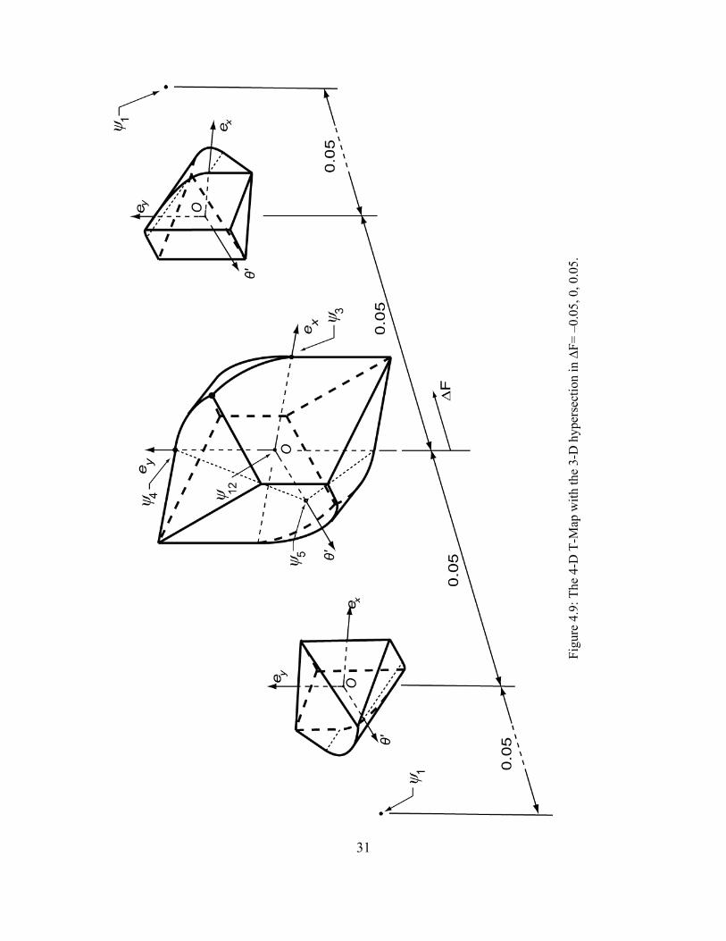
Equations 4.7, 4.8 and 4.9 are algebraic representations for all the surfaces of the

T-Map for the size-changed profile and the model is shown in Figure 4.9.

31

Fig

ure

4.9

: T

he

4-D

T-M

ap w

ith t

he

3-D

hyper

sect

ion i

n ∆

F=

–0

.05

, 0

, 0.0

5.

32

Chapter 5

DECOMPOSED MODELING METHOD

5.1 Decomposed modeling method

Decomposed modeling method is to build the T-Map for line profile by

intersecting T-Maps for all elements of line profile. Three basic elements of line profile

are defined: Straight line, circular arc, and freeform curve.

The boundaries of tolerance-zone constrain the profile displacements which are

used to represent the deviations under tolerancing, and in the corresponding T-Map, the

shell of the T-Map model separates space of deviations into acceptable and inacceptable

regions. The boundaries and shell have the same function, which is to present the

tolerance range, in other words, there is a relation between the shell and the tolerance-

zone’s boundaries.

Because boundaries of tolerance-zone are fixed by theoretic profile shape and

tolerance value, and the geometric properties of a point on boundaries are inherited from

only one point on profile, the boundaries are not influenced by the deviation (or

displacement) of the profile. And because all points on the boundaries play independent

constraint roles that are not defined or influenced by other points on the boundaries, each

point can constrain a series of deviation of profiles, and these deviations are mapped to

parts of shell in the T-Map. Thus, there are independent, unique, one-to-one relations

between the point on profile and part of the corresponding T-Map shell, so that it

becomes possible to construct the shell by combining shells from the profile elements.

Divide the profile into segments, such as points or groups of points, and build a

set for primitive T-Maps each of these segments. When a deviation of profile meets all

33

constraints, its mapped point must lie within all T-Maps for all profile segments, and the

intersection of these T-Maps envelops all possible mapping points of the acceptable

profile deviations.

5.2 Slope conservation and 2-D modeling

In this section, researches are only focused on 2-D space, which is to map the

translational displacements of profile in two directions on a plane. This 2-D model is a

section of 4-D T-Map at rotational angle equal to 0 and for the size (∆F=0) of the profile.

A property between the shape of profile and the shape T-Map model, called slope

conservation, is introduced in 5.2.1. Corresponding 2-D T-Maps are built for all basic

elements of line profile, and the intersection of these operand T-Map forms the single T-

Map for the whole profile.

5.2.1 Slope conservation

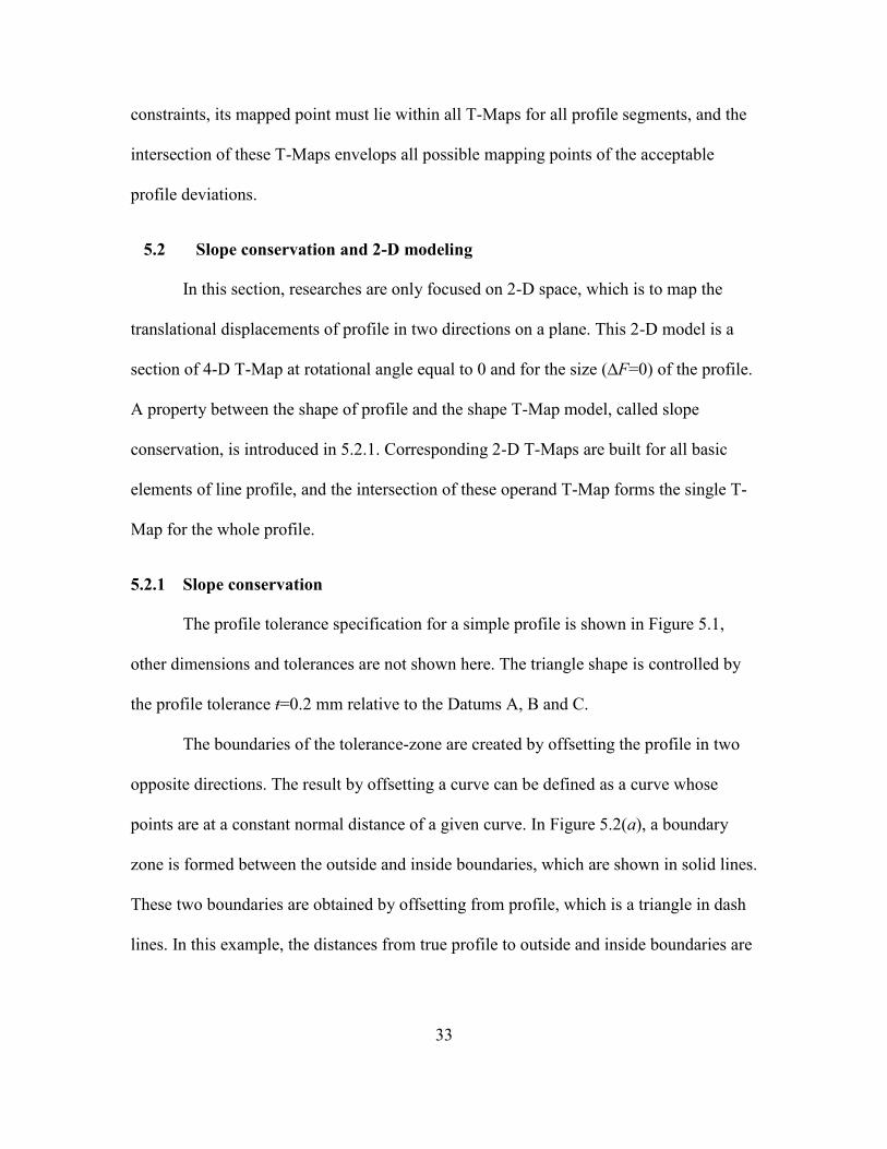
The profile tolerance specification for a simple profile is shown in Figure 5.1,

other dimensions and tolerances are not shown here. The triangle shape is controlled by

the profile tolerance ŧ=0.2 mm relative to the Datums A, B and C.

The boundaries of the tolerance-zone are created by offsetting the profile in two

opposite directions. The result by offsetting a curve can be defined as a curve whose

points are at a constant normal distance of a given curve. In Figure 5.2(a), a boundary

zone is formed between the outside and inside boundaries, which are shown in solid lines.

These two boundaries are obtained by offsetting from profile, which is a triangle in dash

lines. In this example, the distances from true profile to outside and inside boundaries are

34

equal to half tolerance. Thus, the width of tolerance-zone along a curve is equal to

tolerance value ŧ (0.2 mm).

In Figure 5.2(b), the T-Map coordinates ex and ey represent the translational

displacements of the mid-sized profile in x and y direction in Figure 5.2(a). Every point

is a translated mapping of profile position. For example, the true profile ψ12, which is

coincident with true (theoretic) profile, has no translational displacements, and in T-Map

it is the point at origin. When the mid-sized profile is moved in the direction (positive y),

which is normal to bottom edge of the triangle, to the place where its bottom edge

contacts with inside boundary (A’), the profile gets its limit position, which is labeled as

ψA’ in Figure 5.2 (a) (b). In the limit position, the profile cannot move any more in

positive y-direction, because the bottom edge of inside boundary constrains it within

tolerance-zone, but it is still free in x-direction. Because the profile can only move in

either of the positive or negative x-direction, the trace of these displacements mapping

Figure 5.1: Boss with its shape controlled by the profile tolerance ŧ = 0.2 mm relative to Datums

A, B, and C.

35

points is a straight line, which has the same slope as the bottom edge of the profile, and

its normal distance to origin is ŧ/2 (0.1 mm).

Figure 5.2(a): Exaggerated tolerance-zone (between two solid-lined triangles) for a triangular

profile (dashed-lined triangle). Edges of outside boundaries is labeled in A, B, C, and inside is in A’,

B’, C’. Five spatial positions are also labeled.

Figure 5.2(b): Corresponding 2-D T-Map that is only confined to translations.

Because the homogeneous coordinate systems of tolerance-zone and T-Map have

the same scale, there must be an edge of 2-D T-Map model that has the same slope as one

or more lines in tolerance-zone, and this property called slope conservation. Six edges of

the hexagonal T-Map model are parallel to one of the triangular profile edges and accord

with slope conservation.

36

A reference circle, called tolerance circle, is introduced to this 2-D T-Map. In

figure 5.2(b), all edges of the hexagon are tangent lines of this circle. All points on this

circle represent the displaced profile positions that are translated ŧ/2 in any planar

directions. When the direction (as ψA’) is normal to the slope of one profile edge, the limit

displace distance of the profile is ŧ/2, that is a point on the tolerance circle. This reference

circle will be used in section 5.2.3 for discussion of curves.

5.2.2 2-D modeling

The first step to modeling a 2-D T-Map is to decompose the triangular profile in

Figure 5.1 into three line-segments, and build individual primitive models for each of

them, and then combine these models to get the T-Map for the whole profile.

Take the bottom edge of the profile as an example for building a primitive model,

as shown in Figure 5.3. One trace of profile movement is made by translating in the

positive y-direction that is discussed in section 5.2.1. If we move the true profile in the

negative y-direction, the profile will touch the bottom edge of outside boundary (A) in the

location (ψA), and the other corresponding trace in the T-Map is formed. Since the

constraints coming from other two triangle edges are independent of this line-segment,

there is no limit in the direction parallel to this line.

Figure 5.3: One (bottom edge of triangle) of the decomposed line-segment, and its exaggerated

tolerance-zone. ψ12, ψA’, ψA are labeled.

37

In the T-Map model shown in Figure 5.4(a), these two trace lines (same as dash

lines in Figure 5.2(b)) are both derived from the bottom edge of the triangular profile, and

the region between these lines represents the acceptable deviations of the profile, so far

only constrained by one side of the triangle. These two lines of T-Map obey the slope

conservation property and tangent to the tolerance circle (Figure 5.2(b)).

Figure 5.4: (a)(b)(c) are individual T-Maps for each portion of the triangular profile, and (d) is the

intersection of these three T-Map. The shaded areas are the acceptable deviation regions of T-

Maps.

Similarly, other two primitive models are obtained from the remaining two edges

as shown in Figure 5.4 (b) (c). The reference systems of these three primitive models are

38

same. Axes ex and ey represent the displacements of profile segments in x and y

directions, and the scales of these axes are same. Thus, the intersection of these primitive

T-Map models can be realized. The shaded area shown in Figure 5.4(d) is the 2-D T-Map

build by decomposed modeling method that is same as the T-Map in Figure 5.2(b).

5.2.3 Slope conservation for curves

Profiles are not always combinations of straight lines, and a way to modeling

primitive 2-D T-Maps for circular arcs and other curves required. The slopes at points on

non-straight curves are also keeping the conservation property.

In Figure 5.5, a rounded corner is added to the profile, and this profile can be

decomposed into four pieces: three straight line-segments and a curve. The primitive 2-D

T-Maps of three straight lines are discussed and built in Figure 5.4 (a)(b)(c). A primitive

T-Map model is required for the circular arc in order to build the T-Map for whole profile

using intersection.

Figure 5.5: Boss with its shape controlled by the profile tolerance ŧ = 0.2 mm relative to Datums

A, B, and C.

39

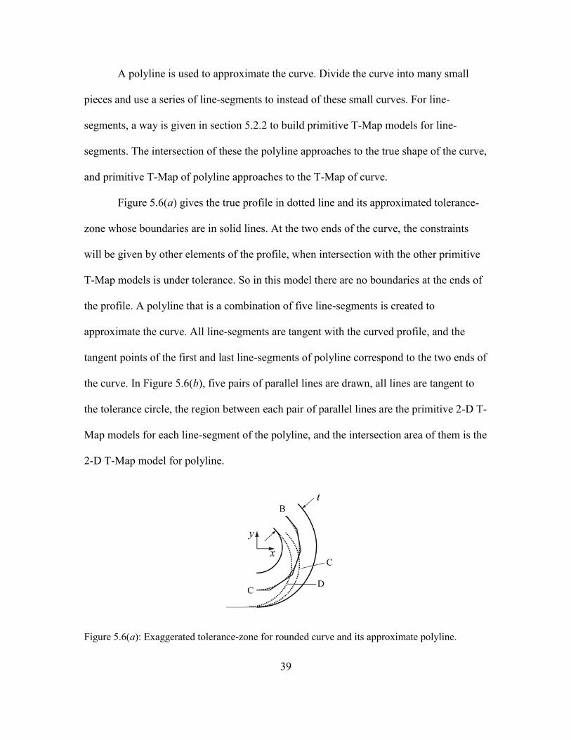
A polyline is used to approximate the curve. Divide the curve into many small

pieces and use a series of line-segments to instead of these small curves. For line-

segments, a way is given in section 5.2.2 to build primitive T-Map models for line-

segments. The intersection of these the polyline approaches to the true shape of the curve,

and primitive T-Map of polyline approaches to the T-Map of curve.

Figure 5.6(a) gives the true profile in dotted line and its approximated tolerance-

zone whose boundaries are in solid lines. At the two ends of the curve, the constraints

will be given by other elements of the profile, when intersection with the other primitive

T-Map models is under tolerance. So in this model there are no boundaries at the ends of

the profile. A polyline that is a combination of five line-segments is created to

approximate the curve. All line-segments are tangent with the curved profile, and the

tangent points of the first and last line-segments of polyline correspond to the two ends of

the curve. In Figure 5.6(b), five pairs of parallel lines are drawn, all lines are tangent to

the tolerance circle, the region between each pair of parallel lines are the primitive 2-D T-

Map models for each line-segment of the polyline, and the intersection area of them is the

2-D T-Map model for polyline.

Figure 5.6(a): Exaggerated tolerance-zone for rounded curve and its approximate polyline.

40

Figure 5.6(b): Primitive model for polyline. (Intersection of models of line-segments, all tangent

to the tolerance circle)

Figure 5.6(c): Primitive model for curve.

In Figure 5.6(b), line AD separates the shell of the T-Map model into two parts.

The points on the left part corresponds to translational profile deviations that contact the

inside boundary of the tolerance-zone, and the right part correspond to positions that

contact the outside boundary. These two parts are symmetric at origin, because from the

tolerance specifications the two boundaries are equally disposed about the true profile.

Taking right part of shell to study, it can be divided into three portions: line-segments AB

and CD, and polyline BC. AB and CD are tangent to the tolerance circle at points B and

C. Because the directions of these two line-segments are the same as the tangent

directions at two ends of the profile, AB and CD will not change when the number of

41

line-segments in polyline increases to approach the true curved shape of the profile. For

polyline BC, with the increasing number of line-segments, its vertexes will close to the

tolerance circle, and when the number goes to infinity, the vertexes will approach to the

tolerance circle. This enables using the shell of the T-Map for polyline BC, as shown in

Figure 5.6(c), and similarly for the left part of the edge.

In the process to make the T-Map in Figure 5.6(c), only one geometric property is

used, that is slope. Any point on the arc-profile corresponds to a point on the tolerance

circle by a tangent line through this point. For the slopes of tangent lines of the profile, a

group of points is created on the tolerance circle, and these points can be expressed by

one or several arcs, such as arc BC in Figure 5.6(c). Because the 2-D T-Map only

depends on slopes of points on the profile, the positions of these points can vary. If a free

form profile has the same slope range with a circular arc profile, both free form profile

and the arc will have the same 2-D T-Map. That means this modeling process is suitable

not only for arc but for more generally shapes of curves.

5.3 3-D modeling of polygonal profile

The decomposition method can be used to build a T-Map model in the 3-D space

for deviations that can be presented by two translations in two mutually perpendicular

directions and a rotation. Use an example in Figure 5.7. The dimensions and tolerance for

the triangular profile shape are shown in Figure 5.7.

42

Figure 5.7: Boss with its shape controlled by the profile tolerance ŧ = 0.2 mm relative to Datums

A, B, and C.

5.3.1 First-order approximation for rotation deviation

Similar to 2-D model, the triangular profile is decomposed into three line-

segments. Use bottom edge (line-segment) of triangle as an example. Before working on

the line-segment, one approximation is needed for the boundary of the tolerance-zone. In

Figure 5.8, the boundaries of the line-segment are shown in solid lines. These two lines

are from part of the boundaries for the whole profile, which is shown in Figure 5.2(a).

One of the boundaries is shorter than the other. It is because of the influence from other

adjacent line-segments. The purpose of this approximation is to eliminate the second-

order influence of the length difference, and to make the line-segments independent of

each other.

To get the maximum rotation deviation, rotate the line-segment of mid-sized

profile to its limit rotate position, and the line-segment contacts to the boundaries at

points A and B in Figure 5.8. This is the way to get the accurate limit position. The

approximation is to define the position where two ends of the line-segment contact the

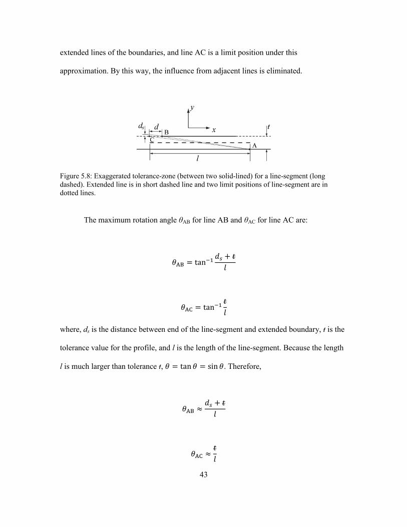
43

extended lines of the boundaries, and line AC is a limit position under this

approximation. By this way, the influence from adjacent lines is eliminated.

Figure 5.8: Exaggerated tolerance-zone (between two solid-lined) for a line-segment (long

dashed). Extended line is in short dashed line and two limit positions of line-segment are in

dotted lines.

The maximum rotation angle θAB for line AB and θAC for line AC are:

where, ds is the distance between end of the line-segment and extended boundary, ŧ is the

tolerance value for the profile, and l is the length of the line-segment. Because the length

l is much larger than tolerance ŧ, . Therefore,

44

From the Figure 5.8, a relation can be found:

where d is the distance between points B and C.

So the angular deviation between lines AB and AC is:

Because d and t are both much smaller than l, the angular deviation is a second

order small value that can be ignored in T-Map building process.

Figure 5.9: Exaggerated tolerance-zone (between two solid-lined) for a line-segment (long

dashed). Line-segment (dotted line) in limit rotation position for maximum rotation deviation.

In figure 5.9, it shows the boundaries of line-segment with approximation, and the

tolerance-zone is the region between the two boundaries. Boundaries and the tolerance-

zone are only dependent on picked line-segment.

45

5.3.2 3-D primitive model for straight line-segment

To measure the deviation, a work coordinate system (WCS) is needed to avoid

ambiguity. This reference system is bonded with the tolerance-zone. Set the origin of the

coordinate at the midpoint of line-segment, point O in Figure 5.10, x1-axis is parallel to

the line-segment. Because the tolerance-zone is symmetric in x1 and y1, the axes direction

will not influence result of T-Map. All line-segments that are decomposed from line

profile have the same process to set work coordinate system, so that this same process is

easy to realize by a computer program.

In figure 5.10, ψar is an arbitrary deviation. The location of this deviation can be

expressed by a combination of a rotation (angle θ) and a translation in the y direction

(distance y) from the mid-sized position (ψ12). To get the arbitrary deviation position, the

first step is to rotate the profile from ψ12 around origin of its WCS by θ to ψa, and then

translate ψa in y-direction to the position of arbitrary deviation by ey.

Figure 5.10: Exaggerated tolerance-zone (between the two solid-lines) for a line-segment

(dashed). ψ12, ψar, ψa and ψb are the positions (dotted line) for the line-segment that floats inside

the tolerance-zone.

46

When the profile is moved to limit positions, such as ψb, where the line-segment

contacts the boundaries of tolerance-zone, the mapped points of these positions will form

the surfaces of the shell of T-Map models. An equation is found in Figure 5.10:

In this equation, half tolerance

is composed by ey,θ, the distance caused by

rotation, and ey,max, the maximum allowable translation distance in y-direction of the

rotated line-segment. Because the rotation angle θ is a small value, so that:

Substitute ey,θ, and get the equation for making surfaces of T-Map model:

Another three equations can be created for different combinations of positive and

negative rotations and translations. Four edges of the T-Map model are made from these

equations, shown in Figure 5.11(a), and their envelop area is the 2-D T-Map in the

dimensions ey and θ. For this line-segment, there is no constraint in x-direction, which is

discussed and shown in Figure 5.4(a). Extrude the 2-D model in x-direction and get the

3-D primitive model. Its section in ex ey plane is accord with the T-Map shown in Figure

5.4(a).

47

Figure 5.11(a): 2-D T-Map (model is rescaled in direction θ). ψ12, ψar, ψa and ψb are points

corresponding to specific positions in Figure 5.10.

Figure 5.11(b): A 3-D primitive model is got by extruding the 2-D model (shaded face) in x-

direction.

For the triangular profile shown in Figure 5.7, there are other two line-segments,

and their primitive models have the same geometric shape but are different in scale and

orientation. The cross-section of these primitive models are also, similar to Figure

5.11(a), but they have different aspect scales and different orientation, as given in Figure

5.4(a)(b)(c).

48

5.3.3 Uniformity of reference system

When primitive models are created for individual decomposed line-segments of

the line profile in Figure 5.7, the next step is to intersect these primitive models to get the

3-D T-Map for the whole profile, as we do in 2-D modeling. But in the definition of

WCS, the mid-point of the line-segment is the origin of WCS, and in the process to

achieve deviation position, we rotate the line-segment around its WCS origin. Since each

line-segment has its own origin and orientations of coordinate axes, the primitive models

cannot be intersected directly to provide the T-Map for the entire profile. For example in

Figure 5.12(a), the dotted profile is a possible deviation whose position can be expressed

by a pure rotation from the mid-sized profile by angle θ, and its mapped point is (0, 0, θ).

But for decomposed profiles, this mapped point represents positions by rotating around

their own WCS origins, as shown in Figure 5.12(b). These dotted lines in Figure 5.12(b)

have the same orientation and length as those in Figure 5.12(a). Rotating profiles around

different points is the reason for this problem, and an additional translation is required to

accompany the rotation of each line-segment. To offset the translations, the translation

deviation of the line-segment ex ey will be changed, that means the shape of primitive T-

Map models need to be modified, and this is called the deformation of T-Map. Before

compose primitive T-Map models, models have to be deformed by a mount which is

defined from the relation between WCS’s and the point the whole profile rotates around.

Section 5.4 gives a method to compute the deformation of T-Map model.

49

Figure 5.12(a): A deviation position (dotted lines) of the mid-sized profile in the exaggerated

tolerance-zone.

Figure 5.12(b): Deformation result (dotted lines) by rotating around individual WCS origins. An

additional translation is required for each line-segment (dotted line) to help the entire profile to

keep its shape as in Figure 5.12(a).

5.4 Deformation of T-Map

Definition of the common reference system determines the shape and location T-

Map model in the point-space that maps the deviation of line profile. This section

contains a description of the deformation of T-Map on different reference systems by

applying transform matrixes.

5.4.1 Space of mapping points

By the definition of T-Map, the point-space for a line profile is a four dimensional

space. Any point in this space maps a deviation of the profile from its ideal size and

location. This mapping is a one to one map, and a deviation of the profile has a unique

50

mapping point in the space of mapped points. The model of the T-Map divides the space

into two regions. The region inside of the model contains all points mapping the

deviations that are acceptable under the tolerance, and the points outside of the model

map those unacceptable deviations.

Four dimensions of the space are: two translations in two mutually perpendicular

directions, rotation and size of the profile. To measure the deviations and map them, a

common reference system is needed. This reference system is fixed with the ideal profile

and tolerance-zone. The orientation of the reference system determines orientation of the

T-Map model, and the origin of the reference system influence the shape of the T-Map

model.

5.4.2 Orientation and origin location of the reference system

The coordinates of mapped points in the T-Map depend on the orientation of

reference system. In Figure 5.2(a) the axis x is parallel to one edge of the triangle, and 2-

D T-Map for the edge is shown in Figure 5.2(b). When we choose another direction x’ for

the axis, which has an angle α to axis x, as shown in Figure 5.13(a), a different 2-D T-

Map is made in Figure 5.13(b). Comparing to the 2-D model in Figure 5.2(b), the model

in the new reference system is rotated by angle –α from the model in Figure 5.2(b). In

other words, the same point in different reference system may have different coordinate

values.

The origin of reference system does not influence the whole mapping space for 2-

D the T-Map model in exey plane, but it influences the 3-D mapping space in the θ

direction. The 3-D mapping space is a point space that contains all points whose

coordinates can be expressed by three values of deviation (ex, ey , θ). When mapping an

51

arbitrary deviation of a profile, such as ψar in Figure 5.14, two steps to determine the

values of ex, ey , θ. The rotational deviation value θ can be measured between the deviated

profile (ψar) and the mid-sized at its theoretical position (ψ12). Then rotate the profile by

angle θar around the origin of the coordinate system, such as rotating around O to position

ψa, and measure the displacement between rotated profile and the deviation (ψar) we want

to measure.

Figure 5.13(a): Choose another axes x’ and y’ for the reference system.

Figure 5.13(b): Corresponding 2-D T-Map for Figure 5.13(a)

Figure 5.14 gives two different reference systems which are fixed to the plane of

mid-sized profile (ψ12). These two reference systems have the same orientation but two

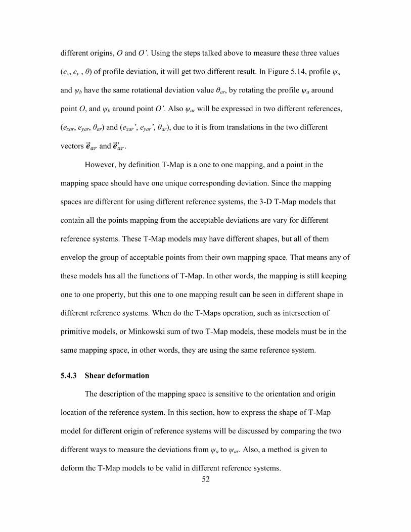
52

different origins, O and O’. Using the steps talked above to measure these three values

(ex, ey , θ) of profile deviation, it will get two different result. In Figure 5.14, profile ψa

and ψb have the same rotational deviation value θar, by rotating the profile ψa around

point O, and ψb around point O’. Also ψar will be expressed in two different references,

(exar, eyar, θar) and (exar’, eyar’, θar), due to it is from translations in the two different

vectors and .

However, by definition T-Map is a one to one mapping, and a point in the

mapping space should have one unique corresponding deviation. Since the mapping

spaces are different for using different reference systems, the 3-D T-Map models that

contain all the points mapping from the acceptable deviations are vary for different

reference systems. These T-Map models may have different shapes, but all of them

envelop the group of acceptable points from their own mapping space. That means any of

these models has all the functions of T-Map. In other words, the mapping is still keeping

one to one property, but this one to one mapping result can be seen in different shape in

different reference systems. When do the T-Maps operation, such as intersection of

primitive models, or Minkowski sum of two T-Map models, these models must be in the

same mapping space, in other words, they are using the same reference system.

5.4.3 Shear deformation

The description of the mapping space is sensitive to the orientation and origin

location of the reference system. In this section, how to express the shape of T-Map

model for different origin of reference systems will be discussed by comparing the two

different ways to measure the deviations from ψa to ψar. Also, a method is given to

deform the T-Map models to be valid in different reference systems.

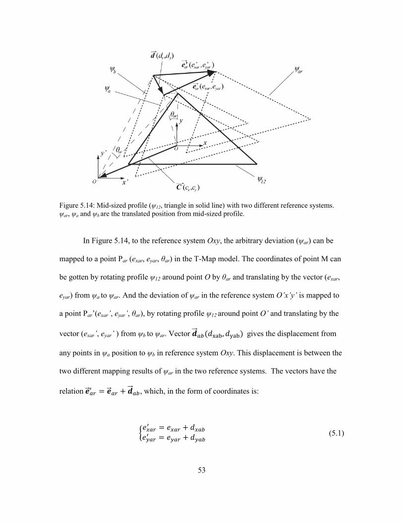
53

In Figure 5.14, to the reference system Oxy, the arbitrary deviation (ψar) can be

mapped to a point Par (exar, eyar, θar) in the T-Map model. The coordinates of point M can

be gotten by rotating profile ψ12 around point O by θar and translating by the vector (exar,

eyar) from ψa to ψar. And the deviation of ψar in the reference system O’x’y’ is mapped to

a point Par’(exar’, eyar’, θar), by rotating profile ψ12 around point O’ and translating by the

vector (exar’, eyar’ ) from ψb to ψar. Vector ( ) gives the displacement from

any points in ψa position to ψb in reference system Oxy. This displacement is between the

two different mapping results of ψar in the two reference systems. The vectors have the

relation , which, in the form of coordinates is:

{

(5.1)

Figure 5.14: Mid-sized profile (ψ12, triangle in solid line) with two different reference systems.

ψar, ψa and ψb are the translated position from mid-sized profile.

54

Equation 5.1 gives a relationship between the coordinates of an arbitrary point in

T-Maps for the profile at two different reference systems. If the values dx and dy are

known, the coordinates of all points in the T-Map for the profiles which are expressed

with coordinates at reference system Oxy can be translated into the point-space for

reference system O’x’y’, by using equation 5.1.

To compute the dx and dy, the relation between two reference system needs to be

defined. In reference system Oxy create a vector from O to O’ to present the relation

between the origins of the two reference systems. And the value of vector or the

coordinate of point O in reference system Oxy is (cx, cy). The values cx and cy are

measured between the coordinate origins. For different reference systems that are located

at the profiles or designed parts, the displacement (cx and cy) between them may be vary,

but they are fixed with the profiles or parts, cx and cy are constants in the T-Map

deformation process.

To compute the values dx and dy, transformation matrices are used to express the

movements of the profile. Assume there are two laminas in Figure 5.15. One fixed lamina

contains the mid-sized profile (solid line) and reference systems Oxy and O’x’y’, and the

other one, which contains a profile in mid-sized position and floats upon the fixed lamina,

will be translated by matrices. For example, any point (x1, y1) on the triangle or on the

plane of the floating lamina (such as in the position ψ1) can be transformed to a point (x3,

y3) on another lamina in the position (such as ψ3) by multiply a matrix T:

[

] [ ] [

]

55

In reference system O’x’y’, use two different ways to transform points on the

lamina from ψ12 to ψa, and one of them is:

( ) ( ) (5.2)

where, is the transform matrix from ψ12 to ψa, ( ) is the translation by

vector ( ), which are the values we want to compute, and ( ) is the rotation

around point O’ by angle θar. This way is the process to measure the deviation of profile

in reference system O’x’y’, that is rotating the lamina around point O’ to ψb and then

translating from ψb to ψa. Another way to transform the profile from ψ12 to ψa is needed

to simulate the pure rotation around point O in reference system O’x’y’. The rotation of

the profile on the lamina in ψ12 around the point O to ψa, may be expressed as the product

of three transportation matrices, i.e.

( ) ( ) ( ) (5.3)

in which the elements of each transform are expressed in reference system O’x’y’.

Processing leftward through the transforms in equation (5.3), the profile translates by the

vector ( ) to profile ψ’12, rotate around point O’ by θ to profile ψ’a, and translate

back by the vector ( ) to profile ψa.

Because and are both the transform matrices from ψ12 to ψa, these two

matrices are same, and the right sides of equation (5.2) and (5.3) are equal to each other:

56

( ) ( )

( ) ( ) ( ) (5.4)

Rewrite (5.4) in matrix form:

[

] [

]

[

] [

] [

] (5.5)

And simplify (5.5):

Figure 5.15: Mid-sized profile (ψ12, triangle in solid line) with two different reference systems.

ψ12, ψa, ψb, ψ’12and ψ’a are the translated position from mid-sized profile.

57

[

]

[

] (5.6)

Compare elements in (5.6), two equations can be got:

{

(5.7)

In equation set (5.7), because cx and cy are measure directly between O and O’, dx

and dy are only depend on the rotational angle θar. For all T-Maps the angle θar is a very

small value, some simplifications can be made: , and .

So (5.7) is simplified to:

{

(5.8)

Now we get the vector ( ) which only depends on the relative displacement

between origins of two reference systems cx, cy, and the arbitrary angle θar.

Displacements cx and cy are fixed when we are defining the reference systems. Because

θar is a measurement to an arbitrary position of deviation, it can represent the rotational

58

angle of any possible deviations of the profile. In equation set (5.8), dx and dy have a

linear relation with θar. And then substitute (5.8) into (5.1):

{

(5.9)

where five variables exar, eyar, e’xar, e’yar, θar can be rewritten into two coordinates (exar,

eyar, θar) and (e’xar, e’yar, θar), and cx, cy are the displacements between the origins of

reference system. In the T-Map these two coordinates represent a point that maps the

deviation ψar in two different reference systems Oxy are O’x’y’. Rewrite (5.9) in a matrix

form:

[

] [

] [

] (5.10)

The vector on left side contains the coordinate values of the mapping point for the

deviation of profile at ψar in the reference system O’x’y’, and the vector on right side

contains the coordinate values for the same deviation at ψar in the reference system Oxy.

The matrix only contains constants, and it translates the coordinate of mapping point

from Oxy to O’x’y’. Because the coordinate (exar, eyar, θar) of profile deviation ψar can be

any value, the matrix can be applied on the whole mapping point-space:

59

[

] [

] [

] (5.11)

And from the format of this matrix, its transformation type is shearing, that

means when we change the origin of a reference system to measure a profile, such as

from Oxy to O’x’y’, the mapping point-space will be sheared. Here name this

deformation matrix shear matrix.

5.5 Case study for polygonal profile

This section provides the process to build a 3-D T-Map for the MSP of the

example in Figure 5.7. The first step is to decompose this triangular profile into three

line-segments, each of these segments has a WCS (Section 5.2.3), shown in Figure 5.16.

Figure 5.16: Here the triangle is the mid-sized profile. Three WCS’s were created for each line-

segment. A temporary reference system for the whole profile is set on a vertex of the triangle.

O’x’y’ is the reference system whose origin locates at invariant point.

In section 5.3.2, a primitive model is created for the line-segment which is

parallel to x-direction. So we can get the primitive model for the bottom edge of the

triangle from Figure 5.11. In this example, the length of bottom line lbot = 50, tolerance t

= 0.2, the cross-section 2-D T-Map is shown in Figure 5.17(a), and its coordinate is

60

rescaled in direction θ by multiplying half-length of line-segment 25. Similar for the

remaining line-segments, but they have different length, and

. For these reason, they intersect with θ-axis at different points in Figure 5.17(a).

Extrude the section in x-direction, and get primitive T-Map models. In Figure 5.17(b),

only show the primitive model of bottom edge.

Figure 5.17(a): 2-D T-Map sections for three line-segments (θ’=25θ) at their WCS O1x1y1, O2x2y2

and O3x3y3. Use θ’ is to make sure the height of 3-D model for mid-sized profile in θ axis is equal

to half tolerance.

Figure 5.17(b): 3-D primitive model is got by extruding the left 2-D sections (shaded face) in x-

direction. Here only show the shape of model for bottom edge, and the other two edges have the

same shape.

61

Next step is using one reference system to present T-Map models for these line-

segments. A temporary reference system is set on a vertex of the mid-sized profile. Its

origin may not be at the invariant point of the profile, and in the following step the

invariant point will be found. Using the reference systems O2’x2’y2’ and O3’x3’y3’ for left

edge and right edge of the profile, the primitive model is rotated around the θ’-axis by an

angle that is equal to the angle between edge and x-axis of temporary reference system.

The rotated primitive models for the other two segments are given in Figure 5.18. The

cross-sections of these primitive models in Figure 5.18 are same as the 2-D T-Map in

Figure 5.17(a).

After rotation, the shear deformation will be applied to the rotated model. In

Table 5.1, the displacements between the origins of its WCS’s and the temporary

reference system are listed, and shear matrix is get from equation 5.11. Use these

matrices to deform rotated primitive models in Figure 5.17(b), 5.18(a) and 5.18(b), and

get the final primitive models which are ready to intersect. These models are shown in

Figure 5.19.

Table 5.1 Displacements between the origins and Shear matrix

Edge Displacement between the origins Shear matrices

Bottom (-25,0) [

]

Left (-10,-15) [

]

Right (-35,-15) [

]

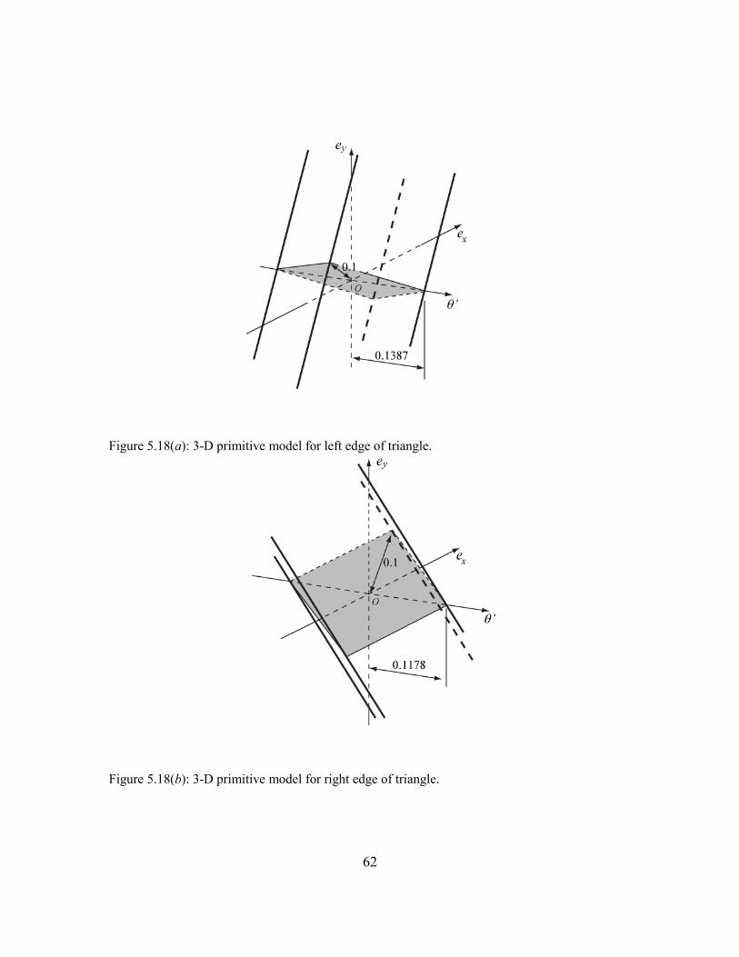
62

Figure 5.18(a): 3-D primitive model for left edge of triangle.

Figure 5.18(b): 3-D primitive model for right edge of triangle.

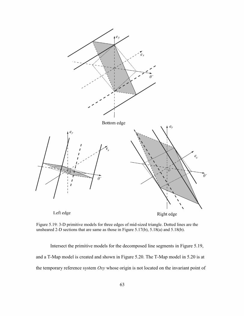
63

Figure 5.19: 3-D primitive models for three edges of mid-sized triangle. Dotted lines are the

unsheared 2-D sections that are same as those in Figure 5.17(b), 5.18(a) and 5.18(b).

Intersect the primitive models for the decomposed line segments in Figure 5.19,

and a T-Map model is created and shown in Figure 5.20. The T-Map model in 5.20 is at

the temporary reference system Oxy whose origin is not located on the invariant point of

64

the triangle profile. Assume there is a reference system O’x’y’ whose origin located at the

invariant point, the shear matrix can relate the points of the T-Map as:

[

] [

] [

] (5.12)

If we can calculate the values cx and cy, we will know the location of the origin of the

reference system O’x’y’ at the temporary reference system.

In the T-Map the coordinates of mapped points for a special location (fully rotated

location) can be found to help calculate the values cx and cy. By the definition of the

invariant point in Chapter 4, fully rotate the lamina around a unique point that does not

displace, and this point is the invariant point. In the reference system O’x’y’ the fully

rotated location means in the T-Map the rotation angle θ at its maximum value .

Another property of invariant point is the profile to fully rotated location without

displacement in x or y direction, in other words, the values of ex’ and ey’ should be equal

to zero. The special point at reference system O’x’y’ is ( ). In the T-Map of

Figure 5.20, the points have the maximum θ’ are on two lines, both for CCW and CW. In

this situation, we usually choose the mid-point of the line as the point which is mapping

fully rotated location. And in this example the points for special locations are

( ) and ( ) for CCW and CW. Because the shear

deformation is on the plane Oxy, the value of maximum rotation angle is not changed by

shear deformation, so that or . Substitute the coordinates of the points at

special locations:

65

Figure 5.20: Intersection of primitive models. Shaded area is the intersection with plane Oexey

and it is same as the shape in Figure 5.2(b). Points for fully rotated locations lie on two lines.

[

] [

] [

] (5.13)

[

] [

] [

] (5.14)

Solve equation 5.13 or 5.14, we can get and . The invariant point O’ is

shown in Figure 5.16. Deform the T-Map in Figure 5.20 by the matrix

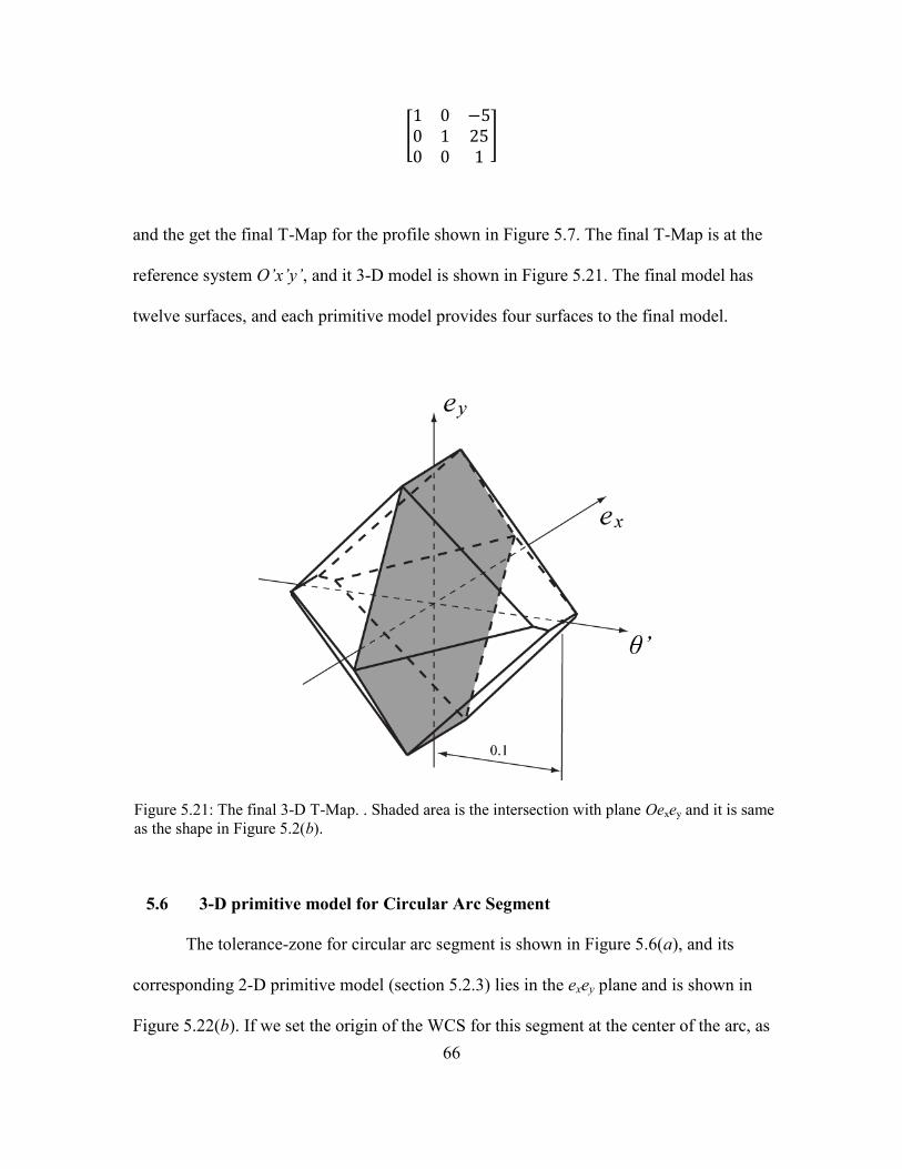
66

[

]

and the get the final T-Map for the profile shown in Figure 5.7. The final T-Map is at the

reference system O’x’y’, and it 3-D model is shown in Figure 5.21. The final model has

twelve surfaces, and each primitive model provides four surfaces to the final model.

Figure 5.21: The final 3-D T-Map. . Shaded area is the intersection with plane Oexey and it is same

as the shape in Figure 5.2(b).

5.6 3-D primitive model for Circular Arc Segment

The tolerance-zone for circular arc segment is shown in Figure 5.6(a), and its

corresponding 2-D primitive model (section 5.2.3) lies in the exey plane and is shown in

Figure 5.22(b). If we set the origin of the WCS for this segment at the center of the arc, as

67

in Figure 5.22(a), the lamina with mid-sized profile (arc) can rotate by any angle around

its center. Therefore, the 3-D model in Figure 5.22(a) is open-ended and formed by

extruding the 2-D T-Map in the θ direction.

Figure 5.22(a): The tolerance-zone same as in Figure 5.6(a). The origin of WCS at the center of

the arc.

Figure 5.22(b): 3-D primitive model for circular arc segment, the shaded section is same with

Figure 5.6(c).

Add a rounded corner to the example of triangle, and get the profile shown in

Figure 5.23. The origin of the profile segments are shown in Table 5.2. Comparing to the

Table 5.1, the length and the mid-points of the line-segments may be changed. And

follow the procedure for building a 3-D T-Map. A 3-D T-Map for the profile with

circular arc is in Figure 5.24.

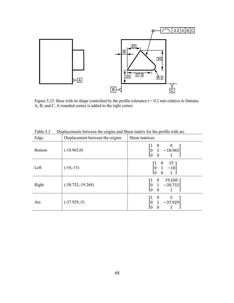
68

Figure 5.23: Boss with its shape controlled by the profile tolerance ŧ = 0.2 mm relative to Datums

A, B, and C. A rounded corner is added to the right corner.

Table 5.2 Displacements between the origins and Shear matrix for the profile with arc

Edge Displacement between the origins Shear matrices

Bottom (-18.965,0) [

]

Left (-10,-15) [

]

Right (-30.732,-19.268) [

]

Arc (-37.929,-5) [

]

69

Figure 5.24: 3-D T-Map model for the profile tolerance in Figure 5.23. The shaded area is the

section in exey plane.

5.7 3-D primitive Models for free curve element

This section gives a method to create an approximate 3-D T-Map model for the

free curve element. This method needs the computer programming to create many open

ended primitives to approximate the real model.

Because the straights or arcs have the constant tangents or curvatures, the shapes

of 3-D T-Maps for straight lines are extruded from rhombus, and the shapes of 3-D T-

Maps for circular arcs are extruded from a plane shape by truncating a rhombus with two

congruent, but opposite circular arcs that are tangent to it. However, the free curve

elements don’t have the constant tangents or curvatures. Unlike straights and arcs, there

is no similar shape between primitive models for free curves. Primitive models for free

curve elements are created based on the geometric properties of the profile shapes, but

70

every point on a curve may have different geometric properties. If all the points on a

curve can be decomposed into independent point elements, accurate models can be

created for these points. But, on the curve, the number of points is infinite. It is

impossible to intersect infinite number of the models. Only an approximate T-Map model

can be created.

Figure 5.25(a): The tolerance-zone, and sampling points.

Figure 5.25(b): Tangent direction and osculating circle at point P.

A group of sampling points is picked from the curve. In the sampling, the turnings

of tangents at two sampling points are same. The number of sampling points defines the

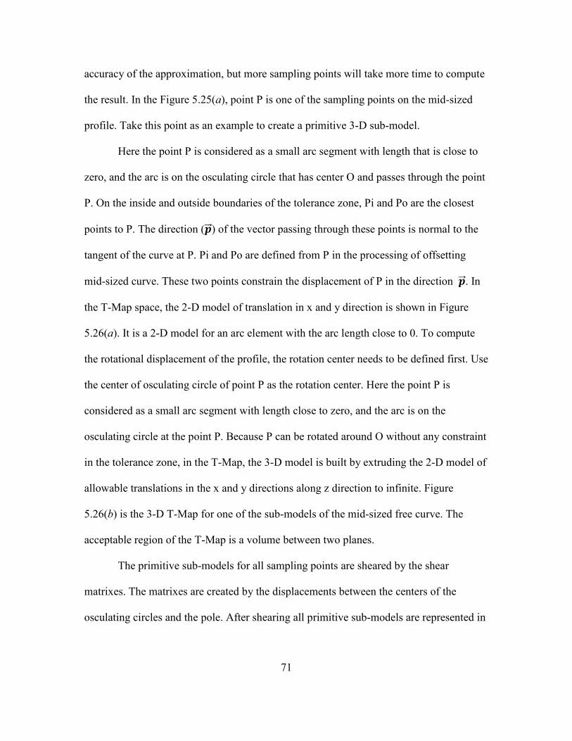
71

accuracy of the approximation, but more sampling points will take more time to compute

the result. In the Figure 5.25(a), point P is one of the sampling points on the mid-sized

profile. Take this point as an example to create a primitive 3-D sub-model.

Here the point P is considered as a small arc segment with length that is close to

zero, and the arc is on the osculating circle that has center O and passes through the point

P. On the inside and outside boundaries of the tolerance zone, Pi and Po are the closest

points to P. The direction ( ) of the vector passing through these points is normal to the

tangent of the curve at P. Pi and Po are defined from P in the processing of offsetting

mid-sized curve. These two points constrain the displacement of P in the direction . In

the T-Map space, the 2-D model of translation in x and y direction is shown in Figure

5.26(a). It is a 2-D model for an arc element with the arc length close to 0. To compute

the rotational displacement of the profile, the rotation center needs to be defined first. Use

the center of osculating circle of point P as the rotation center. Here the point P is

considered as a small arc segment with length close to zero, and the arc is on the

osculating circle at the point P. Because P can be rotated around O without any constraint

in the tolerance zone, in the T-Map, the 3-D model is built by extruding the 2-D model of

allowable translations in the x and y directions along z direction to infinite. Figure

5.26(b) is the 3-D T-Map for one of the sub-models of the mid-sized free curve. The

acceptable region of the T-Map is a volume between two planes.

The primitive sub-models for all sampling points are sheared by the shear

matrixes. The matrixes are created by the displacements between the centers of the

osculating circles and the pole. After shearing all primitive sub-models are represented in

72

the same reference system, and they are ready to intersect. The intersection of these sub-

models is the approximate 3-D primitive model for the whole free curve.

Figure 5.26(a): The 2-D T-Map model of allowable translations in x and y directions.

Figure 5.26(b): 3-D primitive sub-model for point P, the shaded section is same with Figure

5.26(a).

Take the profile example in Figure 5.23, and use a free curve to represent the arc

in the right corner of the triangle. The 3-D T-Map of this mid-sized profile is similar to

the one in Figure 5.24, but curved faces are replaced by groups of small faces which are

used to approach to the real shapes.

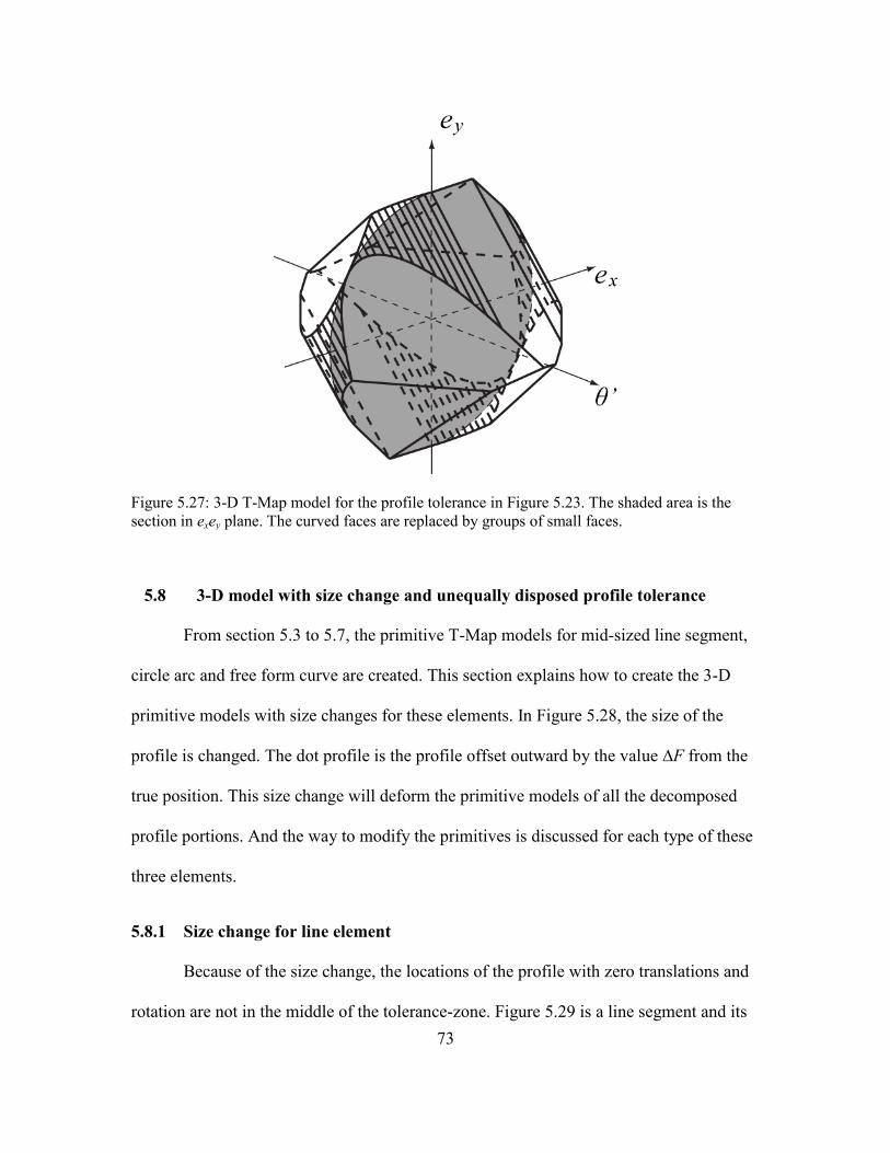
73

Figure 5.27: 3-D T-Map model for the profile tolerance in Figure 5.23. The shaded area is the

section in exey plane. The curved faces are replaced by groups of small faces.

5.8 3-D model with size change and unequally disposed profile tolerance

From section 5.3 to 5.7, the primitive T-Map models for mid-sized line segment,

circle arc and free form curve are created. This section explains how to create the 3-D

primitive models with size changes for these elements. In Figure 5.28, the size of the

profile is changed. The dot profile is the profile offset outward by the value ∆F from the

true position. This size change will deform the primitive models of all the decomposed

profile portions. And the way to modify the primitives is discussed for each type of these

three elements.

5.8.1 Size change for line element

Because of the size change, the locations of the profile with zero translations and

rotation are not in the middle of the tolerance-zone. Figure 5.29 is a line segment and its

74

tolerance zone. The dot line is offset from the mid-sized profile, and the distance between

them is ∆F.

For the line-segment element, the size change can be considered as a translation.

In Figure 5.29, the dotted line can be gotten by either offsetting or translating from the

true position. The extension of length of the line-segment caused by increased size can be

ignored, because only keep first order terms. Figure 5.11(a) gives the tolerance-zone and

the location of the profile with zero translations and rotation. It has the same tolerance-

zone as the one in Figure 5.9, and the only difference is where we define the location of

Figure 5.28: Exaggerated tolerance-zone (between two solid-lined triangles) for a triangular

profile (dashed-lined triangle) with a rounded corner in figure 5.23. The dot-line is the offset

profile for mid-sized profile.

Figure 5.29: Exaggerated tolerance-zone (between the two solid-lines) for a line-segment

(dashed). The dot-line is the location of the profile with zero translations and rotation.

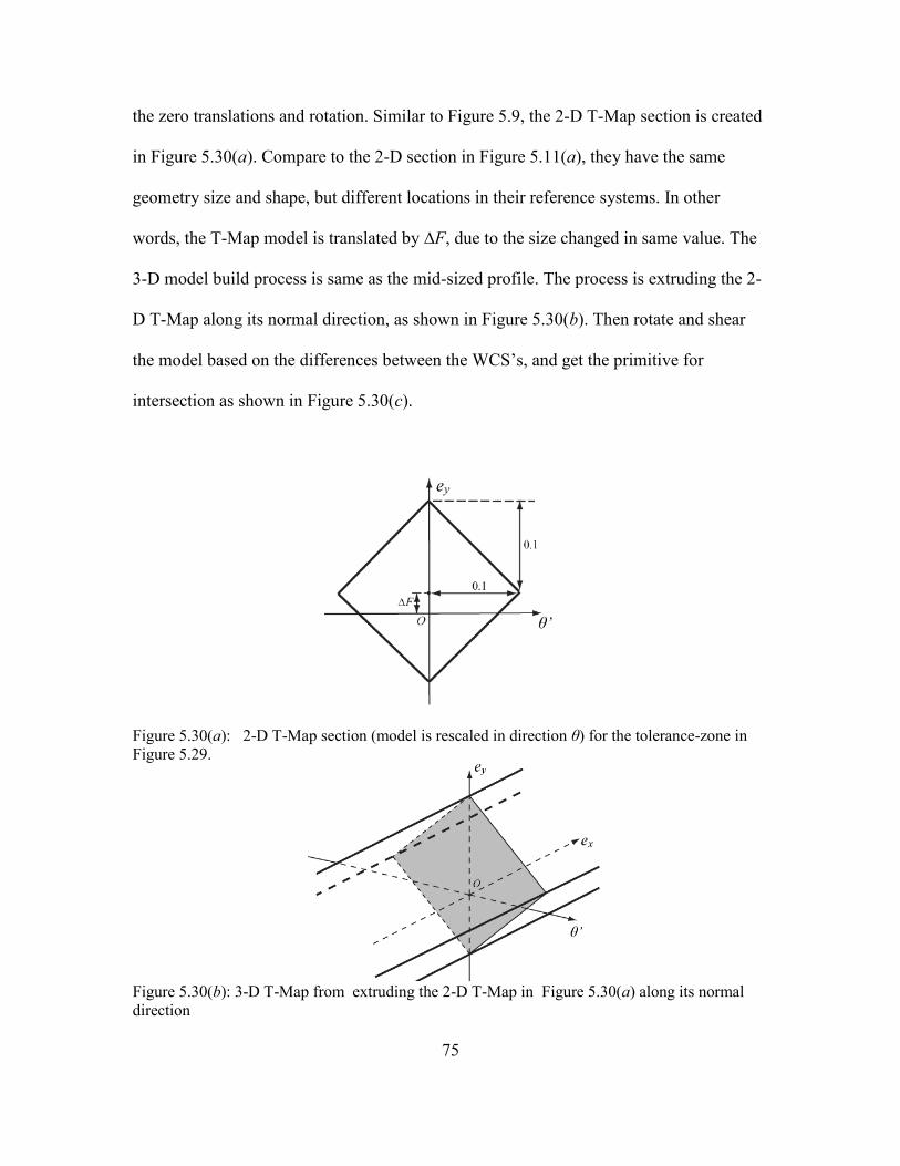
75

the zero translations and rotation. Similar to Figure 5.9, the 2-D T-Map section is created

in Figure 5.30(a). Compare to the 2-D section in Figure 5.11(a), they have the same

geometry size and shape, but different locations in their reference systems. In other

words, the T-Map model is translated by ∆F, due to the size changed in same value. The

3-D model build process is same as the mid-sized profile. The process is extruding the 2-

D T-Map along its normal direction, as shown in Figure 5.30(b). Then rotate and shear

the model based on the differences between the WCS’s, and get the primitive for

intersection as shown in Figure 5.30(c).

Figure 5.30(a): 2-D T-Map section (model is rescaled in direction θ) for the tolerance-zone in

Figure 5.29.

Figure 5.30(b): 3-D T-Map from extruding the 2-D T-Map in Figure 5.30(a) along its normal

direction

76

Figure 5.30(c): An example of 3-D primitive T-Map for the triangle profile with a size change as

shown in Figure 5.30(a).

5.8.2 Size change for circular arc

The size-changed arc in its tolerance zone is shown in Figure 5.31(a). ∆F is the

value changed from the true profile. Section 5.2.3 gives a way to create the 2-D model for

the mid-sized profile, and the 2-D T-Map model for the example is given in the Figure

5.6(c). The boundary of this 2-D T-Map model can be separated into two parts. One is

from the outside boundary of the tolerance zone and the other is from the inside boundary

of the tolerance zone. The arc BC in the 2-D T-Map model is mapping the limit locations

of the profile that is moved to the outside boundary of the tolerance zone. Arc BC is on

the tolerance circle which radius is half tolerance value. The tolerance value is equal to

the distance between the true profile and the outside boundary of the tolerance zone.

However, for the profile that has size change, the distances between the profile without

translation or rotation and the boundaries of the tolerance zone is unequal. In Figure

5.31(a), the distances are ŧ/2 – ∆F to the outside boundary and ŧ/2 + ∆F to the inside

boundary. Figure 5.31(b) is the 2-D model for the size-changed profile in Figure 5.31(a).

77

In Figure 5.31(a), arc BC and arc EF are on two tolerance circles with different radii. The

enveloped area of these two arcs and their extension lines is the 2-D T-Map for the size-

changed profile.

Once the 2-D T-Map model is generated, the 3-D primitive is created follow the

same steps that were used in creating the 3-D primitive for the mid-sized circular arc

shaped profile. Because the size changed arcs have the same center, the 3-D model is

sheared just as the 3-D model for the mid-sized profile. The result is the primitive T-Map

of the arc ready for intersection.

Figure 5.31(a): Exaggerated tolerance-zone for circular arc. Dash line is true profile and dot

line is the profile with size change.

Figure 5.31(b): 2-D T-Map model (shaded area) limited by two arcs have radii ŧ/2 ± ∆F for

size- changed profile in 5.31(a).

78

5.8.3 Size change for free form curve

In the process to build sub-model for mid-sized free form curve, the sampling

points on the curve is considered as arcs with zero arc length. The sub-model for a

sampling point on the curve is shown in Figure 5.32(a). In this 2-D model, two lines are

tangent to two tolerance circles. That means this sampling point has the distant ŧ/2 – ∆F

to the outside boundary and ŧ/2 + ∆F to the inside boundary. Similar to circular arc, the 3-

D sub-model is shown in 5.32(b). The 3-D primitive model is generated by intersecting

all the sub-models.

Figure 5.32(a): The 2-D T-Map model of translation in x and y direction.

Figure 5.32(b): 3-D primitive sub-model for a sampling point, the shaded section is same with

Figure 5.32(a).

79

5.8.4 Unequally disposed profile tolerance

A unilateral and unequally disposed profile tolerance is indicated with an

unequally disposed profile symbol placed in the feature control frame. In Figure 5.33, a

second value 0.15 is added to indicate the tolerance in the inward direction that would

allow additional material to be removed from the true profile.

For the unequally disposed and unilateral profile tolerance, the true profile

location has different distances to two boundaries of the tolerance zone. The distance to

the inside boundary is 0.15, and the distance to the outside boundary is 0.05. Compare to

the size-changed profile and its tolerance zone in Figure 5.28, the unequally disposed

profile in the true profile location can be expressed as an equally disposed profile

tolerance in the same tolerance zone, but added an initial size change.

Figure 5.33: Boss with its shape controlled by the profile tolerance ŧ = 0.2 mm relative to Datums

A, B, and C. A second value 0.15 is added. A rounded corner is added to the right corner.

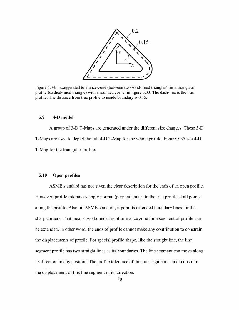
80

Figure 5.34: Exaggerated tolerance-zone (between two solid-lined triangles) for a triangular

profile (dashed-lined triangle) with a rounded corner in figure 5.33. The dash-line is the true

profile. The distance from true profile to inside boundary is 0.15.

5.9 4-D model

A group of 3-D T-Maps are generated under the different size changes. These 3-D

T-Maps are used to depict the full 4-D T-Map for the whole profile. Figure 5.35 is a 4-D

T-Map for the triangular profile.

5.10 Open profiles

ASME standard has not given the clear description for the ends of an open profile.

However, profile tolerances apply normal (perpendicular) to the true profile at all points

along the profile. Also, in ASME standard, it permits extended boundary lines for the

sharp corners. That means two boundaries of tolerance zone for a segment of profile can

be extended. In other word, the ends of profile cannot make any contribution to constrain

the displacements of profile. For special profile shape, like the straight line, the line

segment profile has two straight lines as its boundaries. The line segment can move along

its direction to any position. The profile tolerance of this line segment cannot constrain

the displacement of this line segment in its direction.

81

Fig

ure

5.3

5:

Th

e m

orp

holo

gy

of

the

4-D

T-M

ap a

s a

funct

ion o

f si

ze f

or

the

tria

ngula

r li

ne-

pro

file

sp

ecif

ied

in

Fig

ure

5.1

. T

he

scal

e in

th

e

dir

ecti

on

of

size

ch

ang

e is

no

t li

nea

r. O

ne

shap

e is

show

n f

or

size

dec

reas

e to

ill

ust

rate

the

thro

ug

h-t

he-

ori

gin

sy

mm

etry

in

th

e dir

ecti

on o

f

size

.

82

In the process of building T-Maps for closed profiles, the profiles are

decomposed into some segments. They can be considered several independent profiles.

The tolerance zones for these segments are open at their ends. In previous study of

primitive T-Maps for three types of profile elements, there is no constraint for the profile

at their ends. In Figure 5.9, Figure 5.22(a) and Figure 5.25(a), only the boundaries and

their extension lines are used for primitive T-Map building. Because the tolerance zone

for the open profile in ASME standard is same with the tolerance zone used for primitive

T-Map, the process for building primitives meets the ASME standard. These segments

can be considered open profiles. The T-Map of the whole open profile can be directly

obtained by intersect the T-Map primitives of these segments. The steps for constructing

T-Maps for the open profile are same as for the T-Maps for the closed profile.

5.11 T-Map under ISO Standard

By the definition of the ISO standard, the tolerance zone is limited by two lines

enveloping circles whose diameter is tolerance value. The centers of these circles are

situated on the true profile. Take the triangular profile as an example, the tolerance zone

for the profile under ISO standard is shown in Figure 5.36. The corner of outsider

boundary is rounded, because the boundary envelop circles are situated on the true

profile.

Comparing the tolerance zones under two standards, the tolerance zone under ISO

standard is smaller than the tolerance zone under ASME standard near the corner. In

Figure 5.36, the different areas are shown in shaded. The reduction of tolerance zone

means more constraint for the displacements of the profile. Under ISO standard, the T-

83

Map model will be removed some volume from the model under the freedom permitted

with the ASME standard.

Trim faces are created to modify the T-Map models for ISO standard. The trim

face is generated from the circular arc of the boundary at each sharp corner. Take the

right corner of the triangular profile as an example. The vertex at the corner is considered

as a circular arc profile with zero radius. The circular arc profile has a tangent range that

is between the tangents of the arc at its ends. This “point” arc profile keeps the tangent

range that is between the directions of the two edges of the corner. The boundary of this

“point” arc profile is shown in Figure 5.37(a). The boundary is offset from the “point”

arc profile by half tolerance value. Based on the boundary, in the 2-D T-Map the plane is

separated into two areas. The shaded area is the acceptable region of the mapping point

space. Because the circular arc has infinite rotational value in the T-Map, the unsheared

trim face can be got by extruding the 2-D T-Map in the direction of θ’. The unsheared

trim face separates the 3-D space into two parts, acceptable mapping points and

unacceptable mapping points. Appling the shear deformation to the trim face by the

Figure 5.36: Exaggerated tolerance-zone (between two solid-lined triangles) for a triangular

profile (dashed-lined triangle). The corner of outside boundary is rounded. Shaded area is the area

that reduced from the tolerance zone under ASME standard.

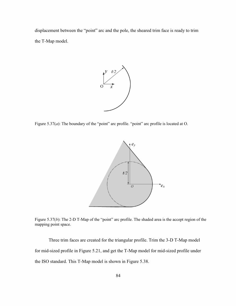
84

displacement between the “point” arc and the pole, the sheared trim face is ready to trim

the T-Map model.

Three trim faces are created for the triangular profile. Trim the 3-D T-Map model

for mid-sized profile in Figure 5.21, and get the T-Map model for mid-sized profile under

the ISO standard. This T-Map model is shown in Figure 5.38.

Figure 5.37(a): The boundary of the “point” arc profile. “point” arc profile is located at O.

Figure 5.37(b): The 2-D T-Map of the “point” arc profile. The shaded area is the accept region of the

mapping point space.

85

5.12 Hypersections of the 4-D T-Maps

The 3-D modeling discussed in sections from 5.5 to 5.8 is to create a 3-D

hypersection of the 4-D T-Map in the dimensions of ex, ey, and θ’. In this section other

hypersections of the 4-D T-Map will be discussed. The dimensions of these 3-D

hypersections would be exθ’∆F, eyθ’∆F, and exey∆F. The procedure of creating these 3-D

hypersections is similar to the method for constructing the 3-D T-Map for the mid-sized

profile. The first step is to build a primitive model for each decomposed segment in its

WCS, and then transfer the primitive model to the global reference system. Finally, do

the Boolean operation to the primitive.

The primitives of each element may have different shapes in the different

dimensions. For the straight line segment in Figure 5.9, the primitives of the straight line

Figure 5.38: 3-D T-Map model for mid-sized profile under the ISO standard. Compare to the T-

Map in Figure 5.21 for the triangular profile under the ASME standard. The heavy dashed lines

are hidden, and the light dotted line identifying points having C2 discontinuity.

86

segment in the space with the dimensions exθ’∆F are shown in the Figure 5.39(a). The

primitive model with the change in the fourth dimension ey is shown in Figure 5.39(b).

Because the size change of the profile can be seen as an additional translation of the

profile in y direction, the primitive will translate in the ∆F direction when there is a non-

zero ey. After transfer these primitives to the global reference system, the primitive will

be sheared. In the space exθ’∆F, the 3-D primitive need sheared only in the ex direction.

Figure 5.39(a): The 3-D primitives of the T-Map in the space with dimensions exθ’∆F at zero ey.

The shaded area is the 2-D section at the plane Oθ’∆F.

Figure 5.39(b): The 3-D primitives of the T-Map in the space with dimensions exθ’∆F at non-zero

ey. The shaded area is the 2-D section at the plane Oθ’∆F.

87

The primitive of the straight line segment (Figure 5.9) in the space with the

dimensions eyθ’∆F is shown in the Figure 5.40. The primitive model will not change

with the change in the fourth dimension ex, because there is no influence between ex and

other dimensions. In the space eyθ’∆F, the 3-D primitive need sheared in direction only in

the ey direction.

The primitives of the straight line segment (Figure 5.9) in the space with the

dimensions exey∆F are shown in the Figure 5.41(a). When the rotational angle changed,

the allowable range of the translation in ey and size change ∆F will decrease, and the

Figure 5.40: The 3-D primitives of the T-Map in the space with dimensions eyθ’∆F. The light

shaded areas are the 2-D sections with the dimensions ey and θ’. The dark one is the 2-D section

at the plane Oθ’∆F. The extrude direction is 45 degree to axis ∆F and axis ey.

88

primitive model is shown in the Figure 5.41(b). Because the space exey∆F does not have

dimension θ’, the sharing deformation does not apply to the primitive.

Figure 5.41(a): The 3-D primitives of the T-Map in the space with dimensions exey∆F at zero ex.

The model is a volume between two planes. The shaded area is the 2-D section at the plane

Oey∆F.

Figure 5.41(b): The 3-D primitives of the T-Map in the space with dimensions exey∆F non-zero

ex. The model is a volume between two planes. The shaded area is the 2-D section at the plane

Oey∆F.

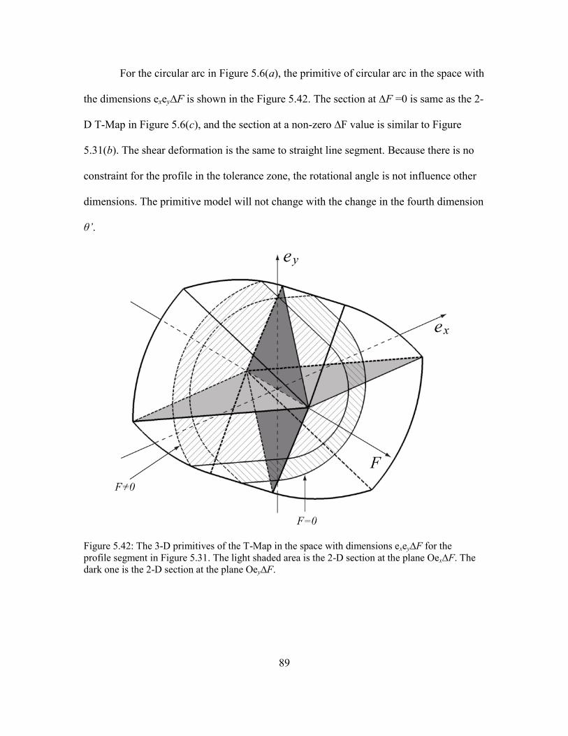
89

For the circular arc in Figure 5.6(a), the primitive of circular arc in the space with

the dimensions exey∆F is shown in the Figure 5.42. The section at ∆F =0 is same as the 2-

D T-Map in Figure 5.6(c), and the section at a non-zero ∆F value is similar to Figure

5.31(b). The shear deformation is the same to straight line segment. Because there is no

constraint for the profile in the tolerance zone, the rotational angle is not influence other

dimensions. The primitive model will not change with the change in the fourth dimension

θ’.

Figure 5.42: The 3-D primitives of the T-Map in the space with dimensions exey∆F for the

profile segment in Figure 5.31. The light shaded area is the 2-D section at the plane Oex∆F. The

dark one is the 2-D section at the plane Oey∆F.

90

Since, for the circular arc, there is no limit in the rotation, the primitives of the

circular arc (Figure 5.6(a)) in the space with the dimensions exθ’∆F or eyθ’∆F can be

obtained by extruding a 2-D T-Map to infinity along the θ’ axis. Extruding the light

shaded area (section in ey=0) in Figure 5.42 along the θ’ axis will create the primitive in

the space exθ’∆F, and extruding the dark shaded area (section in ex=0) along the θ’ axis

will create the primitive in the space eyθ’∆F. When the fourth dimension changes, for

example, ey is a non-zero value for the space with the dimensions exθ’∆F, the 2-D T-Map

will be created by intersecting the 3-D model in Figure 5.42 with a plane parallel to the

Oex∆F. The distance between these two planes is equal to the change of ey.

The primitive for a free form curve is the combination of the sub-models of the

profile at the sampling points. In the study in section 3.7, the sub-model is considered as

a special case of the circular. For example, there is a sampling point at which the tangent

of the profile is along the x axis. The 3-D sub-model in the space exey∆F is shown in

Figure 5.43. Same as the construction of primitive for circular arc, the sub-model will not

change, when the fourth dimension θ’ changed. The sub-model in the space exθ’∆F or

eyθ’∆F can be built using the same constructing method for the primitive for circular arc.

91

Figure 5.43: The 3-D primitives of the T-Map in the space with dimensions exey∆F. The shaded

area is the 2-D section at the plane Oex∆F.

92

Chapter 6

COMPUTER PROGRAMMING OF T-MAP CONSTRUCTION

6.1 Requirements of programming

The object of programming is to use computer software to create 3-D T-Maps for

tolerances applied to line profiles. Because the 4-D model cannot be directly shown by

the computer system, the 4-D T-Map model is depicted in this thesis with a set of 3-D

models at different allowable sizes within the tolerance-zone. Consequently, the software

creates a 3-D T-Map (hypersection of the 4-D T-Map for a specific size ∆F). The

program supports the profiles formed from combinations of straight line-segments,

circular arcs, and free form curves. The program supports both closed profiles and open

profiles, and it supports convex profiles and concave profiles. The program is under the

ASME Standard. The codes are packed and can be used in other programs.

The input information includes the profile geometric date in the form of

computer math data. Another input is the tolerance value. The tolerance value has two

parts to define the maximum allowable displacements of the profile form the true profile

position in the two opposite direction. Because the tolerance may be disposed unilaterally

or unequally, the tolerance value is entered with two values. And a change in size can be

presented by adjusting these two tolerance values. Amplification factors for final

presentation can be set in the input information. With the appropriate amplification

factor, the model can represent the T-Map more clearly. Because the free form curves are

approximated with short line segments, a value is needed to control the accuracy of the

construction for the free form curves.

93

The output of the program is a 3-D T-Map with the given tolerance values. The

model is in the form of computer math data. And the program also gives the coordinates

of all points in the fixed reference system having its origin at the invariant point (pole).

The coordinates of the pole may be used in the operation of the T-Map in the future

works.

6.2 Programming environment and tools

The program is created in Visual Studio 2008, and the programming language is

C++. It is because in the previous researches of T-Map, C++ is used for most

programming works. Considering the factors of hereditability and compatibility, this new

program should be in the same programming environment.

The 3D ACIS Modeler (ACIS) is the tool used to create and operate the models in

the C++. ACIS is an open, object-oriented C++ architecture that enables robust, 3D

modeling capabilities. It gives a sound base of 3D modeling functionality, plus the

flexibility to meet our programming requirements. The T-Map building process for line

profiles needs the functions to extract the geometric properties of the profiles, to create

the solid geometric models and to operate these models. All these requirements can be

realized with ACIS. Also ACIS is widely used in previous works by the researchers in

ASU Design Automation Lab. The math data of T-Map model is outputted in the form of

Standard ACIS Text (file extension .sat). SolidWorks is used to visualize and read the .sat

file.

94

6.3 Class and functions

A class is created for the generation of 3-D T-Map for the line profile. Its name is

LineProfileToTMAP. This class saves all the data of the profile and T-Map models, and

also provides all the functions for the 3-D T-Map for the line profile. This class can be

used in other programs, and it is created and tested in Visual C++ Win32 Console

Application.

The variables of the class are shown in the Table 6.1. The amplification factors

are used to change the scale reference frame, in order to get a better view of the T-Map

models. Inside tolerance value and outside tolerance value are calculated from the size

change and the unilaterally dispose profile tolerance.

Table 6.1 Variables of class LineProfileToTMAP

Variable name Description

amp_angle The amplification factor of the axis of rotational angle.

amp_tmap The amplification factor of the whole T-Map model.

input_profile Save the input math data of profile as an ENTITY.

inside_tol The tolerance value to the inside direction.

outside_tol The tolerance value to the outside direction.

pole The coordinates of the pole position.

primitive_list Save the primitive T-Map models in the ENTITY_LIST.

ptmap The pointer of output 3-D T-Map model.

segments_list Save the segments of decomposed profile in the ENTITY_LIST.

95

Figure 6.1: Flowchart of function get_tmap and function build_tmap.

The functions of the class are used to compute the model of T-Map, input and

output the data. The function get_tmap is the main entrance of the program. This function

will return the final T-Map with the given tolerance and size change, also will compute

and save the pole coordinates. Flowchart of the function get_tmap is shown in Figure 6.1.

Decompose the profile is realized by the function decompose_to_segments. Here the

profile is broken at its vertexes. The segments of the profile are saved in the

segments_list. The location of the pole needs to be got first. From the maximum

rotational value of the mid-sized T-Map model, the true location of the pole can be

96

calculated. With the true location of the pole, the required T-Map model can be

generated.

The function build_tmap is used twice in the function get_tmap. One time is

building the T-Map for the mid-sized profile which is used for calculating the pole. The

other time is building the T-Map with the true location of the pole. In function

build_tmap, the primitives are created for each member in the segments_list and the

models of primitives are saved in the primitive_list. After all of the primitives are created,

intersect the primitives to get a T-Map model and save the pointer of the model to ptmap.

The primitive of straight line is built by the function build_primitive_straight. In

build_primitive_straight, four vertexes of the 2-D T-Map are created, as the four vertexes

in Figure 5.11(a). Then the four vertexes are translated based on position relation

between the WCS and the pole. A face is created by these vertexes, and the primitive

solid is created by extruding the face in its normal direction.

The function build_primitive_arc builds the primitive for a circular arc. In this

function the circular arc will be separated into two pieces, if the angle of the arc is larger

than 180 degrees. The function build_primitive_sub_arc is used to build the sub-models

for the separated arcs, and the sub-models are intersected in function build_primitive_arc

to get the final primitive model for the arc. In the function build_primitive_sub_arc, a

face with six vertexes is created. The 2-D model shown in the Figure 5.6(c) is one

example of this face. The 3-D model of the primitive solid is created by extruding the

face in a direction. The direction is calculated by the relation between the center of the

circular arc and the location of the pole. The function build_primitive_sub_arc will return

this 3-D model to the function build_primitive_arc.

97

The primitive of free form curve is built by the function build_primitive_intcur. In

ACIS all curves can be classified into four types, ellipse, helix, intcurve, and straight.

Ellipse, intcurve and straight can be planar curves. The intcurve is used to restore and

operate the free form curves in ACIS. In the function build_primitive_intcur, the free

curve is broken into segments at the zero curvature, and build_primitive_sub_intcur

creates the models for these free curve segments. In the function

build_primitive_sub_intcur, a group sampling points are picked from the curve. The

tangents and curvatures of the curve at those sampling points are used to build the sub-

models. The 3-D model is built same as introduced in section 5.7.

6.4 Test of the class

The class LineProfileToTMAP is tested in the Win32 console application. The

steps to use this class as follow:

1. Include the class LineProfileToTMAP in the header file.

2. Create an object of this class.

3. Set the parameters of this object, including inside and outside tolerances,

maximum distance of sampling point, and amplify factor of angle and whole

T-Map.

4. Import the profile into the object.

5. Run the function get_tmap, and get the 3-D T-Map model.

If there are some errors in the program, error information will be output. The

information includes the notes to locate the error, and also includes the ACIS error codes.

98

Chapter 7

CONCLUSION AND FUTURE WORK

7.1 Conclusion

In this thesis new methods were developed to generate the Tolerance Map (T-

Map) for a line profile. Two methods were explored: the parametric method and the

method of the decomposition and intersection, with the objective of identifying and

implementing the most promising one for use in computer aided tolerancing. The T-Map

is a new math model to represent the variations of a toleranced feature as points in a

hypothetical, Euclidian space. The points in the 4-D T-Map model for line profile

represented the deviations of a manufactured profile from the true profile. The deviations

are represented with four variables: translations in two directions of the plane, one

rotation in the plane, and size change. With the examples of profiles, the decomposition

method is introduced. In this method, the profile is decomposed at its vertexes into three

types: straight line, circular arc and free form curve. Each of these types has a procedure

to build the corresponding primitive model. The primitive models are deformed to be

represented in the same reference system. Apply the intersection of the Boolean operation

to all primitives, and get the T-Map for the whole profile. A parametric method for T-

Map generation is also developed sufficient to verify the decomposition method.

The decomposition method is the only method that has been developed for

generating the T-Map for line profile having any geometric shape. It can be used to

generate open and closed profiles, convex profiles and ones having concave portions.

And this method is compatible with the ASME standard Y 14.5 and ISO standards.

99

The decomposition method has been implemented in computer software to

generate the 3-D hypersections of a T-Map for a given tolerance and size change on a

line-profile. T-Maps for some example profiles are included in the appendix of the thesis.

7.2 Future work

The T-Map created in this thesis is for a single class of geometric tolerance

defined from designers, the line-profile tolerance. Line profiles are usually linked to other

features, such as one or more planes or lines, so designers need a way to integrate the T-

Map for a line-profile with those of other features and tolerance classes. So, one

extension of this thesis would be to apply T-Maps for line-profiles to parts and

assemblies that require such integration.

Another line of investigation would be to use the decomposition idea of this thesis

to develop T-Maps for surface profiles. It should be possible to again use T-Maps for

primitive surface elements and use Boolean intersection of these to get the T-Map for the

whole surface profile.

100

REFERENCES

[1] Lieu, D.K and Sorby, A.S. (2009). Visualization, Modeling, and Graphics for

Engineering Design. Cengage Learning.

[2] American National Standard ASME Y14.5. (2009). Dimensioning and

Tolerancing. NY, American Society of Mechanical Engineers.

[3] ISO 1101:2004 Geometrical Product Specifications (GPS) — Geometrical

tolerancing —Tolerancing of form, orientation, location and run-out.

[4] Davidson, J.K., Mujezinović, A., and Shah, J. J. (2002). A New Mathematical

Model for Geometric Tolerances as Applied to Round Faces. ASME Transactions,

J. of Mechanical Design, Vol. 124, pp. 609-622.

[5] Gossard, D. C., Zuffante, R. P., and Sakurai, H. (1988). Representing

Dimensions, Tolerances, and Features in MCAE Systems, IEEE transactions on

computer graphics and applications, 8 (2), pp. 51–59.

[6] Hillyard, R. C., and Braid, I. C. (1978). Analysis of Dimensions and Tolerances in

Computer-Aided Mechanical Design. Computer-Aided Design, 10 (3), pp. 161–

166.

[7] Light, R. A., and Gossard, D. C. (1982). Modification of Geometric Models

through Variational Geometry. Computer-Aided Design, 14 (4), pp. 209–214.

[8] Lin, V. C., Gossard, D. C., and Light, R. A. (1981). Variational Geometry in

Computer-Aided Design. Proc. of Siggraph '81, Comput. Graph., 15(3), pp. 171–

177.

[9] Turner, J. U., and Wozny, M. (1988). A Mathematical Theory of Tolerances.

Geometric Modeling for CAD Applications. New York. Wozny, McLaughlin,

Encarnacao, eds., Elsevier.

[10] Turner, J. U., and Wozny, M. J. (1990). The M-space Theory of Tolerances, Proc.

of 16th ASME Design Automation Conf., ASME Press, (ed. B. Ravani), pp. 217–

225.

[11] Requicha, A. A. G. (1983). Toward a Theory of Geometric Tolerances. Int. J.

Robot. Res., 2(4), pp. 45–60.

101

[12] Requicha, A. A. G., and Chan, S. C. (1986). Representation of Geometric

Features, Tolerances, and attributes in Solid Modelers Based on Constructive

Geometry. IEEE J. Rob. Autom., RA-2 (3), pp. 156–166.

[13] Roy, U., and Liu, C. R. (1988). Feature-Based Representational Scheme of a

Solid Modeler for roviding Dimensioning and Tolerancing Information. Rob.

Computer-Integr. Manufact., 4 (3/4), pp. 335–345.

[14] Martinsen, K. (1993) Vectorial Tolerancing for All Types of Surfaces, Proc. of

19th ASME Design Automation Conf., Albuquerque, Vol. 2, ASME Press.

[15] Turner, J. U. (1990) Exploiting Solid Models for Tolerance Computations.

Geometric Modeling for Product Engineering, M. J. Wozny, J. U. Turner, and K.

Preiss, eds., pp. 237–258, North-Holland.

[16] Chase, K., Gao, J., Magelby, S., and Sorensen, C. (1998). Including Geometric

Feature Variations in Tolerance Analysis of Mechanical Assemblies, IIE

Transactions, 28, pp. 795–807.

[17] Rivest, L., Fortin, C. and Morel, C. (1994). Tolerancing a solid model with a

kinematic formulation. Computer-Aided Des, 26, pp. 465–476.

[18] Bernstein, N., and Preiss, K. (1989). Representation of Tolerance Information in

Solid Models, Proc., 15th ASME Design Automation Conf., Montreal, September

17–21, DE-Vol. 19–1, ASME Press, pp. 37–48.

[19] Zhang, B. C. (1992). Geometric Modeling of Dimensioning and Tolerancing, PhD

Thesis, Arizona State University.

[20] Kramer, G. A. (1992). Solving Geometric Constraint Systems: A Case Study in

Kinematics, MIT Press.

[21] Clément, A., Desrochers, A., Rivière, A. (1991). Theory and Practice of 3D

Tolerancing for Assembly, Proc., 2nd CIRP Seminar on Computer-Aided

Tolerancing, Pennsylvania State, May.

[22] Clément, A., Rivière, A., and Temmerman, M. (1992). Cotation Tridimensionelle

des Systemes Mecaniques, Theorie et Pratique, in French, Yvry-sur-Siene.

(English translation in progress by Addison-Wesley, Boston).

[23] Reuleaux, F. (1875). Theoretische Kinematik: Grundzüge einer Theorie des

Maschinenwesens, Vieweg, Braunschweig. Trans. Kennedy, A. B. W. (1876) as

The Kinematics of Machinery, MacMillan, London. Reprinted (1963) with a new

introduction by E. S. Ferguson, Dover, NY.

102

[24] Hunt, K. H. (1976). Geometry—The Key to Mechanical Movements, Mech.

Mach. Theory, 11, pp. 79–89.

[25] Giordano, M., Pairel, E., and Samper, S. (1999). Mathematical Representation of

Tolerance Zones. Proc., 6th CIRP Int’l Seminar on Computer-Aided Tolerancing,

University of Twente, Enschede, Netherlands, March 22-24, pp. 177-186.

[26] Mujezinović, A. (1999). A New Mathematical Model for Representing Geometric

Tolerances, M.S. Thesis, Arizona State University.

[27] Davidson, J.K. and Shah, J.J. (2002). Geometric Tolerances: A New Application

for Line Geometry and Screws, IMechE J. of Mechanical Engineering Science,

Part C, Vol. 216, No. C1, pp. 95-104.

[28] Davidson, J.K. and Shah, J.J. (2003). Using Tolerance-Maps® to Represent

Material Condition on both a Feature and a Datum, 8th CIRP Int’l Seminar on

Computer-Aided Tolerancing, Charlotte, North Carolina, USA, April 28-29, pp.

92-101.

[29] Davidson, J.K. and Shah, J.J. (2009). The Method of Isosceles Triangulation

Validated for Constructing T-Maps for Size of Parts Having Round and

Rectangular Cross-Sections, 11th CIRP Int’l Seminar on Computer-Aided

Tolerancing, Annecy, France, March 26-27.

[30] Bhide, S.S. (2002). A new mathematical model for geometric tolerances applied

to cylindrical features, M.S. Thesis, Arizona State University.

[31] Ameta, G. (2004). Tolerance-maps applied to angled faces and two clusters of

features, M.S. Thesis, Arizona State University.

[32] Patrick, C. (2010). Tolerance-Maps for Runout and Straightness Tolerances, and

for a Line-Plane Cluster, M.S. Thesis, Arizona State University.

[33] Davidson J.K. and Shah J.J. (2012). Modeling of Geometric Variations for Line-

Profiles. ASME Transactions, J. of Computing & Information Science in Engrg.,

Vol. 12, #041004, 10 pp.

[34] Hunt, K.H. (1979). Kinematic geometry of mechanisms. Clarendon Press, Oxford.

Reprinted with corrections in 1990.

[35] Hain, K. (1967). Applied kinematics. 2nd

ed. McGraw-Hill

[36] Davidson J. K., Savaliya S. B., He. Y., & Shah J.J. (2012). Methods Of Robotics

And The Pseudoinverse To Obtain The Least-Squares Fit Of Measured Points On

103

Line-Profiles, ASME 2012 International Design Engineering Technical

Conferences & 17th Design for Manufacturing and the Life Cycle Conference

[37] McCarthy, J.M. (1990). An introduction to theoretical kinematics, MIT Press,

Cambridge, MA.

104

APPENDIX A

OUTPUTS OF THE COMPUTER PROGRAM TESTING

105

Examples of profile tolerances are used to test the program. Figure A.1 is the

profile tolerance used in Chapter 4. 3-D T-Maps outputted from the program with

different size changes are shown in Table A.1. The models get from the computer are

same as those in Chapter 4.

Figure A.1: Boss with its shape controlled by the profile tolerance ŧ = 0.2 mm relative to Datums

A, B, and C.

106

Table A.1 The 3-D models for the profile tolerance in Figure A.1 in different size change values

NO Size change

value 3-D T-Map model

1 -0.75

2 -0.5

3 -0.25

107

4 0

5 0.25

6 0.5

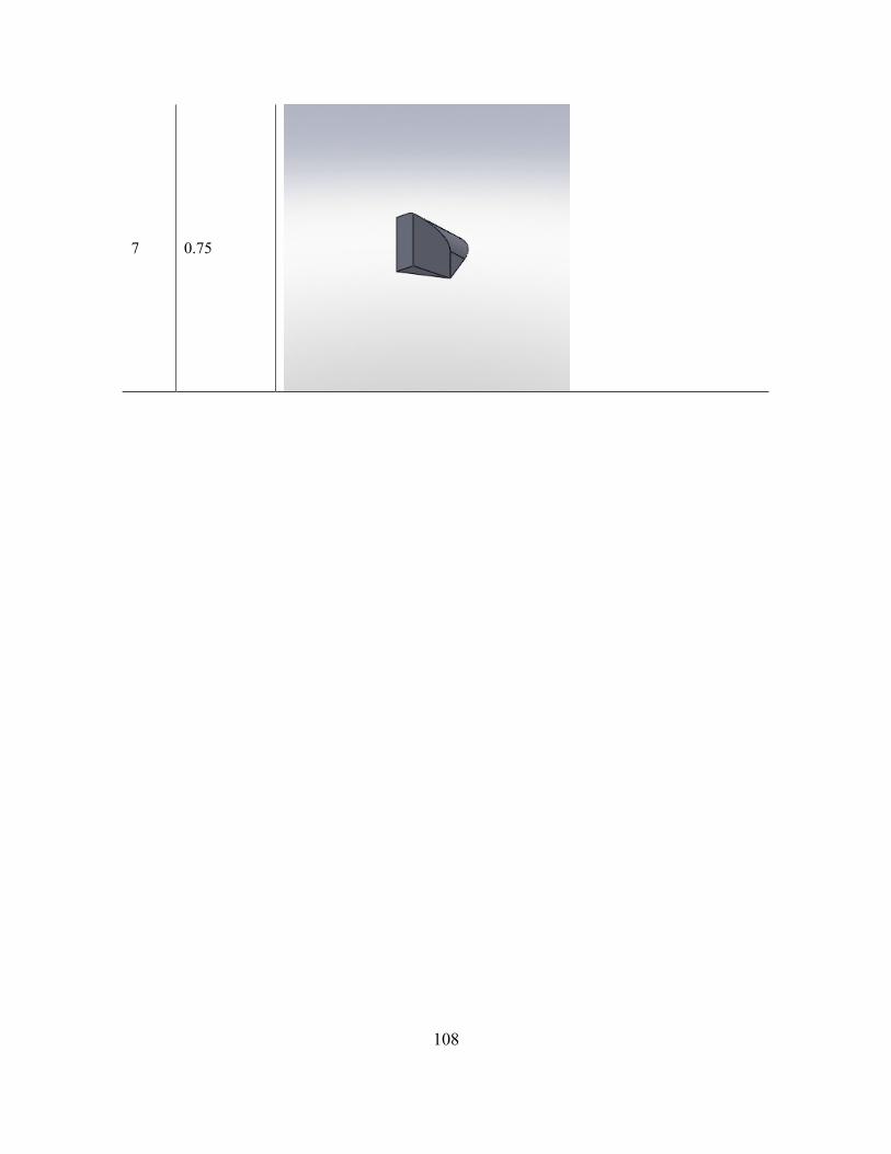
108

7 0.75

109

Figure A.2 is an example of concave shape of the profile tolerance. Table A.2

give the 3-D T-Maps outputted from the program with different size changes. All of the

T-Map models are convex.

Figure A.2: Boss with concave shape controlled by the profile tolerance ŧ = 0.2 mm relative to

Datums A, B, and C.

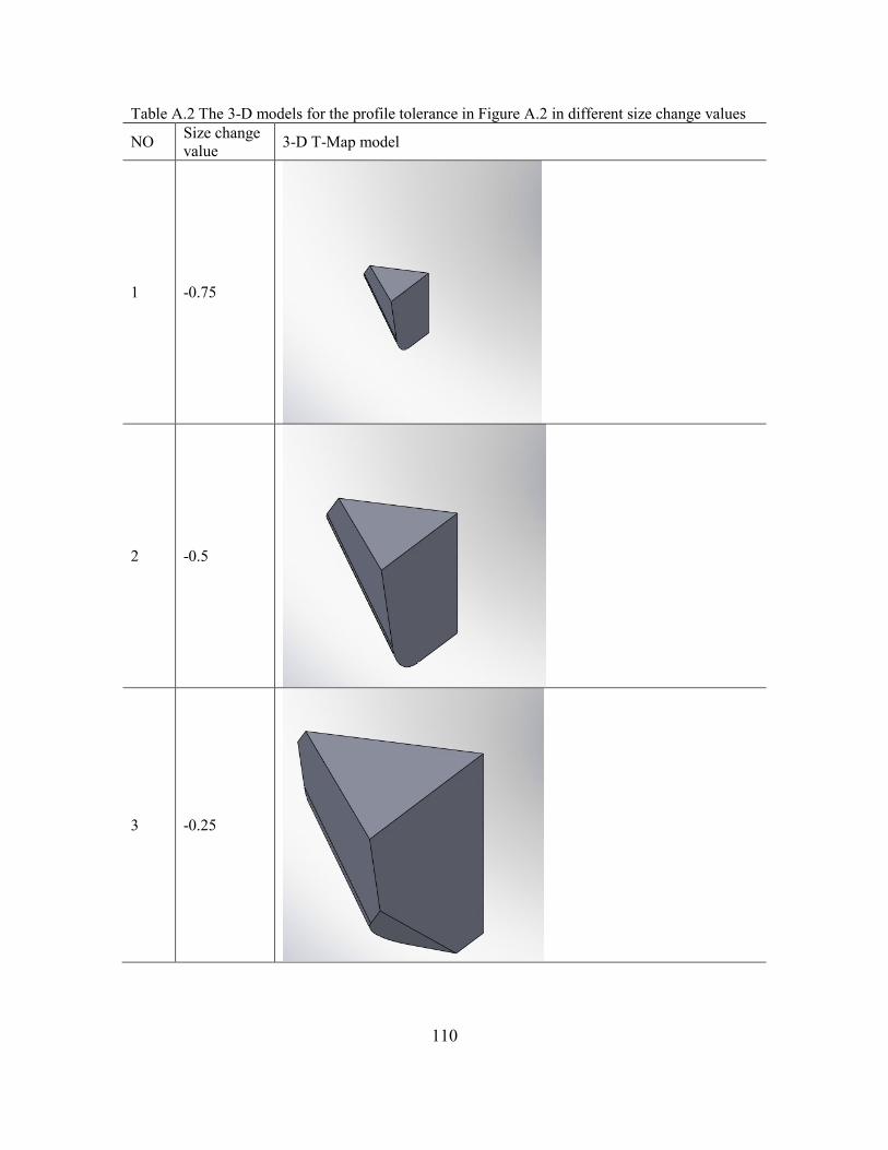
110

Table A.2 The 3-D models for the profile tolerance in Figure A.2 in different size change values

NO Size change

value 3-D T-Map model

1 -0.75

2 -0.5

3 -0.25

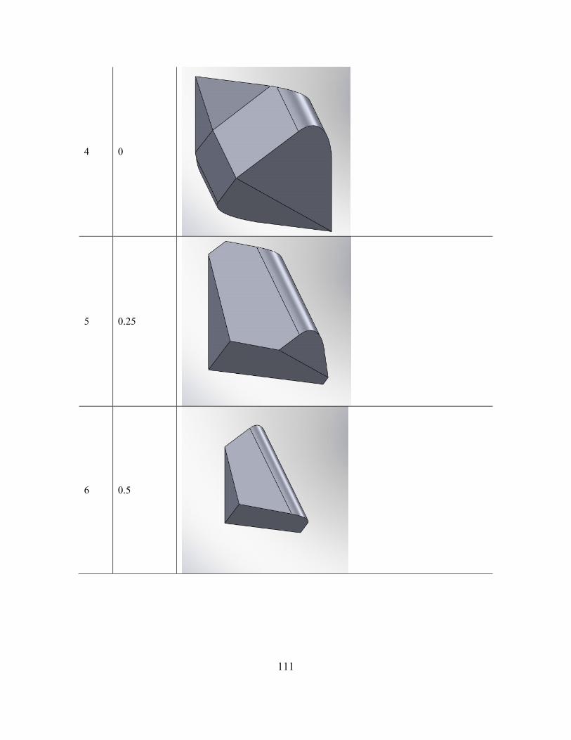
111

4 0

5 0.25

6 0.5

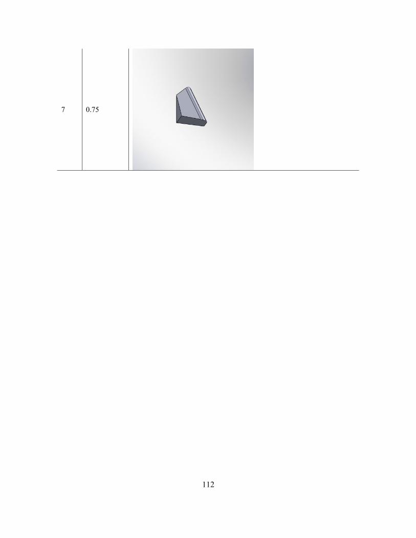
112

7 0.75