generation costs estimation in the spanish … · generation costs estimation in the spanish...
TRANSCRIPT

UNIVERSIDAD PONTIFICIA COMILLAS ESCUELA TÉCNICA SUPERIOR DE INGENIERÍA (ICAI)
MÁSTER OF THE ELECTRIC POWER INDUSTRY
MASTER THESIS
Generation Costs Estimation in the Spanish Mainland Power System from
2011 to 2020
AUTHOR: Jesús David Crisóstomo Ramírez
MADRID, July, 2011

i
Acknowledgements
This work is the result of two years of study abroad in Spain and Netherlands. Living far away
from home and sometimes under extreme weather conditions that made things harder, this is the
price for never giving up and always listen to many people who encouraged me to keep going
ahead.
First, I want to thank the European Commission that gave me the opportunity to live an amazing
experience with the scholarship “Eramus Mundus”. Thanks to this I was able to study in two
excellent universities namely University Pontifical Comillas and Delft University of
Technology. I also thank to both of the universities that hosted me in their rooms made their
excellent teaching staff to share their knowledge.
Second, thanks to Iberdrola that gave the opportunity to close this adventure with an interesting
internship and gave me the opportunity to work on my final thesis with an interesting topic. I am
also thankful with Elena Lopez and Rafael Bedillo who led me during the last 5 months sharing
their knowledge and putting me back on track when something was going away. Thanks for
your invaluable help and patience during this 5 months.
Then, I really want to thank my family and especially my parents who have been strong enough
to support me every day even in the hardest days when they went through different surgeries.
They never gave up and always had words to encourage me. I love them and I am very grateful
for their support.
To my girlfriend for being willing to wait for two years in which we were far away from each
other and showing every day her love and patience to cope with the distance. I love her and I’m
looking forward to huge her and never being apart again.
To all my friends and people I met during this two years master program and especially to my
friend Shahiryar Khan Yousafsai with whom I moved everywhere in this program. Thanks dude
for your sincere friendship.
Finally, thanks to all people that directly and indirectly helped me out in all the things I had to
do during these two years. Just to mention some people, Javier Gonzalez, EMIN director.
Andres Gonzalez in Comillas. Toke Hoek in TU Delft. Andres Ramos my thesis supervisor in
Comillas. Thanks to all of you.
ii
Abstract
Generation Costs Estimation in the Spanish Mainland Power System from 2011 to 2020
AUTHOR: J. DAVID CRISÓSTOMO R.
The electricity sector in Spain had been evolving steadily in an ascendant rate since the
liberalization in late 90’s. Demand was expected to keep growing but it suddenly dropped in
2009 creating and unbalance ion the system in term of demand and installed capacity. In
addition the increasing share of renewable energy contribution has also imposed an additional
pressure on the ordinary regime technology leaving less and less residual demand for such
technologies. The current and expected scenario in the Spanish mainland power system seems to
be harder for the ordinary regime technologies for the next years. It has just issued a Royal
Decree to support the autochthonous coal mines, imposing quotas for coal units using such coal.
This work has the purpose of gather all the regulatory and economical constraints and apply
them to estimate the generation costs for the following ten years. The approach to do such
extensive task is to apply a regulated cost structure based on fixed and variable costs already
proved as a reference model of the system costs in the SEP. The generation dispatch is done
using a traditional approach of unit commitment based on the least costly units and taking into
consideration the different constraint to reflect the most plausible behavior of market players.
The result are consistent with the costs associated to the different technologies. Nuclear units
are base load during the whole year and CCGT is the technology that balances the system to
keep equilibrium because of demand-generation variations. The most stable technology is the
Nuclear while the technology with the lowest costs is hydro. Coal and CCGT technologies
appear to be the most expensive and become the marginal technology. With respect to the
evolution of the generation mix, there were thermal units decommissioned from the installed
capacity according with its decommissioning schedule but there is also the assumption of what
in reality would happen when the existing thermal capacity is not being dispatched and the
owners decide closure. The implication of such hypothesis go straight to the Coverage index
which will be affected and start dropping compromising the minimum safe level required by the
system operator
Index Terms: regulated cost structure, optimization model, coverage index

iii
List of definitions
Closed-cycle pumping generation. Production of electrical energy carried out by the hydroelectric power stations whose higher elevation reservoir does not receive any type of natural contributions of water, but uses water solely from the lower elevation reservoir.
Combined cycle Technology for the generation of electrical energy in which two thermodynamic cycles coexist in one system: one involves the use of steam, and the other one involves the use of gas. In a power station, the gas cycle generates electrical energy by means of a gas turbine and the steam cycle involves the use of one or more steam turbines. The heat generated by combustion in the gas turbine is passed to a conventional boiler or to a heat-recovery element which is then used to move a steam turbine, increasing the yield of the process. Electricity generators are coupled to both the gas and steam turbines.
Environmental impact. Environmental change, be it adverse or beneficial, derived wholly or partially from the activities, products or services of an organization.
Generation consumption. Energy used by the auxiliary elements of power stations, necessary for the everyday functioning of the production facilities.
International physical exchanges. The movements of energy which have taken place across lines of international interconnection during a certain period of time. It includes the flow of energy as a consequence of the network design.
Net national consumption. This is energy introduced into the electrical transmission grid from the ordinary regime power plants (conventional), special regime (cogeneration and renewables) and from the balance of the international exchanges. In order to transfer this energy to the point of consumption it would be necessary to deduct the losses originating from the transmission and distribution network.
Non-renewable energies. Those obtained from fossil fuels (liquid or solid) and their derivatives
Ordinary regime. The production of electrical energy from all those facilities which are not included under the special regime (see below Ordinary regime).
Outage Situation in which the transmission grid facility -line, transformer, busbar, etc.- is disconnected from the rest of the electricity system and, consequently, power cannot flow through it. The facilities that are put temporarily out-of-service for maintenance or other works, additionally are also grounded to earth in one or various points with the objective of ensuring that their voltage is zero. In this way, any type of works can be executed on the element without risk to the safety of the people that carry it out.
Pumped storage This is a type of hydroelectric power generation used by some power plants for load balancing. The method stores energy in the form of water, pumped from a lower elevation reservoir to a higher elevation. Low-cost off-peak electric power is used to run the pumps. During periods of high demand of electricity, the stored water is released through turbines.

iv
Renewable energies Those obtained from natural resources and both industrial and urban waste. These different types of energy sources include the hydroelectric, solar, wind, solid industrial and urban residues, and biomass.
Special regime Production of electrical energy which falls under a unique economic regime, originating from facilities with installed power not exceeding 50 MW whose generation originates from cogeneration or other forms of production of electricity associated with non electrical activities, if and when, they entail a high energy yield, groups that use renewable non-consumable energies, biomass or any type of biofuel as a primary energy source, groups which use non-renewable or agricultural waste, livestock and service sector waste as primary energy sources, with an installed power lower than or equal to 25 MW, when they entail a high energy yield.
System operator A trading corporation whose main function is to guarantee the continuity and security of the electricity supply, as well as the correct coordination of the production and transmission system. It exerts its functions in coordination with the operators and agents of the Iberian Electricity Market and under the principles of transparency, objectivity and independence. In the current Spanish model, the operator of the system is also the manager of the transmission grid.
Transmission grid Set of lines, parks, transformers and other electrical elements with 220 kV or more, and those other facilities, regardless of their power, which fulfill transmission functions, international interconnections and the interconnections with the Spanish peninsular and extra-peninsular power systems

v
List of abbreviations
CCGT Combined Cycle Gas Turbine
CI Coverage Index (Indice de Cobertura)
CNE National Commission for Energy (Comisión Nacional de Energía)
DGPEM General Direction of Energy Policy and Mines (Dirección General de Política
Energética y Minas)
EU European Union
ELV Emission Limit Values
GAMS General Algebraic Modeling System
GHG Green House Gases
IED Industrial Emissions Directive
IGCC Integrated Gasification in Combined Cycle (Gasificación Integrada en Ciclo
Combinado)
INE National Institute of Statistics (Instituto Nacional de Estadística)
IPC Consumption Price Index (Índice de Precios del Consumo)
IPI Industrial Price Index (Índice de Precios Industriales)
LNG Liquefied Natural Gas
MIBEL Iberian Power Market (Mercado Ibérico de Electricidad)
MIP Mixed Integer Problem
MITC Ministry of Industry, Tourism and Commerce (Ministerio de Indústria, Turismo
y Comércio)
MLE Legal Stable Framework (Marco Legal Estable)
O&M Operation and Maintenance
OMEL Iberian Power Market Operator – Spanish Pole (Operador del Mercado Ibérico
de Energía – Polo Español)
OMIP Iberian Power Market Operator – Portuguese Pole (Operador do Mercado
Ibérico de Energia – Pólo Português)
PNA National Assignation Plan (Plan Nacional de Asignación)
RD Royal Decree

vi
REE Spanish National Grid Company (Red Eléctrica de España)
SCR Selective Catalytic Reduction
SEIE Insular and Extapeninsular Power System (Sistema Electrico Insular y
Extrapeninuslar)
SEP Mainland Spanish Power System (Sistema Eléctrico Español Peninsular)
VOC Volatile Organic Compounds

vii
Table of Contents
LIST OF TABLES ....................................................................................................................... X
LIST OF FIGURES ................................................................................................................... XI
1. INTRODUCTION AND CONTEXT ......................................................................... 1
1.1 Background .................................................................................................................................... 2
1.2 Overview of the Spanish Power System ...................................................................................... 2
1.3 Motivation and Objectives ............................................................................................................ 4
1.4 Report Structure............................................................................................................................ 5
2. METHODOLOGY APPLIED .................................................................................... 6
2.1 The notion of regulated cost structure ......................................................................................... 6
2.1.1 Fixed costs formulation ............................................................................................................... 8
2.1.2 Variable costs formulation ........................................................................................................ 12
2.2 The reference model applied to the SEP ................................................................................... 16
2.2.1 Fixed cost retribution in the SEP .............................................................................................. 17
2.2.2 Variable cost retribution in the SEP .......................................................................................... 18
2.2.2.1 Methodology for thermal units ............................................................................................. 18
2.2.2.2 Methodology for natural gas units ........................................................................................ 20
2.2.3 Variable costs associated to hydro and pumping power plants ................................................. 24
2.3 Coverage Index formulation ....................................................................................................... 25
3. TECHNOLOGY OVERVIEW ................................................................................. 26
3.1 Presentation of the power technologies and technical parameters ......................................... 26
3.1.1 Common technical parameter ................................................................................................... 27
3.1.2 Nuclear power plants ................................................................................................................ 27
3.1.3 Coal units .................................................................................................................................. 28
3.1.4 CCGT power plants .................................................................................................................. 29
3.1.5 Fuel – gas power plants ............................................................................................................. 30
3.1.6 Hydro power plants ................................................................................................................... 30
3.2 Data on generation costs by technology ..................................................................................... 30
3.2.1 Fixed costs by technology ......................................................................................................... 31
3.2.2 Variable costs by technology .................................................................................................... 32
4. DATA COLLECTION, ASSUMPTIONS AND KEY MILESTONES ................. 34
4.1 Electricity demand growth ......................................................................................................... 35
4.1.1 Monthly and daily distribution of the demand .......................................................................... 36
4.1.2 Peak demand ............................................................................................................................. 39
4.2 Generation constraints ................................................................................................................ 39

viii
4.2.1 Expected hydroelectric contribution and pumping ................................................................... 40
4.2.2 Impact of special regime generation ......................................................................................... 42
4.2.3 Residual demand for thermal units ........................................................................................... 44
4.3 Evolution of the generation mix ................................................................................................. 45
4.3.1 Hydro, nuclear and fuel-gas power plans evolution .................................................................. 45
4.3.2 Regulatory constraints............................................................................................................... 46
5. MODEL CONSTRUCTION .................................................................................... 49
5.1 Computation of fixed costs ......................................................................................................... 49
5.2 Optimization model for variable cost calculation ..................................................................... 51
5.2.1 Model Indexes and sets ............................................................................................................. 51
5.2.2 Parameter and variables ............................................................................................................ 52
5.2.3 Objective function ..................................................................................................................... 53
5.2.4 Constraints ................................................................................................................................ 53
5.2.5 Singularities .............................................................................................................................. 54
5.3 Calculation of the final generation price ................................................................................... 56
6. SIMULATION AND RESULT ANALYSIS ........................................................... 58
6.1 Simulation and Assessment of the model results ...................................................................... 58
6.1.1 Ordinary regime demand coverage and generation costs .......................................................... 58
6.1.2 Thermal generation evolution ................................................................................................... 61
6.1.3 CO2 Emissions scenario ............................................................................................................ 64
6.2 Assessment on the impact of the special regime and regulatory constraints ......................... 65
6.3 Impact on Coverage Index (IC) .................................................................................................. 67
7. FINAL CONCLUSIONS .......................................................................................... 70
7.1 Assessment of security of supply ................................................................................................ 71
7.2 Social impact of generation costs ............................................................................................... 73
7.3 Meeting the EU-2020 targets ...................................................................................................... 74
REFERENCES .......................................................................................................................... 76
APPENDIXES .......................................................................................................................... 79
Appendix 1 – Factors of availability ....................................................................................................... 79
Appendix 2 – Standard nuclear fuel recharge schedule ........................................................................ 80
Appendix 3 – Emissions Quantity factors .............................................................................................. 81
Coal Technology ....................................................................................................................................... 81
CCGT Technology .................................................................................................................................... 82
Fuel-Gas Technology ................................................................................................................................ 84
Appendix 4 – Components of LNG costs ................................................................................................ 85
Appendix 5 – Historical and project demand per month ...................................................................... 86

ix
Appendix 6 – Evolution of special regime technologies ......................................................................... 88
Appendix 7 – Evolution of thermal technologies ................................................................................... 89
Appendix 8 – GAMS Code ....................................................................................................................... 91
Appendix 9 – Generation Dispatch in period 2011-2020 ....................................................................... 97
Appendix 9 – Generation costs by technology...................................................................................... 101

x
List of Tables
Table 3.1 Factors of minimum and maximum production .......................................................... 27
Table 3.2 Nuclear units fuel recharge schedule for 2011 ............................................................ 28
Table 3.3 Emission quantity factor for coal units ....................................................................... 28
Table 3.4 Fixed costs by technology ........................................................................................... 31
Table 3.5 Fixed costs of new technologies in 2011 .................................................................... 32
Table 3.6 Main variable costs by technology .............................................................................. 33
Table 4.1 Annual demand projection in GWh ............................................................................ 36
Table 4.2 Annual demand projection in GWh ............................................................................ 36
Table 4.3 National holidays in Spain .......................................................................................... 37
Table 4.4 Percentage of daily demand by day type and month ................................................... 38
Table 4.5 Peak demand for winter and summer .......................................................................... 39
Table 4.6 Classification of day level and hours in hydro production and pumping .................... 40
Table 4.7 Total energy produced and pumped by month and type of day .................................. 41
Table 4.8 Monthly and intra-month weights of hydro generation and pumping ......................... 42
Table 4.9 Expected annual hydro production and pumping in GWh .......................................... 42
Table 4.10 Evolution of special regime installed capacity in MW ............................................. 43
Tale 4.11 Expected annual contribution of special regime generation........................................ 44
Table 4.12 Total expected residual demand in GWh .................................................................. 45
Table 4.13 Evolution of Hydro, nuclear and fuel-gas units ........................................................ 46
Table 4.14 Coal units’ quotas ...................................................................................................... 48
Table 5.1 Seasonality factors ...................................................................................................... 50
Table 5.2 Quotas for coal units [GWh] ....................................................................................... 55
Table 5.2 Fuel recharge schedule for nuclear units from 2011-2015 .......................................... 55
Table 6.1(a) Generation cost from 2011 to 2015 ........................................................................ 61
Table 6.1(b) Generation cost from 2016 to 2020 ........................................................................ 61
Table 6.2 Coal units’ quotas subject to SGC in GWh ................................................................. 62
Table 6.3 Coal units subject to 17,500 hours production ............................................................ 63
Table 6.4 Scenario of thermal units decommissioned and new additions ................................... 64
Table 6.4 Expected contribution of special and ordinary regime in GWh .................................. 66
Table 6.5 Summary of additional costs due to SGC ................................................................... 67
Table 6.6 Coverage Index evolution in the SEP ......................................................................... 68
Table 7.1 Qualitative assessment of generating technologies risks ............................................ 72
xi
List of Figures
Figura 1.1 Share by technology of total installed cpactiy in Spain in 2010 .................................. 4
Figure 2.1 Regulated cost structure ............................................................................................... 7
Figure 3.1 Energy vs. Operating costs curve for the coal unit Puentes 2 .................................... 29
Figure 4.1 Monthly distribution of demand ................................................................................ 37
Figure 6.1 Generation dispatch in the year 2011 ......................................................................... 59
Figure 6.2 Evolution of generation by technology in GWh ........................................................ 59
Figure 6.4 Total CO2 emissions and rate of emissions ................................................................ 65
Figure 6.5 Average generation cost compared with market prices ............................................. 66

1. Introduction and Context
The electricity sector provides one of the most important drivers of the economy in a
country and its supply is an essential input for the well functioning of the entire society. As a
result, governments are always pursuing to achieve the so called triple A policy goals;
Availability for a highly reliable system in terms of security of supply, Affordability in terms of
lower prices for the end users and Acceptability by promoting sustainability in its development
[VRIE10]; however a tradeoff is expected among these goals specially in liberalized markets. In
order to overcome these challenges it is compulsory to implement large scope policies and
collaborate worldwide to achieve agreements. To do so, it also desirable to have a broader
vision and periodical studies about the current features, difficulties and trends in the energy
sector specially for Europe who is highly dependent of gas supply and other commodities.
The case of Spain is particularly special in the world. It has become one of the countries
with the largest installed capacity and energy produced by renewable energy sources and it has
been already recognized by the EU as a successful case of designing policies to promote the use
renewable energy sources. In fact, it was reported in 2009 that contribution of renewable energy
was 25% of the total energy produced, a trend that is expected to keep growing in the coming
years [PANER10]. The policy choices made by Spain are moving towards achieving the above
mentioned goals and seem to go a step ahead from other European countries however this
successful implementation of renewable energy policies along with other domestic constraints

1. Introduction and Context
2
have brought uncertainty and are pushing players in the liberalized market to redesign their own
strategies both to meet global and individual goals.
This work has been carried out in order to provide a plausible scenario of the generation
costs expected in the Spanish mainland power systems taking into consideration the above
mentioned constraints.
1.1 Background
This work has been developed as Master Thesis for the international Erasmus Mundus
Program Economics and Management of Network Industries (EMIN). It is the result of a
internship program between Pontifical Univertity of Comillas and Iberdrola. This particular
work has an additional justification and it is linked to a previous work developed by a former
EMIN student called “Generation Cost Evaluation in Centralized Systems. A contrast over
market mechanism”. In that work, the application of the regulated cost structure was applied
first to the Insular and Extapeninsular systems namely SEIE, in order to validate what the
regulator in Spain is doing to compensate generating companies in those systems and then, it
was adapted to the Spanish mainland power system in order to be contrasted against historical
market prices.
The results of such study were consistent. For the same operational and
investment expansion decisions the theoretical centralized generation prices simulated
and those from the current liberalized market in Spain seem to concur in the short term.
Therefore, there is a strong indication that liberalized market has been working
efficiently, setting prices in accordance with the most rational centralized decisions that
would have been taken in a Reference Model. Taking this into account, this work is
intended to estimate the generation costs in the Spanish mainland power system for the
period 2011 to 2020 based on the current and expected scenario in the sector.
Assumption and hypothesis were made trying to reflect the most rational behavior of
market players and using mostly public sources that provides the most plausible
evolution of the electricity sector in Spain.
1.2 Overview of the Spanish Power System
The Spanish electricity sector currently works under a liberalized scheme as a result of
the Law 54/1997 from November 27th that basically establishes the unbundling of regulated

1. Introduction and Context
3
activities from those that can operated under a competitive market. The law considers
transmission and distribution of electricity as natural monopolies due to scale of such sectors.
On the other hand, it gives free competition to the generation and retailing sector leading to the
freedom to contract and choice of the best provider for the end consumer. In addition, this law
establishes that any market player is entitled to have network access for transmission and
distribution purposes. To do so, it creates the so called system operator who is in charge of
technical management of the system and another entity who is the market operator en charge of
economical management in the market.
After liberalization in the generation sector two main figures were created. Ordinary
regime generation and special regime generation. The first type of generation is mainly
composed by the traditional thermal technologies which are the targer technologies in this work
while the special regime technologies are mainly the renewable enrgy sources as well as
cogeneration.
The transmission system in Spain is highly interconnected to provide reliability to the
system. This sector as already said above is a natural monopoly and is not subject to
competition. REE is the system operator and is in charge of the technical management of the
network as well as to plan the network expansion for future needs. REE must give third party
access to the network under the regulated cost defined by the regulator. On the other hand, the
distribution sector is also regulated and distribution companies should provide all different
services required for the well functioning of the distribution network. The access to the
distribution network should be charged according with the regulated tariff defined by the
regulator. Retailing sector is also subject to competition and there is a market for this purpose in
which end user can choose the best retailing company in the market.
In Spain, there are different markets in which transaction are done. There is a market in
which player buy-sell energy to be delivered I the future. This market uses period that can go
from 24 to years. These kinds of contracts are bilateral contracts, contracts under the OMPI, and
auctions. For shorter periods there is the so called spot market in which negotiations are done
for the energy to be delivered either next day in the daily market or in the same day with the
intra-day market. In the first type, the market operator receives bid from suppliers and
consumers and the price is fixed on an hourly base according with the supply-demand curve.
The second market is mainly to adjust any unbalance seen during the real time operation of the
system.

1. Introduction and Context
4
According with the system operator, in respect to the generation mix in the SEP there are
97,447 MW installed capacity by the end of 2010. From this total, 26% are CCGT followed by
20% from wind farms. Figure below show the distribution of the total generation mix.
Figura 1.1 Share by technology of total installed cpactiy in Spain in 20101
1.3 Motivation and Objectives
The market regime present in the electricity sector in Spain is constantly subject to
unpredictable regulatory changes that not always are satisfactory for the participant players in
the market and can lead to an inadequate equilibrium in the long run. Apart from the well
known uncertainties in fuel prices evolution, under the current regulatory framework there are
already some constraints that will impose volatility to the future electricity prices and might, as
a consequence discourage investment in the sector compromising the triple A goals mentioned
above. Besides, there are also communitarian regulations issued by the EU to achieve the 20-20-
20 targets by 2020 related to cut in CO2 emissions, renewable energy sources share and energy
efficiency which ultimately define the path to follow in the coming years. This scenario makes
challenging the coordination in all the links of the electricity supply chain.
This work has been developed to explore the trend in the generation costs in the Spanish
mainland power system for the next 10 years based on two main foundations. First of all, as it
has been explained above, the regulated cost structure used in the SEIEs has been proved to be
consistent with the market price observed in the SEP from 2006 to 2009 in [WOTT2010]. The
evolution of the market prices under the study period was slightly below the calculated with
regulated cost structure which was an indication of the competition effect reflected in lower
prices for end user as expected in a market mechanism. This methodology is now adapted to the
current and expected evolution of the Spanish energy sector as a plausible approach to estimate
the generation costs. Secondly, the regulatory pressure in the sector to meet EU targets as well
as the local regulatory constraints, fuel and CO2 prices are indeed constraints that will have a
significant effect in the energy prices. It is expected that such constraints will be in the long run
affecting decisions made by players in the market that can influence the functioning of the
market.
1 Taken from REE annual report 2010.

1. Introduction and Context
5
In this context, this study has been carried out with all the data needed for the formulation
obtained only from public sources and trustworthy parties in the SEP in order to achieve the
main goals below.
• To estimate the expected demand growth and share of renewable energy sources as a
constraint for the ordinary regime technologies.
• To estimate the generation costs in the study period by using a regulated cost structure
as a reference model and contrast them with the hypothetical market prices using the
marginal generator of the economic dispatch.
• To assess the impact in the triple A goals as follows. Availability, by using the
Coverage Index evolution according with the new and decommissioned unit during the
study period. Affordability, by drawing conclusion about what the consequences are of
evolution of generation costs and regulatory constraints imposed by the regulator, and
Acceptability by assessing to what extent the renewable energy sources would
contribute to meet targets.
1.4 Report Structure
This work starts in Chapter 2 by developing in detail the methodology applied to estimate
the generations costs in the SEP. Its main purpose is to provide the conceptual structure cost
used in the SEIEs for the generation costs retribution and use such methodology as a reference
model for the SEP. Then, in Chapter 3 an introduction to the main technologies in which this
work is most interested in will be given. This chapter will present firstly, a brief review of the
technology in the SEP and the technical parameters required to calculate the generation costs,
and secondly, the fixed and variable costs related and needed to be able to apply the
methodology. Chapter 4 provides an extensive development of the data gathering and the
assumptions made to forecast some important inputs in the study. Besides it provides insight
about the key milestones that the current regulatory framework in Spain will impose in the
evolution of the electricity sector. Chapter 5 is intended to provide the final mathematical
formulation of the problem to be used in the language programming GAMS defining objective
function to be optimized in the generation dispatch as well as the different constraint derived
mainly from regulatory rules. In Chapter 6, an assessment of the results will be done paying
special attention to the estimated costs compared with the hypothetical market price defined, the
demand coverage with existing capacity installed and security of supply in the system. Finally,
Chapter 7 is a compilation of the main conclusions drawn.

2. Methodology Applied
The methodology described in this Chapter provides the reference model of the approach
used in this work to estimate the generation cost in the Spanish mainland power system. The
actual methodology is usually applied in the SEIEs for the generation cost retribution based on a
regulated scheme and will be adapted to be applied in the SEP. In this context, the Chapter is
divided in two main parts. In the first part (Section 2.1), the methodology is explained as used in
the SEIEs describing what the overall concept of the method is and its main components and
then in the second part the methodology is used as a reference model and adapted to the SEP for
the generation cost estimation, highlighting the main differences and changes needed with
respect to the actual methodology. Finally, a short description of the Coverage Index (CI) will
be given as an important index to measure the security of supply in the system.
2.1 The notion of regulated cost structure
In Spain, there are four SEIEs which are Canary Islands, Balearic Island, Ceuta and
Melilla. Due to their size and isolation, these power systems do not fit into a market mechanism
as the SEP does and had to be regulated under a different framework. The latter is supported by
the Law 54/1997 in its article 12.2 that excludes the SEIEs from the market and also by the
European Directive 96/92/CE which states that “it should be foreseen that some exception might
apply to common norms for the electricity market especially for those small isolated systems”

2. Methodology Applied
7
[ME__03]. The Royal Decree RD1747/2003 provides a regulatory framework for the SEIEs
focusing mainly on warranting security of electricity supply and quality at the lowest cost. The
main regulations derived from this Royal decree are the establishment of a generation dispatch
in which generating units in the ordinary regime are dispatched based on their variable costs
and, consequently, on their economic merit taking into account the technical and environmental
constraint. Besides, it states the main duties to be performed by the system operator and the
market operator. The first one is mainly in charge of the generation dispatch in real time and
management of any technical constraint that comes up in order to meet the demand while the
second has to manage all the information related with final prices, payments and costs in the
SEIEs. There are other regulations described in this Decree related with transmission,
distribution and retailing, however, an important highlight is the generation cost methodology
used for the retribution of ordinary regime generation units which is the foundation of this work.
As described in the Royal Decree, the cost structure for generating companies under the
ordinary regime scheme has two main components; firstly, the so called variable costs which are
the costs associated to fuel consumption and any other variable nature cost such as O&M
expenses and secondly, the fixed costs or capacity payments which are given to generating
companies to compensate investments and to maintain a required level of security in the system.
The figure below shows the important factors considered in the components described above.
Figure 2.1 Regulated cost structure
The mathematical formulation for such cost structure is defined according with the
RD1747 and it is extensively developed in [ITC91306] for variable costs and [ITC91406] for
fixed costs considering the exiting generating units in the SEIE and their most important
parameters in an hourly basis. However, before starting any mathematical formulation, it is
important to point out that even though the actual methodology is formulated in a hourly basis,
the aim of this work is not to estimate such detailed costs, therefore from now onwards, the
formulas presented in this document will be expressed considering a daily basis analysis but
Generation Costs
Variable Costs
� Fuel consumption
� Star-up
� Warming-up
� Variable O&M
� Secondary regulation
Fixed Costs
� Capacity payment
� Investment & O&M
� Availability

2. Methodology Applied
8
keeping in mind that the actual calculations en each of the concepts can be done if hourly data is
available.
Two concepts are the base to begin the analysis for the cost structure, first, the total daily
cost of each generating unit in the system and second, the final generation system price per day
which will actually be an average of the hourly price per day.
The first concept relates what was shown in Fig 1 and is an actual indicator of the
retribution given to generating companies under a regulated scheme. Equation below represents
the total generation costs in the SEIE.
gc�g, d� � gc��g, d� gc���g, d� (2.1)
Where:
gc�g, d�: Total cost of unit g in the day d [Euros]
gc��g, d�: Fixed cost of generation unit g in the day d [Euros]
gc���g, d�: Variable cost of generation unit g in the day d [Euros]
On the other hand, the final generation price gives an indication of how much end users
are paying for the electricity supply in each SEIE and might be used to benchmark with a free
market scheme. It is defined as follows.
FGP�d� � ∑ ����,���∑ ���,��� (2.2)
With:
FGP�d�: Final generation price in the day d [Euros/MWh]
e�g, d�: Energy generated by the unit g in the day d [MWh].
The following sections will develop in detail the different components of the fixed costs
term of equation 2.1 as well as the variable costs term.
2.1.1 Fixed costs formulation
Fixed costs are also known as capacity payments and are intended to provide an incentive
to generating companies to assure security of electricity supply not only in the short term but
also to meet the future needs in the SEIE´s power systems. These payments must mainly
compensate the investment done by firms and the fixed operation and maintenance costs

2. Methodology Applied
9
associated for maintaining a necessary reserve level in such systems. The order [ITC91406]
develops extensively the methodology used for the fixed costs retribution to generating units in
the ordinary regime. Its two main components are as follow.
gc��g, d� � G����g, d�. P���������g, d� (2.3)
Being:
G����g, d�: Fixed cost retribution of the unit g in the day d [Euros/MW]
P���������g, d�: Available power of the unit g in the day d [MW]
First of all, the second component of the equation refers to the actual net power available
per unit and can be easily obtained by using a factor of hourly average power availability
published by the system operator. The data needed is the net power of each unit, the aforesaid
factor and the assumption that the unit works 24 hours per day.
On the other hand, the daily capacity payment requires a deeper analysis which has to
start by defining its main components. First, the annual capacity payment, Gpow, is the
retribution for the annual investment cost as well as for annual O&M fixed costs for each unit in
the system. This component is published annually by the DGPEM before January 1st for each
generating unit in the SEIE and applies for the whole year until it is updated for the following
year. The next component is a normalized seasonality factor which is a relation between the
representative demand in each season of the year (peak, shallow and shoulder) and the
representative demand of the year. This value was originally defined in the [ITC91406] but can
be updated according with the evolution of the system´s load curve and its reserve levels.
Finally, there is a component related with the number of hours that each unit operates in the year
considering a standard number of hours off because of unplanned outages and/or maintenance.
This value is also published by [ITC91406] in general but it has been updated according with
different technologies present in the SEIE. The formulation for the calculation of the daily
capacity payment is as follows:
Gpow�g, d� � "������#$� . fsea( (2.4)
Where:
Gpow�g�): Annual capacity payment of the unit g [Euros/MW]
fsea(: Seasonality factor
Hi: Annual equivalent operating hours of the unit g [h]

2. Methodology Applied
10
As stated above, the term Gpow is obtained by adding up the annual investment cost
(CITin) and the annual O&M fixed costs (COMTin) for each unit and there are values published
annually for both terms. The formula below is the base for the calculation for each of the terms
which will be done first for the CITin and then for the COMTin term.
Gpow�g�) � CIT�) COMT�) [Euros/MW] (2.5)
The [ITC91406] considers two possible cases for the calculation of the annual investment
cost. The first case takes into account the retribution for amortization and the financial
retribution of the investment (Eq. 2.6). This case applies when the total operation time of certain
unit is less than a standardized maximum lifecycle time which will be defined later as 25 years
for thermal units and 65 years for hydraulic units. The second case is used when the lifespan of
the unit is over and it is still operating meaning that such time is greater than the standard
lifecycle defined. In this case the retribution will be just 50% of the investment cost paid in its
last year of the lifecycle (Eq. 2.7). See equations below.
CIT�) � A� R�) (2.6)
CIT�) � 0,5. CIT45� (2.7)
Being:
A�: Retribution for investment´s annual amortization of unit g [Euros/MW]
R�): Financial retribution of the investment for unit g [Euros/MW]
LC�: Lifecycle of the unit g [yr]
CIT45�: Annual investment cost of unit g in last year of its lifecycle
[Euros/MW]
The fist term of 2.6, the retribution for investment’s annual amortization, can be
calculated from the recognized investment value and the lifecycle if the unit as shown in the
equation 2.8. In this equation the term VIin can take two possible values. The first one does
consider the real audited investment and the maximum investment value for each year according
with equation 2.9 and the second is calculated according with equation 2.10 when the difference
between the maximum investment value and the real one is negative. A� � 78�#
45� (2.8)
With:
VI�): Recognized investment value of unit g [Euros/MW]
2. Methodology Applied
11
VI�) � VI�):;<= 0,5. >VI�)?<@ A VI�):;<=B C �VI�)?<@ A VI�):;<=� D 0 (2.9)
VI�) � VI�#?<@ C �VI�)?<@ A VI�#:;<=� E 0 (2.10)
Where:
VI�):;<=: real audited investment value of unit g [Euros/MW]
VI�)?<@: maximum investment value of unit g [Euros/MW]
The real audited investment value is easily obtained from the records of each unit in
which the actual investment done is available. On the other hand, the maximum investment
values are defined by the DGPEM and are updated each year with the annual variation of
Industrial Price Index (IPI). With the calculations done so far, the first term of equation 2.6 has
already a value.
The second term of 2.6, financial retribution of the investment is calculated yearly by
applying the financial retribution rate to the net investment value for each unit as follows.
R�) � VNI�). Rr) (2.11)
With:
VNI�): Investment´s net value of unit g in the year n [Euros/MW]
Rr): Financial retribution rate to be applied in year n
The term VNIin is calculated considering the difference between the recognized
investment value and the accumulated amortization in the year n-1 (Eq. 2.12). The latter is
obtained by a linear depreciation of the recognized investment value of the unit within its
lifecycle.
VNI�) � VI�) A Aai)IJ (2.12)
With:
Aai)IJ: accumulated amortization of unit g until the year n-1 [Euros/MW]
With the last equation, the calculation of the first term of 2.5 is completed and then it just
misses the value of COMTin. These costs are computed as the sum of the maximum annual
O&M fixed costs published by the DGPEM for each unit plus the recurrent nature's unitary
expenses which are 1.5% of the recognized investment value for thermal units (Eq. 2.13).
COMT�) � COMT�)?<@ φ. VI�) (2.13)
2. Methodology Applied
12
Being:
COMT�)?<@: maximum annual operation and maintenance fixed costs of the unit g
[Euros/MW]
φ: rate of unitary recurrent nature costs
So far, the calculation of the daily capacity payments can be done by using the results of
2.4 and the values of power available explained above. Next section will be dedicated to the
methodology described in [ITC91306] regarding variable cost calculations.
2.1.2 Variable costs formulation
This section deals with the methodology to compute the second component of equation
2.1, the variable cost. These costs are defined in [ITC91306] and include 5 main concepts
namely operating cost, start-up cost, warming-up cost, O&M costs and secondary regulation
costs. All these cost are part of the premium given to generating units to compensate the cost
associated to fuel consumption and are a complement to the average peninsular price. Equation
below shows the general definition for the viable costs. The same criteria is used in this
explanation as it was used in the fixed cost calculation, the [ITC91306] also considers an hourly
calculation for the variable costs, however, due to constraints related with data availability and
expected results in this work, the variable costs will be calculated considering a daily basis too.
gc���g, d� � e�g, d�. LAPP PrF�g, d�M (2.14)
Where:
APP: Average peninsular price [Euros/MWh]
PrF�g, d�: Premium for the generation unit g in the day d [Euros/MWh]
e�g, d�: Energy generated by the unit g in the day d [MWh].
The average peninsular price works as a reference tariff which is published annually in
the Royal Decree and it includes the charge for auxiliary services provided in the peninsular
system without considering secondary reserve so its value can be easily found. The premium,
which includes the variable costs aforesaid, requires an extensive explanation for each of its
components. According with the [ITC91306], this premium is obtained as follows
PrF�g, d� � 5NO��,��P5QR��,��P5ST��,��P5N?��,��P5:;U��,���ONS��,�� A APP (2.15)
With:

2. Methodology Applied
13
C���g, d�: Variable operating (fuel) costs of the unit g in the day d [Euros/d]
CVW�g, d�: Variable start-up costs of the unit g in the day d [Euros/d]
C(V�g, d�: Variable hot standby costs of the unit g in the day d [Euros/d]
C�X�g, d�: Variable operation and maintenance costs of the unit g in the day d
[Euros/d]
C����g, d�: Variable secondary regulation costs of the unit g in the day d [Euros/d]
e����g, d�: Average power of the unit g in the day d [MW]
a) Variable operating costs
These are the costs for each generating unit associated to the fuel consumption derived
from the functioning of the unit.
C���g, h� � Za�g� b�g�. e����g, h� c�g�. e���\�g, h�]. pr�g, h� (2.16)
Being:
a�g�: Quadratic adjustment parameter [th/h]
b�g�: Quadratic adjustment parameter [th/h.MW]
c�g�: Quadratic adjustment parameter [th/h.MW2]
pr�g, d�: Fuel therm average price utilized by unit g in the day d [Euros/th]
The term pr(i,d) gives the thermal average value of the fuel used by the unit an it is
computed as follows. Its definition includes the low heating values of the fuels used and they
are defined for each of the fuel authorized to be used in each SEIE.
pr�g, d� � ∑ ^��,�,��.�����,�,���(��,�,��� (2.17)
Where:
x�c, g, d�: Fraction of the total therms of fuel c utilized by the unit g in the day d
prf�c, g, d�: Price of fuel c utilized by the unit g in the day d [Euros/t]
lhv�c, g, d�: Low heating value of fuel c utilized by the unit g in the day d [th/t]
In turn, the fraction of the total therms of fuel is stipulated as:
x�c, g, d� � b��,�,��.�(��,�,��∑ b��,�,��.�(��,�,��c (2.18)
With:
2. Methodology Applied
14
Q�c, g, d�: Consumption of fuel c by the unit g in the day d [t/h]
The price of fuel is composed by the product price (CIF international value on the spot
market); and the logistic costs (unload, port services, intermediate storage, transmission to the
central cistern, ships and trucks, quality control and adequacy, commercialization tariffs and
costs). The first is given according to the geographic zone and fuel package for each SEIE. They
are defined each six months by the DGPEM, in January and July, and are calculated as the
average of monthly prices, corresponding to the previous six months, depending on the fuel
type. The six-months calculated fuel prices used to the variable dispatch of generation costs are
regularized each January and July by the real average values (from the last six months) and they
are regularly revised in the end of each year to take into account the internalization of emissions
price rights by the generation units. Regarding the logistic costs, they are updated annually with
the IPC foreseen in the tariff minus one-hundred basis points. The DGPEM could revise these
values each four years.
prf�c, g, d� � prp�c, g, d� log�c, g, d� (2.19)
Where:
prp�c, g, d�: Product price of fuel c by the unit g in the day d [Euros/t]
log�c, g, d�: Logistic cost of fuel c by the unit g in the day d [Euros/t]
b) Variable Start-up costs
This term provides the costs associated to fuel consumption in starting-up the unit to be
dispatched. The exponential adjustment parameters are also obtained from test approved by
DGPEM. The formulations is as follows
CVW�g, d� � ae�g�. f1 A exp hA W�i���jk . pr�g, d� d (2.20)
Being:
t: time period since the last unit stop [h]
ae�g�: exponential adjustment parameter [th]
be�g�: exponential adjustment parameter [h]
d: additional operation and maintenance costs [Euros]
c) Variable Warming-up costs

2. Methodology Applied
15
These cost pop up when the system operator has decided to avoid the stop and start-up of
a generation unit and put it into a warming-up status which means that the unit keeps the
thermal boiler conditions to be able to connect immediately to the network.
C�m�g, d� � Q�m�g, d�. prf�g, d� (2.21)
With:
Qm��g, d�: fuel consumption of unit g in the day d during hot standby [t/h].
d) Variable O&M costs
These costs are associated to raw material and works related to scheduled inspections due
to working hours of the units and maintenance schedule. This expenditure also includes other
expenses related with the operation of the unit and the working capital costs. It is formulated as
follows:
C�X�g, h� � aee�g� �ii���Jnn . C���g, h� (2.22)
Where:
aee�g�: O&M functioning hour’s parameter [Euros/h]
bee�g�: Raw material and working capital’s parameter [%]
Both parameters are obtained following the same procedure as the parameters previously
discussed.
e) Secondary regulation costs
These are the cost associated to the need of maintaining the equilibrium between demand
and supply. There should be units ready to either increase or decrease production so the system
is always in equilibrium. Besides, there is a cost associated to the reserve margin included in
this term. The formulation is as follows.
C����g, d� � aeee�g, d�. p����g, d� (2.23)
Where:
aeee�g, d�: Secondary regulation price [Euros/MW]
p����g, d�: Assigned secondary regulation of the unit g in the day d [MW]
2. Methodology Applied
16
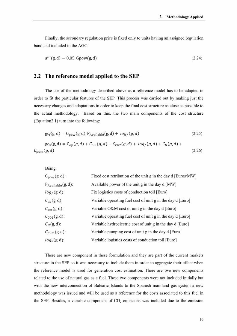
Finally, the secondary regulation price is fixed only to units having an assigned regulation
band and included in the AGC:
aeee�g, d� � 0,05. Gpow�g, d� (2.24)
2.2 The reference model applied to the SEP
The use of the methodology described above as a reference model has to be adapted in
order to fit the particular features of the SEP. This process was carried out by making just the
necessary changes and adaptations in order to keep the final cost structure as close as possible to
the actual methodology. Based on this, the two main components of the cost structure
(Equation2.1) turn into the following:
gc��g, d� � G����g, d�. P���������g, d� opqr�q, s� (2.25)
gc�g, d� � C���q, s� tuv�q, s� twx\�q, s� opqr�q, s� ty�q, s� tz{v�q, s� (2.26)
Being:
G����g, d�: Fixed cost retribution of the unit g in the day d [Euros/MW]
P���������g, d�: Available power of the unit g in the day d [MW]
opqr�g, d�: Fix logistics costs of conduction toll [Euro]
tuz�g, d�: Variable operating fuel cost of unit g in the day d [Euro]
tuv�g, d�: Variable O&M cost of unit g in the day d [Euro]
twx\�g, d�: Variable operating fuel cost of unit g in the day d [Euro]
ty�g, d�: Variable hydroelectric cost of unit g in the day d [Euro]
tz{v�g, d�: Variable pumping cost of unit g in the day d [Euro]
opq|�g, d�: Variable logistics costs of conduction toll [Euro]
There are new component in these formulation and they are part of the current markets
structure in the SEP so it was necessary to include them in order to aggregate their effect when
the reference model is used for generation cost estimation. There are two new components
related to the use of natural gas as a fuel. These two components were not included initially but
with the new interconnection of Balearic Islands to the Spanish mainland gas system a new
methodology was issued and will be used as a reference for the costs associated to this fuel in
the SEP. Besides, a variable component of CO2 emissions was included due to the emission

2. Methodology Applied
17
scheme present in the SEP. And finally, the two additional components CH and Cpum are related
to O&M costs of normal and pumping units and the second to the extra cost for pumping water
by pure and mixed pumping units. All of them are further discussed in the next two sections.
2.2.1 Fixed cost retribution in the SEP
The fixed cost retribution will be applied to three main concepts in this work. First of all,
a part from the CCGT units that were mostly built in the new market structure, most of the
power plants in the SEP are older and started operations before the new markets structure came
up. The impact of this goes the recognized investment value that is needed in the methodology
and for the sake of simplicity, it was selected an approach in which units starting operation
before the market model in Spain, were already amortized by 2006. This assumption is
supported by stranded competition costs which were used as a compensation given to owner
companies due to a regulatory change derived from the liberalization of the Spanish electricity
sector. On the other hand, units built under the new market scheme were treated with the
methodology described above.
Secondly, according with the energy policy present in the Spanish sector and the aim to
increase energy efficiency and lowering GHG emissions some incentives are given by the
regulator to promote such investments by those units above 50MW which may include
enlargement or new facilities to increase efficiency as stated by the [ITC386007]. This led to
some coal units to invest in both new boilers and desulphurization facilities. The first one was
installed for those coal units aiming to burn coal with a lower content of sulfur while the
desulfurization plant is a technology used to remove sulfur dioxide (SO2) from the exhaust flue
gases of fossil fuel power plants. Both of these facilities will be given a fixed retribution based
on the regulatory framework applicable.
Finally, late in 2010 it was issued a new European Directive [EUD7510] which is the
Industrial Emissions Directive (IED) and sets objectives regarding environment protection. This
new Directive aims to push the use of the best technologies available to tackle the emission for
SO2, NOX and VOC (Volatile Organic Compounds). In order to achieve such aggressive goals,
the Directive provides two main mechanisms that may be applied to the coal units in the SEP.
The first one is an “opt-out’ of 17500 hours as maximum operating time in the period from 2016
to 2023 and the second is the investment by the coal units in a Selective Catalytic Reduction
technology to tackle the NOX emissions. The latter supposes an investment by the owner
companies and consequently a fixed cost retribution according with was it is stated in
[ITC386007].

2. Methodology Applied
18
The three concepts explained above are the main sources used for the fixed costs
calculations and will be explained step by step in Chapter 5.
2.2.2 Variable cost retribution in the SEP
The methodology described in the Section 2.1.2 is based on [ITC91306] for the SEIE
which are special systems in the Spanish market. Its application to the SEP requires some
adaptations and assumptions. It is important to mention at this point that the previous study done
in [WOTT10] provides support for the validation of the results. The main goal in that study was
to replicate the generation cost structure in the SEP for period from 2006 to 2009 in the Spanish
market and make a comparison of the recorded prices under the market mechanism with the
generation cost methodology used in the SEIE. It is not the goal of this work to prove again
those assumptions and they will be taken as given and already validated. On the other hand,
there will be an adaptation to the methodology used for the natural gas as a fuel in CCGT and
Fuel-Gas units. With the new pipeline built in the Balearic system a new methodology for
Natural Gas costs was published [ITC155910] this gives a clearer method to compute with more
accuracy.
First, the methodology for the conventional thermal units will be explained highlighting
important adaptation and assumptions made. Then, the new methodology explained in
[ITC155910] will be extensively explained and finally a brief explanation of variable costs
associated to hydro and pumping units.
2.2.2.1 Methodology for thermal units
As seen in the Section 2.1.2 there are 5 main components of the equation 2.15 to be
calculated related to variable cost of the units. First, it will be explained briefly why some of
those costs are not being considered in the SEP adaptation and then the specific calculation done
for the different thermal technologies as well as other variable cost incurred by the generation
units under the SEP context.
First of all, the cost associated to start-up require the exponential parameters and O&M
costs associated to this action, however, there is not a public source with such information for
the SEP’s units. This cost won’t be considered in this work and is supported by the fact that
historical replication of this methodology done by [WOTT10] showed that such costs don’t
have a significant impact on final energy price. In addition to start-up costs, secondary
2. Methodology Applied
19
regulation costs are not considered either. In the SEP, there is already a market for these
services and the daily bids are not affected by this cost.
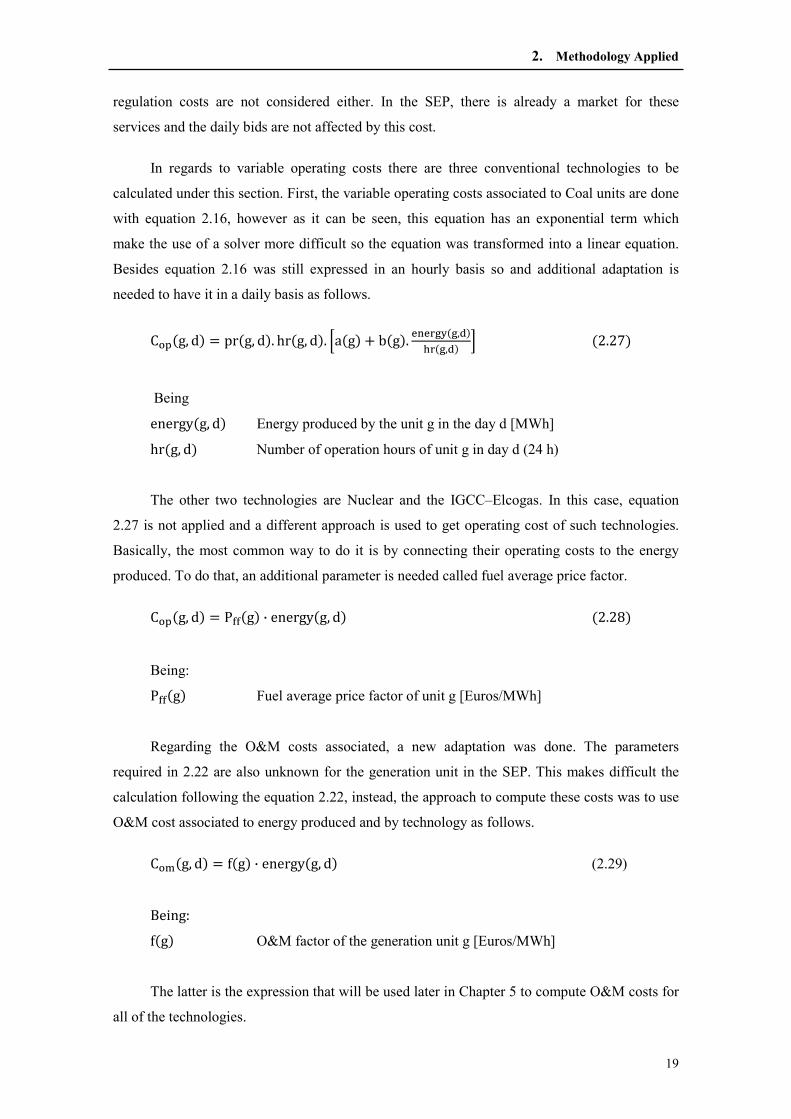
In regards to variable operating costs there are three conventional technologies to be
calculated under this section. First, the variable operating costs associated to Coal units are done
with equation 2.16, however as it can be seen, this equation has an exponential term which
make the use of a solver more difficult so the equation was transformed into a linear equation.
Besides equation 2.16 was still expressed in an hourly basis so and additional adaptation is
needed to have it in a daily basis as follows.
C���g, d� � pr�g, d�. hr�g, d�. fa�g� b�g�. �)���}��,��(���,�� k (2.27)
Being energy(g, d) Energy produced by the unit g in the day d [MWh]
hr(g, d) Number of operation hours of unit g in day d (24 h)
The other two technologies are Nuclear and the IGCC–Elcogas. In this case, equation
2.27 is not applied and a different approach is used to get operating cost of such technologies.
Basically, the most common way to do it is by connecting their operating costs to the energy
produced. To do that, an additional parameter is needed called fuel average price factor.
C��(g, d) � P��(g) · energy(g, d) (2.28) Being:
P��(g) Fuel average price factor of unit g [Euros/MWh]
Regarding the O&M costs associated, a new adaptation was done. The parameters
required in 2.22 are also unknown for the generation unit in the SEP. This makes difficult the
calculation following the equation 2.22, instead, the approach to compute these costs was to use
O&M cost associated to energy produced and by technology as follows.
C�X(g, d) � f(g) · energy(g, d) (2.29) Being: f(g) O&M factor of the generation unit g [Euros/MWh]
The latter is the expression that will be used later in Chapter 5 to compute O&M costs for
all of the technologies.

2. Methodology Applied
20
Finally, the costs associated to CO2 are also considered here. This component is not
explicitly included in the SEIE methodology because the fuel costs are revised and emissions
are internalized in it. In contrast, according with the EU there should be a “cap and trade”
mechanism for CO2 emission in liberalized markets in which countries have to allocate
emissions rights by a PNA. This allocation can be done either by free emission rights or by
auction and allowing market gents to trade them. For this methodology it has been taken the free
emission rights allocated according with the [PNAII07]2 for the years 2011 and 2012 and the
extra cost to be paid for exceeding the free rights as well. Afterwards this cost is fully
considered as a criterion for minimizing the costs in the dispatch due to the end of the free rights
mechanism allocated by the government.
C5�\(g, d) � P�(d) · Q�(g). energy(g, d) (2.30) C5�\(g, d) � P�(d) · fQ�(g). energy(g, d) A ��(�)
$�k (2.31)
Being Q�(g) Emission quantity factor of unit g [tCO2/MWh]
P�(d) Average price of CO2 emissions [Euro/tCO2]
A�(g) Annual free assigned certificates of unit g [tCO2]
H� Average equivalent hours per year
One of the main features of the methodology is the focus on the economic dispatch of
generators. The first equation aims to achieve this goal especially in the first two years of the
simulation in which there are free allocated rights for thermal units. This means that on the one
hand, the CO2 costs are fully internalized in the opportunity cost of units and on the other, that
the merit order changes the dispatch of generators and sets a priority for the more efficient units.
The second equation is used to compute the actual final energy price once the free rights have
been used, however this equation will be used only in 2011 and 2012 as stated above.
2.2.2.2 Methodology for natural gas units
This methodology has been issued for the SEIEs as a result of the new pipeline
connecting Spanish mainland gas system to the Balearic system. Before this pipeline was built,
there were no power plants in any of the SEIE prepared to use natural gas as a fuel. The method
is given to compute variable cost associated to natural gas use and it is described in
2 The PNAII (Assignment National Plan - Plan Nacional de Assignacion de Derecho de Emission in Spanish) cover the period 2008-2012 and it allocate individual emission rights. It considers a decrease of 36% in total emission rights with respect to PNA I.

2. Methodology Applied
21
[ITC155910]. Ultimately, the operating costs associated to the units working with natural gas
are actually calculated by using equation 2.27 however, the fuel therrmie average price is an
unknown parameter. What the CNE publishes in a monthly basis is the product price of the
natural gas in [€/MWh] which is an input for the following description.
First of all, the cost of natural gas is given by the next expression:
C � V · Lp4�" · (1 l� lW� C7���M C���� T�� (2.30) pLNG: LNG product price [€/MWh]
lr: Re-gasification losses
lt: Transmission losses
CVTPA: Variable component of gas third party access [€/MWh]
CFTPA: Fix component of gas third party access [€/MWh]
TTD: Monthly invoicing of the conduction component of transmission
and distribution toll [€]
This expression gives an indication not only of the variable costs associated to the use of
natural gas for the product price and the variable component of costs such as re-gasification,
unloading, storage and underground storage, it also gives the fixed component for the third party
access to the gas network which includes fixed re-gasification toll as well as the fixed
component for the capacity reserve. The first step is to calculate the different subcomponents of
the variable third party access costs as follows;
C7��� � CR CU CS CUS (2.31) CRV: Variable cost of re-gasification toll [€/MWh]
CU: Cost of unloading [€/MWh]
CS: Cost of LNG storage [€/MWh]
CUS: Cost of underground storage [€/MWh]
Then after defining the four components of the latter term the formulation for each of
them is necessary. The variable cost of re-gasification toll includes the CVR term which is
annually published by the MITC and the transmission losses term which is consider as 0.39%
considering these facilities are units connected to a pipeline with pressures between 4 and 60
bars [ITC399306]. Finally the percentage of LNG in Spain’s gas income is published in the
[ITC155910] with a value of 0.74.
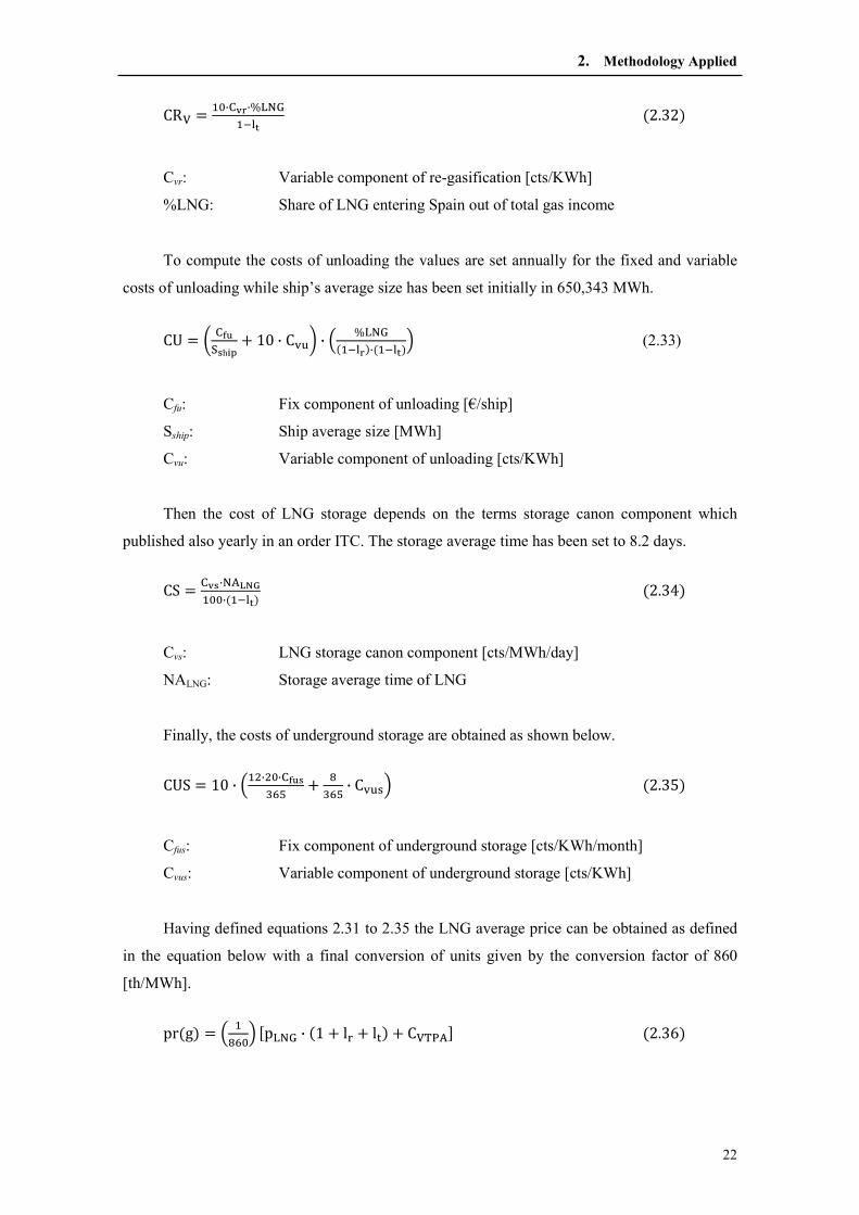
2. Methodology Applied
22
CR7 � Jn·5�:·%4�"JI�R
(2.32) Cvr: Variable component of re-gasification [cts/KWh]
%LNG: Share of LNG entering Spain out of total gas income
To compute the costs of unloading the values are set annually for the fixed and variable
costs of unloading while ship’s average size has been set initially in 650,343 MWh.
CU � � 5�T�Qh�O
10 · Cm� · h %4�"�JI�:�·�JI�R�j (2.33)
Cfu: Fix component of unloading [€/ship]
Sship: Ship average size [MWh]
Cvu: Variable component of unloading [cts/KWh]
Then the cost of LNG storage depends on the terms storage canon component which
published also yearly in an order ITC. The storage average time has been set to 8.2 days.
CS � 5�Q·�����Jnn·�JI�R� (2.34)
Cvs: LNG storage canon component [cts/MWh/day]
NALNG: Storage average time of LNG
Finally, the costs of underground storage are obtained as shown below.
CUS � 10 · hJ\·\n·5�TQ��� �
��� · CmVj (2.35) Cfus: Fix component of underground storage [cts/KWh/month]
Cvus: Variable component of underground storage [cts/KWh]
Having defined equations 2.31 to 2.35 the LNG average price can be obtained as defined
in the equation below with a final conversion of units given by the conversion factor of 860
[th/MWh].
pr(g) � h J��nj Lp4�" · (1 l� lW) C7���M (2.36)
2. Methodology Applied
23
Then the formulation of the fixed cost associated to the use of LNG is also implicit in this
methodology. From equation 2.30 the fix component of gas third party access is divided into
two terms. The first is realted with fixed re-gasification costs (CRf) and the second is the cost of
capacity reserve (CCR).
C���� � CR� C5 (2.37) CR� � h 5�:
Jnnj · hb;·%4�"JI�R
j (2.38)
C5 � h 5�cJnnj · h b;
JI�Rj (2.39)
Cfr: Fix component of re-gasification [(cts/KWh/day)/month]
Cfc: Fix component of capacity reserve [(cts/KWh/day)/month]
Qe: Daily volume contracted taken from the fix component of T & D
conduction toll [MWh/day]
The term to be used as Qe in the lasts two equations correspond to volume of flow applied
in the fixed term of the transmission and distribution toll which is defined in [RD94901] and
quantified as follows:
Q� � QX) C 0,85. QX� ¢ QX) E 1,05. QX� (2.40)
Q� � 0,85. QX� C QX) E 0,85. QX� (2.41)
Q� � QX) 2. £LQX) A 1,05. QX�M£ C QX) D 1,05. QX� (2.42)
With:
QX): Maximum daily measured volume of the user g in the month [MWh/day]
QX�: Maximum daily contracted volume of the user g in the month [MWh/day]
The maximum volume contracted by the user in the month can be estimated taking into
account a forecast maximum need of gas. This estimation is based on the assumption that units
using gas will be contracting a having a peak demand of 90% of their full capacity per month.
The contracted volume is estimated accordingly,
QX�(g) � \¤.�#(�).¥�(�)
¦(�) (2.43)
Being:
P)(g): Net power of unit g [MW]

2. Methodology Applied
24
UF(g): Gas utility factor in the month of unit g
η(g): Efficiency of the unit
Finally just the term TTD in 2.30 is missing which is the conduction component of the
transmission and distribution toll and is defined as shown below
C5 � C� · QX� C7 · Q� (2.44) Cf: Fix component of conduction toll [(Euro/MWh/day)/month]
Cv: Variable component of conduction toll [Euro/MWh]
Qr: Real amount of gas consumed by the unit g [MWh/day]
The fixed component of the last equation is combined with equation 2.37 and both
together provide the formulation for the fixed cost associated to the use of natural gas. On the
other hand, there is still the variable component of equation 2.44 which will be later used as a
variable cost to be used in the model for those units working with natural gas.
It should be kept in mind that important equation to be used in for the natural gas costs
calculation are first equation 2.36 for the computation of the fuel operating costs for gas units.
In addition, equation 2.45 shown below will be used as an additional variable cost to be used in
the economic dispatch to be explained later in chapter 5. Finally, the formulation of the fixed
cost calculation will be as shown below in equation 2.46.
log(g, d) � �)���}¦ · C (2.45)
logr(g, d) � CR� C5 Cr · QX� (2.46) logv: Variable logistic costs of conduction toll [Euro/day]
logf: Fixed logistic costs of conduction toll [Euro/day]
2.2.3 Variable costs associated to hydro and pumping power plants
These costs are mainly attached to the energy produced by or for pumping. Mixed
pumping units defined as those units with a significant natural contribution in the upper
reservoir and pure pumping units were grouped together so the variable costs totally depend on
the daily pumping profile [WOTT10]. The same assumption is done for normal hydro power
plants in which the cost is considered as the total cost of generating certain energy in a daily
basis. The latter assumptions are best understandable considering the following formulation.

2. Methodology Applied
25
C$(d) � f(H) · energy(H, d) (2.47) C�mX(d) � f(pum) · energy(pum, d)
Being:
f(H) � f(pum) O&M factor of the generation and pumping consumption
[Euros/MWh]
2.3 Coverage Index formulation
This One of the main issues related with meeting the electricity demand is the evolution
of the installed capacity. The system operator has defined a coverage index equal 1.1 which
means that there should be a 10% reserve margin with respect to the demand [CNE_11]. The
way to compute this index is by taking the peak demand in the both summer and winter seasons
of the year and compares it against the expected available installed capacity. Mathematically it
is as follows
CI � ������
(2.46) Being:
AP� Expected available power in period i[MW]
PD� Peak demand in period i [MW]
It will be explored in more detail in chapter 6 what the effects of the different constraints
are related with the evolution of the installed capacity in the SEP and its consequences
regarding new power plants needed to keep the system within a safe reserve margin.

3. Technology Overview
This chapter is intended to present an overview of the different technologies covered in
this work. First, it will be given the most relevant technical parameters needed to achieve the
goal of the model and secondly, the expected costs for the calculation of both variable and fixed
costs will be presented as well. Many of these parameters have been taking as given by
[WOTT2011] while some others have been estimated taking into account an stable scenario
given the fact that future estimations are always subject to unpredictable and immeasurable
changes.
3.1 Presentation of the power technologies and technical parameters
As it will be shown in more detail in next chapter, the increasing share of special regime
generation in the SEP has left less energy to be produced by the traditional thermal generation
technologies and this has imposed an additional constraint for them making difficult to have a
significant contribution in the generation dispatch. In the Spanish case, there are four main
technologies to compete for that residual demand left by the technologies that have priority in
the dispatch such as wind energy. The main technologies are:
• Nuclear
• Coal
• CCGT

3. Technology Overview
27
• Fuel-Gas
• Hydro generation
Indeed, hydro generation power plants are not thermal units but their contribution for
meeting the demand and its impact in the variable const calculation for the economic dispatch
are part of the constraints for the model which will be dealt with later.
3.1.1 Common technical parameter
There are some technical parameters that were common for all the units under study. The
first parameter is the so called minimum stable load which is introduced as a production
constraint. It is given as a percentage of the maximum energy that can be produced and will
prevent thermal units not to operate below in day. In contrast, the maximum energy produced
has been also set up taking into account unplanned outages and O&M works in the units. These
values are shown in the table below. For the Elcogas IGCC plant these values were set different
as the coal units.
Technology Minimum
stable load factor
Factor of maximum production
Nuclear 0.90 0.970
Coal 0.55 0.912
Fuel-Gas 0.35 0.877
CCGT 0.45 0.917
Elcogas 0.50 0.800
Table 3.1 Factors of minimum and maximum production
Finally, for the fixed capacity payment it is also needed the availability factor but in a
monthly basis. For getting so, it was taken the historical availability of nuclear power plants
published by the system operator. These figures can be found in Appendix 1.
3.1.2 Nuclear power plants
There are currently in the SEP eight nuclear generation units with total installed capacity
of 7,515 MW. Its main primary fuel is the uranium. According with the system operator, this
technology has provided the energy to meet 21% of the final electricity demand in year 2010
[REE2010]. For calculation of variable costs, there is not technical parameter associated
because those cost are only related to the energy produced by the unit multiplied by factors for

3. Technology Overview
28
both operating fuel and O&M costs. There is a standard fuel recharge schedule for the nuclear
power plants which have been defined from the experience observed in the past years and will
be used in the economic dispatch. Table below shows an example of such schedule for 2011 and
the extended version can be found in Appendix 2.
Nuclear Unit 2011
Month Days
Almaraz 1 Abr 40
Almaraz 2 -- --
Cofrentes Sep 60
Garoña May 35
Trillo Jun 35
Vandellós 2 -- --
Asco 2 Oct 40
Asco 1 May 40
Table 3.2 Nuclear units fuel recharge schedule for 2011
There is no expected growth of the installed capacity of nuclear power plants. In fact
these technology is currently facing a stronger opposition due to the pressure of the current
events and many decision made in the EU might drastically affect the future scenario of the
electricity supply.
3.1.3 Coal units
The share of coal technology in the SEP is around 12% with 11,102 MW and a
contribution of 8% in 2010 according with [REE_10]. For these units some other parameters are
considered. An emissions quantity factor is defined for each of the coal units and was taken
from an Iberdrola´s source for 2010 and kept constant for the whole period. The later was
estimated taking the verified emissions and production estimated by unit.
Unit CO2 emissions factor
[tCO2/MWh]
Puentes 1 0.897
Puentes 2 0.897
Puentes 3 0.897
Puentes 4 0.897
Meirama 0.916
Table 3.3 Emission quantity factor for coal units

3. Technology Overview
29
In regards to the quadratic adjustment parameters a and b needed to compute the
operating fuel costs in 2.25, these were taken from [WOTT10] who compared the last public
data available used when the MLE was the regime in Spain and the data provided by Iberdrola
portfolio for all the existing units. These values were already validated and proved to be
accurate enough in the energy-operating fuel cost curve (See Figure 3.1 below).
Finally, Elcogas, is an IGCC unit that uses as a fuel a mixture of coal and oil coke to be
gasified and then run a CCGT unit so it was treated as such but its outputs were referenced to
the coal to have its impact in the economic dispatch.
Figure 3.1 Energy vs. Operating costs curve for the coal unit Puentes 23
Coal power plants play an important role in the Spanish electricity market due to the just
approved [RD13410] which will impose quotas for some coal units, however this issues will be
explored in more detail in the next chapter.
3.1.4 CCGT power plants
Combined cycle units are indeed the most popular technology of the investors in the
Spanish sector and it has experienced the most remarkable growth from 8,280 MW in 2005 to
24,831 MW of installed capacity by the end of 2010 reaching a 26% of the total installed
capacity and contributing with 23% of the total energy supplied in 2010. Its fuel is the natural
gas. It is the technology with the highest availability index during the year and it is reflected in
its fixed cost retribution. The emission quantity factor is lower than the values for coal units
and fuel-gas units which gives them an advantage when the CO2 variable costs are calculated.
The factor for every unit can be seen in Appendix 3 but broadly they are not larger than 0.4
[tCO2/MWh] which is more than half the factors of coal units in some cases. The quadratic
3 Graph taken from [WOT2010]
-14,000
86,000
186,000
286,000
386,000
486,000
586,000
686,000
786,000
886,000
986,000
0 100 200 300 400
Op
era
tin
g C
ost
(E
uro
s/h
)
Energy (MWh)
IBE MLE

3. Technology Overview
30
adjustment parameters a and b defined previously were also taken from Iberdrola portfolio.
Finally, the nominal efficiency used for this technology is 52%.
This technology will be kept growing, however it is currently uncertain which the most
likely scenario will be. According with the system operator’s scenario there will be an
additional installed capacity of 5130 MW by the end of 2014; however this figure contrasts with
the number set by promoter’s scenario which estimates a more conservative increase of 1945
MW for the same horizon.
3.1.5 Fuel – gas power plants
Even though these units have a small contribution to meet the demand, they are still
present in the generation mix in Spain and are expected to be in it until 2015 as it will be shown
in the analysis of mix generation evolution in next chapter. Currently there are just four power
plants left. It has been recently approved by MITC in [RES919811] that San Adrian units 1 and
3 leaving just 806 MW of installed capacity however due to security of supply reason this
groups will be still present.
These units use natural gas as their fuel because of the Integrated Environmental
Authorization issued per unit in their local community which imposes environmental constrains
that force them to use gas a fuel. Their technical parameter a and b were taken in the same way
as the other technologies. The efficiency of fuel-gas power units used is 33%.
3.1.6 Hydro power plants
For such power plants no relevant technical parameter was needed. As it will be seen its
variable costs depends on the energy produced and an O&M factor which will be exposed in the
next section.
3.2 Data on generation costs by technology
A part from the technical parameters described above, other important inputs in this work
are the costs needed for the complete calculation of both variable and fixed costs. The
estimation of such cost has a slight difficulty mainly because it is the intention of this work to
foresee a plausible evolution of such costs. However, it should be kept in mind that future is
always uncertain and unexpected events might change even the most accurate forecast. Below it
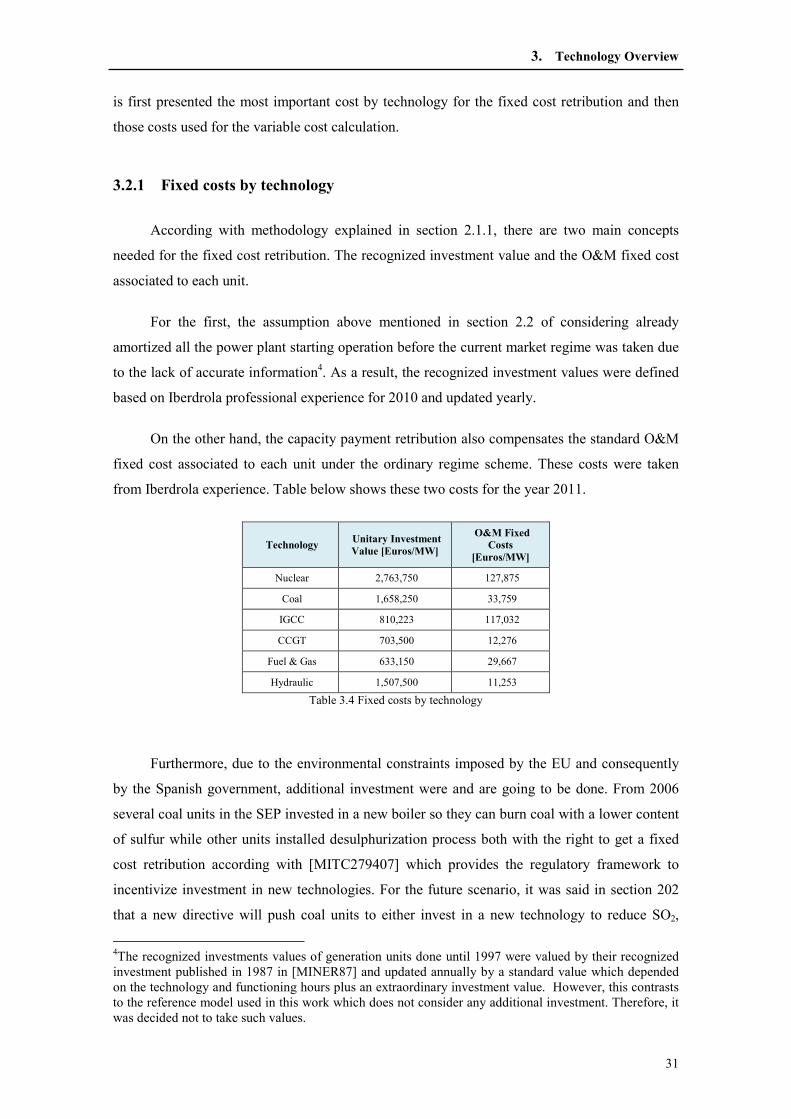
3. Technology Overview
31
is first presented the most important cost by technology for the fixed cost retribution and then
those costs used for the variable cost calculation.
3.2.1 Fixed costs by technology
According with methodology explained in section 2.1.1, there are two main concepts
needed for the fixed cost retribution. The recognized investment value and the O&M fixed cost
associated to each unit.
For the first, the assumption above mentioned in section 2.2 of considering already
amortized all the power plant starting operation before the current market regime was taken due
to the lack of accurate information4. As a result, the recognized investment values were defined
based on Iberdrola professional experience for 2010 and updated yearly.
On the other hand, the capacity payment retribution also compensates the standard O&M
fixed cost associated to each unit under the ordinary regime scheme. These costs were taken
from Iberdrola experience. Table below shows these two costs for the year 2011.
Technology Unitary Investment Value [Euros/MW]
O&M Fixed Costs
[Euros/MW]
Nuclear 2,763,750 127,875
Coal 1,658,250 33,759
IGCC 810,223 117,032
CCGT 703,500 12,276
Fuel & Gas 633,150 29,667
Hydraulic 1,507,500 11,253
Table 3.4 Fixed costs by technology
Furthermore, due to the environmental constraints imposed by the EU and consequently
by the Spanish government, additional investment were and are going to be done. From 2006
several coal units in the SEP invested in a new boiler so they can burn coal with a lower content
of sulfur while other units installed desulphurization process both with the right to get a fixed
cost retribution according with [MITC279407] which provides the regulatory framework to
incentivize investment in new technologies. For the future scenario, it was said in section 202
that a new directive will push coal units to either invest in a new technology to reduce SO2,
4The recognized investments values of generation units done until 1997 were valued by their recognized investment published in 1987 in [MINER87] and updated annually by a standard value which depended on the technology and functioning hours plus an extraordinary investment value. However, this contrasts to the reference model used in this work which does not consider any additional investment. Therefore, it was decided not to take such values.

3. Technology Overview
32
NOX, and VOC or decide a cap 17,500 hours connected to the network in a period no longer
than 2023. This investment in the SCR can also receive a fixed retribution. For the latter, an
additional investment in will be needed to enlarge the lifespan of the coal units but this
investment given in Euro/MW will be taken from the recognized investment value for the
corresponding year. Below are shown the investment costs and their corresponding O&M costs
for the year 2011.
Technology Unitary Investment
Value [Euro] O&M Fixed
Costs [Euros]
Desulphurization process
60,000,000 5,695
Boiler Installation 30,000,000 --
SCR installation 120,000,000 52,570
Table 3.5 Fixed costs of new technologies in 2011
It is important to mention at this point how different costs were estimated for the future
scenario. This indeed presents a source of uncertainty mainly because the forward estimation is
done using the industrial price index (IPI) and the consumption price index for the (IPC) for the
unitary investment and the O&M fixed costs respectively. Indeed the estimation of such indexes
is strongly linked to the macroeconomic situation in Spain and so far it is still a challenge for the
coming years to tackle the effects of the crisis so a conservative estimation was done to set them
in 1.5% for the IPI and 2.5% for the IPC.
3.2.2 Variable costs by technology
There are different costs to be considered for the variable cost calculation. To begin with,
O&M variable costs are standardized for the different technologies according with an
Iberdrola´s study with a basis in 2010. Then, they are estimated forwards with the forecast IPC
minus 100 points. This component is called the O&M cost factor and will be used in that way to
obtain the O&M variable cost. For the case of hydro and pumping units, this factor is used to
calculate their variable payment because there is no merit mechanism in the dispatch for them
and they receive a payment directly linked to the energy the produce or pump. For coal units,
logistic costs were also needed to reflect its impact in the fuel average price. The source used for
such cost was estimated by Iberdrola in 2010 taking into consideration location of the coal units
and all their costs associated such as unloading, storage and transport.
Regarding nuclear power plants and Elcogas, it was stated before that their operation fuel
costs are linked with the energy produced and a fuel price factor. In the first case, this factor
reflects not only the price of the primary fuel namely uranium but also the cost associated to the

3. Technology Overview
33
safe management of the residues produced. For Elcogas, this factor was taken from a study done
for the IGCC technology in Spain [TREVINO] . In both the case the factor is estimated
forwards in the same way as the O&M costs. Table below summarizes the aforesaid costs for
the year 2011.
Technology O&M Cost Factor
(Euros/MWh) Logistic Costs
(Euros/th)
Fuel Cost Factor
(Euros/MWh)
Nuclear 1.2262 N/A 12.240
Coal 1.2262 12.120 N/A
IGCC 1.2262 N/A 12.210
CCGT 2.1458 N/A N/A
Fuel-Gas 3.5000 N/A N/A
Hydraulic 2.0402 N/A N/A
Table 3.6 Main variable costs by technology
Finally, all the LNG logistic components mentioned in the section 2.3.2 were taken from
the last published source available by the MITC in [ITC335410] and then estimated forwards
using the IPC as a measure of the inflation in Spain. These values and the previous costs can be
further seen in Appendix 4.

4. Data collection, assumptions and key milestones
Once the methodology has been explained in Chapter 2 and the different technical and
economical parameters were described in Chapter 3, it is time to go into the data gathering and
development of the main assumptions and key milestones to be considered in this work. At this
point it is important to emphasize once again that this study is done based on public information
available relevant to the aim of the work. Several public sources were consulted and compared
each other in order to come up with the most plausible scenario and apply the regulated cost
structure. In particular cases Iberdrola’s professional criterion was used to estimate some values
mainly due to the lack of public information to do so.
One of the most important inputs for this work is the electricity demand growth. This
sections starts by providing an estimated demand growth which was done based on the public
information and the most plausible scenario given the current and expected situation in the
electricity sector in Spain. The second important input is the expected special regime generation
and its installed capacity growth for the period under study. Later in this work, it will be seen
how special regime generation becomes a constraint for the model especially due to the targets
imposed be the EU in terms of renewable energy sources. Afterwards, an overview of the
evolution of installed capacity in general will be given taking into account the hydro unit
currently under construction and also the ones to be decommissioned according with different
regulatory constraints.

4. Data collection, assumptions and key milestone
35
4.1 Electricity demand growth
The estimation done for the demand growth is the base for achieving the goal of this
study. This estimation was done taking several assumptions made mainly by the system operator
and CNE in [CNE_11]. It was observed that he electricity demand in Spain had been
experienced a steady growth from the year 2000 with an annual average growth of 4.16% until
2009 in which it suddenly falls and register a negative growth of 4.7% leading demand levels
observed in 2007. This situation represents a difficulty because the trend observed in the
previous years was lost and a new forecasting is subject to uncertainty.
According with the CNE in [CNE_11] the electricity demand would evolve according
with the expected economic scenario for the period 2010-2014 which shows a moderated
growth in the first 3 three years and then a more pronounced spike in the last year. On the other
hand, the document [DC__10] which was launched in December 2010 provides an annual
demand growth of 2.3% for the period 2011-2020 with the latest information available. As it is
not the intention of this work to develop a model to forecast exactly what the demand will be, it
was considered that such estimation provides a plausible scenario to be considered because it
reflects the most likely demand growth foreseen by different entities5.
In order to estimate the annual demand for the whole period, it was taken the total
electricity demand provided by REE in 2010 and then the estimated percentage growth was
applied. Below it is shown the table with the annual values obtained in the scenario used in this
work. These projected values are net demand and already exclude the energy used for auxiliary
services in the power plants.
Besides, the estimated values were compared with two additional scenarios proposed by
REE in order to validate the assumptions made here. These two scenarios reflect, on the one the
hand the most likely demand growth according with current trends and constraints (central
scenario) and on the other, it proposes the so called design scenario which supposes a larger
demand growth which could have been done in order not to compromise demand meeting and
justify additional investments. Unfortunately, the source consulted [REE_11] do not provide
values for the whole period; however it still can be compared with the values in this work. An
additional remark about the comparison is that these values are presented as demand after
considering pumping consumption and international exchanges mainly because those were the
values provided by REE. In order to obtain such values in the scenario presented here, first, it
5 The annual demand growth estimation takes the economic growth as one of the most influencing factors. In order to calculate the effect of the economic activity on electricity demand, GDP´s annual growth is usually taken into account as well as the demand response to any changes in the economic activity.

4. Data collection, assumptions and key milestone
36
was deducted the estimated pumping consumption which will be explained later in this chapter
and for the international exchanges it was taken the same projections used by REE in its
scenarios leading to the final values in the table below.
Year Net demand
2011 279,124
2012 286,244
2013 292,333
2014 298,897
2015 305,831
2016 313,730
2017 319,639
2018 327,339
2019 334,966
2020 343,731
Table 4.1 Annual demand projection in GWh
Results show that the projected demand used in this work is in line with the scenarios
given by REE who is certainly approaching the issue considering more variables that go beyond
of the scope of this work.
Scenario 2011 2012 2013 2014 2015 2016 2017 2018 2019 2020
Own 265,700 271,892 276,804 281,415 287,403 294,358 299,353 306,140 313,733 322,463
Central 265,000 - - - - 295,000 - - - 325,000
Design - 273,610 - 289,020 - 302,260 - - - 330,660
Source. REE, Own Elaboration
Table 4.2 Annual demand projection in GWh
4.1.1 Monthly and daily distribution of the demand
After having the expected annual demand in the SEP, the next step was to distribute it in
the year according with the logical pattern observed in the actual demand. To do so, two main
steps were done. First of all, the annual demand was distributed in the year according with peaks
and valleys observed historically and then these monthly values were again distributed in each
months in order to reflect tan actual pattern followed by the demand in a day, however it is
important to say that no efficiency effect was included in order to tackle extreme demand
values.
The approach used for the monthly distribution was based on the historical consumption
patterns observed in the last 5 years. This approach is intended to reflect the different season

observed in Spain and it is robust enough to
the goals of this study. Figure 6.1 shows the historical average monthly demand from 2006 to
2010 which were the values used for the whole period. The
for each year can be seen in Appendix 5
In regards to the daily distribution,
off days which mostly represent national holydays in Spain
represents the working days and a final division was made between Saturdays with day type 2
and Sundays with day type 3.
Afterwards, these days were
year was used for the leap years and the second for a normal year but in both the cases the
procedure was as follows:
4. Data collection, assumptions and
in Spain and it is robust enough to be considered in a future projection and
Figure 6.1 shows the historical average monthly demand from 2006 to
which were the values used for the whole period. The monthly demand
be seen in Appendix 5.
Figure 4.1 Monthly distribution of demand
ards to the daily distribution, the month was divided in four types of days
off days which mostly represent national holydays in Spain shown in table 4.3. Then day type 1
working days and a final division was made between Saturdays with day type 2
and Sundays with day type 3.
Day 2011
New Year’s Day 01/01/2011
12th Night 06/01/2011
Good Thursday 21/04/2011
Good Friday 22/04/2011
Labor day 01/05/2011
Asumption Day 15/08/2011
Columbus Day 12/10/2011
All saints 01/11/2011
Constitution Day 06/12/2011
Immaculate Con 08/12/2011
Christmas Day 25/12/2011
Table 4.3 National holidays in Spain
Afterwards, these days were classified in two reference years, 2008 and 2010. The first
was used for the leap years and the second for a normal year but in both the cases the
ssumptions and key milestone
37
be considered in a future projection and to achieve
Figure 6.1 shows the historical average monthly demand from 2006 to
obtained in GWh
of days; type 0 for
shown in table 4.3. Then day type 1
working days and a final division was made between Saturdays with day type 2
s, 2008 and 2010. The first
was used for the leap years and the second for a normal year but in both the cases the
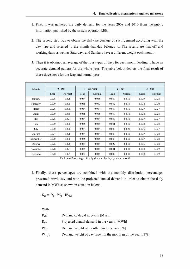
4. Data collection, assumptions and key milestone
38
1. First, it was gathered the daily demand for the years 2008 and 2010 from the public
information published by the system operator REE.
2. The second step was to obtain the daily percentage of such demand according with the
day type and referred to the month that day belongs to. The results are that off and
working days as well as Saturdays and Sundays have a different weight each month.
3. Then it is obtained an average of the four types of days for each month leading to have an
accurate demand pattern for the whole year. The table below depicts the final result of
these three steps for the leap and normal year.
Month
0 - Off 1 - Working 2 – Sat 3 - Sun
Leap Normal Leap Normal Leap Normal Leap Normal
January 0.026 0.026 0.034 0.035 0.030 0.030 0.027 0.028
February 0.000 0.000 0.036 0.037 0.032 0.033 0.030 0.030
March 0.028 0.000 0.034 0.034 0.030 0.030 0.027 0.027
April 0.000 0.030 0.035 0.035 0.030 0.031 0.028 0.028
May 0.026 0.027 0.034 0.034 0.030 0.030 0.027 0.027
June 0.000 0.000 0.035 0.035 0.031 0.030 0.028 0.028
July 0.000 0.000 0.034 0.034 0.030 0.029 0.026 0.027
August 0.027 0.026 0.034 0.034 0.030 0.030 0.027 0.028
September 0.000 0.000 0.035 0.035 0.030 0.030 0.027 0.028
October 0.026 0.028 0.034 0.034 0.029 0.030 0.026 0.028
November 0.028 0.027 0.035 0.035 0.031 0.031 0.028 0.029
December 0.028 0.029 0.034 0.034 0.030 0.031 0.028 0.029
Table 4.4 Percentage of daily demand by day type and month
4. Finally, these percentages are combined with the monthly distribution percentages
presented previously and with the projected annual demand in order to obtain the daily
demand in MWh as shown in equation below.
«¬ � « · ®v · ®v,¯
With:
D�: Demand of day d in year n [MWh]
D}: Projected annual demand in the year n [MWh]
WX: Demand weight of month m in the year n [%]
WX,W: Demand weight of day type t in the month m of the year n [%]

4. Data collection, assumptions and key milestone
39
It is important to say that two minor difficulties arose when the method was applied. First
of all, the days related to the Easter vary from year to year and are not in the same month as the
reference years used and second due to the natural movement of the calendar weekends and
working days also vary, leading to unreal demand patterns. However, these inconvenient were
adjusted and can be verified on the yearly demand graphs.
4.1.2 Peak demand
Peak demand represents the highest demand in a year and it is usually given for winter
and summer. These two values were taken from the estimation done in [CNE_10] for the period
2011-2014 and for the next years of the period it was decided to apply the same growth rate as
applied for the annual demand.
Year Winter Summer
CNE REE CNE REE
2011 46,400 - 42,500 42,200
2012 47,200 47,300 43,200 -
2013 48,400 - 44,300 -
2014 49,650 49,700 45,450 -
2015 50,792 - 46,495 -
2016 51,960 52,200 47,565 47,600
2017 53,155 - 48,659 -
2018 54,378 - 49,778 -
2019 55,629 - 50,923 -
2020 56,908 58,000 52,094 53,000
Table 4.5 Peak demand for winter and summer
The values are compared in the table above with the latest values provided by REE;
however, they are not given for the whole period but they still can provide a reference point.
Peak demand values are important for the coverage index analysis that will be done later in this
work.
4.2 Generation constraints
Once the total expected demand has been estimated, the next step is to find out what the
impact of the exiting generation technologies will be in the system and what their share in
production will be for the period under study. Two main generation constraint were taken into
consideration to estimate the residual demand left for the thermal technologies which the main

4. Data collection, assumptions and key milestone
40
focus of this work. First, it should be considered the impact of the special regime generation and
its contribution to meet the demand and second, the yearly hydro production. These generation
constraints will reduce the so called residual demand for the thermal technologies which are the
target technologies for the goal of this work.
4.2.1 Expected hydroelectric contribution and pumping
Historically, the hydro generation has represented around 9% of the total energy in the
SEP with a particular case in 2010 in which its production was close to 15% because of the rain
patter in that year. This production is one of the two important generation constraints for
thermal technologies and has to be estimated of the period under study. The first step is to
define the hydro production and pumping for the year 2011. Then, the yearly hydro production
and pumping will be estimated based on the total installed capacity for each and will be updated
according with new hydro and pumping units and afterwards an approach will be defined to
distribute monthly both the energy production and pumping.
To begin with, the total hydro production for 2011 has been estimated according with the
historical series from 2006 to 2010 and will be assumed to be constant until new capacity is
added to the system. This value was set in 27,120 GWh annual. The same criterion was used
for pumping and its consumption was fixed in 4,424 GWh annual. Pumping consumption is
needed to variable costs and will be further explained in Chapter 5. Afterwards, the distribution
of hydro production was made based on Iberdrola experience in hydro forecasting considering
an average year and applying a similar approach described below using 2012 as the reference
year.
1. The method considers two type of day, working and off days and then it takes three
different periods in a day namely peak, shallow and valley and their corresponding hours
per day. Finally, the equivalent hours for the month are computed for each period. Table
4.6 depicts this information for January.
Jan 2012
Day type Work 22 Off 9
Level within the day Peak Shallow Valley Peak Shallow Valley
Hours per level and day [hr/day] 4 14 6 4 14 6
Hours per level per month [hr ] 88 308 132 88 308 132
Table 4.6 Classification of day level and hours in hydro production and pumping

4. Data collection, assumptions and key milestone
41
2. Then it is estimated the total capacity in MW producing and pumping in the three
different periods and by combining this information with last row of table 4.6 it is
possible to obtain the energy produced and pumped in each period and ultimately in the
whole month by type of day. Table 4.7 summarizes the main results for January 2012.
Jan-12
Day type Work Off
Level within the day Peak Shallow Valley Peak Shallow Valley
Pumping consumption [MW] 28 328 1,594 75 569 1,582
Generation [MW] 6,682 4,773 2,114 5,735 3,650 2,023
Total pumping by level and day [MWh] 2,429 100,906 210,375 2,693 71,719 85,440
Production by level and day [MWh] 587,976 1,470,026 279,040 206,478 459,869 109,261
Total pumping by month and day [MWh] 313,711 159,851
Production by month and day [MWh] 2,337,041 775,608
Table 4.7 Total energy produced and pumped by month and type of day
3. With this information it is now possible to estimate what will be called intra-month
weight by type of day and month weight for both generation and pumping. The first one is
calculated just by finding the percentage over the total generation and pumping in each
month which will give a percentage for working and off days in the month. The second
one is also a percentage of the generation and pumping in the month with respect to the
total in the whole year. Table below summarizes this intra-month and monthly weight for
the reference year considering that type of day 0 is off day and 1 working day.
Month Monthly pumping
weight
Monthly generation
weight
Intra-month pumping
weight
Intra-month generation
weight Day type
January 0.1032 0.1073 0.63 0.72 1
0.37 0.28 0
February 0.0737 0.0926 0.66 0.77 1
0.34 0.23 0
March 0.0714 0.1029 0.66 0.76 1
0.34 0.24 0
April 0.0647 0.0897 0.58 0.68 1
0.42 0.32 0
May 0.0670 0.0939 0.66 0.76 1
0.34 0.24 0
June 0.0819 0.0817 0.61 0.76 1
0.39 0.24 0
July 0.0880 0.0698 0.68 0.77 1
0.32 0.23 0
August 0.0800 0.0597 0.69 0.77 1
0.31 0.23 0
September 0.0810 0.0548 0.63 0.75 1
0.37 0.25 0
October 0.0846 0.0583 0.67 0.77 1
0.33 0.23 0

4. Data collection, assumptions and key milestone
42
November 0.0859 0.0770 0.63 0.75 1
0.37 0.25 0
December 0.1188 0.1123 0.56 0.66 1
0.44 0.34 0 Table 4.8 Monthly and intra-month weights of hydro generation and pumping
The results obtained above are the departing point to estimate the hydro generation and
pumping in a monthly basis and for the whole period. To do so, the monthly weights were taken
for both generation and pumping and applied to the annual values set previously of 27,120 GWh
and 4,424 GWh respectively. As already said before, annual production is considered constant
unless new units are connected to the network. Table below shows the expected hydro
production and pumping. It already includes the additional generation and pumping considering
the expected installed capacity in the coming years.
Total 2011 2012 2013 2014 2015 2016 2017 2018 2019 2020
Hydro production 27,120 27,120 28,502 29,314 29,314 29,314 29,973 30,631 30,631 30,631
Pumping 4,300 4,300 5,793 6,877 6,877 6,877 7,755 8,633 8,633 8,633
Table 4.9 Expected annual hydro production and pumping in GWh
The additional hydro generation and pumping was estimated taking an average operating
time of 1,500 hours for the hydro power plants and for the pumping units it was first estimated
the average energy pumped according with an utilization factor of 20% out of the total capacity
of the plant and then it was considered an efficiency of 75% for the energy produced by such
units.
4.2.2 Impact of special regime generation
The EU Directive 2009/28/CE was launched to boost the use of renewable energy source
and increase their share by 2020 up to 20% out of the total gross energy consumption
[PANER10]. In Spain the goal is that renewable energy sources will have a share of 20% in the
final energy consumption as the directive establishes for the EU countries along with a
contribution of 10% in the transportation sector. These targets imply a 35% production in the
electricity sector coming from renewable energy sources, a target that seems achievable taking
into consideration that few years ago the share of such sources was limited to the hydro
production and nowadays their production has achieved values above 20% in the Spanish sector.
The above mentioned targets depend on the evolution of the special regime technologies
in the SEP and especially on the evolution of renewable energy sources. In 2010 the total

4. Data collection, assumptions and key milestone
43
installed capacity of especial regime technologies was 36,636 MW and their energy contribution
was slightly above 33% according with REE. Out of this amount of energy renewable sources
contributed with nearly 20% on the total energy produced without considering the big hydro
production. According with this figures and supported by the new PANER 2011-2020, Spain
seems to be on the way to achieve the EU target, however this trend has an important impact on
the goal of this study because the more energy produced by renewable energy sources, the less
residual demand for thermal technologies.
The scenario presented here for the special regime mostly considers the assumptions
made in [PANER10] and [CNE_10] as well as other rational assumptions based on the historical
evolution of the renewable and non-renewable sources in the special regime. The estimated
evolution of the installed capacity is shown below in table 4.6 and it reflects the most rational
evolution of the different technologies. PANER is mostly focused on renewable energy sources
and as such, it considers than apart from the more mature technologies such as wind and solar,
there will be also new capacity from technologies such as geothermal, waves and wind offshore,
however given the cost and technological constraints to boost the development of such
technologies it was assumed a more conservative growth for such technologies. On the other
hand, it was considered that most of the new installed capacity will be in the renewable sources
side which will be reflected in their final contribution. The full scenario provided can be found
in Appendix 6.
Technology 2011 2013 2015 2017 2019 2020
Wind Onshore
19,956 24,560 27,310 30,098 32,913 34,320
Solar PV 3,990 4,585 5,065 5,688 6,403 6,760
Solar Thermal
1,330 2,375 3,010 3,675 4,425 4,800
Others Renewable
2,870 3,135 3,380 3,800 4,340 4,610
Cogeneration 7,410 8,415 9,210 9,685 10,155 10,390
Others Non Renewable
80 80 90 115 145 160
Total 35,636 43,150 48,065 53,060 58,380 61,040
Table 4.10 Evolution of special regime installed capacity in MW
Given the total installed capacity estimated, the next step is to define energy
contributions. It is not the aim of this work to estimate the individual contribution of each
technology; instead, it will be presented the total contribution according with its observed trend
and the data available in [PANER10] and [CNE_10]. As a result of, and in order to meet the EU
target in 2020 it has been defined the following percentages of special regime production and it

4. Data collection, assumptions and key milestone
44
equivalent energy contribution. In Appendix 6 it can be found the complete set of tables for
special regime generation.
Year % GWh
2011 34.2 95,462
2012 35.4 101,084
2013 36.6 106,915
2014 37.8 112,960
2015 39.0 119,226
2016 40.2 125,721
2017 41.4 132,452
2018 42.6 139,426
2019 43.8 146,651
2020 45.0 154,134
Tale 4.11 Expected annual contribution of special regime generation
The values above are given in yearly basis, however as this work aims at simulating the
SEP in a daily basis, it was necessary to make assumptions on how the total energy would be
distributed. To do so, the same approach used for the total demand was adapted here with some
differences. It should be kept in mind that special regime generation involves a high production
of renewable energy sources and their daily production considering their randomness would be
a huge an extensive task to do and would not lead to a more accurate result. Therefore, a simpler
way to estimate daily production was by finding the historical monthly distribution of special
regime generation and their equivalent in energy produced monthly and then it was equally
distributed in each month. This approach is valid enough considering that historical monthly
production followed a similar path from 2006 to 2010.
4.2.3 Residual demand for thermal units
The two previous sections represent constraints due to the fact that both of them have
special treatment in the generation dispatch. This situation directly affects the aim of this work
that is more focused on estimating costs for the thermal units. In terms of economic theory the
residual demand is defined as the market demand minus the supply if other firms in the market.
This concept is taken here to define what the residual demand, or also known as thermal gap,
will be in the period under analysis. In simple terms, the market demand will be equal to the
total expected demand by year and the supply to be deducted will be the special regime
contribution and hydro generation.
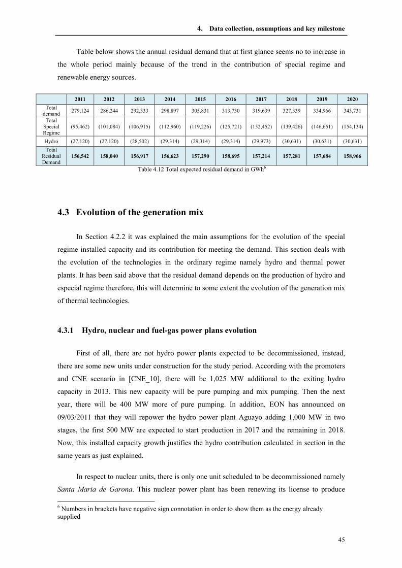
4. Data collection, assumptions and key milestone
45
Table below shows the annual residual demand that at first glance seems no to increase in
the whole period mainly because of the trend in the contribution of special regime and
renewable energy sources.
2011 2012 2013 2014 2015 2016 2017 2018 2019 2020
Total demand
279,124 286,244 292,333 298,897 305,831 313,730 319,639 327,339 334,966 343,731
Total Special Regime
(95,462) (101,084) (106,915) (112,960) (119,226) (125,721) (132,452) (139,426) (146,651) (154,134)
Hydro (27,120) (27,120) (28,502) (29,314) (29,314) (29,314) (29,973) (30,631) (30,631) (30,631)
Total Residual Demand
156,542 158,040 156,917 156,623 157,290 158,695 157,214 157,281 157,684 158,966
Table 4.12 Total expected residual demand in GWh6
4.3 Evolution of the generation mix
In Section 4.2.2 it was explained the main assumptions for the evolution of the special
regime installed capacity and its contribution for meeting the demand. This section deals with
the evolution of the technologies in the ordinary regime namely hydro and thermal power
plants. It has been said above that the residual demand depends on the production of hydro and
especial regime therefore, this will determine to some extent the evolution of the generation mix
of thermal technologies.
4.3.1 Hydro, nuclear and fuel-gas power plans evolution
First of all, there are not hydro power plants expected to be decommissioned, instead,
there are some new units under construction for the study period. According with the promoters
and CNE scenario in [CNE_10], there will be 1,025 MW additional to the exiting hydro
capacity in 2013. This new capacity will be pure pumping and mix pumping. Then the next
year, there will be 400 MW more of pure pumping. In addition, EON has announced on
09/03/2011 that they will repower the hydro power plant Aguayo adding 1,000 MW in two
stages, the first 500 MW are expected to start production in 2017 and the remaining in 2018.
Now, this installed capacity growth justifies the hydro contribution calculated in section in the
same years as just explained.
In respect to nuclear units, there is only one unit scheduled to be decommissioned namely
Santa Maria de Garona. This nuclear power plant has been renewing its license to produce
6 Numbers in brackets have negative sign connotation in order to show them as the energy already supplied

4. Data collection, assumptions and key milestone
46
energy since 1971 and almost every year since then, however in 1999 it got a 10 years license
even thought the power plant was already close to the 30 years old. Its final allowance to extend
its license was given in [ITC178509] and allowed the owner until July 2013 to decommission
the facilities considering that it will achieve 40 years old which was the maximum design
criterion. Apart from this, there is no plant to either build new nuclear power plants or
decommissioning the existing.
Finally, in the beginning of 2011 there was 1,402 MW installed of fuel-gas units,
however due to their technical characteristics this power units have not been supplying
continuously energy to the system but they were kept in order to warranty security of supply.
However on may 26 of this year, it was published the [RES919811] that allows the closure of
units San Adrian 1 and 3 without compromising the security of supply of the system and they
were already considered decommissioned since the beginning of 2011 taking into consideration
that their production was too little. Aceca 1 and Foix 1 are expected to be decommissioned in by
the end of 2015. Table below summarizes the evolution for the aforesaid technologies.
Unit Technology New [MW] Decommission
[MW] Date
C.H.B. La Muela II
Hydraulic
850.00 - 01/01/13
UGH. San Esteban 175.00 - 01/01/13
C.H.B. Moralets 400.00 - 01/01/14
C.H.B. Aguayo 500.00 - 01/01/17
C.H.B. Aguayo 500.00 - 01/01/18
Santa Maria de Garona Nuclear - 455.20 01/07/13
Aceca 1
Fuel-Gas
- 301.00 12/31/15
San Adrian 1 - 313.00 01/01/11
San Adrian 2 - 283.30 01/01/11
Foix 1 - 505.50 12/31/15
Table 4.13 Evolution of Hydro, nuclear and fuel-gas units
The case of CCGT evolution is actually constrained by the current overcapacity context
in the SEP. There is a extensive CCGT portfolio either in planned phase or in the approval
process however, the assumption made in regards to its evolution was that new CCGT unit
won’t be added until the Coverage Index drops below the value set by the system operator.
4.3.2 Regulatory constraints
There are four main regulatory constraints that have an important effect especially on the
coal units. The first one is a derived from the EU Directive 2001/80/CE related with
environmental issues, the second is the already approved RD134 which is intended to support

4. Data collection, assumptions and key milestone
47
autochthonous coal mines in Spain. The third one is the Mining Help Plan that is intended to
help the lest efficient minis in the country to keep operating until 2018 and finally the future
situation for the ELV which is developed ion the Directive 2010/75/EU which was launched on
December 17 in 2010. Below it is explained what are the main arguments of such constraints
and what the implications are for the goal of this study.
a) Directive 2001/80/CE
In the EU, one of the most important environmental regulations with effects on the
electricity sector is the Directive 2001/80/CE. This directive sets emission limitations for some
pollutants agents coming from big combustion facilities. Spain has designed its own plan
[MITC07] in order to meet the ELV imposes by the EU. This has plan has the goal to reduce
NOX, SO2 and VOC and proposes two options to achieve such a goal. The first one consists in
grouping firms in bubbles with fixed annual limits in tons of NOX, SO2 and VOC so its use
should be rational because it imposes an extra variable cost. The second alternative is that units
should be connected to the network more than 20,000 hours as the latest on the 31 of December
in 2015. The facilities affected by this regulation are mainly the coal units Lada 3, Cercs 1 and
Escucha 1 and the fuel-gas Aceca 1. Therefore its decommissioning is assumed to be imminent
in 2015 if they do not reach the maximum hours allowed.
b) RD 134/2010 – SGR and the Mining Help Plan
According with the article 25 of the Law 54/1997, the government can come up with
different mechanisms respecting the fundamental of the free market in order to make work those
power plants using any kind of autochthonous primary energy up to 15% of the total demand.
The RD134 takes this rule from the law and it establishes the so called Supply Guarantee
Restriction which is defined as the necessary energy production from units using autochthonous
coal and force owner for these kinds of units to buy an annual quota. In addition, the RD134
also establishes the maximum volumes of production per years. The latter is the special interest
for the aim of this work, first because by having an annual quota to fulfill with coal units, the
residual demand will be even less that it was estimated in the previous section, letting to a
excess of installed capacity and second because the application of the RD is currently estimated
to be done until 2014. So it will condition the evolution of the thermal units in the SEP. Besides,
after the RD134 finished in 2014 these units were assumed to follow the mining help plan in
which coal mines are candidates to receive support from the state. These helps are decreasing
with the years and they were estimated in terms of energy quotas for the coal units. Table 4.14
shows quotas for both RD134 and then according with the mining plan.

4. Data collection, assumptions and key milestone
48
c) Directive 2010/75/EU
Finally, this directive tries in essence to achieve the same goals as the first one. This new
directive harmonizes criteria and achieve the best values for the NOX, SO2 and VOC. The two
options available for the coal units are first the so called opt-out similar to the previous directive
in which units cannot be connected to the network for more than 17,500 hours from the period
2016-2023. And the second option, is with same kind of bubble, however this option implies a
huge investment first in a NOx-SCR to reduce anthracite from NOx and also an additional
investment to extend the lifespan of the unit.
Unit RD134 Mining Plan
2011-2015 2015 2016 2017 2018
ELCOGAS 1,400,000 1,120,000 840,000 700,000 420,000
Compostilla (2-5) 5,444,250 3,266,550 2,722,125 2,177,700 1,633,275
Teruel (1-3) 6,183,800 4,328,660 3,710,280 3,091,900 1,855,140
Soto de Ribera 3 1,311,940 918,358 787,164 655,970 393,582
Puente Nuevo 3 1,482,090 1,037,463 889,254 741,045 444,627
Escucha 371,860 260,302 223,116 185,930 111,558
Anllares 1,968,150 1,377,705 1,180,890 984,075 590,445
Narcea 3 1,205,880 844,116 723,528 602,940 361,764
La Robla 2 2,035,200 1,424,640 1,221,120 1,017,600 610,560
Guardo 2 1,943,140 1,360,198 1,165,884 971,570 582,942
Table 4.14 Coal units’ quotas
These regulatory constraints will determine to some extent the evolution of the coal
capacity in the system and will have a huge impact first on the total generation cost and then in
the coverage index required. Appendix 7 shows the complete scenario proposed for this work.
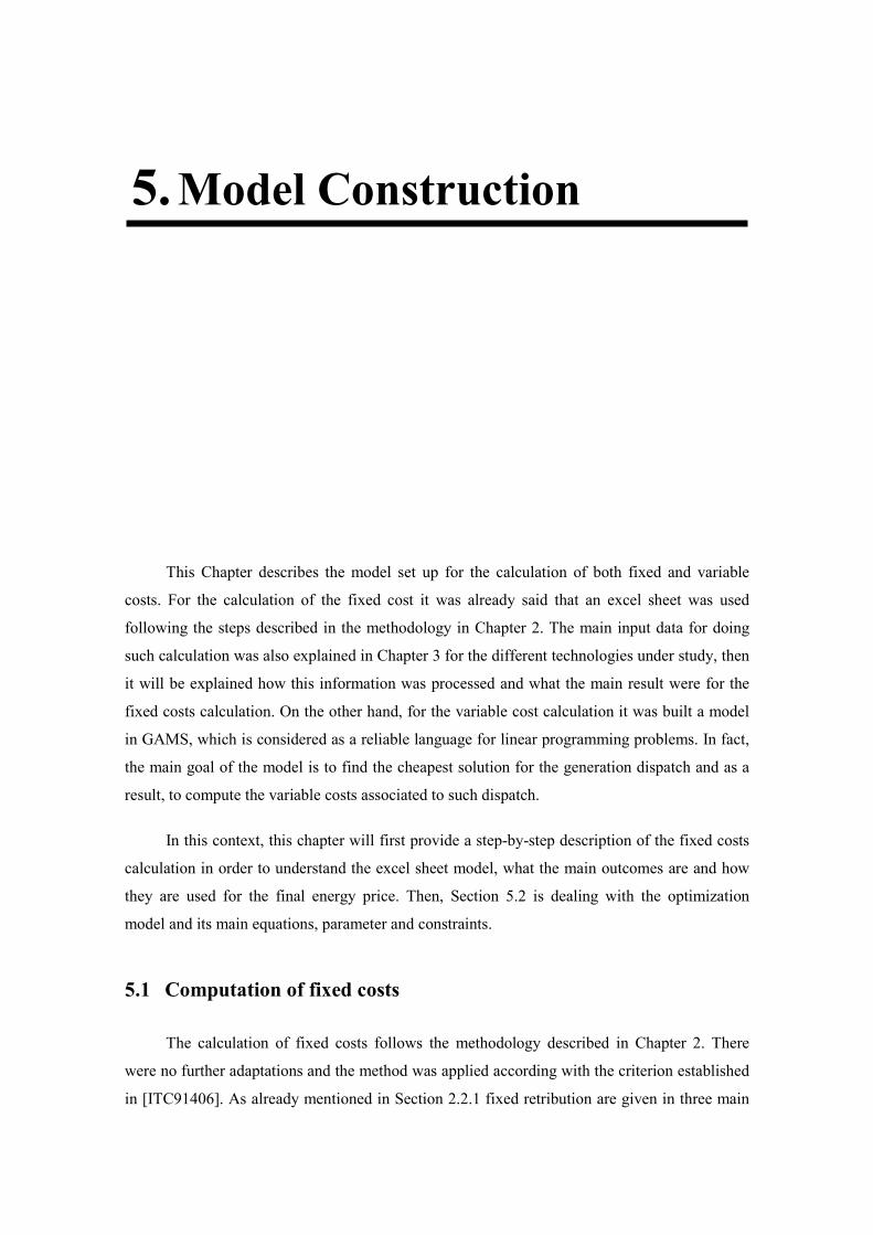
5. Model Construction
This Chapter describes the model set up for the calculation of both fixed and variable
costs. For the calculation of the fixed cost it was already said that an excel sheet was used
following the steps described in the methodology in Chapter 2. The main input data for doing
such calculation was also explained in Chapter 3 for the different technologies under study, then
it will be explained how this information was processed and what the main result were for the
fixed costs calculation. On the other hand, for the variable cost calculation it was built a model
in GAMS, which is considered as a reliable language for linear programming problems. In fact,
the main goal of the model is to find the cheapest solution for the generation dispatch and as a
result, to compute the variable costs associated to such dispatch.
In this context, this chapter will first provide a step-by-step description of the fixed costs
calculation in order to understand the excel sheet model, what the main outcomes are and how
they are used for the final energy price. Then, Section 5.2 is dealing with the optimization
model and its main equations, parameter and constraints.
5.1 Computation of fixed costs
The calculation of fixed costs follows the methodology described in Chapter 2. There
were no further adaptations and the method was applied according with the criterion established
in [ITC91406]. As already mentioned in Section 2.2.1 fixed retribution are given in three main

5. Model Construction
50
cases. First, they are given to existing and new power plants in order to guarantee the security of
supply and to incentivize investments in new capacity. Second, to new facilities used to improve
efficiency, especially to coal units that have invested in new facilities to burn other coal type.
And finally, they are given for the expected future investment in new technologies to reduce the
GHG emissions.
The relations in the methodology for the fixed costs calculations are given by simple
linear equations and its computation has been made using an Excel spreadsheet. The main input
data in fixed costs calculations are the unitary investment value of facilities and the maximum
O&M costs given in Chapter 3 for the different technologies. The following are steps are
intended to provide a description of how the daily fixed costs is obtained.
1. The spreadsheet is organized by the technology and each one has its individual
calculation. The values to be introduced are the unitary investment value and the
maximum O&M costs. The first will allow to obtain the annual investment cost and the
second will be used to obtain the fixed O&M costs.
2. By adding up the two terms above it is found the annual capacity payment. The latter
explains the simplest case in which units are only paid by the power plant itself like the
case of nuclear units; however some coal units made investments in new boilers and
desulfurization processes which are candidates to get fixed payments. For the case of
boilers, the only cost considered was the unitary investment value and for the second both
the investment and O&M expenses are taken into account. The latter case also applies for
the future investments in SCR. The final annual capacity payment will be the sum of those
individual payments where it applies. Finally, this payment is decomposed in seasons
according with the table below which indicates a seasonality factor and the months
considered in each season. By doing so, there are three different capacity payments
namely peak, shallow and valley.
PERIOD Applied Months Seasonality factors
Peak January, February, July,
December 1.15
Shallow March, June, September,
November 1
Valley April, May, August, October 0.85
Table 5.1 Seasonality factors
3. Finally, these three values obtained in the step before are distributed according with the
months they apply and multiplied by a monthly availability factor (See Appendix 1)
which will give the daily individual capacity payments.

5. Model Construction
51
5.2 Optimization model for variable cost calculation
This section describes the main features of the model used for the variable costs
calculations. The main goal of the model is to represent the current and expected composition of
the SEP in terms of power installed capacity in order to find the less costly generation dispatch
in a ten years period, taking into account the different constrains, assumptions and evolution of
the generation mix.
The model will run in a daily base and will match the expected residua demand for each
day according with the estimation done in Chapter 4. Because of the huge number of variables
managed in the model, simulations were done in separate years starting in 2011. It was assumed
for the first year of the simulations that units connected to the network in the first day were the
usual base power plants namely nuclear units plus the coal units with a quota to be met. Then
the model is run and fixes the economic dispatch in the whole year. These units dispatched in
the last days of the year are used for the first day in the following year and so on. The main
output of the model is the generation dispatch as well as the daily variable costs; however it will
also provide the natural gas consumed by gas units and the CO2 costs associated to energy
produced.
The optimization tool chosen for building the model was GAMS (General Algebraic
Modeling System) using the solver CPLEX. GAMS imports data from a input excel sheet and
the operates this data in a GDX file and then the results are again exported to the excel sheet
automatically. The complete GAMS code can be found in Appendix 8.
5.2.1 Model Indexes and sets
The following are the model indexes used for the formulation of the model.
d It takes values of 1 to 365 for normal year and 366 for leap years
q Thermal units in the SEP. The thermal units number varies
± Technology type. It is used for defining some technical parameters
²³´oµ¶·(q) Subset of thermal units belonging to nuclear technology
´p¶o(q) Subset of thermal units belonging to coal technology
q¸´´(q) Subset of ELCOGAS unit
¹³µo_q¶»(q) Subset of thermal units belonging to fuel-gas technology
´´q±(q) Subset of thermal units belonging to combined cycle technology

5. Model Construction
52
Input data for indexes and set are mainly the thermal units in the SEP and then they are
rearranged internally by GAMS to differentiate them according with the different technologies.
5.2.2 Parameter and variables
These are the second group of important data to achieve the goal of the model. It is first
shown the parameters of the system and units, which usually are constant values, and then the
main equations.
a) System Parameters
sµ¼_±µ(s) Residual demand to be met by thermal technologies [GWh]
t½(s) Variable O&M costs of hydro generation by day [MEuro]
t½(s) Variable pumping cost by day [MEuro]
sµ¼_q¸ Elcogas target production [GWh]
¾½ Target production of coal units in the RD 134 [GWh]
b) Units’ parameters
¿¼¶À(q) Maximum energy produced by the unit g in a day [GWh]
¿¼¸²�q� Minimum energy produced by the unit g in a day [GWh]
Á³¶sÂ�q� Quadratic adjustment parameter A of generator g [th/h]
Á³¶sÅ�q� Quadratic adjustment parameter B of generator g [th/h.GW]
¹�q� O&M cost factor of generator g [MEuro/GWh]
ȵ�q� Emissions quantity factor of generator g [MEuro/GWh]
¹�q� Annual free emissions rigths of generator g [tCO2]
Ê·´�q� Coal fuel thermie price [MEuro/th]
Ê·q Gas fuel thermie price [MEuro/th]
¿¹¹²�±� Nominal efficiency of unit g �only for CCGT and fuel-gas units�
ʹ�±� Fuel cost price factor [MEuro/GWh]
Ê·µ CO2 emission price [MEuro/tCO2]
Cv Variable component of LNG conduction toll [MEuro/GWh]
The following list gives the most important variables that are needed to model the system.
It includes variables that are part of the outcomes and also variables to represent particular
characteristics of the units such as state, star-up and shutdown decisions.

5. Model Construction
53
µ²µ·qÌ(s, q) Energy dispatched by unit g in a day [GWh]
tq�s, q� Total generation costs of unit g in a day [MEuro]
tp½�s, q� Variable operating costs of unit g in a day [MEuro]
tp¼�s, q� Variable O&M costs of unit g in a day [MEuro]
t´p2_µ¶�s, q� Variable ex-ante emissions costs of unit g in a day [MEuro]7
opq�s, q� Variable LNG logistic costs of unit g in a day [MEuro]
ȼ²�s, q� LNG consumed by unit g in a day [GWh]
t´p2_µ½�s, q� Variable ex-post emissions costs of unit g in a day [MEuro]8
³�s, q� Binary variable indicating the state of unit g in a day [1,0]
�s, q� Start-up decision of unit g in a day [1,0]
�s, q� Shut down decision of unit g in a day [1,0]
5.2.3 Objective function
The objective function represents the target equation in the model. It is either minimized
or maximized depending of the formulation or the aim of the model. As already said several
times, the aim of the model is to minimize the variable cost in the SEP.
¼¸² ∑ ∑ tuz�s, q� tuv�s, q� twx\_ÏÐ�s, q�Ñ opq|�s, q�¬ ty�s� tz{v�s�
Equation 1 Objective function of the model
The first four terms are related with thermal units variable costs already explained. For CH
and Cpum it was also said that there is not merit mechanism for them and they are just receiving a
variable payment linked to the energy produced and pumped.
5.2.4 Constraints
This set of equation fixes the boundaries for the model. Minimizing the objective function
is controlled by a set of constraints that will help to assure that the solution is accurate and
meets all the technical and any other limitation.
7 This variable is used of the economic dispatch and suggests that emissions costs of opportunity of individual units are fully internalized in their recognized costs. Thus, in a market where bids are submitted and compete with each others, the merit order changes and gives incentives to low polluting and more efficient units. 8These variable includes the free emission rights assigned by the PNA I and II. In a centralized system this rights ease the transition towards a mechanism where all the generation costs are internalized in the generation prices so this variable is intended to estimate the actual daily cost needed to final energy price.
5. Model Construction
54
sµ¼_±µ(s) � Ò µ²µ·qÌ(s, q)Ñ
Equation 2 Meet thermal demand in day d
C��(d, g) � 24 · Pr�g� Óu�d, g� · a�g� b�g�. energy�d, g�hr�d, g� Ô C g � coal, gas, CCGT
Equation 3 Operating variable cost for coal, gas and CCGT units
C���d, g� � P�� · µ²µ·qÌ�s, q� C q � ²³´oµ¶·, ¿o´pq¶»
Equation 4 Operating variable cost for nuclear and Elcogas
C�X�d, g� � f�g� · energy�d, g� Equation 5 Operation and maintenance variable costs
C5�\_ea�d, g� � Qe�g� · energy�d, g� · Pre Equation 6 Ex-ante CO2 emissions costs
logv�d, g� � energy�d, g�η�g� · Cv C g � CCGT, gas
Equation 7 Variable LNG logistic costs
The economical constraints are given in equations 2 to 7 and they depict the main terms
of the methodology used in this work. The following set represents the main technical
constraints considered in this model.
µ²µ·qÌ�s, q� ¢ ³�s, q� · ¿¼¶À�q� Equation 8 Upper bound for the energy produced by a unit g in one day
energy�d, g� D u�d, g� · Emin�g� Equation 9 Lower bound for the energy produced by a unit g in one day
u�d, g� � u�d A 1, g� y�d, g� A z�d, g� Equation 10 Logic of start up and shut down
Ì�s, q� Î�s, q� ¢ 1
Equation 11 Respect logic of start up and shut down
5.2.5 Singularities
The equations explained above represent the base case for the model. However there are
also other particular constraints imposed by either coal quotas or scheduled maintenance for

5. Model Construction
55
nuclear units. This equations vary from year to year and won´t be put in this section, instead, it
will be shown in a table two of the most relevant constraints that change every years.
First of all, the already mentioned coal quotas are part first of the RD 134 which has a
scope until 2014, and then a decreasing quota as a result of the Mining Plan until 2018 with a
decreasing quota. Table below shows these quotas and the coal units involved.
Unit RD134 Mining Plan
2011-2015 2015 2016 2017 2018
ELCOGAS 1,400 1,120 840 700 420
Compostilla (2-5)
5,444 3,267 2,722 2,178 1,633
Teruel (1-3) 6,184 4,329 3,710 3,092 1,855
Soto de Ribera 3
1,312 918 787 656 394
Puente Nuevo 3
1,482 1,037 889 741 445
Escucha 372 260 223 186 112
Anllares 1,968 1,378 1,181 984 590
Narcea 3 1,206 844 724 603 362
La Robla 2 2,035 1,425 1,221 1,018 611
Guardo 2 1,943 1,360 1,166 972 583
Total 23,346 15,938 13,463 11,129 7,004
Table 5.2 Quotas for coal units [GWh]
Secondly, the nuclear units have a fuel recharge schedule which can vary according with
the season of the year. This schedule has been set according with the table below from 2011 to
2015 trying to represent the actual impact of this power plants being unavailable. The complete
schedule can be found Appendix 2.
Nuclear Unit 2011 2012 2013 2014 2015
Month Days Month Days Month Days Month Days Month Days
Almaraz 1 Abr 40 Nov 40 - - Abr 40 Nov 40
Almaraz 2 - - Abr 40 Nov 40 - - Abr 40
Cofrentes Sep 60 - - Sep 60 - - Sep 60
Garoña May 35 - -
Trillo Jun 35 Jun 35 Jun 35 Jun 35 Jun 35
Vandellós 2 - - May 40 Oct 40 - - May 40
Asco 2 Oct 40 - - May 40 Oct 40 - -
Asco 1 May 40 Oct 40 - - May 40 Oct 40
Table 5.2 Fuel recharge schedule for nuclear units from 2011-2015
A final remark about the optimization model is related with the units used. It is usually
found in the literature that prices or costs are given in Euro/MWh but this would imply to work

5. Model Construction
56
in such units the whole set of input and outputs in the model. However, because of the huge
number of variables and equations generated when the model was run, the order of the objective
function was too high and the stability of the model was compromised, leading to long solving
times and inaccurate solutions so in order to cope with such issues it was necessary to scale
variable to the order GWh and MEuro so the solution found was more reliable and the solving
times.
5.3 Calculation of the final generation price
For the calculation of the final energy price, equation 2.2 is used. Then, both results fixed
costs calculation and variable costs calculations from the optimization model are combined
according with equation 2.1. The following steps describe the way the final energy price is
obtained.
1. Fixed costs are exported from the Excel book called FC to a new book usually called
GC20119. These costs are placed in a daily basis and for each of the units in the year
under study.
2. Variable costs obtained with the optimization model are taken from the input-output Excel
book and exported to the same GC2011 book. In this step, costs are brought back to the
order of Euros.
3. The production for each of the units is also exported from the input-output Excel book
and placed in a separate sheet in the GC2011 file. In this step, costs are brought back to
the order of MWh.
4. The total generation costs of each unit are computed on a daily basis by adding up fixed
costs and variable costs according with equation 2.1 in Chapter 2. This information can be
used to know what total costs of the units are in a year and also the total daily costs.
5. Finally, the final generation price is equal the total costs in the day divided by the total
generation in that day. This price represents the total average price for the day but in
addition to this, it was obtained the final generation price by technology with the same
information in order to have an overview of the evolution of prices.
6. A final step was done to have the monthly average prices by taking the average of the
prices per month. This result was compared with the hypothetical marginal prices fixed in
9 The last four digits correspond to the year being simulated

5. Model Construction
57
a market mechanism. This price was considered as the price of the marginal generator,
excluding the coal units subject to quotas in order to exclude the effect of such imposition.
Next chapter will deal with the analysis and further explanations of the results obtained
with the model and Excel sheet.

6. Simulation and Result Analysis
This Chapter will present the most noticeable results achieved with the model. Key
aspects to be studied are the expected generation costs based on the assumptions and
simplifications made, the evolution of the demand coverage by technology and the impact of
special regime generation as well as the expected consequences of the implementation of
current regulatory constraints.
6.1 Simulation and Assessment of the model results
This section is intended to assess some of the most interesting result found with the model
regarding demand coverage and generation cost for the different technologies It should be kept
in mind that most of the results presented are associated to the ordinary regime technologies
described in Chapter 3 and any reference done to any other technology will be explicitly pointed
out.
6.1.1 Ordinary regime demand coverage and generation costs
The Figure 6.1 below shows the dispatch in 2011. The daily dispatch during the years is
consistent with the costs associated to the different technologies. Nuclear units are mostly
running a maximum capacity and just stop production during scheduled fuel recharging. Hydro
generation is only an input and its dispatch does not depend on the variable cost. Indeed it

influences the economic dispatch by imposing an
objective function but its daily production has been estimat
reduces the thermal gap to be filled
in the following years either;
supply issues. The generation dispatch for the whole p
Figure 6.1
In regards to coal production
and they normally meet the maximum production required per year
becomes the technology that
generation variations. This behavior is observed dur
6.2 shows how CCGT production is
variations in the residual demand for thermal units
nuclear power plants and finally it
decommissioned, however in the years 2014, 2017 and 2018 this growth is minimized due to
new hydro units which can supply at a lower cost than CCGTs.
Figure
6. Simulation and Result Analysis
influences the economic dispatch by imposing an additional variable cost component
objective function but its daily production has been estimated beforehand which ultimately
reduces the thermal gap to be filled. Fuel-gas units are not part of the dispatch and won’t appear
either; however they are kept by the system operator due to security of
The generation dispatch for the whole period is presented in Appendix 9
Figure 6.1 Generation dispatch in the year 2011
production, the units being dispatched are the ones subject to the
and they normally meet the maximum production required per year in the [RD134
becomes the technology that balances the system in order to keep equilibrium in demand
s behavior is observed during the whole simulation period and
s how CCGT production is growing through the years, first, because of the slight
variations in the residual demand for thermal units second, as a result of unavailability of
lear power plants and finally it is also absorbing the production of those units being
owever in the years 2014, 2017 and 2018 this growth is minimized due to
units which can supply at a lower cost than CCGTs.
Figure 6.2 Evolution of generation by technology in GWh
Simulation and Result Analysis
59
component to the
ed beforehand which ultimately
gas units are not part of the dispatch and won’t appear
however they are kept by the system operator due to security of
eriod is presented in Appendix 9.
units being dispatched are the ones subject to the SGC
in the [RD13410]. CCGT
in order to keep equilibrium in demand-
ing the whole simulation period and Figure
first, because of the slight
second, as a result of unavailability of
absorbing the production of those units being
owever in the years 2014, 2017 and 2018 this growth is minimized due to
6. Simulation and Result Analysis
60
The average yearly generation costs under the regulated scheme which includes fixed plus
variable costs rises steadily from 65.71 Euro/MWh in 2011 until reaching 78.6 Euro/MWh in
2020 mainly because the assumptions made in all the cost involved follow the same behavior
and any unexpected event was considered apart from the already known constraints. However, it
should be pointed out that this cost structure is subject to mandatory production of coal units
which are increasing considerably the price per MWh. The most stable technology in term of
price is the Nuclear which has an average cost of 43.2 Euro/MWh (± 2 Euro/MWh). The
cheapest energy is still coming from hydro power plants with an average cost of 40.8
Euro/MWh however it experiences a considerably increases in cost due to new units in 2013,
2017 and 2018. Coal and CCGT technologies appear to be the most expensive however in the
economic dispatch, coal production is limited to quota required by the RD134 and this increases
its generation costs becoming the most expensive with costs around 105.9 Euro/MWh from
2011 to 2014 and rising exponentially from 2015 onwards. This leaves the remaining energy to
CCGT with more stable costs around 88.6 Euro/MWh during the simulation period. The latter is
supported by the fact that the generation dispatch is done based on variable costs and the general
expectation is that CCGT units will have cheaper variable costs as compared with coal units.
This trend can be clearly observed after the end of the RD134 where the coal productions does
remain at same level because its competitiveness in terms of variable costs is not enough to
compete with CCGT units. Appendiz 10 show generation costs by technology.
The information given above is supported by the total costs computed. Tables 6.1 (a) and
(b) show a division between variable and fixed cost for the different technologies in the ordinary
regime during the whole simulation period which also gives a clearer idea of what the regulated
scheme is about. First, the fuel-gas units are just receiving the fixed cost associated for being
available in the system because they are not being dispatched which causes this cost to be
present until 2015 when they are decommissioned. It is important to mention that at a first
glance these costs are excessive, however the [ITC91410] considers a fixed payment of 50% its
last fixed payment after the unit has been completely amortized which applies to all units in the
system. Secondly, nuclear units cost confirm that such units usually have a larger fix component
than other base load units while their variable cost are the second cheapest in the system just
below hydro power plants which have the lowest variable costs. CCGT units represent the
largest expense for the system on the one hand, for the large amount of units installed in the
system and on the other for the energy supplied. Finally, the coal units show high fixed cost as
compared with the energy dispatched for the system. This trend remains in the whole period and
is more evident from 2015 onwards where the energy dispatched is even less and the costs
reached level above 200 Euro/MWh.

6. Simulation and Result Analysis
61
Technology
2011 2012 2013 2014 2015
Fix Variable Fix Variable Fix Variable Fix Variable Fix Variable
Nuclear 1,595 739 1,632 809 1,587 772 1,574 782 1,598 756
Coal 1,149 1,356 1,160 1,425 1,160 1,505 1,165 1,569 1,174 1,081
Fuel & Gas 58 0 61 0 61 0 63 0 64 0
CCGT 2,638 3,548 2,644 3,725 2,607 4,007 2,579 4,160 2,552 4,997
Hydro 831 64 841 65 1,036 71 1,113 76 1,112 77
Total 6,270 5,708 6,338 6,024 6,452 6,355 6,493 6,587 6,500 6,911
TOTAL [MEuro] 11,978 12,362 12,807 13,080 13,412
Table 6.1(a) Generation cost from 2011 to 2015
Technology
2016 2017 2018 2019 2020
Fix Variable Fix Variable Fix Variable Fix Variable Fix Variable
Nuclear 1,629 801 1,648 785 1,674 800 1,700 801 1,734 833
Coal 1,195 886 1,193 755 1,194 607 940 76 991 57
Fuel & Gas - - - - - - - - - -
CCGT 2,533 5,287 2,498 5,613 2,472 5,911 2,831 6,610 2,994 6,799
Hydro 1,115 77 1,212 82 1,203 86 1,293 87 1,356 87
Total 6,472 7,051 6,552 7,234 6,543 7,405 6,764 7,573 7,075 7,776
TOTAL [MEuro] 13,523 13,786 13,948 14,337 14,851
Table 6.1(b) Generation cost from 2016 to 2020
6.1.2 Thermal generation evolution
The evolution of the thermal technologies is linked mainly to regulatory constraints,
especially for the coal units which first, according with the RD134 starting in 2011, some units
have to meet and annual quota as a compulsory requirement for helping the mining sector in
Spain and secondly, are subject to an EU Directive which pushes to close the most pollutant
units or invest in the newest technology available to decrease emissions. However, it is
important to emphasize that this regulatory constraints were introduced as a variable for the
model in order to assess their possible consequences in the system but they cannot be taken as
simulation of the actual behavior of the players involved because in reality there are other
factors out of the scope of this work that influence their decisions.
First of all, there is a restriction to some units (Cercs, Escucha, Lada 3, & fuel-gas units)
not to be connected to the network for more than 20,000 hours before 2015. Apart from Escucha
none of these units has a quota to be met during the year, however not even Escucha goes
further than 20,000 hours being connected. As a result of this, none of the units was
decommissioned for reaching the limit.
The second important regulatory constraint is the so called SGC imposed by RD134. This
RD gives annual constant quota to some coal units from 2011 to 2014 (See Table 6.2). The

6. Simulation and Result Analysis
62
application of this RD is initially set to be finished by the end of 2014. Their production has
been constant and every year the goal is reached. It is expected that after finishing SGC the
more inefficient unit will be decommissioned. In this context it was considered that from the
group of units in the SGC, Compostilla 2, Escucha y Anllares are going to be closed in 2015.
Finally, after completing the SGC there is a new IED Directive issued by the EU in which
the existing installations should meet the ELV accordingly either by a limited number of
operating hours (17,500) from 2016 to maximum 2023 or by installing the best available
technology (SCR) to reduce emissions. The coal units subject to these mechanisms were
monitored in order to keep track of both number of hours connected to the network and energy
production for those units investing in the new technology.
Coal Unit 2011
Quota
Escucha 372
Teruel (1-3) 6,184
Guardo 2 1,943
Compostilla (2-5) 5,444
Puente Nuevo 3 1,482
Anallares 1,968
Narcea 3 1,206
Robla 2 2,035
Soto de R. 3 1,312
ELCOGAS 1,400
Total RSG 23,346
Table 6.2 Coal units’ quotas subject to SGC in GWh
Based on the previous information, some decisions were made in order to meet the
regulatory constraint as well as to reflect what in reality could happen with the current
information known. First, there were thermal units decommissioned from the installed capacity
according with its decommissioning schedule such as Garona in 2013 and the two of fuel-gas
units in 2015. Regarding coal units, Compostilla 2, Anllares 1 and Escucha 1 were dismantled in
2015 and 7 more coal units accounting to 1,257.20 MW were decommissioned in 2016. This
effect in the coal units is expected to show up as a result of the SGC´s end in 2015 and the more
rigorous environmental constraints imposed by the EU-IED. It was observed that after
completing the SGC the production rate of coal units falls as a result of a disadvantage in
variable costs with CCGT plants. Besides, EU requires that such units should invest in best
available technologies to cope with the high rate of emissions from these units, however the
investment required is not only for the new technology but also to extend the lifespan of the
already aged power plant therefore given the low production rate expected from coal units it is
not justified to make such a huge investment. Afterwards it was considered that units in Table

6. Simulation and Result Analysis
63
6.3 below are taking the 17,500 hours of maximum production to avoid investment in new
technology which might not be profitable for them if they are not being dispatched. From these
group, a decision was made to decommission Teruel 1, 2 and 3 and Compostilla 4 in 2018 due
to the fact that by that year their operating hours are close to the limit and the residual time
cannot be reached in the following year because the mining plan has also finished and in 2019
and 2020 the generation dispatch do not include any minimum production for coal units. On the
other hand, just three groups are assumed to make investment in SCR in 2015 which are Litoral
1 and 2 and Barrios mainly because they are the groups being dispatched during the simulation
period along with those groups in the SGC.
Coal Unit 2016 2017 2018 2019 2020
Total Hours Production [hr]
Production [hr]
Production [hr]
Production [hr]
Production [hr]
Puentes GR 1 0 0 1,680 240 120 2,040 Puentes GR2 0 0 3,336 48 0 3,384
Puentes GR 3 0 0 0 216 0 216
Puentes GR 4 0 0 0 144 2616 2,760
Meirama 0 0 0 72 0 72
Teruel 1 6,192 5,640 3,240 - - 15,072
Teruel 2 6,600 5,400 3,672 - - 15,672
Teruel 3 6,408 5,112 4,080 - - 15,600
Guardo 2 3,912 3,456 1,992 528 0 9,888
Lada 4 0 0 0 144 0 144
Compostilla 4 8,016 7,032 1,104 - - 1,6152
Compostilla 5 1,248 24 4,176 0 0 5,448
Pte nuevo 3 3,432 2,760 1,680 48 0 7,920
Narcea 2 0 0 0 528 312 840
Narcea 3 2,472 1,944 1,152 96 0 5,664
Robla 1 0 0 0 624 168 792
Robla 2 4,104 3,336 2,448 696 0 10,584
Soto 3 2,760 2,328 1,248 72 0 6,408
Abono 1 0 0 0 984 0 984
Pasajes 0 0 0 192 0 192 Table 6.3 Coal units subject to 17,500 hours production
In summary, the change in thermal installed capacity is driven by scheduled
decommissioning of old power plants as well as assumptions of what in reality would happen
when the existing thermal capacity is not being dispatched. This massive take away of thermal
units during the period represents a total 4,833 MW decommissioned which will bring the need
of installing new capacity to keep the system in safe reserve margins. For doing so, additional
hydro capacity already schedule in 2013, 2017 and 2018 was taken for coverage index
calculation. In addition, a decision was made based on the desirable IC to install an additional
4,000 MW of CCGT in the years 2019 and 2020. Figure 6.3 below summarizes the units to be
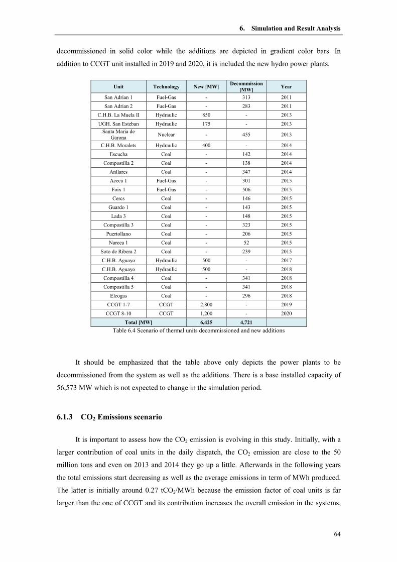
6. Simulation and Result Analysis
64
decommissioned in solid color while the additions are depicted in gradient color bars. In
addition to CCGT unit installed in 2019 and 2020, it is included the new hydro power plants.
Unit Technology New [MW] Decommission
[MW] Year
San Adrian 1 Fuel-Gas - 313 2011
San Adrian 2 Fuel-Gas - 283 2011
C.H.B. La Muela II Hydraulic 850 - 2013
UGH. San Esteban Hydraulic 175 - 2013
Santa Maria de Garona
Nuclear - 455 2013
C.H.B. Moralets Hydraulic 400 - 2014
Escucha Coal - 142 2014
Compostilla 2 Coal - 138 2014
Anllares Coal - 347 2014
Aceca 1 Fuel-Gas - 301 2015
Foix 1 Fuel-Gas - 506 2015
Cercs Coal - 146 2015
Guardo 1 Coal - 143 2015
Lada 3 Coal - 148 2015
Compostilla 3 Coal - 323 2015
Puertollano Coal - 206 2015
Narcea 1 Coal - 52 2015
Soto de Ribera 2 Coal - 239 2015
C.H.B. Aguayo Hydraulic 500 - 2017
C.H.B. Aguayo Hydraulic 500 - 2018
Compostilla 4 Coal - 341 2018
Compostilla 5 Coal - 341 2018
Elcogas Coal - 296 2018
CCGT 1-7 CCGT 2,800 - 2019
CCGT 8-10 CCGT 1,200 - 2020
Total [MW] 6,425 4,721
Table 6.4 Scenario of thermal units decommissioned and new additions
It should be emphasized that the table above only depicts the power plants to be
decommissioned from the system as well as the additions. There is a base installed capacity of
56,573 MW which is not expected to change in the simulation period.
6.1.3 CO2 Emissions scenario
It is important to assess how the CO2 emission is evolving in this study. Initially, with a
larger contribution of coal units in the daily dispatch, the CO2 emission are close to the 50
million tons and even on 2013 and 2014 they go up a little. Afterwards in the following years
the total emissions start decreasing as well as the average emissions in term of MWh produced.
The latter is initially around 0.27 tCO2/MWh because the emission factor of coal units is far
larger than the one of CCGT and its contribution increases the overall emission in the systems,

however, as soon as the SGC
produced by coal units and this factor starts decreasing until reaching 0.20 tCO
as can be seen in the figure below.
Figure 6.4 Total CO
6.2 Assessment on the impact of the special regime and regulatory
constraints
The imposed targets by the EU to its member countries related to renewable energy use
imply a new challenge for markets. For the period under study
generation has consequences for the ordinary regime technologies. According with
estimation done in Chapter 4
installed capacity will be reflected in its production especially from renewable energy sources.
In the Table 6.4 below it can be seen the limited demand growth
technologies mainly because renewable energy sources ar
30% of the total demand by 2020
technologies namely CCGT and coal which are
and have to compete for the re
structure this would be a problem for those units with the highest costs because they won´t be
dispatched, on the other hand, in
strategies mainly because there will be a new supply
production expectations decrease for those technologies putting an additional risk in the
term fuel contracts usually signed by power plants using gas which typically have a take or pay
clause.
Along with the above mentioned constraint, the imposition of minimum generation for
coal units in the SGC has impact on the generation costs and e
represents around 12% of the remaining energy, the overall generation costs tend to rise
considerably. These costs in the SEP were compared to
6. Simulation and Result Analysis
finishes in 2014 the CCGT technology takes the energy previously
y coal units and this factor starts decreasing until reaching 0.20 tCO
as can be seen in the figure below.
Figure 6.4 Total CO2 emissions and rate of emissions
Assessment on the impact of the special regime and regulatory
posed targets by the EU to its member countries related to renewable energy use
imply a new challenge for markets. For the period under study, the assumption of special regime
has consequences for the ordinary regime technologies. According with
in Chapter 4, the evolution of the special regime technologies
installed capacity will be reflected in its production especially from renewable energy sources.
can be seen the limited demand growth for the ordinary regime
mainly because renewable energy sources are expected to meet slightly more than
30% of the total demand by 2020. The consequence of such problem goes straight to the thermal
technologies namely CCGT and coal which are the most expensive technologies in the system
and have to compete for the residual demand after nuclear production. Under a regulated cost
structure this would be a problem for those units with the highest costs because they won´t be
er hand, in a market mechanism this will force companies to redesign
because there will be a new supply - demand balance
production expectations decrease for those technologies putting an additional risk in the
usually signed by power plants using gas which typically have a take or pay
Along with the above mentioned constraint, the imposition of minimum generation for
coal units in the SGC has impact on the generation costs and even though the SGC´s quota
represents around 12% of the remaining energy, the overall generation costs tend to rise
considerably. These costs in the SEP were compared to marginal cost of the last unit dispatched
Simulation and Result Analysis
65
finishes in 2014 the CCGT technology takes the energy previously
y coal units and this factor starts decreasing until reaching 0.20 tCO2/MWh in 2020
Assessment on the impact of the special regime and regulatory
posed targets by the EU to its member countries related to renewable energy use
the assumption of special regime
has consequences for the ordinary regime technologies. According with the
the evolution of the special regime technologies in terms of
installed capacity will be reflected in its production especially from renewable energy sources.
for the ordinary regime
slightly more than
. The consequence of such problem goes straight to the thermal
the most expensive technologies in the system
Under a regulated cost
structure this would be a problem for those units with the highest costs because they won´t be
a market mechanism this will force companies to redesign
demand balance and the energy
production expectations decrease for those technologies putting an additional risk in the long
usually signed by power plants using gas which typically have a take or pay
Along with the above mentioned constraint, the imposition of minimum generation for
ven though the SGC´s quota
represents around 12% of the remaining energy, the overall generation costs tend to rise
marginal cost of the last unit dispatched

in the day but without taking into account t
reflect the actual price under a market mechanism. Figure 6.5 below shows the trend in
generation cost during the simulation period and the
average costs under the regulated scheme. In regards with the average generation cost in the
system it can be observed that the regulated costs rise in the whole period, especially from 2011
to 2014 when the SGC is applied. Afterwards, the costs seem to be more stable from 2015 t
2017 most likely because the model finds less production constraints and is able to dispatch
more uniformly with the increases in costs
Regarding the marginal costs
generation costs mainly because these prices belong to the cheapest CCGT units and, in some
cases, to coal units.
2011 2012
Ordinary Regime
183,662 185,159
SR-Renewable 56,619 61,718
SR- Non Renewable
38,843 39,366
Special Regime 95,462 101,084
Total 279,124 286,244
Table 6.4 Expected contribution of special and ordinary regime in GWh
It can be observed too in the figure that
between the regulated cost and the marginal costs
On the one hand, as a result of the economical crisis in 2009 the electricity demand felt
dramatically as was mentioned in Chapter 4
therefore the regulated costs are absorb
overcapacity in the system. On the other hand, it also reflects the imposed production by the
RD134 for the coal units which are considerably more expensive according with the scenario in
this work. These extra costs can
Figure 6.5
6. Simulation and Result Analysis
in the day but without taking into account the coal units forced to produce because this wouldn´t
reflect the actual price under a market mechanism. Figure 6.5 below shows the trend in
generation cost during the simulation period and the marginal cost which is lower than the
regulated scheme. In regards with the average generation cost in the
system it can be observed that the regulated costs rise in the whole period, especially from 2011
to 2014 when the SGC is applied. Afterwards, the costs seem to be more stable from 2015 t
2017 most likely because the model finds less production constraints and is able to dispatch
uniformly with the increases in costs just reflected by the increase in variable c
Regarding the marginal costs used in the study, it is clear that they are far below the overall
generation costs mainly because these prices belong to the cheapest CCGT units and, in some
2013 2014 2015 2016 2017 2018
185,159 185,418 185,938 186,604 188,009 187,187 187,913
65,625 70,297 75,985 81,882 87,336 93,012
41,290 42,662 43,241 43,839 45,116 46,414
101,084 106,915 112,960 119,226 125,721 132,452 139,426
286,244 292,333 298,897 305,831 313,730 319,639 327,339
Expected contribution of special and ordinary regime in GWh
It can be observed too in the figure that from 2011 to 2017 there is a huge difference
ulated cost and the marginal costs. This effect has mainly a twofold explanation.
On the one hand, as a result of the economical crisis in 2009 the electricity demand felt
tioned in Chapter 4 leading to a four years lag in the demand growth
therefore the regulated costs are absorbing this lag and the marginal costs
overcapacity in the system. On the other hand, it also reflects the imposed production by the
for the coal units which are considerably more expensive according with the scenario in
These extra costs can be seen in Table 6.5.
Figure 6.5 Average generation cost compared with marginal costs
Simulation and Result Analysis
66
he coal units forced to produce because this wouldn´t
reflect the actual price under a market mechanism. Figure 6.5 below shows the trend in
which is lower than the
regulated scheme. In regards with the average generation cost in the
system it can be observed that the regulated costs rise in the whole period, especially from 2011
to 2014 when the SGC is applied. Afterwards, the costs seem to be more stable from 2015 to
2017 most likely because the model finds less production constraints and is able to dispatch
just reflected by the increase in variable costs.
y are far below the overall
generation costs mainly because these prices belong to the cheapest CCGT units and, in some
2018 2019 2020
187,913 188,315 189,597
93,012 99,576 106,377
46,414 47,075 47,757
139,426 146,651 154,134
327,339 334,966 343,731
7 there is a huge difference
. This effect has mainly a twofold explanation.
On the one hand, as a result of the economical crisis in 2009 the electricity demand felt
leading to a four years lag in the demand growth
ing this lag and the marginal costs reflects an
overcapacity in the system. On the other hand, it also reflects the imposed production by the
for the coal units which are considerably more expensive according with the scenario in

6. Simulation and Result Analysis
67
In terms of total cost for the system, it can be computed in a simple way what the total
cost for establishing coal quotas in the SGC. For the sake of simplicity the estimation is done
taking the marginal cost and the average generation costs of the units in the SGC considering
that each of them has its own cost. Then the total costs were computed taking the annual
production for the annual SGC´s quota of 23,346 GWh.
2011 2012 2013 2014
Maginal Cost [Euro/MWh]
51.07 53.58 55.49 57.72
SGC costs [Euro/MWh]
80.29 83.39 86.03 88.56
∆ Price [Euro/MWh]
29.22 29.81 30.54 30.83
Total [MEuro]
682 696 713 720
Table 6.5 Summary of additional costs due to SGC
The total extra costs incurred for dispatching the units in the SGC is considerably high
and accounts to slightly more than 50% of the total fixed costs paid to the whole coal units. This
is indeed a burden not only for the end user but also for the system and generation companies
which are expected to be affected in their production and ultimately in loss of profit. By giving
incentives to some technologies and reducing the residual demand even more, the system prices
drops affecting ultimately to both hydro and nuclear unit who could have obtained a better price
if this constraint is not present.
6.3 Impact on Coverage Index (IC)
Once the previous analysis is done, it is possible to use such results to evaluate the
expected availability of the installed capacity. In section 2.4 it was said that a safe parameter
established by the system operator is the so called Coverage Index which is just a relation
between the available capacity and the peak demand.
The first step is to formulate a medium scenario in order to compute the coverage index.
The scenario has been based on [CNE_10] and is valid based on the fact that it is an average of
the two opposite scenarios proposed by the system operator, the design scenario which includes
measures to increase efficiency and the trend scenario which do not include measures at all.
This scenario considers the peak demand in winter which has been historically larger than peak
in summer therefore the coverage in summer is assumed to be guaranteed when the CI in winter
is within safe values. On the other hand, the available installed capacity has been calculated
yearly based on the availability factor by technology and evolution of the power plants in the
next years given in Chapter 4.

6. Simulation and Result Analysis
68
Table 6.6 summarizes the different assumption made in regards to net available capacity
and evolution of the installed capacity as well as the rational decisions made with respect to
decommissioning of coal power plants not being dispatched in the last years of the simulation
Table 6.6 Coverage Index evolution in the SEP
It can be seen how CI drops considerably in 2015 and 2016 when there is a massive
decommission of coal units and by 2018 the index is close the minimum required. REE, show it
its prevision an According with the assumption made regarding coal units being
decommissioned, in 2019 the index is already below 1.1 and it is necessary to install new
capacity in the system. To do so it was considered the installation of CCGT units which have
been proved to be efficient in the last years; however, this assumption depends on the
willingness to invest by market players. Another scenario might be that no investment is
expected for those years and the system operator wouldn’t allow those coal units to be
dismantled.
On the other hand, it can be said that the CI clearly reflect the lack of investment in
backup technologies. It was said in Chapter 4 that special regime technologies are expected to
grow considerably in the coming years, however most these technologies do not provide
security to the systems for peak hours, in fact, it is in the other way around, they are expected to
have back up technologies.
Finally, in order to validate the results above, they were contrasted with the scenarios
provided by the system operation, REE. Unfortunately, it doesn’t provide information about the
units being decommissioned in the study period but still its results are comparables with the
ones obtained in this work. REE does consider two different scenarios so called trend scenario
and design scenario and in both the cases in only provides values for 2012, 2014, 2016 and
2020. For the design scenario it gives a CI of 1.18, 1.15, 1.11 and 1.07 respectively which
Year Net Installed
Capacity Available
Base Scenario [MW]
CI Additional
MW required CI
corrected
2011 58108 46,400 1.25 0 --
2012 58178 47,200 1.23 0 --
2013 59543 48,400 1.23 0 --
2014 60246 49,650 1.21 0 --
2015 60056 50,792 1.18 0 --
2016 58517 51,960 1.13 0 --
2017 59318 53,155 1.12 0 --
2018 60120 54,378 1.11 0 --
2019 58616 55,629 1.05 2,800 1.10
2020 58968 56,908 1.04 4,000 1.10

6. Simulation and Result Analysis
69
would imply and additional power capacity of 1,800 MW in 2020 and for the trend scenario it
provides a CI of 1.15, 1.11, 1.08 and 1.02 with additional firm capacity in 2019 and 2020 of
1,300 MW and 4,500 MW respectively. Even thought the assumptions made by REE are not
explicitly shown, these values can be contrasted with the ones obtained in this work which
shows similar trends.

7. Final Conclusions
70
7. Final Conclusions
During the whole simulation period it was observed that the daily dispatch during the
years is consistent with the costs associated to the different technologies. Nuclear units are base
load during the whole year and CCGT is the technology that balances the system to keep
equilibrium because of demand-generation variations. In terms of costs, the most stable
technology is the Nuclear while the technology with the lowest costs is hydro. Coal and CCGT
technologies appear to be the most expensive however in the economic dispatch, coal
production is limited to quota required by the RD134 and this increases its generation costs
becoming the most expensive from 2011 to 2014 and rising exponentially from 2015 onwards.
Fuel-gas units are just receiving the fixed cost associated for being available in the system
because they are not being dispatched which causes this fixed cost to be present until 2015 when
they are decommissioned. With respect to the evolution of the generation mix, there were
thermal units decommissioned from the installed capacity according with its decommissioning
schedule such as Garoña in 2013 and assumption of what in reality would happen when the
existing thermal capacity is not being dispatched and the owners decide closure which
represented a total 4,833 MW decommissioned. The implication of such hypothesis go straight
o the Coverage index which will be affected and start dropping compromising the minimum
safe level required by the system operator.
Whit the above mentioned results it is possible to draw interesting conclusions.
Available, affordable and acceptable are the three important goals for EU in the following years.
It was said before that availability can be measured in terms of security of supply meaning

7. Final Conclusions
71
reliability in the system and capacity available to meet the demand. The first point relates more
to quality of electricity however the most important aspect in this work is related with capacity
available. On the other hand, affordability is seen from the point of view of lower prices for end
users and even though this work is not intended to predict prices, the generation costs estimated
can be used as a reference. Finally, acceptability has become important for achieving EU target
by 2020 and the role of the electricity sector in achieving such goal is very important. This final
Chapter is developed to draw conclusion about the results obtained in this work and how they
can either boost or constraint the achievement of such triple A goals in Spain.
7.1 Assessment of security of supply
Ensuring security of supply requires opportune, diverse correctly sized and placed
investments in all segments of the value chain specially in the generation and transmission
sectors. The reality is that there are major barriers for investment, including policy and market
uncertainties. In the currently weak economic environment, with low and uncertain energy
demand growth, generating technologies with high fixed generation costs and long lead times
such as nuclear facilities may struggle.
As aforesaid, an important factor in the choice of the technologies for meeting electricity
demand is certainly the generation costs associated to it; however investment decisions in new
capacity not only consider such costs but also take into account other risks and uncertainties
such as regulatory risks. Firms usually use the best information available and are always trying
to gain additional information through the time in order to reduce uncertainty and risk. By
having the expected generation costs, investors have an additional tool to assess whether their
projects have good values and can go ahead in new investments. In the end, investments
decisions in specific technologies depend on a number of different factors such as generation
costs however policy uncertainties might act as a barrier specially when there are not long term
commitments and the policy framework is more focus on fulfilling short term needs.
In Spain, the current scenario puts market players with different risk and uncertainties.
According with [CNE_10] there are currently in the portfolio for new capacity in Spain around
14,000 MW of CCGT technology without starting operation date mainly because investors do
not find profitable to build new facilities under the current scenario in the SEP. Table below
provides a qualitative assessment of the different technologies reviewed in this work from of the
point of view of risk and uncertainties in the process of investment decision making. Nuclear
technology will be facing a huge pressure in the coming years due to, one the recent nuclear
disaster in Japan and two the announcement made by Germany about closing its nuclear power

7. Final Conclusions
72
plants by 2022 which certainly puts some pressure in other EU countries. Coal and fuel-gas
units are not only under pressure for CO2 emission prices but also are subject to fuel prices and
to some extend to regulatory pressures specially coal technology. Finally, even though CCGT
technology is subject to a high risk in fuel prices it is still the preferred technology by investors.
Technology Unit size Fixed costs Variable costs Fuel costs CO2 Emissions Regulatory framework
Nuclear Very large High Medium Low Nil Very high
Coal Larga High Low High Very high High
Fuel-Gas Large High Low High Very high High
CCGT Medium Low Low High Medium Low
Hydro Very large Very high Very Low Nil Nil Medium
Table 7.1 Qualitative assessment of generating technologies risks
From table above it is important to highlight that regulatory framework risk includes also
a social factor which can be considered to inside the regulatory framework. Nuclear technology
is always under pressure due to safety issues while coal and fuel-gas have to face environmental
rejection. Finally, even though hydro power plants can bring other benefits a part from
electricity, they also face rejection due to the flooding needed which can affect local
communities.
Nowadays the electricity Spanish sector is experiencing an over capacity due to the drop
in demand in 2009. It is expected according with this analysis that for the next 5 years the
Coverage Index will be still far above the minimum required by the system operator but the
increasing share of renewable energy sources will affect this trend because of the fact that these
technologies do not provide security to the system.
On the other hand, after 2015 the massive decommissioning of thermal power units
specially coal and fuel-gas units will challenge the system in order to incentivize investment and
maintain the capacity available in safe levels. Both coal and fuel-gas units are subject to two
main constraints, firstly, there are environmental pressure on pollutant technologies and many of
these power plants will have to close because of that and secondly, these technologies could
invest in cleaner solutions to cope with emissions and also to extend the lifespan of the unit,
however their low load factor observed in the simulations do not provide incentive to recover
investments. So far, the signals needed from investors are weak and need to be strengthened
especially considering that coal units are expected to experience an intensive program of
decommission after 2014.

7. Final Conclusions
73
Finally, it should be said that investment in new capacity is just one of the options to
assure electricity supply however there are also other options that have to be exploited such as
improvements in interconnection with neighboring countries and improvements in efficiency in
the end-use or the so called demand response effect which certainly is hard to measure and
boost.
7.2 Social impact of generation costs
Under current market mechanism in Spain prices are set by the marginal cost of the last
dispatched technology and any forecast under this mechanism is not an easy task to do for a 10
years future period. This mechanism is the so called day-ahead market in which market players
send bids with the amount of energy they want to sell and the price which reflects the cost of
opportunity for the firm. This means that average costs thus cannot be automatically recovered
from consumers, and therefore companies and operators must accept the risk associated with the
energy produced that can be either limited or for some units even without production at all
which ultimately affects the companies’ revenue. On the other hand, in the traditional context
the regulated electricity prices charged to consumers reflected the long term average cost of
producing electricity. The methodology used in this work to estimate the generation costs does
consider a final generation price which meets all the cost associated for producing an MWh by a
power unit.
Using the estimated generation costs in this work it is possible to make assumptions about
the expected electricity prices under a market mechanism considering these results as a
reference model. First, it can be said that if under the current market mechanism the decisions
are made taking into account the different constraints in a rational way, prices should reflect
those conditions. Secondly, it was assumed that under a market mechanism, marginal costs of
the last unit dispatched should be similar and reflect the market prices of electricity therefore the
marginal cost of the last unit dispatched in the model was used in order to have a reference to
compare. Saying that, the marginal costs observed and the average generation cost differ in the
first years of the period due to the fall in demand in 2009 which causes a disequilibrium in the
capacity available and the demand and there should be a time to balance supply-demand.
Another cause for this effect is the quota imposed for coal units which displaces more efficient
and cheaper technologies. The latter two reasons might explain why the investments plans in the
SEP are stopped and might compromise the well functioning of the market.
Another important issue which can affect the future prices is the decisions made by the
owners. Assumption of decommissions were made just considering regulatory constraints such

7. Final Conclusions
74
as the end of RD134 or the European Directive IED which forces certain units to close,
however, there are several units in the system that are not producing energy in the whole year
and there is no certainty whether owners will close the power plants because no incentive is
given to them. The consequences of such a problem are that in an only energy market these units
can affect considerably the price because as they are not producing and when required they can
set a extremely high price in order to recover investments. This is problem that the regulator
should take into account by assuming the risk of such situation considering the evolution of the
coverage index or copping with the problem by implementing an capacity payment mechanism
to avoid closure of units without production. On the other hand, the assumptions made regarding
investments decisions were mainly focus on new CCGT units; however it can also be argued
that due to the low production of several units in the system, a feasible solution could be gas
turbines for those periods where peak demand requires more capacity.
7.3 Meeting the EU-2020 targets
There are various and complementary reason to boost the growth of renewable energy
sources in Spain and all over Europe. Firsts, an important incentive to issue new policies has
been to reduce the environmental impact of energy usage at both levels local and global. There
is also an additional incentive for replacing fossil fuels sources related with the Europe´s
dependency on foreign sources which it is expected to grow in the following decade. Further
arguments in favor of renewable energy sources are the economic and social benefits they bring
along such as job creation, industry development and ultimately the positive structural effects in
on regional economics. In addition, the growing integration of Europe continues to highlight the
importance of the future development of these sources.
For Spain, the development of renewable energy sources has brought several positive
effects. In addition to the aforesaid mentioned, emissions reduction, a technological change and
distribution generation are other benefits of renewable energy sources. Although deployment of
such technologies has implied a greater economic effort in Spain, this has been tackled with the
time not only considering that more experience is gained in the learning curve but also thanks to
the considerable improvements made in the technical management of the system integrating
storage techniques such as pumping power plants. Besides, in Spain the goal is also focus in the
long term considering that initial investments in renewable sources were high, however these
costs have been going down lately and it is expected that in the long term the benefits surpass
the current costs.

7. Final Conclusions
75
The bet of Spain for renewable energy sources has already been recognized by the EU as
an example of proper design for renewable energy promotion which is reflected with the volume
of electricity achieved in 2009 when their contribution was around 25% out of the total
electricity generated and around 12.2% out of the total energy consumed in the country
[PANER10]. The most noticeable share in Europe is the one from wind energy in which Spain
reported 19,149 MW in 2009 and became the second country with the largest installed capacity
only below Germany which had 25,777 MW in the same year.
In regards to back up needs, the large scale deployment of generation from renewable
resources implies challenges in security of supply issues. An expected generation system with
an increasing share of intermittent renewable energy sources will require the development of a
market for the provision of ancillary services, with significantly larger volume and variety than
present systems. Thermal power plants will have to manage these burdens and will have a
additional market where they can recover part of their costs. Flexible thermal generation and the
expansion of energy storage will be integral to this market.

8. References
76
References
[CNE_10] National Energy Commission. “Inform about the electric energy demand
and natural gas towards the future” Spain, 2011.
[DC__10] Congress members. “Subcomission for the analysis of the Spanish
energy strategy in the next 25 years”. Spain, 2010
[TREVINO] Trevino, Manuel. “ Integrated Gasified Combined Cycle technology.
Real application in Spain”. Spain.
[EUD7510] European Union. “Industrial Emissions Directive EU 2010/75/EU”
[ITC91306] Ministry of Industry, Tourism and Commerce. ‘Order ITC913/2006 that
approves the methodology to calculate the variable costs for the different
fuels used in the insular and extrapeninsular power systems” Spain 2006.
[ITC91406] Ministry of Industry, Tourism and Commerce. ‘Order ITC913/2006 that
approves the methodology to calculate the capacity payments retribution
for the different technologies in the ordinary regime in the insular and
extrapeninsular power systems” Spain 2006.
[ITC155910] Ministry of Industry, Tourism and Commerce. “Order ITC1559/2010
that regulates different aspects of the insular and extrapeninsular power
systems”Madrid, 2010.
[ITC178509] Ministry of Industry, Tourism and Commerce. “Order ITC1785/2009
that fixes the date for the closure of the Nuclear power plant Santa Maria
de Garoña by July 6th, 2013” Spain, 2009.
[ITC279407] Ministry of Industry, Tourism and Commerce. “Order ITC3860/2007
that reviews the electric tariffs from October 2007” Madrid, 2007.
[ITC335410] Ministry of Industry, Tourism and Commerce. “Order ITC3354/2010
that establishes the tolls and canons associated to gas network third party
access” Spain, 2010.
[ITC399306] Ministry of Industry, Tourism and Commerce. “Order ITC3996/2006
which establishes the retribution of some regulated activities of the gas
sector” Spain, 2006.

8. References
77
[ITC386007] Ministry of Industry, Tourism and Commerce. “Order ITC3860/2007
that reviews the electric tariffs from January 2008” Madrid, 2007.
[ME__03] Ministry of Economy. “Royal Decree 1747 that regulates the insular and
extrapeninsular power systems” Madrid, 2003.
[MINER87] Ministry of Industry and Energy. “Order of December 29th which fixes
the standard net and nominal values and lifetimes of installations for
electrical generation that started operation before December 31th 1987.
[MITC07] Ministry of Industry, Tourism and Commerce. “National Plan for
Emissions Reduction in Large Combustion Facilities” Spain, 2007.
[PANER10] Ministry of Industry, Tourism and Commerce. “National Action Plan for
Renewable Energy in Spain - PANER” Madrid, 2010.
[PNAII07] Presidential Ministry. “PRE3420/2007 that approves the individual
emissions rights for the period 2008-2012” Madrid, 2007.
[RD13410] Ministry of Industry, Tourism and Commerce. “Royal Decree
RD134/2010 that establishes the procedure for the guarantee of supply
restriction “ Spain 2010.
[RD94901] Ministry of Economy. “Royal Decree 949/2001which regulates the third
party access to gas installations and establishes and economic system to
the natural gas sector” Spain, 2001.
[REE_10] Spanish System Operator, REE. “Abstract of the 2010 SEP inform”
Madrid 2011.
[REE_11] Spanish System Operator, REE. “REE´s Planning Group” Presentation
in Madrid, April 2011.
[RES919811] Ministry of Industry, Tourism and Commerce. “Resolution that
authorizes the definite closure of the groups 1 and 3 of the thermal
power plant San Adrian” Spain , 2011.
[VRIE10] Vries, Laurens de. “Electricty and Gas. Market design and policy issues”
TU Delft – Reader. Delft 2010.

8. References
78
[WOTT10] Wottrich, Breno. “Generation costs evaluation in centralized mechanism.
A contrast over market mechanism” Master Thesis. Madrid 2010.

9. Appendixes
79
Appendixes
Appendix 1 – Factors of availability
Month Power Availability (%)
Nuclear Coal Fuel & Gas CCGT Hydro
January 94.8 89.3 81.4 95.5 100.0 February 95.0 87.6 85.4 95.2 100.0 March 87.8 87.1 86.7 91.8 100.0 April 82.6 82.9 85.8 90.4 100.0 May 75.4 84.0 85.0 88.2 100.0 June 76.3 86.6 84.0 94.9 100.0 July 83.1 88.0 85.3 97.5 100.0 August 92.1 88.3 82.2 95.0 100.0 September 90.7 88.3 80.3 91.4 100.0 October 86.5 84.8 83.9 87.5 100.0 November 81.4 84.8 75.9 88.2 100.0 December 86.4 89.8 76.4 94.6 100.0

9. Appendixes
80
Appendix 2 – Standard nuclear fuel recharge schedule
Nuclear Unit 2011 2012 2013 2014 2015
Month Days Month Days Month Days Month Days Month Days
Almaraz 1 Abr 40 Nov 40 - - Abr 40 Nov 40
Almaraz 2 - - Abr 40 Nov 40 - - Abr 40
Cofrentes Sep 60 - - Sep 60 - - Sep 60
Garoña May 35 - - End End
Trillo Jun 35 Jun 35 Jun 35 Jun 35 Jun 35
Vandellós 2 - - May 40 Oct 40 - - May 40
Asco 2 Oct 40 - - May 40 Oct 40 - -
Asco 1 May 40 Oct 40 - - May 40 Oct 40
Nuclear Unit 2016 2017 2018 2019 2020
Month Days Month Days Month Days Month Days Month Days
Almaraz 1 - - Abr 40 Nov 40 - - Abr 40
Almaraz 2 Nov 40 - - Abr 40 Nov 40 - -
Cofrentes - - Sep 60 - - Sep 60 - -
Garoña
Trillo Jun 35 Jun 35 Jun 35 Jun 35 Jun 35
Vandellós 2 Oct 40 - - May 40 Oct 40 - -
Asco 2 May 40 Oct 40 - - May 40 Oct 40
Asco 1 - - May 40 Oct 40 - - May 40

9. Appendixes
81
Appendix 3 – Emissions Quantity factors
Coal Technology
Generation Unit Emission Quantity Factor [tCO2/MWh] Free Certificates [tCO2]
2011 2012 2013 2014 2015 2016 2017 2018 2019 2020 2011 2012
PUENTES_GR_1 0.8969 0.8969 0.8969 0.8969 0.8969 0.8969 0.8969 0.8969 0.8969 0.8969 1,054,994 1,054,994
PUENTES_GR_2 0.8969 0.8969 0.8969 0.8969 0.8969 0.8969 0.8969 0.8969 0.8969 0.8969 1,055,595 1,055,595
PUENTES_GR_3 0.8969 0.8969 0.8969 0.8969 0.8969 0.8969 0.8969 0.8969 0.8969 0.8969 1,052,889 1,052,889
PUENTES_GR_4 0.8969 0.8969 0.8969 0.8969 0.8969 0.8969 0.8969 0.8969 0.8969 0.8969 1,054,693 1,054,693
MEIRAMA 0.9156 0.9156 0.9156 0.9156 0.9156 0.9156 0.9156 0.9156 0.9156 0.9156 1,618,787 1,618,787
CERCS 1.0055 1.0055 1.0055 1.0055 1.0055 -- -- -- -- -- 0 0
ESCUCHA 0.958 0.958 0.958 0.958 -- -- -- -- -- -- 301,196 292,426
TERUEL_1 0.9602 0.9602 0.9602 0.9602 0.9602 0.9602 0.9602 0.9602 0.9602 0.9602 1,332,872 1,332,872
TERUEL_2 0.9602 0.9602 0.9602 0.9602 0.9602 0.9602 0.9602 0.9602 0.9602 0.9602 1,332,494 1,332,494
TERUEL_3 0.9602 0.9602 0.9602 0.9602 0.9602 0.9602 0.9602 0.9602 0.9602 0.9602 1,329,845 1,329,845
GUARDO_1 0.9558 0.9558 0.9558 0.9558 0.9558 -- -- -- -- -- 282,823 274,587
GUARDO_2 0.9466 0.9466 0.9466 0.9466 0.9466 1,036,730 1,036,730
LADA_3 0.9410 0.9410 0.9410 0.9410 0.9410 -- -- -- -- -- 306,977 306,977
LADA_4 0.9410 0.9410 0.9410 0.9410 0.9410 723,142 723,142
COMPOSTILLA_2 0.9377 0.9377 0.9377 0.9377 -- -- -- -- -- -- 404,887 403,745
COMPOSTILLA_3 0.9377 0.9377 0.9377 0.9377 0.9377 -- -- -- -- -- 946,493 943,823
COMPOSTILLA_4 0.9377 0.9377 0.9377 0.9377 0.9377 0.9377 0.9377 0.9377 0.9377 0.9377 998,604 995,787
COMPOSTILLA_5 0.9377 0.9377 0.9377 0.9377 0.9377 0.9377 0.9377 0.9377 0.9377 0.9377 997,141 994,327
PTE_NUEVO_3 0.8815 0.8815 0.8815 0.8815 0.8815 0.8815 0.8815 0.8815 0.8815 0.8815 929,809 929,809
PUERTOLLANO 0.9174 0.9174 0.9174 0.9174 0.9174 -- -- -- -- -- 527,272 511,919
ANLLARES 1.0451 1.0451 1.0451 1.0451 -- -- -- -- -- -- 1,042,306 1,011,956
NARCEA_1 0.9350 0.9350 0.9350 0.9350 0.9350 -- -- -- -- -- 120,620 119,958
NARCEA_2 0.9733 0.9733 0.9733 0.9733 0.9733 0.9733 0.9733 0.9733 0.9733 0.9733 359,297 357,328
NARCEA_3 0.9733 0.9733 0.9733 0.9733 0.9733 0.9733 0.9733 0.9733 0.9733 0.9733 809,176 804,741

9. Appendixes
82
ROBLA_1 0.9498 0.9498 0.9498 0.9498 0.9498 0.9498 0.9498 0.9498 0.9498 0.9498 687,876 681,077
ROBLA_2 0.9498 0.9498 0.9498 0.9498 0.9498 0.9498 0.9498 0.9498 0.9498 0.9498 925,246 916,101
SOTO_R_2 0.9310 0.9310 0.9310 0.9310 0.9310 -- -- -- -- -- 580,028 575,487
SOTO_R_3 0.9310 0.9310 0.9310 0.9310 0.9310 0.9310 0.9310 0.9310 0.9310 0.9310 839,381 832,810
ABONO_1 1.1729 1.1729 1.1729 1.1729 1.1729 1.1729 1.1729 1.1729 1.1729 1.1729 1,069,899 1,069,899
ABONO_2 1.1729 1.1729 1.1729 1.1729 1.1729 1.1729 1.1729 1.1729 1.1729 1.1729 1,677,469 1,677,469
ELCOGAS -- -- -- -- -- -- -- -- -- -- -- --
PASAJES 0.9447 0.9447 0.9447 0.9447 0.9447 0.9447 0.9447 0.9447 0.9447 0.9447 0 0
LITORAL_1 0.8762 0.8762 0.8762 0.8762 0.8762 0.8762 0.8762 0.8762 0.8762 0.8762 1,658,622 1,658,622
LITORAL_2 0.8762 0.8762 0.8762 0.8762 0.8762 0.8762 0.8762 0.8762 0.8762 0.8762 1,672,307 1,672,307
BARRIOS 0.8487 0.8487 0.8487 0.8487 0.8487 0.8487 0.8487 0.8487 0.8487 0.8487 1,631,146 1,631,146
CCGT Technology
Generation Unit Emissions Quantity Factor [tCO2/MWh] Free certificates [tCO2]
2011 2012 2013 2014 2015 2016 2017 2018 2019 2020 2011 2012
ACECA_IB_3 0.3891 0.3891 0.3891 0.3891 0.3891 0.3891 0.3891 0.3891 0.3891 0.3891 297,645 297,645
ARCOS_IB_1 0.3952 0.3952 0.3952 0.3952 0.3952 0.3952 0.3952 0.3952 0.3952 0.3952 300,739 300,739
ARCOS_IB_2 0.3914 0.3914 0.3914 0.3914 0.3914 0.3914 0.3914 0.3914 0.3914 0.3914 288,393 288,393
ARCOS_IB_3 0.3940 0.3940 0.3940 0.3940 0.3940 0.3940 0.3940 0.3940 0.3940 0.3940 636,903 636,903
CASTELLON_IB_3 0.3815 0.3815 0.3815 0.3815 0.3815 0.3815 0.3815 0.3815 0.3815 0.3815 602,990 602,990
CASTELLON_IB_4 0.3805 0.3805 0.3805 0.3805 0.3805 0.3805 0.3805 0.3805 0.3805 0.3805 649,044 649,044
CASTEJON_IB_2 0.3773 0.3773 0.3773 0.3773 0.3773 0.3773 0.3773 0.3773 0.3773 0.3773 292,384 292,384
ESCOMBRERAS_IB_6 0.3955 0.3955 0.3955 0.3955 0.3955 0.3955 0.3955 0.3955 0.3955 0.3955 618,818 618,818
SANTURCE_IB_4 0.3866 0.3866 0.3866 0.3866 0.3866 0.3866 0.3866 0.3866 0.3866 0.3866 306,091 306,091
BAHIA_VIZCAYA 0.3703 0.3703 0.3703 0.3703 0.3703 0.3703 0.3703 0.3703 0.3703 0.3703 604,017 604,017
TARRAGONA_POWER 0.4396 0.4396 0.4396 0.4396 0.4396 0.4396 0.4396 0.4396 0.4396 0.4396 550,795 550,795
SANROQUE_END_2 0.3710 0.3710 0.3710 0.3710 0.3710 0.3710 0.3710 0.3710 0.3710 0.3710 310,363 310,363
BESOS_END_3 0.3675 0.3675 0.3675 0.3675 0.3675 0.3675 0.3675 0.3675 0.3675 0.3675 318,771 318,771
TARRAGONA_END 0.3725 0.3725 0.3725 0.3725 0.3725 0.3725 0.3725 0.3725 0.3725 0.3725 307,844 307,844
COLON_END_4 0.3725 0.3725 0.3725 0.3725 0.3725 0.3725 0.3725 0.3725 0.3725 0.3725 302,518 302,518
PUENTES_END_5 0.3725 0.3725 0.3725 0.3725 0.3725 0.3725 0.3725 0.3725 0.3725 0.3725 635,307 635,307

9. Appendixes
83
CC_ESCATRON_2 0.3725 0.3725 0.3725 0.3725 0.3725 0.3725 0.3725 0.3725 0.3725 0.3725 146,720 146,720
ACECA_UF_4 0.3725 0.3725 0.3725 0.3725 0.3725 0.3725 0.3725 0.3725 0.3725 0.3725 284,197 284,197
C_GIBRALTAR_UF_1 0.3836 0.3836 0.3836 0.3836 0.3836 0.3836 0.3836 0.3836 0.3836 0.3836 300,739 300,739
C_GIBRALTAR_UF_2 0.3836 0.3836 0.3836 0.3836 0.3836 0.3836 0.3836 0.3836 0.3836 0.3836 300,739 300,739
PALOS_UF_1 0.3836 0.3836 0.3836 0.3836 0.3836 0.3836 0.3836 0.3836 0.3836 0.3836 300,926 300,926
PALOS_UF_2 0.3836 0.3836 0.3836 0.3836 0.3836 0.3836 0.3836 0.3836 0.3836 0.3836 300,926 300,926
PALOS_UF_3 0.3836 0.3836 0.3836 0.3836 0.3836 0.3836 0.3836 0.3836 0.3836 0.3836 300,926 300,926 SABON_UF_3 0.3836 0.3836 0.3836 0.3836 0.3836 0.3836 0.3836 0.3836 0.3836 0.3836 304,084 304,084 SAGUNTO_UF_1 0.3836 0.3836 0.3836 0.3836 0.3836 0.3836 0.3836 0.3836 0.3836 0.3836 358,426 358,426 SAGUNTO_UF_2 0.3836 0.3836 0.3836 0.3836 0.3836 0.3836 0.3836 0.3836 0.3836 0.3836 328,558 328,558 SAGUNTO_UF_3 0.3836 0.3836 0.3836 0.3836 0.3836 0.3836 0.3836 0.3836 0.3836 0.3836 238,951 238,951 CASTEJON_HC_1 0.3580 0.3580 0.3580 0.3580 0.3580 0.3580 0.3580 0.3580 0.3580 0.3580 303,514 303,514
CASTEJON_HC_3 0.3580 0.3580 0.3580 0.3580 0.3580 0.3580 0.3580 0.3580 0.3580 0.3580 300,000 300,000
SOTO_DE_RIBERA_4 0.3580 0.3580 0.3580 0.3580 0.3580 0.3580 0.3580 0.3580 0.3580 0.3580 328,304 328,304
SANROQUE_GN_1 0.3773 0.3773 0.3773 0.3773 0.3773 0.3773 0.3773 0.3773 0.3773 0.3773 300,412 300,412
BESOS_GN_4 0.3720 0.3720 0.3720 0.3720 0.3720 0.3720 0.3720 0.3720 0.3720 0.3720 309,086 309,086
ARRUBAL_GN_1 0.3773 0.3773 0.3773 0.3773 0.3773 0.3773 0.3773 0.3773 0.3773 0.3773 300,340 300,340
ARRUBAL_GN_2 0.3773 0.3773 0.3773 0.3773 0.3773 0.3773 0.3773 0.3773 0.3773 0.3773 300,340 300,340
CARTAGENA_GN_1 0.3773 0.3773 0.3773 0.3773 0.3773 0.3773 0.3773 0.3773 0.3773 0.3773 321,657 321,657
CARTAGENA_GN_2 0.3773 0.3773 0.3773 0.3773 0.3773 0.3773 0.3773 0.3773 0.3773 0.3773 321,657 321,657
CARTAGENA_GN_3 0.3773 0.3773 0.3773 0.3773 0.3773 0.3773 0.3773 0.3773 0.3773 0.3773 321,657 321,657
PLANA_DE_VENT_1 0.3773 0.3773 0.3773 0.3773 0.3773 0.3773 0.3773 0.3773 0.3773 0.3773 348,682 348,682
PLANA_DE_VENT_2 0.3773 0.3773 0.3773 0.3773 0.3773 0.3773 0.3773 0.3773 0.3773 0.3773 305,098 305,098
MALAGA_GN_1 0.3773 0.3773 0.3773 0.3773 0.3773 0.3773 0.3773 0.3773 0.3773 0.3773 251,439 251,439
AMOREBIETA_ESB 0.3756 0.3756 0.3756 0.3756 0.3756 0.3756 0.3756 0.3756 0.3756 0.3756 604,693 604,693
CASTELLNOU_ELB_1 0.3756 0.3756 0.3756 0.3756 0.3756 0.3756 0.3756 0.3756 0.3756 0.3756 606,518 606,518
ESCOMBRERAS_AES_1 0.3756 0.3756 0.3756 0.3756 0.3756 0.3756 0.3756 0.3756 0.3756 0.3756 298,527 298,527
ESCOMBRERAS_AES_2 0.3756 0.3756 0.3756 0.3756 0.3756 0.3756 0.3756 0.3756 0.3756 0.3756 298,527 298,527
ESCOMBRERAS_AES_3 0.3756 0.3756 0.3756 0.3756 0.3756 0.3756 0.3756 0.3756 0.3756 0.3756 298,527 298,527
ESCATRON_EON_3 0.3756 0.3756 0.3756 0.3756 0.3756 0.3756 0.3756 0.3756 0.3756 0.3756 596,962 596,962
BESOS_END_5 0.3675 0.3675 0.3675 0.3675 0.3675 0.3675 0.3675 0.3675 0.3675 0.3675 163,339 163,339
PUERTO_BCN_GN_1 0.3773 0.3773 0.3773 0.3773 0.3773 0.3773 0.3773 0.3773 0.3773 0.3773 250,000 250,000
PUERTO_BCN_GN_2 0.3773 0.3773 0.3773 0.3773 0.3773 0.3773 0.3773 0.3773 0.3773 0.3773 250,000 250,000
SOTO_DE_RIBERA_HC_5 0.3580 0.3580 0.3580 0.3580 0.3580 0.3580 0.3580 0.3580 0.3580 0.3580 250,000 250,000
ALGECIRAS_EON_3 0.3756 0.3756 0.3756 0.3756 0.3756 0.3756 0.3756 0.3756 0.3756 0.3756 250,000 250,000
CCGT_1 -- -- -- -- -- -- -- -- 0.3580 0.3580 -- --
CCGT_2 -- -- -- -- -- -- -- -- 0.3580 0.3580 -- --
CCGT_3 -- -- -- -- -- -- -- -- 0.3580 0.3580 -- --

9. Appendixes
84
CCGT_4 -- -- -- -- -- -- -- -- 0.3580 0.3580 -- --
CCGT_5 -- -- -- -- -- -- -- -- 0.3580 0.3580 -- --
CCGT_6 -- -- -- -- -- -- -- -- 0.3580 0.3580 -- --
CCGT_7 -- -- -- -- -- -- -- -- 0.3580 0.3580 -- --
CCGT_8 -- -- -- -- -- -- -- -- -- 0.3580 -- --
CCGT_9 -- -- -- -- -- -- -- -- -- 0.3580 -- --
CCGT_10 -- -- -- -- -- -- -- -- -- 0.3580 -- --
Fuel-Gas Technology
Generation Unit Emissions Quantity Factor [tCO2/MWh]
Free Certificates
[tCO2]
2011 2012 2013 2014 2015 2011 2012
ACECA_1 0.6274 0.6274 0.6274 0.6274 0.6274 0 0
FOIX_1 0.6274 0.6274 0.6274 0.6274 0.6274 0 0

9. Appendixes
85
Appendix 4 – Components of LNG costs
LNG Component Unit 2011 2012 2013 2014 2015
Cfr (cts/kWht/day)/month 1.7323 1.9055 1.9532 2.0020 2.0520
Cvr cts/kWht 0.0103 0.0113 0.0116 0.0119 0.0122
Cfu Euros/ship 30,013 33014 33,840 34,686 35,553
Cvu cts/kWht 0.0060 0.0066 0.0068 0.0069 0.0071
Cvs cts/MWht/day 2.8907 3.1798 3.2593 3.3407 3.4243
Cfus cts/kWht 0.0411 0.0452 0.0463 0.0475 0.0487
Cvus cts/kWht 0.0375 0.0413 0.0423 0.0433 0.0444
Cfc (cts/kWht/day)/month 0.9582 1.0540 1.0804 1.1074 1.1351
Cf (Euros/MWht/day)/month 30.783 33.8613 34.7078 35.5755 36.4649
Cv Euros/MWht 0.753 0.8283 0.8490 0.8702 0.8920
LNG Component
Unit 2016 2017 2018 2019 2020
Cfr (cts/kWht/day)/month 2.1033 2.1559 2.2098 2.2651 2.3217
Cvr cts/kWht 0.0125 0.0128 0.0131 0.0135 0.0138
Cfu Euros/ship 36,442 37,353 38,286 39,244 40,225
Cvu cts/kWht 0.0073 0.0075 0.0077 0.0078 0.0080
Cvs cts/MWht/day 3.5099 3.5976 3.6876 3.7797 3.8742
Cfus cts/kWht 0.0499 0.0512 0.0524 0.0537 0.0551
Cvus cts/kWht 0.0455 0.0467 0.0478 0.0490 0.0503
Cfc (cts/kWht/day)/month 1.1634 1.1925 1.2223 1.2529 1.2842
Cf (Euros/MWht/day)/month 37.3765 38.3110 39.2687 40.2504 41.2567
Cv Euros/MWht 0.9143 0.9371 0.9606 0.9846 1.0092
LNG Constants
%GNL % 0.74
Cmship MWht 650343
AD day 8.2

9. Appendixes
86
Appendix 5 – Historical and project demand per month
Historical generation per month (MWh & %)
2006 2007 2008 2009 2010 Average
Month Monthly demand [MWh]
Percentage
Monthly demand [MWh]
Percentage
Monthly demand [MWh]
Percentage
Monthly demand [MWh]
Percentage
Monthly demand [MWh]
Percentage
Historical Average
Consumption [MWh]
Historical Average
Percentage
January 24,241,657 9.25% 24,347,178 8.97% 25,212,660 9.07% 24,987,172 9.49% 24,626,920 9.03% 24,683,117 9.16%
February 22,201,661 8.47% 21,720,528 8.00% 23,536,184 8.46% 21,498,385 8.17% 22,842,897 8.37% 22,359,931 8.30%
March 22,953,733 8.76% 23,103,718 8.51% 23,813,798 8.56% 21,310,992 8.10% 23,840,104 8.74% 23,004,469 8.53% April 18,787,062 7.17% 20,701,400 7.63% 22,888,179 8.23% 19,642,443 7.46% 21,022,549 7.70% 20,608,327 7.64%
May 20,541,051 7.84% 21,640,564 7.97% 21,811,218 7.84% 20,166,906 7.66% 21,319,778 7.81% 21,095,903 7.83%
June 21,391,409 8.17% 21,551,833 7.94% 22,313,066 8.02% 21,370,340 8.12% 21,475,840 7.87% 21,620,498 8.02%
July 23,819,436 9.09% 23,395,179 8.62% 24,188,325 8.70% 23,708,811 9.01% 24,420,297 8.95% 23,906,410 8.87% August 20,850,518 7.96% 21,696,247 7.99% 22,534,962 8.10% 22,336,586 8.48% 22,442,786 8.23% 21,972,220 8.15%
September 21,543,346 8.22% 22,009,233 8.11% 22,070,458 7.94% 21,582,179 8.20% 21,811,676 7.99% 21,803,378 8.09%
October 21,075,075 8.04% 22,589,272 8.32% 22,285,803 8.01% 21,526,658 8.18% 21,998,908 8.06% 21,895,143 8.12%
November 21,272,425 8.12% 23,873,988 8.80% 23,149,509 8.32% 21,784,115 8.27% 22,892,032 8.39% 22,594,414 8.38% December 23,308,510 8.90% 24,812,477 9.14% 24,302,718 8.74% 23,343,169 8.87% 24,159,608 8.85% 23,985,296 8.90% Total Annual 261,985,883 100.00% 271,441,617 100.00% 278,106,880 100.00% 263,257,756 100.00% 272,853,395 100.00% 269,529,106 100.00%
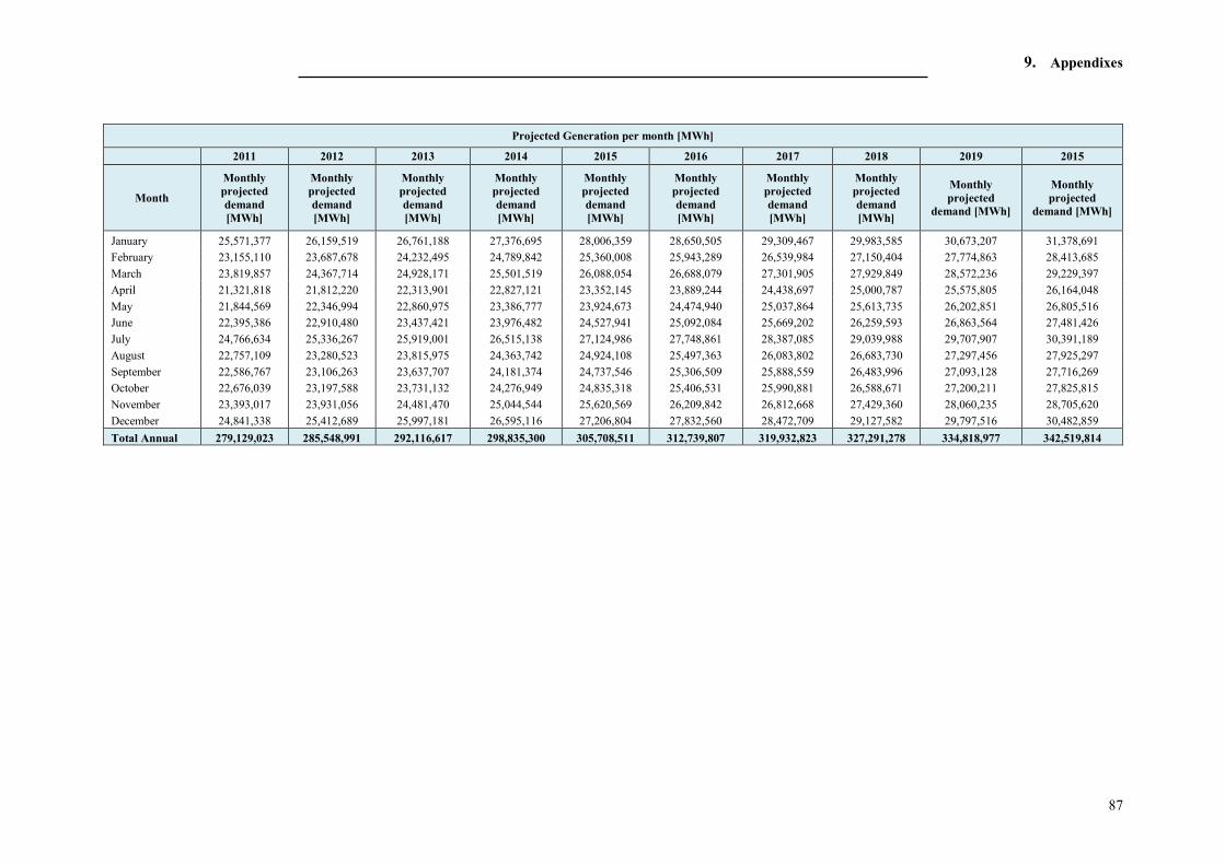
9. Appendixes
87
Projected Generation per month [MWh]
2011 2012 2013 2014 2015 2016 2017 2018 2019 2015
Month
Monthly projected demand [MWh]
Monthly projected demand [MWh]
Monthly projected demand [MWh]
Monthly projected demand [MWh]
Monthly projected demand [MWh]
Monthly projected demand [MWh]
Monthly projected demand [MWh]
Monthly projected demand [MWh]
Monthly projected
demand [MWh]
Monthly projected
demand [MWh]
January 25,571,377 26,159,519 26,761,188 27,376,695 28,006,359 28,650,505 29,309,467 29,983,585 30,673,207 31,378,691
February 23,155,110 23,687,678 24,232,495 24,789,842 25,360,008 25,943,289 26,539,984 27,150,404 27,774,863 28,413,685
March 23,819,857 24,367,714 24,928,171 25,501,519 26,088,054 26,688,079 27,301,905 27,929,849 28,572,236 29,229,397
April 21,321,818 21,812,220 22,313,901 22,827,121 23,352,145 23,889,244 24,438,697 25,000,787 25,575,805 26,164,048
May 21,844,569 22,346,994 22,860,975 23,386,777 23,924,673 24,474,940 25,037,864 25,613,735 26,202,851 26,805,516
June 22,395,386 22,910,480 23,437,421 23,976,482 24,527,941 25,092,084 25,669,202 26,259,593 26,863,564 27,481,426
July 24,766,634 25,336,267 25,919,001 26,515,138 27,124,986 27,748,861 28,387,085 29,039,988 29,707,907 30,391,189
August 22,757,109 23,280,523 23,815,975 24,363,742 24,924,108 25,497,363 26,083,802 26,683,730 27,297,456 27,925,297
September 22,586,767 23,106,263 23,637,707 24,181,374 24,737,546 25,306,509 25,888,559 26,483,996 27,093,128 27,716,269
October 22,676,039 23,197,588 23,731,132 24,276,949 24,835,318 25,406,531 25,990,881 26,588,671 27,200,211 27,825,815
November 23,393,017 23,931,056 24,481,470 25,044,544 25,620,569 26,209,842 26,812,668 27,429,360 28,060,235 28,705,620
December 24,841,338 25,412,689 25,997,181 26,595,116 27,206,804 27,832,560 28,472,709 29,127,582 29,797,516 30,482,859
Total Annual 279,129,023 285,548,991 292,116,617 298,835,300 305,708,511 312,739,807 319,932,823 327,291,278 334,818,977 342,519,814

9. Appendixes
88
Appendix 6 – Evolution of special regime technologies
Expected evolution of Special Regime [MW]
2011 2012 2013 2014 2015 2016 2017 2018 2019 2020
Wind Onshore 19956 23190 24560 25930 27310 28690 30097.5 31505 32912.5 34320
Solar PV 3990 4370 4585 4800 5065 5330 5687.5 6045 6402.5 6760
Solar Thermal 1330 2030 2375 2720 3010 3300 3675 4050 4425 4800
Others Renewable 2870 3040 3135 3230 3380 3530 3800 4070 4340 4610
Cogeneration 7410 7860 8415 8970 9210 9450 9685 9920 10155 10390
Others Non Renewable 80 80 80 80 90 100 115 130 145 160
Total 35,636 40,570 43,150 45,730 48,065 50,400 53,060 55,720 58,380 61,040
Expected SR-Renewable contribution
Year % MWh GWh
2011 20.3% 56,619,153 56,619 2012 21.6% 61,717,907 61,718 2013 22.5% 65,624,936 65,625 2014 23.5% 70,297,367 70,297 2015 24.9% 75,985,195 75,985 2016 26.2% 81,881,969 81,882 2017 27.3% 87,335,779 87,336 2018 28.4% 93,011,934 93,012 2019 29.7% 99,575,938 99,576 2020 31.1% 106,376,513 106,377
Expected SR-Non Renewable contrubution Year % MWh GWh
2011 13.9% 38,842,973 38,843 2012 13.8% 39,366,436 39,366 2013 14.1% 41,289,746 41,290 2014 14.3% 42,662,376 42,662 2015 14.1% 43,241,124 43,241 2016 14.0% 43,839,434 43,839 2017 14.1% 45,116,409 45,116 2018 14.2% 46,414,151 46,414 2019 14.1% 47,074,774 47,075 2020 13.9% 47,757,403 47,757
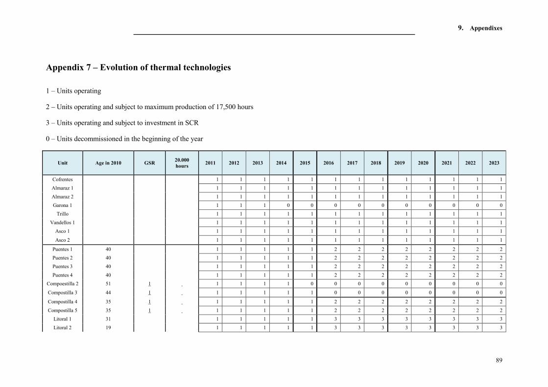
9. Appendixes
89
Appendix 7 – Evolution of thermal technologies
1 – Units operating
2 – Units operating and subject to maximum production of 17,500 hours
3 – Units operating and subject to investment in SCR
0 – Units decommissioned in the beginning of the year
Unit Age in 2010 GSR 20.000 hours
2011 2012 2013 2014 2015 2016 2017 2018 2019 2020 2021 2022 2023
Cofrentes 1 1 1 1 1 1 1 1 1 1 1 1 1
Almaraz 1 1 1 1 1 1 1 1 1 1 1 1 1 1
Almaraz 2 1 1 1 1 1 1 1 1 1 1 1 1 1
Garona 1 1 1 1 0 0 0 0 0 0 0 0 0 0
Trillo 1 1 1 1 1 1 1 1 1 1 1 1 1
Vandellos 1 1 1 1 1 1 1 1 1 1 1 1 1 1
Asco 1 1 1 1 1 1 1 1 1 1 1 1 1 1
Asco 2 1 1 1 1 1 1 1 1 1 1 1 1 1
Puentes 1 40 1 1 1 1 1 2 2 2 2 2 2 2 2
Puentes 2 40 1 1 1 1 1 2 2 2 2 2 2 2 2
Puentes 3 40 1 1 1 1 1 2 2 2 2 2 2 2 2
Puentes 4 40 1 1 1 1 1 2 2 2 2 2 2 2 2
Compoestilla 2 51 1 1 1 1 1 0 0 0 0 0 0 0 0 0
Compostilla 3 44 1 1 1 1 1 1 0 0 0 0 0 0 0 0
Compostilla 4 35 1 1 1 1 1 1 2 2 2 2 2 2 2 2
Compostilla 5 35 1 1 1 1 1 1 2 2 2 2 2 2 2 2
Litoral 1 31 1 1 1 1 1 3 3 3 3 3 3 3 3
Litoral 2 19 1 1 1 1 1 3 3 3 3 3 3 3 3

9. Appendixes
90
Teruel 1 37 1 1 1 1 1 1 2 2 2 2 2 2 2 2
Teruel 2 37 1 1 1 1 1 1 2 2 2 2 2 2 2 2
Teruel 3 37 1 1 1 1 1 1 2 2 2 2 2 2 2 2
Soto 2 1 1 1 1 1 0 0 0 0 0 0 0 0
Soto 3 32 1 1 1 1 1 1 2 2 2 2 2 2 2 2
Abono 1 42 1 1 1 1 1 2 2 2 2 2 2 2 2
Abono2 31 1 1 1 1 1 3 3 3 3 3 3 3 3
Barrios1 31 1 1 1 1 1 3 3 3 3 3 3 3 3
Puente Nuevo 3 35 1 1 1 1 1 1 2 2 2 2 2 2 2 2
Puertollano 1 44 1 1 1 1 1 0 0 0 0 0 0 0 0
Cercs 1 1 1 1 1 1 1 0 0 0 0 0 0 0 0
Escucha 1 1 1 1 1 1 1 0 0 0 0 0 0 0 0 0
Meilla 1 36 1 1 1 1 1 2 2 2 2 2 2 2 2
Anllares 1 34 1 1 1 1 1 0 0 0 0 0 0 0 0 0
Narcea 1 51 1 1 1 1 1 0 0 0 0 0 0 0 0
Narcea 2 47 1 1 1 1 1 2 2 2 2 2 2 2 2
Narcea 3 31 1 1 1 1 1 1 2 2 2 2 2 2 2 2
Robla 1 45 1 1 1 1 1 2 2 2 2 2 2 2 2
Robla 2 31 1 1 1 1 1 1 2 2 2 2 2 2 2 2
Pasajes 1 49 1 1 1 1 1 2 2 2 2 2 2 2 2
Guardo 1 52 1 1 1 1 1 0 0 0 0 0 0 0 0
Guardo 2 32 1 1 1 1 1 1 2 2 2 2 2 2 2 2
Lada 3 1 1 1 1 1 1 0 0 0 0 0 0 0 0
Lada 4 35 1 1 1 1 1 2 2 2 2 2 2 2 2
Elcogas 1 1 1 1 1 1 1 1 1 1 0 0 0 0 0
Aceca 1 1 1 1 1 1 1 0 0 0 0 0 0 0 0
Sand Adria 1 1 1 1 1 1 1 0 0 0 0 0 0 0 0
Sand Adrian 3 1 1 1 1 1 1 0 0 0 0 0 0 0 0
Fox 1 1 1 1 1 1 0 0 0 0 0 0 0 0
CICLOS 1 1 1 1 1 1 1 1 1 1 1 1 1
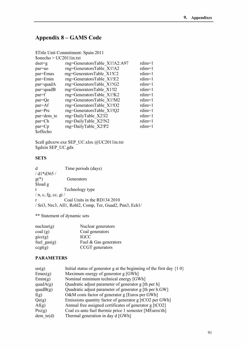
9. Appendixes
91
Appendix 8 – GAMS Code
$Title Unit Commitment: Spain 2011 $onecho > UC2011in.txt dset=g rng=GeneratorsTable_X1!A2:A97 rdim=1 par=uo rng=GeneratorsTable_X1!A2 rdim=1 par=Emax rng=GeneratorsTable_X1!C2 rdim=1 par=Emin rng=GeneratorsTable_X1!E2 rdim=1 par=quadA rng=GeneratorsTable_X1!G2 rdim=1 par=quadB rng=GeneratorsTable_X1!I2 rdim=1 par=f rng=GeneratorsTable_X1!K2 rdim=1 par=Qe rng=GeneratorsTable_X1!M2 rdim=1 par=Af rng=GeneratorsTable_X1!O2 rdim=1 par=Prc rng=GeneratorsTable_X1!Q2 rdim=1 par=dem_te rng=DailyTable_X2!J2 rdim=1 par=Ch rng=DailyTable_X2!N2 rdim=1 par=Cp rng=DailyTable_X2!P2 rdim=1 $offecho $call gdxxrw.exe SEP_UC.xlsx @UC2011in.txt $gdxin SEP_UC.gdx SETS d Time periods (days) / d1*d365 / g(*) Generators $load g t Technology type / n, c, fg, cc, gi / r Coal Units in the RD134 2010 / Sri3, Nrc3, All1, Robl2, Comp, Ter, Guad2, Pnn3, Ech1/ ** Statement of dynamic sets nuclear(g) Nuclear generators coal (g) Coal generators gicc(g) IGCC fuel_gas(g) Fuel & Gas generators ccgt(g) CCGT generators PARAMETERS uo(g) Initial status of generator g at the beginning of the first day {1 0} Emax(g) Maximum energy of generator g [GWh] Emin(g) Nominal minimum technical energy [GWh] quadA(g) Quadratic adjust parameter of generator g [th per h] quadB(g) Quadratic adjust parameter of generator g [th per h.GW] f(g) O&M costs factor of generator g [Euros per GWh] Qe(g) Emissions quantity factor of generator g [tCO2 per GWh] Af(g) Annual free assigned certificates of generator g [tCO2] Prc(g) Coal ex-ante fuel thermie price 1 semester [MEuros\th] dem_te(d) Thermal generation in day d [GWh]

9. Appendixes
92
Ch(d) Variable hydro generation operation and maintenence costs in the day d [MEuros] Cp(d) Variable pumping costs in the day d [MEuros] $load uo Emax Emin quadA quadB f Qe Af Prc dem_te Ch, Cp $gdxin EFFn(t) Nominal efficiency [%] / fg 0.33, cc 0.53 / dem_gi GICC production objective [GWh] / 1400.000 / Pf(t) Fuel cost average price factor [MEuros per GWh] / n 0.01224, gi 0.01221 / Cv Variable component of LNG conduction toll [MEuros\GWht] / 0.0007530 / Prg Gas fuel thermie price [MEuro\th] /0.00000002650/ Pre CO2 emission price [MEuro\tCO2] /0.00001410/ Tp Target Production of Coal Units in the RD134 [GWh] /Sri3 1311.940, Nrc3 1205.880, Robl2 2035.200, Comp 5444.250, Ter 6183.800, Guad2 1943.140, Pnn3 1482.090, All1 1968.150, Ech1 371.860/ VARIABLES fobj Value of objective function Cco2_ep(d,g) Variable ex-post emissions costs of the unit g in the day d [MEuro] Cg(d,g) Total ex-post variable generation costs of generator g in the day d [MEuro] ; POSITIVE VARIABLES energy(d,g) Energy dispatched by generator g in the day d [GWh] Cop(d,g) Variable operating (fuel) costs of the unit g in the day d [MEuro] Com(d,g) Variable operation and maintenance costs of the unit g in the day d [MEuro] Cco2_ea(d,g) Variable ex-ante emissions costs of the unit g in the day d [MEuro] logv(d,g) Variable LNG logistic costs of the unit g in the day d [MEuro] Qmn(d,g) LNG consumed by generator g in the day d [GWht] Sri3(g) Soto de Ribera 2 annual production [GWh] Nrc3(g) Narcea 3 annual production [GWh] Robl2(g) Robla 2 annual production [GWh] Guad2(g) Guardo 2 annual production [GWh] Pnn3(g) Puente Nuevo 3 annual production [GWh] Comp(g) Compostilla annual production [GWh] Ter(g) Teruel annual production [GWh] All1(g) Anllares annual production [GWh] Ech1(g) Escucha annual production [GWh] ; BINARY VARIABLES u(d,g) Binary variable indicating whether unit g is connected (1) or disconnected (0) in the day d y(d,g) Start-up decision for unit g in the day d z(d,g) Shut Down decision for unit g in the day d ; EQUATIONS E_fobj Objective Function

9. Appendixes
93
E_Cop(d,g) Operating (fuel) costs E_Com(d,g) Operation and maintenance costs E_Cco2_ea(d,g) Ex-ante emissions costs E_Cco2_ep(d,g) Ex-post emissions costs E_logv(d,g) Variable LNG logistic costs E_Cg(d,g) Total generation costs E_TeDem(d) Meet thermal demand in day d E_gicc Meet the annual GICC demand E_coal Meet the annual coal demand E_Emax(d,g) Respect maximum generator power E_Emin(d,g) Respect minimum generator power E_Acop(d,g) Logic of start ups and shut downs E_rAcop(d,g) Respect logic of start ups and shut downs E_Qmn(d,g) LNG consumed E_Sri3(g) Soto de Ribera 2 annual production E_Nrc3(g) Narcea 3 annual production E_Robl2(g) Robla 2 annual production E_Guad2(g) Guardo 2 annual production E_Pnn3(g) Puente Nuevo 3 annual production E_Comp(g) Compostilla annual production E_Ter(g) Teruel annual production E_All1(g) Anllares annual production E_Ech1(g) Escucha annual production ; * Formulation of equations: ** Objetive function E_fobj.. fobj =e= SUM[(d,g), (Cop(d,g) + Com(d,g) + Cco2_ea(d,g) + logv(d,g) + Ch(d) + Cp(d))/100000]; E_TeDem(d).. dem_te(d) =e= SUM(g,energy(d,g)); *=================================================================== ** Variable costs computation (for economic dispatch). There is an ex-ante computation for CO2 emissions cost *=================================================================== E_Cop(d,g).. Cop(d,g) =e= 24 * (Prg $[fuel_gas(g) OR ccgt(g)] + Prc(g) $[coal(g)]) * (u(d,g) * quadA(g) + quadB(g) * (energy(d,g) / 24)) + [(Pf('n')$[nuclear(g)] + Pf('gi')$[gicc(g)]) * energy(d,g)]; E_Com(d,g).. Com(d,g) =e= f(g) * energy(d,g); E_Cco2_ea(d,g).. Cco2_ea(d,g) =e= Qe(g) * energy(d,g) * Pre;

9. Appendixes
94
E_logv(d,g).. logv(d,g) =e= [(energy(d,g) / (EFFn('fg')$[fuel_gas(g)] + EFFn('cc')$[ccgt(g)]) ) * Cv] $[ccgt(g) OR fuel_gas(g)]; E_gicc.. SUM[(d,gicc), energy(d,gicc)] =e= dem_gi; E_coal.. SUM[(d,coal), energy(d,coal)] =g= 23346.320; *** Respect units energy boundaries E_Emax(d,g).. energy(d,g) =l= u(d,g)*Emax(g); E_Emin(d,g).. energy(d,g) =g= u(d,g)*Emin(g); *** Respect units operating logic: shut-down and start-up E_Acop(d,g).. u(d,g) =e= u(d-1,g)$[ORD(d) > 1] + uo(g)$[ORD(d) = 1] + y(d,g) - z(d,g); E_rAcop(d,g).. y(d,g) + z(d,g) =l= 1; *** Respect coal target production of units in RD134 E_Sri3(g).. Sri3(g) =e= SUM[d, energy(d,'SOTO_R_3')]; E_Nrc3(g).. Nrc3(g) =e= SUM[d, energy(d,'NARCEA_3')]; E_Robl2(g).. Robl2(g) =e= SUM[d, energy(d,'ROBLA_2')]; E_Guad2(g).. Guad2(g) =e= SUM[d, energy(d,'GUARDO_2')]; E_Pnn3(g).. Pnn3(g) =e= SUM[d, energy(d,'PTE_NUEVO_3')]; E_Comp(g).. Comp(g) =e= SUM[d, energy(d,'COMPOSTILLA_2')] + SUM[d, energy(d,'COMPOSTILLA_3')] + SUM[d, energy(d,'COMPOSTILLA_4')] + SUM[d, energy(d,'COMPOSTILLA_5')]; E_Ter(g).. Ter(g) =e= SUM[d, energy(d,'TERUEL_1')] + SUM[d, energy(d,'TERUEL_2')] + SUM[d, energy(d,'TERUEL_3')]; E_All1(g).. All1(g) =e= SUM[d, energy(d,'ANLLARES')]; E_Ech1(g).. Ech1(g) =e= SUM[d, energy(d,'ESCUCHA')];

9. Appendixes
95
*=================================================================== ** Variable costs computation (for energy prices computation) *=================================================================== E_Cco2_ep(d,g).. Cco2_ep(d,g) =e= [Qe(g) * energy(d,g) - Af(g) / 8760] * Pre; E_Cg(d,g).. Cg(d,g) =e= Cop(d,g) + Com(d,g) + Cco2_ep(d,g) + logv(d,g); E_Qmn(d,g).. Qmn(d,g) =e= [energy(d,g) / (EFFn('fg')$[fuel_gas(g)] + EFFn('cc')$[ccgt(g)])] $[ccgt(g) OR fuel_gas(g)]; *=================================================================== ***Initial dynamic sets y.fx('d1',g) = 0; z.fx('d1',g) = 0; ***Respect unavilability for fuel recharge in nuclear units u.fx(d,'COFRENTES')$[(ORD(d)>=244) AND (ORD(d)<=303)] = 0; u.fx(d,'ALMARAZ_1')$[(ORD(d)>=91) AND (ORD(d)<=130)] = 0; u.fx(d,'GARONA')$[(ORD(d)>=121) AND (ORD(d)<=180)] = 0; u.fx(d,'TRILLO')$[(ORD(d)>=152) AND (ORD(d)<=186)] = 0; u.fx(d,'ASCO_2')$[(ORD(d)>=274) AND (ORD(d)<=313)] = 0; u.fx(d,'ASCO_1')$[(ORD(d)>=121) AND (ORD(d)<=160)] = 0; ***Respect coil units production Sri3.fx(g) = Tp('Sri3'); Nrc3.fx(g) = Tp('Nrc3'); Robl2.fx(g) = Tp('Robl2'); Guad2.fx(g) = Tp('Guad2'); Pnn3.fx(g) = Tp('Pnn3'); Comp.fx(g) = Tp('Comp'); Ter.fx(g) = Tp('Ter'); All1.fx(g) = Tp('All1'); Ech1.fx(g) = Tp('Ech1'); * Options for execution: ** Selection of the optimizer for solving binary variables OPTION MIP = cplex; ** Tolerance for optimization convergence with binary variables OPTION OPTCR = 0.01; OPTION iterlim=1e+6 ; OPTION ResLim = 18000 ; MODEL SUC2011 /all/;

9. Appendixes
96
** Option to include zero values in excel sheet energy.scale(d,g)=0.1; Cop.scale(d,g)=0.1; Com.scale(d,g)=0.1; Cco2_ep.scale(d,g)=0.1; logv.scale(d,g)=0.1; Cg.scale(d,g)=0.1; Qmn.scale(d,g)=0.1; SOLVE SUC2011 USING MIP MINIMIZING fobj; * Open data in gdxviewer EXECUTE_UNLOAD 'SEP_UC.gdx', energy, Cop, Com, Cco2_ep, logv, Cg, Qmn, u; EXECUTE 'gdxxrw.exe SEP_UC.gdx o=SEP_UC.xlsx Squeeze=N var=energy.l rng=UnitCommitment!B2'; EXECUTE 'gdxxrw.exe SEP_UC.gdx o=SEP_UC.xlsx Squeeze=N var=Cco2_ep.l rng=CO2!B2'; EXECUTE 'gdxxrw.exe SEP_UC.gdx o=SEP_UC.xlsx Squeeze=N var=Cg.l rng=GenCosts!B2'; EXECUTE 'gdxxrw.exe SEP_UC.gdx o=SEP_UC.xlsx Squeeze=N var=Qmn.l rng=LNG!B2';

9. Appendixes
97
Appendix 9 – Generation Dispatch in period 2011-2020
Yearly Contribution by Technology [GWh]
2011 2012 2013 2014 2015 2016 2017 2018 2019 2020
Nuclear 58,133 59,490 56,171 56,387 53,961 56,550 54,901 55,447 54,923 56,551
Coal 24,746 24,746 24,746 24,768 16,645 13,047 10,716 8,200 940 710
Fuel&Gas 0 0 0 0 0 0 0 0 0 0
CCGT 73,663 73,804 76,000 75,468 86,684 89,097 91,597 93,634 101,821 101,705
Hydro 27,120 27,120 28,502 29,314 29,314 29,314 29,973 30,631 30,631 30,631
Total Ordinary Regime
183,662 185,159 185,418 185,938 186,604 188,009 187,187 187,913 188,315 189,597
SR-Renewable
56,619 61,718 65,625 70,297 75,985 81,882 87,336 93,012 99,576 106,377
SR- Non Renewable
38,843 39,366 41,290 42,662 43,241 43,839 45,116 46,414 47,075 47,757
Total Special Regime
95,462 101,084 106,915 112,960 119,226 125,721 132,452 139,426 146,651 154,134
Total 279,124 286,244 292,333 298,897 305,831 313,730 319,639 327,339 334,966 343,731
2011
2012

9. Appendixes
98
2013
2014
2015

9. Appendixes
99
2016
2017
2018
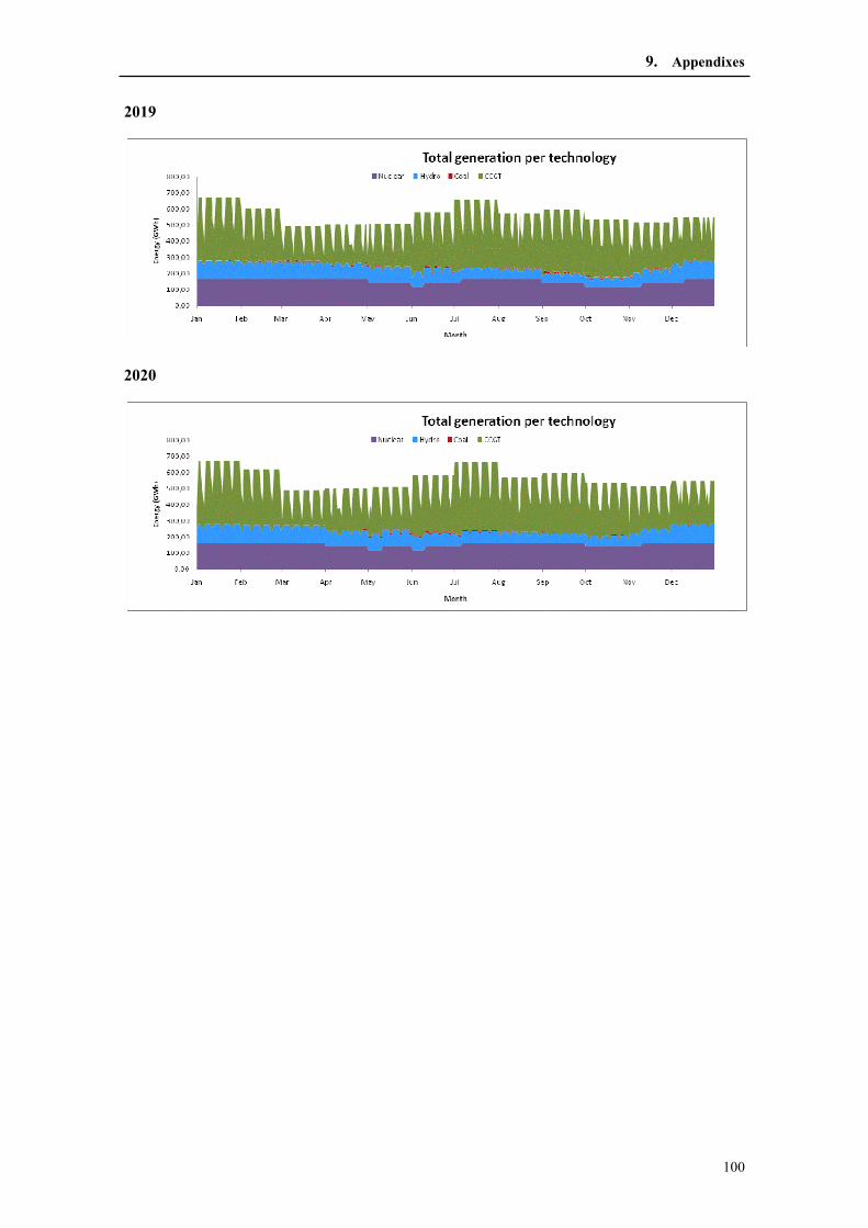
9. Appendixes
100
2019
2020

9. Appendixes
101
Appendix 9 – Generation costs by technology
2011 2012 2013 2014 2015
Fix
[Euros/MWh]
Variable [Euros/MWh]
Total [Euros/MWh]
Fix [Euros/MWh]
Variable [Euros/MWh]
Total [Euros/MWh]
Fix [Euros/MWh]
Variable [Euros/MWh]
Total [Euros/MWh]
Fix [Euros/MWh]
Variable [Euros/MWh]
Total [Euros/MWh]
Fix [Euros/MWh]
Variable [Euros/MWh]
Total [Euros/MWh]
Nuclear 27.43 13.47 40.90 27.44 13.60 41.04 28.25 13.74 41.99 27.92 13.87 41.79 29.62 14.02 43.64
Coal 46.43 54.81 101.24 46.88 57.59 104.47 46.89 60.80 107.69 47.02 63.36 110.38 70.53 64.96 135.48 Fuel & Gas -- -- -- -- -- -- -- 0.00 -- -- -- -- -- -- --
CCGT 35.81 48.17 83.98 35.83 50.47 86.30 34.31 52.72 87.02 34.17 55.12 89.29 29.44 57.64 87.09
Hydro 30.64 2.36 33.01 31.02 2.38 33.39 36.35 2.50 38.86 37.95 2.60 40.55 37.94 2.62 40.56
Total 34.14 31.32 65.46 34.23 32.53 66.76 34.80 34.27 69.07 34.74 35.43 70.35 34.84 37.04 71.87
2016 2017 2018 2019 2020
Fix
[Euros/MWh]
Variable [Euros/MWh]
Total [Euros/MWh]
Fix [Euros/MWh]
Variable [Euros/MWh]
Total [Euros/MWh]
Fix [Euros/MWh]
Variable [Euros/MWh]
Total [Euros/MWh]
Fix [Euros/MWh]
Variable [Euros/MWh]
Total [Euros/MWh]
Fix [Euros/MWh]
Variable [Euros/MWh]
Total [Euros/MWh]
Nuclear 28.80 14.16 42.96 30.02 14.29 44.31 30.19 14.43 44.63 30.96 14.59 45.55 30.66 14.73 45.39
Coal 91.59 67.89 159.48 111.36 70.43 181.79 145.63 74.06 219.68 1,000.11 80.37 1,080.49 1,396.31 80.23 1,476.54 Fuel & Gas -- -- -- -- -- -- -- -- -- -- -- -- -- -- --
CCGT 28.43 59.34 87.77 27.28 61.28 88.55 26.40 63.13 89.54 27.80 64.92 92.72 29.44 66.85 94.08
Hydro 38.05 2.64 40.69 40.45 2.73 43.18 39.27 2.80 45.40 42.20 2.83 45.03 44.26 2.85 47.12
Total 34.42 37.50 71.92 35.00 38.65 73.65 34.82 39.41 74.77 35.92 40.22 76.13 37.32 41.01 78.33