generation and life cycle of the dipole in the south china

Generation and life cycle of the dipole in the South China Sea

summer circulation

Guihua Wang,1 Dake Chen,2,1 and Jilan Su1

Received 25 September 2005; revised 13 February 2006; accepted 3 March 2006; published 1 June 2006.

[1] The South China Sea (SCS) summer circulation often has a dipole structure associatedwith an eastward jet, appearing off central Vietnam. The dipole has an anticyclonic eddy(AE) south of the jet and a cyclonic eddy (CE) north of it. The life cycle of the dipolestructure is analyzed using satellite altimetry data and a reduced gravity model. Onaverage the dipole structure begins in June, peaks in strength in August or September, anddisappears in October. The dipole evolution lags behind the basin scale wind byabout 40 days, and 40 days are exactly what it takes for baroclinic planetary waves tocross the southern SCS. Our results show that the vorticity transports from thenonlinear effect of the western boundary currents are crucial for the generation of thedipole structure. In addition, the strength and direction of the offshore wind jetalso play a significant role in determining the magnitudes and the core positions of thetwo concomitant eddies.

Citation: Wang, G., D. Chen, and J. Su (2006), Generation and life cycle of the dipole in the South China Sea summer circulation,

J. Geophys. Res., 111, C06002, doi:10.1029/2005JC003314.

1. Introduction

[2] The South China Sea is the largest semi-enclosedmarginal sea in the western tropic Pacific (Figure 1). Itsupper layer circulation is driven mainly by the monsoon,with additional influence from the Kuroshio in its northernpart [Qu, 2000; Su, 2004]. In winter there is a basin-widecyclonic gyre, while in summer the circulation splits into aweakened cyclonic gyre north of about 12�N and a stronganticyclonic gyre south of it. These large scale circulationsare established in a relatively short thermocline adjustmenttime of 1 to 4 months [Liu et al., 2001]. Associated withthese gyres are strong western boundary currents. In wintera southward jet flows along the entire western boundary[Wyrtki, 1961; Liu et al., 2004]. In summer, there is anorthward jet flowing along the western boundary in thesouthern SCS [Xu et al., 1982]. The jet apparently veerseastward off central Vietnam near 12�N, which can be seenfrom many observations such as sea surface temperatureand the chlorophyll signature [Kuo et al., 2000; Xie et al.,2003]. To the north, there is a narrow southwestern jet alongthe continental slope in the northwest SCS [Qu, 2000;Metzger and Hurlburt, 1996; Su, 2004]. In summary, aschematic diagram for the existing knowledge of the SCScirculation, modified after Liu et al. [2002], is shown inFigure 1. In their original diagram, the southwestward jetalong the continental slope in the northwest SCS was notdepicted for the summer.

[3] There is often a dipole structure associated with thesummer eastward jet, with an anticyclonic eddy (AE) southof the jet and a cyclonic eddy (CE) north of it [e.g., Shaw etal., 1999; Wu et al., 1999; Metzger and Hurlburt, 1996;Wang et al., 2003]. In fact, the eastward jet is ratherconspicuous in the infrared satellite imageries because ofthe cold water from upwelling associated with the jet [Kuoet al., 2000; Xie et al., 2003]. Dynamic topography maps ofFang et al. [2002] and Su et al. [1999] indicate that the AEhas a diameter of about 300 km and the eastward jet has amaximum velocity of around 0.8 ms�1. Although numericalmodels by Wu et al. [1999] and Metzger and Hurlburt[1996] have produced this dipole structure, little is knownabout its generation mechanism. The present work focuseson the possible generation mechanism and the life cycle ofthe dipole structure.

2. Data

[4] Two satellite data sets, sea surface height anomaly(SSHA) and sea surface winds, are used to analyze the lifecycle of the dipole. The SSHA data set is a multiple-altimeter product on a 1/8� � 1/8� grid covering the periodof January 1993 to December 2000 from the US NavalResearch Laboratory. It is derived from TOPEX/Poseidon(T/P), ERS and Geosat Follow On (GFO) altimetry, with theorbit error and tides removed, as discussed by Jacobs et al.[2002]. To avoid tidal aliasing from residual tidal effects, weapply a simple Hanning filter with a cut-off period around60 days [Wang et al., 2000]. The surface wind we use is ablended product from ERS1, ERS2, NSCAT and QuikSCATdata sets for the same period. The spatial resolutions ofthese four data sets are 1.0�, 1.0�, 0.5� and 0.25�, respec-tively. They are interpolated into a composite data set with a

JOURNAL OF GEOPHYSICAL RESEARCH, VOL. 111, C06002, doi:10.1029/2005JC003314, 2006

1State Key Laboratory of Satellite Ocean Environment Dynamics,Second Institute of Oceanography, SOA, Hangzhou, China.

2Lamont-Doherty Earth Observatory, Columbia University, Palisades,New York, USA.

Copyright 2006 by the American Geophysical Union.0148-0227/06/2005JC003314$09.00

C06002 1 of 9

spatial resolution of 0.25� and a temporal resolution of oneweek. The surface wind data is also used to force ournumerical model to be discussed in section 4.

3. Methods

[5] We use a combination of observational data andmodel simulations for our analyses, with emphasis on thesummer conditions. Based on the monsoonal nature ofthe SCS circulation, summer is defined in this study asthe months from June to September. We also apply thePrincipal Component Analysis (PCA) [Preisendorfer, 1988]to examine the spatial pattern and the temporal variability ofthe SSHA and wind fields.[6] The SSHA data from 1993 to 2000 show the appear-

ance of the dipole structure each summer except for 1995and 1998, when the cyclonic half of the dipole disappeared[Wang, 2004]. Strong warm events took place in the SCS inthese two years, during which the SCS circulation was verydifferent from other years, most likely due to changes in thewind field [Shaw et al., 1999; Xie et al., 2003]. To avoiddata from the two warm events polluting the dipole signalsof the other 6 normal years, all the mean fields in this studyare obtained with the data from 1995 and 1998 excluded.

For the PCA, however, we use all data from the 8 yearsbetween 1993 and 2000. Note that not every ENSO yearresults in a strong warm event in the SCS.[7] A 1.5-layer reduced gravity model is applied to the

SCS. Previous studies have shown the validity of such amodel in simulating the SCS circulation [e.g., Metzger andHurlburt, 1996]. The model equations are:

@U

@tþ U

@u

@xþ V

@u

@yþ u

@U

@xþ v

@U

@y� fV ¼ �g0h

@h

@x

þ Ah

@2U

@x2þ @2U

@y2

� �� v

@u

@z

��z¼h

þv@u

@z

��z¼0

ð1Þ

@V

@tþ U

@v

@xþ V

@v

@yþ u

@V

@xþ v

@V

@yþ fU ¼ �g0h

@h

@y

þ Ah

@2V

@x2þ @2V

@y2

� �� v

@v

@z

��z¼h

þv@v

@z

��z¼0

ð2Þ

@h

@tþ @U

@xþ @V

@y¼ 0 ð3Þ

where x, y and z are the conventional Cartesian coordinates,h the thermocline depth, u and v the components of velocitycorresponding to x and y, respectively, U = hu and V = hvthe total flows integrated over the entire water column fromthe thermocline to the surface, r the density, g0 = g r/r0 =0.03 ms�2 the reduced gravity, n the vertical diffusioncoefficient and Ah the lateral friction coefficient. For thewind stress term, we let n(@u/@z, @v/@z)jz=0 = Cd rair Uw

(uw, vw), where Cd is the drag coefficient, rair the air density,Uw the wind speed and (uw, vw) the wind velocity. For thedrag coefficient we take Cd = 0.0013 and the air density is1.2 Kgm�3. Except at the sea surface, we set the verticalfriction to be zero. Ah is chosen so that stable statistics canbe reached in long-term integration, facilitating analysis ofthe mesoscale eddies from the simulation results [Hurlburtand Thompson, 1980]. The grid Reynolds number, Re =uDx/Ah, should also be greater than 10 [Preller, 1986]. Inthis study, through a series of sensitivity tests, we choose itsvalue to be 500 m2s�1. Nonslip condition is applied at solidboundaries. As we shall explain in the following, all theboundaries of our model domain are solid boundaries. Themodel has been tested through simulating the classicalproblems addressed by Veronis [1966] and repeating themodel results by Hurlburt and Thompson [1980]. Theformer is to test the nonlinear effect on a single gyre, whilethe latter is for eddy shedding. These tests give usconfidence on the capability of the model in simulatingmesoscale eddies.[8] We choose the model SCS as the area in the SCS

bordered by the 200 m isobath (Figure 1). The model gridsare 0.25� � 0.25�. The grid size is shorter than the meanMunk width in the SCS, about 28 Km, satisfying theresolution requirement for western boundary currents innumerical simulation [Berloff and McWilliams, 1999]. It isalso shorter than the climatological mean of the firstbaroclinic Rossby radius of deformation for the deep basinof the SCS, which is larger than 50 km [Gan and Cai,2001]. To focus on the regional dynamics within the SCS in

Figure 1. Map of the South China Sea. The two isobathsare for 200 m and 2000 m, respectively. The model SCScovers areas with water deeper than 200 m. The dottedrectangle represents the ideal rectangular basin used forsimulations shown in Figures 5, 6 and 8. The schematicdashed streamline represents the basin-scale cyclonic gyrein winter, while the schematic solid streamlines represent, insummer, a basin-scale anticyclone gyre in the southern SCSand a cyclone gyre in the northern SCS (modified from Liuet al. [2002]).

C06002 WANG ET AL.: GENERATION AND LIFE CYCLE OF THE DIPOLE

2 of 9

C06002

response to the winds, the only forcing imposed, we closethe Luzon Strait. The initial thermocline depth is 200 m.The model is spun up with the winds switched on graduallyfrom zero to that of January 1993 over a period of 1 month.Then the model is forced with 1993 wind repeated for fouryears to allow the upper ocean circulation to reach a quasi-steady state. Finally, the model is forced with the windsfrom January 1993 to December 2000. However, the meansimulated fields are computed without using the resultsfrom 1995 and 1998, for the reason mentioned above.

4. Results

4.1. Observations

[9] The satellite-data derived mean summer wind stresscurl (WSC) is positive (negative) in the northwestern(southeastern) SCS (Figure 2a), as was demonstrated inpast studies [e.g., Qu, 2000]. The WCS pattern is associatedwith the southwest summer wind jet off the central Vietnam,which is in fact a result of the orographic effects on thesummer monsoon from the Annam Cordillera mountainrange [Xie et al., 2003]. The mean summer SSHA fieldderived from altimetry satellite (Figure 2b) reflects the WSCpattern, with a cyclonic gyre north of about 12�N and ananticyclonic gyre south of it. There is also a sub-basinanticyclonic gyre off northwestern Luzon, likely reflectingthe anticyclonic eddy generated there yearly during thesummer between 1993 and 2000 [Wang, 2004]. The dipolestructure of AE-CE eddy pair off central Vietnam is alsoclearly evident in Figure 2b.[10] The southwest monsoon establishes rapidly over the

SCS in June, reaches peak in July to August, slackens off inSeptember, and finally is replaced by the northeast monsoonin October [Liang, 1991]. Figures 3a and 3b show, respec-tively, the satellite-data derived monthly mean WSC andSSHA from June to October. The WSC has a cyclonic(anticyclonic) pattern in the northwest (southwest) SCSduring the summer months, but such a pattern disappearsin October. The dipole structure begins to take its form inJune with the AE to the south and the CE to the north. Thedipole intensifies as summer progresses, along with thedevelopment of the eastward jet between the two eddies.Both the AE and CE are the strongest in September, with

the eddy center’s SSHA reaching 17 cm and �16 cm,respectively. In October the AE is much weakened anddissipates out.[11] We use the PCA to investigate the relation between

the WSC field and the dipole identified from the SSHAfield, both based on satellite data. To focus on the signal ofthe dipole structure, we only use the data from the area of110–116�E, 6–10�N for the PCA. Since circulation in theSCS is driven primarily by the monsoon, there are only twodominant modes, the summer and winter modes, respec-tively, for either WSC or SSHA. Here we only analyze thesummer modes of the two fields. The summer mode for theWSC field (Figure 4a) is positive (negative) north (south) ofabout 10�N and accounts for 57% of the total WSCvariance. The summer mode for the SSHA (Figure 4b)shows a clear dipole structure and accounts for 28% of thetotal SSHA variance. The two time series of the normalizedexpansion coefficients for the two summer modes(Figure 4c) show a good correlation in every summer exceptfor 1995 and 1998. Furthermore, there is a time lag betweenthe dipole and the WSC. The lag-correlation for the twotime series (Figure 4d) suggests that the dipole usually lagsbehind WSC by about 40 days. This is roughly the time forthe first baroclinic wave to propagate across the southernbasin of the SCS, indicating that the dipole structure isstrongly associated with the SCS basin scale circulation.

4.2. Dynamics of the Dipole Structure

[12] It is well known that nonlinearity is important for thegeneration of mesoscale eddies in the large-scale wind-driven ocean circulation [Bryan, 1963; Veronis, 1966]. Liuet al. [2001] has shown that the dynamics of the basin-widecirculation in the SCS is similar to the wind-driven generalcirculation and that a reduced gravity model can be used tounderstand its basic dynamics. Therefore, it should beinstructive to look at the generation of the summer dipolestructure off central Vietnam with a reduced gravity model.[13] Figures 2c and 2d show the modeled mean summer

circulation anomaly over the model SCS from 1993 to 2000(excluding 1995 and 1998) from our reduced-gravity modeland its linearized version, respectively, both driven by thewind field derived from satellite-data. The dipole structureand the accompanying eastward current between the two

Figure 2. Satellite-data derived summertime mean fields, (a) WSC and (b) SSHA, during 1993–2000(excluding the warm years of 1995 and 1998). Thermocline depth anomaly over the model SCS from (c) thenonlinearmodel and (d) the linearizedmodel. Contour intervals in Figures 2a–2d are 0.3�Nm�2, 2 cm, 5mand 5 m, respectively.


3 of 9

C06002

eddies are clearly evident from the results of the nonlinearsystem. Both systems generate a mean cyclonic (anticy-clonic) gyre in the northern (southern) SCS. The northerngyre has a southward western boundary current, in agree-

ment with observations [Qu, 2000, Figure 2b] and previousmodeling studies [Metzger and Hurlburt, 1996]. Offshore ofthis southward western boundary current there is a north-ward current, also in agreement with the observations and

Figure 3. Monthly mean maps of (a) WSC and (b) SSHA derived from satellite data during 1993–2000(excluding warm years of 1995 and 1998). Thermocline depth anomaly over the model SCS from (c) thenonlinear model and (d) the linear model. Contour intervals in Figures 3a–3d are 0.2 N m�2, 3 cm, 3 mand 3 m, respectively.


4 of 9

C06002

modeling results mentioned above. In the linearized system,however, the dipole and the eastward jet off central Vietnamare not present. Comparing the two simulated mean dipolestructures (jet width, jet length and the strength of the twoeddies) with the mean SSHA observation derived fromsatellite data, it is evident that the nonlinear model simula-tion is much more realistic than the linearized one.[14] To further examine the effects of nonlinearity, we

show the life cycle of the dipole structure off centralVietnam from the reduced-gravity model and its linearized

version, respectively, both driven by the wind field derivedfrom the satellite-data. For the nonlinear system (Figure 3c),both the eastward jet and the strength of the dipole are weakin June, intensify in July, and reach their peaks in Augustand September. In October, the AE of the dipole is dissi-pating out. These simulations resemble the satellite dataderived SSHA observations of the life cycle of the dipole(Figure 3b). As to the linear system (Figure 3d), from Junethrough October the eastward jet and the dipole are neverfully developed. We conclude that nonlinearity is very

Figure 4. Normalized summer modes of (a) WSC and (b) SSHA, based on satellite data from 1993 to2000. (c) Time series of the expansion coefficients (principal components, PC) of Figures 4a and 4b,normalized by the standard deviation of the respective original PC. (d) Lag correlation between SSHAand WSC.


5 of 9

C06002

important to the dipole dynamics. We note that there is asmall but prominent anticyclonic core at the southwesterncorner of the model domain in the simulated thermoclinedepth anomaly (Figures 3c and 3d), which is not found inthe observation (Figure 3b). The model result is actually areflection of the cyclonic eddy there in winter, a dominantfeature in the simulation [Wang, 2004; also see Metzger andHurlburt, 1996]. Both field [Fang et al., 2002] and SSHAobservations in winter, however, show only a weak cycloniceddy appearing, sometimes, around that general area. Defi-ciency of our model, (such as lack of bathymetry andreduced domain with closed boundaries at the southwesterncorner) is likely the reason for this discrepancy.[15] Veronis [1966] has analyzed the effect of nonlinear

terms on the wind-driven general circulation in the AtlanticOcean. His findings can be used to explain the dipolestructure of the SCS as following: In the southern SCS,the net effect of inertial process of the wind-driven southerngyre is to advect negative vorticity northward by its north-ward western boundary current, concentrating negativevorticity into the northwest corner of the southern gyre toform AE. While in the northern SCS, the net effect of

inertial process of the wind-driven northern gyre is to advectpositive vorticity southward by its southward westernboundary current, concentrating positive vorticity into thesouthwest corner of the northern gyre to form CE. Suchvorticity transports from the two western boundary currentsresult in the dipole structure off central Vietnam, with aneastward current jet in between. It is interesting to note thatthis pair of eddies are elongated toward the east, with the jetextending quite far offshore. This is obviously caused by theinertial effect of the jet itself.

4.3. Wind Field and the Dipole Structure

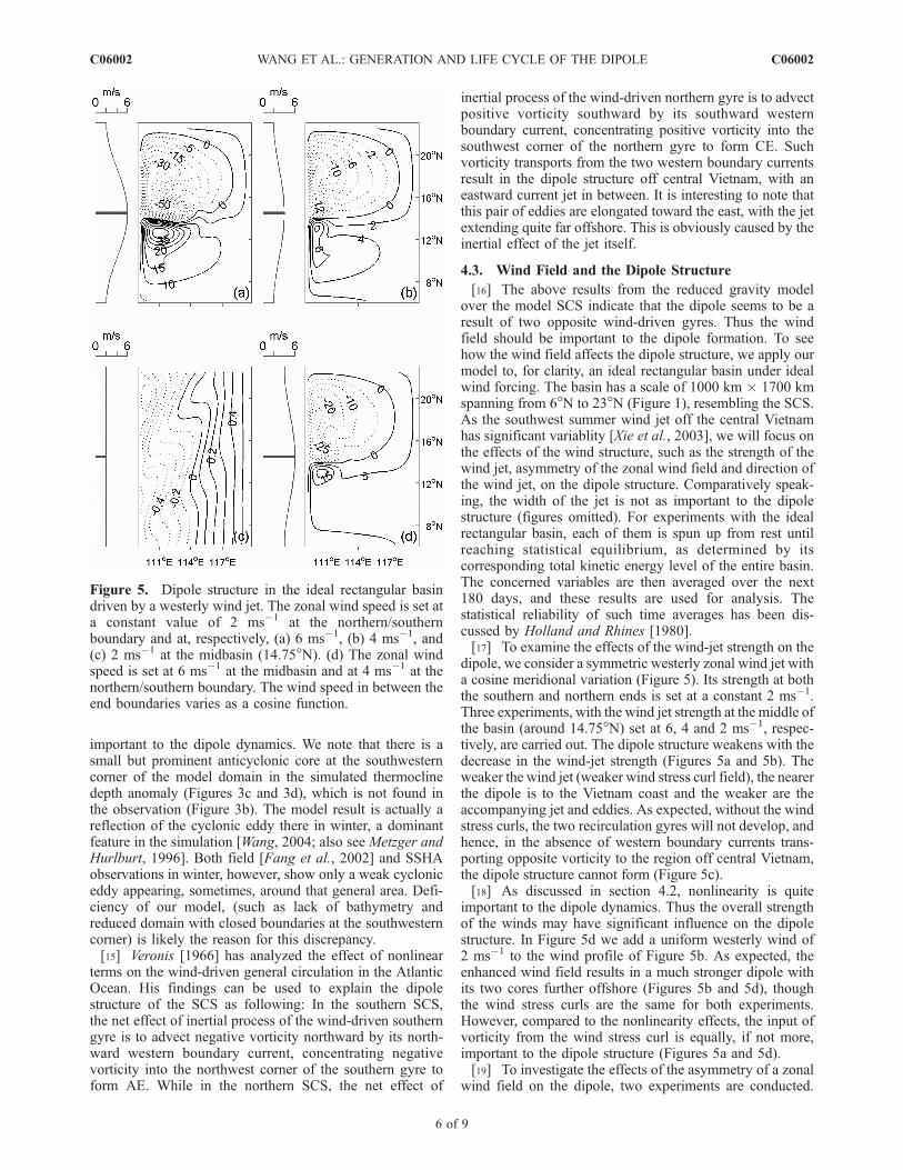
[16] The above results from the reduced gravity modelover the model SCS indicate that the dipole seems to be aresult of two opposite wind-driven gyres. Thus the windfield should be important to the dipole formation. To seehow the wind field affects the dipole structure, we apply ourmodel to, for clarity, an ideal rectangular basin under idealwind forcing. The basin has a scale of 1000 km � 1700 kmspanning from 6�N to 23�N (Figure 1), resembling the SCS.As the southwest summer wind jet off the central Vietnamhas significant variablity [Xie et al., 2003], we will focus onthe effects of the wind structure, such as the strength of thewind jet, asymmetry of the zonal wind field and direction ofthe wind jet, on the dipole structure. Comparatively speak-ing, the width of the jet is not as important to the dipolestructure (figures omitted). For experiments with the idealrectangular basin, each of them is spun up from rest untilreaching statistical equilibrium, as determined by itscorresponding total kinetic energy level of the entire basin.The concerned variables are then averaged over the next180 days, and these results are used for analysis. Thestatistical reliability of such time averages has been dis-cussed by Holland and Rhines [1980].[17] To examine the effects of the wind-jet strength on the

dipole, we consider a symmetric westerly zonal wind jet witha cosine meridional variation (Figure 5). Its strength at boththe southern and northern ends is set at a constant 2 ms�1.Three experiments, with the wind jet strength at the middle ofthe basin (around 14.75�N) set at 6, 4 and 2 ms�1, respec-tively, are carried out. The dipole structure weakens with thedecrease in the wind-jet strength (Figures 5a and 5b). Theweaker the wind jet (weaker wind stress curl field), the nearerthe dipole is to the Vietnam coast and the weaker are theaccompanying jet and eddies. As expected, without the windstress curls, the two recirculation gyres will not develop, andhence, in the absence of western boundary currents trans-porting opposite vorticity to the region off central Vietnam,the dipole structure cannot form (Figure 5c).[18] As discussed in section 4.2, nonlinearity is quite

important to the dipole dynamics. Thus the overall strengthof the winds may have significant influence on the dipolestructure. In Figure 5d we add a uniform westerly wind of2 ms�1 to the wind profile of Figure 5b. As expected, theenhanced wind field results in a much stronger dipole withits two cores further offshore (Figures 5b and 5d), thoughthe wind stress curls are the same for both experiments.However, compared to the nonlinearity effects, the input ofvorticity from the wind stress curl is equally, if not more,important to the dipole structure (Figures 5a and 5d).[19] To investigate the effects of the asymmetry of a zonal

wind field on the dipole, two experiments are conducted.

Figure 5. Dipole structure in the ideal rectangular basindriven by a westerly wind jet. The zonal wind speed is set ata constant value of 2 ms�1 at the northern/southernboundary and at, respectively, (a) 6 ms�1, (b) 4 ms�1, and(c) 2 ms�1 at the midbasin (14.75�N). (d) The zonal windspeed is set at 6 ms�1 at the midbasin and at 4 ms�1 at thenorthern/southern boundary. The wind speed in between theend boundaries varies as a cosine function.


6 of 9

C06002

The zonal wind speed distribution is chosen to be the sum ofthree components, namely, a constant, a linear shear and acosine function, namely, as 3 + (1 � y/850) + 2 � cos(py/850) and 3 + (1 + y/850) + 2 � cos(py/850), respectively,for the two experiments (Figures 6a and 6b), where y is thedistance (km) from the zero at the midbasin. The maximumwind speed is slightly off the midbasin position, i.e., at(850/p) � Arcsin(1/2p) km south of the midbasin forFigure 6a and north of the midbasin for Figure 6b. Approx-imately speaking, such a wind speed distribution is likeimposing a constant positive (or negative) wind stress curlto the one used in Figure 5a. Compared with the symmetricwind field case (Figure 5a), the experiment in Figure 6ashows a strengthened CE, a weakened AE and an east-northeastward ocean jet, whereas the experiment inFigure 6b shows a weakened CE, a strengthened AE anda southeastward ocean jet. It is known that, for a wind fieldwith a constant positive (or negative) wind stress curl, theresulting circulation is a single basin-wide cyclonic (oranticyclonic) gyre with energetic currents at its southwest(northwest) part because of the inertia effects. The changingstrength of the eddies in Figures 6a and 6b can thus beunderstood. Furthermore, the position of eddies are influ-enced by planetary and nonlinear self advective propagationtendencies. For Figure 6a, stronger cyclonic gyre over thenorth basin results in stronger southward western boundarycurrent, thus the southward advective propagation tendencyof the CE is strengthened and the inertial southward westernboundary current overshoots the maximum wind stress line(at middle basin). Furthermore, the nonlinear process alsocauses the appearance of a tighter cyclonic eddy, whichleads to the separation moving to the north of the middlebasin line and the northeastward jet wrapping around the

stronger cyclonic eddy [Jiang et al., 1995]. The opposite istrue for the circulation in Figure 6b.[20] Circulations in the model SCS forced by the sum-

mer-mean wind data and only its zonal component areshown, respectively, in Figures 7a and 7b. The two circu-lation patterns are similar. However, compared to the truewind field case, the zonal wind component forced circula-tion show a weaker CE and a more eastward ocean jetsituated slightly further to the south. For the case with onlythe meridional winds imposed, there is no dipole structureformed (figure not shown). These suggest that, for the SCS,the zonal winds are essential to the formation of the dipole,but the meridional winds also play an important role in thedipole strength and the position/orientation of the ocean jetoff central Vietnam.[21] To further study the effects of the meridional

component of the wind jet on the dipole structure, wecarry out 3 experiments with a southerly wind jet orient-ing at an angle of 10�, 20� and 30�, respectively,counterclockwise from the east (Figure 8). The wind jetvelocity along the middle basin is again set at 6 ms�1, asin Figure 5a, for all three experiments. Both the direc-tions and the middle basin wind-jet strength are chosen asthe representative ones, based on the monthly means ofthe eight years wind data. Compared with the westerlywinds case (Figure 5), the southwesterly winds cause theCE positioning closer to the western boundary of thebasin and the AE extending further offshore (Figure 8),similar to the SSHA pattern from the observation (Figure 3b).The greater the inclination of the winds, the further the CE(AE) is pushed westward (eastward). The orientation of thewind jet changes the vorticity input to the southern andnorthern gyre, thus altering the dipole strength and the relativeposition of the two concomitant eddies through changingthe strength of the western boundary currents associatedwith the two gyres. However, how the wind jet itselfdrives the eastward ocean jet is not clear.[22] The above experiments show that, through nonlinear

processes, the strength and location of the recirculationgyres are sensitive to the input of vorticity, wind strengthand wind direction. Such conclusion has been reached bymany previous studies, using both quasigeostrophic baro-tropic models [e.g., Cessi and Ierley, 1995; Jayne and

Figure 6. Dipole structure in an ideal rectangular basindriven by an asymmetric westerly wind jet. The zonal windspeed distribution is the sum of three components, namely, aconstant, a linear shear and a cosine function. The wind speedat the midbasin (14.75�N) is set at a constant value of 6 ms�1

and varies as (a) 4 + 2� cos (py/850)� y/850 and (b) 4 + 2�cos (py/850) + y/850, where y is the distance (km) from thezero at the midbasin. Note that the maximum wind speed isslightly off the midbasin position, at (850/p) � Arcsin(1/2p)km south of the midbasin for Figure 6a and north of themidbasin for Figure 6b.

Figure 7. Dipole structure in SCS basin driven by summermean wind field derived from satellite data. (a) Both zonalwind and meridional wind; (b) only zonal wind.


7 of 9

C06002

Hogg, 1999; Fox-Kemper and Pedlosky, 2004] and reducedgravity shallow models [e.g., Jiang et al., 1995; Simonnet etal., 2003]. Furthermore, they have also demonstrated thatthe strength and location of the recirculation gyres are verysensitive to other details such as the Reynolds number of theflow, bottom drag, numerical discretization, stratification,entrainment etc. However, many issues warrant furtherstudy. For example, our circulation pattern in Figure 5a,including its inertia and Munk boundary layer parameters, issimilar to case N2, an unstable circulation, of Cessi andIerley [1995], who uses a quasigeostrophic barotropicmodel. On the other hand, results from the reduced gravitymodel by Simonnet et al. [2003] show a similar but stablecirculation. Other factors can also influence the eddydynamics. For example, entrainment of water from deeperlayer may cool the sea surface temperature offshore andthen virtually eliminates the cyclonic eddy [McCreary et al.,1989]. Thus, for the SCS, many details of the dipole andtheir relative strength and location must be further exploredin a three-dimensional high-resolution model. Nevertheless,the fundamental dynamics of the summer dipole in the SCSshown here are basically correct.

5. Summary and Discussion

[23] Based on the results shown above, we can describethe dynamics of the summer dipole structure off centralVietnam as follows. As the summer monsoon windimpinges on the Annam Cordillera, a strong southwest windjet appears, with positive (negative) WSC in the northern(southern) SCS. The WSC field drives two basin-scale gyresin the SCS, a cyclonic one north of about 12�N and ananticyclonic one south of it. Associated with these gyres area southward boundary current along the northwesternboundary and a northward one along the southwesternboundary. The vorticity transport through the inertial pro-cess by these currents results in the formation of the AE(CE) off the central Vietnam in summer. An eastward jet isformed between the AE and CE, and is extended furtheroffshore by the inertia of the jet itself.

[24] Both the SSHA observations and the numericalsimulations show that the dipole structure begins in June,peaks in August and September, and dissipates out inOctober. The SSHA field lags behind the wind field byabout 40 days, which corresponds to the basin-crossing timeof the baroclinic Rossby waves near 12�N. The reason isthat, when the wind field changes, the gyre circulation andthus the western boundary currents will respond accordinglywith a Rossby adjustment time of approximately 40 days.The dipole, being associated with vorticity transport by thewestern boundary currents, also fluctuates with the windfield at a 40-day lag.[25] Our numerical results show that the strength of the

wind stress curl is responsible for the generation andmaintenance of the dipole structure. The strength andrelative positions of the two concomitant eddies are sensi-tive to the direction of the wind jet and zonal wind fields’asymmetry.[26] There are four possible deficiencies associated with

our model settings that may account for the differencesbetween simulated and observed dipole structure. Firstly,we defined the 200 m isobaths as a solid wall boundary,which will result in western boundary currents stronger thanwhat are present in the SCS. Secondly, we have closed theLuzon Strait, which cuts off the strong influence from theKuroshio [Liu et al., 2001]. Thirdly, we have also closedthe strait between the SCS and the Sulu Sea, which mayunderestimate the strength of the eastward current as there islikely a significant outflow through the Sulu Sea [Su, 2004].Finally, lack of entrainment mechanism in our model mayaffect the dipole structure because of the accompanyingstrong upwelling off Vietnam in summer. Since the funda-mental dynamics of the summer dipole in the SCS is shown tobe wind-driven and nonlinear, further understanding of itsdynamics needs high-resolution three-dimensional models.

[27] Acknowledgments. The study was supported by NSFC (grants40576019 and 40576012) and the Major State Basic Research Program ofChina (grant G1999043805). We wish to thank Yu Zuojun for helpfuldiscussions and constructive suggestions on the paper. Suggestions by thetwo anonymous reviewers have greatly improved this paper.

Figure 8. Dipole structure in an idealized model basin driven by a southwesterly wind jet. The windspeed is 2 ms�1 at the northern/southern boundary, 6 ms�1 in the middle basin, and varies as a cosinefunction in between. The direction of the southwest wind jet is (a) 10�, (b) 20� and (c) 30�counterclockwise from the east. The wind jet’s meridional part is equal to zonal part multiplied by atangent function of the direction.


8 of 9

C06002

ReferencesBerloff, P., and J. McWilliams (1999), Large-scale low-frequency variabil-ity in wind-driven ocean gyres, J. Phys. Oceanogr., 29, 1925–1949.

Bryan, K. (1963), A numerical investigation of a nonlinear model of awind-driven ocean, J. Atmos. Sci., 20, 594–606.

Cessi, P., and G. R. Ierley (1995), Symmetry-breaking multiple equilibria inquasigeostrophic, wind-driven flows, J. Phys. Oceanogr., 25, 1196–1205.

Fang, W. D., G. H. Fang, P. Shi, Q. Z. Huang, and Q. Xie (2002), Seasonalstructures of upper layer circulation in the southern South China Sea fromin situ observations, J. Geophys. Res., 107(C11), 3202, doi:10.1029/2002JC001343.

Fox-Kemper, B., and J. Pedlosky (2004), Wind-driven barotropic gyre I:Circulation control by eddy vorticity fluxes to an enhanced removalregion, J. Mar. Res., 62, 169–193.

Gan, Z. J., and S. Q. Cai (2001), Geographical and seasonal variability ofRossby Radii in South China Sea, J. Trop. Oceanogr., 20(1), 1–9.

Holland, W. R., and P. B. Rhines (1980), An example of eddy inducedocean circulation, J. Phys. Oceanogr., 10, 1010–1031.

Hurlburt, H. E., and J. D. Thompson (1980), A numerical study of LoopCurrent intrusions and eddy shedding, J. Phys. Oceanogr., 10, 1611–1651.

Jacobs, G. A., C. N. Barron, D. N. Fox, K. R. Whimer, S. Klingenberger,D. May, and J. P. Blaha (2002), Operational altimeter sea levelproducts, Oceanography, 15, 13–21.

Jayne, S. R., and N. G. Hogg (1999), On recirculation forced by an unstablejet, J. Phys. Oceanogr., 29, 2711–2718.

Jiang, S., F.-F. Jin, and M. Ghil (1995), Multiple-equilibria, periodic andaperiodic solutions in a wind-driven, double-gyre shallow-water model,J. Phys. Oceanogr., 25, 764–786.

Kuo, N. J., Q. A. Zheng, and C. R. Ho (2000), Satellite observation ofupwelling along the western coast of the South China Sea, Remote Sens.Environ., 74, 463–470.

Liang, B. Q. (1991), Tropical Atmospheric Circulation System Over theSouth China Sea (in Chinese), 224 pp., China Meteorol. Press, Beijing.

Liu, K.-K., S.-Y. Chao, P.-T. Shaw, G. C. Gong, C. C. Chen, and T. Y. Tang(2002), Monsoon forced chlorophyll distribution and primary productiv-ity in the South China Sea: Observations and a numerical study, Deep SeaRes., Part I, 49, 1387–1412.

Liu, Q. Y., X. Jiang, S. P. Xie, and W. T. Liu (2004), A gap in the Indo-Pacific warm pool over the South China Sea in boreal winter: Seasonaldevelopment and interannual variability, J. Geophys. Res., 109, C07012,doi:10.1029/2003JC002179.

Liu, Z. Y., H. J. Yang, and Q. Y. Liu (2001), Regional dynamics ofseasonal variability in the South China Sea, J. Phys. Oceanogr., 31,272–284.

McCreary, J. P., H. S. Lee, and D. B. Enfield (1989), The response ofthe coastal ocean to strong offshore winds: With application to circula-tions in the Gulfs of Tehuantepec and Papagayo, J. Mar. Res., 47, 81–109.

Metzger, E. J., and H. Hurlburt (1996), Coupled dynamics of the SouthChina Sea, the Sulu Sea, and the Pacific Ocean, J. Geophys. Res., 101,12,331–12,352.

Preisendorfer, R. W. (1988), Principal Component Analysis in Meteorologyand Oceanography, 425 pp., Elsevier, New York.

Preller, R. H. (1986), A numerical model study of Alboran Sea Gyre, Prog.Oceanogr., 16, 113–146.

Qu, T. D. (2000), Upper-layer circulation in the South China Sea, J. Phys.Oceanogr., 30, 1450–1460.

Shaw, P. T., S. Y. Chao, and L. L. Fu (1999), Sea surface height variation inthe South China Sea from satellite altimetry, Oceanol. ACTA, 22, 1–17.

Simonnet, E., M. Ghil, K. Ide, R. Temam, and S. Wang (2003), Low-frequency variability in shallow-water models of the wind-driven oceancirculation, J. Phys. Oceanogr., 33, 712–752.

Su, J. (2004), Overview of the South China Sea circulation and its influenceon the coastal physical oceanography near the Pearl River Estuary, Cont.Shelf Res., 24, 1745–1760.

Su, J., J. P. Xu, S. Q. Cai, and O. Wang (1999), Gyres and eddies inthe South China Sea, in Onset and Evolution of the South China SeaMonsoon and Its Interaction With the Ocean, edited by Y. Ding and C. Li,pp. 272–279, China Meteorol. Press, Beijing.

Veronis, G. (1966), Wind-driven ocean circulation—part 2: Numericalsolutions of the nonlinear problem, Deep Sea Res., 13, 17–29.

Wang, G. H. (2004), Discussion on the movement of mesoscale eddies inthe South China Sea (in Chinese), Ph.D. dissertation, Sch. of Phys.Oceanogr., Ocean Univ. of China, Qingdao, China.

Wang, G. H., J. Su, and P. C. Chu (2003), Mesoscale eddies in the SouthChina Sea detected from altimeter data, Geophys. Res. Lett., 30(21),2121, doi:10.1029/2003GL018532.

Wang, L. P., C. J. Koblinsky, and S. Howden (2000), Mesoscale variabilityin the South China Sea from the TOPEX/Poseidon altimetry data, DeepSea Res., Part I, 47, 681–708.

Wu, C. R., P. T. Shaw, and S. Y. Chao (1999), Assimilating altimetric datainto a South China Sea model, J. Geophys. Res., 104, 29,987–30,005.

Wyrtki, K. (1961), Scientific results of marine investigation of the SouthChina Sea and Gulf of Thailand, NAGA Rep., 2, 195 pp.

Xie, S. P., Q. Xie, D. X. Wang, and W. T. Liu (2003), Summer upwelling inthe South China Sea and its role in regional climate variations, J. Geo-phys. Res., 108(C8), 3261, doi:10.1029/2003JC001867.

Xu, X. Z., Z. Qiu, and H. C. Chen (1982), The general descriptions of thehorizontal circulation in the South China Sea, in Proceedings of the 1980Symposium on Hydrometeorology (in Chinese), pp. 137–145, Chin. Soc.of Oceanol. and Limnol., Sci. Press, Beijing.

��D. Chen, Lamont-Doherty Earth Observatory, Columbia University,

Palisades, NY 10964-1000, USA.J. Su and G. Wang, State Key Laboratory of Satellite Ocean Environment

Dynamics, Second Institute of Oceanography, SOA, 310012 Hangzhou,China. ([email protected])


9 of 9

C06002

generation and life cycle of the dipole in the south china

Documents