Generalized large-scale semigeostrophic

approximations for the f -plane primitive equations

Marcel Oliver1 and Sergiy Vasylkevych2

1School of Engineering and Science, Jacobs University, 28759 Bremen,Germany, oliver@member.ams.org

2Department of Mathematics, University of Bristol, Bristol BS8 1TW,UK, s.vasylkevych@bristol.ac.uk

February 16, 2016

Abstract

We derive a family of balance models for rotating stratified flow inthe primitive equation setting. By construction, the models possessconservation laws for energy and potential vorticity and are formallyof the same order of accuracy as Hoskins’ semigeostrophic equations.Our construction is based on choosing a new coordinate frame for theprimitive equation variational principle in such a way that the consis-tently truncated Lagrangian degenerates. We show that the balancerelations so obtained are elliptic when the fluid is stably stratified andcertain smallness assumptions are satisfied. Moreover, the potentialtemperature can be recovered from the potential vorticity via inver-sion of a non-standard Monge–Ampere problem which is subject tothe same ellipticity condition. While the present work is entirely for-mal, we conjecture, based on a careful rewriting of the equations ofmotion and a straightforward derivative count, that the Cauchy prob-lem for the balance models is well posed subject to conditions on theinitial data. Our family of models includes, in particular, the stratifiedanalog of the L1 balance model of R. Salmon.

1 Introduction

In 1996, R. Salmon published the last in a series of original papers promotingthe use of Hamiltonian approximation methods in the context of balance

To appear in Journal of Physics A: Mathematical and Theoretical.

1

models for geophysical fluid flow [15]. His construction starts out fromthe f -plane primitive equations in semigeostrophic scaling and derives asimple Hamiltonian balance model, the large-scale semigeostrophic (LSG)equations.

Salmon’s construction is a two-step process. The first step is a variationalanalog of the geostrophic momentum approximation—certain terms in themodel Lagrangian are replaced by their geostrophic counterparts. Alterna-tively, this step can be interpreted as imposing a constraint to geostrophicbalance in the underlying Hamilton’s principle. The second step is a near-identity change of coordinates that brings the resulting equations of motioninto a very simple form. Salmon introduced his method first in the contextof the shallow water equations [14] where the two steps are clearly sepa-rated and explained; the corresponding argument in [15] is less explicit inthis regard, but two steps can be performed in sequence there as well.

In the context of the shallow water equations, Salmon named the resultof the first step the “L1 model” referring to the fact that it accuratelyrepresents the shallow water Lagrangian up to first order in the Rossbynumber ε. The L1 model is globally well posed under mild conditions [6]and is numerically robust, while its further simplification in the second stepof Salmon’s procedure yields a model which is dynamically ill posed for all weknow. Salmon’s derivation has been re-interpreted and generalized in [11],the key idea being that Salmon’s two steps can be reversed: choosing a newcoordinate system first, expanding the Lagrangian in the small parameter,and truncating the result at a chosen order of approximation will imply abalance relation so long as the truncated Lagrangian is degenerate. Thebalance relation may be interpreted as a Dirac constraint. Thus, achievingdegeneracy emerges as the key construction principle of balance models andleads to a much greater flexibility in the possible choices of coordinates. Inthis view, the apparent ill-posedness of Salmon’s LSG model emerges as theloss of ellipticity in the potential vorticity inversion when a scalar parameterλ, which controls the change of coordinates, approaches a critical value.

For stratified flow, the situation is less well studied. An early study ofShepherd [16] focused on the depth invariant temperature (DIT) equations—the restriction of the LSG equations to a single thermally active layer—whichshow clear signs of numerical ill-posedness. To our knowledge, the matterhas not been pursued since, but by all appearance, the general stratifiedLSG equations suffer from similar loss of regularity.

The stratified analog of the L1 model, implicit in Salmon’s work, wasfirst written out and solved numerically by Allen et al. [2] who also derive asecond order correction; cf. [1] for earlier work in the shallow water setting.

2

They find that the L1 and L2 models perform rather well. Here, we askthe following questions: Can the stratified L1 model be cast in a potentialvorticity formulation? Is it as well behaved as its shallow water counterpart?And is there a stratified analog of the generalized large-scale semigeostrophicmodels introduced in [11]?

This paper provides, at a formal level, a positive answer to all of thesequestions. Our construction follows [11] with one crucial difference. Forthe shallow water equations, geostrophic balance determines the velocityfield completely. For the primitive equations, geostrophic balance can onlydetermine the velocity up to a constant of vertical integration which maybe a function of horizontal position. Without loss of generality, we can takethe vertical mean velocity u as this constant of integration and split thevelocity field u = u + u into its vertical average u and perturbation fieldu. Degeneracy of the Lagrangian can be imposed on the perturbation fieldonly. As in [11], this principle leads to a family of balance models controlledby a parameter λ. The structure of the resulting Euler–Lagrange equationsis somewhat more complicated: they split into a transport equation forthe relative vorticity which determines the evolution of u and a kinematicbalance relation which determines u.

By construction, this family of balance models has a materially advectedpotential vorticity. The potential temperature can be computed from thepotential vorticity as the solution of a Monge–Ampere equation, therebygaining regularity in Sobolev space. Moreover, the perturbation field u isdetermined by a second order linear balance relation. It turns out that theellipticity conditions for the two problems coincide: ellipticity requires astable stratification and sufficient smallness of the Rossby number relativeto relative vorticity and to gradients of potential temperature.

With this structure in place, we can identify three interesting specialcases for the parameter λ. When λ = 1

2 , the transformation reduces to theidentity up to the formal order of accuracy of the model and we obtain thestratified analog of Salmon’s L1 model. We expect that this model is wellposed at least locally in time. When λ = 0, the balance relation gains twoadditional derivatives relative to the general case. This corresponds directlyto the shallow water case discussed in [11]. Finally, when λ = −1

2 , weobtain Salmon’s LSG equations. The balance relation ceases to be ellipticand well-posedness is expected to fail.

Our work is entirely formal at this point, but we formulate the equationsof motion in a way we believe will be useful for proving well-posedness aswell as for numerical simulations. A complete proof of well-posedness willrequire work well beyond the scope of this paper due to the nonlinear nature

3

of the kinematic relations.For simplicity, we assume a basin with a flat bottom, infinite horizontal

extent with decay toward a steady state at infinity, and a constant Coriolisparameter. We believe that it is relatively straightforward to include bot-tom topography terms and a spatially varying Coriolis parameter, as hasbeen done in the shallow water case [13], although the computation and theresulting equations of motion will be much more complicated. The conser-vation laws for energy and potential vorticity, however, remain simple evenwhen f is varying in the horizontal spatial variables, so that we provide abrief account of the necessary modifications at the end of Section 6.

The paper is structured as follows. In Section 2, we introduce nota-tion and state the primitive equations in semigeostrophic scaling. Section 3reviews how the primitive equations arise as the Euler–Poincare equationsfrom a variational principle and states the leading order thermal wind bal-ance for later use. Section 4 contains the key steps of the derivation viathe method of degenerate variational asymptotics. Although it is a rou-tine exercise to derive the resulting equations of motion, they need carefulrewriting to fully separate the dynamic from the kinematic part. This isdone in Section 5. In Section 6 we derive the expression for the potentialvorticity and show that the potential vorticity inversion is given by a non-standard Monge–Ampere equation. The paper closes with a discussion ofthe full system of balance model equations, three special cases, and briefconclusions.

2 The primitive equations

The starting point of our investigation are the primitive equations (PE),which describe atmospheric and oceanic flows in the Boussinesq and the hy-drostatic approximation. Here, we consider the primitive equations in a verysimple setting: we neglect dissipation, write the equations on the f -plane,use rigid lid upper boundary conditions, and exclude bottom topography.

Throughout the paper, we adapt the following notation: bold-face lettersalways denote three-component objects, while regular typeface is used fortheir horizontal parts; e.g., u = (u1, u2, u3)T = (u, u3)T , x = (x1, x2, z)

T =(x, z)T , and∇ = (∂x1 , ∂x2 , ∂z) = (∇, ∂z). Further, we write u⊥ = (−u2, u1)T

to denote the counter clockwise rotation of u by π/2 and uh = (u, 0)T todenote the projection of u onto the horizontal coordinate plane.

The non-dimensionalized primitive equations then read

ε (∂tu+ u · ∇u) + u⊥ =ε

Fr2 ∇φ , (1a)

4

∂zφ = θ , (1b)

∂tθ + u · ∇θ = 0 , (1c)

∇ · u = 0 , (1d)

where u denotes the full three-dimensional fluid velocity. For the sake ofbrevity, we will refer to φ and θ as geopotential and potential temperature,respectively, with the understanding that for the oceanic flows the respec-tive physical quantities are pressure and buoyancy. We remark that theatmospheric primitive equations take the form (1) in pressure coordinates.

The physical regime is determined by the Rossby number ε = U0/(fL0)and the Froude number Fr = U0/(NH0), where U0, L0, F0, H0 are charac-teristic values for horizontal velocity, horizontal length scale, and verticallength scale, respectively; f denotes the Coriolis parameter which we as-sume constant, and N is the Brunt–Vaisala frequency. In what follows, weassume semigeostrophic scaling where Fr2 = ε 1.

For simplicity, we study (1) in the strip Ω = R2 × [0,−H] of constantheight H with a solid bottom boundary and a rigid lid upper boundary, sothat

u3 = 0 for z = 0 and z = −H , (2a)

φ = 0 for z = 0 . (2b)

In the horizontal, we impose a sufficient rate of decay at infinity so that wecan freely integrate by parts in the horizontal variables without incurringboundary terms. Thus, we are in exactly the setting in which Hoskins firstintroduced a transformation to semigeostrophic coordinates [10].

We note that we could endow the balance models derived below withperiodic lateral boundary conditions. However, in the periodic setting, theCoriolis parameter is not an exact scalar field (it cannot be written as thetwo-dimensional curl of a vector potential), so that our derivation does notliterally apply; see [12] for a discussion of this issue in the shallow watercontext.

3 Variational principle for the primitive equations

The primitive equations (1) can be derived from a variational principle asfollows. Let g denote the Lie algebra of vector fields on Ω satisfying theincompressibility condition (1d) and boundary conditions (2), and let ηdenote the flow of a time dependent vector field u ∈ g, i.e.,

η(a, t) = u(η(a, t), t) with η(a, 0) = a . (3)

5

Here and in the following, the letter a is used for Lagrangian label coor-dinates, while x = η(a, t) denotes the corresponding Eulerian position attime t. As u is divergence free, η is volume preserving. In the following,we shall write η = u η for short. Correspondingly, advection of potentialtemperature (1c) is equivalent to

θ η = θ0 , (4)

where θ0 is the given initial distribution of potential temperature.Throughout the article, we use the letters L and ` (with appropriate sub-

scripts as necessary) to distinguish Lagrangians expressed in Lagrangian andEulerian quantities, respectively. With this notation in place, the primitiveequation Lagrangian reads

LPE(η, η; θ0) =

∫ΩR η · η +

ε

2|η|2 + θ0 η3 da , (5)

where ∇ × R = ez, the unit vector in z-direction. In other words, itshorizontal part R is a two-dimensional vector potential for the Coriolis pa-rameter which, in non-dimensionalized variables, equals one. We note thatLPE can be expressed in terms of purely Eulerian quantities as

LPE(η, η; θ0) =

∫ΩR · u+

ε

2|u|2 + θz dx ≡ `PE(u, θ) . (6)

More generally, LPE is invariant under compositions of the flow map witharbitrary volume and domain preserving maps. This is known as the particlerelabelling symmetry, which implies a conservation law for the potentialvorticity, further discussed in Section 6 below.

Given a Lagrangian L satisfying the relabelling symmetry L(η, η; θ0) =`(u, θ), the Euler–Poincare theorem for continua ([8] or [9, Theorem 17.8])asserts that the following are equivalent.

(i) η satisfies the variational principle

δ

∫ t2

t1

L(η, η; θ0) dt = 0 (7)

with respect to variations of the flow map δη = w η where w is acurve in g vanishing at the temporal end points.

(ii) u and θ satisfy the reduced variational principle

δ

∫ t2

t1

`(u, θ) dt = 0 , (8)

6

where the variations δu and δθ are subject to the Lin constraints

δu = w +∇wu−∇uw = w + [u,w] , (9a)

δθ +w · ∇θ = 0 , (9b)

with w as in (i).

(iii) m and θ satisfy the Euler–Poincare equation∫Ω

(∂t + Lu)m ·w +δ`

δθLwθ dx = 0 (10)

for every w ∈ g, where L denotes the Lie derivative and m is themomentum one-form

m =δ`

δu. (11)

In the language of vector fields in a region of R3, the Euler–Poincareequation (10) reads∫

Ω

(∂tm+ (∇×m)× u+∇(m · u) +

δ`

δθ∇θ)·w dx = 0 (12)

for every w ∈ g. Due to the Hodge decomposition, the term in parenthesesmust be a gradient, i.e.,

∂tm+ (∇×m)× u+δ`

δθ∇θ =∇φ . (13)

Noting thatδ`PE

δu= R+ εuh and

δ`PE

δθ= z , (14)

re-defining the geopotential φ = φ − zθ + 12 ε |u|

2, and using the vectoridentity

(∇× uh)× u = u · ∇uh − 12∇|u|

2 , (15)

we can write the Euler–Poincare equation for LPE as

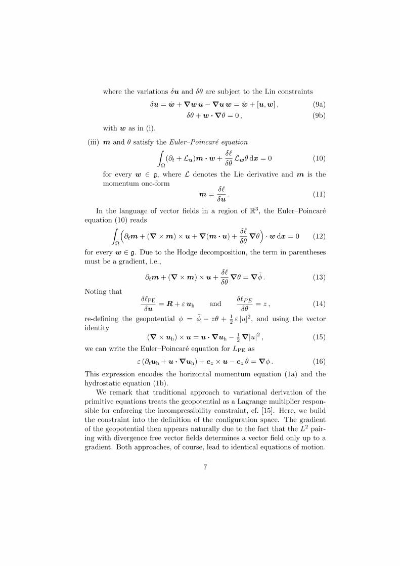
ε (∂tuh + u · ∇uh) + ez × u− ez θ =∇φ . (16)

This expression encodes the horizontal momentum equation (1a) and thehydrostatic equation (1b).

We remark that traditional approach to variational derivation of theprimitive equations treats the geopotential as a Lagrange multiplier respon-sible for enforcing the incompressibility constraint, cf. [15]. Here, we buildthe constraint into the definition of the configuration space. The gradientof the geopotential then appears naturally due to the fact that the L2 pair-ing with divergence free vector fields determines a vector field only up to agradient. Both approaches, of course, lead to identical equations of motion.

7

4 Derivation of the balance model Lagrangian

We observe that any notion of balance entails restricting the motion to asubmanifold of the phase space. Therefore, when a balance model arisesfrom a variational principle, its Lagrangian is necessarily degenerate. Ourgeneral strategy for the derivation of approximate balance models is to finda near-identity configuration space transformation such that the originalLagrangian becomes degenerate when truncated at the desired order of anexpansion in the small parameter. The truncated degenerate Lagrangianthen determines the balance model variational principle. Its degeneracyimplies a Dirac constraint on the system, which is precisely the balancerelation.

To implement this strategy, we largely follow the construction in [11].We consider the primitive equation flow map as a family of maps ηε param-eterized by ε. They relate to a balance model flow map η via a change ofcoordinates generated by a vector field vε ∈ g, so that

η′ε = vε ηε with η0 = η , (17)

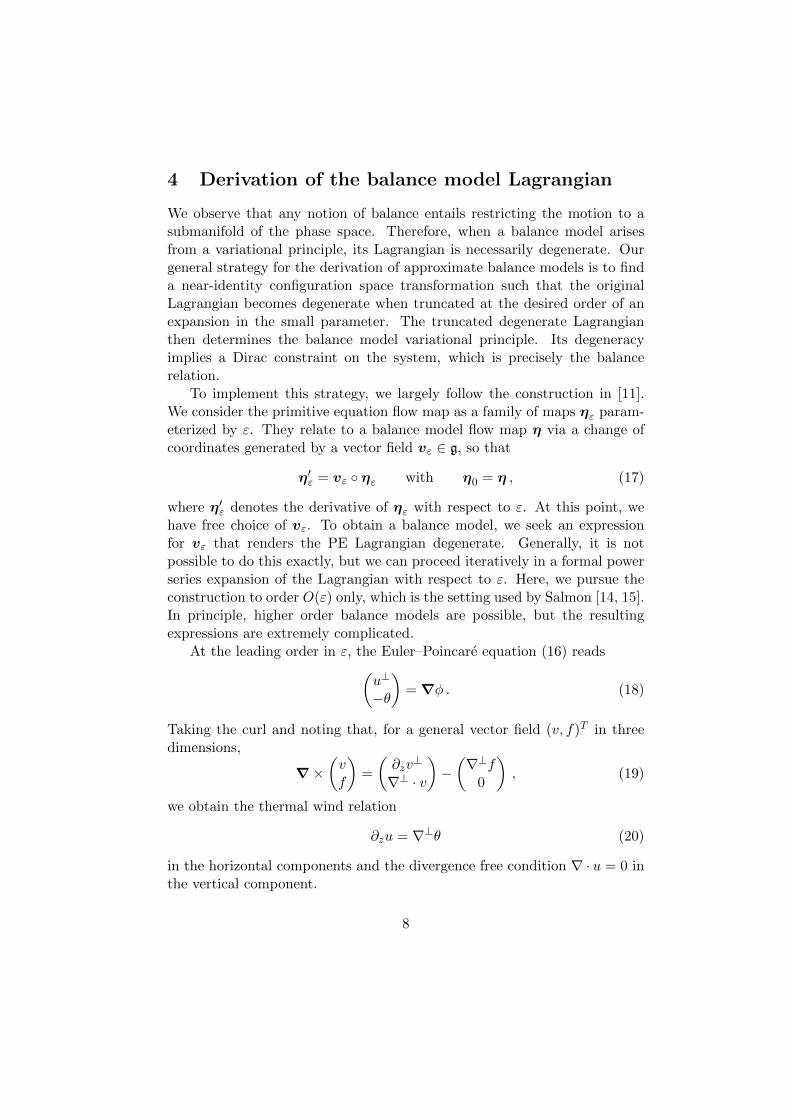
where η′ε denotes the derivative of ηε with respect to ε. At this point, wehave free choice of vε. To obtain a balance model, we seek an expressionfor vε that renders the PE Lagrangian degenerate. Generally, it is notpossible to do this exactly, but we can proceed iteratively in a formal powerseries expansion of the Lagrangian with respect to ε. Here, we pursue theconstruction to order O(ε) only, which is the setting used by Salmon [14, 15].In principle, higher order balance models are possible, but the resultingexpressions are extremely complicated.

At the leading order in ε, the Euler–Poincare equation (16) reads(u⊥

−θ

)=∇φ . (18)

Taking the curl and noting that, for a general vector field (v, f)T in threedimensions,

∇×(vf

)=

(∂zv⊥

∇⊥ · v

)−(∇⊥f

0

), (19)

we obtain the thermal wind relation

∂zu = ∇⊥θ (20)

in the horizontal components and the divergence free condition ∇ · u = 0 inthe vertical component.

8

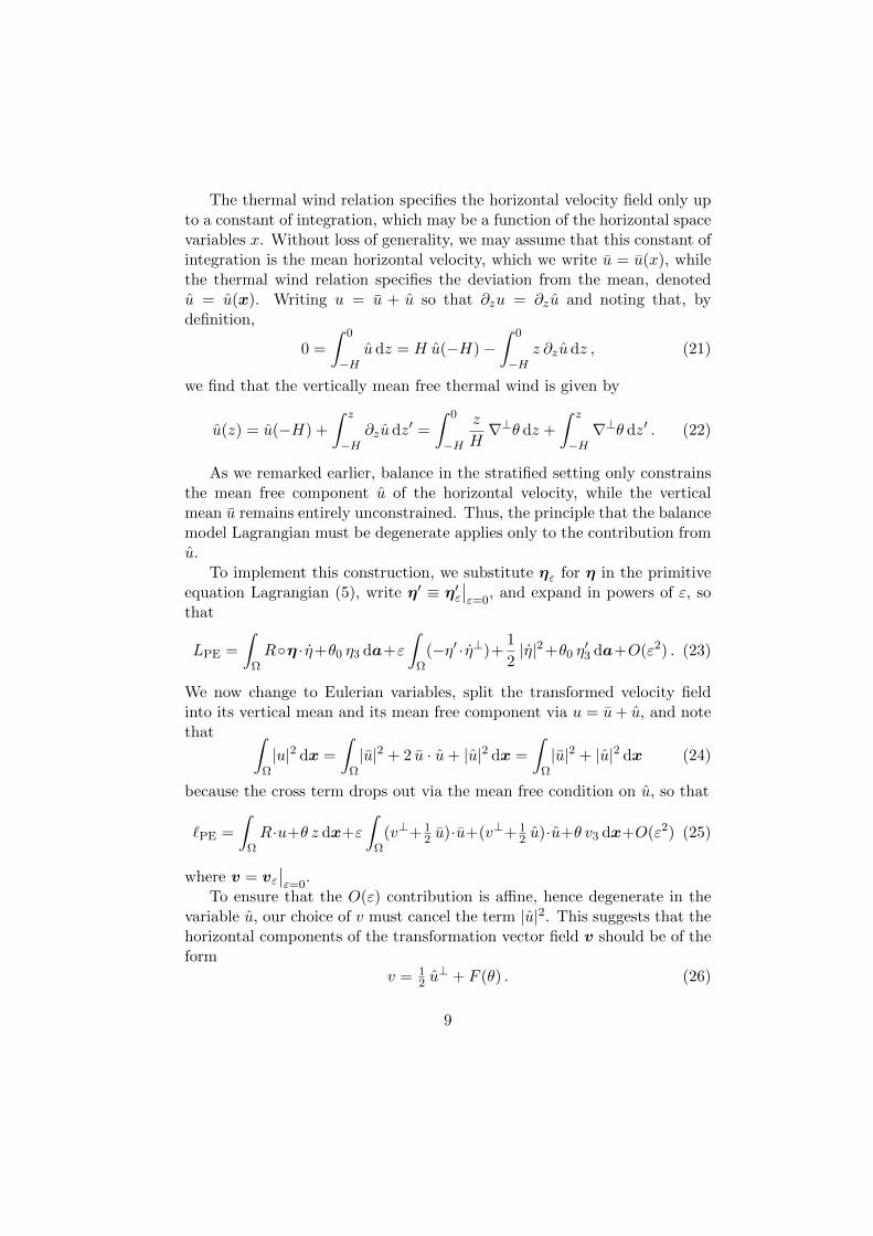
The thermal wind relation specifies the horizontal velocity field only upto a constant of integration, which may be a function of the horizontal spacevariables x. Without loss of generality, we may assume that this constant ofintegration is the mean horizontal velocity, which we write u = u(x), whilethe thermal wind relation specifies the deviation from the mean, denotedu = u(x). Writing u = u + u so that ∂zu = ∂zu and noting that, bydefinition,

0 =

∫ 0

−Hudz = H u(−H)−

∫ 0

−Hz ∂zudz , (21)

we find that the vertically mean free thermal wind is given by

u(z) = u(−H) +

∫ z

−H∂zudz′ =

∫ 0

−H

z

H∇⊥θ dz +

∫ z

−H∇⊥θ dz′ . (22)

As we remarked earlier, balance in the stratified setting only constrainsthe mean free component u of the horizontal velocity, while the verticalmean u remains entirely unconstrained. Thus, the principle that the balancemodel Lagrangian must be degenerate applies only to the contribution fromu.

To implement this construction, we substitute ηε for η in the primitiveequation Lagrangian (5), write η′ ≡ η′ε

∣∣ε=0

, and expand in powers of ε, sothat

LPE =

∫ΩRη · η+θ0 η3 da+ε

∫Ω

(−η′ · η⊥)+1

2|η|2 +θ0 η

′3 da+O(ε2) . (23)

We now change to Eulerian variables, split the transformed velocity fieldinto its vertical mean and its mean free component via u = u+ u, and notethat ∫

Ω|u|2 dx =

∫Ω|u|2 + 2 u · u+ |u|2 dx =

∫Ω|u|2 + |u|2 dx (24)

because the cross term drops out via the mean free condition on u, so that

`PE =

∫ΩR·u+θ z dx+ε

∫Ω

(v⊥+ 12 u)·u+(v⊥+ 1

2 u)·u+θ v3 dx+O(ε2) (25)

where v = vε∣∣ε=0

.To ensure that the O(ε) contribution is affine, hence degenerate in the

variable u, our choice of v must cancel the term |u|2. This suggests that thehorizontal components of the transformation vector field v should be of theform

v = 12 u⊥ + F (θ) . (26)

9

The third component of v is then determined by the condition that v isdivergence free and tangent to the top and bottom boundaries.

As in [11], motivated by dimensional considerations, we specialize to theone-parameter family of transformation vector fields

v =1

2

(u⊥

∇⊥ · U

)− λ

(g⊥

∇⊥ ·G

), (27)

where g is the thermal wind defined through an expression of the form (22),namely

g = ∇⊥Θ (28)

with

Θ =

∫ 0

−H

z

Hθ dz +

∫ z

−Hθ dz′ , (29)

and where

G = −∫ 0

zg dz′ and U = −

∫ 0

zudz′ (30)

are the vertical antiderivatives of g and u, respectively. By construction, vis a divergence free field, v3(0) = v3(−H) = 0, and v has zero vertical mean.

The case λ = 12 is special: whenever u satisfies the thermal wind rela-

tion, then v = 0 so that O(ε) deviations from thermal wind correspond toa transformation vector field that is O(ε) small. Hence, the transformationfor λ = 1

2 is overall an O(ε2) change of variables so that quantities in phys-ical and computational coordinates may be identified up to errors that arebeyond the order of accuracy of the approximation.

We further remark that Salmon’s [15] transformation corresponds to thechoice λ = −1

2 up to terms of higher order, as the leading order balanceimplies that

vSalmon =

(g⊥

∇⊥ ·G

)=

1

2

(u⊥

∇⊥ · U

)+

1

2

(g⊥

∇⊥ ·G

)+O(ε) . (31)

Returning to the general case, we plug the transformation (27) back into(25), drop all higher order terms, and note that the integral of v⊥ · u iszero as v has zero vertical mean. This yields the balance model reducedLagrangian

`BM =

∫ΩR · u+ θ z dx+ ε

∫Ω

12 |u|

2 + λ g · u+ θ∇⊥ · (12 U − λG) dx . (32)

10

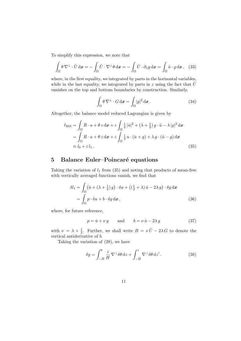
To simplify this expression, we note that∫Ωθ∇⊥ · U dx = −

∫ΩU · ∇⊥θ dx = −

∫ΩU · ∂zg dx =

∫Ωu · g dx , (33)

where, in the first equality, we integrated by parts in the horizontal variables,while in the last equality, we integrated by parts in z using the fact that Uvanishes on the top and bottom boundaries by construction. Similarly,∫

Ωθ∇⊥ ·Gdx =

∫Ω|g|2 dx . (34)

Altogether, the balance model reduced Lagrangian is given by

`BM =

∫ΩR · u+ θ z dx+ ε

∫Ω

12 |u|

2 + (λ+ 12) g · u− λ |g|2 dx

=

∫ΩR · u+ θ z dx+ ε

∫Ω

12 u · (u+ g) + λ g · (u− g) dx

≡ l0 + ε l1 . (35)

5 Balance Euler–Poincare equations

Taking the variation of l1 from (35) and noting that products of mean-freewith vertically averaged functions vanish, we find that

δl1 =

∫Ω

(u+ (λ+ 1

2) g)· δu+

((1

2 + λ) u− 2λ g)· δg dx

=

∫Ωp · δu+ b · δg dx , (36)

where, for future reference,

p = u+ ν g and b = ν u− 2λ g (37)

with ν = λ + 12 . Further, we shall write B = ν U − 2λG to denote the

vertical antiderivative of b.Taking the variation of (28), we have

δg =

∫ 0

−H

z

H∇⊥δθ dz +

∫ z

−H∇⊥δθ dz′ . (38)

11

When integrated against the vertically mean-free vector field b, the contri-bution from the first term vanishes, so that, reversing the order of the z andthe z′ integration, we obtain∫

Ωb · δg dx =

∫Ω∇⊥δθ ·

∫ 0

zbdz′ dx =

∫Ωδθ∇⊥ ·B dx . (39)

Combining (35), (36), and (39), we find that

mBM ≡δ`BM

δu= R+ εph and

δ`BM

δθ= ∇⊥ ·B , (40)

so that the Euler–Poincare equation (13) for LBM reads

ez × u− θ ez + ε(∂tph + (∇× ph)× u+∇θ∇⊥ ·B

)=∇φ . (41)

Introducing the relative vorticity

ζ = ∇⊥ · p = ∇⊥ · u+ ν∆Θ (42)

and separating the horizontal and vertical component equations, we write(41) in the form(

u⊥

−θ

)+ ε

(∂tp+ u⊥ ζ + u3 ∂zp

−u · ∂zp

)+ ε∇θ∇⊥ ·B =∇φ . (43)

Notice that incompressibility implies ∂zu3 = −∇ · u, so that

u3 =

∫ 0

z∇ · u dz′ = −∇ · U , (44)

where the second equality is due to u3(−H) = 0, which implies that∇·u = 0.Since g and G are horizontally divergence free, we can write

u3 = −ν−1∇ ·B (45)

so long as ν 6= 0. Then, taking the curl of (43), noting that ∂zp = ν∇⊥θand ∂zζ = ν∆θ, using (19), and applying the vector identity

∇× (f∇θ) =∇f ×∇θ =

(∂zf ∇⊥θ − ∂zθ∇⊥f

∇⊥f · ∇θ

), (46)

we rewrite the Euler–Poincare equation in the form

12

(∇⊥θ − ∂zu∇ · u

)+ ε

(−ν∇θ − ∂zu ζ − ν u∆θ + ν∇ · u∇θ − ν u3 ∂z∇θ)

∂tζ +∇ · (uζ)−∇ · (∇θ∇ ·B)

)+ νε

(∇⊥(u · ∇⊥θ)

0

)+ ε

(∇⊥θ∇⊥ · b− ∂zθ∇⊥∇⊥ ·B

∇θ · ∇⊥∇⊥ ·B

)= 0 . (47)

The vertical component of (47) describes the evolution of relative vor-ticity ζ. Rearranging terms, we can write it in the form

∂tζ +∇ · (ζu) = −ε−1∇ · u+∇ · (∇θ∇ ·B)−∇θ · ∇⊥∇⊥ ·B≡ F1(∇ · u,∇θ,∇∇θ,∇B,∇∇B) . (48)

Since, by (54), ∇· u is formally an O(ε) quantity, all terms on the right handside are O(1) so that ζ evolves on the slow time scale.

Setting ω = ∇⊥ · u and taking the vertical average of (48), we obtain

∂tω + u · ∇ω = ∇ · (∇θ∇ ·B − ν u∆Θ)−∇θ · ∇⊥∇⊥ ·B ≡ F2 . (49)

The horizontal component equation of the Euler–Poincare equation (47),on the other hand, is entirely kinematic and will lead to an equation for U ,the balance relation. To make this relation more explicit, we note that theadvection equation for θ implies

∂t∇θ = −∇(u ·∇θ) = −∇(u · ∇θ)−∇(u3 ∂zθ) . (50)

Then, after rearrangement of terms, the horizontal part of (47) reads

∇⊥θ − ∂zu+ ε(−ζ ∂zu+∇⊥θ∇⊥ · b− ∂zθ (∇⊥∇⊥ ·B +∇∇ ·B)

)+ νε

(∇(u · ∇θ)− u∆θ +∇ · u∇θ +∇⊥(u · ∇⊥θ)

)= 0 . (51)

Now we use the general vector identifies

∇∇ ·B +∇⊥∇⊥ ·B = ∆B , (52)

∇(u · ∇θ)− u∆θ +∇ · u∇θ +∇⊥(u · ∇⊥θ) = 2 Def u∇θ , (53)

where Def u = 12 (∇u+ (∇u)T ), to obtain

(1 + ε ζ) ∂zu− (1 + ε∇⊥ · b)∇⊥θ + ε ∂zθ∆B = 2εν Def u∇θ . (54)

Recalling the definition of b and using the identity

(∇⊥ · u)J + 2 Def u = 2∇u , (55)

13

where J denotes the standard 2× 2 symplectic matrix, we obtain

(1+ε ζ) ∂2z U+ε ∂zθ∆B−2εν∇∂zU ∇θ = (1−2ελ∆Θ)∇⊥θ+2εν Def u∇θ .

(56)We note that the balance relation (56) together with the advection of

potential temperature and vorticity transport equation (49) imply (48).When ν 6= 0, it is better to write out an equation for B, so that the third

order horizontal derivative on Θ implicit in the second term of (56) appearson the domain side rather than on the range side of an elliptic operator.Our final expression for the horizontal balance relation then reads

(1 + ε ζ) ∂2zB + εν ∂zθ∆B − 2εν∇∂zB∇θ

=(ν − 2λ− 2λε ζ − 2ελν∆Θ

)∇⊥θ + 2εν2 Def u∇θ + 4ελν∇g∇θ

≡ F3(∇2Θ,∇θ,∇u) . (57)

For fixed u and θ, equation (57) is a linear second order PDE in B. It iselliptic as long as the matrix

Λ(ζ, θ) =

εν ∂zθ 0 −εν ∂x1θ0 εν ∂zθ −εν ∂x2θ

−εν ∂x1θ −εν ∂x2θ 1 + ε ζ

(58)

is positive definite, or, equivalently,

ν ∂zθ > 0 and 1 + ε

(ζ − ν|∇θ|2

∂zθ

)> 0 . (59)

Moreover, the operator on the left-hand side of (57) is uniformly ellipticwhenever the bounds (59) hold uniformly in space, i.e.,

infx∈Ω

ν ∂zθ ≥ µ1 > 0 and infx∈Ω

1 + ε

(ζ − ν|∇θ|2

∂zθ

)≥ µ2 > 0 . (60)

Thus, assuming ν > 0, uniform ellipticity holds so long as the fluid is stablystratified and provided ζ and horizontal gradient of θ are not too large.

6 Conservation of energy and potential vorticity

As the balance model Lagrangian is invariant under time translation, themodel possesses a conserved energy of the form

HBM =

∫Ω

δ`BM

δu· u dx− `BM(u, θ) =

∫Ωε(

12 |u|

2 + λ |∇⊥Θ|2)− θ z dx .

(61)

14

The symmetry of the balance model Lagrangian under particle relabelingleads to a material conservation law for the balance model potential vorticity.It can be derived geometrically as follows. First note that the abstractEuler–Poincare equation (10) can be written as

(∂t + Lu)m+δ`

δθdθ = dφ , (62)

where d denotes the exterior derivative. Taking the exterior (wedge) productbetween the exterior derivative of (62) and dθ, we find that

0 = d((∂t + Lu)m+

δ`

δθdθ − dφ

)∧ dθ

= (∂t + Lu)(dm ∧ dθ)− dm ∧ d(∂t + Lu)θ

= (∂t + Lu)(dm ∧ dθ) , (63)

where we used the commutativity of Lie and exterior derivatives in thesecond equality and the advection of θ in the third equality. In three dimen-sions, we can identify this conservation law with material advection of thescalar quantity

q = ∗(dm ∧ dθ) , (64)

where ∗ denotes the Hodge dual operator. Indeed, writing µ = dx1∧dx2∧dzto denote the canonical volume form on Ω, we have dm ∧ dθ = qµ, so that

0 = (∂t + Lu)(qµ) = µ (∂t + Lu)q + qLuµ . (65)

Since the flow is volume preserving and µ is non-degenerate, this proves that∂tq + Luq = 0, i.e., q is conserved on fluid particles.

In the language of vector calculus, expression (64) for the potential vor-ticity reads

q = (∇×m) · ∇θ . (66)

In fact, the derivation above corresponds to taking the inner product ofthe curl of the Euler–Poincare equations (13) with ∇θ and manipulatingcorrespondingly; the advantage of the abstract approach is that commut-ing exterior and Lie derivative in traditional notation is not linked to anyintrinsic operation, thus requires tedious verification.

To write out the explicit balance model potential vorticity, note that

∇×(R0

)= ez , ∇×

(u0

)=

(0ω

), ∇×

(g0

)=

(∂zg⊥

∇⊥ · g

), (67)

15

where once again ω = ∇⊥ · u, and insert g from (28) into the expression (40)for mBM, so that

q = ∂2zΘ (1 + ε ω + εν∆Θ)− εν |∇∂zΘ|2 ≡ F (D2Θ;ω) . (68)

This expression is a fully nonlinear second order equation for Θ. The stan-dard solvability condition for equations of this type is uniform ellipticity ofF (see, e.g., [4, 18]). Ellipticity for a nonlinear equation is essentially de-fined as ellipticity of its linearization. To be precise, we follow the definitiongiven in [18]. Let U be an open subset Rn, Sn the space of symmetric n×nmatrices, and F a real-valued function on U ×R×Rn×Sn that is C1 in itslast argument. Then the operator

F (x,Θ, DΘ, D2Θ) (69)

is elliptic on some subset Γ ⊂ U × R× Rn × Sn provided the matrix

[Fij ] =∂F

∂M(x, α, β,M) ≡

[∂F (x, α, β,M)

∂Mij

](70)

is positive definite for all (x, α, β,M) ∈ Γ. Furthermore, F is uniformly el-liptic on Γ provided there exist positive functions λ1, λ2 on Γ and a constantµ such that for any ξ ∈ Rn,

λ1 |ξ|2 ≤ Fij ξi ξj ≤ λ2 |ξ|2 with λ2/λ1 ≤ µ . (71)

When F is defined by (68), we find that

∂F

∂D2Θ= Λ(ζ, θ) . (72)

Thus, the ellipticity conditions for the nonlinear equation (68) and for thebalance relation (57) coincide and are both given by (59). Moreover, ifcondition (60) is satisfied and, in addition, there is a uniform upper boundof the form

1 + ε ζ + εν ∂zθ ≤ µ3 , (73)

they are uniformly elliptic.In fact, (68) has the form of a generalized Monge–Ampere equation. To

expose this structure, we define the generalized Hessian

Hess Θ =

(∆Θ |∂z∇Θ||∂z∇Θ| ∂2

zΘ

), (74)

16

so thatq = ∂2

zΘ (1 + ε ω) + εν det Hess Θ . (75)

Finally, defining

Ψ =1√εν

∆−1(1 + ε ω) +√ενΘ , (76)

we haveq = det Hess Ψ . (77)

Thus, the potential vorticity inversion relation is of Monge–Ampere type,albeit in a non-standard form. For Monge–Ampere equations coming froma standard Hessian, Cafferelli [3] proved W 2,p regularity provided the righthand side is sufficiently close to a constant; also see [7]. We expect thatsimilar results hold for (77), where Caffarelli’s condition would impose arestriction on the deviation from linear stratification. We remark that thepassage from (68) to (77) is not possible for periodic lateral boundary con-ditions as the Laplacian is not invertible on constants; however, this is notan issue as everything can be done using (68) directly.

In the context of classical semigeostrophic theory, Cullen and Purser[5] have shown that for the system to be dynamically stable, the matrixHess Ψ defining the PV has to be positive definite, which is equivalent to acertain convexity condition for Ψ. We expect this condition to be applicablehere as well. However, we stress that the nature of our results is differentfrom classical semigeostrophic theory, which asserts existence of possiblydiscontinuous front-type solutions under only natural stability conditions forthe front, see Shutts and Cullen [17]. Here we need to impose, additionally, asmallness assumption on gradients of θ which is more restrictive, but appearsto allow a stronger notion of solutions.

When the Coriolis parameter f = ∇⊥ · R varies horizontally in space,the balance model equations become rather cumbersome and shall not bepursued further in this paper. However, we note that the conservation lawsremain simple even in this case and outline the principal changes comparedto the case of non-varying f .

When f = f(x) but non-dimensionalized as before, the thermal windrelation becomes

∂zu =1

f∇⊥θ , (78)

so that we define the thermal wind as g/f with g still given by (28). Pro-ceeding as in Section 4, we use the transformation vector field

v =1

2

(u⊥

∇⊥ · U

)− λ

f

(g⊥

∇⊥ ·G

), (79)

17

which yields the balance model Lagrangian

`BM =

∫ΩR · u+ θ z dx+ ε

∫Ω

1

2u · (u+ g) +

λ

fg · (u− g) dx. (80)

Therefore, (40) becomes

mBM ≡δ`BM

δu= R+ εph , (81)

where

p = u+ νf g with νf =1

2+λ

f. (82)

Substituting the expressions for `BM and mBM into the general formulasof the balance model energy (61) and potential vorticity (66), we obtain,respectively,

HBM =

∫Ωε(1

2|u|2 +

λ

f|∇⊥Θ|2

)− θ z dx (83)

andq = ∂2

zΘ (f + ε ω + ε νf ∆Θ)− ε νf |∇∂zΘ|2 . (84)

PV inversion is given by the generalized Monge-Ampere problem

q = ∂2zΘ (f + ε ω) + ε νf det Hess Θ . (85)

or, equivalently,νf q = det Hess Ψ , (86)

where

Ψ =1√ε

∆−1(f + ε ω) +√εΘ . (87)

Hence, potential vorticity satisfies an equation of the same type as in thecase of constant Coriolis parameter provided νf and f are bounded awayfrom zero. In particular, the invertibility conditions do not change when fis a small perturbations of a constant.

We remark that a spatially variable Coriolis parameter in a shallow watersetting leads to similarly simple balance model energy and potential vorticity[13].

18

7 Balance model evolution and special cases

We are now ready to collect the complete set of balance model equations.It comprises the two transport equations

∂tθ + u · ∇θ = 0 , (88a)

∂tω + u · ∇ω = F2 , (88b)

the two kinematic linear second order equations

(1 + ε ζ) ∂2zB + εν ∂zθ∆B − 2εν∇∂zB∇θ = F3(∇2Θ,∇θ,∇u) , (88c)

∆ψ = ω , (88d)

and a number of direct relations between the variables,

Θ =

∫ 0

−H

z

Hθ dz +

∫ z

−Hθ dz′ , (88e)

u = ∇⊥ψ , (88f)

u = ν−1 (∂zB + 2λ∇⊥Θ) , (88g)

u3 = −ν−1∇ ·B , (88h)

u = u+ u . (88i)

The balance relation (88c) is elliptic provided ν > 0, the fluid is stablystratified so that ∂zθ > 0, the vorticity ζ and horizontal gradient ∇θ are nottoo large, and ε is sufficiently small; it is complemented with homogeneousDirichlet conditions on the vertical boundaries. The nonlinearities F2 andF3 are defined in (49) and (57), respectively.

We conjecture that this system is well-posed at least locally in time,which is supported by a simple count of derivatives. Suppose that initiallyoutside of a compact domain of sufficiently large radius the fluid is at rest,horizontal gradients of θ vanish, and, furthermore, that both θ and Θ areof Sobolev class Hs+1

loc and u ∈ Hs with s large enough so that Hs−1 is atopological algebra. Then, initially, ζ = ω + ν∆Θ ∈ Hs−1 and, by ellipticregularity, B ∈ Hs+1 from the balance relation (88c).

We now need to assure that these regularity classes are maintained forat least a short interval of time. This is not obvious from the two advectionequations (88a) and (88b), which each seem to be one derivative short.However, we note that ζ also satisfies the evolution equation (48), whichimplies that class Hs−1 is maintained provided that θ and B remain at theindicated level of the hierarchy. Via the balance relation (88c), the condition

19

on B is satisfied provided θ, Θ, and u remain at the indicated level of thehierarchy.

To guarantee Hs+1-regularity of Θ, we note that q ∈ Hs−1 initially, soby PV advection with the Hs vector field u, it remains in this class for ashort interval of time. We then use elliptic regularity of the Monge–Ampereproblem (68) directly to conclude that Θ ∈ Hs+1.

Achieving Hs+1-regularity of θ is more subtle. We need to assume, inaddition, that initially q ∈ Hs, this better regularity class is also maintainedover short intervals of time provided u ∈ Hs. Now differentiate (68) withrespect to z to find that

∂2zθ (1 + ε ω + εν∆Θ) + ∂zθ (1 + εν∆θ)− 2εν∇θ · ∇∂zθ = ∂zq . (89)

Then, provided ∂zθ > 0 and 1 + ε ω + εν∆Θ > 0, the required θ ∈ Hs+1

follows by linear elliptic regularity. Further, the positivity conditions aremaintained by continuity for at least a short interval of time.

The argument above is not a full proof, but rather a plausibility checkwhich demonstrates that we have brought the equations into a form thatis consistent with standard strategies of proof. A full proof of local well-posedness will require a careful study of the solvability conditions for thePV inversion and balance relation.

Finally, it is not clear whether solutions to (88) have a chance to persistfor all times subject only to conditions on the initial data. As written,it is not given that the ellipticity condition (59) will persist. Hence, webelieve that an argument toward global well-posedness necessarily requiresadditional structural insight. In this context, we note that the balance modelHamiltonian (61) provides a global a priori bound on ∇Θ in L2.

We now discuss three special choices for the model parameter λ.

Case λ = 12 : stratified L1 dynamics

The case λ = 12 is special because then the transformation vector field v =

O(ε), hence the transformation is an identity to order O(ε2). With thischoice, we obtain the stratified L1 model. In this case ν = 1, B = U − G,and the balance relation (88c) simplifies to

(1 + ε ζ) ∂2zB + ε ∂zθ∆B − 2ε∇∂zB∇θ = 2ε (∇(u+ g))T∇θ . (90)

We remark that the L1 model could have been derived within Salmon’s [15]procedure simply replacing u in the primitive equation Lagrangian by g.However, as we saw in Section 5, the bare Euler–Poincare equations are

20

not immediately useful. The new insight we suggest here is that we shouldnot try to “simplify” the L1 model by further approximation, but ratherunderstand it as an already fine model by leveraging the conservation ofpotential vorticity, implicit in its derivation, as a dynamic variable.

Case λ = 0: more regularity for U

In the special case when λ = 0 so that ν = 12 , b = 1

2 u and B = 12 U , the

balance relation (88c) reads

(1 + ε ζ) ∂2z U + ε

2 ∂zθ∆U − ε∇∂zU ∇θ = ∇⊥θ + ε J Def u∇⊥θ . (91)

We note that in this case, the right hand side of the balance relation containsonly first horizontal derivatives, so U is more regular than in the generic case.Whether this leads to a different functional setting for the entire system, as in[6] for the shallow water analog, or is helpful for a numerical implementationremains open.

Case λ = −12 : Salmon’s LSG model

Finally, when λ = −12 so that ν = 0 and B = G, (54) reads

(1 + ε∇⊥ · u) ∂2z U = (1 + ε∆Θ)∇⊥θ − ε ∂zθ∆G . (92)

It is clear that this balance relation is not elliptic, thus u is expected to losethree horizontal derivatives with respect to Θ and one horizontal derivativewith respect to q. Hence, we cannot expect that the regularity class of Θpersists for any time t > 0; the problem appears to be ill posed.

8 Conclusions

In this paper, we have shown that the method of degenerate variationalasymptotics applies to a stratified fluid described by the primitive equationsin semigeostrophic scaling. The construction is in many respects parallel tothe well-explored case of rapidly rotating shallow water.

Specifically, we derived a family of balance model for stratified flow whichconserve energy and potential vorticity. We rewrote the model equations in arobust form, emphasizing the importance of advection of potential vorticity,which appears to be a crucial ingredient for the proof of local well-posedness.It is worth noting that both balance relation and PV inversion are ellipticsubject to identical physically reasonable conditions.

21

Subject to stable stratification and a small data assumption, the modelsare formally in the same regularity class as their shallow water counterparts.We believe techniques we had used to prove well-posedness for balance mod-els of shallow water [12, 6] can be adapted to the stratified case, hence expectexistence and uniqueness of solutions for as long as stable stratification andsmallness of data assumptions persist.

Acknowledgments

We thank Mike Cullen and Darryl Holm for many interesting discussions andthe Isaac Newton Institute for its hospitality during the Mathematics of theFluid Earth program where this work was begun. We further acknowledgepartial support through German Science Foundation grant OL-155/3.

References

[1] J.S. Allen and D.D. Holm, Extended-geostrophic Hamiltonian modelsfor rotating shallow water motion, Phys. D 98 (1996), 229–248.

[2] J.S. Allen, D.D. Holm, and P.A. Newberger, Toward an extended-geostrophic Euler–Poincare model for mesoscale oceanographic flow, in“Large-Scale Atmosphere-Ocean Dynamics 1: Analytical Methods andNumerical Models,” J. Norbury & I. Roulstone, eds., Cambridge Uni-versity Press, Cambridge, 2002, pp. 101–125.

[3] L.A. Caffarelli, Interior W 2,p estimates for solutions of the Monge–Ampere equation, Ann. Math. 131 (1990), 135–150.

[4] L.A. Caffarelli and X. Cabre, “Fully nonlinear elliptic equations,” Amer.Math. Soc. Colloq. Publ., Vol. 43, Amer. Math. Soc., Providence, RI,1995.

[5] M.J.P. Cullen and R.J. Purser, An extended Lagrangian theory of semi-geostrophic frontogenesis, J. Atmos. Sci. 41 (1984), 1477–1497.

[6] M. Calık, M. Oliver, and S. Vasylkevych, Global well-posedness for thegeneralized large-scale semigeostrophic equations, Arch. Ration. Mech.An. 207 (2013), 969–990.

[7] G. De Philippis and A. Figalli, The Monge–Ampere equation and itslink to optimal transportation, B. Am. Math. Soc. 51 (2014), 527–580.

22

[8] D.D. Holm, J.E. Marsden, and T.S. Ratiu, Euler–Poincare equationsand semidirect products with applications to continuum theories, Adv.in Math. 137 (1998), 1–81.

[9] D.D. Holm, T. Schmah, and C. Stoica, “Geometric mechanics and sym-metry: from finite to infinite dimensions,” Oxford University Press,2009.

[10] B.J. Hoskins, The geostrophic momentum approximation and the semi-geostrophic equations, J. Atmos. Sci. 32 (1975), 233–242.

[11] M. Oliver, Variational asymptotics for rotating shallow water neargeostrophy: A transformational approach, J. Fluid Mech. 551 (2006),197–234.

[12] M. Oliver and S. Vasylkevych, Hamiltonian formalism for models ofrotating shallow water in semigeostrophic scaling, Discret. Contin. Dyn.S. 31 (2011), 827–846.

[13] M. Oliver and S. Vasylkevych, Generalized LSG models with varyingCoriolis parameter, Geophys. Astrophys. Fluid Dyn. 107 (2013), 259–276.

[14] R. Salmon, New equations for nearly geostrophic flow, J. Fluid. Mech.153 (1985), 461–477.

[15] R. Salmon, Large-scale semi-geostrophic equations for use in ocean cir-culation models, J. Fluid Mech. 318 (1996), 85–105.

[16] J.R. Shepherd, “Modelling ocean circulation with large-scale semi-geostrophic equations,” PhD thesis, Imperial College, London, 1999.

[17] G.J. Shutts and M.J.P. Cullen, Parcel stability and its relation to semi-geostrophic theory, J. Atmos. Sci. 44 (1987), 1318–1330.

[18] N.S. Trudinger, Fully nonlinear, uniformly elliptic equations under nat-ural structure conditions, Trans. Amer. Math. Soc. 278 (1983), 751–769.

23