Generalized Focal Loss V2: Learning Reliable Localization Quality Estimationfor Dense Object Detection

Xiang Li1,2, Wenhai Wang3, Xiaolin Hu4, Jun Li1, Jinhui Tang1, and Jian Yang1*

Abstract

Localization Quality Estimation (LQE) is crucial andpopular in the recent advancement of dense object detec-tors since it can provide accurate ranking scores that benefitthe Non-Maximum Suppression processing and improve de-tection performance. As a common practice, most existingmethods predict LQE scores through vanilla convolutionalfeatures shared with object classification or bounding boxregression. In this paper, we explore a completely novel anddifferent perspective to perform LQE – based on the learneddistributions of the four parameters of the bounding box.The bounding box distributions are inspired and introducedas “General Distribution” in GFLV1, which describes theuncertainty of the predicted bounding boxes well. Such aproperty makes the distribution statistics of a bounding boxhighly correlated to its real localization quality. Specifi-cally, a bounding box distribution with a sharp peak usuallycorresponds to high localization quality, and vice versa. Byleveraging the close correlation between distribution statis-tics and the real localization quality, we develop a consid-erably lightweight Distribution-Guided Quality Predictor(DGQP) for reliable LQE based on GFLV1, thus producingGFLV2. To our best knowledge, it is the first attempt in ob-ject detection to use a highly relevant, statistical represen-tation to facilitate LQE. Extensive experiments demonstratethe effectiveness of our method. Notably, GFLV2 (ResNet-101) achieves 46.2 AP at 14.6 FPS, surpassing the previousstate-of-the-art ATSS baseline (43.6 AP at 14.6 FPS) by ab-solute 2.6 AP on COCO test-dev, without sacrificing theefficiency both in training and inference. Codes are avail-able at https://github.com/implus/GFocalV2.

*Corresponding author. Xiang Li, Jun Li and Jian Yang are from PCALab, Key Lab of Intelligent Perception and Systems for High-DimensionalInformation of Ministry of Education, and Jiangsu Key Lab of Image andVideo Understanding for Social Security, School of Computer Scienceand Engineering, Nanjing University of Science and Technology.

1Nanjing University of Science and Technology 2Momenta3Nanjing University 4Tsinghua University {xiang.li.implus, jinhuitang,csjyang}@njust.edu.cn, wangwenhai362@163.com, xlhu@mail.tsinghua.edu.cn,junl.mldl@gmail.com

1.0 General Distribution

𝑦

𝑃(𝑥)

（a） （b）

𝑦

𝑃(𝑥)Top 1 value

1.0 General Distribution

𝑦

𝑃(𝑥)

（a） （b）𝑦

𝑃(𝑥)Top 1 value

Ambiguous & Flatten

Lower Localization Quality: 0.69 IoU

Certain & Sharp

Higher Localization Quality: 0.90 IoU

（c）

（d）

（c）

（d）

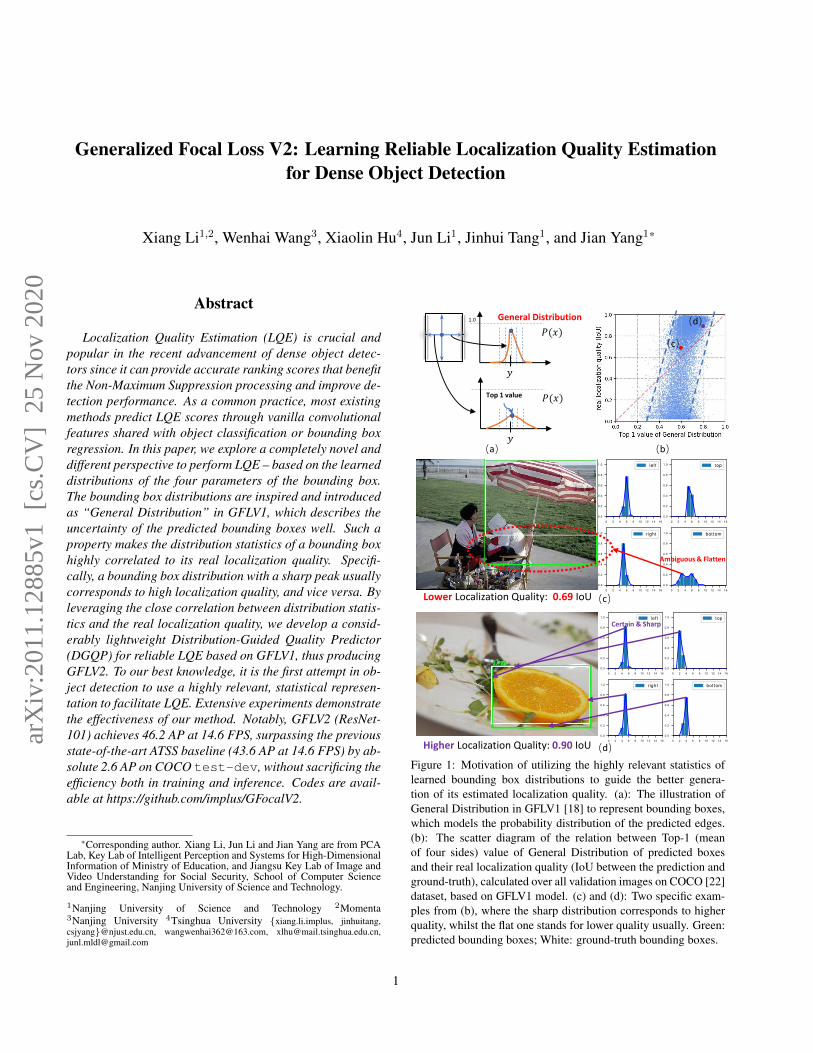
Figure 1: Motivation of utilizing the highly relevant statistics oflearned bounding box distributions to guide the better genera-tion of its estimated localization quality. (a): The illustration ofGeneral Distribution in GFLV1 [18] to represent bounding boxes,which models the probability distribution of the predicted edges.(b): The scatter diagram of the relation between Top-1 (meanof four sides) value of General Distribution of predicted boxesand their real localization quality (IoU between the prediction andground-truth), calculated over all validation images on COCO [22]dataset, based on GFLV1 model. (c) and (d): Two specific exam-ples from (b), where the sharp distribution corresponds to higherquality, whilst the flat one stands for lower quality usually. Green:predicted bounding boxes; White: ground-truth bounding boxes.

1

arX

iv:2

011.

1288

5v1

[cs

.CV

] 2

5 N

ov 2

020

Classification-IoU Joint Representation Classification-IoU Joint Representation

General Distribution of Bounding Box

Convolutional Features (Existing Works) Statistic of General Distribution (Ours)

(a) (b) (c) (d) (e)

classification branch

regression branch

ℱ(∙) ℱ(∙)

(g)(f)

Flat? or Sharp?

Figure 2: Comparisons of input features for predicting localization quality between existing works (left) and ours (right). Existing worksfocus on different spatial locations of convolutional features, including (a): point [28, 29, 30, 33, 40, 36, 14, 18], (b): region [13], (c):border [27] dense points, (d): border [27] middle points, (e): border [27] extreme points, (f): regular sampling points [39], and (g):deformable sampling points [4, 5]. In contrast, we use the statistic of learned box distribution to produce reliable localization quality.

1. Introduction

Dense object detector [28, 23, 42, 33, 18, 27] which di-rectly predicts pixel-level object categories and boundingboxes over feature maps, becomes increasingly popular dueto its elegant and effective framework. One of the cru-cial techniques underlying this framework is LocalizationQuality Estimation (LQE). With the help of better LQE,high-quality bounding boxes tend to score higher than low-quality ones, greatly reducing the risk of mistaken suppres-sion in Non-Maximum Suppression (NMS) processing.

Many previous works [28, 29, 30, 33, 40, 36, 14, 18, 39,43, 27] have explored LQE. For example, the YOLO family[28, 29, 30] first adopt Objectness to describe the localiza-tion quality, which is defined as the Intersection-over-Union(IoU) between the predicted and ground-truth box. Afterthat, IoU is further explored and proved to be effective inIoU-Net [13], IoU-aware [36], PAA [14], GFLV1 [18] andVFNet [39]. Recently, FCOS [33] and ATSS [40] intro-duce Centerness, the distance degree to the object center, tosuppress low-quality detection results. Generally, the afore-mentioned methods share a common characteristic that theyare all based on vanilla convolutional features, e.g., featuresof points, borders or regions (see Fig. 2 (a)-(g)), to estimatethe localization quality.

Different from previous works, in this paper, we explorea brand new perspective to conduct LQE – by directly uti-lizing the statistics of bounding box distributions, insteadof using the vanilla convolutional features (see Fig. 2).Here the bounding box distribution is introduced as “Gen-eral Distribution” in GFLV1 [18], where it learns a discreteprobability distribution of each predicted edge (Fig. 1 (a))for describing the uncertainty of bounding box regression.Interestingly, we observe that the statistic of the GeneralDistribution has a strong correlation with its real localiza-tion quality, as illustrated in Fig. 1 (b). More specificallyin Fig. 1 (c) and (d), the shape (flatness) of bounding boxdistribution can clearly reflect the localization quality of thepredicted results: the sharper the distribution, the more ac-curate the predicted bounding box, and vice versa. Con-sequently, it can potentially be easier and very efficient to

conduct better LQE by the guidance of the distribution in-formation, as the input (distribution statistics of boundingboxes) and the output (LQE scores) are highly correlated.

Inspired by the strong correlation between the dis-tribution statistics and LQE scores, we propose a verylightweight sub-network with only dozens of (e.g., 64) hid-den units, on top of these distribution statistics to pro-duce reliable LQE scores, significantly boosting the detec-tion performance. Importantly, it brings negligible addi-tional computation cost in practice and almost does not af-fect the training/inference speed of the basic object detec-tors. In this paper, we term this lightweight sub-networkas Distribution-Guided Quality Predictor (DGQP), since itrelies on the guidance of distribution statistics for qualitypredictions.

By introducing the lightweight DGQP that predicts re-liable LQE scores via statistics of bounding box distribu-tions, we develop a novel dense object detector based on theframework of GFLV1, thus termed GFLV2. To verify theeffectiveness of GFLV2, we conduct extensive experimentson the challenging benchmark COCO [22]. Notably, basedon ResNet-101 [11], GFLV2 achieves impressive detectionperformance (46.2 AP), i.e., 2.6 AP gains over the state-of-the-art ATSS baseline (43.6 AP) on COCO test-dev,under the same training schedule and without sacrificing theefficiency both in training and inference.

In summary, our contributions are as follows:

• To our best knowledge, our work is the first to bridgethe statistics of bounding box distributions and localizationquality estimation in an end-to-end dense object detectionframework.

• The proposed GFLV2 is considerably lightweight andcost-free in practice. It can also be easily plugged into mostdense object detectors with a consistent gain of ∼2 AP, andwithout loss of training/inference speed.

• Our GFLV2 (Res2Net-101-DCN) achieves very com-petitive 53.3 AP (multi-scale testing) on COCO datasetamong dense object detectors.

2

2. Related WorkFormats of LQE: Early popular object detectors [9, 31, 1,10] simply treat the classification confidence as the formu-lation of LQE score, but there is an obvious inconsistencybetween them, which inevitably degrades the detection per-formance. To alleviate this problem, AutoAssign [43] andBorderDet [27] employ additional localization features torescore the classification confidence, but they still lack anexplicit definition of LQE.

Recently, FCOS [33] and ATSS [40] introduce a novelformat of LQE, termed Centerness, which depicts the dis-tance degree to the center of the object. Although Center-ness is effective, recent researches [18, 39] show that it hascertain limitations and may be suboptimal for LQE. SABL[35] introduces boundary buckets for coarse localization,and utilizes the averaged bucketing confidence as a formu-lation of LQE.

After years of technical iterations [28, 29, 30, 13, 34, 12,36, 14, 18, 39], IoU has been deeply studied and becomesincreasingly popular as an excellent measurement of LQE.IoU is first known as the Objectness in YOLO [28, 29, 30],where the network is supervised to produce estimated IoUsbetween predicted boxes and ground-truth ones, to reduceranking basis during NMS. Following the similar paradigm,IoU-Net [13], Fitness NMS [34], MS R-CNN [12], IoU-aware [36], PAA [14] utilize a separate branch to performLQE in the IoU form. Concurrently, GFLV1 [18] andVFNet [39] demonstrate a more effective format, by merg-ing the classification score with IoU to reformulate a jointrepresentation. Due to its great success [18, 39], we buildour GFLV2 based on the Classification-IoU Joint Represen-tation [18], and develop a novel approach for reliable LQE.Input Features for LQE: As shown in the left part ofFig. 2, previous works directly use convolutional features asinput for LQE, which only differ in the way of spatial sam-pling. Most existing methods [28, 29, 30, 33, 40, 36, 14, 18]adopt the point features (see Fig. 2 (a)) to produce LQEscores for high efficiency. IoU-Net [13] predicts IoU basedon the region features as shown in Fig. 2 (b). BorderDet[27] designs three types of border-sensitive features (seeFig. 2 (c)-(e)) to facilitate LQE. Similar with BorderDet, astar-shaped sampling manner (see Fig. 2 (f)) is designed inVFNet [39]. Alternatively, HSD [2] and RepPoints [38, 4]focus on features with learned locations (see Fig. 2 (g)) viathe deformable convolution [5, 46].

The aforementioned methods mainly focus on extractingdiscriminating convolutional features with various spatialaspects for better LQE. Different from previous methods,our proposed GFLV2 is designed in an artful perspective:predicting LQE scores by its directly correlated variables—the statistics of bounding box distributions (see the rightpart of Fig. 2). As later demonstrated in Table 3, com-pared with convolutional features shown in Fig. 2 (a)-(g),

the statistics of bounding box distributions achieve an im-pressive efficiency and a high accuracy simultaneously.

3. Method

In this section, we first briefly review the GeneralizedFocal Loss (i.e., GFLV1 [18]), and then derive the proposedGFLV2 based on the relevant concepts and formulations.

3.1. Generalized Focal Loss V1

Classification-IoU Joint Representation: This represen-tation is the key component in GFLV1, which is designedto reduce the inconsistency between localization quality es-timation and object classification during training and in-ference. Concretely, given an object with category labelc ∈ {1, 2, ...,m} (m indicates the total number of cat-egories), GFLV1 utilizes the classification branch to pro-duce the joint representation of Classification and IoU asJ = [J1, J2, ..., Jm], which satisfies:

Ji =

{IoU(bpred, bgt), if i = c;0, otherwise,

(1)

where IoU(bpred, bgt) denotes the IoU between the predictbounding box bpred and the ground truth bgt.General Distribution of Bounding Box Representation:Modern detectors [31, 21, 33] usually describe the boundingbox regression by Dirac delta distribution: y =

∫ +∞−∞ δ(x−

y)x dx. Unlike them, GFLV1 introduces a flexible Gen-eral Distribution P (x) to represent the bounding box, whereeach edge of the bounding box can be formulated as: y =∫ +∞−∞ P (x)x dx =

∫ yn

y0P (x)xdx, under a predefined out-

put range of [y0, yn]. To be compatible with the convolu-tional networks, the continuous domain is converted intothe discrete one, via discretizing the range [y0, yn] into alist [y0, y1, ..., yi, yi+1, ..., yn−1, yn] with even intervals ∆(∆ = yi+1 − yi,∀i ∈ {0, 1, ..., n − 1}). As a result, giventhe discrete distribution property

∑ni=0 P (yi) = 1, the esti-

mated regression value y can be presented as:

y =

n∑i=0

P (yi)yi. (2)

Compared with the Dirac delta distribution, the GeneralDistribution P (x) can faithfully reflect the prediction qual-ity (see Fig. 1 (c)-(d)), which is the cornerstone of this work.

3.2. Generalized Focal Loss V2

Decomposed Classification-IoU Representation: Al-though the joint representation solves the inconsistencyproblem [18] between object classification and quality es-timation during training and testing, there are still somelimitations in using only the classification branch to pre-dict the joint representation. In this work, we decompose

3

Head

Head

Head

Generalized Focal Loss V2

x4

x4

FC

TopK (4), Mean

ReLU

FC

Sigmoid

𝐻 ×𝑊 × 4𝑛

x4 directions𝑛

𝐻 ×𝑊 × 20

𝐻 ×𝑊 × 64

𝐻 ×𝑊 × 64

𝐻 ×𝑊 × 1

𝐻 ×𝑊 × 1

1

integral

Classification-IoU Joint Representation

𝐻 ×𝑊 × 256

𝐻 ×𝑊 × 𝐶

𝐻 ×𝑊 × 256 Classification 𝐻 ×𝑊 × 𝐶

Distribution𝐻 ×𝑊 × 4𝑛

𝐻 ×𝑊 × 4

Regression

Head

Head

C3

C4

C5

P3

P4

P5

P6

P7multiplication

Backbone Feature Pyramid Head of GFLV2

Distribution-GuidedQuality Predictor (DGQP)

𝐉𝐂𝐼

𝐅

𝐏

Figure 3: The illustration of the proposed Generalized Focal Loss V2 (GFLV2), where a novel and tiny Distribution-Guided QualityPredictor (DGQP) uses the statistics of learned bounding box distributions to facilitate generating reliable IoU quality estimations.

the joint representation explicitly by leveraging informationfrom both classification (C) and regression (I) branches:

J = C× I, (3)where C = [C1, C2, ..., Cm], Ci ∈ [0, 1] denotes the Classi-fication Representation of total m categories, and I ∈ [0, 1]is a scalar that stands for the IoU Representation.

Although J is decomposed into two components, we usethe final joint formulation (i.e., J) in both the training andtesting phases, so it can still avoid the inconsistency prob-lem as mentioned in GFLV1. Specifically, we first com-bine C from the classification branch and I from the pro-posed Distribution-Guided Quality Predictor (DGQP) in re-gression branch, into the unified form J. Then, J is super-vised by Quality Focal loss (QFL) as proposed in [18] dur-ing training, and used directly as NMS score in inference.Distribution-Guided Quality Predictor: DGQP is thekey component of GFLV2. It delivers the statistics of thelearned General Distribution P into a tiny sub-network (seered dotted frame in Fig. 3) to obtain the predicted IoU scalarI , which helps to generate high-quality Classification-IoUJoint Representation (Eq. (3)). Following GFLV1 [18], weadopt the relative offsets from the location to the four sidesof a bounding box as the regression targets, which are rep-resented by the General Distribution. For convenience, wemark the left, right, top and bottom sides as {l, r, t, b}, anddefine the discrete probabilities of the w side as Pw =[Pw(y0), P

w(y1), ..., Pw(yn)], where w ∈ {l, r, t, b}.

As illustrated in Fig. 1, the flatness of the learned distri-bution is highly related to the quality of the final detectedbounding box, and some relevant statistics can be used toreflect the flatness of the General Distribution. As a result,such statistical features have a very strong correlation withthe localization quality, which will ease the training diffi-culty and improves the quality of estimation. Practically,we recommand to choose the Top-k values along with the

mean value of each distribution vector Pw, and concatenatethem as the basic statistical feature F ∈ R4(k+1):

F = Concat({

Topkm(Pw) | w ∈ {l, r, t, b}}), (4)

where Topkm(·) denotes the joint operation of calculatingTop-k values and their mean value. Concat(·) means thechannel concatenation. Selecting Top-k values and theirmean value as the input statistics have two benefits:• Since the sum of Pw is fixed (i.e.,

∑ni=0 P

w(yi) =1), Top-k values along with their mean value can basicallyreflect the flatness of the distribution: the larger, the sharper;the smaller, the flatter;• Top-k and mean values can make the statistical feature

insensitive to its relative offsets over the distribution domain(see Fig. 4), resulting in a robust representation which is notaffected by object scales.

Topkm )1 𝑛 𝑛1

0.6 0.2 0.1 0.3

Top-k mean

( Topkm( )scale scale

Figure 4: Topkm(·) feature is robust to object scales.

Given the statistical feature F of General Distribution asinput, we design a very tiny sub-network F(·) to predictthe final IoU quality estimation. The sub-network has onlytwo Fully-Connected (FC) layers, which are followed byReLU [16] and Sigmoid, respectively. Consequently, theIoU scalar I can be calculated as:

I = F(F) = σ(W2δ(W1F)), (5)where δ and σ refer to the ReLU and Sigmoid, respectively.W1 ∈ Rp×4(k+1) and W2 ∈ R1×p. k denotes the Top-k parameter and p is the channel dimension of the hiddenlayer (k = 4, p = 64 is a typical setting in our experiment).Complexity: The overall architecture of GFLV2 is illus-trated in Fig. 3. It is worth noting that the DGQP moduleis very lightweight. First, it only brings thousands of ad-

4

Top-k (4) Mean Var Dim AP AP50 AP75

X 16 40.8 58.5 44.2X 4 40.2 58.5 43.6

X 4 40.3 58.3 43.7X X 20 41.1 58.8 44.9X X 20 40.9 58.5 44.7X X X 24 40.9 58.4 44.7

Table 1: Performances of different combinations of the inputstatistics by fixing k = 4 and p = 64. “Mean” denotes the meanvalue, “Var” denotes the variance number, and “Dim” is short for“Dimension” that means the total amount of the input channels.

ditional parameters, which are negligible compared to thenumber of parameters of the entire detection model. Forexample, for the model with ResNet-50 [11] and FPN [20],the extra parameters of the DGQP module only accountfor ∼0.003%. Second, the computational overhead of theDGQP module is also very small due to its extremely lightstructure. As shown in Table 5 and 8, the use of the DGQPmodule hardly reduces the training and inference speed ofthe original detector in practice.

4. Experiment

Experimental Settings: We conduct experiments onCOCO benchmark [22], where trainval35k with 115Kimages is used for training and minival with 5K imagesfor validation in our ablation study. Besides, we obtainthe main results on test-dev with 20K images from theevaluation server. All results are produced under mmde-tection [3] for fair comparisons, where the default hyper-parameters are always adopted. Unless otherwise stated, weapply the standard 1x learning schedule (12 epochs) withoutmulti-scale training for the ablation study, based on ResNet-50 [11] backbone. The training/testing details follow thedescriptions in previous works [18, 4].

4.1. Ablation Study

Combination of Input Statistics: In addition to the pureTop-k values, there are some statistics that may reflect morecharacteristics of the distributions, such as the mean andvariance of these Top-k numbers. Therefore, we conductexperiments to investigate the effect of their combinationsas input, by fixing k = 4 and p = 64. From Table 1, we ob-serve that the Top-4 values with their mean number performbest. Therefore, we default to use such a combination as thestandard statistical input in the following experiments.Structure of DGQP (i.e., k, p): We then examine the im-pact of different parameters of k, p in DGQP on the de-tection performance. Specifically, we report the effect of kand p by fixing one and varying another in Table 2. It isobserved that k = 4, p = 64 steadily achieves the optimalaccuracy among various combinations.

k p AP AP50 AP75 APS APM APL

0 – 40.2 58.6 43.4 23.0 44.3 53.01

64

40.2 58.3 44.0 23.4 44.1 52.12 40.9 58.5 44.6 23.3 44.8 53.53 40.9 58.5 44.6 24.3 44.9 52.34 41.1 58.8 44.9 23.5 44.9 53.38 41.0 58.6 44.5 23.5 44.5 53.4

16 40.8 58.5 44.4 23.4 44.2 53.1

4

8 40.9 58.4 44.5 23.1 44.5 52.616 40.8 58.3 44.1 23.3 44.6 52.032 40.9 58.7 44.3 23.1 44.6 53.264 41.1 58.8 44.9 23.5 44.9 53.3128 40.9 58.3 44.6 23.2 44.4 52.7256 40.7 58.3 44.4 23.4 44.3 52.9

Table 2: Performances of various k, p in DGQP. k = 0 denotesthe baseline version without the usage of DGQP (i.e., GFLV1).

Input Feature AP AP50 AP75 FPS

Baseline (ATSS [40] w/ QFL [18]) 39.9 58.5 43.0 19.4

Convolutional Features

(a) 40.2 58.6 43.7 19.3(b) 40.5 59.0 44.0 14.0(c) 40.5 58.7 44.1 16.2(d) 40.6 59.0 44.0 18.3(e) 40.6 58.9 44.1 17.8(f) 40.7 59.0 44.1 17.9(g) 40.8 58.9 44.6 18.4

Distribution Statistics (ours) 41.1 58.8 44.9 19.4

Table 3: Comparisons among different input features by fixing thehidden layer dimension of DGQP.

Statistic of General Distribution

Decomposed Form

𝐼

𝐉𝐂𝑑

𝐼Composed Form

𝐉𝐂

Figure 5: Different ways to utilize the distribution statistics, in-cluding Decomposed Form (left) and Composed Form (right).

Type of Input Features: To the best of our knowledge, theproposed DGQP is the first to use the statistics of learneddistributions of bounding boxes for the generation of betterLQE scores in the literature. Since the input (distributionstatistics) and the output (LQE scores) are highly correlated,we speculate that it can be more effective or efficient thanordinary convolutional input proposed in existing methods.Therefore, we fix the hidden layer dimension of DGQP (i.e.,p = 64) and compare our statistical input with most exist-ing possible types of convolutional inputs, from point (a),region (b), border (c)-(e), regular points (f), and deformablepoints (g), respectively (Fig. 2). Table 3 shows that our dis-tribution statistics perform best in overall AP, also fastest ininference, compared against various convolutional features.Usage of the Decomposed Form: Next, we examine what

5

Type AP AP50 AP75 FPS

Baseline (GFLV1 [18]) 40.2 58.6 43.4 19.4

Composed Form

d = 16 40.5 58.5 43.7 19.2d = 32 40.5 58.5 43.7 19.2d = 64 40.7 58.5 44.3 19.1d = 128 40.7 58.6 44.4 18.9d = 256 40.7 58.3 44.2 18.5

Decomposed Form (ours) 41.1 58.8 44.9 19.4Table 4: Comparisons between Decomposed Form (proposed) andComposed Form (with various dimension d settings).

Method GFLV2 AP AP50 AP75 FPS

RetinaNet [21] 36.5 55.5 38.7 19.0RetinaNet [21] X 38.6 (+2.1) 56.2 41.7 19.0FoveaNet [15] 36.4 55.8 38.8 20.0FoveaNet [15] X 38.5 (+2.1) 56.8 41.6 20.0

FCOS [33] 38.5 56.9 41.4 19.4FCOS [33] X 40.6 (+2.1) 58.2 43.9 19.4ATSS [40] 39.2 57.4 42.2 19.4ATSS [40] X 41.1 (+1.9) 58.8 44.9 19.4

Table 5: Integrating GFLV2 into various popular dense object de-tectors. A consistent ∼2 AP gain is observed without loss of in-ference speed.

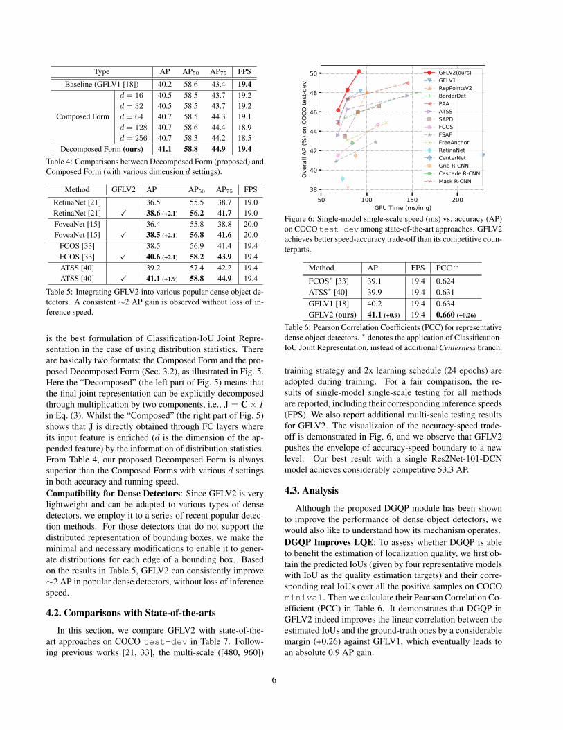
is the best formulation of Classification-IoU Joint Repre-sentation in the case of using distribution statistics. Thereare basically two formats: the Composed Form and the pro-posed Decomposed Form (Sec. 3.2), as illustrated in Fig. 5.Here the “Decomposed” (the left part of Fig. 5) means thatthe final joint representation can be explicitly decomposedthrough multiplication by two components, i.e., J = C× Iin Eq. (3). Whilst the “Composed” (the right part of Fig. 5)shows that J is directly obtained through FC layers whereits input feature is enriched (d is the dimension of the ap-pended feature) by the information of distribution statistics.From Table 4, our proposed Decomposed Form is alwayssuperior than the Composed Forms with various d settingsin both accuracy and running speed.Compatibility for Dense Detectors: Since GFLV2 is verylightweight and can be adapted to various types of densedetectors, we employ it to a series of recent popular detec-tion methods. For those detectors that do not support thedistributed representation of bounding boxes, we make theminimal and necessary modifications to enable it to gener-ate distributions for each edge of a bounding box. Basedon the results in Table 5, GFLV2 can consistently improve∼2 AP in popular dense detectors, without loss of inferencespeed.

4.2. Comparisons with State-of-the-arts

In this section, we compare GFLV2 with state-of-the-art approaches on COCO test-dev in Table 7. Follow-ing previous works [21, 33], the multi-scale ([480, 960])

50 100 150 200GPU Time (ms/img)

38

40

42

44

46

48

50

Over

all A

P (%

) on

COCO

test

-dev

GFLV2(ours)GFLV1RepPointsV2BorderDetPAAATSSSAPDFCOSFSAFFreeAnchorRetinaNetCenterNetGrid R-CNNCascade R-CNNMask R-CNN

Figure 6: Single-model single-scale speed (ms) vs. accuracy (AP)on COCO test-dev among state-of-the-art approaches. GFLV2achieves better speed-accuracy trade-off than its competitive coun-terparts.

Method AP FPS PCC ↑FCOS∗ [33] 39.1 19.4 0.624ATSS∗ [40] 39.9 19.4 0.631GFLV1 [18] 40.2 19.4 0.634GFLV2 (ours) 41.1 (+0.9) 19.4 0.660 (+0.26)

Table 6: Pearson Correlation Coefficients (PCC) for representativedense object detectors. ∗ denotes the application of Classification-IoU Joint Representation, instead of additional Centerness branch.

training strategy and 2x learning schedule (24 epochs) areadopted during training. For a fair comparison, the re-sults of single-model single-scale testing for all methodsare reported, including their corresponding inference speeds(FPS). We also report additional multi-scale testing resultsfor GFLV2. The visualizaion of the accuracy-speed trade-off is demonstrated in Fig. 6, and we observe that GFLV2pushes the envelope of accuracy-speed boundary to a newlevel. Our best result with a single Res2Net-101-DCNmodel achieves considerably competitive 53.3 AP.

4.3. Analysis

Although the proposed DGQP module has been shownto improve the performance of dense object detectors, wewould also like to understand how its mechanism operates.DGQP Improves LQE: To assess whether DGQP is ableto benefit the estimation of localization quality, we first ob-tain the predicted IoUs (given by four representative modelswith IoU as the quality estimation targets) and their corre-sponding real IoUs over all the positive samples on COCOminival. Then we calculate their Pearson Correlation Co-efficient (PCC) in Table 6. It demonstrates that DGQP inGFLV2 indeed improves the linear correlation between theestimated IoUs and the ground-truth ones by a considerablemargin (+0.26) against GFLV1, which eventually leads toan absolute 0.9 AP gain.

6

Method Backbone Epoch MStrain FPS AP AP50 AP75 APS APM APL Referencemulti-stage:Faster R-CNN w/ FPN [20] R-101 24 14.2 36.2 59.1 39.0 18.2 39.0 48.2 CVPR17Cascade R-CNN [1] R-101 18 11.9 42.8 62.1 46.3 23.7 45.5 55.2 CVPR18Grid R-CNN [24] R-101 20 11.4 41.5 60.9 44.5 23.3 44.9 53.1 CVPR19Libra R-CNN [26] X-101-64x4d 12 8.5 43.0 64.0 47.0 25.3 45.6 54.6 CVPR19RepPoints [38] R-101 24 13.3 41.0 62.9 44.3 23.6 44.1 51.7 ICCV19RepPoints [38] R-101-DCN 24 X 11.8 45.0 66.1 49.0 26.6 48.6 57.5 ICCV19RepPointsV2 [4] R-101 24 X 11.1 46.0 65.3 49.5 27.4 48.9 57.3 NeurIPS20RepPointsV2 [4] R-101-DCN 24 X 10.0 48.1 67.5 51.8 28.7 50.9 60.8 NeurIPS20TridentNet [19] R-101 24 X 2.7∗ 42.7 63.6 46.5 23.9 46.6 56.6 ICCV19TridentNet [19] R-101-DCN 36 X 1.3∗ 46.8 67.6 51.5 28.0 51.2 60.5 ICCV19TSD [32] R-101 20 1.1 43.2 64.0 46.9 24.0 46.3 55.8 CVPR20BorderDet [27] R-101 24 X 13.2∗ 45.4 64.1 48.8 26.7 48.3 56.5 ECCV20BorderDet [27] X-101-64x4d 24 X 8.1∗ 47.2 66.1 51.0 28.1 50.2 59.9 ECCV20BorderDet [27] X-101-64x4d-DCN 24 X 6.4∗ 48.0 67.1 52.1 29.4 50.7 60.5 ECCV20

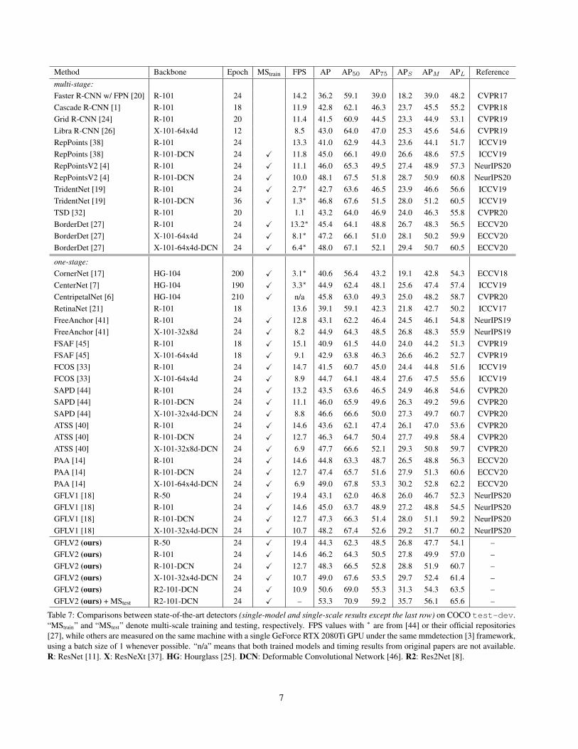
one-stage:CornerNet [17] HG-104 200 X 3.1∗ 40.6 56.4 43.2 19.1 42.8 54.3 ECCV18CenterNet [7] HG-104 190 X 3.3∗ 44.9 62.4 48.1 25.6 47.4 57.4 ICCV19CentripetalNet [6] HG-104 210 X n/a 45.8 63.0 49.3 25.0 48.2 58.7 CVPR20RetinaNet [21] R-101 18 13.6 39.1 59.1 42.3 21.8 42.7 50.2 ICCV17FreeAnchor [41] R-101 24 X 12.8 43.1 62.2 46.4 24.5 46.1 54.8 NeurIPS19FreeAnchor [41] X-101-32x8d 24 X 8.2 44.9 64.3 48.5 26.8 48.3 55.9 NeurIPS19FSAF [45] R-101 18 X 15.1 40.9 61.5 44.0 24.0 44.2 51.3 CVPR19FSAF [45] X-101-64x4d 18 X 9.1 42.9 63.8 46.3 26.6 46.2 52.7 CVPR19FCOS [33] R-101 24 X 14.7 41.5 60.7 45.0 24.4 44.8 51.6 ICCV19FCOS [33] X-101-64x4d 24 X 8.9 44.7 64.1 48.4 27.6 47.5 55.6 ICCV19SAPD [44] R-101 24 X 13.2 43.5 63.6 46.5 24.9 46.8 54.6 CVPR20SAPD [44] R-101-DCN 24 X 11.1 46.0 65.9 49.6 26.3 49.2 59.6 CVPR20SAPD [44] X-101-32x4d-DCN 24 X 8.8 46.6 66.6 50.0 27.3 49.7 60.7 CVPR20ATSS [40] R-101 24 X 14.6 43.6 62.1 47.4 26.1 47.0 53.6 CVPR20ATSS [40] R-101-DCN 24 X 12.7 46.3 64.7 50.4 27.7 49.8 58.4 CVPR20ATSS [40] X-101-32x8d-DCN 24 X 6.9 47.7 66.6 52.1 29.3 50.8 59.7 CVPR20PAA [14] R-101 24 X 14.6 44.8 63.3 48.7 26.5 48.8 56.3 ECCV20PAA [14] R-101-DCN 24 X 12.7 47.4 65.7 51.6 27.9 51.3 60.6 ECCV20PAA [14] X-101-64x4d-DCN 24 X 6.9 49.0 67.8 53.3 30.2 52.8 62.2 ECCV20GFLV1 [18] R-50 24 X 19.4 43.1 62.0 46.8 26.0 46.7 52.3 NeurIPS20GFLV1 [18] R-101 24 X 14.6 45.0 63.7 48.9 27.2 48.8 54.5 NeurIPS20GFLV1 [18] R-101-DCN 24 X 12.7 47.3 66.3 51.4 28.0 51.1 59.2 NeurIPS20GFLV1 [18] X-101-32x4d-DCN 24 X 10.7 48.2 67.4 52.6 29.2 51.7 60.2 NeurIPS20GFLV2 (ours) R-50 24 X 19.4 44.3 62.3 48.5 26.8 47.7 54.1 –GFLV2 (ours) R-101 24 X 14.6 46.2 64.3 50.5 27.8 49.9 57.0 –GFLV2 (ours) R-101-DCN 24 X 12.7 48.3 66.5 52.8 28.8 51.9 60.7 –GFLV2 (ours) X-101-32x4d-DCN 24 X 10.7 49.0 67.6 53.5 29.7 52.4 61.4 –GFLV2 (ours) R2-101-DCN 24 X 10.9 50.6 69.0 55.3 31.3 54.3 63.5 –GFLV2 (ours) + MStest R2-101-DCN 24 X – 53.3 70.9 59.2 35.7 56.1 65.6 –

Table 7: Comparisons between state-of-the-art detectors (single-model and single-scale results except the last row) on COCO test-dev.“MStrain” and “MStest” denote multi-scale training and testing, respectively. FPS values with ∗ are from [44] or their official repositories[27], while others are measured on the same machine with a single GeForce RTX 2080Ti GPU under the same mmdetection [3] framework,using a batch size of 1 whenever possible. “n/a” means that both trained models and timing results from original papers are not available.R: ResNet [11]. X: ResNeXt [37]. HG: Hourglass [25]. DCN: Deformable Convolutional Network [46]. R2: Res2Net [8].

7

FCOS ATSS GFLV1 GFLV2 (ours)

BeforeNMS

AfterNMS

Figure 7: Visualization of predicted bounding boxes before and after NMS, along with their corresponding predicted LQE scores (onlyTop-4 scores are plotted for a better view). For many existing approaches [33, 40, 18], they fail to produce the highest LQE scores for thebest candidates. In contrast, our GFLV2 reliably assigns larger quality scores for those real high-quality ones, thus reducing the risk ofmistaken suppression in NMS processing. White: ground-truth bounding boxes; Other colors: predicted bounding boxes.

1 2 3 4 5 6 7 8 9 10 11 12epoch

0.30

0.35

0.40

0.45

0.50

0.55

loss

of L

QE

GFLV2 (ours)GFLV1

Figure 8: Comparisons of losses on LQE between GFLV1 andGFLV2. DGQP helps to ease the learning difficulty with lowerlosses during training.

DGQP Eases the Learning Difficulty: Fig. 8 provides thevisualization of the training losses on LQE scores, whereDGQP in GFLV2 successfully accelerates the training pro-cess and converges to lower losses.Visualization on Inputs/Outputs of DGQP: To study thebehavior of DGQP, we plot its inputs and correspondingoutputs in Fig. 9. For a better view, we select the mean Top-1 values to represent the input statistics. It is observed thatthe outputs are highly correlated with inputs as expected.Training/Inference Efficiency: We also compare the train-ing and inference efficiency among recent state-of-the-artdense detectors in Table 8. Note that PAA [14], Rep-PointsV2 [4] and BorderDet [27] bring an inevitable timeoverhead (52%, 65%, and 22% respectively) during train-ing, and the latter two also sacrifice inference speed by 30%and 14%, respectively. In contrast, our proposed GFLV2can achieve top performance (∼41 AP) while still maintain-ing the training and inference efficiency.Qualitative Results: In Fig. 7, we qualitatively demon-

0.0 0.2 0.4 0.6 0.8 1.0Top 1 value of General distribution

0.0

0.2

0.4

0.6

0.8

1.0

qual

ity (I

oU) p

redi

ctio

n by

DGQ

P DGQP

Figure 9: Visualization of the input Top-1 values (mean of foursides) from the learned distribution and the output IoU quality pre-diction given by DGQP.

Method AP Training Hours ↓ Inference FPS ↑ATSS∗ [40] 39.9 8.2 19.4GFLV1 [18] 40.2 8.2 19.4PAA [14] 40.4 12.5 (+52%) 19.4RepPointsV2 [4] 41.0 14.4 (+65%) 13.5 (-30%)

BorderDet [27] 41.4 10.0 (+22%) 16.7 (-14%)

GFLV2 (ours) 41.1 8.2 19.4

Table 8: Comparisons of training and inference efficiency based onResNet-50 backbone. “Training Hours” is evaluated on 8 GeForceRTX 2080Ti GPUs under standard 1x schedule (12 epochs). ∗

denotes the application of Classification-IoU Joint Representation.

strate the mechanism how GFLV2 makes use of its morereliable IoU quality estimations to maintain accurate pre-dictions during NMS. Unfortunately for other detectors,high-quality candidates are wrongly suppressed due to theirrelatively lower localization confidences, which eventuallyleads to a performance degradation.

8

5. ConclusionIn this paper, we propose to learn reliable localization

quality estimation, through the guidance of statistics ofbounding box distributions. It is an entirely new and com-pletely different perspective in the literature, which is alsoconceptually effective as the information of distribution ishighly correlated to the real localization quality. Based onit we develop a dense object detector, namely GFLV2. Ex-tensive experiments and analyses on COCO dataset furthervalidate its effectiveness, compatibility and efficiency. Wehope GFLV2 can serve as simple yet effective baseline forthe community.

References[1] Zhaowei Cai and Nuno Vasconcelos. Cascade r-cnn: Delving

into high quality object detection. In CVPR, 2018.[2] Jiale Cao, Yanwei Pang, Jungong Han, and Xuelong Li. Hi-

erarchical shot detector. In ICCV, 2019.[3] Kai Chen, Jiaqi Wang, Jiangmiao Pang, Yuhang Cao, Yu

Xiong, Xiaoxiao Li, Shuyang Sun, Wansen Feng, Ziwei Liu,Jiarui Xu, et al. Mmdetection: Open mmlab detection tool-box and benchmark. arXiv preprint arXiv:1906.07155, 2019.

[4] Yihong Chen, Zheng Zhang, Yue Cao, Liwei Wang, StephenLin, and Han Hu. Reppoints v2: Verification meets regres-sion for object detection. arXiv preprint arXiv:2007.08508,2020.

[5] Jifeng Dai, Haozhi Qi, Yuwen Xiong, Yi Li, GuodongZhang, Han Hu, and Yichen Wei. Deformable convolutionalnetworks. In ICCV, 2017.

[6] Zhiwei Dong, Guoxuan Li, Yue Liao, Fei Wang, Pengju Ren,and Chen Qian. Centripetalnet: Pursuing high-quality key-point pairs for object detection. In CVPR, 2020.

[7] Kaiwen Duan, Song Bai, Lingxi Xie, Honggang Qi, Qing-ming Huang, and Qi Tian. Centernet: Keypoint triplets forobject detection. In ICCV, 2019.

[8] Shanghua Gao, Ming-Ming Cheng, Kai Zhao, Xin-YuZhang, Ming-Hsuan Yang, and Philip HS Torr. Res2net: Anew multi-scale backbone architecture. TPAMI, 2019.

[9] Ross Girshick. Fast r-cnn. In ICCV, 2015.[10] Kaiming He, Georgia Gkioxari, Piotr Dollar, and Ross Gir-

shick. Mask r-cnn. In ICCV, 2017.[11] Kaiming He, Xiangyu Zhang, Shaoqing Ren, and Jian Sun.

Deep residual learning for image recognition. In CVPR,2016.

[12] Zhaojin Huang, Lichao Huang, Yongchao Gong, ChangHuang, and Xinggang Wang. Mask scoring r-cnn. In CVPR,2019.

[13] Borui Jiang, Ruixuan Luo, Jiayuan Mao, Tete Xiao, and Yun-ing Jiang. Acquisition of localization confidence for accurateobject detection. In ECCV, 2018.

[14] Kang Kim and Hee Seok Lee. Probabilistic anchor assign-ment with iou prediction for object detection. ECCV, 2020.

[15] Tao Kong, Fuchun Sun, Huaping Liu, Yuning Jiang, andJianbo Shi. Foveabox: Beyond anchor-based object detec-tor. arXiv preprint arXiv:1904.03797, 2019.

[16] Alex Krizhevsky, Ilya Sutskever, and Geoffrey E Hinton.Imagenet classification with deep convolutional neural net-works. In NeurIPS, 2012.

[17] Hei Law and Jia Deng. Cornernet: Detecting objects aspaired keypoints. In ECCV, 2018.

[18] Xiang Li, Wenhai Wang, Lijun Wu, Shuo Chen, Xiaolin Hu,Jun Li, Jinhui Tang, and Jian Yang. Generalized focal loss:Learning qualified and distributed bounding boxes for denseobject detection. In NeurIPS, 2020.

[19] Yanghao Li, Yuntao Chen, Naiyan Wang, and ZhaoxiangZhang. Scale-aware trident networks for object detection.In ICCV, 2019.

[20] Tsung-Yi Lin, Piotr Dollar, Ross Girshick, Kaiming He,Bharath Hariharan, and Serge Belongie. Feature pyramidnetworks for object detection. In CVPR, 2017.

[21] Tsung-Yi Lin, Priya Goyal, Ross Girshick, Kaiming He, andPiotr Dollar. Focal loss for dense object detection. In ICCV,2017.

[22] Tsung-Yi Lin, Michael Maire, Serge Belongie, James Hays,Pietro Perona, Deva Ramanan, Piotr Dollar, and C LawrenceZitnick. Microsoft coco: Common objects in context. InECCV, 2014.

[23] Wei Liu, Dragomir Anguelov, Dumitru Erhan, ChristianSzegedy, Scott Reed, Cheng-Yang Fu, and Alexander CBerg. Ssd: Single shot multibox detector. In ECCV, 2016.

[24] Xin Lu, Buyu Li, Yuxin Yue, Quanquan Li, and Junjie Yan.Grid r-cnn. In CVPR, 2019.

[25] Alejandro Newell, Kaiyu Yang, and Jia Deng. Stacked hour-glass networks for human pose estimation. In ECCV, 2016.

[26] Jiangmiao Pang, Kai Chen, Jianping Shi, Huajun Feng,Wanli Ouyang, and Dahua Lin. Libra r-cnn: Towards bal-anced learning for object detection. In CVPR, 2019.

[27] Han Qiu, Yuchen Ma, Zeming Li, Songtao Liu, and Jian Sun.Borderdet: Border feature for dense object detection. ECCV,2020.

[28] Joseph Redmon, Santosh Divvala, Ross Girshick, and AliFarhadi. You only look once: Unified, real-time object de-tection. In CVPR, pages 779–788, 2016.

[29] Joseph Redmon and Ali Farhadi. Yolo9000: better, faster,stronger. In CVPR, 2017.

[30] Joseph Redmon and Ali Farhadi. Yolov3: An incrementalimprovement. arXiv preprint arXiv:1804.02767, 2018.

[31] Shaoqing Ren, Kaiming He, Ross Girshick, and Jian Sun.Faster r-cnn: Towards real-time object detection with regionproposal networks. In NeurIPS, 2015.

[32] Guanglu Song, Yu Liu, and Xiaogang Wang. Revisiting thesibling head in object detector. In CVPR, 2020.

[33] Zhi Tian, Chunhua Shen, Hao Chen, and Tong He. Fcos:Fully convolutional one-stage object detection. In ICCV,2019.

[34] Lachlan Tychsen-Smith and Lars Petersson. Improving ob-ject localization with fitness nms and bounded iou loss. InCVPR, 2018.

[35] Jiaqi Wang, Wenwei Zhang, Yuhang Cao, Kai Chen, Jiang-miao Pang, Tao Gong, Jianping Shi, Chen Change Loy, andDahua Lin. Side-aware boundary localization for more pre-cise object detection. ECCV, 2020.

9

[36] Shengkai Wu, Xiaoping Li, and Xinggang Wang. Iou-awaresingle-stage object detector for accurate localization. Imageand Vision Computing, 2020.

[37] Saining Xie, Ross Girshick, Piotr Dollar, Zhuowen Tu, andKaiming He. Aggregated residual transformations for deepneural networks. In CVPR, 2017.

[38] Ze Yang, Shaohui Liu, Han Hu, Liwei Wang, and StephenLin. Reppoints: Point set representation for object detection.In ICCV, 2019.

[39] Haoyang Zhang, Ying Wang, Feras Dayoub, and NikoSunderhauf. Varifocalnet: An iou-aware dense object de-tector. arXiv preprint arXiv:2008.13367, 2020.

[40] Shifeng Zhang, Cheng Chi, Yongqiang Yao, Zhen Lei, andStan Z Li. Bridging the gap between anchor-based andanchor-free detection via adaptive training sample selection.In CVPR, 2020.

[41] Xiaosong Zhang, Fang Wan, Chang Liu, Rongrong Ji, andQixiang Ye. Freeanchor: Learning to match anchors for vi-sual object detection. In NeurIPS, 2019.

[42] Xingyi Zhou, Dequan Wang, and Philipp Krahenbuhl. Ob-jects as points. arXiv preprint arXiv:1904.07850, 2019.

[43] Benjin Zhu, Jianfeng Wang, Zhengkai Jiang, Fuhang Zong,Songtao Liu, Zeming Li, and Jian Sun. Autoassign: Differ-entiable label assignment for dense object detection. arXivpreprint arXiv:2007.03496, 2020.

[44] Chenchen Zhu, Fangyi Chen, Zhiqiang Shen, and MariosSavvides. Soft anchor-point object detection. In CVPR,2020.

[45] Chenchen Zhu, Yihui He, and Marios Savvides. Feature se-lective anchor-free module for single-shot object detection.In CVPR, 2019.

[46] Xizhou Zhu, Han Hu, Stephen Lin, and Jifeng Dai. De-formable convnets v2: More deformable, better results. InCVPR, 2019.

10