generalized emp and nonlinear schrodinger-type
TRANSCRIPT

University of Massachusetts Amherst University of Massachusetts Amherst
ScholarWorks@UMass Amherst ScholarWorks@UMass Amherst
Open Access Dissertations
5-2010
Generalized EMP and Nonlinear Schrodinger-type Reformulations Generalized EMP and Nonlinear Schrodinger-type Reformulations
of Some Scaler Field Cosmological Models of Some Scaler Field Cosmological Models
Jennie D'Ambroise University of Massachusetts Amherst
Follow this and additional works at: https://scholarworks.umass.edu/open_access_dissertations
Part of the Mathematics Commons, and the Statistics and Probability Commons
Recommended Citation Recommended Citation D'Ambroise, Jennie, "Generalized EMP and Nonlinear Schrodinger-type Reformulations of Some Scaler Field Cosmological Models" (2010). Open Access Dissertations. 225. https://scholarworks.umass.edu/open_access_dissertations/225
This Open Access Dissertation is brought to you for free and open access by ScholarWorks@UMass Amherst. It has been accepted for inclusion in Open Access Dissertations by an authorized administrator of ScholarWorks@UMass Amherst. For more information, please contact [email protected].

GENERALIZED EMP AND NONLINEAR
SCHRODINGER-TYPE REFORMULATIONS OF SOME
SCALAR FIELD COSMOLOGICAL MODELS
A Dissertation Presented
by
JENNIE D’AMBROISE
Submitted to the Graduate School of theUniversity of Massachusetts Amherst in partial fulfillment
of the requirements for the degree of
DOCTOR OF PHILOSOPHY
May 2010
Department of Mathematics and Statistics

c© Copyright by Jennie D’Ambroise 2010
All Rights Reserved

GENERALIZED EMP AND NONLINEAR
SCHRODINGER-TYPE REFORMULATIONS OF SOME
SCALAR FIELD COSMOLOGICAL MODELS
A Dissertation Presented
by
JENNIE D’AMBROISE
Approved as to style and content by:
Floyd Williams, Chair
Panayotis Kevrekidis, Member
Robert Kusner, Member
Jennie Traschen, Member
George Avrunin, Department HeadMathematics and Statistics

Dedication
This paper is dedicated to my family,
for supporting me even when I am incomprehensible.

ACKNOWLEDGMENTS
One would like to believe that life is simple and that mathematics is
easy to understand. I would like to thank Floyd Williams for showing
me that sometimes it is possible for both to be true.
To my thesis committee members, Professors Panayotis Kevrekidis,
Robert Kusner and Jennie Traschen, thank you for many useful sug-
gestions on my research. Also, thanks to Michael Satz for always enter-
taining mathematical conversation.
I would like to thank the countless individuals who have made possible a
rich and diverse experience over the course of more than a decade of edu-
cation at the University of Massachusetts at Amherst. The programs in
place have allowed me to have numerous abroad and professional expe-
riences, and the friendly and inquisitive nature of the individuals in the
Department of Mathematics and Statistics has made for an enjoyable
and rigorous graduate experience.
To my students, thank you for surprising me with your willingness to
listen to me talk about mathematics.
To my fellow martial artists, thank you for always welcoming me with-
out question.
To my dear friend John Gusler, thank you for always helping me to get
where I need to go.
v

ABSTRACT
GENERALIZED EMP AND NONLINEAR
SCHRODINGER-TYPE REFORMULATIONS OF SOME
SCALAR FIELD COSMOLOGICAL MODELS
MAY 2010
JENNIE D’AMBROISE,
B.S., UNIVERSITY OF MASSACHUSETTS AT AMHERST
Ph.D., UNIVERSITY OF MASSACHUSETTS AT AMHERST
Directed by: Professor Floyd L. Williams
We show that Einstein’s gravitational field equations for the Friedmann-
Robertson-Lemaıtre-Walker (FRLW) and for two conformal versions of the Bianchi
I and Bianchi V perfect fluid scalar field cosmological models, can be equivalently
reformulated in terms of a single equation of either generalized Ermakov-Milne-
Pinney (EMP) or (non)linear Schrodinger (NLS) type. This work generalizes or
presents an alternative to similar reformulations published by the authors who in-
spired this thesis: R. Hawkins, J. Lidsey, T. Christodoulakis, T. Grammenos, C.
Helias, P. Kevrekidis, G. Papadopoulos and F. Williams. In particular we cast much
of these authors’ works into a single framework via straightforward derivations of
the EMP and NLS equations from a simple linear combination of the relevant
vi

Einstein equations. By rewriting the resulting expression in terms of the volume
expansion factor and performing a change of variables, we obtain an uncoupled
EMP or NLS equation that is independent of the imposition of additional con-
servation equations. Since the correspondences shown here present an alternative
route for obtaining exact solutions to Einstein’s equations, we reconstruct many
known exact solutions via their EMP or NLS counterparts and show by numerical
analysis the stability properties of many solutions.
vii

TABLE OF CONTENTS
ACKNOWLEDGMENTS . . . . . . . . . . . . . . . . . . . . . . . . . . . . . . . . . . . . . . . . . . . . . v
ABSTRACT . . . . . . . . . . . . . . . . . . . . . . . . . . . . . . . . . . . . . . . . . . . . . . . . . . . . . . . . vi
LIST OF TABLES . . . . . . . . . . . . . . . . . . . . . . . . . . . . . . . . . . . . . . . . . . . . . . . . . . x
LIST OF FIGURES . . . . . . . . . . . . . . . . . . . . . . . . . . . . . . . . . . . . . . . . . . . . . . . . . xi
CHAPTER
1. INTRODUCTION . . . . . . . . . . . . . . . . . . . . . . . . . . . . . . . . . . . . . . . . . . . . 1
1.1 Einstein’s field equations (EFE) . . . . . . . . . . . . . . . . . . . . . . . . . . . 11.2 Conservation equations . . . . . . . . . . . . . . . . . . . . . . . . . . . . . . . . . . 41.3 Guide to numerical and exact solutions . . . . . . . . . . . . . . . . . . . . 5
2. THE GENERAL CORRESPONDENCES . . . . . . . . . . . . . . . . . . . . . . . 6
2.1 Scale factor and generalized EMP equations . . . . . . . . . . . . . . . . 62.2 Generalized EMP and Schrodinger-type equations . . . . . . . . . . . 102.3 Scale factor and Schrodinger-type equations . . . . . . . . . . . . . . . . . 16
3. REFORMULATIONS OF THE FRIEDMANN - ROBERTSON -LEMAITRE - WALKER MODEL . . . . . . . . . . . . . . . . . . . . . . . . . . . . . . 29
3.1 In terms of a Generalized EMP . . . . . . . . . . . . . . . . . . . . . . . . . . . 30
3.1.1 First reduction to classical EMP: pure scalar field . . . . . . 343.1.2 Second reduction to classical EMP: zero curvature . . . . . 49
3.2 In terms of a Schrodinger-Type Equation . . . . . . . . . . . . . . . . . . . 56
3.2.1 Reduction to linear Schrodinger: pure scalar field . . . . . . 603.2.2 A nonlinear Schrodinger example . . . . . . . . . . . . . . . . . . . . 70
3.3 In terms of an Alternate Schrodinger-Type Equation . . . . . . . . . 71
3.3.1 Reduction to linear Schrodinger: zero curvature . . . . . . . 753.3.2 A nonlinear Schrodinger example . . . . . . . . . . . . . . . . . . . . 79
4. REFORMULATIONS OF A BIANCHI I MODEL . . . . . . . . . . . . . . . . 82
4.1 In terms of a Generalized EMP . . . . . . . . . . . . . . . . . . . . . . . . . . . 83
4.1.1 Reduction to classical EMP: pure scalar field . . . . . . . . . . 93
4.2 In terms of a Schrodinger-Type Equation . . . . . . . . . . . . . . . . . . . 97
4.2.1 Reduction to linear Schrodinger: pure scalar field . . . . . . 104
viii

5. REFORMULATIONS OF A CONFORMAL BIANCHI I MODEL . . 110
5.1 In terms of a Generalized EMP . . . . . . . . . . . . . . . . . . . . . . . . . . . 111
5.1.1 Reduction to classical EMP: pure scalar field . . . . . . . . . . 119
5.2 In terms of Schrodinger-Type Formulation . . . . . . . . . . . . . . . . . . 120
5.2.1 Reduction to linear Schrodinger: pure scalar field . . . . . . 125
6. REFORMULATIONS OF A BIANCHI V MODEL . . . . . . . . . . . . . . . 132
6.1 In terms of a Generalized EMP . . . . . . . . . . . . . . . . . . . . . . . . . . . 133
6.1.1 Reduction to classical EMP: pure scalar field . . . . . . . . . . 145
6.2 In terms of a Schrodinger-Type Equation . . . . . . . . . . . . . . . . . . . 1486.3 In terms of an Alternate Schrodinger-Type Equation . . . . . . . . . 155
7. REFORMULATIONS OF A CONFORMAL BIANCHI V MODEL . 163
7.1 In terms of a Generalized EMP . . . . . . . . . . . . . . . . . . . . . . . . . . . 164
7.1.1 Reduction to generalized EMP with classical term . . . . . 1737.1.2 Another Bianchi V metric . . . . . . . . . . . . . . . . . . . . . . . . . . 175
7.2 In terms of a Schrodinger-Type Equation . . . . . . . . . . . . . . . . . . . 178
APPENDICES
A. A SHORT LEMMA . . . . . . . . . . . . . . . . . . . . . . . . . . . . . . . . . . . . . . . . . . 185
B. THE EINSTEIN TENSOR IN d+ 1 DIMENSIONS . . . . . . . . . . . . . . . 186
C. THE NON-POSITIVITY OF∑
l<k clck . . . . . . . . . . . . . . . . . . . . . . . . . . 197
D. EXACT SOLUTIONS TO EMP EQUATIONS . . . . . . . . . . . . . . . . . . . 201
E. EXACT SOLUTIONS TO NLS EQUATIONS . . . . . . . . . . . . . . . . . . . . 211
F. EXTRA CONSERVATION EQUATION . . . . . . . . . . . . . . . . . . . . . . . . 221
BIBLIOGRAPHY . . . . . . . . . . . . . . . . . . . . . . . . . . . . . . . . . . . . . . . . . . . . . . . . . . . . 226
ix

LIST OF TABLES
Table Page
1. Theorem 2.1.1 applied to FRLW . . . . . . . . . . . . . . . . . . . . . . . . . . . . . . . . . 32
2. Corollary 2.3.1 applied to FRLW . . . . . . . . . . . . . . . . . . . . . . . . . . . . . . . . 58
3. Corollary 2.3.1 applied to FRLW, alternate . . . . . . . . . . . . . . . . . . . . . . . 73
4. Theorem 2.1.1 applied to Bianchi I . . . . . . . . . . . . . . . . . . . . . . . . . . . . . . . 85
5. Corollary 2.3.1 applied to Bianchi I . . . . . . . . . . . . . . . . . . . . . . . . . . . . . . 99
6. Theorem 2.1.1 applied to conformal Bianchi I . . . . . . . . . . . . . . . . . . . . . 113
7. Corollary 2.3.2 applied to conformal Bianchi I . . . . . . . . . . . . . . . . . . . . . 122
8. Theorem 2.1.1 applied to Bianchi V . . . . . . . . . . . . . . . . . . . . . . . . . . . . . . 135
9. Corollary 2.3.1 applied to Bianchi V . . . . . . . . . . . . . . . . . . . . . . . . . . . . . 150
10. Corollary 2.3.1 applied to Bianchi V, alternate . . . . . . . . . . . . . . . . . . . . 157
11. Theorem 2.1.1 applied to conformal Bianchi V . . . . . . . . . . . . . . . . . . . . . 166
12. Theorem 2.1.1 applied to a third Bianchi V . . . . . . . . . . . . . . . . . . . . . . . 176
13. Corollary 2.3.2 applied to conformal Bianchi V . . . . . . . . . . . . . . . . . . . . 180
14. Exact Solutions of EMP . . . . . . . . . . . . . . . . . . . . . . . . . . . . . . . . . . . . . . . . 202
15. Exact Solutions of NLS . . . . . . . . . . . . . . . . . . . . . . . . . . . . . . . . . . . . . . . . . 211
x

LIST OF FIGURES
Figure Page
1. Stability of FRLW Example 1 . . . . . . . . . . . . . . . . . . . . . . . . . . . . . . . . . . . . 36
2. Stability of FRLW Example 2 . . . . . . . . . . . . . . . . . . . . . . . . . . . . . . . . . . . . 37
3. Instability of FRLW Example 3, d0 = 1/2 . . . . . . . . . . . . . . . . . . . . . . . . . 39
4. Instability of FRLW Example 3, d0 = 1/3 . . . . . . . . . . . . . . . . . . . . . . . . . 39
5. Instability of FRLW Example 4 . . . . . . . . . . . . . . . . . . . . . . . . . . . . . . . . . . 40
6. Instability of FRLW Example 5 . . . . . . . . . . . . . . . . . . . . . . . . . . . . . . . . . . 41
7. Instability of FRLW Example 6, k = 1 . . . . . . . . . . . . . . . . . . . . . . . . . . . . 42
8. Instability of FRLW Example 6, k = −1 . . . . . . . . . . . . . . . . . . . . . . . . . . . 43
9. Instability of FRLW Example 7, k = 0, θ = 1 . . . . . . . . . . . . . . . . . . . . . . . 44
10. Instability of FRLW Example 7, k = 1, θ = 1 . . . . . . . . . . . . . . . . . . . . . . . 45
11. Instability of FRLW Example 7, k = −1, θ = 4 . . . . . . . . . . . . . . . . . . . . . 45
12. Instability of FRLW Example 8 . . . . . . . . . . . . . . . . . . . . . . . . . . . . . . . . . . 47
13. Instability of FRLW Example 9 . . . . . . . . . . . . . . . . . . . . . . . . . . . . . . . . . . 48
14. Instability of FRLW Example 15 . . . . . . . . . . . . . . . . . . . . . . . . . . . . . . . . . 54
15. Instability of FRLW Example 16 . . . . . . . . . . . . . . . . . . . . . . . . . . . . . . . . . 55
16. Instability of FRLW Example 19 . . . . . . . . . . . . . . . . . . . . . . . . . . . . . . . . . 63
17. Instability of FRLW Example 20 . . . . . . . . . . . . . . . . . . . . . . . . . . . . . . . . . 64
18. Instability of FRLW Example 22 . . . . . . . . . . . . . . . . . . . . . . . . . . . . . . . . . 66
19. Instability of FRLW Example 23 . . . . . . . . . . . . . . . . . . . . . . . . . . . . . . . . . 67
20. Instability of FRLW Example 24 . . . . . . . . . . . . . . . . . . . . . . . . . . . . . . . . . 68
21. Instability of FRLW Example 25 . . . . . . . . . . . . . . . . . . . . . . . . . . . . . . . . . 69
xi

22. Instability of FRLW Example 26 . . . . . . . . . . . . . . . . . . . . . . . . . . . . . . . . . 71
23. Instability of FRLW Example 27 . . . . . . . . . . . . . . . . . . . . . . . . . . . . . . . . . 76
24. Instability of FRLW Example 29 . . . . . . . . . . . . . . . . . . . . . . . . . . . . . . . . . 78
25. Instability of FRLW Example 31 . . . . . . . . . . . . . . . . . . . . . . . . . . . . . . . . . 81
26. Instability of Bianchi I Example 34 . . . . . . . . . . . . . . . . . . . . . . . . . . . . . . . 106
27. Instability of Bianchi I Example 36 . . . . . . . . . . . . . . . . . . . . . . . . . . . . . . . 109
28. Instability of conformal Bianchi I Example 37 . . . . . . . . . . . . . . . . . . . . . . 127
29. Instability of conformal Bianchi I Example 38 . . . . . . . . . . . . . . . . . . . . . . 129
30. Instability of conformal Bianchi I Example 39 . . . . . . . . . . . . . . . . . . . . . . 131
xii

C H A P T E R 1
INTRODUCTION
1.1 Einstein’s field equations (EFE)
Einstein’s gravitational field equations (EFE)
Gij = −κTij + Λgij (1.1)
for i, j ∈ 0, . . . , d, are the essential equations of general relativity in d+ 1 space-
time dimensions. The Einstein tensor is Gijdef.= Rij − 1
2Rgij where Rij is the Ricci
tensor, R is the scalar curvature and gij is the metric. Also Λ is the cosmologi-
cal constant and κ is a generalization of 8πG, for G Newton’s constant, to d + 1
spacetime dimensions. In terms of Christoffel symbols of the second kind
Γkij
def.=
1
2
∑
s=0
gsk (gsi,j − gij,s + gjs,i) (1.2)
for i, j, k ∈ 0, 1, . . . , d, we define the Ricci tensor to be
Rijdef.=
d∑
k=0
(
Γkkj,i − Γk
ij,k
)
+
d∑
m=0
d∑
n=0
ΓnimΓm
nj −d∑
m=0
d∑
n=0
ΓmijΓ
nnm (1.3)
for i, j ∈ 0, 1, . . . , d (note that others may define the Ricci tensor to be the
negative of (1.3), in which case the Einstein equations would be Gij = κTij −Λgij).
In (1.2), the subscript ,n denotes differentiation with respect to xn.
1

We will consider an energy-momentum tensor
Tij = T(1)ij + T
(2)ij (1.4)
that is the sum of two terms. The first term is the energy-momentum tensor for a
minimally coupled scalar field φ with potential V so that
T(1)ij = ∂iφ∂jφ− gij
[
1
2
d∑
k=0
∂kφ∂kφ+ V φ]
, (1.5)
where denotes composition and ∂kφdef.=∑d
l=0 gkl∂lφ. We take φ(t) to depend only
on time x0 = t so that (1.5) reduces to
T(1)ij = δ0iδ0jφ
2 − gij
[
1
2g00φ2 + V φ
]
(1.6)
where δ0idef.=
1 if i = 0
0 if i 6= 0. The second term in (1.4) is defined as
T (2) =
−ρ(t)g00
p(t)g11
p(t)g22
. . .
p(t)gdd
(1.7)
for density and pressure functions ρ(t), p(t), and where the off-diagonal entries are
zero.
In the special case when the metric is diagonal and g00 = −1, (1.6) shows that
T(1)00 =
1
2φ2 + V φ (1.8)
and
T(1)ii = gii
(
1
2φ2 − V φ
)
(1.9)
2
for 1 ≤ i ≤ d. That is, T(1)ij reduces to the energy-momentum tensor for a perfect
fluid with density and pressure
ρφ(t) =1
2φ2 + V φ and pφ(t) =
1
2φ2 − V φ, (1.10)
respectively, in terms of the scalar field and potential.
In Chapter 2 we show the equivalence of solving three types of ordinary differ-
ential equations: a generalized Ermakov-Milne-Pinney type equation, a non-linear
Schrodinger type equation and a third equation that we will see arises in each of the
cosmological models considered in this thesis. Since the third type of equation is
derived from Einstein’s field equations in terms of scale factors, we will refer to it as
a scale factor equation. Each subsection of Chapters 3-7 shows the application of a
correspondence established in Chapter 2 to a specific cosmological model. Follow-
ing each theorem in Chapters 3-7, we consider special cases where exact solutions
of Einstein’s equations are derived from exact solutions of an NLS or EMP. For
many examples we show numerical (in-)stability graphs of the exact solutions. The
appendices show some extra calculations including some computations with exact
solutions to EMP and NLS equations [3, 7, 21].
This thesis is a partial response to the proposal by R. Hawkins and J. Lidsey
that EMP equations may appear in certain pure scalar field or other classes of
cosmological models [18]. The results in Chapters 3-7 either generalize or present
an alternative to the reformulations of Einstein’s equations seen in [5, 6, 9, 10, 12,
18, 20, 22, 24, 30, 31]. In [5] and [31], the presence of an exponential term in the
EMP formulation of a Bianchi I model couples the system to a second equation;
in contrast, we find a simpler term so that the Bianchi I EMP here is not coupled
to a second equation. The methods here have been noticed by other researchers
[16, 17] and have been used in some cosmological applications. A brief overview of
3

the methods in this thesis can be found in a shorter paper by the author [11]. For
future work one may consider whether the methods presented here can be extended
to non-Bianchi universes such as a Kantowski-Sachs.
1.2 Conservation equations
The divergence of Einstein’s tensor Gij = Rij − 12Rgij is zero. Therefore by
Einstein’s equations (1.1) the divergence of the energy-momentum tensor is zero.
That is, the conservation equation
div(T )l =∑
i,j
gij
[
∂iTlj −∑
k
ΓkijTlk −
∑
k
ΓkilTkj
]
= 0 (1.11)
for i, j, k, l ∈ 0, 1, . . . d is automatically satisfied by any solution gij of Einstein’s
equations. When Tij is taken to be a sum as in (1.4), one can further impose the
condition
div(T (2))l = 0 (1.12)
for 0 ≤ l ≤ d. The results of this thesis do not rely on T(2)ij satisfying (1.12), which
is not imposed in the theorems in Chapters 3-7. For example, if the scalar field φ(t)
and the potential V are non-constant, the conservation equation (1.12) may not
hold for arbitrary density ρ(t) and pressure p(t) satisfying a corresponding EMP
or NLS. To obtain T(2)ij satisfying (1.12) one can impose an analogue conservation
equation on the EMP or NLS side of the correspondence. We record in Appendix
F equivalent versions of the conservation equation (1.12) for l = 0, translated into
EMP and NLS variables for each of the theorems in Chapters 3-7.
4

1.3 Guide to numerical and exact solutions
The mapping of closed form solutions of EMP or NLS equations to solutions of
Einstein’s equations cannot always be executed analytically, but we will consider
some solutions for which an exact solution to Einstein’s equations can indeed be
(re-)derived via the correspondences in this thesis. Some exact solutions of Ein-
stein’s equations in the literature [1, 2, 4, 13, 14, 15, 16, 17, 19, 20, 23, 24, 26, 27, 29]
will be seen to arise from an exact solution of an EMP or NLS equation.
For some solutions we show a stability graph, where the exact solution is shown
in bold font for comparison. The numerical solutions were generated by running
the Livermore solver (LSODE) [28] on the second order EMP or NLS equation,
coupled to the differential equation for the reparameterization function. In all cases
we graph the volume expansion factor and show that most exact solutions seen here
are unstable. Solutions are said to be unstable here if the difference between the
exact and numerical solutions grow by at least two orders of magnitude over the
graphed time interval.
5

C H A P T E R 2
THE GENERAL CORRESPONDENCES
2.1 Scale factor and generalized EMP equations
In this thesis, the Einstein equations (1.1) for a number of cosmological models
are reduced to a scale factor equation of the form
H(t) + δH(t)2 + εφ(t)2 =
N∑
i=0
Gi(t)
a(t)Ai(2.1)
for H(t)def.= a(t)/a(t) and δ, ε, Ai ∈ R. In this section we show a mapping be-
tween solution sets (a(t), φ(t), G0(t), . . . , GN(t)) of (2.1) and solution sets (Y (τ),
Q(τ), λ0(τ), . . . , λN(τ)) of the generalized EMP equation
Y ′′(τ) +Q(τ)Y (τ) =
N∑
i=0
λi(τ)
Y (τ)Bi(2.2)
for Bi ∈ R. The dictionary between solutions of (2.1) and (2.2) is as follows:
a(t) = Y (τ(t))1/q (2.3)
qεϕ′(τ)2 = Q(τ) (2.4)
Gi(t) =θ2
qλi(τ(t)) (2.5)
for 0 ≤ i ≤ N ∈ N,
φ(t) = ϕ(τ(t)) (2.6)
6

and where τ(t) is a solution to the differential equation
τ (t) = θa(t)q−δ (2.7)
for some constants θ > 0 and q ∈ R\0. Here dot denotes differentiation with
respect to t and prime denotes differentiation with respect to τ . Also the powers
Ai and Bi in (2.1) and (2.2) respectively, are related by the equation
Bi =Ai + q − 2δ
q. (2.8)
Theorem 2.1.1 Suppose you are given a twice differentiable function a(t) > 0, a
once differentiable function φ(t), and also functions G0(t), . . . , GN(t) which satisfy
the scale factor equation (2.1) for some δ, ε, A0, . . . , AN ∈ R and N ∈ N. If f(τ) is
the inverse of a function τ(t) which satisfies (2.7) for some θ > 0 and q ∈ R\0,
then by (2.3)-(2.5) the functions
Y (τ) = a(f(τ))q (2.9)
Q(τ) = qεϕ′(τ)2 (2.10)
λi(τ) =q
θ2Gi(f(τ)) (2.11)
solve the generalized EMP equation (2.2) for Bi as in (2.8) and for
ϕ(τ) = φ(f(τ)) (2.12)
(by (2.6)). Note that since the function a(t) and the constant θ are both positive,
τ(t) > 0 so that τ(t) is an increasing function mapping t ∈ R to τ ∈ R and
therefore the inverse function f(τ) exists.
Conversely, suppose you are given a twice differentiable function Y (τ) > 0,
a continuous function Q(τ), and also functions λ0(τ), . . . , λN(τ) which satisfy the
7
generalized EMP equation (2.2) for some Bi ∈ R and N ∈ N. In order to construct
functions which solve (2.1), first find τ(t) and ϕ(τ) which solve
τ(t) = θY (τ(t))(q−δ)/q (2.13)
and (2.4) respectively, for some θ > 0, q ∈ R\0 and δ ∈ R (note that (2.13)
was obtained by combining (2.3) and (2.7)). Then the set of functions (a(t), φ(t),
G0, . . . , GN ) given by (2.3), (2.6) and (2.5) solves the scale factor equation (2.1)
for Ai as in (2.8). That is, the powers Ai are given in terms of Bi by the equation
Ai = q(Bi − 1) + 2δ. (2.14)
Proof. To prove the forward implication, we begin by computing f ′(τ), a quantity
that will be required to simplify the derivatives of Y (τ). Since f(τ(t)) = t we
differentiate this relation with respect to t to obtain f ′(τ(t))τ (t) = 1 so that f ′(τ) =
1/τ(f(τ)), and by (2.7) we have
f ′(τ) =1
θa(f(τ))δ−q. (2.15)
Differentiating the definition (2.9) of Y (τ) and using (2.15) we obtain
Y ′(τ) = qa(f(τ))q−1a(f(τ))f ′(τ)
=q
θH(f(τ))a(f(τ))δ. (2.16)
Differentiating again and using (2.15) we obtain
Y ′′(τ) =q
θf ′(τ)
[
H(f(τ))a(f(τ))δ + δH(f(τ))2a(f(τ))δ]
=q
θ2a(f(τ))2δ−q
[
H(f(τ)) + δH(f(τ))2]
. (2.17)
Since a(t) is assumed to satisfy the scale factor equation (2.1), (2.16) can be written
Y ′′(τ) =q
θ2a(f(τ))2δ−q
[
−εφ(f(τ))2 +
N∑
i=0
Gi(f(τ))
a(f(τ)))Ai
]
= −qεθ2φ(f(τ))2a(f(τ))2δ−2qa(f(τ))q +
N∑
i=0
qθ2Gi(f(τ))
a(f(τ))Ai+q−2δ. (2.18)
8

Differentiating the definition (2.12) of ϕ(τ) and again using (2.15) we have
ϕ′(τ) = φ(f(τ))f ′(τ) =1
θφ(f(τ))a(f(τ))δ−q, (2.19)
so that the definition (2.10) of Q(τ) can be written as
Q(τ) =qε
θ2φ(f(τ))2a(f(τ))2δ−2q . (2.20)
By (2.20) and the definitions (2.9), (2.11) and (2.8) of Y (τ), λi(τ) and Bi ∈ R
respectively, (2.18) becomes
Y ′′(τ) +Q(τ)Y (τ) =N∑
i=0
λi(τ)
Y (τ)Bi. (2.21)
To prove the converse statement, differentiate the definition (2.3) of a(t) and
use the definition (2.13) of τ(t) to obtain
a(t) =1
qY (τ(t))(1−q)/qY ′(τ(t))τ (t)
=θ
qY (τ(t))(1−δ)/qY ′(τ(t)). (2.22)
Dividing by a(t), we have that
H(t)def.=
a(t)
a(t)=θ
qY ′(τ(t))Y (τ(t))−δ/q . (2.23)
Differentiating (2.23) and again using the definition (2.13) of τ(t), we obtain
H(t) =θ
qτ(t)
[
Y ′′(τ(t))Y (τ(t))−δ/q − δ
qY ′(τ(t))2Y (τ(t))−(δ+q)/q
]
=θ2
qY (τ(t))(q−δ)/q
[
Y ′′(τ(t))Y (τ(t))−δ/q − δ
qY ′(τ(t))2Y (τ(t))−(δ+q)/q
]
=θ2
qY (τ(t))(q−2δ)/qY ′′(τ) − δθ2
q2Y ′(τ(t))2Y (τ(t))−2δ/q. (2.24)
9

Since Y (τ) is assumed to satisfy the generalized EMP equation (2.2), equation
(2.24) can be written as
H(t) =θ2
qY (τ(t))(q−2δ)/q
[
−Q(τ(t))Y (τ(t)) +N∑
i=0
λi(τ(t))
Y (τ(t))Bi
]
−δθ2
q2Y ′(τ(t))2Y (τ(t))−2δ/q
= −θ2
qQ(τ(t))Y (τ(t))2(q−δ)/q +
N∑
i=0
θ2
qλi(τ(t))
Y (τ(t))(q(Bi−1)+2δ)/q
−δθ2
q2Y ′(τ(t))2Y (τ(t))−2δ/q . (2.25)
By definitions (2.6) and (2.13) of φ(t) and τ(t) respectively, we have that
φ(t) = ϕ′(τ(t))τ (t) = θϕ′(τ(t))Y (τ(t))(q−δ)/q . (2.26)
Using definition (2.4) of ϕ(τ) in terms of Q(τ) and squaring (2.26), we have
φ(t)2 =θ2
qεQ(τ(t))Y (τ(t))2(q−δ)/q . (2.27)
This shows that the first term in (2.25) is equal to −εφ(t)2. Noting that by (2.23)
the last term of (2.25) is equal to −δH(t)2, and using definitions (2.3), (2.5) and
(2.14) of a(t), Gi(t) and Ai respectively, (2.25) becomes
H(t) = −εφ(t)2 +
N∑
i=0
Gi(t)
a(t)Ai− δH(t)2. (2.28)
This proves the theorem.
⋄
2.2 Generalized EMP and Schrodinger-type equations
We now record a mapping between any solution set (Y (τ), Q(τ), λ(τ), λ1(τ),
. . . , λN(τ)) of the generalized EMP equation
Y ′′(τ) +Q(τ)Y (τ) =λ(τ)
Y (τ)B+
N∑
i=1
λi(τ)
Y (τ)Bi(2.29)
10

for B ∈ R\−1, 1, Bi ∈ R\−1, N ∈ N, and a corresponding solution set
(u(σ), E(σ), P (σ), F1(σ), . . . , FN(σ)) of what we will call a non-linear Schrodinger-
type equation
u′′(σ) + [E(σ) − P (σ)]u(σ) =
N∑
i=1
Fi(σ)
u(σ)Ci(2.30)
for Ci ∈ R.
In general, the Schrodinger-type equation (2.30) contains one less non-linear
term than the generalized EMP equation (2.29). Therefore although the correspon-
dence does hold when λ = λi = E = 0, the point is that a nonzero nonlinear term
λ(τ)/Y (τ)B in (2.29) transforms to the linear term E(σ)u(σ) in (2.30). Therefore
the “Schrodinger” nature of this latter equation is most apparent when λi(τ) = 0
for 1 ≤ i ≤ N and when the function λ(τ) = λ is constant in (2.29). In this case
(as we will see in this section), solutions to the generalized EMP
Y ′′(τ) +Q(τ)Y (τ) =λ
Y (τ)B(2.31)
correspond to solutions of a one-dimensional linear Schrodinger equation
u′′(σ) + [E − P (σ)]u(σ) = 0 (2.32)
for E constant. This slightly generalizes a result of F. Williams in which solutions
of a classical EMP (that is, for B = 3 in (2.31)) are shown to be in correspondence
with solutions of a linear Schrodinger equation (2.32). One can also refer to the
paper of W. Milne [25].
The dictionary between solutions to (2.29) and (2.30) is as follows:
Y (τ(t))B−1 = u(σ(t))−2 (2.33)
ϑ2(B − 1)Q(τ(t))(B−1)/(B+1) = 2P (σ(t))u(σ(t))2 (2.34)
ϑ2(B − 1)λ(τ(t)) = 2E(σ(t)) (2.35)
ϑ2(B − 1)λi(τ(t)) = 2Fi(σ(t)) (2.36)
11

where τσ(t) and σ(t) are solutions to the differential equations
τσ(t) =√ϑY (τσ(t))
14(B+1) (2.37)
and
σ(t) =1√ϑu(σ(t))
12(B+1)/(B−1) (2.38)
respectively, for some ϑ > 0. Also the powers Bi and Ci in (2.29) and (2.30)
respectively, are related by the equation
Ci = 1 − 2(Bi − 1)
(B − 1). (2.39)
Note that by (2.33), (2.37) and (2.38), we have
τσ(t) =1
σ(t). (2.40)
We notate the function τσ(t) with the subscript σ in order to distinguish it from
the separate quantity τ(t) which appears in section 2.1.
Theorem 2.2.1 Suppose you are given a twice differentiable function Y (τ) > 0
and also functions Q(τ), λ(τ), λ1(τ), . . . , λN(τ) which satisfy the generalized EMP
equation (2.29) for some B ∈ R\−1, 1, Bi ∈ R\−1 and N ∈ N. In order to
construct a set of functions which solve the Schrodinger-type equation (2.30), begin
by solving for the function τσ(t) in (2.37) (for any ϑ > 0) and then solve (2.40) for
σ(t) . Let g(σ) denote the inverse of σ(t) (which exists since σ(t) > 0 for all t).
Then by (2.33)-(2.36) the following functions solve the Schrodinger-type equation
(2.30):
u(σ) = Y (τσ(g(σ)))12(1−B) (2.41)
P (σ) =ϑ2
2(B − 1)Q(τσ(g(σ)))Y (τσ(g(σ)))B+1 (2.42)
E(σ) =ϑ2
2(B − 1)λ(τσ(g(σ))) (2.43)
Fi(σ) =ϑ2
2(1 −B)λi(τσ(g(σ))) (2.44)
12

for Ci as in (2.39).
Conversely, suppose you are given a twice differentiable function u(σ) > 0 and
also functions E(σ), P (σ), Fi(σ) which satisfy the Schrodinger-type equation (2.30)
for some Ci ∈ R and N ∈ N. In order to construct functions which solve (2.29),
first solve (2.38) for σ(t) and for any constants ϑ > 0 and B ∈ R\−1, 1. Then
solve for τσ(t) in (2.40) and let fσ(τ) denote its inverse (which exists since τσ(t) > 0
for all t). By (2.33)-(2.36), the functions
Y (τ) = u(σ(fσ(τ)))2/(1−B) (2.45)
Q(τ) =2
ϑ2(B − 1)P (σ(fσ(τ)))u(σ(fσ(τ)))2(B+1)/(B−1) (2.46)
λ(τ) =2
ϑ2(B − 1)E(σ(fσ(τ))) (2.47)
λi(τ) =2
ϑ2(1 − B)Fi(σ(fσ(τ))) (2.48)
satisfy the generalized EMP (2.29) for
Bi =1
2((1 − B)Ci + (B + 1))) (2.49)
(by (2.39)).
Proof. To prove the forward statement, we begin by computing g′(σ), a quantity
that will be required to simplify the derivatives of u(σ). Since g(σ(t)) = t, we
differentiate this relation with respect to t and obtain g′(σ(t))σ(t) = 1 so that
g′(σ) = 1/σ(g(σ)) = τσ(g(σ)). Therefore by (2.37) we have
τσ(g(σ))g′(σ) = ϑ Y (τσ(g(σ)))(B+1)/2. (2.50)
Differentiating the definition (2.41) of u(σ) and using (2.50), we obtain
u′(σ) =1
2(1 −B)Y (τσ(g(σ)))−(B+1)/2Y ′(τσ(g(σ)))τσ(g(σ))g′(σ)
=ϑ
2(1 − B)Y (τσ(g(σ)))−(B+1)/2+(B+1)/2Y ′(τσ(g(σ)))
=ϑ
2(1 − B)Y ′(τσ(g(σ))). (2.51)
13

Differentiating again and using (2.50), we see that
u′′(σ) =ϑ
2(1 −B)Y ′′(τσ(g(σ)))τσ(g(σ))g′(σ)
=ϑ2
2(1 − B)Y ′′(τσ(g(σ)))Y (τσ(g(σ)))(B+1)/2. (2.52)
Since Y (τ) is assumed to satisfy the generalized EMP equation (2.29), (2.52) be-
comes
u′′(σ) =ϑ2
2(1 − B)Y (τσ(g(σ)))(B+1)/2 [−Q(τσ(g(σ)))Y (τσ(g(σ)))
+λ(τσ(g(σ)))
Y (τσ(g(σ)))B+
N∑
i=1
λi(τσ(g(σ)))
Y (τσ(g(σ)))Bi
]
=ϑ2
2(B − 1)Q(τσ(g(σ)))Y (τσ(g(σ)))B+1Y (τσ(g(σ)))(1−B)/2
−ϑ2(B − 1)λ(τσ(g(σ)))
2Y (τσ(g(σ)))(B−1)/2+
N∑
i=1
ϑ2(1 −B)λi(τσ(g(σ)))
2Y (τσ(g(σ)))Bi− 12(B+1)
.
(2.53)
By the definitions (2.41),(2.42), (2.43) and (2.44) of u(σ), P (σ), E(σ) and Fi(σ)
respectively, we have that
u′′(σ) = P (σ)u(σ)− E(σ)
u(σ)−1+
N∑
i=1
Fi(σ)
u(σ)2Bi−(B+1)
1−B
.
= P (σ)u(σ)− E(σ)u(σ) +
N∑
i=1
Fi(σ)
u(σ)Ci(2.54)
for Ci as in (2.39). This proves the forward implication.
To prove the converse statement, we will need f ′σ(τ) in order to simplify the
derivatives of Y (τ). Differentiating the relation fσ(τσ(t)) = t with respect to t
implies f ′σ(τσ(t))τσ(t) = 1 therefore f ′
σ(τ) = 1/τσ(fσ(τ)) = σ(fσ(τ)). By (2.38) we
can form the useful quantity
σ(fσ(τ))f ′σ(τ) =
1
ϑu(σ(fσ(τ)))
(B+1)(B−1) . (2.55)
14

Now differentiating the definition of Y (τ) and using (2.55), we see that
Y ′(τ) =2
(1 −B)u(σ(fσ(τ)))
(B+1)(1−B)u′(σ(fσ(τ)))σ(fσ(τ))f ′
σ(τ)
=2
ϑ(1 − B)u(σ(fσ(τ)))
(B+1)(1−B)
+ (B+1)(B−1)u′(σ(fσ(τ)))
=2
ϑ(1 − B)u′(σ(fσ(τ))). (2.56)
Differentiating Y ′(τ) and again using (2.55), we obtain
Y ′′(τ) =2
ϑ(1 −B)u′′(σ(fσ(τ)))σ(fσ(τ))f
′σ(τ)
=2
ϑ2(1 − B)u′′(σ(fσ(τ)))u(σ(fσ(τ)))
(B+1)(B−1) . (2.57)
Since u(σ) is assumed to satisfy the Schrodinger-type equation (2.30), the equation
(2.57) can be written as
Y ′′(τ) =2
ϑ2(1 − B)u(σ(fσ(τ)))
(B+1)/(B−1) [−E(σ(fσ(τ)))u(σ(fσ(τ)))
+P (σ(fσ(τ)))u(σ(fσ(τ))) +
N∑
i=1
Fi(σ(fσ(τ)))
u(σ(fσ(τ)))Ci
]
=2E(σ(fσ(τ)))
ϑ2(B − 1)u(σ(fσ(τ)))−2B/(B−1)
− 2
ϑ2(B − 1)P (σ(fσ(τ)))u(σ(fσ(τ)))2(B+1)/(B−1)u(σ(fσ(τ)))
2/(1−B)
+N∑
i=1
2Fi(σ(fσ(τ)))/(1 − B)
ϑ2u(σ(fσ(τ)))((B−1)Ci−(B+1))/(B−1). (2.58)
By the definitions (2.45), (2.46), (2.47) and (2.48) of Y (τ), Q(τ), λ(τ) and λi(τ)
respectively, we obtain
Y ′′(τ) =λ(τ)
Y (τ)B−Q(τ)Y (τ) +
N∑
i=1
λi(τ)
Y (τ)Bi(2.59)
for Ci as in (2.39). This proves the theorem.
⋄
15

2.3 Scale factor and Schrodinger-type equations
By composing the maps in Theorems 2.1.1 and 2.2.1, one can see that a direct
reformulation of the scale factor equation
H(t) + δH(t)2 + εφ(t)2 =G(t)
a(t)A+
N∑
i=1
Gi(t)
a(t)Ai(2.60)
(again H(t) = a(t)/a(t)) in terms of the nonlinear Schrodinger-type equation
u′′(σ) + [E(σ) − P (σ)]u(σ) =N∑
i=1
Fi(σ)
u(σ)Ci(2.61)
is possible by identifying B0 in Theorem 2.1.1 with B in Theorem 2.2.1. The
theorem below is exactly the resulting statement. As we noted in Section 2.2,
this reformulation of the scale factor equation (2.60) in terms of the non-linear
Schrodinger-type equation (2.61) will have one less non-linear term than the alter-
nate generalized EMP reformulation seen in Section 2.1.
For the forward implication of the theorem in this section, composing the re-
spective notations of Theorems 2.1.1 and 2.2.1 is convenient. However this is not
true for the converse implication, in which we now use new notation which is equiv-
alent to identifying (A0 − 2δ)/q and A0/(q− δ) of Theorem 2.1.1 with n/3 and m,
respectively, used here. Here we also rename A0 of Theorem 2.1.1 to just A.
In summary, the dictionary between functions which solve (2.60) and functions
which solve (2.61) is as follows:
a(f(τσ(t)))(A−2δ) = u(σ(t))−2 (2.62)
ε(A− 2δ)ψ′(σ)2 = 2P (σ) (2.63)
(A− 2δ)θA/(q−δ)G(f(τσ(t))) = 2E(σ(t)) (2.64)
(2δ −A)θA/(q−δ)Gi(f(τσ(t))) = 2Fi(σ(t)) (2.65)
16

where f(τ) is the inverse function of τ(t) and each of τ(t) and σ(t) are solutions to
the differential equations
τ (t) = θa(t)q−δ, (2.66)
σ(t) =1√ϑu(σ(t))(n+6)/2n (2.67)
respectively for some constants θ, ϑ > 0, q ∈ R\δ and n ∈ R\0. Also φ and ψ
are related by the composition
φ(f(τσ(t))) = ψ(σ(t)), (2.68)
and the powers Ai and Ci in (2.60) and (2.61) respectively, are related by the
equation
Ci = 1 − 2(Ai − 2δ)
(A− 2δ). (2.69)
In addition, depending on which direction one is mapping solutions, it may be
convenient to define τσ(t) as the solution to either
τσ(t) =1
σ(t)(2.70)
or equivalently by (2.67), (2.62) and (2.66),
τσ(t) = τ(f(τσ(t)))(A+2q−2δ)/4(q−δ). (2.71)
Theorem 2.3.1 Suppose you are given a twice differentiable function a(t) > 0, a
once differentiable function φ(t), and also functions G(t), G1(t), . . . , GN(t) which
satisfy the scale factor equation (2.60) for some N ∈ N and δ, ε, A,A1, . . . , AN
∈ R where A 6= 2δ. In order to construct a set of functions which solve the non-
linear Schrodinger-type equation (2.61), begin by solving for τ(t) in the differential
equation (2.66) for any constants θ > 0 and q ∈ R\δ. Let f(τ) denote the inverse
of τ(t) (which exists since τ(t) > 0 for all t), find the solution τσ(t) to (2.71) and
17

then find σ(t) which solves (2.70). Let g(σ) to denote the inverse function of σ(t)
(which exists since τ(t) > 0 for all t). Then by (2.62)-(2.65) the following functions
solve the Schrodinger-type equation (2.61):
u(σ) = a(f(τσ(g(σ)))(2δ−A)/2 (2.72)
P (σ) =1
2ε(A− 2δ)ψ′(σ)2 (2.73)
E(σ) =1
2(A− 2δ)θA/(q−δ)G(f(τσ(g(σ)))) (2.74)
Fi(σ) =1
2(2δ −A)θA/(q−δ)Gi(f(τσ(g(σ)))) (2.75)
for Ci as in (2.69) and for
ψ(σ) = φ(f(τσ(g(σ)))) (2.76)
(by (2.68)).
Conversely, suppose you are given a twice differentiable function u(σ) > 0, a
continuous function P (σ) and also functions E(σ), F1(σ), . . . , FN(σ) which satisfy
the Schrodinger-type equation (2.61) for some Ci ∈ R, and N ∈ N. In order to
construct functions which solve the scale factor equation (2.60), begin by solving for
σ(t) in the differential equation (2.67) for some ϑ > 0 and n ∈ R\0. Then find a
solution τσ(t) to (2.70) and let fσ(τ) denote the inverse of τσ(t) (which exists since
σ(t) > 0 for all t). Next find functions τ(t) and ψ(σ) which solve the differential
equations
τ (t) = τσ(fσ(τ(t)))4/(m+2) (2.77)
and
ψ′(σ)2 =6
εqnP (σ) (2.78)
respectively, for any m ∈ R\−2 and ε, q ∈ R\0 (these equations are obtained
by writing (2.71) and (2.63) in the converse notation). Then by (2.62)-(2.65), the
18

following functions solve the scale factor equation (2.60):
a(t) = u(σ(fσ(τ(t))))−6/qn (2.79)
φ(t) = ψ(σ(fσ(τ(t))))) (2.80)
G(t) =6
qnϑ−2m/(m+2)E(σ(fσ(τ(t)))) (2.81)
Gi(t) = − 6
qnϑ−2m/(m+2)Fi(σ(fσ(τ(t)))) (2.82)
for coefficient
δ =q(3m− n)
3(m+ 2)(2.83)
and for powers
A =qm(n+ 6)
3(2 +m), Ai =
q
6
(
(nm− 2n+ 12m)
(m+ 2)− nCi
)
(2.84)
(by (2.69) in the converse notation).
Proof. To prove the forward implication, we first compute f ′(τ) and g′(σ). Dif-
ferentiating the relation f(τ(t)) = t with respect to t gives f ′(τ(t))τ (t) = 1 so that
f ′(τ) = 1/τ(f(τ)). Therefore by (2.66), we have
f ′(τ) =1
θa(f(τ))δ−q. (2.85)
Similarly g(σ(t)) = t implies g′(σ(t))σ(t) = 1 so that g′(σ) = 1/σ(g(σ)) = τσ(g(σ)),
and then by (2.71) and (2.66) we obtain
g′(σ) = τ (f(τσ(g(σ))))(A+2q−2δ)/4(q−δ)
= θ(A+2q−2δ)/4(q−δ)a(f(τσ(g(σ))))(A+2q−2δ)/4. (2.86)
By (2.85), (2.86) and (2.71), we find that
f ′(τσ(g(σ)))τσ(g(σ))g′(σ) = θ(A+2q−2δ)/2(q−δ)−1a(f(τσ(g(σ))))(A+2q−2δ)/2+δ−q
= θA/2(q−δ)a(f(τσ(g(σ))))A/2. (2.87)
19

Differentiating the definition (2.72) of u(σ) and using (2.87), we have that
u′(σ) =1
2(2δ −A)a(f(τσ(g(σ))))(2δ−A−2)/2a(f(τσ(g(σ))))
·f ′(τσ(g(σ)))τσ(g(σ))g′(σ)
=1
2(2δ −A)θA/2(q−δ)a(f(τσ(g(σ))))a(f(τσ(g(σ))))δ−1
=1
2(2δ −A)θA/2(q−δ)H(f(τσ(g(σ))))a(f(τσ(g(σ))))δ (2.88)
for H(t)def.= a(t)/a(t). Differentiating u′(σ) and using (2.87) and the assumed scale
factor equation (2.60), the second derivative of u is
u′′(σ) =1
2(2δ −A)θA/2(q−δ)f ′(τσ(g(σ)))τσ(g(σ))g′(σ)
·[
H(f(τσ(g(σ))))a(f(τσ(g(σ))))δ + δH(f(τσ(g(σ))))2a(f(τσ(g(σ))))δ]
=1
2(2δ −A)θA/(q−δ)a(f(τσ(g(σ))))A/2+δ
·[
−εφ(f(τσ(g(σ))))2 +G(f(τσ(g(σ))))
a(f(τσ(g(σ))))A+
N∑
i=1
Gi(t)
a(f(τσ(g(σ))))Ai
]
=1
2(A− 2δ)εθA/(q−δ)a(f(τσ(g(σ))))A/2+δφ(f(τσ(g(σ))))2
+1
2(2δ − A)θA/(q−δ)G(f(τσ(g(σ))))a(f(τσ(g(σ))))δ−A/2
+1
2(2δ −A)θA/(q−δ)
N∑
i=1
Gi(f(τσ(g(σ))))
a(f(τσ(g(σ))))(2Ai−A−2δ)/2. (2.89)
Differentiating the definition (2.76) of ψ(σ) and using (2.87) we see that
ψ′(σ) = θA/2(q−δ)φ(f(τσ(g(σ))))a(f(τσ(g(σ))))A/2 (2.90)
so that by (2.73), we can write P (σ) as
P (σ) =1
2ε(A− 2δ)θA/(q−δ)φ(f(τσ(g(σ))))2a(f(τσ(g(σ))))A. (2.91)
By (2.91) and the definitions (2.72), (2.74) and (2.75) of u(σ), E(σ) and Fi(σ)
20

respectively, (2.89) becomes
u′′(σ) = P (σ)u(σ) −E(σ)u(σ) +
N∑
i=1
Fi(σ)
u(σ)(2Ai−A−2δ)/(2δ−A)
= P (σ)u(σ) −E(σ)u(σ) +N∑
i=1
Fi(σ)
u(σ)Ci(2.92)
for Ci as in (2.69). This proves the forward implication.
To prove the converse statement, we will need the function f ′σ(τ). Differentiating
the relation fσ(τσ(t)) = t with respect to t implies that f ′σ(τσ(t))τσ(t) = 1 and so
we have f ′σ(τ) = 1/τσ(fσ(τ)) = σ(fσ(τ)). Therefore by (2.77) and (2.70), we obtain
the useful quantity
σ(fσ(τ(t)))f ′σ(τ(t))τ (t) = σ(fσ(τ(t)))2τσ(fσ(τ(t)))4/(m+2)
= σ(fσ(τ(t)))2σ(fσ(τ(t)))−4/(m+2)
= σ(fσ(τ(t)))2m/(m+2). (2.93)
Using (2.67) to write this in terms of u(σ), we have
σ(fσ(τ(t)))f′σ(τ(t))τ (t) = ϑ−m/(m+2)u(σ(fσ(τ(t))))
m(n+6)n(m+2) . (2.94)
Differentiating definition (2.79) of a(t) gives
a(t) = − 6
qnu(σ(fσ(τ(t))))−(6+qn)/qnu′(σ(fσ(τ(t))))σ(fσ(τ(t)))f ′
σ(τ(t))τ (t).
(2.95)
Dividing by a(t) = u(σ(fσ(τ(t))))−6/qn and using (2.94), we obtain
H(t) = − 6
qnϑ−m/(m+2)u′(σ(fσ(τ(t))))u(σ(fσ(τ(t))))
m(n+6)n(m+2)
−1
= − 6
qnϑ−m/(m+2)u′(σ(fσ(τ(t))))u(σ(fσ(τ(t))))
2(3m−n)n(m+2) (2.96)
for H(t)def.= a(t)/a(t) as usual. Differentiating H(t) and again using (2.94), we get
21

that
H(t) = − 6
qnϑ−m/(m+2)σ(fσ(τ(t)))f
′σ(τ(t))τ (t) ·
[
u′′(σ(fσ(τ(t))))u(σ(fσ(τ(t))))2(3m−n)n(m+2)
+2(3m− n)
n(m+ 2)u′(σ(fσ(τ(t))))2u(σ(fσ(τ(t))))
2(3m−n)n(m+2)
−1
]
= − 6
qnϑ−2m/(m+2)u′′(σ(fσ(τ(t))))u(σ(fσ(τ(t))))
(12m−2n+mn)/n(m+2)
−12(3m− n)
qn2(m+ 2)ϑ−2m/(m+2)u′(σ(fσ(τ(t))))2u(σ(fσ(τ(t))))
4(3m−n)n(m+2) ,
(2.97)
where we have simplified the powers of u(σ(fσ(τ(t)))) for the first and second terms
by adding
m(n+ 6)
n(m+ 2)+
2(3m− n)
n(m+ 2)=
12m− 2n+mn
n(m+ 2)(2.98)
and
m(n + 6)
n(m+ 2)+
2(3m− n)
n(m+ 2)− 1 =
4(3m− n)
n(m+ 2), (2.99)
respectively. Since u(σ) is assumed to satisfy the Schrodinger-type equation (2.61),
H in (2.97) now becomes
H(t) = − 6
qnϑ−2m/(m+2)u(σ(fσ(τ(t))))
(12m−2n+mn)/n(m+2) ·
[P (σ(fσ(τ(t))))u(σ(fσ(τ(t)))) − E(σ(fσ(τ(t))))u(σ(fσ(τ(t))))
+N∑
n=1
Fi(σ(fσ(τ(t))))
u(σ(fσ(τ(t))))Ci
]
−12(3m− n)
qn2(m+ 2)ϑ−2m/(m+2)u′(σ(fσ(τ(t))))2u(σ(fσ(τ(t))))
4(3m−n)n(m+2) .
(2.100)
Multiplying out the terms, we obtain
H(t) = − 6
qnϑ−2m/(m+2)u(σ(fσ(τ(t))))
2m(n+6)n(m+2) P (σ(fσ(τ(t))))
+6
qnϑ−2m/(m+2)u(σ(fσ(τ(t))))
2m(n+6)n(m+2) E(σ(fσ(τ(t))))
22

− 6
qnϑ−2m/(m+2)
N∑
n=1
Fi(σ(fσ(τ(t))))
u(σ(fσ(τ(t))))Ci+(2n−12m−mn)/n(m+2)
−12(3m− n)
qn2(m+ 2)ϑ−2m/(m+2)u′(σ(fσ(τσ(t))))2u(σ(fσ(τ(t))))
4(3m−n)n(m+2)
(2.101)
where for the first two terms, we have simplified the powers of u by adding
12m− 2n +mn
n(m+ 2)+ 1 =
2m(n + 6)
n(m+ 2). (2.102)
By the definition (2.83) of the constant δ, and by the computation (2.96) of H in
terms of u, we have that
δH(t)2 =12(3m− n)
qn2(m+ 2)ϑ−2m/(m+2)u′(σ(fσ(τ(t))))2u(σ(fσ(τ(t))))
4(3m−n)n(m+2) . (2.103)
This shows that the last term in (2.101) is equal to −δH(t)2 so that we have
H(t) + δH(t)2 = − 6
qnϑ−2m/(m+2)u(σ(fσ(τ(t))))
2m(n+6)n(m+2) P (σ(fσ(τ(t))))
+6
qnϑ−2m/(m+2)u(σ(fσ(τ(t))))
2m(n+6)n(m+2) E(σ(fσ(τ(t))))
− 6
qnϑ−2m/(m+2)
N∑
n=1
Fi(σ(fσ(τ(t))))
u(σ(fσ(τ(t))))Ci+(2n−12m−mn)/n(m+2).
(2.104)
Differentiating the definition (2.80) of φ(t) and using (2.94), we have that
φ(t) = ψ′(σ(fσ(τ(t))))σ(fσ(τ(t)))f ′σ(τ(t))τ (t)
= ϑ−m/(m+2)u(σ(fσ(τ(t))))m(n+6)n(m+2)ψ′(σ(fσ(τ(t)))). (2.105)
Using the definition (2.78) of ψ(σ) in terms of P (σ) and squaring (2.105), we obtain
φ(t)2 =6
εqnϑ−2m/(m+2)P (σ(fσ(τ(t))))u(σ(fσ(τ(t))))
2m(n+6)n(m+2) . (2.106)
23

This shows that the first term in (2.104) is equal to −εφ(t)2 so that
H(t) + δH(t)2 = −εφ(t)2 +6
qnϑ−2m/(m+2)u(σ(fσ(τ(t))))
2m(n+6)n(m+2) E(σ(fσ(τ(t))))
− 6
qnϑ−2m/(m+2)
N∑
n=1
Fi(σ(fσ(τ(t))))
u(σ(fσ(τ(t))))Ci+(2n−12m−mn)/n(m+2).
(2.107)
Now utilizing the definitions (2.79), (2.81) and (2.82) of a(t), G(t) and Gi(t) re-
spectively, (2.107) becomes
H(t) + δH(t)2 = −εφ2 +G(t)
a(t)qm(n+6)3(m+2)
+
N∑
i=1
Gi(t)
a(t)−qn6
Ci−q(2n−12m−mn)/6(m+2)
= −εφ2 +G(t)
a(t)A+
N∑
i=1
Gi(t)
a(t)Ai, (2.108)
which proves the theorem for A and Ai as in (2.124). ⋄
The statement of this theorem would have been much simpler if we were able
to choose τ(t) = τσ(t), since then many compositions of functions would cancel. In
fact, such cancellations would make the use of τ(t) obsolete, leaving only σ(t) and
its inverse g(σ) to be required for the reparameterization which takes place in the
translation between the functions a(t) and u(σ). By (2.71) in the forward direction
or equivalently (2.77) in the converse, τ (t) = τσ(t) for (A + 2q − 2δ)/4(q − δ) = 1
and 4/(m + 2) = 1 respectively. This corresponds to the choice of parameter
q = A/2 + δ, or equivalently m = 2 and n = 6 in the converse notation. Also for
this choice δ = 0 by (2.83). As stated above, the theorem only holds for q 6= δ = 0,
so the choice q = A/2 + δ = A/2 is only possible for A 6= 0. In summary, when
A 6= 0 and δ = 0, we apply the theorem with q = A/2 or equivalently m = 2, n = 6
in the converse notation. This will allow us to take the integration constant zero
when integrating the relation τ (t) = τσ(t) so that τ(t) = τσ(t) and the statement
of the theorem will become simpler.
24

Therefore in application, the following two versions of the theorem will be useful.
If A 6= 0 and δ = 0 then the theorem will be implemented with q = A/2, m = 2, n =
6 and τ(t) = τσ(t). If A = 0 and δ 6= 0 then in the converse notation m = 0 and
by the comments on notation at the beginning of this section, q = −6δ/n and the
theorem also takes a simpler form in this case. In particular by integrating (2.87)
and (2.93) with A = m = 0, we have that f(τσ(g(σ))) = σ + t0 and σ(fσ(τ(t))) =
t − t0 for some constant t0 ∈ R (If A, δ are both nonzero then the theorem would
be implemented as-is).
Also in the statement of the above theorem, one can show that the constants
θ and ϑ are related by ϑ = θ(A+2q−2δ)/2(q−δ) or equivalently θ = ϑ2/(m+2) in the
converse notation. This was, in fact, why we chose to state the theorem more simply
by using two separate constants θ and ϑ for the forward and converse implications
respectively - but this is not necessary in the case of the first δ = 0 corollary since
q = A/2 implies ϑ = θ2.
Corollary 2.3.1 (A 6= 0, δ = 0choose→ q = A/2, τσ(t) = τ(t) ⇒ m = 2, n =
6, ϑ = θ2) Suppose you are given a twice differentiable function a(t) > 0, a once
differentiable function φ(t), and also functions G(t), G1(t), . . . , GN(t) which satisfy
the scale factor equation
H(t) + εφ(t)2 =G(t)
a(t)A+
N∑
i=1
Gi(t)
a(t)Ai(2.109)
for some N ∈ N and A 6= 0, ε, A1, . . . , AN ∈ R (H(t)def.= a(t)/a(t)). In order to
construct a set of functions which solve the Schrodinger-type equation
u′′(σ) + [E(σ) − P (σ)]u(σ) =
N∑
i=1
Fi(σ)
u(σ)Ci, (2.110)
begin by solving for σ(t) in the differential equation
σ(t) =1
θa(t)−A/2 (2.111)
25

for some θ > 0. Now allow g(σ) to denote the inverse function of σ(t) (which exists
since σ(t) > 0 for all t). Then the following functions solve the Schrodinger-type
equation (2.110):
u(σ) = a(g(σ))−A/2 (2.112)
P (σ) =εA
2ψ′(σ)2 (2.113)
E(σ) =θ2A
2G(g(σ)) (2.114)
Fi(σ) = −θ2A
2Gi(g(σ)) (2.115)
for
Ci = 1 − 2Ai
A, 1 ≤ i ≤ N (2.116)
and
ψ(σ) = φ(g(σ)). (2.117)
Conversely, suppose you are given a twice differentiable function u(σ) > 0
and also functions E(σ), P (σ), F1(σ), . . . , FN(σ) which satisfy the Schrodinger-type
equation (2.110) for some Ci ∈ R, and N ∈ N. In order to construct functions
which solve the scale factor equation (2.109), begin by solving for σ(t) in the dif-
ferential equation
σ(t) =1
θu(σ(t)) (2.118)
for some θ > 0. Next find a function ψ(σ) which solves the differential equation
ψ′(σ)2 =2
εAP (σ) (2.119)
for any ε, A ∈ R\0. Then the following functions solve the scale factor equation
26

(2.109):
a(t) = u(σ(t))−2/A (2.120)
φ(t) = ψ(σ(t))) (2.121)
G(t) =2
Aθ2E(σ(t)) (2.122)
Gi(t) = − 2
Aθ2Fi(σ(t)) (2.123)
for
Ai =A
2(1 − Ci) , 1 ≤ i ≤ N. (2.124)
Corollary 2.3.2 (A = 0, δ 6= 0 ⇒ − qn6
= δ,m = 0 ⇒ f(τσ(g(σ))) = σ +
t0, σ(fσ(τ(t))) = t− t0) Suppose you are given a twice differentiable function a(t) >
0, a once differentiable function φ(t), and also functions G(t), G1(t), . . . , GN(t)
which satisfy the scale factor equation
H(t) + δH(t)2 + εφ(t)2 = G(t) +
N∑
i=1
Gi(t)
a(t)Ai(2.125)
for some N ∈ N and δ 6= 0, ε, A1, . . . , AN ∈ R (where as usual, H(t)def.= a(t)/a(t)).
Then the functions
u(σ) = a(σ + t0)δ (2.126)
P (σ) = −εδψ′(σ)2 (2.127)
E(σ) = −δG(σ + t0) (2.128)
Fi(σ) = δGi(σ + t0) (2.129)
solve the Schrodinger-type equation
u′′(σ) + [E(σ) − P (σ)]u(σ) =N∑
i=1
Fi(σ)
u(σ)Ci(2.130)
for
Ci =Ai
δ− 1, 1 ≤ i ≤ N (2.131)
27

and
ψ(σ) = φ(σ + t0). (2.132)
Conversely, suppose you are given a twice differentiable function u(σ) > 0
and also functions E(σ), P (σ), F1(σ), . . . , FN(σ) which satisfy the Schrodinger-type
equation (2.130) for some Ci ∈ R and N ∈ N. For ψ(σ) such that
ψ′(σ)2 = − 1
εδP (σ) (2.133)
for any ε, δ ∈ R\0, the following functions solve the scale factor equation (2.125):
a(t) = u(t− t0)1/δ (2.134)
φ(t) = ψ(t− t0) (2.135)
G(t) = −1
δE(t− t0) (2.136)
Gi(t) =1
δFi(t− t0) (2.137)
for
Ai = δ (1 + Ci) , 1 ≤ i ≤ N. (2.138)
28

C H A P T E R 3
REFORMULATIONS OF THE FRIEDMANN -
ROBERTSON - LEMAITRE - WALKER MODEL
This cosmological model assumes that the d+ 1-dimensional spacetime is both
homogeneous and isotropic, resulting in a metric of the form
ds2 = −dt2 + a(t)2
(
dr2
1 − kr2+ r2dΩ2
d−1
)
(3.1)
where a(t) is the scale factor, k ∈ −1, 0, 1 is the curvature parameter and
dΩ2d−1 = dθ2
1 + sin2 θ1dθ22 + · · ·+ sin2 θ1 · · · sin2 θd−2dθ
2d−1. (3.2)
In this section, we take the energy density and pressure in equation (1.7) to be
ρ(t) =M∑
i=1
Di(t)
a(t)ni+ ρ′(t) (3.3)
and
p(t) =M∑
i=1
(ni − d)Di(t)
da(t)ni+ p′(t) (3.4)
respectively, for some ni ∈ R and 1 ≤ i ≤M . The nontrivial and distinct Einstein’s
equations gijGij = −κgijTij + Λ are the (i, j) = (0, 0) and (i, j) = (1, 1) equations.
29

Dividing by (d− 1), these equations are
d
2H2(t) +
dk
2a(t)2
(i)=
κ
(d− 1)
[
1
2φ(t)2 + V (φ(t)) +
M∑
i=1
Di(t)
a(t)ni+ ρ′(t)
]
+Λ
(d− 1)
(3.5)
H(t) +d
2H(t)2 +
(d− 2)k
2a(t)2
(ii)= − κ
(d− 1)
[
1
2φ(t)2 − V (φ(t)) +
M∑
i=1
(ni − d)Di(t)
da(t)ni
+p′(t)] +Λ
(d− 1)
where H(t)def.= a(t)
a(t).
3.1 In terms of a Generalized EMP
Theorem 3.1.1 Suppose you are given a twice differentiable function a(t) > 0, a
once differentiable function φ(t), and also functions Di(t), ρ′(t), p′(t), V (x) which
satisfy the Einstein equations (i), (ii) in (3.5) for some k, n1, . . . , nM ,Λ ∈ R, d ∈
R\0, 1, κ ∈ R\0 and M,M2 ∈ N. If f(τ) is the inverse of a function τ(t)
which satisfies
τ (t) = θa(t)q (3.6)
for some θ > 0 and q ∈ R\0, then
Y (τ) = a(f(τ))q and Q(τ) =qκ
(d− 1)ϕ′(τ)2 (3.7)
solve the generalized EMP equation
Y ′′(τ) +Q(τ)Y (τ) = (3.8)
qk
θ2Y (τ)(2+q)/q−
M∑
i=1
qniκTi(τ)
θ2d(d− 1)Y (τ)(ni+q)/q− qκ((τ) + <(τ))
θ2(d− 1)Y (τ)
for
ϕ(τ) = φ(f(τ)) (3.9)
30

Ti(τ) = Di(f(τ)), 1 ≤ i ≤M (3.10)
and
(τ) = ρ′(f(τ)), <(τ) = p′(f(τ)). (3.11)
Conversely, suppose you are given a twice differentiable function Y (τ) > 0, a
continuous function Q(τ), and also functions Ti(τ) for 1 ≤ i ≤ M,M ∈ N and
(τ),<(τ) which solve (3.8) for some constants θ > 0, q, κ ∈ R\0, k ∈ R, d ∈
R\0, 1 and ni ∈ R for 1 ≤ i ≤ M . In order to construct functions which solve
(i), (ii), first find τ(t), ϕ(τ) which solve the differential equations
τ(t) = θY (τ(t)) and ϕ′(τ)2 =(d− 1)
qκQ(τ). (3.12)
Then the functions
a(t) = Y (τ(t))1/q (3.13)
φ(t) = ϕ(τ(t)) (3.14)
Di(t) = Ti(τ(t)), 1 ≤ i ≤ M (3.15)
ρ′(t) = (τ(t)), p′(t) = <(τ(t)), (3.16)
and
V (φ(t))
=
[
d(d− 1)
2κ
(
θ2(Y ′)2
q2+
k
Y 2/q
)
− θ2
2Y 2(ϕ′)2 −
M∑
i=1
Ti
Y ni/q− − Λ
κ
]
τ(t) (3.17)
satisfy equations (i), (ii).
31

Proof. This proof will implement Theorem 2.1.1 with constants and functions as
indicated in the following table.
Table 1. Theorem 2.1.1 applied to FRLW
In Theorem substitute In Theorem substitute
δ 0 ε κ/(d− 1)
G0(t) constant k A0 2
Gi(t), 1 ≤ i ≤M −niκd(d−1)
Di(t) Ai ni
GM+1(t)−κ
(d−1)(ρ′(t) + p′(t)) AM+1 0
λ0(τ) constant qk/θ2 B0 (2 + q)/q
λi(τ), 1 ≤ i ≤M −qniκθ2d(d−1)
Ti(τ) Bi (ni + q)/q
λM+1(τ)−qκ
θ2(d−1)((τ) + <(τ)) BM+1 1
To prove the forward implication, we assume to be given functions which solve
the Einstein field equations (i) and (ii). Subtracting equations (ii)− (i) we obtain
H(t) − k
a(t)2= − κ
(d− 1)
[
φ(t)2 +M∑
i=1
niDi(t)
da(t)ni+ (ρ′(t) + p′(t))
]
. (3.18)
This shows that a(t), φ(t), Di(t), ρ′(t) and p′(t) satisfy the hypothesis of Theorem
2.3.1, applied with constants ǫ, ε, N,A0, . . . , AN and functions G0(t), . . . , GN(t) ac-
cording to Table 1. Since τ(t), Y (τ), Q(τ) and ϕ(τ) defined in (3.6), (3.7) and (3.9)
are equivalent to that in the forward implication of Theorem 2.3.1, by this theorem
and by definitions (3.10) and (3.11) of T(τ) and (τ),<(τ), the generalized EMP
equation (2.2) holds for constants B0, . . . , BN and functions λ0(τ), . . . , λN(τ) as
indicated in Table 1. This proves the forward implication.
To prove the converse implication, we assume to be given functions which solve
the generalized EMP equation (3.8) and we begin by showing that (i) is satisfied.
Differentiating definition (3.13) of a(t) and by the definition of τ(t) in (3.12), we
32

have that
a(t) =1
qY (τ(t))
1q−1Y ′(τ(t))τ (t)
=θ
qY (τ(t))1/qY ′(τ(t)). (3.19)
Dividing by a(t) we obtain
H(t)def.=
a(t)
a(t)=θ
qY ′(τ(t)). (3.20)
Differentiating the definition (3.14) of φ(t) and using definition of τ(t) in (3.12),
we find that
φ(t) = ϕ′(τ(t))τ (t) = θϕ′(τ(t))Y (τ(t)). (3.21)
Using (3.20), (3.21), and the definitions (3.13), (3.15) and (3.16) of a(t), Di(t) and
ρ′(t) respectively, the definition (3.17) of V φ can be written as
V (φ(t)) =d(d− 1)
2κ
(
H(t)2 +k
a(t)2
)
− 1
2φ(t)2 −
M∑
i=1
Di(t)
a(t)ni− ρ′(t) − Λ
κ. (3.22)
This shows that (i) holds (that is, the definition of V (φ(t)) was designed to be such
that (i) holds).
To conclude the proof we must also show that (ii) holds. In the converse
direction the hypothesis of the converse of Theorem 2.1.1 holds, applied with con-
stants N,B0, . . . , BN and functions λ0(τ), . . . , λN(τ) as indicated in Table 1. Since
τ(t), ϕ(τ), a(t) and φ(t) defined in (3.12), (3.13) and (3.14) are consistent with the
converse implication of Theorem A.1, applied with δ and ε as in Table 1, by this the-
orem and by the definitions (3.15) and (3.16) of Di(t) and ρ′(t), p′(t) the scale factor
equation (2.1) holds for constants δ, ε, A0, . . . , AN and functions G0(t), . . . , GN(t)
according to Table 1. That is, we have regained (3.18) which shows that the sub-
traction of equations (ii)-(i) holds in the converse direction. Now solving (3.22) for
ρ′(t) and substituting this into (3.18), we obtain (ii). This proves the theorem. ⋄
33

3.1.1 First reduction to classical EMP: pure scalar field
As a special case we take ρ′ = p′ = Di = 0 and we choose the parameter q = 1.
Then Theorem 3.1.1 shows that solving the Einstein equations
d
2H2(t) +
dk
2a(t)2
(i)′=
κ
(d− 1)
[
1
2φ(t)2 + V (φ(t))
]
+Λ
(d− 1)(3.23)
H(t) +d
2H(t)2 +
(d− 2)k
2a(t)2
(ii)′
= − κ
(d− 1)
[
1
2φ(t)2 − V (φ(t))
]
+Λ
(d− 1)
is equivalent to solving the classical EMP equation
Y ′′(τ) +Q(τ)Y (τ) =k
θ2Y (τ)3(3.24)
for any constant θ > 0. The solutions of (i)′, (ii)′ and (3.24) are related by
a(t) = Y (τ(t)) and ϕ′(τ)2 =(d− 1)
κQ(τ) (3.25)
for φ(t) = ϕ(τ(t)) and
τ(t) = θa(t) = θY (τ(t)). (3.26)
Also in the converse direction, V is taken to be
V (φ(t)) =
[
d(d− 1)
2κ
(
θ2(Y ′)2 +k
Y 2
)
− θ2
2Y 2(ϕ′)2 − Λ
κ
]
τ(t). (3.27)
Referring to Appendix D for solutions of the classical and corresponding ho-
mogeneous EMP equation (3.24), we will use the theorem to compute some exact
solutions of Einstein’s equations. By comparing (3.26) and (D.5), we note to only
consider solutions of (D.5) in Appendix D corresponding to r0 = 1. Also note that
σ(t) in (D.6) is not relevant in the FRLW model.
34

Example 1 For zero curvature k = 0 and for θ = 1, we take solution 1 in
Table 14 of the homogeneous equation Y ′′(τ) + Q(τ)Y (τ) = 0 with Q(τ) =
Q0 > 0. That is, Y (τ) = cos(√Q0τ) and by (D.8) - (D.10) we obtain τ(t) =
2√Q0Arctan
(
tanh(√
Q0
2(t− t0)
))
and
a(t) = Y (τ(t)) = sech(
√
Q0(t− t0))
(3.28)
for t0 ∈ R. Then by (D.17) with α0 = (d− 1)/κ, we obtain the scalar field
φ(t)def.= ϕ(τ(t)) = 2
√
(d− 1)
κArctan
(
tanh
(√Q0
2(t− t0)
))
+ β0 (3.29)
for β0 ∈ R. Finally, by (3.27), (D.11) and (D.10) we get
V (φ(t)) =
[
d(d− 1)
2κ(Y ′)2 − 1
2Y 2(ϕ′)2 − Λ
κ
]
τ(t) (3.30)
=(d− 1)Q0
2κ
[
d tanh2(
√
Q0(t− t0))
− sech2(
√
Q0(t− t0))]
− Λ
κ.
so that
V (w) =(d− 1)Q0
2κ
[
d tanh2
(
2Arctanh
(
tan
(
1
2
√
κ
(d− 1)(w − β0)
)))
−sech2
(
2Arctanh
(
tan
(
1
2
√
κ
(d− 1)(w − β0)
)))]
− Λ
κ(3.31)
since
φ−1(w) =2√Q0
Arctanh
(
tan
(
1
2
√
κ
(d− 1)(w − β0)
))
+ t0. (3.32)
For Q0 = 1 and t0 = 0, the solver was run with Y and Y ′ both perturbed by .05.
The graphs of a(t) below show that this solution is stable.
35

Figure 1. Stability of FRLW Example 1
0
0.2
0.4
0.6
0.8
1
1.2
0 0.5 1 1.5 2 2.5 3
scale
facto
r a(t
)
time t
Example 2 For zero curvature k = 0 and for θ = 1, we take solution 2 in
Table 14 of the homogeneous equation Y ′′(τ) + Q(τ)Y (τ) = 0 with Q(τ) =
Q0 > 0. That is, Y (τ) = sin(√Q0τ) and by (D.12) - (D.14) we obtain
τ(t) = 2√Q0Arctan
(
e√
Q0(t−t0))
and
a(t) = Y (τ(t)) = sech(
√
Q0(t− t0))
(3.33)
for t0 ∈ R. Then by (D.18) with α0 = (d− 1)/κ, the scalar field is
φ(t)def.= ϕ(τ(t)) = 2
√
(d− 1)
κArctan
(
e√
Q0(t−t0))
+ β0 (3.34)
for β0 ∈ R. Finally, by (3.27), (D.15) and (D.14) we have
V (φ(t)) =
[
d(d− 1)
2κ(Y ′)2 − 1
2Y 2(ϕ′)2 − Λ
κ
]
τ(t) (3.35)
=(d− 1)Q0
2κ
[
d tanh2(
√
Q0(t− t0))
− sech2(
√
Q0(t− t0))]
− Λ
κ.
so that
V (w) =(d− 1)Q0
2κ
[
d tanh2
(
ln
(
tan
(
1
2
√
κ
(d− 1)(w − β0)
)))
−sech2
(
ln
(
tan
(
1
2
√
κ
(d− 1)(w − β0)
)))]
− Λ
κ(3.36)
36

since
φ−1(w) =1√Q0
ln
(
tan
(
1
2
√
κ
(d− 1)(w − β0)
))
+ t0. (3.37)
This differs from Example 1 only in the form of the potential V .
For Q0 = 1 and t0 = 0, the solver was run with Y and Y ′ both perturbed by .05.
The graphs of a(t) below show that this solution is stable.
Figure 2. Stability of FRLW Example 2
0
0.2
0.4
0.6
0.8
1
1.2
0 0.5 1 1.5 2 2.5 3
scale
facto
r a(t
)
time t
Example 3 For zero curvature k = 0 and for θ = 1, we take solution 4 in Table
14 of the homogeneous equation Y ′′(τ) +Q(τ)Y (τ) = 0 with Q(τ) = d0(1 − d0)/τ2
for an arbitrary constant 0 ≤ d0 < 1. That is, Y (τ) = a0τd0 and by setting r0 = 1
in (D.19) - (D.21) we obtain τ(t) = ((1 − d0)a0(t− t0))1
1−d0 and
a(t) = Y (τ(t)) = A0(t− t0)d0
1−d0 (3.38)
for t > t0 ∈ R and A0def.=(
a0(1 − d0)d0)1/(1−d0)
. Then by (D.43) with α0 =
(d− 1)/κ, the scalar field is
φ(t)def.= ϕ(τ(t)) = B ln(t− t0) + β0 (3.39)
37

for β0 ∈ R and Bdef.=√
d0(d−1)κ(1−d0)
. Finally, by (3.27), (D.22) and (D.21), we get
V (φ(t)) =
[
d(d− 1)
2κ(Y ′)2 − 1
2Y 2(ϕ′)2 − Λ
κ
]
τ(t)
=B2
2
(
d0(d+ 1) − 1
(1 − d0)
)
1
(t− t0)2− Λ
κ. (3.40)
and
V (w) =B2
2
(
d0(d+ 1) − 1
(1 − d0)
)
e−2B
(w−β0) − Λ
κ(3.41)
since
φ−1(w) = e1B
(w−β0) + t0. (3.42)
By setting d = 3, Λ = t0 = 0 and identifying d0/(1 − d0) here with n in [13], we
obtain the zero curvature solution in example 4.4 of Ellis and Madsen [13]. Also,
by setting d = 2, Λ = 0, a0 = (√κ/d0)
d0 and identifying (1−d0)/d0 and κ here with
γ2 and κ2 in [15], we obtain the Cruz-Martinez solution with ǫa = 1, where one
must note that our integration constant β0 corresponds to ln(γ2√κ2)/
√κ2γ2 + φ0
in [15]. Similarly with d = 3, Λ = 0, a0 = (√
κ/3/d0)d0 and identifying (1− d0)/d0
and κ here with 3γ3/2 and κ3 in [15], we obtain the (3+1) counterpart of the Cruz-
Martinez solution with ǫa = 1, where again our integration constant β0 corresponds
to 2ln(
γ3
√3κ3/2
)
/√
3κ3γ3 + φ0 in [15]. One can also compare this example with
solutions in [5, 16]
For a0 = 1 and t0 = 0, the solver was run with Y, Y ′ and τ perturbed by .01. The
graphs of a(t) below show that the solution is unstable. In both cases, the absolute
error grows by two orders of magnitude over the graphed time intervals.
38

Figure 3. Instability of FRLW Example 3, d0 = 1/2
0
1
2
3
4
5
6
2 4 6 8 10 12
scale
facto
r a(t
)
time t
Figure 4. Instability of FRLW Example 3, d0 = 1/3
0
2
4
6
8
10
20 40 60 80 100 120 140 160 180 200
scale
facto
r a(t
)
time t
39

Example 4 For zero curvature k = 0 and θ = 1, we take solution Y (τ) =
τ, Q(τ) = 0 from line 4 in Table 14 with d0 = 1 for the homogeneous equation
Y ′′(τ) +Q(τ)Y (τ) = 0. By following (D.23) - (D.25) we obtain τ(t) = a0et−t0 and
a(t) = Y (τ(t)) = a0et−t0 (3.43)
for a0, t0 ∈ R and t > t0. Since Q(τ) = 0 = ϕ′(τ) we have constant scalar field
φ(t)def.= ϕ(τ(t)) = φ0 ∈ R. Finally, by equation (3.27) for V (φ(t)) and using that
Y ′(τ) = 1, we obtain constant potential V = 1κ
(
d(d−1)2
− Λ)
.
For a0 = 1 and t0 = 0, the solver was run with Y, Y ′ and τ perturbed by .1. The
graphs of a(t) below show that the solution is unstable. The absolute error grows by
up to four orders of magnitude over the graphed time interval.
Figure 5. Instability of FRLW Example 4
0
10
20
30
40
50
60
70
80
0 2 4 6 8 10
scale
facto
r a(t
)
time t
Example 5 For negative curvature k = −1 and for θ = 1, we consider the classical
EMP equation Y ′′(τ) + Q(τ)Y (τ) = −1/Y (τ)3. For solution 5 in Table 14 with
b0 = d0 = 0 and c0 = 1, we have that Q(τ) = 0 and Y (τ) = (a0 + 2τ)1/2 for some
40

a0 ∈ R. Following (D.27) - (D.29) we obtain τ(t) = 12((t− t0)
2 − a0) and
a(t) = Y (τ(t)) = t− t0 (3.44)
for t0 ∈ R. Since Q(τ) = 0 = ϕ′(τ) we obtain constant scalar field φ(t)def.=
ϕ(τ(t)) = φ0 ∈ R. Finally, by (3.27), (D.30) and (D.29) we obtain constant
potential V (φ(t)) = −Λ/κ.
For a0 = t0 = 0, the solver was run with Y, Y ′ and τ perturbed by .1. The graphs
of a(t) below show that the solution is unstable. The absolute error grows by two
orders of magnitude over the graphed time interval.
Figure 6. Instability of FRLW Example 5
0.4
0.6
0.8
1
1.2
1.4
1.6
1.8
2
0.5 1 1.5 2 2.5
scale
facto
r a(t
)
time t
Example 6 For θ = 1 and arbitrary curvature k = a0b0 − c20 for some b0 > 0 and
a0, c0 ∈ R, we consider the classical EMP equation Y ′′(τ) + Q(τ)Y (τ) = (a0b0 −
c20)/Y (τ)3. For solution 5 in Table 14 with d0 = 0, we have that Q(τ) = 0 and
Y (τ) = (a0 + b0τ2 + 2c0τ)
1/2. Following (D.33) - (D.35) with k = λ we obtain
τ(t) = 1
4b3/20
(
b0e√
b0(t−t0) − 4ke−√
b0(t−t0) − 4√b0c0
)
and
a(t) = Y (τ(t)) =1
4e√
b0(t−t0) +k
b0e−
√b0(t−t0) (3.45)
for t0 ∈ R. Since Q(τ) = 0 = ϕ′(τ) we obtain constant scalar field
φ(t)def.= ϕ(τ(t)) = φ0 (3.46)
41

for constant φ0 ∈ R. Finally, by (3.27), (D.36) and (D.35) we obtain
V (φ(t)) =d(d− 1)
2κ
b0
(
b0e√
b0(t−t0) − 4ke−√
b0(t−t0))2
+ 16b20k(
b0e√
b0(t−t0) + 4ke−√
b0(t−t0))2
− Λ
κ
=1
κ
(
d(d− 1)b02
− Λ
)
. (3.47)
For a0 = b0 = 1 and t0 = c0 = 0, the solver was run with Y, Y ′ and τ perturbed by
.1. The graphs of a(t) show that the solution is unstable. In both cases the absolute
error grows by up to two orders of magnitude over the graphed time intervals.
Figure 7. Instability of FRLW Example 6, k = 1
0
10
20
30
40
50
0 1 2 3 4 5 6 7
scale
facto
r a(t
)
time t
42

Figure 8. Instability of FRLW Example 6, k = −1
0
10
20
30
40
50
0 1 2 3 4 5 6 7
scale
facto
r a(t
)
time t
Example 7 For curvature k and θ > 0, we consider the EMP equation Y ′′(τ) +
Q(τ)Y (τ) = k/θ2Y (τ)3. For solution 5 in Table 14 with a0 = b0 = 0 and c0 = 1/2,
we have that Q(τ) = d0(1 − d0)/τ2 for the choice d0 = (1/2) − (
√−k/θ), and
Y (τ) =√τ . Following (D.38)-(D.39) we obtain τ(t) = θ2
4(t− t0)
2 and
a(t) = Y (τ(t)) =θ
2(t− t0) (3.48)
for t > t0 ∈ R. Then by (D.44) with α0 = (d− 1)/κ we obtain scalar field
φ(t) = ϕ(τ(t)) =
√
(d− 1)(θ2 + 4k)
κθ2ln(t− t0) + β0. (3.49)
Also by (3.27) we obtain
V (φ(t)) =
[
d(d− 1)
2κ
(
θ2(Y ′)2 +k
Y 2
)
− θ2
2Y 2(ϕ′)2 − Λ
κ
]
τ(t)
=(d− 1)2
2κθ2
(θ2 + 4k)
(t− t0)2− Λ
κ(3.50)
so that
V (w) =(d− 1)2
2κθ2
(
θ2 + 4k)
e−2
r
κθ2
(d−1)(θ2+4k)(w−β0) − Λ
κ(3.51)
43

since
φ−1(w) = e
r
κθ2
(d−1)(θ2+4k)(w−β0)
+ t0. (3.52)
Note that although the number d0 may be complex, the above solution is real for
each k ∈ −1, 0, 1 by a proper choice of θ > 0. By taking d = 3,Λ = t0 = 0 and
also identifying θ/2 here with A in [13], we obtain the solutions in example 4.5 of
Ellis and Madsen [13]. One can also compare with solutions in [5].
For t0 = 0, the solver was run with Y, Y ′ and τ perturbed by .01. The graphs of
a(t) below show that the solution is unstable. In all three cases below the absolute
error grows by up to two orders of magnitude over the graphed time interval.
Figure 9. Instability of FRLW Example 7, k = 0, θ = 1
0
0.5
1
1.5
2
0.5 1 1.5 2 2.5 3 3.5 4 4.5 5
scale
facto
r a(t
)
time t
44

Figure 10. Instability of FRLW Example 7, k = 1, θ = 1
0
2
4
6
8
10
1 2 3 4 5 6 7 8 9 10
scale
facto
r a(t
)
time t
Figure 11. Instability of FRLW Example 7, k = −1, θ = 4
0
2
4
6
8
10
0.5 1 1.5 2 2.5 3 3.5 4 4.5 5
scale
facto
r a(t
)
time t
45

Example 8 For k ∈ 0, 1 and θ > 0, we consider the EMP equation Y ′′(τ) +
Q(τ)Y (τ) = k/θ2Y (τ)3. For solution 6 in Table 14 with λ1 = k/θ2 and B1 = 3,
we have that Q(τ) = k/θ2τ 4 and Y (τ) = τ . Following (D.45) - (D.46) we obtain
τ(t) = a0eθ(t−t0) and
a(t) = Y (τ(t)) = a0eθ(t−t0) (3.53)
for a0 > 0 and t > t0. Then by (D.48) with α0 = (d− 1)/κ, the scalar field is
φ(t)def.= ϕ(τ(t)) = − 1
a0
√
(d− 1)k
θ2κe−θ(t−t0) + β0. (3.54)
Finally, by (3.27) we obtain
V (φ(t)) =
[
d(d− 1)
2κ
(
θ2(Y ′)2 +k
Y 2
)
− θ2
2Y 2(ϕ′)2 − Λ
κ
]
τ(t)
=d(d− 1)
2κθ2 +
(d− 1)2k
2κa20
e−2θ(t−t0) − Λ
κ
so that
V (w) =(d− 1)θ2
2
(
d
κ+ (w − β0)
2
)
− Λ
κ(3.55)
by composition with φ−1. By taking d = 3, Λ = t0 = 0 and identifying θ with ω,
a0 with A and β0 with φ0 in [13], this is example 4.1 of Ellis and Madsen [13].
One can also compare this example with the (non-phantom) exponential expansion
solution in [17], and also other solutions in [5].
For a0 = θ = k = 1 and t0 = 0, the solver was run with Y, Y ′ and τ perturbed
by .1. The graphs of a(t) below show that the solution is unstable. The absolute
error grows by two orders of magnitude over the graphed time interval.
46

Figure 12. Instability of FRLW Example 8
0
5
10
15
20
0.5 1 1.5 2 2.5 3 3.5 4
scale
facto
r a(t
)
time t
Example 9 For θ = 1 and positive curvature k = 1, we consider the classical EMP
equation Y ′′(τ)+Q(τ)Y (τ) = 1/Y (τ)3. For solution 7 in Table 14 we have Y (τ) =
(a20τ
2 + b20)1/2 with λ1 = 1 and we take Q(τ) = (1−a2
0b20)/ (a2
0τ2 + b20)
2for a0, b0 > 0
and (1 − a20b
20) > 0. Following (D.49)-(D.51) we obtain τ(t) = b0
a0sinh(a0(t − t0))
and
a(t) = Y (τ(t)) = b0 cosh(a0(t− t0)) (3.56)
for t0 ∈ R. Then by (D.54) with α0 = (d− 1)/κ, we have scalar field
φ(t) =Bd
a0
√
2
(d− 1)Arctan (sinh(a0(t− t0))) + β0 (3.57)
for Bddef.=√
(d−1)2(1−a20b20)
2κb20. By (3.17) we obtain
V (φ(t)) =
[
d(d− 1)
2κ
(
(Y ′)2 +1
Y 2
)
− 1
2Y 2(ϕ′)2 − Λ
κ
]
τ(t)
=d(d− 1)a2
0
2κ+B2
dsech2(a0(t− t0)) −
Λ
κ(3.58)
so that
V (w) =d(d− 1)a2
0
2κ+B2
d cos2
(
a0
Bd
√
(d− 1)
2(w − β0)
)
− Λ
κ(3.59)
47

by composition with φ−1. By taking d = 3,Λ = t0 = 0 and identifying a0 with ω, b0
with A and Bd = B3 with B in [13], this is comparable to example 4.3 of Ellis and
Madsen [13]. One can verify via differentiation that φ(t) in (3.57) agrees up to a
constant with φ(t) in example 4.3 of [13].
For a0 = θ = 1 and t0 = 0, the solver was run with Y, Y ′ and τ perturbed by
.01. The graphs of a(t) below show that the solution is unstable. The absolute error
grows by up to two orders of magnitude over the graphed time interval.
Figure 13. Instability of FRLW Example 9
0
10
20
30
40
50
0 1 2 3 4 5 6
scale
facto
r a(t
)
time t
Example 10 For θ = 1 and arbitrary curvature k, we consider the classical EMP
equation Y ′′(τ)+Q(τ)Y (τ) = k/Y (τ)3. For solution 7 in Table 14, we have Y (τ) =
(a20τ
2−b20)1/2 with λ1 = k and we take Q(τ) = (k+a20b
20)/ (a2
0τ2 − b20)
2for a0, b0 > 0
such that (k + a20b
20) > 0. Following (D.55)-(D.57) we obtain τ(t) = b0
a0cosh(a0(t−
t0)) and
a(t) = Y (τ(t)) = b0 sinh(a0(t− t0)) (3.60)
for t0 ∈ R. Then by (D.60) with α0 = (d− 1)/κ, the scalar field is
φ(t) = −Bd
a0
√
2
(d− 1)Arctanh (cosh(a0(t− t0))) + β0 (3.61)
48
for Bddef.=√
(d−1)2(k+a20b20)
2κb20. By (3.17) we obtain
V (φ(t)) =
[
d(d− 1)
2κ
(
(Y ′)2 +k
Y 2
)
− 1
2Y 2(ϕ′)2 − Λ
κ
]
τ(t)
=d(d− 1)a2
0
2κ+B2
dcsch2(a0(t− t0)) −
Λ
κ(3.62)
so that
V (w) =d(d− 1)a2
0
2κ+B2
d sinh2
(
a0
Bd
√
(d− 1)
2(w − β0)
)
− Λ
κ(3.63)
by composition with φ−1. By taking d = 3,Λ = t0 = 0 and identifying a0 with ω, b0
with A and Bd = B3 with B in [13], this is comparable to example 4.2 of Ellis and
Madsen [13]. One can verify via differentiation that φ(t) in (3.57) agrees up to a
constant with φ(t) in example 4.2 of [13].
3.1.2 Second reduction to classical EMP: zero curvature
For a second set of examples, we take special case with curvature k = 0 and
ρ′ = p′ = Di = 0 for all i 6= 1. For non-zero matter density D1/a(t)n1 ≡ D/a(t)n
with D, n 6= 0 constants, and we choose parameter q = n/2. Then Theorem 3.1.1
shows that solving Einstein’s equations
d
2H2(t)
(i)′′=
κ
(d− 1)
[
1
2φ(t)2 + V (φ(t)) +
D
a(t)n
]
+Λ
(d− 1)(3.64)
H(t) +d
2H(t)2 (ii)′′
= − κ
(d− 1)
[
1
2φ(t)2 − V (φ(t)) +
(n− d)D
da(t)n
]
+Λ
(d− 1)
is equivalent to solving the classical EMP equation
Y ′′(τ) +Q(τ)Y (τ) =−n2κD
2θ2d(d− 1)Y (τ)3(3.65)
for any constant θ > 0. The solutions of (i)′′, (ii)′′ and (3.65) are related by
a(t) = Y (τ(t))2/n and ϕ′(τ)2 =2(d− 1)
nκQ(τ) (3.66)
49

for φ(t) = ϕ(τ(t)) and
τ (t) = θa(t)n/2 = θY (τ(t)). (3.67)
Also in the converse direction, V is taken to be
V (φ(t)) =
[
2θ2d(d− 1)
κn2(Y ′)2 − θ2
2Y 2(ϕ′)2 − D
Y 2− Λ
κ
]
τ(t). (3.68)
We now refer to Appendix D for solutions of the classical and corresponding
homogeneous EMP equation (3.65) that we will map over to solutions of Einstein’s
equations. By comparing (3.67) and (D.5), we note to only consider solutions of
(D.5) in Appendix D corresponding to r0 = 1. Also note that σ(t) in (D.6) is not
relevant in the FRLW model.
Example 11 For zero matter density (D = 0) and for θ = 1, we take solution
1 in Table 14 of the homogeneous equation Y ′′(τ) + Q(τ)Y (τ) = 0 with Q(τ) =
Q0 > 0. That is, Y (τ) = cos(√Q0τ) and by (D.8) - (D.10) we obtain τ(t) =
2√Q0Arctan
(
tanh(√
Q0
2(t− t0)
))
and
a(t) = Y (τ(t))2/n = sech2/n(
√
Q0(t− t0))
(3.69)
for t0 ∈ R. Then by (D.17) with α0 = 2(d− 1)/nκ, we have scalar field
φ(t)def.= ϕ(τ(t)) = 23/2
√
(d− 1)
nκArctan
(
tanh
(√Q0
2(t− t0)
))
+ β0 (3.70)
for β0 ∈ R. Finally, by (3.68), (D.11) and (D.10) we obtain
V (φ(t)) =
[
2d(d− 1)
n2κ(Y ′)2 − 1
2Y 2(ϕ′)2 − Λ
κ
]
τ(t) (3.71)
=(d− 1)Q0
nκ
(
2d
ntanh2
(
√
Q0(t− t0))
− sech2(
√
Q0(t− t0))
)
− Λ
κ.
so that
V (w) =(d− 1)Q0
nκ
(
2d
ntanh2
(
2Arctanh
(
tan
(
1
23/2
√
nκ
(d− 1)(w − β0)
)))
−sech2
(
2Arctanh
(
tan
(
1
23/2
√
nκ
(d− 1)(w − β0)
))))
− Λ
κ.(3.72)
50

since
φ−1(w) =2√Q0
Arctanh
(
tan
(
1
23/2
√
nκ
(d− 1)(w − β0)
))
+ t0. (3.73)
This solution is the same as Example 1 when n = 2. One reasonably expects the
convergence properties to be the same as Example 1, since Y (τ) and the EMP
equation do not depend on n.
Example 12 For zero matter density (D = 0) and for θ = 1, we take solution
2 in Table 14 of the homogeneous equation Y ′′(τ) + Q(τ)Y (τ) = 0 with Q(τ) =
Q0 > 0. That is, Y (τ) = sin(√Q0τ) and by (D.12) - (D.14) we obtain τ(t) =
2√Q0Arctan
(
e√
Q0(t−t0))
and
a(t) = Y (τ(t))2/n = sech2/n(
√
Q0(t− t0))
(3.74)
for t0 ∈ R. Then by (D.18) with α0 = 2(d− 1)/nκ, the scalar field is
φ(t)def.= ϕ(τ(t)) = 23/2
√
(d− 1)
nκArctan
(
e√
Q0(t−t0))
+ β0 (3.75)
for β0 ∈ R. Finally, by (3.68), (D.15) and (D.14) we have
V (φ(t)) =
[
2d(d− 1)
n2κ(Y ′)2 − 1
2Y 2(ϕ′)2 − Λ
κ
]
τ(t) (3.76)
=(d− 1)Q0
nκ
(
2d
ntanh2
(
√
Q0(t− t0))
− sech2(
√
Q0(t− t0))
)
− Λ
κ.
so that
V (w) =(d− 1)Q0
nκ
[
2d
ntanh2
(
ln
(
tan
(
1
22/3
√
nκ
(d− 1)(w − β0)
)))
−sech2
(
ln
(
tan
(
1
22/3
√
nκ
(d− 1)(w − β0)
)))]
− Λ
κ(3.77)
since
φ−1(w) =1√Q0
ln
(
tan
(
1
22/3
√
nκ
(d− 1)(w − β0)
))
+ t0. (3.78)
51
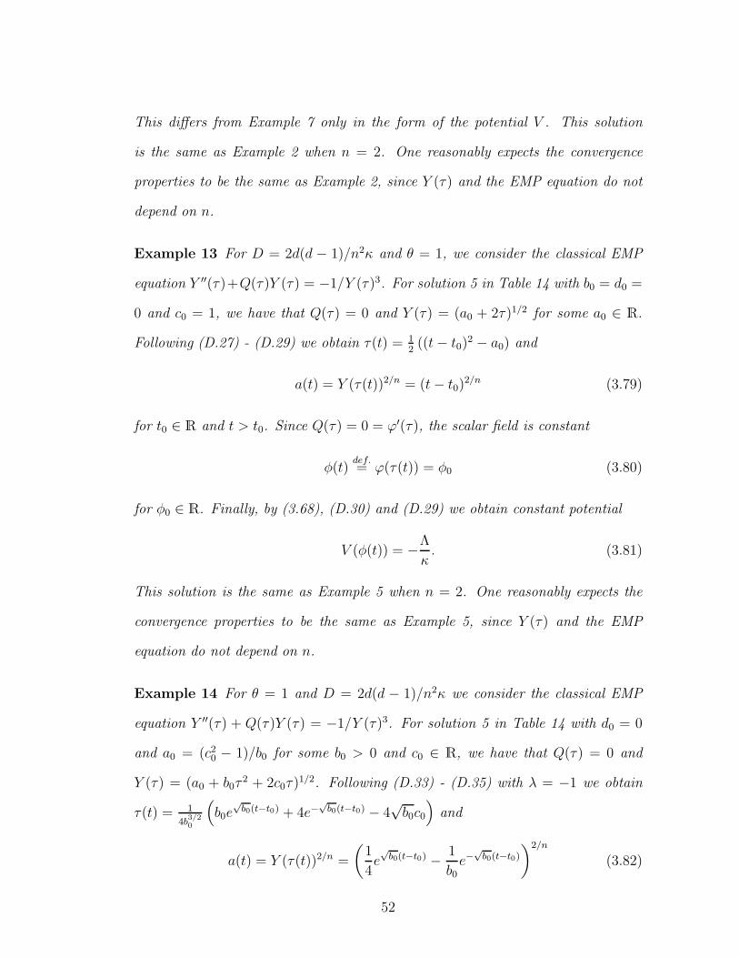
This differs from Example 7 only in the form of the potential V . This solution
is the same as Example 2 when n = 2. One reasonably expects the convergence
properties to be the same as Example 2, since Y (τ) and the EMP equation do not
depend on n.
Example 13 For D = 2d(d − 1)/n2κ and θ = 1, we consider the classical EMP
equation Y ′′(τ)+Q(τ)Y (τ) = −1/Y (τ)3. For solution 5 in Table 14 with b0 = d0 =
0 and c0 = 1, we have that Q(τ) = 0 and Y (τ) = (a0 + 2τ)1/2 for some a0 ∈ R.
Following (D.27) - (D.29) we obtain τ(t) = 12((t− t0)
2 − a0) and
a(t) = Y (τ(t))2/n = (t− t0)2/n (3.79)
for t0 ∈ R and t > t0. Since Q(τ) = 0 = ϕ′(τ), the scalar field is constant
φ(t)def.= ϕ(τ(t)) = φ0 (3.80)
for φ0 ∈ R. Finally, by (3.68), (D.30) and (D.29) we obtain constant potential
V (φ(t)) = −Λ
κ. (3.81)
This solution is the same as Example 5 when n = 2. One reasonably expects the
convergence properties to be the same as Example 5, since Y (τ) and the EMP
equation do not depend on n.
Example 14 For θ = 1 and D = 2d(d − 1)/n2κ we consider the classical EMP
equation Y ′′(τ) + Q(τ)Y (τ) = −1/Y (τ)3. For solution 5 in Table 14 with d0 = 0
and a0 = (c20 − 1)/b0 for some b0 > 0 and c0 ∈ R, we have that Q(τ) = 0 and
Y (τ) = (a0 + b0τ2 + 2c0τ)
1/2. Following (D.33) - (D.35) with λ = −1 we obtain
τ(t) = 1
4b3/20
(
b0e√
b0(t−t0) + 4e−√
b0(t−t0) − 4√b0c0
)
and
a(t) = Y (τ(t))2/n =
(
1
4e√
b0(t−t0) − 1
b0e−
√b0(t−t0)
)2/n
(3.82)
52

for t0 ∈ R. Since Q(τ) = 0 = ϕ′(τ), the scalar field is any constant
φ(t)def.= ϕ(τ(t)) = φ0 ∈ R. (3.83)
Finally, by (3.68), (D.36) and (D.35) we obtain constant potential
V (φ(t)) =2d(d− 1)
κn2
b0
(
b0e√
b0(t−t0) + 4e−√
b0(t−t0))2
− 16b20(
b0e√
b0(t−t0) − 4e−√
b0(t−t0))2
− Λ
κ
=1
κ
(
2d(d− 1)b0n2
− Λ
)
. (3.84)
This solution is the same as Example 6 when n = 2. One reasonably expects the
convergence properties to be the same as Example 6, since Y (τ) and the EMP
equation do not depend on n.
Example 15 For constant Cdef.= n2κD
2θ2d(d−1)> 0, we consider the EMP equation
Y ′′(τ)+Q(τ)Y (τ) = −C/θ2Y (τ)3. For solution 5 in Table 14 with a0 = b0 = 0 and
c0 = 1/2, we have that Q(τ) = d0(1 − d0)/τ2 for the choice d0 = (1/2) − (
√C/θ),
and Y (τ) =√τ . Following (D.38)-(D.39) we obtain τ(t) = θ2
4(t− t0)
2 and
a(t) = Y (τ(t))2/n =
(
θ
2(t− t0)
)2/n
(3.85)
for t > t0 ∈ R. Then by (D.44) with α0 = 2(d− 1)/nκ, we get scalar field
φ(t) = ϕ(τ(t)) =
√
2(d− 1)(θ2 − 4C)
nκθ2ln(t− t0) + β0. (3.86)
Also by (3.27) we obtain
V (φ(t)) =(d− 1)(θ2 − 4C)(2d− n)
κn2θ2(t− t0)2− Λ
κ(3.87)
so that
V (w) =(d− 1)(θ2 − 4C)(2d− n)
κn2θ2e−2
r
nκθ2
2(d−1)(θ2−4C)(w−β0) − Λ
κ(3.88)
53
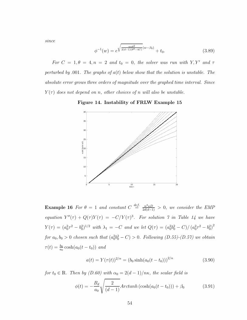
since
φ−1(w) = e
r
nκθ2
2(d−1)(θ2−4C)(w−β0)
+ t0. (3.89)
For C = 1, θ = 4, n = 2 and t0 = 0, the solver was run with Y, Y ′ and τ
perturbed by .001. The graphs of a(t) below show that the solution is unstable. The
absolute error grows three orders of magnitude over the graphed time interval. Since
Y (τ) does not depend on n, other choices of n will also be unstable.
Figure 14. Instability of FRLW Example 15
5
10
15
20
25
30
35
40
0 5 10 15 20
scale
facto
r a(t
)
time t
Example 16 For θ = 1 and constant Cdef.= n2κD
2d(d−1)> 0, we consider the EMP
equation Y ′′(τ) + Q(τ)Y (τ) = −C/Y (τ)3. For solution 7 in Table 14 we have
Y (τ) = (a20τ
2 − b20)1/2 with λ1 = −C and we let Q(τ) = (a2
0b20 − C)/ (a2
0τ2 − b20)
2
for a0, b0 > 0 chosen such that (a20b
20 − C) > 0. Following (D.55)-(D.57) we obtain
τ(t) = b0a0
cosh(a0(t− t0)) and
a(t) = Y (τ(t))2/n = (b0 sinh(a0(t− t0)))2/n (3.90)
for t0 ∈ R. Then by (D.60) with α0 = 2(d− 1)/nκ, the scalar field is
φ(t) = −Bd
a0
√
2
(d− 1)Arctanh (cosh(a0(t− t0))) + β0 (3.91)
54

for Bddef.=√
(d−1)2(a20b20−C)
nκb20. By (3.17) we obtain
V (φ(t)) =
[
2d(d− 1)
κn2(Y ′)2 − 1
2Y 2(ϕ′)2 − D
Y 2− Λ
κ
]
τ(t)
=2d(d− 1)a2
0
n2κ+B2
d(2d− n)
n(d− 1)csch2(a0(t− t0)) −
Λ
κ
(3.92)
so that
V (w) =2d(d− 1)a2
0
n2κ+B2
d(2d− n)
n(d− 1)cosh2
(
a0
Bd
√
(d− 1)
2(w − β0)
)
− Λ
κ(3.93)
by composition with φ−1.
For C = b0 = 1, a0 = 2, n = 3 and t0 = 0, the solver was run with Y, Y ′ and τ
perturbed by .01. The graphs of a(t) below show that the solution is unstable. The
absolute error grows 16 orders of magnitude over the graphed time interval. Since
Y (τ) does not depend on n, other choices of n will also be unstable.
Figure 15. Instability of FRLW Example 16
0
2e+16
4e+16
6e+16
8e+16
1e+17
1.2e+17
1.4e+17
25 26 27 28 29 30
scale
facto
r a(t
)
time t
55
3.2 In terms of a Schrodinger-Type Equation
To reformulate the Einstein field equations (i),(ii) in (3.5) in terms of a
Schrodinger-type equation (with one less non-linear term than that which is pro-
vided by the generalized EMP formulation), one can apply Corollary 2.3.1 to the
difference (ii)-(i). In doing so, Corollary 2.3.1 may be applied in a few different
ways: either by taking G(t)a(t)A = k
a(t)2in which case this term transforms into the
linear term Eu(σ) = θ2ku(σ) in the corresponding Schrodiner-type equation, or by
taking G(t)a(t)A = − κnjDj(t)
d(d−1)a(t)nj where j is some index with nj 6= 0 in which case this
nonlinear term transforms into the linear term E(σ)u(σ) = − θ2κn2j
2d(d−1)Dj(σ)u(σ) in
the corresponding Schrodinger-type equation. We will state both applications.
Theorem 3.2.1(
Apply Corollary 2.3.1 with G(t)a(t)A = k
a(t)2
)
Suppose you are given a twice differentiable function a(t) > 0, a once differentiable
function φ(t), and also functions Di(t), ρ′(t), p′(t), V (x) which satisfy the Einstein
equations (i), (ii) in (3.5) for some k, n1, . . . , nM ,Λ ∈ R, d ∈ R\0, 1, κ ∈ R\0
and M ∈ N. Let g(σ) denote the inverse of a function σ(t) which satisfies
σ(t) =1
θa(t)(3.94)
for some θ > 0. Then the following functions
u(σ) =1
a(g(σ))(3.95)
P (σ) =κ
(d− 1)ψ′(σ)2 (3.96)
solve the Schrodinger-type equation
u′′(σ) + [θ2k − P (σ)]u(σ) =
M∑
i=1
θ2κniDi(σ)
d(d− 1)u(σ)1−ni+θ2κ(ρ(σ) + p(σ))
(d− 1)u(σ)(3.97)
for
ψ(σ) = φ(g(σ)) (3.98)
56

Di(σ) = Di(g(σ)), 1 ≤ i ≤M (3.99)
and
ρ(σ) = ρ′(g(σ)), p(σ) = p′(g(σ)). (3.100)
Conversely, suppose you are given a twice differentiable function u(σ) > 0, and
also functions P (σ),Di(σ) for 1 ≤ i ≤ M,M ∈ N and ρ(σ), p(σ) which solve
(3.97) for some constants θ > 0, k ∈ R, κ ∈ R\0, d ∈ R\0, 1 and ni ∈ R for
1 ≤ i ≤ M . In order to construct functions which solve (i), (ii), first find σ(t), ψ(σ)
which solve the differential equations
σ(t) =1
θu(σ(t)) and ψ′(σ)2 =
(d− 1)
κP (σ). (3.101)
Then the functions
a(t) =1
u(σ(t))(3.102)
φ(t) = ψ(σ(t)) (3.103)
Di(t) = Di(σ(t)), 1 ≤ i ≤M (3.104)
ρ′(t) = ρ(σ(t)), p′(t) = p(σ(t)), (3.105)
and
V (φ(t)) =
[
d(d− 1)
2κ
(
1
θ2(u′)2 + ku2
)
− u2(ψ′)2
2θ2−
M∑
i=1
Diuni − ρ − Λ
κ
]
σ(t)
(3.106)
satisfy the equations (i), (ii).
Proof. This proof will implement Corollary 2.3.1 with con-
stants and functions as indicated in the following table.
57

Table 2. Corollary 2.3.1 applied to FRLW
In Corollary substitute In Corollary substitute
ε κ/(d− 1) E(σ) constant θ2k
G(t) constant k A 2
Gi(t), 1 ≤ i ≤M − κni
d(d−1)Di(t) Ai ni
GM+1(t)−κ
(d−1)(ρ′(t) + p′(t)) AM+1 0
Fi(σ), 1 ≤ i ≤M θ2κni
d(d−1)Di(σ) Ci 1 − ni
FM+1(σ) θ2κ(d−1)
(ρ(σ) + p(σ)) CM+1 1
To prove the forward implication, we assume to be given functions which solve
the Einstein field equations (i) and (ii). Subtracting equations (ii) − (i),
H(t) − k
a(t)2= − κ
(d− 1)
[
φ(t)2 +
M∑
i=1
niDi(t)
da(t)ni+ (ρ′(t) + p′(t))
]
. (3.107)
This shows that a(t), φ(t), Di(t), ρ′(t) and p′(t) satisfy the hypothesis of
Corollary 2.3.1, applied with constants ε,N,A,A1 . . . , AN and functions
G(t), G1(t) . . . , GN(t) according to Table 2. Since σ(t), u(σ), P (σ) and ψ(σ) defined
in (3.94), (3.95), (3.96) and (3.98) are equivalent to that in the forward implica-
tion of Corollary 2.3.1, by this corollary and by definitions (3.99) and (3.100) of
Di(σ) and ρ(σ), p(σ), the Schrodinger-type equation (2.110) holds for constants
C1, . . . , CN and functions F1(σ), . . . , FN(σ) as indicated in Table 2. This proves
the forward implication.
To prove the converse implication, assume we are given functions which solve
the Schrodinger-type equation (3.97) and we begin by showing that (i) is satisfied.
Differentiating the definition (3.102) of a(t) and by the definition in (3.101) of σ(t),
we see that
a(t) = − u′(σ(t))
u(σ(t))2σ(t)
58
= − u′(σ(t))
θu(σ(t)). (3.108)
Dividing by a(t), we obtain
H(t)def.=
a(t)
a(t)= −1
θu′(σ(t)). (3.109)
Differentiating the definition (3.103) of φ(t) and using definition in (3.101) of σ(t),
we get that
φ(t) = ψ′(σ(t))σ(t) =1
θψ′(σ(t))u(σ(t)). (3.110)
Using (3.109) and (3.110), and also the definitions (3.102), (3.104) and (3.105) of
a(t), Di(t) and ρ′(t), p′(t) respectively, the definition (3.106) of V φ can be written
V (φ(t)) =d(d− 1)
2κ
(
H(t)2 +k
a(t)2
)
− 1
2φ(t)2 −
M∑
i=1
Di(t)
a(t)ni− ρ′(t) − Λ
κ. (3.111)
This shows that (i) holds (That is, the definition of V (φ(t)) was designed to be
such that (i) holds).
To conclude the proof we must also show that (ii) holds. In the converse direc-
tion the hypothesis of the converse of Corollary 2.3.1 holds, applied with constants
N,C1, . . . , CN and functions E(σ), F1(σ), . . . , FN (σ) as indicated in Table 2. Since
σ(t), ψ(σ), a(t) and φ(t) defined in (3.101), (3.102) and (3.103) are consistent with
the converse implication of Corollary 2.3.1, applied with ε and A as in Table 2,
by this corollary and by definitions (3.104) and (3.105) of Di(t) and ρ′(t), p′(t)
the scale factor equation (2.109) holds for constants ε, A,A1, . . . , AN and functions
G(t), G1(t), . . . , GN(t) according to Table 2. That is, we have regained (3.107)
which shows that the subtraction of equations (ii)-(i) holds in the converse direc-
tion. Now solving (3.111) for ρ′(t) and substituting this into (3.107), we obtain (ii).
This proves the theorem. ⋄
59

3.2.1 Reduction to linear Schrodinger: pure scalar field
To compute some exact solutions, we take special case ρ′ = p′ = Di = 0 so that
Theorem 3.2.1 shows that solving the Einstein equations
d
2H2(t) +
dk
2a(t)2
(i)′′′=
κ
(d− 1)
[
1
2φ(t)2 + V (φ(t))
]
+Λ
(d− 1)(3.112)
(3.113)
H(t) +d
2H(t)2 +
(d− 2)k
2a(t)2
(ii)′′′= − κ
(d− 1)
[
1
2φ(t)2 − V (φ(t))
]
+Λ
(d− 1)
is equivalent to solving the linear Schrodinger equation
u′′(σ) + [θ2k − P (σ)]u(σ) = 0 (3.114)
for any constant θ > 0. The solutions of (i)′′′, (ii)′′′ and (3.114) are related by
a(t) =1
u(σ(t))and ψ′(σ)2 =
(d− 1)
κP (σ) (3.115)
for φ(t) = ψ(σ(t)) and
σ(t) =1
θa(t)=
1
θu(σ(t)). (3.116)
Also in the converse direction, V is taken to be
V (φ(t)) =
[
d(d− 1)
2κ
(
1
θ2(u′)2 + ku2
)
− u2(ψ′)2
2θ2− Λ
κ
]
σ(t). (3.117)
We now refer to Appendix E for solutions of the linear Schrodinger equation
(3.114), which we will map to solutions of Einstein’s equations using the theorem.
Example 17 For zero curvature k = 0 and θ = 1, we take solution 1 in Table 15
with a0 = d0 = 0 so that we have u(σ) = b0σ + c0 and P (σ) = 0 for b0 > 0 and
c0 ∈ R. By (E.4) - (E.6) we obtain σ(t) = eb0(t−t0) − c0b0
and
a(t) =1
u(σ(t))=
1
b0e−b0(t−t0) (3.118)
60

for t0 ∈ R. Since P = 0 = ψ′(σ), the scalar field is constant
ψ(σ) = ψ0 ∈ R. (3.119)
Finally, by (3.117) and (E.7) we obtain constant potential
V (φ(t)) =
[
d(d− 1)
2κ(u′)2 − Λ
κ
]
σ(t)
=d(d− 1)
2κb20 −
Λ
κ. (3.120)
Example 18 For zero curvature k = 0 and θ = 1, we take solution 1 in Ta-
ble 15 with a0 > 0 and d0 = 0 so that we have u(σ) = a0σ2 + b0σ + c0
and P (σ) = 2a0/(a0σ2 + b0σ + c0). By (E.8) - (E.10) we obtain σ(t) =
12a0
(√−∆ tan
[√−∆2
(t− t0)]
− b0
)
and
a(t) =1
u(σ(t))=
4a0
−∆cos2
[√−∆
2(t− t0)
]
(3.121)
for negative discriminant ∆ = b20 − 4a0c0 < 0 and t0 ∈ R. Then by (E.13) with
α0 = (d− 1)/κ, the scalar field is
φ(t)def.= ψ(σ(t)) =
√
2(d− 1)
κln
[√−∆
a0
(
tan
[√−∆
2(t− t0)
]
+sec
[√−∆
2(t− t0)
])]
+ β0 (3.122)
for β0 ∈ R. Finally, by (3.117), (E.11) and (E.10) we obtain
V (φ(t)) =
[
d(d− 1)
2κ(u′)2 − 1
2u2(ψ′)2 − Λ
κ
]
σ(t)
=−∆(d− 1)
2κ
(
d tan2
[√−∆
2(t− t0)
]
− 1
2sec2
[√−∆
2(t− t0)
])
− Λ
κ.
(3.123)
Example 19 For positive curvature k = 1 and θ = 1, we take solution 2 in
Table 15 with b0 = 1/√
2 and a0 > 0 so that we have u(σ) = a0 cos2(σ/√
2),
61

P (σ) = tan2(σ/√
2) and E = 1. By (E.14) - (E.16) we obtain σ(t) =√
2Arctan(
a0√2(t− t0)
)
and
a(t) =1
u(σ(t))=
1
a0
(
1 +a2
0
2(t− t0)
2
)
(3.124)
for t0 ∈ R. Then by (E.19) with α0 = (d− 1)/κ, the scalar field becomes
φ(t) =
√
(d− 1)
2κln
[
a20
2(t− t0)
2 + 1
]
+ β0 (3.125)
for β0 ∈ R. Finally, by (3.117), (E.17) and (E.16), we obtain
V (φ(t)) =(d− 1)
κ
(
(2d− 1)a40(t− t0)
2 + 2da20
(2 + a20(t− t0)2)
2
)
− Λ
κ. (3.126)
That is, we have
V (w) = C1e−
q
2κ(d−1)
w − C2e−2
q
2κ(d−1)
w − Λ
κ(3.127)
for constants
C1 =(d− 1)(2d− 1)a2
0
2κe
q
2κ(d−1)
β0 , C2 =(d− 1)2a2
0
2κe2
q
2κ(d−1)
β0 (3.128)
and w ≥√
(d−1)2κ
ln(a20/2) + β0, since
φ−1(w) =
√2
a0
√
e
q
2κ(d−1)
(w−β0) − 1 + t0. (3.129)
By taking d = 3 and t0 = 0, replacing a0 with 1/a0, and identifying κ and β0 here
with K2 and φ0 in [26] respectively, we obtain the string-inspired solution II of [26].
One can check that the conditions on the constants C1, C2 in [26] (with d = 3) agree
with the example here since
a20 =
2κC21
(2d− 1)2C2and β0 =
√
(d− 1)
2κln
(
(2d− 1)C2
(d− 1)C1
)
. (3.130)
For a0 = 1 and t0 = 0, the solver was run with u, u′ and σ perturbed by .001.
The graphs of a(t) below show that the solution is unstable. The absolute error
grows by up to five orders of magnitude over the graphed time interval.
62

Figure 16. Instability of FRLW Example 19
0
10
20
30
40
50
0 2 4 6 8 10
scale
facto
r a(t
)
time t
Example 20 For negative curvature k = −1 and θ = 1, we take solution 4 in
Table 15 with c0 = −1 and b0 = 0 so that we have u(σ) = a0e−σ, P (σ) = 0 and
E = −1. By (E.28) - (E.30) with r0 = 1 we obtain σ(t) = ln (a0(t− t0)) and
a(t) =1
u(σ(t))= (t− t0) (3.131)
for t0 ∈ R. Since P = 0 = ψ′(σ), we get ψ(σ) = ψ0 for constant ψ0 ∈ R. Finally,
by (3.117), (E.31) and (E.30), we obtain constant potential V (φ(t)) = −Λ/κ.
For a0 = 1 and t0 = 0, the solver was run with u, u′ and σ perturbed by .001.
The graphs of a(t) below show that the solution is unstable. The absolute error
grows four orders of magnitude over the graphed time interval.
63

Figure 17. Instability of FRLW Example 20
0
10
20
30
40
50
0 2 4 6 8 10
scale
facto
r a(t
)
time t
Example 21 For negative curvature k = −1 and θ = 1, we take solution 4 in Table
15 with c0 = −1 and a0, b0 > 0 so that we have u(σ) = a0e−σ − b0e
σ, P (σ) = 0 and
E = −1. By (E.32) - (E.34) we obtain σ(t) = ln(√
a0
b0tanh(
√a0b0(t− t0))
)
and
a(t) =1
u(σ(t))=
1
2√a0b0
sinh(2√
a0b0(t− t0)) (3.132)
for t0 ∈ R. Since P = 0 = ψ′(σ), we have that ψ(σ) = ψ0 for constant ψ0 ∈ R.
Finally, by (3.117), (E.35) and (E.34), we obtain constant potential
V (φ(t)) =
[
d(d− 1)
2κ
(
(u′)2 − u2)
− Λ
κ
]
σ(t)
=2d(d− 1)
κa0b0 −
Λ
κ(3.133)
since coth2(x) − csch2(x) = 1.
Example 22 For arbitrary curvature k and θ = 1, we take solution 5 in Table
15 with c0 = −1 and b0 = k + 1 so that we have u(σ) = (a0/σ)e−σ2/2, P (σ) =
σ2 + 2/σ2 + (k + 1) and E = k for a0 > 0. By (E.36) - (E.38) we obtain σ(t) =√
2 ln(a0(t− t0)) and
a(t) =1
u(σ(t))=
√2(t− t0)
√
ln(a0(t− t0)) (3.134)
64

for t > 1/a0 + t0 ∈ R. Then by (E.41) with α0 = (d− 1)/κ, the scalar field is
φ(t) = ψ(σ(t))
=
√
(d− 1)
2κ
(
√
2 ln2(a0(t− t0)) + (k + 1) ln(a0(t− t0)) + 1
+ ln [2 ln(a0(t− t0))] − ln [2(1 + k) ln(a0(t− t0)) + 4
+ 4
√
2 ln2(a0(t− t0)) + (1 + k) ln(a0(t− t0)) + 1
]
−(1 + k)√2
ln
[
2√
2
√
2 ln2(a0(t− t0)) + (1 + k) ln(a0(t− t0)) + 1
−(1 + k) − 4 ln(a0(t− t0))]) + β0 (3.135)
for β0 ∈ R. Finally, by (3.117), (E.39) and (E.38), we obtain
V (φ(t)) =
[
d(d− 1)
2κ
(
(u′)2 + ku2)
− u2(ψ′)2
2− Λ
κ
]
σ(t) (3.136)
=(d− 1)
2κ(t− t0)2
(
d
(
1 +1
2 ln(a0(t− t0))
)2
+dk
2 ln(a0(t− t0))
−[
2 ln2(a0(t− t0)) + 1 + (k + 1) ln(a0(t− t0))]
2 ln2(a0(t− t0))
)
− Λ
κ
For a0 = k = 1 and t0 = 0, the solver was run with u, u′ and σ perturbed by
.001. The graphs of a(t) below show that the solution is unstable. The absolute
error grows up to four orders of magnitude over the graphed time interval. Since
E − P (σ) is independent of k, the below graph is also applicable to k = 0,−1.
65

Figure 18. Instability of FRLW Example 22
0
10
20
30
40
50
1 2 3 4 5 6 7 8
scale
facto
r a(t
)
time t
Example 23 For positive curvature k = 1 and θ = 1, we take solution 5 in Table
15 with c0 = 0 and a0 = b0 = 1 so that we have u(σ) = 1/σ, P (σ) = 2/σ2 + 1 and
E = 1. By (E.42) - (E.44) with r0 = 1 we obtain σ(t) =√
2(t− t0) and
a(t) =1
u(σ(t))=√
2(t− t0) (3.137)
for t > t0 ∈ R. Then by (E.47) with α0 = (d− 1)/κ, we have
φ(t) =
√
(d− 1)
κ
(
√
g(t) +1√2
ln [2(t− t0)] −√
2 ln[√
2 +√
g(t))]
)
+ β0
for g(t) = 2(t− t0) + 2 and β0 ∈ R. Finally, by (3.117), (E.45) and (E.44), we get
V (φ(t)) =(d− 1)
4κ
(
(d− 2)
2(t− t0)2+
(d− 1)
(t− t0)
)
− Λ
κ. (3.138)
For t0 = 0, the solver was run with u, u′ and σ perturbed by .01. The graphs of
a(t) below show that the solution is unstable. The absolute error grows two orders
of magnitude over the graphed time interval.
66

Figure 19. Instability of FRLW Example 23
0
1
2
3
4
5
2 3 4 5 6 7 8
scale
facto
r a(t
)
time t
Example 24 For zero curvature k = 0 and θ = 1, we take solution 5 in Table 15
with b0 = c0 = 0 and a0 = 0 so that we have u(σ) = 1/σ, P (σ) = 2/σ2 and E = 0.
By (E.42) - (E.44) with r0 = 1 we obtain σ(t) =√
2(t− t0) and
a(t) =1
u(σ(t))=√
2(t− t0) (3.139)
for t > t0 ∈ R. Then by (E.47) with α0 = (d− 1)/κ and b0 = 0, we have
φ(t) =
√
(d− 1)
2κln [2(t− t0)] + β0
for β0 ∈ R. Finally, by (3.117), (E.45) and (E.44), we obtain
V (φ(t)) =(d− 1)(d− 2)
8κ(t− t0)2− Λ
κ. (3.140)
For t0 = 0, the solver was run with u, u′ and σ perturbed by .001. The graphs of
a(t) below show that the solution is unstable. The absolute error grows up to three
orders of magnitude over the graphed time interval.
67

Figure 20. Instability of FRLW Example 24
0
1
2
3
4
5
0 0.5 1 1.5 2 2.5 3 3.5 4
scale
facto
r a(t
)
time t
Example 25 We take solution 7 in Table 15 with c0 = kθ2 and b0 > 0 and a0 > 0
so that we have u(σ) = a0/σb0, P (σ) = b0(b0 +1)/σ2 +kθ2 and E = kθ2. By (E.54)
- (E.56) we obtain
σ(t) =A1/b0
a0(t− t0)
1/(1+b0) (3.141)
and
a(t) =1
u(σ(t))= A(t− t0)
b0/(b0+1) (3.142)
for t > t0 ∈ R and Adef.= 1
a0
(
(1+b0)a0
θ
)b0/(1+b0)
. Then by (E.59) with α0 = (d−1)/κ,
the scalar field is
φ(t) = β0 +
√
(d− 1)
κ
(
√
b0(b0 + 1) + kθ2σ(t)2 (3.143)
−√
b0(b0 + 1) log
(
√
b0(b0 + 1) +√
b0(b0 + 1) + kθ2σ(t)2
σ(t)
))
for σ(t) in (3.141). Also by (3.117), (E.56) and (E.57), we obtain potential
V (φ(t)) = −Λ
κ+
B2
2(t− t0)2
(
((d− 1)b0 − 1)
(1 + b0)+
k(d− 1)(1 + b0)
b0A2(t− t0)−2/(1+b0)
)
(3.144)
for B2 def.= (d−1)b0
(1+b0)κ.
68

By taking d = 3, Λ = t0 = 0, θ = a0(1 + b0) and identifying b0/(b0 + 1) here with
n in [13], we obtain example 4.4 of Ellis and Madsen for 0 < n < 1. Note that the
above form of φ(t) is the integrated version of φ(t) in [13]. Since φ(t) in (3.143)
and has the property that
φ(t)2 =B2
(t− t0)2
(
1 +kθ2(a0A)2/b0
b0(b0 + 1)(t− t0)
2/(1+b0)
)
, (3.145)
we are in agreement with [13] for the above choice of θ. Also note that there is
a typo in equation (45) of [13], where one should multiply V by 1/4 to obtain the
correct V with a two appearing in the denominator instead of the numerator. In
contrast to example 3 in this thesis, this example generalizes the Ellis and Madsen
example for nonzero curvature.
For a0 = b0 = 1 and t0 = 0, the solver was run with u, u′ and σ perturbed by
.001. The graphs of a(t) below show that the solution is unstable. The absolute error
grows three orders of magnitude over the graphed time interval. Since E − P (σ)
is independent of k, the below graph is applicable to all values of the curvature
k = 1, 0,−1.
Figure 21. Instability of FRLW Example 25
0
1
2
3
4
5
6
7
8
1 2 3 4 5 6
scale
facto
r a(t
)
time t
69

3.2.2 A nonlinear Schrodinger example
Example 26 We consider equation (3.97) with ρ = p = 0, M = k = θ = 1, n = 4
and D1(σ) = D > 0 a constant. For solution 3 in Table 15 with a0 =√
d(d−1)2κD
b0,
c0 = 1 − 2b20 and b0 > 0 chosen such that c0 > 0, we have u(σ) = a0tanh(b0σ) and
P (σ) = c0. By (E.22) - (E.24) we obtain σ(t) = 1b0Arcsinh
(
ea0b0(t−t0))
and
a(t) =1
u(σ(t))=
√1 + e2a0b0(t−t0)
a0ea0b0(t−t0)(3.146)
for t0 ∈ R. Then by (E.27) with α0 = (d− 1)/κ, we get
φ(t) = ψ(σ(t)) =
√
(d− 1)(1 − 2b20)
b0√κ
Arcsinh(
ea0b0(t−t0))
+ β0 (3.147)
for β0 ∈ R. Finally, by (3.106) and (E.25) we obtain
V (φ(t)) =
[
d(d− 1)
2κ
(
(u′)2 + u2)
− 1
2u2(ψ′)2 −Du4 − Λ
κ
]
σ(t).
=a2
0(d− 1)
2κ(1 + e2a0b0(t−t0))2
[(
(d− 1)(1 − b20) + b20)
e4a0b0(t−t0)
+(
d− 1 + 2b20)
e2a0b0(t−t0) + db20]
− Λ
κ
(3.148)
For a0 = 1, b0 = 1/2 and t0 = 0, the solver was run with u, u′ and σ perturbed
by .001. The graphs of a(t) below show that the solution is unstable. The absolute
error grows two orders of magnitude over the graphed time interval.
70

Figure 22. Instability of FRLW Example 26
0.8
0.9
1
1.1
1.2
1.3
0.5 1 1.5 2 2.5 3 3.5 4 4.5 5
scale
facto
r a(t
)
time t
3.3 In terms of an Alternate Schrodinger-Type Equation
Theorem 3.3.1(
Apply Corollary 2.3.1 with G(t)a(t)A = − κnjDj(t)
d(d−1)a(t)nj
)
Suppose you are given a twice differentiable function a(t) > 0, a once differentiable
function φ(t), and also functions Di(t), ρ′(t), p′(t), V (x) which satisfy the Einstein
equations (i), (ii) in (3.5) for some k, n1, . . . , nM ,Λ ∈ R, d ∈ R\0, 1, κ ∈ R\0
and M ∈ N. Let g(σ) denote the inverse of a function σ(t) which satisfies
σ(t) =1
θa(t)−nj/2 (3.149)
for some θ > 0 and where j is some index for which nj 6= 0. Then the functions
u(σ) = a(g(σ))−nj/2 (3.150)
P (σ) =njκ
2(d− 1)ψ′(σ)2 (3.151)
solve the Schrodinger-type equation
u′′(σ) +
[ −θ2n2jκ
2d(d− 1)Dj(σ) − P (σ)
]
u(σ) =−θ2njk
2u(σ)1− 4
nj
+∑
1≤i≤M
i6=j
θ2njniκDi(σ)
2d(d− 1)u(σ)1−2
ninj
71

+θ2njκ(ρ(σ) + p(σ))
2(d− 1)u(σ)(3.152)
for
ψ(σ) = φ(g(σ)) (3.153)
Di(σ) = Di(g(σ)), 1 ≤ i ≤M (3.154)
and
ρ(σ) = ρ′(g(σ)), p(σ) = p′(g(σ)). (3.155)
Conversely, suppose you are given a twice differentiable function u(σ) > 0, and
also functions P (σ),Di(σ) for 1 ≤ i ≤ M,M ∈ N and ρ(σ), p(σ) which solve
(3.152) for some constants θ > 0, k ∈ R, κ ∈ R\0, d ∈ R\0, 1 and ni ∈ R for
1 ≤ i ≤ M . In order to construct functions which solve (i), (ii), first find σ(t), ψ(σ)
which solve the differential equations
σ(t) =1
θu(σ(t)) and ψ′(σ)2 =
2(d− 1)
njκP (σ). (3.156)
Then the functions
a(t) = u(σ(t))−2/nj (3.157)
φ(t) = ψ(σ(t)) (3.158)
Di(t) = Di(σ(t)), 1 ≤ i ≤M, (3.159)
ρ′(t) = ρ(σ(t)), p′(t) = p(σ(t)) (3.160)
and
V (φ(t))
=
[
d(d− 1)
2κ
(
4
n2jθ
2(u′)2 +
k
u−4/nj
)
− 1
2θ2u2(ψ′)2 −
M∑
i=1
Di
u−2ni/nj− ρ − Λ
κ
]
σ(t)
(3.161)
satisfy the equations (i), (ii).
72

Proof. This proof will implement Corollary 2.3.1 with constants and functions as
indicated in the following table.
Table 3. Corollary 2.3.1 applied to FRLW, alternate
In Corollary substitute In Corollary substitute
ε κ/(d− 1) E(σ) − θ2n2jκ
2d(d−1)Dj(σ)
G(t)−njκ
d(d−1)Dj(t) A some nj 6= 0
Gi(t), 1 ≤ i ≤M, i 6= j −niκd(d−1)
Di(t) Ai6=j ni
Gj(t) k Aj 2
GM+1(t)−κ
(d−1)(ρ′(t) + p′(t)) AM+1 0
Fi(σ), 1 ≤ i ≤M, i 6= jθ2njniκ
2d(d−1)Di(σ) Ci6=j 1 − 2 ni
nj
Fj(σ) −θ2njk/2 Cj 1 − 4nj
FM+1(σ)θ2njκ
2(d−1)(ρ(σ) + p(σ)) CM+1 1
To prove the forward implication, we assume to be given functions which solve
the Einstein field equations (i) and (ii) from (3.5). Subtracting equations (ii)− (i),
we see that
H(t) − k
a(t)2= − κ
(d− 1)
[
φ(t)2 +
M∑
i=1
niDi(t)
da(t)ni+ (ρ′(t) + p′(t))
]
. (3.162)
This shows that a(t), φ(t), Di(t), ρ′(t) and p′(t) satisfy the hypothesis of
Corollary 2.3.1, applied with constants ε,N,A,A1 . . . , AN and functions
G(t), G1(t) . . . , GN(t) according to Table 3. Since σ(t), u(σ), P (σ) and ψ(σ) defined
in (3.149), (3.150), (3.151) and (3.153) are equivalent to that in the forward im-
plication of Corollary 2.3.1, by this theorem and by definitions (3.154) and (3.155)
of Di(σ) and ρ(σ), p(σ), the Schrodinger-type equation (2.110) holds for constants
C1, . . . , CN and functions F1(σ), . . . , FN(σ) as indicated in Table 3. This proves the
forward implication.
73

To prove the converse implication, we assume to be given functions which solve
the Schrodinger-type equation (3.152) and we begin by showing that (i) is satisfied.
By differentiating the definition (3.157) of a(t) and using the definition of σ(t) in
(3.156), we obtain
a(t) = − 2
nj
u(σ(t))−2/nj−1u′(σ(t))σ(t)
= − 2
njθu(σ(t))−2/nju′(σ(t)). (3.163)
Dividing by a(t), we have that
H(t)def.=
a(t)
a(t)= − 2
njθu′(σ(t)). (3.164)
Differentiating the definition (3.158) of φ(t) and using definition in (3.156) of σ(t),
we have
φ(t) = ψ′(σ(t))σ(t) =1
θψ′(σ(t))u(σ(t)). (3.165)
Using (3.164) and (3.165), and also the definitions (3.157), (3.159) and (3.160) of
a(t), Di(t) and ρ′(t), p′(t), the definition (3.161) of V φ can be written as
V (φ(t)) =d(d− 1)
2κ
(
H(t)2 +k
a(t)2
)
− 1
2φ(t)2 −
M∑
i=1
Di(t)
a(t)ni− ρ′(t) − Λ
κ. (3.166)
This shows that (i) holds (that is, the definition of V (φ(t)) was designed to be such
that (i) holds).
To conclude the proof we must also show that (ii) holds. In the converse direc-
tion the hypothesis of the converse of Corollary 2.3.1 holds, applied with constants
N,C1, . . . , CN and functions E(σ), F1(σ), . . . , FN (σ) as indicated in Table 3. Since
σ(t), ψ(σ), a(t) and φ(t) defined in (3.156), (3.157) and (3.158) are consistent with
the converse implication of Corollary 2.3.1, applied with ε and A as in Table 3,
by this corollary and by definitions (3.159) and (3.160) of Di(t) and ρ′(t), p′(t)
the scale factor equation (2.109) holds for constants ε, A,A1, . . . , AN and functions
74

G(t), G1(t), . . . , GN(t) according to Table 3. That is, we have regained (3.162)
which shows that the subtraction of equations (ii)-(i) holds in the converse direc-
tion. Now solving (3.166) for ρ′(t) and substituting this into (3.162), we obtain (ii).
This proves the theorem. ⋄
3.3.1 Reduction to linear Schrodinger: zero curvature
To compute some examples, we take k = 0 and ρ′ = p′ = Di = 0 for all i 6= j
and also nj = n, Dj = D > 0 so that Theorem 3.3.1 shows that solving the Einstein
equations
d
2H2(t)
(i)′′′′=
κ
(d− 1)
[
1
2φ(t)2 + V (φ(t)) +
D
a(t)n
]
+Λ
(d− 1)(3.167)
H(t) +d
2H(t)2 (ii)′′′′
= − κ
(d− 1)
[
1
2φ(t)2 − V (φ(t)) +
(n− d)D
da(t)n
]
+Λ
(d− 1)
is equivalent to solving the linear Schrodinger equation
u′′(σ) +
[−θ2n2κD
2d(d− 1)− P (σ)
]
u(σ) = 0
for any constant θ > 0. The solutions of (i)′′′′, (ii)′′′′ and (3.168) are related by
a(t) =1
u(σ(t))2/nand ψ′(σ)2 =
2(d− 1)
nκP (σ) (3.168)
for φ(t) = ψ(σ(t)) and
σ(t) =1
θa(t)n/2=
1
θu(σ(t)). (3.169)
Also in the converse direction, V is taken to be
V (φ(t)) =
[
2d(d− 1)(u′)2
κn2θ2− 1
2θ2u2(ψ′)2 −Du2 − Λ
κ
]
σ(t). (3.170)
We now refer to Appendix E for solutions of the linear Schrodinger equation
(3.168). We will map these solutions to exact solutions of Einstein’s equations.
Since E = −θ2n2κD2d(d−1)
< 0, we only consider entries in Table 15 for which E < 0.
75

Example 27 For θ = 1 and choice of constant D = 2d(d−1)n2κ
, we take solution 4 in
Table 15 with c0 = −1 and b0 = 0 so that we have u(σ) = a0e−σ, P (σ) = 0 and
E = −1. By (E.28) - (E.30) with r0 = 1 we obtain σ(t) = ln (a0(t− t0)) and
a(t) =1
u(σ(t))2/n= (t− t0)
2/n (3.171)
for t0 ∈ R. Since P = 0 = ψ′(σ), the scalar field is constant ψ(σ) = ψ0 ∈ R.
Finally, by (3.170), (E.31) and (E.30), we obtain constant potential
V (φ(t)) =
[
2d(d− 1)(u′)2
n2κ− 2d(d− 1)
n2κu2 − Λ
κ
]
σ(t)
= −Λ
κ. (3.172)
For a0 = 1, n = 3 and t0 = 0, the solver was run with u, u′ and σ perturbed
by .001. The graphs of a(t) below show that the solution is unstable. The absolute
error grows at least two orders of magnitude over the graphed time interval. Since
u is independent of n, a(t) is unstable for all values of n.
Figure 23. Instability of FRLW Example 27
0
5
10
15
20
0 2 4 6 8 10
scale
facto
r a(t
)
time t
76

Example 28 For θ = 1 and choice of constant D = 2d(d−1)n2κ
, we take solution 4 in
Table 15 with c0 = −1 and a0, b0 > 0 so that we have u(σ) = a0e−σ−b0eσ, P (σ) = 0
and E = −1. By (E.32) - (E.34) we obtain σ(t) = ln(√
a0
b0tanh(
√a0b0(t− t0))
)
and
a(t) =1
u(σ(t))2/n=
1
(2√a0b0)2/n
sinh2/n(2√
a0b0(t− t0)) (3.173)
for t0 ∈ R. Since P = 0 = ψ′(σ), the scalar field is constant
ψ(σ) = ψ0 ∈ R (3.174)
Finally, by (3.170), (E.35) and (E.34), we obtain constant potential
V (φ(t)) =
[
2d(d− 1)(u′)2
n2κ− 2d(d− 1)
n2κu2 − Λ
κ
]
σ(t)
=8d(d− 1)a0b0
n2κ− Λ
κ(3.175)
since coth2(x) − csch2(x) = 1.
Example 29 For θ = 1 and choice of constant D = 2d(d−1)/n2κ, we take solution
5 in Table 15 with c0 = −1 and b0 = 0 so that we have u(σ) = (a0/σ)e−σ2/2,
P (σ) = σ2 + 2/σ2 and E = −1 for a0 > 0. By (E.36) - (E.38) we obtain σ(t) =√
2 ln(a0(t− t0)) and
a(t) =1
u(σ(t))2/n
=(√
2(t− t0)√
ln(a0(t− t0)))2/n
=(
2(t− t0)2 ln(a0(t− t0))
)1/n(3.176)
for t > t0. Then by (E.41) with α0 = 2(d− 1)/nκ, we obtain scalar field
φ(t) = ψ(σ(t))
=
√
(d− 1)
nκ
(
√
2 ln2(a0(t− t0)) + 1 + ln [2 ln(a0(t− t0))]
− ln
[
4 + 4
√
2 ln2(a0(t− t0)) + 1
])
+ β0 (3.177)
77

for β0 ∈ R. Finally, by (3.117), (E.39) and (E.38), we have that
V (φ(t)) =
[
2d(d− 1)
n2κ(u′)2 − 1
2u2(ψ′)2 −Du2 − Λ
κ
]
σ(t)
=(d− 1)
2nκ(t− t0)2 ln2(a0(t− t0))·
(
−2 ln2(a0(t− t0)) − 1
+d
n
(
(2 ln(a0(t− t0)) + 1)2 − 2 ln(a0(t− t0)))
)
− Λ
κ
(3.178)
For a0 = 1, n = 3 and t0 = 0, the solver was run with u, u′ and σ perturbed
by .001. The graphs of a(t) below show that the solution is unstable. The absolute
error grows three orders of magnitude over the graphed time interval. Since u is
independent of n, a(t) is unstable for all values of n.
Figure 24. Instability of FRLW Example 29
0
2
4
6
8
10
12
14
1 2 3 4 5 6 7 8
scale
facto
r a(t
)
time t
Example 30 For Cdef.= n2κD
2d(d−1)and θ = 1, we take solution 6 in Table 15 with
c0 = 2b20 −C so that we have u(σ) = −a0 cosh2(b0σ), P (σ) = 2b20 tanh2(b0σ) + c0 =
2b20 tanh2(b0σ) + 2b20 − C and E = −C. By (E.48) - (E.50) we obtain σ(t) =
78

−1b0Arctanh (a0b0(t− t0)) and
a(t) =1
u(σ(t))2/n=
(
1
a0
(
a20b
20(t− t0)
2 − 1)
)2/n
(3.179)
for t0 ∈ R. Then by (E.53) with α0 = 2(d− 1)/nκ, the scalar field is
φ(t) = ψ(σ(t))
= ±(√
4(d− 1)
nκln
[
2
(
√
2b40a20(t− t0)2 + 2b20 − C −
√2b20a0(t− t0)
)]
+1
b0
√
2(d− 1)
nκ
√
4b20 − CArctanh
[
√
4b20 − Ca0b0(t− t0)√
2b40a20(t− t0)2 + 2b20 − C
])
+ β0
for β0 ∈ R. Finally, by (3.117), (E.50) and (E.51), we have that
V (φ(t)) =
[
2d(d− 1)(u′)2
κn2− 1
2u2(ψ′)2 −Du2 − Λ
κ
]
σ(t).
=a2
0(d− 1) [(4d− n)2a20b
40(t− t0)
2 − 2nb20 + C(n− 2d)]
κn2(a20b
20(t− t0)2 − 1)2
− Λ
κ.
(3.180)
One can compare this to the solutions in [23] and in section 5 of [15].
3.3.2 A nonlinear Schrodinger example
Example 31 For Dj = ρ = p = 0 and Di = 0 for all i, we take nj = 4, θ = 1 and
positive curvature k = 1. We use solution 2 in Table 15 with a0 = 1/b20 and b0 > 0
so that we have u(σ) = 1b20
cos2(b0σ). Using the second potential for solution 2 in
the table, we have P (σ) = 4b20 tan2(b0σ) and F1 = −2. By (E.14)-(E.16) we have
σ(t) = 1b0Arctan
(
θb0
(t− t0))
and
a(t) =1
u(σ(t))1/2=√
b20 + (t− t0)2 (3.181)
for t > t0 ∈ R. Then by (E.21) with α0 = (d− 1)/2κ, we obtain scalar field
φ(t) =
√
(d− 1)
2κln
(
1 +1
b20(t− t0)
2
)
+ β0 (3.182)
79

for β0 ∈ R. Finally, by (3.161), (E.16) and (E.17) we obtain
V (φ(t)) =
[
d(d− 1)
2κ
(
1
4(u′)2 + u
)
− 1
2u2(ψ′)2 − Λ
κ
]
σ(t)
=(d− 1)
2κ
(
db20 + 2(d− 1)(t− t0)2
(b20 + (t− t0)2)2
)
− Λ
κ.
(3.183)
Composing V (φ(t)) with the inverse
φ−1(w) = b0
√
e√
2κ/(d−1)(w−β0) − 1 + t0 (3.184)
for w ≥ β0, we obtain the potential
V (w) = C1e−√
2κ/(d−1)w − C2e−2√
2κ/(d−1)w − Λ
κ(3.185)
for constants
C1 =(d− 1)2
κb20e√
2κ/(d−1)β0 and C2 =(d− 1)(d− 2)
2κb20e2√
2κ/(d−1)β0. (3.186)
By taking d = 3, t0 = 0, and identifying a0, κ and β0 here with b0, K2 and φ0
respectively in the Ozer and Taha paper, we obtain the string-inspired solution I of
[26]. One can check that the conditions on the constants C1, C2 in [26] (with d = 3)
agree with the example here since we have
b20 =2(d− 1)3C2
(d− 2)κC21
and β0 =
√
(d− 1)
2κln
(
2(d− 1)C2
(d− 2)C1
)
. (3.187)
For b0 = 1 and t0 = 0, the solver was run with u, u′ and σ perturbed by .001.
The graphs of a(t) below show that the solution is unstable. The absolute error
grows by three orders of magnitude over the graphed time interval.
80
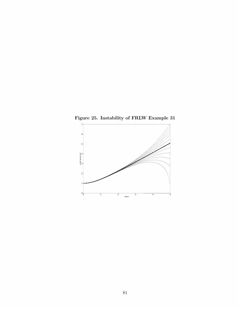
Figure 25. Instability of FRLW Example 31
0
1
2
3
4
5
6
7
0 1 2 3 4 5
scale
facto
r a(t
)
time t
81

C H A P T E R 4
REFORMULATIONS OF A BIANCHI I MODEL
For the homogeneous, anisotropic Bianchi I metric
ds2 = −dt2 +X21 (t)dx2
1 + · · ·+X2d (t)dx2
d (4.1)
in a d + 1-dimensional spacetime for d 6= 0, 1, the nonzero Einstein equations
gijGij = −κgijTij + Λ are
∑
l<k
HlHk(I0)= κ
[
1
2φ2 + V φ+ ρ
]
+ Λ (4.2)
∑
l 6=1
(Hl +H2l ) +
∑
l<kl,k 6=1
HlHk(I1)= −κ
[
1
2φ2 − V φ+ p
]
+ Λ
...
∑
l 6=i
(Hl +H2l ) +
∑
l<kl,k 6=i
HlHk(Ii)= −κ
[
1
2φ2 − V φ+ p
]
+ Λ
...
∑
l 6=d
(Hl +H2l ) +
∑
l<kl,k 6=d
HlHk(Id)= −κ
[
1
2φ2 − V φ+ p
]
+ Λ
where Hl(t)def.= al/al and i, l, k ∈ 1, . . . , d.
82

4.1 In terms of a Generalized EMP
Theorem 4.1.1 Suppose you are given twice differentiable functions
X1(t), . . . , Xd(t) > 0, a once differentiable function φ(t), and also functions
ρ(t), p(t), V (x) which satisfy the Einstein equations (I0), . . . , (Id) in (4.2) for some
Λ ∈ R, d ∈ N\0, 1, κ ∈ R\0. Denote
R(t)def.= (X1(t) · · ·Xd(t))
ν (4.3)
for some ν 6= 0. If f(τ) is the inverse of a function τ(t) which satisfies
τ (t) = θR(t)q (4.4)
for some constants θ > 0 and q 6= 0, then
Y (τ) = R(f(τ))q and Q(τ) =qνdκ
(d− 1)ϕ′(τ)2 (4.5)
solve the generalized EMP equation
Y ′′(τ) +Q(τ)Y (τ) =−2qνdκD
θ2(d− 1)Y (τ)(2+qν)/qν− qνdκ ((τ) + <(τ))
θ2(d− 1)Y (τ)(4.6)
for
ϕ(τ) = φ(f(τ)) (4.7)
(τ) = ρ(f(τ)), <(τ) = p(f(τ)) (4.8)
and where
Ddef.=
1
2dκX2
1X22 · · ·X2
d
(
∑
l<k
η2lk
)
(4.9)
is a constant for
ηlkdef.= Hl −Hk, l 6= k, l, k ∈ 1, . . . , d. (4.10)
Conversely, suppose you are given a twice differentiable function Y (τ) > 0, a
continuous function Q(τ), and also functions (τ),<(τ) which solve (4.6) for some
83

constants θ > 0 and q, ν, κ ∈ R\0, k,D ∈ R, d ∈ N\0, 1. In order to construct
functions which solve (I0), . . . , (Id), first find τ(t), ϕ(τ) which solve the differential
equations
τ(t) = θY (τ(t)) and ϕ′(τ)2 =(d− 1)
qνdκQ(τ). (4.11)
Next find a function σ(t) such that
σ(t) =1
τ (t)1/qν(4.12)
and let
R(t) = Y (τ(t))1/q αl(t)def.= clσ(t), l ∈ 1, . . . , d (4.13)
where cl are any constants for which both
d∑
l=1
cl = 0 and∑
l<k
clck = −θ2/qνDκ. (4.14)
Then the functions
Xl(t) = R(t)1/νdeαl(t) (4.15)
φ(t) = ϕ(τ(t)) (4.16)
ρ(t) = (τ(t)), p(t) = <(τ(t)) (4.17)
and
V (φ(t)) =
[
(d− 1)θ2
2ν2dκq2(Y ′)2 − D
Y 2/qν− θ2
2Y 2(ϕ′)2 − − Λ
κ
]
τ(t) (4.18)
satisfy the Einstein equations (I0), . . . , (Id).
Proof. This proof will implement Theorem 2.1.1 with constants and functions as
indicated in the following table.
84

Table 4. Theorem 2.1.1 applied to Bianchi I
In Theorem substitute In Theorem substitute
a(t) R(t) N 1
δ 0 ε νdκ/(d− 1)
G0(t) constant − 2νdκD/(d− 1) A0 2/ν
G1(t)−νdκ(d−1)
(ρ(t) + p(t)) A1 0
λ0(τ) constant −2qνdκD/θ2(d− 1) B0 (2 + qν)/qν
λ1(τ)−qνdκ
θ2(d−1)((τ) + <(τ)) B1 1
To prove the forward implication, we assume to be given functions which solve
the Einstein field equations (I0), . . . , (Id). Forming the linear combination d(I0) −d∑
i=1
(Ii) of Einstein’s equations, we obtain
d∑
l<k
HlHk −d∑
i=1
∑
l 6=i
(Hl +H2l ) −
d∑
i=1
∑
l<kl,k 6=i
HlHk = dκ[
φ2 + (ρ+ p)]
(4.19)
where l, k ∈ 1, . . . , d. The second double sum on the left-hand side of (4.19)
contains the quantity (Hl +H2l ) (d−1)-times for any fixed l, and the third double
sum contains the quantity HlHk (d − 2)-times for any fixed l, k pair with l < k
so that we have
d∑
l<k
HlHk − (d− 1)
d∑
l=1
(Hl +H2l )− (d− 2)
∑
l<k
HlHk = dκ[
φ2 + (ρ+ p)]
. (4.20)
Collecting the first and third sums gives the equation
2∑
l<k
HlHk − (d− 1)d∑
l=1
(Hl +H2l ) = dκ
[
φ2 + (ρ+ p)]
. (4.21)
Using the definition (4.3) of R(t), we define
HRdef.=
R
R=ν (X1 · · ·Xd)
ν−1(
X1X2 · · ·Xd + · · · +X1X2 · · · Xd
)
(X1 · · ·Xd)ν = ν
d∑
l=1
Hl.
(4.22)
85

Differentiating HR shows that
HR = ν
d∑
l=1
Hl, (4.23)
therefore (4.21) can be written as
2∑
l<k
HlHk − (d− 1)
(
1
νHR +
d∑
l=1
H2l
)
= dκ[
φ2 + (ρ+ p)]
. (4.24)
Multiplying this by −ν(d−1)
and rearranging, we find that
HR +ν
(d− 1)
(
(d− 1)
d∑
l=1
H2l − 2
∑
l<k
HlHk
)
=−νdκ(d− 1)
[
φ2 + (ρ+ p)]
. (4.25)
Using the definition (4.10) of the quantities ηlk, we have that
∑
l<k
η2lk =
∑
l<k
(
H2l − 2HlHk +H2
k
)
. (4.26)
The first and last terms on the right-hand side of (4.26) sum to
∑
l<k
(
H2l +H2
k
)
=
d−1∑
l=1
d∑
k=l+1
H2l +
d∑
k=2
k−1∑
l=1
H2k
=
d−1∑
l=1
(d− l)H2l +
d∑
k=2
(k − 1)H2k
= (d− 1)H21 +
d−1∑
j=2
(d− j)H2j +
d−1∑
j=2
(j − 1)H2j + (d− 1)H2
d
= (d− 1)d∑
j=1
H2j , (4.27)
therefore (4.26) becomes
∑
l<k
η2lk = (d− 1)
d∑
l=1
H2l − 2
∑
l<k
HlHk. (4.28)
Using this to rewrite (4.25), we obtain
HR +ν
(d− 1)
∑
l<k
η2lk =
−νdκ(d− 1)
[
φ2 + (ρ+ p)]
. (4.29)
86

Next we will confirm that D is a constant. Since the right-hand sides of Einstein
equations (Ii) are the same for all i ∈ 1, . . . , d, by equating the left-hand sides of
any two equations (Ii) and (Ij) for i 6= j, we get that
∑
l 6=i
(Hl +H2l ) +
∑
l<kl,k 6=i
HlHk =∑
l 6=j
(Hl +H2l ) +
∑
l<kl,k 6=j
HlHk (4.30)
where we recall that the sum indices l, k ∈ 1, . . . , d. For the first sum on each
side of (4.30), the left and the right-hand sides of (4.30) contain all the same terms,
except for the jth indexed term which appears on the left, and the ith indexed term
which appears on the right. Therefore many terms cancel and we are left with
Hj +H2j +
∑
l<kl,k 6=i
HlHk = Hi +H2i +
∑
l<kl,k 6=j
HlHk. (4.31)
For the second (double) sum on each side of (4.30), the left and right-hand sides of
(4.31) contain all the same terms, except for the terms where either l, k = j which
appear on the left, and the terms where either l, k = i which appear on the right.
Therefore many terms cancel and by adding HjHi to both sides we obtain
Hj +H2j +Hj
∑
l 6=j
Hl = Hi +H2i +Hi
∑
l 6=i
Hl, (4.32)
or equivalently
ηij +1
νηijHR = 0 (4.33)
where we have used the expression (4.22) for HR, the definition (4.10) of ηij , and
as usual dot denotes differentiation with respect to t. By Lemma A.1 with µ =
1/ν 6= 0 (which applies since R(t) is positive and differentiable), (4.33) shows that
the function f = ηijR1/ν = ηijX1X2 · · ·Xd is constant for any pair i, j (for the pair
i = j, f is clearly a constant function, namely zero). Therefore the definition (4.9)
of D is also constant, being proportional to a sum of squares of these constant
87

functions. By the definitions (4.9) and (4.3) of the constant D and the function
R(t), we now rewrite (4.29) as
HR =−νdκ(d− 1)
[
φ2 +2D
R2/ν+ (ρ+ p)
]
. (4.34)
This shows that R(t), φ(t), ρ(t) and p(t) satisfy the hypothesis of Theorem 2.1.1,
applied with constants ǫ, ε, N,A0, . . . , AN and functions a(t), G0(t), . . . , GN(t) ac-
cording to Table 4. Since τ(t), Y (τ), Q(τ) and ϕ(τ) defined in (4.4), (4.5) and (4.7)
are equivalent to that in the forward implication of Theorem 2.1.1, by this theorem
and by definition (4.8) of (τ),<(τ), the generalized EMP equation (2.2) holds for
constants B0, . . . , BN and functions λ0(τ), . . . , λN(τ) as indicated in Table 4. This
proves the forward implication.
Note that equation (4.34) with ν = 1/d is the same as the FRLW analogue
equation (3.18) with M = 1, n1 = 2d, k = 0 and by identifying R(t) here with a(t)
in the FRLW model. One can compare this observation with J. Lidsey’s results on
the 3 + 1-dimensional Bianchi I model in [22].
To prove the converse implication, we assume to be given functions which solve
the generalized EMP equation (4.6) and we begin by showing that (I0) is satisfied.
Differentiating the definition of R(t) in (4.13) and using the definition in (4.11) of
τ(t), we have
R(t) =1
qY (τ(t))
1q−1Y ′(τ(t))τ (t)
=θ
qY (τ(t))1/qY ′(τ(t)). (4.35)
so that
HR(t)def.=
R(t)
R(t)=θ
qY ′(τ(t)). (4.36)
88

Differentiating the definition (4.16) of φ(t) and using the definition (4.11) of τ(t)
gives
φ(t) = ϕ′(τ(t))τ (t) = θϕ′(τ(t))Y (τ(t)). (4.37)
Using (4.36) and (4.37), and also the definitions (4.13) and (4.17) of R(t) and ρ(t)
respectively, the definition (4.18) of V φ can be written as
V φ =1
κ
(
(d− 1)
2ν2dH2
R − Dκ
R2/ν
)
− 1
2φ2 − ρ− Λ
κ. (4.38)
The quantity in parenthesis here is in fact equal to the left-hand-side of equation
(I0). To see this, we differentiate the definition (4.15) of Xl(t), divide the result by
Xl and use the definition (4.36) of HR to obtain
Hldef.=
Xl
Xl
=1νdR1/νd−1Reαl + αlR
1/νdeαl
R1/νdeαl=
1
νdHR + αl (4.39)
so that∑
l<k
HlHk =∑
l<k
(
1
ν2d2H2
R +1
νd(αl + αk)HR + αlαk
)
. (4.40)
The first term on the right-hand side of (4.40) does not depend on the indices l, k,
and is therefore equal to 1ν2d2H
2R times the quantity
∑
l<k
1 =d∑
k=2
k−1∑
l=1
1 =d∑
k=2
(k − 1) =d−1∑
j=1
j =d(d− 1)
2. (4.41)
The second term on the right-hand side of (4.40) sums to zero since
∑
l<k
(αl + αk) =
d−1∑
l=1
d∑
k=l+1
αl +
d∑
k=2
k−1∑
l=1
αk
=
d−1∑
l=1
(d− l)αl +
d∑
k=2
(k − 1)αk
= (d− 1)α1 +d−1∑
j=2
(d− j + j − 1)αj + (d− 1)αd
= (d− 1)d∑
l=1
αl
89
= (d− 1)σ(t)
d∑
l=1
cl
= 0 (4.42)
where on the last lines, we have used the definition (4.13) of αl(t) and the condition
(4.14) on the constants cl. For the third term on the right-hand side of (4.40), we
use the definitions of αl(t), σ(t), τ(t) and R(t) in (4.13), (4.12) and (4.11) to write
αlαk = clckσ2 =
clckτ 2/qν
=clck
θ2/qν(Y τ)2/qν=
clckθ2/qνR2/ν
. (4.43)
Therefore (4.40) becomes
∑
l<k
HlHk =(d− 1)
2ν2dH2
R +∑
l<k
clckθ2/qνR2/ν
. (4.44)
Then by the condition (4.14) on the constants cl, (4.44) becomes
∑
l<k
HlHk =(d− 1)
2ν2dH2
R − Dκ
R2/ν. (4.45)
That is, the expression (4.38) for V can now be written as
V φ =1
κ
∑
l<k
HlHk −1
2φ2 − ρ− Λ
κ, (4.46)
showing that (I0) holds under the assumptions of the converse implication.
To conclude the proof we must also show that the equations (I1), . . . , (Id) hold.
In the converse direction the hypothesis of the converse of Theorem 2.1.1 holds,
applied with constants N,B0, . . . , BN and functions λ0(τ), . . . , λN(τ) as indicated
in Table 4. Since τ(t), ϕ(τ), R(t) and φ(t) defined in (4.11), (4.13) and (4.16)
are consistent with the converse implication of Theorem 2.1.1, applied with a(t), δ
and ε as in Table 4, by this theorem and by the definition (4.17) of ρ(t), p(t)
the scale factor equation (2.1) holds for constants δ, ε, A0, . . . , AN and functions
G0(t), . . . , GN(t) according to Table 4. That is, we have regained (4.34). Now
90

solving (4.38) for ρ(t) and substituting this into (4.34), we obtain
HR =−νdκ(d− 1)
[
1
2φ2 − V φ+
D
R2/ν+ p+
(d− 1)
2ν2dκH2
R − Λ
κ
]
. (4.47)
Multiplying by (d−1)νd
and rearranging, we get that
(d− 1)
νdHR +
(d− 1)
2ν2dH2
R +κD
R2/ν= −κ
[
1
2φ2 − V φ+ p
]
+ Λ (4.48)
The left-hand side of this equation is in fact equal to the left-hand-side of (Ii) for
any i ∈ 1, . . . , d. To see this, first recall (4.39) and write
Hl +H2l =
1
νdHR +
1
ν2d2H2
R + αl +2
νdαlHR + α2
l , (4.49)
therefore for any fixed i
∑
l 6=i
(Hl +H2l ) =
∑
l 6=i
(
1
νdHR +
1
ν2d2H2
R + αl +2
νdαlHR + α2
l
)
. (4.50)
Since the first two terms on the right-hand side of (4.50) do not depend on the
indices l, k, and also using the definitions (4.13) and (4.14) of αl and the constants
cl to write∑
l αl = 0 ⇒∑
l 6=i αl = −αi, (4.50) becomes
∑
l 6=i
(Hl +H2l ) =
(d− 1)
νdHR +
(d− 1)
ν2d2H2
R − 2
νdHRαi +
∑
l 6=i
(
αl + α2l
)
. (4.51)
By the definitions (4.13), (4.12) and (4.11) of αl(t), σ(t), τ(t) and R(t), we see that
αl(t)R(t)1/ν = clσ(t)R(t)1/ν
=cl
τ(t)1/qνR(t)1/ν
=cl
θ1/qνY (τ(t))1/qνR(t)1/ν
=cl
θ1/qνis a constant. (4.52)
By Lemma A.1 with µ = 1/ν 6= 0, equation (4.52) shows that
αl +1
ναlHR = 0 (4.53)
91

for all l ∈ 1, . . . , d. Therefore in total, we have that (4.50) is
∑
l 6=i
(Hl +H2l ) =
(d− 1)
νdHR +
(d− 1)
ν2d2H2
R +(2 − d)
νdHR
∑
l 6=i
αl +∑
l 6=i
α2l . (4.54)
To form the rest of the left-hand side of (Ii), again use (4.39) to obtain
HlHk =1
ν2d2H2
R +1
νd(αl + αk)HR + αlαk. (4.55)
Therefore for any fixed i, we have
∑
l<kl,k 6=i
HlHk =∑
l<kl,k 6=i
(
1
ν2d2H2
R +1
νd(αl + αk)HR + αlαk
)
. (4.56)
As we saw in (4.41),∑
l<k 1 = d(d−1)2
therefore the first term on the right-side of
(4.56), which does not depend on the indices l, k, is equal to 1ν2d2H
2R times
∑
l<kl,k 6=i
1 =∑
l<k
1 −∑
l 6=i
1 =d(d− 1)
2− (d− 1) =
(d− 1)(d− 2)
2. (4.57)
As we saw in (4.42),∑
l<k(αl + αk) = 0 therefore the second term on the right-hand
side of (4.56) sums to 1νdHR times the quantity
∑
l<kl,k 6=i
(αl + αk) =∑
l<k
(αl + αk) −∑
l 6=i
(αl + αi)
= −∑
l 6=i
αl − (d− 1)αi
= αi − (d− 1)αi
= (2 − d)αi (4.58)
where we have used the definitions (4.13) and (4.14) of αl and the constants cl to
write∑
l 6=i αl = −αi. Considering the third term on the right-hand side of (4.56),
92

we have that
∑
l<kl,k 6=i
αlαk =∑
l<k
αlαk − ci∑
l 6=i
cl
=∑
l<k
αlαk +
(
∑
l 6=i
cl
)2
=∑
l<k
αlαk + 2∑
l<kl,k 6=i
clck +∑
l 6=i
c2l
= −∑
l<k
αlαk −∑
l 6=i
c2l
= −∑
l<k
clckθ2/qνR2/ν
−∑
l 6=i
c2l (4.59)
where again we have used that∑
l 6=i αl = −αi, and on the last line we recall (4.43).
So by (4.57), (4.58) and (4.59), in total (4.56) becomes
∑
l<kl,k 6=i
HlHk =(d− 1)(d− 2)
2ν2d2H2
R +(2 − d)
νdαiHR −
∑
l<k
clckθ2/qνR2/ν
−∑
l 6=i
c2l . (4.60)
Summing (4.54) and (4.60), the left-hand side of any (Ii) Einstein equation is
∑
l 6=i
(Hl +H2l ) +
∑
l<kl,k 6=i
HlHk =(d− 1)
νdHR +
d(d− 1)
2ν2d2H2
R −∑
l<k
clckθ2/qνR2/ν
. (4.61)
Then by the condition (4.14) on the constants cl, (4.62) becomes
∑
l 6=i
(Hl +H2l ) +
∑
l<kl,k 6=i
HlHk =(d− 1)
νdHR +
d(d− 1)
2ν2d2H2
R +Dκ
R2/ν. (4.62)
Therefore by (4.48) and (4.62), we obtain (Ii) for all i ∈ 1, . . . , d. This proves
the theorem. ⋄
4.1.1 Reduction to classical EMP: pure scalar field
To compute some exact solutions to Einstein’s equations for the Bianchi I met-
ric, we take ρ = p = 0 and choose parameter ν = 1/q in Theorem 4.1.1. Therefore
93

solving the Bianchi I Einstein equations
∑
l<k
HlHk(I0)′= κ
[
1
2φ2 + V φ
]
+ Λ (4.63)
∑
l 6=i
(Hl +H2l ) +
∑
l<kl,k 6=i
HlHk(Ii)
′= −κ
[
1
2φ2 − V φ
]
+ Λ
for l, k, i ∈ 1, . . . , d is equivalent to solving the classical EMP equation
Y ′′(τ) +Q(τ)Y (τ) =−2dκD
θ2(d− 1)Y (τ)3(4.64)
for constants θ,D > 0. The solutions of (I0)′, (I1)
′, . . . , (Id)′ and (4.64) are related
by
R(t) = Y (τ(t))1/q and ϕ′(τ)2 =(d− 1)
dκQ(τ) (4.65)
for q 6= 0, φ(t) = ϕ(τ(t)), R(t)def.= (X1(t) · · ·Xd(t))
1/q and
τ (t) = θR(t)q = θY (τ(t)) (4.66)
for any θ > 0. Also the quantity
Ddef.=
1
2dκX2
1X22 · · ·X2
d
(
∑
l<k
η2lk
)
(4.67)
is constant for
ηlkdef.= Hl −Hk, l 6= k, l, k ∈ 1, . . . , d. (4.68)
In the converse direction we have
Xl(t) = R(t)q/deαl(t) (4.69)
for αl(t)def.= clσ(t) where σ(t) satisfies
σ(t) = 1/τ(t) (4.70)
and cl are any constants for which both
d∑
l=1
cl = 0 and∑
l<k
clck = −θ2/qνDκ. (4.71)
94

Also V is taken to be defined as
V (φ(t)) =
[
(d− 1)θ2
2dκ(Y ′)2 − D
Y 2− θ2
2Y 2(ϕ′)2 − Λ
κ
]
τ(t). (4.72)
We now refer to Appendix D for solutions of the classical EMP equation (3.24),
which we will map to a solution of the Bianchi I Einstein equations. By compar-
ing (4.66) and (D.5), we note to only consider solutions of (D.5) in Appendix D
corresponding to r0 = 1. Also by comparing (4.70) to (D.6), we see to take s0 = 1
in Appendix D. Of course when D = 0 in (4.67), ηlk = 0 for all pairs l, k so that
X1(t), X2(t), . . . , Xd(t) agree up to a constant multiple. In this case, if we take
R(t) = X1(t) = · · · = Xd(t)def.= a(t) and q = d we obtain the FRLW cosmology
with curvature k = 0 and n = 2d,D = 0 so that we may refer to sections 3.1.1
and 3.2.2 for exact solutions to the Bianchi I Einstein equations if D = 0. Here
we consider solutions to the classical EMP (4.64) by referring to Table 14 with
λ1 = −2dκDθ2(d−1)
< 0.
Example 32 For θ = 1 and choice of constant D = (d − 1)/2dκ, we consider
solution 5 in Table 14 with d0 = b0 = 0 and c0 = 1. That is, we have solution
Y (τ) = (a0 + 2τ)1/2 to the classical EMP Y ′′(τ) + Q(τ)Y (τ) = −1/Y (τ)3 for
Q(τ) = 0 and a0 ∈ R. By (D.27) - (D.29) we have τ(t) = 12((t− t0)
2 − a0) and
R(t) = Y (τ(t))1/q = (t− t0)1/q (4.73)
for any q 6= 0 and t0 ∈ R. Also by (D.32) we have σ(t) = ln(t− t0) so that
Xi(t) = R(t)q/deciσ(t)
= (t− t0)1/deci ln(t−t0)
= (t− t0)1/d+ci (4.74)
95
for 1 ≤ i ≤ d and for constants c1, . . . , cd that satisfy
d∑
l=1
cl = 0 and∑
l<k
clck = −(d− 1)
2d(4.75)
by (4.14). Since Q(τ) = 0 = ϕ′(τ) the scalar field φ(t)def.= ϕ(τ(t)) = φ0 ∈ R
is constant. Finally, by (4.72), (D.30) and (D.29), we obtain constant potential
V (φ(t)) = −Λ/κ.
One can verify by hand that X1(t), . . . , Xd(t), φ(t) and V (φ(t)) in (4.74), (32)
and (6.79) satisfy the vacuum Bianchi I equations (I0)′ and (Ii)
′ for 1 ≤ i ≤ d and
for ci as in (4.75), with use of the identity in equation (4.59). This example is the
well-known Kasner solution ds2 = −dt2 +∑d
i=1 t2pidx2
i , in which the constants pi
must satisfy the Kasner conditions∑d
i=1 pi =∑d
i=1 p2i = 1. By setting pi = 1/d+ci,
we see that our conditions (4.75) are equivalent to the Kasner conditions since
∑di=1 pi =
∑di=1(1/d+ci) = 1+
∑di=1 ci = 1+0 = 1 and
∑di=1 p
2i =
∑di=1(1/d+ci)
2 =
(1/d) +∑d
i=1 c2i = (1/d) − 2
∑
l<k clck = (1/d) + 2((d− 1)/2d) = 1.
Example 33 For θ = q = 1 and choice of constant D = (d− 1)/2dκ, we consider
solution 5 in Table 14 with d0 = a0 = 0, b0 = 4 and c0 = 1. That is, we have solution
Y (τ) = (4τ(t)2 +2τ(t))1/2 to the classical EMP Y ′′(τ)+Q(τ)Y (τ) = −1/Y (τ)3 for
Q(τ) = 0. By (D.33) - (D.35) we have τ(t) = 18
(
e2(t−t0) + e−2(t−t0) − 8)
and
R(t) = Y (τ(t)) =1
2sinh(2(t− t0)) (4.76)
for any t0 ∈ R. Also by (D.37) we have that
σ(t) = −2Arccoth(
e2(t−t0))
= ln (tanh(t− t0)) (4.77)
so that
Xi(t) = R(t)1/deciσ(t) =1
21/dsinh(2(t− t0))
1/deciσ(t)
=1
21/dsinh(2(t− t0))
1/dtanhci(t− t0) (4.78)
96

for σ(t) as in (4.77) and constants that satisfy
d∑
l=1
cl = 0 and∑
l<k
clck = −(d − 1)
2d. (4.79)
Since Q(τ) = 0 = ϕ′(τ), the scalar field is constant φ(t)def.= ϕ(τ(t)) = φ0 ∈ R.
Finally, by (4.72), (D.36) and (D.35), we obtain constant potential V (φ(t)) =
2(d−1)dκ
− Λκ. One can compare this solution with the higher-dimensional solution of
Lorenz-Petzold in [24].
As an example for d = 3, one can take c1 = − 1√3, c2 = 0 and c3 = 1√
3so that
X1(t) =13√
2sinh(2(t− t0))
1/3tanh−1/√
3(t− t0)
X2(t) =13√
2sinh(2(t− t0))
1/3
X3(t) =13√
2sinh(2(t− t0))
1/3tanh1/√
3(t− t0) (4.80)
and potential V (φ(t)) = 43κ
− Λκ
solve the Bianchi I equations in 3 + 1 spacetime
dimensions. One can compare this solution to the Bali and Jain solution in [1].
4.2 In terms of a Schrodinger-Type Equation
To reformulate the Einstein field equations (I0), . . . , (Id) in terms of a
Schrodinger-type equation with one less non-linear term than the generalized EMP,
one can apply Corollary 2.3.1 to the difference d(I0)−d∑
i=1
(Ii). Below is the resulting
statement.
Theorem 4.2.1 Suppose you are given twice differentiable functions
X1(t), . . . , Xd(t) > 0, a once differentiable function φ(t), and also functions
ρ(t), p(t), V (x) which satisfy the Einstein equations (I0), . . . , (Id) for some
97

Λ ∈ R, d ∈ N\0, 1, κ ∈ R\0. Let g(σ) denote the inverse of a function σ(t)
which satisfies
σ(t) =1
θ (X1(t) · · ·Xd(t))(4.81)
for some θ > 0. Then the following functions
u(σ) =
[
1
X1 · · ·Xd
]
g(σ) (4.82)
P (σ) =dκ
(d− 1)ψ′(σ)2 (4.83)
solve the Schrodinger-type equation
u′′(σ) + [E − P (σ)]u(σ) =θ2dκ(ρ(σ) + p(σ))
(d− 1)u(σ)(4.84)
for
ψ(σ) = φ(g(σ)) (4.85)
ρ(σ) = ρ(g(σ)), p(σ) = p(g(σ)) (4.86)
and where
Edef.=
−θ2
(d− 1)X2
1X22 · · ·X2
d
∑
l<k
η2lk (4.87)
is a constant for
ηlkdef.= Hl −Hk, l 6= k, l, k ∈ 1, . . . , d. (4.88)
Conversely, suppose you are given a twice differentiable function u(σ) > 0, and
also functions P (σ) and ρ(σ), p(σ) which solve (4.84) for some constants E <
0, θ > 0, κ ∈ R\0 and d ∈ N\0, 1. In order to construct functions which solve
(I0), . . . , (Id), first find σ(t), ψ(σ) which solve the differential equations
σ(t) =1
θu(σ(t)) and ψ′(σ)2 =
(d− 1)
dκP (σ). (4.89)
Let
R(t) = u(σ(t))−ν and αl(t)def.= clσ(t), l ∈ 1, . . . , d (4.90)
98

where cl are any constants for which both
d∑
l=1
cl = 0 and∑
l<k
clck =(d− 1)E
2d. (4.91)
Then the functions
Xl(t) = R(t)1/νdeαl(t) (4.92)
φ(t) = ψ(σ(t)) (4.93)
ρ(t) = ρ(σ(t)), p(t) = p(σ(t)) (4.94)
and
V (φ(t)) =
[
(d− 1)
2θ2dκ
(
(u′)2 + Eu2)
− 1
2θ2u2(ψ′)2 − ρ − Λ
κ
]
σ(t) (4.95)
satisfy the equations (I0), . . . , (Id).
Proof. This proof will implement Corollary 2.3.1 with constants and functions as
indicated in the following table.
Table 5. Corollary 2.3.1 applied to Bianchi I
In Corollary substitute In Corollary substitute
a(t) R(t) ε νdκ/(d− 1)
G(t) constant νE/θ2 A 2/ν
G1(t)−νdκ(d−1)
(ρ(t) + p(t)) A1 0
F1(σ) θ2dκ(d−1)
(ρ(σ) + p(σ)) C1 1
Much of this proof will rely on computations that are exactly the same as those
seen in the proof of Theorem 4.1.1 (the generalized EMP formulation of Bianchi
I). Therefore we will restate the relevant results here, but point the reader to the
details in the proof of Theorem 4.1.1.
99

To prove the forward implication, we assume to be given functions which solve
the Einstein field equations (I0), . . . , (Id). Forming the linear combination d(I0) −d∑
i=1
(Ii) of Einstein’s equations and simplifying, as was done in (4.19) - (4.29),
HR +ν
(d− 1)
∑
l<k
η2lk =
−νdκ(d− 1)
[
φ2 + (ρ+ p)]
(4.96)
where
HR(t)def.=
R(t)
R(t)(4.97)
and
R(t)def.= (X1(t) · · ·Xd(t))
ν (4.98)
for any ν 6= 0. Next we will confirm that E is constant. As was done in (4.30)-
(4.33), since the right-hand sides of Einstein’s equations (Ii) are the same for all
i ∈ 1, . . . , d, by equating the left-hand sides of any two equations (Ii) and (Ij)
for i 6= j, and after some rearranging we obtain
ηij +1
νηijHR = 0 (4.99)
for ηij defined in (4.88). Therefore the definition (4.87) of E is constant, being
proportional to a sum of squares of these constant functions. By the definitions
(4.87) and (4.98) of the constant E and the function R(t), we now rewrite (4.96)
from above as
HR =−νdκ(d− 1)
[
φ2 + (ρ+ p)]
+νE
θ2R2/ν. (4.100)
This shows that R(t), φ(t), ρ(t) and p(t) satisfy the hypothesis of Corollary 2.3.1,
applied with constants ε,N,A,A1 . . . , AN and functions a(t), G(t), G1(t), . . . , GN(t)
according to Table 9. Since σ(t), u(σ), P (σ) and ψ(σ) defined in (4.81), (4.82),
(4.83) and (4.85) are equivalent to that in the forward implication of Corollary
2.3.1, applied with constants and functions according to Table 9, by this corollary
100

and by definition (4.86) of ρi(σ), p(σ), the Schrodinger-type equation (2.110) holds
for constants C1, . . . , CN and functions F1(σ), . . . , FN(σ) as indicated in Table 9.
This proves the forward implication.
To prove the converse implication, we assume to be given functions which solve
the Schrodinger-type equation (4.84) and we begin by showing that (I0) is satisfied.
Differentiating the definition of R(t) in (4.90) and using the definition in (4.89) of
σ(t), we obtain
R(t) = −νu(σ(t))−ν−1u′(σ(t))σ(t)
= −νθu(σ(t))−νu′(σ(t)). (4.101)
so that
HRdef.=
R
R= −ν
θu′(σ(t)). (4.102)
Differentiating the definition (4.93) of φ(t) and using the definition in (4.90) of σ(t),
we obtain
φ(t) = ψ′(σ(t))σ(t) =1
θψ′(σ(t))u(σ(t)). (4.103)
Using (4.102) and (4.103), and also the definitions (4.90) and (4.94) of R(t) and
ρ(t) respectively, the definition (4.95) of V φ can be written as
V φ =1
κ
(
(d− 1)
2ν2dH2
R +(d− 1)E
2dθ2R2/ν
)
− 1
2φ2 − ρ− Λ
κ. (4.104)
The quantity in parenthesis here is in fact equal to the left-hand-side of equation
(I0). To see this, first note that the definitions Xl(t)def.= R(t)1/νdeαl(t) in (4.92)
and H(t)def.= R(t)
R(t)in (4.102), and the condition
∑
l cl = 0, are the same as those in
Theorem 4.1.1. Also by the definitions (4.90), (4.89) and (4.90) of αl(t), σ(t) and
R(t), we obtain
αlαk = clckσ2 =
clckθ2
(u σ)2 =clck
θ2R(t)2/ν, (4.105)
101

which is a slightly modified version of (4.43) from our computation in the proof of
Theorem 4.1.1. Therefore by the arguments in (4.40)-(4.44), and using (4.105) to
slightly modify the last term to apply here, we have that
∑
l<k
HlHk =(d− 1)
2ν2dH2
R +∑
l<k
clckθ2R2/ν
. (4.106)
Then by the condition (4.91) on the constants cl, (4.106) becomes
∑
l<k
HlHk =(d− 1)
2ν2dH2
R +(d− 1)E
2dθ2R2/ν. (4.107)
That is, the expression (4.104) for V can now be written as
V φ =1
κ
∑
l<k
HlHk −1
2φ2 − ρ− Λ
κ, (4.108)
showing that (I0) holds under the assumptions of the converse implication.
To conclude the proof we must also show that the equations (I1), . . . , (Id) hold.
In the converse direction the hypothesis of the converse of Corollary 2.3.1 holds,
applied with constants N,C1, . . . , CN and functions F1(σ), . . . , FN(σ) as indicated
in Table 9. Since σ(t), ψ(σ), R(t) and φ(t) defined in (4.89), (4.90) and (4.93)
are consistent with the converse implication of Corollary 2.3.1, applied with a(t)
and ε as in Table 9, by this corollary and by the definition (4.94) of ρ(t), p(t)
the scale factor equation (2.109) holds for constants ε, A,A1, . . . , AN and functions
G(t), G1(t), . . . , GN(t) according to Table 9. That is, we have regained (4.100).
Now solving (4.104) for ρ(t) and substituting this into (4.100), we obtain
HR =−νdκ(d− 1)
[
1
2φ2 − V φ+
(d− 1)E
2dθ2κR2/ν+ p +
(d− 1)
2ν2dκH2
R − Λ
κ
]
. (4.109)
Multiplying by (d−1)νd
and rearranging, we see that
(d− 1)
νdHR +
(d− 1)
2ν2dH2
R +(d− 1)E
2dθ2R2/ν= −κ
[
1
2φ2 − V φ+ p
]
+ Λ. (4.110)
102

The left-hand side of this equation is in fact equal to the left-hand-side of (Ii)
for any i ∈ 1, . . . , d. To see this, again we use that the definitions Xl(t)def.=
R(t)1/νdeαl(t) in (4.92) and HR(t)def.= R(t)
R(t)in (4.102), and the condition
∑
l cl = 0,
are the same as those in Theorem 4.1.1. Also by the definitions (4.90) and (4.89)
of αl(t), σ(t) and R(t), we see that
αl(t)R(t)1/ν = clσ(t)R(t)1/ν
=clθu(σ(t))R(t)1/ν
=clθ
is a constant (4.111)
which shows that
αl +1
ναlHR = 0 (4.112)
holds here as it does in Theorem 4.1.1. Therefore by the arguments in (4.49)-(4.61),
and as above using (4.105) to slightly modify the last term of (4.61) to apply here,
we have that
∑
l 6=i
(Hl +H2l ) +
∑
l<kl,k 6=i
HlHk =(d− 1)
νdHR +
d(d− 1)
2ν2d2H2
R −∑
l<k
clckθ2R2/ν
. (4.113)
Then by the condition (4.91) on the constants cl, (4.113) becomes
∑
l 6=i
(Hl +H2l ) +
∑
l<kl,k 6=i
HlHk =1
νd(d− 1)HR +
d(d− 1)
2ν2d2H2
R −∑
l<k
(d− 1)E
2dθ2R2/ν. (4.114)
Combining (4.110) and (4.114), we obtain (Ii) for all i ∈ 1, . . . , d. This proves
the theorem.
⋄
103

4.2.1 Reduction to linear Schrodinger: pure scalar field
To show some examples we take ρ = p = 0 so that Theorem shows that solving
the Bianchi I Einstein equations
∑
l<k
HlHk(I0)′′= κ
[
1
2φ2 + V φ
]
+ Λ (4.115)
∑
l 6=i
(Hl +H2l ) +
∑
l<kl,k 6=i
HlHk(Ii)′′= −κ
[
1
2φ2 − V φ
]
+ Λ
is equivalent to solving the linear Schrodinger equation
u′′(σ) + [E − P (σ)]u(σ) = 0. (4.116)
The solutions of (I0)′′, (Ii)
′′ in (4.115) and the solutions of (4.116) are related by
R(t) = (X1(t) · · ·Xd(t))ν = u(σ(t))−ν and ψ′(σ)2 =
(d− 1)
dκP (σ) (4.117)
for any ν 6= 0 and where φ(t) = ψ(σ(t)) and
σ(t) =1
θX1(t) · · ·Xd(t)=
1
θu(σ(t)), (4.118)
for θ > 0. Also the constant E is
Edef.=
−θ2
(d− 1)X2
1X22 · · ·X2
d
(
∑
l<k
η2lk
)
(4.119)
for ηlkdef.= Hl −Hk, l, k ∈ 1, . . . , d. In the converse direction
Xl(t) = R(t)1/νdeαl(t) (4.120)
for αl(t)def.= clσ(t) and where the constants cl satisfy
d∑
l=1
cl = 0 and∑
l<k
clck =(d− 1)E
2d. (4.121)
104

Also V is taken to be such that
V (φ(t)) =
[
(d− 1)
2θ2dκ
(
(u′)2 + Eu2)
− 1
2θ2u2(ψ′)2 − Λ
κ
]
σ(t). (4.122)
We now refer to Appendix E for solutions of the linear Schrodinger equation
(4.116). We will map them using the theorem to exact solutions of Einstein’s
equations. Of course when E = 0 in (4.119), ηlk = 0 for all pairs l, k so that
X1(t), X2(t), . . . , Xd(t) agree up to a constant multiple. In this case, if we take
R(t) = X1(t) = · · · = Xd(t)def.= a(t) and ν = 1/d we obtain the FRLW cosmology
with curvature k = 0, n = 2d and D = 0 so that we may refer to section 3.3.1
for exact solutions to the Bianchi I Einstein equations if E = 0. Here we consider
solutions to the linear Schrodinger equation (4.116) by referring to Table 15 with
E < 0.
Example 34 For θ = 1 and choice of constant E = −1, we take solution 4 in
Table 15 with c0 = −1, a0 = 1 and b0 = 0 so that we have u(σ) = e−σ, P (σ) = 0.
By (E.28) - (E.30) with r0 = 1 we obtain σ(t) = ln ((t− t0)) and
R(t) =1
u(σ(t))ν= (t− t0)
ν (4.123)
for any ν 6= 0 t0 ∈ R so that
Xi(t) = R(t)1/νdeciσ(t) = (t− t0)1/d+ci (4.124)
for constants that satisfy
d∑
l=0
cl = 0 and∑
l<k
clck = −(d− 1)
2d. (4.125)
Since P = 0 = ψ′(σ), ψ(σ) = ψ0 for constant ψ0 ∈ R. Finally, by (4.122),
(E.31) and (E.30), we obtain constant potential V (φ(t)) = −Λ/κ. This is alternate
derivation of the Kasner vacuum solution seen above in Example 32.
105

For ν = 1/2 and t0 = 0, the solver was run with u and u′ both perturbed by
.01. The graphs of R(t) below show that this solution is unstable, since the absolute
error grows up to two orders of magnitude over the graphed time interval.
Figure 26. Instability of Bianchi I Example 34
0
1
2
3
4
5
2 3 4 5 6 7
scale
facto
r a(t
)
time t
Example 35 For θ = 1 and choice of constant E = −1, we take solution 4 in
Table 15 with c0 = −1 and a0, b0 > 0 so that we have u(σ) = a0e−σ − b0e
σ and
P (σ) = 0. By (E.32) - (E.34) we obtain σ(t) = ln(√
a0
b0tanh(
√a0b0(t− t0))
)
and
R(t) =1
u(σ(t))ν=
1
(2√a0b0)ν
sinhν(2√
a0b0(t− t0)) (4.126)
for ν 6= 0 and t0 ∈ R so that
Xi(t) = R(t)1/νdeciσ(t) (4.127)
=
√a0
ci−1/d
√b0
ci+1/dsinh1/d+ci(
√
a0b0(t− t0))cosh1/d−ci(
√
a0b0(t− t0)).
Since P = 0 = ψ′(σ), the scalar field is constant
ψ(σ) = ψ0 ∈ R. (4.128)
106

Finally, by (4.122), (E.35) and (E.34), we obtain constant potential
V (φ(t)) =2(d− 1)a0b0
dκ− Λ
κ(4.129)
since coth2(x) − csch2(x) = 1.
As an example for d = 3, one can take c1 = − 1√3, c2 = 0, c3 = 1√
3and a0 =
b0 = 1 so that
X1(t) = sinh(1−√
3)/3((t− t0))cosh(1+
√3)/3((t− t0))
X2(t) = sinh1/3((t− t0))cosh1/3((t− t0))
X3(t) = sinh(1+√
3)/3((t− t0))cosh(1−
√3)/3((t− t0)) (4.130)
and the potential V (φ(t)) = 43κ
− Λκ
solve the Bianchi I equations in 3+1 spacetime
dimensions. One can also compare this solution with the Bali and Jain solution in
section 2 of [1].
Example 36 For θ = 1 and choice of constant E = −1, we take solution 5 in
Table 15 with c0 = −1 and b0 = 0 so that we have u(σ) = (a0/σ)e−σ2/2 and
P (σ) = σ2+2/σ2 for a0 > 0. By (E.36) - (E.38) we obtain σ(t) =√
2 ln(a0(t− t0))
and
R(t) =1
u(σ(t))ν=(√
2(t− t0)√
ln(a0(t− t0)))ν
(4.131)
for t > t0 so that
Xi(t) = R(t)1/νdeciσ(t)
=(√
2(t− t0)√
ln(a0(t− t0)))1/d
eci
√2 ln(a0(t−t0)). (4.132)
for constants ci that satisfy
d∑
l=1
cl = 0 and∑
l<k
clck = −(d− 1)
2d. (4.133)
107

By (E.41) with α0 = (d− 1)/dκ, we have scalar field
φ(t) = ψ(σ(t))
=
√
(d− 1)
2dκ
(
√
2 ln2(a0(t− t0)) + 1 + ln [2 ln(a0(t− t0))]
− ln
[
4 + 4
√
2 ln2(a0(t− t0)) + 1
])
+ β0 (4.134)
for β0 ∈ R. Finally, by (4.122), (E.39) and (E.38), we obtain
V (φ(t)) =
[
(d− 1)
2dκ
(
(u′)2 − u2)
− 1
2θ2u2(ψ′)2 − Λ
κ
]
σ(t)
=(d− 1)(2 ln(a0(t− t0)) − 1)
8dκ(t− t0)2 ln2(a0(t− t0))− Λ
κ. (4.135)
For example when d = 3, we can take c1 = − 1√3, c2 = 0 and c3 = 1√
3to obtain
X1(t) =(√
2(t− t0)√
ln(a0(t− t0)))1/3
e− 1√
3
√2 ln(a0(t−t0))
X2(t) =(√
2(t− t0)√
ln(a0(t− t0)))1/3
X3(t) =(√
2(t− t0)√
ln(a0(t− t0)))1/3
e1√3
√2 ln(a0(t−t0))
, (4.136)
φ(t) =
√
1
3κ
(
√
2 ln2(a0(t− t0)) + 1 + ln [2 ln(a0(t− t0))]
− ln
[
4 + 4
√
2 ln2(a0(t− t0)) + 1
])
+ β0 (4.137)
and
V (φ(t)) =(2 ln(a0(t− t0)) − 1)
12κ(t− t0)2 ln2(a0(t− t0))− Λ
κ(4.138)
for β0, t0 ∈ R and a0 > 0. Note that this is similar to the FRLW solution found
in Example 21 by setting n = 2d and by identifying a(t) in Example 21 with R(t)
here.
For ν = a0 = 1 and t0 = 0, the solver was run with u and u′ both perturbed by
.01. The graphs of R(t) below show that this solution is unstable, since the absolute
error grows three orders of magnitude over the graphed time interval.
108

Figure 27. Instability of Bianchi I Example 36
0.5
1
1.5
2
2.5
3
3.5
4
4.5
5
1.5 2 2.5 3 3.5 4
scale
facto
r a(t
)
time t
109

C H A P T E R 5
REFORMULATIONS OF A CONFORMAL BIANCHI I
MODEL
For a change of coordinates in comparison to chapter 4, we consider a Bianchi
I metric of the form
ds2 = − (a1(t)a2(t) · · ·ad(t))2 dt2 + a1(t)
2dx21 + a2
2(t)dx22 + · · ·+ a2
d(t)dx2d (5.1)
in a d + 1−dimensional spacetime. The nonzero Einstein equations gijGij =
−κgijTij + Λ, multiplied by |g00| = (a1a2 · · ·ad)2 are
∑
l<k
HlHk(I0)= κ
[
φ2
2+ (a1a2 · · ·ad)
2
(
V φ+ ρ+Λ
κ
)
]
(5.2)
∑
l 6=1
Hl −∑
l<k
HlHk(I1)= κ
[
− φ2
2+ (a1a2 · · ·ad)
2
(
V φ− p+Λ
κ
)
]
...
∑
l 6=i
Hl −∑
l<k
HlHk(Ii)= κ
[
− φ2
2+ (a1a2 · · ·ad)
2
(
V φ− p+Λ
κ
)
]
...
∑
l 6=d
Hl −∑
l<k
HlHk(Id)= κ
[
− φ2
2+ (a1a2 · · ·ad)
2
(
V φ− p+Λ
κ
)
]
where Hl(t)def.= al
al.
110

5.1 In terms of a Generalized EMP
Theorem 5.1.1 Suppose you are given twice differentiable functions
a1(t), . . . , ad(t) > 0, a once differentiable function φ(t) and also functions
ρ(t), p(t), V (x) which satisfy the Einstein equations (I0), . . . , (Id) for some
Λ ∈ R, d ∈ N\0, 1, κ ∈ R\0. Denote
R(t)def.= (a1(t)a2(t) · · ·ad(t))
ν (5.3)
for some ν 6= 0. If f(τ) is the inverse of a function τ(t) which satisfies
τ (t) = θR(t)q+ 1ν , (5.4)
for some constants θ > 0 and q 6= 0, then
Y (τ) = R(f(τ))q and Q(τ) =qνdκ
(d− 1)ϕ′(τ)2 (5.5)
solve the generalized EMP equation
Y ′′(τ) +Q(τ)Y (τ) =qνL
θ2Y (τ)(qν+2)/qν− qνdκ ((τ) + <(τ))
θ2(d− 1)Y (τ)(5.6)
for
ϕ(τ) = φ(f(τ)) (5.7)
(τ) = ρ(f(τ)), <(τ) = p(f(τ)). (5.8)
Ldef.=
2
(d− 1)
∑
1<l<k≤d
µlµk −d∑
j=2
µ2j , (5.9)
where µi ∈ R are such that ai(t) = ωieµita1(t) for some ωi ∈ R, i ∈ 2, . . . , d.
Conversely, suppose you given a twice differentiable function Y (τ) > 0, a con-
tinuous function Q(τ) and also functions (τ),<(τ) which solve (5.6) for some
constants θ > 0 and q, ν, κ ∈ R\0, L ∈ R, d ∈ N\0, 1. In order to construct
111
functions which solve (I0), . . . , (Id), first find τ(t), ϕ(τ) which solve the differential
equations
τ (t) = θY (τ(t))(qν+1)/qν and ϕ′(τ)2 =(d− 1)
qνdκQ(τ). (5.10)
Next find constants µi, i ∈ 2, . . . , d which satisfy
L =2
(d− 1)
∑
2≤l<k≤d
µlµk −d∑
j=2
µ2j , (5.11)
and let
R(t) = Y (τ(t))1/q. (5.12)
Then the functions
a1(t) = R(t)1/νd(ω2 · · ·ωde(µ2+···+µd)t)−1/d (5.13)
ai(t) = ωieµita1(t) (5.14)
φ(t) = ϕ(τ(t)) (5.15)
ρ(t) = (τ(t)), p(t) = <(τ(t)) (5.16)
and
V (φ(t)) =
[
(d− 1)
2dκ
(
θ2
ν2q2(Y ′)2 +
L
Y 2/qν
)
− θ2
2(ϕ′)2Y 2 − Λ
κ−
]
τ(t) (5.17)
satisfy the Einstein equations (I0), . . . , (Id) for any ωi > 0, 2 ≤ i ≤ d.
Proof. This proof will implement Theorem 2.1.1 with constants and functions as
indicated in the following table.
112

Table 6. Theorem 2.1.1 applied to conformal Bianchi I
In Theorem substitute In Theorem substitute
a(t) R(t) N 1
δ −1/ν ε νdκ/(d− 1)
G0(t) constant νL A0 0
G1(t)−νdκ(d−1)
(ρ(t) + p(t)) A1 −2/ν
λ0(τ) constant qνL/θ2 B0 (2 + qν)/qν
λ1(τ)−qνdκ
θ2(d−1)((τ) + <(τ)) B1 1
To prove the forward implication, we assume to be given functions which solve
the Einstein field equations (I0), . . . , (Id). Since the right-hand sides of Einstein
equations (Ii) are the same for all i ∈ 1, . . . , d, we begin by equating the left-
hand side of (I1) with the left-hand side of any (Ij) for j ∈ 2, . . . , d since it will
give us a simplifying relation among the scale factors a1(t), . . . , ad(t). Doing this,
we obtain∑
l 6=1
Hl −∑
l<k
HlHk =∑
l 6=j
Hl −∑
l<k
HlHk. (5.18)
All terms cancel except for the jth term from the first sum on the left-hand side,
and also the 1st term from the first sum on the right-hand side. This leaves
Hj = H1, (5.19)
which holds for all j ∈ 1, . . . , d. Integrating, we obtain
Hj = H1 + µj (5.20)
for µj ∈ R, j ∈ 1, . . . , d (µ1 = 0). Since in general ddt
ln(ai) = ai
ai= Hi, (5.20) can
be written
d
dtln(aj) =
d
dtln(a1) + µj. (5.21)
113
Integrating again we get
ln(aj) = ln(a1) + µjt+ c′j (5.22)
for some cj ∈ R, j ∈ 1, . . . , d (c1 = 0). Exponentiating and letting ωjdef.= ecj > 0,
we have that
aj(t) = ωjeµjta1(t), (5.23)
where of course this holds trivially for j = 1 where ω1 = 1 and µ1 = 0. By (5.20),
the left-hand side of (I0) can be written as
∑
l<k
HlHk =∑
l<k
(H1 + µl)(H1 + µk) =∑
l<k
(H21 + (µl + µk)H1 + µlµk). (5.24)
The first term on the right-hand side of (5.24) does not depend on the indices l, k.
By using our computation in (4.41), this term is equal to H21 times
∑
l<k 1 = d(d−1)2
.
The second term on the right-hand side of (5.24) sums to H1 times the quantity
∑
l<k
(µl + µk) =d−1∑
l=1
d∑
k=l+1
µl +d∑
k=2
k−1∑
l=1
µk
=
d−1∑
l=1
(d− l)µl +
d∑
k=2
(k − 1)µk
= (d− 1)µ1 +
d−1∑
j=2
(d− j + j − 1)µj + (d− 1)µd
= (d− 1)
d∑
j=1
µj. (5.25)
Therefore (5.24) becomes
∑
l<k
HlHk =d(d− 1)
2H2
1 + (d− 1)H1
d∑
j=1
µj +∑
l<k
µlµk. (5.26)
114

Next using the definition (5.3) of R(t), we further define
HRdef.=
R
R
=ν(a1 · · ·ad(t))
ν−1(a1 · · ·ad + · · ·+ a1 · · · ad)
(a1 · · ·ad)ν
= ν
d∑
j=1
Hj
= ν
d∑
j=1
(H1 + µj)
= ν
(
dH1 +
d∑
j=1
µj
)
(5.27)
by (5.20). Therefore
H1 =1
νdHR − 1
d
d∑
j=1
µj (5.28)
and
H1 =1
νdHR (5.29)
so that (5.26) becomes
∑
l<k
HlHk = (5.30)
d(d− 1)
2
(
1
νdHR − 1
d
d∑
j=1
µj
)2
+(d−1)
(
1
νdHR − 1
d
d∑
j=1
µj
)
d∑
j=1
µj +∑
l<k
µlµk.
Collecting terms (the HR terms sums to zero), we obtain
∑
l<k
HlHk =(d− 1)
2ν2dH2
R − (d− 1)
2d
(
d∑
j=1
µj
)2
+∑
l<k
µlµk. (5.31)
Also using that(
d∑
j=1
µj
)2
= 2∑
l<k
µlµk +
d∑
j=1
µ2j (5.32)
the equation (5.31) becomes
∑
l<k
HlHk =(d− 1)
2ν2dH2
R +1
d
∑
l<k
µlµk −(d− 1)
2d
d∑
j=1
µ2j . (5.33)
115

Defining the quantity
Ldef.=
2
(d− 1)
∑
l<k
µlµk −d∑
j=1
µ2j
=2
(d− 1)
∑
2≤l<k≤d
µlµk −d∑
j=2
µ2j (since µ1 = 0), (5.34)
we see that (5.33) becomes
∑
l<k
HlHk =(d− 1)
2ν2dH2
R +(d− 1)
2dL. (5.35)
Similarly by (5.19), (5.29) and (5.35), the left-hand side of (Ii) for 1 ≤ i ≤ d can
be written as
∑
l 6=i
Hl −∑
l<k
HlHk =(d− 1)
νdHR − (d− 1)
2ν2dH2
R − (d− 1)
2dL. (5.36)
That is, by (5.33), (5.36) and the definition (5.3) of R(t), equations (I0) and (Ii)
for 1 ≤ i ≤ d can be written as
(d− 1)
2ν2dH2
R +(d− 1)
2dL
(I0)′= κ
[
φ2
2+R2/ν
(
V φ+ ρ+Λ
κ
)
]
(d− 1)
νdHR − (d− 1)
2ν2dH2
R − (d− 1)
2dL
(Ii)′= κ
[
− φ2
2+R2/ν
(
V φ− p+Λ
κ
)
]
.
Forming the linear combination (I0)′ − (Ii)
′, and multiplying by −νd(d−1)
,
HR − 1
νH2
R − νL =−νdκ(d− 1)
[
φ2 +R2/ν(ρ+ p)]
. (5.37)
This shows that R(t), φ(t), ρ(t) and p(t) satisfy the hypothesis of Theorem 2.1.1,
applied with constants ǫ, ε, N,A0, . . . , AN and functions a(t), G0(t), . . . , GN(t) ac-
cording to Table 6. Since τ(t), Y (τ), Q(τ) and ϕ(τ) defined in (5.4), (5.5) and (5.7)
are equivalent to that in the forward implication of Theorem 2.1.1, by this theorem
and by definition (5.8) of (τ),<(τ), the generalized EMP equation (2.2) holds for
116

constants B0, . . . , BN and functions λ0(τ), . . . , λN(τ) as indicated in Table 6. This
proves the forward implication.
To prove the converse implication, we assume to be given functions which solve
the generalized EMP equation (5.6) and we begin by showing that (I0) is satisfied.
Differentiating the definition of R(t) in (5.12) and using the definition in (5.10) of
τ(t), we see that
R(t) =1
qY (τ(t))
1q−1Y ′(τ(t))τ (t) (5.38)
=θ
qY (τ(t))
1q(1+ 1
ν)Y ′(τ(t)) (5.39)
Dividing by R(t), we obtain
HR(t)def.=
R(t)
R(t)=θ
qY (τ(t))1/qνY ′(τ(t)). (5.40)
Differentiating the definition (5.15) of φ(t) and using definition (5.10) of τ(t) gives
φ(t) = ϕ′(τ(t))τ (t) = θϕ′(τ(t))Y (τ(t))(qν+1)/qν . (5.41)
Using (5.40) and (5.41), and also the definitions (5.12) and (5.16) of R(t) and ρi(t)
respectively, the definition (5.17) of V φ can be written as
V φ =1
R2/ν
[
1
κ
(
(d− 1)
2ν2dH2
R +(d− 1)
2dL
)
− φ2
2
]
− Λ
κ− ρ. (5.42)
The quantity in the inner parenthesis here is in fact equal to the left-hand-side of
equation (I0). To see this, we differentiate the definitions in (5.13) and (5.14) of
ai(t), divide the results by ai(t), and use the definition (5.40) of HR to obtain
H1def.=
a1
a1=
1
νdHR − 1
d(µ2 + · · ·+ µd) (5.43)
and
Hidef.=
ai
ai
=a1
a1
+ µi = H1 + µi (5.44)
117

for i ∈ 1, . . . , d by taking µ1def.= 0. This confirms that the identities (5.19),
(5.20), (5.28) and (5.29) hold in the converse direction, so that the computations
(5.26)-(5.35) are also valid in the converse direction for L in (5.11). That is,
∑
l<k
HlHk =(d− 1)
2ν2dH2
R +(d− 1)
2dL (5.45)
which shows that (5.42) can be written
V φ =1
R2/ν
[
1
κ
(
∑
l<k
HlHk
)
− φ2
2
]
− Λ
κ− ρ (5.46)
so that (I0) holds.
To conclude the proof we must also show that the equations (I1), . . . , (Id) hold.
In the converse direction the hypothesis of the converse of Theorem 2.1.1 holds,
applied with constants N,B0, . . . , BN and functions λ0(τ), . . . , λN(τ) as indicated
in Table 6. Since τ(t), ϕ(τ), R(t) and φ(t) defined in (5.10), (5.12) and (5.15)
are consistent with the converse implication of Theorem 2.1.1, applied with a(t), δ
and ε as in Table 6, by this theorem and by the definition (5.16) of ρ(t), p(t)
the scale factor equation (2.1) holds for constants δ, ε, A0, . . . , AN and functions
G0(t), . . . , GN(t) according to Table 6. That is, we have regained equation (5.37).
Now solving (5.42) for R2/νρ(t) and substituting this into (5.37), we obtain
HR − 1
2νH2
R − ν
2L =
−νdκ(d− 1)
[
φ2
2+R2/ν
(
−V φ+ p− Λ
κ
)
]
. (5.47)
Multiplying by (d−1)νd
and rearranging, we get that
(d− 1)
νdHR − (d− 1)
2ν2dH2
R − (d− 1)
2dL = −κ
[
φ2
2+R2/ν
(
−V φ+ p− Λ
κ
)
]
.
(5.48)
As noted above, the computations (5.26)-(5.35) still hold in the converse direction
so that by (5.36), we see that the left-hand side of (5.48) is in fact equal to the
left-hand side of (Ii) for any i ∈ 1, . . . , d. Since R = (a1 · · ·ad)ν , the right-hand
118

side of (5.48) agrees with the right-hand side of (Ii) for all i ∈ 1, . . . , d. This
proves the theorem. ⋄
5.1.1 Reduction to classical EMP: pure scalar field
To show some examples we take ρ = p = 0 and choose parameter ν = 1/q in
Theorem 5.1.1 to find that solving the Bianchi I Einstein equations
∑
l<k
HlHk(I0)′= κ
[
φ2
2+ (a1a2 · · ·ad)
2
(
V φ+Λ
κ
)
]
(5.49)
∑
l 6=i
Hl −∑
l<k
HlHk(Ii)′= κ
[
− φ2
2+ (a1a2 · · ·ad)
2
(
V φ+Λ
κ
)
]
for l, k, i ∈ 1, . . . , d is equivalent to solving the classical EMP equation
Y ′′(τ) +Q(τ)Y (τ) =L
θ2Y (τ)3(5.50)
for constants θ, L > 0. The solutions of (I0)′, (I1)
′, . . . , (Id)′ and (5.50) are related
by
R(t) = Y (τ(t))1/q and ϕ′(τ)2 =(d− 1)
dκQ(τ) (5.51)
for q 6= 0, φ(t) = ϕ(τ(t)), R(t)def.= (a1(t) · · ·ad(t))
1/q and
τ (t) = θR(t)2q = θY (τ(t))2, (5.52)
for any θ > 0. Also we define the constant
Ldef.=
2
(d− 1)
∑
2<l<k≤d
µlµk −d∑
j=2
µ2j , (5.53)
where µi ∈ R are such that ai(t) = cieµita1(t) for some ci ∈ R, i ∈ 2, . . . , d. In
the converse direction we also define
a1(t) = R(t)q/d(ω2 · · ·ωde(µ2+···+µd)t)−1/d (5.54)
and take V to be
V (φ(t)) =
[
(d− 1)
2dκ
(
θ2(Y ′)2 +L
Y 2
)
− θ2
2(ϕ′)2Y 2 − Λ
κ
]
τ(t). (5.55)
119

5.2 In terms of Schrodinger-Type Formulation
To reformulate the Bianchi I Einstein equations (I0), . . . , (Id) in (5.2) in terms
of an equation with one less non-linear term than that which is provided by the
generalized EMP formulation, one can apply Corollary 2.3.1 to the difference d(I0)−d∑
i=1
(Ii) (and similar to above, define V φ in u−notation to be such that (I0) holds).
Below is the resulting statement.
Theorem 5.2.1 Suppose you are given twice differentiable functions
a1(t), . . . , ad(t) > 0, a once differentiable function φ(t), and also functions
ρ(t), p(t), V (x) which satisfy the Einstein equations (I0), . . . , (Id) for some
Λ ∈ R, d ∈ N\0, 1, κ ∈ R\0. Denote
R(t)def.= (a1(t) · · ·ad(t))
ν (5.56)
for some ν 6= 0, then the functions
u(σ) = R(σ + t0)−1/ν (5.57)
P (σ) =dκ
(d− 1)ψ′(σ)2 (5.58)
solve the Schrodinger-type equation
u′′(σ) + [E − P (σ)] u(σ) =dκ(ρ(σ) + p(σ))
(d− 1)u(σ)(5.59)
for
ψ(σ) = φ(σ + t0) (5.60)
ρ(σ) = ρ(σ + t0), p(σ) = p(σ + t0). (5.61)
and where
Edef.=
2
(d− 1)
∑
l<k
µlµk −d∑
j=1
µ2j (5.62)
120
for constants µj such that aj(t) = ωjeµjta1(t) for some ωj > 0, j ∈ 1, . . . , d.
Conversely, suppose you are given a twice differentiable function u(σ) > 0, and
also functions P (σ) and ρ(σ), p(σ) which solve (5.59) for some constants E <
0, κ ∈ R\0 and d ∈ N\0, 1. Then we define ψ(σ) such that
ψ′(σ)2 =(d− 1)
dκP (σ), (5.63)
and constants µi, i ∈ 2, . . . , d which satisfy
E=2
(d− 1)
∑
l<k
µlµk −d∑
j=1
µ2j , (5.64)
and let
R(t) = u(t− t0)−ν . (5.65)
Then the functions
a1(t) = R(t)1/νd(ω2 · · ·ωde(µ2+···+µd)t)−1/d (5.66)
ai(t) = ωieµita1(t) (5.67)
φ(t) = ψ(t− t0) (5.68)
ρ(t) = ρ(t− t0), p(t) = p(t− t0) (5.69)
and
V (φ(t)) =
[
(d− 1)
2dκ
(
(u′)2 + Eu2)
− 1
2(ψ′)2u2 − Λ
κ− ρ
]
(t− t0) (5.70)
satisfy the equations (I0), . . . , (Id) for any ωi > 0, 2 ≤ i ≤ d.
Proof. This proof will implement Corollary 2.3.2 with constants and functions as
indicated in the following table.
121

Table 7. Corollary 2.3.2 applied to conformal Bianchi I
In Corollary substitute In Corollary substitute
a(t) R(t) N 1
δ −1/ν ε νdκ/(d− 1)
G(t) constant νE A 0
G1(t)−νdκ(d−1)
(ρ(t) + p(t)) A1 −2/ν
F1(σ) dκ(d−1)
(ρ(σ) + p(σ)) C1 1
Much of this proof will rely on computations that are exactly the same as those
seen in the proof of Theorem 5.1.1 (the generalized EMP formulation of conformally
Bianchi I). Therefore we will restate the relevant results here, but point the reader
to the details in the proof of Theorem 5.1.1.
To prove the forward implication, we assume to be given functions which solve
the Einstein field equations (I0), . . . , (Id). Since the right-hand sides of Einstein
equation (Ii) are all the same for i ∈ 1, . . . , d, we begin by equating the left-hand
side of (I1) with the left-hand side of any (Ij) for j ∈ 2, . . . , d since it will give
us a simplifying relation among the scale factors a1(t), . . . , ad(t). Exactly this was
done in (5.18)-(5.23) so that again we obtain
Hj = H1 + µj (5.71)
and
aj(t) = ωjeµj ta1(t) (5.72)
for ωj > 0, µj ∈ R, j ∈ 1, . . . , d, and µ1 = 0, ω1 = 1. This allows us to follow the
arguments given in (5.24)-(5.36), so that the Einstein equations (I0) and (Ii) for
1 ≤ i ≤ d can be written as
(d− 1)
2ν2dH2
R +(d− 1)
2dE
(I0)′= κ
[
φ2
2+R2/ν
(
V φ+ ρ+Λ
κ
)
]
122

(d− 1)
νdHR − (d− 1)
2ν2dH2
R − (d− 1)
2dE
(Ii)′= κ
[
− φ2
2+R2/ν
(
V φ− p +Λ
κ
)
]
.
where again R(t)def.= (a1(t) · · ·ad(t))
ν for ν 6= 0 by (5.56),
Ldef.=
2
(d− 1)
∑
l<k
µlµk −d∑
j=1
µ2j = E (by (5.62)) (5.73)
and
HRdef.=
R
R, (5.74)
so that
H1 =1
νdHR − 1
d
d∑
j=1
µj (5.75)
H1 =1
νdHR. (5.76)
Again we form the linear combination (I0)′ − (Ii)
′, multiply by −νd(d−1)
, and obtain
HR − 1
νH2
R − νE =−νdκ(d− 1)
[
φ2 +R2/ν(ρ+ p)]
. (5.77)
This shows that R(t), φ(t), ρ(t) and p(t) satisfy the hypothesis of Corollary 2.3.2, ap-
plied with constants ǫ, ε, N,A,A1 . . . , AN and functions a(t), G(t), G1(t), . . . , GN(t)
according to Table 7. Since u(σ), P (σ) and ψ(σ) defined in (5.57)-(5.58) and (5.60)
are equivalent to that in the forward implication of Corollary 2.3.1, by this corollary
and by definition (5.61) of ρ(σ), p(σ), the Schrodinger-type equation (2.130) holds
for constants C1, . . . , CN and functions F1(σ), . . . , FN(σ) as indicated in Table 7.
This proves the forward implication.
To prove the converse implication, we assume to be given functions which solve
the Schrodinger-type equation (5.59) and we will show that equations (I0), . . . , (Id)
are satisfied. To show that (I0) is satisfied, we differentiate the definition of R(t)
in (5.65) to obtain
R(t) = −νu(t− t0)−ν−1u′(t− t0). (5.78)
123
Dividing by R(t), we have
HRdef.=
R
R= −ν u
′(t− t0)
u(t− t0). (5.79)
Differentiating the definition (5.68) of φ(t), we get that
φ(t) = ψ′(t− t0). (5.80)
Using (5.79) and (5.80), and also the definitions (5.65) and (5.69) of R(t) and ρ(t)
respectively, the definition (5.70) of V φ can be written as
V φ =1
R2/ν
[
1
κ
(
(d− 1)
2ν2dH2
R +(d− 1)E
2d
)
− 1
2φ2
]
− Λ
κ− ρ. (5.81)
The quantity in parenthesis here is in fact equal to the left-hand-side of equation
(I0). To see this, note that the definitions of a1(t), ai(t) in (5.66), (5.67) and also
HRdef.= R/R are the same as those in Theorem 5.1.1. Therefore we may follow the
arguments given in (5.26)-(5.35) and (5.43)-(5.45) to see that the identity
∑
l<k
HlHk =(d− 1)
2ν2dH2
R +(d− 1)
2dE (5.82)
still holds in the converse direction (since (7.85) in Theorem 5.1.1 and (5.11) here
show that L = E). This shows that (5.81) can be written
V φ =1
R2/ν
[
1
κ
(
∑
l<k
HlHk
)
− 1
2φ2
]
− Λ
κ− ρ (5.83)
so that (I0) holds under the assumptions of the converse implication.
To conclude the proof we must also show that the equations (I1), . . . , (Id) hold.
In the converse direction the hypothesis of the converse of Corollary 2.3.2 holds, ap-
plied with constants N,C1, . . . , CN and functions F1(σ), . . . , FN(σ) as indicated in
Table 7. Since ψ(σ), R(t) and φ(t) defined in (5.63), (5.65) and (5.68) are con-
sistent with the converse implication of Corollary 2.3.2, applied with a(t) and
124

δ, ε as in Table 7, by this corollary and by the definition (5.69) of ρ(t), p(t) the
scale factor equation (2.125) holds for constants δ, ε, A,A1, . . . , AN and functions
G(t), G1(t), . . . , GN(t) according to Table 7. That is, we have regained (5.77). Now
solving (5.81) for R2/νρ(t) and substituting this into (5.77), we obtain
HR − 1
2νH2
R − ν
2E =
−νdκ(d− 1)
[
1
2φ2 +R2/ν
(
−V φ+ p− Λ
κ
)]
. (5.84)
Multiplying by (d−1)νd
and rearranging, we get that
(d− 1)
νdHR−
(d− 1)
2ν2dH2
R−(d − 1)
2dE = κ
[
−1
2φ2 +R2/ν
(
V φ− p+Λ
κ
)]
. (5.85)
As noted above, the computations (5.26)-(5.35) from Theorem 5.1.1 still hold in
this theorem, in the converse direction. Therefore the left-hand side of (5.85) is in
fact equal to the left-hand side of (Ii) for any i ∈ 1, . . . , d. Since R = (a1 · · ·ad)ν ,
the right-hand side of (5.85) agrees with the right-hand side of (Ii) for any i ∈
1, . . . , d. This proves the theorem. ⋄
5.2.1 Reduction to linear Schrodinger: pure scalar field
By applying Theorem 5.2.1 with ρ = p = 0, we obtain a linear Schrodinger
equation. We now refer to Appendix E for solutions of the linear Schrodinger
equation.
Example 37 For ϑ = ν = 1 and choice of constant E = −1, we take solution 4
in Table 15 with c0 = −1, a0 = 1 and b0 = 0 so that we have u(σ) = e−σ and
P (σ) = 0. By (5.65),
R(t) =1
u(t− t0)= et−t0 (5.86)
so that
a1(t) = R(t)1/de−(µ2+···+µd)t/d
= e(1−µ2−···−µd)(t−t1)/d, (5.87)
125

ai(t) = eµita1(t)
= e((1−µ2−···−µd)/d+µi)(t−t1) (5.88)
for constants µi that satisfy
E = −1 =2
(d− 1)
∑
l<k
µlµk −d∑
j=1
µ2j . (5.89)
Since P = 0 = ψ′(σ), we get
ψ(σ) = ψ0 (5.90)
for constant ψ0 ∈ R. Finally, by (5.70), we obtain constant potential
V (φ(t)) = =
[
(d− 1)
2dκ
(
(u′)2 − u2)
− Λ
κ
]
(t− t0)
= −Λ
κ. (5.91)
For example when d = 3, we can take µ2 = 1√3
and µ3 = 2√3
to obtain the
vacuum solution
a1(t) = e(1−√
3)(t−t1)/3
a2(t) = e(t−t1)/3
a3(t) = e(1+√
3)(t−t1)/3
φ(t) = φ0
V = −Λ/κ. (5.92)
For t0 = 0, the solver was run with u, u′ and σ perturbed by .001. The graphs of
R(t) below show that the solution is unstable. The absolute error grows three orders
of magnitude over the graphed time interval.
126

Figure 28. Instability of conformal Bianchi I Example 37
0
5
10
15
20
0 0.5 1 1.5 2 2.5
scale
facto
r a(t
)
time t
Example 38 For ϑ = 1, n = 6, ν = 1 and choice of constant E = −1, we take
the negative of solution 4 in Table 15 with c0 = −1 and a0, b0 > 0 so that we have
u(σ) = b0eσ − a0e
−σ and P (σ) = 0. By (5.65)
R(t) =1
u(t− t0)=
1
b0e(t−t0) − a0e−(t−t0)(5.93)
so that
a1(t) = R(t)1/de−(µ2+···+µd)t/d
=e−(µ2+···+µd)t/d
(b0e(t−t0) − a0e−(t−t0))1/d, (5.94)
ai(t) = eµita1(t)
=e−(µ2+···+µd)t/d+µit
(b0e(t−t0) − a0e−(t−t0))1/d
(5.95)
for constants µi that satisfy
E = −1 =2
(d− 1)
∑
l<k
µlµk −d∑
j=1
µ2j . (5.96)
Since P = 0 = ψ′(σ), we have
ψ(σ) = ψ0 (5.97)
127

for constant ψ0 ∈ R. Finally, by (5.70), we obtain constant potential
V (φ(t)) = =
[
(d− 1)
2dκ
(
(u′)2 − u2)
− Λ
κ
]
(t− t0)
=2(d− 1)a0b0
dκ− Λ
κ(5.98)
since cosh2(x) − sinh2(x) = 1.
For example when d = 3, we can take a0 = b0 = 1, µ2 = 1√3
and µ3 = 2√3
to
obtain the solution
a1(t) =
(
1
2csch(t− t0)
)1/3
e−t/√
3
a2(t) =
(
1
2csch(t− t0)
)1/3
a3(t) =
(
1
2csch(t− t0)
)1/3
et/√
3
φ(t) = φ0
V =4
3κ− Λ/κ. (5.99)
For a0 = b0 = 1 and t0 = 0, the solver was run with u, u′ and σ perturbed by
.01. The graphs of R(t) below show that the solution is stable.
128

Figure 29. Instability of conformal Bianchi I Example 38
0
0.5
1
1.5
2
2.5
3
3.5
4
0 0.1 0.2 0.3 0.4 0.5
scale
facto
r a(t
)
time t
Example 39 For ϑ = ν = 1 and choice of constant E = −1, we take solution 5
in table 15 with c0 = −1, a0 = 1 and b0 = 0 so that we have u(σ) = (1/σ)e−σ2/2
and P (σ) = σ2 + 2/σ2. By (5.65)
R(t) =1
u(t− t0)= (t− t0)e
(t−t0)2/2 (5.100)
so that
a1(t) = R(t)1/de−(µ2+···+µd)t/d
= (t− t0)1/de(t−t0)2/2de−(µ2+···+µd)t/d, (5.101)
ai(t) = eµita1(t)
= (t− t0)1/de(t−t0)2/2de(−(µ2+···+µd)/d+µi)t (5.102)
for constants µi that satisfy
E = −1 =2
(d− 1)
∑
l<k
µlµk −d∑
j=1
µ2j . (5.103)
129

By (E.40) with α0 = (d− 1)/dκ, we have scalar field
φ(t) = ψ(t− t0)
=
√
(d− 1)
2√dκ
(
√
(t− t0)4 + 2 +√
2 ln
[
(t− t0)2
2√
2√
(t− t0)4 + 2 + 4
])
+ β0
(5.104)
and finally by (5.70),
V (φ(t)) =
[
(d− 1)
2dκ
(
(u′)2 − u2)
− 1
2(ψ′)2u2 − Λ
κ
]
(t− t0)
=(d− 1)
2dκe−(t−t0)2
(
1
(t− t0)2− 1
(t− t0)4
)
− Λ
κ. (5.105)
For example when d = 3, we can take t0 = 0, µ2 = 1√3
and µ3 = 2√3
to obtain
the solution
a1(t) = t1/3et2/6−t/√
3
a2(t) = t1/3et2/6
a3(t) = t1/3et2/6+t/√
3
φ(t) =1√6κ
(
t√t2 + 2 +
√2 ln
[
t2
2√
2√t4 + 2 + 4
])
V (φ(t)) =1
3κe−t2
(
1
t2− 1
t4
)
− Λ
κ. (5.106)
For t0 = 0, the solver was run with u, u′ and σ perturbed by .001. The graphs of
R(t) below show that the solution is unstable. The absolute error grows up to three
orders of magnitude in the small graphed time interval.
130

Figure 30. Instability of conformal Bianchi I Example 39
0
1
2
3
4
5
6
0 0.2 0.4 0.6 0.8 1 1.2
scale
facto
r a(t
)
time t
131

C H A P T E R 6
REFORMULATIONS OF A BIANCHI V MODEL
For the inhomogeneous, anisotropic Bianchi V metric
ds2 = −dt2 +X21 (t)dx2
1 +d∑
i=2
e2βx1Xi(t)2dx2
i (6.1)
in a d + 1−dimensional spacetime for d 6= 0, 1 and β 6= 0, the nonzero Einstein’s
equations gijGij = −κgijTij + Λ are
∑
l<k
HlHk −d(d− 1)β2
2X21
(I0)= κ
[
1
2φ2 + V φ+ ρ
]
+ Λ (6.2)
∑
l 6=1
(Hl +H2l ) +
∑
l<kl,k 6=1
HlHk −(d− 1)(d− 2)β2
2X21
(I1)= −κ
[
1
2φ2 − V φ+ p
]
+ Λ
...
∑
l 6=i
(Hl +H2l ) +
∑
l<kl,k 6=i
HlHk −(d− 1)(d− 2)β2
2X21
(Ii)= −κ
[
1
2φ2 − V φ+ p
]
+ Λ
...
∑
l 6=d
(Hl +H2l ) +
∑
l<kl,k 6=d
HlHk −(d− 1)(d− 2)β2
2X21
(Id)= −κ
[
1
2φ2 − V φ+ p
]
+ Λ
where Hl(t)def.= al/al and i, l, k ∈ 1, . . . , d. There is one more equation, the
off-diagonal entry G01 = −κT01 + Λg01 which states
β
d∑
l=2
Hl − (d− 1)βH1(I01)= 0. (6.3)
132

6.1 In terms of a Generalized EMP
Theorem 6.1.1 Suppose you are given twice differentiable functions
X1(t), . . . , Xd(t) > 0, a once differentiable function φ(t), and also functions
ρ(t), p(t), V (x) which satisfy the Einstein equations (I0), . . . , (Id) in (6.2) and (I01)
in (6.3) for some Λ ∈ R, d ∈ N\0, 1, κ ∈ R\0 and M ∈ N. Denote
R(t)def.= (X1(t) · · ·Xd(t))
ν (6.4)
for some ν 6= 0. If f(τ) is the inverse of a function τ(t) which satisfies
τ (t) = θR(t)q (6.5)
for some constants θ > 0 and q 6= 0, then
Y (τ) = R(f(τ))q and Q(τ) =qνdκ
(d− 1)ϕ′(τ)2 (6.6)
solve the generalized EMP equation
Y ′′(τ) +Q(τ)Y (τ) =−2qνdκD
θ2(d− 1)Y (τ)(2+qν)/qν− qνdβ2
θ2e2α1Y (τ)(2+qνd)/qνd
−M∑
i=1
qνdκ (i(τ) + <i(τ))
θ2(d− 1)Y (τ)(6.7)
for some α1 ∈ R,
ϕ(τ) = φ(f(τ)) (6.8)
(τ) = ρ(f(τ)), <(τ) = p(f(τ)) (6.9)
and where
Ddef.=
1
2dκX2
1X22 · · ·X2
d
(
∑
l<k
η2lk
)
(6.10)
is a constant for
ηlkdef.= Hl −Hk, l 6= k, l, k ∈ 1, . . . , d. (6.11)
133

Conversely, suppose you are given a twice differentiable function Y (τ) > 0, a
continuous function Q(τ), and also functions (τ),<(τ) which solve (6.7) for some
constants θ > 0 and q, ν, κ ∈ R\0, k,D, α1, β ∈ R, d ∈ N\0, 1. In order to
construct functions which solve (I0), . . . , (Id), (I01), first find τ(t), ϕ(τ) which solve
the differential equations
τ(t) = θY (τ(t)) and ϕ′(τ)2 =(d− 1)
qνdκQ(τ). (6.12)
Next find a function σ(t) such that
σ(t) =1
τ (t)1/qν(6.13)
and let
R(t) = Y (τ(t))1/q and αl(t)def.= clσ(t), l ∈ 2, . . . , d (6.14)
where cl are any constants for which both
d∑
l=2
cl = 0 and∑
2≤l<k≤d
clck = −θ2/qνDκ. (6.15)
Then the functions
X1(t) = R(t)1/νdeα1 , α1 ∈ R (6.16)
Xl(t) = R(t)1/νdeαl(t), 2 ≤ l ≤ d (6.17)
φ(t) = ϕ(τ(t)) (6.18)
ρ(t) = (τ(t)), p(t) = <(τ(t)) (6.19)
and
V (φ(t)) =
[
(d− 1)θ2
2ν2dκq2(Y ′)2 − D
Y 2/qν− d(d− 1)β2
2κe2α1Y 2/qνd− θ2
2Y 2(ϕ′)2 − − Λ
κ
]
τ(t)
(6.20)
satisfy the Einstein equations (I0), . . . , (Id).
Proof. This proof will implement Theorem 2.1.1 with constants and functions as
indicated in the following table.
134

Table 8. Theorem 2.1.1 applied to Bianchi V
In Theorem substitute In Theorem substitute
a(t) R(t) N 1
δ 0 ε νdκ/(d− 1)
G0(t) constant − 2νdκD/(d− 1) A0 2/ν
G1(t)−νdκ(d−1)
(ρ(t) + p(t)) A1 0
G2(t) constant −νdβ2e−2α1 A2 2/νd
λ0(τ) constant −2qνdκD/θ2(d− 1) B0 (2 + qν)/qν
λ1(τ)−qνdκ
θ2(d−1)((τ) + <(τ)) B1 1
λ2(τ) constant −qνdβ2/θ2e2α1 B2 (2 + qνd)/qνd
To prove the forward implication, we assume to be given functions which solve
the Einstein field equations (I0), . . . , (Id). Forming the linear combination d(I0) −d∑
i=1
(Ii) of Einstein’s equations, we have that
d∑
l<k
HlHk −d∑
i=1
∑
l 6=i
(Hl +H2l ) −
d∑
i=1
∑
l<kl,k 6=i
HlHk −d(d− 1)β2
X21
= dκ[
φ2 + (ρ+ p)]
(6.21)
since −d2(d− 1) + d(d− 1)(d− 2) = d(d− 1)(−d+ d− 2) = −2d(d− 1) and where
the summing indices l, k ∈ 1, . . . , d. The first double sum in (6.21) contains the
quantity Xl
Xl(d − 1)-times for any fixed l, and the second double sum contains the
quantity XlXk
XlXk(d − 2)-times for any fixed l, k pair with l < k. Therefore (6.21)
simplifies to
d∑
l<k
HlHk − (d− 1)d∑
l=1
(Hl +H2l ) − (d− 2)
∑
l<k
HlHk −d(d− 1)β2
X21
= dκ[
φ2 + (ρ+ p)]
. (6.22)
135

Collecting the first and third sums, we have
2∑
l<k
HlHk − (d− 1)
d∑
l=1
(Hl +H2l ) − d(d− 1)β2
X21
= dκ[
φ2 + (ρ+ p)]
. (6.23)
Using the definition (6.4) of R(t), we define
HRdef.=
R
R=ν (X1 · · ·Xd)
ν−1(
X1X2 · · ·Xd + · · · +X1X2 · · · Xd
)
(X1 · · ·Xd)ν = ν
d∑
l=1
Hl.
(6.24)
Differentiating HR gives
HR = νd∑
l=1
Hl. (6.25)
Therefore (6.23) can be written as
2∑
l<k
HlHk − (d− 1)
(
1
νHR +
d∑
l=1
H2l
)
− d(d− 1)β2
X21
= dκ[
φ2 + (ρ+ p)]
. (6.26)
Multiplying by −ν(d−1)
and rearranging, we get
HR +ν
(d− 1)
(
(d− 1)
d∑
l=1
H2l − 2
∑
l<k
HlHk
)
+νdβ2
X21
=−νdκ(d− 1)
[
φ2 + (ρ+ p)]
.
(6.27)
By definition (6.11) of the quantities ηlk, we have
∑
l<k
η2lk =
∑
l<k
(
H2l − 2HlHk +H2
k
)
. (6.28)
The first and last terms on the right-hand side of (6.28) sum to
∑
l<k
(
H2l +H2
k
)
=
d−1∑
l=1
d∑
k=l+1
H2l +
d∑
k=2
k−1∑
l=1
H2k
=d−1∑
l=1
(d− l)H2l +
d∑
k=2
(k − 1)H2k
= (d− 1)H21 +
d−1∑
j=2
H2j +
d−1∑
j=2
(j − 1)H2j + (d− 1)H2
d
= (d− 1)d∑
j=1
H2j (6.29)
136

therefore (6.28) becomes
∑
l<k
η2lk = (d− 1)
d∑
l=1
H2l − 2
∑
l<k
HlHk. (6.30)
Using this to rewrite (6.27) shows that
HR +ν
(d− 1)
∑
l<k
η2lk +
νdβ2
X21
=−νdκ(d− 1)
[
φ2 + (ρ+ p)]
. (6.31)
Next we will confirm that D is a constant. Since the right-hand sides of Einstein
equations (Ii) are the same for all i ∈ 1, . . . , d, by equating the left-hand sides of
any two equations (Ii) and (Ij) for i 6= j,
∑
l 6=i
(Hl +H2l ) +
∑
l<kl,k 6=i
HlHk =∑
l 6=j
(Hl +H2l ) +
∑
l<kl,k 6=j
HlHk (6.32)
where we recall that the sum indices l, k ∈ 1, . . . , d. For the first sum on each
side, the left and the right-hand sides of (6.32) contain all the same terms, except
for the jth indexed term which appears on the left, and the ith indexed term which
appears on the right. Therefore many terms cancel and we are left with
Hj +H2j +
∑
l<kl,k 6=i
HlHk = Hi +H2i +
∑
l<kl,k 6=j
HlHk. (6.33)
For the second (double) sum on each side, the left and right-hand sides of (6.33)
contain all the same terms, except for the terms where either l, k = j which appear
on the left, and the terms where either l, k = i which appear on the right. Therefore
many terms cancel and we are left with
Hj +H2j +
∑
l 6=j
HjHl = Hi +H2i +
∑
l 6=i
HiHl. (6.34)
Adding −H2j +H2
j = 0 to the left and −H2i +H2
i = 0 to the right, we obtain
ηij +1
νηijHR = 0 (6.35)
137

where we have used the expression (6.24) for HR, the definition (6.11) of ηij , and
as usual dot denotes differentiation with respect to t. By Lemma A.1 with µ =
1/ν 6= 0, which applies since R(t) is positive and differentiable, (6.35) shows that
the function f = ηijR1/ν = ηijX1X2 · · ·Xd is constant for any pair i, j (for the
pair i = j, f is clearly a constant function, namely zero). Therefore the definition
(6.10) ofD is also constant, being proportional to a sum of squares of these constant
functions. By the definitions (6.10) and (6.4) of the constant D and the function
R(t), we now rewrite (6.31) as
HR +νdβ2
X21
=−νdκ(d− 1)
[
φ2 +2D
R2/ν+ (ρ+ p)
]
. (6.36)
Finally, we use the remaining Einstein equation (I01) and the relationHR = ν
d∑
l=1
Hl
in (6.24) to obtain
HR = νdH1. (6.37)
That is, ddt
ln(R) = νd ddt
ln(X1) which implies ln(R) + c0 = νd ln(X1) for some
integration constant c0 ∈ R so that
X1 = eα1R1/νd (6.38)
for arbitrary constant α1 = −c0/νd ∈ R. Therefore (6.36) becomes
HR =−νdκ(d− 1)
[
φ2 +2D
R2/ν+
(d− 1)β2
κe2α1R2/νd+ (ρ+ p)
]
. (6.39)
This shows that R(t), φ(t), ρ(t) and p(t) satisfy the hypothesis of Theorem 2.1.1,
applied with constants ǫ, ε, N,A0, . . . , AN and functions a(t), G0(t), . . . , GN(t) ac-
cording to Table 4. Since τ(t), Y (τ), Q(τ) and ϕ(τ) defined in (6.5), (6.6) and (6.8)
are equivalent to that in the forward implication of Theorem 2.1.1, by this theorem
and by definition (6.9) of (τ),<(τ), the generalized EMP equation (2.2) holds for
138

constants B0, . . . , BN and functions λ0(τ), . . . , λN(τ) as indicated in Table 4. This
proves the forward implication.
To prove the converse implication, we assume to be given functions which solve
the generalized EMP equation (6.7) and we begin by showing that (I0) is satisfied.
Differentiating the definition of R(t) in (6.14) and using the definition in (6.12) of
τ(t) shows that
R(t) =1
qY (τ(t))
1q−1Y ′(τ(t))τ (t)
=θ
qY (τ(t))1/qY ′(τ(t)). (6.40)
Dividing by R(t) gives
HR(t)def.=
R(t)
R(t)=θ
qY ′(τ(t)). (6.41)
Differentiating the definition (6.18) of φ(t) and using definition (6.12) of τ(t), we
get
φ(t) = ϕ′(τ(t))τ (t) = θϕ′(τ(t))Y (τ(t)). (6.42)
Using (6.41) and (6.42), and also the definitions (6.14) and (6.19) of R(t) and ρ(t)
respectively, the definition (6.20) of V φ can be written as
V φ =1
κ
(
(d− 1)
2ν2dH2
R − Dκ
R2/ν− d(d− 1)β2
2e2α1R2/νd
)
− 1
2φ2 − ρ− Λ
κ. (6.43)
The quantity in parenthesis here is in fact equal to the left-hand-side of equation
(I0). To see this, we differentiate the definition (6.17) of Xl(t), divide the result by
Xl and use the definition (6.41) of HR to obtain
Hldef.=
Xl
Xl=
1νdR1/νd−1Reαl + αlR
1/νdeαl
R1/νdeαl=
1
νdHR + αl. (6.44)
Therefore we have
∑
l<k
HlHk =∑
l<k
(
1
ν2d2H2
R +1
νd(αl + αk)HR + αlαk
)
. (6.45)
139

The first term on the right-hand side of (6.45) does not depend on the indices l, k,
and is therefore equal to 1ν2d2H
2R times the quantity
∑
l<k
1 =
d∑
k=2
k−1∑
l=1
1 =
d∑
k=2
(k − 1) =
d−1∑
j=1
j =d(d− 1)
2. (6.46)
The second term on the right-hand side of (6.45) sums to zero since
∑
l<k
(αl + αk) =
d−1∑
l=1
d∑
k=l+1
αl +
d∑
k=2
k−1∑
l=1
αk
=d−1∑
l=1
(d− l)αl +d∑
k=2
(k − 1)αk
= (d− 1)α1 +d−1∑
j=2
(d− j + j − 1)αj + (d− 1)αd
= (d− 1)d∑
l=1
αl
= (d− 1)
d∑
l=2
αl since α1 constant
= (d− 1)σ(t)
d∑
l=2
cl
= 0 (6.47)
where on the last lines, we have used the definition (6.14) of αl(t) for l ∈ 2, . . . , d
and the condition (6.15) on the constants cl. For the third term on the right-hand
side of (6.45), we use the definitions of αl(t), σ(t), τ(t) and R(t) in (6.14), (6.13)
and (6.12) to write
αlαk = clckσ2 =
clckτ 2/qν
=clck
θ2/qν(Y τ)2/qν=
clckθ2/qνR2/ν
(6.48)
for l ∈ 2, . . . , d. Therefore (6.45) becomes
∑
l<k
HlHk =(d− 1)
2ν2dH2
R +∑
2≤l<k≤
clckθ2/qνR2/ν
(6.49)
140

since α1 = 0. Then by the condition (6.15) on the constants cl, (6.49) becomes
∑
l<k
HlHk =(d− 1)
2ν2dH2
R − Dκ
R2/ν. (6.50)
Using this and the definition (6.16) of X1(t) = eα1R(t)1/νd, the expression (6.43)
for V can now be written as
V φ =1
κ
(
∑
l<k
HlHk −d(d− 1)β2
2X21
)
− 1
2φ2 − ρ− Λ
κ, (6.51)
showing that (I0) holds under the assumptions of the converse implication.
To conclude the proof we must also show that the equations (I1), . . . , (Id) hold.
In the converse direction the hypothesis of the converse of Theorem 2.1.1 holds,
applied with constants N,B0, . . . , BN and functions λ0(τ), . . . , λN(τ) as indicated
in Table 4. Since τ(t), ϕ(τ), R(t) and φ(t) defined in (6.12), (6.14) and (6.18)
are consistent with the converse implication of Theorem 2.1.1, applied with a(t), δ
and ε as in Table 4, by this theorem and by the definition (6.19) of ρ(t), p(t)
the scale factor equation (2.1) holds for constants δ, ε, A0, . . . , AN and functions
G0(t), . . . , GN(t) according to Table 4. That is, we have regained (6.36). Now
solving (6.43) for ρ(t) and substituting this into (6.36), we obtain
HR =−νdκ(d− 1)
[
1
2φ2 − V φ+
D
R2/ν− d(d− 1)β2
2κe2α1R2/νd+ p+
(d− 1)
2ν2dκH2
R − Λ
κ
]
.
(6.52)
Multiplying by (d−1)νd
and rearranging we get
(d− 1)
νdHR +
(d− 1)
2ν2dH2
R +κD
R2/ν− d(d− 1)β2
2e2α1R2/νd= −κ
[
1
2φ2 − V φ+ p
]
+Λ (6.53)
The left-hand side of this equation is in fact equal to the left-hand-side of (Ii) for
any i ∈ 1, . . . , d. To see this, first recall (6.44) and write
Hl +H2l =
1
νdHR +
1
ν2d2H2
R + αl +2
νdαlHR + α2
l , (6.54)
141

therefore for any fixed i
∑
l 6=i
(Hl +H2l ) =
∑
l 6=i
(
1
νdHR +
1
ν2d2H2
R + αl +2
νdαlHR + α2
l
)
. (6.55)
The last term on the right-hand side sums to zero since
∑
l 6=i
α2l =
∑
l 6=i
αl(−αi −∑
k 6=i,k 6=l
αk)
= −αi
∑
l 6=i
αl − 2∑
l<kl,k 6=i
αlαk
= (∑
k 6=i
αk)(∑
l 6=i
αl) − 2∑
l<kl,k 6=i
αlαk
= 0. (6.56)
Since the first two terms on the right-hand side of (6.55) do not depend on the
indices l, k, and also using the definitions (6.14) and (6.15) of αl and the constants
cl to write∑
l αl = 0 ⇒∑
l 6=i αl = −αi, (6.55) becomes
∑
l 6=i
(Hl +H2l ) =
(d− 1)
νdHR +
(d− 1)
ν2d2H2
R − 2
νdHRαi +
∑
l 6=i
αl. (6.57)
By the definitions (6.14), (6.13) and (6.12) of αl(t), σ(t), τ(t) and R(t),
αl(t)R(t)1/ν = clσ(t)R(t)1/ν
=cl
τ(t)1/qνR(t)1/ν
=cl
θ1/qνY (τ(t))1/qνR(t)1/ν
=cl
θ1/qνis a constant (6.58)
for l ∈ 2, . . . , d. By Lemma A.1 with µ = 1/ν 6= 0, which applies since R(t) is a
positive differentiable function, (6.58) shows that
αl +1
ναlHR = 0 (6.59)
142

for all l ∈ 2, . . . , d. Therefore in total, we have that (6.55) is
∑
l 6=i
(Hl +H2l ) =
(d− 1)
νdHR +
(d− 1)
ν2d2H2
R +(2 − d)
νdHR
∑
l 6=i
αl. (6.60)
To form the rest of the left-hand side of (Ii), again use (6.44) to obtain
HlHk =1
ν2d2H2
R +1
νd(αl + αk)HR + αlαk, (6.61)
therefore for any fixed i
∑
l<kl,k 6=i
HlHk =∑
l<kl,k 6=i
(
1
ν2d2H2
R +1
νd(αl + αk)HR + αlαk
)
. (6.62)
As we saw in (6.46),∑
l<k 1 = d(d−1)2
therefore the first term on the right-side of
(6.62), which does not depend on the indices l, k, is equal to 1ν2d2H
2R times
∑
l<kl,k 6=i
1 =∑
l<k
1 −∑
l 6=i
1 =d(d− 1)
2− (d− 1) =
(d− 1)(d− 2)
2. (6.63)
As we saw in (6.47),∑
l<k(αl + αk) = 0 therefore the second term on the right-hand
side of (6.62) sums to 1νdHR times
∑
l<kl,k 6=i
(αl + αk) =∑
l<k
(αl + αk) −∑
l 6=i
(αl + αi)
= −∑
l 6=i
αl − (d− 1)αi
= αi − (d− 1)αi
= (2 − d)αi (6.64)
where again we have used the definitions (6.14) and (6.15) of αl and the constants
cl to write∑
l 6=i αl = −αi. Considering the third term on the right-hand side of
143

(6.62), we have that
∑
l<kl,k 6=i
αlαk = −∑
l<kl,k 6=i
αlαk + (∑
k 6=i
αk)(∑
l 6=i
αl)
= −∑
l<kl,k 6=i
αlαk − αi
∑
l 6=i
αl
= −∑
l<k
αlαk
= −∑
2≤l<k≤d
clckθ2/qνR2/ν
(6.65)
where again we have used that∑
l 6=i αl = −αi, and on the last line we recall (6.48)
and also that α1 is constant. So by (6.63), (6.64) and (6.65), in total (6.62) becomes
∑
l<kl,k 6=i
HlHk =(d− 1)(d− 2)
2ν2d2H2
R +(2 − d)
νdαiHR −
∑
2≤l<k≤d
clckθ2/qνR2/ν
. (6.66)
By (6.60), (6.66) and the definition (6.38) of X1(t) , the left-hand side of any (Ii)
Einstein equation is
∑
l 6=i
(Hl +H2l ) +
∑
l<kl,k 6=i
HlHk −(d− 1)(d− 2)β2
2X21
=(d− 1)
νdHR +
d(d− 1)
2ν2d2H2
R −∑
2≤l<k≤d
clckθ2/qνR2/ν
− (d− 1)(d− 2)β2
2e2α1R2/νd.
(6.67)
Then by the condition (6.15) on the constants cl, (6.67) becomes
∑
l 6=i
(Hl +H2l ) +
∑
l<kl,k 6=i
HlHk −(d− 1)(d− 2)β2
2X21
=(d− 1)
νdHR +
d(d− 1)
2ν2d2H2
R +Dκ
R2/ν− (d− 1)(d− 2)β2
2e2α1R2/νd. (6.68)
Therefore by (6.53) and (6.68), we obtain (Ii) for all i ∈ 1, . . . , d. This proves
the theorem. ⋄
144

6.1.1 Reduction to classical EMP: pure scalar field
We take ρ = p = D = 0 and choose parameter q = 1/dν in Theorem 6.1.1.
Then ci = 0 for all 2 ≤ i ≤ d and we take α1 = 0 so that X1(t) = · · · = Xd(t) and
by the theorem solving the Bianchi V Einstein equations
∑
l<k
HlHk −d(d− 1)β2
2X21
(I0)′= κ
[
1
2φ2 + V φ
]
+ Λ (6.69)
∑
l 6=i
(Hl +H2l ) +
∑
l<kl,k 6=i
HlHk −(d− 1)(d− 2)β2
2X21
(Ii)′
= −κ[
1
2φ2 − V φ
]
+ Λ
for l, k, i ∈ 1, . . . , d and
βd∑
l=2
Hl − (d− 1)βH1(I01)′= 0. (6.70)
is equivalent to solving the classical EMP equation
Y ′′(τ) +Q(τ)Y (τ) =−β2
θ2Y (τ)3(6.71)
for constant θ > 0. The solutions of (I0)′, (I1)
′, . . . , (Id)′ and (I01)
′ in (6.69) and
the solutions of (6.71) are related by
R(t) = Y (τ(t))dν and ϕ′(τ)2 =(d− 1)
κQ(τ) (6.72)
for ν 6= 0, φ(t) = ϕ(τ(t)), R(t)def.= (X1(t) · · ·Xd(t))
ν and
τ (t) = θR(t)1/dν = θY (τ(t)) (6.73)
for any θ > 0. In the converse direction
Xl(t) = R(t)1/νd (6.74)
for 1 ≤ l ≤ d and where V is taken to be
V (φ(t)) =
[
d(d− 1)θ2
2κ(Y ′)2 − d(d− 1)β2
2κY 2− θ2
2Y 2(ϕ′)2 − Λ
κ
]
τ(t) (6.75)
145

We now refer to Appendix D with λ1 = −β2/θ2 < 0 for solutions of the classical
EMP equation (6.71). Since by reducing to classical EMP we have taken D = 0 in
(6.10), c2 = · · · = cd = 0 and in this case we do not require σ(t) from Appendix
D. By comparing (6.73) and (D.5), we note to only consider solutions of (D.5) in
Appendix D corresponding to r0 = 1.
Example 40 For θ = 1 and choice of constants β = ν = 1, we consider solution
5 in Table 14 with d0 = b0 = 0 and c0 = a0 = 1. That is, we have solution Y (τ) =
(1 + 2τ)1/2 to the classical EMP Y ′′(τ) +Q(τ)Y (τ) = −1/Y (τ)3 for Q(τ) = 0. By
(D.27) - (D.29) we have τ(t) = 12((t− t0)
2 − 1) and
R(t) = Y (τ(t))d = (t− t0)d (6.76)
for t0 ∈ R so that
Xi(t) = R(t)1/d = (t− t0) (6.77)
for 1 ≤ i ≤ d. Since Q(τ) = 0 = ϕ′(τ),
φ(t)def.= ϕ(τ(t)) = φ0 (6.78)
for constant φ0 ∈ R, and by (6.75), (D.30) and (D.29), we obtain constant potential
V (φ(t)) =
[
d(d− 1)
2κ
(
(Y ′)2 − 1
Y 2
)
− Λ
κ
]
τ(t)
= −Λ
κ. (6.79)
Since Hl(t) = Xl(t)/Xl(t) = 1/(t− t0) for all 1 ≤ l ≤ d,∑
l<k HlHk =∑
l<k 1/(t−
t0)2 = d(d − 1)/2(t− t0)
2 so that Einstein equation (I0)′ is satisfied. Also for any
fixed i,∑
l 6=i(Hl +H2l )+
∑
l<kl,k 6=i
HlHk =∑
l 6=i 0+ [d(d− 1)/2 − (d− 1)] /(t− t0)2 =
(d−1)(d−2)/2(t− t0)2 therefore the Einstein equations (Ii)
′ for 1 ≤ i ≤ d are also
satisfied. Of course, this is a vacuum solution.
146

Example 41 For θ = 1 and choice of constants β = ν = 1, we consider solution
5 in Table 14 with d0 = a0 = 0, b0 = 4 and c0 = 1. That is, we have solution
Y (τ) = (4τ(t)2 +2τ(t))1/2 to the classical EMP Y ′′(τ)+Q(τ)Y (τ) = −1/Y (τ)3 for
Q(τ) = 0. By (D.33) - (D.35) we have τ(t) = 18
(
e2(t−t0) + e−2(t−t0) − 8)
and
R(t) = Y (τ(t))d
=1
4d
(
e2(t−t0) − e−2(t−t0))d
=1
2dsinh(2(t− t0))
d (6.80)
for any t0 ∈ R so that
Xi(t) = R(t)1/d =1
2sinh(2(t− t0)). (6.81)
Since Q(τ) = 0 = ϕ′(τ),
φ(t)def.= ϕ(τ(t)) = φ0 (6.82)
for constant φ0 ∈ R and by (6.75), (D.36) and (D.35), we obtain constant potential
V (φ(t)) =
[
d(d− 1)
2κ
(
(Y ′)2 − 1
Y 2
)
− Λ
κ
]
τ(t)
=d(d− 1)
2κ
(
16cosh2(2(t− t0)) − 16
4sinh2(2(t− t0))
)
− Λ
κ
=2d(d− 1)
κ− Λ
κ(6.83)
Since Hl(t) = Xl(t)/Xl(t) = 2coth(t − t0) for all 1 ≤ l ≤ d,∑
l<k HlHk =
∑
l<k 4coth2(t − t0) = 2d(d − 1)coth2(t − t0) so that the left side of the Einstein
equation (I0)′ is
2d(d− 1)coth2(t− t0) − 2d(d− 1)csch2(t− t0) = 2d(d− 1) (6.84)
by the identity coth2(x) − csch2(x) = 1, and therefore (I0)′ is satisfied by
the solution. Also for any fixed i,∑
l 6=i(Hl + H2l ) +
∑
l<kl,k 6=i
HlHk = (d −
147
1) (−4csch2(t− t0) + 4coth2(t− t0))+ [d(d− 1)/2 − (d− 1)] 4coth2(t− t0) = 4(d−
1) + 2(d − 1)(d − 2)coth2(t − t0) therefore the left side of Einstein equations (Ii)′
for 1 ≤ i ≤ d equal
4(d− 1) + 2(d− 1)(d− 2)coth2(t− t0) − 2(d− 1)(d− 2)csch2(t− t0)
= 4(d− 1) + 2(d− 1)(d− 2) = 2d(d− 1) (6.85)
so that (Ii)′ are also satisfied for 1 ≤ i ≤ d.
6.2 In terms of a Schrodinger-Type Equation
If one would like to reformulate the Einstein field equations (I0), . . . , (Id) in (6.2)
in terms of an equation with one less non-linear term than that which is provided
by the generalized EMP formulation, one can apply Corollary 2.3.1 to the difference
d(I0) −d∑
i=1
(Ii) (and similar to above, define V φ in u−notation to be such that
(I0) holds). Below is the resulting statement.
Theorem 6.2.1 Suppose you are given twice differentiable functions
X1(t), . . . , Xd(t) > 0, a once differentiable function φ(t), and also functions
ρ(t), p(t), V (x) which satisfy the Einstein equations (I0), . . . , (Id) for some
Λ, β ∈ R, d ∈ N\0, 1, κ ∈ R\0. Let g(σ) denote the inverse of a function σ(t)
which satisfies
σ(t) =1
θ (X1(t) · · ·Xd(t))(6.86)
for some θ > 0. Then the following functions
u(σ) =
[
1
X1 · · ·Xd
]
g(σ) (6.87)
P (σ) =dκ
(d− 1)ψ′(σ)2 (6.88)
148

solve the Schrodinger-type equation
u′′(σ) + [E − P (σ)]u(σ) =θ2dκ(ρ(σ) + p(σ))
(d− 1)u(σ)+
θ2dβ2
e2α1u(σ)1−2/d(6.89)
for some α1 ∈ R,
ψ(σ) = φ(g(σ)) (6.90)
ρ(σ) = ρ(g(σ)), p(σ) = p(g(σ)). (6.91)
and where
Edef.=
−θ2
(d− 1)X2
1X22 · · ·X2
d
∑
l<k
η2lk (6.92)
is a constant for
ηlkdef.= Hl −Hk, l 6= k, l, k ∈ 1, . . . , d. (6.93)
Conversely, suppose you are given a twice differentiable function u(σ) > 0, and
also functions P (σ) and ρi(σ), p(σ) which solve (6.89) for some constants E <
0, θ > 0, κ ∈ R\0, β, α ∈ R and d ∈ N\0, 1. In order to construct functions
which solve (I0), . . . , (Id), first find σ(t), ψ(σ) which solve the differential equations
σ(t) =1
θu(σ(t)) and ψ′(σ)2 =
(d− 1)
dκP (σ). (6.94)
Let
R(t) = u(σ(t))−ν αl(t)def.= clσ(t), l ∈ 1, . . . , d (6.95)
where cl are any constants for which both
d∑
l=1
cl = 0 and∑
l<k
clck =(d− 1)E
2d. (6.96)
Then the functions
X1(t) = R(t)1/νdeα1 , α1 ∈ R (6.97)
Xl(t) = R(t)1/νdeαl(t), 2 ≤ l ≤ d (6.98)
149

φ(t) = ψ(σ(t)) (6.99)
ρ(t) = ρ(σ(t)), p(t) = p(σ(t)) (6.100)
and
V (φ(t))
=
[
(d− 1)
2θ2dκ(u′)2 +
(d− 1)E
2dθ2κu2 − d(d− 1)β2
2κe2α1u2/d − 1
2θ2u2(ψ′)2 − ρ − Λ
κ
]
σ(t)
(6.101)
satisfy the equations (I0), . . . , (Id) in (6.2).
Proof. This proof will implement Corollary 2.3.1 with constants and functions as
indicated in the following table.
Table 9. Corollary 2.3.1 applied to Bianchi V
In Corollary substitute In Corollary substitute
a(t) R(t) ε νdκ/(d− 1)
G(t) constant νE/θ2 A 2/ν
G1(t)−νdκ(d−1)
(ρ(t) + p(t)) A1 0
G2(t) constant −νdβ2e−2α1 A2 2/νd
F1(σ) θ2dκ(d−1)
(ρ(σ) + p(σ)) C1 1
F2(σ) constant θ2dβ2e−2α1 C2 1 − 2/d
Much of this proof will rely on computations that are exactly the same as those
seen in the proof of Theorem 6.1.1 (the generalized EMP formulation of Bianchi
V). Therefore we will restate the relevant results here, but point the reader to the
details in the proof of Theorem 6.1.1.
To prove the forward implication, we assume to be given functions which solve
the Einstein field equations (I0), . . . , (Id) in (6.2). Forming the linear combination
150

d(I0)−d∑
i=1
(Ii) of Einstein’s equations and simplifying, as was done in (6.21) - (6.31),
HR +ν
(d− 1)
∑
l<k
η2lk +
νdβ2
X21
=−νdκ(d− 1)
[
φ2 + (ρ+ p)]
. (6.102)
where
HR(t)def.=
R(t)
R(t)= ν
d∑
l=1
Hl (6.103)
and
R(t)def.= (X1(t) · · ·Xd(t))
ν (6.104)
for any ν 6= 0. Next we will confirm that E is constant. As was done in (6.32)-
(6.35), since the right-hand sides of Einstein’s equations (Ii) are the same for all
i ∈ 1, . . . , d, by equating the left-hand sides of any two equations (Ii) and (Ij)
for i 6= j, and after some rearranging we obtain
ηij +1
νηijHR = 0 (6.105)
for ηij defined in (6.93). Therefore the definition (6.92) of E is constant, being
proportional to a sum of squares of these constant functions. By the definitions
(6.92) and (6.104) of the constant E and the function R(t), we now rewrite (6.102)
from above as
HR +νdβ2
X21
=−νdκ(d− 1)
[
φ2 + (ρ+ p)]
+νE
θ2R2/ν. (6.106)
Finally, we use the remaining Einstein equation (I01) and the relationHR = ν
d∑
l=1
Hl
in (6.103) to obtain
HR = νdH1 (6.107)
so that again we have
X1 = eα1R1/νd (6.108)
151

for α1 ∈ R and (6.106) becomes
HR =−νdκ(d− 1)
[
φ2 + (ρ+ p)]
+νE
θ2R2/ν− νdβ2
e2α1R2/νd. (6.109)
This shows that R(t), φ(t), ρ(t) and p(t) satisfy the hypothesis of Corollary 2.3.1,
applied with constants ε,N,A,A1 . . . , AN and functions a(t), G(t), G1(t), . . . , GN(t)
according to Table 9. Since σ(t), u(σ), P (σ) and ψ(σ) defined in (6.86), (6.87),
(6.88) and (6.90) are equivalent to that in the forward implication of Corollary
2.3.1, applied with constants and functions according to Table 9, by this corollary
and by definition (6.91) of ρ(σ), p(σ), the Schrodinger-type equation (2.110) holds
for constants C1, . . . , CN and functions F1(σ), . . . , FN(σ) as indicated in Table 9.
This proves the forward implication.
To prove the converse implication, we assume to be given functions which solve
the Schrodinger-type equation (6.89) and we begin by showing that (I0) is satisfied.
Differentiating the definition of R(t) in (6.95) and using the definition in (6.94) of
σ(t),
R(t) = −νu(σ(t))−ν−1u′(σ(t))σ(t)
= −νθu(σ(t))−νu′(σ(t)). (6.110)
Dividing by R(t),
HRdef.=
R
R= −ν
θu′(σ(t)). (6.111)
Differentiating the definition (6.99) of φ(t) and using the definition in (6.95) of σ(t),
φ(t) = ψ′(σ(t))σ(t) =1
θψ′(σ(t))u(σ(t)). (6.112)
Using (6.111) and (6.112), and also the definitions (6.95) and (6.100) of R(t) and
ρ(t) respectively, the definition (6.101) of V φ can be written as
V φ =1
κ
(
(d− 1)
2ν2dH2
R +(d− 1)E
2dθ2R2/ν− d(d− 1)β2
2e2α1R2/νd
)
− 1
2φ2 − ρ− Λ
κ. (6.113)
152

The quantity in parenthesis here is in fact equal to the left-hand-side of equation
(I0). To see this, first note that the definitions Xl(t)def.= R(t)1/νdeαl(t) in (6.98)
and H(t)def.= R(t)
R(t)in (6.111), and the condition
∑
l cl = 0, are the same as those in
Theorem 4.1.1. Also by the definitions (6.95), (6.94) and (6.95) of αl(t), σ(t) and
R(t), we obtain
αlαk = clckσ2 =
clckθ2
(u σ)2 =clck
θ2R(t)2/ν, (6.114)
which is a slightly modified version of (6.48) from our computation in the proof of
Theorem 4.1.1. Therefore by the arguments in (6.45)-(6.49), and using (6.114) to
slightly modify the last term to apply here,
∑
l<k
HlHk =(d− 1)
2ν2dH2
R +∑
l<k
clckθ2R2/ν
. (6.115)
Then by the condition (6.96) on the constants cl, (6.115) becomes
∑
l<k
HlHk =(d− 1)
2ν2dH2
R +(d− 1)E
2dθ2R2/ν. (6.116)
Using this and the definition (6.97) of X1(t) = eα1R(t)1/νd, the expression (6.113)
for V can now be written as
V φ =1
κ
(
∑
l<k
HlHk −d(d− 1)β2
2X21
)
− 1
2φ2 − ρ− Λ
κ, (6.117)
showing that (I0) holds under the assumptions of the converse implication.
To conclude the proof we must also show that the equations (I1), . . . , (Id) hold.
In the converse direction the hypothesis of the converse of Corollary 2.3.1 holds,
applied with constants N,C1, . . . , CN and functions F1(σ), . . . , FN(σ) as indicated
in Table 9. Since σ(t), ψ(σ), R(t) and φ(t) defined in (6.94), (6.95) and (6.99)
are consistent with the converse implication of Corollary 2.3.1, applied with a(t)
and ε as in Table 9, by this corollary and by the definition (6.100) of ρ(t), p(t)
the scale factor equation (2.109) holds for constants ε, A,A1, . . . , AN and functions
153

G(t), G1(t), . . . , GN(t) according to Table 9. That is, we have regained (6.109).
Now solving (6.113) for ρ(t) and substituting this into (6.109), we obtain
HR =−νdκ(d− 1)
[
1
2φ2 − V φ+
(d− 1)E
2dθ2κR2/ν− d(d− 1)β2
2κe2α1R2/νd+ p
+(d− 1)
2ν2dκH2
R − Λ
κ
]
+νE
θ2R2/ν− νdβ2
e2α1R2/νd. (6.118)
Multiplying by (d−1)νd
and rearranging,
(d− 1)
νdHR +
(d− 1)
2ν2dH2
R − (d− 1)E
2dθ2R2/ν− (d− 1)(d− 2)β2
2e2α1R2/νd
= −κ[
1
2φ2 − V φ+ p
]
+ Λ. (6.119)
The left-hand side of this equation is in fact equal to the left-hand-side of (Ii) for any
i ∈ 1, . . . , d. To see this, again we use that the definitions Xl(t)def.= R(t)1/νdeαl(t)
in (6.98) and HR(t)def.= R(t)
R(t)in (6.111), and the condition
∑
l cl = 0, are the same
as those in Theorem 4.1.1. Also by the definitions (6.95) and (6.94) of αl(t), σ(t)
and R(t), we obtain
αl(t)R(t)1/ν = clσ(t)R(t)1/ν
=clθu(σ(t))R(t)1/ν
=clθ
is a constant, (6.120)
which shows that
αl +1
ναlHR = 0 (6.121)
holds here, as it does in Theorem 4.1.1. Therefore by the arguments in (6.54)-
(6.67), and as above using (6.114) to slightly modify the last term of (6.67) to
apply here,
∑
l 6=i
(Hl +H2l ) +
∑
l<kl,k 6=i
HlHk =(d− 1)
νdHR +
(d− 1)
2ν2dH2
R −∑
l<k
clckθ2R2/ν
. (6.122)
154

Then by the condition (6.96) on the constants cl and the definition (6.97) of X1(t),
the left-hand side of any Einstein equation (Ii), i > 0 is
∑
l 6=i
(Hl +H2l ) +
∑
l<kl,k 6=i
HlHk −(d− 1)(d− 2)β2
2X21
=(d− 1)
νdHR +
(d− 1)
2ν2dH2
R − (d− 1)E
2dθ2R2/ν− (d− 1)(d− 2)β2
2e2α1R2/νd. (6.123)
Combining (6.119) and (6.123), we obtain (Ii) for all i ∈ 1, . . . , d. This proves
the theorem. ⋄
6.3 In terms of an Alternate Schrodinger-Type Equation
Theorem 6.3.1 Suppose you are given twice differentiable functions
X1(t), . . . , Xd(t) > 0, a once differentiable function φ(t), and also functions
ρ(t), p(t), V (x) which satisfy the Einstein equations (I0), . . . , (Id) in (6.2) for some
Λ, β ∈ R, d ∈ N\0, 1, κ ∈ R\0. Let g(σ) denote the inverse of a function σ(t)
which satisfies
σ(t) =1
θ (X1(t) · · ·Xd(t))(6.124)
for some θ > 0. Then the following functions
u(σ) =
[
1
X1 · · ·Xd
]
g(σ) (6.125)
P (σ) =dκ
(d− 1)ψ′(σ)2 (6.126)
solve the Schrodinger-type equation
u′′(σ) + [E − P (σ)]u(σ) =θ2dκ(ρ(σ) + p(σ))
(d− 1)u(σ)− θ2D
νu(σ)1−d(6.127)
for some α1 ∈ R,
ψ(σ) = φ(g(σ)) (6.128)
155

ρ(σ) = ρ(g(σ)), p(σ) = p(g(σ)). (6.129)
and where
Edef.= −θ2dβ2e−2α1 , α1 ∈ R (6.130)
and
Ddef.=
−ν(d− 1)
X21X
22 · · ·X2
d
∑
l<k
η2lk (6.131)
is a constant for
ηlkdef.= Hl −Hk, l 6= k, l, k ∈ 1, . . . , d. (6.132)
Conversely, suppose you are given a twice differentiable function u(σ) > 0,
and also functions P (σ) and ρ(σ), p(σ) fwhich solve (6.127) for some constants
E < 0, θ > 0, κ ∈ R\0, β, α ∈ R and d ∈ N\0, 1. In order to construct
functions which solve (I0), . . . , (Id), first find σ(t), ψ(σ) which solve the differential
equations
σ(t) =1
θu(σ(t)) and ψ′(σ)2 =
(d− 1)
dκP (σ). (6.133)
Let
R(t) = u(σ(t))−ν αl(t)def.= clσ(t), l ∈ 1, . . . , d (6.134)
where cl are any constants for which both
d∑
l=1
cl = 0 and∑
l<k
clck =(d− 1)θ2D
2dν. (6.135)
Then the functions
X1(t) = R(t)1/νdeα1 , α1 ∈ R (6.136)
Xl(t) = R(t)1/νdeαl(t), 2 ≤ l ≤ d (6.137)
φ(t) = ψ(σ(t)) (6.138)
ρ(t) = ρ(σ(t)), p(t) = p(σ(t)) (6.139)
156

and
V (φ(t))
=
[
(d− 1)
2θ2dκ(u′)2 +
(d− 1)D
2dνκu2 − d(d− 1)β2
2κe2α1u2/d − 1
2θ2u2(ψ′)2 − ρ − Λ
κ
]
σ(t)
(6.140)
satisfy the equations (I0), . . . , (Id).
Proof. This proof will implement Corollary 2.3.1 with constants and functions as
indicated in the following table.
Table 10. Corollary 2.3.1 applied to Bianchi V, alternate
In Corollary substitute In Corollary substitute
a(t) R(t) ε νdκ/(d− 1)
G(t) constant − νdβ2e−2α1 A 2/νd
G1(t)−νdκ(d−1)
(ρ(t) + p(t)) A1 0
G2(t) constant D A2 2/ν
F1(σ) θ2dκ(d−1)
(ρ(σ) + p(σ)) C1 1
F2(σ) constant −θ2D/ν C2 1 − d
Much of this proof will rely on computations that are exactly the same as those
seen in the proof of Theorem 6.1.1 (the generalized EMP formulation of Bianchi
V). Therefore we will restate the relevant results here, but point the reader to the
details in the proof of Theorem 6.1.1.
To prove the forward implication, we assume to be given functions which solve
the Einstein field equations (I0), . . . , (Id) in (6.2). Forming the linear combination
d(I0)−d∑
i=1
(Ii) of Einstein’s equations and simplifying, as was done in (6.21) - (6.31),
HR +ν
(d− 1)
∑
l<k
η2lk +
νdβ2
X21
=−νdκ(d− 1)
[
φ2 + (ρ+ p)]
. (6.141)
157

where
HR(t)def.=
R(t)
R(t)= ν
d∑
l=1
Hl (6.142)
and
R(t)def.= (X1(t) · · ·Xd(t))
ν (6.143)
for any ν 6= 0. Next we will confirm that D is constant. As was done in (6.32)-
(6.35), since the right-hand sides of Einstein’s equations (Ii) are the same for all
i ∈ 1, . . . , d, by equating the left-hand sides of any two equations (Ii) and (Ij)
for i 6= j, and after some rearranging we obtain
ηij +1
νηijHR = 0 (6.144)
for ηij defined in (6.132). Therefore the definition (6.131) of D is constant, being
proportional to a sum of squares of these constant functions. By the definitions
(6.131) and (6.143) of the constant D and the function R(t), we now rewrite (6.141)
from above as
HR +νdβ2
X21
=−νdκ(d− 1)
[
φ2 + (ρ+ p)]
+D
R2/ν. (6.145)
Finally, we use the remaining Einstein equation (I01) and the relationHR = νd∑
l=1
Hl
in (6.142) to obtain
HR = νdH1 (6.146)
so that again we have
X1 = eα1R1/νd (6.147)
for α1 ∈ R and (6.145) becomes
HR =−νdκ(d− 1)
[
φ2 +M∑
i=1
(ρi + pi)
]
+D
R2/ν− νdβ2
e2α1R2/νd. (6.148)
This shows that R(t), φ(t), ρ(t) and p(t) satisfy the hypothesis of Corollary 2.3.1,
applied with constants ε,N,A,A1 . . . , AN and functions a(t), G(t), G1(t), . . . , GN(t)
158

according to Table 10. Since σ(t), u(σ), P (σ) and ψ(σ) defined in (6.124), (6.125),
(6.126) and (6.128) are equivalent to that in the forward implication of Corollary
2.3.1, applied with constants and functions according to Table 10, by this corollary
and by definition (6.129) of ρ(σ), p(σ), the Schrodinger-type equation (2.110) holds
for constants C1, . . . , CN and functions F1(σ), . . . , FN(σ) as indicated in Table 10.
This proves the forward implication.
To prove the converse implication, we assume to be given functions which solve
the Schrodinger-type equation (6.127) and we begin by showing that (I0) is satisfied.
Differentiating the definition of R(t) in (6.134) and using the definition in (6.133)
of σ(t),
R(t) = −νu(σ(t))−ν−1u′(σ(t))σ(t)
= −νθu(σ(t))−νu′(σ(t)). (6.149)
Dividing by R(t),
HRdef.=
R
R= −ν
θu′(σ(t)). (6.150)
Differentiating the definition (6.138) of φ(t) and using the definition in (6.134) of
σ(t),
φ(t) = ψ′(σ(t))σ(t) =1
θψ′(σ(t))u(σ(t)). (6.151)
Using (6.150) and (6.151), and also the definitions (6.134) and (6.139) of R(t) and
ρi(t) respectively, the definition (6.140) of V φ can be written as
V φ =1
κ
(
(d− 1)
2ν2dH2
R +(d− 1)D
2dνR2/ν− d(d− 1)β2
2e2α1R2/νd
)
− 1
2φ2 − ρ− Λ
κ. (6.152)
The quantity in parenthesis here is in fact equal to the left-hand-side of equation
(I0). To see this, first note that the definitions Xl(t)def.= R(t)1/νdeαl(t) in (6.137)
and H(t)def.= R(t)
R(t)in (6.150), and the condition
∑
l cl = 0, are the same as those
159

in Theorem 4.1.1. Also by the definitions (6.134), (6.133) and (6.134) of αl(t), σ(t)
and R(t), we obtain
αlαk = clckσ2 =
clckθ2
(u σ)2 =clck
θ2R(t)2/ν, (6.153)
which is a slightly modified version of (6.48) from our computation in the proof of
Theorem 4.1.1. Therefore by the arguments in (6.45)-(6.49), and using (6.153) to
slightly modify the last term to apply here,
∑
l<k
HlHk =(d− 1)
2ν2dH2
R +∑
l<k
clckθ2R2/ν
. (6.154)
Then by the condition (6.135) on the constants cl, (6.154) becomes
∑
l<k
HlHk =(d− 1)
2ν2dH2
R +(d− 1)D
2dνR2/ν. (6.155)
Using this and the definition (6.136) of X1(t) = eα1R(t)1/νd, the expression (6.152)
for V can now be written as
V φ =1
κ
(
∑
l<k
HlHk −d(d− 1)β2
2X21
)
− 1
2φ2 − ρ− Λ
κ, (6.156)
showing that (I0) holds under the assumptions of the converse implication.
To conclude the proof we must also show that the equations (I1), . . . , (Id) hold.
In the converse direction the hypothesis of the converse of Corollary 2.3.1 holds,
applied with constants N,C1, . . . , CN and functions F1(σ), . . . , FN(σ) as indicated
in Table 10. Since σ(t), ψ(σ), R(t) and φ(t) defined in (6.133), (6.134) and (6.138)
are consistent with the converse implication of Corollary 2.3.1, applied with a(t)
and ε as in Table 10, by this corollary and by the definition (6.139) of ρ(t), p(t)
the scale factor equation (2.109) holds for constants ε, A,A1, . . . , AN and functions
G(t), G1(t), . . . , GN(t) according to Table 10. That is, we have regained (6.148).
Now solving (6.152) for ρ(t) and substituting this into (6.148), we obtain
160

HR =−νdκ(d− 1)
[
1
2φ2 − V φ+
(d− 1)D
2dνκR2/ν− d(d− 1)β2
2κe2α1R2/νd+ p
+(d− 1)
2ν2dκH2
R − Λ
κ
]
+D
R2/ν− νdβ2
e2α1R2/νd. (6.157)
Multiplying by (d−1)νd
and rearranging,
(d− 1)
νdHR +
(d− 1)
2ν2dH2
R − (d− 1)D
2dνR2/ν− (d− 1)(d− 2)β2
2e2α1R2/νd
= −κ[
1
2φ2 − V φ+ p
]
+ Λ. (6.158)
The left-hand side of this equation is in fact equal to the left-hand-side of (Ii) for any
i ∈ 1, . . . , d. To see this, again we use that the definitions Xl(t)def.= R(t)1/νdeαl(t)
in (6.137) and HR(t)def.= R(t)
R(t)in (6.150), and the condition
∑
l cl = 0, are the same
as those in Theorem 4.1.1. Also by the definitions (6.134) and (6.133) of αl(t), σ(t)
and R(t), we obtain
αl(t)R(t)1/ν = clσ(t)R(t)1/ν
=clθu(σ(t))R(t)1/ν
=clθ
is a constant, (6.159)
which shows that
αl +1
ναlHR = 0 (6.160)
holds here, as it does in Theorem 4.1.1. Using the arguments in (6.54)-(6.67) and
also using (6.153) to slightly modify one term in (6.67) to apply here, we obtain
∑
l 6=i
(Hl +H2l ) +
∑
l<kl,k 6=i
HlHk =(d− 1)
νdHR +
(d− 1)
2ν2dH2
R −∑
l<k
clckθ2R2/ν
. (6.161)
161
Then by the condition (6.135) on the constants cl and the definition (6.136) of
X1(t), the left-hand side of any Einstein equation (Ii), i > 0 is
∑
l 6=i
(Hl +H2l ) +
∑
l<kl,k 6=i
HlHk −(d− 1)(d− 2)β2
2X21
=(d− 1)
νdHR +
(d− 1)
2ν2dH2
R − (d− 1)D
2dνR2/ν− (d− 1)(d− 2)β2
2e2α1R2/νd. (6.162)
Combining (6.158) and (6.162), we obtain (Ii) for all i ∈ 1, . . . , d. This proves
the theorem.
⋄
162

C H A P T E R 7
REFORMULATIONS OF A CONFORMAL BIANCHI V
MODEL
We now consider a Bianchi V metric of the form
ds2 = − (a2(t) · · ·ad(t))d dt2 + (a2(t) · · ·ad(t))dx
21 + ad−1
2 (t)e2βx1dx22 +
· · ·+ ad−1d (t)e2βx1dx2
d, (7.1)
which represents a change of coordinate systems in comparison with Chapter 4. In a
d+1−dimensional spacetime the nonzero Einstein equations gijGij = −κgijTij +Λ,
multiplied by |g00| = (a2 · · ·ad)d and 4
(d−1), are
d∑
l=2
H2l + (d+ 1)
∑
l<k
HlHk − 2dβ2(a2 · · ·ad)d−1
(I0)=
4κ
(d− 1)
[
φ2
2+ (a2 · · ·ad)
d
(
V φ+ ρ+Λ
κ
)
]
(7.2)
d∑
l=2
(
2Hl −H2l
)
− (d+ 1)∑
l<k
HlHk − 2(d− 2)β2(a2 · · ·ad)d−1
(I1)=
4κ
(d− 1)
[
− φ2
2+ (a2 · · ·ad)
d
(
V φ− p+Λ
κ
)
]
−2Hi −d∑
l=2
H2l +
2d
(d− 1)
d∑
l=2
Hl − (d+ 1)∑
l<k
HlHk − 2(d− 2)β2(a2 · · ·ad)d−1
163

(Ii)=
4κ
(d− 1)
[
− φ2
2+ (a2 · · ·ad)
d
(
V φ− p+Λ
κ
)
]
where Hl(t)def.= al
aland i, l, k ∈ 2, . . . , d.
7.1 In terms of a Generalized EMP
Theorem 7.1.1 Suppose you are given twice differentiable functions
a2(t), . . . , ad(t) > 0, a once differentiable function φ(t) and also functions
ρ(t), p(t), V (x) which satisfy the Einstein equations (I0), . . . , (Id) in (7.2) for some
Λ ∈ R, d ∈ N\0, 1, and κ ∈ R\0. Denote
R(t)def.= (a2(t)a3(t) · · ·ad(t))
ν (7.3)
for some ν 6= 0. If f(τ) is the inverse of a function τ(t) which satisfies
τ (t) = θR(t)q+ d2ν , (7.4)
for some constants θ > 0 and q 6= 0, then
Y (τ) = R(f(τ))q and Q(τ) =2qνκ
(d− 1)ϕ′(τ)2 (7.5)
solve the generalized EMP equation
Y ′′(τ) +Q(τ)Y (τ) =qν(d− 2)L
2θ2Y (τ)qν+d
qν
− 2qνβ2
θ2Y (τ)(1+qν)/qν− 2qνκ((τ) + <(τ))
(d− 1)θ2Y (τ)(7.6)
for
ϕ(τ) = φ(f(τ)) (7.7)
(τ) = ρ(f(τ)), <(τ) = p(f(τ)). (7.8)
Ldef.=
2
(d− 2)
∑
3≤l<k≤d
µlµk −d∑
j=3
µ2j , (7.9)
164

where µi ∈ R are such that ai(t) = ωieµita2(t) for some ωi ∈ R, i ∈ 3, . . . , d.
Conversely, suppose you given a twice differentiable function Y (τ) > 0, a con-
tinuous function Q(τ) and also functions (τ),<(τ) which solve (7.6) for some
constants θ > 0 and q, ν, κ ∈ R\0, L ∈ R, d ∈ N\0, 1. In order to construct
functions which solve (I0), . . . , (Id), first find τ(t), ϕ(τ) which solve the differential
equations
τ (t) = θY (τ(t))(2qν+d)/2qν and ϕ′(τ)2 =(d− 1)
2qνκQ(τ). (7.10)
Next find constants µi, i ∈ 3, . . . , d which satisfy
L =2
(d− 2)
∑
3≤l<k≤d
µlµk −d∑
j=3
µ2j , (7.11)
and let
R(t) = Y (τ(t))1/q. (7.12)
Then the functions
a2(t) = R(t)1/ν(d−1)(ω3 · · ·ωde(µ3+···+µd)t)−1/(d−1) (7.13)
ai(t) = ωieµita2(t) (7.14)
φ(t) = ϕ(τ(t)) (7.15)
ρ(t) = (τ(t)), p(t) = <(τ(t)) (7.16)
and
V (φ(t)) =
[
(d− 1)
8κ
(
dθ2
q2ν2(Y ′)2 +
(d− 2)L
Y d/qν− 4dβ2
Y 1/qν
)
− θ2
2(ϕ′)2Y 2 − − Λ
κ
]
τ(t)
(7.17)
satisfy the Einstein equations (I0), . . . , (Id) for any ωi > 0, 2 ≤ i ≤ d.
Proof. This proof will implement Theorem 2.1.1 with constants and functions as
indicated in the following table.
165

Table 11. Theorem 2.1.1 applied to conformal Bianchi V
In Theorem substitute In Theorem substitute
a(t) R(t) N 2
δ −d/2ν ε 2νκ/(d− 1)
G0(t) constant ν(d− 2)L/2 A0 0
G1(t)−2νκ(d−1)
(ρ(t) + p(t)) A1 −d/ν
G2(t) constant −2νβ2 A2 −(d − 1)/ν
λ0(τ) constant qν(d− 2)L/2θ2 B0 (d+ qν)/qν
λ1(τ)−2qνκ
θ2(d−1)((τ) + <(τ)) B1 1
λ2(τ) constant −2qνβ2/θ2 B2 (1 + qν)/qν
To prove the forward implication, we assume to be given functions which solve
the Einstein field equations (I0), . . . , (Id) in (7.2). Since the right-hand sides of
Einstein equations (Ii) are the same for all i ∈ 2, . . . , d, we begin by equating the
left-hand side of (I2) with the left-hand side of any (Ij) for j ∈ 3, . . . , d. After
dividing by 2, we obtain
Hj = H2. (7.18)
Integrating, we obtain
Hj = H2 + µj (7.19)
for µj ∈ R, j ∈ 2, . . . , d and where µ2def.= 0. Since in general d
dtln(ai) = ai
ai= Hi,
(7.19) can be written
d
dtln(aj) =
d
dtln(a2) + µj. (7.20)
Integrating,
ln(aj) = ln(a2) + µjt+ c′j (7.21)
166

for some cj ∈ R, j ∈ 2, . . . , d and where c′1def.= 0. Exponentiating and letting
ωidef.= eci > 0,
aj(t) = ωjeµjta2(t), (7.22)
where of course this holds trivially for j = 2 where ω2 = 1 and µ2 = 0.
Forming the linear combination d(I0) −d∑
i=1
(Ii) of Einstein’s equations,
2dd∑
l=2
(
H2l − Hl
)
+ 2d(d+ 1)∑
l<k
HlHk − 4dβ2(a2 · · ·ad)d−1
=4dκ
(d− 1)
[
φ2 + (a2 · · ·ad)d(ρ+ p)
]
. (7.23)
Using the definition (7.3) of R(t), we define
HRdef.=
R
R
=ν(a2 · · ·ad(t))
ν−1(a2 · · ·ad + · · ·+ a2 · · · ad)
(a2 · · ·ad)ν
= ν
d∑
j=2
Hj
= ν
d∑
j=2
(H1 + µj)
= ν
(
(d− 1)H2 +
d∑
j=2
µj
)
, (7.24)
therefore we have that
H2 =1
ν(d− 1)HR − 1
(d− 1)
d∑
j=2
µj (7.25)
and
H2 =1
ν(d− 1)HR. (7.26)
By equation (7.19) we obtain
∑
l<k
HlHk =∑
l<k
(H2 + µl)(H2 + µk) =∑
l<k
(H22 + (µl + µk)H2 + µlµk) (7.27)
167

for l, k ∈ 2, . . . , d. The first term on the right-hand side of (7.27) does not depend
on the indices l, k and therefore is equal to H22 times
∑
l<k
1 =
d∑
k=3
k−1∑
l=2
1 =
d∑
k=3
(k − 2) =
d−2∑
j=1
j =(d− 1)(d− 2)
2. (7.28)
The second term on the right-hand side of (7.27) sums to H2 times
∑
l<k
(µl + µk) =d−1∑
l=2
d∑
k=l+1
µl +d∑
k=3
k−1∑
l=2
µk
=d−1∑
l=2
(d− l)µl +d∑
k=3
(k − 2)µk
= (d− 2)µ2 +
d−1∑
j=3
(d− j + j − 2)µj + (d− 2)µd
= (d− 2)
d∑
j=2
µj. (7.29)
Therefore (7.27) becomes
∑
l<k
HlHk =(d− 1)(d− 2)
2H2
2 + (d− 2)H2
d∑
j=2
µj +∑
l<k
µlµk. (7.30)
By (7.25) and (7.26), we also have that
∑
l<k
HlHk =(d− 1)(d− 2)
2
(
1
ν(d− 1)HR − 1
(d− 1)
d∑
j=2
µj
)2
(7.31)
+(d− 2)
(
1
ν(d− 1)HR − 1
(d− 1)
d∑
j=2
µj
)
d∑
j=2
µj +∑
l<k
µlµk.
Collecting terms (the HR terms sums to zero),
∑
l<k
HlHk =(d− 2)
2ν2(d− 1)H2
R − (d− 2)
2(d− 1)
(
d∑
j=2
µj
)2
+∑
l<k
µlµk. (7.32)
Also we have that(
d∑
j=2
µj
)2
= 2∑
l<k
µlµk +
d∑
j=2
µ2j (7.33)
168
for l, k ∈ 2, . . . , d therefore (7.32) becomes
∑
l<k
HlHk =(d− 2)
2ν2(d− 1)H2
R +1
(d− 1)
∑
l<k
µlµk −(d− 2)
2(d− 1)
d∑
j=2
µ2j . (7.34)
Defining the quantity
Ldef.=
2
(d− 2)
∑
l<k
µlµk −d∑
j=2
µ2j
=2
(d− 2)
∑
3≤l<k≤d
µlµk −d∑
j=3
µ2j (since µ2 = 0), (7.35)
we can now rewrite equation (7.34) to say that
∑
l<k
HlHk =(d− 2)
2ν2(d− 1)H2
R +(d− 2)
2(d− 1)L. (7.36)
Similarly by (7.18), (7.19), (7.25), (7.26), (7.33) and (7.35), we have that
d∑
l=2
Hl =d∑
l=2
H2
= (d− 1)H2
=1
νHR (7.37)
and also
d∑
l=2
H2l =
d∑
l=2
(H2 + µl)2
= (d− 1)H22 + 2H2
d∑
l=2
µl +
d∑
l=2
µ2l
=1
(d− 1)
(
1
νHR −
d∑
j=2
µj
)2
+2
(d− 1)
(
1
νHR −
d∑
j=2
µj
)
d∑
l=2
µl +
d∑
l=2
µ2l
=1
ν2(d− 1)H2
R − 1
(d− 1)
(
d∑
j=2
µj
)2
+d∑
l=2
µ2l
=1
ν2(d− 1)H2
R − 2
(d− 1)
∑
l<k
µlµk +(d− 2)
(d− 1)
d∑
l=2
µ2l
=1
ν2(d− 1)H2
R − (d− 2)
(d− 1)L.
(7.38)
169

That is, the linear combination d(I0) −d∑
i=1
(Ii) of Einstein equations in (7.23) can
be written in terms of R and HR by using (5.35), (7.37) and (7.38) so that we
obtain
d2
ν2H2
R + d(d− 2)L− 2d
νHR − 4dβ2R(d−1)/ν =
4dκ
(d− 1)
[
φ2 +Rd/ν(ρ+ p)]
. (7.39)
Multiplying by − ν2d
,
HR − d
2νH2
R − ν(d− 2)
2L+ 2νβ2R(d−1)/ν =
−2νκ
(d− 1)
[
φ2 +Rd/ν(ρ+ p)]
. (7.40)
This shows that R(t), φ(t), ρ(t) and p(t) satisfy the hypothesis of Theorem 2.1.1,
applied with constants ǫ, ε, N,A0, . . . , AN and functions a(t), G0(t), . . . , GN(t) ac-
cording to Table 11. Since τ(t), Y (τ), Q(τ) and ϕ(τ) defined in (7.4), (7.5) and
(7.7) are equivalent to that in the forward implication of Theorem 2.1.1, by this
theorem and by definition (7.8) of (τ),<(τ), the generalized EMP equation (2.2)
holds for constants B0, . . . , BN and functions λ0(τ), . . . , λN(τ) as indicated in Table
11. This proves the forward implication.
To prove the converse implication, we assume to be given functions which solve
the generalized EMP equation (7.6) and we begin by showing that (I0) is satisfied.
Differentiating the definition of R(t) in (7.12) and using the definition in (7.10) of
τ(t),
R(t) =1
qY (τ(t))
1q−1Y ′(τ(t))τ (t) (7.41)
=θ
qY (τ(t))
1q(1+d/2ν)Y ′(τ(t)) (7.42)
Dividing by R(t),
HR(t)def.=
R(t)
R(t)=θ
qY (τ(t))d/2qνY ′(τ(t)). (7.43)
Differentiating the definition (7.15) of φ(t) and using definition (7.10) of τ(t),
φ(t) = ϕ′(τ(t))τ (t) = θϕ′(τ(t))Y (τ(t))1+d/2qν . (7.44)
170

Using (7.43) and (7.44), and also the definitions (7.12) and (7.16) of R(t) and ρ(t)
respectively, the definition (7.17) of V φ can be written as
V φ =1
Rd/ν
[
(d− 1)
4κ
(
d
2ν2H2
R +(d− 2)
2L− 2dβ2R(d−1)/ν
)
− φ2
2
]
− ρ− Λ
κ.
(7.45)
The quantity in the inner parenthesis here is in fact equal to the left-hand-side of
equation (I0). To see this, we differentiate the definitions in (7.13) and (7.14) of
ai(t), divide the results by ai(t), and use the definition (7.43) of HR to obtain
H2def.=
a2
a2
=1
ν(d− 1)HR − 1
(d− 1)(µ3 + · · ·+ µd) (7.46)
and
Hidef.=
ai
ai=a2
a2+ µi = H2 + µi (7.47)
for i ∈ 2, . . . , d by taking µ2def.= 0. Therefore we obtain
Hi = H2 =1
ν(d− 1)HR. (7.48)
This confirms that the identities (7.18), (7.19), (7.25) and (7.26) hold in the converse
direction, so that the computations (7.27)-(7.38) are also valid in the converse
direction for L in (7.11). That is,
∑
l<k
HlHk =(d− 2)
2ν2(d− 1)H2
R +(d− 2)
2(d− 1)L (7.49)
andd∑
l=2
H2l =
1
ν2(d− 1)H2
R − (d− 2)
(d− 1)L (7.50)
which shows that the left-hand side of (I0) is equal to
d∑
l=2
H2l + (d+ 1)
∑
l<k
HlHk − 2dβ2(a2 · · ·ad)d−1
=d
2ν2H2
R +(d− 2)
2L− 2dβ2R(d−1)/ν (7.51)
(7.52)
171

therefore (7.102) can be written V φ =
1
R2/ν
[
(d− 1)
4κ
(
d∑
l=2
H2l + (d+ 1)
∑
l<k
HlHk − 2dβ2(a2 · · ·ad)d−1
)
− φ2
2
]
− ρ− Λ
κ
(7.53)
so that (I0) holds.
To conclude the proof we must also show that the equations (I1), . . . , (Id) hold.
In the converse direction the hypothesis of the converse of Theorem 2.1.1 holds,
applied with constants N,B0, . . . , BN and functions λ0(τ), . . . , λN(τ) as indicated
in Table 6. Since τ(t), ϕ(τ), R(t) and φ(t) defined in (7.10), (7.12) and (7.15)
are consistent with the converse implication of Theorem 2.1.1, applied with a(t), δ
and ε as in Table 11, by this theorem and by the definition (7.16) of ρ(t), p(t)
the scale factor equation (2.1) holds for constants δ, ε, A0, . . . , AN and functions
G0(t), . . . , GN(t) according to Table 11. That is, we have regained equation (7.40).
Now solving (7.45) for Rd/νρ(t) and substituting this into (7.40), we obtain
HR − d
2νH2
R − ν(d− 2)
2L+ 2νβ2R(d−1)/ν =
−2νκ
(d− 1)
[
φ2
2+
(d− 1)
4κ
(
d
2ν2H2
R
+(d− 2)
2L− 2dβ2R(d−1)/ν
)
+Rd/ν
(
−V φ+ p− Λ
κ
)]
. (7.54)
Collecting terms, multiplying the equation times 2ν, and using that by definitions
(7.13) and (7.14) of a2, . . . , ad we have that R = (a2 · · ·ad)ν ,
2
νHR − d
2ν2H2
R − (d− 2)
2L− 2(d− 2)β2R(d−1)/ν
=−4κ
(d− 1)
[
φ2
2+ (a2 · · ·ad)
d
(
−V φ+ p− Λ
κ
)
]
. (7.55)
The left-hand side of this equation is in fact equal to the left-hand side of each of the
Einstein equations (I1) and (Ii) for i ∈ 2, . . . , d. To see this, we use (7.48)-(7.50)
to obtain
d∑
l=2
(
2Hl −H2l
)
− (d+ 1)∑
l<k
HlHk − 2(d− 2)β2(a2 · · ·ad)d−1
172

=2
νHR − d
2ν2H2
R − (d− 2)
2L− 2(d− 2)β2R(d−1)/ν (7.56)
and
−2Hi−d∑
l=2
H2l +
2d
(d− 1)
d∑
l=2
Hl−(d+1)∑
l<k
HlHk−2(d−2)β2(a2 · · ·ad)d−1
=2
νHR − d
2ν2H2
R − (d− 2)
2L− 2(d− 2)β2R(d−1)/ν (7.57)
for i ∈ 2, . . . , d. By (7.56) and (7.55) equation (I1) holds, and by (7.57) and
(7.55) equation (Ii) holds for i ∈ 2, . . . , d. This proves the theorem. ⋄
7.1.1 Reduction to generalized EMP with classical term
We take ρ = p = 0 and choose parameter q = 1/2ν in Theorem 7.1.1 to find
that solving the Bianchi V Einstein equations
d∑
l=2
H2l + (d+ 1)
∑
l<k
HlHk − 2dβ2(a2 · · ·ad)d−1
(I0)′=
4κ
(d− 1)
[
φ2
2+ (a2 · · ·ad)
d
(
V φ+Λ
κ
)
]
(7.58)
d∑
l=2
(
2Hl −H2l
)
− (d+ 1)∑
l<k
HlHk − 2(d− 2)β2(a2 · · ·ad)d−1
(I1)′=
4κ
(d− 1)
[
− φ2
2+ (a2 · · ·ad)
d
(
V φ+Λ
κ
)
]
−2Hi −d∑
l=2
H2l +
2d
(d− 1)
d∑
l=2
Hl − (d+ 1)∑
l<k
HlHk − 2(d− 2)β2(a2 · · ·ad)d−1
(Ii)′=
4κ
(d− 1)
[
− φ2
2+ (a2 · · ·ad)
d
(
V φ+Λ
κ
)
]
is equivalent to solving the classical EMP equation
Y ′′(τ) +Q(τ)Y (τ) =(d− 2)L
4θ2Y (τ)1+2d− β2
θ2Y (τ)3(7.59)
173

for constants θ, L > 0 and β ∈ R. The solutions of (I0)′, (I1)
′, . . . , (Id)′ in (7.58)
and of (7.59) are related by
R(t) = Y (τ(t))2ν and ϕ′(τ)2 =(d− 1)
κQ(τ) (7.60)
for q 6= 0, φ(t) = ϕ(τ(t)), R(t)def.= (a2(t) · · ·ad(t))
2ν and
τ(t) = θR(t)(d+1)/2ν = θY (τ(t))d+1, (7.61)
for any θ > 0. Also the constant
Ldef.=
2
(d− 2)
∑
3≤l<k≤d
µlµk −d∑
j=3
µ2j , (7.62)
where µi ∈ R are such that ai(t) = ωieµita2(t) for some ci ∈ R, i ∈ 3, . . . , d. In
the converse direction
a2(t) = R(t)1/ν(d−1)(ω3 · · ·ωde(µ3+···+µd)t)−1/(d−1) (7.63)
and
V (φ(t)) =
[
(d− 1)
8κ
(
4dθ2(Y ′)2 +(d− 2)L
Y 2d− 4dβ2
Y 2
)
− θ2
2(ϕ′)2Y 2 − Λ
κ
]
τ(t)
(7.64)
Example 42 For d = 3, θ = β = ν = 1 and L = −12, (7.59) becomes Y ′′(τ) +
Q(τ)Y (τ) = −3/Y (τ)7 − 1/Y (τ)3. We take the solution Y (τ) = (4τ 2 − 1)1/4 in
equation (D.3) and refer to (D.61) - (D.63) to obtain solution τ(t) = −12coth(2(t−
t0)) of the differential equation τ (t) = Y (τ(t))4 = 4τ(t)2 − 1. Therefore by (D.63)
we have
R(t) = Y (τ(t))2
= csch(2(t− t0)) (7.65)
174

for t > t0, and
a2(t) = R(t)1/2e−√
3t =√
csch(2(t− t0))e−√
3t
a3(t) = e2√
3ta2(t) =√
csch(2(t− t0))e√
3t (7.66)
where we have taken µ3 = 2√
3 so that L = −12 = −µ23. Since Q(τ) = 0 = ϕ′(τ),
φ(t)def.= ϕ(τ(t)) = φ0 (7.67)
for constant φ0 ∈ R and by (7.64), (D.63), (D.64)
V (φ(t)) =
[
3
κ
(
(Y ′)2 − 1
Y 6− 1
Y 2
)
− Λ
κ
]
τ(t)
=3
κsinh(2(t− t0))
(
cosh2(2(t− t0)) − sinh2(2(t− t0)) − 1)
− Λ
κ
= −Λ
κ. (7.68)
That is, we obtain a vacuum solution.
7.1.2 Another Bianchi V metric
Although it is not included as a special case of the above metric (7.1), we will
additionally consider the metric ds2 = −X(t)Y (t)dt2+X(t)Y (t)dx2+X(t)2eβxdy2+
Y (t)2eβxdz2 for X(t), Y (t) > 0 with the energy-momentum tensor Tij = T(1)ij to be
that of a minimally coupled scalar field φ with a potential V as in (1.5). This will
show how the methodology developed in this thesis can be applied to this additional
form of the Bianchi V metric. The Einstein equations gijGij = −κgijTij + Λ,
multiplied by 2|g00| = 2XY , in this case are
H2X +H2
Y + 4HXHY − 3
2β2 (I0)′
= κ[
φ2 + 2XY V φ]
2HX +H2X + 2HY +H2
Y − 1
2β2 (I1)′
= κ[
−φ2 + 2XY V φ]
HX + 3HY + 2H2Y − 1
2β2 (I2)′
= κ[
−φ2 + 2XY V φ]
HY + 3HX + 2H2X − 1
2β2 (I3)′
= κ[
−φ2 + 2XY V φ]
175

where as usual HX(t) = X(t)/X(t) and HY (t) = Y (t)/Y (t). Forming the linear
combination 3(I0)′ − (I1)
′ − (I2)′ − (I3)
′ and dividing by 6, we obtain
2HXHY − 1
2β2 − HX − HY = κφ2. (7.69)
Equating the left sides of (I1), (I2) we obtain η + 1νηHR = 0 for η(t)
def.= HX(t) −
HY (t), R(t)def.= (X(t)Y (t))ν for some ν 6= 0, and HR(t) = R(t)/R(t). By Lemma
A.1 with µ = 1/ν 6= 0 this shows that ηXY is a constant function. Setting
D = ν2η2X2Y 2 and writing (7.69) in terms of R, we obtain
HR − 1
2νH2
R + νκφ2 = − D
R2/ν− β2ν
2. (7.70)
Next we apply Theorem 2.1.1 with substitutions made according to the following
table.
Table 12. Theorem 2.1.1 applied to a third Bianchi V
In Theorem substitute In Theorem substitute
a(t) R(t) N 2
δ − 12ν
ε νκ
G0 −D A0 2/ν
G1 −β2ν/2 A1 0
λ0 −qD/θ2 B0 (3 + qν)/qν
λ1 −β2νq/2θ2 B1 (qν + 1)/qν
176
By Theorem 2.1.1 we obtain the generalized EMP equation
Y ′′(τ) +Q(τ)Y (τ) =−qD
θ2Y (τ)(3+qν)/qν− β2νq
2θ2Y (τ)(qν+1)/qν(7.71)
for Y (τ) = R(f(τ))q, q 6= 0 and Q(τ) = qνκϕ′(τ)2 where f(τ) is the inverse of τ(t)
satisfying τ (t) = θR(t)(2qν+1)/2ν and ϕ(τ) = φ(f(τ)). Conversely, given a solution
Y (τ) > 0, Q(τ) to (7.71) one solves for τ(t) and σ(t) in the equations τ (t) =
θY (τ(t))(2νq+1)/2νq and σ(t) = 1/τ(t)2/(2qν+1) for some θ > 0. Also in the converse
direction we define φ(t) = ϕ(τ(t)), R(t) = Y (τ(t))1/q, X(t) = R(t)1/2νecσ(t), Y (t) =
R(t)1/2νe−cσ(t) for a constant c such that c2 = Dθ2/(1+2qν)/2ν, and the potential
V (φ(t)) =
[
1
κ
(
3θ2
4ν2q2(Y ′)2 − D
2νY 3/qν− 3β2
4Y 1/qν
)
− θ2
2Y 2(ϕ′)2
]
τ(t). (7.72)
Taking ν = 1, q = 1/2, D = 6 and β = −2, (7.71) becomes Y ′′(τ) + Q(τ)Y (τ) =
−3/Y (τ)7−1/Y (τ)3. We take solution Y (τ) =(
4θ2 τ
2 − 1)1/4
and use (D.66)-(D.67)
to obtain the solution τ(t) = θ2cosh(2(t − t0) of the differential equation τ(t) =
θY (τ(t))2. We also solve for σ(t) = 1/τ(t) to obtain σ(t) = 12θ
ln(tanh(t − t0)).
Therefore by (D.67) we have
R(t) = Y (τ(t))2 = sinh(2(t− t0)) (7.73)
for t > t0, and
X(t)2 = R(t)e2√
3θσ(t) = sinh(2(t− t0))tanh√
3/√
θ(t− t0) (7.74)
Y (t)2 = R(t)e−2√
3θσ(t) = sinh(2(t− t0))tanh−√
3/√
θ(t− t0). (7.75)
Since Q(τ) = 0, φ(t) = φ0 is constant and by (7.72), (D.67) and (D.68),
V (φ(t)) = 0. (7.76)
By identifying X(t)2, Y (t)2 and X(t)Y (t) here with A1(t), A2(t) and A3(t) in [19],
we obtain the Joseph vacuum solution with the constants k1 = k2 = k3 = 1.
177
7.2 In terms of a Schrodinger-Type Equation
To reformulate Einstein’s field equations (I0), . . . , (Id) in (7.2) in terms of an
equation with one less non-linear term than that which is provided by the general-
ized EMP formulation, one can apply Corollary 2.3.2 to the difference d(I0)−d∑
i=1
(Ii)
(and similar to above, define V φ in u−notation to be such that (I0) holds). Below
is the resulting statement.
Theorem 7.2.1 Suppose you are given twice differentiable functions
a2(t), . . . , ad(t) > 0, a once differentiable function φ(t), and also functions
ρ(t), p(t), V (x) which satisfy the Einstein equations (I0), . . . , (Id) for some
Λ ∈ R, d ∈ N\0, 1, κ ∈ R\0. Denote
R(t)def.= (a2(t) · · ·ad(t))
ν (7.77)
for some ν 6= 0, then the functions
u(σ) = R(σ + t0)−d/2ν (7.78)
P (σ) =dκ
(d− 1)ψ′(σ)2 (7.79)
solve the Schrodinger-type equation
u′′(σ) + [E − P (σ)]u(σ) =dβ2
u(d−2)/d+dκ(ρ(σ) + p(σ))
(d− 1)u(σ)(7.80)
for
ψ(σ) = φ(σ + t0) (7.81)
ρ(σ) = ρ(σ + t0), p(σ) = p(σ + t0). (7.82)
and where
Edef.=
d(d− 2)
4
(
2
(d− 2)
∑
l<k
µlµk −d∑
j=3
µ2j
)
(7.83)
178

for constants µj such that aj(t) = ωjeµjta2(t) for some ωj > 0, j ∈ 2, . . . , d.
Conversely, suppose you are given a twice differentiable function u(σ) > 0, and
also functions P (σ) and ρ(σ), p(σ) which solve (7.80) for some constants E < 0, κ ∈
R\0 and d ∈ N\0, 1. In order to construct functions which solve (I0), . . . , (Id),
If ψ(σ) is such that
ψ′(σ)2 =(d− 1)
dκP (σ), (7.84)
constants µi, i ∈ 3, . . . , d satisfy
E=d(d− 2)
4
(
2
(d− 2)
∑
l<k
µlµk −d∑
j=3
µ2j
)
, (7.85)
and
R(t) = u(t− t0)−2ν/d. (7.86)
Then the functions
a2(t) = R(t)1/ν(d−1)(ω3 · · ·ωde(µ2+···+µd)t)−1/(d−1) (7.87)
ai(t) = ωieµita2(t) (7.88)
φ(t) = ψ(t− t0) (7.89)
ρ(t) = ρ(t− t0), p(t) = p(t− t0) (7.90)
and
V (φ(t))
=
[
(d− 1)
2κ
(
1
d(u′)2 + u2E
d− dβ2u2/d
)
− 1
2(ψ′)2u2 − ρ − Λ
κ
]
(t− t0) (7.91)
satisfy the equations (I0), . . . , (Id) for any ωi > 0, 2 ≤ i ≤ d.
Proof. This proof will implement Corollary 2.3.2 with constants and functions as
indicated in the following table.
179

Table 13. Corollary 2.3.2 applied to conformal Bianchi V
In Corollary substitute In Corollary substitute
a(t) R(t) N 2
δ −d/2ν ε 2νκ/(d− 1)
G(t) constant 2νE/d A 0
G1(t)−2νκ(d−1)
(ρ(t) + p(t)) A1 −d/ν
G2(t) constant −2νβ2 A2 −(d− 1)/ν
F1(σ) dκ(d−1)
(ρ(σ) + p(σ)) C1 1
F2(σ) constant dβ2 C2 (d− 2)/d
Much of this proof will rely on computations that are exactly the same as those
seen in the proof of Theorem 7.1.1 (the generalized EMP formulation of conformally
Bianchi V). Therefore we will restate the relevant results here, but point the reader
to the details in the proof of Theorem 7.1.1.
To prove the forward implication, we assume to be given functions which solve
the Einstein field equations (I0), . . . , (Id). Since the right-hand sides of Einstein
equation (Ii) are all the same for i ∈ 1, . . . , d, we begin by equating the left-hand
side of (I2) with the left-hand side of any (Ij) for j ∈ 2, . . . , d since it will give
us a simplifying relation among the scale factors a2(t), . . . , ad(t). Exactly this was
done in (7.18)-(7.22) so that again we obtain
Hj = H2 + µj (7.92)
and
aj(t) = ωjeµj ta2(t) (7.93)
for ωj > 0, µj ∈ R, j ∈ 2, . . . , d, and µ2 = 0, ω2 = 1. Following the arguments
given in (7.23)-(7.40), we form the linear combination d(I0) −d∑
i=1
(Ii) and write
180

everything in terms of R = (a2 · · ·ad)ν as defined in (7.77) to obtain
HR − d
2νH2
R − 2ν
dE + 2νβ2R(d−1)/ν =
−2νκ
(d− 1)
[
φ2 +Rd/ν(ρ+ p)]
. (7.94)
Since
Ldef.=
2
(d− 2)
∑
l<k
µlµk −d∑
j=2
µ2j ⇒ ν(d− 2)
2L =
2ν
dE (by (7.83)) (7.95)
and
HRdef.=
R
R, (7.96)
we again have that
H2 =1
ν(d− 1)HR − 1
(d− 1)
d∑
j=2
µj (7.97)
H2 =1
ν(d− 1)HR. (7.98)
This shows that R(t), φ(t), ρ(t) and p(t) satisfy the hypothesis of Corollary 2.3.2, ap-
plied with constants ǫ, ε, N,A,A1 . . . , AN and functions a(t), G(t), G1(t), . . . , GN(t)
according to Table 13. Since u(σ), P (σ) and ψ(σ) defined in (7.78)-(7.79) and (7.81)
are equivalent to that in the forward implication of Corollary 2.3.1, by this corollary
and by definition (7.82) of ρ(σ), p(σ), the Schrodinger-type equation (2.130) holds
for constants C1, . . . , CN and functions F1(σ), . . . , FN(σ) as indicated in Table 13.
This proves the forward implication.
To prove the converse implication, we assume to be given functions which solve
the Schrodinger-type equation (7.80) and we will show that equations (I0), . . . , (Id)
are satisfied. To show that (I0) is satisfied, we differentiate the definition of R(t)
in (7.86) to obtain
R(t) = −2ν
du(t− t0)
−2ν/d−1u′(t− t0). (7.99)
Dividing by R(t),
HRdef.=
R
R= −2ν
d
u′(t− t0)
u(t− t0). (7.100)
181

Differentiating the definition (7.89) of φ(t)
φ(t) = ψ′(t− t0). (7.101)
Using (7.100) and (7.101), and also the definitions (7.86) and (7.90) of R(t) and
ρ(t) respectively, the definition (5.70) of V φ can be written as
V φ =1
Rd/ν
[
(d− 1)
4κ
(
d
2ν2H2
R +2
dE − 2dβ2R(d−1)/ν
)
− φ2
2
]
− ρ− Λ
κ. (7.102)
The quantity in parenthesis here is in fact equal to the left-hand-side of equation
(I0). To see this, note that the definitions of a2(t), ai(t) in (7.87), (7.88) and also
HRdef.= R/R are the same as those in Theorem 7.1.1. Therefore we may follow the
arguments given in (7.24)-(7.38) to see that the identities
∑
l<k
HlHk =(d− 2)
2ν2(d− 1)H2
R +2
d(d− 1)E, (7.103)
d∑
l=2
Hl =1
νHR
andd∑
l=2
H2l =
1
ν2(d− 1)H2
R − 4
d(d− 1)E (7.104)
hold in the converse direction (since (7.11) in Theorem 7.1.1 and (7.85) here show
that L = 4E/d(d− 2)). This shows that the left-hand side of (I0) is equal to
d∑
l=2
H2l + (d+ 1)
∑
l<k
HlHk − 2dβ2(a2 · · ·ad)d−1
=d
2ν2H2
R +2
dE − 2dβ2R(d−1)/ν (7.105)
and therefore (7.102) can be written as V φ =
1
Rd/ν
[
(d− 1)
4κ
(
d∑
l=2
H2l + (d+ 1)
∑
l<k
HlHk − 2dβ2(a2 · · ·ad)d−1
)
− φ2
2
]
− ρ− Λ
κ
(7.106)
182

which shows that (I0) holds in the converse direction.
To conclude the proof we must also show that the equations (I1), . . . , (Id) hold.
In the converse direction the hypothesis of the converse of Corollary 2.3.2 holds,
applied with constants N,C1, . . . , CN and functions F1(σ), . . . , FN(σ) as indicated
in Table 13. Since ψ(σ), R(t) and φ(t) defined in (7.84), (7.86) and (7.89) are
consistent with the converse implication of Corollary 2.3.2, applied with a(t) and
δ, ε as in Table 13, by this corollary and by the definition (7.90) of ρ(t), p(t) the
scale factor equation (2.125) holds for constants δ, ε, A,A1, . . . , AN and functions
G(t), G1(t), . . . , GN(t) according to Table 13. That is, we have regained (7.94).
Now solving (7.102) for Rd/νρ(t) and substituting this into (7.94), we obtain
HR − d
2νH2
R − 2ν
dE + 2νβ2R(d−1)/ν =
−2νκ
(d− 1)
[
φ2
2+Rd/ν
(
−V φ+ p− Λ
κ
)
+(d− 1)
4κ
(
d
2ν2H2
R +2
dE − 2dβ2R(d−1)/ν
)]
. (7.107)
Simplifying and multiplying by 2/ν,
2
νHR − d
2ν2H2
R − 2
dE − 2(d− 2)β2R(d−1)/ν
=−4κ
(d− 1)
[
φ2
2+Rd/ν
(
−V φ+ p− Λ
κ
)
]
. (7.108)
As noted above, the computations (7.30)-(7.38) from Theorem 7.1.1 still hold in
this theorem, in the converse direction. Therefore by (7.103)-(7.104) the left-hand
side of (I1) is equal to
d∑
l=2
(
2Hl −H2l
)
− (d+ 1)∑
l<k
HlHk − 2(d− 2)β2(a2 · · ·ad)d−1
=2
νHR − d
2ν2H2
R − 2
dE − 2(d− 2)β2R(d−1)/ν (7.109)
183

and the left-hand side of (Ii) is equal to
−2Hi−d∑
l=2
H2l +
2d
(d− 1)
d∑
l=2
Hl−(d+1)∑
l<k
HlHk−2(d−2)β2(a2 · · ·ad)d−1
=2
νHR − d
2ν2H2
R − 2
dE − 2(d− 2)β2R(d−1)/ν (7.110)
for i ∈ 2, . . . , d. By (7.108), (7.109) and (7.110), (Ii) hold in the converse direction
for i ∈ 1, . . . , d. This proves the theorem. ⋄
184

A P P E N D I X A
A SHORT LEMMA
Lemma A.1 For any differentiable function f(t), any positive differentiable func-
tion R(t), and constant µ ∈ R,
f(t)R(t)µ is a constant (A.1)
if and only if
f(t) + µf(t)H(t) = 0 (A.2)
where H(t)def.= R(t)
R(t).
Proof. f(t)R(t)µ is a constant function if and only if
d
dt(f(t)R(t)µ) = 0. (A.3)
Or equivalently,
f(t)R(t)µ + µf(t)R(t)µ−1R(t) = 0. (A.4)
Since R(t) is positive, (A.4) holds if and only if the same equation divided by R(t)µ
holds. That is,
f(t) + µf(t)H(t) = 0. (A.5)
⋄
185

A P P E N D I X B
THE EINSTEIN TENSOR IN d + 1 DIMENSIONS
In this thesis we consider a number of different metrics on pseudo-Riemannian
spacetime manifolds of arbitrary dimension. For a fixed dimension, one can use
a computer program, like Mathematica or Maple, to compute the Einstein tensor
Gijdef.= Rij − 1
2Rgij in terms of the Ricci tensor Rij and the scalar curvature R.
However on a space of arbitrary dimension, the use of computer programs involves
a bit of guesswork (to the best of the author’s knowledge) since one must choose a
few fixed dimensions in which to compute Gij , then deduce a more general form for
Gij for arbitrary dimension, and in all cases computing power will limit the ability
to check one’s formula for very high dimension.
We will show a by-hand method for computing Gij on a manifold of arbitrary
dimension, which is manageable to apply at least when the metric is diagonal with
coefficient functions that depend only on a few of the coordinate variables. As an
example, we will use the conformal Bianchi V metric
ds2 = −(a2 · · ·ad)ddt2 + (a2 · · ·ad)dx
21 + ad−1
2 e2βx1dx22 + · · · + ad−1
d e2βx1dx2d (B.1)
for ai = ai(t), β 6= 0, and i, j ∈ 0, 1, . . . , d, as in Chapter 7.
We will compute the Ricci tensor in three pieces, each computed directly from
186

Christoffel symbols of the second kind Γkij , by
Rij = R(1)ij +R
(2)ij −R
(3)ij (B.2)
for
R(1)ij
def.=
d∑
k=0
(
Γkkj,i − Γk
ij,k
)
, (B.3)
R(2)ij
def.=
d∑
m=0
d∑
n=0
ΓnimΓm
nj, (B.4)
and
R(3)ij
def.=
d∑
m=0
d∑
n=0
ΓmijΓ
nnm (B.5)
where , i denotes differentiation ∂∂xi
with respect to xi. Γkij are given in terms of the
metric components by
Γkij
def.=
1
2
d∑
s=0
gsk (gsi,j − gij,s + gjs,i) . (B.6)
We will first form matrices of Christoffel symbols and their derivatives. Since
the metric (B.1) is diagonal, the sum in (B.6) reduces to
Γkij
def.=
1
2gkk (gki,j − gij,k + gjk,i) , (B.7)
which is only nonzero if at least two of i, j, k are equal. Since the metric is sym-
metric, if k = i then
Γkkj = Γk
jk =1
2gkkgkk,j (B.8)
and if i = j then
Γkii =
1
2gkk(2gki,i − gii,k). (B.9)
We denote by[
Γkij
]
the matrix with rows indexed by i, columns indexed by j, and
k fixed, and we use (B.9) to compute the diagonal entries and (B.8) to compute
the nonzero non-diagonal entries of this matrix to obtain
187

[
Γ0ij
]
=
d2
d∑
l=2
Hl
12(a2···ad)d−1
d∑
l=2
Hl
A2
. . .
Ad
(B.10)
for Aidef.=
(d−1)ad−1i Hie2βx1
2(a2···ad)d , 2 ≤ i ≤ d,
[
Γ1ij
]
=
0 12
d∑
l=2
Hl
12
d∑
l=2
Hl 0
B2
. . .
Bd
(B.11)
for Bidef.= −β ad−1
i e2βx1
(a2···ad), 2 ≤ i ≤ d, and
[
Γkij
]
=
0 0 · · · (d−1)2Hk in kth
column · · · 0
0 0 · · · β in kthcolumn · · · 0
......
(d−1)2Hk in kth
row β in kthrow
......
0 0
(B.12)
for each k ∈ 2, . . . , d.
188

Taking derivatives of the Christoffel symbols in (B.10), (B.11) and (B.12) with
respect to x0 = t (denoted by dot), we get
[
Γ0ij,0
]
=
d2
d∑
l=2
Hl
12(a2···ad)d−1
d∑
l=2
Hl − (d− 1)
(
d∑
l=2
Hl
)2
C2
. . .
Cd
(B.13)
for Cidef.= Ai =
(d−1)ad−1i e2βx1
2(a2···ad)d
(
(d− 1)H2i + Hi − dHi
d∑
l=2
Hl
)
, 2 ≤ i ≤ d,
[
Γ1ij,0
]
=
0 12
d∑
l=2
Hl
12
d∑
l=2
Hl 0
D2
. . .
Dd
(B.14)
for Didef.= Bi =
−βad−1i e2βx1
(a2···ad)
(
(d− 1)Hi −d∑
l=2
Hl
)
, 2 ≤ i ≤ d and for 2 ≤ k ≤ d,
[
Γkij,0
]
=
0 0 · · · (d−1)2Hk in kth
column · · · 0
0 0 · · · 0 · · · 0
......
(d−1)2Hk in kth
row 0
......
0 0
. (B.15)
189

Taking derivatives of the Christoffel symbols in (B.10), (B.11) and (B.12) with
respect to x1,
[
Γ0ij,1
]
=
0
0
E2
. . .
Ed
(B.16)
for Eidef.= ∂
∂x1Ai =
β(d−1)ad−1i Hie2βx1
(a2···ad)d , 2 ≤ i ≤ d,
[
Γ1ij,1
]
=
0
0
F2
. . .
Fd
(B.17)
for Fidef.= ∂
∂x1Bi = −2β2 ad−1
i e2βx1
(a2···ad), 2 ≤ i ≤ d, and also
[
Γkij,1
]
= 0. (B.18)
for each k ∈ 2, . . . , d.
To form the first sum in R(1)ij we note that the metric, and therefore the Christof-
fel symbols, depend only on x0, x1 and we use the matrices (B.13) and (B.17) to
obtain
[
d∑
k=0
Γkij,k
]
=
[
d∑
k=0
Γ0ij,0 +
d∑
k=0
Γ1ij,1
]
=
190

d2
d∑
l=2
Hl
12(a2···ad)d−1
d∑
l=2
Hl − (d− 1)
(
d∑
l=2
Hl
)2
J2
. . .
Jd
(B.19)
for Jidef.= Ci+Fi =
ad−1i e2βx1
(a2···ad)d
(
(d−1)2
2H2
i + (d−1)2Hi − d(d−1)
2Hi
d∑
l=2
Hl − 2β2(a2 · · ·ad)d−1
)
for 2 ≤ i ≤ d. To form the second sum in R(1)ij , again since the Christoffel symbols
depend only on the variables x0, x1, all nonzero entries of the resulting matrix are
contained in the rows indexed by i = 0, 1. Therefore
[
d∑
k=0
Γkkj,i
]
=
−−−−−→d∑
k=0
Γkkj,0
−−−−−→d∑
k=0
Γkkj,1
−→0
...
−→0
. (B.20)
For a fixed column j,d∑
k=0
Γkkj,0 = Γ0
0j,0 + · · · + Γddj,0 is the sum of the i = 0 entry
of the jth column of (B.13), the i = 1 entry of the jth column of (B.14), the i = 2
entry of the jth column of (B.15) with k = 2, and so on until finally the i = d entry
of the jth column of (B.15) with k = d. A similar methodology of summing entries
of (B.16), (B.17) and (B.18) will give the column entries of the row vector
−−−−−→d∑
k=0
Γkkj,1.
Therefore (B.20) becomes
191

[
d∑
k=0
Γkkj,i
]
=
d
d∑
l=2
Hl
0
. . .
0
. (B.21)
Subtracting (B.19) from (B.21), we obtain R(1) def.=[
R(1)ij
]
=
d2
d∑
l=2
Hl
−12(a2···ad)d−1
d∑
l=2
Hl − (d− 1)
(
d∑
l=2
Hl
)2
−J2
. . .
−Jd
. (B.22)
Next we define matrices
γ(j) =
[
γ(j)mk
]
def.= Γm
jk, (B.23)
indexed by j ∈ 0, 1, . . . , d, which will help to compute the double sums R(2)ij and
R(3)ij in (B.4) and (B.5). For example, the matrix γ
(0) has rows that are equal to
the i = 0 rows of the matrices (B.10), (B.11) and (B.12) of Christoffel symbols, the
matrix γ(1) has rows that are equal to the i = 1 rows of the matrices (B.10), (B.11)
192

and (B.12), etc. Therefore we obtain
γ(0) =
d2
d∑
l=2
Hl
12
d∑
l=2
Hl
(d−1)2H2
. . .
(d−1)2Hd
, (B.24)
γ(1) =
0 12(a2···ad)d−1
d∑
l=2
Hl
12
d∑
l=2
Hl 0
β
. . .
β
, (B.25)
and
γ(j) =
0 0 · · · Aj in the jthcolumn · · · 0
0 0 · · · Bj in the jthcolumn · · · 0
......
(d−1)2Hj in the jth
row β in the jthrow
......
0 0
(B.26)
for each 2 ≤ j ≤ d.
193

Since Γkij = Γk
ji, the double sum R(2)ij in (B.4) is
R(2)ij =
d∑
m=0
d∑
n=0
ΓnimΓm
nj =d∑
m=0
d∑
n=0
ΓnimΓm
jn =d∑
m=0
d∑
n=0
γ(i)nmγ
(j)mn = Tr
(
γ(i)
γ(j))
.
(B.27)
That is, R(2) def.=[
R(2)ij
]
=
(d2+1)4
(
d∑
l=2
Hl
)2
+ (d−1)2
4
d∑
l=2
H2l
β(d−1)2
d∑
l=2
Hl
β(d−1)2
d∑
l=2
Hl1
2(a2···ad)d−1
(
d∑
l=2
Hl
)2
+ β2(d− 1)
K2
. . .
Kd
(B.28)
for Ki = (d− 1)HiAi + 2βBi =ad−1
i e2βx1
(a2···ad)d
(
(d−1)2
2H2
i − 2β2(a2 · · ·ad)d−1)
, 2 ≤ i ≤ d.
Again since Γkij = Γk
ji, the double sum R(3)ij in (B.5) is
R(3)ij =
d∑
m=0
d∑
n=0
ΓmijΓ
nnm =
d∑
m=0
d∑
n=0
ΓmjiΓ
nmn =
d∑
m=0
d∑
n=0
γ(j)miγ
(m)nn =
d∑
m=0
γ(j)mi Tr γ
(m).
(B.29)
That is, the jth column of the matrix R(3) def.=[
R(3)ij
]
is equal to(
γ(j))T · γ or
equivalently γT · γ(j) where γ is the column vector
γdef.=
Tr γ(0)
Tr γ(1)
Tr γ(2)
...
Tr γ(d)
=
dd∑
l=2
Hl
β(d− 1)
0
...
0
(B.30)
194
and T denotes transposition. Therefore R(3) =
d2
2
(
d∑
l=2
Hl
)2
β(d−1)2
d∑
l=2
Hl
β(d−1)2
d∑
l=2
Hld
2(a2···ad)d−1
(
d∑
l=2
Hl
)2
L2
. . .
Ld
(B.31)
for
Li = dAi
d∑
l=2
Hl + β(d− 1)Bi
=ad−1
i e2βx1
(a2 · · ·ad)d
(
d(d− 1)
2Hi
d∑
l=2
Hl − β2(d− 1)(a2 · · ·ad)d−1
)
.
(B.32)
By (B.22), (B.28) and (B.31), the coefficients of the Ricci tensor (B.2) are
[Rij ] = R(1) +R(2) − R(3) =
M
N
P2
. . .
Pd
(B.33)
for
Mdef.=
d
2
d∑
l=2
Hl +(1 − d2)
2
∑
2≤l<k≤d
HlHk −(d− 1)
2
d∑
l=2
H2l , (B.34)
Ndef.=
−1
2(a2 · · ·ad)d−1
d∑
l=2
Hl + β2(d− 1) (B.35)
195

and
Pidef.= −Ji +Ki − Li =
ad−1i e2βx1
(a2 · · ·ad)d
(
−(d− 1)
2Hi + β2(d− 1)(a2 · · ·ad)
d−1
)
,
(B.36)
2 ≤ i ≤ d, and where we have used that
(
d∑
l=2
Hl
)2
=d∑
l=2
H2l + 2
∑
2≤l<k≤d
HlHk.
The scalar curvature is defined as Rdef.=
d∑
k=0
Rkk
def.=
d∑
k=0
d∑
l=0
gklRlk therefore for
our example,
R =−1
(a2 · · ·ad)dM +
1
(a2 · · ·ad)N +
d∑
i=2
Pi
ad−1i e2βx1
=1
(a2 · · ·ad)d
(
(d− 1)
2
d∑
l=2
H2l − d
d∑
l=2
Hl +(d2 − 1)
2
∑
2≤l<k≤d
HlHk
+β2d(d− 1)(a2 · · ·ad)d−1)
(B.37)
Finally, the nonzero coefficients of the Einstein tensor Gij = Rij − 12Rgij are
G00 = −(d− 1)
4
(
d∑
l=2
H2l + (d+ 1)
∑
l<k
HlHk − 2dβ2(a2 · · ·ad)d−1
)
(B.38)
G11 = −(d−1)4(a2···ad)d−1 ·(
d∑
l=2
(H2l − 2Hl) + (d+ 1)
∑
l<k
HlHk + 2(d− 2)β2(a2 · · ·ad)d−1
)
and Gii =−(d−1)ad−1
i e2βx1
4(a2···ad)d ·(
2Hi +d∑
l=2
(
H2l − 2d
(d− 1)Hl
)
+ (d+ 1)∑
l<k
HlHk + 2(d− 2)β2(a2 · · ·ad)d−1
)
for 2 ≤ i, l, k ≤ d.
196

A P P E N D I X C
THE NON-POSITIVITY OF∑
l<k clck
For the Bianchi I and Bianchi V models considered in Chapters 4 and 6, we
make use of the quantity
ydef.=∑
1≤l<k≤d
clck (C.1)
for arbitrary constants c1, . . . , cd ∈ R and d ∈ N such that
c1 + · · · + cd = 0. (C.2)
We will show that y is non-positive for all values of c1, . . . , cd, d.
By (C.2), we obtain
y =∑
1≤l<k≤d−1
clck + cd
d−1∑
l=1
cl
=∑
1≤l<k≤d−1
clck −(
d−1∑
l=1
cl
)2
=∑
1≤l<k≤d−1
clck −d−1∑
l=1
c2l − 2∑
1≤l<k≤d−1
clck
= −d−1∑
l=1
c2l −∑
1≤l<k≤d−1
clck (C.3)
so that by the following Lemma, y ≤ 0.
197

Lemma C.1 The sum
zM,Ndef.=
M∑
l=1
c2l +2
N
∑
1≤l<k≤M
clck (C.4)
is non-negative for all M,N ∈ N and c1, . . . , cM ∈ R.
Proof. We will prove this Lemma by induction on M . We begin with M = 1, for
which z1,N = c21 ≥ 0 for all c1 ∈ R and for all N ∈ N. For M = 2, we complete the
square to obtain
z2,N = c21 + c22 +2
Nc1c2
= c22 +
(
2
Nc1
)
c2 +(
c21)
=(
c2 +c1N
)2
− c21N2
+ c21
=(
c2 +c1N
)2
+
(
N2 − 1
N2
)
c21. (C.5)
Therefore z2,N ≥ 0 for all N ≥ 1. By induction on M , we assume that
zM−1,N =M−1∑
l=1
c2l +2
N
∑
1≤l<k≤M−1
clck ≥ 0 for all N, (C.6)
and we consider zM,N . If N = 1, then
zM,1 =M∑
l=1
c2l + 2∑
1≤l<k≤M
clck
=
(
M∑
l=1
cl
)2
≥ 0. (C.7)
If N = 2,
zM,2 =
M∑
l=1
c2l +∑
1≤l<k≤M
clck. (C.8)
Now, consider the quantity
(c12
+c22
+ · · · + cM−1
2+ cM
)2
=
M−1∑
l=1
c2l4
+c2M +2cM
M−1∑
l=1
(cl2
)
+2∑
1≤l<k≤M−1
(cl2
)(ck2
)
.
(C.9)
198

One can double check that (C.9) contains the correct number of terms by noting
that
(M − 1) + 1 + 2(M − 1) + 2(M − 2)(M − 1)
2
= M + 2M − 2 +M2 − 3M + 2
= M2. (C.10)
The last term in (C.10) is due to the fact that the sum∑
1≤l<k≤M−1
contains (M −
2)(M − 1)/2 terms. One can see this by
∑
1≤l<k≤M−1
1 =
M−1∑
k=2
k−1∑
l=1
1
=
M−1∑
k=2
(k − 1)
=M−2∑
i=1
i
=(M − 2)(M − 1)
2. (C.11)
Simplifying (C.9) we obtain
(c12
+c22
+ · · ·+ cM−1
2+ cM
)2
=
M−1∑
l=1
c2l4
+ c2M + cM
M−1∑
l=1
cl +1
2
∑
1≤l<k≤M−1
clck (C.12)
so that we may write (C.8) as
zM,2 =(c1
2+c22
+ · · ·+ cM−1
2+ cM
)2
+3
4
M−1∑
l=1
c2l +1
2
∑
1≤l<k≤M−1
clck
=(c1
2+c22
+ · · ·+ cM−1
2+ cM
)2
+3
4
(
M−1∑
l=1
c2l +2
3
∑
1≤l<k≤M−1
clck
)
.
(C.13)
By the inductive assumption on M in (C.6), the second quantity in parenthesis
on the right-hand side of (C.13) is non-negative. Therefore zM,2 is non-negative.
199

Finally, to rewrite
zM,N =
M∑
l=1
c2l +2
N
∑
1≤l<k≤M
clck (C.14)
for general N we consider the quantity
( c1N
+c2N
+ · · · + cM−1
N+ cM
)2
=
M−1∑
l=1
c2lN2
+c2M+2cM
M−1∑
l=1
( clN
)
+2∑
1≤l<k≤M−1
( clN
)(ckN
)
.
(C.15)
As in (C.10), one can double check that the right-hand side of (C.15) contains M2
terms. Simplifying (C.15) we obtain
( c1N
+c2N
+ · · · + cM−1
N+ cM
)2
=1
N2
M−1∑
l=1
c2l + c2M +2
NcM
M−1∑
l=1
cl +2
N2
∑
1≤l<k≤M−1
clck
(C.16)
so that we may write (C.14) as zM,N =
( c1N
+c2N
+ · · · + cM−1
N+ cM
)2
+(N2 − 1)
N2
M−1∑
l=1
c2l + 2
(
1
N− 1
N2
)
∑
1≤l<k≤M−1
clck
=( c1N
+c2N
+ · · · + cM−1
N+ cM
)2
+(N2 − 1)
N2
(
M−1∑
l=1
c2l +2
(N + 1)
∑
1≤l<k≤M−1
clck
)
.
(C.17)
By the inductive assumption on M in (C.6), the second quantity in parenthesis on
the right-hand side of (C.17) is non-negative. This proves the Lemma.
⋄
200

A P P E N D I X D
EXACT SOLUTIONS TO EMP EQUATIONS
Below in Table 14, we list some exact solutions of the generalized EMP equation
with one non-linear term
Y ′′(τ) +Q(τ)Y (τ) =λ1
Y (τ)B1(D.1)
for constants λ1, B1. In Table 14, a0, b0, c0, d0, Q0 ∈ R are constants.
In special cases when the EMP reduces to a classical EMP equation
Y ′′(τ) +Q(τ)Y (τ) =λ
Y 3, (D.2)
for λ ∈ R, exact solutions to the classical EMP can be obtained by a superpo-
sition principle: if Y1(τ) and Y2(τ) are two linearly independent solutions of the
homogeneous equation Y ′′(τ) +Q(τ)Y (τ) = 0, then their Wronskian W (Y1, Y2)def.=
∣
∣
∣
∣
∣
∣
∣
Y1 Y ′1
Y2 Y ′2
∣
∣
∣
∣
∣
∣
∣
is constant and Y (τ) = (AY 21 (τ) +BY 2
2 (τ) + 2CY1(τ)Y2(τ))1/2
is a solu-
tion to (D.2) where A,B,C ∈ R are constants that satisfy AB−C2 = λ/W (Y1, Y2)2.
Some of the entries in Table 14 are obtained from this superposition principle.
We also record solution
Y (τ) =
(
4
θ2τ 2 − 1
)1/4
(D.3)
201

to the generalized EMP with two non-linear terms
Y ′′(τ) +Q(τ)Y (τ) =λ1 = −1/θ2
Y (τ)B1=3+λ2 = −3/θ2
Y (τ)B2=7(D.4)
for Q = 0 and constant θ > 0.
Table 14. Exact Solutions of EMP
Y (τ) Q(τ) λ1 B1
1 cos(√Q0τ) Q0 > 0 0 n/a
2 sin(√Q0τ) Q0 > 0 0 n/a
3(
a0cos2(√Q0τ) + b0sin
2(√Q0τ)
+2c0cos(√Q0τ)sin(
√Q0τ)
)1/2Q0 > 0 Q0(a0b0 − c20) 3
4 a0τd0 d0(1−d0)
τ2 0 n/a
5(
a0τ2d0 + b0τ
2(1−d0) + 2c0τ)1/2 d0(1−d0)
τ2 (1 − 2d0)2(a0b0 − c20) 3
6 τ λ1
τB1+1 λ1 B1
7 (a20τ
2 ± b20)1/2 λ1∓a2
0b20
(a20τ2±b20)
2 λ1 3
In order to map an exact solution Y (τ) of a generalized or classical EMP equa-
tion to an exact solution of Einstein’s equations via the correspondences in this
thesis, one must first solve for τ(t) in the differential equation
τ(t) = Y (τ(t))r0 (D.5)
for some constant r0 6= 0 that is dependent on the cosmological model. For the
EMP reformulations of Bianchi I and Bianchi V one must then solve for σ(t) in
σ(t) =1
τ (t)s0(D.6)
for some constant s0 6= 0. Also, in each cosmological model, in order to find the
scale factor φ(t), one must first integrate some constant multiple of the square root
202

of the function Q(τ) (and then compose the result with τ(t)). That is, to find φ(t)
one must first compute
ϕ(τ) =
∫
√
α0Q(τ)dτ (D.7)
for some constant α0. Therefore for each solution in Table 14, we now record some
solutions to (D.5), (D.6) and (D.7).
For Y (τ) from line 1 in Table 14, equation (D.5) for r0 = 1 is
τ (t) = cos(
√
Q0τ(t))
(D.8)
which has solution
τ(t) =2√Q0
Arctan
(
tanh
(√Q0
2(t− t0)
))
(D.9)
for t0 ∈ R. One can check this by noting that
τ (t) = Y (τ(t))1 =sech2
(√Q0
2(t− t0)
)
1 + tanh2(√
Q0
2(t− t0)
) = sech(
√
Q0(t− t0))
. (D.10)
Also, we record that
Y ′(τ(t)) = −√
Q0 sin
(
2Arctan
(
tanh
(√Q0
2(t− t0)
)))
=−2
√Q0tanh
(√Q0
2(t− t0)
)
1 + tanh2(√
Q0
2(t− t0)
)
= −√
Q0tanh(
√
Q0(t− t0))
(D.11)
since sin(2Arctan(x)) = 2cos(Arctan(x))sin(Arctan(x)) = 2x1+x2 .
For Y (τ) from line 2 in Table 14, equation (D.5) for r0 = 1 is
τ(t) = sin(
√
Q0τ(t))
(D.12)
which has solution
τ(t) =2√Q0
Arctan(
e√
Q0(t−t0))
(D.13)
203
for t0 ∈ R. One can check this by noting that
τ(t) = Y (τ(t))1 =2e
√Q0(t−t0)
1 + e2√
Q0(t−t0)= sech
(
√
Q0(t− t0))
. (D.14)
Also, we record that
Y ′(τ(t)) =√
Q0 cos(
2Arctan(
e√
Q0(t−t0)))
=
√Q0
(
1 − e2√
Q0(t−t0))
(
1 + e2√
Q0(t−t0))
=
√Q0
(
e−√
Q0(t−t0) − e√
Q0(t−t0))
(
e−√
Q0(t−t0) + e√
Q0(t−t0))
= −√
Q0tanh(
√
Q0(t− t0))
(D.15)
since cos(2Arctan(x)) = cos2(Arctan(x)) − sin2(Arctan(x)) = 1−x2
1+x2 .
For Q(τ) = Q0 > 0 from lines 1-3, (D.7) becomes
ϕ(τ) =
∫
√
α0Q0dτ =√
α0Q0τ + β0 (D.16)
for integration constant β0 ∈ R.
Composing (D.16) with τ(t) in (D.9),
φ(t)def.= ϕ(τ(t)) = 2
√α0Arctan
(
tanh
(√Q0
2(t− t0)
))
+ β0. (D.17)
Composing (D.16) with τ(t) in (D.13),
φ(t)def.= ϕ(τ(t)) = 2
√α0Arctan
(
e√
Q0(t−t0))
+ β0. (D.18)
For Y (τ) from line 4 in Table 14, equation (D.5) is
τ(t) =(
a0τ(t)d0)r0
(D.19)
which has solution
τ(t) = ((1 − r0d0)ar00 (t− t0))
11−r0d0 (D.20)
204

for t0 ∈ R and r0 6= 1/d0. One can check this by noting that
τ (t) = Y (τ(t))r0 = ar00 ((1 − r0d0)a
r00 (t− t0))
r0d01−r0d0 . (D.21)
Also, we record that
Y ′(τ(t)) = d0a0τ(t)d0−1
= d0a0 ((1 − r0d0)ar00 (t− t0))
d0−11−r0d0 . (D.22)
For Y (τ) from line 4 in Table 14, equation (D.5) for r0 = 1/d0 is
τ (t) = τ(t) (D.23)
which has solution
τ(t) = a0et−t0 (D.24)
for a0, t0 ∈ R. One can check this by noting that
τ (t) = Y (τ(t))r0=1/d0 = a0et−t0 . (D.25)
Also, we record that
Y ′(τ(t)) = d0τ(t)d0−1
= d0ad0−10 e(d0−1)(t−t0). (D.26)
For Y (τ) from line 5 in Table 14 with b0 = d0 = 0, equation (D.5) for r0 = 1 is
τ(t) = (a0 + 2c0τ(t))1/2 (D.27)
which has solution
τ(t) =1
2
(
c0(t− t0)2 − a0
c0
)
(D.28)
for c0 > 0 and t0 ∈ R. One can check this by noting that
τ(t) = Y (τ(t)) = c0(t− t0). (D.29)
205

Also, we record that
Y ′(τ(t)) =c0
(a0 + 2c0τ(t))1/2
=1
t− t0(D.30)
for t > t0 and c0 > 0. Equation (D.6) for s0 = 1 then becomes
σ(t) =1
c0(t− t0). (D.31)
Integrating, we obtain
σ(t) =1
c0ln(c0(t− t0)). (D.32)
For Y (τ) from line 5 in Table 14 with b0 > 0 and d0 = 0, equation (D.5) for
r0 = 1 is
τ (t) = (a0 + b0τ(t)2 + 2c0τ(t))
1/2 (D.33)
which has solution
τ(t) =1
4b3/20
(
b0e√
b0(t−t0) − 4λe−√
b0(t−t0) − 4√
b0c0
)
(D.34)
for t0 ∈ R and λdef.= a0b0 − c20. One can check this by noting that
τ(t) = Y (τ(t)) =1
4e√
b0(t−t0) +λ
b0e−
√b0(t−t0). (D.35)
Also, we record that
Y ′(τ(t)) =b0τ(t) + c0Y (τ(t))
=√
b0
(
b0e√
b0(t−t0) − 4λe−√
b0(t−t0))
(
b0e√
b0(t−t0) + 4λe−√
b0(t−t0)) . (D.36)
206

For s0 = 1, (D.6) shows that
σ(t) =
(
b0λ
)∫
e√
b0(t−t0)
(
1 − b0−4λ
e2√
b0(t−t0))dt
=
(√b0λ
)∫
1(
1 − b0−4λ
u2)du
∣
∣
∣
∣
∣
u=e√
b0(t−t0)
=
√
−4λ
b0
(√b0λ
)
Arccoth
(
√
b0−4λ
u
)∣
∣
∣
∣
∣
u=e√
b0(t−t0)
=−2√−λ
Arccoth
(
√
b0−4λ
e√
b0(t−t0)
)
(D.37)
for λ < 0.
For Y (τ) from line 5 in Table 14 with a0 = b0 = 0 and c0 = 1/2, the equation
τ(t) = θY (τ(t)) is
τ (t) = θ√
τ(t) (D.38)
which has solution
τ(t) =θ2
4(t− t0)
2 (D.39)
for t > t0 ∈ R and θ > 0. One can check this by calculating
τ(t) = θY (τ(t)) =θ2
2(t− t0). (D.40)
Also, we record that
Y ′(τ(t)) =1
2√
τ(t)=
1
θ(t− t0). (D.41)
For Q(τ) from lines 4-5 in Table 14, (D.7) becomes
ϕ(τ) =
∫
√
α0d0(1 − d0)
τdτ =
√
α0d0(1 − d0) ln(τ) + β0 (D.42)
for τ > 0, 0 ≤ d0 ≤ 1 and integration constant β0 ∈ R.
Composing (D.42) with τ(t) in (D.20),
φ(t)def.= ϕ(τ(t)) =
√
α0d0(1 − d0)
(1 − r0d0)ln [((1 − r0d0)(t− t0))] + β0 (D.43)
207
for r0 < d0 and t > t0.
Composing (D.42) with τ(t) in (D.39),
φ(t)def.= ϕ(τ(t)) = 2
√
α0d0(1 − d0) ln(t− t0) + β0 (D.44)
for t > t0.
For Y (τ) from line 6 in Table 14, we solve for τ(t) in the equation
τ (t) = θY (τ(t)) = θτ(t) (D.45)
which has solution
τ(t) = a0eθ(t−t0) (D.46)
for a0, t0 ∈ R and θ > 0. For Q(τ) from line 6 in Table 14, (D.7) becomes
ϕ(τ) =
∫√α0λ1
τ (B1+1)/2dτ =
2√α0λ1
(1 − B1)τ (B1−1)/2+ β0 (D.47)
for β0 ∈ R. Composing (D.47) with τ(t) in (D.46),
φ(t)def.= ϕ(τ(t)) =
2√α0λ1
(1 − B1)a
(1−B1)/20 eθ(1−B1)(t−t0)/2 + β0. (D.48)
For Y (τ) from line 7 in Table 14 with the plus sign and a0, b0 > 0, equation
(D.5) for r0 = 1 is
τ (t) =(
a20τ(t)
2 + b20)1/2
(D.49)
which has solution
τ(t) =b0a0
sinh(a0(t− t0)) (D.50)
for t0 ∈ R. One can check this by computing
τ(t) = Y (τ(t)) = b0 cosh(a0(t− t0)). (D.51)
Also, we record that
Y ′(τ(t)) = a0 tanh(a0(t− t0)). (D.52)
208

For Q(τ) from line 7 in Table 14 with the plus sign, (D.7) becomes
ϕ(τ) =√
α0(λ1 − a20b
20)
∫
dτ
a20τ
2 + b20=
√
α0(λ1 − a20b
20)
a0b0Arctan
(
a0
b0τ
)
+ β0
(D.53)
for τ > −b0/a0 and assuming a0, b0, (λ1−a20b
20) > 0 and β0 ∈ R. Composing (D.53)
with τ(t) in (D.50),
φ(t)def.= ϕ(τ(t)) =
√
α0(λ1 − a20b
20)
a0b0Arctan (sinh(a0(t− t0))) + β0. (D.54)
For Y (τ) from line 7 in Table 14 with the minus sign and a0, b0 > 0, equation
(D.5) for r0 = 1 is
τ (t) =(
a20τ(t)
2 − b20)1/2
(D.55)
which has solution
τ(t) =b0a0
cosh(a0(t− t0)) (D.56)
for t0 ∈ R. One can check this by computing
τ (t) = Y (τ(t)) = b0 sinh(a0(t− t0)). (D.57)
Also, we record that
Y ′(τ(t)) = a0 coth(a0(t− t0)) (D.58)
for t > t0.
For Q(τ) from line 7 in Table 14 with the minus sign, (D.7) becomes
ϕ(τ) =√
α0(λ1 + a20b
20)
∫
dτ
a20τ
2 − b20= −
√
α0(λ1 + a20b
20)
a0b0Arctanh
(
a0
b0τ
)
+ β0
(D.59)
for τ > b0/a0 and assuming a0, b0, (λ1 + a20b
20) > 0 and β0 ∈ R. Composing (D.59)
with τ(t) in (D.56),
φ(t)def.= ϕ(τ(t)) = −
√
α0(λ1 + a20b
20)
a0b0Arctanh (cosh(a0(t− t0))) + β0. (D.60)
209

For Y (τ) in (D.3) with θ = 1, equation (D.5) for r0 = 4 is
τ(t) = 4τ(t)2 − 1 (D.61)
which has solution
τ(t) =−1
2coth(2(t− t0)) (D.62)
for t0 ∈ R. One can check this by noting that
τ (t) = Y (τ(t))4 = csch2(2(t− t0)) (D.63)
by the identity coth2(x) − 1 = csch2(x). Also, we record that
Y ′(τ(t)) =2τ(t)
(4τ(t)2 − 1)3/4
=−coth(2(t− t0))
csch3/2(2(t− t0))
= −cosh(2(t− t0))√
sinh(2(t− t0)) (D.64)
for t > t0.
For Y (τ) in (D.3), we solve for τ(t) in the equation
τ (t) = θY (τ(t))2 = θ(
4τ(t)2 − 1)1/2
(D.65)
which has solution
τ(t) =θ
2cosh(2(t− t0)) (D.66)
for t0 ∈ R. One can check this by noting that
τ(t) = θY (τ(t))2 = θsinh(2(t− t0)) (D.67)
by the identity cosh2(x) − 1 = sinh2(x). Also, we record that
Y ′(τ(t)) =2τ(t)
θ2(
4θ2 τ(t)2 − 1
)3/4
=cosh(2(t− t0))
θsinh3/2(2(t− t0))
=coth(2(t− t0))
θ√
sinh(2(t− t0))(D.68)
for t > t0.
210
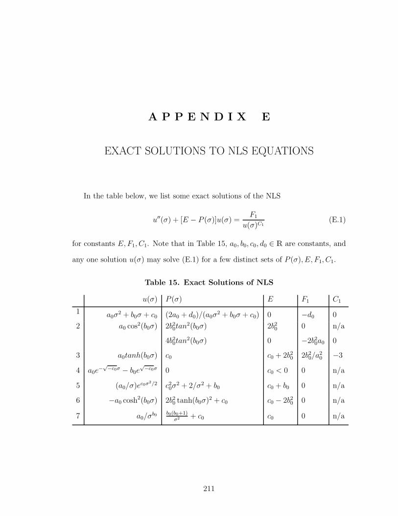
A P P E N D I X E
EXACT SOLUTIONS TO NLS EQUATIONS
In the table below, we list some exact solutions of the NLS
u′′(σ) + [E − P (σ)]u(σ) =F1
u(σ)C1(E.1)
for constants E,F1, C1. Note that in Table 15, a0, b0, c0, d0 ∈ R are constants, and
any one solution u(σ) may solve (E.1) for a few distinct sets of P (σ), E, F1, C1.
Table 15. Exact Solutions of NLS
u(σ) P (σ) E F1 C1
1 a0σ2 + b0σ + c0 (2a0 + d0)/(a0σ
2 + b0σ + c0) 0 −d0 0
2 a0 cos2(b0σ) 2b20tan2(b0σ) 2b20 0 n/a
4b20tan2(b0σ) 0 −2b20a0 0
3 a0tanh(b0σ) c0 c0 + 2b20 2b20/a20 −3
4 a0e−√−c0σ − b0e
√−c0σ 0 c0 < 0 0 n/a
5 (a0/σ)ec0σ2/2 c20σ2 + 2/σ2 + b0 c0 + b0 0 n/a
6 −a0 cosh2(b0σ) 2b20 tanh(b0σ)2 + c0 c0 − 2b20 0 n/a
7 a0/σb0 b0(b0+1)
σ2 + c0 c0 0 n/a
211

In order to map an exact solution u(σ) of a non-linear (or linear) Schrodinger-
type equation to an exact solution of Einstein’s equations via the correspondences
in this thesis, one may first need to solve for σ(t) in the differential equation
σ(t) =1
θu(σ(t)) (E.2)
for θ > 0. Also the scalar field φ(t) is obtained by integrating a constant multiple
of the square root of P (σ) (and then composing the result with σ(t) or σ(fσ(τ(t)))
). That is, to find φ(t) one must first compute
ψ(σ) =
∫
√
α0P (σ)dσ (E.3)
for some constant α0. Therefore for each solution in Table 15, we now record some
solutions to (E.2) and (E.3).
For u(σ) from line 1 in Table 15 with a0 = 0, equation (E.2) with θ = 1 is
σ(t) = b0σ(t) + c0 (E.4)
which has solution
σ(t) = eb0(t−t0) − c0b0
(E.5)
for b0 6= 0 and t0 ∈ R. One can check this by computing that
σ(t) = u(σ(t)) = b0eb0(t−t0). (E.6)
Also, we note that
u′(σ(t)) = b0. (E.7)
For u(σ) from line 1 in Table 15, equation (E.2) with θ = 1 is
σ(t) = a0σ(t)2 + b0σ(t) + c0 (E.8)
which has solution
σ(t) =1
2a0
(√−∆ tan
[√−∆
2(t− t0)
]
− b0
)
(E.9)
212

for t0 ∈ R, a0 > 0 and discriminant ∆ = b20 − 4a0c0 < 0. One can check this by
computing that
σ(t) = u(σ(t)) =−∆
4a0sec2
[√−∆
2(t− t0)
]
. (E.10)
Also, we record that
u′(σ(t)) =√−∆ tan
[√−∆
2(t− t0)
]
. (E.11)
For P (σ) from line 1 in Table 15 with a0 > 0, (E.3) becomes
ψ(σ) =
∫
√
α0(2a0 + d0)
a0σ2 + b0σ + c0dσ
=
√
α0
a0(2a0 + d0) ln
[
2
(
σ +b02a0
+
√
σ2 +b0a0σ +
c0a0
)]
+ β0(E.12)
for ∆ = b20 − 4a0c0 < 0 and integration constant β0 ∈ R.
Composing (E.12) with (E.9),
φ(t)def.= ψ(σ(t)) =
√
α0
a0
(2a0 + d0) ln
[
1
a0
(√−∆ tan
[√−∆
2(t− t0)
]
+√−∆sec
[√−∆
2(t− t0)
])]
+ β0. (E.13)
For u(σ) from line 2 in Table 15, equation (E.2) is
σ(t) =a0
θcos2(b0σ(t)) (E.14)
which has solution
σ(t) =1
b0Arctan
(
b0a0
θ(t− t0)
)
(E.15)
for t0 ∈ R. One can check this by noting that
σ(t) =1
θu(σ(t)) =
a0θ
θ2 + a20b
20(t− t0)2
. (E.16)
213

For the record, we also compute
u′(σ(t)) = −a0b0 sin(2b0σ(t))
= −a0b0 sin
(
2Arctan
(
b0a0
θ(t− t0)
))
=−2b20a
20(t− t0)θ
θ2 + a20b
20(t− t0)2
(E.17)
since sin(2Arctan(x)) = 2cos(Arctan(x))sin(Arctan(x)) = 2x1+x2 .
For P (σ) from line 2 in Table 15, (E.3) becomes
ψ(σ) =√α0
∫
√
2b20 tan2(b0σ)dσ
=√α0
∫ √2b0 tan(b0σ)dσ
=√
2α0 ln [sec(b0σ)] + β0 (E.18)
for b0, σ > 0 and integration constant β0 ∈ R.
Composing (E.18) with (E.15),
φ(t) = ψ(σ(t))
=√
2α0 ln [sec (Arctan(b0a0(t− t0)))] + β0
=√
2α0 ln
[
√
b20a20(t− t0)2 + 1
]
+ β0
=
√
α0
2ln
[
b20a20
θ2(t− t0)
2 + 1
]
+ β0. (E.19)
since sec(Arctan(x)) = 1/cos(Arctan(x)) =√
1 + x2
For P (σ) = 4b20 tan2(b0σ) for solution 2 in the table, (E.3) becomes
ψ(σ) =√α02b0
∫
tan(b0σ)dσ = −2√α0 ln(cos(b0σ)) + β0 (E.20)
for 0 < b0σ < π/2 and β0 ∈ R.
Composing (E.20) with (E.15),
φ(t) = −2√α0 ln
(
cos
(
Arctan
(
b0a0
θ(t− t0)
)))
=√α0 ln
(
1 +b20a
20
θ2(t− t0)
2
)
(E.21)
214

For u(σ) from line 3 in Table 15, equation (E.2) with θ = 1 is
σ(t) = a0 tanh(b0σ(t)) (E.22)
which has solution
σ(t) =1
b0Arcsinh
(
ea0b0(t−t0))
(E.23)
for t0 ∈ R. One can check this by computing that
σ(t) = u(σ(t)) = a0tanh(
Arcsinh(
ea0b0(t−t0)))
=a0e
a0b0(t−t0)
√1 + e2a0b0(t−t0)
. (E.24)
Also, we will use that
u′(σ(t)) = a0b0sech2(b0σ(t))
=a0b0
cosh2(Arcsinh (ea0b0(t−t0)))
=a0b0
1 + e2a0b0(t−t0)
=a0b02e−a0b0(t−t0)sech(a0b0(t− t0)) (E.25)
since cosh2(Arcsinh(x)) = 1 + x2.
For P (σ) = c0 from line 3 in Table 15, (E.3) becomes
ψ(σ) =
∫ √α0c0dσ =
√α0c0σ + β0 (E.26)
for integration constant β0 ∈ R.
Composing (E.26) with (E.23),
φ(t) = ψ(σ(t)) =
√α0c0b0
Arcsinh(
ea0b0(t−t0))
+ β0. (E.27)
For u(σ) from line 4 in Table 15 with b0 = 0, equation (E.2) with θ = 1 is
σ(t) = a0e−√−c0σ(t) (E.28)
215

which has solution
σ(t) =1√−c0
ln(√
−c0a0(t− t0))
(E.29)
for a0 > 0 and t0 ∈ R. One can check this by noting that
σ(t) = u(σ(t)) =1√−c0(t− t0)
. (E.30)
Also, we record that
u′(σ(t)) = −a0
√−c0e−
√−c0σ(t)
=−1
(t− t0). (E.31)
For u(σ) from line 4 in Table 15, equation (E.2) for θ = 1 is
σ(t) = a0e−√−c0σ(t) − b0e
√−c0σ(t) (E.32)
which has solution
σ(t) =1√−c0
ln
(√
a0
b0tanh(
√
−a0b0c0(t− t0))
)
(E.33)
for a0, b0 > 0 and t0 ∈ R. One can check this by computing that
σ(t) = u(σ(t)) = 2√
a0b0 csch(2√
−a0b0c0(t− t0)). (E.34)
We also record that
u′(σ(t)) = −√−c0
(
a0e−√−c0σ(t) + b0e
√−c0σ(t)
)
= −√
−c0a0b0
(
coth(√
−a0b0c0(t− t0)) + tanh(√
−a0b0c0(t− t0)))
= −2√
−c0a0b0 coth(2√
−a0b0c0(t− t0)) (E.35)
since coth(x) + tanh(x) = 2coth(2x).
For u(σ) from line 5 in Table 15, equation (E.2) with θ = 1 is
σ(t) =a0
σ(t)ec0σ(t)2/2 (E.36)
216

which has solution
σ(t) =
√
−2
c0ln(−c0a0(t− t0)) (E.37)
for c0 < 0 and t0 ∈ R. One can check this by computing that
σ(t) = u(σ(t)) =1
√−2c0(t− t0)
√
ln(−c0a0(t− t0)). (E.38)
We also record that
u′(σ(t)) = a0ec0σ(t)2/2
(
c0 −1
σ(t)2
)
=−1
(t− t0)
(
1 +1
2 ln(−c0a0(t− t0))
)
. (E.39)
For P (σ) from line 5 in Table 15, (E.3) becomes
ψ(σ) =√α0
∫
√
c20σ2 +
2
σ2+ b0dσ
=
√α0
2
(
√
c20σ4 + 2 + b0σ2 +
√2 ln[σ2] −
√2 ln
[
2√
2√
c20σ4 + b0σ2 + 2
+b0σ2 + 4
]
+b02c0
ln
[
2√
c20σ4 + b0σ2 + 2 +
b0c0
+ 2c0σ2
])
+ β0(E.40)
for σ > 0 and integration constant β0 ∈ R.
Composing (E.40) with (E.37),
φ(t) = ψ(σ(t)) =
=
√
α0
2
(
√
2 ln2(−c0a0(t− t0)) +b0−c0
ln(−c0a0(t− t0)) + 1
+ ln
[
2
−c0ln(−c0a0(t− t0))
]
− ln
[
2b0−c0
ln(−c0a0(t− t0)) + 4
+ 4
√
2 ln2(−c0a0(t− t0)) +b0−c0
ln(−c0a0(t− t0)) + 1
]
+b0
c02√
2ln
[
2√
2
√
2 ln2(−c0a0(t− t0)) +b0−c0
ln(−c0a0(t− t0)) + 1
+b0c0
− 4 ln(−c0a0(t− t0))
])
+ β0 (E.41)
217

for c0 < 0 and t > −1/c0a0 + t0.
For u(σ) from line 5 in Table 15 with c0 = 0, equation (E.2) with θ = 1 is
σ(t) =a0
σ(t)(E.42)
which has solution
σ(t) =√
2a0(t− t0) (E.43)
for a0 > 0 and t > t0 ∈ R. One can check this by computing that
σ(t) = u(σ(t)) =a0
√
2a0(t− t0). (E.44)
We also record that
u′(σ(t)) =−a0
σ(t)2
=−1
2(t− t0)(E.45)
For P (σ) from line 5 in Table 15 with c0 = 0, (E.3) becomes
ψ(σ) =√α0
∫
√
2
σ2+ b0dσ
=√α0
(
√
b0σ2 + 2 +√
2 ln
[
σ√2 +
√b0σ2 + 2
])
+ β0 (E.46)
for integration constant β0 ∈ R.
Composing (E.46) with (E.43) for c0 = 0,
ψ(t) = ψ(σ(t))
=√α0
(
√
g(t) +1√2
ln [2a0(t− t0)] −√
2 ln[√
2 +√
g(t)]
)
+ β0 (E.47)
for g(t) = 2a0b0(t− t0) + 2.
For u(σ) from line 6 in Table 15, equation (E.2) with θ = 1 is
σ(t) = −a0 cosh2(b0σ(t)) (E.48)
218

which has solution
σ(t) =−1
b0Arctanh(b0a0(t− t0)) (E.49)
for t0 ∈ R. One can check this by noting that
σ(t) = u(σ(t)) =a0
a20b
20(t− t0)2 − 1
. (E.50)
For the record, we also compute
u′(σ(t)) = −a0b0 sinh(2b0σ(t))
= −a0b0 sinh(2Arctanh(b0a0(t− t0)))
=2b20a
20(t− t0)
a20b
20(t− t0)2 − 1
(E.51)
since sinh(2Arctanh(x)) = 2cosh(Arctanh(x))sinh(Arctanh(x)) = 2x1−x2 .
For P (σ) from line 6 in Table 15, (E.3) becomes
ψ(σ) =√α0
∫√
2b20 tanh2(b0σ) + c0dσ
= −√
2α0 ln
[
2
(√2b0 tanh(b0σ) +
√
c0 + 2b20 tanh2(b0σ)
)]
+
√α0
b0
√
c0 + 2b20Arctanh
[
√
c0 + 2b20tanh(b0σ)√
c0 + 2b20tanh2(b0σ)
]
+ β0 (E.52)
for c0 ≥ −2b20 and integration constant β0 ∈ R.
Composing (E.52) with (E.49),
φ(t) = ψ(σ(t)) =
−√
2α0 ln
[
2
(
√
c0 + 2b40a20(t− t0)2 −
√2b20a0(t− t0)
)]
−√α0
b0
√
c0 + 2b20Arctanh
[√
(c0 + 2b20)b20a
20(t− t0)2
c0 + 2b40a20(t− t0)2
]
+ β0. (E.53)
For u(σ) from line 7 in Table 15, equation (E.2) is
σ(t) =a0
θσ(t)b0, (E.54)
219

which has solution
σ(t) =
(
(1 + b0)a0
θ(t− t0)
)1/(1+b0)
(E.55)
for θ > 0 and t0 ∈ R. One can check this by computing
σ(t) =1
θu(σ(t)) =
a0
θ
(
(1 + b0)a0
θ(t− t0)
)−b0/(1+b0)
. (E.56)
Also, we will use that
u′(σ(t)) =−b0θ
(1 + b0)(t− t0). (E.57)
For P (σ) from line 7, (E.3) is
ψ(σ) =√α0
∫
√
b0(b0 + 1)
σ2+ c0 dσ
= β0 +√α0
(
√
b0(b0 + 1) + c0σ2
−√
b0(b0 + 1) log
(
√
b0(b0 + 1) +√
b0(b0 + 1) + c0σ2
σ
))
(E.58)
for b0 > 0 and β0 ∈ R. Composing (E.58) with (E.55),
φ(t) = β0 +√α0
(
√
b0(b0 + 1) + c0σ(t)2
−√
b0(b0 + 1) log
(
√
b0(b0 + 1) +√
b0(b0 + 1) + c0σ(t)2
σ(t)
))
(E.59)
for σ(t) in (E.55).
220
A P P E N D I X F
EXTRA CONSERVATION EQUATION
As noted in section 1.2, the correspondences in this thesis do not rely on T(2)ij
in (1.7) satisfying the conservation equation (1.12). For each theorem in Chapters
3-7, we now record the EMP or NLS analogue of (1.12) for l = 0. For an arbitrary
diagonal metric gij one can compute, using the definition of the Christoffel symbols
in (1.2), that the equation
div(T (2))l=0 = 0 (F.1)
for T(2)ij in (1.7) takes the form
ρ+
(
1
2
d∑
i=1
giigii
)
(ρ+ p) = 0 (F.2)
where dot denotes differentiation with respect to x0 = t.
For the FRLW metric (3.1), the conservation equation (F.2) is
ρ+ dH(ρ+ p) = 0 (F.3)
for H(t) = a(t)/a(t).
Composing (F.3) with f(τ) from the EMP Theorem 3.1.1 and multiplying by
f ′(τ) , we obtain ρ(f(τ))f ′(τ) + dH(f(τ))f ′(τ)(ρ(f(τ)) + p(f(τ))) = 0. That is,
by the relation (3.20) and the definition (3.12) of τ(t), we obtain the analogue
conservation equation
′ +d
qHY (+ <) = 0 (F.4)
221

in the EMP variables, for HY (τ)def.= Y ′(τ)/Y (τ), Y (τ) = a(f(τ))q (q 6= 0) and
(τ) = ρ(f(τ)), <(τ) = p(f(τ)).
Composing (F.3) with g(σ) from the NLS Theorem 3.2.1 and multiplying by
g′(σ), we obtain ρ(g(σ))g′(σ) + dH(g(σ))g′(σ)(ρ(g(σ)) + p(g(σ))) = 0. That is,
by the relation (3.109) and the definition (3.101) of σ(t), we obtain the analogue
conservation equation
ρ′ − dHu(ρ + p) = 0 (F.5)
in the NLS variables, for Hu(σ)def.= u′(σ)/u(σ), u(σ) = 1/a(g(σ)) and ρ(σ) =
ρ(g(σ)), p(σ) = p(g(σ)).
Composing (F.3) with g(σ) from the alternate NLS Theorem 3.3.1 and mul-
tiplying by g′(σ) we obtain ρ(g(σ))g′(σ) + dH(g(σ))g′(σ)(ρ(g(σ)) + p(g(σ))) = 0.
That is, by the relation (3.164) and the definition (3.156) of σ(t), we obtain the
analogue equation
ρ′ − 2d
njHu(ρ + p) = 0 (F.6)
in the alternate NLS variables for Hu(σ)def.= u′(σ)/u(σ), u(σ) = 1/a(g(σ))nj/2
(nj 6= 0) and ρ(σ) = ρ(g(σ)), p(σ) = p(g(σ)).
For the Bianchi I metric (4.1), the conservation equation (F.2) is
ρ+1
νHR(ρ+ p) = 0 (F.7)
for HR(t) = R(t)/R(t) and R(t) = (X1(t) · · ·Xd(t))ν .
Composing (F.7) with f(τ) from the EMP Theorem 4.1.1 and multiplying by
f ′(τ) we obtain ρ(f(τ))f ′(τ)+ 1νHR(f(τ))f ′(τ)(ρ(f(τ))+ p(f(τ))) = 0. That is, by
the relation (4.36) and the definition (4.11) of τ(t) we obtain
′ +1
νqHY (+ <) = 0 (F.8)
222

in the EMP variables for HY (τ)def.= Y ′(τ)/Y (τ), Y (τ) = R(f(τ))q (q 6= 0) and
(τ) = ρ(f(τ)), <(τ) = p(f(τ)).
Composing (F.7) with g(σ) from the NLS Theorem 4.2.1, multiplying by g′(σ)
and using (4.102) and (4.89) we obtain
ρ′ −Hu(ρ + p) = 0 (F.9)
for Hu(σ)def.= u′(σ)/u(σ), u(σ) = 1/R(g(σ))1/ν (ν 6= 0) and ρ(σ) = ρ(g(σ)), p(σ) =
p(g(σ)).
For the conformal version (5.1) of the Bianchi I metric, the conservation equa-
tion (F.2) is
ρ+1
νHR(ρ+ p) = 0 (F.10)
for HR(t) = R(t)/R(t) and R(t) = (a1(t) · · ·ad(t))ν .
Composing (F.10) with f(τ) from Theorem 5.1.1 and using (5.10), (5.40) we
get the analogue conservation equation
′ +1
qνHY (+ <) = 0 (F.11)
in the EMP variables for HY (τ)def.= Y ′(τ)/Y (τ), Y (τ) = R(f(τ))q (q 6= 0) and
(τ) = ρ(f(τ)), <(τ) = p(f(τ)).
Composing (F.10) with g(σ)def.= σ + t0 from Theorem 5.2.1 we obtain ρ(σ +
t0) + 1νHR(σ + t0)(ρ(σ + t0) + p(σ + t0)) = 0. By (5.79), we obtain
ρ′ −Hu(ρ + p) = 0 (F.12)
for the conservation equation in NLS variables for the Bianchi I metric (5.1), where
Hu(σ)def.= u′(σ)/u(σ), u(σ) = 1/R(σ+ t0)
1/ν and ρ(σ) = ρ(σ+ t0), p(σ) = p(σ+ t0).
For the Bianchi V metric (6.1), the conservation equation (F.2) is
ρ+1
νHR(ρ+ p) = 0 (F.13)
223

for HR(t) = R(t)/R(t) and R(t) = (X1(t) · · ·Xd(t))ν .
Composing (F.13) with f(τ) from the EMP Theorem 6.1.1 and multiplying by
f ′(τ) we obtain ρ(f(τ))f ′(τ)+ 1νHR(f(τ))f ′(τ)(ρ(f(τ))+ p(f(τ))) = 0. That is, by
the relation (6.41) and the definition (6.12) of τ(t) we obtain
′ +1
νqHY (+ <) = 0 (F.14)
in the EMP variables for HY (τ)def.= Y ′(τ)/Y (τ), Y (τ) = R(f(τ))q (q 6= 0) and
(τ) = ρ(f(τ)), <(τ) = p(f(τ)).
Composing (F.13) with g(σ) from the NLS Theorem 6.2.1, multiplying by g′(σ)
and using (6.111) and (6.94) we obtain
ρ′ −Hu(ρ + p) = 0 (F.15)
for Hu(σ)def.= u′(σ)/u(σ), u(σ) = 1/R(g(σ))1/ν (ν 6= 0) and ρ(σ) = ρ(g(σ)), p(σ) =
p(g(σ)).
Composing (F.13) with g(σ) from the alternate Bianchi V NLS Theorem
6.3.1 and multiplying by g′(σ) we obtain ρ(g(σ))g′(σ) + 1νHR(g(σ))g′(σ)(ρ(g(σ)) +
p(g(σ))) = 0. That is, by the relation (6.150) and the definition (6.133) of σ(t), we
obtain the analogue equation
ρ′ −Hu(ρ + p) = 0 (F.16)
in for Hu(σ)def.= u′(σ)/u(σ), u(σ) = 1/R(g(σ))1/ν (ν 6= 0) and ρ(σ) =
ρ(g(σ)), p(σ) = p(g(σ)).
For the conformal version (7.1) of the Bianchi V metric, the conservation equa-
tion (F.2) is
ρ+d
2νHR(ρ+ p) = 0 (F.17)
for HR(t) = R(t)/R(t) and R(t) = (a2(t) · · ·ad(t))ν .
224

Composing (F.17) with f(τ) from Theorem 7.1.1 and using (7.10), (7.43) we
get the analogue conservation equation
′ +d
2qνHY (+ <) = 0 (F.18)
in the EMP variables for HY (τ)def.= Y ′(τ)/Y (τ), Y (τ) = R(f(τ))q (q 6= 0) and
(τ) = ρ(f(τ)), <(τ) = p(f(τ)).
Composing (F.17) with g(σ)def.= σ + t0 from Theorem 7.2.1 we obtain ρ(σ +
t0) + d2νHR(σ + t0)(ρ(σ + t0) + p(σ + t0)) = 0. By (7.100), we obtain
ρ′ −Hu(ρ + p) = 0 (F.19)
for the conservation equation in NLS variables for the Bianchi V metric in (5.1) for
Hu(σ)def.= u′(σ)/u(σ), u(σ) = 1/R(σ+t0)
2ν/d and ρ(σ) = ρ(σ+t0), p(σ) = p(σ+t0).
225

BIBLIOGRAPHY
[1] R. Bali and C. Jain, Bianchi I inflationary universe in general relativity, Pra-mana - Journal of Physics 59 (2002), No. 1, pp. 1-7.
[2] J. D. Barrow, A. B. Burd and D. Lancaster, Three-dimensional classical space-times, Classical and Quantum Gravity 3 (1986), No. 4, pp. 551-567.
[3] D. Bazeia, Scalar fields: from domain walls to nanotubes and fulurenes, Brazil-ian Journal of Physics 32 (2002), No. 4, pp. 869-879, e-print arXiv:hep-th/0203050v2.
[4] V. H. Cardenas and S. del Campo, Scalar field potentials for cosmology,Physical Review D 69 (2004), No. 8, 083508-083513, e-print arXiv:astro-ph/0401031v1.
[5] T. Christodoulakis, T. Grammenos, C. Helias, P. Kevrekidis, G. Papadopoulosand F. Williams, On 3+1−dimensional scalar field cosmologies, from Progressin General Relativity and Quantum Cosmology Research, Nova Science Pub-lishers (2006), pp. 37-48, e-print arXiv:gr-qc/0408056v1.
[6] T. Christodoulakis, T. Grammenos, C. Helias, P. Kevrekidis and A. Spanou,Decoupling of the general scalar field mode and the solution space for Bianchitype I and V cosmologies, Journal of Mathematical Physics 47 (2006), 042505.
[7] J. W. Dabrowska, A. Khare and U. P. Sukhatme, Explicit wavefunctions forshape-invariant potentials by operator techniques, Journal of Physics A 21(1988), L195-L200.
[8] N. Dadhich, Derivation of the Raychaudhuri Equation, (2005), arXiv: gr-gc/0511123 v2.
[9] J. D’Ambroise, EMP and linear Schrodinger models for a conformally BianchiI cosmology, to appear in International Journal of Pure and Applied Mathe-matics, e-print arXiv: hep-th/0809.4817.
[10] J. D’Ambroise, A Schrodinger formulation of Bianchi I scalar field cosmology,International Journal of Pure and Applied Mathematics 42 (2008), No. 3, pp.405-410, e-print arXiv: hep-th/0711.3916v1.
226
[11] J. D’Ambroise, EMP reformulations of Einstein’s equations as an application ofa property of suitable second order differential equations, from Proceedings ofthe 8th International Workshop on Lie Theory and Its Applications in Physics,Varna, Bulgaria (2009), to appear.
[12] J. DAmbroise and F. L. Williams, A Non-linear Schrodinger Type Formulationof FLRW Scalar Field Cosmology, International Journal of Pure and AppliedMathematics 34 (2007), No. 1, pp. 117-126, e-print arXiv: hep-th/0609125v1.
[13] G. Ellis and M. Madsen, Exact scalar field cosmologies, Classical and QuantumGravity 8 (1991), pp. 667-676.
[14] A. Garcia and S. Carlip, n-dimensional generalizations of the Friedmann-Robertson-Walker cosmology, Physics Letters B 645 (2007), No. 2-3, pp. 101-107.
[15] A. Garcia, M. Cataldo and S. del Campo, Relationship between (2 + 1)and (3 + 1)-Friedmann-Robertson-Walker cosmologies, General Relativity andGravitation 37 (2005), No. 4, pp. 685-711, e-print arXiv:hep-th/0309098v1.
[16] B. Gumjudpai, Power-law expansion cosmology in Schrodinger-type formula-tion, Astroparticle Physics 30 (2008), No. 4, pp. 186-191.
[17] B. Gumjudpai, Scalar field exact solutions for non-flat FLRW cosmology: atechnique from non-linear Schrodinger-type formulation, General Relativityand Gravitation 41 (2009), No. 2, pp. 249-265.
[18] R. Hawkins and J. Lidsey, The Ermakov-Pinney equation in scalar field cos-mologies, Physical Review D 66 (2002), 023523-023531, e-print arXiv: astro-ph/0112139v2.
[19] V. Joseph, A spatially homogeneous gravitational field, Mathematical Proceed-ings of the Cambridge Philosophical Society 62 (1966), pp. 87-89.
[20] P. Kevrekidis and F. Williams, On 2 + 1−dimensional Friedmann-Robertson-Walker universes: an Ermakov-Pinney equation approach, Classical and Quan-tum Gravity 20 (2003), L177-L184.
[21] G. Levai, A search for shape-invariant solvable potentials, Journal of PhysicsA 22 (1989), pp. 689-702.
[22] J. Lidsey, Multiple and anisotropic inflation with exponential potentials, Clas-sical and Quantum Gravity 9 (1992), pp. 1239-1253.
[23] J. Lima, Note on solving for the dynamics of the universe, American Journal ofPhysics 69 (2001), No. 12, pp. 1245-1247, e-print arXiv:astro-ph/0109215v1.
227

[24] D. Lorenz-Petzold, Higher-Dimensional Bianchi Type-V Cosmologies, Lettersin Mathematical Physics 10 (1985), pp. 279-282.
[25] W. Milne, The Numerical Determination of Characteristic Numbers, PhysicalReview 35 (1930), pp. 863-870.
[26] M. Ozer and M. Taha, Exact solutions in string-motivated scalar field cosmol-ogy, Physical Review D 45 (1992) R997-R999.
[27] T. Padmanabhan, Accelerated expansion of the universe driven by tachyonicmatter, Physical Review D 66 (2002), D021301-D021305, e-print arXiv:hep-th/0204150.
[28] K. Radhakrishnan and A. C. Hindmarsh, Description and Use of LSODE, theLivermore Solver for Ordinary Differential Equations, NASA Reference Pub-lication (1993), Glenn Research Center, Document ID 19940030753, e-printhttp : //ntrs.nasa.gov/archive/nasa/casi.ntrs.nasa.gov/ 19940030753 1994030753.pdf .
[29] R. De Ritis, C. Rubano and P. Scudellaro, Some considerations on inflationarycosmology with matter and scalar field, Il Nuovo Cimento B 108 (1993), No.11, pp. 1243-1252.
[30] F. L. Williams, Einstein field equations: An alternate approach towards exactsolutions for an FRW universe, from Proceedings of the Sixth Alexander Fried-mann International Seminar on Gravitation and Cosmology, Cargese, France(2004), International Journal of Modern Physics A 20 (2005), pp. 2481-2484.
[31] F. L. Williams, An EMP model of Bianchi I cosmology, from Proceedings of theeleventh Marcel Grossmann Meeting On General Relativity, Berlin, Germany,2006 (2008), Vol. 3, pp. 2222-2224.
228