generalizations of fourier analysis, and...

GENERALIZATIONS OF FOURIER ANALYSIS, AND HOW TO APPLYTHEM

W.T. GOWERS

1. Introduction

This year’s Colloquium Lectures are about an important theme in additive combina-

torics. Additive combinatorics is a fairly recent branch of mathematics, though it grew

out of much older ones. These notes are intended as an informal document to accompany

the lectures and give more detail than it will be possible to give in the lectures themselves,

though not full details about everything that is discussed. One aspect of its informality is

that I have not provided a bibliography and many of the results I have mentioned, which

are due to a variety of authors, are not attributed. In due course I will write a more formal

version in which references will be provided. This will probably be published, and will

definitely be posted on the arXiv.

Additive combinatorics is not very easy to characterize, but a good way to understand

the flavour of the area is to look at one of its central theorems, the following famous result

of Szemeredi from 1974, which solved a conjecture made by Erdos and Turan in 1936.

Theorem 1.1. For every positive integer k and every δ > 0 there exists a positive inte-

ger n such that every subset A ⊂ {1, 2, . . . , n} of size at least δn contains an arithmetic

progression of length k.

This is a combinatorial theorem in the sense that we make no structural assumptions

about A – it is just a subset of {1, 2, . . . , n} of density at least δ. However, the set

{1, 2, . . . , n} has a rich additive structure, and that structure is highly relevant to the

problem, since an arithmetic progression can be thought of as a sequence (x1, x2, . . . , xk)

such that

x2 − x1 = x3 − x3 = · · · = xk − xk−1.

(Of course, we also need to add the non-degeneracy condition that x1 6= x2.)

However, there is more to additive combinatorics than a set of combinatorial theorems

that involve addition in one way or another. To appreciate this, it is helpful to look at1

2 W.T. GOWERS

the following statement, which turns out to be an equivalent reformulation of Szemeredi’s

theorem. The equivalence is a reasonably straightforward exercise to prove.

Theorem 1.2. For every positive integer k and every δ > 0 there exists a constant c > 0

such that for every positive integer n and every function f : Zn → [0, 1] that averages at

least δ we have the inequality

Ex,df(x)f(x+ d) . . . f(x+ (k − 1)d) ≥ c.

Here Zn is the cyclic group of order n and the notation Ex,d means the average over all

x and d – that is, it is another way of writing n−2∑

x,d.

As n gets large, Zn is a better and better discrete approximation to the circle T, which

we can think of as the Abelian group consisting of all complex numbers of modulus 1. It

is not hard to prove that the discrete statement is equivalent to the following continuous

version.

Theorem 1.3. For every positive integer k and every δ > 0 there exists a constant c > 0

such that for every measurable function f : T→ [0, 1] that averages at least δ we have the

inequality

Ex,df(x)f(x+ d) . . . f(x+ (k − 1)d) ≥ c.

This time Ex,d stands for the integral with respect to the Haar measure on T2.

This last reformulation illustrates an important point about many of the theorems of ad-

ditive combinatorics (and extremal combinatorics more generally), which is that although

they are combinatorial, they are also analytic. In fact, the more one thinks about them,

the less important the distinction between discrete and continuous seems to be. And it is

not just the statements that are (or can be made to be) analytic: a characteristic feature of

much of additive combinatorics is that the proofs of its theorems use methods from areas

of analysis such as functional analysis, Fourier analysis, and ergodic theory.

Here we shall focus on the last of these. Fourier analysis is an extremely useful tool

for additive problems, and one of the aims of the Colloquium Lectures will be to explain

why. Another aim, which is in some ways even more interesting, will be to demonstrate

the limitations of Fourier analysis – that is, to look at problems that do not immediately

yield to a Fourier-analytic approach. Sometimes that just means that one needs to look

for a completely different kind of argument. However, with some problems the best way

to make progress is not to abandon Fourier analysis altogether, but to generalize it in a

suitable, and not always obvious, way. Thus, it sometimes happens that the limitations of

one type of Fourier analysis lead to the development of another.

GENERALIZATIONS OF FOURIER ANALYSIS, AND HOW TO APPLY THEM 3

2. Discrete Fourier analysis

Let f : Zn → C. We define its discrete Fourier transform f : Zn → C by the formula

f(r) = Exf(x)ω−rx,

where ω = exp(2πix/n) is a primitive nth root of unity. Note that there is a close resem-

blance between this formula, which we could equally well write as

f(r) = Exf(x) exp(−2πirx/n),

and the familiar formulae for Fourier coefficients and Fourier transforms in the continuous

setting. Of course, this is to be expected. Note also that the number ω−rx is well-defined,

since if r and n are integers, then adding a multiple of n to either of them makes no

difference to it.

Although f can be thought of as a function defined on Zn, it is more correct to regard

it as defined on the dual group Zn, which happens to be (non-naturally) isomorphic to

Zn. The distinction has some importance in additive combinatorics, because the natural

measures we put on Zn and Zn are different: for Zn we use the uniform probability measure,

whereas for Zn we use the counting measure. This difference feeds into the definitions of

some key concepts such as inner products, p-norms and convolutions. Given functions

f, g : Zn → C and 1 ≤ p ≤ ∞, we have the following definitions.

• 〈f, g〉 = Exf(x)g(x).

• ‖f‖p = (Ex|f(x)|p)1/p.

• f ∗ g(x) = Ey+z=xf(y)g(z).

The corresponding definitions for functions f , g : Zn → C are the same, but with sums

replacing expectations. That is, they are as follows.

• 〈f , g〉 =∑

x f(x)g(x).

• ‖f‖p = (∑

x |f(x)|p)1/p.

• f ∗ g(x) =∑

y+z=x f(y)g(z).

With these measures in place, the familiar properties of the Fourier transform hold for the

discrete Fourier transform as well, and have easier proofs. In particular, constant use is

made of the following five rules, of which the first two are equivalent. All five are easy

exercises.

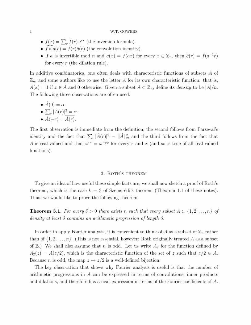
• 〈f, g〉 = 〈f , g〉 (Parseval’s identity).

• ‖f‖2 = ‖f‖2 (also Parseval’s identity).

4 W.T. GOWERS

• f(x) =∑

r f(r)ωrx (the inversion formula).

• f ∗ g(r) = f(r)g(r) (the convolution identity).

• If a is invertible mod n and g(x) = f(ax) for every x ∈ Zn, then g(r) = f(a−1r)

for every r (the dilation rule).

In additive combinatorics, one often deals with characteristic functions of subsets A of

Zn, and some authors like to use the letter A for its own characteristic function: that is,

A(x) = 1 if x ∈ A and 0 otherwise. Given a subset A ⊂ Zn, define its density to be |A|/n.

The following three observations are often used.

• A(0) = α.

•∑

r |A(r)|2 = α.

• A(−r) = A(r).

The first observation is immediate from the definition, the second follows from Parseval’s

identity and the fact that∑

r |A(r)|2 = ‖A‖22, and the third follows from the fact that

A is real-valued and that ωrx = ω−rx for every r and x (and so is true of all real-valued

functions).

3. Roth’s theorem

To give an idea of how useful these simple facts are, we shall now sketch a proof of Roth’s

theorem, which is the case k = 3 of Szemeredi’s theorem (Theorem 1.1 of these notes).

Thus, we would like to prove the following theorem.

Theorem 3.1. For every δ > 0 there exists n such that every subset A ⊂ {1, 2, . . . , n} of

density at least δ contains an arithmetic progression of length 3.

In order to apply Fourier analysis, it is convenient to think of A as a subset of Zn rather

than of {1, 2, . . . , n}. (This is not essential, however: Roth originally treated A as a subset

of Z.) We shall also assume that n is odd. Let us write A2 for the function defined by

A2(z) = A(z/2), which is the characteristic function of the set of z such that z/2 ∈ A.

Because n is odd, the map z 7→ z/2 is a well-defined bijection.

The key observation that shows why Fourier analysis is useful is that the number of

arithmetic progressions in A can be expressed in terms of convolutions, inner products

and dilations, and therefore has a neat expression in terms of the Fourier coefficients of A.


Indeed, using the rules given earlier, we have that

Ex+y=2zA(x)A(y)A(z) = Ex+y=zA(x)A(y)A(z/2)

= EzA ∗ A(z)A2(z)

= 〈A ∗ A,A2〉

= 〈A ∗ A, A2〉

= 〈A2, A2〉

=∑r

A(r)2A2(r)

=∑r

A(r)2A(2r)

=∑r

A(r)2A(−2r).

Why should this be useful? To answer that question, we need to bring in another simple

but surprisingly powerful tool: the Cauchy-Schwarz inequality. First, recalling that A(0)

is equal to the density of A, which we shall denote by α, we split the last expression up as

α3 +∑r 6=0

A(r)2A(−2r).

Thus, we have shown that

Ex+y=2zA(x)A(y)A(z) = α3 +∑r 6=0

A(r)2A(−2r).

The left-hand side of this expression is the probability that x, y, z all belong to A if you

choose them randomly to satisfy the equation x + y = 2z. Without the constraint that

x+ y = 2z this probability would be α3, since each of x, y and z would have a probability

α of belonging to A. So the term α3 on the right-hand side can be thought of as “what

one would expect” and the remainder of the right-hand side is a measure of the effect of

the dependence of x, y and z on each other.

6 W.T. GOWERS

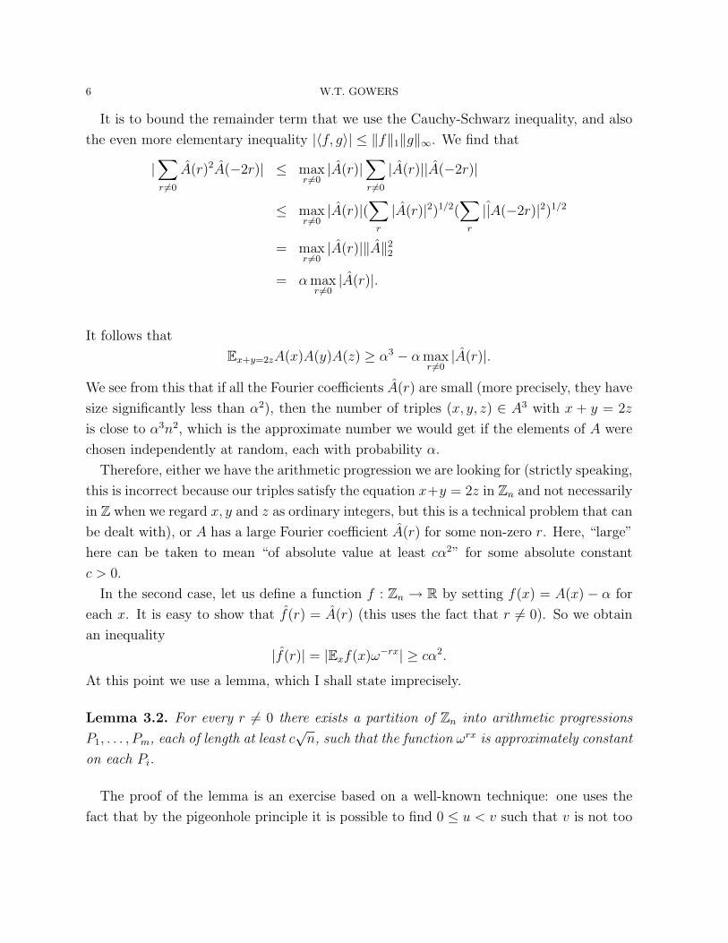
It is to bound the remainder term that we use the Cauchy-Schwarz inequality, and also

the even more elementary inequality |〈f, g〉| ≤ ‖f‖1‖g‖∞. We find that

|∑r 6=0

A(r)2A(−2r)| ≤ maxr 6=0|A(r)|

∑r 6=0

|A(r)||A(−2r)|

≤ maxr 6=0|A(r)|(

∑r

|A(r)|2)1/2(∑r

||A(−2r)|2)1/2

= maxr 6=0|A(r)|‖A‖22

= αmaxr 6=0|A(r)|.

It follows that

Ex+y=2zA(x)A(y)A(z) ≥ α3 − αmaxr 6=0|A(r)|.

We see from this that if all the Fourier coefficients A(r) are small (more precisely, they have

size significantly less than α2), then the number of triples (x, y, z) ∈ A3 with x + y = 2z

is close to α3n2, which is the approximate number we would get if the elements of A were

chosen independently at random, each with probability α.

Therefore, either we have the arithmetic progression we are looking for (strictly speaking,

this is incorrect because our triples satisfy the equation x+y = 2z in Zn and not necessarily

in Z when we regard x, y and z as ordinary integers, but this is a technical problem that can

be dealt with), or A has a large Fourier coefficient A(r) for some non-zero r. Here, “large”

here can be taken to mean “of absolute value at least cα2” for some absolute constant

c > 0.

In the second case, let us define a function f : Zn → R by setting f(x) = A(x) − α for

each x. It is easy to show that f(r) = A(r) (this uses the fact that r 6= 0). So we obtain

an inequality

|f(r)| = |Exf(x)ω−rx| ≥ cα2.

At this point we use a lemma, which I shall state imprecisely.

Lemma 3.2. For every r 6= 0 there exists a partition of Zn into arithmetic progressions

P1, . . . , Pm, each of length at least c√n, such that the function ωrx is approximately constant

on each Pi.

The proof of the lemma is an exercise based on a well-known technique: one uses the

fact that by the pigeonhole principle it is possible to find 0 ≤ u < v such that v is not too


large and |ωru − ωrv| = |1 − ωr(v−u)| is small. One can then partition Zn into arithmetic

progressions of common difference v − u.

Given the lemma, one observes that

cα2n ≤ |∑

xf(x)ω−rx| ≤∑i

|∑x∈Pi

f(x)ω−rx| ≈∑i

|∑x∈Pi

f(x)|,

and also that

0 =∑x

f(x) =∑i

∑x∈Pi

f(x).

Adding these equations together and using an averaging argument, we find that there exists

i such that

|∑x∈Pi

f(x)|+∑x∈Pi

f(x) ≥ c′α2|Pi|,

where c′ is a slightly smaller absolute constant (because of the approximation in the first

equation), which implies that ∑x∈Pi

f(x) ≥ c′α2|Pi|.

Recalling that f(x) = A(x)− α for each x, we find that this is telling us that

|A ∩ Pi| ≥ (α + c′α2)|Pi|.

Thus, what we have managed to do is find an arithmetic progression Pi of length at least

c√n such that the density of A inside Pi is greater than the density of A inside Zn by c′α2.

We can iterate this argument: either A∩Pi contains an arithmetic progression of length

3 or Pi contains a subprogression of length at least c√|Pi| inside which A has density at

least α + 2c′α2, and so on. The iteration must eventually terminate, because the density

cannot exceed 1, and Roth’s theorem is proved.

If one analyses carefully the bound that comes out of the above argument, one finds

that it shows that if A is a subset of {1, 2, . . . , n} of density at least C/ log log n, for some

absolute constant C, then A must contain an arithmetic progression of length 3. This

bound has been improved in interesting ways several times. While these improvements are

not the topic of these notes, it would be wrong not to mention them at all. The following

table gives an idea of how the bounds have progressed over the years. The publication

dates of the papers of Szemeredi and Heath Brown are slightly misleading: those results

were actually independent. Also, the papers of Sanders obviously came out in the opposite

order to the order in which the results were proved. The problem of improving the bounds

for Roth’s theorem has been an extremely fruitful one: the 2008 paper of Bourgain and

8 W.T. GOWERS

Bounds for Roth’s theorem

Author Density bound PublishedRoth C/ log log n 1953

Heath-Brown C/(log n)c, some c > 0 1987Szemeredi C/(log n)1/20 1990Bourgain C(log log n/ log n)1/2 1999Bourgain C(log log n)2/(log n)2/3 2008Sanders (log n)−3/4+o(1) 2012Sanders C(log log n)6/ log n 2011Bloom C(log log n)4/ log n 2012

the 2012 paper of Sanders could perhaps be regarded as clever refinements of existing

techniques, but all the other papers introduced significant new ideas, many of which have

been very influential and led to the solutions of several other problems.

To put these results in perspective, it is worth mentioning that the best known lower

bound on the density (that is, the largest density known to be possible for a set that con-

tains no progression of length 3) is exp(−c√

log n), which is far lower than Bloom’s current

record upper bound. But even if that gap turns out to be very hard to close, we are tanta-

lizingly close to a bound of 1/ log n, which would be enough to give a purely combinatorial

proof that the primes contain infinitely many arithmetic progressions of length 3 (a result

that was proved by number-theoretic methods soon after Vinogradov proved his 3-primes

theorem). In fact, a bound of c log log n/ log n would suffice for this, since the fact that the

primes have very small intersection with some arithmetic progressions (such as the even

numbers) can be used to show that there are arithmetic progressions of length n inside

which the primes have at least that density.

4. A first generalization – to arbitrary finite Abelian groups

Many of the proof techniques that give us results about subsets of Zn work just as well

in an arbitrary Abelian group. This turns out to be a very useful observation, as there

are some Abelian groups, in particular the groups Fnp for fixed p and large n, where the

proofs are much cleaner. So sometimes to work out the proof of a result about Zn it is a

good strategy to prove an analogue for a group such as Fn3 first and then work out how to

modify the argument so that it works in Zn.


Recall the inversion formula for the Fourier transform on Zn, which states that

f(x) =∑r

f(r)ωrx.

If we write ωr for the function x 7→ ωrx, then we can write the formula in the slightly more

abstract form

f =∑r

f(r)ωr,

which is showing us how to write f as a linear combination of the functions ωr.

What is special about the functions ωr? The property that singles them out is that they

are the characters of Zn, that is, the homomorphisms from Zn to C. It turns out to be

straightforward to generalize Fourier analysis to all finite Abelian groups G by decomposing

functions f : G→ C as linear combinations of characters.

For this to work, we would like the characters to form an orthonormal basis, which they

do, by a well-known argument. To see the orthonormality, let χ be a non-trivial character,

let y ∈ G be such that χ(y) 6= 1, and observe that

Exχ(x) = Exχ(xy) = χ(y)Exχ(x),

from which it follows that Exχ(x) = 0. But then if χ1 and χ2 are distinct characters, we

have that

〈χ1, χ2〉 = Exχ1(x)χ2(x) = Exχ1(x)χ2(x)−1,

which is zero, since χ1χ−12 is a non-trivial character.

Less elementary is the fact that the characters span G. For this one needs the structure

theorem for finite Abelian groups, which gives us that G is a product of cyclic groups. We

know that each cyclic group has a complete basis of characters, and the products of those

characters form a basis of characters for the whole group, which gives us a complete set.

Given that the characters form an orthonormal basis, we can expand a function f as a

linear combination∑

χ〈f, χ〉χ. The coefficients 〈f, χ〉 are called the Fourier coefficients of

f and denoted f(χ). That is, we have the formula

f(χ) = Exf(x)χ(x)

for the Fourier transform, and the statement that f =∑

χ〈f, χ〉χ is giving us our inversion

formula

f(x) =∑χ

f(χ)χ(x).

10 W.T. GOWERS

The fact that we are writing f(χ) represents a slight change of notation from the Zn case,

where we wrote f(r) instead of f(ωr). This emphasizes the fact that properly speaking the

Fourier transform is defined on the dual group G rather than on G. It happens that these

two groups are isomorphic, but the isomorphism is not natural in the category-theoretic

sense.

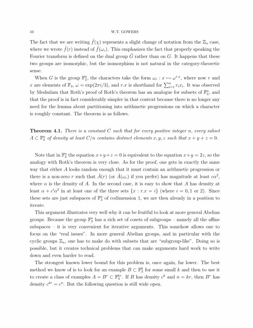
When G is the group Fn3 , the characters take the form ωr : x 7→ ωr.x, where now r and

x are elements of F3, ω = exp(2πi/3), and r.x is shorthand for∑n

i=1 rixi. It was observed

by Meshulam that Roth’s proof of Roth’s theorem has an analogue for subsets of Fn3 , and

that the proof is in fact considerably simpler in that context because there is no longer any

need for the lemma about partitioning into arithmetic progressions on which a character

is roughly constant. The theorem is as follows.

Theorem 4.1. There is a constant C such that for every positive integer n, every subset

A ⊂ Fn3 of density at least C/n contains distinct elements x, y, z such that x+ y + z = 0.

Note that in Fn3 the equation x+y+z = 0 is equivalent to the equation x+y = 2z, so the

analogy with Roth’s theorem is very close. As for the proof, one gets in exactly the same

way that either A looks random enough that it must contain an arithmetic progression or

there is a non-zero r such that A(r) (or A(ωr) if you prefer) has magnitude at least cα2,

where α is the density of A. In the second case, it is easy to show that A has density at

least α + c′α2 in at least one of the three sets {x : r.x = i} (where i = 0, 1 or 2). Since

these sets are just subspaces of Fn3 of codimension 1, we are then already in a position to

iterate.

This argument illustrates very well why it can be fruitful to look at more general Abelian

groups. Because the group Fn3 has a rich set of cosets of subgroups – namely all the affine

subspaces – it is very convenient for iterative arguments. This somehow allows one to

focus on the “real issues”. In more general Abelian groups, and in particular with the

cyclic groups Zn, one has to make do with subsets that are “subgroup-like”. Doing so is

possible, but it creates technical problems that can make arguments hard work to write

down and even harder to read.

The strongest known lower bound for this problem is, once again, far lower. The best

method we know of is to look for an example B ⊂ Fk3 for some small k and then to use it

to create a class of examples A = Br ⊂ Fkr3 . If B has density ck and n = kr, then Br has

density ckr = cn. But the following question is still wide open.


Question 4.2. Let cn be the greatest possible density of a subset A ⊂ Fn3 that contains no

three distinct elements x, y, z such that x + y + z = 0. Does there exist θ < 1 such that

cn ≤ θn for every n?

Until fairly recently, the best known upper bound was given by the simple argument

outlined above. But in 2011 Bateman and Katz improved the bound to one of the form

C/n1+ε for fixed constants C and ε > 0. This was a remarkable achievement, given how

long the bound had stood still, but the gap that remains is still huge.

5. The U2 norm

In the proof of Roth’s theorem, we had a useful measure of the quasirandomness of a

function, namely the size of its largest Fourier coefficient – the smaller that size, the more

quasirandom the function. However, this measure has the disadvantage that there isn’t

an obvious physical-space interpretation of ‖f‖∞ – that is, an expression in terms of the

values of f that does not mention the Fourier transform. Instead, one often prefers to

use the measure ‖f‖4. In the contexts we care about, these two quantities are roughly

equivalent, since we have the trivial inequalities

‖f‖4∞ ≤ ‖f‖44 ≤ ‖f‖2∞‖f‖22,

and we usually deal with functions f such that ‖f‖2 = ‖f‖2 ≤ 1. This tells us that ‖f‖∞is small if and only if ‖f‖4 is small (though if we pass from one equivalent statement to

the other and back again, we obtain a worse constant of smallness than the one we started

with).

The reason that ‖f‖4 is nice is that

‖f‖44 =∑r

|f(r)|4 = 〈f 2, f 2〉 = 〈f ∗ f, f ∗ f〉 = Ex+y=z+wf(x)f(y)f(z)f(w),

where in the above argument we used the definition of the `4 norm, the definition of the

inner product on Zn, Parseval’s identity and the convolution identity, and the definition of

convolutions and inner products in Zn. (It is also possible to prove the identity above using

a direct calculation, but it is nicer to use the basic properties of the Fourier transform.)

Quadruples (x, y, z, w) with x + y = z + w are the same as quadruples of the form

(x, x+ a+ b, x+ a, x+ b), so the final expression above can be written in the form

Ex,a,bf(x)f(x+ a)f(x+ b)f(x+ a+ b).

12 W.T. GOWERS

Since this equals ‖f‖44, we find that it is possible to define a norm ‖f‖U2 by the formula

‖f‖U2 = (Ex,a,bf(x)f(x+ a)f(x+ b)f(x+ a+ b))1/4.

This may seem pointless, since it is just renaming the norm f 7→ ‖f‖4, but we use a

different name to emphasize that we are using a purely physical-space definition. The

great advantage of doing this is that it gives us an alternative definition that is sometimes

easier to generalize than the definition in terms of Fourier coefficients.

A useful fact about the U2 norm is that it satisfies a kind of Cauchy-Schwarz inequality.

Let us define a generalized inner product by the formula

[f1, f2, f3, f4] = Ex,a,bf1(x)f2(x+ a)f3(x+ b)f4(x+ a+ b).

Then ‖f‖4U2 = [f, f, f, f ]. The inequality states that

[f1, f2, f3, f4] ≤ ‖f1‖U2‖f2‖U2‖f3‖U2‖f4‖U2 .

We quickly sketch a proof. We have that

[f1, f2, f3, f4] = Ex,y,af1(x)f2(x+ a)f3(y)f4(y + a)

= Ea(Exf1(x)f2(x+ a))(Eyf3(y)f4(y + a))

≤ (Ea|Exf1(x)f2(x+ a)|2)1/2(Ea|Eyf3(y)f4(y + a)|2)1/2

by the usual Cauchy-Schwarz inequality. But this last expression is easily seen to be

[f1, f2, f1, f2]1/2[f3, f4, f3, f4]

1/2.

Furthermore, we have the symmetry [f1, f2, f3, f4] = [f1, f3, f2, f4], so we can rewrite the

last expression as

[f1, f1, f2, f2]1/2[f3, f3, f4, f4]

1/2.

Applying the argument again we find that

[f1, f1, f2, f2] ≤ [f1, f1, f1, f1]1/2[f2, f2, f2, f2]

1/2,

and similarly for f3 and f4, and from this the result follows.


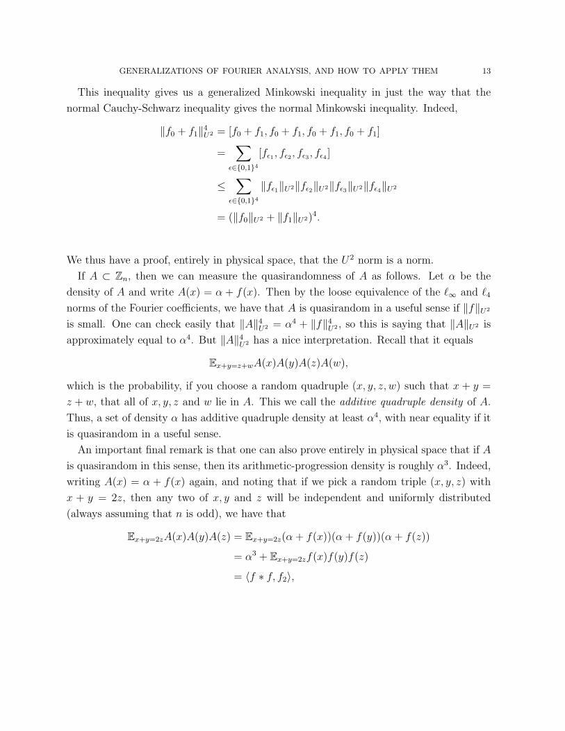
This inequality gives us a generalized Minkowski inequality in just the way that the

normal Cauchy-Schwarz inequality gives the normal Minkowski inequality. Indeed,

‖f0 + f1‖4U2 = [f0 + f1, f0 + f1, f0 + f1, f0 + f1]

=∑

ε∈{0,1}4[fε1 , fε2 , fε3 , fε4 ]

≤∑

ε∈{0,1}4‖fε1‖U2‖fε2‖U2‖fε3‖U2‖fε4‖U2

= (‖f0‖U2 + ‖f1‖U2)4.

We thus have a proof, entirely in physical space, that the U2 norm is a norm.

If A ⊂ Zn, then we can measure the quasirandomness of A as follows. Let α be the

density of A and write A(x) = α + f(x). Then by the loose equivalence of the `∞ and `4

norms of the Fourier coefficients, we have that A is quasirandom in a useful sense if ‖f‖U2

is small. One can check easily that ‖A‖4U2 = α4 + ‖f‖4U2 , so this is saying that ‖A‖U2 is

approximately equal to α4. But ‖A‖4U2 has a nice interpretation. Recall that it equals

Ex+y=z+wA(x)A(y)A(z)A(w),

which is the probability, if you choose a random quadruple (x, y, z, w) such that x + y =

z + w, that all of x, y, z and w lie in A. This we call the additive quadruple density of A.

Thus, a set of density α has additive quadruple density at least α4, with near equality if it

is quasirandom in a useful sense.

An important final remark is that one can also prove entirely in physical space that if A

is quasirandom in this sense, then its arithmetic-progression density is roughly α3. Indeed,

writing A(x) = α + f(x) again, and noting that if we pick a random triple (x, y, z) with

x + y = 2z, then any two of x, y and z will be independent and uniformly distributed

(always assuming that n is odd), we have that

Ex+y=2zA(x)A(y)A(z) = Ex+y=2z(α + f(x))(α + f(y))(α + f(z))

= α3 + Ex+y=2zf(x)f(y)f(z)

= 〈f ∗ f, f2〉,

14 W.T. GOWERS

where f2(z) = f(z/2) for each z. But by Cauchy-Schwarz and the fact that f takes values

of modulus at most 1,

|〈f ∗ f, f2〉|2 ≤ ‖f ∗ f‖22‖f2‖22≤ Ex+y=z+wf(x)f(y)f(z)f(w)

= ‖f‖4U2 .

Therefore, if ‖f‖U2 is small, then Ex+y=2zA(x)A(y)A(z) ≈ α3.

In due course, we shall see how the arguments given above are more amenable to gener-

alization than the Fourier-analytic proof we gave earlier.

We close this section by remarking that the definition of the U2 norm and the basic

observations we have made about it work just as well in an arbitrary finite Abelian group.

6. Generalization to matrices

Given a function f we can define a linear map Tf that takes a function g to the convo-

lution f ∗ g. That is, we have

Tf (g)(x) = Euf(x− u)g(u).

If we define a matrix Mf by Mf (x, u) = f(x− u), then this formula becomes

Tf (g) = EuM(f, u)g(u),

which is just the normal formula for multiplying a matrix by a vector, except that instead

of summing over u we have taken the expectation. It will be convenient, for the purposes

of this section, to adopt a non-standard definition of matrix multiplication by using this

normalization. That is, we will say that if A and B are two matrices, then

(AB)(x, z) = EyA(x, y)B(y, z).

Since

TfTgh = Tf (g ∗ h) = f ∗ (g ∗ h) = (f ∗ g) ∗ h,

we get that MfMg = Mf∗g with this normalization.

Notice that

Tf (ωr)(x) = f ∗ ωr(x) = Euf(u)ωr(x−u) = f(r)ωr(x).

Thus, ωr is an eigenvector of Tf with eigenvalue f(r).


A more conceptual way of seeing this is to note that by the convolution identity, the

convolution of f with the function g =∑

r g(r)ωr is the function∑

r f(r)g(r)ωr, so with

respect to the basis ω0, . . . , ωn−1 all convolution maps Tf are multipliers (that is, given by

diagonal matrices).

These observations allow us to translate some of the concepts we have defined so far into

matrix language. The Fourier coefficients of a function f become the eigenvalues of the

matrix Mf . However, that is just the beginning. Let us write a⊗ b for the rank-1 matrix

with

(a⊗ b)(u, v) = a(u)b(v).

Note that if a, b, f : Zn → C, then

(a⊗ b)(f)(x) = a(x)Eyf(y)b(y) = a(x)〈f, b〉.

Thus, the diagonalization of f is telling us that

Mf =∑r

f(r)ωr ⊗ ωr,

since if we apply either side to the function ωs we obtain f(x)ωs.

We are now in a position to write down Parseval’s identity in matrix terms. First, note

that

Ex,y|Mf (x, y)|2 = Ex,y|f(x− y)|2 = Ex|f(x)|2 = ‖f‖22.

Therefore, by Parseval’s identity, we find that

Ex,y|Mf (x, y)|2 =∑r

|f(r)|2.

The left-hand side is the L2 norm of the matrix entries of Mf , which is often known as

the (normalized) Hilbert-Schmidt norm. And the right-hand side, though it appears to be

expressed in terms of f , can be thought of as the sum of squares of the eigenvalues of Mf .

This connection can be generalized to all matrices that have an orthonormal basis

u1, . . . , un of eigenvectors. In that case we can write M =∑

i λiui ⊗ ui and we find

16 W.T. GOWERS

that

Ex,y|M(x, y)|2 = Ex,y

∑i,j

λiλjui(x)ui(y)uj(x)uj(y)

=∑i,j

λiλjEx,yui(x)ui(y)uj(x)uj(y)

=∑i,j

λiλj|〈ui, uj〉|2

=∑i

|λi|2.

More generally still, if M does not have an orthonormal basis of eigenvectors, it will still

have a singular value decomposition, that is, a decomposition of the form∑

i λiui⊗vi where

(ui)n1 and (vi)

n1 are both orthonormal bases and the λi are non-negative real numbers. (The

non-negativity can be obtained by multiplying the vi by suitable scalars of modulus 1.)

The above argument carries over with very little change, and we find that ‖M‖22 (that is,

the square of the normalized Hilbert-Schmidt norm) is equal to the sum of the squares of

the singular values.

As we have already made clear, this fact specializes to Parseval’s identity when the

matrix is the matrix Mf of a convolution operator Tf .

More importantly, singular values of matrices play a rather similar role in graph theory

to the role played by Fourier coefficients in additive combinatorics. To see this, let us first

find an analogue for matrices of the U2 norm. Given the correspondence so far, it should

be equal to the `4 norm of the singular values, and its fourth power should have a nice

interpretation in terms of the matrix values. This does indeed turn out to be the case. An

argument similar to the one just given for the Hilbert-Schmidt norm, but slightly more

complicated, shows that∑i

|λi|4 = Ex,y,a,bM(x, y)M(x+ a, y)M(x, y + b)M(x+ a, y + b).

Now the fourth root of the left-hand side is a well-known matrix norm – the fourth-power

trace class norm. From this one can deduce that the fourth root of the right-hand side is

a norm, which we write as ‖M‖� and call the box norm (because we are summing over

aligned rectangles). But as with the U2 norm, one can prove this fact directly by first


defining a generalized inner product for two-variable functions

[f1, f2, f3, f4] = Ex,y,a,bf1(x, y)f2(x+ a, y)f3(x, y + b)f4(x+ a, y + b),

using the Cauchy-Schwarz inequality to prove that

[f1, f2, f3, f4] ≤ ‖f1‖�‖f2‖�‖f3‖�‖f4‖�,

and finally deducing that ‖f + g‖4� ≤ (‖f‖� + ‖g‖�)4 in more or less the same way as we

did for the U2 norm.

After this it will come as no surprise to learn that the box norm specializes to the U2

norm when the matrix is a Toeplitz matrix (that is, the matrix of a convolution operator).

Indeed, we have that

‖Mf‖4� = Ex,y,a,bf(x− y)f(x+ a− y)f(x− y − b)f(x+ a− y − b)

= Ex,a,bf(x)f(x+ a)f(x− b)f(x+ a− b)

= Ex,a,bf(x)f(x+ a)f(x+ b)f(x+ a+ b)

= ‖f‖4U2 .

Of course, we could also have deduced this less directly by using the relationship between

eigenvalues, Fourier coefficients, and the two norms.

Now let us take a graph G and let M be its adjacency matrix. (That is, M(x, y) = 1

if there is an edge from x to y and 0 otherwise.) Then the analogy between subsets of

Zn (or more general finite Abelian groups) and matrices strongly suggests that the box

norm ‖.‖� should be a useful measure of quasirandomness. That is indeed the case. If G

has density δ, meaning that Ex,yM(x, y) = δ, then a straightforward argument using the

Cauchy-Schwarz inequality shows that ‖M‖� ≥ δ. If equality almost holds, then G turns

out to enjoy a number of properties that typical random graphs have.

To see this, we begin by noting that the box norm relates to the largest singular value

in much the way that the U2 norm relates to the largest Fourier coefficient. If the singular

values are λ1, . . . , λn and if λ = (λ1, . . . , λn), then

‖λ‖4∞ ≤ ‖λ‖44 ≤ ‖λ‖22‖λ‖2∞,

and if the matrix entries have modulus at most 1 then we know in addition that ‖λ‖22 =

‖M‖22 ≤ 1. Therefore, the largest singular value (which is equal to the operator norm of

the matrix) is small if and only if the box norm is small.

18 W.T. GOWERS

For convenience let us now assume that G is regular, so every vertex has degree δn.

(The proofs become slightly more complicated if we do not have this.) Then the constant

function u(x) = 1 is an eigenvector of M with eigenvalue δ. (Recall that we are using

expectations in our matrix multiplication, which is why we get δ here rather than δn.)

Now consider the matrix A = M − δu ⊗ u. That is, A(x, y) = M(x, y) − δ. Since G is

regular, we find that ExA(x, y) = 0 for every y and EyA(x, y) = 0 for every x. From this

it is not hard to prove that ‖M‖4� = δ4 + ‖A‖4�: we expand ‖A + δu ⊗ u‖4� as a sum of

sixteen terms and the only ones that are not zero are the term with all As and the term

with all δs.

Therefore, if ‖M‖� is close to δ, it follows that ‖A‖� is close to zero, which implies that

the largest singular value of A is small, and therefore that A has a small operator norm.

Let θ be this operator norm.

Now let f and g be two functions defined on the vertex set of G that take values in the

interval [−1, 1]. Then

|〈Af, g〉| ≤ ‖Af‖2‖g‖2 ≤ θ‖f‖2‖g‖2 ≤ θ.

We also have that

〈(δu⊗ u)(f), g〉 = 〈(δExf(x))u, g〉 = δExf(x)Eyg(y).

It follows that

|〈Mf, g〉 − δExf(x)Eyg(y)| ≤ θ.

But 〈Mf, g〉 = Ex,yM(x, y)f(x)g(y), so if θ is small then this is telling us that

Ex,yM(x, y)f(x)g(y) ≈ δEx,yf(x)g(y).

Suppose now that f and g are the characteristic functions of sets U and V of density α

and β. Now we have that

Ex,yM(x, y)U(x)V (y) ≈ δEx,yU(x)V (y) = δαβ.

This tells us that the number of edges from U to V in the graph is approximately δ|U ||V |,which is exactly the number one would expect if G was a random graph with density δ.

Now the fourth power of the box norm of M can be seen to equal the 4-cycle density of

the graph G, that is, the probability, if vertices x1, x2, x3, x4 are chosen independently at

random, that x1x2, x2x3, x3x4 and x4x1 are all edges of G. Thus, we have started with a

“local” assumption – that the number of 4-cycles in the graph is almost as small as it can

possibly be given the density of the graph – and ended up with a global conclusion – that


the number of edges between any two large sets is approximately what one would expect

in a random graph of the same density. This fact has many applications in graph theory.

The converse can also be shown without too much difficulty. In fact, there turn out to

be several properties that are all loosely equivalent and all say that in one way or another

a graph G behaves like a random graph. A particularly interesting one from the point of

view of comparison with Roth’s theorem is the statement that if a graph G of density δ is

quasirandom (in, for example, the sense of having box norm approximately δ) then for any

graph H with k edges (here k is fixed and the size of G is tending to infinity) the H density

in G is approximately δk, as it would be in a random graph. Conversely, if G contains the

“wrong” number of copies of H, then we can find a subgraph that is substantially denser

than the original graph.

It is worth pointing out that not all the basic properties of the Fourier transform carry

over in a nice way to matrices. For example, the inner product corresponding to the

normalized Hilbert-Schmidt norm is

〈A,B〉 = ExyA(x, y)B(x, y) = tr(AB∗)

(where I have also defined the trace in a normalized way – that is, tr(A) = ExAxx). If the

singular-value decompositions of A and B are∑

i λiui ⊗ vi and∑

j µjwj ⊗ zj, then 〈A,B〉works out to be ∑

i,j

λiµj〈ui, wj〉〈vi, zj〉.

If it happens that ui = wi and vi = zi for every i, as it does when A = B, then this

simplifies to∑

i λiµi, the formula we would like, but if not then we have to make do with

the more complicated formula above (which nevertheless can be useful sometimes).

Similarly, there is no tidy analogue of the convolution identity except under very special

circumstances. In general,

(∑i

λiui ⊗ vi)(∑j

µjwj ⊗ zj) =∑i,j

λiµj〈wj, vi〉ui ⊗ zj.

If vi = wi for every i, then this simplifies to∑

i λiµiui⊗zi, so we find that the singular values

of the matrix product are products of the singular values of the original matrices. But this

is an unusual situation (that happens to occur when the two matrices are convolution

matrices and all the bases are the same basis of trigonometric functions).

20 W.T. GOWERS

7. Quadratic Fourier analysis

In this section I shall discuss a generalization of Fourier analysis that lacks a satisfactory

inversion formula. This might seem to be such a fundamental property of the Fourier

transform that the generalization does not deserve to be called a generalization of Fourier

analysis. However, for several applications of Fourier analysis, a weaker property suffices,

and that weaker property can be generalized. It is, however, a very interesting open

problem to develop the theory further so as to make the analogy with conventional discrete

Fourier analysis closer. But first, let us look at a problem that demonstrates the need for

a generalization at all, namely Szemeredi’s theorem for progressions of length 4.

At the heart of the proof for progressions of length 3 is the identity

Ex+y=2zf(x)g(y)h(z) =∑r

f(r)g(r)h(−2r).

We have essentially proved this already, but a variant of the argument is to observe that

both sides are equal to Ex,y,zf(x)g(y)h(z)∑

r ω−r(x+y−2z). So it is natural to look for a

similar identity for progressions of length 4. Such a progression can be thought of as a

quadruple (x, y, z, w) such that x+ z = 2y and y + w = 2z. However,

Ex+z=2y,y+w=2zf1(x)f2(y)f3(z)f4(w)

= Ex,y,z,wf1(x)f2(y)f3(z)f4(w)∑r,s

ω−r(x−2y+z)−s(y−2z+w)

=∑r,s

f1(r)f2(−2r + s)f3(r − 2s)f4(s).

A quadruple (a, b, c, d) can be written in the form (r,−2r + s, r − 2s, s) if and only if

3a + 2b + c = b + 2c + 3d = 0. So we have ended up with a sum over four variables that

satisfy two linear equations, which is what we had before we took the Fourier transform.

So we have not gained anything.

An even more compelling argument that the Fourier transform is too blunt a tool for

our purposes is to note that it is possible for all the Fourier coefficients of f1, f2, f3 and f4

to be tiny, but for the expectation Ex,df1(x)f2(x+d)f3(x+2d)f4(x+3d) to be large. (This

is another way of writing the expression that we have just evaluated in terms of Fourier

transforms.) Let f1(x) = f4(x) = ωx2

and let f2(x) = f3(x) = ω3x2. Then

Ex,df1(x)f2(x+ d)f3(x+ 2d)f4(x+ 3d) = Ex,dωx2−3(x+d)2+3(x+2d)2−(x+3d)2 .


But the exponent on the right-hand side is identically zero, so both sides are equal to 1,

which is as large as the expectation can possibly be given that all four functions take values

of modulus 1. On the other hand, functions like ωx2

have tiny Fourier coefficients. To see

this (assuming for convenience that n is odd), note that if f(x) = ωx2, then

f(r) = Exωx2−rx = Exω

(x−r/2)2−r2/4 = ω−r2/4Exω

x2

.

This shows that |f(r)| = |Exωx2| is the same for all r, and therefore by Parseval it equals

n−1/2 for all r. In other words, the largest Fourier coefficient is as small as Parseval’s

identity will allow.

It is almost impossible at this stage not to have the following thought. For Roth’s

theorem, the functions that caused trouble by not being sufficiently random-like were the

trigonometric functions x 7→ ωrx. These are linear phase functions – that is, compositions

of linear functions with the function x 7→ ωx. We have just seen that when it comes to

discussing arithmetic progressions of length 4, quadratic phase functions, that is, functions

of the form ωq(x) where q is a quadratic, cause problems. Could it be that these are somehow

the only functions that cause problems? Does there exist some kind of “quadratic Fourier

analysis” that allows one to expand a function as a linear combination of quadratic phase

functions and thereby to generalize the proof of Roth’s theorem to progressions of length 4?

The answer to this question turns out to be a partial yes. More precisely, one can gen-

eralize “linear” Fourier analysis by just enough to obtain a proof of Szemeredi’s theorem

for progressions of length 4, but the generalized Fourier analysis lacks some of the nice

properties of the usual Fourier transform, as a result of which the proof becomes substan-

tially harder. In particular, it turns out that the quadratic phase functions are not the

only ones that cause trouble – there are also some more general functions that exhibit

sufficiently quadratic-like behaviour to cause problems similar to the ones caused by the

“pure” quadratic phase functions. But before we get on to that, it will be useful to look

at another concept that comes into the picture.

8. The U3 norm

Discrete Fourier analysis decomposes a function into characters. It is far from obvious

how to define a “quadratic” analogue of this decomposition, since one’s natural first guesses

turn out not to have the properties one wants, as we shall see later. But already it is clear

that there are problems, because there are n2 functions of the form x 7→ ωax2+bx, so we

cannot hope to define a quadratic Fourier transform by simply writing down a suitable

basis of Cn and expanding functions in terms of that basis.

22 W.T. GOWERS

It is for this reason that the reformulation of the norm f 7→ ‖f‖4 in purely physical-

space terms is so important. It gives us a concept that is easy to generalize. As one might

expect, there are Uk norms for all k ≥ 2 (and also a seminorm when k = 1), but it is clear

what they are once one has seen the U3 norm. It is defined by the formula

‖f‖8U3 = Ex,a,b,cf(x)f(x+ a)f(x+ b)f(x+ a+ b)f(x+ c)

f(x+ a+ c)f(x+ b+ c)f(x+ a+ b+ c)

That is, where the U2 norm involves an average over “squares”, the U3 norm involves a sim-

ilar average over “cubes”, and the Uk norm involves a similar average over k-dimensional

cubes. The letter U stands for “uniformity”, because when a function has a small unifor-

mity norm, its values are “uniformly distributed” in a useful sense.

There are a few remarks to make about the U3 norm to give an idea of its basic properties

and of why it is likely to be important to us.

• First, it really is a norm. This is proved in much the same way as it is for the U2

norm: one defines an appropriate generalized inner product (by using eight different

functions in the formula above instead of just one), deduces a generalized Cauchy-

Schwarz inequality from the conventional Cauchy-Schwarz inequality, and finally a

generalized Minkowski inequality from the generalized Cauchy-Schwarz inequality.

• Secondly, if f is a quadratic phase function f(x) = ωrx2+sx, then ‖f‖U3 takes the

largest possible value (given that all the values of f have modulus 1), namely 1.

This is simple to check, and boils down to the fact that

x2 − (x+ a)2 − (x+ b)2 + (x+ a+ b)2 − (x+ c)2

+ (x+ a+ c)2 + (x+ b+ c)2 − (x+ a+ b+ c)2 = 0

for every x, a, b and c.

• Thirdly, the Uk norms increase as k increases. In particular, the U3 norm is larger

than the U2 norm. This means that the statement that ‖f‖U3 is small is stronger

than the statement that ‖f‖U2 is small. That fact, combined with the observation

that ‖f‖U3 is large for quadratic phase functions, gives some reason to hope that

the U3 norm could be a useful measure of quasirandomness for Szemeredi’s theorem

for progressions of length 4.


• Fourthly, if A is a set of density α, then an easy Cauchy-Schwarz argument shows

that ‖A‖U3 ≥ α. Also, ‖A‖8U3 counts the number of “cubes” in A. So when we

talk about sets, we will want to regard a set as “quadratically uniform” if it has

almost the minimum number of cubes, and this will be a stronger property than

the “linear uniformity” that we used in the proof of Roth’s theorem.

Presenting those remarks is slightly misleading, however, as it suggests that the definition

of the U3 norm is a purely speculative generalization of the definition of the U2 norm that

just happens to be useful. In fact, the definition arises naturally (or at least can arise

naturally) when one tries to generalize the physical-space argument we saw earlier that

shows that a set with small U2 norm has roughly the expected number of arithmetic

progressions of length 3. One ends up being able to show that if f1, f2, f3 and f4 are

functions that take values of modulus at most 1, then

|Ex,df1(x)f2(x+ d)f3(x+ 2d)f4(x+ 3d)| ≤ mini‖fi‖U3 .

In other words, if one of the four functions has a small U3 norm, then the arithmetic

progression count must be small.

The point I am making here is that if one sets out to prove a bound for the left-hand

side in terms of some suitable function of f4, say, knowing that one’s main tool is the

Cauchy-Schwarz inequality, then the function that one obtains is precisely the U3 norm.

The inequality above can be used to show that if A is a set of density α and ‖A‖U3 ≤α+ c(α), then A is sufficiently quasirandom to contain an arithmetic progression of length

4, and in fact to have 4-AP density approximately α4. To prove this, one writes A = α+ f

with ‖f‖U3 small, one expands out the expression

Ex,dA(x)A(x+ d)A(x+ 2d)A(x+ 3d)

as a sum of 16 terms, and one uses the inequality above to show that all these terms are

small apart from the main term α4.

9. Generalized quadratic phase functions

In the previous section we noted that if q is a quadratic function defined on Zn, and f is

the function f(x) = ωq(x), then ‖f‖U3 = 1, which is as large as it can possibly be. The key

24 W.T. GOWERS

to this fact, as we have already noted, is that quadratic functions have the property that

q(x)− q(x+ a)− q(x+ b) + q(x+ a+ b)− q(x+ c)

+ q(x+ a+ c) + q(x+ b+ c)− q(x+ a+ b+ c) = 0

for every x, a, b, c. Moreover, this property characterizes quadratic functions.

However, if we do not insist on maximizing ‖f‖U3 but merely getting close to the max-

imum, then we suddenly let in a whole lot more functions. In this section I shall describe

one or two of them.

There is a general recipe for producing them, which is to take a set A ⊂ Zn and construct

a quadratic homomorphism on A – that is, a map ψ : A→ C that takes values of modulus

1 and satisfies the equation

ψ(x)ψ(x+ a)ψ(x+ b)ψ(x+ a+ b)ψ(x+ c)ψ(x+ a+ c)ψ(x+ b+ c)ψ(x+ a+ b+ c) = 1

whenever all of x, x+a, x+ b, x+ c, x+a+ b, x+a+ c, x+ b+ c and x+a+ b+ c all belong

to A. (As we have already noted, if A has density α, there will be at least α8n4 “cubes” of

this kind.) We then define f(x) to be ψ(x) for x ∈ A and 0 otherwise. For this to produce

interesting examples, we need to choose our set A carefully, but that can be done.

As a first example, take A to be the set {1, . . . , bn/2c}. If we now let β be any real

number, we can define f(x) to be e2πiβx2

on A and zero outside. If β is a multiple of 1/n,

then this will give us a function ωrx2

restricted to A. However, if we choose β not to be

close to a multiple of 1/n we can obtain functions that do not even correlate with functions

of the form ωrx2+sx. Suppose, for example, that we take β = 1/2n. Then our best chance

of a correlation will be with either the constant function 1 or the function ωx2

= e4πiβx2.

In both cases, the inner product has modulus n−1|∑

x∈A eπix2/n|, which can be shown to

be small by a simple trick known as Weyl differencing: we observe that

|∑x∈A

eπix2/n|2 =

∑x,y

eπi(x2−y2)/n =

∑x,y

eπi(x+y)(x−y).

The last sum can be split into a sum of geometric progressions, each of which can be

evaluated explicitly, and almost all of which turn out to be small. Essentially the same

technique proves that in fact our function f has a very small correlation with any function

of the form ωq(x) for a quadratic function q defined on Zn.

It is worth stopping to think about why a similar argument does not show that we have

to consider more functions even in the linear case. What if we take a function on the set


A above of the form e2πiβx with β far from a multiple of 1/n? In fact, what if we take

β = 1/2n as before?

In this case the correlation with a constant function has magnitude n−1|∑

x∈A eπix/n|,

and x/n lies between 0 and 1/2. It follows that all the numbers eπx/n are on one side of

the unit circle, and the result is that we do not get the cancellation that occurred with the

quadratic example above. The difference between the two situations is that the function

eπix2/n jumps round the circle many times, whereas the function eπix/n does not – which is

due to the fact that the function x2 grows much more rapidly than the function x.

Another way of choosing a set A is to make it look like a portion of Zd for some small

d. To give an example with d = 2, let m = b√n/2c and let A consist of all numbers of the

form x+2my such that x, y ∈ {0, 1, . . . ,m−1}. This we can think of as a two-dimensional

set with basis 1 and 2m: the pair (x, y) then represents the point x + 2my in coordinate

form.

An obvious class of functions to take on a multidimensional set is the class of quadratic

forms, and we can do that here. We pick coefficients a, b, c ∈ Zn and define f(x+ 2my) to

be ωax2+bxy+cy2 for all x, y ∈ {0, 1, . . . ,m− 1} and take all other values of f to be zero. It

is easy to check that f is a quadratic homomorphism in the sense just defined, and it can

also be shown that f does not correlate with any pure quadratic phase function.

We can of course combine these ideas by taking more general coefficients. We can also

define a wide variety of two-dimensional sets by taking different “basis vectors”, and we

can increase the dimension. Thus, the set of functions we are forced to consider is much

richer than the corresponding set for the U2 norm.

10. Szemeredi’s theorem for progressions of length 4

We remarked at the end of Section 8 that if a set A is quasirandom in the sense of

having an almost minimal U3 norm, then it contains an arithmetic progression of length 4.

Furthermore, the proof of this fact is closely analogous to the proof of the corresponding

fact relating the U2 norm to arithmetic progressions of length 3. So it is natural to try

to continue the analogy and complete a proof of Szemeredi’s theorem for progressions of

length 4. That is, we would like to argue that if the U3 norm of A is not approximately

minimal, then we can obtain a density increase on an appropriate subspace.

At this point we find that we are a little stuck. In the U2 case we used the fact that if

f is a function taking values of modulus at most 1, and ‖f‖U2 = ‖f‖4 is bounded below

by a positive constant c, then ‖f‖∞ is bounded below by c2, which we can use to argue

26 W.T. GOWERS

that a set with no arithmetic progression of length 3 must be sufficiently “unrandom” to

correlate well with a trigonometric function. So to continue the analogy, it looks as though

we need to find norms ‖.‖ and |||.||| with the following properties.

(1) The norm ‖.‖ is defined in a different way from the U3 norm, but happens to be

equal to it.

(2) If ‖f‖∞ ≤ 1 and ‖f‖ ≥ c, then one can prove very straightforwardly that |||f ||| ≥γ(c) (where γ(c) > 0 if c > 0, and ideally the dependence will be a good one).

(3) The fact that |||f ||| ≥ γ is telling us that there is some function ψ ∈ Ψ for which

|〈f, ψ〉| ≥ θ(γ), where Ψ is a class of “nice” functions (which will probably exhibit

behaviour similar to that of quadratic phase funtions).

(4) If A is a set of density α, f = A− α, and |〈f, ψ〉| ≥ θ for some ψ ∈ Ψ, then there

is a long subprogression P inside which A has density at least α + η(θ).

Implicit in the third of these conditions is that |||.||| and Ψ are related by the formula

max{|〈f, ψ〉| : ψ ∈ Ψ}.The big problem we face is that there is no obvious reformulation of the U3 norm

analogous to the reformulation ‖f‖U2 = ‖f‖4 of the U2 norm. So we do not know of a

candidate for ‖.‖. However, that does not mean that there is nothing we can do, since there

is still the possibility of passing directly from the statement that ‖f‖U3 ≥ c to the statement

that |〈f, ψ〉| ≥ θ(c) for some suitably nice function ψ, or even bypassing this statement

and heading straight for the conclusion that A is denser in some long subprogression. Both

approaches turn out to be possible.

It is not possible here to do more than give a very brief sketch of how the proof works.

We start with a function f with ‖f‖∞ ≤ 1 and ‖f‖8U3 ≥ γ. That inequality expands to

the inequality

Ex,a,b,cf(x)f(x− a)f(x− b)f(x− a− b)f(x− c)

f(x− a− c)f(x− b− c)f(x− a− b− c) ≥ γ,

where we have switched from plus signs to minus signs for unimportant aesthetic reasons.

We now define, for each a, a function ∂af by the formula ∂af(x) = f(x)f(x− a), which

allows us to rewrite the inequality above as

EaEx,b,c∂af(x)∂af(x− b)∂af(x− c)∂af(x− b− c) ≥ γ.


Now this is just telling us that Ea‖∂af‖4U2 ≥ θ, from which it follows that there must be

several a for which ‖∂af‖U2 is large. By the rough equivalence of the U2 norm with the

magnitude of the largest Fourier coefficient, we can deduce from this that several of the

functions ∂af have at least one large Fourier coefficient. It follows that there is a large set

B and a function φ : B → Zn such that ∂af(φ(a)) is large for every a ∈ B. More formally,

we can obtain an inequality

EaB(a)|∂af(φ(a))|2 ≥ θ

for some θ that depends (polynomially) on γ.

It turns out that one can perform some algebraic manipulations with this statement and

eventually prove that the function φ has an interesting “partial additivity” property, which

states that there are at least ηn3 quadruples (x, y, z, w) ∈ B4 (for some η that depends on

γ only) such that

x+ y = z + w

and

φ(x) + φ(y) = φ(z) + φ(w).

This property appears at first to be somewhat weak, since it tells us that φ is additive on

only a small percentage of the quadruples x + y = z + w. Remarkably, however, this is

another instance where a local assumption can be used to prove a global conclusion: the

only way that φ can be this additive is if it has a form that can be described very precisely.

Recall the two-dimensional set we defined in the previous section. It is an example

of a two-dimensional arithmetic progression. More generally, a k-dimensional arithmetic

progression is a set of the form

{x+ a1d1 + a2d2 + · · ·+ akdk : 0 ≤ ai < mi}.

The numbers d1, . . . , dk are the common differences and the numbers m1, . . . ,mk are the

lengths. The arithmetic progression is called proper if it has cardinality m1 . . .mk – that

is, no two of the a1d1 + · · ·+ akdk coincide.

Given such a progression and coefficients µ0, µ1, . . . , µk ∈ Zn one can define something

like a linear form by the obvious formula

x+ a1d1 + a2d2 + · · ·+ akdk 7→ µ0 +∑i

µiai.

Let us call such a map quasilinear.

The result that tells us about the structure of φ is the following.

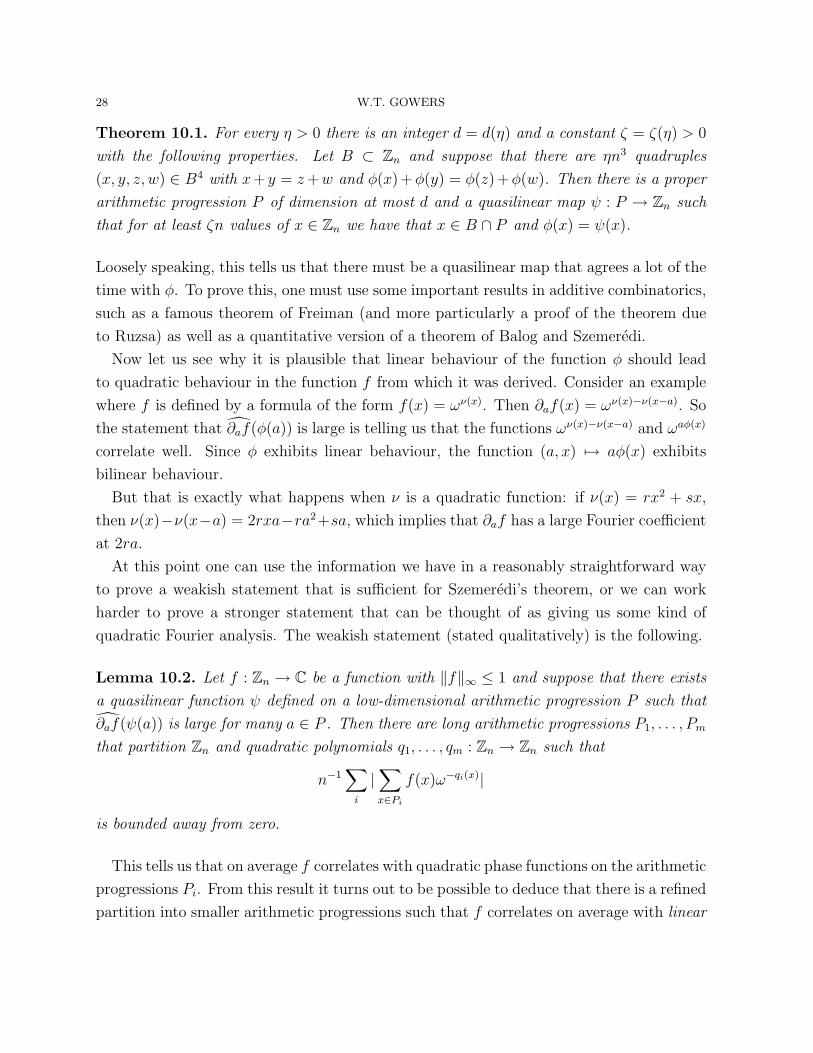
28 W.T. GOWERS

Theorem 10.1. For every η > 0 there is an integer d = d(η) and a constant ζ = ζ(η) > 0

with the following properties. Let B ⊂ Zn and suppose that there are ηn3 quadruples

(x, y, z, w) ∈ B4 with x+ y = z+w and φ(x) +φ(y) = φ(z) +φ(w). Then there is a proper

arithmetic progression P of dimension at most d and a quasilinear map ψ : P → Zn such

that for at least ζn values of x ∈ Zn we have that x ∈ B ∩ P and φ(x) = ψ(x).

Loosely speaking, this tells us that there must be a quasilinear map that agrees a lot of the

time with φ. To prove this, one must use some important results in additive combinatorics,

such as a famous theorem of Freiman (and more particularly a proof of the theorem due

to Ruzsa) as well as a quantitative version of a theorem of Balog and Szemeredi.

Now let us see why it is plausible that linear behaviour of the function φ should lead

to quadratic behaviour in the function f from which it was derived. Consider an example

where f is defined by a formula of the form f(x) = ων(x). Then ∂af(x) = ων(x)−ν(x−a). So

the statement that ∂af(φ(a)) is large is telling us that the functions ων(x)−ν(x−a) and ωaφ(x)

correlate well. Since φ exhibits linear behaviour, the function (a, x) 7→ aφ(x) exhibits

bilinear behaviour.

But that is exactly what happens when ν is a quadratic function: if ν(x) = rx2 + sx,

then ν(x)−ν(x−a) = 2rxa−ra2+sa, which implies that ∂af has a large Fourier coefficient

at 2ra.

At this point one can use the information we have in a reasonably straightforward way

to prove a weakish statement that is sufficient for Szemeredi’s theorem, or we can work

harder to prove a stronger statement that can be thought of as giving us some kind of

quadratic Fourier analysis. The weakish statement (stated qualitatively) is the following.

Lemma 10.2. Let f : Zn → C be a function with ‖f‖∞ ≤ 1 and suppose that there exists

a quasilinear function ψ defined on a low-dimensional arithmetic progression P such that

∂af(ψ(a)) is large for many a ∈ P . Then there are long arithmetic progressions P1, . . . , Pm

that partition Zn and quadratic polynomials q1, . . . , qm : Zn → Zn such that

n−1∑i

|∑x∈Pi

f(x)ω−qi(x)|

is bounded away from zero.

This tells us that on average f correlates with quadratic phase functions on the arithmetic

progressions Pi. From this result it turns out to be possible to deduce that there is a refined

partition into smaller arithmetic progressions such that f correlates on average with linear


phase functions, and then we are in essentially the situation we were in with Roth’s theorem

and can complete the proof of Szemeredi’s theorem for progressions of length 4.

From the point of view of generalizing Fourier analysis, however, Lemma 10.2 is unsat-

isfactory. Our previous deductions tell us that the hypotheses of the lemma holds when f

is a function with ‖f‖∞ ≤ 1 and ‖f‖U3 ≥ c, so the conclusions hold too. That gives us

a lot of information about f , but it says nothing about how the quadratic polynomials qi

might be related. It therefore gives us only local information about f , from which it is not

possible to deduce a converse: just because f correlates with quadratic phase functions on

the progressions Pi, it does not follow that ‖f‖U3 is large. (In fact, even constant functions

do not do the job: if we were to choose for each i a random εi ∈ {−1, 1} and set f(x) to

equal εi everywhere on Pi, we would not have a function with large U3 norm.)

By contrast, if ‖f‖U2 is large, then we obtain very simply that ‖f‖∞ is large, which tells

us that f correlates with a function of the form ωrx, and that, equally simply, implies that

‖f‖U2 is large.

What we would really like is to get from the hypothesis of Lemma 10.2 to a more global

conclusion, that would say that f correlates with a generalized quadratic phase function

of the kind described in the previous section. It is plausible that such a result should

exist: from linear behaviour of the function φ one can deduce straightforwardly that f

correlates with a pure quadratic phase function, so if we have generalized linear behaviour

(of a rather precise kind) then it seems reasonable to speculate that f should correlate

with a correspondingly generalized quadratic phase function.

The main obstacle to proving this is that the function (a, x) 7→ aφ(x) is not symmetric.

If it were, then the proof would be easy. However, Green and Tao found an ingenious

“symmetrization argument” that allowed them to deduce from the hypotheses of Lemma

10.2 a more symmetric set of hypotheses that yielded the desired result. I shall state it

somewhat imprecisely here. It is known as the inverse theorem for the U3 norm.

Theorem 10.3. For every c > 0 there exists c′ > 0 with the following property. Let

f : Zn → C be a function with ‖f‖∞ ≤ 1 and ‖f‖U3 ≥ c. Then there exists a generalized

quadratic phase function g such that 〈f, g〉 ≥ c′. Conversely, every function that correlates

well with a generalized quadratic phase function has a large U3 norm.

The imprecision is of course that I have not said exactly what a quadratic phase function

is. There are in fact several non-identical ways of defining them and the theorem is true for

each such way. The way I presented them in the previous section (where the exponent is

something like a quadratic form on a multidimensional arithmetic progression) is perhaps

30 W.T. GOWERS

the easiest to understand for a non-expert, but it is not the most convenient to use in

proofs.

A natural question to ask at this point is what happens for the Uk norm when k ≥ 4. If

one is aiming for a generalization of Lemma 10.2, and thereby for a proof of Szemeredi’s

theorem, the case k = 4 (which corresponds to arithmetic progressions of length 5) is

significantly harder than the case k = 3, and after that the difficulty does not increase

further. As for the inverse theorem, one would like to show that a function with large Uk

norm correlates well with a generalized polynomial phase function of degree k−1, but it is

far from easy even to come up with a satisfactory definition of what such a function should

be. This Green and Tao did in a famous paper entitled Linear Equations in the Primes,

which is about a programme to hugely extend their even more famous paper The Primes

Contain Arbitrarily Long Arithmetic Progressions. Actually proving the resulting inverse

conjecture took several years, but finally, with Tamar Ziegler, they managed it. So we now

have something like a higher-order Fourier analysis for every degree.

11. Hypergraphs

A graph is a collection of pairs of elements of a set. What happens if we generalize from

pairs to triples and beyond? A k-uniform hypergraph is a set X and a subset of X(k), where

X(k) denotes the set of all subsets of X of size k. In this section I shall concentrate on the

case k = 3, though it should be fairly clear how to generalize what I say to higher values.

Just as it is natural, when one thinks about graphs in an analytic way, to think of them

as special kinds of matrices, or functions of two variables, so hypergraphs can be thought

of as functions of three variables. Furthermore, there is a natural three-variable analogue

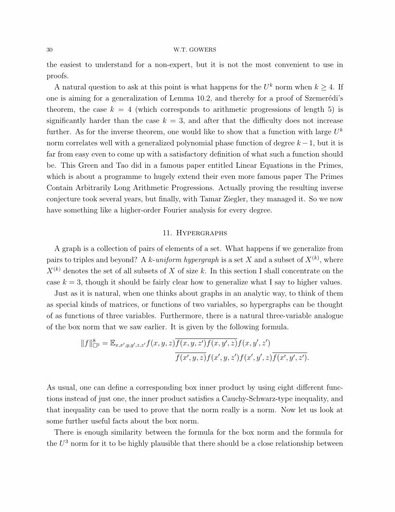
of the box norm that we saw earlier. It is given by the following formula.

‖f‖8�3 = Ex,x′,y,y′,z,z′f(x, y, z)f(x, y, z′)f(x, y′, z)f(x, y′, z′)

f(x′, y, z)f(x′, y, z′)f(x′, y′, z)f(x′, y′, z′).

As usual, one can define a corresponding box inner product by using eight different func-

tions instead of just one, the inner product satisfies a Cauchy-Schwarz-type inequality, and

that inequality can be used to prove that the norm really is a norm. Now let us look at

some further useful facts about the box norm.

There is enough similarity between the formula for the box norm and the formula for

the U3 norm for it to be highly plausible that there should be a close relationship between


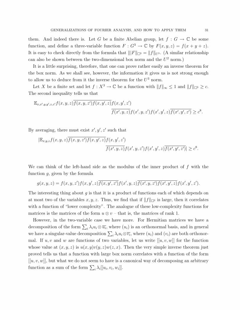
them. And indeed there is. Let G be a finite Abelian group, let f : G → C be some

function, and define a three-variable function F : G3 → C by F (x, y, z) = f(x + y + z).

It is easy to check directly from the formula that ‖|F‖�3 = ‖f‖U3 . (A similar relationship

can also be shown between the two-dimensional box norm and the U2 norm.)

It is a little surprising, therefore, that one can prove rather easily an inverse theorem for

the box norm. As we shall see, however, the information it gives us is not strong enough

to allow us to deduce from it the inverse theorem for the U3 norm.

Let X be a finite set and let f : X3 → C be a function with ‖f‖∞ ≤ 1 and ‖f‖�3 ≥ c.

The second inequality tells us that

Ex,x′,y,y′,z,z′f(x, y, z)f(x, y, z′)f(x, y′, z)f(x, y′, z′)

f(x′, y, z)f(x′, y, z′)f(x′, y′, z)f(x′, y′, z′) ≥ c8.

By averaging, there must exist x′, y′, z′ such that

|Ex,y,zf(x, y, z)f(x, y, z′)f(x, y′, z)f(x, y′, z′)

f(x′, y, z)f(x′, y, z′)f(x′, y′, z)f(x′, y′, z′)| ≥ c8.

We can think of the left-hand side as the modulus of the inner product of f with the

function g, given by the formula

g(x, y, z) = f(x, y, z′)f(x, y′, z)f(x, y′, z′)f(x′, y, z)f(x′, y, z′)f(x′, y′, z)f(x′, y′, z′).

The interesting thing about g is that it is a product of functions each of which depends on

at most two of the variables x, y, z. Thus, we find that if ‖f‖�3 is large, then it correlates

with a function of “lower complexity”. The analogue of these low-complexity functions for

matrices is the matrices of the form u⊗ v – that is, the matrices of rank 1.

However, in the two-variable case we have more. For Hermitian matrices we have a

decomposition of the form∑

i λiui⊗ui, where (ui) is an orthonormal basis, and in general

we have a singular-value decomposition∑

i λiui⊗vi, where (ui) and (vi) are both orthonor-

mal. If u, v and w are functions of two variables, let us write [[u, v, w]] for the function

whose value at (x, y, z) is u(x, y)v(y, z)w(z, x). Then the very simple inverse theorem just

proved tells us that a function with large box norm correlates with a function of the form

[[u, v, w]], but what we do not seem to have is a canonical way of decomposing an arbitrary

function as a sum of the form∑

i λi[[ui, vi, wi]].

32 W.T. GOWERS

What happens if we try to deduce the inverse theorem for the U3 norm from the inverse

theorem for the box norm in three variables? If ‖f‖U3 ≥ c, then the argument gives us

functions f1, . . . , f6, all of `∞ norm at most 1, such that

|Ex,y,zf(x+ y + z)f1(x+ y)f2(y + z)f3(z + x)f4(x)f5(y)f6(z)| ≥ c8.

However, it does not tell us anything much about the structure of the functions f1 . . . , f6.

It is possible to deduce from the inequality above that they have quadratic structure, and

that the inverse theorem therefore holds, but the proof is no easier than the proof of the

inverse theorem was already – it just uses the same general approach in an unnecessarily

complicated way.

Despite this, the theory of hypergraphs has been important and useful in additive com-

binatorics. I will not explain why here, except to mention a theorem about hypergraphs

that turns out to imply Szemeredi’s theorem, known as the simplex removal lemma. (The

implication is fairly straightforward, but slightly too long to give here.) Define a simplex

in a k-uniform hypergraph H to be a set of k+ 1 vertices such that any k of them form an

edge H. (The word “edge” here means one of the sets of size k that belongs to H. When

k = 2, a simplex is a triangle.)

Theorem 11.1. For every c > 0 and positive integer k there exists a > 0 with the following

property. If H is a k-uniform hypergraph with n vertices that contains at most ank+1

simplices, then it is possible to remove at most cnk edges from H to create a k-uniform

hypergraph that contains no simplices at all.

Rather surprisingly, even when k = 2, when the result says that a graph with few trian-

gles is close to a graph with no triangles, this result is not straightforward. In particular,

the best known dependence of a on c is extremely weak: its reciprocal is a tower of 2s of

height proportional to log(1/c). So a bound of the form exp(−(1/c)A) for some fixed A > 0

would, for example, be a major improvement.

12. Fourier analysis on non-Abelian groups

The following result is easy to prove. We say that a subset of an Abelian group is sum

free if it contains no three elements x, y, z with x+ y = z.

Theorem 12.1. There exists a constant c > 0 such that every finite Abelian group G has

a subset A of cardinality at least c|G| that is sum free.


To see this, let Zm be one of the cyclic groups of which G is a product, and take all

elements whose coordinate in this copy of Zm lies between m/3 and 2m/3 (and strictly

between on one of the two sides).

Babai and Sos asked whether a similar result held for general finite groups. They almost

certainly expected the answer no, but it turns out not to be completely obvious how to

disprove it.

One thing it is natural to do is to look at groups that are “highly non-Abelian”. This

can be measured in various ways. One is to look at the sizes of conjugacy classes. If a

group G is Abelian, then all its conjugacy classes are singletons, so if a group has large

conjugacy classes, then that is saying that in some sense it is far from Abelian: not only

are the conjugates gxg−1 not all equal to x, they are not even concentrated in a small

subset of the group.

Another property that characterizes Abelian groups is that all their irreducible repre-

sentations are one-dimensional. So another potential way of measuring non-Abelianness is

to look at the lowest dimension of an irreducible representation.

Since we have already made use of characters of finite Abelian groups – that is, their

irreducible representations – and since we are trying to count solutions to a simple equation

in a dense subset of a group, the second measure looks promising. And it does indeed turn

out to be possible to solve this problem by using a more general Fourier analysis, in which

characters are replaced by more general irreducible representations.

The definition of the Fourier transform of a function f : G→ C is more or less the first

thing one writes down. If ρ : G→ U(k) is an irreducible unitary representation of G, then

f(ρ) = Exf(x)ρ(x).

(Another candidate for the definition would be as above but with the conjugate ρ(x)

replaced by the adjoint ρ(x)∗, but the conjugate turns out to be more convenient.)

For this to be a useful definition, we would like it to satisfy natural analogues of the

basic properties of the Abelian Fourier transform. And indeed it does. Parseval’s identity,

for example, takes the following form. If f and g are functions from G to C, then

Exf(x)g(x) =∑ρ

nρtr(f(ρ)g(ρ)∗),

34 W.T. GOWERS

where the sum is over all irreducible representations and for each such representation ρ its

dimension is nρ. Let us briefly see how this is proved. We have∑ρ

nρtr(f(ρ)g(ρ)∗) =∑ρ

nρEx,yf(x)g(y)tr(ρ(x)ρ(y)∗)

= Ex,yf(x)g(y)∑ρ

nρtr(ρ(x)ρ(y)∗)

We now use a fundamental orthogonality result from basic representation theory, which

states that∑

ρ nρtr(ρ(x)ρ(y)∗) = n if x = y and 0 otherwise. It follows that

Ex,yf(x)g(y)∑ρ

nρtr(ρ(x)ρ(y)∗) = Exf(x)g(x)

and the proof is complete.

How about the convolution identity? It states, as we would hope, that

f ∗ g(ρ) = f(ρ)g(ρ)

for any two functions f, g : G → C and any irreducible representation ρ. Again it is

instructive to see the proof. We have

f ∗ g(ρ) = Ex(f ∗ g)(x)ρ(x)

= ExEuv=xf(u)g(v)ρ(x)

= Eu,vf(u)g(v)ρ(u)ρ(v)

= (Euf(u)ρ(u))(Evg(v)g(v))

= f(ρ)g(ρ).

Note that we used the fact that ρ(uv) = ρ(u)ρ(v) in the proof above. Had we defined

the Fourier transform using adjoints, we would have had to use instead the fact that

ρ(uv)∗ = ρ(v)∗ρ(u)∗, so we would have obtained the identity f ∗ g(ρ) = g(ρ)f(ρ).

The last property I want to discuss is the inversion formula. Here we have what looks

at first like a puzzle: in the Abelian case we decomposed functions as linear combina-

tions of characters, but irreducible representations are matrix-valued functions of different

dimensions, so we cannot express scalar-valued functions as linear combinations of them.


There is of course a natural way of converting a matrix-valued function into a scalar-

valued function, and that is to take the trace. Moreover, traces of representations are

well known to be important functions – they are characters in the sense of representation

theory.

So can we decompose a function as a linear combination of functions of the form χ(x) =

tr(ρ(x))? No we cannot, since such functions are constant on conjugacy classes. (We can,

however, decompose functions if they are constant on conjugacy classes – such functions are

called class functions.) In fact, since there are not n inequivalent irreducible representations

(except when the group is Abelian), there is no hope of writing down some scalar-valued

functions uρ and expanding every f as a linear combination of the uρ.

However, we shouldn’t necessarily expect to be able to do so. We would like the coeffi-

cients in our inversion formula to be the matrices f(ρ) in some suitable sense. And once we

make that our aim, it is a short step to writing down the following slightly subtler formula.

f(x) =∑ρ

nρtr(f(ρ)ρ(x)∗).

This can be verified easily using the orthogonality property we used earlier.

It is not hard to check that this formula specializes to the formula given earlier when

the group is Abelian. One way of making it look more like that formula is to define G to

be the set of all irreducible representations of G (up to equivalence), to define M(G) to be

the set of all matrix-valued functions f on G such that f(ρ) is an nρ× nρ matrix for every

ρ, and to define an inner product on M(G) by the formula

〈f , g〉 =∑ρ

nρ〈f(ρ), g(ρ)〉,

where the inner product on the right-hand side is the matrix inner product 〈A,B〉 =

tr(AB∗) =∑

i,j AijBij. Note that Parseval’s identity now becomes the usual formula

〈f, g〉 = 〈f , g〉. As for the inversion formula, it can be written as follows.

f(x) = 〈f , δ∗x〉,

where δ∗x is the evaluation function ρ 7→ ρ(x)∗. The right-hand side can be expanded to∑ρ nρ〈f(ρ), ρ(x)〉, which is equal to

∑χ f(χ)χ(x) when G is Abelian.

Before we explain how the problem of Babai and Sos can be solved, we need a couple of

simple results about matrices. I should remark that because we are on the Fourier side, we

are dealing with sums rather than expectations. In particular, we are using the standard

notion of matrix multiplication, and the box norm will be defined using sums.

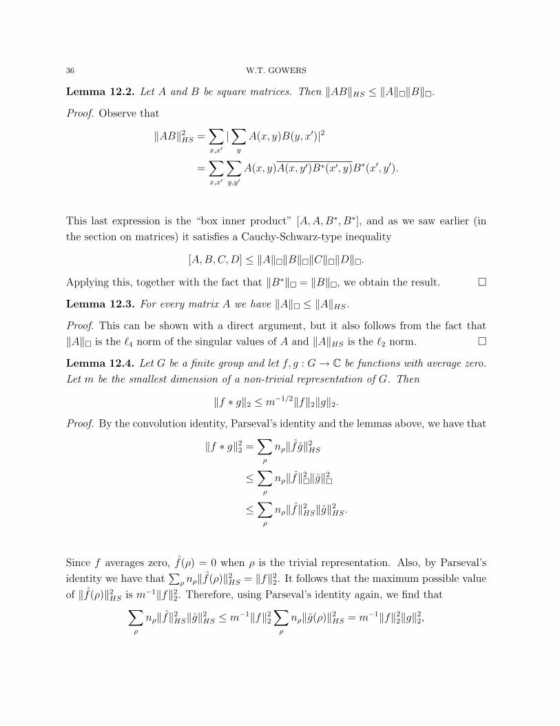
36 W.T. GOWERS

Lemma 12.2. Let A and B be square matrices. Then ‖AB‖HS ≤ ‖A‖�‖B‖�.

Proof. Observe that

‖AB‖2HS =∑x,x′

|∑y

A(x, y)B(y, x′)|2

=∑x,x′

∑y,y′

A(x, y)A(x, y′)B∗(x′, y)B∗(x′, y′).

This last expression is the “box inner product” [A,A,B∗, B∗], and as we saw earlier (in

the section on matrices) it satisfies a Cauchy-Schwarz-type inequality

[A,B,C,D] ≤ ‖A‖�‖B‖�‖C‖�‖D‖�.

Applying this, together with the fact that ‖B∗‖� = ‖B‖�, we obtain the result. �

Lemma 12.3. For every matrix A we have ‖A‖� ≤ ‖A‖HS.

Proof. This can be shown with a direct argument, but it also follows from the fact that

‖A‖� is the `4 norm of the singular values of A and ‖A‖HS is the `2 norm. �

Lemma 12.4. Let G be a finite group and let f, g : G→ C be functions with average zero.

Let m be the smallest dimension of a non-trivial representation of G. Then

‖f ∗ g‖2 ≤ m−1/2‖f‖2‖g‖2.

Proof. By the convolution identity, Parseval’s identity and the lemmas above, we have that

‖f ∗ g‖22 =∑ρ

nρ‖f g‖2HS

≤∑ρ

nρ‖f‖2�‖g‖2�

≤∑ρ

nρ‖f‖2HS‖g‖2HS.

Since f averages zero, f(ρ) = 0 when ρ is the trivial representation. Also, by Parseval’s

identity we have that∑

ρ nρ‖f(ρ)‖2HS = ‖f‖22. It follows that the maximum possible value

of ‖f(ρ)‖2HS is m−1‖f‖22. Therefore, using Parseval’s identity again, we find that∑ρ

nρ‖f‖2HS‖g‖2HS ≤ m−1‖f‖22∑ρ

nρ‖g(ρ)‖2HS = m−1‖f‖22‖g‖22,


which completes the proof. �

Now let us quickly deduce that if a group G has no non-trivial low-dimensional repre-

sentations, then it does not contain a large product-free set.

Theorem 12.5. Let G be a finite group and let m be the smallest dimension of a non-

trivial representation of G. Then G contains no product-free subset of density greater than

m−1/3.

Proof. Let α be the density of A and as usual let f be the function f(x) = A(x)− α. We

shall now try to show that

Exy=zA(x)A(y)A(z) 6= 0,

which obviously implies that A is not product free.

We have that

Exy=zA(x)A(y)A(z) = Exy=z(α + f(x))(α + f(y))(α + f(z)),

and since f averages zero, if we expand the right-hand side into eight separate sums, we

find that all terms are zero apart from two, and we obtain the expression

α3 + Exy=zf(x)f(y)f(z) = α3 + 〈f ∗ f, f〉.

By the Cauchy-Schwarz inequality and Lemma 12.4 we have that

|〈f ∗ f, f〉| ≤ ‖f ∗ f‖2‖f‖2 ≤ m−1/2‖f‖32.

We also have that ‖f‖22 = α(1 − α)2 + (1 − α)α2 = α(1 − α). Therefore, if A is product

free we must have the inequality

α3/2(1− α)3/2m−1/2 ≥ α3,

which implies that α ≤ m−1/3. �

It remains to remark that there do exist groups with no low-dimensional representations.

Indeed, any family of finite simple groups has this property, though some have it much more

strongly than others. The “most” non-Abelian family of groups is the family PSL(2, q).

If a group in this family has order n, then its non-trivial representations have dimension

at least cn1/3, where c > 0 is an absolute constant. Therefore, these groups have no

product-free subsets of density greater than c′n−1/9.

The same argument shows that if A, B and C are sets of density greater than m−1/3,

then ABC = {abc : a ∈ A, b ∈ B, c ∈ C} = G.

38 W.T. GOWERS

There turns out to be a close connection between groups with no low-dimensional rep-

resentations and quasirandom graphs. If G is a finite group with no low-dimensional

non-trivial representations, then for any dense set A ⊂ G we can define a bipartite graph

with two copies of G as its vertex sets and x joined to y if and only if y = ax for some

a ∈ A. The remark above about sets A,B and C tells us that this graph is quasirandom.

As a final remark, we note that the U2 norm can be generalized easily to a non-Abelian

context. A good definition turns out to be as follows.

‖f‖4U2 = Exy−1zw−1=ef(x)f(y)f(z)f(w).

The properties of this norm are just what one would hope. For example, one can define a

generalized inner product in the obvious way, and we do indeed have the inequality

[f1, f2, f3, f4] ≤ ‖f1‖U2‖f2‖U2‖f3‖U2‖f4‖U2 ,

which can then be used in the usual way to prove that this U2 norm is a norm. We also

have the Fourier interpretation that one would guess, namely

‖f‖4U2 =∑ρ

nρ‖f(ρ)‖4�.

This is the natural guess because it involves fourth powers on the right-hand side, both

in the obvious sense that there is a fourth power visible in the expression, and also in the

less obvious sense that the box norm of a matrix is equal to the `4 norm of the singular

values. (Thus, in a certain sense we have fourth powers of generalized Fourier coefficients

in two different ways.) Indeed, there is a natural way of defining an `p norm on G for every

p. For an m × m matrix A, one defines the trace-class norm ‖A‖p to be the `p norm of

the singular values of A, and then for a matrix-valued function f one defines ‖f‖p by the

formula

‖f‖pp =∑ρ

nρ‖f(ρ)‖pp.

That is, we take the `p norm in G of the function x 7→ ‖f(x)‖p. Once we have done this,

we have the familiar identity

‖f‖U2 = ‖f‖4.

Functions with small U2 norms (given their averages) behave like random functions, and

when a group has no non-trivial low-dimensional representations, Lemma 12.4 tells us that

all reasonably spread out functions behave like random functions. To see this, note that


‖f‖4U2 = ‖f ∗ f ∗‖22, where f ∗(x) is defined to be f(x−1), so if f averages zero, then we have

the inequality ‖f‖4U2 ≤ m−1‖f‖22.

13. Fourier analysis for matrix-valued functions

Let G be a finite group and let f : G →Mn(C) be a matrix-valued function. (We are

not assuming that n is the order of G.) We can define a Fourier transform for f by simply

applying the definition of the previous section to each matrix coefficient. That is, for

each i, j ≤ n we define fij to be the function x 7→ f(x)ij, and then for each irreducible

representation ρ we define f(ρ) to be the n×n block matrix whose ijth entry is the nρ×nρmatrix fij(ρ). Thus, f(ρ) is an nnρ × nnρ matrix.

We can write this definition more concisely as follows.

f(ρ) = Exf(x)⊗ ρ(x).

Thus, whereas with Abelian groups we had scalar-valued functions and scalar-valued rep-

resentations, and in the previous section we had scalar-valued funtions and matrix-valued

representations, now we have matrix-valued functions and matrix-valued representations.

In each case we take tensor products, but in the first two cases they are trivial.

In order to state the basic properties of the Fourier transform, we need to be clear about

our notation. For a matrix-valued function f on the physical side, we shall write ‖f‖2 for

the norm defined by the formula

‖f‖22 = Ex‖f(x)‖22

Here it turns out to be convenient to take ‖A‖2 to be the non-normalized Hilbert-Schmidt

norm. Thus, the norm scales with the dimension of f , but not with the size of the group.

On the Fourier side, we have similar definitions but using sums all the way through, so

these are the same as the definitions of the norms in the scalar case.

With these normalizations, the first few basic properties of the Fourier transform now

read as follows.

• ‖f‖22 = ‖f‖2. (Parseval’s identity).

• 〈f, g〉 = 〈f , g〉. (Parseval’s identity).

• f ∗ g(ρ) = f(ρ)g(ρ). (Convolution formula).

The proofs are more or less the same as in the scalar case, but to clarify the point about

normalizations, we give a proof of the second version of Parseval’s identity, which goes like

this. (It is important to realize that the meaning of the inner product varies from expression

40 W.T. GOWERS

to expression – sometimes we are talking about the inner product of two matrices, and

sometimes about the inner product of two matrix-valued functions.)

〈f , g〉 =∑ρ

nρ〈f(ρ), g(ρ)〉

=∑ρ

nρ〈Exf(x)⊗ ρ(x),Eyg(y)⊗ ρ(y)〉

= Ex,y〈f(x), g(y)〉∑ρ

nρ〈ρ(x), ρ(y)〉

In the last expression, both inner products use sums.

By the basic orthogonality property from representation theory, the sum over ρ is equal

to |G|δxy, so we end up with Ex〈f(x), g(x)〉, which is the definition of 〈f, g〉.The inversion formula is also straightforward, but it needs a little notation. Recall that

for scalar-valued functions the inversion formula was f(x) =∑

ρ nρtr(f(ρ)ρ(x)∗). Since the

Fourier transform for matrix-valued functions is obtained by applying the Fourier transform

for scalar-valued functions to each matrix entry, we obtain the formula

f(x)ij =∑ρ

nρtr(fij(ρ)ρ(x)∗).

Let us write trρ for the operation that takes an n× n block matrix A with blocks that are

nρ×nρ matrices and returns the n×n matrix whose ijth value is the (unnormalized) trace

of the ijth block of A. Then we can write the inversion formula in the form

f(x) =∑ρ

trρ(f(ρ)ρ(x)∗),

which is just like the formula when f takes scalar values except that the trace function tr

has been replaced by the matrix-of-traces function trρ.

What is this definition good for? At least one situation in which it is useful is when one

wishes to measure the extent to which a matrix-valued function behaves like a represen-

tation. To illustrate this, let me discuss a very nice result of Moore and Russell (not the

famous philosophers, but a pair of contemporary mathematicians).

In the previous section, we remarked that if G is a finite group with no low-dimensional

non-trivial representations, then for every function f : G → C such that ‖f‖∞ ≤ 1 and


Exf(x) = 0 the U2 norm of f is small. That is,

Exy−1zw−1f(x)f(y)f(z)f(w)

is small. Now if we could find a non-trivial character of G, in the sense of a homomorphism

from G to C that is not the identity, then this would not be true: whenever xy−1zw−1 = e

we would have f(x)f(y)f(z)f(w) = 1 so the average would be 1, which is the largest it

can possibly be. So the observation that the U2 norm has to be small is telling us that G

not only fails to have a non-trivial character (which we know because it has no non-trivial

low-dimensional representations), but it does not admit any functions that are even very

slightly close to being a non-trivial character: if f averages zero, then it not possible for

the average real part of f(x)f(y)f(z)f(w) to be greater than some small constant when

xy−1zw−1 = e.

Moore and Russell showed that this observation can be extended to matrix-valued func-

tions. (Actually, the precise result they showed was not quite this one, but it was very

similar and can be proved by similar methods.) That is, if the dimension of the smallest

non-trivial representation is m, if n is substantially less than m, and if f takes values that

are n× n matrices with operator norm at most 1, and if Exf(x) = 0, then the U2 norm of

f is small. This is a stronger statement, because matrix-valued functions have more elbow

room and therefore more room to create the necessary correlations. It is also stronger in

a more obvious way: it tells us that not only are scalar-valued functions on G as unlike

non-trivial characters as they could possibly be, low-dimensional matrix-valued functions

are as far from non-trivial representations as they could possibly be.

We begin by observing that the statement and proof of Lemma 12.4 carry over almost

word for word to the matrix-valued case. (The proof is identical, so we do not give it

again.)

Lemma 13.1. Let G be a finite group and let m be the smallest dimension of a non-trivial

representation of G. Let f, g : G →Mn(C) be two matrix-valued functions that average

zero. Then

‖f ∗ g‖2 ≤ m−1/2‖f‖2‖g‖2.

There is, however, an important new factor to take into account here, which is that

the two sides of the inequality scale differently with the dimension. Suppose, for instance,

that both f and g are equal to the same n-dimensional representation ρ. Then the 2-

norms of every single f(x), g(x) and f ∗ g(x) are all equal to n, so ‖f ∗ g‖22 = n, while

m−1‖f‖22‖g‖22 = m−1n2. So the inequality does not stop f and g from being representations

42 W.T. GOWERS

when n = m, which of course is as it should be, since m is defined to be the dimension of

a representation of G.

With that remark in mind, let us turn to U2 norms. The natural definition of the U2

norm in the matrix-valued case is

‖f‖4U2 = Exy−1zw−1=etr(f(x)f(y)∗f(z)f(w)∗),

where the trace is not normalized. This is equal to ‖f ∗ f ∗‖22 and it is also equal to ‖f‖44.(Recall that this is defined to be

∑ρ nρ‖f‖4�.) Therefore, by Lemma 13.1 we find that

‖f‖4U2 ≤ m−1‖f‖42.

In particular, if f takes values f(x) with Hlibert-Schmidt norm at most n1/2 (which is

the case, for example, if they are all unitary, and more generally if they all have operator

norm at most 1), then ‖f‖4U2 ≤ m−1n2. For f to be a unitary representation, we would

need ‖f‖4U2 to be equal to n (since f(x)f(y)∗f(z)f(w)∗ would be the identity whenever

xy−1zw−1 = e), which would equal n−1‖f‖42, which is at most n, by hypothesis. Therefore,

if n is significantly less than m, so that m−1n2 is significantly less than n, we see that f

is not even close to being a representation, in the sense that there is almost no correlation

between f(x)f(y)∗ and f(w)f(z)∗ even if we are given that xy−1 = wz−1.

14. An inverse theorem for the matrix U2 norm

Recall the very simple inequalities that we used earlier to relate the `4 and `∞ norms

of the Fourier transform of a function f from an Abelian group to C. If we know that

‖f‖2 ≤ 1, then we find that

‖f‖4∞ ≤ ‖f‖44 ≤ ‖f‖2∞‖f‖22 ≤ ‖f‖2∞.

Since ‖f‖4 = ‖f‖U2 , we deduce that if ‖f‖U2 ≥ c, then there exists a character χ such

that |〈f, χ〉| = |f(χ)| ≥ c2.

What happens if we try to generalize this to non-Abelian groups and to matrix-valued

functions? Let us assume that f(x) is an n× n matrix with operator norm at most 1 for

every x. (The operator norm is the maximum of the singular values, and thus the natural

`∞ norm of a matrix.) Then just as before, we have

‖f‖4∞ ≤ ‖f‖44 =∑ρ

nρ‖f(ρ)‖44 ≤ maxρ‖f(ρ)‖2∞

∑ρ

nρ‖f(ρ)‖22 = ‖f‖2∞‖f‖22.


Unfortunately, if n is large, then this is no longer a rough equivalence, since the best we

can say about ‖f‖22 is that it is at most n (since it is the sum of the squares of n singular

values, each of which lies between 0 and 1).

However, that does not mean that there is nothing we can say. The largest possible value

of ‖f‖44 = ‖f‖4U2 is, as we have seen, n. Let us take a function f such that ‖f‖4U2 ≥ cn. Then

we obtain from the second inequality above that there exists an irreducible representation

ρ such that ‖f(ρ)‖∞ ≥ c1/2.

If G is Abelian and f : G→ C, then ‖f(χ)‖∞ is just |〈f, χ〉|, so this statement is saying

that f correlates in a significant way with a character. But in our situation we have the

more complicated statement that

‖Exf(x)⊗ ρ(x)‖∞ ≥ c1/2.

Is this telling us that f correlates in some sense with ρ?

Let us try to interpret it. We shall first use the fact that ‖A‖∞, the operator norm of A,

is the largest possible value of ‖Au‖2 over all unit vectors u, which in turn is the largest

possible value of 〈Au, v〉 over all pairs of unit vectors u and v. Therefore, we can find unit

vectors u and v such that

〈(Exf(x)⊗ ρ(x))u, v〉 ≥ c1/2.

Now let us rewrite this in coordinate form. Because of the special form of the n×nρ matrix

f(x)⊗ρ(x) it is natural to give it four indices instead of two: we have that (f(x)⊗ρ(x))ijkl =

f(x)ikρ(x)jl. Then indexing u and v in the corresponding way, and writing them as U and

V since they have now become matrices, we have that

〈(f(x)⊗ ρ(x))U, V 〉 =∑i,j,k,l

f(x)ikρ(x)jlUklVij = 〈f(x)Uρ(x)∗, V 〉,

where the product in the last expression is just normal matrix multiplication. Taking

expectations, we deduce that

Ex〈f(x)Uρ(x)∗, V 〉 ≥ c1/2

for two n × nρ matrices U and V that have Hilbert-Schmidt norm 1. We can write this

more symmetrically as

Ex〈f(x)U, V ρ(x)〉 ≥ c1/2.

It is natural to rescale U and V so that they have Hilbert-Schmidt norm n1/2ρ . That is,

we can say that there exist an irreducible representation ρ and matrices U and V with

44 W.T. GOWERS

‖U‖22 = ‖V ‖22 = nρ such that

Ex〈f(x)Uρ(x)∗, V 〉 = Ex〈f(x)U, V ρ(x)〉 = Ex〈f(x), V ρ(x)U∗〉 ≥ c1/2nρ.

This seems quite satisfactory, but it falls short of being a true inverse theorem for the

matrix U2 norm because the converse does not hold. That is, if we are given ρ, U and V

satisfying the above conditions, we cannot deduce that f has a large U2 norm unless nρ is

comparable to n, which it does not have to be.

However, we have not yet exhausted our options. If ‖f‖4U2 = ‖f‖44 ≥ cn, then we are

given that ∑ρ

nρ‖f(ρ)‖44 ≥ cn,

where ‖f(ρ)‖44 denotes the sum of the fourth powers of the singular values of f(ρ). Let

these singular values be λρ,i for i = 1, 2, . . . , nρ. Then we find that∑ρ

nρ

nρ∑i=1

λ4ρ,i ≥ cn.

From Parseval’s inequality and the assumption that each f(x) has operator norm at most

1 (and hence Hilbert-Schmidt norm at most n) we also have that∑ρ

nρ

nρ∑i=1

λ2ρ,i ≤ n.

Also, since f(ρ) = Exf(x)⊗ ρ(x) is an average of matrices with operator norm at most 1,

every λρ,i is at most 1.

Let λ1, . . . , λm be the singular values λρ,i arranged in some order, and for each i let ni

be the nρ that corresponds to λi. Then we can rewrite these inequalities as∑i

niλ4i ≥ cn,

∑i

niλ2i ≤ n,

and

λi ≤ 1.

Note that if c = 1, then the only way of achieving the above inequalities is for λ4i to

equal λ2i for every i (assuming that none of the ni is zero). Thus, each λi is either 0

or 1, and∑{ni : λi = 1} = n. It is a straightforward exercise to prove that the more


relaxed assumptions above lead to similar but more relaxed conclusion: we can find a set

A and constants c1 > 0 and C that depend on c only (with a power dependence) such that

c1n ≤∑

i∈A ni ≤ Cn, and λi ≥ c1 for every i ∈ A. In short, we can find a set of large

singular values (coming from the various f(ρ) of size roughly comparable to n.

With each such singular value λi we can associate n × ni matrices Ui and Vi with

Hilbert-Schmidt norm ni such that Ex〈f(x)Ui, Viρi〉 ≥ λini, where ρi is the representation

corresponding to λi. Moreover, if two pairs (Ui, Vi) and (Uj, Vj) come from the same ρ, then

because of the nature of singular value decompositions, we have that 〈Ui, Uj〉 = 〈Vi, Vj〉 = 0.

I hope I have now written enough to make it plausible that we can put together these

matrices and irreducible representations to create a representation-like function that corre-

lates with f , and moreover that gives us an inverse theorem in the sense that the correlation

in its turn implies that f has a large U2 norm. Exactly how the putting together should

work is not obvious, but it turns out that it can be done, and that it yields the following

theorem. In the statement, recall that ‖f‖∞ means the largest operator norm of any f(x).

Also, we define a partial unitary matrix to be an n × m matrix such that the rows are

orthonormal if n ≤ m and the columns are orthonormal if n ≥ m. (In particular, if n = m

then the matrix is unitary.)

Theorem 14.1. Let G be a finite group, let c > 0 and let f : G →Mn(C) be a function

such that ‖f‖∞ ≤ 1 and ‖f‖4U2 ≥ cn. Then there exists m such that cn/4 ≤ m ≤ 4n/c, an

m-dimensional representation σ, and n×m partial unitary matrices U and V , such that

Ex〈f(x)U, V σ(x)〉 ≥ c2m/16.

Note that σ will not normally be irreducible. This theorem tells us that f correlates

with the function V σU∗. The extra strength of this theorem over what we remarked earlier

is that the dimension of σ is comparable to that of f . It turns out to be simple to deduce

a converse statement – i.e., that if f correlates with a function of the above form, then

‖f‖4U2 ≥ c′n for some suitable c′. Therefore, Theorem 14.1 is indeed an inverse theorem

for the matrix U2 norm.

It is possible to give a more careful argument when c = 1−ε for some small ε that allows

us to show that (1−2ε)n ≤ m ≤ (1−4ε)−1n, and to obtain a lower bound of (1−16ε)m in

the last inequality. From this result it is not too hard to deduce a so-called stability theorem

for near representations. Roughly speaking, it states that any unitary-valued function that

almost obeys the condition to be a representation is close to a unitary representation.

46 W.T. GOWERS

Theorem 14.2. Let G be a finite group and let f : G → U(n) be a function such that

‖f(x)f(y) − f(xy)‖HS ≤ ε√n for every x, y ∈ G. Then there exist m with (1 − ε2)n ≤

m ≤ (1 − 2ε2)−1n, an n × m partial unitary matrix U , and a unitary representation

ρ : G→ U(m), such that

‖f(x)− Uρ(x)U∗‖ ≤ 31ε√n

for every x ∈ G.

15. Conclusion

Now that we have seen several different generalizations of Fourier analysis (though not

a complete list), we can draw up a checklist of the properties that a generalization is likely

to need in order to be useful. Ideally we would have all of the following.

• A Parseval identity

• A convolution identity

• An inversion formula

• A quasirandomness-measuring norm

• An inverse theorem for the quasirandomness-measuring norm

Sometimes we can indeed get all of these, but in situations where we can’t, it turns out that

just having the last two properties is sufficient for some very interesting applications. And

in some cases it remains a fascinating challenge to find new versions of the generalizations

with some of the properties that the current versions lack.

generalizations of fourier analysis, and...

Documents