generalization of height points in trail maps
TRANSCRIPT

GENERALIZATION OF HEIGHT POINTS IN TRAIL MAPS.
JESÚS PALOMAR VÁZQUEZ JOSEP PARDO PASCUAL
Departament of Cartographic Engineering, Geodesy and Photogrammetry.
Polytechnic University of Valencia
ABSTRACT
This article describes a methodology that takes advantage of the potential of the data management, attributes and spatial relationships of geographic information systems (GIS) for the automatization of one of the most complex cartographic tasks: the process of generalization. The methodology is designed to be applied to thematic recreational maps, and develops a concrete method for the generalization of height points. Specifically, an elimination method based on assigning an individual weight to each point is used. Each weight is previously established using selection operations and geomorphometric studies based on the digital elevation model (DEM). In order to maintain a uniform elimination criteria, a method of space division is used in combination with the calculation of a concentration coefficient assigned to each area resulting from that division.
Keywords: GIS, Generalization, Geomorphometrics, Digital Elevation Model (DEM)
1. INTRODUCTION.
This article describes a methodology based on Geographic Information Systems (GIS) for the automatization
of a Complex process in the field of cartographic generalization, such as the generalization of topographic height points. In this case, the generalization of a DEM as a whole is not addressed, as occurs with different techniques used in vector applications (Dwyer, 1987; Weibel, 1991; Luebke, 1997; Gesch, 1998) or raster (Gesch, 1996; Patterson, 2001; Firkowski, 2003) This article studies the automatization of the process of generalization of the height points in a topographic cartography, as a step prior to that of scale reduction, and always with the objective that the final map will be used for recreation purposes. As such, all of the criteria established in the methodology shown will follow this premise, although the global philosophy can be used with any other type of map.
To this effect, this article will first consider the establishment of the criteria that will be used in the decision
to assign a numeric value to each point. Thus, an order of relative importance between all of the points will be established. Once this hierarchy has been established, the group of data will be submitted to a progressive elimination process, in which the most relevant height points will always tend to remain on the final map. All of this will be done trying to respect the uniformity of the initial distribution of points.
Specific software has been designed to make the application of the whole process possible, and by means of
which all of the relevant parameters can be modified. It must not be forgotten that the use of this tool must be

carried out in a responsible way and always with the expert opinion of a cartographer who, in the end, will decide which selection parameters to use and which percentage of the points will be eliminated.
The article is structured in the following manner: after the introduction, the conceptual base for the
establishment of the main steps of the process will be discussed (section 2); then (section 3), the general selection criteria will be developed based on the previous phase (what are the criteria?); in section 4 the practical development of the application of each of these criteria will be studied (how will these selection criteria be applied?); in section 5, once all the points are classified, the methodology used for their elimination will be discussed (how to eliminate points?). In the last section some of the results obtained, as well as the main conclusions, will be presented.
2. CONCEPTUAL BASES
The selection process of the height points that remain on the map should be subject to a hierarchical
organization that classifies, first of all, the points that are candidates according to the application of different criteria which are juxtaposed so that one height point appears or not on a recreational map.
These criteria can be deduced by analyzing the needs of the user: (1) how is a height point useful to a user?,
(2) what sort of precision should it have?, (3) where should they appear?, etc. The reasonable answers to these questions are that the height points would be more useful in the areas close to the recreational routes, at characteristic points of the terrain and in reference elements that help in the orientation of the user. Additionally, the accuracy of the height information should be that which is necessary for the purpose of the map (inform about the approximate altitude of the place), so that the decimal points can be suppressed in the notation of the height points, freeing up space on the map. Lastly, the density of height points will tend to be higher in elevated areas than in flat areas, since the recreational routes normally pass through these areas and the users are generally more interested in knowing the heights of the peaks rather than the intermediate or low areas.
Keeping these ideas in mind, a series of general preference criteria can be established for the selection of
those height points that should be respected. These rules can be considered from different points of view, can be put in a different order and do not have to be the only ones applied. In this article we have considered the following classification of points, according to their resistance to disappear:
- Points near transit areas. An initial categorization of the points will be established, based on criteria of
proximity to all of the places where the existence of a height point would be useful, so that the users will always have an altitude point in close proximity to know in which height value they are located, to calibrate its altimeter, calculate the difference in height, etc.
- Geomorphologically important points. From the remaining points unclassified in the previous phase, those in which the shape and magnitude of the surrounding terrain make them particularly visible in the terrain will be chosen and classified: peaks, sinkholes and saddle points.
The process of elimination should be done in a way in which more points are eliminated where there is

greater density and, on the other hand, a larger percentage of points in low areas will be eliminated as compared to high areas.
3. ESTABLISHING SELECTION CRITERIA.
Based upon the above mentioned reasoning the following selection criteria can be established:
1. Selection of points based on criteria of proximity to areas of special interest: - Points situated next to inhabited or constructed areas (the user may want to quickly know the height of a
town). - Strategically located points within the existing network of roads and trails, especially in singular points of transit (bridges, crossroads, mountain passes, etc.) - Height points near locations having toponyms with generic geographic names (peña, morro, tossal, etc.) which are potential sources of attraction.
- Height points belonging to geodetic benchmarks, not so much for their inherent metric and geodetic value, but for the special panoramic visibility characteristics they usually offer.
- Points that are close to areas of special interest (geomorphologically relevant environments, singular constructions, ruins, etc.).
2. Selection of points with singular morphology: peaks, saddle points and sinkholes.
- Peaks are always high points with respect to their surroundings, and as such, are easily visible from far away. Additionally, they are usually points that have wider panoramic views than the rest of the areas. Because of this, they are of interest from the perspective of the hikers and, consequently, are candidates to be included in the final map. However, not all of the peaks will have the same level of interest or attraction, and only those that are more important with respect to other nearby peaks will remain. - Saddle points normally represent viable passes between higher areas. The interest they hold for the user is obvious, as they can be useful in the selection of alternative routes. - Sinkholes or depressions are singular and infrequent areas, that fact alone makes them interesting, because they are a peculiarity in the landscape.
4. DEVELOPMENT AND APPLICATION OF THE SELECTION CRITERIA.
The methodological process, graphically described in figure 1, passes through the following stages: (1) first, a
filter is applied by which all of the points that are considered of interest, according to the first group of selection criteria seen in the previous section, are identified; (2) secondly, classification criteria are applied to the remaining points, with regards to the geomorphometric characterization of their environment, using the DEM and a series of metric parameters which will characterize the shape and magnitude of each point; (3) thirdly, a new filter will be applied which considers the proximity of the different points, their altitude and the relative importance of each point, in such a way that the density and quality of the points increase as the altitude increases; (4) lastly, the height points that remain after the three previous filters will be submitted to a final sieve in order to avoid the overlapping that comes from the competition of the cartographic elements resulting from

reduced space due to the scale change. The above mentioned methodological process can be seen in the following diagram (figure 1):
SELECTION OF POINTS OFINTEREST
GEOMORPHOLOGICCHARACTERIZATION
DENSITY ANDALTITUDEANALYSIS
OVERLAPANALYSIS
Application of proximitycriteria using:-Areas of influence-Inclusion analysis
Planimetric information,Toponyms and heightPoints (vectorial format)
Height points classifiedaccording to their interest
DEM in TIN format carriet outusing:-Remaning height points.-Contours-Hidrographic networks, ravinesand ridge lines.
Analysis of neighborhoods(detection of the type ofheight point and itsmagnitude)
Geomorphometric analysis(characterization of theshape of the point's immediatesurroundings)
Height points classified accordingto their type, magnitude and shape
- Classified height points- Information about their altitude
Analysis of neighborhoods withineach established altitude interval
Height points(first sieve)
Height points(first sieve) Analysis of neighborhoods
Height points(second sieve)
HIERARCHICALCLASSIFICATION
Phases Input data Operations Output dataSubphases
Figure 1.Diagram of the proposed methodology.
4.1. Selection of the points of interest.
In this phase, a selection and classification of all of the height points that could be interesting to maintain,
from the point of view of the first group of criteria seen in section 2, will be made. These criteria never lose sight of the final objective of the map, which is no other than to present useful and practical information to the hikers that will move about the territory.
Some of the spatial analysis operators available in GIS can be used to carry out the automatization of the
selection tasks of this phase. For example, for the proximity criteria we can use a combination of operations such as a buffer operator, or area of influence, and the topological relationship of inclusion, in order to see which height points are found close to elements of interest.
4.2. Geomorphometric characterization.
In this phase, the points that were not maintained in the previous phase are taken and analyzed to determine
which points are geomorphologically singular, that is, peaks, mountain passes and sinkholes. Their magnitude is then analyzed and, finally, some operations are applied to the peaks, which are by far the most abundant, to

categorize and classify them according to their shape: conic, asymmetrical (escarpments), open or closed. These operations are an attempt to categorize each point taking into account its magnitude and the shape of the area in which it is found, so that this categorization can later be used to make a selection of the points that should remain based on objective, and not arbitrary, criteria.
4.2.1. Pre-processing of the information.
It is necessary to have a DEM with the highest possible accuracy, which can be generated using the same cartography to be generalized, using all of the significant altimetry data available (height points, contours, and break lines, represented by the hydrographic network, talwegs and divides). With these elements we can generate a DEM in vectorial format by means of triangulation, obtaining a TIN model. Theoretically, a vectorial DEM or a raster DEM can be used, although the latter poses some difficulties in generalizing height points: (1) it does not preserve the original height, since it is generated using interpolation methods, and (2) it requires more computational time. For these reasons, it is preferable to work with the TIN DEM.
4.2.2. Determination of peaks, sinkholes and saddle points.
In this phase, the height points that are geomorphologically singular should be determined. Three basic types of shapes are differentiated: summit points (peaks), depression points (sinkholes) and mountain passes (saddle points). There are current methods and software that use a DEM raster to detect these singular points (Felicísimo, 1994 and 2002; Wood, 1999, with his program LandSerf). These methods are based on the analysis of the slope and curvature of the terrain, then these topographical variables are analyzed in a finite environment defined by the operator.
The method used here follows a similar philosophy: the information is analyzed in specific areas, with the
advantage that it is not necessary to analyze an infinite amount of points, only the height points considered for selection.
a) Processing the summits.
For a given height point, a surrounding area (Ei) is chosen and analyzed. If that point is maximum (has the largest height value) in the area, the point is the peak of that area (Ei). Then, the surrounding area is enlarged (Ei+1) and the analysis is done again for that same point. This analysis will determine the extent of the area of which they are considered as peaks and what classification of hierarchical importance exists between those peaks, classifying them as elevations of greater magnitude as the area becomes larger (figure 2).
accepted peak
minimum neighborhood
Refusedpeak
accepted peak
minimum neighborhood
Refusedpeak
10121050
1250
10121050
1250
10121050
1250
a) b) c)
10121050
1250
10121050
1250
10121050
1250
a) b) c) Figure 2. Analysis by surrounding areas.

The objective of this process is to evaluate the relative magnitude of some peaks with respect to others, with the purpose of establishing an initial classification that tends to maintain the higher points within larger areas.
b) Depression points.
In this case, interest is focused on large depressions, so the same process used in the analysis by neighborhoods for the calculation of peaks can be applied. This time the surrounding area used will be sufficiently large so as to avoid micro-depressions, and every point will be analyzed to determine if it is the one with the minimum height of its area.
c) Mountain passes.
These points are important for recreational cartography, as they allow for easier access to the summits or they act as points of passage between the slopes of a mountain range. For this reason, they should remain on the map.
Their location is deduced by the analysis of circular areas or neighborhoods (figure 3), by studying the
relative maxima and minima of the topographic profile resulting from the analyzed circle. It is determined whether or not the selected point is a saddle point (2 maximums and 2 minimums). This is achieved by applying simplification techniques on the topographical profile to extract the main tendencies (figure 4).
A
B
C
D
A B C D AAcimuth
Hei
ght
Maximum
MinimumA
B
C
D
A
B
C
D
A B C D AAcimuth
Hei
ght
Maximum
Minimum
A B C D AAcimuth
Hei
ght
Maximum
Minimum
Figure 3. Determination of saddle points
715
720
725
730
735
740
745
0 50 100 150 200 250 300 350 400715
720
725
730
735
740
745
0 50 100 150 200 250 300 350 400715
720
725
730
735
740
745
0 50 100 150 200 250 300 350 400
Figure 4. Simplification of the topographical profile.
4.2.3. Peak shape determination From what has been done until now, the peaks can be classified according to their magnitude, but their
individual morphological characteristics remain unknown. If, in addition to knowing that it is the highest peak in a given area, it is also known that the peak has a centered conical shape, is cliff-like, or has low elevation with respect to its surroundings, we are provided with more criteria to decide if the peak should remain on the map or not.
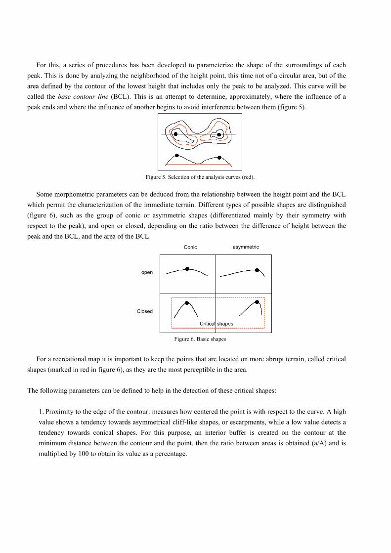
For this, a series of procedures has been developed to parameterize the shape of the surroundings of each
peak. This is done by analyzing the neighborhood of the height point, this time not of a circular area, but of the area defined by the contour of the lowest height that includes only the peak to be analyzed. This curve will be called the base contour line (BCL). This is an attempt to determine, approximately, where the influence of a peak ends and where the influence of another begins to avoid interference between them (figure 5).
Figure 5. Selection of the analysis curves (red).
Some morphometric parameters can be deduced from the relationship between the height point and the BCL which permit the characterization of the immediate terrain. Different types of possible shapes are distinguished (figure 6), such as the group of conic or asymmetric shapes (differentiated mainly by their symmetry with respect to the peak), and open or closed, depending on the ratio between the difference of height between the peak and the BCL, and the area of the BCL.
Figure 6. Basic shapes
For a recreational map it is important to keep the points that are located on more abrupt terrain, called critical
shapes (marked in red in figure 6), as they are the most perceptible in the area.
The following parameters can be defined to help in the detection of these critical shapes: 1. Proximity to the edge of the contour: measures how centered the point is with respect to the curve. A high value shows a tendency towards asymmetrical cliff-like shapes, or escarpments, while a low value detects a tendency towards conical shapes. For this purpose, an interior buffer is created on the contour at the minimum distance between the contour and the point, then the ratio between areas is obtained (a/A) and is multiplied by 100 to obtain its value as a percentage.
Closed
Conic asymmetric
open
Critical shapes

A
a
A
a
Figure 7. Proximity to the edge of the contour
2. Average slope: The average of the slopes of the straight lines that connect the peak to each of the points of the curve. Each of these straight lines is segmented into three sections to be able to consider intermediate slope changes. This parameter denotes the more open or closed peaks depending on whether the values are larger or smaller.
Figure 8. Average slope.
Determining and combining these magnitudes offers information about the type of pattern that the peak
belongs to. Choosing the limits of these parameters depends on the type of shapes desired, although obviously it is easier to detect extreme shapes than intermediate shapes. For the case presented here, the objective was to look for these extreme situations, so a series of tests with different types of data models was used to establish the limits of the parameters and determine how these points were detected (figure 9), by means of the following decision diagram:
Proximity>50%
Asymmetrical shapeSi Average slope
>16.5º
Conic shape
Smooth shape
Average slope>16.5º
No
Smooth shape
NoNo
Si
Si
Proximity>50%
Asymmetrical shapeSi Average slope
>16.5º
Conic shape
Smooth shape
Average slope>16.5º
No
Smooth shape
NoNo
Si
Si
a) Escarpment
a) Pointed shape
a) Escarpment
a) Pointed shape Figure 9. Decision diagram of the types of shapes and examples of critical shapes.
In practice, all of the peaks that have critical shapes are placed at the same categorical level as those peaks classified in the maximum category using the analysis of neighborhoods (section a) of 3.3.2).

4.3. Application of the elimination criteria.
Once all of the height points are classified according to the established criteria, they can be ordered according to their relative importance, which allows for an objective selection of those that should remain on the map.
Due to the scale change, a reduction of the altimetric information is necessary, preserving those height points that are most significant to the final map. The objective of this phase is to ensure that the elimination process follows two main premises: (1) that the elimination of height points is done in a spatially balanced manner, so that points will first be eliminated from areas where they are more concentrated; and (2) the elimination rate decreases with height, so that fewer points are eliminated in areas with higher altitudes.
To achieve these objectives, the following process has been designed: a) How can a balanced elimination process be carried out?
The problem arises in deciding which points should be compared to decide which has a lower category and can be eliminated. In principle, it makes no sense to try to compare points that are too far apart, because the more separated they are the less possibility there is that they belong to the same geomorphological unit. So the solution adopted was to use a space division method that groups together a determined number of nearby points and assures the same density value for each area created.
The method chosen is based on the binary division of space. This method creates rectangular areas with a
similar number of points in each (figure 10).
Figure 10. Binary space division.
b) How can we eliminate first the points in those areas where there is a larger level of concentration?
The coefficient given by the Minimum Spanning Tree is used to determine the concentration value within each divided area. This coefficient calculates the minimum connected graph without forming cycles that pass by all of the points (Kruskal, 1956). This parameter offers information about the relative concentration of some groups compared to others (figure 11).

d1
d2
d3
d4d5
d6d7
d8
d1
d2
d3
d4d5
d6d7
d8
Figure 11. Minimum spanning tree of a group of points (MSP = d1+...+d8 = minimum distance).
c) How can fewer points be eliminated in the highest areas?
Using the percentage of point reduction entered in by the operator, territory division can be done in a series of equidistant altitude intervals and that percentage can be distributed between the different intervals using a function that ensures a higher elimination rate in the lower areas. In this case, the following expression is proposed to assign a percentage to each interval:
∑ =
=
=ni
i i
Px
1
1
[1] P being the total reduction percentage, n the number of intervals and x, x/2, x/3,…, x/n, the successive
percentages corresponding to each interval. In this way, in each altitude interval, processes identical to those seen in points a) and b) are generated, and
only the height points within each interval are subject to the process of elimination.
5. POINT ELIMINATION.
The criteria selected to assign a numeric value to each point are the result of an arbitrary decision, but one which will have an objective application based on the characterization previously carried out. The criteria applied in this case, for the elaboration of recreational maps, are the following: from the most to the least important are (1) points of interest, (2) peaks, (3) mountain passes, (4) sinkholes and (5) the rest of the points. Within the points of interest, the hierarchy will be: geodetic points, heights located in crossroads, heights in urban areas, near roads, near toponyms and near areas of special interest (this category can vary in importance depending on the operators own criteria). In the event that elements of the same type coincide, the element with the higher category would be that with higher class or magnitude, and if these coincide, the element with the highest altitude will be taken.
This way, the ordering of the points can be easily achieved by combining all of the previously obtained
parameters. A simple way of doing so is to calculate a final weight for each point according to the individual category assigned to each one. One proposal is that shown in the following equation:
final weight=(w_int*1.000.000)+(w_peak*100.000)+(p_pass*r_pass*100)+(p_sinkhole*r_sinkhole)+height [2]

where:
1 w_int = weight according to the type of point of interest 2 w_peak = weight according to the type of peak. 3 p_pass = 1 or 0, depending on if the point is a pass or not. 4 r_pass = magnitude of the pass in function of its altitudinal range. 5 p_sinkhole = 1 or 0, depending on if the point is a sinkhole or not. 6 r_sinkhole = magnitude of the sinkhole in function of its altitudinal range. 7 height = height of the point.
To summarize, the elimination process within a given range of altitude is the following: after classifying all the height points, a division of the area is made according to the desired percentage of reduction. After that, the concentration coefficient is calculated for each divided area and the process of analyzing the points in each area begins, eliminating one height point in each area, starting with the area with the highest concentration coefficient. If the number of points to be eliminated is higher than the number of areas generated, the process is repeated, eliminating another point in each area.
The end of this phase results in a progressive and controlled decrease in height point density, in such a way that the decrease in density is lower as the altitude increases. The rest of the points are evenly distributed throughout the geographical area, maintaining the quality of the most important points.
Further refinement of the previous phase is possible, since within the remaining height points, there are sometimes two or more that are sufficiently close to each other so as to create a problem of visual overlapping in the final map. To address that, the remaining points could be subjected to a final filter which will check all the points that are within a certain proximity to another point (normally that proximity threshold is the limit of visual perception, depending on the scale of the output map). In case of conflict, it will be handled like in the previous phase, eliminating the point of a lesser category.
6. ANALYSIS OF OPERATION.
A series of tests have been done to try to analyze how the developed method works, given that, as previously demonstrated, different morphometric and spatial criteria are considered in order to categorize each point. To carry out an application example, four sheets of the ICV10 series of the Institut Cartogràfic Valencià with a scale of 1:10,000 (Cabezudo et al., 2000) were used that contains the geographic area of La Serrella (Alicante), with 993 input height points. The objective is to unite the four sheets and obtain only one sheet at a scale of 1:20,000 with which, among other tasks, the generalization of height points should be carried out. The software GIS ArcView 3.2 was used to develop this application.
6.1. Quantitative verification of the elimination process
For the first task, the model was submitted to a generalization process through the progressive increase in the percentage of point elimination and always using only one altitude interval (table 1). Points of interest were not pre-established in order to simplify the interpretation of the results, so only the topography and the geographical
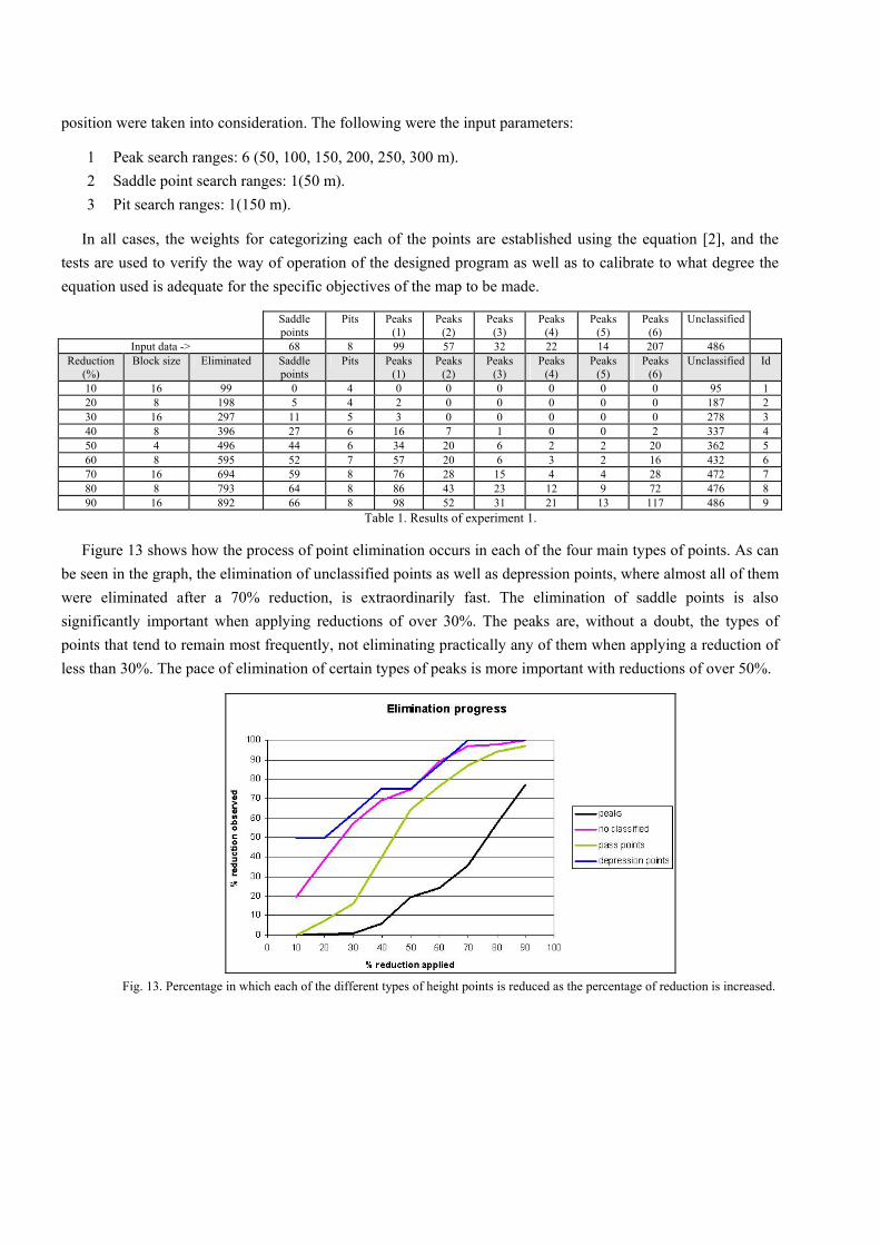
position were taken into consideration. The following were the input parameters:
1 Peak search ranges: 6 (50, 100, 150, 200, 250, 300 m). 2 Saddle point search ranges: 1(50 m). 3 Pit search ranges: 1(150 m).
In all cases, the weights for categorizing each of the points are established using the equation [2], and the tests are used to verify the way of operation of the designed program as well as to calibrate to what degree the equation used is adequate for the specific objectives of the map to be made.
Saddle points
Pits Peaks (1)
Peaks (2)
Peaks (3)
Peaks (4)
Peaks (5)
Peaks (6)
Unclassified
Input data -> 68 8 99 57 32 22 14 207 486 Reduction
(%) Block size Eliminated Saddle
points Pits Peaks
(1) Peaks
(2) Peaks
(3) Peaks
(4) Peaks
(5) Peaks
(6) Unclassified Id
10 16 99 0 4 0 0 0 0 0 0 95 1 20 8 198 5 4 2 0 0 0 0 0 187 2 30 16 297 11 5 3 0 0 0 0 0 278 3 40 8 396 27 6 16 7 1 0 0 2 337 4 50 4 496 44 6 34 20 6 2 2 20 362 5 60 8 595 52 7 57 20 6 3 2 16 432 6 70 16 694 59 8 76 28 15 4 4 28 472 7 80 8 793 64 8 86 43 23 12 9 72 476 8 90 16 892 66 8 98 52 31 21 13 117 486 9
Table 1. Results of experiment 1.
Figure 13 shows how the process of point elimination occurs in each of the four main types of points. As can be seen in the graph, the elimination of unclassified points as well as depression points, where almost all of them were eliminated after a 70% reduction, is extraordinarily fast. The elimination of saddle points is also significantly important when applying reductions of over 30%. The peaks are, without a doubt, the types of points that tend to remain most frequently, not eliminating practically any of them when applying a reduction of less than 30%. The pace of elimination of certain types of peaks is more important with reductions of over 50%.
Fig. 13. Percentage in which each of the different types of height points is reduced as the percentage of reduction is increased.

Saddle points
11
27
44
05
52
666459
0
10
20
30
40
50
60
70
10 20 30 40 50 60 70 80 90
% Reduction
Nº
100% (68 points)
Pits
888
766
544
0123456789
10 20 30 40 50 60 70 80 90
% Reduction
Nº
100% (8 points)
Figure 14.a. Graphic of the reduction of saddle points. Figure 14.b. Graphic of the reduction of pits
The results shown in figure 13 can be used along with an analysis of the elimination process according to the
types of points and with absolute values. Graphics 14 a and b, show how the reduction in saddle points and pits occurs. The first thing one notices is the very different number of points in each type of points: Notice that there are only eight pits in the entire analyzed map, what is substantially less than for any other type of point. This circumstance could lead to a reconsideration of the applied evaluation system and the assigning of a larger value to the pit. This is possible because the small number of this type of points would only slightly alter the configuration of the final map if they are kept, and also because that information in itself is interesting for the user given that it can be related to karstic dissolution phenomena.
Fig. 15. Number of height points that are eliminated from each of the six magnitudes established in the test. It should be remembered that the peaks of higher category are related to those that are peaks in a larger area. However, also included in category 6 are all of those peaks with a conical or symmetrical but closed shape, considered critical points.
Figure 15 shows how the elimination process happens, in absolute values of the height points of the peaks. A
series of interesting considerations can be deduced from the analysis of this figure and the data from table 1, about the nature of the data that is being treated as well as the designed methodology for the reduction of height points.
One thing that stands out is that the number of peaks of lesser order is usually substantially more than the next highest order, following a potentially negative distribution. It occurs in this way in all cases, except in those of the highest category. This is especially interesting since the same type of function fits with other types of

hierarchical distributions occurring in nature (number of different order canal segments in Strahler's classification, ratio between the slope-area to a point in the catchment area and the local slope, etc.) and deserves a more detailed analysis.
In any event, for the analysis that is being done here it is interesting to consider the fact that the tendency
does not repeat itself in the peaks of the highest category. This is because after the shape analysis - section 3.2.3- all of the peaks considered critical shapes are turned into peaks of maximum category. The procedure followed here has transformed 45% of the peaks into points of the highest category, according to the shape of the terrain. The remaining 55% are non-critical shapes that maintain the category type established according to their relative magnitude in their surrounding area. The decision of whether it is adequate or it is able to be improved should be made taking into account the objectives of the final map and, if change is needed, a small modification can be made slightly altering the parameters that establish what the critical shapes are.
The analysis of graph 15 also makes apparent that the reduction process in each type does not follow a
continuous tendency but instead shows oscillations. As shown in figure 15, when the height points are reduced between the 50 and 60%, the number of peaks whose type is 2, 3, and 5 does not change. This demonstrates that factors other than categorization take part in the elimination process, otherwise a basically progressive elimination of each of the points would occur beginning with those of lesser category and later affecting those of higher categories. The fact that the process does not follow the described tendency shows the correct functioning of the selection processes associated with the spatial distribution of the points.
6.2. Visual verification of the results
The experiment shown in the previous section has allowed us to observe how the selective process works and
how the equation [2] or the morphometric parameters should be modified if there is not agreement on how points are to be selected. Nevertheless, it should not be forgotten that the final product is a map and, for this reason, it is important to evaluate these results graphically. To do this, a second experiment was done applying all of the proposed criteria, that is, those that define the points of interest as well as those that make reference to the shape of the terrain. Table 2 shows the input data, the parameters used to establish criteria and the numeric results obtained. Figure 16 shows the initial distribution of height points and the distribution that remains after applying the proposed method with the parameters established in table 2.
Initial scale: 1:10.000; final scale: 1:20.000; number of height points: 993; Reduction of points:40% Type of operation Subtype of operation Comments Points of interest: 259 Near toponyms: 44
Near constructions: 11 Near road network: 180 Near places of special interest: 20 Geodetic points: 4
Tolerance: 100 metros. Tolerance: 10 metros. Tolerance: 10 metros.
Peaks: 254 Neighborhood 1: 63 Neighborhood 2: 25 Neighborhood 3: 17 Neighborhood 4: 12 Neighborhood 5: 11 Neighborhood 6: 126
Tolerance: 100 metros. Tolerance: 150 metros. Tolerance: 200 metros. Tolerance: 250 metros. Tolerance: 300 metros. Tolerance: 350 metros.
Saddle points: 54 Single Neighborhood: 54 Tolerance: 50 metros.

Pits: 1 Single Neighborhood: 1 Tolerance: 150 metros. Remaining points: 425 Points of a lower category Eliminated points: 390 Elimination of overlap: 392 Final result: 392/993 (39,4%) eliminated
Table 2. Example of application of the methodology.
a) b)a) b)
Figure 16. a) Input height points; b) generalized height points.
The analysis of figure 16 shows that the process of elimination has been clearly greater in the north-west part
of the map, formed by a lower terrain, reducing the density at the bottoms of the valleys. Other low altitude areas where there are accumulations have also had a significant reduction in the number of points. On the other hand, the central mountain range -la Serrella- has maintained a large part of its height points.
On the other hand, figure 16 shows that the method applied does not make the distribution of points in the map visually unbalanced. From observing figure 16b it cannot be deduced that there are no areas without points - except where they already existed initially- but the points are simply eliminated to a greater extent in low altitude areas as opposed to high altitude areas.
5. Conclusions Taking into account the methodology, the following conclusions are obtained: 1. The potential of GIS is demonstrated for the automatization of complex cartographic processes, such as
generalization. The methodology presented here is shown to be effective in the automated selection process of height points and is an advance relative to the traditional method, although the quality of the final results depends on an appropriate selection of the criteria and its parameters. In this sense, the tool designed is of assistance to the cartographer, but it is the cartographer who makes the appropriate decision according to his knowledge and the characteristics and objectives of the final map.
2. This type of application helps in the making of thematic recreational cartography, integrating the operator
into a more rigorous production process and, above all, avoiding a part of the subjective component. 3. The geomorphometric terrain analyses are shown to be of great support, not only for the selection of height

points, but also for the characterization of landforms that can be used in other geomorphological analyses. 4. Working with DEM in vectorial format involves, for these purposes, maintaining the original altitude data
and a simplification in the treatment of information, which makes the process quicker.
5. With the tests done, the correct functioning of the applications developed can be observed and, at the same time, they offer key information to permit the alteration of some of the established criteria to achieve the desired objectives.
6. The use of a space partitioning system such as the one proposed assure that a minimum balance will be maintained in the distribution of the points that must remain.
We understand, however, that the main contribution of this article is that it presents a methodology that
permits the process of generalization of height points to be objective, which has allowed for the automatization of the process. We consider of special interest the use of morphometric parameters that make the selection of points objective. Likewise, we think that the global philosophy of the proposed method and the computer application that accompanies it always offers an expert user sufficient freedom of choice so that it can be applied to many types of maps.
ACKNOWLEDGEMENTS This study has been partially funded by the BTE2002-04552-C03-01 and REN-2003-04998 research grants from Spain’s Ministry of Science and Technology. References
Baella, B.; Pla, M.(1999): Eines de Generalització Automàtica utilitzades a l'Institut Cartogràfic de Catalunya. Actas del Congreso ICA. pp. 54-62
Buttendfielf, Barbara P.; McMaster, Robert B. (1991): Map generalization. Making rules for knowledge representation,
Longman Scientific & Technical, 244 pp. Cabezudo de la Muela, L.; Porres de la Haza, M.J.; Rubio Soler, M.(2000): La serie CV10 del Instituto Cartográfico
Valenciano. VII Congreso Nacional de Cartografía (TOPCAR 2000). pp. 52-57 Dwyer, R.A. (1987). A master Divide-And-Conquer Algorithm for Constructing Delaunay Triangulations. Algorithmica 2(2).
137-151.
Felicísimo, A.M. (1994): Modelos digitales del terreno. Introducción y aplicaciones en las ciencias ambientales. Indurot. Universidad de Oviedo. 207 pp.
Firkowski, h. (2003): Regular grid DEM generalization based on theory information. 21st International Cartographic
Conference. Durban.

Gesch D.B. (1998). The efects of digital elevation model generalizatíon methods on derived hidrologic features. 1998. 3rd Intemational Symposium on Spatial Accuracy Assesment in Natural Resources and Environmental Sciences. Quebec. Canadá.
Gesch, D.B., and Larson, K.S., (1996). Techniques for development of global 1-kilometer digital elevation models. Pecora Thirteen, Human Interactions with the Environment - Perspectives from Space, Sioux Falls, South Dakota, August 20-22.
Iribas Cardona, J. (2000): Diseño y elaboración de un procedimiento interactivo de obtención del Mapa Topográfico Nacional a escala 1:50.000 por generalización cartográfica del MTN25, Tesis Doctoral.
Kruskal, J. B. (1956). On the shortest spanning tree of a graph and the traveling salesman problem. Proc. Amer. Math. Soc. 7,
48-50. Luebke, D. (1997). A Survey of polygonal simplification algorithms. En UNC Technical Report TR97-045.
Müller, J.C.; Lagrange, J.P.; Weibel, R.(1995): Gis and generalization. Methodology and practice. Taylor & Francis .GISDATA 1. 257 pp.
Palomar Vázquez, J. (2001). Los SIG como herramientas de ayuda en la generalización cartográfica bajo demanda. Ias jornadas
sobre Sistemas de Información Geográfica. Almagro (Ciudad Real). Actas de las jornadas. pp. 157-165 Patterson, Tom. (2001). Resolution bumping GTOPO30 in Photoshop: How to make high mountains more legible. Special ICA
Commission on Mountain Cartography issue (Vol. 38) of Cartographica, the journal of the Canadian Cartographic.
Weibel, R. Heller, M., (1991). Digital terrain modelling, In Maguire, D.J., et al. (eds), Geographical Information Systems: Principies and Applications, Longman Scientific & Technical, England).
Wood, J.D. (1996). The geomorphological characterisation of Digital Elevations Models. Tesis Doctoral. Universidad de Leicester.