NBER WORKING PAPER SERIES

GENERAL EQUILIBRIUM EFFECTS OF (IMPROVING) PUBLIC EMPLOYMENT PROGRAMS: EXPERIMENTAL EVIDENCE FROM INDIA

Karthik MuralidharanPaul Niehaus

Sandip Sukhtankar

Working Paper 23838http://www.nber.org/papers/w23838

NATIONAL BUREAU OF ECONOMIC RESEARCH1050 Massachusetts Avenue

Cambridge, MA 02138September 2017, Revised January 2018

We thank David Atkin, Abhijit Banerjee, Prashant Bharadwaj, Gordon Dahl, Taryn Dinkelman, Roger Gordon, Gordon Hanson, Clement Imbert, Supreet Kaur, Dan Keniston, Aprajit Mahajan, Edward Miguel, Ben Moll, Dilip Mookherjee, Mark Rosenzweig and participants in various seminars for comments and suggestions. We are grateful to officials of the Government of Andhra Pradesh, including Reddy Subrahmanyam, Koppula Raju, Shamsher Singh Rawat, Raghunandan Rao, G Vijaya Laxmi, AVV Prasad, Kuberan Selvaraj, Sanju, Kalyan Rao, and Madhavi Rani; as well as Gulzar Natarajan for their continuous support of the Andhra Pradesh Smartcard Study. We are also grateful to officials of the Unique Identification Authority of India (UIDAI) including Nandan Nilekani, Ram Sevak Sharma, and R Srikar for their support. We thank Tata Consultancy Services (TCS) and Ravi Marri, Ramanna, and Shubra Dixit for their help in providing us with administrative data. This paper would not have been possible without the continuous efforts and inputs of the J-PAL/UCSD project team including Kshitij Batra, Prathap Kasina, Piali Mukhopadhyay, Michael Kaiser, Frances Lu, Raghu Kishore Nekanti, Matt Pecenco, Surili Sheth, and Pratibha Shrestha. Finally, we thank the Omidyar Network (especially Jayant Sinha, CV Madhukar, Surya Mantha, and Sonny Bardhan) and the Bill and Melinda Gates Foundation (especially Dan Radcliffe) for the financial support that made this study possible. The views expressed herein are those of the authors and do not necessarily reflect the views of the National Bureau of Economic Research.

NBER working papers are circulated for discussion and comment purposes. They have not been peer-reviewed or been subject to the review by the NBER Board of Directors that accompanies official NBER publications.

© 2017 by Karthik Muralidharan, Paul Niehaus, and Sandip Sukhtankar. All rights reserved. Short sections of text, not to exceed two paragraphs, may be quoted without explicit permission provided that full credit, including © notice, is given to the source.

General Equilibrium Effects of (Improving) Public Employment Programs: Experimental Evidence from IndiaKarthik Muralidharan, Paul Niehaus, and Sandip SukhtankarNBER Working Paper No. 23838September 2017, Revised January 2018JEL No. D50,D73,H53,J38,J43,O18

ABSTRACT

A public employment program's effect on poverty depends on both program earnings and market impacts. We estimate this composite effect, exploiting a large-scale randomized experiment across 157 sub-districts and 19 million people that improved the implementation of India's employment guarantee. Without changing government expenditure, this reform raised low-income households' earnings by 13%, driven primarily by market earnings. Real wages rose 6% while days without paid work fell 7%. Effects spilled over across sub-district boundaries, and adjusting for these spillovers substantially raises point estimates. The results highlight the importance and feasibility of accounting for general equilibrium effects in program evaluation.

Karthik MuralidharanDepartment of Economics, 0508University of California, San Diego9500 Gilman DriveLa Jolla, CA 92093-0508and NBERkamurali@ucsd.edu

Paul NiehausDepartment of EconomicsUniversity of California, San Diego9500 Gilman Drive #0508La Jolla, CA 92093and NBERpniehaus@ucsd.edu

Sandip SukhtankarDepartment of EconomicsUniversity of VirginiaCharlottesville, VA 22904 sandip.sukhtankar@virginia.edu

1 Introduction

Public employment programs, in which the government provides jobs to those who seek them,

are among the most common anti-poverty programs in developing countries. The economic

rationale for such programs (as opposed to unconditional income support for the poor)

include self-targeting through work requirements, public asset creation, and making it easier

to implement a wage floor in informal labor-markets by making the government an employer

of last resort.1 An important contemporary variant is the National Rural Employment

Guarantee Scheme (NREGS) in India. It is the world’s largest workfare program, with 600

million rural residents eligible to participate and a fiscal allocation of 0.5% of India’s GDP.

A program of this scale and ambition raises several fundamental questions for research

and policy. First, how does it affect rural incomes and poverty? In particular, while the

wage income provided by such a scheme should reduce poverty, the market-level general

equilibrium effects of public employment programs could amplify or attenuate the direct

gains from the program for beneficiaries.2 Second, what is the relative contribution of direct

gains in income from the program and indirect changes in income (gains or losses) outside

the program? Third, what are the impacts on wages, employment, assets, and migration?

Given the importance of NREGS, a growing literature has tried to answer these questions,

but the evidence to date has been hampered by three factors. The first is the lack of

experimental variation, with the consequence that studies often reach opposing conclusions

depending on the data and identification strategy used (see Sukhtankar (2017) and the

discussion in section 2.1). Second, “construct validity” remains a challenge. Specifically,

the wide variation in program implementation quality (Imbert and Papp, 2015), and the

difficulty of measuring effective NREGS presence makes it difficult to interpret the varied

estimates of the impact of “the program” to date (Sukhtankar, 2017). Third, since market-

level general equilibrium effects of NREGS are likely to spill over across district boundaries,

existing estimates that use the district-level rollout for identification may be biased by not

accounting for spillovers to untreated units (as in Miguel and Kremer (2004)).

In this paper we aim to provide credible estimates of the anti-poverty impact of public

employment programs by combining exogenous experimental variation, a demonstrable first-

stage impact on implementation quality, units of randomization large enough to capture

general equilibrium effects, and geocoded units of observation disaggregated enough to test

1Workfare programs may also be politically more palatable to taxpayers than unconditional “doles.” Suchprograms have a long history, with recorded instances from as early as the 18th century in India (Kramer,2015), the public works constructed in the US by the WPA during the Depression-era in the 1930s, and moremodern programs across Sub-Saharan Africa, Latin America, and Asia (Subbarao et al., 2013).

2These general equilibrium effects include for example changes in market wages and employment, relativeprices, and broader changes in economic activity induced by the program.

1

and correct for spatial spillovers. Specifically, we worked with the Government of the Indian

state of Andhra Pradesh (AP) to randomize the order in which 157 sub-districts (mandals)

with an average population of 62,500 each introduced a new system (biometric “Smartcards”)

for making payments in NREGS.3 In prior work, we show that Smartcards substantially

improved the performance of NREGS on several dimensions: it reduced leakage or diversion

of funds, reduced delays between working and getting paid, reduced the time required to

collect payments, and increased real and perceived access to work, without changing fiscal

outlays on the program (Muralidharan et al. (2016), henceforth MNS). Thus, Smartcards

brought NREGS implementation closer - in specific, measured ways - to what its architects

intended. This in turn lets us open up the black box of “implementation quality” and link

GE effects to these tangible improvements in NREGS implementation.4

The impacts of improving NREGS implementation are unlikely to be the same as the

impacts of rolling out the program itself. Yet, given well-documented implementation chal-

lenges – including poor access to work, high rates of leakage, and long delays in receiving

payments (Mehrotra, 2008; Imbert and Papp, 2011; Khera, 2011; Niehaus and Sukhtankar,

2013b) – improving implementation on these metrics is likely to meaningfully increase any

measure of effective NREGS. As one imperfect summary statistic, we find (below) that treat-

ment raised prime aged adults’ reservation wages for market labor by 5.8%; one can thus

think of the experiment as capturing the effects of making the NREGS that much more

attractive and beneficial to workers. Further, since improvements in the effective presence of

NREGS were achieved without increasing NREGS expenditure in treated areas, our results

are likely to be a lower bound on the anti-poverty impact of rolling out a well-implemented

NREGS from scratch (which would also transfer incremental resources to rural areas).

We report five main sets of results. First, using our survey data, we find a large (12.7%)

increase in incomes of households registered for the NREGS (49.5% of all rural households)

in treated mandals two years after the Smartcards rollout began.5 We also find evidence of

significant income gains in the entire population using data from the Socio-Economic and

Caste Census (SECC), a census of both NREGS-registered and non-registered households

conducted by the national government independently of our activities.

Second, the majority of these income gains are attributable to indirect market effects

3The original state was divided into two states on June 2, 2014. Since this division took place after ourstudy, we use “AP” to refer to the original undivided state. The combined rural population in our studydistricts (including sub-districts randomized into a “buffer” group) was 19 million people.

4Smartcards also reduced leakage in delivering rural pensions, but these are unlikely to have affectedlabor markets because pension recipients were typically physically unable to work (see Section 2.3).

5Putting the magnitude of these effects in the context of policy debates on the trade-off between growthand redistribution, it would take 12 years of an extra percentage point of growth in rural GDP to generatean equivalent rise in the incomes of the rural poor.

2

rather than direct increases in NREGS income. Among NREGS-registered households in

the control group, the mean household earned 7% of its income from NREGS and 93% from

other sources. Treatment increased earnings in similar proportions, with 10% of the gain

coming from NREGS earnings and the other 90% from outside the program. Thus, the

general equilibrium impacts of NREGS through the open market appear to be a much more

important driver of poverty reduction than the direct income provided by the program.

Third, these gains in non-NREGS earnings are driven by a significant increase in earnings

from market labor. During the period for which we have the most detailed data, market

wages rose by 6.1% and employment in the private sector rose (insignificantly) by 6.7% in

treated areas, enough to account for the observed income gain. We also find a 5.8% increase

in reported reservation wages in treated areas. Importantly, these wage gains accrue to

all NREGS-registered households and do not vary as a function of whether they actually

participated in NREGS, highlighting the general equilibrium nature of the wage effects.

While we have less precise measures of wages year-round, point estimates suggest that wages

in treated mandals increased throughout the year (consistent with several mechanisms we

discuss later, e.g. productivity-enhancing asset creation or nominal wage rigidity). We find

no evidence of corresponding changes in consumer goods prices, implying that earnings and

wage gains were real and not merely nominal.

Fourth, we find little evidence of efficiency-reducing effects on factor allocation. As men-

tioned above, private sector employment weakly increased, and this increase is significant

once we adjust the estimates for spatial spillovers (below). Days idle or doing unpaid work

fell significantly by 7.1%. We find no impacts on migration or on available measures of land

use, and in most cases can rule out sizeable effects.

Fifth, we find evidence that households used the increased income to purchase major

productive assets, which may have contributed to further income gains. We find an 8.3%

increase in the rate of land ownership among NREGS-registered households. We also find a

significant increase in overall livestock ownership using data from an independent government

livestock census. Households in treated mandals also had higher outstanding informal loans,

suggesting reduced credit constraints that may have facilitated asset accumulation.

All the results above compare treated to control regions. If effects spill over across ad-

ministrative boundaries, they may mis-estimate the “total treatment effect” of a scaled-up

policy that treats all regions (compared to not having the program at all). We therefore

develop simple methods to test and correct for such spillovers. We find evidence of spillover

effects on most outcomes, which are consistent in sign with the main effects, and validate

these using a different source of variation.6 More importantly, adjusting for these spillovers

6Specifically, while the experimental ITT effects are based on a mandal’s own treatment status, the

3

yields estimates of the total treatment effect that are significant and typically double the

magnitude of the unadjusted estimates, suggesting that research designs that ignore spatial

spillovers may understate the total effects of NREGS.

The results above present the policy-relevant general-equilibrium estimates of the total ef-

fect on wages, employment, income, and assets of increasing the effective presence of NREGS.

Mapping these magnitudes into mechanisms is subtle since – unlike in a partial equilibrium

analysis – we cannot equate treatment effects with any particular partial elasticity, or even

to the decomposable sum of some set of distinct “channels.” Instead our estimates reflect

a potentially complex set of feedback loops, multipliers, and interactions between several

channels operating in general equilibrium. This makes isolating or quantifying the role of

individual mechanisms an implausible exercise. Thus, while we do find significant evidence

of some mechanisms – such as increased labor market competition, credit access, and own-

ership of productive assets – we do not rule out the possibility that other factors and the

interplay between them also contributed to the overall effects (see discussion in Section 6).

This paper contributes to several literatures. The first is the growing body of work on the

impact of public works programs on rural labor markets and economies (Imbert and Papp,

2015; Beegle et al., 2017; Sukhtankar, 2017). In addition to confirming some prior findings,

like the increase in market wages (Imbert and Papp, 2015; Berg et al., forthcoming; Azam,

2012), our data and methodology allow us to report several new results. The most important

of these are: (a) the significant gains in income and reduction in poverty, (b) finding that

90% of the impact on income was due to indirect market effects rather than direct increases

in NREGS income, and (c) finding positive effects on private sector employment. The last

finding is particularly salient for the larger policy debate on NREGS and is consistent with

the idea that public employment programs can be efficiency-enhancing if they enable the

creation of productive assets (public or private), or if local labor markets are oligopsonistic.

Second, our results highlight the importance of accounting for general equilibrium effects

in program evaluation (Acemoglu, 2010). Ignoring these effects (say by randomizing program

access at an individual level) would have led to us to sharply underestimate the impact of a

better-implemented NREGS on rural wages and poverty. Even analyzing our own data while

ignoring geographic spillovers meaningfully understates impacts. On a more optimistic note,

our study demonstrates the feasibility of conducting experiments with units of randomization

large enough to capture general equilibrium effects on outcomes of interest for program

evaluation (Cunha et al., 2017; Muralidharan and Niehaus, 2017).

Third, our results contribute to the literature on wage determination in rural labor markets

in developing countries generally (Rosenzweig, 1978; Jayachandran, 2006; Kaur, forthcoming)

spillover results use variation in the exposure of sample villages to treated neighbors.

4

and on the impacts of minimum wages specifically (e.g. Dinkelman and Ranchhod (2012)).

This literature also relates directly to policy debates about the NREGS, whose critics have

argued that it could not possibly have meaningfully affected rural poverty because NREGS

work constitutes only a small share (under 4%) of total rural employment (Bhalla, 2013).

Our results suggest that this argument is incomplete. Much larger shares of rural households

in AP are registered for NREGS (˜50%) and actively participate (32%) in the program, and

the data suggest that the existence of a well-implemented public employment program can

raise wages for these workers in the private sector (Dreze and Sen, 1991; Basu et al., 2009).

Fourth, our results highlight the importance of implementation quality for the effectiveness

of policies and programs in developing countries. Our estimates of the wage impacts of

improving NREGS implementation, for example, are about as large as the most credible

estimates of the impact of rolling out the program itself (Imbert and Papp, 2015). More

generally, in settings with high corruption and inefficiency, investing in better implementation

of a program could be a more cost-effective way of achieving desired policy goals than

spending more on the program as is. For instance, Niehaus and Sukhtankar (2013b) find

that increasing the official NREGS wage had no impact on workers’ program earnings, while

we find that improving NREGS implementation significantly increased their earnings from

market wages (despite no change in official NREGS wages).7

Finally, we contribute to the literature on the political economy of anti-poverty programs

in developing countries. Landlords typically benefit at the cost of workers from low wages and

from the wage volatility induced by productivity shocks, and may be hurt by programs like

NREGS that raise wages and/or provide wage insurance to the rural poor (Jayachandran,

2006). Anderson et al. (2015) have argued that “a primary reason... for landlords to control

governance is to thwart implementation of centrally mandated initiatives that would raise

wages at the village level.” While we do not directly observe landlord or employer profits, the

fact that improving NREGS substantially raised market wages underscores their incentive

to oppose such improvements and helps rationalize their widely documented resistance to

the program (Khera, 2011; Jenkins and Manor, 2017; Mukherji and Jha, 2017).

The rest of the paper is organized as follows. Section 2 describes the context, related

literature, and Smartcard intervention. Section 3 describes the research design, data, and

estimation. Section 4 presents our main results on income, wages, employment, and assets.

Section 5 examines spillover effects. Section 6 discusses mechanisms, and Section 7 concludes

with a discussion of policy implications.

7In a similar vein, Muralidharan et al. (2017) show that reducing teacher absence by increasing monitoringwould be ten times more cost-effective at reducing effective student-teacher ratios (net of teacher absence)in Indian public schools than the default policy of hiring more teachers.

5

2 Context and intervention

2.1 The NREGS

The NREGS is the world’s largest public employment program, entitling any household living

in rural India (i.e. 11% of the world’s population) to up to 100 days per year of guaranteed

paid employment. It is one of the country’s flagship social protection programs, and the

Indian government spends roughly 3.3% of its budget (∼ 0.5% of GDP) on it. Coverage

is broad: 50% of rural households in Andhra Pradesh have at least one jobcard, which

registers them for the NREGS and entitles them to request work. Legally, they may do so

at any time, and the government is obligated either to provide work or pay unemployment

benefits (though the latter are rare in practice).

NREGS jobs involve manual labor compensated at statutory piece rates, and are meant

to induce self-targeting. NREGS projects are typically public infrastructure improvement

such as irrigation or water conservation works, minor road construction, and land clear-

ance for cultivation. Projects are proposed by village-level local governance bodies (Gram

Panchayats) and approved by sub-district (mandal) offices.

As of 2010, NREGS implementation quality suffered from several known issues. Ra-

tioning was common even though de jure jobs should be available on demand, with access to

work constrained both by budgetary allocations and by local capacity to implement projects

(Dutta et al., 2012). Corruption occured through over-invoicing the government to reim-

burse wages for work not actually done and paying workers less than their due, among other

methods (Niehaus and Sukhtankar, 2013a,b). Finally, the payment process was slow and

unreliable: payments were time-consuming to collect, and were often unpredictably delayed

for over a month beyond the 14-day period prescribed by law.

The impact of the NREGS on labor markets, poverty, and the rural economy have been

extensively debated (see Sukhtankar (2017) for a review). Supporters claim that it has

transformed the rural countryside by increasing wages and incomes, creating useful rural

infrastructure, and reduced negative outcomes like distress migration (Khera, 2011). Skeptics

claim that funding is largely captured by middlemen and wasted, arguing that the scheme

could not meaningfully affect the rural economy since it accounts for only a small share

of rural employment (“how can a small tail wag a very very large dog?” Bhalla (2013)).

Even if it did increase rural wages, others have argued that this would come at at the

cost of crowding out more efficient private employment (Murgai and Ravallion, 2005). The

debate continues to matter for policy: Although NREGS is implemented through an Act of

Parliament, national and state governments can in practice decide how much to prioritize it

6

by adjusting fiscal allocations to the program.8

Evidence to inform this debate is inconclusive. Most empirical work has exploited the

fact that the NREGS was rolled out across districts in three phases between 2006-2008,

with districts prioritized in part based on an index of deprivation and in part on political

considerations (Chowdhury, 2014). Difference-in-differences and regression discontinuity ap-

proaches based on this rollout have known limitations.9 NREGS implementation quality

also varies widely and has typically not been directly measured. Thus, differences in findings

across studies may reflect differences in unmeasured implementation quality. Estimates that

exploit the staggered NREGS rollout are especially sensitive to this issue because implemen-

tation in the early years of the program was thought to be particularly weak, so that the

impacts of rollout need not predict steady state effects once teething problems were resolved

(Mehrotra, 2008). Finally, it has proven difficult to test and correct for potential spillovers

from program to non-program (control) areas, simply because the available identifying vari-

ation and the geocoding of the available outcome data are both at the district level.10 In

practice, findings to date for a range of outcomes have varied widely. For wages, for ex-

ample, studies using a difference-in-differences approach estimate a positive 4-5% effect on

rural unskilled wages (Imbert and Papp, 2015; Berg et al., forthcoming; Azam, 2012) while

a study using a regression discontinuity approach finds no impact (Zimmermann, 2015).11

2.2 Smartcards

To address leakage and payments challenges, the Government of Andhra Pradesh (GoAP)

introduced a new payments system. This intervention – which we refer to as “Smartcards”

for short – had two major components. First, it changed the flow of payments in most cases

from government-run post offices to banks, who worked with Technology Service Providers

and Customer Service Providers (CSPs) to manage the technological back-end and make

last-mile payments in cash (typically in the village itself). Second, it changed the process

of identifying payees from one based on paper documents and ink stamps to one based on

8For instance, work availability fell sharply in the second half of 2016 following a budget contracting:http://thewire.in/75795/mnrega-centre-funds-whatsapp/, accessed November 3, 2016.

9Specifically, the parallel trends assumption required for differences-in-differences estimation does nothold for many outcomes without additional controls, while small sample sizes limit the precision and powerof regression discontinuity estimators at reasonable bandwidth choices (Sukhtankar, 2017).

10In one recent exception, Merfeld (2017) finds some evidence of spillovers using ARIS/REDS data withvillage geo-identifiers. While imprecise due to sample size, these results suggest that ignoring spatial spilloversmay bias existing estimates of the impact of NREGS.

11Findings on other outcomes (such as education and civil violence related to the leftist Naxalite or Maoistinsurgency) vary similarly across otherwise well-executed studies, suggesting that the differences may reflectvariation in identification, and NREGS implementation quality across study sites and time periods; see(Sukhtankar, 2017) for a detailed review of this evidence.

7

biometric authentication. More details on the Smartcard intervention and the ways in which

it changed the process of authentication and payments are available in MNS.

Using the randomization design described in Section 3.1, we find in MNS that Smartcards

significantly improved NREGS implementation on most dimensions. Two years after the

intervention began, payments in treatment mandals arrived in 29% fewer days, with arrival

dates 39% less varied, and took 20% less time to collect. Households earned more working

on NREGS (24%), and there was a substantial 12.7 percentage point (∼ 41%) reduction in

leakage (defined as the difference between fiscal outlays and beneficiary receipts). Program

access also improved: both perceived access and actual participation in NREGS increased

(17%). These positive effects were found even though the implementation of Smartcards

was incomplete, with roughly 50% of payments in treated mandals being authenticated at

the time of our endline surveys. These effects were achieved without any increase in fiscal

outlay on NREGS itself in treated areas. Finally, gains were widely distributed. We find

little evidence of heterogenous impacts, and treatment distributions first order stochastically

dominate control distributions for all outcomes on which there was a significant mean impact.

Reflecting this, users were strongly in favor of Smartcards, with 90% of households preferring

it to the status quo and only 3% opposed.

2.3 Interpreting Smartcards’ impacts on the economy

Given that Smartcards brought the effective presence of NREGS in treated areas closer to

the intentions of the program’s framers, a natural interpretation is to think of the randomized

rollout of Smartcards as an instrumental variable for a composite endogenous variable called

“effective NREGS.” However, given the many dimensions on which NREGS implementation

quality can and did change, constructing such a uni-dimensional endogenous variable is im-

plausible. Our results are therefore best interpreted as the reduced form impact of improving

NREGS implementation quality on multiple dimensions.

A separate question is whether Smartcards could have affected the rural economy directly,

independent of their effects on the NREGS. Three relevant channels are pensions, financial

inclusion, and identity verification. We consider each of these below.

In addition to NREGS, Smartcards were also used to make payments in the rural social

security pensions (SSP) program, raising the possibility that they might have affected rural

markets through this channel. This appears unlikely for at least four reasons. First, the scale

and scope of SSP is narrow: only 7% of rural households are eligible (whereas 49.5% have

NREGS jobcards). Second, the benefit is modest, with a median and mode of Rs. 200 per

month (˜$3, or less than two days earnings for a manual laborer). Third, the improvements

8

in pensions from Smartcards were much less pronounced than those in NREGS: there were

no improvements in the payments process, and the reduction in leakage was small in absolute

terms (falling from 6% to 3%) – in part because payment delays and leakage rates were low

to begin with. Fourth, and perhaps most important, the SSP programs were targeted to the

poor who were not able to work (and complemented the NREGS, which was the safety net

for those who could).12 Thus, SSP beneficiaries are those least likely to have affected or been

affected by the labor market. As we show later, treatment did not generate income gains in

households where all adults were eligible for the SSP (see Section 4.3).

The creation of Smartcard-linked bank accounts might also have affected local economies

by promoting financial inclusion. In practice, this appears not to have been the case. This

was the result of a conscious choice by the government, which was most concerned about

delayed payments, underpayment, and ghost accounts, and therefore did not allow undis-

bursed funds to remain in Smartcard accounts. Instead they pressured banks to fully disburse

NREGS wages as soon as possible to improve compliance with the 14-day statutory require-

ment for payment delivery. Further, the bank accounts created had limited functionality:

they were not connected to the online core banking servers and instead relied on offline au-

thentication with periodic reconciliation, and as a result could only be accessed through a

single Customer Service Provider. Reflecting these factors, only 0.3% of households in our

survey reported having money in their account, with an (unconditional) mean balance of just

Rs. 7 (˜5% of daily wage for unskilled labor).13 Note that we only need to rule out direct

financial inclusion through Smartcard-enabled bank accounts. Increases in borrowing and

access to informal credit that result from an improved NREGS are one of the mechanisms

for potential economic impact which we examine (and find evidence of) in Section 4.7.

Finally, Smartcards were not considered legally valid proof of identity or otherwise usable

outside the NREGS and SSP programs, in contrast with the more recent national ID program

Aadhaar. Specifically, unlike Aadhaar, the database of Smartcard accounts was never de-

duplicated, which precluded the legal use of Smartcards as a proof of identity.

Overall, the Smartcard intervention was run by GoAP’s Department of Rural Develop-

ment with the primary goal of improving the payments process and reducing leakage in the

NREGS and SSP programs, but was not integrated into any other program or function ei-

ther by the government or the private sector. Since (as described above) we can rule out the

SSP improvement channel and financial inclusion channel, we interpret the results below as

consequences of improving NREGS implementation.

12Specifically, pensions are restricted to those who are Below the Poverty Line (BPL) and either widowed,disabled, elderly, or had a displaced traditional occupation.

13See Mukhopadhyay et al. (2013), especially pp. 54-56, for a more detailed discussion on why Smartcardswere not able to deliver financial inclusion.

9

3 Research design

3.1 Randomization

We summarize the randomization design here, and refer the reader to MNS for further

details. The experiment was conducted in eight districts with a combined rural population

of around 19 million in the erstwhile state of Andhra Pradesh.14 As part of a Memorandum

of Understanding with JPAL South Asia, GoAP agreed to randomize the order in which the

Smartcard system was rolled out across mandals (sub-districts). We randomly assigned 296

mandals - with average population of approximately 62,500 - to treatment (112), control

(45), and a “buffer” group (139). Figure 1 shows the geographical spread and size of these

units. We created the (temporal) buffer group to ensure that we could conduct endline

surveys before Smartcard deployment began in control mandals, and restricted survey work

to treatment and control mandals. We stratified randomization by district and by a principal

component of mandal socio-economic characteristics.

We examine balance in Tables A.3 and A.4. The former shows balance on variables used

as part of stratification, as well as other mandal characteristics from the census. Treatment

and control mandals are reasonably well balanced, with differences significant at the 5%

level in 2 out of 22 cases. The latter shows balance on focal outcomes for this paper along

with other socio-economic household characteristics from our baseline survey. Four out of

34 variables are significantly different at the 10% level, slightly more than one might expect

by chance. We test the sensitivity of results to chance imbalances by controlling for village

level baseline mean values of the outcomes.

3.2 Data

Our first data source is the Socio-Economic and Caste Census (SECC), an independent

nation-wide census for which surveys in Andhra Pradesh were conducted during 2012, our

endline year. The SECC aimed to enable governments to rank households by socio-economic

status in order to determine which were “Below the Poverty Line” (BPL) and thereby eli-

gible for various benefits. The survey collected data on income categories for the household

member with the highest income (less than Rs. 5000, between Rs. 5000-10,000, and greater

than Rs. 10,000), the main source of this income, household landholdings (including amount

of irrigated and non-irrigated land), caste, and the highest education level completed for

14The 8 study districts are similar to AP’s remaining 13 non-urban districts on major socioeconomicindicators, including proportion rural, scheduled caste, literate, and agricultural laborers; and represent allthree historically distinct socio-cultural regions (see Table A.1). Tables A.1 and A.2 compare study andnon-study districts and mandals, and are reproduced exactly from MNS.

10

each member of the household. The SECC was conducted using the layout maps and lists of

houses prepared for the 2011 Census. The SECC data include slightly more than 1.8 million

households in our study mandals.

We complement the broad coverage of the SECC data with original and more detailed

household surveys, that are representative of the universe of NREGS jobcard holders - who

are the intended beneficiaries of the program. We conducted these surveys during August

to October of 2010 (baseline) and 2012 (endline). Surveys covered both participation in and

experience with NREGS, annual earnings and expenditure, and the current stock of assets

and liabilities. Within earnings, we asked detailed questions about household members’

labor market participation, wages, reservation wages, and earnings during June, the month

of peak NREGS participation in Andhra Pradesh.

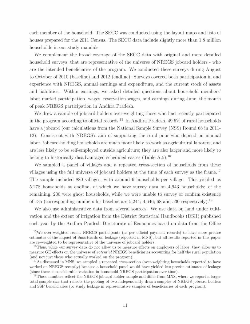
We drew a sample of jobcard holders over-weighting those who had recently participated

in the program according to official records.15 In Andhra Pradesh, 49.5% of rural households

have a jobcard (our calculations from the National Sample Survey (NSS) Round 68 in 2011-

12). Consistent with NREGS’s aim of supporting the rural poor who depend on manual

labor, jobcard-holding households are much more likely to work as agricultural laborers, and

are less likely to be self-employed outside agriculture; they are also larger and more likely to

belong to historically disadvantaged scheduled castes (Table A.5).16

We sampled a panel of villages and a repeated cross-section of households from these

villages using the full universe of jobcard holders at the time of each survey as the frame.17

The sample included 880 villages, with around 6 households per village. This yielded us

5,278 households at endline, of which we have survey data on 4,943 households; of the

remaining, 200 were ghost households, while we were unable to survey or confirm existence

of 135 (corresponding numbers for baseline are 5,244; 4,646; 68 and 530 respectively).18

We also use administrative data from several sources. We use data on land under culti-

vation and the extent of irrigation from the District Statistical Handbooks (DSH) published

each year by the Andhra Pradesh Directorate of Economics based on data from the Office

15We over-weighted recent NREGS participants (as per official payment records) to have more preciseestimates of the impact of Smartcards on leakage (reported in MNS), but all results reported in this paperare re-weighted to be representative of the universe of jobcard holders.

16Thus, while our survey data do not allow us to measure effects on employers of labor, they allow us tomeasure GE effects on the universe of potential NREGS beneficiaries accounting for half the rural population(and not just those who actually worked on the program).

17As discussed in MNS, we sampled a repeated cross-section (over-weighting households reported to haveworked on NREGS recently) because a household panel would have yielded less precise estimates of leakage(since there is considerable variation in household NREGS participation over time).

18These numbers reflect the NREGS jobcard holder sample and differ from MNS, where we report a largertotal sample size that reflects the pooling of two independently drawn samples of NREGS jobcard holdersand SSP beneficiaries (to study leakage in representative samples of beneficiaries of each program).

11

of the Surveyor General of India.19 We use unit cost data from Round 68 (2011-2012) of

the National Sample Survey (NSS) published by the Ministry of Statistics and Programme

Implementation. The NSS contains detailed household × item-level data for a sample repre-

sentative at the state and sector level (rural and urban). The data cover over 300 goods and

services in categories including food, fuel, clothing, rent and other fees or services over mixed

reference periods varying from a week to a year. Note that because the overlap between vil-

lages in our study mandals and the NSS sample is limited to 60 villages, we use the NSS

data primarily to examine price levels, for which it is the best available data source. We also

use data on mandal-wise headcounts of livestock from the Livestock Census of India, which

is conducted quinquennially by the Government of India. We use data from the 19th round

conducted in 2012, which is also the year of our endline survey. Finally, we use geocoded

point locations for each census village from the 2001 Indian Census.

Figure 2 presents a summary of the data sources used in this paper, the recall period that

they correspond to, and the specific outcomes for which each data source is used.

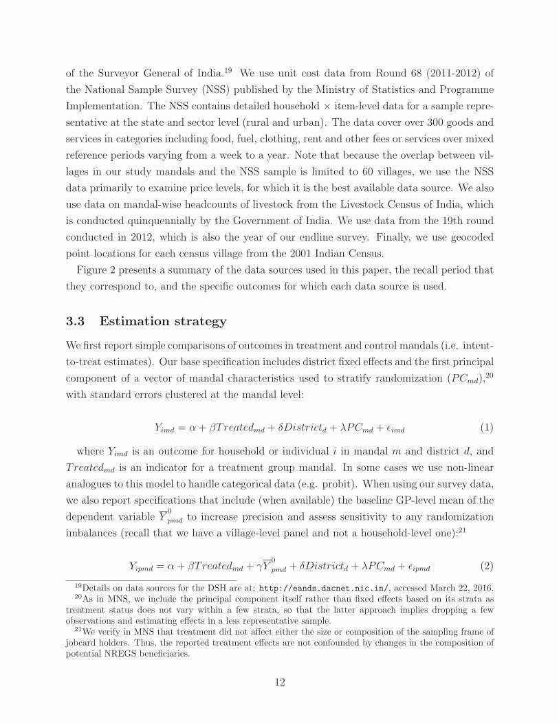
3.3 Estimation strategy

We first report simple comparisons of outcomes in treatment and control mandals (i.e. intent-

to-treat estimates). Our base specification includes district fixed effects and the first principal

component of a vector of mandal characteristics used to stratify randomization (PCmd),20

with standard errors clustered at the mandal level:

Yimd = α + βTreatedmd + δDistrictd + λPCmd + ǫimd (1)

where Yimd is an outcome for household or individual i in mandal m and district d, and

Treatedmd is an indicator for a treatment group mandal. In some cases we use non-linear

analogues to this model to handle categorical data (e.g. probit). When using our survey data,

we also report specifications that include (when available) the baseline GP-level mean of the

dependent variable Y0

pmd to increase precision and assess sensitivity to any randomization

imbalances (recall that we have a village-level panel and not a household-level one):21

Yipmd = α + βTreatedmd + γY0

pmd + δDistrictd + λPCmd + ǫipmd (2)

19Details on data sources for the DSH are at: http://eands.dacnet.nic.in/, accessed March 22, 2016.20As in MNS, we include the principal component itself rather than fixed effects based on its strata as

treatment status does not vary within a few strata, so that the latter approach implies dropping a fewobservations and estimating effects in a less representative sample.

21We verify in MNS that treatment did not affect either the size or composition of the sampling frame ofjobcard holders. Thus, the reported treatment effects are not confounded by changes in the composition ofpotential NREGS beneficiaries.

12

where p indexes panchayats or GPs. We easily reject γ = 1 in all cases and therefore do

not report difference-in-differences estimates. Regressions using SECC data are unweighted,

while those using survey samples are weighted by inverse sampling probabilities to be repre-

sentative of the universe of jobcard-holders. When using survey data on wages and earnings

we trim the top 0.5% of observations in both treatment and control groups to remove outliers,

but results are robust to including them.

An improved NREGS is likely to affect wages, employment, and income through several

channels that not only take place simultaneously, but are also likely to interact with each

other. Thus, β in Equation 1 should be interpreted as reflecting a composite mix of several

factors. This is the policy-relevant general-equilibrium estimate of the total effect on rural

economic outcomes of increasing the effective presence of NREGS, and is our primary focus;

we discuss specific mechanisms of impact in Section 6.

If outcomes for a given unit (household, GP, etc.) depend only on that unit’s own treat-

ment status, then β in Equation 1 identifies a well-defined treatment effect. However, general

equilibrium effects need not be confined to the treated units. Upward pressure on wages in

treated mandals, for example, might affect wages in nearby areas of control mandals. In the

presence of such spillovers, β in Equation 1 could misestimate the “total treatment effect”

(TTE), conceptualized as the difference between average outcomes when all units are treated

and those when no units are treated. We defer estimation of this TTE to Section 5 and note

for now that our initial estimates are likely to be conservative.

4 Results

4.1 Effects on earnings and poverty

Figure A.1 compares the distributions of SECC income categories in treatment and control

mandals, using raw data (without district fixed effects conditioned out) to show the absolute

magnitudes. We see that the treatment distribution first-order stochastically dominates the

control, with 4.1 percentage points fewer households in the lowest category (less than Rs.

5,000/month), 2.6 percentage points more households in the middle category (Rs. 5,000 to

10,000/month), and 1.4 percentage points more in the highest category (greater than Rs.

10,000/month). Table 1a reports experimental estimates of impact, showing marginal effects

from logistic regressions for each category individually and an ordered logistic regression

across all categories. Treatment significantly increased the log-odds ratio of being in a

higher income category, with estimates unaltered by controls for (arguably predetermined)

demographic characteristics such as age of household head, caste, and literacy.

13

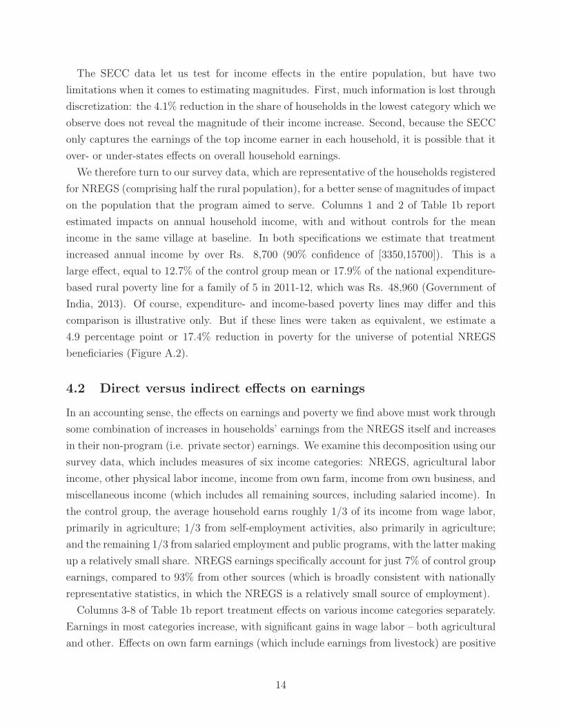
The SECC data let us test for income effects in the entire population, but have two

limitations when it comes to estimating magnitudes. First, much information is lost through

discretization: the 4.1% reduction in the share of households in the lowest category which we

observe does not reveal the magnitude of their income increase. Second, because the SECC

only captures the earnings of the top income earner in each household, it is possible that it

over- or under-states effects on overall household earnings.

We therefore turn to our survey data, which are representative of the households registered

for NREGS (comprising half the rural population), for a better sense of magnitudes of impact

on the population that the program aimed to serve. Columns 1 and 2 of Table 1b report

estimated impacts on annual household income, with and without controls for the mean

income in the same village at baseline. In both specifications we estimate that treatment

increased annual income by over Rs. 8,700 (90% confidence of [3350,15700]). This is a

large effect, equal to 12.7% of the control group mean or 17.9% of the national expenditure-

based rural poverty line for a family of 5 in 2011-12, which was Rs. 48,960 (Government of

India, 2013). Of course, expenditure- and income-based poverty lines may differ and this

comparison is illustrative only. But if these lines were taken as equivalent, we estimate a

4.9 percentage point or 17.4% reduction in poverty for the universe of potential NREGS

beneficiaries (Figure A.2).

4.2 Direct versus indirect effects on earnings

In an accounting sense, the effects on earnings and poverty we find above must work through

some combination of increases in households’ earnings from the NREGS itself and increases

in their non-program (i.e. private sector) earnings. We examine this decomposition using our

survey data, which includes measures of six income categories: NREGS, agricultural labor

income, other physical labor income, income from own farm, income from own business, and

miscellaneous income (which includes all remaining sources, including salaried income). In

the control group, the average household earns roughly 1/3 of its income from wage labor,

primarily in agriculture; 1/3 from self-employment activities, also primarily in agriculture;

and the remaining 1/3 from salaried employment and public programs, with the latter making

up a relatively small share. NREGS earnings specifically account for just 7% of control group

earnings, compared to 93% from other sources (which is broadly consistent with nationally

representative statistics, in which the NREGS is a relatively small source of employment).

Columns 3-8 of Table 1b report treatment effects on various income categories separately.

Earnings in most categories increase, with significant gains in wage labor – both agricultural

and other. Effects on own farm earnings (which include earnings from livestock) are positive

14

but insignificant. NREGS earnings increase modestly (p = 0.12) and the increase in annual

NREGS earnings is consistent with treatment effects on weekly NREGS earnings reported

in MNS (estimated during the peak NREGS period).22

Overall, the increase in NREGS income accounts for only 10% of the increase in total

earnings (proportional to the share of NREGS in control group income). Nearly 90% of

the income gains are attributable to non-NREGS earnings, with the primary driver being an

increase in earnings from market labor, both in the agricultural and non-agricultural sectors.

4.3 Distribution of earnings gains

Figure A.2 plots the empirical CDF of household earnings for treatment and control groups

in our survey data. We see income gains throughout the distribution, with the treatment

income distribution in the treatment group first-order stochastically dominating that in

the control group. Finally, the broad-based gains seen in the universe of NREGS jobcard

holders (comprising two thirds of the rural population) are also seen in the the SECC data

representing the full population (Figure A.1). One caveat, given the wage results we report

below, is that that the SECC earnings measure likely does not capture effects on the profits

of landholders because it is coarsely topcoded.23

Table A.6 tests for differential treatment effects in our survey data by household charac-

teristics using a linear interaction specification. We find no differential impacts by caste or

education, suggesting broad-based income gains consistent with Figure A.2. More impor-

tantly, we see that the treatment effects on earnings are not seen for households who are less

likely to work (those headed by widows or those eligible for social security pensions). Since

a household with a pension-eligible resident may also have working-age adults, we examine

heterogeneity by the fraction of adults in the households who are eligible for pensions, and

see that there are no income gains for households where all adults are eligible for pensions.

This confirms that (a) labor market earnings are the main channel for increased income, and

(b) improvements in SSP payments from Smartcards are unlikely to be responsible for the

large increases in earnings we find.

22In MNS, we report a significant increase in weekly earnings of Rs. 35/week during seven weeks corre-sponding to the peak NREGS season. Average weekly NREGS earnings per year are 49.6% of the averageweekly NREGS earnings in these seven weeks (calculated using official payment records in the control man-dals as shown in Figure A.3). Thus, the annualized treatment effect on NREGS earnings should be Rs. 35X 52 weeks X 0.496 or Rs. 903/year, which is exactly in line with the Rs. 914 measured in the annual recalldata reported in Table 1b. However, the results here are marginally insignificant (p = 0.12) compared tothe significant ones in MNS, likely due to the lower precision of annual recall data compared to the moreprecise data collected for the seven-week reference period in MNS, with job cards on hand to aid recall.

23The SECC measure is also based on a question phrasing that respondents could have interpreted asreferring to labor income.

15

In summary, evidence on the distribution of effects suggests that the increase in earnings

were broad-based across categories of households who were registered for the NREGS, but

did not accrue to households whose members were unable to work.

4.4 Effects on private labor markets

4.4.1 Wages

To examine wage effects we use our survey data, as the SECC does not include wage infor-

mation. We define the dependent variable as the average daily wage earned on private-sector

work across all respondents who report a private-sector wage. We report results for the full

sample of workers reporting a wage, and also check that results are robust to restricting the

sample to adults aged 18-65, with additional checks for robustness with respect to sample

composition in Section 4.8 below.

We estimate a significant increase of Rs. 7.8 in daily market wages (Table 2, Column 2).

This is a large effect, equal to 6.1% of the control group mean. In fact, it is slightly larger

than the highest estimates of the market-wage impacts of the rollout of the NREGS itself as

reported by Imbert and Papp (2015).

One mechanism that could contribute to this effect is labor market competition: a (better-

run) public employment guarantee may improve the outside option for workers, putting

pressure on labor markets that drives up wages and earnings. Theoretical models emphasize

this mechanism (Ravallion, 1987; Basu et al., 2009), and it has motivated earlier work on

NREGS wage impacts (e.g. Imbert and Papp (2015)), but prior work has not been able to

directly test for this hypothesis in the absence of data on reservation wages.

We are able to test this prediction using data on reservation wages that we elicited in our

survey. Specifically, we asked respondents if in the month of June they would have been

“willing to work for someone else for a daily wage of Rs. X,” where X started at Rs. 20

(15% of average wage) and increased in Rs. 5 increments until the respondent agreed. One

advantage of this measure is that it applies to everyone, and not only to those who actually

worked. Respondents appeared to understand the question, with 98% of those who worked

reporting reservation wages less than or equal to the wages they actually earned (Table A.7).

We find that treatment significantly increased workers’ reservation wages by approximately

Rs. 5.5, or 5.7% of the control group mean (Table 2, columns 3-4). The increase in reservation

wage in treated areas provides direct evidence that making NREGS a more appealing option

would have required private employers to raise wages to attract workers. Finally, as further

evidence of general equilibrium effects, we find that there is no difference in the increase in

market wages as a function of whether the worker actually worked on NREGS (Table A.9).

16

Consistent with market wages increasing for all workers, we see that the gains in income

seen in Figure A.2 occur all the way up to per-capita incomes of Rs. 40,000/year (or 4 times

the poverty line), which likely includes workers who did not actively participate in NREGS.

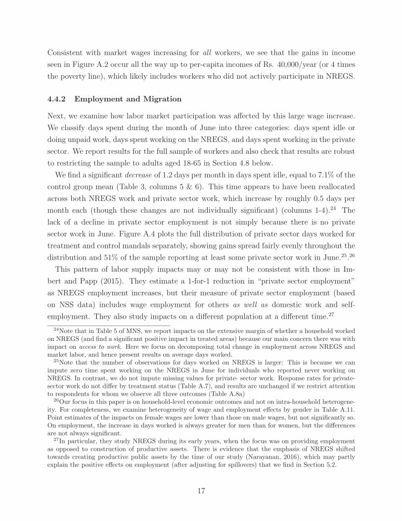
4.4.2 Employment and Migration

Next, we examine how labor market participation was affected by this large wage increase.

We classify days spent during the month of June into three categories: days spent idle or

doing unpaid work, days spent working on the NREGS, and days spent working in the private

sector. We report results for the full sample of workers and also check that results are robust

to restricting the sample to adults aged 18-65 in Section 4.8 below.

We find a significant decrease of 1.2 days per month in days spent idle, equal to 7.1% of the

control group mean (Table 3, columns 5 & 6). This time appears to have been reallocated

across both NREGS work and private sector work, which increase by roughly 0.5 days per

month each (though these changes are not individually significant) (columns 1-4).24 The

lack of a decline in private sector employment is not simply because there is no private

sector work in June. Figure A.4 plots the full distribution of private sector days worked for

treatment and control mandals separately, showing gains spread fairly evenly throughout the

distribution and 51% of the sample reporting at least some private sector work in June.25.26

This pattern of labor supply impacts may or may not be consistent with those in Im-

bert and Papp (2015). They estimate a 1-for-1 reduction in “private sector employment”

as NREGS employment increases, but their measure of private sector employment (based

on NSS data) includes wage employment for others as well as domestic work and self-

employment. They also study impacts on a different population at a different time.27

24Note that in Table 5 of MNS, we report impacts on the extensive margin of whether a household workedon NREGS (and find a significant positive impact in treated areas) because our main concern there was withimpact on access to work. Here we focus on decomposing total change in employment across NREGS andmarket labor, and hence present results on average days worked.

25Note that the number of observations for days worked on NREGS is larger: This is because we canimpute zero time spent working on the NREGS in June for individuals who reported never working onNREGS. In contrast, we do not impute missing values for private- sector work. Response rates for private-sector work do not differ by treatment status (Table A.7), and results are unchanged if we restrict attentionto respondents for whom we observe all three outcomes (Table A.8a)

26Our focus in this paper is on household-level economic outcomes and not on intra-household heterogene-ity. For completeness, we examine heterogeneity of wage and employment effects by gender in Table A.11.Point estimates of the impacts on female wages are lower than those on male wages, but not significantly so.On employment, the increase in days worked is always greater for men than for women, but the differencesare not always significant.

27In particular, they study NREGS during its early years, when the focus was on providing employmentas opposed to construction of productive assets. There is evidence that the emphasis of NREGS shiftedtowards creating productive public assets by the time of our study (Narayanan, 2016), which may partlyexplain the positive effects on employment (after adjusting for spillovers) that we find in Section 5.2.

17

Finally, we examine impacts on labor allocation through migration. Our survey asked

two questions about migration for each family member: whether or not they spent any days

working outside of the village in the last year, and if so how many such days. Table A.10

reports effects on each measure. We estimate a small and insignificant increase in migration

on both the extensive and intensive margins. The former estimate is more precise, ruling

out reductions in the prevalence of migration greater than 1.0 percentage point, while the

latter is less so, ruling out a 58 percent or greater decrease in total person-days. As our

migration questions may fail to capture permanent migration, we also examine impacts on

household size and again find no significant difference. These results are consistent with the

existence of countervailing forces that may offset each other: higher rural wages may make

migration less attractive, while higher rural incomes make it easier to finance the search

costs of migration (Bryan et al., 2014; Bazzi, 2017).

4.5 Seasonality and Magnitude of Overall Income Effects

Our point estimates for annual earnings are broadly consistent with those for wages and

employment during June 2012. Specifically, the 13.4% increase in non-NREGS earnings is

roughly equal to the sum of the 6.1% increase in wages and (insignificant) 6.7% increase in

employment. These are our most precise measures of labor market activity, as they referred

to a period shortly before surveys were conducted (see data collection timeline in Figure 2).

While we do not have similarly detailed data for the entire annual cycle, those we have

suggest that impacts persisted throughout the year. In interviews with village leaders we

asked them to report the “going wage rate” for each month of the year. Figure A.5 plots

impacts on this measure by month; the estimates are imprecise (since we have only one data

point per village), but suggest that wage appreciation persisted throughout the year.

This pattern is consistent with several (non mutually exclusive) interpretations. To the

extent that wage impacts are due to increased NREGS asset creation, we would expect them

to persist and potentially even increase throughout the year. To the extent they are driven

by the effects of a more attractive NREGS “outside option,” we would expect them to mirror

the availability of NREGS work; as Figure A.6 shows, almost all study villages had at least

one NREGS project active for a majority of 2012, with availability dropping to a low of

40-50% of villages towards the end of the year.28 Finally, wages may be linked across time

due to various forms of nominal rigidity, including concerns for fairness (Kaur, forthcoming)

and labor tying over the agricultural cycle (Bardhan, 1983; Mukherjee and Ray, 1995). The

latter literature in particular suggests that landlords who provide wage insurance in the lean

28While not much NREGS work appears to have been done during the end of the year (Figure A.3), thepresence of active projects suggests that NREGS may still have been a viable outside option in many villages.

18

season pay lower wages in the peak season. In these models, better NREGS availability

and higher market wages in the lean season would imply a reduced need for insurance from

landlords and a resulting higher wage in the peak (non-NREGS) season.

To summarize, the magnitude of the annual income gains we find are consistent with the

estimated changes in wages and employment estimated precisely during the peak NREGS

period where we have detailed data. However, as the discussion above suggests, there are

several reasons for why the wage increases may persist throughout the year, and the (limited)

data we have are consistent with this.

4.6 Effects on consumer goods prices

One potential caveat to the earnings results above is that they show impacts on nominal,

and not real, earnings. Given that Smartcards affected local factor (i.e. labor) prices, they

could also have affected the prices of local final goods, and thus the overall price level facing

consumers, if local markets are not sufficiently well-integrated into larger product markets.

To test for impacts on consumer goods prices we use data from the 68th round of the National

Sample Survey. The survey collected data on expenditure and number of units purchased for

a wide variety of goods; we define unit costs as the ratio of these two quantities. We restrict

the analysis to goods that have precise measures of unit quantities (e.g. kilogram or liter)

and drop goods that likely vary a great deal in quality (e.g. clothes and shoes). We then

test for price impacts in two ways. First, we define a price index Pvd equal to the price of

purchasing the mean bundle of goods in the control group, evaluated at local village prices,

following Deaton and Tarozzi (2000):

Pvd =n∑

c=1

qcdpcv (3)

Here qcd is the estimated average number of units of commodity c in panchayats in control

areas of district d, and pcv is the median unit cost of commodity c in village v. Conceptually,

treatment effects on this quantity can be thought of as analogous to the “compensating

variation” that would be necessary to enable households to continue purchasing their old

bundle of goods at the (potentially) new prices.29

The set of goods for which non-zero quantities are purchased varies widely across house-

holds and, to a lesser extent, across villages. To ensure that we are picking up effects on

prices (rather than compositional effects on the basket of goods purchased), we initially re-

29Theoretically we would expect any price increases to be concentrated among harder-to-trade goods.Since our goal here is to understand welfare implications, however, the overall consumption-weighted indexis the appropriate construct.

19

strict attention to goods purchased at least once in every village in our sample. The major

drawback of this approach is that it excludes roughly 40% of the expenditure per village in

our sample. We therefore also present a complementary set of results in which we calculate

(3) using all available data. In addition, we report results using (the log of) unit cost defined

at the household-commodity level as the dependent variable and including all available data.

While these later specifications potentially blur together effects on prices with effects on the

composition of expenditure, they do not drop any information.

Regardless of method, we find little evidence of impacts on price levels (Table 4). The

point estimates are small and insignificant and, when we use the full information available,

are also precise enough to rule out effects as large as those we found earlier for wages. These

results suggest that the treated areas are sufficiently well-integrated into product markets

that higher local wages and incomes did not affect prices of the most commonly consumed

items, and can thus be interpreted as real wage and income gains for workers.

4.7 Balance sheet effects

If households interpreted the income gains measured above as temporary (or volatile), we

would expect to see them translate into the accumulation of liquid or illiquid assets. Our

survey collected information on two asset categories: liquid savings and land-ownership. We

find positive estimated effects on both measures (Table 5), with the effect on land-ownership

significant; treatment increased the share of households that owned some land by 4.9%

percentage points, or 8.3%. This likely reflects the sale of land from those that had a lot

of it (who were outside our sample of jobcard holders) to those that had none, and we find

that the distribution of landholding in treatment group first-order stochastically dominates

that in the control group (p = 0.013) (Figure A.7).

We also see a 16% increase in total borrowing, which could reflect either crowding-in of

borrowing to finance asset purchases or the use of those assets as collateral. Importantly,

this is driven entirely by increases in informal borrowing, with no increase in borrowing

from formal financial institutions, consistent with the fact that Smartcards were not a viable

means of accessing financial services beyond public-sector benefits (Table A.12).

After land, livestock are typically the most important asset category for low-income house-

holds in rural India, and a relatively easy one to adjust as a buffer stock. We test for effects

on livestock holdings using data from the Government of India’s 2012 Livestock Census.

The Census reports estimated numbers of 13 different livestock categories; in Table 6 we

report impacts on the 9 categories for which the average control mandal has at least 100

animals. We find positive impacts on every category of livestock except one, including sub-

20

stantial increases in the number of buffaloes (p < 0.001), dogs (p = 0.067), backyard poultry

(p = 0.093), and fowls (p = 0.104). A Wald test of joint significance across the livestock

categories easily rejects the null of no impacts (p = 0.01). The 50% increase in buffalo

holdings is especially striking since these are among the highest-returning livestock asset in

rural India, but often not accessible to the poor because of the upfront costs of purchasing

them (Rosenzweig and Wolpin, 1993).

Overall, we see positive impacts on holdings of arguably the two most important invest-

ment vehicles available to the poor (land and livestock). This is consistent with the view that

households saved some or all of the increased earnings they received due to Smartcards, and

acquired productive assets in the process. The livestock results are particularly convincing

as evidence of an increase in total productive assets in treated areas because they (a) come

from a census, and (b) represent a net increase in assets, whereas increased land-ownership

among NREGS jobcard holders must reflect net sales by landowners.

Any residual earnings not saved or invested should show up in increased expenditure, but

our power to detect such effects is limited, as expenditure was not a focus of our household

survey.30 With that caveat in mind, Table A.13 shows estimated impacts on household

expenditure on both frequently (columns 1 & 2) and infrequently (columns 3 & 4) purchased

items from our survey. Both estimates are small and statistically insignificant, but not very

precisely estimated. In particular, we cannot rule a 8% increase in expenditure on frequently

purchased items or a 15% increase in spending on infrequently purchased items. In Column

5 we use monthly per capita expenditure as measured by the NSS, which gives us a far

smaller sample but arguably a more comprehensive measure of expenditure. The estimated

treatment effect is positive and insignificant, but again imprecise, and we cannot rule out

a 16% increase in expenditure (consistent with a marginal propensity to consume ranging

from 0 to 1, and hence not very informative).

4.8 Robustness & other concerns

The estimated income effects in Table 1b are robust to a number of checks. Results are

similar using probits or linear probability models instead of logits (Table A.14). They are

also robust to alternative ways of handling possible outliers; including observations at the

top 0.5% in treatment and control does not change the results qualitatively (Table A.15).

Our wage results are robust to alternative choices of sample. The main results include

30The entire expenditure module in our survey was a single page covering 26 categories of expenditure;for comparison, the analogous NSS consumer expenditure module is 12 pages long and covers 23 categoriesof cereals alone. The survey design reflects our focus on measuring leakage in NREGS earnings and impactson earnings from deploying Smartcards.

21

data on anyone in the household who reports a market wage. Restricting the sample to

only those of working age (18-65) again does not affect results for either wages (Table A.16)

or employment (Table A.8b). Next, dropping the small number of observations who report

wages but zero actual employment again does not matter (Table A.16). Results are also

robust to estimating wage effects in logs rather than levels, though impacts on reservation

wages become marginally insignificant (p = 0.11, not reported).

Given that we only observe wages for those who work, the effects we estimate could poten-

tially reflect changes in who reports work (or wages) rather than the distribution of market

wages. We test for such selection effects as follows. First, we confirm that essentially all

respondents (99%) who reported working also reported the wages they earned, and that non-

response is the same across treatment and control (first row of Table A.7). Second, we check

that the probability of reporting any work is not significantly different between treatment

and control groups (Table A.7). Third, we check composition and find that treatment did

not affect composition of those reporting in Table A.17. Finally, as we saw above treatment

also increased reservation wages, which we observe for nearly the entire sample (89%) of

working-age adults (including those reporting no actual work).

5 Spatial spillovers

Improving NREGS implementation in one mandal may have affected outcomes in other

neighboring mandals. We turn now to testing for such spillover effects and to estimating

“total” treatment effects that account for them. Our goal is twofold: First, to validate the

ITT results using a different source of variation, and second, to provide a sense of how the

policy effects of rolling out NREGS universally would compare with the naive ITT estimates.

As with any such spatial problem, outcomes in each GP could in principle be an arbitrary

function of the treatment status of all the other GPs. No feasible experiment could identify

these functions nonparametrically. We therefore take a simple approach, modeling spillovers

as a function of the fraction of GPs (NRp ) within various radii R of a given panchayat p that

were assigned to treatment. Figure 3 illustrates the construction of this measure.31

The random assignment of mandals to treatment does not necessarily ensure that the

neighborhood measure NRp is also “as good as” randomly assigned. To see this, consider

constructing the measure for GPs in a treated mandal: on average, GPs closer to the center

of the mandal will have higher values of NRp (as more of their neighbors are from the same

31Note that we implicitly treat GPs assigned to mandals in the “buffer group” as untreated here. Treatmentrolled out in these mandals much later than in the treatment group and we do not have survey data to estimatethe extent to which payments had been converted in these GPs by the time of our endline.

22

mandal), while those closer to the border will have lower values (as more of their neighbors

are from other mandals). The opposite pattern will hold in control mandals. Thus, we

cannot interpret a coefficient on NRp as solely a measure of spillover effects without making

the (strong) assumption that the direct effects of treatment are unrelated to location.32

To address this issue, we construct a second measure NRp defined as the fraction of GPs

within a radius R of panchayat p which were assigned to treatment and within a different

mandal, so that both the numerator and denominator in NRp exclude the GPs in the same

mandal. This has the advantage of being exogenous conditional on own treatment status,

and the disadvantage that it is not defined for a GP when R is so small that p is more than

R kilometers from the nearest border. We use this measure both to test for the existence

of spillovers and as an instrument for estimating the effects of NRp , which we view as the

“structural” variable of interest.

To examine the sensitivity of our conclusions to the definition of “neighborhoods”, we

measure neighborhood treatment intensity at radii of 10, 15, 20, 25, and 30 kilometers.

These distances are economically relevant given what we know about rural labor markets.

For instance, workers can travel by bicycle at speeds up to 20 km / hour, so that working

on a job 30 km from home implies a high but not implausible daily two-way commute of 3

hours. Of course, effects could also propagate much further than the distance over which

any single actor is willing to arbitrage, with changes in one market rippling on to the next.

Figure A.8 plots smoothed kernel density estimates by treatment status for NRp and for

NRp . As discussed above, the former is mechanically correlated with own treatment status

(Panel A), while the latter is not (Panel B). Tables A.18 and A.19 report tests showing that

our outcomes of interest are balanced with respect to these measures at baseline.33

5.1 Testing for spillovers

To test for the existence of spillovers, we estimate

Yipmd = α + βNRp + δDistrictd + λPCmd + ǫimd (4)

separately for the treatment and control groups. This approach allows for the possibility

that neighborhood effects differ depending on one’s own treatment status. We also estimate

a variant that pools both treatment and control groups (and adds an indicator for own

32Merfeld (2017) finds intra-district differences in wages as a function of distance to the district border,suggesting that this assumption may not hold.

33A richer model of spillovers might allow for treated GPs at different radii to have different effects – forexample, the share of treated GPs at 0-10km, 11-20km, etc. might enter separately into the same model.We do not have sufficient power to distinguish these effects statistically, however (results not reported).

23

treatment status), which imposes equality of β across groups. In either case, we interpret

rejection of the null β = 0 as evidence of spillover effects.

We find robust evidence of spillover effects on market wages, consistent in sign with the

direct effects we estimated above (Table 7, columns 1-5). The effects are strongest for

households in control mandals, where we estimate a significant relationship at all radii greater

than 10km; for those in treatment mandals the estimates are smaller and significant for three

out of five radii, but uniformly positive. For days spent on unpaid work or idle, the estimated

effects are all negative, and significant except at smaller radii when we split the sample (Table

7, columns 6-10). Since we never reject equality of β across control and treatment groups,

the pooled samples provide the most power, and we estimate significant spillover effects at

all radii (except at R = 10 for days spent on unpaid work or idle).34.

These spillover results validate the ITT ones with a completely different source of variation

(since the measure of exogenous spatial exposure to treatment that we define and use is

uncorrelated with the direct treatment status of a sampled village). They also suggest that

the ITT results may be biased downwards and need to be corrected for, which we do next.

5.2 Estimating total treatment effects

The conceptual distinction between the unadjusted and total treatment effects can be seen

in Figure 4. The difference between the intercepts (βT ) represents the effect of a village being

treated when none of its neighbors are treated, and movement along the x-axis represents the

additional effect of having more neighbors treated. Thus, the unadjusted treatment effects

(reported in Section 4), represented by yITT , captures both the effect of a village being

treated, and the mean difference in the fraction of treated neighbors between treatment and

control villages (xITT ), which is positive but less than 1 (as seen in Figure A.8). The total

treatment effect, represented by yTTE, is the difference in expected outcomes between a

village in a treated mandal with 100% of its neighborhood treated (Tm = NRp = 1), and that

for a village in a control mandal with 0% of its neighborhood treated (Tm = NRp = 0). This

is inevitably a partially extrapolative exercise, as much of our sample is in neither of these

conditions (as seen in Panel A of Figure A.8). Nevertheless, we are interested in estimating

it since it is this “total” effect one would ideally use for determining policy impacts under a

universal scale up of the program.

34We can also use the same methods to estimate the effects of having GPs in mandals assigned to theintermediate “buffer” wave as neighbors. These effects are hard to interpret, as we do not have data fromthe field to assess the extent to which buffer mandals had been treated at the time of our endline survey.In practice, the point estimates on the percent of neighboring GPs in buffer mandals are generally the samesign as the point estimates on treated neighbors but smaller and insignificant (consistent with some rolloutin these mandals - greater than zero, but less than the extent in the treated mandals)

24

To estimate this effect with our data, we first estimate

Yipmd = α + βTTm + βNNRp + βTNTm ·NR

p + δDistrictd + λPCmd + ǫimd (5)

Here βT captures the effect of own treatment status, βN the effect of neighborhood treat-

ment exposure, and βTN any interaction between the two. The total treatment effect of a

universal rollout of treatment (with all neighbours being treated) is then given by:

β = βT + βN + βTN (6)

Since NRp is potentially endogenous for reasons discussed above, we instrument for it in

(5) using NRp (and instrument for its interaction with Tm using the corresponding interac-

tion). Not surprisingly, we estimate a strong first-stage relationship between the two, with

a minimum F -statistic across specifications reported here of F = 115. For completeness we

also report OLS estimates of (5) in Table A.20; these are qualitatively similar to the results

we present here, and mostly significant, but less precise.

After adjusting for spillovers, we estimate total treatment effects (TTE) on wages and

employment – which are (i) significant for most or all values of R, (ii) consistent in sign

with those we estimate in simple binary treatment specifications, and (iii) meaningfully

larger, suggesting that the unadjusted estimates may be significantly biased downwards (as

suggested by Figure 4).

Table A.21 presents the results of estimating Equation (5) above, and also calculates the

TTE as shown in Equation (6). We focus our discussion on the results in Table 8, which

present the TTE calculated above, the unadjusted treatment effects, and formal tests of

equality of the two.35

We begin in panel (a) with wage outcomes. Depending on choice of R, the estimated TTE

on realized wages is 14-20% of the control mean, and uniformly significant. Further, these

estimates are typically three times as large as the unadjusted estimates in Table 2, suggesting

that not accounting for spatial spillovers could substantially understate the impact of NREGS

on market wages. The estimated TTE on reservation wages is 8-10% of the control mean,

and also larger than the unadjusted estimates (though not significantly so).

In panel (b) we examine impacts on labor allocation. As above, we see that adjusting

for spillovers makes the results in Table 3 stronger. Most importantly, we see that TTE of

35To do this, we use equation-by-equation generalized method of moments estimation, and estimate ourspecifications for unadjusted and total treatment effects on the same analysis sample (which matches theanalysis sample of Table A.21). Note that the estimates for the unadjusted treatment effect differ slightlyfrom those from Tables 1b, 2, and 3 as the analysis sample only includes observations where the spatialexposure measures are defined.

25

work done in the private sector is positive and significant (for all R > 10km), suggesting

that improved NREGS raised not only wages, but also raised private sector employment.

The differences with the unadjusted estimates are substantial and underscore the extent to

which estimates that do not adjust for spillovers may be biased. Correspondingly, we also

see a larger reduction in the total number of days spent idle or doing unpaid work.36

One natural question about these estimates is whether specifying outcomes as linear func-

tions of NRp yields a good fit. We prefer linear models as the relationship between NR

p and our

main outcomes of interest does not display any obvious curvature (Figures A.9 and A.10),

implying that fitting higher-order polynomials to the data is very likely to over-fit them. We

also estimated variants of (5) that include higher-order terms, however, and obtained similar

estimates of the TTE (available on request).

To summarize, our results suggest that there were meaningful spatial spillovers to both

treatment and control villages as a function of the fraction of treated neighbors, with the

direction of the effects being the same as those of the main effects. These results have three

substantive implications. First, they validate our core results using a different source of

variation that is orthogonal to the randomization of mandals to treatment status. Second,

they reinforce the GE nature of our results by highlighting that the right way to think about

the policy-relevant treatment effect is not at the level of the individual or even village, but

rather the overall labor market. Third, they suggest that the total policy effects of NREGS

are likely to be larger than our experimental ITT estimates and that existing estimates that

do not account for spillovers may understate the total effects of NREGS (as shown in a

different setting by Miguel and Kremer (2004)).

6 Discussion

Like any change to a complex economy, an improved NREGS could affect economic outcomes

in many ways, with multiplier effects, feedback loops, and interactions all contributing to

the overall impact. It is thus implausible to decompose effects into distinct, independent

channels as in a partial equilibrium analysis. We can still test, however, whether there is

evidence that specific mechanisms suggested by theory are operative.

One hypothesis is that a (better-run) employment guarantee puts competitive pressure

36We focus the analysis in Tables 7 and 8 on wages and employment in June, because these are measuredrelatively precisely with a one-month recall window. We present analogous results for income (measuredon the basis of annual recall) in Table A.22 and also report robustness to different levels of top-censoringbecause the distribution of earnings is right-skewed. Overall, we find the same pattern of results includingevidence of spillovers, and point estimates of TTE that are always larger than the unadjusted ITT estimates(though not significantly so).

26

on labor markets, driving up wages and earnings. Consistent with this, we find a signifi-

cant positive impact not only on market wages, but also on reservation wages. It is also

suggestive that the difference between the unadjusted and total treatment effects in Table

8 is smaller (∼75-100%) and insignificant for reservation wages compared to the difference

for market wages (>300%, statistically significant). Changes in reservation wages appear to

depend mainly on whether a worker’s own village was treated (reflecting the improvement

of NREGS as a local outside option), while changes in market wages appear to also depend

on the proportion of treated villages – and hence, the number of treated workers – in the

neighborhood. This suggests that market wages had to respond to the extent of increased

competition from NREGS in other nearby villages.37

An improved NREGS may also have created additional productive assets – roads, irrigation

facilities, soil conservation structures, etc. – which raised productivity. We can rule out large

changes in the number and composition of projects reported (Table A.23). However, the

reductions in leakage, and proportional (albeit insignificant) increase in workers observed at

works-sites during unannounced visits reported in MNS, suggest that actual asset creation

may have increased (though we do not have independent measures of assets created). We can

also test for productivity gains by examining changes in land utilization, which might result

from land improvements or minor irrigation works. We do not see effects on the amount of

land sown or on the total area irrigated (Table A.24), ruling out effect sizes larger than 16%

and 10%, respectively. A caveat, however, is that the irrigation data in district handbooks

may reflect only major works undertaken by the Ministry of Irrigation and not the smaller

ones typically undertaken under NREGS. Overall, while we find no direct evidence that

assets created under NREGS improved productivity, we cannot rule out the possibility.38

Increased cash flow could also potentially stimulate local economic activity, driving up

wages and earnings (Magruder, 2013). Because the intervention did not affect NREGS

disbursements, this effect is relevant only to the extent that the redistribution of some income

from officials to workers increased local spending. In practice we find insignificantly positive

effects on household expenditure (Table A.13): this is not direct evidence for an aggregate

demand mechanism, but leaves open the possibility that redistribution towards workers with

a higher propensity to consume locally played some role in the effects we find.

Improved NREGS access could also improve credit access. We do see increased borrowing

37Note that changes in reservation wages can affect market wages even without direct bargaining betweenworkers and employers. In practice, workers are often hired in spot labor markets where contractors postwages and hire workers; any reduction in the supply of labor to these markets at a given wage will tend toincrease the market-clearing wage.

38Unfortunately, we were unable to obtain data on cropping patterns or land prices, which might haveprovided further evidence on productivity gains.

27

in treated areas (Table 5), all of which is informal, along with the increased asset ownership

among the poor noted above. These changes could then have had secondary effects: land

redistribution could increase productivity (Banerjee et al. (2002)) and livestock increases

could raise the marginal product of labor (Bandiera et al. (2017)).

Finally, the fact that private sector employment did not fall as wages rose is notable given

that rising wages in a competitive labor market should reduce employment. This suggests

either that productivity improved through one of the channels above and increased labor

demand, or that labor markets in rural Andhra Pradesh may be oligopsonistic. There is

a long-standing debate over the market power of rural employers, with several qualitative

accounts suggesting the existence of such power (e.g. Griffin (1979); Ghosh (2007)). Our

evidence is indirect, but is consistent with the possibility that imperfectly competitive labor

markets contributed to the overall result pattern.39

In summary, rural economies are complex, and a public employment program is likely to

affect them through many mechanisms that operate simultaneously, interact with each other,

and accumulate over time. We find evidence consistent with several channels, but emphasize

that the absence of evidence for others should not be interpreted as evidence of absence.

7 Conclusion

This paper contributes to our understanding of the economic impact of public employment

programs in developing countries. In particular, it contributes (a) improved identification:

using experimental variation with units of randomization large enough to capture general

equilibrium effects and units of measurement granular enough to capture spatial spillover

effects; (b) measures of implementation quality: enabling us to interpret impacts as the

results of demonstrable changes in actual presence of the program; and (c) new outcome

measures: including reservation wages, income, and assets, with independent census data on

the latter two.

The results suggest that well-implemented public employment programs can be highly

effective at raising the incomes of the rural poor in developing countries. In addition, these

gains are largely attributable not directly to income from the program, but indirectly to

general equilibrium changes that it induced. The fact that market employment increased

despite higher wages further suggests that these changes may have been efficiency-enhancing.

One natural question is how the effects of improving the NREGS compare to the (hypo-

thetical) comparison between a “well-implemented NREGS” and “no NREGS.” We expect

that the effects would be broadly comparable, but with larger income effects. Smartcards

39See Manning (2011) and Naidu et al. (2016) for recent evidence of oligopsony in other settings.

28

increased the labor-market appeal of and participation in NREGS without increasing fund

flows. In contrast, the NREGS per se transfers large sums from urban to rural areas. A de

novo rollout of a well-implemented NREGS would thus likely have effects on wages, employ-

ment and income larger than those we find here, though in the same direction.

Our results speak directly to active policy debates on the design of anti-poverty programs

in developing countries. For instance, the latest Economic Survey of India asks whether the

NREGS budget would be better-spent on direct cash transfers (a “universal basic income”) to

the poor (Government of India, Ministry of Finance (2017)). Past analyses have emphasized

three reasons that it might not: an employment scheme (a) induces self-targeting towards

those willing to do hard physical labor; (b) could create valuable public goods (e.g. roads,

shared irrigation facilities); and (c) could address labor market imperfections such as oligop-

sony power among local employers by forcing wages up towards perfectly competitive levels

(e.g. Besley and Coate (1992); Murgai and Ravallion (2005)). Comprehensively assessing

these issues is beyond the scope of the paper, but our results do bear on on them. The re-

ductions in unpaid time and increases (adjusting for spillovers) in private sector employment

we see are consistent with either (b) or (c). To the extent they result from reducing labor

market imperfections, they are clearly efficiency enhancing. To the extent they result from

the creation of public goods, they could be efficiency-enhancing. Of course the gains may

not have been worth the incurred costs, but given the widespread prior that NREGS assets

are worthless (World Bank, 2011), even this interpretation is a positive update. On net,

the results raise our own posterior beliefs that an EGS could be a cost-effective anti-poverty

strategy relative to a direct transfer.

Finally, our results illustrate how the costs of corruption and weak implementation may

go beyond the direct costs of diverted public resources and extend to the broader economy

(Murphy et al., 1993). Empirical work on corruption has made great strides quantifying

leakage as the difference between fiscal outlays and actual receipts by beneficiaries (Reinikka

and Svensson, 2004; Niehaus and Sukhtankar, 2013a; Muralidharan et al., 2017) and study-

ing the impacts of interventions on these measures (Olken, 2007; Muralidharan et al., 2016).

However, it has been more difficult to identify the broader economic costs of corruption. Our

results suggest that weak NREGS implementation may hurt the poor much more through

diluting its general equilibrium effects than through the diversion of NREGS wages them-

selves.40 Consequently they also underscore the importance of building state capacity in

developing countries for better implementation of social programs.

40Analogously, the reduced human potential resulting from corrupt and inefficient health and education ser-vice delivery in developing countries likely far exceeds the direct fiscal costs, which are now well-documented(World Bank, 2003; Chaudhury et al., 2006).

29

References

Acemoglu, Daron, “Theory, General Equilibrium, and Political Economy in Development

Economics,” Journal of Economic Perspectives, 2010, 24 (3), 17–32.

Anderson, Siwan, Patrick Francois, and Ashok Kotwal, “Clientilism in Indian Vil-

lages,” American Economic Review, 2015, 105 (6), 1780–1816.

Azam, Mehtabul, “The Impact of Indian Job Guarantee Scheme on Labor Market Out-

comes: Evidence from a Natural Experiment,” Working Paper 6548, IZA 2012.

Bandiera, Oriana, Robin Burgess, Narayan Das, Selim Gulesci, Imran Rasul, and

Munshi Sulaiman, “Labor markets and poverty in village economies,” The Quarterly

Journal of Economics, 2017, 132 (2), 811–870.

Banerjee, Abhijit V, Paul J Gertler, and Maitreesh Ghatak, “Empowerment and

efficiency: tenancy reform in West Bengal,” Journal of political economy, 2002.

Bardhan, Pranab K., “Labor-Tying in a Poor Agrarian Economy: A Theoretical and

Empirical Analysis,” The Quarterly Journal of Economics, 1983, 98 (3), 501–514.

Basu, Arnab K., Nancy H. Chau, and Ravi Kanbur, “A Theory of Employment

Guarantees: Contestability, Credibility and Distributional Concerns,” Journal of Public

Economics, April 2009, 93 (3-4), 482–497.

Bazzi, Samuel, “Wealth heterogeneity and the income elasticity of migration,” American

Economic Journal: Applied Economics, 2017, 9 (2), 219–255.

Beegle, Kathleen, Emanuela Galasso, and Jessica Goldberg, “Direct and Indirect

Effects of Malawi’s Public Works Program on Food Security,” Journal of Development

Economics, 2017, 128, 1–23.

Berg, Erlend, Sambit Bhattacharyya, Rajasekhar Durgam, and Manjula Ra-

machandra, “Can Rural Public Works Affect Agricultural Wages? Evidence from India,”

Technical Report, World Development forthcoming.

Besley, Timothy and Stephen Coate, “Workfare versus Welfare: Incentive Arguments

for Work Requirements in Poverty-Alleviation Programs,” The American Economic Re-

view, 1992, 82 (1), 249–261.

Bhalla, Surjit, “The Unimportance of NREGA,” The Indian Express, July 24 2013.

Bryan, Gharad, Shyamal Chowdhury, and Ahmed Mushfiq Mobarak, “Under-

investment in a profitable technology: The case of seasonal migration in Bangladesh,”

Econometrica, 2014, 82 (5), 1671–1748.

Chaudhury, Nazmul, Jeffrey Hammer, Michael Kremer, Karthik Muralidharan,

and F Halsey Rogers, “Missing in action: teacher and health worker absence in devel-

oping countries,” The Journal of Economic Perspectives, 2006, 20 (1), 91–116.

30

Chowdhury, Anirvan, “Poverty Alleviation or Political Calculation? Implementing Indiaıs

Rural Employment Guarantee Scheme,” Technical Report, Georgetown University 2014.

Cunha, Jesse, Giacomo DeGiorgi, and Seema Jayachandran, “The Price Effects of

Cash Versus In-Kind Transfers,” Technical Report, Northwestern University July 2017.

Deaton, Angus and Alessandro Tarozzi, “Prices and poverty in India,” 2000.

Dinkelman, Taryn and Vimal Ranchhod, “Evidence on the impact of minimum wage

laws in an informal sector: Domestic workers in South Africa,” Journal of Development

Economics, 2012, 99 (1), 27 – 45.

Dreze, Jean and Amartya Sen, Hunger and Public Action, Oxford University Press,

1991.

Dutta, Puja, Rinku Murgai, Martin Ravallion, and Dominique van de Walle,

“Does India’s Employment Guarantee Scheme Guarantee Employment?,” Policy Research

Working Paper Series 6003, World Bank 2012.

Ghosh, B.N., Gandhian political economy: Principles, practice and policy, Ashgate Pub-

lishing, Ltd., 2007.

Government of India, Ministry of Finance, “Economic Survey 2016-2017,” Technical

Report, http://indiabudget.nic.in/survey.asp January 2017.

Griffin, Keith, The political economy of agrarian change: An essay on the Green Revolu-

tion., Springer, 1979.

Imbert, Clement and John Papp, “Estimating leakages in India’s employment guar-

antee,” in Reetika Khera, ed., The Battle for Employment Guarantee, Oxford University

Press, 2011.

and , “Labor Market Effects of Social Programs: Evidence from India’s Employment

Guarantee,” American Economic Journal: Applied Economics, 2015, 7 (2), 233–263.

Jayachandran, Seema, “Selling Labor Low: Wage Responses to Productivity Shocks in

Developing Countries,” Journal of Political Economy, 2006, 114 (3), pp. 538–575.

Jenkins, R and J Manor, Politics and the Right to Work: India’s Mahatma Gandhi

National Rural Employment Guarantee Act, New Delhi: Orient BlackSwan/Hurst/Oxford

University Press USA, 2017.

Kaur, Supreet, “Nominal wage rigidity in village labor markets,” Technical Report, Amer-

ican Economic Review forthcoming.

Khera, Reetika, The Battle for Employment Guarantee, Oxford University Press, 2011.

Kramer, Howard, “The Complete Pilgrim,” http://thecompletepilgrim.com/

bara-imambara/ 2015.

Magruder, Jeremy R., “Can minimum wages cause a big push? Evidence from Indonesia,”

Journal of Development Economics, 2013, 100 (1), 48 – 62.

31

Manning, Alan, “Imperfect competition in the labor market,” Handbook of labor eco-

nomics, 2011, 4, 973– 1041.

Mehrotra, Santosh, “NREG Two Years on: Where Do We Go from Here?,” Economic

and Political Weekly, 2008, 43 (31).

Merfeld, Josh, “Spatially Heterogeneous Effects of a Public Works Program,” Working

Paper, University of Washington 2017.

Miguel, Edward and Michael Kremer, “Worms: identifying impacts on education and

health in the presence of treatment externalities,” Econometrica, 2004, 72 (1), 159–217.

Mukherjee, Anindita and Debraj Ray, “Labor tying,” Journal of Development Eco-

nomics, 1995, 47 (2), 207 – 239.

Mukherji, Rahul and Himanshu Jha, “Bureaucratic Rationality, Political Will, and

State Capacity,” Economic and Political Weekly, December 2017, LII (49), 53–60.

Mukhopadhyay, Piali, Karthik Muralidharan, Paul Niehaus, and Sandip

Sukhtankar, “Implementing a Biometric Payment System: The Andhra Pradesh Ex-

perience,” Technical Report, University of California, San Diego 2013.

Muralidharan, Karthik and Paul Niehaus, “Experimentation at Scale,” Journal of

Economic Perspectives, 2017, 31 (4), 103–124.

, Jishnu Das, Alaka Holla, and Aakash Mohpal, “The fiscal cost of weak governance:

Evidence from teacher absence in India,” Journal of Public Economics, January 2017, 145,

116–135.

, Paul Niehaus, and Sandip Sukhtankar, “Building State Capacity: Evidence from

Biometric Smartcards in India,” American Economic Review, 2016, 106 (10), 2895–2929.

Murgai, Rinku and Martin Ravallion, “Is a guaranteed living wage a good anti-poverty

policy?,” Policy Research Working Paper Series 3640, The World Bank June 2005.

Murphy, Kevin M, Andrei Shleifer, and Robert W Vishny, “Why Is Rent-Seeking

So Costly to Growth?,” American Economic Review, May 1993, 83 (2), 409–14.

Naidu, Suresh, Yaw Nyarko, and Shing-Yi Wang, “Monopsony power in migrant

labor markets: evidence from the United Arab Emirates,” Journal of Political Economy,

2016, 124 (6), 1735 – 1792.

Narayanan, Sudha, “MNREGA and its assets,” http://www.ideasforindia.in/

article.aspx?article_id=1596 March 2016.

Niehaus, Paul and Sandip Sukhtankar, “Corruption Dynamics: The Golden Goose

Effect,” American Economic Journal: Economic Policy, 2013, 5.

and , “The Marginal Rate of Corruption in Public Programs: Evidence from India,”

Journal of Public Economics, 2013, 104, 52 – 64.

of India, Planning Commission Government, “Press Notes on Poverty Estimates,

32

2011-12,” Technical Report 2013.

Olken, Benjamin A., “Monitoring Corruption: Evidence from a Field Experiment in

Indonesia,” Journal of Political Economy, April 2007, 115 (2), 200–249.

Pai, Sandeep, “Delayed NREGA payments drive workers to suicide,” Hindustan Times,

December 29 2013.

Ravallion, Martin, “Market Responses to Anti-Hunger Policies: Effects on Wages, Prices,

and Employment,” Technical Report November 1987. World Institute for Development

Economics Research WP28.

Reinikka, Ritva and Jakob Svensson, “Local Capture: Evidence From a Central Gov-

ernment Transfer Program in Uganda,” The Quarterly Journal of Economics, May 2004,

119 (2), 678–704.

Rosenzweig, Mark R., “Rural Wages, Labor Supply, and Land Reform: A Theoretical

and Empirical Analysis,” The American Economic Review, 1978, 68 (5), 847–861.

Rosenzweig, Mark R and Kenneth I Wolpin, “Credit market constraints, consumption

smoothing, and the accumulation of durable production assets in low-income countries:

Investments in bullocks in India,” Journal of Political Economy, 1993, 101 (2), 223–244.

Subbarao, Kalanidhi, Carlo Del Ninno, Colin Andrews, and Claudia Rodrıguez-

Alas, “Public works as a safety net: design, evidence, and implementation,” Technical

Report, Washington, D.C: The World Bank 2013.

Sukhtankar, Sandip, “India’s National Rural Employment Guarantee Scheme: What Do

We Really Know about the World’s Largest Workfare Program?,” India Policy Forum,

2017.

World Bank, “World Development Report 2004: Making Services Work for Poor People,”

Technical Report, World Bank 2003.

, “Social protection for a changing India,” Technical Report, World Bank 2011.

Zimmermann, Laura, “Why Guarantee Employment? Evidence from a Large Indian

Public-Works Program,” Working Paper, University of Georgia April 2015.

33

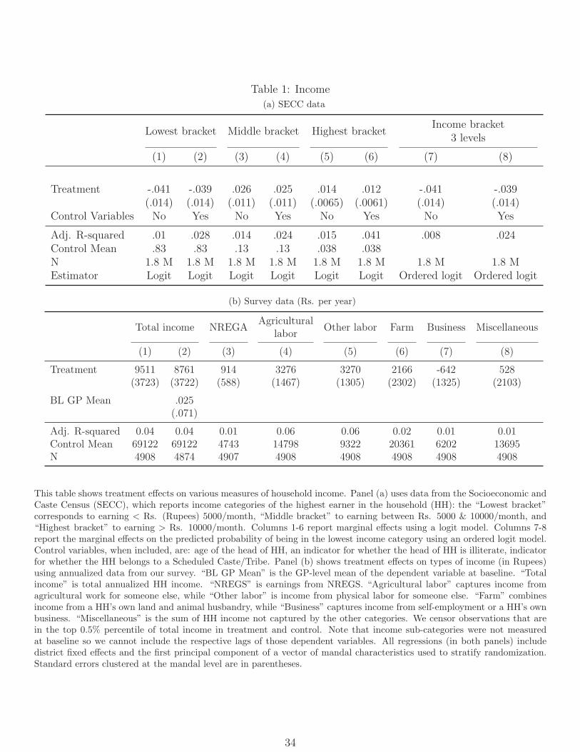
Table 1: Income

(a) SECC data

Lowest bracket Middle bracket Highest bracketIncome bracket

3 levels

(1) (2) (3) (4) (5) (6) (7) (8)

Treatment -.041 -.039 .026 .025 .014 .012 -.041 -.039(.014) (.014) (.011) (.011) (.0065) (.0061) (.014) (.014)

Control Variables No Yes No Yes No Yes No Yes

Adj. R-squared .01 .028 .014 .024 .015 .041 .008 .024Control Mean .83 .83 .13 .13 .038 .038N 1.8 M 1.8 M 1.8 M 1.8 M 1.8 M 1.8 M 1.8 M 1.8 MEstimator Logit Logit Logit Logit Logit Logit Ordered logit Ordered logit

(b) Survey data (Rs. per year)

Total income NREGAAgricultural

laborOther labor Farm Business Miscellaneous

(1) (2) (3) (4) (5) (6) (7) (8)

Treatment 9511 8761 914 3276 3270 2166 -642 528(3723) (3722) (588) (1467) (1305) (2302) (1325) (2103)

BL GP Mean .025(.071)

Adj. R-squared 0.04 0.04 0.01 0.06 0.06 0.02 0.01 0.01Control Mean 69122 69122 4743 14798 9322 20361 6202 13695N 4908 4874 4907 4908 4908 4908 4908 4908

This table shows treatment effects on various measures of household income. Panel (a) uses data from the Socioeconomic andCaste Census (SECC), which reports income categories of the highest earner in the household (HH): the “Lowest bracket”corresponds to earning < Rs. (Rupees) 5000/month, “Middle bracket” to earning between Rs. 5000 & 10000/month, and“Highest bracket” to earning > Rs. 10000/month. Columns 1-6 report marginal effects using a logit model. Columns 7-8report the marginal effects on the predicted probability of being in the lowest income category using an ordered logit model.Control variables, when included, are: age of the head of HH, an indicator for whether the head of HH is illiterate, indicatorfor whether the HH belongs to a Scheduled Caste/Tribe. Panel (b) shows treatment effects on types of income (in Rupees)using annualized data from our survey. “BL GP Mean” is the GP-level mean of the dependent variable at baseline. “Totalincome” is total annualized HH income. “NREGS” is earnings from NREGS. “Agricultural labor” captures income fromagricultural work for someone else, while “Other labor” is income from physical labor for someone else. “Farm” combinesincome from a HH’s own land and animal husbandry, while “Business” captures income from self-employment or a HH’s ownbusiness. “Miscellaneous” is the sum of HH income not captured by the other categories. We censor observations that arein the top 0.5% percentile of total income in treatment and control. Note that income sub-categories were not measuredat baseline so we cannot include the respective lags of those dependent variables. All regressions (in both panels) includedistrict fixed effects and the first principal component of a vector of mandal characteristics used to stratify randomization.Standard errors clustered at the mandal level are in parentheses.

34

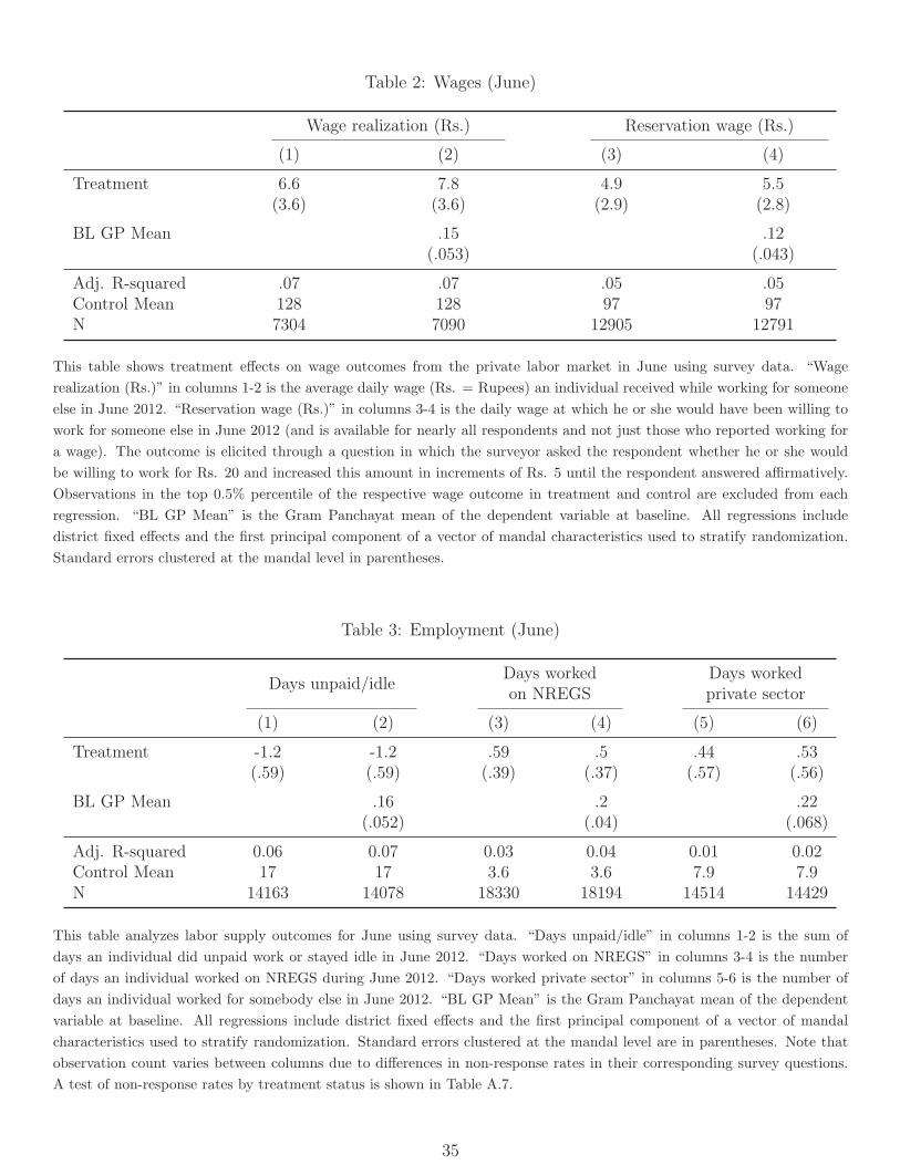
Table 2: Wages (June)

Wage realization (Rs.) Reservation wage (Rs.)

(1) (2) (3) (4)

Treatment 6.6 7.8 4.9 5.5(3.6) (3.6) (2.9) (2.8)

BL GP Mean .15 .12(.053) (.043)

Adj. R-squared .07 .07 .05 .05Control Mean 128 128 97 97N 7304 7090 12905 12791

This table shows treatment effects on wage outcomes from the private labor market in June using survey data. “Wage

realization (Rs.)” in columns 1-2 is the average daily wage (Rs. = Rupees) an individual received while working for someone

else in June 2012. “Reservation wage (Rs.)” in columns 3-4 is the daily wage at which he or she would have been willing to

work for someone else in June 2012 (and is available for nearly all respondents and not just those who reported working for

a wage). The outcome is elicited through a question in which the surveyor asked the respondent whether he or she would

be willing to work for Rs. 20 and increased this amount in increments of Rs. 5 until the respondent answered affirmatively.

Observations in the top 0.5% percentile of the respective wage outcome in treatment and control are excluded from each

regression. “BL GP Mean” is the Gram Panchayat mean of the dependent variable at baseline. All regressions include

district fixed effects and the first principal component of a vector of mandal characteristics used to stratify randomization.

Standard errors clustered at the mandal level in parentheses.

Table 3: Employment (June)

Days unpaid/idleDays workedon NREGS

Days workedprivate sector

(1) (2) (3) (4) (5) (6)

Treatment -1.2 -1.2 .59 .5 .44 .53(.59) (.59) (.39) (.37) (.57) (.56)

BL GP Mean .16 .2 .22(.052) (.04) (.068)

Adj. R-squared 0.06 0.07 0.03 0.04 0.01 0.02Control Mean 17 17 3.6 3.6 7.9 7.9N 14163 14078 18330 18194 14514 14429

This table analyzes labor supply outcomes for June using survey data. “Days unpaid/idle” in columns 1-2 is the sum of

days an individual did unpaid work or stayed idle in June 2012. “Days worked on NREGS” in columns 3-4 is the number

of days an individual worked on NREGS during June 2012. “Days worked private sector” in columns 5-6 is the number of

days an individual worked for somebody else in June 2012. “BL GP Mean” is the Gram Panchayat mean of the dependent

variable at baseline. All regressions include district fixed effects and the first principal component of a vector of mandal

characteristics used to stratify randomization. Standard errors clustered at the mandal level are in parentheses. Note that

observation count varies between columns due to differences in non-response rates in their corresponding survey questions.

A test of non-response rates by treatment status is shown in Table A.7.

35

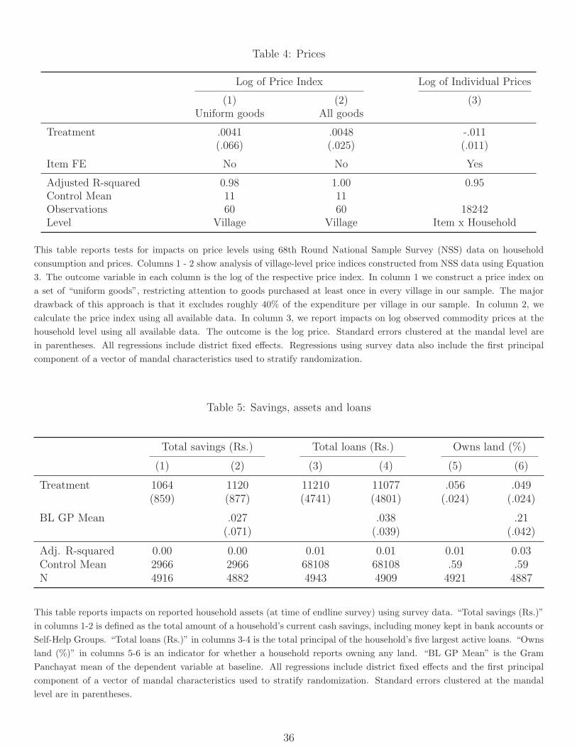
Table 4: Prices

Log of Price Index Log of Individual Prices

(1) (2) (3)Uniform goods All goods

Treatment .0041 .0048 -.011(.066) (.025) (.011)

Item FE No No Yes

Adjusted R-squared 0.98 1.00 0.95Control Mean 11 11Observations 60 60 18242Level Village Village Item x Household

This table reports tests for impacts on price levels using 68th Round National Sample Survey (NSS) data on household

consumption and prices. Columns 1 - 2 show analysis of village-level price indices constructed from NSS data using Equation

3. The outcome variable in each column is the log of the respective price index. In column 1 we construct a price index on

a set of “uniform goods”, restricting attention to goods purchased at least once in every village in our sample. The major

drawback of this approach is that it excludes roughly 40% of the expenditure per village in our sample. In column 2, we

calculate the price index using all available data. In column 3, we report impacts on log observed commodity prices at the

household level using all available data. The outcome is the log price. Standard errors clustered at the mandal level are

in parentheses. All regressions include district fixed effects. Regressions using survey data also include the first principal

component of a vector of mandal characteristics used to stratify randomization.

Table 5: Savings, assets and loans

Total savings (Rs.) Total loans (Rs.) Owns land (%)

(1) (2) (3) (4) (5) (6)

Treatment 1064 1120 11210 11077 .056 .049(859) (877) (4741) (4801) (.024) (.024)

BL GP Mean .027 .038 .21(.071) (.039) (.042)

Adj. R-squared 0.00 0.00 0.01 0.01 0.01 0.03Control Mean 2966 2966 68108 68108 .59 .59N 4916 4882 4943 4909 4921 4887

This table reports impacts on reported household assets (at time of endline survey) using survey data. “Total savings (Rs.)”

in columns 1-2 is defined as the total amount of a household’s current cash savings, including money kept in bank accounts or

Self-Help Groups. “Total loans (Rs.)” in columns 3-4 is the total principal of the household’s five largest active loans. “Owns

land (%)” in columns 5-6 is an indicator for whether a household reports owning any land. “BL GP Mean” is the Gram

Panchayat mean of the dependent variable at baseline. All regressions include district fixed effects and the first principal

component of a vector of mandal characteristics used to stratify randomization. Standard errors clustered at the mandal

level are in parentheses.

36

Table 6: Livestock

Cattle Buffaloes Sheep Goats Pigs Dogs Fowls DucksBackyardPoultry

(1) (2) (3) (4) (5) (6) (7) (8) (9)

Treatment 1261 4671 -35 2473 120 244 8150 209 8381(2463) (1776) (4593) (1877) (116) (132) (4961) (286) (4980)

Adj. R-squared .20 .14 .21 .09 .04 .13 .11 .04 .11Control Mean 11483 9328 33857 10742 275 387 29147 220 29383N 157 157 157 157 157 157 157 157 157

This table reports impacts on livestock headcounts using mandal-level data from the 2012 Livestock Census. Results foranimals with average headcounts greater than 100 in control mandals are included. A Wald test of joint significance rejectsthe null of no impacts (p = 0.01). All regressions include district fixed effects and the first principal component of a vectorof mandal characteristics used to stratify randomization. Robust standard errors are included in parentheses.

37

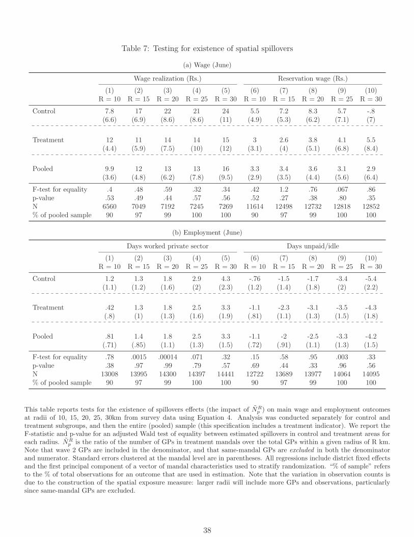
Table 7: Testing for existence of spatial spillovers

(a) Wage (June)

Wage realization (Rs.) Reservation wage (Rs.)

(1) (2) (3) (4) (5) (6) (7) (8) (9) (10)R = 10 R = 15 R = 20 R = 25 R = 30 R = 10 R = 15 R = 20 R = 25 R = 30

Control 7.8 17 22 21 24 5.5 7.2 8.3 5.7 -.8(6.6) (6.9) (8.6) (8.6) (11) (4.9) (5.3) (6.2) (7.1) (7)

Treatment 12 11 14 14 15 3 2.6 3.8 4.1 5.5(4.4) (5.9) (7.5) (10) (12) (3.1) (4) (5.1) (6.8) (8.4)

Pooled 9.9 12 13 13 16 3.3 3.4 3.6 3.1 2.9(3.6) (4.8) (6.2) (7.8) (9.5) (2.9) (3.5) (4.4) (5.6) (6.4)

F-test for equality .4 .48 .59 .32 .34 .42 1.2 .76 .067 .86p-value .53 .49 .44 .57 .56 .52 .27 .38 .80 .35N 6560 7049 7192 7245 7269 11614 12498 12732 12818 12852% of pooled sample 90 97 99 100 100 90 97 99 100 100

(b) Employment (June)

Days worked private sector Days unpaid/idle

(1) (2) (3) (4) (5) (6) (7) (8) (9) (10)R = 10 R = 15 R = 20 R = 25 R = 30 R = 10 R = 15 R = 20 R = 25 R = 30

Control 1.2 1.3 1.8 2.9 4.3 -.76 -1.5 -1.7 -3.4 -5.4(1.1) (1.2) (1.6) (2) (2.3) (1.2) (1.4) (1.8) (2) (2.2)

Treatment .42 1.3 1.8 2.5 3.3 -1.1 -2.3 -3.1 -3.5 -4.3(.8) (1) (1.3) (1.6) (1.9) (.81) (1.1) (1.3) (1.5) (1.8)

Pooled .81 1.4 1.8 2.5 3.3 -1.1 -2 -2.5 -3.3 -4.2(.71) (.85) (1.1) (1.3) (1.5) (.72) (.91) (1.1) (1.3) (1.5)

F-test for equality .78 .0015 .00014 .071 .32 .15 .58 .95 .003 .33p-value .38 .97 .99 .79 .57 .69 .44 .33 .96 .56N 13008 13995 14300 14397 14441 12722 13689 13977 14064 14095% of pooled sample 90 97 99 100 100 90 97 99 100 100

This table reports tests for the existence of spillovers effects (the impact of NRp ) on main wage and employment outcomes

at radii of 10, 15, 20, 25, 30km from survey data using Equation 4. Analysis was conducted separately for control andtreatment subgroups, and then the entire (pooled) sample (this specification includes a treatment indicator). We report theF-statistic and p-value for an adjusted Wald test of equality between estimated spillovers in control and treatment areas foreach radius. NR

p is the ratio of the number of GPs in treatment mandals over the total GPs within a given radius of R km.Note that wave 2 GPs are included in the denominator, and that same-mandal GPs are excluded in both the denominatorand numerator. Standard errors clustered at the mandal level are in parentheses. All regressions include district fixed effectsand the first principal component of a vector of mandal characteristics used to stratify randomization. “% of sample” refersto the % of total observations for an outcome that are used in estimation. Note that the variation in observation counts isdue to the construction of the spatial exposure measure: larger radii will include more GPs and observations, particularlysince same-mandal GPs are excluded.

38

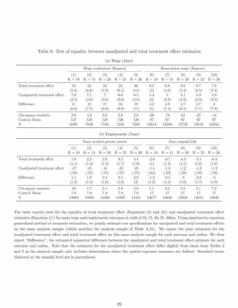
Table 8: Test of equality between unadjusted and total treatment effect estimates

(a) Wage (June)

Wage realization (Rupees) Reservation wage (Rupees)

(1) (2) (3) (4) (5) (6) (7) (8) (9) (10)R = 10 R = 15 R = 20 R = 25 R = 30 R = 10 R = 15 R = 20 R = 25 R = 30

Total treatment effect 18 23 24 22 26 8.5 9.8 9.9 8.7 7.8(5.6) (6.6) (7.8) (9.1) (11) (4) (4.6) (5.4) (6.5) (7.4)

Unadjusted treatment effect 7.6 7.1 7 6.6 6.5 4.3 5 5.1 4.9 4.9(3.5) (3.6) (3.6) (3.6) (3.6) (3) (2.9) (2.9) (2.9) (2.9)

Difference 11 15 17 16 19 4.2 4.8 4.7 3.7 3(6.6) (7.5) (8.6) (9.8) (11) (5) (5.4) (6.1) (7.1) (7.9)

Chi-square statistic 2.6 4.3 3.8 2.6 2.9 .68 .78 .61 .27 .14Control Mean 127 128 128 128 128 97 97 97 97 97N 6560 7049 7192 7245 7269 11614 12498 12732 12818 12852

(b) Employment (June)

Days worked private sector Days unpaid/idle

(1) (2) (3) (4) (5) (6) (7) (8) (9) (10)R = 10 R = 15 R = 20 R = 25 R = 30 R = 10 R = 15 R = 20 R = 25 R = 30

Total treatment effect 1.6 2.3 2.8 3.5 4.4 -2.6 -3.7 -4.3 -5.1 -6.3(1.1) (1.3) (1.5) (1.7) (1.9) (1) (1.3) (1.5) (1.6) (1.8)

Unadjusted treatment effect .47 .45 .44 .45 .45 -1.4 -1.3 -1.2 -1.3 -1.3(.59) (.57) (.57) (.57) (.57) (.63) (.59) (.59) (.59) (.59)

Difference 1.1 1.9 2.4 3.1 3.9 -1.2 -2.5 -3 -3.9 -5(1.2) (1.4) (1.6) (1.8) (2) (1.2) (1.4) (1.6) (1.7) (1.9)

Chi-square statistic .84 1.7 2.1 2.9 3.9 1.1 3.2 3.5 5.1 7.2Control Mean 7.8 7.9 7.9 7.9 7.9 17 17 17 17 17N 13008 13995 14300 14397 14441 12677 13640 13928 14015 14046

The table reports tests for the equality of total treatment effect (Equations (5) and (6)) and unadjusted treatment effect

estimates (Equation (1)) for main wage and employment outcomes at radii of 10, 15, 20, 25, 30km. Using equation-by-equation

generalized method of moments estimation, we jointly estimate our specifications for unadjusted and total treatment effects

on the same analysis sample (which matches the analysis sample of Table A.21). We report the joint estimates for the

unadjusted treatment effect and total treatment effect on this same analysis sample for each outcome and radius. We then

report “Difference”, the estimated numerical difference between the unadjusted and total treatment effect estimate for each

outcome and radius. Note that the estimates for the unadjusted treatment effect differ slightly from those from Tables 2

and 3 as the analysis sample only includes observations where the spatial exposure measures are defined. Standard errors

clustered at the mandal level are in parentheses.

39

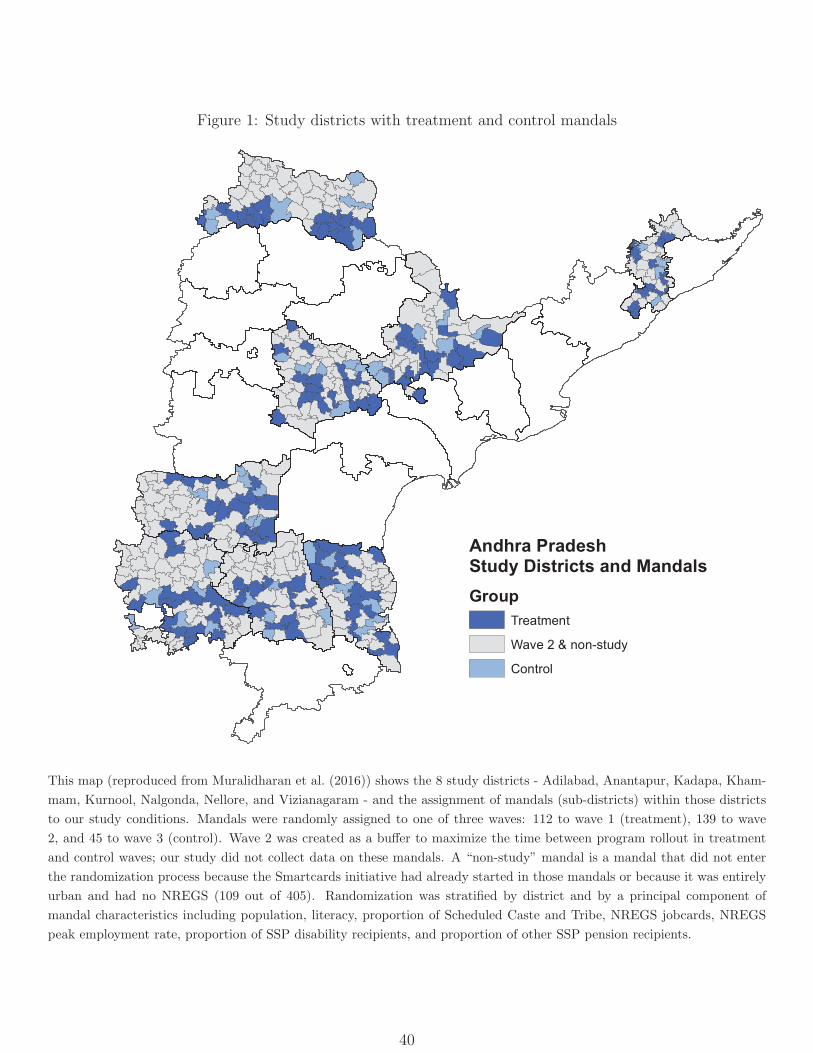
Figure 1: Study districts with treatment and control mandals

!"#$%&'(%&#)*$+,-#.'/0*,%01,*'&"#'2&"#&3*

4%5-6

!"#$%&#'%

($)#*+*,*'-'./%012

3-'%"-4

This map (reproduced from Muralidharan et al. (2016)) shows the 8 study districts - Adilabad, Anantapur, Kadapa, Kham-

mam, Kurnool, Nalgonda, Nellore, and Vizianagaram - and the assignment of mandals (sub-districts) within those districts

to our study conditions. Mandals were randomly assigned to one of three waves: 112 to wave 1 (treatment), 139 to wave

2, and 45 to wave 3 (control). Wave 2 was created as a buffer to maximize the time between program rollout in treatment

and control waves; our study did not collect data on these mandals. A “non-study” mandal is a mandal that did not enter

the randomization process because the Smartcards initiative had already started in those mandals or because it was entirely

urban and had no NREGS (109 out of 405). Randomization was stratified by district and by a principal component of

mandal characteristics including population, literacy, proportion of Scheduled Caste and Tribe, NREGS jobcards, NREGS

peak employment rate, proportion of SSP disability recipients, and proportion of other SSP pension recipients.

40

Figure 2: Timeline of endline survey reference periods

!"#$%% &'($%% )*+$%% ,-.$%% /'*$%% 012$%3 4'5$%3 617$%3 !(7$%3 618$%3 0"2$%3 0"9$%3 !"#$%3 &'($%3

%$8'17$7'*199$

$%$

:-2+;$

7'*199$

&"7.'8$('7<-=>$

!"#"?+$@$

&'(+':5'7$

6,&$3A%B$

7'C'7'2*'$('7<-=$

0"2'$

7'*199$

1D$

5D$

*D$

=D$

CDEE$F;<7=$(17+8$=1+1$?-"7*'?$

'DE$F<:'$-C$?"7.'8$

This figure shows the timeline of reference periods from our endline survey, which was conducted August - September 2012.a) The 1 year recall period corresponds to questions about household earnings/income and longer-term expenses.b) “MNS 2016 reference period” refers to the 7-week reference period from May 18 - July 14, 2012 used in outcomes for MNS2016, including NREGS work and leakage.c) The June recall period corresponds to private sector wage outcomes and employment outcomes. To construct NREGSoutcomes for June (e.g. days worked on NREGS), we use data from weeks that overlap with month of June, allocating timefor the first and last week in proportion to the number of days overlapping in June.d) The 1 month reference period corresponds to questions on shorter-term expenses.e)* Respondents were asked about savings, assets (including landholdings), and loans at time of survey.

f)** Third party data sources include the 2011- 2012 Socio-Economic and Caste Census (SECC), the 2012 Livestock Census,

the 68th Round of the National Sample Survey, and the AP District Statistical Handbook data. The 2011-2012 SECC was

conducted in rural AP during 2012. The data contains household-level data on earnings (in month up to time of survey)

and land holdings (at time of survey). The 2012 Livestock Census was conducted with October 15, 2012 as the reference

date. The data contains mandal-level livestock headcounts by livestock category. The 68th Round of the National Sample

survey was conducted in AP between July 2011 - June 2012. The data contains household-level expenditure and number

of units purchased for a wide variety of goods (in month up to time of survey). The District Statistical Handbooks (DSH)

data, which is published each year by the Andhra Pradesh Directorate of Economics, is from 2012-2013. We use the DSH a

for mandal-level data on land utilization and irrigation.

41

Figure 3: Constructing measures of exposure to spatial spillovers

R

p

R

p

This figure illustrates the construction of measures of spatial exposure to treatment for a given panchayat p (denoted by

the black X symbol) and radius R in a treatment mandal. Dark (light) blue dots represent treatment (control) panchayats;

black lines represent mandal borders. As in the text, NRp is the fraction of GPs within a radius R of panchayat p which were

assigned to treatment. NRp is the fraction of GPs within a radius R of panchayat p and within a different mandal (excluding

GPs in the same mandal from both the numerator and denominator) which were assigned to treatment. The entire sample

of census GP in mandals that were used in randomization are included. In the figure above, these measures are NRp = 5

11

and NRp = 1

3.

Figure 4: Conceptual illustration of Total Treatment Effect (TTE) after adjusting for spillovers

!"#$%&'()*+,-.&"/(0"*#1*2(

3#,*/(

4( 5(

!"##$ 6007(

((

0"*#18*'1(

9&'1"&:(

;0(

This figure corresponds to Equations (5) and (6) in the text and illustrates how an outcome (say wages) is a function of

both the treatment status of one’s own village as well as the fraction of treated neighbors. βT on the y-axis represents the

effect of a village being treated when none of its neighbors are treated. Moving along the x-axis corresponds to increasing

the fraction of treated neighbors, and the corresponding changes in wages are represented by light and dark blue solid lines

(we allow the gradient to vary by a village’s own treatment status as in Equation (5)). Vertical dotted lines represent mean

exposure of treatment (dark blue) and control (light blue) groups. The bracket range on the x-axis, labelled xITT , represents

the mean difference in the fraction of treated neighbors between treatment and control villages, which is positive but less

than 1 (as seen in Panel (a) of Figure A.8). The gray bracket range, labelled yITT , represents the unadjusted treatment

effect. The black bracket range, labelled yTTE , represents the total treatment effect that a policy maker would care about

and corresponds to the estimate in Equation (6).

42

For Online Publication: Appendix

This section provides further background on the NREGS program, including the status quo

payments system, as well as the the changes introduced by Smartcards and subsequent

impacts on the payments process and leakage.

A Further details on NREGS

NREGS refers collectively to state-level employment schemes mandated by the National

Rural Employment Guarantee Act (NREGA) of 2005. The Act guarantees one hundred

days of paid employment to any rural household in India, with no eligibility requirement for

obtaining work. After beneficiaries obtain a jobcard - a household level document that lists

adult members, with pages assigned to record details of work done, payment owed, dates of

employment, etc - they are meant to approach local level officials for employment, and work

must be provided within two weeks and within a five kilometer radius of the beneficiary’s

residence. In practice, obtaining a jobcard is not a significant hurdle, and almost anyone

who might conceivably work on the program has a jobcard (49.5% of rural households in

Andhra Pradesh according to National Sample Survey data). The greater hurdle is obtaining

employment, which is available when there is a project working in the village, with greatest

availability during the slack labor seasons of April, May and June.

Given the seasonality, the 100 day limit is rarely a binding constraint, particularly since

practical work-arounds (obtaining multiple jobcards per household) are possible. In 2009-10

the average number of days worked was 38 (mean is 30), according to Imbert and Papp

(2015), with participants moving in and out of the program at high frequency. Altogether,

this means that 32.1% of all households (and 64.8% of households with jobcards) in Andhra

Pradesh worked on NREGS at some point during 2009. This work involves (for the most part)

manual labor paid at minimum wages that are set at the state level. In Andhra Pradesh

most wages are piece rates, set to allow workers to attain the daily minimum wage with

roughly a day’s worth of effort. Projects, chosen in advance via consultation with villagers

at a village-wide meeting (the “Gram Sabha”) and mandal and district officials, generally

involve public infrastructure such as road construction, clearing fields for agricultural use,

and irrigation earthworks.

Project management is delegated for the most part to local village officials, including

elected village chiefs (Sarpanch) and a variety of appointed officials (Field Assistants, Tech-

nical Assistants, NREGS Village Workers, etc). These officials record attendance and output,

creating paper “muster rolls” which are digitized at the sub-district level. These digitized

records upon approval trigger the release of funds to pay workers.

43

A.1 Smartcard-introduced Changes in Payments

The Smartcards system was introduced in Andhra Pradesh in 2006, and while rollout in

treatment areas in our study districts began in 2010. The payments system was based on

electronic benefit transfers into special “no-frills” bank accounts tied to individual beneficia-

ries, and biometric authentication of beneficiaries before withdrawing these transfers. Figure

A.11 shows the status quo payment system and the changes introduced by Smartcards.

In the status quo, money was transferred electronically from the State government to the

district to the mandal, and from there cash moved on to the local post-office. Beneficiaries

either traveled to the local post-office to get payments themselves, or, more commonly, simply

handed over jobcards to local NREGS officials (Sarpanch, Field Assistant) and collected

money from them in the village (since most post offices are far from local habitations).

There was no formal authentication procedure required, which allowed the informal practice

to continue.

In the Smartcards system, money was transferred electronically from the State government

to private and public sector banks; banks worked with Technology Service Providers (TSPs)

to manage last-mile delivery and authentication. Together, the bank and TSP received 2% of

every transaction in villages in which they handled the payment system. Bank/TSP pairings

competitively bid to manage transactions in every district. Last-mile delivery of cash was

done by village level Customer Service Providers (CSPs), who were hired by TSPs as per the

criteria laid down by the government. CSPs typically authenticated fingerprints and made

payments locally at a central village location.

Payments were deposited into no-frills accounts for beneficiaries who had enrolled for

Smartcards. These accounts were not maintained on the “core banking server”, but rather

on small local Point-of-Service (PoS) devices managed by the CSPs. Since there was no real-

time connectivity on these devices and no linkage with central bank servers, beneficiaries

could only access their accounts through CSPs; they had no ability to go to a bank branch

or an ATM to access this account. Beneficiaries therefore typically did not make deposits

into accounts, and would not be able to even figure out whether there was a balance without

contacting the CSP. Although in theory they could simply not claim payment if they wanted

to leave a balance in the account, in practice only 0.3% of respondents claimed to leave

money in the account; moreover, only 29% of beneficiaries who experienced the system said

that they trusted the Smartcards system enough to deposit money into their Smartcard

accounts if they could. In Nalgonda district, where the winning bid was actually from the

post office, there were no bank accounts at all.

Compared to other documents that the household would have had (e.g. jobcard that

was required in order to obtain Smartcard, voter ID card, etc), the Smartcard’s value as

an identity document was limited. Unlike the national Unique ID (Aadhaar), Smartcards

were not de-duplicated at the national level, and were therefore not legally admissible as

44

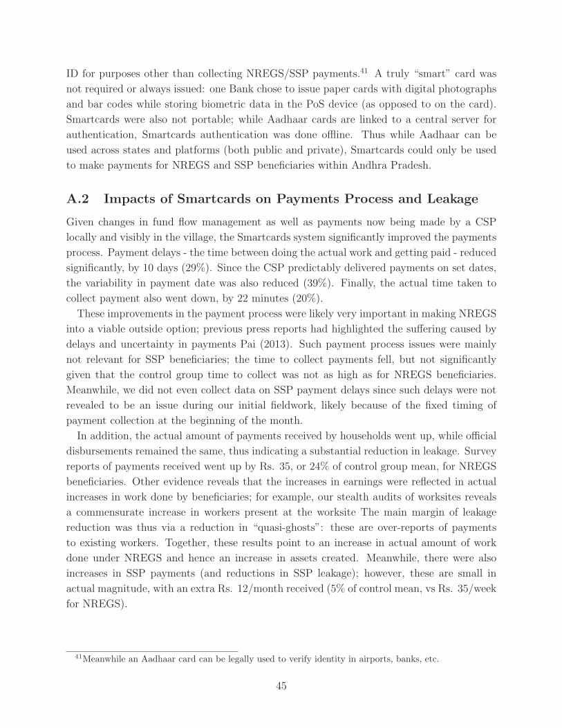
ID for purposes other than collecting NREGS/SSP payments.41 A truly “smart” card was

not required or always issued: one Bank chose to issue paper cards with digital photographs

and bar codes while storing biometric data in the PoS device (as opposed to on the card).

Smartcards were also not portable; while Aadhaar cards are linked to a central server for

authentication, Smartcards authentication was done offline. Thus while Aadhaar can be

used across states and platforms (both public and private), Smartcards could only be used

to make payments for NREGS and SSP beneficiaries within Andhra Pradesh.

A.2 Impacts of Smartcards on Payments Process and Leakage

Given changes in fund flow management as well as payments now being made by a CSP

locally and visibly in the village, the Smartcards system significantly improved the payments

process. Payment delays - the time between doing the actual work and getting paid - reduced

significantly, by 10 days (29%). Since the CSP predictably delivered payments on set dates,

the variability in payment date was also reduced (39%). Finally, the actual time taken to

collect payment also went down, by 22 minutes (20%).

These improvements in the payment process were likely very important in making NREGS

into a viable outside option; previous press reports had highlighted the suffering caused by

delays and uncertainty in payments Pai (2013). Such payment process issues were mainly

not relevant for SSP beneficiaries; the time to collect payments fell, but not significantly

given that the control group time to collect was not as high as for NREGS beneficiaries.

Meanwhile, we did not even collect data on SSP payment delays since such delays were not

revealed to be an issue during our initial fieldwork, likely because of the fixed timing of

payment collection at the beginning of the month.

In addition, the actual amount of payments received by households went up, while official

disbursements remained the same, thus indicating a substantial reduction in leakage. Survey

reports of payments received went up by Rs. 35, or 24% of control group mean, for NREGS

beneficiaries. Other evidence reveals that the increases in earnings were reflected in actual

increases in work done by beneficiaries; for example, our stealth audits of worksites reveals

a commensurate increase in workers present at the worksite The main margin of leakage

reduction was thus via a reduction in “quasi-ghosts”: these are over-reports of payments

to existing workers. Together, these results point to an increase in actual amount of work

done under NREGS and hence an increase in assets created. Meanwhile, there were also

increases in SSP payments (and reductions in SSP leakage); however, these are small in

actual magnitude, with an extra Rs. 12/month received (5% of control mean, vs Rs. 35/week

for NREGS).

41Meanwhile an Aadhaar card can be legally used to verify identity in airports, banks, etc.

45

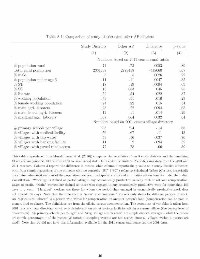
Table A.1: Comparison of study districts and other AP districts

Study Districts Other AP Difference p-value

(1) (2) (3) (4)

Numbers based on 2011 census rural totals

% population rural .74 .73 .0053 .89Total rural population 2331398 2779458 -448060 .067% male .5 .5 .0026 .22% population under age 6 .11 .11 .0047 .35% ST .18 .19 -.0094 .69% SC .13 .083 .045 .25% literate .52 .54 -.022 .37% working population .53 .51 .016 .23% female working population .24 .22 .015 .34% main agri. laborers .23 .22 .0094 .65% main female agri. laborers .12 .1 .014 .29% marginal agri. laborers .067 .064 .0032 .64

Numbers based on 2001 census village directory

# primary schools per village 2.3 2.4 -.14 .68% villages with medical facility .56 .67 -.11 .13% villages with tap water .53 .56 -.037 .76% villages with banking facility .11 .2 -.094 .32% villages with paved road access .72 .78 -.06 .39

This table (reproduced from Muralidharan et al. (2016)) compares characteristics of our 8 study districts and the remaining

13 non-urban (since NREGS is restricted to rural areas) districts in erstwhile Andhra Pradesh, using data from the 2001 and

2011 censuses. Column 3 reports the difference in means, while column 4 reports the p-value on a study district indicator,

both from simple regressions of the outcome with no controls. “ST” (“SC”) refers to Scheduled Tribes (Castes), historically

discriminated-against sections of the population now accorded special status and affirmative action benefits under the Indian

Constitution. “Working” is defined as participating in any economically productive activity with or without compensation,

wages or profit. “Main” workers are defined as those who engaged in any economically productive work for more than 183

days in a year. “Marginal” workers are those for whom the period they engaged in economically productive work does

not exceed 182 days. Note that the difference in “main” and “marginal” workers only stems for different periods of work.

An “agricultural laborer” is a person who works for compensation on another person’s land (compensation can be paid in

money, kind or share). The definitions are from the official census documentation. The second set of variables is taken from

2001 census village directory which records information about various facilities within a census village (the census level of

observation). “# primary schools per village” and “Avg. village size in acres” are simple district averages - while the others

are simple percentages - of the respective variable (sampling weights are not needed since all villages within a district are

used). Note that we did not have this information available for the 2011 census and hence use the 2001 data.

46

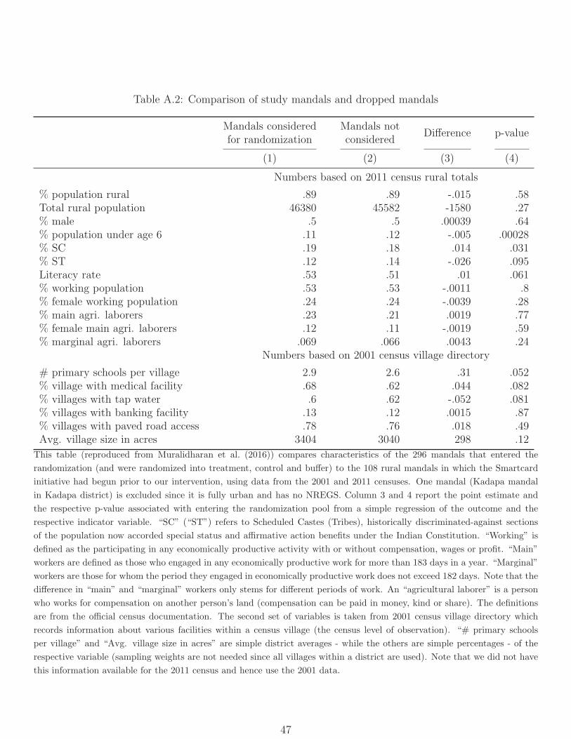
Table A.2: Comparison of study mandals and dropped mandals

Mandals consideredfor randomization

Mandals notconsidered

Difference p-value

(1) (2) (3) (4)

Numbers based on 2011 census rural totals

% population rural .89 .89 -.015 .58Total rural population 46380 45582 -1580 .27% male .5 .5 .00039 .64% population under age 6 .11 .12 -.005 .00028% SC .19 .18 .014 .031% ST .12 .14 -.026 .095Literacy rate .53 .51 .01 .061% working population .53 .53 -.0011 .8% female working population .24 .24 -.0039 .28% main agri. laborers .23 .21 .0019 .77% female main agri. laborers .12 .11 -.0019 .59% marginal agri. laborers .069 .066 .0043 .24

Numbers based on 2001 census village directory

# primary schools per village 2.9 2.6 .31 .052% village with medical facility .68 .62 .044 .082% villages with tap water .6 .62 -.052 .081% villages with banking facility .13 .12 .0015 .87% villages with paved road access .78 .76 .018 .49Avg. village size in acres 3404 3040 298 .12

This table (reproduced from Muralidharan et al. (2016)) compares characteristics of the 296 mandals that entered the

randomization (and were randomized into treatment, control and buffer) to the 108 rural mandals in which the Smartcard

initiative had begun prior to our intervention, using data from the 2001 and 2011 censuses. One mandal (Kadapa mandal

in Kadapa district) is excluded since it is fully urban and has no NREGS. Column 3 and 4 report the point estimate and

the respective p-value associated with entering the randomization pool from a simple regression of the outcome and the

respective indicator variable. “SC” (“ST”) refers to Scheduled Castes (Tribes), historically discriminated-against sections

of the population now accorded special status and affirmative action benefits under the Indian Constitution. “Working” is

defined as the participating in any economically productive activity with or without compensation, wages or profit. “Main”

workers are defined as those who engaged in any economically productive work for more than 183 days in a year. “Marginal”

workers are those for whom the period they engaged in economically productive work does not exceed 182 days. Note that the

difference in “main” and “marginal” workers only stems for different periods of work. An “agricultural laborer” is a person

who works for compensation on another person’s land (compensation can be paid in money, kind or share). The definitions

are from the official census documentation. The second set of variables is taken from 2001 census village directory which

records information about various facilities within a census village (the census level of observation). “# primary schools

per village” and “Avg. village size in acres” are simple district averages - while the others are simple percentages - of the

respective variable (sampling weights are not needed since all villages within a district are used). Note that we did not have

this information available for the 2011 census and hence use the 2001 data.

47

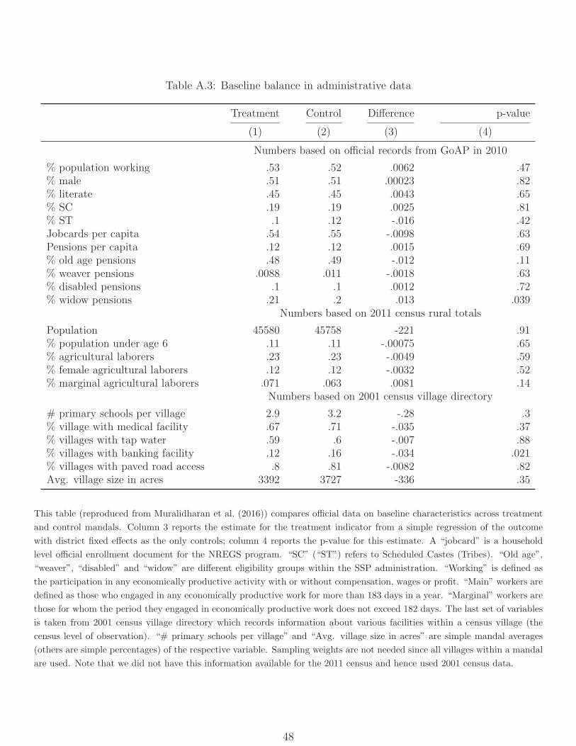
Table A.3: Baseline balance in administrative data

Treatment Control Difference p-value

(1) (2) (3) (4)

Numbers based on official records from GoAP in 2010

% population working .53 .52 .0062 .47% male .51 .51 .00023 .82% literate .45 .45 .0043 .65% SC .19 .19 .0025 .81% ST .1 .12 -.016 .42Jobcards per capita .54 .55 -.0098 .63Pensions per capita .12 .12 .0015 .69% old age pensions .48 .49 -.012 .11% weaver pensions .0088 .011 -.0018 .63% disabled pensions .1 .1 .0012 .72% widow pensions .21 .2 .013 .039

Numbers based on 2011 census rural totals

Population 45580 45758 -221 .91% population under age 6 .11 .11 -.00075 .65% agricultural laborers .23 .23 -.0049 .59% female agricultural laborers .12 .12 -.0032 .52% marginal agricultural laborers .071 .063 .0081 .14

Numbers based on 2001 census village directory

# primary schools per village 2.9 3.2 -.28 .3% village with medical facility .67 .71 -.035 .37% villages with tap water .59 .6 -.007 .88% villages with banking facility .12 .16 -.034 .021% villages with paved road access .8 .81 -.0082 .82Avg. village size in acres 3392 3727 -336 .35

This table (reproduced from Muralidharan et al. (2016)) compares official data on baseline characteristics across treatment

and control mandals. Column 3 reports the estimate for the treatment indicator from a simple regression of the outcome

with district fixed effects as the only controls; column 4 reports the p-value for this estimate. A “jobcard” is a household

level official enrollment document for the NREGS program. “SC” (“ST”) refers to Scheduled Castes (Tribes). “Old age”,

“weaver”, “disabled” and “widow” are different eligibility groups within the SSP administration. “Working” is defined as

the participation in any economically productive activity with or without compensation, wages or profit. “Main” workers are

defined as those who engaged in any economically productive work for more than 183 days in a year. “Marginal” workers are

those for whom the period they engaged in economically productive work does not exceed 182 days. The last set of variables

is taken from 2001 census village directory which records information about various facilities within a census village (the

census level of observation). “# primary schools per village” and “Avg. village size in acres” are simple mandal averages

(others are simple percentages) of the respective variable. Sampling weights are not needed since all villages within a mandal

are used. Note that we did not have this information available for the 2011 census and hence used 2001 census data.

48

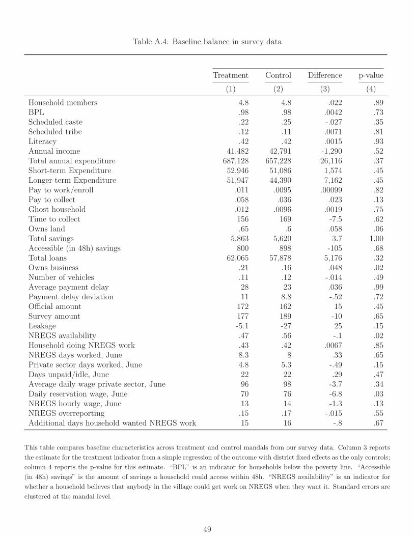
Table A.4: Baseline balance in survey data

Treatment Control Difference p-value

(1) (2) (3) (4)

Household members 4.8 4.8 .022 .89BPL .98 .98 .0042 .73Scheduled caste .22 .25 -.027 .35Scheduled tribe .12 .11 .0071 .81Literacy .42 .42 .0015 .93Annual income 41,482 42,791 -1,290 .52Total annual expenditure 687,128 657,228 26,116 .37Short-term Expenditure 52,946 51,086 1,574 .45Longer-term Expenditure 51,947 44,390 7,162 .45Pay to work/enroll .011 .0095 .00099 .82Pay to collect .058 .036 .023 .13Ghost household .012 .0096 .0019 .75Time to collect 156 169 -7.5 .62Owns land .65 .6 .058 .06Total savings 5,863 5,620 3.7 1.00Accessible (in 48h) savings 800 898 -105 .68Total loans 62,065 57,878 5,176 .32Owns business .21 .16 .048 .02Number of vehicles .11 .12 -.014 .49Average payment delay 28 23 .036 .99Payment delay deviation 11 8.8 -.52 .72Official amount 172 162 15 .45Survey amount 177 189 -10 .65Leakage -5.1 -27 25 .15NREGS availability .47 .56 -.1 .02Household doing NREGS work .43 .42 .0067 .85NREGS days worked, June 8.3 8 .33 .65Private sector days worked, June 4.8 5.3 -.49 .15Days unpaid/idle, June 22 22 .29 .47Average daily wage private sector, June 96 98 -3.7 .34Daily reservation wage, June 70 76 -6.8 .03NREGS hourly wage, June 13 14 -1.3 .13NREGS overreporting .15 .17 -.015 .55Additional days household wanted NREGS work 15 16 -.8 .67

This table compares baseline characteristics across treatment and control mandals from our survey data. Column 3 reports

the estimate for the treatment indicator from a simple regression of the outcome with district fixed effects as the only controls;

column 4 reports the p-value for this estimate. “BPL” is an indicator for households below the poverty line. “Accessible

(in 48h) savings” is the amount of savings a household could access within 48h. “NREGS availability” is an indicator for

whether a household believes that anybody in the village could get work on NREGS when they want it. Standard errors are

clustered at the mandal level.

49

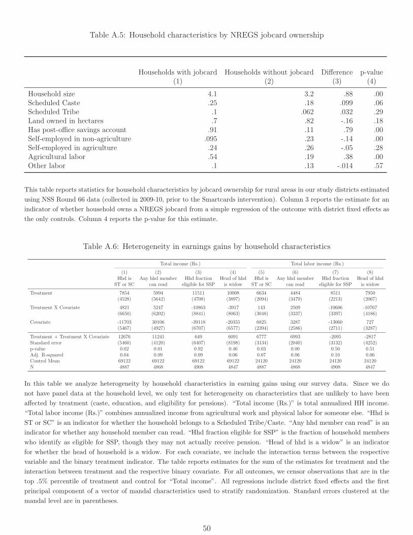
Table A.5: Household characteristics by NREGS jobcard ownership

Households with jobcard Households without jobcard Difference p-value(1) (2) (3) (4)

Household size 4.1 3.2 .88 .00Scheduled Caste .25 .18 .099 .06Scheduled Tribe .1 .062 .032 .29Land owned in hectares .7 .82 -.16 .18Has post-office savings account .91 .11 .79 .00Self-employed in non-agriculture .095 .23 -.14 .00Self-employed in agriculture .24 .26 -.05 .28Agricultural labor .54 .19 .38 .00Other labor .1 .13 -.014 .57

This table reports statistics for household characteristics by jobcard ownership for rural areas in our study districts estimated

using NSS Round 66 data (collected in 2009-10, prior to the Smartcards intervention). Column 3 reports the estimate for an

indicator of whether household owns a NREGS jobcard from a simple regression of the outcome with district fixed effects as

the only controls. Column 4 reports the p-value for this estimate.

Table A.6: Heterogeneity in earnings gains by household characteristics

Total income (Rs.) Total labor income (Rs.)

(1) (2) (3) (4) (5) (6) (7) (8)Hhd is

ST or SCAny hhd member

can readHhd fraction

eligible for SSPHead of hhdis widow

Hhd isST or SC

Any hhd membercan read

Hhd fractioneligible for SSP

Head of hhdis widow

Treatment 7854 5994 11511 10008 6634 4484 8511 7950(4528) (5642) (4708) (3897) (2094) (3479) (2213) (2067)

Treatment X Covariate 4821 5247 -10863 -3917 143 2509 -10606 -10767(6650) (6202) (8841) (8063) (3048) (3337) (3397) (4186)

Covariate -11703 30106 -39118 -20355 6825 3287 -13060 727(5467) (4927) (6707) (6577) (2394) (2586) (2711) (3287)

Treatment + Treatment X Covariate 12676 11241 649 6091 6777 6993 -2095 -2817Standard error (5460) (4120) (6407) (8198) (3134) (2040) (3132) (4252)p-value 0.02 0.01 0.92 0.46 0.03 0.00 0.50 0.51Adj. R-squared 0.04 0.09 0.09 0.06 0.07 0.06 0.10 0.06Control Mean 69122 69122 69122 69122 24120 24120 24120 24120N 4887 4868 4908 4847 4887 4868 4908 4847

In this table we analyze heterogeneity by household characteristics in earning gains using our survey data. Since we do

not have panel data at the household level, we only test for heterogeneity on characteristics that are unlikely to have been

affected by treatment (caste, education, and eligibility for pensions). “Total income (Rs.)” is total annualized HH income.

“Total labor income (Rs.)” combines annualized income from agricultural work and physical labor for someone else. “Hhd is

ST or SC” is an indicator for whether the household belongs to a Scheduled Tribe/Caste. “Any hhd member can read” is an

indicator for whether any household member can read. “Hhd fraction eligible for SSP” is the fraction of household members

who identify as eligible for SSP, though they may not actually receive pension. “Head of hhd is a widow” is an indicator

for whether the head of household is a widow. For each covariate, we include the interaction terms between the respective

variable and the binary treatment indicator. The table reports estimates for the sum of the estimates for treatment and the

interaction between treatment and the respective binary covariate. For all outcomes, we censor observations that are in the

top .5% percentile of treatment and control for “Total income”. All regressions include district fixed effects and the first

principal component of a vector of mandal characteristics used to stratify randomization. Standard errors clustered at the

mandal level are in parentheses.

50

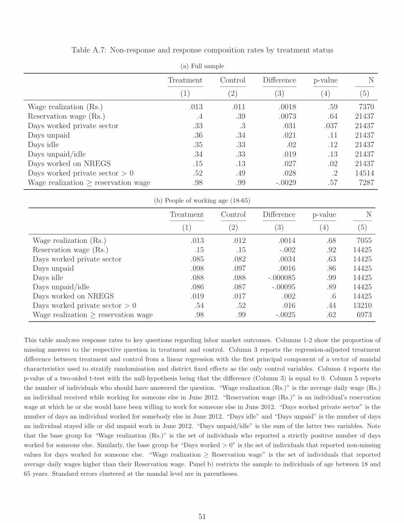
Table A.7: Non-response and response composition rates by treatment status

(a) Full sample

Treatment Control Difference p-value N

(1) (2) (3) (4) (5)

Wage realization (Rs.) .013 .011 .0018 .59 7370Reservation wage (Rs.) .4 .39 .0073 .64 21437Days worked private sector .33 .3 .031 .037 21437Days unpaid .36 .34 .021 .11 21437Days idle .35 .33 .02 .12 21437Days unpaid/idle .34 .33 .019 .13 21437Days worked on NREGS .15 .13 .027 .02 21437Days worked private sector > 0 .52 .49 .028 .2 14514Wage realization ≥ reservation wage .98 .99 -.0029 .57 7287

(b) People of working age (18-65)

Treatment Control Difference p-value N

(1) (2) (3) (4) (5)

Wage realization (Rs.) .013 .012 .0014 .68 7055Reservation wage (Rs.) .15 .15 -.002 .92 14425Days worked private sector .085 .082 .0034 .63 14425Days unpaid .098 .097 .0016 .86 14425Days idle .088 .088 -.000085 .99 14425Days unpaid/idle .086 .087 -.00095 .89 14425Days worked on NREGS .019 .017 .002 .6 14425Days worked private sector > 0 .54 .52 .016 .44 13210Wage realization ≥ reservation wage .98 .99 -.0025 .62 6973

This table analyzes response rates to key questions regarding labor market outcomes. Columns 1-2 show the proportion of

missing answers to the respective question in treatment and control. Column 3 reports the regression-adjusted treatment

difference between treatment and control from a linear regression with the first principal component of a vector of mandal

characteristics used to stratify randomization and district fixed effects as the only control variables. Column 4 reports the

p-value of a two-sided t-test with the null-hypothesis being that the difference (Column 3) is equal to 0. Column 5 reports

the number of individuals who should have answered the question. “Wage realization (Rs.)” is the average daily wage (Rs.)

an individual received while working for someone else in June 2012. “Reservation wage (Rs.)” is an individual’s reservation

wage at which he or she would have been willing to work for someone else in June 2012. “Days worked private sector” is the

number of days an individual worked for somebody else in June 2012. “Days idle” and “Days unpaid” is the number of days

an individual stayed idle or did unpaid work in June 2012. “Days unpaid/idle” is the sum of the latter two variables. Note

that the base group for “Wage realization (Rs.)” is the set of individuals who reported a strictly positive number of days

worked for someone else. Similarly, the base group for “Days worked > 0” is the set of individuals that reported non-missing

values for days worked for someone else. “Wage realization ≥ Reservation wage” is the set of individuals that reported

average daily wages higher than their Reservation wage. Panel b) restricts the sample to individuals of age between 18 and

65 years. Standard errors clustered at the mandal level are in parentheses.

51

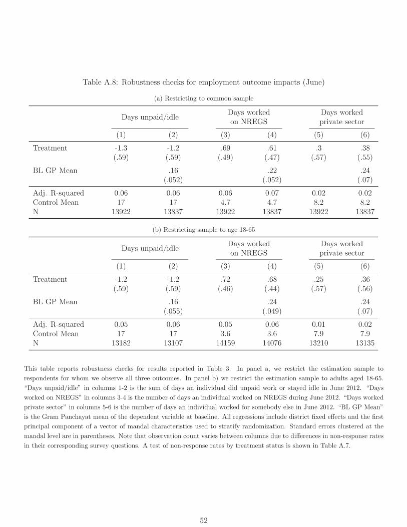
Table A.8: Robustness checks for employment outcome impacts (June)

(a) Restricting to common sample

Days unpaid/idleDays workedon NREGS

Days workedprivate sector

(1) (2) (3) (4) (5) (6)

Treatment -1.3 -1.2 .69 .61 .3 .38(.59) (.59) (.49) (.47) (.57) (.55)

BL GP Mean .16 .22 .24(.052) (.052) (.07)

Adj. R-squared 0.06 0.06 0.06 0.07 0.02 0.02Control Mean 17 17 4.7 4.7 8.2 8.2N 13922 13837 13922 13837 13922 13837

(b) Restricting sample to age 18-65

Days unpaid/idleDays workedon NREGS

Days workedprivate sector

(1) (2) (3) (4) (5) (6)

Treatment -1.2 -1.2 .72 .68 .25 .36(.59) (.59) (.46) (.44) (.57) (.56)

BL GP Mean .16 .24 .24(.055) (.049) (.07)

Adj. R-squared 0.05 0.06 0.05 0.06 0.01 0.02Control Mean 17 17 3.6 3.6 7.9 7.9N 13182 13107 14159 14076 13210 13135

This table reports robustness checks for results reported in Table 3. In panel a, we restrict the estimation sample to

respondents for whom we observe all three outcomes. In panel b) we restrict the estimation sample to adults aged 18-65.

“Days unpaid/idle” in columns 1-2 is the sum of days an individual did unpaid work or stayed idle in June 2012. “Days

worked on NREGS” in columns 3-4 is the number of days an individual worked on NREGS during June 2012. “Days worked

private sector” in columns 5-6 is the number of days an individual worked for somebody else in June 2012. “BL GP Mean”

is the Gram Panchayat mean of the dependent variable at baseline. All regressions include district fixed effects and the first

principal component of a vector of mandal characteristics used to stratify randomization. Standard errors clustered at the

mandal level are in parentheses. Note that observation count varies between columns due to differences in non-response rates

in their corresponding survey questions. A test of non-response rates by treatment status is shown in Table A.7.

52

Table A.9: Heterogeneity in wages outcomes by whether worked on NREGS in June

Wage realization (Rs.) Reservation wage (Rs.)

(1) (2) (3) (4)

Treatment 8.3 11 8.3 8.9(4.4) (4.5) (3.8) (3.8)

Treatment X Did not work on NREGS in June -1.4 -3.4 -4.9 -4.9(6.2) (6.4) (4) (4)

Did not work on NREGS in June 16 17 13 13(5.6) (5.7) (3.6) (3.6)

BL GP Mean .15 .088(.05) (.032)

p-value of Treatment + Interaction .16 .14 .26 .18Adj. R-squared .079 .085 .06 .063Control Mean 131 131 99 99N 7227 7014 12788 12674

This table shows heterogeneity in wage outcomes by whether an individual worked on NREGS in June using survey data.

“Did not work on NREGS in June” is an indicator of whether an individual worked on NREGS in June. “Treatment X Did

not work on NREGS in June” is an interaction term between “Treatment” and “Did not work on NREGS in June”. “Wage

realization (Rs.)” in columns 1-2 is the average daily wage (Rs. = Rupees) an individual received while working for someone

else in June 2012. “Reservation wage (Rs.)” in columns 3-4 is an individual’s reservation wage at which he or she would have

been willing to work for someone else in June 2012. The outcome is elicited through a question in which the surveyor asked

the respondent whether he or she would be willing to work for Rs. 20 and increased this amount in increments of Rs. 5 until

the respondent answered affirmatively. Observations in the top .5% percentile of the respective wage outcome in treatment

and control are excluded from each regression. “BL GP Mean” is the Gram Panchayat mean of the dependent variable at

baseline. All regressions include district fixed effects and the first principal component of a vector of mandal characteristics

used to stratify randomization. Standard errors clustered at the mandal level in parentheses.

53

Table A.10: Migration

Did migrate? Days migrated Household sizeMigration common

in May?

(1) (2) (3) (4) (5) (6) (7) (8)

Treatment .024 .022 1.1 .75 .059 .054 .047 .049(.017) (.018) (4.9) (5.1) (.1) (.1) (.055) (.038)

BL GP Mean .093 .3 .044(.09) (.19) (.048)

Migration previously common .54(.044)

Adj. R-squared 0.03 0.03 0.01 0.02 0.02 0.02 0.12 0.45Control Mean .075 .075 16 16 4.3 4.3 .21 .21N 4907 4873 4943 4909 4943 4909 809 808Level Hhd Hhd Hhd Hhd Hhd Hhd GP GP

This table illustrates treatment effects on various measures of migration using data from both our household survey and a

separately conducted village survey. In columns 1 and 2, the outcome is an indicator for whether any household member

stayed away from home for the purpose of work during the last year. In columns 3 and 4, the outcome is sum of all days

any household member stayed away from home for work, while in columns 5 and 6 the number of household members is the

dependent variable. “BL GP Mean” is the Gram Panchayat mean of the dependent variable at baseline. In columns 7-8, the

outcome is an indicator for whether it was common for workers to migrate out of the village in search of work during the

month of May since the implementation of NREGS. “Migration previously common” is an indicator for whether the same

type of migration during the same time was common prior to the start of NREGS. Note that “prior to NREGS” does not refer

to the Smartcards intervention but rather to the rollout of the entire employment guarantee scheme. All regressions include

district fixed effects and the first principal component of a vector of mandal characteristics used to stratify randomization.

Standard errors clustered at the mandal level are in parentheses.

54

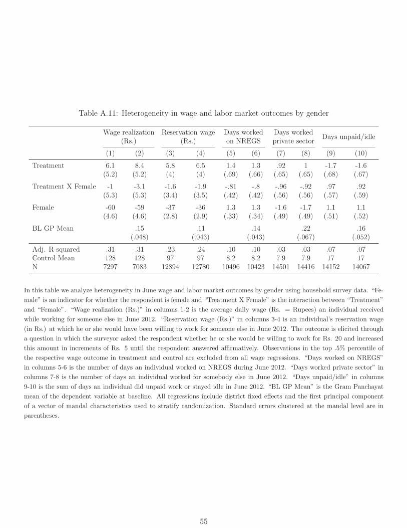
Table A.11: Heterogeneity in wage and labor market outcomes by gender

Wage realization(Rs.)

Reservation wage(Rs.)

Days workedon NREGS

Days workedprivate sector

Days unpaid/idle

(1) (2) (3) (4) (5) (6) (7) (8) (9) (10)

Treatment 6.1 8.4 5.8 6.5 1.4 1.3 .92 1 -1.7 -1.6(5.2) (5.2) (4) (4) (.69) (.66) (.65) (.65) (.68) (.67)

Treatment X Female -1 -3.1 -1.6 -1.9 -.81 -.8 -.96 -.92 .97 .92(5.3) (5.3) (3.4) (3.5) (.42) (.42) (.56) (.56) (.57) (.59)

Female -60 -59 -37 -36 1.3 1.3 -1.6 -1.7 1.1 1.1(4.6) (4.6) (2.8) (2.9) (.33) (.34) (.49) (.49) (.51) (.52)

BL GP Mean .15 .11 .14 .22 .16(.048) (.043) (.043) (.067) (.052)

Adj. R-squared .31 .31 .23 .24 .10 .10 .03 .03 .07 .07Control Mean 128 128 97 97 8.2 8.2 7.9 7.9 17 17N 7297 7083 12894 12780 10496 10423 14501 14416 14152 14067

In this table we analyze heterogeneity in June wage and labor market outcomes by gender using household survey data. “Fe-

male” is an indicator for whether the respondent is female and “Treatment X Female” is the interaction between “Treatment”

and “Female”. “Wage realization (Rs.)” in columns 1-2 is the average daily wage (Rs. = Rupees) an individual received

while working for someone else in June 2012. “Reservation wage (Rs.)” in columns 3-4 is an individual’s reservation wage

(in Rs.) at which he or she would have been willing to work for someone else in June 2012. The outcome is elicited through

a question in which the surveyor asked the respondent whether he or she would be willing to work for Rs. 20 and increased

this amount in increments of Rs. 5 until the respondent answered affirmatively. Observations in the top .5% percentile of

the respective wage outcome in treatment and control are excluded from all wage regressions. “Days worked on NREGS”

in columns 5-6 is the number of days an individual worked on NREGS during June 2012. “Days worked private sector” in

columns 7-8 is the number of days an individual worked for somebody else in June 2012. “Days unpaid/idle” in columns

9-10 is the sum of days an individual did unpaid work or stayed idle in June 2012. “BL GP Mean” is the Gram Panchayat

mean of the dependent variable at baseline. All regressions include district fixed effects and the first principal component

of a vector of mandal characteristics used to stratify randomization. Standard errors clustered at the mandal level are in

parentheses.

55

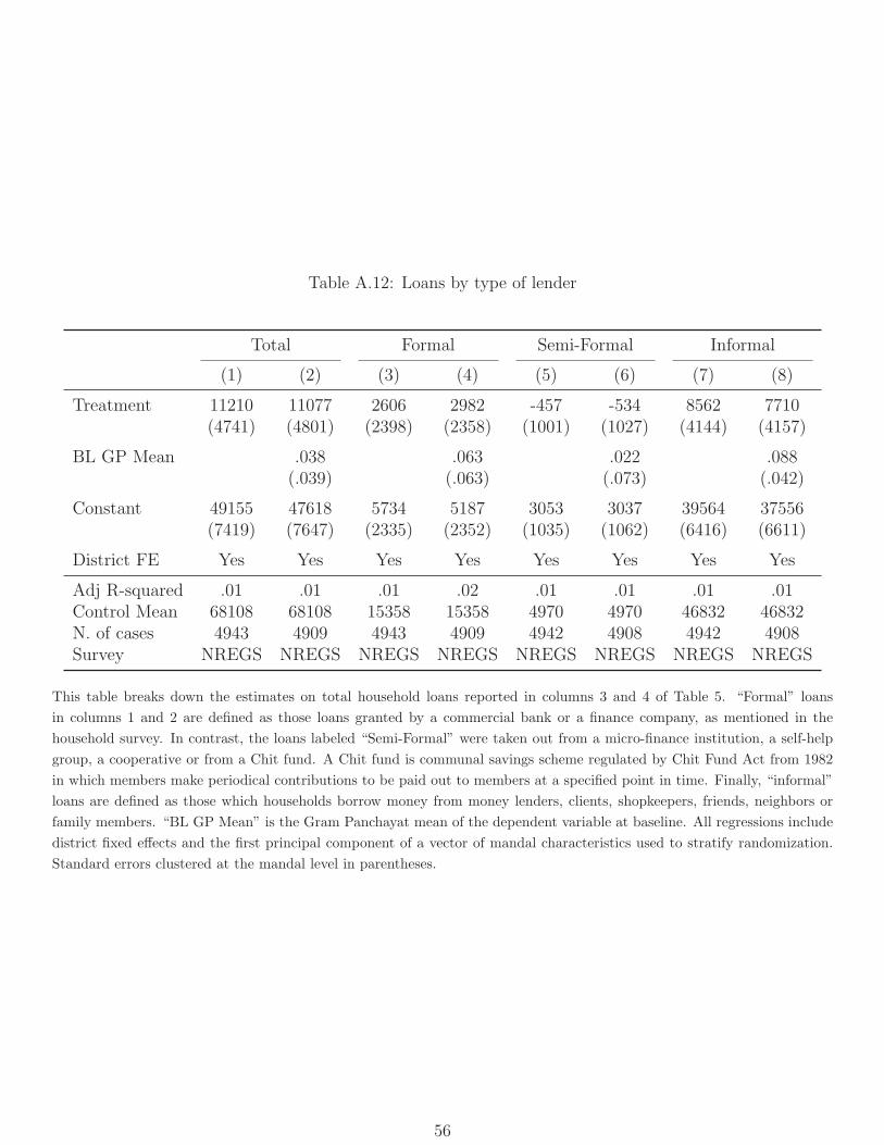
Table A.12: Loans by type of lender

Total Formal Semi-Formal Informal

(1) (2) (3) (4) (5) (6) (7) (8)

Treatment 11210 11077 2606 2982 -457 -534 8562 7710(4741) (4801) (2398) (2358) (1001) (1027) (4144) (4157)

BL GP Mean .038 .063 .022 .088(.039) (.063) (.073) (.042)

Constant 49155 47618 5734 5187 3053 3037 39564 37556(7419) (7647) (2335) (2352) (1035) (1062) (6416) (6611)

District FE Yes Yes Yes Yes Yes Yes Yes Yes

Adj R-squared .01 .01 .01 .02 .01 .01 .01 .01Control Mean 68108 68108 15358 15358 4970 4970 46832 46832N. of cases 4943 4909 4943 4909 4942 4908 4942 4908Survey NREGS NREGS NREGS NREGS NREGS NREGS NREGS NREGS

This table breaks down the estimates on total household loans reported in columns 3 and 4 of Table 5. “Formal” loans

in columns 1 and 2 are defined as those loans granted by a commercial bank or a finance company, as mentioned in the

household survey. In contrast, the loans labeled “Semi-Formal” were taken out from a micro-finance institution, a self-help

group, a cooperative or from a Chit fund. A Chit fund is communal savings scheme regulated by Chit Fund Act from 1982

in which members make periodical contributions to be paid out to members at a specified point in time. Finally, “informal”

loans are defined as those which households borrow money from money lenders, clients, shopkeepers, friends, neighbors or

family members. “BL GP Mean” is the Gram Panchayat mean of the dependent variable at baseline. All regressions include

district fixed effects and the first principal component of a vector of mandal characteristics used to stratify randomization.

Standard errors clustered at the mandal level in parentheses.

56

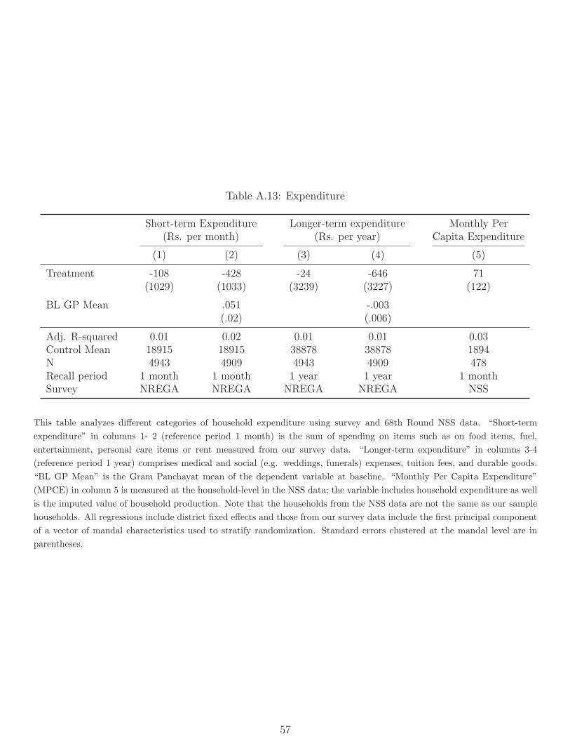
Table A.13: Expenditure

Short-term Expenditure(Rs. per month)

Longer-term expenditure(Rs. per year)

Monthly PerCapita Expenditure

(1) (2) (3) (4) (5)

Treatment -108 -428 -24 -646 71(1029) (1033) (3239) (3227) (122)

BL GP Mean .051 -.003(.02) (.006)

Adj. R-squared 0.01 0.02 0.01 0.01 0.03Control Mean 18915 18915 38878 38878 1894N 4943 4909 4943 4909 478Recall period 1 month 1 month 1 year 1 year 1 monthSurvey NREGA NREGA NREGA NREGA NSS

This table analyzes different categories of household expenditure using survey and 68th Round NSS data. “Short-term

expenditure” in columns 1- 2 (reference period 1 month) is the sum of spending on items such as on food items, fuel,

entertainment, personal care items or rent measured from our survey data. “Longer-term expenditure” in columns 3-4

(reference period 1 year) comprises medical and social (e.g. weddings, funerals) expenses, tuition fees, and durable goods.

“BL GP Mean” is the Gram Panchayat mean of the dependent variable at baseline. “Monthly Per Capita Expenditure”

(MPCE) in column 5 is measured at the household-level in the NSS data; the variable includes household expenditure as well

is the imputed value of household production. Note that the households from the NSS data are not the same as our sample

households. All regressions include district fixed effects and those from our survey data include the first principal component

of a vector of mandal characteristics used to stratify randomization. Standard errors clustered at the mandal level are in

parentheses.

57

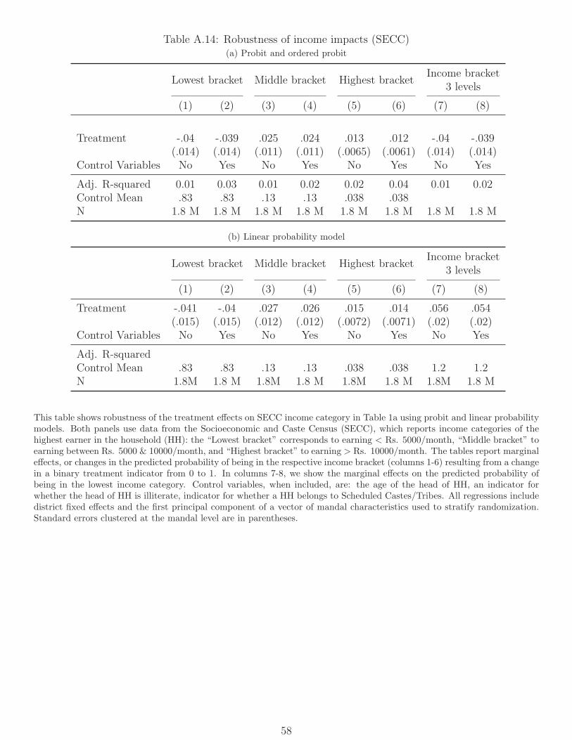
Table A.14: Robustness of income impacts (SECC)(a) Probit and ordered probit

Lowest bracket Middle bracket Highest bracketIncome bracket

3 levels

(1) (2) (3) (4) (5) (6) (7) (8)

Treatment -.04 -.039 .025 .024 .013 .012 -.04 -.039(.014) (.014) (.011) (.011) (.0065) (.0061) (.014) (.014)

Control Variables No Yes No Yes No Yes No Yes

Adj. R-squared 0.01 0.03 0.01 0.02 0.02 0.04 0.01 0.02Control Mean .83 .83 .13 .13 .038 .038N 1.8 M 1.8 M 1.8 M 1.8 M 1.8 M 1.8 M 1.8 M 1.8 M

(b) Linear probability model

Lowest bracket Middle bracket Highest bracketIncome bracket

3 levels

(1) (2) (3) (4) (5) (6) (7) (8)

Treatment -.041 -.04 .027 .026 .015 .014 .056 .054(.015) (.015) (.012) (.012) (.0072) (.0071) (.02) (.02)

Control Variables No Yes No Yes No Yes No Yes

Adj. R-squaredControl Mean .83 .83 .13 .13 .038 .038 1.2 1.2N 1.8M 1.8 M 1.8M 1.8 M 1.8M 1.8 M 1.8M 1.8 M

This table shows robustness of the treatment effects on SECC income category in Table 1a using probit and linear probabilitymodels. Both panels use data from the Socioeconomic and Caste Census (SECC), which reports income categories of thehighest earner in the household (HH): the “Lowest bracket” corresponds to earning < Rs. 5000/month, “Middle bracket” toearning between Rs. 5000 & 10000/month, and “Highest bracket” to earning > Rs. 10000/month. The tables report marginaleffects, or changes in the predicted probability of being in the respective income bracket (columns 1-6) resulting from a changein a binary treatment indicator from 0 to 1. In columns 7-8, we show the marginal effects on the predicted probability ofbeing in the lowest income category. Control variables, when included, are: the age of the head of HH, an indicator forwhether the head of HH is illiterate, indicator for whether a HH belongs to Scheduled Castes/Tribes. All regressions includedistrict fixed effects and the first principal component of a vector of mandal characteristics used to stratify randomization.Standard errors clustered at the mandal level are in parentheses.

58

Table A.15: Income (Survey Data), no censoring

Total income NREGAAgricultural

laborOther labor Farm Business Miscellaneous

(1) (2) (3) (4) (5) (6) (7) (8)

Treatment 10308 9580 905 3675 4471 1738 -773 293(4638) (4628) (589) (1485) (1585) (2704) (1359) (2437)

BL GP Mean .055(.05)

Adj. R-squared 0.03 0.03 0.02 0.04 0.03 0.01 0.01 0.01Control Mean 71935 71935 4743 14784 9315 21708 6620 14765N 4932 4898 4931 4932 4932 4932 4932 4932

This table reports robustness check of earnings gains in Table 1b, which shows treatment effects on various types of income

using annualized data from our survey, to including all observations (instead of censoring the top 0.5%). “BL GP Mean” is the

Gram Panchayat mean of the dependent variable at baseline. “NREGS” is the earnings from NREGS. “Agricultural labor”

captures income from agricultural work for someone else, while “Other labor” is income from physical labor for someone

else. “Farm” combines income from a households’ own land and animal husbandry, while “Business” captures income from

self-employment or through a household’s own business. “Other” is the sum of household income not captured by any of

the other categories. Note that the income categories were not as precisely measured at baseline which is why we cannot

include the respective lag of the dependent variable “ BL GP Mean”. All regressions include district fixed effects and the

first principal component of a vector of mandal characteristics used to stratify randomization. Standard errors clustered at

the mandal level are in parentheses.

59

Table A.16: Robustness checks for private sector wage outcomes

(a) No censoring

Wage realization (Rs.) Reservation wage (Rs.)

(1) (2) (3) (4)

Treatment 5.6 6.8 5 5.6(4.1) (4.1) (3.3) (3.2)

BL GP Mean .15 .091(.054) (.039)

Adj R-squared 0.05 0.05 0.03 0.03Control Mean 131 131 99 99N 7326 7112 12955 12841

(b) Restricting sample to age 18-65

Wage realization (Rs.) Reservation wage (Rs.)

(1) (2) (3) (4)

Treatment 6.6 7.9 5 5.7(3.7) (3.8) (3) (2.9)

BL GP Mean .16 .1(.049) (.033)

Adjusted R-squared 0.07 0.07 0.05 0.06Control Mean 129 129 98 98N 6989 6782 12227 12124

(c) Excluding respondents who did not work in June

Wage realization (Rs.) Reservation wage (Rs.)

(1) (2) (3) (4)

Treatment 6.4 7.6 6.8 7.3(3.6) (3.6) (3.2) (3.1)

BL GP Mean .16 .13(.048) (.05)

Adjusted R-squared 0.07 0.07 0.06 0.06Control Mean 128 128 98 98N 7256 7043 7282 7212

This table reports several robustness checks for results reported in Table 2. In panel a), the analysis sample includes all

observations, in particular the top .5% percentile of the respective wage outcome in treatment and control, of the respective

wage outcome. In panel b), the sample is restricted to respondents in ages 18 to 65 and excludes observations in the top .5%

percentile of the respective wage outcome in treatment and control. In panel c), we drop observations for respondents who

have did not work in June and excludes observations in the top .5% percentile of the respective wage outcome in treatment

and control.“Wage realization (Rs.)” in columns 1-4 is the average daily wage (in Rs.) an individual received while working

for someone else in June 2012. “Reservation wage (Rs.)” in columns 5-8 is an individual’s reservation wage (in Rs.) at

which he or she would have been willing to work for someone else in June 2012. The outcome is based on an a question in

which the surveyor asked the respondent whether he or she would be willing to work for Rs. 20 and increased this amount

in increments of Rs. 5 until the respondent answered affirmatively. “BL GP Mean” is the Gram Panchayat mean of the

dependent variable at baseline. All regressions include district fixed effects and the first principal component of a vector of

mandal characteristics used to stratify randomization. Standard errors clustered at the mandal level are in parentheses.60

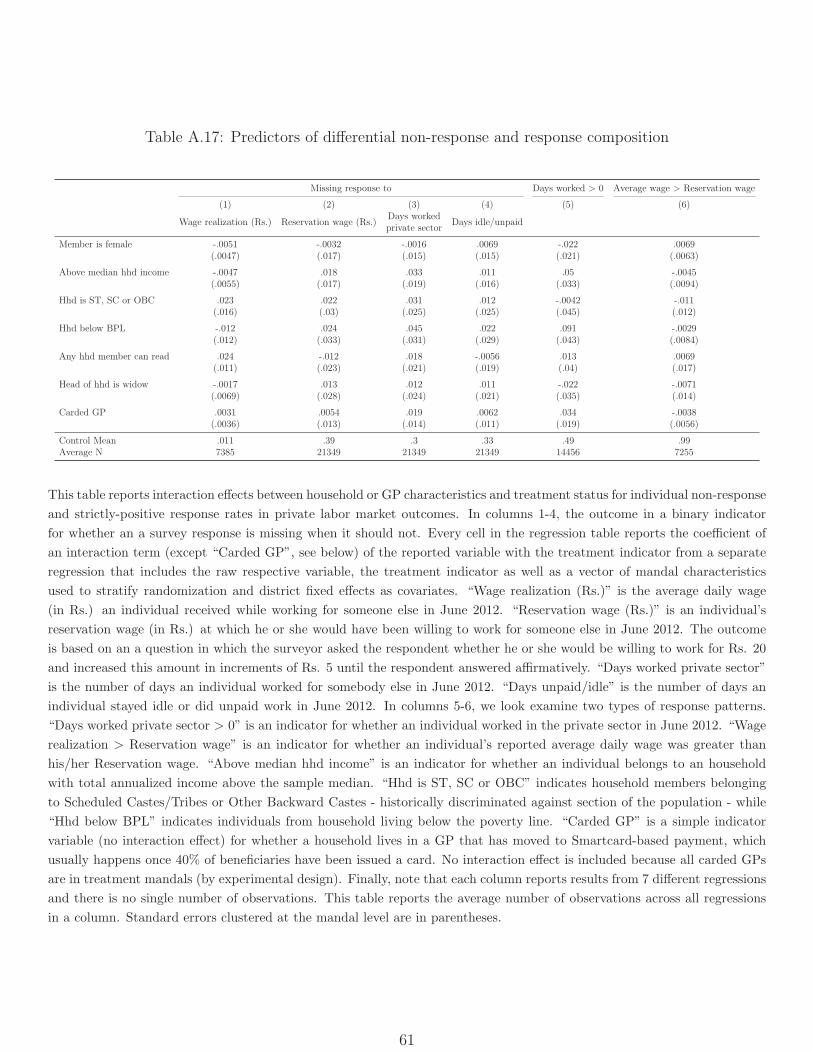
Table A.17: Predictors of differential non-response and response composition

Missing response to Days worked > 0 Average wage > Reservation wage

(1) (2) (3) (4) (5) (6)

Wage realization (Rs.) Reservation wage (Rs.)Days workedprivate sector

Days idle/unpaid

Member is female -.0051 -.0032 -.0016 .0069 -.022 .0069(.0047) (.017) (.015) (.015) (.021) (.0063)

Above median hhd income -.0047 .018 .033 .011 .05 -.0045(.0055) (.017) (.019) (.016) (.033) (.0094)

Hhd is ST, SC or OBC .023 .022 .031 .012 -.0042 -.011(.016) (.03) (.025) (.025) (.045) (.012)

Hhd below BPL -.012 .024 .045 .022 .091 -.0029(.012) (.033) (.031) (.029) (.043) (.0084)

Any hhd member can read .024 -.012 .018 -.0056 .013 .0069(.011) (.023) (.021) (.019) (.04) (.017)

Head of hhd is widow -.0017 .013 .012 .011 -.022 -.0071(.0069) (.028) (.024) (.021) (.035) (.014)

Carded GP .0031 .0054 .019 .0062 .034 -.0038(.0036) (.013) (.014) (.011) (.019) (.0056)

Control Mean .011 .39 .3 .33 .49 .99Average N 7385 21349 21349 21349 14456 7255

This table reports interaction effects between household or GP characteristics and treatment status for individual non-response

and strictly-positive response rates in private labor market outcomes. In columns 1-4, the outcome in a binary indicator

for whether an a survey response is missing when it should not. Every cell in the regression table reports the coefficient of

an interaction term (except “Carded GP”, see below) of the reported variable with the treatment indicator from a separate

regression that includes the raw respective variable, the treatment indicator as well as a vector of mandal characteristics

used to stratify randomization and district fixed effects as covariates. “Wage realization (Rs.)” is the average daily wage

(in Rs.) an individual received while working for someone else in June 2012. “Reservation wage (Rs.)” is an individual’s

reservation wage (in Rs.) at which he or she would have been willing to work for someone else in June 2012. The outcome

is based on an a question in which the surveyor asked the respondent whether he or she would be willing to work for Rs. 20

and increased this amount in increments of Rs. 5 until the respondent answered affirmatively. “Days worked private sector”

is the number of days an individual worked for somebody else in June 2012. “Days unpaid/idle” is the number of days an

individual stayed idle or did unpaid work in June 2012. In columns 5-6, we look examine two types of response patterns.

“Days worked private sector > 0” is an indicator for whether an individual worked in the private sector in June 2012. “Wage

realization > Reservation wage” is an indicator for whether an individual’s reported average daily wage was greater than

his/her Reservation wage. “Above median hhd income” is an indicator for whether an individual belongs to an household

with total annualized income above the sample median. “Hhd is ST, SC or OBC” indicates household members belonging

to Scheduled Castes/Tribes or Other Backward Castes - historically discriminated against section of the population - while

“Hhd below BPL” indicates individuals from household living below the poverty line. “Carded GP” is a simple indicator

variable (no interaction effect) for whether a household lives in a GP that has moved to Smartcard-based payment, which

usually happens once 40% of beneficiaries have been issued a card. No interaction effect is included because all carded GPs

are in treatment mandals (by experimental design). Finally, note that each column reports results from 7 different regressions

and there is no single number of observations. This table reports the average number of observations across all regressions

in a column. Standard errors clustered at the mandal level are in parentheses.

61

Table A.18: Baseline balance with respect to exogenous measure of neighbor’s treatment

% GPs treated within R km

(1) (2) (3) (4) (5)R = 10 R = 15 R = 20 R = 25 R = 30

Wage realization (Rs.) 3.3 4.2 2 .21 1.3(4.1) (5.5) (6.6) (7.8) (9.6)

Reservation wage (Rs.) 1.4 3.1 2.4 2.7 5.6(3.3) (4.1) (4.8) (5.1) (6.1)

Days worked private sector -.27 -.46 -.42 -.21 .026(.42) (.55) (.64) (.76) (.89)

Days unpaid/idle .34 .44 .19 -.3 -.54(.53) (.68) (.95) (1.5) (1.7)

Total income (Rs.) -377 2653 2177 -2032 -3232(2872) (4168) (4826) (5421) (6738)

This table reports baseline balance of key outcomes with respect to NRp for GPs in treatment mandals. Each cell shows the

respective coefficient from a separate regression where the outcome is given by the row header. “Wage realization (Rs.)” the

average daily wage (in Rs.) an individual received while working for someone else in June 2012. “Reservation wage (Rs.)”

is an individual’s reservation wage (in Rs.) at which he or she would have been willing to work for someone else in June

2012. The outcome is based on an a question in which the surveyor asked the respondent whether he or she would be willing

to work for Rs. 20 and increased this amount in increments of Rs. 5 until the respondent answered affirmatively. “Days

worked private sector” is the number of days an individual worked for somebody else in June 2012. “Total income” is total

annualized household income, where the top .5% of observations are separately trimmed in treatment and control. The “%

GPs treated within R” is NRp , or the ratio of the number of GPs in treatment mandals within radius R km over the total

GPs within wave 1, 2 or 3 mandals. Note that wave 2 GPs are included in the denominator, and that same-mandal GPs

are excluded from both the denominator and numerator. Note that each cell shows a separate regression of the outcome

with NRp and district fixed effects as the only covariates. The entire GP sample used in randomization is included. Each

column reports results from 5 different regressions with distinct observation counts, which are not reported. Standard errors

clustered at the mandal level are in parentheses.

62

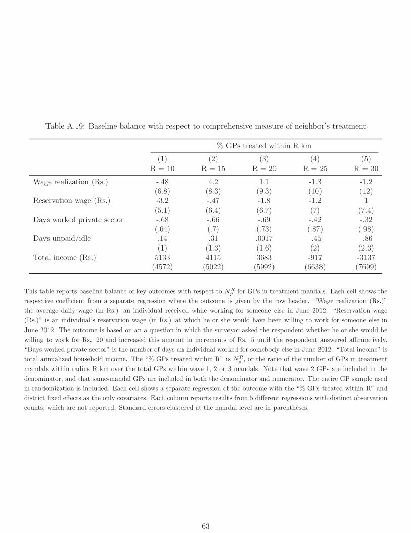
Table A.19: Baseline balance with respect to comprehensive measure of neighbor’s treatment

% GPs treated within R km

(1) (2) (3) (4) (5)R = 10 R = 15 R = 20 R = 25 R = 30

Wage realization (Rs.) -.48 4.2 1.1 -1.3 -1.2(6.8) (8.3) (9.3) (10) (12)

Reservation wage (Rs.) -3.2 -.47 -1.8 -1.2 1(5.1) (6.4) (6.7) (7) (7.4)

Days worked private sector -.68 -.66 -.69 -.42 -.32(.64) (.7) (.73) (.87) (.98)

Days unpaid/idle .14 .31 .0017 -.45 -.86(1) (1.3) (1.6) (2) (2.3)

Total income (Rs.) 5133 4115 3683 -917 -3137(4572) (5022) (5992) (6638) (7699)

This table reports baseline balance of key outcomes with respect to NRp for GPs in treatment mandals. Each cell shows the

respective coefficient from a separate regression where the outcome is given by the row header. “Wage realization (Rs.)”

the average daily wage (in Rs.) an individual received while working for someone else in June 2012. “Reservation wage

(Rs.)” is an individual’s reservation wage (in Rs.) at which he or she would have been willing to work for someone else in

June 2012. The outcome is based on an a question in which the surveyor asked the respondent whether he or she would be

willing to work for Rs. 20 and increased this amount in increments of Rs. 5 until the respondent answered affirmatively.

“Days worked private sector” is the number of days an individual worked for somebody else in June 2012. “Total income” is

total annualized household income. The “% GPs treated within R” is NRp , or the ratio of the number of GPs in treatment

mandals within radius R km over the total GPs within wave 1, 2 or 3 mandals. Note that wave 2 GPs are included in the

denominator, and that same-mandal GPs are included in both the denominator and numerator. The entire GP sample used

in randomization is included. Each cell shows a separate regression of the outcome with the “% GPs treated within R” and

district fixed effects as the only covariates. Each column reports results from 5 different regressions with distinct observation

counts, which are not reported. Standard errors clustered at the mandal level are in parentheses.

63

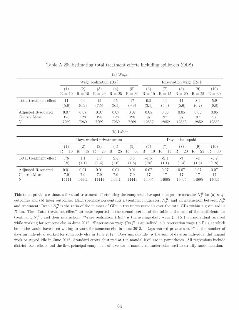
Table A.20: Estimating total treatment effects including spillovers (OLS)

(a) Wage

Wage realization (Rs.) Reservation wage (Rs.)

(1) (2) (3) (4) (5) (6) (7) (8) (9) (10)R = 10 R = 15 R = 20 R = 25 R = 30 R = 10 R = 15 R = 20 R = 25 R = 30

Total treatment effect 11 14 15 15 17 9.5 11 11 8.4 5.9(5.6) (6.9) (7.5) (8.5) (9.8) (3.1) (4.3) (5.6) (6.2) (6.8)

Adjusted R-squared 0.07 0.07 0.07 0.07 0.07 0.05 0.05 0.05 0.05 0.05Control Mean 128 128 128 128 128 97 97 97 97 97N 7269 7269 7269 7269 7269 12852 12852 12852 12852 12852

(b) Labor

Days worked private sector Days idle/unpaid

(1) (2) (3) (4) (5) (6) (7) (8) (9) (10)R = 10 R = 15 R = 20 R = 25 R = 30 R = 10 R = 15 R = 20 R = 25 R = 30

Total treatment effect .76 1.1 1.7 2.5 3.5 -1.5 -2.1 -3 -4 -5.2(.8) (1.1) (1.4) (1.6) (1.8) (.78) (1.1) (1.4) (1.6) (1.8)

Adjusted R-squared 0.01 0.01 0.01 0.01 0.01 0.07 0.07 0.07 0.07 0.07Control Mean 7.9 7.9 7.9 7.9 7.9 17 17 17 17 17N 14441 14441 14441 14441 14441 14095 14095 14095 14095 14095

This table provides estimates for total treatment effects using the comprehensive spatial exposure measure NRp for (a) wage

outcomes and (b) labor outcomes. Each specification contains a treatment indicator, NRp , and an interaction between NR

p

and treatment. Recall NRp is the ratio of the number of GPs in treatment mandals over the total GPs within a given radius

R km. The “Total treatment effect” estimate reported in the second section of the table is the sum of the coefficients for

treatment, NRp , and their interaction. “Wage realization (Rs.)” is the average daily wage (in Rs.) an individual received

while working for someone else in June 2012. “Reservation wage (Rs.)” is an individual’s reservation wage (in Rs.) at which

he or she would have been willing to work for someone else in June 2012. “Days worked private sector” is the number of

days an individual worked for somebody else in June 2012. “Days unpaid/idle” is the sum of days an individual did unpaid

work or stayed idle in June 2012. Standard errors clustered at the mandal level are in parentheses. All regressions include

district fixed effects and the first principal component of a vector of mandal characteristics used to stratify randomization.

64

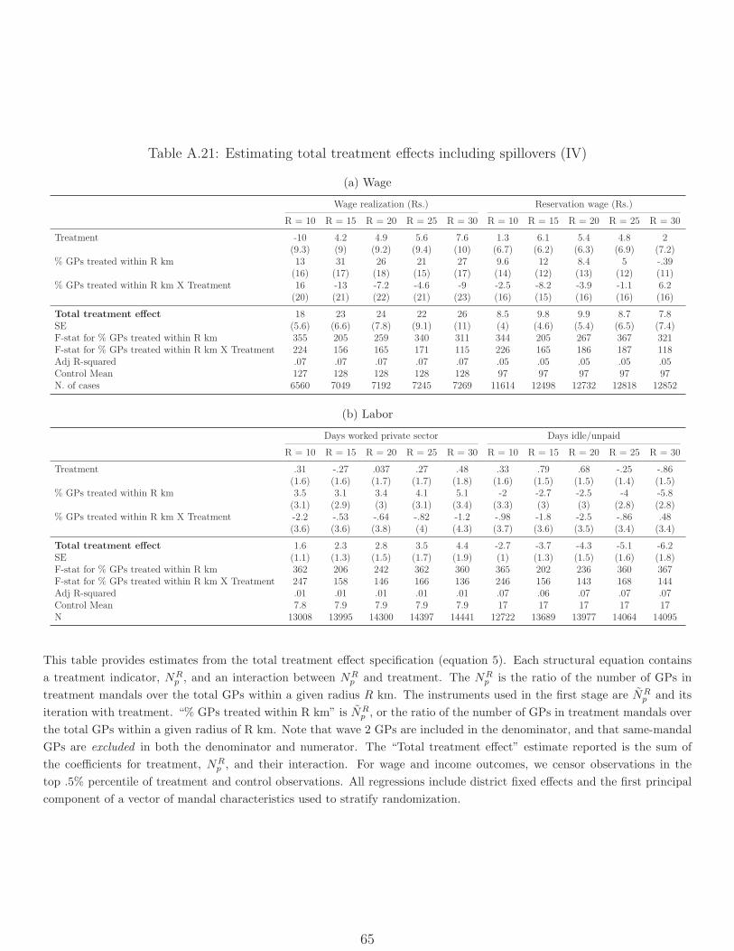
Table A.21: Estimating total treatment effects including spillovers (IV)

(a) Wage

Wage realization (Rs.) Reservation wage (Rs.)

R = 10 R = 15 R = 20 R = 25 R = 30 R = 10 R = 15 R = 20 R = 25 R = 30

Treatment -10 4.2 4.9 5.6 7.6 1.3 6.1 5.4 4.8 2(9.3) (9) (9.2) (9.4) (10) (6.7) (6.2) (6.3) (6.9) (7.2)

% GPs treated within R km 13 31 26 21 27 9.6 12 8.4 5 -.39(16) (17) (18) (15) (17) (14) (12) (13) (12) (11)

% GPs treated within R km X Treatment 16 -13 -7.2 -4.6 -9 -2.5 -8.2 -3.9 -1.1 6.2(20) (21) (22) (21) (23) (16) (15) (16) (16) (16)

Total treatment effect 18 23 24 22 26 8.5 9.8 9.9 8.7 7.8SE (5.6) (6.6) (7.8) (9.1) (11) (4) (4.6) (5.4) (6.5) (7.4)F-stat for % GPs treated within R km 355 205 259 340 311 344 205 267 367 321F-stat for % GPs treated within R km X Treatment 224 156 165 171 115 226 165 186 187 118Adj R-squared .07 .07 .07 .07 .07 .05 .05 .05 .05 .05Control Mean 127 128 128 128 128 97 97 97 97 97N. of cases 6560 7049 7192 7245 7269 11614 12498 12732 12818 12852

(b) Labor

Days worked private sector Days idle/unpaid

R = 10 R = 15 R = 20 R = 25 R = 30 R = 10 R = 15 R = 20 R = 25 R = 30

Treatment .31 -.27 .037 .27 .48 .33 .79 .68 -.25 -.86(1.6) (1.6) (1.7) (1.7) (1.8) (1.6) (1.5) (1.5) (1.4) (1.5)

% GPs treated within R km 3.5 3.1 3.4 4.1 5.1 -2 -2.7 -2.5 -4 -5.8(3.1) (2.9) (3) (3.1) (3.4) (3.3) (3) (3) (2.8) (2.8)

% GPs treated within R km X Treatment -2.2 -.53 -.64 -.82 -1.2 -.98 -1.8 -2.5 -.86 .48(3.6) (3.6) (3.8) (4) (4.3) (3.7) (3.6) (3.5) (3.4) (3.4)

Total treatment effect 1.6 2.3 2.8 3.5 4.4 -2.7 -3.7 -4.3 -5.1 -6.2SE (1.1) (1.3) (1.5) (1.7) (1.9) (1) (1.3) (1.5) (1.6) (1.8)F-stat for % GPs treated within R km 362 206 242 362 360 365 202 236 360 367F-stat for % GPs treated within R km X Treatment 247 158 146 166 136 246 156 143 168 144Adj R-squared .01 .01 .01 .01 .01 .07 .06 .07 .07 .07Control Mean 7.8 7.9 7.9 7.9 7.9 17 17 17 17 17N 13008 13995 14300 14397 14441 12722 13689 13977 14064 14095

This table provides estimates from the total treatment effect specification (equation 5). Each structural equation contains

a treatment indicator, NRp , and an interaction between NR

p and treatment. The NRp is the ratio of the number of GPs in

treatment mandals over the total GPs within a given radius R km. The instruments used in the first stage are NRp and its

iteration with treatment. “% GPs treated within R km” is NRp , or the ratio of the number of GPs in treatment mandals over

the total GPs within a given radius of R km. Note that wave 2 GPs are included in the denominator, and that same-mandal

GPs are excluded in both the denominator and numerator. The “Total treatment effect” estimate reported is the sum of

the coefficients for treatment, NRp , and their interaction. For wage and income outcomes, we censor observations in the

top .5% percentile of treatment and control observations. All regressions include district fixed effects and the first principal

component of a vector of mandal characteristics used to stratify randomization.

65

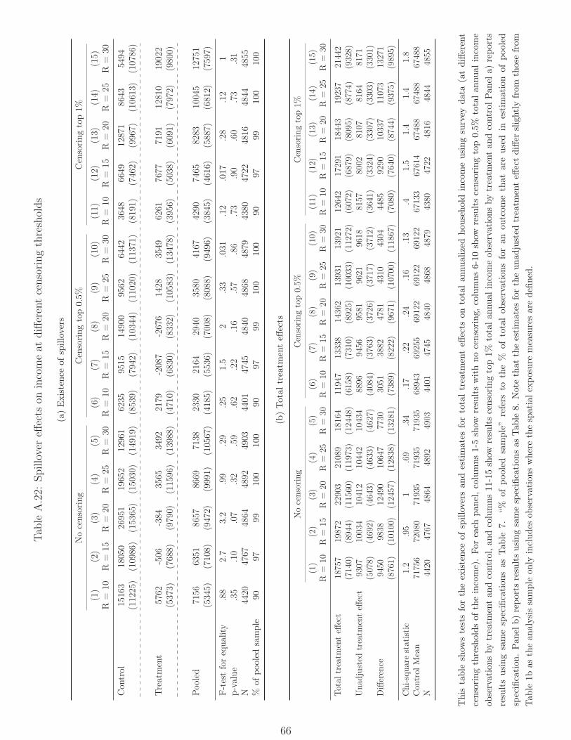
Tab

leA.22:

Spillovereff

ects

onincomeat

differentcensoringthresholds

(a)Existence

ofspillovers

Nocensoring

Censoringtop0.5%

Censoringtop1%

(1)

(2)

(3)

(4)

(5)

(6)

(7)

(8)

(9)

(10)

(11)

(12)

(13)

(14)

(15)

R=

10R

=15

R=

20R

=25

R=

30R

=10

R=

15R

=20

R=

25R

=30

R=

10R

=15

R=

20R

=25

R=

30

Con

trol

15163

18050

26951

19652

12961

6235

9515

14900

9562

6442

3648

6649

12871

8643

5494

(11225)

(10986)

(15365)

(15030)

(14919)

(8539)

(7942)

(10344)

(11020)

(11371)

(8191)

(7462)

(9967)

(10613)

(10786)

Treatment

5762

-506

-384

3565

3492

2179

-2087

-2676

1428

3549

6261

7677

7191

12810

19022

(5373)

(7688)

(9790)

(11596)

(13988)

(4710)

(6830)

(8332)

(10583)

(13478)

(3956)

(5038)

(6091)

(7972)

(9800)

Pooled

7156

6351

8657

8669

7138

2330

2164

2940

3580

4167

4290

7465

8283

10045

12751

(5345)

(7108)

(9472)

(9991)

(10567)

(4185)

(5536)

(7008)

(8088)

(9496)

(3845)

(4616)

(5887)

(6812)

(7597)

F-testforequality

.88

2.7

3.2

.99

.29

.25

1.5

2.33

.031

.12

.017

.28

.12

1p-value

.35

.10

.07

.32

.59

.62

.22

.16

.57

.86

.73

.90

.60

.73

.31

N4420

4767

4864

4892

4903

4401

4745

4840

4868

4879

4380

4722

4816

4844

4855

%of

pooled

sample

9097

99100

100

9097

99100

100

9097

99100

100

(b)Total

treatm

enteff

ects

Nocensoring

Censoringtop0.5%

Censoringtop1%

(1)

(2)

(3)

(4)

(5)

(6)

(7)

(8)

(9)

(10)

(11)

(12)

(13)

(14)

(15)

R=

10R

=15

R=

20R

=25

R=

30R

=10

R=

15R

=20

R=

25R

=30

R=

10R

=15

R=

20R

=25

R=

30

Total

treatm

enteff

ect

18757

19872

22903

21089

18164

11947

13338

14362

13931

13921

12642

17291

18443

19237

21442

(7140)

(8944)

(11560)

(11973)

(12448)

(6158)

(7310)

(8925)

(10033)

(11272)

(6072)

(6879)

(8095)

(8774)

(9328)

Unad

justed

treatm

enteff

ect

9307

10034

10412

10442

10434

8896

9456

9581

9621

9618

8157

8002

8107

8164

8171

(5078)

(4692)

(4643)

(4633)

(4627)

(4084)

(3763)

(3726)

(3717)

(3712)

(3641)

(3324)

(3307)

(3303)

(3301)

Difference

9450

9838

12490

10647

7730

3051

3882

4781

4310

4304

4485

9290

10337

11073

13271

(8761)

(10100)

(12457)

(12838)

(13281)

(7389)

(8222)

(9671)

(10700)

(11867)

(7080)

(7640)

(8744)

(9375)

(9895)

Chi-squarestatistic

1.2

.95

1.69

.34

.17

.22

.24

.16

.13

.41.5

1.4

1.4

1.8

Con

trol

Mean

71756

72080

71935

71935

71935

68943

69255

69122

69122

69122

67133

67614

67488

67488

67488

N4420

4767

4864

4892

4903

4401

4745

4840

4868

4879

4380

4722

4816

4844

4855

This

table

show

stestsfortheexistence

ofspillovers

andestimates

fortotaltreatm

enteff

ects

ontotalan

nualizedhousehold

incomeusingsurvey

data

(atdifferent

censoringthresholdsof

theincome).For

each

pan

el,columns1-5show

resultswithnocensoring,

columns6-10show

resultscensoringtop0.5%

totalannualincome

observationsbytreatm

entan

dcontrol,an

dcolumns11-15show

resultscensoringtop1%

totalan

nual

incomeobservation

sbytreatm

entandcontrol

Panel

a)reports

resultsusingsamespecification

sas

Tab

le7.

“%of

pooled

sample”refers

tothe%

oftotalob

servationsforan

outcomethatare

used

inestimation

ofpooled

specification

.Pan

elb)reports

resultsusingsamespecification

sas

Tab

le8.

Notethat

theestimates

fortheunadjusted

treatm

enteff

ectdiffer

slightlyfrom

those

from

Tab

le1b

asthean

alysissample

only

includes

observationswherethespatialexposure

measuresaredefined.

66

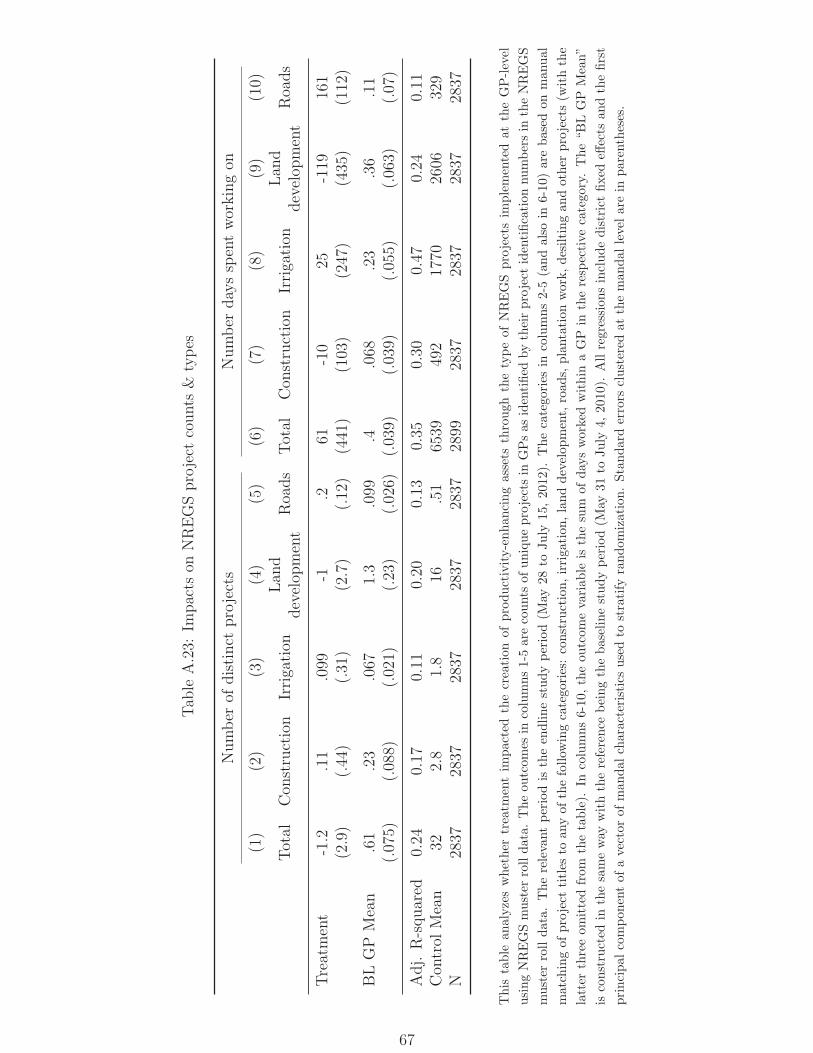
Tab

leA.23:

Impacts

onNREGSproject

counts

&types

Number

ofdistinct

projects

Number

daysspentworkingon

(1)

(2)

(3)

(4)

(5)

(6)

(7)

(8)

(9)

(10)

Total

Con

struction

Irrigation

Lan

ddevelop

ment

Roads

Total

Con

struction

Irrigation

Lan

ddevelop

ment

Roads

Treatment

-1.2

.11

.099

-1.2

61-10

25-119

161

(2.9)

(.44)

(.31)

(2.7)

(.12)

(441)

(103)

(247)

(435)

(112)

BLGPMean

.61

.23

.067

1.3

.099

.4.068

.23

.36

.11

(.075)

(.088)

(.021)

(.23)

(.026)

(.039)

(.039)

(.055)

(.063)

(.07)

Adj.

R-squared

0.24

0.17

0.11

0.20

0.13

0.35

0.30

0.47

0.24

0.11

Con

trol

Mean

322.8

1.8

16.51

6539

492

1770

2606

329

N2837

2837

2837

2837

2837

2899

2837

2837

2837

2837

This

table

analyzeswhether

treatm

entim

pactedthecreation

ofproductivity-enhan

cingassets

through

thetypeofNREGSprojectsim

plementedattheGP-level

usingNREGSmuster

rolldata.

Theou

tcom

esin

columns1-5arecounts

ofuniqueprojectsin

GPsas

identified

bytheirproject

identificationnumbersin

theNREGS

muster

rolldata.

Therelevantperiodis

theendlinestudyperiod(M

ay28

toJuly

15,2012).

Thecategories

incolumns2-5

(andalsoin

6-10)are

basedonmanual

matchingof

project

titles

toan

yof

thefollow

ingcategories:construction,irrigation

,landdevelop

ment,road

s,plantationwork,desiltingandother

projects(w

iththe

latter

threeom

ittedfrom

thetable).

Incolumns6-10,theou

tcom

evariab

leis

thesum

ofdaysworked

within

aGP

intherespectivecategory.

The“BLGP

Mean”

isconstructed

inthesameway

withthereference

beingthebaselinestudyperiod(M

ay31

toJuly

4,2010).

Allregressionsincludedistrictfixed

effects

andthefirst

principal

compon

entof

avector

ofman

dal

characteristicsusedto

stratify

random

ization.Standarderrors

clustered

atthemandallevelare

inparentheses.

67

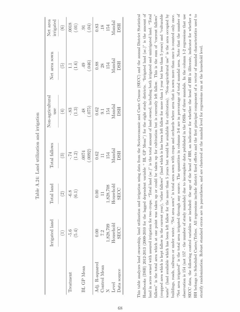
Tab

leA.24:

Lan

dutilization

andirrigation

Irrigatedland

Total

land

Total

fallow

sNon

-agricultural

use

Net

area

sown

Net

area

irrigated

(1)

(2)

(3)

(4)

(5)

(6)

Treatment

-5.6

-6.8

-.74

-.83

1.1

.0018

(5.4)

(6.1)

(1.2)

(1.3)

(1.6)

(.01)

BLGPMean

.0074

.48

.49

.91

(.0092)

(.075)

(.046)

(.04)

Adj.

R-squared

0.00

0.00

0.62

0.62

0.88

0.83

Con

trol

Mean

7.2

1111

9.1

28.18

N1,828,709

1,828,708

154

154

154

154

Level

Hou

sehold

Hou

sehold

Man

dal

Man

dal

Man

dal

Man

dal

Datasource

SECC

SECC

DSH

DSH

DSH

DSH

This

table

analyzeslandow

nership,landutilization

andirrigation

usingdatafrom

theSocioeconom

ican

dCasteCensus(SECC)andthean

nualDistrictStatistical

Han

dbook

s(D

SH)2012-2013(2009-2010

forthelagged

dep

endentvariab

le“BL

GP

Mean”)

fortheeigh

tstudydistricts.“Irrigatedland(ac.)”

istheamountof

landin

acresow

ned

withassuredirrigation

fortw

ocrop

s.“T

otal

land(ac.)”

isthetotalam

ountof

landow

ned,includingboth

irrigatedandunirrigatedland.“Total

fallow

s”is

thetotalarea

whichat

onepointwas

taken

upor

could

betakenupforcultivationbutis

currentlyleft

fallow

.This

isthesum

of“cu

rrentfallow

s”

(cropped

area

whichiskeptfallow

inthecurrentyear),“other

fallow

s”(lan

dwhichishas

beenleft

fallow

formore

than1yearbutless

than5years)and“culturable

waste”(lan

davailable

whichhas

beenleft

fallow

forthemorethan

5yearsbutwou

ldbeavailable

forcultivation).

“Non-agriculturaluse”is

theareaoccupiedby

buildings,road

s,railwaysor

under

water.“N

etarea

sown”is

totalarea

sownwithcrop

san

dorchardswhereareathatis

sownmore

thanonce

iscountedonly

once.

“Net

area

irrigated”is

thetotalarea

irrigatedthrough

anysource.

Thequan

tities

incolumns3-6arein

percentageoftotalmandalarea.Note

thatthenumber

of

observationis

154(not

157-thenumber

ofstudyman

dals)

dueto

incomplete

datapublished

intheDSHsof

threeman

dals.In

thecolumn1-2

regressionsthatuse

SECC

data,

thefollow

ingcontrol

variab

lesareincluded:theageof

theheadof

HH,an

indicator

forwhether

theheadofHH

isilliterate,indicatorforwhether

a

HH

belon

gsto

ScheduledCastes/Tribes.Allregression

sincludedistrictfixed

effects

andthefirstprincipal

componentofavectorofmandal

characteristics

usedto

stratify

random

ization.Rob

ust

stan

darderrors

arein

parentheses,an

dareclustered

attheman

dal

levelforregressionsrunatthehou

sehold

level.

68

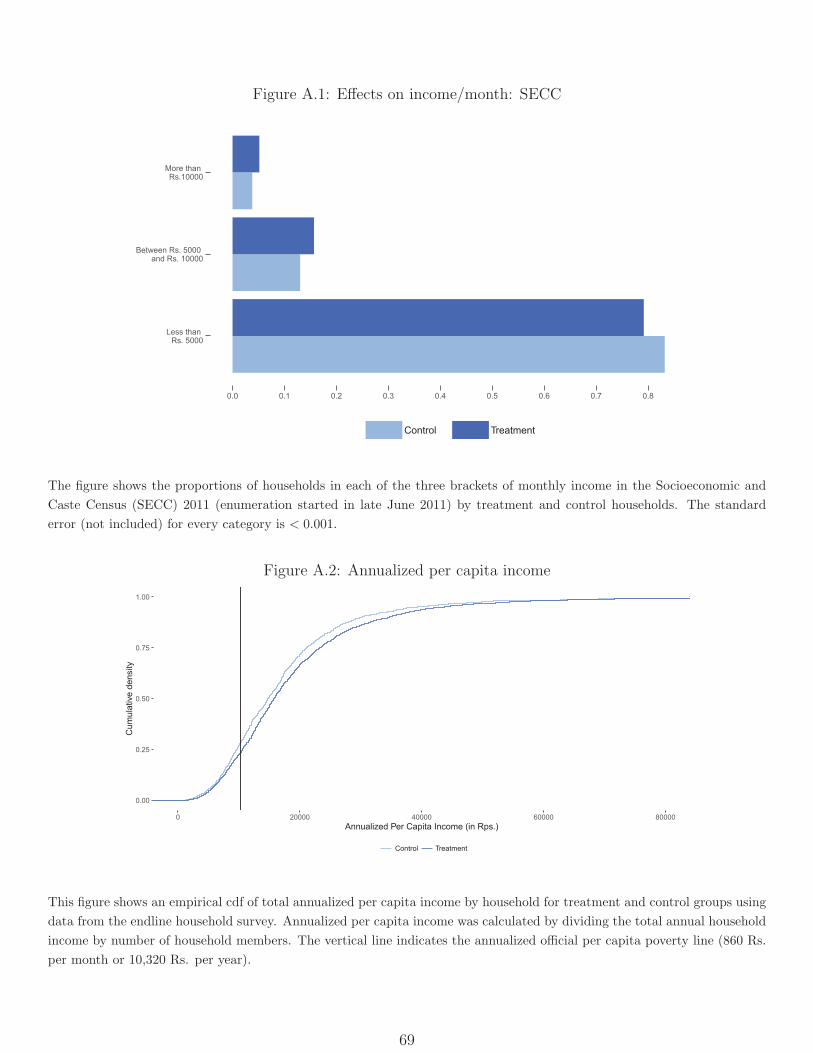
Figure A.1: Effects on income/month: SECC

Less than Rs. 5000

Between Rs. 5000 and Rs. 10000

More than Rs.10000

0.0 0.1 0.2 0.3 0.4 0.5 0.6 0.7 0.8

Control Treatment

The figure shows the proportions of households in each of the three brackets of monthly income in the Socioeconomic and

Caste Census (SECC) 2011 (enumeration started in late June 2011) by treatment and control households. The standard

error (not included) for every category is < 0.001.

Figure A.2: Annualized per capita income

0.00

0.25

0.50

0.75

1.00

0 20000 40000 60000 80000

Annualized Per Capita Income (in Rps.)

Cum

ula

tive d

ensity

Control Treatment

This figure shows an empirical cdf of total annualized per capita income by household for treatment and control groups using

data from the endline household survey. Annualized per capita income was calculated by dividing the total annual household

income by number of household members. The vertical line indicates the annualized official per capita poverty line (860 Rs.

per month or 10,320 Rs. per year).

69

Figure A.3: Official disbursement trends in NREGS

0

5

10

15

Mar−2012 May−2012 Jul−2012 Sep−2012 Nov−2012Month

Avera

ge A

mount

Dis

burs

ed

ControlTreatment

This figure (reproduced from Muralidharan et al. (2016)) shows official NREGS payments for all workers averaged at the

GP-week level for treatment and control areas. The grey shaded bands denote the endline study periods on which our survey

questions focus (May 28 to July 15, 2012).

Figure A.4: Private sector work in June

0.00

0.25

0.50

0.75

1.00

0 10 20 30

Days of private sector paid work

Cum

ula

tive d

ensity

Control Treatment

This figure shows an empirical cdf of the number of days an individual worked for someone else during June 2012, using data

from the endline household survey. The dashed lines indicate in-sample means (not weighted by sampling probabilities) in

treatment and control, respectively.

70

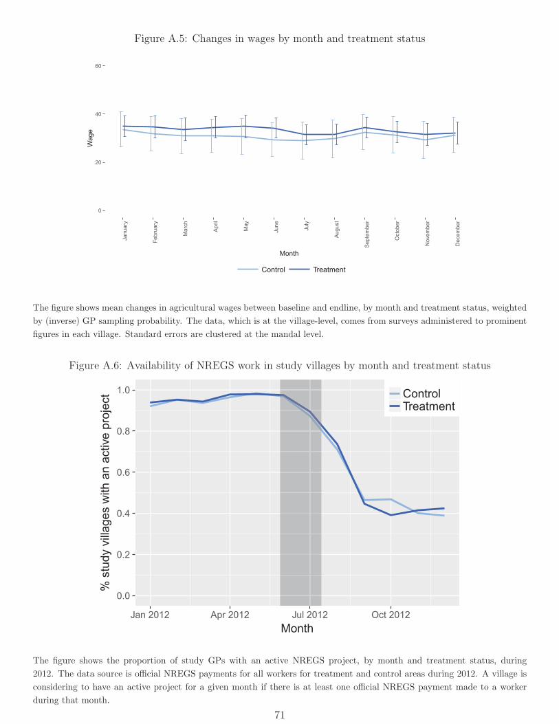
Figure A.5: Changes in wages by month and treatment status

0

20

40

60

January

Febru

ary

Marc

h

Apri

l

May

June

July

August

Septe

mber

Octo

ber

Novem

ber

Decem

ber

Month

Wage

Control Treatment

The figure shows mean changes in agricultural wages between baseline and endline, by month and treatment status, weighted

by (inverse) GP sampling probability. The data, which is at the village-level, comes from surveys administered to prominent

figures in each village. Standard errors are clustered at the mandal level.

Figure A.6: Availability of NREGS work in study villages by month and treatment status

0.0

0.2

0.4

0.6

0.8

1.0

Jan 2012 Apr 2012 Jul 2012 Oct 2012

Month

% s

tudy v

illages w

ith a

n a

ctive p

roje

ct Control

Treatment

The figure shows the proportion of study GPs with an active NREGS project, by month and treatment status, during

2012. The data source is official NREGS payments for all workers for treatment and control areas during 2012. A village is

considering to have an active project for a given month if there is at least one official NREGS payment made to a worker

during that month.

71

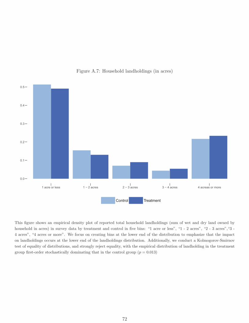
Figure A.7: Household landholdings (in acres)

0.0

0.1

0.2

0.3

0.4

0.5

1 acre or less 1 − 2 acres 2 − 3 acres 3 − 4 acres 4 acreas or more

Control Treatment

This figure shows an empirical density plot of reported total household landholdings (sum of wet and dry land owned by

household in acres) in survey data by treatment and control in five bins: “1 acre or less”, “1 - 2 acres”, “2 - 3 acres”,“3 -

4 acres”, “4 acres or more”. We focus on creating bins at the lower end of the distribution to emphasize that the impact

on landholdings occurs at the lower end of the landholdings distribution. Additionally, we conduct a Kolmogorov-Smirnov

test of equality of distributions, and strongly reject equality, with the empirical distribution of landholding in the treatment

group first-order stochastically dominating that in the control group (p = 0.013)

72

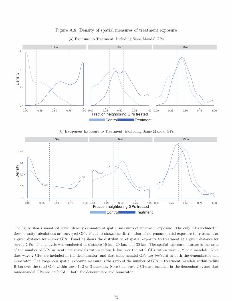
Figure A.8: Density of spatial measures of treatment exposure

(a) Exposure to Treatment: Including Same Mandal GPs

10km 20km 30km

0

1

2

3

0.00 0.25 0.50 0.75 1.00 0.00 0.25 0.50 0.75 1.00 0.00 0.25 0.50 0.75 1.00

Fraction neighboring GPs treated

Density

Control Treatment

(b) Exogenous Exposure to Treatment: Excluding Same Mandal GPs

10km 20km 30km

0.0

0.5

1.0

1.5

2.0

0.00 0.25 0.50 0.75 1.00 0.00 0.25 0.50 0.75 1.00 0.00 0.25 0.50 0.75 1.00

Fraction neighboring GPs treated

Density

Control Treatment

The figure shows smoothed kernel density estimates of spatial measures of treatment exposure. The only GPs included in

these density calculations are surveyed GPs. Panel a) shows the distribution of exogenous spatial exposure to treatment at

a given distance for survey GPs. Panel b) shows the distribution of spatial exposure to treatment at a given distance for

survey GPs. The analysis was conducted at distance 10 km, 20 km, and 30 km. The spatial exposure measure is the ratio

of the number of GPs in treatment mandals within radius R km over the total GPs within wave 1, 2 or 3 mandals. Note

that wave 2 GPs are included in the denominator, and that same-mandal GPs are included in both the denominator and

numerator. The exogenous spatial exposure measure is the ratio of the number of GPs in treatment mandals within radius

R km over the total GPs within wave 1, 2 or 3 mandals. Note that wave 2 GPs are included in the denominator, and that

same-mandal GPs are excluded in both the denominator and numerator.

73

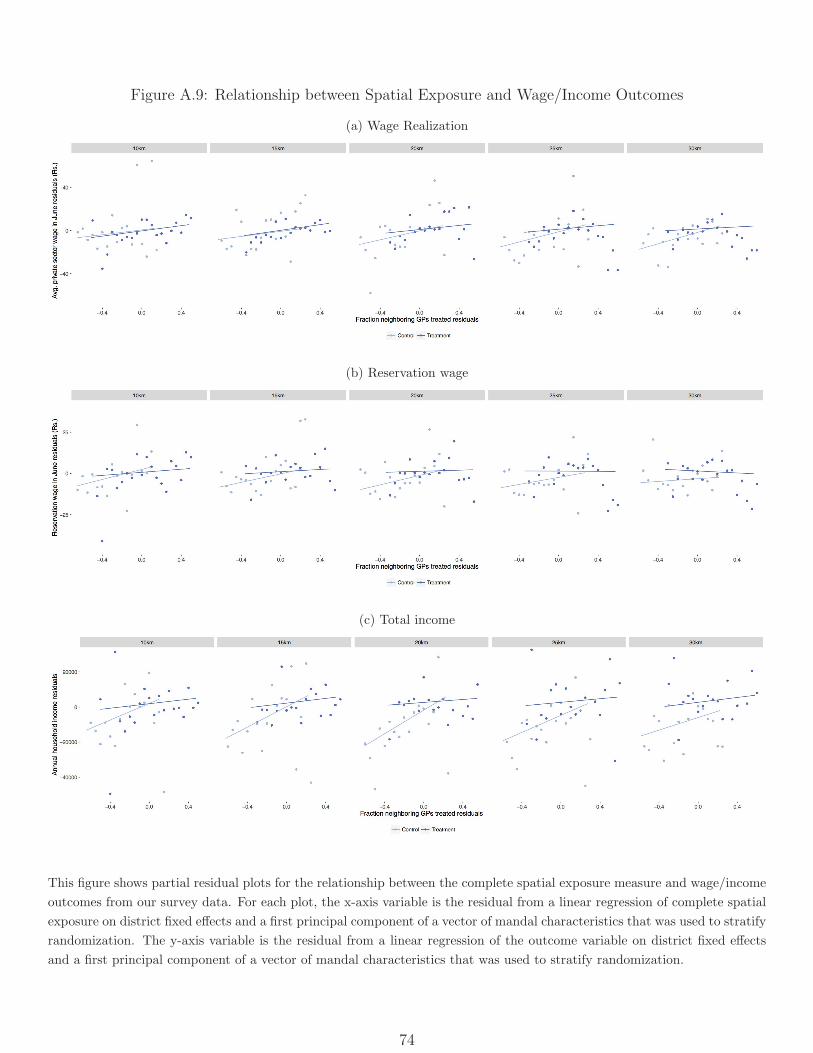
Figure A.9: Relationship between Spatial Exposure and Wage/Income Outcomes

(a) Wage Realization

(b) Reservation wage

(c) Total income

This figure shows partial residual plots for the relationship between the complete spatial exposure measure and wage/income

outcomes from our survey data. For each plot, the x-axis variable is the residual from a linear regression of complete spatial

exposure on district fixed effects and a first principal component of a vector of mandal characteristics that was used to stratify

randomization. The y-axis variable is the residual from a linear regression of the outcome variable on district fixed effects

and a first principal component of a vector of mandal characteristics that was used to stratify randomization.

74

Figure A.10: Relationship between Spatial Exposure and Labor Outcomes

(a) Days worked private sector

(b) Days unpaid/idle

The figure shows partial residual plots for the relationship between the complete spatial exposure measure and labor outcomes

from our survey data. For each plot, the x-axis variable is the residual from a linear regression of complete spatial exposure

on district fixed effects and a first principal component of a vector of mandal characteristics that was used to stratify

randomization. The y-axis variable is the residual from a linear regression of the outcome variable on district fixed effects

and a first principal component of a vector of mandal characteristics that was used to stratify randomization.

75

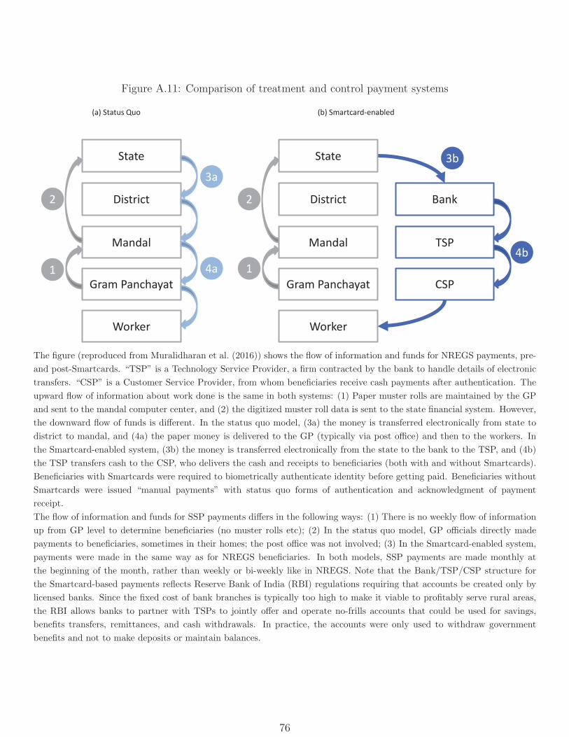
Figure A.11: Comparison of treatment and control payment systems

State

District

Mandal

Gram Panchayat

Worker

State

District

Mandal

Gram Panchayat

Worker

Bank

TSP

CSP

(a) Status Quo (b) Smartcard-enabled

1 1

3b

2

3a

2

4a

4b

The figure (reproduced from Muralidharan et al. (2016)) shows the flow of information and funds for NREGS payments, pre-

and post-Smartcards. “TSP” is a Technology Service Provider, a firm contracted by the bank to handle details of electronic

transfers. “CSP” is a Customer Service Provider, from whom beneficiaries receive cash payments after authentication. The

upward flow of information about work done is the same in both systems: (1) Paper muster rolls are maintained by the GP

and sent to the mandal computer center, and (2) the digitized muster roll data is sent to the state financial system. However,

the downward flow of funds is different. In the status quo model, (3a) the money is transferred electronically from state to

district to mandal, and (4a) the paper money is delivered to the GP (typically via post office) and then to the workers. In

the Smartcard-enabled system, (3b) the money is transferred electronically from the state to the bank to the TSP, and (4b)

the TSP transfers cash to the CSP, who delivers the cash and receipts to beneficiaries (both with and without Smartcards).

Beneficiaries with Smartcards were required to biometrically authenticate identity before getting paid. Beneficiaries without

Smartcards were issued “manual payments” with status quo forms of authentication and acknowledgment of payment

receipt.

The flow of information and funds for SSP payments differs in the following ways: (1) There is no weekly flow of information

up from GP level to determine beneficiaries (no muster rolls etc); (2) In the status quo model, GP officials directly made

payments to beneficiaries, sometimes in their homes; the post office was not involved; (3) In the Smartcard-enabled system,

payments were made in the same way as for NREGS beneficiaries. In both models, SSP payments are made monthly at

the beginning of the month, rather than weekly or bi-weekly like in NREGS. Note that the Bank/TSP/CSP structure for

the Smartcard-based payments reflects Reserve Bank of India (RBI) regulations requiring that accounts be created only by

licensed banks. Since the fixed cost of bank branches is typically too high to make it viable to profitably serve rural areas,

the RBI allows banks to partner with TSPs to jointly offer and operate no-frills accounts that could be used for savings,

benefits transfers, remittances, and cash withdrawals. In practice, the accounts were only used to withdraw government

benefits and not to make deposits or maintain balances.

76