General Characteristics of Stratospheric Singular Vectors

Ronald M. Errico1,2

Ronald Gelaro2

Elena Novakovskaia3,2

Ricardo Todling4,2

Submitted to Meteorologische Zeitschrift

28 February 2007

1 Goddard Earth Science Technology Center, University of Maryland Baltimore County

2 Global Modeling and Assimilation Office, Goddard Space Flight Center

3 Earth Resources Technology, Inc.

4 Science Applications International Corporation

Corresponding author’s address: Ronald M. Errico, Global Modeling and Assimilation Of-

fice, NASA/GSFC Code 610.1, Greenbelt, MD 20771. Email: rerrico@gmao.gsfc.nasa.gov

Abstract

Leading singular vectors have been computed for a numerical weather prediction model

that can resolve dynamical structures within the stratosphere and lower mesosphere. The

norm applied at the final time is the commonly used energy norm but confined to mea-

suring the stratosphere. These stratospheric singular vectors are described by presenting

three examples. They are produced using either of two initial norms that weight per-

turbations within the troposphere versus stratosphere very differently. For either initial

norm, singular values are typically smaller than their tropospheric counterparts and they

are less geographically local. They also retain their relevance to corresponding nonlinear

evolutions for longer periods and larger amplitudes. For these reasons, stratospheric SVs

may be useful for explaining observed stratospheric dynamical behaviors.

1. Introduction

The examination of atmospheric singular vectors (SVs) has fostered new insights into

tropospheric dynamics and the behavior of short-term, forecast error growth (Farrell, 1989;

Buizza and Palmer, 1995; Ehrendorfer and Errico, 1995; Buizza et al., 1997; Palmer et al.,

1998; Gelaro et al., 2000; Reynolds et al., 2001). Until now, attention has focused on the

troposphere, motivated by applications in numerical weather prediction (NWP) and due

to limitations in older models for which adjoints were available. These limitations included

low stratospheric resolutions, strong, artificial stratospheric ”sponges” to filter amplifying

vertically propagating waves, and a common numerical need to restrict measuring norms

to the troposphere.

There are many questions concerning stratospheric dynamics for which singular vectors

may also provide fresh insights. These concern the genesis of sudden warmings and the

nature of interactions with the troposphere (Andrews et al., 1987). Stratospheric dynamics

are often described in terms of waves and quasi-linear behaviors, suggesting that tangent-

linear SVs may be particularly useful for stratospheric applications. Since highly nonlinear

boundary layer and precipitation–generating processes play little role at high altitudes, it

is possible that the tangent linear approximation upon which SVs are based will hold even

better than in the troposphere.

In this first examination of stratospheric SVs at the U.S. National Aeronautics and

Space Administration (NASA), rather than jump to a specific stratospheric question, the

general characteristics of these SVs are examined. In particular, the several ways in which

they are dramatically different than their tropospheric cousins are noted. Also, additional

issues that must be considered regarding the choices of norms are described.

Aspects of the NASA model that are particularly relevant to SV determination are

1

presented in the next section. The norms used to determine the SVs are defined in section

3 followed in section 4 by a brief description of the reference state for the period forming

the focus of this presentation. The leading SVs determined for the two norms during this

focus period are described in sections 5–6 along with a noteworthy one for an earlier period.

Comparisons of tangent linear and nonlinearly evolved perturbations initialized using these

SVs appear in section 7, followed by a summary.

2. Model

The NASA model used here is the Goddard Earth Observing System (GEOS–5) general

circulation model with the finite–volume dynamical core developed by Lin and Rood (1996).

The model has a hybrid (mixed, terrain–following, standard σ and constant pressure)

vertical coordinate defined on 72 levels, with those above 150 hPa (model level index

k = 40, counting from the top) being constant pressure surfaces. The spacing of the levels

is further described in the next section and the model top (pt) is at 0.01 hPa. The model

filters tendencies having short longitudinal scales near the poles in order to avoid the very

short time steps otherwise required. Attached to the dynamics are parameterizations for

all the standard physical processes found in most general circulation and NWP models.

The tangent linear version of the dynamics is exact, but a minimal set of simplified

linearized physics has been added. This includes standard second–order, temporally semi–

implicit, vertical diffusion applied throughout the depth of the atmosphere, with the diffu-

sion coefficients defined at each time step by those in the reference trajectory forecast about

which the linearization is performed. No perturbations of these coefficients are considered,

however, to ensure numerical stability of this linearized version. This scheme includes sur-

face momentum drag with a coefficient that is determined from the reference state using

the surface physics in the nonlinear model. There is no linearized surface temperature flux

2

term. The tangent linear version also includes a semi–implicit, fourth–order horizontal

diffusion scheme. There is no such scheme in the nonlinear model because, apparently,

the nonlinear finite–volume algorithm, along with the time filtering of tendencies near the

poles, provides enough spatial smoothing.

Additionally, a damping factor νk is applied to the tangent linear u′, v′ and T ′ fields

above 70 hPa at each time step after the field is updated by the dynamics and other

physical tendencies, where

νk = exp

[

−∆t

c1

(

c1

ckm

)k−1

km−1

]

,

with k = 1, . . . , km being the levels over which the sponge is applied, ∆t being the physics

time step (1800 s here), and c1 and ckmcorresponding to the minimum and maximum

e-folding damping times of 0.7 days and 30. days, respectively. This term is intended to

represent effects of the nonlinear model’s sponge applied to all fields in the mesosphere as

well as effects of radiative cooling in the stratosphere.

The adjoint model is exact with respect to the tangent linear model, such that its

resolvent matrix is an exact transpose (Errico 1997). The time steps used in the nonlinear,

tangent linear, and adjoint models are identical. Trajectory information is stored for every

time step, and no additional approximations to the time scheme are made for linearization.

3. Norms

There are two norms considered for this study. One is the commonly used, total energy

norm (Talagrand, 1981; Errico, 2000a):

E =1

2

∑

i,j,k

∆Aj∆σi,j,k

(

u′2 + v′2 + aT ′2 + bp′2s)

, (1)

3

where u′, v′, T ′, and p′s are perturbation wind components, temperature, and surface

pressure fields with understood longitude, latitude and vertical indexes i, j, k, respec-

tively, where appropriate, and ∆Aj is a fractional surface area for each horizontal grid

point. The weights a = Cp/Tr and b = RTr/p2

sr, with cp being the specific heat of air,

R the gas constant, and Tr and psr prescribed, location-independent (e.g., mean) val-

ues of temperature and surface pressure. Values of Tr = 280 K and psr = 1000 hPa

are used, yielding a ≈ 3.59(J/kg)/K2 and b ≈ 8 × 10−6(J/kg)/Pa2. The vertical weight

∆σi,j,k = ∆pi,j,k/(ps i,j − pt) is computed for each layer of pressure “thickness” ∆p within

each column using the values obtained from the reference trajectory at the times the norm

is computed.

This E may also be considered a combined measure of the mean squares of u′, v′, T ′ and

p′s using fractional mass as a vertical weight. Note that above 150 hPa where the model

levels are isobaric surfaces, this vertical weight tends to be larger over high topography

where ps is small (by as much as a factor of 2 over Tibet). Near the surface, however,

where the vertical coordinate is purely terrain following, all geographic regions are almost

equally weighted. For a more lengthy discussion of the properties and interpretation of

this norm, see Errico (2000a).

The motivation for another norm is described in section 6. This second norm is given

by

V =1

2

∑

i,j,k

∆Aj∆zi,j,k

(

u′2 + v′2 + aT ′2 + bp′2s)

. (2)

It is identical to the E norm except that ∆σi,j,k is replaced by

∆zi,j,k = ∆ ln pi,j,k/(ln ps i,j − ln pt) , (3)

where ∆z is the difference in ln p between the two interfaces sandwiching each layer. If

the temperature throughout a column of air were constant, ∆z would be proportional to

4

the spatial thickness of a layer. The denominator in (3) is included so that, as for ∆σ, the

vertical weights sum to 1. Analogous to E, the V norm may also be considered a combined

mean square of the fields, but with a fractional distance rather than fractional mass as the

vertical weight. It also will tend to weight the norm over high topography more than low,

but by a factor less than approximately 1.06 at ps = 500 hPa. The possible need for this

new norm is also discussed in Lewis et al. (2001).

Values of ∆σ and ∆z for the particular reference–state value ps = 1000 hPa are pre-

sented in Fig. 1. The ∆σ are a maximum near 300 hPa with values a factor of 3.3

smaller near the surface. Above 300 hPa, however, they rapidly decay approximately

exponentially so that the ratio of values at 500 hPa and 0.1 hPa is 1200. In contrast, for

0.1 hPa< p <500 hPa, ∆z varies by less than a factor of 5. Values of ∆z below 800 hPa

are approximately 10 times smaller than those near the tropopause.

At the final time, only a form of the E norm is applied in all the experiments. It differs

from (1) in that it is only applied to a region of interest, specified here as 30◦N – 90◦N and

10 hPa – 90 hPa (15 ≤ k ≤ 37). The normalizations of ∆σ and A are recomputed for this

application so that both sum to 1 over the specific region of interest. This localization of

the norm does not constrain the evolved SV at final time to lie wholly within this region

but does mean that only the portion of its structure that is within this region is measured

by the norm and thus is considered by the optimization problem defining the SVs. At the

initial time, either the E or V norm is applied, with both computed globally. The SVs

are determined using 12 or more iterations of a Lanczos algorithm such that the first few

squared singular values and singular vectors appear to be converged.

5

4. Reference states

The reference states for which the SVs are computed are determined by 5–day forecasts

begun from analyses produced using the GEOS–5 data assimilation system. Observations

directly affecting the stratosphere include satellite–observed radiances and, at only low

altitudes, a few rawindsondes. The analysis and subsequent nonlinear forecasts used to

define the evolving state are produced at a horizontal resolution of 1◦ latitude by 1.25◦

longitude. The tangent linear and adjoint versions, however, are produced at a resolution

of 4.5◦ latitude by 5◦ longitude. This low resolution appears sufficient based on the rather

large scales of the SVs that have been produced.

SVs were computed for 34 periods throughout the summer of 2005 and the following

winter. Attention in this report is primarily focused on the single 5–day period of 21–26

January 2006, beginning 0 UTC. During this focus period, a dramatic sudden warming

occured in the winter polar stratosphere. The 50 hPa temperature at the North Pole rose

by approximately 20◦C and the zonal–mean zonal winds at 60◦N for 10 hPa and 5 hPa

became easterly and vanished, respectively. Results for other periods are mentioned here

only for the purpose of supporting the generality of the presented results and revealing

some ranges of behaviors.

Although not assured a–priori, the 5–day, model–produced reference forecast for the

focus period also reveals a dramatic sudden warming. The initial and final 50 hPa geopo-

tential height fields between 20◦N and the North Pole appear in Fig. 2. At first glance, the

initial pattern may be characterized as a single polar vortex centered just north of Scandi-

navia, with a notable smaller scale trough reaching into central Russia. The initial heights

at the center of the vortex and at the North Pole are 1940 dm and 1975 dm, respectively.

After 5 days, the single vortex is replaced by a wavenumber 3 (or larger scale) pattern,

6

with large scale troughs just west of the Ural Mountains, over Northern Siberia, and over

the Queen Elizabeth Islands, and two smaller scale troughs embedded in the latter. At

this time, the height at the pole is 2005 dm and the lowest height within the region shown

is 1955 dm. At 60◦N, the mean height gradient and thus zonal mean geostrophic wind are

dramatically smaller than initially.

5. Properties of E norm SVs

The leading squared singular values determined for individual 5–day periods sampled

for the winter period November 2005 through February 2006 computed using the E norm

range between 155 and 12. These values are the factor by which E increases during the

5–day periods. For the focus period, this factor is 64.

For the focus period, the vertical integral of the contribution to E at each horizontal

grid point is shown in Fig. 3 for the leading SV at both initial and final times. Note that

these values are spread over a much greater geographical area than is typical for leading

tropospheric E–norm SVs (Buizza et al., 1997; Gelaro et al., 2000; Reynolds et al., 2001).

In fact, when such non–local leading tropospheric SVs are obtained, the result almost

always indicates non–convergence of the Lanczos algorithm used to obtain the solutions.

Experiments conducted to explore this issue will be described later in this section. At

the initial and final times, the fractions of E contributed by kinetic energy are 0.51 and

0.65, respectively. The wind perturbations are almost entirely nondivergent at both times.

Leading tropospheric E norm SVs typically have smaller kinetic energy fractions than this

at their initial times but larger fractions at their final times.

The horizontal integral of the contributions to E at each model level appear in Fig. 4a.

The labeled ordinate is the level’s pressure presented on a logarithmic scale, with values

7

for hybrid–defined coordinate levels specified by assuming ps = 1000 hPa. The two curves

are for initial and final times, with each curve normalized such that its sum over all model

levels is 1. Note that the E contributions are largest near 20 hPa at both times, with very

little contributions from the troposphere. Thus, this SV appears to describe a growing non–

modal structure essentially confined to the stratosphere. This stratospheric confinement is

a common feature of the leading E–norm SVs produced for all the winter 5–day periods

examined.

Plots of the contribution to E by each model level (or layer) as in Fig. 4a can be

misleading. For example, if the horizontally mean squared value of u′2 in each layer were

the same, contributions to E can still vary greatly in the vertical unless ∆σ is identical for

each layer. In this model, ∆σ varies greatly as shown in Fig. 1, as it must for all NWP

models that attempt to simultaneously model the troposphere, stratosphere, and lower

mesosphere. So, a presentation as in Fig. 4a can be revealing more about the grid structure

of the model than about its dynamics. An analogous warning about interpretations of

vertical distributions for adjoint model results is presented in Lewis et al. (2001).

For the above reason, the vertical distribution of E is instead presented as an energy

density in Fig. 4b. This is E/∆σ computed for each level. This may also be interpreted as

a weighted sum of the horizontal mean squares of the perturbations over all model levels

and fields. It reveals that the largest values occur for p < 1 hPa at both times rather than

near 20 hPa. The dramatic change in the presentation occurs because at this height in the

model atmosphere, the spacing of the levels is approximately equal in ∆ ln (p), so that ∆σ

decreases nearly exponentially with decreasing p. The vertical distribution of E in Fig. 4a

is in large part due to this distribution of model layer thicknesses. The vertical weighting

determined by this vertical spacing has other implications as well that will be presented in

the following section.

8

Cross sections of v′ at initial and final times appear in Figs. 5a,b, respectively. These

are along 60◦N and 75◦N, respectively, where magnitudes of the fields are large. Note

the strong westward tilt with increasing height at the initial time. This is an even more

extraordinary tilt than typically obtained for tropospheric SVs (e.g., as discussed in Hoskins

et al., 2000). In strong contrast, at final time the SV has much less tilt, analogous to the

lessening of tilt obtained as typical tropospheric SVs evolve (e.g., Gelaro et al., 2000).

In the remainder of this section, the leading E–norm SV for the period is described for

the purpose of revealing additional aspects of the non–local nature of the stratospheric SV

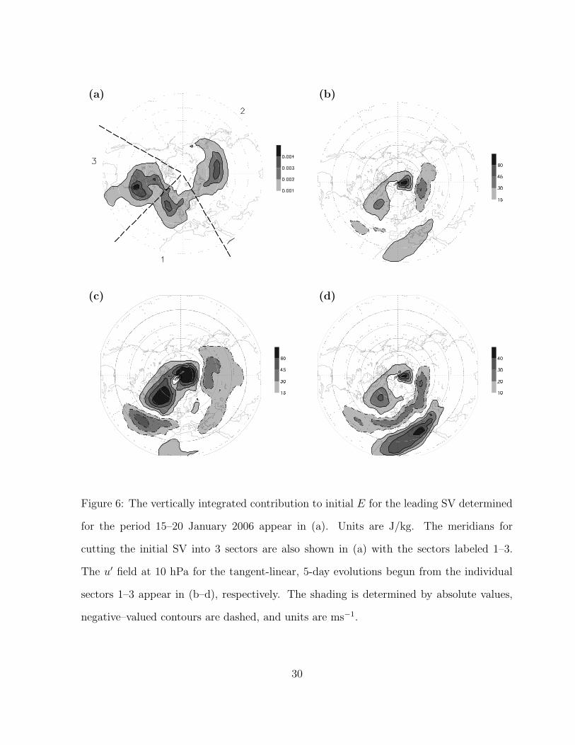
structures. The initial horizontal distribution of vertically–integrated E appears in Fig. 6a.

Note that it is highly nonlocal with three centers of activity: over Eastern Canada, the

North Atlantic, and Siberia. To investigate whether these should actually be associated

with distinct SVs and appear combined here only due to non–convergence of the Lanczos

algorithm used to determine the SVs, this particular SV has been dissected into three com-

ponents using the partitioning along the meridians indicated in the figure. Each component

includes all fields at all levels in the indicated sector. Since the distribution and especially

distinctiveness of local maxima or minima at individual levels for individual initial fields

may dramatically differ from the integrated E shown in Fig. 6a, this specific dissection is

therefore somewhat arbitrary. The dissection is only applied to create three distinct and

uncorrelated initial conditions that are each then evolved independently using the tangent

linear model.

The 5–day evolved u′ field at 10 hPa begun from the sectors labeled 1–3 appear in

Figs. 6b–d, respectively. The three separate sections apparently produce highly correlated

results. Area–weighted correlations for the 10 hPa u′ fields north of 30◦N are 0.80 for

results produced from sectors 1 and 2, 0.89 for 1 and 3, and 0.59 for 2 and 3. These values

are typical of corresponding u′, v′, and T ′ results at all levels within the domain over which

9

the final E norm is measured. Thus, although initially well separated, the three evolutions

produce solutions that reinforce each other when added. The SV that optimizes E at

the final time given a constrained value of E at the initial time will therefore necessarily

include initial contributions by all three sectors, for the general reason described by Errico

(2000b). This is analogous to the combining of rotational and gravitational components to

yield optimal E–norm growth for tropospheric SVs (Errico, 2000b). The nonlocalness is

therefore due to the dynamics that render the distinct evolved results so similar rather than

evidence of non–convergence of the Lanczos algorithm. This conclusion was confirmed by

doubling the number of Lanczos iterations to check that the additional iterations negligibly

affected the structure of the leading SV.

6. Properties of V–norm SVs

An effect of the spacing of the model’s vertical grid on interpreting the E norm was

presented in the last section, however, it also profoundly affects the structures determined

by the SV optimization problem. Maximizing the ratio of E at the final time compared

with its value at the initial time concerns not only maximizing the final value but also

minimizing the initial one. The value of E at the initial time can be considered a penalty.

Since the E norm gives much more weight to tropospheric levels than to stratospheric

or mesospheric ones, it effectively penalizes the placement of initial perturbations in the

lower atmosphere. For example, ∆σ at 500, 50, and 5 hPa are respectively 0.043, 0.009,

and 0.001. Placing a mean value of u′2 at 500 hPa therefore creates 43 times the penalty

of doing the same at 5 hPa. As long as the dynamics can yield enough growth for a

perturbation placed at higher levels, the smaller penalty for initially placing perturbations

there can outweigh a weaker dynamical response.

In the previous section, the E norm SVs were revealed to be essentially confined to the

10

stratosphere. In light of the caveat above, it is therefore appropriate to ask if this general

result is revealing more about the model’s vertical grid structure or about stratospheric

dynamics. For this reason, SVs were also produced using the V norm at the initial time. At

the end time, the E norm confined to the stratosphere was still used, so that the squared

singular values therefore equal the ratios of final stratospheric E to initial V . As revealed

in Fig. 1, these new SVs will penalize tropospheric variances less severely compared to

their stratospheric or mesospheric counterparts.

The fractional contributions to E at each model level and the corresponding energy

densities for this V –norm SV appear in Fig. 7. These values are very unlike those in Fig. 4

for the E norm. For the V norm initially, 80% of the E is located below 500 hPa, with

its maximum at 790 hPa. At the final time, the maximum occurs at 300 hPa with a much

smaller secondary peak in the stratosphere. Only 13% of E is in the stratospheric layers

where it is considered in determining the ratio E/V to be maximized for defining the leading

SV. The energy densities (Fig. 7b) are even more dominant in the lower troposphere, where

∆σ is defined to be small. With its reduced penalty on initial tropospheric perturbations,

the initial SV produced for the V norm is predominately tropospheric. Presumably, the

tropospheric dominance at the final time is simply due to the large initial values at those

levels, since the optimization problem defining the SV does not explicitly consider the final

tropospheric fields.

For the initial V –norm SV, examination of cross sections (not shown here) through the

lower troposphere where its fields have local maxima reveal tilts more like those observed

for leading tropospheric SVs than as appearing in Fig. 5. This result, and comparison of

Figs. 7 and 4 suggests that the V – and E–norm SVs bear little resemblance to each other.

Examination of their corresponding horizontal fields at each model level, however, reveals

remarkable similarities in the shapes of structures. This is confirmed in Fig. 8 where the

11

horizontal correlations of corresponding u′ and T ′ fields at individual model levels for the

two SVs are shown for both initial and final times. At the initial time for both u′ and

T ′, correlations are above 0.8 except in the mid–stratosphere. At the final time they are

between 0.6 and 0.8 at almost all levels. So, the change of vertical weights (between the

E and V norms) has primarily changed the amplitudes of the SV structures at each level

rather than the shapes of the structures within each level.

7. Relevance to nonlinear evolution

Since SVs are determined based on linearized dynamics, if their relevance is to be

claimed in the nonlinear context as well, evidence must be offered. This relevance can

depend critically on amplitudes, time periods, synoptic situations, and metrics (Errico et

al., 1993), and thus is difficult to state generally, without regard to any specific application.

Here, the time period and synoptic situation are given by those that define the SVs and the

metrics are correlations and final maximum magnitudes of the perturbation fields (Errico

and Raeder, 1999, Reynolds and Rosmond, 2003).

For the test here, the initial magnitudes of the SV structures used to create differences

in the nonlinear forecasts have been chosen by simply multiplying the initial E or V norm

SVs by a scalar factor of 0.1. For the E norm SVs, this yields maximum initial magnitudes

of u′, v′, and T ′ equal to 16 ms−1, 7 ms−1, and 3.6 K, respectively. All of these maxima are

located in the upper stratosphere or lower mesosphere. These rather large amplitudes were

investigated because they yielded final–time perturbations having magnitudes similar to

the temporal changes occurring in the nonlinear reference forecast over five days, and thus

may be of interest in future examinations of the stratospheric sudden warming problem.

For the E norm, the maximum initial wind perturbations are less than 0.1 ms−1 below

500 hPa.

12

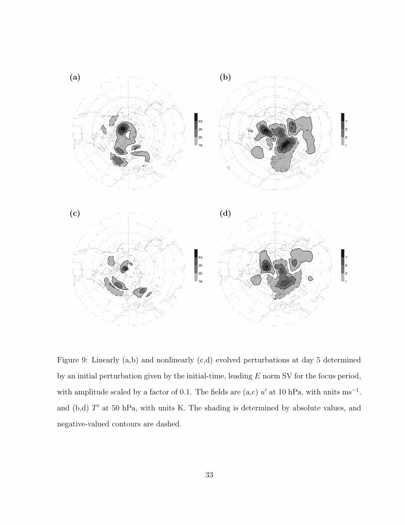
Representative stratospheric fields for the leading evolved E norm SV at day 5 for the

focus period are presented in Fig. 9. Specifically, these are u′ at 10 hPa (Figs. 9a,c) and

T ′ at 50 hPa (Fig. 9b,d). The tangent linear evolution of the perturbation appears in

Figs, 9a,b and the corresponding differences between the perturbed and reference nonlin-

early evolved solutions appear in Figs. 9c,d. The latter are computed using the model with

its complete physics package, so the comparison concerns not simply dynamical nonlinear-

ity but also the faithfulness of the greatly simplified physics included in the tangent linear

and adjoint models with respect to the complete nonlinear model.

For the nonlinear difference fields shown in Fig. 9, the maximum absolute values for u′

and T ′ are 49 ms−1 and 8.4 K, respectively, with corresponding values less than 10% lower

for the tangent linear result. The correlations between the two u′ fields is 0.66 and for T ′,

0.82. This is remarkable agreement given the large perturbation magnitudes and long time

period examined.

The horizontal correlations for u′, v′, and T ′ at all levels for the above experiment appear

in Fig. 10a. Near 50 hPa, the correlations for all fields are larger than 0.7. Within the

stratosphere, the correlations generally drop as levels for successively lower p < 50 hPa are

considered. In the troposphere, the correlations for all fields are below 0.3. The result that

local maxima or minima in the horizontal correlations for T ′ appearing in Fig. 10a occur

closely below those for winds is related to the fact that winds at any level are hydrostatically

and geostrophically related only to the temperatures at and primarily below that level. The

maximum absolute magnitudes for the nonlinearly determined perturbations at levels p <

1 hPa are slightly larger than the corresponding linear results, but within the troposphere,

these magnitudes are typically ten times larger than their tangent linear values. For this

SV with this initial magnitude, the tropospheric portions of the tangent linear solutions

are therefore unreliable in the nonlinear context.

13

Since the V norm SV is characterized by relatively larger tropospheric perturbations

than its E norm counterpart and tropospheric agreement between nonlinearly and tangent

linearly evolved perturbations appears more problematic, the above comparison was re-

peated for the V norm SV. Its initial magnitude was also produced using a scaling of 0.1

applied to the original SV. This scaling yields initial maximum absolute values of u′, v′,

and T ′ equal to 1.8 ms−1, 1.9 ms−1, and 3.1 K, respectively. These values occur near the

surface and are much smaller than those in the previous experiment.

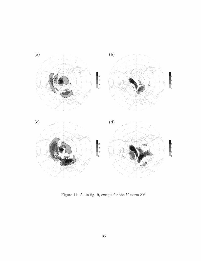
Results for the V norm experiment appear in Figs. 11 and 10b (analogous to Figs. 9

and 10a, respectively). Note the apparently strong correlations and similar magnitudes

appearing in the 2 pairs of corresponding fields in Fig. 11. Correlations (Fig. 10b) are

above 0.5 for all fields at levels in the stratosphere, with the wind correlations greater than

0.8 at several levels. Within the stratosphere at the final time, the nonlinear results have

the maximum absolute magnitudes of u′, v′ and T ′ equal to 30 ms−1, 27 ms−1 and 22 K,

respectively. The better stratospheric agreements in this experiment may be due to these

magnitudes being smaller than in the previous one, although they are still quite large. As in

the previous experiment, the tangent linear and nonlinear tropospheric results are poorly

correlated, although unlike in that experiment, their mean squared values are similar.

Although the V –norm SVs are at least initially driven by tropospheric perturbations, the

lack of tropospheric correlation obtained by day 5 of its evolution apparently has had little

detrimental affect on the stratospheric agreement.

Agreement between nonlinear and tangent linear results above the troposphere depends

on how well the sponge is tuned. In the experiments here, only a gross tuning was per-

formed. In an earlier, developmental set of experiments, the sponge coefficients were so

large as to damp almost all perturbations within the stratosphere. For the experiments

reported here, those coefficients were therefore radically reduced within the lower strato-

14

sphere to the magnitudes reported in section 2. No change of the functional form of the

coefficients was attempted, however, and it was deemed more important to ensure that

numerically spurious structures do not appear near the upper boundary than to obtain a

better match between the tangent linear and nonlinear results.

The 5–day period over which the SVs have been evolved here is longer than linearity

typically holds for leading tropospheric SVs having the magnitude of initial condition uncer-

tainty (Reynolds and Errico, 1999). Since the E norm growth factors for the stratospheric

SVs are much smaller than for leading tropospheric ones, the extended linear applicability

is not so surprising. What remains surprising is that the linearity holds even for the large

initial magnitudes applied here. Smaller perturbations should yield at least as good agree-

ment between tangent linear and nonlinear results unless the perturbation magnitudes are

specified to be so small such that missing tangent linear physical parameterizations rather

than nonlinear dynamics become the major source of disagreement. For reasons stated

earlier, it is difficult to generalize the applicability of these SVs, especially without a spe-

cific objective for their use. Even so, the limited results here suggest that SVs having large

initial amplitude may adequately describe nonlinear stratospheric perturbations out to 5

days.

8. Conclusion

Only three SVs were described in detail here. These were all leading SVs for 5–day

periods in January 2006, defined using the same final–time norm but for two different, but

related, initial norms. SVs were computed for several other 5–day periods for the initial

E norm and for both 2– and 5–day periods for the initial V norm. The latter periods

included summer as well as winter ones. The first several leading SVs were computed for

each period. The qualitative results reported here appeared to generally apply to all these

15

other SVs as well.

These stratospheric SVs have both notable similarities and differences compared with

their typical tropospheric counterparts. Singular values are much larger in the winter, com-

pared with summer, hemisphere. Perturbation shapes change strongly in time. Rotational

winds strongly dominate divergent ones. The initial E norm SVs exhibit a strong eastward

tilt as height increases, which becomes less pronounced as the SV evolves in time.

One important difference compared with their E–norm tropospheric counterparts is

that, for periods of the same duration, singular values for stratospheric SVs are much

smaller. This conclusion is based both on unpublished studies of E–norm tropospheric SVs

with the same NASA adjoint model and with published results for tropospheric spectral

models. Low resolution (e.g., T21L19), short period (e.g., 36 hour), SVs computed by

considering only dry tangent linear dynamics and simple physics yield leading singular

values of less than 7 for non–summer cases (Buizza at al., 1997; Palmer et al., 1998;

Reynolds et al., 2001), and much higher values for longer periods, higher resolution, and

more complete physics (Errico et al., 2004). Here the largest E norm singular value for 5

days during the winter season averaged less than 8.

The stratospheric SVs are also geographically (horizontally) less local than typical

tropospheric ones. This result is not due to a lack of convergence by the Lanczos algorithm,

which often explains any nonlocalness obtained for tropospheric SVs. Rather, it was shown

to be due to the correlations that can develop from initially disparate SV structures:

Initially distant and therefore distinct perturbation structures can yield remarkably similar

perturbation structures by day 5. A linear combination of those distinct structures is

therefore optimal when quadratic norms are applied at both initial and final times.

The vertical distribution of E for the SVs at both initial and final times was shown to

16

be very sensitive to the vertical weighting implied by the initial norm used to constrain

the initial perturbations. Specifically, the usual, fractional mass (∆σ) vertical weighting

employed in the perturbation energy (E) norm necessarily decays almost exponentially

in stratospheric resolving models, such that initial perturbations in the troposphere are

penalized much more strongly than in the stratosphere or above. This weighting therefore

effectively precludes significant initial perturbations within the troposphere if any strato-

spheric perturbations themselves can produce significant E norm growth. Thus, unless it

can be claimed that the E norm provides the most appropriate initial constraint, the result

that initial, leading SV perturbations are confined to the stratosphere may be revealing

more about the constraining norm itself than about atmospheric dynamics.

For the above reason, a norm that is like E but with an approximate fractional volume

(V ) weighting in the vertical was introduced. This norm produced SV structures with

vertical partitionings of E at initial and final times dominated by the troposphere. Re-

markably, however, the shapes of the corresponding horizontal structures of each dynamic

field at each model level are highly correlated for the 2 different norms. Thus, the V norm

primarily changes the relative scaling of perturbations at different model levels rather than

entirely reshaping the structures.

If initial perturbations having the structure of tropospheric SVs and the amplitude

of initial condition uncertainty (e.g., a local maximum of 3 ms−1 in wind and 1 K in

temperature) are introduced in a nonlinear weather forecast model, after two days both

the shapes and amplitudes of the perturbations will significantly depart from counterparts

evolved using a tangent linear model (Reynolds and Rosmond, 2003; Errico and Raeder

1999). For the stratospheric SVs here, qualitative agreement between nonlinear and tangent

linear evolutions was obtained for as long as 5 days. This was true for SVs initially

dominated either by stratospheric perturbations (as constrained by an initial E norm) or

17

by tropospheric perturbations (as constrained by an initial V norm), with both having

even larger initial and final magnitudes than in reported tropospheric experiments. So,

these stratospheric SV structures are relevant in the nonlinear context. This relevance is

aided by the facts that compared to the troposphere, highly nonlinear, moist precipitation

physics is not very important in the stratosphere and singular values are smaller so that

amplitudes do not become unrealistically large.

Leading stratospheric SVs potentially can be used to explain observed dynamical be-

haviors concerning the stratosphere. Their corresponding singular values, although gener-

ally smaller than their tropospheric counterparts, indicate significant growth. For suitable

norms, tropospheric interactions are highlighted. For perturbation magnitudes of interest,

the tangent linear results that define the SVs apply to the nonlinear context as well. Thus

these SVs appear both interesting and relevant.

18

Acknowledgments

The authors thank Steven Pawson for useful discussions on stratospheric dynamics,

Runhua Yang for providing some figures used in this manuscript and Nathan Winslow for

initial versions of some processing software. The NASA tangent linear and adjoint models

were developed with the assistance of Ralf Giering and Thomas Kaminski (www.fastopt.com)

using their automatic differentiation tool TAF. The work was supported by the United

States National Aeronautics and Space Administration grant MAP/04–0000–0080.

19

List of references

Andrews, D.G., J.R. Holton, C.B. Leovy, 1987: Middle Atmosphere Dynamics. –

Academic Press, 489 pp.

Buizza, R., R. Gelaro, F. Moltani, T.N. Palmer, 1997: The impact of increased resolu-

tion on predictability studies with singular vectors. –Quart. J. Roy. Meteor. Soc. 123,

1007–1033.

Buizza, R., T.N. Palmer, 1995: The singular vector structure of the atmospheric general

circulation. –J. Atmos. Sci. 52, 1434–1456.

Ehrendorfer, M., R.M. Errico, 1995: Mesoscale predictability and the spectrum of

optimal perturbations. –J. Atmos. Sci. 52, 3475–3500.

Errico, R.M., 1997: What is an adjoint model. Bull. Am. Meteor. Soc. 78, 2577–2591.

Errico, R.M., 2000a: Interpretations of the total energy and rotational energy norms

applied to determination of singular vectors. –Quart. J. Roy. Meteor. Soc. 126A,

1581–1599.

Errico, R. M., 2000b: The dynamical balance of singular vectors in a primitive equation

model. –Quart. J. Roy. Meteor. Soc., 126A, 1601–1618.

Errico, R.M., K.D. Raeder, 1999: An examination of the accuracy of the linearization

of a mesoscale model with moist physics. –Quart. J. Roy. Met. Soc. 125, 169–195.

Errico, R.M., K.D. Raeder, M. Ehrendorfer, 2004: Singular Vectors for Moisture Mea-

suring Norms. –Quart. J. Roy. Met Soc. 130A, 963–988.

20

Errico, R.M., T. Vukicevic, K. Raeder, 1993: Examination of the accuracy of a tangent

linear model. –Tellus 45A, 462–477.

Farrell, B.F., 1989: Optimal excitation of baroclinic waves. –J. Atmos. Sci. 46, 1193–

1206.

Gelaro, R., C. A. Reynolds, R.H. Langland, G.D. Rohaly, 2000: A predictability study

using geostationary satellite wind observations during NORPEX. –Mon. Wea. Rev. 128,

3789–3807.

Hoskins, B. J., R. Buizza, J. Badger, 2000: The nature of singular vector growth and

structure. –Quart. J. Roy. Met. Soc. 126, 1565–1580.

Lewis, J., K.D. Raeder, R.M. Errico, 2001: Vapor flux associated with return flow over

the Gulf of Mexico: A sensitivity study using adjoint modeling. –Tellus 53A, 74–93.

Lin, S.–J., R. Rood, 1996: Multidimensional flux–form semi-Lagrangian transport

schemes. –Mon. Wea. Rev. 124, 2046–2070.

Palmer, T. N., R. Gelaro, J. Barkmeijer, R. Buizza, 1998: Singular vectors, metrics,

and adaptive observations. –J. Atmos. Sci. 55, 633–653.

Reynolds, C.A., R. Gelaro, J.D. Doyle, 2001: Relationship between singular vectors and

transient features in the background flow. –Quart. J. Roy. Meteor. Soc. 127, 1731–1760.

Reynolds, C., R.M. Errico, 1999. Convergence of singular vectors toward Lyapunov

vectors. –Mon. Wea. Rev. 127, 2309–2323.

Reynolds, C.A., T.E. Rosmond, 2003: Nonlinear growth of singular vector based per-

turbations. –Quart. J. Roy. Met. Soc. 129, 3059–3078.

21

Talagrand, O., 1981: A study in the dynamics of four–dimensional data assimilation.

–Tellus 33, 43–60.

22

List of figure captions

Fig. 1. The fractional vertical weights ∆σ (solid) and ∆z (dashed) used for calculating

the E and V norms, respectively. The dots appearing on the dashed curve indicate the

placement of model levels when ps = 1000 hPa.

Fig. 2. The 50 hPa geopotential heights on (a) 21 January 2006 0UTC and (b) 26

January 2006 0UTC produced by the reference forecast for that period. Values are labeled

in dm and the contour interval is 10dm.

Fig. 3. The vertically integrated contribution to E for the leading SV for the focus

period at (a) initial and (b) final times. Units indicating the shading are J/kg.

Fig. 4. The vertical distribution of (a) E for the focused, E norm SV at both initial

(dashed) and final (solid times), presented as fractions of the total value of E and (b) the

corresponding fractional energy densities.

Fig. 5. Cross section of v′ through the stratosphere for the focused, E norm SV at (a)

initial time along 60◦N and (b) final time along 75◦N. Units are in ms−1.

Fig. 6. The vertically integrated contribution to initial E for the leading SV determined

for the period 15–20 January 2006 appear in (a). Units are J/kg. The meridians for cutting

the initial SV into 3 sectors are also shown in (a) with the sectors labeled 1–3. The u′

field at 10 hPa for the tangent-linear, 5-day evolutions begun from the individual sectors

1–3 appear in (b–d), respectively. The shading is determined by absolute values, negative–

valued contours are dashed, and units are ms−1.

Fig. 7. The vertical distribution of (a) E for the focused, V norm SV at both initial

(dashed) and final (solid times), presented as fractions of the total value of E and (b) the

23

corresponding fractional energy densities.

Fig. 8. The horizontal correlations of the corresponding E and V norm fields at

individual model levels of u′ at (dotted line) initial and (open circles) final times and for T ′

at (solid line) initial and (closed squares) final times. The correlations have been computed

globally.

Fig. 9. Linearly (a,b) and nonlinearly (c,d) evolved perturbations at day 5 determined

by an initial perturbation given by the initial-time, leading E norm SV for the focus period,

with amplitude scaled by a factor of 0.1. The fields are (a,c) u′ at 10 hPa, with units ms−1.

and (b,d) T ′ at 50 hPa, with units K. The shading is determined by absolute values, and

negative-valued contours are dashed,

Fig. 10. The horizontal correlations of corresponding linearly and nonlinearly evolved,

day–5 perturbations for the (a) E and (b) V norm SVs for u′ (open circles), v′ (closed

squares) and T ′ (thin solid line) fields. The correlations have been computed globally.

Fig. 11. As in Fig. 9, except for the leading V norm SV for the focus period.

24

Figure 1: The fractional vertical weights ∆σ (solid) and ∆z (dashed) used for calculating

the E and V norms, respectively. The dots appearing on the dashed curve indicate the

placement of model levels when ps = 1000 hPa.

25

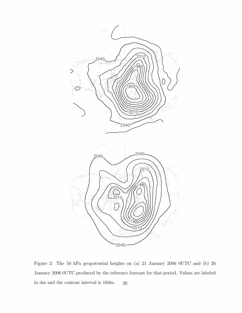
Figure 2: The 50 hPa geopotential heights on (a) 21 January 2006 0UTC and (b) 26

January 2006 0UTC produced by the reference forecast for that period. Values are labeled

in dm and the contour interval is 10dm. 26

Figure 3: The vertically integrated contribution to E for the leading SV for the focus

period at (a) initial and (b) final times. Units indicating the shading are J/kg.

27

Figure 4: The vertical distribution of (a) E for the focused, E norm SV at both initial

(dashed) and final (solid times), presented as fractions of the total value of E and (b) the

corresponding energy densities. 28

Figure 5: Cross section of v′ through the stratosphere for the focused, E norm SV at (a)

initial time along 60◦N and (b) final time along 75◦N. Units are in ms−1.

29

(a) (b)

(c) (d)

Figure 6: The vertically integrated contribution to initial E for the leading SV determined

for the period 15–20 January 2006 appear in (a). Units are J/kg. The meridians for

cutting the initial SV into 3 sectors are also shown in (a) with the sectors labeled 1–3.

The u′ field at 10 hPa for the tangent-linear, 5-day evolutions begun from the individual

sectors 1–3 appear in (b–d), respectively. The shading is determined by absolute values,

negative–valued contours are dashed, and units are ms−1.

30

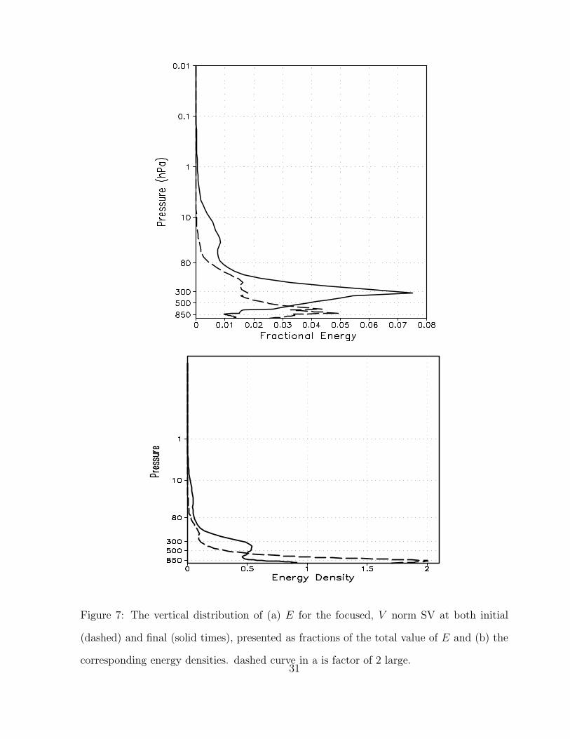
Figure 7: The vertical distribution of (a) E for the focused, V norm SV at both initial

(dashed) and final (solid times), presented as fractions of the total value of E and (b) the

corresponding energy densities. dashed curve in a is factor of 2 large.31

Figure 8: The horizontal correlations of the corresponding E and V norm fields at indi-

vidual model levels of u′ at (dotted line) initial and (open circles) final times and for T ′ at

(solid line) initial and (closed squares) final times. The correlations have been computed

globally.

32

(a) (b)

(c) (d)

Figure 9: Linearly (a,b) and nonlinearly (c,d) evolved perturbations at day 5 determined

by an initial perturbation given by the initial-time, leading E norm SV for the focus period,

with amplitude scaled by a factor of 0.1. The fields are (a,c) u′ at 10 hPa, with units ms−1.

and (b,d) T ′ at 50 hPa, with units K. The shading is determined by absolute values, and

negative-valued contours are dashed.

33

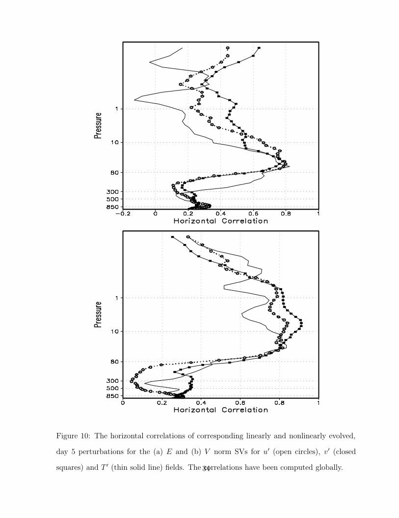
Figure 10: The horizontal correlations of corresponding linearly and nonlinearly evolved,

day 5 perturbations for the (a) E and (b) V norm SVs for u′ (open circles), v′ (closed

squares) and T ′ (thin solid line) fields. The correlations have been computed globally.34

(a) (b)

(c) (d)

Figure 11: As in fig. 9, except for the V norm SV.

35