gender disparities in completing school education in india
TRANSCRIPT

MPRAMunich Personal RePEc Archive
Gender disparities in completing schooleducation in India: Analyzing regionalvariations
Zakir Husain
Institute of Economic Growth, Delhi
26. September 2010
Online at https://mpra.ub.uni-muenchen.de/25748/MPRA Paper No. 25748, posted 11. October 2010 02:49 UTC

Draft dated 26/09/2010
Gender Disparities in Completing School Education in India Analyzing Regional Variations
Zakir Husain
Associate Professor Population Research Centre, Institute of Economic Growth
Delhi University Enclave, North Campus, Delhi 110007, India Cell: 9582553984
Fax: 011-23377164 Email: [email protected]
Abstract Is gender disparity greater in North India? This paper seeks to answer this question by examining gender differences in probability of completing school education across regions in India. A Gender Disparity Index is calculated using National Sample Survey Organization unit level data from the 61st Round and regional variations in this index analyzed to examine the hypothesis that gender disparity is greater in the North, comparative to the rest of India. This is followed by an econometric exercise using a logit model to confirm the results of the descriptive analysis after controlling for socio-economic correlates of completing school education. Finally, the Fairlie decomposition method is used to estimate the contribution of explanatory variables in explaining differences in probabilities of completing schooling across regions. The results reveal that gender disparities are greater in North India, for total and rural population, and in Eastern India, for urban population. However, the ‘residual effect’ after accounting for effect of explanatory variables - often referred to as ‘discrimination effect’, as opposed to disparity – is higher in Eastern India, irrespective of the place of residence. Key Words: discrimination, disparity, gender, Oaxaca decomposition, school education, India.

Gender Disparities in Completing School Education in India
Analyzing Regional Variations
1. Introduction
Is gender discrimination greater in North India? Based on an analysis of infant and child
mortality rates, sex ratios and fertility trends, Dyson and Moore (1983) concluded that,
relative to their South Indian states counterparts, women in Northern states were
subjected to higher levels of discrimination. Despite disagreement over the explanation,1
the empirical finding that gender disparity is stronger in northern India has not been
contested.2
However, Dyson and Moore (1983) fail to distinguish between disparity and
discrimination. Disparity simply refers to differences in the outcome under consideration
(wages, mortality rates, educational attainments, or any such indicator). Such disparities
may be caused by differences in socio-economic characteristics. Alternately, differences
in outcomes may occur due to socio-cultural forces independent of these characteristics –
the inferior outcome may be a consequence of deliberately unfair treatment from the
family or society. This is referred to as discrimination – the practice of treating members
of a group less fairly than others, simply because the person(s) belong to a particular race,
1 This observation was explained by Dyson and Moore (1983) in terms of cultural practices – the prevalence of endogamous marriages in South India implied that women had more access to her kin, thereby increasing autonomy. Alternative explanations have been offered for this phenomenon. Bardhan (1974) and Miller (1981) have argued that the prevalence of wet rice cultivation in southern states has created demand for women labour, increasing their participation in economic activities; this has empowered South Indian women. Rosenzweig and Schultz (1982) analysis also associates differences in child survival rates to differences in male and female labor force participation rates. Jeffrey (1993), on the other hand, links lower levels of gender disparities in the south to higher levels of State investment on education and health. Murthi et al (1995) and Dasgupta et al (2004) also argue that public investment in these spheres in states like Kerala and Karnataka have promoted female agency and reduce gender differences in demographic outcomes. 2 Basu's (1992) largely qualitative analysis comparing female agency among South and North Indian migrants to Delhi slums finds that the former enjoy greater mobility and freedom of expression than their Northern counterparts. Jejeebhoy's (2001) quantitative study concludes that Tamil women in the South have more mobility and authority than women in Uttar Pradesh. Southern states also performed better in terms of the Rural Human Development Index - a weighted average of expenditures, literacy, formal education, life expectancy, and infant mortality rate - developed by the Planning Commission (GOI 2002). Shariff’s study also observes higher level of human development in the south (Shariff 1999). However, these analyses have not rigorously tested for different levels gender discrimination between northern and southern states. Nor has there been an attempt to examine this research issue in the context of educational disparities.

social class, religion or gender. This will result in disparity levels, even if the two groups
are similar with respect to social and economic characteristics. It is not easy to segregate
the individual effects of discrimination and differences in socio-economic characteristics
in explaining group (in this case, gender) differences in outcome. However, certain
econometric techniques have emerged that address this issue. These techniques identify
the residual effect - after taking into account the effect of explanatory variables in
explaining disparity levels between groups - with discrimination (Blinder 1973; Fairlie
2005; Oaxaca 1973).
This paper examines regional variations in gender differences in the probability of
completing school education,3 and employs econometric tests to examine whether such
differences are indeed greater in North India. Having established the regional pattern of
disparity, we will then proceed to estimate the contribution of the residual effect in
explaining gender gap in regional outcomes.
Although gender disparity and discrimination is present in different spheres, this paper
focuses specifically on education because of its importance in human development and as
a determinant of the quality of life. The importance of education in economic growth
(Schultz 1961) and human development (Sen 1985, 1993) has been widely recognized.
Recently, the Government of India has made the right to education a fundamental right,
under its Constitution, of every child. However, the focus of policy makers and
researchers generally has been on the primary level. The four-five years of education
imparted as primary education is undoubtedly useful in ensuring the functional literacy of
recipients of such education. Despite the importance of functional literacy, economic
returns to primary education – in terms of increasing probability of securing work, getting
better jobs or bargaining for higher wages – is much less. In comparison, completion of
schooling marks an important landmark in the educational career, and makes children
better equipped to fend for themselves in the labour market.
3 In India, this consists 12 years of schooling.

The paper is based on unit level data from the quinquennial survey on Employment and
Unemployment (2004-05) undertaken by National Sample Survey Organization. The
survey was spread over 7,999 villages and 4,602 urban blocks covering 1,24,680
households (79,306 in rural areas and 45,374 in urban areas) and enumerating 6,02,833
persons (3,98,025 in rural areas and 2,04,808 in urban areas). A two-stage stratified
sample design, with census villages and urban blocks as the first-stage units for the rural
and urban areas respectively, and households as the second-stage units was adopted. The
fieldwork for the survey was handled by the Field Operations Division of NSSO.
2. Context, objective and methodology
2.1 Determinants of educational attainments
The literature on socio-economic determinants of educational attainments has mainly
focused on enrolment and primary education. Generally employing limited dependent
regression models, studies have identified factors like family income or wealth, parental
education, empowerment and education of mother, credit constraints, age of the child,
family size or presence of siblings, caste affiliations, place of residence and educational
infrastructure as determinants of enrolment and primary school completion rates (Akhtar
1996; Deolalikar 1997; Tansel 1998; Brown and Park 2002; Connelly and Zheng 2003;
Boissiere 2004; Desai and Kulkarni 2008; SIS/DPP 2005; Okumu et al 2008; Husain and
Chatterjee 2009). These studies have also found the presence of strong gender
differences.
In India, the education of girls has historically lagged behind that of boys (Aggarwal
1987; Agrawal and Aggarwal 1994). In addition studies have shown that certain
communities and classes fare much worse than the others. Though some researchers have
recently attempted to lay down the determinants of the inequality in educational
attainment for boys and girls, only a handful of these (Bandopadhyay and Subrahmaniam
2008; Das and Mukherjee 2007, 2008; Sengupta and Guha 2002; Raju 1991; Burney and
Irfan 1991), have explicitly looked at the factors responsible for the relative gender
inequality in educational attainment. But none of these works have examined variations
in gender discrimination over regions.

Similarly, Vaid’s analysis of trends in gender discrimination across the schooling career
of children finds that transition probabilities of girls increase, relative to that of boys, at
higher levels of education. Although she finds that locality specific effect decreases at
higher levels, except for Rajasthan, variation in gender discrimination across regions is
not examined. In a similar study, Husain and Sarkar (2010) found that, on an average,
gender disparity is lower across educational levels in southern states. Econometric
analysis revealed that, after controlling for socio-economic characteristics, gender
disparity decreases. However, region-specific effects were not incorporated in the
econometric model.
The finding that gender disparity reduces at higher levels of education is interesting. In
fact, Husain and Sarkar (2010) found a reversal of gender disparity at the secondary and
higher secondary levels in several states. Unfortunately, gender disparities at higher
levels of education have been rarely examined in the Indian context. Hasan and Mehta’s
study (2006) of college education focuses on disparities across social castes, but ignores
gender dimensions, as also does Sundaram (2006). Thorat (2006) notes gender
differences in access to higher education but does not look at regional variations. Overall,
studies have tended to neglect the study of regional dimensions in gender disparities at
higher levels of education. This lacuane forms the motivation of this paper.
2.2 Research hypothesis and methodology
The hypothesis being tested in this paper is that gender disparities in school completion
rates is higher in North Indian states, compared to the rest of India. However, instead of
using a binary classification, we have grouped Indian states into three groups – Northern
states (comprising of Jammu & Kashmir, Punjab, Haryana, Himachal Pradesh, Rajasthan,
Chandigarh, Bihar, Jharkhand, Uttar Pradesh, Chattisgarh, Madhya Pradesh,
Uttaranchal), Eastern states (consisting of West Bengal, Assam, Orissa, Tripura,
Mizoram, Megalaya, Nagaland, Sikkim) and Southern states (including Kerala,
Karnataka, Andhra Pradesh, Maharashtra, Gujarat, Tamil Nadu, Pondicherry, Goa,
Dadra, Nagar Haveli, Andaman & Nicobar).

The paper uses a Disparity Index suggested by Sopher (1980), and modified by Kundu
and Rao (1986). The index measures disparity between two groups in their possession of
a particular property (in this case completion of school education) in terms of the
logarithm of the odds ratio - that is, the ratio of the odds that any member of one group
(male) has completed school to the odds that any member of the other group (female)
does. In brief, if p and q are the probabilities of males and females completing school
respectively, then the disparity index (DI) is given by:
DI = log [p)(1*qq)(1*p
].
The objective of taking log is to reduce the leveling off effect (states with high levels of
attainments may show a lower level of disparity than states with low levels of attainments
even though the gender gap is the same for both states) (Sopher 1980).
Kundu and Rao (1986) have shown that the above index fails to satisfy the additive
monotonocity axiom.4 They have, therefore, proposed a modification to this Index as
follows:
DI KR= log [p)(2*qq)(2*p
].
Based on this Index we examine regional variations in the probabilities of completing
school education. Cohort-wise analysis is also undertaken to get an idea of the trend in
disparities across regions.
The descriptive analysis is followed by an econometric analysis that seeks to identify the
factors causing discrimination. A logit model is used for this purpose as the dependant
variable is binary (whether respondent has completed schooling or not). Based upon the
literature cited in Section 2.1, as well as availability of data from the NSSO database, we
hypothesize that – apart from gender and regional location - the probability of completing
school depends upon personal traits (age and socio-religious identity), household
characteristics (place of residence, household size, expenditure levels, and sex and 4 The additive monotonocity axiom specifies that if a constant is added to all observations in a non-negative series, ceteris paribus, the inequality index must report a decline.

educational level of household head). These variables are included in the regression
model. Now, the gender and region variables are incorporated in the initial model as
dummy variables. Statistically significant coefficients of the gender and regional
dummies will indicate the presence of gender discrimination and regional effects.
However, as our objective is to examine regional variations in gender differences, we re-
estimated the regression for each individual region. The statistical significance and signs
of the coefficients will help to establish the validity of Dyson and Moore’s hypothesis,
viz., that gender disparity is more accentuated in the north.
2.3 Measuring discrimination
Now this analysis merely establishes whether the difference in outcome is significant
after controlling for socio-economic characteristics. We also have to measure the
contribution of discrimination in explaining the observed gender disparities.
Oaxaca (1973) and Blinder (1973) have shown that the difference in outcomes between
two groups may be attributed to differences in explanatory variables or endowments
(referred to as explained component) and differences in coefficients of explanatory
variables (referred to as residuary or unexplained component). The latter is commonly
accepted as a measure of discrimination in literature. Their work has resulted in the
development of a methodology to estimate the contribution of discrimination in
explaining disparities in outcome. Having established regional patterns in gender
disparity, we next attempt to estimate how the extent of discrimination varies across
regions. This may be undertaken as follows.
For the regression model:
y = α + βx [1]
estimated after pooling a superior group (in terms of having a ‘better’ outcome, denoted
by S) and an inferior group (in terms of having a relatively ‘worse’ outcome, denoted by
W), the difference in mean outcomes can be decomposed as follows:
y S – y W = ΔxβW + Δβ xS, [2]

or, y S – y W = ΔxβS + Δβ xW. [3]
This method has been used to measure gender ‘discrimination’ in educational attainments
(Kingdon 2002). A generalized form of the decomposition for a multi-variate case is:
y S – y W = ΔX[DβW + (I – D) βS] + Δ β [XSD + XW (I – D)] [4]
when I is the identity matrix and D is the matrix of weights. It is easy to see that [2] and
[3] are special cases of D equal to I and 0 respectively. In addition, alternative weights
have been suggested by researchers.5
Now the above decomposition is based on the relation: __
xβ̂y . Unfortunately, this does
not hold for discrete choice models – predicted probability evaluated at means of the
independent variables is not necessarily equal to the proportion of ones. Instead we have
the relation that average value of the dependant variable equals the average values of
predicted probabilities in the sample.6 Therefore, Fairlie (1999, 2005) argues, for the non-
linear model Y = F(X β̂ ), the decomposition may be written as:
Y S - Y W = ]N
)β̂F(X - N
)β̂F(X [WS
N
1iW
SWi
N
1iS
SSi
+ ]N
)β̂F(X - N
)β̂F(X [WW
N
1iW
WWi
N
1iW
SWi
[5]
While [5] corresponds to [2], the equivalent to [3] in the non-linear case is:
Y S - Y W = ]N
)β̂F(X - N
)β̂F(X [WS
N
1iW
WWi
N
1iS
WSi
+ ]N
)β̂F(X - N
)β̂F(X [SS
N
1iS
WSi
N
1iS
SSi
[6].
Again the difference lies in the weighting system, with the alternative weighting systems
suggested by Cotton (1988), Reimers (1983), Oaxaca and Ransom (1994), and Neumark
(1988) being applicable here also.
3. Regional patterns in disparity levels
At the all-India level, the probability of a girls completing schooling is 0.11, compared to
0.20 for a boy. This implies a disparity of 0.30. Predictably, disparity is higher in rural
5 Cotton (1988) suggests that weights should be mean of the coefficient vector, Reimers (1983) argues that weights should reflect proportion of the two groups, while Neumark (1988) and Oaxaca and Ransom (1994) opt for coefficients estimated from pooled sample. 6 This holds exactly for the logit model, which is another reason for preferring logit models to probit models. In the latter, the relation does not hold exactly, but approximates the relation as an empirical regularity (Fairlie, 2005: 307).

areas (0.39), relative to urban areas (0.18). What is interesting, however, is the regional
variation in gender disparity in completion of school education. Fig. 1 reveals that gender
disparity is higher in Northern states, relative to the rest of India. Further, disparity is
lowest in South India. This is also true for rural areas. In urban areas, variations in
disparity levels are lower than in rural areas. The interesting finding is that, it is in
Eastern states that girls lag behind boys to a greater extent than in Northern or Southern
states.
Fig. 1: Regional variations in gender disparity in completing school education
0.32
0.46
0.18
0.280.37
0.200.220.31
0.16
0.00
0.10
0.20
0.30
0.40
0.50
T otal Rural Urban
Disp
arity
Inde
x
North East South
3.1 Cohort-wise analysis
Now these estimates were based on a sample containing several generations. It would be
interesting to decompose the sample by generations, and study trends in disparity over
time. The sample is therefore divided into the following groups – 18-25 years, 26-30
years, 31-40 years, 4-50 years, 51-60 years and 61 years and above.7
In Fig. 2 we present trends in disparity across the generations for the total population. We
can see that disparity levels have fallen in all regions. This is consistent with Husain and
Sarkar’s finding that disparity levels has fallen across all educational levels at the all-
India level (Husain and Sarkar 2010). Disparity in the South has traditionally remained 7 The 18-25 years group has been formed to maintain parity with subsequent econometric analysis.

lower than in other regions. In North, on the other hand, disparity levels have always
been relatively higher than the rest of India. But the gap between East and North is
decreasing and, for the ‘current’ generation (18-26 year group), differences are marginal.
Fig. 2: Sopher-Kundu Index of Gender disparity by Regions and Cohorts - Total
0.00
0.20
0.40
0.60
0.80
1.00
60+ years 51-60 years 41-50 years 31-40 years 26-30 years 18-25 years
North East South
Similar trends are observed in rural areas, though a faster convergence rate is seen (Fig.
3).
Fig. 3: Sopher-Kundu Index of Gender disparity by Regions and Cohorts - Rural
0.00
0.50
1.00
1.50
60+ years 51-60 years 41-50 years 31-40 years 26-30 years 18-25 years
North East South
In urban areas, on the other hand, regional differences have always been marginal (Fig.
4). Although Southern India has tended to display lower disparity levels, the performance
of North India is better for the ‘current’ generation. Interestingly, we observe a negative
value of the disparity index for these two regions, implying that girls ‘out-perform’ boys.
Eastern states, on the other hand, have performed somewhat erratically, starting off with

higher levels of disparity, improving thereafter, but then falling behind even Northern
states.
Fig. 4: Sopher-Kundu Index of Gender disparity by Regions and Cohorts - Urban
-0.10
0.00
0.10
0.20
0.30
0.40
0.50
0.60
0.70
0.80
0.90
60+ years 51-60 years 41-50 years 31-40 years 26-30 years 18-25 years
North East South
3.2 State-wise analysis
While the regional result is interesting in itself, we should also examine whether
disaggregative state-wise analysis reveals any variation within regions. The results of the
state-wise analysis are presented in Table 1.
In rural areas of Northern India, Punjab and Himachal Pradesh has low levels of gender
disparity, comparable to that of even Southern states. This contrasts with substantial
levels of disparities observed in Rajasthan, Bihar, Jharkhand, Madhya Pradesh,
Chattisgarh and Uttar Pradesh. In urban areas disparities are low states like Himachal
Pradesh, Haryana and Chandigarh. On the other hand, states like Bihar, Rajasthan,
Jharkhand, Chattisgarh, and Bihar exhibit high levels of disparity.
State-wise variation is less marked in Eastern states. An exception is rural West Bengal,
which has a disparity level of 0.48.8 This is surprising, given the long period of rule by a
8 Dropping, West Bengal, the Disparity Index for the remaining Eastern states is 0.35.

coalition of Leftist parties and the impressive record of land reforms in the state. Cohort-
wise analysis, however, reveals that gender disparities were extremely high after
Independence (possibly because of the migration patterns after partition), fell gradually
since then, with a sharp fall in the 1980s – when the positive effect of land reforms would
take place with a lag.
Table 1: Probabilities of completing schooling and disparity between gender across
State
Rural Urban Region/State Male Female SK Index Male Female SK Index
North 0.151 0.055 0.46 0.322 0.223 0.18 Jammu & Kashmir 0.137 0.051 0.45 0.252 0.213 0.08 Himachal Pradesh 0.168 0.103 0.23 0.411 0.366 0.06 Punjab 0.146 0.100 0.17 0.311 0.306 0.01 Chandigarh 0.228 0.135 0.25 0.487 0.420 0.08 Uttaranchal 0.195 0.096 0.33 0.405 0.310 0.14 Haryana 0.157 0.069 0.38 0.293 0.245 0.09 Delhi 0.330 0.182 0.30 0.418 0.348 0.10 Rajasthan 0.118 0.020 0.79 0.282 0.145 0.32 Uttar Pradesh 0.169 0.057 0.49 0.291 0.199 0.19 Bihar 0.153 0.026 0.79 0.326 0.126 0.46 Jharkhand 0.099 0.026 0.60 0.320 0.169 0.32 Chhattisgarh 0.189 0.055 0.57 0.378 0.217 0.28 Madhya Pradesh 0.134 0.039 0.56 0.327 0.206 0.23 East 0.131 0.058 0.37 0.292 0.194 0.20 Sikkim 0.097 0.060 0.21 0.175 0.169 0.02 Arunachal Pradesh 0.142 0.061 0.39 0.394 0.221 0.30 Nagaland 0.286 0.121 0.41 0.430 0.309 0.18 Manipur 0.203 0.094 0.36 0.377 0.216 0.28 Mizoram 0.133 0.059 0.37 0.206 0.167 0.10 Tripura 0.099 0.045 0.35 0.292 0.190 0.21 Meghalaya 0.071 0.039 0.27 0.346 0.250 0.16 Assam 0.114 0.048 0.39 0.347 0.220 0.23 West Bengal 0.120 0.041 0.48 0.278 0.187 0.19 Orissa 0.120 0.056 0.34 0.258 0.149 0.27 South 0.146 0.075 0.31 0.279 0.201 0.16 Gujrat 0.136 0.059 0.38 0.276 0.194 0.17

Rural Urban Region/State Male Female SK Index Male Female SK Index
Daman & Diu 0.269 0.113 0.41 0.491 0.236 0.39 Dadra & Nagar Haveli 0.120 0.056 0.35 0.375 0.287 0.14 Maharastra 0.185 0.072 0.44 0.328 0.245 0.15 Andhra Pradesh 0.112 0.033 0.55 0.275 0.139 0.33 Karnataka 0.131 0.051 0.42 0.256 0.177 0.18 Goa 0.265 0.207 0.12 0.346 0.293 0.09 Lakshadweep 0.090 0.000 - 0.126 0.077 0.23 Kerala 0.171 0.170 0.00 0.226 0.212 0.03 Tamil Nadu 0.132 0.074 0.26 0.265 0.194 0.15 Pondicheri 0.192 0.076 0.48 0.213 0.155 0.15 Andaman & Nicobar 0.135 0.124 0.04 0.300 0.311 -0.02
Source: Estimated from unit level NSS data, 61st Round, 2004-2005.
Southern states, too, exhibit some variation in disparity levels. While the record of Kerala
is remarkable – it has very low levels of disparity in urban areas, and no disparity in rural
areas – disparity levels are high in specific areas. Rural areas of Andhra Pradesh,
Maharashtra and Karnataka, along with urban Andhra Pradesh, are found to display
relatively high levels of disparity. In fact, disparity levels in Andhra Pradesh are
substantially higher than the average disparity in North India.
Thus, the picture for gender disparity observed for school education is more complex
than the over-simplified hypothesis formed on the basis of Dyson and Moore’s paper.
There are considerable variations within regions, and occasionally even between rural
and urban areas of the same state (Madhya Pradesh and Uttar Pradesh are examples).
3.3 Regional variation across correlates
Now the differences in gender disparity across regions may be partly explained by
differences in socio-economic structure. Table 2 indicates, for instance, smaller sized
families and higher urbanization levels in the South. Differences in share of socio-
religious communities may also be observed between the South and North. It is
necessary, therefore, to examine variations in disparity levels across regions after
decomposing the sample by the socio-economic correlates.

Table 2: Variations in socio-economic characteristics over regions
Groups North East South Total Monthly per capita expenditure groups BPL HHs 21.0 18.0 18.4 19.4 DBPL HHs 51.4 52.3 48.9 50.8 Affluent HHs 27.6 29.7 32.7 29.9 Total 182,856 109,391 152,865 445,112 Household size 0-3 members 13.7 16.9 23.1 17.7 4 members 13.5 18.6 22.4 17.8 5 members 17.1 20.7 19.4 18.8 6 members 15.3 15.9 13.5 14.8 7-10 members 30.1 23.4 17.4 24.1 More than 10 members 10.3 4.5 4.4 6.8 Total 182,856 109,391 152,865 445,112 Socio-religious identity Muslims 12.4 11.8 11.2 11.8 H-SC 5.9 8.7 5.5 6.4 H-ST 17.0 12.3 12.8 14.4 H-Others 56.0 39.3 63.7 54.5 All Others 8.72 27.99 6.89 12.83 Place of residence Rural 71.1 72.7 58.5 67.2 Urban 29.0 27.3 41.5 32.9 Total 182,856 109,391 152,865 445,112
Source: Estimated from unit level NSS data, 61st Round, 2004-2005. Note: [1] BPL is acronym for Below Poverty Line households, while DBPL stands for Households below Double Poverty Line. The justification for taking DBPL is that these households are also targeted in some Government programmes.
[2] Planning Commission poverty lines for each state has been taken. See
Table 3 presents the results of bi-variate analysis. Once again, the results challenges our
starting proposition, viz. that disparity levels are greater in North India. Gender disparity
levels are higher in Eastern India, than in Northern India, among affluent households,
households with 4-5 members, Muslim households and in urban areas. South displays
lowest disparity levels in all cases.

Table 3: Regional variation in disparity across some socio-economic correlates
North East South Socio-economic correlates Male Female SK
Index Male Female SK Index Male Female SK
Index Monthly per capita expenditure groups BPL HHs 0.077 0.026 0.49 0.058 0.031 0.28 0.064 0.036 0.26 DBPL HHs 0.160 0.067 0.40 0.118 0.059 0.31 0.129 0.069 0.28 Affluent HHs 0.380 0.224 0.27 0.346 0.198 0.28 0.385 0.266 0.19 Household size 0-3 members 0.216 0.106 0.34 0.198 0.110 0.28 0.241 0.139 0.26 4 members 0.235 0.135 0.26 0.193 0.100 0.31 0.223 0.150 0.19 5 members 0.208 0.115 0.28 0.167 0.088 0.30 0.193 0.125 0.20 6 members 0.192 0.100 0.31 0.159 0.084 0.29 0.175 0.108 0.22 7-10 members 0.179 0.086 0.34 0.160 0.096 0.24 0.168 0.102 0.23 More than 10 members 0.220 0.081 0.47 0.184 0.099 0.29 0.171 0.089 0.30 Socio-religious identity Muslims 0.127 0.059 0.35 0.103 0.041 0.42 0.140 0.090 0.20 H-SC 0.108 0.028 0.61 0.089 0.035 0.42 0.109 0.051 0.34 H-ST 0.107 0.037 0.48 0.094 0.038 0.41 0.121 0.073 0.23 H-Others 0.258 0.131 0.32 0.239 0.139 0.26 0.229 0.137 0.24 All Others 0.209 0.149 0.16 0.180 0.100 0.28 0.283 0.241 0.08 Place of residence Rural 0.151 0.055 0.46 0.131 0.058 0.37 0.146 0.075 0.31 Urban 0.322 0.223 0.18 0.293 0.194 0.20 0.279 0.201 0.16
Source: Estimated from unit level NSS data, 61st Round, 2004-2005. Note: [1] BPL is acronym for Below Poverty Line households, while DBPL stands for Households below Double Poverty Line. The justification for taking DBPL is that these households are also targeted in some Government programmes.
[2] Planning Commission poverty lines for each state has been taken. See
To sum, up, gender disparities in the probability of completing school education is lowest
in Southern states. Comparison between Northern and Eastern states, however, does not
reveal any clear picture. While disparity levels tend to be higher in North India, it is
higher in East India for specific socio-economic groups. To get a clearer picture,
therefore, we turn to an econometric analysis.

4. Econometric analysis
Since disparity is estimated for region/state, while our unit of analysis is individual child,
we have to abandon the Sopher-Kundu index and use a different method to test for
gender disparity. We therefore regress probability of completing school education upon
gender of the child, controlling for individual and household traits like age of child,
socio-religious identity, monthly per capita expenditure groups, household size, place of
residence and region. Gender of the child is a dummy and we use boys as the reference
category. A statistically significant coefficient of this dummy variable indicates the
presence of gender disparity, while a negative sign indicates that girls have a lower
probability of completing school than boys. Apart from this main regression, we have
also estimated separate models for rural and urban areas.
4.1 Gender disparity in schooling
The results of this basic model are given in Table 4. Note that we have reported odd
ratios and not coefficients. Thus, odd ratios lower (higher) than unity corresponds to a
negative (positive) coefficient. For each of the models reported in Table 4, the odd ratios
for girls are statistically significant and lower than unity. This indicates the presence of
gender disparities in completing school education, even after controlling for socio-
economic traits. Predictably, gender differences are higher in rural areas.
Table 4: Results of Logit Regression Model – All India
Model 1: Total Model 2: Rural Model 3: Urban Independent variables Odds
Ratio z Odds Ratio z
Odds Ratio z
Male (RC) 1.00 1.00 1.00 Female 0.45 -83.96 0.36 -75.23 0.56 -41.66 Age Cohort 0.72 -106.10 0.69 -83.42 0.74 -66.46 Muslims (RC) 1.00 1.00 1.00 H-SC 1.31 9.14 1.15 3.72 1.50 7.81 H-ST 1.15 6.38 1.26 7.42 0.96 -1.11 H-Others 2.30 48.94 2.09 29.49 2.45 38.58 All Others 1.62 23.41 1.47 13.28 1.81 20.23 Household size 1.06 35.19 1.06 28.44 1.06 22.56 Per capita exp. group 4.01 172.94 3.66 110.38 4.29 129.56

Model 1: Total Model 2: Rural Model 3: Urban Independent variables Odds
Ratio z Odds Ratio z
Odds Ratio z
Rural (RC) 1.00 Urban 3.89 140.14 East (RC) 1.00 1.00 1.00 North 1.14 10.15 1.01 0.49 1.38 16.46 South 0.99 -0.41 1.09 4.63 0.96 -2.06 Observations 445111 298904 146207 LR χ2 77204.19 0.00 29869.26 0.00 32497.06 0.00 Pseudo R2 0.20 0.15 0.20
Note: Per capita expenditure groups have been preferred to absolute levels of per capita expenditure as expenditure is a time variant variable. We require expenditure when the respondent was a student, while NSS reports current expenditure levels. Our assumption is expenditure may change since the respondent was a student, but the family remains within the broad expenditure group as before. RC indicates reference category for dummy variable.
Regional variations in probability of completing school are somewhat surprising. At the
all-India level, a child from Northern India has a higher probability of completing school
than counterparts from the South or East. Differences in the probability of completing
school education between a Southern and Eastern child is statistically insignificant. In
rural areas, however, a child from North and East India are equally likely to complete
schooling, while a child from Southern India has an advantage over both. In urban areas,
on the other hand, North Indian children are better off than East Indian children, while
South Indian children have a lowest probability of completing school. It should be
emphasized that we are not referring to gender disparity, but to all children.
Among other important results are: children from urban areas, and those belonging to
younger age cohorts are more likely to complete school. Children from Forward Caste
Hindus, Scheduled Tribe Hindus, OBC Hindus and All Others are more advantaged than
Muslim children. These are expected results (refer citations in Section 2.1). However, the
absence of difference between Muslim and Scheduled Tribe children (in urban areas) is
surprising.
4.2 Variations in disparity across regions
While Models 1-3 indicated the presence of gender disparity, our research hypothesis was
that this disparity is higher in northern states. This was not addressed in Section 4.1. To

test this hypothesis we have to study differences in probabilities for each region. We have
therefore estimated Model 1-3 for each region separately, reporting results for rural and
urban areas in each region in the Appendix. Table 5 states the regression results using an
urban dummy.
Table 5: Results of Logit Regression Model – Region-wise, Rural + Urban
Model 4: North Model 5: East Model 6: South Independent variables Odds
Ratio z Odds Ratio z
Odds Ratio z
Male (RC) 1 1 1 Female 0.39 -62.16 0.43 -41.81 0.54 -39.25 Age Cohort 0.72 -67.03 0.78 -37.38 0.67 -76.54 Muslims (RC) 1 1 1 H-SC 1.45 7.66 1.12 2.03 1.34 5.67 H-ST 1.07 2.03 1.06 1.20 1.36 8.35 H-Others 2.55 35.63 2.44 23.45 2.04 25.62 All Others 1.72 16.03 1.19 4.43 2.95 29.62 Household size 1.06 28.13 1.07 18.75 1.05 15.37 Per capita exp. group 3.84 108.64 3.99 81.56 4.45 108.43 Rural (RC) 1 1 1 Urban 4.82 101.05 3.52 62.46 3.26 74.44 Observations 182855 109391 152865 LR χ2 34267.29 0.00 16187.37 0.00 28562.54 0.00 Pseudo R2 0.22 0.18 0.21
Note: Per capita expenditure groups have been preferred to absolute levels of per capita expenditure as expenditure is a time variant variable. We require expenditure when the respondent was a student, while NSS reports current expenditure levels. Our assumption is expenditure may change since the respondent was a student, but the family remains within the broad expenditure group as before. RC indicates reference category for dummy variable.
Once again the gender dummy is significant and less than unity. But what is important is
how the value of the odds ratio fluctuates across regions. It can be seen that girls have a
61 percent lower probability of completing schooling in North India, compared to boys.
In South and East India this percentage is 46 and 57, respectively. This implies that –
after controlling for socio-economic traits – gender disparity is highest in North India,
and lowest in South India. This is also observed for rural areas (Appendix A1). In urban
areas, however, the gender gap in probability of completing school is higher in Eastern
India, compared to North India

Fig. 5: Predicted probabilities of completing school and gender gap - By region and place of residence
0
0.05
0.1
0.15
0.2
0.25
0.3
North East South North East South North East South
Total Rural Urban
0
10
20
30
40
50
60
70
Male Female Gap
This is summarized in Fig. 5, which depicts regional variations in predicted probabilities
of completing school education by place of residence, and the gender gaps in these
predicted values between boys and girls. It can be seen that ratio of predicted
probabilities is lowest in South India, and highest in North India if we consider rural
areas. In urban areas, however, it is in Eastern India where the gender gap is highest.
4.3: Estimating residual effects
Now, the above econometric analysis was implicitly based on the assumption that gender
of the child leads to a difference in intercept (captured by the intercept dummy, Female),
but not in the regression coefficients. But part of it may be attributed to the gender
differences in coefficients of explanatory variables (Blinder 1973; Oaxaca 1973). If this
assumption is relaxed, the gender difference in outcomes (viz. probability in completing
schooling) may be decomposed into two components – explained (difference attributable
to differences in socio-economic characteristics) and unexplained (difference attributable
to difference in regression coefficients). The latter, residual, component is often taken to
be a measure of discrimination.

In this section we decompose the difference in outcomes to estimate the contribution of
the residual effects in explaining the difference in outcome. To check robustness of
results, we have used extreme weights (Ω = 0 and Ω = 1).
Table 6: Results of Decomposition Analysis
Discrimination (Percent) Place of Residence Region Difference in
outcomes Ω = 0 Ω = 1 North 0.10 94.04 95.88 East 0.08 103.86 102.14 Total South 0.08 87.91 88.08 North 0.10 99.38 100.80 East 0.07 102.71 102.69 Rural South 0.07 91.63 91.94 North 0.10 93.96 96.16 East 0.10 104.43 100.23 Urban South 0.08 89.99 89.18
Note: The user-written module in Stata (st0152_1), written by Sinning, Hahn and Bauer (2008), is used.
The results indicate that, although disparity may be greater in Eastern India only for the
urban population, the residual (discrimination) effect is greater in this region for not only
the urban population, but also for the total and rural population. In fact, the residual
unexplained effect is found to be consistently greater than 100 per cent in Eastern India.
This implies that socio-economic characteristics explain “less than nothing” of the gender
disparity. The socio-economic context in Eastern India is actually more favourable for
girls, and should have lead to girls having higher probabilities in completing school
education, vis-à-vis boys. However, the unexplained effect is so strong that it reverses the
situation.
5. Conclusion
In conclusion, thisr paper raises questions about the common perception that gender
discrimination is higher in North India. The picture is more complex than the simple
claim that “the country can be roughly divided in two by a line that approximates the
contours of the Satpura hill range, extending eastward to join the Chota Nagpur hills of
southern Bihar” (Dyson and Moore 1983: 38). While it is true that disparity levels in

completion of school education are higher in North India (except in urban areas), the
level of discrimination may be consistently higher in Eastern states. This is somewhat
surprising given the prevalence of matrilinear structure and the influence of missionaries
in the North-eastern states. In fact we re-estimated residual effects in Eastern India, after
dropping the states of Assam, West Bengal and Orissa, but failed to find any major
difference in results.
This finding is contrary to common beliefs about the prevalence of gender discrimination
in the so called BIMARU states9 and in Punjab and in Haryana. The starting hypothesis
was based on studies using demographic indicators. These studies establish that North
India has low sex ratios and high incidence of sex selection and female infanticides.
These are also important determinants of gender discrimination, and it is important to link
such demographic indicators with educational decisions. Why regional variations in
gender discrimination in education do not match with the observed regional patterns in
demographical indicators is an interesting question. Extending the regression model by
incorporating district level demographic characteristics like sex ratios, female literacy
rates, age of marriage, etc. is a possible area of extension of this work.
9 Bihar, Madhya Pradesh, Uttar Pradesh and Rajasthan, before bifurcation of these states. Now, in addition to these states, BIMARU includes Jharkhand, Chattisgarh and Uttaranchal.

Reference
Aggarwal, J. C. (1987). Indian women: Education and status. New Delhi: Arya Book
Depot.
Agrawal, S. P. & Aggarwal, J. C. (1994). Third Historical Survey of Educational
Development in India: Select Documents, 1990-1992. New Delhi: Concept Publishing
Company.
Akhtar, S. (1996). Do Girls Have a Higher School Drop-out Rate Than Boys? A Hazard
Rate Analysis of Evidence from a Third World City. Urban Studies, 33(1), 49-62.
Bandopadhyay, M. & Subrahmanian, R. (2010). Gender Equity in Education: A Study of
Trends and Factors. Research Monograph No. 18. New Delhi: National University of
Education & Planning.
Bardhan, P. K. (1974). On life and death questions. Economic and Political Weekly, 9,
32-34.
Basu, A. M. (1992). Culture, the Status of Women, and Demographic Behaviour:
Illustrated with the Case of India. Oxford: Clarendon Press.
Bauer, T. K. & Sinning, M. (2008). An Extension of the Blinder-Oaxaca Decomposition
to Non-Linear Models. Advances in Statistical Analysis, 92, 197-206.
Blinder, A. S. (1973). Wage Discrimination: Reduced Form and Structural Estimates.
Journal of Human Resources, 8, 436-55.
Boissiere, M. (2004). Determinants of Primary Education Outcomes in Developing
Countries. Background paper for evaluation of the World Bank’s support to primary
education. Washington DC: The World Bank.
Brown, P. H. & Park, A. (2002). Education and Poverty in Rural China. Economics of
Education Review, 21(6), 523-41.
Burney, N. A. & Irfan, M. (1991). Parental Characteristics, Supply of Schools, and Child
School Enrolment in Pakistan. The Pakistan Development Review, 30(1), pp 21-62.
Connelly, R. & Zheng, Z. (2003). Determinants of School Enrolment and Completion of
10-18 Year Olds in China, Economics of Education Review, 22(4), 379-88.
Cotton, J. (1988). On the Decomposition of Wage-Differentials, The Review of
Economics and Statistics, 70, 236-43.

Das, S. & Mukherjee, D. (2007). Role of Women in Schooling and Child Labour
Decision: The Case of Urban Boys in India. Social Indicators Research, 82(3), 463-86.
Das, S. & Mukherjee, D. (2008). Role of Parental Education in Schooling and Child
Labour Decision: Urban India in the Last Decade. Social Indicators Research, 89(2), 305-
322.
Das Gupta, M., Lee, S., Uberoi, P., Wang, D., & Zhang, X. (2004). State policies and
women's agency in China, the Republic of Korea, and India 1950-2000: Lessons from
contrasting experiences. In V. Rao & M. Walton (Eds.), Culture and Public Action (pp.
234-259). Stanford: Stanford University Press.
Deolalikar, A. (1997). The Determinants of Primary School Enrolment and Household
School Expenditures in Kenya: Do They Vary by Income? Mimeograph. Washngton:
Department of Economics, University of Washington.
Desai, S. & Kulkarni, V. (2008). Changing Educational Inequalities in India in the
Context of Affirmative Action. Demography, 45(2), 245-270.
Dyson, T. & Moore, M. (1983). On kinship structure, female autonomy, and
demographic behavior in India. Population and Development Review, 9(1), 35-60.
Fairlie, R. W (2005). An extension of the Blinder-Oaxaca Decomposition Technique to
Logit and Probit Models. Journal of Economic and Social Measurement, 30, 305-16.
GOI (Government of India) (2006). Social, Economic and Educational Backwardness of
Muslims in India: A Report, Report of the Prime Minister’s High Level Committee, New
Delhi: Government of India.
Hadden, K. & London, B. (1996). Educating Girls in the Third World: The Demographic,
Basic Needs, and Economic Benefits. International Journal of Comparative Sociology,
37, 1-2.
Hasan, R. & Mehta, A. (2006). Under-representation of Disadvantaged Classes in
Colleges: What Do the Data Tell Us. Economic and Political Weekly, September, 3791-
3796.
Husain, Z. & Sarkar, S. (2010). Gender Disparities in Educational trajectories in India:
Do Girls Become More Robust at Higher levels? Social Indicators Research,
forthcoming. DOI 10.1007/s11205-010-9633-4.

Husain, Z. & Chatterjee, A. (2009). Primary Completion Rates across Socio-religious
Communities in India. Economic and Political Weekly, XLIV(15), 59-67.
Jejeebhoy, S. J. (2001). Women's autonomy in rural India: Its dimensions, determinants,
and the influence of context. In H. B. Presser & G. Sen (Eds.), Women's Empowerment
and Demographic Processes: Moving Beyond Cairo (pp. 205-238). Oxford: Oxford
University Press.
Jeffrey, R. (1993). Politics, Women and Well-Being: How Kerala Became ‘A Model’.
Delhi: Oxford University Press.
Kingdon, G. G. (2002). The Gender Gap in Educational Attainment in India: How much
can be explained. Journal of Development Studies, 39(2), 25-53.
Kundu, A. & Rao, J. M. (1986). Inequity in educational development: Issues in
measurement, changing structure and its socio-economic correlated with special reference
to India. In Raza, M. (Ed.), Educational planning: A long term perspective (pp. 435–466).
New Delhi: NIEPA and Concept Publishing Company.
Miller, B. D. (1981). The Endangered Sex: Neglect of Female Children in Rural North
India. Ithaca: Cornell University Press.
Murthi, M., Guio, A. C. & Dreze, J. (1995). Mortality, fertility, and gender bias in India:
A district-level analysis. Population and Development Review, 21(4), 745- 782.
Planning Commission, Government of India (2002). National Human Development
Report. Delhi: Oxford University Press.
Neumark, D. (1988). Employers’ Discriminatory Behaviour and the Estimation of Wage
Discrimination. Journal of Human Resources, 23, 279-95.
Oaxaca, R. L. (1973). Male-Female Wage Differentials in Urban Labour Markets.
International Economic Review, 14, 693-709.
Oaxaca, R. L. & Ransom, M. (1994). On Discrimination and the Decomposition of Wage
Differentials. Journal of Econometrics, 61, 5-21.
Okumu, I. M., Nakajjo, A. & Isoke, D. (2008). Socioeconomic Determinants of Primary
School Dropout: The Logistic Model Analysis. Munich Personal Repec Archive.
http://mpra.ub.uni-muenchen.de/view/ people/Okumu,_Ibrahim_M=2E.html. Accessed
20 November 2008.

Rahman, L. & Rao, V. (2004). The Determinants of Gender Equity in India: Examining
Dyson and Moore's Thesis with New Data. Population and Development Review, 30(2),
239-268.
Raju, S. (1991). Gender and Deprivation. A Theme Revisited with a Geographical
Perspective. Economic and Political Weekly, 26 (49), 2827-39.
Reimers, C. (1983). Labour Market Discrimination Against Hispanic and Black Men.
The Review of Economics and Statistics, 65, 570-79.
Rosenzweig, M. R. & Schultz, T. P. (1982). Market opportunities, genetic endowments,
and intrafamily resource distribution: Child survival in rural India. American Economic
Review, 72 (4), 803-815.
Schultz, T. W. (1961) Investment in Human Capital. The American Economic Review,
51, (1), 1-17.
Shariff, A. (1999). Indian Human Development Report New Delhi, Oxford University
Press.
Schultz, T. P. (1993). Investments in the Schooling and Health of Women and Men. The
Journal of Human Resources, 28(4), 689-734.
Sen, A. (1985). Commodities and Capabilities. Amsterdam: North Holland.
Sen, A. (1999). Development as Freedom. New York: Knopf.
Sengupta, P. & Guha, J. (2002). Enrolment, Dropout and Grade Completion of Girl
Children in West Bengal, Economic and Politic Weekly, 37(17), 1621-1637.
Sinning M., Hahn, M. & Bauer, T.K. (2008). The Blinder-Oaxaca Decomposition for
Non-Linear Regression Models. The Stata Journal, 8(4), 490-492.
Strategic Information Section and Division of Policy and Planning (SIS/DPP) (2005).
Levels, Trends and Determinants of Primary School Participation and Gender Parity.
New York: UNICEF.
Sopher, D. E. (1980). Sex disparity in Indian literacy. In D. E. Sopher (Ed.), An
exploration of India: Geographical perspectives on society and culture (pp. 130–188).
New York: Cornell Press.
Sundaram, K. (2006). On backwardness and fair access to higher education. Economic
and Political Weekly, 41(50), 5173-5182.

Thorat, S. (2004). Higher Education in India: Emerging Issues Related to Access,
Inclusiveness and Equity. Nehru Memorial Lecture, University of Mumbai, Mumbai.
Tansel, A. (1998). Differences in School Attainments of Boys and Girls in Turkey,
Discussion Paper 789, Economic Growth Center, Yale University.
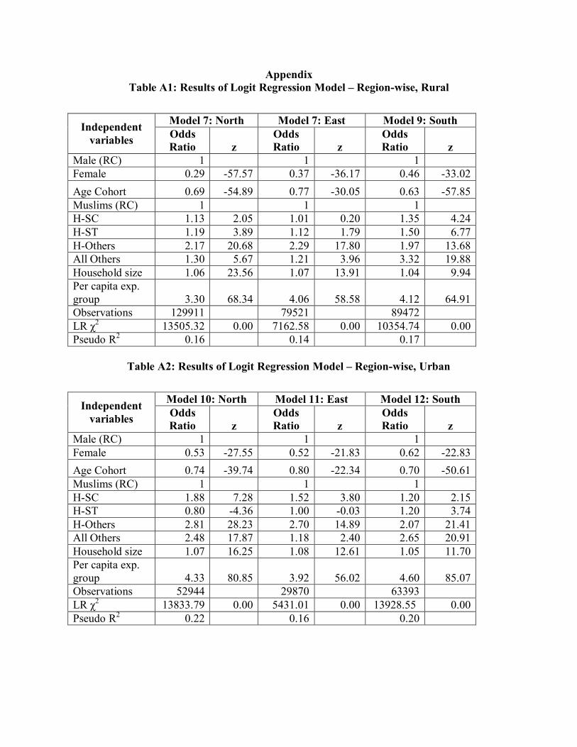
Appendix Table A1: Results of Logit Regression Model – Region-wise, Rural
Model 7: North Model 7: East Model 9: South Independent
variables Odds Ratio z
Odds Ratio z
Odds Ratio z
Male (RC) 1 1 1 Female 0.29 -57.57 0.37 -36.17 0.46 -33.02 Age Cohort 0.69 -54.89 0.77 -30.05 0.63 -57.85 Muslims (RC) 1 1 1 H-SC 1.13 2.05 1.01 0.20 1.35 4.24 H-ST 1.19 3.89 1.12 1.79 1.50 6.77 H-Others 2.17 20.68 2.29 17.80 1.97 13.68 All Others 1.30 5.67 1.21 3.96 3.32 19.88 Household size 1.06 23.56 1.07 13.91 1.04 9.94 Per capita exp. group 3.30 68.34 4.06 58.58 4.12 64.91 Observations 129911 79521 89472 LR χ2 13505.32 0.00 7162.58 0.00 10354.74 0.00 Pseudo R2 0.16 0.14 0.17
Table A2: Results of Logit Regression Model – Region-wise, Urban
Model 10: North Model 11: East Model 12: South Independent
variables Odds Ratio z
Odds Ratio z
Odds Ratio z
Male (RC) 1 1 1 Female 0.53 -27.55 0.52 -21.83 0.62 -22.83 Age Cohort 0.74 -39.74 0.80 -22.34 0.70 -50.61 Muslims (RC) 1 1 1 H-SC 1.88 7.28 1.52 3.80 1.20 2.15 H-ST 0.80 -4.36 1.00 -0.03 1.20 3.74 H-Others 2.81 28.23 2.70 14.89 2.07 21.41 All Others 2.48 17.87 1.18 2.40 2.65 20.91 Household size 1.07 16.25 1.08 12.61 1.05 11.70 Per capita exp. group 4.33 80.85 3.92 56.02 4.60 85.07 Observations 52944 29870 63393 LR χ2 13833.79 0.00 5431.01 0.00 13928.55 0.00 Pseudo R2 0.22 0.16 0.20