GEncode: Geometry–driven compression for general meshes

THOMAS LEWINER1,2 , MARCOS CRAIZER1 , HELIO LOPES1 , SINESIO PESCO1, LUIZ VELHO3 ANDESDRAS MEDEIROS3

1 Department of Mathematics — Pontifıcia Universidade Catolica — Rio de Janeiro — Brazil2 Geometrica Project — INRIA – Sophia Antipolis — France

3 Visgraf Project — IMPA — Rio de Janeiro — Brazil{tomlew, craizer, lopes, sinesio}@mat.puc--rio.br. {lvelho, esdras}@visgraf.impa.br.

Abstract. Performances of actual mesh compression algorithms vary significantly depending on the type of modelit encodes. These methods rely on prior assumptions on the mesh to be efficient, such as regular connectivity,simple topology and similarity between its elements. However, these priors are implicit in usual schemes,harming their suitability for specific models. In particular, connectivity–driven schemes are difficult to generaliseto higher dimensions and to handle topological singularities. GEncode is a new single–rate, geometry–drivencompression scheme where prior knowledge of the mesh is plugged into the coder in an explicit manner. It encodesmeshes of arbitrary dimension without topological restrictions, but can incorporate topological properties, such asmanifoldness, to improve the compression ratio. Prior knowledge of the geometry is taken as an input of thealgorithm, represented by a function of the local geometry. This suits particularly well for scanned and remeshedmodels, where exact geometric priors are available. Compression results surfaces and volumes are competitivewith existing schemes.Keywords: Mesh Compression. Geometry–driven techniques. Arbitrary Meshes. Arbitrary Dimension.

1(a): geometric criterion 1(b): geometric range

1(c): max identifier 1(d): apex identifier

Figure 1: GEncode compression: once the geometry is decoded, the decoder attaches triangles to edges of the front by identifyingits apex w: A list of candidates is computed from an encoded geometric range and ordered according to a geometric criterion (herethe distance from w to the edge midpoint). Then w is identified by its position in the list.

Preprint MAT. 02/06, communicated on March 17th, 2006 to the Depart-ment of Mathematics, Pontifıcia Universidade Catolica — Rio de Janeiro,Brazil.

1 IntroductionComputer Graphics developments handle each time big-

ger meshes, using processes of increasing complexity.Compression algorithms followed these developments by

T. Lewiner, M. Craizer, H. Lopes, S. Pesco, L. Velho and E. Medeiros 2

improving the compression ratio, enlarging the range ofmodels that can be encoded, simplifying their implementa-tion and increasing execution performances. However, theyare still not fully adapted to the wide variety of modelsand applications of Computer Graphics: scans in artisticand archaeological modelling, isosurfaces for medical andmathematical visualisation, re–meshed models for reverseengineering, finite–element meshes for simulation, high–dimensional meshes for solid representation, meshes withhigh co–dimension for non–linear optimisation, among oth-ers. Actually, the performances of state–of–the–art com-pression algorithms highly depend on the nature of themodel. We will focus here on compression schemes adaptedto the priors of specific applications, in particular for themost time–consuming mesh generation algorithms: recon-struction and the re-meshing.

Geometry–driven compression. Meshes are usually de-scribed by their geometry (the coordinates of its vertices)and their connectivity (the combinatorial elements that in-terpolate these vertices, usually triangles or simplices). Thiscomposite nature leads to classify compression algorithmsbetween: on one hand connectivity–driven ones, when theconnectivity is coded separately and the geometry is par-tially deduced from it, and on the other side geometry–driven ones, when the geometry is coded separately and theconnectivity is coded using the geometry. The efficiencyof connectivity–driven algorithms usually relies on a reg-ular connectivity, whereas the newer trend of geometry–driven methods are expected to perform better on geomet-rical meshes, such as reconstructed or re-meshed models.This work proposes a new geometry–driven method, whichencodes arbitrary meshes in arbitrary dimension, and com-pares nicely to connectivity–driven methods for surfaces(Figure 1) and for volumes (Figure 11).

Related works. The first mesh-compression algorithmswere connectivity–driven, in the sense that the geometryencoding depends on the connectivity encoding rules.Among those, the Edgebreaker [33, 29, 27, 23] per-forms well on generic mesh, with guaranteed practicalworst–case close to the theoretical optimum [19]. On theother side, Valence Coding [35, 9, 18] has a theoreticalasymptotic compression ratio close to the optimum [1].It has been widely extended since the original work, andperforms very well in practise, especially on meshes witha regular connectivity. Some singularities of the mesh canfurther be handled by specific algorithm, in particular forthe non–manifold case [13, 30].

These connectivity–driven approaches can be extendedto higher dimension, but the complexity of the codesincreases dramatically. Even for tetrahedral meshes, the ex-tensions of the surface approaches [14, 32, 17] are delicate.

As an intermediate towards geometry–driven ap-

proaches, some connectivity–driven schemes use thepreviously coded geometry to predict the connectiv-ity [20, 21, 11, 18]. Each of these algorithms uses adifferent prior on the geometric regularity of the mesh.

On the contrary, geometry–driven approaches intro-duced by [12] handle gracefully complex connectivity.Still, the compression ratios of the geometry are not yet op-timal, since these schemes are quite new to the community.However, for the case of isosurfaces, specific compressionschemes [34, 22, 24] outperform any connectivity–drivenapproach.

Contributions. This work proposes a new geometry–driven scheme called GEncode, which works for meshesof arbitrary topology and dimension embedded in spacesof arbitrary dimension. To our knowledge, GEncode is thefirst compression method that works at that level of gener-ality and still compares nicely to state–of–the–art compres-sion methods for triangulated surfaces and volumes. As op-posed to [12], GEncode is single rate, but copes with gen-eral meshes, and shows better compression ratios: For sur-face, the resulting compression ratios are competitive withthe Edgebreaker with the parallelogram prediction, andfor volumes it is highly competitive with Grow&Fold [32]and with streaming compression [16].

Aside from its generality, GEncode treats the priorsof the mesh as an input, and can therefore easily adaptto specific classes of meshes. These priors include on oneside global topological properties such as manifoldness,the presence of boundary and eventually the degree of thefacets, and on the other side local geometrical propertiesrepresented by a scalar function of the vertices of a facet.For example, a common prior for usual Computer Graph-ics models assumes that the mesh is a triangulated mani-fold without boundary, and that the triangles maximise theircircumradius or their aspect ratio. In particular, if the meshcan be reconstructed from its vertices with a geometricprior, the GEncode connectivity encoding with that priorleads to a zero entropy code.

This work is an extended version of [25] and part ofThomas Lewiner’s Ph.D. [26]. It describes GEncode at itshigh level of generality, investigates different geometric pri-ors and separates the geometric range definition from thegeometric prior in order to reduce the constraints on the ge-ometric function defining the prior. Moreover, the authorsare grateful to the referees, since they motivated tests ontetrahedral meshes, where GEncode turned out to be par-ticularly competitive.

Overview. This work is organised as follow. section 2 Gen-eral Meshes recalls the basic notions of meshes, expressedin arbitrary dimension. Then section 3 Independent Encod-ing of the Geometry introduces the two methods we consid-ered for compressing the geometry, and how we synthe-

Preprint MAT. 02/06, communicated on March 17th, 2006 to the Department of Mathematics, Pontifıcia Universidade Catolica — Rio de Janeiro, Brazil.

3 GEncode: Geometry–driven compression for general meshes

apex w′

boundary vertex

boundary edge

non–pure edge

interior edge

front cell τ

interior vertex

apexes w1, w2

front cell τ′

Figure 2: Cell complex elements topology and cell attachmentoperation.

sised them. The main part of GEncode is introduced atsection 4 Connectivity Encoding: Geometric Range and ApexIdentifiers, followed in section 5 Geometric Priors by a dis-cussion on priors that can be plugged into the algorithm tocompress efficiently usual models. Finally, section 6 Resultsprovides some results and comparisons with state–of–the–art methods on common models, and compares them withthe Edgebreaker for surfaces, and with Grow&Fold andstreaming methods for volumes.

2 General MeshesThis section introduces the basic definitions that are used

in this work, especially the notion of convex cell com-plexes [15]. This notion is introduced formally, but corre-sponds to the usual meshes used in Computer Graphics,and the reader can think of this notion as a generalisation oftriangulated surfaces. They can be constructed in an incre-mental manner by the single operation of cell attachment.This construction is usually referred as advancing front, andentails most of the mesh decoding algorithms.

Convex cells. A convex cell σ in Rp is a non-empty com-pact subset ofRn which is the solution set of a finite numberof equations fipxq � 0 and inequalities gipxq ¥ 0, wherefi and gi are affine functions of the form px1, x2, ..., xpq ÞÑλ0 � λ1x1 � λ2x2 � ...� λpxp.

A cell σd has dimension d if it contains d � 1 affine in-dependent points but no more. A subcell τ of σ is a cellobtained by changing some of the inequalities gipxq ¥ 0 toequalities. We will say that σ is incident to τ . The collec-tion of all the subcells of σd of dimension d�1 is denotedBσ.

Points, line segments, triangles, quadrangles, tetrahedræ,cubes are examples of convex cells. Among these convexcells are the simplices, which generalise the notion of linesegment, triangle and tetrahedron: A d–simplex is the con-vex hull of pd�1q affine independent points in the space.

Convex cell complex. A convex cell complex K is a co-herent collection of distinct convex cells, where coherencemeans that the collection contains the subcells of each cell

and the intersection of any two cells. A convex cell complexK is pure of dimension n if every cell in K is of dimensionn or is a subcell of a cell of dimension n belonging to K. Afacet of a pure n–complex K is a cell of K of dimension n.

The vertices of a cell are its subcells of dimension 0. Thegeometry of a complex usually refers to the coordinates ofits vertices, while its connectivity refers to the incidence ofhigher dimensional cells on these vertices. Observe that acell is uniquely determined by its vertices.

Cell attachment. An n–cell σ can be attached to acomplex K by identifying a collection of its subcellstτ1, � � � , τku with some of the cells of K, preserving itsnature of cell complex.

If one of the cells τ of K is of dimension n�1, this cellattachment can be considered as the attachment of σ onto τ ,and we will write σ � τ �tw1, . . . , wmu, where the verticestw1, . . . , wmu are those of σ not subcells of τ (Figure 2).These vertices are called the apexes of the cell attachment.If σ is a simplex, there is only one apex (m � 1).

Manifolds. Among these convex cell complexes, the classof combinatorial manifolds is the most widely used. A com-binatorial n–manifold M is a pure complex of dimensionn where for each vertex v, the union of each open simplexcontaining v is homeomorphic to the open n–ball Bn or theintersection of Bn with a closed half–space. This impliesthat each pn�1q–cell is a subcell of either one or two n–cells. The set of pn�1q–cells subcells of only one n–cell iscalled the boundary ofM (Figure 2).

3 Independent Encoding of the GeometryGEncode is a pure geometry–driven scheme, and the

coordinates of the vertices of the mesh are thus encodedseparately before the connectivity compression. We con-sidered two geometry coding techniques, described in [12]and in [8], and propose a synthesis of them. This synthesishas similar compression ratios as both [12] and [8], but em-phasises their strong points and could be the basis for fur-ther improvements on this part of the coding. In our exper-iments, the proposed synthesis is generally more efficienton small models (below 3000 vertices) or on the three–dimensional meshes we tested (Figure 11), whereas [12]gets the best results for larger models.

Space partition encoding. The coordinates of all the ver-tices are encoded globally as a space partition tree. Thiskind of techniques works for vertices with an arbitrary num-ber of coordinates, allowing encoding meshes of arbitraryco–dimension. In particular in [12] and [8], the space is di-vided with a particular binary space partition where eachseparator is perpendicular to the axis, as an octree for di-mension 3: the axis alternates from one level to the nextone (X,Y,Z,X,Y. . . in R3), and each part is subdivided intwo equal sub-parts, as on Figs. 3, 4 and 5. The subdivision

Preprint MAT. 02/06, communicated on March 17th, 2006 to the Department of Mathematics, Pontifıcia Universidade Catolica — Rio de Janeiro, Brazil.

T. Lewiner, M. Craizer, H. Lopes, S. Pesco, L. Velho and E. Medeiros 4

is performed until each part contains only one vertex. Wewill now compare and synthesise these techniques.

5

5

⇒ 0

4⇒ 1

2

⇒ 2

1 1

⇒ 1⇒ 1

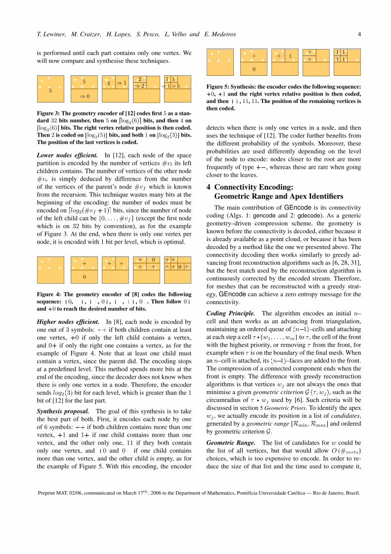
Figure 3: The geometry encoder of [12] codes first 5 as a stan-dard 32 bits number, then 5 on rlog2p6qs bits, and then 4 onrlog2p6qs bits. The right vertex relative position is then coded.Then 2 is coded on rlog2p5qs bits, and both 1 on rlog2p3qs bits.The position of the last vertices is coded.

Lower nodes efficient. In [12], each node of the spacepartition is encoded by the number of vertices #vl its leftchildren contains. The number of vertices of the other node#vr is simply deduced by difference from the numberof the vertices of the parent’s node #vf which is knownfrom the recursion. This technique wastes many bits at thebeginning of the encoding: the number of nodes must beencoded on rlog2p#vf � 1qs bits, since the number of nodeof the left child can be t0, . . . ,#vfu (except the first nodewhich is on 32 bits by convention), as for the exampleof Figure 3. At the end, when there is only one vertex pernode, it is encoded with 1 bit per level, which is optimal.

+

0

+ ++

+

+ +

++ ++

0

0

Figure 4: The geometry encoder of [8] codes the followingsequence: �0, ��, ��, 0�, ��, ��, 0�. Then follow 0�and �0 to reach the desired number of bits.

Higher nodes efficient. In [8], each node is encoded byone out of 3 symbols: �� if both children contain at leastone vertex, �0 if only the left child contains a vertex,and 0� if only the right one contains a vertex, as for theexample of Figure 4. Note that at least one child mustcontain a vertex, since the parent did. The encoding stopsat a predefined level. This method spends more bits at theend of the encoding, since the decoder does not know whenthere is only one vertex in a node. Therefore, the encodersends log2p3q bit for each level, which is greater than the 1bit of [12] for the last part.

Synthesis proposal. The goal of this synthesis is to takethe best part of both. First, it encodes each node by oneof 6 symbols: �� if both children contains more than onevertex, �1 and 1� if one child contains more than onevertex, and the other only one, 11 if they both containonly one vertex, and �0 and 0� if one child containsmore than one vertex, and the other child is empty, as forthe example of Figure 5. With this encoding, the encoder

+

0

+ 1+

+

1 1

11

Figure 5: Synthesis: the encoder codes the following sequence:�0, �1 and the right vertex relative position is then coded,and then ��, 11, 11. The position of the remaining vertices isthen coded.

detects when there is only one vertex in a node, and thenuses the technique of [12]. The coder further benefits fromthe different probability of the symbols. Moreover, theseprobabilities are used differently depending on the levelof the node to encode: nodes closer to the root are morefrequently of type ��, whereas these are rare when goingcloser to the leaves.

4 Connectivity Encoding:Geometric Range and Apex IdentifiersThe main contribution of GEncode is its connectivity

coding (Algs. 1: gencode and 2: gdecode). As a genericgeometry–driven compression scheme, the geometry isknown before the connectivity is decoded, either because itis already available as a point cloud, or because it has beendecoded by a method like the one we presented above. Theconnectivity decoding then works similarly to greedy ad-vancing front reconstruction algorithms such as [6, 28, 31],but the best match used by the reconstruction algorithm iscontinuously corrected by the encoded stream. Therefore,for meshes that can be reconstructed with a greedy strat-egy, GEncode can achieve a zero entropy message for theconnectivity.

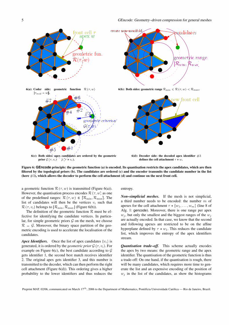
Coding Principle. The algorithm encodes an initial n–cell and then works as an advancing front triangulation,maintaining an ordered queue of pn�1q–cells and attachingat each step a cell τ �tw1, . . . , wmu to τ , the cell of the frontwith the highest priority, or removing τ from the front, forexample when τ is on the boundary of the final mesh. Whenan n–cell is attached, its pn�1q–faces are added to the front.The compression of a connected component ends when thefront is empty. The difference with greedy reconstructionalgorithms is that vertices wj are not always the ones thatminimise a given geometric criterion G pτ, wjq, such as thecircumradius of τ � wj used by [6]. Such criteria will bediscussed in section 5 Geometric Priors. To identify the apexwj , we actually encode its position in a list of candidates,generated by a geometric range rRmin,Rmaxs and orderedby geometric criterion G.

Geometric Range. The list of candidates for w could bethe list of all vertices, but that would allow O p#vertsqchoices, which is too expensive to encode. In order to re-duce the size of that list and the time used to compute it,

Preprint MAT. 02/06, communicated on March 17th, 2006 to the Department of Mathematics, Pontifıcia Universidade Catolica — Rio de Janeiro, Brazil.

5 GEncode: Geometry–driven compression for general meshes

front cell τapex w

geometric fun.R(τ, w)

6(a): Coder side: geometric function R pτ, wq �}τmid � w}.6(b): Both sides: geometric rangeRmin ¤ R pτ, wq   Rmax.

6(c): Both sides: apex candidates are ordered by the geometricprior G pτ, viq � ρ pτ � viq.

new front cell

6(d): Decoder side: the decoded apex identifier #3defines the cell attachment τ � w.

Figure 6: GEncode principle: the geometric function (a) is encoded. Its quantisation restricts the apex candidates, which are thenfiltered by the topological priors (b). The candidates are ordered (c) and the encoder transmits the candidate number in the list(here #3), which allows the decoder to perform the cell attachment (d) and continue on the next front cell.

a geometric function R pτ, wq is transmitted (Figure 6(a)).However, the quantisation process encodesR pτ, wq as oneof the predefined ranges: R pτ, wq P rRmin,Rmaxs. Thelist of candidates will then be the vertices vi such thatR pτ, viq belongs to rRmin,Rmaxs (Figure 6(b)).

The definition of the geometric function R must be ef-fective for identifying the candidate vertices. In particu-lar, for simple geometric priors G on the mesh, we chooseR � G. Moreover, the binary space partition of the geo-metric encoding is used to accelerate the localisation of thecandidates.

Apex Identifiers. Once the list of apex candidates tviu isgenerated, it is ordered by the geometric prior G pτ, viq. Forexample on Figure 6(c), the best candidate according to Ggets identifier 1, the second best match receives identifier2. The original apex gets identifier 3, and this number istransmitted to the decoder, which can then perform the rightcell attachment (Figure 6(d)). This ordering gives a higherprobability to the lower identifiers and thus reduces the

entropy.

Non–simplicial meshes. If the mesh is not simplicial,a third number needs to be encoded: the number m ofapexes for the cell attachment τ � tw1, . . . , wmu (line 8 ofAlg. 1: gencode). Moreover, there is one range per apexwj , but only the smallest and the biggest ranges of the wjare actually encoded. In that case, we know that the secondand following apexes are restricted to be on the affinehyperplane defined by τ � w1. This reduces the candidatelist, which improves the entropy of the apex identifiersstream.

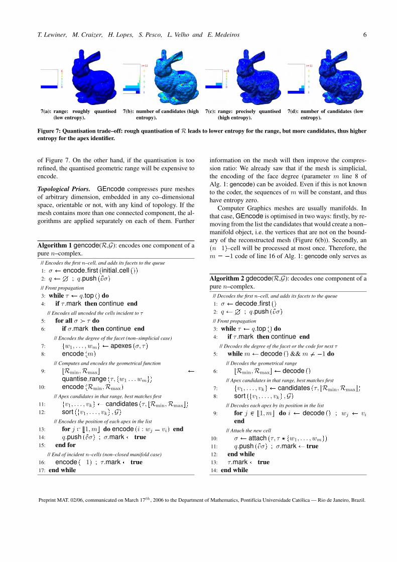
Quantisation trade–off. This scheme actually encodesthe apex by two means: the geometric range and the apexidentifier. The quantisation of the geometric function is thusa trade-off: On one hand, if the quantisation is rough, therewill be many candidates, which requires more time to gen-erate the list and an expensive encoding of the position ofwj in the list of the candidates, as show the histograms

Preprint MAT. 02/06, communicated on March 17th, 2006 to the Department of Mathematics, Pontifıcia Universidade Catolica — Rio de Janeiro, Brazil.

T. Lewiner, M. Craizer, H. Lopes, S. Pesco, L. Velho and E. Medeiros 6

7(a): range: roughly quantised(low entropy).

7(b): number of candidates (highentropy).

7(c): range: precisely quantised(high entropy).

7(d): number of candidates (lowentropy).

Figure 7: Quantisation trade–off: rough quantisation of R leads to lower entropy for the range, but more candidates, thus higherentropy for the apex identifier.

of Figure 7. On the other hand, if the quantisation is toorefined, the quantised geometric range will be expensive toencode.

Topological Priors. GEncode compresses pure meshesof arbitrary dimension, embedded in any co–dimensionalspace, orientable or not, with any kind of topology. If themesh contains more than one connected component, the al-gorithms are applied separately on each of them. Further

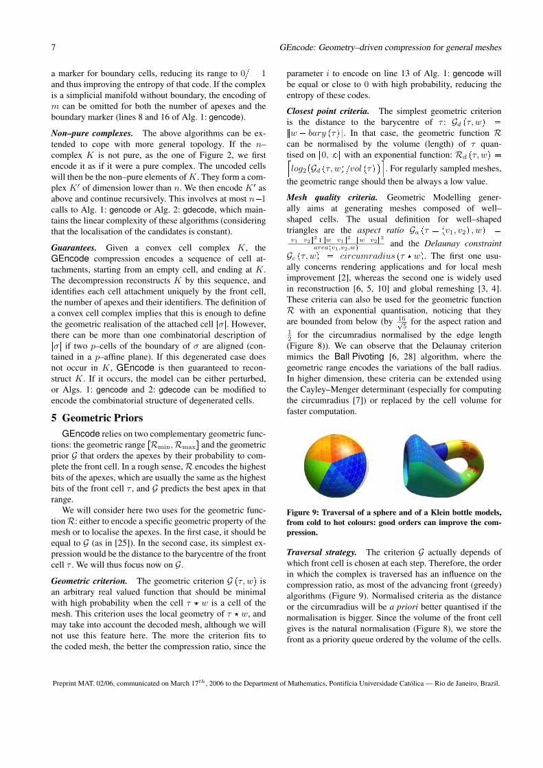
Algorithm 1 gencode(R,G): encodes one component of apure n–complex.

// Encodes the first n–cell, and adds its facets to the queue

1: σ Ð encode first pinitial cell pqq2: q ÐH ; q.push pBσq// Front propagation

3: while τ Ð q.top pq do4: if τ .mark then continue end

// Encodes all uncoded the cells incident to τ

5: for all σ ¡ τ do6: if σ.mark then continue end

// Encodes the degree of the facet (non–simplicial case)

7: tw1, . . . , wmu Ð apexes pσ, τq8: encode pmq

// Computes and encodes the geometrical function

9: rRmin,Rmaxs Ðquantise range pτ, tw1 . . . wmuq

10: encode pRmin,Rmaxq// Apex candidates in that range, best matches first

11: tv1, . . . , vku Ð candidates pτ, rRmin,Rmaxsq12: sort ptv1, . . . , vku ,Gq

// Encodes the position of each apex in the list

13: for j P v1,mw do encode pi : wj � viq end14: q.push pBσq ; σ.mark Ð true15: end for

// End of incident n–cells (non–closed manifold case)

16: encode p�1q ; τ.mark Ð true17: end while

information on the mesh will then improve the compres-sion ratio: We already saw that if the mesh is simplicial,the encoding of the face degree (parameter m line 8 ofAlg. 1: gencode) can be avoided. Even if this is not knownto the coder, the sequences of m will be constant, and thushave entropy zero.

Computer Graphics meshes are usually manifolds. Inthat case, GEncode is optimised in two ways: firstly, by re-moving from the list the candidates that would create a non–manifold object, i.e. the vertices that are not on the bound-ary of the reconstructed mesh (Figure 6(b)). Secondly, anpn�1q–cell will be processed at most once. Therefore, them � �1 code of line 16 of Alg. 1: gencode only serves as

Algorithm 2 gdecode(R,G): decodes one component of apure n–complex.

// Decodes the first n–cell, and adds its facets to the queue

1: σ Ð decode first pq2: q ÐH ; q.push pBσq// Front propagation

3: while τ Ð q.top pq do4: if τ .mark then continue end

// Decodes the degree of the facet or the code for next τ

5: while mÐ decode pq && m � �1 do// Decodes the geometrical range

6: rRmin,Rmaxs Ð decode pq// Apex candidates in that range, best matches first

7: tv1, . . . , vku Ð candidates pτ, rRmin,Rmaxsq8: sort ptv1, . . . , vku ,Gq

// Decodes each apex by its position in the list

9: for j P v1,mw do i Ð decode pq ; wj Ð viend

// Attach the new cell

10: σ Ð attach pτ, τ � tw1, . . . , wmuq11: q.push pBσq ; σ.mark Ð true12: end while13: τ.mark Ð true14: end while

Preprint MAT. 02/06, communicated on March 17th, 2006 to the Department of Mathematics, Pontifıcia Universidade Catolica — Rio de Janeiro, Brazil.

7 GEncode: Geometry–driven compression for general meshes

a marker for boundary cells, reducing its range to 0{ � 1and thus improving the entropy of that code. If the complexis a simplicial manifold without boundary, the encoding ofm can be omitted for both the number of apexes and theboundary marker (lines 8 and 16 of Alg. 1: gencode).

Non–pure complexes. The above algorithms can be ex-tended to cope with more general topology. If the n–complex K is not pure, as the one of Figure 2, we firstencode it as if it were a pure complex. The uncoded cellswill then be the non–pure elements ofK. They form a com-plex K 1 of dimension lower than n. We then encode K 1 asabove and continue recursively. This involves at most n�1calls to Alg. 1: gencode or Alg. 2: gdecode, which main-tains the linear complexity of these algorithms (consideringthat the localisation of the candidates is constant).

Guarantees. Given a convex cell complex K, theGEncode compression encodes a sequence of cell at-tachments, starting from an empty cell, and ending at K.The decompression reconstructs K by this sequence, andidentifies each cell attachment uniquely by the front cell,the number of apexes and their identifiers. The definition ofa convex cell complex implies that this is enough to definethe geometric realisation of the attached cell |σ|. However,there can be more than one combinatorial description of|σ| if two p–cells of the boundary of σ are aligned (con-tained in a p–affine plane). If this degenerated case doesnot occur in K, GEncode is then guaranteed to recon-struct K. If it occurs, the model can be either perturbed,or Algs. 1: gencode and 2: gdecode can be modified toencode the combinatorial structure of degenerated cells.

5 Geometric PriorsGEncode relies on two complementary geometric func-

tions: the geometric range rRmin,Rmaxs and the geometricprior G that orders the apexes by their probability to com-plete the front cell. In a rough sense,R encodes the highestbits of the apexes, which are usually the same as the highestbits of the front cell τ , and G predicts the best apex in thatrange.

We will consider here two uses for the geometric func-tionR: either to encode a specific geometric property of themesh or to localise the apexes. In the first case, it should beequal to G (as in [25]). In the second case, its simplest ex-pression would be the distance to the barycentre of the frontcell τ . We will thus focus now on G.

Geometric criterion. The geometric criterion G pτ, wq isan arbitrary real valued function that should be minimalwith high probability when the cell τ � w is a cell of themesh. This criterion uses the local geometry of τ � w, andmay take into account the decoded mesh, although we willnot use this feature here. The more the criterion fits tothe coded mesh, the better the compression ratio, since the

parameter i to encode on line 13 of Alg. 1: gencode willbe equal or close to 0 with high probability, reducing theentropy of these codes.

Closest point criteria. The simplest geometric criterionis the distance to the barycentre of τ : Gd pτ, wq �}w � bary pτq}. In that case, the geometric function Rcan be normalised by the volume (length) of τ quan-tised on r0,8r with an exponential function: Rd pτ, wq �Qlog2

�Gd pτ, wq {vol pτq �U. For regularly sampled meshes,the geometric range should then be always a low value.

Mesh quality criteria. Geometric Modelling gener-ally aims at generating meshes composed of well–shaped cells. The usual definition for well–shapedtriangles are the aspect ratio Ga pτ � pv1, v2q , wq �}v1�v2}2�}w�v1}2�}w�v2}2

areapv1,v2,wq and the Delaunay constraintGc pτ, wq � circumradius pτ � wq. The first one usu-ally concerns rendering applications and for local meshimprovement [2], whereas the second one is widely usedin reconstruction [6, 5, 10] and global remeshing [3, 4].These criteria can also be used for the geometric functionR with an exponential quantisation, noticing that theyare bounded from below (by 16?

5for the aspect ration and

12 for the circumradius normalised by the edge length(Figure 8)). We can observe that the Delaunay criterionmimics the Ball Pivoting [6, 28] algorithm, where thegeometric range encodes the variations of the ball radius.In higher dimension, these criteria can be extended usingthe Cayley–Menger determinant (especially for computingthe circumradius [7]) or replaced by the cell volume forfaster computation.

Figure 9: Traversal of a sphere and of a Klein bottle models,from cold to hot colours: good orders can improve the com-pression.

Traversal strategy. The criterion G actually depends ofwhich front cell is chosen at each step. Therefore, the orderin which the complex is traversed has an influence on thecompression ratio, as most of the advancing front (greedy)algorithms (Figure 9). Normalised criteria as the distanceor the circumradius will be a priori better quantised if thenormalisation is bigger. Since the volume of the front cellgives is the natural normalisation (Figure 8), we store thefront as a priority queue ordered by the volume of the cells.

Preprint MAT. 02/06, communicated on March 17th, 2006 to the Department of Mathematics, Pontifıcia Universidade Catolica — Rio de Janeiro, Brazil.

T. Lewiner, M. Craizer, H. Lopes, S. Pesco, L. Velho and E. Medeiros 8

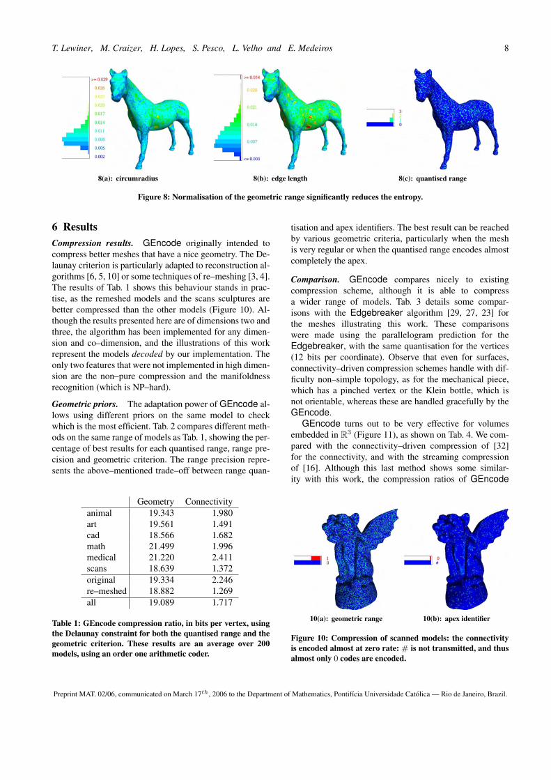
8(a): circumradius 8(b): edge length 8(c): quantised range

Figure 8: Normalisation of the geometric range significantly reduces the entropy.

6 ResultsCompression results. GEncode originally intended tocompress better meshes that have a nice geometry. The De-launay criterion is particularly adapted to reconstruction al-gorithms [6, 5, 10] or some techniques of re–meshing [3, 4].The results of Tab. 1 shows this behaviour stands in prac-tise, as the remeshed models and the scans sculptures arebetter compressed than the other models (Figure 10). Al-though the results presented here are of dimensions two andthree, the algorithm has been implemented for any dimen-sion and co–dimension, and the illustrations of this workrepresent the models decoded by our implementation. Theonly two features that were not implemented in high dimen-sion are the non–pure compression and the manifoldnessrecognition (which is NP–hard).

Geometric priors. The adaptation power of GEncode al-lows using different priors on the same model to checkwhich is the most efficient. Tab. 2 compares different meth-ods on the same range of models as Tab. 1, showing the per-centage of best results for each quantised range, range pre-cision and geometric criterion. The range precision repre-sents the above–mentioned trade–off between range quan-

Geometry Connectivityanimal 19.343 1.980art 19.561 1.491cad 18.566 1.682math 21.499 1.996medical 21.220 2.411scans 18.639 1.372original 19.334 2.246re–meshed 18.882 1.269all 19.089 1.717

Table 1: GEncode compression ratio, in bits per vertex, usingthe Delaunay constraint for both the quantised range and thegeometric criterion. These results are an average over 200models, using an order one arithmetic coder.

tisation and apex identifiers. The best result can be reachedby various geometric criteria, particularly when the meshis very regular or when the quantised range encodes almostcompletely the apex.

Comparison. GEncode compares nicely to existingcompression scheme, although it is able to compressa wider range of models. Tab. 3 details some compar-isons with the Edgebreaker algorithm [29, 27, 23] forthe meshes illustrating this work. These comparisonswere made using the parallelogram prediction for theEdgebreaker, with the same quantisation for the vertices(12 bits per coordinate). Observe that even for surfaces,connectivity–driven compression schemes handle with dif-ficulty non–simple topology, as for the mechanical piece,which has a pinched vertex or the Klein bottle, which isnot orientable, whereas these are handled gracefully by theGEncode.

GEncode turns out to be very effective for volumesembedded in R3 (Figure 11), as shown on Tab. 4. We com-pared with the connectivity–driven compression of [32]for the connectivity, and with the streaming compressionof [16]. Although this last method shows some similar-ity with this work, the compression ratios of GEncode

10(a): geometric range 10(b): apex identifier

Figure 10: Compression of scanned models: the connectivityis encoded almost at zero rate: # is not transmitted, and thusalmost only 0 codes are encoded.

Preprint MAT. 02/06, communicated on March 17th, 2006 to the Department of Mathematics, Pontifıcia Universidade Catolica — Rio de Janeiro, Brazil.

9 GEncode: Geometry–driven compression for general meshes

Quantised RangeR Quantisation precision Geometric Criterion Gdistance circumradius rough regular detailed distance volume aspect circumradius

animal 17% 83% 7% 17% 76% 100% 83% 77% 83%art 5% 95% 43% 90% 0% 26% 31% 67% 54%cad 45% 55% 96% 3% 1% 47% 19% 7% 50%math 67% 33% 55% 21% 24% 54% 5% 22% 35%medical 0% 100% 100% 0% 0% 61% 0% 0% 39%sculpture 78% 22% 21% 41% 38% 80% 0% 1% 19%

Table 2: Percentage of best results obtained by each geometric function, range precision, geometric criterion on the models usedfor Tab. 1. The best result can be reached by various geometric criteria, leading to a sum over 100%.

nv EB GEncodegeom conn geom conn

terrain 16641 17.09 0.28 13.11 2.71mechanical 71150 NA NA 15.86 0.82david 24988 25.80 2.71 16.99 1.63horse 19851 24.86 3.01 18.22 0.85gargoyle 30059 20.99 2.32 18.38 0.58bunny 34834 17.05 2.18 18.77 0.97blech 4102 21.55 2.10 20.73 2.79fandisk 6475 19.56 2.25 21.52 1.31klein 4120 NA NA 22.11 2.63sphere 642 27.98 2.27 24.65 0.03rotor 600 31.67 3.69 24.08 5.18

Table 3: GEncode compression ratio (in bits per vertex) fortriangulated surfaces compared with Edgebreaker [29, 23].The mechanical model is not manifold, and the Klein bottleis not orientable, which prevented the Edgebreaker to work.

are in average more than 35% better than for streamingcompression, to the cost of being slower.

7 ConclusionThis works proposed a new geometry–driven compres-

sion scheme that is, to our knowledge, the first compressionmethod that encodes meshes of any dimension and arbitrarytopology, while being efficient compared to compressionmethods for triangulates surfaces. Prior knowledge on themodel is used independently by GEncode: as an input forthe geometric priors and as optimisation of the executionand compression ratio for the topological priors. In particu-lar for scanned and re–meshed models, classical geometricpriors such as the aspect ratio or Delaunay constraint im-prove significantly the compression ratio.

There is a computational price for the gain in compres-sion: the localisation procedure, which consumes the mainpart of the execution time, is still slow for general geomet-rical ranges. In particular when comparing with streamingcompression methods, the 35% gain required a three or fourtimes more time in our experiments. Moreover, the separate

nv G&F Stream GEncodeconn geom conn geom conn

sph simul. 12229 76.36 34.00 75.87 22.50 12.76iron piece 6103 51.93 29.90 25.17 18.17 10.45molecule 5853 54.00 34.57 23.51 21.77 19.82triceratops 4344 55.41 34.84 25.82 19.39 18.06seismic fault 3403 63.50 36.17 35.15 22.57 11.97dog 3286 55.50 34.31 17.13 20.13 16.86fandisk 3000 64.85 36.23 18.11 24.26 9.06turbine 2953 NA 33.91 11.80 22.95 14.71rattle 2514 NA 33.84 11.40 22.48 13.12solid torus 1004 60.52 41.04 15.69 26.68 9.22sphere1000 986 65.01 41.19 18.76 31.46 10.01points on S2 770 43.56 33.14 8.76 21.87 8.34bended cube 400 57.86 42.52 15.36 23.54 14.59gear 234 48.62 47.18 15.01 26.18 10.92finite elem 141 53.22 53.05 19.29 29.77 11.98sphere100 100 55.84 57.36 19.68 31.49 8.61

Table 4: GEncode compression ratio (in bits per vertex) fortetrahedral meshes compared with Grow & Fold [32] andstreaming compression [16].

encoding of the geometry still limits the final compressionratio. On one hand, the geometric compression can be im-proved, and the synthesis proposed in this work is a firstattempt in that direction. On the other hand, improvementsbased on mixed geometry/connectivity encoding are feasi-ble with GEncode.

References[1] P. Alliez and M. Desbrun. Valence–driven connectivity

encoding of 3D meshes. In Computer Graphics Forum,pages 480–489, 2001.

[2] P. Alliez, M. Meyer and M. Desbrun. Interactive Ge-ometry Remeshing. In Siggraph, pages 347–354. ACM,2002.

[3] P. Alliez, D. Cohen–Steiner, O. Devillers, B. Levy andM. Desbrun. Anisotropic polygonal remeshing. In

Preprint MAT. 02/06, communicated on March 17th, 2006 to the Department of Mathematics, Pontifıcia Universidade Catolica — Rio de Janeiro, Brazil.

T. Lewiner, M. Craizer, H. Lopes, S. Pesco, L. Velho and E. Medeiros 10

11(a): A bended cube, decompressed fromcold to hot colours.

11(b): A mesh of poor quality, generated frompoints closed to the sphere S2, with thedistribution of their circumradii.

11(c): A turbine model, similar to the ro-tor surface, with the distribution of theapex identifiers during the decoding.

Figure 11: Compression on tetrahedral meshes works exactly as for triangulated surfaces.

Siggraph. ACM, 2003.

[4] P. Alliez, E. Colin de Verdiere, O. Devillers andM. Isenburg. Isotropic surface remeshing. In ShapeModeling International. IEEE, 2003.

[5] N. Amenta, S. Choi and R. Kolluri. The Power Crust,unions of balls, and the medial axis transform. Com-putational Geometry: Theory and Applications, 19(2–3):127–153, 2001.

[6] F. Bernardini, J. Mittleman, H. Rushmeier, C. Silva andG. Taubin. The Ball–Pivoting Algorithm for surface re-construction. Transactions on Visualization and Com-puter Graphics, 5(4):349–359, 1999.

[7] L. M. Blumenthal. Theory and applications of distancegeometry. Chelsea, New York, 1970.

[8] M. Botsch, A. Wiratanaya and L. Kobbelt. Efficienthigh quality rendering of point sampled geometry. InEurographics Workshop on Rendering, pages 53–64,2002.

[9] L. Castelli Aleardi and O. Devillers. Canonical trian-gulation of a graph, with a coding application. INRIApreprint, 2004.

[10] D. Cohen–Steiner and T. K. F. Da. A greedyDelaunay–based surface reconstruction algorithm. TheVisual Computer, 20(1):4–16, 2002.

[11] V. Coors and J. Rossignac. Delphi: geometry-basedconnectivity prediction in triangle mesh compression.The Visual Computer, 20(8–9):507–520, 2004.

[12] P.-M. Gandoin and O. Devillers. Progressive losslesscompression of arbitrary simplicial complexes. In Sig-graph, volume 21, pages 372–379. ACM, 2002.

[13] A. Gueziec, F. Bossen, G. Taubin and C. Silva. Effi-cient compression of non–manifold polygonal meshes.Computational Geometry: Theory and Applications,14(1–3):137–166, 1999.

[14] S. Gumhold, S. Guthe and W. Straser. Tetrahedralmesh compression with the Cut–Border machine. InVisualization, pages 51–58. IEEE, 1999.

[15] A. Hatcher. Algebraic topology. Cambridge Univer-sity Press, 2002.

[16] M. Isenburg, P. Lindstrom, S. Gumhold and J. R.Shewchuk. Streaming Compression of Tetrahedral Vol-ume Meshes. www.cs.unc.edu/˜isenburg/research/sctvm.

[17] M. Isenburg and P. Alliez. Compressing hexahedralvolume meshes. In Pacific Graphics, pages 284–293,2002.

[18] F. Kalberer, K. Polthier, U. Reitebuch and M. Wardet-zky. Freelence — coding with free valences. ComputerGraphics Forum, 24(3):469–478, 2005.

[19] D. King and J. Rossignac. Guaranteed 3.67v bit en-coding of planar triangle graphs. In Canadian Confer-ence on Computational Geometry, pages 146–149, 1999.

[20] B. Kronrod and C. Gotsman. Efficient coding ofnontriangular mesh connectivity. Graphical Models,63:263–275, 2001.

[21] H. Lee, P. Alliez and M. Desbrun. Angle-Analyzer: ATriangle-Quad Mesh Codec. In Eurographics, volume21(3), 2002.

[22] H. Lee, M. Desbrun and P. Schroder. Progressive en-coding of complex isosurfaces. Transactions on Graph-ics, 22(3):471–476, 2003.

Preprint MAT. 02/06, communicated on March 17th, 2006 to the Department of Mathematics, Pontifıcia Universidade Catolica — Rio de Janeiro, Brazil.

11 GEncode: Geometry–driven compression for general meshes

[23] T. Lewiner, H. Lopes, J. Rossignac and A. W. Vieira.Efficient Edgebreaker for surfaces of arbitrary topology.In Sibgrapi, pages 218–225, Curitiba, Oct. 2004. IEEE.

[24] T. Lewiner, L. Velho, H. Lopes and V. Mello. Simpli-cial isosurface compression. In Vision, Modeling and Vi-sualization, pages 299–306, Stanford, 2004. IOS Press.

[25] T. Lewiner, M. Craizer, H. Lopes, S. Pesco, L. Velhoand E. Medeiros. GEncode: geometry–driven compres-sion in arbitrary dimension and co–dimension. In Sib-grapi, pages 249–256, Natal, Oct. 2005. IEEE.

[26] T. Lewiner. Mesh Compression from Geometry. PhDthesis, Geometrica Project, INRIA–Sophia Antipolis, de-livered by Universite Paris VI, Dec. 2005. Advised byJean–Daniel Boissonnat.

[27] H. Lopes, J. Rossignac, A. Safonova, A. Szymczakand G. Tavares. Edgebreaker: a simple compression forsurfaces with handles. In C. Hoffman and W. Bronsvort,editors, Solid Modeling and Applications, pages 289–296, Saarbrucken, Germany, 2002. ACM.

[28] E. Medeiros, L. Velho and H. Lopes. Restricted bpa:applying ball–pivoting on the plane. In Sibgrapi, pages372–379, Curitiba, Oct. 2004. IEEE.

[29] J. Rossignac. Edgebreaker: connectivity compressionfor triangle meshes. Transactions on Visualization andComputer Graphics, 5(1):47–61, 1999.

[30] J. Rossignac and D. Cardoze. Matchmaker: manifoldBReps for non–manifold r–sets. In C. Hoffman andW. Bronsvort, editors, Solid Modeling and Applications,pages 31–41. ACM, 1999.

[31] C. E. Scheidegger, S. Fleishman and C. T. Silva. Tri-angulating point–set surfaces with bounded error. InSymposium on Geometry Processing, pages 63–72. Eu-rographics, 2005.

[32] A. Szymczak and J. Rossignac. Grow & Fold:compressing the connectivity of tetrahedral meshes.Computer–Aided Design, 32(8/9):527–538, 2000.

[33] G. Taubin and J. Rossignac. Geometric compressionthrough topological surgery. Transactions on Graphics,17(2):84–115, 1998.

[34] G. Taubin. Blic: bi–level isosurface compression. InVisualization, pages 451–458, Boston, Massachusetts,2002. IEEE.

[35] C. Touma and C. Gotsman. Triangle mesh compres-sion. In Graphics Interface, pages 26–34, 1998.

Preprint MAT. 02/06, communicated on March 17th, 2006 to the Department of Mathematics, Pontifıcia Universidade Catolica — Rio de Janeiro, Brazil.