GBC: Gradient Boosting Consensus Modelfor Heterogeneous Data

Xiaoxiao Shi∗ Jean-Francois Paiement† David Grangier‡ Philip S. Yu∗§

Abstract

With the rapid development of database technologies, multiple data sources may beavailable for a given learning task (e.g., collaborative filtering). However, the data sourcesmay contain different types of features. For example, users’ profiles can be used to buildrecommendation systems. In addition, a model can also use users’ historical behaviors andsocial networks to infer users’ interests on related products. We argue that it is desirable tocollectively use any available multiple heterogeneous data sources in order to build effectivelearning models. We call this framework heterogeneous learning. In our proposed setting,data sources can include (i) non-overlapping features, (ii) non-overlapping instances, and(iii) multiple networks (i.e. graphs) that connect instances. In this paper, we proposea general optimization framework for heterogeneous learning, and devise a correspondinglearning model from gradient boosting. The idea is to minimize the empirical loss with twoconstraints: (1) There should be consensus among the predictions of overlapping instances(if any) from different data sources; (2) Connected instances in graph datasets may havesimilar predictions. The objective function is solved by stochastic gradient boosting trees.Furthermore, a weighting strategy is designed to emphasize informative data sources, anddeemphasize the noisy ones. We formally prove that the proposed strategy leads to atighter error bound. This approach consistently outperforms a standard concatenation ofdata sources on movie rating prediction, number recognition and terrorist attack detectiontasks. Furthermore, the approach is evaluated on a distributed database from a nationa widephone provider with over 500,000 instances, 91 different data sources, and over 45,000,000joined features. We observe that the proposed model can improve out-of-sample error ratesubstantially.

1 Introduction

With the rapid development of database technologies, multiple related data sources can be used tobuild prediction models given a target task. Each of the related data sources may have a distinctset of features and instances, and we argue that the combination of all data sources may yieldbetter prediction results. An example is illustrated in Fig. 1. The task is to predict movie ratings

∗Computer Science Department, University of Illinois at Chicago, USA. {xshi9, psyu}@uic.edu.†AT&T Labs, USA. jpaiement@research.att.com.‡Microsoft Research, USA. grangier@microsoft.com; D. Grangier was with AT&T Labs Research when this research has been

performed§Computer Science Department, King Abdulaziz University, Jeddah, Saudi Arabia

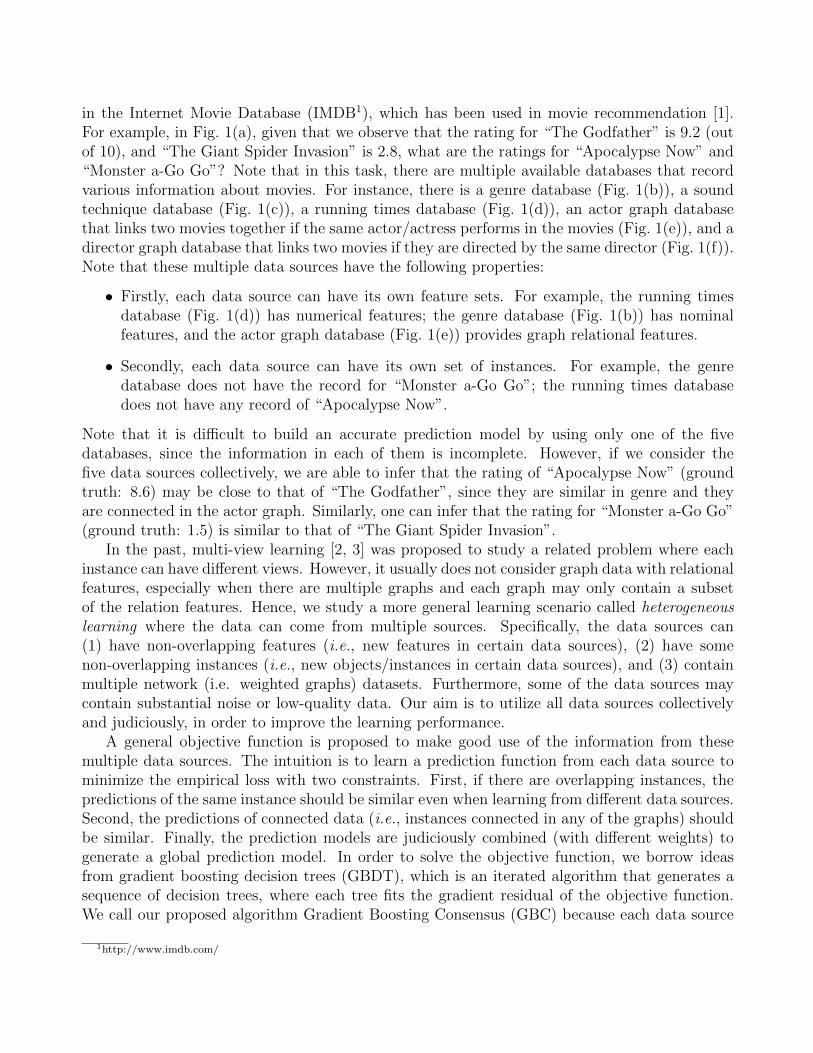
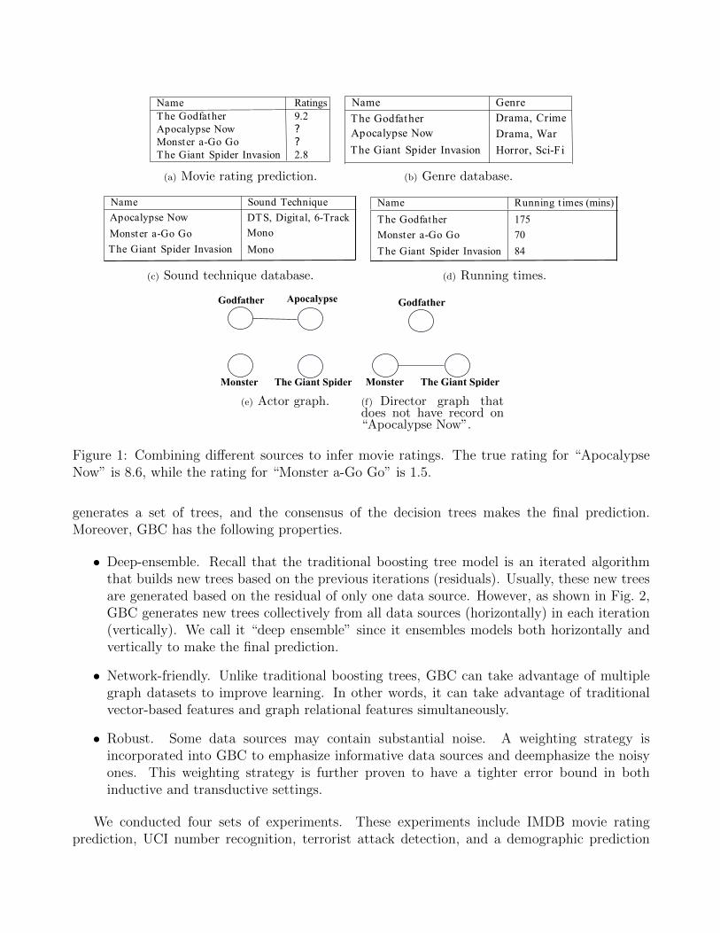
in the Internet Movie Database (IMDB1), which has been used in movie recommendation [1].For example, in Fig. 1(a), given that we observe that the rating for “The Godfather” is 9.2 (outof 10), and “The Giant Spider Invasion” is 2.8, what are the ratings for “Apocalypse Now” and“Monster a-Go Go”? Note that in this task, there are multiple available databases that recordvarious information about movies. For instance, there is a genre database (Fig. 1(b)), a soundtechnique database (Fig. 1(c)), a running times database (Fig. 1(d)), an actor graph databasethat links two movies together if the same actor/actress performs in the movies (Fig. 1(e)), and adirector graph database that links two movies if they are directed by the same director (Fig. 1(f)).Note that these multiple data sources have the following properties:

• Firstly, each data source can have its own feature sets. For example, the running timesdatabase (Fig. 1(d)) has numerical features; the genre database (Fig. 1(b)) has nominalfeatures, and the actor graph database (Fig. 1(e)) provides graph relational features.

• Secondly, each data source can have its own set of instances. For example, the genredatabase does not have the record for “Monster a-Go Go”; the running times databasedoes not have any record of “Apocalypse Now”.

Note that it is difficult to build an accurate prediction model by using only one of the fivedatabases, since the information in each of them is incomplete. However, if we consider thefive data sources collectively, we are able to infer that the rating of “Apocalypse Now” (groundtruth: 8.6) may be close to that of “The Godfather”, since they are similar in genre and theyare connected in the actor graph. Similarly, one can infer that the rating for “Monster a-Go Go”(ground truth: 1.5) is similar to that of “The Giant Spider Invasion”.

In the past, multi-view learning [2, 3] was proposed to study a related problem where eachinstance can have different views. However, it usually does not consider graph data with relationalfeatures, especially when there are multiple graphs and each graph may only contain a subsetof the relation features. Hence, we study a more general learning scenario called heterogeneouslearning where the data can come from multiple sources. Specifically, the data sources can(1) have non-overlapping features (i.e., new features in certain data sources), (2) have somenon-overlapping instances (i.e., new objects/instances in certain data sources), and (3) containmultiple network (i.e. weighted graphs) datasets. Furthermore, some of the data sources maycontain substantial noise or low-quality data. Our aim is to utilize all data sources collectivelyand judiciously, in order to improve the learning performance.

A general objective function is proposed to make good use of the information from thesemultiple data sources. The intuition is to learn a prediction function from each data source tominimize the empirical loss with two constraints. First, if there are overlapping instances, thepredictions of the same instance should be similar even when learning from different data sources.Second, the predictions of connected data (i.e., instances connected in any of the graphs) shouldbe similar. Finally, the prediction models are judiciously combined (with different weights) togenerate a global prediction model. In order to solve the objective function, we borrow ideasfrom gradient boosting decision trees (GBDT), which is an iterated algorithm that generates asequence of decision trees, where each tree fits the gradient residual of the objective function.We call our proposed algorithm Gradient Boosting Consensus (GBC) because each data source

1http://www.imdb.com/

Name Ratings

The Godfather 9.2

Apocalypse Now ?

Monster a-Go Go ?

The Giant Spider Invasion 2.8

(a) Movie rating prediction.

Name Genre

The Godfather Drama, Crime

Apocalypse Now Drama, War

The Giant Spider Invasion Horror, Sci-Fi

(b) Genre database.

Name Sound Technique

Apocalypse Now DTS, Digital, 6-Track

Monster a-Go Go Mono

The Giant Spider Invasion Mono

(c) Sound technique database.

Name Running t imes (mins)

The Godfather 175

Monster a-Go Go 70

The Giant Spider Invasion 84

(d) Running times.

Godfather Apocalypse

Monster The Giant Spider

(e) Actor graph.

Godfather

Monster The Giant Spider

(f) Director graph thatdoes not have record on“Apocalypse Now”.

Figure 1: Combining different sources to infer movie ratings. The true rating for “ApocalypseNow” is 8.6, while the rating for “Monster a-Go Go” is 1.5.

generates a set of trees, and the consensus of the decision trees makes the final prediction.Moreover, GBC has the following properties.

• Deep-ensemble. Recall that the traditional boosting tree model is an iterated algorithmthat builds new trees based on the previous iterations (residuals). Usually, these new treesare generated based on the residual of only one data source. However, as shown in Fig. 2,GBC generates new trees collectively from all data sources (horizontally) in each iteration(vertically). We call it “deep ensemble” since it ensembles models both horizontally andvertically to make the final prediction.

• Network-friendly. Unlike traditional boosting trees, GBC can take advantage of multiplegraph datasets to improve learning. In other words, it can take advantage of traditionalvector-based features and graph relational features simultaneously.

• Robust. Some data sources may contain substantial noise. A weighting strategy isincorporated into GBC to emphasize informative data sources and deemphasize the noisyones. This weighting strategy is further proven to have a tighter error bound in bothinductive and transductive settings.

We conducted four sets of experiments. These experiments include IMDB movie ratingprediction, UCI number recognition, terrorist attack detection, and a demographic prediction

Set of treesfor data source 1

Set of treesfor data source 2

EnsembleVertically Ensemble Horizontally

Iter t

Iter t+1

+ +

Figure 2: Gradient Boosting Consensus.

task in a big dataset from a nationa wide phone provider with over 500,000 samples, 91 differentdata sources, and over 45,000,000 joined features. Each task has a set of data sources withheterogeneous features. For example, in the IMDB movie rating prediction task, we have datasources about the plots of the movies (text data), technologies used by the movies (nominalfeatures), running times of the movies (numerical features), and several movie graphs (such asdirector graph, actor graph). All these mixture types of data sources were used collectively tobuild a prediction model. Since there is no previous model that can handle the problem directly,we have constructed a straightforward baseline which first appends all data sources together intoa single database, and uses traditional learning models to make predictions. Experiments showthat the proposed GBC model consistently outperforms our baseline, and can decrease the errorrate by as much as 80%.

2 Related Work

There are several areas of related works upon which our proposed model is built. First, multi-view learning (e.g., [2, 4, 5]) is proposed to learn from instances which have multiple viewsin different feature spaces. For example, in [4], a co-training algorithm is proposed to classifythe web pages by the text on the web page, and the text on hyperlinks pointing to the webpage. In [5], a general clustering framework is proposed to reconcile the clustering results fromdifferent views. In [6], a term called consensus learning is proposed. The general idea is toperform learning on each heterogeneous feature space independently and then summarize theresults via ensemble. Recently, [7] proposes a recommendation model (collaborative filtering)that can combine information from different contexts. It finds a latent factor that connectsall data sources, and propagate information through the latent factor. There are mainly twodifferences between our work and the previous approaches. First, most of the previous works donot consider the vector-based features and the relational features simultaneously. Second andforemost, most of the previous works require the data sources to have records of all instances inorder to enable the mapping, while the proposed GBC model does not have this constraint.

Another area of related work is collective classification (e.g., [8]) that aims at predictingthe class label from a network. Its key idea is to combine the supervision knowledge fromtraditional vector-based feature vectors, as well as the linkage information from the network.It has been applied to various applications such as part-of-speech tagging [9], classification ofhypertext documents using hyperlinks [10], etc. Most of these works study the case when there

is only one vector-based feature space and only one relational feature space, and the focus is howto combine the two. Different from traditional collective classification framework, we considermultiple vector-based features and multiple relational features simultaneously. Specifically, [11]proposes an approach to combine multiple graphs to improve the learning. The basic idea is toaverage the predictions during training. There are three differences between the previous worksand the current model. Firstly, we allow different data sources to have non-overlapping instances.Secondly, we introduce a weight learning process to filter out noisy data sources. Thirdly, weconsider multiple vector-based sources and multiple graphs at the same time. Hence, all theaforementioned methods could not effectively learn from the datasets described in Section 4, asthey all contain multiple vector-based data sources and relational graphs.

Another related field is transfer learning (e.g., [12, 13, 14, 15, 16]) which aims at learning thetarget task from a related out-of-domain source task. Most research work on transfer learningfocus on how to make good use of the training data that distributes differently with the testdata. A general approach is based on re-sampling (e.g., [12]), where the motivation of it isto “emphasize” the knowledge among “similar” and discriminating instances. Another line ofresearch is to find a new feature space in which the training and test data have strong similarities(e.g., [17, 18, 19, 20, 21, 22, 23, 24]). For instance, [25] applies sparse learning techniques totransfer the knowledge across multiple tasks. There is also a set of works that enable transferlearning on document-related tasks. For example, [21] finds the commonality among differenttasks, such as common words, to attack NLP tasks. However, documents are usually viewed ascoming from the same feature space, since any document can be represented as “bag of words”where the dictionary contains all possible words. Different from these works, we do not requirethe original training and test datasets to be in the same feature space, or have a subset of commonfeatures. Instead, they can be from completely different feature spaces, and they can even begraph datasets.

The proposed model is also related to the research of ensemble learning. For example, gradientboosting tree [26] is a work proposed by J. H. Friedman to approach the learning objective bybuilding an ensemble of weak learners (i.e., decision tree in this case). It is achieved by fitting adecision tree to the residual error of the model at each iteration, and the final model is composedof a weighted summation of all the fitted trees. GBDT is a new model widely used in the industry.For instance, it is used in Yahoo and the search engine company Yandex in the field of “learningto rank” [27]; it is also adopted by the winning team of the Netflix competition [28]. In thispaper, we borrow the idea of gradient boosting to solve the problem of aggregating multipleheterogeneous data sources. There are mainly two reasons that we choose this technique. First,in heterogeneous learning, ensemble approach is a natural choice since it is not straightforwardto come up with a single model to deal with multiple heterogeneous data sources. Second, itis required that the prediction model to be efficient since large dataset is used as input. Assuch, gradient boosting tree is a clear option, especially given that it can be easily deployed in adistributed computing environment. Note that there are some other ensemble learning researchesdeveloped with the idea of consensus. For instance, [29] is proposed to perform clustering via anensemble learning approach. The basic idea is to model the pairwise relationships from multiplesources, and construct the “belief” graphs that maximizes the consensus among the data sources.Furthermore, a generalized unsupervised learning model is proposed in [30], which also adoptsthe idea of aggregating multiple data sources via consensus principle. However, so far as we

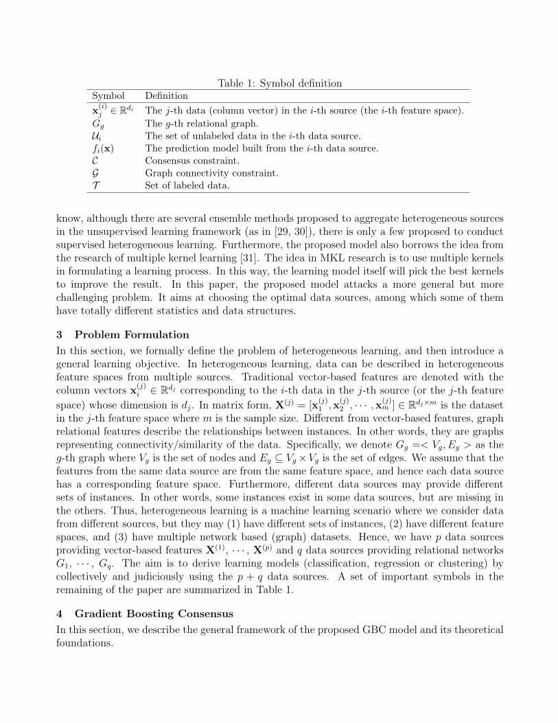
Table 1: Symbol definitionSymbol Definition

x(i)j ∈ Rdi The j-th data (column vector) in the i-th source (the i-th feature space).

Gg The g-th relational graph.Ui The set of unlabeled data in the i-th data source.fi(x) The prediction model built from the i-th data source.C Consensus constraint.G Graph connectivity constraint.T Set of labeled data.

know, although there are several ensemble methods proposed to aggregate heterogeneous sourcesin the unsupervised learning framework (as in [29, 30]), there is only a few proposed to conductsupervised heterogeneous learning. Furthermore, the proposed model also borrows the idea fromthe research of multiple kernel learning [31]. The idea in MKL research is to use multiple kernelsin formulating a learning process. In this way, the learning model itself will pick the best kernelsto improve the result. In this paper, the proposed model attacks a more general but morechallenging problem. It aims at choosing the optimal data sources, among which some of themhave totally different statistics and data structures.

3 Problem Formulation

In this section, we formally define the problem of heterogeneous learning, and then introduce ageneral learning objective. In heterogeneous learning, data can be described in heterogeneousfeature spaces from multiple sources. Traditional vector-based features are denoted with thecolumn vectors x

(j)i ∈ Rdj corresponding to the i-th data in the j-th source (or the j-th feature

space) whose dimension is dj. In matrix form, X(j) = [x(j)1 ,x

(j)2 , · · · ,x(j)

m ] ∈ Rdj×m is the datasetin the j-th feature space where m is the sample size. Different from vector-based features, graphrelational features describe the relationships between instances. In other words, they are graphsrepresenting connectivity/similarity of the data. Specifically, we denote Gg =< Vg, Eg > as theg-th graph where Vg is the set of nodes and Eg ⊆ Vg×Vg is the set of edges. We assume that thefeatures from the same data source are from the same feature space, and hence each data sourcehas a corresponding feature space. Furthermore, different data sources may provide differentsets of instances. In other words, some instances exist in some data sources, but are missing inthe others. Thus, heterogeneous learning is a machine learning scenario where we consider datafrom different sources, but they may (1) have different sets of instances, (2) have different featurespaces, and (3) have multiple network based (graph) datasets. Hence, we have p data sourcesproviding vector-based features X(1), · · · , X(p) and q data sources providing relational networksG1, · · · , Gq. The aim is to derive learning models (classification, regression or clustering) bycollectively and judiciously using the p + q data sources. A set of important symbols in theremaining of the paper are summarized in Table 1.

4 Gradient Boosting Consensus

In this section, we describe the general framework of the proposed GBC model and its theoreticalfoundations.

4.1 The GBC framework In order to use multiple data sources, the objective function aimsat minimizing the overall empirical loss in all data sources, with two more constraints. First,the overlapping instances should have similar predictions from the models trained on differentdata sources, and we call this the principle of consensus. Second, when graph relational data isprovided, the connected data should have similar predictions, and we call this the principle ofconnectivity similarity. In summary, the objective function can be written as follows:

minL =∑i

wi∑x∈T

L(fi(x), y)

s.t. C(f ,w

)= 0

G(f ,w

)= 0

(4.1)

where L(fi(x), y) is the empirical loss on the set of training data T , wi is the weight of importanceof the i-th data source, which is discussed in Section 4.3. Furthermore, the two constraintsC(f ,w

)= 0 and G

(f ,w

)= 0 are the two assumptions discussed above, which are the principle of

consensus and principle of connectivity similarity, respectively. More specifically, the consensusconstraint C

(f ,w

)= 0 is defined as follows:

C(f ,w

)=∑i

wi∑x∈Ui

L(fi(x),E

(f(x)

))E(f(x)

)=

∑{i|x∈Ui}

wifi(x)(4.2)

s.t.∑i

wi = 1

It first calculates the expected prediction E(f(x)

)of a given unlabeled instance x, by summa-

rizing the current predictions from multiple data sources∑{i|x∈Ui}wifi(x). This expectation is

computed only from the data sources that contain x; in other words, it is from the data sourceswhose indices are in the set {i|x ∈ Ui} where Ui is the set of unlabeled instances in the i-th datasource. Hence, if the j-th data source does not have record of x, it will not be used to calcu-late the expected prediction. This strategy enables GBC to handle non-overlapping instances inmultiple data sources, and uses overlapping instances to improve the consensus. Eq. 4.2 forcesthe predictions of x (e.g., f1(x), f2(x), · · · ) to be close to E

(f(x)

).

Furthermore, according to the principle of connectivity similarity, we introduce anotherconstraint G

(f ,w

)as follows:

G(f ,w

)=∑i

wi∑x∈Ui

L(fi(x), Ei

(f(x)

)Ei(f(x)

)=∑g

wg|{(z, x) ∈ Gg}|

∑(z,x)∈Gg

fi(z)(4.3)

s.t.∑g

wg = 1

The above constraint encourages connected data to have similar predictions. It works bycalculating the graph-based expected prediction of x by looking at the average prediction( 1|{(z,x)∈Gg}|

∑(z,x)∈Gg fi(z)) of all its connected neighbors (z’s). If there are multiple graphs,

all the expected predictions are summarized by the weights wg.We use the method of Lagrange multipliers [32] to solve the constraint optimization in Eq. 4.1.

The objective function becomes

minL =∑i

wi∑x∈T

L(fi(x), y) + λ0C(f ,w

)+ λ1G

(f ,w

)(4.4)

where the two constraints C(f ,w

)and G

(f ,w

)are regularized by Lagrange multipliers λ0 and

λ1. These parameters are determined by cross-validation, which is detailed in Section 5. Notethat in Eq. 4.4, the weights wi and wg (i, g = 1, 2, · · · ) are essential. On one hand, the wisare introduced to assign different weights to different vector-based data sources. Intuitively, ifthe t-th data source is more informative, wt should be large. On the other hand, the wgs arethe weights for the graph relational data sources. Similarly, the aim is to give high weights toimportant graph data sources, while deemphasizing the noisy ones. We define different weightsymbols (wi and wg) for the data sources with vector-based features (wi) and graph relationalfeatures (wg). The values of the weights are automatically learned and updated in the trainingprocess, as discussed in Section 4.3.

4.2 Model training of GBC We use stochastic gradient descent [26] to solve the optimizationproblem in Eq. 4.4. In general, it is an iterated algorithm that updates the prediction functionsf(x) in the following way:

f(x)← f(x)− ρ ∂L∂f(x)

It is updated iteratively until a convergence condition is satisfied. Specifically, inspired bygradient boosting decision trees (or GBDT [26]), a regression tree is built to fit the gradient∂L∂f(x)

, and the best parameter ρ is explored via line search [26]. Note that the calculation of ∂L∂f(x)

depends on the loss function L(f, y) as reflected in Eq. 4.1. In the following, we use the L-2loss (for regression problems) and the binary logistic loss (for binary classification problem) asexamples:

GBC with L-2 Loss: In order to update the prediction function of the i-th data source, wefollow the gradient descent formula as follows.

fi(x)← fi(x)− ρ ∂L∂fi(x)

(4.5)

If the L-2 loss is used in L, we have

∂L∂fi(x)

=2wi

(∑x∈T

(fi(x)− y) + λ0∑x∈U

(fi(x)− E)

+ λ1∑x∈U

(fi(x)− Ei))

The L-2 loss is a straightforward loss function for the GBC model, and it is used to performregression tasks in Section 5.

GBC with Logistic Loss: With logistic loss, the partial derivative in Eq. 4.5 becomes:

∂L∂fi(x)

=wi

(∑x∈T

−ye−yfi(x)

1 + e−yfi(x)+ λ0

∑x∈U

−Ee−Efi(x)

1 + e−Efi(x)

+ λ1∑x∈U

−Ee−Efi(x)

1 + e−Efi(x)

)Note that the above formula uses the binary logistic loss where y = −1 or y = 1, but one caneasily extend this model to tackle multi-class problems by using the one-against-others strategy.In Section 5, we adopt this strategy to handle multi-class problems.

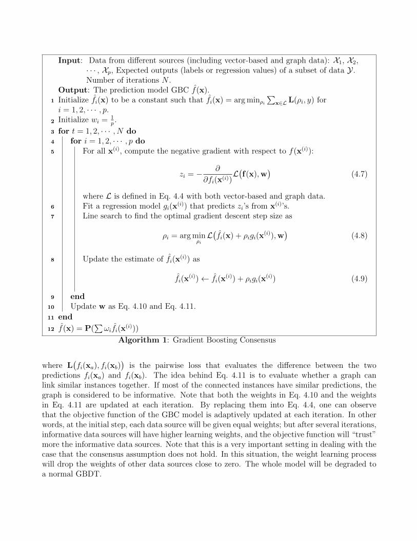
With the updating rule, we can build the GBC model as described in Algorithm 1. It firstfinds the initial prediction models for all data sources in Step 1. Then, it goes into the iteration(Step 3 to Step 11) that generates a series of decision trees. The basic idea is to follow theupdating rule in Eq. 4.5, and build a decision tree gi(x

i) to fit the partial derivative of the loss(Step 5). Furthermore, we follow the idea of [26], and let the number of iterations N be set byusers. In the experiment, it is determined by cross-validation.

Then given a new data x, the predicted output is

f(x) = P(∑

ωifi(xi)) (4.6)

where P(y) is a prediction generation function, where P(y) = y in regression problems, andP(y) = 1 iff y > 0 (P(y) = −1 otherwise) in binary classification problems.

4.3 Weight Learning In the objective function described in Eq. 4.4, one important elementis the set of weights (wi and wg) for the data sources. Ideally, informative data sources will havehigh weights, and noisy data sources will have low weights. As such, the proposed GBC modelcan judiciously filter out the data sources that are noisy. To this aim, we design the weights bylooking at the empirical loss of the model trained from the data source. Specifically, if a datasource induces large loss, its weight should be low. Following this intuition, we design the weightas follows:

wi = exp(−∑x∈L

L(fi(x), y

)/z)

(4.10)

where L(fi(x), y

)is the empirical loss of the model trained from the i-th data source, and z is a

normalization constant to ensure the summation of wis equals to one. Note that the definitionof the weight wi is derived from the weighting matrix in normalized cut [33]. The exponentialpart can effectively give penalty to large loss. Hence, wi will be large if the empirical loss of thei-th data source is small; it becomes small if the loss is large. It is proven in Theorem 4.1 thatthe updating rule of the weights in Eq. 4.10 can result in a smaller error bound. Similarly, wedefine the weights for graph data sources as follows:

wg = exp(− 1

c

∑xga∼xgb

∑i

wiL(fi(xa), fi(xb)

)/z)

(4.11)

Input: Data from different sources (including vector-based and graph data): X1, X2,· · · , Xp, Expected outputs (labels or regression values) of a subset of data Y .Number of iterations N .

Output: The prediction model GBC f(x).Initialize fi(x) to be a constant such that fi(x) = arg minρi

∑x∈L L(ρi, y) for1

i = 1, 2, · · · , p.Initialize wi = 1

p.2

for t = 1, 2, · · · , N do3

for i = 1, 2, · · · , p do4

For all x(i), compute the negative gradient with respect to f(x(i)):5

zi = − ∂

∂fi(x(i))L(f(x),w

)(4.7)

where L is defined in Eq. 4.4 with both vector-based and graph data.Fit a regression model gi(x

(i)) that predicts zi’s from x(i)’s.6

Line search to find the optimal gradient descent step size as7

ρi = arg minρiL(fi(x) + ρigi(x

(i)),w)

(4.8)

Update the estimate of fi(x(i)) as8

fi(x(i))← fi(x

(i)) + ρigi(x(i)) (4.9)

end9

Update w as Eq. 4.10 and Eq. 4.11.10

end11

f(x) = P(∑ωifi(x

(i)))12

Algorithm 1: Gradient Boosting Consensus

where L(fi(xa), fi(xb)

)is the pairwise loss that evaluates the difference between the two

predictions fi(xa) and fi(xb). The idea behind Eq. 4.11 is to evaluate whether a graph canlink similar instances together. If most of the connected instances have similar predictions, thegraph is considered to be informative. Note that both the weights in Eq. 4.10 and the weightsin Eq. 4.11 are updated at each iteration. By replacing them into Eq. 4.4, one can observethat the objective function of the GBC model is adaptively updated at each iteration. In otherwords, at the initial step, each data source will be given equal weights; but after several iterations,informative data sources will have higher learning weights, and the objective function will “trust”more the informative data sources. Note that this is a very important setting in dealing with thecase that the consensus assumption does not hold. In this situation, the weight learning processwill drop the weights of other data sources close to zero. The whole model will be degraded toa normal GBDT.

4.4 Generalization bounds In this section, we consider the incompatibility framework in [34]and [35] to explain the proposed GBC model. Specifically, we show that the weight learningprocess described in Section 4.3 can help reduce an error bound. For the sake of simplicity,we consider the case where we have two data sources X1 and X2, and the case with more datasources can be analyzed with similar logic. Note that the goal is to learn a pair of predictors(f1; f2), where f1 : X1 → Y and f2 : X2 → Y , and Y is the prediction space. Further denote F1

and F2 as the hypothesis classes of interest, consisting of functions from X1 (and, respectively,X2 ) to the prediction space Y . Denote by L(f1) the expected loss of f1, and L(f2) is similarlydefined. Let a Bayes optimal predictor with respect to loss L be denoted as f ∗. We now applythe incompatibility framework for the multi-view setting [34] to study GBC. We first define theincompatibility function χ : F1×F2 → R+, and some t ≥ 0 as those pairs of functions which arecompatible to the tune of t, which can be written as:

Cχ(t) = {(f1, f2) : f1 ∈ F1, f2 ∈ F2 and E[χ(f1, f2)] ≤ t}

Intuitively, the function Cχ(t) captures the set of function pairs f1 and f2 that are compatiblewith respect to a “maximal expected difference” t. From [34], it is proven that there exists asymmetric function d : F1 ×F2, and a monotonically increasing non-negative function Φ on thereals such that for all f ,

E[d(f1(x); f2(x))] ≤ Φ(L(f1)− L(f2))

With these functions at hand, we can derive the following theorems:

Theorem 4.1. Let |L(f1) − L(f ∗)| < ε1 and |L(f2) − L(f ∗)| < ε2, then for the incompatibility

function Cχ(t), if we set χ = d, for t = cd(Φ(√

2ε1ε2ε1+ε2

) + Φ(εbayes)) where cd is a constant depends

on the function d [34], we have

inf(f1,f2)∈Cχ(t)

LGBC(f1, f2) ≤ L(f ∗) + εbayes +

√2ε1ε2ε1 + ε2

(4.12)

Proof. Note that |L(f1) − L(f ∗)| < ε1 and |L(f2) − L(f ∗)| < ε2, and the proposed model GBCadopts a weighted strategy linear to the expected loss, which is approximately LGBC(f1, f2) =ε2

ε1+ε2L(f1) + ε1

ε1+ε2L(f2). According to Lemma 8 in [35], we have E[χ(f1, f2)] ≤ c2d(Φ(

√2ε1ε2ε1+ε2

) +

Φ(εbayes)), andmin

(f1,f2)∈Cχ(t)LGBC(f1, f2) ≤ LGBC(f∗1, f∗2) + εbayes (4.13)

With Lemma 7 in [35], we can get

min(f1,f2)∈Cχ(t)

LGBC(f1, f2) ≤ L(f ∗) + εbayes +

√2ε1ε2ε1 + ε2

(4.14)

�

Similarily, we can derive the error bound of GBC in a transductive setting.

Theorem 4.2. Consider the transductive formula Eq. 4 in [35]. Given the regularized parameterλ > 0, we denote Lλ(f) as the expected loss with the regularized parameter λ. If we setλc = λ

4(K+λ)2√

2ε1ε2ε1+ε2

then for the pair of functions (f1, f2) ∈ F1 × F2 returned by the transductive

learning algorithm, with probability at least 1− δ over labeled samples,

LλGBC(f1, f2) ≤ Lλ(f ∗) +1√n

(2 + 3

√ln(2

δ)

2

)+2CLipR(Cχ(

1

λc)) +

√2ε1ε2ε1 + ε2

(4.15)

where n is the number of labeled examples, and CLip is the Lipschitz constant for the loss, and

R(Cχ( 1λc

)) is a term bounded by the number of unlabeled examples and the bound of the losses.

Proof. We first note that |Lλ(f1) − Lλ(f ∗)| < ε1 and |L(f2)λ − Lλ(f ∗)| < ε2. Similar to the

logic in Theorem 4.1, GBC employs a weighting strategy which is linear to the expected loss:LλGBC(f1, f2) = ε2

ε1+ε2Lλ(f1) + ε1

ε1+ε2Lλ(f2). With Lemma 7 in [35], we then have

|Lλ(f1)− LλGBC|+ |Lλ(f1)− LλGBC|

≤√

ε2ε1 + ε2

√ε1 +

√ε1

ε1 + ε2

√ε2

= 2

√ε1ε2ε1 + ε2

(4.16)

Hence, we can further get the following relationship:

E[χ(f1, f2)] ≤ c2d(E[χ(f1, y1)] + E[χ(y1, y2)] + E[χ(f2, y2)])

≤ c2d(Lλ(f1)− Lλ(f ∗) + Lλ(f2)− Lλ(f ∗) + 2Φ(εbayes))

≤ c2d(Φ(

√2ε1ε2ε1 + ε2

) + Φ(εbayes))

(4.17)

andmin

(f1,f2)∈Cχ(t)LλGBC(f1, f2) ≤ LλGBC(f∗1, f∗2) + εbayes (4.18)

We then have

LλGBC(f1, f2) ≤ Lλ(f ∗) +1√n

(2 + 3

√ln(2

δ)

2

)+2CLipR(Cχ(

1

λc)) +

√2ε1ε2ε1 + ε2

(4.19)

�

Note that Theorem 4.1 and Theorem 4.2 derive the error bounds of GBC in inductive andtransductive setting respectively. In effect, the weighting strategy reduces the last term of

the error bound to√

2ε1ε2ε1+ε2

, as compared to the equal-weighting strategy whose last term is√ε1+ε2

2[34]. Hence, the weighting strategy induces a tighter bound since

√2ε1ε2ε1+ε2

≤√

ε1+ε22

. It is

important to note that if the the predictions of different data sources vary significantly (|ε1− ε2|is large), the proposed weighting strategy has a much tighter bound than the equal-weightingstrategy. In other words, if there are some noisy data sources that potentially lead to large errorrate, GBC can effectively reduce their effect. This is an important property of GBC to handlenoisy data sources. This strategy is evaluated empirically in the next section.

5 Experiments

In this section, we report four sets of experiments that were conducted in order to evaluate theproposed GBC model applied to multiple data sources. We aim to answer the following questions:

• Can GBC make good use of multiple data sources? Can it beat other more straightforwardstrategies?

• What is the performance of GBC if there exist non-overlapping instances in different datasources?

• How does GBC perform on big dataset?

5.1 Datasets The aim of the first set of experiments is to predict movie ratings from theIMDB database.2 Note that there are 10 data sources in this task. For example, there is adata source about the plots of the movies, and a data source about the techniques used in themovies (e.g., 3D IMAX). Furthermore, there are several data sources providing different graphrelational data about the movies. For example, in a director graph, two movies are connected ifthey have the same director. A summary of the different data sources can be found in Table 2.It is important to note that each of the data sources may provide certain useful information forpredicting the ratings of the movies. For instance, the Genre database may reflect that certaintypes of movies are likely to have high ratings (e.g., Fantasy); the Director graph databaseimplicitly infers movie ratings from similar movies of the same director (e.g., Steven Spielberghas many high-rating movies.). Thus, it is desirable to incorporate different types of data sourcesto give a more accurate movie rating prediction. This is an essential task for online TV/movierecommendation, such as the famous $1,000,000 Netflix prize [36].

The second set of experiments is about handwritten number recognition. The dataset contains2000 handwritten numerals (“0”–“9”) extracted from a collection of Dutch utility maps.3 Thehandwritten numbers are scanned and digitized as binary images. They are represented in termsof the following seven data sources with different vector-based feature spaces: (1) 76 Fouriercoefficients of the character shapes, (2) 216 profile correlations, (3) 64 Karhunen-Love coefficients,(4) 240 pixel averages in 2 × 3 windows, (5) 47 Zernike moments, (6) a graph dataset constructedfrom the morphological similarity (i.e., two objects are connected if they have similar morphologyappearance), and (7) a graph generated with the same method as (6), but with random Gaussiannoise imposed in the morphological similarity. This dataset is included to test the performance

2http://www.imdb.com/3http://archive.ics.uci.edu/ml/datasets/Multiple+Features

Table 2: IMDB Movie Rating PredictionData source Type of features

Quote Database TextPlot Database TextTechnology Database NominalSound Technology Database NominalRunning Time Database RealGenre Database BinaryActor Graph GraphActress Graph GraphDirector Graph GraphWritter Graph Graph

of GBC on noisy data. The aim is to classify a given object to one of the ten classes (“0”–“9”).The statistics of the dataset are summarized in Table 3.

The third set of datasets is downloaded from the UMD collective classification database 4.The database consists of 1293 different attacks in one of the six labels indicating the type ofthe attack: arson, bombing, kidnapping, NBCR attack, weapon attack and other attack. Eachattack is described by a binary value vector of attributes whose entries indicate the absence orpresence of a feature. There are a total of 106 distinct vector-based features, along with threesets of relational features. One set connects the attacks together if they happened in the samelocation; the other connects the attacks if they are planned by the same organization. In orderto perform robust evaluation of the proposed GBC model, we add another data source based onthe vector-based dataset, but with a random Gaussian noise N (0, 1). Again, this is to test thecapability of the proposed model to handle noise.

The fourth set of datasets is collected from a tier-1 telegraph network provider in the U.S. Westudy a subset of the demographic database with over 500,000 anonymous users. The databaserecords 196 demographic features per user, which includes education level, age group, language,hobbies, etc.. As the objective in [37], we aim at predicting four demographic features, whichinclude the age group, gender, credit level, and whether the user rents the house. For thetask of predicting the age group and credit level, we only concern whether the user belongs toa specific group of interest (e.g., mid age and good credit level). As a result, all four taskshave binary classification labels. Furthermore, we construct 90 different social graphs from thephone call networks similar to the ones introduced in [38]. These generated social graphs areconsidered to be close approximations to the real-world social connections, and they cover thesocial connections among anonymous users in different time periods. In summary, we have onevector-based demographic dataset and 90 graph datasets, and each of them involves a subset ofthe 500,000 anonymous users. Another very important characteristic is that the dataset containssubstantial missing values, owing to the difficulty of obtaining the demographic features (e.g., lovefishing? speak Japanese?, etc.). In the dataset, over 50% of samples contain over 60% of missingvalues. Classic feature based algorithms such as SVM cannot easily handle this case. On the

4http://www.cs.umd.edu/projects/linqs/projects/lbc/

index.html

contrary, GBC is designed to fit to the situation with missing values and with many heterogeneousdata sources. We design four prediction tasks to predict four important demographic features ofthe samples, and they include the prediction of the age group, gender, credit level, and whetherthe user rents the house. Our objective is then to evaluate the four prediction tasks, all of whichinvolve big and heterogeneous data.

5.2 Comparison Methods and Evaluations It is important to emphasize again that thereis no previous model that can handle the same problem directly; i.e., building a learning modelfrom multiple graphs and multiple vector-based datasets with some non-overlapping instances.Furthermore, as far as we know, there is no state-of-the-art approaches that use the benchmarkdatasets described in the previous section in the same way. For instance, in the movie predictiondataset, we crawl the 10 data sources directly from IMDB and use them collectively in learning.In the case of the number recognition dataset, we have two graph data sources, which aredifferent from previous approaches that only look at vector-based features [39], clustering [40],or feature selection problems [41]. In order to evaluate the proposed GBC model, we designa straightforward comparison strategy, which is to directly join all features together. In otherwords, given the sources with vector-based features X(1), · · · , X(p) and the adjacency matricesof the graphs M(1), · · · , M(q), the joined features can be represented as follows:

X = [X(1)T , · · · ,X(p)T ,M(1)T , · · · ,M(q)T ]T (5.20)

Since there is only one set of joined features, traditional learning algorithms can be appliedon it to give predictions (each row is an instance; each column is a feature from a specific source).We include support vector machines (SVM) in the experiments as it is used widely in practice.Note that in GBC, the consensus term in Eq. 4.2 and the graph similarity term in Eq. 4.3 can useunlabeled data to improve the learning. Hence, we also compare it with semi-supervised learningmodels. Specifically, semi-supervised SVM (Semi-SVM) with a self-learning technique [42] isused as the second comparison model. Note that we have four tasks in the experiment whereone of them (i.e., the movie rating prediction task) is a regression task. In this task, regressionSVM [43] is used to give predictions. Additionaly, since the proposed model is derived fromgradient boosting decision trees, GBDT [26] is used as the third comparison model, and itssemi-supervised version [42] is included as well. It is important to note that in order to use thejoined features from Eq. 5.20, these comparison models require that there is no non-overlappinginstances. In other words, all data sources should have records of all instances; otherwise, thejoined features will have many missing values since some data sources may not have records ofthe corresponding instances. To evaluate GBC more comprehensively, we thus conducted theexperiments on two settings:

• Uniform setting: the first setting is to force all data sources to contain records of allinstances. We only look at the instances that have records in all data sources. Table 3presents the statistics of the datasets in this setting. In this case, we can easily join thefeatures from different sources as in Eq. 5.20. Note that we do not perform the uniformsetting in AT&T’s big dataset. The reason is that there is only a couple of users that appearin all 91 different data sources. The uniform setting thus cannot generate statisticallysignificant results on AT&T’s big dataset.

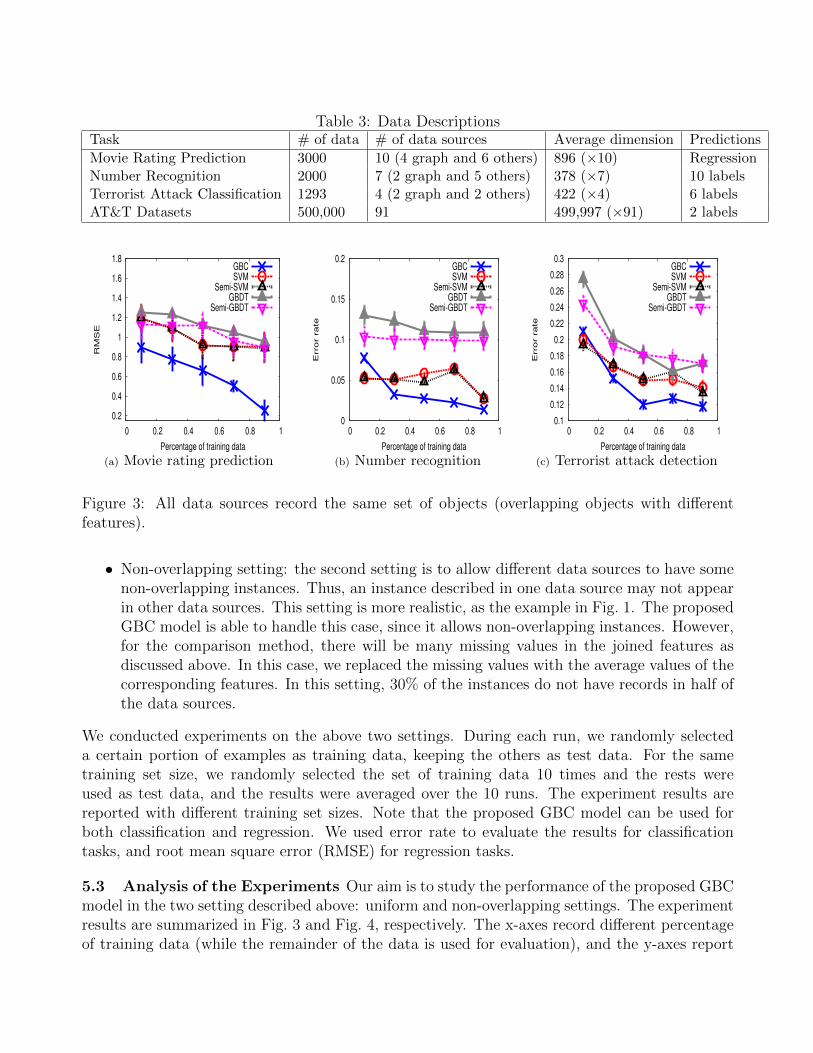
Table 3: Data DescriptionsTask # of data # of data sources Average dimension Predictions

Movie Rating Prediction 3000 10 (4 graph and 6 others) 896 (×10) RegressionNumber Recognition 2000 7 (2 graph and 5 others) 378 (×7) 10 labelsTerrorist Attack Classification 1293 4 (2 graph and 2 others) 422 (×4) 6 labelsAT&T Datasets 500,000 91 499,997 (×91) 2 labels

0.2

0.4

0.6

0.8

1

1.2

1.4

1.6

1.8

0 0.2 0.4 0.6 0.8 1

RM

SE

Percentage of training data

GBCSVM

Semi-SVMGBDT

Semi-GBDT

(a) Movie rating prediction

0

0.05

0.1

0.15

0.2

0 0.2 0.4 0.6 0.8 1

Error r

ate

Percentage of training data

GBCSVM

Semi-SVMGBDT

Semi-GBDT

(b) Number recognition

0.1

0.12

0.14

0.16

0.18

0.2

0.22

0.24

0.26

0.28

0.3

0 0.2 0.4 0.6 0.8 1

Error r

ate

Percentage of training data

GBCSVM

Semi-SVMGBDT

Semi-GBDT

(c) Terrorist attack detection

Figure 3: All data sources record the same set of objects (overlapping objects with differentfeatures).

• Non-overlapping setting: the second setting is to allow different data sources to have somenon-overlapping instances. Thus, an instance described in one data source may not appearin other data sources. This setting is more realistic, as the example in Fig. 1. The proposedGBC model is able to handle this case, since it allows non-overlapping instances. However,for the comparison method, there will be many missing values in the joined features asdiscussed above. In this case, we replaced the missing values with the average values of thecorresponding features. In this setting, 30% of the instances do not have records in half ofthe data sources.

We conducted experiments on the above two settings. During each run, we randomly selecteda certain portion of examples as training data, keeping the others as test data. For the sametraining set size, we randomly selected the set of training data 10 times and the rests wereused as test data, and the results were averaged over the 10 runs. The experiment results arereported with different training set sizes. Note that the proposed GBC model can be used forboth classification and regression. We used error rate to evaluate the results for classificationtasks, and root mean square error (RMSE) for regression tasks.

5.3 Analysis of the Experiments Our aim is to study the performance of the proposed GBCmodel in the two setting described above: uniform and non-overlapping settings. The experimentresults are summarized in Fig. 3 and Fig. 4, respectively. The x-axes record different percentageof training data (while the remainder of the data is used for evaluation), and the y-axes report

0.5

1

1.5

2

2.5

3

0 0.2 0.4 0.6 0.8 1

RM

SE

Percentage of training data

GBCSVM

Semi-SVMGBDT

Semi-GBDT

(a) Movie rating prediction

0

0.05

0.1

0.15

0.2

0 0.2 0.4 0.6 0.8 1

Error r

ate

Percentage of training data

GBCSVM

Semi-SVMGBDT

Semi-GBDT

(b) Number recognition

0.1

0.15

0.2

0.25

0.3

0 0.2 0.4 0.6 0.8 1

Error r

ate

Percentage of training data

GBCSVM

Semi-SVMGBDT

Semi-GBDT

(c) Terrorist attack detection

Figure 4: Each data source is independent (with 30% of overall non-overlapping instances).

the errors of the corresponding learning model.We observe two major phenomena in the experiments. Firstly, the proposed GBC model

effectively reduces the error rate as compared to the other learning models in both settings. Itis especially obvious in the movie rating prediction dataset where 10 data sources are used tobuild the model. In this dataset, GBC reduces the error rate by as much as 80% in the firstsetting (when there are 90% of training instances), and 60% in the second setting (when thereare 10% of training instances). This shows that GBC is especially advantageous when a largenumber of data sources are available. We further analyze this phenomenon in the next sectionwith Table 4. On the other hand, the comparison models have to deal with a longer and noisierfeature vector. GBC beats the four approaches by judiciously reducing the noise (as discussedin Section 4.3 and 4.4). Secondly, we can observe that GBC outperforms the other approachessignificantly and substantially in the second setting (Fig. 4) where some instances do not haverecords on all data sources. As analyzed in the previous section, this is one of the advantages ofGBC over the comparison models that have to deal with missing values.

It is also interesting to analyze the performance of GBC on the demographic prediction task.Recall that the learning task has at least three challenges. First, it contains a large set of samples(over 500,000) as compared to normal machine learning tasks. Second, it has 91 different datasources, among which one is a demographic dataset with around 200 features, and the other 90data sources are social graphs. As a result, it generates over 45,000,000 joined features (as inEq. 5.20). Third, it contains substantial missing values (50% of samples miss 60% of features),which brings in more difficulty in finding the valuable information. This is also the reason wecannot conduct uniform setting on this big dataset, since there is only a couple of users thatappear in all 91 different data sources. The uniform setting thus cannot generate statisticallysignificant results. All the experiments reported in Fig. 6 were run on a distributed computingsystem with the Condor framework. It can be clearly observed that GBC outperforms the othercomparison models in all four tasks. For instance, in the task of predicting genders, the errorrate has been reduced around 20% when there is 50% of training data, and 25% when thereis 90% of training examples. The good performance of GBC comes from its unique design to

0

5

10

15

20

25

30

35

40

45

0:0.001 0.001:0.01 0.01:0.02 0.02:0.03 0.03:0.04 0.04:0.05 0.05:0.06 >0.06

Fre

qu

en

cy (

%)

Weights

Figure 5: Frequency of the Learned Weights

distill useful information from multiple heterogeneous data sources. Each of the individual datasource may be very noisy owing to the missing values and unknown data quality. However, GBCis able to distinguish the useful data sources for the learning tasks, and judiciously uses themin improving learning results. The distribution of the learned weights of the data sources areplotted in Fig. 5. It can be shown that among the 91 data sources, some of them are very useful(with large weights), while many of them are quite noisy and are assigned low weights. GBC isable to judiciously treat them differently to achieve a better model.

6 Discussion

In this section, we would like to answer the following questions:

• To what extent GBC helps to integrate the knowledge from multiple sources, compared tolearn from each source independently? Specifically, how do the principles of consensus andconnectivity similarity help GBC?

• Is the weight learning algorithm necessary?

• Do we need multiple data sources? Does the number of data sources affects theperformance?

In GBC, both λ0 and λ1 (from Eq. 4.4) are determined by cross-validation. In the followingset of experiments, we tune the values of λ0 and λ1 in order to study the specific effects of theconsensus and connectivity terms. We compare the proposed GBC model with three algorithmson the number recognition dataset in the uniform setting (i.e., all data sources contain allinstances):

• The first comparison model is to set λ0 to zero, and determine λ1 by cross-validation. Inthis case, the consensus term is removed. In other words, the algorithm can only apply theconnectivity similarity principle. We denote this model as “GBC without consensus”.

• The second comparison model is to set λ1 to zero, and let λ0 be determined by cross-validation. In other words, the connectivity similarity term is removed, and the algorithmonly depends on the empirical loss and the consensus term. We denote this model as “GBCwithout graph”.

• The third comparison model is to set both λ0 and λ1 to 0. Hence, the remaining term isthe empirical loss, and it is identical to the traditional GBDT model.

0.02

0.03

0.04

0.05

0.06

0.07

0.08

0.09

0.1

0.11

0 0.2 0.4 0.6 0.8 1

Error r

ate

Sample rate

GBCSVM

Semi-SVMGBDT

Semi-GBDT

(a) Credit Level

0.05

0.06

0.07

0.08

0.09

0.1

0.11

0.12

0.13

0.14

0.15

0 0.2 0.4 0.6 0.8 1

Error r

ate

Sample rate

GBCSVM

Semi-SVMGBDT

Semi-GBDT

(b) Age Group

0.1

0.12

0.14

0.16

0.18

0.2

0.22

0.24

0 0.2 0.4 0.6 0.8 1

Error r

ate

Sample rate

GBCSVM

Semi-SVMGBDT

Semi-GBDT

(c) Gender

0

0.01

0.02

0.03

0.04

0.05

0.06

0 0.2 0.4 0.6 0.8 1

Error r

ate

Sample rate

GBCSVM

Semi-SVMGBDT

Semi-GBDT

(d) Renter

Figure 6: Demographic Prediction

The empirical results on the number recognition task are presented in Fig. 7. It can beobserved that all three models outperforms traditional GBDT. We draw two conclusions fromthis experiment. First, as was already observed in previous experiments, learning from multiplesources is advantageous. Specifically, the GBDT model builds classifiers for each of the datasource independently, and average the predictions at the last step. However, it does not“communicate” the prediction models during training. As a result, it has the worst performancein Fig. 7. Second, both the principle of consensus and the principle of connectivity similarityimprove the performance. Furthermore, it shows that the connectivity similarity term helpsimprove the performance more when the number of training data is limited. For example, whenthere are only 10% of training instances, the error rate of GBC with only the connectivity term(i.e., GBC without consensus) is less than 9%, while that of GBC with only the consensus term(i.e., GBC without Graph) is around 13%. This is because when the number of labeled trainingdata is limited, the graph connectivity serves as a more important source of information whenconnecting unlabeled data with the limited labeled data. Again, it is important to note thatin GBC, the weights of different data sources are adjusted at each iteration. The aim is toassign higher weights to the data sources that contain useful information, and filter out the noisysources. This step is analyzed as an important one in Theorem 4.1 since it can help reduce the

0

0.05

0.1

0.15

0.2

0 0.2 0.4 0.6 0.8 1

Error r

ate

Sample rate

GBCGBC without Consensus

GBC without GraphGBDT

Figure 7: How do consensus principle and connectivity similarity principle help?

0

0.1

0.2

0.3

0.4

0.5

0.6

0.7

0.8

0 0.2 0.4 0.6 0.8 1

Error r

ate

Sample rate

GBCGBC without Weight Learning

Figure 8: Why is the weighting strategy necessary?

upper bound of the error rate. We specifically evaluate this strategy on the terrorist detectiontask. Note that in order to perform a robust test, one of the vector-based sources containsGaussian noise, as described in Section 5.1. The empirical results on the terrorist detection taskare presented in Fig. 8. It can be clearly observed that the weighting strategy is reducing theerror rate by as much as 70%. Hence, an appropriate weighting strategy is an important stepwhen dealing with multiple data sources with unknown noise.

It is also interesting to evaluate to what extent GBC performance is improved as the numberof data sources increases. For this purpose, the movie rating prediction dataset is used as anexample. We first study the case when there is only one data source. In order to do so, we runGBC on each of the data source independently, then on 2 and 4 data sources. In the experimentswith 2 data sources, we randomly selected 2 sources from the pool (Table 2) as inputs to GBC.These random selections of data sources were performed 10 times, and the average error isreported in Table 4. A similar strategy was implemented to conduct the experiment with 4 datasources. In Table 4, the results are reported with different percentages of training data, and thebest performances are highlighted with bold letters. It can be observed that the performancewith only one data source is the worst, and has high root mean square error and high variance.With more data sources available, the performance of GBC tends to be better. This is because

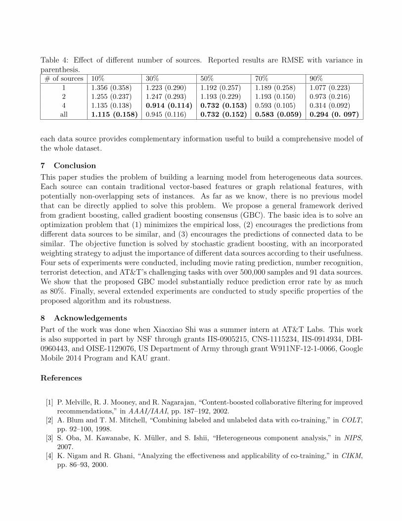
Table 4: Effect of different number of sources. Reported results are RMSE with variance inparenthesis.# of sources 10% 30% 50% 70% 90%

1 1.356 (0.358) 1.223 (0.290) 1.192 (0.257) 1.189 (0.258) 1.077 (0.223)2 1.255 (0.237) 1.247 (0.293) 1.193 (0.229) 1.193 (0.150) 0.973 (0.216)4 1.135 (0.138) 0.914 (0.114) 0.732 (0.153) 0.593 (0.105) 0.314 (0.092)

all 1.115 (0.158) 0.945 (0.116) 0.732 (0.152) 0.583 (0.059) 0.294 (0. 097)

each data source provides complementary information useful to build a comprehensive model ofthe whole dataset.

7 Conclusion

This paper studies the problem of building a learning model from heterogeneous data sources.Each source can contain traditional vector-based features or graph relational features, withpotentially non-overlapping sets of instances. As far as we know, there is no previous modelthat can be directly applied to solve this problem. We propose a general framework derivedfrom gradient boosting, called gradient boosting consensus (GBC). The basic idea is to solve anoptimization problem that (1) minimizes the empirical loss, (2) encourages the predictions fromdifferent data sources to be similar, and (3) encourages the predictions of connected data to besimilar. The objective function is solved by stochastic gradient boosting, with an incorporatedweighting strategy to adjust the importance of different data sources according to their usefulness.Four sets of experiments were conducted, including movie rating prediction, number recognition,terrorist detection, and AT&T’s challenging tasks with over 500,000 samples and 91 data sources.We show that the proposed GBC model substantially reduce prediction error rate by as muchas 80%. Finally, several extended experiments are conducted to study specific properties of theproposed algorithm and its robustness.

8 Acknowledgements

Part of the work was done when Xiaoxiao Shi was a summer intern at AT&T Labs. This workis also supported in part by NSF through grants IIS-0905215, CNS-1115234, IIS-0914934, DBI-0960443, and OISE-1129076, US Department of Army through grant W911NF-12-1-0066, GoogleMobile 2014 Program and KAU grant.

References

[1] P. Melville, R. J. Mooney, and R. Nagarajan, “Content-boosted collaborative filtering for improvedrecommendations,” in AAAI/IAAI, pp. 187–192, 2002.

[2] A. Blum and T. M. Mitchell, “Combining labeled and unlabeled data with co-training,” in COLT,pp. 92–100, 1998.

[3] S. Oba, M. Kawanabe, K. Muller, and S. Ishii, “Heterogeneous component analysis,” in NIPS,2007.

[4] K. Nigam and R. Ghani, “Analyzing the effectiveness and applicability of co-training,” in CIKM,pp. 86–93, 2000.

[5] B. Long, P. S. Yu, and Z. Zhang, “A general model for multiple view unsupervised learning,” inSDM, pp. 822–833, 2008.

[6] J. Gao, W. Fan, Y. Sun, and J. Han, “Heterogeneous source consensus learning via decisionpropagation and negotiation,” in KDD, pp. 339–348, 2009.

[7] D. Agarwal, B. Chen, and B. Long, “Localized factor models for multi-context recommendation,”in KDD, pp. 609–617, 2011.

[8] P. Sen, G. Namata, M. Bilgic, L. Getoor, B. Gallagher, and T. Eliassi-Rad, “Collective classificationin network data,” AI Magazine, vol. 29, no. 3, pp. 93–106, 2008.

[9] J. D. Lafferty, A. McCallum, and F. C. N. Pereira, “Conditional random fields: Probabilisticmodels for segmenting and labeling sequence data.,” in Proceedings of the International Conferenceon Machine Learning, 2001.

[10] B. Taskar, P. Abbeel, and D. Koller, “Discriminative probabilistic models for relational data.,” inProceedings of the Annual Conference on Uncertainty in Artificial Intelligence, 2002.

[11] H. Eldardiry and J. Neville, “Across-model collective ensemble classification,” in AAAI, 2011.[12] S. Bickel, M. Bruckner, and T. Scheffer, “Discriminative learning for differing training and test

distributions,” in ICML, pp. 81–88, 2007.[13] R. Caruana, “Multitask learning,” Machine Learning, vol. 28, no. 1, pp. 41–75, 1997.[14] J. Gao, W. Fan, J. Jiang, and J. Han, “Knowledge transfer via multiple model local structure

mapping,” in KDD, pp. 283–291, 2008.[15] X. Shi, Q. Liu, W. Fan, P. S. Yu, and R. Zhu, “Transfer learning on heterogenous feature spaces

via spectral transformation,” in ICDM, pp. 1049–1054, 2010.[16] S. Ben-David, J. Blitzer, K. Crammer, and F. Pereira, “Analysis of representations for domain

adaptation,” in NIPS, pp. 137–144, 2006.[17] J. Blitzer, M. Dredze, and F. Pereira, “Biographies, bollywood, boom-boxes and blenders: Domain

adaptation for sentiment classification,” in ACL, 2007.[18] W. Dai, G.-R. Xue, Q. Yang, and Y. Yu, “Co-clustering based classification for out-of-domain

documents,” in KDD, pp. 210–219, 2007.[19] R. K. Ando and T. Zhang, “A high-performance semi-supervised learning method for text

chunking,” in ACL, 2005.[20] J. Blitzer, R. T. McDonald, and F. Pereira, “Domain adaptation with structural correspondence

learning,” in EMNLP, pp. 120–128, 2006.[21] H. D. III, “Frustratingly easy domain adaptation,” CoRR, vol. abs/0907.1815, 2009.[22] S.-I. Lee, V. Chatalbashev, D. Vickrey, and D. Koller, “Learning a meta-level prior for feature

relevance from multiple related tasks,” in ICML, pp. 489–496, 2007.[23] T. Jebara, “Multi-task feature and kernel selection for svms,” in ICML, 2004.[24] C. Wang and S. Mahadevan, “Manifold alignment using procrustes analysis,” in ICML, pp. 1120–

1127, 2008.[25] A. Argyriou, T. Evgeniou, and M. Pontil, “Convex multi-task feature learning,” Machine Learning,

vol. 73, no. 3, pp. 243–272, 2008.[26] J. H. Friedman, “Stochastic gradient boosting,” Computational Statistics & Data Analysis, vol. 38,

no. 4, pp. 367–378, 2002.[27] T.-Y. Liu, Learning to Rank for Information Retrieval. Springer, 2011.[28] Y. Koren, “The bellkor solution to the netflix grand prize,” 2009.[29] J. Gao, W. Fan, Y. Sun, and J. Han, “Heterogeneous source consensus learning via decision

propagation and negotiation,” in KDD, pp. 339–347, 2009.[30] X. Shi and P. S. Yu, “Dimensionality reduction on heterogeneous feature space,” in ICDM, 2012.[31] M. Gonen and E. Alpaydin, “Multiple kernel learning algorithms,” Journal of Machine Learning

Research, vol. 12, pp. 2211–2268, 2011.[32] D. P. Bertsekas, Nonlinear Programming (Second ed.). Cambridge, MA.: Athena Scientific, 1999.[33] J. Shi and J. Malik, “Normalized cuts and image segmentation,” IEEE Trans. Pattern Anal. Mach.

Intell., vol. 22, no. 8, pp. 888–905, 2000.[34] M. Balcan and A. Blum, “A pac-style model for learning from labeled and unlabeled data,” in

COLT, pp. 111–126, 2005.[35] K. Sridharan and S. M. Kakade, “An information theoretic framework for multi-view learning,” in

COLT, pp. 403–414, 2008.[36] Y. Koren, R. M. Bell, and C. Volinsky, “Matrix factorization techniques for recommender systems,”

IEEE Computer, vol. 42, no. 8, pp. 30–37, 2009.[37] J. Hu, H.-J. Zeng, H. Li, C. Niu, and Z. Chen, “Demographic prediction based on user’s browsing

behavior,” in WWW, pp. 151–160, 2007.[38] M. Z. Shafiq, L. Ji, A. X. Liu, J. Pang, and J. Wang, “A first look at cellular machine-to-machine

traffic: large scale measurement and characterization,” in SIGMETRICS, pp. 65–76, 2012.[39] M. van Breukelen and R. Duin, “Neural network initialization by combined classifiers,” in ICPR,

pp. 16–20, 1998.[40] X. Z. Fern and C. Brodley, “Cluster ensembles for high dimensional clustering: An empirical

study,” Journal of Machine Learning Research., vol. 22, no. 8, pp. 888–905, 2004.[41] X. He and P. Niyogi, “Locality preserving projections,” in NIPS, 2003.[42] X. Zhu and A. B. Goldberg, Introduction to Semi-Supervised Learning. Synthesis Lectures on

Artificial Intelligence and Machine Learning, Morgan & Claypool Publishers, 2009.[43] P. Laskov, “An improved decomposition algorithm for regression support vector machines,” in

NIPS, pp. 484–490, 1999.