For more information, please contact:

World Meteorological Organization

Research Department

Atmospheric Research and Environment Branch

7 bis, avenue de la Paix – P.O. Box 2300 – CH 1211 Geneva 2 – Switzerland

Tel.: +41 (0) 22 730 81 11 – Fax: +41 (0) 22 730 81 81

E-mail: AREP-MAIL@wmo.int – Website: http://www.wmo.int/pages/prog/arep/index_en.html

GAW Report No. 191

Instruments to Measure Solar Ultraviolet Radiation

Part 4: Array Spectroradiometers

WMO/TD - No. 1538

© World Meteorological Organization, 2010

The right of publication in print, electronic and any other form and in any language is reserved by WMO. Short extracts from WMO publications may be reproduced without authorization, provided that the complete source is clearly indicated. Editorial correspondence and requests to publish, reproduce or translate these publication in part or in whole should be addressed to:

Chairperson, Publications BoardWorld Meteorological Organization (WMO)7 bis, avenue de la Paix Tel.: +41 (0) 22 730 84 03P.O. Box 2300 Fax: +41 (0) 22 730 80 40CH-1211 Geneva 2, Switzerland E-mail: Publications@wmo.int

NOTE

The designations employed in WMO publications and the presentation of material in this publication do not imply the expression of any opinion whatsoever on the part of the Secretariat of WMO concerning the legal status of any country, territory, city or area, or of its authorities, or concerning the delimitation of its frontiers or boundaries.

Opinions expressed in WMO publications are those of the authors and do not necessarily reflect those of WMO. The mention of specific companies or products does not imply that they are endorsed or recommended by WMO in preference to others of a similar nature which are not mentioned or advertised.

This document (or report) is not an official publication of WMO and has not been subjected to its standard editorial procedures. The views expressed herein do not necessarily have the endorsement of the Organization.

WORLD METEOROLOGICAL ORGANIZATION GLOBAL ATMOSPHERE WATCH

No. 191

Instruments to Measure Solar Ultraviolet Radiation

Part 4: Array Spectroradiometers

Lead Author: G. Seckmeyer

Co-authors: A. Bais, G. Bernhard, M. Blumthaler, S. Drüke, P. Kiedron, K. Lantz, R.L. McKenzie and S. Riechelmann

Contributors:

N. Kouremeti, C. Sinclair

WMO/TD-No. 1538 November 2010

TABLE OF CONTENTS

1. INTRODUCTION ...............................................................................................................................................1 2. OBJECTIVES ....................................................................................................................................................3 3. RECOMMENDED SPECIFICATIONS...............................................................................................................4 3.1 Remarks on specifications.........................................................................................................................4 3.2 Ancillary measurements, data processing and maintenance.....................................................................7 4. GUIDELINES FOR INSTRUMENT CHARACTERIZATION..............................................................................8 GLOSSARY.....................................................................................................................................................................18 REFERENCES................................................................................................................................................................. 25 Annex A - Contact Addresses ..........................................................................................................................................29

1

1. INTRODUCTION

Ultraviolet radiation from the sun causes a considerable global disease burden including acute and chronic health effects on the skin, eye and immune system. Worldwide up to 60,000 deaths a year are estimated to be caused by ultraviolet radiation, most of which are due to malignant melanoma (Lucas et.al, 2008). Much of the UV-related illness and death can be avoided through a series of simple prevention measures. On the other hand, some UV is essential for the production of vitamin D in people. Emerging evidence suggests an association between vitamin D levels as an indicator of health risk [WHO, 2008] relating to some cancers, cardiovascular disease and multiple sclerosis among others, along with the established link with musculo-skeletal health.

This paper is part four of a series of documents dedicated to instruments for the measurement of solar ultraviolet radiation. The series of documents has been drawn up by the WMO Scientific Advisory Group on UV Monitoring and the UV Instrumentation Subgroup. The aim of the series is to define instrument specifications and guidelines for instrument characterization that are needed for reliable UV measurements. The documents are directed to scientists, instrument manufacturing companies, state organizations and funding agencies dealing with research and monitoring related to measurements of spectral UV irradiance. They should serve as guides and are based on current experience and scientific knowledge about the measurement of UV radiation. This version of the document can be considered as the first edition. It is a working document and will evolve when new technologies or new objectives for UV spectroradiometry emerge. This may require an adjustment of the recommendations given. Readers are therefore encouraged to send comments and suggestions to the lead author (see address at the end of the document).

The spectral instruments described in Part 1 of this series [Seckmeyer et al., 2001] are able to separate the radiation into small wavelength bands with a typical resolution of 1 nm or less. Broadband instruments to measure erythemally-weighted UV radiation are described in Part 2 of this series [Seckmeyer et al., 2005]. Part 3 describes multi-channel filter radiometers [Seckmeyer et al., 2010], i.e. instruments providing signals that correspond to irradiance integrated over a number of discrete wavelength bands, typically with bandwidths of 1 to 10 nm full width at half maximum (FWHM) These instruments can be used to reconstruct the solar global spectral irradiance, or to derive specific products, such as erythemally weighted (or “sunburning”) irradiances, or estimates of total column ozone.

This document describes spectroradiometers for measuring UV radiation based on a different measurement principle: instead of rotating the grating to scan the spectrum across an exit slit onto a photomultiplier detector, in these instruments the spectrum of UV irradiance is imaged onto a detector consisting of many elements e.g., a diode array. Thus the entire spectral region of interest is measured at essentially the same time. This is the so-called multiplex advantage.

The major advantage of array spectroradiometers is their relatively fast detection of the spectrum. While scanning spectroradiometers (see Part 1 document of the series) typically measure a spectrum within several minutes, the array instruments are capable of measuring a spectrum within a second or faster. This enables new applications of these instruments, such as measuring spectral radiance or irradiance under changing conditions. Other advantages include: (1) portability that arises from their compact design, (2) stability and reliability that arises from having no moving parts, and (3) good stability of the photodiodes compared with photomultipliers.

For the measurement of solar UV radiation received at the Earth’s surface, the main disadvantage of array spectroradiometers is their inability to reduce stray light to an acceptable level. In conventional scanning instruments, the stray light problem can be reduced appreciably by the use of double dispersion. This option is not available in array instruments, and typically limits the lowest wavelength achievable to longer than 300 nm for solar measurements. Other disadvantages include: (1) the higher detection threshold of diode array spectroradiometers compared with scanning spectroradiometers using photomultipliers, and (2) the uncertainties

2

associated with the correction of the dark current, which may vary from diode to diode and is strongly temperature dependent. In Section 2, the objectives for these instruments are given and discussed. In contrast to the Parts 1-3 of this series, there is no longer a restriction to irradiance measurements alone, and the objectives here are extended to three other physical quantities: actinic spectral irradiance, direct spectral irradiance and spectral radiance. These quantities may also be measured with scanning spectroradiometers (Part 1 of series), but such measurements were far less common and less in demand when that document was published 10 years ago. In Section 3, the array spectroradiometers for the measurement of the above four physical UV quantities are defined and their specifications are given, including remarks on how these specifications are connected to the scientific objectives of UV research. In Section 4, guidelines for the characterization of array UV spectroradiometers are compiled. In a comprehensive glossary at the end of the document, all technical terms used in the document are defined or explained.

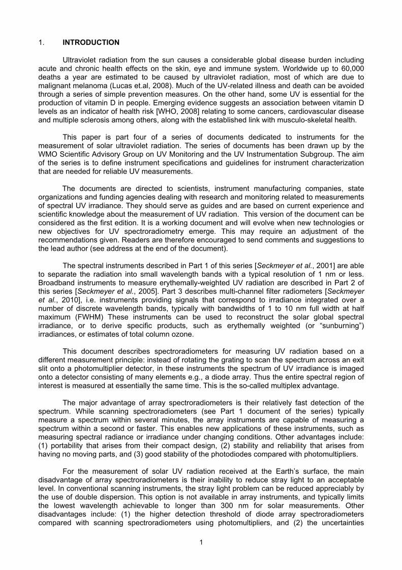
Figure 1 - Typical array spectroradiometer. Usually array spectroradiometers are encapsulated and the optical parts cannot be seen. The cable on the left is an optical fibre for the optical input. The dispersion grating can be recognized on top and

the detector array at the bottom of the monochromator

3

2. OBJECTIVES The required specifications of UV instrumentation discussed in this document depend on the objectives of the measurements. These include: 1. To study the short-term characteristics of spectral global and direct solar irradiance, e.g. in

process studies on the impact of clouds and aerosols on UV irradiance. 2. To study the characteristics of spectral sky radiance as a function of zenith and azimuth

angle, e.g. for process studies on the impact of clouds and aerosols on UV irradiance. 3. To study the characteristics of spectral actinic irradiance (sometimes called spectral

scalar irradiance, or spectral actinic flux), e.g. in process studies on the impact of clouds and aerosols on UV irradiance.

4. To contribute to the development of a spectral UV climatology by long-term monitoring. 5. To understand geographic differences in spectral UV irradiance and radiance. 6. To understand temporal variations of spectrally resolved UV radiation quantities on different

time scales. 7. To provide datasets for the validation of radiative transfer models and/or satellite derived

UV irradiance at the Earth’s surface. 8. To determine real-time UV levels, such as the UV Index (UVI). 9. To determine biologically weighted radiation quantities. These instruments may also be used in applications such as the derivation of trace gas column density, trace gas profiles, aerosol optical properties, and the measurement of reflectance or transmission properties in the field. Some of the objectives (e.g., trend detection) require high accuracy instruments with a superior long-term stability, because the expected magnitude of UV trends is rather small. In some of the cases listed above, currently available array spectroradiometers cannot yet achieve the required performance specifications throughout the UV-B region. To specify the array spectroradiometers the instruments are differentiated according to the following four measurement quantities:

• Global spectral irradiance. • Actinic spectral irradiance. • Direct spectral irradiance. • Spectral radiance. For each type of measurement a set of specifications is given in Section 3.

The definition of the four types is based on the scientific needs imposed by the different research objectives, which in turn are linked with the desired overall uncertainty of the radiation measurements. Therefore, the specifications introduced below are given in terms of instrument performance rather than instrument set-up. Some parameters, like the wavelength accuracy, refer to the accuracy of the final data, which are derived from raw-data by post-processing. Thus, corrections need to be applied, to reduce the uncertainty of the result. These include for example:

• The improvement of wavelength alignment by correlation methods. • Deconvolution algorithms to reduce or standardize the bandwidth. • Cosine error correction methods to improve the accuracy of measured global

irradiance. • Stray light correction, which is especially important for array spectrometers as they are

single monochromators.

4

These array instruments – like the broadband instruments described in Part 2 of the series - are sometimes used to characterise the output of artificial UV sources such as sunbeds. For accurate radiative measurements of artificial sources, proper consideration of stray light issues is mandatory. 3. RECOMMENDED SPECIFICATIONS

Global spectral irradiance

Actinic spectral irradiance

Direct spectral irradiance

Spectral radiance

Field of view 180° 360° < 2° < 5° Angular response

(a) For incidence angles (b) To integrated isotropic radiance (c) Azimuth error

Cosine error < ±5 % for angles <60°

< ±5 % < ±3 %

Deviation < ±10 % for all angles

< ±10 % < ± 3 %

Not applicable Not applicable

Accuracy in positioning the optics

< 0.2° (levelling accuracy)

< 1° (levelling accuracy) < 0.2° < 1°

Maximum irradiance at 400 nm (noon) > 2 W m-2 nm-1 > 4 W m-2 nm-1 > 2 W m-2 nm-1 >1 W m-2 nm-1 sr-1

Detection threshold < 10-3 W m-2 nm-1 < 10-3 W m-2 nm-1

sr-1

Stray light (noon) < 10-3 W m-2 nm-1 < 10-3 W m-2 nm-1

sr-1 Typical spectral range 280 – 400 nm

Bandwidth (FWHM) < 1 nm

Slit function < 10-3 of maximum at 2.5·FWHM away from centre

Sampling wavelength interval < 0.2 FWHM (> 5 pixels/FWHM)

Wavelength precision < ±0.05 nm

Wavelength accuracy < ±0.1 nm

Instrument temperature Monitored and sufficiently stable to maintain overall instrument stability

Frequency of recording spectra > 0.1 Hz

Overall calibration uncertainty < ±10% (unless limited by detection threshold)

Scan date and time Recorded with each spectrum such that timing is known to within 1 s

Nonlinearity < 2 % for signals more than 50 times above detection threshold

3.1 Remarks on specifications Field of view (FOV) The angular response of radiometers to measure global spectral irradiance should vary with the cosine of the incidence angle. The response is therefore non-zero above the horizon, resulting in a field of view of 180°. Radiometers for measuring actinic spectral irradiance should have a field of view of 360° to measure both upwelling and downwelling radiation. It should be noted that the required quantity “actinic spectral irradiance” does not represent the upwelling and downwelling irradiance on horizontal surfaces. When the UV albedo is small (i.e., at most snow-free locations), the upwelling component contributes typically less than 5% to the measurement. For these cases, a field of view of 180° (upper hemisphere) may be sufficient.

5

For direct spectral irradiance — when using a FOV smaller than 2° — more accurate tracking may be required for the derivation of optical properties such as aerosol optical depth, especially at shorter wavelengths [Arola and Koskela, 2004]. For spectral radiance — when using a FOV smaller than 2° — more accurate tracking may be required for trace gas profiling [Frieß et al., 2006; Hönninger et al., 2004; Richter, 2006]. Angular response Global spectral irradiance entrance optics of many spectroradiometers currently in use have a cosine error of about -5% at 60° incidence angle. These instruments underestimate global irradiance. Although appropriate correction procedures may lead to an improvement, uncertainties caused by the cosine error contribute significantly to the overall uncertainty and are comparable to the uncertainties introduced by the irradiance or wavelength calibration. Broken-cloud conditions present a particular challenge. It is therefore preferable to use input optics with cosine errors as small as possible. For actinic spectral irradiance entrance optics that are currently available, angular response errors are typically of the order of 10%. Better entrance optics would be highly desirable because deviations at large incident angles lead to large uncertainties in the measured actinic irradiance. Within this document we assume that for direct spectral irradiance entrance optics with a field of view of < 2° the radiance contribution from the area around the solar disk is negligible. Therefore, the specification of the angular response is noted as “not applicable” for direct spectral irradiance. Similarly, the spectral radiance is assumed to be sufficiently homogeneous within the field of view of 5°. Therefore, the specification is also noted as “not applicable”. However, the input optics should measure radiation within the specified field of view only and the sensitivity outside the FOV should be negligible; thus the input optics need to be manufactured accordingly. Accuracy in positioning the optics For global and actinic irradiance measurements the optics are fixed. But they should be accurately levelled at installation and checked regularly (see also Section 3.6). This can be accomplished, for example, with a spirit level attached to the optics. Incorrect levelling of global irradiance entrance optics can lead to significant uncertainties, especially at large solar zenith angles [Seckmeyer et al., 2005]. Incorrect levelling of actinic irradiance entrance optics should cause significantly smaller uncertainty due to their spherical design [e.g., Wendisch et al., 2001]. The azimuth and elevation angles for each spectral radiance measurement should be recorded. Detection threshold

In chapter 4 a description for determining the detection threshold can be found. The detection threshold shall be determined for the signal to noise ratio SNR = 1 at 1 nm FWHM. For several reasons (e.g., stray light, dynamic range, nonlinearities) the detection threshold of array instruments is higher than those of scanning spectroradiometers. Stray light

Stray light characterization and correction is of particular importance for the array instruments. There are various methods for stray light correction, described in Section 4 with their advantages and limitations. Bandwidth Generally, a smaller bandwidth allows a more accurate wavelength assignment and, in addition, systematic errors in the spectral irradiance or radiance arising from the steep increase of the solar UV-B spectrum at the Earth’s surface become smaller. For an instrument with a triangular

6

slit function of 1 nm FWHM, the contribution from the long wavelength wings of the slit causes the irradiance measured at 300 nm, 60° solar elevation and 320 DU to be increased by about 2%. At shorter wavelengths this becomes more of an issue. On the other hand, a smaller bandwidth reduces the signal and thus leads to a lower signal-to-noise ratio. Therefore, the bandwidth setting of a spectroradiometer is a compromise between accuracy of wavelength assignment, systematic errors arising from the slope of the spectrum and the signal-to-noise ratio. Based on these considerations, it is recommended that the bandwidth is about 1 nm FWHM. But for some specific tasks (e.g., trace gas determination) it should be less. For array instruments the bandwidth usually varies across their operational spectral range. The wavelength assignment may be improved by post processing using deconvolution techniques (e.g., Slaper et.al. 1995). Slit function

Although some instruments might not fulfil this specification, it is usually not the limiting factor for the uncertainty. In general far field stray light is more problematic. Sampling wavelength interval

Oversampling of the spectrum [Hofmann et al., 1995] is required for assuring the accuracy in the wavelength registration, which is based on the determination of the slit function. The sampling wavelength interval is recommended to be significantly smaller than the bandwidth defined by the slit function of the spectroradiometer. The advantages of such ‘oversampling’ are: a) The correlation of measured to referenced spectra is improved. This is particularly

important when trace gas concentrations are derived from measurements of spectral radiance or direct spectral irradiance using the method of differential optical absorption spectroscopy (DOAS) [e.g., Camy-Peyret et al., 1996; Hofmann et al., 1995; Vandaele et al., 2005].

b) Only by oversampling can unknown features in the spectra be unambiguously identified. Such unknowns could include sharp emission features in spectral calibration standards (e.g., tungsten halogen lamps of FEL type), or be the result of atmospheric pollutants. According to the sampling theorem [Brigham, 1974] a sampling interval less than 1/2 the highest frequency of interest is required. In hardware terms, the highest frequency observable is limited by the slit function, which in turn is limited by the resolving power of the spectrometer. For a given instrument, reductions in the slit function’s FWHM are achieved only at the expense of throughput. According to the sampling theorem, the sampling interval for a triangular bandpass should be less than 0.5 FWHM. In practice the sampling interval should be less than 0.2 FWHM because of the problem that it is not possible to determine a slit function for each pixel.

c) The determination of wavelength can be achieved more accurately (e.g., when measuring the signal of a spectral line).

Wavelength precision and accuracy Due to the steep increase of UV-B irradiance towards longer wavelengths, small uncertainties in wavelength assignment of a spectroradiometer lead to pronounced uncertainties in the measured irradiance. For array instruments, the wavelength corresponding to each element of the detector array is essentially fixed and determined by the geometry and characteristics (grating density and array size) of the spectrometer. It is therefore impossible to physically adjust the wavelength, and hence the effort centres on assigning the correct wavelength to each pixel.

Uncertainties in measurements of solar (ir)radiance resulting from wavelength uncertainties depend on wavelength, sun angle and total ozone column. For example, at 300 nm, the irradiance uncertainty arising from a wavelength uncertainty of ±0.1 nm is ±6% for a solar zenith angle of 40° and 320 DU [Bernhard and Seckmeyer, 1999]. Larger solar zenith angles and ozone amounts increase the slope of the solar spectrum and lead to even greater uncertainties. A wavelength accuracy of 0.1 nm ensures that its contribution to the overall uncertainty remains low. Variations in the wavelength assignment (i.e., the wavelength precision), which may for example be caused by changes in instrument temperature, should be smaller than ±0.05 nm.

7

Instrument temperature Many array spectroradiometers show a dependence of several instrument parameters (e.g.,

wavelength accuracy, dark current offset and spectral responsivity) on temperature. The instrument temperature should be sufficiently stable that the thresholds of the specified instrument parameters are not exceeded. Frequency for recording of spectra

For many applications recording as many spectra as possible is desirable. However, the frequency for recording of spectra limits the time available for integration and signal averaging. In turn these limit the signal to noise ratio (SNR) which is connected to the detection threshold. SNR can be improved by applying longer integration times or by averaging spectra. The following simple relationship applies: Maximum data frequency = 1/ (Integration time * number of spectra + processing time)

Many array instruments provide a function for signal averaging. The integration time of array spectroradiometers can usually be chosen between a few milliseconds and several seconds. Nonlinearity

Uncertainties in linearity translate directly into uncertainties of measured quantities. For many array instruments nonlinearity effects are a serious concern. 3.2 Ancillary measurements, data processing and maintenance Ancillary measurements The range of ancillary measurements depends on the data objectives for the measurements, but in general the more supporting data are available, the better. In order to allow a better interpretation of the data, the measurements of spectral radiance or irradiance should therefore be supplemented by ancillary measurements. a) Recommended:

• Independent measurements of global irradiance insensitive to ozone absorption, e.g., measurements of short wave global irradiance with a pyranometer.

b) Desirable:

• Direct normal spectral irradiance or diffuse spectral irradiance. • Total ozone column, e.g., derived from measurements of direct normal spectral

irradiance. • Erythemally weighted irradiance, measured with a broad-band radiometer. • Atmospheric pressure. • Cloud information. • Illuminance, measured with a luxmeter. • Direct irradiance at normal incidence measured with a pyrheliometer. • Aerosol optical properties. • Visibility.

Data Frequency The data frequency depends on the integration time and on the purpose of the measurements. With data frequencies of about 0.1 Hz a huge amount of data is produced. Depending on the purpose of the measurements, longer averaging or integration times (e.g., one minute) for increasing the SNR or for reducing the data storage may be suitable. The specification just refers to the possibility to perform frequent measurements.

8

Data Processing The post-processing of raw-data should comprise the following capabilities:

• Dark current correction. • Stray light corrections including their uncertainty. • Cosine error correction (where applicable). • Wavelength and bandwidth standardization.

Even after data processing it is important to retain the original logged data. Instrument characterization All calibration information and procedures should be clearly documented and archived at the observations site. The following instrument characterizations should be performed regularly; depending on the instrument, these checks may be needed even more frequently than recommended here:

• Daily:

1. Dark current measurements. Depending on instrument performance these measurements may be required more frequently, e.g., for each measurement.

2. Check of the input optics and cleaning if necessary. 3. Checking of sun tracking if applicable.

• Weekly/monthly:

1. Test of the stability of the spectroradiometer’s spectral responsivity. 2. Check of the wavelength alignment by correlation methods and/or by measurements of line spectra (e.g., with a low-pressure mercury lamp). 3. Determination of the spectroradiometer’s bandwidth. 4. Checking of levelling of global irradiance optics.

• Yearly (or as required) 1. Calibration of working standards and reference standards (if necessary). 2. Measurement of the angular response of the spectroradiometer with respect to incidence and azimuth angle. 3. Characterization of linearity and offsets. 4. Stray light tests.

4. GUIDELINES FOR INSTRUMENT CHARACTERIZATION AND DATA CORRECTION

The following guidelines for instrument characterization represent methods that are currently used by the scientific community. They should be understood as suggestions for the user and should not be regarded as hard and fast rules or standard methods. Additionally, it has to be emphasized that there may be many other methods for instrument characterization which may be equally applicable. Measurement of the angular response

The angular response of a spectroradiometer may be measured (1) by rotating a lamp about the input aperture of radiometer or (2) by rotating the input optics relative to a fixed lamp. For both methods, the dependence of the spectroradiometer’s signal is measured with respect to the incidence angle ε and the azimuth angle ϕ . Method (1) is recommended only if it can be assured that the movement of the lamp does not influence its output. Method (2) is recommended only if the turning of the instrument does not influence its sensitivity.

9

Remarks: a) The angular response of the input optics should be reliably characterized in the laboratory

to the extent that the cosine error can also be known with confidence when the instrument is deployed at the measuring site. The measurement system must therefore ensure that repeatable results are obtained when the instrument is removed and replaced, and that the orientation of the receiving surface can be reliably transferred from the laboratory to the measuring site.

b) The measurements should be made: i) At incidence anglesε between 0° and 85° in steps no larger than 5°; ii) At least at two wavelengths covering the spectral range of the instrument and at more

wavelengths if these results indicate that this is necessary; iii) In at least two azimuth planes.

c) Azimuthal dependencies of the entrance optics should be avoided as far as possible because resulting errors are difficult to correct.

d) The equipment for determining the cosine error should be designed such that an uncertainty of less than 0.2° can be maintained for all incidence angles (at 85° incidence angle, an angular uncertainty of ±0.2° gives an uncertainty in angular response of ±4%.)

e) Illumination of the entrance optics must be homogeneous with an almost parallel beam and maintained as such irrespective of the incidence angle

Characterization of the entrance optics

Apart from the angular response, the characterization of the entrance optics should include: a) Tests of weather durability. b) Tests of ageing with respect to transmission and angular response. c) Tests of fluorescence of the diffusing material. d) Tests of the polarization dependence either with respect to angular response or spectral

responsivity. e) Determination of the field of view for radiance and direct irradiance measurements. f) Characterization of attenuation (or other) filters, if applicable.

A more detailed description of the appropriate methods may be found in [Bernhard and Seckmeyer, 1997]. Cosine error correction

Methods for the correction of the cosine error must take into consideration: (1) the deviation of the directional response of the spectroradiometer from the ideal cosine response and (2) the distribution of the radiation field, i.e., the distribution of radiance, when measuring solar radiation. Because the radiation field is generally not known in detail, approximations must be made. The most common approximations and simplifications are:

a) The global spectral irradiance is defined as the sum of direct horizontal spectral irradiance

and diffuse spectral irradiance. For clear-sky conditions, the proportion of both can be either measured directly or calculated by a model. For overcast conditions, the direct spectral irradiance is set to zero. For partly cloudy conditions, the accuracy of cosine error correction methods is generally limited.

b) The directional distribution of sky radiance is regarded as isotropic. This assumption has proved to be approximately valid in the UV-B [Blumthaler et al., 1996]. Methods of cosine error corrections should provide estimates of their uncertainty. Description of implementations and validations of cosine error correction algorithms can be

found in [Bais et al., 1998; Bernhard and Seckmeyer, 1997; Cordero et al., 2008; Feister et al., 1996; Gröbner et al., 1996; Hofzumahaus et al., 2004; McKenzie et al., 1992; Seckmeyer and Bernhard, 1993].

10

Determination of the bandwidth The bandwidth is determined from measurements of spectral lines, e.g., from a low-

pressure mercury lamp or a laser. Remarks: a) Since bandwidth may be wavelength dependent, it should be determined at several

wavelengths covering the entire operational spectral range. b) For the UV range, e.g. a Helium-Cadmium laser operating at 325 nm is suitable. However,

other wavelengths may be needed. The ideal source for such measurements would be a tuneable laser.

Determination of the dark current offset

The dark current is measured by recording the spectroradiometer’s detector signal when no radiation is falling on it. For example, the measurement can take place during the night, or the light may be blocked by a shutter. Some operators determine the dark current by measuring signals at a wavelength below the detection threshold of the array spectroradiometer (e.g., below 250 nm). This is not recommended because the measured signal includes a stray light contribution which varies with wavelength and because dark current varies from pixel to pixel. The dark current depends on the temperature of the instrument. Determination of noise equivalent Radiation

The noise equivalent radiation (NER) is defined as the ratio of the standard deviation σ of the dark current to the responsivity of the instrument [Bernhard and Seckmeyer, 1999]. It depends on the integration time, usually becoming smaller with increasing integration time. For the determination of NER it is necessary to record a sufficient number of dark spectra and to calculate the standard deviation and to repeat this procedure for all integration times used in routine solar measurements. NER is used here as a generalized term valid for global irradiance, direct irradiance, actinic irradiance and radiance expressed in their respective units. Determination of detection threshold

The smallest signal that can be measured with a reasonable certainty is defined as DT )(λ in units of the measured quantity. Within this document we define: )()()( λλλ STRAYDARK YYDT Δ+Δ= (1) where STRAYYΔ is the uncertainty of the stray light correction. The uncertainty in the dark current

correction DARKYΔ includes the statistical noise (NER) and possible drift of the mean dark current (e.g. a drift during the time between a dark signal determination and the actual measurement). A major cause for drifts is the sensitivity of the array spectroradiometer to temperature changes. DT is not a universal instrument feature, but depends on the solar spectrum to be measured and on the chosen instrument settings such as integration time and signal averaging during the determination of DT according to equation (1). It is important to determine DT with exactly the same instrument settings that will be used during the solar measurements.

STRAYYΔ is determined by an uncertainty analysis of the stray light correction method (see stray light section within guidelines), which is a complex task. For array instruments the contributions to DT (equation 1 above) are not statistically independent. Furthermore the interdependencies can be nonlinear. A method on how to treat nonlinear dependencies is described in [Cordero et al., 2007]. It should be noted that such methods are rather complex. Furthermore digitisation effects may contribute to the determination of DT [Häusler et al., 1986]

11

“Slit function” determination and wavelength registration The complete spectral characterization of an array spectroradiometer including the

determination of the wavelength corresponding to each pixel requires the determination of the slit function. In scanning spectroradiometers, this is done by scanning a well defined spectral line at small wavelength steps. The major problem with array instruments arises from the need to approximate the slit function using measurements at a limited number of wavelengths, according to the pixel density of the array. This increases the uncertainty in the determination of the shape of the slit function and the exact pixel corresponding to the wavelength of the spectral line. A nonlinear regression between the pixel numbers corresponding to different spectral lines at known wavelengths, spanning throughout the operational spectral range of the instrument, is used to assign the appropriate wavelength to each pixel of the array. Various approaches have been proposed for different types of instruments [e.g., Chen et al., 2009; Cho et al., 1995; Kiedron et al., 2002b]. The wavelength assignment is an important procedure that should be applied to every instrument, as the wavelength scales provided usually by the manufacturers can result in deviations of several nanometres. Remarks: a) For spectroradiometers situated at Earth’s surface the wavelength scale should be referred

to wavelengths in air at local pressure and temperature. b) It is not recommended to set the centre wavelength at the maximum of the measured line

since its accuracy is limited by the sampling interval and noise. c) Wavelength assignment may be improved by correction algorithms, e.g. [Slaper et al.,

1995]. The specification of wavelength accuracy may therefore refer to the corrected data. However, a correction is appropriate only if the correction method is equally applicable for all the atmospheric conditions of interest. The Fraunhofer structure in a measured spectrum is compared with the same structure in a reference spectrum, e.g., an extraterrestrial spectrum. By shifting the wavelength scale of the measured spectrum the deviation of both spectra from each other are reduced and corrections for the wavelength alignment are calculated. Implementations of this method are described in [Huber et al., 1993; McKenzie et al., 1992; Slaper et al., 1995].

d) It is recommended that a careful wavelength alignment by means of spectral lamps is performed before any correlation (e.g., those mentioned in remark c) above) method is applied.

e) The accuracy of this method depends strongly on the wavelength accuracy of the reference spectrum used. Currently, the following extraterrestrial spectra are recommended for wavelength alignment: SUSIM/ATLAS3 [Brueckner et al., 1993; VanHoosier, 1996], McMath/Pierce (NSF/NOAO) [Kurucz et al., 1984], ETS- Gueymard [Bernhard et al., 2004].

f) Extraterrestrial spectra, which refer to vacuum wavelength (e.g., SUSIM/ATLAS3), have to be shifted to air wavelengths.

Determination of nonlinearity

The linearity in output signal strength may be measured using a variety of methods. A comprehensive summary can be found in [Budde, 1983]. In the following, three main methods are briefly described, namely the ‘inverse square law’, ‘beam addition’, and ‘reference detector’ methods. Furthermore a simple linearity test is presented that takes advantage of the ability of array spectroradiometers to measure over a large range of integration times. 1. The inverse square law method [Budde, 1983]

This method is based on the fact that the irradiance produced by a point source is inversely proportional to the square of the distance r from that point to the aperture. For testing the linearity, the irradiances 1E and 2E produced by the source are measured for two different distances 1r and 2r . For linearity of response it follows that:

12

⎟⎟⎠

⎞⎜⎜⎝

⎛= 2

1

22

2

1

rr

EE

.

Deviations from this relation quantify the nonlinearity. Remarks: a) Since real lamps are not point sources, the minimum distance r must be at least ten

times the dimension of the lamp (including the filament and the envelope). b) For measuring linearity over several orders of magnitude, repetitions of measurements

for a number of source levels may be necessary. c) The expression ( )Yf3 quantifies the correction for nonlinearity to be applied to

measured irradiance

( )EE

YYYf K⋅=

Kread,

read3

where readY is the signal (reading) of the radiometer Kread,Y is the signal (reading) at the calibration level

E is the irradiance corresponding to the signal readY and KE is the irradiance corresponding to the signal Kread,Y d) An additional complication arises from the uncertainty in determination of the reference

plane of the input optics [Bernhard and Seckmeyer, 1997; Gröbner and Blumthaler, 2007].

2. The beam addition method By this method, a beam from the radiation source is split into two paths, path A and path B,

and it is determined whether the combined signal from both light paths (A+B) equals the sum of the signals from the individual light paths: i.e. where I(A+B) = IA + IB. Repetitions of such sets of measurements for a number of source levels permit the evaluation of linearity. An automated linearity tester based on this method is described in [Saunders and Shumaker, 1984].

3. The reference detector method

This method compares the signal of the test device with the signal of a reference detector that has already been characterized for linearity. The method can be implemented by splitting the beam from a radiation source into two paths, for example by using a cubical beam splitter. One of the exit beams is directed onto the test device and the second beam on the reference detector. When changing the intensity of the radiation source (for example by adjusting its power or by using neutral density filters) the signals of the two detectors should change proportionally.

Simple linearity test

A simple linearity test can be used to check whether the system is linear over the full dynamic range. First, measure the output of a quartz halogen lamp for a close separation so that the peak signal is close to the saturation level. Second, measure the output from the same lamp at a large separation, so the minimum signal is close to the detection threshold. In each case the dark signal offsets and the stray light must be carefully removed. Finally, take the ratio of the two measurements. The ratio as a function of wavelength should be flat. Any departures from linearity will manifest themselves as regions of non-zero slope in these ratios. The stability of linearity over several orders of magnitude can readily be achieved by these means.

13

Linearity and integration time Measurements of array spectroradiometers can usually be performed at integration times

ranging between milliseconds and several seconds. By changing the integration time, the dynamical range of the system can be extended beyond the range defined by the digitization scheme. For a linear device, the net-signal should change proportionally with integration time. For example, the net-signal measured at 1000 ms should be 1000 times larger than that measured at 1 ms. Tests should be performed both with monochromatic and polychromatic (e.g., tungsten lamps) radiation sources. Since the detectability of nonlinearity is limited by the stability of the radiation sources, the characterization by a laser is limited. Experiments with several commercial spectrographs suggest that deviations from linearity are typically larger when polychromatic radiation sources are used, and these departures are usually largest at small signal levels.

It has been observed that array spectroradiometers may require a few seconds until the sensitivity stabilizes after switching the integration time. Determination of the spectral responsivity )(λs

Different methods apply for the determination of the spectral responsivity, according to the measured radiation quantity (irradiance, direct irradiance, actinic irradiance and radiance). It is emphasized that stray light correction is necessary for all calibration measurements as well as for solar measurements.

Global spectral irradiance

The signal of a spectroradiometer while measuring a calibration lamp (e.g., a working standard) is recorded and divided by the spectral irradiance from the lamp at the place of the radiometer’s entrance optics, as stated in the lamp’s certificate. Remarks: a) The determination of the spectral responsivity is often denoted as the irradiance calibration

of a spectroradiometer. b) The prescribed conditions for the determination of the spectral responsivity should be

stated in the lamp’s certificate and must be followed closely. These include: i) The distance between lamp and the reference plane of the spectroradiometer’s

entrance optics. This is a critical parameter. For a flat diffuser, the reference plane is usually the front surface of the diffuser. For an integrating sphere, the reference plane normally lies in the entrance aperture of the sphere. For curved diffusers, the determination of the reference plane is more difficult; an appropriate method to determine the plane is given in [Bernhard and Seckmeyer, 1997; Gröbner and Blumthaler, 2007].

ii) The alignment of the lamp and entrance optics. iii) The orientation of the lamp (e.g., horizontal or vertical). iv) The direction of the lamp current. v) The lamp current. This should be monitored by the voltage drop across a precision

resistor (shunt) calibrated by a standard laboratory. Shunts and precision voltmeters to measure the voltage drop should be recalibrated at least every two years.

vi) The voltage drop across the lamp should be monitored. c) The accurate determination of the lamp current is crucial because variations in the lamp

current of 1% result in UV radiant power of up to 10%. d) Since irradiance values stated in calibration certificates of standard lamps are often given in

steps of 5 to 20 nm, values at intermediate wavelengths should be calculated by an appropriate interpolation (e.g., spline or Langrangian interpolation). Linear interpolation may lead to errors exceeding 4%. Additional errors may arise from sharp emission features in lamp spectra (sometimes, such features can even be observed in spectra of tungsten halogen lamps, including FEL calibration lamps).

e) Stray light in the laboratory should be diminished as much as possible, e.g., by appropriate baffles and use of a darkroom.

f) The spectral irradiance is determined by dividing the signal of the spectroradiometer when

14

measuring solar radiation by )(λs . Appropriate corrections (e.g., for nonlinearities and cosine errors) may then have to be applied.

g) When possible, the spectral responsivity should be determined at the place where the measurement of global spectral irradiance is performed. This avoids uncertainties due to changes in )(λs that may result from transportation of the spectroradiometer.

h) the lamp measurement has to be corrected for stray light. Radiance

The spectral radiance is calibrated by measuring the radiation emitted by a calibrated reflectance plate made of optically diffuse material, which is illuminated by a calibrated lamp of spectral irradiance, placed at the distance specified by its certificate. A baffle with an opening is placed between the lamp and the plate to allow illumination only by radiation emitted directly from the lamp and to eliminate stray light from the surroundings. The radiance input optics is positioned in front of the plate e.g. at 45° angle to the diffuser plate at a distance of several centimetres, so that the field of view (FOV) is filled by radiation reflected by the plate (see Figure 2).

Figure 2 - Alignment of diffuser plate (left) with a HeNe Laser for a laboratory calibration of an array instrument measuring spectral radiance

If the distance is too large, the FOV may not be uniformly illuminated by the plate and the calibration procedure may be invalid. With such a setup the diffuser plate presents a uniform radiance source to the radiance optics. The radiance L(λ) is given by:

( )( ) (0 / 45 , ) EL R λλ λπ

= o o

where R(0/45, λ) is the bidirectional reflectance factor of the diffuser plate, and E(λ) is the spectral irradiance of the calibrated lamp at the reference distance interpolated to the designated wavelength λ.

15

Alternatively, a calibrated integrating sphere may be used to produce a uniform radiance field L(λ), which is measured by the spectroradiometer. The sphere is illuminated by a lamp of spectral irradiance mounted at its entrance port, while the radiance entrance optics of the spectroradiometer is positioned at the exit port of the sphere. More details for both methods can be found in [Pissulla et al., 2009].

The remarks for calibration of global spectral irradiance also apply. Spectral direct irradiance

In principle the spectral responsivity for direct irradiance is determined analogously to the responsivity for global irradiance: the signal of a spectroradiometer while measuring a calibration lamp (e.g., a working standard) is recorded and divided by the spectral irradiance which is produced by the lamp at the place of the radiometer’s entrance optics and stated in the lamp’s certificate. It is necessary to ensure that the FOV of the direct optics does not limit the view of the lamp’s bulb. For this it might be necessary to use a larger distance between lamp and entrance optics than indicated in the lamp’s certificate and to correct the irradiance given in the certificate by applying the inverse square law. However, an additional uncertainty arises because the lamp is not an ideal point source. Another option to avoid the problem of limiting FOV could be to remove the limiting baffles of the input optics while measuring the lamp at the nominal distance given in the certificate, ensuring that radiation from other sources is excluded.

Finally it is sometimes possible to determine the spectral responsivity for direct irradiance with the ‘Langley method’ [Liou, 2001]. However, this requires cloud free and very stable conditions (e.g., aerosols and ozone) for several hours of a day, ideally including morning and afternoon. Usually these conditions occur only at high altitude stations.

The remarks for calibration of global spectral irradiance also apply. Spectral actinic irradiance

Actinic irradiance calibration is performed in a similar way as for irradiance. The correct determination of the distance between the reference plane of the input optics and the lamp is important and should be performed with great care [Hofzumahaus et al., 1999]

See also remarks described in section global spectral irradiance Tests of the stability of a spectroradiometer’s spectral responsivity

Tests are performed by regular (e.g., weekly) checks of the spectral responsivity with calibration lamps, i.e., working standards. The measured signal produced by the lamp should be compared with previous measurements of the same lamp. To exclude the possibility that differences of the lamp measurements are attributable to changes of the working standard, the lamp should also be intercompared regularly with other lamps [Webb et al., 1998]. Stability of spectroradiometers can be monitored by measuring working standard lamps mounted in specially designed enclosures which are attached in very repeatable way to the entrance optics. The operating conditions of the lamps should comply with the operational specifications discussed in the previous paragraph. Stray light corrections

Stray light is a serious problem of array spectroradiometers because it limits the detectable irradiance and if not corrected is a large contribution to the overall uncertainty.

16

1

10

100

1000

10000

100000

200 300 400 500 600 700 800 900Wavelength in nm

Dar

k cu

rren

t cor

rect

ed s

igna

l in

coun

ts .

No Filter WG-280

WG-305 WG-320

WG-385 GG-400

Signal from stray light

Figure 3 - An example of stray light determination from a spectrograph using cut-off filters

Figure 3 shows measurement of a FEL 1000-W tungsten-halogen lamp with an array spectroradiometer. To demonstrate the effect of stray light, several cut-off filters were placed between lamp and the radiometer’s input optics. These filters block radiation below a certain wavelength. For example, the GG-400 filter attenuates radiation with wavelengths below 380 nm by more than five orders of magnitude but has a transmission of more than 90% above 420 nm. Measurements with the spectroradiometer should therefore increase by the same amount between 380 and 420 nm. The figure shows that this is not the case: signals below 380 nm are larger than 35 counts, which is only about three orders of magnitude below the maximum signal. The signal below 380 nm is stray light stemming from photons with wavelengths longer than 400 nm. The figure indicates that the stray light level does not have to be constant but may increase or decrease with decreasing wavelength. Because of this spectral dependence, which is present in all array radiometers, it is not sufficient to subtract measurements at short wavelengths (e.g. 200 nm) from the spectrum to correct for stray light. Stray light corrections may be performed by the following methods 1) Using a tuneable laser or a set of spectral lines to determine the stray light in the spectral

range far from the measured line [Zong et al., 2006]. 2) Using a combination of method 1 and use one cut-off filter [Kreuter and Blumthaler, 2009]. 3) Using a deconvolution method. Method 1

According to this method [Zong et al., 2006], several monochromatic light sources are measured and the “stray light distribution function” (SDF) is characterized for different wavelengths. The stray light correction matrix C, based on the SDF matrix D, is derived by

1][ −+= DIC where I is the identity matrix. The instrument’s response for stray light is corrected using the equation:

17

measIB YCY ⋅= where measY is the column vector of measured signals, IBY is a column vector of stray light corrected signals. Method 2

According to this method [Kreuter and Blumthaler, 2009], the spectral line spread function is measured at a single line in the blue/UV wavelength range using a laser source, and the line shape is approximated with an analytical function. The stray light distribution functions (SDF) for each wavelength is inserted in the columns of a square matrix. The inverse of the SDF plus the identity matrix is the desired stray light correction (C in the formulation of method 1). In addition one cut-off filter is used to determine the stray light of the calibration lamp and the ozone cut-off is used for solar measurements. Method 3

Method 3 is a deconvolution method described in [Jansson, 1984; Kiedron et al., 2002a; Kiedron et al., 2002b] Method 1 requires that the SDF is measured over more than 5 orders of magnitude. This is difficult in practice. In addition, the stray light contribution from wavelengths above the upper sensitivity limit of the instrument cannot be determined. The major advantage of method 2 is that the stray light can in principle be determined for any source. Calibration of working standards

Working standards are calibrated against a reference standard. In a first step, the spectral responsivity of a spectroradiometer has to be determined by the methods described above using the reference standard. In a second step, the signal of the spectroradiometer when measuring the working standard is divided by the spectral responsivity to derive the spectral irradiance produced by the working standard. Remarks: a) The stability of the spectroradiometer should be checked by measurement of an additional

standard before and after the calibration of working standards. b) Calibration standards, either reference standards or working standards, should be

recalibrated (or replaced) after 20 hours of use, unless otherwise stated in the lamp’s certificate. A recalibration of reference standards should be performed by standard laboratories.

c) A calibration certificate for each working standard should be prepared including irradiance values and conditions during calibration.

d) The calibration of working standards should be traceable back to national standard laboratories (e.g., NIST, NPL, PTB) in no more than two steps since for each further step the uncertainty of the irradiance scale may escalate.

e) The noise in the spectra of working standards can be reduced by smoothing but great care has to be taken because instrument features or emission lines of the lamps can affect the accuracy of the calibration.

Acknowledgements The authors wish to express special thanks to Liisa Jalkanen (Chief, Atmospheric Environment Research Division, WMO) for her support. We also express our thanks to the members of WMO Scientific Advisory Group (SAG) on UV monitoring for their helpful comments on the contents of this document.

_______

18

GLOSSARY Accuracy The closeness of agreement between test result and the accepted reference value (ISO, 1994). Remarks: a) The test result is a value of the quantity to be measured by carrying out a complete

specified measurement method, once. b) The accepted reference value is a value that serves as an agreed-upon reference for

comparison, and which is derived as (i) a theoretical or established value, based on scientific principles, (ii) an assigned or certified value, based on experimental work of some national or international organization, or (iii) a consensus or certified value, based on collaborative experimental work under the auspices of a recognised scientific or engineering group.

c) Wavelength accuracy of a spectroradiometer is the closeness of agreement between the measured positions of a spectral line and the agreed actual position of the line [e.g., Lide, 1990].

Actinic flux See Spectral Actinic irradiance Actinic irradiance Is the integral over all wavelengths of interest of the spectral actinic irradiance. It has units Wm-2. Aerosol optical depth Quantity expressing the attenuation of the solar beam passing through the Earth’s atmosphere due to Aerosols (see [Iqbal, 1983] for details): m

aaT )(-e)( λτλ =

where )(λaT is the transmittance of the aerosol layer )(λτ a is the aerosol optical depth m is the relative optical air mass at actual pressure Bandwidth Full width at half maximum (FWHM) of a spectroradiometer’s slit function, usually expressed in nm. Cosine error The deviation of the angular response of a radiometer from the ideal cosine response is specified with two parameters in this document. The first of these (a) is defined according to [CIE, 1982] and is expressed by the quantity f2(ε,ϕ):

%1001)cos(),0(

),(),(

reading

reading2 ×⎟

⎟⎠

⎞⎜⎜⎝

⎛−

°==

εϕεϕε

ϕεY

Yf

where ε is the incidence angle of the radiation ϕ is the azimuth angle Yreading (ε,ϕ) is the reading of the radiometer at angles ε and ϕ Yreading (ε = 0°,ϕ) cos(ε) is the ideal response

19

The second specification (b) refers to isotropic radiation and is defined as follows:

%1001)sin()cos(

)sin(),0(/),(),(' 2/

0

2

0

reading

2/

0reading

2

02 ×

⎟⎟⎟⎟⎟

⎠

⎞

⎜⎜⎜⎜⎜

⎝

⎛

−°=

=

∫∫

∫∫ππ

ππ

ϕεεε

ϕεεϕεϕεϕε

dd

ddYYf

The cosine error may be wavelength dependent. In this case these quantities must be considered as spectral quantities. Dark current Signal of a detector or radiometer when no radiation is received by its sensitive area.

Deconvolution Deconvolution is a technique to account for the distortion in a measured spectrum caused by the finite bandwidth of the monochromator. By this technique, spectra with a particular bandwidth can be derived from spectra of the same source measured with a different bandwidth. An implementation of a deconvolution technique suitable for measurements of global spectral irradiance can be found in [Slaper et al., 1995]. Detection threshold The detection threshold DT is the smallest radiation quantity - in this context spectral irradiance, spectral radiance or spectral actinic irradiance - that can be detected by an instrument with a reasonable certainty. Direct spectral irradiance Eλ,D Radiant energy dQ arriving from the disk of the sun per time interval dt, per wavelength interval dλ, and per area dA on a surface normal to the solar beam.

λλ ddAdt

dQE D =,

The angular field of view of an instrument measuring direct normal spectral irradiance must be sufficiently small to reduce uncertainties caused by the circumsolar radiation. Recommendations for view-limiting geometries can be found in [WMO, 1983]. Erythemally weighted irradiance ECIE Global spectral irradiance EG (λ) multiplied with the action spectrum for erythema, C (λ), proposed by CIE [McKinlay and Diffey, 1987], and integrated over wavelength λ:

∫ ⋅=nm400

nm250

)()( λλλ dCEE GCIE

Global spectral irradiance Eλ,G Radiant energy dQ arriving per time interval dt, per wavelength interval dλ, and per area dA on a horizontally oriented surface from all parts of the sky above the horizontal, including the disc of the sun itself:

SDG EEddAdt

dQE ,,, )cos( λλλ ϑλ

+⋅==

where ϑ is the solar zenith angle

20

Luxmeter Instrument measuring illuminance. Illuminance may be calculated from measurements of Irradiance using the following equation:

∫ ⋅=nm780

nm380

)()( λλλ dVEKE Gm

Where E is the illuminance, Km = 683 lm/W is the photometric radiation equivalent illuminance,

)(λGE is the spectral irradiance and )(λV⋅ is the normalized relative responsivity of the human eye for daylight vision. (DIN 5032, Teil 2) Maximum irradiance Maximum spectral irradiance that can be measured with a spectroradiometer without overloading (saturation) of detector or amplifier.

Noise equivalent Radiation (NER) The noise equivalent radiation (NER) is defined as the ratio of the standard deviation σ of the dark current to the responsivity of the instrument [Bernhard and Seckmeyer, 1999]. It depends on the integration time, usually becoming smaller with increasing integration time. Nonlinearity The linearity of a radiometer is the degree to which the output quantity of the radiometer (e.g., a current) is proportional to the input quantity (e.g., global spectral irradiance) [CIE, 1982].

The expression ( )Yf3 quantifies the correction for nonlinearity to be applied to measured irradiance

( )EE

YYYf K⋅=

Kread,

read3

where readY is the reading of the radiometer Kread,Y is the reading at the calibration level

E is the irradiance at the reading readY and KE is the irradiance at the reading Kread,Y

Precision The closeness of agreement between independent test results obtained under stipulated conditions [ISO, 1994]. a) The test result is a value of the quantity to be measured by completely carrying out a

specified measurement method, once. b) Wavelength alignment precision of a spectroradiometer is the closeness of agreement

between the results of several measurements of the position of a spectral line. The measurements have to be performed within a period of time comparable with the time interval between consecutive wavelength calibrations of the spectroradiometer.

Primary standard A standard that is designated or widely acknowledged as having the highest metrological quality. The value of a primary standard is accepted without reference to other standards of the same quantity [DIN, 1984]. For radiation measurements, primary standards are usually blackbodies or synchrotrons.

21

Process studies with respect to global spectral irradiance Studies which investigate the dependence of global spectral irradiance on the parameters by which it is influenced (e.g., total ozone column, aerosols, and albedo). Pyranometer Instrument for the measurement of short-wave irradiance, i.e., the radiant energy in the wavelength range 0.3 μm - 3 μm arriving per time interval dt, and per area dA on a plane surface. If the surface is oriented horizontally, the pyranometer measures short-wave global irradiance. Pyrheliometer Instrument for the measurement of short-wave direct solar irradiance, i.e., the radiant energy in the wavelength range 0.3 μm - 3 μm arriving from the disk of the sun per time interval dt, and per area dA on a plane surface normal to the solar beam. Radiant energy Energy Q of the radiation. Radiant power Φ Radiant energy dQ per time interval dt. Radiance Is the integral over all wavelengths of interest of the spectral radiance. Reference standard A standard, generally having the highest metrological quality available at a given location or in a given organization, from which measurements made are derived [DIN, 1984]. For radiation measurements, lamps which are supplied by national standard laboratories (e.g., NIST, NPL, and PTB) are usually considered as reference standards. Sampling wavelength interval The sampling wavelength interval is defined as the wavelength interval between subsequent measurements of a spectrum. In the context of this document the sampling interval is the deduced wavelength separation of adjacent pixels. Signal-to-Noise ratio (SNR) Ratio between the average readings Y of a radiometer calculated from sufficient single measurements to the standard deviation Yσ of the readings of single measurements. For the determination of the SNR, all conditions (e.g., radiant energy received by the radiometer) have to remain unchanged.

Y

Yσ

=SNR

For the determination of the SNR, all measurements should be recorded in the same manner, i.e., with the same integration time as during the normal operation of the radiometer. Slit function Function which represents the relative spectral transmittance of a spectroradiometer as a function of wavelength for a given setting of wavelength λ0 [CIE, 1984; Kostkowski, 1997]. The slit function should be normalized to 1 at λ0.: The slit function is sometimes denoted slit-scattering function. Spectral Actinic irradiance Spherically integrated spectral radiance at a point in the earth’s atmosphere, originating from the Sun’s direct beam and any scattered components. Often this quantity is called scalar irradiance or actinic flux density. It has units Wm-2nm-1.

22

Ω= ∫ dLF

πλλ

4

Spectral radiance Lλ,

Spectral radiance can be a source or a receiver based quantity. In this document it is usually used as a receiver based source. Here we define it in terms of a receiver based quantity. Lλ, is the radiant energy dQ per time interval dt, per wavelength interval dλ, per area dA, and per solid angle dΩ on a receiver oriented normal to the source.

Ω

=dddAdt

dQLλλ

Spectral responsivity )(λs Ratio of the radiometer output )(λdY by the radiometer input )(λdX at wavelength λ [CIE, 1982]:

)()()(

λλλ

dXdYs =

Remarks: a) For measurement of global spectral irradiance the radiometer input )(λdX is GdE ,λ . b) The spectral responsivity may also be denoted spectral sensitivity. Spectroradiometer Instrument for the spectrally resolved measurement of electromagnetic radiation. Stray light Radiation with wavelengths outside the wavelength range of the slit function that is detected together with radiation inside this range by the detector of a spectroradiometer. Remarks: a) The definition of stray light in this document is adjusted to the needs of solar UV

measurements and is defined as apparent spectral global irradiance, direct irradiance, actinic irradiance or radiance measured at a spectral range where no detectable radiation reaches the Earth’s surface due to ozone absorption. For example, this is the case for wavelengths below 285 nm. Therefore, if measurements of solar irradiance at 285 nm are above the noise level, e.g. 1.10-4 W/(m2 nm), the amount of stray light at 285 nm in the sense of this document is greater than 1.10-4 W/(m2 nm).

b) The amount of stray light detected depends, amongst other factors, on wavelength, bandwidth, spectral response of the detector, spectral transmittance of the monochromator and all auxiliary optics, the spectral distribution from the source [CIE, 1984].

c) The term "out-of-band (OOB) rejection" is sometimes used to address the same issue but its definition is different, although related to, stray light. The term out-of-band rejection is not used in this document.

d) Stray light may be denoted as stray radiation.

23

Short-wave global irradiance EG Radiant energy dQ in the wavelength range 0.3 μm - 3 μm arriving per time interval dt, and per area dA on a horizontally oriented surface from all parts of the sky above the horizontal, including the disc of the sun itself. The short-wave global irradiance is the global spectral irradiance integrated over the wavelength range 0.3 μm - 3 μm. In meteorology, short-wave global irradiance is usually denoted as global radiation. In order to avoid confusion between spectral and broad band quantities the term short-wave global irradiance is used throughout this document. Total ozone column Height of a hypothetical layer which would result if all ozone molecules in a vertical column above the Earth’s surface were brought to standard pressure (1013.25 hPa) and temperature (273.15 K). The total ozone column is usually reported in milli-atmosphere-centimeters (m-atm-cm), commonly called ‘Dobson units’ (DU). The global average ozone amount is close to 300 DU, which corresponds to a layer of thickness 3 mm at STP. One DU - Defines the amount of ozone in a vertical column which, when reduced to standard pressure

and temperature, will occupy a depth of 0.01 mm. - Corresponds to 161069.2 ⋅ molecules/cm2. Uncertainty A parameter, associated with the result of a measurement, that characterizes the dispersion of the values that could reasonably be attributed to the quantity to be measured [DIN, 1984]. The parameter may be, for example, a standard deviation (or a given multiple of it), or the half-width of an interval having a stated level of confidence.

UV index A measure of solar UV radiation at the Earth’s surface which is used for public information. According to [WMO, 1994; 1998], the UV index is calculated considering the following items:

1. Calculation of the erythemally weighted irradiance ECIE (see above) by utilisation of the CIE

action spectrum [McKinlay and Diffey, 1987] normalized to 1.0 at 298 nm. 2. A minimum requirement is to report the daily maximum UV index [WMO, 1998]. 3. The index is expressed by multiplying the weighted irradiance in Wm-2 by 40.0 (this will lead

to an open-ended index which is normally between 0 and 16 at sea level, but with larger values possible at high altitudes).

Remarks: a) The definition of the UV index given above may be revised in future. b) According to the alternative definition given in [ICNIRP, 1995], the UV index is calculated as

the daily maximum erythemally weighted irradiance in Watts per square meter, averaged over a duration of between 10 and 30 minutes and multiplied by 40.

UV-A radiation Electromagnetic radiation between 315 and 400 nm [CIE, 1970]. UV-B radiation Electromagnetic radiation between 280 and 315 nm [CIE, 1970]. Visibility Horizontal distance over which a prominent dark object can be clearly discerned against a contrasting background with the unaided eye [Huschke, 1959]. Remarks: a) The object should be black and either well ahead of the background or on the horizon.

24

b) The visibility may be denoted meteorological range or visual range. Wavelength assignment Assignment of a wavelengths scale to the pixels of a spectroradiometer. This is sometimes also called wavelength calibration. The agreed wavelength scale may be represented by spectral lines of a low-pressure mercury lamp. Working standard A standard that is used routinely to calibrate or check material measures, measuring instruments or reference materials. A working standard is usually calibrated against a reference standard [DIN, 1984]. For radiation measurements in the UV, working standards are usually based on tungsten halogen lamps and these lamps are finally used to calibrate radiometers. Working standards are the last part of the calibration chain which starts with the primary standard.

_______

25

REFERENCES Arola, A., and T. Koskela (2004), On the sources of bias in aerosol optical depth retrieval in the UV

range, Journal of Geophysical Research, 109, D08209, doi:08210.01029/02003JD004375.

Bais, A. F., et al. (1998), Correcting global solar ultraviolet spectra recorded by a Brewer spectroradiometer for its angular response error, Applied Optics, 37(27), 6339-6344.

Bernhard, G., and G. Seckmeyer (1997), New entrance optics for solar spectral UV measurements, Photochemistry and Photobiology, 65(6), 923-930.

Bernhard, G., and G. Seckmeyer (1999), Uncertainty of measurements of spectral solar UV irradiance, Journal of Geophysical Research-Atmospheres, 104(D12), 14321-14345.

Bernhard, G., et al. (2004), Version 2 data of the National Science Foundation's Ultraviolet Radiation Monitoring Network: South Pole, Journal of Geophysical Research-Atmospheres, 109(D21), D21207, doi:21210.21029/22004JD004937.

Blumthaler, M., et al. (1996), Measuring spectral and spatial variations of UVA and UVB sky radiance, Geophysical Research Letters, 23(5), 547-550.

Brigham, E. O. (1974), The Fast Fourier Transform, 252 pp., Prentice-Hall, Inc., Englewood Cliffs, NJ.

Brueckner, G. E., et al. (1993), The Solar Ultraviolet Spectral Irradiance Monitor (SUSIM) Experiment on Board the Upper Atmosphere Research Satellite (UARS), Journal of Geophysical Research - Atmospheres, 98.

Budde, W. (1983), Optical Radiation Measurements: Physical Detectors of Optical Radiation (Optical radiation measurements Volume 4), Academic Press Inc., Orlando, Florida.

Camy-Peyret, C., et al. (1996), Intercomparison of instruments for tropospheric measurements using Differential Optical Absorption Spectroscopy, Journal of Atmospheric Chemistry, 23, 51-80.

Chen, Y., et al. (2009), Wavelength calibration and spectral line bending determination of an imaging spectrometer, in Proceedings of SPIE, edited, Beijing.

Cho, J., et al. (1995), Wavelength Calibration Method for a CCD Detector and Multichannel Fiber-Optic Probes, Applied Spectroscopy, 49, 1841.

CIE (1970), Internationales Wörterbuch der Lichttechnik, Commission International de l’Éclairage, Paris.

CIE (1982), Methods of characterizing the performance of radiometers and photometers, Commission International de l’Éclairage, Paris.

CIE (1984), The spectroradiometric measurement of light sources, Commission International de l’Éclairage, Paris.

Cordero, R. R., et al. (2007), Evaluating the uncertainties of data rendered by computational models, Metrologia, 44(3), L23.

Cordero, R. R., et al. (2008), Uncertainty evaluation of spectral UV irradiance measurements, Measurement Science and Technology, 19(4).

DIN (1984), International vocabulary of basic and general terms in metrology, Beuth Verlag, Berlin.

26

Feister, U., et al. (1996), A method for correction of cosine errors in measurements of spectral UV Irradiance, Solar Energy, 60, 313-332.

Frieß, U., et al. (2006), MAX-DOAS O4 measurements: A new technique to derive information on atmospheric aerosols: 2. Modeling studies, Journal of Geophysical Research - Atmospheres, 111, D14, doi:10.1029/2005JD006618.

Gröbner, J., et al. (1996), Experimental investigation of spectral global irradiance measurement errors due to a non ideal cosine response, Geophysical Research Letters, 23(18), 2493-2496.

Gröbner, J., and M. Blumthaler (2007), Experimental determination of the reference plane of shaped diffusers by solar UV measurements, Optics Letters, 32(1), 80-82.

Häusler, G., et al. (1986), Chaos and cooperation in nonlinear pictorial feedback systems. 1: Experiments, Applied Optics(25), 4656-4663.

Hofmann, D., et al. (1995), Intercomparison of UV/visible spectrometers for measurements of stratospheric NO2 for the Network for the Detection of Stratospheric Change, Journal of Geophysical Research, 100(D8), 16765-16791.

Hofzumahaus, A., et al. (1999), Solar actinic flux spectroradiometry: a technique measuring photolysis frequencies in the atmosphere, Applied Optics, 38(21), 4443-4460.

Hofzumahaus, A., et al. (2004), Photolysis frequency of O3 to O(D1): Measurements and modeling during the International Photolysis Frequency Measurement and Modeling Intercomparison (IPMMI), Journal of Geophysical Research-Atmospheres, 109(D8), D08S90, doi:10.1029/2003JD004333.

Hönninger, G., et al. (2004), Multi axis differential optical absorption spectroscopy (MAX-DOAS), Atmospheric Chemistry and Physics, 4(1), 231.

Huber, M., et al. (1993), A method for determining the wavelength shift for measurements of solar UV-radiation, Proc. Internat. Symposium Tromso, Norway.

Huschke, R. E. (Ed.) (1959), Glossary of meteorology, American Meteorological Society, Boston, Massachusetts.

ICNIRP (1995), Global solar UV index, International Commission on Non-Ionizing Radiation Protection, Bundesamt für Strahlenschutz, Oberschleißheim, Germany.

Iqbal, M. (1983), An introduction to solar radiation, 390 pp., Academic Press, Toronto.

ISO (1994), Accuracy (trueness and precision) of measurement methods and results - Part 1: General principles and definitions, International organization for standardization, ΙSO 5725-1.

Jansson, P. A. (1984), Deconvolution: with applications in spectroscopy, Academic Press, New York, USA.

Kiedron, P. W., et al. (2002a), Specifications and performance of UV rotating shadowband spectroradiometer (UV-RSS), SPIE.

Kiedron, P. W., et al. (2002b), Data and Signal Processing of Rotating Shadowband Spectroradiometer (RSS) Data, in Ultraviolet Ground- and Space-based Measurements, Models, and Effects edited by J. R. Slusser, et al., p. 10, San Diego, Ca, USA.

Kostkowski, H. J. (1997), Reliable spectroradiometry 610 pp., Spectroradiometery Consulting, La Plata, MD.

27

Kreuter, A., and M. Blumthaler (2009), Stray light correction for solar measurements using array spectrometers, Review of Scientific Instruments, 80(9).

Kurucz, R. L., et al. (1984), Solar flux atlas from 296 to 1300 nm, in National Solar Observatory Atlas No. 1, edited, University Publisher, Harvard University, New Mexico, USA.

Lide, D. R. (Ed.) (1990), Handbook of chemistry and physics, CRC Press, Boca Raton, USA.

Liou, K. N. (2001), An Introduction to Atmospheric Radiation (Second Edition), Academic Press, San Diego, Ca, USA.

McKenzie, R. L., et al. (1992), Solar ultraviolet spectroradiometry in New Zealand: Instrumentation and sample results from 1990, Applied Optics, 31, 6501-6509.

McKinlay, A. F., and B. L. Diffey (1987), A Reference Action Spectrum for Ultra-violet Induced Erythema in Human Skin, in Human Exposure to Ultraviolet Radiation: Risks and Regulations, edited by W. F. Passchier and B. F. M. Bosnajakovic, pp. 83-87, Elsevier, Amsterdam.

Pissulla, D., et al. (2009), Comparison of atmospheric spectral radiance measurements from five independently calibrated systems, Photochemical & Photobiological Sciences, 8(4), 516-527.

Richter, A. (2006), Differential optical absorption spectroscopy as a tool to measure pollution from space, Spectroscopy Europe, 18, 14-21.

Saunders, R. D., and J. B. Shumaker (1984), Automated radiometric linearity tester, Applied Optics, 23, 3504 - 3506.

Seckmeyer, G., and G. Bernhard (1993), Cosine error correction of spectral UV-irradiances, paper presented at Atmospheric Radiation, SPIE, Tromsoe, Norway, 30 June - 1 July.

Seckmeyer, G., et al. (2001), Instruments to measure solar ultraviolet irradiance. Part 1: Spectral instruments, World Meteorological Organization, Global Atmosphere Watch, Report No. 125, WMO TD No. 1066, 30 pp, Geneva, Switzerland.

Seckmeyer, G., et al. (2005), Instruments to measure solar ultraviolet irradiance. Part 2: Broadband instruments measuring erythemally weighted solar irradiance, World Meteorological Organization, Global Atmosphere Watch, Report No. 164, WMO TD No. 1289, 54 pp, Geneva.

Seckmeyer, G., et al. (2010), Instruments to measure solar ultraviolet irradiance. Part 3: Multi-channel filter instruments, World Meteorological Organization, Global Atmosphere Watch, Report No. 190, WMO TD No. 1537, 55 pp. Geneva.

Slaper, H., et al. (1995), Comparing ground-level spectrally resolved solar UV measurements using various instruments: a technique resolving effects of wavelength shift and slit width, Geophysical Research Letters, 22(20), 2721-2724.

Vandaele, A. C., et al. (2005), An intercomparison campaign of ground-based UV-visible measurements of NO2, BrO, and OClO slant columns: Methods of analysis and results for NO2, Journal of Geophysical Research - Atmospheres, 110, D8, doi:10.1029/2004JD005423.

VanHoosier, M. E. (1996), Solar ultraviolet spectral irradiance data with increased wavelength and irradiance accuracy, paper presented at Ultraviolet Atmospheric and Space Remote Sensing: Methods and Instrumentation SPIE, Denver, CO, USA, 7 August 1996.

Webb, A. R., et al. (1998), Guidelines for site quality control of UV monitoring, Global Atmosphere Watch, Report No. 126, WMO TD No. 884, 39 pp, Geneva, Switzerland.

28

Wendisch, M., et al. (2001), An airborne spectral albedometer with active horizontal stabilization, Journal of Atmospheric and Oceanic Technology, 18(11), 1856-1866.

WMO (1983), Guide to meteorological instruments and methods of observation (Fifth edition), World Meteorological Organization, Report No. 8, Geneva.

WMO (1994), Report of the WMO meeting of experts on UV-B measurements, data quality and standardization of UV indices, Global Atmosphere Watch, Report No. 95, WMO TD No. 625, World Meteorological Organization, Geneva.

WMO (1998), Report of the WMO-WHO Meeting of Experts on Standardization of UV Indices and their Dissemination to the Public, Global Atmosphere Watch, Report No. 127, WMO TD No. 921, 187 pp, World Meteorological Organization, Geneva.

Zong, Y., et al. (2006), Simple spectral stray light correction method for array spectroradiometers, Applied Optics, 45(6), 1111-1119.

_______

29

ANNEX B

Contact Addresses

Lead author Prof. Dr Gunther Seckmeyer Institute for Meteorology and Climatology University of Hannover Herrenhaeuser Str.2 30419 Hannover Germany Tel: +49 511 762 4022 Fax: +49 511 762 4418 Email: seckmeyer@muk.uni-hannover.de http://www.muk.uni-hannover.de/~seckmeyer World Ultraviolet Radiation Data Centre (WUDC) Meteorological Service of Canada 4905 Dufferin Street North York, Ontario Canada M3H 5T4 Email: woudc@ec.gc.ca WWW access: http://www.msc-smc.ec.gc.ca/woudc World Meteorological Organization Dr Liisa Jalkanen World Meteorological Organization 7 bis, avenue de la Paix Case Postale No. 2300 1211 Genève 2 Switzerland Tel: +41 22 730 8587 Fax: +41 22 730 8049 Email: ljalkanen@wmo.int

31

GLOBAL ATMOSPHERE WATCH REPORT SERIES 1. Final Report of the Expert Meeting on the Operation of Integrated Monitoring Programmes, Geneva, 2 -5 September 1980. 2. Report of the Third Session of the GESAMP Working Group on the Interchange of Pollutants Between the Atmosphere and

the Oceans (INTERPOLL-III), Miami, USA, 27-31 October 1980. 3. Report of the Expert Meeting on the Assessment of the Meteorological Aspects of the First Phase of EMEP, Shinfield Park,

U.K., 30 March - 2 April 1981. 4. Summary Report on the Status of the WMO Background Air Pollution Monitoring Network as at April 1981. 5. Report of the WMO/UNEP/ICSU Meeting on Instruments, Standardization and Measurements Techniques for Atmospheric

CO2, Geneva, 8-11; September 1981. 6. Report of the Meeting of Experts on BAPMoN Station Operation, Geneva, 23–26 November 1981. 7. Fourth Analysis on Reference Precipitation Samples by the Participating World Meteorological Organization Laboratories by

Robert L. Lampe and John C. Puzak, December 1981. 8. Review of the Chemical Composition of Precipitation as Measured by the WMO BAPMoN by Prof. Dr. Hans-Walter Georgii,

February 1982. 9. An Assessment of BAPMoN Data Currently Available on the Concentration of CO2 in the Atmosphere by M.R. Manning,

February 1982. 10. Report of the Meeting of Experts on Meteorological Aspects of Long-range Transport of Pollutants, Toronto, Canada, 30

November - 4 December 1981. 11. Summary Report on the Status of the WMO Background Air Pollution Monitoring Network as at May 1982. 12. Report on the Mount Kenya Baseline Station Feasibility Study edited by Dr. Russell C. Schnell. 13. Report of the Executive Committee Panel of Experts on Environmental Pollution, Fourth Session, Geneva, 27 September - 1

October 1982. 14. Effects of Sulphur Compounds and Other Pollutants on Visibility by Dr. R.F. Pueschel, April 1983. 15. Provisional Daily Atmospheric Carbon Dioxide Concentrations as Measured at BAPMoN Sites for the Year 1981, May 1983. 16. Report of the Expert Meeting on Quality Assurance in BAPMoN, Research Triangle Park, North Carolina, USA, 17-21

January 1983. 17. General Consideration and Examples of Data Evaluation and Quality Assurance Procedures Applicable to BAPMoN

Precipitation Chemistry Observations by Dr. Charles Hakkarinen, July 1983. 18. Summary Report on the Status of the WMO Background Air Pollution Monitoring Network as at May 1983. 19. Forecasting of Air Pollution with Emphasis on Research in the USSR by M.E. Berlyand, August 1983. 20. Extended Abstracts of Papers to be Presented at the WMO Technical Conference on Observation and Measurement of

Atmospheric Contaminants (TECOMAC), Vienna, 17-21 October 1983. 21. Fifth Analysis on Reference Precipitation Samples by the Participating World Meteorological Organization Laboratories by

Robert L. Lampe and William J. Mitchell, November 1983. 22. Report of the Fifth Session of the WMO Executive Council Panel of Experts on Environmental Pollution, Garmisch-

Partenkirchen, Federal Republic of Germany, 30 April - 4 May 1984 (WMO TD No. 10). 23. Provisional Daily Atmospheric Carbon Dioxide Concentrations as Measured at BAPMoN Sites for the Year 1982. November

1984 (WMO TD No. 12).

32

24. Final Report of the Expert Meeting on the Assessment of the Meteorological Aspects of the Second Phase of EMEP, Friedrichshafen, Federal Republic of Germany, 7-10 December 1983. October 1984 (WMO TD No. 11).

25. Summary Report on the Status of the WMO Background Air Pollution Monitoring Network as at May 1984. November 1984

(WMO TD No. 13). 26. Sulphur and Nitrogen in Precipitation: An Attempt to Use BAPMoN and Other Data to Show Regional and Global Distribution

by Dr. C.C. Wallén. April 1986 (WMO TD No. 103). 27. Report on a Study of the Transport of Sahelian Particulate Matter Using Sunphotometer Observations by Dr. Guillaume A.

d'Almeida. July 1985 (WMO TD No. 45). 28. Report of the Meeting of Experts on the Eastern Atlantic and Mediterranean Transport Experiment ("EAMTEX"), Madrid and

Salamanca, Spain, 6-8 November 1984. 29. Recommendations on Sunphotometer Measurements in BAPMoN Based on the Experience of a Dust Transport Study in

Africa by Dr. Guillaume A. d'Almeida. September 1985 (WMO TD No. 67). 30. Report of the Ad-hoc Consultation on Quality Assurance Procedures for Inclusion in the BAPMoN Manual, Geneva, 29-31

May 1985. 31. Implications of Visibility Reduction by Man-Made Aerosols (Annex to No. 14) by R.M. Hoff and L.A. Barrie. October 1985

(WMO TD No. 59). 32. Manual for BAPMoN Station Operators by E. Meszaros and D.M. Whelpdale. October 1985 (WMO TD No. 66). 33. Man and the Composition of the Atmosphere: BAPMoN - An international programme of national needs, responsibility and

benefits by R.F. Pueschel, 1986. 34. Practical Guide for Estimating Atmospheric Pollution Potential by Dr. L.E. Niemeyer. August 1986 (WMO TD No. 134). 35. Provisional Daily Atmospheric CO2 Concentrations as Measured at BAPMoN Sites for the Year 1983. December 1985

(WMO TD No. 77). 36. Global Atmospheric Background Monitoring for Selected Environmental Parameters. BAPMoN Data for 1984. Volume I:

Atmospheric Aerosol Optical Depth. October 1985 (WMO TD No. 96). 37. Air-Sea Interchange of Pollutants by R.A. Duce. September 1986 (WMO TD No. 126). 38. Summary Report on the Status of the WMO Background Air Pollution Monitoring Network as at 31 December 1985.

September 1986 (WMO TD No. 136). 39. Report of the Third WMO Expert Meeting on Atmospheric Carbon Dioxide Measurement Techniques, Lake Arrowhead,

California, USA, 4-8 November 1985. October 1986. 40. Report of the Fourth Session of the CAS Working Group on Atmospheric Chemistry and Air Pollution, Helsinki, Finland, 18-

22 November 1985. January 1987. 41. Global Atmospheric Background Monitoring for Selected Environmental Parameters. BAPMoN Data for 1982, Volume II:

Precipitation chemistry, continuous atmospheric carbon dioxide and suspended particulate matter. June 1986 (WMO TD No. 116).

42. Scripps reference gas calibration system for carbon dioxide-in-air standards: revision of 1985 by C.D. Keeling, P.R.

Guenther and D.J. Moss. September 1986 (WMO TD No. 125). 43. Recent progress in sunphotometry (determination of the aerosol optical depth). November 1986. 44. Report of the Sixth Session of the WMO Executive Council Panel of Experts on Environmental Pollution, Geneva, 5-9 May

1986. March 1987. 45. Proceedings of the International Symposium on Integrated Global Monitoring of the State of the Biosphere (Volumes I-IV),

Tashkent, USSR, 14-19 October 1985. December 1986 (WMO TD No. 151).

33

46. Provisional Daily Atmospheric Carbon Dioxide Concentrations as Measured at BAPMoN Sites for the Year 1984. December 1986 (WMO TD No. 158).

47. Procedures and Methods for Integrated Global Background Monitoring of Environmental Pollution by F.Ya. Rovinsky, USSR

and G.B. Wiersma, USA. August 1987 (WMO TD No. 178). 48. Meeting on the Assessment of the Meteorological Aspects of the Third Phase of EMEP IIASA, Laxenburg, Austria, 30 March

- 2 April 1987. February 1988. 49. Proceedings of the WMO Conference on Air Pollution Modelling and its Application (Volumes I-III), Leningrad, USSR, 19-24

May 1986. November 1987 (WMO TD No. 187). 50. Provisional Daily Atmospheric Carbon Dioxide Concentrations as Measured at BAPMoN Sites for the Year 1985. December

1987 (WMO TD No. 198). 51. Report of the NBS/WMO Expert Meeting on Atmospheric CO2 Measurement Techniques, Gaithersburg, USA, 15-17 June

1987. December 1987. 52. Global Atmospheric Background Monitoring for Selected Environmental Parameters. BAPMoN Data for 1985. Volume I:

Atmospheric Aerosol Optical Depth. September 1987. 53. WMO Meeting of Experts on Strategy for the Monitoring of Suspended Particulate Matter in BAPMoN - Reports and papers

presented at the meeting, Xiamen, China, 13-17 October 1986. October 1988. 54. Global Atmospheric Background Monitoring for Selected Environmental Parameters. BAPMoN Data for 1983, Volume II:

Precipitation chemistry, continuous atmospheric carbon dioxide and suspended particulate matter (WMO TD No. 283). 55. Summary Report on the Status of the WMO Background Air Pollution Monitoring Network as at 31 December 1987 (WMO

TD No. 284). 56. Report of the First Session of the Executive Council Panel of Experts/CAS Working Group on Environmental Pollution and

Atmospheric Chemistry, Hilo, Hawaii, 27-31 March 1988. June 1988. 57. Global Atmospheric Background Monitoring for Selected Environmental Parameters. BAPMoN Data for 1986, Volume I:

Atmospheric Aerosol Optical Depth. July 1988. 58. Provisional Daily Atmospheric Carbon Dioxide Concentrations as measured at BAPMoN sites for the years 1986 and 1987

(WMO TD No. 306). 59. Extended Abstracts of Papers Presented at the Third International Conference on Analysis and Evaluation of Atmospheric

CO2 Data - Present and Past, Hinterzarten, Federal Republic of Germany, 16-20 October 1989 (WMO TD No. 340). 60. Global Atmospheric Background Monitoring for Selected Environmental Parameters. BAPMoN Data for 1984 and 1985,

Volume II: Precipitation chemistry, continuous atmospheric carbon dioxide and suspended particulate matter. 61. Global Atmospheric Background Monitoring for Selected Environmental Parameters. BAPMoN Data for 1987 and 1988,

Volume I: Atmospheric Aerosol Optical Depth. 62. Provisional Daily Atmospheric Carbon Dioxide Concentrations as measured at BAPMoN sites for the year 1988 (WMO TD

No. 355). 63. Report of the Informal Session of the Executive Council Panel of Experts/CAS Working Group on Environmental Pollution

and Atmospheric Chemistry, Sofia, Bulgaria, 26 and 28 October 1989. 64. Report of the consultation to consider desirable locations and observational practices for BAPMoN stations of global

importance, Bermuda Research Station, 27-30 November 1989. 65. Report of the Meeting on the Assessment of the Meteorological Aspects of the Fourth Phase of EMEP, Sofia, Bulgaria, 27

and 31 October 1989. 66. Summary Report on the Status of the WMO Global Atmosphere Watch Stations as at 31 December 1990 (WMO TD No.

419).

34

67. Report of the Meeting of Experts on Modelling of Continental, Hemispheric and Global Range Transport, Transformation and Exchange Processes, Geneva, 5-7 November 1990.

68. Global Atmospheric Background Monitoring for Selected Environmental Parameters. BAPMoN Data For 1989, Volume I:

Atmospheric Aerosol Optical Depth. 69. Provisional Daily Atmospheric Carbon Dioxide Concentrations as measured at Global Atmosphere Watch (GAW)-BAPMoN

sites for the year 1989 (WMO TD No. 400). 70. Report of the Second Session of EC Panel of Experts/CAS Working Group on Environmental Pollution and Atmospheric

Chemistry, Santiago, Chile, 9-15 January 1991 (WMO TD No. 633). 71. Report of the Consultation of Experts to Consider Desirable Observational Practices and Distribution of GAW Regional

Stations, Halkidiki, Greece, 9-13 April 1991 (WMO TD No. 433). 72. Integrated Background Monitoring of Environmental Pollution in Mid-Latitude Eurasia by Yu.A. Izrael and F.Ya. Rovinsky,

USSR (WMO TD No. 434). 73. Report of the Experts Meeting on Global Aerosol Data System (GADS), Hampton, Virginia, 11 to 12 September 1990 (WMO

TD No. 438). 74. Report of the Experts Meeting on Aerosol Physics and Chemistry, Hampton, Virginia, 30 to 31 May 1991 (WMO TD No. 439). 75. Provisional Daily Atmospheric Carbon Dioxide Concentrations as measured at Global Atmosphere Watch (GAW)-BAPMoN

sites for the year 1990 (WMO TD No. 447). 76. The International Global Aerosol Programme (IGAP) Plan: Overview (WMO TD No. 445). 77. Report of the WMO Meeting of Experts on Carbon Dioxide Concentration and Isotopic Measurement Techniques, Lake

Arrowhead, California, 14-19 October 1990. 78. Global Atmospheric Background Monitoring for Selected Environmental Parameters BAPMoN Data for 1990, Volume I:

Atmospheric Aerosol Optical Depth (WMO TD No. 446). 79. Report of the Meeting of Experts to Consider the Aerosol Component of GAW, Boulder, 16 to 19 December 1991 (WMO TD

No. 485). 80. Report of the WMO Meeting of Experts on the Quality Assurance Plan for the GAW, Garmisch-Partenkirchen, Germany, 26-

30 March 1992 (WMO TD No. 513). 81. Report of the Second Meeting of Experts to Assess the Response to and Atmospheric Effects of the Kuwait Oil Fires,

Geneva, Switzerland, 25-29 May 1992 (WMO TD No. 512). 82. Global Atmospheric Background Monitoring for Selected Environmental Parameters BAPMoN Data for 1991, Volume I:

Atmospheric Aerosol Optical Depth (WMO TD No. 518). 83. Report on the Global Precipitation Chemistry Programme of BAPMoN (WMO TD No. 526). 84. Provisional Daily Atmospheric Carbon Dioxide Concentrations as measured at GAW-BAPMoN sites for the year 1991 (WMO

TD No. 543). 85. Chemical Analysis of Precipitation for GAW: Laboratory Analytical Methods and Sample Collection Standards by Dr Jaroslav

Santroch (WMO TD No. 550). 86. The Global Atmosphere Watch Guide, 1993 (WMO TD No. 553). 87. Report of the Third Session of EC Panel/CAS Working Group on Environmental Pollution and Atmospheric Chemistry,

Geneva, 8-11 March 1993 (WMO TD No. 555). 88. Report of the Seventh WMO Meeting of Experts on Carbon Dioxide Concentration and Isotopic Measurement Techniques,

Rome, Italy, 7-10 September 1993, (edited by Graeme I. Pearman and James T. Peterson) (WMO TD No. 669). 89. 4th International Conference on CO2 (Carqueiranne, France, 13-17 September 1993) (WMO TD No. 561).

35

90. Global Atmospheric Background Monitoring for Selected Environmental Parameters GAW Data for 1992, Volume I: Atmospheric Aerosol Optical Depth (WMO TD No. 562).

91. Extended Abstracts of Papers Presented at the WMO Region VI Conference on the Measurement and Modelling of

Atmospheric Composition Changes Including Pollution Transport, Sofia, 4 to 8 October 1993 (WMO TD No. 563). 92. Report of the Second WMO Meeting of Experts on the Quality Assurance/Science Activity Centres of the Global Atmosphere

Watch, Garmisch-Partenkirchen, 7-11 December 1992 (WMO TD No. 580). 93. Report of the Third WMO Meeting of Experts on the Quality Assurance/Science Activity Centres of the Global Atmosphere

Watch, Garmisch-Partenkirchen, 5-9 July 1993 (WMO TD No. 581). 94. Report on the Measurements of Atmospheric Turbidity in BAPMoN (WMO TD No. 603). 95. Report of the WMO Meeting of Experts on UV-B Measurements, Data Quality and Standardization of UV Indices, Les

Diablerets, Switzerland, 25-28 July 1994 (WMO TD No. 625). 96. Global Atmospheric Background Monitoring for Selected Environmental Parameters WMO GAW Data for 1993, Volume I:

Atmospheric Aerosol Optical Depth. 97. Quality Assurance Project Plan (QAPjP) for Continuous Ground Based Ozone Measurements (WMO TD No. 634). 98. Report of the WMO Meeting of Experts on Global Carbon Monoxide Measurements, Boulder, USA, 7-11 February 1994

(WMO TD No. 645). 99. Status of the WMO Global Atmosphere Watch Programme as at 31 December 1993 (WMO TD No. 636). 100. Report of the Workshop on UV-B for the Americas, Buenos Aires, Argentina, 22-26 August 1994. 101. Report of the WMO Workshop on the Measurement of Atmospheric Optical Depth and Turbidity, Silver Spring, USA, 6-10

December 1993, (edited by Bruce Hicks) (WMO TD No. 659). 102. Report of the Workshop on Precipitation Chemistry Laboratory Techniques, Hradec Kralove, Czech Republic, 17-21 October

1994 (WMO TD No. 658). 103. Report of the Meeting of Experts on the WMO World Data Centres, Toronto, Canada, 17 - 18 February 1995, (prepared by

Edward Hare) (WMO TD No. 679). 104. Report of the Fourth WMO Meeting of Experts on the Quality Assurance/Science Activity Centres (QA/SACs) of the Global

Atmosphere Watch, jointly held with the First Meeting of the Coordinating Committees of IGAC-GLONET and IGAC-ACE, Garmisch-Partenkirchen, Germany, 13 to 17 March 1995 (WMO TD No. 689).

105. Report of the Fourth Session of the EC Panel of Experts/CAS Working Group on Environmental Pollution and Atmospheric

Chemistry (Garmisch, Germany, 6-11 March 1995) (WMO TD No. 718). 106. Report of the Global Acid Deposition Assessment (edited by D.M. Whelpdale and M-S. Kaiser) (WMO TD No. 777). 107. Extended Abstracts of Papers Presented at the WMO-IGAC Conference on the Measurement and Assessment of

Atmospheric Composition Change (Beijing, China, 9-14 October 1995) (WMO TD No. 710). 108. Report of the Tenth WMO International Comparison of Dobson Spectrophotometers (Arosa, Switzerland, 24 July - 4 August

1995). 109. Report of an Expert Consultation on 85Kr and 222Rn: Measurements, Effects and Applications (Freiburg, Germany, 28-31

March 1995) (WMO TD No. 733). 110. Report of the WMO-NOAA Expert Meeting on GAW Data Acquisition and Archiving (Asheville, NC, USA, 4-8 November

1995) (WMO TD No. 755). 111. Report of the WMO-BMBF Workshop on VOC Establishment of a “World Calibration/Instrument Intercomparison Facility for

VOC” to Serve the WMO Global Atmosphere Watch (GAW) Programme (Garmisch-Partenkirchen, Germany, 17-21 December 1995) (WMO TD No. 756).

36

112. Report of the WMO/STUK Intercomparison of Erythemally-Weighted Solar UV Radiometers, Spring/Summer 1995, Helsinki, Finland (WMO TD No. 781).

112A. Report of the WMO/STUK ’95 Intercomparison of broadband UV radiometers: a small-scale follow-up study in 1999, Helsinki,

2001, Addendum to GAW Report No. 112. 113. The Strategic Plan of the Global Atmosphere Watch (GAW) (WMO TD No. 802). 114. Report of the Fifth WMO Meeting of Experts on the Quality Assurance/Science Activity Centres (QA/SACs) of the Global

Atmosphere Watch, jointly held with the Second Meeting of the Coordinating Committees of IGAC-GLONET and IGAC-ACEEd, Garmisch-Partenkirchen, Germany, 15-19 July 1996 (WMO TD No. 787).

115. Report of the Meeting of Experts on Atmospheric Urban Pollution and the Role of NMSs (Geneva, 7-11 October 1996) (WMO

TD No. 801). 116. Expert Meeting on Chemistry of Aerosols, Clouds and Atmospheric Precipitation in the Former USSR (Saint Petersburg,

Russian Federation, 13-15 November 1995). 117. Report and Proceedings of the Workshop on the Assessment of EMEP Activities Concerning Heavy Metals and Persistent

Organic Pollutants and their Further Development (Moscow, Russian Federation, 24-26 September 1996) (Volumes I and II) (WMO TD No. 806).

118. Report of the International Workshops on Ozone Observation in Asia and the Pacific Region (IWOAP, IWOAP-II), (IWOAP,

27 February-26 March 1996 and IWOAP-II, 20 August-18 September 1996) (WMO TD No. 827). 119. Report on BoM/NOAA/WMO International Comparison of the Dobson Spectrophotometers (Perth Airport, Perth, Australia, 3-

14 February 1997), (prepared by Robert Evans and James Easson) (WMO TD No. 828). 120. WMO-UMAP Workshop on Broad-Band UV Radiometers (Garmisch-Partenkirchen, Germany, 22 to 23 April 1996) (WMO TD

No. 894). 121. Report of the Eighth WMO Meeting of Experts on Carbon Dioxide Concentration and Isotopic Measurement Techniques

(prepared by Thomas Conway) (Boulder, CO, 6-11 July 1995) (WMO TD No. 821). 122. Report of Passive Samplers for Atmospheric Chemistry Measurements and their Role in GAW (prepared by Greg

Carmichael) (WMO TD No. 829). 123. Report of WMO Meeting of Experts on GAW Regional Network in RA VI, Budapest, Hungary, 5 to 9 May 1997. 124. Fifth Session of the EC Panel of Experts/CAS Working Group on Environmental Pollution and Atmospheric Chemistry,

(Geneva, Switzerland, 7-10 April 1997) (WMO TD No. 898). 125. Instruments to Measure Solar Ultraviolet Radiation, Part 1: Spectral Instruments (lead author G. Seckmeyer) (WMO TD No.

1066), 2001. 126. Guidelines for Site Quality Control of UV Monitoring (lead author A.R. Webb) (WMO TD No. 884), 1998. 127. Report of the WMO-WHO Meeting of Experts on Standardization of UV Indices and their Dissemination to the Public (Les

Diablerets, Switzerland, 21-25 July 1997) (WMO TD No. 921). 128. The Fourth Biennial WMO Consultation on Brewer Ozone and UV Spectrophotometer Operation, Calibration and Data

Reporting, (Rome, Italy, 22-25 September 1996) (WMO TD No. 918). 129. Guidelines for Atmospheric Trace Gas Data Management (Ken Masarie and Pieter Tans), 1998 (WMO TD No. 907). 130. Jülich Ozone Sonde Intercomparison Experiment (JOSIE, 5 February to 8 March 1996), (H.G.J. Smit and D. Kley) (WMO TD

No. 926). 131. WMO Workshop on Regional Transboundary Smoke and Haze in Southeast Asia (Singapore, 2 to 5 June 1998) (Gregory R.

Carmichael). Two volumes. 132. Report of the Ninth WMO Meeting of Experts on Carbon Dioxide Concentration and Related Tracer Measurement Techniques

(Edited by Roger Francey), (Aspendale, Vic., Australia).

37

133. Workshop on Advanced Statistical Methods and their Application to Air Quality Data Sets (Helsinki, 14-18 September 1998) (WMO TD No. 956).

134. Guide on Sampling and Analysis Techniques for Chemical Constituents and Physical Properties in Air and Precipitation as

Applied at Stations of the Global Atmosphere Watch. Carbon Dioxide (WMO TD No. 980). 135. Sixth Session of the EC Panel of Experts/CAS Working Group on Environmental Pollution and Atmospheric Chemistry

(Zurich, Switzerland, 8-11 March 1999) (WMO TD No.1002). 136. WMO/EMEP/UNEP Workshop on Modelling of Atmospheric Transport and Deposition of Persistent Organic Pollutants and

Heavy Metals (Geneva, Switzerland, 16-19 November 1999) (Volumes I and II) (WMO TD No. 1008). 137. Report and Proceedings of the WMO RA II/RA V GAW Workshop on Urban Environment (Beijing, China, 1-4 November

1999) (WMO-TD. 1014) (Prepared by Greg Carmichael). 138. Reports on WMO International Comparisons of Dobson Spectrophotometers, Parts I – Arosa, Switzerland, 19-31 July 1999,

Part II – Buenos Aires, Argentina (29 Nov. – 12 Dec. 1999 and Part III – Pretoria, South Africa (18 March – 10 April 2000) (WMO TD No. 1016).

139. The Fifth Biennial WMO Consultation on Brewer Ozone and UV Spectrophotometer Operation, Calibration and Data

Reporting (Halkidiki, Greece, September 1998)(WMO TD No. 1019). 140. WMO/CEOS Report on a Strategy for Integrating Satellite and Ground-based Observations of Ozone (WMO TD No. 1046). 141. Report of the LAP/COST/WMO Intercomparison of Erythemal Radiometers Thessaloniki, Greece, 13-23 September 1999)

(WMO TD No. 1051). 142. Strategy for the Implementation of the Global Atmosphere Watch Programme (2001-2007), A Contribution to the

Implementation of the Long-Term Plan (WMO TD No.1077). 143. Global Atmosphere Watch Measurements Guide (WMO TD No. 1073). 144. Report of the Seventh Session of the EC Panel of Experts/CAS Working Group on Environmental Pollution and Atmospheric

Chemistry and the GAW 2001 Workshop (Geneva, Switzerland, 2 to 5 April 2001) (WMO TD No. 1104). 145. WMO GAW International Comparisons of Dobson Spectrophotometers at the Meteorological Observatory Hohenpeissenberg,

Germany (21 May – 10 June 2000, MOHp2000-1), 23 July – 5 August 2000, MOHp2000-2), (10 – 23 June 2001, MOHp2001-1) and (8 to 21 July 2001, MOHp2001-2). Prepared by Ulf Köhler (WMO TD No. 1114).

146. Quality Assurance in monitoring solar ultraviolet radiation: the state of the art. (WMO TD No. 1180), 2003. 147. Workshop on GAW in RA VI (Europe), Riga, Latvia, 27-30 May 2002. (WMO TD No. 1206). 148. Report of the Eleventh WMO/IAEA Meeting of Experts on Carbon Dioxide Concentration and Related Tracer Measurement

Techniques (Tokyo, Japan, 25-28 September 2001) (WMO TD No 1138). 149. Comparison of Total Ozone Measurements of Dobson and Brewer Spectrophotometers and Recommended Transfer

Functions (prepared by J. Staehelin, J. Kerr, R. Evans and K. Vanicek) (WMO TD No. 1147). 150. Updated Guidelines for Atmospheric Trace Gas Data Management (Prepared by Ken Maserie and Pieter Tans (WMO TD No.

1149). 151. Report of the First CAS Working Group on Environmental Pollution and Atmospheric Chemistry (Geneva, Switzerland, 18-19

March 2003) (WMO TD No. 1181). 152. Current Activities of the Global Atmosphere Watch Programme (as presented at the 14th World Meteorological Congress, May

2003). (WMO TD No. 1168). 153. WMO/GAW Aerosol Measurement Procedures: Guidelines and Recommendations. (WMO TD No. 1178). 154. WMO/IMEP-15 Trace Elements in Water Laboratory Intercomparison. (WMO TD No. 1195). 155. 1st International Expert Meeting on Sources and Measurements of Natural Radionuclides Applied to Climate and Air Quality

Studies (Gif sur Yvette, France, 3-5 June 2003) (WMO TD No. 1201).

38

156. Addendum for the Period 2005-2007 to the Strategy for the Implementation of the Global Atmosphere Watch Programme (2001-2007), GAW Report No. 142 (WMO TD No. 1209).

157. JOSIE-1998 Performance of EEC Ozone Sondes of SPC-6A and ENSCI-Z Type (Prepared by Herman G.J. Smit and

Wolfgang Straeter) (WMO TD No. 1218). 158. JOSIE-2000 Jülich Ozone Sonde Intercomparison Experiment 2000. The 2000 WMO international intercomparison of

operating procedures for ECC-ozone sondes at the environmental simulation facility at Jülich (Prepared by Herman G.J. Smit and Wolfgang Straeter) (WMO TD No. 1225).

159. IGOS-IGACO Report - September 2004 (WMO TD No. 1235), 68 pp, September 2004. 160. Manual for the GAW Precipitation Chemistry Programme (Guidelines, Data Quality Objectives and Standard Operating

Procedures) (WMO TD No. 1251), 186 pp, November 2004. 161 12th WMO/IAEA Meeting of Experts on Carbon Dioxide Concentration and Related Tracers Measurement Techniques

(Toronto, Canada, 15-18 September 2003), 274 pp, May 2005. 162. WMO/GAW Experts Workshop on a Global Surface-Based Network for Long Term Observations of Column Aerosol Optical

Properties, Davos, Switzerland, 8-10 March 2004 (edited by U. Baltensperger, L. Barrie and C. Wehrli) (WMO TD No. 1287), 153 pp, November 2005.

163. World Meteorological Organization Activities in Support of the Vienna Convention on Protection of the Ozone Layer (WMO

No. 974), 4 pp, September 2005. 164. Instruments to Measure Solar Ultraviolet Radiation: Part 2: Broadband Instruments Measuring Erythemally Weighted Solar

Irradiance (WMO TD No. 1289), 55 pp, July 2008, electronic version 2006. 165. Report of the CAS Working Group on Environmental Pollution and Atmospheric Chemistry and the GAW 2005 Workshop,

14-18 March 2005, Geneva, Switzerland (WMO TD No. 1302), 189 pp, March 2005. 166. Joint WMO-GAW/ACCENT Workshop on The Global Tropospheric Carbon Monoxide Observations System, Quality

Assurance and Applications (EMPA, Dübendorf, Switzerland, 24 – 26 October 2005) (edited by J. Klausen) (WMO TD No. 1335), 36 pp, September 2006.

167. The German Contribution to the WMO Global Atmosphere Watch Programme upon the 225th Anniversary of GAW

Hohenpeissenberg Observatory (edited by L.A. Barrie, W. Fricke and R. Schleyer (WMO TD No. 1336), 124 pp, December 2006.

168. 13th WMO/IAEA Meeting of Experts on Carbon Dioxide Concentration and Related Tracers Measurement Techniques

(Boulder, Colorado, USA, 19-22 September 2005) (edited by J.B. Miller) (WMO TD No. 1359), 40 pp, December 2006. 169. Chemical Data Assimilation for the Observation of the Earth’s Atmosphere – ACCENT/WMO Expert Workshop in support of

IGACO (edited by L.A. Barrie, J.P. Burrows, P. Monks and P. Borrell) (WMO TD No. 1360), 196 pp, December 2006. 170. WMO/GAW Expert Workshop on the Quality and Applications of European GAW Measurements (Tutzing, Germany, 2-5

November 2004) (WMO TD No. 1367). 171. A WMO/GAW Expert Workshop on Global Long-Term Measurements of Volatile Organic Compounds (VOCs) (Geneva,

Switzerland, 30 January – 1 February 2006) (WMO TD No. 1373), 36 pp, February 2007. 172. WMO Global Atmosphere Watch (GAW) Strategic Plan: 2008 – 2015 (WMO TD No. 1384), 108 pp, August 2008. 173. Report of the CAS Joint Scientific Steering Committee on Environmental Pollution and Atmospheric Chemistry (Geneva,

Switzerland, 11-12 April 2007) (WMO TD No.1410), 33 pp, June 2008. 174. World Data Centre for Greenhouse Gases Data Submission and Dissemination Guide (WMO TD No. 1416), 50 pp, January

2008. 175. The Ninth Biennial WMO Consultation on Brewer Ozone and UV Spectrophotometer Operation, Calibration and Data

Reporting (Delft, Netherlands, 31-May – 3 June 2005) (WMO TD No. 1419), 69 pp, March 2008.

39

176. The Tenth Biennial WMO Consultation on Brewer Ozone and UV Spectrophotometer Operation, Calibration and Data Reporting (Northwich, United Kingdom, 4-8 June 2007) (WMO TD No. 1420), 61 pp, March 2008.

177. Joint Report of COST Action 728 and GURME – Overview of Existing Integrated (off-line and on-line) Mesoscale

Meteorological and Chemical Transport Modelling in Europe (ISBN 978-1-905313-56-3) (WMO TD No. 1427), 106 pp, May 2008.

178. Plan for the implementation of the GAW Aerosol Lidar Observation Network GALION, (Hamburg, Germany, 27 - 29 March

2007) (WMO TD No. 1443), 52 pp, November 2008. 179. Intercomparison of Global UV Index from Multiband Radiometers: Harmonization of Global UVI and Spectral Irradiance

(WMO TD No. 1454), 61 pp, March 2009. 180. Towards a Better Knowledge of Umkehr Measurements: A Detailed Study of Data from Thirteen Dobson Intercomparisons

(WMO TD No. 1456), 50 pp, December 2008. 181. Joint Report of COST Action 728 and GURME – Overview of Tools and Methods for Meteorological and Air Pollution

Mesoscale Model Evaluation and User Training (WMO TD No. 1457), 121 pp, November 2008. 182. IGACO-Ozone and UV Radiation Implementation Plan (WMO TD No. 1465), 49 pp, April 2009. 183. Operations Handbook – Ozone Observations with a Dobson Spectrophotometer (WMO TD No. 1469), 91 pp, March 2009. 184. Technical Report of Global Analysis Method for Major Greenhouse Gases by the World Data Center for Greenhouse Gases

(WMO TD No. 1473), 29 pp, June 2009. 185. Guidelines for the Measurement of Methane and Nitrous Oxide and their Quality Assurance (WMO TD No. 1478), 49 pp,

September 2009. 186. 14th WMO/IAEA Meeting of Experts on Carbon Dioxide Concentration and Related Tracers Measurement Techniques

(Helsinki, Finland, 10-13 September 2007) (WMO TD No. 1487), 31 pp, April 2009. 187. Joint Report of COST Action 728 and GURME – Review of the Capabilities of Meteorological and Chemistry-Transport

Models for Describing and Predicting Air Pollution Episodes (ISBN 978-1-905313-77-8) (WMO TD No. 1502), 69 pp, December 2009, electronic version -July 2009.

188. Revision of the World Data Centre for Greenhouse Gases Data Submission and Dissemination Guide (WMO TD No.1507),

55 pp, November 2009. 189. Report of the MACC/GAW Session on the Near-Real-Time Delivery of the GAW Observations of Reactive Gases, Garmisch-

Partenkirchen, Germany, 6-8 October 2009, (WMO TD No. 1527), 31 pp. August 2010. 190. Instruments to Measure Solar Ultraviolet Radiation Part 3: Multi-channel filter instruments (lead author: G. Seckmeyer) (WMO

TD No. 1537). 55 pp. November 2010.