gaussian pulse dynamics in gain media with kerr nonlinearity

1TaeltIobssfwt

anoopgceutrmctvacPg

tt

1776 J. Opt. Soc. Am. B/Vol. 23, No. 9 /September 2006 C. Jirauschek and F. X. Kärtner

Gaussian pulse dynamics in gain media with Kerrnonlinearity

Christian Jirauschek and Franz X. Kärtner

Department of Electrical Engineering and Computer Science and Research Laboratory of Electronics,Massachusetts Institute of Technology, 77 Massachusetts Avenue, Cambridge, Massachusetts 02139

Received January 17, 2006; accepted March 9, 2006; posted April 20, 2006 (Doc. ID 67258)

Using the Kantorovitch method in combination with a Gaussian ansatz, we derive the equations of motion forspatial, temporal, and spatiotemporal optical propagation in a dispersive Kerr medium with a general trans-verse and spectral gain profile. By rewriting the variational equations as differential equations for the tempo-ral and spatial Gaussian q parameters, optical ABCD matrices for self-focusing and self-phase modulation, ageneral transverse gain profile, and nonparabolic spectral gain filtering are obtained. Further effects can easilybe taken into account by adding the corresponding ABCD matrices. Applications include the temporal pulsedynamics in gain fibers and the beam propagation or spatiotemporal pulse evolution in bulk gain media. As anexample, the steady-state spatiotemporal Gaussian pulse dynamics in a Kerr-lens mode-locked laser resonatoris studied. © 2006 Optical Society of America

OCIS codes: 140.3410, 140.4050, 190.3270, 190.5530.

acgfppGtfitKrpr

ttioeAipSt

2Arbt

w

. INTRODUCTIONhe optical propagation in Kerr media with a transversend spectral gain profile is of much interest in many ar-as. For instance, a combination of gain guiding and non-inear self-focusing can play an important role for the spa-ial propagation of a laser beam in high-power laser rods.n nonlinear dispersive gain fibers, e.g., in fiber lasers orptical transmission lines equipped with erbium-doped fi-er amplifiers, the temporal pulse evolution is affected byelf-phase modulation and spectral filtering.1 The coupledpatiotemporal dynamics in the gain medium is relevantor the operation of Kerr-lens mode-locked (KLM) lasers,here the pulse stabilization is governed by a combina-

ion of spatial and temporal effects.2–4

The variational approach has been extensively used forn approximate description of the optical propagation inonlinear media. By describing the optical field in termsf a trial function with free parameters, a set of coupledrdinary differential equations can be extracted from theartial differential equation governing the optical propa-ation. This allows for an analytical analysis or an effi-ient numerical treatment using a standard differentialquation solver. The Rayleigh–Ritz method is a widelysed variational technique for the treatment of conserva-ive systems and has been applied to the spatial, tempo-al, and spatiotemporal optical propagation in Kerredia.5–9 Different approaches have been developed to in-

lude dissipative effects.10–12 Here, we use a generaliza-ion of the Rayleigh–Ritz method known as the Kantoro-itch method.12 This technique has, for example, beenpplied to the nonlinear temporal pulse propagation in-luding parabolic spectral gain filtering1,13 using aereira–Stenflo-type ansatz and to Gaussian beam propa-ation in air.14

In the following, we apply the Kantorovitch method tohe description of the full spatiotemporal optical propaga-ion of Gaussian light bullets in Kerr media, taking into

0740-3224/06/091776-9/$15.00 © 2

ccount an arbitrary gain profile. As temporal effects, weonsider dispersion, self-phase modulation, and spectralain filtering. The spatial effects include diffraction, self-ocusing, and a transverse gain profile. Also, the cases ofurely spatial beam propagation and purely temporalulse evolution are considered. The assumption of aaussian ansatz allows us to relate the equations of mo-

ion to the compact and elegant ABCD matrix formalismor Gaussian beam and pulse propagation.15,16 By rewrit-ng the variational equations as differential equations forhe q parameters, we can extract ABCD matrices for theerr effect, a general transverse gain profile, and nonpa-

abolic spectral gain filtering. Further effects, such as aarabolic refractive index profile, can easily be incorpo-ated by adding the corresponding matrix elements.

The paper is organized as follows. In Section 2, the spa-ial, temporal, and spatiotemporal equations of motion forhe Gaussian parameters are obtained from the general-zed nonlinear Schrödinger equation, which governs theptical propagation in Kerr media. In Section 3, thesequations are reformulated within the framework of theBCD matrix formalism, taking advantage of the Gauss-

an q parameter description. As an example, the Gaussianulse dynamics in a KLM laser resonator is studied inection 4, including a soft gain aperture and spectral fil-ering. The paper is concluded in Section 5.

. VARIATIONAL APPROACHlinearly polarized light pulse, propagating in the z di-

ection through a dispersive Kerr medium with a para-olic transverse and spectral gain profile, is described byhe generalized nonlinear Schrödinger equation

i�zU − D�tr

2 U + B��x2 + �y

2�U + ��U�2U = Q �1�

ith the gain term

006 Optical Society of America

Tltsv=tfHwttdt=ntektbdpmp

iseandsTfufitifo

ttitncp

ATiaopi

wtca

Tpd

wwithpr

wt

a

w

Setdls

C. Jirauschek and F. X. Kärtner Vol. 23, No. 9 /September 2006 /J. Opt. Soc. Am. B 1777

Q = i�g0 − gxx2 − gyy

2 + g��tr

2 �U. �2�

he retarded time is defined as tr= t−z /vg with group ve-ocity vg, and x and y are the transverse coordinates. U ishe slowly varying envelope, normalized such that its ab-olute square gives the intensity of the wave. The trans-erse electrical field component Et is related to U by Et�2Z0 /n0 R�U exp�i�kz−�0t��, where n0 and k=n0k0 are

he refractive index and the wavenumber at the centerrequency �0, and Z0 is the wave resistance in vacuum.ere we use the physics convention, in which a planeave is described by exp�i�kz−�0t��. The engineering no-

ation exp�j��0t−kz�� can easily be obtained by the formalranscription i→−j in all expressions. The parameters forispersion and diffraction are given by D= 1

2k�, where k� ishe second derivative of the wavenumber at �0, and B1/ �2k�. The nonlinearity parameter is �=k0n2I, where2I is the intensity-dependent refractive index, so that theotal refractive index is given by n=n0+n2I�U�2. In gen-ral, the coefficients D, B, �, g0, gx, gy, g�, and thus n0 and�, depend on the position z in the medium. For example,he material parameters change abruptly at the interfaceetween two materials; and in optically pumped gain me-ia, g0, gx, and gy depend on z due to the divergence of theump beam. Although the z argument is suppressed for aore compact notation, all the equations given in this pa-

er are valid for z-dependent coefficients.As a trial function for U, we choose a complex Gauss-

an, which has been widely used for the variational analy-is of optical propagation in Kerr media.5,7–9 Since it is anxact solution of Eq. (1) for �=0, we expect it to be a goodpproximation to the exact solution, at least for moderateonlinearity. It has been shown that for the temporalispersion-managed soliton dynamics, the Gaussian de-cription is applicable over a wide parameter range.17,18

he transverse Gaussian field distribution, which is theundamental mode in linear paraxial resonators, is widelysed as an approximate description for the transverseeld distribution in nonlinear resonators.3,4,19 In addition,he Gaussian trial function can conveniently be character-zed in terms of the complex q parameters, which allowor a compact description of the optical propagation basedn the ABCD matrix formalism.15,16

In the following, the Gaussian equations of motion, ob-ained by the Kantorovitch method, are given for the spa-ial beam propagation and the temporal pulse evolutionn a Kerr medium with a parabolic transverse and spec-ral gain profile, as well as for the full spatiotemporal dy-amics. The derivation of the spatiotemporal equationsan be found in Appendix A; the purely spatial and tem-oral equations are obtained in an analogous manner.

. Equations of Motionhe generalized nonlinear Schrödinger equation, as given

n Eq. (1), describes the spatiotemporal pulse dynamics indispersive Kerr medium, for example, the propagation

f a light bullet in a KLM laser, taking into account aarabolic transverse and spectral gain profile. The Gauss-an test function is given by

U�z,tr,x,y� = U�z�exp− 1

2T2�z�− ib�z��tr

2 − 1

2wx2�z�

− iax�z��x2 − 1

2wy2�z�

− iay�z��y2� , �3�

ith the beam widths wx and wy, the pulse duration T,he spatial chirp parameters ax and ay, and the temporalhirp parameter b. The complex amplitude can be writtens

U�z� = A�z�exp�i��z��. �4�

he derivation of the equations of motion is given in Ap-endix A. The equations for the beam width and the pulseuration are given by

wp� = 4Bapwp − gpwp3, �5a�

T� = − 4DbT + g� 1

T− 4b2T3� , �5b�

here p=x ,y, and the prime denotes a partial derivativeith respect to z. Taking the full spatiotemporal dynam-

cs into account, the intensity-dependent contributions inhe equations for the chirp parameters and the phaseave different prefactors ca,�, as compared with theurely temporal or spatial dynamics. For the chirp pa-ameters, we obtain

ap� = B 1

wp4 − 4ap

2� − ca�A2

wp2 , �6a�

b� = − D 1

T4 − 4b2� − 4g�

b

T2 − ca�A2

T2 , �6b�

ith p=x ,y and ca=�2/8. For the amplitude, the varia-ional principle yields

A� = A g0 −g�

T2 + 2Db − 2Bax − 2Bay� , �7�

nd the phase evolution is described by

�� = 2g�b + D1

T2 − B1

wx2 − B

1

wy2 + c��A2, �8�

ith c�=7�2/16.Setting D=g�=0 in Eqs. (1) and (2) yields the nonlinear

chödinger equation for the purely spatial dynamics. Thisquation describes the cw propagation of a beam with aransverse field distribution U=U�z ,x ,y� in a Kerr me-ium with a transverse gain profile, for example, the non-inear gain medium of an optically pumped solid-state la-er. The Gaussian trial function is given by

U�z,x,y� = U�z�exp− 1

2wx2�z�

− iax�z��x2

− 1

2wy2�z�

− iay�z��y2� , �9�

we(grmb

pEowpbp

wea=m1tf

t�i(rrmltbci

BTgtw

apspTptwmspe

[

w

FoAtbgr

w1

H

S

S

T


ith the complex amplitude defined in Eq. (4). The rel-vant equations of motion here are Eqs. (5a), (6a), (7), and8) with D=g�=0. The nonlinearity coefficients are nowiven by ca=1/4 and c�=3/4, which are the same as de-ived using the method of minimum weighted squareean error,20 but are different from the results obtained

y a Taylor expansion.19

The propagation equations for the purely temporalulse dynamics are obtained by setting B=gx=gy=0 inqs. (1) and (2). This equation describes the propagationf a pulse U=U�z , tr� in a nonlinear dispersive mediumith frequency-dependent loss or gain, like an optical am-lifier. This equation is also referred to as the complex cu-ic Ginzburg–Landau equation. The temporal Gaussianulse shape is described by

U�z,tr� = U�z�exp− 1

2T2�z�− ib�z��tr

2� , �10�

ith the complex amplitude U [see Eq. (4)]. The relevantquations of motion are given here by Eqs. (5b), (6b), (7),nd (8) with B=0, and the nonlinearity coefficients ca�2/4, c�=5�2/8, which are the same as obtained by theethod of minimum weighted square mean error.21 Tablecontains an overview of the suitable Gaussian test func-

ion; the relevant equations of motion; and the coefficientsor the spatiotemporal, spatial, and temporal dynamics.

For �=0, the Gaussian is an exact solution, and thushe variational principle yields the exact result. For �0, the Kerr nonlinearity results in an additional

ntensity-dependent spatial and temporal chirp [see Eqs.6)] and phase shift [see Eq. (8)]. Equations (5)–(8) lookather complicated. However, the physics can be madeather obvious by casting those formulas into mappingatrices for the complex q parameters of Gaussian bul-

ets (see Section 3). In the following, we extend the equa-ions of motion to take into account arbitrary gain profilesy introducing effective parabolic gain coefficients. In thisase, the Gaussian is not an exact solution of Eq. (1) evenf �=0.

. Nonparabolic Gain Profilehe equations of motion for the parabolic gain profileiven in Eq. (2) can be modified to describe a generalransverse and spectral gain dependence g�z ,� ,x ,y�,here � is a relative frequency coordinate, centered

Table 1. Gaussian Test Function; RelevantEquations of Motion; and Coefficients for

Spatiotemporal, Spatial, and Temporal Dynamics

Propagation PulseEquations of

Motion Coefficients

patiotemporal Eq. (3) Eqs. (5)–(8) ca=�2/8,c�=7�2/16

patial Eq. (9) Eqs. (5a), (6a),(7), and (8)

ca=1/4,c�=3/4,D=g�=0

emporal Eq. (10) Eqs. (5b), (6b),(7), and (8)

ca=�2/4,c�=5�2/8,B=gx,y=0

round the carrier frequency �0. The inherent symmetryroperties of the Gaussian ansatz make it particularlyuited for describing the propagation in media with gainrofiles that are symmetric around x=0, y=0, and �=0.hen a second-order Taylor expansion of g results in aarabolic gain profile. However, this parabolic approxima-ion is viable only if the transverse and spectral pulseidth are narrow as compared to the gain profile. In laseredia, where a large spatial overlap with the gain is de-

ired, this assumption generally fails. Also, the spectralulse width can significantly exceed the gain bandwidth,specially for few-cycle laser pulses.

The gain term of the nonlinear Schrödinger equationEq. (1)] is given here by

Q = iFt−1�gFt�U��, �11�

ith the definition of the Fourier transform

Ft�U� = U =�−�

�

dtrU exp�i�tr�. �12�

or general gain profiles, the Gaussian test function isnly an approximate solution even for �=0. In Appendix, the Kantorovitch method is used to extract the equa-

ions of motion for a general gain profile, which can berought into the form of Eqs. (5)–(8) by defining g�,x,y and0 as functions of the position-dependent Gaussian pa-ameters:

g� =1

2�

1

�4E�−�

� �−�

� �−�

�

��2 − 2�2�g�U�2d�dxdy,

�13a�

gx =1

2�

1

wx4E�−�

� �−�

� �−�

�

�wx2 − 2x2�g�U�2d�dxdy,

�13b�

gy =1

2�

1

wy4E�−�

� �−�

� �−�

�

�wy2 − 2y2�g�U�2d�dxdy,

�13c�

g0 =1

2�

1

E�−�

� �−�

� �−�

�

g�U�2d�dxdy +gx

2wx

2 +gy

2wy

2

+gw

2�2, �13d�

ith the pulse energy E=�3/2A2Twxwy and the spectral/e width defined as

� =� 1

T2 + 4b2T2. �14�

ere, �U�2 is given by

Eptt(u

w

F[g

w

wgb

W

E

a

E

tftt

3IffmcwetrihtttKrw

w

C

w

Hvsh


�U�2 = A22�T

�exp�− x2/wx

2 − y2/wy2 − �2/�2�. �15�

quations (13) provide a position-dependent effectivearabolic profile, which depends on g as well as the spec-ral and transverse pulse widths. If we are interested inhe purely spatial propagation of a Gaussian beam [Eq.9)] in a medium with a gain profile g�z ,x ,y�, we have tose the effective parabolic gain parameters

gx =1

wx4P�−�

� �−�

�

�wx2 − 2x2�g�U�2dxdy, �16a�

gy =1

wy4P�−�

� �−�

�

�wy2 − 2y2�g�U�2dxdy, �16b�

g0 =1

P�−�

� �−�

�

g�U�2dxdy +gx

2wx

2 +gy

2wy

2, �16c�

ith the power P=�A2wxwy and

�U�2 = A2 exp�− x2/wx2 − y2/wy

2�. �17�

or the purely temporal dynamics of a Gaussian pulseEq. (10)], the effective parabolic gain parameters for aain profile g�z ,�� are given by

g� =1

2�

1

�4F�−�

�

��2 − 2�2�g�U�2d�, �18a�

g0 =1

2�

1

F�−�

�

g�U�2d� +g�

2�2, �18b�

ith the fluence F=�1/2A2T and

�U�2 = A22�T

�exp�− �2/�2�. �19�

As an example, let us consider a Gaussian gain profile

g = g exp�− �x−2x2 − �y

−2y2 − ��−2�2�, �20�

ith the transverse 1/e gain widths �x and �y and the 1/eain bandwidth ��. The equations for the effective para-olic gain profile [Eqs. (13)] evaluate to

g� = g��−2��

−2�2 + 1�−3/2��x−2wx

2 + 1�−1/2��y−2wy

2 + 1�−1/2,

gx = g�x−2��

−2�2 + 1�−1/2��x−2wx

2 + 1�−3/2��y−2wy

2 + 1�−1/2,

gy = g�y−2��

−2�2 + 1�−1/2��x−2wx

2 + 1�−1/2��y−2wy

2 + 1�−3/2,

g0 =1

6�g��5�2 + 2��

2� + gx�5wx2 + 2�x

2� + gy�5wy2 + 2�y

2��.

�21�

ith the transverse gain profile

g = g exp�− �x−2x2 − �y

−2y2�, �22�

qs. (16) for the spatial beam propagation give

gx = g�x−2��x

−2wx2 + 1�−3/2��y

−2wy2 + 1�−1/2,

gy = g�y−2��x

−2wx2 + 1�−1/2��y

−2wy2 + 1�−3/2,

g0 = gx�wx2 + �x

2/2� + gy�wy2 + �y

2/2�; �23�

nd with the spectral gain profile

g = g exp�− ��−2�2�, �24�

qs. (18) for the temporal pulse propagation become

g� = g��−2��

−2�2 + 1�−3/2,

g0 = g� 3

2�2 + ��

2� . �25�

The implementation of a general gain profile opens uphe possibility of including a broad range of saturation ef-ects. For example, the equations of motion can be coupledo a differential equation for the gain profile g, describinghe evolution of g in dependence on the pulse parameters.

. DESCRIPTION BY OPTICAL MATRICESt is convenient to recast the equations of motion in aorm consistent with the familiar q parameter analysisor Gaussian optical propagation, where the optical ele-ents are described by matrices.15,16,22 This notation is

ompact and practical, since it allows for a straightfor-ard treatment of the successive propagation through lin-ar optical elements and nonlinear Kerr media. Addi-ional effects in the Kerr medium, such as a parabolicefractive index profile, can be easily incorporated by add-ng the corresponding matrix elements. On the otherand, by rewriting the variational equations as differen-ial equations for the q parameters, ABCD matrices forhe Kerr effect and a nonparabolic gain profile can be ex-racted. We note that the matrices for the spatiotemporalerr effect obtained here are different from the ones de-

ived previously based on a Taylor expansion approach,hich significantly overestimates the nonlinearity.23

Using the complex q parameters qx, qy, and qt, we canrite the spatiotemporal Gaussian ansatz as

U�z,tr,x,y� = U�z�exp ik0x2

2qx�z�+

ik0y2

2qy�z�−

i�0tr2

2qt�z�� .

�26�

omparison with Eq. (3) yields

qp−1 =

1

k0 i

wp2 + 2ap� , �27�

ith p=x ,y, and

qt−1 = −

1

�0 i

T2 + 2b� . �28�

ere, qx and qy are the reduced q parameters,15 with theacuum wavenumber k0 in the exponent of Eq. (26), in-tead of the wavenumber in the medium. This definitionas the advantage that a z-dependent refractive index

dttwcs

p

ap

Ifc

w

tm

dfiw

wno

Tb(G=

BfEtfe=(pditoTtaf

ftbcvA

4Adteprstaetr

ps

K

tggt


oes not lead to additional terms in the equations of mo-ion for the q parameter formalism. Likewise, qt is theemporal analog to the spatial reduced q parameters,16

ith �0 in the exponent, instead of the dispersion coeffi-ient. Here, the dispersion is allowed to depend on the po-ition z, without modifications of the equations.

With the q parameters, the Gaussian beam profile forurely spatial propagation [Eq. (9)] can be written as

U = U exp ik0x2

2qx+

ik0y2

2qy� , �29�

nd the temporal Gaussian pulse for describing theurely temporal dynamics [Eq. (10)] becomes

U = U exp −i�0tr

2

2qt� . �30�

n Appendix B it is shown that the propagation equationsor the q parameters and the amplitude can be written asoupled differential equations

�zqs = − qs2Cs� + Bs�, �31�

ith s=x ,y , t, and

�zU = U −Bt�

2qt−

Bx�

2qx−

By�

2qy+ �� . �32�

The coefficients Bs� and Cs�, which in general depend onhe position z, can be interpreted as elements in an ABCDatrix of the form

Ms = 1 Bs��z

Cs��z 1 � , �33�

escribing the propagation in the medium through an in-nitely small section with length �z. In a gain mediumith Kerr nonlinearity, they are given by

Bp� = 2Bk0 =1

n0,

Bt� = 2D�0 + 2i�0g�,

Cp� =2igp

k0−

2ca�

k0wp2 �U�2,

Ct� =2ca�

�0T2 �U�2, �34�

ith p=x ,y, wp= �k0I�qp−1��−1/2, T= �−�0I�qt

−1��−1/2, and theonlinearity coefficients listed in Table 1. For the complexn-axis transmission coefficient, we obtain

� = g0 + ic��U�2. �35�

he purely spatial propagation equations for a Gaussianeam [Eq. (29)] are given by Eq. (31) with s=x ,y and Eq.32) with Bt�=0. The evolution of a purely temporalaussian pulse [Eq. (30)] is described by Eq. (31) with st and Eq. (32) with B�=B�=0.
x y
The coefficients are composed of various contributions

s�=�iBs,i� , Cs�=�iCs,i� , where the index i represents the dif-erent physical mechanisms affecting the propagation.ach of these effects itself can be described by a matrix of

he form of Eq. (33). We identify the matrix elements forree-space propagation (Bp,1=n0

−1�z and Cp,1=0), soft ap-rturing (Bp,2=0 and Cp,2=2igpk0

−1�z), dispersion (Bt,12D�0�z and Ct,1=0), and spectral parabolic filtering

Bt,2=2i�0g��z and Ct,2=0).15,16,24 The Kerr effect is incor-orated as an intensity-dependent lens20 in the spatialomain, describing the self-focusing action, and anntensity-dependent chirper or temporal lens25 in theime domain for the self-phase modulation. An overviewf the matrix elements for the different effects is given inable 2. Note that a general gain profile deviating fromhe parabolic approximation can be incorporated by usingbove gain matrix elements together with the equationsor gp, g�, and g0 given in Subsection 2.B.

Additional effects can easily be incorporated by addingurther matrix elements. For instance, a parabolic refrac-ive index profile n�r�=n0− �n2,xx2+n2,yy2� /2, as generatedy thermal lensing in a laser rod, can be taken into ac-ount by the elements Bp�=0, Cp�=−n2,p. Also, transverselyarying saturable gain can be treated by additionalBCD matrices.26

. EXAMPLEn important application of the Gaussian approximationescribed above is the simulation of the optical propaga-ion in laser resonators. Examples are the temporal pulsevolution in mode-locked fiber lasers, the laser beamropagation in high-power laser rods, or the spatiotempo-al pulse dynamics in KLM lasers. Here, the steady-stateolutions cannot be obtained directly from the optical ma-rices, since the matrix elements for the Kerr nonlinearitynd the general gain profile depend on the pulse param-ters. Rather, the steady state must be found by itera-ively solving the equations, i.e., propagation over manyound trips until the steady state is reached.

As an example, we choose here the spatiotemporalulse propagation in a KLM laser resonator. The setup,hown in Fig. 1, consists of a nonlinear Kerr medium and

Table 2. Optical Matrix Elements forSpatiotemporal Gaussian Pulse Propagation

through Kerr Media with a Spatialand Spectral Gain Profilea

Effect Bp� Cp� Bt� Ct� �

Free space n0−1 0 0

Dispersion 2D�0 0 0Parabolic

gain0 2igpk0

−1 2ig��0 0 g0

err effect 0 −ca2�

k0wp2 �U�2 0 ca

2�

�0T2 �U�2 ic��U�2

aBt�=Ct�=0 for purely spatial beam propagation; likewise, Bp�=Cp�=0 for purelyemporal pulse propagation. The Kerr parameters ca and c� are listed in Table 1. Aeneral nonparabolic gain profile can be taken into account by using the g�, gp, and

0 given in Eqs. �13�, �16�, and �18� for spatiotemporal, purely spatial, and purelyemporal propagation, respectively.

lael−T====

acGa(mmps

mrirtaoo

mgbvcptaetttcw

oecpetfcs

wpftfiSv

5Wrscrgewgain

sqt

Fr

Ffr(Gss�r


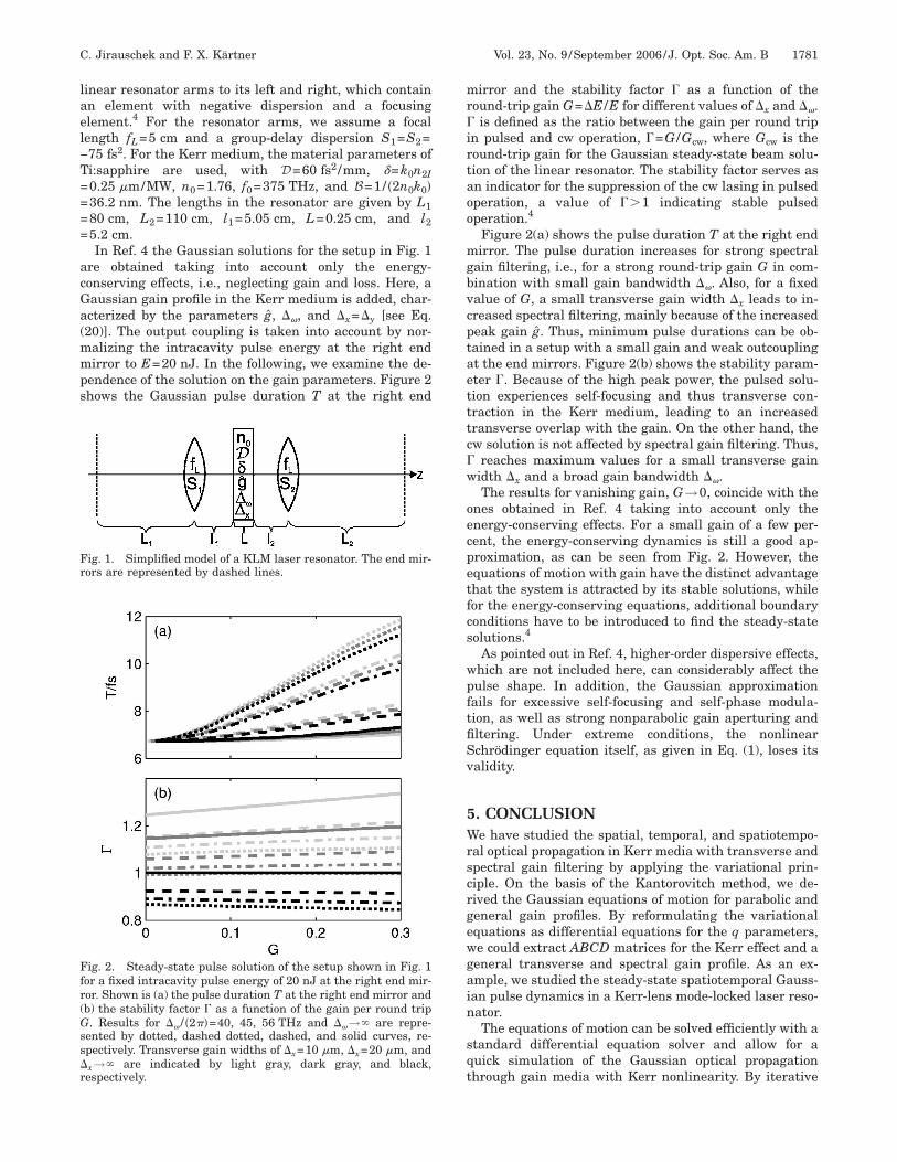
inear resonator arms to its left and right, which containn element with negative dispersion and a focusinglement.4 For the resonator arms, we assume a focalength fL=5 cm and a group-delay dispersion S1=S2=75 fs2. For the Kerr medium, the material parameters ofi:sapphire are used, with D=60 fs2/mm, �=k0n2I0.25 m/MW, n0=1.76, f0=375 THz, and B=1/ �2n0k0�36.2 nm. The lengths in the resonator are given by L180 cm, L2=110 cm, l1=5.05 cm, L=0.25 cm, and l25.2 cm.In Ref. 4 the Gaussian solutions for the setup in Fig. 1

re obtained taking into account only the energy-onserving effects, i.e., neglecting gain and loss. Here, aaussian gain profile in the Kerr medium is added, char-cterized by the parameters g, ��, and �x=�y [see Eq.20)]. The output coupling is taken into account by nor-alizing the intracavity pulse energy at the right endirror to E=20 nJ. In the following, we examine the de-

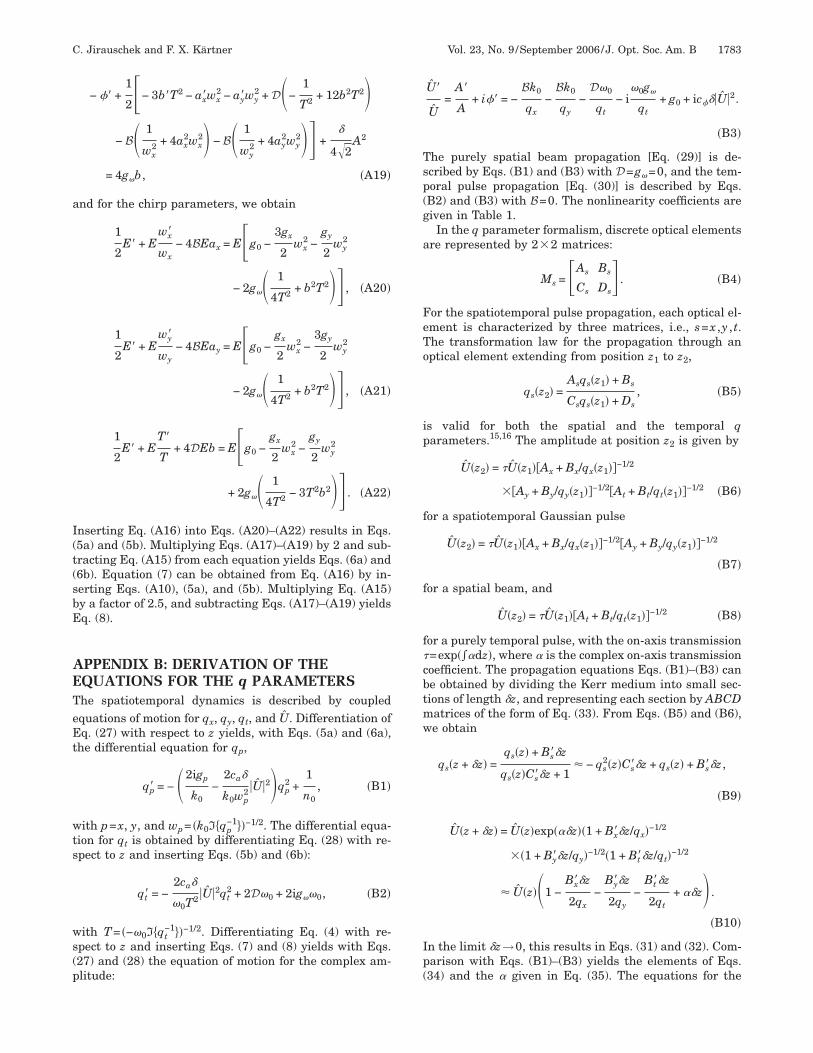
endence of the solution on the gain parameters. Figure 2hows the Gaussian pulse duration T at the right end

ig. 1. Simplified model of a KLM laser resonator. The end mir-ors are represented by dashed lines.

ig. 2. Steady-state pulse solution of the setup shown in Fig. 1or a fixed intracavity pulse energy of 20 nJ at the right end mir-or. Shown is (a) the pulse duration T at the right end mirror andb) the stability factor as a function of the gain per round trip. Results for �� / �2��=40, 45, 56 THz and ��→� are repre-

ented by dotted, dashed dotted, dashed, and solid curves, re-pectively. Transverse gain widths of �x=10 m, �x=20 m, andx→� are indicated by light gray, dark gray, and black,espectively.

irror and the stability factor as a function of theound-trip gain G=�E /E for different values of �x and ��.is defined as the ratio between the gain per round trip

n pulsed and cw operation, =G /Gcw, where Gcw is theound-trip gain for the Gaussian steady-state beam solu-ion of the linear resonator. The stability factor serves asn indicator for the suppression of the cw lasing in pulsedperation, a value of �1 indicating stable pulsedperation.4

Figure 2(a) shows the pulse duration T at the right endirror. The pulse duration increases for strong spectral

ain filtering, i.e., for a strong round-trip gain G in com-ination with small gain bandwidth ��. Also, for a fixedalue of G, a small transverse gain width �x leads to in-reased spectral filtering, mainly because of the increasedeak gain g. Thus, minimum pulse durations can be ob-ained in a setup with a small gain and weak outcouplingt the end mirrors. Figure 2(b) shows the stability param-ter . Because of the high peak power, the pulsed solu-ion experiences self-focusing and thus transverse con-raction in the Kerr medium, leading to an increasedransverse overlap with the gain. On the other hand, thew solution is not affected by spectral gain filtering. Thus,

reaches maximum values for a small transverse gainidth �x and a broad gain bandwidth ��.The results for vanishing gain, G→0, coincide with the

nes obtained in Ref. 4 taking into account only thenergy-conserving effects. For a small gain of a few per-ent, the energy-conserving dynamics is still a good ap-roximation, as can be seen from Fig. 2. However, thequations of motion with gain have the distinct advantagehat the system is attracted by its stable solutions, whileor the energy-conserving equations, additional boundaryonditions have to be introduced to find the steady-stateolutions.4

As pointed out in Ref. 4, higher-order dispersive effects,hich are not included here, can considerably affect theulse shape. In addition, the Gaussian approximationails for excessive self-focusing and self-phase modula-ion, as well as strong nonparabolic gain aperturing andltering. Under extreme conditions, the nonlinearchrödinger equation itself, as given in Eq. (1), loses itsalidity.

. CONCLUSIONe have studied the spatial, temporal, and spatiotempo-

al optical propagation in Kerr media with transverse andpectral gain filtering by applying the variational prin-iple. On the basis of the Kantorovitch method, we de-ived the Gaussian equations of motion for parabolic andeneral gain profiles. By reformulating the variationalquations as differential equations for the q parameters,e could extract ABCD matrices for the Kerr effect and aeneral transverse and spectral gain profile. As an ex-mple, we studied the steady-state spatiotemporal Gauss-an pulse dynamics in a Kerr-lens mode-locked laser reso-ator.The equations of motion can be solved efficiently with a

tandard differential equation solver and allow for auick simulation of the Gaussian optical propagationhrough gain media with Kerr nonlinearity. By iterative

sbeesct

AVImug

wpeEt

w

a

UaE

Sfo

ae

Fg

TtpI(

a

Tt


olution of these equations, the steady-state pulse oream shape in a laser resonator can be obtained. Furtherffects, such as a parabolic refractive index profile as gen-rated by thermal lensing in a laser rod, can easily be con-idered by additional ABCD matrices. Gain saturationan be taken into account by complementing the equa-ions of motion with suitable gain saturation equations.

PPENDIX A: DERIVATION OF THEARIATIONAL EQUATIONS

n this appendix, we derive from Eq. (1) the equations ofotion for the spatiotemporal Gaussian pulse parameterssing the Kantorovitch method.12 The conservative La-rangian is given by9

L =i

2 U*�U

�z− U

�U*

�z � + D� �U

�tr�2

− B� �U

�x �2

− B� �U

�y �2

+�

2�U�4, �A1�

hile the nonconservative process is described by the ex-ression Q, given in Eqs. (2) and (11), respectively. For thenvelope U, we insert the test function Eq. (3). Theuler–Lagrange equations for the real parameter func-

ions f=A ,� ,T ,wx ,wy ,b ,ax ,ay are then given by12

��L�

�f−

d

dz

��L�

�f�= Rf, �A2�

ith the reduced Lagrangian

�L� =�−�

� �−�

� �−�

�

Ldtrdxdy �A3�

nd the nonconservative term

Rf = 2R�−�

� �−�

� �−�

�

Q�U*

�fdtrdxdy� . �A4�

sing the definition of the Fourier transform in Eq. (12)nd Parseval’s theorem, with Ft�Q�=igU, we can expressq. (A4) as

Rf =1

�Ri�

−�

� �−�

� �−�

�

gU�U*

�fd�dxdy� . �A5�

ince g is real, we have RA=Rwx=Rwy

=0. Furthermore,or a parabolic gain profile with the gain term Eq. (2), webtain

R� = E�2g0 − gxwx2 − gywy

2 − g��2�, �A6�

RT = 4g�EbT−1, �A7�

Rb =1

2ET2�2g0 − gxwx

2 − gywy2 + g��T−2 − 12T2b2��,

�A8�

Rax=

1

2Ewx

2�2g0 − 3gxwx2 − gywy

2 − g��2�, �A9�

nd a corresponding expression for Ray, where the pulse

nergy is given by

E = �3/2A2Twxwy. �A10�

rom Eqs. (A6)–(A9), we can extract equations for g�, gx,y, and g0:

g� = RTT/�4Eb�, �A11�

gx = �R�wx2/2 − Rax

�/�Ewx4�, �A12�

gy = �R�wy2/2 − Ray

�/�Ewy4�, �A13�

g0 = �R�/E + gxwx2 + gywy

2 + g��2�/2. �A14�

his enables us to express any gain profile formallyhrough effective parabolic gain parameters, which de-end on both the gain function and the pulse parameters.nserting Eq. (A5) into Eqs. (A11)–(A14), we arrive at Eqs.13).

Setting f=A in Eq. (A2) yields

− 2�� − �b�T2 + ax�wx2 + ay�wy

2� + D 1

T2 + 4b2T2�− B 1

wx2 + 4ax

2wx2� − B 1

wy2 + 4ay

2wy2� + �

A2

�2= 0,

�A15�

nd for f=�, we get

E� = E2g0 − gxwx2 − gywy

2 − g� 1

T2 + 4b2T2�� .

�A16�

he Euler–Lagrange equations for the pulse duration andhe beam widths are given by

− �� +1

2− b�T2 − 3ax�wx2 − ay�wy

2 + D 1

T2 + 4b2T2�− B −

1

wx2 + 12ax

2wx2� − B 1

wy2 + 4ay

2wy2�� +

�

4�2A2 = 0,

�A17�

− �� +1

2− b�T2 − ax�wx2 − 3ay�wy

2 + D 1

T2 + 4b2T2�− B 1

wx2 + 4ax

2wx2� − B −

1

wy2 + 12ay

2wy2�� +

�

4�2A2 = 0,

�A18�

a

I(t(sbE

AETeEt

wts

ws(p

Tsp(g

a

FeTo

ip

f

f

f cbtmw

Ip(


− �� +1

2− 3b�T2 − ax�wx2 − ay�wy

2 + D −1

T2 + 12b2T2�− B 1

wx2 + 4ax

2wx2� − B 1

wy2 + 4ay

2wy2�� +

�

4�2A2

= 4g�b, �A19�

nd for the chirp parameters, we obtain

1

2E� + E

wx�

wx− 4BEax = Eg0 −

3gx

2wx

2 −gy

2wy

2

− 2g� 1

4T2 + b2T2�� , �A20�

1

2E� + E

wy�

wy− 4BEay = Eg0 −

gx

2wx

2 −3gy

2wy

2

− 2g� 1

4T2 + b2T2�� , �A21�

1

2E� + E

T�

T+ 4DEb = Eg0 −

gx

2wx

2 −gy

2wy

2

+ 2g� 1

4T2 − 3T2b2�� . �A22�

nserting Eq. (A16) into Eqs. (A20)–(A22) results in Eqs.5a) and (5b). Multiplying Eqs. (A17)–(A19) by 2 and sub-racting Eq. (A15) from each equation yields Eqs. (6a) and6b). Equation (7) can be obtained from Eq. (A16) by in-erting Eqs. (A10), (5a), and (5b). Multiplying Eq. (A15)y a factor of 2.5, and subtracting Eqs. (A17)–(A19) yieldsq. (8).

PPENDIX B: DERIVATION OF THEQUATIONS FOR THE q PARAMETERShe spatiotemporal dynamics is described by coupledquations of motion for qx, qy, qt, and U. Differentiation ofq. (27) with respect to z yields, with Eqs. (5a) and (6a),

he differential equation for qp,

qp� = − 2igp

k0−

2ca�

k0wp2 �U�2�qp

2 +1

n0, �B1�

ith p=x, y, and wp= �k0I�qp−1��−1/2. The differential equa-

ion for qt is obtained by differentiating Eq. (28) with re-pect to z and inserting Eqs. (5b) and (6b):

qt� = −2ca�

�0T2 �U�2qt2 + 2D�0 + 2ig��0, �B2�

ith T= �−�0I�qt−1��−1/2. Differentiating Eq. (4) with re-

pect to z and inserting Eqs. (7) and (8) yields with Eqs.27) and (28) the equation of motion for the complex am-litude:

U�

U=

A�

A+ i�� = −

Bk0

qx−

Bk0

qy−

D�0

qt− i

�0g�

qt+ g0 + ic��U�2.

�B3�

he purely spatial beam propagation [Eq. (29)] is de-cribed by Eqs. (B1) and (B3) with D=g�=0, and the tem-oral pulse propagation [Eq. (30)] is described by Eqs.B2) and (B3) with B=0. The nonlinearity coefficients areiven in Table 1.

In the q parameter formalism, discrete optical elementsre represented by 2�2 matrices:

Ms = As Bs

Cs Ds� . �B4�

or the spatiotemporal pulse propagation, each optical el-ment is characterized by three matrices, i.e., s=x ,y , t.he transformation law for the propagation through anptical element extending from position z1 to z2,

qs�z2� =Asqs�z1� + Bs

Csqs�z1� + Ds, �B5�

s valid for both the spatial and the temporal qarameters.15,16 The amplitude at position z2 is given by

U�z2� = U�z1��Ax + Bx/qx�z1��−1/2

��Ay + By/qy�z1��−1/2�At + Bt/qt�z1��−1/2 �B6�

or a spatiotemporal Gaussian pulse

U�z2� = U�z1��Ax + Bx/qx�z1��−1/2�Ay + By/qy�z1��−1/2

�B7�

or a spatial beam, and

U�z2� = U�z1��At + Bt/qt�z1��−1/2 �B8�

or a purely temporal pulse, with the on-axis transmission=exp��dz�, where � is the complex on-axis transmissionoefficient. The propagation equations Eqs. (B1)–(B3) cane obtained by dividing the Kerr medium into small sec-ions of length �z, and representing each section by ABCDatrices of the form of Eq. (33). From Eqs. (B5) and (B6),e obtain

qs�z + �z� =qs�z� + Bs��z

qs�z�Cs��z + 1� − qs

2�z�Cs��z + qs�z� + Bs��z,

�B9�

U�z + �z� = U�z�exp��z��1 + Bx��z/qx�−1/2

��1 + By��z/qy�−1/2�1 + Bt��z/qt�−1/2

� U�z� 1 −Bx��z

2qx−

By��z

2qy−

Bt��z

2qt+ ��z� .

�B10�

n the limit �z→0, this results in Eqs. (31) and (32). Com-arison with Eqs. (B1)–(B3) yields the elements of Eqs.34) and the � given in Eq. (35). The equations for the

pa

ATsA0

R

1

1

1

1

1

11

1

1

1

2

2

2

2

2

2

2


urely spatial or temporal dynamics can be derived in annalogous manner.

CKNOWLEDGMENThis work was supported by the U.S. Office of Naval Re-earch and the Defense Advanced Research Projectsgency under contracts N00014-02-1-0717 and HR0011-5-C-0155, respectively.

EFERENCES1. M. Manousakis, S. Droulias, P. Papagiannis, and K.

Hizanidis, “Propagation of chirped solitary pulses in opticaltransmission lines: perturbed variational approach,” Opt.Commun. 213, 293–299 (2002).

2. I. P. Christov and V. D. Stoev, “Kerr-lens mode-locked lasermodel: role of space–time effects,” J. Opt. Soc. Am. B 15,1960–1966 (1998).

3. V. P. Kalosha, M. Müller, J. Herrmann, and S. Gatz,“Spatiotemporal model of femtosecond pulse generation inKerr-lens mode-locked solid-state lasers,” J. Opt. Soc. Am.B 15, 535–550 (1998).

4. C. Jirauschek, F. X. Kärtner, and U. Morgner,“Spatiotemporal Gaussian pulse dynamics in Kerr-lensmode-locked lasers,” J. Opt. Soc. Am. B 20, 1356–1368(2003).

5. D. Anderson and M. Bonnedal, “Variational approach tononlinear self-focusing of Gaussian laser beams,” Phys.Fluids 22, 105–109 (1979).

6. D. Anderson, M. Bonnedal, and M. Lisak, “Self-trappedcylindrical laser beams,” Phys. Fluids 22, 1838–1840(1979).

7. D. Anderson, “Variational approach to nonlinear pulsepropagation in optical fibers,” Phys. Rev. A 27, 3135–3145(1983).

8. M. Desaix, D. Anderson, and M. Lisak, “Variationalapproach to collapse of optical pulses,” J. Opt. Soc. Am. B 8,2082–2086 (1991).

9. C. Jirauschek, U. Morgner, and F. X. Kärtner, “Variationalanalysis of spatio-temporal pulse dynamics in dispersiveKerr media,” J. Opt. Soc. Am. B 19, 1716–1721 (2002).

0. D. J. Kaup and B. A. Malomed, “The variational principlefor nonlinear waves in dissipative systems,” Physica D 87,
155–159 (1995).
1. F. Riewe, “Nonconservative Lagrangian and Hamiltonianmechanics,” Phys. Rev. E 53, 1890–1899 (1996).

2. S. C. Cerda, S. B. Cavalcanti, and J. M. Hickmann, “Avariational approach of nonlinear dissipative pulsepropagation,” Eur. Phys. J. D 1, 313–316 (1998).

3. D. Anderson, F. Cattani, and M. Lisak, “On the Pereira-Stenflo solitons,” Phys. Scr. T82, 32–35 (1999).

4. N. Aközbek, C. M. Bowden, A. Talebpour, and S. L. Chin,“Femtosecond pulse propagation in air: variationalanalysis,” Phys. Rev. E 61, 4540–4549 (2000).

5. A. E. Siegman, Lasers (University Science, 1986).6. S. P. Dijaili, A. Dienes, and J. S. Smith, “ABCD matrices for

dispersive pulse propagation,” IEEE J. Quantum Electron.26, 1158–1164 (1990).

7. Y. Chen and H. A. Haus, “Dispersion-managed solitons inthe net positive dispersion regime,” J. Opt. Soc. Am. B 16,24–30 (1999).

8. Y. Chen, F. X. Kärtner, U. Morgner, S. H. Cho, H. A. Haus,E. P. Ippen, and J. G. Fujimoto, “Dispersion-managedmode locking,” J. Opt. Soc. Am. B 16, 1999–2004(1999).

9. A. Penzkofer, M. Wittmann, M. Lorenz, E. Siegert, and S.MacNamara, “Kerr lens effects in a folded-cavity four-mirror linear resonator,” Opt. Quantum Electron. 28,423–442 (1996).

0. V. Magni, G. Cerullo, and S. De Silvestri, “ABCD matrixanalysis of propagation of Gaussian beams through Kerrmedia,” Opt. Commun. 96, 348–355 (1993).

1. M. A. Larotonda and A. A. Hnilo, “Short laser pulseparameters in a nonlinear medium: differentapproximations of the ray-pulse matrix,” Opt. Commun.183, 207–213 (2000).

2. A. G. Kostenbauder, “Ray-pulse matrices: a rationaltreatment for dispersive optical systems,” IEEE J.Quantum Electron. 26, 1148–1157 (1990).

3. J. L. A. Chilla and O. E. Martínez, “Spatial-temporalanalysis of the self-mode-locked Ti:sapphire laser,” J. Opt.Soc. Am. B 10, 638–643 (1993).

4. M. Nakazawa, H. Kubota, A. Sahara, and K. Tamura,“Time-domain ABCD matrix formalism for laser mode-locking and optical pulse transmission,” IEEE J. QuantumElectron. 34, 1075–1081 (1998).

5. B. H. Kolner and M. Nazarathy, “Temporal imaging with atime lens,” Opt. Lett. 14, 630–632 (1989).

6. E. J. Grace, G. H. C. New, and P. M. W. French, “SimpleABCD matrix treatment for transversely varying saturable
gain,” Opt. Lett. 26, 1776–1778 (2001).

gaussian pulse dynamics in gain media with kerr nonlinearity

Documents