gaussian excitations model for glass-former …caangell/448 gaussian excitations model...

Gaussian excitations model for glass-former dynamics and thermodynamicsDmitry V. Matyushova�

Department of Chemistry and Biochemistry and Department of Physics, Arizona State University,P.O. Box 871604, Tempe, Arizona 85287-1604

C. Austen Angellb�

Department of Chemistry and Biochemistry, Arizona State University, P.O. Box 871604,Tempe, Arizona 85287-1604

�Received 21 November 2006; accepted 11 January 2007; published online 6 March 2007�

We describe a model for the thermodynamics and dynamics of glass-forming liquids in terms ofexcitations from an ideal glass state to a Gaussian manifold of configurationally excited states. Thequantitative fit of this three parameter model to the experimental data on excess entropy and heatcapacity shows that “fragile” behavior, indicated by a sharply rising excess heat capacity as the glasstransition is approached from above, occurs in anticipation of a first-order transition—usuallyhidden below the glass transition—to a “strong” liquid state of low excess entropy. The distinctionbetween fragile and strong behavior of glass formers is traced back to an order of magnitudedifference in the Gaussian width of their excitation energies. Simple relations connect the excessheat capacity to the Gaussian width parameter, and the liquid-liquid transition temperature, andstrong, testable, predictions concerning the distinct properties of energy landscape for fragile liquidsare made. The dynamic model relates relaxation to a hierarchical sequence of excitation events eachinvolving the probability of accumulating sufficient kinetic energy on a separate excitable unit.Super-Arrhenius behavior of the relaxation rates, and the known correlation of kinetic withthermodynamic fragility, both follow from the way the rugged landscape induces fluctuations in thepartitioning of energy between vibrational and configurational manifolds. A relation is derived inwhich the configurational heat capacity, rather than the configurational entropy of the Adam–Gibbsequation, controls the temperature dependence of the relaxation times, and this gives a comparableaccount of the experimental observations without postulating a divergent length scale. The familiarcoincidence of zero mobility and Kauzmann temperatures is obtained as an approximateextrapolation of the theoretical equations. The comparison of the fits to excess thermodynamicproperties of laboratory glass formers, and to configurational thermodynamics from simulations,reveals that the major portion of the excitation entropy responsible for fragile behavior resides in thelow-frequency vibrational density of states. The thermodynamic transition predicted for fragileliquids emerges from beneath the glass transition in case of laboratory water and the unusual heatcapacity behavior observed for this much studied liquid can be closely reproduced by the model.© 2007 American Institute of Physics. �DOI: 10.1063/1.2538712�

I. INTRODUCTION

Viscous liquids close to the glass transition are usuallycharacterized by a broad distributions of �their� relaxationtimes �stretched exponential kinetics� and stronger thanArrhenius �super-Arrhenius� dependence of the relaxationtimes on temperature.1,2 The stretched exponential kinetics isoften represented by Kohlrausch–Williams–Watts �KWW�relaxation function

�KWW�t� = exp�− �t/�� , �1�

where ��1 is a stretching exponent and �KWW�t� is a nor-malized function representing some relaxing property. Thetemperature dependence of the relaxation time � in this equa-tion has been given many forms,3 but is most commonly

represented by the empirical Vogel–Fulcher–Tammann�VFT� law

ln��/�0� = DT0/�T − T0� , �2�

were �0 is a characteristic time for liquid quasilattice vibra-tions. According to this equation, the relaxation time di-verges at the VFT temperature T0 below the glass transitiontemperature Tg; T0 is close to Tg for fragile liquids withsuper-Arrhenius kinetics and tends to zero for strong liquidswith nearly Arrhenius relaxation.

At sufficiently low temperature, below the range of tem-peratures described by the mode-coupling theory,4 a liquidcan be characterized by a set of minima �inherent structures�of the potential energy landscape divided by Stillinger into“basins of attraction.”5 The relaxation then occurs by a se-quence of activated transitions6 between basins or collectionsof basins separated by low barriers �metabasins�.7–9 Whileopinions of its origin differ, there is much evidence for adynamic crossover temperature in fragile liquids, usually

a�Electronic mail: [email protected]�Electronic mail: [email protected]

THE JOURNAL OF CHEMICAL PHYSICS 126, 094501 �2007�

0021-9606/2007/126�9�/094501/19/$23.00 © 2007 American Institute of Physics126, 094501-1

Downloaded 02 May 2008 to 129.219.253.225. Redistribution subject to AIP license or copyright; see http://jcp.aip.org/jcp/copyright.jsp

http://dx.doi.org/10.1063/1.2538712

http://dx.doi.org/10.1063/1.2538712

corresponding to the critical temperature of mode couplingtheory, where relaxation times are about 10−7 s.10 Phenom-enological theories, usually operating below this critical tem-perature, differ in their attribution of the driving force re-sponsible for activated events.

The Adam–Gibbs theory11 suggests that entropy controlsthe activation process. According to this line of thought,12–14

the divergence of the relaxation time at T0 is caused by adecrease of the number of available states related to the con-figurational entropy Sc�T�. The relaxation time is given bythe Adam–Gibbs relation

ln�t/�0� =�

TSc�T�, �3�

which anticipates a growing length-scale � attributed to co-operatively rearranging regions. � diverges as Sc�T�−1/3 onapproach to the Kauzmann temperature TK at which the con-figurational entropy vanishes11,15,16

Sc�TK� = 0. �4�

The free-volume theory17,18 also considers entropy as thedriving force for the glass transition in terms of the volumeavailable for reorganizing the liquid. This “free” volume be-comes increasingly scarce on cooling, eventually leading to adivergent relaxation time at the VFT temperature. The analy-sis of T , P viscosity data, however, indicates that it is tem-perature and not density that is the primary factor behind thesuper-Arrhenius kinetics.19

The coefficient � in Eq. �3� can be related to systemproperties within the concept of entropic droplet.20–22 Fol-lowing arguments by Lubchenko and Wolynes23 and byBouchaud and Biroli,24 the probability of creation of a drop-let of size � is a competition of the surface, ��2, and entropicbulk, ��3, effects

P�� exp�− ��2 + Sc�3� . �5�

The probability minimizes at the stationary point of the ex-ponent. Scaling of the surface tension with the droplet size ofthe form ��−1/2 results in the Adam–Gibbs law for therelaxation time, which, in this concept, corresponds to thetime of creating a mobile region rich in configurationalentropy. This picture, however, does not directly address thequestion of the origin of viscous flow,6 assuming that themosaic structure of the dynamically exchanging mobile andimmobile regions will have all the properties necessary tofacilitate shear relaxation. The divergent length scale ofmosaic regions scales as25 ��Sc�T�−2/3 in contrast to ��Sc�T�−1/3 scaling for the length of cooperative regions inthe Adam–Gibbs theory.

The Adam–Gibbs relation can be tested bycalorimetry26,27 or by using relaxation times and configura-tional entropies from computer experiments.28–34 In theformer case, one has to assume that Sc can be approximatedby the excess entropy of a liquid over the crystal Sex, al-though this is known to be a poor approximation in manycases.35–39 Nevertheless, the Adam–Gibbs equation is knownto work well for both Sex and Sc, although it does not pro-duce perfectly straight lines for ln�� vs 1/TSex, in particularfor fragile liquids. The use of Sex in the Adam–Gibbs equa-

tion generally fails above the temperature TB at which thedynamics change character �e.g., bifurcation into and �processes�.27 The Adam–Gibbs equation with Sex used for Sc

is often equivalent to the VFT equation because many glassformers27,40 empirically follow the 1/T entropy decay

Sex�T� = S0�1 − TKexp/T� , �6�

where TKexp is what we will call the experimental Kauzmann

temperature obtained by extrapolating Sex�T� to zero, in con-trast to the thermodynamic Kauzmann temperature TK de-fined by Eq. �4�. Equation �6� often applies to configurationalentropies obtained from simulations, although bilinear in 1/Tforms have also been used to fit the data.41,42

A strong experimental argument in favor of the Adams–Gibbs picture is the near equality43 of the Kauzmann tem-perature TK

exp and the VFT temperature T0. Further evidenceis provided by the good account it gives of the pressure de-pendence of the glass transition temperature.44–46 However,the theoretical relevance of the concept of nucleation of co-operatively rearranging regions is not clear. Given the factthat laboratory glass formers and model fluids equilibrated athigher temperatures in computer experiment approximatelyfollow Eq. �6�, one wonders to what extent the combinationof Eqs. �3� and �6� is just a successful mathematical relation,reproducing the VFT law in Eq. �2�, and whether activatedevents in supercooled liquids are really driven by the en-tropy. The resolution of this problem is important from ageneral perspective since the Adam–Gibbs picture puts su-percooled liquids in a unique position within the more gen-eral problem of activated events in condensed matter. Formost cases, including the vast majority of chemical reac-tions, excess kinetic energy at a transforming unit or a mo-lecular mode, and not the entropy, is the driving force whichlifts the system to the top of the activation barrier. This, moretraditional, view of relaxation of supercooled liquids is ad-vocated by models that consider kinetic energy or enthalpyas the driving force of activated transitions.47

In models of activation controlled by the kinetic energy,one considers excitations to a common high-energy levelabove the “top” of the landscape corresponding to high-temperature diffusion.48 The energy of the starting point at abasin minimum is treated as a random variable within trapmodels9,49 or random-walk models.50–52 All such models re-sult in activated kinetics with a temperature-dependent acti-vation energy. However, since the probability of transition isfinite at each temperature, no divergent relaxation time ap-pears in these models.

A potential advantage of the energy models is the oppor-tunity to unite the thermodynamics and dynamics of super-cooled liquids within one conceptual framework and this isthe motivation of the present paper. In the past, the two-statemodel by Angell and Rao53 led to configurational entropiesthat are in quite good agreement with experimental data.54

The model suggests that the thermodynamics of supercooledliquids can be described by an ensemble of noninteractingtwo-state excitations,55 each creating an excess of entropy.56

A recent extension of the model57 considered two Gaussianmanifolds of levels �2G model� instead of two discrete statesof the original two-state model. This variant of the random

094501-2 D. V. Matyushov and C. A. Angell J. Chem. Phys. 126, 094501 �2007�


energy model, conceptually related to Bässler’s random-walkpicture,50,51 allowed an accurate fit of the laboratory andsimulation data for heat capacities and configurational entro-pies. Here, we present a somewhat simplified version of thismodel that considers excitations from the single-energy levelof the ideal glass to a Gaussian manifold of configurationallyexcited states �1G model�. The thermodynamic analysis isthen further used as a basis for a dynamic model of configu-rational excitations.

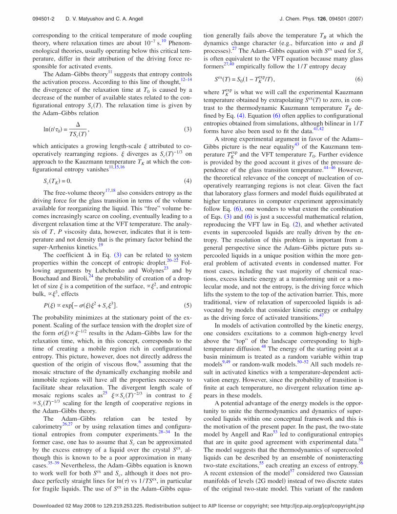
Our model of dynamics of viscous liquids follows thephilosophy of the energy models of activation in that it con-siders the probability of accumulating kinetic energy suffi-cient to lift a “structural element” �or “excitable unit,” seeFig. 1� to an energy level corresponding to the activated stateof the high-temperature relaxation. The kinetic energy sup-plied by the surroundings of a given excitable unit is a fluc-tuating variable with a fluctuation width related to the rug-gedness of the landscape through the configurational heatcapacity. The average of the fluctuations of the kinetic en-ergy results in a relation for the relaxation time which givesan increase of the activation energy with decreasing tempera-ture in terms of the configurational heat capacity, rather thanthe configurational entropy of the Adam–Gibbs theory. Thenew relation gives an account of experimental dielectric re-laxation comparable to the Adam–Gibbs formula, but moreacceptable in several ways to be discussed later.

II. THERMODYNAMICS OF CONFIGURATIONALEXCITATIONS

A. Formulation of the model

We conceive an excitation53,54,57 to be a local increase inpotential energy that results from a collisional redistributionof kinetic energy among some minimum group of “rear-rangeable units” of the liquid structure. In this redistributiona “unit” �Fig. 1� that undergoes an excessively anharmonicvibrational displacement can get trapped by the motions ofneighbors that act to prevent a return of the unit to its origi-nal center of oscillation, such that some kinetic energy willbe lost from the vibrational manifold and stored in the con-

figurational manifold. It is the constant and repeated ex-change of energy between these manifolds that is the essenceof configurational equilibration. The ability to store potentialenergy by this mechanism determines the configurationalheat capacity.

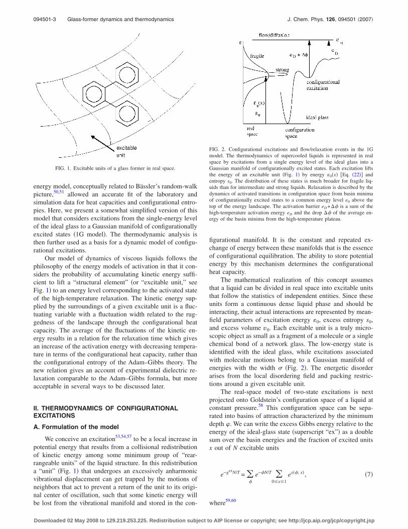
The mathematical realization of this concept assumesthat a liquid can be divided in real space into excitable unitsthat follow the statistics of independent entities. Since theseunits form a continuous dense liquid phase and should beinteracting, their actual interactions are represented by mean-field parameters of excitation energy 0, excess entropy s0,and excess volume v0. Each excitable unit is a truly micro-scopic object as small as a fragment of a molecule or a singlechemical bond of a network glass. The low-energy state isidentified with the ideal glass, while excitations associatedwith molecular motions belong to a Gaussian manifold ofenergies with the width � �Fig. 2�. The energetic disorderarises from the local disordering field and packing restric-tions around a given excitable unit.

The real-space model of two-state excitations is nextprojected onto Goldstein’s configuration space of a liquid atconstant pressure.58 This configuration space can be sepa-rated into basins of attraction characterized by the minimumdepth �. We can write the excess Gibbs energy relative to theenergy of the ideal-glass state �superscript “ex”� as a doublesum over the basin energies and the fraction of excited unitsx out of N excitable units

e−gexN/T = ��

e−�N/T �0�x�1

es��, x�, �7�

where59,60

FIG. 1. Excitable units of a glass former in real space.

FIG. 2. Configurational excitations and flow/relaxation events in the 1Gmodel. The thermodynamics of supercooled liquids is represented in realspace by excitations from a single energy level of the ideal glass into aGaussian manifold of configurationally excited states. Each excitation liftsthe energy of an excitable unit �Fig. 1� by energy 0�x� �Eq. �22�� andentropy s0. The distribution of these states is much broader for fragile liq-uids than for intermediate and strong liquids. Relaxation is described by thedynamics of activated transitions in configuration space from basin minimaof configurationally excited states to a common energy level e0 above thetop of the energy landscape. The activation barrier eD+�� is a sum of thehigh-temperature activation energy eD and the drop �� of the average en-ergy of the basin minima from the high-temperature plateau.

094501-3 Glass-former dynamics and thermodynamics J. Chem. Phys. 126, 094501 �2007�


es��, x� =N!

�N − xN� ! �xN�!��Qv

e/Qvg�xP��, x��N. �8�

Here, P�� , x� is the distribution of minimum energies inconfiguration space obtained by projecting the excitation en-ergy x�0+ Pv0+�� on the Gaussian manifold

P��, x� =� �� − x�0 + Pv0 + ��G��d� , �9�

where G�� is a Gaussian distribution

G�� exp�− ��2/2�2� . �10�

All energies here and below are in kelvin, entropies and heatcapacities are in units of kB.

The ratio of vibrational-rotational partition functionsQv

g, e in the ground �superscript g� and excited �superscript e�states can be absorbed into the excitation entropy

s0 = ln�Qve/Qv

g� = s0v + s0

c , �11�

which is composed of the harmonic vibrational contribution,s0

v, and a configurational contribution, s0c. The vibrational ex-

citation entropy is related to the excess density of states oflow-frequency vibrational modes near and below the bosonpeak61

s0v = �

�g e − g

g �ln� � . �12�

In Eq. �12�, the sum runs over the vibrational frequencies �eigenvalues of the Hessian matrix� with the densities of vi-brational states in the ground and excited states g

g, e.The thermodynamic limit N→� transforms the entropy

s�� , x� in Eq. �7� into a sum of the ideal mixing entropy,s0�x�, and a Gaussian term57

s��, x� = s0�x� −�� − x�0 + Pv0��2

2x2�2 , �13�

where

s0�x� = xs0 − x ln�x� − �1 − x�ln�1 − x� . �14�

The sum over x in Eq. �7� is determined by its largest sum-mand at x=x��. One then arrives at the landscape thermo-dynamics in which the thermodynamic observables are de-termined by the excess free-energy function depending on ��we omit the dependence on P for brevity�

gex�� = � + eanhex �� − Tsex�� ,

sex�� = s��, x�� , �15�

where eanhex �� is the energy related to the anharmonicity ef-

fects not included in the harmonic approximation �entropyfrom anharmonicity is small as indicated by computersimulations30�. The excess free energy gex�� is composed ofthe configurational and vibrational parts

gex�� = gc�� + gv�� , �16�

where

gv�� = eanhex �� − x��s0

vT . �17�

One can alternatively consider the sum over � in Eq. �7�that maximizes at the average basin energy ��x��. The �par-tial� Gibbs energy can be considered as a function of thepopulation

gex�x� = ��x�� + eanhex ��x�� − Ts��x��, x� . �18�

The minimum of gex�x� gives the thermodynamic Gibbs en-ergy gex in Eq. �7�. The formulation in terms of gex�x� isthermodynamically equivalent to the landscape thermody-namics in terms of gex�� since the thermodynamic Gibbsenergy gex is achieved at the largest summand in both x and� in the double sum in Eq. �7�. We will, however, obtainboth gex�� and gex�x� in order to gain better insight into thephysics of the model.

The excitation energy 0 can, to the first approximation,be considered as independent of temperature. The situation isquite different with the Gaussian width �2 �Eq. �10��. Theenergy of the localized excited state is randomized by inter-actions with the thermal motions of the liquid which are notquenched and therefore affected by temperature. Thefluctuation-dissipation theorem then requires that �2=2�Tscales linearly with temperature,62,63 as does the mean-squaredisplacement of a classical harmonic oscillator, �x2��T.Here, � is the trapping energy or the energy of stabilizationof an excitation by the disorder of the medium in which itexists.50,64 Once this real space Gaussian width is substitutedinto Eqs. �8� and �10�, it results in an approximately lineartemperature scaling of ��2� �which is more complex be-cause of a generally nonparabolic form of gex�� and tem-perature dependence of the population x�.57

The notion of the linear ��T� temperature dependence of��2� �which we will verify later� is one of the centralcomponents of the present model.57 The energy landscape ofthe system, i.e., energy as a function of 3N coordinates of themolecules making up the liquid, is determined by intermo-lecular interactions and is expected to be weakly temperaturedependent at constant volume of the liquid. However, whenthe manifold of all possible states in 3N space is projectedonto one single coordinate of the basin energy �, the distri-bution of �, given in terms of the �partial� free energygex��, gains temperature dependence. Not only the first mo-ment of this distribution, the average basin energy, is tem-perature dependent, as indeed described by random-energymodels,65 but essentially all higher moments are temperaturedependent as well. The random-energy model, originally de-veloped for spin glasses,66 assumes that the width of theGaussian distribution of random spin configurations is inde-pendent of temperature. This assumption is well justified forsystems with quenched disorder, but probably not as well forliquids in a metastable �slow nucleation� equilibrium. Like-wise the original Stillinger–Weber formulation67 assumedthat temperature affects only the average energy �� in theform of “descending into the landscape” but not any highermoments of the distribution. The simulation evidence on thismatter is insufficient and somewhat controversial. Whilesome simulations of small ensembles of binaryLennard-Jones7,8,68,69 �LJ� and dipolar70 fluids give clear in-dication of an approximately linear dependence of ��2� on



T, simulations of larger LJ ensembles give virtually constantwidth.42 This distinction is not accidental. The width of thedistribution of inherent structures scales as 1 /N and needsto be measured on small ensembles.

The ideal-glass state should in principle involve random-ness �simulations for network liquids show a finite configu-rational entropy at the cutoff energy71� and the previous ver-sion of the model57 �2G model� assumed Gaussiandistributions for both the ideal glass energies and the excitedconfigurations with the widths �i

2=2kBT�i �i=1, 2�. How-ever, as we noted in Ref. 57, the fit of the 2G model toexperimental heat capacities and configurational entropiesresulted in a small and almost constant �115−40 K for theideal-glass state. The application of the model to a moreextensive list of glass-forming liquids performed in this pa-per has shown that �1 can be set equal to zero without sac-rificing the quality of the fit. This will be the model adoptedhere. This version of the model, with only one Gaussianmanifold for the configurationally excited states, will be re-ferred to as the 1G model. The random energy statistics weconsider here have much in common with the model of pro-tein folding proposed by Bryngelson and Wolynes59,72 andthe equations we derive share features with the earlier coop-erative two-state model of Strässler and Kittel73 �which is aforerunner of the two species nonideal liquid model ofRapoport,74 the “two liquids” model of Aptekar75 and Pon-yatovsky and co-workers,76 and the cooperative defects mod-els of Granato77 and of Angell–Moynihan78�.

Now we turn to the thermodynamics of configurationalexcitations. The excess Gibbs energy gex�� minimizes at theaverage basin energy

�� = x�0 + Pv0� − 2x2��1 + �eanhex /�� . �19�

In what follows we will neglect the generally unknown de-rivative �eanh

ex /��. This approximation is expected to be ac-curate at low temperatures close to Tg, but will fail at highertemperatures above the onset temperature at which the sys-tem starts to descent into the energy landscape. In this ap-proximation, the excited-state population is defined by theself-consistent equation

x = �1 + eg0�x�/T�−1, �20�

where the free energy per excitable unit is

g0�x� = 0�x� − Ts0. �21�

Because of the energetic disorder of the exited states theactual excitation energy is lowered by twice the trappingenergy 2�.57,79 However, only configurationally excitedstates can “solvate” �stabilize� the excitation and the stabili-zation energy is proportional to the population x of the ex-cited states. The effective excitation energy 0�x� in Eq. �21�and Fig. 2 then becomes

0�x� = 0 + Pv0 − 2x� , �22�

where the factor of 2 comes from counting all interactions ofa given unit with the rest of the ensemble of configurationalexcitations.

By relating x to the spin variable �=2x−1, Eq. �20� canbe brought to the form usually considered by models offerromagnetism80

� = tanh��

2T−

g0 − �

2T� , �23�

where the excess Gibbs energy of configurational excitationsis

g0 = 0 + Pv0 − Ts0. �24�

At s0=0 and �=0+ Pv0 Eq. �23� transforms into the Weissformula for spontaneous magnetization80 with �� /2 playingthe role of the effective field of the magnetic moments.

The self-consistent equation for the population of con-figurational excitations �Eq. �20�� bears some similarity withthe results of previous studies minimizing the mean-fieldfree-energy functionals of liquid-state theories. The densityof the liquid ��r� can then be found from the self-consistentequation81,82

��r� = q exp�� c�r − r��r��dr�� , �25�

where q is the activity and c�r� is the direct correlation func-tion. Solution of this equation predicts a first-order transitionto aperiodic crystal.81 Molecular dynamics simulations, how-ever, indicate83 that a kinetic transition happens before thethermodynamic transition is reached, in qualitative agree-ment with our analysis of experimental data �see later�.

The combination of the average energy �Eq. �19�� andexcess entropy �Eqs. �13� and �15�� as functions of popula-tion yields gex�x� in Eq. �18�

gex�x� = xg0 − x2� + eanhex ��x��

+ T�x ln x + �1 − x�ln�1 − x�� . �26�

Except for the anharmonic correction, this equation has beenderived in many previous publications.73–76,84 Minimizationof gex�x� with respect to x �neglecting the derivative�eanh

ex /�x� leads to Eq. �20�. The parameter � then plays therole of the average energy of interaction between the con-figurational excitations. Consequently, the quadratic in xterm in Eqs. �19� and �26�, originating from the energy ran-domness in our model, is equivalent to direct mean-field�Bragg–Williams80� interaction between the excited units. Inother words, randomness is effectively equivalent to attrac-tion when separate units independently seek the same satis-factory configuration.79 Notice that derivation of Eq. �26�requires the explicit account of the linear temperature scalingof the real-space Gaussian width �2 in Eq. �10�. The assump-tion of a temperature-independent width would result in a1/T scaling of the energy term in gex�x� quadratic in x.

Since the full calculation of the excess thermodynamicsof the supercooled liquid over its crystal is too a complextask even for phenomenological models we next assume thatthe configurational entropy of two-state excitations, sex�T�,gives the excess entropy of the liquid over its crystal. Wewill use this excess entropy for the rest of our thermody-namic analysis warning at this point that this entropy, notbeing the thermodynamic entropy, is not thermodynamically



consistent with the excess Gibbs energies in Eqs. �15� and�26�, i.e., sex�T��−��gex�T� /�T�P. A thermodynamicallyconsistent gex�T� can of course be obtained by temperatureintegration of sex�T�.

According to our derivation above, sex�T� is the sum ofthe configurational entropy sc�T� and the vibrational entropyx�T�s0

v,

sex�T� = s ��x�T��, x�T�� = sc�x�T�, T� + x�T�s0v, �27�

where ��x�T�� and x�T� are given by Eqs. �19� and �20�,respectively. The configurational entropy thus accommodatesonly that part of s0 which is not related to the change in thevibrational density of states. It is given as a sum of the idealmixture entropy s0

c�x� and the fluctuation entropy −x2� /Tconsequent on the shrinking of the Gaussian width with de-creasing temperature57

sc�x, T� = s0c�x� − x2�/T , �28�

where

s0c�x� = xs0

c − x ln x − �1 − x�ln�1 − x� . �29�

B. Application to experimental data

We now proceed to applying the model to laboratory andsimulation data for supercooled molecular liquids. In theformer case, excess entropy �s of the liquid over the crystalis identified with the excess entropy over the ideal-glass statesex�T� �Eq. �27��. In the case of simulations, conjugate gra-dient minimization of simulated trajectories allows samplingof inherent structures and equations for the configurationalcomponent of the excess entropy will be used �Eqs. �28� and�29��. The two sets of equations are formally equivalentwhen the overall excitation entropy s0 is used for the excessdata and only its configurational component s0

c is used for thestatistics of inherent structures.

No progress can be made without recognizing that themolar quantity, heat capacity, determined in a laboratorymeasurement contains contributions from z “rearrangeablesubunits” of the molecule which are the microscopic dy-namic elements of the system. This is most obvious in thecase of chain molecule systems like selenium or like4-methyl nonane40 where each methyl group constitutes one“bead” according to Wunderlich’s original description.85 Thenumber of subunits or beads per molecule is not always evi-dent. In selenium the atom is clearly the bead but in theglass-former 9-bromo phenanthrene,86 the whole C20 “raft” isrigid and can only rearrange as a single unit.

Stevenson and Wolynes have suggested an operationalapproach to determining z, based on the entropy of fusionrelative to that of the simple LJ system.87 While this methoddoes not take account of the fact that the LJ fusion entropy isdetermined at a temperature where the liquid is enormouslymore fluid than the glass formers at their melting points �en-tropy per bead 1.68kB compared to Wunderlich’s 1.36kB,which leads to gross overestimates in the case of low fusionentropy network liquids, e.g., ZnCl2�, it does give a measurethat is roughly consistent with others. These range from theoriginal Wunderlich85 and Privalko40 estimates, through

Takeda et al. based on structural arguments88 down toMoynihan and Angell whose estimates were based on bestfitting of the excess entropy to an excitations model.54 Somecomparisons are provided in Table I.

The separation of a molecule into z statistically indepen-dent subunits neglects the finite correlation length of the dis-ordering field. Indeed, if two units are within the field’s cor-relation length, they contribute to the statistics of basins as asingle unit. The number of units z is thus an effective param-eter necessarily smaller or equal to the number of conforma-tionally distinct units �cf. the difference between Privalko’sconformational and Stevenson’s effective numbers in TableI�. Because of its effective nature, z can be represented byfractional numbers as was done by Stevenson and Wolynes�Table I�. Although this approach provides more flexibility infitting the experiment, we will follow here Takeda et al.88

and Moynihan and Angell54 and use integral numbers for z.In order to distinguish between thermodynamic propertiesreferring to excitable units and molecules �or generallymoles�, we will use lower-case letters for the former andupper-case letters for the latter. Lower-case and upper-caseextensive variables are connected through z, e.g., for theconstant-pressure heat capacity, CP=zcP.

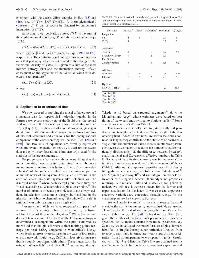
We will apply the model to constant-pressure data andconsider the excitation energy 0 as an adjustable parameter.Therefore, for the rest of our analysis, the term Pv0 in theexcess Gibbs energy �Eq. �24�� is fused into 0. Therefore,given the number of excitable units per molecule z has beenspecified, the 1G model contains three model parameters, 0,�, and s0. We have tested the model for a set of glass formersidentified as fragile �strong super-Arrhenius kinetics, fromtoluene to salol� and intermediate �weak super-Arrhenius ki-netics, from 3-bromopentane to n-propanol� liquids. Resultsshown in Fig. 3 and listed in Table II were obtained from asimultaneous fit of the model to excess heat capacities and

TABLE I. Number of excitable units �beads� per mole of a glass former. Thelast column represents the effective number of classical oscillators in a mol-ecule �mole� of a substance at Tg.

Substance Privalkoa Takedab Moynihanc Stevensond CPex�Tg� /3

InorganicsSe 1 1 1 0.9 1ZnCl2 1 1.2 3

AromaticsToluene 4 1 2.7 3.2o-terphenyl �OTP� 9 2 3.7Paraffinics2-methylpentane 6 3 3.8 3.2

AlcoholsMethanol 2 2 1.3 1.76Glycerol 6 6 7 4.5 3.5

HydratesCa�NO3�2 ·4H2O 13 7.0 11.7

aSee Ref. 40.bSee Ref. 88.cSee Ref. 54.dSee Ref. 87.



entropies from Ref. 54, bound by the constraint 0�x��0�Eq. �22�� required for the mechanical stability of the ideal-glass state.

The experimental excess entropies are calculated fromthe constant-pressure heat capacity CP

ex�T� and the fusion en-tropy �Sfus according to the relation

Sex�T� = �Sfus + �Tfus

T

CPex�T��dT�/T�� , �30�

where Tfus is the fusion temperature and Sex�T�=zsex�T�. Thenumber of excitable units per molecule �mole� z was takenfrom Moynihan and Angell54 and varied additionally to findthe best-fit integral numbers. Equal quality fits can be ob-

tained in some cases with different numbers z, e.g., for tolu-ene z=1 and z=2 can be adopted. In that latter case, z=1 wastaken to maintain the consistency of parameter values withother fragile liquids �Table II�. The choice of z here does notaffect our qualitative conclusions discussed later.

The constant-pressure heat capacity, used to fit the ex-perimental data, was obtained by the direct differentiation ofthe excess entropy constrained by the assumption that thetrapping energy � is independent of temperature. This as-sumption is supported by spectroscopic studies showingweak dependence of the Stokes shift �which is an analog ofthe trapping energy for electronic transitions� ontemperature.91 With this assumption one gets

cPex =

x2�

T+ x�1 − x�

0�x��0�x� − 2x��T2�1 − x�1 − x��2�/T��

. �31�

At �=0 this equation reduces to Schottky’s heat capacitycP

ex=x�1−x��0 /T�2, which is further reduced to the Hirai–Eyring equation,92 proposed on the basis of transition-stateideas, in the limit x�1. For fragile liquids, x1, as weshow later, and the heat capacity becomes

cPex = �/T . �32�

Notice that Eq. �31� anticipates a Curie type, �T−Tc�−1, di-vergence of the heat capacity at the critical temperature de-fined by the equation Tc=2�x�Tc��1−x�Tc��.

The fragility of a glass former is often characterized bythe steepness index1,2

m = �d log �/d�Tg/T��T=Tg�33�

�listed in Table II� or by its thermodynamic equivalent.93,94

What appears to be a smooth transition from fragile salol tointermediate 3-brombenzene according to the steepness in-dex in fact corresponds to a drastic decrease in the trappingenergy by a factor of about 50. Low values of � turn out tobe characteristic of all intermediate liquids in Table II. Theresult is a profound change in the relative importance of the

FIG. 3. Excess entropy �a� and excess heat capacity �b� for some of thesupercooled liquids listed in Table II �per molecule, in units of kB�. The thinlines refer to fits to the 1G model, the thick lines refer to the experimentaldata �see Ref. 54�.

TABLE II. Best-fit parameters of the 1G model to experimental excess entropies and heat capacities. Also shown are the experimental Kauzmann temperatureTK

exp obtained by extrapolating experimental entropies to zero �Ref. 54� and by using Eq. �38�, experimental VFT temperature T0, and the thermodynamicKauzmann temperature TK calculated from Eq. �4� using the 1G excess entropy from Eqs. �27� and �29�. The temperature of liquid-liquid transition TLL iscalculated from Eq. �34�, Tg is the experimental glass transition temperature. All energies and temperatures are in kelvin, the entropy s0 is in kB units.

Substance ma,b zc 0 � s0 TKexp T0

b TKexp,d TLL TK

e Tg

Fragile liquidsToluene 105f 1 2171 1020 10.2 100 96.5e 100 113 108 117D , L-propene carbonate 104 1 2921 1383 10.7 129 129 144 123 156OTP 81 2 3576 1686 8.3 204 202.4 206 228 170 2462-methyltetrahydrofurane �MTHF� 65 2 899 414 5.9 69 70 70 82 50 91Salol 63 3 2070 988 5.6 175 175 176 193 115 220

Intermediate liquids3-bromopentane �3BP� 53 4 348 20 2.0 84 83 75 108Glycerol 53 7 738 5.0 1.6 137 130g 59 190n-propanol �nPOH� 35 2 406 22 2.8 72 70 30 96

aSteepness fragility index, Eq. �33�.bTaken from Ref. 27 unless indicated otherwise.cFrom Ref. 88.dCalculated from Eq. �38�.eObtained as the temperature of crossing zero for the excess entropy calculated in the 1G model.fReference 89.gReference 90.



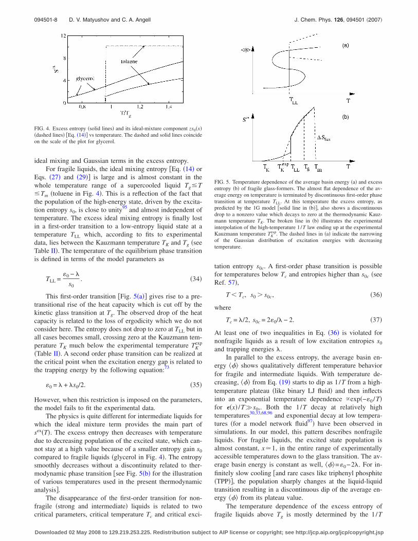
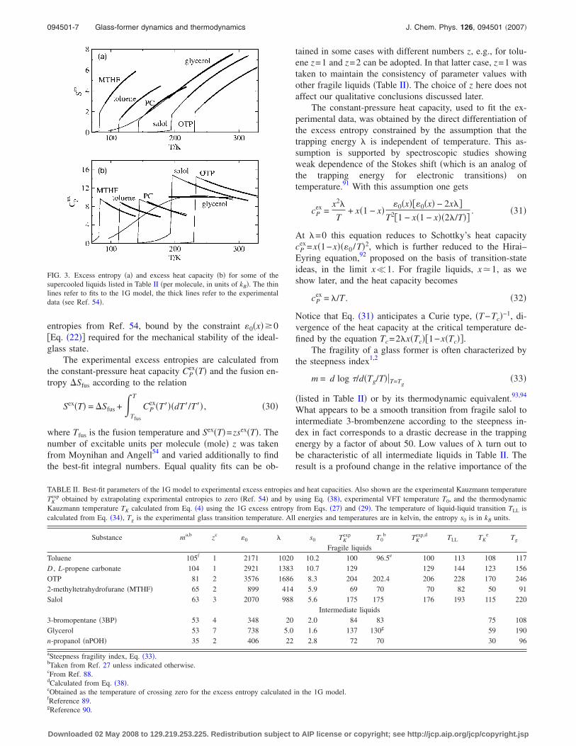
ideal mixing and Gaussian terms in the excess entropy.For fragile liquids, the ideal mixing entropy �Eq. �14� or

Eqs. �27� and �29�� is large and is almost constant in thewhole temperature range of a supercooled liquid Tg�T�Tm �toluene in Fig. 4�. This is a reflection of the fact thatthe population of the high-energy state, driven by the excita-tion entropy s0, is close to unity95 and almost independent oftemperature. The excess ideal mixing entropy is finally lostin a first-order transition to a low-entropy liquid state at atemperature TLL which, according to fits to experimentaldata, lies between the Kauzmann temperature TK and Tg �seeTable II�. The temperature of the equilibrium phase transitionis defined in terms of the model parameters as

TLL =0 − �

s0. �34�

This first-order transition �Fig. 5�a�� gives rise to a pre-transitional rise of the heat capacity which is cut off by thekinetic glass transition at Tg. The observed drop of the heatcapacity is related to the loss of ergodicity which we do notconsider here. The entropy does not drop to zero at TLL but inall cases becomes small, crossing zero at the Kauzmann tem-perature TK much below the experimental temperature TK

exp

�Table II�. A second order phase transition can be realized atthe critical point when the excitation energy gap is related tothe trapping energy by the following equation:73

0 = � + �s0/2. �35�

However, when this restriction is imposed on the parameters,the model fails to fit the experimental data.

The physics is quite different for intermediate liquids forwhich the ideal mixture term provides the main part ofsex�T�. The excess entropy then decreases with temperaturedue to decreasing population of the excited state, which can-not stay at a high value because of a smaller entropy gain s0

compared to fragile liquids �glycerol in Fig. 4�. The entropysmoothly decreases without a discontinuity related to ther-modynamic phase transition �see Fig. 5�b� for the illustrationof various temperatures used in the present thermodynamicanalysis�.

The disappearance of the first-order transition for non-fragile �strong and intermediate� liquids is related to twocritical parameters, critical temperature Tc and critical exci-

tation entropy s0c. A first-order phase transition is possiblefor temperatures below Tc and entropies higher than s0c �seeRef. 57�,

T � Tc, s0 � s0c, �36�

where

Tc = �/2, s0c = 20/� − 2. �37�

At least one of two inequalities in Eq. �36� is violated fornonfragile liquids as a result of low excitation entropies s0

and trapping energies �.In parallel to the excess entropy, the average basin en-

ergy �� shows qualitatively different temperature behaviorfor fragile and intermediate liquids. With temperature de-creasing, �� from Eq. �19� starts to dip as 1/T from a high-temperature plateau �like binary LJ fluid� and then inflectsinto an exponential temperature dependence �exp�−0 /T�for ��x� /T�s0,. Both the 1/T decay at relatively hightemperatures30,33,68,96 and exponential decay at low tempera-tures �for a model network fluid97� have been observed insimulations. In our model, this pattern describes nonfragileliquids. For fragile liquids, the excited state population isalmost constant, x1, in the entire range of experimentallyaccessible temperatures down to the glass transition. The av-erage basin energy is constant as well, ��=0−2�. For in-finitely slow cooling �and rare cases like triphenyl phosphite�TPP��, the population sharply changes at the liquid-liquidtransition resulting in a discontinuous dip of the average en-ergy �� from its plateau value.

The temperature dependence of the excess entropy offragile liquids above Tg is mostly determined by the 1/T

FIG. 4. Excess entropy �solid lines� and its ideal-mixture component zs0�x��dashed lines� �Eq. �14�� vs temperature. The dashed and solid lines coincideon the scale of the plot for glycerol.

FIG. 5. Temperature dependence of the average basin energy �a� and excessentropy �b� of fragile glass-formers. The almost flat dependence of the av-erage energy on temperature is terminated by discontinuous first-order phasetransition at temperature TLL. At this temperature the excess entropy, aspredicted by the 1G model �solid line in �b��, also shows a discontinuousdrop to a nonzero value which decays to zero at the thermodynamic Kauz-mann temperature TK. The broken line in �b� illustrates the experimentalinterpolation of the high-temperature 1/T law ending up at the experimentalKauzmann temperature TK

exp. The dashed lines in �a� indicate the narrowingof the Gaussian distribution of excitation energies with decreasingtemperature.



decay of the second fluctuation term in Eq. �28�. The result isthe overall temperature dependence in the form of Eq. �6�with S0=zs0. The experimental Kauzmann temperature isthen obtained by extrapolating Eq. �6� to zero entropy, whichleads, in terms of the model parameters, to the followingrelation:

TKexp =

�

s0. �38�

Equation �38� holds quite well for the fit parameters in TableII. In addition, the constant-pressure heat capacity scales as1 /T �Eq. �32��. Therefore, parameter � can be set by the heatcapacity at the glass transition

� = TgcPex�Tg� . �39�

The fit of experimental data for fragile liquids shows that0 is close to 2� and in fact can be put equal to 2� withoutsacrificing the accuracy of the fit. As a result, the thermody-namics of fragile liquids is defined by the following relationsoften used empirically:21,27,87,88,98

sex�T� = cPex�Tg��Tg/TK

exp − Tg/T� ,

cPex�T� = cP

ex�Tg��Tg/T� . �40�

We note that random energy models, which do not anticipatetemperature variation of the width of basin energydistribution,65 result in T−2 scaling of the heat capacity in-consistent with Eq. �40�.

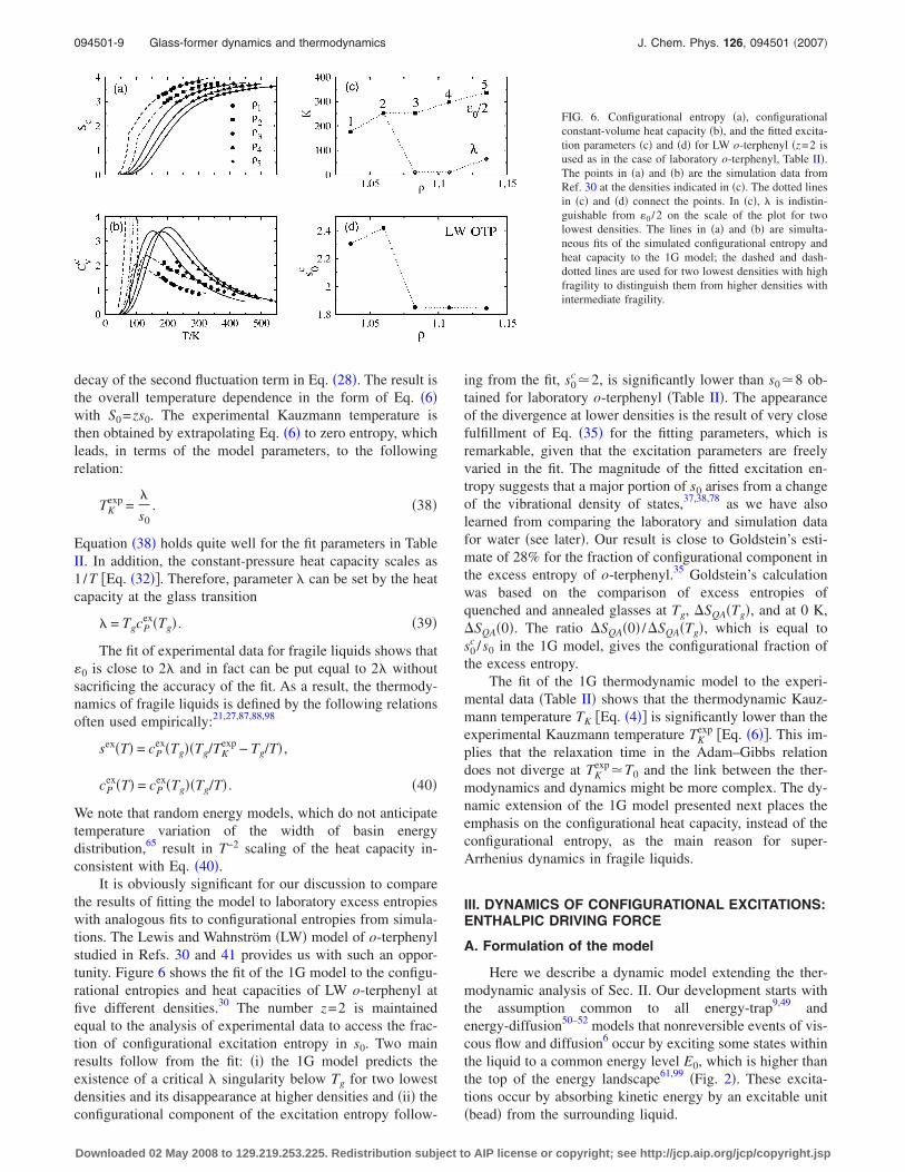
It is obviously significant for our discussion to comparethe results of fitting the model to laboratory excess entropieswith analogous fits to configurational entropies from simula-tions. The Lewis and Wahnström �LW� model of o-terphenylstudied in Refs. 30 and 41 provides us with such an oppor-tunity. Figure 6 shows the fit of the 1G model to the configu-rational entropies and heat capacities of LW o-terphenyl atfive different densities.30 The number z=2 is maintainedequal to the analysis of experimental data to access the frac-tion of configurational excitation entropy in s0. Two mainresults follow from the fit: �i� the 1G model predicts theexistence of a critical � singularity below Tg for two lowestdensities and its disappearance at higher densities and �ii� theconfigurational component of the excitation entropy follow-

ing from the fit, s0c 2, is significantly lower than s08 ob-

tained for laboratory o-terphenyl �Table II�. The appearanceof the divergence at lower densities is the result of very closefulfillment of Eq. �35� for the fitting parameters, which isremarkable, given that the excitation parameters are freelyvaried in the fit. The magnitude of the fitted excitation en-tropy suggests that a major portion of s0 arises from a changeof the vibrational density of states,37,38,78 as we have alsolearned from comparing the laboratory and simulation datafor water �see later�. Our result is close to Goldstein’s esti-mate of 28% for the fraction of configurational component inthe excess entropy of o-terphenyl.35 Goldstein’s calculationwas based on the comparison of excess entropies ofquenched and annealed glasses at Tg, �SQA�Tg�, and at 0 K,�SQA�0�. The ratio �SQA�0� /�SQA�Tg�, which is equal tos0

c /s0 in the 1G model, gives the configurational fraction ofthe excess entropy.

The fit of the 1G thermodynamic model to the experi-mental data �Table II� shows that the thermodynamic Kauz-mann temperature TK �Eq. �4�� is significantly lower than theexperimental Kauzmann temperature TK

exp �Eq. �6��. This im-plies that the relaxation time in the Adam–Gibbs relationdoes not diverge at TK

expT0 and the link between the ther-modynamics and dynamics might be more complex. The dy-namic extension of the 1G model presented next places theemphasis on the configurational heat capacity, instead of theconfigurational entropy, as the main reason for super-Arrhenius dynamics in fragile liquids.

III. DYNAMICS OF CONFIGURATIONAL EXCITATIONS:ENTHALPIC DRIVING FORCE

A. Formulation of the model

Here we describe a dynamic model extending the ther-modynamic analysis of Sec. II. Our development starts withthe assumption common to all energy-trap9,49 andenergy-diffusion50–52 models that nonreversible events of vis-cous flow and diffusion6 occur by exciting some states withinthe liquid to a common energy level E0, which is higher thanthe top of the energy landscape61,99 �Fig. 2�. These excita-tions occur by absorbing kinetic energy by an excitable unit�bead� from the surrounding liquid.

FIG. 6. Configurational entropy �a�, configurationalconstant-volume heat capacity �b�, and the fitted excita-tion parameters �c� and �d� for LW o-terphenyl �z=2 isused as in the case of laboratory o-terphenyl, Table II�.The points in �a� and �b� are the simulation data fromRef. 30 at the densities indicated in �c�. The dotted linesin �c� and �d� connect the points. In �c�, � is indistin-guishable from 0 /2 on the scale of the plot for twolowest densities. The lines in �a� and �b� are simulta-neous fits of the simulated configurational entropy andheat capacity to the 1G model; the dashed and dash-dotted lines are used for two lowest densities with highfragility to distinguish them from higher densities withintermediate fragility.



We will next assume that only unjammed configuration-ally excited units will participate in activated events. Evenwhen a sufficient amount of energy has been accumulated ata given unit, relaxation event may require facilitation fromother units. This is particularly clear in a case of a moleculecomposed of z units �beads�. One could imagine that, e.g.,translational relaxation of such molecule would require exci-tation of all z units, although relaxation of conformationallyflexible molecules can also proceed in a diffusive way, as asequence of low-amplitude motions of consecutive units. Be-cause of the assumed low amplitude of the motions involved,we will not distinguish between pairs of units within themolecule and pairs of units belonging to different molecules.

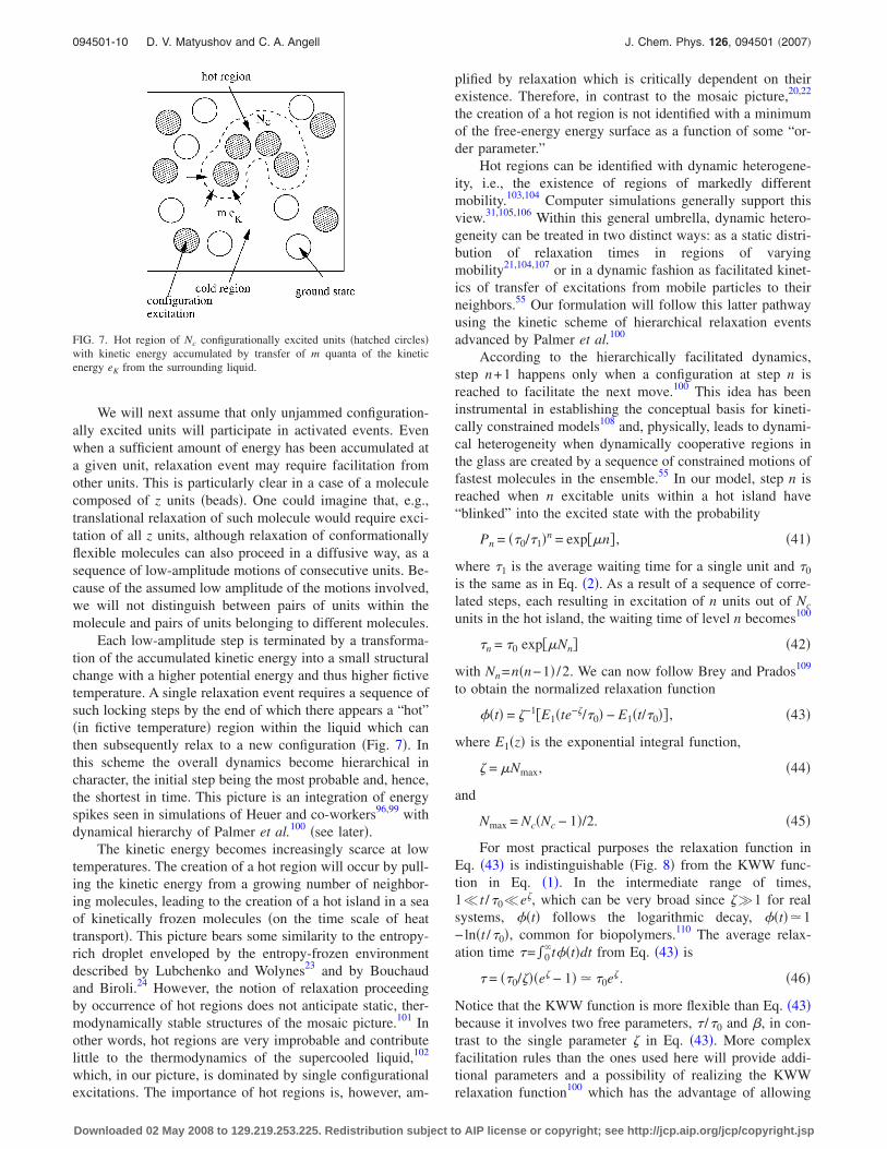
Each low-amplitude step is terminated by a transforma-tion of the accumulated kinetic energy into a small structuralchange with a higher potential energy and thus higher fictivetemperature. A single relaxation event requires a sequence ofsuch locking steps by the end of which there appears a “hot”�in fictive temperature� region within the liquid which canthen subsequently relax to a new configuration �Fig. 7�. Inthis scheme the overall dynamics become hierarchical incharacter, the initial step being the most probable and, hence,the shortest in time. This picture is an integration of energyspikes seen in simulations of Heuer and co-workers96,99 withdynamical hierarchy of Palmer et al.100 �see later�.

The kinetic energy becomes increasingly scarce at lowtemperatures. The creation of a hot region will occur by pull-ing the kinetic energy from a growing number of neighbor-ing molecules, leading to the creation of a hot island in a seaof kinetically frozen molecules �on the time scale of heattransport�. This picture bears some similarity to the entropy-rich droplet enveloped by the entropy-frozen environmentdescribed by Lubchenko and Wolynes23 and by Bouchaudand Biroli.24 However, the notion of relaxation proceedingby occurrence of hot regions does not anticipate static, ther-modynamically stable structures of the mosaic picture.101 Inother words, hot regions are very improbable and contributelittle to the thermodynamics of the supercooled liquid,102

which, in our picture, is dominated by single configurationalexcitations. The importance of hot regions is, however, am-

plified by relaxation which is critically dependent on theirexistence. Therefore, in contrast to the mosaic picture,20,22

the creation of a hot region is not identified with a minimumof the free-energy energy surface as a function of some “or-der parameter.”

Hot regions can be identified with dynamic heterogene-ity, i.e., the existence of regions of markedly differentmobility.103,104 Computer simulations generally support thisview.31,105,106 Within this general umbrella, dynamic hetero-geneity can be treated in two distinct ways: as a static distri-bution of relaxation times in regions of varyingmobility21,104,107 or in a dynamic fashion as facilitated kinet-ics of transfer of excitations from mobile particles to theirneighbors.55 Our formulation will follow this latter pathwayusing the kinetic scheme of hierarchical relaxation eventsadvanced by Palmer et al.100

According to the hierarchically facilitated dynamics,step n+1 happens only when a configuration at step n isreached to facilitate the next move.100 This idea has beeninstrumental in establishing the conceptual basis for kineti-cally constrained models108 and, physically, leads to dynami-cal heterogeneity when dynamically cooperative regions inthe glass are created by a sequence of constrained motions offastest molecules in the ensemble.55 In our model, step n isreached when n excitable units within a hot island have“blinked” into the excited state with the probability

Pn = ��0/�1�n = exp��n� , �41�

where �1 is the average waiting time for a single unit and �0

is the same as in Eq. �2�. As a result of a sequence of corre-lated steps, each resulting in excitation of n units out of Nc

units in the hot island, the waiting time of level n becomes100

�n = �0 exp��Nn� �42�

with Nn=n�n−1� /2. We can now follow Brey and Prados109

to obtain the normalized relaxation function

��t� = �−1�E1�te−�/�0� − E1�t/�0�� , �43�

where E1�z� is the exponential integral function,

� = �Nmax, �44�

and

Nmax = Nc�Nc − 1�/2. �45�

For most practical purposes the relaxation function inEq. �43� is indistinguishable �Fig. 8� from the KWW func-tion in Eq. �1�. In the intermediate range of times,1� t /�0�e�, which can be very broad since ��1 for realsystems, ��t� follows the logarithmic decay, ��t�1−ln�t /�0�, common for biopolymers.110 The average relax-ation time �=�0

�t��t�dt from Eq. �43� is

� = ��0/��e� − 1� �0e�. �46�

Notice that the KWW function is more flexible than Eq. �43�because it involves two free parameters, � /�0 and �, in con-trast to the single parameter � in Eq. �43�. More complexfacilitation rules than the ones used here will provide addi-tional parameters and a possibility of realizing the KWWrelaxation function100 which has the advantage of allowing

FIG. 7. Hot region of Nc configurationally excited units �hatched circles�with kinetic energy accumulated by transfer of m quanta of the kineticenergy eK from the surrounding liquid.



an approximate correlation between the stretch exponent andfragility.111

Each elementary step within the hierarchical sequencerequires overcoming the activation barrier between the aver-age energy of the basin minimum �� and the common en-ergy level E0=ze0 �Fig. 9�,

ED�x� = ED − z��x� , �47�

where ED is the activation barrier per molecule �mole� asso-ciated with the activated relaxation in the high-temperatureliquid112 and

��x� = �x − 1�0 − 2�x2 − 1�� 48�

is the drop of the minimum energy from the high-temperature plateau below the onset temperature.

One can next assume that the kinetic energy necessaryfor activation is distributed in “quanta” of thermal kineticenergy EK=zeK throughout the liquid, where EK and eK referto a molecule �mole� and excitable unit, respectively. Thisphysical picture seems appropriate for describing activatedevents in disordered materials since, according to theories ofheat conductivity, the quasilattice vibrations in glasses aremore appropriately described �in the temperature rangeabove �30 K� as quasilocalized vibrations rather than wave-like motions.113 The momentum exchange �heat transport�occurs by diffusional transport of vibrational energy by thesequasilocalized modes in the vicinity of the boson peak.114,115

Activation of one unit then requires accumulating m

=ED�x� /EK quanta of kinetic energy, provided that unit is notjammed being in the configurationally excited state. There-fore, the probability of activating one unit is equal to theprobability of absorbing m quanta of kinetic energy out of amanifold of xN configurational excitations uniformly distrib-uted over N units �beads� in the liquid. This type of problemis considered in the theory of unimolecular bond dissocia-tion. The solution by Kassel116 gives the probability of com-bining at least m quanta of energy at one bond

P�m =�N + xN − m − 1� ! �xN�!�xN − m� ! �N + xN − m�!

. �49�

For condensed-phase problems one takes the thermody-namic limit in the above equation, N→�, with the result

P�m = �1 + 1/x�−m = exp�− E�x�/EK� , �50�

where

E�x� = ED�x�ln�1 + 1/x� , �51�

and ED�x� is given by Eq. �47�.Because of similar combinatorial rules, not surprisingly,

Eq. �50� is analogous to the equation for the probability offinding a hole with the volume exceeding some critical vol-ume v�,

P�v�� = exp�− �v�/v f� , �52�

where v f is the free volume and � is a numerical coefficient.This equation is the key result of free-volume models ofdiffusion and relaxation in glass formers.17,18 The ideal glasstransition is predicted to occur because the liquid is supposedto run out of free volume at a finite temperature. In contrastto that, the kinetic energy in Eq. �50� is a fluctuating variablewhich can approach zero for some basins in the distributionsampled at temperature T �eK

�3� in Fig. 9�, but whose averagevalue is proportional to T.

The combinatorial arguments of the Kassel model envi-sion the system as a microcanonical ensemble characterizedby the average energy �e� uniformly distributed over thesample �Fig. 9�. In order to apply these combinatorial rulesto a macroscopic liquid, we need to use the microcanonicalensemble characterized by the average energy �e� �analo-gously to the use of microcanonical ensemble to calculate theexcess entropy in Eqs. �8� and �13��. Since energy is an ex-tensive variable, this description is equivalent in the thermo-dynamic limit to the canonical one in the sense that the fluc-tuations of the total energy can be neglected.

Each unit undergoing excitation to the common level e0

by collecting kinetic energy from the surrounding moleculeswill find itself in a local disordering field characteristic of aparticular basin of the rugged energy landscape �Fig. 9�. Thekinetic energy available to the surrounding molecules to ex-cite a given molecule will be a fluctuating variable producingdisorder of eK which is quenched on the time scale of mo-mentum relaxation. The relaxation time of a single molecule�1 then needs to be averaged over possible realizations of thekinetic energy

FIG. 8. ��t� from Eq. �43� �solid lines� and the closest corresponding KWWrelaxation function �dashed lines, Eq. �1��. The values of � used to plot ��t�are indicated in the plot.

FIG. 9. Activation barrier from the average energy �e� to the energy level e0

above the top of the landscape and fluctuations of the kinetic energy eK in arugged landscape of fragile liquids. The activation barrier eD refers to relax-ation in a high-temperature liquid, ��= ��T��− �� is the change of theaverage minimum energy from the high-temperature plateau. The real spaceregions on the right illustrate fluctuations in the kinetic energy of the mol-ecules due to variations of the basin depths.



�1 = �0e� = �0� exp�E�x�/�zeK��P�eK�deK, �53�

where P�eK� is the distribution of the kinetic energy.For the energy landscape characteristic of strong and in-

termediate liquids the canonical narrow distribution of basinenergies projects itself, in the microcanonical ensemble, intoa narrow distribution of kinetic energy eK. The distributionfunction P�eK� in Eq. �53� can be replaced by a delta func-tion. Assuming that the average kinetic energy is equal toEK= �3/2�T �translations for diffusion and viscous flow androtations for dielectric relaxation�, and using Eq. �51� forE�x� in Eq. �53� one gets for the average relaxation time

ln��/�0� = �2/3T��ED − z��x��ln�2 + e−s0+0�x�/T� . �54�

The relaxation is Arrhenius at high temperatures�0�x� /T�s0 and z��ED�. Two things happen when thetemperature is lowered. First, the energy gap between theaverage minimum energy ��m� and the energy level e0 startsto increase52 as a+b /T since ��x� scales as 1 /T right be-low the onset temperature.28 Second, at 0�x� /T�s0 thelogarithmic term in Eq. �54� generates a 1/T factor. Overall,the temperature law at these low temperatures becomes

ln��/�0� = E1/T2 + E2/T3, �55�

which is a linear combination of the Bässler64 and Litovitz117

temperature laws.This sort of non-Arrhenius kinetics is capable of describ-

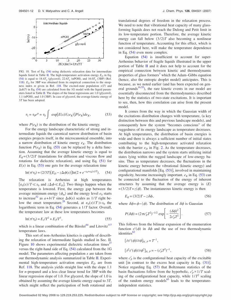
ing the relaxation of intermediate liquids studied in Sec. II.Figure 10 shows experimental dielectric relaxation times27

versus the right-hand side of Eq. �54� calculated from the 1Gmodel. The parameters affecting population x are taken fromour thermodynamic analysis summarized in Table II. Experi-mental high-temperature activation energies ED are fromRef. 118. The analysis yields straight line with the slope 1.1for n-propanol and a less clear linear trend for 3BP with thelinear regression slope of 1.0. For glycerol, the slope of 1.0 isobtained by assuming the average kinetic energy equal to 3T,which might reflect the participation of both rotational and

translational degrees of freedom in the relaxation process.We need to note that vibrational heat capacity of many glass-forming liquids does not reach the Dulong and Petit limit inits low-temperature portion. Therefore, the average kineticenergy can fall below �3/2�T also becoming a nonlinearfunction of temperature. Accounting for this effect, which isnot considered here, will make the temperature dependencein Eq. �54� even more complex.

Equation �54� is insufficient to account for super-Arrhenius behavior of fragile liquids illustrated in the upperportion of Table II and it does not help to account for theempirical connection between kinetic and thermodynamicproperties of glass formers3 which the Adam–Gibbs equation�hence, also the entropic droplet model� anticipates. This isbecause, as we noted earlier �and has been expected on gen-eral grounds16,55�, the rare kinetic events in our model areessentially disconnected from the thermodynamics describedhere by the statistics of two-state excitations. It is importantto see, then, how this correlation can arise from the presentmodel.

It comes from the way in which the Gaussian width ofthe excitations distribution changes with temperature, �a keydistinction between this and previous landscape models�, andconsequently how the system “becomes conscious” of theruggedness of its energy landscape as temperature decreases.At high temperatures, the distribution of basin energies iswide and there is always a sufficient number of initial statescontributing to the high-temperature activated relaxationwith the barrier eD in Fig. 2. As the temperature decreases,the distribution narrows and the system starts utilizing initialstates lying within the rugged landscape of low-energy ba-sins. Thus as temperature decreases, the fluctuations in thekinetic energy between the vibrational �kinetic energy� andconfigurational manifolds �Eq. �53��, involved in maintainingergodicity, become increasingly important. eK in Eq. �53� canbe connected to the fluctuation of the energy of inherentstructures by assuming that the average energy is �E�= �3/2�T+z��. The instantaneous kinetic energy is then

EK = �3/2�T − z�� , �56�

where ��=�− ��. The distribution of �� is Gaussian

P�� = �2�cPc T2�−1/2 exp�−

��2

2cPc T2� . �57�

This follows from the bilinear expansion of the enumerationfunction sc�� in �� and the use of two thermodynamicidentities62

��sc��/��N, P = T−1,

��2sc��/��2�N, P = − �cPc T2�−1, �58�

where cPc is the configurational heat capacity of the excitable

unit �in contrast to the excess heat capacity in Eq. �31��.Notice regarding Eq. �57� that Boltzmann statistics of thebasin fluctuations follow from the hyperbolic, cP

c �1/T scal-ing of the configurational heat capacity, while 1 /T2 scalingof the random energy models65 leads to the temperature-independent statistics.

FIG. 10. Test of Eq. �54� using dielectric relaxation data for intermediateliquids listed in Table II. The high-temperature activation energy ED in Eq.�54� is equal to 18.4Tg �glycerol�, 22.6Tg �nPOH�, and 16.0Tg �3BP� �Ref.118�. ED for 3BP was obtained from its empirical connection to the steep-ness index m given in Ref. 118. The excited-state population x�T� and��T� in Eq. �54� are calculated from the 1G model with the liquid param-eters listed in Table II. The slopes of the linear regressions are 1.0 �glycerol�,1.1 �nPOH�, and 1.0 �3BP�. In case of glycerol, the average kinetic energy of3T has been adopted.



The average waiting time of one-unit excitation then in-corporates the thermodynamic quantity, configurational heatcapacity, into the kinetics through P�� in the integral:

�1/�0 = �−�

3T/2z

exp� E�x�3T/2 − z��

�P��d�� . �59�

A simple estimate of the integral in Eq. �59� can be obtainedby linearly expanding the exponent in ��, integrating over��, and reverting to the fractional form. Combining Eqs.�44�, �46�, and �59�, the average relaxation time of the hotregion is then obtained as

ln��/�0� =2NmaxE�x�

3T − �4E�x�/9�zCPc �T�

, �60�

where Nmax is given by Eq. �45� and the molecular �molar�configurational heat capacity CP

c �T� appears in the denomi-nator. For fragile liquids, E�x� is nearly independent of tem-perature down to the liquid-liquid transition point �x1, seeFig. 5�a�� and can be considered as constant. This consider-ation yields the following equation for the relaxation time:

ln��/�0� =DT�

T − T�CPc �T�

, �61�

where the constant D is

D = �9/4z�Nc�Nc − 1� �62�

and the temperature T� is described further later.The parameters D and T� in Eq. �61� can be considered

as empirical fitting quantities for the sake of interpreting theexperiment. According to Eq. �32�, the excess and configu-rational heat capacities are equal to each other for fragileliquids. The 1/T scaling of the configurational heat capacitythen results in the overall temperature dependence of theform

ln��/�0� =DT�T

T2 − z�T�. �63�

This type of the temperature law was previously obtained forhard-sphere fluids by Jagla119 who combined the Adam–Gibbs formalism with an empirical equation of state. Note,however, that the configurational entropy in Jagla’s modelhas a 1/T2 temperature scaling inconsistent with the empiri-cal 1 /T law �Eqs. �6� and �40��.

B. Application to experimental data

Equations �61� and �63� suggest some qualitative resultsconsistent with experimental observations. First, the modelestablishes a direct link between fragility andconfigurational/excess heat capacity. The configurationalheat capacity in the denominator of Eq. �61� decreases athigh temperatures, e.g., above the melting temperature Tm.Therefore, the relaxation kinetics will change from super-Arrhenius at low temperatures to Arrhenius at hightemperatures.112 The extent of fragile behavior is controlledby � in the denominator of Eq. �63� which, according to ourthermodynamic analysis, is large for fragile liquids, resultingin curved Arrhenius plots. Note that parameter D in Eqs. �61�

and �63� is essentially constant across all liquids studied�Table III� in contrast to parameter D in the VFT equation�Eq. �2�� which correlates with fragility. Finally, Eq. �61�predicts a return to the Arrhenius behavior3 on passing belowTg because of the drop of CP

c which defines Tg. This featurehas previously been unique to the Adam–Gibbs equation andis also shared by the random first-order transition theory.22

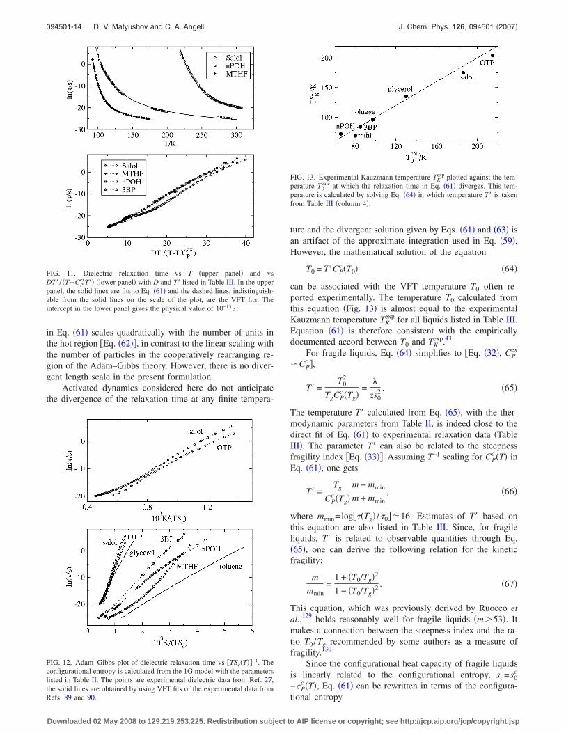
In addition to providing a qualitatively correct picture,Eq. �61� performs surprisingly well in fitting the dielectricrelaxation times27,89,90 of both intermediate and fragile liq-uids �Fig. 11 and Table III�, as well as of simulation data �seelater�. Fits of experimental dielectric relaxation times to Eq.�61�, with �0, D, and T� considered as fitting parameters, areindistinguishable from VFT fits in all cases studied �Fig. 11,upper panel�. ln�� plotted against DT� / �T−T�CP

ex� alsoyields straight lines and physically reasonable intercepts�Fig. 11, lower panel�. The quality of the linear correlationsis as good as for the Adam–Gibbs plot �cf. Figs. 11 and 12�and in some cases is even better �MTHF�. Even more grati-fying is the invariable slope of the plots in Fig. 11 comparedto a large variance of slopes of Adam–Gibbs plots in Fig. 12.In all fits, experimental CP

ex�T� were used instead of CPc �T�

suggested by the denominator of Eq. �61� �in the 1G model,CP

exCPc for fragile liquids�.

The nominator parameter D in Eq. �61� can be related tothe average number of excitations in the hot region via Eq.�62�. From Table III, we obtain Nc10−20. With the usualmolecular diameter of �5.5 Å, this number projects into alength scale of 1.5 nm for a spherical cluster or larger ifrelaxation is facilitated through chains of molecules.33 Thislength is in general accord with current estimates of spatialheterogeneities in supercooled liquids,126 although falls be-low the estimate � /�=4.5 given by Berthier et al.127 and therandom first-order transition theory.128 The activation barrier

TABLE III. Best-fit parameters of Eq. �61� to experimental dielectric relax-ation data with �0, D, and T� considered as fitting parameters. The experi-mental �superscript “exp”� and calculated �superscript “calc”� pressurevariation of the glass transition temperature dTg /dP is given in K/MPa, alltemperatures are in kelvin.

Substance log��0 /s� D T� T�a T�

b dTg /dPexp dTg /dPcalc

Toluene −15.6 145 9.3 9.8 8.7OTPc −14.0 161 13.8 12.2 13.7 0.26d 0.22MTHF −13.5 95.6 7.9 5.9 8.9Salol −14.4 204 11.9 10.5 13.3 0.20e 0.263BP −13.6 209 7.1 9.4Glycerol −14.2 159 13.2 10.0 0.03f 0.05g

nPOH −13.2 218 7.9 6.5 0.07h 0.05i

aCalculated for fragile liquids from Eq. �65� by applying the thermodynamicfitting parameters from Table II.bBased on the steepness fragility index according to Eq. �66�.cFit to Eq. �61� for OTP was obtained by restricting log��0� to be equal to−14.dFrom Ref. 120.eFrom Ref. 121. The calculated dTg /dP refers to P=300 MPa instead ofatmospheric pressure in case of OTP since the data in Ref. 121 apply to highpressures only.fFrom Ref. 122.gUsing high-temperature T , P-data for viscosity from Ref. 123.hFrom Ref. 124.iUsing the dielectric data at 0.1 and 100 MPa from Ref. 125.



in Eq. �61� scales quadratically with the number of units inthe hot region �Eq. �62��, in contrast to the linear scaling withthe number of particles in the cooperatively rearranging re-gion of the Adam–Gibbs theory. However, there is no diver-gent length scale in the present formulation.

Activated dynamics considered here do not anticipatethe divergence of the relaxation time at any finite tempera-

ture and the divergent solution given by Eqs. �61� and �63� isan artifact of the approximate integration used in Eq. �59�.However, the mathematical solution of the equation

T0 = T�CPc �T0� �64�

can be associated with the VFT temperature T0 often re-ported experimentally. The temperature T0 calculated fromthis equation �Fig. 13� is almost equal to the experimentalKauzmann temperature TK

exp for all liquids listed in Table III.Equation �61� is therefore consistent with the empiricallydocumented accord between T0 and TK

exp.43

For fragile liquids, Eq. �64� simplifies to �Eq. �32�, CPex

CPc �,

T� =T0

2

TgCPc �Tg�

=�

zs02 . �65�

The temperature T� calculated from Eq. �65�, with the ther-modynamic parameters from Table II, is indeed close to thedirect fit of Eq. �61� to experimental relaxation data �TableIII�. The parameter T� can also be related to the steepnessfragility index �Eq. �33��. Assuming T−1 scaling for CP

c �T� inEq. �61�, one gets

T� =Tg

CPc �Tg�

m − mmin

m + mmin, �66�

where mmin=log��Tg� /�0�16. Estimates of T� based onthis equation are also listed in Table III. Since, for fragileliquids, T� is related to observable quantities through Eq.�65�, one can derive the following relation for the kineticfragility:

m

mmin=

1 + �T0/Tg�2

1 − �T0/Tg�2 . �67�

This equation, which was previously derived by Ruocco etal.,129 holds reasonably well for fragile liquids �m�53�. Itmakes a connection between the steepness index and the ra-tio T0 /Tg recommended by some authors as a measure offragility.130

Since the configurational heat capacity of fragile liquidsis linearly related to the configurational entropy, sc=s0

c

−cPc �T�, Eq. �61� can be rewritten in terms of the configura-

tional entropy

FIG. 11. Dielectric relaxation time vs T �upper panel� and vsDT� / �T−CP

exT�� lower panel� with D and T� listed in Table III. In the upperpanel, the solid lines are fits to Eq. �61� and the dashed lines, indistinguish-able from the solid lines on the scale of the plot, are the VFT fits. Theintercept in the lower panel gives the physical value of 10−13 s.

FIG. 12. Adam–Gibbs plot of dielectric relaxation time vs �TSc�T��−1. Theconfigurational entropy is calculated from the 1G model with the parameterslisted in Table II. The points are experimental dielectric data from Ref. 27,the solid lines are obtained by using VFT fits of the experimental data fromRefs. 89 and 90.

FIG. 13. Experimental Kauzmann temperature TKexp plotted against the tem-

perature T0calc at which the relaxation time in Eq. �61� diverges. This tem-

perature is calculated by solving Eq. �64� in which temperature T� is takenfrom Table III �column 4�.



ln��/�0� =DT�

T + T��Sc − zs0c�

. �68�

The current formulation still provides a link between therelaxation time and configurational entropy, but the algebrais different from the Adam–Gibbs relation �Eq. �3��. The va-lidity of either functional dependence of the relaxation timeis often tested by calculating the slope of the glass transitiontemperature with pressure. Equation �61� suggests thatT /T�−CP

c �T� remains constant at the glass transition tem-peratures measured at different pressures. FollowingGoldstein,16,44 the condition d�T /T�−CP

c �T��=0 provides theslope of the glass transition temperature with pressure,dTg /dP. One needs to calculate the derivative of T� overpressure and the pressure and temperature derivatives of CP

c .The pressure derivative gives ��CP

c /�P�T=−TgVg�P2 /kB,

where Vg is the molecular volume of the glass. The differ-ence of the isobaric expansivities of the liquid and glass,�P, is in the range 5�10−4 K−1 �Refs. 44 and 120� al-lowing one to neglect the pressure derivative of CP

c . One thengets

dTg

dP=

Tg

T�

�T�

�P�1 − T��CP

c /�T�P�−1. �69�

Equation �69� should be compared to what follows from theAdam–Gibbs scaling16

dTg/dP = TgVg�p/�Sc + CPc � . �70�

Most data, available for strong/intermediateliquids,44,45,124 indicate that Eq. �70� adequately describes theexperiment. Since �T0 /�P�0 �Refs. 123, 124, and 131�, onecan expect from Eq. �65� that �T� /�P�0. The actual num-bers for this derivative can be obtained from T , P relaxationdata.120–125,132 The results of these calculation are given inTable III. The relaxation times were fitted to Eq. �61� atambient pressure with D and T� considered as fitting param-eters and experimental CP

ex�T� and ambient pressure. The pa-rameter D was then kept constant at elevated pressures and�T� /�P was evaluated from the fit. The results of these cal-culations are in reasonable agreement with reported dTg /dPand reproduce the drop of this derivative in going from frag-ile to intermediate glass formers �Table III�.

IV. DISCUSSION

The model developed here describes the thermodynamicproperties of glass formers in terms of statistics of excita-tions from a single-energy state of the ideal glass to a Gauss-ian manifold of configurationally unjammed states withhigher energy and entropy. The model suggests that the ther-modynamic signatures of fragile liquids, in particular asharply increasing configurational heat capacity close to theglass transition, can be identified with the existence of athermodynamic phase transition �“LL line” in Fig. 14�a��,usually hidden below the glass transition temperature.12,82,134

The strong/fragile behavior is distinguished within the modelby two parameters, the trapping energy parameter � and theentropy gain for a single configurational excitation s0, theratio of them equal to the experimental Kauzmann tempera-

ture �Eq. �38��. Both parameters significantly decrease whengoing from fragile to intermediate/strong liquids, with theparameter � showing the most significant change �Table II�.Fragile liquids are therefore characterized by a broad rangeof configurationally excited states, whereas the energy distri-bution for intermediate/strong liquids is very narrow �Fig. 1�.Because of low values of either � or s0 �or both of them�strong/intermediate liquids fall in the range of temperaturesand excitation entropies �T�Tc, s0�s0c, Eq. �37�� not allow-ing a first-order transition.

The critical point �Tc , s0c�, separating fragile from non-fragile liquids �Fig. 14�a��, makes the descent into the energylandscape qualitatively different for them. The average basinenergy of nonfragile liquids first starts to drop from the high-energy plateau according to the 1/T law and then inflectsinto an exponential decay. The distribution of basin energiesis narrow, and its maximum shifts to lower energies withcooling �Figs. 15�a� and 15�b��. This behavior, often ob-served in simulations of binary LJ liquids,30,33,68,96 is wellreproduced by the present model which places these fluidsinto the strong/intermediate category. As an example, weshow in Fig. 16 the fit of the 1G model to Sastry’s data onbinary LJ mixture �BLJM�.28,135 The calculations were done

FIG. 14. The liquid-liquid coexistence line �LL line� and the line of maxi-mum heat capacity �Widom line� �Ref. 133� in the �T , s0� parameters plane�a�. Thermodynamic fragile behavior is limited by the critical point �Tc , s0c��Eq. �37��. The vertical arrow shows the cooling path along which the re-laxation time is calculated using Eq. �61� �b�. Tmax denotes the temperatureat which the of heat capacity �dash-dotted line in �b�� passes through amaximum, CP

max=CP�Tmax�. All the plots have been generated at contstant0, �, and z.

FIG. 15. Illustration of the temperature behavior of the average basin energy�� and the distribution of basin energies P�� in nonfragile and fragileliquids.



for the highest density studied in simulations at which theBLJM liquid is most fragile. Equations �28� and �31� wereused, respectively, for the configurational entropy and heatcapacity, while Eq. �61� was applied to the simulated diffu-sion coefficient. The excitation energy �0=219 K� and thetrapping energy ��=71 K� obtained from the fit produce thefollowing critical parameters: Tc=35.5 K and s0c=4.2 �acci-dentally, Tc is close to TK

exp�. On the other hand, the excitationentropy from the fit, s0

c =0.32, and the temperature rangeT�Tc together put the BLJM liquid into the category ofintermediate fragility. With such low excitation entropy, thepopulation of the excited state is close to 0.5 at high tem-peratures. From Eq. �28� one then gets �z=1� S0=s0

c /2+ln�2�0.85. The same number, 0.85, is reported by Sastryfor the top of the enumeration function smax

c .28

The behavior of fragile liquids is quite different. Theconfigurationally excited state is almost entirely populated�x1� in the entire range of experimentally accessible tem-peratures down to the glass transition. The average basinenergy is almost temperature independent and the only effectof lowering the temperature on the distribution of basin en-ergies is its narrowing according to the fluctuation-dissipation theorem �Figs. 15�c� and 15�d��. The invariantpopulation of the configurationally excited states is abruptlyterminated at the equilibrium first-order transition or �on su-percooling� at spinodal instability at which point it drops to alow value representative of an entropy-poor, low-temperaturephase as experimentally confirmed for TPP.136

The fit of the model to experimental excess heat capaci-ties and entropies of molecular glass formers �Table II� has

pushed the liquid-liquid phase transition below the glasstransition. For some substances,3,133,137,138 the thermody-namic liquid-liquid transition can be found above the glasstransition. As an example of this situation, the 1G model isapplied to excess entropy and heat capacity of laboratorywater.139,140 The thick lines in Figs. 17�a� and 17�b� show theresults of measurements on bulk samples,139 while opencircles refer to samples confined in 3 nm pores of silicagel.140 The two sets of data coincide at high temperatures.Because of the limited temperature range of the bulk waterdata, the fit to the thermodynamic 1G model is done fornanoconfined water �Table IV�. The 1G model predicts aweak first-order phase transition at TLL=229 K �P=1 atm�.This number is very close to previous estimates for the tem-perature of crossing the “Widom line” at which the heat ca-pacity gets a maximum137 and more recent measurementsplacing this point at 223 K.144 After the kink at TLL, theentropy slowly decays to zero at TK→0.

FIG. 16. Configurational entropy �a�, configurational �constant-volume� heatcapacity �b�, and diffusion coefficient �c� of the 80�A�:20�B� BLJM liquid at��AA

3 =1.35, where �AA is the LJ diameter of the component with higherconcentration. The thick solid lines are the results of simulations from Ref.28 arbitrarily limited to T�100 K. The diffusion coefficients from Ref. 135�circles, �c�� are fitted to Eq. �61� �solid line� and to the VFT relation�dashed line�. The two fits are almost indistinguishable on the scale of theplot. The fitting to 1G model �Eqs. �28�, �31�, and �61�� results in the fol-lowing fitting parameters: 0=219 K, �=71 K, s0

c =0.32, T�=92.8 K, andD=3.1. The thermodynamic Kauzmann temperature TK is zero when calcu-lated in the 1G model �the thin lines in �a� and �b��.

FIG. 17. �a� Excess entropy for bulk laboratory water �bulk�, nanoconfinedwater �confined�, and configurational entropy for SPC/E water �SPC/E�. Thethick line and open points refer to bulk �Ref. 139� and nanoconfined experi-ments, respectively. The closed points refer to constant-volume simulations�Ref. 137�. �b� Experimental excess heat capacity for bulk �thick line� �Ref.139� and hard nanoconfined �Ref. 140� �open points� water. The thin lines in�a� and �b� are fits to the thermodynamic 1G model �Eqs. �27� and �29��. Theconfigurational heat capacity of SPC/E water in �b� is calculated from the1G model based on the fit of the configurational entropy in �a�. �c� Simula-tion �constant-volume� results for the Debye relaxation time �SPC/E, �� anddiffusivity �SPC/E, D� of SPC/E water �Ref. 141�. Diamonds show experi-mental diffusivity of laboratory water �Ref. 142�. The solid lines are fits toEq. �61� with the configurational heat capacity obtained by numerical dif-ferentiation of Sc for SPC/E water �see Table IV for the fitting parameters�.The diffusivity curves have been arbitrarily shifted to fit to the scale of theplot. For all three panels, the closed points refer to simulations and openpoints are used to indicate the laboratory experiment.



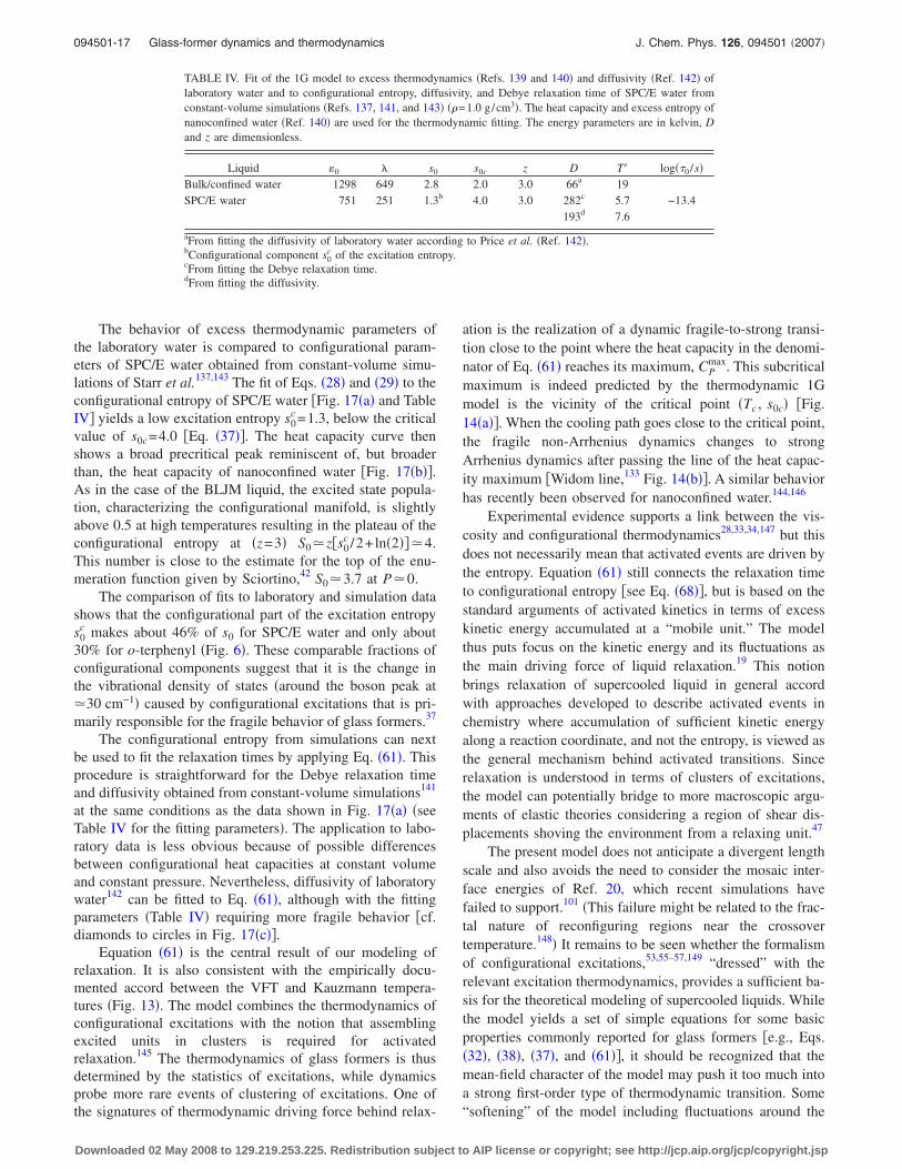
The behavior of excess thermodynamic parameters ofthe laboratory water is compared to configurational param-eters of SPC/E water obtained from constant-volume simu-lations of Starr et al.137,143 The fit of Eqs. �28� and �29� to theconfigurational entropy of SPC/E water �Fig. 17�a� and TableIV� yields a low excitation entropy s0

c =1.3, below the criticalvalue of s0c=4.0 �Eq. �37��. The heat capacity curve thenshows a broad precritical peak reminiscent of, but broaderthan, the heat capacity of nanoconfined water �Fig. 17�b��.As in the case of the BLJM liquid, the excited state popula-tion, characterizing the configurational manifold, is slightlyabove 0.5 at high temperatures resulting in the plateau of theconfigurational entropy at �z=3� S0z�s0

c /2+ln�2��4.This number is close to the estimate for the top of the enu-meration function given by Sciortino,42 S03.7 at P0.

The comparison of fits to laboratory and simulation datashows that the configurational part of the excitation entropys0

c makes about 46% of s0 for SPC/E water and only about30% for o-terphenyl �Fig. 6�. These comparable fractions ofconfigurational components suggest that it is the change inthe vibrational density of states �around the boson peak at30 cm−1� caused by configurational excitations that is pri-marily responsible for the fragile behavior of glass formers.37

The configurational entropy from simulations can nextbe used to fit the relaxation times by applying Eq. �61�. Thisprocedure is straightforward for the Debye relaxation timeand diffusivity obtained from constant-volume simulations141

at the same conditions as the data shown in Fig. 17�a� �seeTable IV for the fitting parameters�. The application to labo-ratory data is less obvious because of possible differencesbetween configurational heat capacities at constant volumeand constant pressure. Nevertheless, diffusivity of laboratorywater142 can be fitted to Eq. �61�, although with the fittingparameters �Table IV� requiring more fragile behavior �cf.diamonds to circles in Fig. 17�c��.

Equation �61� is the central result of our modeling ofrelaxation. It is also consistent with the empirically docu-mented accord between the VFT and Kauzmann tempera-tures �Fig. 13�. The model combines the thermodynamics ofconfigurational excitations with the notion that assemblingexcited units in clusters is required for activatedrelaxation.145 The thermodynamics of glass formers is thusdetermined by the statistics of excitations, while dynamicsprobe more rare events of clustering of excitations. One ofthe signatures of thermodynamic driving force behind relax-

ation is the realization of a dynamic fragile-to-strong transi-tion close to the point where the heat capacity in the denomi-nator of Eq. �61� reaches its maximum, CP

max. This subcriticalmaximum is indeed predicted by the thermodynamic 1Gmodel is the vicinity of the critical point �Tc , s0c� �Fig.14�a��. When the cooling path goes close to the critical point,the fragile non-Arrhenius dynamics changes to strongArrhenius dynamics after passing the line of the heat capac-ity maximum �Widom line,133 Fig. 14�b��. A similar behaviorhas recently been observed for nanoconfined water.144,146

Experimental evidence supports a link between the vis-cosity and configurational thermodynamics28,33,34,147 but thisdoes not necessarily mean that activated events are driven bythe entropy. Equation �61� still connects the relaxation timeto configurational entropy �see Eq. �68��, but is based on thestandard arguments of activated kinetics in terms of excesskinetic energy accumulated at a “mobile unit.” The modelthus puts focus on the kinetic energy and its fluctuations asthe main driving force of liquid relaxation.19 This notionbrings relaxation of supercooled liquid in general accordwith approaches developed to describe activated events inchemistry where accumulation of sufficient kinetic energyalong a reaction coordinate, and not the entropy, is viewed asthe general mechanism behind activated transitions. Sincerelaxation is understood in terms of clusters of excitations,the model can potentially bridge to more macroscopic argu-ments of elastic theories considering a region of shear dis-placements shoving the environment from a relaxing unit.47

The present model does not anticipate a divergent lengthscale and also avoids the need to consider the mosaic inter-face energies of Ref. 20, which recent simulations havefailed to support.101 �This failure might be related to the frac-tal nature of reconfiguring regions near the crossovertemperature.148� It remains to be seen whether the formalismof configurational excitations,53,55–57,149 “dressed” with therelevant excitation thermodynamics, provides a sufficient ba-sis for the theoretical modeling of supercooled liquids. Whilethe model yields a set of simple equations for some basicproperties commonly reported for glass formers �e.g., Eqs.�32�, �38�, �37�, and �61��, it should be recognized that themean-field character of the model may push it too much intoa strong first-order type of thermodynamic transition. Some“softening” of the model including fluctuations around the

TABLE IV. Fit of the 1G model to excess thermodynamics �Refs. 139 and 140� and diffusivity �Ref. 142� oflaboratory water and to configurational entropy, diffusivity, and Debye relaxation time of SPC/E water fromconstant-volume simulations �Refs. 137, 141, and 143� ��=1.0 g/cm3�. The heat capacity and excess entropy ofnanoconfined water �Ref. 140� are used for the thermodynamic fitting. The energy parameters are in kelvin, Dand z are dimensionless.

Liquid 0 � s0 s0c z D T� log��0 /s�Bulk/confined water 1298 649 2.8 2.0 3.0 66a 19SPC/E water 751 251 1.3b 4.0 3.0 282c 5.7 −13.4

193d 7.6

aFrom fitting the diffusivity of laboratory water according to Price et al. �Ref. 142�.bConfigurational component s0

c of the excitation entropy.cFrom fitting the Debye relaxation time.dFrom fitting the diffusivity.



mean field would result in greater flexibility, but this wouldonly come at the expense of an increase in the number ofparameters.

ACKNOWLEDGMENTS

The authors are grateful to Ranko Richert for the helpwith dielectric relaxation data and to Srikanth Sastry for use-ful discussions. This work was supported by the NSFthrough the Grant Nos. CHE-0616646 �D.V.M.� and DMR-0082535 �C.A.A.�. C.A.A. thanks Francesco Sciortino for anumber of illuminating discussions. They also thank KarlFreed and Peter Wolynes for critical comments on the manu-script.

1 K. L. Ngai, J. Non-Cryst. Solids 275, 7 �2000�.2 C. A. Angell, Science 267, 1924 �1995�.3 C. A. Angell, K. L. Ngai, G. B. McKenna, and S. W. Martin, J. Appl.Phys. 88, 3113 �2000�.

4 W. Götze, in Liquids, Freezing and Glass Transition, edited by J. P.Hansen, D. Levesque, and J. Zinn-Justin �Elsevier, Amsterdam, 1991�,Vol. 1, p. 287.

5 P. G. Debenedetti and F. H. Stillinger, Nature �London� 410, 259 �2001�.6 M. Goldstein, J. Chem. Phys. 51, 3728 �1969�.7 B. Doliwa and A. Heuer, Phys. Rev. E 67, 031506 �2003�.8 R. A. Denny, D. R. Reichman, and J.-P. Bouchaud, Phys. Rev. Lett. 90,025503 �2003�.

9 A. Heuer, B. Doliwa, and A. Saksaengwijit, Phys. Rev. E 72, 021503�2005�.

10 V. N. Novikov and A. P. Sokolov, Phys. Rev. E 67, 031507 �2003�.11 G. Adam and J. H. Gibbs, J. Chem. Phys. 43, 139 �1965�.12 J. H. Gibbs and E. A. D. Marzio, J. Chem. Phys. 28, 373 �1958�.13 E. A. D. Marsio and A. J. M. Yang, J. Res. Natl. Inst. Stand. Technol.

102, 135 �1997�.14 J. Dudowicz, K. F. Freed, and J. F. Douglas, Adv. Chem. Phys. �in press�.15 W. Kauzmann, Chem. Rev. �Washington, D.C.� 43, 219 �1948�.16 P. G. Debenedetti, Metastable Liquids: Concepts and Principles �Prince-

ton University Press, Princeton, NJ, 1996�.17 M. H. Cohen and D. Turnbull, J. Chem. Phys. 31, 1164 �1959�.18 M. H. Cohen and G. Grest, Adv. Chem. Phys. 48, 370 �1981�.19 M. L. Ferrer, C. Lawrence, B. G. Demirjian, and D. Kivelson, J. Chem.

Phys. 109, 8010 �1998�.20 X. Xia and P. G. Wolynes, Proc. Natl. Acad. Sci. U.S.A. 97, 2990 �2000�.21 X. Xia and P. G. Wolynes, J. Phys. Chem. B 105, 6570 �2001�.22 V. Lubchenko and P. G. Wolynes, J. Chem. Phys. 121, 2852 �2004�.23 V. Lubchenko and P. G. Wolynes, cond-mat/0506708.24 J.-P. Bouchaud and G. Biroli, J. Chem. Phys. 121, 7347 �2004�.25 T. R. Kirkpatrick, D. Thirumalai, and P. G. Wolynes, Phys. Rev. A 40,

1045 �1989�.26 C. A. Angell, J. Non-Cryst. Solids 131–133, 13 �1991�.27 R. Richert and A. C. Angell, J. Chem. Phys. 108, 9016 �1998�.28 S. Sastry, Nature �London� 409, 164 �2001�.29 I. Saika-Voivod, P. H. Poole, and F. Sciortino, Nature �London� 412, 514

�2001�.30 S. Mossa, E. L. Nave, H. E. Stanley, C. Donati, F. Sciortino, and P.

Tartaglia, Phys. Rev. E 65, 041205 �2002�.31 N. Giovambattista, S. V. Buldyrev, F. W. Starr, and H. E. Stanley, Phys.

Rev. Lett. 90, 085506 �2003�.32 I. Saika-Voivod, F. Sciortino, and P. H. Poole, Phys. Rev. E 69, 041503

�2004�.33 Y. Gebremichael, M. Vogel, M. N. J. Bergroth, F. W. Starr, and S. C.

Glotzer, J. Phys. Chem. B 109, 15068 �2005�.34 I. Saika-Voivod, F. Sciortino, and P. H. Poole, cond-mat/0309481.35 M. J. Goldstein, J. Chem. Phys. 64, 4767 �1976�.36 G. P. Johari, J. Chem. Phys. 112, 7518 �2000�.37 C. A. Angell and S. Borick, J. Non-Cryst. Solids 307–310, 393 �2002�.38 R. J. Speedy, J. Chem. Phys. 116, 4228 �2002�.39 G. P. Johari, J. Phys. Chem. B 107, 5048 �2003�.40 Y. Privalko, J. Phys. Chem. 84, 3307 �1980�.41 E. La Nave, S. Mossa, and F. Sciortino, Phys. Rev. Lett. 88, 225701

�2002�.

42 F. Sciortino, J. Stat. Mech.: Theory Exp. 2005, P05015.43 C. A. Angell, J. Res. Natl. Inst. Stand. Technol. 102, 171 �1997�.44 M. Goldstein, J. Chem. Phys. 39, 3369 �1963�.45 C. A. Angell and W. Sichina, Ann. N.Y. Acad. Sci. 279, 53 �1976�.46 A. Barkatt and C. A. Angell, J. Chem. Phys. 70, 901 �1979�.47 J. C. Dyre, Rev. Mod. Phys. 78, 953 �2006�.48 S. A. Brawer, J. Chem. Phys. 81, 954 �1984�.49 C. Monthus, and J.-P. Bouchaud, J. Phys. A 29, 3847 �1996�.50 H. Bässler, Phys. Rev. Lett. 58, 767 �1987�.51 V. I. Arkipov and H. Bässler, J. Phys. Chem. 98, 662 �1994�.52 J. C. Dyre, Phys. Rev. B 51, 12276 �1995�.53 C. A. Angell and K. J. Rao, J. Chem. Phys. 57, 470 �1972�.54 C. T. Moynihan and C. A. Angell, J. Non-Cryst. Solids 274, 131 �2000�.55 J. P. Garrahan and D. Chandler, Proc. Natl. Acad. Sci. U.S.A. 100, 9710

�2003�.56 M. Goldstein, Symp. Faraday Soc. 6, 7 �1972�.57 D. V. Matyushov and C. A. Angell, J. Chem. Phys. 123, 034506 �2005�.58 F. H. Stillinger, J. Chem. Phys. 88, 7818 �1988�.59 J. D. Bryngelson and P. G. Wolynes, Proc. Natl. Acad. Sci. U.S.A. 84,

7524 �1987�.60 K. F. Freed, J. Chem. Phys. 119, 5730 �2003�.61 A. A. Angell, Y. Yue, L.-M. Wang, J. R. D. Copley, S. Borick, and S.

Mossa, J. Phys.: Condens. Matter 15, S1051 �2003�.62 L. D. Landau and E. M. Lifshits, Statistical Physics �Pergamon, New

York, 1980�.63 J. P. Hansen and I. R. McDonald, Theory of Simple Liquids �Academic,

New York, 2003�.64 R. Richert and H. Bässler, J. Phys.: Condens. Matter 2, 2273 �1990�.65 B. Derrida, Phys. Rev. B 24, 2613 �1981�.66 K. H. Fischer and J. A. Hertz, Spin Glasses �Cambridge University Press,

Cambridge, 1999�.67 F. H. Stillinger and T. A. Weber, Phys. Rev. A 25, 978 �1982�.68 S. Sastry, P. G. Debenedetti, and F. H. Stllinger, Nature �London� 393,

554 �1998�.69 A. Heuer and S. Büchner, J. Phys.: Condens. Matter 12, 6535 �2000�.70 D. V. Matyushov, cond-mat/0701056.71 A. Saksaengwijit, J. Reinisch, and A. Heuer, Phys. Rev. Lett. 93, 235701

�2004�.72 J. D. Bryngelson and P. G. Wolynes, J. Phys. Chem. 93, 6902 �1989�.73 S. Strässler and C. Kittel, Phys. Rev. 139, A758 �1965�.74 E. Rapoport, J. Chem. Phys. 46, 2891 �1967�.75 L. I. Aptekar, Sov. Phys. Dokl. 24, 993 �1979�.76 E. G. Ponyatovsky, J. Phys.: Condens. Matter 15, 6123 �2003�.77 A. V. Granato, Phys. Rev. Lett. 68, 974 �1992�.78 C. A. Angell and C. T. Moynihan, Metall. Mater. Trans. B 31B, 587

�2000�.79 P. G. Wolynes, J. Res. Natl. Inst. Stand. Technol. 102, 187 �1997�.80 J. M. Ziman, Models of Disorder �Cambridge University Press, Cam-

bridge, 1979�.81 Y. Singh, J. P. Stoessel, and P. G. Wolynes, Phys. Rev. Lett. 54, 1059

�1985�.82 W. Klein, H. Gould, R. A. Ramos, I. Clejan, and A. I. Mel’cuk, Physica

A 205, 738 �1994�.83 A. I. Mel’cuk, R. A. Ramos, H. Gould, W. Klein, and R. D. Mountain,

Phys. Rev. Lett. 75, 2522 �1995�.84 R. V. Chamberlin, Nature �London� 408, 337 �2000�.85 B. Wunderlich, J. Phys. Chem. 64, 1052 �1960�.86 L.-M. Wang, V. Velikov, and C. A. Angell, J. Chem. Phys. 117, 10184

�2002�.87 J. D. Stevenson and P. G. Wolynes, J. Phys. Chem. B 109, 15093 �2005�.88 K. Takeda, O. Yamamuro, I. Tsukushi, T. Matsuo, and H. Suga, J. Mol.

Struct. 479, 227 �1999�.89 A. Döss, G. Hinze, B. Schiener, J. Hemberger, and R. Böhmer, J. Chem.

Phys. 107, 1740 �1997�.90 N. Menon, K. P. O’Brien, P. K. Dixon, L. Wu, and S. R. Nagel, J.

Non-Cryst. Solids 141, 61 �1992�.91 P. K. Ghorai and D. V. Matyushov, J. Phys. Chem. A 110, 8857 �2006�.92 N. Hirai and H. Eyring, J. Appl. Phys. 29, 810 �1958�.93 L.-M. Martinez and C. A. Angell, Nature �London� 410, 663 �2001�.94 L.-M. Wang, C. A. Angell, and R. Richert, J. Chem. Phys. 125, 074505

�2006�.95 D. Chandler and J. P. Garrahan, J. Chem. Phys. 123, 044511 �2005�.96 S. Büchner and A. Heuer, Phys. Rev. E 60, 6507 �1999�.97 A. J. Moreno, I. Saika-Voivod, E. Zaccarelli, E. L. Nave, S. V. Buldyrev,



P. Tartaglia, and F. Sciortino, J. Chem. Phys. 124, 204509 �2006�.98 J. Gerardin, S. Mohanty, and U. Mohanty, J. Chem. Phys. 119, 4473

�2003�.99 A. Saksaengwijit and A. Heuer, Phys. Rev. E 73, 061503 �2006�.

100 R. G. Palmer, D. L. Stein, E. Abrahams, and P. W. Anderson, Phys. Rev.Lett. 53, 958 �1984�.

101 A. Cavagna, T. S. Grigera, and P. Verrocchio, cond-mat/0607817 �2006�.102 J. S. Langer, Phys. Rev. Lett. 97, 115704 �2006�.103 M. D. Ediger, Annu. Rev. Phys. Chem. 51, 99 �2000�.104 R. Richert, J. Phys.: Condens. Matter 14, R703 �2002�.105 C. Donati, J. F. Douglas, W. Kob, S. J. Plimpton, P. H. Poole, and S. C.

Glotzer, Phys. Rev. Lett. 80, 2338 �1998�.106 A. Widmer-Cooper, P. Harrowell, and H. Fynewever, Phys. Rev. Lett.

93, 135701 �2004�.107 T. A. Vilgis, in Disorder Effects on Relaxational Processes, edited by R.

Richert and A. Blumen �Springer, Berlin, 1994�, p. 153.108 F. Ritort and P. Sollich, Adv. Phys. 52, 219 �2003�.109 J. J. Brey and A. Prados, Phys. Rev. E 63, 021108 �2001�.110 E. Abrahams, Phys. Rev. E 71, 051901 �2005�.111 R. Böhmer and C. A. Angell, in Disorder Effects on Relaxational Pro-

cesses, edited by R. Richert and A. Blumen �Springer, Berlin, 1994�.112 J. Frenkel, Kinetic Theory of Liquids �Dover, New York, 1955�.113 D. G. Cahill and R. O. Pohl, Annu. Rev. Phys. Chem. 39, 93 �1988�.114 P. Sheng, M. Zhou, and Z.-Q. Zhang, Phys. Rev. Lett. 72, 234 �1994�.115 W. Schirmacher, G. Diezemann, and C. Ganter, Phys. Rev. Lett. 81, 136

�1998�.116 W. Forst, Unimolecular Reactions. A Concise Introduction �Cambridge

University Press, Cambridge, 2003�.117 T. A. Litovitz, J. Chem. Phys. 20, 1088 �1952�.118 V. N. Novikov, Y. Ding, and A. P. Sokolov, Phys. Rev. E 71, 061501

�2005�.119 E. A. Jagla, J. Phys.: Condens. Matter 11, 10251 �1999�.120 T. Atake and C. A. Angell, J. Phys. Chem. 83, 3218 �1979�.121 R. Casalini, M. Paluch, and C. M. Roland, J. Phys. Chem. A 107, 2369

�2003�.122 C. M. Roland, S. Hensel-Bielowka, M. Paluch, and R. Casalini, Rep.

Prog. Phys. 68, 1405 �2005�.123 R. L. Cook, J. H. E. King, C. A. Herbst, and D. R. Herschbach, J. Chem.

Phys. 100, 5178 �1994�.124 S. Takahara, O. Yamamuro, and H. Suga, J. Non-Cryst. Solids 171, 259

�1994�.125 A. Gilchrist, J. E. Earley, and R. H. Cole, J. Chem. Phys. 26, 196 �1957�.126 E. Donth, J. Non-Cryst. Solids 131–133, 204 �1991�.127 L. Berthier, G. Biroli, J.-P. Bouchaud, L. Cipelletti, D. E. Marsi, D.

L’Hôte, F. Ladieu, and M. Pierno, Science 310, 1797 �2005�.128 J. D. Stevenson and P. G. Wolynes, cond-mat/0609677.129 G. Ruocco, F. Sciortino, F. Zamponi, C. D. Michele, and T. Scopigno, J.

Chem. Phys. 120, 10666 �2004�.130 E. Donth, The Glass Transition: Relaxation Dynamics in Liquids and

Disordered Materials �Springer, Berlin, 2001�.131 R. Casalini, S. Capaccioli, M. Lucchesi, and P. A. Rolla, Phys. Rev. E

63, 031207 �2001�.132 C. Dreyfus, A. Aouadi, M. Matos-Lopes, W. Steffen, A. Patkowski, and

R. M. Pick, Phys. Rev. E 68, 011204 �2003�.133 L. Xu, P. Kumar, S. V. Buldyrev, S.-H. Chen, P. H. Poole, F. Sciortino,

and H. E. Stanley, Proc. Natl. Acad. Sci. U.S.A. 102, 16558 �2005�.134 J. S. Sethna, J. D. Shore, and M. Huang, Phys. Rev. B 44, 4943 �1991�.135 S. Sastry, Phys. Rev. Lett. 85, 590 �2000�.136 R. Kurita and H. Tanaka, Science 306, 845 �2004�.137 F. W. Starr, C. A. Angell, and H. E. Stanley, Physica A 323, 51 �2003�.138 H. Tanaka, Phys. Rev. E 62, 6968 �2000�.139 C. A. Angell, in Water and Steam, edited by J. Staub and K. Scheffler

�Pergamon, Oxford, 1980�, p. 233.140 S. Maruyama, K. Wakabayashi, and M. Oguni, AIP Conf. Proc. 708, 675

�2004�.141 P. K. Ghorai and D. V. Matyushov, J. Phys. Chem. B 110, 1866 �2006b�.142 W. S. Price, H. Ide, and Y. Arata, J. Phys. Chem. A 103, 448 �1999�.143 F. W. Starr, S. Sastry, E. L. Nave, A. Scala, H. E. Stanley, and F. Scior-

tino, Phys. Rev. E 63, 041201 �2001�.144 F. Mallamace, M. Broccio, C. Corsaro, A. Faraone, U. Wanderlingh, L.

Liu, C.-Y. Mou, and S. H. Chen, J. Chem. Phys. 124, 161102 �2006�.145 J. F. Douglas, J. Dudowicz, and K. F. Freed, J. Chem. Phys. 125, 144907

�2006�.146 L. Liu, S.-H. Chen, A. Faraone, C.-W. Yen, and C.-Y. Mou, Phys. Rev.

Lett. 95, 117802 �2005�.147 G. W. Scherer, J. Non-Cryst. Solids 123, 75 �1990�.148 J. D. Stevenson, J. Schmalian, and P. G. Wolynes, Nat. Phys. 2, 268

�2006�.149 H. Tanaka, J. Phys.: Condens. Matter 15, L491 �2003�.



gaussian excitations model for glass-former …caangell/448 gaussian excitations model...

Documents