gaussian eliminationedx-org-utaustinx.s3.amazonaws.com/ut501x/summer2015/notes/wee… · 6.1....
TRANSCRIPT

Week 6Gaussian Elimination
6.1 Opening Remarks
6.1.1 Solving Linear Systems
* View at edX
193

Week 6. Gaussian Elimination 194
6.1.2 Outline
6.1. Opening Remarks . . . . . . . . . . . . . . . . . . . . . . . . . . . . . . . . . . . . . . . . . . . . . . . . . 1936.1.1. Solving Linear Systems . . . . . . . . . . . . . . . . . . . . . . . . . . . . . . . . . . . . . . . . . . 1936.1.2. Outline . . . . . . . . . . . . . . . . . . . . . . . . . . . . . . . . . . . . . . . . . . . . . . . . . . . 1946.1.3. What You Will Learn . . . . . . . . . . . . . . . . . . . . . . . . . . . . . . . . . . . . . . . . . . . . 195
6.2. Gaussian Elimination . . . . . . . . . . . . . . . . . . . . . . . . . . . . . . . . . . . . . . . . . . . . . . . 1966.2.1. Reducing a System of Linear Equations to an Upper Triangular System . . . . . . . . . . . . . . . . . 1966.2.2. Appended Matrices . . . . . . . . . . . . . . . . . . . . . . . . . . . . . . . . . . . . . . . . . . . . . 1986.2.3. Gauss Transforms . . . . . . . . . . . . . . . . . . . . . . . . . . . . . . . . . . . . . . . . . . . . . 2016.2.4. Computing Separately with the Matrix and Right-Hand Side (Forward Substitution) . . . . . . . . . . 2046.2.5. Towards an Algorithm . . . . . . . . . . . . . . . . . . . . . . . . . . . . . . . . . . . . . . . . . . . 205
6.3. Solving Ax = b via LU Factorization . . . . . . . . . . . . . . . . . . . . . . . . . . . . . . . . . . . . . . . 2096.3.1. LU factorization (Gaussian elimination) . . . . . . . . . . . . . . . . . . . . . . . . . . . . . . . . . . 2096.3.2. Solving Lz = b (Forward substitution) . . . . . . . . . . . . . . . . . . . . . . . . . . . . . . . . . . . 2126.3.3. Solving Ux = b (Back substitution) . . . . . . . . . . . . . . . . . . . . . . . . . . . . . . . . . . . . 2146.3.4. Putting it all together to solve Ax = b . . . . . . . . . . . . . . . . . . . . . . . . . . . . . . . . . . . 2186.3.5. Cost . . . . . . . . . . . . . . . . . . . . . . . . . . . . . . . . . . . . . . . . . . . . . . . . . . . . . 219
6.4. Enrichment . . . . . . . . . . . . . . . . . . . . . . . . . . . . . . . . . . . . . . . . . . . . . . . . . . . . . 2246.4.1. Blocked LU Factorization . . . . . . . . . . . . . . . . . . . . . . . . . . . . . . . . . . . . . . . . . 2246.4.2. How Ordinary Elimination Became Gaussian Elimination . . . . . . . . . . . . . . . . . . . . . . . . 228
6.5. Wrap Up . . . . . . . . . . . . . . . . . . . . . . . . . . . . . . . . . . . . . . . . . . . . . . . . . . . . . . 2296.5.1. Homework . . . . . . . . . . . . . . . . . . . . . . . . . . . . . . . . . . . . . . . . . . . . . . . . . 2296.5.2. Summary . . . . . . . . . . . . . . . . . . . . . . . . . . . . . . . . . . . . . . . . . . . . . . . . . . 229

6.1. Opening Remarks 195
6.1.3 What You Will Learn
Upon completion of this unit, you should be able to
• Apply Gaussian elimination to reduce a system of linear equations into an upper triangular system of equations.
• Apply back(ward) substitution to solve an upper triangular system in the form Ux = b.
• Apply forward substitution to solve a lower triangular system in the form Lz = b.
• Represent a system of equations using an appended matrix.
• Reduce a matrix to an upper triangular matrix with Gauss transforms and then apply the Gauss transforms to a right-handside.
• Solve the system of equations in the form Ax = b using LU factorization.
• Relate LU factorization and Gaussian elimination.
• Relate solving with a unit lower triangular matrix and forward substitution.
• Relate solving with an upper triangular matrix and back substitution.
• Create code for various algorithms for Gaussian elimination, forward substitution, and back substitution.
• Determine the cost functions for LU factorization and algorithms for solving with triangular matrices.

Week 6. Gaussian Elimination 196
6.2 Gaussian Elimination
6.2.1 Reducing a System of Linear Equations to an Upper Triangular System
* View at edX
A system of linear equations
Consider the system of linear equations2x + 4y − 2z = −10
4x − 2y + 6z = 20
6x − 4y + 2z = 18.
Notice that x, y, and z are just variables for which we can pick any symbol or letter we want. To be consistent with the notationwe introduced previously for naming components of vectors, we identify them instead with χ0, χ1, and and χ2, respectively:
2χ0 + 4χ1 − 2χ2 = −10
4χ0 − 2χ1 + 6χ2 = 20
6χ0 − 4χ1 + 2χ2 = 18.
Gaussian elimination (transform linear system of equations to an upper triangular system)
Solving the above linear system relies on the fact that its solution does not change if
1. Equations are reordered (not used until next week);
2. An equation in the system is modified by subtracting a multiple of another equation in the system from it; and/or
3. Both sides of an equation in the system are scaled by a nonzero number.
These are the tools that we will employ.The following steps are knows as (Gaussian) elimination. They transform a system of linear equations to an equivalent
upper triangular system of linear equations:
• Subtract λ1,0 = (4/2) = 2 times the first equation from the second equation:
Before After
2χ0 + 4χ1 − 2χ2 = −10
4χ0 − 2χ1 + 6χ2 = 20
6χ0 − 4χ1 + 2χ2 = 18
2χ0 + 4χ1 − 2χ2 = −10
− 10χ1 + 10χ2 = 40
6χ0 − 4χ1 + 2χ2 = 18
• Subtract λ2,0 = (6/2) = 3 times the first equation from the third equation:
Before After
2χ0 + 4χ1 − 2χ2 = −10
− 10χ1 + 10χ2 = 40
6χ0 − 4χ1 + 2χ2 = 18
2χ0 + 4χ1 − 2χ2 = −10
− 10χ1 + 10χ2 = 40
− 16χ1 + 8χ2 = 48

6.2. Gaussian Elimination 197
• Subtract λ2,1 = ((−16)/(−10)) = 1.6 times the second equation from the third equation:
Before After
2χ0 + 4χ1 − 2χ2 = −10
− 10χ1 + 10χ2 = 40
− 16χ1 + 8χ2 = 48
2χ0 + 4χ1 − 2χ2 = −10
− 10χ1 + 10χ2 = 40
− 8χ2 = −16
This now leaves us with an upper triangular system of linear equations.
In the above Gaussian elimination procedure, λ1,0, λ2,0, and λ2,1 are called the multipliers. Notice that their subscriptsindicate the coefficient in the linear system that is being eliminated.
Back substitution (solve the upper triangular system)
The equivalent upper triangular system of equations is now solved via back substitution:
• Consider the last equation,
−8χ2 =−16.
Scaling both sides by by 1/(−8) we find that
χ2 =−16/(−8) = 2.
• Next, consider the second equation,
−10χ1 +10χ2 = 40.
We know that χ2 = 2, which we plug into this equation to yield
−10χ1 +10(2) = 40.
Rearranging this we find that
χ1 = (40−10(2))/(−10) =−2.
• Finally, consider the first equation,
2χ0 +4χ1−2χ2 =−10
We know that χ2 = 2 and χ1 =−2, which we plug into this equation to yield
2χ0 +4(−2)−2(2) =−10.
Rearranging this we find that
χ0 = (−10− (4(−2)− (2)(2)))/2 = 1.
Thus, the solution is the vector
x =
χ0
χ1
χ2
=
1
−2
2
.
Week 6. Gaussian Elimination 198
Check your answer (ALWAYS!)
Check the answer (by plugging χ0 = 1, χ1 =−2, and χ2 = 2 into the original system)
2(1) + 4(−2) − 2(2) = −10 X
4(1) − 2(−2) + 6(2) = 20 X
6(1) − 4(−2) + 2(2) = 18 X
Homework 6.2.1.1
* View at edXPractice reducing a system of linear equations to an upper triangular system of linear equations by visiting thePractice with Gaussian Elimination webpage we created for you. For now, only work with the top part of thatwebpage.
Homework 6.2.1.2 Compute the solution of the linear system of equations given by
−2χ0 + χ1 + 2χ2 = 0
4χ0 − χ1 − 5χ2 = 4
2χ0 − 3χ1 − χ2 = −6
•
χ0
χ1
χ2
=
���
Homework 6.2.1.3 Compute the coefficients γ0, γ1, and γ2 so that
n−1
∑i=0
i = γ0 + γ1n+ γ2n2
(by setting up a system of linear equations).
Homework 6.2.1.4 Compute γ0, γ1, γ2, and γ3 so that
n−1
∑i=0
i2 = γ0 + γ1n+ γ2n2 + γ3n3.
6.2.2 Appended Matrices
* View at edX

6.2. Gaussian Elimination 199
Representing the system of equations with an appended matrix
Now, in the above example, it becomes very cumbersome to always write the entire equation. The information is encoded inthe coefficients in front of the χi variables, and the values to the right of the equal signs. Thus, we could just let
2 4 −2 −10
4 −2 6 20
6 −4 2 18
represent
2χ0 + 4χ1 − 2χ2 = −10
4χ0 − 2χ1 + 6χ2 = 20
6χ0 − 4χ1 + 2χ2 = 18.
Then Gaussian elimination can simply operate on this array of numbers as illustrated next.
Gaussian elimination (transform to upper triangular system of equations)
• Subtract λ1,0 = (4/2) = 2 times the first row from the second row:
Before After2 4 −2 −10
4 −2 6 20
6 −4 2 18
2 4 −2 −10
−10 10 40
6 −4 2 18
.
• Subtract λ2,0 = (6/2) = 3 times the first row from the third row:
Before After2 4 2 −10
−10 10 40
6 −4 2 18
2 4 −2 −10
−10 10 40
−16 8 48
.
• Subtract λ2,1 = ((−16)/(−10)) = 1.6 times the second row from the third row:
Before After2 4 −2 −10
−10 10 40
−16 8 48
2 4 −2 −10
−10 10 40
−8 −16
.
This now leaves us with an upper triangular system of linear equations.
Back substitution (solve the upper triangular system)
The equivalent upper triangular system of equations is now solved via back substitution:
• The final result above represents 2 4 −2
−10 10
−8
χ0
χ1
χ2
=
−10
40
−16
or, equivalently,
2χ0 + 4χ1 − 2χ2 = −10
− 10χ1 + 10χ2 = 40
− 8χ2 = −16

Week 6. Gaussian Elimination 200
• Consider the last equation,8χ2 =−16.
Scaling both sides by by 1/(−8) we find that
χ2 =−16/(−8) = 2.
• Next, consider the second equation,−10χ1 +10χ2 = 40.
We know that χ2 = 2, which we plug into this equation to yield
−10χ1 +10(2) = 40.
Rearranging this we find thatχ1 = (40−10(2))/(−10) =−2.
• Finally, consider the first equation,2χ0 +4χ1−2χ2 =−10
We know that χ2 = 2 and χ1 =−2, which we plug into this equation to yield
2χ0 +4(−2)−2(2) =−10.
Rearranging this we find thatχ0 = (−10− (4(−2)+(−2)(−2)))/2 = 1.
Thus, the solution is the vector
x =
χ0
χ1
χ2
=
1
−2
2
.
Check your answer (ALWAYS!)
Check the answer (by plugging χ0 = 1, χ1 =−2, and χ2 = 2 into the original system)
2(1) + 4(−2) − 2(2) = −10 X
4(1) − 2(−2) + 6(2) = 20 X
6(1) − 4(−2) + 2(2) = 18 X
Alternatively, you can check that 2 4 −2
4 −2 6
6 −4 2
1
−2
2
=
−10
20
18
X
Homework 6.2.2.1
* View at edXPractice reducing a system of linear equations to an upper triangular system of linear equations by visiting thePractice with Gaussian Elimination webpage we created for you. For now, only work with the top two parts of thatwebpage.

6.2. Gaussian Elimination 201
Homework 6.2.2.2 Compute the solution of the linear system of equations expressed as an appended matrix givenby
−1 2 −3 2
−2 2 −8 10
2 −6 6 −2
•
χ0
χ1
χ2
=
���
6.2.3 Gauss Transforms
* View at edX

Week 6. Gaussian Elimination 202
Homework 6.2.3.1Compute ONLY the values in the boxes. A ? means a value that we don’t care about.
•
1 0 0
−2 1 0
0 0 1
2 4 −2
4 −2 6
6 −4 2
=
.
•
1 0 0
0 1 0
345 0 1
2 4 −2
4 −2 6
6 −4 2
=
? ? ?
.
•
1 0 0
0 1 0
−3 0 1
2 4 −2
4 −2 6
6 −4 2
=
.
•
1 0 0
1 0
0 0 1
2 4 −2
2 −2 6
6 −4 2
=
0
.
•
1 0 0
1 0
0 1
2 4 −2
2 −2 6
−4 −4 2
=
0
0
.
•
1 0 0
0 1 0
0 1
2 4 −2
0 −10 10
0 −16 8
=
0
.
•
1 0
0 1
0 0 1
2 4 −8
1 1 −4
−1 −2 4
=
0
0
.
Theorem 6.1 Let L j be a matrix that equals the identity, except that for i > jthe (i, j) elements (the ones below the diagonal inthe jth column) have been replaced with −λi,, j:
L j =
I j 0 0 0 · · · 0
0 1 0 0 · · · 0
0 −λ j+1, j 1 0 · · · 0
0 −λ j+2, j 0 1 · · · 0...
......
.... . .
...
0 −λm−1, j 0 0 · · · 1
.
Then L jA equals the matrix A except that for i > j the ith row is modified by subtracting λi, j times the jth row from it. Such amatrix L j is called a Gauss transform.

6.2. Gaussian Elimination 203
Proof: Let
L j =
I j 0 0 0 · · · 0
0 1 0 0 · · · 0
0 −λ j+1, j 1 0 · · · 0
0 −λ j+2, j 0 1 · · · 0...
......
.... . .
...
0 −λm−1, j 0 0 · · · 1
and A =
A0: j−1,:
aTj
aTj+1
aTj+2...
aTm−1
,
where Ik equals a k× k identity matrix, As:t,: equals the matrix that consists of rows s through t from matrix A, and aTk equals
the kth row of A. Then
L jA =
I j 0 0 0 · · · 0
0 1 0 0 · · · 0
0 −λ j+1, j 1 0 · · · 0
0 −λ j+2, j 0 1 · · · 0...
......
.... . .
...
0 −λm−1, j 0 0 · · · 1
A0: j−1,:
aTj
aTj+1
aTj+2...
aTm−1
=
A0: j−1,:
aTj
−λ j+1, jaTj + aT
j+1
−λ j+2, jaTj + aT
j+2...
−λm−1, jaTj + aT
m−1
=
A0: j−1,:
aTj
aTj+1−λ j+1, jaT
j
aTj+2−λ j+2, jaT
j...
aTm−1−λm−1, jaT
j
.
Gaussian elimination (transform to upper triangular system of equations)
• Subtract λ1,0 = (4/2) = 2 times the first row from the second row and subtract λ2,0 = (6/2) = 3 times the first row fromthe third row:
Before After1 0 0
−2 1 0
−3 0 1
2 4 −2 −10
4 −2 6 20
6 −4 2 18
2 4 −2 −10
0 −10 10 40
0 −16 8 48
• Subtract λ2,1 = ((−16)/(−10)) = 1.6 times the second row from the third row:
Before After1 0 0
0 1 0
0 −1.6 1
2 4 −2 −10
0 −10 10 40
0 −16 8 48
2 4 −2 −10
0 −10 10 40
0 0 −8 −16
This now leaves us with an upper triangular appended matrix.

Week 6. Gaussian Elimination 204
Back substitution (solve the upper triangular system)
As before.
Check your answer (ALWAYS!)
As before.
Homework 6.2.3.2
* View at edXPractice reducing an appended sytem to an upper triangular form with Gauss transforms by visiting the Practicewith Gaussian Elimination webpage we created for you. For now, only work with the top three parts of thatwebpage.
6.2.4 Computing Separately with the Matrix and Right-Hand Side (Forward Substitution)
* View at edX
Transform to matrix to upper triangular matrix
• Subtract λ1,0 = (4/2) = 2 times the first row from the second row and subtract λ2,0 = (6/2) = 3 times the first row fromthe third row:
Before After1 0 0
−2 1 0
−3 0 1
2 4 −2
4 −2 6
6 −4 2
2 4 −2
2 −10 10
3 −16 8
Notice that we are storing the multipliers over the zeroes that are introduced.
• Subtract λ2,1 = ((−16)/(−10)) = 1.6 times the second row from the third row:
Before After1 0 0
0 1 0
0 −1.6 1
2 4 −2
2 −10 10
3 −16 8
2 4 −2
2 −10 10
3 1.6 −8
(The transformation does not affect the (2,0) element that equals 3 because we are merely storing a previous multiplierthere.) Again, notice that we are storing the multiplier over the zeroes that are introduced.
This now leaves us with an upper triangular matrix and the multipliers used to transform the matrix to the upper triangularmatrix.
6.2. Gaussian Elimination 205
Forward substitution (applying the transforms to the right-hand side)
We now take the transforms (multipliers) that were computed during Gaussian Elimination (and stored over the zeroes) andapply them to the right-hand side vector.
• Subtract λ1,0 = 2 times the first component from the second component and subtract λ2,0 = 3 times the first componentfrom the third component:
Before After1 0 0
−2 1 0
−3 0 1
−10
20
18
−10
40
48
• Subtract λ2,1 = 1.6 times the second component from the third component:
Before After1 0 0
0 1 0
0 −1.6 1
−10
40
48
−10
40
−16
The important thing to realize is that this updates the right-hand side exactly as the appended column was updated in the
last unit. This process is often referred to as forward substitution.
Back substitution (solve the upper triangular system)
As before.
Check your answer (ALWAYS!)
As before.
Homework 6.2.4.1 No video this time! We trust that you have probably caught on to how to use the webpage.Practice reducing a matrix to an upper triangular matrix with Gauss transforms and then applying the Gauss trans-forms to a right-hand side by visiting the Practice with Gaussian Elimination webpage we created for you. Nowyou can work with all parts of the webpage. Be sure to compare and contrast!
6.2.5 Towards an Algorithm
* View at edX
Gaussian elimination (transform to upper triangular system of equations)
• As is shown below, compute
λ1,0
λ2,0
=
4
6
/2 =
2
3
and apply the Gauss transform to the matrix:
Week 6. Gaussian Elimination 206
Algorithm: A := GAUSSIAN ELIMINATION (A)
Partition A→
AT L AT R
ABL ABR
where AT L is 0×0
while m(AT L)< m(A) do
Repartition AT L AT R
ABL ABR
→
A00 a01 A02
aT10 α11 aT
12
A20 a21 A22
a21 := a21/α11 (= l21)
A22 := A22−a21aT12 (= A22− l21aT
12)
Continue with AT L AT R
ABL ABR
←
A00 a01 A02
aT10 α11 aT
12
A20 a21 A22
endwhile
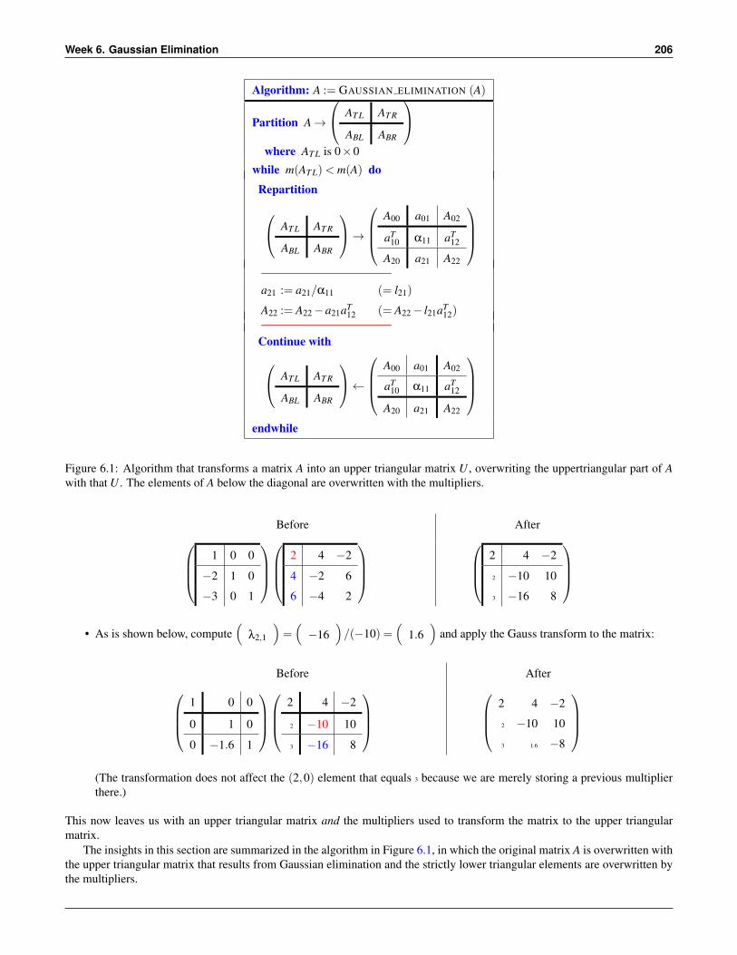
Figure 6.1: Algorithm that transforms a matrix A into an upper triangular matrix U , overwriting the uppertriangular part of Awith that U . The elements of A below the diagonal are overwritten with the multipliers.
Before After1 0 0
−2 1 0
−3 0 1
2 4 −2
4 −2 6
6 −4 2
2 4 −2
2 −10 10
3 −16 8
• As is shown below, compute
(λ2,1
)=(−16
)/(−10) =
(1.6
)and apply the Gauss transform to the matrix:
Before After1 0 0
0 1 0
0 −1.6 1
2 4 −2
2 −10 10
3 −16 8
2 4 −2
2 −10 10
3 1.6 −8
(The transformation does not affect the (2,0) element that equals 3 because we are merely storing a previous multiplierthere.)
This now leaves us with an upper triangular matrix and the multipliers used to transform the matrix to the upper triangularmatrix.
The insights in this section are summarized in the algorithm in Figure 6.1, in which the original matrix A is overwritten withthe upper triangular matrix that results from Gaussian elimination and the strictly lower triangular elements are overwritten bythe multipliers.

6.2. Gaussian Elimination 207
Algorithm: b := FORWARD SUBSTITUTION(A,b)
Partition A→
AT L AT R
ABL ABR
, b→
bT
bB
where AT L is 0×0, bT has 0 rows
while m(AT L)< m(A) do
Repartition AT L AT R
ABL ABR
→
A00 a01 A02
aT10 α11 aT
12
A20 a21 A22
,
bT
bB
→
b0
β1
b2
b2 := b2−β1a21 (= b2−β1l21)
Continue with AT L AT R
ABL ABR
←
A00 a01 A02
aT10 α11 aT
12
A20 a21 A22
,
bT
bB
←
b0
β1
b2
endwhile
Figure 6.2: Algorithm that applies the multipliers (stored in the elements of A below the diagonal) to a right-hand side vector b.
Forward substitution (applying the transforms to the right-hand side)
We now take the transforms (multipliers) that were computed during Gaussian Elimination (and stored over the zeroes) andapply them to the right-hand side vector.
• Subtract λ1,0 = 2 times the first component from the second component and subtract λ2,0 = 3 times the first componentfrom the third component:
Before After1 0 0
−2 1 0
−3 0 1
−10
20
18
−10
40
48
• Subtract λ2,1 = 1.6 times the second component from the third component:
Before After1 0 0
0 1 0
0 −1.6 1
−10
40
48
−10
40
−16
The important thing to realize is that this updates the right-hand side exactly as the appended column was updated in the
last unit. This process is often referred to as forward substitution.The above observations motivate the algorithm for forward substitution in Figure 6.2.

Week 6. Gaussian Elimination 208
Back substitution (solve the upper triangular system)
As before.
Check your answer (ALWAYS!)
As before.
Homework 6.2.5.1 Implement the algorithms in Figures 6.1 and 6.2
• [ A out ] = GaussianElimination( A )
• [ b out ] = ForwardSubstitution( A, b )
You can check that they compute the right answers with the following script:
• test GausianElimination.m
This script exercises the functions by factoring the matrix
A = [2 0 1 2
-2 -1 1 -14 -1 5 4
-4 1 -3 -8]
by calling
LU = GaussianElimination( A )
Next, solve Ax = b where
b = [22
11-3
]
by first apply forward substitution to b, using the output matrix LU:
bhat = ForwardSubstitution( LU, b )
extracting the upper triangular matrix U from LU:
U = triu( LU )
and then solving Ux = b (which is equivalent to backward substitution) with the MATLAB intrinsic function:
x = U \ bhat
Finally, check that you got the right answer:
b - A * x
(the result should be a zero vector with four elements).
6.3. Solving Ax = b via LU Factorization 209
6.3 Solving Ax = b via LU Factorization
6.3.1 LU factorization (Gaussian elimination)
* View at edXIn this unit, we will use the insights into how blocked matrix-matrix and matrix-vector multiplication works to derive and
state algorithms for solving linear systems in a more concise way that translates more directly into algorithms.The idea is that, under circumstances to be discussed later, a matrix A ∈ Rn×n can be factored into the product of two
matrices L,U ∈ Rn×n:A = LU,
where L is unit lower triangular and U is upper triangular.Assume A ∈ Rn×n is given and that L and U are to be computed such that A = LU , where L ∈ Rn×n is unit lower triangular
and U ∈ Rn×n is upper triangular. We derive an algorithm for computing this operation by partitioning
A→
α11 aT12
a21 A22
, L→
1 0
l21 L22
, and U →
υ11 uT12
0 U22
.
Now, A = LU implies (using what we learned about multiplying matrices that have been partitioned into submatrices)
A︷ ︸︸ ︷ α11 aT12
a21 A22
=
L︷ ︸︸ ︷ 1 0
l21 L22
U︷ ︸︸ ︷ υ11 uT
12
0 U22
=
LU︷ ︸︸ ︷ 1×υ11 +0×0 1×uT12 +0×U22
l21υ11 +L22×0 l21uT12 +L22U22
.
=
LU︷ ︸︸ ︷ υ11 uT12
l21υ11 l21uT12 +L22U22
.
For two matrices to be equal, their elements must be equal, and therefore, if they are partitioned conformally, their submatricesmust be equal:
α11 = υ11 aT12 = uT
12
a21 = l21υ11 A22 = l21uT12 +L22U22
or, rearranging,υ11 = α11 uT
12 = aT12
l21 = a21/υ11 L22U22 = A22− l21uT12
.
This suggests the following steps for overwriting a matrix A with its LU factorization:
• Partition
A→
α11 aT12
a21 A22
.
• Update a21 = a21/α11(= l21). (Scale a21 by 1/α11!)

Week 6. Gaussian Elimination 210
Algorithm: A := LU UNB VAR5(A)
Partition A→
AT L AT R
ABL ABR
whereAT L is 0×0
while m(AT L)< m(A) do
Repartition AT L AT R
ABL ABR
→
A00 a01 A02
aT10 α11 aT
12
A20 a21 A22
whereα11 is 1×1
a21 := a21/α11 (= l21)
A22 := A22−a21aT12 (= A22− l21aT
12)
Continue with AT L AT R
ABL ABR
←
A00 a01 A02
aT10 α11 aT
12
A20 a21 A22
endwhile
Figure 6.3: LU factorization algorithm.
• Update A22 = A22−a21aT12(= A22− l21uT
12) (Rank-1 update!).
• Overwrite A22 with L22 and U22 by repeating with A = A22.
This will leave U in the upper triangular part of A and the strictly lower triangular part of L in the strictly lower triangular partof A. The diagonal elements of L need not be stored, since they are known to equal one.
The above can be summarized in Figure 6.14. If one compares this to the algorithm GAUSSIAN ELIMINATION we arrivedat in Unit 6.2.5, you find they are identical! LU factorization is Gaussian elimination.
We illustrate in Fgure 6.4 how LU factorization with a 3×3 matrix proceeds. Now, compare this to Gaussian eliminationwith an augmented system, in Figure 6.5. It should strike you that exactly the same computations are performed with thecoefficient matrix to the left of the vertical bar.

6.3. Solving Ax = b via LU Factorization 211
Step
A00 a01 A02
aT10 α11 aT
12
A20 a21 A22
a21/α11 A22−a21aT12
1-2
−2 −1 1
2 −2 −3
−4 4 7
2
−4
/(−2) =
−1
2
−2 −3
4 7
−−1
2
(−1 1)
=
−3 −2
6 5
3
−2 −1 1
−1 −3 −2
2 6 5
(6)/(−3) =
(−2) (
5)−(−2) (−2)
=(
1)
−2 −1 1
−1 −3 −2
2 −2 1
Figure 6.4: LU factorization with a 3×3 matrix
Step Current system Multiplier Operation
1
−2 −1 1 6
2 −2 −3 3
−4 4 7 −3
2−2 =−1
2 −2 −3 3
−1×(−2 −1 1 6)
0 −3 −2 9
2
−2 −1 1 6
0 −3 −2 9
−4 4 7 −3
−4−2 = 2
−4 4 7 −3
−(2)×(−2 −1 1 6)
0 6 5 −15
3
−2 −1 1 6
0 −3 −2 9
0 6 5 −15
6−3 =−2
0 6 5 −15
−(−2)×(0 −3 −2 9)
0 0 1 3
4
−2 −1 1 6
0 −3 −2 9
0 0 1 3
Figure 6.5: Gaussian elimination with an augmented system.

Week 6. Gaussian Elimination 212
Homework 6.3.1.1 Implement the algorithm in Figures 6.4.
• [ A out ] = LU unb var5( A )
You can check that they compute the right answers with the following script:
• test LU unb var5.m
This script exercises the functions by factoring the matrix
A = [2 0 1 2
-2 -1 1 -14 -1 5 4
-4 1 -3 -8]
by calling
LU = LU_unb_var5( A )
Next, it extracts the unit lower triangular matrix and upper triangular matrix:
L = tril( LU, -1 ) + eye( size( A ) )
U = triu( LU )
and checks if the correct factors were computed:
A - L * U
which should yield a 4×4 zero matrix.
Homework 6.3.1.2 Compute the LU factorization of1 −2 2
5 −15 8
−2 −11 −11
.
6.3.2 Solving Lz = b (Forward substitution)
* View at edX
Next, we show how forward substitution is the same as solving the linear system Lz = b where b is the right-hand side andL is the matrix that resulted from the LU factorization (and is thus unit lower triangular, with the multipliers from GaussianElimination stored below the diagonal).
Given a unit lower triangular matrix L ∈Rn×n and vectors z,b ∈Rn, consider the equation Lz = b where L and b are knownand z is to be computed. Partition
L→
1 0
l21 L22
, z→
ζ1
z2
, and b→
β1
b2
.

6.3. Solving Ax = b via LU Factorization 213
Algorithm: [b] := LTRSV UNB VAR1(L,b)
Partition L→
LT L 0
LBL LBR
, b→
bT
bB
whereLT L is 0×0, bT has 0 rows
while m(LT L)< m(L) do
Repartition LT L 0
LBL LBR
→
L00 0 0
lT10 λ11 0
L20 l21 L22
,
bT
bB
→
b0
β1
b2
whereλ11 is 1×1 , β1 has 1 row
b2 := b2−β1l21
Continue with LT L 0
LBL LBR
←
L00 0 0
lT10 λ11 0
L20 l21 L22
,
bT
bB
←
b0
β1
b2
endwhile
Figure 6.6: Algorithm for solving Lx = b, overwriting b with the result vector x. Here L is a lower triangular matrix.
(Recall: the horizontal line here partitions the result. It is not a division.) Now, Lz = b implies that
b︷ ︸︸ ︷ β1
b2
=
L︷ ︸︸ ︷ 1 0
l21 L22
z︷ ︸︸ ︷ ζ1
z2
=
Lz︷ ︸︸ ︷ 1×ζ1 +0× z2
l21ζ1 +L22z2
=
Lz︷ ︸︸ ︷ ζ1
l21ζ1 +L22z2
so that
β1 = ζ1
b2 = l21ζ1 +L22z2or, equivalently,
ζ1 = β1
L22z2 = b2−ζ1l21.
This suggests the following steps for overwriting the vector b with the solution vector z:
• Partition
L→
1 0
l21 L22
and b→
β1
b2
• Update b2 = b2−β1l21 (this is an AXPY operation!).

Week 6. Gaussian Elimination 214
• Continue with L = L22 and b = b2.
This motivates the algorithm in Figure 6.15. If you compare this algorithm to FORWARD SUBSTITUTION in Unit 6.2.5, youfind them to be the same algorithm, except that matrix A has now become matrix L! So, solving Lz = b, overwriting b with z,is forward substitution when L is the unit lower triangular matrix that results from LU factorization.
We illustrate solving Lz = b in Figure 6.8. Compare this to forward substitution with multipliers stored below the diagonalafter Gaussian elimination, in Figure ??.
Homework 6.3.2.1 Implement the algorithm in Figure 6.15.
• [ b out ] = Ltrsv unb var1( L, b )
You can check that they compute the right answers with the following script:
• test Ltrsv unb var1.m
This script exercises the function by setting the matrix
L = [1 0 0 0
-1 1 0 02 1 1 0
-2 -1 1 1]
and solving Lx = b with the right-hand size vector
b = [22
11-3
]
by calling
x = Ltrsv_unb_var1( L, b )
Finally, it checks if x is indeed the answer by checking if
b - L * x
equals the zero vector.
x = U \ z
We can the check if this solves Ax = b by computing
b - A * x
which should yield a zero vector.
6.3.3 Solving Ux = b (Back substitution)
* View at edXNext, let us consider how to solve a linear system Ux = b. We will conclude that the algorithm we come up with is the same
as backward substitution.

6.3. Solving Ax = b via LU Factorization 215
Step
L00 0 0
lT10 λ11 0
L20 l21 L22
b0
β1
b2
b2− l21β1
1-2
1 0 0
−1 1 0
2 −2 1
6
3
−3
3
−3
−−1
2
(6) =
9
−15
3
1 0 0
−1 1 0
2 −2 1
6
9
−15
(−15
)−(−2)(9) = (3)
1 0 0
−1 1 0
2 −2 1
6
9
3
Figure 6.7: Solving Lz = b where L is a unit lower triangular matrix. Vector z overwrites vector b.
StepStored multipliers
and right-hand side Operation
1
− − − 6
−1 − − 3
2 −2 − −3
3
−(−1)×( 6)
9
2
− − − 6
−1 − − 9
2 −2 − −3
−3
−(2)×( 6)
−15
3
− − − 6
−1 − − 9
2 −2 − −15
−15
−(−2)×( 9)
3
4
− − − 6
−1 − − 9
2 -2 − 3
Figure 6.8: Forward substitutions with multipliers stored below the diagonal (e.g., as output from Gaussian Elimination).

Week 6. Gaussian Elimination 216
Given upper triangular matrix U ∈Rn×n and vectors x,b ∈Rn, consider the equation Ux = b where U and b are known andx is to be computed. Partition
U →
υ11 uT12
0 U22
, x→
χ1
x2
and b→
β1
b2
.
Now, Ux = b implies
b︷ ︸︸ ︷ β1
b2
=
U︷ ︸︸ ︷ υ11 uT12
0 U22
x︷ ︸︸ ︷ χ1
x2
=
Ux︷ ︸︸ ︷ υ11χ1 +uT12x2
0×χ1 +U22x2
=
Ux︷ ︸︸ ︷ υ11χ1 +uT12x2
U22x2
so that
β1 = υ11χ1 +uT12x2
b2 =U22x2or, equivalently,
χ1 = (β1−uT12x2)/υ11
U22x2 = b2.
This suggests the following steps for overwriting the vector b with the solution vector x:
• Partition
U →
υ11 uT12
0 U22
, and b→
β1
b2
• Solve U22x2 = b2 for x2, overwriting b2 with the result.
• Update β1 = (β1−uT12b2)/υ11(= (β1−uT
12x2)/υ11).(This requires a dot product followed by a scaling of the result by 1/υ11.)
This suggests the following algorithm: Notice that the algorithm does not have “Solve U22x2 = b2” as an update. The reason isthat the algorithm marches through the matrix from the bottom-right to the top-left and through the vector from bottom to top.Thus, for a given iteration of the while loop, all elements in x2 have already been computed and have overwritten b2. Thus, the“Solve U22x2 = b2” has already been accomplished by prior iterations of the loop. As a result, in this iteration, only β1 needsto be updated with χ1 via the indicated computations.
Homework 6.3.3.1 Side-by-side, solve the upper triangular linear system
−2χ0− χ1+ χ2= 6
−3χ1−2χ2= 9
χ2= 3
via back substitution and by executing the above algorithm with
U =
−2 −1 1
0 −3 −2
0 0 1
and b =
6
9
3
.
Compare and contrast!

6.3. Solving Ax = b via LU Factorization 217
Algorithm: [b] := UTRSV UNB VAR1(U,b)
Partition U →
UT L UT R
UBL UBR
, b→
bT
bB
where UBR is 0×0, bB has 0 rows
while m(UBR)< m(U) do
Repartition UT L UT R
0 UBR
→
U00 u01 U02
0 υ11 uT12
0 0 U22
,
bT
bB
→
b0
β1
b2
β1 := β1−uT
12b2
β1 := β1/υ11
Continue with UT L UT R
0 UBR
←
U00 u01 U02
0 υ11 uT12
0 0 U22
,
bT
bB
←
b0
β1
b2
endwhile
Figure 6.9: Algorithm for solving Ux = b where U is an uppertriangular matrix. Vector b is overwritten with the result vectorx.
Homework 6.3.3.2 Implement the algorithm in Figure 6.16.
• [ b out ] = Utrsv unb var1( U, b )
You can check that it computes the right answer with the following script:
• test Utrsv unb var1.m
This script exercises the function by starting with matrix
U = [2 0 1 20 -1 2 10 0 1 -10 0 0 -2
]
Next, it solves Ux = b with the right-hand size vector
b = [2432
]
by calling
x = Utrsv_unb_var1( U, b )
Finally, it checks if x indeed solves Ux = b by computing
b - U * x
which should yield a zero vector of size four.

Week 6. Gaussian Elimination 218
6.3.4 Putting it all together to solve Ax = b
* View at edXNow, the week started with the observation that we would like to solve linear systems. These could then be written more
concisely as Ax = b, where n×n matrix A and vector b of size n are given, and we would like to solve for x, which is the vectorsof unknowns. We now have algorithms for
• Factoring A into the product LU where L is unit lower triangular;
• Solving Lz = b; and
• Solving Ux = b.
We now discuss how these algorithms (and functions that implement them) can be used to solve Ax = b.Start with
Ax = b.
If we have L and U so that A = LU , then we can replace A with LU :
(LU)︸ ︷︷ ︸A
x = b.
Now, we can treat matrices and vectors alike as matrices, and invoke the fact that matrix-matrix multiplication is associative toplace some convenient parentheses:
L(Ux) = b.
We can then recognize that Ux is a vector, which we can call z:
L (Ux)︸︷︷︸z
= b
so that
Lz = b and Ux = z.
Thus, the following steps will solve Ax = b:
• Factor A into L and U so that A = LU (LU factorization).
• Solve Lz = b for z (forward substitution).
• Solve Ux = z for x (back substitution).
This works if A has the right properties for the LU factorization to exist, which is what we will discuss next week...

6.3. Solving Ax = b via LU Factorization 219
Homework 6.3.4.1 Implement the function
• [ A out, b out ] = Solve( A, b )
that
• Computes the LU factorization of matrix A, A = LU , overwriting the upper triangular part of A with U andthe strictly lower triangular part of A with the strictly lower triangular part of L. The result is then returnedin variable A out.
• Uses the factored matrix to solve Ax = b.
Use the routines you wrote in the previous subsections (6.3.1-6.3.3).You can check that it computes the right answer with the following script:
• test Solve.m
This script exercises the function by starting with matrix
A = [2 0 1 2
-2 -1 1 -14 -1 5 4
-4 1 -3 -8]
Next, it solves Ax = b with
b = [22
11-3
]
by calling
x = Solve( A, b )
Finally, it checks if x indeed solves Ax = b by computing
b - A * x
which should yield a zero vector of size four.
6.3.5 Cost
* View at edX
LU factorization
Let’s look at how many floating point computations are needed to compute the LU factorization of an n× n matrix A. Let’sfocus on the algorithm:
Assume that during the kth iteration AT L is k× k. Then
• A00 is a k× k matrix.

Week 6. Gaussian Elimination 220
Algorithm: A := LU UNB VAR5(A)
Partition A→
AT L AT R
ABL ABR
whereAT L is 0×0
while m(AT L)< m(A) do
Repartition AT L AT R
ABL ABR
→
A00 a01 A02
aT10 α11 aT
12
A20 a21 A22
whereα11 is 1×1
a21 := a21/α11 (= l21)
A22 := A22−a21aT12 (= A22− l21aT
12)
Continue with AT L AT R
ABL ABR
←
A00 a01 A02
aT10 α11 aT
12
A20 a21 A22
endwhile
Figure 6.10: LU factorization algorithm.
• a21 is a column vector of size n− k−1.
• aT12 is a row vector of size n− k−1.
• A22 is a (n− k−1)× (n− k−1) matrix.
Now,
• a21/α11 is typically implemented as (1/α11)× a21 so that only one division is performed (divisions are EXPENSIVE)and (n− k−1) multiplications are performed.
• A22 := A22−a21aT12 is a rank-1 update. In a rank-1 update, for each element in the matrix one multiply and one add (well,
subtract in this case) is performed, for a total of 2(n− k−1)2 floating point operations.
Now, we need to sum this over all iterations k = 0, . . . ,(n−1):
n−1
∑k=0
((n− k−1)+2(n− k−1)2) floating point operations.
Here we ignore the divisions. Clearly, there will only be n of those (one per iteration of the algorithm).

6.3. Solving Ax = b via LU Factorization 221
Let us compute how many flops this equals.
∑n−1k=0
((n− k−1)+2(n− k−1)2
)= < Change of variable: p = n− k− 1 so that p = 0 when k = n− 1 and
p = n−1 when k = 0 >
∑0p=n−1
(p+2p2
)= < Sum in reverse order >
∑n−1p=0
(p+2p2
)= < Split into two sums >
∑n−1p=0 p+∑
n−1p=0(2p2)
= < Results from Week 2! >(n−1)n
2 +2 (n−1)n(2n−1)6
= < Algebra >3(n−1)n
6 +2 (n−1)n(2n−1)6
= < Algebra >(n−1)n(4n+1)
6
Now, when n is large n−1 and 4n+1 equal, approximately, n and 4n, respectively, so that the cost of LU factorization equals,approximately,
23
n3 flops.
Forward substitution
Next, let us look at how many flops are needed to solve Lx = b. Again, focus on the algorithm: Assume that during the kthiteration LT L is k× k. Then
• L00 is a k× k matrix.
• l21 is a column vector of size n− k−1.
• b2 is a column vector of size n− k−1.
Now,
• The axpy operation b2 := b2−β1l21 requires 2(n− k−1) flops since the vectors are of size n− k−1.
We need to sum this over all iterations k = 0, . . . ,(n−1):
n−1
∑k=0
(n− k−1) flops.
Let us compute how many flops this equals:
∑n−1k=0 2(n− k−1)
= < Factor out 2 >
2∑n−1k=0(n− k−1)
= < Change of variable: p = n− k− 1 so that p = 0 when k = n− 1 andp = n−1 when k = 0 >
2∑0p=n−1 2p
= < Sum in reverse order >

Week 6. Gaussian Elimination 222
Algorithm: [b] := LTRSV UNB VAR1(L,b)
Partition L→
LT L 0
LBL LBR
, b→
bT
bB
whereLT L is 0×0, bT has 0 rows
while m(LT L)< m(L) do
Repartition LT L 0
LBL LBR
→
L00 0 0
lT10 λ11 0
L20 l21 L22
,
bT
bB
→
b0
β1
b2
whereλ11 is 1×1 , β1 has 1 row
b2 := b2−β1l21
Continue with LT L 0
LBL LBR
←
L00 0 0
lT10 λ11 0
L20 l21 L22
,
bT
bB
←
b0
β1
b2
endwhile
Figure 6.11: Algorithm for solving Lx = b, overwriting b with the result vector x. Here L is a lower triangular matrix.
2∑n−1p=0 p
= < Results from Week 2! >
2 (n−1)n2
= < Algebra >
(n−1)n.
Now, when n is large n−1 equals, approximately, n so that the cost for the forward substitution equals, approximately,
n2 flops.
Back substitution
Finally, let us look at how many flops are needed to solve Ux = b. Focus on the algorithm:
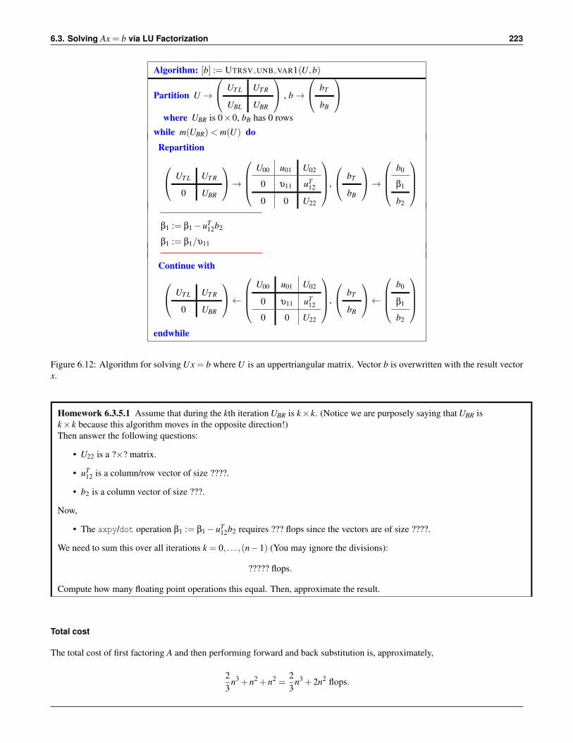
6.3. Solving Ax = b via LU Factorization 223
Algorithm: [b] := UTRSV UNB VAR1(U,b)
Partition U →
UT L UT R
UBL UBR
, b→
bT
bB
where UBR is 0×0, bB has 0 rows
while m(UBR)< m(U) do
Repartition UT L UT R
0 UBR
→
U00 u01 U02
0 υ11 uT12
0 0 U22
,
bT
bB
→
b0
β1
b2
β1 := β1−uT
12b2
β1 := β1/υ11
Continue with UT L UT R
0 UBR
←
U00 u01 U02
0 υ11 uT12
0 0 U22
,
bT
bB
←
b0
β1
b2
endwhile
Figure 6.12: Algorithm for solving Ux = b where U is an uppertriangular matrix. Vector b is overwritten with the result vectorx.
Homework 6.3.5.1 Assume that during the kth iteration UBR is k×k. (Notice we are purposely saying that UBR isk× k because this algorithm moves in the opposite direction!)Then answer the following questions:
• U22 is a ?×? matrix.
• uT12 is a column/row vector of size ????.
• b2 is a column vector of size ???.
Now,
• The axpy/dot operation β1 := β1−uT12b2 requires ??? flops since the vectors are of size ????.
We need to sum this over all iterations k = 0, . . . ,(n−1) (You may ignore the divisions):
????? flops.
Compute how many floating point operations this equal. Then, approximate the result.
Total cost
The total cost of first factoring A and then performing forward and back substitution is, approximately,
23
n3 +n2 +n2 =23
n3 +2n2 flops.

Week 6. Gaussian Elimination 224
When n is large n2 is very small relative to n3 and hence the total cost is typically given as
23
n3 flops.
Notice that this explains why we prefer to do the LU factorization separate from the forward and back substitutions. If wesolve Ax = b via these three steps, and afterwards a new right-hand side b comes along with which we wish to solve, thenwe need not refactor A since we already have L and U (overwritten in A). But it is the factorization of A where most of theexpense is, so solving with this new right-hand side is almost free.
6.4 Enrichment
6.4.1 Blocked LU Factorization
What you saw in Week 5, Units 5.4.1 and 5.4.2, was that by carefully implementing matrix-matrix multiplication, the perfor-mance of this operation could be improved from a few percent of the peak of a processor to better than 90%. This came at aprice: clearly the implementation was not nearly as “clean” and easy to understand as the routines that you wrote so far in thiscourse.
Imagine implementing all the operations you have encountered so far in this way. When a new architecture comes along,you will have to reimplement to optimize for that architecture. While this guarantees job security for those with the skill andpatience to do this, it quickly becomes a distraction from more important work.
So, how to get around this problem? Widely used linear algebra libraries like LAPACK (written in Fortran)
E. Anderson, Z. Bai, C. Bischof, L. S. Blackford, J. Demmel, Jack J. Dongarra, J. Du Croz, S. Hammarling, A.Greenbaum, A. McKenney, and D. Sorensen.LAPACK Users’ guide (third ed.).SIAM, 1999.
and the libflame library (developed as part of our FLAME project and written in C)
F. G. Van Zee, E. Chan, R. A. van de Geijn, E. S. Quintana-Orti, G. Quintana-Orti.The libflame Library for Dense Matrix Computations.IEEE Computing in Science and Engineering, Vol. 11, No 6, 2009.
F. G. Van Zee.libflame: The Complete Reference.www.lulu.com , 2009
implement many linear algebra operations so that most computation is performed by a call to a matrix-matrix multiplicationroutine. The libflame library is coded with an API that is very similar to the FLAME@lab API that you have been using foryour routines.
More generally, in the scientific computing community there is a set of operations with a standardized interface known asthe Basic Linear Algebra Subprograms (BLAS) in terms of which applications are written.
C. L. Lawson, R. J. Hanson, D. R. Kincaid, F. T. Krogh.Basic Linear Algebra Subprograms for Fortran Usage.ACM Transactions on Mathematical Software, 1979.
J. J. Dongarra, J. Du Croz, S. Hammarling, R. J. Hanson.An Extended Set of FORTRAN Basic Linear Algebra Subprograms.ACM Transactions on Mathematical Software, 1988.
J. J. Dongarra, J. Du Croz, S. Hammarling, I. Duff.A Set of Level 3 Basic Linear Algebra Subprograms.ACM Transactions on Mathematical Software, 1990.
F. G. Van Zee, R. A. van de Geijn.BLIS: A Framework for Rapid Instantiation of BLAS Functionality.ACM Transactions on Mathematical Software, to appear.

6.4. Enrichment 225
It is then expected that someone optimizes these routines. When they are highly optimized, any applications and librarieswritten in terms of these routines also achieve high performance.
In this enrichment, we show how to cast LU factorization so that most computation is performed by a matrix-matrixmultiplication. Algorithms that do this are called blocked algorithms.
Blocked LU factorization
It is difficult to describe how to attain a blocked LU factorization algorithm by starting with Gaussian elimination as we did inSection 6.2, but it is easy to do so by starting with A = LU and following the techniques exposed in Unit 6.3.1.
We start again by assuming that matrix A ∈ Rn×n can be factored into the product of two matrices L,U ∈ Rn×n, A = LU ,where L is unit lower triangular and U is upper triangular. Matrix A ∈ Rn×n is given and that L and U are to be computed suchthat A = LU , where L ∈ Rn×n is unit lower triangular and U ∈ Rn×n is upper triangular.
We derive a blocked algorithm for computing this operation by partitioning
A→
A11 A12
A21 A22
, L→
L11 0
L21 L22
, and U →
U11 U12
0 U22
,
where A11,L11,U11 ∈ Rb×b. The integer b is the block size for the algorithm. In Unit 6.3.1, b = 1 so that A11 = α11, L11 = 1,and so forth. Here, we typically choose b > 1 so that L11 is a unit lower triangular matrix and U11 is an upper triangular matrix.How to choose b is closely related to how to optimize matrix-matrix multiplication (Units 5.4.1 and 5.4.2).
Now, A = LU implies (using what we learned about multiplying matrices that have been partitioned into submatrices)
A︷ ︸︸ ︷ A11 A12
A21 A22
=
L︷ ︸︸ ︷ L11 0
L21 L22
U︷ ︸︸ ︷ U11 U12
0 U22
=
LU︷ ︸︸ ︷ L11×U11 +0×0 L11×U12 +0×U22
L21×U11 +L22×0 L21×U12 +L22×U22
.
=
LU︷ ︸︸ ︷ L11U11 L11U12
L21U11 L21U12 +L22U22
.
For two matrices to be equal, their elements must be equal and therefore, if they are partitioned conformally, their submatricesmust be equal:
A11 = L11U11 A12 = L11U12
A21 = L21U11 A22 = L21U12 +L22U22
or, rearranging,A11 = L11U11 A12 = L11U12
A21 = L21U11 A22−L21U12 = L22U22
This suggests the following steps for overwriting a matrix A with its LU factorization:
• Partition
A→
A11 A12
A21 A22
.
• Compute the LU factorization of A11: A11→ L11U11. Overwrite A11 with this factorization.Note: one can use an unblocked algorithm for this.

Week 6. Gaussian Elimination 226
• Now that we know L11, we can solve L11U12 = A12, where L11 and A12 are given. U12 overwrites A12.This is known as an triangular solve with multiple right-hand sides. More on this later in this unit.
• Now that we know U11 (still from the first step), we can solve L21U11 = A21, where U11 and A21 are given. L21 overwritesA21.This is also known as a triangular solve with multiple right-hand sides. More on this also later in this unit.
• Update A22 = A22−A21A12(= A22−L21U12).This is a matrix-matrix multiplication and is where, if b is small relative to n, most of the computation is performed.
• Overwrite A22 with L22 and U22 by repeating the above steps with A = A22.
This will leave U in the upper triangular part of A and the strictly lower triangular part of L in the strictly lower triangular partof A. The diagonal elements of L need not be stored, since they are known to equal one.
The above is summarized in Figure 6.13. In that figure, the derivation of the unblocked algorithm from Unit 6.3.1 is givenon the left and the above derivation of the blocked algorithm is given on the right, for easy comparing and contrasting. Theresulting algorithms, in FLAME notation, are given as well. It is important to note that the algorithm now progresses b rowsand b columns at a time, since A11 is a b×b block.
Triangular solve with multiple right-hand sides
In the above algorithm, we needed to perform two subproblems:
• L11U12 = A12 where unit lower triangular matrix L11 and (general) matrix A12 are known and (general) matrix U12 is tobe computed; and
• L21U11 = A21 where upper triangular matrix U11 and (general) matrix A21 are known and (general) matrix L21 is to becomputed.
These operations are known as special cases of the “triangular solve with multiple right-hand side” operation.Let’s simplify the discussion to solving LX = B where L is unit lower triangular and X and B are general matrices. Here L
and B are known and X is to be computed. We slice and dice B and X into columns to observe that
L(
x0 x1 · · ·)=(
b0 b1 · · ·)
and hence (Lx0 Lx1 · · ·
)=(
b0 b1 · · ·).
We therefore conclude that Lx j = b j for all pairs of columns x j and b j. But that means that to compute x j from L and b j we needto solve with a unit lower triangular matrix L. Thus the name “triangular solve with multiple right-hand sides”. The multipleright-hand sides are the columns b j.
Now let us consider solving XU = B, where U is upper triangular. If we transpose both sides, we get that (XU)T = BT orUT XT = BT . If we partition X and B by columns so that
X =
xT
0
xT1...
and B =
bT
0
bT1...
,
then
UT(
x0 x1 · · ·)=(
UT x0 UT x1 · · ·)=(
b0 b1 · · ·).
We notice that this, again, is a matter of solving multiple right-hand sides (now rows of B that have been transposed) with alower triangular matrix (UT ). In practice, none of the matrices are transposed.

6.4. Enrichment 227
Unblocked algorithm Blocked algorithm
A→
α11 aT12
a21 A22
,L→
1 0
l21 L22
,U →
υ11 uT12
0 U22
A→
A11 A12
A21 A22
,L→
L11 0
L21 L22
,U →
U11 U12
0 U22
α11 aT
12
a21 A22
=
1 0
l21 L22
υ11 uT12
0 U22
︸ ︷︷ ︸ υ11 uT
12
l21υ11 l21uT12 +L22U22
A11 A12
A21 A22
=
L11 0
L21 L22
U11 U12
0 U22
︸ ︷︷ ︸ L11U11 L11U12
L21U11 L21UT12 +L22U22
α11 = υ11 aT
12 = uT12
a21 = l21υ11 A22 = l21uT12 +L22U22
A11 = L11U11 A12 = L11U12
A21 = L21U11 A22 = L21U12 +L22U22
α11 := α11
aT12 := aT
12
a21 := a21/α11
A22 := A22−a21aT12
A11→ L11U11 (overwriting A11 with L11 and U11)
Solve L11U12 := A12 (overwiting A12 with U12)
Solve U21U11 := A21 (overwiting A21 with U21)
A22 := A22−A21A12
Algorithm: [A] := LU UNB VAR5(A)
Partition A→
AT L AT R
ABL ABR
where AT L is 0×0
while m(AT L)< m(A) doRepartition
AT L AT R
ABL ABR
→
A00 a01 A02
aT10 α11 aT
12
A20 a21 A22
a21 := a21/α11
A22 := A22−a21aT12
Continue with
AT L AT R
ABL ABR
←
A00 a01 A02
aT10 α11 aT
12
A20 a21 A22
endwhile
Algorithm: [A] := LU BLK VAR5(A)
Partition A→
AT L AT R
ABL ABR
where AT L is 0×0
while m(AT L)< m(A) doRepartition
AT L AT R
ABL ABR
→
A00 A01 A02
A10 A11 A12
A20 A21 A22
Factor A11→ L11U11 (Overwrite A11)
Solve L11U12 = A12 (Overwrite A12)
Solve L21U11 = A21 (Overwrite A21)
A22 := A22−A21A12
Continue with
AT L AT R
ABL ABR
←
A00 A01 A02
A10 A11 A12
A20 A21 A22
endwhile
Figure 6.13: Side-by-side derivation of the unblocked and blocked algorithms.

Week 6. Gaussian Elimination 228
Cost analysis
Let us analyze where computation is spent in just the first step of a blocked LU factorization. We will assume that A is n× nand that a block size of b is used:
• Partition
A→
A11 A12
A21 A22
.
This carries no substantial cost, since it just partitions the matrix.
• Compute the LU factorization of A11: A11→ L11U11. Overwrite A11 with this factorization.One can use an unblocked algorithm for this and we saw that the cost of that algorithm, for a b×b matrix, is approximately23 b3.
• Now that we know L11, we can solve L11U12 = A12, where L11 and A12 are given. U12 overwrites A12.This is a triangular solve with multiple right-hand sides with a matrix A12 that is b× (n−b). Now, each triangular solvewith each column of A12 costs, approximately, b2 flops for a total of b2(n−b) flops.
• Now that we know U11, we can solve L21U11 = A21, where U11 and A21 are given. L21 overwrites A21.This is a triangular solve with multiple right-hand sides with a matrix A21 that is (n−b)×b. Now, each triangular solvewith each row of A21 costs, approximately, b2 flops for a total of b2(n−b) flops.
• Update A22 = A22−A21A12(= A22−L21U12).This is a matrix-matrix multiplication that multiplies (n−b)×b matrix A21 times b× (n−b) matrix A12 to update A22.This requires b(n−b)2 flops.
• Overwrite A22 with L22 and U22 by repeating with A = A22, in future iterations. We don’t count that here, since we saidwe were only going to analyze the first iteration of the blocked LU factorization.
Now, if n is much larger than b, 23 b3 is small compared to b2(n− b) which is itself small relative to 2b(n− b)2. Thus, if n is
much larger than b, most computational time is spent in the matrix-matrix multiplication A22 := A22−A21A12. Since we sawin the enrichment of Week 5 that such a matrix-matrix multiplication can achieve extremely high performance, the blocked LUfactorization can achieve extremely high performance (if n is large).
It is important to note that the blocked LU factorization algorithm executes exactly the same number of floating pointoperations as does the unblocked algorithm. It just does so in a different order so that matrix-matrix multiplication can beutilized.
More
A large number of algorithms, both unblocked and blocked, that are expressed with our FLAME notation can be found in thefollowing technical report:
P. Bientinesi and R. van de Geijn.Representing Dense Linear Algebra Algorithms: A Farewell to Indices.FLAME Working Note #17. The University of Texas at Austin, Department of Computer Sciences. TechnicalReport TR-2006-10, 2006.
It is available from the FLAME Publications webpage.
6.4.2 How Ordinary Elimination Became Gaussian Elimination
Read
Joseph F. Grcar.How Ordinary Elimination Became Gaussian Elimination.
Cite as
Joseph F. Grcar.How ordinary elimination became Gaussian elimination.Historia Math, 2011.

6.5. Wrap Up 229
6.5 Wrap Up
6.5.1 Homework
There is no additional graded homework. However, we have an additional version of the ”Gaussian Elimination” webpage:
• Practice with four equations in four unknowns.
Now, we always joke that in a standard course on matrix computations the class is asked to solve systems with three equationswith pencil and paper. What defines an honor version of the course is that the class is asked to solve systems with four equationswith pencil and paper...
Of course, there is little insight gained from the considerable extra work. However, here we have webpages that automatemost of the rote work, and hence it IS worthwhile to at least observe how the methodology extends to larger systems. DO NOTDO THE WORK BY HAND. Let the webpage do the work and focus on the insights that you can gain from this.
6.5.2 Summary
Linear systems of equations
A linear system of equations with m equations in n unknowns is given by
α0,0χ0 + α0,1χ1 + · · · + α0,n−1χn−1 = β0
α1,0χ0 + α1,1χ1 + · · · + α1,n−1χn−1 = β1...
......
......
......
...
αm−1,0χ0 + αm−1,1χ1 + · · · + αm−1,n−1χn−1 = βm−1
Variables χ0,χ1, . . . ,χn−1 are the unknowns.This Week, we only considered the case where m = n:
α0,0χ0 + α0,1χ1 + · · · + α0,n−1χn−1 = β0
α1,0χ0 + α1,1χ1 + · · · + α1,n−1χn−1 = β1...
......
......
......
...
αn−1,0χ0 + αn−1,1χ1 + · · · + αn−1,n−1χn−1 = βn−1
Here the αi, js are the coefficients in the linear system. The βis are the right-hand side values.
Basic tools
Solving the above linear system relies on the fact that its solution does not change if
1. Equations are reordered (not used until next week);
2. An equation in the system is modified by subtracting a multiple of another equation in the system from it; and/or
3. Both sides of an equation in the system are scaled by a nonzero.
Gaussian elimination is a method for solving systems of linear equations that employs these three basic rules in an effort toreduce the system to an upper triangular system, which is easier to solve.
Appended matrices
The above system of n linear equations in n unknowns is more concisely represented as an appended matrix:α0,0 α0,1 · · · α0,n−1 β0
α1,0 α1,1 · · · α1,n−1 β1...
......
...
αn−1,0 αn−1,1 · · · αn−1,n−1 βn−1

Week 6. Gaussian Elimination 230
This representation allows one to just work with the coefficients and right-hand side values of the system.
Matrix-vector notation
The linear system can also be represented as Ax = b where
A =
α0,0 α0,1 · · · α0,n−1
α1,0 α1,1 · · · α1,n−1...
......
αn−1,0 αn−1,1 · · · αn−1,n−1
, x =
χ0
χ1...
χn−1
, and
β0
β1...
βn−1
.
Here, A is the matrix of coefficients from the linear system, x is the solution vector, and b is the right-hand side vector.
Gauss transforms
A Gauss transform is a matrix of the form
L j =
I j 0 0 0 · · · 0
0 1 0 0 · · · 0
0 −λ j+1, j 1 0 · · · 0
0 −λ j+2, j 0 1 · · · 0...
......
.... . .
...
0 −λn−1, j 0 0 · · · 1
.
When applied to a matrix (or a vector, which we think of as a special case of a matrix), it subtracts λi, j times the jth row fromthe ith row, for i = j+1, . . . ,n−1. Gauss transforms can be used to express the operations that are inherently performed as partof Gaussian elimination with an appended system of equations.
The action of a Gauss transform on a matrix, A := L jA can be described as follows:
I j 0 0 0 · · · 0
0 1 0 0 · · · 0
0 −λ j+1, j 1 0 · · · 0
0 −λ j+2, j 0 1 · · · 0...
......
.... . .
...
0 −λn−1, j 0 0 · · · 1
A0
aTj
aTj+1...
aTn−1
=
A0
aTj
aTj+1−λ j+1, jaT
j...
aTn−1−λn−1, jaT
j
.
An important observation that was NOT made clear enough this week is that the rows of A are updates with an AXPY!A multiple of the jth row is subtracted from the ith row.
A more concise way to describe a Gauss transforms is
L =
I 0 0
0 1 0
0 −l21 I
.
Now, applying to a matrix A, LA yieldsI 0 0
0 1 0
0 −l21 I
A0
aT1
A2
=
A0
aT1
A2− l21aT1
.
In other words, A2 is updated with a rank-1 update. An important observation that was NOT made clear enough this weekis that a rank-1 update can be used to simultaneously subtract multiples of a row of A from other rows of A.

6.5. Wrap Up 231
Algorithm: A := LU UNB VAR5(A)
Partition A→
AT L AT R
ABL ABR
whereAT L is 0×0
while m(AT L)< m(A) do
Repartition AT L AT R
ABL ABR
→
A00 a01 A02
aT10 α11 aT
12
A20 a21 A22
whereα11 is 1×1
a21 := a21/α11 (= l21)
A22 := A22−a21aT12 (= A22− l21aT
12)
Continue with AT L AT R
ABL ABR
←
A00 a01 A02
aT10 α11 aT
12
A20 a21 A22
endwhile
Figure 6.14: LU factorization algorithm.
Forward substitution
Forward substitution applies the same transformations that were applied to the matrix to a right-hand side vector.
Back(ward) substitution
Backward substitution solves the upper triangular system
α0,0χ0 + α0,1χ1 + · · · + α0,n−1χn−1 = β0
α1,1χ1 + · · · + α1,n−1χn−1 = β1
. . ....
......
αn−1,n−1χn−1 = βn−1
This algorithm overwrites b with the solution x.
LU factorization
The LU factorization factorization of a square matrix A is given by A = LU , where L is a unit lower triangular matrix and U isan upper triangular matrix. An algorithm for computing the LU factorization is given by
This algorithm overwrites A with the matrices L and U . Since L is unit lower triangular, its diagonal needs not be stored.The operations that compute an LU factorization are the same as the operations that are performed when reducing a system
of linear equations to an upper triangular system of equations.

Week 6. Gaussian Elimination 232
Algorithm: [b] := LTRSV UNB VAR1(L,b)
Partition L→
LT L 0
LBL LBR
, b→
bT
bB
whereLT L is 0×0, bT has 0 rows
while m(LT L)< m(L) do
Repartition LT L 0
LBL LBR
→
L00 0 0
lT10 λ11 0
L20 l21 L22
,
bT
bB
→
b0
β1
b2
whereλ11 is 1×1 , β1 has 1 row
b2 := b2−β1l21
Continue with LT L 0
LBL LBR
←
L00 0 0
lT10 λ11 0
L20 l21 L22
,
bT
bB
←
b0
β1
b2
endwhile
Figure 6.15: Algorithm for solving Lx = b, overwriting b with the result vector x. Here L is a lower triangular matrix.
Solving Lz = b
Forward substitution is equivalent to solving a unit lower triangular system Lz = b. An algorithm for this is given by Thisalgorithm overwrites b with the solution z.
Solving Ux = b
Back(ward) substitution is equivalent to solving an upper triangular system Ux = b. An algorithm for this is given by Thisalgorithm overwrites b with the solution x.
Solving Ax = b
If LU factorization completes with an upper triangular matrix U that does not have zeroes on its diagonal, then the followingthree steps can be used to solve Ax = b:
• Factor A = LU .
• Solve Lz = b.
• Solve Ux = z.
Cost
• Factoring A = LU requires, approximately, 23 n3 floating point operations.
• Solve Lz = b requires, approximately, n2 floating point operations.

6.5. Wrap Up 233
Algorithm: [b] := UTRSV UNB VAR1(U,b)
Partition U →
UT L UT R
UBL UBR
, b→
bT
bB
where UBR is 0×0, bB has 0 rows
while m(UBR)< m(U) do
Repartition UT L UT R
0 UBR
→
U00 u01 U02
0 υ11 uT12
0 0 U22
,
bT
bB
→
b0
β1
b2
β1 := β1−uT
12b2
β1 := β1/υ11
Continue with UT L UT R
0 UBR
←
U00 u01 U02
0 υ11 uT12
0 0 U22
,
bT
bB
←
b0
β1
b2
endwhile
Figure 6.16: Algorithm for solving Ux = b where U is an uppertriangular matrix. Vector b is overwritten with the result vectorx.
• Solve Ux = z requires, approximately, n2 floating point operations.

Week 6. Gaussian Elimination 234