A guide to gathering financial data for financial analysis from Mergent Online® Prepared by Pamela Peterson Drake, James Madison University

Table of contents 1.  What is Mergent Online®? ......................................................................................................... 1 2.  Go to the James Madison Libraries’ web page ............................................................................. 2 3.  Select the Mergent Online® database ......................................................................................... 2 4.  Select data from Mergent Online® .............................................................................................. 4 5.  Download the data ................................................................................................................... 7 6.  Get the data ready in Microsoft Excel® ........................................................................................ 8 7.  Calculate ratios ....................................................................................................................... 11 8.  Graph the ratios ..................................................................................................................... 12 

1. What is Mergent Online®? Mergent Online® provides a wealth of financial data on a large number of corporations, both in the U.S. (11,000+ companies) and elsewhere (17,000+ companies). Launched in 2003, Mergent Online is the descendant of Moody’s Manuals, which had been one of the primary providers of financial data for U.S. firms.1 You can find and download up to fifteen years of annual data or fifteen quarters of quarterly data for a company. This data consists of the items reported on the corporation’s income statement, balance sheet, statement of cash flows, and statement of shareholders equity. You can also find financial ratios, other corporation-specific information, and information about competitors. The purpose of this guide is to provide step-by-step instructions on gathering financial data from Mergent Online® using the James Madison University’s libraries and transforming it into a Microsoft Excel® worksheet for analysis. If you are accessing the data from off-campus, you will need to use one of two methods of authenticating your use (see http://www.lib.jmu.edu/proxy/).

1 The Financial Information Services division of Moody’s Investor Service was acquired by Mergent, Inc. in 1998. Mergent, Inc., was acquired in 2004 by Xinhua Finance, a Chinese financial services and media company.

1 of 16

2. Go to the James Madison Libraries’ web page Go to www.jmu.edu and follow the links to the Libraries & Educational Technologies web page:

3. Select the Mergent Online® database Click on the link to “Research Databases & Resources” in the right-hand menu.

2 of 16

Select the letter M in the Databases by Title section.

Click on M and the scroll down until you see the Mergent Online® link:

Select the link and then select the link eenntteerr mmeerrggeenntt oonnlliinnee . You will then see the Search page at Mergent Online®:

3 of 16

4. Select data from Mergent Online® Type in the company’s name or ticker symbol in the left-most data-entry box. For this example, I’ll use Kellogg, which has a ticker symbol of K:

4 of 16

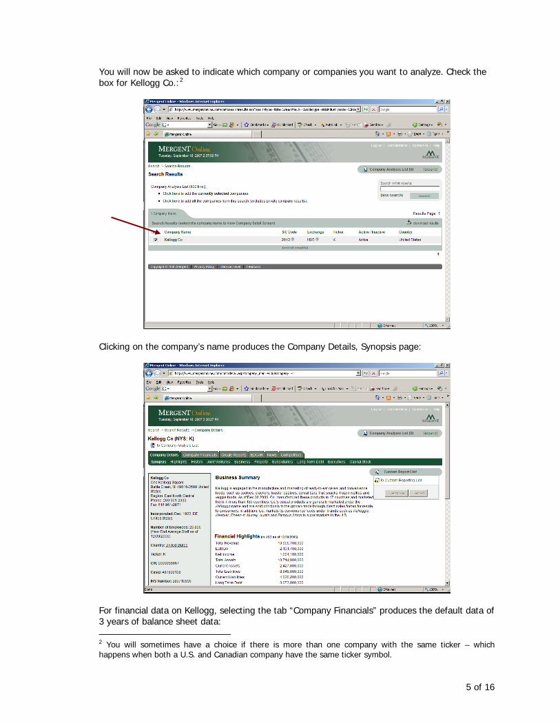
You will now be asked to indicate which company or companies you want to analyze. Check the box for Kellogg Co.:2

Clicking on the company’s name produces the Company Details, Synopsis page:

For financial data on Kellogg, selecting the tab “Company Financials” produces the default data of 3 years of balance sheet data: 2 You will sometimes have a choice if there is more than one company with the same ticker – which happens when both a U.S. and Canadian company have the same ticker symbol.

5 of 16

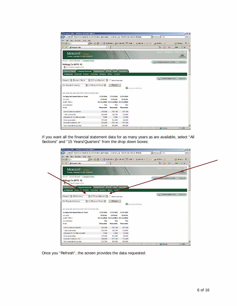
If you want all the financial statement data for as many years as are available, select “All Sections” and “15 Years/Quarters” from the drop down boxes:

Once you “Refresh”, the screen provides the data requested:

6 of 16

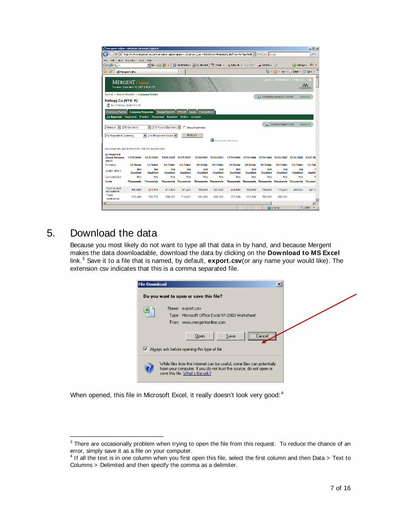
5. Download the data Because you most likely do not want to type all that data in by hand, and because Mergent makes the data downloadable, download the data by clicking on the Download to MS Excel link.3 Save it to a file that is named, by default, export.csv(or any name your would like). The extension csv indicates that this is a comma separated file.

When opened, this file in Microsoft Excel, it really doesn’t look very good:4

3 There are occasionally problem when trying to open the file from this request. To reduce the chance of an error, simply save it as a file on your computer. 4 If all the text is in one column when you first open this file, select the first column and then Data > Text to Columns > Delimited and then specify the comma as a delimiter.

7 of 16

But with a little “fixing-up”, it will be easy to use.

6. Get the data ready in Microsoft Excel® You will need to spruce this up by widening some of the columns. First highlight the columns you want to widen, and then move one of the vertical borders to a highlighted column slightly to the right:

Once you get the columns so you can see what’s going on, you can then manipulate the worksheet:

8 of 16

One thing that is useful is to sort the columns by the date, oldest to most recent, so that you can form ratios and graph time-series more easily. To sort the columns, first highlight the columns (which in a 15-year spreadsheet is the set of columns from B through P), and then use Excel’s “Data” “Sort” commands (generally located in one of the main menus at the top) to sort the data.

When you go to Data and then Sort, you see the following in Microsoft Excel 2003:

9 of 16

Or, in Excel 2007,

Select Options, which will produce the following box, from which you will select the option Sort left to right. Depending on whether you have Excel 2003 or 2007:

Excel 2003 Excel 2007

10 of 16

The fiscal year ending dates are in Row 3 of the worksheet, so this is the Sort by element:

Excel 2003 Excel 2007

Select OK and you now have a sorted worksheet. You can save this as an Excel® worksheet, which will make your analysis a bit easier (than working with a .csv file). Now you are ready to calculate ratios and graph the ratios.

7. Calculate ratios There are many ways to structure the worksheets for ratio calculation using this data. I’ll show you one way, but you may have other methods that you prefer. Label the worksheet with the data as “data”. To change the label, go to the tab for the worksheet (found in the lower left of your screen) and double-click it. Type in the new name. Insert a new worksheet [Insert -- Worksheet] and label this liquidity.

11 of 16

Now you are ready to calculate ratios. Let’s calculate the current and quick ratios over time. To do this, we will be using information contained in cells in the data worksheet, specifically rows 24 (current assets), 16 (inventories), and 55 (current liabilities). I first copy the fiscal year end dates from the data worksheet to the liquidity worksheet. Our formulas in the liquidity worksheet will refer to these rows in the data worksheet. We do this using the reference “data!” before each cell reference. For example, the formula for the current ratio is current assets divided by current liabilities, which in the worksheet that we downloaded refers to elements in row 24 divided by elements in row 56: e.g., for the first year, the cell formula for the current ratio is data!B24/data!B56 and the formula for the quick ratio is =(data!B24-data!B16)/data!B56. So far, this is what you will have:

Copy the formulas in cells B4 and B5 across through P4 and P5 (this is a straight “copy and paste” because these are formulas and the columns are automatically adjusted from B to the appropriate column. Once you copy and paste, you have the current and quick ratios for all fifteen years. You can repeat this procedure for all the ratios that you want to calculate. You can make one worksheet for each type of ratio, or you could have one large worksheet with all the ratios.

8. Graph the ratios It is very effective to look at financial ratios over time because trends are very important in determining the future operating performance and condition of a company. Therefore, we would like to graph these liquidity ratios over time. I’ll show you how to create one graph that shows both ratios over time. Select the data that you want to graph: highlight the data using the cursor (left mouse button and drag) and then “Insert” “Chart” from the Excel menu. You will then get a choice of types of

12 of 16

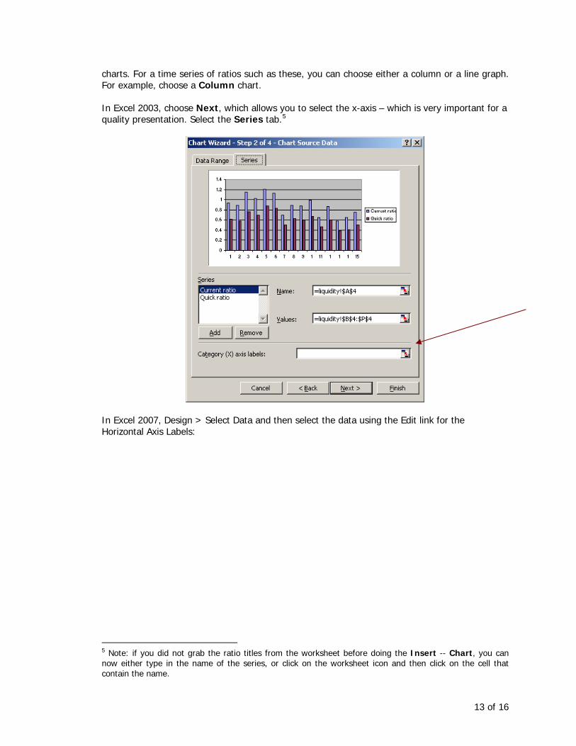
charts. For a time series of ratios such as these, you can choose either a column or a line graph. For example, choose a Column chart. In Excel 2003, choose Next, which allows you to select the x-axis – which is very important for a quality presentation. Select the Series tab.5

In Excel 2007, Design > Select Data and then select the data using the Edit link for the Horizontal Axis Labels:

5 Note: if you did not grab the ratio titles from the worksheet before doing the Insert -- Chart, you can now either type in the name of the series, or click on the worksheet icon and then click on the cell that contain the name.

13 of 16

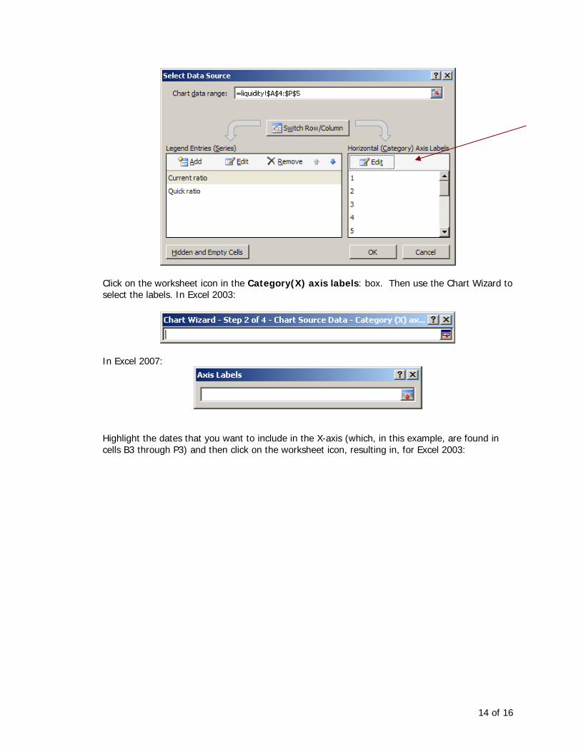
Click on the worksheet icon in the Category(X) axis labels: box. Then use the Chart Wizard to select the labels. In Excel 2003:

In Excel 2007:

Highlight the dates that you want to include in the X-axis (which, in this example, are found in cells B3 through P3) and then click on the worksheet icon, resulting in, for Excel 2003:

14 of 16

Or, in Excel 2007:

Once you click on “Next” it is your opportunity to make the chart interesting. Add titles, remove gridlines, insert a legend at the top, etc.. You can do what you would like, but remember you need to communicate clearly.

Once you specify these options (available at the different tabs) and then click on Next, you then are asked where you’d like the chart – on the same worksheet as the ratios or as a separate worksheet:

15 of 16

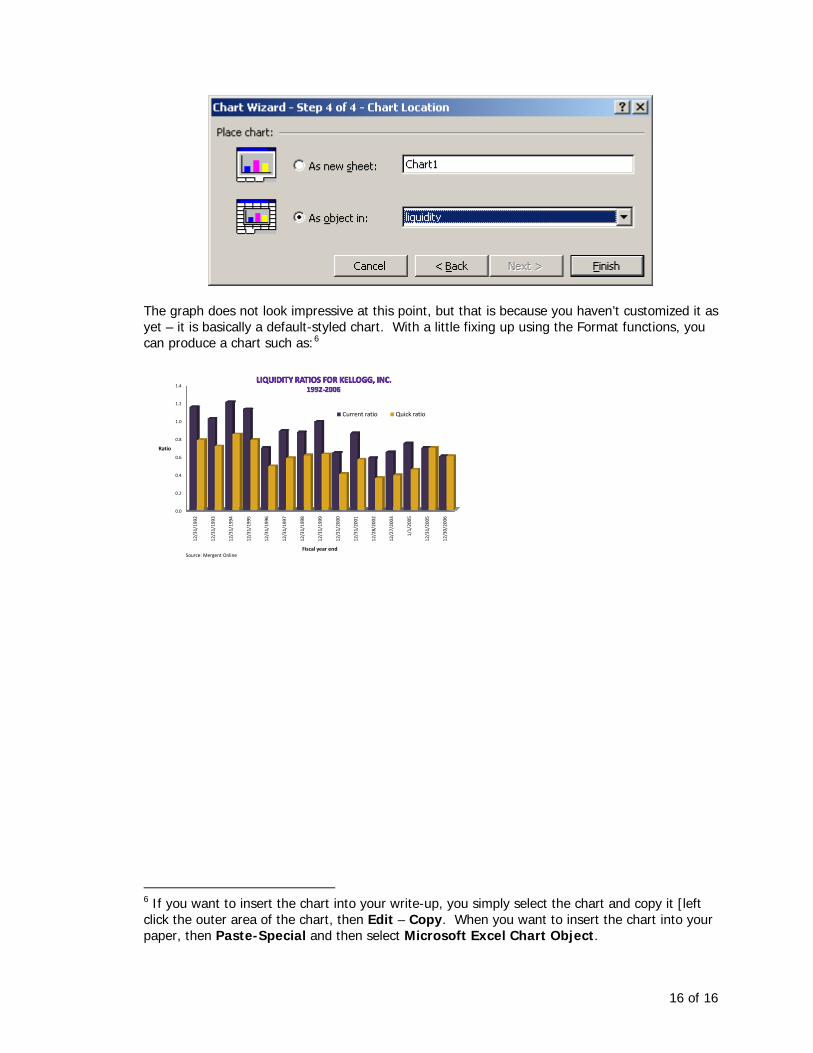
The graph does not look impressive at this point, but that is because you haven’t customized it as yet – it is basically a default-styled chart. With a little fixing up using the Format functions, you can produce a chart such as:6

0.0

0.2

0.4

0.6

0.8

1.0

1.2

1.4

12/31/1992

12/31/1993

12/31/1994

12/31/1995

12/31/1996

12/31/1997

12/31/1998

12/31/1999

12/31/2000

12/31/2001

12/28/2002

12/27/2003

1/1/2005

12/31/2005

12/30/2006

Ratio

Fiscal year end

Current ratio Quick ratio

Source: Mergent Online

6 If you want to insert the chart into your write-up, you simply select the chart and copy it [left click the outer area of the chart, then Edit – Copy. When you want to insert the chart into your paper, then Paste-Special and then select Microsoft Excel Chart Object.

16 of 16