gas fired power plants: investment timing, operating ... · pdf file1 gas fired power plants:...
TRANSCRIPT

1
Gas Fired Power Plants: Investment Timing, Operating Flexibility and
Abandonment
Stein-Erik Fleten1, Erkka Näsäkkälä 2
This version: March 13, 2003
Abstract
Many firms are considering investment in gas fired power plants. We consider a firm holding a license,
i.e. an option, to build a gas fired power plant. The operating cash flows from the plant depend on the
spark spread, defined as the difference between the unit price of electricity and cost of gas. The plant
produces electricity when the spark spread exceeds emission costs, otherwise the plant is ramped down
and held idle. The owner has also an option to abandon the plant and realize the salvage value of the
equipment. We compute optimal entry and exit threshold values for the spark spread. Also the effects
of emission costs on the value of installing CO2 capture technology are analyzed.
Key words: Real options, spark spread, natural gas, power plant, CO2 capture
1 Department of Industrial Economics and Technology Management, Norwegian University of Science and Technology,
NO-7491 Trondheim, Norway. E-mail: [email protected]
2 Corresponding author. Systems Analysis Laboratory, Helsinki University of Technology, P.O. Box 1100, FIN-02015
HUT, Finland. E-mail: [email protected]

2
1 Introduction
The emergence of spot and derivative markets for electricity has facilitated the use of market based
valuation methods for electricity production units. We analyze the problem of valuing a gas fired
power plant. The plant’s operating cash flows depend on the spark spread, defined as the difference
between the price of electricity and the cost of fuel used for the generation of electricity. Spark spread
based valuation of power plants has been studied in Deng, Johnson, and Sogomonian (2001). Deng
(2003) extends the study to take into account jumps and spikes in price processes.
Investment valuation using the traditional discounted cash flow method ignores the asset holder’s
ability to react to changing market conditions. Real options theory captures these options inherent in
investment opportunities. A thorough review of real options is given in Dixit and Pindyck (1994). Real
options are usually analyzed under the risk-neutral probability measure, which can be inferred from
forward prices (see e.g. Schwartz, 1997). We use electricity and gas forward prices.
An investment in a gas fired power plant contains both timing, operating flexibility and abandonment
options. We consider an investor having a license to build a gas fired power plant. The license can be
seen as an American call option on the plant value. Options to postpone an investment decision have
been studied for example in McDonald and Siegel (1986).
Future cash flows from the plant depend on the spark spread between electricity and gas. If the spark
spread is positive the plant produces electricity and the profits are given by the spark spread less
nonfuel variable costs, emission costs and fixed costs. Once the spark spread becomes negative the
plant is ramped down and only fixed costs remain. It is also possible to abandon the plant permanently
and realize the salvage value of the plant. Options to alter operating scale have been studied for
example in Brennan and Schwartz (1985). We compute optimal threshold values to build and abandon
a gas fired power plant.

3
The paper is organized as follows. We present the mathematical model in Section 2, and in Section 3
the solution method is introduced. In Section 4 we apply our model to value a combined cycle gas fired
power plant. In Section 5 we discuss the results of the application. Finally, Section 6 concludes the
study.
2 Mathematical model
We assume that there exist spot and derivative markets for both electricity and gas. In these markets
electricity, gas and their derivative instruments are traded continuously. In describing the probabilistic
structure of the markets, we will refer to a probability space ),,( PFΩ , where Ω is a set, F is a σ -
algebra of subsets of Ω , and P is a probability measure on F. The following assumption characterizes
our derivative markets.
ASSUMPTION 1. There exist forward contracts on both electricity and gas. The derivative markets are
complete and there are no arbitrages.
Given the no arbitrage condition all the portfolios with the same future payoffs have the same current
value. This is often called the law of one price. If all derivative instruments traded in the market can be
replicated with some replicating portfolio the market is complete.
We denote by ( )TtSe , the T-maturity forward price on electricity at time t. Respectively, the T-
maturity forward price on gas at time t is ( )TtS g , . By allowing T to vary from t to τ we get forward
curves [ ] +→⋅ Rτ,:),( ttSe and [ ] +→⋅ Rτ,:),( ttS g for electricity and gas. Seasonality of electricity and
gas causes cycles and peaks in the forward curves.
The value of a gas fired power plant is determined by the spark spread. Spark spread is defined as the
difference between the price of electricity and the cost of gas used for the generation of electricity.
Thus, the T-maturity forward price on spark spread is
),(),(),( TtSKTtSTtS gHe −= , (1)

4
where parameter HK is the heat rate. Heat rate is the amount of gas required to generate 1 MWh of
electricity. Heat rate measures the efficiency of the gas plant: the lower the heat rate, the more efficient
the facility. The efficiency of a gas fired power plant does not vary much over time. Thus, the use of a
constant heat rate is plausible. Note that the value of the spark spread can be negative as well as
positive.
The absence of arbitrage assumption guarantees existence of an equivalent martingale measure Q.
Under the martingale measure Q all expected rates of return equal the risk-free interest rate (see e.g.
Schwartz, 1997). The value of a forward contract when initiated is defined to be zero. Thus the T-
maturity forward price on spark spread at time t is
[ ]tQ FTSETtS |)(),( = , (2)
where )(TS is the spark spread at time T. Thus, the dynamics of the spark spread process under the
pricing measure Q can be can be inferred from forward prices. When long-term commodity projects are
valued, models with constant convenience yield give practically the same results as models using
stochastic convenience yield (see e.g. Schwartz, 1998). Motivated by this, we ignore the seasonality in
the spark spread and use the long term average as a price process. The following assumption gives the
dynamics of the spark spread process.
ASSUMPTION 2. The spark spread has following dynamics
)()( tdBdttdS σα += (3)
where α andσ are non-negative constants and )(⋅B is a standard Brownian motion on the probability
space ),,( QFΩ , along with standard filtration [ ] TtFt ,0: ∈ .
Assumption 2 states that changes in spark spread are normally distributed with mean dtα and
variance dt2σ . As the spark spread values are normally distributed the values are not bounded. Thus
spark spread can be negative as well as positive. Commodity forward prices tend to have time

5
structured volatility reflecting the mean reverting nature of spot prices (see e.g. Schwartz, 1997). For
simplicity we ignore the time structure in the volatility and use the long term average volatility. The
estimation of drift and volatility from forward prices will be considered in Section 4.
The following assumptions give the operational characteristics of the gas plant.
ASSUMPTION 3. Ramp ups and ramp downs of the plant can be done immediately. The costs associated
with starting up and shutting down can be amortized into fixed costs. The lifetime of the power plant is
assumed to be infinite.
In a gas fired power plant the operation and maintenance costs do not vary much over time and the
response times are in the order of several hours. Usually, the life time of a gas fired power plant is
assumed to be around 25 years. Upgrading and reconstructions can increase the lifetime considerably.
Thus, we assume that the plant is more flexible than it really is, but for efficient plants such as this one
the error will be small, judging by the results in Deng and Oren (2003).
We consider an investor having a license to build a gas plant. In order to keep the license alive the firm
faces constant payments W due to salaries etc. The investor can build the plant at any time, thus the
license can bee seen as a perpetual American call option. Perpetual options have a constant threshold
value HS under which exercising is not optimal. Once the spark spread exceeds the threshold value
HS , building becomes optimal. The option to invest 0F must satisfy the following Bellman equation
[ ] HQ SSwhenWdtdFEdtrF ≤−= 00 , (4)
where QE is the expectation operator under the pricing measure Q. For simplicity risk-free interest r is
assumed to be constant. Itô’s lemma gives following differential equation for the option value
HSSwhenWrFSF
SF
≤=−−∂∂
+∂∂
021
00
20
22 ασ . (5)

6
Once the option to build has been exercised the investor has a power plant, which will be ramped down
whenever emission costs E exceed spark spread (i.e. E > S(t)). Moreover, the investor can always
abandon the plant and realize the salvage value of the plant. As the lifetime of the plant was assumed to
be infinite, there is a constant threshold value LS for the abandonment. The value of the plant 1F
consists of three terms: the present value of operating cash flows, the value of the option to ramp down,
and the value of the option to abandon. The value 1F must satisfy the following Bellman equation
[ ] LQ StSwhendtGEtSCdFEdtrF ≥
−−+= + )())((
_
11 , (6)
where +− ))(( EtS denotes )0,)(max( EtS − . _
C is the capacity of the plant. For simplicity, we assume
that the emission and fixed costs G are constant. Uncertainty in emission costs E will be considered in
Section 4. By using Itô’s lemma we get that the value of the plant 1F must satisfy following differential
equations
ESwhenGESCrFSF
SF
≥=−−+−∂∂
+∂∂ 0)(
21 _
11
21
22 ασ . (7)
LSSEwhenGrFSF
SF
≥≥=−−∂∂
+∂∂
021
11
21
22 ασ . (8)
In addition to differential equation (5) the option to build 0F must satisfy following boundary
conditions
0)(lim 0 =−∞>−
SFS
(9)
ISFSF HH −= )()( 10 (10)
SSF
SSF HH
∂∂
=∂
∂ )()( 10 . (11)

7
Equation (9) arises from the observation that as the value of the spark spread decreases the option to
build should become valueless. The value-matching equation (10) follows from the fact that when the
option is exercised the values lost should be equal to value gained. The investment costs are denoted by
I. The smooth-pasting condition (11) states that also the derivatives of the values must match when the
option is exercised. For an intuitive proof of smooth-pasting condition see Dixit and Pindyck (1994)
and for a rigorous derivation see Samuelson (1965).
In addition to differential equations (7) and (8) the value of the plant 1F has following boundary
conditions
( ) dtGEtSCeSF rt
SS ∫∞
+−
∞>−∞>−
−−+=
0
_
1 lim)(lim α (12)
DSFSF LL += )()( 01 (13)
)(lim)(lim 11 EFEFESES ↑↓
= (14)
SSF
SSF LL
∂∂
=∂
∂ )()( 01 (15)
SEF
SEF
ESES ∂∂
=∂
∂↑↓
)(lim)(lim 01 . (16)
Equation (12) states that as the value of the spark spread increases the value of the plant should
approach the net present value of the plant. When spark spread is large it is very unlikely that the spark
spread will decrease to a level where it is optimal to ramp down or abandon the plant. The value-
matching condition must hold when it is optimal to exit the market, as well as when it is optimal to
ramp up or down. In equation (13) the salvage value of the plant is D. Equations (15) and (16) are the
smooth-pasting conditions.
To summarize: we have derived three partial differential equations (equations (5), (7), and (8)) and
eight boundary conditions (equations from (9) to (16)) for the values 0F and 1F .

8
3 Solution method
Generally a solution to a partial differential equation is a linear combination of two independent
solutions plus any particular solution. Let us start with the option to build 0F . The solution of the
partial differential equation (5) is of the form
r
WSASASF −+= )exp()exp()( 22110 ββ , (17)
where 1A and 2A are unknown parameters. 1β and 2β are the roots of the fundamental quadratic
equation
021 22 =−+ rαββσ , (18)
which are
022
22
1 >++−
=σ
σααβ r (19)
022
22
2 <+−−
=σ
σααβ r . (20)
In order to satisfy boundary condition (9) the parameter 2A must be zero. Thus, the value of the option
to build is
r
WSASF −= )exp()( 110 β . (21)
Similarly, we get for the value of the plant
ESwhenr
Cr
GECSrCSBSBSF ≥+
+−++= 2
___
22111 )exp()exp()( αββ (22)
LSSEwhenrGSKSKSF ≥≥−+= )exp()exp()( 22111 ββ . (23)

9
The particular solution in equation (22) is equal to the net present value of an operating gas plant, i.e.
ESwhenr
Cr
GECSrCdtGEtSCe rt ≥+
+−=
−−+∫
∞+−
2
___
0
_
)( αα . (24)
Thus, due to the boundary condition (12) the general solution in equation (22) must approach zero as S
increases (i.e. 01 =B ). We get for the value of the plant
−+
++
−+=
rGSKSK
rC
rGCES
rCSB
SF)exp()exp(
)exp()(
2211
2
___
221
ββ
αβSEwhenESwhen
≥≥
. (25)
We assume that the investment and variable costs satisfy following natural conditions
ID < (26)
GW < . (27)
When the investment and variable costs are realistic (satisfy conditions (26) and (27)) it is never
optimal to build a plant if it is not optimal to use it. Thus the threshold to build the plant must exceed
emission costs, i.e.
HSE ≤ . (28)
Moreover, the threshold value to build the plant must be bigger than the threshold value to abandon,
i.e.
HL SS ≤ . (29)
The inequalities (28) and (29) state that either
HL SES ≤≤ (30)
or
HL SSE ≤≤ . (31)

10
In the case of inequality (30) the emission costs are greater than the threshold value to abandon. Thus,
if the investor has built the plant and the spark spread is between emission costs and threshold value to
abandon it is optimal to hold the plant idle. In the case of inequality (31) the threshold value to
abandon is greater than emission costs. Thus, the option to ramp down the plant is valueless. In other
words, it is optimal to abandon before it is optimal to ramp down the plant. The value-matching and
smooth-pasting conditions (10), (11) and (13)-(16) give following six equations for six unknown
parameters ( HS , LS , 2B , 1A , 1K , 2K ) when inequality (30) holds
Ir
Cr
GECSrCSB
rWSA HHH −+
+−+=− 2
___
2211 )exp()exp( αββ (32)
rCSBSA HH
_
222111 )exp()exp( += ββββ (33)
Dr
WSArGSKSK LLL +−=−+ )exp()exp()exp( 112211 βββ (34)
)exp()exp()exp( 111222111 LLL SASKSK ββββββ =+ (35)
)exp()exp()exp( 22112
_
22 EKEKrCEB ββαβ +=+ (36)
)exp()exp()exp( 222111
_
222 EKEKrCEB ββββββ +=+ . (37)
By eliminating 2B , 1A and 2K from equations (32)-(37) we get following two equations for the
threshold values
)(
)exp()exp(21
__
22
11211 ββ
β
βββ−
+
−
−=−+rCS
rCM
SSMK
H
HL (38)

11
)exp()(
)exp()exp()exp( 21121
__
21
22
_
112 L
H
H SMrCS
rCM
Sr
CEKE ββββ
β
βαββ −−−
+
−
−=
−− , (39)
where
−−
−=)()(
)exp(21
22
_
11 ββαβ
βr
rCEK . (40)
)(
)(
211 ββ −
+−=
rDrWGM (41)
Ir
Cr
WGECM +−−+
= 2
__
2α . (42)
The value-matching and smooth-pasting conditions (10), (11) and (13) - (16) give following four
equations for four unknown parameters ( HS , LS , 2B , 1A ) when the option to ramp down is not
needed, i.e. inequality (31) holds
Ir
Cr
GECSrCSB
rWSA HHH −+
+−+=− 2
___
2211 )exp()exp( αββ (43)
rCSBSA HH
_
222111 )exp()exp( += ββββ (44)
Dr
WSAr
Cr
GECSrCSB LLL +−=+
+−+ )exp()exp( 112
___
22 βαβ (45)
)exp()exp( 111
_
222 LL SArCSB ββββ =+ . (46)
By eliminating 1A and 2B from the equations (43) - (46) we get following two equations for the
threshold values.

12
−
+−−=
−
++−−
rCS
rCILS
rCS
rCLDS HHLL
__
121
__
121 )exp()exp( ββββ (47)
−
+−−=
−
++−−
rCS
rCILS
rCS
rCLDS HHLL
__
112
__
112 )exp()exp( ββββ , (48)
where
r
WGECr
CL −+−=
_
2
_
1α . (49)
To summarize; the threshold values are found either by equations (38), (39) and inequality (30) or by
equations (47), (48) and inequality (31). In the case that the solution is found by equations (38) and
(39) it is optimal to ramp down the plant before it is abandoned. If the solution is given by equations
(47) and (48), the option to ramp down is not needed. Neither of the cases can be solved analytically,
but a numerical solution can easily be attained.
4 Application
Norwegian energy and environmental authorities have given three licenses to build a gas fired power
plant. All potential plants are situated along the western coast of southern Norway. In this section we
illustrate our framework by taking the view of an investor having one of these licenses.
The example consists of four parts. First, we introduce the data used for the valuation including
methods to estimate the parameters from the data. Second, we calculate threshold values to build and
abandon the plant. The threshold values are compared to the threshold values calculated with
discounted cash flows. The sensitivity of the threshold values to some key parameters are illustrated in
part three. In the final part we study the effects of carbon emission costs to the installation of CO2
capture technology. We assume that a plant with CO2 capture technology does not face emission costs.

13
The costs of building and running a combined cycle gas plant in Norway are estimated by Undrum,
Bolland, Aarebrot (2000). We use an exchange rate of 7 NOK/$. Table 1 contains a summary of the
parameters needed for our model.
Table 1: The gas plant parameters
Parameter W _C G I D
Unit MNOK/year MMwh/year MNOK/year MNOK MNOK
Value 2.5 3.27 50 1620 570
Let us make few comments on the parameters. Undrum, Bolland, Aarebrot (2000) estimate that
building a natural gas fired combined cycle power plant in Norway costs approximately 1620 MNOK,
and that the maintenance costs G are approximately 50 MNOK/year. We estimate that the costs of
holding the license W are 5% of the fixed costs of a running a plant. In Undrum, Bolland, Aarebrot
(2000) approximately 35% of the investment costs are used for capital equipment. We assume that if
the plant is abandoned, all the capital equipment can be realized on second hand market, thus we
assume that D is 570 MNOK. The estimated parameters are for a gas plant whose maximum capacity is
415 MW. We assume that the capacity factor of the plant is 90%. Thus the production capacity is 3.27
MMWh/year.
The drift parameter α in the spark spread process is estimated with linear regression from electricity
and gas forward prices. For electricity, long term prices from Nord Pool and 10-year contracts traded
bilaterally are used. For natural gas we use data from International Petroleum Exchange (IPE). Gas
prices are adjusted by the heat rate so that a unit of gas corresponds to 1 MWh of electricity generated.
The efficiency of a combined cycle gas fired turbine is estimated to be 58.1% (see Undrum, Bolland,
Aarebrot, 2000).

14
For the estimation of the volatility parameter σ the correlation between the spot price of electricity
and gas in the period 1998-2001 was estimated at 0.53. The estimation of electricity and gas forward
volatilities is based on data from Nord Pool and IPE from 1997 to 2001. The one year average forward
volatilities were 0.1 for electricity and 0.2 for gas.
Table 2 contains estimates for the spark spread process parameters and the risk-free interest rate. The
interest rate is quite high, but the long term average interest rate in Norway is approximately 6%.
Commodity forward prices under stochastic interest rate have been studied for example in Schwartz
(1997).
Table 2: Spark spread process parameters
Parameter α σ r
Value 0.16 28 6%
The long term average spark spread was estimated to be approximately 19 NOK/MWh. The expected
spark spread values with 68% confidence level are illustrated in Figure 1.
[Figure 1 about here]
Table 3 contains threshold values HS and LS computed when emission costs are assumed to be zero
(i.e. E = 0). The solution is found with equations (38), (39) and with inequality (30). Thus, with the
given parameters it is optimal to ramp down the plant before abandoning. Threshold values DCFHS and
DCFLS are calculated with discounted cash flows. The upper threshold value DCF
HS is calculated by
setting the difference of expected cash flows before and after investment equal to investment costs. The
lower threshold value DCFLS is calculated by setting the difference of expected cash flows before and
after abandonment equal to salvage value.

15
Table 3: Threshold values
Variable LS HS DCFLS DCF
HS
Value -39 NOK/MWh 95 NOK/MWh 22 NOK/MWh 42 NOK/MWh
The optimal threshold values calculated using real options approach differ considerably from values
calculated using traditional discounted cash flow method. Uncertainty makes waiting more favorable
(see e.g. Dixit and Pindyck, 1994). Thus, uncertainty increases threshold value to build the plant and
decreases threshold value to abandon the plant. Deng, Johnson, and Sogomonian (2001) find that the
value of a gas power plant calculated with a simple spark spread valuation method is over six times the
value calculated with a discounted cash flow method. Note that the discounted cash flow approach
suggests that it is optimal to abandon the plant with current spark spread. With real options method the
current value of spark spread is almost equally distant from the threshold values.
The upper picture in Figure 2 illustrates the values 0F and 1F as a function of spark spread. Also the
threshold values are shown. Note that )(1 LSF exceeds )(0 LSF by the resale value of the equipment (D
= 570 MNOK) and )(0 HSF is 1620 MNOK below )(1 HSF , corresponding to the investment costs.
Incremental values for building a plant (i.e. 1F - 0F ) are presented in the lower picture of Figure 2.
Incremental values illustrate how much more valuable an investor with a plant is compared to a firm
with just the license to build. Note the tangency to the horizontal lines I and D caused by the smooth
pasting conditions.
[Figure 2 about here]
Next we study how the threshold values change as a function of some key parameters. In Figure 3 the
threshold values as a function of volatility σ are illustrated.

16
[Figure 3 about here]
The gray parts in the threshold lines are given with equations (38), (39) and the black parts with
equations (47), (48). When the lines are gray the option to ramp down the plant has no value, while for
the black parts the ramp down option has value and may thus be exercised. If volatility is less than 11
the option to ramp down the plant is valueless. In Figure 3 additional uncertainty increases the
threshold value to build a plant, but at the same time the threshold value to abandon the plant
decreases, i.e. uncertainty makes waiting more favorable (see e.g. Dixit and Pindyck, 1994). Note that
when the uncertainty in spark spread process approaches zero the threshold values converge to the
DCF values in Table 3.
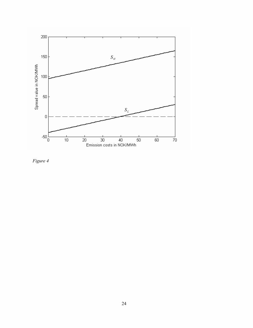
Figure 4 illustrates threshold values as a function of emission costs. In Figure 4 the unit of emission
costs is NOK/MWh. Usually the unit for emission costs is $/ton. The CO2 production of a gas fired
power plant is 363 kg/MWh, thus with an exchange rate of 7 NOK/$ an emission cost of 10 NOK/MWh
corresponds 3.94 $/ton.
[Figure 4 about here]
In Figure 4 threshold values increase linearly as a function of emission costs. Moreover, the slope is
one. If the emission costs are increased by one NOK/MWh both threshold values are also increased by
one NOK/MWh. This is a consequence of a normally distributed spread process. Change in emission
costs can be seen as a change in initial value of the spread process.
Even though we have used constant emission costs, there is great amount of uncertainty in emission
costs. The uncertainty in emission costs can be seen as an additional uncertainty in the spread process.
Thus, uncertainty in emission costs increases the threshold value to build the plant and decreases the
threshold value to abandon.

17
Undrum, Bolland, Aarebrot (2000) evaluate different alternatives to capture CO2 from gas turbine
power cycles. They estimate that costs to install equipment to capture CO2 from exhaust gas using
absorption by amine solutions are 2140 MNOK. Thus, the costs of a gas power plant with CO2 capture
technology are 3760 MNOK. Figure 5 illustrates threshold values as a function of investment costs
when the salvage value is 35% of the investment costs (i.e. D = 0.35I). Thus, the resale value of a plant
with CO2 capture technology is 1316 MNOK. We have ignored the reduced efficiency of the plant
when the greenhouse gas capture equipment is in place.
[Figure 5 about here]
In Figure 5 the threshold value to build a gas turbine with CO2 capture equipment is 146 NOK/MWh.
Figure 4 indicates that once the emission costs are 51 NOK/MWh the upper threshold value for a plant
without CO2 capture equipment is 146 NOK/MWh. By assuming that all emission costs are caused by
CO2 we get that it is optimal to install the CO2 capture equipment when emission costs are larger than
20.1 $/ton (i.e. 51 NOK/MWh).
The current estimate is that emission costs will be somewhere between 5$/ton and 20$/ton, where the
lower range is most likely. When emission costs are 8 $/ton threshold value to build a plant without
CO2 capture equipment is 115 NOK/MWh. As is calculated earlier the upper threshold value for the
plant with CO2 capture equipment is 146 NOK/MWh. The upper threshold value for a plant with CO2
capture equipment is 115 NOK/MWh if the investment costs are lowered to 2550 MNOK. Thus, if
companies building a gas plant with CO2 capture equipment are subsidized with 1210 MNOK it is
optimal to build gas plants with such equipment.
5 Discussion
Our results indicate that even with zero emission costs it is not optimal to exercise the option to build a
gas fired power plant. Regardless, the reality may be different. Some of the three firms holding a

18
license to build gas fired power plant have stated publicly that they are willing to invest if the
government relieves them of emission costs. There are several possible explanations why our results
differ from the apparent policies of the actual investors.
First, we have ignored the effects of competition between the firms holding the license. The preemptive
effect of early investment gives the license holders an incentive to build the plant (see e.g. Smets,
1991).
Secondly, we have used the UK market as a reference for gas. There is lot of natural gas available in
the Norwegian continental shelf. Due to the physical distance from the Norwegian coastline to the UK,
the gas price at a Norwegian terminal will be equal to the UK price less the transportation costs. By
using price quotas from IPE we overestimate the gas price for delivery at a Norwegian terminal.
There is also a tax issue that has not been considered. Oil and gas companies operating on the
Norwegian shelf have a 78% tax rate, while onshore activities are taxed at 28%. If an oil company
invested in a gas power plant, it could sell the gas at a loss with offshore taxation, and buy the same gas
as a power plant owner with onshore taxation.
We have also calculated the value of a CO2 capture plant attached to the gas fired power plant. We
found that if the emission costs are over 20.1 $/ton it is optimal to install such an equipment. When
emission costs were assumed to be 8$/ton building of a gas fired power plants with CO2 capture
equipment is optimal if companies building such a plant are subsidized with 1210 MNOK.
6 Conclusions
We use real options theory to analyze the investment in a gas fired power plant. Our valuation is based
on electricity and gas forward prices. We have derived a method to compute threshold values for
building and abandoning a gas fired power plant when the plant can be ramped down if it turns to be

19
unprofitable. Normally it is optimal to ramp down the plant before abandoning, while sometimes it is
optimal to abandon a running plant directly.
In our example we take a view of an investor having a license to build a gas fired power plant in
Norway. The example is based on forward prices from Nord Pool and International Petroleum
Exchange (IPE). Our results indicate that the investors should wait and hope the electricity prices go up
or gas prices go down before they commence the power plant project. Our numerical results also
indicate that with current estimates of emission costs it is not optimal to attach a CO2 capture plant to a
gas plant.

20
References
Brennan, M., Schwartz, E.S. (1985) Evaluating natural resource investments, Journal of Business 58
(2), pp. 135-157
Deng, S.J. (2003) Valuation of Investment and Opportunity to Invest in Power Generation Assets with
Spikes in Power Prices, Working paper, Georgia Institute of Technology
Deng, S.J., Johnson B., Sogomonian A. (2001) Exotic electricity options and the valuation of electricity
generation and transmission assets, Decision Support Systems, (30) 3, pp. 383-392
Deng, S.J., Oren S.S. (2003) Valuation of Electricity Generation Assets with Operational
Characteristics, Probability in the Engineering and Informational Sciences, forthcoming
Dixit, A.K., Pindyck, R.S. (1994) Investment under Uncertainty, Princeton University Press
McDonald, R., and Siegel D. (1986) The value of waiting to invest, Quarterly Journal of Economics
101 (4), pp. 707-727
Samuelson, P.A. (1965) Rational theory of warrant pricing, Industrial Management Review 6, pp. 13-31
Schwartz, E.S. (1997) The Stochastic Behavior of Commodity Prices: Implications for Valuation and
Hedging, The Journal of Finance, 52 (3), pp. 923-973
Schwartz, E.S. (1998) Valuing Long-Term Commodity Assets, Financial Management, 27 (1), pp. 57-
66
Smets, F. (1991) Exporting versus FDI: The Effect of Uncertainty, Irreversibilities and Strategic
Interactions" Working paper, Yale University.
Undrum, H., Bolland, O., and Aarebrot, E. (2000) Economical assessment of natural gas fired
combined cycle power plant with CO2 capture and sequestration, presented at the Fifth International
Conference on Greenhouse Gas Control Technologies, Cairns, Australia

21
Figures
Figure 1: Spread process
Figure 2: Option values
Figure 3: Threshold values as a function of volatility
Figure 4: Threshold values as a function of emission costs
Figure 5: Threshold values as a function of investment costs
Figure 1

22
Figure 2
HS1F
0FLS
01 FF −
HSLS

23
Figure 3
HS
LS
24
Figure 4
HS
LS

25
Figure 5
LS
LS
HS