gamma-ray bursts of first stars · gamma-ray bursts of first stars yudai suwa (yitp, ... for the...
TRANSCRIPT
Gamma-Ray Bursts of First Stars
Yudai Suwa(YITP, Kyoto University)
Collaboration with K. Ioka
I009.600IarXiv:

GRB 2010 Conference @ AnnapolisNov 2 2010
Most distant object?
We observed a high-z GRB 090423 (z~8.3), which was the most distant object we observed ever.
Can we reach the first object in the universe?
Tanvir’s talk @ Kyoto 2010
GRB 090423@z=8.2
GRB 2010 Conference @ AnnapolisNov 2 2010
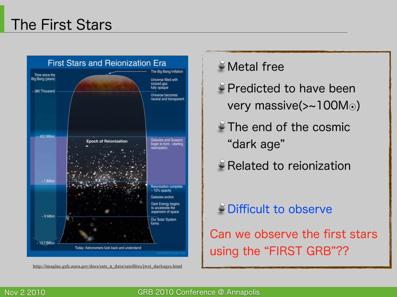
The First Stars
Metal free
Predicted to have been very massive(>~100M⦿)
The end of the cosmic “dark age”
Related to reionization
Difficult to observe
http://imagine.gsfc.nasa.gov/docs/sats_n_data/satellites/jwst_darkages.html
Can we observe the first stars using the “FIRST GRB”??
GRB 2010 Conference @ AnnapolisNov 2 2010
......
......
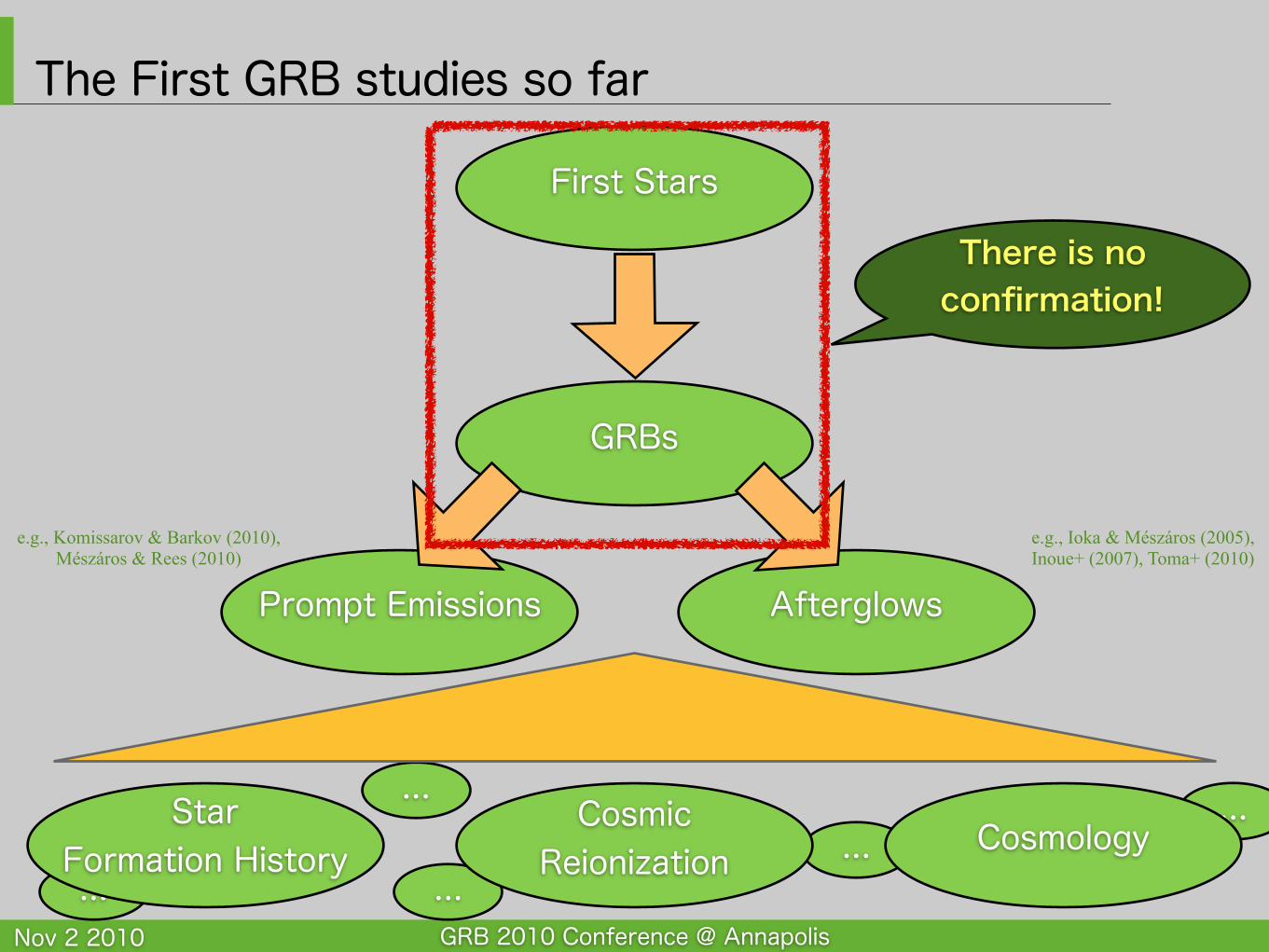
The First GRB studies so far
First Stars
GRBs
Prompt Emissions Afterglows
Star Formation History
Cosmic Reionization Cosmology
There is no confirmation!
...
e.g., Ioka & Mészáros (2005), Inoue+ (2007), Toma+ (2010)
e.g., Komissarov & Barkov (2010), Mészáros & Rees (2010)
GRB 2010 Conference @ AnnapolisNov 2 2010
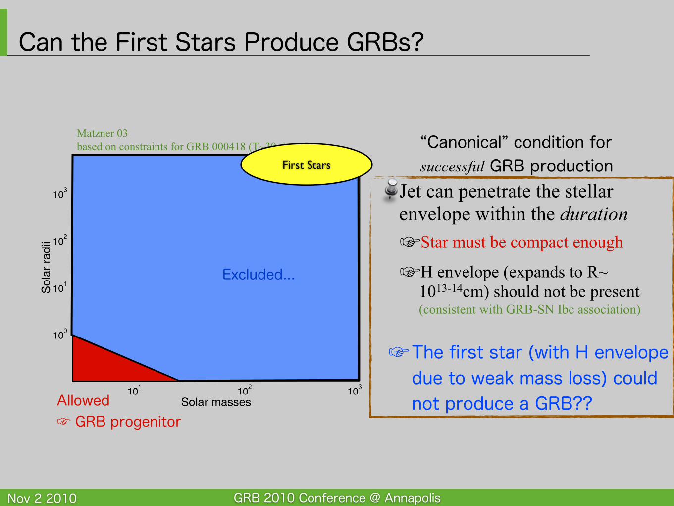
Can the First Stars Produce GRBs?
Jet can penetrate the stellar envelope within the duration☞Star must be compact enough
☞H envelope (expands to R~ 1013-14cm) should not be present(consistent with GRB-SN Ibc association)
2003MNRAS.345..575M
Matzner 03based on constraints for GRB 000418 (T~30 s)
Excluded...
Allowed☞ GRB progenitor
“Canonical” condition for successful GRB productionFirst Stars
☞The first star (with H envelope due to weak mass loss) could not produce a GRB??
GRB 2010 Conference @ AnnapolisNov 2 2010
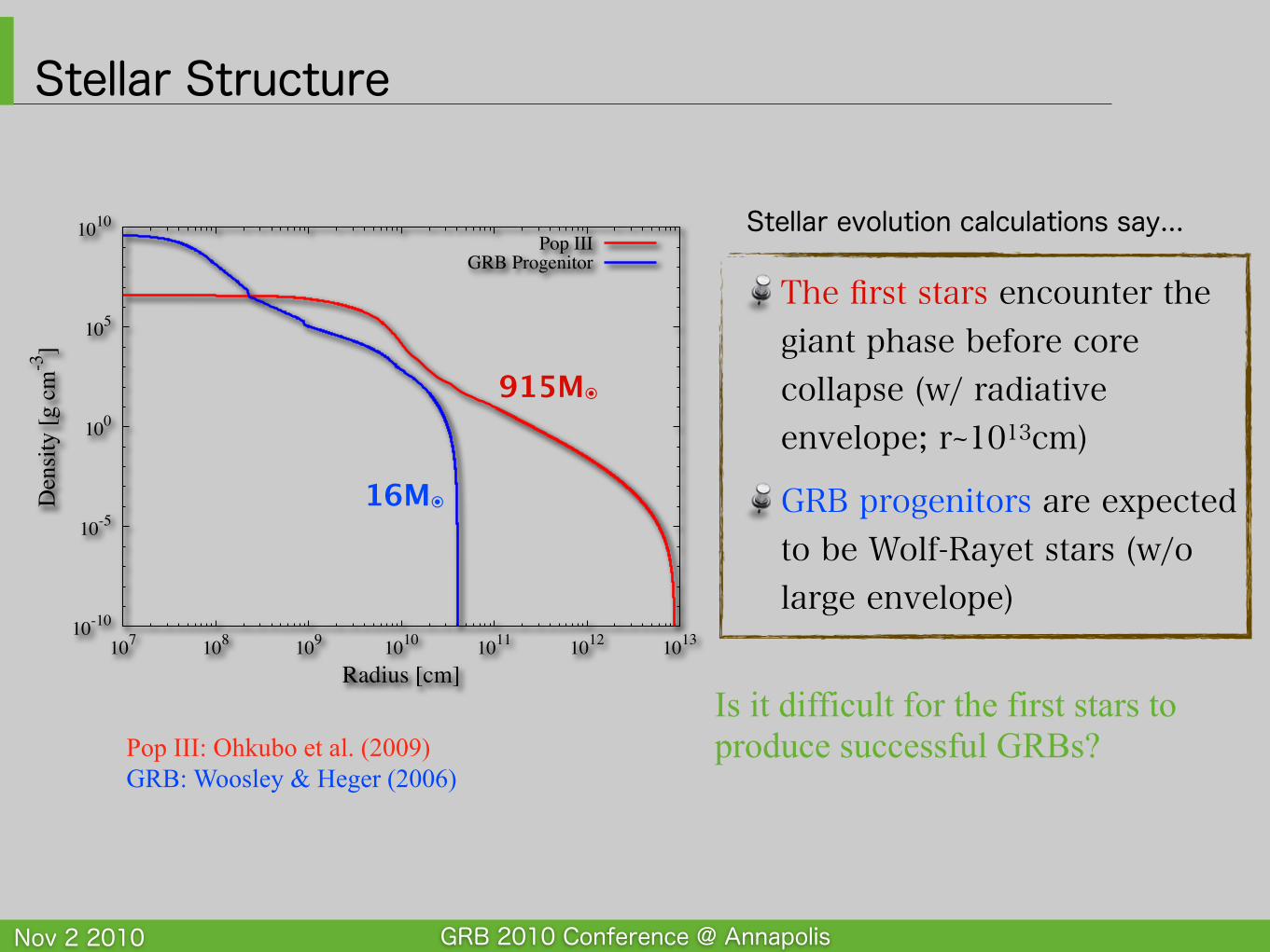
Stellar Structure
The first stars encounter the giant phase before core collapse (w/ radiative envelope; r~1013cm)
GRB progenitors are expected to be Wolf-Rayet stars (w/o large envelope)
Pop III: Ohkubo et al. (2009)GRB: Woosley & Heger (2006)
Stellar evolution calculations say...
10-10
10-5
100
105
1010
107 108 109 1010 1011 1012 1013
Den
sity
[g c
m-3
]
Radius [cm]
Pop IIIGRB Progenitor
Is it difficult for the first stars to produce successful GRBs?
915M⦿
16M⦿
GRB 2010 Conference @ AnnapolisNov 2 2010
Question “Can the first stars produce GRBs?”Absence of H envelope is required for successful GRB
But the first stars might not loose their massive envelope
More investigations are necessary
GRB 2010 Conference @ AnnapolisNov 2 2010
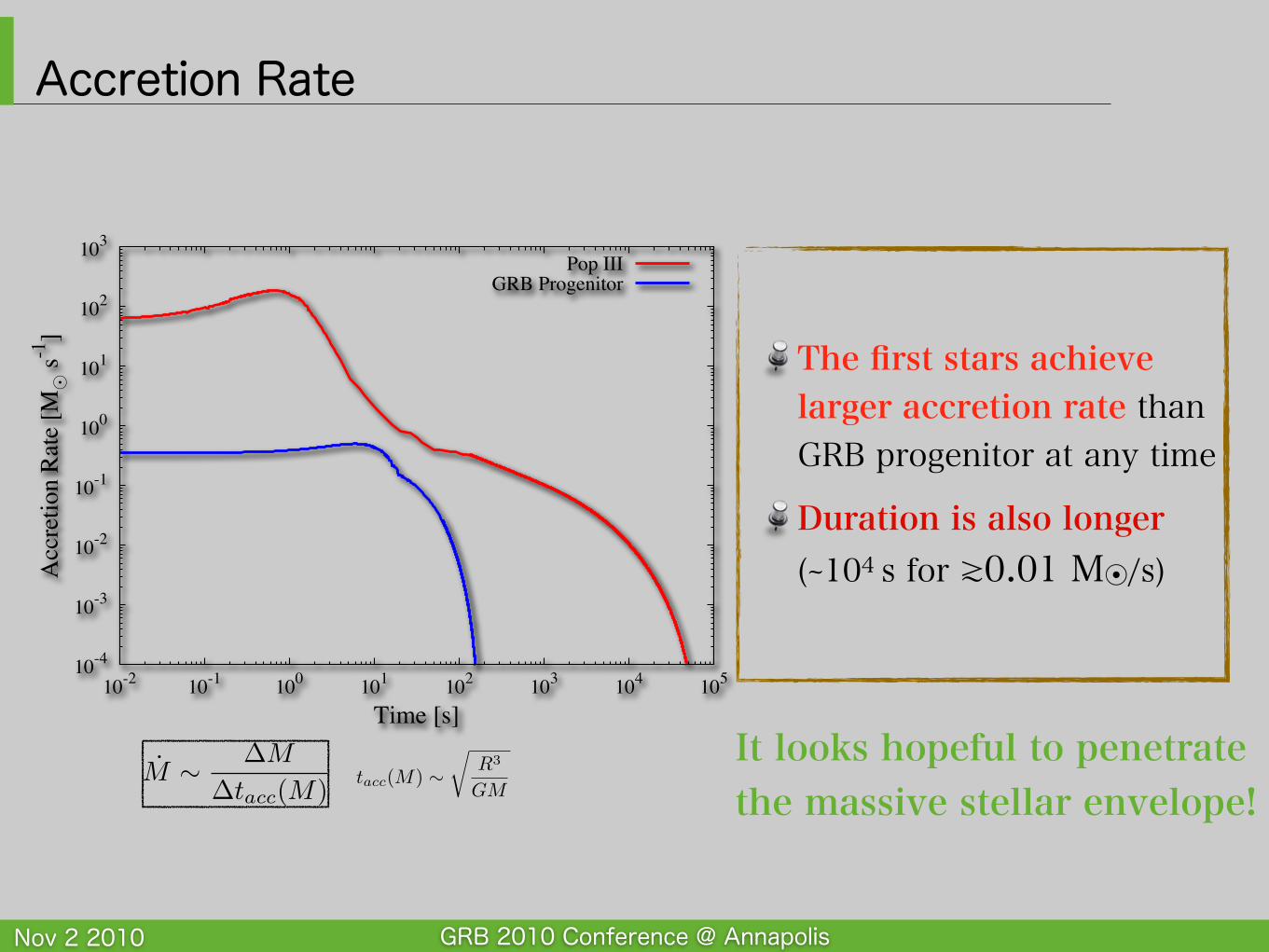
Accretion Rate
The first stars achieve larger accretion rate than GRB progenitor at any time
Duration is also longer (~104 s for ≳0.01 M⦿/s)
M ∼ ∆M
∆tacc(M) tacc(M) ∼�
R3
GM
10-4
10-3
10-2
10-1
100
101
102
103
10-2 10-1 100 101 102 103 104 105
Acc
retio
n Ra
te [M
! s-1
]
Time [s]
Pop IIIGRB Progenitor
It looks hopeful to penetrate the massive stellar envelope!
GRB 2010 Conference @ AnnapolisNov 2 2010
which
approxim
atelybalan
cesthepressu
rein
theshocked
jet;here
h,thespecifi
centhalp
y,is
!e"p#=!!c
2#,where
e,thetotal en
ergydensity, in
cludes
restmass
density.
Tosummarize, as
seenbyapiece
ofjet
startingat
theori-
gin:(1)
intern
alenergy
isconverted
toexp
ansio
nuntil
the
reverseshock
isencountered
;(2)
kinetic
energy
isthen
con-
vertedmostly
back
into
intern
al energy
atthereverse
shock,
though
the
motio
nrem
ains
moderately
relativistic(!
$5
10);an
d(3)
thehotjet
isfurth
erdecelerated
to
subrelativistic
speed
sat
thejet
head
.In
what
follo
wswe
shall
referto
jetmaterial
instage
1as
the‘‘ u
nshocked
jet ’’an
dstage
2as
the‘‘ sh
ocked
jet.’’Theinteractio
noftheshocked
jetwith
thestar
isesp
e-cially
interestin
gsin
ceKelvin
-Helm
holtz
instab
ilitiesan
dobliq
ueshocksinsid
ethecocooncan
imprin
ttim
estru
cture
onits
Loren
tzfacto
r(see
alsoMartı et
al. 1997an
dreferen
-ces
therein
).Theconseq
uences
di!er
inthethree
models.
Becau
seofits
largerinitial
openingan
gle,thejet
inmodel
Fig. 1.—
Density
structu
rein
thelocal rest
frameformodel JA
at(a)
t %2:1
san
d(b)
7.2s. In
(a), onlythecen
tral regionofthestar
isshown. T
herad
iusof
thestar
is8&10
10cm
. Notethemorphological d
i!eren
cesam
ongmodels
JA(Fig. 1), JB
(Fig. 2), an
dJC
(Fig. 3).
TABLE
2
EnergiesatBreakout
Model
tba
(s)Einj b
(&10
51ergs)
E1c
(&10
51ergs)
E2d
(&10
51ergs)
E3e
(&10
51ergs)
E4f
(&10
51ergs)
Esng
(&10
51ergs)
JA....................
6.913.8
9.82.6
0.74.3
6.2JB
....................3.3
6.63.6
0.40.1
4.91.2
JC....................
5.53.3
7.40.3
0.21.6
1.2
aTim
eforthejet
tobreak
outofthestar.
bTotal en
ergyinjected
astw
injets
befo
rethejet
break
soutofthestar.
cTotal en
ergyin
material w
ithaLoren
tzof !
<1:005.
dTotal en
ergyin
material w
ithaLoren
tzof1:005
<!<
2.eTotal en
ergyin
material w
ithaLoren
tzof2<
!<
5.fT
otal en
ergyin
material w
ithaLoren
tzof !
>5.
gEstim
atedenergy
insupern
ova
(see x3.2).
No.1,
2003RELATIV
ISTIC
JETS
INCOLLAPSARS
359
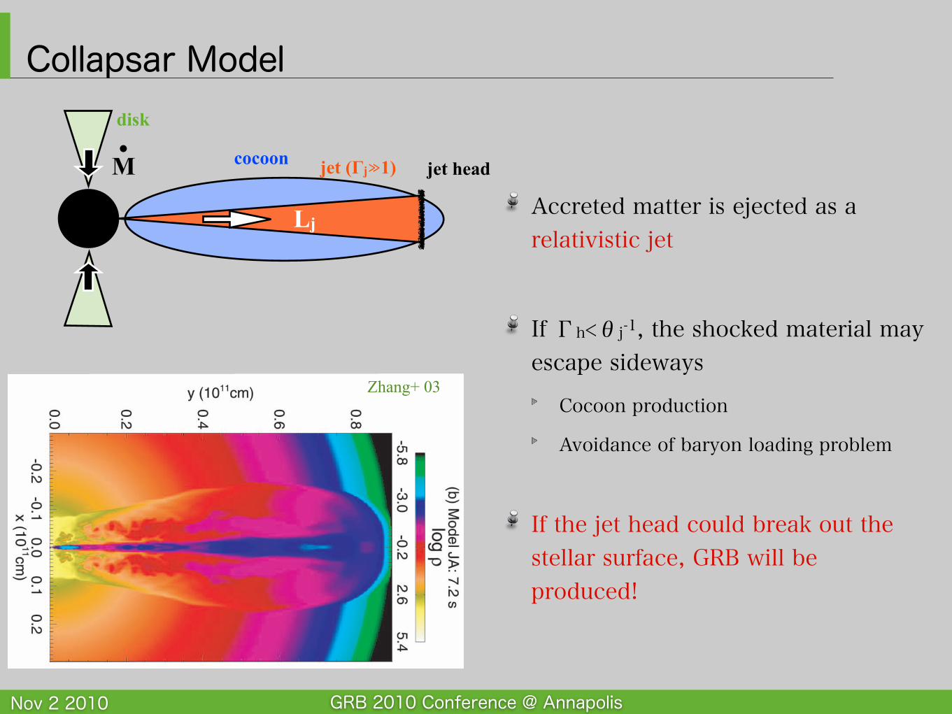
Collapsar Model
Accreted matter is ejected as a relativistic jet
If Γh<θj-1, the shocked material may escape sideways
Cocoon production
Avoidance of baryon loading problem
If the jet head could break out the stellar surface, GRB will be produced!
Zhang+ 03
jet (!j≫1)cocoon
Lj
jet head
disk
M•
GRB 2010 Conference @ AnnapolisNov 2 2010
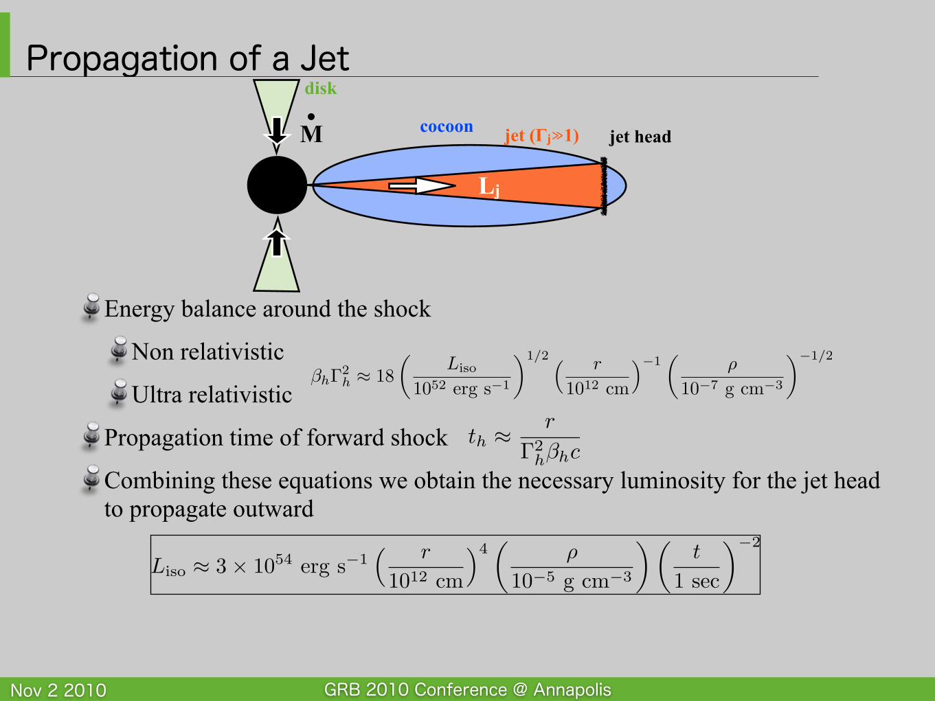
Energy balance around the shock
Non relativistic
Ultra relativistic
Propagation time of forward shock
Combining these equations we obtain the necessary luminosity for the jet head to propagate outward
Propagation of a Jet
Liso ≈ 3× 1054 erg s−1� r
1012 cm
�4�
ρ
10−5 g cm−3
� �t
1 sec
�−2
jet (!j≫1)cocoon
Lj
jet head
disk
M•
βhΓ2h ≈ 18
�Liso
1052 erg s−1
�1/2 � r
1012 cm
�−1�
ρ
10−7 g cm−3
�−1/2
th ≈r
Γ2hβhc
GRB 2010 Conference @ AnnapolisNov 2 2010
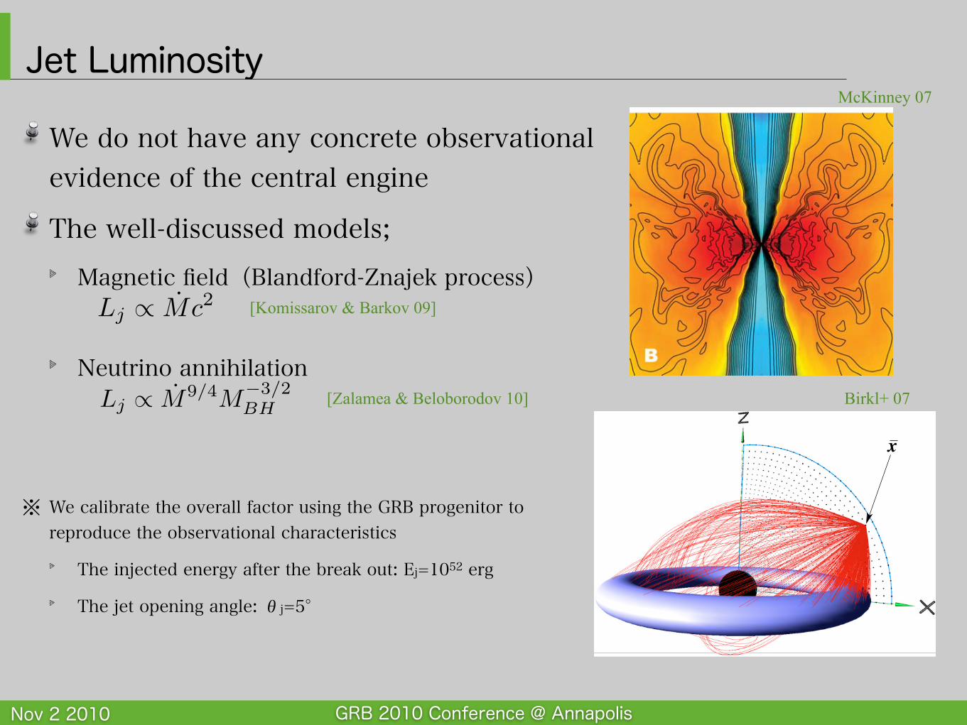
We do not have any concrete observational evidence of the central engine
The well-discussed models;Magnetic field(Blandford-Znajek process)
Neutrino annihilation
※ We calibrate the overall factor using the GRB progenitor to reproduce the observational characteristics
The injected energy after the break out: Ej=1052 erg
The jet opening angle: θj=5°
Jet Luminosity
R. Birkl et al.: Neutrino pair annihilation near accreting black holes 53
!!-annihilation. We analyze how the neutrino distribution andthe resulting !!-annihilation are influenced by GR e!ects, thegeometry and the properties of the neutrinosphere, and the massand spin of the central BH. To this end, we examine the mostlikely configurations occurring in compact astrophysical sys-tems: spherical neutrinospheres present in NSs, and thin disksand thick tori surrounding stellar-mass BHs. We explicitly re-mark that the absolute values of the neutrino luminosity and ofthe energy-momentum deposition rate by !!-annihilation do notplay an important role for the discussion in this paper. Due tothe simplicity of the neutrino source models considered here, ournumbers for these quantities should not be interpreted quantita-tively. They sensitively depend on the location and temperatureof the neutrinospheres, which must be expected to be di!erent indetailed hydrodynamic simulations that include some treatmentof the neutrino transport. However, for the purpose of compar-ing the di!erent e!ects, on which this paper focuses, only therelative changes of the neutrino luminosity and !!-annihilationmatter.
The paper is organized as follows: in Sect. 2 we discuss thetheoretical fundamentals for calculating the !!-annihilation ratein a given Kerr spacetime, and how we construct equilibriumaccretion tori surrounding Kerr BHs. In Sect. 3 we give a de-scription of the numerical implementation of the ray-tracing al-gorithm used to calculate the annihilation rate. The results of ourparameter study are discussed in Sect. 4, and the conclusionsof our work are presented in Sect. 5. Finally, technical detailsconcerning the calculation of the annihilation rate are given inAppendix A, and convergence tests performed on our ray-tracingalgorithm are presented in Appendix B.
2. Theoretical fundamentals
Unless stated otherwise, we use geometrized units throughoutthis paper, so that c = G = 1, where c is the speed of lightin vacuum and G is Newton’s gravitational constant. Greek andRoman indices denote spacetime components (0–3) and spatialcomponents (1–3) of 4-vectors, respectively. The signature ofthe metric is chosen to be (+,!,!,!), and 3-vectors are denotedby a bar above the respective symbol, e.g. A.
2.1. Calculation of the annihilation rate
In order to compute the deposition of 4-momentum Q"i (t, x) bythe annihilation of neutrinos and antineutrinos of flavor i withi " {e, µ, #} into e+e!-pairs at a spatial point x per unit of timeand unit of volume, we follow a formalism very close to that ofMiller et al. (2003).
In flat spacetime the local annihilation rate is computed fromthe Lorentz invariant neutrino and antineutrino phase space dis-tribution functions f!i = f!i (t, x, p) and f!i = f!i (t, x, p#) (fortheir exact definition see Appendix A) by the following integral
Q"i =!
d3 pd3 p#A"i"p, p##
f!i f!i , (1)
where the A"i are functions defined in Appendix A. They arebased on a covariant generalization of the expressions given inRu!ert et al. (1997). Note that although we are concerned onlywith time-independent models here, we include the argument tin the distribution functions f!i and f!i for the sake of generality.In the following we omit the indices of f .
Except for minor redefinitions Eq. (1) can also be used incurved spacetimes (Miller et al. 2003), because the annihila-tion process, which is a microphysical phenomenon, happens so
x
Fig. 1. Ray-tracing of neutrinos in a Kerr BH spacetime. At everypoint x where the annihilation rate is to be calculated, geodesics (redcurves) arriving from random directions are traced back until they hitthe neutrinosphere (blue torus). The computational grid is marked bythe small black dots and its boundary by the blue circle. See the elec-tronic edition for a color version of the figure.
rapidly and on such small length scales that the e!ects of stellargravitational fields can be safely neglected. Gravity a!ects onlythe propagation of the (anti)neutrinos between their emission (oremergence from the neutrinosphere) and their annihilation.
In our models the gravitational field, which leads to raybending and redshift, is provided by the central Kerr BH ofmass M and (dimensionless) angular momentum parameter a $J/M2 (where J is the angular momentum of the BH, and 0 %a % 1), whose metric is given in Boyer-Lindquist coordinates(t, r, $, %) by
ds2 = gtt dt2 + g%% d%2 + 2gt% dtd% + grr dr2 + g$$ d$2 (2)
with
gtt = 1 ! 2Mr&2 ,
g%% = !$r2 + M2a2 +
2rM3a2 sin2 $
&2
%sin2 $,
gt% =2rM2a sin2 $
&2 ,
grr = !&2
",
g$$ = !&2,
where
" = r2 ! 2Mr + (aM)2,
&2 = r2 + (aM)2 cos2 $.
Let us now consider an observer located at the point x wherethe annihilation happens (Fig. 1). We will refer to this observeras the local observer, and the quantities measured in his frameare denoted by the subscript “L”. The local frame is defined byan orthonormal base {et, er, e$, e%} such that a local observer isat rest in the global (r, $, %) coordinate system, i.e. its 4-velocityfulfills ua = 0 (the resulting orthonormal base vectors are givenin Appendix A). Hence, one cannot calculate the annihilationrate inside the ergosphere, where no observers can be at rest.This restriction could be lifted by using observers dragged alongby the BH, i.e. for observers with ua = ga'u' = 0. However, the
Birkl+ 07
GRMHD simulations of Poynting-dominated jets 1569
Figure 2. Same as Fig. 1, but outer scale is r = 102r g.
Fig. 6 shows !!, which reaches up to !! " 103–104, for an outerscale of r = 104r g (panel A) and an outer scale of r = 103r g (panelB). The inner-radial region is not shown, since !! is divergent nearthe injection region where the ideal MHD approximation breaksdown. Different realizations (random seed of perturbations in disc)lead up to about !! " 104 as shown for the lower pole in thecolour figures. This particular model was chosen for presentationfor its diversity between the two polar axes. The upper polar axisis fairly well structured, while the lower polar axis has undergonean atypically strong magnetic pinch instability. Various realizationsshow that the upper polar axis behaviour is typical, so this is studiedin detail below. The strong hollow-cone structure of the lower jet isdue to the strongest field being located at the interface between thejet and the surrounding medium, and this is related to the fact that the
Figure 3. Contours for the disc–corona, corona–wind, and wind–jet bound-aries at t # 1500t g and an outer scale of r # 102r g. The disc–corona bound-ary is a cyan contour where " # u/b2 = 3, the corona–wind boundary isa magenta contour where " = 1, and the wind–jet boundary is a red con-tour where b2/(#0c2) = 1. The black contour denotes the boundary beyondwhich material is unbound and outbound (wind + jet).
Figure 4. Same as Fig. 3, but for t # 1.4 $ 104t g and an outer scale of r #103r g. At large scales, the cyan and magenta contours closer to the equatorialplane are not expected to cleanly distinguish any particular structure.
BZ-flux is % sin2 $ , which vanishes identically along the polar axis.It is only the disc+corona that has truncated the energy extracted,otherwise the peak power would be at the equator. As described inthe next section, at larger radii the jet undergoes collimation thatresults in more of the energy near the polar axis.
5.1 Radial jet structure
Fig. 7 shows the velocity structure of the Poynting-dominatedjet along a mid-level field line, which starts at $ j # 46& on theblack hole horizon and goes to large distance, where the funnel
C' 2006 The Author. Journal compilation C' 2006 RAS, MNRAS 368, 1561–1582
McKinney 07
Lj ∝ Mc2 [Komissarov & Barkov 09]
[Zalamea & Beloborodov 10]
GRB 2010 Conference @ AnnapolisNov 2 2010
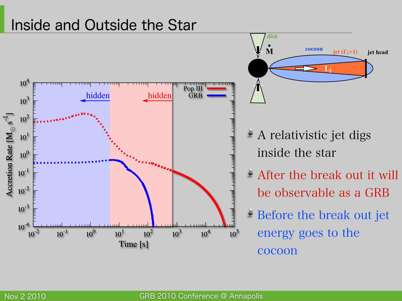
Inside and Outside the Star
A relativistic jet digs inside the star
After the break out it will be observable as a GRB
Before the break out jet energy goes to the cocoon
10-4
10-3
10-2
10-1
100
101
102
103
104
10-2 10-1 100 101 102 103 104 105
Acc
retio
n R
ate
[M!
s-1]
Time [s]
Pop IIIGRB
10-4
10-3
10-2
10-1
100
101
102
103
104
10-2 10-1 100 101 102 103 104 105
Acc
retio
n R
ate
[M!
s-1]
Time [s]
hiddenhidden
jet (!j≫1)cocoon
Lj
jet head
disk
M•
GRB 2010 Conference @ AnnapolisNov 2 2010
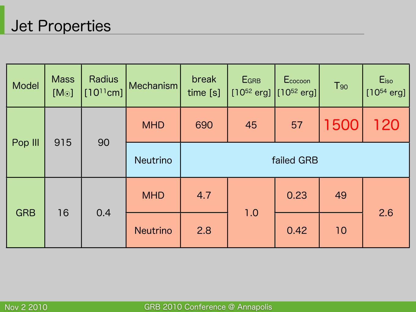
Jet Properties
Model Mass[M⦿]
Radius[1011cm]
Mechanism break time [s]
EGRB
[1052 erg]Ecocoon
[1052 erg]T90
Eiso
[1054 erg]
Pop III 915 90
MHD 690 45 57 1500 120Pop III 915 90
Neutrino failed GRBfailed GRBfailed GRBfailed GRBfailed GRB
GRB 16 0.4
MHD 4.7
1.0
0.23 49
2.6GRB 16 0.4
Neutrino 2.8
1.0
0.42 10
2.6
GRB 2010 Conference @ AnnapolisNov 2 2010
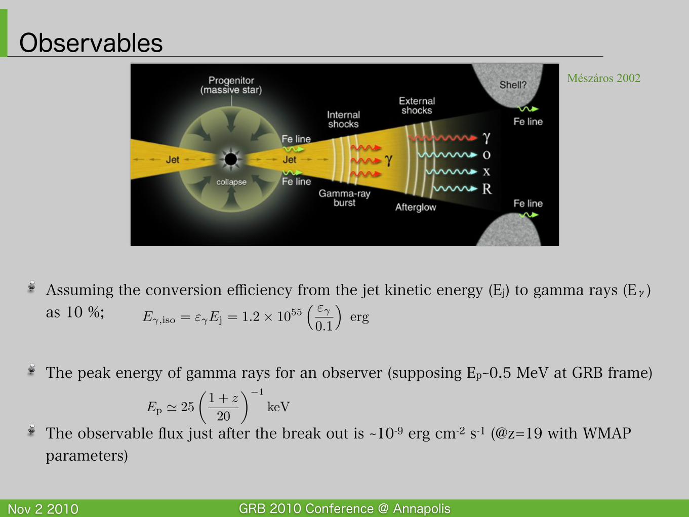
Assuming the conversion efficiency from the jet kinetic energy (Ej) to gamma rays (Eγ) as 10 %;
The peak energy of gamma rays for an observer (supposing Ep~0.5 MeV at GRB frame)
The observable flux just after the break out is ~10-9 erg cm-2 s-1 (@z=19 with WMAP parameters)
Observables
Eγ,iso = εγEj = 1.2× 1055� εγ
0.1
�erg
Mészáros 2002
Ep � 25�
1 + z
20
�−1
keV
GRB 2010 Conference @ AnnapolisNov 2 2010
Summary
Question “Can the first stars produce GRBs?”Absence of H envelope is required for successful GRB
But the first stars might not loose their massive envelope
More investigations are necessary
Stellar property “Powerful & long accretion”The central engine keep its powerful activity for the long time
Answer “It’s possible!”But very dim...
How to trigger them?