game theory, maximum entropy, minimum discrepancy and robust
TRANSCRIPT

Game Theory, Maximum Entropy, Minimum
Discrepancy and Robust Bayesian Decision Theory
Peter D. Grunwald and A. Philip Dawid
Presented by: Arindam Banerjee
. – p.1
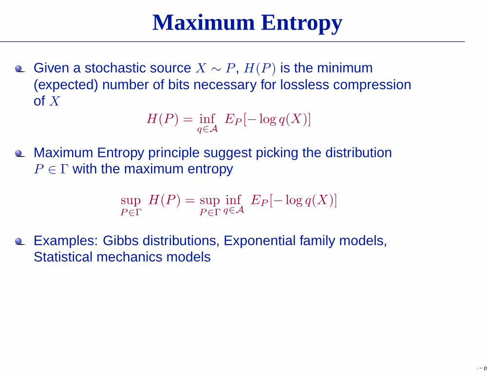
Maximum Entropy
Given a stochastic source X ∼ P , H(P ) is the minimum(expected) number of bits necessary for lossless compressionof X
H(P ) = infq∈A
EP [− log q(X)]
Maximum Entropy principle suggest picking the distributionP ∈ Γ with the maximum entropy
supP∈Γ
H(P ) = supP∈Γ
infq∈A
EP [− log q(X)]
Examples: Gibbs distributions, Exponential family models,Statistical mechanics models
. – p.2
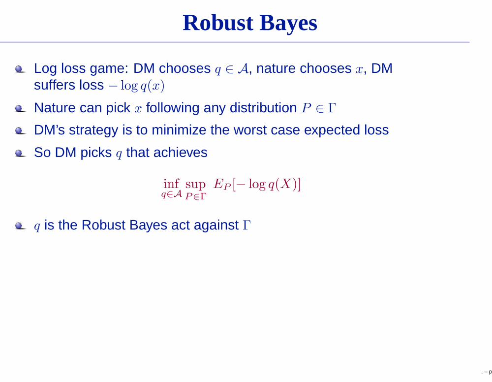
Robust Bayes
Log loss game: DM chooses q ∈ A, nature chooses x, DMsuffers loss − log q(x)
Nature can pick x following any distribution P ∈ Γ
DM’s strategy is to minimize the worst case expected loss
So DM picks q that achieves
infq∈A
supP∈Γ
EP [− log q(X)]
q is the Robust Bayes act against Γ
. – p.3

Maximum Entropy is Robust Bayes
Following the minimax results of game theory, conjecture:
supP∈Γ
infq∈A
EP [− log q(X)] = infq∈A
supP∈Γ
EP [− log q(X)]
Conjecture is true under very general conditions
The robust Bayes act q = p∗, the density of the maximumentropy distribution P ∗
Hence, maximum entropy is robust Bayes
A game-theoretic/statistical justification of “maxent”
. – p.4

Example
Maxent models with mean-value constraintsΓ = {P : EP (T ) = τ}, where T = t(X) ∈ R
k is a statistic
. – p.5

Example
Maxent models with mean-value constraintsΓ = {P : EP (T ) = τ}, where T = t(X) ∈ R
k is a statistic
There will exist a distribution P ∗ with p∗(x) = exp(αT t(x) + α0)and EP∗ [T ] = τ
. – p.5

Example
Maxent models with mean-value constraintsΓ = {P : EP (T ) = τ}, where T = t(X) ∈ R
k is a statistic
There will exist a distribution P ∗ with p∗(x) = exp(αT t(x) + α0)and EP∗ [T ] = τ
Then, for any P ∈ Γ
EP [− log p∗(X)] = α0 + αT τ = H(P ∗)
. – p.5

Example
Maxent models with mean-value constraintsΓ = {P : EP (T ) = τ}, where T = t(X) ∈ R
k is a statistic
There will exist a distribution P ∗ with p∗(x) = exp(αT t(x) + α0)and EP∗ [T ] = τ
Then, for any P ∈ Γ
EP [− log p∗(X)] = α0 + αT τ = H(P ∗)
P ∗ maximizes entropy as
H(P ) = infq∈A
EP [− log q(X)] ≤ EP [− log p∗(X)] = H(P ∗)
P ∗ is robust Bayes since (equality for q = p∗)
supP∈Γ
EP [− log q(X)] ≥ EP∗ [− log q(X)] ≥ EP∗ [− log p∗(X)] ≥ H(P ∗)
Further, the value
supP∈Γ
infq∈A
EP [− log q(X)] = infq∈A
supP∈Γ
EP [− log q(X)] = H(P ∗)
. – p.5

Decision Problems
A basic game: DM chooses action a ∈ A, nature reveals x ∈ X ,DM suffers loss L(x, a)
If nature is using x ∼ P, P ∈ P, the expected lossL(P, a) = EP [L(X, a)]
If DM is using randomized act a ∼ ζ, L(P, ζ) = EP×ζ [L(X, A)]
ζP is a Bayes act if ∀ζ
EP [L(X, ζ) − L(X, ζP )] ≥ 0
Generalized entropy H(P ) = infa∈A L(P, a)
Consider the action space A to be a set of distributions Q overnature’s set X
Scoring rule S(x, Q) = L(x, ζQ) is proper if S(P, P ) = H(P )
. – p.6

Examples
Brier Score: S(x, Q) = ‖δx − q‖2 so that
S(P, Q) =∑
j
q2
j − 2∑
j
qjpj + 1
H(P ) = S(P, P ) = 1 −∑
j
p2
j
. – p.7

Examples
Brier Score: S(x, Q) = ‖δx − q‖2 so that
S(P, Q) =∑
j
q2
j − 2∑
j
qjpj + 1
H(P ) = S(P, P ) = 1 −∑
j
p2
j
Logarithm Score: S(x, Q) = − log q(x) with
S(P, Q) = EP [− log q(X)]
H(P ) = S(P, P ) = EP [− log p(x)]
. – p.7
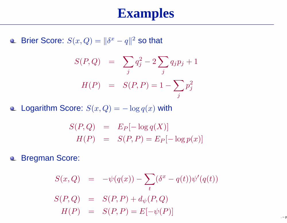
Examples
Brier Score: S(x, Q) = ‖δx − q‖2 so that
S(P, Q) =∑
j
q2
j − 2∑
j
qjpj + 1
H(P ) = S(P, P ) = 1 −∑
j
p2
j
Logarithm Score: S(x, Q) = − log q(x) with
S(P, Q) = EP [− log q(X)]
H(P ) = S(P, P ) = EP [− log p(x)]
Bregman Score:
S(x, Q) = −ψ(q(x)) −∑
t
(δx − q(t))ψ′(q(t))
S(P, Q) = S(P, P ) + dψ(P, Q)
H(P ) = S(P, P ) = E[−ψ(P )]. – p.7

Maximum Entropy and Robust Bayes
DM only knows that nature picks some P ∈ Γ
The “robust” Bayes criterion
infζ∈Z
supP∈Γ
L(P, ζ)
The maximum entropy criterion
supP∈Γ
infζ∈Z
L(P, ζ)
(P ∗, ζ∗) is an equilibrium of the game if H∗ = L(P ∗, Q∗) is finiteand the following holds:(a) L(P ∗, ζ∗) ≤ L(P ∗, ζ), ζ ∈ Z
(b) L(P ∗, ζ∗) ≥ L(P, ζ∗), P ∈ Γ
. – p.8

Maximum Entropy and Robust Bayes (Contd)
Lemma: Suppose there exist maximum entropy distributionP ∗ ∈ Γ and robust Bayes act ζ∗ ∈ Z. Then,
supP∈Γ
infζ∈Z
L(P, ζ) ≤ L(P ∗, ζ∗) ≤ infζ∈Z
supP∈Γ
L(P, ζ)
Further, if the game has a value V ∗, then V ∗ = L(P ∗, ζ∗) and(P ∗, ζ∗) is an equilibrium of the game
. – p.9

Maximum Entropy and Robust Bayes (Contd)
Lemma: Suppose there exist maximum entropy distributionP ∗ ∈ Γ and robust Bayes act ζ∗ ∈ Z. Then,
supP∈Γ
infζ∈Z
L(P, ζ) ≤ L(P ∗, ζ∗) ≤ infζ∈Z
supP∈Γ
L(P, ζ)
Further, if the game has a value V ∗, then V ∗ = L(P ∗, ζ∗) and(P ∗, ζ∗) is an equilibrium of the game
Theorem: Suppose that an equilibrium (P ∗, ζ∗) exists in a game.Then(i) The game has value H∗ = L(P ∗, ζ∗)
(ii) ζ∗ is a Bayes act against P ∗
(iii) H(P ∗) = H∗
(iv) P ∗ maximizes the entropy H(P ) over Γ
(v) ζ∗ is robust Bayes against Γ
. – p.9

Minimax Theorems
Simple Case: X is finite and L is bounded
. – p.10

Minimax Theorems
Simple Case: X is finite and L is bounded
Theorem: If Γ is a closed convex subset of P, then the gamehas a finite value H∗, and H(P ) achieves its maximum H∗ forsome P ∗ ∈ Γ
. – p.10
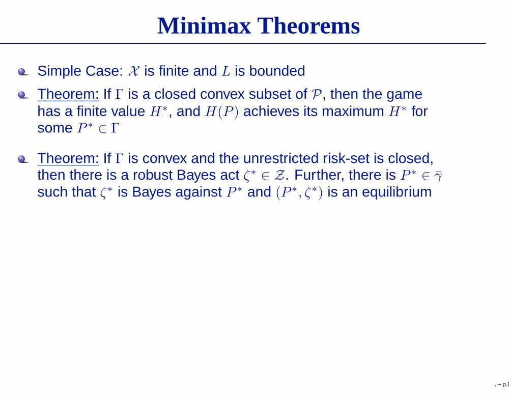
Minimax Theorems
Simple Case: X is finite and L is bounded
Theorem: If Γ is a closed convex subset of P, then the gamehas a finite value H∗, and H(P ) achieves its maximum H∗ forsome P ∗ ∈ Γ
Theorem: If Γ is convex and the unrestricted risk-set is closed,then there is a robust Bayes act ζ∗ ∈ Z. Further, there is P ∗ ∈ γ
such that ζ∗ is Bayes against P ∗ and (P ∗, ζ∗) is an equilibrium
. – p.10
Minimax Theorems
Simple Case: X is finite and L is bounded
Theorem: If Γ is a closed convex subset of P, then the gamehas a finite value H∗, and H(P ) achieves its maximum H∗ forsome P ∗ ∈ Γ
Theorem: If Γ is convex and the unrestricted risk-set is closed,then there is a robust Bayes act ζ∗ ∈ Z. Further, there is P ∗ ∈ γ
such that ζ∗ is Bayes against P ∗ and (P ∗, ζ∗) is an equilibrium
More general minimax theorems can be derived for muchweaker conditions on Γ and L
. – p.10

Mean Value Constraints
Let T = t(x) be a fixed real/vector statistic
Consider the class of distributions with mean value constraints
Γ = Γτ = {P ∈ P : EP (T ) = τ}
Specific entropy function h(τ) = supP∈Γτ
H(P )
An act ζ is linear if L(x, ζ) = β0 + βT t(x)
P is linear if it has a linear Bayes act ζ; (P, ζ) is called a linearpair; if EP (T ) = τ is finite, τ is a linear point
. – p.11

Mean Value Constraints
Let T = t(x) be a fixed real/vector statistic
Consider the class of distributions with mean value constraints
Γ = Γτ = {P ∈ P : EP (T ) = τ}
Specific entropy function h(τ) = supP∈Γτ
H(P )
An act ζ is linear if L(x, ζ) = β0 + βT t(x)
P is linear if it has a linear Bayes act ζ; (P, ζ) is called a linearpair; if EP (T ) = τ is finite, τ is a linear point
Theorem: If τ is linear with associated linear pair (Pτ , ζτ ) andlinear coefficients (β0, β), then(i) ζτ is an equalizer rule against Γτ
(ii) (Pτ , ζτ ) is an equilibrium(iii) ζτ is robust Bayes against Γτ
(iv) h(τ) = H(Pτ ) = β0 + βT τ
. – p.11

Discrepancy
Discrepancy between distribution P and act ζ
D(P, ζ) = L(P, ζ) − H(P )
If a Bayes act ζP exists, then
D(P, ζ) = EP [L(X, ζ) − L(X, ζP )]
When the loss is a proper scoring rule S, divergenced(P, Q) = S(P, Q) − H(P )
. – p.12

Discrepancy
Discrepancy between distribution P and act ζ
D(P, ζ) = L(P, ζ) − H(P )
If a Bayes act ζP exists, then
D(P, ζ) = EP [L(X, ζ) − L(X, ζP )]
When the loss is a proper scoring rule S, divergenced(P, Q) = S(P, Q) − H(P )
Lemma: Let P1, . . . , Pn have finite entropies and (p1, . . . , pn) bea probability vector. Then, with P =
∑i piPi
H(P ) =∑
i
piH(Pi) + pid(Pi, P )
d(P , Q) =∑
i
pid(Pi, Q) −∑
i
pid(Pi, P )
. – p.12

Relative Entropy
Given a reference act ζ0, the relative loss
L0(x, a) = L(x, a) − L(x, ζ0)
Similarly L0(x, ζ) = L(x, ζ) − L(z, ζ0) andL0(P, ζ) = L(P, ζ) − L(P, ζ0)
If a Bayes act ζP against P exists, the generalized relativeentropy H0(P ) = infa∈A L0(P, a) is
H0(P ) = EP [L(X, ζP ) − L(X, ζ0)]
Maximum generalized relative entropy is same as minimumdiscrepancy
H0(P ) = H(P ) − L(P, ζ0) = −D(P, ζ0)
Choose P ∈ Γ to minimize D(P, ζ0) from the reference act ζ0
. – p.13
Pythagorean Inequality
Theorem: Suppose (P ∗, ζ∗) is an equilibrium. Then for all P ∈ Γ,
D(P, ζ∗) + D(P ∗, ζ0) ≤ D(P, ζ0)
Further, if the inequality holds with rhs finite for all P ∈ Γ, then(P ∗, ζ∗) is an equilibrium
. – p.14

Pythagorean Inequality
Theorem: Suppose (P ∗, ζ∗) is an equilibrium. Then for all P ∈ Γ,
D(P, ζ∗) + D(P ∗, ζ0) ≤ D(P, ζ0)
Further, if the inequality holds with rhs finite for all P ∈ Γ, then(P ∗, ζ∗) is an equilibrium
Corollary: If S is a proper scoring function, then in the relativegame with loss S0(P, Q), if (P ∗, P ∗) is an equilibrium, then for allP ∈ Γ,
d(P, P ∗) + d(P ∗, P0) ≤ d(P, P0)
Theorem: Suppose (P ∗, ζ∗) is an equilibrium of the relativegame. If ζ∗ is an equalizer rule, i.e., L0(P, ζ∗) = H0(P
∗) for allP ∈ Γ, then Pythagorean equality holds. Conversely, if thePythagorean equality holds, then L0(P, ζ∗) = H(P ∗) for all P ∈ Γ
with D(P, ζ0) < ∞; in particular, if D(P, ζ0) < ∞ for all P ∈ Γ, ζ∗
is an equalizer rule
. – p.14