game theory and natural resources

Game Theory and Policymakingin Natural Resources andthe Environment

Game theory has become one of the main analytical tools for addressingstrategic issues in the field of economics and is expanding its influence inother fields of social sciences. With the increased level of extraction of naturalresources and pollution of environments, game theory gains its place in theliterature and it is seen more and more as a tool for policymakers and notonly for theoreticians.

The book is structured in four parts dealing with the management of nat-ural resources, the negotiation aspects of water management, water alloca-tion through pricing and markets, and how conflicts and regulation shape themanagement of the environment. The first part explores game theory con-cepts applied to fisheries and grazing lands, which are two important naturalresources. In the next two parts, several game theory methodologies are con-sidered in the negotiation approach to water management and approaches towater pricing and markets. The last section looks at environmental protectionas the end process of the interplay between conflict and regulation.

This book includes chapters by experts from developing and developedcountries that apply game theory to actual issues in natural resources and theenvironment. As such, the book is extremely useful for graduate students andtechnical experts interested in the sustainable management of naturalresources and the environment. It is also relevant to all game theory andenvironmental economics students.

Ariel Dinar is a Lead Economist in the Development Research Group ofthe World Bank and Adjunct Professor at the Johns Hopkins School ofAdvanced International Studies, Washington, DC, USA.

José Albiac is a Research Fellow at CITA, an agricultural research centreof the Government of Aragón, Zaragoza, Spain.

Joaquín Sánchez-Soriano is an Associate Professor at the Department ofStatistics, Mathematics and Computer Science of the University MiguelHernández, Elche, Spain.

Routledge Explorations in Environmental Economics

Edited by Nick HanleyUniversity of Stirling, UK

Greenhouse EconomicsValue and EthicsClive L. Spash

Oil Wealth and the Fate of Tropical RainforestsSven Wunder

The Economics of Climate ChangeEdited by Anthony D. Owen and Nick Hanley

Alternatives for Environmental ValuationEdited by Michael Getzner, Clive Spash and Sigrid Stagl

Environmental SustainabilityA Consumption ApproachRaghbendra Jha and K. V. Bhanu Murthy

Cost-Effective Control of Urban SmogThe Significance of the Chicago Cap-and-Trade ApproachRichard F. Kosobud, Houston H. Stokes, Carol D. Tallarico and Brian L. Scott

Ecological Economics and Industrial EcologyJakub Kronenberg

Environmental Economics, Experimental MethodsEdited by Todd L. Cherry, Stephan Kroll and Jason F. Shogren

Game Theory and Policymaking in Natural Resources and the EnvironmentEdited by Ariel Dinar, José Albiac and Joaquín Sánchez-Soriano

Game Theory and Policymakingin Natural Resources and theEnvironment

Edited by Ariel Dinar, José Albiac, andJoaquín Sánchez-Soriano

First published 2008by Routledge2 Park Square, Milton Park, Abingdon, Oxon OX14 4RN

Simultaneously published in the USA and Canadaby Routledge270 Madison Ave, New York, NY 10016

Routledge is an imprint of the Taylor & Francis Group,an informa business

© 2008 Editorial matter and selection, Ariel Dinar, José Albiac andJoaquín Sánchez-Soriano; individual chapters, the contributors

All rights reserved. No part of this book may be reprinted orreproduced or utilized in any form or by any electronic,mechanical, or other means, now known or hereafterinvented, including photocopying and recording, or in anyinformation storage or retrieval system, without permission inwriting from the publishers.

British Library Cataloguing in Publication DataA catalogue record for this book is available from the British Library

Library of Congress Cataloging in Publication DataGame theory and policy making in natural resources and theenvironment / edited by Ariel Dinar, José Albiac and Joaquín Sánchez-Soriano.p. cm.Includes bibliographical references and index.1. Natural resources—Management—Mathematical models. 2.Environmental policy—Mathematical models. 3. Game theory.I. Dinar, Ariel, 1947– II. Albiac, José. III. Sánchez-Soriano,Joaquín.HC85.G36 2008333.701′5193—dc222007032312

ISBN 10: 0–415–77422–5 (hbk)ISBN 10: 0–203–93201–3 (ebk)

ISBN 13: 978–0–415–77422–2 (hbk)ISBN 13: 978–0–203–93201–8 (ebk)

This edition published in the Taylor & Francis e-Library, 2008.

“To purchase your own copy of this or any of Taylor & Francis or Routledge’scollection of thousands of eBooks please go to www.eBookstore.tandf.co.uk.”

ISBN 0-203-93201-3 Master e-book ISBN

Contents

List of illustrations viiList of contributors xiAcknowledgments xviiList of abbreviations and acronyms xix

1 Game theory: a useful approach for policy evaluation innatural resources and the environment 1JOSÉ ALBIAC, JOAQUÍN SÁNCHEZ-SORIANO, AND ARIEL DINAR

2 Game theory and the development of resource managementpolicy: the case of international fisheries 12GORDON R. MUNRO

3 Traditional grazing rights in sub-Saharan Africa and the roleof policy 42RACHAEL E. GOODHUE AND NANCY McCARTHY

4 Application of partition function games to the managementof straddling fish stocks 65PEDRO PINTASSILGO AND MARKO LINDROOS

5 To negotiate or to game theorize: evaluating water allocationmechanisms in the Kat basin, South Africa 85ARIEL DINAR, STEFANO FAROLFI, FIORAVANTE PATRONE, ANDKATE ROWNTREE

6 Cooperation and equity in the river-sharing problem 112STEFAN AMBEC AND LARS EHLERS

7 Negotiating over the allocation of water resources: thestrategic importance of bargaining structure 132RACHAEL E. GOODHUE, GORDON C. RAUSSER, LEO K. SIMON,AND SOPHIE THOYER

8 Rural–urban water transfers with applications to theUS–Mexico border region 155GEORGE B. FRISVOLD AND KYLE J. EMERICK

9 WAS-guided cooperation in water management: coalitionsand gains 181FRANKLIN M. FISHER AND ANNETTE T. HUBER-LEE

10 Experimental insights into the efficiency of alternative watermanagement institutions 209AURORA GARCÍA-GALLEGO, NIKOLAOS GEORGANTZÍS, ANDPRAVEEN KUJAL

11 A fair tariff system for water management 236RITA DE AGOSTINI AND VITO FRAGNELLI

12 Game-theoretic modeling of water allocation regimes appliedto the Yellow River basin in China 248XIAOKAI LI, HAIFENG SHI, AND XUEYU LIN

13 Contributions of game theory to the analysis of consumerboycotts 266PHILIPPE DELACOTE

14 How does environment awareness arise? An evolutionaryapproach 278PALOMA ZAPATA-LILLO

15 Effects of alternative CDM baseline schemes under animperfectly competitive market structure 307HARUO IMAI, JIRO AKITA, AND HIDENORI NIIZAWA

Index 335

vi Contents

Illustrations

Figures

1.1 Pollution abatement under noncooperative and cooperativesolutions 4

2.1 General migratory pattern of Pacific salmon 262.2 South Tasman Rise trawl fishery 282.3 Benguela Current large marine ecosystem 302.4 Western and Central Pacific Ocean: Convention limits 323.1 Pastoralist mobility under fuzzy property regime as a

function of rainfall 523.2 Comparison of A’s profits under fuzzy property and private

property regimes as a function of rainfall 543.3 Comparison of social welfare under fuzzy property and

private property regimes as a function of rainfall 553.4 Differences in mobility between fuzzy property and common

property regimes as a function of rainfall 565.1 Kat basin and stylized subbasins in the role-playing game 886.1 Example of inefficient noncooperative extraction with

Pareto improving reallocation of water 1167.1 Participation constraints in round T − 1 1397.2 Effect of access shift on round T − 1 proposals 1457.3 Beggar-thy-neighbor behavior by farmers 1498.1 Urban water demand 1608.2 Urban willingness to pay for transferred water 1618.3 Irrigation district and municipal water provider payoff

contours, disagreement curves, and the contract curve 1629.1 Efficient water allocation and water values 1899.2 Partial regional map with water systems 1939.3 Gains from bilateral cooperation between Israel and

Palestine in 2010 1979.4 Gains from bilateral cooperation between Israel and Jordan

in 2010 1999.5 Gains from trilateral cooperation (grand coalition) in 2010 200

9.6 Continuity of flows at node i 20810.1 Pipeline network 21510.2 Evolution of average stock levels (low-quality water) 22110.3 Evolution of average stock levels (high-quality water) 22110.4 Average market-clearing prices (low-quality water) 22310.5 Average market-clearing prices (high-quality water) 22310.6 Average quality/average price ratio for the four treatments 22411.1 Contested garment approach 24512.1 Regions of Yellow River basin 25912.2 Net social benefit in the case of P50 26112.3 Net social benefit in the case of P75 26112.4 Net social benefit in the case of P95 26214.1 Changes in player’s Nash equilibrium payoff as β changes 29014.2 Possible changes in the strategy structure of society during

the learning process 298

Tables

4.1 Example of a characteristic function 684.2 Coalition payoffs for bluefin tuna fishery 765.1 Actual and transformed values for use in role-playing game

of main variables in Kat basin 905.2 Exogenous factors in role-playing game session: initial, final,

and difference values 925.3 Strategies and outcomes for the five farms during

role-playing game session: initial and final values 935.4 Strategies and outcomes for the three villages during

role-playing game session: initial and final values 945.5 Profit, job creation, and water consumption in the three

subbasins during role-playing game session 965.6 Allocation of annual (and annualized) profits according to

the role-playing game, Shapley value, and nucleolus in theKat game 102

8.1 Water sales and leases in US border states 1990–2000 1568.2 Effect on water transfers of changes in market, policy, or

technology parameters 1658.3 Values used in numerical simulation 1708.4 Impact of irrigation efficiency on water transfers, transfer

price, and consumptive use 1718.5 Impacts of transfers and irrigation efficiency on

consumptive use 17210.1 Descriptive statistics (treatments 1, 2, 3 and coordinated

duopoly aggregates and last 30 period averages and standarddeviations) 222

viii Illustrations

10.2 Average quantity sold for high- and low-quality water, byfive-period intervals 224

10.3 Table of costs (expressed in ExCUs) 23211.1 Definition of K using weighted average tariff 23911.2 Definition of K using actual average tariff 24011.3 Tariff system of ATO/6, 2002 24012.1 Regional annual runoff of different frequencies 25912.2 Water demand 2000 25912.3 Effective irrigated area of regions 2000 26012.4 Regional cropping patterns 26012.5 P50 water use and net social benefit 26012.6 P75 water use and net social benefit 26112.7 P95 water use and net social benefit 26215.1 Summary data for two food companies in project 0455 for

years 2004 and 2006 324

Illustrations ix

Contributors

Jiro Akita is Professor of Economics at the Graduate School of Economicsand Management, Tohoku University. He is currently Vice-Chair of theDepartment of Economics. His research area is international finance,macroeconomics, and environmental economics. His translated book onenvironmental economics has become one of the major references inJapan.

José Albiac is Researcher at the Department of Agricultural Economics,Agrifood Research and Technology Center (Government of Aragon,Spain). His main fields of work are water resource management and foresteconomics.

Stefan Ambec is Research Fellow in Economics at the Grenoble AppliedEconomics Laboratory, National Institute for Agricultural Research(INRA-GAEL), at the University of Grenoble, France. His main researchinterests are in environmental economics and natural resources, and indus-trial organization. His works on river management have been published inthe Journal of Economic Theory and the Canadian Journal of Economics.

Rita De Agostini graduated in Mathematics in 2004 at the University ofEastern Piedmont, with a Masters thesis on water management. Her maininterest is in applications of game theory.

Philippe Delacote is PhD Researcher at the European University Institute(Florence, Italy). His field of specialization lies at the frontier of develop-ment and environmental economics. His precedent work focused mainlyon forest economics, more precisely the use of forest products by pooragricultural households and corruption issues in the context of forestexploitation.

Ariel Dinar is a Lead Economist in the Development Research Group of theWorld Bank and Adjunct Professor at the Johns Hopkins School ofAdvanced International Studies, Washington, DC, United States. Hiswork focuses on application of game theory to issues of water and naturalresource conflicts at regional and international levels.

Lars Ehlers is Associate Professor in Economics at the Université de Mon-tréal, Canada, a member of the Center for Interuniversity Research inQuantitative Economics (CIREQ), and an elected member of the Councilof the Society of Social Choice and Welfare. He is a specialist in matchingtheory (with applications to entry-level labor markets and public schoolchoice) and he has worked on social choice and axiomatic mechanismdesign. He has had numerous papers published in the Journal of EconomicTheory and Games and Economic Behavior.

Kyle J. Emerick is a graduate student in the Department of Agricultural andResource Economics at the University of Arizona. He is also a GraduateResearch Assistant with the Climate Assessment for the Southwest project(CLIMAS) of the University of Arizona’s Institute for the Study of PlanetEarth.

Stefano Farolfi is a CIRAD Senior Researcher in Environmental and NaturalResource Economics. He is Senior Lecturer and Research Fellow at theCentre for Environmental Economics and Policy in Africa (CEEPA), Uni-versity of Pretoria, South Africa. He is experienced in water managementand governance and is currently leading several research projects and is amember of the external advisory board of the Water Research Commis-sion of South Africa.

Franklin M. Fisher is Jane Berkowitz Carlton and Dennis William CarltonProfessor of Economics, Emeritus at the Massachusetts Institute of Tech-nology. He is Chair of the Water Economics Project and the senior authorof its book, Liquid Assets, and of sixteen other books.

Vito Fragnelli is Associate Professor of Game Theory at the University ofEastern Piedmont. He organized the International Meeting on GamePractice and the Environment held in Alessandria in 2002 and edited theproceedings with C. Carraro. He is Scientific Director of the SummerSchool on Game Theory and Operations Research. He is responsible foror cooperates in several Italian and European research projects. He isauthor of about twenty papers published in international journals andbooks.

George B. Frisvold is Professor in the Department of Agricultural andResource Economics at the University of Arizona. He is also an Investiga-tor with the Climate Assessment for the Southwest project (CLIMAS) ofthe University of Arizona’s Institute for the Study of Planet Earth.

Aurora García-Gallego is Associate Professor and Co-Director at the Labora-tori d’Economia Experimental, Universitat Jaume I, Castellón, Spain. Sheholds a PhD (1994) from the European University Institute, Florence,Italy. She has had articles published in the Journal of Economic Behaviorand Organization, International Journal of Industrial Organization,Regional Science and Urban Economics, International Review of Law and

xii Contributors

Economics, Environmental and Resource Economics, and EcologicalEconomics.

Nikolaos Georgantzís is Associate Professor and Director at the Laboratorid’Economia Experimental, Universitat Jaume I, Castellón, Spain. Heholds a PhD (1993) from the European University Institute, Florence,Italy. He has had articles published in the Journal of Economic Behaviorand Organization, International Journal of Industrial Organization,Regional Science and Urban Economics, Journal of Economics and Man-agement Strategy, Environmental and Resource Economics, and EcologicalEconomics.

Rachael E. Goodhue is Associate Professor in the Department of Agriculturaland Resource Economics at the University of California, Davis. Herresearch addresses a number of areas, including contracting, industrialorganization, agricultural organization, agricultural policy, pesticide useand regulation, and natural resource use policies and property rights.

Annette T. Huber-Lee leads Theme 5: Global and National Food and WaterSystem of the Challenge Program on Water and Food. She is ResearchFellow at the International Food Policy Research Institute and SeniorResearch Fellow at the Stockholm Environment Institute.

Haruo Imai is Professor of Economics at the Institute of Economic Research,Kyoto University. He has served as editor of the Economic Studies Quar-terly (now called the Japanese Economic Review). His research field is ingame theory, mathematical economics, microeconomics, and their applica-tion in industrial economics and environmental policy. He is the leader ofseveral research projects.

Praveen Kujal is Associate Professor at the Universidad Carlos III de Madrid,Spain. He holds a PhD (1994) from the University of Arizona, UnitedStates. His published work includes articles in the Economic Journal,Journal of International Economics, Journal of Economic Behavior andOrganization, International Journal of Industrial Organization, ResearchPolicy, Economics Letters, and Information Economics and Policy.

Xiaokai Li, of the Institute of Water Sciences, Beijing Normal University,is a water professional and manager of international water resourcedevelopment investments with wide exposure to transboundary waterissues.

Xueyu Lin, of the Institute of Water Sciences, Beijing Normal University, is arenowned academician in applied hydrology and groundwater studies andmanagement.

Marko Lindroos holds a PhD in Economics. He is a Lecturer at the Depart-ment of Economics and Management, University of Helsinki. His mainresearch field is game theory and bioeconomic modeling.

Contributors xiii

Nancy McCarthy is Research Fellow at the International Food PolicyResearch Institute (IFPRI) and Levy Fellow at George Mason UniversitySchool of Law. Her research emphasizes property rights and collectivemanagement. She joined IFPRI in 1996 to research property rights andrisk in livestock management as a joint postdoctoral fellow with IFPRIand the International Livestock Research Institute.

Gordon R. Munro is Professor Emeritus with the Department of Economicsand the Fisheries Centre, University of British Columbia, and VisitingProfessor with the Centre for the Economics and Management of AquaticResources, University of Portsmouth. He has been involved, for overthirty years, in research on fisheries management problems, particularlythose arising under the New Law of the Sea. He has published widely onboth theoretical and policy issues. Along with research, he has undertakenconsulting work for Asia–Pacific Economic Cooperation, the Food andAgriculture Organization of the United Nations, the Organisation forEconomic Co-operation and Development, the United Nations Develop-ment Programme, and the Department of Fisheries and Oceans Canada.

Hidenori Niizawa is Professor of Environmental Economics in the School ofEconomics, University of Hyogo. His research area is environmental pol-icy, emissions trading, the Kyoto Protocol, and post-Kyoto Protocol. Heis chief editor of the Annual Report of the Society of EnvironmentalEconomics and Policy Studies, and is the project leader of some researchfunds of the Kyoto Protocol.

Fioravante Patrone is Professor of Game Theory at the Faculty of Engineer-ing, University of Genoa, Italy. He is author of more than fifty publica-tions in mathematical analysis and game theory. He has been the promoterof the Game Practice meetings that started in 1998 and of the internationalsummer schools, Game Theory + . He has served as Director of the Inter-university Centre for Game Theory and Applications for many years.

Pedro Pintassilgo holds a PhD in Natural Resource Economics. He is cur-rently an Assistant Professor at the Faculty of Economics, University ofAlgarve. His main research field is game theory applied to high seasfisheries.

Gordon C. Rausser is Robert Gordon Sproul Distinguished Professor in theDepartment of Agricultural and Resource Economics, University ofCalifornia, Berkeley. He is a leading scholar on the forces driving thedramatic changes under way in agriculture, such as new technologies,globalization, population change, and economic growth. He has developedseveral highly respected research programs in such areas as public policyfor food and agricultural sectors, futures and options markets, politicaleconomics of policy reform, environmental and natural resource analysis,and applied econometrics.

xiv Contributors

Kate Rowntree is Professor of Geography at Rhodes University in EasternCape Province of South Africa. She has been engaged in research in waterresource management since 1990 and has published on Kenyan, SouthAfrican, and European water management issues. Since 1997 she and herstudents have been actively engaged in a project in the Kat Valley in EasternCape, supporting the participation by all stakeholders in the developmentof a catchment management plan. This project has embraced the spiritand intent of South Africa’s national Water Act of 1998, which promotesintegrated water resource management through stakeholder participation.

Joaquín Sánchez-Soriano is Professor of Statistics and Operations Researchat the Faculty of Engineering and Director of the Operations ResearchCenter at University Miguel Hernández of Elche. His current researchinterests include game theory and its applications, in particular to radioresource management, transportation problems, and market design, andoperations research applications to telecommunications problems andwater resource management.

Haifeng Shi, of the Department of Planning, Ministry of Water Resources,Beijing, has extensive experience in water resource planning and manage-ment policies in China.

Leo K. Simon has research interests ranging from theoretical game theory tosimulation modeling to applied political economy. His most recent theor-etical work introduces a new class of incomplete information games, calledaggregation games. His current work in political economy compares theagrienvironmental policy formation processes in Europe and the UnitedStates, and the role played by the World Trade Organization in these tworegions.

Sophie Thoyer is a Senior Lecturer at the Department of Agricultural andResource Economics at the Higher National School of Agronomy(ENSAM), Montpellier. Her main research work focuses on the politicaleconomy of agricultural and environmental reforms, with a particularfocus on the modeling of negotiation processes. She also works on thecomparison between negotiation instruments and market-like instruments,such as auctions, to allocate agrienvironmental contracts to farmers.

Paloma Zapata-Lillo is Associate Professor of Mathematics at the Universi-dad Nacional Autónoma de México. Her areas of interest are the theoriesof repeated games and evolutionary games. She has written the booksFundamentación Matemática de los Algoritmos Simpliciales (MathematicalFoundation of the Simplicial Algorithms) and Economía, Política y OtrosJuegos: Una Introducción a los Juegos no Cooperativos (Economics, Polit-ics, and Other Games: An Introduction to Noncooperative Games), thelatter to be published soon. A third book, Los Juegos del ComportamientoSocial (Social Behavior Games) is in preparation.

Contributors xv

Technical Editor

John Dawson is a freelance writer and editor based in Nairobi, Kenya. Heedits, upgrades, writes, and rewrites documents for a number of inter-national organizations, including the World Bank and the World HealthOrganization, and attends conferences as a report writer for the UnitedNations. His two published books, Quiz Setting Made Easy and EastAfrica Alive, reflect his interest in mind puzzles and wildlife.

xvi Contributors

Acknowledgments

This book is one of the products of the Sixth Meeting on Game Theory andPractice Dedicated to Development, Natural Resources and the Environ-ment, held in July 2006 in Zaragoza, Spain. The meeting, one of a series ofbiennial meetings on game theory and practice commencing in 1998, was co-funded by the Government of Aragon, Spain, and the Spanish Ministry ofEducation and Science, and was hosted by the Mediterranean AgronomicInstitute of Zaragoza (IAMZ-CIHEAM).

Many people and organizations were involved in the process leading to thepublication of this book and it is our honor to mention them here.

We would like to acknowledge the efforts of our friends in the OrganizingCommittee of the meeting, Fioravante Patrone, Rashid Sumaila, and DunixiGabiña. We are indebted to the support from the members of the meeting’sScientific Committee, Serdar Güner, Carlo Carraro, Marc Kilgour, Fiora-vante Patrone, Michael Maschler, Stef Tijs, Rashid Sumaila, Ignacio Garcia-Jurado, H. Peyton Young, Henk Folmer, Gian-Italo Bischi, Vito Fragnelli,Leon A. Petrosjan, and David W.K. Yeung.

The 100 participants of the meeting and the 65 who presented papersbenefited greatly from the professional organization by IAMZ-CIHEAM,led by the Institute’s deputy director, Dunixi Gabiña, and director, LuisEsteruelas, and supported by the Center for Agrofood Research andTechnology (CITA), Government of Aragon.

Special thanks are due to the reviewers of the various chapters: DirkEngelmann, Victor Galaz, Serdar Güner, Brian H. Hurd, Kieran Kelleher,Pham Do Kim Hang, Van W. Kolpin, Takanoby Kosugi, Raul P. Lejano,Carmen Marchiori, Stefano Moretti, Elinor Ostrom, Wu Xun, and DavidYeung, who provided us with guidance and feedback on needed modifica-tions and revisions.

The technical editing of the chapters deserves special mention, mainlybecause it was not an obvious job. The final product, which all of us are proudof, was meticulously edited in a very careful process led by John Dawson.

Ariel Dinar, José Albiac, and Joaquín Sánchez-SorianoJune 2007

Abbreviations and acronyms

ATO ambito territoriale ottimale (optimal territorial area)CDM clean development mechanismCDM-EB clean development mechanism Executive BoardCER certified emission reductionCQ common quotaCUT Comité de Unidad de Tepoztlán (Unified Tepoztlán Committee)ERU emission reduction unitEU-ETS European Union Emissions Trading SchemeFAO Food and Agriculture Organization of the United NationsICCAT International Commission for the Conservation of Atlantic

TunaIQ independent quotaNEIO new empirical industrial organizationOECD Organisation for Economic Co-operation and DevelopmentRFMO regional fisheries management organizationSAGE schéma d’aménagement et de gestion des eauxSDAGE schéma directeur d’aménagement et de gestion des eauxUNFCCC United Nations Framework Convention on Climate ChangeWAS water allocation systemWCPFC Western and Central Pacific Fisheries CommissionWUA Water Users Association

1 Game theoryA useful approach for policyevaluation in natural resourcesand the environment

José Albiac, Joaquín Sánchez-Soriano,and Ariel Dinar

This chapter sets the tone for the book by posing the intriguing questionof whether or not game theory has developed sufficiently, and the conflictsand problems associated with sharing of natural resources and environ-mental amenities have worsened enough, that game theory may assist inevaluating various policies aimed to improve their management. The chapteruses several examples from the cases discussed in the book as well assome examples not included in the book to convince the reader that thereare a number of opportunities to apply game theory to policy issues innatural resources and the environment. The chapter also highlights the prob-lems that still exist and the aspects that have to be addressed in the interpret-ation of the results and in the application of the various game theoryapproaches.

1.1 Background

Since the middle of the twentieth century, principles, concepts, and method-ologies originating in the theory of games have been successfully applied tosuch diverse fields as economics, politics, evolutionary biology, computer sci-ence, statistics, mathematics, accounting, social psychology, law, epistemology,and ethics, providing analytical, insightful ideas and explanations to variousimportant problems in each of these fields. Particularly, the significant role ofgame theory in economics and social sciences has been recognized by theaward of the Nobel Prize for Economics to game theorists on two occasions,in 1994 and 2005.

Generally speaking, game theory could potentially be useful in any contextwhere there are two or more agents facing conflict of interest, with the finalresult of these interactions depending on their (strategic) behavior. Thus,with globalization and openness of societies, and with the increased level ofextraction of natural resources and pollution of environments, game theorygains its place in the literature and is increasingly seen as a tool not only fortheoreticians but also of actual benefit to policymakers.

Since the industrial revolution, technological advances have triggered amassive increase in production, wealth, and population to levels that appear to

be unsustainable. This extraordinary growth in human activities is pressuringnatural resources and leading to extensive environmental damage, which inturn threatens the proper functioning of ecosystems and the well-being ofmany societies that rely on their services.

As population increases and availability of natural resources remains con-stant or decreases, the potential for conflict over management, extraction,and allocation of basic natural resources such as land, water, and fisheriesbecomes more likely, and the resultant increase in negative environmentalexternalities—arising, for example, from the stress put on fisheries, forests,and water—affects individuals, groups, and territories. One important impli-cation is that strategic behavior by individuals and groups becomes moreessential if they are to maintain their livelihoods and continue to survive.

What makes water resources a natural candidate for cooperativegame theory applications?

“Indeed this is a question that intrigues many scholars involved inthis field. First, water-related conflicts involve usually a small numberof stakeholders (players) that are interrelated to each other. Therefore,there is a greater scope for strategic behavior among players in water-related conflicts. Second, the level of externalities associated with waterutilization is a big incentive to cooperate. Externalities include (a) thezero-sum (or constant-sum) outcomes of unilateral use of the resource(e.g., if party B uses more of the resource in the aquifer, less is left toparty A, and also the cost of pumping party A faces is much moresubstantial due to the depth to the water table), and (b) the negativeimpact of water quality degradation that party A—the upstream—imposes on party B—the downstream (in the case of a river). Third, thegreat economies of scale associated with water infrastructure make itmore attractive to build bigger rather than smaller water projects, henceproviding incentives to joint considerations. Fourth, water projects arein many cases multi-objective ones, leading to inclusion interests. There-fore, a major issue of water projects investment and management isthe allocation of the cost and benefits among the various stated pro-ject objectives (e.g., sub-sectors, groups of beneficiaries). And fifth,many water problems are transboundary in nature, leading to inter-jurisdictional, interregional, or international conflicts. Since the playersand the problems will last, it is likely that cooperation may be attractivefor part or all the players.” (See additional discussion in Chapters 5, 6,7, and 10.)

(Dinar et al. 2007)

2 José Albiac et al.

The compelling reason for the application of game theory to environ-mental and natural resource problems is that these problems stem from inter-dependence among agents, through their interrelated actions and strategies.Not only are the outcomes of decisions by agents interrelated, but also indi-vidual decisions are often taken without knowledge of the decisions of otheragents (see box above for the case of water resources).

The public good aspects of natural resources at local or global scales, andthe externalities associated with them, make their management challenging,as there are incentives to free riding. Sustainable management calls for con-trol mechanisms designed to induce collective action and cooperation amongstakeholders.

There are many examples of lack of enforcement by authorities or absenceof any authority; for example, in the cases of carbon emissions, air quality,water resource quantity and quality (especially for groundwater), and loss ofbiodiversity and natural capital. And when enforcement is in place, there arealso problems of asymmetric information between the regulatory agency andthe agents using the resource.

Game theory demonstrates that under noncooperative solutions, eachindividual agent maximizes its own benefit taking into account that otheragents also maximize their individual benefits. Noncooperation is driven bythe structure of incentives, theoretical dimensions of which include the pri-soner’s dilemma game, the so-called tragedy of the commons, and free riding(Axelrod 1984; Hardin 1968).

Cooperative solutions could result from binding agreements with built-inpenalties that are enforced by the agents themselves, called self-enforcingagreements. In such a setting, a characteristic function is defined that com-putes for each coalition of players the total benefits that all members of thecoalition can attain by themselves. The best-known noncooperative gamesolution is the Nash equilibrium of the game, while the full cooperationgame solution maximizes the coalition payoff, in which case the agents haveto find a reasonable distribution of the additional benefits obtained fromcooperation. These points are demonstrated in Figure 1.1, using economicconcepts that are applied to a problem of pollution abatement.

Figure 1.1 depicts a situation of pollution abatement where linear marginalbenefit and cost functions are assumed. MBi are marginal benefits and MCi

are marginal costs from pollution abatement by each player i, and MB aretotal marginal benefits from abatement. Under A0, the noncooperative state,there is no effort by players on pollution abatement. The noncooperativesolution ANC is the Nash equilibrium where players equalize individual mar-ginal benefits MBi with individual marginal costs MCi. The level of abate-ment in the full cooperative solution AC maximizes welfare and applies thecondition for efficient provision of public goods MB = ΣiMBi = MCi. Thespecification of the marginal benefit function requires knowledge of bio-physical processes and pollution damages to ecosystems. When this informa-tion is not available, the optimum level of abatement AC is not known. In

Game theory: a useful approach to evaluate policy 3

such a case the alternative is to establish an abatement threshold AT, wherecooperation implies minimizing total abatement costs across players to reachthe threshold.1

Full cooperation is not usually an equilibrium because of possible freeriding by some players, and also because some players may end up beingworse off due to the nature of the cooperative solution and their relativelygood status quo situation. To make sure that all players improve upon theindividual Nash equilibrium solution, gains could be redistributed throughside payments. This is the usual outcome of partial cooperation in real-worldsituations, which involve both cooperating and free-riding players, andwhere negotiations lead to agreements with built-in incentives that reward orpenalize individuals joining or disrupting the agreement.

Several mechanisms have been suggested to redistribute gains among play-ers. In practice, allocation mechanisms are frequently based on equity rules,which are a type of social norm. Percentage reductions in emissions have beenapplied in the Montreal and Kyoto Protocols, and percentage allocation ofresources is embodied in many water resource agreements to reduce waterextractions or to share river flows. Other allocation mechanisms include theShapley value, Nash bargaining, and cost-sharing rules. These will not beexplained here.

Cost-sharing rules could be implemented using taxes, tradable permits andlump sum fines or subsidies. In the case of pollution, side payments maycontradict the polluter pays principle as pollution abatement may requirecompensation to polluters, and also anticipated side payments may induceabatement efforts below noncooperation.

Figure 1.1 Pollution abatement under noncooperative and cooperative solutions.


1.2 Focus of the book

Given this background, readers who are not specialist economists or gametheorists are invited to read the book to gain insight into the usefulness ofapplying game theory to various real-life issues. The reader of the variouschapters of this book will find examples of game theory applications tofamiliar problems of natural resource and environment management and theirpolicy implications. Among the fields considered are pollution, fishery man-agement, land management, water management (including negotiation andpricing), and environmental management (including conflict and regulation).These applications are distributed over the next fourteen chapters, which wereoriginally presented as papers at a conference dedicated to game theory andpractice in natural resources and the environment in Zaragoza, Spain, in 2006.2

The meeting in Zaragoza was the sixth in a series of biennial meetings ongame theory and practice commencing in 1998.3

1.3 Components of the book

The book is structured in four parts dealing with the management of naturalresources, the negotiation aspects of water management, water allocationthrough pricing and markets, and how conflicts and regulation shape themanagement of the environment. The first part explores game theory con-cepts applied to fisheries and grazing lands, which are two important naturalresources. In the next two parts, several game theory methodologies are con-sidered in the negotiation approach to water management and approaches towater pricing and markets. The last part looks at environmental protection asthe end process of the interplay between conflict and regulation.

The first part includes three chapters addressing international fisheriesand grazing rights. Chapter 2, by Munro, makes an assessment of the rele-vance of game theory to the management of internationally shared fisheries,presenting the game theory concepts and demonstrating their essential rolefor a sound understanding of the policy issues and the design of workablemeasures. Chapter 3, by Goodhue and McCarthy, analyzes pastoralist sys-tems in Africa where several groups with different property rights share theresource. The authors compare the different property rights arrangements(traditional, private, common), indicating the conditions for the strengthen-ing of traditional or private property rights. Chapter 4, by Pintassilgo andLindroos, analyzes coalition formation in straddling stock fisheries by apply-ing game theory to a fishery represented by the Gordon–Schaefer model andthe North Atlantic bluefin tuna fishery. Results show that cooperationagreements break down because of free riding by third-party countries, andenforcement against noncooperation is the key issue in protecting straddlingstock fisheries.

The second part deals with negotiation in water management. Chapter 5,by Dinar, Farolfi, Patrone, and Rowntree, compares alternative negotiation


(role playing) and mediation (cooperative game) mechanisms in solving waterallocation problems in the Kat basin in South Africa. Both negotiation andcooperative game approaches result in similar benefit shares to players fromvarious scenario arrangements, providing complementary valuable guidancefor future water allocation decisions. Chapter 6, by Ambec and Ehlers,investigates the river-sharing problem among riparian users. Acceptable out-comes from cooperation require coalition stability and fairness, and they canbe implemented through negotiation rules or decentralized water markets.Chapter 7, by Goodhue, Rausser, Simon, and Thoyer, explores water alloca-tion among stakeholders by emphasizing the importance of the structureof the negotiation process on eventual outcomes. The Rausser–Simon bar-gaining model is used to illustrate these questions in the Adour basin inFrance, and to reveal basic relationships between negotiation structure andbargaining power. Chapter 8, by Frisvold and Emerick, examines net gainsfrom large rural–urban water transfers, considering such issues as bilateralmonopoly, asymmetric capacity and bargaining power, and negative external-ities. Results indicate that irrigation technology subsidies may have uninten-ded effects that hinder water conservation, and that while water transfersbenefit contracting parties they may also entail negative environmental andthird-party externalities.

The third part looks at water pricing and markets as instruments for watermanagement. Chapter 9, by Fisher and Huber-Lee, looks into the resolutionof water conflicts by using the water allocation system tool. The empiricalresults presented show gains from cooperation between Israel, Jordan, andPalestine. The tool can be used also to provide guidelines for infrastruc-ture planning and allocation among sectors, and to solve conflicts in otherregions of the world. Chapter 10, by García-Gallego, Georgantzís, and Kujal,investigates the level of centralization and the use of markets to allocatewater. Several public and private market structures are simulated in anexperimental setting, and results show that centralized public managementgenerates more efficient outcomes in terms of welfare and water quality.Chapter 11, by De Agostini and Fragnelli, explores the design of urban tariffsystems in Italy, which comply with principles of fairness and reduction ofwater wastage. Several water pricing mechanisms are analyzed, taking intoaccount household characteristics and cost-sharing rules, and the implica-tions for water planning by suppliers. Chapter 12, by Li, Shi, and Lin,presents a water allocation model for the Yellow River basin. Different man-agement regimes, such as unregulated withdrawal, quotas, and water markets,are examined by using the Nash–Harsanyi negotiation approach. Large wel-fare gains are possible by implementing water markets or by enforcing thepresent flimsy quota regime, although implementation and transaction costscould be quite large.

The fourth part considers the impact of conflict and regulation in shapingenvironmental management. Chapter 13, by Delacote, analyzes the impact ofconsumer boycotts using game theory, looking at the war of attrition between


consumers and the firm under pressure. The potential for success by environ-mental boycotts is low because the opportunity cost to consumers seems to begreater than the damage sustained by targeted firms. Chapter 14, by Zapata-Lillo, uses evolutionary game theory to assess the emergence of social aware-ness for environmental amenities. The analysis shows the conditions andeventual incentives that would strengthen the process of spontaneous collect-ive actions, in order to preserve natural resources and the environment. Thisknowledge is a key ingredient for the design of sound environmental policies.Chapter 15, by Imai, Akita, and Niizawa, investigates the performance ofalternative baseline-setting methods for the clean development mechanismintroduced by the Kyoto Protocol. The results demonstrate that the choiceof the baseline is important for project evaluation under the clean develop-ment mechanism, and may affect the output scale and emissions of firmsundertaking such projects.

1.4 Policy messages from the book

If there was a simple way to summarize the possible contribution of gametheory to natural resources and the environment, it would be to say that gametheory could provide guidance for arrangements that increase the stability ofpolicies aimed at improving management and allocations of the resourcesamong users. The following chapters demonstrate, using many applicationsof game theory, that it is indeed along these lines that game theory can maketangible contributions.

Game theory not only suggests stable solutions to resource allocation prob-lems but also points to the social loss and volatility of existing arrangementsamong various agents. The value of awareness raising is not less importantthan that of solution crafting. As such, the chapters by Munro and byPintassilgo and Lindroos address global considerations of an internationalopen pool resource—fisheries. International fisheries disputes have been onthe agenda of many countries and development agencies attempting to findnew and stable regimes. But because of strategic interaction between, andamong, those States sharing fishery resources, it is all but impossible to ana-lyze the economics of the management of the resources other than throughgame theory, which may suggest the necessary conditions for stability of thenew regime. Closer examination reveals that the success of the managementof straddling fish stocks under existing international agreements is at seriousrisk unless such agreements contain complementary measures that empowerthem to combat noncooperative behavior by member States.

Remaining still in the international arena, additional perspectives byAmbec and Ehlers in the case of international water highlight the importanceof utility transfers from downstream to upstream countries in order to achieveefficiency and stability of international agreements. The possible transferarrangements are many (for example water markets, fiscal transfers, sharingrules for benefits and costs, and trade of water for other commodities). The


importance of partial coalitions in regional water arrangements is furtherdiscussed in the case of more than three countries, where a grand coalitionsolution might not be manageable. In such a case partial agreements withonly few main countries in the basin may provide a reasonably stableagreement.

Providing further support to the importance of partial coalitions, Fisherand Huber-Lee conclude, from an analysis of various possible coalitionsin the Jordan River basin, that regional cooperation can benefit the partiesin several ways (for example, a joint project for the construction of aneffluent treatment plant in Gaza is of potential benefit to both Israel andPalestine). The chapter also highlights an extremely important point for sus-tainable cooperation as conditions change—development of a flexible toolthat allows adjustment of water allocations, with all parties benefiting fromthe adjustments.

Climate change, an issue of global importance and impact, has beenaddressed by the Kyoto Protocol. The clean development mechanism (CDM)is among the mechanisms developed under the Kyoto Protocol to reducelevels of greenhouse gases in the atmosphere. Imai, Akita, and Niizawa arguethat the CDM baseline level may lead to important outcomes and analyzehow alternative CDM baseline-setting methods (for example ex ante, ex post)perform when applied to a CDM project undertaken by a profit-maximizingfirm operating in an imperfectly competitive industry. They conclude that it isdifficult to draw policy implications from their analysis because of the differ-ent policy objectives of the policymakers in each of the nodes comprising theCDM market (host countries, investors, international organizations), and thedifferent outcomes of the ex ante and ex post methods. For example, a firm’smarginal cost is lower under the ex post baseline; the ex post baseline resultsin more pollution credits; price per unit of carbon is lower, and thus con-sumers are better off, under the ex post baseline; and the net increase inemission is larger under the ex post baseline (though this depends also on thetype of market—monopoly or oligopoly).

Sharing resource rights among users within the resource boundaries ortransferring resources between resource boundaries are extremely importantand timely issues on the agenda of policymakers. Several chapters addressthese issues and provide relevant policy insights.

Frisvold and Emerick focus on water transfers between sectors or basins.By demonstrating how a game-theoretic analysis of rural–urban water trans-fers can examine both the gains from trade and the issues of bilateral mon-opoly, asymmetric capacity, and bargaining power that are likely to affect anyagreement, the authors expand the set of policy variables that are relevant forsuch analysis. First, it is clear from the game theory analysis that, at least inthe case of agriculture, pre-existing distortions in agricultural output andinput markets should be carefully addressed. Second, it is essential that theanalysis includes all necessary physical parameters; otherwise the allocationplan might lead to an unsustainable agreement. The case of transfers in the


US–Mexico border region demonstrates the negative third-party environ-mental effects that need to be addressed through the adoption of monitoringand management practices, with implications for efficiency and costs in thecontext of the regional agreement.

In a similar setting, the analysis by Li, Shi, and Lin of the Yellow Riverallocation in China provides messages that could be of value to policymakerselsewhere. Several options, including unregulated allocation, prior agreedwater quotas by subbasins and user types, and clearly defined water rights,cover many of the cases where water allocation is being practiced. The best-performing option, namely clearly defined water rights, maximizes socialbenefits through water conservation and efficient use. However, there is a riskof increase in actual water use resulting from a water market without properregulation, leading to a need for minimum ecological flows to be enforced bythe regulator. This point is also discussed by Frisvold and Emerick, and in thecase of the Kat basin in South Africa in the chapter by Dinar et al.

Additionally, Goodhue and McCarthy (in Chapter 3) focus on grazingsystems that are subject to competition among various herders. As in the caseof the Yellow River allocation, there are conditions under which it may bedesirable to define property rights under an alternative grazing system toincrease social welfare. However, in the case of grazing there are indigenousinstitutions that provide much more stability to the game. It may be the casethat it is preferable to strengthen the traditional system, perhaps by reaffirm-ing rights to forage and water and eliminating any expropriation of theseresources by specific user groups.

Two chapters introduce negotiation games in the water sector. Negotiationis a form of game where the players follow a set of rules for achievingtheir interests. Negotiations allow the players to include multi-issues in theirobjective function. The questions always asked are whether or not negoti-ations can produce a stable agreement and whether or not they can address allmultiple sets of the impact of relevant issues on the agenda of the players.

Goodhue et al. (in Chapter 7) focus on water transfer games, where thevalue of access to the water source (quota or right) can only be assessedwithin the context of the composition of the group of negotiators and theirpreferences. There are broader lessons from the chapter regarding the designof water allocation negotiation processes. When defining an interest groupand identifying stakeholders to participate in a specific negotiation, policy-makers should seek to define key objectives and distinguishing characteristicsof specific stakeholders, perhaps through a prenegotiation process wherebythe participants share information. Another important factor affecting thegame outcome is the stochastic nature of the physical system. Under suchconditions, the major natural situations have to be kept separated in order toallow a meaningful outcome.

Questions may be asked as to whether or not the negotiation process istoo lengthy or too costly. Dinar et al. (in Chapter 5) compare cooperativegame theory and role-playing game solutions related to water allocations and


payoff distributions. They suggest that such comparison is useful for policypurposes as it allows assessment of the nature of the assumptions and, ifneeded, a revisitation of them. A particularly important policy implicationcould be derived for the role local representative groups may undertake withregards to fairness and environmental sustainability in decentralization ofmanagement of river basins.

Another aspect of water allocation and efficient use has been addressed viamarket games and pricing games. The water market mechanism has beencriticized for leading to unfair outcomes because of some agents’ greatereconomic or political power over other less strategic or weaker players.García-Gallego, Georgantzís, and Kujal, applying experimental economics toa decentralized water system, argue that in a system where agents can learnfrom past actions, the decisionmakers’ incentives dominate possible efficiencylosses because of an increased complexity of the underlying system managedseparately by each type of agent. The policy implication is that where themarket mechanism is vulnerable to private agents’ anticompetitive strategieswhen a market mechanism is to be implemented to allocate water resources,competition among decentralized private owners should be safeguarded andpromoted by the regulator.

De Agostini and Fragnelli argue that a declarative tariff system can lead towater savings by introducing penalties for overuse and prizes for underusedquota. An important point that could be relevant for policymakers that intro-duce pricing is the inequitable impact that a pricing system can have on smallusers and large users, if the latter are small in number. Addressing the fairnessissue through various game theory allocation approaches (for example bank-ruptcy, Shapley value, and Owen value) provides several rules for computingthe tariff for each user and keeping the water provider’s budget covered.

When dealing with strategic behavior, the environment and natural resour-ces are issues that often generate organized responses from groups that areaffected by policies or unilateral behavior.

Delacote explores the conditions under which a consumer boycott uponenvironmental considerations may be successful. One policy implication forconsumer groups is that the ability to affect the behavior of producers dependsheavily on the share represented by the boycotting group in total demand. Butlarge consumers usually have high boycotting costs and thus are less likely toparticipate, leading to less effective or failed impact. Environmental impact-improving policies may include awareness building, informing, and educating,all of which can induce a decrease in overall polluting consumption, whichwould in turn reduce environmental degradation, and increase the share ofpopulation more likely to participate in the boycotting. The game theorymodel suggests that while environmental policies and consumer boycotts maynot be good substitutes, they could be effective complements.

Considering the impact of environmental degradation on indigenouspeoples in Mexico, Zapata-Lillo, using an evolutionary game approach,shows that sufficiently large human conglomerates may act both by forcing


themselves to change their own environment-damaging activities, and bypreventing those of the large corporations and State powers. Evolutionarygames may be useful in comparing policies and evaluating how some mayendanger the existence of many communities important to the protection ofecology and the environment.

1.5 Conclusion

This book deals with several issues related to natural resources and theenvironment, including use of such resources as fisheries, climate change,water transfer and management, land allocation and management, andcitizens’ responses to environmental disputes with governments and corpor-ations. The different game-theoretic approaches developed and applied to thecase studies in the individual chapters provide meaningful messages that canbe of use to parties involved in each of the cases and to policymakers ingeneral.

The aim of this book, then, is to demonstrate to policymakers, in an under-standable form, the potential applications of game theory to issues of directrelevance to them. As Munro says in Chapter 2, after observing that gametheory concepts are, as yet, poorly understood by policymakers: “What thisrequires of economists is that they become effective expositors, taking theresults of their game theory analysis and expressing these results in a formthat can be readily understood and appreciated by the practitioners.”

Notes

1. See Perman et al. 2003 and Hanley and Folmer 1998 for additional details.2. The Sixth Meeting on Game Theory and Practice Dedicated to Development,

Natural Resources and the Environment was funded by the government ofAragon and the Spanish Ministry of Education and Science, and was hosted by theMediterranean Agronomic Institute of Zaragoza (CIHEAM).

3. Genoa, Italy (1998), Valencia, Spain (2000), Hilvareenbeek, the Netherlands(2002), and Elche, Spain (2004) were general in nature; another meeting focusingon game practice and the environment was held in Alessandria, Italy (2002).

References

Axelrod, R. (1984) The Evolution of Cooperation, New York: Basic Books.Dinar, A., Dinar, S., McCaffrey, S., and McKinney, D. (2007) Bridges over Water:

Understanding Transboundary Water Conflicts Negotiation and Cooperation, NewJersey: World Scientific.

Hanley, N. and Folmer, H. (1998) Game Theory and the Environment, Cheltenham:Edward Elgar.

Hardin, G. (1968) “The tragedy of the commons”, Science, 162: 1243–8.Perman, R., Ma, Y., McGilvray, J., and Common, M. (2003) Natural Resource and

Environmental Economics, Harlow: Pearson Education.


2 Game theory and thedevelopment of resourcemanagement policyThe case of internationalfisheries

Gordon R. Munro 1

This chapter is concerned with the relevance, if any, of game theory to amajor resource management issue, namely the management of internation-ally shared fishery resources. It is argued that the economics of the manage-ment of such resources cannot be understood other than through the lens ofgame theory. Several elementary game theory concepts are discussed that areof utmost policy relevance, but which are, as of yet, poorly understood bymost policymakers. In addition, the chapter discusses a key policy problem inthe management of shared fishery resources that demands a game-theoreticanalysis. The required analysis, however, has yet to be developed.

2.1 Introduction

This chapter considers the impact, actual and potential, of game theory uponpolicymakers concerned with a major fishery resource management issue.The issue is that of the management of what the Food and AgricultureOrganization of the United Nations (FAO) terms “internationally sharedfish stocks” (FAO 2002), which can be defined as fish stocks, not confinedto a single national jurisdiction, that are exploited by two or more States(FAO 2002; 2003: 7.1.3).

While there are freshwater shared fish stocks, the management issue will beexamined solely within the context of marine capture fisheries.2 These fisher-ies, worldwide, have annual harvests in the order of 80 million tonnes, with afirst-sale value of approximately US$70 billion, and are estimated to provideemployment (direct and indirect) for as many as 200 million persons (Garciaand Newton 1997).3 It is estimated that, of the world capture fishery harvests,up to one third can be accounted for by internationally shared fish stocks(Munro et al. 2004).

The issue of internationally shared fish stock management arose out ofthe Third United Nations Conference on the Law of the Sea, 1973–82.This conference, which was to have a revolutionary impact on the manage-ment of world marine capture fisheries,4 brought forth the 1982 UnitedNations Convention on the Law of the Sea (1982 Convention, hereafter).

The 1982 Convention achieved the status of international treaty law in1994, and has come to serve as the bedrock source of the “rules of thegame” for the management of world marine capture fishery resources(United Nations 1982).

Under the 1982 Convention, coastal States are given the right to establish200-nautical-mile exclusive economic zones off their coasts. To all intentsand purposes, coastal States have property rights to the fishery resourcesencompassed by the exclusive economic zones (McRae and Munro 1989). Itwas estimated, at the time of the Third Conference on the Law of the Sea,that the exclusive economic zones, if spread throughout the world, wouldencompass fishery resources accounting for 90 percent of the world’s marinecapture fishery harvests (Alexander and Hodgson 1975).

Capture fishery resources are, with few exceptions, mobile. Consequently, itwas recognized during the 1973–82 Conference that the typical coastal Statewould find that it was sharing some of the fishery resources of its exclusiveeconomic zone with neighboring coastal States, or with so-called distantwater fishing States, operating in the remaining high seas adjacent to theexclusive economic zone.

Since the close of that conference, it has come to be recognized that themanagement of internationally shared fishery resources is one of the mostsignificant resource management issues to have arisen under the exclusiveeconomic zone regime. The FAO categorizes these internationally shared fishstocks as follows:

A Transboundary fish stocks: fishery resources that are to be found in twoor more neighboring exclusive economic zones

B Straddling fish stocks (broadly defined): fish stocks that are to be foundboth within the exclusive economic zone and the adjacent high seas5

C Discrete high seas fish stocks: fish stocks that are confined to theremaining high seas (FAO 2003, 7.1.3; Munro et al. 2004)6

Categories A and B, it must be emphasized, are not mutually exclusive. Thereare many examples of transboundary fish stocks that also cross the exclusiveeconomic zone boundary into the adjacent high seas.

There are several elementary game theory concepts that have significant, ifnot profound, policy consequences in the real world of fisheries management.These concepts are, at the time of writing, only poorly understood by mostpolicy practitioners, although there are hopeful signs that this is beginning tochange. There is, however, an emerging issue in the management of sharedfishery resources that has yet to be addressed adequately by game theorists.

The discussion commences with two background sections designed to pro-vide an outline of the relevant resource management issues. The two sectionsalso incorporate a brief review of the development of the economic analysisdesigned to address these issues. The background sections are then followedby specific applications of game theory concepts to the policy issue at hand.

Game theory and fishery resource management policy 13

2.2 Review of the management of internationally shared fisheryresources: stage one—transboundary fish stocks

The background survey begins with a discussion of the relatively straight-forward case of transboundary fish stock management. This is followed by anexamination of the more complex case of straddling fish stocks.

Economists view capture fishery resources, as they do all natural resources,as a form of natural capital, assets that are capable of yielding a stream ofeconomic returns (broadly defined) through time. Since fishery resources arecapable of growth (like forests, but unlike minerals), these resources—naturalcapital—can be managed on a sustained basis, essentially by skimming offthe growth through harvesting. This also means that the resources can pro-vide economic benefits to society indefinitely. It means further that onecan, within limits, engage in positive investment in the natural capital byharvesting less than the growth.

World capture fishery resources have, however, been seen historically as thequintessential common pool resource, in that, in the past at least, it wasdeemed to be too costly to put in place effective property rights to theresource. The common pool aspects of the resource have been seen to lead toresource overexploitation and economic waste.

Economists have traditionally analyzed management of capture fisheryresources confined to the waters of a single State by contrasting managementof a fishery by an all-powerful social manager—the ideal, the target—with apure, open-access, common pool fishery, in which the resource is exploited bya very large number of fishers, and in which there is a complete absence ofresource property rights or government regulations. The models developedare referred to as bioeconomic models, because they represent an explicitfusion of marine biology and economics.

In any event, the all-powerful social manager is seen as managing the port-folio of natural capital assets, in the form of the capture fishery resources, insuch a manner as to maximize the economic returns from the resources—loosely referred to as resource rent—to society through time. In the contrast-ing case of an open-access, common pool fishery, no fisher has any incentiveto invest in the resources. No rational investor will incur the cost of invest-ment (forgoing harvests today), unless a future return from the investment,exceeding the cost of the investment, could be expected. No fisher, in thesecircumstances, could expect such a return on a resource investment. Anyfisher who refrains from harvesting is likely to do no more than increase theharvests of its competitor. The fishers will, in fact, have an incentive to engagein extensive resource disinvestment. The economic theory of fisheries man-agement demonstrates that, in these circumstances, the fishery resources willbe driven down to the point that the economic rent forthcoming from thefishery will have been eliminated. One of the pioneers of modern fisherieseconomics, H. Scott Gordon, characterized the resultant economic rent-freeequilibrium as “bionomic equilibrium” (Gordon 1954).

14 Gordon R. Munro

There is no question that, at bionomic equilibrium, there will, fromsociety’s point of view, have been excessive disinvestment in the fisheries’natural capital (overexploitation) (Clark 1990; Bjørndal et al. 2000). Bio-nomic equilibrium is to be seen as a benchmark of resource managementundesirability.

While the overexploitation of particular local fisheries has been a matter ofconcern for many centuries, the overexploitation of the great ocean fisheryresources was not a concern until the first half of the twentieth century,because these resources were seen as being inexhaustible. Perhaps pure openaccess would lead to the loss of some economic benefits, but at least theresources were safe from dangerous overexploitation, as seen from a bio-logical standpoint. Attempting to regulate such fisheries was hardly worth theeffort, or so it was argued.

This point of view found its clearest expression in the doctrine of thefreedom of the seas, as propounded by the seventeenth-century Dutch jurist,Hugo Grotius, in his volume Mare Liberum (“The Free Sea”). Under thisdoctrine, the oceans are classed either as the territorial sea of coastal States or(the remainder) as the high seas. The territorial sea is a narrow strip of water,by tradition no wider than 3 nautical miles.7 The resources in the high seas aredeemed res communis, the property of all, and thus open to exploitationby all.

The doctrine of the freedom of the seas, as it pertained to fisheries, restedupon two fundamental premises:

• The high seas fishery resources are inexhaustible.

• Coastal States are unable to control effectively resource exploitationactivities beyond their territorial seas (Orrego Vicuña 1999).

These premises were defensible in Grotius’ day. Given the then existing stateof fishing technology, the high seas fishery resources were, to all intents andpurposes, safe from (biological) overexploitation. It was too costly (not to saydangerous) to exploit them extensively (Orrego Vicuña 1999).

Since the seventeenth century, and in particular since the late nineteenthcentury, both of these premises have become increasingly untenable. Thisdecline in tenability has, in turn, led to a steady erosion of the freedom ofthe seas, as it pertains to fisheries. The erosion is not complete, however.A residue persists that continues to exacerbate the difficulty of managinginternational fishery resources.

Rapid advances in fishing technology, for example the shift from sail tosteam, reduced harvesting costs and thereby increased the vulnerability ofocean fishery resources. By the end of World War II it was apparent that thegreat ocean fishery resources were anything but inexhaustible. The erosion ofthe freedom of the seas doctrine appeared first in the form of internationalconventions designed to put restrictions on fishing activities in certain seg-ments of the high seas. The International Commission for the Northwest


Atlantic Fisheries, 1949–77, which attempted to impose some managementrules over Atlantic high seas fisheries off North America, from Greenland tothe Carolinas in the United States, provides one example.

Following the end of World War II, several coastal States attempted, uni-laterally, to extend their jurisdiction over seabed resources beyond their terri-torial seas. In order to prevent a chaotic extension of coastal State marinejurisdiction, the United Nations convened a series of Conferences on the Lawof the Sea. The First and Second Conferences did little to address fisheriesissues. The Third Conference (1973–82), as has been seen, revolutionizedmarine capture fisheries management, and led, through the establishment ofthe exclusive economic zone regime, to a massive erosion of the freedom of theseas, as it related to fisheries. With only 10 percent of capture fishery harvestsbeing accounted for by fishery resources in the remaining high seas, thefreedom of the seas seemed, as far as fisheries were concerned, to be all butirrelevant in 1982.

As noted, negotiators in the Third United Nations Conference on the Lawof the Sea, and outside observers, were quick to discern that the comingexclusive economic zone regime would carry with it the problem of manage-ment of shared fishery resources. Since fishery resources lying in the remain-ing high seas were seen to be of minor importance, it seemed obvious that theonly shared fishery resources worthy of serious consideration were categoryA fish stocks—transboundary stocks occurring in neighboring exclusive eco-nomic zones. Thus, it is no surprise that the development of the economics ofshared fish stock management commenced with a focus solely on trans-boundary stocks.

When economists first began to write on this issue in the mid-1970s, thearticles forthcoming were generally not clearly argued and as a result lackedpolicy value. There was a simple reason for this. The articles failed to recog-nize the fact that there will, except in unusual circumstances, be a strategicinteraction between, and among, States sharing a fishery resource. To take anelementary example, consider two coastal States, A and B, sharing a trans-boundary fishery resource. The harvesting activities of A will (except underunusual circumstances) have an impact upon the harvesting opportunities ofB, and vice versa—hence the strategic interaction.

Research into the economics of shared fish stock management made no realprogress until this strategic interaction was recognized explicitly. This meantthat economists studying this issue had to draw upon the theory of strategicinteraction, more commonly known as the theory of games. Economistscannot analyze the economics of the management of internationally sharedfishery resources, with the hope of providing useful insights to policymakers,other than through the lens of game theory.

The lesson has been learned. Economists’ models of shared fish stockmanagement are now blends of their bioeconomic models, used to analyzethe economics of the management of fishery resources confined to theexclusive economic zone of a single State, and game theory.

16 Gordon R. Munro

With this in mind, economists, approaching the issue of the managementof transboundary fish stocks, have to address two questions. These are:

• What are the consequences of coastal States sharing such a resourcemanaging the resource noncooperatively?

• What conditions must be met if a cooperative fisheries managementarrangement is to be stable over the long run?

Needless to say, if the answer to the first question is that the negative con-sequences of noncooperative resource management are negligible, then thesecond question becomes of no interest.

With regards to the first question, let it first be noted that if neighboringcoastal States sharing a transboundary fish stock attempt to manage theresource noncooperatively they are not necessarily in violation of the 1982Convention, which specifies that coastal States “shall seek . . . to agree uponthe measures necessary to coordinate and ensure the conservation and devel-opment of such stocks” (United Nations 1982: Article 63(1)). Importantly,however, the coastal States are not required to reach an agreement. If theStates negotiate in good faith, but are unable to reach an agreement, theneach coastal State is to manage its segment of the resource independentlyin accordance with the other provisions of the 1982 Convention (UnitedNations 1982; Munro et al. 2004). Hence, noncooperative management of thetransboundary fish stock is countenanced under the 1982 Convention.

The first question is addressed, appropriately, by drawing upon the theoryof noncooperative games, with the model of Nash (1951) being the mostpopular among economists. The question was first examined in 1980 in twoarticles appearing almost simultaneously, by Clark (1980) and Levhari andMirman (1980). Both come to essentially the same conclusion, namely thatone can anticipate a prisoner’s dilemma type of outcome, in which the players(the coastal States) will be driven to adopt policies that will lead to over-exploitation of the resource.8 Clark goes so far as to argue that if the coastalStates are symmetrical (identical in all relevant respects) the outcome will becomparable to the bionomic equilibrium to be found in open-access fisheriesconfined to a single exclusive economic zone (Clark 1980).9

The basic nature of the prisoner’s dilemma outcome, in a fisheries context,can be illustrated as follows. Consider a transboundary fishery resourceshared by two coastal States, A and B, and suppose further that there is nosignificant resource management cooperation between the two. A and Bmanage their respective segments of the resource on their own, in accordancewith the provisions of the 1982 Convention. If A were to undertake to restrictharvests in order to invest in the resource, the benefits from this action wouldnot be enjoyed by A alone, but would rather be shared with B. What assur-ance would A have that B would also undertake to conserve the resource?Since there is no cooperation, the answer is none. It is only too possible thatB would be content to be a free rider taking advantage of A’s resource


investment efforts. In these circumstances, it is likely that A will conclude thatthe return on its resource investment would be less than the cost, and thatits best course of action (“strategy”) would be to do nothing. B could beexpected to come to the same conclusion.

Worse, A has to allow for the possibility that B might deliberately depletethe resource. If A seriously believes this, then it could decide that its beststrategy is to strike first. Once again, B could follow the same line ofreasoning.

Thus one can conclude that a failure on the part of neighboring coastalStates to cooperate can have severe consequences. To those versed in gametheory, the conclusion is apparent. However, it will be argued that, in theworld of policymakers, while all policymakers acknowledge that cooperationis advantageous, there is not full recognition of the possible consequences ofnoncooperation.

In analyzing cooperative resource management arrangements, economistsnaturally draw upon the theory of cooperative games, with the model ofNash (1953) once again being the most popular. The number involved ina typical transboundary fishery arrangement is small, so that considerableprogress can be made with simple two-player models (Munro 1979).

In the cooperative management of transboundary fish stocks, a key issue isthat of allocation among cooperating coastal States. It is not the only issue,however. The cooperative management arrangement must, in addition, dealwith the issue of the optimal management strategy through time. There is noguarantee that the players will have identical management goals. A third, andcritical, issue is that of implementation and enforcement of the cooperativearrangement.

The simple two-player cooperative game models bring to light two funda-mental conditions that must be met if the cooperative resource managementarrangement is to be stable. They also bring forth one aspect of cooperativemanagement that can serve to increase the likelihood of stability beingachieved. The first condition is straightforward, and easily described. Thesolution to the cooperative game—the cooperative management agreement—must be collectively rational, in the sense that there does not exist anotheragreement that could make one player better off without harming the others.10

The second condition is obvious, but is often ignored in practice, as shall beillustrated at a later point. It is that the solution must be individually rational,in the sense that each and every player has to be assured of receiving a return,a payoff, from the cooperative arrangement at least as great as it wouldreceive under noncooperation. This assurance has to last throughout the lifeof the arrangement. In game-theoretic terms, these minimum payoffs arereferred to as the threat point payoffs, and are normally assumed to be thosearising from the solution to a noncooperative game.

This second fundamental condition is closely linked to the third issue withwhich a cooperative fisheries management arrangement must deal, namelyimplementation and enforcement. Assume that the allocations among the

18 Gordon R. Munro

players, the cooperating coastal States, are seen by all to be fair, but supposefurther that at least one player has no confidence in the enforcement mechan-isms. That player, supposing that there will be no effective checks on cheating,may quickly conclude that its actual payoff under the cooperative arrange-ment will be less than what it would receive under noncooperation. Actingrationally, the player could be expected to refuse to enter into the cooperativearrangement.

The aspect of cooperative games that can increase the likelihood of a stablecooperative resource management arrangement arising involves side pay-ments, which are transfers that can take many forms. A cooperative trans-boundary fish stock game without side payments can be defined as one inwhich the economic returns to coastal State A from the cooperative arrange-ment will be determined solely by the harvest taken by coastal State A’s fleetwithin that State’s exclusive economic zone. What holds true for coastal StateA holds true for all other coastal States in the cooperative arrangement.

There are at least two advantages of side payments. First, the existence ofside payments shifts the allocation focus from the sharing of the harvest to thesharing of the economic returns from the fishery. The two are not necessarilythe same. Consider the case of coastal States sharing the resource havingdifferent management goals. As Munro (1987) remarked, this difference inmanagement goals more often than not reflects a difference in the valuationthat the States place on the resource. In order to maximize the economicreturns from the resource, it is necessary to allow the management preferencesof the State placing the greatest value on the resource to hold sway. In order, inturn, for this to happen, that State will have to be prepared to compensate itspartner, or partners, which involves the use of side payments.11

A current real-world example involves different groups of users of aresource, rather than States per se. The Atlantic salmon, which extends fromthe Atlantic coast of North America to Western Europe, has suffered a pre-cipitous decline as a consequence of ineffective cooperative management.Among the users of the resource are commercial fishers of several States,anglers in the rivers of North America and Europe, and conservation groups,which place a value on the continued existence of the salmon. The anglers andconservationists place a substantially greater value on the salmon than do thecommercial fishers. Through a private sector initiative, the North AtlanticSalmon Fund was established in 1989. The fund is supported by anglers andconservation groups, but also obtains assistance from governments. Throughits fund-raising activities, the North Atlantic Salmon Fund has been able tobuy up quotas issued to groups of commercial Atlantic salmon fishers inseveral States, with very beneficial consequences for the resource.12 The buyingup of the quota is a side payment exercise, pure and simple.13

The second advantage of side payments is that they increase the scope forbargaining. This helps to ensure (but does not guarantee) that the individualrationality condition will be met for all players.

The early articles on cooperative management of transboundary fish stocks


(for example Munro 1979) made several controversial assumptions. Oneof these assumptions attracted a host of critics, namely the assumptionthat cooperative management agreements, upon being achieved, are bindingthrough time. These critics were then faced with the task of attempting toshow how one establishes stable cooperative management agreements whenthey are not binding through time. The most successful attempt came from agroup of economists based in Helsinki, the most prominent member of whichwas Veijo Kaitala (see, for example, Kaitala 1985).

The main threat to stability in a nonbinding cooperative resource man-agement agreement is that of cheating. Kaitala demonstrates that the problemcan be addressed with credible mutual threat schemes (Kaitala 1985).

The Helsinki group did much more than address the problem of possiblecheating, however. It brought to light a problem that has a high degree ofrelevance in the real world of policymaking. The problem arises from the factthat shifting underlying conditions through time can have an impact on therelative bargaining power of the players.

The problem was addressed by Kaitala and Pohjola (1988), who consider asimple two-player game in which the cooperative agreement between them isnonbinding. Cooperation begins after the resource has been heavily exploited.The two players differ, but only in terms of costs of fishing. Side payments aregiven full sway, with the result that the low-cost player effectively buys out itshigh-cost partner. A credible mutual threat scheme is in place. The high-costplayer’s bargaining power is low at the beginning of the arrangement, butwill change as the resource is rebuilt under cooperative management. Essen-tially, the high-cost player’s threat point payoff will increase as the resourcerebuilds. Kaitala and Pohjola demonstrate that, even with a mutual threatscheme in place, it could pay the high-cost player to breach the agreementafter the stock is rebuilt. To prevent this from occurring, the low-cost playermust, when putting a side payments scheme into effect at the beginning ofthe cooperative resource management program, recognize that its partner’sbargaining power will increase over time (Kaitala and Pohjola 1988).

The Kaitala–Pohjola model is deterministic, in the sense that the future canbe predicted accurately. Hence, the low-cost player can plan accordingly. Asshall be pointed out, experience from the real world shows that shifts affect-ing relative bargaining power can often be no more than anticipated. Theycannot be predicted with any accuracy, in terms of either timing or directionof effect. Real-world experience also demonstrates that such shifts can readilydestabilize cooperative resource management agreements that are ostensiblybinding in nature.

2.3 Review of the management of internationally shared fisheryresources: stage two—straddling fish stocks

The anticipation, throughout the Third United Nations Conference on theLaw of the Sea, that fishery resources in the remaining high seas beyond

20 Gordon R. Munro

the exclusive economic zones would be of minor importance, proved to bedramatically wrong. While discrete high seas stocks have yet to achievegreat importance, there was, following the close of the conference, extensiveexploitation of the high seas segments of straddling stocks, which under-mined coastal State attempts to manage those stocks found within exclusiveeconomic zones.14

The high seas segments of straddling fish stocks, which are subject toexploitation by both coastal States and distant water fishing States, arecovered in Part VII: High Seas of the 1982 Convention (see Articles 87 and116–120, in particular). The articles related to fisheries in Part VII are veryunclear regarding the rights, duties, and obligations of coastal States on theone hand, and those of distant water fishing States on the other, with respectto the high seas segments of straddling fish stocks (Munro 2000).

This lack of clarity arose, presumably, for two reasons. The first was theapparent unimportance of fishery resources in the remaining high seas,which has already been noted. The second was that the drafters of the 1982Convention had a difficult balancing act to perform. The principle of thefreedom of the high seas, including freedom to fish, is set forth in Article 87of the Convention (United Nations 1982). This freedom had to be balancedagainst the interests of coastal States in managing the exclusive economiczone segments of the straddling stocks (United Nations 1982: Article 116;Munro et al. 2004).

The lack of clarity of the fisheries articles of Part VII of the 1982 Conven-tion made it difficult to effect cooperative management of the resources. Theexperience of the 1980s, following the conclusion of the Third UnitedNations Conference on the Law of the Sea, and the early 1990s, demon-strated that the economist’s model of noncooperative management of trans-boundary stocks applied, without modification, to straddling stocks. Caseafter case of overexploitation of such resources emerged.

An example is provided by Alaska pollock, the species that has historicallyyielded the largest harvest in the North Pacific. Large concentrations are tobe found in the Bering Sea. A significant part of the resource straddles theAmerican zone and a high seas enclave between the American and Russianzones, referred to as the “Doughnut Hole”. The management of the strad-dling stock was noncooperative. The pollock resources in the DoughnutHole were not just overexploited but, in the words of the FAO, plundered(FAO 1994). As Munro et al. (2004: 45) remark, “the overexploitation ofstraddling/highly migratory fish stocks worldwide . . . bears powerful testi-mony to the predictive powers of the economic analysis of the noncooperativemanagement of such resources”.

The growing concern over the state of world straddling fish stocks ledthe United Nations to convene an international conference to address theissue—the United Nations Conference on Straddling Fish Stocks and HighlyMigratory Fish Stocks (1993–95)—which adopted in 1995 what is commonlyreferred to as the United Nations Fish Stocks Agreement.15 The agreement,


which achieved the status of international treaty law in late 2001, is not meantto replace any part of the 1982 Convention, but is rather designed to buttressthe Convention (Bjørndal and Munro 2003).16

Under the terms of the United Nations Fish Stocks Agreement, straddlingstocks (broadly defined) are to be managed on a region-by-region basisthrough regional fisheries management organizations (RFMOs). The RFMOsare to have as members both coastal States and distant water fishing States.Examples are provided by the Northwest Atlantic Fisheries Organization, theNortheast Atlantic Fisheries Commission, and the Western Central PacificFisheries Convention.

The question then becomes, to what extent do the economic game theorymodels developed for transboundary fish stocks have to be modified whendealing with straddling fish stocks? One part of this question has alreadybeen answered. The model of noncooperative management of transboundarystocks can be applied without modification to straddling stocks (Sumaila1999).

When one turns to the cooperative management of the resources, theanswer is quite different. The economic game theory model of cooperativemanagement of transboundary stocks requires substantial modification whenthe issue of cooperative management of straddling stocks is confronted.First, one can anticipate that the number of players in the typical straddlingstock game will be large. In the analysis of transboundary fish stock man-agement, considerable progress can be made using two-player models. Two-player models are simply inadequate for straddling stocks. Economists arecompelled to employ models in which the number of players exceeds two,often by a wide margin. This, in turn, means that they have to allow for thepossibility that players will form themselves into subcoalitions. The coalitionof all the players together in a fisheries game is referred to as the grandcoalition.

With subcoalitions possible, it is no longer sufficient to be concerned aboutthe individual rationality condition being satisfied. For the solution to thecooperative game to be stable through time, the solution must also be suchthat no subcoalition believes that it would be better off on its own, playingcompetitively against the remaining members of the grand coalition.

Second, in contrast to transboundary stock management, the number andnature of the players cannot be expected to be constant through time. Somemembers of the RFMO are distant water fishing States, the fleets of whichare very mobile. An original, or “charter”, member of an RFMO may with-draw. More importantly, a distant water fishing State, hitherto not a memberof the RFMO, may apply for membership. The United Nations Fish StocksAgreement makes it clear that the charter members of an RFMO cannot barprospective new members outright (United Nations 1995: Articles 8, 10, and11; Munro et al. 2004). This gives rise to the so-called new member problem(Kaitala and Munro 1993).

The third difference falls under the heading of free riding, which can be

22 Gordon R. Munro

defined as enjoyment of the fruits of cooperation by nonparticipants in thecooperative management arrangement. Let it be conceded that the boundarybetween free riding and noncompliance may be fuzzy.

Be that as it may, while Munro et al. (2004) maintain that free riding istheoretically possible in the management of transboundary fish stocks, theyare hard pressed to come up with any real-world examples. Free riding, bycontrast, has historically been a very serious problem in the management ofstraddling stocks.

The difference arises largely because of the distinction between illegal andunregulated fishing. According to the FAO, illegal fishing involves fishing byone State, or entity, in the exclusive economic zone of another State withoutthe latter’s permission, or willful noncompliance with the management provi-sions of an RFMO by a member of the RFMO (FAO 2001: 3.1). Thus, if anonmember free rides by fishing without permission in the exclusive eco-nomic zone of a coastal State member of the RFMO, the nonmember isengaging in poaching, and the affected coastal State can take vigorous action.

On the other hand, if vessels flying the flag of a nonmember of an RFMOfish in the high seas portion of the area governed by the RFMO in a mannerinconsistent with the management provisions of the RFMO, such vessels aredeemed to be engaging in unregulated fishing (FAO 2001: 3.3.1). Unregulatedfishing is a much vaguer concept than illegal fishing and reflects the influenceof the lingering freedom of the seas doctrine. While unregulated fishing isdeemed to be morally reprehensible, it has, in the past, been unclear whatRFMO members can to do curb such activities. If nonmembers can engage insuch unregulated fishing with impunity, then the disincentive for nonmem-bers to free ride by fishing in the high seas under RFMO governance will beweak indeed.

Measures are now being taken to deal with the problem of unregulatedfishing. As shall be related, the United Nations, through the FAO, and theHigh Seas Task Force based at the Organisation for Economic Co-operationand Development (OECD), are actively attempting to address the problem(FAO 2001; OECD 2006).

Applied game theorists, using what is known as a coalitional bargainingapproach, have addressed the free-riding problem in straddling stock man-agement (Pintassilgo 2003; Pintassilgo and Lindroos 2008). The fundamentalconcept of stand-alone stability is introduced. The grand coalition, that is anRFMO, is stand-alone stable if “no player is interested in leaving the coopera-tive agreement to adopt a free-rider behavior” (Pintassilgo 2003: 183).

Pintassilgo (2003) applies this coalitional bargaining analysis to the case ofthe bluefin tuna fishery of the Eastern North Atlantic and Mediterranean,which is currently under the management of an RFMO in the form ofthe International Commission for the Conservation of Atlantic Tuna. Heargues convincingly that, if there are no effective curbs on unregulated fish-ing, the grand coalition of the players in the Eastern North Atlantic andMediterranean bluefin tuna fishery game is not stand-alone stable. In other


words, the RFMO can be expected to collapse. If unregulated fishing is in facteffectively curbed, the prospects for the RFMO are much brighter.

Next to be considered is the so-called new member problem. Kaitala andMunro (1997) argue that the new member problem can lead to a subtle formof free riding that has nothing to do with unregulated fishing. Consider thecase of a group of charter members of an RFMO undertaking to rebuild ahitherto overexploited straddling stock. They engage in a resource investmentprogram over time. As they are about to enjoy the fruits of their investment,they are approached by a prospective new member, which agrees to abide bythe management regime of the RFMO, but which demands a pro rata shareof the total allowable catch, and thus net economic returns from the fishery,free of charge. If the new member’s demands are acceded to, the new memberwill effectively be free riding by enjoying a share of the return on the resourceinvestment while having borne none of the cost of the investment (Kaitalaand Munro 1997; Munro et al. 2004). Kaitala and Munro demonstrate thatanticipation of such new member free riding could lead to charter RFMOmembers calculating that their expected cooperative payoffs would fall belowtheir threat point payoffs. In other words, the individual/subcoalition ration-ality condition would not be satisfied, with the consequence that the RFMOwould be stillborn.

Kaitala and Munro argue that a solution to the problem could lie in grant-ing the charter members collective property rights to resources encompassedby the RFMO, and then allowing new members to buy their way in, much likenew entrants to a domestic individual transferable quotas fishery (Kaitalaand Munro 1997). While Kaitala and Munro do not say so explicitly, if thecharter members are granted effective collective property rights to the highseas fishery resources encompassed by the RFMO, unregulated fishing will betransformed into illegal fishing, and the high seas portion of the RFMO willbecome high seas in name only.

If the aforementioned effective property rights are not created, the chartermembers can try to turn poachers into gamekeepers by persuading free ridersto join the club, that is, to become new members. Then, however, a dilemmaarises. If prospective new members are granted too generous a share of thereturns from the fishery, the RFMO could be undermined by the implicit freeriding. If the prospective new members believe that they are being offered toolittle, they will return to their explicit free-riding ways.17 The clear implicationof the Pintassilgo and Lindroos analysis (Pintassilgo 2003; Pintassilgo andLindroos 2008) is that there will be cases in which there is no way out, and thedilemma will remain unresolved (see also Munro 2006).

With the review now complete, it becomes appropriate to turn to the ques-tion of the relevance of this game-theoretic analysis to the real world ofpolicymaking in internationally shared fishery resources. The implicationarising from the review is that the game-theoretic analysis is highly relevant.The question is now discussed more fully.

24 Gordon R. Munro

2.4 Relevance of game theory analysis to real-worldpolicymaking in internationally shared fishery resources

An assertion made in an earlier part of the chapter now bears repeating,namely that it is all but impossible to analyze effectively the economics ofinternationally shared fish stock management other than through the lens ofthe theory of strategic interaction—game theory. It can also be added thatgame theory analysis and concepts, applied to the management of suchshared stocks, have long since moved beyond the realm of academia, andappear in publications forthcoming from such international bodies as theWorld Bank, the OECD, and the FAO.18

First to be examined in the ensuing sections are three interrelated conceptsfrom elementary game theory that have a high degree of relevance to real-world fisheries management but which are imperfectly understood by policy-makers. They are (a) the individual/subcoalition rationality condition; (b) theprisoner’s dilemma; and (c) side payments. This will be followed by a discus-sion of two nonelementary issues, namely (d) the analysis of the problem ofunregulated fishing in the emerging RFMO regime; and (e) the question ofthe dynamic resilience of cooperative fisheries management arrangements. Itwill be argued that the dynamic resilience question has yet to be fullyexplored by game theorists.

2.4.1 Individual (subcoalition) rationality condition

The 2002 Norway–FAO Expert Consultation on the Management of SharedFish Stocks, to which reference was made at an earlier point, establishedseveral working groups, including Working Group A on resolving allocationissues. In its report to the Expert Consultation plenary, Working GroupA stated that it intended to list general features of the allocation issuethat it felt were not sufficiently understood in the realm of policy. One ofthese was:

the basic requirement for stable long term cooperation: it has to be rec-ognized that each and every participant in a cooperative arrangementmust anticipate receiving long term benefits from the cooperative arrange-ment that are at least equal to the long term benefits, which it wouldreceive, if it refused to cooperate. This fact, which should be obvious, isoften ignored in practice.

(FAO 2002: 8)

An example of this fact being insufficiently acknowledged is provided bythe Treaty between the government of Canada and the government of theUnited States of America Concerning Pacific Salmon, 1985, governing themanagement of Pacific salmon from northern California to the Gulf ofAlaska (Figure 2.1).19 The Canada–United States Pacific salmon fisheries


game is reasonably complex. While Canada can be regarded as a single player,the United States is really a coalition consisting of Alaska, the combinedstates of Washington and Oregon, the so-called treaty Indian tribes ofWashington and Oregon, and the United States federal government. Bargain-ing, historically, has proceeded in two stages. There is a subgame playedamong the players in the United States coalition, followed by a game betweenthe coalition and Canada.

Having said that, both the United States and Canada are wealthy developedStates. Both take pride in the quality of their fisheries research and manage-ment. At the time that the treaty was being negotiated, Pacific salmon was themost important resource for the fishing industries of the states of Oregon,Washington, and Alaska, and the province of British Columbia.

After many years of painful negotiations, a treaty was concluded betweenthe governments of Canada and the United States in 1983. The treaty wasblocked in the United States Senate by the senior senator from Alaska. Thesenator, by taking this action, was neither irrational nor malicious. A historicalreview shows that Alaska was worse off under the 1983 version of the treatythan it would have been in the absence of a treaty (Munro and Stokes 1989).

Expressing outrage at the blocking of the treaty, Canada reverted to com-petitive behavior through deliberate overfishing, as the theory would predict

Figure 2.1 General migratory pattern of Pacific salmon.Source: Miller and Munro 2004.

26 Gordon R. Munro

(Munro and Stokes 1989). The states of Washington and Oregon and thetreaty tribes, though not Alaska, suffered from Canada’s reversion to com-petitive behavior.20 The strategy was effective. Washington and Oregon andthe treaty tribes were compelled to renegotiate with Alaska. Treaty negoti-ations recommenced and the treaty was ratified in 1985. The solution to thecooperative game was only temporary, however. By the early 1990s, environ-mental shifts had brought about a situation in which Alaska once againfound itself having nothing to gain from the treaty (Huppert 1995).

In the early 1990s, the subcoalitions reconfigured, with Canada enteringinto a de facto subcoalition with Washington and Oregon and the treatytribes. Alaska played competitively against this subcoalition. The cooperativegame crumbled. While the treaty, in a strictly legal sense, remained in place, itentered into a state of paralysis that lasted for six years. The prisoner’sdilemma played itself out, with damaging consequences for the resources(Miller et al. 2001).

With the consequences of noncooperation becoming increasingly evident,a series of negotiations took place that resulted in a Canada–United Statesagreement being signed in 1999 to patch up the treaty, which appeared tosatisfy the Alaskan individual rationality condition. How stable the solutionto the new cooperative game will prove to be over time remains to be seen(United States Department of State 1999; Miller et al. 2001).

2.4.2 Prisoner’s dilemma

The 1982 Convention does, as has been pointed out, allow for the possibilitythat States or other entities sharing a fishery resource will not be able toachieve an agreement and will, as a result, manage their segments of theresource independently, without the benefit of cooperation. While someStates sharing a resource appear to have at least some degree of awareness ofthe consequences of noncooperation, in other cases States seem only dimlyaware of the potentially damaging consequences of noncooperation.

An example of States being caught by surprise by the consequences ofineffective cooperation is provided by the case of the South Tasman Risetrawl fishery (Figure 2.2), the details of which are to be found in Munro et al.2004. The resource is an orange roughy stock that straddles the boundary ofthe Australian fishing zone (that is, its exclusive economic zone) and theadjacent high seas. Orange roughy is usually exploited during its spawningphase, when it is concentrated. Orange roughy is highly valued, and isextremely slow growing. It is thus very vulnerable to overfishing.

Australia became aware of the resource in 1997, and saw New Zealand asthe only other State likely to attempt to harvest the resource. The Australianauthorities approached their New Zealand counterparts with the objective ofestablishing a cooperative management arrangement. Australia and NewZealand are both developed, and have a common cultural background,since both are former British colonies. Each country has an exemplary


record of domestic fisheries management. Establishing an effective coopera-tive management arrangement would seem straightforward.

An agreement was put into place in late December 1997. The implementa-tion was, however, faulty. The first fishing season under the agreement was tocommence on 1 March 1998. Allowable activities of the two fleets duringJanuary and February 1998 were ill defined, thus creating an unanticipatedwindow of noncooperation. Given that the two fleets probably regardedone another with some suspicion during this period, and that the resourcewas highly valued and vulnerable, the outcome was not difficult to predict,applying the principles of game theory.

Figure 2.2 South Tasman Rise trawl fishery.Source: Munro et al. 2004.

28 Gordon R. Munro

The Australians acted first. The Australian fleet took much of the totalallowable catch, set by the December 1997 agreement, before the March startdate. The New Zealand fleet fished after the start date regardless. The nextyear the Australian fleet promised to behave, but the New Zealand fleetgreatly exceeded its assigned share of the total allowable catch—no surprise,given that it had been stung in the previous year. The situation was furtheraggravated by unexpected free riding by a third party, in the form of SouthAfrican flagged vessels (Munro et al. 2004).

In 2000, Australia and New Zealand signed a well thought-out, airtight,cooperative management agreement, which, among other things, dealt withthird-party free riding. Effectively, there had been a set of repeated prisoner’sdilemma games leading ultimately to cooperation. The cooperation had,however, come too late. The resource had been heavily overfished between1998 and 2000. Given the extremely slow-growing nature of the resource, itwill be a very long time before the resource recovers, if in fact it ever does(Munro et al. 2004).21

In another situation, Angola, Namibia, and South Africa share fisheryresources, particularly hake, in the Benguela Current region (Figure 2.3).Sumaila et al. (2005), undertaking a study for a United Nations-sponsoredproject in the region, looked at the advisability of these States entering into afull-scale cooperative management arrangement, with particular emphasis onhake. With regards to the fishery resources examined in the study, they couldfind no convincing evidence of the prisoner’s dilemma at work (at least thatcould be ascribed to the sharing of stocks). There was no obvious overexploi-tation of the resources. Thus, tacit cooperation appeared to prevail. Thestudy did, nonetheless, recommend that the coastal States proceed to fullcooperation for several reasons, an important one being that tacit cooper-ation could turn out to be a weak reed; since there has been uncertainty andconfusion about the true extent of the sharing of the fishery resources amongthe three coastal States, the apparent tacit cooperation was perhaps basedupon the fishing industries’ temporary ignorance of the impact of their fishingactivities upon one another (Sumaila et al. 2005).

2.4.3 Side payments

Side payments, which involve transfers in some form, serve, it will be recalled,both to shift the focus from sharing the harvests to sharing the economicbenefits from the fishery, and to increase the scope for bargaining. Untilrecently the value of side payments has been understood only vaguely bypolicymakers. There are, however, some encouraging signs that this may bechanging.22

An example of the message getting through, as it were, is provided by theCanada–United States Pacific Salmon Treaty, to which reference has alreadybeen made. The fish are produced in rivers, streams, and lakes. After spawn-ing the fish go downriver to the ocean, where they may live for several years.


They are harvested as they are about to return to their freshwater habitat,where the survivors spawn and die. The resource is shared by virtue of thefact that Canadian fishers inevitably intercept and catch some American-produced salmon, and that American fishers inevitably intercept Canadian-produced salmon.

The original treaty made no provision for side payments between Canadaand the American subcoalition. American interceptions were to be balanced

Figure 2.3 Benguela Current large marine ecosystem.Source: Sumaila et al. 2005.

30 Gordon R. Munro

by Canadian interceptions. Over time, it became evident that this “fish-for-fish” rule seriously narrowed the scope for bargaining. The 1999 agreementdesigned to repair the treaty, to which reference was made earlier, doescontain provisions for side payments, although they are certainly not labeledas such. The side payments are modest, but what is important is that theprecedent has been set.

A second example is provided by the Pacific Island States of the Western andCentral Pacific. This region has the largest stock of tropical tuna resources inthe world. The resources are both transboundary and straddling in nature.

The Pacific Island States undertook to manage their resources coopera-tively in 1979, using the emerging United Nations Law of the Sea Conventionas a framework. The tuna resources are not spread evenly throughoutthe region, tending to concentrate around the equator. Two subcoalitionsemerged: the “haves”, States close to the equator, such as Papua New Guinea;and the “have-nots”, States more distant from the equator, such as Fiji. Thereis clear evidence that there have been side payments from the haves to thehave-nots, with the objective of enhancing cooperation, although the termtransfers, let alone side payments, has never been used (Munro 1990; Munroet al. 2004).23

The Pacific Island States, along with neighboring Indonesia and the Philip-pines and distant water fishing States operating in the region, for examplethe United States and Japan, have recently established what is undoubtedlythe largest RFMO in the world, the Western and Central Pacific FisheriesCommission (WCPFC) (Figure 2.4). The subcoalition that is the PacificIsland States has a coordinating body in the form of the Pacific Islands ForumFisheries Agency. A recent publication on the issue of allocations within theWCPFC, coauthored by a former deputy director of the Forum FishingAgency, states the following:

A number of economists and other parties have indicated that “gametheory” offers prospects for examining the nature of cooperative andnon-cooperative approaches to allocation. In particular, it has been sug-gested that the best way forward is likely to go beyond simply allocatingrights (e.g., shares of a total allowable catch of particular species orspecies group or the equivalent) to national fleets. A more sophisticatedapproach, involving “side payments” or “negotiation facilitators” . . .may be required.

(Willock and Cartwright 2006: 5)

The need for this “more sophisticated” approach is demonstrated by an issuethat concerns the WCPFC at the time of writing. The issue provides anexample of the potential for side payments to resolve differences between,and among, players regarding resource management objectives and plans.

The WCPFC governs the management of four tuna species: skipjack,albacore, bigeye, and yellowfin. Concern has been expressed about the


Fig

ure

2.4

Wes

tern

and

Cen

tral

Pac

ific

Oce

an: C

onve

ntio

n lim

its.

Sour

ce: M

unro

et

al. 2

004.

current status of two of these species—yellowfin and bigeye (Reid 2006). TheScientific Committee of the WCPFC has recommended, as one possible solu-tion, a 15 percent reduction in fishing effort across the board for all tunaspecies. The extensive intermingling of the tuna species (FAO 2005) almostcertainly underlies this across-the-board recommendation. A senior econo-mist employed by the Forum Fishing Agency has undertaken an assessmentof the economic consequences of the Scientific Committee’s across-the-board proposal (Reid 2006).

There is good reason to believe that the proposal would increase the globaleconomic benefits from the fishery to the WCPFC grand coalition. The onedifficulty is that the targeting of the four species is not uniform throughoutthe region. Reid concludes in his assessment that the vessels of distant waterfishing States operating on the high seas portion of the WCPFC would bene-fit substantially from the proposed resource investment. The Pacific IslandStates, as a group, would actually suffer an economic loss. Needless to say, ifno further action is taken, the Pacific Island States subcoalition can beexpected to block the proposal—the subcoalition rationality condition onceagain.

What then, asks Reid, is to be done? Noting the support for side payments(negotiation facilitators) in the Report of the Norway–FAO Expert Consult-ation on the Management of Shared Fish Stocks (FAO 2002), he concludes:

To overcome the difficulties inherent in obtaining agreement on man-agement measures, members of the WCPFC will need to give seriousconsideration to the possibility of the use of “negotiation facilitators,” or“side payments,” in order to ensure that the costs and benefits of anysuch management measures are borne equitably between members.

(Reid 2006: 7)

This particular case is relatively easy, in that it is one of evident winnerscompensating evident losers. Nonetheless, if the advice were to be followed,an important precedent would have been set.

A further comment is in order. Those economists who originally wroteabout the value of side payments (for example Munro 1979, 1987) discussedthem in the context of two-player games involving the management of asingle species. In the RFMO regime, one has to deal with far more than twoplayers. Furthermore, many cooperative fisheries arrangements are con-cerned not with just one species but several, as in the case of the WCPFC.If one thinks of a fishery resource as a natural capital asset, these arrange-ments are thus called upon to manage cooperatively a portfolio of suchassets. FAO economist Rolf Willmann has asserted that as the number ofplayers increases and the resource portfolio broadens, the scope for the use ofside payments can be expected to increase exponentially (Rolf Willmann,personal communication).24


2.4.4 Unregulated fishingThe new international Law of the Sea, as it pertains to fisheries, is not rigid andstatic; rather it is in a process of evolution through State practice. Game theoryanalysis can contribute by helping to direct the evolution along appropriatelines.

The problem of unregulated fishing provides an example. The FAO has putforward a plan of action to curb what it refers to as illegal, unreported, andunregulated fishing (FAO 2001). The efforts of the FAO are being supple-mented by the OECD (2006). It is of utmost importance that economists,undertaking game-theoretic analysis of the economic management of sharedfish stocks,25 support the efforts of the FAO and the OECD by transmitting topolicymakers the results of their analysis, demonstrating the consequences ofunchecked unregulated fishing.

There is evidence that the economist’s message is beginning to gain someacceptance within the community of international legal experts. Rayfuse(2006), at the Sharing the Fish Conference 2006 in Fremantle, Australia,raised the question of whether a new legal paradigm was called for in inter-national fisheries. She argued that the freedom of the seas, as it pertained tofisheries, had seen its day, and explicitly raised the question of whether“RFMOs [should be] vested with ‘property rights’ in high seas fisheries”(Rayfuse 2006: slide 8). She acknowledged that her questions would be highlycontroversial.26 What is important is that they are now up for open discussionin the international legal community.

2.4.5 ResilienceThe final issue pertains to the dynamic resilience of cooperative fisheriesmanagement regimes through time. As has been mentioned, the importanceof shifting threat point payoffs over time was raised by Kaitala and Pohjolaas long ago as 1988. It was also pointed out, however, that the Kaitala andPohjola model is limited by the fact that it is deterministic (that is, it assumesthat the future is known fully).

For an example of the problem of resilience, the Canada–United StatesPacific Salmon Treaty once again provides a source. When the treaty wasratified in 1985, there was more or less balance between Canadian andAmerican interceptions. Furthermore, the Alaskans had been placated. Ifenvironmental and economic conditions had remained unchanged throughtime, the treaty would have remained stable.

Environmental conditions did not remain unchanged. What was not real-ized at the time the treaty was ratified was that a climate regime shift wasunder way. The regime shift was to have a strongly negative impact on Pacificsalmon stocks off southern British Columbia and the states of Washingtonand Oregon. The regime shift was also to have a very positive impact uponthe Pacific salmon stocks off northern British Columbia and Alaska (Milleret al. 2001; Miller and Munro 2004).

34 Gordon R. Munro

By the early 1990s, the effects of the climate regime shift had becomeevident. The interception balance was upset and, more importantly, theAlaskan individual rationality condition was no longer satisfied. The treaty,as noted before, seized up.

There is no evidence that the Alaskans cheated. The treaty was, and is,effectively legally binding. What the experience revealed is that the disaffectedplayer does not have to resort to cheating to destabilize the cooperative game.The player can easily create difficulties so that the cooperative processbecomes unworkable (Miller and Munro 2004). The Canada–United StatesPacific Salmon Treaty has been repaired for the time being. As noted, itremains to be seen whether or not the repaired version survives.

Another example, recently resolved at the time of writing, involvesthe Norwegian spring-spawning herring stock in the North Atlantic. Thisstock, which historically has been one of the largest fish stocks in the NorthAtlantic, migrates, when it is healthy, between Norway and Iceland. Theresource crashed in the early 1970s. The remnants of the resource were con-fined to Norwegian waters and were subject to a harvest moratorium. By themid-1990s the resource had recovered and recommenced its migratorypattern.

The resource, which is both transboundary and straddling, is now subjectto exploitation by Russia, the Faeroe Islands, and the European Union, aswell as Norway and Iceland. In time, a cooperative management arrangementwas established under the framework of the 1995 United Nations Fish StocksAgreement. The arrangement came complete with what were close to sidepayments, and was put forward as a model of cooperative management of astraddling stock (Munro 2000).

The harvest allocations are based, more or less, on zonal attachments ofthe resource, determined by the quantity of stock and time spent in eachplayer’s zone during the resource’s migration. Norway and Russia can be seenas constituting a subcoalition (T. Bjørndal, personal communication). TheNorway–Russia subcoalition, due either to unexpected shifts in resourcemigratory patterns or to faulty earlier biological research, claimed in 1993that its share fell far short of what its zonal attachment dictates. It beganacting as if its subcoalition rationality condition was not being satisfied(Bjørndal and Munro 2005). The subcoalition played competitively againstthe rest.

There was not a complete breakdown in the cooperative resource manage-ment arrangement, which could have led to the resource crashing once again.Nonetheless, the prisoner’s dilemma has started to make its presence felt. Theplayers began unilaterally raising their quotas. Furthermore, the players hadpreviously entered into side deals to allow one another to take part of theirquotas in each other’s zones. This was done to increase the size of the globaleconomic pie (Bjørndal and Munro 2001). Norway announced that all play-ers, save Russia, were to be barred from its zone, thereby diminishing theglobal economic pie (Bjørndal and Munro 2005).


In late 2006 to early 2007, the cooperative game was restored. Theplayers, having peered into the abyss, pulled back (Terje Lobach, personalcommunication).

Thus, both the Canada–United States Pacific Salmon Treaty and theNorwegian spring-spawning herring cooperative arrangements have, in theirhistories, displayed a lack of dynamic resilience in the face of uncertainty.Working Group A of the Norway–FAO Expert Consultation on the Man-agement of Shared Fish Stocks completed its list of general features of theallocations issue that are insufficiently understood by emphasizing the impor-tance of cooperative resource management arrangements having sufficientresilience (FAO 2002: 8).

Miller and Munro (2004) argue that shocks, particularly environmentalones, can be anticipated, but they cannot be predicted. While the need forensuring flexibility is plain, they claim that they can obtain no clear guidanceon this question from the existing literature on the application of game the-ory to resource management issues (Miller and Munro 2004). Such guidanceis still lacking.

2.5 Conclusion and policy implications

This chapter has been concerned with the relevance, if any, of game theoryanalysis to a specific resource management issue, namely the management ofinternationally shared fishery resources. The immediate response to the ques-tion is that it is all but impossible to analyze the economics of the manage-ment of these resources other than through the lens of game theory. Strategicinteraction between, and among, those States sharing the resources lies at theheart of the resource management problem.

It has been argued that there are several basic, indeed elementary, gametheory concepts that are of direct and immediate relevance to policymakers.It was also argued that these concepts are, as yet, poorly understood bypolicymakers. What this requires of economists is that they become effectiveexpositors, taking the results of their game theory analysis and expressingthese results in a form that can be readily understood and appreciated by thepractitioners.

This is an urgent matter. The implementation of the RFMO regime,described in this chapter, is an ambitious undertaking. Game theory has agreat deal to say about the necessary conditions for the stability of the newregime. If the regime proves, in the end, to be unstable and collapses, theconsequences for world capture fishery resources, many of which are alreadythreatened, will be severe.

Notes

1. The author wishes to express his gratitude for the generous support providedby the Sea Around Us project of the Fisheries Centre, University of British

36 Gordon R. Munro

Columbia, which is, in turn, sponsored by the Pew Charitable Trust of Philadel-phia, United States. The author would also like to express his appreciation for theuseful and thoughtful comments provided by an anonymous reviewer.

2. Capture fisheries involve the harvesting of fish in the wild, as opposed to aqua-culture, popularly referred to as fish farming.

3. World capture fishery harvests have been more or less stationary since themid-1990s. Hence, one can continue to accept the Garcia and Newton estimate.

4. The negotiations on fisheries issues were more or less completed by 1975.5. The United Nations makes a distinction between highly migratory fish stocks and

straddling fish stocks (see for example United Nations 1995). Highly migratoryfish stocks, tuna primarily, are, because of their highly migratory nature, tobe found both within the exclusive economic zone and the adjacent high seas.Straddling fish stocks are all other fish stocks (except anadromous and catadrom-ous stocks) to be found both within the exclusive economic zone and the adjacenthigh seas. The distinction was made largely for political reasons, and can bedefended on neither biological nor economic grounds (Munro et al. 2004). Hence,the two are merged into what shall be termed straddling fish stocks broadlydefined.

6. There is not uniform agreement on the categorization of these fish stocks. Whilethere is no disagreement on the definitions of straddling and discrete high seasstocks, what might be termed a second school of thought prefers to use the term“transboundary stocks” as the generic term and to use the term “shared stocks”to denote those fish stocks crossing the exclusive economic zone boundary of onecoastal State into the exclusive economic zone(s) of one, or more, other coastalState(s). See Van Houtte 2003.

7. It now extends to 12 nautical miles (United Nations 1982: Article 3).8. The term “prisoner’s dilemma” is derived from a theoretical game that explores

the possible payoffs that may result when two prisoners, arrested for the samecrime but kept separate, adopt various bargaining strategies intended to maximizetheir own benefit. See http://plato.stanford.edu/entries/prisoner-dilemma/.

9. With the usual proviso that there can be exceptions in unusual circumstances.10. Another way of expressing this condition, using some economists’ jargon, is to

say that the solution to the cooperative game must be Pareto optimal.11. This has come to be known as the compensation principle (Munro 1987).12. See North Atlantic Salmon Fund, www.nasfonline.org.13. Surely, however, Atlantic salmon must be considered to be a straddling stock. The

answer is no. Salmon, in both the Atlantic and the Pacific, constitute a specialcase. Under Article 66 of the 1982 Convention, directed high seas fishing ofsalmon is made illegal (United Nations 1982: Article 66; Burke 1994).

14. The reason for this surprising development lies mainly in the fact that distantwater fishing State fleets were driven out of the newly formed exclusive economiczones. This is discussed in detail in Munro 2000.

15. The full title is the Agreement for the Implementation of the Provisions of theUnited Nations Convention on the Law of the Sea of 10 December 1982 Relatingto the Conservation and Management of Straddling Fish Stocks and HighlyMigratory Fish Stocks (United Nations 1995).

16. That is, to correct the weaknesses of Part VII of the 1982 Convention.17. It is true that, under the terms of the 1995 Agreement, States are not to allow their

vessels to exploit fishery resources under RFMO jurisdiction, unless the State is amember of the RFMO or has committed itself to abide by the managementregulations laid down by the RFMO (United Nations 1995). There are two dif-ficulties with this, however. Until the RFMO regime becomes declared part ofcustomary international law, these requirements are binding only upon Statesthat are party to the 1995 Agreement. At this point, many fishing States are not


(High Seas Task Force 2006). Second, there is the problem of enforcement, giventhat those who flout the 1995 Agreement in this manner are deemed to beengaging in unregulated, as opposed to illegal, fishing (see Munro et al. 2004 fordetails).

18. For examples see Agüero and Gonzalez 1996; Munro et al. 2004; OECD 1997.19. See Pacific Salmon Commission website: www.psc.org/pubs/treaty.pdf.20. Canada was generally on very good terms with the states of Washington and

Oregon, and the treaty tribes of Washington and Oregon. The Canadian strategycan be described as that of punishing one’s friends.

21. There is a moral to this story. The moral is not that the two coastal States shouldbe censured. The moral is, rather, that, if coastal States such as Australia and NewZealand can fall into the prisoner’s dilemma hole, then no States coming togetherto manage a shared fishery resource cooperatively can consider themselves to besafe. The predictive power of the economist’s model of noncooperative manage-ment of shared fishery resources proves to be brutally strong.

22. Part of the problem may lie in the terminology, a not uncommon problem ingame theory. To many, the term side payment sounds suspiciously like “bribe”.The 2002 Norway–FAO Expert Consultation discussed side payments, andrecommended their use. Many participants at the Expert Consultation, however,preferred to substitute the less provocative term “negotiation facilitators” (FAO2002).

23. One example is provided by a treaty that the Pacific Islands signed with theUnited States in 1987. Under the treaty the United States fleet has multilateralharvesting rights. American license fees were to be paid into a single fund that thePacific Islands were to allocate among themselves. The Pacific Islands agreed that75 percent should be paid out on the basis of American harvests within theirrespective exclusive economic zones. The remaining 25 percent was to be dividedequally, without reference to American harvests. Effectively, this meant that thehave-nots would receive more than could be justified by American harvests intheir exclusive economic zones. Hence, the have-nots received implicit side pay-ments from the haves (Munro 1990).

24. Willmann notes that no game theorist has yet to confirm or repudiate the asser-tion. He is confident that some game theorist will rise to the challenge (RolfWillmann, personal communication).

25. In particular, game theory analysis involving the coalitional bargaining approach.26. Rather than criticizing her, Professor Rayfuse’s legal colleagues at the conference

congratulated her for raising questions that very much needed to be asked.

References

Agüero, M. and Gonzalez, E. (1996) “Managing transboundary stocks of small pela-gic fisheries: problems and options”, World Bank Discussion Paper 329: FisheriesSeries, World Bank, Washington, DC.

Alexander, L.M. and Hodgson, R.D. (1975) “The impact of the 200-mile economiczone on the Law of the Sea”, San Diego Law Review, 12: 569–99.

Bjørndal, T. and Munro, G. (2001) “The management of high seas fisheries and theimplementation of the U.N. Agreement of 1995: problems and prospects”, inR. Johnston and A. Shriver (eds) Proceedings of the Tenth Biennial Conference ofthe International Institute of Fisheries Economics and Trade, International Instituteof Fisheries Economics and Trade, Corvallis.

Bjørndal, T. and Munro, G. (2003) “The management of high seas fisheries resourcesand the implementation of the UN Fish Stocks Agreement”, in T. Tietenberg

38 Gordon R. Munro

and H. Folmer (eds) The International Yearbook of Environmental and ResourceEconomics 2003/2004, Cheltenham: Edward Elgar.

Bjørndal, T. and Munro, G. (2005) “Shared fish stocks and high seas issues”, inA. Weintraub, T. Bjørndal, R. Epstein, and C. Romero (eds) Management ofNatural Resources: A Handbook of Operations Research Models, Algorithms, andImplementations, International Series in Operations Research and ManagementScience, Amsterdam: Kluwer Academic Publishers.

Bjørndal, T., Kaitala, V., Lindroos, M., and Munro, G. (2000) “The management ofhigh seas fisheries”, Annals of Operations Research, 94: 183–96.

Burke, W.T. (1994) The New International Law of Fisheries: UNCLOS 1982 andBeyond, Oxford: Clarendon Press.

Clark, C.W. (1980) “Restricted access to a common property resource: a game-theoreticanalysis”, in P. Liu (ed.) Dynamic Optimization and Mathematical Economics,New York: Plenum Press.

Clark, C.W. (1990) Mathematical Bioeconomics: The Optimal Management of Renew-able Resources, 2nd edn, New York: Wiley Interscience.

FAO (Food and Agriculture Organization of the United Nations) (1994) “Worldreview of highly migratory species and straddling stocks”, FAO Fisheries Tech-nical Paper 337, Rome.

FAO (Food and Agriculture Organization of the United Nations) (2001) InternationalPlan of Action to Prevent, Deter and Eliminate Illegal, Unreported and UnregulatedFishing, FAO, Rome.

FAO (Food and Agriculture Organization of the United Nations) (2002) Report ofthe Norway-FAO Expert Consultation on the Management of Shared Fish Stocks,Bergen, Norway, 7–10 October 2002, FAO Fisheries Report 695, Rome.

FAO (Food and Agriculture Organization of the United Nations) (2003) Code ofConduct for Responsible Fisheries, FAO, Rome.

FAO (Food and Agriculture Organization of the United Nations) (2005) “Reviewof the state of world marine fishery resources”, FAO Fisheries Technical Paper457, Rome.

Garcia, S. and Newton, C. (1997) “Current situation, trends and prospects in worldcapture fisheries”, in E. Pikitch, D. Huppert, and M. Sissenwine (eds) GlobalTrends in Fisheries Management, American Fisheries Symposium 20, AmericanFisheries Society, Bethesda.

Gordon, H.S. (1954) “The economic theory of a common property resource: thefishery”, Journal of Political Economy, 62: 124–42.

High Seas Task Force (2006) Closing the Net: Stopping Illegal Fishing on the HighSeas, Governments of Australia, Canada, Chile, Namibia, New Zealand, and theUnited Kingdom, World Wide Fund for Nature (WWF), World ConservationUnion (IUCN), and the Earth Institute at Columbia University. Available online:www.high-seas.org (accessed February 20, 2007).

Huppert, D.D. (1995) Why the Pacific Salmon Treaty Failed to End the Salmon Wars,SMA 94–1, School of Marine Affairs, University of Washington, Seattle.

Kaitala, V.T. (1985) Game Theory Models of Dynamic Bargaining and Contracting inFisheries Management, Institute of Mathematics, Helsinki University of Technol-ogy, Helsinki.

Kaitala, V.T. and Munro, G. (1993) “The management of high seas fisheries”, MarineResource Economics, 8: 313–29.

Kaitala, V.T. and Munro, G. (1997) “The conservation and management of high seas


fishery resources under the New Law of the Sea”, Natural Resource Modeling, 10:87–108.

Kaitala, V.T. and Pohjola, M. (1988) “Optimal recovery of a shared resource stock: adifferential game with efficient memory equilibrium”, Natural Resource Modeling,3: 91–119.

Levhari, D. and Mirman, L.J. (1980) “The great fish war: an example using a dynamicCourant-Nash solution”, Bell Journal of Economics, 11: 649–61.

McRae, D. and Munro, G. (1989) “Coastal State ‘rights’ within the 200-mile exclusiveeconomic zone”, in P. Neher, R. Arnason, and N. Mollet (eds) Rights BasedFishing, Dordrecht: Kluwer.

Miller, K. and Munro, G. (2004) “Climate and cooperation: a new perspective on themanagement of shared fish stocks”, Marine Resource Economics, 19: 367–93.

Miller, K., Munro, G., McDorman, T., McKelvey, R., and Tydemers, P. (2001) “The1999 Pacific Salmon Agreement: a sustainable solution?” Canadian–AmericanPublic Policy Occasional Paper 47, Canadian–American Center, University ofMaine, Orono.

Munro, G. (1979) “The optimal management of transboundary renewable resources”,Canadian Journal of Economics, 12(3): 355–76.

Munro, G. (1987) “The management of shared fishery resources under extendedjurisdiction”, Marine Resource Economics, 3: 271–96.

Munro, G. (1990) “Extended jurisdiction and the management of Pacific highlymigratory species”, Ocean Development and International Law, 21: 289–307.

Munro, G. (2000) “The UN Fish Stocks Agreement of 1995: history and problems ofimplementation”, Marine Resource Economics, 15: 265–80.

Munro, G. (2006) “International allocation issues and the high seas: an economist’sperspective”, paper presented at the Sharing the Fish Conference 2006, Fremantle,Australia, February 26–March 2, 2006.

Munro, G. and Stokes, R. (1989) “The Canada–United States Pacific Salmon Treaty”,in D. McRae and G. Munro (eds) Canadian Oceans Policy: National Strategies andthe New Law of the Sea, Vancouver: University of British Columbia Press.

Munro, G., Van Houtte, A., and Willmann, R. (2004) “The conservation andmanagement of shared fish stocks: legal and economic aspects”, FAO FisheriesTechnical Paper 465, Rome.

Nash, J.F. (1951) “Noncooperative games”, Annals of Mathematics, 54: 289–95.Nash, J.F. (1953) “Two-person cooperative games”, Econometrica, 21: 128–40.OECD (Organisation for Economic Co-operation and Development) (1997) Towards

Sustainable Fisheries: Economic Aspects of the Management of Living MarineResources, Paris: OECD.

OECD (Organisation for Economic Co-operation and Development) (2006)High Seas Task Force. Available online: www.high-seas.org (accessed April 15,2007).

Orrego Vicuña, F. (1999) The Changing International Law of High Seas Fisheries,Cambridge: Cambridge University Press.

Pintassilgo, P. (2003) “A coalition approach to the management of high seas fisheriesin the presence of externalities”, Natural Resource Modeling, 16: 175–97.

Pintassilgo, P. and Lindroos, M. (2008) “Application of partition function games tothe management of straddling fish stocks”, this volume, Chapter 4.

Rayfuse, R. (2006) “Regional allocation issues or zen and the art of pie cutting”,presentation to the Sharing the Fish Conference 2006, Fremantle, Australia,

40 Gordon R. Munro

26 February–2 March 2006. Available online: www.fishallocation.com/papers/index.html (accessed February 21, 2007).

Reid, C. (2006) “Economic implications of an implicit allocation of bigeye harvestrights through an across the board reduction in effort levels in the Western andCentral Pacific tuna fishery”, paper presented at the Sharing the Fish Conference2006, Fremantle, Australia, 26 February–2 March 2006. Available online:www.fishallocation.com/papers/index.html (accessed February 21, 2007).

Sumaila, U.R. (1999) “A review of game-theoretic models of fishing”, Marine Policy,23: 1–10.

Sumaila, U.R., Munro, G., and Keith, H. (2005) Benguela Current Commission(BCC) Economic Study, prepared for the United Nations Office for ProjectsServices (UNOPS) and Benguela Current Large Marine Ecosystem (BCLME)Programme. Available online: www.earthmind.net/marine/docs/bcc-economic-study.pdf (accessed February 19, 2007).

United Nations (1982) United Nations Convention on the Law of the Sea, UnitedNations Doc. A/Conf.62/122.

United Nations (1995) United Nations Conference on Straddling Fish Stocks andHighly Migratory Fish Stocks: Agreement for the Implementation of the UnitedNations Convention on the Law of the Sea of 10 December 1982 Relating to theConservation and Management of Straddling Fish Stocks and Highly Migratory FishStocks, United Nations Doc. A/Conf./164/37.

United States Department of State (1999) Diplomatic Note No. 0225 from Canada tothe United States; Reply; Attached Agreement, June 30.

Van Houtte, A. (2003) “Legal aspects in the management of shared fish stocks:a review”, in Papers Presented at the Norway–FAO Expert Consultation on theManagement of Shared Fish Stocks, Bergen, Norway, 7–10 October 2002, FAOFisheries Technical Paper 422, Rome.

Willock, A. and Cartwright, I. (2006) Conservation Implications of Allocation underthe Western and Central Pacific Fisheries Commission, WWF Australia andTRAFFIC Oceania, Sydney.


3 Traditional grazing rights insub-Saharan Africa and therole of policy

Rachael E. Goodhue andNancy McCarthy

Traditional sub-Saharan pastoralist systems are characterized by mobility,which allows pastoralists to respond to the “patchy” nature of rainfall andpasture. In many cases, multiple groups can use an area and have differenttypes of property rights. This chapter develops a model that incorporatesthe key features of traditional property rights using fuzzy sets, and examineswhen the traditional system will be privately and socially preferable to pri-vate property and common property systems. The chapter concludes bydiscussing the implications for policies regarding land management insti-tutions, including when it may be desirable to strengthen the traditionalsystem.

3.1 Introduction

Pastoralist systems play an important economic role in sub-Saharan Africa.According to Dixon et al. (2001), pastoralist systems account for 7 percent ofthe agricultural region including sub-Saharan Africa, North Africa, and theMiddle East. Thornton et al. (2002) estimate that approximately 10 percentof the poor in sub-Saharan Africa are pastoralists. Given the importanceof pastoralism, efforts by governments and international donors to alleviatepoverty and encourage economic growth must include policies designed toimprove the welfare of pastoralists.

The traditional land management institutions underlying pastoralist sys-tems in the region have been subject to a number of significant stressors overthe last few decades: increasing populations; private expropriation of com-munal grazing lands for private use in grazing or agriculture; government-sponsored privatization, including some induced by land titling programs;localized rangeland degradation; increased, increasingly violent, conflictsbetween tribes; and severe droughts (Oba 1992; Swallow 1994; Bruce andMearns 2002; McPeak 2003; World Bank et al. 2003; Cotula et al. 2004;Toulmin 2005; Hammel 2001; Hundie 2006). In many areas, these factors haveled to the weakening or disappearance of traditional institutions. As a result,policymakers considering interventions designed to improve pastoralists’ wel-fare must consider land management institutions explicitly. Should traditional

institutions be strengthened or supported? Are they still viable, in a givensituation? Would pastoralists be made better off if alternative land manage-ment institutions were introduced, or strengthened if they have replaced trad-itional ones?

Policymakers’ interest in land management institutions corresponds to agrowing consensus by governments, nongovernmental organizations, andresearchers that many previous property rights reform initiatives have failed(Graham 1988; Sserunkuuma and Olson 2001; Bruce and Mearns 2002;Cotula et al. 2004). Early reform efforts tended to center on attempts to pri-vatize common use resources by assigning them to individuals or small groups,such as Kenya’s group ranches, as part of efforts to transform pastoralistsystems into commercial ranching systems (Fratkin 2001). Often, such poli-cies led to increased sedentarization among pastoralist groups, as did effortsto “modernize” pastoralists’ economic systems by introducing improved live-stock production methods and increasing the land devoted to agriculture(Pantuliano 2002). This in turn led to greater privatization of land and waterresources. More recently, there have been recommendations to clarify resourceuse; that is, to limit the use of clearly defined water and grazing resources tospecific, clearly defined groups of users, and exclude others (Hammel 2001;Haro et al. 2005).

Each type of policy prescription is linked to a familiar economic paradigm.Privatization is linked to the economic efficiency of private ownership, rela-tive to common resource exploitation. Access clarification is an outgrowthof the common property literature, which often models resource use as anoncooperative game. Studies such as those of Ostrom (1990) and Thompsonand Wilson (1994) have concluded that the inefficiency of common use can bemitigated in cases where the common property regime is a well-defined usergroup using a clearly defined resource. Such conditions encourage users tocooperate in resource management, which increases social returns. Accessclarification is viewed also as a means of correcting an open-access situation,where a resource is available to all users, when this regime results in overuseof the resource or deterioration of the resource base. Bruce and Mearns(2002: 16) conclude that while the link between policy and paradigm is“attractive in theory, there has been little success with such ‘fixed-boundary’common-property approaches”.

In part, this failure may be due to policymakers’ misinterpretation of theconclusions of the common property literature regarding well-defined bound-aries.1 While seminal common property studies such as those of Netting(1972, 1976, 1981) studied cases of successful common grazing land man-agement with fixed resource boundaries, fixed user definitions, and specificwritten, formal rules regarding resource access and use that applied the sameguidelines to all eligible users, the common property literature also encom-passes studies of the successful management of fugitive resources, such as fishpopulations. The intention of the term “well-defined” as a requirement forsuccessful common property management is simply to indicate that it must

Traditional grazing rights in sub-Saharan Africa 43

be possible to exclude potential users who do not have rights to utilize theresource (Ostrom 2002).

Another factor that may contribute to the failure of both types of policyprescriptions is a tendency among some analysts and some policymakersto ignore or underestimate the importance of the relationship between asociety’s culture and its institutions, such as its system of property rights(Ensminger 1996). An institution evolves within a specific cultural context,and its performance is dependent on that context. Imposing that institutionwithin a different cultural context (“institutional monocropping”) may leadto a very different outcome (Evans 2004).

Observers have identified the imprecision, or fuzziness, of access rights asone of the strengths of pastoralist systems in sub-Saharan Africa and else-where (Lane and Moorhead 1994; Scoones 1994; Toulmin 1994). The objec-tives of this chapter are to explore the key features of traditional pastoralistsystems, incorporate these features into a noncooperative game-theoreticmodel of resource use, use the model to compare the performance of thetraditional system to noncooperative common property and private propertysystems, and identify implications for policy.

The remainder of the chapter is organized as follows. Section 3.2 discussesimportant features of traditional pastoralist systems, and section 3.3 dis-cusses measures of their performance. Section 3.4 provides background onfuzzy set theory and its use in game theory. Section 3.5 presents the noncoop-erative fuzzy game that models the key features of traditional pastoralistsystems. Section 3.6 presents results comparing the performance of thetraditional pastoralist system modeled as a noncooperative fuzzy game to theperformance of alternative property rights regimes, including private pro-perty modeled as a profit maximization problem, and common propertymodeled as a noncooperative game. Section 3.7 concludes with a discussionof the policy implications of the analysis in the context of drought andglobal climate change, and the broader implications for government policiesregarding property rights and pastoralist systems.

3.2 Nature of traditional pastoralist systems

Sub-Saharan Africa’s pastoralist systems are characterized by three key fea-tures: mobility, shared use of forage and water resources, and the imprecisenature of the institutional rules governing common resource use and theunderlying property rights. These institutional features are responses to thenature of the ecological system pastoralists face. Average rainfall is low in sub-Saharan Africa, and its variability is high. As a result, forage is “patchy”, sothat productivity can vary substantially within the range available to a givenpastoralist or pastoralist group. Mobility allows pastoralists to access areaswith relatively high rainfall realizations, rather than settling themselves in asingle location. Shared use allows multiple pastoralists or pastoralist groupsto include a specific area in their resource portfolio. The property rights

44 Rachael E. Goodhue and Nancy McCarthy

regime enables the management of grazing areas to reflect resource limitationswithout excluding lower-priority users in order to secure rights for higher-priority users.

Rights to forage and water are defined within an extremely complex system.The boundaries of grazing areas are not well defined, except perhaps at thebroadest, tribal level, nor is the set of users with rights to a given area (McPeakand Barrett 2001; Haro et al. 2005). Often, relatively productive areas have aprimary user or manager group, and a large number of secondary users, whoseuse is managed by the primary user group to a greater or lesser extent (Cossinsand Upton 1987; Niamir 1991; Oba 1992). Within the imprecise nature of thedefinition of a user group, different users can have different degrees of rights,and a number of factors can influence the ability of a given pastoralist orpastoralist group to utilize a specific resource (Cossins and Upton 1987;Coppock 1994). Kinship, networks, and other relationships, such as agegroups, can all affect a group’s use of a specific resource (Haro et al. 2005).Rights also vary depending on the users’ livestock. In most cases, home herdswith lactating and young animals receive higher priority when resources arelimited. Satellite herds are much more mobile, so they have low priority forgrazing near the base camp or a given water resource (Cossins and Upton1987; Coppock 1994). Finally, access may depend on conditions in othergrazing areas to which a group also has rights (Hogg 1990; Solomon et al.forthcoming). If a group’s core areas are suffering from drought, then it ismore likely to have a greater degree of access sanctioned by other users thanwould be the case if its home range was in good condition. Increased accessto other areas in times of drought is often part of a mutual insurance agree-ment, with the arrangement reciprocated by the other user group whenweather conditions are reversed (Bartels et al. 1990). In sum, the forageavailable to a given group at a given time is very difficult to define precisely.

3.3 Performance of traditional pastoralist systems:existing measures

Given its complexity and its ill-defined boundaries, the property rights systemunderlying traditional sub-Saharan pastoralist systems does not closelyresemble any of the standard economic models of property rights regimes:open access, noncooperative common property, or private property. The ques-tion then arises: is the traditional system then less efficient than alternativesystems? Some analysts argue that the definition of property rights is anessential part of what makes a traditional pastoralist system responsive to itsrisky, patchy environment.

Overlapping claims to resources, shifting assertions of rights and con-tinuous contestation and negotiation of access rules dominate tenurialarrangements in uncertain environments. The solution is not to imposeparticular tenure types on a variable setting; whether these are uniquely


communal or private they are unlikely to work. Instead, the need forflexible tenure arrangement must be recognized. . . . Customary tenuresystems operate shared, overlapping forms of tenure rights in such settingsas maintaining strict boundaries is usually untenable.

(Scoones 1994: 27)

This assessment runs counter to the standard economic analyses of the rela-tionships between property rights and economic efficiency. Conventionally,well-defined resource boundaries and user groups are predicted to lead tomore efficient resource allocation. As discussed in section 3.2, the examinedsystems do not possess these characteristics, except perhaps at extremelyaggregated levels, such as tribes. In order to determine whether or not it maybe worthwhile to strengthen traditional land management institutions, theperformance of these institutions must be compared to those of alternativesystems. In the case of pastoralist systems, one can begin with two physicalmeasures: the stocking rate, or the number of animals per unit of land; andthe energy produced by the system.

3.3.1 Stocking rate

The stocking rate is sometimes used by economists as a measure of the effi-ciency of an institutional system in maximizing profits. In the conventionalstatic models of open access and noncooperative common property, users willstock more animals than would maximize the profits of the group of users asa whole, because each user ignores the effect of its animals on the grazingavailable for other users’ animals. This externality leads to a suboptimal out-come. Under open access, users continue to increase the stocking rate untilprofits are driven to zero, while under noncooperative common propertyusers still realize some profits. If a single user controlled the pasture, or if allusers cooperated when choosing the stocking rate, then the profit-maximizingstocking rate would be achieved. Intuitively, this externality translates easilyinto a dynamic economic model when grazing today reduces currently avail-able forage and affects the ability of the pasture to regenerate and provideadditional forage in the next period.

3.3.2 Carrying capacity and energy production

Range scientists have a measure of the stocking rate that represents thedynamic physical optimum: carrying capacity. Loosely speaking, an area’scarrying capacity is the number of livestock per unit area that can be sus-tained over time. If higher stocking rates are used, then the area will degrade,making it less productive for future grazing. Carrying capacity was originallydeveloped for use in areas with higher average rainfall and lower rainfallvariability than sub-Saharan Africa. Given these differences, scientists havedebated its relevance for the systems modeled here. In a related debate, some


range scientists have argued that weather shocks, rather than livestock popu-lations, determine range conditions, which suggests that pastoralists are notusing their resources at an unsustainable rate. Empirical studies have tendedto show that degradation of grazing areas is not a serious concern, with theexception of localized degradation near towns and important water resources(McPeak 2003).

Cossins and Upton (1987) take a different approach to evaluating the per-formance of a traditional sub-Saharan pastoralist system. For the case of theBorana pastoral system of southern Ethiopia, they document the physical pro-ductivity of the area, the water management system, management of cattleand other livestock, features of the household and settlements, and marketparticipation. They then estimate the net energy, animal liveweight, and pro-tein offtake produced by the system. The result compares favorably with thenet energy produced by other livestock-based systems with similar averagerainfall, including average performers among Kenyan ranches, and Australiancattle stations in three different districts. Given the rainfall, they conclude thatit would be difficult to enhance the performance of the pastoralist system. Ina closely related article, they examine possible policy interventions designedto improve the system’s efficiency (Cossins and Upton 1988). They concludethat improving access to markets has little scope for increasing efficiency, andthat increasing dry season water supplies in some areas may lead to over-stocking, actually reducing productivity. They suggest that supplementalfeeding for calves may result in small productivity improvements.

3.3.3 Other approaches

In another comparison in their 1987 article, Cossins and Upton find thatalthough the pastoralist they study produces less food than an agropastoralistin the nearby Ethiopian highlands, the pastoralist produces more cash output.Hence, they conclude that the pastoralist will be better off, provided there issufficient access to markets for livestock and food. Van den Brink et al. (1995)undertake a more general evaluation of the performance of a traditionalpastoralist system compared to an agricultural system. Rather than a detailedempirical study of a specific area and people, they construct a dynamic pro-gramming model, and discuss its relevance to climatic and social conditions inthe West African Sahel. They compare the relative performance of a pastoral-ist system to an agricultural system as a function of average rainfall andrainfall variability. They find that in areas where rainfall is sufficiently lowand variable the pastoralist system is more productive than the agriculturalsystem. Their analysis does not consider the possibility of noncooperativeinteractions between multiple pastoralists; implicitly, they consider a singleprofit-maximizing user, or a group of perfectly cooperative users.2


3.3.4 Summary of performance measures

These evaluations suggest that pastoralist systems can be productive adapta-tions to specific ecosystems. However, these evaluations do not indicatewhether or not the performance of these systems would be improved if adifferent property rights regime replaced the complex traditional system.Cossins and Upton (1987, 1988) take property rights as given. Van den Brinket al. (1995) focus on mobility, although they discuss management institu-tions in the Sahel and their effects on resource use, and distinguish them froman open-access situation.

In order to address this omission in the existing literature, and compare theperformance of the traditional system to alternative property rights regimes,fuzzy set theory is used to model the traditional property regime as a nonco-operative game, and compare its performance to a noncooperative commonproperty regime and a private property regime. The latter two regimes, con-ventional economic property rights paradigms, have been associated withfailed policy prescriptions for sub-Saharan pastoralist systems; this analysisexplores whether the omission of critical features of these systems was acontributing factor. Because these conventional paradigms rely on standardset theory, they are ill suited to modeling complex property rights systemswith imprecise definitions of resources and user groups. The model used inthis analysis utilizes fuzzy set theory, which generalizes the concept of setmembership in order to model complex systems.

3.4 Fuzzy set theory

Economic applications of fuzzy sets in game theory can be grouped into twocategories. The first set of applications uses fuzzy logic to model players’strategies in a game (Bogataj and Usenik 2005; Aristidou and Sarangi 2006).Those in the second category use fuzzy sets to describe aspects of an economicsystem modeled as a noncooperative game, such as firms’ information setsand consumer preferences (Dompere 1995; Greenhut et al. 1995; Mansur1995; Goodhue 1998). This analysis falls into this category, termed “restrictedfuzzy games”, because players have crisply defined strategies and beliefs overtheir opponents’ actions and only parameters affecting their decisions arefuzzy. The remainder of this section introduces fuzzy set theory, which is usedto model traditional property rights in a noncooperative game regardingpastoralists’ grazing decisions in section 3.5. As discussed in section 3.2, pro-perty rights under traditional systems are contingent and incomplete. Fuzzysets are capable of modeling these characteristics in a direct, analyticallytractable way.

Fuzzy set theory was introduced as a means of modeling complex systems(Zadeh 1965). When a system is very complex, it becomes very complicatedto model precisely. Fuzzy set theory allows for imprecision in the way spe-cific objects or events are categorized, in order to reduce the computational


costliness of modeling the system. It does so by relaxing set boundaries, sothat a specific object or event can be a partial (fuzzy) member of both a setand its complement.

A simple illustration of the value of fuzzy sets in the context of the analysisin this chapter regards rainfall and drought. Does an annual rainfall that is80 percent of average annual rainfall constitute a drought year for forageand water resources? Using conventional set theory, either that rainfall levelis in the set “rainfall defining a drought year”, or it is not. The relationshipbetween annual rainfall and drought-limited resources is not so clear-cut.The allocation of the rainfall between the short and long rainy seasons mat-ters, as does the previous year’s rainfall. Even temperatures may affect theoutcome. One possibility for the analyst is to introduce rules relating all ofthese factors to each other and resource levels into his or her model, andsolve the resulting complex system. Another is to utilize fuzzy sets to modelthe relationship between annual rainfall and drought. The extent to whicha given level of annual rainfall is associated with a drought year is definedby that level’s “degree of membership” in the set “rainfall defining a droughtyear”.

In addition to reducing complexity, another advantage of fuzzy set theoryis that it is well suited to incorporating verbal variables into a model. Forexample, fuzzy sets are used to represent uncertain outcomes, using informa-tion obtained from experts. It can be difficult or impossible to elicit specificprobability density functions from individuals. It can be easier to elicit roughgroupings of outcomes into categories such as “highly possible”, “possible”,and “not very possible”.

3.5 Noncooperative fuzzy game-theoretic model of grazingdecisions under traditional property rights

This section develops and solves a noncooperative game between two pastor-alists utilizing two pastures, when traditional property rights are modeledusing fuzzy sets. “Fuzzy rights”, or the fuzzy property regime, are imple-mented by using absolute and relative rainfall shocks as imprecise indicatorsof a pastoralist group’s access to a given area.

3.5.1 Players and strategies

Consider two profit-maximizing pastoralists (or pastoralist groups), A and B.Each pastoralist has a herd of fixed size a and b, respectively. Normalizing theprice of output to 1 and ignoring inputs other than forage, pastoralist i’sprofits are equal to i’s animals’ total weight gain (or any other measure ofanimal productivity, such as a combination of weight gain and milk produc-tion). Each pastoralist chooses the share of a season spent on each of twopastures, 1 and 2, in order to maximize weight gain. Each pastoralist takesthe other’s pasturing decision as given when making this decision, so the two


pastoralists are playing a noncooperative Nash game over their use of theavailable pasture resources. In equilibrium, neither pastoralist will wish toalter its pasturing decision.

3.5.2 Production

The two pastures, 1 and 2, are identical in every way except that their rainfallrealizations are independently and identically distributed. On a pasture,weight gain is a linear-quadratic function of the number of animals (McCarthy1996). It increases linearly with the total forage αrj, which is a function ofrainfall rj. The effect of an increased number of animals on a pasture whenboth pastoralists use it for some share s of the season reduces available forage

relative to total forage by −β (a + b)

1 − s. Both pastoralists observe the rainfall

realizations for both pastures, where 0 < rj ≤ 1. This assumption can be inter-preted as representing network communications regarding the quantity andquality of forage available in various areas.

3.5.3 Fuzzy property rights

In order to implement the noncooperative game-theoretic model in the con-text of the traditional property rights system, consider the case where thepastoralists’ rights to a given pasture are asymmetric. Each pastoralist i hasa home pasture, to which i has relatively strong rights: 1 is A’s home pasture,and 2 is B’s home pasture. Each pastoralist has weaker rights regarding theother pastoralist’s home pasture. These weaker rights represent the shareof the season that A can graze pasture 2, or that B can graze pasture 1. Torepresent the difference in rights between the two pastures, define the fuzzyset Accessi as “pasture to which pastoralist i has access”, and represent i’sright to use a pasture as the degree of membership of that pasture in thefuzzy set. Each pastoralist i ’s home pasture is a full member of Accessi, so itsdegree of membership in Accessi is 1.

The membership of the nonhome pasture in Accessi depends on absoluterainfall realizations and relative rainfall realizations on the two pastures. Thelower the rainfall realization in i ’s home pasture, the greater i ’s fuzzy right tothe other pasture, and the lower the rainfall realization in i ’s home pasturerelative to the rainfall realization in the other pasture, the greater i ’s fuzzyright to the other pasture. For analytical convenience, rainfall is normalizedto lie on the closed interval [0,1]. Low absolute rainfall and low relativerainfall are represented by two fuzzy sets. Fuzzy set notation takes the follow-ing form: set = {degree of membership of item j in set/item j, for all j}. In thiscase, the items in the two rainfall-related fuzzy sets are pastures 1 and 2. Thefuzzy set corresponding to low absolute rainfall is the statement “Pasture j isin a drought year”, or


drought = {max(0,1-γrj)/ pasture j, j = {1,2}},

where γ > 1, so that some rainfall realizations are not considered to bemembers of the drought fuzzy set at all. The fuzzy set corresponding to lowrelative rainfall is the statement “Pasture j is in more of a drought year thanpasture ≠ j is”, or

worse = {max(0, r2-r1)/pasture 1, max(0, r1-r2)/pasture 2}.

This fuzzy set defines the pasture that receives less rainfall as being worse off.The degree of membership indicates how much worse off the pasture withless rainfall is.

The membership of i ’s nonhome pasture in the fuzzy set defining i’s accessto the two pastures, “pastures to which i has access”, or Accessi, is a fuzzyfunction of the pasture’s absolute and relative rainfall. Consider pastoralistA. Because pasture 1 is A’s home pasture, it has a degree of membership of1 in AccessA. Pasture 2 has a degree of membership that is no greater than1, based on the minimum of its membership in the drought fuzzy set, theworse fuzzy set, and the common property stocking rate, XA2. In otherwords, the more forage 2 has, and the more forage it has relative to 1 (even ifit has a small absolute amount of forage), the greater the access A has to it.Notice that if 1’s rainfall realization is greater than 2’s then A has no accessrights to pasture 2. The noncooperative common property stocking rate isincluded simply to recognize that A will never use pasture 2 more than theprofit-maximizing share of the season under a conventional noncooperativecommon property regime, because it will never be profitable to do so. Forpastoralist A, AccessA takes the following form:

AccessA = {1/pasture 1, min(drought,worse,XA2)/pasture 2}.

For notational convenience, pasture 2’s membership in AccessA is labeled PA2,and pasture 1’s membership in AccessB is labeled PB1.

3.5.4 Equilibrium of the fuzzy game

Given these specifications, the pastoralists will choose the share of the seasonto spend on each pasture. Consider the case where r1 < r2, so that A has rightsto pasture 2. A chooses whether to remain on pasture 1 for the entire seasonor to move to pasture 2 for some share of the season. If A remains on pasture1, A’s returns are αr1 − βa. If A moves to pasture 2 for some share s of theseason, A’s returns are

s �αr2 −β (a + b)

1 − s � + (1 − s ) (αr1 − βa).


For a given s, A will move to pasture 2 if

α r2 −β (a + b)

1 − s> α r1 − βa.

Similarly, if r1 > r2, then for a given s B will move to pasture 1 if

α r1 −β (a + b)

1 − s> α r2 − βb.

Comparing the two conditions, it is apparent that at most one pastoralist willmove in the equilibrium outcome associated with a given pair of rainfall reali-zations. Furthermore, given that pastoralist i chooses to move, i will move tothe other pasture for the maximum amount of time permissible under i’sfuzzy right.

Figure 3.1 illustrates when each pastoralist will move under the fuzzy prop-erty system for a specific set of parameter values: γ, the parameter definingthe drought fuzzy set, is 2, the forage productivity parameter α is 12, theexternality parameter β is 0.5, and herd sizes a and b are normalized to 1.Rainfall realizations for pasture 1 are listed on the vertical axis, and rainfallrealizations for pasture 2 are listed on the horizontal axis. Mobility is depicted

Figure 3.1 Pastoralist mobility under fuzzy property regime as a function of rainfall.


as a function of rainfall realization pairs, with different outcomes representedby the different areas on the graph. Each cell corresponds to a rainfall realiza-tion pair, and the areas reflect the pairs for which each pastoralist moves tothe other pastoralist’s home pasture for part of the season, and for whichneither pastoralist moves. The black-shaded area indicates rainfall realizationpairs for which pastoralist B will first graze pasture 2 and then move to pas-ture 1, and the crosshatched area indicates rainfall realization pairs for whichpastoralist A will first graze pasture 1 and then move to pasture 2. These areasindicate pairs of rainfall realizations for which one pastoralist has access tothe other pastoralist’s home pasture. Notice that when the rainfall realizationsfor the two pastures are the same, neither pastoralist will move. In such cases,the membership of both pastures in the worse fuzzy set is zero, so that accessto the other pastoralist’s home pasture is zero for both pastoralists. Noticethat if both pastures receive rainfall realizations that are high enough in bothabsolute and relative terms, then neither pastoralist will move. In these cases,the membership of both pastures in the drought fuzzy set is zero, so that accessto the other pastoralist’s home pasture is zero for both pastoralists.

3.6 Evaluating the performance of the fuzzy property regime

This section evaluates the effect of the fuzzy property regime on the welfareof an individual pastoralist, and on the social welfare of the two pastoralists.In order to compare the performance of the fuzzy property regime to the per-formance of common and private property regimes, one must consider whenmobility occurs, and the share of the season the two pastoralists share a singlepasture. This requires the specification of a rainfall distribution, which isassumed to be uniformly distributed on the interval [0,1].

3.6.1 Comparing fuzzy property and private property

Under a private property regime, the pastoralists remain on their home pas-tures regardless of rainfall realizations. For a given pair of rainfall realizations,pastoralist i ’s profits are higher under private property than fuzzy property ifthe pair of rainfall realizations is such that the other pastoralist has the rightto share i ’s home pasture for part of the season. Conversely, i ’s profits arehigher under fuzzy property than private property if the pair of rainfall realiza-tions is such that i would have the right to migrate and share the other pastora-list’s home pasture for part of the season under the fuzzy property regime.

Using the same parameters as Figure 3.1, Figure 3.2 compares A’s profitsfrom the two property rights regimes for the same set of rainfall realizationpairs. The crosshatched area indicates pairs of rainfall realizations for whichA’s returns are higher under the fuzzy property regime than under the privateproperty regime. This area corresponds to the crosshatched area in Figure 3.1that indicated pairs of rainfall realizations for which A would move to B’shome pasture for part of the season. The black area indicates pairs of rainfall


realizations for which A’s returns are higher under the private property regimethan under the fuzzy property regime. This area corresponds to the blackarea in Figure 3.1 that indicated pairs of rainfall realizations for which Bwould move to A’s home pasture for part of the season. When neither pas-toralist moves for part of the season, for the pairs of rainfall realizations inthe white area in Figure 3.1, profits are identical under the two propertyregimes, indicated by the white area in Figure 3.2, because the pastoralists’returns are obtained from grazing only their respective home pastures for theentire season.

Figure 3.3 compares social welfare under the fuzzy property regime and theprivate property regime, using the same parameters as Figures 3.1 and 3.2. Asindicated by the crosshatched areas in Figure 3.3, for most of the rainfallrealization pairs where A is worse off under the fuzzy property regime, thegains to B are larger than A’s losses, and vice versa, resulting in a net improve-ment in social welfare. When that is not the case, as indicated by the blackarea in Figure 3.3, rainfalls are relatively similar and low. In such instances,the cost of sharing limited resources is greater than the insurance it provides,from a social perspective.

While Figures 3.2 and 3.3 plot which regime a pastoralist or society prefersfor each pair of rainfall realizations, the expected welfare under each systemmust be computed in order to determine which regime is preferable ex ante.A pastoralist, and society as a whole, will prefer the fuzzy property regime exante if the insurance it provides through mobility outweighs the externality of

Figure 3.2 Comparison of A’s profits under fuzzy property and private propertyregimes as a function of rainfall.


having both pastoralists share the pasture with more forage for part of the sea-son. This trade-off is a function of parameter values and the distribution ofrainfall realizations. For given values of other parameters, including herd sizesa and b, externality parameter β, and drought parameter γ, provided α is suf-ficiently large each pastoralist’s welfare and thus social welfare will be higherunder the fuzzy property regime. Essentially, if there is very little forage, evenif conditions are good, there is not much benefit to sharing it.

3.6.2 Comparing fuzzy property and common property

Under a common property regime, each pastoralist has complete rights toboth pastures. In fuzzy set terminology, the fuzzy set Accessi becomes Accessi ={1/pasture 1, 1/pasture 2}. Both pastoralists are mobile under the commonproperty regime, as they are under the fuzzy property regime. However,because access is not a function of absolute, as well as relative, rainfall, undercommon property one pastoralist will move unless the rainfall realizationsare identical. Thus, for a given set of parameter values mobility occurs undermore pairs of rainfall realizations under the common property regime thanunder the fuzzy property regime, as illustrated in Figure 3.4.

As in Figure 3.1, mobility is depicted as a function of rainfall realization

Figure 3.3 Comparison of social welfare under fuzzy property and private propertyregimes as a function of rainfall.


pairs by the different areas in Figure 3.4. Here, however, the figure comparesmobility under two property rights regimes, so there are more areas to con-sider. Three areas represent pairs of rainfall realizations for which mobility isthe same for the two regimes. The white cells indicate pairs of rainfall realiza-tions for which neither pastoralist will move under either regime. The blackand crosshatched areas in Figure 3.4 indicate rainfall realization pairs forwhich one pastoralist moves to the other’s home pasture for part of the seasonunder both regimes. The black-shaded area indicates rainfall realization pairsfor which pastoralist B will first graze pasture 2 and then move to pasture 1,and the crosshatched area indicates rainfall realization pairs for which pas-toralist A will first graze pasture 1 and then move to pasture 2 under bothcommon property and fuzzy property.

The grey and dotted areas illustrate differences in mobility between the tworegimes. Under the fuzzy property regime, if both pastures have sufficientlyhigh rainfall realizations, neither pasture is considered to be a member of thedrought fuzzy set, so neither pastoralist has access rights to the other’s homepasture. However, under common property one pastoralist will always benefitfrom moving to the other’s home pasture unless rainfall is the same for bothpastures. The grey area includes rainfall realization pairs for which A willmove to B’s home pasture for some share of the season under the commonproperty regime, but will remain on pasture 1 under the fuzzy property regime.The dotted area includes rainfall realization pairs for which B will move toA’s home pasture for some share of the season under the common propertyregime, but will remain on pasture 2 under the fuzzy property regime.

Figure 3.4 Differences in mobility between fuzzy property and common propertyregimes as a function of rainfall.


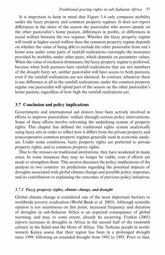
It is important to keep in mind that Figure 3.4 only compares mobilityunder the fuzzy property and common property regimes. It does not reportdifferences in the share of the season the pastoralist who moves spends onthe other pastoralist’s home pasture, differences in profits, or differences insocial welfare between the two regimes. Whether the fuzzy property regimewill result in higher social welfare than the common property regime dependson whether the value of being able to exclude the other pastoralist from one’shome area under some pairs of rainfall realizations outweighs the insuranceprovided by mobility under other pairs, which depends on parameter values.When the value of exclusion dominates, the fuzzy property regime is preferred,because when both pastures have rainfall realizations that are not membersof the drought fuzzy set, neither pastoralist will have access to both pastures,even if the rainfall realizations are not identical. In contrast, whenever thereis any difference at all in the rainfall realizations, under the common propertyregime one pastoralist will spend part of the season on the other pastoralist’shome pasture, regardless of how high the rainfall realizations are.


Governments and international aid donors have been actively involved inefforts to improve pastoralists’ welfare through various policy interventions.Some of these efforts involve reforming the underlying system of propertyrights. This chapter has defined the traditional rights system analyticallyusing fuzzy sets in order to reflect how it differs from the private property andnoncooperative common property regimes generally used in economic analy-ses. Under some conditions, fuzzy property rights are preferred to privateproperty rights, and to common property rights.

Due to the stresses on traditional institutions, they have weakened in manyareas. In some instances they may no longer be viable, even if efforts aremade to strengthen them. This section discusses the policy implications of theanalysis in two contexts: its predictions regarding the potential impacts ofdroughts associated with global climate change and possible policy responses,and its contribution to explaining the outcomes of previous policy initiatives.

3.7.1 Fuzzy property rights, climate change, and drought

Global climate change is considered one of the most important barriers toworldwide poverty eradication (World Bank et al. 2003). Although scientificopinion is not unanimous on this point, increased frequency and durationof droughts in sub-Saharan Africa is an expected consequence of globalwarming, and may, to some extent, already be occurring. Fratkin (2001)reports increases in droughts in Africa in the second half of the twentiethcentury in the Sahel and the Horn of Africa. The Turkana people in north-western Kenya assess that their region has been in a prolonged droughtsince 1999, following an extended drought from 1992 to 1995. Prior to that,


the last prolonged drought was in 1979 through 1980, and before that in 1970(Oxfam 2006).

The fuzzy property regime provides insight into the likely effects ofincreased generalized and localized droughts associated with climate change.Under the fuzzy property regime, pastoralist i’s right to the other pastoralist’shome pasture increases with i ’s home pasture’s degree of membership in thedrought fuzzy set, given the rainfall realization on the other pasture. Thus,under normal conditions of patchy rainfall, mobility allows pastoralists torespond to localized drought conditions. However, under generalized droughtconditions, pastoralists’ home pasture rainfall realizations are similar, as wellas low, which restricts mobility within customarily used areas. This corres-ponds to the observed behavior of the drought-stricken Turkana, who havefollowed two strategies: congregating in towns and relief camps, near foodaid and water supplies; and moving herds far outside their traditional grazingareas in an attempt to find pasture (Oxfam 2006). The widespread nature ofthe drought eliminated the value of mutual insurance, which is the primarybenefit provided by traditional property rights. Widespread droughts overlong periods of time are likely to reduce the viability of traditional institu-tions, since mutual insurance is not applicable in such cases.

Increased frequency and severity of localized droughts has differentimplications. Within the fuzzy property regime, this corresponds to increasedfrequency of mobility, since a greater share of rainfall realizations will bemembers of the drought and worse fuzzy sets. The pastoralist with the lowerrainfall realization will spend a greater share of the season, on average, on theother pastoralist’s home pasture. This will place greater pressure on the areaswith relatively good supplies of water and forage in a given year, as wasobserved in the Ngorongoro Conservation Area in northern Tanzania duringthe 1997 drought (Galvin et al. 2004). This will reduce returns to the hostpastoralist. While this analysis focused on homogeneous pastures, in caseswhere some pastoralists have naturally more productive pastures, increaseduse by others may not be offset by the benefits of mutual insurance. In suchcases, the profitability of the traditional system may decline, and privateproperty or common property may become most profitable for pastoralists inmore productive areas.

3.7.2 Fuzzy property rights and the implications of accessclarification policies

The fuzzy property regime provides insight into some of the unintended con-sequences of policies intended to clarify resource boundaries and user groups.Consider a common outcome of land reform efforts intended to improveresource use through privatizing land rights in favor of individuals or rela-tively small groups. Pastoralist groups who had home pastures in relativelyproductive areas would be more likely to benefit from privatization, andhence would be more likely to participate in land titling efforts and land


enclosure. Observers have noted that the richer and better-connected indi-viduals within a region have tended to benefit disproportionately from landprivatization efforts, such as the group ranches and later privatizationsin Kenya’s Maasailand (Graham 1988; Thompson and Homewood 2002;Mwangi 2005), and the Widou Thiengoli borehole controlled grazing schemein Senegal (Cotula et al. 2004).

Apart from any correlation of wealth or connections with the quality of agroup’s home pasture, the fuzzy property model suggests an additional impli-cation of this outcome, which is consistent with empirical observations inthese two cases. Less successful participants in privatization efforts in theirhome area are likely to do one of three things: abandon pastoralism entirely,either voluntarily or involuntarily; increase reliance on agriculture and otherincome-generating activities; or become more mobile and attempt to utilizemore intensively other grazing areas to which they have traditionally hadaccess. In the latter case, if they are successful then greater stress will be placedon less productive grazing areas, even in years where these areas have rela-tively high rainfall, and the enclosure efforts will have eliminated or greatlyreduced the insurance that the more productive area would have provided inother years. Clearly, this outcome places additional stress on the traditionalsystem in these less productive areas.

Information obtained in interviews with Maasai elders suggested such apattern emerging in Kenya’s Narok District. In recent years, Maasai in moreproductive areas have leased land to wheat farmers, eliminating access toforage for a portion of the dry season, until after the wheat harvest. Thistrend has occurred in conjunction with the subdivision of group ranches inthese areas into private parcels. Privatization allows individuals to benefitdirectly from land leasing, while simultaneously restricting the scope of live-stock movement for the group as a whole. Consequently, Maasai based inother, less productive areas not suitable for wheat production lost access toan area they could traditionally graze. In the year the interviews were con-ducted, the interviewees had seen an influx of herders from other areas intothe settlement areas they controlled, because they had relatively more pas-ture. The elders stated that they would deny permission to graze to Maasaiwho had leased their own land for wheat.

Consistent with the statements made by the interviewees, the analysis sug-gests that it may be welfare improving for the pastoralists in the lessproductive areas to eliminate the traditional system and exclude secondaryusers entirely, or at least to modify the traditional system in a way that wouldallow them to exclude pastoralists who can no longer reciprocate with accessto areas for which they are the primary managers. However, the poorer pas-toralists from the productive area who were effectively excluded from thebenefits of the privatization process are not considered in this welfare analy-sis. Balancing their welfare with other considerations is a difficult social andeconomic trade-off, well beyond the scope of this chapter.


3.7.3 Conclusion

The results of the analysis in this chapter suggest that policy efforts dealingwith property rights need to take a holistic view regarding the sustainabilityof the entire system. If there is no longer a large enough, or diverse enough,area to physically support the fuzzy property regime’s traditional mobilitypatterns, including the lack of mobility when there is insufficient forage in anarea to support both its primary users and other users, then it may be desir-able to make active efforts to define property rights under an alternative sys-tem. Creating rights of exclusion may, in this case, increase social welfare. Onthe other hand, it may be the case that it is preferable to strengthen the tradi-tional system, perhaps by reaffirming rights to forage and water and eliminat-ing any expropriation of these resources by specific user groups. Empiricalstudies have found evidence of partial cooperation among pastoralists in theabsence of strict formal rules, which suggests that traditional fuzzy rightspersist successfully in some areas (McCarthy et al. 2003; McCarthy andVanderlinden 2004; Benin and Pender 2006).

Determining which of these cases is likely to hold is a difficult problem,and almost certainly cannot be done without extensive stakeholder participa-tion, as in the case reported in Haro et al. 2005. An advantage of using thefuzzy set theory approach to model traditional property rights is that it is wellsuited to model linguistic variables. This approach could be used as the basisfor a negotiation support system for participants in negotiations regardingproperty rights reform. Doing so would add value because information aboutthe rights underlying possible location choices could be integrated into themodel, not just information on the realized location choices. Rather thansimply using a history of resource use in specific years and seasons, which aredependent on the pattern of rainfall realizations, as a basis for defining therights of groups in different areas, fuzzy set theory could combine this infor-mation with stakeholders’ verbal characterization of the rights underlyingthese movement choices, and the determinants of these rights.

Notes

1. The authors thank an anonymous referee for identifying and emphasizing thispoint.

2. Netting (1972, 1976, 1981) reaches similar conclusions in his study of the southernSwiss village of Törbel. Lower-elevation agricultural lands were owned privately,while higher-elevation forests and grazing lands with lower productivity wereowned in common. Interestingly, both the common property and private propertyregimes addressed the patchiness and variability of agricultural and forage pro-duction. The common property nature of the grazing land combined with themanagement of all of the village’s cows by a single group of herders allowed allto benefit equally from the available forage, even when it was patchy. Within thedifferent agricultural microclimates, households owned multiple, geographicallyseparated plots.


References

Aristidou, M. and Sarangi, S. (2006) “Games in fuzzy environments”, SouthernEconomic Journal, 72: 645–59.

Bartels, G.B., Norton, B.E., and Perrier, G.K. (1990) “The applicability of thecarrying capacity concept in Africa”, Network Paper Set 30, Paper 30e, PastoralDevelopment Network, Overseas Development Institute. Available online:www.odi.org.uk/pdn/papers/paper30e.html (accessed February 22, 2007).

Benin, S. and Pender, J. (2006) “Collective action in community management ofgrazing lands: the case of the highlands of northern Ethiopia”, Environment andDevelopment Economics, 11: 127–49.

Bogataj, M. and Usenik, J. (2005) “Fuzzy approach to the spatial games in the totalmarket area”, International Journal of Production Economics, 93–4: 493–503.

Bruce, J.W. and Mearns, R. (2002) “Natural resource management and land policyin developing countries: lessons learned and new challenges for the World Bank”,Issue Paper 115, Drylands Program, International Institute for Environment andDevelopment.

Coppock, D.L. (1994) The Borana Plateau of Southern Ethiopia: Synthesis of PastoralResearch Development and Change 1980–1991, Systems Study 5, InternationalLivestock Centre for Africa.

Cossins, N.J. and Upton, M. (1987) “The Borana pastoral system of southernEthiopia”, Agricultural Systems, 25: 199–218.

Cossins, N.J. and Upton, M. (1988) “Options for improvement of the Borana pastoralsystem”, Agricultural Systems, 27: 251–78.

Cotula, L., Toulmin, C., and Hesse, C. (2004) Land Tenure and Administration inAfrica: Lessons of Experience and Emerging Issues, International Institute forEnvironment and Development.

Dixon, J. and Gulliver, A., with Gibbon, D. (2001) Farming Systems and Poverty:Improving Farmers’ Livelihoods in a Changing World, Rome and Washington, DC:FAO and World Bank.

Dompere, K. (1995) “The theory of social costs and costing for cost-benefit analysisin a fuzzy decision space”, Fuzzy Sets and Systems, 76: 1–24.

Ensminger, J. (1996) “Culture and property rights”, in S. Hanna, C. Folke, andK.-G. Mäler (eds) Rights to Nature: Ecological, Economic, Cultural, and PoliticalPrinciples of Institutions for the Environment, Washington, DC: Island Press.

Evans, P. (2004) “Development as institutional change: the pitfalls of monocroppingand the potentials of deliberation”, Studies in Comparative International Develop-ment, 38: 30–52.

Fratkin, E. (2001) “East African pastoralism in transition: Maasai, Boran, andRendille cases”, African Studies Review, 44: 1–25.

Galvin, K.A., Thornton, P.K., Boone, R.B., and Sunderland, J. (2004) “Climate vari-ability and impacts on East African livestock herders: the Maasai of NgorongoroConservation Area, Tanzania”, African Journal of Range and Forest Science, 21:183–9.

Goodhue, R.E. (1998) “Sustaining collusion via a fuzzy trigger”, Review of IndustrialOrganization, 13: 333–45.

Graham, O. (1988) “Enclosure of the East African rangelands: recent trends andtheir impact”, Network Paper Set 25, Paper 25a, Pastoral Development Network,


Overseas Development Institute. Available online: www.odi.org.uk/pdn/papers/paper25a.html (accessed February 22, 2007).

Greenhut, J., Greenhut, M.L., and Mansur, Y. (1995) “Oligopoly and behavioraluncertainty: an application of fuzzy set theory”, Review of Industrial Organization,10: 269–88.

Hammel, R. (2001) “Securing land for herders in Niger”, Drylands Issue Paper E102,International Institute for Environment and Development.

Haro, G.O., Doyo, G.J., and McPeak, J.G. (2005) “Linkages between community,environmental, and conflict management: experiences from northern Kenya”,World Development, 33: 285–99.

Hogg, R. (1990) “An institutional approach to pastoral development: an example fromEthiopia”, Network Paper Set 30, Paper 30d, Pastoral Development Network,Overseas Development Institute. Available online: www.odi.org.uk/pdn/papers/paper30d.html (accessed February 22, 2007).

Hundie, B. (2006) “Property rights among Afar pastoralists of northeastern Ethiopia:forms, changes and conflicts”, unpublished paper, Humboldt University of Berlin,presented at Pastoralism and Poverty Reduction in East Africa: A Policy ResearchConference, Nairobi, June.

Lane, C. and Moorhead, R. (1994) “New directions in rangeland and resourcetenure and policy”, in I. Scoones (ed.) Living with Uncertainty: New Directions inPastoralist Development in Africa, International Institute for Environment andDevelopment, Intermediate Technology Publications, London.

Mansur, Y. (1995) Fuzzy Sets and Economics: Applications of Fuzzy Mathematicsto Non-Cooperative Oligopoly, London: Edward Elgar Co.

McCarthy, N. (1996) “Common property and cooperation in rural Mexico”, PhDdissertation, University of California, Berkeley.

McCarthy, N. and Vanderlinden, J.-P. (2004) “Resource management under climaticrisk: a case study from Niger”, Journal of Development Studies, 40: 120–42.

McCarthy, N., Kamara, A.B., and Kirk, M. (2003) “Co-operation in risky environ-ments: evidence from southern Ethiopia”, Journal of African Economies, 12:236–70.

McPeak, J.G. (2003) “Analyzing and addressing localized degradation in the com-mons”, Land Economics, 79: 515–36.

McPeak, J.G. and Barrett, C.B. (2001) “Differential risk exposure and stochasticpoverty traps among East African pastoralists”, American Journal of AgriculturalEconomics, 83: 674–9.

Mwangi, E. (2005) “The transformation of property rights in Kenya’s Maasailand:triggers and motivations”, CAPRi Working Paper 35, CGIAR SystemwideProgram on Collective Action and Property Rights. Available online:www.capri.cgiar.org/pdf/capriwp35.pdf (accessed February 24, 2007).

Netting, R. (1972) “Of men and meadows: strategies of alpine land use”, Anthropo-logical Quarterly, 45: 132–44.

Netting, R. (1976) “What alpine meadows have in common: observations oncommunal tenure in a Swiss village”, Human Ecology, 4: 135–46.

Netting, R. (1981) Balancing on an Alp, Cambridge University Press, Cambridge.Niamir, M. (1991) “Traditional African range management techniques: implica-

tions for rangeland development”, Network Paper Set 31, Paper 31d, PastoralDevelopment Network, Overseas Development Institute. Available online:www.odi.org.uk/pdn/papers/31d.pdf (accessed February 22, 2007).


Oba, G. (1992) “Ecological factors in land use conflicts, land administration andfood insecurity in Turkana, Kenya”, Network Paper Set 33, Paper 33a, PastoralDevelopment Network, Overseas Development Institute. Available online:www.odi.org.uk/pdn/papers/paper33a.html (accessed February 22, 2007).

Ostrom, E. (1990) Governing the Commons: The Evolution of Institutions for CollectiveAction, Cambridge: Cambridge University Press.

Ostrom, E. (2002) “Common-pool resources and institutions: toward a revisedtheory”, in B. Gardner and G. Rausser (eds) Handbook of Agricultural Economics:Volume 2, Amsterdam: Elsevier Science.

Oxfam (2006) Climate Change and the Sahel Drought: Stories and Case Studies, Oxfam,Oxford. Available online: www.oxfam.org.uk/what_we_do/issues/climate_change/story_turkana.htm (accessed February 24, 2007).

Pantuliano, S. (2002) Sustaining Livelihoods across the Rural-Urban Divide: Changesand Challenges Facing the Beja Pastoralists of North Eastern Sudan, Pastoral LandTenure Series 14, International Institute for Environment and Development.Available online: www.iied.org/pubs/pdf/full/9163IIED.pdf (accessed February 22,2007).

Scoones, I. (ed.) (1994) Living with Uncertainty: New Directions in Pastoralist Develop-ment in Africa, International Institute for Environment and Development,Intermediate Technology Publications, London.

Solomon, T.B., Snyman, H.A., and Smit, G.N. (forthcoming) “Cattle-rangeland man-agement practices and perceptions of pastoralists towards rangeland degradationin the Borana zone of southern Ethiopia”, Journal of Environmental Management.

Sserunkuuma, D. and Olson, K. (2001) “Private property rights and overgrazing: anempirical assessment of pastoralists in Nyabushozi County, western Uganda”,Economic Development and Cultural Change, 49: 769–92.

Swallow, B. (1994) The Role of Mobility within the Risk Management Strategies ofPastoralists and Agro-Pastoralists, Gatekeeper Series 47, International Institute forEnvironment and Development, London.

Thompson, G. and Wilson, P. (1994) “Ejido reforms in Mexico: conceptual issues,potential outcomes”, Land Economics, 70: 448–65.

Thompson, M. and Homewood, K. (2002) “Entrepreneurs, elites, and exclusion inMaasailand: trends in wildlife conservation and pastoralist development”, HumanEcology, 30: 107–38.

Thornton, P.K., Kruska, R.L., Henninger, N., Kristjanson, P.M., Reid, R.S., Atieno,F., Odero, A.N., and Ndegwa, T. (2002) Mapping Poverty and Livestock inthe Developing World, International Livestock Research Institute, Kenya. Avail-able online: www.ilri.cgiar.org/InfoServ/Webpub/Fulldocs/Mappoverty/index.htm(accessed February 22, 2007).

Toulmin, C. (1994) “Tracking through drought: options for destocking and restock-ing”, in I. Scoones (ed.) Living with Uncertainty: New Directions in PastoralistDevelopment in Africa, International Institute for Environment and Development,Intermediate Technology Publications, London.

Toulmin, C. (2005) “Securing land and property rights in sub-Saharan Africa: the roleof local institutions”, in T. Bigg and D. Satterthwaite (eds) How to Make PovertyHistory: The Central Role of Local Organizations in Meeting the MDGs, Inter-national Institute for Environment and Development, London. Available online:www.iied.org/Gov/mdgs/documents/mdg3/ch2_28pp.pdf (accessed February 22,2007).


van den Brink, R., Bromley, D., and Chavas, J. (1995) “The economics of Cain andAbel: agro-pastoral property rights in the Sahel”, Journal of Development Studies,31: 373–99.

World Bank et al. (2003) Poverty and Global Climate Change: Reducing the Vulner-ability of the Poor through Adaptation, World Bank, Washington, DC. Avail-able online: lnweb18.worldbank.org/ESSD/envext.nsf/46ByDocName/KeyThemesVulnerabilityandAdaptationPovertyandClimateChange (accessed February 22,2007).

Zadeh, L. (1965) “Fuzzy sets”, Information and Control, 8: 338–53.


4 Application of partitionfunction games to themanagement of straddlingfish stocks

Pedro Pintassilgo and Marko Lindroos

The formation of coalitions among fishing States is a central issue in strad-dling stock fisheries. In this chapter, this is approached through a game inpartition function form. The game is applied to a fishery represented by theclassical Gordon–Schaefer bioeconomic model and to the North Atlanticbluefin tuna fishery. Both cases show very pessimistic prospects regarding thecooperative management of the fish resources. This study concludes that thebreakdown of cooperative agreements on straddling stock fisheries is a verylikely scenario if countries can adopt free-ride strategies.

4.1 Introduction

This chapter addresses straddling stock fisheries through coalition games.Straddling fish stocks are a special category of internationally shared fisheryresources that straddle exclusive economic zones (territorial seas claimed bycoastal States) and the adjacent high seas.1 These species, usually targeted byboth coastal States and distant water fishing States, became increasingly dis-puted after the establishment of exclusive economic zones by the UnitedNations Convention on the Law of the Sea (United Nations 1982). Lack ofcooperation between coastal States and distant water fishing States has led tothe overexploitation of many stocks worldwide.

Munro (1999) refers to the Alaska pollock fishery in the Bering Sea as aparadigmatic example of noncooperative behavior among fishing States andconsequent stock overexploitation. A significant part of this straddling fishstock, one of the largest groundfish resources in the world, straddles theexclusive economic zone of the United States of America and a high seasenclave between the United States and Russian exclusive economic zonescommonly known as the Doughnut Hole. The fishing pressure on the highseas portion of the stock exerted by distant water fishing States after 1984resulted in the depletion of the stock in the early 1990s. The increasing tensionbetween the United States and distant water fishing States led the US coast-guards to seize several foreign fishing vessels allegedly using the DoughnutHole as a base for fishing operations within United States waters. In 1992,after the stock crash, all States involved in the fishery reached an agreement

to impose a fishing moratorium in the Doughnut Hole. Another classicalexample, given by Munro (1999), concerns the groundfish stocks on theGrand Banks of Newfoundland. The lack of cooperation between Canadaand the European Union led to the overexploitation of the stocks and toconflicts that reached a climax in 1995 when Canadian authorities arrested aSpanish vessel in international waters.

The economic and biological overexploitation of the stocks and the increas-ing conflicts among countries, often called “international fish wars”, inducedthe United Nations to convene the United Nations Conference on StraddlingFish Stocks and Highly Migratory Fish Stocks (1993–95). In 1995 the confer-ence adopted the United Nations Fish Stocks Agreement2 (United Nations1995), which entered into force in 2001. The core of the agreement consists ofplacing regional fisheries management organizations (RFMOs) as the basiccells for the management of these marine resources. These organizationsshould integrate both the coastal States and the distant water fishing Stateseffectively interested in the fishery. According to Munro (2006), the UnitedNations Fish Stocks Agreement left a few problems unsolved that mayundermine cooperative agreements achieved under the aegis of RFMOs. Oneproblem is the possibility of prospective new members wanting to join anRFMO and share the harvest following recovery of the stock, thus reapingthe benefits of stock management without having borne any of the cost of theinvestment (free riding). Another problem is the one posed by nonmemberswho do not follow an RFMO management regime and thus behave noncoop-eratively when exploiting the fishery resources in their exclusive economiczones or in the high seas. Munro (2006) refers to the Commission for theConservation of Southern Bluefin Tuna as an example where both theseproblems have surfaced.

The economics of straddling stock fisheries is based on coalition games. Inthis chapter the main studies on coalition games applied to the managementof straddling fish stocks are reviewed. The core aim of the chapter is toexplore the potential of partition function games, a class of coalition gamesrecently introduced into the fisheries literature. In these games the payofffor each player is defined by a partition function that depends not only onthe coalition the player belongs to but also on the way the other players formcoalitions. Partition function games have been suggested for cases in whichcoalition formation produces externalities that affect nonmembers (Yi 1997).This is a typical situation in the management of straddling fish stocks underRFMOs. The more RFMO member players the better for nonmembers, asthey can adopt free-rider strategies. Thus, partition function games are anappropriate framework to address free-rider problems faced by RFMOs. Inthe present chapter a partition function game on a straddling stock fisheryis defined. In addition, the stability of cooperative agreements and theequilibrium of the game are analyzed.

The chapter is structured as follows. Section 4.2 presents a brief revision ofcoalition games on straddling fish stocks. Section 4.3 discusses the relevance

66 Pedro Pintassilgo and Marko Lindroos

of partition function games and defines the main concepts. Section 4.4presents the partition function game used in the chapter, and is followed bytwo applications: section 4.5, a straddling stock fishery represented by theclassical Gordon–Schaefer model, and section 4.6, the North Atlantic bluefintuna fishery. Section 4.7 concludes with a discussion of the main findings andpolicy recommendations.

4.2 Coalition games

A straddling stock fishery usually involves many countries or fleets. Theanalysis of games in which the number of players exceeds two requires analy-sis of coalitions. A coalition means a subset of the set of players. Two ormore countries are considered to form a coalition if they ratify (or sign) amultilateral agreement on the particular fishery.

Three types of coalition scenarios may result. If all parties concernedsign the agreement the situation is denoted as full cooperation, and a grandcoalition is said to be formed. If some countries are left outside the agree-ment the situation is denoted as partial cooperation and outsiders may act asfree riders. Finally, in the case of noncooperation there are no agreementsbetween the countries, and each is only interested in maximizing individualbenefit from the fishery.

Based on the three possible outcomes described above a characteristicfunction of the game can be established. The characteristic function assigns avalue to each possible coalition. The value in the case of straddling fish stocksis, generally, interpreted as the net present value of the fishery to a certaincoalition.

The value for coalition members depends on the particular behavior ofnonmembers. The different assumptions about their behavior give rise to theα, β, and γ characteristic functions. The α and β characteristic functionsassume that the nonmembers jointly try to punish the coalition members. Theproblem with this assumption in the context of international fisheries gamesis that the punishments decrease the payoff of the nonmembers. Therefore,the γ-characteristic function, introduced by Chander and Tulkens (1995), istypically preferred. The assumption made by the authors is that nonmembersplay as singletons and adopt individually best-reply strategies against thecoalition. This results in a Nash equilibrium between the coalition and thenonmembers.

An example of a γ-characteristic function based on a game between threeplayers exploiting Norwegian spring-spawning herring (Lindroos and Kaitala2000) is given in Table 4.1. The players are Norway, Iceland, and the EuropeanUnion (EU).

In Table 4.1, the first value (US$6,800 million) corresponds to the payoffof the grand coalition formed by all the players. This payoff is calculated bymaximizing the joint net present value of profits over a period of 50 years.Under the full cooperative case, the stock level in the long run is the highest

Partition function games and straddling fish stocks 67

compared to the partial and noncooperative cases. The next three values arethe payoffs of the two-player coalitions under partial cooperation. Thesevalues result from the Nash equilibrium of the game among a two-playercoalition, maximizing its joint benefits, and a single country (free rider). Thelast three values give the noncooperative equilibrium payoffs. Clearly, coun-tries gain by joining together; for example, a coalition of Norway and Icelandwould receive $3,000 million compared to $1,100 million, the sum of theirpayoffs under noncooperation. Whether a grand coalition can be formed isa more complex problem. In this case, the conditions when the grand coali-tion would be stable need to be defined. This is discussed in detail later insection 4.4. The following sections present an overview of coalition gameliterature (see also Lindroos et al. 2006 for a detailed and more technicalreview).

Kaitala and Lindroos (1998) introduced coalition games to the economicanalysis of straddling stocks and fisheries economics in general by using athree-player model. Their main result is that there is a partial cooperationequilibrium stock level that is higher than the noncooperative stock level(Clark 1980), though lower than the cooperative stock level (Clark andMunro 1975). They also applied Shapley value and nucleolus as cooperativesolutions to the sharing of full cooperative benefits. Contrary to previousresults, uneven distribution of benefits was suggested because of coalitionalbargaining power differences.

Lindroos (2004a) extended the Kaitala–Lindroos model (1998) by allowingfor restricted coalition formation in a four-player game. This was analyzed inthe context of straddling stock negotiations where distant water fishing Statesnegotiated with coastal States. The main result was that, by joining together,distant water fishing States gained compared to unrestricted negotiations.Arnason et al. (2000) studied the case of Atlanto-Scandian herring and foundthat Norway was a crucial country for any coalition to be stable. Their find-ings relate to those of Lindroos (2004a), who considered the possibilityof veto countries. The effect of uncertainty and selectivity was studied byLindroos (2004b). He showed that the safe minimum economic stock level

Table 4.1 Example of a characteristic function

Coalition Payoffs (net present value)a

Norway, Iceland, EU (grandcoalition)

6,800

Norway, Iceland 3,000Norway, EU 2,800Iceland, EU 2,700Norway 750Iceland 350EU 140

a. Approximate values in 106 US$ (constant prices of 1998).


that would maximize the possibilities for cooperation was higher than thesafe minimum biological level (precautionary level).

Kennedy (2003) applied the concept of coalition-proof equilibrium to theNortheast Atlantic mackerel fishery. Sang Kwon (2006), in one of the mostrecent applications of coalition games to straddling stocks, extended theLevhari–Mirman (1980) model to include coalitions.

4.3 Partition function gamesCharacteristic function games have been applied to straddling stock fisheriessince the late 1990s. Nonetheless, as observed by Greenberg (1994), the frame-work of a characteristic function approach, although sufficiently generalto encompass many contributions of coalition formation theory, is notfully satisfactory. Most importantly, it ignores the possibility of externalitiesamong coalitions, that is, the effects that coalition mergers have on the pay-offs of players who belong to the other coalitions.

Definition 1: Externalities are present, in a game in coalition form, if andonly if there is at least a merger of coalitions that changes the payoff of aplayer belonging to a coalition not involved in the merger. If the mergerincreases (decreases) the payoff of the player, the externality is con-sidered as positive (negative).

In the context of straddling fish stock management through RFMOs,externalities are generally present. In fact, as these organizations tend toadopt conservative management strategies, nonmembers are typically betteroff when more players become members, as free-rider strategies can beadopted. Therefore, when a player joins an RFMO it generally creates apositive externality for nonmembers.

According to Yi (1997), the formation of economic coalitions withexternalities has opened a new strand of literature on noncooperative gametheory. Most studies (for example Bloch 1996; Yi 1996) are centered on find-ing the equilibrium number and size of coalitions and share a common two-stage game framework. In the first stage players form coalitions, whereas inthe second stage coalitions engage in noncooperative behavior. The coalitionpayoffs are represented by a partition function (definition 3). This functionassigns a value to each coalition as a function of the entire coalition structure(definition 2). Therefore, it captures the externalities across coalitions that areassumed to be absent in the characteristic function.

Definition 2: A coalition structure C = {S1,S2, . . ., Sz} is a set of coali-tions that altogether integrates all the players, with each player belongingto only one coalition.

Definition 3: The partition function Π (Sk; C ) yields the payoff of coali-tion Sk, which is an element of the coalition structure C = {S1,S2, . . .,Sz}. The payoff of player i, which is a member of coalition Sk, is given bythe per-member partition function πi (Sk; C ).


Recently, games in partition function form have been applied to inter-nationally shared fish stocks. Pintassilgo (2003) models straddling stock fish-eries as a partition function game and derives general results regarding thestability of coalition structures and the equilibrium of the game. The authorexplores, in particular, the case in which positive externalities are present. Anapplication to the North Atlantic bluefin tuna fishery is undertaken using anage-structured, multigear bioeconomic model. Pham Do and Folmer (2003)study the feasibility of partial cooperation and its impacts on fishing effortthrough a game in partition function form. Using a static model, generalresults on the coalition structure in the competitive equilibrium are derived.

4.4 Stylized game

In this section, the game framework used by Pintassilgo (2003) is described.This will be applied to specific bioeconomic fishery models in the followingsections. Assume that an RFMO is established with the purpose of managingand conserving a straddling fish stock. Consider a two-stage game and a finitenumber of players. In the first stage, each player decides whether to become amember of the RFMO or to remain a nonmember. As nonmembers typicallyadopt noncooperative behavior and do not join together, it is assumed thatthey will act individually as singletons. This is a standard assumption inthe literature on international environmental agreements (Finus 2001). Inparticular, Chander and Tulkens (1997) adopt it in modeling an economywith multilateral externalities. The authors assume that when a coalition isformed, the players outside the coalition adopt only individual best-replystrategies. According to this assumption, coalition payoffs are described by aγ-characteristic function.

Regarding the rule of coalition formation, the simultaneous-move openmembership game (Yi 1997) is assumed. Under this rule, the membership ofeach coalition is open to all players who are willing to follow its strategies.This game is designed to model an institutional environment in which playersare allowed to form coalitions freely, as long as no player is excluded fromjoining any coalition. Thus, any player can choose to be either a member or anonmember of the RFMO. This assumption is clearly within the legalframework set by the United Nations Fish Stocks Agreement. According toArticle 8(3), any State with a real interest in the fisheries concerned shouldnot be precluded from becoming a member of the regional RFMO (UnitedNations 1995). Furthermore, the agreement appears to leave open the possi-bility of nonmembers fishing in their exclusive economic zones or in the highseas (Munro 1999).

In the second stage it is assumed that the grand coalition members actcooperatively by choosing the fishing strategy that maximizes their aggregatepayoff. For all the other coalition structures, each coalition chooses thestrategy that maximizes its own payoff given the behavior of the remainingplayers. This noncooperative behavior leads to a noncooperative solution for


each coalition structure, assumed to be unique. Thus, the coalition payoffs inthe second stage can be defined as a partition function. Given the partitionfunction, which yields the equilibrium payoffs of the second-stage game,the equilibrium coalition structures of the first-stage game are the Nashequilibrium outcomes of the open membership game of coalition formation.

An important issue that emerges by setting a coalition approach to a strad-dling stock fishery is the coalition structure stability. As the United NationsFish Stocks Agreement calls for cooperative management, special interest iscentered on the stability of the grand coalition. According to Greenberg(1994), since the merger of players into an RFMO tends to create positiveexternalities for nonmembers, the analysis of stability based on single-playerdeviations emerges naturally. Moreover, in the context of positive external-ities, Yi (1997) refers to the concept of stand-alone stability as being particu-larly useful in characterizing equilibrium coalition structures. This concept isdefined as follows.

Definition 4: A coalition structure is stand-alone stable if and only if noplayer finds it profitable to leave its coalition to form a singleton (one-player) coalition, holding the rest of the coalition structure constant(including its former coalition). In the case of the grand coalition, thisoccurs when no player is interested in leaving the cooperative agreementto adopt free-rider behavior.

The following proposition, presented by Pintassilgo (2003), establishes acondition under which a given coalition structure is not stand-alone stable.

Proposition 1: A sufficient condition for a coalition structure not to bestand-alone stable is that the sum of the payoffs of the singleton coali-tions, resulting from unilateral deviations from any of its coalitions,exceeds the value of that coalition.

This proposition provides a tool to determine those cases in which nosharing rule can make a coalition structure stand-alone stable. Specifically, itcan be used to assess the possibility of a stable cooperative agreement.

4.5 Application 1: a classical bioeconomic modelThe game setting established in the previous section is now applied to astraddling fish stock fishery represented by the classical Gordon–Schaeferbioeconomic model (Gordon 1954). Because of its simplicity, this staticmodel is commonly used in game-theoretic approaches to internationallyshared fish resources (for example Ruseski 1998; Lindroos 2002).

Consider n ex ante symmetric players3 (fleets/countries) in a straddling fishstock fishery. The fish stock dynamics follow the standard Schaefer model(Schaefer 1954), which can be represented through the following equations:

dX

dt= G (X) − �

n

i =1

Hi (4.1)


G (X ) = rX �1 −X

k � (4.2)

Hi = qEiX (4.3)

where X presents fish stock biomass; t the time; G(X ) the logistic growthfunction; r the intrinsic growth rate of fish; k the carrying capacity of theecosystem; Hi the harvest of player i ; q the catchability coefficient; and Ei thefishing effort of player i.

According to (4.1), the variation of the stock in time is given by the differ-ence between stock growth and total harvest. Stock growth is defined by alogistic function (4.2). This is an inverted U-shaped function. Stock growthincreases with the stock level up to a maximum value, often designated asmaximum sustainable yield. As the stock continues to increase, the growthstarts to decrease, and upon reaching zero, the stock stabilizes at the carryingcapacity of the ecosystem. Thus, for low levels the fish multiply, but once theybegin to compete for food, growth reduces and the stock tends to the levelthat can be sustained by the environment. The harvest function (4.3) indicatesthat the harvest of each player increases with stock level and fishing effort—an aggregate measure of the inputs devoted to harvesting, such as days at sea.

Equations (4.1) to (4.3) can be used to determine the equilibrium, or steadystate, stock level that corresponds to a given fishing effort that is constantthrough time. This steady state relation is given by:

X =k

r �r − q�n

i =1

Ei�. (4.4)

As expected, (4.4) indicates a negative relation between the equilibriumstock level and the players’ fishing effort.

Assuming constant price and cost per unit of effort, the aggregate eco-nomic rent from the fishery is:

ER = p�n

i = 1

Hi − c�n

i = 1

Ei (4.5)

where ER denotes the aggregate economic rent; p the price; c and the cost perunit of effort.

Formalizing the economic rent, or economic profit, is the most commonway to introduce the fishery economic dimension in bioeconomic model-ing. Herein, the standard assumption that agents maximize their profits isadopted.

The Gordon–Schaefer model is still the main reference in theoreticalapproaches to fisheries bioeconomics. This aggregated model has shown


significant potential to demonstrate fundamental economic principles in fish-eries management. In particular, it has been the principal bioeconomic modelused in addressing noncooperative management of internationally sharedstocks (Munro 1999). Nonetheless, the scope of application of this model toempirical studies is very limited, because of its simplicity.

Consider the two-stage framework presented in the previous section. Theper-member partition function is determined assuming that each coalitionchooses the fishing strategy that maximizes its steady state economic profit,given the behavior of other coalitions. Furthermore, as players are ex antesymmetric, an equal sharing of coalition payoffs is assumed.

In the case of full cooperation, all players adhere to the RFMO. Thisgrand coalition maximizes its steady state profit (4.5). The correspondingaggregate fishing effort and the payoff received by each member are givenrespectively by:

E =r

2q (1 − b) (4.6)

π =1

n ( pqk − c)

r

4q (1 − b) (4.7)

where b =c

pqk. This is usually designated an “inverse efficiency parameter”,

as it increases with the cost per unit of effort and decreases with price andcatchability coefficient. Therefore the higher b, the lower players’ efficiency.

As expected the payoff decreases with the number of players and the costper unit of effort, and increases with the remaining parameters (price, catch-ability coefficient, intrinsic growth rate of fish, and carrying capacity of theecosystem).

In the partial cooperation scenario, a coalition of two or more RFMOmembers plays against singleton nonmembers. In the Nash equilibrium, thefishing effort of each coalition is the following:

E =r

(m + 2) q (1 − b) (4.8)

where m denotes the number of nonmembers. Hence, n − m represents thenumber of RFMO members, and m + 1 the number of coalitions.

The per-member payoff of the coalition formed by the players that adhereto the RFMO is given by:

π =( pqk − c) r (1 − b)

(n − m) (m + 2)2 q(4.9)


The singleton nonmembers receive:

π =( pqk − c) r (1 − b)

(m + 2)2 q(4.10)

From (4.9), it can be concluded that the payoff of the RFMO membersdecreases with the number of players, for a given number of nonmembers.Regarding the payoff of nonmembers, (4.10) indicates that it decreases withthe number of coalitions.

Finally, under noncooperation all the players are nonmembers of theRFMO and behave as singletons. In the Nash equilibrium, the fishing effortand the payoff of each player are given, respectively, by:

E = r

(n + 1) q (1 − b) (4.11)

π =( pqk − c) r (1 − b)

(n + 1)2 q(4.12)

The payoff of each singleton decreases with the number of players. Moreover,it converges to zero as the number becomes infinitely large.

Having determined the values of the per-member partition function of thisgame, the next step is to explore the properties of this function.

Proposition 2: The per-member partition function game presents positiveexternalities.4

This proposition indicates that the merger of coalitions increases the pay-off of players who belong to the other coalitions. Having established thepresence of positive externalities in the game, its consequences will now beanalyzed in terms of coalition structure stability and equilibrium. The follow-ing proposition addresses the coalition structure stand-alone stability for thepresent straddling stock fishery game.

Proposition 3: In a two-player game both the grand coalition and thecoalition structure formed by singletons are stand-alone stable. In a gamewith three or more players the only stand-alone stable coalition structureis the one formed by singletons.

From this proposition it can be concluded that, aside from the unusualcase of two players, no cooperative agreement is stand-alone stable. This isbecause of the presence of free-rider incentives associated with positiveexternalities. The free-rider behavior of nonmember fleets, which tends tooccur in the presence of externalities, has been pointed out as one of the mainfactors behind the difficulties faced by RFMOs in the cooperative manage-ment of straddling fish stocks. A paradigmatic case is the Commission for theConservation of Southern Bluefin Tuna. In order to protect itself againstfree riders, this RFMO has been trying to encourage nonmembers to adhere


to the organization and has implemented a trade information scheme withthe aim of deterring illegal, unreported, and unregulated fishing by effectivelydenying access to markets for the species.

Finally, the equilibrium of the game will be considered. This is a veryrelevant aspect since it is the expected scenario in the straddling stock fisheryafter all strategic adjustments have been made.

Proposition 4: In a two-player game the grand coalition, formed by thetwo players, is the Nash equilibrium coalition structure. If the number ofplayers is three or more, the Nash equilibrium is the coalition structure inwhich all players act as singletons, that is, complete noncooperation.

Proposition 4 indicates that the cooperative management of a straddlingfish stock under an RFMO is a very unlikely outcome. This result emphasizesthe importance of dealing effectively with free-rider behavior by nonmembers.

4.6 Application 2: North Atlantic bluefin tuna fisheryIn this section the game in partition function form is applied to the easternstock of the North Atlantic bluefin tuna. This straddling fish stock, whosemanagement falls under the aegis of the International Commission for theConservation of Atlantic Tunas (ICCAT), has been pointed out as oneof the most typical cases of failure to implement a cooperative agreement(Pintassilgo 2003).

4.6.1 The fishery

The North Atlantic bluefin tuna is a large oceanic pelagic and also thelargest of the tunas. Its normal fork length, in adult stage, is between 1.6 and2.4 meters, but can reach more than 3 meters. Like many other tunas, thebluefin tend to be found in schools of similar-sized individuals. This speciesspawns in two main areas: the West Atlantic (Gulf of Mexico and FloridaStraits) and the Mediterranean Sea (around the Balearic Islands and in thesouthern Tyrrhenian Sea). Based on the spawning areas, ICCAT defines twostocks for management purposes: the West Atlantic and the East Atlantic.5

Hereafter, the analysis is centered on the eastern stock, which is distributedroughly from the Canary Islands to southern Iceland and in all the Mediter-ranean Sea.

In the Northeast Atlantic and Mediterranean Sea, the bluefin tuna is har-vested by a large number of fleets from European Union member coastal States(Cyprus, France, Greece, Italy, Malta, Portugal, Spain), other coastal States(Algeria, Croatia, Libya, Morocco, Turkey), and distant water fishingStates (China, Japan, Republic of Korea, Taiwan, United States). A varietyof fishing gears are used, including purse seine, longline, trap, and baitboat.The different fishing gears target different quality and size specimens, whichhave different market values. Large-size and high-quality bluefin tunas areabsorbed by the Japanese sashimi market, where prices are highest.


According to recent stock assessments, the eastern bluefin tuna stock isseverely depleted and current reported catches (28,889 tonnes in 2004) cannotbe sustained (ICCAT 2005). Furthermore, ICCAT suspects that there hasbeen an increasing underreporting of catches over recent years. One of themain factors contributing to this situation is the high number of fleetsinvolved in the fishery, both members and nonmembers of ICCAT. Anotherfactor is the high price of the bluefin tuna in the Japanese market. Thismarket has a strong and selective demand towards large-size and high-qualityspecimens, for which it is virtually the only consumer. The depletion of thesouthern bluefin tuna stock in the Pacific Ocean also contributes to thefishing pressure on the North Atlantic bluefin tuna.

4.6.2 Partition function game

Assume that all the countries participating in the bluefin tuna fishery inthe East Atlantic and Mediterranean are represented in the RFMO, ICCAT,by one of the following players: European Union (EU), other coastal States(OCSs), and distant water fishing States (DWFSs). Consider the two-stagegame framework presented in section 4.4. In the first stage, the coali-tion structure is determined by the players’ choice to join ICCAT or playoutside as singletons. In the second stage, the coalitions choose their fishingstrategy.

The optimal fishing strategy for the coalition formed by ICCAT membersis assumed to be the one that maximizes the net present value of profits over a25-year period, given the behavior of the nonmembers. Nonmembers areassumed to follow market behavior by adjusting effort according to the signof profits.6 The coalition strategies and payoffs were computed by using anage-structured, multigear bioeconomic model (Pintassilgo and Costa Duarte2002). For all the coalition structures, a unique equilibrium7 payoff vectorwas obtained. The resulting payoff matrix (Pintassilgo 2003) is shown inTable 4.2. In representing the coalition structures, all the players that belong

Table 4.2 Coalition payoffs for bluefin tuna fishery

Payoffs (net present value)a

Coalition structure Total ICCAT EU OCS DWFS

(EU, OCSs, DWFSs) 1,291.7 1,291.7 — — —(EU, OCSs), (DWFSs) 991.8 154.2 — — 837.6(EU, DWFSs), (OCSs) 976.4 224.0 — 752.4 —(OCS, DWFSs), (EU)b 7.6 21.4 −13.8 — —(EU), (OCSs), (DWFSs) 7.6 — −13.8 −5.0 26.4

a. Values in 106 US$ (constant prices of 1995).b. If ICCAT is composed of OCSs and DWFSs, there is no conservative strategy that can yield

higher payoff for these players than in the case in which the three players act noncooperativelyas singletons.


to the same coalition are placed within the same parentheses. As it is assumedthat nonmembers act as singleton coalitions, all the coalitions with more thanone member belong to ICCAT. Moreover, it is also assumed that ICCATmembers will never be singletons, as no single player can gain by adopting aconservative strategy.

This game presents positive externality characteristics. In fact, Table 4.2shows that when the EU joins the OCSs the payoff of the DWFSs increasesfrom US$26.4 million to $837.6 million. A similar external effect occurs whenthe EU joins the DWFSs. The stability of the cooperative agreement will nowbe analyzed.

Proposition 5: There is no sharing rule that makes the cooperative agree-ment stand-alone stable.

This can easily be shown through proposition 1. The values of the single-ton coalitions, resulting from unilateral deviations from the grand coalition,are −$13.8 million, $752.4 million, and $837.6 million for the EU, OCSs, andDWFSs, respectively. As the sum of these values ($1,576.2 million) exceedsthe payoff of the grand coalition ($1,291.7 million), it can be concluded thatthere is no sharing rule that can make the grand coalition stand-alone stable.Since stand-alone stability is a necessary condition for a coalition structure tobe a Nash equilibrium, the grand coalition cannot be a Nash equilibriumoutcome of this game.

What is the Nash equilibrium of the game? It must be a stand-alonestable coalition structure. Using definition 4, it can be shown that thereare only three coalition structures that can potentially follow this property:{(EU, OCSs), (DWFSs)}; {(EU, DWFSs), (OCSs)}; and {(EU), (OCSs),(DWFSs)}. Whether any is a Nash equilibrium depends on the particularsharing rule adopted for the division of the coalition payoffs. By using avariable sharing rule, endogenously determined, that can differ among coali-tion structures, Pintassilgo (2003) shows that there is no Nash equilibriumcoalition structure for this game.

From these results, a successful cooperative agreement on the managementof this fishery seems an unlikely outcome. However, as shown by Pintassilgo(2003), if DWFSs are not allowed to adopt free-rider behavior then thereare sharing rules that make the grand coalition stand-alone stable. Thus, theresults indicate that legal restrictions, prohibiting fishing to fleets that donot follow the regulations set by RFMOs, are essential in order to sustaincooperative agreements.

4.7 Conclusion and policy implicationsThe management of straddling fish stocks has become a major internationalproblem since the drafting of the United Nations Convention on the Law ofthe Sea (United Nations 1982). According to Munro (1999), the segment ofthe convention that addresses the management of these fishery resources


“proved in retrospect to be seriously inadequate”. In 1995, the UnitedNations Fish Stocks Agreement was adopted in order to supplement theconvention. However, some problems still remained to be solved; for example,the threat to the cooperative management of RFMOs posed by prospectivenew members and nonmembers (Munro 2006). These problems are stillclearly faced by such RFMOs as the Commission for the Conservation ofSouthern Bluefin Tuna and ICCAT.

Coalition games have been the main tool used by economists to address themanagement of straddling fish stocks. This chapter explores the potential ofpartition function games, a particular type of coalition game recently intro-duced into the fisheries literature. The main advantage of this approach,compared to traditional characteristic function games, is that it capturesexternalities among coalitions, which are generally present in straddling stockfishery games.

In the chapter, a game in partition function form is defined and appliedin order to address the stability of cooperative agreements and the equi-librium coalition structures. The first application is a straddling stock fisheryrepresented through the classical Gordon–Schaefer bioeconomic model. Theresults show that the game exhibits positive externalities. Moreover, in thecase of three or more players, no cooperative agreement is stand-alone stableand the only Nash equilibrium coalition structure is the one formed by single-tons. Thus, complete noncooperation is the most likely outcome. The secondapplication is the bluefin tuna fishery in the Northeast Atlantic and Mediter-ranean Sea. In this application a fairly disaggregated bioeconomic model isused. It is also concluded that positive externalities are present and there is nosharing rule that can make the grand coalition stable.

Both games show very pessimistic prospects regarding the cooperativemanagement of straddling fish stocks under RFMOs. This conclusion is inline with the results obtained by Yi (1997) for classical economic coalitionscharacterized by the presence of positive externalities, such as output cartelsand coalitions formed to provide public goods. The author concludes thatan open membership game rarely supports the grand coalition as a Nashequilibrium, and equilibrium coalition structures are often very fragmented.

According to the results obtained, the breakdown of cooperative agree-ments on straddling stock fisheries is a very likely scenario if countries canfree ride on cooperative agreements. Thus, in order to protect cooperation,the legal regime must prevent those who engage in noncooperative behaviorfrom having access to the resource. As Munro (2006) stresses, if the RFMOregime is to prosper, unregulated fishing by nonmembers must be eliminated.This is clearly on the agenda of the Food and Agriculture Organization ofthe United Nations (FAO) and is specifically addressed in its InternationalPlan of Action to Prevent, Deter, and Eliminate Illegal, Unreported, andUnregulated Fishing (FAO 2001). This is a voluntary instrument that recom-mends, among other measures, that States should develop and implementnational plans of action to achieve the objectives of the International Plan of


Action, and adopt trade restrictions on fish and fish products derived fromillegal, unreported, and unregulated fishing, including import and exportcontrols or prohibitions. According to the International Plan of Action,institutional and policy strengthening of RFMOs is a key element in address-ing the problem of illegal, unreported, and unregulated fishing.

In 2003 a group of fisheries ministers and director-generals of inter-national nongovernmental organizations created the High Seas Task Forcewith the aim of tackling “the root causes” of illegal, unreported, andunregulated fishing in the high seas. The final report (High Seas Task Force2006) established a set of proposals intended to enhance enforcement,thereby increasing the risks to those engaged in illegal, unreported, andunregulated fishing operations, and making such fishing less profitable.Among the most prominent measures proposed by the High Seas Task Forceare the improvement of the exchange of knowledge derived from monitor-ing, control, and surveillance activities through the development of a globalinformation system on high seas fishing vessels; providing guidance toRFMOs in order to disseminate best practices in implementation of inter-national fishery instruments; setting guidelines on flag State performance andmeasures in order to promote port State controls; and supporting developingcountries in overcoming illegal, unreported, and unregulated fishing.

A key idea that emerges from this chapter is that the success of the man-agement of straddling fish stocks under RFMOs, prescribed by the UnitedNations Fish Stocks Agreement, is at serious risk unless the gaps in thisdocument are filled with complementary measures that empower RFMOs tocombat noncooperative behavior.

Notes

1. This broad definition includes what, in the terminology of the Food and Agri-culture Organization of the United Nations, is called highly migratory fish stocks(mainly the six major tuna species). According to Munro (2006), there is no mean-ingful difference between straddling fish stocks and highly migratory fish stocks asfar as economic analysis is concerned.

2. This is the most common abbreviated designation of the agreement and is usedthroughout the chapter. The full title is: Agreement for the Implementation of theProvisions of the United Nations Convention on the Law of the Sea of 10 December1982 Relating to the Conservation and Management of Straddling Fish Stocks andHighly Migratory Fish Stocks.

3. The assumption of ex ante symmetric players is dominant in the literature onpartition function games (for example Yi 1997; Finus 2001). Allowing for asym-metric players raises significantly the level of complexity of the analysis becausethe results depend on the particular rule chosen to share the benefits fromcooperation.

4. The proofs of this and the following propositions are provided in the Appendix tothis chapter.

5. Nonetheless, recent data on bluefin tuna releases and recoveries show significantmixing between the two stocks (ICCAT 2006).

6. This is a very common way to model noncooperative behavior in fisheries (for


example Amundsen et al. 1995). One of its main advantages is that it can incorpor-ate the natural restrictions on the effort adjustment.

7. The uniqueness of the equilibrium payoffs was one of the main factors behindthe option for a particular modeling of nonmembers’ strategies rather than the useof the traditional Nash equilibrium. In fact, the complexity of the bioeconomicmodel raised the problem of nonuniqueness of the Nash equilibrium.

References

Amundsen, E., Bjørndal, T., and Conrad, J. (1995) “Open-access harvesting of theNortheast Atlantic minke whale”, Environmental and Resource Economics, 6(2):167–85.

Arnason, R., Magnusson, G., and Agnarsson, S. (2000) “The Norwegian spring-spawning herring fishery: a stylized game model”, Marine Resource Economics, 15:293–319.

Bloch, F. (1996) “Sequential formation of coalitions in games with externalities andfixed payoff division”, Games and Economic Behavior, 14: 90–123.

Chander, P. and Tulkens, H. (1995) “A core-theoretic solution for the design ofcooperative agreements on transfrontier pollution”, International Tax and PublicFinance, 2(2): 279–93.

Chander, P. and Tulkens, H. (1997) “The core of an economy with multilateralenvironmental externalities”, International Journal of Game Theory, 26: 379–401.

Clark, C. (1980) “Restricted access to common property fisheries resources: a game-theoretic analysis”, in P. Liu (ed.) Dynamic Optimization and MathematicalEconomics, New York: Plenum Press.

Clark, C. and Munro, G. (1975) “Economics of fishing and modern capital theory: asimplified approach”, Journal of Environmental Economics and Management, 2:92–106.

FAO (Food and Agriculture Organization of the United Nations) (2001) InternationalPlan of Action to Prevent, Deter and Eliminate Illegal, Unreported and UnregulatedFishing, Rome: FAO.

Finus, M. (2001) Game Theory and International Environmental Cooperation, Chelten-ham, UK: Edward Elgar.


Greenberg, J. (1994) “Coalition structures”, in R.J. Aumann and S. Hart (eds) Hand-book of Game Theory with Applications to Economics, Volume 2, Amsterdam:North-Holland.

High Seas Task Force (2006) Closing the Net: Stopping Illegal Fishing on the HighSeas, Governments of Australia, Canada, Chile, Namibia, New Zealand, and theUnited Kingdom, World Wide Fund for Nature (WWF), World ConservationUnion (IUCN), and the Earth Institute at Columbia University. Available online:www.high-seas.org (accessed February 20, 2007).

ICCAT (International Commission for the Conservation of Atlantic Tunas) (2005)Report for the Biennial Period 2004–2005, Part II, Volume 2, 81–8, Madrid.

ICCAT (International Commission for the Conservation of Atlantic Tunas) (2006)Statistical Bulletin, 35: 136–7, Madrid.

Kaitala, V. and Lindroos, M. (1998) “Sharing the benefits of cooperation in high sea


fisheries: a characteristic function game approach”, Natural Resource Modeling,11: 275–99.

Kennedy, J. (2003) “Scope for efficient multinational exploitation of North-EastAtlantic mackerel”, Marine Resource Economics, 18: 55–80.

Levhari, D. and Mirman, L.J. (1980) “The great fish war: an example using a dynamicCournot-Nash solution”, Bell Journal of Economics, 11: 322–34.

Lindroos, M. (2002). “Coalitions in fisheries”, paper presented at the XIVth AnnualConference of the European Association of Fisheries Economists, Faro, Portugal.

Lindroos, M. (2004a) “Restricted coalitions in the management of regional fisheriesorganizations”, Natural Resource Modeling, 17: 45–70.

Lindroos, M. (2004b) “Sharing the benefits of cooperation in the Norwegian spring-spawning herring fishery”, International Game Theory Review, 6: 35–54.

Lindroos, M. and Kaitala, V. (2000) “Nash equilibria in a coalition game of theNorwegian spring-spawning herring fishery”, Marine Resource Economics, 15:321–40.

Lindroos, M., Kronbak, L., and Kaitala, V. (2006) “Coalitions in fisheries games”, inT. Bjørndal, D. Gordon, R. Arnason, and U.R. Sumaila (eds) Advances in FisheriesEconomics: Festschrift in Honour of Professor Gordon R. Munro, London:Blackwell.

Munro, G. (1999) “An economic review of the United Nations Agreement for theImplementation of the United Nations Convention on the Law of the Sea of10 December 1982 Relating to the Conservation and Management of Straddlingand Highly Migratory Fish Stocks”, in Proceedings from the Conference on theManagement of Straddling Fish Stocks and Highly Migratory Fish Stocks, and theUN Agreement. Papers on Fisheries Economics 38, Centre for Fisheries Econom-ics, Norwegian School of Economics and Business Administration.

Munro, G. (2006) “International allocation issues and the high seas: an economist’sperspective”, paper presented at the Sharing the Fish Conference 2006, Fremantle,Australia, 26 February–2 March 2006.

Pham Do, K. and Folmer, H. (2003) International Fisheries Agreements: The Feasibil-ity and Impacts of Partial Cooperation, CentER DP 2003–52, Tilburg University,Netherlands.

Pintassilgo, P. (2003) “A coalition approach to the management of high seas fisheriesin the presence of externalities”, Natural Resource Modeling, 16: 175–97.

Pintassilgo, P. and Costa Duarte, C. (2002) “Optimal management of the NorthernAtlantic bluefin tuna”, Marine Resource Economics, 17: 47–67.

Ruseski, G. (1998) “International fish wars: the strategic roles for fleet licensing andeffort subsidies”, Journal of Environmental Economics and Management, 36: 70–88.

Sang Kwon, O. (2006) “Partial international coordination in the great fish war”,Environmental and Resource Economics, 33: 463–83.

Schaefer, M. (1954) “Some aspects of the dynamics of populations important to themanagement of commercial marine fisheries”, Bulletin Inter-American TropicalTuna Commission, 1: 25–56.

United Nations (1982) United Nations Convention on the Law of the Sea, UnitedNations Doc. A/Conf.62/122.

United Nations (1995) United Nations Conference on Straddling Fish Stocks andHighly Migratory Fish Stocks: Agreement for the Implementation of the Provisionsof the United Nations Convention on the Law of the Sea of 10 December 1982


Relating to the Conservation and Management of Straddling Fish Stocks and HighlyMigratory Fish Stocks, United Nations Doc. A/Conf./164/37.

Yi, S.-S. (1996) “Endogenous formation of customs unions under imperfect com-petition: open regionalism is good”, Journal of International Economics, 41:151–75.

Yi, S.-S. (1997) “Stable coalitions with externalities”, Games and Economic Behavior,20: 201–37.

Appendix

Proof of proposition 2

Note that as all players are ex ante identical a coalition can be identified byits size. Thus, following Yi (1997), C = {S1,S2,. . .,Sz} is hereafter written asC = {n1,n2,. . .,nz} where ni is the size of coalition Si.

The presence of positive externalities in this game, according to definition 1,can be proved by showing that the merger of coalitions increases the payoffof all the players who belong to the other coalitions. Formally, this can bewritten as:

π (ni;C ) < π (ni;C ′) (4.A1)

where {ni} � C, {ni} � C ′, and C ′ \{ni} can be derived from C \{ni} by mergingcoalitions in C \{ni}.

As it is assumed that all nonmembers of the RFMO behave as singletons,(4.A1) can be proven by showing that nonmembers are better off when add-itional players join the organization. Consider the general coalition structureC = {1,. . .,1, n − m}, m ∈ {1,. . .,n − 1}. Note that it includes all noncoopera-tive coalition structures. Let C ′ = {1,. . .,1,n − m + l}, l ∈ {1,. . .,m − 1}. Thus,the condition (4.A1) can be written as:

π (1;{1,. . .,1, n − m}) < π (1;{1,. . .1, n − m + l}) (4.A2)

Using the per-member partition function (equation (4.10)):

( pqk − c) r (1 − b)

(m + 2)2 q<

(pqk − c) r (1 − b)

(m − l + 2)2 q(4.A3)

This yields:

�m − l + 2

m + 2 �2

< 1 (4.A4)

which is always verified.



A two-player game will first be considered. The per-member payoff of thegrand coalition and singletons, respectively, are given by:

π (2;{2}) =(pqk − c) r (1 − b)

8q(4.A5)

π (1;{1,1}) =(pqk − c) r (1 − b)

9q(4.A6)

The grand coalition is stand-alone stable as the per-member payoff exceedsthat of noncooperation. In addition, the coalition structure formed by single-tons is stand-alone stable by definition.

Take now the case of a game with three or more players. Consider firstthe grand coalition, and assume that this coalition structure is stand-alonestable. Using definition 4:

π (n;{n}) ≥ π (1;{1,n − 1}) (4.A7)

Applying the per-member partition function (equations (4.7) and (4.10)):

1

n (pqk − c)

r

4q (1 − b) ≥

(pqk − c) r (1 − b)

9q(4.A8)

Simplifying the inequality:

n ≤9

4(4.A9)

Thus, the grand coalition is not stand-alone stable in a game with three ormore players.

Consider now the coalition structures with at least two coalitions. This canbe represented by C = {1,. . .,1,n − m}, m ∈ {1,. . .,n − 1}. Assume that C isstand-alone stable. Thus:

π (n − m;{1,. . .,1, n − m}) ≥ π (1;{1,. . .,1, n − m − 1}) (4.A10)

Using the per-member partition function (equations (4.9) and (4.10)):

(pqk − c) r (1 − b)

(n − m) (m + 2)2 q≥

(pqk − c) r (1 − b)

(m + 3)2 q(4.A11)


Rewriting the inequality:

n − m ≤ �m + 3

m + 2�2

(4.A12)

As 1 < �m + 3

m + 2 �2

< 2, � m ∈ {1,. . .,n − 1}, then n − m ≤ 1.

Hence, the only stand-alone stable coalition structure is the one formed bysingletons.


Consider n = 2. From proposition 3 the grand coalition C = {2} is stand-alone stable. Thus, C = {2} is a Nash equilibrium coalition structure, becausefor the grand coalition there is equivalence between stand-alone stability andNash equilibrium. The coalition structure C {1,1} is not a Nash equilibriumas each player becomes better off by joining the other and establishing acooperative agreement. This is shown in the proof of proposition 3.

Consider n ≥ 3. From proposition 3, C = {1,. . .,1} is the only stand-alonestable coalition structure and therefore the only candidate to be an equi-librium. C = {1,. . .,1} is a Nash equilibrium if and only if:

π (1;{1,. . .,1}) ≥ π (2;{1,. . .,1,2}) (4.A13)

Using the per-member partition function (equations (4.12) and (4.9)):

(pqk − c) r (1 − b)

(n + 1)2 q≥

1

2

(pqk − c) r (1 − b)

n2 q(4.A14)

This yields:

� n

n + 1�2

≥1

2(4.A15)

This inequality is verified for n ≥ 3. Thus, in the case of three or more playersthe coalition structure formed by singletons is the only Nash equilibrium ofthe game.


5 To negotiate or to gametheorizeEvaluating water allocationmechanisms in the Kat basin,South Africa

Ariel Dinar, Stefano Farolfi, FioravantePatrone, and Kate Rowntree

Governments and developing agencies promote participatory approaches insolving common pool resource problems such as in the water sector. Twomain participatory approaches have been applied separately, namely negoti-ation and mediation. This chapter applies the role-playing game that is acomponent of the companion modeling approach—a negotiation procedure—and cooperative game theory (Shapley value and the nucleolus solutionconcepts), which can be mirrored as a mediated mechanism, to a water alloca-tion problem in the Kat basin1 in South Africa. While the absolute results ofthe two approaches differ, the negotiation and cooperative game theoryapproaches provide similar shares of the benefit allocated to the players fromvarious cooperative arrangements. By evaluating the two approaches, thechapter provides useful tips for future extension of both the role-playinggame and the cooperative game theory applications.

5.1 Introduction

Common pool resources are those resources to which a community ratherthan a private individual has right of access, and which are managed jointlyby that community. Examples of such resources (and relevant studies of theconflicts that may arise and the management arrangements among the com-munity members who may have free access) include grazing land (Goodhueand McCarthy 2008), watershed (basin) resources (White and Ford Runge1994), fisheries (Munro 1979), and irrigation water (Ostrom 1992; Aadlandand Kolpin 1998, 2004).

Common pool resource disputes are increasing because of increase incompetition and deterioration of resource quality. Cooperative and partici-patory arrangements have long been in the center of public interest, especiallyregarding the mechanisms used by communities to share and manage theresource. Governments and development agencies promote participatoryapproaches that allow the stakeholders to agree on the arrangements by whichthe common property resource is managed, allocated, and used. Negotiation

approaches have been used by communities as a cooperative mechanism forsolving common pool resource problems (Farrington and Boyd 1997; Steinsand Edwards 1999; Ostrom et al. 1994). In parallel, cooperative game theory,which involves an agreed-upon mediated mechanism that, among otherthings, explores the conditions supporting specific mediated solutions, hasbeen applied with success to many common pool resource problems (seereview of relevant literature by Parrachino et al. 2006).

Although the two approaches of negotiation and cooperative game theorycome from different directions and are based on different assumptions, theycomplement each other in that they are both based on the principles offairness that were suggested by Carraro et al. (2005b: 39): “The perception offairness plays a crucial role in determining how a surplus is divided, and thepotential allocation rules must be perceived as ‘equitable’ and ‘envy-free’ byall parties.” These principles of fairness together with the efficiency principlelead, under certain circumstances, to stable cooperative outcomes.

Negotiation approaches focus on the resolution of conflicts originatingfrom stakeholders’ different perceptions and use of natural resources. Recentliterature on environmental management and catchment or basin manage-ment in particular places strong emphasis on achieving negotiated settle-ments to such conflicts (Becu et al. 2003). In the water sector, there havebeen many applications of both negotiation and cooperative game theoryapproaches at various levels, from sectoral to international (Carraro et al.2005a; Parrachino et al. 2006). So far, the literature has applied negotiationand cooperative game theory approaches separately to the evaluation of allo-cation issues and has not attempted to compare the solutions emerging fromboth approaches. Other authors argue that participation in knowledgesharing for water is a fundamental requirement for efficient and equitableuse because of the cumulative effects of individual actions on the patterns ofwater use at the irrigation system and river basin scales (Lankford andWatson 2006). Although it is expected that, under certain conditions ofinteraction among the parties, negotiation and cooperative game theoryapproaches will lead to similar allocation solutions, there is still no clearempirical evidence that this is the case.

In this chapter a negotiation procedure and a cooperative game theorysolution approach are applied to a water allocation problem in the Kat basinin South Africa. Simplifying assumptions are used to allow an evaluation,based on similar parameters, of the allocation solutions. The role-playinggame that is applied is a component of the companion modeling approach(Barreteau et al. 2003), which has already demonstrated its usefulness inpromoting discussion among stakeholders with contrasted and eventuallyconflicting viewpoints (Dray et al. 2006). The same allocation problem is thenalso formulated as a cooperative game theory problem, explaining and evalu-ating a couple of allocation solution concepts (Shapley value and the nucle-olus); these allocations in the present case are contained in the core, whichmeans that they enjoy a relevant stability property. An explanation is given

86 Ariel Dinar et al.

for sources of differences between the role-playing game and the cooperativegame. Although the approach is centered on a specific case, the general issueof stable allocation arrangements in a basin that is characterized by multipleexternalities is of interest to many around the world. Therefore, this chapteraims to demonstrate the application and usefulness of the cooperative gametheory and role-playing game methods.

The chapter is structured as follows. Section 5.2 provides a short descrip-tion of the geographical, historical, political, and institutional aspects of theKat basin. In section 5.3 the water allocation issues in that basin is discussed.Section 5.4 formulates the water allocation problem as a negotiation gameand section 5.5 presents the cooperative game solution to the allocationproblem. Section 5.6 evaluates and explains the differences, and section5.7 provides possible extensions. The chapter is then concluded.

5.2 The Kat basin in South Africa2

The valley of the Kat River (Figure 5.1), a tributary of the Great Fish River,is situated in Eastern Cape Province, South Africa. Although the catchmenthas a relatively high rainfall, much of the climate of the 1,700 square kilo-meter Kat basin is subhumid to semiarid. The fertile valley land can beutilized only through irrigation, using water from the Kat River. Prior to1969, irrigators relied on the natural flow in the river, but since 1969 waterfrom the Kat Dam (24 million cubic meters storage capacity) has been avail-able. While irrigation takes up the majority of the water in the basin,domestic water users (about 49,500 inhabitants in 2001) represent an increas-ingly important component of the demand for water in the basin.

Four groups of irrigators can be identified in the Kat basin: small-scale blackfarmers, often forming cooperatives; large-scale “emerging” black farmers;3

white commercial farmers with scheduled water rights; and white commercialfarmers without scheduled water rights. The main water-related stakeholdersin the Kat basin are therefore (a) the four groups of irrigators; (b) domesticwater users; and (c) the municipality of Nkonkombe. The South AfricanDepartment of Water Affairs and Forestry, currently operating the Kat Dam,is considered the fourth important stakeholder in the system. The complex andcontentious political history of the valley has given rise to power dynamics thathave historically favored the white commercial farmers producing citrus, whocontrolled water use through the Kat River Irrigation Board.4

5.3 Water allocation issues in the Kat basinWater sources in the Kat basin are currently almost exclusively from surfacewater. Some groundwater developments are foreseen in the near future andthis could increase water availability in the basin by nearly 10 percent(DWAF 2001).5 As mentioned above, decisions about water allocationstrategies will become the responsibility of the recently established Water

Water allocation mechanisms in the Kat basin 87

Fig

ure

5.1

Kat

bas

in a

nd s

tyliz

ed s

ubba

sins

in

the

role

-pla

ying

gam

e (S

ourc

e: L

eft

pane

l is

bas

ed o

n m

ap p

repa

red

by A

lista

ir M

cMas

ter

(McM

aste

r 20

02))

.

Not

e: F

or t

he c

onve

rsio

n fa

ctor

s us

ed s

ee T

able

5.1

.

Users Association (WUA), which represents the various groups of stake-holders in the basin.

Irrigated agriculture is at present the largest water user in the basin, account-ing for 60 percent of the total water requirements. The other use requirementsin the basin are the environmental flow requirement, known as the ecologicalReserve6 (12 percent), domestic uses (13 percent), afforestation (10 percent),and losses arising from alien vegetation (5 percent). The recent history ofSouth Africa has led to the coexistence of different groups of irrigators inthe basin. These farmers are located in specific portions of the basin7 (Figure5.1), namely smallholders and emerging farmers in the upper subbasin (U ),emerging and large-scale farmers in the middle subbasin (M ), and large-scalefarmers in the lower subbasin (L) (Farolfi and Rowntree 2005).

Domestic water consumption per capita is low by modern standards,mainly because of striking rural poverty and limited services (Farolfi andAbrams 2005). A crucial issue for the National Water Resource Strategy ofSouth Africa is the protection of environmental and ecological needs, whichis translated into the definition of and respect for the ecological Reserve ineach subbasin. Therefore, it is taken for granted in this study that the WUAthat represents the water users respects the ecological Reserve.

The Kat Dam is certainly the main tool for water supply management in thebasin. The dam is currently operated by the Department of Water Affairs andForestry based on a mechanism of water licenses and scheduled and nonsched-uled users. It is expected that soon the WUA will be responsible for the man-agement of the dam. Therefore, in this chapter it is assumed that it is the WUAand not the Department of Water Affairs and Forestry that decides on damwater allocation. Future demands were identified (Farolfi and Abrams 2005) toinclude increase in citrus area; increase in small-scale irrigation schemes;increase in domestic uses, particularly in rural areas; and more tourism, gamefarms, and possibly golf courses. These will be addressed in future analyses.

5.4 Formulating water allocation decisions as anegotiation process

To facilitate discussions about water allocation strategies within the KatRiver WUA, stakeholders’ representatives agreed to take part in a process ofcompanion modeling (Barreteau et al. 2003) consisting of an iterative andparticipatory development of a simulation model, KatAware (Farolfi andBonté 2005), which illustrates alternative scenarios of water allocation in thebasin (Farolfi and Rowntree 2005).

An important component of companion modeling is the use of role-playing games to facilitate stakeholders’ comprehension of the developingmodel and to allow modelers to better understand the stakeholders’ strategiesand behavior. For this purpose, a role-playing game was constructed based onthe model KatAware, which is being developed with the WUA following thecompanion modeling approach.


5.4.1 Structural details of the role-playing game

In the role-playing game, the Kat basin (Figure 5.1) is divided into threesubbasins corresponding to the three mentioned areas: upper, middle, andlower. For the purpose of this game, two smallholding irrigation schemes(20 hectares each)8 are located in the upper subbasin (U ), two citrus farmers(30 hectares each) are located in the middle subbasin (M ), and a citrus farmer(40 hectares) is located in the lower subbasin (L). Farmers have irrigated landon which they produce cabbages if they are smallholders or citrus if theyare large-scale farmers. Domestic water users live in three villages: one inU (3,000 inhabitants), one in M (5,000 inhabitants), and one in L (15,000inhabitants). An average amount of rainfall equivalent to 2 million cubicmeters per year falls on U, whilst annual rainfall equivalent to 1 million cubicmeters per year falls on M and on L. A dam with a storage capacity of 4million cubic meters is located in U. A WUA exists in the basin and is respon-sible for water management and allocation according to the principles ofsocial equity, environmental sustainability, and economic efficiency, as indi-cated in the water legislation of South Africa. All players are members of theWUA.

To simplify the game while still reflecting its reality, data representingthe actual basin are transformed into values that are relatively proportionalto the real ones, and only eight players plus the WUA are left to interact(Table 5.1).9 The primary goal of the game is to allow for the available waterresource of the basin as a whole to be managed in a sustainable way, takinginto consideration the above-mentioned principles. At the same time, the goalfor each player is to maximize his or her individual economic gain and if theyare a village manager, to also maximize villagers’ satisfaction, within thecontext of the group goal (see additional discussion in section 5.5). The gameis set to allow sessions of up to seven simulated years. This choice is a com-promise between playability and a time span sufficient to provide elements ofdiscussion on midterm consequences of water allocation. The role-playinggame session presented here spans six years.

Table 5.1 Actual and transformed values for use in role-playing game of mainvariables in Kat basin

Variablea Actual values Values in role-playing game

Dam capacity (m3) 24,000,000 4,000,000Natural runoff (m3) 13,500,000 3,300,000Domestic consumption (m3) 1,500,000 580,000Irrigation consumption (m3) 11,000,000 1,064,000Cabbage area (ha) 180 40Citrus area (ha) 1,300 100Inhabitants in basin 49,000 23,000Annual outflow 1,600,000 550,000

a. m3 = cubic meters; ha = hectares.


At the beginning of the game farmers receive the number of hectarescorresponding to their farm (or irrigation scheme) and for each hectare asymbol corresponding to their production (cabbage or citrus). As the gameprogresses, farmers also receive an amount of money corresponding to theirprevious year’s profit and a number of workers indicating how many per-manent or seasonal employees they hired the previous season (see Appendixat end of this chapter). Every year farmers may decide to increase or reducetheir irrigated area. They can also decide to change their crop (cabbage tocitrus or vice versa). If they decide to plant new citrus, they can choose amore advanced irrigation technology (drip), which would cost more but willsave water. Cabbage producers can decide to have one cycle, two cycles, orthree cycles of cabbage production per year on their fields. Budgets and waterconsumption data for citrus and cabbage are provided to farmers at thebeginning of the game. Village managers receive, and pay for, bulk water fromthe WUA, which manages the entire water in the basin and provides waterservices (including water distribution) to the households of each village. Theystart with a given ratio of water sources for the households of their village.These water sources are river water, collective tap, and in-dwelling tap. Eachwater source has a different cost (investment + operating cost) that has to beadded to the cost of the bulk water the managers “buy” from the WUA.Village managers can charge their inhabitants a per capita tariff for the waterservices they provide, and this corresponds to their annual income. Thehouseholds derive a certain level of satisfaction (utility) from their incomethat can be spent on consumption goods. Because households have differentlevels of effort associated with the various water sources they are providedwith, they also obtain different levels of utility from each of the three sourcesof water.

The village manager’s objective is twofold: to maximize his or her profitresulting from the difference between the tariff collection and the water pro-vision cost + bulk water cost; and at the same time to maximize the sum ofhouseholds’ utility (see profit function in Appendix). Elements of budgetsand utility values for households are provided to local village managers at thebeginning of the game.

A number of factors that vary annually, such as rainfall, market prices, andpopulation dynamics, can influence players’ strategies. Variations in rainfalland prices over time in the presented role-playing game session are illustratedin the following section.

5.4.2 Negotiation results

This section illustrates some outcomes of a role-playing game session held inthe Kat basin in November 2005. The setup of the game and the playersparticipating in the session are presented in Figure 5.1 (panel to the right ofthe map). Table 5.2 shows the initial values of the exogenous factors con-trolled by the game operators, and the final values at the end of year 6 of the


negotiation game. In Tables 5.3, 5.4, and 5.5, year 1 is the initial state and wasset by the game facilitators; years 2 to 6 were actually played.

The game facilitators introduced a general trend of increasing water scar-city. This stress was produced by a combination of lower rainfall and increas-ing population in the basin. Some marginal changes (mainly reductions)affected crop prices. A relatively low level of uncertainty was introduced inthe session, corresponding to a small difference between expected (fore-casted) and actual exogenous factors stakeholders faced.

Clear differences in behavior and strategies among players were observedfor the different sectors and in the three subbasins (Tables 5.3 and 5.4). Insubbasin U the two irrigation schemes opted first for an intensification oftheir cabbage production (from two to three cycles per year). At the end ofthe game session the second irrigation scheme decided to reduce the culti-vated area by 50 percent. In subbasin M, the two citrus farmers adopted twovery different strategies: one farmer opted first for diversification (cabbage inaddition to citrus) and then abandoned citrus, whilst the other farmer keptthe citrus area constant but also planted an equivalent area of cabbage. Insubbasin L, the large citrus farm adopted quite a conservative strategy con-sisting of reducing the planted area of citrus by 25 percent and not moving tocabbage. All new citrus plantations in the three farms were equipped withadvanced irrigation technologies consisting of drip systems, more costly interms of investment, but water saving.

Table 5.4 shows the dynamics in the village managers’ decisions regardingwater services and tariffs for their households. As a general trend, betterwater provision was introduced in all villages, and this was accompanied byan increase in water tariffs required from the households. In some cases theincrease in domestic water tariffs was perceived as too high by local residents(village L), affecting negatively their utility. On the other hand, this watertariff increase in village L triggered a significant increase in the village man-ager’s profit.

It was clear that the WUA gave priority to the domestic uses of water, not

Table 5.2 Exogenous factors in role-playing game session: initial, final, and differencevalues

Variable Initial Final Difference %

Rainfall upper (m3) 2,000,000 1,400,000 −30Rainfall middle (m3) 1,000,000 600,000 −40Rainfall lower (m3) 1,000,000 600,000 −40Population upper (inhabs.) 3,000 3,500 17Population middle (inhabs.) 5,000 5,500 10Population lower (inhabs.) 15,000 16,000 7Market price citrus (R/tonne)a 2,000 2,000 0Market price cabbage (R/bag)a 6 5 −17

a. R = rand, the South African currency. US$1 = 6 rands at the time of the experiment.


Table 5.3 Strategies and outcomes for the five farms during role-playing game session:initial and final values

Farma Initial Final Difference (%)

Irrigation scheme 1 (U)Citrus old technology (ha) 0 0 0.0Citrus new technology (ha) 0 0 0.0Cabbage (ha) 20 20 0.0Cycles cabbage 2 3 50.0Total ha 20 20 0.0Employment (n) 51 77 50.1Profit (R) 64,208 250,000 289.4

Irrigation scheme 2 (U)Citrus old technology (ha) 0 0 0.0Citrus new technology (ha) 0 0 0.0Cabbage (ha) 20 10 −50.0Cycles cabbage 2 2 0.0Total ha 20 10 −50.0Employment (n) 51 25 −51.0Profit (R) 64,208 250,000 289.4

Citrus farm 1 (M)Citrus old technology (ha) 30 0 −100.0Citrus new technology (ha) 0 5Cabbage (ha) 0 30Cycles cabbage 0 1Total ha 30 35 16.7Employment (n) 46 46 0.0Profit (R) 829,300 3,290,000 296.7

Citrus farm 2 (M)Citrus old technology (ha) 30 0 −100.0Citrus new technology (ha) 0 30Cabbage (ha) 0 30Cycles cabbage 0 1Total ha 30 60 100.0Employment (n) 46 84 82.6Profit (R) 829,300 740,000 −10.8

Citrus farm 3 (L)Citrus old technology (ha) 40 0 −100.0Citrus new technology (ha) 0 30Cabbage (ha) 0 0 0.0Cycles cabbage 0 0 0.0Total ha 40 30 −25.0Employment (n) 62 44 −29.0Profit (R) 1,105,700 2,710,000 145.1

a. Key:U = upper subbasin, M = middle subbasin, L = lower subbasin,ha = hectares, R = rand.


hampering any initiative by the local managers to increase water provision.Respect of an ecological Reserve set at 500,000 cubic meters per year indrought years and 750,000 cubic meters per year in normal years was anotherWUA priority, arising from recognition of legal requirements. Agriculturaluses were more controlled and the release of new water licenses to farmerswas less automatic, especially when the dam reserve became scarce (in the lastthree years of the game session).

The water allocation policy of the WUA allowed positive results (profit) interms of economic outputs for four farms out of five. Cabbage was moreprofitable than citrus because of a relatively steady rise in market price(excluding the final two years) and, more importantly, because no investmentis required for new plantations. Farm 4, in the M subbasin, registered the worstperformance, paying the cost of heavy investment in new hectares plantedwith citrus combined with lower market prices in years 3 and 4. In addition,the session was too short to allow the farmer to recover the investment

Table 5.4 Strategies and outcomes for the three villages during role-playing gamesession: initial and final values

Villagea Initial Final Difference (%)

Village 1 (U)Population (inhabs.) 3,000 3,500 16.7Share of river source 0.8 0.0 −100.0Share of collective tap 0.2 0.2 0.0Share of in-dwelling tap 0.0 0.8Water tariff (R/m3) 1.0 2.0 100.0Satisfaction index 40.6 41.7 2.8Manager’s profit (R) 20,500 420,000 1,948.8

Village 2 (M)Population (inhabs.) 5,000 5,500 10.0Share of river source 0.8 0.0 −100.0Share of collective tap 0.2 0.2 0.0Share of in-dwelling tap 0.0 0.8Water tariff (R/m3) 1.0 1.7 70.0Satisfaction index 40.6 42.89 5.7Manager’s profit (R) 34,180 300,000 777.7

Village 3 (L)Population (inhabs.) 15,000 16,000 6.7Share of river source 0.1 0.0 −100.0Share of collective tap 0.4 0.0 −100.0Share of in-dwelling tap 0.5 1.0 100.0Water tariff (R/m3) 1.5 2.0 33.3Satisfaction index 42.7 41.9 −1.8Manager’s profit (R) 128,130 2,110,000 1,546.8

a. Key:U = upper subbasin, M = middle subbasin, L = lower subbasin,m3 = cubic meters, R = rand.


through production from the new citrus plants (in the role-playing game,citrus takes two years after plantation to become productive).

Job creation was generally positive for all farms. The water shortage pro-voked by the WUA’s decision to stop releasing water in the last year had verynegative impacts on job creation, particularly in the M and L subbasins,where citrus is cultivated.

Table 5.5 shows also the dynamics of water consumption in the threesubbasins. At year 1 L is the most water consuming (large village and largecitrus farm) followed by M and U. Subbasin U consistently increased itswater consumption during years 2 to 4 because of the intensification ofcabbage production. The increases in water consumption in the remainingsubbasins stemmed from higher domestic demand. At year 5, water con-sumption in U decreased because of a change in strategy in one of the twoirrigation schemes from three to two cycles of cabbage production per year.In year 6 the WUA decided to stop releasing water from the dam in order toallow it to refill.

The increasing water demand in the three subbasins is partially compensatedby water releases from the dam decided by the WUA (Table 5.5). During thefirst four years of the game the WUA opted for the use of the dam water tosatisfy users’ water demand and to provide a water flow in the river able tomaintain ecosystem functioning (the ecological Reserve).

At the end of year 5, as the dam level reached 1.3 million cubic meters,the WUA decided to stop suddenly and completely water releases. This deci-sion contributed to an improvement in the dam water quantity, but had animmediate and dramatic consequence on the socioeconomic and environ-mental indicators in the basin. It is worth mentioning that in the role-playinggame farmers could not pump groundwater nor extract water from the riveragainst the allocation rules. Therefore, the WUA decision to stop waterreleases at year 6 had an amplified effect compared to reality.

Table 5.5 allows a comparison of general socioeconomic and environ-mental trends by subbasin. Job creation is linked to the area cropped and tothe intensity of production (cycles of cabbages on the same area); therefore,it closely follows the dynamics of water consumption. As a general trend,annual job creation is positive in all subbasins (except for the last two years).Profit is more sensitive to water availability and during the first years of thegame it is (negatively) influenced by high investments in the citrus farms.10

This is also why the profits of M and L decline dramatically during the gamecompared with that of U, which increases. The net present value figures showclearly the dramatic impact of the WUA decision at year 5 on profit gener-ation for the three subbasins. Again, M and L, where citrus farms are located,suffer because of the water shortage. Annual profit values are obtained byfirst calculating the net present value of the stream of profits for each sub-basin and then spreading it over the game duration, using the capital recoverymultiplier of 0.20336. A 6 percent discount rate, reflecting the real interestrate in South Africa, and six years are used.


Tab

le 5

.5P

rofi

t, jo

b cr

eati

on, a

nd w

ater

con

sum

ptio

n in

the

thr

ee s

ubba

sins

dur

ing

role

-pla

ying

gam

e se

ssio

n

Var

iabl

eaY

ear

1Y

ear

2Y

ear

3Y

ear

4Y

ear

5Y

ear

6A

nnua

l/ave

rage

profi

t va

lueb

Ran

ds

Pro

fit

U14

8,92

419

1,23

525

8,12

132

8,45

014

2,43

7−1

27,3

1117

3,37

1P

rofi

t M

1,69

2,87

41,

089,

725

332,

920

1,04

7,16

91,

196,

990

−949

,883

840,

854

Pro

fit

L1,

233,

926

688,

012

337,

207

1,33

0,59

61,

585,

825

−333

,844

875,

872

Tota

l pro

fit

3,07

5,72

41,

968,

972

928,

248

2,70

6,21

52,

925,

252

−1,4

11,0

381,

890,

097

Ran

ds

Agr

ic. p

rofi

t U

128,

416

168,

774

184,

898

228,

657

40,4

74−2

34,9

3810

1,81

9A

gric

. pro

fit

M1,

658,

694

1,08

1,25

825

6,00

699

1,82

91,

132,

383

−1,0

38,0

6178

5,10

1A

gric

. pro

fit

L1,

105,

796

525,

873

143,

245

833,

148

1,03

1,81

8−9

06,5

1152

2,40

0

Num

ber

of e

mpl

oyee

s (r

ound

ed)

Em

ploy

men

t U

102

140

179

191

108

102

137

Em

ploy

men

t M

9211

913

314

215

613

012

9E

mpl

oym

ent

L62

7677

8485

4471

Cub

ic m

eter

s

Ann

ual w

ater

con

s. U

376,

893

557,

852

754,

369

886,

709

568,

552

280,

028

570,

734

Ann

ual w

ater

con

s. M

464,

526

612,

535

657,

732

800,

720

843,

208

564,

019

657,

123

Ann

ual w

ater

con

s. L

784,

335

994,

810

998,

942

1,14

8,84

71,

193,

328

658,

260

963,

087

Dam

leve

lc4,

000,

000

3,67

4,80

02,

774,

144

1,81

4,24

01,

368,

704

2,36

1,64

82,

665,

589

Eco

logi

cal R

eser

vec

1,70

0,00

01,

500,

000

750,

000

850,

000

950,

000

350,

000

1,01

6,66

7

a.U

=up

per

subb

asin

, M=

mid

dle

subb

asin

, L=

low

er s

ubba

sin.

b.A

nnua

l pro

fit

valu

es a

re c

alcu

late

d us

ing

a ca

pita

l rec

over

y m

ulti

plie

r co

effici

ent,

16 c

alcu

late

d at

6 p

erce

nt d

isco

unt

rate

.c.

Dam

leve

l and

eco

logi

cal R

eser

ve fi

gure

s ar

e fo

r th

e w

hole

bas

in.

Finally, it is worthwhile noticing that the decision to stop completely waterreleases from the dam had a negative impact also on the ecological Reserve,with flow well below the limit of 500,000 cubic meters per year at year 6.On average, the ecological Reserve was kept at about 1 million cubic metersper year, corresponding to 40 percent less than its level at the beginning of thenegotiation game session, but 33 percent more than the limit set for wet yearsand 100 percent more than the limit set for dry years.

5.5 Formulating water allocation decisions as acooperative game

The cooperative game theory model will introduce several assumptions. It isassumed that the players are rational price takers11 and profit maximizers.They will engage in cooperative arrangements only if it can improve theireconomic situation compared with the status quo.

5.5.1 Physical characteristics and economic behavior of playersin the cooperative game

The basin includes three players (each with several water activities)—upper,middle, and lower subbasin—designated U, M, and L, as is described in theright panel of Figure 5.1 (using i = 1 for U, i = 2 for M, and i = 3 for L). Thereis water storage (a dam) in the U subbasin, and an outlet of the river beyondthe L subbasin. There is a determinable rainfall quantity that falls on the areaof each subbasin and ends up in the river. There are no losses of water and allthe rainfall can be used as a source for the water activities (this assumptioncan also be modified by having a fraction of the rainfall available for use,assuming losses and evaporation). So, each player refers to the amount ofrainfall on its area as water in the river available for use. There are alsogroundwater sources not yet fully developed, so they are not included. Playerscan also use water from the reservoir that is released (flushed) by the WUAupon a request from the player (if supplies last). The WUA can refuse tosupply water from the reservoir if the amount in the reservoir is below a givenlevel.

The WUA in this game is the authority that oversees and regulates theplayers’ behavior. From the point of view of cooperative game theory, theWUA could decide on an allocation of water that respects agreed-on prin-ciples (for example social equity, environmental sustainability, and economicefficiency). It is assumed that the players obey the WUA rules of behavior.The objective of each player is to maximize annual profits subject to wateravailability, prices and costs, and the WUA rules of behavior.

A rule of behavior respected by the players is that no player extracts waterthat runs in the river that does not belong to that player. Such water includesthe ecological Reserve that flows through the segments of the river runningthrough U, M, and L, and water that was released from the dam at the request


of a given player and has to run in the river through the “territory” of otherplayers. While such behavioral requirements may look naïve in the light ofcheating attempts on the part of the users, one can include monitoring andenforcement costs associated with operating such a system in a real-worldsituation.

The cooperative game played is an annual one. Therefore, constraints foreach player include (a) fixed citrus land; (b) limited land for cabbage; (c) fixednumber of inhabitants consuming water; and (d) given amount of rainfallthat can be utilized via the flow of the river. The cooperative game uses thevalues applied in the role-playing game. Constraints or rules for the WUAinclude (a) a given amount of water in the storage at the beginning of theyear; (b) a given amount of water required in the storage at the end of theyear; (c) a given amount to be released from the Kat to the Fish River; (d) agiven amount to be left in the river for local benefits; (e) a minimum annualamount of water per inhabitant to fulfill human needs; and (f ) a given amountof available laborers to work in citrus or cabbage operations. It is assumedthat these laborers can move freely between the three subbasins. Additionalassumptions represent the linkage between the water use and water flow inthe river. These linkages are expressed in the equations of the cooperativegame theory model in the Appendix.

The study investigates the likelihood of cooperation among the threeplayers, U, M, and L. Cooperative game theory introduces the concept of thecharacteristic function for each set of coalitional arrangements among theplayers in the subbasin. A characteristic function is the best outcome of acoalition. Further assumptions are needed. As indicated above, in this analy-sis a one-year game period is considered. The essential aspect of this choice isthat investment decisions will not be considered.12 This is a clear limitation,but in the game players are not in a position to make optimal investmentdecisions (especially because of the short time span allowed). Hence, theone-year time span used in the cooperative game theory approach shouldoffer an appropriate benchmark as far as evaluation of the role-playing gameand the cooperative game is concerned.

The status quo individual coalitions will first be considered. The status quois represented by each player (subbasin) working on their own to maximizetheir utility (profits) from the available water they have, subject to the indi-vidual constraints of each player and the rule of behavior constraints imposedby the WUA. There is no special treatment of the water activities and the landconstraints. However, in the maximization problem for each player in the caseof the status quo, there is a need to add several assumptions to deal with thesubbasin constraints: labor, minimum ecological flow in the Kat River, and agiven amount be released for the Fish River.13 A total amount of availablelabor in each subbasin and a total amount of environmental flow to be releasedto the Fish River are assumed. The total labor available to each player will bebased on the relative total available land of that player (indicating the poten-tial employment ability of that player). The allocation of the environmental


flow amount will be made on the basis of the total amount of water used bythat player. The minimum flow in the Kat River will be simply deducted fromthe amount of water available for each player.

The next step involves calculation of the characteristic functions of thepartial coalitions. It is assumed that all permutations are possible, even thatbetween player 1 (U ) and player 3 (L). However, for these players it willsimply be assumed that what they can achieve in cooperating with each otheris just the sum of what they can get separately. The difference between thecalculation of the value of the other partial coalitions and the individualcoalitions will be that the decision on water allocation and the total amountsof the minimum flow and the environmental flow can be made jointly ratherthan individually. Additionally, the allocation of the rule values for labor,minimum flow, and environmental flow will follow the pattern suggested inthe case of the individual coalition calculations.

The final step involves calculation of the characteristic function of thegrand coalition. In this case the labor constraint is at the subbasin level, theminimum flow constraint is also at the subbasin level, and the environmentalflow constraint can be met at the outlet of the Kat when it leaves the area ofplayer 3 (L).

The variables will now be introduced (remember that i = 1,2,3 is equivalentto i = U, M, L). Fiα is the (natural) available flow (with probability greater thanor equal to α). In this model, α = 1 in subbasin i. Si is the stream enteringsubbasin i (S1 = 0). Ei is the ecological Reserve constraint for part i (flowleaving part i). Since the ecological Reserve level that is of interest is thequantity that leaves the subbasin, each subbasin i is expected to release to thenext one, and L is expected to release to the environment that same quantity,denoted by E. This is another simplifying assumption, as the level of E in eachsubbasin i could quite easily be a decision variable. Ci: water for domestic usein part i. W(D) is the additional water available from the dam.

A player, or a coalition, will use its available water to maximize its revenue.Actually, it is assumed that each player solves an optimization problem tomaximize the use of the available water via allocation among all possiblewater uses. The plan that maximizes the returns is called the characteristicfunction of the coalition or player. A very general exposition of the optimiz-ation problem (generalized to each coalition) is as follows:14

Max �(land under citrus); (land, water intensity, �water from dam, water fee, cycles of cabbage); (water consumption inwater from river villages by source); (environmental release)

Subject to:(1) environmental Reserve outflow(2) rain availability


(3) water in river(4) land(5) labor force(6) other institutional and technical constraints

Such an optimization problem is solved to yield solutions to the followingcoalitions (individuals, partials, and grand coalition): {U}, {M}, {L},{U, M}, {M, L}, and {U, M, L}. In the solution for each coalition, thecharacteristic functions are denoted by: v({U}), v({M}), v({L}), v({U, M}),v({M, L}), and v({U, M, L}). Note that according to the simplifying assump-tion v({U, L}) will be replaced by v({U}) + v({L}).

Using various game theory solution concepts, allocations of payoffs aremade among the three players. For demonstration the Shapley value solutionconcept is used (Shapley 1953):

�i =1

n �n

s = 1

1

c(s) �i � s|S| = s

[v(S) − v(S \ {i})], i = U, M, L

where c(s) is the number of coalitions of size s containing player i:

c(s) = �n − 1s − 1� �

(n − 1)!

(n − s)! (s − 1)!

Another cooperative game theory solution concept, the nucleolus (Sch-meidler 1969), is also used (for a definition of the nucleolus see standardreferences, such as Owen 1995). The nucleolus always lies in the core, providedthat it is nonempty. In these results, the values of the nucleolus differ verylittle from those of the Shapley value.

5.5.2 Cooperative game solution results

Based on the model calculations (see Appendix at end of this chapter), thefollowing are the characteristic values of the Kat cooperative game (in rands):

v({U}) = 336,060v({M}) = 1,758,946v({L}) = 1,185,693v({U, M}) = 2,341,140v({U, L}) = 1,521,753v({M, L}) = 2,944,639v({U, M, L}) = 3,552,913

The resulting Shapley allocation is:


�U = 467,820.33�M = 1,890,706.33�L = 1,194,386.33

with

�U + �M + �L = v({U, M, L}), since the Shapley value provides an efficientallocation,�i ≥ v({i}), i = U, M, L, which suggest individual rationality, and�U + �M ≥ v({U, M}), �U + �L ≥ v({U, L}), and �M + �L ≥ v({M, L}), whichsuggests group rationality (otherwise stated, the Shapley value lies in the core).

The payoff is distributed among the three players such that U, M, and L get13 percent, 53 percent, and 34 percent of the total cooperative profits, respect-ively. U is clearly the main beneficiary from the cooperative game allocation,increasing its share in the cooperative payoff by 39 percent compared withthe noncooperation payoff, while M and L gained 7 percent and 1 percent,respectively. Cooperative game theory assumes utility transfer in the form ofpayments (or compensations).

For the nucleolus, the allocation is 465,647 for U, 1,888,533 for M, and1,198,733 for L (all allocations in rands). Since the core is nonempty (theShapley value, as seen, lies in it), the nucleolus is also in the core. Sincethe allocations provided by the nucleolus are so close to those provided by theShapley value (the differences are much smaller than variations because ofthe approximations used or to the assumptions done), the same comments inthe next section will apply for both.

5.6 Evaluation of the negotiation and cooperative gametheory allocations

This section attempts to evaluate the results from the role-playing game andthe cooperative game allocations. The basic features of both approaches thatlead to the solutions obtained will be reviewed. Some extensions will then besuggested that may be likely to bring the results of the two closer. Table 5.6displays the annualized allocations of profits by the role-playing game, theShapley value, and the nucleolus.

Any comparative evaluation of the negotiation approach (role-playinggame) and cooperative game outcomes has to be subject to several caveats.First, the role-playing game is based on an empirical/real negotiation frame-work and the cooperative game is based on an axiomatic model. Second, therole-playing game has a dynamic nature that cannot be captured with thepresent version of the cooperative game model. And third, the main differences(between the role-playing game and the cooperative game) in the calculationsof the profits of the players lead to possible discrepancies between the totaland individual profits. While the calculation of profits to the U, M, and Lplayers in the case of the cooperative game is a result of an optimization


process that takes into account a very strict set of variables, the role-playinggame process incorporates “real” players that take into consideration manymore factors than the algorithm used in the cooperative game. Just thesethree caveats may explain possible differences in total basin outcomes.

As for the behavior of individual players, observations from the role-playinggame session suggest that both irrigators and village managers aim at improv-ing their respective indicators of performance (profit for irrigators; profit +residents’ satisfaction for village managers) without necessarily maximizingthem. This might be because of a lack of information on the possible alterna-tive strategies they could adopt during the game session and exemplifies abehavior called “satisficing”, where satisficing is an alternative to optimiza-tion in cases where there are multiple and competitive objectives and onegives up the idea of obtaining a “best” solution (Simon 1992). Players there-fore adopt year-after-year strategies of incremental improvement of theirindicators. These strategies take into account external factors and must bediscussed within (and cleared by) the WUA before they can be put in practice.In addition, willingness to reach an improved state does not correspondnecessarily to an improved state for all the players through the role-playinggame session: lack of play skills or external factors whose dynamics are worsethan forecast can be the causes of performances less positive than expected.There is another reason behind the difference in the results: in cooperativegame theory there are less “players” than in the role-playing game approach.In the cooperative game, each of the three players corresponds to a group ofplayers in the role-playing game approach.15 For example, farm 1 and farm 2and the village in U are merged and transformed into player U in the coopera-tive game. Because of the optimization approach used in cooperative gametheory, this leads to an optimal coordination and allocation among theseplayers. This is a condition that cannot be taken for granted in the role-playing game approach. A further caveat is that UV (and similarly othervillage managers) is assumed not to have any strategic role in the cooperativegame theory approach.

As can be seen from Table 5.6, the basin profit (outcome) based on the role-playing game outcomes is 1.891 million rands on an annualized basis for eachof the six years. The annual profit based on the cooperative game characteristic

Table 5.6 Allocation of annual (and annualized) profits according to the role-playinggame, Shapley value, and the nucleolus in the Kat game

Role-playing game Shapley value Nucleolus

Player Rands

U 173,371 467,820 465,647M 840,854 1,890,706 1,888,533L 875,872 1,194,386 1,198,733Total 1,890,097 �3,552,913 3,552,913


function calculations is 3.553 million rands. The difference arises from eco-nomic decisions that are based on different algorithms and assumptions.While the total payoff at the basin level may be different in the role-playinggame and cooperative game procedures, because of use of different assump-tions, a more useful insight is obtained from the distribution of the payoffamong the players. In this case, the shares of the three subbasins U, M, and L inthe basin total profit were 9 percent, 45 percent, and 46 percent respectively inthe role-playing game based on the annualized allocation, and 13 percent, 53percent, and 34 percent respectively in the cooperative game solution. Note theequal share of profit for M and L in the role-playing game solution, comparedwith a lower share to L (compared to M ) in the cooperative game solution.


This chapter has developed a framework that helps to evaluate cooperativegame theory and role-playing game solutions to a problem of water alloca-tions and payoff distribution among competing uses. Such a framework isuseful for several reasons. First, it allows the analysts to assess the nature ofthe assumptions made during the calculations or negotiation session. Second,it creates feedback loops between the cooperative game and the role-playinggame that may assist further development of the tools. And third, it maysuggest complementary roles for each approach under different conditionsthat the parties in the allocation problem face.

The role-playing game results indicate a clear willingness of the WUAmembers to interact and cooperate for better management of water resourcesin the basin. Domestic water provision and the protection of the ecologicalReserve are priorities for the local stakeholders, and as a consequence theimprovement of individual profits is subject to these objectives. These find-ings have important policy implications, as the WUA will be responsible forwater allocation in the near future. The WUA attitude during the role-playinggame session will be discussed and possibly translated into a water manage-ment plan that the WUA will submit for approval to the Department ofWater Affairs and Forestry.

With the present level of analysis, it is believed that the role-playinggame approach has the potential to support management of common poolresources. Interest groups that are associated with the resource have a reliableand flexible tool, allowing them to respond to various states of nature andchanges in prices and other institutional reforms that could be imposed by theregulator. Cooperative game theory provides a fast and dirty approximationto the details that the role-playing game is capable of obtaining. It is believedthat with the proposed improvements in both approaches, synchronizationwith and reflection of real-life policies would be better captured.

Acknowledging the overly simplified optimization procedure in the case ofcooperative game theory, it is suggested that the baseline scenario in thecooperative game will be modified in order to address new constraints and


scenarios that have been considered in the role-playing game session. Thiswill include the dynamic nature of the allocation problem, and various struc-tures to consider the environmental flow needs. Outstanding issues that havean intrinsic dynamic characteristic are investment decisions and dam man-agement. The latter issue, in particular, calls for due consideration on the partof the WUA, taking into account its (already mentioned) future responsi-bilities. Future sessions of the role-playing game will take cooperative gametheory results into consideration, such as allowing for negotiation amongsubbasins, and integrating WUA and subbasin procedures in order to elimin-ate unilateral decisions, such as the decision to stop releasing water fromthe dam.

As was indicated in the introduction, there is already a sizeable number ofcontributions using individual negotiation and bargaining theory and usingcooperative game theory to analyze common pool resource management andallocation. The approach used in this chapter offers the possibility of creatinga bridge between these two theories.

Notes

1. The term “basin” is used here to mean the total area drained by a river and itstributaries. Other terms for this area used in the literature include “catchment”, ahydrological term referring to the area from which a river catches or collects itswater; and “watershed”, a term that properly refers to the high ground forminga dividing line between two river basins, but is often used as synonymous with“basin”.

2. Modified from Farolfi and Rowntree 2005.3. “Emerging” citrus farmers are black farmers who after 1994 had the right to

occupy and develop citrus farms located during the apartheid period in theCiskei Bantustan and previously owned and managed by the public Bantustanadministration.

4. The Irrigation Board was transformed recently into a more participatory WaterUsers Association including representatives of all main groups of stakeholders inthe Kat basin. This organization is now responsible for defining the water businessplan indicating water allocation strategies and resource management for thebasin. While the difference between the Irrigation Board and the Water UsersAssociation may not be essential for cooperative game theory, it is very importantfor the negotiation process, as will be discussed later in the chapter.

5. Developing groundwater resources in the basin would help irrigators overcomedroughts. However, in this chapter groundwater development is not consideredbecause of the need for external financial support.

6. Defined in the National Water Act as “the quantity and quality of water requiredto protect the aquatic ecosystems of the water resource in order to secureecologically sustainable development and use of the resource”.

7. These portions of the basin correspond to the three voting areas identified to nom-inate the Kat River Valley Water Users Association representatives (Figure 5.1).

8. 1 hectare = 2.5 acres.9. The conversion factors for the different variables range between 2.1 (Inhabitants

in basin) and 13 (Area citrus). The arbitrary choice of the conversion factorsarose from the tradeoff between having a role-playing game that represents thereality and a role-playing game that is “playable”. It may be noted that players


validated the role-playing game representation of the Kat during the first session.The only criticism was for the disproportionately high importance of domesticwater consumption in the role-playing game compared to the real one. This issuewas addressed in a second version of the game by changing the conversion factorof “Inhabitants in basin” from 2.1 to 4.9.

10. In this game, profit = total income less total costs. If a farmer invests in citrusplantations, therefore, that farmer’s annual income during the first years of neworchards is constant (no production) whilst the costs increase. It was noticed bycitrus farmers during the game debriefing that this is not really how they seethings because an investment is calculated as a positive asset in their budget,whereas here it is a negative (cost) item. They suggested calling “cash flow” whatis called “profit” in the game outcomes.

11. Price takers face given prices rather than affecting the prices in the market.12. It should be stressed that the formulation of this cooperative game theory prob-

lem allows consideration of longer time horizons by creating for each playerand coalition optimization problems that span over T years but what the playerconsiders is the expected annualized value.

13. It is assumed that the ecological Reserve serves both for environmental health inthe Kat River and for releases into the Fish River’s estuary.

14. A multiyear problem will be developed in future work.15. We are indebted to a referee for having suggested giving due emphasis to this fact.16. The capital recovery multiplier equation used is [r · (1 + r)t] /[(1 + r)t − 1], where r is

discount rate (0.06), and t is number of years of the game (6).

References

Aadland, D. and Kolpin, V. (1998) “Shared irrigation costs: an empirical and axiomaticanalysis”, Mathematical Social Sciences, 35: 203–18.

Aadland, D. and Kolpin, V. (2004) “Erratum to ‘environmental determinants of costsharing’ ”, Journal of Economic Behavior and Organization, 55: 105–21.

Barreteau, Olivier, et al. (2003) “Our companion modelling approach”, Journal ofArtificial Societies and Social Simulation, 6(1). Available online: http://jasss.soc.surrey.ac.uk/6/2/1.html (accessed January 5, 2007).

Becu, N., Perez, P., Walker, A., Barreteau, O., and Le Page, C. (2003) “Agentbased simulation of a small catchment water management in northernThailand: description of the CATCHSCAPE model”, Ecological Modelling, 170:319–31.

Carraro, C., Marchiori, C., and Sgobbi, A. (2005a) “Application of negotiationtheory to water issues”, Policy Research Working Paper 3641, World Bank,Washington, DC.

Carraro, C., Marchiori, C., and Sgobbi, A. (2005b) “Advances in negotiation theory:bargaining, coalitions and fairness”, Policy Research Working Paper 3642, WorldBank, Washington, D.C.

Dray, A., Perez, P., Jones, N., Le Page, C., D’Aquino, P., and Auatabu, T. (2006) “TheAtollGame experience: from knowledge engineering to a computer-assisted roleplaying game”, Journal of Artificial Societies and Social Simulation, 9(1). Availableonline: http://jasss.soc.surrey.ac.uk/9/1/6.html (accessed January 5, 2007).

DWAF (Department of Water Affairs and Forestry) (2001) “Fish to Tsitsikammawater management area: water resources situation assessment”, WMA 15 Report PWMA 150000/00/0203.


Farolfi, S. and Abrams, M. (2005) “Water uses and their socio-economic impact in theKat River catchment: a report based on primary data”, unpublished WaterResearch Commission Report, Project K5/1496, Institute for Water Research,Rhodes University, Grahamstown.

Farolfi, S. and Bonté, B. (2005) “KatAware: a negotiation-support tool for participa-tory water resource management in the Kat River Valley (prototype model)”,unpublished Water Research Commission Report, Project K5/1496, Institute forWater Research, Rhodes University, Grahamstown.

Farolfi, S. and Bonté, B. (2006) “KatAware: from prototype to version 1—developmentof the model following the iterative process of companion-modelling”, unpub-lished Water Research Commission Report, Project K5/1496, Institute for WaterResearch, Rhodes University, Grahamstown.

Farolfi, S. and Rowntree, K. (2005) “Accompanying local stakeholders in negotia-tion processes related to water allocation through simulation models and role-playing games: an experience from South Africa”, paper presented at conferenceon End-User Ownership and Involvement in Integrated Water Resource Manage-ment, Cairo, Egypt, 13–17 November 2005. Available online: www.empowers.info/page/704 (accessed January 5, 2007).

Farrington, J. and Boyd, C. (1997) “Scaling up the participatory management ofcommon pool resources”, Development Policy Review, 15(4): 371–91.

Goodhue, R.E. and McCarthy, N. (2008) “Traditional grazing rights in sub-SaharanAfrica and the role of policy”, this volume, Chapter 3.

Lankford, B. and Watson, D. (2006) “Exploring metaphor in natural resource gaming:insights from the river basin game”, in O. Barreteau, M. Etienne, C. Le Page, and P.Perez (eds) Symposium Issue of Simulation and Gaming, SAGE, USA.

McMaster, A. (2002) “GIS in participatory catchment management: a case studyin the Kat River Valley, Eastern Cape, South Africa”, unpublished MSc thesis,Rhodes University, Grahamstown.

Munro, G. (1979) “The optimal management of transboundary renewable resources”,Canadian Journal of Economics, 12(8): 355–76.

Ostrom, E. (1992) Crafting Institutions for Self-Governing Irrigation Systems, SanFrancisco: Institute for Contemporary Studies.

Ostrom, E., Gardner, R., and Walker, J. (1994) Rules, Games, and Common-PoolResources, Ann Arbor, MI: University of Michigan Press.

Owen, G. (1995) Game Theory, San Diego: Academic Press.Parrachino, I., Dinar, A., and Patrone, F. (2006) “Cooperative game theory and its

application to natural, environmental, and water resource issues: 3. Applicationto natural and environmental resources”, Policy Research Working Paper 4074,World Bank, Washington, DC.

Schmeidler, D. (1969) “The nucleolus of a characteristic function game”, SIAM Journalof Applied Mathematics, 17: 1163–70.

Shapley, L.S. (1953) “A value of n-person games”, Annals of Mathematical Studies,2(28): 307–18.

Simon, H.H. (1992) “Methodological foundations of economics”, in J.L. Auspitzet al. (eds) Praxiologies and the Philosophy of Economics, New Brunswick, NJ:Transaction Publishers.

Steins, N.A. and Edwards, V.M. (1999) “Platforms for collective action in multiple-usecommon pool resource management”, Agriculture and Human Values, 16(3):241–55.


White, T.A. and Ford Runge, C. (1994) “Common property and collective action:lessons from cooperative watershed management in Haiti”, Economic Developmentand Cultural Change, 43: 1–20.

Appendix: The formulation of the profit function in the KatAwaremodel and the characteristic function in the cooperative game

The assumptions used in the calculation of the annual profit in the role-playing game and in the formulation of the characteristic function in thecooperative model are provided here.

Since the cooperative game model and the role-playing game differ in theway they calculate payoffs and players, different symbols will be used forthe same variables in the calculations of the characteristic function and in theprofit function.

Calculation of the profit functions in the KatAware model

In the role-playing game, irrigators’ annual profit per hectare is calculatedby subtracting a unitary production cost from the income resulting from theproduced crop multiplied by the crop price for that year:

Πij = QijPi − Cij,

where Π is annual profit per hectare (in rands); Q is annual crop yield perhectare (in tonnes for citrus and in bags for cabbage) using technology j.However, in the empirical calculations no distinction is made between theyields obtained by each technology; P is price per unit of crop, net of market-ing and harvesting cost; C is annual cost per hectare (in rands); i = crop(citrus or cabbage); j = irrigation technology (traditional or innovative).

A crop yield response to available water is introduced in the modelfollowing a linear relationship:

Q = mx + k,

where x is irrigation water (in cubic meters per hectare); m is an irrigationcoefficient with a value of 0.00434 for citrus and 0.2057 for cabbage; and k isan intercept having a value of 14.62 for citrus and 1,800 for cabbage.

The profit function for a village manager is:

π =maxy · xi

�y · xi · N [p · qxi− wxi

− τ · qxi]�

where y · xi is the proportion of water source for villagers (0 < y · xi < 1); i = 1for river, 2 for collective tap, 3 for in-dwelling tap (to each source an amountper capita of consumption is fixed); p is tariff that villagers pay to the villagemanager for water; qxi

is water consumption per capita per month for each


water source; wxi is cost of water source (rands per capita per year); τ is water

price paid to the Department of Water Affairs and Forestry; N is number ofinhabitants in the village.

The formulation of the characteristic function in the cooperative game

The physical model

Denote by D0 the water stock behind the dam at the beginning of the plan-ning period. Ri (i = 1,2,3) is the amount of rainfall on the area of player i(1 = U, 2 = M, and 3 = L are used interchangeably). The variable D0 is alsointerpreted to be the amount of water available for use by player i, and alsothe amount of water in the river that player i can use. Di is the request forflashes of water from the dam operator by player i. RD

1 is the amount of waterstored behind the dam during the planning period. As noticed, only rainfallin the part of the area of player 1 can be dammed. D will be the amount ofwater behind the dam that can be used during the planning period.

Several relationship hold so far:

RD1 ≤ R1 (5.A1)

D = D0 + RD1 ≥ �

i

Di (5.A2)

Denote by Wi the total demand for water, during the planning period, byplayer i and by E the demand (allocation) for environmental needs where thebasin ends and the Kat River becomes a tributary of the Fish River. Thisoccurs after player L’s area.

Here several more relationships are added:

Wi ≤ Si, (5.A3)

where, Si is the supply of water available to player i as follows:

S1 = D1 + R1 − RD1 (5.A4)

S2 = D2 + R2 + (S1 − W1) (5.A5)

S3 = D3 + R3 + (S2 − W2) (5.A6)

It is now necessary to include more specific relationships representing thetotal water demand by each player. Given the water use patterns by eachplayer, there are agricultural uses (citrus and cabbage), and domestic uses (inthe villages and urban centers). This amount is imposed on the subbasin andis subject to a policy decision.


For the purposes of this study, let V vi, V

ui, C

Ci , and CB

i be the amounts ofwater used by the village, the urban center, the citrus, and the cabbage,respectively, for player i. The total demand for water by player i is:

Wi V vi + V u

i + CCi + CB

i . (5.A7)

Additional constraints

The WUA imposes minimum flow (MFi) to keep the river flowing in eachsubbasin. This minimum flow amount is deducted from each player’s amountof available water Si.

SMFi = Si − MFi (5.A8)

In addition, the WUA imposes the environmental flow constraint. Thatconstraint is handled in the following way: a total of EF has to leave theKat River to the Fish River; this amount has to fulfill the followingrelationship:

EF ≤ �i

EFi (5.A9)

The optimization process in each subbasin

The villages. Assume that each village has a given population N ri , that the

annual water consumption per person is v ri , the cost of providing each unit

of water is Prri, and that the utility per inhabitant in the village from being

provided a unit of water is ur ri. It is assumed that the utility is linear in

money. For simplicity assume that the ratio is 1:1. The total “benefits” (U vi)

from providing water to the village is therefore:

U ri = V r

i · (ur ri − Pr r

i ),

where V ri = N r

i · v ri ,

with V vi being the amount of water consumed in village i.

A constraint is introduced on the minimal amount per year that a villageinhabitant should be receiving:

vri ≥ v (5.A10)

The citrus industry. Assume that citrus is grown with three factors of pro-duction, namely land, water, and labor. Since this is a perennial crop and itcan be assumed there will be no investment in new plantation, the area ofcitrus in each subbasin will be fixed at LC

i . Since in this model the area is


fixed, the decision growers make is how much water per hectare to apply; theymay opt not to irrigate at all, giving a minimum yield (Farolfi and Bonté2006).

The payoff for citrus production in subbasin i is:

F Ci = LC

i · [Y Ci (CC

i ) · PC − CCi · PCC

ii − BC

i · PB ],

where YCi (C

Ci ) is the citrus production function. It has a positive intercept

at CCi = 0; PC is the price per unit of citrus produced, which is a function of

the amount of water applied per hectare, CCi ; and PCC

ii is the cost of water

charged to the citrus operation in subbasin i. Note that different watercharges are allowed per crop and subbasin; BC

i is the labor per hectare ofcitrus; and PB is the cost per unit of labor, assuming the same for the entireKat basin.

The cabbage industry. Production is very similar to that of citrus exceptthat, under the set of assumptions used here, the land for growing cabbage isnot fixed (however, for realism a constraint of 60 hectares is imposed on theextension of land that can be used for cabbage; this constraint turns out to bebinding only for player U and for the subcoalition {U,M}). In the case ofcabbage, the growers do not vary the amount of water per hectare, butdecide only the area to be cultivated with cabbage with a given amount ofwater per hectare. The payoff per hectare of cabbage is:

FBi = LB

i · �CBi · PB − CB

i · PCBi

i − BBi · PB,

where PB is the cost per unit of cabbage produced (cost of labor has thesame symbol); CB

i is the amount of water applied per hectare of cabbage; PCBi

i

is the cost of water charged to the cabbage operation in subbasin i; BBi is the

labor per hectare of cabbage. Cabbage growers decide on the area they plantwith cabbage LB

i .The objective function of subbasin i. Subbasin i maximizes payoff from the

three activities, subject to physical and institutional constraints:

Yi =MaxV V

i + C Ci + C B

i�U u

i + U vi + FC

i + FBi �, i = 1, 2, 3 (5.A11)

s.t. the relevant constraints in (5.A1)–(5.A10).

The characteristic functions

The value of the characteristic function for each individual coalition is actu-ally a solution to a linear programming problem that is unique to the coali-tion at stake. In the case of the individual coalitions, (5.A11) is solved subjectto relevant constraints in (5.A1)–(5.A10), including imposed rules of alloca-tion of water from the dam, allocation of the minimum flow, and allocationof the environmental flow among players 1, 2, 3.


Then there is the possibility of subcoalitions. Clearly a coalition of {1, 2}and a coalition of {2, 3} can be envisioned. As said, a coalition of {1, 3} isless obvious. Such coalitions can be included on the premise that the WUAenforces rules and water transfers that are respected by its members.


6 Cooperation and equity in theriver-sharing problem

Stefan Ambec and Lars Ehlers

This chapter considers environments in which several agents (countries,farmers, cities) share water from a river. Each agent enjoys a concave benefitfunction from consuming water up to a satiation level. Noncooperative extrac-tion is typically inefficient and any group of agents can gain if they agree onhow to allocate water with monetary compensations. This chapter describeswhich allocations of water and money are acceptable to riparian agentsaccording to core stability and several criteria of fairness. It reviews sometheoretical results and then discusses the implementation of the proposedallocation with negotiation rules and in water markets. Lastly, it providessome policy insights.

6.1 Introduction

Water is essential to life. It is consumed for a variety of purposes, from domes-tic to agricultural and industrial uses. Because of population growth, thedevelopment of irrigated agriculture, and industrialization, demand has tre-mendously increased, and water has become a locally scarce resource in manyregions on earth. The so-called tragedy of the commons has considerablerelevance to water resources: free-access (or decentralized) extraction leads toinefficiencies, and increasing benefits to all users requires centralized planningand cooperation of the economic agents (farmers, firms, cities, countries)who share a water resource. In practice, concretization of such coordinationmay take many forms, from international agreements signed by sovereigncountries to allocation rules or water markets established by communities offarmers. The process is often facilitated by local authorities, in many caseswith the involvement of users.

This chapter deals with the issue of coordinating water management alongrivers. It investigates the incentives of riparian agents to agree to share waterefficiently. It examines what kind of agreement is acceptable. The definitionof “acceptability” is twofold. First, the river-sharing agreement (or allocation)should be stable in the sense that no users or group of users are better offdesigning another river-sharing agreement. Second, it should be perceived asfair according to certain justice principles.

This issue is tackled using cooperative game theory and the axiomatictheory of justice. The chapter describes the cooperative game induced by ariver-sharing problem, and analyzes the stable river-sharing agreements inthis cooperative game. Next, it considers standard axiomatic principles of fairdivision and adapts them to the river-sharing problem.1 It posits fair sharingrules for total welfare.

The chapter reviews several important theoretical papers on the river-sharing problem in an informal and simple way, without formal proofs. Thegoal is to provide the intuition of these results and their policy implications.

Note that the focus here is on the direct benefits of water consumption.The model ignores other benefits for which water is not directly consumed,such as flood control, navigation, recreation activities, biodiversity, andhydropower production.2

Rivers are common water resources that possess several interesting features.First, each agent can only consume water entering the river upstream of itslocation. Therefore, agents have unequal access to the resource, depending ontheir location on the river. Upstream agents have a first mover advantage inwater extraction. Yet, as river flow increases downstream, this advantage isoffset by the lower amount of water available upstream. Second, the welfareachieved by cooperation depends on the locations of the cooperating agents.In order to increase welfare, a group of agents exchanges water. This can onlybe done from upstream agents to downstream agents and, preferably, byneighbors: water exchange among distant agents is subject to extraction orfree riding by those located in between.

International river-sharing agreements are numerous worldwide. Forinstance, the Nile Treaty, signed in 1929, specifies a sharing rule for the NileRiver water flow between Egypt and Sudan. The Columbia River Treatyspecifies a sharing rule for the costs and benefits from flood control and hydro-power production between Canada and the United States (Barrett 1994). Inthe case of the Syr Darya River, the upstream country, Kyrgyzstan, agreed toincrease summer discharges to supply the downstream country, Uzbekistan,in exchange for fossil fuel transfers (Abbink et al. 2005). Similarly, the LaoPeople’s Democratic Republic and Thailand signed an agreement on develop-ing hydropower production on one of the tributaries of the Mekong Riverinside the former country. It specifies a payment in hard currency fromThailand to the Lao People’s Democratic Republic in exchange for electricitysupply (Barrett 1994). In the United States, states sign interstate river com-pacts that prescribe a fixed or a percentage allocation of water (Bennett et al.2000).

Governments or farmers themselves set up rules to encourage efficientexploitation of water for irrigation, including water pricing, subsidies, andwater markets (Ostrom 1990; Dinar et al. 1997). Such rules lead to an alloca-tion of water and can result in a redistribution of the benefits arising fromwater extraction. Because different users (for example farmers, urban dwellers)use water for different purposes and thus derive different values from an

Cooperation and equity in the river-sharing problem 113

additional unit of water, there is an impetus for moving water from lower-value to higher-value uses. During this process, the seller of a certain volumeof water obtains monetary compensation from those who buy it. In general,farmers have to pay for water consumption. The money collected is thenspent on maintenance or transferred to some users through subsidies. Forinstance, Thomas et al. (2004) provide evidence that French farmers receiveon average four times more subsidy than the amount they pay to the wateragencies.

These monetary transfers, whether they are direct (peer-to-peer in a watermarket) or not (through centralized water pricing, taxes, or subsidies), andthe allocation of water comprise the total benefit from consuming water,defining a particular distribution of the total welfare. When water is exclu-sively consumed to irrigate crops, the farmer’s total welfare is simply the valueof total production, though it could include the monetary equivalent of theutility consumers derive from consuming water.

This chapter proceeds as follows. Section 6.2 introduces a general modelto address the issue of cooperation and equity in river sharing. Section 6.3examines the optimal allocation of water in this model. Section 6.4 showshow noncooperative free-access extraction leads to an inefficient allocationof water. Therefore, any movement towards Pareto optimality requires coop-eration and monetary compensation mechanisms that are acceptable to allagents. The transfers are only acceptable if the allocation of water and moneybelongs to the core of the cooperative game (section 6.5) or is perceived asfair (section 6.6). Section 6.7 presents a negotiation game that lead to anefficient allocation of water and fair and stable transfer schemes in the sub-game perfect equilibrium. Section 6.8 posits property rights that lead toefficient water allocation and fair transfers in competitive water markets. Theconcluding section discusses the policy implications of the analysis of theriver-sharing problem.

6.2 General framework

The river-sharing problem is represented by the following stylized model.Agents are ranked according to their location along the river and numberedfrom upstream to downstream: i < j means that i is upstream of j and j isdownstream of i. There are n agents. The set of agents is denoted by N ={1, . . ., n}. Agent i’s benefit or production function from consuming a level xi

of water is bi (xi). Benefits are measured in monetary terms. The function bi isstrictly concave and differentiable for every xi and i ∈ N. It is increasing up toa satiation level yi. Above this level, the agent infers a loss from over-consumption. Indeed, above satiation, the cost of extraction and sanitationexceeds the benefit from consumption; or, even worse, the agent suffers fromflooding. Marginal benefits are strictly decreasing and positive up to thesatiation level. Above that, they are strictly decreasing and negative. It is alsoassumed that the marginal benefit at 0 (no water) is high enough to avoidcorner-type solutions (no water consumption by some agents) in the efficient

114 Stefan Ambec and Lars Ehlers

water allocation program. This means that water is indispensable for a user,as it is very costly (or deadly) to be deprived of water. Examples of suchbenefit functions are quadratic forms such as

bi (xi) = ai xi − bi

x2i

2

where yi =ai

bi

, provided that the marginal benefit at zero ai is high enough

that everybody should be supplied with water. Our assumptions on the bene-fit functions are broadly consistent with the production function for irrigatedcrops, as represented, for example, by Griffin (2006: 19), except for the mar-ginal benefit at 0.

The amount of water entering the river at the location of the most upstreamagent 1 is e1 > 0. In addition, several tributaries might enter the river after thelocation of agent 1. Denote by ei ≥ 0 the amount of water flowing fromtributaries located between agents i − 1 and i for i = 2, . . ., n. The highesttotal amount of water available at location i (without extraction upstream) isthus Ei = e1 + e2 + . . . + ei − 1 + ei > 0. A river-sharing problem is formallydefined by a set of agents N, a vector of (strictly concave and single-peaked)benefit functions (b1, . . ., bn), and a vector of water inflows along the river(e1, . . ., en).

6.3 Noncooperative extractionUnder noncooperative extraction, the river-sharing problem defines the fol-lowing sequential game. Player 1 chooses how much to consume x1 under theconstraint that this level does not exceed the amount available e1. Then player2 selects x2 from the remaining water e1 − x1 + e2, that is, the water left by theupstream agent 1 added to the water flowing between 1 and 2. And so forthuntil agent n. Of course, guided by selfishness, each player i maximizes itsbenefit function bi when choosing xi subject to the constraint xi ≤ e1 − x1 +. . . + ei − 1 − xi − 1 + ei.

In the subgame perfect equilibrium of this game, each player i extracts themaximum between its satiation level yi and the amount of water available atits location e1 − x1 + . . . + ei − 1 − xi − 1 + ei. The remaining water is left in theriver to be consumed by the downstream agents.

The noncooperative equilibrium is in general inefficient in the sense thatthe payoff of players can be increased with another allocation of water throughmonetary compensations. In other words, there is often room for Paretoimprovement by allowing transfers between agents.

To understand that, consider simply a river shared by two agents (n = 2)with no tributaries (e2 = 0). The upstream agent 1 consumes the minimum ofy1 and e1, enjoying a benefit b1 (min{e1,y1}). If e1 ≥ y1 then the downstream agent2 gets nothing. If e1 > y1 and e1 − y1 < y2, agent 2 consumes e1 − y1 and enjoysb2(e1 − y1). This case is represented in Figure 6.1.

Now reduce the upstream agent’s extraction by ε, as in Figure 6.1, to


increase the downstream agent’s consumption by the same amount, thusbenefiting the latter. Because of the strict concavity of the benefit functions(or because of diminishing marginal benefits), the increase in benefit to thedownstream agent is larger than the loss of benefit to the upstream agent.Formally, for ε > 0 small enough b2(e1 − y1 + ε) − b2(e1 − y1) > b1(y1)− b1(y1 − ε). In Figure 6.1, the vertical downward arrow is shorter than thevertical upward arrow. Of course, the same argument applies if the upstreamagent consumes e1 so there is no water left downstream (and also for otherassumptions on the number of agents and water inflows). This change ofwater allocation is Pareto improving if the upstream agent is somehow com-pensated by the downstream agent for its loss of benefit. It therefore requiressome sort of transfer from agent 2 to agent 1. But which transfer?

With two agents, the problem is easy. Let us denote (x*1, x*2) the efficientallocation of water (where x*i stands for the water consumed by agent i),which, by definition, maximizes the sum of the two agent’s benefits, b1(x1) +b2 (x2) subject to the resource constraint x1 + x2 ≤ e1. The two parties willagree to change their water consumption to (x*1, x*2), provided that 2 pays atransfer t to 1, if they are both better off doing so. The upstream agent 1accepts if b1(x*1) + t ≥ b1(y1) while downstream agent 2 agrees if b2(x*2) −t ≥ b2(e1 − y1). The transfer must therefore satisfy the two acceptability con-straints b2(x*2) − b2(e1 − y1) ≥ t ≥ b1(y1) − b1(x*1). With more than twoagents, the transfers need to be acceptable not only to individual agents butalso to any group (or coalition) of agents. Otherwise, a group of agents isbetter off refusing the agreement and signing its own agreement on the partof the river it controls. Technically speaking, the transfer scheme defines adistribution of welfare. To be acceptable, this distribution of welfare should

Figure 6.1 Example of inefficient noncooperative extraction with Pareto improvingreallocation of water.


be in the core of the cooperative game in the sense that no coalition of agentsis better off forming its own river-sharing agreement.

Furthermore, the transfer should be perceived as fair by riparian agents.Indeed fairness is often invoked as the main principle for sharing life-essentialnatural resources such as water. Several fair ways to share the benefit of riverwater extraction will be considered.

This chapter focuses on transfer schemes that implement efficient alloca-tions of water while being acceptable to n riparian agents (in ways to bedefined) for any n > 1 (for example more than two agents). It then discusses howto implement them. First, the optimal allocation of water in the river-sharingproblem is analyzed.

6.4 Efficient extractionTo simplify the analysis without loss of generality, assume ei ≤ yi for every i.Indeed, if ei > yi for one i, then since agent i will never choose to consume morethan yi, the next downstream agent i + 1 can rely on e′i + 1 = ei + 1 + ei − yi. Sothe river-sharing problem can always be redefined with water supplies e′i = yi

and e′i + 1 = ei + 1 + ei − yi and so forth.The efficient allocation of water is the allocation that maximizes the total

benefit from water extraction. Formally, it is the vector x = (x1, . . ., xn) thatmaximizes the sum of all bi, that is, b1(x1) + . . . + bn(xn). Such an allocationshould be feasible in the sense that what is extracted up to any location ishould not exceed what is available up to that point, that is, x1 + . . .+ xi ≤ Ei = e1 + . . . + ei for i = 1, . . ., n.

The above feasibility conditions define n resource constraints. The solutionto this problem is formally described in Ambec and Sprumont 2002 andKilgour and Dinar 2001. An informal description is provided here.

Basically, the efficient allocation divides the set of agents N into K subsetsof consecutive agents N1 = {1, . . ., i}, N2 = {i + 1, . . ., j}, . . ., NK = {h + 1,. . ., n}. In a given subset Nk, the allocation of water equalizes marginalbenefits among all members. Across subsets, the marginal benefits decrease.Agents consuming their satiation level have marginal benefit 0 and they mustbelong to NK. The intuition is as follows. Since the marginal benefits aredecreasing, the efficient way to share the total amount of water flowing downthe river En = e1 + . . . + en is to equalize marginal benefits across agentswhen possible. This marginal benefit is positive as soon as water becomesscarce (that is, if not everybody can consume its satiated level yi) and is equalto the shadow cost of the water.

In the special case of all water inflows coming from the source e1 (i.e.,e2 = e3 = . . . = en = 0 or e1 = En) and with the same benefit functions, the totalamount of water e1 is optimally shared equally among all users, each of them

getting e1

n. But, in general, agents are heterogeneous. Then those with higher

marginal benefits (for example the more productive farmers) obtain morethan the others. Still, with only one source of water e1, the water is shared


such that the marginal benefits of all agents in the river are equal to theshadow cost of the unique resource constraint x1 + . . . + xn = e1.

Now, if the water picks up volume along its course, there is more waterdownstream than upstream. The total amount of water available at thedownstream end En is efficiently shared among riparian agents if marginalbenefits are equalized. The condition might not be feasible because of thelack of water at some location along the river. At say location j, there mightnot be enough water to achieve this goal. For instance, if agents are endowed

with identical benefits, it might not be possible to assign En

n to agent j and,

therefore, to those upstream of j. This means that water is more scarce at jthan downstream. Therefore the shadow value is higher. Then it is efficient tomake the agents upstream of j, including j, share the total inflow up to jEj = e1 + . . . + ej, those downstream of j relying on the water flowing fromtributaries j + 1, . . ., n. This defines the subset NK in which agents’ marginalbenefits are equal. Again, efficiency prescribes that Ej is shared so as to equal-ize marginal benefit among agents 1, . . ., j. But this might not be feasible atsay i < j, in which case marginal benefits are equalized among agents i and jand all others in between. This defines the subset NK − 1. And so on until thesource of the river is reached.

To sum up, the efficient allocation defines the subset of consecutive agentsor portions of the river Nk in which the total water inflow is shared so as toequalize marginal benefits among agents and to the shadow value of water.This shadow value decreases strictly moving downstream from one portionof river Nk to the next one Nk + 1.

For instance, suppose that n = 3, b1(x) = 20x − x2 = b3(x), and b2(x) =8x − x2. The satiated consumption levels are y1 = y3 = 10 and y2 = 4. Supposefirst that (e1, e2, e3) = (9, 3, 6). Then efficiency is achieved when the totalamount of water e1 + e2 + e3 = 18 is divided such as to equalize marginalbenefits among agents. Formally, (x*1, x*2, x*3) satisfies 20 − 2x*1 = 8− 2x*2 = 20 − 2x*3 and the binding resource constraint at the end of the riverx*1 + x*2 + x*3 = 18. This leads to x*1 = x*3 = 8 and x*2 = 2. The shadow cost ofthe resource is then 4 at any location on the river. Now suppose that (e1, e2,e3) = (6, 4, 8), that is, most water flow comes from a downstream tributaryand not the source, but still the total amount of water to be shared ise1 + e2 + e3 = 18. Then agent 1 cannot consume 8 units of water so as toequalize all marginal benefits. The resource constraint at that agent’s loca-tion, formally x1 ≤ e1, is binding and therefore x*1 = e1 = 6. The next twoagents share the rest of the water flow e2 + e3 = 4 + 8 = 12 = x*2 + x*3 so as toequalize marginal benefits, that is, 8 − 2x*2 = 20 − 2x*3, which leads to x*2 = 3and x*3 = 9. Therefore the set of agents N is divided into two subsets N1 = {1}and N2 = {2,3} whose agents share the water they control. The marginalbenefit of agent 1 in N1 is 8. This is the shadow value of water at its location,and is higher than the marginal benefits of agents 2 and 3 in N2, or theshadow value of water downstream, which is 2.


6.5 Cooperation

The efficient allocation of water x* = (x*1, . . ., x*n ) described above generallyrequires that upstream users refrain from extracting water from the river. Ifnobody (for example a regulator) can oblige them to act thus, they will acceptonly if they receive (monetary) compensation, which should at least cover theloss from consuming less water than available. But, since such compensationwould be financed by downstream agents, it should not exceed the gain inbenefit of the downstream agents. In the two-agent example in Figure 6.1, theupstream agent would accept a reduction in consumption of ε if compensatedby at least the amount represented by the vertical downward arrow. On theother hand, the maximum compensation of the upstream agent acceptable tothe downstream agent is represented by the vertical upward arrow. With morethan two agents, the arguments should apply not only to individuals, but alsoto groups. Any group of agents should be compensated at least for the totalof the amounts that the agents could obtain if operating individually. Theseacceptability conditions of transfers, which implement the efficient allocationx*, are based on the notion of the core in cooperative game theory. Theyrequire defining formally what a group of agents can achieve by itself in theriver-sharing problem—the value or characteristic function, in the jargon ofcooperative game theory.

Consider a group of agents or coalition S. The total benefit or welfare thata coalition can achieve alone is called the “value” of that coalition. In theriver-sharing problem, it is the total benefit of the best way to share the waterthe coalition can rely on. In other words, it is the group’s benefit from theefficient allocation of water available. Yet what is available to a coalition stillhas to be defined. A coalition can, of course, rely on the flow from tributariesthey control, or ei for every i ∈ S. But they might also receive inflow of waterfrom outside the coalition. The amount of external water flow depends on howthe agents outside the coalition behave, in particular whether they cooperate(by forming a coalition) or not (by playing noncooperatively). To understandthat, consider a river shared by three agents. Consider the middle agent 2,located between 1 and 3. How much water can 2 expect to rely on at its loca-tion? It will depend on whether the other two agents 1 and 3 cooperate or not.If they do not, 1 consumes the maximum of the water inflows e1 in the river atits location, with a satiation consumption y1. This maximum is equal to e1

(recall that by assumption ei ≤ yi for every i). Thus the amount of water avail-able at 2’s location is just the inflow from the tributary it controls e2. Themaximal benefit that 2 achieves is therefore b2(e2) when agents 1 and 3 actnoncooperatively, that is, when they belong to different coalitions. Now, if 1and 3 group together, then it might be in their interest to pass some waterfrom 1 to 3 through 2 (even if 2 consumes part of this water flow). This isparticularly likely if there are no tributaries between 2 and 3 (e3 = 0), when themost downstream agent 3 can rely on is water left in the river by upstreamagents 1 and 2. Agent 3 thus consumes 0 if agent 1 does not leave any water


running down the river (which is very costly or deadly). But if agent 1 leaves asufficient amount of water, at least more than y2 − e2, then even if 2 consumesup to its satiation level y2 (which it would do), 3 enjoys a positive consump-tion level of water. The marginal benefit of these first units of water beinghigh, 3 might overcome the loss of benefit by 1 even if there is some water lostto agent 2. Therefore, passing some water between 1 and 3 sometimesincreases the total benefit of {1,3} even if it is at the cost of supplying 2,an outsider of {1,3}. Then 2 consumes its satiation level y2 and obtains itshighest benefit b2(y2), while the coalition {1,3} loses y2 − e2 from e1 in thistransfer.

The above argument can easily be illustrated with the example introducedin section 6.4. Suppose n = 3, b1(x) = 20x − x2 = b3(x), b2(x) = 8x − x2 and(e1,e2,e3) = (9,3,6). Consider agent 2. How much water can it expect to rely onat its location? What benefit can it achieve on its own? If agents 1 and 3 donot cooperate, then agent 1 consumes e1 = 9 units of water flow coming fromthe source and, therefore, agent 2 relies only on e2 = 3 units, enjoying a benefitof b2(e2) = b2(3) = 15. If agents 1 and 3 do cooperate, in other words if 1 and3 are in the same coalition, then agent 1 might supply agent 3 with some of its9 units of water. In this case, agent 2 would extract the water flowing down atits location up to its satiated level y2 = 4. Since e2 = 3, it would consume up to1 unit of the water transferred by agent 1 to agent 3. To reach agent 3, thewater flow left by agent 1 should therefore exceed 1 unit. By transferringwater downstream, the coalition {1,3} loses y2 − e2 = 1 unit of water and,therefore, can rely on e1 + e3 − 1 = 9 + 6 − 1 = 14 units of water. Since theyhave the same benefit function, the efficient way to share these 14 units is todivide the amount equally x1 = x3 = 7 (which is feasible because 7 ≤ e1).In doing so, the coalition {1,3} enjoys a benefit of b1(7) + b3(7) = 196, whichis higher than its benefit without transferring water, which isb1(e1) + b3(e3) = b1(9) + b3(6) = 99 + 84 = 183 < 196. Therefore, despite theloss of 1 unit of water, if agents 1 and 3 cooperate, agent 1 leaves 3 units ofwater flowing down the river but only 2 units reach agent 3. Agent 2 con-sumes its satiated level y2 = 4, enjoying a benefit of b2(4) = 16, which isstrictly more than the 15 units it gets if 1 and 3 do not cooperate.

As shown above, the maximal benefit or value of a coalition S depends onthe coalition structure of the other agents N\S.3 At one extreme, all membersoutside S can act cooperatively by forming a single coalition N\S. Similarly,as above, they might pass some water through some agents that belong to S.At the other extreme, all members outside S form singletons. They act non-cooperatively and thus pass no water through subsets of S. Between thosetwo extremes, one can think of other more or less coarse coalition structuresor partitions of N\S. In general, a partition of N defines a sequential game inwhich agents cooperate within coalitions but not between coalitions. Broadlyspeaking, such a game is similar to that described in the noncooperativeextraction section (6.3) except that the players are consecutive subcoali-tions.4,5 Moreover, those who belong to the same coalition cooperate while


the others do not. This game is formally described and analyzed in Ambecand Ehlers 2006.

As suggested by the above example and proved in Ambec and Ehlers2006, the value of a coalition is higher if outside members cooperate than ifthey do not. The basic idea is that if people outside S cooperate, they mightpass some water through members of S, while they are unlikely to do so if theyact noncooperatively. When computing how much welfare they can achieveby their own, the members of a coalition must have expectations about howthe others will behave. They might thus expect to get some water from outsidethe part of the river they control. The pessimistic view is that outsiders do notcooperate at all. They form singletons in the partition of the sequential game.They thus never leave any water from their inflows to downstream agents,including members of S (recall that we have normalized to ei ≤ yi but theymight leave what exceeds their peak consumption yi if the amount of watercoming from the upstream agents is sufficiently large). Call the value functionthe “cooperative value” when members outside cooperate, and the “nonco-operative value” when they do not cooperate.6

Going back to the problem of searching for acceptable contributions andcompensations, denote by t = (t1, . . ., tn) the allocation of “money” or transferscheme, where ti denotes the compensation assigned to agent i (which is nega-tive in the case of a contribution). The allocation should be budget balanced:it must sum up to 0 or less. The transfer scheme t and the water allocation x*yield a payoff or utility bi (x*i ) + ti to any agent i for every i ∈ N. A transferscheme defines a distribution of the maximal total welfare. The transferscheme t or the allocation (x*,t) is acceptable in the sense of the core if everygroup of agents S obtains at least what it can achieve on its own, that is, itsvalue. Formally, the sum of the payoffs bi (x*i ) + ti of the agents belonging to Sis at least v(S) for any S�N. The core defines the lower bounds on agents’payoffs or, equivalently, on transfers ti (given the optimal allocation of waterx*). They depend on the value function v under consideration. The coopera-tive (or noncooperative) core lower bounds are the ones defined using thecooperative (or noncooperative) values of coalitions.

Since the cooperative value characteristic function is greater than or equalto the noncooperative function, the noncooperative lower bounds are easierto satisfy. Ambec and Ehlers (2006) show that, in any river-sharing problem,the transfer scheme that assigns to every agent its marginal contribution to itspredecessors satisfies the noncooperative core lower bounds, yielding a so-called downstream incremental distribution. Formally, denoting Pi = {1, . . .,i} the set of predecessors of i (including i) and P˚i = {1, . . ., i − 1} the set ofstrict predecessors of i, the downstream incremental distribution assigns toany agent i the payoff bi (x*i ) + ti = v (Pi) − v (Pi̊). It thus prescribes a transferscheme t d with t d

i = − bi (x*i ) + v (Pi) − v (Pi̊) for every i ∈ N. Furthermore,other transfer schemes might also satisfy the noncooperative core lowerbounds. In the particular case where benefit functions are always increasing(so yi goes to infinity), Ambec and Sprumont (2000) show that then the


cooperative game is convex. This implies that the noncooperative core lowerbounds might be satisfied by many transfer schemes, including the one thatassigns to any agent its marginal contribution to the coalition composed ofits followers v (Fi) − v (F ˚i), where Fi = {i, . . ., n} and F ˚i = {i + 1, . . ., n},namely the upstream incremental distribution; and also including the well-known Shapley value, which is the barycenter of the core in convex games.

The cooperative core lower bounds are less easy to satisfy. If the river isshared among two or three agents, then there is always a distribution satisfy-ing them. With four agents or more, the cooperative core lower bounds mightnot be satisfied in some river-sharing problems. Ambec and Ehlers (2006)provide an example in which this is indeed the case with four agents. The logicis the following. If one of the two middle agents 2 and 3 is alone, it obtains itssatiation benefit bi (yi) because the remaining agents pass some water throughits location. As a consequence, agent 2’s and 3’s payoff should be higher thanv ({2}) = b2 (y2) and v({3}) = b3(y 3), respectively. Moreover, each of theagents at the extremes of the river, 1 and 4, should get at least their stand-alone benefits, v ({1}) = b1(e1) and v ({4}) = b4(e4), respectively. However, thetotal benefit of the efficient water allocation b1(x*1 ) + b2 (x*2 ) + b3(x*3) +b4(x*4) = v ({1,2,3,4}) is strictly lower than b1(e1) + b2(y2 ) + b3(y3) + b4(e4).Therefore, here it is impossible to distribute the benefit from x* while givingevery agent more than its stand-alone cooperative core lower bound v ({i}).7

To sum up, the set of transfers that are acceptable in the sense of the core(in that the members of any group obtain at least what they would get ontheir own) depends on the cooperative behavior of members outside thegroup. If they cooperate then this set might be empty, meaning that no(budget-balanced) transfer is acceptable. As a consequence, the agents mightfail to implement the efficient allocation of water x*. If they do not cooper-ate, then existence is guaranteed, and the set of transfers might be quite large.The next section reviews some fairness principles that may be used to selecttransfer schemes in this set.

6.6 Equity

While efficiency is defined by the application of the Pareto principle, there aremany ways to define fairness or equity, depending on how people determinejudgments that can be translated formally into axioms. The section starts bydefining three axioms inspired by different judgments on what is fair. It thenposits transfer schemes that satisfy the defined axioms while implementingthe efficient allocation of water x*. Yet some fairness axioms or criteria mightnot be compatible, thereby implying that no transfers satisfy all of them. Thefirst two axioms, equal sharing individual rationality and envy-free, arestandard in fair division problems. The third, the aspiration upper bounds, isa solidarity axiom that particularly suits the river-sharing problem.

Note that the noncooperative core (or the noncooperative core lowerbounds) can be seen as a fairness principle by itself. Without well-defined


property rights for water, an agent or group of agents may claim propertyrights on the water it controls. For instance, in international river disputes,the principle of absolute territorial sovereignty grants to a country the rightto water originating in its territory. It is then fair that the agent or group ofagents obtains at least the benefit from consuming the water that it claims toown (Ambec and Sprumont 2002).

The first fairness principle is equal sharing individual rationality. It is basedon the oldest axiom of the literature, on fair division, often taken as the defini-tion of fairness (Steinhaus 1948; Moulin 1991). It stipulates that any agentshould get at least the benefit of an equal division of the resources. Like thecore lower bounds, it thus defines a lower bound on agents’ payoffs.

The equal sharing individual rationality axiom can be easily adapted to theriver-sharing problem when all water originates from one source, that is, if0 = e2 = e3 = . . . = en and, therefore, e1 = En, for instance when agents arefarmers located along a canal devoted to irrigation and linked to a singlewater pool. In this case, an equal sharing of water means that everybody is

entitled to claim at least e1

n. In term of benefits or payoffs, it means that every

agent i ∈ N should obtain at least bi �min �e1

n, y1�� , assuming free disposal.

The transfer scheme t is thus equal sharing individual rational if:

bi (x *i ) + ti ≥ bi �min�e1

n, y1�� for every agent i ∈N. (6.1)

With more than one tributary, one way to adapt the axiom is to assumethat any agent i can claim an equal share of all tributaries located upstream(including ei ). Formally, agent i has the right to a consumption level

Ci =e1

n+

e2

n − 1+ . . . +

e1

n + 1 − i. The transfer scheme t is equal sharing

individual rational if bi (x*i) + ti ≥ bi (min {Ci, yi}) for every agent i ∈N.A second fairness principle also central to the axiomatic theory of jus-

tice is no envy (or envy-freeness), also called superfairness (Baumol 1986).According to the standard definition, an agent does not envy another agent ifits payoff is higher with its assigned consumption bundle (here water andmoney) than it would be with the other agent’s bundle. An allocation satisfiesno envy if no agent envies the bundle assigned to another agent (Varian1974).

The no envy principle can easily be defined in the river-sharing problemwhen, again, all water inflow comes from one point, that is, 0 = e2 = e3 = . . .= en. In this case, all agents can claim to consume the water level assigned

elsewhere in the river to another agent. Under free disposal, an allocation(x*,t) satisfies no envy (or is superfair) if


bi (x*i) + ti ≥ bi �min{x*

j, yi} � + tj for every i,j εN. (6.2)

Similarly, a transfer scheme t implements x* without envy if condition (6.2) issatisfied.

With tributaries (eh > 0 for h > 1), the problem is that an agent locatedupstream might not be able to consume the level of water assigned to adownstream agent it envies because of lack of water at its location. One wayto deal with this problem is to restrain envy-freeness to feasible water alloca-tions; or, more precisely, to consider the feasible level of water the closest tothe one the agents might envy. Formally, to consider Ei = e1 + . . . + ei as thealternative allocation for i if the bundle (xj,tj ) it might envy is such thatxj < Ei. So, in the general case, an allocation (x*, t) satisfies feasible no envy(or a transfer scheme t implements x* without feasible envy) if

bi (x*i) + ti ≥ bi �min�x*j, yi, Ei�� + tj for every i,j ∈N. (6.3)

Obviously if condition (6.2) holds, then so does condition (6.3). Therefore,if an allocation (or a transfer scheme) satisfies no envy according to theoriginal definition, it also satisfies feasible no envy.8

Concerning the two above fairness axioms, Ambec (2006) provides a generalresult in the case of only one source e1, assuming that the benefit functionsare single crossing. Denote λ the shadow value of water with the efficientallocation, which is also the marginal benefit of agents at x*:

∂bi (x*i)

∂x= λ for every i ∈N. (6.4)

The transfers t ei = λ �e1

n− x*i� for i = 1, . . ., n implement the efficient alloca-

tion of water x* while satisfying both equal sharing individual rationality andno envy. Furthermore, when the number of agents is large and agents aresufficiently heterogeneous, these transfers are unique.

One way to achieve the transfer scheme t e is to price water or tax extractionat λ and to distribute the money collected equally. Then every agent i willextract water up to an equalized marginal benefit λ, thus selecting x*i. Thetotal amount of money collected is thus λ(x*1 + . . . + x*n ) = λe1, where thelast equality arises from the binding resource constraint. Each agent obtains

a share λe1

n of the money collected λe1. Therefore, each agent i obtains in the

end bi (x*i ) − λx*i + λe1

n= bi (x*i ) + t e

i. It will be clear later that another way to

allocate money as in t e is to define property rights for water in a competitivewater market.

Although the result in Ambec 2006 relies on the one water source case, itcan be adapted to the general river-sharing problem as follows. Consider the


subsets N1, . . ., NK of N defined by the efficient allocation of water (seesection 6.4). Denote λk the shadow value of water in the subset k for k = 1,. . ., K. It is equal to the marginal benefit of agents in Nk and decreases strictlymoving downstream from Nk to Nk + 1. Denote also E(Nk ) = ei + . . . + ej forany Nk = {i, . . ., j} for k = 1, . . ., K the total flow of water controlled bymembers of Nk. Notice that efficiency requires that the agents in Nk shareE(Nk ) for k = 1, . . ., K. Thus in a river-sharing problem with one source

E(Nk ) shared by the agents in Nk, following Ambec (2006), t*i = λ �E(Nk)

|Nk |− x*i�

for every i ∈ Nk (where | Nk | denotes the number of agents in Nk) satisfies equalsharing individual rationality and no envy in the subset Nk for k = 1, . . ., K.Since the no envy conditions are more stringent than the feasible no envyones, t f = (t f

l, . . ., t fn ) defined above satisfies equal sharing (of E (Nk )) indi-

vidual rationality and feasible no envy among agents in Nk for k = 1, . . ., K.The third fairness principle is a solidarity axiom. It relies on the idea that,

since water is scarce, everybody should make an effort. It starts by consider-ing the welfare that an agent could achieve if it were alone on the river. In theabsence of others, an agent i could consume up to the full water streamoriginating from upstream of its location Ei = e1 + . . . + ei. Call the benefit fromconsuming up to Ei the agent’s aspiration welfare. Formally, i’s aspirationwelfare is bi (min{Ei,yi}). Of course, it is not possible to assign to every agentits aspiration welfare because the sum of the individuals’ aspiration welfares

exceeds the total welfare, that is, �i ∈ N

bi (min{Ei, yi}) > �i ∈ N

bi (X*1). Therefore,

by solidarity, no agent should end up with a welfare or payoff higher than itsaspiration welfare, that is, bi(x*i) + ti ≤ bi (min{Ei, yi}) for every i ∈ N. InMoulin’s (1991) terms, since the river-sharing problem exhibits negativegroup externalities, it is natural to ask that everyone takes up a share of theseexternalities. In addition, as argued in Ambec and Sprumont 2002, theaspiration uppers bounds can be seen as an interpretation of the unlimitedterritorial integrity principle often invoked in international river conflicts (seeGodona 1985; Sadoff et al. 2003).

The above argument applies not only for individuals but also for coalitions.The aspiration welfare of a coalition S � N is the highest welfare it couldachieve in the absence of N\S. It is denoted by w(S) and formally defined inAmbec and Sprumont 2002. The aspiration welfare of a coalition S is thetotal benefit achieved by the members of coalition S if they share efficientlythe full stream of water in the river. A transfer scheme that implements x*satisfies the aspiration welfare upper bounds if any coalition welfare is lowerthat its aspiration welfare, formally,

�i ∈ S

bi (x*i) + ti ≤ w (S ) for every S � N. (6.5)


Ambec and Ehlers (2006) show that the unique transfer scheme that satis-fies both the noncooperative core lower bounds and the aspiration welfareupper bounds is t d: the one that implements the downstream incrementaldistribution. It yields to every agent i its marginal contribution to its pre-decessors, that is, bi(x*i) + t d

i = v(Pi) − v(P˚i) for every i ∈N. The next sectionaddresses the issue of implementing the downstream welfare distributionwith negotiation rules.

6.7 Implementation with negotiation rules

In practice, agents often negotiate to decide how much water each of them isentitled to consume. They may also bargain over compensation, as in the caseof the Columbia River (Barrett 1994) or the Syr Darya River (Abbink et al.2005).9

To coordinate international river management, countries often join institu-tions or sign treaties with specific negotiation rules. For instance, the “principed’approbation des Etats” (principle of approval by the States) included in thetreaty founding the Organisation pour la Mise en Valeur du Fleuve Sénégal(OMVS), an international institution that manages the Senegal River, forbidsany member from changing the water flow without the consent of all others.Another example of negotiation rules is the process leading to interstate river(or water) compacts to solve interstate river conflicts in the United States.These agreements are subject to congressional consent. In the case of dis-agreement, an allocation can be forced by the US Supreme Court (Bennett andHowe 1998; Bennett et al. 2000). International treaties or negotiation rulessometimes come close to explicit game forms. This section describes a game,proposed in Ambec and Sprumont 2000, that implements the downstreamincremental distribution as a subgame perfect equilibrium of this game.10

The game gives priority lexicographically to the most downstream user n,n − 1, . . ., 2, 1. At the first stage, agent n proposes an allocation of water andmoney (x,t) to the other agents in the river. Of course (x,t) should be feasible:x must satisfy the resource constraints at every location in the river and tmust be budget balanced. If all accept, the allocation is enforced. If atleast one refuses, agent n leaves the negotiation table, obtaining the bundle(xn,tn) = (en,0). Then the next upstream agent n − 1 proposes a (feasible) allo-cation of water (x1, . . ., xn − 1) and money (t1, . . ., tn − 1) for the river-sharingproblem upstream. It is enforced if unanimously accepted. Otherwise, agentn − 1 gets (en − 1,0) and leaves the negotiation table. And the game proceeds thisway until the last stage (if reached), in which agent 2 proposes a feasible waterallocation (x1,x2) and budget-balanced transfer scheme (t1,t2) to 1, whoaccepts or refuses. It is enforced if 1 agrees. Otherwise, 2 gets (e2,0) and 1 gets(e1,0). Straightforward backward induction shows that every subgame perfectequilibrium of this game implements the efficient allocation x* and the trans-fer scheme t d that yields the incremental welfare distribution.


6.8 Decentralization in water markets

For centuries markets for water have existed worldwide in irrigation com-munities (see Ostrom 1990 for case studies). Application of a market sys-tem is often recommended by economists to achieve efficiency because theinefficiency of free-access extraction arises from the lack of well-definedproperty rights for water. It thus seems natural to define property rights,leading to an efficient allocation of water on the premise that traders are pricetakers. But which rights? How should water be divided? Obviously, the assign-ment of property rights affects the payoffs of agents in the market through anallocation of money, leading to a transfer scheme in the river-sharing prob-lem. As for transfers, an allocation of property rights is acceptable by agentsif it is perceived as fair.

In the case of a one-source river (e2 = . . . = en = 0), it is easy to show thatequal division (of the water e1) leads to the equal sharing individual rationaland envy-free transfer scheme te. At the (competitive) market equilibrium, theagent’s marginal benefits are all equal to the equilibrium price, which is thenthe shadow value of water λ. This equilibrium therefore implements x*. At

this price, any agent i buys or sells the difference between its endowment e1

n

and its efficient water consumption x*i. Agent i thus obtains λ �e1

n− x*i� = te

i.

More generally, in any river-sharing problem, equally dividing the watercontrolled by the agents in the subsets Nk of N (described in section 6.4) fork = 1, . ., K leads to a transfer scheme that satisfies no envy and equal sharingindividual rationality among the members of Nk for k = 1, . . ., K.

Notice that, in the one-source river-sharing problem, equally splitting watermight violate aspiration welfare upper bounds. Indeed, Ambec (2006) showsthat the three fairness axioms outlined in section 6.6 might not be compatible,and posits a transfer scheme that implements x* while satisfying no envy, theaspiration welfare upper bounds, and the weaker requirement of individualrationality (agents’ payoffs are nonnegative) in a one-source river-sharingproblem. The scheme can be implemented by pricing water or taxing extrac-tion at λ but without redistributing the money collected.


This synthetic review of the river-sharing problem is now concluded by pro-posing some insights for public policies.

First, the analysis of the cooperative game helps to assess the potentialgains from cooperation in the management of international or interstaterivers. There is no doubt that some form of transfer from downstream coun-tries to upstream ones is needed to achieve efficiency. Such a transfer maytake several forms, including of course direct monetary compensation,through a water market or fiscal transfers among states in a federal State, or


compensatory payments through international treaties. But it could also takethe form of a sharing rule of joint costs and benefits of utilities such as dams,canals, or hydropower plants, as for the Columbia River (Barrett 1994) andthe Senegal River. Water can also be traded in exchange for other commod-ities, for example fuel supply on the Syr Darya River (Abbink et al. 2005)or electricity supply on the Mekong River between Thailand and the LaoPeople’s Democratic Republic.

The likelihood of reaching an international river-sharing agreementdepends on the country’s expectations about the status quo in the case ofdisagreement. If a country expects that the others will cooperate by reachingan agreement among them, it might be tempted to free ride on the agreement.Otherwise, an agreement is feasible. Nevertheless, for rivers shared by twoor three countries, which is the case for many of them, an agreement ispossible for any expectations. With more than three countries, it might not bemanageable. These results might therefore provide some support for partialagreements with only the few main countries (for example Thailand and theLao People’s Democratic Republic on the Mekong).

To illustrate the main argument of the chapter, let us consider as anexample the section of the Nile River shared by Egypt, Sudan, and Ethiopia.The largest consumer, Egypt, is located downstream, whereas most of theflow (80 percent) originates from the most upstream country, Ethiopia. Egyptmight be tempted to deal with Ethiopia to secure the water inflow exitingEthiopian territory in exchange for some compensation. But then Sudan canfree ride on the deal by extracting this increased supply of water entering itsown territory without paying its cost (in the form of a compensation toEthiopia). An inclusive agreement among the three countries must take intoaccount this temptation to free ride by Sudan. With three countries or less, itis always possible to find such an inclusive agreement. But if one more coun-try, for example Uganda, is included, no agreement might be acceptable byall. In this case, a partial agreement, for example between Egypt, Sudan, andEthiopia, might be recommended.

Second, there are at least three reasons to expect or recommend the imple-mentation of the downstream incremental distribution (or the transferscheme t d ) in international river agreements: (a) it assigns to every coalitionof sovereign countries at least its noncooperative value (that is, the welfarethat this coalition can achieve on its own); (b) it is a compromise between twoconflicting fairness principles invoked during international river disputes,the absolute territorial sovereignty and the unlimited territorial integrity; and(c) it is the outcome of a game defined by simple negotiation rules. Basically,those rules assign more negotiation power to downstream countries thanto upstream countries. If they adhere to the absolute territorial sovereigntyand unlimited territorial integrity principles, countries might include thesenegotiation rules in international river-sharing agreements.

In practice, river-sharing treaties include international negotiation rules.For instance, the Indus Water Treaty establishes that a permanent Indus


Commission is required to meet regularly to discuss potential disputes and toplan cooperative arrangements for the development of the basin. In the caseof disagreement, the matter may be taken up by intergovernmental negoti-ations or, failing these, arbitration (Barrett 1994). In the United States, statesmust follow specific negotiation procedures to sign an interstate river watercompact. The disagreement outcome is a solution imposed by the federalgovernment (Bennett and Howe 1998).

Third, the axiomatic analysis of equitable transfer schemes might shedlight on how to divide water among farmers producing irrigated crops. Theanalysis deals with heterogeneous farmers (differing land size, crops) sharingthe same pool of water. The only way to sustain no envy and equal sharingindividual rationality is to split this pool equally, provided that the watermarket is competitive and production functions satisfy some regularityproperty. If not, or if farmers are reluctant to market, one way to implementan efficient allocation of water complying with no envy and equal sharingindividual rationality is to price or tax water at its shadow cost (whichnevertheless has to be estimated) and to redistribute equally the moneycollected.

Notes1. Complementary to this approach is that of Tsur and Dinar (1995), who examine

the equity properties of real-world pricing methods for irrigation water.2. For a model of hydropower production with several agents, see Ambec and

Doucet 2002.3. The notation N\S refers to the set of agents in N outside S.4. A coalition is connected or consecutive if for all i,j ∈ S and all k ∈ N, i < k < j

implies k ∈ S.5. The analysis of noncooperative games between coalitions goes back to Aumann

and Dreze (1974) and leads to the literature on stable coalition structures (forexample Bloch 1996; Ray and Vohra 1997).

6. This feature is common to cooperative games with externalities, such as the inter-national pollution reduction game (Tulkens 1997).

7. For extensions of the Shapley value for a cooperative game with externalities, seeMaskin 2003 and Macho-Stadler et al., forthcoming.

8. Sadoff et al. (2003) also mention no envy or superfairness as a fairness principlethat can be applied to the river-sharing problem.

9. See Carraro et al. 2005 for a review of negotiation on water issues.10. See Moore 1992 for an introduction to the theory of implementation through

game forms in complete information environments.

ReferencesAbbink, K., Moller, L.C., and O’Hara, S. (2005) “The Syr Darya River conflict: an

experiment case study”, Working Paper, University of Nottingham.Ambec, S. (2006) “Sharing a common resource with concave benefits”, Working Paper,

GAEL, Grenoble.Ambec, S. and Doucet, J. (2002) “Decentralizing hydropower production”, Canadian

Journal of Economics, 36(3): 587–607.


Ambec, S. and Ehlers, L. (2006) “Sharing a river among satiable countries”, WorkingPaper, GAEL and Université de Montréal.

Ambec, S. and Sprumont, Y. (2000) “Sharing a river”, Working Paper 2000–08, Uni-versité de Montréal.

Ambec, S. and Sprumont, Y. (2002) “Sharing a river”, Journal of Economic Theory,107(2): 453–62.

Aumann, R.J. and Dreze, J.H. (1974) “Cooperative games with coalition structures”,International Journal of Game Theory, 3(4): 217–37.

Barrett, S. (1994) “Conflict and cooperation in managing international waterresources”, Policy Research Working Paper 1303, World Bank, Washington, DC.

Baumol, W.J. (1986) Superfairness, Cambridge, MA: MIT Press.Bennett, L.L. and Howe, C.W. (1998) “The interstate river compact: incentives for

non-compliance”, Water Resources Research, 34(3): 485–95.Bennett, L.L., Howe, C.W., and Shope, J. (2000) “The interstate river compact as

water allocation: efficiency aspects”, American Journal of Agricultural Economics,82(4): 1006–15.

Bloch, F. (1996) “Sequential formation of coalitions in games with externalities andfixed payoff division”, Games and Economic Behavior, 14: 90–123.

Carraro, C., Marchiori, C., and Sgobbi, A. (2005) “Application of negotiation theoryto water issues”, Working Paper 656.06, Fondazione Eni Enrico Mattei.

Dinar, A., Rosegrant, M.W., and Meinzen-Dick, R. (1997) “Water allocation mechan-isms: principles and examples”, Policy Research Working Paper 1779, World Bank,Washington, DC.

Godona, B. (1985) Africa’s Shared Water Resources, London: Frances Pinter.Griffin, R.C. (2006) Water Resource Economics, Cambridge, MA: MIT Press.Kilgour, D.M. and Dinar, A. (2001) “Flexible water sharing within an international

river basin”, Environmental and Resource Economics, 18: 43–60.Macho-Stadler, I., Pérez-Castrillo, D., and Wettstein, D. (forthcoming) “Sharing the

surplus: an extension of the Shapley value for environments with externalities”,Journal of Economic Theory.

Maskin, E. (2003) “Bargaining, coalitions, and externalities”, manuscript, PrincetonUniversity.

Moore, J. (1992) “Implementation, contracts, and renegotiation in environments withcomplete information”, in J.-J. Laffont (ed.) Advances in Economic Theory, Cam-bridge: Cambridge University Press.

Moulin, H. (1991) “Welfare bounds in the fair division problem”, Journal of EconomicTheory, 54: 321–37.


Ray, D. and Vohra, R. (1997) “Equilibrium binding agreements”, Journal of EconomicTheory, 73: 30–78.

Sadoff, C.W., Whittington, D., and Grey, D. (2003) Africa’s International Rivers: AnEconomic Perspective, World Bank, Washington, DC.

Steinhaus, H. (1948) “The problem of fair division”, Econometrica, 59(2): 509–19.Thomas, A., Feres, J.G., and Nauges, C. (2004) “Country case: France”, in R. Seroa

da Motta, A. Thomas, L. Saade Hazin, J.G. Feres, C. Nauges, and A. Saade Hazin(eds) Economic Instruments for Water Management, Cheltenham: Edward ElgarPublishing.

Tsur, Y. and Dinar, A. (1995) “Efficiency and equity considerations in pricing and


allocating irrigation water”, Policy Research Working Paper 1460, World Bank,Washington, DC.

Tulkens, H. (1997) “Cooperation vs. free riding in international environmental affairs:two approaches”, CORE Working Paper 9752, Université Catholique de Louvain,Belgium.

Varian, H.R. (1974) “Equity, envy and efficiency”, Journal of Economic Theory, 9:63–91.


7 Negotiating over the allocationof water resourcesThe strategic importance ofbargaining structure

Rachael E. Goodhue, Gordon C.Rausser, Leo K. Simon, andSophie Thoyer

Stakeholder negotiation is an increasingly important policymaking tool.However, relatively little is understood about the relationship between thestructure of the negotiating process and the effectiveness with which partici-pating stakeholders can pursue their individual interests. In this chapter, theRausser–Simon bargaining model is applied to a specific negotiation regard-ing the use of a water resource in order to illustrate the effects that decisionsregarding negotiation structure have on the ultimate outcome of the bargain-ing process. The results highlight a number of aspects of the relationshipbetween negotiation structure and bargaining power.

7.1 Introduction

Stakeholder participation is an increasingly important component of effect-ive policymaking in a number of areas, including water policy. Negotiationsthat include stakeholder groups, as well as government representatives, haveresolved thorny water allocation and quality issues. However, the inclusion ofstakeholders does not guarantee a successful outcome. Designing policiesthat meet environmental and economic objectives and satisfy stakeholders’political requirements is a challenging undertaking. Policymakers have animportant opportunity to enhance the likelihood that a negotiation is suc-cessful when designing the structure of the negotiation process. Unfortunately,relatively little is understood about the relationship between the structureof the negotiating process and the effectiveness with which participatingstakeholders can pursue their individual interests.

This chapter analyzes how the “rules of the game” affect the outcome of anegotiation, and derives lessons for the design of stakeholder negotiation pro-cesses. To do so, the Rausser–Simon multilateral bargaining model (Rausserand Simon 1999) is applied to a specific negotiation process over water alloca-tion in the basin of the Adour River in southwestern France. The objectiveof this negotiation was to relax the water supply constraints facing users byconstructing one or more dams. While the government would fund dam

construction costs, users were supposed to determine the number of damsbuilt, and who would be responsible for funding the cost of ongoing oper-ations. The Adour negotiation process is an interesting case to examine,because the negotiations ultimately deadlocked. By identifying some nego-tiation structure decisions made by the French government, the presentstudy may contribute to an understanding of why the negotiations wereunsuccessful.

The analysis provides insights for policymakers seeking to design stake-holder negotiation processes elsewhere by examining the consequences ofdesign choices that influence the ultimate outcome of the negotiation, andits stability. It demonstrates that the structure of the negotiation, which isunder the control of the policymaker, interacts with the preferences of theparticipants to determine an outcome. The analysis focuses on two specificnegotiation design choices that are under the control of the policymakerinitiating the negotiation process: first, the assignment of access to thenegotiation process for specific interest groups; and second, the extent towhich a group of individual stakeholders, whose interests are relatively simi-lar compared to the overall set of stakeholder interests, can be representedat the bargaining table by a single negotiator. For the second design choice,an evaluation is made of how the outcome is affected by the definition ofthe “issue space” over which the interest groups negotiate. Fundamentally,both these design choices relate to the task of delineating the set of stake-holders for a specific negotiation. When these stakeholders are broadlydefined (“the environment”, “agriculture”), specific organized groups, oftenwith more selective interests, must be assigned to represent these broaderinterests. The results highlight the effects of these design choices on bargain-ing outcomes for relatively similar stakeholder groups. The focus is on rela-tively similar stakeholder groups because these groups may be representedcollectively by a single negotiating stakeholder when the structure of thenegotiation process is defined, or else entitled to represent their own interestsindividually.

The following specific results were obtained. First, a stakeholder may obtaina better bargaining outcome when that stakeholder’s access is reduced, pro-vided that the redistribution increases the access of another stakeholder withsimilar interests but with a more favorable strategic location. Second, theinterests of the coalition as a whole will usually, but not always, be advancedif the access allocated to its members is reassigned to a spokesperson repre-senting their common interests. However, some coalition members may beadversely affected. The definition of the issue space affects how much thecoalition’s welfare improves. When the issue space allows greater room forcoalition members to make bargaining proposals that further their own indi-vidual interests at the expense of the interests of other coalition members, thebenefit from the spokesperson is greater.

This analysis contributes to the economic literature applying bargainingtheory to negotiations regarding water allocation and water quality. This

Negotiating over the allocation of water resources 133

literature can be divided into three categories: negotiation support systems,applications of cooperative bargaining theory, and applications of noncoop-erative bargaining and game theory. Because of space considerations, thisreview is extremely brief. For a more thorough discussion, see Simon et al.2007.

Carraro et al. (2005) survey the literature regarding negotiation supportsystems, a relatively new field of research, as well as the literature regardingwater management applications of negotiation theory. Negotiation supportsystems are designed to facilitate specific negotiation processes by optimizingover multiple objectives and issues, given the system’s physical constraints.In some cases, such as in Barreteau et al. 2003, the outcomes of scenariosgenerated by the negotiation support systems are presented to stakeholders inthe negotiations. Based on their reactions, a new set of simulations is gener-ated and analyzed. In this approach, the support system is used iteratively,and its outcomes more closely reflect stakeholder preferences over successiverounds. Another approach is explicitly interactive, as in Thiesse et al. 1998.Under this approach, the system begins with information regarding stake-holders’ preferences, rather than collecting it over time. The model is used togenerate alternatives based on preferences and the system’s physical con-straints. In this case, the model is intended to introduce mutually beneficialoutcomes to negotiators early in the negotiation process.

Dinar et al. (2008) describe a recent example of the application of coopera-tive game theory to water negotiations. They compare the cooperativeapproach to a negotiated approach utilizing a negotiation support system forthe case of water allocation in the Kat basin in South Africa. They find thatthe theoretical results of the cooperative game theory model are similar tothose obtained utilizing a negotiation support system, which suggests thatthere may be complementary roles for the two approaches. Parrachino et al.(2006) and Dinar et al. (1992) provide extensive reviews of analyses that usecooperative game theory to analyze water negotiations.

While cooperative game theory assumes that players maximize their jointwelfare, noncooperative game theory assumes that each player maximizes itsown welfare, subject to the other players receiving sufficient utility to partici-pate in the negotiation process. Noncooperative game theory has been usedto model negotiations over water resources in other contexts. Adams et al.(1996) utilize the Rausser–Simon multilateral bargaining model to examinethe three-way negotiations over water allocation and quality conducted inCalifornia in the early 1990s. Frisvold and Emerick (2008) model water trans-fers in the United States–Mexico border region as bargaining games. Theyfind that the use of contingency contracts will increase water trades, and thatincreasing the efficiency of water use may reduce, rather than increase, watertrades. Noncooperative models of water allocation negotiations also identifya role for negotiation support systems: an interactive model of the negoti-ation problem may aid in identifying mutually beneficial solutions to complexproblems that may not be immediately obvious to self-interested players.

134 Rachael E. Goodhue et al.

Such systems may also aid in clearly defining player preferences, which mayincrease the chance of reaching a negotiated solution that is satisfactory to allparticipants.

The Adour negotiation process is modeled here as a noncooperative bar-gaining problem for two reasons. First, the diversity of stakeholder prefer-ences and the large number of stakeholder groups suggest that it is moreplausible for each group to seek to maximize its own welfare, rather than thejoint welfare of all groups. Second, the specification of the bargaining problemimposed by the French government does not provide any obvious incentivesfor joint welfare maximization. While stakeholders other than water userswere included in the negotiations over the number and size of dams, onlywater users, in this case farmers, were required to pay operation costs, eventhough other stakeholders stood to benefit from the construction of larger,and hence more expensive, dams.

The remainder of the chapter is structured as follows. Section 7.2 introducesthe Adour negotiation process. Section 7.3 introduces the modeling frame-work. Section 7.4 describes how the modeling framework is implemented inthe context of the case study, and section 7.5 presents the results. The studyconcludes in section 7.6 with an application of the results to other negoti-ations over water resources and an extensive discussion of the implications ofthese findings for policymakers designing other stakeholder negotiations.

7.2 Adour River negotiations

The analysis in this chapter is based on a specific negotiation process regard-ing water allocation, water storage capacity, and water prices for users in theAdour catchment area in southwestern France. This example provides anexcellent case study for analysis using the Rausser–Simon multilateral bar-gaining model, because a substantial amount of information about the con-text of the negotiations is available. This information includes details aboutthe hydrology of the river, the use of the water in agriculture, specific min-imum flow requirements at specific points along the river, the political econ-omy of water allocation in the region, and the explicit rules governing thenegotiation process specified by the French central government, including theset of issues contained in the negotiation, the definition of different stake-holder groups included in the negotiation process, and what would happenif the negotiation process proved unsuccessful.1 The information on riverhydrology allows modeling of the effects of surface water use in a givensubbasin on the availability of water for use elsewhere and on residual flows,as well as the effects of the different potential dams; and the minimum flowrequirements allow modeling of the physical constraints governing the nego-tiation outcome. The information on water use in agriculture allows modelingof agricultural production and profits as a function of the price and quantityof water available, which in turn enables modeling of farmers as profit-maximizing agents in the negotiation. Information on negotiation process


rules allows implementation of a model of the negotiation process thatincorporates much of the actual negotiation structure.

7.2.1 The Adour basin

The Adour catchment area includes three subbasins above its intersectionwith the Midouze. The upper subbasin is significantly larger than the middleand lower subbasins, with 18,997 hectares of agricultural land, compared to14,363 hectares in the middle subbasin and 13,814 in the lower subbasin. Overthe past thirty years, irrigation has become the primary water use in theregion, with approximately 47,500 irrigated hectares. Irrigated area as a shareof total agricultural area is relatively similar across subbasins: 61 percent inthe lower subbasin, 56 percent in the middle subbasin, and 58 percent in theupper subbasin (Thoyer et al. 2001).

The pattern of agricultural activity differs across subbasins, so that themarginal value of water per hectare in agriculture varies across subbasins.Farmers who primarily grow corn account for 72 percent of all irrigated areain the upper subbasin, and for 65 percent of all irrigated area in the middleand lower subbasins. In the upper subbasin, beef and dairy cattle account fora larger share of total area than in the middle and lower subbasins. Perhapsthe most critical difference is that in the middle subbasin farmers who pro-duce corn and seed or vegetable crops account for 28 percent of irrigatedarea, while farmers in this category account for only 7 percent of irrigatedarea in the upper subbasin and 5 percent of irrigated area in the lower sub-basin. Because seed and vegetable crops are relatively high valued, the mar-ginal value of irrigation water per hectare is higher in the middle subbasinthan in the other two (Thoyer et al. 2001).

Within each subbasin, farmers withdraw water for irrigation. Under thecurrent system, farmers pay a fixed price for a fixed amount of quota performally registered irrigated hectare. No additional land can be registered asirrigated land. Given the hydrology of the catchment area, water flows areinsufficient to provide farmers with their quotas in approximately two yearsout of ten. When flows are deemed insufficient to meet minimum flow object-ives, all irrigation is halted.

7.2.2 National water policy and the Adour negotiations

The Adour negotiations were part of a nationwide water policy reform.France’s 1992 Water Law renationalized the water supply, and specified a newwater management structure that devolved decisionmaking authority belowthe central government. While the implementation of policy was devolved,the structure of the devolution was tightly controlled by the center. All six ofFrance’s major hydrological basins were required to develop and implement awater development plan (schéma directeur d’aménagement et de gestion deseaux, or SDAGE), and water regulations were required to be negotiated at the


smaller, catchment scale by stakeholders, under the supervision of localauthorities, and with participation by local, regional, and national govern-ment representatives as schéma d’aménagement et de gestion des eaux (SAGE)projects. Negotiations for a SAGE project were to be undertaken by a localwater commission (commission locale de l’eau), with membership specifiedby the 1992 Water Law: 50 percent of the membership to be elected represen-tatives from the relevant political entities (regions, departments, towns), 25percent from the central government, and 25 percent from users, consumers,and nongovernmental organizations. Except for farmers, who have formallyelected representatives who can be appointed to the commission, the 1992Water Law does not specify how seats should be apportioned among thedifferent interest groups.

The Adour-Garonne SDAGE recommended the formation of an AdourSAGE to consider the construction of up to three dams in order to balancethe irrigation needs of agriculture in the Adour catchment area above itsintersection with the Midouze with the need to maintain water flows in theriver. As part of the SDAGE, the three subbasins are separated by points atwhich specific minimum flow requirements are defined. The middle and uppersubbasins are separated by a flow monitoring point at Estirac. The middleand lower subbasins are separated by a flow monitoring point at Aire surAdour. The lower subbasin is separated from further downstream by a flowmonitoring point at Audon.

Because of their different locations, the three dams would have differentimplications for residual water flows (the flow rate after deducting total agri-cultural water diversion rates), total water storage, and the pattern of wateruse for irrigation. Dams 1 and 3 are in the upper subbasin. Water storedbehind either of these two dams can be used for irrigation purposes in anysubbasin, or can be used to enhance residual water flows at every flow moni-toring point. Dam 2 is in the lower subbasin. It can only be used for irrigationin that subbasin, and water stored behind it will only enhance residual waterflows at Audon. In addition, technical considerations restricted the maximumpossible storage capacity of dam 1 to approximately one fourth of the max-imum possible storage capacity of the other two dams.

As mandated by the central government, stakeholder negotiations wererequired to determine whether or not any of the dams would be built, andhow their operation would be funded by water users through the assignmentof water quotas and water prices. The government specified that the negoti-ations would include elected representatives of agricultural producers; a grouprepresenting the interests of all nonagricultural water users; environmentalgroups; and a number of government representatives, including national andlocal environmental and agricultural agencies, elected local governments, andthe Adour Basin Water Authority, which is a semipublic institution withresponsibilities including infrastructure maintenance, irrigation water deliv-ery, and monitoring of river flows.

In the Adour case, negotiations were not technically undertaken within the


context of the formation of an official SAGE recommended by the SDAGE.Rather, the initial negotiations were undertaken as part of a low water flowmanagement plan (plan de gestion des étiages) among the relevant parties.In the initial negotiations, stakeholders agreed to initiate and fund studiesregarding future water consumption needs and supplies, and agreed on a totalwater consumption volume, and farmers agreed to fund a substantial portionof system management and maintenance costs. However, the second stageof negotiations deadlocked over the specifics of water allocation, includingallocating quotas across farmers and managing limited supplies in times ofdrought (Thoyer et al. 2004). The failure to agree upon quotas and pricessufficient to fund the desired water storage capacity after reaching an initialagreement resulted in a failed SAGE: because the negotiations deadlocked,the SAGE was stillborn. Consistent with the central government’s specifica-tion, the current water administration system remained in effect. Farmers payfor quotas. If necessary, all irrigation is halted in order to meet (or attemptto meet) residual flow requirements.

7.3 Conceptual framework: Rausser–Simon multilateralbargaining model

The noncooperative multilateral bargaining model developed in Rausser andSimon 1999 is designed to model the complex structure of multiplayer, multi-issue negotiations. It is a computational model that can be calibrated to theparameters of a specific bargaining problem, including the structure of thebargaining process itself. In contrast to most multilateral bargaining modelsin the literature, its solution is particularly sensitive to bargaining effortsmade at the last minute before negotiations break down. Often, deadlinesmay induce negotiators to reach an eleventh-hour resolution, as in the caseof an impending strike deadline leading a labor union and an employer toreach an agreement. Because the Rausser–Simon model is responsive to sucheffects, it is particularly well suited to evaluating changes in the structure ofthe negotiation process.

In the Rausser–Simon model, a finite number of players negotiate over aset of issues. Each possible outcome in this “issue space” is referred to as a“policy vector”. If the players fail to agree unanimously on an outcome, thenall players receive their “disagreement payoffs”.2 The number of negotiatingrounds is finite and is known to all players. In each round, one player israndomly chosen to propose a policy vector. The probability with which agiven player is chosen is referred to as that player’s “access probability”. Thisprobability, which represents the strength of the player’s institutional role inthe bargaining process, is one determinant of the strength of its bargainingposition. If all players vote to accept the player’s proposal, the game ends.If some player rejects it, then they begin another round of bargaining. If theproposals are rejected in every bargaining round, then players receive theirdisagreement payoffs and the negotiation process is terminated.


The model is solved by backward induction. Intuitively, since each playerknows every other player’s access probability and objective function, a playercan adjust its proposal to ensure that all players prefer to accept the proposalrather than advance to the next bargaining round. By repeatedly applying thisprinciple, it is shown that if the number of bargaining rounds is sufficientlylarge, then essentially the same policy vector will be proposed in the firstbargaining round, regardless of which player is randomly chosen to make theproposal.

Figure 7.1, adapted from Adams et al. 1996, illustrates the backwardinduction solution procedure for the Rausser–Simon model, for an examplein which three players bargain over three issues. Three policymakers are nego-tiating over how to allocate a fixed, total national budget between threespending categories: military, education, and health. The policymakers arenamed M, E, and H, after the expenditure categories. Each one, if it had totalcontrol over the negotiation process, would choose to spend 100 percent ofthe available budget on its own expenditure category. These allocations arereferred to as the policymakers’ “ideal points”. For example, M’s ideal pointis to devote the entire budget to military expenditure. In Figure 7.1, all pos-sible expenditure allocations are represented by the unit simplex: the closer apoint is to a vertex of the simplex, the greater is the fraction of expendituredevoted to the corresponding category. The utility that a player derives froman expenditure allocation in the simplex decreases quadratically with thePythagorean distance between the allocation and the player’s ideal point. (Inother words, each indifference curve for player i is a circle centered at i’s idealpoint.) The consequences of failing to reach an agreement are assumed to beso dire that each policymaker would prefer to accept any budget division than

Figure 7.1 Participation constraints in round T − 1.


to incur these consequences. Given this assumption, in the final round ofbargaining, T, each player will propose its ideal point, since both opponentswill agree to it.

Now consider the problem facing proposer i in the penultimate round(T − 1). Since i knows the probability aj with which each player j will beselected to make a proposal in round T, as well as the proposal, X j

T, that j willmake in this event, i can calculate all players’ expected utilities conditional ondisagreement in round T − 1. These expected utilities are represented by theindifference curves drawn in Figure 7.1. In order for i’s round T − 1 proposal,X i

T − 1, to be accepted, each player j ≠ i must obtain at least as much utility fromthis proposal as its expected utility from rejecting it and advancing to roundT. In the analysis below, this requirement is referred to as player j’s “roundT − 1 participation constraint”. Formally, player i’s proposal will be accepted

in round T − 1 if, for all j, U j (X iT − 1) ≥ EU j = �N

k=1 ak U

j (X kT). The set of

proposals that will be accepted by all three players in period T − 1 is repre-sented in Figure 7.1 by the area bounded by the three indifference curves. Ifselected to make the round T − 1 proposal, each player will select the budgetallocation in this set that yields it the highest utility, that is, the one that isclosest to that player’s ideal point.

By the same logic, since each player knows what the others will do in roundT − 1, a player in round T − 2 can calculate what each player’s expected utilitywill be if negotiations proceed to round T − 1. Necessarily, each player inround T − 1 receives with certainty at least its expected utility from enteringround T, and strictly more than this with positive probability. Hence, for eachplayer, the indifference curve associated with the player’s expected utilityconditional on entering round T − 1 is strictly closer to the player’s ideal pointthan the curve associated with the player’s expected utility conditional onentering round T; it follows that the set of proposals that will be accepted inround T − 2 is strictly smaller than the set for round T − 1. Iterating back-wards to round 1, the set of acceptable proposals continues to shrink. If T issufficiently large, the available set in the first round will be, essentially, a singlepoint P*. Thus, in the unique equilibrium of the bargaining game, whicheverplayer is selected in the first round of bargaining will make a proposal essen-tially equal to P*, and it will be accepted.

The solution P* depends on the access probabilities of the three players.Figure 7.1 is drawn assuming equal access probabilities. If one player obtainsadditional access at the expense of the other two players, the solution willshift closer to that player’s ideal point. For example, if player H’s accessincreased, perhaps through a successful campaign that increased the numberof player H’s supporters in a representative assembly, the new negotiatedsolution would assign more resources to healthcare than the original one.


7.4 Model implementation

To implement the Rausser–Simon model for the case of the Adour negoti-ations, the following functions and relationships must be specified: thehydrology and budget constraints that the outcome of the negotiation mustnot violate; players’ objective functions as the interests of stakeholders withgovernment-mandated access to the negotiation process; and the issue spaceregarding how stakeholders can negotiate over dam sizes, irrigation quotas,and quota prices.3 There is a hydrology constraint at the measurement pointseparating each subbasin, and one where the negotiation area ends, at theAdour’s intersection with the Midouze. Each hydrology constraint is a min-imum flow requirement. To meet the hydrology constraint for a subbasin, thesum of water flowing into the subbasin, plus water released from dams inthe basin, minus water use within the subbasin, must be at least equal to theresidual flow requirement. Two possible cases regarding the hydrology con-straints are considered: normal years, in which the hydrology constraints arenot binding on water users, and drought years, in which they are. In additionto the hydrology constraints, there is a budget constraint, stipulating that theadministrator’s revenue from quota sales must weakly exceed operating costs.

Seven players are defined, who represent the stakeholders included in thenegotiation process by the French central government: three farmers, anenvironmentalist, a downstream user, a water manager, and a taxpayer. Eachplayer is risk averse, meaning that it prefers a certain income to a risky incomewith the same expected value. The farmers represent agricultural water users ineach subbasin. The environmentalist represents citizens and environmentalgroups who are concerned primarily with the negative aesthetic impacts of thepotential dams on rural landscapes, although they also care about the impactof reduced flows on water quality and aquatic life. The downstream user repre-sents citizens and businesses concerned with the impacts of reduced waterflows downstream from the study area, as well as citizens and environmentalgroups who are concerned primarily with the impacts of reduced water flowson water quality and aquatic life, although they also care about the negativeaesthetic impacts of the potential dams on rural landscapes. The water man-ager’s goal is to maximize revenue from the sale of water quotas. Since themaximum revenue obtainable is a regulated rate of return on operating costs,and since costs increase with the scale of the system administered, the watermanager’s goal is to maximize this scale. The taxpayer represents nonlocal,nonagricultural interests who are primarily concerned with mitigating theburden of dam construction on nonlocal taxpayers and with maximizing thebenefit of residual flows for nonagricultural users, both local and nonlocal.

The administrator’s budget constraint imposes certain relationshipsbetween the variables in the model. When this constraint binds, the expositioncan be simplified by reducing the dimensionality of the problem, and repre-senting players’ objective functions in terms only of prices and quotas. Farm-ers prefer higher quotas and lower prices; to induce other parties—especially


the downstream user—to agree to higher quotas, they can propose largerdams, which increase total water flows enough that both quotas and residualflows can be increased. However, since the administrator’s operating costsincrease with dam sizes, farmers’ quota prices must increase also, in order tosatisfy the administrator’s budget constraint. In this sense, farmers face anupward-sloping effective supply schedule for quotas. Under drought condi-tions, this schedule becomes significantly steeper. Both the environmentalistand the downstream user value residual flows (the difference between totalflows and total quotas) and hence prefer lower quotas to higher ones. Boththese players recognize that associated with dam expansion there are pros—residual flows increase—and cons—the quality of the landscape is degraded.The environmentalist is relatively more concerned about the landscape thanthe downstream user. Up to a point, both players are willing to agree tohigher quotas at higher prices; through the budget constraint, the higherprices can be mapped to expanded dams. For the taxpayer, a preference forlower dam construction expenditures and increased residual water flows alsoimplies a preference for lower quotas. The water manager prefers higherquotas and higher prices, as both are associated with an increase in the scaleof the system managed.

The analysis considers two alternative specifications of the issue space.These specifications are differentiated by the extent to which negotiated quotascan differ across farmers. The more restrictive regime requires that playerspropose a common quota level per hectare that applies to all three subbasins.This regime is referred to as CQ (common quota). The second regime allowsthe quota rate per hectare to vary across farmers, and is referred to as IQ(independent quotas). In both cases, farmers negotiate in addition a commonprice per unit quota. Only a limited degree of independence is allowed in theIQ regime, since, in the absence of any restriction, each farmer would attemptto appropriate all the available water for its own subbasin, leaving the othertwo subbasins with no water at all. For similar reasons, an issue space whereboth the negotiated prices and the negotiated dam scales can differ acrossbasins is not considered. Intuitively, such a broad issue space would likelylead to a deadlocked negotiation in real life, as each farmer would seek tocapture the entire benefit of increased water supplies while offloading all ofthe associated costs onto other farmers.

7.5 Analysis and results

The analysis focuses upon the implications of certain structural optionsavailable to the policymaker responsible for designing the negotiation pro-cess. It addresses two specific questions regarding the effects of the structureof the bargaining process on its outcome: Will a stakeholder ever benefit froma reduction in that stakeholder’s own access to the bargaining process in favorof another stakeholder with relatively similar interests? Will a group ofstakeholders with relatively similar interests ever benefit from being assigned


a single negotiator, or common spokesperson, to represent their interests?For the second question, this study investigates whether or not the outcomedepends on the space of issues over which the negotiation takes place. Theanalysis is conducted using comparative statics. The structural parametersthat are varied are under the control of the policymaker designing the negoti-ation process. Under this approach, the parameter of interest is increased ordecreased many times by a small amount each time, and the outcomes arecompared. This procedure allows isolation of the effects of the parameter inquestion on player payoffs and on policy variables, which in this case includeprices, quotas, and dam capacities.

7.5.1 Effects of reduced access on player welfare

The first question is considered in a simplified version of the model thatcontains only three players: the upper subbasin farmer, the middle subbasinfarmer, and the downstream user. For this subsection, these players will bereferred to, respectively, as U, M, and D. The simplified model considers onlyone potential dam: dam 1. Attention is restricted to the CQ regime, so thatthe two farmers must pay a common price for a common quota. In order toevaluate the effects of transferring access between players a series of scenariosare compared, where U’s access is steadily reduced, and M’s access is cor-respondingly increased. Intuitively, one would expect that reducing (increas-ing) a player’s role in the negotiations would reduce (increase) how much theplayer benefits in the negotiation outcome. In this particular case, however,both farmers benefit from shifting access to the middle subbasin farmer. Thesimple intuition that reducing U’s access will reduce that player’s welfareholds only for the final round of negotiations. Because U prefers its ownproposal to M’s, U’s expected utility declines in this round when access isreduced in favor of the other farmer. Because of the offsetting indirect effectsdiscussed below, however, U benefits in earlier rounds from M’s increasedaccess.

Penultimate (T − 1) round effects. Recall that at any given quota level, themarginal value of irrigation water per hectare is higher for the middle subbasinfarmer than for the other two subbasins. For the purpose of this exercise, itis assumed that other differences between the two farmers are relativelyinsignificant. Because M has a higher willingness to pay for water, the inten-sity of conflict between D and M is greater than it is between D and U. As aresult, M’s constraint is binding on D in round T − 1, while U’s is slack.(Specifically, D offers fewer quotas in round T − 1 than the level that isexpected to be offered in round T, but at a price sufficiently lower that M isjust willing to accept the offer; U, whose willingness to pay for quotas is lowerthan M’s, is less negatively impacted than M by the quota reduction, and sostrictly prefers D’s offer to the prospect of continuing to round T.) Now asM’s access increases, its round T − 1 participation constraint tightens, so thatD’s offer in round T − 1 must become more and more palatable to M. There is


a corresponding slackening in U’s round T − 1 participation constraint, but Dobtains no offsetting benefit from this, since this constraint was not initiallybinding. To summarize, the additional effect in round T − 1 of the shift inaccess in favor of M is that D makes a proposal in this round that is worse forD and better not only for farmer M but also for farmer U.

T − 2 round effects. The effect of the access shift in round T − 2 is illus-trated in Figure 7.2. The upper panel displays players’ T − 2 participationconstraints and the proposals that each player will make in round T − 2, giventhose constraints. Notice that as in round T − 1, M’s constraint is binding onD but U’s constraint is slack. Note also that D’s participation constraint isbinding on both farmers in this round, but that M’s proposed price and quotaare both higher than U’s, reflecting M’s higher willingness to pay. The lowerpanel of Figure 7.2 depicts how things change as M gains access at theexpense of U. The new participation constraints are labeled and indicated bydashed lines. For purposes of comparison, the original constraints areincluded as well, as unlabeled solid lines. The direct effect of shifting accessfrom U to M is evident from the relative positions of the old and newconstraints for the two players: U’s constraint has slackened slightly becauseof reduced access, while M’s constraint has tightened. As in round T − 1,however, only M’s constraint is binding on D, and as this constraint tightens,D is obliged to adjust its proposal by increasing the quota and reducing theprice. This benefits both farmers. In addition, because of the effect on Ddescribed in the previous paragraph, D’s round T − 2 participation constraintis slacker than initially, enabling both M and U to make proposals that theyboth strictly prefer to their original ones.

The net impact of all these effects in round T − 2 is to increase U’s expectedutility, relative to the benchmark case, conditional on entering this round.Moreover, as one proceeds backwards up the game tree, the positive effectsaccumulate, so that in the first round, the shift in the equilibrium outcomeresulting from the access shifts ultimately benefits U. Essentially, the result isdriven by the positive externality that M’s increased access generates for U, byweakening D’s bargaining position. In this case, the similarity in the farmers’interests, relative to the downstream user’s interests, outweighs the differencesbetween them.

Implications of the access result for negotiation design. This result identifiessome possible problems with the design of the Adour negotiation, and hasimplications for negotiation process design more broadly. Differences in playeraccess and interests interact to determine player welfare under the negoti-ation outcome. In this case, the more “moderate” farmer, U, benefited froman increase in the access of the more “extreme” farmer, M. When designingnegotiation processes, policymakers should be aware of the possibility thatthis scenario may hold for their moderates on either side of an issue, who mayprefer to let extremists dominate the process. In an actual negotiation, how-ever, this tactic may increase the likelihood of the negotiation failing. In thismodeling of the Adour negotiation, the calibration of the model was based


Figure 7.2 Effect of access shift on round T − 1 proposals.


on the premise that even for the most diametrically opposed stakeholders,accommodation was preferable to disagreement. Given the outcome of thenegotiations, it appears that this assessment may have underestimated theintensity of the actual conflict.

7.5.2 Effects of a common spokesperson on player welfare

In order to consider the second question, the complete, seven-player versionof the model is analyzed, and a spokesperson is introduced representing thethree farmer stakeholder groups. The spokesperson has no personal interestsin the negotiation process, but is charged with the task of maximizing asimple weighted average of the three farmers’ objective functions. The impactof the spokesperson’s participation is evaluated by transferring access fromthe farmers to the spokesperson, holding constant both total farmer access(including the spokesperson) and the relative access of the three farmers.Intuitively, evaluation of the spokesperson’s impact addresses a negotiationdesign problem relating to which stakeholders should be at the bargainingtable: Will defining a broad stakeholder group enable its members to presenta united front, and increase their welfare in the negotiated outcome, or willit inhibit its ability to negotiate effectively, because increasing the welfare ofsome group members necessarily implies reducing the welfare of others? Thisanalysis indicates that defining a broad stakeholder group represented by asingle spokesperson will increase the overall welfare of group members,although some group members may be made worse off.

Issue space. In addition to selecting the configuration of interests at thebargaining table, the negotiation designer must also specify the issue space. Inorder to examine the interaction between these two design dimensions, theeffects of the spokesperson in both the CQ and IQ regimes are considered.Under the CQ regime, the spokesperson’s role is necessarily limited, becausethe farmers do not have sufficient flexibility to benefit themselves at the expenseof the other farmers by adjusting individual quotas. In contrast, under the IQregime each farmer has an incentive to increase its own quota, at the expenseof the other two farmers.

As noted above in section 7.4, individual farmers and the spokesperson facean upward-sloping effective supply schedule for quotas. In order to increasequotas, they must “purchase” them from the nonagricultural players. Becauseof the downstream user’s strategic location, that player’s preferences shape theeffective supply schedule facing farmers. Because the downstream user primar-ily cares about residual river flows, there is a range of dam capacities that it iswilling to accept provided that a sufficiently large share of the stored water willbe devoted to increasing residual flows, rather than to agricultural uses. Asdam capacities increase, the downstream user demands that an increasinglylarge share of marginal capacity be devoted to residual flows, which increasesthe marginal cost per unit quota for farmers. (Recall that prices must increasewith dam capacity to satisfy the administrator’s budget constraint.)


Effect of the spokesperson under the common quota regime. Under the CQregime, the effect of the spokesperson’s participation on farmer welfaredepends on hydrological conditions. The spokesperson increases farmer wel-fare in a normal year, but has no effect in a drought year. Intuitively, in adrought year the hydrology constraints limit the ability of the spokespersonand individual farmers to construct welfare-enhancing proposals. If the con-straints bind sufficiently tightly, then the lowest quota on the political supplyschedule that will satisfy these constraints is higher (and more expensive)than the optimal level for any of the farmers, even the middle subbasinfarmer, who has the highest willingness to pay for quotas. Therefore, differ-ences in farmer preferences do not emerge during the negotiations, becauseall farmers (and the spokesperson) must propose the same superoptimal quotain order to meet the hydrology constraints.

In contrast, under normal conditions each farmer maximizes individualutility by selecting the price-quota pair from the political supply schedule thatis tangent to its induced indifference map in price-quota space. Because thevalue of water in production varies by subbasin, farmers’ optimal points willvary as well. The spokesperson’s effect on farmer utility hinges on risk aver-sion. Because the spokesperson’s proposal maximizes average farmer utility,the utility that each farmer obtains from the spokesperson’s proposal exceedsthat farmer’s expected utility from the three proposals that maximize thefarmers’ individual utilities. The variance in utilities associated with the farmergroup’s proposals declines as the spokesperson’s access increases.

The above result, however, is by no means a general one. The nonfarmerplayers are also risk averse. If they were sufficiently more risk averse than thefarmers, they would benefit more from the reduction in the variance of thefarmers’ proposals than the farmers themselves do, which would increasetheir bargaining strength relative to the farmers’. These results suggest thatif the issue space for a negotiation is defined in such a way that partieswith similar but nonidentical interests have very little scope to differentiatetheir proposals, then replacing them by a single negotiating player has anindeterminate effect on their welfare, and on the welfare of other players.

Effect of the spokesperson under the independent quota regime. Under theIQ regime, by contrast, the spokesperson has a determinate, and much moresignificant, effect on the farmers’ welfare. Moreover, the spokesperson’s roledoes not depend on hydrological conditions, improving the average farmer’swelfare in both drought and normal conditions, although this average benefitcomes at the expense of the upper subbasin farmer. The potential forimprovement arises because farmers in this regime, negotiating as individuals,create two kinds of inefficiencies. The first source of inefficiency is that whenfarmers negotiate individually, the resulting allocation of quotas does notfully reflect the different environmental and financial costs of providingquota to different subbasins. One unit of quota assigned to the upper sub-basin farmer reduces water flows at every residual flow monitoring point. Oneunit of quota assigned to the lower subbasin farmer only reduces water flows


at the final residual flow monitoring point at Audon, which separates thelower subbasin from downstream. Similarly, an increase in dam capacityneeded to provide the upper or middle subbasin farmer with an additionalunit of quota must come from dams 1 or 3, while all three dams can be usedto provide quota to the lower subbasin farmer. Thus, it is cheapest to provideadditional quota to the lower subbasin farmer. The middle subbasin farmerhas the highest marginal value of quota. Hence, the spokesperson raisesaverage farmer utility by allocating additional quota to these farmers andreducing the quota allocated to the upper subbasin farmer, relative to theaverage of the proposals made by the three individual farmers.

The second source of inefficiency is that each farmer has an incentive toengage in “beggar-thy-neighbor” behavior, by assigning itself a relativelylarge quota at the expense of the other two farmers’ shares. However, since allfarmers behave this way, they end up on average buying more quotas thanthey would choose to buy if they had made their decisions based on the correctexpected cost-benefit computation. Focusing on the difference between thespokesperson’s and the average of the three farmers’ proposals in the finalround provides some intuition for this problem, and for how the spokespersonmitigates it. As noted above, each farmer faces an effective supply curve inthis space. There is, however, an important difference between the curve afarmer faces ex post—that is, after that farmer has been selected to make aproposal—and ex ante—that is, at the start of the bargaining round. Tosimplify the exposition of the difference, assume for the moment that allfarmers are identical in all respects, with identical induced preferences inprice-quota space, identical technological considerations, and equal access.Once a proposer has been selected, that player can, and will, allocate to itselfa disproportionate share of the total quotas available at any given price, andthe smallest admissible level to each of the other farmers. Since all farmersbehave identically, the ex ante quota level that a farmer can expect to realize,conditional on some member of the farmer group being chosen as a proposer,will be less than the level that that farmer will propose ex post if selected.It follows that ex post each farmer will propose a higher common price forquotas than the price that would have been optimal if it had selected theproposal optimally from the set of possibilities available ex ante.

This point is illustrated in Figure 7.3: the ex post supply curve is drawn as abroken line, on the assumption that the negotiation rules prohibit a farmerfrom allocating more than two thirds of all quotas to its own subbasin. Giventhis rule, each farmer will propose a common price of p, and a quota vectorcomprising 2q for its own subbasin, and q/2 for each of the other subbasins.Since each farmer is equally likely to be selected as the proposer, however, thequota that each farmer can expect to receive ex ante, conditional on one ofthe three farmers being selected, is only q. But as the indifference curveindicates, each farmer would ex ante prefer to propose a lower price inexchange for a lower expected quota, and was only willing to purchase 2qwhen able to seize a disproportionate fraction of the total available quota


supply from neighboring farmers. Since the spokesperson’s task is to maximizeaggregate farmer utility, it will allocate quotas equally, and hence is not subjectto any disjunction between ex ante and ex post. The spokesperson proposes alower quota for each subbasin and a lower common price, thus increasingfarmers’ ex ante utility.

Implications of the common spokesperson results for negotiation design. Thespokesperson results illustrate how critical the definition of the issue space isfor the negotiation outcome. First, differences in outcomes between droughtand normal conditions suggest that perhaps the issue space should be specif-ically designed to incorporate relevant physical constraints. Second, resultsdiffer depending on the extent to which farmers’ interests are forcibly alignedby requiring a common quota across subbasins, rather than individual quotasallowed to vary by subbasin. Under a common quota, there is no guaranteethat farmers will benefit from the introduction of a common spokesperson.Under individual quotas, farmers as a group will benefit, although not everyfarmer will benefit individually. Intuitively, the difference between the twocases is that under the common quota there is very little scope for the spokes-person to improve farmer welfare by rationalizing the farmers’ proposals inorder to maximize their welfare, given the interests of the other players. Morebroadly, this suggests that from a policymaker’s perspective there may besome substitutability between the definition of the players and the definitionof the issue space when designing a negotiation, but that this substitutabilitymay not exist from a player’s perspective.

Figure 7.3 Beggar-thy-neighbor behavior by farmers.



In most bargaining models, the effectiveness with which participants canpursue their interests during a negotiation is considered to be a function oftheir access to the negotiation process and how well they will fare if thenegotiations break down. This analysis has illustrated that in multi-issue,multiplayer negotiation situations, there are other important determinants ofbargaining performance. This chapter has focused on considerations relatingto the design of the negotiation structure, and has illustrated how these designfactors can have important effects on the outcomes realized by stakeholders.The effect of access to the bargaining process on the outcome for a givenstakeholder depends on the opportunity cost of the stakeholder’s access. Inconsidering the impact of reassigning access from one farmer to another, ithas been shown that if the recipient of access had a more favorable strategiclocation, this transfer could benefit not only the recipient but the donor aswell. In the example used, the middle subbasin farmer’s higher willingness topay for quotas enabled that farmer to extract greater concessions from thedownstream user than the upper subbasin farmer could have extracted, andthis benefited the upper subbasin farmer. Thus, in the context of the model,the value of access can only be assessed within the context of the compositionof the group of negotiators and their preferences.

The study considered in a variety of contexts the effect of assigning aspokesperson to a set of stakeholders with similar interests, rather thanallowing each of them independent access to the negotiation process.Whether or not assigning a spokesperson benefited farmers significantlydepended on the issue space and the set of constraints facing the negotiators.When farmers were limited to proposing a common price and commonquota (CQ regime), the spokesperson had no effect on farmer welfare underdrought conditions, because all farmers and the spokesperson were con-strained to offer the same proposal in order to meet the hydrology con-straints. Under normal conditions, the spokesperson improved welfareslightly by reducing the riskiness of expected utility for the farmers. In con-trast, when farmers could propose different quotas for each subbasin (the IQregime), under both normal and drought conditions the spokespersonincreased average farmer welfare significantly, although the upper subbasinfarmer was left worse off.

The deadlocking of the Adour negotiations has contributed to a worseningof the water shortage problem. In recent years, there has been increasedconcern regarding the effects of reduced water flows on fish stocks in the river(Cuende and Marty 2005). Government analysts have recommended thatirrigation technologies that conserve water be adopted, and have urged therapid development of new water resources, such as the dams that were thesubject of the deadlocked negotiations (Nau et al. 2005). The deadlockednegotiations have been recognized as contributing to current problems. Nauet al. (2005) urge the development of a new governance structure for the


Adour, characterized by greater cooperation between the water managementagency and other government institutions.

The present analysis suggests some structural factors that may have con-tributed to the deadlocking of the Adour negotiations, and provides broaderlessons regarding the design of water allocation negotiation processes. First,the definition of the interest groups, the stakeholders chosen to representthose groups, and their access to the negotiation process will affect how wellthe interest groups will fare in the negotiation. In the case of the Adour, electedfarmer representatives participated in the negotiation process. Their electoralbases, defined by administrative area, did not correspond to hydrologicalareas, such as subbasins. Because of the differences in the environmental costsand economic benefits of increasing irrigation quotas through building damsacross the subbasins, it became more complex for representatives to identifyclearly the interests they were to advocate.

More broadly, when defining an interest group and identifying stake-holders to participate in a specific negotiation, policymakers should seekto define key objectives and distinguishing characteristics of specific stake-holders, perhaps through a prenegotiation process whereby stakeholdergroups contribute information regarding their own objectives and character-istics, and then evaluate the information provided by other groups in terms ofits similarity to their own. For example, each group could be asked to assignaccess to all other participating groups, excluding itself, although such aprocess could be subject to strategic manipulation. One interesting possibilitysuggested by the access experiment is that a player may wish to yield accessto another one. Perhaps in some cases it would be feasible for a policymakerto identify two broad groups of stakeholders with divergent interests, such asthe agricultural and environmental water users in this case, and appoint onewell-defined stakeholder from each broad group to screen other stakeholderswho wish to enter the negotiation. If the two screeners do not agree, then theywould both have to explain their positions to the policymaker designing thenegotiation process.

A second factor that may have influenced the Adour negotiations is thedifference in feasible outcomes under normal conditions and under droughtconditions, paired with the existing water management system. Hydrologicalconstraints play an important role under drought conditions. It becomesmore costly for a farmer to obtain an additional quota unit, because muchmore dam capacity must be built in order to meet residual flow demandsimposed at other measurement points. If, in contrast to the present model,drought and normal conditions are not separated in terms of prices andquotas, or cannot be aggregated in a unanimously accepted way, the negoti-ation may fail. The existing water management approach may have exacer-bated such problems, because all upstream irrigation must be halted wheneverit appears that minimum flow objectives will not be met. Given the differentmarginal values of water in agricultural production, the efficient solutionwould almost certainly suggest halting irrigation in different subbasins (or for


different crops, although this was not analyzed) at different times. Given thisimplementation constraint, which is not modeled formally in the presentstudy, it may have simply become impossible for farmer representatives toagree upon a way of allocating scarce water resources in times of droughtthat the other stakeholders would approve. If the implementation method forallocating scarce resources during a drought had been included in the issuespace, perhaps the players could have agreed upon a means of doing so.

This problem suggests that in general, the issue space addressed in thenegotiation process must be defined carefully, and that the policymakerdesigning the structure must consider how the outcome of the negotiationprocess will interact with pre-existing policies and regulations. For example,in negotiations regarding surface water allocation, policies regarding ground-water extraction may affect the strategic location of some stakeholders, aswell as their welfare if the negotiations fail. One unanticipated consequenceof not incorporating groundwater use into a negotiation regarding surfacewater could be the overdraft of groundwater resources by some users, whichcould lead to negative environmental effects.

This chapter has illustrated the implementation of the Rausser–Simonmultilateral bargaining model for a specific negotiation process. The issuesdiscussed provide a good indication of the kinds of challenges that mightarise when implementing the model in other contexts. First, in water alloca-tion negotiations, a great deal of technical information regarding hydrologyand water use is required, including information regarding the value of waterto users. Obtaining this information can be quite difficult, but the value ofmodeling the negotiation process in its absence can be quite limited, as wasdemonstrated here by the sensitivity of some results to the difference betweennormal conditions, when hydrology constraints were not binding, and droughtconditions, when they were. Second, the definition of the players in the nego-tiation process can be challenging. In the present application farmers weremodeled by subbasin, based on differences in hydrology and the value ofwater in agricultural production. In the actual negotiations, these differenceswere not the basis for the identification of stakeholders, which may havecontributed to the deadlock. More broadly, it may be challenging to defineplayers, and their objective functions, in a given context. The formally identi-fied players may not correspond to the actual interests at stake. Because theissues faced by analysts seeking to implement the Rausser–Simon bargainingmodel are also faced by policymakers designing negotiation processes, per-haps the best way to address them, and maximize the value of the analysis topolicymakers, is to seek to implement the model during the period when thenegotiation process in question is actually being designed. This will enable themodel to be used to identify potential solutions to complex problems thatmay not be readily apparent without the formal identification of interestgroups, their objective functions, and the issue space.


Notes

1. Detailed information on these subjects is available in Cemagref 1994; Faÿsse1998; Faÿsse and Morardet 1999; Gleyses and Morardet 1997; Simon et al. 2007;Thoyer et al. 2001; and Thoyer et al. 2004.

2. The Rausser–Simon bargaining model requires that negotiation proposals beaccepted unanimously, rather than simply by a majority of the participants. Thereason for this stringent requirement is technical. Under majority rule, the modeltypically exhibits “cycling” between periods: players who are going to be excludedfrom the majority coalitions in round T will generally have slacker participationconstraints in that round than the players who are included; in round T − 1, there-fore, they will tend to be included in coalitions because they are easier to please.Thus, coalition membership changes from period to period, with the result that itis extremely difficult to guarantee convergence to a unique solution.

3. The interested reader is referred to Simon et al. 2007 for the complete technicalspecification of the model.

References

Adams, G., Rausser, G.C., and Simon, L.K. (1996) “Modeling multilateral negoti-ations: an application to California water policy”, Journal of Economic Behavior andOrganization, 30: 97–111.

Barreteau, O., Garin, P., Dumontier, P.A., and Arami, G. (2003) “Agent based facili-tation of water allocation: case study in the Drôme River Valley”, Group Decisionand Negotiations, 12: 441–61.

Carraro, C., Marchiori, C., and Sgobbi, A. (2005) “Applications of negotiation theoryto water issues”, Working Paper 656.06, Fondazione Eni Enrico Mattei.

Cemagref (1994) “Schema directeur de gestion des étiages de l’Adour”, Working Paper,Montpellier.

Cuende, F.X. and Marty, S. (2005) Indicang: Rapport d’étape, bassin de l’Adour,Institution Adour/Migradour.

Dinar, A., Ratner, A., and Yaron, D. (1992) “Evaluating cooperative game theoryin water resources”, Theory and Decision, 32: 1–20.

Dinar, A., Farolfi, S., Patrone, P., and Rowntree, K. (2008) “To negotiate or to gametheorize: evaluating water allocation mechanisms in the Kat basin, South Africa”,this volume, Chapter 5.

Faÿsse, N. (1998) “L’eau entre Etat et usager dans le bassin de l’Adour: de la gestionréglementaire à la gestion concertée”, unpublished thesis, DEA-Sciences del’eau dans l’environnement continental, University Montpellier II, ENGREF,Cemagref.

Faÿsse, N. and Morardet, S. (1999) “La mise en place d’une gestion négociée de l’eauen France: l’exemple de la gestion des étiages sur le bassin de l’Adour”, paperpresented at the 17th International Congress on Irrigation and Drainage,Granada, September 1999.

Frisvold, G.B. and Emerick, K.J. (2008) “Rural–urban water transfers with applica-tions to the US–Mexico border region”, this volume, Chapter 8.

Gleyses, G. and Morardet, S. (1997) Barrage de Gardères-Eslourenties: évaluationéconomique de l’agriculture irriguée, Cemagref, Division Irrigation, Institutioninterdépartementale pour l’aménagement hydraulique du bassin de l’Adour,Compagnie d’Aménagement des Coteaux de Gascogne, Montpellier.


Nau, F., Payen, D., Ollivier, J.-Y., and Roux, A. (2005) Bilan du plan de gestion desétiages de l’Adour et du plan de crise interdépartemental: rapport définitif, AffaireIGE n 03/060, rapport de l’Inspection Générale de l’Environnement, Ministère del’Ecologie et du Développement Durable.

Parrachino, I., Dinar, A., and Patrone, P. (2006) “Cooperative game theory and itsapplication to natural, environmental, and water resource issues: 3. Applicationto water resources”, Policy Research Working Paper 4074, World Bank, Washing-ton, D.C.

Rausser, G.C. and Simon, L.K. (1999) “A non-cooperative model of collective decision-making: a multilateral bargaining approach”, Working Paper number 620,Department of Agricultural and Resource Economics, University of California,Berkeley.

Simon, L.K., Goodhue, R.E., Rausser, G.C., Thoyer, S., Morardet, S., and Rio,P. (2007) “Structure and power in multilateral negotiations: an application toFrench water policy”, Monograph No. 47, Giannini Foundation of AgriculturalEconomics, University of California.

Thiesse, E., Loucks, D., and Stedinger, J. (1998) “Computer assisted negotiation ofwater resource conflicts”, Group Decision and Negotiations, 7: 109–29.

Thoyer, S., Morardet, S., Rio, P., and Goodhue, R.E. (2004) “Comparaison desprocédures de décentralisation et de négociation de la gestion de l’eau en Franceet en Californie”, Natures Sciences Sociétés, 12: 7–17.

Thoyer, S., Morardet, S., Rio, P., Simon, L., Goodhue, R., and Rausser, G. (2001)“A bargaining model to simulate negotiations among water users”, Journal ofArtificial Societies and Social Simulation, 4. Available online: www.soc.surrey.ac.uk/JASSS/4/2/6.html (accessed January 3, 2007).


8 Rural–urban water transferswith applications to theUS–Mexico border region

George B. Frisvold and Kyle J. Emerick

This chapter examines large-scale rural–urban water transfers between irriga-tion districts and municipal providers as a bargaining game, drawing onempirical examples from the US–Mexico border region. While irrigationtechnology subsidy programs have been instituted to facilitate transfers andconserve water, increased irrigation efficiency can have unintended effectsthat actually discourage transfers and conservation. Numerical simulationsof the bargaining game, based on the largest rural–urban water transferagreement in US history, illustrate the usefulness of a game-theoretic approachto assessing transfers. While the transfer agreement provides significantbenefits to contracting parties, policy questions concerning negative external-ities of transfers remain unresolved.

8.1 Introduction

The population in the US–Mexico border region has grown twelvefold since1945. In 1980, about 4 million people lived within 100 kilometers of theborder. By 2000, this population exceeded 11 million and is projected toexceed 19 million by 2030 (Peach and Williams 2000). Rapid growth in urbanwater demand has accompanied this population growth. Yet water suppliesare limited in this arid environment, with little scope for increasing futuresupplies. Most major rivers have already been dammed for water supply, theColorado River is overallocated, and the scope for new dam projects islimited by economic and environmental constraints.

Growing urban water demand is being, and will continue to be, met bytransfers from agriculture. Surveying data from 12 western US states, Libecapet al. (2005) estimate that more than 3 million acre-feet (3.7 billion cubicmeters) of water was transferred out of agriculture through leases and salesin 2003.1 This is significant considering that total water withdrawal by publicwater providers was 17.4 million acre-feet (21.5 billion cubic meters) in 2000(Hutson et al. 2004). Table 8.1 shows water lease and sales activity in the fourUS border states from 1990 to 2000. While agriculture-to-agriculture leasesare common, permanent sales transferred water out of agriculture in 97 per-cent of transactions. Agriculture remains the dominant water user in the

region. Irrigation accounts for 80 percent of the water withdrawals in Arizona,79 percent in California, and 88 percent in New Mexico (Hutson et al. 2004).Small reductions in agricultural water use translate into large percentageincreases in urban water use.

While rural–urban water transfers vary in size, this chapter focuses onlarge-scale agreements between irrigation districts and municipal water pro-viders. Such agreements can reallocate significant amounts of water fromagricultural to urban use. For example, the Metropolitan Water District ofSouthern California has entered into a number of bilateral agreements withdifferent irrigation districts, with transfers of 50,000–100,000 acre-feet (61.7to 123.3 million cubic meters) of water per agreement per year. The Quantifi-cation Settlement Agreement reached between the Imperial Irrigation Dis-trict and the San Diego County Water Authority will transfer up to 200,000acre-feet (246.7 million cubic meters) of water per year after 10 years withthe option of increasing this amount to 303,000 acre-feet (373.7 million cubicmeters) per year in later years (Imperial Irrigation District 2004). Transfers ofthis size are much larger than the historical average (Table 8.1).

Given growing demand for water in the border region, large-scale transferagreements may become increasingly common on both sides of the border.Some smaller-scale rural–urban transfers have already occurred in Mexico(Rosegrant and Schleyer 1996). Tijuana is considering construction of anaqueduct to transfer agricultural water from the Mexicali Valley to the coast.At one point, there was serious discussion of a binational aqueduct thatwould transport Colorado River water to San Diego, Tijuana, and Ensenada(Michel 2002; Mumme and Lybecker 2006). The North American Develop-ment Bank has also established a Water Conservation Investment Fund toease transfers of water used in Mexico to the United States in order to meettreaty obligations. The Central Arizona Groundwater Replenishment Districtis looking to meet over 200,000 acre-feet (246.7 million cubic meters) infuture demand from leases from Indian tribes and from irrigation districtsalong the Colorado River (Jacobs and Megdal 2004).

This chapter examines rural–urban negotiations over large-scale water

Table 8.1 Water sales and leases in US border states 1990–2000

State Numberof sales

Numberof leases

Meanacre-feetper salea

Meanacre-feetper leasea

Number ofagriculturalbuyers

Number ofagriculturalleasees

Arizona 34 71 3,148 85,168 0 14California 31 299 16,222 19,301 4 104New Mexico 36 25 574 14,050 0 4Texas 31 131 2,002 2,572 0 40

a. 1 acre-foot 1,233.5 cubic meters.

Source: Adams et al. 2004.

156 George B. Frisvold and Kyle J. Emerick

transfers as a bilateral game between an irrigation district and municipalwater provider. Large municipal wholesalers of water control large segmentsof urban markets, while individual irrigation districts with secure and seniorwater rights may face little competition on the supply side. Hence, a game-theoretic approach is a useful way to characterize these negotiations andtransactions.

The problem is similar to a classic bilateral monopoly problem with someimportant institutional differences that create deviations from a textbookbilateral monopoly solution. First, the municipal water provider is not aprofit-maximizing buyer, but a regulated public utility. The provider maxi-mizes consumer benefits minus charges for cost recovery of acquiring newwater supplies. The provider may also engage in two-part pricing, so thatconsumers pay a fixed rate plus a per unit fee for water. This per unit fee neednot equal the marginal cost of acquiring water. Such two-part pricing forurban water is common in the United States and much of the developingworld (Dinar and Subramanian 1998).

Second, bilateral water transfer agreements have considerable scope togenerate negative pecuniary and environmental externalities. Reductions inirrigated acreage can reduce demand for agricultural labor and other agri-cultural inputs, leading to localized unemployment and reduced sales byinput suppliers. While many economists might argue that these pecuniaryexternalities should be ignored, Howe (2005) counters that reduced economicactivity in already depressed areas may lead to longer-term unemploymentand reductions in the value of nonmobile farm assets. Further, water trans-fers may erode the rural tax base needed to provide social services at just thetime when such services are most needed. By reducing local water used forirrigation, transfers can reduce subsequent groundwater recharge and surfacewater return flows. This, in turn, can take water away from other local waterusers or reduce water that maintains riparian habitats. Negotiated terms oflarge-scale transfers will thus be sensitive to laws governing mitigation ofthese external costs. Western states rely on state agencies or the courts toredress third-party damages and compensation to affected parties may berequired to approve a transfer (Howe 2005). Transboundary externalities arean additional complication, affecting international relations between theUnited States and Mexico.

In an analysis of urban demand for farmers’ water rights, Merrett (2003)points out that water markets are not the active, perfectly competitive mar-kets portrayed in simple supply and demand graphs of basic neoclassicaleconomic textbooks, and observes that “the absolutely predominant form oftransaction is the bilateral deal” (p. 326). He argues that because markets arethin, there is significant scope for exercise of monopsony power by buyers ormonopoly power by sellers. Asymmetries in technical capacity and bargain-ing power are likely to be important (particularly if sellers are small-scaleproducers in developing countries). Also important are negative effects oftransfers on third parties. He concludes that “the market equilibrium approach

Rural–urban water transfers 157

is rarely applicable” (p. 319) and “theory of the neoclassical type does notwell represent social processes” (p. 326) of water transfers. Merrett does con-cede, however, that a “rural monopoly–urban monopsony approach” mightbe useful and that “concepts of a farmer’s minimum release price and an urbanactor’s maximum bid price are still appropriate, as is the account of howthese prices are shaped” (p. 326).

This chapter illustrates that, rather than being outside the realm of neo-classical economics, the real-life complexities Merrett introduces—bilateralmonopoly, asymmetric capacity and bargaining power, and negative external-ities of transfers—can be addressed using a game-theoretic approach. Theminimum release price and maximum bid price, important in Merrett’s dis-cussion, are central to determining the game-theoretic bargaining solution.

This chapter characterizes the nature of efficient contracts and the bargain-ing process. It also considers the impacts of agricultural policy, technology,and environmental change. For example, agricultural price support paymentscan discourage transfers. National and bilateral agencies have institutedtechnology adoption subsidies, financing improved irrigation efficiency toencourage reallocation of irrigation water to environmental and urban uses.Increasing irrigation efficiency, however, does not necessarily encouragetransfers, and can actually discourage them. Increasing irrigation efficiencymeans less water needs to be applied to achieve a given yield of a crop. Butgreater efficiency also reduces the cost of effective water (water actually usedby crops). It may thus encourage expanded production or shifts to morewater-intensive crops, both of which could increase demand for water forirrigation and thus discourage transfers.

In other cases, improving efficiency increases transfers and overall con-sumptive use. Here, rather than truly conserving water, there is only a reductionin return flows. Reduced return flows can also have unanticipated negativeimplications for downstream users or the environment.

The rest of this chapter proceeds as follows. Sections 8.2 and 8.3 introducesimple models of rural supply of water for transfers and urban demand forwater transfers. Section 8.4 combines these models to derive the set of effi-cient water transfer contracts. Section 8.5 then characterizes negotiationsover water transfers as a sequential offer, noncooperative bargaining game.The analysis makes use of the fact that the two-player Nash bargaining gameclosely approximates the sequential offer game (as long as time between offersis short enough or player discount rates are high enough). Section 8.6 presentscomparative static results, showing how changes in agricultural prices, inputcosts, water endowments, irrigation efficiency, mitigation requirements, anddrought parameters affect the volume of water transferred. Section 8.7 exam-ines the effect of interactions between irrigation technology and mitigationrequirements on third-party impacts of water transfers. A main finding is thatthird-party damages of water transfers are highly sensitive to changes inirrigation technology; to limit these damages, mitigation requirements willneed to be regularly monitored and recalibrated. Section 8.8 uses numerical


simulations based on the Quantification Settlement Agreement involving theImperial Irrigation District and the San Diego County Water Authority toillustrate this point. While the transfer agreement provides significant benefitsto contracting parties, policy questions concerning transboundary external-ities remain unresolved. The conclusion summarizes policy implications anddiscusses the applicability of the approach to other regions and situations.

8.2 Rural supply of water

The source of water for rural–urban transfers is an irrigation district thatreceives a fixed allotment of water, X. The district can enter into a contract totransfer x acre-feet of its allotment to a municipal water provider for a fixedprice of w per acre-foot of water.

If an agreement is reached, the district may be required to allocate a portionof its water allotment, m, to mitigate damages to other water users or to theenvironment resulting from the transfer. Irrigation water not taken up by thecrop or lost to evaporation may become available to other water users asreturn flows or groundwater recharge. Data from Shiklomanov (2000) suggestthat globally, 70 percent of irrigation withdrawals are consumed and 30 per-cent are recycled. Return flows may also replenish riparian habitat and becritical for environmental protection. By sending water out of the basin, atransfer agreement may reduce return flows or recharge. This can lead tothird-party damages to other water users, damages to the environment,or both.

The district’s problem is to allocate water between rural–urban transfersand irrigation to maximize overall district profits, π, subject to any mitigationrequirements. To simplify analysis, one can think of the district as made up ofmany homogeneous irrigators. This abstracts from differences between irriga-tors, intradistrict bargaining, and the distribution of gains between irrigators(Rosen and Sexton (1993) provide an interesting analysis of these issues).Following Caswell and Zilberman (1986), agricultural production q is afunction of effective water e used by the crop, q = f (e), where f ′(e) > 0 andf ″(e) < 0. Effective water e = h[X − (x + m)], where X is the district’s waterallotment, x is the quantity of water transferred, m is water devoted tomitigation, and h measures irrigation efficiency. The efficiency parameter hmeasures the share of applied water that is used by the crop.

If there is no sale to the municipal provider, the district’s entire allocationof water X is used for irrigation and no water is required for mitigation. Thecost of production is a constant c per acre-foot of water used for irrigation.Quantity rationing of irrigation district water is also assumed. In the UnitedStates and Mexico, districts often receive water at subsidized rates. Because oflow water prices, irrigation demand for water is frequently quantity rationedrather than price rationed (Moore 1991; Moore and Dinar 1995).


8.3 Urban demand for water

A municipal water provider supplies an urban market. The provider cansupply water at a low cost P 0 but faces a capacity constraint, C (Figure 8.1). Ifthe urban water demand curve is D0 then demand can be met at price P0. Ifdemand increases to D1, however, the municipal provider would have to eitherraise price or impose quantity rationing. Politically, these may be unattractiveoptions. For example, in June 1976 a “reform” coalition of four city councilmembers in Tucson, Arizona, voted to increase water rates in response towater demand growing beyond existing capacity. Public response to waterrate increases was swift and negative. By November, three of the councilmembers were removed in a special recall election, while the fourth resignedprior to the election (Gelt et al. 1998). To avoid rationing or price increases,the provider can seek out additional supplies by leasing water or purchasingwater rights from agricultural sources. In Figure 8.2, urban total willingnessto pay for agricultural water is represented by the area under D1 to the rightof the capacity constraint, C. Net consumer benefits from consuming waterup to the provider’s current capacity, C, is v. The provider can expand urbanconsumption to C + x through transfers, where B(x) is total willingnessto pay for x units of transferred water, given that C units are already beingconsumed.

Figure 8.1 Urban water demand.


The provider is a regulated public utility whose objective is to maximizeconsumer benefits of new water supplies acquired from agriculture, B(x),subject to a break-even constraint. The provider must cover the cost of acquir-ing water by charging fees to urban customers. Total fees collected must equalwx, the amount paid to the irrigation district. Fees can be collected fromurban users through a combination of fixed payments and per unit charges.Urban water consumers in the United States and many parts of the develop-ing world are typically charged this type of two-part fee for water, with mar-ginal payments lower than the marginal cost of supplying water (Dinar andSubramanian 1998). The municipal water provider’s objective is to negotiate aquantity and price of transferred water to maximize V(x, w) = v + (B(x) − wx).If no transfer agreement is reached, the provider’s payoff V(x = 0) = v.

8.4 The contract curve

Rural–urban water transfer agreements can be thought of as contracts thatjointly specify x (the quantity transferred) and w (the transfer price), subjectto any mitigation requirement, m. The contract curve is the set of Paretooptimal contracts between the irrigation district and municipal provider.Pareto optimal contracts are x − w pairs that, once agreed upon, cannot be

Figure 8.2 Urban willingness to pay for transferred water.


altered to make one party better off without making the other worse off. Thereare no deviations from Pareto optimal contracts that can simultaneouslymake both parties better off.

Mathematically, the contract curve is the locus of points of tangencybetween the iso-payoff curves of the district and the municipal provider(Appendix 8.1 at the end of this chapter). These iso-payoff curves are likeindifference curves and show which combinations (of x and w) yield a givenlevel of return to the district and the provider. Figure 8.3 shows the iso-payoffcurves along with disagreement points and the contract curve. The contractcurve is the vertical line AB in w − x space. Given all the exogenous variables,there is a single, efficient quantity of water, x*, to be transferred that isdetermined independently of w. The vertical contract curve with a unique,optimal quantity of the good transferred is a basic result of simple bilateralmonopoly models (Blair et al. 1989; Truett and Truett 1993).

The transfer price, w, determines the distribution of gains between theirrigation district and the municipal water provider. At a transfer price of wA,the irrigation district captures all the gains from the transfer, while at wB themunicipal provider captures all the gains from trade. The transfer price wA

represents the provider’s maximum willingness to pay for x* acre-feet ofwater, while price wB represents the minimum payment that the irrigationdistrict would be willing to accept to sell x* acre-feet of water.

The highest payoff the irrigation district can obtain is π(x*, wA), while thehighest payoff the municipal provider can obtain is V(x*, wB) = v + (B(x*) −wBx*). The remaining Pareto optimal points are all the combinations wherex = x* and wA > w > wB. All the points on the contract curve—the set of all

Figure 8.3 Irrigation district and municipal water provider payoff contours, dis-agreement curves, and the contract curve.


Pareto optimal x − w combinations—have a single common, optimal quan-tity of water transferred, x*.

The set of efficient (Pareto optimal) water transfer contracts have beenidentified, but which (x*, wA ≥ w ≥ wB) combination will be chosen? Mosteconomics textbooks are vague about how the transfer price (in particular) isdetermined. Here, game theory is particularly useful in describing the negoti-ated contract as the result of a bargaining process. In the next section, thewell-known Nash solution concept (1953) is applied to determine whichPareto optimal point on the contract curve is selected (that is, the negotiatedx, and w).

There are other solution concepts that require Pareto optimality as acriterion, such as the Kalai–Smorodinsky (1975), the asymmetric Kalai–Smorodinsky (Dubra 2001), or the equal loss (Chun 1988) solutions. Thesealternative solutions may yield different values of the transfer price w*, but—because of the Pareto optimality requirement—will all pick some point onthe contract curve AB and the same x* as in Figure 8.3. The Nash bargainingsolution has an advantage of being straightforward to implement. Also, theNash solution can be more easily extended to multilateral bargaining thanother bargaining solutions (Roth 1979; Thomson and Lensberg 1989). Thiswould facilitate extending the present analysis to more than two players.

8.5 Nash bargaining model for water transfers

This section considers negotiations between the municipal water provider andthe irrigation district as a two-person Nash bargaining game. The Nashcooperative bargaining framework is relatively straightforward to implement.The Nash solution can closely approximate noncooperative games such asstrategic models of sequential offers if those games have high enough discountrates or the period between offers is sufficiently short (Binmore et al. 1986;Chae 1993; Krishna and Serrano 1996).

The bargaining process may represent a noncooperative sequential game,where two parties have the opportunity to exploit some mutually advanta-geous opportunity, but there is an exogenous risk that negotiations will breakdown and the opportunity will be lost. For example, during negotiationsbetween the Imperial Irrigation District and the San Diego County WaterAuthority, federal and state agencies offered to fund some mitigation pro-grams as part of a negotiated deal. However, when negotiations temporarilybroke down, the US Department of Interior moved to reduce the ImperialIrrigation District’s water allotment by 275,900 acre-feet (340.3 million cubicmeters) and California’s overall use of Colorado River water by 800,000 acre-feet (986.9 million cubic meters).

The Nash solution is found by choosing to x and w to maximize the Nashproduct, N:

N = [π(X − (x + m), w) − π0]γ [V(x) − V 0 ]1 − γ (8.1)


The term π0 is the payoff to the irrigation district if bargaining breaks down.In this case, the district applies all of its water allotment X to irrigation. Theprovider’s payoff is the net benefit from existing water capacity, v, plus netgains from acquiring new water, so V(x) = v + B(x) − wx. If negotiationsbreak down, the municipal provider receives no additional water from agri-culture, so V 0 = v. The parameter γ ranges from 0 to 1 and measures thebargaining strength of the irrigation district relative to the municipal provider.Including the bargaining power parameter γ allows for asymmetries in thebargaining game. The Nash product can be rewritten as:

N = [π(X − (x + m), w) − π(X)]γ [B(x) − wx]1 − γ. (8.2)

The negotiated transfer price w* can be written as

w* = γwA + (1 − γ)wB (8.3)

where wA is the provider’s maximum willingness to pay for x* and wB isthe minimum payment that the irrigation district would be willing to acceptto sell x* acre-feet of water. As the bargaining power of the irrigationdistrict increases (as γ tends toward 1), the transfer price approaches themaximum willingness to pay of the municipal provider. Conversely, asthe bargaining power of the municipal provider increases (γ tends toward 0),the transfer price approaches the price that is the minimum willingness toaccept for x*.

8.6 Factors affecting water transfers

In this particular model, the Nash bargaining solution is recursive. The opti-mal quantity of water transferred x* from the contract curve (Figure 8.3) canbe determined independently of w*. Table 8.2 summarizes how the quantityof water transferred changes in response to economic, policy, technology, andenvironmental parameters (Appendix 8.1 discusses how these responses werederived). The quantity of water transferred:

• increases as urban demand increases

• increases as the costs of agricultural production increase

• decreases as agricultural output price increases

• increases as the irrigation district’s water allotment increases

• decreases as the mitigation requirement increases

• may increase or decrease as irrigation efficiency increases.

Increases in urban demand encourage rural–urban transfers. In the model theincreased demand is captured by two parameters. A parallel outward shift isrepresented by an increase in α while a pivotal outward shift is captured by areduction in slope, β. One would thus expect demand for transferred water to


increase with urban population growth, especially in areas where urbandemand begins to outstrip existing urban water supply capacity.

Given the diminishing marginal productivity of effective water, an increasein the water allotment of the district X will increase the amount of watertransferred. Districts with ample water allotments are more likely to extendirrigation to marginal lands or to lower-value bulk commodity crops. Suchdistricts are more likely to take marginal lands out of production to transferwater.

Combined, these results suggest that the impacts of drought on the quan-tity of water transferred can be quite complex. Drought can affect both thedemand for and the supply of water. Drought can cause the regular watersupplies of a city to contract and increase urban water requirements (forexample for landscaping), increasing demand for transferred water (αincreases, β decreases, or both). On the supply side, though, drought mayreduce water available to the irrigation district (X decreases). In the westernUnited States, water rights follow a prior appropriation doctrine, whereowners of junior water rights have their water allotments reduced first intimes of drought. Consequently, urban water providers may not be able tonegotiate larger transfers from such junior rights holders in response tosevere, prolonged drought. Senior water rights holders with secure waterallotments, in contrast, would be placed in a relatively strong bargainingposition relative to urban providers.

The mitigation requirement acts as a tax on water transfers, so increasingm reduces the quantity transferred. In contrast, lax (or no) mitigationrequirements imply not only greater transfers, but larger negative environ-mental impacts or larger third-party pecuniary externalities from transfers.

Turning to agricultural policies, higher agricultural prices increase returnsto irrigation and reduce transfers. A policy implication is that a movementfrom coupled to decoupled farm support payments would encourage largerwater transfers. Decoupling farm support programs would lead to a declinein P, with lump sum transfers being made to the irrigation district. In theearly 1990s, Mexico instituted market liberalization of its agricultural sector,

Table 8.2 Effect on water transfers of changes in market, policy, or technologyparameters

Effect on water transfers of an increase in: on the quantity of watertransferred (x)

• urban water demand (α, 1/β) Increase• agricultural production costs (c) Increase• agricultural output price or subsidies (P) Decrease• the irrigation district’s water allotment (X) Increase• the mitigation requirement (m) Decrease• irrigation efficiency (h) May increase or decrease


moving from direct price supports to decoupled support payments to farmers(Rosegrant and Schleyer 1996; Hearne 2004). In the United States, there hasalso been greater decoupling of farm program payments. Yet, the prices ofcotton, rice, and sugar beet and sugar cane are still supported through federalprograms. Alfalfa and other hay also receive indirect demand stimulusthrough US dairy price supports. Together, these crops account for a third ofirrigation water applied in US border states (USDA/NASS 2003).

Increasing the cost of irrigated production c will increase the quantity ofwater transferred. Irrigation water is generally subsidized in both the UnitedStates and Mexico. Given that agricultural input and output subsidies dis-courage transfers, a policy implication is that reallocation of water to urbanuses can be achieved simply by removing current market distortions.

The comparative static results suggest that increasing irrigation efficiency(increasing h) need not lead to greater water transfers. Economists have longrecognized that improving irrigation efficiency can, under certain conditions,increase agricultural demand for water (Boggess et al. 1993; Caswell andZilberman 1986).

Mirroring earlier results of Caswell and Zilberman (1986), whetherimproved irrigation technology increases or decreases agricultural water usedepends crucially on the elasticity of the marginal product of effective waterwith respect to the irrigation efficiency parameter. The elasticity of the mar-ginal product measures how responsive the crop is to further irrigation. It isdenoted as e(h), where

ε(h) = f ″(e)(e /f ′(e)). (8.4)

The specific comparative static derivative for the effects of irrigation efficiencyon quantity transferred is written as

dx*/dh = − [Pf ′(e) (1 + m /x)(1 + ε)]/ [β − h 2(1 + m /x)2Pf ″(e)]. (8.5)

The denominator is positive, so when | ε | > 1 (high elasticity case), dx*/dh > 0,and when | ε | < 1 (low elasticity case) dx*/dh < 0. Caswell and Zilberman(1986) show that the low elasticity of marginal product case is more likelyto occur when soil quality is poor and when initial irrigation efficiency, h, islow. In this case increasing h increases demand for applied irrigation andconsequently discourages transfers.

Although beyond the scope of the current study to explore in detail, thisresult when combined with other results of Caswell and Zilberman (1986)suggests that increased irrigation efficiency may also discourage transfers inareas with deep wells.

This result has important implications for agricultural conservation policy.Technology adoption subsidies encouraging improvements in irrigation effi-ciency are provided both in the United States and Mexico. The 2002 US FarmBill expanded the Environmental Quality Incentive Program to US$5.8 billion


from 2002–07. The program provides “cost sharing” (federal subsidies) foradoption of agricultural conservation practices. Program payments were bud-geted to improve irrigation efficiency on nearly 25 million acres (10.1 millionhectares), primarily in the arid western United States, with projected reduc-tion of agricultural water applications of 5.4 inches per acre (1,322 cubicmeters per hectare). According to the US Department of Agriculture, “anywater saved would be available for alternative uses such as by municipalities,utility generation, and wildlife habitat restoration” (USDA/NRCS 2003).Assuming 20 percent loss in storage and transmission, the program wouldfree 8.9 million acre-feet (11 billion cubic meters) of water per year over 10years. This is sizeable considering total water withdrawals by public suppliers,industry, and domestic self-suppliers in the 17 westernmost contiguous stateswere 25.1 million acre-feet (31 billion cubic meters) per year in 2000 (Hutsonet al. 2004).

In 2002, in response to drought-induced disputes over Rio Grande water,the North American Development Bank initiated a Water ConservationInvestment Fund, which provides grants to finance investments in improvedirrigation conveyance and efficiency. The fund provides US$40 million eachto the United States and Mexico to be allocated principally to irrigationdistricts along the US–Mexico border. Also, under the 1944 Water Treaty,Mexico is required to deliver an average of 350,000 acre-feet (431.7 millioncubic meters) of water per year to the United States, mostly from the RioConchos basin in Chihuahua. Improved irrigation efficiency is intended toincrease Mexico’s ability to meet this commitment.

These ambitious projects prompt the question: will improving irrigationefficiency actually conserve agricultural water and encourage transfers? Pre-vious studies have also considered the possibility that subsidizing irrigationtechnology adoption can backfire, working counter to water conservationgoals (Huffaker and Whittlesey 1995, 2000, 2003; Peterson and Ding 2005).

The following simple example illustrates how this might happen. Assume anirrigation district with an irrigation efficiency of h = 0.5 diverts 100,000 acre-feet of water from a river, allowing 20,000 acre-feet to pass downstream. Halfthe diverted water, 50,000 acre-feet, is consumed by the district, while 50,000goes downstream as return flow. Downstream users then have 70,000 acre-feetof water available. Now suppose irrigation efficiency improves to h = 0.7 andthe district reduces diversions to 90,000 acre-feet of water. Now 30,000 acre-feet pass directly downstream, but the district consumes 63,000 acre-feet,return flows fall to 27,000 acre-feet, and total water available downstreamis reduced to 57,000 acre-feet. Although the district’s diversions declines,consumptive use increases and there is less water available downstream.

Without imposing more structure on the general model, it is not possible toderive unambiguous signs for comparative static results regarding w*. Anexception is the bargaining power parameter, γ. The price of transferredwater w* increases with the bargaining power of the irrigation district anddecreases with the bargaining power of the municipal provider. Because x* is


determined independently of w*, an increase in γ will unambiguously increasethe payoff to the irrigation district.

Binmore et al. (1986) discussed how the size of γ will depend on the lengthof time it takes each player to respond to proposals and make counterpro-posals. Negotiators who can formulate and evaluate proposals and makecounterproposals more quickly will have greater bargaining power. Someresearchers have pointed out that small-scale irrigators in developing coun-tries often lack the technical capacity or knowledge to effectively bargain withlarger, urban demanders of water (Bauer 2004; Galaz 2004; Merrett 2003).To change this bargaining asymmetry, one policy intervention might be forgovernment agencies (or nongovernmental organizations) to provide technicalassistance to irrigation districts or water user associations. The game-theoreticresults suggest that improved technical capacity to evaluate and respond tooffers would increase the bargaining position of rural water suppliers.

8.7 Water transfers and externalities

Now consider how rural–urban water transfers affect third parties. Irrigationwater not taken up by the crop or lost to evaporation may become available toother water users as return flows or groundwater recharge. Return flows mayalso replenish riparian habitat. Unused water available for these other usesunder the Nash bargaining solution R* = (1 − h)(X − (x + m)) + m, where mis the quantity of water dedicated to mitigation. Water transfers reduce R*,while mitigation increases it. Reductions in return flow thus capture third-party damages. Other damages would include pecuniary externalities result-ing from lower demand for agricultural labor and other purchased inputs inthe region, along with associated multiplier effects. These pecuniary external-ities would be an increasing function of expenditures on agricultural inputs.

There are (at least) two possible institutional responses to limit third-partydamages. One would be to allow downstream water users or groups con-cerned about environmental impacts into the coalition with the irrigationdistrict. The Imperial Irrigation District in southern California has, in add-ition to irrigators, representatives from the local community as voting mem-bers, while neighboring Palo Verde Irrigation District does not. In the recentwater transfer to San Diego, the Imperial Irrigation District negotiated formitigation payments to compensate for pecuniary externalities, while watertransfers from the Palo Verde Irrigation District do not include such provi-sions. However, including more heterogeneous actors may greatly increasetransaction costs (Rosen and Sexton 1993).

A regulatory body may also set the mitigation requirement m such thatreturn flows are not lower than those with no transfers, m = m0 = x(1 − h)/h,where m is strictly decreasing in h. Holding transferred quantities x constant,improved irrigation efficiency (greater h) reduces the extent of mitigationrequired to prevent third-party damages. Conversely, if h is low, water trans-fers have the potential to create significant third-party damages, absent


mitigation requirements. In many developing countries (and even parts of theUnited States) irrigation efficiency is low. In Mexico, Rosegrant and Schleyer(1996: 266) report, “losses through the irrigation infrastructure were as highas 50–70%”. Yet, when h is low, the amount of water needed for mitigation issignificant, relative to the amount of water transfers. If h < 0.5, then m0 > x*;to prevent a reduction in return flows, more water would have to be dedicatedto mitigation than would be transferred.

What might this mean for water policy? One might argue that, to limitthird-party damages, one should encourage investments to increase h, priorto encouraging water markets. But a complication arises here because increas-ing h has a direct negative effect on return flows and indirect effects (viadx/dh), which may be positive or negative. These results, and the numericalsimulations in the next section, suggest that limiting third-party damages ofwater transfers via technological improvements alone will be difficult and thatchanges in mitigation requirements m will need to be continually monitoredand adjusted over time.

8.8 Empirical applicationThis section applies the Nash bargaining model to the recent QuantificationSettlement Agreement, which transfers water from the Imperial IrrigationDistrict to the San Diego County Water Authority. The agreement is thelargest rural–urban water transfer agreement in US history. It is a multiyearagreement with payments and transfers growing over time that could reach300,000 acre-feet (370 million cubic meters) of water per year. In 2005, 30,000acre-feet (37 million cubic meters) were transferred at US$276 per acre-foot.The numeric simulation is calibrated to price and quantity accounting rela-tionships observed in 2005. Choosing a single year abstracts from the multi-year nature of the agreement. However, the contract curve in each yeardepends only on exogenous parameter values for that year. The static modelis sufficient to illustrate key comparative static results.

Under the agreement, the Imperial Irrigation District was also required toprovide 15,000 acre-feet (18.5 million cubic meters) in 2005 for environmentalmitigation of impacts to the Salton Sea, California’s largest lake, famous forsport fishing and recreational uses. The Salton Sea National Wildlife Refugeis a critical stop on the Pacific flyway for migrating birds, including severalstate and federally listed endangered and threatened species. Agriculturaldrain water from the Imperial Valley accounts for about 75 percent of thefreshwater inflow to the sea. Colorado River water transferred by theImperial Irrigation District directly to the San Diego County Water Author-ity reduces agricultural drain water feeding the sea. Total return flows, R,from the Imperial Irrigation District are as follows:

R = (1 − h)(X − x − m) + m. (8.6)

Consumptive use of water in the system C = X − R.


Table 8.3 reports parameter values and accounting relationships used inthe numerical simulations. Appendix 8.2 discusses how values were developed.Given model assumptions, the minimum price that the irrigation district wouldaccept to transfer 30,000 acre-feet of water, WB, was estimated to be $41.41per acre-foot. Based on Draper et al. 2003, the marginal willingness to payof the district for additional water was assumed to be $24.30 at the disagree-ment point. The Imperial Irrigation District solicits bids from its members toparticipate in the land-fallowing program that frees up water for transfer andmitigation, offering a flat payment of $60 per acre-foot to participants. Atthis payment rate, the Imperial Irrigation District can obtain more water thanthe minimum needed and has instituted a policy to ration participation. Thissuggests that the $41.41 figure, lying between $24.30 and $60, is reasonable.The San Diego County Water Authority’s estimated maximum willingness topay for 30,000 acre-feet, WA, was $315.46. This rate is based on what theauthority (a water wholesaler) charges smaller retail providers for treatedwater deliveries net of treatment and delivery costs for Imperial IrrigationDistrict water. Given estimates of WA, WB, and an observed transfer pricew of $276 per acre-foot, the parameter measuring relative bargaining powerγ was 0.85. This suggests asymmetric bargaining power favoring the ImperialIrrigation District.

Table 8.3 Values used in numerical simulation

Variablename

Variable description Parameter oraccounting value

X Irrigation district water allotment 3.2 million acre-feeta

x Quantity of water transferred 30,000 acre-feetm Quantity of water used for environmental

mitigation15,000 acre-feet

h System irrigation efficiency 0.7pf(X) Gross revenues of irrigation district without

transfers$1.198 billion

c Variable cost of production $115 / acre-footwB Irrigation district’s minimum acceptable price to

transfer 30,000 acre-feet$41.41 / acre-foot

wA Municipal provider’s maximum acceptable transferprice to acquire 30,000 acre-feet

$315.46 / acre-foot

w Negotiated transfer price $276 / acre-footα Municipal provider’s inverse demand intercept for

additional sources of water$600

β Municipal provider’s inverse demand slopeparameter

0.01897

γ Bargaining power coefficient 0.856

a. 1 acre-foot = 1233.489238 cubic meters.


Table 8.4 reports estimates of the effects of changing irrigation efficiencyon water transfers and transfer price. The system irrigation efficiency for theImperial Irrigation District was assumed to be 70 percent (h = 0.7), approxi-mating previous estimates (Rosen and Sexton 1993). Around the baselinevalue the simulations show that dx/dh > 0 and dw/dh < 0. In the ImperialIrrigation District case, improving irrigation efficiency appears to facilitatetransfers. Table 8.4 shows, however, that if h is low, a small increase in h canreduce incentives to transfer water. Increasing h from 0.35 to 0.45 reducesincentives to transfer water. This has important implications for technologysubsidy policies in the border region aimed at facilitating transfers by increas-ing h. In some irrigation systems in the border region, system efficiencyis quite low. For example, Irrigation District 005 in Delicias, Chihuahua,Mexico, has received US$40 million of North American Development Bankfunding to improve irrigation efficiency to facilitate transfers to the UnitedStates. However, the system efficiency in the district is only 37 percent (NorthAmerican Development Bank 2004).

Table 8.4 also shows that transfers tend to increase overall consumptive userelative to a no-transfer baseline. This occurs because transfers come at theexpense of return flows. The effect of transfers on overall consumptive useis lessened as h increases, however. The environmental mitigation provisionsof the Quantification Settlement Agreement are intended to prevent reduc-tions in return flows reaching the Salton Sea. Table 8.4 shows that, based onthe empirically based numerical simulations, the combination of transferswith mitigation leads to a small decrease in consumptive use (increase inreturn flows). Mitigation transfers of 15,000 acre-feet (18.5 million cubicmeters) appear sufficient to maintain return flows for h > 0.66.

Table 8.4 Impact of irrigation efficiency on water transfers, transfer price, andconsumptive use

Irrigationefficiency

Transferprice

Acre-feettransferred a

Change in consumptive water useresulting from transfer (in acre-feet)a

h w x with mitigationb without mitigation

0.35 $304.60 27,738 12,780 18,0490.40 $309.86 27,316 10,390 16,4120.45 $311.97 27,143 8,179 14,9550.50 $310.95 27,219 6,110 13,6390.55 $306.79 27,544 4,145 12,4270.60 $299.54 28,116 2,246 11,2800.65 $289.25 28,935 377 10,1620.70c $276.00c 30,000c −1,500c 9,0350.75 $259.86 31,310 −3,422 7,861

a. 1 acre-foot = 1233.489238 cubic meters.b. 15,000 acre-feet of water devoted to mitigation.c. Baseline simulation values.


Table 8.5 shows the impacts on consumptive use of simultaneously intro-ducing transfers and increasing irrigation efficiency. Here, a lower h no-transfer baseline can be compared with an alternative scenario with transferscombined with a higher h. In the early phases of the Quantification Settle-ment Agreement, water conservation is to be achieved primarily by landfallowing. In later phases, however, it is expected that increasing irrigationefficiency will play a more prominent role in reducing agricultural water use.In Table 8.5, consider a movement from no trades with h = 0.70 to one withtrades and h = 0.75. Here, transfers combined with a larger h increase con-sumptive use by over 156,000 acre-feet (192.4 million cubic meters). Now,consider a movement from no trades with h = 0.65 to one with trades andh = 0.75. Here, consumptive use increases by over 300,000 acre-feet (370million cubic meters), even with 15,000 acre-feet set aside to supplementreturn flows. These results suggest that increasing irrigation efficiency withincreased trading may well lead to greater overall consumptive use of water atthe expense of return flows to the Salton Sea or subsurface flows that supplyMexico with groundwater.

The results from Tables 8.3 and 8.4 suggest that (a) current mitigationprovisions appear adequate to achieve stated short-run objectives, but that(b) future mitigation requirements are highly sensitive to both base levels ofh and changes in h. The numerical simulations imply that close environmentalmonitoring and water accounting will be necessary to recalibrate mitigationrequirements to protect the Salton Sea. The Quantification SettlementAgreement includes provisions for detailed and precise water accounting aswell as an adaptive management plan for environmental mitigation. Thesimulation results suggest these types of provisions will be necessary to meetthe long-term environmental objectives of the Quantification SettlementAgreement.

A key element to increase h and facilitate future transfers is a plan to linethe All-American Canal, which transports water from the Colorado River tothe Imperial Valley. The unlined canal is built on sandy soils and loses water

Table 8.5 Impacts of transfers and irrigation efficiency on consumptive use

Irrigation efficiency Acre-feet transferred a Consumptive use b

h x C0.65 0 2,080,000c

0.65 28,935 2,080,3770.70 0 2,240,000c

0.70 30,000 2,238,5000.75 0 2,400,000c

0.75 31,310 2,396,578

a. 1 acre-foot = 1,233.489238 cubic meters.b. 15,000 acre-feet of water devoted to mitigation.c. Result without transfer agreement.


to seepage. The United States plans to build a concrete-lined canal parallel tothe original to capture 67,700 acre-feet (83.5 million cubic meters) of water,most of which will be sent to the San Diego County Water Authority.

Lining the canal, however, will impose external costs on Mexico. Ground-water seepage from the canal recharges the aquifer below the Mexicali Valleythat supplies irrigated agriculture on the Mexican side of the border. Sailleet al. (2006) estimate that canal lining would reduce water available in themost affected area of Mexicali Valley by 14 percent. Also, because waterfrom seepage is less saline than other water in the aquifer, canal lining wouldalso increase the concentration of dissolved salts in the aquifer. The increasein soluble salts could lead to a 9 percent reduction in agricultural productionand a 13 percent increase in energy costs (Saille et al. 2006). Canal seepagealso supports the Andrade Mesa wetlands in Mexico (Dibble 2005). Thewetlands consist of 500 acres (202 hectares) of marsh and more extensiveareas of mesquite bosque. They also provide habitat for endangered birds andmigratory birds on the Pacific flyway.

Historically, the position of the United States has been that canal seepageis US surface waters allocated to it by the 1944 Water Treaty with Mexico andthat environmental mitigation under the Endangered Species Act (or otherUS environmental laws) is not required for impacts beyond the US border.Mexico has argued that the United States is taking action that adverselyaffects its groundwater and that a protocol to the 1944 treaty requires that thecountries formally consult with each other prior to undertaking such a pro-ject. However, a requirement for consultation is not necessarily a requirementfor mitigation. The United States and Mexico have never signed a com-prehensive agreement to manage transboundary groundwater resources.

In August 2006 the US Ninth Circuit Court, in response to a lawsuit broughtby Mexican business groups and environmental groups from both countries,issued a temporary injunction halting the lining of the All-American Canal(Dibble 2006a). At the time of writing the case was scheduled to be heard by athree-judge panel of the Ninth Circuit in December 2006. The injunctionillustrates how third parties can increase the negotiating parties’ transactioncosts if mitigation is not undertaken. According to the San Diego CountyWater Authority, litigation has delayed the project at least a year and raisedcosts by tens of millions of dollars (Dibble 2006b). One of the last acts ofthe 109th Congress was to pass legislation ordering the US secretary of theinterior to begin canal lining “without delay” (Dibble 2006b). The secretary’sability to do this will depend on the Ninth Circuit’s ruling. Given that theUnited States and Mexico share 17 groundwater basins (Hall 2004), thiscould also have implications for future rural–urban transfers on the border.


8.9 Conclusions and policy implications

Rural–urban water transfers in developing countries have received increasingattention from economists and other social scientists (Bauer 2004; Biswas2006; Galaz 2004; Hearne 2004; Merrett 2003; Michel 2002; Mumme andLybecker 2006; Riaz 2002; Rosegrant and Schleyer 1996). Demand for large-scale transfers will probably increase with the rise of megacities (large urbanagglomerations) in many developing countries (Biswas 2006; Varis 2006).

The issues highlighted in the stylized theoretical and numerical modelsaddress issues pertinent to other areas. For example, Chennai, India, is facingquestions of whether improved irrigation efficiency truly conserves water ormerely reduces return flows available to third parties (Biswas 2006). Irrigatorssupplying water to Chennai have begun to address questions of collectivebargaining in determining water transfers and whether and how to includethird parties in negotiations (Ramalingam 2005).

A goal of this chapter has been to demonstrate how a game-theoreticanalysis of rural–urban water transfers can examine not only gains from tradebut also issues of bilateral monopoly, asymmetric capacity and bargainingpower, and negative externalities of transfers. But what policy lessons can bedrawn from this analysis?

First, agricultural output and input subsidies discourage rural–urban watertransfers. One way to encourage reallocation of water to urban uses throughmarket transfers would be to remove pre-existing distortions in agriculturaloutput and input markets.

Second, the model results suggest that improving irrigation efficiency neednot encourage water transfers. Depending on agronomic conditions, increas-ing efficiency can increase the demand for irrigation water, thus discouragingtransfers. The numerical simulations suggest a U-shaped relationship, whereimproving efficiency reduces transfers in areas with very low efficiency, butencourages transfers once efficiency reaches a minimum threshold. This hasimportant implications for Mexico and other developing countries, wherebaseline efficiencies are often quite low.

Third, resource management agencies on both sides of the border appearto be counting on improving irrigation efficiency to conserve water. Yet,increasing efficiency can reduce return flows and groundwater recharge andincrease consumptive use of water. Numerical simulations based on theQuantitative Settlement Agreement in California suggest that introducingtransfers and new irrigation technology simultaneously can generate largeincreases in consumptive use. This occurs because, while diversions for irriga-tion decline, return flows decline even more, causing consumptive use toincrease. So, irrigation technology subsidies intended to encourage transfersor conserve water may not achieve these goals. This is not to discourageefforts to improve irrigation efficiency per se, but care must be taken to ensurethat hydrologic and economic factors are such that improved efficiency trulyconserves water.


Fourth, mitigation requirements will be needed to prevent negativeenvironmental impacts or other third-party impacts of transfers. Huffakerand Whittlesey (2000) have noted that a number of western states have passedlaws to encourage increased farm-level irrigation efficiency and to reducediversions for irrigation. Their analysis and the analysis in this chapter sug-gest that, in areas where return flows are important, this can lead to increasesin water consumption. They recommend that policies to encourage conserva-tion should define water conservation in terms of reduced consumptive use,not merely reduced diversions.

Fifth, not only are mitigation requirements important, they are highlysensitive to small changes in irrigation efficiency. The numerical analysis sug-gests that mitigation policies will have to be dynamic and flexible to preventthird-party damages. To avoid such damages, large-scale water transferswill require regular environmental monitoring, recalibration of mitigationrequirements, and adaptive environmental management.

Finally, in the US–Mexico border region, large-scale transfers are con-fronting (and will continue to confront) unresolved questions about how todeal with transboundary externalities of water transfers. Unresolved legalquestions remain over transboundary environmental mitigation requirementsand transboundary groundwater management.

Note

1. An acre-foot is a unit of volume commonly used in the United States for large-scalewater resources. It is the volume of water necessary to cover one acre of surfacearea to a depth of one foot. One acre-foot 1,233.5 cubic meters.

References

Adams, J., Crews, D., and Cummings, R. (2004) “The sale and leasing of water rightsin the western United States: an update to mid-2003”, Water Policy Working Paper2004–004.

Bauer, C.J. (2004) “Results of Chilean water markets: empirical research since 1990”,Water Resources Research, 40: W09S06, doi:10.1029/2003WR002838.

Binmore, K., Rubinstein, A., and Wolinsky, A. (1986) “The Nash bargaining solutionin economic modelling”, RAND Journal of Economics, 17: 176–88.

Biswas, A.K. (2006) “Water management for major urban centres”, InternationalJournal of Water Resources Development, 22: 183–97.

Blair, R.D., Kaserman, D.L., and Romano, R.E. (1989) “A pedagogical treatmentof bilateral monopoly”, Southern Economic Journal, 55: 831–40.

Boggess, W., Zilberman, D., and Lacewell, R. (1993) “Economics of water use inagriculture”, in G. Carlson, D. Zilberman, and J. Miranowski (eds) Agriculturaland Environmental Economics, Oxford: Oxford University Press.

Burt, C. (1999) “Irrigation water balance fundamentals”, paper presented at USCIDConference on Benchmarking Irrigation System Performance Using Water Meas-urement and Water Balances.


Caswell, M. and Zilberman, D. (1986) “The effects of well depth and land quality onthe choice of irrigation technology”, American Journal of Agricultural Economics,68: 798–811.

Chae, S. (1993) “The n-person Nash bargaining solution with time preference”,Economics Letters, 41: 21–4.

Chun, S. (1988) “The equal-loss principle for bargaining problems”, Economics Letters,26: 103–6.

Dibble, S. (2005) “Wetlands become a focus in debate over canal lining”, San DiegoUnion-Tribune, June 6, 2005.

Dibble, S. (2006a) “All-American canal lining halted by court injunction”, San DiegoUnion-Tribune, August 26, 2006.

Dibble, S. (2006b) “Congress OKs bill to speed lining of all-American canal”, SanDiego Union-Tribune, December 12, 2006.

Dinar, A. and Subramanian, A. (1998) “Policy implications from water pricingexperiences in various countries”, Water Policy, 1: 239–50.

Draper, A., Jenkins, M., Kirby, K., Lund, J., and Howitt, R. (2003) “Economic-engineering optimization for California water management”, Journal of WaterResource Planning and Management, 129: 155–64.

Dubra, J. (2001) “An asymmetric Kalai–Smorodinsky solution”, Economics Letters,73: 131–6.

Galaz, V. (2004) “Stealing from the poor? Game theory and the politics of watermarkets in Chile”, Environmental Politics, 13: 414–37.

Gelt, J., Henderson, J., Seasholes, K., Tellman, B., and Woodard, G. (1998) Water inthe Tucson Area: Seeking Sustainability, Tucson, AZ: Water Resources ResearchCenter, College of Agriculture, University of Arizona.

Hall, R. (2004) “Transboundary groundwater management: opportunities underinternational law for groundwater management in the United States–Mexico borderregion”, Arizona Journal of International and Comparative Law, 21: 873–5.

Hearne, R.R. (2004) “Evolving water management institutions in Mexico”, WaterResources Research 40: W12S04, doi:10.1029/2003WR002745.

Howe, C. (2005) “Property rights, water rights and the changing scene in westernwater”, in C. Gopalakrishnan, C. Tortajada, and A.K. Biswas (eds) Water Institu-tions: Policies, Performance and Prospects, Berlin: Springer.

Huffaker, R. and Whittlesey, N. (1995) “Agricultural conservation legislation: will itsave water?”, Choices, 10: 24–8.

Huffaker, R. and Whittlesey, N. (2000) “The allocative efficiency and conservationpotential of water laws encourage investments in on-farm irrigation technology”,Agricultural Economics, 24: 47–60.

Huffaker, R. and Whittlesey, N. (2003) “A theoretical analysis of economic incentivepolicies encouraging agricultural water conservation”, International Journal ofWater Resources Development, 19: 37–53.

Hutson, S., Barber, N., Kenny, J., Linsey, K., Lumia, D., and Maupin, M. (2004)Estimated Use of Water in the United States in 2000, USGS Circular 1268, USGeological Survey, Reston, Virginia.

Imperial Irrigation District (2004) Quantification Settlement Agreement AnnualImplementation Report, Imperial, California.

Jacobs, K. and Megdal, S. (2004) “Water management in the active managementareas”, in P. Likins (ed.) Arizona’s Water Future: Challenges and OpportunitiesBackground Report, Tucson, AZ: University of Arizona.


Kalai, E. and Smorodinsky, M. (1975) “Other solutions to Nash’s bargaining prob-lem”, Econometrica, 43: 513–18.

Krishna, V. and Serrano, R. (1996) “Multilateral bargaining”, Review of EconomicStudies, 63: 61–80.

Libecap, G., Glennon, R., and Ker, A. (2005) “The implications of legal and politicalinstitutions on water transfers in the west”, Arizona Review, 3: 3–4.

Merrett, S. (2003) “The urban market for farmers’ water rights”, Irrigation andDrainage, 52: 319–26.

Michel, S. (2002) “The geography of water transfers and urbanization in Baja andSouthern California”, in L. Fernandez and R. Carson (eds) Both Sides of theBorder: Transboundary Environmental Management Issues Facing Mexico and theUnited States, Dordrecht: Kluwer Academic Publishers.

Moore, M. (1991) “The Bureau of Reclamation’s new mandate for irrigation water con-servation: purposes and policy alternatives”, Water Resources Research, 27: 145–55.

Moore, M. and Dinar, A. (1995) “Water and land as quantity-rationed inputsin California agriculture: empirical tests and water policy implications”, LandEconomics, 71: 445–61.

Mumme, S.P. and Lybecker, D. (2006) “The All-American Canal: perspectives on thepossibility of reaching a bilateral agreement”, in V.S. Munguía (ed.) The US–Mexican Border Environment: Lining the All-American Canal—Competition orCooperation for the Water in the US–Mexican Border? SCERP Monograph Series13, San Diego: San Diego State University Press.

Nash, J. (1953) “Two-person cooperative games”, Econometrica, 21: 128–40.North American Development Bank (2004) Water Conservation Investment Fund Fact

Sheet: Irrigation District 005 Delicias, Chihuahua, San Antonio, Texas.Peach, J. and Williams, J. (2000) “Population and economic dynamics on the US–

Mexican border: past, present and future”, in P. Ganster (ed.) The US–MexicanBorder Environment, SCERP Monograph Series, San Diego: San Diego State Uni-versity Press.

Peterson, J. and Ding, Y. (2005) “Economic adjustments to groundwater depletionin the high plains: do water-saving irrigation systems save water?” American Journalof Agricultural Economics, 87: 147–59.

Ramalingam, K. (2005) “Chennai sucking up rural water”, India Together, 25 April2005.

Riaz, K. (2002) “Tackling the issue of rural–urban water transfers in the Ta’iz Region,Yemen”, Natural Resources Forum, 26: 89–100.

Rosegrant, M.W. and Schleyer, R.G. (1996) “Establishing tradable water rights:implementation of the Mexican Water Law”, Irrigation and Drainage Systems,10: 263–79.

Rosen, M.D. and Sexton, R.J. (1993) “Irrigation districts and water markets: an appli-Cation of cooperative decision-making theory”, Land Economics, 69: 39–53.

Roth, A.E. (1979) Axiomatic Models of Bargaining, Berlin: Springer.Saille, G.G., López, A.L., and Navarro Urbina, J.A. (2006) “Lining the All-American

Canal: its impact on aquifer water quality and crop yield in Mexicali Valley”, in V.S.Munguía (ed.) The US–Mexican Border Environment: Lining the All-AmericanCanal—Competition or Cooperation for the Water in the US–Mexican Border?SCERP Monograph Series 13, San Diego: San Diego State University Press.

Shiklomanov, I.A. (2000) “Appraisal and assessment of world water resources”,Water International, 25: 11–35.


Thomson, W. and Lensberg, T. (1989) Axiomatic Theory of Bargaining with a VariablePopulation, Cambridge: Cambridge University Press.

Truett, D.B. and Truett, L.J. (1993) “Joint profit maximization, negotiation, anddeterminacy of price in bilateral monopoly”, Journal of Economic Education, 24:260–70.

USDA/NASS (United States Department of Agriculture, National AgriculturalStatistics Service) (2003) Farm and Ranch Irrigation Survey, 2003, Washington,DC: United States Government Printing Office.

USDA/NRCS (United States Department of Agriculture, Natural Resources Conser-vation Service) (2003) EQIP Benefit Cost Analysis: Final Report, Washington, DC:Natural Resource Conservation Service.

Varis, O. (2006) “Megacities, development and water”, International Journal of WaterResources Development, 22: 199–225.

Appendix 8.1: Mathematical derivations

Irrigation district’s problem

If no water is transferred, irrigation district profits πd are

πd = Pf (hX) − cX, (8.A1)

where P is the agricultural output price, X is the district’s water allotment, h isthe irrigation efficiency parameter, and c is the cost of production per acre-foot of water. If the district sells water to an urban municipal provider, itsprofits are

π = Pf(h(X − x(1 + s))) − c(X − x(1 + s)) + wx (8.A2)

where x is the quantity of water transferred. Water required for mitigation mcan be expressed as a proportion of water transferred, m = sx. The district’siso-payoff function in w–x space shows combinations of x and w that yield afixed profit π0

w =π0 − Pf(h(X − x(1 + s))) + c(X − x(1 + s))

x(8.A3)

For a given value of x, the minimum acceptable price for the district is

w =Pf(hX) − Pf(h(X − x(1 + s))) − cx(1 + s)

x. (8.A4)

Municipal water provider’s problem

Urban demand for additional water (beyond current capacity) is

pm = α − β x, (8.A5)


where pm is the inverse demand for water and α and β are positive constants.The urban water provider is a regulated public utility whose objective is tomaximize consumer benefits from obtaining new water subject to a costrecovery constraint. Urban water consumers must pay wx, the cost of obtain-ing agricultural water. The urban water provider seeks to negotiate x and w tomaximize this objective function, V, where

V = (v + α x) − �1

2β x2 + wx� (8.A6)

In w–x space, the iso-payoff curve for the provider shows combinations of xand w that yield a fixed payoff V 0:

w =

αx −1

2βx2 − (V0 − v)

x. (8.A7)

For a given value of x, the provider’s maximum willingness to pay is

w = α −1

2β x. (8.A8)

The contract curve

The contract curve, the set of efficient x–w pairs, is obtained by equating theslopes of the district’s and provider’s iso-payoff curves (8.A3) and (8.A7).The efficient volume of water transferred can then be derived:

x* =(1 + s)(−hPfe + c) + α

β. (8.A9)

The efficient volume of water traded can be determined independently of thetransfer price, w. Comparative static results can then be obtained by totallydifferentiating (8.A9) to determine how changes in exogenous variables affectx*. These comparative static results (such as dx/ds, dx/dα, etc.) are summarizedin Table 8.2.

Appendix 8.2: Simulation model parameters

Water diversions (X): obtained from US Bureau of Reclamation ColoradoRiver Accounting and Water Use Report: Arizona, California, and Nevada(various years). BOR Boulder Canyon Operations Office, Boulder City,Nevada.


Gross farm returns (Pf(hX)): estimated from statistics for Imperial Countyfrom USDA, NASS 2002 Census of Agriculture and the EnvironmentalWorking Group Farm Subsidy Data Base (www.ewg.org/farm/findings.php).

Variable cost of production (c): obtained from USDA, NASS 2002 Censusof Agriculture production expenditure data for Imperial County. Excludeslivestock purchases, feed purchases, and land rental payments.

Irrigation production function (f (e)): the irrigation district productionfunction was assumed quadratic. Parameters of the marginal value product(MVP) of water function were chosen such that the marginal willingness topay for additional water at X was $24.30, approximating Draper et al. (2003)and integrating the MVP curve yielded gross farm returns.

Irrigation efficiency (h): results from Rosen and Sexton (1993) suggest an hclose to 0.7. Internal Imperial Irrigation District documents state on-farmefficiency is about 0.79, but Burt (1999) suggests Imperial Irrigation Districtsystem efficiency will be less than on-farm efficiency.

Water transfer parameters (x, w, m): the quantity of water transferred,price paid, and water used for Salton Sea Mitigation come from the Quantifi-cation Settlement Agreement Annual Implementation Report.

Return flows and consumptive use (R, C ): data were derived based onreturn flows going to the Salton Sea and Colorado River. These came fromUS BOR Reclamation Colorado River Accounting and Water Use Reportand the California Environmental Protection Agency California RegionalWater Quality Control Board, Colorado River Basin Region.

Municipal demand for additional water (α, β ): parameters were derived toobtain maximum willingness to pay for transferred water based on wholesalerates charged by the San Diego County Water Authority to retail municipalproviders.


9 WAS-guided cooperation inwater managementCoalitions and gains

Franklin M. Fisher andAnnette T. Huber-Lee1

The water allocation system (WAS) is a tool for optimal water managementand the resolution of water conflicts. Countries or parties using WAS-guidedcooperation all gain in total benefits from water. Estimates of the benefits ofsuch cooperation to Israel, Jordan, and Palestine are given, for various coali-tions among them, and the relation of bilateral cooperation to trilateralcooperation is discussed and generalized. The tool is applicable anywhere inthe world and not just in the Middle East.

9.1 Introduction

Starting in 1993, the Water Economics Project developed economics-basedmethods for optimal water management, especially for resolving water dis-putes. That work is extensively described in Fisher et al. 2005.2 There itis shown that an agreement to trade in water permits (permits to use eachother’s water in specified amounts) sold at the shadow values generatedby the water allocation system (WAS) model is never inferior and usuallysuperior to the standard international treaty with a fixed division of waterquantities among countries.

Of course, the realization that water can (and should) be treated as aneconomic commodity—with special properties—is not new. It goes back atleast as far as the Harvard Water Program of the 1950s and 1960s (see Eckstein1958; Maass et al. 1962; see also Hirshleifer et al. 1960). That realization hasled to a large literature on water markets, to policy recommendations forwater markets, particularly by the World Bank, and, in some cases, to theadoption of such recommendations (see for example Saliba and Bush 1987).

But, for reasons discussed below, actual water markets will often, indeedgenerally, not lead to efficient or optimal results. There are several reasons forthis, but perhaps the most important is because, in allocating water, there aresocial benefits and costs that are not simply private benefits and costs. Whilesome of these “externalities” are recognized in the literature (environmentalissues, for example), others are not. In particular, the fact that subsidizationof water for a particular use (usually agriculture) implies a policy decisionthat there are social benefits from such use above and beyond those realized

by the direct users themselves is typically ignored. But private markets will failto handle this, and, where such views are held by policymakers, such failurewill properly make them unwilling to institute actual market mechanisms.

The present work, as will be seen, overcomes such difficulties by the use ofWAS, an explicit optimizing model that allows the policymaker to impose hisor her own views as to water values or, equivalently, to impose certain waterpolicies and also to take other externalities into account. This is a form ofsystems analysis.

The application of systems analysis to water management is also not new(see for example Rogers and Fiering 1986 and the papers cited in endnote 3).As Rogers and Fiering state (1986: 146S):

Systems analysis is particularly promising when scarce resources must beused effectively. Resource allocation problems are worldwide and affectthe developed and the developing countries that today must make effi-cient use of their resources. At any given time some factor such as skilledmanpower, energy, transport, material or capital is in short supply andthat scarcity impedes progress. Under these conditions, governments andtheir planners, but particularly those in less developed countries (LDCs),are constantly faced with the need to make the best use of those resourcesthat will be needed at further stages of progress, and with the future needto balance current needs against investment for the future. This is thedomain of systems analysis.

However, they also point out (p. 150S) that:

[M]any, if not most, conventional uses of mathematical programming tosolve water resource problems pursue optimality indiscriminately. . . .Unfortunately, the stated . . . goals and measures of merit do not fullyreflect the true concerns of the decision makers, and experience showsthat mathematical programming, while often used in some vague way byplanners, is rarely used to make the critical decisions associated withproject planning.

As discussed above, the WAS tool attempts to solve this problem by permittingthe user of WAS to impose his or her own values.

In addition, there are other differences between the present work and itspredecessors. First, much previous work concerns the cost-benefit analysisof particular projects, whereas the present work provides a tool for the over-all management of water and water projects taking into account country-wide (or regionwide) effects while using a model that is geographically quitedisaggregated.

Second, perhaps the most familiar use of such models is that of minimizingcost in connection with fixed demand quantities.3 The WAS model describedbelow goes beyond that in more than one respect:

182 Franklin M. Fisher and Annette T. Huber-Lee

• WAS takes account of demand considerations and the benefits tobe derived from water use rather than fixing water quantities to bedelivered.

• WAS permits the user to impose social values that differ from privateones and to impose policies that the optimization must respect.

• Beyond mere optimization, WAS models can be used in conflict reso-lution, an area highly important in water issues, as they can be used tovalue disputed water, thus effectively monetizing and de-emotionalizingthe dispute. Moreover, for international disputes, the water systems ofeach party can be analyzed separately, testing options of links to otherparties, or of analyzing the combined territory of two or more parties asone. This provides estimates of the benefits of cooperation, which canthen be weighed against the political issues involved in such cooperation.

Fisher et al. (2005) applied those methods to Israel, Jordan, and Palestine,which have a long history of water disputes, and examines the gains to suchcooperation compared to the much lower values of plausible changes in own-ership of the water in dispute. Most of the discussion concerned two-waycooperation between Israel and Palestine4 and Israel and Jordan.5 Cooper-ation among all three countries was considered, giving results on particularaspects of the water flows that would occur, but the analysis did not exhibitfully the gains from three-way cooperation (although the case in which thethird country joins a cooperative agreement already in place between theother two was also discussed).

This chapter considers the benefits of different coalitions and presents anumber of results thereon. Before this is done, however, a related question isconsidered. Suppose that there are n countries. Is the “grand coalition”—thatis, WAS-guided cooperation among all countries involved—stable? In game-theoretic terms, is the grand coalition in the core or can there exist a subset ofcountries that, by cooperating among themselves, can all do better than theycan in the grand coalition and therefore block the latter?

It is shown that the answer to this question is in the negative6—an importantfact with an easy demonstration, once one understands how WAS-guidedcooperation works. Since this is also essential for an understanding of theresults for the three countries discussed below, that mechanism is firstsummarized.

9.2 Water ownership and the value of water

There are two basic questions involved in thinking about water agreements.These are:

• The question of water ownership.

• The question of water usage.

WAS-guided cooperation in water management 183

One must be careful to distinguish these questions.All water users are effectively buyers irrespective of whether they own the

water themselves or purchase water from another. An entity that owns itswater resources and uses them itself incurs an opportunity cost equal to theamount of money it could otherwise have earned through selling the water.An owner will thus use a given amount of its water if and only if it valuesthat use at least as much as the money to be gained from selling. Thedecision of such an owner does not differ from that of an entity that doesnot own its water and must consider buying needed quantities of water: thenonowner will decide to buy if and only if it values the water at least asmuch as the money involved in the purchase. Ownership only determines whoreceives the money (or the equivalent compensation) that the waterrepresents.

Water ownership is thus a property right entitling the owner to the eco-nomic value of the water. Hence a dispute over water ownership can betranslated into a dispute over the right to monetary compensation for thewater involved, taking into account social and environmental values.

The property rights issue of water ownership and the essential issue ofwater usage are analytically independent. For example, resolving the questionof where water should be efficiently pumped does not depend on who ownsthe water. While both ownership and usage issues must be properly addressedin an agreement, they can and should be analyzed separately.7

The fact that water ownership is a matter of money can be broughthome in a different way. It is common for countries to regard water asessential to their security because water is essential for agriculture andcountries wish to be self-sufficient in their food supply. This may or maynot be a sensible goal, but the possibility of desalination implies the follow-ing. Every country with a seacoast can have as much water as it wants if itchooses to spend the money to do so. Hence, so far as water is concerned,every country with a seacoast can be self-sufficient in its food supply if it iswilling to incur the costs of acquiring the necessary water. Disputes overwater among such countries are merely disputes over costs, not over lifeand death.

Note that, in valuing water, one must consider the following:

• Unless water is very abundant, the value of water does not simply consistof the costs of extraction, treatment, and conveyance. In general, watervalue also includes a scarcity rent, reflecting the opportunity cost of itsuse—the value of using or selling it elsewhere.

• When one speaks of “the value of water”, one is speaking of the valueof molecules of H2O. That is not the only value of importance, how-ever. There may be religious or historical values placed on particularwater sources. Further, water in certain uses (agriculture, for example),may be considered as more valuable to society than is reflected in theprivate valuations of the users. And water in sources thought to be


secure may be considered more valuable than water in less securesources. In the WAS model, the user is permitted to take such thingsinto account by constraining the model to reflect such considerations.In that sense, this analysis is not confined to narrowly defined economicconsiderations.

9.3 Why actual free water markets will not work

In the case of most scarce resources, free markets can be used to secure effi-cient allocations. This does not always work, however; the important proposi-tions about the efficiency of free markets require the following conditions:

• The markets involved must be competitive, consisting only of very many,very small buyers and sellers.

• All social benefits and costs associated with the resource must coincidewith private benefits and costs, respectively, so that they will be taken intoaccount in the profit-and-loss calculus of market participants.

Neither of these conditions is generally satisfied when it comes to water, fortwo reasons. First, water markets will not generally be competitive, with manysmall sellers and buyers. Second (and perhaps more important), water incertain uses—for example agricultural or environmental uses—is often con-sidered to have social value in addition to the private value placed on it byits users. The common use of subsidies for agricultural water, for example,implies that the subsidizing government believes that water used by agricultureis more valuable than the farmers themselves consider it to be.

This does not mean, however, that economic analysis has no role to play inwater management or the design of water agreements. One can build a modelof the water economy of a country or region that explicitly optimizes thebenefits to be obtained from water, taking into account the issues mentionedabove.8 Its solution, in effect, provides an answer in which the optimal natureof markets is restored and serves as a tool to guide policymakers.9

Such a tool does not itself make water policy. Rather it enables the user toexpress his or her priorities and then shows how to implement them whilemaximizing the net benefits to be obtained from the available water. Whilesuch a model can be used to examine the costs and benefits of different policies,it is not a substitute for, but an aid to, the policymaker.

It would be a mistake to suppose that such a tool only takes economicconsiderations (narrowly conceived) into account. The tool leaves room forthe user to express social values and policies through the provision of low (orhigh) prices for water in certain uses, the reservation of water for certainpurposes, and the assessment of penalties for environmental damage. Theseare, in fact, the ways that social values are usually expressed in the real world.


9.4 The water allocation system (WAS) tool

As already indicated, the tool is called WAS for “water allocation system”(see Appendix at the end of this chapter for a detailed mathematical descrip-tion). As here discussed, it is a single-year, annual model, although the condi-tions of the year can be varied and different situations evaluated.10 Theobjective function maximizes net water benefits for a given region, subject toconstraints. These include:

• The capacity of various pieces of infrastructure (water treatment plants,desalination plants, and conveyance lines or canals)

• The constraints represented by social policies arising from environmentalor other factors, including constraints restricting the water taken fromany natural source to be no greater than the annual renewable flow avail-able from that source (although that maximum can be adjusted accordingto climatic conditions)

• The price policies (such as subsidization of water for agriculture) that areprescribed by the model user

• Most important of all, the constraint that the quantity of water consumedin a particular location cannot exceed the quantity produced there plus thequantity imported into less the quantity exported from that location.

The country or region to be studied is divided into districts. Within eachdistrict, demand curves for water are defined for household, industrial, andagricultural use of water. Extraction from each water source is limited to theannual renewable amount. Allowance is made for treatment and reuse ofwastewater and for interdistrict conveyance. This procedure is followed usingactual data for a recent year and projections for future years.

Environmental issues are handled in several ways. Water extraction isrestricted to annual renewable amounts; an effluent charge can be imposed;the use of treated wastewater can be restricted; and water can be set aside forenvironmental (or other) purposes. Other environmental restrictions can alsobe introduced.

The WAS tool permits experimentation with different assumptions as tofuture infrastructure. For example, the user can install wastewater treatmentplants, expand or install conveyance systems, and create seawater desalin-ation plants.

Finally, the user specifies policies toward water. Such policies can includespecifying particular price structures for particular users; reserving water forcertain uses; and imposing ecological or environmental restrictions.

Given the choices made by the user, the model allocates the available waterso as to maximize total net benefits from water. These are defined as the totalamount that consumers are willing to pay for the amount of water providedless the cost of providing it.11


9.5 Shadow values and scarcity rents

It is an important theorem that, under very general conditions, when anobjective function is maximized under constraints, the solution also generatesa set of nonnegative numbers, usually called “shadow prices”, but here called“shadow values” to emphasize that these are not necessarily the prices to becharged to water users. Such shadow values (which are the LaGrange multi-pliers corresponding to the various constraints) have the property that theyshow the amount by which the value of the thing being maximized wouldincrease if the corresponding constraints were to be relaxed a little.

In the case of the WAS model, the shadow value associated with a particu-lar constraint shows the extent by which the net benefits from water wouldincrease if that constraint were loosened by 1 unit. For example, where apipeline is limited in capacity, the associated shadow value shows the amountby which benefits would increase per unit of pipeline capacity if that capacitywere slightly increased. This is the amount that those benefiting would just bewilling to pay for more capacity.

The central shadow values in the WAS model, however, are those of wateritself. The shadow value of water at a given location corresponds to theconstraint that the quantity of water consumed in that location cannotexceed the quantity produced there plus the quantity imported less the quan-tity exported. That shadow value is thus the amount by which the benefits towater users (in the system as a whole) would increase were there an additionalcubic meter per year available free at that location. It is also the price thatthe buyers at that location who value additional water the most wouldjust be willing to pay to obtain an additional cubic meter per year, given thenet-benefit maximizing water flows of the model solution.12

Experience shows that the following points about shadow values cannot beoveremphasized:

• Shadow values are not necessarily the prices that water consumers arecharged. That would be true in a purely private, free-market system. Butin the WAS model, as in reality, the prices charged to some or all con-sumers can (and often will) be a matter of social or national policy. Whensuch policy-driven prices are charged, the shadow values of water willreflect the net benefits of additional water given the policies adopted.

• Related to this is the fact that shadow values are outputs of the modelsolution, not inputs specified a priori. They depend on the policies andvalues put in by the user of the model.

It is important to note that the shadow value of water in a given location doesnot generally equal the direct cost of providing it there. Consider a limitedwater source whose pumping costs are zero. If demand for water from thatsource is sufficiently high, the shadow value of that water will not be zero;benefits to water users would be increased if the capacity of the source were


greater. Equivalently, buyers will be willing to pay a nonzero price for water inshort supply, even though its direct costs are zero.

A proper view of costs accommodates this phenomenon. When demand atthe source exceeds capacity, it is not costless to provide a particular user withan additional unit of water. That water can only be provided by deprivingsome other user of the benefits of the water; that loss of benefits represents anopportunity cost. In other words, scarce resources have positive values andpositive prices even if their direct cost of production is zero. Such a positivevalue—the shadow value of the water in situ—is called a “scarcity rent”.

Where direct costs are zero, the shadow value of the resource involvedconsists entirely of scarcity rent. More generally, the scarcity rent of water ata particular location equals the shadow value at that location less the directmarginal cost of providing the water there.13 Just as in a competitive market, apositive scarcity rent is a signal that more water from that source would bebeneficial were it available.

Water shadow values and, accordingly, water scarcity rents depend uponthe infrastructure assumed to be in place.

When water is efficiently allocated, as in the solution of the WAS model,the following relationships must hold. Equivalently, if they do not hold, thenwater is not being efficiently allocated. (All values are per unit of water.)

• The shadow value of water used in any location equals the direct mar-ginal cost plus the scarcity rent. For water in situ, the shadow value is thescarcity rent.

• Water will be produced at a given location only if the shadow value ofwater at that location exceeds the marginal cost of production. Equiva-lently, water will only be produced from sources whose scarcity rents arenonnegative.

• If water can be transported from location a to location b, then theshadow value of water at b can never exceed the shadow value at a bymore than the cost of such transportation. Water will actually be trans-ported from a to b only if the shadow value at b exactly equals theshadow value at a plus the transportation cost. Equivalently, if water istransported from a to b, then the scarcity rent of that water will be thesame in both locations.

This situation is illustrated in Figure 9.1, where water in a lake (L) is conveyedto locations a, b, and c. It is assumed that the only direct costs are conveyancecosts. The marginal conveyance cost from the lake to a is denoted tLa; simi-larly, the marginal conveyance cost from a to b is denoted tab; and that from bto c is denoted tbc. The shadow values at the four locations are denoted PL,,Pa, Pb, and Pc, respectively.

To see that the equations in Figure 9.1 must hold, begin by assuming thatPa > PL + tLa and that there is extra conveyance capacity from L to a at theoptimal solution. Then transferring one more cubic meter of water from L to


a would have the following effects. First, since there would be 1 cubic meterless at L net benefits would decline by PL, the shadow value of water at L.(That is what shadow values measure.) Second, since conveyance costs of tLa

would be incurred, there would be a further decline in net benefits of thatamount. Finally, however, an additional cubic meter at a would produce anincrease in net benefits of Pa, the shadow value of water at a. Since, byassumption, Pa > PL + tLa, the proposed transfer would increase net benefits;hence, we cannot be at an optimum.

Similarly, assume that Pa < PL + tLa. Then too much water has been trans-ferred from L to a, and transferring one less cubic meter would increase netbenefits. Hence, again, we cannot be at an optimum.

It follows that, at an optimum, Pa = PL + tLa, and a similar demonstrationholds for conveyance between any two points.

Now, the first part of the demonstration just given requires the assumptionthat conveyance capacity is adequate to carry an additional cubic meter ofwater from L to a. Even were this not true, however, it would remain true that,in a generalized sense, Pa = PL + tLa at an optimum. Suppose that, with theconveyance system operating at capacity, it would increase net benefits if anadditional cubic meter of water could be transferred from L to a. In this case,the capacity of the conveyance system would itself have a positive shadowvalue measuring the additional benefit that would occur if that capacity wereincreased by 1 cubic meter. If one includes that shadow value in tLa (adding itto the operating costs), then the relation, Pa = PL + tLa is restored.

Note that shadow values play a guiding role in the same way that actual

Figure 9.1 Efficient water allocation and water values.


market prices do in competitive markets. An activity that is profitable at themargin when evaluated at shadow values is one that should be increased. Anactivity that loses money at the margin when so evaluated is one that shouldbe decreased. In the solution to the net-benefit maximizing problem, anyactivity that is used has such shadow marginal profits zero, and, indeed,shadow profits are maximized in the solution.

That shadow values generalize the role of market prices can also be seenfrom the inference that, where there are only private values involved, at eachlocation, the shadow value of water is the price at which buyers of waterwould be just willing to buy and sellers of water just willing to sell an add-itional unit of water.

Of course, where social values do not coincide with private ones, this neednot hold. In particular, the shadow value of water at a given location is theprice at which the user of the model would just be willing to buy or sell anadditional unit of water there. That payment is calculated in terms of netbenefits measured according to the user’s own standards and values.

This immediately implies how the water in question should be valued.Water in situ should be valued at its scarcity rent. That value is the price atwhich additional water is valued at any location at which it is used, less thedirect costs involved in conveying it there.

Note that the propositions about profitable and unprofitable activitiesinvolve water being so valued. Those propositions take full account of thefact that using or processing water in one activity can reduce the amount ofwater available for other activities. The shadow values accompanying themaximizing solution include such opportunity costs, taking into accountsystemwide effects. (This is particularly important in using WAS for cost-benefit analysis.)

One should not be confused by the use of marginal valuation in all this (thevalue of an additional unit of water). The fact that people would be willing topay much larger amounts for the quantity of water necessary for human life isimportant. It is taken into account in the optimizing model by assigningcorrespondingly large benefits to the first relatively small quantities of waterallocated. But the fact that the benefits derived from the first units are greaterthan the marginal value does not distinguish water from any other economicgood. It merely reflects the fact that water would be (even) more valuable if itwere scarcer.

It is the scarcity of water and not merely its importance for existence thatgives it its value. Where water is not scarce, it is not valuable.

9.6 Cost-benefit analysis of infrastructure and the treatment ofcapital costs

Before proceeding, it is important to understand how WAS can be used in thecost-benefit analysis of proposed infrastructure projects and how it handlescapital costs (which can be quite substantial).


Consider the discussion of the lake and the conveyance line (Figure 9.1).Suppose that there were no existing conveyance line to carry water from thelake to city a. Suppose further that, if the WAS model were run without sucha conveyance line, the resulting shadow values would be such that Pa < PL +tLa, where tLa is the per-cubic-meter conveyance operating cost that would beincurred were such a conveyance line in place. Such a result would show thatthe conveyance line in question should not be built, because it would not beused even if it were. On the other hand, if the inequality were reversed, so thatPa > PL + tLa, then that conveyance line might well be worth building—butwhether it should be built would depend on the capital costs involved.

There are two ways of incorporating capital costs into the analysis of WASresults. One option is to impute an appropriate charge for capital costs toeach cubic meter of water processed by the proposed facility. The secondoption is more direct. The WAS model is run with and without the proposedinfrastructure.14 This generates an estimate of the annual increase in benefitsthat would result from having such infrastructure in place. Given the esti-mated life of the projected infrastructure, the exercise can be repeated for theexpected conditions of the various years of that life. Then, choosing a dis-count rate, the present value of such benefits is calculated and compared withthe capital costs.

In MYWAS, the multiyear version of WAS (discussed briefly in section9.10), the treatment of capital costs is more straightforward. They are treatedas cash outlays incurred at various times when the project in question isbegun or expanded. MYWAS then takes them directly into account in thecalculation of the present value of total net benefits being maximized.

9.7 Conflict resolution: negotiations and the gains from tradein water permits

By using the WAS model to value water in dispute, water disputes can bemonetized, and this may be of some assistance in resolving them. Considerbilateral negotiations between two countries, A and B. Each of the two coun-tries can use its WAS tool to investigate the consequences to it (and, if datapermit, to the other) of each proposed water allocation. This should help indeciding on what terms to settle, possibly trading off water for other, non-water concessions. Indeed, if, at a particular proposed allocation, A wouldvalue additional water more highly than B, then both countries could benefitby having A get more water and B getting other things that it values more.(Note that this does not mean that the richer country gets more water. Thatonly happens if it is to the poorer country’s benefit to agree.)15

Of course, the positions of the parties will be expressed in terms of owner-ship rights and international law, often using different principles to justifytheir respective claims. The use of the methods here described in no waylimits such positions. Indeed, the point is not that the model can be used tohelp decide how allocations of property rights should be made. Rather the


point is that water can be traded off for nonwater concessions, with the trade-offs measured by WAS.

In addition to monetizing water disputes, WAS can facilitate water negoti-ations by permitting each party, using its own WAS model, to evaluate theeffects on it of different proposed water arrangements. As exemplified below,this can show that the trade-offs just discussed need not be large.

Water on the Golan Heights (see Figure 9.2) is sometimes said to be amajor problem in negotiations between Israel and Syria, because the BaniasRiver, which rises on the mountains of the Golan, is one of the three princi-pal sources of the Jordan River. This question is evaluated by running theIsraeli WAS model with different amounts of water.

In 2010, the loss of an amount of water roughly equivalent to the entireflow of the Banias River (125 million cubic meters annually) would be worthno more than $5 million per year to Israel in a year of normal water supplyand less than $40 million per year in the event of a reduction of 30 percent innaturally occurring water sources.16 These results take into account Israelifixed-price policies toward agriculture.

Note that it is not suggested that giving up so large an amount of water isan appropriate negotiating outcome, but water is not an issue that shouldhold up a peace agreement. These are trivial sums compared to the Israeligross domestic product of approximately $100 billion per year or to the costof fighter planes.

Similarly, a few years ago, Lebanon announced plans to pump water fromthe Hasbani River—another source of the Jordan. Israel called this a casusbelli and international efforts to resolve the dispute were undertaken. Butwhatever one thinks about Lebanon’s right to take such an action, it shouldbe understood that the results for the Banias apply equally well to theHasbani. The effects on Israel would be fairly trivial.17 Water, it would seem,is not worth war.

Monetization of water disputes, however, is neither the only nor, perhaps,the most powerful way in which the use of WAS can promote agreement.Indeed, WAS can assist in guiding water cooperation in such a way that allparties gain.

The simple allocation of water quantities, after which each party then useswhat it “owns”, is not an optimal design for a water agreement. Suppose thatproperty rights issues have been resolved. Since the question of water owner-ship and the question of water usage are analytically independent, it willgenerally not be the case that it is optimal for each party simply to use its ownwater.

Instead, consider a system of trade in water permits—short-term licensesto use each other’s water. The purchase and sale of such permits would be inquantities and at prices (shadow values) given by an agreed-on version of theWAS model run jointly for the two (or more) countries together. (The factthat such trades would take place at WAS-produced prices would preventmonopolistic exploitation.) There would be mutual advantages from such a


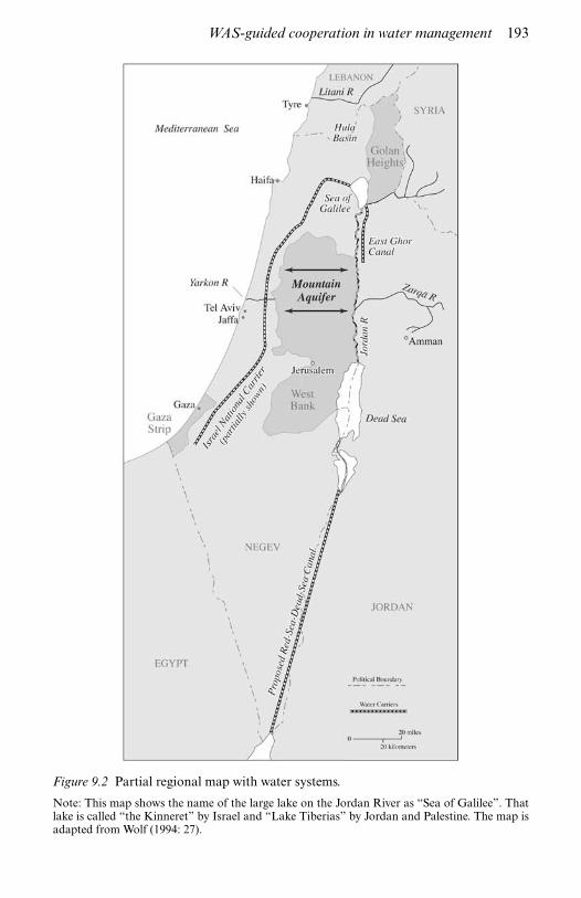
Figure 9.2 Partial regional map with water systems.

Note: This map shows the name of the large lake on the Jordan River as “Sea of Galilee”. Thatlake is called “the Kinneret” by Israel and “Lake Tiberias” by Jordan and Palestine. The map isadapted from Wolf (1994: 27).


system, and the economic gains would be a natural source of funding forwater-related infrastructure.

Both parties would gain from such a voluntary trade. The seller wouldreceive money it values more than the water given up (otherwise, it would notagree); the buyer would receive water it values more than the money paid(otherwise, it would not pay it). While one party might gain more than theother, such a trade would not be a zero-sum game but a win–win opportunity.

Such gains are illustrated for Israel, Jordan, and Palestine below. Theygenerally exceed the value of changes in ownership that reflect reasonabledifferences in negotiating positions. First, however, the stability of the grandcoalition is considered.

9.8 Stability of the grand coalition

Consider a group of n countries all in the same river basin or otherwiseconnected as to water. Let G denote the grand coalition—where, by “coali-tion” is meant a WAS-guided cooperation arrangement as described above. Itwill be shown that G is stable—that is, that there exists no nonempty propersubset, S, of the countries such that a coalition of the members of S, usingtheir own water resources, can lead to all such members being better off thanthey would be in G. (Of course, this applies to single-member subsets where asingle country optimizes the use of its own water.)

Proposition: The grand coalition is stable.Proof: The proof begins with:Lemma: The proposition is true for n = 2.Proof of lemma: Let the two countries be denoted by X and Y respect-ively. Suppose that the joint WAS solution calls for a transfer of waterfrom some district of X to some district of Y. (For simplicity of notation,assume that each country has only one district.) Then it must be the casethat, without such transfer, PX < PY + t*XY, where PX denotes the (pre-transfer) shadow value of water at X, PY denotes the (pretransfer)shadow value of water at Y, and t*XY denotes the per-cubic-meter con-veyance cost—this time including the appropriate capital charge.18 Then,after the transfer from X to Y, the shadow value at X will be higher thanPX, and the shadow value at Y will be lower than PY, the respectivepretransfer shadow values. But then both X and Y must have total bene-fits higher than they would be without the transfer—X because it hasreceived money that it values more than the water given up, and Ybecause it has received water that it values more than the money it haspaid.19

Proof of proposition: Now, consider any nonempty proper subset, S,whose members form a coalition. Let T be the set of all countries that arenot in S. Consider a coalition formed by the members of T. Then thewater resources of the members of S are being used optimally as though


S were a single country, and similarly for T. But the grand coalition isnothing but a coalition formed by S and T. This is a bilateral agreement.Hence, by the lemma, both S and T must be at least as well off as theywere alone. It follows that it cannot be true that the members of S (or themembers of T ) can all be better off than they would be in G.

Some comments need adding. First, note that the special water valu-ations of each of the countries are respected in any WAS-guidedarrangement in which they participate.

Second, because the use of WAS shadow values, given those valuations,essentially restores the properties of a competitive market, the result justgiven is not surprising. It essentially mirrors the well-known result thatthe competitive equilibrium is always in the core of the economy.

Third, as already remarked in note 6, the result does not imply thatevery country does better in the grand coalition than it would in othercoalitions. For example, in the case of Israel, Jordan, and Palestine, forplausible (but not inevitable) distributions of water ownership, Israel isa net seller and the other two countries are net buyers of water underWAS-guided arrangements.20 It is therefore not surprising that Israeldoes better in the grand coalition than in bilateral ones, while the othertwo countries do (slightly) better in bilateral coalitions with Israel than inthe grand coalition. Note, however, that, as should be expected from theproposition under discussion, if side payments are allowed, then all threecountries can be made better off when a third one joins an existingbilateral coalition.21

9.9 Gains from WAS-guided cooperation: case studies involvingIsrael, Jordan, and Palestine

Results are now presented for Israel, Jordan, and Palestine, illustrating thegains from cooperation—and especially those from participation in the grandcoalition. Attention is concentrated on predictions for 2010, those for 2020being qualitatively similar.22

For perspective on the scarcity of water in these three countries, a greatproportion is arid to semi-arid, receiving as little as 50 to 250 millimeters ofrainfall per year—drier than Phoenix, Arizona. The estimated total renew-able water supply for the region is approximately 2,400 million cubic metersper year, while water use averages 3,000 million cubic meters—an amountthat is clearly unsustainable without some level of intervention.

The study concentrates on two sources of water that are the subjects ofconflicting claims. These are the Jordan River and the so-called MountainAquifer (see Figure 9.2). Both of these are (very roughly) of equal size, eachyielding about 650 million cubic meters a year. The Jordan River is claimedby all three countries, while the Mountain Aquifer is claimed only by Israeland Palestine. Since the gains from cooperation depend on assumptionsabout water ownership, results are obtained for selected varying assumptions


about such ownership. It must be emphasized that such assumptions are notmeant as a political statement. They are illustrative only.

For the Jordan River, ownership cases are examined as follows:

• Israel 92 percent; Jordan 8 percent; Palestine 0 percent (This is approxi-mately the existing situation.)

• Israel 66 percent; Jordan 17 percent; Palestine 17 percent

• Israel 33 percent; Jordan 33 percent; Palestine 34 percent.

For the Mountain Aquifer, ownership cases are examined varying from Israel80 percent–Palestine 20 percent (close to the existing situation) to Israel20 percent–Palestine 80 percent by shifts of 20 percent at a time.23

First, results on two-way cooperation are presented. These differ from thosein Fisher et al. 2005 primarily because of the expanded set of ownershipassumptions.24 It is assumed that, both for Israel and for Jordan, fixed-pricepolicies are in place. For both countries, this means subsidies for agricul-ture and, for Israel, higher fixed prices for the other sectors. The Palestinianwater price in each district is assumed to equal the corresponding shadowvalue.

9.9.1 Israel–Palestine bilateral cooperation

First, bilateral Israeli–Palestinian cooperation is considered. Figure 9.3 showsthe gains from such cooperation as a function of the different ownershipassumptions. (Note that cooperation here is not merely cooperation on theMountain Aquifer but full cooperation in water.) Effectively, this and thefollowing two figures represent slices of a multidimensional diagram. (InFigures 9.3, 9.4, and 9.5 Israel is represented by black, Jordan by white, andPalestine by white with diagonal stripes.)

Look first at Figure 9.3(i)—the case of an 80:20 Israel–Palestinian divisionof the Mountain Aquifer. As should be expected, in case A of Jordan Riverownership, where Israel has most of the river and Palestine has none, it isPalestine that benefits most from cooperation—far more than relativelywater-rich Israel. Further, the same is true for the other cases of Jordan Riverownership. But an interesting phenomenon appears. As expected, Palestinegains more from cooperation in case A, where it owns no Jordan River water,than it does in case B, where it has 17 percent of the river. Moving on to caseC, however, where Palestine has 34 percent of the river, the gains to Palestineonce again increase, being very nearly as high ($171 million dollars per year)as in case A ($172 million dollars per year), even though Palestine has con-siderably more water in case C than in case A.

The reason for this is not hard to find. Palestine has considerably morewater in case C than in case A, but Israel has considerably less. Both buyerand seller gain from WAS-guided cooperation, and, in case C, Palestine gainsby selling water to Israel, despite its low share of the Mountain Aquifer.


Correspondingly, Israel, whose gains as a seller decrease slightly from case Ato case B, has increased gains as a buyer in case C.

This phenomenon becomes even more pronounced in the other panels ofFigure 9.3, in which Palestine has increased shares of the Mountain Aquifer.In each of those panels, Palestinian’s gain from cooperation increases as itowns more and more Jordan River water; that is because it gains as a seller.Correspondingly, Israel gains as a buyer.

Moreover, the gains from cooperation are typically higher—and often

Figure 9.3 Gains from bilateral cooperation between Israel and Palestine in 2010.


much higher—than the gains from a shift in ownership of the MountainAquifer of 10 percent of that aquifer’s water. This is true even if it is assumedthat there is no cooperation when shifting ownership; it is even more true ifcooperation is assumed, where the value of such a shift (to either party)ranges from about $5.5 million per year in case A to about $17 million peryear in case C. The corresponding numbers for the noncooperation caserange from $3 million to $36 million per year but are not the same for thetwo countries. And, where such values are highest, so are the gains fromcooperation.

9.9.2 Israel–Jordan bilateral cooperation

Figure 9.4 shows the gains from bilateral cooperation between Israel andJordan for 2010. Here the gains are generally lower than in the Israel–Palestinecase. The interesting phenomena are as follows.

Where Israel has the lion’s share of the Mountain Aquifer (Figures 9.4(i)and 9.4(ii)) and also 92 percent of the Jordan River (case A), there are nogains from cooperation at all. Neither Israel nor Jordan gains from tradingJordan River water—despite Jordan’s small share thereof. Staying with thesame shares of the Mountain Aquifer and moving to case B for the JordanRiver, small gains do appear25 and the gains are quite a bit larger in case C.In Figures 9.4(iii) and 9.4(iv), where Israel has 40 percent and 20 percent ofthe Mountain Aquifer, respectively, there are larger gains for Jordan, theincrease being most noticeable in case B (although the gains remain largest incase C).

What is going on here is that, as Jordan owns more and more of the river, itpays both parties for Jordan to transfer water to Israel by selling water per-mits. This is even true when Israel owns 92 percent and Jordan only 8 percentof the river,26 but is more pronounced in cases B and C as Israel’s share of theriver goes down and Jordan’s goes up. This reflects the finding in Fisher et al.2005 that Jordan has a major problem of conveyance infrastructure in usingJordan River water.

It is also interesting to note that Israel’s gains from such purchases in caseC are greatest when it owns 80 percent of the Mountain Aquifer (Figure9.4(i)) and hence presumably needs the Jordan River water less than it doeswhen it has less Mountain Aquifer water. The explanation is that Figure9.4(i) shows a case in which Israel has sufficient water to make the shadowvalue of the Jordan River water lower than in the other cases. Hence the pricethat Israel pays for such water is also lower, and this benefits Israel (whilecorrespondingly reducing Jordan’s gains as a seller).

9.9.3 Jordan–Palestine bilateral cooperation

The case of bilateral cooperation between Jordan and Palestine can behandled quickly (and requires no figure to illustrate it). Here the only


possible beneficial trades are those that involve Jordan River water—andboth countries have relatively little water to trade. As a result, the only case inwhich gains from cooperation are not totally negligible is that where Palestineowns only 20 percent of the Mountain Aquifer and none of the Jordan River(case A). There, even though Jordan only owns 8 percent of the river, it gains$10 million per year by selling a permit to Palestine to use river water, andPalestine gains $12 million per year by buying it.

Figure 9.4 Gains from bilateral cooperation between Israel and Jordan in 2010.


9.9.4 Trilateral cooperation (grand coalition)

Figure 9.5 gives the results for trilateral cooperation. Here what stands out isthat, in general, the largest gains are Palestinian and the smallest Jordanian.Not surprisingly, generally the less water Israel owns, the more it has to gainfrom cooperation. On the other hand, Jordan gains more from cooperationthe more water it owns—selling permits to Israel.

Like Jordan, Palestine presents a picture that is somewhat more mixed. Italso tends to benefit more from cooperation the larger its share of the Jordan,

Figure 9.5 Gains from trilateral cooperation (grand coalition) in 2010.


selling permits to use river water to Israel. On the other hand (Figure 9.5(i)),when Palestine owns relatively little Mountain Aquifer water, it also benefitsas a buyer.


So far as Israel, Jordan, and Palestine are concerned, the most importantgeneral conclusion from all these cases should be clear. WAS-guided cooper-ation in water would benefit all parties—Israel and Palestine the most. Thegains from such cooperation exceed those that can be had from obtainingreasonable amounts of ownership shifts.

Moreover, such cooperation would benefit the parties in other ways. Forone thing, runs of the WAS model strongly suggest that Israel and Palestinewould both benefit from the construction of an effluent treatment plant inGaza with the output sold to Israel for use in agriculture in the Negev desert,which would provide needed investment for Gaza and cheaper water forIsrael. This means that Israel has a positive economic incentive to assist withthe construction of such a plant. That would be a positive gesture of cooper-ation, and one that does not impinge on the really difficult core issues thatseparate the two parties.

Further, the usual quantity-oriented water treaty may be adequate fora time, but as populations, economies, and climate change it can becomedated and place strains on a peace arrangement. This certainly can happenin the region under discussion. WAS-guided cooperation provides a flexiblemethod for adjusting water allocations with all parties benefiting from theadjustments.

Is such cooperation likely in the region? It is not easy to tell. On the onehand, for the last several years, the Israeli–Palestinian situation has beendominated by conflict over nonwater issues. On the other hand, that conflicthas not prevented all cooperation in water. Even during the al-Aqsa Intifada,which began in September 2000, the Israeli and Palestinian water authoritiesmet regularly to discuss water issues—particularly because of the substantialdrought conditions then prevailing. Further, there were no attacks on thewater system of either party.

Israel and Jordan signed a water (quantity) treaty in 1994, and have gener-ally lived up to its terms, even though there have been various difficulties.

Nevertheless, cooperation has been limited. Israel’s attitude towards pro-viding more water for the Palestinians has generally been that it will assist thePalestinians in finding new sources of water, but that it will not change theallocations of existing water resources. At one point, Israel even suggestedproviding, for the southern West Bank, water that would be pumped uphill aconsiderable distance from a desalination plant in Ashkelon (Israel). Thatwould be a very inefficient way of providing water to that area—much lessefficient than keeping the desalinated water in Israel and permitting thePalestinians to pump more water from the Mountain Aquifer than they have


heretofore been permitted to do. That suggests that symbolism plays a con-siderable role in these matters.27

Nevertheless, there are some hopeful signs. Partly because of the efforts ofthe Water Economics Project and others, the Israeli government appears tohave come to understand that water ownership issues can be considered amatter of money and that, in particular, desalination provides a way out ofthe problem. Large desalination facilities have been constructed with moreplanned, and there is discussion of the fact that there may now be enoughwater to avoid the water conflict problem. Even though such a solution isinferior to WAS-guided cooperation, and even though such cooperationwould still be useful when desalination becomes a necessity some years fromnow, solving the ownership issue with the aid of desalinated water is betterthan not solving it at all.

The prospects for the use of WAS and even WAS-guided cooperation arecertainly not dead, however. The Palestinian and Lebanese water authoritieshave both expressed interest in using WAS at least for their own domesticmanagement purposes, and there has been some activity at the Israeli WaterCommission in this regard. Further, the Lebanese have indicated an interestin the use of WAS to prepare for negotiations with Lebanon’s neighbors,and, at least before the Israel–Hezbollah war of 2006, that interest includednegotiations with Israel.

For Lebanon, as for all countries either in the Middle East or elsewhere,the use of WAS can serve two purposes. First, WAS provides a powerful toolfor infrastructure planning. Second, it provides a way of resolving waterconflicts, changing water negotiations from a zero-sum game to a win–winsituation, whether the conflict is between competing uses domestically, orbetween countries.

As suggested earlier, the usefulness and power of WAS is being enhanced bythe construction of a multiyear version (MYWAS). In that version, one canspecify a menu of possible infrastructure projects, together with their costs anduseful lives. MYWAS will then give results as to which (if any) of the specifiedprojects should be built, in what order, at what time, and to what capacity.Those results can be examined for their dependence on predictions as to suchthings as population growth, climatic conditions, and technological advances.

Further, MYWAS can be easily used to examine issues of storage (in aqui-fers or reservoirs). And it can give guidance on aquifer management—advisingon overpumping in dry years and replenishment in wet ones. Finally, MYWAScan be used to study the effects of climatic uncertainty.

WAS and MYWAS have recently (mid-1996) been adopted by the Energy,Water, and Environment Community—a high-profile program on environ-mental cooperation in the Middle East coordinated academically at theLondon School of Economics and Political Science and politically sponsoredby Prague Forum 2000, a leading European vehicle of track two (informal,nongovernmental) diplomacy. Efforts are currently under way to feature WASand MYWAS in a major round of awareness raising on water optimization in


the Middle East, seeking long-term political sponsorship from sympatheticEuropean Union States and institutions.

While WAS has been first developed for the Middle East (in particular, forIsrael, Jordan, and Palestine), its methods and use are not restricted to thatregion. Domestically, the WAS (or MYWAS) model provides a powerful toolfor water management, especially for infrastructure planning and waterpolicy with respect to allocation, pricing, and subsidies. Thus WAS is relevantfor all countries, even those with well-developed infrastructure.

Beyond that, however, there are disputes over water ownership and alloca-tions all over the globe. These are not only international disputes: sectoraland subnational disputes are increasing as well. WAS methodology providesa way of resolving those disputes to the advantage of all parties.

Notes

1. We are indebted to Ariel Dinar for raising the questions that prompted this chap-ter and for urging us to write it.

2. See also our expository article (Fisher and Huber-Lee 2006).3. For examples that go beyond mere cost minimization, see Brown and McGuire

1967; Dandy et al. 1984; and McCarl 1999. The model that appears most similarto WAS is the CALVIN model, an optimizing water model for Californiadeveloped at the University of California, Davis (see for example Newlin et al.2002; Jenkins et al. 2003; and Jenkins et al. 2004).

4. We use the term “Palestine” and refer to Palestine as a “country” both for con-venience and out of respect for our Palestinian colleagues.

5. Two-way cooperation between Palestine and Jordan was not investigated. This isconsidered in subsection 9.9.3.

6. Note that this result does not imply that every country in the grand coalition doesbetter than it would in some partial coalition. This problem is discussed in Fisheret al. 2005: 216–17.

7. This is an application of the well-known Coase Theorem of economics. See Coase1960.

8. The pioneering version of such a model (although one that does not explicitlyperform maximization of net benefits) is that of Eckstein et al. 1994.

9. There is a large literature and much discussion about actual free water markets,but it is crucial to understand that what is proposed here is not such a market.Later in the chapter a system of water trading among (in this case) countries isrecommended, but even such trading is not at freely bargained prices but rather atprices and quantities prescribed by joint operation of an optimizing model.Hence, the water market literature is not discussed explicitly.

10. A multiyear version has now largely been developed and is briefly discussed insection 9.10.

11. The total amount that consumers are willing to pay for an amount of water, Q*, ismeasured by the area up to Q* under their aggregate demand curve for water.Note that “willingness to pay” includes ability to pay. The provision of water toconsumers that are very poor is taken to be a matter for government policyembodied in the pricing decisions made by the user of WAS.

12. If the user of the model—for example the government of a country—would valueadditional water in a particular location more than would private buyers, then theshadow value reflects that valuation.


13. If this calculation gives a negative figure, then the scarcity rent is zero, and water isnot scarce at the given location.

14. A similar method can be used to analyze different proposed water policies.15. If trading off ownership rights considered sovereign is unacceptable, the parties

can agree to trade short-term permits to use each other’s water. See later in thissection.

16. All money values are in 1995 US dollars.17. Of course, the question naturally arises as to what the effects on Syria and Leba-

non, respectively, would be in these two situations. Without a WAS model forthose two countries, that question cannot be answered. Both countries wouldsurely profit from such a model.

18. The simplest case is to assume that the conditions of the year being studied willcontinue for the life of the project. More realistic cases only complicate the dis-cussion without changing the nature of the proof.

19. Note that this is true regardless of how the transfer costs, t*XY, are allocated. Yultimately pays those costs—either directly to X or by building and operating theconveyance system itself—but the surplus benefits generated are large enough tocover such payments and still leave Y better off than it would have been withoutthe transfer.

20. This does not mean that sales go in only one direction. It is typically found thatthe direction of sales differs at different locations.

21. See Fisher et al. 2005: 216–17.22. At this time, it is appropriate for us to correct a minor error in Fisher et al. 2005

pointed out to us by Yoav Kislev, whom we thank (not desiring to shoot themessenger). In that work, all prices are meant to be at the city gate, so to speak.But, when dealing with Israeli fixed-price policies for households and industry, wemistakenly set the fixed price for urban and industry at the prices charged at theuser tap. We also calibrated the household and industry demand curves usingthose too-high prices. Correction of this slip has almost no effect on our import-ant qualitative statements (indeed, it strengthens the finding that desalination isnot yet an efficient technology except in times of extreme drought), but it doesaffect numerical results. We have corrected the mistake in the results discussed inthis section.

23. The Mountain Aquifer in fact consists of several subaquifers. No attempt is madeto divide ownership except in the arbitrary manner described in the text.

24. In Fisher et al. 2005, the gains from cooperation for each of the two water sourcesare examined separately while assuming that Israel had most or all of the othersource.

25. In the 80:20 split of the Mountain Aquifer, the gain to Jordan in case B rounds offto zero.

26. In the 40:60 split of the Mountain Aquifer, Jordan gains $1 million a year—toosmall to show up in Figure 9.3(iii).

27. Incidentally, a country that withholds a particular water source from a WAS-guided agreement hurts both itself and its cooperating partners. WAS can be usedto evaluate such effects. See Fisher et al. 2005: 217–18.

28. The notation used is restricted to this Appendix.29. Note that the first term of the objective function is the integral of the inverse

demand function:

Pid = Bid × (QDid + QFRYid)ALPHAid.


References

Brown, G. and McGuire, C. (1967) “A socially optimum pricing policy for a publicwater agency”, Water Resources Research, 3: 33–43.

Coase, R. (1960) “The problem of social cost”, Journal of Law and Economics, 3:1–44.

Dandy, G., McBean, E., and Hutchinson, B. (1984) “A model for constrainedoptimum water pricing and capacity expansion”, Water Resources Research, 20:511–20.

Eckstein, O. (1958) Water-Resource Development: The Economics of Project Evalu-ation, Cambridge, MA: Harvard University Press.

Eckstein, Z., Zackay, D., Nachtom, Y., and Fishelson, G. (1994) “The allocation ofwater resources between Israel, the West Bank and Gaza: an economic analysis”,Economic Quarterly, 41: 331–69 (Hebrew).

Fisher, F.M. and Huber-Lee, A. (2006) “Economics, water management, and conflictresolution in the Middle East and beyond”, Environment, 48(3): 26–41.

Fisher, F.M., Huber-Lee, A., Arlosoroff, S., Eckstein, Z., Haddadin, M., Hamati,S.G., Jarrar, A., Jayyousi, A., Shamir, U., and Wesseling, H., with a special contri-bution by Salman, A.Z. and Al-Karablieh, E.K. (2005) Liquid Assets: An Eco-nomic Approach for Water Management and Conflict Resolution in the Middle Eastand Beyond, Washington: RFF Press.

Hirshleifer, J., DeHaven, J.C., and Milliman, J.W. (1960) Water Supply: Economics,Technology, and Policy, Chicago: University of Chicago Press.

Jenkins, M.W., Lund, J.R., and Howitt, R.E. (2003) “Using economic loss functionsto value urban water scarcity in California”, Journal of the American Water WorksAssociation, 95: 58–70.

Jenkins, M.W., Lund, J.R., Howitt, R.E., Draper, A.J., Msangi, S.M., Tanaka, S.T.,Ritzema, R.S., and Marques, G.F. (2004) “Optimization of California’s watersupply system: results and insights”, Journal of Water Resources Planning andManagement, 130: 271–80.

Maass, A., Hufschmidt, M.M., Dorfman, R., Thomas, H.A., and Marglin, S.A.(1962) Design of Water Resource Systems, Cambridge, MA: Harvard UniversityPress.

McCarl, B. (1999) “Limiting pumping from the Edwards Aquifer: an economicinvestigation of proposals, water markets and spring flow guarantees”, WaterResources Research, 35: 257–68.

Newlin, B.D., Jenkins, M.W., Lund, J.R., and Howitt, R.E. (2002) “Southern Califor-nia water markets: potential and limitations”, Journal of Water Resources Planningand Management, 128(1–2): 21–32.

Rogers, P.P. and Fiering, M.B. (1986) “Use of systems analysis in water management”,Water Resources Research, 22: 146S–158S.

Saliba, B.C. and Bush, D.B. (1987) Water Markets in Theory and Practice: MarketTransfers, Water Values, and Public Policy, Boulder, CO, and London: WestviewPress.

Wolf, A. (1994) “A hydropolitical history of the Nile, Jordan, and Euphrates Riverbasins”, in A.S. Biswas (ed.) International Waters of the Middle East from Euphrates–Tigris to Nile, Oxford: Oxford University Press.


Appendix: the mathematics of the WAS model

The WAS model is written in the generalized algebraic modeling system(GAMS) language. As the objective function is not linear, the MINOS nonlin-ear operating system is used to solve the WAS model. The model is presentedbelow in the standard form for optimization, namely, the objective functionfollowed by the constraints. In mathematical terms,28 the model is as follows:29

Max Z = �i�

d�Bid × (QDid + QFRYid ) ALPHAid + 1

ALPHAid + 1 � − �i�

s

(QSis × CSis)

− �i�

j

(QTRij × CTRij) − �i�

j

(QRYij × CRij)

− �i�

j

(QTRYij × CTRYij) − �i�

j

[CEid × (QDid + QFRYid)]

Subject to:

�d

QDid = �s

QSis + �j

QTRji − �j

QTRij � i

QRYid = PRid × (QDid + QFRYid) � i,d

�d

QFRYid = �d

QRYid + �j

QTRYji − �j

QTRYij � i

(QDid + QFRYid) ≥ �PMAX

Bid�

1/ALPHAid

� i,d

With the following bounds:

QSis ≤ QSMAXis � i,s

PRid ≤ PRMAXid � i,d

All variables positive.Where:

Indices

i = district (Israel: I1,I3 . . . I15; Jordan: J1 . . . J8; Palestinian Authority:P1 . . . P10; Golan: GOL; Jerusalem: JER)


d = demand type (urban, industrial, or agricultural)s = supply source or steps (S1 . . . S5)

Parameters

ALPHAid Exponent of inverse demand function for demand d indistrict i

Bid Coefficient of inverse demand curve for demand d in district iCEid Unit environmental cost of water discharged by demand

sector d in district i ($/m3)CRid Unit recycling cost of water supplied from demand sector d

in district i ($/m3)CSis Unit cost of water supplied from supply step s in district

i ($/m3)CTRid Unit cost of water transported by demand sector d in

district i ($/m3)CTRYid Unit cost of recycled water transported by demand sector d

in district i ($/m3)PMAXid Maximum price of water from demand sector d in district iPRMAXid Maximum percent of water from demand sector d that can

be recycled in district iQSMAXis Maximum amount of water from supply step s in district

i (Mm3)Pid Shadow value of water for demand sector d in district i

(computed) in $

Variables

Z Net benefit in from water in million $QSis Quantity supplied by source s in district i in Mm3

QDid Quantity demanded by sector d in district i in Mm3

QTRij Quantity of freshwater transported from district i to j inMm3

QTRYij Quantity of recycled water transported from district i to j inMm3

QRYid Quantity of water recycled from use d in district i in Mm3

QFRYid Quantity of recycled water supplied to use d in district i inMm3

PRid Percentage of water recycled from sector d in district i

Note: Mm3 = million cubic meters.Figures 9.6A and 9.6B give an illustration of continuity for freshwater

and recycled water, respectively, as given in the first two constraint equationslisted above.


Figure 9.6 Continuity of flows at node i.


10 Experimental insights into theefficiency of alternative watermanagement institutions

Aurora García-Gallego, NikolaosGeorgantzís, and Praveen Kujal1

An increasing number of local governments all over the world are adoptingregional hydrological plans aimed at integrated management of their waterresources. The effect of such integrated management plans on the final qual-ity of water is a central but underinvestigated issue in the ongoing debateconcerning the desirability of centralization of the decisionmaking processand the use of market mechanisms to allocate water among its users. Basedon the results obtained from a series of experimental sessions, this chapterpresents insights into the efficiency and quality-enhancing effects of central-ized public management using block rate bidding in a water market withuniform market-clearing prices.

10.1 Introduction

Water is a basic input to many human activities. Its allocation among differentusers has traditionally depended on centralized, publicly controlled manage-ment mechanisms that significantly underestimate the true value of water tomost of its users. The increasing threat of drought and water shortages, even inthe most developed areas of the world, has forced many governments to adoptinnovative ways of managing their water resources. Among the numerousinstitutional innovations, privatization of infrastructure2 and private man-agement3 of water resources have attracted the attention of researchers andpolicymakers. This chapter focuses on the performance of private and publicwater management institutions, taking the underlying infrastructure as given.

Several countries have already implemented measures of water utility privat-ization. In the European Union, the Water Framework Directive (EuropeanCommission 2004) explicitly refers to the need for improved management tohelp ensure the quality and sustainability of water resources.4 A central pointof the European Union directive is recognition of the need for groundwaterbody identification (European Commission 2005). A groundwater body isdefined as a set of aquifers whose management is undertaken through aunified decisionmaking process. Clear examples of such unified managementof aquifers can be found in Finland and Norway, which are confronted with ahuge number of groundwater bodies because of their specific geological

characteristics. Finland has identified about 3,700 groundwater bodies. InNorway the grouping of individual aquifers (8,000–11,000) into less than1,000 groundwater bodies is based on the analogous principle and has theaims of reducing administrative costs and enhancing water managementefficiency.

Whereas the management of water resources within the geographic andadministrative limits of a river basin has been analyzed by economists in theframework of common pool extraction, the role of aquifer integration hasnot been studied so far. In fact, despite the clear message of the WaterFramework Directive and the implementation of integrated aquifer man-agement by the aforementioned Nordic countries, the joint management ofdifferent water resources has found little if any administrative support in theEuropean Union, especially in countries where the tradition often defineswater as a regional or national property.

Despite numerous technical and institutional barriers, water transfersacross regions with different endowments and the use of market mechanismsare two innovative (and controversial) strategies that are increasingly beingadopted by water managers all over the world. A successful example ofjointly managing water resources from different sources in order to satisfydifferent types of users can be found in California.5 Apart from a centralizedplan of action, a market mechanism has been established in California, thevolume of which in 2001 was well above 10 times its initial volume in 1985,although it still accounts for only 3 percent of the state’s water use. Evensmall suppliers participate in this market, contributing with their excess waterendowments, or even with the entire resource they own, idling their crops tosell water.

The debate concerning the desirability of the aforementioned managementstrategies has often focused on the issue of water quality arising from differ-ent water allocation mechanisms. Concerning this, two issues are of specialinterest to this study: the heterogeneity of users’ needs, and the crucial effectsof decentralized actions on water quality.

Both the California Water Plan update of 2005 and the European UnionWater Framework Directive discuss these two points. Concerning the firstpoint, the California Water Plan update6 states that:

High quality water sources can be used for drinking and industrial pur-poses that benefit from higher quality water, and lesser quality water canbe adequate for some uses, such as riparian streams with plant materialsbenefiting fish.

(Department of Water Resources 2005, vol. 2, ch. 12)

With respect to the second point, which is a central issue dealt with in thepresent chapter, the California Water Plan update states:

Many water management actions, such as conjunctive use, water banking,

210 Aurora García-Gallego et al.

water use efficiency, and water transfers, intentionally or unintentionally,result in one type of water quality traded for, or blended with, another.


The importance of mixing multiple water qualities is further highlighted bythe increasing use of recycled water. Regarding the role of recycled water inproviding water of sufficient quality to the users, the California Water Planupdate mentions that:

Further, some new water supplies like recycled water can be treated to awide range of purities that can be matched to different uses. The use ofother water sources, again, like recycled water, can serve as a new sourceof water that substitutes for uses not requiring potable water quality.


Needless to say, as in the aforementioned example of the two Nordic countries,defining the scope of aquifer integration and identifying the right type ofagent who should be responsible for the decisionmaking process are twocentral questions to be answered from a number of different viewpoints: cul-tural, political, social, and economic. This chapter focuses on the economicaspects of the decisionmaking process.

An ideal solution to the problem described above would require a heavilycomputerized and, necessarily, centralized engineering approach to the man-agement of adjacent aquifer systems. From a theoretical point of view, thisapproach is feasible as long as the specification of the underlying demandmodel and the statistical properties of the stochastic elements on the supplyside are known to the decisionmaker. However, this is a rather unrealisticdesideratum, especially because policymakers, even when assisted by complexcomputerized decisionmaking algorithms, cannot have but approximationsof the underlying demand model. Thus, even if the stochastic elements affect-ing the supply of water were ruled out, the decisionmaking process shouldnot be expected to be the result of applying explicit optimization rules. Insuch cases, adaptive decisionmaking7 based on trial-and-error strategies canbe seen as the real-world counterpart of explicit optimization assumed byoptimal control theory. However, in the presence of such an adaptive deci-sionmaking process, there is no clear-cut prediction concerning the perform-ance of different water management institutions. For example, the obviousadvantages from centralized public management may be offset by decisionerrors arising from the increased complexity of the problem faced by thedecisionmaker.

Decentralized management, and even the use of privately participated watermarkets, might offer an appealing alternative with much weaker requirementsconcerning the rationality of decisionmakers. In fact, a decentralized solutionwould reduce the complexity of the partial decisionmaking problems faced byprivate profit-driven agents. But, again, there is no readily available prediction

Efficiency of alternative water management institutions 211

on the degree to which such a reduction in the complexity of the problemfaced by each decisionmaking entity would offset the social welfare loss aris-ing from the suboptimality induced by the decentralization of incentives.Furthermore, even in the case of resources that are fully controlled by thepublic sector, allocations are implemented using price mechanisms, which arethe only feasible way of eliciting an individual user’s need for an extra unit ofwater. Thus, a further nontrivial problem that arises concerns the interactionbetween each one of the aforementioned management alternatives and theprice mechanisms usually adopted in order to allocate different quantities ofwater to different users. An underinvestigated question arising in this contextis which institution can best allocate water to different users, accounting foreach institution’s effect on the quality resulting from a mixture of differentwater qualities.

This chapter experimentally investigates the case in which water qualityis endogenously determined as the combination of water extracted fromtwo sources of different qualities. Without replicating any real-world mar-ket, insights are gained into the advantages and disadvantages of alterna-tive water management institutions, considering two different scenarios ofcentralization—private and public—and two different levels of decentralizedmarket competition.

Although not addressing the issue of water quality, a number of authorshave studied various aspects of water markets and water management.Moench (1992) showed that competitive water withdrawal can lead to over-exploitation. This was previously argued by Gordon (1954), who showed thatcomplete rent dissipation may occur from the exploitation of an open-accessresource. This result was confirmed and generalized by the findings of Masonand Phillips (1997). Walker et al. (1990), Walker and Gardner (1992), andGardner et al. (1997) also focused on the issue of water resource exploitationin a common pool framework. In a more recent study, Murphy et al. (2000)used laboratory experiments to design “smart” computer-assisted marketsfor water inspired by computer-assisted market institutions developed byMcCabe et al. (1989, 1991). A smart market allows decentralized agents tosubmit messages to a computer dispatch center. The center then computesprices and allocations by applying an optimization algorithm that maximizesthe possible gains from exchange. Using California as a case study, Murphyet al. (2000) tested alternative institutional arrangements for a computer-assisted spot market. They showed that the smart uniform price doubleauction yields highly efficient outcomes in a thin market characterized by alimited set of trading opportunities. Although their study is the only one thatis potentially applicable to integrated aquifer management, their frameworkaccommodates multiple locations but it does not consider any qualitydimension.

The studies mentioned above clearly show that experiments can be a usefultest bed to study alternative property right mechanisms (Walker et al. 1990;Walker and Gardner 1992), or to undertake a direct test of an existing market


mechanism (Murphy et al. 2000). Experiments can replicate important char-acteristics of existing markets and test them in a laboratory setting at minimalcost to the regulator.

The results discussed in this chapter are based on an overview of experi-mental results reported in three different manuscripts. They reflect differentphases of a broader research project undertaken at the experimental labora-tories of the Universities of Valencia8 and Castellón9 in Spain. In the firstpaper, Georgantzís et al. (2004) present an experimental design with decen-tralized action on the demand side. They highlight the difficulties encounteredwhen the allocation of water to its users takes place in a fully decentralizedand possibly inefficient way. The second and third papers present an improvedmarket design where, once water prices are posted by private or public sup-pliers, water allocation is implemented by a smart market-clearing mechan-ism guaranteeing maximal surplus on the demand side. In the second paper,García-Gallego et al. (2005) study the same management institutions as inGeorgantzís et al. 2004, with the exception that the demand side is simulatedto achieve maximal consumer surplus. In the third paper, García-Gallegoet al. (2006) consider an alternative market mechanism that focuses on mar-ket competition versus coordination. These experiments replicate the privateduopoly case, implementing a pre-play coordination mechanism inspiredby games with confirmed strategies. The results indicate that centralizedmanagement of the resources by a public entity leads to the highest levels ofeconomic efficiency, lowest prices for users, and the highest quality-to-priceratio.

The experimental markets whose results are reported here represent anaquifer system with extraction from two different sources of water. The ter-minology adopted is specific to the case of potentially integrated aquifersthat, adopting the European Union Water Framework Directive definition,may form a unified groundwater body. However, the framework adopted isapplicable to a broader spectrum of real-world cases including, for instance,the case of mixing different types of recycled water. Such situations wouldlead to endogenous water quality supplied to different types of users. Fur-thermore, a costly depuration procedure is introduced, which is activated atthe consumer’s location when quality falls below the potable standard. Tosimplify the analysis, it is assumed that the quality of farm water has no suchrestriction.

Four different market structures (private monopoly, duopoly, coordinatedduopoly, and public monopoly) and their effects on market outcomes arestudied, paying special attention to the resulting stock depletion, quantitysupplied to the users, and the quality-to-price ratio. The four managementscenarios are chosen to compare, on the one hand, private to public central-ized management of the integrated aquifer system and, on the other hand, amore competitive to a less competitive decentralized market structure. Theresults reported below indicate that a social welfare-driven monopolist offersthe highest quality-to-price ratio and exploits the resource at a faster rate


than a private monopoly or duopoly. However, the most stable stocks corres-pond to the private management scenarios (monopoly and duopoly), althoughthe corresponding stock levels are inefficiently high.

The chapter is structured as follows. Section 10.2 discusses the featuresof the aquifer system. Section 10.3 presents the experimental design. Section10.4 discusses the results. Section 10.5 concludes.

10.2 Underlying theoretical framework

In this section the theoretical framework is discussed, focusing on the intu-ition underlying the formal assumptions of the model. There are two renew-able stocks, of high quality (SH) and low quality (SL), from which water maybe extracted. Quality of water in an aquifer may be lower because of marineintrusion, or because of infiltration of fertilizer from agriculture. The twoqualities are assumed to be constant over time. However, any intermediatequality may be supplied to the consumers as a result of mixing water from thetwo sources. Note that, usually, quality choice is studied in the context ofproduct differentiation models. In these models, product quality is directlyand consciously chosen in a way that takes into account the competition-reducing effect of product differentiation. Thus, quality choice determinesthe fierceness of price competition. In the present framework, the causality isreversed. Final product quality is the result of price-setting behavior. Thus,strategic interaction determines the final quality, which is unique and notdirectly controlled by any single agent. Because of this, and the dynamic natureof this framework, there are no theoretical predictions that are immediatelyapplicable to the case studied here.

For the sake of simplicity, the recharge to the respective basin is assumed tobe deterministic and constant. This assumption does not imply that the extrauncertainty arising from fluctuating supply conditions observed in the realworld is a problem of negligible importance. However, it has been ruled outfrom the analysis in order to reduce the complexity of the microworld man-aged by the subjects and isolate the dynamic and complex elements of thewater market studied from the nonstrategic uncertainty on the supply side.Thus, the aim of the experiments reported here is to illustrate possible advan-tages and disadvantages of the alternative institutions in isolation from theaforementioned types of supply-side uncertainty. The inflow to the basins isassumed to cease when the storage capacity of the aquifer is reached. That is,once the maximum storable stock is reached, extra water inflow is lost. Thereturn flow of consumed water is assumed to be negligible. Thus, changes inthe stocks exclusively arise from extraction and recharge.10 Extracting more isassumed to be more costly and the marginal cost increases. Also, it is easier toextract from a stock in which the water surface is at a higher level.

Mixing the two qualities (QH and QL) results in water whose quality is givenby the weighted average (QM) of both types of water. Quality of potable watershould weakly exceed the constant minimum quality standard Qmin, where


QH > Qmin > QL. Mixed water of quality QM may, or may not, satisfy theminimum quality standard. This depends on the quantities and the qualitiesthat are mixed. The quality of water supplied to households may be improvedto achieve the potable quality standard at a cost. This cost is an increasingfunction of the difference between the quality before and after purification.Moreover, a given improvement of a lower quality is less costly than thesame improvement performed on a higher quality. Resource flow between thesources and the consumers is coordinated by a pair of knots, which centralizethe mixing process at the consumer’s location. The distribution schemedescribed above is presented in Figure 10.1.

Suppose that the behavior of the consumers can be aggregated under oneof two types: households (h) or farmers (F ). Consumers differ in their respect-ive preferences regarding the quality of water. Both types prefer a higherquality and quantity of water to a lower one. Households consume waterwhose quality weakly exceeds a minimum standard. If mixed quality does notsatisfy this condition, it will be subject to purification. The purification pro-cedure is assumed to be costly enough that it is not profitable to improvequality above the minimum standard. Hence, the quality consumed byhouseholds is the maximum between the minimum and the mixed quality.

The assumptions presented here concerning consumer utility are qualita-tively similar to those in Williams et al. 1986 on multiple commodities thatare interdependent in consumption. Two features, which are rather specific tothe dynamics of water, are added to the structure: first, buyers are restrictedto purchase up to a certain amount of each type of water;11 second, a con-stant inflow (recharge) in each period maintains the stock of water in thebasins of each producer. In fact, following a standard formulation of similar

Figure 10.1 Pipeline network.


groundwater extraction problems, a lower stock implies a higher extractioncost. Thus, each period’s marginal cost and past levels of extraction arepositively correlated.12

10.3 Water resource management: from theory to the lab13

From an experimentalist’s or a behavioral economist’s point of view, themanagement of a complex system raises a large number of stimulating ques-tions that can be addressed within many scientific disciplines and studiedfrom many different points of view. Psychologists, for almost half a century,have used simulated complex “microworlds” to identify patterns of humanlearning and assess the performance of behavior in the presence of complextasks. An economist’s, or a management scientist’s, interest in complex sys-tems relates not only to efficiency-related issues, but also to the behavioralaspects of market functioning. These cannot be reliably described by staticmodels based on standard simplifying assumptions aimed at analytical tract-ability. In static simple contexts, rational decisionmaking is often obser-vationally equivalent to the limited behavior of adaptive subjects usingtrial-and-error learning algorithms. However, as complexity increases, explicitoptimization becomes a less powerful descriptive model of human behavior,yielding predictions that significantly deviate from trial-and-error processes.Such deviations arise from different factors, among which are strategic inter-action, multitask and multiperiod interdependence, complexity of the math-ematical functions (relating actions to feedback), and imperfect information.Rather than the exception, complexity arising from the aforementionedfactors is the rule in most real-world markets.

A central question motivating the focus and methodology adopted here iswhether some well-known results on static market functioning are applicableto complex dynamic markets. Textbook industrial organization theory recom-mends competition almost as the panacea to market imperfections. This veryinfluential view has inspired the most widespread type of state interventionin the market, namely the establishment of competition authorities. Whileenhanced competition is a relatively straightforward process in simple staticmarkets, complex market setups call for policies based on a more informedview of market management by imperfect human decisionmakers.14 Forexample, in imperfect information settings, a multiproduct monopolist who islearning from trial-and-error algorithms may fail to behave differently from aduopoly selling the same products (García-Gallego and Georgantzís 2001).Thus, the standard result concerning efficiency losses arising from monopolymay not be as globally applicable as is usually thought. Such learning failuresseem to be more likely the more we deviate from the standard static sym-metric setup.15 The addition of dynamics and nonlinearities in the functionsdictating the feedback from the underlying cost and demand models rendermost textbook wisdom inapplicable to some real-world markets. A furtherobstacle in understanding the functioning of complex dynamic markets stems


from the fact that human actions exhibit a far richer range of behavioralpatterns than any analytically tractable model can afford or any simulatedmarket can include. Over the last half a century, economic experiments withhuman subjects have increasingly proved to be a reliable source of informa-tion tackling all (or at least most) of the aforementioned problems. Far fromattempting an exhaustive review of the related literature in economics,management, and psychology, some related issues and their correspondingstylized facts are reviewed as they are reported in the literature.

The experimental design focuses on how different market structures affectwater resource management. The analysis focuses on the case in which prop-erty rights to a given groundwater source are exclusively granted to a singledecisionmaking unit. Implicitly, the model highlights the vertical nature ofthese markets, in which coordination is required between water extraction,supply, and purification.16 The quality of water reaching the final consumer isnot directly controlled by any one of the agents in the market. Instead, it isthe result of the agents’ bidding behavior controlling the resources. Theironly strategic variables are the minimum price bids at which they are willingto sell each unit of each type of water to the consumer.

The model described in the previous section is implemented with thefollowing values for the parameters:17

• Recharge (ai = 3, i ∈ {H,L})

• Initial and maximum stocks: (SH,SL) = (20,20)

• Water qualities: (QH,QL) = (5,1)

• Minimum quality standard demanded by the household: Qmin = 3.

In the steady state of the social optimum a stock size of (SH,SL) = (4.84,5.01)is obtained associated with the prices (pH, pL) = (102,86). However, in order tosimplify subjects’ perceived feedback conditional on their strategies, thedesign allows only for discrete quantities and prices. Thus, if subjects adoptthe discrete version of this steady state equilibrium stock policy, they mustaim at stabilizing stocks at (SH,SL) = (5,5). Obviously, this is achieved whenthe 3-unit inflow of each water quality equals the quantity sold in each period.Assuming that this is so, then, maximizing total surplus the quantities,(KHh,KLh) = (2.55,0) and (KHF,KLF) = (0.45,3), are automatically assigned bythe server, respectively, for household (h) and agriculture (F ) consumption.To avoid subjects making uncontrolled guesses concerning the end of thesession, a deterministic end game horizon was used (a total of 50 periods),which was known by subjects from the beginning of the experiment.18

Subjects knew the type of water they were managing.19 Furthermore, theywere conscious of the generic preference of consumers for the high-qualitygood over the other. Moreover, they knew that their products were demandsubstitutes (though not perfect) and that their extraction cost structures wereidentical. Subjects received a table with their unit costs depending on the stocksize. A simulator (made available to them on their decision screen) informed


them of the hypothetical costs and gains they would make if they sold all theunits of each product for which they were currently submitting post bids.They knew that the actual number of units they sold would be known onlyafter they had posted their period bids and that the (automated) demand’sreaction to these bids was announced to them on the feedback screen.

Four different market structures are studied and compared in terms ofeconomic efficiency. These are designed to address the effect of two differentfactors that are usually considered to be competing solutions to the problemof efficiency losses arising from monopolistic market power: competition, andcentralization of decisions by a public monopolist. In order to address theseissues, four experimental conditions are implemented. Three of them arelabeled as treatments, while the fourth condition is implemented as a variationto one of the three basic treatments. They are as follows.

• Treatment 1 (private monopoly). The monopoly has joint ownership ofboth sources and optimal (simulated) coordination of consumer behavioris assumed. Each subject posts price offers for both water qualities.20 Thebundle of high- and low-quality water that produces the highest consumerrent is allocated in the economy. The corresponding offers of the subjectsthen establish the clearing prices. Monetary rewards are proportional toaccumulated total profits over the whole session.

• Treatment 2 (noncooperative duopoly). Under the noncooperativeduopoly each firm-subject offers one of the two types of water andindependently decides on prices. This is a noncooperative decisionmak-ing scenario. As in all treatments reported here, there is optimal simulatedcoordination in the downstream part of the market. Each water resourceis managed by a different subject sitting in front of a separate PC21 andcommunication between competitors is not permitted. Duopolies areformed randomly at the beginning of the session and then matchingremains fixed over the 50 periods of the experiment (“partners” proto-col). Although a “strangers” protocol, forming a different subject pair(duopoly) in each period, would be an interesting extension, the resultingnoisy feedback would require allowing for longer experimental sessions.22

An alternative duopolistic setup, coordinated duopoly, was run using thesame experimental market as in treatment 2. A single session was runusing this design as a collusion-facilitating variant of the duopoly treat-ment. In the coordinated duopoly session, each resource is managed by adifferent subject, but the interface used is that of the private monopolywith two subjects sitting in front of each of the PCs. Communication andagreement on the timing of decision submission and the possibility ofiterated inspection of the competitor’s strategy before jointly pressing the“OK” button render this setup highly collusive. However, individualincentives remain uncoordinated and no side payments were feasible.Therefore, as the results show, this structure lies in many senses betweentreatments 1 and 2.


• Treatment 3 (public monopoly). Here subjects decide on both water qual-ities. As in all treatments reported here, there is optimal simulatedcoordination in the downstream part of the market. In this treatmentsubjects act as public monopolists caring for total social welfare ratherthan private profits. Subject rewards were proportional to total socialwelfare (also referred to as social utility).

The experiment was run using the software Hydromanagement.23 Theresults reported here are based on data obtained from experimental sessionsrun during 2004 in the Laboratori d’Economia Experimental (UniversitatJaume I, Castellón, Spain). Three 20-subject sessions were run for each oftreatments 1 and 3 (20 monopolies per session) and five 20-subject sessions(10 duopolies per session) were run for treatment 2. Finally, a single 40-subject (20 duopolies) session was run for the coordinated duopoly treatment.A number of pilot sessions (not presented here) were run at the beginning ofthe whole project. Subjects were recruited following standard protocols of theLaboratori d’Economia Experimental and they were assigned only once to asingle session. Sessions from different treatments were run in a random orderin order for undesirable social learning to be avoided. Each session lasted anaverage of 80 minutes.

Demand is simulated in all treatments according to the assumption ofutility maximization contingent to the block rate bids made by suppliers ineach period. The simulated consumer represents a population of farmers andhouseholds with different preferences for water quantity and quality. Qualityis the result of mixture of the two qualities of water sold in the market. Ifquality falls below a certain potable threshold, an extra cost is borne by theconsumer (reducing consumer surplus) for the water to be depurated up to thethreshold level. The resulting feedback from the demand model is difficult tointerpret by the subjects or linearize in any sense. Unit extraction costs increasein steps as the level of stock of each water quality decreases. Therefore, ineach period costs depend on extraction in previous periods.

Given each bidding schedule posted by a seller, consumer surplus maxi-mization determines the quantity of each quality consumed. This is a rathercomplex problem, especially because of the uncoordinated action of sellers inthe duopoly scenario, but also because of the dynamic nature of the marketand the horizontal externality effect of each water type on the other.

A history window on each subject’s screen displays all past outcomesregarding own decisions on quantities, payoffs, and market prices. In duopolymarkets, each subject also receives the clearing price at which the other waterquality was sold. In each period, subjects are asked to submit their respectivereservation prices (offer bids) for each unit of product (from the 1st unit tothe 5th, the maximum quantity each one of them could trade). Subjects weretold that offer bids had to weakly exceed the extraction cost of the corres-ponding unit, and offers of subsequent units would have to be nondecreasing.Once offer bids were submitted, behavior on the demand side was simulated


by a program that automatically calculates the optimal consumption of eachwater quality by consumer type for which total consumer surplus is maxi-mized. All units of the same product were sold at the same market price,which was determined from the intersection of product-specific supply anddemand schedules resulting from sellers’ and buyers’ behavior describedabove.

10.4 Results

In order to make the discussion of the results easier to follow, let us first recallsome intuitive implications of the benchmark solution obtained in the previ-ous section. The steady state equilibrium stock level for the discrete strategyspace version of the model implemented here is 5 for both water qualities.Once this level is reached, the optimal extraction rate is dictated by the rate ofthe inflow. That is, in each period a manager should aim at selling 3 unitsof each water type (the same number as enter the tank because of the naturalrate of inflow). Also, the socially optimal path leading to this steady staterequires the fastest possible rate of convergence to it. Under efficient man-agement all these predictions are fulfilled over the maximum number ofperiods possible. Of course, behavioral and strategic considerations areabsent from the socially optimal solution. For example, competing privateprofit-driven subjects should be expected to restrict present extraction in orderto guarantee lower extraction costs and a competitive advantage against rivalmanagers in future periods. There might even be idiosyncratic factors such asrisk aversion, or excessive fear of overexploitation, that are relevant in theobserved behavior but have not been accounted for in the benchmark model.Other indicators that are usually not present in other studies on complexresource markets are price levels for each water quality, and price-weightedaverage quality sold to the consumers.

Results concerning market-clearing prices, quantities sold, stocks, andquality/price ratios are discussed using descriptive statistics and plots ofperiod averages in each treatment.24 Table 10.1 (see page 222) provides descrip-tive statistics concerning aggregate treatment averages obtained in the last30 periods of each experimental session.

Some graphs that combine comparable magnitudes across treatments willnow be discussed. Given that a fixed matching protocol was used, dataobtained from the same subject acting in the same market in different periodscannot be treated as independent observations. Consequently, the evolutionof averages over the 50 periods of a session is a reliable source of informationfrom which useful insights can be gained.

In all cases, average stocks (Figures 10.2 and 10.3) are above the steadystate optimum levels (5 units). Comparison across treatments indicates thatthe average stock of both water qualities is the lowest in the public mono-poly treatment. Note that a sustained decreasing tendency is only observedin the public monopoly case (although without reaching the benchmark


optimum). Other treatments stabilize their corresponding average stock levelsfrom early periods onwards to over 10 units, which is well above theoptimum.

In general, competitive environments and social welfare-oriented deci-sionmaking yield lower stock levels for both water qualities. Both monopolies

Figure 10.2 Evolution of average stock levels (low-quality water).

Figure 10.3 Evolution of average stock levels (high-quality water).


(especially the public one) present persistently decreasing stocks, while arather stable pattern over time is observed in duopolies.

As is seen in Table 10.1 and Figures 10.4 and 10.5, prices are highest in theprivate monopoly case and lowest in the public monopoly case. The differencesin average qualities are reflected for all treatments (but to different degrees).

Overall, price averages per treatment indicate that the public monopolyreflects significantly the effects of different qualities on prices (51.05 of thelow quality versus 67.14 of the high quality), while the coordinated duopolyproduces an insignificant difference (98.63 versus 96.67). The other twotreatments produce intermediate differences (75.71 versus 69.82 in theduopoly and 108.76 versus 101.85 in the private monopoly case). Data yieldthe expected result that relatively more competitive environments and socialwelfare maximization yield lower prices. Also note that public monopoliesreach a stable average level throughout the second half of the session.

Table 10.2 presents quantity averages per treatment in 5-period intervals.Even in the initial 5 periods, subjects achieve the objective dictated by thehydrological equilibrium of the system. Namely, in all treatments and for

Table 10.1 Descriptive statistics (treatments 1, 2, 3 and coordinated duopoly aggregatesand last 30 period averages and standard deviations)

Low-quality stock High-quality stock

T1 T2 CD T3 T1 T2 CD T3

Average 11.4 12.4 11.2 9.5 12.7 11.1 12.2 9.3Std. Dev. 1.2 1.2 1.2 1.7 1.1 1.2 0.9 1.9Av. 20–50 10.9 11.7 10.9 8.7 12.2 10.5 12.0 8.3St. D. 20–50 0.3 0.4 0.4 0.5 0.4 0.3 0.2 0.7

Low-quality quantity High-quality quantity

T1 T2 CD T3 T1 T2 CD T3

Average 3.0 3.0 3.0 3.1 2.9 3.0 2.9 3.1Std. Dev. 0.3 0.2 0.3 0.3 0.2 0.3 0.3 0.3Av. 20–50 2.9 2.9 2.9 3.0 2.8 2.9 2.8 3.0St. D. 20–50 0.1 0.2 0.2 0.1 0.2 0.1 0.3 0.1

Low-quality price High-quality price Average quality/price

T1 T2 CD T3 T1 T2 CD T3 T1 T2 CD T3

Average 101.9 69.8 96.7 51.1 108.8 75.7 98.6 67.1 0.04 0.04 0.04 0.11St. Dev. 11.9 5.2 12.8 9.1 12.0 8.1 11.7 12.3 0.01 0.01 0.01 0.05Av. 20–50 108.4 72.2 102.9 52.0 113.6 80.0 103.8 69.8 0.03 0.04 0.03 0.10St. D. 20–50 6.5 3.6 4.4 8.7 9.5 5.3 4.3 12.7 0.00 0.00 0.00 0.03


most 5-period intervals considered, quantity averages are not significantlydifferent from 3, implying levels of water consumption that are equal tothe constant per period recharge of the aquifers. Learning this rule has takensubjects less than 5 periods, which confirms their decisionmaking capacityand understanding of the functioning of the market.

Figure 10.4 Average market-clearing prices (low-quality water).

Figure 10.5 Average market-clearing prices (high-quality water).


The more interesting aspect of the design, namely the quality of wateroffered, will now be considered. Define the quality/price ratio obtainedas a division of average quality by the average price paid in each period.Figure 10.6 presents quality/price index averages defined as Q̄/P̄, where

Q̄ = KH · QH + KL · QL

KH + KL

and P̄ =KH · PH + KL · PL

KH + KL

. It can be easily seen that

the public monopoly provides the highest quality of all the treatments. It isworth noting that the average quality offered by the public monopoly followsa relatively volatile pattern compared to the (average) qualities offered byother treatments. This difference can be understood by recalling that the

Figure 10.6 Average quality/average price ratio for the four treatments.

Table 10.2 Average quantity sold for high- and low-quality water, by five-periodintervals

High-quality quantity Low-quality quantity

Periods T1 T2 CD T3 T1 T2 CD T3

5–10 3.04 3.08 2.95 3.20 3.22 3.00 3.19 3.2211–15 2.83 2.88 2.78 3.11 2.94 2.96 2.91 3.0216–20 2.76 2.95 2.75 3.03 2.93 2.81 2.84 2.9721–25 2.80 2.91 2.88 3.08 2.89 2.82 2.67 3.0326–30 2.76 2.92 2.66 2.89 2.95 3.00 2.91 2.9031–35 2.76 2.84 2.82 2.97 2.89 2.94 2.84 3.0536–40 2.83 2.87 2.76 3.07 2.88 2.98 2.99 2.9741–45 2.87 2.91 2.91 3.09 2.90 2.90 3.01 3.0846–50 3.05 3.00 2.78 3.15 2.95 3.02 3.02 3.17


public monopolist receives feedback that partly, but directly, depends on theconsumer’s social welfare. Specifically, the consumer’s loss associated withthe cost of depuration (in case quality falls below the potable threshold)negatively affects the feedback received by subjects on the success of theirstrategies. Volatility is thus the result of a continuous effort by subjects(representing the social planner) to cope with the additional objective ofmaintaining quality above a certain level in order not to trigger the inefficient(understood as costly) depuration procedure.

Noncooperative duopoly stocks are closer to those of the public monopolywhile the collusive duopoly treatment leaves stock levels closer to thoseobtained under the private monopoly scenario.25 As expected, under a duopolyresource depletion is faster than under tacit or explicit monopolization. Thisresult resembles a similar finding that is recurring in most common poolresource experiments (see Walker et al. 1990; Walker and Gardner 1992). Itshould be noted that in this setting there is no competition at the extractionstage. Instead, this setup assumes extraction from separate pools and com-petition in the distribution stage. The findings reported here could be used tosupport the view that disaggregation increases the rate at which a resource isdepleted. This is confirmed by comparison of treatments 1 and 2, in whichsubjects’ incentives are related to private profitability. Price levels presenta similar but weaker confirmation of the same principle applied to pricecompetition.

Only the public monopoly solution gets close to the socially optimal steadystate stocks. Full convergence, however, is not achieved at the end of 50periods. The aspect in which management by a public monopolist dominatesall other configurations is the quality/price ratio. Achieving a high quality/price ratio implies balanced exploitation of the two resources by the publicmonopolist using exactly the same instruments as those used by subjects inthe other treatments. Of course, the public monopoly has the right incentivesto do so, as it aims at maximization of total social welfare. Some volatility isobtained regarding the quality/price ratio as the public monopolists’ taskrequires a global view of the performance achieved with both policy instru-ments available (bids for the two water qualities). This contrasts with thesmoother patterns of the other treatments in which profit maximization is theonly objective pursued.

In profit-driven treatments subjects post significantly higher bids aimed atlowering present consumption. This is done in order to maintain a higher stockand, thus, lower unit extraction costs in the future. This is a basic differencebetween pure profit-driven, and social welfare-oriented, decisionmaking. Inthe former, subjects seem to care too much for maintaining a high stock inorder to guarantee low extraction costs and competitiveness (in treatment 2)in future periods. On the other hand, the social planners’ treatment induceshigher levels of extraction, without letting overexploitation emerge.

This finding, however, should not be understood as an argument againstthe use of market mechanisms altogether. On the contrary, it must be


emphasized that in this setup social planners achieve their results by learn-ing to set the appropriate prices for each type of water. This also implies theneed for distinguishing between incentives and market-clearing mechanisms.The behavior of the social planners in treatment 3 is an example of howmarket-clearing prices can be used as a strategy aimed at social welfaremaximization.


Most of the debate concerning the use of market mechanisms as a means ofallocating water among different types of users has focused on the appropri-ate definition of property rights. Several researchers have argued that the mar-ket mechanism may entail unfair outcomes because of some agents’ greatereconomic or political power over other less strategic or weaker players.26

Although the definition of property rights is of great importance in decen-tralized water management, the present study looks at a different and certainlyunderinvestigated issue that should be taken into account when assessing thedesirability of alternative water management institutions. The central questionaddressed here is whether adaptively learning from past actions negativelyinterferes with the usual benefits from centralized and, thus, informationallydemanding public management. If this conjecture were true, decentralizationand privatization of water resource management might mitigate the complex-ity of the problem faced by each decisionmaker, offsetting the well-knownwelfare losses because of incompatibility between private and social incen-tives. Thus, a further argument would be provided to support decentralizedprivate management of the resources.

Contrary to the aforementioned conjecture, the answer provided by theexperiments reported here is that the decisionmakers’ incentives dominatepossible efficiency losses because of an increased complexity of the underlyingsystem managed by each type of agent. This main result establishes a straight-forward ranking of management institutions in terms of their correspondinglevels of social welfare.

Therefore, despite the fact that centralized public management has to dealwith a more complex problem whose feedback depends on a broader setof signals than private profit alone, the public monopoly treatment of theexperimental setup yields the most efficient outcomes both in terms of socialwelfare and in terms of the final quality of water supplied to the users.Interestingly, centralization of the decisionmaking process by a private profit-driven entity yields the worst outcomes, suggesting that centralization aloneis not enough and it should always be accompanied by the right incentives.

Otherwise, if the public monopoly solution is impossible to implementbecause of, say, economic, institutional, legal, or historical reasons, marketmechanisms should be implemented under the usual rule of thumb, favoringcompetition against monopolization of the market by a private agent. Thecoordinated duopoly treatment was shown to move the market away from the


competitive outcome and close to the monopoly solution. Therefore, anotherwell-known rule of thumb for market regulation is also shown to hold in thecomplex market studied here. Namely, the market mechanism is vulnerable toprivate agents’ anticompetitive strategies, so that, if a market mechanism wereimplemented to allocate water resources, competition among decentralizedprivate owners should be safeguarded and promoted.

Notes

1. The authors gratefully acknowledge the financial support of the FundaciónBBVA, Bancaixa (project P1 1B2004–28), and the Spanish Ministry of Educationand Science (project SEJ 2005–07544/ECON). Kujal acknowledges financial sup-port from the Spanish Ministry of Education and Science (Secretaría del Estadode Universidades e Investigación and grant SEJ 2005–08633/ECON). The chapterwas written while Kujal was visiting ICES, George Mason University. J.C. Pernías-Cerrillo provided excellent programing assistance. Comments by the participantsat the Sixth Meeting on Game Theory and Practice (Zaragoza, Spain, July 2006)and detailed discussion between Victor Galaz and the editors of this chapter aregratefully acknowledged.

2. In a recent study, Holland (2006) focuses on the costs and benefits from privat-izing the construction of the Central Arizona project, reporting several shortcom-ings in the resulting incentive structure.

3. For example, Saal and Parker (2001) study the effects on costs and prices inprivatized water and sewerage companies in the United Kingdom. Their resultsyield some pessimism regarding the efficiency gains from privatization, which maynot offset the resulting increases in prices. Bhattacharyya et al. (1994), Noll et al.(2000), Bauer (1997), Cowan (1998), and Ogden (1997) also reach conclusionsthat imply that privatization measures should be taken with caution.

4. Detailed information on the European Union Water Framework Directive canbe found at the corresponding European Union website: http://ec.europa.eu/environment/water/water-framework/index_en.html.

5. It is important to bear in mind the mission statement appearing in the CaliforniaWater Plan update, 2005: “To develop a strategic plan that guides State, local, andregional entities in planning, developing, and managing adequate, reliable, secure,affordable, and sustainable water of suitable quality for all beneficial uses”(Department of Water Resources 2005).

6. This and other documents on the management of California’s water resources canbe found on the following website: www.water.ca.gov.

7. A similar suggestion on the need for adaptive management is made by Pahl-Wostl(2007), although the adaptive process there includes social learning and takes intoaccount more complex feedback concerning both economic and noneconomicmagnitudes. An even broader point of view can be adopted looking at variouscross-effects between water and land use activities, as reported by Ramankuttyet al. (2006).

8. LINEEX, University of Valencia (www.uv.es/lineex).9. LEE, Universitat Jaume I, Castellón (www.lee.uji.es).

10. Extraction costs are supposed to be twice differentiable functions of quantity andstock size. First derivatives are assumed to be, respectively, positive and negative,whereas second derivatives are positive.

11. Given that their water consumption in each period is used to serve their currentneeds.

12. All these elements lead to a certainly complex but well-defined dynamic economic


problem that, as shown by García-Gallego et al. (2005, 2006), has an interiorsteady state solution for all the scenarios considered here. In any case, most of theinteresting features analyzed by Dasgupta and Mäler (2004) are not present inthis model.

13. The design is inspired by the hydrological system proposed in Georgantzís et al.2004.

14. A vast literature has been dedicated to various factors that may be responsible forobserved shortcomings of human behavior in complex environments, such asmisperception of feedback (Paich and Sterman 1993; Sterman 1994), limitationsin subjects’ learning when exposed to strategic complexity (Richards and Hays1998), or multitask decisionmaking (Kelly 1995). A number of factors that favorsubjects’ improvement of performance have, also, been identified. For example,trial-and-error algorithms have been shown to facilitate convergence of thestrategies played by uninformed subjects toward symmetric, full-informationequilibrium predictions, as shown in García-Gallego 1998 for the case of a price-setting oligopoly.

15. While full convergence near the theoretical single-product symmetric benchmarkis obtained in settings such as that outlined in García-Gallego 1998, the intro-duction of a slightly more complex task in the multiproduct oligopolies in García-Gallego and Georgantzís 2001 or the asymmetry in García-Gallego et al. 2004provide a sufficiently unfavorable environment for the hypothesis based on thecorresponding theoretical prediction to be rejected.

16. Issues related to vertical integration are not considered in this analysis, although itcould be interesting to study a scenario in which one of the two resources is runby, say, a consumer association.

17. The specific utility, extraction, and purification cost functions used are providedin Georgantzís et al. 2004.

18. Given the complex nature of the experiment 50-period sessions were run in orderto give subjects a sufficiently long time for learning.

19. See the details on the organization of sessions and the instructions to experi-mental subjects in Appendix 10.2.

20. Given these offers, the maximal consumer rent is determined in the simulatedcentralized downstream market: V(KH,KL) − w′ k, where w denotes the vector ofsealed offers and k denotes the vector of quantities Ki, i = H,L.

21. This treatment is based on a version of the software requiring a number of PCsand a server forming a local network. The software can be obtained by theauthors upon request and assistance is subject to usual protocols of the Laboratorid’Economia Experimental (UJI, Castellón, Spain).

22. Pilot sessions not reported here indicate that sessions lasting longer than 70 periodsare required.

23. Jointly developed by the LINEEX at the University of Valencia and the Labora-tori d’Economia Experimental (LEE) of the Universitat Jaume I of Castellón(Spain).

24. Detailed statistical tests supporting the findings reported here are provided inGarcía-Gallego et al. 2005, 2006.

25. This is especially true in the case of the high-quality water (see Figure 10.3).26. See for example the discussion by Galaz (2002) on the Chilean water market,

in which the peasant farmers are awarded “theoretical rights” which are thenlikely to be violated by the actions of a strategically stronger urban watercompany.

27. The instructions to subjects were originally written in Spanish. A unified trans-lated version for the three treatments is presented here, emphasizing the detailsthat are specific to each one of them.


References

Bauer, C. (1997) “Bringing water markets down to earth: the political economy ofwater rights in Chile, 1976–95”, World Development, 25: 639–56.

Bhattacharyya, A., Parker, E., and Raffiee, K. (1994) “An examination of the effect ofownership on the relative efficiency of public and private water utilities”, LandEconomics, 70: 197–209.

Cowan, S. (1998) “The water industry”, in H. Dieter and T. Jenkinson (eds)Competition in Regulated Industries, Oxford and New York: Oxford UniversityPress.

Dasgupta, P. and Mäler, K.G. (2004) “The economics of non-convex ecosystems”, inP. Dasgupta and K.G. Mäler (eds) The Economics of Non-Convex Ecosystems,Dordrecht: Kluwer Academic Publishers.

Department of Water Resources (2005) California Water Plan Update 2005, Gov-ernment of California. Available online: www.waterplan.water.ca.gov/cwpu2005/(accessed April 21, 2007).

European Commission (2004) Moving to the Next Stage in the Common Implementa-tion Strategy for the Water Framework Directive (2000/60/EC), Progress and WorkProgramme for 2005 and 2006, European Commission.

European Commission (2005) “Common implementation strategy for the water frame-work directive (2000/60/EC): groundwater summary report”, technical report ongroundwater body characterization, monitoring and risk assessment issues asdiscussed at the WGC workshops in 2003–04.

Galaz, V. (2002) Water and Equity: A Game-Theoretic Exploration of the ChileanWater Market’s Social Impacts, FLASCO draft.

García-Gallego, A. (1998) “Oligopoly experimentation of learning with simulatedmarkets”, Journal of Economic Behavior and Organization, 35: 333–55.

García-Gallego, A. and Georgantzís, N. (2001) “Multiproduct activity in an experi-mental differentiated oligopoly”, International Journal of Industrial Organization,19: 493–518.

García-Gallego, A., Georgantzís, N., and Kujal, P. (2005) “How do markets managewater resources? An experiment on water management with endogenous quality”,mimeo LEE/LINEEX, Universitat Jaume I, Spain.

García-Gallego, A., Georgantzís, N., and Kujal, P. (2006) “Water management in anexperimental dynamic duopoly with endogenous quality”, mimeo LEE/LINEEX,Universitat Jaume I, Spain.

García-Gallego, A., Georgantzís, N., and Sabater-Grande, G. (2004) “Identified con-sumers: on the informativeness of cross-demand price effects”, Cuadernos deEconomía, 27: 185–216.

Gardner, R., Moore, M.R., and Walker, J.M. (1997) “Governing a groundwater com-mons: a strategic and laboratory analysis of Western law”, Economic Inquiry, 35:218–34.

Georgantzís, N., García-Gallego, A., Fatás, E., Neugebauer, T., and Kujal, P. (2004)“Mixture and distribution of different water qualities: an experiment on verticalstructure in a complex market”, Cuadernos de Economía, 27: 95–138.


Holland, S.P. (2006) “Privatization of water-resource development”, Environmentaland Resource Economics, 34: 291–315.


Kelly, F.S. (1995) “Laboratory subjects as multiproduct monopoly firms: an experi-mental investigation”, Journal of Economic Behavior and Organization, 27: 401–20.

Mason, C.F. and Phillips, O.R. (1997) “Mitigating the tragedy of the commonsthrough cooperation: an experimental evaluation”, Journal of EnvironmentalEconomics and Management, 34: 148–72.

McCabe, K.A, Rassenti, S.J., and Smith, V.L. (1989) “Designing ‘smart’ computerassisted markets in an experimental auction for gas networks”, European Journalof Political Economy, 5: 259–83.

McCabe, K.A., Rassenti, S.J., and Smith, V.L. (1991) “Smart computer assistedmarkets”, Science, 254: 534–38.

Moench, M. (1992) “Chasing the water table: equity and sustainability in groundwatermanagement”, Economic and Political Weekly, 27(51–52): A171–7.

Murphy, J.J., Dinar, A., Howitt, R.E., Rassenti, S.J., and Smith, V.L. (2000) “The designof smart water market institutions using laboratory experiments”, Environmentaland Resource Economics, 17: 375–94.

Noll, R., Shirley, M., and Cowan, S. (2000) “Reforming urban water systems in devel-oping countries”, in A. Krueger (ed.) Economic Policy Reform: The Second Stage,Chicago and London: University of Chicago Press.

Ogden, S. (1997) “Transforming frameworks of accountability: the case of waterprivatization”, in K. Keasey, S. Thompson, and M. Wright (eds) Corporate Gov-ernance: Economic and Financial Issues, New York: Oxford University Press.

Pahl-Wostl, C. (2007) “The implications of complexity for integrated resource man-agement”, Environmental Modelling and Software, 22(5): 561–9.

Paich, M. and Sterman, J.D. (1993) “Boom, bust and failures to learn in experimentalmarkets”, Management Science, 39: 1439–58.

Ramankutty, N., Delire, C., and Snyder, P. (2006) “Feedbacks between agriculture andclimate: an illustration of the potential unintended consequences of human landuse activities”, Global and Planetary Change, 54: 79–93.

Richards, D. and Hays, J.C. (1998) “Navigating a nonlinear environment: an experi-mental study of decision making in a chaotic setting”, Journal of EconomicBehavior and Organization, 35: 281–308.

Saal, D. and Parker, D. (2001) “Productivity and price performance in the privatizedwater and sewerage companies of England and Wales”, Journal of RegulatoryEconomics, 20: 61–90.

Sterman, J.D. (1994) “Learning in and about complex systems”, System DynamicsReview, 10: 291–330.

Walker, J.M. and Gardner, R. (1992) “Probabilistic destruction of common-poolresources: experimental evidence”, The Economic Journal, 102: 1149–61.

Walker, J.M., Gardner, R., and Ostrom, E. (1990) “Rent dissipation in limitedaccess common pool resource environments: experimental evidence”, Journal ofEnvironmental Economics and Management, 19: 203–11.

Williams, A., Smith, V.L., and Ledyard, J.O. (1986) “Simultaneous trading in twocompetitive markets: an experimental examination”, Working Paper, IndianaUniversity.


Appendix: organization of experimental sessions andinstructions to the subjects

The experiments whose results are reported here were organized at theLaboratori d’Economia Experimental (www.lee.uji.es) at the UniversitatJaume I (Castellón, Spain). Subjects were recruited among students ofadvanced Engineering and Economics courses using standard protocols aim-ing at a balanced gender representation and good history of compliance withthe laboratory’s rules in the past (punctuality, discretion, motivation). Aver-age per subject earnings were slightly below �25. Thus, the total cost of thesessions reported here was about �6,500. Another �4,200 were spent onprogramming and subject rewards in the initial pilot sessions that were run toimprove several feedback and interface features. Duopoly sessions were sys-tematically more expensive. A higher exchange rate was used in the duopolysessions to avoid significant differences in individual subject rewards acrosstreatments (apart from the horizontal externality arising from competition,each duopolist manages only a part of the market supplied by each subject inthe monopoly treatments). Before each session, the following detailed writteninstructions were distributed to the subjects:

Instructions to experimental subjects27

Treatments 1, 2, and 3

The aim of this experiment is to study how people make their decisions incertain contexts. Your decisions in the scenario explained below in detail willbe directly related to a monetary reward you will receive in cash at the end ofthe experiment. Any doubt you may have will be clarified personally to youby one of the organizers after you raise your hand. Beyond these questions,any other communication is strictly forbidden and is subject to immediateexclusion from the experiment.

You participate in a market which is characterized by the following features:

• You are the only producer of two commodities: product H and productL. [Treatment 2: There are two producers (1 and 2) and two commodities(product H and product L).] [Treatment 3: You represent a social plannerwho produces two commodities: product H and product L.] Specifically,product H is water of High quality, while product L is water of Lowquality. Products H and L are substitutes, namely, consumers may, to acertain extent, substitute one type of water with the other.

• Treatment 2: You are one of the two producers in this market. At thebeginning of the session, the computer will indicate if you are producer 1or 2. Your competitor will be one (always the same) of the subjects in thisroom, randomly selected by the computer when the session starts.

• There are two types of consumers: households and farmers. Although


they have different preferences with respect to the two types of water,they all prefer water of high quality (product H) to water of low quality(product L). That is, they are willing to pay more for H than for L.

• The market will last for 50 rounds.

Decisionmaking

Your only decision as a producer is announcing the minimum price at whichyou are willing to sell each one from a maximum of 5 units you may sell foreach product. Such announcements of minimum prices are called price bids.In order to make your decisions, you have to take into account that:

• The extraction cost per additional unit extracted and by product isincluded in the “table of costs” (Table 10.3). These costs are the samefor the two products [Treatment 2: (therefore, costs conditions for youand your competitor are identical)], and they are expressed in ExCUs, afictitious Experimental Currency Unit.

• Taking into account the costs of the table, you have to announce fiveminimum prices at which you are willing to sell each unit of the 5 unitsof each [Treatment 2: your] product you may sell in each round. Therefore,your decisionmaking consists of fixing five price bids for each [Treatment2: your] product.

• You should have in mind that, in order not to make any losses, price bidscannot be lower than the corresponding unit costs included in the tableof costs.

• Price bids cannot be decreasing. That is, your bid for the 1st unit cannotbe higher than your bid for the 2nd unit; the bid for the second cannot behigher than the bid for the 3rd unit, and so on and so forth.

• Observe in Table 10.3 that the unit costs decrease with the stock size.At the beginning of the session, you have an initial stock size of 20 units[Treatments 1 and 3: for each product]. At the beginning of each round,you get 3 more units [Treatments 1 and 3: for each type of water].

• Your stock size [Treatments 1 and 3: for each type of water] can neverexceed 20 units and, therefore, once 20 units are reached, any additionalunits you may receive are lost.

Table 10.3 Table of costs (expressed in ExCUs)

Stock size 20 19 18 17 16 15 14 13 12 11

Unit cost 0 0 0 0 0 1 1 2 2 4

Stock size 10 9 8 7 6 5 4 3 2 1

Unit cost 7 11 18 30 50 82 135 223 368 607


Example. Suppose that at the end of a round your stock size [Treatments 1and 3: of one of your products] is 9 units. At the beginning of the new round,you get your additional 3 units (so that your stock now is 12 units). Observein the table that, for a stock size of 12 units, the unit cost for the first 5 unitsextracted is the following:

• The cost of the 1st unit: 2 ExCUs.

• The cost of the 2nd unit: 4 ExCUs.

• The cost of the 3rd unit: 7 ExCUs.

• The cost of the 4th unit: 11 ExCUs.

• The cost of the 5th unit: 18 ExCUs.

In order not to make losses, each one of your bids should not be lower thanthe corresponding unit cost. Therefore, in this example, your bid for the 1stunit should not be lower than 2 ExCUs (cost of the 1st unit); your bid forthe 2nd unit should not be lower than either 4 ExCUs (cost of this unit) oryour bid for the 1st unit; your bid for the 3rd unit should not be lowerthan either 7 ExCUs or your bid for the 2nd unit, and so on for the rest ofthe units.

In case you sell 5 units [Treatments 1 and 3: of this product], the stocksize at the beginning of the next round would be 10 units (seven you keptplus three you get in the new round). If, given your bids for the 5 units, yoursales are zero, your stock would be 15 units (12 you already had plus 3you get at the beginning of the round).

Decisions

• You make decisions on the minimum price at which you are willing to selleach unit of each one of the two products [Treatment 2: of your product].You will fill in all the boxes that appear at your computer screen withyour price bids [Treatments 1 and 3: (five bids for product H and five forproduct L)]. In each box, you will also get information related to thecorresponding unit cost. The bids you submit have to be integer numbersbetween zero and 2,000.

• Although you may propose five different price bids, all units of thesame product will be sold to consumers at a single price. This price will beyour bid for the “last” unit sold of each product. The number of unitssold each period is calculated by a program which simulates the optimalbehavior of consumers.

Example. In the example above, assume that your bids for [Treatment 2: yourproduct] one of the products are: 10 (for the 1st unit), 12 (for the 2nd), 14(for the 3rd), 16 (for the 4th) and 20 (for the 5th). Given your bids, theprogram which simulates the optimal behavior of consumers determines that


3 units of this product will be sold. The price at which you will sell the3 units will be your bid for the 3rd unit, that is, 14 ExCUs.

Only Treatments 1 and 2: the profits

• Your net profit of selling each unit of a product will be the differencebetween the market price at which you sold all units [Treatment 1: ofthat specific product] (your unit income) and the corresponding unitextraction cost. Total profits will be the sum of the unit profits for allperiods.

Example. Taking again the previous example, if, at the beginning of a round,your stock size is 12 units, your total profits in that round will be 29 ExCUs,which are broken down as follows:

• 12 ExCUs for the 1st unit sold (14 ExCUs you receive for that unit minus2 ExCUs it costs you extracting it).

• 10 ExCUs for the 2nd unit sold (14 ExCUs you receive for that unitminus 4 ExCUs it costs you extracting it).

• 7 ExCUs for the 3rd unit sold (14 ExCUs you receive for that unit minus7 ExCUs it costs you extracting it).

Only Treatment 3: the aim

• As a social planner, your aim in each round is to maximize the socialbenefit per unit sold in this market, which is defined as the differencebetween the utility level generated by each unit consumed and the corres-ponding unit extraction cost.

The information

• During decisionmaking, the computer will provide you with a table simu-lating results [Treatment 1: (for each product)], conditional to your bidand cost for the corresponding unit in five possible scenarios: (a) Incase you only sell the 1st unit; (b) If you just sell the first 2 units; . . .(e) In case you sell 5 units.

• Only Treatment 3: At the beginning of each round, the computer willprovide you with a table containing, conditional to the stock size for eachtype of water and all possible combinations of consumption of the twoproducts, the corresponding social benefits (measured as the differencebetween the utility level and corresponding extraction costs) of thatround.

• At the end of each round, the computer screen will show you the totalprofits [Treatment 3: social benefits] obtained in that round, including


information about unit cost, market price and number of units sold ofeach product [Treatment 2: as well as your rival’s price].

• During the experiment, you will be provided with a screen containing thehistory of past rounds (market price for each product, number of unitssold [Treatments 1 and 3: of each product], [Treatments 1 and 2: totalrevenue and total profits [Treatment 1: per product]], [Treatment 3: andsocial benefit]).

Monetary reward

• Your monetary reward at the end of the session will be the sum of yourprofits accumulated in 15 rounds (randomly selected by the computer) ofthe total of 50 rounds, at an equivalence rate of 800 ExCUs = 1 Euro[Treatment 2: 500 ExCUs = 1 Euro]. You will be paid in cash at the end ofthe session.

In order to make sure you understood correctly the market described above,we will proceed next to run a pilot session of 5 rounds. Please, feel free to makeany questions you may have during this pilot session.

Thank you for your collaboration. Good luck!


11 A fair tariff system forwater management

Rita De Agostini and Vito Fragnelli 1

Access to water will be one of the most challenging problems in coming years.It involves many aspects, one of which is considered by this chapter: thepossibility of designing a tariff system that respects fairness and allows anaccurate evaluation of the amount of water that a community will need in agiven period. The Italian situation is analyzed, taking into account the lawand the consequent organization of water management. Particular emphasisis devoted to the truthfulness and implementation aspects.

11.1 Introduction

According to many environmentalists, water management will assume anincreasing relevance in the near future. In the recent past water shortage wasoften thought of as a problem related to developing or tropical countries, butnow governments are realizing that water shortage, in the face of increasingdemand, is becoming a usual situation in countries throughout the globe.Increasing competition and conflict over access to water between countriessharing the same river basin was among the factors prompting the UnitedNations to declare 2003 the International Year of Freshwater, which helpedpromote the analysis of water-related issues.

In Europe a series of hot, dry summers, for example those of 2002 and 2003,have exacerbated water shortage problems. In Italy, for example, many regionssuffered from scarcity of water. In southern Italy the situation was particu-larly grave, with such factors as low rainfall levels, permeability of the ground,and limited number of natural or artificial basins aggravated by longstandingmanagement problems and old and badly maintained water networks. Forexample, some aqueducts have a water loss larger than 50 percent.

Some of these factors are natural (for example the characteristics of theground), and are beyond realistic remedy; other factors are historical andcultural (for example, water problems were never suitably tackled where largelandowners had little interest in less productive areas); and others are relatedto political choices about the development and maintenance of infrastructure,better care of which could significantly reduce water supply problems.

On the other hand, the Italian northern regions, thanks to their geographical

position at the foot of the Alps, and the central regions, located close to theApennines, have suffered few water problems in the past. Both of thesemountain chains represent a very large reservoir of water; the River Po, forexample, which draws tributaries from both ranges, drains an area of over70,000 square kilometers.

Analogously, the northern and southern regions of Italy differ in the qual-ity of water, which is higher in the north than in the south. In the southpollution and infiltration of salt in coastal areas reduce the quality of water;in the northern regions, despite the large degree of industrialization, the waterquality is generally good. One simple reason is the location of natural reser-voirs and artificial basins close to the cities, so that the water reaches the urbannetwork after traveling a short distance, maintaining its quality. Moreover, themost recent depuration tools (for example active carbon) allow a limited add-ition of chlorine derivates, improving the quality of the water in recent years.As a result, the water quality in some municipalities (for example Genoa andFlorence) is higher than for some commercially produced mineral waters.

An element that reduces the availability of high-quality water is the fre-quent use of drinking water (about 90 percent) for purposes for which it is notneeded, particularly irrigation and industrial use. A proposal suggests havingtwo separate networks: one for high-quality water and one for low-qualitywater, especially for farm usage, which takes over half of the water supply,mostly for irrigation, for which water from sewage disposal could be exploited.The objections to this solution arise from the potential hazard of confusingthe two types of water and from the necessity for construction of large-scaleand expensive infrastructure. It has been suggested that building the requiredinfrastructure be devolved to consortia of users, with suitable reductions inwater tariffs for a period.

The climatic conditions in 2002 caused a number of problems. From thebeginning of the year the reduced rainfall failed to fill the lakes and otherreservoirs to expected levels; the summer was extremely hot, resulting notonly in a high level of evaporation of water from the reservoirs, but also in anincreased usage of water, mainly for irrigation but also for home usage.Municipalities forbade use of water for unnecessary purposes, for examplegarden irrigation and car washing, but such measures were insufficient tocompensate for the scarcity of water.

The so-called Legge Galli (5/1/94 n. 36),2 a set of technical and economicrules on water resource management, has two main targets: a new approachto management operations in order to preserve the resources and a newtariff policy. In particular, the Legge Galli states that the management ofwater has to be centralized, as opposed to the current decentralized systemof many small managers, public and private, currently in charge of parts ofthe water system; the size of the area managed should be optimized, requiringthe determination of suitable areas, each constituting an ambito territorialeottimale (optimal territorial area) or ATO; the programing and control of thewater services, devolved to the local authority or autorità d’ambito, are to be

A fair tariff system for water management 237

separated from the management of the service; and the tariff policy is a toolfor increasing the efficiency and quality of the service and reducing manage-ment costs.

As regards the tariff system, the Legge Galli was improved by the technicalannex of Ministerial Act 1/8/1996,3 according to which the average (normal-ized) tariff for the current year has to take into account the operating costs,mortgage costs, and investments of the preceding year and the inflation rateof the current year. In other words, the tariff can be increased in order to fullycover the costs of the water system, but this increase cannot be applied in asingle year; to justify such an increase, the quality of the water is a relevantparameter; nevertheless, the tariff should be reduced in special situations,such as low-income users, critical areas, and small amount used.

A note of the Interministerial Committee for Economic Programing (CIPE)specifies other targets. First, low-income domestic users are to receive particu-lar priority; second, it is possible to identify other priority categories whererelevant differences from the standard situation exist; and third, incentives forsaving water should be provided.

The geographical area considered, ATO/6 (ATO n.6 of Piedmont), includes133 municipalities of the province of Alessandria and 14 municipalities ofthe province of Asti, with about 350,000 inhabitants, about half of themconcentrated in five main towns: Alessandria (85,000), Tortona (25,000),Acqui Terme (19,000), Novi Ligure (27,000), and Ovada (12,000).

The preceding summary outlines the political, legal, and geographicalscenario within which the work described here was carried out.

Cooperation with the autorità d’ambito led to the idea of designing a tariffsystem that may allow a reduction in water usage and, particularly, in waterwaste. Clearly, such a relevant problem should be tackled through a jointeffort, involving experts from all related fields: economists, engineers, mathe-maticians, geologists, and politicians.

This chapter proposes a tariff system that respects the current directivesand is based on the declarations of the users about the amounts of water theyforecast they will use each year, so it is called a “declarative tariff”. The aimof this proposal is threefold: a fair tariff system, that is a system that respectssocial welfare features; a reduction in water waste; and the possibility of themanager obtaining in advance good data about the total water requirementfor each year.

The chapter is organized as follows: in section 11.2 the actual tariff sys-tem in ATO/6 is presented; section 11.3 is devoted to the proposed tariffsystem, analyzing its potential features; and section 11.4 provides some finalcomments.

11.2 Current tariff system

As described in the previous section, Italian law gives some suggestions andrules for a fair water tariff system; in particular, the tariff should balance the

238 Rita De Agostini and Vito Fragnelli

quality standards offered to the users and the costs for the service, includingfinancial costs and capital risk. Other relevant points are the incentives foroptimal use of water, the reduction of water waste and the environmentalimpact of such measures, and the setting of a socially sustainable tariff.

The tariff system adopted in ATO/6 (see ATO/6 2002a, 2002b) alreadyrespects some of the requirements of the Legge Galli; in particular, it con-siders different categories of users, with different tariffs on the basis of usageranges, taking into account geographical and local characteristics.

More precisely, the current tariff system is strongly rooted in the so-calledtariffa di riferimento (reference tariff), which is defined in the Ministerial Act1/8/1996 as “a tool that allows suitable levels of service to be obtained andprovides incentives for developing programs, reducing the costs for users andincreasing the efficiency of management”.

The reference tariff is defined as Tn = (C + A + R) n − 1 (1 + π + K ), where:

Tn is the tariff for year nC is the operating costsA is the mortgage costsR is the capital costsπ is the programmed inflation rate for the year nK is the limite di prezzo (fare bound).

The reference tariff for the starting year, T0, can be obtained as the weightedaverage of the costs of the previous managers that were in charge of the watersystem in the area corresponding to the current ATO, including the rent feesfor public water, cost of the water purchased from third parties, rent fees forthe water system, costs arising from current laws, and costs for current loans.

K represents a percentage that preserves the users from an increase in tariffsufficient to completely cover management costs. This percentage is necessaryas the subsidization of water costs in some areas of Italy was very high, largerthan 90 percent, too great to be covered by a single increase of the tariff. Forthis reason the law fixes the maximum percentage increase for each yearaccording to the costs in the previous year.

For the first year the value of K is defined with reference to the weightedaverage tariff per cubic meter in 1995 (WAT) expressed in Italian lire. For thefollowing years the value of K is defined with reference to the actual averagetariff per cubic meter in the previous year (AAT) expressed in Italian lire(Tables 11.1 and 11.2).

Table 11.1 Definition of K using weighted average tariff

WAT ≤ 1000 ( 0.52 euros) WAT ≥ 1600 ( 0.83 euros) 1001 ≤ WAT ≤ 1599

K = 25.0% K = 7.5% K is computed by linearinterpolation


Referring to the average use of 150 liters per inhabitant per day reported inthe Decree of the Council of Ministries n.47 of 4 March 1996, a note of theInterministerial Committee for Pricing (CIP) proposed the following limitsfor usage ranges: 50 cubic meters per year for applying reduced tariffs and150 cubic meters per year for applying penalties for large use.

The tariff is the sum of two parts: one fixed, namely the rent fee, andone variable, depending on the amount of water used, with increasing pricesper cubic meter of usage. For ATO/6, the tariff system for 2002 was as inTable 11.3.

11.3 Proposed tariff system

The basic aim was to develop a new tariff system that fully considered andaccommodated the future needs of water users. The idea was inspired byinformal communication with the general manager of ATO/6, who spokeabout the difficulties and the advantages of forecasting the future needs ofusers. As water can be easily stored for long periods, this information couldbe used to reduce the problems arising during periods of scarcity. Of course itis possible that the total demand forecast by users exceeds the availableamount of water, but even in this case the information can be useful to themanager, who can then anticipate some restrictions on usage, making themless stringent. The system could also act as an incentive for the manager to

Table 11.2 Definition of K using actual average tariff

AAT ≤ 1100 ( 0.57 euros) AAT ≥ 1750 ( 0.90 euros) 1101 ≤ AAT ≤ 1749

K = 10.0% K = 5.0% K is computed by linearinterpolation

Table 11.3 Tariff system of ATO/6, 2002

Usage Rentfee

Reducedtariff

Basic tariff Firstexceeding

Secondexceeding

up to 60 cubicmeters/year

60–150 cubicmeters/year

150–240 cubicmeters/year

over 240 cubicmeters/year

House user 24.00 0.50 0.80 0.95 1.20

Nonhouse user 48.00 0.80 1.20 1.30

Farm user 48.00 0.50

Public user 24.00 0.80

Large user decided by agreements

Note: The rent fees are in euros per year; the tariffs are in euros per cubic meter.


undertake a deeper analysis of the problem, taking into account the possibil-ity of building more efficient infrastructure in the future, or of purchasingwater from other ATOs, interconnecting the different networks or reservoirs.The new tariff system refers mainly to domestic users but it can be tailored toother kinds of users.

The system works as follows. Each user commits to a forecast amount ofwater at the beginning of each year, on the hypothesis that a larger declaredamount corresponds to a higher basic tariff per cubic meter of water. At the endof the year, penalties are assigned to those users who required a larger amountof water. The penalty system assigns larger penalties to users that made largermisevaluations. The penalty has a twofold motivation: first, it should avoid theusage of a large quantity of water; second, it should encourage truthful declar-ations in order to allow the water manager to calculate a required amount ofwater as close as possible to actual needs. The users may take into account theirnecessities in previous years but they may be influenced by other factors; forexample, number of members in the family group, announcement of a watershortage, or imposition of a higher price for greater usage.

The following notations will be used:

d declared cubic metersx used cubic metersp standard price per cubic meterp′ penalty price per cubic meter (p′ > p).

11.3.1 Alternative tariff systems

The first step in setting a declarative tariff is to ask users for the forecastamount of water needed for the following year, d, and then to apply the stand-ard price, p, to the used quantity of water, x, up to the declared cubic meters,and the penalty price, p′, to the quantity exceeding that amount, as follows:

Tariff 1px if x ≤ dpd + p′(x – d ) if x > d

This tariff system provides incentives for the users that reduce water waste, butfails in the truthfulness of the declaration; in fact the users may declare verylarge amounts of water required in order to be sure of paying the standardprice, whatever the amount of water actually used.

The simplest way to offer an incentive for truthfulness is to ask the users topay the whole declared amount at the standard price, as follows:

Tariff 2pd if x ≤ dpd + p′(x – d ) if x > d


It is straightforward to check the truthfulness of the declaration: if the realused amount of water is larger than the declared amount, the penalty price isapplied; if it is smaller, the whole declared amount is paid anyhow. On theother hand, this tariff fails to reduce water waste, as a user may think that thewater up to the declared amount can be used for free.

A possible way to achieve both the aims is the introduction of variableprices. More precisely, the standard price can be defined using an increasingfunction π that fixes the price per cubic meter up to the quantity d, and thepenalty price using an increasing function π′, with π′ (x) > π(x) for each x,which is applied to the exceeding quantity of water, as follows:

Tariff 3π (d )x if x ≤ dπ (d )d + π′(d )(x – d ) if x > d

This third proposal seems effective but the following example shows that itmay fail.

Example 1Let the standard price be expressed by π (d ) = 0.50 + 0.01d and thepenalty price by π′ (d) = 0.70 + 0.015d. If a user who needs 150 cubicmeters per year declares 150, then the standard price is 2.00 euros andthe penalty price is 2.95 euros, so the final tariff is 2.00 × 150 = 300.00euros; but if the user declares 148 the standard price is 1.98 euros andthe penalty price is 2.92 euros, so the final tariff is 1.98 × 148 + 2.92 × 2 =298.88 euros.

So, a user may gain an advantage from a nontruthful declaration. To avoidthese situations, and taking into account the first two tariffs, the priceswhen the actual usage is larger than the declaration can be computedreferring to the actual usage instead of to the declared one, as follows:

Tariff 4π (d )x if x ≤ dπ (x)d + π′ (x)(x − d ) if x > d

Referring to Example 1, when the declaration is 148 but the actual usage is150 the standard price is 2.00 euros and the penalty price is 2.95 euros, so thefinal tariff is 2.00 × 148 + 2.95 × 2 = 301.90 euros.

It is possible to enforce the penalty for nontruthful declaration by applyingthe standard price π(x) to the whole amount x and adding the penalty pricefor the exceeding part (x − d):

π (x)x + π′ (x)(x − d) if x > d


Referring again to Example 1, the final tariff becomes 2.00 × 150 + 2.95 × 2 =305.90 euros.

Tariff 4 and the modified version penalize mistakes in the declarations. Ifd > x, then for both tariffs π(d ) > π (x) as π is increasing; on the other hand, ifd < x, then for tariff 4, π(x)d + π′ (x)(x − d ) > π(x)x ⇔ π′ (x)(x − d ) > π(x)(x − d ) ⇔ π′ (x) > π(x) holds for the hypothesis on the penalty function π′ andfor the modified tariff π(x)x + π′ (x)(x − d ) > π(x)x trivially holds.

So, both tariffs achieve the stated objectives, limiting water waste and pro-viding incentives for an accurate evaluation of the total water needed througha system of increasing standard and penalty prices.

It is possible, of course, to modify the penalty function π′ in order to reducethe charge for “small” mistakes, taking into account the characteristics of thecurrent year.

11.3.2 Variable prices and the Italian law

The idea of variable prices is consistent with the Italian directives on reducedusages. In this case it is simpler to define the standard costs and the penaltycosts instead of the prices per cubic meter. For example, the standard costfunction C can be defined taking into account the ranges and the tariff fordomestic users stated by ATO/6 (see section 11.2) as:

C (x) =�0.50x30.00 + 0.80 (x − 60)102.00 + 0.95 (x − 150)187.50 + 1.20 (x − 240)

if x ≤ 60if 60 < x ≤ 150if 150 < x ≤ 240if x > 240

In this case the function is piecewise linear, so each user has an advan-tage in declaring the upper bound of its range (the cost per cubic meter isconstant in each range), paying the penalties only if the upper bound isexceeded.

Also, the amount of the rent fee plays an important role, as it increases thefinal price per cubic meter, with a higher influence on small amounts of water,but this is beyond the focus of this chapter. Anyhow, it seems reasonable thatthe rent fee, the reduced tariff for small usage, and the limit for reduced tariffshould be correlated so that the cost per cubic meter increases if the usage islarger than the quantity fixed for the reduced tariff.

In the case of ATO/6 the average cost per cubic meter, including the rentfee, for reduced usage can be expressed as:

π (x) =24.00

x+ 0.50 if x ≤ 60,

which leads to a reduction of the cost for increasing usage until 0.90 euros percubic meter when the usage x is 60 cubic meters. The cost of further water, up


to 150 cubic meters, is 0.80 euros per cubic meter. In order to improve fair-ness, the function π(x) should assume its minimum for the upper limitof the range of reduced usage, that is for x = 60 in the case of ATO/6. Thiscan be done by modifying the rent fee or the range of reduced usage or thetariff system.

For example, in the case of ATO/6 fixing the rent fee at 18.00 euros, the

average cost per cubic meter for reduced usage is π(x) =18.00

x+ 0.50 and the

cost per cubic meter for x = 60 is 0.80 euros, that is, it is equal to the cost ofthe following range. Extending the range of reduced usage fee up to 80 cubicmeters and using the actual tariff the cost per cubic meter for x = 80 is again0.80 euros, as in the following range. Other possibilities depend on changes inthe tariffs; for example, decreasing the reduced tariff to 0.40 euros per cubicmeter or increasing the basic tariff to 0.90 euros per cubic meter.


The results of the declarative tariff system were satisfactory, not only from atheoretic point of view, but also in the evaluation of the technical expertsof ATO/6, compared with the current tariff system. In order to increase thewater savings, it is possible to introduce not only a penalty in case of largeruse but also a prize in case of less use.

It is necessary to take into account that a strong pricing policy, aimed atreducing water wasting, cannot be carried out. Water is essential for health,so its supply has to be guaranteed to all, both by providing a connection tothe network and by maintaining a low cost per cubic meter. This means that itis not possible to raise the price of water by any great amount (10 euros ormore per cubic meter), as users may, as a consequence, reduce usage foressential purposes as well as for inessential purposes such as car washing.

A comparison was also made with another game-theoretic approach, theRabbi rule or contested garment (Young 1995); in this case the total monet-ary amount that has to be covered by the users is assigned as a claim to thehighest user and the claims of the other users are obtained via a linearapproximation of their real usage or of the range of usage they belong to. Inthis way the total amount is divided into several intervals; the amount corres-ponding to each interval is equally shared among the users that appear in theinterval. The following example may make the procedure clearer.

Example 2Consider four users that require 40, 100, 130, and 210 cubic meters ofwater, respectively (see Figure 11.1); let the total amount of moneyrequired for the current period be 630 euros, taking into account also thetotal amount of 480 cubic meters used.

The amount of 630 euros is associated to the largest usage of 210 cubicmeters and, correspondingly, using a linear approximation, the amounts


of 120, 300, and 390 euros are associated to usage of 40, 100, and 130cubic meters, respectively.

In this case there are four intervals that correspond to the monetaryamount associated to each level of usage. All the four users are in the firstinterval, so the monetary amount of 120 is divided among all the users;in the second interval only the last three users appear, so the correspond-ing amount of 180 is divided among three users; the third interval involvesonly the third and the fourth users, so the amount of 90 is divided amongthe two users; finally, only the fourth user is concerned with the last inter-val and pays the amount of 240. Summing up, the four users pay 30, 90,135, and 375 euros, respectively, and the costs per cubic meter are 0.75,0.90, 1.04, and 1.78 euros, respectively.

This approach could make the cost per cubic meter too great, depending onthe amount needed. It should be clear that, considering a reasonable numberof users, those using smaller amounts of water, or those in the first ranges,have a low cost per cubic meter, while those using larger amounts of watermay be penalized by this tariff system, if their numbers are small. A simplepossibility is to use a nonlinear approximation of the usages, but this systemis difficult to implement in a fair way.

Returning to the proposed tariff system it is possible to remark that thehigh level of freedom in determining the cost function π and the penaltyfunction π′ allows matching many possible requirements and constraints,both technical and normative.

Another relevant question is the fixed tariff, namely the rent fee; the under-lying idea is that the fixed costs of the water system should be equally paid byall the users. Nevertheless this approach does not take into account otherfeatures of the problem, such as the amount of the rent fee could be signifi-cant for low-income users, but could be a very small fraction of income forother users; or it is possible that for very small water usage the rent fee islarger than the amount for water and in this case it is necessary, at least from asocial welfare point of view, to distinguish between people living alone thattry to save water (and, consequently, money) and people that use their houseonly for short periods of the year. These particular situations may be at

Figure 11.1 Contested garment approach.


odds with the analysis in the previous section, and further analysis may berequired.

Again game theory may be a valid instrument for determining a fair tariff;it is possible to take into account the different requirements of the agentsinvolved using bankruptcy approaches (Young 1987). More precisely, it ispossible to define a bankruptcy (or taxation) problem where the users havethe role of the agents, the estate to be divided is represented by the totalamount of money required for the current period, and the claims are repre-sented by the needs of the users. The related literature provides several rulesfor computing the tariff for each user. Another game-theoretic approach mayinvolve the class of infrastructure cost games that were successfully applied torailway infrastructure (Fragnelli et al. 1999) and to urban solid waste con-sortia (Fragnelli and Iandolino 2004). The tariff is computed by defininga suitable game that considers the users divided into different groups withdifferent needs and applying a game-theoretic solution of the game; forexample, the Shapley value (Shapley 1953) or the Owen value (Owen 1977).In the case under study this approach could easily be applied as the usersare naturally divided into groups according to usage range, income, or geo-graphical location. This approach may be applied both to determine fair rentfees and to compute usage costs.

Notes

1. The authors are grateful to the anonymous internal reviewers and external refereefor useful suggestions. The cooperation of Ing. Renzo Tamburelli, general managerof ATO/6, is also gratefully acknowledged.

2. See Legge 5/1/1994 n. 36, Disposizioni in materia di risorse idriche (in Italian), atwebsite www.cipecomitato.it/Documentazione/Normativa/Tariffe_idriche/L.36-94.htm.

3. See Decreto Ministeriale 1/8/1996 (in Italian), at website www.cipecomitato.it/Documentazione/Normativa/Tariffe_idriche/D.M.1.8.1996.htm.

References

ATO/6 (2002a) “Piano d’ambito: programma di infrastrutture, piano economico-finanziario e dinamica tariffaria per l’erogazione del servizio idrico nell’ATO/6”,Rapporto Tecnico (in Italian).

ATO/6 (2002b) “Regolamento di utenza per l’erogazione del servizio idrico integratonell’ATO/6”, Rapporto Tecnico (in Italian).

Fragnelli, V. and Iandolino, A. (2004) “A cost allocation problem in urban solidwastes collection and disposal”, Mathematical Methods of Operations Research,59: 447–64.

Fragnelli, V., García-Jurado, I., Norde, H., Patrone, F., and Tijs, S. (1999) “How toshare railway infrastructure costs?” in I. García-Jurado, F. Patrone, and S. Tijs (eds)Game Practice: Contributions from Applied Game Theory, Amsterdam: Kluwer.

Owen, G. (1977) “Values of games with a priori unions”, Lecture Notes in Economicand Mathematical Systems, 141: 76–88.


Shapley, L.S. (1953) “A value for n-person games”, Annals of Mathematical Studies,2(28): 307–318.

Young, H.P. (1987) “On dividing an amount according to individual claims or liabil-ities”, Mathematics of Operations Research, 12: 398–414.

Young, H.P. (1995) Equity: In Theory and Practice, Princeton: Princeton UniversityPress.


12 Game-theoretic modeling ofwater allocation regimesapplied to the Yellow Riverbasin in China

Xiaokai Li, Haifeng Shi, and Xueyu Lin

This chapter presents a review of water allocation modeling studies and dis-cusses sustainable water allocation in a river basin context from the perspec-tive of game theory. The Nash–Harsanyi negotiation model is applied to theexamination of several water allocation and management options, includingunregulated withdrawal, allocation through agreed quota, and water rightsand water pricing mechanisms. Some conclusions and policy implications arederived from the case study of the Yellow River basin and are applicable toother river basins for improving water management.

12.1 Introduction

The sustainable socioeconomic development and well-being of China areincreasingly under threat from such problems as floods, droughts, waterpollution, and deterioration of the eco-environment in major river basins(Ministry of Water Resources 2001). As the country continues to grow eco-nomically and in population, accompanied by higher levels of urbanizationand industrialization, water scarcity and pollution, predominantly in thenorth and northwest, are becoming worse. Therefore, how to allocate verylimited water resources effectively in those river basins has become one of themost critical challenges facing the water sector (Zhang 1999).

The current practice of water allocation in China is dominated by adminis-trative mechanisms for most rivers. While such a regime may serve to main-tain a reasonable equity of water sharing among different user sectors andregions, many question the true fairness of this approach because it uninten-tionally encourages waste and misuse of water by making water a resource offree access. It is against the basic principles of water allocation for maximiz-ing returns on water use. Consequences in the Yellow River basin includefrequent drying up of the river and water shortage crises, with enormoussocial and economic costs; raising of the riverbed in the lower reaches ofthe river; and irrigation efficiency lower than 30 percent in many parts ofthe river’s upper reaches. An unsustainable situation thus prevails, whichnecessitates further investment to augment water supply capacity throughgiant operations such as the South–North Water Transfer project. Such

situations can be attributed to lack of an effective allocation and managementmechanism.

Aware of escalating conflicts over transboundary water use worldwide,particularly in many parts of Asia and in Africa, professionals in China’swater sector are devoting more effort toward developing a fairer and moreefficient water allocation regime in China (Liu and He 1999; Guan 2002).Naturally, the troubled Yellow River becomes a focus of research by many.

The Yellow River is the major water source for north and northwest China.It irrigates 15 percent of China’s total cultivated land and supplies water to12 percent of China’s total population with water resources accounting for2 percent of China’s total average annual runoff. The water resource devel-opment in this basin has reached an alarming 70 percent, and consequentlywater security and the eco-environment in the river system, particularly in thelower reaches, are at high risk. For example, in 21 (eight of which occurredin the 1990s) of the 27 years from 1972 to 1998, the river ran dry for a total of1,050 days at Lijin station in the lower reach. The negative impact was enor-mous, on flood management, ecological environment, drinking water supply,and economic and social services.

The situation described above can be well explained using the arguments ofthe “tragedy of the commons” (Hardin 1968). According to Hardin’s theory,if there is no right defined to a property (water in this case), even when themarginal benefit of water use is close to zero and tomorrow’s return on wateris lower than today, it is still a “rational” decision for water users to use morewater today because the water is of no or negligible value to them andnobody could guarantee them that water available today would still be avail-able to them tomorrow. Such rational decisions by individual water users,taken together, ultimately lead to such disasters as the long-lasting drying upof the Yellow River lower reaches. The question now is how such tragediescan be prevented from happening by improving the way water resources areallocated and managed.

Section 12.2 provides a brief review of the various approaches of waterallocation modeling studies undertaken by different scholars. Section 12.3introduces game theory and its application in mathematical modeling ofwater allocation through a case study of the Yellow River basin in China,looking at several management options. Section 12.4 concludes the chapterwith discussion of the policy implications of the modeling analysis.

12.2 Review of water allocation studies

A literature review of previous modeling studies of water allocation issuesand water conflict management indicates that the approaches for water allo-cation modeling fall into four broad categories: (a) system simulation;(b) optimum allocation based on optimization theory or economics theory;(c) optimum allocation based on eco-economics theory; and (d) optimumallocation based on institutional economics theory or game theory.

Game-theoretic modeling for the Yellow River basin 249

The system simulation approach, category (a), is the earliest in application.It simulates the pattern, character, and essence of a prototype water resourcesystem using computer, network, and 3S technologies. Examples include thefive-reservoir basin model used in the Harvard water resource research pro-gram (Maass et al. 1962), and the water resource model developed by the USCorps of Army Engineers for operational study of cascade reservoirs on theMissouri River (Hall and Dracup 1970). Such an approach can vividly pres-ent the movement and transformation of water systems, and is usually usedwith relatively certain system management rules and regimes. It is, however,difficult to adapt to effective evaluation of a water allocation regime.

Category (b) includes optimization of allocation based on the theory ofoptimization and on economics theory, particularly Pareto optimization the-ory. The most common approach of the first variety is the so-called linear anddynamic programming model, which many scholars worldwide use in analy-sis of water resource allocation issues. The Institute of Water and HydropowerResearch and Tsinghua University in China used this method in a NorthChina Water Resources Study (Xu et al. 1997). The second variety is alsoreferred to as the marginal analysis method. An example of this application isthe Yellow River Basin Investment Planning Study jointly completed bythe Ministry of Water Resources and the World Bank using a GAMS-programmed model (World Bank and Ministry of Water Resources 1993).The limitation of the first optimization approach is that it is hard to achieveoptimization of an entire system, while that of the second is that it cannot yettake into account the social factors and assess the impact of such importantfactors as allocation regime, planning, and tradition in water allocation,although it can to a certain extent assess the efficiency of allocating water asa marketable scarce resource.

The next approach, category (c), is optimum allocation based on eco-economics theory. It treats water resources as an element of an integratednature–society–economy system, and aims at maximizing ecological servicevalue or total system ecological benefits with minimum material inputs. Thecore concept of this method is to minimize water consumption intensity perunit of service. Based on the comprehensive service capacity of waterresources available, the level and limit of nature–society–economy systemdevelopment can be scientifically assessed. The main shortcoming of thisapproach is that it lacks an established theory and detailed rules in its evalu-ation criteria and research application, and many aspects such as the water–environment interaction mechanism and the roles of water in the integratedsystem are still being explored. However, there are cases where researchershave tried to apply this method to analyze water allocation and use efficiencyissues; for example, Liu explored ways of assessing the value of sustainablewater resource development using the so-called marginal ecological utilitytheory (Fu and Hu 2004).

The fourth approach, category (d), is optimum allocation based on insti-tutional economics theory or game theory. Such an approach has a broad

250 Xiaokai Li et al.

range of interactive analysis and involves more variables (monetary andnonmonetary) than other approaches, and focuses more on integrity andevolution of the issues, and the influence of regime and rights on the market.In studying water allocation, the approach can take into consideration botheconomic and social system factors. Nevertheless, its application in this field,especially quantitative study, is still at an early stage. Carraro et al. (2005), intheir discussion of noncooperative game model applications, pointed out thelimitation of negotiation support systems developed by different researchersin solving practical problems, and concluded that development of negoti-ation models appropriate for studying issues of multiple objectives andn-players with incomplete information is feasible. Similarly, Wang (2003a)provided some preliminary recommendations for improvement of the waterallocation regime of the Yellow River, on the basis of a qualitative analysis ofwater allocation evolution history.

This method tackles sustainability of water allocation through analyzingthe system stability using game theory. It considers the roles of market,regime, and tradition, and accommodates the principles of efficiency, fair-ness, and stability by satisfying market, social value, and sustainable devel-opment requirements in relation to water allocation. Therefore it is, atthe present stage, a comparatively more comprehensive and effective way ofpresenting water allocation issues. This approach is thus adopted in thediscussions and case study presented in this chapter.

12.3 Game-theoretic modeling of water allocation and casestudy of the Yellow River

12.3.1 Game theory and its application to water allocation analysis

Game theory is a good mathematical tool for analyzing resource use conflictissues. Unfortunately its application in the water sector to date is very muchlimited to qualitative study of water quality and environment-related conflicts,and cooperation in sharing of transboundary water. Early applications of thegame theory approach include studies of international river issues by Rogers(1969) and Dufournaud (1982). Starting from the late 1980s, game theoryfound wider applications in water resource planning, such as benefit-sharinganalysis (Dinar et al. 1986) and a cooperative game approach to costs andbenefit distribution (Dufournaud and Harrington 1990). Scholars in Chinahave begun to tap game theory for qualitative assessment of water allocationconflicts and water market issues in recent years (Liu et al. 2002; Kong et al.2005).

12.3.2 Mathematical representation of water allocation

Before discussing the mathematical model for water allocation analysis, it isimportant to clearly define rational water allocation. While there are different


descriptions in the literature, Chen and Wang (1996) provided a very cleardefinition, that is, rational water allocation refers to distribution and dis-patching of water resources among different water users, in a river basin orhydraulic unit, following the principles of efficiency, fairness, and sustain-ability, through various structural and nonstructural measures and the mar-ket mechanism, to rationally curtail water demand and ensure effective watersupply and preservation of river ecology. With this definition, the followingdescribes the mathematical presentation of water allocation. For the purposeof illustration, a water supply system is used as an example.

Water supply system. If the total amount of exploitable water is Z0, ofwhich x0 (x0 < Z0) is diverted by a water supply system without delivery loss,and xi represents the amount of water supplied to region i, then the waterbalance and water consumption of each region can be calculated.

Assuming that the total return water, represented by k as part of totalwater use (0 < k < 1), goes into the aquifer, (1 − k) will be the evapotranspira-tion (ET). If k remains constant across regions, then Gi, the changes ingroundwater arising from groundwater withdrawal and recharge from returnsurface water in region i, can be derived accordingly.

Economic benefit of a water supply system. The costs of water supplyinclude fixed (C0) and variable costs. The variable costs for delivering water xi

to region i, which is di away from the water source, is ζ0dixi, where ζ0 isconstant. Assuming the water supplier is nonprofitable and it provides waterto region i at price pi, then its total costs equal to water supply revenue plusgovernment subsidy S, namely:

C0 + ζ0 Σ dixi = Σ pixi + S, (12.1)

where S (S < 0) is net tax. The costs of groundwater withdrawal increase withthe water amount pumped and the fall in the water table Q. The groundwaterwithdrawal cost function of region i will then be Ci (Fi,Q), subject to

∂Ci

∂Fi

> 0,∂Ci

∂Q< 0,

∂2Ci

∂F 2i

> 0,∂2Ci

∂Q∂Fi

< 0,∂2Ci

∂Q2< 0.

Obviously the marginal cost of groundwater withdrawal declines as the watertable drops. Within a particular region, it does not incur additional costs totransfer water or pump water. Because a region is considered a single andunified decisionmaking unit, and it only serves water users within the region,the production function of region i is

f i = f i(Ai, Ii, yi),

where yi represents the level of other inputs. Assuming that there exist sec-ondary differential and concave production functions, and xi is not allocatedbased on existing water rights and not subject to water rights, and the total


amount of water inflow is decided by region i itself, then the aggregate netproduction function of each region will become the following:

Πi = f i(Ai, Ii, yi) − Ci (Fi, Q) − pi xi − yi.

Social system description. There are (n + 2) players in this game: n regions, thewater pricing agency, and the government. It is well known that water pricingis a major political matter because of its effect on the welfare of all parties,and is an important means for government to manage water resources. Thusany water price the government is not happy with cannot be passed.

A water resource allocation management organization or water supplyorganization is a nonprofitable legal entity. Its performance is normally judgedby the cost-effectiveness of its operation. Concern for a water supply organiza-tion can also develop into an interest in economic efficiency in general.Accordingly, the organization’s social objective function can be defined as

u0i = Vi(p, Q) = { f i [Ai(Qi), Ii, yi] − Ci(Fi, Q) − yi} − ζ0 �n

i = 1

di xi − C0. (12.2)

However, the decisionmakers in a water supply organization are also inter-ested in such personal benefits as political responsibility, personal promotion,better material welfare, and succeeding in competition. To obtain such per-sonal benefits, they need to win support and avoid the criticism of otherparties or players. However, this is not a one-sided relationship, as the deci-sionmakers in the organization are able to reward and penalize the otherparties or players. These relationships are introduced into the model by thedevices of strength of power and cost of power function, so the extendedobjective function of a water supply organization can be written as

Uoi = uoi + si(c0i, δi ) + Sn + 1, o(c

0n + 1, δ 0

n + 1) − c n + 10 , (12.3)

in which si is the power of player i toward the water supply organization;Sn + 1, 0(c

0n + 1, δ0

n + 1) is that of government toward the organization; c 0i is the cost

of player i in influencing the organization’s decision; and δi is a variablereflecting the tactics of player i toward the organization, that is,

δi = �αi when player i rewards WSO ,βi when player i penalizes WSO

where c 0n + 1 is the cost of government in influencing the water supply organiza-

tion; δ0n + 1 is a variable reflecting the tactics of government toward the organ-

ization; and c n + 10 is the cost of the organization in influencing government’s


decision through nonprice factors. Note that all regions (i = 1,2,3,. . .,n) andthe government (i = n + 1) have influence over the water supply organization’sdecisionmaking.

The objective function of region i can be defined as its net income, namely,

ui = Πi (pi, Q). (12.4)

Accordingly its expanded objective function will be

Ui = ui − c0i − cn + 1

i , (12.5)

where c0i and c n + 1

i are costs of region i in influencing the water supply organ-ization and government respectively.

The values of Si, Sn + 1, 0 and Ci can be determined as weighted averagesbased on the initial values provided by experts.

Water resource allocation. The relevant policy measures are confined towater price p and net subsidy S. p is positive and subject to the amount ofwater disposable by the water supply organization, that is, Σ xi(pi, Q) ≤ Z0.

It is obvious from equation (12.5) that p and S are interdependent. Theobjective function of water allocation for region i can be defined as follows:

Wi = u0i + bi ui = Vi [p, Qs(p)] + bi Πi (pi, Qs). (12.6)

The long-term goal of water resource allocation in a stable system is tomaximize the value of the above management function W and the net socialgains or benefits of the entire water resource system, for example a riverbasin.

12.3.3 Nash–Harsanyi bargaining model

A standard game theory approach assumes that every player possesses thesame information at the beginning of the game. In reality, informationasymmetry among players is a common phenomenon. To accommodatethe need for modeling such circumstances, Harsanyi developed in 1967–68the Bayesian model for incomplete information, and defined the consistentBayesian game as all players sharing the same prior belief, their differentbeliefs at the start of the game originating from the observation of differentstochastic variables, namely the different experiences of the players. As aresult, the general consistent Bayesian model developed by Harsanyi becamethe standard analysis framework of information economics (Zhang 1996).

On the issue of fairness in a society, Harsanyi expressed the view that ifsufficiently informed any group of individuals born with the same preferenceare able to judge the fairness of a society for themselves individually and forothers. If one assumes that all players in a game are born with the samepreference, each player will have its individual utility function Ui. Then one


can compare the utilities of different players and sum them up to arrive at theso-called social welfare function:

W = �i ∈ I

Ui.

Later Harsanyi, through his second theorem, changed the equal factor (1/n)into a variable, assuming that the probability of certain events for some play-ers is higher than for others, that is, the weight of player i (αi) varies. So thesocial welfare function can be rewritten as

W = �i ∈ I

αiUi.

Furthermore, according to the Nash–Harsanyi theorem on the independenceof independent solutions, for a known negotiation problem, if one or moreoriginal or inappropriate solutions are dropped from the solution pool, thefinal solutions to the original problem and problems so modified are consist-ent (Zhang 1996). Therefore, the Nash–Harsanyi negotiation model can besimplified to a matter of maximizing the value of an objective or manage-ment function. Similarly, a public choice problem could be converted intothat of finding a solution to maximizing an objective function. Consideringthe multiplayers involved and the highly interactive nature of water alloca-tion, the study in this chapter adopts the Nash–Harsanyi negotiation (orbargaining) model for evaluation of water allocation regimes.

12.3.4 Yellow River water allocation regime analysis

Water allocation among the 11 different provinces of the Yellow River basin,including Tianjin municipality, dates back to 1954, when 47 billion cubicmeters of the total 54.5 billion cubic meters natural runoff were allocated forirrigation. Adjustments were made in 1959, 1961, 1970, and 1987 accordingto various criteria. The amount of water allocated for consumptive useapproved by China’s State Council in 1987 was 37 billion cubic meters,against the estimated annual average runoff of 58 billion cubic meters.

However, in the Yellow River basin, the lower reaches, particularly thedelta area, began to run dry for many miles over a long period of each yearin the 1990s. There is no doubt that natural factors and human activitiesall contributed to this phenomenon, but the root cause was lack of clearwater entitlements and an appropriate water allocation and managementmechanism.

Prior to 1999, the major water control works and canal intakes of largeirrigation schemes along the Yellow River belonged to different jurisdictions


and sectors. Despite that a river basin commission, the Yellow River Con-servancy Commission, was established with a somewhat vague legal status,hardly able to fulfill its mandate of effective water allocation and dispatch-ment in the basin under the hybrid basin and jurisdiction management system(Wang 2003b). Consequently, the lower reaches of the river dried up each andevery year, leading to social crises, heavy economic losses, siltation of themain river course, and a deteriorating eco-environment in the river delta.

To address these issues, the national government authorized the YellowRiver Conservancy Commission to undertake unified water resource man-agement and water quantity dispatchment with an upper ceiling of water usefor each jurisdiction (province) in the basin. The impact was prominent andfar reaching. From 2000, no drying up of the river has occurred up to thetime of writing, even under consecutive years of drought. Some argue thatthis has resulted from the operationalization of a new giant multipurposereservoir on the main stream in 2000. However, studies indicate that a keyfactor has been the enforcement of unified water management and water usequota measures (Qian et al. 2001).

12.3.5 Allocation regime options

Based on historical surface water allocation practices and water conflicts inthe basin, this chapter endeavors to examine three options of water allocationregimes commonly used.

Option 1: Water allocation through unregulated withdrawals. Under such aregime, each region withdraws water freely according to its needs. The actualwater withdrawal depends mainly on its diversion capacity and the costs ofincreasing diversion capacity.

Option 2: Water allocation through prior agreed water quotas. Each regionwithdraws water, under the oversight of a river basin organization, within thecap of a predetermined quota that specifies minimum ecological flows andlimits on pollution loads discharged to the basin (both point and nonpoint).The upper limit (quota) of water use for each region is determined through anintensive consultation process. Water supply will be stopped once withdrawalreaches the allocation quota for that region.

Option 3: Water allocation through a water market with clearly defined(tradable) water rights and limited regulation of public good usage. Withinsuch a regime, regions or use sectors have well-defined water rights, includingminimum ecological flows, for their respective river segments. They can with-draw water freely within their entitlement limit. When they need more waterthan they are entitled to, they need to first purchase the additional use right.The basin organization takes the responsibility of ensuring river ecologicalenvironment preservation and sustainable development. Water users cantrade their use rights through a market mechanism under the limited regula-tion of basin organization. Water pricing is determined by the market.


12.3.6 Model development and analysis

The following Nash–Harsanyi bargaining model was used in developing themodel for the Yellow River case analysis:

Max �n

i = 1

(Wi − ci)

s.t. Wi � ci i = 1,2,. . .,n

�n

i = 1

xi ≤ Qc

�n

i = 1

x 0i ≤ Qc

x ∈ R (12.7)

where ci is current net benefit of user i ; Wi is negotiated net benefit of user i ;x 0

i and x i are current and negotiated water uses respectively; and Qc is totalamount of exploitable water.

Therefore, the utility function of water users can be described similarly toequation (12.6), namely:

W1 = W (x1)

W2 = W (Qc − x1, x2)

. . .

Wn = W (Qc − x1 − x2 − . . . − xn, Qc − x2 − . . . − xn,. . .,xn)

By computing the values of si, Sn + 1, 0(C0

n + 1, δ 0n + 1), and c0

i, and makingassumptions about δi and ci corresponding to different regime options, onecan convert the public choice problem of multiple water users (players) to aproblem of maximizing the water allocation management function:

�n

i = 1

(Wi − ci).

To solve this problem, one needs to compute the available water amountQai for each water use region under every option of water allocation andensure that actual water use of each region Qi is no more than Qai (that is,Qi ≤ Qai ) to allow for ecological flows.


For option 1:

C 0i =�

= water supply cost × water supply amount, when water use is smaller than existing withdrawal capacity

= water supply cost × water supply amount + incremental supplycost, when water use is bigger than existing withdrawal capacity

cn + 1i = 0.

Since costs only increase with water use and withdrawal capacity, users willcontinue to increase their water use until benefits from increased water usefall below the corresponding costs. As equilibrium can be reached under thebargaining model when no user is worse off than at present, an allocationagreement acceptable to all users can only be found under this option whenthere is abundant water in the basin.

For option 2:

C 0i =�

= (water supply cost + water price) × water supply amount,when water use is smaller than existing withdrawal capacity;(water supply cost + water price) × water supply amount +=incremental supply cost, when water use is bigger thanexisting withdrawal capacity

cn + 1i = ( − δi + management cost) × water supply amount.

Under this option, management facilities and personnel are required toensure users stay within their water use quota. That means there will beadditional costs of monitoring and enforcement. The amount of water usewill change with the water allocation quota and water price. Users’ responseto water quota and water price under this option was analyzed and discussedin a study of north China’s river basins (World Bank 2002).

For option 3:

C 0i =�

= (water supply cost + water price) × water supply amount −water right trade revenue, when water use is smaller than water right;

= (water supply cost + water price) + incremental water supplycost + water right trade revenue, when water use is biggerthan water right

cn + 1i = − δi × water supply amount.

Under this option, lower water use means lower costs, so that users will


intentionally reduce their water use when the cost savings from using lesswater exceed the benefits from increasing water use. The values of c0

i and cn + 1i

for all three options can be obtained, and then Ui and Wi can be derived fromequations (12.5) and (12.6).

For modeling purposes, the whole basin is divided into a number ofregions, based on the natural geographic locations, socioeconomic features,and administrative boundaries (Figure 12.1). Equation (12.7) is adopted todevelop the mathematical model for the water allocation. The main data andparameters used are summarized in Tables 12.1 to 12.4.

For the purposes of illustration, the modeling results are shown in Tables12.5, 12.6, and 12.7 in terms of water use and net social benefits, and thecorresponding figures, 12.2, 12.3, and 12.4, respectively show net social bene-fits across regions for the three allocation regime options.

It is evident from the above calculations that no rational results can bederived for option 1 from the model in extremely dry years, which helpsexplain the phenomenon of consecutive years of drying up of the lower

Figure 12.1 Regions of Yellow River basin.

Table 12.1 Regional annual runoff of different frequencies

Region P25 P50 P75 P95

Total (billion cubic meters) 69.59 56.35 48.94 39.71

Table 12.2 Water demand 2000

Region IV-2 IV-3A IV-3B IV-4 IV-5A IV-5B IV-6 IV-7A IV-7B

2000 (billioncubic meters)a

1.363 2.049 0.000 0.375 3.746 0.000 1.381 0.901 0.000

a. Excluding irrigation


reaches of the Yellow River in the 1990s. It can also be observed that the totalnet social benefit is the highest under option 3, followed by option 2. Never-theless, it is not very obvious whether option 3 is better than option 2 becausethe transaction costs of option 3 are not easy to quantify at this stage.

Table 12.3 Effective irrigated area of regions 2000

Region IV-2 IV-3A IV-3B IV-4 IV-5A IV-5B IV-6 IV-7A IV-7B

2000 (millionmu)a

3.313 8.690 13.727 5.079 8.130 14.750 4.548 5.762 3.507

a. 1 mu = 0.067 hectare

Table 12.4 Regional cropping patterns (% of cropping area)

Region

Crop IV-2 IV-3A IV-4 IV-5A IV-6 IV-7A

Winter wheat 35 50 65 67Summer wheat 68 33 2.5 0.6Spring maize 32 49 38 30 6Summer maize 15 37 38 58 60Rice 5.7 4.1 8.9Cotton 5 9 13 12Vegetables 3.5 1 2 4.6 3 4.1Peanuts 9.2Soybeans 6.5 2.3 14.2 13Millet 14.8 11Sesame 4

Note: Totals for each region exceed 100 due to double cropping.

Table 12.5 P50 water use and net social benefit

Option 1 Option 2 Option 3

Region Waterusea

Net socialbenefitb

Waterusea

Net socialbenefitb

Waterusea

Net socialbenefitb

IV-1 0.30 0.11 0.26 0.14 0.27 0.09IV-2 3.80 2.95 3.40 2.63 3.22 3.10IV-3 18.10 13.80 18.17 13.18 17.86 14.70IV-4 1.10 1.02 1.25 0.91 1.30 1.54IV-5 10.70 8.54 10.61 9.33 11.50 12.10IV-6 3.40 3.31 2.85 3.98 2.40 3.80IV-7 4.23 5.13 4.62 7.23 5.80 10.00IV-8 0.48 0.67 0.34 0.43 0.45 0.65Total 42.11 35.54 41.50 37.84 42.80 45.98

a. Billion cubic metersb. 109 yuan


Figure 12.2 Net social benefit in the case of P50.



Option 1 Option 2 Option 3

Region Waterusea

Net socialbenefitb

Waterusea

Net socialbenefitb

Waterusea

Net socialbenefitb

IV-1 0.31 0.14 0.3 0.14 0.3 0.14IV-2 4.89 3.09 4.6 3.02 4.01 3.47IV-3 21.76 15.14 19.9 14.45 17.98 15.14IV-4 2.98 1.95 2.4 2.09 2.42 2.34IV-5 11.50 9.33 12.7 9.76 13.1 11.59IV-6 3.71 3.34 3.6 3.56 4.23 4.31IV-7 4.87 8.32 5.7 9.33 7.23 12.02IV-8 1.34 1.21 0.46 0.60 0.45 0.60Total 51.36 42.52 49.66 42.95 49.72 49.61

a. Billion cubic metersb. 109 yuan


Moving from option 1 to option 2, the general trend is that the net socialbenefits decrease in upper reach regions, but not to the extent by which thebenefits increase in the lower reaches. From option 1 to option 3, the netsocial benefits virtually increase throughout the basin, although the transac-tion costs of water rights are not fully accounted. Theoretically the modelingresults tend to suggest that option 3 would be the most ideal option. However,for the Yellow River basin, the fact of the matter is that a water market is justemerging, and there is an extremely long way to go before such an allocationregime could find its roots there.



Option 1a Option 2 Option 3

Region Wateruse

Net socialbenefit

Wateruseb

Net socialbenefitc

Wateruseb

Net socialbenefitc

IV-1 n.a. n.a. 0.26 0.30 0.26 0.30IV-2 n.a. n.a. 3.30 3.55 3.29 3.55IV-3 n.a. n.a. 15.72 16.22 14.60 15.85IV-4 n.a. n.a. 0.95 1.20 0.95 1.20IV-5 n.a. n.a. 9.26 13.18 9.36 13.49IV-6 n.a. n.a. 2.94 3.39 2.93 3.24IV-7 n.a. n.a. 3.68 5.62 3.73 6.46IV-8 n.a. n.a. 0.32 0.83 0.69 0.83Total n.a. n.a. 36.82 44.30 35.83 44.92

n.a. Not applicable.a. There are no rational results that can be derived for option 1 from the model in extremely dry

yearsb. Billion cubic metersc. 109 yuan



On the basis of the analysis summarized above, some preliminary conclu-sions can be drawn. It should be noted that despite the fact that the analysis isbasin specific, the game theory approach to water allocation regime analysisas a decision support tool can be extended to other river basins with adapta-tion to local water and socioeconomic conditions and political systems.

The amount of water available in the Yellow River basin at present is notsufficient to meet the increasing water demands of domestic use, production,and the eco-environment. Adoption of a much more effective system of waterallocation is the best solution to sustainable water resource developmentin the basin, which requires changes to the present allocation regime (forexample in design, enforcement, and monitoring mechanisms), the operatingenvironment, and behaviors of water users.

Of the three options of water allocation regime discussed, the first option,unregulated water withdrawal and diversion, is the least desired and hasthe lowest total net social benefit, and would be harmful to river ecology andthe water environment, and to management of water use conflicts amongdifferent regions of the basin. Such an allocation regime would encourageusers to pursue their short-term benefits, leading to increasing water shortageand waste of water resources. One should be very cautious in applying thisallocation mechanism, because even for a water-rich basin, it is likely to leadto a further decline in water quality, an increase in salinization, and deterior-ation of the ecological environment because of uncontrolled overuse ofwater.

The second option, water allocation through prior agreed water quotas fordifferent users, including the minimum ecological flows and limits to thepollution load discharge to the river, is practiced in some parts of the world.This allocation mechanism is close to the present allocation arrangement inthe Yellow River basin, and it requires a strong management authority inplace. The need for management facilities and management costs wouldincrease with the level of competition among water uses. From the perspec-tive of total basinwide benefits, this may not be an optimal allocation regime,especially for a water-scarce basin such as the Yellow River basin, where thereis very strong competition for water among various users.

This can, however, be a good intermediate allocation mechanism for someyears to come, before the government and the river basin organization areable to work out and establish a more rational water entitlement system,particularly for allocation of irrigation water, given the great difficultiesand long path linked with charging irrigation water in most developingnations (Dinar et al. 1997). If the water quotas are determined with adequateconsultation and participation of the stakeholders and enforced effectively,this can be a very good water allocation mechanism even in the long run.

The third option, allocation through clearly defined water rights, serves topromote water conservation and efficient use. It is the most favorable regime


in terms of total social benefit for the basin. For the Yellow River basin, it isstill premature to adopt such an allocation mechanism. Some of the mostcrucial requirements to lay the foundation for transition into water marketallocation are strict control of the monitoring and supervision costs of thegovernment and river basin organizations; making best use of market forcesin optimizing water allocation; and limitation of government regulation tothe bare minimum for managing the perceptions and behavior of water usersand involving them in allocation decisions.

Nevertheless, one must remember that it takes tremendous effort to have afunctional water market. At times it could become a close to impossible task,especially in the case of irrigation, as international experiences have demon-strated (Bruns et al. 2005). Proper functioning of water markets requires agood operating environment and effective monitoring and enforcement,involving high transaction costs. For instance, in the case of water manage-ment in the Murray–Darling basin of Australia, it has proven an enormouseffort for the water authorities to enforce water withdrawal control, in par-ticular control over groundwater pumping. Furthermore, there is a risk of anincrease in actual water use resulting from a water market without properregulation and stakeholder participation. Also, minimum ecological flowswould have to be enforced through quotas because of natural variations inwater flows and possible failures in enforcing water rights. Despite all ofthese difficulties, this option can be the preferred model for most river basinsin the long run, especially in countries with well-established marketeconomies.

Finally, analysis of the modeling results indicates that the developmenthistory of water allocation regimes in the basin and the perceptions of differ-ent stakeholders have a profound effect on allocation regime evolution.Quantitative analysis of such effect calls for further modeling study usingcognition theory.

References

Bruns, B.R., Ringler, C., and Meinzen-Dick, R. (eds) (2005) Water Rights Reform:Lessons for Institutional Design, Washington, DC: International Food PolicyResearch Institute.

Carraro, C., Marchiori C., and Sgobbi, A. (2005) “Application of negotiation theoryto water issues”, Policy Research Working Paper 3641, World Bank, Washington,DC.

Chen, J. and Wang, H. (1996) Fundamental Principles and Theory of Water Resources,Beijing: Water and Hydropower Press.

Dinar, A., Rosegrant, M.W., and Meinzen-Dick, R. (1997) “Water allocation mechan-isms: principles and examples”, Policy Research Working Paper 1779, World Bank,Washington, DC.

Dinar, A., Yaron, D., and Kannai, Y. (1986) “Sharing regional cooperative gains fromreusing effluent for irrigation”, Water Resource Research, 22(3): 339–44.

Dufournaud, C.M. (1982) “On the mutually beneficial cooperative scheme: dynamic


change in the payoff matrix of international river basin schemes”, Water ResourceResearch, 18: 764–72.

Dufournaud, C.M. and Harrington, J.J. (1990) “Temporal and spatial distribution ofbenefits and costs in river basin schemes: a cooperative game approach”, Environ-ment and Planning A22: 615–25.

Fu, C. and Hu, Z. (2004) “A literature review of water right studies”, Advances inWater Science and Technology, 2004(2).

Guan, Y. (2002) “Essence of rational water resources allocation approach”, ChinaWater Resources, 2002(5).

Hall, W.A. and Dracup, J.A. (1970) Water Resources Systems Engineering, London:McGraw Hill.

Hardin, G. (1968) “The tragedy of the commons”, Science, 162: 1243–8.Kong, K. et al. (2005) “An analysis of water market games”, Academic Journal of

Water Resources, 2005(4).Liu, C. and He, X. (1999) China Water Strategies for the 21st Century, Beijing: Press

of Science and Technology.Liu, W. et al. (2002) “Game theoretic analysis of water distribution conflicts”, System

Engineering Theory and Practice, 1: 16–25 (in Chinese).Maass, A., Hufschmidt, M.M., Dorfman, R., Thomas, H.A., and Marglin, S.A.

(1962) Design of Water Resource Systems, Cambridge, MA: Harvard UniversityPress.

Ministry of Water Resources, China (2001) “Water resources”, in “Country report:China sustainable development report”, unpublished internal report.

Qian, Z., Zhang, G., et al. (2001) Reports on Water Resources Strategy Study forChina’s Sustainable Development, Volume 1, Beijing: Water and Hydropower Press.

Rogers, P.P. (1969) “A game theory approach to the problem of international riverbasins”, Water Resource Research, 5(4): 749–60.

Wang, Y. (2003a) “On improvement of water allocation regime in the Yellow Riverbasin”, People’s Yellow River, 25(4).

Wang, Y. (2003b) “Water dispute in the Yellow River: challenges to a centralizedsystem”, China Environmental Series, 3: 94–8, Woodrow Wilson Center, Washing-ton, DC.

World Bank (2002) China: Agenda for Water Sector Strategy for North China, WorldBank Report 22040-CHA.

World Bank and Ministry of Water Resources, China (1993) China: Yellow RiverBasin Investment Planning Study, World Bank Report 11146-CHA.

Xu, X. et al. (1997) Theory and Methodology of Water Resources Planning for NorthChina, Zhengzhou: Yellow River Press.

Zhang, W. (1996) Game Theory and Information Economics, Shanghai: ShanghaiPeople’s Press.

Zhang, Y. (1999) China Water Resources and Sustainable Development, Beijing: Waterand Hydropower Press.


13 Contributions of game theoryto the analysis of consumerboycotts

Philippe Delacote

Consumer boycotts are commonly used by citizens protesting against unfairenvironmental, social, or health practices by firms. Game theory offers simpletools to analyze the impact and the potential for success of such actions.Consumer boycotts may be viewed as a war of attrition between a group ofconsumers and the targeted firm. Focusing on environmental boycotts, thischapter shows that a simple trade-off between the consumers’ hurting cap-acity and their opportunity cost of boycotting makes the potential for successof a boycott quite low.

13.1 Introduction

A new consumption pattern has emerged recently whereby citizens use con-sumption as a political act, “a new way to save the world” (McLaughlin2004). These political consumption practices constitute a way to signal pref-erences and to conciliate consumption with social, environmental, or healthconsiderations. Consumer boycotts may be considered by dissatisfied con-sumers as a means by which they can actively compensate for governmentalinactivity, in effect acting as a substitute for public policies. The objectiveis to put sufficient pressure on the target to make it adopt more acceptablepractices.

Most researchers have focused on field studies (Miller and Sturdivan 1977;Pruitt and Friedman 1986; Garrett 1987; Koku et al. 1997; Teoh et al. 1999)or the history of consumer boycotts (Friedman 1985, 1991, 1995; Smith1990). Tyran and Engelmann (2005) provide an experimental analysis ofconsumer boycotts. Overall, most papers find a weak impact of consumerboycotts on firms’ behavior.

Only few papers provide theoretical analysis of consumer boycotts. Innes(2006) considers a duopoly choosing between a clean and a dirty technology,where environmental organizations may invest in consumer boycotts to deterchoice of the dirty technology. The boycott effectiveness is determined by theenvironmental organization’s investment. Baron (2002) considers that theaction of boycotting by some consumers provides information to other cit-izens about the seriousness of a situation. Boycotting constitutes a way for

consumers to signal their private information. Diermeier and Van Mieghem(2005) describe coordination between boycotting consumers as a stochasticprocess with threshold effects.

Applying a simple game theory tool, this chapter makes a simple point:boycott successes are quite unlikely, because of a simple trade-off betweenthe opportunity cost of boycotting and the boycott potential to hurt thefirm’s profit. A boycott is here considered effective if it induces a change inthe targeted firm’s behavior consistent with the boycotting group’s objective.Therefore, cases of boycotts that aim only to signal disapproval to their targetsare not considered.

The focus of the chapter is on environmental boycotts, though consumerboycotts on social and health grounds follow roughly the same analysis.Consumer boycott based on environmental arguments is a strategy com-monly used by environmental nongovernmental organizations. An example isthe boycott of cosmetic firms (for example Procter and Gamble, Colgate-Palmolive) because of their use of animal testing. Another case is the boycottof major oil companies (for example Total, Esso, Shell) for their allegedenvironmental damages and lobbying efforts to deter climate change poli-cies. Some large fast-food companies (for example McDonald’s) have beentargeted by boycott campaigns because of their supposed environmentallyunfriendly methods of producing meat. Finally, some nongovernmentalorganizations support the boycott of noncertified tropical timber to protestagainst unsustainable harvest practices.

Consider a firm producing a good with a polluting technology, with nogovernment intervention to internalize the negative externality. This firmcould opt for another technology, less or not polluting, but more expensive.The choice of the cheap and polluting technology would result from a desireto maximize profits. The success of an environmental boycott is thereforedetermined by its capacity to hurt the firm’s profit sufficiently to make thesecond technology more profitable. The main factor determining the successof the boycott is therefore consumer preference, which determines thedemand structure.

The conditions for success of an environmental boycott depend on severalmarket characteristics. First, the consumers’ environmental preferences maycreate some scale for ecological certification and product differentiation. Withfree entry, a second firm may enter the market and provide the good usingclean production methods. Market structure is not considered explicitly in thischapter. Only one firm is boycotted and the existence of an imperfect substi-tute, which produces more cleanly but provides lower utility, is considered.

Second, information is crucial to both producers and consumers. On theone hand, a firm needs, if it is to maximize its profits, complete and perfectinformation about demand and consumer preferences (otherwise, there isstill room for consumers to signal their preferences through a boycott).Consumers, also, need information on demand characteristics, availabletechnologies, and boycott modalities.

Game theory analysis of consumer boycotts 267

Finally, coordination issues and strategic considerations need to be takeninto account. Even a potentially successful boycott may fail because ofcoordination failures. Moreover, boycotting is subject to free riding. Anyindividual consumer, even if dissatisfied with the use of the polluting tech-nology and hoping for the boycott to succeed, has an incentive to free ride andto consume the good anyway. Anonymity of consumer behavior reinforcesthis incentive.

Of course, with perfect information, no coordination issue, and no free-rider behavior, one could only witness successful boycotts. If such was thecase, the perfectly informed consumer would only participate in a boycott ifits success was certain. This ideal scenario is, however, considered here inorder to determine which patterns of demand provide room for successfulenvironmental consumer boycotts. It is assumed therefore that both con-sumers and the firm have perfect information about demand patterns and theproduction process. Moreover, by assumption, the dissatisfied consumersbehave as one community, which avoids coordination failures and free riding.The addition of coordination issues and strategic behaviors would onlydecrease the likelihood of the boycott being successful.

In the situation described, an environmental consumer boycott would be acomplete information war of attrition with asymmetric preferences betweenthe targeted firm and the boycotting consumers. Complete information warof attrition models were first introduced by Maynard Smith (1974, 1982) instudies of animal behavior. Economic applications of war of attrition modelsinclude predatory pricing (Roth 1996), exit in oligopoly (Fudenberg andTirole 1986), and the provision of public goods (Bilodeau and Slivinsky1996). Kornhauser et al. (1989) and Fudenberg and Tirole (1986) proposedcriteria for selection among potential perfect equilibria.

Overall, the potential for success of a consumer boycott depends mainly onthe trade-off between the hurting capacity of the boycott group and theopportunity cost of boycotting. The consumers most able to hurt a firm’sprofit have large amounts of consumption. Thus, their opportunity costof boycotting is high. Overall, this simple trade-off makes the likelihood ofboycott success quite low.

Section 13.2 describes consumer boycott as a complete information war ofattrition. Section 13.3 analyzes which factors influence the outcome of thegame. Finally, the analysis is applied to real-life boycotts in section 13.4.Section 13.5 concludes.

13.2 Boycott as a war of attrition with perfect information

A war of attrition is a model of aggression between two players. The gametakes the form of a succession of identical periods. In each period, the twoplayers choose simultaneously between remaining in the game or withdraw-ing. The model is stationary: each period represents the same type of problemfor both players, with no information gain or change in costs or benefits. The

268 Philippe Delacote

winning player is the one able to remain longer in the game. In the contextstudied here, the two players are a group of consumers and a firm. Someconsumers refuse to consume the firm’s good as long as it is produced with apolluting technology. Boycotting consumers act as a single group. Potentialcoordination failures between consumers are not considered explicitly.

Overall, both players compare their maximum conflict duration, which isthe point in time after which they would never plan to remain in the game.Indeed, with net cumulative payoffs decreasing with time, there is a point intime at which these payoffs become negative. Basically, the boycott succeedsif the consumers’ maximum boycott duration is longer than the maximumconflict duration of the firm.

13.2.1 Technology choice and consumers behavior

In the first stage, the firm chooses between two available technologies. Thefirst is cheap but polluting, while the second is clean but more expensive. Inthis case the firm chooses the dirty technology, which implies that it generateslarger profit than the clean one. The firm does not consider potential boycottswhen choosing its technology.

A group of environmentalist consumers would prefer the firm to use theclean technology. An environmental organization announces a consumerboycott, requiring any consumer dissatisfied with the use of the dirty tech-nology to stop consuming the good. Boycotting consumers switch theirconsumption of the good to consumption of an imperfect substitute thatprovides lower utility, but for which the method of production is clean. Thusboycotting is costly in terms of welfare, because it decreases the boycottingconsumers’ utility. In an extreme case the targeted firm is in a monopolyposition, and there is no substitute available on the market. At anotherextreme, if the market is very competitive and fragmented there is room forecological certification; a firm may provide the good with clean production.In that case, boycotting is welfare improving. More generally, a better substi-tute generates lower utility loss. The opportunity cost of boycotting is there-fore the difference between the status quo utility (that is, consuming thegood produced using dirty technology and not boycotting) and the utility ofboycotting (and consuming the substitute).

The aim of the boycott is to decrease the firm’s profit sufficiently to makethe clean technology desirable. Success depends essentially on the size of theboycotting group and its capacity to coordinate. A consumer boycott there-fore represents a kind of war of attrition, with an asymmetry in the players’motivations.

The set of strategies is as follows. In each period, the environmental-ists choose whether to continue or discontinue the boycott, while the firmchooses whether to keep on using the dirty technology or to switch tocleaner production. It is assumed that switching technology is costless.


13.2.2 Structure of the game

The game proceeds as follows. Both players consider how long they couldstay in the game without making loss. The consumers’ maximum boycottduration and the maximum conflict duration of the firm are the points intime at which their cumulative net payoffs become negative. More precisely,the firm’s maximum conflict duration is the point at which it would be worseoff than if it had chosen the clean technology since the beginning. Con-versely, the boycott maximum duration is the point at which boycotting con-sumers are worse off than if they had decided not to boycott at all. Obviously,no player would consider staying longer in the game than its maximum dur-ation. Therefore the boycott is successful if the maximum boycott duration islonger than the maximum conflict duration.

This setup ignores coordination patterns and free-riding possibilities.However, it describes the necessary conditions of the demand patterns for asuccessful boycott. Introducing coordination issues would only decrease theboycott likelihood for success.

13.2.3 Outcome of the game

The outcome of the game depends on the two maximum durations. If theconsumers know that they cannot stay long enough in the game to induce achange in the firm’s behavior, they will choose to withdraw immediately andwill never boycott. Conversely, if the firm knows that it cannot stay longer inthe conflict than the consumers, its best response is to switch immediately tothe clean technology.

There are several extreme cases, which lead to different outcomes. First, ifthe residual profit, that is the profit derived when the good is boycotted, islarger than the profit derived with the clean technology, the boycott is notcostly enough to induce the technology change. Indeed, if the decrease in thefirm’s profit is too small to induce change, the firm always chooses to keep thepolluting technology whatever the behavior of the environmentalists. In thiscase, if the opportunity cost of boycotting is positive, the environmentalistsknow that their pressure is too weak to induce the technology change, andthey never boycott.

Second, if boycotting derives higher utility than consuming the good whenit is produced with the dirty technology, the environmentalists always boy-cott, whatever the firm’s strategy. In this case the opportunity cost is negative,which means that consumers derive positive net utility from boycotting. Thiscase can explain why one may often witness unsuccessful boycotts that neverend. If boycotting is costless for some consumers, they will always participate.But they are likely to have small amounts of consumption, which generatetoo small a decrease in the firm’s profit to make it change its behavior.

Most commonly, however, boycotting is costly for the consumers and theboycott hurts the firm’s profit. In such a war of attrition playing is costly for


both players. In this case, the player able to remain longer in the gamewins the conflict. It is possible then to determine which factors influencethe likelihood for a boycott success.

13.3 What make a boycott successful?

Two main characteristics determine the boycott potential for success. Thefirst refers to the market structure and especially the existence of a substitutegood, while the second refers to the structure of the demand and thus theconsumers’ preferences.

13.3.1 Quality of the substitute

The quality of the substitute increases the potential for success by decreasingthe opportunity cost of boycotting. First, market structure is important. Ifthe firm is in a monopoly position, there is no substitute and boycottingis therefore very costly. At another extreme, if the firm plays in a very frag-mented market, there is room for eco-certification or labeling, and anotherfirm may enter and provide the good using clean production technology.Then the environmentalists would always choose to boycott, because boycott-ing would induce no utility loss. Therefore, boycotts are more likely to suc-ceed if the targeted firm plays in a very fragmented and competitive marketthan if the firm is a monopoly, because the opportunity cost is likely to besmaller. Moreover, boycotting a single firm should be more efficient thanboycotting an entire sector, because it increases the chance of finding anacceptable substitute.

Second, the substitute, even if of good quality, may be quite difficult to findon the market, which creates potentially important transaction costs and thusreduces the utility of boycotting. On the other hand, boycotting may haveutility per se. Indeed, participation in collective action to improve the qualityof the environment may provide positive utility for an environmentalist. Theutility of boycotting is likely to be positively correlated with the number ofconsumers participating in the boycott. Being part of a large community withnoble objectives may increase a consumer’s utility.

13.3.2 Demand structure

Overall, the chance of success of a boycott depends on the consumers’ abilityto hurt the firm’s profit sufficiently to induce change. Thus, if the share ofenvironmentalists’ consumption in the firm’s demand is large, the residualprofit, that is the profit received when the good is boycotted, will be low,because the boycott deprives the firm of a large share of its profit.

First, a large number of environmentalists unambiguously raise the boy-cott’s potential for success. A large boycotting population therefore increasesthe utility of boycotting. Thus, it is negatively correlated with the opportunity


cost of boycotting and positively correlated with the maximum boycott dur-ation of the consumers. Moreover, a large boycotting population decreasesthe residual profit of the firm. Therefore, it decreases the maximum durationof the firm. Even if coordination issues are not considered here, one mayconsider that a large number of potentially boycotting consumers increasescoordination problems.

Second, the amount consumed by environmentalist consumers is likely todecrease the maximum conflict duration of the firm because it increases thepressure of the boycott. However, this amount is also likely to decrease themaximum boycott duration, as a consumer used to consuming large amountsof the boycotted good will have a larger opportunity cost than one consum-ing small amounts, simply because that consumer has a larger amount torenounce.

Overall, it appears that the consumers most able to hurt the firm’s profitare also those with the highest opportunity cost. Therefore, they are less likelyto participate in the boycott. In the light of this proposition, it is easier tounderstand the existence of infinite consumer boycotts that never succeed.Indeed, people participating in boycott campaigns are often the minority ofthe population who are most aware of and most sensitive to their own pollu-tion. Moreover, they will probably consume relatively small amounts, becausethey take into account the pollution induced by their own consumption.Boycotting is almost costless for them, but their consumption only representsa marginal share of the targeted firm’s profit, and thus its withdrawal haslittle effect on that profit.

Take the example of the boycott of major oil companies because of theirlobbying effort to deter climate change policies. Consumers most likely toboycott these companies are those who feel the highest negative utility frompollution. Even if no boycott is announced, these consumers may be expectedto prefer alternative transport (cycles, public transport) to the frequent use oftheir cars, and their capacity to hurt the companies’ profits is small. Con-versely, consumers most able to hurt the firm’s profit consume large amountsof petrol, and thus have high opportunity cost, which makes their participa-tion in a boycott unlikely. It would seem therefore to be to the advantage ofnongovernmental organizations willing to implement an environmental boy-cott to work on informing and educating nonenvironmentalist consumersto increase their awareness of and sensitivity to their responsibility in thedegradation of their environment.

Finally, the maximum durations depend on the players’ discounting rates.This gives the insight that a more patient player would have more chance ofwinning the game, since it places greater value on the future. Consumers willtend to be more patient than the firm if they consider intergenerational well-being while the firm only considers short-term profit. Moreover, it is possiblethat consumers are more patient when considering durable goods than othertypes of goods. Thus boycotts should be more successful when targetingdurable goods.


In the light of these propositions, it is possible to analyze a few case studiesof real-life boycotts.

13.4 Case studies

Several cases of real-life boycotts may be better understood in the light of thepropositions made. First, the Shell and the Brent Spar case reflects a goodexample of boycott success. Conversely, the boycott of cosmetic firms repre-sents a case where a boycott success is quite unlikely. Finally, the boycott ofnoncertified tropical timber is a more complex case.

13.4.1 Shell and the Brent Spar case

In 1995, the Shell Oil Company was planning to sink Brent Spar, a decom-missioned 14,500-tonne oil platform, in the North Atlantic Sea. The environ-mental organization Greenpeace initiated a large-scale protest movement inopposition to this proposal. Activists occupied the Brent Spar platform anddamaged 50 Shell service stations in Germany, and a widespread boycott ofShell took place. After a few months, Shell cancelled its plan for deep-seadisposal and decided to recycle the entire structure.

Several insights given in this chapter can help to explain this boycott suc-cess. First, oil is a relatively homogeneous good, and petrol stations are easyto find almost anywhere. Therefore, one can consider that the nonpollutingsubstitute (oil companies not sinking the platform) is perfect, and the onlytransaction cost is going from any Shell station to the nearest non-Shellstation, which is likely to be quite low. Overall, boycotting Shell was costless.Thus, the maximum boycott duration was virtually infinite.

Moreover, the cost of sinking the platform was estimated at £11.8million, while the cost of alternative disposal was estimated at £46 million.Given that Shell is a worldwide multinational, this difference in costs may beconsidered small compared to the size of the boycotting population, reducingthe maximum duration of the firm.

In other words, Shell was almost costless to boycott and easy to hurt,which can explain why the Brent Spar case is often considered as an exampleof successful boycott.

13.4.2 Cosmetic firms and animal testing

Animal testing (on invertebrates, rabbits, primates) is a commonly usedpractice in several industries (for example cosmetics, pharmaceuticals). Thepractice is considered incompatible with animal rights by many environ-mentalists. Several environmental organizations provide lists of companiesusing animal testing in order to encourage consumer boycotts.

The analysis in this chapter indicates that this type of consumer boycotthas little chance of success. Indeed, boycotting firms using animal testing is


almost equivalent to boycotting the entire cosmetic sector. Good substitutes(cosmetic firms not using animal testing) are therefore difficult to find andtransaction costs are likely to be high. For example, Ahimsa, a French organ-ization lobbying for animal protection, lists more than 200 firms testing theirproducts on animals (cosmetic firms and others). Note first that it is difficultto memorize completely a 200-firm list; there is therefore a problem of clarityof the boycott, which reduces considerably the utility of boycotting. It ispossible to find good substitutes on the market, but this may involve hightransaction costs, as those substitutes may be difficult to find, and searchingfor related information may be time consuming.

Overall, boycotting firms using animal testing is not likely to be very effect-ive, because of high transaction costs, a lack of clarity in the boycott, and thedifficulty of purchasing good (non-animal testing) substitutes. It is thus likelythat only strong environmentalists participate in this type of boycott andtheir hurting capacity is probably quite small. Moreover, alternative strategiesto animal testing, although an important research topic,1 are still far fromachieving profitability.

13.4.3 Boycott of noncertified timber

Several nongovernmental organizations argue for the boycott of noncertifiedtropical timber, as illegal logging in developing countries plagues local devel-opment and degrades forest resources. This type of boycott at first appears tohave a high probability of success. Timber is a relatively homogeneous good,and ecological timber certification offers good substitutes. Overall, the oppor-tunity cost of boycotting noncertified tropical timber seems to be quite low.

However, further consideration modifies this first impression. First, quitea few ecological labels exist (SmartWood, Scientific Certification Systems,Certified Wood Products Council, Good Wood, Forest Stewardship Council),which may create confusion and decrease the clarity of the boycott. Con-sumers may be uncertain which labels are most environmentally friendly, andan indirect cost may be incurred searching for information.

Moreover, boycotting consumers are found mainly in developed countries,while the major part of tropical timber is consumed in the country of produc-tion. The World Resources Institute estimates that only 20 percent of thewood produced is exported (Rezende de Azevedo et al. 2001). The potentialimpact of the boycotting population is thus fairly small as tropical timberoffers multiple market options, reducing the influence of the boycott.

Finally, individual consumers buy more processed goods using timberthan timber directly. These goods are less homogeneous than timber, andcertification might be more difficult to implement. Boycotting this type ofgood should thus be more difficult.

Overall, the boycott of noncertified timber, although presenting smallopportunity cost, does not offer much potential for success, mainly becausethe concerned population is small and has little potential for impact.



This chapter has explored the conditions under which a consumer boycottbased on environmental considerations may be successful. A boycott is pre-sented here as a war of attrition between a firm and a group of consumersover the choice of the producing technology.

The model presented assumes perfect information and ignores coordin-ation issues or free-rider problems. However, even with this very simple setup,some interesting implications can be derived. The ability of the boycottinggroup to hurt the firm’s profit sufficiently to induce change is the main elem-ent determining the chance of success of this type of action. Thus, the sharerepresented by the boycotting group in total demand is crucial. A large pro-portion of environmentalist consumers would tend to increase the likelihoodof success (but would probably make coordination failures more likely).Again, the hurting capacity of the boycotting consumers is greater if theirexpenditure on the targeted product is relatively high. However, such con-sumers usually have high boycotting costs as they renounce a higher utility ofconsumption, and are thus less likely to participate in the boycott.

Overall, it appears that this trade-off makes a consumer boycott unlikely tosucceed. This might explain why so few successful boycotts are witnessed inreal life: boycotting groups are usually composed of consumers with smallopportunity costs, whose boycott does not hurt the targeted firm’s profitsufficiently to induce it to change its behavior.

A potentially more efficient policy for nongovernmental organizationswould be to work on the share of the population sensitive to the quality ofthe environment. Indeed, the game presented here is static, but informing andeducating consumers may increase their awareness of environmental degrad-ation, especially the degradation for which they are responsible. Such a policywould potentially have two main consequences in the long run. First, it couldlead to a decrease in overall polluting consumption, which would in turnreduce environmental degradation. Second, this could result in an increasein the population likely to participate in the boycott. In the long run, thecombination of education and boycott would increase the potential forenvironmentally friendly technology adoption.

Although this model does not explicitly consider the market structure, itseems reasonable to assume that competition increases the chances of theclean technology being present on the market. Indeed, if there is free entry,there is room for ecological certification and green labeling; a firm maychoose to enter the market and to produce the good with the clean technol-ogy, if it is profitable. In that case, there is a perfect substitute on the marketand boycotting is not costly in terms of welfare. In a monopoly case theboycott is less likely to succeed, because there is no good substitute to whichthe environmentalists could switch their consumption. Even if the demandstructure allows for boycott success, consumers need to coordinate and avoidfree riding.


Relaxing the perfect information assumption may modify the results; forexample, where the firm has imperfect information about the demand struc-ture and the environmentalists’ behavior, boycotting consumers may be ableto mimic a long-term boycott.

From the viewpoint of public choice, it is tempting for governments to besufficiently confident in such consumer actions that they allow citizens totake their destiny into their own hands to induce firms to adopt environ-mentally friendly practices. However, in the light of this chapter, it seemsthat consumer boycotts do not constitute a good substitute for publicpolicies. Though the emergence of political consumption practices such asconsumer boycotts may be a useful tool for signaling citizen preferences, theireffectiveness in changing the practices of firms is doubtful.

However, it is often difficult for effective environmental policies to beaccepted politically and implemented. The implementation of lighter environ-mental policies may, however, encourage the emergence of political consump-tion practices. For example, taxes on polluting technologies, or subsides onclean technologies, would reduce the difference between profits derived usingdirty or clean technology, decreasing a firm’s maximum conflict duration.Another potentially effective policy for governments wishing to sanction anincrease in the influence of political consumption could be to facilitate theemergence of credible and trustworthy ecological certification, with com-prehensive and clear sets of rules defining labeled products. Overall, environ-mental policies and consumer boycotts do not seem to be good substitutes,but they may be effective complements.

Note

1. See Johns Hopkins Center for Alternatives to Animal Testing website: http://caat.jhsph.edu/.

References

Baron, D. (2002) “Private politics and private policy: a theory of boycotts”, ResearchPaper 1766, Stanford University.

Bilodeau, M. and Slivinsky, A. (1996) “Toilet cleaning and department chairing:volunteering a public service”, Journal of Public Economics, 59: 299–308.

Diermeier, D. and Van Mieghem, J. (2005) A Stochastic Model of Consumer Boycotts,Department of Managerial Economics and Decision Sciences, Kellogg School ofManagement, Northwestern University.

Friedman, M. (1985) “Consumer boycotts in the United States, 1970–1980”, Journalof Consumer Affairs, 19: 98–117.

Friedman, M. (1991) “Consumer boycotts: a conceptual framework and researchagenda”, Journal of Social Issues, 47: 149–68.

Friedman, M. (1995) “American consumer boycotts in response to rising foodprices: housewives’ protests at the grassroots level”, Journal of Consumer Policy,18: 55–72.


Fudenberg, D and Tirole, J. (1986) “A theory of exit in duopoly”, Econometrica,54: 943–60.

Garrett, D. (1987) “The effectiveness of marketing policy boycotts: environmentalopposition to marketing”, Journal of Marketing, 51: 46–57.

Innes, R. (2006) “A theory of consumer boycotts under symmetric information andimperfect competition”, Economic Journal, 116: 355–81.

Koku, P.S., Akighbe, A., and Springer, T.M. (1997) “The financial impact of boycottsand threats of boycott”, Journal of Business Research, 40: 15–20.

Kornhauser, L., Rubinstein, A., and Wilson, C. (1989) “Reputation and patience inthe ‘war of attrition’ ”, Economica, 56: 15–24.

Maynard Smith, J. (1974) “The theory of games and the evolution of animalconflicts”, Journal of Theoretical Biology, 47: 209–21.

Maynard Smith, J. (1982) Evolution and the Theory of Games, Cambridge: CambridgeUniversity Press.

McLaughlin, K. (2004) “Is your grocery list politically correct?” Wall Street Journal,February 17, 2004.

Miller, K. and Sturdivan, F.D. (1977) “Consumer responses to socially questionablecorporate behaviour: an empirical test”, Journal of Consumer Research, 4: 1–7.

Pruitt, S.W. and Friedman, M. (1986) “Determining the effectiveness of consumerboycotts: a stock price analysis and their impact on corporate targets”, Journal ofConsumer Policy, 9: 375–87.

Rezende de Azevedo, T., Giacini de Freitas, A., and Donovan, R. (2001) ForestCertification: A Catalyst of Forest Conservation? Available online: www.rainforest-alliance.org/forestry/documents/catalyst.pdf (accessed March 3, 2007).

Roth, D. (1996) “Rationalizable predatory pricing”, Journal of Economic Theory, 68:380–96.

Smith, N.C. (1990) Morality and the Market: Consumer Pressure for CorporateAccountability, London: Routledge.

Teoh, S.H., Welch, I., and Wazzan, C.P. (1999) “The effect of socially activist invest-ment policies on the financial markets: evidence from the South African boycott”,Journal of Business, 72: 35–89.

Tyran, J. and Engelmann, D. (2005) “To buy or not to buy? An experimental study ofconsumer boycotts in retail markets”, Economica, 72: 1–16.


14 How does environmentawareness arise?An evolutionary approach

Paloma Zapata-Lillo

The action of large human conglomerates is behind many of the events thathave caused significant environmental damage in recent decades. However,these same conglomerates are the main actors in some important environ-ment protection battles. The selfish interests of many individuals lead toooften to a tragic collective result desired by nobody. Sometimes, however, theylead to the construction of social organizations whose members are willing tocompel them to protect nature. Evolutionary game theory studies this sort ofcontradiction between many individual actions and the emerging social con-sequences. In this chapter, that theory is proposed as a means of analyzing thepossibility of the emergence of social awareness and environment protectionactivities within communities.

14.1 Introduction

Throughout the globe, deforestation caused by irrational human overexploi-tation of forest resources is transforming natural paradises into deserts. It iswitnessed in the appearance of ghost towns, abandoned as the inhabitantshave left in search of work instead of staying and keeping their traditionalactivities and culture; and in the increase in pollution and natural degrad-ation, almost unknown in the past but now provoked by the decisions ofpeople, industries, and governments.

While degradation of the environment has been occurring for centuriesand has not been created by globalization, it has been significantly worsenedby the process. Perhaps the worst consequence of globalization has been thebreaking of community links that used to help maintain a healthy relation-ship with the environment and established a virtuous circle between natureand community. Free market competition has driven the members of manypeasant communities of poor countries to ruin and to the loss of perspectivesinside their communities, leading to unprecedented migration to large cities.For example, in Mexico, according to official data from SAGARPA (theMinistry of Agriculture, Cattle Raising, Rural Development, Fishing andNutrition), in the few years after the North American Free Trade Agreementcame into effect, emigration from Mexican rural communities toward the

United States doubled. Besides the negative economic and social con-sequences, there are two further effects of this massive emigration on ecologyand the environment. First, the old community lands and natural resourcesare left unprotected against adverse natural phenomena and especially againstthe incursion of huge corporations that exploit the resources, causing greatenvironmental damage. Second, large groups of migrants are established inplaces where they do not have any roots and where they do not intend tosettle, so they have little incentive to preserve the local environment.

For game theorists, such environmental conflicts are typical examples ofa game-theoretic model that, though very simple, captures the heart of theproblem. That model is known as the n-person prisoner’s dilemma (Hardin(1968) generalized the model to n players and called it the “tragedy of thecommons”). Authors who have been modeling environmental and othersimilar conflicts using the prisoner’s dilemma include Weissing and Ostrom(1991), Ostrom (1990, 1998), Okada and Sakakibara (1991), Maruta andOkada (2001), and Glance and Huberman (1993, 1997).

However, in the real world, it is not true that all people are apatheticabout environmental and ecological problems. Communities involved inenvironment-related conflicts face their undesired effects and thus try toachieve cooperation. In order to do that, they create organizations (such ascommunity assemblies, trade unions, and ecological organizations) that com-pel their members to cooperate. During the 1960s the ecological movement,previously almost nonexistent, started to burgeon. A multitude of activistsand organizations emerged around the planet, trying to create consciousnessof the environmental problems facing humankind, and taking action to solvethese problems. Perhaps more importantly, numerous communities that hadsucceeded in surviving in the face of globalization organized themselves toresist the environmentally damaging tendencies of the modern world. Thesecommunities can be found in Africa, Asia, and Latin America, as well as indeveloped countries. Examples follow.

In Kenya, poor rural women organized the Green Belt Movement to raiseenvironmental awareness in the country. In 1989 they led protests against a60-story business complex planned for construction in the heart of UhuruPark in Nairobi, succeeding in their battle. The movement has plantedthousand of trees, combating deforestation and soil erosion.

In north India, people from Mehdiganj communities have mobilized todemand the closure of a large soft drink bottling plant that has createdsevere water shortages affecting over 20 villages, and has caused pollution ofagricultural land and groundwater. Their action has so far been unsuccessful.

Indigenous communities in Latin America have been involved in manystruggles related to protection of the environment. In Mexico, for example,during the period 1994–97, in the main case study used in this chapter, thecommunity of Tepoztlán, in the state of Morelos, organized the Comité deUnidad de Tepoztlán (Unified Tepoztlán Committee) and carried out a suc-cessful campaign against powerful interests to stop the construction of a golf

How does environment awareness arise? 279

club. The construction would have damaged local flora and wildlife and pol-luted groundwater reserves, and would have concentrated the water resourcesof the area in the hands of the tourist complex and golf course.

Other examples from Mexico illustrate the range of environment-relatedconflicts in which rural communities are involved. At the time of writing, thecommunity of La Parota, in the state of Guerrero, is continuing its oppos-ition to the construction of a dam. The Zapatista indigenous communities ofChiapas are actively engaged in the defense of water, biodiversity, and othernatural resources, such as forests. The resistance of the ecologist groupsof the Sierra de Guerrero to powerful interests that have threatened the exist-ence of community forests through overexploitation has attracted inter-national attention, with some of the leaders being imprisoned for over ayear. Throughout Mexico numerous communities have attempted to carryout various forms of ecological protection, some of which have solidified intocommunal projects, for example involving ecotourism.

But why do these organizations appear? Game theory provides useful toolsto answer that question. Nash equilibria can represent the behavior thatrational theory anticipates for organizational conflicts, though it cannot beconvincingly argued that people necessarily act according to those equilibria.

Organizations are not the result of inspirational leadership, or forcesoperating from outside the communities. On the contrary—they emerge, inlarge populations, as the free choices of uncoordinated and not very rationalindividuals who interact with one another over long periods of time. It isnecessary to study real people involved in conflicts, not theoretically rationalindividuals, in order to answer the question of why organizations arise. It isalso necessary to identify the social patterns that emerge as a result of thebehavior of a large number of these normal individuals. In this chapter it isconsidered that evolutionary theory is an adequate approach to study theemergence of environment-related organizations. Why should an evolution-ary approach be meaningful in this setting? Because social organizations areshaped by historical processes. That is, they are shaped by the cumulativeeffects of interactions among the members of large populations. Real indi-viduals are not concerned with achieving the optimum in the long run. Fur-thermore, they are not concerned with the social effects of their decisions.People change their behavior according to experience, but they have limitedrationality, and can only improve their payoff according to that experience. Inaddition, they experiment and make mistakes. They also have poor informa-tion. The emergent patterns of behavior (organizations, for example) areequilibria of such dynamic processes. But the dynamic process never stops,because, in each period, experiments and mistakes move the process fromeach state, and evolutionary dynamics never settle down. These processes arestochastic, since chance plays an important role in them. In each encounter,people who interact with other people are drawn at random from a largepopulation. They also gather information, experiment, and make mistakes atrandom. The followed course cannot be predicted, but the probability of each

280 Paloma Zapata-Lillo

pattern happening in the long run can be estimated. Some states occur muchmore frequently than others in the long run. They are the stochastically stableequilibria (Young 1993, 1998). Sometimes those states are (or represent)Nash equilibria, but at other times people operate in cycles, repeating socialstructures that some of them rejected in the past.

Using the theory of evolutionary games, several authors have studied thesetting up of conventions in a society, the making of its ethical concepts andits social institutions (see, for example, Binmore 1995, 1998; Young 1993,1998; Vega-Redondo 1993). Other works study the evolution of cooperativebehavior in the prisoner’s dilemma (Glance and Huberman 1993, 1997).Those studies consider conflicts where large populations are involved in thelong run. As explained above, environmentally cooperative behavior has beenattained by some large populations able to overcome prisoner’s dilemmas inthe long run. An evolutionary approach offers the potential for interestingadvances in understanding how environment awareness arises.

“Collective action” is the name applied in the literature to the process bywhich social organizations form and operate. Olson (1965), in an insightfulheuristic study, pointed out the essential question related to the emergence ofinstitutions, arguing that rational self-interested people should not partici-pate in forming social organizations. Why, then, do social organizationsemerge? He suggested that in forming such organizations people overcome asocial dilemma similar to the prisoner’s dilemma. That is, a social organiza-tion emerges to allow people to enjoy some common goods. But those goodsare public goods, and nobody can be excluded from enjoying them. Why dopeople decide to expend some effort participating in those organizations?People could decide not to participate, but that inaction may lead to a situ-ation where nobody can enjoy common goods. What, then, makes collectiveaction possible? Olson thinks that rational, self-interested individuals willnot act voluntarily participating in organizations in order to achieve theircommon interests. This chapter considers that the common goods dilemma(protecting them or not, facing expropriation and privatization in the lattercase) is a prisoner’s dilemma and may thus provoke a “tragedy” (of thecommons), which people will try to overcome through forming an organiza-tion. However, hyperrationality and imposition are not invoked here in orderto explain the emergence of voluntary organizations. People have limitedrationality, but this can lead to the emergence of an organization through alimited learning process. The approach that is followed here is closer to thatof Ostrom (1990, 1998).

There are some similarities between Ostrom’s work and that presentedhere. She studied the ways in which communities involved in common poolresource dilemmas (of the prisoner’s kind) overcame those dilemmas. Sheconcluded that this was not possible in a one-shot game and considered arepetition process, where individuals have bounded rationality. Chance playsa role in her approach. Nonrational behavior by individuals appears at ran-dom. Repetition of the conflict might lead people to design norms in order to


overcome the dilemma, when there is good communication and trust betweenpeople. Then, some level of cooperation is reached. Only a proportion of thecommunity would cooperate. There are also differences between Ostrom’sapproach and that used in this chapter. In Ostrom’s approach (see Ostromet al. 1994), the process of repetition of the common pool resource dilemmais a game similar to the repeated prisoner’s dilemma that Axelrod analyzed(1984), where the players are always the same. Ostrom assumed that boundedrationality means that individuals have inherited an acute sensitivity forlearning norms that increase their own long-term benefits when confrontingsocial dilemmas with others who have learned and value similar norms. Shefound (in her analysis and laboratory experiences) that people do not actaccording to Nash equilibria, or to finite backward induction. In this chapter,on the other hand, the conflict that is repeated (in the organization game) isnot a prisoner’s dilemma. In a large population, encounters occur betweensmall groups of the members of that population drawn at random. Also, theprocess of repetition is a perturbed Markov process; it is not a repeated game.The bounded or limited rationality implies that individuals are just able togather small amounts of information in a stochastic way and to improve theirpayoffs in response, without necessarily achieving the optimum. They alsomake mistakes in a stochastic way. Finally, the equilibria of the process arestochastic, and they describe which social behavior patterns occur with high-est probability. In the studied dilemma, there are two cases where stochastic-ally stable equilibria are Nash equilibria. In another case, the stochasticallystable equilibria are vertices of some cycles.

This chapter will study communities that face a prisoner’s dilemma, wherecooperation means collaboration in the protection or production of a pub-lic good that is nonexcludable. The members of each community considerwhether or not they should voluntarily form an organization that forces themto cooperate, and the emergent organization dynamics are analyzed, with theconflict repeating in the long run following the evolutionary game approach.The approach follows Kandori et al. (1993), Kandori and Rob (1995), andYoung (1993, 1998) in considering a large population that is involved, throughdifferent communities, in a large number of similar conflicts in the long run andin each period. People learn in a limited way from experience. They look for animprovement in their expected payoff. However, they make mistakes in eachperiod, with small probability. Thus, the Markov process with a system ofregular perturbations is obtained and their stochastically stable equilibria arestudied. Each strategic structure of society (the vector of the strategies thatpeople choose) is a Markov process state. The stochastically stable equilibriaare the states where people form an organization with minimum size, such thateach member’s payoff is larger than the payoff it can obtain by itself. Just a partof the community participates, in general, in the organizations. But people whoform the organization change. There are people who choose to free ride. Thedifferent aspects of the model will be illustrated with a real case, the experienceof the Tepoztlán community (see Rosas 1997 for a chronology of events).


The model only allows a qualitative analysis. However, it can be useful asan instrument for environmental and ecological policy. In the first place, itcan help to convince policymakers of the important roles that different com-munities may play in the solution of environmental problems. Second, it maybe useful as an instrument to measure the effectiveness of policies that try toencourage the environmental activities of communities.

The main objective of the chapter is to study how an environment-protectivesocial pattern emerges within a community that has dispersive and destruc-tive tendencies. This cooperative social pattern should be the result of dynam-ics between people who behave realistically; that is, they are not very rationalor informed. The key concept is the stochastically stable equilibrium thatexpresses the emergent patterns of social behavior. The stochastically stableequilibria that were found here mean that within a community of sufficientsize and social productivity, a part of the population will surely become anucleus able to bind members of the community and maintain a healthyrelationship with the environment.

The chapter is organized as follows. In section 14.2, the experience of theTepoztlán community is summarized. In section 14.3, a particular prisoner’sdilemma is described and the organization game established (which is almostequivalent to the Okada and Sakakibara extensive game, 1991), and theirstrict Nash equilibria considered. Section 14.4 explains how the conflict isrepeated in the long run by a large population, under a learning-mistakingdynamic. The Markov process is established and its stochastically stable equi-libria studied. In section 14.5 other versions of the model are mentioned, andtheir possible applications to the study of some real situations are considered.Those new versions are concerned with the possibility of accumulation of thepublic good, as well as the possibility that the members of the communityhave different trends to their participation because they receive differentbenefits from the public good. Finally, section 14.6 provides some conclu-sions and policy implications of the presented model.

14.2 Tepoztlán community

Tepoztlán is a town in the state of Morelos, Mexico, close to Tepozteco Hill.In 1937 this hill was declared a national park and in 1988 it became part ofa protected zone within the Ajusco-Chichinautzin Biological Corridor. AtTepozteco Hill two geographical regions come together: a forest of pines andholm oaks and a jungle. For this reason, it has a great diversity of flora andwildlife. The hill also accumulates the rainwater that subsequently irrigates agreat deal of the state of Morelos. This privileged zone is the communalproperty of the inhabitants of Tepoztlán.

The Tepoztlán community mostly comprises peasants and artisans withancient pre-Hispanic traditions. The town is a market and trading center witha balance of the traditional and the modern; artists, intellectuals, retiredpeople, and other groups who have settled there enjoy a good relationship


with the established community. Though the area attracts many tourists, theimpact of tourism has not been obtrusive.

The strong links among the Tepoztecos (Tepoztlán villagers) are built andrebuilt in the neighborhood life and especially in the fiestas that embrace theentire district. The organization is loose, however, when there is not a seriousconflict. The decisions about important communal problems are taken inassemblies in which most representatives are seniors who have considerableexperience and who enjoy the trust of the community. Occasionally, otherindividuals will participate in the discussion of particular problems.

There have been several attempts to transform the Tepozteco into a majortourist destination with associated infrastructure, but the villagers’ oppos-ition has thus far prevented this. The strongest attempt came at the end of1994 in the form of a proposed golf club at the center of a tourist, industrial,and residential project. On 240 hectares of the protected zone, the plan envis-aged construction of a golf camp, a clubhouse, a high-tech corporation park,and a service zone including hotels, restaurants, expensive stores, and a com-plex of 700 luxury residences, each with a pool. Enormous environmentaldamage would have resulted from construction of the complex. Of greatestmagnitude would have been the water problem, given the proposed club’srequirement for a water flow of 90 liters per second. In comparison, thecurrent water usage by the Tepoztlán community of 50 liters per secondalready creates water supply problems, especially during the dry season. Thisscarcity has worsened since the construction, in a neighboring community, ofa residential complex of large luxurious houses with gardens and pools (amuch smaller complex than the golf club would be).

The club was never built. The development company started constructionbut was later forced to suspend and, finally, abandon the project becauseof community opposition. The members of the community formed a strongorganization, the Comité de Unidad de Tepoztlán (CUT; Unified TepoztlánCommittee), comprising a majority of community adults, whose main goalwas to stop the execution of the club project. After several months of strugglethey achieved their aim.

Conviction that construction of the club would be harmful to the com-munity, and the subsequent formation of the CUT, was a gradual processthat took place in the context of contradictory expectations about the out-comes that would result from building the club. There was concern, moststrongly voiced by the seniors, about the negative consequences to the com-munity and to individual livelihoods if the project had been constructed,including water scarcity and loss of communal land and rights, and evolutionfrom a community to a multitude of people at the service of the club.

However, the club had another meaning for the Tepoztecos. Each one ofthem evaluated the odds of obtaining an income from the club constructionthat would improve their poor economic situation. They would imagine theclub already built and they would make plans concerning the new opportun-ities available to them. Many people were sure that they would find jobs as


maids, cooks, or gardeners. Some of them would sell handicrafts, flowers, orother agricultural products to the new hotels and restaurants and to thetourists attracted by the club. Others were interested in becoming touristguides or taxi drivers. The teenagers were enthusiastic about the possibilityof working as caddies. Those that were owners of restaurants, hotels, orgreenhouses were certain to extend their businesses. And so on. From thebeginning of construction of the complex there would be opportunities toobtain extra income; the development company had advertised that 13,000people would be necessary to build the club, and masons, plumbers, painters,electricians, and gardeners would be hired.

The club project therefore brought a dilemma to the people of Tepoztlán.For all of them it was clear that the water scarcity problem would worsen,community life would weaken, and communal land was threatened. It was alsoclear to them that if everyone acted as they were tempted to act, the problemwould be very grave, much worse than if the community acted cooperatively.

The process whereby the people of Tepoztlán organized concerted oppos-ition to the club went through several stages, as outlined in the followingsubsections.

14.2.1 First three months of 1995

Announcement of the club project provoked an arousal of individual inter-ests and a significant weakening of community bonds. Only the seniors and afew others were in clear opposition to the club and acted accordingly, organ-izing assemblies in order to study the laws that established the protectedarea in Tepoztlán, and communal rights over the land and resources. Clubopponents began to encourage the Tepoztecos to protest against the project,and to promote and spread the idea that an organization with wide participa-tion and with the capacity to engage the cooperation of the majority ofpeople was much needed. On the other side were a few determined clubsupporters, mainly owners of various business. Many others, while recogniz-ing that there would be both damages and benefits, were of the opinionthat communal rights, in particular those related to water, could coexist withthe club. They also thought that the most senior and socially conscious mem-bers of the community would act as a counterweight to club activities andsafeguard communal interests. The club became an increasing topic of con-versation, contradictory rumors abounded, and it was not clear whetheropposition to the club among the Tepoztlán community would take an organ-izational form. Generally, however, the number of opponents to the club andtheir commitment increased.

14.2.2 From April 1, 1995 to August 23, 1995

In April 1995 the first large assembly met to discuss the situation. Theydecided to oppose the club and to campaign against it. “No to the club”


graffiti started appearing and well-supported demonstrations took place, butthe opposition still lacked strength and unity, and in August the mayor ofTepoztlán granted the development company permission to start buildingwork. Large earthmovers arrived in Tepoztlán to “clean the hill”.

14.2.3 From August 24, 1995 to April 10, 1996

On 24 August, a multitude of protesters took control of the town halland denied access to the municipal council. An assembly was summoned,attended by a large percentage of the local population, and the CUT wasformed. On September 3 the development company and the local governmentorganized an alternative assembly intended to give the impression that con-struction of the club had community support. The police allowed entry toproject supporters only, but again thousands of townspeople mobilized andthe police and authorities were forced to vacate the premises. Tepoztlán heldits own elections and chose a seven-member council, all opposed to thedevelopment. A September 1995 poll in the Reforma national newspapershowed that 86 percent of the Tepoztlán population opposed the club andsupported the CUT. The Tepoztlán movement was given coverage by thenational news media and started to attract the support of several influentialgroups, including students and indigenous populations.

Neighborhood units were organized to maintain discipline in the townwhile demonstrations continued, with representatives of the movement visit-ing Cuernavaca to press the governor or Mexico City to press the federalenvironmental authorities. The federal government arrested three membersof the CUT and, on April 10, 1996, police used considerable force in halting aconvoy of Tepoztecos traveling in buses to Chinameca to attend an anni-versary commemoration of the death of Mexican revolutionary EmilianoZapata; many were injured and an elderly man killed. National outrageensued, and the following night the development company made a televisionannouncement that they had decided to abandon the project to build a golfclub in Tepoztlán.

14.2.4 From April 11, 1996 to November 1996

The government decided to negotiate with the CUT, offering to liberateimprisoned representatives of the movement and to officially prohibit thebuilding of golf clubs in the protected area. In exchange they asked for acommitment of the CUT to new local elections, with the participation of theofficial political parties. The Tepoztecos rejected the offer, because in theiropinion the local authorities were already elected and worked well. At thisstage, however, support for the CUT had somewhat declined, with a numberof people considering that the movement had achieved its goal and the organ-ization was no longer required.


14.2.5 From December 1996 to March 1997

At the end of the year members of the CUT decided to organize the electionof representatives following the same rules they had used in 1995 to elect theautonomous local government. These representatives were then presented ascandidates for the official elections in alliance with the leftwing DemocraticRevolutionary Party (PRD). Following a four-month election campaignthat involved considerable mobilization of Tepoztecos, the CUT candidatesachieved victory over the long-time ruling Institutional Revolutionary Party(PRI), with more than 70 percent of the vote. After the elections, the govern-ment officially prohibited construction of projects such as the club inside theprotected zone.

14.2.6 March 1997 to the present day

After the plans to build the club were abandoned, community conditionsgradually reverted to the preproject status quo. The traditional communaland neighborhood assemblies again became the main modes of organizationand the foci of discussions about the issues affecting Tepoztlán. The CUTsteadily diminished in importance, becoming an inconsequential organizationbefore finally disappearing.

14.3 The models

14.3.1 Prisoner’s dilemma

In this conflict every participant has the option of acting selfishly or coopera-tively. Independently of what other actors decide, each individual actor con-siders that selfish action is the best option, and will thus choose that option.However, all these selfish individuals acting together will build the worstpossible outcome, since each one of them would have been in a better situ-ation if everyone had cooperated. These are the special characteristics of theprisoner’s dilemma; characteristics that would have surprised Adam Smithand that did surprise game theorists when that famous example was designed.Nevertheless, for people who study modern environmental problems, theprisoner’s dilemma is not a curiosity, but a simple model that captures anessential aspect of the behavior of numerous human groups.1

A very simple model of the prisoner’s dilemma is used in this chapter, andwill be illustrated with the experience of the Tepoztlán community. Section14.2 described and explained the dangers the villagers believed they facedbecause of the club project, and the benefits they believed the project wouldbestow. It might help to clarify why this conflict should be categorized as aprisoner’s dilemma.

In order to design the game all the villagers will be considered as players.That set of people will be denoted as N. Each player has two possible strategies,


either cooperation (C), which means to oppose the club and act accordingly,or not to cooperate (NC), supporting the club construction and takingadvantage of it. The payoff functions do not express real earnings but theplayers’ beliefs about the outcomes of building or not building the club. Theexistence of the club would affect the payoffs in two directions. First, peoplemight obtain extra payoffs if they worked for the club in some capacity.Second, people might lose some common goods, such as water. The possibil-ity of maintaining those common goods might depend, at least partially, onthe number of people who choose C (to oppose the club).

Constructing a simple example might help the discussion of payoffs. Let usassume that there are two players. If a player j chooses C, it obtains γ′ units ofutility for itself. On the other hand, if a player chooses NC (to obtain advan-tage from the club), it could obtain for itself a larger payoff γ. The cost ofcooperation (choosing C) is the utility lost by players who cooperate, that is,d = γ − γ′. On the other hand, for each player who chooses C, each of twoplayers would obtain β units of utility. The extra payoff that player j wouldobtain from the club depends on the strategy that j chose (C or NC). It would bezero if it chose C. The extra payoff that player j would obtain from the commongoods depends on the number of players who chose C, but j might choose NC.In fact, that extra payoff arising from all the players who cooperate (socialproductivity) should be a monotonic increasing function of the number ofplayers who are choosing C, and β would be the marginal social productivity.

The following 2 × 2 matrix game expresses the conflict:

C NC

C

NC �(γ′ + 2β, γ′ + 2β) (γ′ + β, γ + β)

(γ + β, γ′ + β) (γ, γ) �If β < d = γ − γ′, (NC, . . ., NC) is the unique Nash equilibrium of the game.However, if nβ > d, it is a tragedy, because if the two players had chosen C,they would obtain a better payoff.

In the general conflict with n players, γ denotes the utility that each indi-vidual player believes it could obtain for itself if the club were built, and ittook advantage from this (choosing NC). If a player decided not to benefitfrom the club, acting against it and trying to preserve communal rights, itwould obtain γ′, which is smaller than γ. Besides, choosing C implies dedicat-ing some time to taking action against the club, which would involve loss ofutility d ′. The cost of cooperation, γ − γ′ − d′, is denoted d. On the other hand,every member of the community will obtain β units of utility for each indi-vidual who chose C (acting for communal rights). It does not matter if j choseC or NC, j would obtain βr units of utility more if r people chose C. Why didpeople believe that the cooperation of every member of the communitywould allow each individual to earn β units of utility more? Because they


thought that if opposition to the club were great enough, the club could notuse the community groundwater (and other community resources) as itwanted. In this chapter it is assumed that people believed the club would bebuilt, and, at the same time, the pressure of some community members couldplace a degree of restraint on the club’s activities. The potential of the com-munity rights over water would be a monotonic increasing function of thenumber of people who are choosing C. It is assumed the function is linear.

When all players have chosen a strategy, the notation σ = (σ1, σ2, . . ., σn)will be used, where σ j is either C or NC, according to what j chose. σ is aprofile of strategies.

For each profile of strategies σ and each individual player j, sσ will denotethe number of people different from j who chose C according to σ. The payoffthat each player believes it will earn depends on its choice and that ofall other players. If j chose C it would expect to earn γ + β(sσ + 1) − d. Onthe other hand, if it chose NC it would expect to earn γ + βsσ. Let fj be thefunction that associates to each σ the payoff for j. Then the possible payoffsmay be written in the following way:

fj(σ) = �γ + β(sσ + 1) − d if σ j = C,

γ + β sσ if σ j = NC.

It is clear from the context (section 14.2) that β < d, but β > d

n, for the

Tepoztlán community. That is, the cooperation cost d, which is γ − γ′ − d ′, islarger than the utility one player adds to itself because of its cooperation (β ).However, the utility that everybody’s cooperation adds to each player (βn) islarger than the cost d. Then, for each player, it is better to choose NC (tosupport the club construction), but this will provoke a tragedy. The game isan n-person prisoner’s dilemma.

14.3.2 Strict Nash equilibrium in a game

Strict Nash equilibrium is a strategy profile such that if a player j changes itsstrategy and the others do not, the payoff of j is smaller than the previouspayoff (Nash 1950). Strict Nash equilibria are pure strategy Nash equilibria,but each pure strategy Nash equilibrium might not be strict.

In the designed game the unique Nash equilibrium is (NC, . . ., NC) and itis strict, because β < d implies γ + β − d < γ.

The conflict within the Tepoztlán community, when there is not a particu-lar situation causing extra pressure, can be expressed through a similarprisoner’s dilemma. In that case, C would mean participation in some tasks inorder to guarantee the care of the communal resources and to prevent somepeople acting in an abusive way. On the other hand, NC would mean toobtain all of the advantages from the communal resources and to avoid all ofthe communal tasks.

There are games with a similar payoff function, but they are not prisoner’s


dilemmas. There is not a general reason why the two inequalities β < d

and β >d

n should be satisfied. If β > d, the unique Nash equilibrium would be

(C, . . ., C) and it would also be strict. If β < d and β <d

n were true, the unique

Nash equilibrium would be (NC, . . ., NC), but it would not mean tragedy.Figure 14.1 shows how each player’s Nash equilibrium payoff ( fj(σ*)) changeswhen β changes. The size of the population n, individual productivity γ, andthe cost of cooperation are constant.

For example, in a society where communal property—the land and otherresources, traditions, beliefs, history, production techniques—leads to com-munity links vital to every individual, it would be the case that β > d, as is thecase in those communities that stay unified for centuries. In other cases, it isquite possible that β is much smaller than dn, as in those Mexican communitieswhose members decide to migrate illegally to the United States, despite therisks involved. In that case, in the game that expresses the conflict, C wouldrepresent staying in the original community, and NC would represent migrat-ing to the United States. The individual productivity that migrants believethey could obtain in the United States would be γ. However, people thatchoose NC (migration) experience some hardship; ds represents the utility lostbecause of such hardship. Therefore, people believe that the utility derivedfrom migration would be γ − ds. That utility would be larger than γ′, theindividual productivity that they usually obtain in their community. If it werenot larger nobody would choose NC. Besides, the unitary social productivityβ, which is obtained from the common resources and from people whochoose C, is very small, because those communities are very poor, lackingsignificant resources. Why do people who migrate obtain utility from peoplewho choose C? Because they retain close links with and affection for thenonmigrating community, whose members have chosen to cooperate. On theother hand, d′ would be zero, because no effort is involved in staying. Isd = γ − ds − γ′ larger than β? Is it larger than βn? In fact, thousands of Mexi-can people migrating to the United States have stated that inequalities are

Figure 14.1 Changes in player’s Nash equilibrium payoff as β changes.


dramatically true for them. Then, the Nash equilibria of that conflict is thateverybody migrates (they choose NC), but it is not a tragedy for each memberof the community. However, it is a social tragedy. The same could be said ofthe members of Moroccan communities that risk drowning when goingacross the Mediterranean Sea in a small crowded boat.

This chapter considers the case where β < d but β >d

n as in the Tepoztlán

community. In such a case no one would choose an ecological stance withoutsome factor forcing them to do so, although there is a natural number k*larger than 1, but smaller than n, such that if k* members of the communitydecided C, the utility of each person in N would be larger than γ. Therefore,within the community a new conflict (game) arises in which each of its mem-bers will try to obtain the best advantages from cooperation, even by usingmandatory means. Some observations will be made before studying theorganization game.

14.3.3 Observations on the model

Four observations will be made on the model.First, though the model has been applied to a specific kind of conflict, its

elements can be reinterpreted or adapted to the study of other cases, forexample where C means the production of a physical good. More detailedpayoff functions (corresponding to prisoner’s dilemmas) may be constructedthat fit more closely to particular studied cases. However, the payoff functionused here has been chosen because it shows the main properties of themodel in an explicit way. Those properties are individual productivity γ′,unitary social productivity β, costs d and d ′, and community size n. Anotheradvantage of the model is that the estimation of the parameters is simple.

Second, people from real communities may have very different individualproductivity and cooperation costs, and the public good protected may givethem different benefits. On the other hand, they may cause very differenttypes and levels of environmental damage, with some industries or nationsproducing considerable damage and showing little interest in cooperation. Insuch circumstances, the game would not be symmetric.

Third, it may be more realistic to consider that the utility from cooperationis not lineal. Therefore, marginal productivity would not be a constant β, buta function that would depend on the number of people who choose C. Thatutility function has to be a monotonic increasing function. In a conflict wherecooperation (C) provokes the production of a physical good, β might beconcave, as it usually is in a production function. In the case where C pro-vokes a social force, as in the studied example, β could be convex, because thesocial force grows in that way.

Fourth, it is assumed that people believe that the golf club will be built inany case, but the opposition of some (or many) people from Tepoztlán wouldmaintain the community rights (maybe partially) over water. In fact, the


opposition of a majority of the community stopped the club project. Anothergame could be designed considering a critical number of protesters (say s′,which is larger than 1) in which the club would not be constructed. Then, ifthe number of players who chose C was greater than s′, everybody wouldobtain all the benefits from the communal resources βn. A player who choseC (opposing the club) would only derive a small utility γ′. from its individualproductivity, and it would lose d ′ because it had to use some of its timeopposing the club. A player who chose NC would derive a larger utility γ

because of its individual productivity (deriving advantages from the club).On the other hand, if the protesters were fewer than s′, the club would beconstructed, and all the rights over the communal resources would disappear.Then, a person who chose NC would just earn γ, while a person who chose C

would earn γ′ − d′. If the assumptions about β < d = γ − γ′ − d′ and β >d

n were

preserved, the game would not be a prisoner’s dilemma. (NC, . . ., NC) isagain strict Nash equilibrium, but there are other strict Nash equilibria. Theyare all the profiles where exactly s′ people choose C, whoever they were. Thecritical number s′ would be exogenous.

14.3.4 The organization game

The Tepoztlán experience tells us that people form organizations in order toovercome the effects of their prisoner’s dilemma. While the communal linkswere strong, it can still be said that, prior to the conflict with the club, theorganizational structure was less developed and looser than under the CUTregime. But in any case, only a small part of the community participated inorganizations. The CUT was a voluntary organization; each individual couldchoose to be a member or not. Nobody was punished for not participating init. As a consequence people outside the CUT could benefit from the club,while free riding on the efforts of the organized people who strove to retaintheir communal rights. On the other hand, if any members of the organiza-tion did not keep their word and supported the club in any significant waythey would have been rejected by their fellow members, placing them in aworse situation than if they had respected their responsibilities as membersof the CUT.

In order to design the organization game, the CUT experience will beconsidered. The members of the community will again be the players. Theoptions available will be the strategies P and NP, respectively.

In order to define the payoff function of the organization game, the follow-ing assumptions corresponding to section 14.2 will be established. Playerswho choose NP would continue believing that they would obtain benefit fromthe club, and from the efforts of the CUT members. On the other hand, if aplayer chooses P but it supports the club in any way, there is an implicitpunishment. This means that its payoff would be worse than if it hadrespected its responsibilities as a member of the CUT. A part of the effort of


the members of the CUT (people who choose P) would not be used directly todefend the community against the club, but to guarantee that the organiza-tion works properly (organization cost). That cost will be modeled as thoughthat part of the effort were done by some of the members of the CUT, say n0,who did not obtain any income, but received γ′ units of utility from the CUT.That is, the organization cost will be γ′n0, and it will be denoted by d0.

Then, if the organization were formed by s persons, the payoff of j, amember of the community, would be γ + β(s − d0) − d or γ + β(s − d0),respectively, depending on j’s choice, P or NP. The CUT would have disap-peared quickly if the size of the organization had not been large enough foreach of the members to obtain a payoff greater than γ. That is, if s were largeenough, γ + β(s − d0) − d should be larger than γ. Then, the size of the

organization should be larger than d0 +d

β. The least integer number larger

than d0 +d

β will be denoted as s*. It is the minimum size of an efficient

organization, that is, an organization size such that it allows people to earnmore than γ. s* might be smaller or larger than n or equal to it, depending onthe values of the community parameters (β, γ, γ′, d′, d0, n). If s* were largerthan n, nobody would think about forming an organization, and the organ-ization game would not mean anything.

As before the utility or payoff for each individual depends on everybody’sdecision. σ denotes (σ1, σ2, . . ., σn), where σi is either P or NP according towhat i has chosen. Given σ and j, we will call sσ the number of players otherthan j that chose P. The payoff function for each individual is defined byusing the following table (analogous to the one used for the prisoner’sdilemma):

hj (σ) =�γ + (sσ + 1)β �1 −

d0

sσ + 1� − d if sσ ≥ s* − 1 and σ j = P,

γ + sσβ �1 −d0

sσ� if sσ ≥ s* and σ j = NP,

γ otherwise.

This function is similar to that found in Okada and Sakakibara 1991.It is possible to interpret and modify functions hj and the involved param-

eters in order to study other conflicts (see section 14.3.3).It will be assumed that s* is smaller than n or equal to it. It is not difficult to

find the organization game’s Nash equilibria in pure strategies. They aredescribed in proposition 1, whose proof is in the Appendix at the end of thischapter.

Proposition 1: If s* is smaller than n or equal to it, a profile σ of pure


strategies is the Nash equilibrium of the organization game if and only ifthe number of people that choose P is equal to s* or is smaller than s* − 1.The equilibria where s* people choose P are strict, the others are not.

Observe that (NP, . . ., NP) is always Nash equilibrium, and (P, . . ., P) isNash equilibrium if and only if s* is equal to n. Therefore, when the size of

the community is equal to the least integer number larger than d0 +d

β, the

participation of all members of the community is Nash equilibrium. That is avery particular case.

As explained in section 14.3.2, when there is not a situation creatingunusual pressure within Tepoztlán, there are conflicts that can be expressedthrough similar prisoner’s dilemmas. Then the organization game makescomplete sense, and proposition 1 has the same meaning in that context.The correspondent s* would, of course, be smaller than that determined inthe case when construction of the club was planned.

However, it is not enough to know what the Nash equilibria are. In manycases they mean acceptable situations or sound very intuitive. But, why dopeople have to choose Nash equilibria strategies? How do they reach thosebehavior patterns? Besides, the Nash equilibrium payoffs of several games,the organization game in particular, are very different for each player. Whichequilibria would occur?

It is important to study what social patterns would appear when the con-flict is repeated period after period by people with limited rationality, as inreal conflicts such as that at Tepoztlán. Young’s dynamics (1998) will be usedto study the long-run emergent patterns in the conflict.

14.4 Repetition of the conflict by a large population

It is necessary to model the Tepoztlán organization process using adequatedynamics. As explained in section 14.2, the emergence of the CUT was agradual process. Many conflicts similar to the organization game took placedaily among different groups of Tepoztecos in which the decision to actindividually or in an organized way was involved. Day by day such conflictsarose in one or another neighborhood, in the fields, at the market, in schools,or in other settings. The emergence of the CUT did not change the fact thatrelationships between people occurred mainly at the local level. Decisionstaken in local assemblies involved members of the local community. Repre-sentatives of local assemblies met in higher-level assemblies, where decisionstaken at local level were discussed. The same is true of more informal set-tings; in a large demonstration, for example, people from every neighborhoodor sector would walk together with their own posters.

The proposed golf club development had many different effects on thecommunity and people had to adopt a position on the issue, often changingtheir way of thinking and acting according to their own and others’ experi-


ences over time. Of course, each person did not have full information aboutother people’s behavior or attitudes; rather, snippets of information weregathered from gossip in the neighborhood, market, or church, from attend-ance at local assemblies, from watching television or listening to the radio.Nobody gathered information systematically; instead, it was received at ran-dom. According to the information obtained people took the best decisionsthey could, although sometimes they made mistakes. Also, rules were loose; itwas possible for a member of the group to free ride in a subtle way, leading tofluctuations in the real size of the CUT. The pattern of events in Tepoztlán isknown; it would be interesting to consider a model that achieved similar long-run patterns to those that occurred there. Are the dynamics of Young and ofKandori et al. a useful model for that purpose?

Those authors model the repetition of the conflicts (which are expressed bya strategic m-person game) by a dynamic that depends on a learning processthat happens in the long run. However, people who play that repeated gameare not always the same m players. Instead it is assumed there is a largepopulation N (the population of Tepoztlán, for example) that comprisesmany community conflicts that are expressed, in each period t, by an m-person game (it may be the organization game), and that game is repeatedtime after time. There are many conflicts of this kind in each period and in thelong run, period after period. The population N is partitioned in subpopula-tions N1, N2, . . ., Nm, one for each player in the studied game. For each j, Nj is

large (the size is, nj, �m

i = 1ni = n). A group of m persons, one of each Ni, can

face a community conflict (organization game). In a conflict such as that inTepoztlán it is coincidental which groups of individuals will face one anotherin one period. But it is assumed that each of those conflicts happens amongjust m people drawn at random from each Ni. It is also assumed that peoplefrom N learn by experience, but they are myopic. The way people gatherinformation in real conflicts such as that involving the Tepoztecos is stochas-tic, because whom would they get information from? What they hear fromone day to another is coincidental. The model assumes that people can onlyaccess a small sample of information. They act according to that informa-tion, but they also make mistakes in each period, with a small probability, andchoose a strategy that is wrong according to any possible sample of informa-tion. That is the approach of Kandori et al. (1993), Kandori and Rob (1995),and Young (1993, 1998). They expressed that process as a perturbed Markovprocess and studied its stochastically stable equilibria, which are the uniquestates of the process that happen with positive probability in the long run.

Applying that approach to the organization game, the process was as fol-lows. In each period t, each j chooses one strategy, either P or NP, and uses itsselected strategy to participate in several organizational conflicts during theperiod. Who are the participants in these encounters? It is incidental, depend-ing on a range of factors including job, neighborhood, family, hobbies,


political or religious ideas, and social concerns. It is assumed that eachencounter happens with m − 1 players drawn at random, one of each Nl, l ≠ j.Besides, people are not very rational. They are myopic and learn by their ownand others’ experiences. According to those experiences, which are only asample of all the encounters that take place, each person j learns in a limitedmanner. That is, j obtains a sample of information about a small number ofconflicts, and the strategies that people from each Ni chose in dealing withthose conflicts, in period t, and decides to use, in t + 1, the strategy (P or NP)that is the best response to that sample. It is assumed that the size of thosesamples is k, and is the same for each person and in each period. k is small inrelation to the size of each Ni. Besides, with a small probability, each personin N deviates from the strategies suggested by the learning dynamics, as hap-pens in real life. The deviations of each j are independent of the deviations ofothers.

If everybody in N chose a strategy, in a period t, the strategy structure ofsociety would be a vector z = (z1 = (z1

1, . . ., z1n1

), . . ., zm = (z m1, . . ., z m

nm)),

where z ji means the strategy that was chosen by the member number i of the

population Nj. zji could be P or NP. Therefore, Z will denote the set of all

those vectors.Each z = (z1 = (z1

1, . . ., z1n1), . . ., zm = (z m

1, . . ., z mnm

)) could be associated toa profile of mixed strategies of the organization game in a natural way. Thatis, z is associated to the profile of frequencies x = (x1, x 2, . . ., x m), where x j is

equal to �nj1

nj

, nj − n j

1

nj�, and n j

1 is the number of people from Nj who chose P. It

will be said that z represents the profile x.A learning dynamic can be modeled as a perturbed finite Markov process,

with Z as its set of possible states (see Kandori et al. 1993; Kandori and Rob1995; Young 1993, 1998) in order to study the long-run behavior. The termQzz′ of the Markov matrix is determined as follows:

Given a state z, a sample of size k of z is a vector

z(k) = (z1(k) = (z1i1, . . ., z1

ik), . . ., zm(k) = (zm

j1, . . ., z m

jk) ),

where zr(k)ls

is one of the coordinates of zr (without replacement).

Given a pair of states z and z′, if there is not a combination {αi} of m samples,one for each player, allowing transition from z to z′ because of the best repliesof each player (according to the profiles of mixed strategies that correspondto the frequencies in the samples), then Qzz′ is defined as zero. If there arecombinations of samples with the mentioned properties then Qzz′ is defined asthe probability of any of those combinations being selected by the m players.The matrix, whose entries are Qzz′, is denoted as Q.

On the other hand, it is taken into account that, with a very small prob-ability η, each person i can choose a strategy that is not the best reply to anypossible sample. The probability of each j making that mistake is independ-


ent of others’ mistakes. There is, then, for each η, another Markov matrix thatis a perturbation of Q:

Qzz′ (η) = (1 − η)n Qzz′ + �y ∈ d(z), y ≠ z′

�Jyz′ ≠ �

q Jyz′yz′ η|Jyz| (′1 − η)n − |Jyz′| Qyz′,

where q Jxx′ is the probability of going from x to x′, when only the members of

J are making mistakes, x and x′ are in Z, and J ≠ θ. Jxx′ means a subset of Nsuch that q Jxx′

xx′ is positive.For each η, Q(η) is an irreducible matrix very close to Q when η is small.

Then, there exists a unique distribution vector q(η) such that q(η)Q(η) = q(η).The vanishing order of Qzz′(η) is equal to the minimum number of errorsneeded to go from z to z′. This number of errors will be called the cost ofgoing from z to z′.

qz(η) is the probability of state z occurring when the rate of making mis-takes is η. The surviving states when the probability of making mistakes tendsto zero would be the behavior patterns that will prevail in the long run. Atheorem of Young (1993), based on some results of Freidlin and Wentzell(1984), proves that the limit of q(η) as η tends to zero exists and is a distribu-tion vector q* such that q* Q = q*.

Definition 1: A state z in Z is a stochastically stable equilibrium of theprocess if and only if the q* coordinate that corresponds to z is positive.

Vector q* describes the probability of state z occurring in the long run. Onlythe stochastically stable equilibria have a positive probability of occurring inthe long run. Then, the process cannot remain in the same state, but visitsmore frequently the stochastically stable equilibria. In fact, when the prob-ability of making mistakes η is small enough, the process can be in any state,but the probability of the majority of those states occurring is very small, andthose of the stochastically stable equilibria are high.

Assume that a finite strategic game is analyzed with dynamics similar tothose described here. The stochastically stable equilibria of the game mightrepresent the Nash equilibria of the game or not. It is possible that thestochastically stable equilibria are vertices of a cycle of the dynamics that donot represent any Nash equilibrium, but the repetition of situations thatpeople visit time after time.

Figure 14.2 shows a simple scheme of part of the flux. Each of the verticesin the graphic is a possible state (a strategy structure of society). Each con-tinual arrow between two vertices shows that it is possible to go from onestate to another without mistakes. Each dotted arrow between two verticesrepresents a situation where it is necessary to make mistakes in order to gofrom one state to another. If there are no arrows between two vertices, then itis not possible to go from one state to another with or without mistakes.


Those vertices that have an asterisk are stochastically stable equilibria. Theymight be isolated, because it is not possible to get outside each one withoutmistakes, or they might belong to a cycle. There is a sequence of continualarrows that join each state that is not a stochastically stable equilibrium toone that is. Therefore, the process always reaches some stochastically stableequilibrium, but again leaves it.

Young (1993, 1998) proves that each stochastically stable equilibrium in aweakly acyclic game is associated to a strict Nash equilibrium, if the sample is

complete enough, that is, if k

min{Ni} is small enough. It will be proved that

the organization game is weakly acyclic, but first that concept will be defined.

Definition 2: A game is weakly acyclic if, for each pure strategies profileσ(1), there is a sequence of pure strategies profiles {σ(1) = (σ1(1),. . . ., σm

(1)), . . ., σ(s) = (σ1(s), . . ., σm (s))}, such that σ(s) is strict Nash equi-librium and, for each i = 2, . . ., s there is a player ji who changed itsstrategy from the profile σ (i − 1) to the profile σ(i), and σ ji(i) is a ji bestreply to σ(i − 1). All of the rest of players did not change their strategiesfrom σ(i − 1) to σ(i).

Proposition 2: The organization game is weakly acyclic.

The proof is not difficult, and it can be seen in the Appendix at the end of thischapter.

Figure 14.2 Possible changes in the strategy structure of society during the learningprocess.


Therefore, the following theorem is a corollary from propositions 1 and 2and the Young’s theorem that establishes that each stochastically stable equi-librium in a weakly acyclic game with a complete sample represents a strictNash equilibrium.

In this case, a complete sample means that k

min{Ni} is small enough that

people can choose the combinations of samples a sufficient number of timesto allow the stochastically stable equilibria to be reached.

Theorem: If k

min{Ni} is small enough, the stochastically stable equilibria

are those where all the people in exactly s* of the N1, N2, . . ., Nm chooseP (participation) and all the rest of the members of N choose NP.

This theorem deals with a large population where many communities areinvolved in the organization game. It means that if people are myopic enough(that is, their sample size is small enough) some people, exactly s*, in each com-munity, will form, almost surely, an organization in the long run. Of course,in each period the members of the emergent organization might be different.With small probability, there would be larger organizations or there wouldnot be any organization at all. Recall that the size s* is linked to the organiza-tion game parameters that in some sense characterize the communal conflict.

How are these stochastically stable equilibria related to the behavior of theTepoztlán community? In a qualitative manner they reflect the long-runbehavior of that community. They reflect more adequately the normal timesin Tepoztlán, because the process has been repeated for many years, and inthe long run the people of Tepoztlán often organize assemblies at local level(wider-level assemblies occur less often). Only some members of the com-munity—neighbors, farmers, vendors, depending on the kind of assembly—participate in them. Different people participate in each assembly, althoughsome people always participate and some others never do. The sizes of theassemblies are very similar. In the conflict concerning the golf club develop-ment, the process was similar, but that conflict happened during less than threeyears. At that time, when the CUT was founded, the assemblies were muchlarger and took place more often. There were also demonstrations and pro-tests, which are forms of organization. The process was concentrated in a shortbut rich period. The number of participants from the community in eachprotest was similar after the CUT was formed, but that number was muchlarger than usual. According to the model this was because of the growth ofparameters γ (the individual productivity people believed the constructed cluballowed them to obtain) and d ′ (the time that people who participated in theCUT had to spend in assemblies, demonstrations, protests, and so on).

However, there are some facts that are not very well represented in themodel. In the following section they will be explained, and some possibilitiesexplored to improve the model to accommodate them.


14.5 Possible modifications to the model

14.5.1 Different tendencies to cooperate

In Tepoztlán there has been, for a long time, a community with a constanttendency to organize. According to the stochastically stable equilibria, eachmember of the community participates in an organization with the sameprobability. In the real community, there are people who are more interestedin particular problems and these people change through time, but it is nottrue that every one participates with the same frequency. Moreover, there arepeople who always participate. They are more conscious or active or experi-enced. There are some people who never take part. Why do people havedifferent tendencies to participate and cooperate? People from real com-munities, as in Tepoztlán, may have very different individual productivity andcooperation costs. Besides, common goods may give them different benefits.It is also obvious that some industries or nations produce great environ-mental damage and are not very interested in cooperating. Because of that,each individual could face the organization dilemma in a different way.

The simplest case would be another prisoner’s dilemma where each playerreceives different benefits from the public good. For example in Tepoztlán,seniors obtain large benefits from the common goods. For them βi shouldbe larger than d. On the other hand, there are people whose βi should be

smaller than d

m, for example people who have business or political interests in

Tepoztlán but do not live there. In a model with those differences, seniorswould always participate in the organization against the club and the otherswould never participate.

In the case of the Tepoztlán community, this consideration would make themodel more realistic. However, there are some interesting problems thatmight be studied as regards this improvement to the model, such as themigration problem and its environmental effects. For example, in a country Awhich is a destination for migrants, native inhabitants form an importantgroup. For them βi is large. Illegal immigrants who live in overcrowded condi-tions and just want to send money to their families would form anothergroup. For them βi is almost zero. Immigrants who have some sort of legalstatus might form another group. They may even have acquired the national-ity of A, and perhaps have brought their family to A. For them βi is close tothe value for the native inhabitants of A. These groups have differentbehaviors that might be explained by this kind of model.

14.5.2 Accumulation of communal stock through cooperation

The community of Tepoztlán has, over the years, been faced with severalattempts to build tourist projects: two different attempts (separated by40 years) to build a golf course, and one attempt to build a scenic train. Aseach of those projects approached the implementation stage, the community


conflict parameters γ and d′ were altered, and it was necessary to build largerorganizations to face the problem. After these projects were abandoned, thecommunity recovered its usual dynamics. To study each case it is necessary tochange the parameters, as is usual in comparative statistics. This process isnot very elegant, and does not explain why such projects are presented fromtime to time.

Until now, it has been assumed that the organization game repeats underthe same conditions year after year. But it could be considered that there is asort of accumulation of environment-protecting stock through the estab-lishment of laws and decrees or social recognition of the need for environ-mental protection. It is necessary to find a way to properly measure thesepseudo-stocks.

A somewhat different approach from the one used in sections 14.3 and 14.4could be established taking into account this accumulation, and might modelthe cycles observed in the Tepoztlán community. This sort of accumulationoccurred, for example, when Tepozteco Hill was decreed a national park andbecame the property of the community, forbidding to some extent outsideexploitation of the lands, forests, and water. Subsequently the decree makingthe hill a reserved zone solidified that prohibition. The community managedto prevent all three of the proposed tourist projects. Locally, at the level ofneighborhoods, schools, and marketplaces, the community achieved similarpartial measures. This meant that the communal rights over natural resourceswould acquire a more stable status and would provide larger individualproductivity as the community accumulation increased. Nobody could beexcluded from this sort of public good stock, even if someone did not par-ticipate in achieving it. It is also considered that the social stock depreciates,at a slow rate, period after period, in the sense that the laws and decrees maycontinually loosen or they may not be observed as before and, at the sametime, the communal watchfulness also relaxes.

The accumulation-learning process will be briefly explained. It is assumedthat the community is large (m > s*), and m and β are constant in time. Therepetition of an organization game similar to the one previously studied willbe considered period after period, although in an altered form, because theindividual productivity and the size of the minimum efficient group changeperiod after period.

In the beginning of the process there is not any accumulated stock, that is,e0 is equal to 0, so s*0 = s*. If, up to a certain period, e units of the publicgood have been accumulated, each individual productivity would have beenγ′e, which is equal to γ′ + βe. As individual productivity grows, then the costof organization, which is an increasing function of that productivity, alsogrows. The community would be immersed in an organization game, but withthe parameter γ′e instead of γ′. The smallest size group that allows people toobtain more than γ′ + βe is s*e, which is the least integer that is larger than

n0(γ′ + βe) +d

β. Even if m were bigger than s*, s*e could change its relation


with m, in some period t > 0. It could continue to be smaller than the size ofthe population, or reach it. In one period s*e will surely overcome that size.For this reason the stochastically stable equilibria of the process would bevertices from some cycles. The set of possible states of this process is Z × E,where E is the set of possible stocks. Then the stochastically stable equilibriaare couples (z, e), where z is a strategy structure of society, and e is theaccumulated stock of the common good. As before each player draws asample of size k from z and chooses a best reply in the organization gamewhen there is an accumulated stock e. Thus, people’s behavior corresponds toa dynamic (Kandori et al. 1993; Kandori and Rob 1995; Young 1993, 1998)similar to the one explained in section 14.3, but now accumulation is anotherelement affecting the strategy selection. People will achieve satisfactory stocke*, stopping organization and cooperation as a result. Then depreciation willlead people into an organization–disorganization cycle as if they were tryingto preserve the stock e*. The cycles in the Tepoztlán people’s process oforganization might be explained in this way.

14.5.3 Effect of natural ties on the probability of conflict

In the model each member of the community could have an encounter withm − 1 members of the community drawn at random, but, in actuality, theprobability of that encounter happening among, for example, neighbors orco-workers should be much higher, establishing an organization game withthe characteristics of a spatial game similar to that described by Young(1998).

14.5.4 Some additional remarks

There are many considerations that could enrich the model in future work. Itcould be interesting, as it is more realistic, to study how organization dynam-ics are transformed when the parameters m and β are not constant. Of course,in real life β can grow, sometimes because of public policies. Both parametersmight be functions that depend on time and the size of the organized group.

In this work, the qualitative behavior of a specific community (that ofTepoztlán) has been compared to the qualitative behavior predicted by themodel. However, the study has not developed the important task of estimatingthe parameters that correspond to a real community in order to contrast, in amore precise way, the model predictions and observed community behavior.This could help to suggest, with better foundations, specific economic andsocial policies. The parameter estimations could be carried out using homesurveys similar to those that are used to model consumer behavior.

The presented model was only intended to study the qualitative behavior ofcommunities with environmental problems. These qualitative features willnot be lost even if the model is enriched in the directions mentioned above orin many other possible directions, or if a precise parameter estimation is


carried out. Nonetheless, in spite of its limitations, some essential aspects inthe tendency of those communities to organize themselves can be studied,and in the relationship between those tendencies and the accumulation ofcommunity wealth. It is also stressed that the model dynamics reproducequalitative properties that are seen in the real dynamics of emerging organiza-tions within different social sectors. This may be useful to guide policymakerstoward better environmental policies.


In spite of its purely qualitative features, the approach that has been followedto study environmental problems is relevant to the consideration of real-world environmental disputes.

The qualitative conclusions obtained using this evolutionary game modelmay be reviewed as follows.

First, it is clear that large human conglomerations are among the mainactors responsible for the modern environmental catastrophe. Other import-ant actors are large corporations and national States, particularly the worldpowers, as they try to satisfy their huge economic and political interests. Themodel justifies the opinion that these human conglomerates are also mainactors in facing the catastrophe. They may act both by forcing themselves tochange their own environment-damaging activities, and by stopping those ofthe large corporations and State powers. If this is true, the evolutionary gameapproach is the proper one to discover what behavior patterns will emerge inthe long run. Many policies are inspired by the idea that prohibitive laws,punishments, and several other projects can by themselves abolish negativebehavior patterns. If these negative patterns are long-run equilibria of theprocess in which the communities are involved that idea may be fanciful andthose laws and projects may not achieve their objectives. The model resultssuggest, for example, that the building of walls and fences and the establish-ment of punitive laws in order to stop the illegal migration from Mexico tothe United States or from Morocco to Spain will not succeed by themselves.On the other hand, environmental protection laws, decrees, and punishmentscan be very useful if they strengthen the virtuous long-run equilibria of theprocess in which the community is involved. They may even transform thegame conditions in order to obtain virtuous equilibria.

The qualitative analysis carried out in this work allows the following con-clusions to be obtained: (a) if the direct payoff that members of the com-munities receive from the environment is very small in relation to the costnecessary to protect it, they are likely to engage in activities, either directly orindirectly, that will lead to the plundering of the environment; (b) if, on theother hand, the benefit is large enough (the larger the better), there willemerge from within the community a nucleus responsible for protecting theenvironment and other communal interests, either continuously or cyclically,watching over it and preventing the negative activities of other members of


the community and of actors with greater capacity to damage, such as somecorporations and States. This nucleus will also maintain the unity of themembers of the community among themselves, as well as their link with theirplace of origin, helping reverse the trend toward emigration.

This approach can also be useful in studying other sorts of social failure,such as the increase of crime in a society, which have their origin in thedisintegration of communal and social links and social capital.

How can a qualitative analysis help environmental policymakers (includingnational governments and international organizations) to design projects,protocols, and agreements? Of course, it can only do that in a qualitative way,and other models and quantitative tools must be used to develop specificprojects. However, models such as this can be useful in distinguishing whichkinds of policies are appropriate and which ones are counterproductive, andin evaluating policy effectiveness and efficiency. They can also help in study-ing how some policies can endanger the existence of many communities thathave an important role to play in the protection of ecology and the environ-ment. From the viewpoint of citizens of many developed countries it is clearthat the environment and human rights should be protected. For them, thisimplies that not all economic and political activities are valid and that therelevant international treaties should be enforced. It is also clear that it isnecessary to protect communities around the world against expropriation oftheir resources. That is, national governments and international organiza-tions should consider the dangers produced when β diminishes to the pointof almost vanishing. On the contrary, they should design policies that resultin β increasing.

Note1. The prisoner’s dilemma is attributed to A.W. Tucker. For an early account of the

game, see Luce and Raiffa 1957.

ReferencesAxelrod, R. (1984) The Evolution of Cooperation, New York: Basic Books.Binmore, K. (1995) Game Theory and the Social Contract, Volume 1, Playing Fair,

Cambridge, MA, and London: MIT Press.Binmore, K. (1998) Game Theory and the Social Contract, Volume 2, Just Playing,

Cambridge, MA, and London: MIT Press.Freidlin, M. and Wentzell, A. (1984) Random Perturbations of Dynamical Systems,

New York: Springer-Verlag.Glance, N.S. and Huberman, B.A. (1993) “The outbreak of cooperation”, Journal of

Mathematical Sociology, 17(4): 281–302.Glance, N.S. and Huberman, B.A. (1997) “Training and turnover in the evolution of

organizations”, Organization Science, 8(1): 84–96.Hardin, G. (1968) “The tragedy of the commons”, Science, 162: 1243–8.Kandori, M. and Rob, R. (1995) “Evolution of equilibria in the long run: a general

theory and applications”, Journal of Economic Theory, 65: 383–414.


Kandori, M., Mailath, G., and Rob, R. (1993) “Learning, mutation and long runequilibria in games”, Econometrica, 61: 29–56.

Luce, R.D. and Raiffa, H. (1957) Games and Decisions, New York: John Willey andSons.

Maruta, T. and Okada, A. (2001) “Stochastic stability of group formation in collect-ive action games”, KIER DP 536, Kyoto University.

Nash, J.F. (1950) “Equilibrium points in n-person games”, Proc. Nat. Acad. Sci., 36:48–9.

Okada, A. and Sakakibara, K. (1991) “The emergence of the state: a game theoreticapproach to the theory of social contract”, Economic Studies Quarterly, 42(4):315–33.

Olson, M. (1965) The Logic of Collective Action, Cambridge, MA: Harvard Uni-versity Press.


Ostrom, E. (1998) “A behavioral approach to the rational choice theory of collectiveaction”, American Political Science Review, 92(1): 1–22.

Ostrom, E., Gardner, R., and Walker, J. (1994) Rules, Games, and Common-PoolResources, Ann Arbor, MI: University of Michigan Press.

Rosas, M. (1997) Tepoztlán Crónica de Desacatos y Resistencia, México: EdicionesERA.

Vega-Redondo, F. (1993) “Competition and culture in an evolutionary processof equilibrium selection: a simple example”, Games and Economic Behavior, 5:618–31.

Weissing, F. and Ostrom, E. (1991) “Irrigation institutions and the games irrigatorsplay: rule enforcement without guards”, in R. Selten (ed.) Game EquilibriumModels II: Methods, Morals, and Markets, Berlin, Heidelberg: Springer-Verlag.

Young, H.P. (1993) “The evolution of conventions”, Econometrica, 61: 57–84.Young, H.P. (1998) Individual Strategy and Social Structure: An Evolutionary Theory

of Institutions, Princeton, NJ: Princeton University Press.

Appendix

Proof of proposition 1: let σ be a profile such that the number of people whochose P is smaller than s* − 1. No organization appears in that profile, andeverybody earns γ. If a player j changed its strategy, and the others did not, itis still not possible to form an organization, and j would continue earning γ.These are Nash equilibria, whatever the values of the parameters are, and itdoes not matter if s* is smaller than n, as is assumed, or if it is larger than n orequal to it. These equilibria are not strict.

Let σ be a profile such that exactly s* people choose P, whoever they are.An organization is formed if s* ≤ n. Let j be a player who chose P. Then, jearned γ + β (s* − d0) − d, but if it changes its strategy, and the others do not,the organization cannot be formed, and j would earn γ, which is smaller thanγ + β (s* − d0) − d. Let i be a player who chose NP in σ. i earned γ + β (s* − d0);if it changes its strategy, and the others do not, it would earn γ + β (s* + 1 −d0) − d, which is smaller than γ + β (s* − d0). Then σ is strict Nash equilibrium.


Let us examine the other profiles. Let σ be a profile of pure strategies(σ1, σ2, . . ., σn), such that the number of people who chose P is s* − 1. Noorganization appears in that profile and each player earns γ. If j chose NP inσ, and it changes its strategy, and the others do not, there would be s* playersthat would choose P, and an organization would appear. Then j would earnγ + β (s* − d0) − d, which is larger than γ. That is to say, σ is not Nashequilibrium. Let σ be a profile where the number of people who chose P islarger than s*. Let j be a player who chose P. An organization, whose size issσ + 1, would appear, then j would have earned γ + β (sσ + 1 − d0) − d, but if itchanges its strategy, and the others do not, an organization, whose size was sσ,would appear. Then j would earn γ + β (sσ − d0), which is larger than γ + β (sσ +1 − d0) − d. Then σ is not Nash equilibrium. There is not another Nash equi-librium in pure strategies in the organization game.

Proof of proposition 2: let σ(1) be a profile of pure strategies such that w,the number of people who chose P, is larger than s*. If a player chose P inσ(1), it will be called j1. The payoff of j1 in σ(1) is γ + β(w − d0) − d. A bestreply of j1 to σ(1) is NP. Let σ(2) be the profile where j1 chooses NP and eachone of the rest of the players chooses the same strategy that it chose in σ(1).If the number of people who chose P in σ(2) is s*, σ(2) is strict Nash equi-librium. If that number is larger than s*, it could proceed by induction tobuild {σ(1), σ(2), . . ., σ(s)}, such that σ(s) is strict Nash equilibrium (there ares* persons that choose P in σ(s)), and, for each i = 2, . . ., s, there is a player ji

who changed its strategy from the profile σ(i − 1), where it chose P, to theprofile σ (i ), and σ ji (i ) = NP is a ji best reply to σ(i − 1). All of the rest ofplayers did not change their strategies from σ(i − 1) to σ(i).

Let σ(1) be a profile of pure strategies such that w, the number of peoplewho chose P, is smaller than s*. If a player chose NP in σ(1), it will be calledj1. The payoff of that player in σ(1) is γ. If it changed its strategy, and w + 1 issmaller than s*, it would again earn γ. If it changed its strategy, and w + 1 isequal to s*, it would earn γ + β (s* + 1 − d0) − d. In both cases, P is a best replyof j1 to σ(1). Let σ(2) be the profile where j1 chooses P and each one of the restof the players chooses the same strategy that it chose in σ(1). If the number ofpeople who chose P in σ(2) is s*, σ(2) is strict Nash equilibrium. If thatnumber is smaller than s* the building of the search sequence could againproceed by induction. In a finite number of steps a strict Nash equilibriumwould be reached.

Then the organization game is weakly acyclic.


15 Effects of alternative CDMbaseline schemes under animperfectly competitivemarket structure

Haruo Imai, Jiro Akita, andHidenori Niizawa1

This chapter investigates how alternative clean development mechanism(CDM) baseline-setting methods perform when applied to a CDM projectundertaken by a profit-maximizing firm in an imperfectly competitive indus-try. A Cournot oligopoly game model is used to analyze how CDM baselinesaffect output scale choice by the firm engaging in the CDM project as well asother firms in the industry. The theoretical analysis is applied and illustratedusing a numerical example inspired by an actual CDM project currentlyunder way.

15.1 Introduction

This chapter uses the standard Cournot oligopoly game analysis to show howalternative clean development mechanism (CDM) baseline-setting methodsperform when applied to CDM emission reduction projects undertaken byprofit-maximizing firms in an imperfectly competitive industry, analyzingparticularly how CDM baselines affect the output scale of the firm engagingin the CDM project as well as other firms in the industry. The CDM wasintroduced in 1997 by the Kyoto Protocol to the United Nations FrameworkConvention on Climate Change (UNFCCC). Efforts have been made since toimplement the CDM, and the number of CDM projects has continued toincrease, though projections regarding the future of this mechanism are notentirely optimistic (Bohm and Carlen 2000).

There have been concerns about how to determine the amount of emissionreduction rightfully attributable to a CDM project, thereby providing anappropriate incentive to each involved party. The determination requires notonly measuring actual emissions accurately, but also imagining counterfactu-ally what would have happened were it not for the CDM project. The latterquestion is known as a baseline-setting problem. When setting such baselines,it is tempting to take into consideration information that becomes availableex post facto, that is, after the CDM project is implemented, in addition todata available prior to the project. Incorporating ex post information, how-ever, inadvertently runs the risk of distorting the incentives of project parti-cipants. Imai and Akita (2003) show how such a risk is associated with

baseline-setting methods when CDM is applied to firms in isolation. Thischapter extends the analysis to firms in an industry in which their outputdecisions are interrelated.

Baseline-setting methods may be broadly classified into ex ante methodsand ex post methods. It was expected that ex ante methods would be primar-ily used, but most methods actually adopted fall into the ex post category.2

Some methods exist that lie between these two extremes, namely conservativebaseline and proxy baseline. Conservative baseline has been employed in real-life CDM methodologies, while proxy baseline is well suited to considerationof CDM firms operating in an oligopolistic industry.

The performance of these methods is compared here in an imperfectlycompetitive market, where the application of game theory has been foundtypically useful to examine the consequence of interdependence amongstfirms in an industry. Specifically, the Cournot oligopoly model is employed,both as an analytically useful benchmark and as a realistic description of themode of competition in some industries to which the CDM is applicable.

The results indicate that different baseline-setting methods indeed bringabout different outputs, profits, emission credits of the firms, and conse-quently world emission levels. It is observed that in some cases, market inter-dependence could mitigate the above-mentioned adverse incentives generatedinadvertently through baselines. The policy implications of these observationsdepend on the priorities of different policymakers with different positions andresponsibilities. With this in mind, the analyses are applied and illustrated ina numerical example inspired by a real-life CDM project.

15.2 Background

15.2.1 Kyoto Protocol and the CDM

The Kyoto Protocol was negotiated in 1997 and came into effect in February2005. More than 30 developed countries and transition economy countrieshave agreed to assume the treaty obligation to control their greenhouse gasemissions below their respective specified levels during the period from 2008through 2012. Those countries are referred to as Annex I Parties (countries)because they are listed in Annex I of the United Nations Framework Conven-tion on Climate Change. On the other hand, those countries that have ratifiedthe Protocol but not assumed any obligation for greenhouse gas reduction arereferred to as non-Annex I countries.

The Kyoto Protocol is notable for including “flexibility mechanisms”,called Kyoto mechanisms, to help Annex I countries to attain their emissionreduction targets. There are three such mechanisms: (a) emissions trading;(b) joint implementation; and (c) the clean development mechanism. Withregard to emissions trading, environmental economists had discussed itsworking long before the development of the Kyoto Protocol.3 The idea hasalready been put into practice to combat actual polluting activities; the acid

308 Haruo Imai et al.

rain program in the United States is an example.4 More innovative are theCDM and joint implementation, both of which grant emission credits toinvestment projects reducing greenhouse gas emissions. In the case of theCDM, investment projects take place in non-Annex I countries. Issued creditsare called certified emission reductions (CERs). In the case of joint imple-mentation, investment projects take place in Annex I countries. Issued creditsare called emission reduction units (ERUs). CERs and ERUs can be used tofulfill the emission reduction obligations of Annex I countries. While theemissions trading system under the Kyoto Protocol is a cap and trade systemthat imposes national caps on greenhouse gas emissions beforehand, theCDM and joint implementation are project based, and CERs and ERUs areissued after reducing emissions by means of project activities.

Since the Kyoto Protocol exempts non-Annex I countries from their obli-gations to control greenhouse gas emissions, the issue of how to containemissions from non-Annex I countries is deemed important in the so-calledpost-Kyoto negotiation. The CDM is a way to promote emission reductionprojects in developing countries, both directly through the projects them-selves, and indirectly through raising awareness and transferring emissionreduction technology by the project. In addition, the CDM also helpsdeveloped countries to economize their emission abatement costs by allowingpart of their reduction to take place outside their own territories (where fur-ther reduction opportunities are presumably scarce and reduction costs areaccordingly high). Such cost economization is desirable from the viewpointof worldwide economic welfare, for the saved resource could be used else-where for the betterment of global equity and of humankind’s ability toavoid further degradation of the natural environment.

The Kyoto Protocol provides merely a rough guideline for each mechan-ism, leaving the details to subsequent negotiations. The details of the mechan-isms were not made clear before the Marrakech Accords in 2001 (UNFCCC2002). In accordance with the decision of the Marrakech Accords to facilitatea prompt start for the CDM, the Executive Board of the CDM (CDM-EB)was set up in the same year. The CDM-EB5 oversees the CDM process andmakes decisions over practical issues, while more fundamental issues arehandled by the so-called Conference of the Parties serving as the Meetingof the Parties to the Kyoto Protocol. However, the first meeting of theJoint Implementation Supervisory Committee was not held until February2006.6

With regard to the current demands for CDM CERs, the European Unionimplemented emissions trading through its Emissions Trading Scheme(EU-ETS) in January 2005. On the one hand, CDM CERs are usable andthus demanded to achieve targets in the EU-ETS. On the other hand,national governments, including Japan, that foresee difficulty in achievingtheir national emission reduction targets have prepared schemes throughwhich they can purchase CERs using public funds, which constitutes anothermajor demand source of CDM CERs at present.

Alternative CDM baseline schemes and market structure 309

The Kyoto Protocol stipulates quantified emission limitation or reductioncommitment only until 2012. Negotiations on emission targets beyond 2012,which have been taking place since the eleventh Conference of the Parties tothe UNFCCC in 2005, are far from being complete. Should countries fail toreach an effective agreement, CDM CERs would be valueless beyond 2012.That is, whether or not the CDM is continued in the next commitment period(after 2013) is still uncertain. Conversely, the fate of the post-Kyoto regimedepends on the role of non-Annex I Parties, which, in turn, is naturallyaffected by the benefits brought by the CDM.

That the future of the Kyoto Protocol CDM is not entirely clear does notmake it sterile to study it in detail. The nature and working of this mechanismshould be studied thoroughly and comprehensively, for analogous project-based mechanisms may well be needed to combat different but perhaps relatedenvironmental problems other than that of global warming in the future. Bythe same token, nor is it necessarily academic to examine options that havealready been ruled out by the actual CDM-EB settlement.

15.2.2 Baseline issue of CDM

Prior to the Marrakech Accords, substantial discussions had taken place onhow the mechanics of the CDM should be designed.7 The topics covered inthe discussions included (a) baselines (Ellis and Bosi 1999; Willems 2000);(b) which activities should be eligible as CDM projects; (c) how to ensure thatissued credits are backed by actual extra emission reduction (the “additional-ity problem”) (Chomitz 1998); (d) who can apply for CDM credits; and(e) whether credits can be freely traded. Some issues, including (b) the CDMeligibility question, are still unsettled and continue to be discussed at theConference of the Parties, the subsidiary bodies of the Protocol, and theCDM-EB, while other issues have been more or less settled. For example, anadditionality test8 has been implemented and applied to approve severalmethodologies. While respecting the settlements and resolutions adopted sofar by the Conference of the Parties, the subsidiary bodies, and the CDM-EB,their consequences should be carefully examined to see whether their designgoals are likely to be achieved (if not already), and whether there is any roomfor improving their performances.

Unlike emissions trading, the CDM is a project-based scheme that by itselfimposes no cap on emissions. Instead, it grants credits to projects based ontheir reduction of emissions from the “business as usual” (BAU) level thatwould have taken place were it not for the CDM. That is, the differencebetween the baseline and actual emissions achieved by a CDM project is theamount of CERs issued and awarded to the project. The credits issued are theCDM CERs, while the BAU reference level is the CDM baseline. Both inemissions trading and the CDM, it is imperative to ensure that emission levelsare accurately measured. In emissions trading, once the measurement isaccurately done, it only remains to see if it is within the tolerance of the given


cap, and there is no residual ambiguity whatsoever. In the case of theCDM, however, it is not always a trivial matter to determine the baseline, asexplained below. Thus, with the CDM, accurate measurement of emissionsalone is not sufficient to ensure appropriate calculation of emission reduc-tion. If the baseline is inappropriate, so will be the amount of issued CERs,which could potentially undermine the purpose of the Kyoto Protocol, evenif emission levels are accurately monitored and measured.

Incidentally, joint implementation is as project based as the CDM. Jointimplementation differs, however, in that both investing country and hostcountry belong to the Annex I group, assuming an obligation to honor theassigned emission reduction levels. Hence, it is as though joint implementa-tion is subject to a grand cap imposed on the participating countries, eventhough ERUs are calculated on a project basis using baselines analogous tothose in the CDM. With the CDM, a host country is supposed to be a non-Annex I country, and there is no overarching cap imposed on the partiesinvolved.

Thus, setting an inappropriate CDM baseline is tantamount to making theKyoto Protocol emission reduction target effectively more stringent or lenientby way of an insufficient or excessive amount of issued CERs. And it is notalways obvious to define what constitutes the appropriate baseline. Thesource of difficulty is an inherent one. That is, the baseline for a CDM projectis meant to capture the emissions that would have prevailed were it not for theproject, or furthermore, if there were no CDM to begin with. Either way, aCDM baseline almost by definition deals with hypothetical or counterfactualscenarios that exclude a CDM. Such scenarios are never realized once CDMprojects are actually implemented. So, there is no way of verifying the appro-priateness of the baseline in the light of actual emissions achieved by theprojects, even after every relevant uncertainty is resolved.

The above-mentioned spirit of capturing what would have happened with-out the CDM, which underlies baseline setting, is also reflected in the add-itionality test. To pass this test, a candidate project must prove that it couldnever be put into place without the benefit and prospect of acquiring CDMCERs. One could reasonably argue that this additionality test constitutes animportant part of the CDM baseline in a broad sense, though the latter ispresumably broader in scope.

With regard to the baseline per se, the Marrakech Accords described a setof practical criteria for baseline setting, which state that a baseline emissionlevel should represent such emissions that would have resulted in the absenceof the proposed project. Such hypothetical emission levels can be estimatedby means of (a) historical record; (b) industry average; or (c) optimal tech-nology (in the language inspired by Fischer (2005)). Most of the time, (a) ahistorical record of some kind should be available. When historical data arenonexistent or inappropriate, (b) industry average is called for. If neitherrecourse is available, as in the case of CDM projects that involve innovativeactivities, it is necessary to resort to (c) optimal technology.


For a project to be eligible for CDM credits, it must first pass the add-itionality test. That is, additionality is a necessary condition for eligibility.This being the case, CDM methodologies submitted to the EB for approvalmostly consist of proof of additionality and description of the baseline.

The CDM-EB has adopted a bottom-up approach in handling methodolo-gies. Rather than spelling out comprehensive prescriptions for every possiblemethodology from the outset, the EB makes rules inductively based uponjudgments made in the course of actually approving or rejecting concretemethodologies submitted to it. Thus, it is unlikely that already registeredmethodologies have exhausted every possibility. In particular, it is worthexploring alternative baseline-setting methodologies from various viewpoints.

To apply for CDM credits, one must first compose a methodology suitablefor the project. Then the methodology must be sent to the EB for approval.Furthermore, this application must be conducted under the auspices of an“operational entity” accredited by the EB.

The EB approval process for new methodologies can be very time consum-ing. Proposed methodologies can be eventually turned down after a longperiod of deliberation. After several years of trial and error, however, a goodnumber of methodologies and operational entities have by now been approved.Projects have already been approved and CERs actually granted. (The KyotoProtocol permitted the issuance of CDM credits as early as in 2000, andpossibly retrospectively.) So it seems that the CDM has been more or lesssuccessfully launched. In fact a concern might be the possibility that toomany projects are approved, generating too many CERs, which may renderthe Protocol target too lenient, given that the United States and Australiahave chosen to withdraw from the Protocol.9 In fact, the secretariat of theUNFCCC announced on June 9, 2006 that their estimate of CDM CERsexpected to be generated by the end of 2012 was as large as 1 billion tonnes ofCO2, which equals the sum of annual emissions of Spain and the UnitedKingdom combined.

15.2.3 Baseline methodology and interdependence of output

The remainder of this chapter investigates the functioning of alternativeCDM baseline-setting methodologies when a CDM project is approved fora firm that belongs to an industry where firms strategically interact againstone another. In particular, attention is focused on the possibility of inter-dependent output levels and the scales of operation of the firms within theindustry.

In order to motivate this situation, consideration will first be given to thefollowing hypothetical CDM project applicable to a firm whose emission levelis proportional to its output level. Let x be the output. Then the emissionlevel is e · x where e > 0 is a constant emission factor that is determined by thetechnology employed by the firm.10 Now let this firm introduce a new tech-nology (with investment costs I), so that its emission factor decreases from


e to eCDM where 0 < eCDM < e. If the output x remains unchanged, then theemissions should decrease from e · x to eCDM · x. In general, however, outputwill be affected by the change in technology. Real-life examples of such pro-jects can be found on the CDM website of the UNFCCC. In particular,registered projects using methodology AM0008 or ACM0005 are typical.11

Under AM0008,12 firms plan to switch from a fuel that is inexpensive butemits more greenhouse gases to a fuel that is more expensive but emits lessgreenhouse gases. Under ACM0005,13 a firm in the cement industry switchesits raw material to reduce emissions. There are in fact many other CDMprojects that share this generic feature of reducing the emission factor. Theabove-mentioned projects are singled out primarily because their associatedindustrial characteristics are nearest to those envisaged by the followinganalysis.

The CERs (credits) generated from this project equal B − eCDM · xCDM,where B is the baseline emission level defined by the methodology adopted bythe project, and xCDM is the output level after the CDM project started. (To bemore precise, the CER amount is max{B − eCDM · xCDM, 0} because the CERamount must be nonnegative.) Now, how is the baseline B set? The above-mentioned methodologies essentially set B equal to e · xCDM, that is, the pre-CDM emission factor times post-CDM output level. (ACM0005 permits expost updating of e by examining current emission factors of the other brandsof cement in the same industry. For simplicity, it is assumed that the emissionfactor remains at e.) This method utilizes observed ex post output level toyield the baseline. Therefore, depending on the scale of operation, the base-line varies ex post facto. This type of baseline is here referred to as an ex postbaseline. (Laurikka (2002) called it a “relative baseline” while Fischer (2005)called it a “rate-based baseline”. Here the naming convention used in Imaiand Akita 2003 is retained). This baseline also resembles the baseline definedusing the average emissions methodology described in the MarrakechAccords.

Some methodology (such as AM001714) imposes an upper limit y to ex postoutput xCDM, so that the baseline becomes B = e · min{xCDM, y}. We may callthis a conservative baseline because it rules out the possibility that an exces-sive number of CERs get issued when the output turns out to be extremelyhigh. If the output upper limit y is set equal to the pre-CDM output level x,the conservative baseline never exceeds the pre-CDM emissions level e · x.This observation motivates another variation where the baseline is set equalto the pre-CDM emissions level, B = e · x. This will be referred to as an exante baseline. There are other baseline methods available when considering aproject for a firm operating in an industry (and in fact this situation is analo-gous to the one for the industry average baseline given in the MarrakechAccords, in that the method exploits the fact that there are firms engaging inthe same activity without applying for CDM credits). First, a baseline may beset using output levels of other firms in the industry that are not engaged in aCDM project. This may be referred to as an intra-industry proxy baseline.


Second, a baseline may be set using the output levels of firms in an industrysimilar to but not the same as the industry the CDM firm in question belongsto. This may be referred to as an inter-industry proxy baseline. Based on theassumption that the other industry remains unaffected by the CDM in oneindustry, then the inter-industry proxy baseline can be identified with theex ante proxy baseline, whereas the intra-industry proxy baseline can be iden-tified with the ex post proxy baseline, for within the industry, other firms’behavior may be affected by the CDM project. These terms will be used forthe analysis below.

In a situation where a profit-maximizing private firm operates in an indus-try where firms strategically interact against one another, different baselinemethodologies can lead to different output, profit, credit, total emission, andwelfare levels. There are many instances where CDM projects are applied infirms that interact with other firms within industries. The presence of otherfirms in the same industry has been explicitly mentioned in some approvedmethodologies and project design documents. In economics, it is customaryto suspect interdependent strategic behaviors among firms in an oligopo-listic environment. When it comes to CDM methodology-related discussions,however, it is intriguing that there has been little emphasis put on suchinterdependence of actions among firms.

The interdependence of particular interest to this study is that amongfirms’ output levels. In order to exemplify such output interdependence, agame-theoretic model of oligopolistic industrial organization, the Cournotcompetition model, is used. It is well known that the interdependence amongfirms’ output levels in an oligopolistic industry can be quite complex anddiverse. In terms of rudimentary textbook taxonomy, industries are classifiedaccording to the mode of regulation (for example regulated or unregulatedindustries), the mode of competition (for example perfectly competitive,imperfectly competitive, or monopolistic), or the pattern of organization (forexample collusive or antagonistic). Precise data on industrial structures inthe non-Annex I countries are unfortunately not easy to come by, thoughavailable documentation and reports suggest that significant changes in theindustrial structure are taking place.

Since the purpose of this study is to identify the impact of the CDM and itsmethodologies on the interdependence of outputs, situations where firms’outputs are somehow fixed regardless of the presence of CDM are of littleinterest. Regulated industry where output levels are subject to regulation, orcollusive industry where firms’ outputs are fixed by collusive agreement, mayfall into this category. For this reason the electricity generation industry, whichtends to be heavily regulated, has not been considered here. Even if outputs areinterdependent, the details of the interdependence could be quite diverse, asnumerous theoretical models indicate.15 Thus, the presence of empirical evi-dence is desirable to select an appropriate model while maintaining simplicityfor the sake of the demonstration. In fact, an abundance of empirical resultshave been recorded, especially with the increasing interest being shown in


technologies that fall within the scope of “new empirical industrial organiza-tion” (NEIO). One typical NEIO method employing a conjectural variationmodel is very useful for identifying the Cournot model in real-life marketsituations. That is, whenever the coefficient of conjectural variation is shownto be 0, then the situation is identified with the Cournot model. However, therehas been much criticism regarding the use of a static conjectural variationmodel as a general description of the mode of competition in an oligopolisticindustry. To address this problem, numerous different methods have beenbrought into the discipline to test the mode of competition.

The present analysis draws on the view expressed in the survey by Reimerand Stiegert (2006) that the most persuasive test may be the menu approach,in which several industrial organization models are tested against each otherand the model that fits best is considered as the relevant model. Studies ofsome food industries, including that by Dong et al. (2006), support a quantity-setting oligopoly model, of which the Cournot model is a special case. Deodharand Sheldon (1996), using other methods, provide evidence supporting appli-cation of the Cournot competition model in particular food sectors. In add-ition, Reimer and Stiegert (2006) list several empirical studies that do notnecessarily attempt to identify or assume any particular model from the menubut support the authors’ observations concerning the magnitude of the profitmargin. Their results indicate that competition in the industries under studyis imperfect but market performance is not much different from that of acompetitive industry, suggesting that the effects of market imperfection neednot be overemphasized. Profit margins were found to be small, implying thatcollusive behavior may not be prevalent, pointing to the relevance of thenoncooperative Cournot model. Based on these studies for food and agri-culture industries, it is tentatively concluded that the empirical results tend tosupport the application of the Cournot competition model, especially whenindustries are faced with international competition.

Now, project 045516 (registered in September 2006) is an umbrella fuel-switching project involving both food and drink industries, and is used here asa good example of a real-life project motivating the use of the Cournot compe-tition model in this analysis. The Cournot competition model has been usedas a benchmark in the NEIO and other approaches.17 So an analysis basedon the Cournot approach has its own merit independent of the empiricalsupport.

This is not to claim any particular robustness for the comparative staticsresults derived from the Cournot model used here. It is acknowledged that theCournot model is not universally applicable, and that the Cournot assump-tion by itself does not yield unequivocal comparative statics results—theresults can be so diverse that the directions of change depend on a number ofother parameters. Such being the case, the central message of this chapter issimply that interdependence among firms can be a factor when consideringalternative baseline-setting methods, thus it has to be properly taken intoaccount when contriving methodology-related policies.


Most of the 321 projects officially registered as of October 2006 are eithersmall-scale or non-CO2-related projects; most of the rest are related to elec-tricity generation or other forms of energy. For these projects, it is harder tojudge the applicability of the Cournot model, and thus of this analysis.Small-scale operations are difficult to investigate in detail other than throughtheir project design documents. Non-CO2-related projects are usually green-field projects requiring a different dimension of methodology. The electricityand energy sector tends to be subject to regulation although the exact situ-ation may vary. Among the remaining projects, it is reported that the Indiancement industry is quite collusive and that the industry environment is rap-idly changing. It appears difficult to capture the situation using a model assimple as the one used in the present analysis.

15.3 Market equilibrium output and emissions inresponse to CDM

The previous section provided an overview of the consequences of alternativeCDM baseline-setting methodologies when firms’ outputs are interdepend-ent. This section further elaborates on and exemplifies how exactly the outputinterdependence is affected by alternative baseline methodologies, while focus-ing attention on the Cournot duopoly model. First, the notion of Cournot–Nash equilibrium outputs is explained, together with the pre-CDM marketequilibrium situation. Second, the linear compensations scheme is explained.Third, an ex ante baseline (inter-industry proxy baseline) that does notdepend on the firm’s own output is discussed. Fourth, the ex post baseline isconsidered. It is argued that an ex post baseline exhibits an in-built bias whenoutput is endogenously adjusted in response to the CDM. Fifth, the intra-industry proxy model is discussed as a way to remedy this bias while retainingthe virtues of the ex post baseline. Finally, the findings are summarized.

15.3.1 Cournot oligopoly and pre-CDM market situation

Consider a Cournot oligopoly market model where a number of firms pro-ducing a homogeneous product compete for customers in an industry. Themarket demand condition is expressed by an inverse demand schedule thatindicates market price for total quantity demanded. In equilibrium, the totalquantity demanded equals the total quantity produced, which is the sum ofthe outputs by each individual firm. Thus the total quantity produced in theindustry determines the market price by way of the inverse demand function.Then, the profit of one firm depends not only on its own output, but also onall other firms’ outputs by way of the industry output and the market price.

In Cournot competition, each firm maximizes its profits taking other firms’decisions into consideration. Their choices are said to be in Cournot–Nashequilibrium if each firm chooses the output level that maximizes its ownprofit given other firms’ output choices.


For simplicity, it is assumed that demand is linear, and that the marginalproduction cost of each firm is independent of its output. It is also assumedthat the greenhouse gas emission level is proportional to output in each firm.That is, the emission level of each firm equals the product of its own constantemission factor and its own output level.

Lemma 1: Cournot–Nash equilibrium output level x*i of firm i in anoligopolistic market consisting of n firms with linear inverse marketdemand P(q) = 1 − q is given by

x*i =1

n + 1− ci +

1

n + 1 �j

cj,

where cj is the constant marginal cost of the jth firm. Hence, x*i isdecreasing in ci and increasing in cj ( j ≠ i).The equilibrium emission level is given by Ex*i = eix*i, where ei is a constantemissions factor of firm i.

15.3.2 CDM project and a linear compensation scheme

Suppose only firm 1 is given an opportunity to undertake a CDM invest-ment project, which increases production marginal cost and decreases theemission factor. Firm 1’s emission level then equals the reduced emissionfactor times its output. Firm 1 gets compensated for its emission reduc-tion in the form of the share of CDM CERs it receives. The emissionreduction that generates CDM CERs is measured by the amount by whichthe emission level falls short of the emission baseline level prescribed to thefirm. Thus, firm 1 receives compensation net of fixed initial investmentcost depending on the emission reduction achieved. For simplicity, it isassumed that the net compensation depends linearly and positively on thereduction.

As in the pre-CDM situation, firm 1’s profit depends on its own output andall other firms’ outputs. With CDM, however, the outputs affect firm 1’s pro-fit also by way of the compensation deriving from the CDM CERs generated.How exactly its own and other firms’ output affects the measured emissionreduction by firm 1 depends, as shall shortly be expounded, on what baselinescheme is adopted.

15.3.3 Ex ante baseline (inter-industry proxy baseline)

The ex ante baseline is first considered. This baseline is supposed to define thebusiness as usual situation; that is, the CDM baseline should capture whatwould have happened were it not for the CDM. The ex ante baseline answersthis question by setting the emission baseline equal to the product of the


pre-CDM emission factor and the pre-CDM equilibrium output level. Theex ante baseline prescribed for firm 1 is therefore independent of the post-CDM output level choice made by firm 1. The larger the output becomes,the larger the resultant emission becomes, and the smaller the measured emis-sion reduction becomes. With this ex ante baseline, firm 1 behaves as if it werefaced with an increased marginal production cost compared to the pre-CDMsituation, for two reasons. First, the CDM project, while reducing the emis-sion factor of the firm, is assumed to increase its output production marginalcost. Second, because the measured emission reduction is a decreasing func-tion of output, producing one more marginal unit of output now incurs anopportunity cost of foregoing achieving extra emission reduction and itsassociated compensation income.

The next proposition summarizes the consequences of this ex ante baselinescheme.

Proposition 2: recall the setting of lemma 1. Suppose firm 1 voluntarilyundertakes a CDM investment project, which increases production mar-ginal cost c1 to cCDM

1 , and decreases the emission coefficient e1 to eCDM1

(< e1). Furthermore, suppose an ex ante emission baseline bex ante = e1x*1(where x*1 is the equilibrium pre-CDM output level) is adopted. Then,the Cournot–Nash equilibrium output level xex ante

i is given by

xex ante1 = x*1 −

n

n + 1∆cex ante

1 ,

xex antei = x*i +

1

n + 1∆cex ante

1 for any i ≠ 1, where

∆cex ante1 � cex ante

1 − c1 = (cCDM1 − c1) + βeCDM

1 > 0.

The total emission reduction of firm 1 is

bex ante − eCDM1 xex ante

1 = (e1 − eCDM1 )x*1 + eCDM

1

n

n + 1∆cex ante

1 .

The intuition behind the proposition above is as follows. In the absence ofuncertainties or any predictable change in the environment, the ex ante base-line may be deemed as the true baseline in the sense that it captures theemission level that would have taken place if firm 1 undertook no CDMproject. The ex ante baseline is completely independent of ex post output.Then, producing an extra unit of output neither loosens nor tightens thebaseline, so that the CDM project only increases the production marginalcost and adds the marginal opportunity cost of foregoing additional units ofemission reduction. Because of this effective increase in marginal cost, firm1’s output is reduced.


15.3.4 Ex post baseline

In the previous section it was noted that the CDM methodologies mentionedthere essentially resort to what is called the ex post baseline. It was also notedthat the ex post baseline level varies ex post facto depending on the scale ofoperation. That is, unlike the ex ante baseline, the ex post baseline prescribedfor firm 1 is not independent of the post-CDM output level choice made byfirm 1. To be precise, the ex post baseline is set equal to the product of thepre-CDM emission factor and the post-CDM output of the firm. Withregard to this ex post baseline, it is seen that the emission reduction of firm 1is now an increasing function of firm 1’s output. This is in striking contrast tothe ex ante baseline case, where a firm’s emission reduction is found to be adecreasing function of its own output. On the one hand, the marginal pro-duction cost becomes greater because of the CDM by assumption. On theother hand, producing one more marginal unit of output leads now toincreased emission reduction. The latter effect may be large enough to offsetand even reverse the former effect, leaving the net effect generally ambiguous.

The next proposition summarizes the consequences of this ex post baselinescheme.

Proposition 3: recall the setting of lemma 1. Suppose firm 1 voluntarilyundertakes a CDM investment project, which alters its production mar-ginal cost from c1 to cCDM

1 , and its emission coefficient from e1 to eCDM1

( < e1). Furthermore, suppose an ex post emission baseline bex post =e1x

ex post1 is adopted. Then, the Cournot–Nash equilibrium output level

xex posti is given by

xex post1 = x*1 −

n

n + 1∆cex post

1 = xex ante1 +

n

n + 1βe1,

xex posti = x*i +

1

n + 1∆cex post

1 = xex ante1 −

1

n + 1βe1 for any i ≠ 1, where

∆cex post1 � cex post

1 − c1 = (cCDM1 − c1) + β(eCDM

1 − e1)

= ∆cex ante1 − βe1.

Lemma 4: the ex post baseline bex post overstates the emissions that wouldhave taken place without the CDM project, that is,

bex post = e1xex post1 > e1x*i = bex ante,

if ∆cex post1 � cex post

1 − c1 = (cCDM1 − c1) + β(eCDM

1 − e1) < 0. The ex post base-line therefore tends to baseline overestimation when the effect of theproduction marginal cost increase dominates, and to baseline under-estimation when the effect of the emission coefficient decrease dominates.


The total emission reduction amount of firm 1 is

bex post − eCDM1 xex post

1 = e1xex post1 − eCDM

1 xex post1

= (e1 − eCDM1 ) x*1 − (e1 − eCDM

1 )n

n + 1∆cex post

1 .

The intuition behind the proposition above is as follows. The ex post baselinedepends on the ex post output of firm 1, which is chosen by the firm itself.Then, producing an extra unit of output loosens the baseline by units ofemission equal to the pre-CDM emission factor, while increasing actual emis-sions by units of emission equal to the post-CDM emission factor. Since aCDM project reduces the emission factor, the pre-CDM factor is strictlygreater than the post-CDM factor. Thus, the CDM project increases mar-ginal production cost on the one hand, while introducing additional marginalrevenue because of the emission factor reduction on the other hand. If thelatter emission-saving effect of the CDM is dominant, firm 1’s ex post outputwill become larger than its pre-CDM equilibrium level because of the effectivedecrease in marginal cost, leading to a baseline overestimation.

15.3.5 Intra-industry proxy baseline

The previous subsection confirms that the ex post baseline is not independentof the CDM project, failing to capture properly what would have happenedwithout the project. On the other hand, the ex post baseline permits dynamicupdating of the information on which the baseline is calculated. That is, theex post baseline is inappropriate because the ex post output is under the directinfluence of the CDM project. The ex ante baseline, however, is completely freeof CDM influence, but throws away all potentially useful ex post information.

A way to combine the best of the two approaches is to search for a proxyvariable that is both reasonably independent and informative. Such a proxyvariable may be sought either from within the same industry as firm 1 (intra-industry proxy baseline), or from a similar industry (inter-industry proxybaseline). With regard to the inter-industry proxy baseline, there is much lessreason to worry that it may be affected by firm 1’s output or the CDM. There-fore its working is analogous to that of the ex ante baseline, which is fixed.With regard to the intra-industry proxy baseline, it should be expected thatfirms’ output levels are interrelated. The chief concern is the extent to whichthe intra-industry proxy is independent of firm 1’s output, and thus of theCDM. The following considers a firm k(≠1) that is comparable to firm 1 but isnot subject to CDM, and its output is used as a proxy for that of firm 1. Sothe intra-industry proxy baseline is set equal to the product of the pre-CDMemission factor of firm 1 and the post-CDM output of firm k.

The next proposition summarizes the consequences of this ex post proxybaseline scheme.


Proposition 5: recall the setting of lemma 1. Suppose firm 1 voluntarilyundertakes a CDM investment project, which alters its production mar-ginal cost from c1 to cCDM

1 , and its emission coefficient from e1 to eCDM1

( < e1). Furthermore, suppose an intra-industry proxy emission baselinebproxy = e1x

proxyk is adopted, where c1 = ck. Then, the Cournot–Nash

equilibrium output level xproxyi is given by

xproxy1 = x*1 −

n

n + 1∆c proxy

1 = xex ante1 ,

xproxyk = x*1 +

1

n + 1∆c proxy

1 = xex antek for any k ≠ 1, where

∆c proxy1 � cproxy

1 − c1 = (cCDM1 − c1) + βeCDM

1 = ∆cex ante1 > 0.

Lemma 6: the intra-industry proxy baseline b proxy overstates the emissionsthat would have taken place without the CDM project, that is,

b proxy = e1xproxyk > e1x*k = e1x*1 = bex ante.

The intra-industry baseline therefore tends to baseline overestimation nomatter how weak the effect of the production marginal cost increase.This bias, however, vanishes as the number of firms n approaches infinity.Total emission reduction amount of firm 1 is

b proxy − e CDM1 x proxy

1 = e1xproxyk − eCDM

1 xproxy1

= (bex ante − eCDM1 xex ante

1 ) + e1

1

n + 1∆cex ante

1 .

The intuition behind the proposition above is as follows. First, note that theintra-industry proxy baseline has a mixed feature. It does incorporate ex postinformation, namely the ex post output level of firm k(≠ 1). At the same time,it is nearer to the ex ante baseline in that it is fixed from the viewpoint of firm1 and is affected by the CDM project only to the extent that firm k’s proxyoutput is indirectly affected by firm 1’s output. That explains why firm 1’soutput is unambiguously smaller than its pre-CDM equilibrium level, andfirm k’s output is greater than its pre-CDM equilibrium level, leading to thebaseline overestimation result.

15.3.6 Discussion

This section briefly summarizes the results obtained above and compares thealternative baseline methodologies.

With regard to the ex ante baseline, it was noted that the CDM baseline is


supposed to capture the emissions that would have taken place if firm 1undertook no CDM project. In this sense, the ex ante baseline may be deemednearest to what the true baseline should be. Thus, the ex ante baselinebecomes completely independent of ex post output. Then, the CDM projectincreases production marginal cost and adds the marginal opportunity costof foregoing additional emission reduction. Hence followed the reduction inoutput.

With regard to the ex post baseline, it was noted that the ex post baselinedepends on a post-CDM firm 1 output that the firm itself chooses. Thus,producing more output loosens the baseline. This baseline-loosening effectmore than offsets the increase in actual emissions because the CDM reducesthe emission factor. Thus, the CDM project increases marginal productioncost on the one hand, while introducing additional marginal revenue on theother hand. If the latter emission-saving effect of the CDM dominates, firm1’s ex post output becomes larger than the pre-CDM level, leading to abaseline overestimation.

With regard to the intra-industry proxy baseline, it was noted that thebaseline has a mixed feature, incorporating ex post information while beingnearer to the ex ante baseline in that it is perceived as fixed from the view-point of firm 1, and is affected by the CDM only through the outputinterdependence between firm 1 and firm k.

Although the ex ante baseline and the intra-industry proxy baseline are notidentical to each other, they are both perceived as given from the viewpoint offirm 1. Hence, the result is obtained that the post-CDM firm 1 output underthe intra-industry proxy baseline coincides with that under the ex ante base-line, and is smaller than the pre-CDM level. In either case, undertaking aCDM project tends to output reduction because of the production marginalcost increase and the emission credit opportunity cost. The output decreasefor firm 1 in turn tends to an output increase for any other firms, includingfirm k. The intra-industry proxy baseline therefore exceeds the ex ante base-line, and the intra-industry proxy baseline grants a larger amount of emissionreduction credit than the ex ante baseline.

On the other hand, the ex post baseline is perceived to depend on theoutput choice by firm 1. That is, when firm 1 decides its output level, it takesinto account that increasing output practically loosens the emission baselinethat it is faced with. Thus, the output level unambiguously exceeds the ex anteor intra-industry proxy output level. However, firm 1’s post-CDM outputunder the ex post baseline may possibly fall short of the pre-CDM level if theproduction marginal cost increase because of the CDM dominates. There-fore, the ex post baseline may actually understate the appropriate (ex ante)baseline.


15.4 A numerical illustration

This section illustrates the analyses conducted in the previous section using anumerical example inspired by project 0455, mentioned in section 15.2.3. Theproject concerns the food sector, for which there exists some evidence insupport of the Cournot competition model, at least in the international mar-ket. Furthermore, the project employs baseline methodology AM0008, whichmakes reference to both ex ante and ex post baseline emission levels.

The project involves conversion from oil to natural gas as a source of fuelin several factories, including those of two firms, say firm A and firm B,operating in the food sector. The data provided by the project design docu-ment include the ex ante baseline and the estimated emission reduction. Theex ante baseline employed is called a dynamic baseline because it describesthe hypothetical future course of emissions without the CDM, as expectedbefore the project period. The project started in 2004. For simplicity, only twopoints in time are considered, namely the years 2004 and 2006. Table 15.1summarizes key data for firm A and firm B, adopted from the project designdocument. The lower panel indicates that the ex ante baseline oil use withoutthe CDM in 2004 equals 148,386 GJ (gigajoules) for firm A, and 34,173 GJfor firm B, totaling 182,559 GJ. Expected consumption of natural gas withthe CDM in 2004 is 147,143 GJ for firm A and 31,447 GJ for firm B, totaling178,590 GJ. Table 15.1 also indicates that switching fuel from oil to naturalgas requires investment of 283 million COP (Colombian pesos) for firm Aand 51 million COP for firm B, totaling 334 million COP.18 The project designdocument establishes that the project is not commercially viable if no CDMcredits are granted, as indicated by the negative net present value figuresshown in the table. The above-mentioned fuel consumption data can be con-verted and expressed in terms of tonnes of CO2 equivalent (tCO2e) usingemission coefficients publicized by the Intergovernmental Panel on ClimateChange and the conversion rate stipulated in the Kyoto Protocol. Then the2004 baseline emission level becomes 11,389 tCO2e for firm A and 2,623tCO2e for firm B, totaling 14,012 tCO2e, whereas the 2004 forecast projectemission level becomes 9,250 tCO2e for firm A and 1,977 tCO2e for firm B,totaling 11,227 tCO2e. The difference—14,012 tCO2e minus 11,227 tCO2e =2,785 tCO2e—is the predicted amount of CDM CERs generated.

The data summarized in Table 15.1 by themselves do not suffice to makethe theory derived in the previous section applicable to the present case. Thefollowing set of auxiliary assumptions and interpretations are thereforeintroduced:

• The firms behave in accordance with the Cournot competition model withn firms. The current scale of operation of each firm is in equilibrium.

• The demand function permits linear approximation in the neighborhoodof equilibrium with respect to quantity changes induced by the CDMproject.


• The ex ante estimates given in the project design document are calculatedunder the assumption that the firms maintain their pre-CDM scales ofoperation throughout the duration of the project.

• Fuel consumption is proportional to the scale of operation.

• Production marginal cost mostly consists of energy marginal cost.

• The capacity constraint does not bind the firms’ scale of operation eitherin the short run or in the long run.

• The CDM project contract makes the CDM firms the residual maxi-mizers. That is, the contract specifies that a fixed amount of benefitshould accrue to investing parties other than the CDM firms, while theCDM firms should receive all the residual benefits from the CDM CERsgenerated.

Table 15.1 Summary data for two food companies in project 0455 for years 2004 and2006

Firm A Firm B

Average fuel consumption (GJ/year)a 148,386 34,173Investment (million COP)b 283 51Net present value (without credits: million COP)b −3,802 −1,535

Firm 2004 2006

Projected fuel price (COP/MBtu: high scenario):c

Residual fuel oil 9,129 10,228Natural gas 14,694 17,328

Baseline residual fuel oil consumption (GJ)a A 148,386 177,994B 34,173 34,173

Natural gas consumption in the project (GJ)a A 147,143 176,503B 31,447 31,447

Project emissions (tCO2e)d A 8,323 9,983B 1,779 1,779

Leakagee A 927 1,112B 198 198

Ex ante project emissions (cum leakage)e A 9,250 11,095B 1,977 1,977

Ex ante baseline emissions A 11,389 13,661B 2,623 2,623

Sources: Project design document of project 0455: Umbrella Fuel-Switching Project inBogotá and Cundinamarca (http://cdm.unfccc.int/UserManagement/FileStorage/QLUPBJXGIPMY5WVXK2KIQ28VX3KU3C). The project involves eight firms in differentindustries and the project is for 10-year periods. Estimated data from 2004 through 2013 areprovided in the project design document.a. GJ = gigajoules.b. COP = Colombian pesos.c. The fuel price was adjusted to COP for consistency of the data, although the document lists it

as US$. MBtu = million British thermal units.d. tCO2e = tonnes CO2 equivalent.e. Leakage means indirect emission increase arising from the emission reduction project (such as

transportation demand for fuel for shipping natural gas).


These auxiliary assumptions are admittedly heroic. Consequently, the analy-ses below should not be construed as judgmental in any way regarding theappropriateness of project 0455 or methodology AM0008. The followingdiscussion is tentative and expository in nature.

Next, an attempt will be made to pin down the effect of alternativeCDM baseline methods, namely the ex ante baseline and the ex post base-line, on the equilibrium outputs and emissions. In addition to the datasummarized in Table 15.1, in 2004 the price of oil was about US$3.00 permillion British thermal units (MBtu, approximately equal to 1 GJ), theprice of natural gas was about $5.60 per MBtu, and the price of CDMCERs was about $5.00 per tCO2e. Recall that Table 15.1 indicates baselinefuel consumption totals for 2004 of about 180,000 GJ for both oil andnatural gas. Given the energy prices above, the energy consumptions trans-late respectively to about $540,000 for oil and $1,008,000 for natural gas.Because of the assumption above that the project design document baselineoil consumption calculation presumes an unchanged scale of operation, theratio of the total energy costs equals the ratio of average energy cost. Thenaverage energy cost equals marginal energy cost since fuel consumption isassumed to be proportional to the scale of operation. Furthermore, energymarginal cost is assumed to be the primary component of overall marginalcost. Hence, energy conversion from oil to natural gas without the benefitof CDM credit effectively makes the production marginal cost 1.87( = $1,008,000/$540,000) times larger. This yields a reasonable measure ofthe ratio of postproject marginal cost to preproject marginal cost under theex ante baseline in that it presumes that the scale of operation remainsunchanged.

Meanwhile, recall that in Table 15.1 the expected total amount of CDMCERs generation in 2004 equaled 2,785 tCO2e. This translates to $13,925( = 5.00[$/tCO2e] × 2,785[tCO2e]) given the CER price of $5.00 per tCO2e.Thus, the ratio of postproject marginal cost cum marginal CER revenue topreproject marginal cost is 1.84 ( = {$1,008,000–$13,925}/$540,000), whichyields a reasonable estimate of marginal cost ratio under the ex post baselinein that it incorporates the effect of postproject change in output on CERincome. The ratio of postproject marginal cost to preproject marginal cost istherefore estimated to be 1.87 under the ex ante baseline, and 1.84 under theex post baseline. The difference between these two numbers is not large,reflecting the low emission price and the low emission reduction amount andhigh energy costs.

In the light of proposition 2 in section 15.3.3, the ex ante baseline casemarginal cost ratio yields the conclusion that output will be smaller than the

pre-CDM level by 1.87 × c ×n

n + 1, where n is the number of firms in the

industry and c is the preproject marginal cost (adjusted to make the meas-urement commensurable to the demand level normalization). Likewise, in thelight of proposition 3 in section 15.3.4, output will be smaller than the


pre-CDM level by 1.84 × c ×n

n + 1 under the ex post baseline. Note that these

effects on output change from the pre-CDM level become larger as the num-ber of firms in the industry grows larger. At this point, recall that proposition3 says that the postproject output level could exceed the preproject level if theCER marginal revenue contribution outweighs production marginal costincrease. In this particular instance, however, the CER marginal revenueeffect is too weak to reverse the effect of the increased energy marginal cost.As the output of the CDM firm decreases, other firms’ outputs increase

from their pre-CDM levels by 1.87 × c ×1

n + 1 under the ex ante baseline, and

by 1.84 × c ×1

n + 1 under the ex post baseline. Thus, total output will

decrease by 1.87 × c ×n + 1

n + 1 under the ex ante baseline, and by

1.84 × c ×n + 1

n + 1 under the ex post baseline.

Finally, the effect of baseline choice on the world emission will be con-sidered, commencing with the following accounting relationship:

Total emission = emission by Annex I (A)+ emission from the CDM firm (EC)+ emission from other firms in the industry (EO)+ emission from the rest of the system (R).

(This assumes that firms’ activities take place within the country under con-sideration. If a competing firm’s production activity is located in an Annex Icountry ratifying the Kyoto Protocol, the induced emission reduction arisingfrom a decline in the output of the foreign firm as a repercussion of anincrease in the CDM firm’s output may be used up by other parties in someAnnex I country, so that the effect pointed out could be cancelled out.)

Component (R) presumably remains unchanged by the CDM, and it islikely that the total CER credits will be used up by the Annex I countries toachieve their assignment level (A). Thus, the net effect of a CDM project onthe world emission equals:

(Change in emissions by other firms in the industry: dEO)+ (gap between the baseline emission level and the emission level thatwould have taken place if the firm did not adopt the project: dB).

For the ex ante baseline, dB = 0 because the total emission is evaluated at theold level. For the ex post baseline, dB is generally nonzero because the firm’sincentive is shifted to make the output scale larger (or smaller as in thepresent example).


Furthermore, the world total emission is affected also by changes in out-puts produced by other firms in the industry. In response to the operationscale change in the CDM firms, other firms in the same industry (possiblyusing older technology) would typically adjust their operation scales andemissions, which in turn affects the world total emission. But it seems thatthis effect is not usually taken into account in baseline calculation. Our tenta-tive numerical calculation indicates that the fuel conversion project imple-mented by the CDM firms reduced their own output and emissions undereither the ex ante baseline or the ex post baseline, but the effect was partlyoffset by increasing the output and emissions of other firms in the sameindustry.

Analogous computations can be carried out using the year 2006 datasummarized in Table 15.1 in conjunction with year 2006 price data. In theinterim, however, the price of oil has risen sharply, and there is a paradoxicalsituation where oil is more expensive than natural gas. At the same time, theprice of CERs has soared to around $12.00. Given these change in the pricedata, almost every result obtained for 2004 is reversed for 2006. The post-project marginal cost becomes smaller (as opposed to larger) under both theex ante baseline and ex post baseline, so the ratio of postproject marginal costto preproject marginal cost equals 0.71 for the ex post baseline and 0.76 forthe ex ante baseline. Output scales of the CDM firms increase (as opposed todecrease) while those of other firms decrease (as opposed to increase). Thus,in this case, the effect of the CDM on the world emission level arising fromthe reaction of other firms in the same industry works favorably (as opposedto unfavorably).


This chapter has studied how alternative CDM baseline-setting methods per-form when applied to a CDM project undertaken by a profit-maximizing firmoperating in an imperfectly competitive industry. First, the general back-ground situations pertaining to the Kyoto Protocol and the CDM wereexplained. The CDM baseline-setting problem was then discussed, showinghow different baseline-setting methods, particularly ex ante baseline andex post baseline, could affect the endogenous choice of output scale andemissions made by the CDM firms as well as other firms in the same industry.This situation was formally analyzed using a standard Cournot oligopolymarket model and the intuitions underlying the main results were discussed.Finally, a tentative numerical illustration was conducted applying the ana-lytical results in a numerical example inspired by a real-life CDM project.

Policymakers with different positions and responsibilities may draw differ-ent policy implications from the analysis offered in this chapter. Nationalpolicymakers may be naturally more interested in the CDM CER incomesand overall profits that accrue to firms in their own countries. Policymakers ina CDM host country would also care about the impact on their consumers’


welfare. Policymakers in international organizations committed to the pre-servation of global environmental integrity may regard the world total emis-sion level as most important. With this in mind, the policy implications of theanalysis in this chapter will be briefly reviewed and discussed.

First, the analysis starts with a simple observation that the marginal cost(net of CDM CER marginal income) of the firm with the CDM project islower under the ex post baseline than under the ex ante baseline. CER incomeis increasing in output scale under the ex post baseline, while it is decreasingin output scale under the ex ante baseline.

Second, it is supposed that interfirm competition in the relevant industry isreasonably well characterized by the Cournot oligopoly model. Then theobservation immediately yields the result that the ex post baseline leads tomore credits and higher total output than under the ex ante baseline. Fur-thermore it is straightforward to show that the market price is lower, andthus consumers are better off under the ex post baseline than under theex ante baseline. It can also be shown that the total profit of the firms in theindustry is higher under the ex post baseline than under the ex ante baselinein relatively weak conditions.

Third, with regard to the world greenhouse gas emission level, the netincrease in emission is larger under the ex post baseline than under the ex antebaseline because of the larger total output. However, it should also be notedthat there is a sense in which this effect on the world emission under theex post baseline is less pronounced under an oligopoly than under a completemonopoly, because in an oligopoly the output expansion of the CDM firm iscounterbalanced by the output contraction of other firms in the same indus-try. Put another way, the ex post baseline does not punish the CDM firm forits own output expansion, but it does not compensate either for the spillovereffect that discourages other firms, which incidentally may well be operatingwith less energy-efficient technologies.

The above-mentioned policy implications, however, mostly hinge on thevalidity of the Cournot competition assumption. For that matter, thisanalysis is not meant to claim any general applicability and should bedeemed at best a first-order approximation to far more complex CDM real-ities. The details of the comparative statics results are by no means robust,and may sensitively depend on model specifications and assumptions. (Forinstance, within the framework of Cournot competition, perturbing the lin-earity of the demand schedule at a small scale would leave the analysis moreor less intact; but once one allows an arbitrary nonlinear demand schedule,then there could be examples in which some comparative statics results arequite different.) The situation is somewhat analogous to that of so-calledstrategic trade policy literature (see Brander 1995). When an industry iscollusive, the effect of the CDM and the baseline becomes even more dif-ficult to estimate. This analysis has, however, highlighted one importantaspect of CDM implementation that has strangely been left unscrutinized,namely the incentive consequences of CDM baseline-setting methods that


operate through the interrelationship between firms in an imperfectlycompetitive market.

As more real-life experiences of actual implementation of CDM are accu-mulated, further insights will be gained into which specific model is moreapplicable when and where. But for now, it seems premature to draw anysweeping conclusions, and it is better to remain open minded with regard tothe effects of market interactions, even if their full manifestations have notyet been witnessed.

The effect of the CDM on emissions and output in the presence of marketinteractions could be so complex that no one-size-fits-all general theory couldpossibly provide a general prescription for all conceivable real-life CDM pro-jects that are to appear in the future. Nevertheless, it is to be hoped thatwhenever policymakers evaluate individual CDM projects or CDM method-ologies, they carefully examine and take into account the relevant marketstructure and potential market interactions. It is important to keep in mindthe market interaction issues that were emphasized in this chapter in thediscussion of the future of the CDM within the post-Kyoto regime, andperhaps in the discussion of some future similarly project-based schemes tocombat other global or regional environmental problems.

Notes

1. The authors are grateful for the financial aid from the Monbu KagakushoGrants-in-Aid for Scientific Research, and from the Nikkei Shorei Fund. Theyalso appreciate the precious comments provided by the anonymous referee andthe editors.

2. “The ex post calculation of baseline emission rates may only be used if pro-per justification is provided. Notwithstanding, the baseline emission rates shallalso be calculated ex ante and reported in the draft CDM-PDD in order tosatisfy the requirements for identification of the elements of a baseline method-ology agreed by the Executive Board at its eighth meeting.” (EB10 ReportAnnex 1, 2003, http://cdm.unfccc.int/EB/010/eb10repan1.pdf (accessed January4, 2007)).

3. Tietenberg 2001 is a convenient volume with a collection of papers on emissionstrading.

4. www.epa.gov/airmarkets/arp/index.html (accessed October 24, 2006).5. http://cdm.unfccc.int/EB.6. http://ji.unfccc.int/Sup_Committee.7. The negotiation text of the Marrakech Accords included a number of options.

Some issues are covered by Stewart (2000).8. Tool for the demonstration and assessment of additionality (version 02),

November 28, 2005 (http://cdm.unfccc.int/methodologies/PAmethodologies/AdditionalityTools/Additionality_tool.pdf (accessed October 9, 2006)).

9. For the current overview of the CDM and the international carbon market, seeCapoor and Ambrosi 2006 and Michaelowa 2005.

10. An emission factor is the estimated average emission rate of a given pollutant fora given source, relative to units of activity.

11. http://cdm.unfccc.int/EB. “AM” means a methodology approved by the CDM-EB. “ACM” means a consolidated methodology that has been approved.


12. http://cdm.unfccc.int/UserManagement/FileStorage/CDMWF_AM_446454474(accessed October 9, 2006).

13. http://cdm.unfccc.int/UserManagement/FileStorage/CDMWF_AM_2R-F4A6B593SVHDHULWXASWD1OWQ7VB (accessed October 9, 2006).

14. http://cdm.unfccc.int/UserManagement/FileStorage/AM0017_version_2.pdf(accessed October 9, 2006).

15. For instance, in their menu study, Carter and MacLaren (1997) test Cournot(static quantity setting game), Bertrand (static price setting game), and Stackel-berg (games with various leader firms for each strategic variable, where a leaderfirm chooses its strategy first and the follower firms choose their strategies afterobserving this). Also among methodologies utilized by NEIO, static as well asdynamic versions are considered (see Bresnahan 1989).

16. http://cdm.unfccc.int/Projects/DB/DNV-CUK1150715630.86/view.html.17. Usually, the Cournot model is regarded as the typical model describing the situ-

ation between monopoly and perfect competition and so, in theory, investigationusing the Cournot model is applicable to most real-life situations. This is also thecase in empirical works, although the Cournot mode of competition is notnecessarily the mode that is most frequently confirmed (its prediction is too sim-ple to accommodate the variety of results occurring in reality, as pointed outby Aiginger (1996)). In the NEIO method, the Cournot model corresponds tocoefficient 0 in the conjectural variation studies. With approaches using othermethods, the Cournot model is still worthy of primary consideration. Forinstance, most empirical studies surveyed by Richardson (1990) included Cournotas an element of the menu, while Harrison (1994) only considers the Cournotmodel for her empirical research.

18. 1,000 Colombian pesos = US$0.5 (January 2007).

References

Aiginger, K. (1996) “Confronting the implications of the Cournot model with indus-try and firm data”, Small Business Economics, 8: 365–78.

Bohm, P. and Carlen, B. (2000) “Cost-effective approaches to attracting low-incomecountries to international emissions trading: theory and experiments”, ResearchPapers in Economics 2000–12, Department of Economics, Stockholm University.

Brander, J. (1995) “Strategic trade policy”, in G. Grossman and K. Rogoff (eds)Handbook of International Economics, Volume 3, Amsterdam: Elsevier SciencePublishers.

Bresnahan, T. (1989) “Empirical studies of industries with market power”, inR. Schmalensee and R. Willig (eds) Handbook of Industrial Organization, Volume2, Amsterdam: Elsevier Science Publishers.

Capoor, K. and Ambrosi, P. (2006) State and Trends of the Carbon Market 2006,World Bank and International Emissions Trading Association.

Carter, C. and MacLaren, D. (1997) “Price or quantity competition? Oligopolisticstructures in international commodity markets”, Review of International Econom-ics, 5: 373–85.

Chomitz, K.M. (1998) Baselines for Greenhouse Gas Reductions: Problems, Precedents,Solutions, prepared for the Carbon Offsets Unit, World Bank.

Deodhar, S. and Sheldon, I. (1996) “Estimation of imperfect competition in foodmarketing: a dynamic analysis of the German banana market”, Journal of FoodDistribution and Research, 27: 1–10.

Dong, F., Marsh, T., and Stiegert, K. (2006) “State trading enterprises in a differenti-


ated environment: the case of global malting barley markets”, American Journal ofAgricultural Economics, 88: 90–103.

Ellis, J. and Bosi, M. (1999) “Options for project emission baselines”, OECD and IEAInformation Paper.

Fischer, C. (2005) “Project based mechanisms for emission reductions: balancingtrade-offs with baselines”, Energy Policy, 33: 1807–23.

Harrison, A. (1994) “Productivity, imperfect competition and trade reform”, Journalof International Economics, 36: 53–73.

Imai, H. and Akita, J. (2003) “On the incentive consequences of alternative CDMbaseline schemes”, in T. Sawa (ed.) International Frameworks and TechnologicalStrategies to Prevent Climate Change, Tokyo: Springer Verlag.

Laurikka, H. (2002) “Absolute or relative baselines for JI/CDM projects in the energysector?”, Climate Policy, 2: 19–33.

Michaelowa, A. (2005) “CDM: current status and possibilities for reform”, HWWIResearch Paper 3, Hamburg Institute of International Economics.

Reimer, J. and Stiegert, K. (2006) “Imperfect competition and strategic trade theory:evidence for international foods and agricultural markets”, Journal of Agriculturaland Food Industrial Organization, 4: 1–25.

Richardson, J. (1990) “Empirical research on trade liberalization with imperfect com-petition: a survey”, NBER Working Paper W2883.

Stewart, R. (2000) The Clean Development Mechanism, Building International Public-Private Partnerships under the Kyoto Protocol: Technical, Financial and InstitutionalIssues, United Nations, UNCTAD/GDS/GFSB/Misc.7.

Tietenberg, T. (ed.) (2001) Emissions Trading Programs Volume I and II, InternationalLibrary of Environmental Economics and Policy, Aldershot: Ashgate.

UNFCCC (United Nations Framework Convention on Climate Change) (2002)Report of the Conference of the Parties on Its Seventh Session, Held at Marrakeshfrom 29 October to 10 November 2001. Addendum Part Two: Action Taken by theConference of the Parties, vols. I and II. Available online: http://unfccc.int/resource/docs/cop7/13a02.pdf (accessed January 21, 2007).

Willems, S. (2000) “Framework for baseline guidelines”, OECD Information Paper.

Appendix

Proof of lemma 1

Proof: given the linear demand assumption, the profit of firm i is πi = (1 − Σj

xj)xi − cixi = (1 − ci − xi − Σj ≠ i xj)xi. This is maximized when x*i =1 − ci − Σj ≠ i x*j

2,

given x − i = x*− 1 � (x*1, x*2, . . . x*i − 1, x*i − 1, . . ., x*n). Thus, in equilibrium, for all i,we have x*i = 1 − ci − Σj ≠ i x*j − x*i = 1 − ci − Σj x*j, which yields Σi x*i = n −

Σici − nΣjx*j, that is, Σjx*j =n

1 + n+

1

1 + n Σici. Hence, x*i = 1 − ci − Σj

x*j = 1 − ci −n

1 + n−

1

1 + n Σi ci =

1

1 + n− ci +

1

1 + nΣj cj.



Proof: since c ex ante1 = c1 + ∆c ex ante

1 , we find

x ex ante1 =

1

n + 1− c ex ante

1 +1

n + 1 ��j≠1

cj + c ex ante1 �

= � 1

n + 1− c1 +

1

n + 1 �j

cj� −n

n + 1∆c ex ante

1 ,

x ex antei =

1

n + 1− ci +

1

n + 1 ��j≠1

cj + c ex ante1 �

= � 1

n + 1− ci +

1

n + 1 �j

cj� +n

n + 1∆c ex ante

1 for i ≠ 1.

Total emissions reduction amount is

bex ante − e CDM1 x ex ante

1 = e1x*1 − eCDM1 �x*1 −

n

n + 1∆c ex ante

1 �

= (e1 − e CDM1 )x*1 + e CDM

1 n

n + 1∆c ex ante

1 .

Proof of proposition 3 and lemma 4

Proof: since c ex post1 = c1 + ∆c ex post

1 , we find

x ex post1 =

1

n + 1− c ex post

1 +1

n + 1 ��j ≠ 1

cj + c ex post1 �

= � 1

n + 1− c1 +

1

n + 1 �j

cj� −n

n + 1∆cex post

1 ,

x ex posti =

1

n + 1− ci +

1

n + 1 ��j ≠ 1

cj + c ex post1 �

= � 1

n + 1− ci +

1

n + 1 �j

cj� +n

n + 1∆c ex post

1 for i ≠ 1.



bex post − e CDM1 x ex post

1 = (e1 − e CDM1 )x ex post

1

= (e1 − e CDM1 )x*1 − (e1 − e CDM

1 )n

n + 1∆c ex post

1

bex ante − e CDM1 x ex ante

1 = (e1 − e CDM1 )x*1 + e CDM

1

n

n + 1∆c ex ante

1

Proof of proposition 5 and lemma 6

Proof: since c proxy1 = c1 + ∆c proxy

1 , we find

x proxy1 =

1

n + 1− c proxy

1 +1

n + 1 ��j ≠ 1

cj + c proxy1 �

= � 1

n + 1− c1 +

1

n + 1 �j

cj� −n

n + 1∆c proxy

1 ,

x proxyk =

1

n + 1− ck +

1

n + 1 ��j ≠ 1

cj + c proxy1 �

= � 1

n + 1− ck +

1

n + 1 �j

cj� +n

n + 1∆c ex post

1 for k ≠ 1.

Given c1 = ck, we find x*k = x*1. Hence bproxy = e1xproxyk > e1x*k = e1x*1 = bex ante.


bproxy − e CDM1 x proxy

1 = e1xproxyk − e CDM

1 x proxy1

= e1�x*k +1

n + 1∆c proxy

1 � − e CDM1 �x*1 −

n

n + 1∆c proxy

1 �

= (e1 − e CDM1 )x*1 + e CDM

1

n

n + 1∆c proxy

1 + e1

1

n + 1∆c proxy

1

= (bex ante − e CDM1 x ex ante

1 ) + e1

1

n + 1∆c ex ante

1


Index

Note: italic page numbers denote references to Figures/Tables.

access: clarification 43, 58–9; pastoralism45, 46, 51, 53, 59; stakeholdernegotiation 133, 143–6, 150, 151

accumulation 283, 300–2Adams, G. 134, 139additionality 310, 311, 312administrative allocation 248, 259Adour River 132–3, 135–8, 141–9, 150–2agriculture 8, 59, 112; Adour River basin

136, 137, 138, 141–2; Kat River basin89, 90; price support payments 158,165–6; private property 60n2; river-sharing problem 129; rural–urbanwater transfers 157, 158, 161, 164,165–6, 165, 174; subsidies 158, 165–7,174, 185, 196; United States–Mexicoborder region 155–6, 173; waterallocation 90, 91, 92, 93, 94–5, 105n10,109–10; water quality 214, 215; YellowRiver basin 260; see also pastoralism

Akita, J. 7, 8, 307–33Alaska 25–7, 34, 35Albiac, J. 1–11All-American Canal 172–3allocation mechanisms: equity rules 4;

Kat River basin 85–111; water quality210; Yellow River basin 255, 256,263–4; see also resource allocation;water allocation

Ambec, S. 6, 7, 112–31ambito territoriale ottimale (ATO)

237–41Angola 29Annex I countries 308–9, 311, 326aquifer systems 209–10, 211, 213Arnason, R. 68Australia 27–9, 264, 312

Axelrod, R. 282axiomatic theory of justice 113, 123

Banias River 192bankruptcy approaches 246bargaining: asymmetries in bargaining

power 157, 158, 164, 167–8, 170, 174;collective 174; Nash bargaining 4, 158,163–4, 168, 169; Nash–Harsanyi model254–5, 257; Rausser–Simonmultilateral bargaining model 6, 132,134, 135, 138–40, 141; relativebargaining power 20; side payments19; stakeholder negotiation 133, 135,150; see also negotiation

Baron, D. 266Barreteau, O. 134baseline issue 310–12baseline-setting methodology 7, 8, 307–8,

312–16, 323, 327, 328–9; see also exante baseline; ex post baseline

“beggar-thy-neighbor” behavior 148, 149Benguela Current region 29, 30best reply 67, 70, 296, 298, 302, 306bilateral agreements 156, 157, 195,

196–200bilateral monopoly 157, 158, 162, 174Binmore, K. 168bioeconomic models 14, 16, 70, 71–5, 78,

80n8bionomic equilibrium 14–15boundaries: grazing areas 45; sharing

resource rights 8; well-defined 43–4, 46bounded rationality 281–2Bruce, J.W. 43

California 210–11, 212

Canada: Columbia River Treaty 113;fisheries 25–7, 29–31, 34–5, 36, 66

capacity: infrastructure 186; rural–urbanwater transfers 157, 158, 160, 174;shadow values 187, 188–9

capital 14capital costs 190–1Carraro, C. 86, 134, 251carrying capacity 46–7Caswell, M. 159, 166centralization 6, 209, 211, 213, 226; Italy

237; shared water resources 112certified emission reductions (CERs)

309, 310–12, 313, 317, 323, 324, 325–7Chander, P. 67, 70cheating 20, 98Chen, J. 252Chennai 174Chiapas 280China 9, 248–65Clark, C.W. 17clean development mechanism (CDM) 7,

8, 307–33; baseline issue 310–12;Cournot–Nash equilibrium 316–17;ex ante baseline 8, 308, 314, 317–18,321–2, 323–4, 325–7, 328; ex postbaseline 8, 307–8, 313–14, 316, 319–20,321, 322, 323, 325–7, 328; intra-industry proxy baseline 313, 320–1,322; Kyoto Protocol 308–10; linearcompensation scheme 317; numericalillustration 323–7; see also baseline-setting methodology

clean development mechanism ExecutiveBoard (CDM-EB) 309, 310, 312

climate change 8, 44, 57, 201, 272;consumer boycotts 267; fisheries 34–5;fuzzy property rights 58; UnitedNations Framework Convention 307,308, 310, 312

coalition-proof equilibrium 69coalitional bargaining approach 22,

23–4, 68coalitions 8, 65, 66, 67–9, 73–5, 78, 82–4;

majority rule 153n2; partition function69–70, 73, 74, 76–7; river-sharingproblem 116–17, 119, 120–1, 125, 128;stakeholder negotiation 133; stand-alone stability 71; stylized game 70–1;WAS-guided cooperation 194–5; waterallocation 98, 99–100, 110–11; see alsogrand coalitions

collective action 3, 7, 271, 281collective bargaining 174

collective rationality 18, 101Colorado River 155, 163, 169, 172Columbia River 113, 126, 128Commission for the Conservation of

Southern Bluefin Tuna 66, 74–5, 78common pool resources 43, 225;

cooperative game theory 86, 104;fishery resources 14; prisoner’sdilemma 281–2; role-playing gameapproach 103; water allocation 85

common property 42, 43–4, 48, 60n2;fuzzy property comparison 55–7;noncooperative 45, 46, 51; pastoralism58

common quotas (CQs) 142, 143, 146,147, 149, 150

compensation: linear compensationscheme 317; river-sharing problem114, 116, 119, 126, 127–8; rural–urbanwater transfers 157

competition: Cournot model 314, 315,323, 328, 330n17; imperfect 315, 329;industrial organization theory 216;water market mechanism 10, 213, 214,221–2, 225, 226, 227

conflict resolution 6, 86, 251; Chinesewater allocation regime 249, 263; waterallocation system 181, 183, 191–4, 203;see also environmental conflict; waterconflict

conservation: agricultural 166–7; salmon19; water 167, 172, 174, 175, 263

consumer boycotts 6–7, 10, 266–77; casestudies 273–4; demand structure271–2, 275; game structure andoutcome 270–1; substitutes 271, 273,274, 275; technology choice 269

consumer surplus 219consumptive use 158, 167, 169, 171–2,

171, 172, 174, 175contested garment approach 244–5contingency contracts 134contracts 158, 161–3cooperation 2–3, 4; accumulation of

communal stock 300–2; coalitiongames 67–8, 73–4, 77; commonproperty regimes 43; costs of 291, 300;environmental awareness 279; fisheries17, 18–20, 25, 27–9, 31–3, 36, 65, 68–9,78; Israel–Palestine 196–8, 197;Jordan–Israel 198, 199; Palestine–Jordan 198–9; pastoralism 47, 60;prisoner’s dilemma 281, 282, 287–9;regional 8; repeated games 282;

336 Index

river-sharing 112, 113, 119–22, 127–8;strict Nash equilibrium 290–1;tendency to organize 300, 302–3;trilateral 200–1, 200; WAS model 181,183, 192, 196–201

cooperative games 9–10, 86; fisheries18–19, 22, 27, 35, 36; river-sharing 113,114, 117, 119–22, 127–8; waterallocation 6, 85, 97–104, 105n12,107–11, 134

coordination: consumer boycotts 268,272, 275; water resource management213, 219, 225, 226–7

core 86, 100, 101, 112; river-sharing 119,121, 122; WAS model 183; waterallocation 117

cosmetic firms 267, 273–4Cossins, N.J. 47, 48cost-sharing rules 4costs: capital 190–1; clean development

mechanism 325, 326; contestedgarment approach 244–5, 245;conveyance of water 188–9, 191;emission abatement 309; fixed 245;Italian tariff system 239, 243–4;pollution abatement 3; social 185;water disputes 184; water markets217–18; water quality 215; watersupply 252, 258; water use 258–9;see also opportunity costs

Cournot–Nash equilibrium 316–17, 319,321

Cournot oligopoly model 307, 308,314–15, 316–17, 323, 327, 328, 330n17

dams: Adour River 132–3, 135, 137, 141,146, 148, 150; Kat Dam 89, 95, 104,108

De Agostini, R. 6, 10, 236–47decentralization 10, 210, 211–12, 213,

226; Italy 237; water markets 127decisionmaking 209, 211–12, 218, 226,

232–5declarative tariffs 238, 241–3deforestation 278Delacote, P. 6–7, 10, 266–77Deodhar, S. 315depreciation 302desalination 184, 201, 202Diermeier, D. 267Dinar, A. 1–11, 85–111, 134Dixon, J. 42Dong, F. 315Doughnut Hole 21, 65–6

Draper, A. 170drought: fuzzy set theory 49; grazing

areas 45; groundwater resources104n5; pastoralism 50–1, 52, 53, 56,57–8; rural–urban water transfers 165;threat of 209, 248; water allocation 94;water negotiations 147, 149, 151, 152;water quotas 142

Dufournaud, C.M. 251duopoly 213–14, 218, 219, 220–5, 226–7

eco-economics 250ecological Reserve 89, 94, 95, 96, 97, 99,

103, 105n13economic efficiency 90, 97; see also

efficiencyeconomic rent 72economies of scale 2efficiency: centralization 213; cooperative

game theory 86; inverse efficiencyparameter 73; irrigation 155, 158,159, 164, 165, 166–7, 168–9, 171–2,174–5; markets 216, 218; pastoralism47; river-sharing 127; stocking rate46; water allocation 90, 97, 116,117–18, 125, 129, 252; watertransfers 7

efficient groups 301Egypt 113, 128Ehlers, L. 6, 7, 112–31Emerick, K.J. 6, 8, 9, 134, 155–80emission reduction units (ERUs) 309,

311emissions 7, 8, 307, 308, 312–16, 328–9;

baseline issue 310–12; Cournot–Nashequilibrium 317; ex ante baseline317–18, 321–2; ex post baseline319–20, 322; intra-industry proxybaseline 320–1, 322; Kyoto Protocol308–10; linear compensation scheme317; numerical illustration 323–7;percentage reductions 4; trading308–9, 310–11

endogenous water quality 212, 213,214–15

Energy, Water, and EnvironmentCommunity 202

Engelmann, D. 266environmental awareness 272, 275,

278–306; accumulation ofcommunal stock 300–2; prisoner’sdilemma 287–9; tendency toorganize 300; Tepoztlán community283–7

Index 337

environmental conflict 2, 6–7, 279–80,284–7, 303; organization game292–4; prisoner’s dilemma 287–9;repeated games 295; strict Nashequilibrium 289–91, 292; see alsoconflict resolution; waterconflict

environmental damage 2, 10, 185, 248,263, 300; community resistance 279,284; consumer boycotts 267, 275;corporations 278, 279, 303–4; humanconglomerates 10–11, 303

environmental flow 89, 98–9, 104, 109,110; see also minimum environmentalflow

environmental management 175environmental restrictions 186environmental sustainability 10, 90, 97;

see also sustainabilityenvironmentalists: consumer boycotts

266, 267, 269, 270–2, 273–4, 275–6;organizations 279–80; waternegotiations 141, 142

envy-freeness 86, 122, 123–4, 125, 127,129

equal sharing individual rationality 122,123, 124, 125, 127, 129

equilibrium: bargaining games 140;bionomic 14–15, 17; coalition-proof69; Cournot–Nash equilibrium316–17, 319, 321; fish stock levels 72;fuzzy game-theoretical model ofgrazing decisions 51–3; partitionfunction games 71, 76; river-sharingproblem 115, 126; rural–urban watertransfers 157–8; stochastically stable280–1, 282, 283, 295, 297–9, 300, 302;uniqueness of payoffs 80n8; virtuous303; water markets 127; water stock217, 220; see also Nash equilibrium

equity 4; river-sharing problem 122–6,127, 129; water allocation 86, 90, 97;see also fairness

Ethiopia 128European Union (EU): Emissions

Trading Scheme 309; fisheries 35, 66,67–8, 75, 76–7; WAS model 203; WaterFramework Directive 209, 210, 213

evolutionary game theory 7, 10–11, 278,280, 281, 282, 303

ex ante baseline 8, 308, 314, 317–18,321–2, 323–4, 325–7, 328

ex post baseline 8, 307–8, 313–14, 316,319–20, 321, 322, 323, 325–7, 328

exclusive economic zones 13, 16, 17, 19,21, 23, 38n23, 70

Executive Board of the CDM(CDM-EB) 309, 310, 312

externalities 2, 87; multilateral 70;partition function games 69, 70, 78;positive 69, 71, 74, 77, 78, 82, 144;river-sharing problem 125; rural–urbanwater transfers 6, 157, 158, 159, 168–9,174; water markets 181

fairness 10, 86, 112; Nash–Harsanyimodel 254; river-sharing problem 117,122–6, 127, 128, 248; tariff systems238, 246; water allocation 252

Farolfi, S. 5–6, 85–111Fiering, M.B. 182fines 4Finland 209–10Fisher, F.M. 6, 8, 181–208fisheries 5, 7, 12–41; bioeconomic model

71–5; coalition games 67–9;overexploitation 15, 21, 66; partitionfunction games 69–70, 76–7; stylizedgame 70–1; transboundary fish stocks13, 14–20, 35, 37n6; see also high seasfisheries; straddling fish stocks

floods 248, 249Folmer, H. 70Food and Agriculture Organization of

the United Nations (FAO) 12, 13, 23,25, 34, 78, 79n1

Fragnelli, V. 6, 10, 236–47France 114, 132–3, 135Fratkin, E. 57free riding 3, 4, 282; consumer boycotts

268, 275; fisheries 5, 17–18, 22–3, 24,29, 65, 66, 69, 74–5, 77, 78;organization game 292; positiveexternalities 74; river-sharing problem128; water exchange 113

free withdrawal 256, 263freedom of the seas doctrine 15, 16, 21,

34Frisvold, G.B. 6, 8, 9, 134,

155–80Fudenberg, D. 268fuzzy property rights 50–7, 60; access

clarification policies 58–9; drought andclimate change 57–8

fuzzy sets 42, 48–57, 60

gains from cooperation 194, 196–201,197, 199, 200

338 Index

game theory 1, 2; coalition games 66,67–9; consumer boycotts 266;environmental organizations 280;evolutionary 7, 10–11, 278, 280, 281,282, 303; fisheries 13, 16, 17–20, 22,23–4, 25–36, 70–1; fuzzy sets 48–57,60; partition function games 69–70;pastoralism 49–57; rural–urban watertransfers 157, 158, 163; tariff systems246; water allocation 250–1, 263; seealso cooperative games;noncooperative games; prisoner’sdilemma

García-Gallego, A. 6, 10, 209–35Gaza 8, 201Georgantzís, N. 6, 10, 209–35globalization 1, 278, 279Golan Heights 192Goodhue, R.E. 5, 6, 9, 42–64, 132–54Gordon, H.S. 14, 212Gordon–Schaefer model 5, 65, 71–5,

78government 253–4; see also regulationgrand coalitions 8, 22, 23, 70, 82–3;

coalition games 67, 68, 74, 78; fullcooperation 73; Nash equilibrium 75;stability of 71, 77, 84, 194–5; WAS-guided cooperation 183, 194–5; waterallocation 99, 100

grazing rights 5, 9, 42–64; accessclarification policies 58–9; drought andclimate change 58; fuzzy game-theoretical model 49–57; see alsopastoralism

Greenberg, J. 69, 71greenhouse gases 308, 309, 313, 317, 328;

see also emissionsGrotius, H. 15groundwater 87, 97, 104n5, 152; aquifer

systems 209–10, 213; canal seepage173; irrigation technology 174; rural–urban water transfers 157, 159, 168,175; water supply system 252; waterwithdrawal control 264

Hardin, G. 249Haro, G.O. 60Hasbani River 192herring 35, 67high seas fisheries 13, 20–1, 37n6;

restrictions on fishing activities 15–16;unregulated fishing 23, 24, 79; see alsostraddling fish stocks

highly migratory fish stocks 37n5

Howe, C. 157Huber-Lee, A.T. 6, 8, 181–208Huffaker, R. 175

Iceland 35, 67–8ideal points 139–40Imai, H. 7, 8, 307–33imperfect competition 315, 329implementation: allocation of scarce

resources during drought 152; river-sharing 117, 124, 126, 128–9; tariffsystems 245

independent quotas (IQs) 142, 146,147–9

India 174, 279indigenous people 10–11individual rationality 18, 19, 22, 24, 25–7,

35; equal sharing 122, 123, 124, 125,127, 129; water allocation 101

Indus Water Treaty 128–9industrial organization theory 216information: asymmetric 3, 254;

consumer boycotts 266–7, 268, 275,276; environmental awareness 295;samples of 295–6

infrastructure 186, 190–1, 203, 209, 236,237

Innes, R. 266institutional economics 250–1interdependence 2, 312, 314, 315, 322International Commission for the

Conservation of Atlantic Tunas(ICCAT) 75–7, 78

investment 14, 104, 105n10irrigation 86, 112, 151–2; Adour River

basin 136, 137, 138; efficiency 155, 158,164, 165, 166–7, 168–9, 171–2, 174–5;equal sharing individual rationality123; Italy 237; Kat River basin 87, 89;quotas 141, 151; river-sharing problem129; rural–urban water transfers 155,156, 157, 159, 164, 165–6, 165, 168,171–2; technology 6, 107, 150, 155,166, 167, 171, 174; water allocation 91,92, 93, 107, 113, 114; water markets127, 264; water quotas 263; YellowRiver basin 248, 255–6, 260

Israel 8, 181, 183, 192, 194, 195–8, 199,200–2

issue space 133, 138, 141, 142, 146, 149,152

Italy 236–44

job creation 95, 96

Index 339

joint implementation 308, 309, 311Jordan 181, 183, 194, 195–6, 198–201Jordan River 8, 192, 193, 195–6, 197–9,

200justice 112, 113, 123

Kaitala, V. 20, 24, 34, 68Kandori, M. 282, 295Kat Dam 89, 95, 104, 108Kat River basin 9, 85–111, 134KatAware model 107–11Kennedy, J. 69Kenya 43, 57, 59, 279Kornhauser, L. 268Kujal, P. 6, 10, 209–35Kyoto Protocol 4, 7, 8, 307, 308–10, 312;

Annex I countries 308–9, 311, 326;baseline issue 311; conversion rate 323;Kyoto mechanisms 308

Kyrgyzstan 113

land management institutions 42–3, 46land reform 58–9land tenure 45–6Lao People’s Democratic Republic 113,

128Latin America 279learning dynamics 295, 296, 297Lebanon 192, 202, 204n17Legge Galli 237–8, 239legislation: French Water Law 136–7;

Legge Galli 237–8, 239; South Africa90; see also regulation

Levhari, D. 17, 69Li, X. 6, 9, 248–65Lin, X. 6, 9, 248–65Lindroos, M. 5, 7, 24, 65–84linear and dynamic programming model

250Liu, W. 250

Maasai 59marginal analysis method 250market games 10markets 6, 216–20; clean development

mechanism 329; consumer boycotts271, 275; pastoralism 47; see also watermarkets

Markov process 282, 283, 295, 296,297

Marrakech Accords 309, 311, 313Maynard Smith, J. 268McCabe, K.A. 212McCarthy, N. 5, 9

Mearns, R. 43mediation 6, 85, 86Mekong River 113, 128Merrett, S. 157–8Mexico: agricultural liberalization

165–6; emigration from 278–9, 290–1,303; environmental conflicts 10–11,279–80; water transfers 134, 155–80

“microworlds” 216Middle East 181, 183, 192–4, 195–203Miller, K. 36minimum environmental flow 141, 151,

256, 263; Kat River basin 98–9, 109,110; regulation 9; water quotas 264

Mirman, L.J. 17, 69mistakes 282, 295, 296–8mitigation 159, 161, 163, 164, 165, 165,

168–9, 171–3, 175Moench, M. 212monopoly 216, 226–7; bilateral 157, 158,

162, 174; private 214, 218, 220–5;public 213–14, 219, 220–5

Montreal Protocol 4Moulin, H. 125Mountain Aquifer 195–6, 197–8, 197,

199, 201multilateral bargaining: Nash solution

163; Rausser–Simon model 6, 132, 134,135, 138–40, 141, 152

Munro, G.R. 5, 7, 11, 12–41, 65,66, 77–8

Murphy, J.J. 212mutual threat 20myopic people 295, 296, 299MYWAS 191, 202, 203

Namibia 29Nash bargaining 4, 158, 163–4, 168, 169Nash equilibrium 3, 4, 283, 297, 305–6;

coalition games 67, 68, 71, 74, 75, 77,78, 84; environmental organizations280, 281; nonuniqueness 80n8;organization game 293–4; prisoner’sdilemma 288; strict 282, 289–91, 292,298, 299, 305, 306

Nash–Harsanyi model 6, 248, 254–5, 257Nash, J.F. 17, 18natural resource management 2, 5, 86;

see also fisheries; water; water resourcemanagement

Nau, F. 150–1negotiation 5–6, 9–10, 85, 86; common

spokespersons 146–9, 150; design ofstakeholder negotiation process 132,

340 Index

133, 144–6, 149, 151, 152; fuzzy settheory 60; Nash–Harsanyi model 255;Rausser–Simon multilateral bargainingmodel 138–40; reduced access 143–6;river-sharing problem 126, 128–9;rural–urban water transfers 156–7;support systems 134, 251; WAS model191–4; water allocation 89–97, 101–4,132–54

neoclassical economics 157, 158net social benefit 260, 260, 261, 262, 262.

263–4Netting, R. 43, 60n2new empirical industrial organization

(NEIO) 315new member problem 22, 24, 66New Zealand 27–9Niizawa, H. 7, 8, 307–33Nile River 113, 128no envy principle 86, 122, 123–4, 125,

127, 129noncooperation: coalition games 67,

70–1, 78, 82, 83; duopoly 218, 225;fisheries 5, 7, 17–18, 21, 27–9, 38n21,65–6, 70–1, 74, 78–9; river-sharingproblem 115–17, 120, 121, 122,128

noncooperative games 3; coalitions 69;fisheries 17; negotiation 134, 135, 251;pastoralism 44, 48, 49–57

North Atlantic Salmon Fund 19Norway 35, 67–8, 209–10nucleolus: fisheries 68; water allocation

86, 100, 101, 102

oil companies 267, 272, 273oligopoly 307, 308, 314–15, 316–17, 323,

327, 328Olson, M. 281open access 45, 46open membership 70, 78opportunity costs 184, 188, 190; clean

development mechanism 318, 322;consumer boycotts 266, 267, 268, 269,271–2, 275

optimal water management 181optimization 99–100, 101–2, 103,

109–10, 211, 250optimum allocation 250Organisation for Economic Co-operation

and Development (OECD) 23, 34organization game 292–4, 298, 301, 302organizational compulsion 278, 279, 281,

292

Ostrom, E. 43, 281–2Owen value 246

Pacific Island States 31–3, 38n23Palestine 8, 181, 183, 194, 195–201, 202Pareto principle 37n10, 114, 161–3, 250;

Pareto improvement 115, 116, 116Parrachino, I. 134partial coalitions 8, 99, 100partial cooperation 60, 67, 68, 70, 73–4participation 85, 295–6, 299, 300partition function 66, 69–70, 71, 73, 74,

76–7, 78, 82–4pastoralism 5, 42–64; access clarification

policies 58–9; drought and climatechange 58; fuzzy game-theoreticalmodel 49–57; nature of traditionalpastoralist systems 44–5; performanceof traditional pastoralist systems 45–8

Patrone, F. 5–6, 85–111perturbed Markov process 282, 295,

296Pham Do, K. 70Pintassilgo, P. 5, 7, 23, 24, 65–84planning model 108–9Pohjola, M. 20, 34policymaking: clean development

mechanism 327–8; negotiation 132,133, 139–40, 143, 144, 149, 151, 152;qualitative analysis 304

political consumption 266, 276political issues 160, 286–7pollock 21, 65polluter pays principle 4pollution 248, 256, 263; abatement 3–4;

baseline-setting methodology 8;consumer boycotts 267, 269, 270,272, 275; taxes 276; see alsoemissions

population growth 2, 112, 155, 165positive externalities 69, 71, 74, 77, 78,

82, 144post-Kyoto regime 309, 310, 329Prague Forum 2000 202prices: centralized water resource

management 213; public watermanagement 212; rural–urban watertransfers 164, 165–6, 165, 170, 171;shadow values 187–8, 190; variable243–4; water allocation system 186;water markets 219–20, 222, 223, 224,224, 226, 232–5; water transfers 157,158, 160, 161, 162, 163; water values185; see also tariffs

Index 341

pricing 6, 129, 253; river-sharing problem113, 124, 127; rural–urban watertransfers 157; water markets 256; seealso tariffs

prisoner’s dilemma 3, 291; cooperativebehavior 281, 282, 287–9;environmental conflicts 279, 287–9,294; fisheries 17–18, 27–9, 35; publicgoods 300; repeated games 282

private management 6, 211–12, 213, 214,218, 220–5, 226, 227

private property 42, 45, 48, 60n2; fuzzyproperty comparison 53–5, 57;pastoralism 58; see also propertyrights

privatization 42, 43, 58–9, 209, 226profit 225, 234–5; consumer boycotts

269, 270, 271, 272, 275; Cournot–Nashequilibrium 316; pollution taxes 276;water allocation 91, 95, 96, 101–3, 102,107–8

project-based mechanisms 310, 329property rights 5, 9; collective 24; fishery

resources 13, 14, 24, 34; fuzzy 50–7;pastoralism 42, 44–5, 48, 50–7; reforminitiatives 43; water markets 124, 127,217, 226; water ownership 184, 191;see also common property; privateproperty

public goods 281, 282, 283; accumulationof communal stock 300–2; coalitiongames 78; prisoner’s dilemma 300

public management 6, 209, 211, 212,213–14, 219, 220–5, 226

public utilities 161purification 215

Quantification Settlement Agreement159, 169–73, 174

quotas 6, 9; fisheries 24, 35; irrigation141, 151; side payments 19; water141–2, 143–4, 146–9, 150, 256, 258,263, 264

Rabbi rule 244rainfall 91, 97, 98; fuzzy set theory 49;

Italy 236, 237; Kat River basin 90;Middle East 195; pastoralism 44, 47,50–7, 58

rationality: bounded 281–2; collective 18,101; limited 282, 294; see alsoindividual rationality

rationing 159, 160Rausser, G.C. 6, 132–54

Rausser–Simon multilateral bargainingmodel 6, 132, 134, 135, 138–40, 141,152

Rayfuse, R. 34, 38n26recycled water 208, 211, 213regional fisheries management

organizations (RFMOs) 22, 23–4, 31,34, 36, 37n17, 66, 75; empowerment of79; FAO International Plan of Action79; full cooperation 73; openmembership 70; partial cooperation73–4; partition function games 69;positive externalities 71; regulations77; threats to cooperative management78

regulation: Cournot oligopoly model314; environmental 303; EU WaterFramework Directive 209, 210, 213;fisheries 12–13, 15–16, 21–2, 78–9;France 136–7; rural–urban watertransfers 168; water markets 9, 256,264; see also legislation

Reid, C. 33Reimer, J. 315repeated games 281–2, 295–9, 301resilience 34–6resource allocation: game theory 7;

systems analysis 182; well-definedboundaries 46; see alsoallocation mechanisms; waterallocation

return flows 157, 158, 159, 168–9, 171–2,174, 175

risk: stakeholder negotiation 141, 147;and uncertainty 45–6

rivers 6, 112–31; Adour River 132–3,135–8, 141–9, 150–2; Banias River192; Colorado River 155, 163, 169,172; Columbia River 113, 126, 128;cooperation 119–22, 127–8;decentralization in water markets 127;efficient extraction 117–18; equity122–6, 129; Hasbani River 192;implementation with negotiation rules126, 128–9; Jordan River 8, 192, 193,195–6, 197–9, 200; Kat River 9,85–111, 134; Mekong River 113, 128;minimum flow 98–9, 109, 141, 151;Nile River 113, 128; noncooperativeextraction 115–17; Senegal River 126,128; Syr Darya River 113, 126, 128;Yellow River 248–65

Rob, R. 282, 295Rogers, P.P. 182, 251

342 Index

role-playing games 5–6, 9–10, 86, 89–97,98, 101–4, 104n9, 107–8

Rosegrant, M.W. 169Rowntree, K. 5–6, 85–111rules: cost-sharing 4; negotiation 126,

128–9, 132, 135–6, 148; waterexploitation 113

rural–urban water transfers 6, 8–9,155–80; contract curve 161–3, 164,179; externalities 168–9; factorsaffecting 164–8; Nash bargaining163–4; Quantification SettlementAgreement 169–73, 174; rural supplyof water 159; urban water demand155, 160–1, 164–5, 165, 174, 178–9

Russia 35, 65

salmon 19, 25–7, 29–31, 34–5, 37n13samples of information 295–6Sánchez-Soriano, J. 1–11Sang Kwon, O. 69satisficing behavior 102scarcity 92, 94, 190, 236; China 248;

Middle East 195; storage of water 240scarcity rent 184, 188, 190, 204n13Schleyer, R.G. 169Scoones, I. 45–6self-enforcing agreements 3Senegal River 126, 128sequential games 115, 121, 158, 163sequential offers 158, 163shadow value 118, 124, 125, 127; Middle

East cooperation 196, 198; waterallocation system 187–90, 191, 194,195, 203n12

Shapely value 4, 68; river-sharingproblem 122; tariff systems 246; waterallocation 86, 100–1, 102

shared fish stocks 12, 13, 14–24, 25–36,37n6, 70; see also straddling fish stocks

Sheldon, I. 315Shell Oil Company 273Shi, H. 6, 9, 248–65Shiklomanov, I.A. 159side payments 4, 19, 20; fisheries 29–33,

38n22; water allocation system 195Simon, L.K. 6, 132–54simultaneous-move open membership

game 70“smart” markets 212, 213Smith, A. 287social benefits 260, 260, 261, 262, 262,

263–4social equity 90, 97; see also equity

social policy 186, 187social system 253–4social values 183, 185social welfare 9, 225; Nash–Harsanyi

model 255; pastoralism 54–5, 55, 57,59, 60; tariff systems 238, 245; waterresource management 212, 213–14,219, 221–2, 225, 226; see also welfare

solidarity 125South Africa 9, 29, 85–111, 134Sprumont, Y. 121–2, 125, 126stability 6, 36, 70; cheating as threat to

20; cooperative games 18; grazingrights game 9; policy 7; stand-alone 23,71, 74, 77, 78, 83, 84; WAS-guidedcooperation 194–5; water allocation86, 112

stakeholders: access 133, 143–6, 150, 151;definition of 133, 151, 152; Kat Riverbasin 87, 89; negotiation 9, 132, 133–4,135–8, 141–9, 150–2; participatoryapproaches 85, 132; water allocation92, 103, 263

stand-alone stability 23, 71, 74, 77, 78,83, 84

Stiegert, K. 315stochastically stable equilibrium 280–1,

282, 283, 295, 297–9, 300, 302stocking rate 46, 51, 72straddling fish stocks 13, 20–4, 35, 37n5,

65–84; bioeconomic model 71–5;coalition games 67–9, 78; NorthAtlantic bluefin tuna 75–7; partitionfunction games 69–70, 76–7, 78;stylized game 70–1

sub-Saharan Africa 42–3; drought 57–8;nature of traditional pastoralistsystems 44–5; performance oftraditional pastoralist systems 45–8

subsidies 4, 113, 181; agricultural 158,165–7, 174, 185, 196; irrigationtechnology 6, 155, 171, 174; Italiantariff system 239; rural–urban watertransfers 165–7, 165, 171, 174; WASmodel 203; water consumption 114

Sudan 113, 128Sumaila, U.R. 29superfairness see no envy principlesurface water 87, 152, 157, 173sustainability 10, 90, 97, 252sustainable development 90, 104n6, 248,

250, 256, 263symmetric players 17, 71–2, 73, 79n3Syr Darya River 113, 126, 128

Index 343

Syria 192, 204n17system simulation 250systems analysis 182

Tanzania 58tariffs 6, 10, 236–47; declarative 238,

241–3; Legge Galli 237–8; waterallocation 91, 92, 107–8; see alsopricing

taxes 4, 276technology choice 267, 269, 270Tepoztlán community 279, 283–95, 299,

300–3territorial integrity 125, 128territorial sovereignty 123, 128Thailand 113, 128Thiesse, E. 134third-party effects 9, 157, 158, 168–9, 175Third United Nations Conference on the

Law of the Sea 12, 16, 20–1Thomas, A. 114Thompson, G. 43Thornton, P.K. 42Thoyer, S. 132–54threat point payoffs 18, 20, 24, 34timber 267, 274Tirole, J. 268tourism 284–5, 300–1tradable permits 4, 192–4tragedy of the commons 3, 112, 249, 279,

281transboundary fish stocks 13, 14–20, 35,

37n6transboundary water 2; China 249;

groundwater management 173, 175;rural–urban water transfers 175; seealso rivers; water allocation

treated wastewater 186truthfulness 241–2Tulkens, H. 67, 70tuna 23–4, 31–3, 65, 66, 70, 74, 75–7, 78two-stage games 26, 70–1, 73Tyran, J. 266

uncertainty 45–6, 68–9, 92, 214United Nations Convention on the Law

of the Sea (1982) 12–13, 17, 21, 22, 27,31, 65, 77

United Nations Fish Stocks Agreement(1995) 21–2, 35, 37n17, 66, 70, 71,77–8, 79

United Nations Framework Conventionon Climate Change (UNFCCC) 307,308, 310, 312

United States: acid rain program 308–9;agricultural subsidies 166–7;Columbia River Treaty 113; fisheries25–7, 29–31, 34–5, 36, 38n23, 65–6;interstate river conflicts 126, 129;Mexican immigration to 278–9, 290–1,303; US–Mexico border 134, 155–80;water transfers 134, 155–80;withdrawal from Kyoto Protocol 312

unregulated fishing 23, 24, 34, 78–9Upton, M. 47, 48urban water demand 155, 160–1, 164–5,

165, 174, 178–9utility: consumer boycotts 269, 270;

Nash–Harsanyi model 254–5;organization game 293; prisoner’sdilemma 288, 289; Rausser–Simonmultilateral bargaining model 139,140; social 219; strict Nashequilibrium 290, 291, 292; waterallocation 91, 101, 109, 143; waternegotiations 147, 149, 150

Uzbekistan 113

value of water 183–5, 190, 191values 182, 190; social vs private 183,

185; see also shadow valuevan den Brink, R. 47, 48Van Mieghem, J. 267

Wang, H. 252Wang, Y. 251war of attrition 266, 268–71, 275wastewater 186, 201, 237, 242water: ownership 184, 191, 192, 198;

pastoralism 43, 44, 47; quality 210–11,212, 213, 214–15, 217–25, 237, 238–9;shortages 209, 236, 241, 248, 263;transportation of 188–9; value of183–5, 190, 191; see also rivers; watermarkets; water resource management;water transfers

water allocation 5–6, 9–10, 85–111,112–14; centralized management 209;as cooperative game 97–101, 107–11;evaluation of approaches 101–3;market mechanisms 212, 213–14,217–27; mathematical representationof 251–4; negotiation 9, 89–97,132–54; quality 212; review of studies249–51; river-sharing 112–31, 248;Yellow River basin 248–65; see alsowater resource management; watertransfers

344 Index

water allocation system (WAS) 6,181–208; conflict resolution 191–4;continuity of flows 208; cost-benefitanalysis 190–1; Israel–Palestinecooperation 196–8; Jordan–Israelcooperation 198; mathematics of206–7; Palestine–Jordan cooperation198–9; shadow values 187–90;trilateral cooperation 200–1

water conflict 181, 236, 249; Tepoztláncommunity 284–5; Yellow Riverbasin 251, 263; see also conflictresolution

Water Economics Project 181, 202Water Framework Directive 209, 210,

213water legislation: French Water Law

136–7; Legge Galli 237–8, 239; SouthAfrica 90

water markets 6, 9, 10, 157, 209, 256,263–4; experimental studies 212–13;inefficiency 181–2, 185; marketstructures 213–14, 217–27; river-sharing problem 112, 113, 124, 127,129; “smart” 212, 213; water transfers210

water permits 181, 192–4, 198water pricing 6, 129, 157, 253; river-

sharing problem 124, 127; watermarkets 256; see also tariffs

water quotas 141–2, 143–4, 146–9, 150,256, 258, 263, 264

water resource management 2–3, 5–6,112, 209–35; experimentalmethodology 216–20; marketstructures 212, 213–14, 217–27;negotiation 9; social system 253–4;tariff systems 236–47; theoreticalframework 214–16; Yellow River 256;see also rivers; water; water allocation;water markets

water rights 9, 165, 252, 256, 263–4

water transfers 7–8, 111; China 248–9;contract curve 161–3, 164, 179;externalities 168–9; factors affecting164–8; fairness issues 123, 124; marketmechanisms 210; Nash bargaining163–4; negotiation 9; QuantificationSettlement Agreement 169–73, 174;river-sharing problem 114, 115–17,119–22, 125–6, 127–8; rural supply ofwater 159; rural–urban 6, 8–9, 155–80;urban water demand 155, 160–1,164–5, 165, 174, 178–9; WAS model194; water markets 127; see also waterallocation

Water Users Association (WUA) 87–9,90, 91, 94–5, 97–8, 102, 103–4, 111

watershed management 85welfare: common spokespersons 146–9;

noncooperative bargaining problem135; reduced access 143–6; river-sharing problem 121, 125, 126, 127;solidarity axiom 125; water allocation114, 116–17, 121; water negotiations150; see also social welfare

Western and Central Pacific FisheriesCommission (WCPFC) 31–3

Whittlesey, N. 175Williams, A. 215willingness to pay: rural–urban water

transfers 160, 161, 162, 164, 170; waterallocation system 186, 190, 203n11;water negotiations 143, 144, 147, 150

Willmann, R. 33, 38n24Wilson, P. 43

Yellow River 9, 248–65Yi, S.-S. 69, 71, 78, 82Young, H.P. 282, 295, 297, 298, 302

Zapata-Lillo, P. 7, 10–11, 278–306Zapatistas 280Zilberman, D. 159, 166

Index 345

game theory and natural resources

Documents