arX

iv:1

407.

7676

v3 [

astr

o-ph

.IM]

15 F

eb 2

015

GAL SIM : The modular galaxy image simulation toolkit

Barnaby Rowea,b,c,∗, Mike Jarvisd,∗, Rachel Mandelbaume,∗, Gary M. Bernsteind, James Boschf, Melanie Simete,Joshua E. Meyersg, Tomasz Kacprzaka,h, Reiko Nakajimai, Joe Zuntzh, Hironao Miyatakef,j , Jörg P. Dietrichk,l, Robert Armstrongf,

Peter Melchiorm, Mandeep S. S. Gilln

aDepartment of Physics & Astronomy, University College London, Gower Street, London, WC1E 6BT, United KingdombJet Propulsion Laboratory, California Institute of Technology, 4800 Oak Grove Drive, Pasadena, CA 91109, United States of America

cCalifornia Institute of Technology, 1200 East California Boulevard, Pasadena, CA 91106, United States of AmericadDepartment of Physics & Astronomy, University of Pennsylvania, Philadelphia, PA 19104, United States of America

eMcWilliams Center for Cosmology, Department of Physics, Carnegie Mellon University, 5000 Forbes Ave., Pittsburgh, PA15213, United States of AmericafDepartment of Astrophysical Sciences, Princeton University, Peyton Hall, Princeton, NJ 08544, United States of America

gKavli Institute for Particle Astrophysics and Cosmology, Department of Physics, Stanford University, Stanford, CA 94305, United States of AmericahJodrell Bank Centre for Astrophysics, University of Manchester, Manchester, M13 9PL, United Kingdom

iArgelander-Institut für Astronomie, Universität Bonn, Auf dem Hügel 71, D-53121 Bonn, GermanyjKavli Institute for the Physics and Mathematics of the Universe (Kavli IPMU, WPI), The University of Tokyo, Kashiwa, Chiba 277-8582, Japan

kUniversitäts-Sternwarte München, Scheinerstr. 1, 81679 München, GermanylExcellence Cluster Universe, 85748 Garching b. München, Germany

mCenter for Cosmology and Astro-Particle Physics and Department of Physics, The Ohio State University, Columbus, OH 43210, United States of AmericanKavli Institute for Particle Astrophysics and Cosmology, SLAC National Accelerator Laboratory, Menlo Park, CA 94025-7015, United States of America

Abstract

GAL SIM is a collaborative, open-source project aimed at providingan image simulation tool of enduring benefit to the astronomicalcommunity. It provides a software library for generating images of astronomical objects such as stars and galaxies in a variety ofways, efficiently handling image transformations and operations such as convolution and rendering at high precision. We describethe GAL SIM software and its capabilities, including necessary theoretical background. We demonstrate that the performance ofGAL SIM meets the stringent requirements of high precision image analysis applications such as weak gravitational lensing, forcurrent datasets and for the Stage IV dark energy surveys of the Large Synoptic Survey Telescope, ESA’sEuclid mission, andNASA’s WFIRST-AFTAmission. The GAL SIM project repository is public and includes the full code history, all open and closedissues, installation instructions, documentation, and wiki pages (including a Frequently Asked Questions section).The GAL SIM

repository can be found athttps://github.com/GalSim-developers/GalSim.

Keywords: methods: data analysis, techniques: image processing, gravitational lensing, cosmology: observations

1. Introduction

Rapid advances in instrumentation and telescope technologyare forcing changes in the techniques used to analyse astronom-ical data. As data volumes increase, and statistical uncertaintiesdecrease correspondingly, systematic biases resulting from im-perfect or approximate inference must be reduced to ensure fullreturn on investments made into increasingly large projects.

An area of research where technology and data volumesare placing increasingly stringent requirements on data anal-ysis methodology is observational cosmology. Recent yearshave seen a number of wide area, long exposure imaging sur-veys of the extragalactic sky from both ground-based tele-scopes (e.g. SDSS1, CFHTLS2,3: see Abazajian et al., 2009;

∗Corresponding authorEmail addresses:browe@star.ucl.ac.uk (Barnaby Rowe),

michael@jarvis.net (Mike Jarvis),rmandelb@andrew.cmu.edu(Rachel Mandelbaum)

1http://www.sdss.org/2http://www.cfht.hawaii.edu/Science/CFHTLS/3http://www.cfhtlens.org/

Heymans et al., 2012, respectively) and space (COSMOS4: seeScoville et al., 2007). Data from these projects continue tobeexploited for their rich scientific content.

More ambitious ground-based projects are already un-derway, including the Dark Energy Survey5 (DES: seee.g. Sánchez et al., 2010), Hyper Suprime-Cam6 (HSC: seeMiyazaki et al., 2012) and the Kilo Degree Survey7 (KiDS: seede Jong et al., 2013). By most measures these upcoming sur-veys of the deep extragalactic sky will bring an order of mag-nitude more imaging data than their recent predecessors. Inthe 2020s, the ground-based Large Synoptic Survey Telescope(LSST8), and the ESAEuclid9 and NASA WFIRST-AFTA10

space missions, will be taking extragalactic imaging data in

4http://cosmos.astro.caltech.edu/5http://www.darkenergysurvey.org/6http://www.naoj.org/Projects/HSC/7http://kids.strw.leidenuniv.nl/8http://www.lsst.org/lsst/9http://sci.esa.int/euclid/, http://www.euclid-ec.

org10http://wfirst.gsfc.nasa.gov/

Preprint submitted to Elsevier February 17, 2015

vast quantities. These successive generations of projectsareexamples of “Stage III” and “Stage IV” dark energy surveys(Albrecht et al., 2006).

The increasing data volumes in these planned surveys aredue to increases in survey area and, to a somewhat lesser ex-tent, depth, as motivated by their science goals (Albrecht et al.,2006; Peacock et al., 2006). Increasing area and depth bringsa greater number of galaxy objects, and thus a decrease in thestatistical uncertainties on final measurements. However,thismeans that the tolerablesystematicerror in the inferred prop-erties of each galaxy needs to be reduced commensurately. Assurveys become larger, the accurate estimation of galaxy prop-erties from noisy images becomes increasingly important. Inthis context the GAL SIM project was conceived, aiming to pro-vide a common image simulation tool for use across multiplesurveys and to aid comparison between measurement methods.

Weak gravitational lensing (for reviews see, e.g., Schneider,2006; Bartelmann, 2010; Huterer, 2010) is a prime example ofascientific application that relies on reliable inference regardingthe properties of astrophysical objects from imperfect images.Here theshapeof the galaxy (typically some property relatedto its ellipticity) is used to construct a noisy estimate of gravi-tationalshear, which can be related to second derivatives of theprojected gravitational potential and is thus sensitive toall mat-ter (including dark matter). Weak lensing can be used to con-strain both cosmic expansion and the growth of matter structureover time, and is thus valuable as a test of dark energy and mod-ified gravity models (e.g. Albrecht et al., 2006; Peacock et al.,2006).

To achieve this potential as a probe of cosmology,however, the weak lensing community must control ad-ditive and multiplicative systematic biases in shear esti-mates to ∼ 2 × 10−4 and 2 × 10−3, respectively (e.g.Huterer et al., 2006; Amara & Réfrégier, 2008; Massey et al.,2013; Mandelbaum et al., 2014). This accuracy must beachieved in the presence of detector imperfections, telescopeblurring and distortion, atmospheric effects (for ground-basedsurveys), and noise (galaxies used for lensing typically have asignal-to-noise ratio of the flux as low as 10). Weak lensinginference for cosmology presents a significant technical chal-lenge.

Simulations of astronomical imaging data will play animportant part in meeting this challenge. For example,weak lensing estimators typically invoke non-linear com-binations of image pixels, and can be shown to suf-fer from generic systematic biases when applied to noisygalaxy images (e.g. Kaiser, 2000; Bernstein & Jarvis, 2002;Hirata et al., 2004; Refregier et al., 2012; Melchior & Viola,2012) unless constructed extremely carefully (Kaiser, 2000;Bernstein & Armstrong, 2014). Simulations of weak lensingsurvey data in the GREAT08 (GRavitational lEnsing AccuracyTesting 2008) challenge (Bridle et al., 2010) clearly showedthe impact of noise in a blind comparison of shear estima-tion methods. This helped reinvigorate activity aimed at bet-ter characterizing these “noise biases” (Refregier et al.,2012;Melchior & Viola, 2012; Kacprzak et al., 2012) or eliminatingthem (Bernstein & Armstrong, 2014).

Another type of bias arises when true galaxy surface bright-ness profiles do not match the models being fit, often referredto as model bias or underfitting bias (e.g. Voigt & Bridle, 2010;Bernstein, 2010; Melchior et al., 2010; Kacprzak et al., 2014).One of the goals of GREAT3 (Mandelbaum et al., 2014), thethird challenge in the GREAT series, is to explore the im-pact of model bias across a range of shear measurement meth-ods. For one of its “experiments”, it takes real galaxy imagesfrom theHubble Space Telescope(HST) as the underlying sur-face brightness profiles of the galaxies, and draws sheared ver-sions of these profiles using a method derived from that ofMandelbaum et al., 2012: see §6.5 in this article. GREAT3also involved controlled tests of the impact of multiepoch (i.e.multiple exposure) imaging and realistic uncertainty about thepoint spread function (PSF) in survey data (Mandelbaum et al.,2014). The initial imperative for developing GAL SIM wasspecifically to enable the creation of the required images forthe GREAT3 challenge.

But there are other issues in both space and ground-based data that are still to be fully addressed for preci-sion photometry and shape estimation. These include ob-ject confusion (or deblending), PSF-object colour mismatch-ing (Cypriano et al., 2010), differential atmospheric chromaticrefraction (Meyers & Burchat, 2014), galaxy colour gradients(Voigt et al., 2012; Semboloni et al., 2013), and non-linearde-tector effects (e.g. Rhodes et al., 2010; Seshadri et al., 2013;Antilogus et al., 2014). Simulation investigations into the manydifferent aspects of the shear measurement problem will con-tinue to improve our understanding of how to meet these chal-lenges for upcoming surveys.

Systematic biases are likely to be present, to some degree, inall practical estimators of shear, and thus simulations of weaklensing observations will berequiredfor precision cosmology:either to estimate (and thus calibrate) biases for a given sur-vey, or (ideally) to demonstrate that they have been controlledto tolerable levels. The same is also true of the many applica-tions that rely on highly accurate photometry and astrometry.These measurements often require steps such as the classifi-cation and removal of outliers, the application of calibrationcorrections, and the fitting of models to data; simulated testsof these techniques are typically necessary. Those who studygalaxy properties by fitting parametric models in order to learnsomething about galaxy evolution also benefit from controlledsimulations with which to test their analysis methods. Moti-vated by these requirements, the GAL SIM project has drawncontributions from members of multiple Stage III and StageIV survey collaborations, aimed at producing an open-source,community-vetted toolkit for building these indispensable im-age simulations.

The structure of this paper is as follows. In §2 we provide anoverview of the GAL SIM software toolkit, and describe the mo-tivation and structure of the different component parts of GAL -SIM . In §2.3 we provide references to where these componentparts are described, in greater detail, in the rest of the paper.

In §3 we describe the types of astronomical objects thatGAL SIM can currently represent. In §4 we describe the GAL -SIM “lensing engine”, which generates cosmologically moti-

2

vated shear fields. In §5 we describe how transformations be-tween coordinate systems are represented, including betweenimage pixel coordinates and “world coordinate systems” (whichmay use either celestial coordinates or a Euclidean tangentplane approximation). In §6 we describe how GAL SIM objectsare rendered to form images, and §7 describes the noise modelsthat can be invoked to add noise to images. In §8 we describesome of the shear estimation routines that come as part of GAL -SIM .

In §9 we describe the numerical validation of GAL SIM viaseries of tests and comparisons, and §10 discusses performance.In §11 we highlight some important effects in real data thatGAL SIM doesnot currently include, and we end with a sum-mary and conclusions in §12.

2. Software overview

The design and characteristics of GAL SIM arose through theneed to meet goals and requirements that were set down early inthe life of the project. We describe these, along with some as-pects of the collaborative development process, and show howthey led to the current state of the GAL SIM software. All ofthe code described in this paper can be found in version 1.2 ofGAL SIM .

2.1. Science requirements

The basic capabilities of GAL SIM were driven by the needto meet the following requirements for simulating astronomicalimages:

1. The ability to flexibly represent and render a broad rangeof models for astronomical objects in imaging data, in-cluding observationally-motivated PSF and galaxy pro-files.

2. Handling of coordinate transformations such as shear, di-lation and rotation for all objects being rendered, moti-vated by the need to simulate weak lensing effects at highprecision.

3. Representation of the convolution of two or more objects,to describe the convolution of galaxy surface brightnessprofiles with PSFs.

4. Accuracy in object transformation, convolution and ren-dering at the level required for Stage IV surveys.

5. Flexibility in specifying image pixel noise models and dataconfigurations (e.g. overlapping objects), so as to allowthe importance of these data properties to be evaluated incontrolled tests.

6. The ability to do all the above for galaxy or PSF modelsgenerated from an input image, e.g. from theHST, so asto be able to compare results against those obtained fromsimpler parametric prescriptions for galaxies and PSF pro-files.

As can be seen, many of these requirements are driven by theneed to simulate weak lensing observations. Precision sim-ulation of astrometry and photometry places similar require-

ments.11 Software which meets the above requirements is there-fore of great value for simulations that require accurate photom-etry (e.g. for photometric redshift estimation).

2.2. Software design requirementsIn addition to the scientific goals for the GAL SIM project, an

emphasis was also placed on software design and implementa-tion considerations. GAL SIM was conceived to be freely avail-able under an open-source (BSD-style) license, and writteninnon-proprietary programming languages, making it available toall. This aim is satisfied by the choice of Python in combinationwith C++.

GAL SIM was also designed to bemodular, i.e. separated intovarious functional components, and thus easily extensible. En-forcing modularity allows parts of the code to be written andmaintained independently by multiple individuals. This designfeature was important in allowing GAL SIM to be developed col-laboratively. Within a modular program design there is scopefor different modules (with a common interface) to be used in-terchangeably, and this property was crucial in providing theflexibility demanded by GAL SIM ’s science goals (§2.1: item1). Future extensions to the project also occur naturally withinthis framework as additional modules.

To ensure that the learning curve for GAL SIM users is as easyas possible, we require clear documentation on all new featuresbefore they are deployed, and major features are demonstratedin heavily-commented example scripts that amount to a kind oftutorial for how to use GalSim. Writing these example scriptshas been very useful as a design tool to help determine whatuser interface is most natural for realistic applications.

Similarly, all new code also requires an accompanying testsuite before being merged into the main code base. While wehave not tried to impose the precepts of test-driven developmentwithin the collaboration, we do take seriously the requirementthat all code be tested as comprehensively as possible. In addi-tion to checking the general validity of new code, the extensiveunit tests have proved extremely valuable for dealing with is-sues of cross-platform portability: we regularly run the tests ona wide variety of systems with various idiosyncrasies.

Finally, we require all new code to undergo extensive codereview by the rest of the development team, including reviewofthe code, the documentation, and the unit tests. This reviewpro-cess is facilitated by the “Pull Request” feature of GITHUB12,where the code is hosted. The other members of the collabora-tion team can easily see the set of changes being proposed andeven comment on individual lines of code. While bugs are in-evitable at some level no matter how much care is taken to avoidthem, these steps have been quite effective at catching bugsanddocumentation errors before code is deployed.

2.3. The structure ofGAL SIM

Given the emphasis on modularity, and the desire to make thesoftware easily useable for as many scientific projects and ap-plications as possible, GAL SIM was conceived from the outset

11For example, seehttp://www.lsst.org/files/docs/SRD.pdf.

12https://github.com

3

to be a toolkit of library routines rather than as a “monolithic”package. From the user’s perspective GAL SIM is fundamen-tally a Pythonclass library, providing a number of objects thatcan be employed for astronomical image simulation in almostany combination specified by the calling code.

In addition, for users who may be more comfortable usingconfiguration files than writing Python code, we also providea stand-alone executable that reads relatively simple configura-tion files, which can carry out most of the important GAL SIM

functionality. In particular, each of the tutorial examplescriptshave a corresponding configuration file that produces the sameoutput files13. Information about the configuration file interfacecan be found on the GAL SIM wiki14.

The classes and functions in the GAL SIM toolkit can beseparated into the following broad categories by functionality.These are (with references to relevant Sections of this article):

• Representing astronomical objects, including any transfor-mations, distortions, and convolutions (see §3).

• Generating gravitational lensing distortions to be appliedto astronomical objects (see §4).

• Characterizing the connection between image coordinatesand world coordinates (see §5).

• Rendering the profiles into images (see §6).

• Generating random numbers, and using these to applynoise to images according to physically-motivated models(see §7).

• Estimating the shapes of objects once these have been ren-dered into images (useful for testing, see §8).

For information about the practical use of these tools, we referthe reader to the online documentation available at the GAL SIM

project page15. Further information and a forum for questionsregarding the structure or usage of the GAL SIM software canbe found in the repository Issues pages, or via thegalsim tagon the StackOverflow web site16.

While Python serves as the principal user interface to GAL -SIM , many of the numerical calculations are actually imple-mented in C++. However, this should be considered a mereimplementation detail; the structure of GAL SIM is intended toprevent the user from needing to interface with the C++ layerdirectly.

In this paper, we will focus on a scientific, theoretical de-scription of the output generated by GAL SIM ’s classes andfunctions, and the validation of those outputs to ensure theymeet our accuracy requirements.

13 Actually, as of version 1.2, the chromatic functionality has yet to beported over to the configuration interface, so the example script for that(demo12) does not yet have a corresponding configuration file. We plan toadd this functionality in the near future.

14 https://github.com/GalSim-developers/GalSim/wiki/Config-Documentation

15See https://github.com/GalSim-developers/GalSim.The example scripts and Quick Reference Guide provide a goodstarting pointfor documentation, in addition to the Python docstrings forindividual functionsand class methods.

16http://stackoverflow.com/tags/galsim/info

3. Surface brightness profiles

In this section we describe the kinds of surface brightnessprofiles that are available in GAL SIM . We include their analyticformulae where appropriate, and the physical and observationalmotivations for the models.3.1. Galaxy models3.1.1. The exponential disk profile

First identified in M33 by Patterson (1940), and observedsystematically by de Vaucouleurs (1959) as a characteristiccomponent of the light profile in a sample of the brightestnearby galaxies, the exponential disk profile provides a gooddescription of the outer, star-forming regions of spiral galaxies(e.g. Lackner & Gunn, 2012).

The surface brightness of an exponential disk profile variesas

I (r) =F

2πr20

e−r/r0 (1)

=F

2.23057r2ee−1.67835r/re, (2)

where F is the total flux, r0 is the scale radius, andre =

1.67835r0 is the half-light radius, the radius that encloses halfof the total flux.

It is represented in GAL SIM by theExponential class,and the size can be specified using eitherr0 or the half-lightradius.

3.1.2. The de Vaucouleurs profileThis profile (first used by de Vaucouleurs, 1948) is found to

give a good fit to the light profiles of both elliptical galaxiesand the central bulge regions of galaxies that are still activelystar-forming (e.g. Lackner & Gunn, 2012).

The surface brightness of a de Vaucouleurs profile varies as

I (r) =F

7! · 8πr20

e−(r/r0)1/4(3)

=F

0.010584r2ee−7.66925(r/re)1/4

, (4)

whereF is the total flux,r0 is the scale radius, andre is thehalf-light radius.

De Vaucouleurs profiles are notorious for having both verycuspy cores and also very broad wings. The cusp occurs aroundthe size of the scale radiusr0, but because of the broad wings,the half-light radius is several orders of magnitude larger17. Assuch, the second formula is more often used in practice.

It is represented in GAL SIM by theDeVaucouleurs class,and the size can be specified using eitherr0 or the half-lightradius.

Because de Vaucouleurs profiles have such broad wings, itis sometimes desirable to truncate the profile at some radius,rather than allow it extend to infinity. Thus, GAL SIM providesthe option of specifying a truncation radius beyond which tohave the surface brightness drop to zero.

17 More precisely,re ≃ 3459.485r0

4

3.1.3. The Sérsic profile

This profile, developed by Sérsic (1963), is a generalizationof both the exponential and de Vaucouleurs profiles. The sur-face brightness of a Sérsic profile profile varies as

I (r) =F

2nπΓ(2n)r20

e−(r/r0)1/n(5)

=F

a(n)r2ee−b(n)(r/re)1/n

, (6)

whereF is the total flux,r0 is the scale radius,re is the half-light radius, anda(n) andb(n) are known functions with nu-merical solutions. Note that the indexn need not be an integer.Flux normalization determinesa(n). To calculateb(n) in GAL -SIM we start with the approximation given by Ciotti & Bertin(1999), then perform a small number of iterations of a numeri-cal, non-linear root solver to increase accuracy.

As with the de Vaucouleurs profile, it is standard practice touse the second formula using the half-light radius, since thatsize more closely matches the apparent size of the galaxy, par-ticularly for largern values (n & 2.5).

The Sérsic profile is represented in GAL SIM by theSer-sic class, and the size can be specified using eitherr0 or thehalf-light radius. Then parameter is allowed to range fromn = 0.3, below which there are serious numerical problems,to n = 6.2, above which rendering inaccuracy may exceed therequirements set for GAL SIM (see §9.1).

As with DeVaucouleurs, it is also possible to specify atruncation radius for the profile, rather than allow it to extendindefinitely.

3.1.4. Galaxy profiles from direct observations

Observations made using theHST provide high resolu-tion images of individual galaxies that can be used as di-rect models of light profiles for simulations (Kaiser, 2000;Mandelbaum et al., 2012). These profiles naturally include re-alistic morphological variation and irregular galaxies, acontri-bution of increasing importance to the galaxy population athighredshift.

The details of the implementation of such galaxy profiles arecovered in two later Sections: §3.3.3, which describes how ob-jects are represented via two-dimensional lookup tables, and§6.5, which discusses the specifics of howHSTgalaxy imagesand their PSFs are handled by GAL SIM . However, it is worthstating here that such a model, based on direct observationsofa large sample of individual galaxies, is available in GAL SIM .It is represented in GAL SIM by theRealGalaxy class.

3.2. Stellar & PSF models

3.2.1. The Airy & obscured Airy profile

The finite circular aperture of a telescope gives rise to adiffraction pattern for the light passing through the aperture, aneffect first explained by Airy (1835). The resulting image has acentral peak surrounded by a series of rings.

The theoretical intensity distribution for a perfectly circularaperture is given by

I (r) =

[J1(ν)ν

]2

, (7)

ν ≡ πrD/λ , (8)

whereD is the diameter of the telescope,λ is the wavelengthof the light (see, e.g., Born & Wolf, 1999), andJ1 is the Besselfunction of the first kind of order one.

In many telescopes, the light is additionally diffracted byacentral circular obscuration – either a secondary mirror oraprime focus camera. The diffraction pattern in this case is alsoanalytic:

I (r) =

[J1(ν) − ǫJ1(ǫν)

ν

]2

, (9)

whereǫ is the fraction of the pupil radius (as a linear dimension,not by area) that is obscured.

It is represented in GAL SIM by theAiry class, and the sizeis specified in terms ofλ/D, which dimensionally gives a sizein radians, but which is typically converted to arcsec in practice.

3.2.2. The Zernike aberration modelComplex, aberrated wavefronts incident on a circular pupil

can often be well approximated by a sum of Zernike polyno-mials (Zernike, 1934). These functions form an orthogonal setover a circle of unit radius.

In GAL SIM the convention of Noll (1976) is adopted, whichlabels these polynomials by an integerj. It is also useful todefine the polynomials in terms ofn andm, which are functionsof j satisfying|m| ≤ n with n− |m| being even18. The integersnandmspecify the Zernike polynomials in polar coordinates as

Zeven j =√

2(n+ 1)Rmn (r) cos(mθ) (10)

Zodd j =√

2(n+ 1)Rmn (r) sin(mθ) (11)

for integerm, 0 and integern, and

Z j =√

n+ 1R0n(r), (12)

for m= 0, where

Rmn (r) =

(n−m)/2∑

s=0

r (n−2s) (−1)s(n−s)!

s![

n+m2 −s

]![

n−m2 −s

]!. (13)

The low order Zernike polynomials map to the low orderaberrations commonly found in telescopes, such as defocus (j =4), astigmatism (j = 5, 6), coma (j = 7, 8), trefoil (j = 9, 10)etc. In practice, Zernike polynomials have been found to pro-vide a convenient, and compact, approximate model for tele-scope aberrations.

Given such a model for the wavefront incident at the pupil,the PSF is also determined at a given image plane location. In

18 Specifically, the rule is that the Noll indicesj are in order of increasingn, and then increasing|m|, and negativem values have oddj (Noll, 1976).

5

the Fraunhofer diffraction limit, the PSF is calculated as theFourier transform of the autocorrelation of the pupil wavefront.

The resulting profile is represented in GAL SIM by theOp-ticalPSF class. The size is specified in terms ofλ/D, just asfor Airy. There are also options for specifying a circular cen-tral obscuration as well as rectangular support struts. In GAL -SIM versions through 1.1, aberrations up to Noll indexj = 11(spherical aberration) can be included, but there are planstoallow for Zernike terms to arbitrary order.

Because the profile is not analytic in either real or Fourierspace, the implementation of this class in GAL SIM involvescreating an image of the PSF in real space by Discrete FourierTransform, and then using theInterpolatedImage classto handle the interpolation across this image. Therefore, thetechniques that we will describe in §6 for interpolated imagesalso apply toOpticalPSF.

3.2.3. The Moffat profileMoffat (1969) investigated the hypothesis that stellar PSFs

could be modelled as a Gaussian seeing kernel convolved byan obstructed Airy diffraction pattern. He discovered thattheGaussian was not a viable model for the seeing component.Instead, he developed an analytic model for stellar PSFs withbroader wings that provides a better fit to observations, a modelwhich now bears his name.

The surface brightness of a Moffat profile varies as

I (r) =F(β − 1)

πr20

[1+ (r/r0)2

]−β(14)

whereF is the total flux,r0 is the scale radius, andβ typicallyranges from 2 to 5. In the limitβ→ ∞, the Moffat profile tendstowards a Gaussian.

It is represented in GAL SIM by theMoffat class, and thesize can be specified usingr0, the full-width at half-maximum(FWHM), or the half-light radius. It is also possible to specifya truncation radius for the Moffat profile, rather than allowit toextend indefinitely.

3.2.4. The Kolmogorov profileIn a long ground-based exposure, the PSF is predicted to fol-

low a particular functional form due to the Kolmogorov spec-trum of turbulence in the atmosphere. Racine (1996) showedthat this prediction was indeed a better fit to the observations ofstars in long exposures than a Moffat profile.

The surface brightness of a Kolmogorov profile is defined inFourier space as

I (k) = Fe−(k/k0)5/3, (15)

whereF is the total flux,k0 = Aλ/r0, A ≃ 2.99 is a constantgiven by Fried (1966), and herer0 is the Fried parameter (tobe distinguished from the use ofr0 to denote the scale radius inother profiles). Typical values for the Fried parameter are on theorder of 10 cm for most observatories and up to 20 cm for ex-cellent sites. The values are usually quoted atλ = 500 nm, andthe Fried parameterr0 depends on wavelength asr0 ∝ λ−6/5.

This profile is represented in GAL SIM by theKolmogorovclass, and the size can be specified usingλ/r0, the FWHM, orthe half-light radius.

3.3. Generic models

3.3.1. The Gaussian profileThe Gaussian profile has convenient properties: it is rel-

atively compact and analytic in both real space and Fourierspace, and convolutions of Gaussian profiles can themselvesbewritten as a new Gaussian profile. Observational propertiesofGaussian profiles, such as their second moments, are also typi-cally analytic.

For this reason the Gaussian profile is often used to representgalaxies and PSFs in simple simulations where speed is valuedabove realism. And thanks to its analytic properties, it hasgreatvalue for testing purposes. Furthermore, while a single Gaus-sian profile is generally a poor approximation to both real PSFsand real galaxies, linear superpositions of Gaussian profiles canbe used to approximate realistic profiles with much greater ac-curacy (e.g. Hogg & Lang, 2013; Sheldon, 2014).

The surface brightness of a Gaussian profile varies as

I (r) =F

2πσ2e−r2/2σ2

, (16)

whereF is the total flux andσ is the usual Gaussian scale pa-rameter.

It is represented in GAL SIM by theGaussian class, andthe size can be specified usingσ, the FWHM, or the half-lightradius.

3.3.2. Shapelet profilesShapelets were developed independently by

Bernstein & Jarvis (2002) and Refregier (2003) as an ef-fective means of characterizing compact surface brightnessprofiles such as galaxies or stars. The shapelets basis setconsists of two-dimensional Gaussian profiles multiplied bypolynomials, and they have a number of useful properties. Forexample, they constitute a complete basis set, so in theory anyimage can be decomposed into a shapelet vector; however,profiles that are not well matched to the size of the Gaussianwill require very high order shapelet terms, such that thedecomposition is unfeasible in practice (e.g. Melchior et al.,2010).

For images that are relatively well approximated by a Gaus-sian, they provide a compact representation of the object, sincemost of the information in the image is described by low ordercorrections to the Gaussian, which is what the shapelet decom-position provides.

The Shapelet class in GAL SIM follows the notationof Bernstein & Jarvis (2002), although it is also similar towhat has been called “polar shapelets” by Massey & Refregier(2005). The shapelet expansion is indexed by two numbers,pandq19:

I (r, θ) =∑

p,q≥0

bpqψσpq(r, θ) (17)

19 The shapelet functions happen to be eigenfunctions of the 2Dquantumharmonic oscillator. In that framework,p andq count the number of quantawith positive and negative angular momentum, respectively. N = p + q is thetotal energy andm= p− q is the net angular momentum.

6

ψσpq(r, θ) =(−1)q√πσ2

√q!p!

( rσ

)m

eimθe−r2/2σ2

× L(m)q (r2/σ2) (p ≥ q) (18)

ψσqp(r, θ) = ψσpq(r, θ) (19)

m≡ p− q. (20)

L(m)q (x) are the Laguerre polynomials, which satisfy the recur-

rence relation:

L(m)0 (x) = 1 (21)

L(m)1 (x) = (m+ 1)− x (22)

(q+ 1)L(m)q+1(x) = [(2q+m+ 1)− x]L(m)

q (x)

− (q+m)L(m)q−1(x). (23)

The functions may also be indexed byN = p + q and m =p − q, which is sometimes more convenient. Both indexingconventions are implemented in GAL SIM .

One of the handy features of shapelets is that their Fouriertransforms are also shapelets:

ψσpq(k, φ) =(−i)m

√π

√q!p!

(kσ)m eimφe−k2σ2/2

× L(m)q (k2σ2) (p ≥ q). (24)

This means convolving shapelets in Fourier space is very effi-cient.

3.3.3. Interpolated imagesIn some cases, it is useful to be able to take a given image

and treat it as a surface brightness profile. This requires defininghow to interpolate between the pixel values at which the surfacebrightness is sampled.

One application for this is the use of direct observations ofindividual galaxies (e.g., fromHST) as the models for furthersimulations, already mentioned in §3.1.4. See §6.5 for moreabout this possibility.

Another application was also mentioned above in §3.2.2. Thegeneral aberrated optical PSF is too complicated to model ana-lytically, so theOpticalPSF class is internally evaluated byinterpolation over a finite grid of samples of the surface bright-ness profile.

TheInterpolatedImage class converts an arbitraryn×nimage array with elementsI i j on pixels of sizes into a continu-ous surface brightness distribution

I (x, y) =∑

i, j

I i jκ(x/s−i, y/s− j), (25)

whereκ is a real-space kernel chosen from those listed in Ta-ble 1. Each interpolant usesK×K input pixel values around thegiven (x, y) to render a sample at that location. Rendering anM × M output image hence requiresK2M2 operations, and thefootprint of theInterpolatedImage is extended byKs/2beyond the original input image.

The delta-function kernel yields infinite (or zero) values indirect rendering and is hence a highly ill-advised choice foranInterpolatedImage that is to be rendered without fur-ther convolutions. The sinc kernel has infinite extent and henceuses allN×N input samples to reconstruct each output sample,leading toN2M2 operations in a direct-space rendering. In ahigh-volume simulation this will also be ill-advised. Approxi-mations to the sinc kernel that provide finite support are oftenfound to give a good compromise. Examples include the kernelthat represents cubic and quintic (i.e. 3rd and 5th order) poly-nomial interpolation, and the Lanczos kernel (see Table 1, alsoBernstein & Gruen, 2014). As will be demonstrated in §9.2and §9.3, these higher-order interpolation kernels meet strin-gent performance requirements for the representation of galaxyimages.

3.4. Transformations

Many of the profiles we have described so far are circularlysymmetric and centred on the coordinate origin. GAL SIM can,however, use these profiles to represent (for example) ellipti-cal, off-centred surface brightness profiles. Various transforma-tions can be applied to a GAL SIM object representing a surfacebrightness distributionI (x), to return a new object representingI ′(x).

The overall amplitude of the profile can be rescaled by somefactor simply by using the* operator. It is also possible to geta rescaled profile with a specified value for the new total flux.Either way, the new profile isI ′(x) = cI(x) for some constantc.

Any one-to-one transformationT of the plane defines an im-age transformation via

I ′(x) = I[T−1(x)

]. (26)

The GAL SIM operationtransform implements local lineartransformations defined by a transformation matrixA as

T(x) = Ax. (27)

This can account for any arbitrary distortion, rotation, parity flipor expansion of the coordinate system. The user can specifyAdirectly; alternatively the GAL SIM operationsrotate, ex-pand, magnify, shear, andlens implement restrictedversions of the transformation that are often convenient inprac-tice.

There is also a command calleddilate that combines anexpansion of the linear size (i.e.A being a multiple of the iden-tity matrix) with an amplitude scale factor to keep the overallflux of the resulting profile unchanged. This is merely a con-venience function, but it is handy, since this operation is fairlycommon.

Finally, theshift function can translate the entire profileby some amountx0. This corresponds to the transformation

T(x) = x + x0. (28)

Together,shift andtransform enable any arbitrary affinetransformation.

7

Table 1: Properties of interpolants

Name Formula Notesa No. of pointsKDelta δ(x) Cannot be rendered inx domain; extreme aliasing∝ 1. 0,1Nearest 1, |x| < 1/2 Aliasing∝ k−1 1Linear 1− |x|, |x| < 1 Aliasing∝ k−2 2Cubic piecewise cubicb Common choice forK 4Quintic piecewise quinticb Optimized choice forKk (cf. §6.2.4) 6Lanczos sincx sinc(x/n), |x| < n Common choice forK with n = 3–5 2nSincInterpolant sincx Perfect band-limited interpolation; slowest ∞

aCoordinate distance from the origin in Fourier space is denotedk.bFormulae forCubic andQuintic interpolants are given in the Appendix to Bernstein & Gruen (2014).

All of these operations are implemented in GAL SIM via awrapper object that exists independently of, and interfaces with,the original profile. This means the code for implementingthese transformations (e.g. the effect in Fourier space, orthe de-flections to apply for photon shooting, see §6.3) exists in a sin-gle place, which helps minimize unnecessary duplication andensure the reliability of the transformation routines.

For reasons discussed in §6, GAL SIM does not currently han-dle non-affine transformations acting on a single profile (asre-quired by simulations of flexion such as Velander et al., 2011;Rowe et al., 2013), but see §5 for how to handle such coordi-nate transformation across a full image, using the appropriatelocally linear approximation at the location of each object.

3.5. Compositions

Two or more individual surface brightness profiles may beadded together using the+ operator to obtain a profile withI ′(x) = I1(x) + I2(x) + . . ..

The convolution of two or more objectsI1, I2 is defined asusual via

I ′(x) = (I1 ◦ I2)(x) =∫

I1(x′)I2(x − x′) d2x′. (29)

This is implemented in GAL SIM with theConvolve function,which takes a list of two or more objects to be convolved to-gether.

There are also two special functions that can afford somemodest efficiency gains if they apply.AutoConvolve per-forms a convolution of an object with itself, i.e. withI2(x) =I1(x) in equation (29). AutoCorrelate performs a con-volution of an object with a 180◦ rotation of itself, i.e. withI2(x) = I1(−x).

Finally, GAL SIM can implement a deconvolution as well.This lets users solve for the solutionI ′ to the equationI1 =

I ′ ◦ I2, which in Fourier space is simply

I ′(k) = I1(k)/I2(k) (30)

The functionDeconvolve implements the inverse of a profile(e.g. I2 above) in Fourier space, which is a deconvolution inreal space. The returned object is not something that can berendered directly. It must be convolved by some other profiletoproduce something renderable (I1 in this example).

One common use case for this is to deconvolve an observedimage (represented by anInterpolatedImage object) byits original PSF and pixel response, producing an object thatwould then be reconvolved by some other PSF corresponding toa different telescope and rendered on an image with a new pixelscale. This is the functionality at the heart of GAL SIM ’s imple-mentation of the reconvolution algorithm described in §6.5andused by theRealGalaxy class (§3.1.4). As will be discussedin §6.5, the latter PSF must be band-limited at a lower spatialfrequency than the original (deconvolved) PSF to avoid seriousartifacts in the final image.

3.6. Chromatic objects

Real astronomical stars and galaxies have wavelength-dependent intensity distributions. To model this, it is possible inGAL SIM to define objects whose surface brightness is a func-tion not only of position, but also of wavelength. These objectscan then be rendered as seen through a particular bandpass (thethroughput as a function of wavelength).

The simplest of the wavelength-dependent classes is theChromatic class, which is constructed from an achromaticprofile (i.e. any of the profiles described above) and a Spec-tral Energy Distribution (SED). The SED defines a wavelength-dependent flux for the object.

Chromatic objects can be transformed, added, and convolvedusing precisely the same syntax as for achromatic objects. Theaddition of multiple chromatic objects provides a simple way tocreating galaxies with non-trivial wavelength-dependentmor-phologies. A bulge and a disk can have different SEDs; starforming regions or HII regions can also be added in with theirown SEDs.

In addition, the various transformations can take functions ofwavelength for their arguments. For example, differentialchro-matic refraction is implemented by a wavelength-dependentshift, and the effects of chromatic variation in Kolmogorovturbulence can be approximately modelled with a wavelength-dependent dilation. GAL SIM provides the helper functionChromaticAtmosphere, which encapsulates both of theseeffects for an atmospheric PSF.

A more detailed discussion of this recent addition tothe GAL SIM toolkit is reserved for future work, but itprovides a valuable resource for simulating a number ofimportant wavelength-dependent effects in cosmology (e.g.

8

Cypriano et al., 2010; Voigt et al., 2012; Plazas & Bernstein,2012; Semboloni et al., 2013; Meyers & Burchat, 2014).

4. Lensing shear and magnification

A primary purpose of GAL SIM is to make simulated imagesthat can be used to test weak gravitational lensing data analy-sis algorithms, which means that a framework for simulatinglensing shear and convergence (see, e.g., Schneider, 2006,fora review) is critical. In the weak gravitational lensing limit, thetransformation between unlensed coordinates (xu, yu; with theorigin taken to be at the center of a distant galaxy light source)and the lensed coordinates in which we observe galaxies (xl , yl ;with the origin at the center of the observed image) is linear:

(xu

yu

)=

(1− γ1 − κ −γ2

−γ2 1+ γ1 − κ

) (xl

yl

). (31)

Here we have introduced the two components of lensing shearγ1 andγ2, and the lensing convergenceκ. The shear describesthe anisotropic stretching of galaxy images in weak lensing.The convergenceκ describes an isotropic change in apparentobject size: areas of the sky for whichκ is non-zero have ap-parent changes in area (at fixed surface brightness). Lensingmagnification is produced from a combination of the shear andconvergence.

It is worth noting that even whenκ = 0 the transformationmatrix in equation (31) will not have a unit determinant in gen-eral. Object area (and thus flux when conserving surface bright-ness) is therefore not conserved by weak lensing shear, an effectwhich is not always desired when simulating images. For con-venience, GAL SIM implements a unit determinant shear trans-formation that conserves object area, while also implement-ing the non-area conserving shear defined by the weak lensingtransformation of equation (31).

In the simplest use case, GAL SIM will take single values forthe lensing shear and convergence and apply them to objects.Inaddition, however, GAL SIM is able to generate fields of coher-ent shear and convergence values corresponding to two physicalscenarios described below: cosmological weak lensing fieldswith some power spectrum, and the weak lensing that arisesfrom a spherical NFW halo (Navarro, Frenk, & White, 1996).4.1. Cosmological lensing fields

GAL SIM provides routines to simulate a Gaussian randomfield approximation to a cosmological lensing signal, charac-terized wholly by its power spectrum. In reality, shear and con-vergence fields show significant non-Gaussianity. The inten-tion, therefore, is not highly cosmologically accurate shear andconvergence fields, such as would be suitable for an end-to-endtest of cosmological parameter determination. The intention israther to provide basic functionality for making semi-realistic,spatially varying lensing fields so as to be able to test measure-ment algorithms that find such regimes challenging in general.

There is nothing to prevent any user from using outputsfrom a more realistic cosmological ray-tracing simulation(e.g.Becker, 2013) to create an observed galaxy shape catalog thatincludes a realistic shear and convergence field. If realismisrequired, this procedure should be followed.

4.1.1. Basic capabilitiesAny shear field can be projected into orthogonalE- andB-

mode components, named for their similarity to the electromag-netic vector fields with zero curl and zero divergence, respec-tively (see, e.g. Schneider, 2006; Mandelbaum et al., 2014).GAL SIM is capable of taking inputE- andB-mode shear powerspectra as user supplied functions, and generating random re-alizations of shear and convergence fields drawn from thosepower spectra. The basic functionality is carried out by thePowerSpectrum class. Shears are generated on a grid ofpositions, but GAL SIM can interpolate to arbitrary positionswithin the bounds of the grid using the interpolants discussedin §6.2.

Observable quantities such as the shear correlation functionsare defined using the vectors connecting pairs of galaxies atsep-arationθ,

ξ±(θ) = ξ++(θ) ± ξ××(θ) (32)

=

∫ ∞

0

12π

[PE(k) ± PB(k)]J0/4(kθ) kdk (33)

where J0/4 denotes the 0th and 4th Bessel function of thefirst kind, as is appropriate forξ+ and ξ−, respectively. SeeSchneider et al. (2002) for more details about relating the cor-relation functions to theE- andB-modes of the flat-sky powerspectra20.

For cosmological shear correlationsPB ≃ 0 to a very goodapproximation, although higher order effects (e.g. sourcered-shift clustering) can introduce physical B-modes (see, e.g.,Schneider, 2006). It is useful to includePB when generatingshears for other purposes, such as when drawing atmosphericPSF anisotropies according to some power spectrum (whichtypically requires similar amounts ofE and B power). HerePE(k) andPB(k) have dimensions of angle2; GAL SIM can ac-cept the power spectra in various formats and sets of units.

These definitions of observables rely on continuous Fouriertransforms, but in practice we implement the calculations us-ing discrete Fourier Transforms (DFT), and we must be care-ful about the DFT conventions. We assume we have a gridwith lengthL along one dimension and spacingd between gridpoints. Given a Fourier-space grid of size consistent with thatof the input real-space grid, the minimum and maximum one-dimensional wavenumbers|k| on the grid arekmin = 2π/L andkmax = π/d. The lensing engine finds the powerP(k) according

to the value ofk =√

k21 + k2

2 on the grid, draws random ampli-

tudes from a Rayleigh distribution based on√

P(k) and randomphases from a uniform distribution, and transforms back to ourreal-space grid to get the real-space shear field, with periodicboundary conditions. The standard definition of the correlationfunction (Eq. 33) uses the angular frequency, non-unitary defi-nition of the 1D Fourier transform:

f (k) =∫ ∞

−∞f (x)e−ikx dx ≡ F { f (x)}; (34)

20Many standard references regarding lensing power spectra work in termsof the spherical harmonicsℓ, with the power spectrum denotedCℓ. In the flat-sky limit we can simply swapℓ with wavenumberk andCℓ with P(k).

9

f (x) =12π

∫ ∞

−∞f (k)eikx dk ≡ F −1{ f (k)}. (35)

If we trace through the impact of this convention on the discrete,finitely-sampled power spectrum, then our use of the NUMPY21

package for Fourier transforms (with the more common unitarydefinition of the DFT) necessitates various normalization fac-tors related to the input grid configuration. For further details,see Appendix A.

4.1.2. Implementation detailsAny DFT-based algorithm to generate shears according to

a power spectrum is subject to limitations due to the implicitchoice of a finite range in wavenumber and the difference be-tween a discrete and continuous Fourier transform. GAL SIM

includes options to ameliorate these limitations:

• GAL SIM can optionally decrease (increase) the minimum(maximum) value ofk by internally expanding (contract-ing) the real-space grid before generating shears. Thishelps avoid problems with missing shear power on vari-ous scales; in the case of cosmological power spectra it isparticularly recommended for those who wish to properlyreproduce the large-scale shear correlation function (onscales comparable to∼ 1/4 the total grid extent). Thereis an important tradeoff implicit in the use of these op-tions: the power spectra that result from using internallyenlarged grids is not strictly the same as the input one, andthere can beE and B mode leakage as a result of usingthese options.

• GAL SIM has a utility to predict the shear correlation func-tion resulting from the use of a limitedk range when gen-erating shears. While the output is not exactly what will begenerated in reality since the algorithm does not accountfor the use of a DFT, it permits users to assess in advancewhether their grid choices permit them to roughly repro-duce shear correlations on the scales they want.

• A natural consequence of the limitedk range is that alias-ing can occur if users supply a power spectrum with powerbelow the grid Nyquist scale. GAL SIM shear generationroutines can optionally band-limit the input power spec-trum by applying a hard or soft cutoff at the Nyquist scaleto avoid aliasing.

4.1.3. Interpolation to non-gridded positionsAfter building a grid of shears and convergences, users can

interpolate them to arbitrary positions within the grid. However,when using this functionality, some care must be employed toprevent the interpolation procedure from spuriously modifyingthe shear power spectrum or correlation function at scales ofinterest.

The key effect of interpolation is to multiply the shear powerspectrum by a quantity proportional to the square of the Fourier

21http://www.numpy.org/

transform of the interpolant. As a result, we found that all inter-polants modify the shear 2-point functions in a significant way(> 10% but sometimes much more) for scales below 3 times theoriginal grid spacing. Thus, when interpolating shears to ran-dom points, the grid spacing should be chosen with care, keep-ing in mind the minimum scale above which the shear two-pointfunctions should be preserved. Edge effects can also be impor-tant depending on the intended use for the resulting interpolatedshears and the choice of interpolant (see Table 1; §3.3.3).

4.2. Lensing by individual dark matter halos

The NFWHalo class can produce shears and convergencescorresponding to a dark matter halo following a spherical NFW(Navarro et al., 1996) profile, using analytic formulae fromBartelmann (1996) and Wright & Brainerd (2000). The formu-lae depend on the cosmology being assumed, which in GAL SIM

is allowed to be an arbitraryΛCDM cosmology. It would notbe difficult to extend this to more sophisticated cosmologicalmodels.

The NFW lensing halo is defined in terms of its mass, con-centration, redshift, and position in the image. Then for anygiven position and redshift of the source galaxy to be lensed, theappropriate lensing quantities can be computed analytically. Itis, however, important to note that the implementation in GAL -SIM adopts the coordinate frame of the observed galaxies, i.e.no deflection angles are calculated or applied to galaxy posi-tions. As a consequence the density of galaxies behind NFWhalos is not altered as would happen in nature. If needed, e.g.for studies of magnification from galaxy clusters, this effectshould be taken into account.

5. World coordinate systems

The galaxy models described above are generally defined interms of angular units on the sky. For example, a Sérsic profilemight be constructed to have a half-light radius of 1.6 arcsec.Before rendering this object onto an image, one must specifyhow the image pixel coordinates relate to sky coordinates (alsoknown as world coordinates).

The simplest such relationship is to assign a pixel scale to theimage, typically in units of arcsec/pixel. However, this isnotthe only possible such relationship; in general, the “worldcoor-dinates” on the sky can be rather complicated functions of theimage coordinates. GAL SIM allows for a variety of “world co-ordinate systems” (WCS) ranging from a simple pixel scale tothe kinds of WCS functions typically found in the FITS (Flex-ible Image Transport System, see e.g. Pence et al., 2010) head-ers of real data images.

5.1. Types of WCS functions

The WCS classes used by GAL SIM can be broken into twobasic types: celestial and euclidean coordinate systems.

Celestial coordinate systems are defined in terms of right as-cension (RA) and declination (Dec). In GAL SIM this kind ofWCS is represented by subclasses ofCelestialWCS. This

10

includesRaDecFunction, which can represent any arbi-trary function the user supplies for RA(x, y) and Dec(x, y), andFitsWCS, which reads in the WCS information from a FITSheader.

Euclidean coordinate systems are defined relative to a tangentplane projection of the sky. Taking the sky coordinates to beon an actual sphere with a particular radius, the tangent planewould be tangent to that sphere. We use the labels (u, v) for thecoordinates in this system, where+v points north and+u pointswest22.

In GAL SIM this kind of WCS is represented by subclasses ofEuclideanWCS. The most general isUVFunction, whichcan represent any arbitrary function the user supplies foru(x, y)andv(x, y). AffineTransform is the most generaluniformcoordinate transformation where all pixels have the same sizeand shape, but that shape is an arbitrary parallelogram.

Other classes representing restricted specializations ofAffineTransform are available. The simplest one,Pix-elScale, describes uniform square pixels. To date, thisis what has been used in simulations testing shear mea-surement methods, including the most recent GREAT3 chal-lenge (Mandelbaum et al., 2014), as well as all previous sheartesting projects (Heymans et al., 2006; Massey et al., 2007;Bridle et al., 2010; Kitching et al., 2012, 2013). GAL SIM there-fore makes it easy to ignore all of the WCS options and just usea pixel scale instead. Any function that can take a WCS param-eter, can also take a pixel scale parameter, which is interpretedas aPixelScale WCS.

5.2. Converting profiles

It is relatively straightforward to convert a surface brightnessprofile from the sky coordinates in which it is defined to imagecoordinates. We only need to assume that the first derivativesof the WCS functions are approximately constant over the sizeof the object being modelled, which is generally a safe assump-tion. That is, we use the local linear approximation of the WCStransformation at the location of the object. Currently, GAL SIM

cannot accurately handle transformations that vary significantlyover the size of the profile being rendered; in fact this opera-tion would be very similar to what is required for implementingflexion, and would most simply be incorporated in the contextof photon shooting (see §6.3).

The first step if we are dealing with a celestial coordinatesystem is to do a local tangent projection at the position of theobject. Specifically, we use the TAN projection described byCalabretta & Greisen (2002), but it is likely that any of the tan-gent plane projections discussed in that work would provideanequivalent conversion to a local Euclidean coordinate system.

The next step is to calculate the Jacobian of the WCS at thelocation of the object:

J =(

du/dx du/dydv/dx dv/dy

)(36)

22This can be counterintuitive to some, but it matches the viewfrom Earth.When looking up into the sky, if north is up, then west is to theright.

This Jacobian defines the local affine approximation of theWCS at the location of the object, which we assume we cantake as uniform over the extent of the profile we need to con-vert.

Applying a general Jacobian transformation in GAL SIM wasdescribed above in §3.4. Here, we are transforming from (u, v)to (x, y), which means the transformation to be applied is reallyJ−1. To preserve the total flux of the profile, we also need tomultiply the resulting profile by|det J|.

The GAL SIM WCS classes have functionstoImage andtoWorld that effect the conversion in either direction, usingwhatever subset of the above steps are required for the givenWCS. If the WCS transformation is not uniform (so it matterswhere the object is in the image), then the position of the object(in either coordinate system) must be specified.

5.3. Integrating over pixels

While the galaxy profiles are naturally defined in world co-ordinates, the pixel response is most naturally defined in imagecoordinates, where it can typically be modelled as a unit squaretop hat profile. The PSF profile may be more naturally consid-ered in either coordinate system depending on where the modelis coming from. Thus, careful attention is required to handle allof these correctly when using a complicated WCS.

We start by ignoring the PSF to show how to properly han-dle a galaxy drawn onto uniform square pixels of dimensions in an image (corresponding to aPixelScale WCS). Letthe galaxy surface brightness be given in world coordinatesasIw(u, v). According to the methods in the previous section, thecorresponding profile in image coordinates would be

I i(x, y) = s2Iw(xs, ys) (37)

wheres2 is the |det J| factor mentioned above, which ensuresthat the integral of each version of the profile gives the sametotal flux.

The pixel response in the two coordinate systems is given bya 2-dimensional top hat function with unit flux:

Pw(u, v) = Ts(u, v) ≡

1s2 |u|<s/2, |v|<s/2

0 otherwise(38)

Pi(x, y) = T1(x, y) (39)

in world and image coordinates respectively, where in the latterthe pixel size is, by definition, equal to 1.

When observed on an image, the galaxy’s surface brightnessprofile is integrated over the area of the pixel. In a particularpixel (i, j), the integrated fluxI i j is

I i j =

∫ is+s/2

is−s/2

∫ js+s/2

js−s/2Iw(u, v) dudv (40)

=

∫+∞

−∞

∫+∞

−∞s2Iw(u, v)Pw(is−u, js−v) dudv (41)

= s2(Iw ◦ Pw)(is, js) (42)

=

∫+∞

−∞

∫+∞

−∞I i(x, y)Pi(i−x, j−y) dxdy (43)

11

= (I i ◦ Pi)(i, j) (44)

We thus find thatI i j is the convolution of the galaxy profile withthe pixel response evaluated at the centre of the pixel, and thenmultiplied by the pixel area. Furthermore, this calculation canbe done in either coordinate system. This well-known result(e.g. Lauer, 1999) is the basis of how GAL SIM implements theintegration of a surface brightness profile over the pixel area.

For more complicated WCS functions, we can still apply thesame procedure. We either convert the galaxy profile to imagecoordinates and convolve by a unit square pixel, or convert theunit square pixel to world coordinates and do the convolutionthere. In GAL SIM thedrawImage method that performs therendering has access to the WCS of the image, and this convolu-tion is handled automatically. The pattern adopted in the code isto transform the galaxy profile into image coordinates and thenconvolve by a unit square pixel, but the converse would havebeen equally valid.

For the PSF, when using a non-trivial WCS, some care is re-quired regarding the coordinate system in which the PSF profileis defined. The processes that cause the image coordinates tobecome distorted from a square pixel are related to the causesof the PSF, namely the atmosphere and the optics of the tele-scope. Therefore, when choosing to apply a distorted WCS,care is needed about whether the PSF is defined in world or im-age coordinates. If it is defined in image coordinates, then itshould be converted to world coordinates (as described in §5.2)prior to convolution by the galaxy profile.

Finally, if a PSF is measured from an image, such as a realdata image of a star, then it already includes a convolution bya pixel response23. To apply this consistently to simulated datausing the same WCS and pixel scale, an additional convolutionby a pixel should not be applied, since that would effectivelyconvolve by the pixel response twice. This kind of renderingwithout the extra pixel convolution is possible in GAL SIM usingtheno_pixel option ofdrawImage.

6. Image rendering

A given object can be rendered onto an image (“drawn”)through three methods in GAL SIM : direct drawing in realspace; drawing via discrete Fourier transform (DFT); or draw-ing via “photon shooting,” whereby the surface brightness pro-file is treated as a probability distribution, and a finite numberof “photons” sampled from this distribution are “shot” ontotheimage.

In principle all three rendering methods should be equivalent,apart from the shot noise that is inherent to the photon-shootingmethod. However, there is one additional difference that isworth noting. The photon-shooting method bins the photonsaccording to the pixels they fall into and hence automatically

23 It is possible to remove the pixel response from the PSF imagewith theDeconvolve operator in GAL SIM which deconvolves by the original pixel.This will only be numerically viable if the resulting objectis drawn onto animage with pixels that are either the same size or (preferably) larger.

integrates the profile over the pixels. Thus, theno_pixel op-tion of drawImage mentioned above in §5.3 will always useeither direct rendering or DFT as appropriate.

There are in practice also further minor differences betweenthe rendered output of the different methods that are due to ap-proximations inherent to each technique. These we highlightbelow.

Not all objects can be rendered with all three methods. In par-ticular, convolution in real space is only implemented for con-volution of two profiles, one of which is typically the pixel re-sponse (cf. §6.1.5). Deconvolution (see §3.5; §6.5) is onlypos-sible with the DFT method. Non-affine transformations suchas flexion (Goldberg & Bacon, 2005; Irwin & Shmakova, 2005;Bacon et al., 2006) cannot be done in Fourier space; flexion isnot currently implemented in GAL SIM for this reason. Table 2summarizes the advantages and disadvantages of each render-ing method.

6.1. Direct rendering

The default way to draw an object in GAL SIM is to integrateits surface brightness over the pixel response by convolving theobject’s profile with a square pixel (cf. §5.3). This means theobject that is actually being drawn will really be a convolution,which is normally rendered using the DFT method (§6.2).

However, it is possible to tell GAL SIM not to convolve bythe pixel and instead draw the profile directly by sampling thesurface brightness at the centre of each pixel. This is the easiestrendering method to understand, so we describe it first. Butof course, it does not directly correspond to a real image, sothe sum of the pixel values may not match the input flux, forinstance.

6.1.1. Analytic objectsIf an analytic surface brightness profile is drawn without con-

volving by the pixel response, GAL SIM will use direct render-ing, which just involves calculatingI (x, y) at the location ofeach output pixel. The formulae forI (x, y) for our various an-alytic objects were given in §3, and they are summarized inTable 3.

Many objects have an analytic formula in real space, sothe direct rendering is straightforward. However, theKol-mogorov profile is only analytic in Fourier space, so the im-plementation ofI (r) in real space uses a cubic spline lookuptable for the Hankel transform ofI (k). This calculation is donethe first time aKolmogorov object is instantiated and savedfor any further instantiations, so the setup cost is only requiredonce.

For the radially symmetric profiles, we can take advantageof the known symmetry to speed up the calculation. There arealso usually vectorization techniques that lead to furtherim-provements in efficiency.

6.1.2. Shapelet profilesThe shapelet functions are not radially symmetric, but the

code to directly renderShapelet objects uses fast recurrencerelations for the shapelet functions given in Bernstein & Jarvis

12

Table 2: Characteristics of different rendering methods

Characteristic Direct real-space Fourier Photon shootingOperations for setupa 0 O(N2 logN) O(N2 logN)Operations for renderinga O(N2) O(N2 logN) O(Nγ logN)Operations for additiona O(N2) O(N2) O(Nγ)Operations for convolutiona O(N4)b O(N2) O(Nγ)Operations for deconvolutiona impossible O(N2) impossibleEasy to apply affine transformations? yes yes yesEasy to apply non-affine transformations? yes no yesInaccuracies - band-limiting, folding shot noise, truncationFastest for analytic objects highS/N low S/N

aFor operation counts,N is the typical linear size of an input or output image, andNγ is the number of photons traced during photon shooting.bDirect rendering can only handle convolution of two profiles.

Table 3: Analytic GAL SIM objects

Class name Real-space formulaa Fourier-space formulaa Photon-shooting methodb

Exponential e−r/rs(1+ k2r2

s

)−3/2Interval

DeVaucouleurs e−7.669(r/re)1/4LUT Interval

Sersic e−b(n)(r/re)1/nLUT Interval

Airy[

J1(ν)−ǫJ1(ǫν)ν

]2, ν = πrD/λ Analyticc Interval

Moffat(1+ r2

r20

)−βLUTd Analytic

Kolmogorov LUT e−(k/k0)5/3Interval

Gaussian e−r2/2σ2e−k2σ2/2 Analytic

Shapelet See §3.3.2 See §3.3.2 Not implementedPixel 1, |x| < s/2, |y| < s/2 sinc(skx) sinc(sky) Analytic

aNormalization factors have been omitted from the given formulae for brevity; the integral of the real-space profile and thek = 0 value in Fourier space should both

equal the fluxF of the object. “LUT” means that the function requires integrations that are precomputed and stored in a cubic-spline look-up table.bThe photon-shooting methods are the following: “Analytic”means that photon locations are derived from a remapping of one or more uniform deviates intox;

“Interval” involves a combination of weighting and rejection sampling, as described in Section 6.3; “Not implemented”means that GAL SIM cannot currently

render this with photon shooting.cFourier representation of the Airy function with obscuration is analytic but too complex for the table.

dFor genericβ values, a lookup table is used. However, some particular values ofβ have analytic Fourier-space formulae, which GAL SIM uses in these cases.

13

(2002), which vectorize conveniently when applied to the pixelsin the image. They are thus also relatively efficient to draw.

6.1.3. Interpolated imagesInterpolatedImage objects are usually the slowest to

directly render, since equation (25) involves a sum over a num-ber of the original pixels for each output pixel value, the exactnumber depending on the interpolant being used (see Table 1).

6.1.4. TransformationsAll of the transformations described in §3.4 are very simple

to apply when directly rendering. The value of the transformedprofile, including all three kinds of effects, is simply

I ′(x) = c I[A−1(x − x0)

]. (45)

whereI (x) is the original profile.

6.1.5. CompositionsDirectly rendering a sum of profiles is trivial, since each pro-

file can be rendered individually, adding the flux to whateverhas already been rendered.

The rendering of a convolution is almost always done viaDFT or photon-shooting methods. However, when convolvingtwo objects that are both known to have high-frequency con-tent, such that an unaliased DFT is impractical, GAL SIM mayelect to render it directly through a Gauss-Kronrod-Pattersonevaluation of the convolution integral, equation (29).

Generally such circumstances do not represent any physi-cally realizable image, since real telescopes and detectors leadto band-limited images. However, in simulated images, it canhappen if two objects being convolved both have hard edges.Here, a “hard edge” means a place where the surface brightnessabruptly drops from some finite value to zero. For example aPixel convolved with a truncatedMoffat profile would bydefault be convolved using direct integration. In this and simi-lar cases, the direct integration is generally both faster and moreaccurate.

6.2. Discrete Fourier transform rendering

When rendering images that include convolution by a pixelresponse (and often other profiles such as a PSF), GAL SIM usesDFTs by default.

6.2.1. Band limiting and foldingTo sample a surface brightness profileI (x) onto anM × M

grid with sample pitch∆x via DFT, we will need to know itsFourier transformI (k) at all points withkx, ky being multiplesof ∆k = 2π/(M∆x). If any frequency modes are present inI (k)beyond the Nyquist frequencyπ/∆x of the output grid thesewill be aliased in the output image, as required for the correctrendering of undersampled data.

The input to the DFT will be theM × M Hermitian array ofFourier coefficients summed over all aliases:

ai j =

∑

p,q

I[(i + pM)∆k, ( j + qM)∆k)

],

− M/2 ≤ i, j < M/2. (46)

These sums must be truncated at some finite (p, q) range. Wemust select a spatial frequencykmax such that we approximateI (kx, ky) = 0 for |kx| > kmax or |ky| > kmax. Any real telescopeproduces bandlimited images, transmitting zero power beyonda wave vector ofkmax = 2πD/λ, whereD is the maximum en-trance aperture dimension andλ is the wavelength of observa-tion. For space-based observations we are typically creating im-ages sampled near the Nyquist scale ofλ/2D for this frequency,and we can run the sum (46) over all physically realizable fre-quencies without approximation.

For ground-based observations, the PSF is typically muchlarger than the diffraction limit, and the pixel scale has Nyquistfrequency well below the physicalkmax. To render imageswith acceptable speed it is often necessary to approximate theFourier transformI (k) as being identically zero beyond a cho-senkmax. This is called band-limiting the image. Commonidealizations of PSFs, such as the Gaussian, Moffat, and Kol-mogorov functions, are unbounded ink, and therefore we mustselect akmax which yields an acceptable approximation.

Every kind of surface brightness profile in GAL SIM is ableto calculate and return itskmax, which we take to be the valueof k where the Fourier-domain profile drops below a thresholdof 10−3 of the peak. See §6.4 for more detail about the param-eter (maxk_threshold) that controls this value. For someprofileskmax can be calculated analytically; where this is notpossiblekmax is determined numerically using an appropriatemethod for each profile.

Another characteristic of the DFT is that each output valueI i j = I (i∆x, j∆x) is actually the true function folded at the pe-riod P = M∆x = 2π/∆k:

I i j =

∑

p,q

I (i∆x+ pP, j∆x+ qP). (47)

Since it is impossible forI (x) to be compact after being band-limited, this leads to some degree of inaccuracy due to foldingof the image. We can limit the aliasing errors by ensuring thatevery DFT is done with a sufficiently large period. Every sur-face brightness profile in GAL SIM also knows whatkstepvalueshould be used for the DFT (cf.folding_threshold in§6.4). The DFT is executed with periodP ≥ 2π/kstep, implying∆k ≤ kstepandM ≥ 1/kstep∆x.

If the user has requested rendering of an image that does notmeet this criterion, GAL SIM will execute the DFT on a grid oflargerM that does, and then extract the output image from theresult of this larger DFT. If the user does not specify an imagesize, GAL SIM will select a value that satisfies this bound.

The DFT image must have dimensionM ≥ 2kmax/kstep. Someof the GAL SIM profiles contain sharp features that cause thisminimumM to exceed the maximum allowed DFT size, in par-ticular thePixel class and theSersic class with higher in-dices, including theDeVaucouleurs class. GAL SIM willraise an error if one attempts to render such an object via DFTwithout first convolving by another object that attenuates thehigh-frequency information. This should not be an issue forrendering of realistic images, in which convolution with the

14

PSF and pixel response will typically limit the bandwidth ofthe image to a manageable value.

6.2.2. Analytic objectsTable 3 lists the profiles for which GAL SIM calculates

Fourier-domain values analytically.For those radial profiles without fast analytic formulae in

Fourier domain, we tabulate numerical transforms into a lookuptable and use cubic spline interpolation to returnI(k). The ini-tial setup of these tables can take some time, but they are cachedso that later Fourier-domain evaluations of the same type ofpro-file are accomplished in constant time.

At small values ofk = |k| we generally replace the splineinterpolation with an analytic quadratic (or higher) orderTay-lor expansion ofI (k), because the behaviour ofI (k) near theorigin has a strong effect on the appearance of poorly-resolvedobjects. In particular the second derivative ofI (k) determinesthe second central moments that are critical for measurementof weak gravitational lensing, and the spline interpolation canproduce incorrect derivatives at the origin.

6.2.3. Shapelet profilesSince shapelets are their own Fourier transforms (cf. equa-

tion (24)), the code to draw aShapelet object in Fourierspace is essentially identical to the code to directly render it. Ituses fast recurrence relations, which are efficient when appliedto the pixels in the Fourier image.

6.2.4. Interpolated imagesGiven anN×N array of samples at pitch∆x, we can perform

a DFT to yield samples of the Fourier transform at a grid of val-uesk i j = (i/N∆x, j/N∆x). To render this function back onto adifferentx-domain grid, or to execute transformations, we needto evaluateI (k) at arbitraryk between the grid of DFT values.This requires somek-space interpolation scheme.

Furthermore we need to account for the facts that (a) the in-terpolated image is finite in extent, while the DFT will yieldthetransform of a periodic function, and (b) it represents a contin-uous, interpolated version of the input sample grid. Thus twodistinct interpolants are required: thex-domain interpolantKx

is chosen by the user and is part of the definition ofI (x); thek-domain interpolantKk is used to generateI (k) by interpolatingover the DFT of the input image and the Fourier transform ofKx.

Correct evaluation of the interpolated function ink-space isnot trivial. Bernstein & Gruen (2014) present a detailed de-scription of the steps required, and we summarize their resultshere. First, they find that the rigorously correct form ofKk isa sinc function wrapped at the extent of thex→ k DFT. Sincethis interpolant spans the entire plane, it means that the inter-polation of I (k) to all the M × M points needed for the DFTrequiresN2M2 operations, which can be prohibitively slow. Asa consequence we normally elect to approximate this using acompact interpolant forKk.

Bernstein & Gruen (2014) demonstrate that the conse-quences of this interpolation are a slight multiplicative scaling

of the image, plus the generation of 4 “ghost images” displacedby N∆x along each axis. They find that these artifacts can bereduced below 0.001 of the input flux by a combination of zero-padding the input image by 4× in each direction before con-ducting thex → k DFT, producing a denser set of samples ink space, and then using a custom-designed, 6-point piecewisequintic polynomial interpolant forKk. This recipe is the defaultfor Fourier-domain rendering of theInterpolatedImagein GAL SIM . Users can override the default 4-fold zero-paddingfactor and/or the choice of theQuintic interpolant when in-tializing anInterpolatedImage object.

The value ofkstep for an interpolated image of input sizeNand pitch∆x would naively be set at 2π/(N∆x) to reflect thebounded size of the input image. We must recall, however, thatthe interpolation of the input image by the kernelKx will ex-tend the support of the object and slightly lower the desiredkstep

(with the sinc interpolant extending the footprint of the imageenormously).

The value ofkmax for a raw sampled image is infinite be-cause it is composed ofδ functions. However the applicationof the interpolantKx to the samples will causeI (k) to roll offyielding kmax = cπ/∆x, wherec is a constant characteristic tothe chosenKx. In this respect the band-limited sinc interpolant,with c = 1, is ideal, but the Lanczos interpolants withn = 3–5 offer much more compact support with 2< c < 3 sufficingto contain all aliases with amplitude> 0.001. See Table 1 inBernstein & Gruen (2014) for the relevant characteristics of theinterpolants.

6.2.5. TransformationsTransformations of functions have well-known correspon-

dents in Fourier domain, which we quickly review here.A shift I ′(x) = I (x − x0) has Fourier-domain equivalent

I ′(k) = eik·x0 I (k). A shift leaveskmax andkstepunchanged.Linear transformations of the plane, such thatI ′(x) =

I (A−1x), are equivalent toI ′(k) = I (ATk).We identify the max-imum and minimum eigenvaluesλ+ andλ− of A, and set

kmax→ λ−1− kmax (48)

kstep→ λ−1+

kstep (49)

6.2.6. CompositionsThe Fourier transform is linear, so that ifI (x) = aIA(x) +

bIB(x), we also haveI (k) = aIA(k) + bIB(k). When we aredealing with a sum of multiple componentsI i , we set

kmax = maxi(kmax,i) (50)

kstep= mini(kstep,i) (51)

The convolutionI (x) = (IA ◦ IB)(x) is equivalent toI (k) =IA(k)IB(k). Under a convolution of multiple elements, we set

kmax = mini(kmax,i) (52)

kstep=

∑

i

k−2step,i

−1/2

(53)

15

While the propagation of the band limitkmax is rigorously cor-rect for convolution, the propagation ofkstep in equation (53) ismerely heuristic. It is based on the exact statement that thecen-tral second moments of objects sum in quadrature under con-volution. But there is no general rule for the propagation ofthe radius enclosing some chosen fraction of the total objectflux, so our heuristic is known to be correct only for Gaussianobjects. For strictly compact functions such as aPixel, themaximum nonzero elementxmax actually adds linearly, not inquadrature, under convolution. GAL SIM provides the option tomanually increase the size of DFTs if one is worried that thekstepheuristic will lead to excessive aliasing.

Finally, a Deconvolve operation applied to some imageIA(x) yields 1/IA(k) in the Fourier domain. We leavekmax andkstep unaltered, because the deconvolved object is usually ill-defined unless it is later re-convolved with an object that has asmallerkmax value.

6.3. Photon shooting

“Photon shooting” was used successfully by Bridle et al.(2009, 2010) and Kitching et al. (2012, 2013) to generate thesimulated images for the GREAT08 and GREAT10 weak lens-ing challenges. The objects were convolutions of ellipticalSérsic-profile galaxies with Moffat-profile PSFs. GAL SIM ex-tends this technique to enable photon shooting for nearly all ofits possible objects, except for deconvolutions.

When we “shoot” a GAL SIM object,Nγ photons are createdwith weightswi and positionsxi . The total weight within anyregion has an expectation value of the flux in that region, andthe total weights in any two regions are uncorrelated24.

We allow for non-uniform weights primarily so that we canrepresent negative values of surface brightness. This is neces-sary to realize interpolation with kernels that have negative re-gions (as will any interpolant that approximates band-limitedbehaviour), and to correctly render interpolated images thathave negative pixel values, such as might arise from using em-pirical, noisy galaxy images.

For photon shooting to be possible on a GAL SIM object, itmust be able to reportfpos and fneg, the absolute values of theflux in regions withI (x) > 0 andI (x) < 0, respectively. WhenNγ photons are requested, we draw their positions from the dis-tribution defined by|I (x)| and then assign weights

wi =fabs

Nγ

sign [I (xi)] =fpos+ fneg

Nγ

sign [I (xi)] . (54)

Shot noise in the fraction of photons that end up in thenegative-brightness regions will lead to variations in thetotalflux of the photons. GAL SIM mostly accounts for this effectautomatically by selecting an appropriate number of photons toget the noise correct (cf. §6.3.6). However, the partial cancel-lations between positive- and negative-flux photons means that

24 This will not be true if you turn off the Poisson variation in the total flux,which is optional but turned on by default, since then the fixed total flux willlead to some correlation in the pixel values.

the resulting noise will not actually be distributed precisely ac-cording to a Poisson distribution for the given flux; only thevariance of the noise will be approximately accurate. For ob-jects constructed purely from positive-flux profiles, this effectis absent, and the noise is indeed Poisson.

We will see below that in some cases,|wi | is allowed to departslightly from the constantfabs/Nγ value, which also alters thenoise properties slightly.

6.3.1. Analytic objectsPhoton shooting a surface-brightness functionI (x) is sim-

plest when there is a known transformation from the unit squareor circle to the plane whose Jacobian determinant is∝ I .Pixel is the simplest such case, since it is just a scaling ofthe unit square.

Many other profiles are circularly symmetric functions witha cumulative radial distribution function

C(r) =

∫ r

0I (r ′)r ′ dr ′

∫ ∞0

I (r ′)r ′ dr ′. (55)

If u is a uniform deviate between 0 and 1,C−1(u) will be dis-tributed asrI (r), the distribution of flux with radius. A seconduniform deviate can determine the azimuthal angle of each pho-ton.

GAL SIM uses fast analyticC−1(u) functions for theGaus-sian (e.g. Press et al., 1992) andMoffat classes.

For the other circularly symmetric profiles we use the follow-ing algorithm to convert a uniform deviate into the radial fluxdistribution of|I |. The algorithm is provided with the functionI (r) and with a finite set of points{R0,R1,R2, . . . ,RM} with theguarantee that each interval (Ri,Ri+1) contains no sign changesand at most one extremum ofI (r). The absolute flux| fi | in eachannulus is obtained with standard numerical integration tech-niques.

Note that this algorithm requires a maximum radius, so thephoton shooting rendering requires truncation of unboundedprofiles. The fraction of excluded flux due to this truncationisgiven by theshoot_accuracy parameter described in §6.4.

The algorithm proceeds as follows:

1. The code first inserts additional nodes into theRi series atthe locations of any extrema.

2. The radial intervals are recursively bisected until eitherthe absolute flux in the interval is small, or the ratiomax|I |/min |I | over the interval is below a chosen thresh-old.

3. The integralfi of the absolute flux is calculated for eachannular interval along with the probabilitypi = fi/

∑i fi of

a photon being shot into the interval. We can also calcu-late the cumulative probabilityPi =

∑j<i p j of the photon

being interior to the annulus.4. For each photon we draw a uniform deviateu. It is mapped

to a radiusr by finding the intervali such thatPi ≤ u <

Pi+1 and then assigning

r2= R2

i +u− Pi

pi

(R2

i+1 − R2i

). (56)

16

In other words we drawr from a flux distribution that ap-proximates|I (r)| as a “wedding cake” of constant-valuedannuli.

5. (a) If r is in an interval that has a narrow range of bright-ness variation, we re-weight the photon by a factor equalto the brightness atr relative to the mean brightness in theannulus:

w =fabs

Nγ

I (r)π(R2

i+1 − R2i

)

fi. (57)

(b) If the range of variation ofI in the annulus is large,which can happen when the annulus is near a zero cross-ing, we implement rejection sampling by drawing an-other uniform deviateu′, and keeping the photonr if|I (r)|/max|I | > u′. If the photon is rejected, we use an-other uniform deviateu to select a new trial radius withinthe interval:

r2= R2

i + u(R2

i+1 − R2i

). (58)

The rejection test is repeated, and the process is iterateduntil a photon radius is accepted. This photon is given thenominal weight (54).

6. The azimuthal angle of the photon is selected with a uni-form deviate.

This procedure yieldsNγ photon locations and weights, em-ploying 2Nγ(1+ǫ) uniform deviates andNγ(1+ǫ) evaluations ofI (r), whereǫ is the fraction of photons rejected in step 5b. Wenote that the finite widths of the annuli must be small for theapproximation to be good: the close correspondence of photonshooting and DFT rendering results in §9.1 demonstrates thatthis is achieved in GAL SIM .

In practice we re-order the intervals into a binary tree (see,e.g., Makinson, 2012) to optimize the selection of an intervalwith the initial uniform deviate. With this tree structure themean number of operations to select an interval approaches theoptimal−∑

pi log pi < log M, whereM is the final number ofradius intervals.

TheSersic, Exponential, DeVaucouleurs, Airy,and Kolmogorov classes use this interval-based photonshooting algorithm. The construction of the interval structureand flux integrals are done only once for theExponentialandDeVaucouleurs profiles and once for each distinct Sér-sic indexn for Sersic profiles or distinct central obscurationfor Airy. These results are cached for use by future instancesof the classes in each case.

6.3.2. ShapeletsBecause shapelet profiles are not radially symmetric, imple-

menting photon shooting for such objects represents a signif-icant challenge (although it is far from impossible). As ofGAL SIM version 1.1, we have not attempted to support photonshooting forShapelet objects.

6.3.3. Interpolated imagesPhoton shooting anInterpolatedImage object requires

two steps: first we distribute the photons among the grid points(i∆x, j∆x) with probabilitiespi j = |ai j |/

∑ |ai j |. We select an

ordering for these probabilities and create the cumulativeprob-abilitiesPi j . For each photon, we draw a uniform deviateu, andassign an (i, j) value as the last one in the ordering withPi j < u.The weight is given the sign ofai j . As we did with the radialfunction intervals above, we create a tree structure which re-duces the selection of each (i, j) to O(logN) for anN ×N inputimage.

The second step in photon shooting theInterpolated-Image is to convolve the gridded samples with the interpola-tion kernelKx by adding to each photon’s location a displace-ment drawn from the kernel. Since our 2D interpolants are allseparable into 1D functions, we can draw anx andy displace-ment from the 1D functions. Theδ-function interpolant canof course skip this step, and the nearest-neighbour and linearinterpolants are trivially generated from uniform deviates. Pho-ton shooting is implemented for the other interpolants using thesame algorithm described for the radial analytic functions, withthe replacement ofr2 → x in equations (56) & (57) because ofthe linear instead of circular geometry.

Attempts to shoot photons through an image with a sinc in-terpolant will throw an exception. The long oscillating tail ofthe sinc function means thatfabs is divergent.

Photon shooting anInterpolatedImage thus requires3Nγ(1+ ǫ) random deviates plus, for most interpolants, 2Nγ(1+ǫ) evaluations of the 1D kernel function.

6.3.4. TransformationsAll the transformations described in §3.4 are very simply im-

plemented in photon shooting. Flux rescaling is simply a rescal-ing of thewi . Any transformation of the plane can be executedby xi → T(xi).

6.3.5. CompositionsTo shootNγ photons from a sum ofM profiles, we draw

the number of photons per summand{n1, n2, . . . , nM} froma multinomial distribution with expectation value〈n j〉 =Nγ fabs, j/

∑j fabs, j . Then we concatenate the lists ofni photons

generated by shooting the individual summands.Convolution is similarly straightforward: to shootNγ pho-

tons throughIA ◦ IB, we drawNγ photons each fromIA andIB,set the output weights towi = wi,Awi,B, and sum the positions togetxi = xi,A+xi,B. To ensure that there is no correlation betweenthe photon positions ofA andB in the sequence, GAL SIM ran-domizes the order of theB photons. This procedure generalizesstraightforwardly to the case of convolving more than two pro-files together.

We are not aware of a practical means of implementing de-convolution via photon shooting, so GAL SIM cannot use pho-ton shooting for any profile that involves a deconvolution.

6.3.6. Selecting an appropriate number of photonsOne of the main advantages of using the photon-shooting

method for rendering images is that for objects with low signal-to-noise (S/N), it can be much faster to shoot a relativelysmall number of photons compared to performing one or moreFourier transforms. However, for this to be effective, one must

17

know how many photons to shoot so as to achieve the desiredfinal S/N value.

The simplest case is when there are no components that re-quire negative-flux photons. Then the fluxf of the object givenin photons25 is exactly equal to the number of photons thatwould be detected by the CCD. In such a case, the flux itselfprovides the number of photons to shoot.

This simple procedure is complicated by a number of con-siderations. The first is that the flux itself is a random variable.So by default, GAL SIM will vary the total number of photonsaccording to Poisson statistics, which is the natural behaviourfor real photons. This means that the actual realized flux of theobject varies according to a Poisson distribution with the givenmean value. This feature can also be turned off if desired, sincefor simulations, users may want a specific flux value, rather thanjust something with the right expectation value.

A more serious complication happens when there are com-ponents that require negative-flux photons to be shot, such asthose involving interpolants (cf. §6.3.3). We need more pho-tons to get the right total flux, since some of them have negativeflux, but then the increased count leads to more noise than wewant. The solution we adopt to address this is to have eachphoton carry somewhat less flux and use even more photons.

Let us defineη to be the fraction of photons being shot thathave negative flux, and let each photon carry a flux of±g. Wewant both the total flux shot and its variance to equal the desiredflux, f :

f = Nphotons(1− 2η)g (59)

Var( f ) = Nphotonsg2 (60)

Setting these equal, we obtain

g = 1− 2η (61)

Nphotons= f /(1− 2η)2 (62)

GAL SIM ’s function drawImage automatically does theabove calculation by default when photon shooting, althoughusers can override it and set a different number of photons tobeshot if they prefer.

Note that the above calculation assumes thatη is a constantover the extent of the profile being shot. In reality, it is notcon-stant, which leads to correlations between different regions of aphoton-shot image using photons of mixed sign. The resultingnoise pattern will roughly resemble the noise of a real photonimage, but one should not rely on the noise being either sta-tionary or uncorrelated in this case. Nor will the noise in anypixel follow Poisson statistics. These inaccuracies gets morepronounced asη nears 0.5.

There is one additional feature, which can be useful for ob-jects with moderately high flux, but which are still dominated

25 Technically, in GAL SIM the flux is defined in so-called analog-to-digitalunits, ADU. These are the units of the numbers on astronomical images. Weallow again parameter, given in photons/ADU, to convert between these unitsand the actual number of photons, combining both the normal gain in e-/ADUand the quantum efficiency in e-/photon. The default behaviour is to ignore allthese issues and use a gain of 1.

by sky background light (a relatively common use case). It maytake many photons to get the noise level correct, a computa-tional cost which is wasted if a larger amount of noise is thenadded from the sky background. The same finalS/N can be ob-tained (to a very good approximation) by shooting fewer pho-tons, each with flux larger than the normal choice ofg = 1−2η.

To address this, GAL SIM has an option to allow the pho-ton shooting process to add an additional noise per pixel overthe Poisson noise expected for each pixel. Each pixel may beallowed to haveν excess variance. The brightest pixel in theimage, with fluxImax, can then have a variance of up toImax+ν.Thus the number of photons can be reduced by as much asImax/(Imax + ν). The flux carried by each photon is increasedto keep the total flux equal to the target value,f :

Nphotons≥Imaxf

(Imax+ ν)(1− 2η)2(63)

g =f

Nphotons(1− 2η)(64)

Clearly, this is only helpful ifν≫ Imax, which is indeed the casewhen the image is sky noise dominated. This is a common usecase in realistic simulations, particularly ones that are meant tosimulate ground-based observations.

Users of this behaviour in GAL SIM must explicitly indicatehow much extra noise per pixel,ν, is tolerable. Typically thiswill be something like 1% of the sky noise per pixel. This isnotthe default behaviour, because at the time of rendering the im-age, the code does not know how much (or whether) sky noisewill be added.

An additional complication with the above prescription isthat the code does not know the value ofImax a priori. So the ac-tual algorithm starts by shooting enough photons to get a decentestimate forImax. Then it continues shooting until it reaches thevalue given by equation (63), while periodically updating theestimatedImax. At the end of this process, it rescales the flux ofall the photons according to equation (64) using the final valueof Nphotons.

6.4. Setting tolerances on rendering accuracy

Some of the algorithms involved in rendering images involvetradeoffs between speed and accuracy. In general, we haveset accuracy targets appropriate for the weak lensing require-ments of Stage IV surveys such as LSST,Euclid (Laureijs et al.,2011), andWFIRST(cf. §9). However, users may prefer fastercode that is slightly less accurate for some purposes, or more ac-curate but slower for others. This is possible in GAL SIM usinga structure calledGSParams, which includes many parameterspertaining to the speed versus accuracy tradeoff, some of whichare described below:

• folding_threshold26 sets a maximum permittedamount of real space image folding due to the periodic

26In earlier versions of GAL SIM this parameter was namedalias_threshold. It was renamed for clarity and to avoid confusion withthe phenomenon of aliasing in undersampled data.

18

nature of DFTs, as described in §6.2.1. It is the critical pa-rameter for defining the appropriate step sizekstep. Addi-tionally, it is relevant when letting GAL SIM choose outputimage sizes: the image will be large enough that at most afractionfolding_threshold of the total flux falls offthe edge of the image. The default is5.e-3.

• maxk_threshold sets the maximum amplitude of thehigh frequency modes in Fourier space that are ex-cluded by truncating the DFT at some maximum valuekmax. As described in §6.2.1, this truncation is requiredfor profiles that are not formally band-limited. Reduc-ing maxk_threshold can help minimize the effect of“ringing” in images for which this consideration applies.The default is1.e-3.

• xvalue_accuracy andkvalue_accuracy set theaccuracies of values in real and Fourier space respectively.When an approximation must be made for some calcula-tion, such as when to transition to Taylor approximation assmall r or k, the error in the approximation is constrainedto be no more than one of these values times the total flux.The default for each is1.e-5.

• realspace_relerr and realspace_abserr setthe relative and absolute error tolerances for real-spaceconvolution. The estimated integration error for the fluxvalue in each pixel is constrained to be less than ei-ther realspace_relerr times its own flux orre-alspace_abserr times the object’s total flux. The de-fault values are1.e-4 and1.e-6 respectively.

• shoot_accuracy sets the relative accuracy on thetotal flux when photon shooting. When the photon-shooting algorithm needs to make approximations, suchas how high in radius it must sample the radial pro-file, the resulting fractional error in the flux is limited toshoot_accuracy. The default value is1.e-5.

There are several less important parameters that can also beset similarly, but the above parameters are the most relevant formost use cases. All the GAL SIM objects described in §3 havean optional parametergsparams that can set any number ofthese parameters to a non-default value when initializing theobject.

6.5. Representing realistic galaxies

GAL SIM can carry out a process (‘reconvolution’) to renderan image of a real galaxy observed at high resolution (with theHST), removingthe HST PSF, with an applied lensing shearand/or magnification, as it would be observed with a lower-resolution telescope. Reconvolution was mentioned in Kaiser(2000) and implemented in Mandelbaum et al. (2012) in theSHERA (SHEar Reconvolution Analysis) software27.

27http://www.astro.princeton.edu/~rmandelb/shera/shera.html

Reconvolution is possible when the target band limitkmax,targ

relates to the originalHSTband limitkmax,HSTvia

kmax,targ<

(1−

√κ2 + γ2

)kmax,HST. (65)

For weak shears and convergences, this condition is easily sat-isfied by all upcoming lensing surveys, even those from space.

In GAL SIM , the RealGalaxy class represents theHSTgalaxy deconvolved by its original PSF. This can then be trans-formed (sheared, etc.) and convolved by whatever final PSF isdesired. Observations of galaxies from theHSTCOSMOS sur-vey (described in Koekemoer et al., 2007), which form the basisof theRealGalaxy class, are available for download from theGAL SIM repository28. Padding the input postage stamp imagesis necessary, for the reasons described in §6.2.4. We carry outnoise padding on the fly, with a noise field corresponding to thatin the rest of the postage stamp (unlikeSHERA, which requiredpadded images as inputs). The amount of padding was exten-sively tested during the numerical validation of the GAL SIM

software, and results for the default (strongly recommended)choice are described in §9.2.

The implementation is updated compared to that inSHERA

in several ways. First,SHERA only implemented a cubic inter-polant, whereas GAL SIM includes many interpolants that canbe tuned to users’ needs (c.f. §3.3.3). Second, GAL SIM fullydeconvolves the originalHST PSF.SHERA uses a techniquecalled pseudo-deconvolution, only deconvolving theHSTPSFon scales accessible in the final low-resolution image. In prac-tice, the difference between pseudo-deconvolution and decon-volution is irrelevant, and what matters is the ability to rendersheared galaxies very accurately (see §9). Finally, the originalHSTimages typically contain correlated noise, and further cor-relations are introduced by the shearing and subsequent convo-lution. In §7.5 we describe how GAL SIM (unlike SHERA) canmodel this correlated noise throughout the reconvolution pro-cess and then whiten the final rendered image so that it containsonly uncorrelated Gaussian noise.7. Noise models

Noise is a feature of all real imaging data, due to finite num-bers of photons arriving at each detector, thermal noise andelectronic noise within the detector and readout, and otherlossyprocesses. GAL SIM therefore provides a number of stochasticnoise models that can be applied to simulated images.

It is worth noting that images rendered by photon shooting(see §6.3) already contain noise: photon counts are drawn froma Poisson distribution of mean equal to the expected flux at eachpixel. But there may still be occasions when it is desirable toadd further noise, such as to simulate a shallower image or toadd detector read noise. Images rendered by DFT (§6.2) neednoise to be added to be made realistic.

28https://github.com/GalSim-developers/GalSim/wiki/RealGalaxy%20Data

19

7.1. Random deviates

Underlying all the noise models in GAL SIM are implementa-tions of random deviates that sample from a range of probabilitydistributions. These include the uniform distributionU(0, 1)(implemented by theUniformDeviate class), the Gaus-sian/normal distributionN(µ, σ2) (GaussianDeviate), andthe Poisson distribution Pois(λ) (PoissonDeviate).

These fundamentally important distributions form the basisof noise models in GAL SIM , but they are also quite useful forgenerating random variates for various galaxy or PSF parame-ters in large simulations. Additionally, we include some otherdistributions that are more useful in this latter context ratherthan for noise models: the binomial distribution, the Gammadistribution, the Weibull distribution (a generalizationof theexponential and Rayleigh distributions) and theχ2 distribution(see, e.g., Johnson et al., 2005).

Finally, GAL SIM also supports sampling from an arbitraryprobability distribution function, supplied by the user intheform of either a lookup table and interpolating function, oracallable Python function with a specified min and max valuerange. This is the implemented by theDistDeviate class.

7.2. Uncorrelated noise models

The majority of noise models that GAL SIM implements gen-erate uncorrelated noise, i.e. noise that takes a statistically inde-pendent value from pixel to pixel. The simplest is theGaus-sianNoise class, which adds values drawn fromN(0, σ2) toan image. The noise is thus spatially stationary, i.e. having aconstant variance throughout the image, as well as being uncor-related.

The PoissonNoise class adds Poisson noise Pois(λi) tothe i-th pixel of the image, whereλi corresponds to the meannumber of counts in that pixel (an optional sky level can besupplied when simulating sky-subtracted images). ThePois-sonNoise model is not stationary, since the variance variesacross the image according to the different pixel fluxes.

TheCCDNoise class provides a good approximation to thenoise found in normal CCD images. The noise model has twocomponents: Poisson noise corresponding to the expected pho-ton countsλi in each pixel (again with optional extra sky level)and stationary Gaussian read noiseN(0, σ2). It is also possi-ble to specify a gain value in photons/ADU (analog-to-digitalunits)29, in which case the Poisson noise applies to the photoncounts, but the image gets values in ADU.

TheVariableGaussianNoise class implements a non-stationary Gaussian noise model, adding noise drawn fromN(0, σ2

i ), using a different variance for each pixeli in the im-age.

Finally, any random deviate from §7.1 can be used as thebasis for a simple GAL SIM noise model, using theDevi-ateNoise class, which draws from the supplied random de-viate independently for each pixel to add noise to the image.

29 Normally the gain is given in e-/ADU, but in GAL SIM we combine theeffect of the gain with the quantum efficiency, given in e-/photon

7.3. Correlated noiseAstronomical images may contain noise that is spatially cor-

related. This can occur at low levels due to detector crosstalk(e.g. Moore et al., 2004; Antilogus et al., 2014) or the use ofpixel-based corrections for charge transfer inefficiency (CTI,Massey et al. 2010), and it can be strikingly seen in imagesthat have been created through the coaddition of two or moredithered input images.

Drizzled HST images (Fruchter & Hook, 2002;Koekemoer et al., 2003) often have correlated noise dueto the assignment of flux from single input pixels to morethan one output pixel. The drizzledHST COSMOS surveyimages (see Koekemoer et al., 2007) used as the basis forempirical galaxy models described in §6.5 contain significantinter-pixel noise correlations. For faint objects, such asthegalaxies typically of interest for weak lensing, such noiseiswell approximated as a set of correlated Gaussian randomvariables.

7.3.1. Statistics of correlated Gaussian noiseThe statistical properties of correlated Gaussian noise are

fully described by a covariance matrix. If we denote a noisefield asη, we may define a discrete pixel-noise autocorrelationfunction

ξnoise[n,m] =⟨η[i, j]η[i′, j′]

⟩i′−i=n, j′− j=m , (66)

where the angle brackets indicate the average over all pairsofpixel locations [i, j] and [i′, j′] for which i′−i = n and j′− j = m.(Here we use square brackets for functions with discrete, inte-ger input variables.) Thereforen, m denote the integer separa-tion between pixels in the positivex andy directions, respec-tively. All physical ξnoise[n,m] functions have two-fold rota-tional symmetry, so thatξnoise[−n,−m] = ξnoise[n,m], and arepeaked atn = m = 0. If the noise is stationary, i.e. its varianceand covariances do not depend upon location in the image, thenξnoise[n,m] fully determines the covariance matrix for all pairsof pixels in an image.

For any physical, discrete pixel-noise correlation functionξnoise[n,m] there is a positive, real-valued noise power spectrumPnoise[p, q] that is its Fourier counterpart (i.e. the two are relatedby a DFT). We usep, q to label array locations in Fourier space,andn, m in real space.

The functionPnoise[p, q] can be used to generate randomnoise as a Gaussian field. We may construct an arrayη[p, q]as

η[p, q] =

√Pnoise[p, q]N

2{N(0, 1)+ iN(0, 1)} (67)

where samples from the standard Gaussian distributionN(0, 1)are drawn independently at each locationp, q (subject to thecondition thatη[p, q] is Hermitian, see below), andN is the to-tal array dimension in either direction (we assume square arraysfor simplicity). The inverse DFT, as defined in equation (A.17),is then applied to generate a real-valued noise field realizationin real spaceη[n,m]. The enforced Hermitian symmetry ofη[p, q] is exploited to enable the use of efficient inverse-realDFT algorithms. It can be seen that the resultantη[n,m] willhave the required discrete correlation functionξnoise[n,m].

20

7.3.2. Representing correlated Gaussian noiseStationary correlated noise is modelled and generated in

GAL SIM by the CorrelatedNoise class. Internally thenoise correlation functionξnoise[n,m] is represented as a 2Ddistribution using the same routines used to describe astro-nomical objects, described in §3. Using these to calculatethe noise power spectrum, and then applying the expression inequation (67) followed by an inverse DFT, theCorrelat-edNoise class can be used to generate a Gaussian randomfield realization with any physical power spectrum or correla-tion function.

Because theCorrelatedNoise class internally uses aregular GAL SIM surface brightness profile to describe the cor-relation function, it is easy to effect the transformation,as in§3.4, since the noise is transformed in the same manner. Simi-larly, multiple noise fields may be summed (as will be requiredin §7.5), since the resultantξnoise is given by the sum of theindividual noise correlation functions.

The effect of convolution of a noise model by some kernelis not quite the same as what happens to surface brightness.Instead,ξnoiseshould be convolved by the autocorrelation of thekernel. The ability to describe transformations, combinationsand convolutions of noise is valuable, as will be discussed in§7.5.

7.3.3. Describing discrete correlation functions inR2

The description of the discrete correlation functionξnoise[n,m] as a distribution inR2 is worthy of some discus-sion. As will be seen in §7.5 it is important to be able to takeinto account the finite size of pixels in images that may con-tain correlated noise, particularly when these images are beingused to form galaxy models that will ultimately be renderedonto a pixel grid of a different scale. We therefore wish to rep-resentξnoise[n,m] as a function of continuous spatial variables,ξnoise(x, y) for which we require

ξnoise(ns,ms) = ξnoise[n,m], (68)

wheres is the pixel scale.Let us consider an image containing noise. In the absence of

any smoothing of the image, it is described mathematically asan array of delta function samples (located at the pixel centres)convolved by the pixel response. This could also be consideredthe formally correct model to use forξnoise(x, y): its values, likethose in an image, should change discontinuously across theboundaries between pixels as separation increases continuously.

However, this description ofξnoise(x, y) presents difficultieswhen performing certain of the operations described in §7.3.2,e.g. convolutions, or transformations followed by a convolution.The presence of sharp discontinuities at every pixel-associatedboundary makes the necessary Fourier space representationofξnoise(x, y) extremely non-compact, and prohibitive in terms ofmemory and computing resources.

Therefore, to reduce the computational costs of handlingGaussian correlated noise to tolerable levels, GAL SIM adoptsbilinear interpolation between the sampled valuesξnoise(ns,ms)to define the continuous-valued functionξnoise(x, y) within theCorrelatedNoise class.

−5 0 5

∆x [pixels]

−5

0

5

∆y

[pix

els

]

COSMOS F814W ACS-WFC log10[|ξnoise|/max|ξnoise|]

−3.2

−2.8

−2.4

−2.0

−1.6

−1.2

−0.8

−0.4

0.0

Figure 1: Illustration of the GAL SIM estimate of the discrete pixel noise cor-relation functionξnoise in the 0.03 arcsec/pixel, unrotated COSMOS F814Wscience images of Leauthaud et al. (2007), made by averagingestimates fromblank sky fields as described in §7.4. The plot depicts the logof the corre-lation function normalized so thatξnoise[0, 0] = 1 for clarity, and shows onlythe central region corresponding to small separations∆x, ∆y, which dominatecovariances.

In practice, the impact of this efficiency-driven approxima-tion may often be small. The primary use case for the rep-resentation of correlated noise within GAL SIM is in handlingnoise in models derived from direct observations of galaxies(see §6.5 and §7.5). In these applications, both the appliedPSFand the pixel scale on which the final image will be renderedare typically significantly larger than the pixel scale of the in-put images. The use of bilinear interpolation represents a smalladditional convolution kernel in these cases.

7.4. COSMOS noise

The HST COSMOS galaxy images made available fordownload with GAL SIM for use in the RealGalaxyclass (see Koekemoer et al., 2007; Leauthaud et al., 2007;Mandelbaum et al., 2012) contain noise that is spatially cor-related due to drizzling. To construct a model for this cor-related noise, we estimated the discrete pixel noise correla-tion function in∼100 rectangular regions selected from emptysky in the public, unrotated, ACS-WFC F814W science im-ages (0.03 arcsec/pixel) from COSMOS (described in detail byKoekemoer et al., 2007; Leauthaud et al., 2007).

Each rectangular region varied in size and dimensions, beingchosen so as not to include any detected objects, but were typ-ically square regions∼50-200 pixels along a side. The meannoise correlation function in these images (calculated by sum-ming over each individual estimate, see §7.3.2) provides anestimate of the mean noise correlation function in COSMOSF814W galaxy images used by GAL SIM as the basis for galaxymodels. The resulting estimate ofξnoise is depicted in Fig. 1.

This model is included with the GAL SIM software for gen-eral use in handling images that contain noise like those in theCOSMOS F814W images, and is accessible via thegetCOS-MOSNoise() convenience function.

21

7.5. Noise whitening

All images of galaxies from telescope observations will con-tain noise. As pointed out by Mandelbaum et al. (2012), thisnoise will become sheared and correlated (in an anisotropicway) by the action of the reconvolution algorithm describedin§6.5, which can result in a significant systematic offset in the re-sults from galaxy shear simulations. Mandelbaum et al. (2012)found that the presence of correlated noise caused∼1% level er-rors in the determination of calibration biases for weak lensingshear for high-S/N galaxies; the effect is worse at lowerS/N,and cannot be ignored for high-precision shear simulations.

GAL SIM addresses the presence of correlated noise in sim-ulated images, such as the sheared, convolved noise fields cre-ated by the reconvolution algorithm, through a process referredto as “noise whitening”. This technique adds further noise toimages, with a correlation function chosen to make the combi-nation of the two noise fields approximately uncorrelated andstationary (aka “white”).

We consider an image containing correlated Gaussian noisethat we label asη. We assume〈η〉 = 0 and we modelη as sta-tionary across the image so that its covariance matrix is fullydescribed by its correlation functionξnoise[n,m] or power spec-trum Pnoise[p, q]. We add additional whitening noise which welabelηwhitening, giving a combined noise field

ηtotal = η + ηwhitening. (69)

The statistics ofηwhiteningare also determined by its power spec-trum, Pwhitening[p, q], andηwhitening will be physically realizableprovided that

Pwhitening[p, q] ≥ 0 (70)

for all p, q. The power spectrum of the combined noise field issimply

Ptotal = Pnoise+ Pwhitening. (71)

We may choosePwhitening so thatηtotal is uncorrelated by re-quiring Ptotal to be a constant (a flat power spectrum corre-sponds to a delta function correlation function, which is whitenoise). This, and the requirementPwhitening ≥ 0, is satisfied bychoosing

Pwhitening[p, q] = maxp,q{Pnoise[p, q]} − Pnoise[p, q]. (72)

In practice, GAL SIM adds a small amount of additional vari-ance so thatPwhitening> 0, defining

Pwhitening[p, q] = (1+ ǫ) ×maxp,q{Pnoise[p, q]}

− Pnoise[p, q] (73)

whereǫ = 0.05 by default. The whitening noiseηwhitening canthen be added following the prescription described in §7.3.1,using the expression forPwhitening above. At a relatively smallfractional cost in additional variance, the ‘headroom’ parameterǫ effectively guaranteesPwhitening[p, q] ≥ 0. Withoutǫ this im-portant condition might not be met, due to numerical roundingand approximations in the description ofξ[n,m] (see §7.3.3).

−3 −2 −1 0 1 2 3Separation ∆x [pixel]

10-5

10-4

10-3

10-2

10-1

100

|ξnoise|

/ max

|ξnoise|

COSMOS noise

−3 −2 −1 0 1 2 3Separation ∆x [pixel]

10-5

10-4

10-3

10-2

10-1

100

Whitened noise

−3 −2 −1 0 1 2 3Separation ∆y [pixel]

10-5

10-4

10-3

10-2

10-1

100

|ξnoise|

/ max

|ξnoise|

−3 −2 −1 0 1 2 3Separation ∆y [pixel]

10-5

10-4

10-3

10-2

10-1

100

Figure 2: Left panels: cross section through the discrete pixel noise correlationfunctionξnoise for the COSMOS F814W blank sky fields described in §7.4 andshown in Fig. 1, normalized to unit zero-lag variance; the upper left panel showsCOSMOS noise correlations in the direction∆y = 0, and the lower left panelshows COSMOS noise correlations in the direction∆x = 0. Right panels: crosssection through the normalized discrete pixel noise correlation functions for asingle∼400 pixel× 300 pixel patch of blank sky, taken from COSMOS, towhich further whitening noise has been added using the §7.4 model forξnoise,using the procedure described in §7.5. As for the left panels, the upper right andlower right panels show correlations along the directions∆y = 0 and∆x = 0,respectively. Unfilled bars represent negative correlation function values.

Fig. 2 shows cross sections throughξtotal[n,m] from a sin-gle ∼ 400× 300 pixel patch of blank sky taken from COS-MOS F814W ACS-WFC images, to which further whiteningnoise has been added.Pwhitening was calculated using the modelfor ξnoise (and thusPnoise) described in §7.4 along with equa-tion (73). Here GAL SIM noise whitening has lowered inter-pixel covariances to∼10−2–10−3 of the zero-lag variance in thewhitened image.

We have tested that applying this whitening procedure toCOSMOS noise fields that have been sheared and convolved(like those produced by the reconvolution algorithm of §6.5)similarly reduce the noise correlations by 2–3 orders of mag-nitude, making them statistically undetectable in all but thelargest simulated images.

The price paid for noise whitening is additional variance inthe output image. The noise added in equation (69) is an ad-ditional stochastic degradation of an image. For the COSMOSF814W noise field whitened in Fig. 2, the final noise field there-fore has a variance that is greater than the variance in the orig-inal images. However, the correlated noise in a COSMOS im-age itself results in a lower effectiveS/N for estimates of ob-ject properties such as flux, or shape, relative to the case ofanimage with the same variance but with pure white noise (fora discussion of these effects, which depend on object size andthe properties of the correlated noise, see, e.g., Casertano et al.,2000; Leauthaud et al., 2007). The effect of additional whiten-ing of the noise in such an image, therefore, reduces theS/Nof estimates of object properties by less than implied by thera-

22

tio of pre- and post-whitening image variances. The amountof information lost in whitening will depend on the propertyin question, the object profile, and the noise correlations in theoriginal image.

In the case of noise fields that have been sheared, convolvedby a PSF, and then rendered on an image with a larger pixelscale (as described in §6.5), the noise added in whitening de-pends not only on the original noise correlation function, butalso on the applied shear, PSF, and final pixel scale. Interest-ingly, it is found to be typically substantially lower in overallvariance than in the case of whitening raw COSMOS noiseat native resolution (the case described above and shown inFig. 2).

On investigation, this was found to be due to a combina-tion of effects. The shear and convolution both increase thenoise correlations at large scales. However, the final imagerendering typically has a pixel scales significantly larger thanthe 0.03 arcsec/pixel of the COSMOS images, which meansthat the values of the correlation function at integer multiplesof s in separation are often smaller than in the original COS-MOS image. Also, convolution with a broad PSF reduces theoverall noise variance considerably, being essentially a smooth-ing kernel. These effects combine fortuitously in practice:Mandelbaum et al. (2014) found that only a relatively modestamount of whitening noise is required to treat the sheared, cor-related noise in images generated by the reconvolution algo-rithm of §6.5 with a ground-based target PSF and pixel scale.

In GAL SIM theImage class has a methodwhitenNoisethat applies the above whitening algorithm to a given im-age. This method also returns the theoretical estimate ofthe noise variance in the final whitened image (namely (1+ǫ) maxp,q {Pnoise[p, q]}). In addition, there is a methodsym-metrizeNoise that imposesN-fold symmetry (for evenN ≥4) on the noise field rather than making it entirely white. Typ-ically far less noise must be added bysymmetrizeNoisecompared towhitenNoise, which makes it a useful optionfor those applications that do not require fully white noise.

TheRealGalaxy class has an attributenoise that keepstrack of the estimated correlated noise in the profile. When thisobject is transformed or convolved, the new object will alsohave anoise attribute that has had the appropriate transforma-tion done to propagate the noise in the new profile. This allowsGAL SIM to automatically track the effect of transformations onnoise fields without much user input required. The final pro-file’s noise attribute can then be used to whiten the renderedimage. Furthermore, users can add anoise attribute them-selves to any object they create and get the same behaviour.

In a larger image with many scattered, possibly overlappinggalaxies, the correlated noise in the original images may differ,further complicating the task of getting uniform white noise inthe final image. GAL SIM handles this by drawing each galaxyon its own postage stamp image and whitening that individu-ally. Still, the final image has a complicated patchwork of noisewith different regions having different variances, but it is rela-tively straightforward in GAL SIM to keep track of these noiselevels: the configuration file interface described in §2.3 allowsthis to be handled automatically. Then theVariableGaus-

sianNoise class can add a variable amount of noise to eachpixel to bring the noise up to a uniform value across the entireimage.

8. Shear estimation

GAL SIM includes routines for estimation of weighted mo-ments of galaxy shapes and for estimation of PSF-correctedshears. The code for these routines was originally introducedby Hirata & Seljak (2003) (hereafter HS03), including an en-tirely new PSF correction method known as re-Gaussianization.These routines were later tested, improved, and optimized insubsequent work (Mandelbaum et al., 2005, 2012; Reyes et al.,2012). The code was developed as a free-standing C packagenamedHSM, and was released publicly under an open sourcelicense simultaneously with its incorporation into GAL SIM .

The functionFindAdaptiveMoments implements the“adaptive moments” method described in §2.1 of HS03, basedon Bernstein & Jarvis (2002). It iteratively computes the mo-ments of the best-fitting elliptical Gaussian, using the fitted el-liptical Gaussian as a weight function.

The functionEstimateShear implements multiple meth-ods that were tested in HS03:

1. The PSF correction method described in Appendix C ofBernstein & Jarvis (2002) tries to analytically account forthe effect of the kurtosis of the PSF (in addition to thesecond order moments) on the galaxy shapes.

2. The “linear” method (described in Appendix B of HS03) isa variant of the previous method that accounts for the first-order departure of both the PSF and galaxy from Gaus-sianity.

3. The “re-Gaussianization” PSF correction method de-scribed in §2.4 of HS03 models the PSF as a Gaussianplus a residual, and subtracts from the observed imagean estimate of the residual convolved with the pre-seeinggalaxy. The resulting image has roughly a Gaussian PSF,for which the methods described above can be used for thefinal PSF correction.

4. A specific implementation of the KSB method(Kaiser et al., 1995; Luppino & Kaiser, 1997), as de-scribed in Appendix C of HS03, is also provided.

These routines work directly on GAL SIM images. The firstthree PSF correction methods output a measure of per-galaxyshape called a distortion, which for an ensemble of galaxiescan be converted to shear estimates via a responsivity factor(cf. Bernstein & Jarvis 2002). The outputs are clearly labeledas being distinct from per-galaxy shear estimates, such as thoseoutput by the KSB routine.

As is typical for all shape measurement algorithms, thereare several tunable parameters for the above methods and formoment estimation overall (with adaptive moment estimationplaying a role in all but the KSB method of PSF estimation).GAL SIM therefore includes two ways of tuning these param-eters. There is anHSMParams structure that allows users to

23

change parameters that affect how the submodule works over-all. Other parameters are given as arguments to the specificfunctions.

Aside from the obvious utility of being able to operate di-rectly on images in memory, rather than files, the versions ofthese routines in GAL SIM come with some improvements overthe free-standing C code. These include an intuitive and moreflexible user interface; optimization of convolutions, theexpfunction (via reduction of the number of function calls), andFourier transforms (using theFFTW package, Frigo & Johnson,2005); a clean way of including masks within images that iseasily extensible to variable weight maps; and a fix for a bugthat caused the original C code to work incorrectly if the inputPSF images were not square.

9. Numerical validation

In this Section we describe the investigations that were un-dertaken to validate the accuracy of GAL SIM image simula-tions. Although an exhaustive validation of the rendering ofevery combination of galaxy/PSF profiles and observing con-ditions is impractical, certain key aspects of GAL SIM perfor-mance are shown here. Emphasis is placed on confirming thatGAL SIM meets the stringent requirements on image transfor-mations for lensing shear and magnification simulation.

In particular, our metric for validating that the rendered im-ages are sufficiently accurate is based on measurements of thesize and ellipticity of the rendered profiles, calculated using theadaptive moment routines described in §8.

We define the following “STEP-like” (see Heymans et al.,2006) models for the errors in the estimates of object ellipticityg1 andg2 and sizeσ:

∆gi = migi + ci , (74)

∆σ = mσσ + cσ, (75)

wherei = 1, 2. The method of estimating the errors∆gi and∆σ varies for each of the validation tests described below, butacommon component is adaptive moments estimates of renderedobject shapes from images (see §8). We will use the formulaeabove when describing the nature of the errors in each test.

As discussed in Mandelbaum et al. (2014), a well-motivatedtarget for simulations capable of testing weak lensing measure-ment is to demonstrate consistency at a level well within theoverall requirements for shear estimation systematics setby Eu-clid (e.g. Cropper et al., 2013; Massey et al., 2013):mi ≃ 2 ×10−3 andci ≃ 2× 10−4. Such values also place conservative re-quirements on galaxy size estimation, as the signal-to-noise ex-pected for cosmological magnification measurements has beenestimated as. 50% relative to shear (e.g. van Waerbeke, 2010;Schmidt et al., 2012; Duncan et al., 2014).

Only if these stringentEuclidconditions are met comfortablywill simulations be widely usable for testing weak lensing shearestimation, and other precision cosmological applications, inthe mid-term future. For each validation test we therefore re-quire that GAL SIM can produce images showing discrepanciesthat are a factor of 10 or more below theEuclid requirements,

i.e. mx < 2 × 10−4, cx < 2 × 10−5, wherex = 1, 2, σ corre-sponding tog1, g2 andσ, respectively. Our intention is to showthat rendering accuracy improves with more stringent renderingparameter settings, and can be raised to meet the requirementabove. GAL SIM default settings for these parameters, however,are chosen to reflect a balance between speed and accuracy forgeneral use. Although these defaults typically take valuesthatguarantee meeting 1/10thEuclid requirements, this is not ex-clusively the case (see §9.3).

For our tests, we use comparisons of rendering methods us-ing adaptive moments measurements. Although there are inac-curacies inherent in such measurements in an individual sense,we take care to construct our comparisons to be sensitive onlyto differences in the image rendering. For example, the testsalways compare noise-free orextremelylow noise images, withthe same underlying galaxy model. Noise bias and model biastherefore affect each test subject in the same way, and differ-ences are due solely to how the test images were rendered.

The tests in this Section were conducted over a period of ex-tended validation of the GAL SIM software between July 2013and the time of writing this paper. During this time period, cor-responding approximately to versions 1.0 and 1.1 of GAL SIM ,the routines for rendering objects did not change significantly(except where modifications were found necessary to meet thevalidation criteria onmx andcx defined above).

9.1. Equivalence of DFT rendering and photon shooting

One of the principal advantages of the photon shootingmethod (see §6.3) is that the implementations of the varioustransformations described in §3.4 are very simple. Photonsarejust moved from their original position to a new position. Con-volutions are similarly straightforward. On the other hand, DFTrendering (see §6.2) needs to deal with issues such as band lim-iting and aliasing due to folding (cf. §6.2.1).

Thus a powerful test of the accuracy of our DFT implementa-tion is that the the two rendering methods give equivalent resultsin terms of measured sizes and shapes of the rendered objects.An unlikely conspiracy of complementing errors on both sideswould be required for this test to yield false positive results.

Of all the objects in Table 3, Sérsic profiles are the most nu-merically challenging to render using Fourier methods. Espe-cially for n & 3, the profiles are extremely cuspy in the cen-tre and have very broad wings, which means that they requirea large dynamic range ofk values when performing the DFT.They therefore provide a good test of our choices for parame-ters such asfolding_threshold andmaxk_threshold(see §6.4) as well as general validation of the DFT implemen-tation strategies.

For our test, we builtSersic objects with Sérsic indices inthe range 1.5 ≤ n ≤ 6.2. The half-light radii and intrinsic el-lipticities |g(s)| were drawn from a distribution that matches ob-served COSMOS galaxies, as described in Mandelbaum et al.(2014). The galaxies were then rotated to a random orienta-tion, convolved with a COSMOS-like PSF (a circularAiryprofile), and then rendered onto an image via both DFT andphoton shooting.

24

The error estimates were taken to be the difference betweenthe adaptive moments shape and size estimates from the twoimages:

∆gi = gi,DFT − gi,phot (76)

∆σ = σDFT − σphot (77)

For each galaxy model, we made multiple trial photon shoot-ing images, each with very highS/N to avoid noise biases (107

photons shot per trial image). The mean and standard error of∆gi and∆σ from these trials were used to estimate values anduncertainties formx,DFT andcx,DFT using standard linear regres-sion.

Differences between shape and size estimates are illustratedin Fig. 3, forn = 1.5 andn = 6.2. Fig. 4 shows derived esti-mates ofmx,DFT for these and other Sérsic indices tested. Toler-ances are met onm-type biases. It was found thatc-type addi-tive biases were consistent with zero for alln indices.

Fig. 5 shows results from a high-precision investigation ofmx,DFT as a function ofGSParams parameters (see §6.4), us-ing a randomly selected sample of 270 galaxies from COS-MOS at each parameter value and large numbers of photons.Each galaxy was generated in an 8-fold ring test configura-tion (Nakajima & Bernstein, 2007) to further reduce statisticaluncertainty. The plot in Fig. 5 shows the impact of increas-ing thefolding_threshold parameter: as expected, therendering agreement decreases asfolding_threshold in-creases, and the representation of object size is most affected.Analogous results were achieved for many of the parametersdiscussed in §6.4, and the defaultGSParams parameters werefound to give conservatively good performance in all tests.

9.2. Accuracy of transformed interpolated images

Interpolated images pose unique challenges for DFT render-ing. As we discussed in §6.2.4, details such as the choice of theFourier-space interpolant and how much padding to use aroundthe original image significantly affect the accuracy of the ren-dering. We thus need to validate that these choices can be variedto produce sufficiently accurate results.

For this test, we randomly selected a sample 6000 Sérsicmodels from the catalogue COSMOS galaxy fits described inMandelbaum et al. (2014). For each galaxy in the sample, weconstructed aSersic object using the best-fitting parametersin the catalogue, which was then convolved by a COSMOS-like PSF (a circularAiry profile). This profile was drawn ontoan image with 0.03 arcsec resolution (matching the COSMOSimages). That image was then used to construct anInterpo-latedImage profile.

For each object in the sample we therefore had the same pro-file modelled both as an analytic convolution and as an interpo-lated image. Small shears were then applied to both models andthe resulting profiles were drawn onto images using the DFTrendering algorithm, although without including the integrationby a pixel. Each profile was convolved by a tiny Gaussian toforce GAL SIM to use the DFT rendering method (as direct ren-dering would otherwise be used when omitting the pixel convo-lution).

−0.6 −0.4 −0.2 0.0 0.2 0.4 0.6

g1 (DFT)

−0.00010

−0.00005

0.00000

0.00005

0.00010

∆g 1

(D

FT -

photo

n)

n = 1.5n = 6.2

−0.6 −0.4 −0.2 0.0 0.2 0.4 0.6

g2 (DFT)

−0.00010

−0.00005

0.00000

0.00005

0.00010∆g 2

(D

FT -

photo

n)

n = 1.5n = 6.2

0.1 0.2 0.3 0.4 0.5 0.6 0.7

σ (DFT) [arcsec]

−0.00001

0.00000

0.00001

0.00002

0.00003

0.00004

0.00005

∆σ (

DFT

- P

hoto

n)

[arc

sec]

n = 1.5n = 6.2

Figure 3: Difference between measured shears (upper panel:g1; central panel:g2; lower panel:σ) for Sérsic profiles simulated using the photon-shooting andDFT rendering methods, plotted against the (shot noise free) shear and sizemeasured from the DFT image. Results are shown for 30 galaxies with realisticsize and shape distribution, and Sérsic index valuesn = 1.5, 6.2. (Note thatthe ‘peakiness’ of the high-n profiles results in their lowσ estimates. The twosamples share the same distributions of half light radii.) The best-fitting linesare shown, and estimates of the slopesmx,DFT for these and other values ofnare plotted in Fig. 4.

25

1 2 3 4 5 6 7

Sersic index n

−0.0003

−0.0002

−0.0001

0.0000

0.0001

0.0002

0.0003

Mult

iplic

ati

ve s

lope m

DFT

g1

g2

σ

Figure 4: Estimates ofm1,DFT, m2,DFT andmσ,DFT, corresponding to rendering-induced discrepancies in ellipticityg1, g2 and sizeσ, respectively, as a func-tion of Sérsic indexn. These slope parameters are defined by equations (74) &(75) for the differences between measurements from DFT and photon-shooting-rendered images of Sérsic profiles. The shaded region shows the target forGAL SIM based on not exceeding one tenth of weak lensing accuracy require-ments for Stage IV surveys such asEuclid (see §9).

10-3 10-2 10-1

folding_threshold

−0.00030

−0.00025

−0.00020

−0.00015

−0.00010

−0.00005

0.00000

Mult

iplic

ati

ve s

lope m

DFT

g1

g2

σ

Figure 5: Estimates ofm1,DFT, m2,DFT andmσ,DFT, corresponding to rendering-induced discrepancies in ellipticityg1, g2 and sizeσ, respectively, as a func-tion of theGSParams parameterfolding_threshold. Each point showsthe average from the randomly-selected sample of 270 unmodified COS-MOS galaxy models described in §9.1. The rendering parameter fold-ing_threshold is described in §6.4 and takes a default value of 5× 10−3,indicated by the dotted line. As for Fig. 4 these parameters are defined by themodel of equations (74) & (75). The shaded region shows the target for GAL -SIM based on not exceeding one tenth of weak lensing accuracy requirementsfor Stage IV surveys (see §9).

Adaptive moments estimates of the change in ellipticity wereseen to be consistent between the parametric model and inter-polated image at better than 1/10thEuclid requirements, for allreal and Fourier space interpolants of higher order than bilinear.Crucially, both were consistent with the known applied shear.Results for changes in object size were similar. These testsvali-dated theInterpolatedImagehandling of transformationsfor simple input images derived from parametric profiles (suchas a Sérsic galaxy convolved with a COSMOS PSF).

The test was then extended to the more complicated case ofRealGalaxy profiles. Once again, adaptive moments esti-mates of the object ellipticity were made before and after ap-plying a shear. This was compared to the expected shear, cal-culable given an adaptive moments estimate of the intrinsicel-lipticity prior to shearing, and the known applied shear. TheRealGalaxy profile was again convolved with a tiny Gaus-sian PSF prior to rendering (see above), but in this case addi-tional whitening noise was applied to verify that the presence ofsheared, correlated noise in the output was being appropriatelyhandled.

This test was repeated for the same sample of 6000 COS-MOS galaxy images. Fig. 6 shows estimates ofmi,interp for arange of Fourier space interpolants, and for two values of thepad_factor parameter, which specifies how large a regionaround the original image to pad with zeroes. A larger valuefor pad_factor produces more accurate results, as shown inFig. 6, but is accompanied by large increases in computationtime.

We performed many similar tests to this for a range of trans-formations (in various combinations) and input parameters. Inall tests performed, settingpad_factor = 4 and using thetwo-dimensional quintic interpolant gave results that satisfiedmi,interp < 2 × 10−4, ci,interp < 2 × 10−5. These results justifythe choice of these as the defaults in GAL SIM . Values ofci,interp

were found to be extremely small in general.In addition to verifying direct shear response, we also

checked for leakage between shear components, i.e., that ap-plying shear in one component does not result in an incorrectlevel of shear in the other component. The leakage was foundto be consistent with zero and comfortably within requirementsfor pad_factor values of 4 and 6, for all interpolants tested.

The onlyRealGalaxy test that did not pass our require-ment was when we simultaneously simulated shears in bothcomponents and a magnification. In this case we foundmσ,interp ∼ (4 ± 0.4) × 10−4, largely irrespective of the choiceof interpolant. The source of this bias, which is larger thanthetarget 2× 10−4, has not yet been identified. However, as mag-nification is a cosmological probe that is typically noisierthanshear, this degree of discrepancy is likely to be tolerable forsimulations of magnification in Stage IV survey data.

9.3. Accuracy of reconvolutionAs a final demonstration of GAL SIM ’s high precision opera-

tion, we tested that we can accurately apply the reconvolutionalgorithm of §6.5 (Mandelbaum et al., 2012). The aim is to rep-resent the appearance of a test object following an applied sheargapplied, when viewed at lower resolution.

26

3.5 4.0 4.5 5.0 5.5 6.0 6.5 7.0 7.5 8.0Input pad_factor

−0.0003

−0.0002

−0.0001

0.0000

0.0001

0.0002

0.0003

Mult

iplic

ati

ve s

lope m

1,interp

k interpolants: slope of ∆g1 as a function ofapplied g1 [only g1 applied]

cubicquinticlanczos3lanczos4lanczos5lanczos7

3.5 4.0 4.5 5.0 5.5 6.0 6.5 7.0 7.5 8.0Input pad_factor

−0.0003

−0.0002

−0.0001

0.0000

0.0001

0.0002

0.0003

Mult

iplic

ati

ve s

lope m

2,interp

k interpolants: slope of ∆g2 as a function ofapplied g2 [only g2 applied]

cubicquinticlanczos3lanczos4lanczos5lanczos7

Figure 6: Multiplicative biasmi,interp in the relationship between an appliedshear and an adaptive moments estimate of the observed shearfor Real-Galaxy objects, for various Fourier space interpolants, e.g. cubic, quintic etc.,and the padding factor (default = 4, indicated by the dotted line). These re-sults include the handling of correlated noise via the noisewhitening proceduredescribed in §7.5. The shaded region shows the target for GAL SIM based onnot exceeding one tenth of weak lensing accuracy requirements for Stage IVsurveys (see §9).

This test was carried out usingSersic profiles convolvedby a known COSMOS-like PSF (a circularAiry profile), ren-dered at high resolution (0.03 arcsec/pixel). These images,along with images of the PSF, were then used as inputs to ini-tializeRealGalaxy objects, mimicking the use of real COS-MOS galaxy images. In the usual manner these objects weresheared and reconvolved by a broader (ground-based or StageIV space-based survey) PSF, then rendered at lower resolution.

Because of the use of an underlying parametric Sérsic profile,the rendering of which has been validated in §9.1, we can alsorender the convolved, sheared objectdirectlyat lower resolutionto provide a reference for comparison. We quantify any errorin the effectively applied shear due to the reconvolution processasmi,reconvandci,reconv, defined according to equation (74).

The test was done for 200 profiles whose parameters wereselected from the real COSMOS galaxy catalogue described inMandelbaum et al. (2014), using random galaxy rotations in an8-fold ring test configuration (Nakajima & Bernstein, 2007).

Since galaxies with different light profiles might be more orless difficult to accurately render using reconvolution, wemustconsider not only the mean values ofm andc, but also investi-gate their ranges, which could identify galaxy types for whichthe method fails to work sufficiently accurately even if it issuc-cessful for most galaxies.

Fig. 7 shows mi,reconv as a function of thefold-ing_threshold parameter described in §6.4. Near theGAL SIM default value of 5× 10−3, our requirementmi,reconv<

2 × 10−4 is met comfortably in the ensemble average.Across the sample of 200 COSMOS galaxies a small frac-tion (3/200) exceeded our requirement for the defaultfold-ing_threshold value form2,reconv. However, we do not be-lieve that this represents enough of a concern to change the de-fault GSParams settings. Provided that a representative train-ing set of galaxy models (such as the COSMOS sample), ofsufficient size, is used, the variation inmi,reconv seen in Fig. 7should not prevent simulations using the reconvolution algo-rithm from being accurate to Stage IV requirements for weaklensing.

If greater accuracy is required, users wishing to reduce theimpact of these effects can modify the values of theGSParamsaccording to their needs. In this case, reducingfold-ing_threshold by a factor of 10 bringsm2,reconvwithin re-quirements for all 200 galaxies tested. Additive biasesci,reconv

were found to be extremely small (and consistent with zero) inall cases.

These results shows that the approximations inherent in thereconvolution process do not significantly interfere with GAL -SIM ’s ability to render accurate images suitable for weak lens-ing simulations, for a realistic range of galaxy profiles drawnfrom COSMOS.

9.4. Limitations

While results presented in this Section are encouraging, withthe default settings providing accuracy that comfortably ex-ceeds our requirements by a factor of 5–10 in many cases, itmust be remembered that no set of tests presented in this arti-

27

cle could be sufficient to positively validate GAL SIM ’s perfor-mance for all possible future applications. Users of GAL SIM

are strongly advised to conduct their own tests, tailored totheirspecific requirements.

One specific caveat worthy of mention is the adoption of acircular PSF for all tests presented. A circularAiry was cho-sen as a simple approximation to the PSF found in COSMOSand otherHSTimages. GAL SIM makes no distinction betweenthose objects describing PSFs and those describing galaxieswhen rendering convolutions of multiple profiles. However,it ispossible that a subtle bug or genuine rendering issue might onlybe activated for cases wherebothgalaxy and PSF break circularsymmetry. We stress again that no set of tests performed herecan cover all possible uses of the code. Where data propertiessuch as the PSF are known we encourage GAL SIM users to per-form their own validation and adjust the rendering parametersas required for their particular use case.

Another caveat is that we only used a particular set of COS-MOS galaxies for the training sample. It is plausible that galaxymodels drawn from a population with a different redshift dis-tribution to the COSMOS sample, or imaged in a filter otherthan F814W, might have sufficiently different morphologicalcharacteristics to fail the rendering requirements adopted in thiswork. In future it will be of value to understand the marginal,mσ,interp ≃ 4× 10−4 failure of galaxy size transformations in theRealGalaxy tests when both shear and magnification wereapplied (see §9.2).

In many cases, therefore, users may find it necessary to mod-ify and refine the tests presented here, especially where thein-puts and requirements of their analyses differ significantly fromthe assumptions adopted. Some of the tests in this Section willhopefully serve as a useful starting point for these investiga-tions.

10. Performance

While the paramount consideration in GAL SIM is the accu-racy of the renderings, especially with respect to the shapes,we have also paid considerable attention to making the code asfast as possible. Code optimization is of course a wide rangingtopic, and we will not attempt to go into detail about all the op-timizations included in the GAL SIM code. We just mention afew optimizations that were particularly helpful and give someestimates of the timings for typical use cases.

10.1. Optimizations

The most important performance decision was to use C++for all time-critical operations. The Python layer provides anice front-end user interface, but it is notoriously difficult todo serious coding optimization in Python. So for all signif-icant calculations, GAL SIM calls C++ functions from withinPython, where we have used the normal kinds of optimizationtechniques that are standard with C and C++ code: precomput-ing values that will be used multiple times, having tight innerloops, using iterators to be more amenable to vectorizationbythe compiler, using lookup tables and LRU caches, etc.

10-3 10-2 10-1

folding_threshold

−0.0004

−0.0002

0.0000

0.0002

0.0004

Mult

iplic

ati

ve s

lope m

reconv

g1

g2

Figure 7: Multiplicative slopemi,reconv for the reconvolution test of §9.3, forg1andg2, as a function of thefolding_threshold parameter (cf. §6.4). Theexterior error bars show the full range of values for the 200 models tested, andthe points and interior error bars show the mean and standarderror. The shadedregion shows the target for GAL SIM based on not exceeding one tenth of weaklensing accuracy requirements for Stage IV surveys (see §9). The default valueof folding_threshold is indicated by the dotted line.

The FFTs for computing convolutions in DFT rendering nor-mally constitute the bulk of the calculation time. For these, weuse the excellentFFTW package (Frigo & Johnson, 2005). Thecalculations are fastest when the image size is either an exactpower of 2, or 3 times a power of 2, so GAL SIM pads the im-ages to meet this criterion before performing the FFT. Asidefrom this consideration, we only use as large an FFT image asis required to achieve the desired accuracy. This balance isoneof the principal speed/accuracy tradeoffs discussed in §6.4.

For some DFT calculations, we can avoid the two-dimensional FFT entirely by turning it into a one-dimensionalHankel transform. This is possible when the profile being trans-formed is radially symmetric, as are many of the analytic pro-files. If f (r, θ) = f (r), then the Fourier transform is similarlyradially symmetric:

f (k) =∫ ∞

0r dr

∫ 2π

0f (r, θ) eikr cos(θ) dθ (78)

= 2π∫ ∞

0f (r) J0(kr) r dr (79)

This optimization is particularly effective for Sérsic profiles.The large dynamic range of these profiles, especially forn > 3,means that a two-dimensional FFT would require a very largeimage to achieve the appropriate accuracy. It is significantlyfaster to precompute the one-dimensional Hankel transformf (k), and use that to fill in thek-space values.

The integration package in GAL SIM uses an efficient, adap-tive Gauss-Kronrod-Patterson algorithm (Patterson, 1968). Itstarts with the 10-point Gaussian quadrature abscissae andcon-tinues adding points at optimally spaced additional locations

28

until it either converges or reaches 175 points. If the integralhas not converged at that point, it splits the original region inhalf and tries again on each sub-region, continuing in this man-ner until all regions have converged. This algorithm is usedinGAL SIM for Hankel transforms, real-space integration, cumu-lative probability integrals for photon shooting, calculating thehalf-light-radius of Sérsic profiles, and a few other placeswhereintegrations are required.

Matrix calculations do not generally account for a large shareof the running time, but to make these as efficient as possible,we use the TMV library30, which calls the system BLAS librarywhen appropriate if such a system library is available (revert-ing to native code otherwise). The matrix calculations are thusabout as efficient as can be expected on a given platform.

One calculation required us to devise our own efficient func-tion evaluation. For interpolated images using the Lanczosin-terpolant, Fourier-space calculations require evaluation of theSine integral:

Si(x) =∫ x

0

sintt

dt (80)

The standard formulae from Abramowitz & Stegun (1964) §5.2for computing this efficiently were only accurate to about 10−6.This was not accurate enough for our needs, and we couldnot find any other source for a more accurate calculation. Wetherefore developed our own formulae for efficiently evalu-ating Si(x), accurate to 10−16. The formulae are given inAppendix B.

10.2. Parallelization

Another important optimization happens in the Python layer.When running GAL SIM using a configuration file, rather thanwriting Python code, it is very easy to get the code to run usingmultiple processes using the configuration parameternproc.Of course, experienced Python programmers can also do thismanually, but multiprocessing in Python is not extremely userfriendly, so it can be convenient to take advantage of this paral-lelism already being implemented in GAL SIM ’s configurationfile parser.10.3. Timings

The time it takes for GAL SIM to render an image dependson many details of the profiles and the image on which they arebeing rendered. Some profiles tend to take longer than others,and the size of the object relative to the pixel scale of the finalimage also matters.

For most analytic profiles, if the image scale is not muchsmaller than the Nyquist scale of the object, rendering usingthe DFT method will generally take of order 0.01 seconds orless per object. For very many purposes, this kind of profile isperfectly appropriate, and it can include a reasonable amount ofcomplication including multiple components to the galaxy sucha bulge plus disk model, offsets of those components, multi-component PSFs, etc.

30https://code.google.com/p/tmv-cpp/

Models that include interpolated images take longer. Thisincludes models with anOpticalPSF component or aRe-alGalaxy. Such profiles typically take of order 0.1 secondsper object for typical sizes of the interpolated images, butthetime is highly dependent on the size of the image being used todefine the profile.

The running time for photon shooting of course scales lin-early with the number of photons. The crossover point wherephoton shooting is faster than DFT rendering depends on theprofile being rendered, but it is typically in the range of 103–104 photons. So for faint objects, it can be significantly fasterto use the photon-shooting method.

10.4. Potential speed pitfalls

There are a number of potential pitfalls that can lead toslower than normal rendering, which are worth highlighting:

• Whitening. Profiles that use aRealGalaxy can be par-ticularly slow if the resulting image is whitened (cf. §7.5)to remove the correlated noise that is present in the origi-nalHSTimages (and gets exacerbated by the PSF convolu-tion). The whitening step can increase the time per objectto about 1 second, although it varies depending on detailssuch as the final pixel scale, what kind of PSF is used, etc.

• Pixel size. Using a DFT to render images with verysmall pixels relative to the size of the galaxy can be veryslow. The time required to perform the FFTs scales asO(N2 logN) whereN is the number of pixels across forthe image, so a moderate increase in the size of the galaxyrelative to the pixel scale can make a big difference in therunning time.

• Sérsic profiles with varying index.Sérsic galaxies requirepre-computation of some integrals for each Sérsic indexused. When simulating manyn = 3.3 galaxies, the setuptime will be amortized over many galaxies and is thus ir-relevant. When using a different indexn for each galaxythough, the setup must be done for each galaxy, potentiallydominating the running time. Thus, it is better to selectnfrom a list of a finite number of values rather than lettingit varying continuously within some range.

• Variable optical PSF parameters. The OpticalPSFclass similarly has a large setup cost to compute theFourier transform of the wavefront in the pupil plane. Ifthere is a single PSF for the image, this setup cost isamortized over all the objects, but for a spatially variablePSF (which is more realistic), each object will require anew setup calculation. The variable PSF branches of theGREAT3 challenge (Mandelbaum et al., 2014) were themost time-consuming to generate for this reason.

• Complicated wavelength dependence.Drawing chromaticobjects with complex SEDs through non-trivial band-passes can take quite a long time. The surface brightnessprofile needs to be integrated over the relevant range of

29

wavelengths. The more complicated the SED and band-pass are, the more samples are required to perform the in-tegration. Thus, depending on the purpose of the imagesbeing rendered, it may be advisable to use simple SEDsand/or bandpasses, instead of more realistic ones. Opti-mizations to this process for non-trivial chromatic objectsare being incorporated into future versions of GAL SIM .

10.5. Example outputFigure 8 shows a portion of an image that can be produced

by GAL SIM . This particular image is from a simulation that isintended to approximate an LSST focal plane.

The simulation has an object density of 70 objects per squarearcminute. The galaxies are bulge plus disk models, and thePSF includes both atmospheric seeing and an optical compo-nent with the appropriate obscuration for the LSST telescope,struts, and plausible aberrations. 20% of the objects are stars.The fluxes of both the galaxies and the stars follow a power lawdistribution, as does the size distribution of the galaxies, andthere is an applied cosmological lensing field including bothshear and magnification. The noise model includes both Gaus-sian read noise and Poisson noise on the counts of the detectedelectrons.

The configuration file to build this image31 is remarkablyshort (just 122 lines), especially considering how many real-istic data features are included. This example showcases whywe consider the configuration mode to be one of the strengthsof GAL SIM . Even for users who are already comfortable writ-ing Python code, the configuration files can be easier to set upand get running in many cases.

Each 4K×4K chip in this simulation takes about 3 minutes torender on a modern laptop using a single core. The simulationis set to use as many processors as are available, and with 8cores running at once, the whole field of view (189 chips in all)can be rendered in a bit more than an hour.

Currently GAL SIM is unable to simulate many of the featuresof real images including saturation, bleeding, vignetting, cos-mic rays, and the like (cf. §11), so those features are not shownhere. For this image, we also chose to cut off the size distribu-tion at 20 arcsec to avoid the rare objects that would requireanextremely large FFT.

Despite these apparent shortcomings, this kind of image isstill very useful for studying image processing algorithms. In-deed, it is often helpful to intentionally make these and othersimplifications to study the behavior of a particular algorithm.

Images similar to the one shown in Figure 8 have been usedto study the effects of blending, star-galaxy separation algo-rithms, and shear estimation. For these and many other inves-tigations, complete realism of the simulated images is not re-quired.

11. Effects not in GAL SIM

It is worth mentioning some of the many physical effects inoptical and near-infrared astronomical observations thatGAL -

31 Available publicly athttp://ls.st/xj0.

SIM cannot yet model. Many of these effects will be importantto model and explore to help ensure that accurate measurementswill be possible from future extragalactic survey data:

• Physical atmospheric PSF models.Examples of publicsoftware that can be used to generate physically motivated,multi-layer phase screen models of atmospheric PSFs in-clude ARROYO32, and the LSST IMSIM 33 software (Pe-terson et al. in prep.). While the possibility of addingsuch an atmospheric PSF module to GAL SIM was investi-gated as part of preparatory work for the GREAT3 project(Mandelbaum et al., 2014), this functionality is still lack-ing.

• Non-linear detector effects. GAL SIM cannot yet modelpixel saturation or bleeding (e.g. Bertin, 2009), interpixelcapacitance (e.g. Moore et al., 2004) and other forms ofcross-talk, all of which affect image flux and shape deter-mination.

• Image artifacts such as ghosts, detector persistence.These effects (e.g. Wynne et al., 1984; Meng et al., 2013;Long et al., 2010; Barrick, Ward, & Cuillandre, 2012;Anderson et al., 2014) can be difficult to model, or evenclassify and remove, when measuring the properties ofastronomical objects in an object-by-object fashion (thecurrent standard procedure34). Simulating observationswith these effects will therefore be important to be ableto demonstrate reliable measurements in their presence.

• Cosmic rays. Simulations of these effects (such as, e.g.,Rolland et al., 2008) are likely to be an important consid-eration for imaging in upcoming Stage IV surveys, par-ticularly for space missions at the second Lagrange point(e.g. Barth, Isaacs, & Poivey, 2000).

• Near field contaminants such as satellite trails and mete-ors. These effects, of relevance to ground-based imaging,are not currently supported by GAL SIM . Like cosmic raysand instrumental artifacts such as ghosts and persistence,these effects will place stringent demands on object clas-sification procedures for upcoming survey experiments.

• Flexion. Although trivially described using a photon-shooting approach, simulations of non-affine image trans-formations such as weak gravitational flexion are incom-patible with the Fourier space rendering of individual pro-files described in §6. Flexion is not currently implementedin GAL SIM . However, the GAL FLEX35 package is a stan-dalone, open-source Python module that can be integratedwith GAL SIM via a NUMPY array interface.

• Vignetting, variable quantum efficiency, and flat fieldingeffects.No variation in the efficiency of photon detection

32http://cfao.ucolick.org/software/arroyo.php33http://lsst.astro.washington.edu/34Although seehttp://thetractor.org/35http://physics.drexel.edu/~jbird/galflex/

30

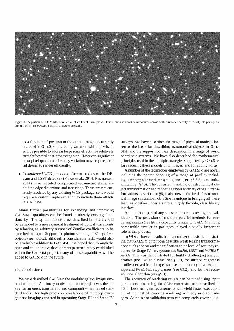
Figure 8: A portion of a GAL SIM simulation of an LSST focal plane. This section is about 5 arcminutes across with a number density of 70 objects per squarearcmin, of which 80% are galaxies and 20% are stars.

as a function of position in the output image is currentlyincluded in GAL SIM , including variation within pixels. Itwill be possible to address large scale effects in a relativelystraightforward post-processing step. However, significantintra-pixel quantum efficiency variation may require care-ful design to render efficiently.

• Complicated WCS functions.Recent studies of the DE-Cam and LSST detectors (Plazas et al., 2014; Rasmussen,2014) have revealed complicated astrometric shifts, in-cluding edge distortions and tree-rings. These are not cur-rently modeled by any existing WCS package, so it wouldrequire a custom implementation to include these effectsin GAL SIM .

Many further possibilities for expanding and improvingGAL SIM capabilities can be found in already existing func-tionality. TheOpticalPSF class described in §3.2.2 couldbe extended to a more general treatment of optical wavefrontsby allowing an arbitrary number of Zernike coefficients to bespecified on input. Support for photon shooting ofShapeletobjects (see §3.3.2), although a considerable task, would alsobe a valuable addition to GAL SIM . It is hoped that, through theopen and collaborative development pattern already establishedwithin the GAL SIM project, many of these capabilities will beadded to GAL SIM in the future.

12. Conclusions

We have described GAL SIM : the modular galaxy image sim-ulation toolkit. A primary motivation for the project was the de-sire for an open, transparent, and community-maintained stan-dard toolkit for high precision simulations of the deep extra-galactic imaging expected in upcoming Stage III and Stage IV

surveys. We have described the range of physical models cho-sen as the basis for describing astronomical objects in GAL -SIM , and the support for their description in a range of worldcoordinate systems. We have also described the mathematicalprinciples used in the multiple strategies supported by GAL SIM

for rendering these models onto images, and for adding noise.A number of the techniques employed by GAL SIM are novel,

including the photon shooting of a range of profiles includ-ing InterpolatedImage objects (see §6.3.3) and noisewhitening (§7.5). The consistent handling of astronomicalob-ject transformation and rendering under a variety of WCS trans-formations, described in §5, is also new in the field of astronom-ical image simulation. GAL SIM is unique in bringing all thesefeatures together under a simple, highly flexible, class libraryinterface.

An important part of any software project is testing and val-idation. The provision of multiple parallel methods for ren-dering images (see §6), a capability unique to GAL SIM amongcomparable simulation packages, played a vitally importantrole in this process.

In §9 we showed results from a number of tests demonstrat-ing that GAL SIM output can describe weak lensing transforma-tions such as shear and magnification at the level of accuracyre-quired for Stage IV surveys such asEuclid, LSSTandWFIRST-AFTA. This was demonstrated for highly challenging analyticprofiles (theSersic class, see §9.1), for surface brightnessprofiles derived from images such as theInterpolatedIm-age andRealGalaxy classes (see §9.2), and for the recon-volution algorithm (see §9.3).

The accuracy of rendering results can be tuned using inputparameters, and using theGSParams structure described in§6.4. Less stringent requirements will yield faster execution,but at the cost of lowering rendering accuracy in output im-ages. As no set of validation tests can completely cover all us-

31

age scenarios, the tests of §9 should be modified by users of theGAL SIM software to tailor them to each application’s specificrequirements.

As discussed in §11, there are a number of important effectsthat GAL SIM cannot yet simulate, but that may significantlyimpact data analysis for upcoming surveys. Work is expectedto continue in these interesting areas: while the developmentand support of GAL SIM began in early 2012, it is an ongoingproject that continues to build on increasing numbers of users(and developers).

As well as being used to generate the images for the GREAT3challenge (Mandelbaum et al., 2014), GAL SIM now providesa considerable open-source toolkit for the simulation of extra-galactic survey images. Having been shown to meet demandingtolerances on rendering accuracy in a number of tests, GAL SIM

simulations can be used as a benchmark for development orcommon reference point for code comparison. It also providesan accessible, well-documented reference codebase. GAL SIM

is easily extended, or can be used simply as a class library inthe development of further astronomical image analysis appli-cations. In these respects GAL SIM achieves its primary aims,and will become an increasingly powerful toolkit for astronom-ical image simulation following development that is planned forthe near future.

Acknowledgments

We wish to thank the two anonymous referees whose insight-ful comments significantly improved the paper. This projectwas supported in part by NASA via the Strategic UniversityResearch Partnership (SURP) Program of the Jet PropulsionLaboratory, California Institute of Technology. Part of BR’swork was done at the Jet Propulsion Laboratory, California In-stitute of Technology, under contract with NASA. BR, JZ andTK acknowledge support from a European Research CouncilStarting Grant with number 240672. MJ acknowledges supportfrom NSF award AST-1138729. RM was supported in part byprogram HST-AR-12857.01-A, provided by NASA through agrant from the Space Telescope Science Institute, which is oper-ated by the Association of Universities for Research in Astron-omy, Incorporated, under NASA contract NAS5-26555; and inpart by a Sloan Fellowship. HM acknowledges support fromJapan Society for the Promotion of Science (JSPS) Postdoc-toral Fellowships for Research Abroad and JSPS Research Fel-lowships for Young Scientists. PM is supported by the U.S. De-partment of Energy under Contract No. DE- FG02-91ER40690.The authors acknowledge the use of the UCL Legion High Per-formance Computing Facility (Legion@UCL), and associatedsupport services, in the completion of this work. This workwas supported in part by the National Science Foundation un-der Grant No. PHYS-1066293 and the hospitality of the AspenCenter for Physics.

32

Appendix A. Conventions in the lensing engine

Appendix A.1. Grid parameters

All calculations in the GAL SIM lensing engine (see §4) approximate real continuous functions using a discrete, finite grid. Thereal-space grid is defined by

L = length of grid along one dimension (angular units) (A.1)

d = spacing between grid points (angular units) (A.2)

N = number of grid points along one dimension= L/d. (A.3)

There is a comparable grid in Fourier-space (i.e., sameN). Given the parameters of the real-space grid, thekmin along one dimensionis 2π/L, so we can think of this quantity as the grid spacing in Fourier space, i.e.,kmin = ∆k. This value ofkmin corresponds to aFourier mode that exactly fits inside of our square grid (in one dimension). Thek range, again in one dimension, is fromk1 = −π/dto π/d, i.e., |k1| < kmax = π/d. This corresponds to a mode that is sampled exactly twice (the minimum possible) given our choiceof grid spacing. For the two-dimensional grid, the maximum value of|k| is then

√2π/d.

Appendix A.2. Fourier transform properties

The convention for the Fourier transform defined by equations (34) & (35) is adopted throughout, as this is the form typicallyused for describing the statistics of cosmological shear and matter fields. Unlike the convention typically used in computing andsignals processing, and in the standard definition of the Discrete Fourier Transform (DFT), this convention is non-unitary and usesan angular (rather than normal) frequency in the exponent36. This introduces some additional factors of 2π into standard results,and so here we re-express these results using the non-unitary, angular frequency convention.

It can be readily shown that if we defineg(xL) ≡ f (x), the following well-known identity holds:

F {g(xL)} = 1L

g

(kL

). (A.4)

If we further defines(h+ x) ≡ g(x) then it is straightforward to show that

F {s(h+ x)} = eikhs(k). (A.5)

There is an additional factor of 2π in the exponent when this property of Fourier transforms is expressed using the normal (ratherthan angular) frequency convention.

The most important result for approximating continuous functions using DFTs is the Poisson summation formula, which underthe conventions of equations (34) & (35) may be stated as

∞∑

n=−∞f (n) =

∞∑

q=−∞f (2πq) (A.6)

for integersn andq. It should be noted that in the normal frequency, unitary transform convention form of the Poisson summationformula the 2π within f (2πq) is absent. Using equations (A.4) & (A.5) we arrive at the following useful expression of the Poissonsummation formula:

∞∑

n=−∞f (nL+ x) =

1L

∞∑

q=−∞f

(2πqL

)ei2πxq/L. (A.7)

By substituting∆k ≡ kmin = 2π/L we write this as

∞∑

n=−∞f

(2πn∆k+ x

)=

(∆k2π

) ∞∑

q=−∞f (q∆k) eix∆kq. (A.8)

36For a discussion of transform conventions seehttp://en.wikipedia.org/wiki/Fourier_transform#Other_conventions

33

Appendix A.3. Fourier transform of discrete samples of the power spectrum

Let us define the following dimensionless function, which takes samples from a power spectrum:

P∆k[q, p] ≡ (∆k)2P(q∆k, p∆k). (A.9)

We will use square brackets to denote functions with discrete, integer input variables, as here. We will also usen,m for integerindices in real space summations, andq, p in Fourier space. It can then be shown that

F −1

∞∑

q,p=−∞δ(k1 − q∆k) δ(k2 − p∆k) P∆k[q, p]

=∞∑

n,m=−∞ξ+

(θ1 −

2πn∆k

, θ2 −2πm∆k

), (A.10)

where we have used the Fourier series expression for the Dirac comb function, and the convolution theorem. We note that thisexpression is still continuous, but describes an infinite, periodic summation (of periodL = 2π/∆k) of copies of the correlationfunctionξ+. For sufficiently small∆k, these copies may be spaced sufficiently widely in the real domain to be able to learn muchaboutξ+(θ1, θ2) in the non-overlapping regions. We therefore define this function as

ξ 2π∆k

(θ1, θ2) ≡∞∑

n=−∞ξ+

(θ1 −

2πn∆k

, θ2 −2πm∆k

). (A.11)

Using the expression of the Poisson summation formula in equation (A.8), we can also write

ξ 2π∆k

(θ1, θ2) =∞∑

q,p=−∞

(∆k2π

)2

P(q∆k, p∆k)ei∆k(θ1q+θ2p)=

1(2π)2

∞∑

q,p=−∞P∆k[q, p]ei∆k(θ1q+θ2p), (A.12)

This is in fact an expression for the inverse of the Discrete Time Fourier Transform (DTFT), although this result is normally derivedusing unitary conventions for the transform pair.

The expression in equation (A.12) is periodic with period 2π/∆k = L. All of the information it contains aboutξ+(θ1, θ2) istherefore also contained in one period of the function only.For approximating this information discretely, as desiredin numericalanalysis, we can imagine takingN equally spaced samples of the function in equation (A.12) along a single periodL in eachdimension. These samples are therefore separated by∆θ = 2π/∆kN = d in real space, and we define the sampled function itself as

ξ∆θ[n,m] ≡ ξ 2π∆k

(n∆θ,m∆θ) =1

(2π)2

∞∑

q,p=−∞P∆k[q, p]ei2π(qn+pm)/N, (A.13)

for the integer indicesn,m= 0, 1, . . . ,N − 1, by substitution into equation (A.12). Using the periodicity of the exponential term inthe expression above, this may be written as

ξ∆θ[n,m] =1

(2π)2

N−1∑

q,p=0

PN[q, p]ei2π(qn+pm)/N (A.14)

where we have defined

PN[q, p] ≡∞∑

i, j=−∞P∆k[q− iN, p− jN]. (A.15)

Needless to say, in order to be able to calculate the values ofPN[q, p] in practice we must also truncate theP∆k sequence to be finitein length. Averycommon choice is to use the same numberN of samples in both real and Fourier space. Choosing to use only Nsamples fromP∆k then gives

ξ∆θ[n,m] =1

(2π)2

N−1∑

q,p=0

P∆k[q, p]ei2π(qn+pm)/N

=1

N2 (∆θ)2

N−1∑

q,p=0

P(q∆k, p∆k)ei2π(qn+pm)/N. (A.16)

For greater detail regarding this calculation, please see the lensing engine document in the GAL SIM repository.37

37https://github.com/GalSim-developers/GalSim/blob/master/devel/modules/lensing_engine.pdf

34

The relationship in equation (A.16) is in fact the inverse Discrete Fourier Transform for our non-unitary convention. The moreusual definition of the inverse DFT, and that adopted by many DFT implementations (including the NUMPY package in Python), is

f [n,m] = numpy.fft.ifft2(f [p, q]

)≡ 1

N2

N−1∑

q,p=0

f [q, p]ei2π(qn+pm)/N (NUMPY convention). (A.17)

(The factor of 1/N2 here is often found in conventions for the inverse DFT, and ensures that the DFT followed by the inverse DFTyields the original, input array.) The Fast Fourier Transform algorithm allows the DFT to be calculated very efficiently.

Appendix A.4. Generating Gaussian fields

Using equation (A.16) we see how to construct a realization of a Gaussian random lensing field on a grid, with an ensembleaverage power spectrum that is approximatelyP(k). We create the following complex, 2D array of dimensionN in Fourier space:

κ[p, q] = κE[p, q] + iκB[p, q], (A.18)

whereκE is defined in terms of the desired E-mode power spectrumPE as

κE[p, q] =1

N∆θ

√PE(p∆k, q∆k)

2{N(0, 1)+ iN(0, 1)} , (A.19)

and likewise forκB. HereN(0, 1) denotes a standard Gaussian random deviate drawn independently at each [p, q] array location.This complex-valued Fourier-space convergence can be usedto construct the Fourier-space shear field via38

g = e2iψκ, (A.20)

where e2iψ is the phase of thek vector defined ask = ∆k(p+ iq). It can be seen that〈g[p, q]g∗[p′, q′]〉 = δp′p δ

q′q P(|k|)/(N∆θ)2 where

|k| = ∆k√

p2 + q2. Taking the inverse DFT ofg provides the realization of the Gaussian lensing fieldg[n,m] on a grid in real space,where the real (imaginary) parts ofg[n,m] correspond to the first (second) shear components. From equation (A.16),g[n,m] willbe correctly scaled to have discrete correlation functionξ∆θ[n,m] by construction.

Appendix B. Efficient evaluation of the Sine and Cosine integrals

The trigonometric integrals are defined as

Si(x) =∫ x

0

sintt

dt =π

2−

∫ ∞

x

sintt

dt (B.1)

Ci(x) = γ + ln x+∫ x

0

cost − 1t

dt = −∫ ∞

x

costt

dt (B.2)

whereγ is the Euler-Mascheroni constant. In GAL SIM , calculations involving Lanczos interpolants require an efficient calculationof Si(x). As we were unable to find a source for an efficient calculation that was suitably accurate, we developed our own, whichwe present here. We do not use Ci(x) anywhere in the code, but for completeness, we provide a similarly efficient and accuratecalculation of it as well.

For small arguments, we use Padé approximants of the convergent Taylor series

Si(x) =∞∑

n=0

(−1)nx2n+1

(2n+ 1)(2n+ 1)!(B.3)

Ci(x) = γ + ln x+∞∑

n=1

(−1)nx2n

2n(2n)!(B.4)

38See, for example, Kaiser & Squires (1993), but note that there is a sign error in equation 2.1.12 in that paper that is corrected in equation 2.1.15.

35

Using the Maple software package39, we derived the following formulae, which are accurate to better than 10−16 for 0 ≤ x ≤ 4:

Si(x) = x ·

1− 4.54393409816329991· 10−2 · x2+ 1.15457225751016682· 10−3 · x4

− 1.41018536821330254· 10−5 · x6+ 9.43280809438713025· 10−8 · x8

− 3.53201978997168357· 10−10 · x10+ 7.08240282274875911· 10−13 · x12

− 6.05338212010422477· 10−16 · x14

1+ 1.01162145739225565· 10−2 · x2+ 4.99175116169755106· 10−5 · x4

+ 1.55654986308745614· 10−7 · x6+ 3.28067571055789734· 10−10 · x8

+ 4.5049097575386581· 10−13 · x10+ 3.21107051193712168· 10−16 · x12

(B.5)

Ci(x) = γ + ln(x)+

x2 ·

−0.25+ 7.51851524438898291· 10−3 · x2 − 1.27528342240267686· 10−4 · x4

+ 1.05297363846239184· 10−6 · x6 − 4.68889508144848019· 10−9 · x8

+ 1.06480802891189243· 10−11 · x10 − 9.93728488857585407· 10−15 · x12

1+ 1.1592605689110735· 10−2 · x2+ 6.72126800814254432· 10−5 · x4

+ 2.55533277086129636· 10−7 · x6+ 6.97071295760958946· 10−10 · x8

+ 1.38536352772778619· 10−12 · x10+ 1.89106054713059759· 10−15 · x12

+ 1.39759616731376855· 10−18 · x14

(B.6)

For x > 4, one can use the helper functions:

f (x) ≡∫ ∞

0

sin(t)t + x

dt =∫ ∞

0

e−xt

t2 + 1dt = Ci(x) sin(x) +

(π

2− Si(x)

)cos(x) (B.7)

g(x) ≡∫ ∞

0

cos(t)t + x

dt =∫ ∞

0

t e−xt

t2 + 1dt = −Ci(x) cos(x) +

(π

2− Si(x)

)sin(x) (B.8)

using which, the trigonometric integrals may be expressed as

Si(x) =π

2− f (x) cos(x) − g(x) sin(x) (B.9)

Ci(x) = f (x) sin(x) − g(x) cos(x) (B.10)

In the limit asx→ ∞, f (x) → 1/x andg(x) → 1/x2. Thus, we can use Chebyshev-Padé expansions of1√y f

(1√y

)and 1

y g(

1√y

)

in the interval 0.. 142 to obtain the following approximants, good to better than 10−16 for x ≥ 4:

f (x) =1x·

1+ 7.44437068161936700618· 102 · x−2+ 1.96396372895146869801· 105 · x−4

+ 2.37750310125431834034· 107 · x−6+ 1.43073403821274636888· 109 · x−8

+ 4.33736238870432522765· 1010 · x−10+ 6.40533830574022022911· 1011 · x−12

+ 4.20968180571076940208· 1012 · x−14+ 1.00795182980368574617· 1013 · x−16

+ 4.94816688199951963482· 1012 · x−18 − 4.94701168645415959931· 1011 · x−20

1+ 7.46437068161927678031· 102 · x−2+ 1.97865247031583951450· 105 · x−4

+ 2.41535670165126845144· 107 · x−6+ 1.47478952192985464958· 109 · x−8

+ 4.58595115847765779830· 1010 · x−10+ 7.08501308149515401563· 1011 · x−12

+ 5.06084464593475076774· 1012 · x−14+ 1.43468549171581016479· 1013 · x−16

+ 1.11535493509914254097· 1013 · x−18

(B.11)

g(x) =1x2·

1+ 8.1359520115168615· 102 · x−2+ 2.35239181626478200· 105 · x−4

+ 3.12557570795778731· 107 · x−6+ 2.06297595146763354· 109 · x−8

+ 6.83052205423625007· 1010 · x−10+ 1.09049528450362786· 1012 · x−12

+ 7.57664583257834349· 1012 · x−14+ 1.81004487464664575· 1013 · x−16

+ 6.43291613143049485· 1012 · x−18 − 1.36517137670871689· 1012 · x−20

1+ 8.19595201151451564· 102 · x−2+ 2.40036752835578777· 105 · x−4

+ 3.26026661647090822· 107 · x−6+ 2.23355543278099360· 109 · x−8

+ 7.87465017341829930· 1010 · x−10+ 1.39866710696414565· 1012 · x−12

+ 1.17164723371736605· 1013 · x−14+ 4.01839087307656620· 1013 · x−16

+ 3.99653257887490811· 1013 · x−18

(B.12)

39http://www.maplesoft.com/

36

Thus we can calculate Si(x) to double precision accuracy for any value ofx. In GAL SIM , all of the above polynomials areimplemented using Horner’s rule, so they are very efficient to evaluate.

References

Abazajian, K. N., Adelman-McCarthy, J. K., Agüeros, M. A., et al. 2009, ApJS, 182, 543Abramowitz, M., & Stegun, I. 1964, Handbook of MathematicalFunctions, 5th edn. (New York: Dover)Airy, G. B. 1835, Transactions of the Cambridge Philosophical Society, 5, 283Albrecht, A., Bernstein, G., Cahn, R., et al. 2006, ArXiv Astrophysics e-prints, astro-ph/0609591Amara, A., & Réfrégier, A. 2008, MNRAS, 391, 228Anderson, R. E., Regan, M., Valenti, J., & Bergeron, E. 2014,ArXiv e-prints, arXiv:1402.4181Antilogus, P., Astier, P., Doherty, P., Guyonnet, A., & Regnault, N. 2014, Journal of Instrumentation, 9, C3048Bacon, D. J., Goldberg, D. M., Rowe, B. T. P., & Taylor, A. N. 2006, MNRAS, 365, 414Barrick, G. A., Ward, J., & Cuillandre, J.-C. 2012, in Society of Photo-Optical Instrumentation Engineers (SPIE) Conference Series, Vol. 8453, High Energy,

Optical, and Infrared Detectors for Astronomy V, article id. 84531K, 8 pp.Bartelmann, M. 1996, A&A, 313, 697—. 2010, Classical and Quantum Gravity, 27, 233001Barth, J., Isaacs, J., & Poivey, C. 2000, The Radiation Environment for the Next Generation Space Telescope, Tech. rep.Becker, M. R. 2013, MNRAS, 435, 115Bernstein, G. M. 2010, MNRAS, 406, 2793Bernstein, G. M., & Armstrong, R. 2014, MNRAS, 438, 1880Bernstein, G. M., & Gruen, D. 2014, PASP, 126, 287Bernstein, G. M., & Jarvis, M. 2002, AJ, 123, 583Bertin, E. 2009, Mem. Societa Astronomica Italiana, 80, 422Born, M., & Wolf, E. 1999, Principles of OpticsBridle, S., Shawe-Taylor, J., Amara, A., et al. 2009, Annalsof Applied Statistics, 3, 6Bridle, S., Balan, S. T., Bethge, M., et al. 2010, MNRAS, 405,2044Calabretta, M. R., & Greisen, E. W. 2002, A&A, 395, 1077Casertano, S., de Mello, D., Dickinson, M., et al. 2000, AJ, 120, 2747Ciotti, L., & Bertin, G. 1999, A&A, 352, 447Cropper, M., Hoekstra, H., Kitching, T., et al. 2013, MNRAS,431, 3103Cypriano, E. S., Amara, A., Voigt, L. M., et al. 2010, MNRAS, 405, 494de Jong, J. T. A., Verdoes Kleijn, G. A., Kuijken, K. H., & Valentijn, E. A. 2013, Experimental Astronomy, 35, 25de Vaucouleurs, G. 1948, Annales d’Astrophysique, 11, 247—. 1959, AJ, 64, 397Duncan, C. A. J., Joachimi, B., Heavens, A. F., Heymans, C., &Hildebrandt, H. 2014, MNRAS, 437, 2471Fried, D. L. 1966, Journal of the Optical Society of America (1917-1983), 56, 1372Frigo, M., & Johnson, S. G. 2005, Proceedings of the IEEE, 93,216, special issue on “Program Generation, Optimization, and Platform Adaptation”Fruchter, A. S., & Hook, R. N. 2002, PASP, 114, 144Goldberg, D. M., & Bacon, D. J. 2005, ApJ, 619, 741Heymans, C., Van Waerbeke, L., Bacon, D., et al. 2006, MNRAS,368, 1323Heymans, C., Van Waerbeke, L., Miller, L., et al. 2012, MNRAS, 427, 146Hirata, C., & Seljak, U. 2003, MNRAS, 343, 459Hirata, C. M., Mandelbaum, R., Seljak, U., et al. 2004, MNRAS, 353, 529Hogg, D. W., & Lang, D. 2013, PASP, 125, 719Huterer, D. 2010, General Relativity and Gravitation, 42, 2177Huterer, D., Takada, M., Bernstein, G., & Jain, B. 2006, MNRAS, 366, 101Irwin, J., & Shmakova, M. 2005, New Astron. Rev., 49, 83Johnson, N., Kemp, A., & Kotz, S. 2005, Univariate Discrete Distributions, Wiley Series in Probability and Statistics (Hoboken, New Jersey: John Wiley & Sons)Kacprzak, T., Bridle, S., Rowe, B., et al. 2014, MNRAS, 441, 2528Kacprzak, T., Zuntz, J., Rowe, B., et al. 2012, MNRAS, 427, 2711Kaiser, N. 2000, ApJ, 537, 555Kaiser, N., & Squires, G. 1993, ApJ, 404, 441Kaiser, N., Squires, G., & Broadhurst, T. 1995, ApJ, 449, 460Kitching, T. D., Balan, S. T., Bridle, S., et al. 2012, MNRAS,423, 3163Kitching, T. D., Rowe, B., Gill, M., et al. 2013, ApJS, 205, 12Koekemoer, A. M., Fruchter, A. S., Hook, R. N., & Hack, W. 2003, in HST Calibration Workshop : Hubble after the Installation of the ACS and the NICMOS

Cooling System, ed. S. Arribas, A. Koekemoer, & B. Whitmore,337Koekemoer, A. M., Aussel, H., Calzetti, D., et al. 2007, ApJS, 172, 196Lackner, C. N., & Gunn, J. E. 2012, MNRAS, 421, 2277Lauer, T. R. 1999, PASP, 111, 227Laureijs, R., Amiaux, J., Arduini, S., et al. 2011, ArXiv e-prints, arXiv:1110.3193Leauthaud, A., Massey, R., Kneib, J.-P., et al. 2007, ApJS, 172, 219Long, K. S., Bagett, S. M., Deustua, S., & Riess, A. 2010, in 2010 Space Telescope Science Institute Calibration Workshop- Hubble after SM4.

Preparing JWST, held 21-23 July 2010 at Space Telescope Science Institute. Edited by Susana Deustua and Cristina Oliveira. Published online athttp://www.stsci.edu/institute/conference/cal10/proceedings, p.26

Luppino, G. A., & Kaiser, N. 1997, ApJ, 475, 20Makinson, D. 2012, Sets, Logic and Maths for Computing, Undergraduate Topics in Computer Science (London: Springer-Verlag)Mandelbaum, R., Hirata, C. M., Leauthaud, A., Massey, R. J.,& Rhodes, J. 2012, MNRAS, 420, 1518Mandelbaum, R., Hirata, C. M., Seljak, U., et al. 2005, MNRAS, 361, 1287

37

Mandelbaum, R., Rowe, B., Bosch, J., et al. 2014, ApJS, 212, 5Massey, R., & Refregier, A. 2005, MNRAS, 363, 197Massey, R., Stoughton, C., Leauthaud, A., et al. 2010, MNRAS, 401, 371Massey, R., Heymans, C., Bergé, J., et al. 2007, MNRAS, 376, 13Massey, R., Hoekstra, H., Kitching, T., et al. 2013, MNRAS, 429, 661Melchior, P., Böhnert, A., Lombardi, M., & Bartelmann, M. 2010, A&A, 510, A75Melchior, P., & Viola, M. 2012, MNRAS, 424, 2757Meng, Z., Zhou, X., Zhang, H., et al. 2013, PASP, 125, 1015Meyers, J. E., & Burchat, P. R. 2014, Journal of Instrumentation, 9, C3037Miyazaki, S., Komiyama, Y., Nakaya, H., et al. 2012, in Society of Photo-Optical Instrumentation Engineers (SPIE) Conference Series, Vol. 8446, Society of

Photo-Optical Instrumentation Engineers (SPIE) Conference SeriesMoffat, A. F. J. 1969, A&A, 3, 455Moore, A. C., Ninkov, Z., & Forrest, W. J. 2004, in Society of Photo-Optical Instrumentation Engineers (SPIE) Conference Series, Vol. 5167, Focal Plane Arrays

for Space Telescopes, ed. T. J. Grycewicz & C. R. McCreight, 204–215Nakajima, R., & Bernstein, G. 2007, AJ, 133, 1763Navarro, J. F., Frenk, C. S., & White, S. D. M. 1996, ApJ, 462, 563Noll, R. J. 1976, Journal of the Optical Society of America (1917-1983), 66, 207Patterson, F. S. 1940, Harvard College Observatory Bulletin, 914, 9Patterson, T. 1968, Mathematics of Computation, 22, 847Peacock, J. A., Schneider, P., Efstathiou, G., et al. 2006, ESA-ESO Working Group on “Fundamental Cosmology”, Tech. rep., arXiv:0610906Pence, W. D., Chiappetti, L., Page, C. G., Shaw, R. A., & Stobie, E. 2010, A&A, 524, A42Plazas, A. A., & Bernstein, G. 2012, PASP, 124, 1113Plazas, A. A., Bernstein, G. M., & Sheldon, E. S. 2014, Journal of Instrumentation, 9, C4001Press, W. H., Teukolsky, S. A., Vetterling, W. T., & Flannery, B. P. 1992, Numerical recipes in C: The art of scientific computing, 2nd ed. (Cambridge: Cambridge

University Press)Racine, R. 1996, PASP, 108, 699Rasmussen, A. 2014, Journal of Instrumentation, 9, C4027Refregier, A. 2003, MNRAS, 338, 35Refregier, A., Kacprzak, T., Amara, A., Bridle, S., & Rowe, B. 2012, MNRAS, 425, 1951Reyes, R., Mandelbaum, R., Gunn, J. E., et al. 2012, MNRAS, 425, 2610Rhodes, J., Leauthaud, A., Stoughton, C., et al. 2010, PASP,122, 439Rolland, G., Pinheiro da Silva, L., Inguimbert, C., et al. 2008, Nuclear Science, IEEE Transactions on, 55, 2070Rowe, B., Bacon, D., Massey, R., et al. 2013, MNRAS, 435, 822Sánchez, E., et al. 2010, Journal of Physics Conference Series, 259, 012080Schmidt, F., Leauthaud, A., Massey, R., et al. 2012, ApJL, 744, L22Schneider, P. 2006, in Saas-Fee Advanced Course 33: Gravitational Lensing: Strong, Weak and Micro, ed. G. Meylan, P. Jetzer, P. North, P. Schneider, C. S.

Kochanek, & J. Wambsganss (Berlin: Springer), 269Schneider, P., van Waerbeke, L., & Mellier, Y. 2002, A&A, 389, 729Scoville, N., Aussel, H., Brusa, M., et al. 2007, ApJS, 172, 1Semboloni, E., Hoekstra, H., Huang, Z., et al. 2013, MNRAS, 432, 2385Sérsic, J. L. 1963, Boletin de la Asociacion Argentina de Astronomia La Plata Argentina, 6, 41Seshadri, S., Shapiro, C., Goodsall, T., et al. 2013, PASP, 125, 1065Sheldon, E. S. 2014, MNRAS, 444, L25van Waerbeke, L. 2010, MNRAS, 401, 2093Velander, M., Kuijken, K., & Schrabback, T. 2011, MNRAS, 412, 2665Voigt, L. M., & Bridle, S. L. 2010, MNRAS, 404, 458Voigt, L. M., Bridle, S. L., Amara, A., et al. 2012, MNRAS, 421, 1385Wright, C. O., & Brainerd, T. G. 2000, ApJ, 534, 34Wynne, C. G., Worswick, S. P., Lowne, C. M., & Jorden, P. R. 1984, The Observatory, 104, 23Zernike, F. 1934, MNRAS, 94, 377

38