galerkin approximations of the generalized hamilton-jacobi-bellman equation

Pergamon PII: sooo5-1098(97)00128-3 Automatica, Vol. 33, No. 12, pp. 2159-2177, 1997 0 1997 Ekvier Science Ltd. All rights reserved

Printed in Great Britain om-1098/97 S17.00 + 0.00

Galerkin Approximations of the Generalized Hamilton-Jacobi-Bellman Equation*

RANDAL W. BEARD,7 GEORGE N. SARIDISS and JOHN T. WENT

The application of Gale&in 3 method yields an eficient algorithm for the approximation of the generalized Hamilton-Jacobi-Bellman equation on a compact set.

The result is a feedback control with a pre-defined set of attraction.

Key Words--Nonlinear control; optimal control; Galerkin approximation; feedback synthesis; generalized Hamilton-Jacobi-Bellman equation.

Abstract-In this paper we study the convergence of the Galer- kin approximation method applied to the generalized Hamil- ton-Jacobi-Bellman (GHJB) equation over a compact set containing the origin. The GHJB equation gives the cost of an arbitrary control law and can be used to improve the performance of this control. The GHJB equation can also be. used to successively approximate the Hamilton-Jacobi-Bellman equation. We state sufficient conditions that guarantee that the Galerkin approximation converges to the solution of the GHJB equation and that the resulting approximate control is stabilix- ing on the same region as the initial control. The method is demonstrated on a simple nonlinear system and is compared to a result obtained by using exact feedback linearization in con- junction with the LQR design method. 0 1997 Elsevier Science Ltd. All rights reserved.

1. INTRODUCTION

The basic mathematical theory for classical optimal control is well established (Anderson and Moore, 1971; Bryson and Ho, 1975; Kirk, 1970; Lewis, 1986; Sage and White III, 1977). If we assume full-state knowledge and if the dynamics of the system are modeled by linear dynamics and the cost functional to be optimized is quadratic in the state and control, then the optimal control is a linear feedback of the states, where the control gains are obtained by solving a standard Riccati equation. The practical success of linear quadratic (LQ) methods in optimal control is directly linked to

*Received 22 June 1995, revised 3 June 1996, received in final form 23 June 1997. An earlier version of this paper was presented at the 13th IFAC World Congress, held in San Francisco, CA, USA, July l-5, 1996. This paper was recommended for publication in revised form by Associate Editor Matt James under the direction of Editor Tamer Basar. Corresponding

Author Professor Randal Beard. Tel. + 801 378-8392; Fax 001 801 378 6586; E-mail [email protected].

TDepartment of Electrical and Computer Engineering Brigham Young University, Provo, UT 84602, U.S.A.

XDepartment of Electrical, Computer and Systems Engineer- ing, Rensselaer Polytechnic Institute, Troy, NY 12180, U.S.A.

successful algorithms for solving the Riccati equation. However, if the system is modeled by nonlinear dynamics or the cost functional to be optimized is not quadratic, then the optimal control is a state feedback function that depends on the solution to the Hamilton-Jacobi-Bellman (HJB) equation. The HJB equation is extremely difficult to solve in general rendering optimal control techniques of limited use for nonlinear systems.

Motivated by the success of optimal control methods for linear systems, there has been a great deal of research devoted to approximating the HJB equation. If an open-loop solution is acceptable then there are a number of methods to solve the optimal control problem. A common approach is to numerically solve for the state and co-state equations obtained from a Hamiltonian formulation of the optimal control problem. The problem can be reduced to a two-point boundary-value problem which can be solved by various methods (Kirk, 1970; Sage and White III, 1977). In Bosarge et al. (1973) the two-point boundary-value problem is solved using the Ritz-Galerkin approximation theory that is employed (in a different context) in this paper. In Hofer and Tibken (1988) the authors reduce the optimal bilinear control problem to successive iterations of a sequence of Riccati equations. In Aganovic and Gajic (1994) the same problem is further reduced to successive approximations of a sequence of Lyapunov equations. In Cebuhar and Costanza (1984) the bilinear control problem is reduced to a sequence of linear control problems that converge uniformly to the optimal bilinear control. Another approach taken in Rosen and Luus (1992) is to cast the nonlinear optimal control problem in the form of a nonlinear programming problem. The method is formulated in path space so the point that solves the nonlinear programming problem is the optimal path of the system.

2159

2160 R. W. Beard et al.

Since open-loop control is undesirable for practical systems, various approaches have been investi- gated to generate closed-loop solutions to the HJB equation. One technique is the perturbation method described in Al’brekht (1961), Lukes (1969), Garrard and Jordan (1977) and Nishikawa et al. (1971). In this method, the nonlinear system is assumed to be a perturbation of a linear system. The optimal cost and control are assumed to be analytic and are expanded in a Taylor series. Various techniques are then employed to find the first few terms in the series. The first term corresponds to the solution of the matrix Riccati equation obtained by linearizing the system about the origin. The next term is a third-order approximation to the control and can also be expressed as matrix equations. Higher-order terms require the solution of a linear partial differential equation and so the algorithm is usually termin- ated after the first two terms. In Lukes (1969), the authors present a definitive study of analytic, infinite-time regulators. In Werner and Cruz (1968), it is shown that an &h-order Taylor series expansion of the optimal control gives a (2n + l)th-order approximation of the performance index. The difficulty with perturbation methods is that they are limited to a small class of systems, i.e. systems that are small perturbations of a linear system and that have analytic optimal cost and control. In addition, these methods are inherently tied to the convergence of a power series for which it is difficult if not imposs- ible to estimate the region of convergence. Conse- quently, it is equally difficult to estimate the stability region of a control calculated from a truncated power series. For bilinear systems, however, it appears that the region of attraction can be estimated, as reported in Cebuhar and Costanza (1984). In Halme and Hamalainen (1975), the authors present a method that is similar to perturbation methods. The basic idea is to represent the integral curve of the solution (via Green’s functions) as a basic linear operator and then invert the operator. The method has several advantages over perturbation methods. Namely, it is possible to estimate the region of convergence of the power series that makes up the final control; therefore, it is possible to estimate the stability region of a truncated control law. One of the main advantages to the method presented in this paper is that there is a clearly defined estimate of the stability region of the approximate control. In addition, the designer has explicit control over this region.

Another approach to approximating the HJB equation is to “regularize” the cost function so that an analytic expression for the control can be obtained. The basic idea is to consider a cost function of the form

J = s

m[xTQx + uTRu + 9(x)] dt, (1) 0

where 9(x) is a function chosen so that the Hamil- ton-Jacobi-Bellman equation reduces to a form similar to the Riccati equation. This method produces a control that minimizes the integral (1) and is therefore suboptimal with respect to the cost function that is really of interest [i.e. (1) without the 9 term]. The approach results in solutions that stabilize the system but it is difficult to estimate how far the control deviates from the optimal since 9 must be carefully selected. Examples of this approach are Ryan (1984), Tzafestas et al. (1984), Lu (1993) and Freeman and Kokotovic (1995). When the method presented in this paper is iterated, the optimal cost and control can be approximated arbitrarily closely when the order of approximation is sufficiently large (see Beard, 1995 for a discussion of this algorithm).

A feedback design method that has been popular in recent years is feedback linearization (Hunt et al.,

1983a,b; Isidori, 1989; Nijmeijer and van der Schaft, 1990). The basic idea is to use feedback to cancel out the nonlinearities in the system. The resulting system is linear and so a feedback control can be designed using any linear synthesis method. There are numerous examples in the literature where LQR methods have been used to optimize the resulting linear system (Lee and Chen, 1983; Gao et al., 1992; Chapman et al., 1993; Wang et al., 1993, 1994; Marino, 1984). Feedback linearization has several disadvantages. First it is difficult to quantify the robustness of the control. Second, the control sometimes cancels out nonlinearities that enhance stability and performance (Freeman and Kokotovic, 1995). Third, to cancel the nonlinearities, the control effort can be unreasonably large. Finally, even if the resulting linear system is optimized, it is not possible to determine how close the original nonlinear system is to optimal.

An important recent development in optimal control is the theory of viscosity solutions. For the solution of the HJB equation to be defined in a classical sense, it must be differentiable over the domain of interest. This restriction excludes a large class of nonlinear systems. For example, the system 1= xu, J = sF(x” + u2)dt has an optimal cost given by V(x) = 1x1: clearly, the HJB is not defined in a classical sense at x = 0. The theory of viscosity solutions allows a continuous function to be defined as the unique solution to Hamilton-Jacobi equations that do not admit continuous solutions in the classical sense. The viscosity method is a fair- ly general theoretical tool for dealing with existence and uniqueness issues of nonlinear partial differential equations. For an introduction to viscosity solutions see Crandall et al. (1992). An important result is that the viscosity solution of the HJB equation is identical to the value function of the associated (stochastic or deterministic) optimal

Generalized HJB equation 2161

control problem. If the solution of the HJB equation is differentiable, then the viscosity solution and the classical solution are identical.

We should note that the algorithm obtained by iterating the method presented in this paper can also be applied to systems that do not admit continuous solutions. However, in its present formulation, it is restricted to system which admit continuous stabilizing (but not necessarily optimal) controls. Using the viscosity method, it should be relatively straightforward to extend the results in this paper to systems that admit stabilizing (but not continuous stabilizing) controls.

The fact that the viscosity solution is equivalent to the value function has inspired work in numerically approximating viscosity solutions for HJ equations. Two broad categories of solutions have been reported: finite-difference solutions and finite-element solutions. Capuzzo Dolcetta (1983) introduces a discrete approximation to the continuous-time, deterministic optimal control problem. The basic idea is to approximate the system equations by an Euler formula with step size h and then to discretize the solution according to h. It is shown that as h -+ 0 the discrete solution Vh converges (locally uniformly) to the viscosity solution of the HJB equation. The optimal control problem can then be approximated by solving the discrete dynamic programming problem. The convergence rate of the scheme is studied in Capuzzo Dolcetta and Ishii (1984), where the approximate controls are also shown to converge in a relaxed sense. Falcone and Ferretti (1994) show that convergence can be improved by using a Rung+Kutta formula instead of Euler’s method to approximate the dynamics of the system. Other convergence acceler- ation methods are discussed in Capuzzo Dolcetta and Falcone (1989). Using the finite-element method, Gonzalez and Rofman (1985a) lists an algorithm for finite-time problems with continuous and impulse controls for stationary systems. The non-stationary case is studied in Gonzalez and Rofman (1985b). A similar approach is considered for infinite-time horizon problems in Falcone (1987). The method is shown to converge to the viscosity solution and error estimates for the convergence of the algorithm are also given. Variations on these two approaches can be found in Kushner (1990) and Fleming and Soner (1993, Chap. 9).

The main disadvantage of both finite-element and finite-difference methods is that they require a discretization of the state space which is parti- cularly problematic in two ways. First, the computational burden scales exponentially in the dimension of the state space, i.e. the methods are O(A4”) where M is the number of partitions of each variable, i.e. Bellman’s “curse of dimensionality”. Second, an enormous amount of data must be

stored and then recalled in real time to produce the feedback control.

The major motivation of using Galerkin’s spectral method in this paper was to avoid discretizing the time and space variable. Of course, the “curse of dimensionality” still exists but it shows up as weighted averages of the dynamics over a compact set Q. The advantage is that this provides numerous options for dealing with the dimensionality problem. For example, if the system equation are separable, and R is rectangular, than the multi- dimensional integrals reduce to iterated one- dimensional integrals which can be computed numerically or symbolically. Another major advantage of our method is that the feedback controls are determined by a small number of coefficients and can be implemented in a variety of ways. In fact, the computer can be completely taken out of the loop by implementing each of the basis functions in hardware, and the coefficients with amplifiers.

In the literature there are many other approaches to approximating optimal control laws (cf. Baumann and Rugh, 1986; Cloutier et al., 1996; Goh, 1993; Johansson, 1990). In approximating optimal controls there are three things that we would like an approximate control to satisfy:

(1)

(2)

(3)

We would like the approximate control to be in an explicit feedback form that is easy to imple- ment. We would like the approximation to converge uniformly to the optimal control, if it exists, as the complexity of the approximation is in- creased. We would like the control to remain stable when the approximation is truncated at a finite degree of complexity.

To our knowledge, the technique presented in this paper, coupled with the successive approximation method as outlined in Beard (1995) is the only method that accomplishes all three of these objectives.

2. PROBLEM STATEMENT

In this paper we restrict ourselves to the state- feedback control problem for the class of nonlinear time-invariant systems described by ordinary differential equations that are affine in the control:

i = f(x) + s(x)n(x), (2)

where XEQRCIP, f:Q+R”, g:Q-+UYxm and u : s1-+ R”’ is the control. To ensure that the control problem is well posed we assume that f and g are Lipschitz continuous on a set &YI that contains the origin as an interior point. We also assume that


f(0) = 0. Define q(t; x0, u) to be the solution at time t to equation (2) with initial conditions x0 and control u. To simplify the notation we write q(t) = q(t; x0, u) when x0 and u are understood. For the system [equation (2)], we say that u is a stabilizing control on R if the resulting closed-loop system is asymptotically stable in the sense of Lyapunov (Khalil, 1992) for all initial conditions in R.

To quantify the performance of the control we use the standard integral performance measure

s

m 4x0,4 = l(M) + IMcp(t))ll: dt, (3)

0

where 1: CJ + R is a positive-definite function on D chosen such that the system is zero state observ- able through Z, RE [w”““’ is a symmetric, positive- definite matrix, Ilull; = uTRu and x0 EQ c Iw”. 1 is called the state penalty function and [lull: is the control penalty function. Typically, 1 is a quadratic weighting of the states, i.e. 1= xTQx where Q is a positive-definite matrix.

For equation (3) to give any indication of the performance of the system, the integral must converge. Unfortunately, stability of i =f+ gu is not sufficient for the integral to be finite. For example, the solution to the system

i = xu, u = - 1x1 is

cp(t) = .---Y- 1 + Ix&’

The control u asymptotically stabilizes the system but if l(x) p 1x1 then

However, if l(x) 4 1x1’ with CI > 1 then the integral is finite.

This necessitates the restriction of stabilizing controls to those controls that render the cost function [equation (3)] finite with respect to a certain penalty on the states.

Dejinition 1 (Admissible Control). Given the system (f, g), a control u : R” + R” is defined to be admissible with respect to the state penalty function 1 on R, written u E &@), if

l u is continuous on 0, l u(0) = 0, l u stabilizes (f,g) on R, l jo”@&;x, 4) + IbMc x, 4)lli dt < ~0 , vx E Q.

When UE &@), a Lyapunov function for the systems on R is given by

v(x) = s

mMN; x, 4) + IMdc x, u,,llil dt. 0

We would like to know when asymptotic stability implies that there exist an 1: R + R such that the integral [equation (3)] is finite. The limitation is the quadratic penalty on u: in short, we are restricted to systems whose control function has finite energy.

Lemma 2. If u is continuous on Sz, u(O) = 0, and u stabilizes the system (f, g) on R, then there exists a continuously differentiable, positive-definite state penalty function 1: s1-+ R such that u E a@) if and only if u has finite energy for all x0 E R, i.e.

x0, u))ll’dt < 00.

Remark 3. In general it is difficult to derive specific conditions under which the control can be made to have finite energy. However, an important case when this is always true is when the linearization of (Jg) at x = 0, i.e.

is stabilizable. In this case the origin can be made exponentially stable by an appropriate linear state feedback. Therefore, there exists a nonlinear state feedback, u, such that the real parts of the eigenvalues of (aCf + gu)/ax)(O) are all negative, i.e. the origin is exponentially stable.

Remark 4. While not all systems can be stabilized by continuous state feedback, there are large classes of systems that can be. For example, feedback linearizable systems can be stabilized via continuous controls (Nijmeijer and van der Schaft, 1990, Chap. 6). In addition, If the linearization of the system at the equilibrium is controllable, then we can find a set n such that there exists a continuous state feedback that stabilizes the system. See Aeyels (1985, 1986) and Battilotti (1996) for additional classes of systems that can be stabilized by continuous state feedback.

In the above discussion, the specification of the set R has been somewhat arbitrary. To be precise, IR can be made as large as the domain of attraction of the system under the closed-loop control of u.

Lemma 5. Given a system (f, g). If u E &@) and the region of stability of the system i =f + gu is T c Iw” where T 2 R, then u E J&‘~( T).

Proof: Since u is asymptotically stabilizing on R, there exists a t’ < co such that

t > t’ * {y: y = ~(t;x,u),xEr} En.


Then Vx EY

+

s

ml(dr; cpW + II4cpkcp(Wll~ dz- f’

The first integral is finite since it is over a finite time period and the second integral is finite since cp(t’; x, u) E R and u E d&2). 0

In general, it is difficult to find the largest stability region, Y, corresponding to ZJ (Genesio et al., 1985; Loparo and Blankenship, 1978). However, it is usually possible to find a region R c Y, or to verify (by Lyapunov methods) that a subset Q is contained in r. Since our method will require some set n over which u is stabilizing, but does not require the entire stability region Y, we will retain the notation u E &@).

We will assume throughout the paper that system [equation (2)] is controllable on R, in that for an appropriate choice of I, there exists at least one admissible control, u E &r(Q).

The standard optimal control problem is to find a control to minimize the cost function given in equation (3). For the problem to be well posed mathematically, a unique optimal control must exist. This requirement places limitations on the applicability of optimal control theory. In addition, the optimal control is very difficult to find, while many controls close to optimal may be much easier to compute. In this section we generalize optimal control by considering the problem of improving the performance of an arbitrary admissible control.

Given an arbitrary control u(x) E ,&@2), the performance of the control at x ~$2 is given by the formula

V(x) = s

mC~(~(~)) + Il+~W)ll~l d7- (4) 0

However, this expression depends on the solution of the system i =f + gu which is generally not available. To obtain an expression that is independent of the solution of the system, we differentiate I/ along the system trajectories to obtain

E.(f+ gu) + I + Ilull; = 0.

The boundary condition is easily seen to be V(0) = 0. The equation is valid over Q c R”. This partial differential equation is an incremental expression of the cost of an arbitrary control u. If we

can solve this equation then we have a compact expression for equation (4) that does not depend on the solution q(t;x, u). This equation will be extremely important throughout the paper and is termed the generalized Hamilton-Jacobi-Bellman equation.

Dejinition 6 (GHJB equation). Given an admissible control UE ZC&‘~Q), the function V: R + R satisfies the generalized Hamilton-Jacobi-Bellman equation, written GHJB( V; u) = 0, if

Z*U+gu)+l+ Ilr&=O, T/(0)=0. (5)

To improve the performance of an arbitrary control u E d&Z) we fix I/ and minimize the pre-Hamil- tonian, i.e.

li(x)=argmin Ed!(Q)

The cost of u^ is given by the solution of the equation GHJB(P; I?) = 0. In Saridis and Lee (1979), Saridis and Wang (1994), Vaisbord (1963), Mil’shtein (1964) and Leake and Liu (1967) it is shown that P(x) < V(x) for each x ER and that when the process is iterated, the value functions converges uniformly (on compact 0) to the solution of the Hamilton-Jacobi-Bellman equation

The GHJB equation answers three fundamental questions. First, its solution is the performance of any admissible control. Second, its solution allows us to find a control law that improves the performance of the original control. Finally, by iterating the process we converge uniformly to the solution of the HJB equation. Since the GHJB equation is linear, it is theoretically easier to solve than the, nonlinear, HJB equation. Unfortunately however, there is no general closed-form solution to this equation. In Section 3 we will show how to approximate the GHJB equation and give sufficient conditions that guarantee that the approximation converges to the actual solution. In Section 4 the method will be used to compute the approximate cost of a feedback linearizing control and to compute a control that improves its performance.

3. THE MAIN RESULT

In this section we use Galerkin’s spectral method to approximate the solution to the GHJB equation.


We also show conditions under which this method converges and show that the resulting feedback control stabilizes the system on R for a high enough order of approximation.

There is a vast literature on the use of Galerkin’s method to solve differential equations. Classical references include Kantorovich and Krylov (1958) Mikhlin (1964), Mikhlin and Smolitskiy (1967) and Petryshyn (1965). A survey of the literature prior to 1972 is given in Finlayson (1972). A modern treat- ment is given in Zeidler (1990a) for linear operators and Zeidler (1990b) for nonlinear operators. These references derive a number of sufficient conditions that guarantee that Galerkin’s method converges as the number of basis functions increase to infinity. To apply these results, a linear operator must be bounded or symmetric or positive bounded below. In Beard (1995) it is shown that the linear operator associated with the GHJB equation does not satisfy any of these requirements. Therefore, a new convergence proof for the GHJB equation is necessary.

We use Galerkin’s method to derive an approximate solution to the GHJB equation. To apply Galerkin’s method it is first necessary to place the solution to the differential equation in a Hilbert space. To do so we restrict attention to a compact subset S& of the stability region of a known stabilizing control u. When the solutions to the GHJB equation are restricted to this set they exist in the Hilbert space L2(Q). We assume that

Cl: We can select a set (not necessarily linearly independent), CD = { @,(x)}j”= 1 where 41: R + R and 4,(O) = 0 (to satisfy the boundary condition), such that I/ E L2(Q.

This implies that there exists coefficients bj such that

II V(X) - f bj4jx) + 0. j=l (1 L'(Q)

Additional conditions on the set {4,(x)}? will be developed in subsequent lemmas.

We seek an approximate solution, VN, to the equation GHJB(V; u) = 0 by letting

vdx) = 5 cj4Xx)* (7) j=l

Substituting this expression into the GHJB equation results in an error

error&) = GHJB[$i cj@,(x); u). (8)

The coefficients cj are determined by setting the projection of the error, (S), on the finite basis {4j}y, to zero VXE~:

n = 1, . . . , N, where the inner product is defined as

U-3 s> - s nf(xMx) dx. (10)

Using equation (5), this expression reduces to the following N equations in N unknowns:

n = 1, . . ..N.

To simplify the notation, define

%(x)4 @1(x), . . . > hw)T, (11)

and let VcPN be the Jacobian of QN. If rl: RN + R is a real-valued function then we define the notation

(?Y@N)"~((%~)T ..+i%6N))T.

If q : RN + RN is a vector-valued function then we define the notation

<? ~@Nh~'[;;;i;;; ;;I :,:-::'i.

The key to the notation is that the jth row corresponds to integration weighted by 4j

Using this notation we can write the Galerkin projection of the GHJB equation in the compact form

(GHJB( I’; u) , @,), = 0. (12)

We will also use bold face letters to denote the coefficients in the Galerkin approximation method, i.e.,

cNB(cl, . . . ,CN)T. (13)

From equation (12), the coefficients are given by the expression

(V%‘((f+ gu),@Nh&N= -(I+ li&@N>".

To approximate the improved control u^ in equation (6), we let u*N depend on I/N instead of I/:

tiN(x) = - + - ‘ST(x) 2 (x) (14)

= - ;R-‘gr(x)V&. (15)

Remark 7. It is, of course, possible to apply Galer- kin’s method to the HJB equation directly. Assum- ing that the optimal cost function exists in L2(Q), we substitute the approximation vN’e$@N into the HJB equation and set the projection of the error to zero

(HJB(I’), (D,), = 0.


After some algebra we obtain the nonlinear alge- control is admissible and that it improves the per- braic equation formance of the system.

(V%f, %)& - ;(il cX+ = 0, (16)

where

Lemma 9. Let the conditions of Lemma 8 hold. If V satisfies the equation GHJB( V; u) = 0, and

VBNgR-‘gTg,ON . m

The difficulty is that equation (16) is a nonlinear algebraic expression with multiple solutions, one of which corresponds to a stabilizing control law. [The situation is similar to the Riccati equation which may have several solutions but only one corresponds to a stabilizing control (Bittanti et al., 1991).] We are now faced with the question of how to solve this equation and how to guarantee that the solution produces a stabilizing control. The answer is given by iterating the procedure outlined in this paper to obtain a successive approximation algorithm with the initial condition u. A complete analysis of this algorithm is given in Beard (1995) and appears in Beard et al. (1998).

We will now develop conditions that guarantee that I/N -+ I/ as N + co. We will also show that for N sufficiently large (but finite) the approximate control t’& stabilizes the system and is robust in the same sense as the optimal control. In the subsequent discussion, it is important to note that for N sufficiently large, the stability region of uIN contains Q the closed and bounded subset of the stability region of U. This is important since R is chosen by the designer and therefore gives a well-defined estimate of the stability region of zi,.

We begin by stating three known results regard- ing the GHJB equation.

Lemma 8. If C2: Q is compact, C3: f and g are Lipschitz continuous on R and

f(0) = 0, C4: 1 is a positive definite, monotonically increas-

ing function on R and R is a symmetric positive- definite matrix,

c5: U E &+@), then:

l On !& there exists a unique continuously differentiable solution V(x) to the equation GHJB(V; u) = 0 with boundary conditions I/(O) = 0,

l V(x) is a Lyapunov function for the system (f, 9, u) on Q

l GHJB(V;u) = 00 V(x) = f(x), where f(x) is the performance index given in equation (3).

Proof: See Saridis and Lee (1979). 0

The next lemma shows that if an updated control is chosen according to equation (6), that the new

t;(x) = - ;R - ‘gT(x&x), (17)

then UIE d!(R). If ? satisfies GHJB(P; u*) = 0 with boundary condition P(O) = 0, then 9(x; I$) I V(x; a), for all x E R.

Proof. See Saridis and Lee (1979) and Beard (1995). 0

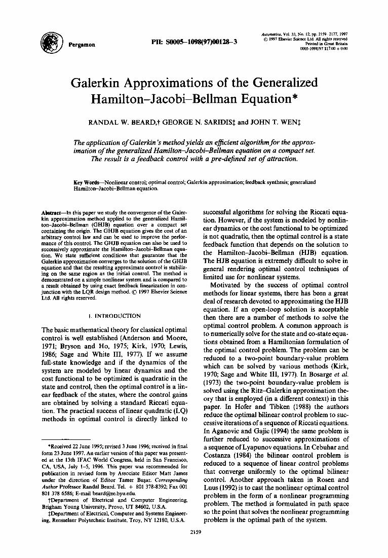
It has been shown in Glad (1985, 1987) and Tsitsiklis and Athans (1984) that the optimal control U* is robust in the sense that it has infinite gain margin and 50% gain reduction margin. A similar result has been shown for the control ii obtained from the GHJB equation via equation (17).

Lemma 10. Let UIE &r(R) be a control obtained from Lemma 9 and let the gain perturbation D : R” + R” satisfy

zTRD(z) 2 ct > 0;

then i =f + gD(l;) is asymptotically stable on Sz.

ProoJ: See Saridis and Balaram (1986) and Beard (1995). cl

For one-dimensional systems, the situation is depicted geometrically in Fig. 1; the system re- mains stable as long as the perturbed control is bounded below by fl;.

The next two lemmas will be needed at several points in subsequent proofs.

Lemma 11. If the set {$j}y is linearly independent and UE&,(~) then the set

is also linearly independent.

Proof: If the vector field f+ gu is asymptotically stable then along the trajectories cp(t; x0, u), x0 E Q, we have that

4(x0) = - s om$,(r; xo, 4) dT

= - pa+ gu)(&;xo, U))dr. s


Now suppose that the lemma is not true. Then there exists a nonzero CE RN such that

cTVcD&+ gu) = 0.

This implies that for all xogR

s

OD cTVcP&+ gu)(cp(z;xo, u) )dt = 0,

0

s

02

*CT WvU-+ gu)(cp(c xo, 4) dt = 0, 0

=dDN(xrJ= 0,

which contradicts the linear independence of

{4j>Y. cl

Corollary 12. Suppose that for all Jo [l,N], 4j is continuously differentiable and 3x0 such that (84j/8x)(Xo) # 0. If the set {4j}T is linearly independent then SO is the set {84j/8X}y.

Proof Suppose not, then 3c E RN such that

cTV@N = 0 =, cTV@& + gu) = 0

which contradicts Lemma 11. cl

Dejinition 13. Given a countable set of functions @ = {$j}T where 4j:sZ -P Iw”, define P(Q, f2) to be the set of all linear combinations of elements in Q that converge pointwise at each XER.

Lemma 14. If the set (4j}y is linearly independent, u E &#2), and (a$j/ax) * cf + gu) E 9(@, Q), then for all N

rank((V@& + gu) , (PN)nr) = N.

ProoJ Define @A(+,,&, . ..)’ and dj’(dtj, I),

4, 2)~ . ..)‘. Then by the hypothesis

z*(f+ gu) = f dcj,k)4k = dT@o k=l

so

where D A [d,, . . . , dN]. Therefore,

rank((V@NCf+ gu) ,@Nh) = rank(<@,QNhJ%

where (a ,@N),,, has rank N since the set {4j} are linearly independent. To prove the result we need to show that D has rank N.

Lemma 11 shows that the set

{$(j-+ gu)); = {d;Q}F

is linearly independent, therefore the Gram matrix of N of these vectors has rank equal to N, i.e.

rank

. . .

= rank((DT(@, a),,$))

= N.

Since the set {Oj};” is linearly independent, (Q , a),,, has full rank, which implies that rank(D) = N. q

The analysis of Galerkin’s method is greatly sim- plified by assuming that the basis functions {4j}p are orthonormal. However, from a practical point of view, orthonormalizing a set of functions can require extensive computational effort: therefore, we do not want to require orthonormality. The next two lemmas show that we can analyze Galer- kin’s method using orthonormal basis functions, while not requiring that they be used in practice.

Lemma 15. Suppose that the set {+j}y is linearly independent but the set (#j)y” is linearly dependent. Let VN = c#N and WN+ I = bz+l@N+l Sat-

isfy the equations

and (GHJB(WN+~;~)(DN+~),=O

respectively, then VN = WN + 1.

Proof: From the hypothesis we know that there exist a nonzero )BN E RN, such that $N+ I = fl@N, so

WN+l =b;F%i+bN+d'N+~

= b%'N + bN+&@N = @N + bN+$N)T@'N.

Therefore, VN E WN+ 1 -cN = bN + bN+lflN. From the hypothesis we know that cN satisfies

(V@ti+ gU),@N)&N+ <I+ bd:,(DN)~=O.

We also know the bN+ 1 satisfies

<V@:+,cf+ +),@iv+l)mhN+1

+ (I+ IlUll; ,@N+l)v = O*

This implies that


After some algebraic manipulation we obtain

( W!+ 1 --&f+ cw),QN

>

= (VQTd + g4 3 @N>,PN. ”

Therefore, cj%, and b, + /&bj,r+ I both satisfy the linear equation

(V@T,(f+gu) v@N)nlt = < -I- bk@Nh

and are therefore equivalent since (VQw+ gu), (DN)m iS invertible by Lemma 14. cl

Lemma 16. Given a set of linearly independent functions {4j}y. Suppose that these functions are orthonormalized to form the set {d;i}T then there exists constants Bij such that

81 = 81141,

$2 =B2141+82242 (18)

(GHJB( I’,; u) aP,>, = 0, (19)

and let WN = c;f& Solve

(GHJB( WN; U) 6;N)” = 0;

then VN G WN.

Proof: First note that we can write 6~ = B& where (BN)ij = pip WN = $&N = cYEBN@N SO CN = B&TN =s+ V, G WN. But since BN is lower diagonal and invertible, we have that

(GHJB(WN; u), @v)v = 0,

oBN(GHJB( WN; U) , QN)" = 0,

*(GHJB(WN;U),QN), = 0.

So B&YN satisfies the same linear equation as cN. The lemma is proved since the invertibility (by Lemma 14) of (VQ&+ gu) , @N),,, implies that the equations solution is unique. cl

Throughout the rest of this paper, we will use the following notation: the set {@j}F will be the original basis functions. The set {$j>y is obtained by first removing linearly dependent functions and then orthonormalizing the set {@j}r according to equation (18). The “tilde” will indicate orthonor- malization. Similar notation will be used for the coefficients weighting the vector. Hence, we will write

where cj and Cj are related through the coefficients flij defined above. Since orthonormality does not

affect convergence, we will use +j when orthonormality is not used in the argument and $j when it is.

The orthonormality of the set { $];> 7 on R implies that if a function #(x) E P(@, 0) and rc/ E L’(n) then

where the series converges pointwise, i.e. for any E > 0 and xoR, we can choose N(x) sufficiently large to guarantee that

To show stability of the approximate control obtained by Galerkin’s method we will need conditions under which a pointwise convergent series converges uniformly.

The next lemma, found in Apostol (1974), Exer- cise 9.8, states necessary and sufficient conditions for pointwise convergence of a series to imply uniform convergence on a compact set.

Dejinition 17. Let %!(a) be the set of infinite series, $Z:C~&~), that converge pointwise R, such that

7 9 ***9 and Q’E > 0, there exists p > 0 and m > 0 such that VxeQ, the conditions n > m and IC$k+ Icj+jx)l < p imply that

1 j=k+n+l I

Remark 18. This condition implies that if the tail of a sequence at some point XER is small, then after removing n > m terms, it is still small, where m is a uniform number for all x~SZ. For example, if a series is monotonically decreasing on 0, then m = 1 and p = E and SO C$~C~~~(X)E%!(R).

Lemma 19. If R c R” is a compact set and W(x) = Cj”= Ic#Ax), Vx E R and the basis functions PAX) are continuous on R, then Cj’ZN+ icj$j(X) converges to zero uniformly on R iff

(i) W(x) is continuous on f2, (ii) Cj”= ICj~j(X)E%!(ISZ).

Proof: See Apostol (1974, Exercise 9.8) and Beard (1995). cl

In the remainder of this section, we use the following notation: UE d,(Q) is an arbitrary admissible control, VN = xi”= IC#j, satisfies the algebraic equation (GHJB( VN; u) , @N)" = 0, UN = - *R - ‘gTaVN/&, V = Cj”= lbj4j, satisfies the

differential equation GHJB( V; u) = 0, fi=

- $R- ‘gTJV/&, P = c,j”= ,6j4j, satisfies the differential eqUatiOII GHJB(V, u*) = 0, eN = (~1, . . . , CN)T,


bN = (b,, . . . , bN)T, 6, = (Ib1, . . . ,^bN)T. The key to the notation is that b and c, respectively, denote the coefficients of the actual and approximate solutions to the GHJB equation. The “hat” notation is used to denote the updated control and value functions.

When u is admissible, the equation (GHJB( V,; u) (I$,)” = 0 forces the error caused by approximating the actual solution I/, projected on the linear space spanned by {4j}y to be zero. Lemma 20 shows that the residual error tends to zero as N + co. We then use this result to show in Lemma 22 that the coefficients for the approximate (V,) solution to the GHJB equation converges to the coefficients of the actual (V) solution. This implies that V, converges to V in the L’(Q) norm, which is shown in Corollary 23.

Lemma 20. If the hypothesis of Lemmas 8 and 14 are satisfied and

C6: a4j/ax. (f + gu), /lull;, Z, are continuous, in the space P(@, CI)nL’(CI), then

lGHJB( I’,; u)l -+ 0

pointwise on Q as N + co.

Proof: Condition C6 implies that GHJB(I/,; U) E 9(@,Q), so

IGHJB(h; uXx)l = f <GHJWT/,; U) 9 $j)$,(x) j=l

where

IAB 4&J = inf II&412

t/.tt2= 1. UOP

II&J~Iz = inf I(UIJZ ud”\(O}

Item (2) follows by showing that for all N

AA sup llc~ll~, which will imply that N=l,Z,

BA sup k=1,2,

Since (a&/ax)(f+ gu) and I+ l/u/: are in L’(Q), equation (20) implies that B and the second term on the right-hand side can be made arbitrarily small by an appropriate choice of N, which gives pointwise convergence on fi if /cNl(z is uniformly bounded for all N.

To show this define

i.e. ANcN = bN, and let

~64~) = min /iA~Uit z

~~U~~,=l,.EWN 1’ANU’12 = .,$& I(#([2

be the minimum singular value of the matrix AN. Lemma 14 guarantees that AN is nonsingular, therefore

To prove that l/cNll2 is uniformly bounded we need to show that there exist constants M1 and M2 such that (1) llbNlls I MI < CO and (2) CYAN) 2 M2 > 0 for all N = 1,2, . . . .

To show item (1) we note that condition C6 implies that

IIbNIIS = 5 I(1 + IIuIIk 6jJ,12 j= 1

s ,f lCz + Il”llk 6j)l’ j=l

= R jgl (I+ IlUlli 9 6jMA~J12dX si = Ill + Il4l~llZyn,~w < co.

To show item (2) define the operator A, by

and the minimum singular value of A, as

/ANI(: 2 c$AN) 2 o(A,)hMz > 0. - -

TO show that g(AN) 2 g(A,) for all N, let ii = ar- gmmlUl= i, U.R~IIAN~(Ir and define w E 1’ as

fij, je Cl, N], Wj =

0, j>N+l.

Then IJwJII~ = Ilu^(12 = 1 and

+L) = inf ll&4l~ 2 ll&~ll~ llull = 1, uel’

= I~AN~IIz = min II ANuII = FAN). Ilu~~=l.ueW


To show that c((Am) > 0, notice that

and that

2 I si L*(o) = n~x)jj+ gu) 2dx

In addition, Bessel’s inequality implies that

IdI? = f h12 I jjW12dx = II Ulik j=l

therefore

We claim that

inf i

ll%t4. (f + s4 II Zw, II VII2 I

> 0 (21) II “II &, f 0 LW

iff the GHJB equation has a unique solution. To show the necessity of this claim assume that equation (21) holds and let VI solve (WT/ax)(j+ gu) = - 1 - /lull& Suppose that V, # VI is also a solution on R, then (dV~/lax)(f+ gu) = - I - [lull& which implies that (a(V, - V#/dxWf+ gu) = 0. Therefore

which is a contradiction. To show the sufficiency let P be the unique

solution to (N/laxNf+ gu) = - I- Ilulj~. Suppose that

This implies that

inf {

IP%@u+ s4ll2w = o IIW-Wl12 L’,*,+o II v - wcn, > .

Since P satisfies the GHJB equation we get that

inf lIGHJW/;4lltwq = o

IIV-fTI12 l.~,nlz 0 II ‘v - w~tn, 1 .

This implies that there exists a sequence { Vk) such that lim,,, V, # V but limk_,, V, is a solution to the GHJB equation. This statement however, contradicts the assumption on uniqueness.

The proof is complete since Lemma 8 guarantees that the solution to the GHJB equation is unique.

q

CoroZlary 21. Under the hypothesis of Lemma 20, if

c7: Cj”= lcz + Il”lli 3 +j’j>Tj<x) E @!(n)7 C8: C.F= l<(a6k/ax)(.f + 9U) 3 $j>BXX) E @(a),

Vk = 1,2, . . . ,

then convergence is uniform on 0.

Proof Immediate from Lemma 19. 0

In the next lemma we show that the GHJB equation is bounded below so that the previous lemma imply convergence of the approximation to the solution.

Lemma 22. If conditions Cl-C6 hold, then

lh - bdlz --* 0.

Proof: Define

qN(x) 4 GHJB( V,; u)(x),

then for all x E Q

GHJB( VN; u)(x) - GHJB( V; u)(x) = Y/~(X).

Substituting the series expansion for V, and V, and moving the terms in the series that are greater than N to the right-hand side we obtain

Since {(84j/ax) .(f + gu)]: are continuous and linearly independent,

hN - hd=V@N(f + ClU)h.,(n, = 0 -G= CN = h. (22)


If cN = bN for all N, then the theorem is proved. Assume that cN # bN. Define W as

W 4 s

[V%(j- + gu)] [V@& + gu)IT dx. n

Since the set {(84j/ax). cf f gu))y is linearly independent, W is positive definite. Therefore,

Il(cN - bN)TV%_f + SU) 11 L,(a)

= (CN - bN)TW(CN - bN)

= s

J?dX)12dx 2 knidW)llcN - hII: > 0,

where n,,“(W) is the minimum eigenvalue of W. Therefore,

But by the mean value theorem, 35~0 such that

SI IN + n

f bjf$*(f+ gu)(X) 2 dx j=N+l

= P(Q) ?NtT) + 2

j=N+l

bj$*(f + SUXS) 2

s P(Q lrldO12 + 21?d5)l f bjf$‘U+ WWO ( j=N+l

+ j=$+l bjz’cT+ SUMS) 2

I>

Y

where ,u(Q) is the Lebesgue measure of R. Lemma 20 implies the pointwise convergence of qN(x), so Vc > 0, X,(g) such that

Since GHJB( I/; u) = 0,

f bjz*(/+ $4)(X) = - l(X) - llU(X)ll~ j=l

converges pointwise so VE > 0, X,(5) such that N > K2(e) implies that

which proves the lemma. 0

Corollary 23. Under the hypothesis of Lemma 22,

11 VN - Vb.,(R) + O.

Proof

= s /(cN - bdT~b,(x)12 dx

+ [jjz$+ 1 bj6Ax)li dx

= (CN - bdT~~,N~~)m(Ch’ - brd

By the mean value theorem, 3<eR such that

11 vN - f%,@-~, = IICN - hII:

It is not sufficient to know that the value function converges, we also need to know that the approximate control uN is admissible. We show in Lemma 24 that uN converges uniformly to fi, where u* is derived from I’ according to equation (6). Since Lemma 9 implies that li is admissible, we are able to show in Lemma 25 that uN is also admissible.

Lemma 24. If conditions Cl-C6 are satisfied then lIudx)(x) - $(x)IIR + 0 pointwise on R. If in addition C7 and C8 are satisfied and

C9: av/ax can be approximated uniformly close

on 0 by {NJj/ax}?,

then lluN(x) - r?(x)\lR + 0 uniformly on 0.

Proof:

bdx) - @)IIR 5 11 - +R- 'gT(x)v@(x#N - bN)llR

+ f-f I/

bjRwlgT(x&x) . J-N+1 II R

12 = - &jt ,bjR- ‘gTd4Jdx implies that the second term on the right-hand side converges pointwise to 0 and uniformly if condition C9 is satisfied. By Lemma 20 we know that

kN - bN)TV@NCf+ &b)l

converges pointwise to 0 and uniformly to 0 if conditions C7 and C8 are satisfied. Since {4i}r are linearly independent and (f + gu) is admissible, we have from Lemma 11 that

I(cN - bNITV@N(f + Cdl + 0 * IkN - bN II 2 + 0.

In addition, from Corollary 12 we have that

1cN - bNI + 0 0 I~v@&#J., - bN)ll2 + 0.

Therefore, IIV@~X)(CN - bN)l12 converges in the same sense as [(cN - bN)Tv@d(f+ gu)(x)l. SinCe


R- ‘gT(x) in continuous on a and hence uniformly bounded, we have that

II R - ‘gTW’@iWhv - h) II ,t --, 0

in the same sense as j(c, - b,)‘VQNdf + gu)(x)l. 0

The next lemma shows that for N sufficiently large, UN iS admissible.

Lemma 25. Under the conditions of Lemma 24, if

ClO: The set { ~~g(0)R-‘gT(O)~(O)~~z}~l is uniformly bounded for all N,

then for N Sufficiently large, #NE &@).

Proof From Lemma 9 we know that U*E &r(Q). Therefore, from Lemma 10, #N is stabilizing on a if

CT(x)Rudx) > @T(x)Rfi(x) o fiT(x)R(2udx)

- u*(x)) > 0

for all XER. In the 1D case, the situation is shown in Fig. 1: if r?(x) > 0 then UN(X) > &j(x) is stable, if t;(x) < 0 then UN(X) < i;(x) is stable. From Lemma 24 we know that UN is within a uniform 6 ball of 2, where 6 can be made arbitrarily small by making N large enough. Therefore, #N is guaranteed to be stabilizing everywhere but some ball R(O;p,) centered at the origin, where PN + 0 as N --* 00 (see Fig. 1). By Lyapunov’s first theorem, UN will be stabilizing on a Small region fi 3 R(Q PN) (for N SUf- ficiently large) if and only if the real parts of the eigenvalues of the linearized system are less than

0.6-

0.4 -

0.2 -

zero. So we need to examine the eigenvalues of the matrix (a/&Wf + guN)(O). Define

af F&&O),

GjP a’+.

- ; dO)R - ‘gT(0) $9.

Since t?(x) is stabilizing on R, we know that

where A(M) are the eigenvalues of M. So for N sufficiently large, UN will be stabilizing if

Note that

Since we know that the series CjZ IbjGj converges, VE > 0, Xi such that

N>K,- /I /I f bjGj < ~12. j=N+l 2

Also, since jIGill are uniformly bounded, Lemma 22 implies that 3Kz such that N > Kz implies

I 5 (bj - cj)Gj 5 IIbN - CNIIzIIGjII2 j=l II 2

Fig. 1. Gain margins for updated control u^.


is less than s/2, which proves that as N + cc,

Since all of the eigenvalues of F + C j”= 1 bjGj are strictly less than zero, there exists some K after which all of the eigenvalues of F + Cj”= iCjGj are strictly less than zero. So for some finite K, N > K implies that uN is stabilizing on 0.

To show that uN E &in) we must show that for all XE~

s

00 J(x; UN) A @(t; x, UN))

0

But since the eigenvalues of (a/axWf + guN)(O) can be made arbitrarily close to the eigenvalues of (a/axXf + St?)(O), the decay rates of f + guN and f + gu* are of the same order in a region close to zero. So (see Remark 3)

We have therefore established the following main result.

Theorem 26. Let

l R satisfy C2, l u satisfy C5, l cf, g, l) satisfy C3 and C4, and l the set {4j>F satisfy Cl, C%-ClO.

Under these conditions, Ve > 0, N > K implies that

3K such that

4. ILLUSTRATIVE EXAMPLE

In this section we will use the method described in the previous section to solve the GHJB equation associated with a feedback linearizing control. We will show how this solution is used to obtain a control law that improves the closed-loop performance of the original control.

Consider the following nonlinear system:

i=( ;:;;;2)+(0)u. (23)

The control objective is to regulate the system while minimizing the quadratic functional of the states and control

s

m J= xT(t)x(t) + u2(x(t)) dt.

0

To apply the method introduced in this paper we must choose

(1) u: a stabilizing control, (2) R: an estimate of the stability region of u, and

(3) f4j>?: a set of complete basis functions.

We will first select these quantities and then show that our selections satisfy conditions Cl-ClO.

System [equation (2311 can be stabilized using feedback linearization. Using the method outlined in Isidori (1989) the system [equation (23)] is linearized with the state feedback

U(X) = 3X: + 3X:X2 - X2 + 2,

and the coordinate transformation

(24)

Zl = Xl,

(25)

z2 = x: + x2.

In the new coordinates, system [equation (23)] becomes

We use standard LQR theory to optimize the transformed system with respect to the cost function

s

m J= zT(t)z(t) + u2(z(t))dt

0

to obtain the control

u(z) = 0.41422, - 1.3522~~. (26)

A continuous stabilizing control for the original system is given by substituting equation (25) into equation (26) to obtain a u as a function of x, and then using the control given in equation (24) to obtain

u(x) = 3x: + 3X:X2 - x2 + 0.4142~~

- 1.3522(x: + x2). (27)

The above control is stabilizing on R2 and so we are free to choose n as any compact set containing the origin. For simplicity, let R = [ - 1, l] x

c - 1,ll. In this example we use polynomials as our ap-

proximating functions:

{4j>~p( x:,XlX2,Xz,X~,X~X2,XlX~,X~,X~,X:xz,

x:x;,x:x:,x;, . . . 1.

In the appendix we show that if R is a rectangle, symmetrically centered at the origin,f + gu is a separable, odd-symmetric function, 1 + I( u II i is a separable, even-symmetric function, and the set { +j} r is composed of separable, even and odd-symmetric

functions then the coefficients associated with the odd-symmetric basis functions are zero. Since the system in this example satisfies these constraints, we will extract all &j’s that are odd-symmetric. Therefore, the basis functions become

{4j>? ’ {x:9 xIx2~d~ xt~ xTxZ~ dxZv xixZ~ Xi, XFv 5

x~x~,x~x~,x:x~,x~x~,x,xl,x~, . . . 1. (28)

We will now show that {f, g, 1, a, {4j}} satisfy conditions Cl-ClO.


Cl: We must show that VEP(Q), Q)nL2(S2). The Weierstrass approximation theorem guarantees that if V(x) is continuous, then V E 9(@,, S2). If V(x) is continuous and finite on compact R then VE L’(a). C2-C5 and Lemma 8 show that I/ is both continuous and finite on R.

C6: Since (a4j/ax) .(f+ gu), I/u/l: and J are all polynomials of degree greater than 2, they are in @I? Q).

C2: R is compact by definition. C3: By the mean value theorem, any differenti-

able function on a compact set is Lipschitz continuous on the same set, thereforefand g are Lipschitz continuous on Q andf(0) = 0.

C4: laxTx and R = 1 are positive definite by definition.

C7: Since 1 + ljt~jl: are polynomials we have that there exists some K such that 1 + l/u112 ~span{c#~~>f, i.e.

Kx) + II u(x) II ’ = F dj4jlx)* 1

Therefore

CS: We must show that u defined in equation (27) satisfies Definition 1. Clearly, u is continuous and satisfies u(O) = 0. u is shown to be stabilizing on R by using the transformed system to find a Lyapunov function

= 5 4&k(x) k=l

VLYaP(x) = (x7;xJT(x;yxJ where P satisfies the Lyapunov PAT = - Z and

A=(; ,1)+@)(0.4142

equation AP +

- 1.3522 >

.

The finiteness of the integral @(l + Ilull$ dt for all XER follows from Remark 3 by noting that

eig{v(O)} = - 0.6761 &- j0.9783.

which clearly satisfies Definition 17 since the tail of the series is zero after K terms.

C8: Follows from a similar argument as C7. C9: Lemma (8) guarantees that aV//ldx is continu-

ous, so the Weierstrass approximation theorem guarantees that this function can be approximated uniformly close by polynomials.

ClO: From equation (28) we see that each basis function can be written as 4j = xpxy where pj + qj 2 2. It can be easily seen that the matrix (a”4j/ax’)(O) is nonzero only when

(Pj,qj)E{(2,0),(0,2),(1, l)},

N=O I.51

-1 -1 -0.5 0 0.5 1

N=8 N=15 1

_I -1 -0.5 0

Fig. 2. Phase portrait for u, uj (x2), us (x4), uls(x6).

N=3 1

2174

3.5

3

I:.. 2.51 ....

-1 -0.8 -0.6 -0.4 -0.2 0 0.2 0.4 0.6 0.8 1

R. W. Beard et al.

“0 :-

“, :

v :__

V 15

:-

Fig. 3. System cost for u, ug, I+,, u15.

in which case it is constant. Therefore, the set

~/;~K’gYO)~/l% is uniformly bounded for

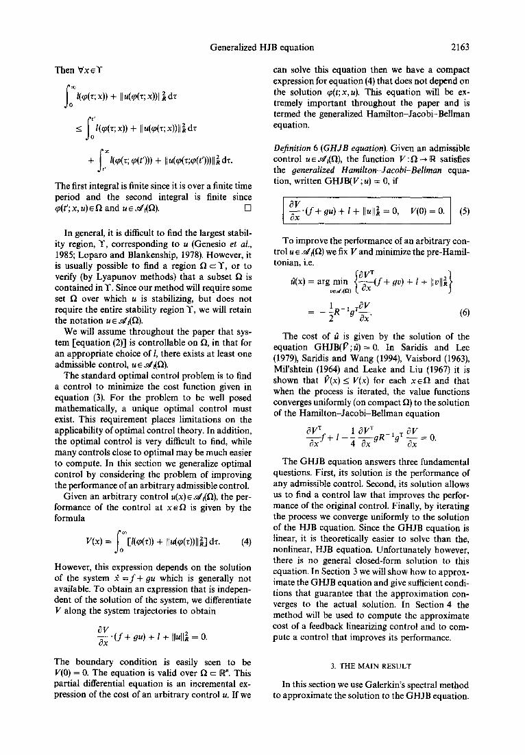
In this example we will use N = 0,3,8,15 basis functions, where N = 0 corresponds to the initial control [equation (27)], and N = 3 (respectively, 8, 15) corresponds to basis functions with terms of order up to x2 (respectively, x4, x6). An approximate control with N terms is given by the formula

For example, when N = 3,815 we obtain the following feedback control laws:

z+(x) = - 0.5484~~ - 2.5258x2

us(x) = - 0.4215~~ - 2.2225x2 - 0.4784x:

+ 0.2719x:x2 + 0.6494~~~; + 0.0588x;,

ai&) = + 0.2652~~ - 2.6857x2 - 1.0960x:

+ 1.2144x:x, - 1.0805x1x; + 0.4505x;

- 0.2191x: - 0.9098x:x2 + 1.0508x:x;

- 0.4009x:x; + 0.2669~~~; - 0.1525x;.

Figure 2 shows the phase portrait to the system under the control uo, ug, aa, and u15. Figure 3 shows the cost of these controls for initial conditions (x~O)~,X, E [ - 1, 11. Increasing N larger than

15 does not result in noticeable improvement in the cost. This plot shows the effectiveness of the method proposed in this paper for improving the closed-loop performance of a control obtained via feedback linearization and the LQR method.

5. CONCLUSIONS

In this paper we posed the problem of finding a practical method to improve the closed-loop performance of a stabilizing feedback control laws for nonlinear systems and showed that the problem reduces to solving the generalized Hamilton-Jac- obi-Bellman (GHJB) equation. We showed that Galerkin’s spectral method could be used to approximate the GHJB equation such that the resulting control is in feedback form and stabilizes the closed-loop system.

There are several advantages of the method. First, the method produces feedback control laws. Second, the controls are robust in the same sense as the optimal control. Third, all computations are performed off-line and once a solution is found, the control can be implemented in hardware and run in real time. Fourth, the stability region contains the set R which is specified by the designer and is only restricted to be contained in the stability region of the initial admissible control. Finally, coefficients for the state and control weighting functions can be taken outside the integral so tuning the control through the penalty function becomes computa- tionally fast. The disadvantages are that O(N’) n- dimensional integrals need to be computed and


that, since the control laws are given as a series of basis functions, they are inherently complex. Imple- mentation issues associated with the method are discussed in Beard (1995) and Beard et al. (1996). In addition, it should be pointed out that the results of this paper only guarantee that for N sufficiently large, the method converges. However, for a given E, we have not given an estimate of how large N might have to be. An additional disadvantage is that it is not clear how conditions C7 and C8 might be checked for a particular system.

The method introduced in this paper can be iterated to produce a procedure similar to Be- llman’s approximation in policy space (Bellman and Dreyfus, 1962) Full implementation of this combined algorithm can be found in Beard (1995) and is the subject of Beard et al. (1998). The method has been extended to finite-time horizon problems for stationary and non-stationary plants as reported in Beard (1995). It has also been applied to the Hamilton-Jacobi-Isaacs equations that arise in nonlinear H, optimal control. The results on topic will be the subject of forthcoming papers.

Acknowledgements-Partially supported by NASA grant NAGW-1333.

REFERENCES

Aeyels, D. (1985). Stabilization of a class of nonlinear systems by a smooth feedback control. System Control Lett., 5, 289-294.

Aeyels, D. (1986). Local and global stabilizability for nonlinear systems. In Theory and Applications of Nonlinear Control Systems, eds C. I. Byrnes and A. Lindquist, pp. 93-105. Elsevier, North-Holland.

Aganovic, Z. and Z. Gajic (1994). The successive approximation procedure for finite-time optimal control of bilinear systems. IEEE Trans. Automat. Control, 39(9), 1932-1935.

Al’brekht, E. G. (1961). On the optimal stabilization of nonlinear systems. J. Appl. Math. Mech., 25(S), 836844.

Anderson, B. d: 0. and J. B. Moore (1971). Linear Optimal Control. Prentice-Hall. Enelewood Cliffs. NJ.

Apostol, T. M. (1974). Mathematical Analysis. Addison-Wesley, Reading, MA.

Battilotti, S. (1996). Global output regulation and disturbance attenuation with global stability via measurement feedback for a class of nonlinear systems. IEEE Trans. Automat. Con- trol, 41(3), 315-327.

Baumann, W. T. and W. J. Rugh (1986). Feedback control of nonlinear systems by extended linearization. IEEE Trans. Automat. Control, 31(l), 40-46.

Beard, R. (1995). Improving the closed-loop performance of nonlinear systems. PhD Thesis. Rensselaer Polytechnic Insti- tute. Troy, New York.

Beard, R., G. Saridis and J. Wen (1996). Improving the performance of stabilizing control for nonlinear systems. Control Systems Mag., 16(5), 27-35.

Beard, R., G. Saridis and J. Wen (1998). Approximate solutions to the time-invariant Hamilton-Jacobi-Bellman equation. J. Optim. Theory Appl., to appear.

Bellman. R. and S. Drevfus (1962). Applied Dvnamic Proaram- ming. Princeton Universit; Press, F%ncetoi, NJ. ”

Bittanti, S., A. Laub and J. C. Willems (1991). The Riccati Equation. Springer, New York.

Bosarge, W. E., 0. G. Johnson, R. S. McKnight and W. P. Timlake (1973). The Ritz-Galerkin procedure for nonlinear control problems. SIAM J. Numer. Anal., 10(l), 94-l 10.

Bryson, A. E. and Y. C. Ho (1975). Applied Optimal Control. Hemisphere, New York.

Capuzzo Dolcetta, I. (1983). On a discrete approximation of the Hamilton-Jacobi equation of dynamic programming. Appl. Math. Optim., 10, 367-377.

Capuzzo Dolcetta, I. and H. Ishii (1984). Approximate solutions of the Bellman equation of deterministic control theory., Appl. Math. Optim. 11, 161-181.

Capuzzo Dolcetta, I. and M. Falcone (1989). Discrete dynamic programming and viscosity solutions of the Bellman equation., Annales Institut Henri Poincare Anal. Nonlinear (suppl.) 6, 161-184.

Cebuhar, W. A. and V. Costanza (1984). Approximation proced- ures for the optimal control of bilinear and nonlinear systems. J. Optim. Theory Appl., 43(4), 615-627.

Chapman, J. W., M. D. Ilic, C. A. King, L. Eng and H. Kaufman (1993). Stabilizing a multimachine power system via decentra- lized feedback linearizing excitation control. IEEE Trans. Power Systems, 8(3), 836839.

Cloutier, J. R., C. N. D’Souza and C. P. Mracek (1996). Nonlin- ear regulation and nonlinear H, control via the state-dependent Riccati equation technique. In ‘IFAC World Congress’, San Francisco, California.

Crandall, M. G., H. Ishii and P.-L. Lions (1992). User’s guide to viscosity solutions of second order partial differential equations. Bull. Am. Math. Sot., 27(l), l-67.

Falcone, M. (1987). A numerical approach to the infinite horizon problem of deterministic control theory. Appl. Math. Optim., 15, l-13.

Falcone, M. and R. Ferretti (1994). Discrete time high-order schemes for viscosity solutions of Hamilton-Jacobi-Bellman equations. Numer. Math., 67, 315-344.

Finlayson, B. A. (1972). The Method of Weighted Residuals and Vuriational Principles. Academic Press, New York.

Fleming, W. H. and H. Mete Soner (1993). Controlled Markou Processes and Viscosity Solurions. Springer, Berlin, Germany.

Freeman, R. A. and P. V. Kokotovic (1995). Optimal nonlinear controllers for feedback linearizable systems. In Proc. Ameri- can Control Cant, Seattle, Washington, pp. 2722-2726.

Gao. L.. Lin Chen. Yushun Fan and Haiwu Ma (1992). A n&linear control’design for power systems. Automhtica; 28, 975-979.

Garrard, W. L. and J. M. Jordan (1977). Design of nonlinear automatic flight control systems. Automatica, 13, 497-505.

Genesio, R., M. Tartaglia, and A. Vicino, (1985). On the estima- tion of asymptotic stability regions: state of the art and new proposals.lEEE Trans. Automat. Control 30(8), 747-755.

Glad, S. T. (1987). Robustness of nonlinear state feedback-a survey. Automatica, 23(4), 425435.

Glad, T. (1985). Robust nonlinear regulators based on Hamilton-Jacobi theory and Lyapunov functions. In IEE Control Con& Cambridge, pp. 276280.

Goh, C. J. (1993). On the nonlinear optimal regulator problem. Automatica, 29, 751-756.

Gonzalez, R. and E. Rofman (1985a). On deterministic control problems: An approximation procedure for the optimal cost i: the stationary problem. SZAM J. Control Optim. 23(2), 242-266.

Gonzalez, R. and E. Rofman (1985b). On deterministic control problems: an approximation procedure for the optimal cost ii: The nonstationary problem. SIAM J. Control Optim. 23(2), 267-285.

Halme, A. and R. P. Hamalainen (1975). On the nonlinear regulator problem. J. Optim. Theory Appl., 16, 255-275.

Hofer, E. P. and B. Tibken (1988). An iterative method for the finite-time bilinear-quadratic control problem. J. Optim. Theory Appl., S7(3), 41 l-427.

Hunt, L. R., R. Su and G. Meyer (1983a). Design for multi-input nonlinear systems. Differential Geometric Control Theory, eds, R. W. Brockett, R. S. Millman and H. Sussmann, pp. 268-298. Birkhaiiser, Basal.

Hunt, L. R., R. Su and G. Meyer (1983b). Global transforma- tions of nonlinear systems. IEEE Trans. Automat. Control, 28(l), 24-31.

Isidori, A. (1989). Nonlinear Control Systems. Communication and Control Engineering, 2nd ed. Springer, New York.


Johansson, R. (1990). Quadratic optimization of motion coord- ination and control. IEEE Trans. Automat. Control, 38(11),

Zeidler, E. (1990a). Nonlinear Functional Analysis and its Ap

1197-1208. plications, II/A: Linear Monotone Operators. Springer, Berlin, Germany.

Kantorovich, L. V. and V. I. Krylov (1958). Approximate Methods of Higher Analysis. Interscience Publishers, Inc, New York.

Zeidler, E. (1990b). No&near Functional Analysis and its Applications, II/B: Nonlinear Monotone Operators. Springer, Berlin, Germany.

Khalil, H. K. (1992). Nonlinear Systems. Macmillan, New York. Kirk, D. E. (1970). Optimal Control Theory. Prentice-Hall,

Englewood Clitfs, NJ. Kushner, H. J. (1990). Numerical methods for stochastic control

problems in continuous time. SIAM J. Control Optim., 28(5), 999-1048.

APPENDIX A. SYMMETRIC SYSTEMS OVER

HYPERCUBES

Leake, R. J. and R.-W. Liu (1967). Construction of suboptimal control sequences. SIAM J. Control Optim., S(l), 5463.

Lee, C. S. Cl. and M. H. Chen (1983). A suboptimal control design for mechanical manipulators. In American Control Con&, Sheraton-Palace Hotel, San Fransico, CA, pp. 1056-1061.

Lewis, F. L. (1986). Optimal Control. Wiley, New York. Loparo, K. A. and G. L. Blankenship (1978). Estimating the

domain of attraction of nonlinear feedback systems. IEEE Trans. Automat. Control, 23(4), 602-608.

Lu, P. (1993). A new nonlinear optimal feedback control law. Control Theory Adv. Technol., 9(4), 947-954.

In this appendix we will show that under certain conditions, we can reduce the number of basis functions used to approximate V. Our motivation is from Lemma 8 where it was shown that V is positive definite. Therefore, it should be sufficient to approximate V with positive-definite basis functions.

We begin by making a number of definitions. f: I?’ -P [w is called “separable on CY if f(x) = IIJ= lfj (xj) for all x E a. f: W” + R is called “even- symmetric on CY’ if f( - x) =f(x) for all XED. f: I?’ -P [w is called “odd-symmetric on N’ iff( - x) = -f(x) for all XER. Define %A {f: R” + R :f is

separable and odd-symmetric on Q> and %A {f: I?’ + [w :f is separable and even-symmetric on Q}. Let 9Z’ (resp. 9’:) be the set of vector-valued functions whose elements are in % (resp., %). We will first state a number of facts that follow directly from the definitions.

Lukes, D. L. (1969). Optimal regulation of nonlinear dynamical systems. SIAM J. Control Optim., 7(l), 75-100.

Marino, R. (1984). An example of a nonlinear regulator. IEEE Trans. Automat. Control, 29(3), 276279.

Mikhlin. S. G. (1964). Variational Methods in Mathematical Physics. MacMillan; New York.

Mikhlin, S. G. and K. L. Smolitskiy (1967). Approximate Methods for Solution of Difjerential and Integral Equations. American Elsevier, New York.

Mil’shtein, G. N. (1964). Successive approiximations for solution of one optimal problem. Automation Remote Control, 25, 298-306.

Nijmeijer, H. and A. J. van der Schaft, (1990). Nonlinear Dynam- ical Control Systems. Springer, New York.

Nishikawa, Y., N. Sannomiya and H. Itakura (1971). A method for suboptimal design of nonlinear feedback systems. Auto- matica, 7, 703-712.

Petryshyn, W. V. (1965). On a class of k-pdand non-k-pdoper- ators and operator equations. J. Math. Anal. Appl., 10, l-24.

Rosen, 0. and R. Luus (1992). Global optimization approach to nonlinear optimal control. J. Optim. Theory Appi., 73(3), 547-562.

Ryan, E. P. (1984). Optimal feedback control of bilinear systems. -J. Optim. Theory Appl., 44(2), 333-362.

Saae. A. P. and C. C. White III (1977). Ovtimum Svstems Control. %l ed. Prentice-Hall, Englewood Cl&, NJ. .

Saridis, G. N. and C.-S. G. Lee (1979). An approximation theory of optimal control for trainable manipulators. IEEE Trans. Systems Man Cybernet., 9(3), 152-159.

Saridis, G. N. and F. Y. Wang (1994). Suboptimal control of nonlinear stochastic systems. Control Theory Adv. Technol., 10(4), 847-871.

Saridis, G. N. and J. Balaram (1986). Suboptimal control for nonlinear systems. Control Theory Adv. Technol., 2(3), 547-562.

Tsitsiklis, J. N. and M. Athans (1984). Guaranteed robustness properties of multivariable nonlinear stochastic optimal regulators. IEEE Trans. Automat. Control. 29(g), 690-696.

Tzafestas, S. G. , K. E. Anagnostou and T. d. Pimenides (1984). Stabilizing optimal control of bilinear systems with a generalized cost. Opt. Control Appl. Methods, 5, 11 l-l 17.

Vaisbord, E. M. (1963). An approximate method for the synthesis of optimal control. Automat. Remote Control, 24, 16261632.

Wang, Y. , D. J. Hill, R. H. Middleton and L. Gao (1993). Transient stability enhancement and voltage regulation of Dower svstems. IEEE Trans. Power Svstems, 8(2). 620-627.

Wang, Y.-, D. J. Hill, R. H. Middle& and’ L: ‘Gao (1994). Transient stabilization of power systems with an adaptive control law. Automatica, 30(9), 1409-1413.

Werner, R. A. and J. B. Cruz (1968). Feedback control which preserves optimality for systems with unknown parameters. IEEE Trans. Automat. Control, 13(6), 621-629.

Fact 1: If ql, ~2 E %” and 01, (~2 E %“, then qTq2 E z, oTo2 E %, ~/Tai E %4p,.

Fact 2: If q: R” -+ R is separable then q = II& I~,(x)E% iff there are an even number (pos- sibly zero) of q’s that are odd-symmetric. Similarly, u = II:= iqj(x) E % iff there are an odd number (at least one) of Q’S that are odd-symmetric.

Fact 3: If R = [ - al,al] x ... x [ - a,,,~] and q E %, then Jo?(x) dx = 0. (Proof: Reorder IIqAxj) such that vi is odd, which fact 2 guarantees is possible, then Jo? = (pa, qi)II:= zpa,qj = 0.)

Fact 4: If qj : R + IF! is even (resp. odd) on 0, then dqj/dxj is odd (resp. even) on R. (Proof. qj- even

* qj (xj) = qj ( - xj) * (dqj/dxjX xi) = (dqj/dxj)(xj) d( - xj)/dxj = - (dqj/dxj)( - xj).)

Fact 5: If q E% (resp. %) then c~~@xE%” (resp. 3). (Proof:

all _= ax

/

Therefore q E Y: (resp. %) implies that there are an even (resp. odd) number of odd-symmetric terms in q. Fact 4 shows that exactly one term in each element of @/ax will change sign. Therefore each element of Q/ax will have an odd (resp. even) number of odd-symmetric terms.)


Theorem A.l. Assume that the conditions of Lemma 14 are satisfied. Let VN = Cj”= 1 c&j satisfy

and suppose that

Tl: Q is a rectangle, symmetrically centered at the origin, i.e. fi = [ - ai, ai] x . . . x [ - a,, anI,

T2:f+ guEY:, T3: 1 + [IuII~E~~, T4: (#j>F s 9*~9ep,.

If 4j E YO, then Cj = 0 (i.e. I’, E Ye,).

ProoJ: Define

K, = {k,, . . . &,,)qw1m he}9 K, = {k,, . . . JqK.p(~~CLKl: &WY),).

Define Q’K. 0 GA,, . . . , 9+JT and CK. A @I, . . . , ck,,JT and QKC and ek_ accordmgly. Then

( gc_f+su)+l+ ,lull:,%) =o 0

can be written as

where

M p

(

(V%cf + gu), %.)m (V@&cf + gu), %.)m

(V%U + gu), %.>fn (V@Kjf + gu), @r&l > *

The previously stated facts show that

(V@df + gn) > %& = 0,

wwf + 94 9 %.hPl = 0,

Cl + lb& ?%.)” = 0.

Therefore, cKO satisfies the equation

(v%jf+ g”) F %.hnCK, = 0.

The theorem follows from Lemma 14 which shows that the matrix (VQKOu+ gu) ,QKO),,, is full rank. q

galerkin approximations of the generalized hamilton-jacobi-bellman equation

Documents