gala cookbook - cosmic-lab · · 2013-02-16gala cookbook alessio mucciarelli ... 3 ... 7. write...

GALA cookbook

Alessio Mucciarelli

Dipartimento di Fisica & Astronomia, Universita degli Studi di Bologna, Viale Berti Pichat, 6/2

- 40127 Bologna, ITALY

[email protected]

1. Introduction

GALA (Mucciarelli et al. 2013) is a code written in standard Fortran 77 and aimed at finding

the best atmospheric parameters and the abundance of individual elements by using the equivalent

widths (EWs) of metallic lines, providing graphical and statistical tools to evaluate the goodness

of the solution. The derivation of the abundances is performed by using a modified version of

the WIDTH9 code1 (originally developed by R. L. Kurucz) in its Linux version (Sbordone et al.

2004). In the current release, GALA can manage the classical grid of ATLAS9 models computed

by Castelli & Kurucz (2004), the grid of new ATLAS9 models computed for the APOGEE survey

(Meszaros et al. 2012) and the MARCS models with the standard composition (Gustafsson et al.

2008). When the ATLAS9 models are used, new model atmospheres are calculated starting from

an existing guess model and according to the pre-tabulated Opacity Distribution Functions (ODF)

and Rosseland opacity tables. When MARCS are used, each new model is obtained by interpolating

within the MARCS grid.

2. Installation

Once you have downloaded the archive file gala.tar.gz from the website

www.cosmic-lab.eu/Cosmic-Lab/Products.html,

type the commands

gunzip gala.tar.gz

tar -xvf gala.tar

These commands unpack the archive file creating a directory named GALA/. Within this direc-

tory there are three subdirectories ( src/, bin/ and tutorial/) together with some information

1http://wwwuser.oat.ts.astro.it/castelli/sources/WIDTH.html.

– 2 –

files. The directory src/ includes all the source files and the Makefile needed to install GALA. The

directory bin/ includes the executables created after the installation. In the directory tutorial/

there are some examples of the input files for GALA as reference.

(1) Install ATLAS9

Before starting the installation of GALA, you need to install in your machine the ATLAS9 code if

you plan to use these models (obviously, if you plan to use only MARCS models you can avoid to

install ATLAS9). GALA includes a dynamical call to the last version of this code, available on the

website of F. Castelli2. Download the source code atlas9mem.for with the command

wget -r -nd http://wwwuser.oat.ts.astro.it/castelli/sources/atlas9/atlas9mem.for

and compile it

ifort -double-size 64 -save -o atlas9mem.exe atlas9mem.for

Note that GALA assumes that you have this code installed and that the executable is named

atlas9mem.exe. Please do not compile ATLAS9 with di!erent names.

(2) Set the Makefile

Firstly, you need to properly update the Makefile. GALA can be compiled with the Intel For-

tran Compiler, that you can download from the Intel website3, after the registration. Also, the

graphical output files are created by the program galaplot using the SuperMongo4 (SM) libraries

(namely libplotsub.a, libdevices.a and libutils.a, compiled in single precision) and the X11

libraries. Set in the first lines of the Makefile the path of your Intel Fortran Compiler and that of

the directory where the SM libraries are located.

(3) Set some useful paths

Now, you need to properly set in the GALA/src/Paths.f file the paths of some directories used by

the code:

(1) ’exe’ = it is the path where the executables of GALA are located (the subdirectory bin/);

(2) ’at9exe’ = it is the path of the directory where the executable atlas9mem.exe is located;

(3) ’at9fc’ = it is the path where the ATLAS9 models by Castelli & Kurucz (2004) are saved, see

2http://wwwuser.oat.ts.astro.it/castelli/sources/atlas9codes.html

3http://software.intel.com/en-us/non-commercial-software-development

4http://www.astro.princeton.edu/!rhl/sm/

– 3 –

Section.7;

(4) ’at9apo’ = it is the path where the ATLAS9 models by Meszaros et al. (2012) are saved, see

Section.7;

(5) ’marcs’ = it is the path where the MARCS models with the standard composition by Gustafsson et al.

(2008) are saved, see Section.7.

The directories of the ATLAS9 models need a precise structure. In each directory you need to

create three subdirectories, namely ODF/, MODELS/ and MODELS-new/, the first including the ODFs

and the Rosseland opacity tables, the second including the grid of model atmospheres used as guess

models, while the third is the directory where the new models created during the run of GALA will

be saved. The directory for the MARCS models does not need a specific substructure. Examples of

these subdirectories, as well as more details about the use of the di!erent model grids, are discussed

in Sect. 7.

Note that you do not need to have necessarily all these models to use GALA. If you plan to use

only a given kind of models, you can delete or leave blank the paths of the other models in the

Paths.f file (but in this case do not try to call them when you run GALA).

(4) And now...install GALA!

To install GALA, type the command

make all

and the executables will be saved in the subdirectory /bin.

Finally, put the path of the subdirectory bin/ in your login file according to the shell environment

of your machine (for instance in the configuration file .bashrc or .tcshrc). The directory /tutorial

includes examples for the three input files. You can check the installation of GALA by using these

files and simply type gala.

Note that GALA is dimensioned to manage up to 1200 spectral lines for each star (parameter INL

in the source file Declare.f). If a given star has more than this number of measured transitions,

GALA skips this star providing a warning message. For our experience this value is reasonable

but if you think the this limit is too low for your stars, you can increase the parameter INL and

recompile the code (note that a uselessly high value for INL will lead to a waste of computer

memory).

3. Installation problems

We list some common installation problems (typically related to the combination Fortran

compiler/system architecture) and their possible solutions.

• The SM libraries compiled in double precision can give problems during the compilation or

– 4 –

(when the compilation well works) galaplot creates corrupted or badly drawn postscript

files. We recommend to use for galaplot SM libraries compiled in single precision. Because

it is usual to compile SM in double precision, we suggest to perform two distinct installations

of SM, in order to save wherever you want the libraries compiled in single precision. The

instructions to perform the installation of SM are explained in the sm.install file in the

directory of the SM source code.

• A warning message appears during the compilation of galaplot like

ld: warning in /Users/alessio/MAGAZZINO/SMONGO-lib-ELE/libplotsub.a, file is

not of required architecture

In this case, you can try to compile galaplot telling the compiler to generate the code

for a specific architecture. You need only to add the option ’-m32’ (if your machine is a 32

architecture) or ’-m64’ (if your machine is a 64 architecture) in the Makefile

$(FORTRAN) -m32 -traceback - galaplot galaplot.f mplot1.f -lX11 -L$(SMLIB)

-lplotsub -ldevices -lutils.

• The SM commands under Fortran are unrecognized, with warning messages like

Undefined symbols: " sm limits ", referenced from: mplot in ifortLFD1nn.o

This happens because some incompatibilities between the di!erent names of the SM com-

mands as defined by Fortran and C compilers can occur. The users with experiences with

other tools devoted to spectroscopic analysis (as MOOG and DAOSPEC) have already dealt

with these problems. We refer the reader to the Chapter 4 of the DAOSPEC Cookbook5 as

useful documentation to solve some of these problems.

With the last versions of the Intel Fortran Compiler, the SM commands have an extra ’ ’ as

su"x (not needed if you compile galaplot with G77 Fortran Compiler for instance). The

source file mplot1.f calls the SM commands as sm limits and so on. Note that we provide a

modified version of this file (named mplot2.f) where the SM commands are called with their

standard names (i.e. sm limits); you can try to compile galaplot with this source file, if the

error messages shown above appear.

• If you cannot compile galaplot with the Intel Fortran Compiler because of incompatibilities

between the SM libraries and the Fortran commands as called in the source code, you have

two alternative options: (1) try to compile only galaplot with another Fortran compiler (as

5http://www.bo.astro.it/!pancino/docs/daospec.pdf

– 5 –

G77 for instance), substituting the file mplot1.f with mplot2.f; (2) if you cannot compile

galaplot with other compilers, you can perform the installation of GALA without galaplot.

In this case, you can easily disable the graphical option by commenting in the file gala.f the

line

call system(’galaplot’)

and then compile the code with the command make gala.

4. Executable files

The executable files that will be created in the subdirectory bin/ are:

1. gala — the executable file to run GALA;

2. galaplot — this program produces the graphical output for each analysed star;

3. interpol marcstoatlas — this is a modified version of the code to interpolate the MARCS

model atmospheres developed by T. Masseron and available in its original version at the web-

site http://marcs.astro.uu.se/software.php. The current version writes the output MARCS

model in the ATLAS9 standard format;

4. marcstoatlas — this routine reads an usual MARCS model atmosphere converting it in the

ATLAS9 standard format. This routine is a modification of the program (developed by B.

Edvardsson) available in the Uppsala website (http://marcs.astro.uu.se/software.php) and it

can be used independently by GALA with the command-line instruction

cat < model-name > / marcstoatlas

(where < model-name > is the input MARCS model), storing in the Fortran unit 88 the

ATLAS9-like output model;

5. width9 gala — this is a modified version of the WIDTH9 code available on the website of F.

Castelli 6. The main di!erences are the formats of the input and output files. Some control

cards of WIDTH9 (see Castelli 1988) have been disabled because not used by GALA;

6. extract kur — this program reads the classical linelists of Kurucz/Castelli 7 stored in a file

named master linelist.tmp and a file (named input.dat) including your linelist (in the

6http://wwwuser.oat.ts.astro.it/castelli/sources/WIDTH.html

7http://wwwuser.oat.ts.astro.it/castelli/linelists.html

– 6 –

first column the wavelength in A and in the second column the code of the element in the

Kurucz formalism: i.e. 26.00 for FeI and 26.01 for FeII). The code matches the two files and

writes in the output file (output.dat) the information needed to the GALA input.

7. write autofl — this program writes the basic structure of the input file autofl.param (de-

scribed in Section 5.1), with the proper name of each keyword.

5. Input files

• autofl.param — it includes the main configuration parameters used by GALA to perform

the analysis (described in Section 5.1);

• list star — it is the list of the stars to analyse and their guess atmospheric parameters

(described in Section 5.2);

• a file (one for each star listed in list star) with extension .in, including the list of the

measured lines, their EWs and their atomic parameters (described in Section 5.3).

5.1. Layout of autofl.param

The input file autofl.param includes two groups of keywords, namely the basic parameters

and the subordinate parameters. The command write autofl writes the basic structure of the file

(with some parameters already filled by default values); note that the order of the keywords (as

well as the presence or not of the header lines) does not really matter. A template of this file is

available in the subdirectory tutorial/.

(1) Basic parameters: these are the parameters that you need to set in order to perform the

analysis:

• model specifies the kind of model atmospheres; the accepted values are

-atlas9 for the ATLAS9 model atmospheres available in the website by F. Castelli;

-apogee cm150 APOGEE-ATLAS9 grid with [C/Fe]=–1.50;






-apogee cp000 APOGEE-ATLAS9 grid with [C/Fe]=+0.00;



– 7 –



-marcs for the MARCS model atmospheres with the standard chemical composition.

We refer to Section 7 to detail about the download of these models and the way to manage

them in order to use correctly GALA. Alternatively, you can specify the name of a given

model (in ATLAS9 format) 8 located in the working directory. If the specified model is found

in the current directory, all the optimization options (together with the guess and refinement

working-blocks) are switched o! and only the analysis working-block is executed (with fixed

parameters). Otherwise, if the specified model does not exist in the directory, GALA stops

the procedure and exits with a warning message.

• guess enables the guess working-block, before the analysis working-block. The parameter is

the number of iterations performed during this working-block. Guess= 0 (or negative values)

disables the execution of this working-block. If you decide to use this option, we suggest to

adopt at least 3 iterations for the guess working-block.

• refine enables the refinement working-block, after the analysis working-block. The parameter

8If you wish to use a model atmosphere calculated with the ATLAS12 code (Castelli 2005a), you need to erase

the 22 lines corresponding to the ’ABUNDANCE TABLE’ control cards. Also, to use a specific MARCS model, you

have to put it in ATLAS9 format with the program marcstoatlas.

– 8 –

accepts the values 0 (disabling the working-block) and 1 (enabling the working-block).

• uncer enables the calculation of the uncertainties in the derived chemical abundances due to

the atmospheric parameters. The accepted values are

0 : no uncertainties calculation is performed;

1 : the uncertainties are calculated according to the prescriptions by Cayrel et al. (2004),

only if Te! has been optimized spectroscopically;

2 : together with the uncertainties estimated with the previous method, also the uncertainties

due to the atmospheric parameters following the classical method are calculated, varying

each time one parameter only (keeping the others fixed) and without taking into account the

covariance terms.

• qiron indicates the code of the element (with its ionization stage) whose lines are used to

perform the optimization. The formalism is the same used in the Kurucz codes (i.e. 26.00

for Fe I and 26.01 for Fe II). In principle, GALA accepts all the elements but obviously only

a few elements (i.e. Ti or Ni) have a su"cient number of available lines to perform a reliable

spectroscopic optimization.

• epot enables the spectroscopic optimization of the temperature. The accepted values are

0 : the temperature is not optimized and rather fixed to the input value;

1 : the temperature is found by erasing any trend in the A(El)9—!ex plane (where !ex is the

excitation potential in eV).

• grc enables the spectroscopic optimization of the gravity.

0 : the gravity is fixed to the input value;

1 : gravity is optimized in order to obtain the same abundance from neutral and single ionized

iron lines;

2 : if this option is chosen, GALA reads in list star the term " = log(4GM#$/L) and for

each iteration log g is computed as log g="+4·Te! (see Section 5.2);

3 : the gravity is computed with a second degree relation logg= A+B·Te!+C·T 2e! . In this

case the coe"cients A, B and C are provided in the list star file (see Section 5.2).

• vtc enables the optimization of the microturbulent velocity.

0 : the velocity is fixed to the input value;

1 : the microturbulent velocity is found by erasing any trend in the A(El)—EWR plane,

where EWR is defined as log(EW/%), where EW and % are expressed in the same units.

• metal enables the optimization of the overall metallicity of the model atmosphere, that is

chosen in order to reproduce the average abundance derived from lines of the element specified

by the parameter qiron (within the metallicity step of the employed models grid).

9A(El) indicates for a given element El the number abundance as calculated by WIDTH9.

– 9 –

• stepgr the step used to investigate log g in the analysis and refinement working-blocks;

• stepte! the step used to investigate Te! in the analysis and refinement working-blocks;

• stepvt the step used to investigate vturb in the analysis and refinement working-blocks;

• ewmin, ewmax these are the minimum and maximum value for EWR. All lines outside

the EWR range defined by these parameters are excluded from the analysis. If you do not

know a priori the optimal EWR range, a first run of GALA with a wide range including

all lines is recommended (with EWR ranging from ewmin= -10 to ewmax= 0), followed by a

more informed second run, with EWR limits deducted from visual inspection of the graphical

outputs.

• error the maximum error in percentage in EW, in the case in which the error for each line

is provided in the linelist file. All the lines with error larger than this threshold are excluded

from the analysis.

• iter the maximum number of allowed iterations. This parameter avoids the risk of infinite

loops. A reasonable value is 10 (if the input parameters are not so far from the real solution),

but you should adapt this value to her/his particular needs.

(2) Subordinate parameters: these parameters specify some finer details of the analysis; we

suggest to use the default values for these parameters, unless you have specific needs

• rj specifies whether the line-rejection uses the mean (rj=0) or the median value (default

rj= 1).

• smax is the number of $ used in the line-rejection process (default smax= 3).

• minnfe corresponds to the minimum number of surviving lines that allows to perform the

optimization. In principle, the spectroscopic optimization of the atmospheric parameters is a

statistical method which requires a large (at least 40-50) set of lines. Optimizations derived

with a low number of lines are a!ected by fluctuations due to the small number statistics and

the lines distribution in the A(El)—!ex and A(El)—EWR planes (but these uncertainties are

taken into account in the calculation of the errors through the Jackknife bootstrap technique).

You should be careful that a very low number of lines (typically ten or less) would provide

very dangerous results (default minnfe= 10).

• eplever the spectroscopic derivation of Te! needs a large range of !ex covered by the used

lines, in our opinion at least 1.5–2 eV. For smaller range, the optimization of Te! can be

unreliable. This keyword specifies the minimum !ex range (in eV) allowed to perform the

optimization of Te! (if requested). If the range of !ex (calculated considering only the lines

– 10 –

surviving line-rejection) is smaller than eplever, then the optimization of Te! is swichted o!;

eventually, if the other parameters are to be optimized, their optmization continues (default

eplever= 1.5).

• maxsig is the maximum dispersion by the mean or median for the element chosen with

qiron allowed to run GALA. When the dispersion exceeds this value, all the optimizations

are disabled and the analysis is performed with the input atmospheric parameters specified

in the list star file (default maxsig= 1.0).

• minl corresponds to the minimum number of lines to perform the process of line-rejection. If

the number of lines is less than the value of minl (Nlines !minl), the lines are rejected only

on the basis of uncertainty in EWs ($EW ) and of the pair of values ewmin–ewmax (default

minl= 3).

• errfit specifies the kind of linear fit performed on the A(El)—!ex and A(El)—EWR planes.

0 : the linear fits are computed without considering the uncertainties in x and/or y;

1 : the linear fits are computed by taking into account the uncertainties in A(El);

2 : the linear fit in A(El)—!ex is computed including the uncertainties in A(El) and that

in A(El)—EWR including the uncertainties both in EWR and A(El), following the method

implemented by Press et al. (1992).

The use of the uncertainties in the slopes computation is recommended, but only if you have

reliable errors in EWs, able to provide a realistic ranking among the used lines. If you do not

trust your EW uncertainties, use errfit= 0. Note that if errfit= 1 or 2 but at least one of

the input lines has $EW= 0.0, the inclusion of the errors in the slope calculation is disabled

(default errfit= 1).

• paropt specifies the kind of optimization parameter used for Te! and vt:

0 : optimizes these parameters by using the slopes (default);

1 : by using the Spearman ranking coe"cient.

• interz enables the interpolation to the zero value of the optimized parameters (interz= 1).

This option is included to provide visually nicer results if one wants to plot temperatures and

gravities in a Te!—logg diagram. It interpolates the slope in the A(El)–!ex and the A(El)I-

A(El)II to zero, and determines the corresponding Te! and logg, thus avoiding the grid e!ect

in the results. If this interpolation is switched o!, all results will be in steps specified by the

stepgr, stepteff, and stepvt parameters, while if the interpolation is switched on, they will

be distributed more continuously. Note, however, that all uncertainties will still be computed

on the best slopes, not on the interpolated zero slopes (default interz= 0) .

• kuriter specifies the number of blocks of 15 iterations each used by ATLAS9 to calculate a

new model atmosphere (default kuriter= 5). This option is ignored if the keyword model is

referred to MARCS models.

– 11 –

• plot enables the graphic output in postscript format

0 : does not produce a plot;

1 : saves the plot of the results in a postscript file (default option).

• verbose specifies the verbosity level on the terminal

0: no message at all. It advises only when GALA ends the analysis;

1: the sequence of the analysed stars is shown, without additional information;

2: this is like verbose= 1 but also specifies the main steps performed by GALA (without

additional information about them);

3: this is the default verbosity level. It is like verbose= 2 but also displays information about

the line rejection, the derived abundances and concerning the Guess Working-Block.

5.2. Starlist file

The file list star includes the sequence of the stars that you plan to analyse, together with

the input atmospheric parameters. The structure of the file depends basically by the kind of the

adopted optimization for the surface gravity (as specified by the basic parameter ’grc’ in the file

autofl.param).

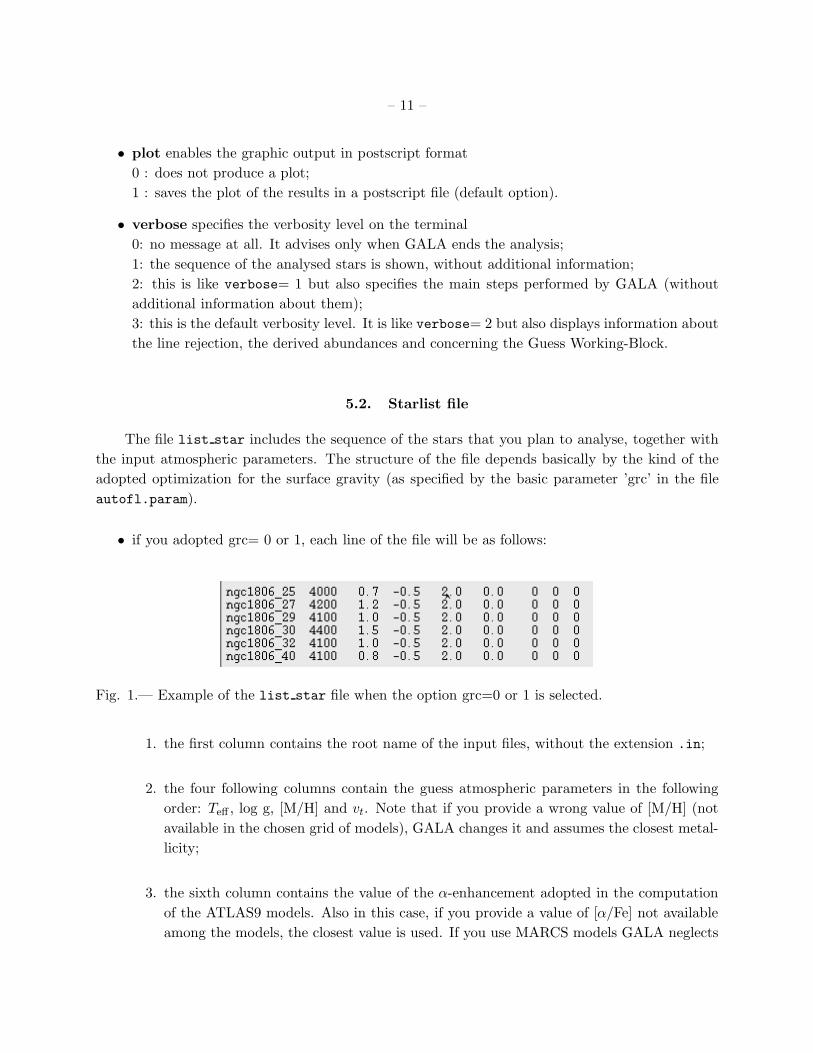
• if you adopted grc= 0 or 1, each line of the file will be as follows:

Fig. 1.— Example of the list star file when the option grc=0 or 1 is selected.

1. the first column contains the root name of the input files, without the extension .in;

2. the four following columns contain the guess atmospheric parameters in the following

order: Te! , log g, [M/H] and vt. Note that if you provide a wrong value of [M/H] (not

available in the chosen grid of models), GALA changes it and assumes the closest metal-

licity;

3. the sixth column contains the value of the &-enhancement adopted in the computation

of the ATLAS9 models. Also in this case, if you provide a value of [&/Fe] not available

among the models, the closest value is used. If you use MARCS models GALA neglects

– 12 –

this parameter;

4. the last three columns are the errors associated to Te! , logg and vt respectively. If

the parameters are optimized spectroscopically, these uncertainties are ignored (you can

also put 0 for all of them, as in the shown case); on the other hand, if a given param-

eter is fixed and the uncertainties with the classical method are requested (uncer=2

in autofl.param), these values are used to vary each parameter computing again the

abundances. If in the input file the parameter uncertainties are 0 but you request to

calculate the abundance uncertainties, the steps used to investigate the parameter space

(and defined by the keywords stepteff, stepgr and stepvt among the basic parameters

in autofl.param) are assumed as parameter errors.

• if you adopted grc= 2, the input file will be

Fig. 2.— Example of the list star file when the option grc=2 is selected.

The additional tenth column " is calculated according to the Stefan-Boltzmann equation as

" = log(4GM#$/L), where G is the gravitational constant, $ the Boltzmann constant and M

and L are the mass and the luminosity of the star. In this case the surface gravity will be

calculated as logg= "+ 4 · log Te!

• if you adopted grc= 3, the input file will be

Fig. 3.— Example of the list star file when the option grc=3 is selected.

where A, B and C are the coe"cients of the quadratic relation log g= A+B·Te!+C·T 2e! .

5.3. Linelist file

For each star (specified by the<rootfilename> in the star list file) an input file<rootfilename>.in

is needed. If the linelist file of a given star listed in list star is not available in the directory,

– 13 –

GALA provides a warning message and moves to the next star. Fig. 4 shows an example of a

linelist input file for GALA. Note that this file does not need a specific numeric format, but it must

contain the following information for each measured line:

• the wavelength (expressed in A);

• the observed EW (expressed in mA);

• the uncertainty in EW (expressed in mA);

• the code of the element in the usual Kurucz notation;

• the logarithm of the oscillator strength;

• the excitation potential (expressed in eV);

• the logarithm of the radiative damping constant, 'rad 10;

• the logarithm of the Stark damping constant, 'stark;

• the logarithm of the Van der Waals damping constant, 'V dW ;

• the velocity parameter & as defined by Barklem et al. (2000) and usually available for many

metallic lines both in the Kurucz/Castelli linelist and VALD databases. If the parameter &

is not available for a given line, the value can be substituted with 0.

Fig. 4.— Example of the linelist input file (<rootfilename>.in) for GALA.

10When one of the ! constants is 0, WIDTH9 calculates its value adopting some theoretical relations (see Castelli

2005b, for more details).

– 14 –

6. Output files

For each star listed in the file list star, GALA will create three output files.

(1) <rootfilename>.abu summarizes the derived parameters, the uncertainties and the

mean abundance for each element available in the input file <rootfilename>.in. Fig. 5 shows an

example of this kind of output file. The first thirteen lines are referred to the adopted analysis:

• the second line is the value of the merit function, that provides an estimate of the goodness

of the solution;

• third, fourth and fifth lines concern the correlation among the lines in the A(El)–EWR ,

A(El)—!ex and A(El)—% planes, summarysing the slope, the Jackknife uncertainty in the

slope, the formal error in the slope, the Spearman rank correlation coe"cient and the zero-

point of the linear fit;

• the sixth line is the di!erence between the average abundances of the chosen element derived

from neutral and single ionized lines, together with its Jackknife uncertainty;

• the seventh line is a flag (Optimization) about the adopted procedure: ’Optimization 1’

indicates that the analysis has been performed as specified in autofl.param, while ’Opti-

mization 0’ advises that during the analysis the optimization of one or more parameters has

been switched o!. The following three lines specify as log g, Te! and vt have been optmized.

The Optimization flag is useful to identify rapidly stars for which the analysis has had some

problems or failures.

• The final atmospheric parameters are written in the twelfth line, together with the adopted

model atmosphere (i.e. ’atlas9’, ’marcs’ or the name of the used individual model). In case of

ATLAS9 models, if some atmospheric layers of the final model atmosphere do not converge

(according to the convergence criteria proposed by Castelli 1988), the number of unconverged

layers is specified. Also, the label PARAMETERS allows to easily extract the final parameters

(for instance with grep or awk commands).

• The uncertainties in the parameters are written in the thirteenth line; at the end of the

line, the parameters of the model atmospheres obtained with the procedure described by

Cayrel et al. (2004) are reported (only if the option uncer= 1 or 2 is used and Te! has been

spectroscopically optimized). Note that these uncertainties in the atmospheric parameters are

calculated by using the Jackknife technique for the optimized parameters: when a parameter

– 15 –

is fixed, the uncertainty is that provided by you in list star, if the latter is 0, the step of

the grid is taken as representative of the error.

• The following lines provide for each element the mean abundance, the dispersion of the mean,

the number of used lines, the net variation of the abundance by using the two models obtained

with the Cayrel et al. (2004) method (columns ’+Cay’ and ’-Cay’) and the net variation of

the abundance by varying each time one only parameter (columns ’+Te!’, ’-Te!’, ’+logg’,

’-logg’, ’+vt’, ’-vt’). Additionally, a summary file (named abundance.final) is provided,

including all the <rootfilename>.abu files for the stars listed in list star;

Fig. 5.— Example of the output file (<rootfilename>.abu) including information about atmo-

spheric parameters, uncertainties and average abundances.

(2) <rootfilename>.EW includes the main information for each transition included in the

input file <rootfilename>.in. Fig. 6 shows a part of this file as reference. The first rows of the

file explain the meaning of the flag about the line rejection. Briefly:

flag = 1 the line is used;

flag = 0 the line is rejected according to the $-clipping algorithm (see Mucciarelli et al. 2013);

flag = –1 the line is rejected because outside the range of valid EWR values specified by ’ewmin’

and ’ewmax’ in ’autofl.param’;

flag = –2 the line is rejected because its error is larger than the boundary value ’error’ in autofl.param;

flag = –3 if the abundance calculation performed byWIDTH9 does not converge, producing a ’NaN’,

the value is substituted with 99.999 and the line excluded by the analysis.

The rest of the file includes for each transition:

– 16 –

• the wavelength (expressed in A);

• the observed EW (expressed in mA);

• the logarithm of the oscillator strength;

• the excitation potential (expressed in eV);

• the derived abundance;

• the error of EW, if provided in input (expressed in mA) ;

• the error in abundance obtained by varying the observed EW of +1$EW ;

• the code of the element in the usual Kurucz notation;

• the flag related to the line rejection;

• the theoretical EW (expressed in mA) calculated by WIDTH9 through Gaussian integration

of the line profile by using the nominal metallicity of the best model (see Castelli 2005b, for

details);

• the net abundance variation calculated according to the method described by Cayrel et al.

(2004) and keeping fixed the e!ective temperature at Te! + $Te! and Te! " $Te! ;

• the net abundance variations due to the variation of each parameter (±$Te! ,±$log g, ±$vt).

Fig. 6.— Example of the output file (<rootfilename>.EW) including information for each indi-

vidual line.

(3) <rootfilename>.ps is the graphical output of GALA where the the main results are

shown and an example of this output is shown in Fig. 7. The first three panels show the behaviour

– 17 –

of the abundances for the chosen element as a function of EWR, !ex and %; the small lower panel

in the first panel shows the behaviour of the EW error as a function of EWR. The blue lines are the

linear fits obtained in each plane. The last panel shows the curve of growth obtained by plotting

EWR as a function of the theoretical EW, defined as EWT= loggf - (!ex.

Black points are the lines in the ionization stage used to optmize Te! and vt, while red points the

lines of the same species but in the other ionization stage; for instance, if you specify 26.00 (Fe I)

in the ’qiron’ parameter, black points in the graphical output will be the neutral iron lines and the

red points the Fe II lines. Empty points are the lines rejected during the analysis (the reason of

the rejection is specified in the <rootfilename>.EW file).

7. How to manage the grids of model atmospheres

The automatization of the chemical analysis as implemented by GALA needs the management

of wide grids of model atmospheres, in order to freely explore the parameter space. Here we briefly

explain how you can obtain the grids of models. It is worth to recall that you do not need to

download all the models described in the following: you can only have the grid of models that

you will use for your analysis. The only caveat is that you cannot call a kind of model in the

autofl.param file if you do not have a directory with all these models.

If you decide to adopt ATLAS9 models for your analysis, you need to create in the correspond-

ing directory three sub-directories, named ODF/, MODELS/ and MODELS-new/ (the latter is

empty and it will be filled with new models progressively using GALA).

Note that the capability to calculate a given ATLAS9 model atmosphere depends on the

availability of the ODF computed with the requested chemical composition. The input guess model

atmosphere has to be as close as possible to the new model in terms of Te! , log g and metallicity in

order to allow a good convergence, but in principle, the output model is independent from the input

one. Thus, when a new ATLAS9 model is requested during the analysis process, GALA looks for

the ODF and Rosseland table corresponding to the requested metallicity, if these tables do exist,

the closest model with that chemical composition is picked as input guess model (GALA recognizes

automatically the closest model), otherwise GALA skips the star and advises you with a warning

message that the selected metallicity is incompatible with the metallicities encoded in GALA. The

extension (in terms of metallicity, &-enhancement and microturbulent velocity) of each ATLAS9

grid is written in the source code of GALA, allowing an easy implementation of additional ATLAS9

grids in the next releases of GALA.

ATLAS9 (F.Castelli)

This dataset includes ODFs calculated for 5 values of microturbulent velocities (namely, 0, 1, 2,

4 and 8 km/s) and two levels of &-enhancement, [&/Fe]=0.0 and +0.4. GALA uses the metal-

licities between –5.5 and +0.5 dex with a step of 0.5. To easily obtain all the needed files, we

provide a wget-based procedure. Move the code downl fx.csh in the directory specified in the file

– 18 –

Fig. 7.— Example of the graphical output (<rootfilename>.ps) of GALA. Left-upper panel

shows the behaviour of the abundances as a function of the reduced EW, EWR (while the small

panel shows the behaviour of the EW error as a function of EWR). Right-upper and left-lower panels

plot the behaviour of the abundances as a function of !ex and of the wavelength, respectively. The

right-lower panel shows an empirical curve of growth. In all the panels the filled circles are the used

lines and empty circles are the rejected lines. Black symbols are the lines used in the optimization

of Te! and vt (Fe I in this case), while red symbols are the lines in the other ionization stage (Fe II

in this case). Blue lines are the linear best-fits.

– 19 –

GALA/src/Paths.f and type

./downl fc.csh

However, in the following we describe the correct way to obtain and manage the ATLAS9 files.

1. In the directory specified in the file GALA/src/Paths.f for this grid of models, create three

subdirectory, named ODF, MODELS and MODELS-new. In the first subdirectory, put ODFs and

Rosseland tables with [M/H] between –5.5 and +0.5 dex (at step of 0.5) and with both the

values of &-enhancement. You can download the ODFs from the website of F. Castelli

http://wwwuser.oat.ts.astro.it/castelli/odfnew.html

(you need only the big ODFs, do not download the lit ODFs), as well as the tables with the

Rosseland mass absorption coe"cients

http://wwwuser.oat.ts.astro.it/castelli/kaprossnew.html.

2. The grids of models are available in the same website

http://wwwuser.oat.ts.astro.it/castelli/grids.html.

For the metallicities used by GALA, all the models of a given [M/H] are available in a single

ASCII file (for instance, master file for [M/H]=+0.5 and [&/Fe]= 0.0 is named ap05k2odfnew.dat,

while for [M/H]=+0.5 and [&/Fe]= +0.4 ap05ak2odfnew.dat.) Save these (14) files in the

subdirectory MODELS. We recommend to download these files (without renaming them), be-

cause GALA looks for these files to pick the input guess model (please, avoid downloading

the grids with peculiar assumptions, as He enhancements and di!erent mixing length values,

because GALA does not (yet) use these grids to search for the input model). Note that when

you ask GALA to use a metallicity outside the range –5.5/+0.5, the star will be analysed by

adopting the closest model.

3. The new ATLAS9 models calculated during the runs of GALA will be saved in the subdi-

rectory MODELS-new, together with a file including the main information about the calcula-

tion of the model. The new models will be named following the same formalism used by

Castelli & Kurucz (2004) for the individual models; for instance, a model with Te!= 4120 K,

log g= 1.32, vturb=2 km/s, [M/H]=–0.5 and [&/Fe]= +0.4 will be saved as am05at4120g132k2odfnew.dat,

will its summary file will be named am05at4120g132k2.log at9.

ATLAS9 (APOGEE)

Recently, Meszaros et al. (2012) computed a new set of ATLAS9 model atmospheres, ODFs and

Rosseland opacity tables, spanning a huge range of metallicity, &-enhancement and C abundances.

– 20 –

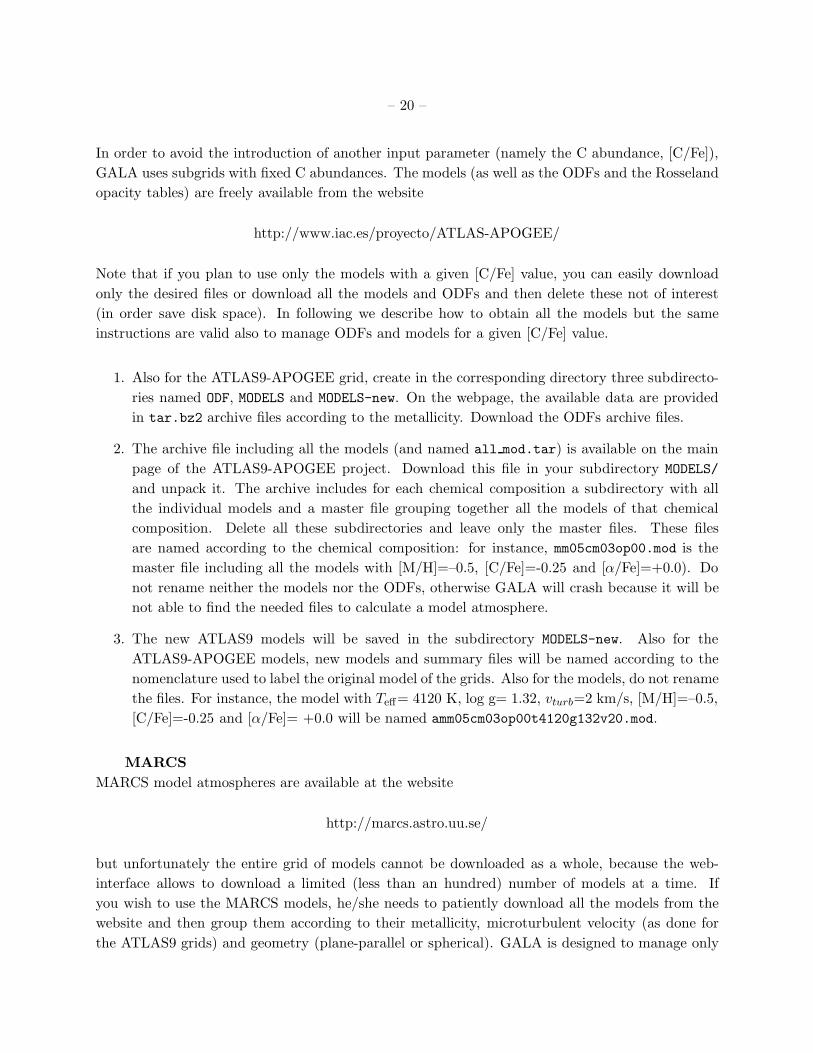
In order to avoid the introduction of another input parameter (namely the C abundance, [C/Fe]),

GALA uses subgrids with fixed C abundances. The models (as well as the ODFs and the Rosseland

opacity tables) are freely available from the website

http://www.iac.es/proyecto/ATLAS-APOGEE/

Note that if you plan to use only the models with a given [C/Fe] value, you can easily download

only the desired files or download all the models and ODFs and then delete these not of interest

(in order save disk space). In following we describe how to obtain all the models but the same

instructions are valid also to manage ODFs and models for a given [C/Fe] value.

1. Also for the ATLAS9-APOGEE grid, create in the corresponding directory three subdirecto-

ries named ODF, MODELS and MODELS-new. On the webpage, the available data are provided

in tar.bz2 archive files according to the metallicity. Download the ODFs archive files.

2. The archive file including all the models (and named all mod.tar) is available on the main

page of the ATLAS9-APOGEE project. Download this file in your subdirectory MODELS/

and unpack it. The archive includes for each chemical composition a subdirectory with all

the individual models and a master file grouping together all the models of that chemical

composition. Delete all these subdirectories and leave only the master files. These files

are named according to the chemical composition: for instance, mm05cm03op00.mod is the

master file including all the models with [M/H]=–0.5, [C/Fe]=-0.25 and [&/Fe]=+0.0). Do

not rename neither the models nor the ODFs, otherwise GALA will crash because it will be

not able to find the needed files to calculate a model atmosphere.

3. The new ATLAS9 models will be saved in the subdirectory MODELS-new. Also for the

ATLAS9-APOGEE models, new models and summary files will be named according to the

nomenclature used to label the original model of the grids. Also for the models, do not rename

the files. For instance, the model with Te!= 4120 K, log g= 1.32, vturb=2 km/s, [M/H]=–0.5,

[C/Fe]=-0.25 and [&/Fe]= +0.0 will be named amm05cm03op00t4120g132v20.mod.

MARCS

MARCS model atmospheres are available at the website

http://marcs.astro.uu.se/

but unfortunately the entire grid of models cannot be downloaded as a whole, because the web-

interface allows to download a limited (less than an hundred) number of models at a time. If

you wish to use the MARCS models, he/she needs to patiently download all the models from the

website and then group them according to their metallicity, microturbulent velocity (as done for

the ATLAS9 grids) and geometry (plane-parallel or spherical). GALA is designed to manage only

– 21 –

the grids with standard chemical composition and microturbulent velocities 1 and 2 km/s, but

modified versions of the code can be provided on request for other sub-grids of MARCS models.

Because the grid of models with standard chemical composition naturally varies the &-enhancement

according to the metallicity, for these models it is not necessary to group them for the value of the

&-enhancement, at variance with the ATLAS9 models. Each master file needs to have a precise

name. In Fig. 8 we summarize the name of these master files, as expected by GALA, together with

the corresponding metallicity and geometry, and the total number of included models.

Fig. 8.— List of the files with the MARCS models grouped according to their metallicity, micro-

turbulent velocities and geometry.

– 22 –

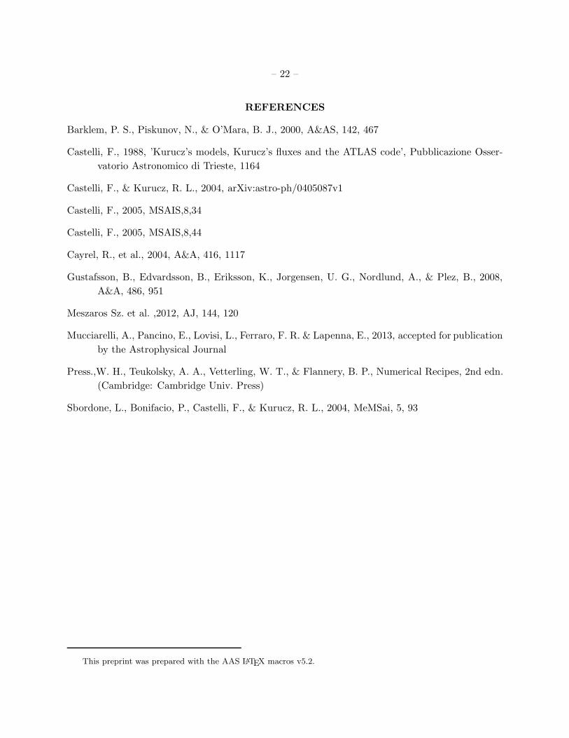
REFERENCES

Barklem, P. S., Piskunov, N., & O’Mara, B. J., 2000, A&AS, 142, 467

Castelli, F., 1988, ’Kurucz’s models, Kurucz’s fluxes and the ATLAS code’, Pubblicazione Osser-

vatorio Astronomico di Trieste, 1164

Castelli, F., & Kurucz, R. L., 2004, arXiv:astro-ph/0405087v1

Castelli, F., 2005, MSAIS,8,34

Castelli, F., 2005, MSAIS,8,44

Cayrel, R., et al., 2004, A&A, 416, 1117

Gustafsson, B., Edvardsson, B., Eriksson, K., Jorgensen, U. G., Nordlund, A., & Plez, B., 2008,

A&A, 486, 951

Meszaros Sz. et al. ,2012, AJ, 144, 120

Mucciarelli, A., Pancino, E., Lovisi, L., Ferraro, F. R. & Lapenna, E., 2013, accepted for publication

by the Astrophysical Journal

Press.,W. H., Teukolsky, A. A., Vetterling, W. T., & Flannery, B. P., Numerical Recipes, 2nd edn.

(Cambridge: Cambridge Univ. Press)

Sbordone, L., Bonifacio, P., Castelli, F., & Kurucz, R. L., 2004, MeMSai, 5, 93

This preprint was prepared with the AAS LATEX macros v5.2.

gala cookbook - cosmic-lab · · 2013-02-16gala cookbook alessio mucciarelli ... 3 ... 7. write...

Documents