gait generation for damaged hexapods using genetic algorithm
TRANSCRIPT

Rochester Institute of Technology Rochester Institute of Technology
RIT Scholar Works RIT Scholar Works
Theses
5-2020
Gait Generation for Damaged Hexapods using Genetic Algorithm Gait Generation for Damaged Hexapods using Genetic Algorithm
Justin Kon [email protected]
Follow this and additional works at: https://scholarworks.rit.edu/theses
Recommended Citation Recommended Citation Kon, Justin, "Gait Generation for Damaged Hexapods using Genetic Algorithm" (2020). Thesis. Rochester Institute of Technology. Accessed from
This Thesis is brought to you for free and open access by RIT Scholar Works. It has been accepted for inclusion in Theses by an authorized administrator of RIT Scholar Works. For more information, please contact [email protected].

RIT
Gait Generation for Damaged Hexapods using Genetic Algorithm
By
Justin Kon
A Thesis Submitted in Partial Fulfillment of the Requirements for the Degree of Master of Science in Electrical Engineering
Supervised by
Professor Dr. Ferat Sahin
Department of Electrical and Microelectronic Engineering Kate Gleason College of Engineering
Rochester Institute of Technology Rochester, New York
May 2020
Approved by: _______________________________________________________________
Dr. Ferat Sahin, Professor Thesis Advisor, Department of Electrical and Microelectronic Engineering _______________________________________________________________
Dr. Jamison Heard, Assistant Professor Committee Member, Department of Electrical and Microelectronic Engineering _______________________________________________________________
Dr. Gill Tsouri, Professor Committee Member, Department of Electrical and Microelectronic Engineering _______________________________________________________________
Dr. Sohail A. Dianat, Department Head Committee Member, Department of Electrical and Microelectronic Engineering

Gait Generation for Damaged Hexapods using a GeneticAlgorithm
Justin Kon
May 5, 2020
1

Acknowledgments
I would like to give special thanks to Dr. Ferat Sahin. For not only supporting but
encouraging the creativity of your students and for always pushing us to achieve at the
highest levels possible.
Thank you as well to the members of the Multi-Agent Bio-robotics Laboratory. This
experience was multitudes better with thanks to the support from Xavier Tarr, Celal Savur,
Anmol Modur, Shitij Kumar and Karthik Subramanian.
I would like to thank my parents Sandra Kon and Douglas Kon. For years of support and
encouragement of my dreams, as well as your tireless efforts to provide every opportunity
imaginable.
To my friends. Nicolas Law, Allison Crim, Xavier Tarr, Eli Laramie, Christopher Swider,
Derek Bargelt and Nathan Messana. You each have had a tremendous impact on my life
and I am so glad to know you all. Thank you for the many years of friendship that have
lead me here and I look forward to the many years to come.
This would not have been possible with out the endless support, and assistance of nu-
merous wonderful people. Whether you served as a sounding board, a guiding hand or even
just lent a supportive ear, know that you helped make this possible.
2
Abstract
This paper discusses the design and implementation of a Genetic Algorithm for the gen-
eration of gaits compensating for system damage on the joint level of a hexapod system.
The hexapod base used for this algorithm consists of six three degree of freedom legs on
a rectangular body. The purpose of this algorithm is to generate a gait such that when N
motors become inoperable, as detected by the robot’s internal software, the system is able to
continue moving about its environment. While algorithms like this have been implemented
before, the generated gaits are a sequence of discrete foot positions. This work aims to gen-
erate continuous motions profiles for each joint of the leg rather than discrete foot positions.
Previous works commonly disable an entire leg when damage occurs, instead this work aims
to disable only individual joint motors.
3

List of Contributions
• Design and implementation of simulation model for the hexapod-quadcopter system.
• Design and implementation of a Genetic Algorithm for the generation of gaits to com-
pensate for damage in a hexapod system.
• J. Kon, F. Sahin, ”Gait Generation for Damaged Hexapods using a Genetic Algorithm”
2020 IEEE International Conference on System of Systems Engineering (SoSE), Ac-
cepted for publication. [17]
4
Contents
1 Introduction 11
2 Literature Review 13
2.1 Gait Generation . . . . . . . . . . . . . . . . . . . . . . . . . . . . . . . . . . 13
2.2 Algorithm . . . . . . . . . . . . . . . . . . . . . . . . . . . . . . . . . . . . . 15
2.3 Simulation Environment . . . . . . . . . . . . . . . . . . . . . . . . . . . . . 16
3 Hexapod Platform 18
4 Model Generation 21
5 Gazebo 33
5.1 PID Tuning . . . . . . . . . . . . . . . . . . . . . . . . . . . . . . . . . . . . 34
5.2 Launching Multiple Robots . . . . . . . . . . . . . . . . . . . . . . . . . . . 34
5.3 Torque Limits . . . . . . . . . . . . . . . . . . . . . . . . . . . . . . . . . . . 36
5.4 Damage Modeling . . . . . . . . . . . . . . . . . . . . . . . . . . . . . . . . . 37
6 Algorithm 38
6.1 Theory of Genetic Algorithms . . . . . . . . . . . . . . . . . . . . . . . . . . 38
6.2 Algorithm Overview . . . . . . . . . . . . . . . . . . . . . . . . . . . . . . . 38
6.3 Homogeneous Population Check . . . . . . . . . . . . . . . . . . . . . . . . . 41
6.4 Crossover . . . . . . . . . . . . . . . . . . . . . . . . . . . . . . . . . . . . . 45
6.5 Mutation Rate . . . . . . . . . . . . . . . . . . . . . . . . . . . . . . . . . . 45
6.6 Example Gait . . . . . . . . . . . . . . . . . . . . . . . . . . . . . . . . . . . 46
6.7 Data Structure . . . . . . . . . . . . . . . . . . . . . . . . . . . . . . . . . . 46
6.8 Development Testing . . . . . . . . . . . . . . . . . . . . . . . . . . . . . . . 47
6.9 Fitness Functions . . . . . . . . . . . . . . . . . . . . . . . . . . . . . . . . . 48
6.10 Population . . . . . . . . . . . . . . . . . . . . . . . . . . . . . . . . . . . . . 50
5

6.11 Parent Selection and Child Generation . . . . . . . . . . . . . . . . . . . . . 52
6.12 Survivor Selection . . . . . . . . . . . . . . . . . . . . . . . . . . . . . . . . . 53
6.13 Search Time . . . . . . . . . . . . . . . . . . . . . . . . . . . . . . . . . . . . 54
6.14 Improvements . . . . . . . . . . . . . . . . . . . . . . . . . . . . . . . . . . . 55
7 MATLAB 55
7.1 Memory leak . . . . . . . . . . . . . . . . . . . . . . . . . . . . . . . . . . . 56
8 Results 57
8.1 Gait Generation . . . . . . . . . . . . . . . . . . . . . . . . . . . . . . . . . . 57
8.2 Damage Compensation . . . . . . . . . . . . . . . . . . . . . . . . . . . . . . 60
8.2.1 Right Center Tibia and Left Center Tibia . . . . . . . . . . . . . . . 64
8.2.2 Left Front Tibia . . . . . . . . . . . . . . . . . . . . . . . . . . . . . . 65
8.2.3 Left Center Coxa . . . . . . . . . . . . . . . . . . . . . . . . . . . . . 66
8.2.4 Left Back Coxa and Right Center Femur . . . . . . . . . . . . . . . . 67
8.2.5 Left Front Femur and Left Center Tibia . . . . . . . . . . . . . . . . 68
8.2.6 Gait Comparisons . . . . . . . . . . . . . . . . . . . . . . . . . . . . . 69
8.2.7 Damage Gait Summary . . . . . . . . . . . . . . . . . . . . . . . . . 71
9 Conclusions 73
10 Future work 73
6
List of Figures
1 Hexapod Platform . . . . . . . . . . . . . . . . . . . . . . . . . . . . . . . . 19
2 Hexapod Leg . . . . . . . . . . . . . . . . . . . . . . . . . . . . . . . . . . . 19
3 Dynamixel ax-12a motor (a) front (b) back . . . . . . . . . . . . . . . . . . . 20
4 SOLIDWORKS assembly of complete hexapod quadcopter model . . . . . . 21
5 SOLIDWORKS hexapod quadcopter Base link model . . . . . . . . . . . . . 22
6 SOLIDWORKS hexapod quadcopter shoulder model . . . . . . . . . . . . . 23
7 SOLIDWORKS hexapod quadcopter coxa model . . . . . . . . . . . . . . . . 23
8 SOLIDWORKS hexapod quadcopter center femur model . . . . . . . . . . . 24
9 SOLIDWORKS hexapod quadcopter outer femur model . . . . . . . . . . . . 24
10 SOLIDWORKS hexapod quadcopter center tibia model . . . . . . . . . . . . 25
11 SOLIDWORKS hexapod quadcopter outer tibia model . . . . . . . . . . . . 25
12 SOLIDWORKS Exporter Selection . . . . . . . . . . . . . . . . . . . . . . . 26
13 SOLIDWORKS Flexible Component . . . . . . . . . . . . . . . . . . . . . . 27
14 URDF Link Tree . . . . . . . . . . . . . . . . . . . . . . . . . . . . . . . . . 27
15 URDF Final Configuration . . . . . . . . . . . . . . . . . . . . . . . . . . . . 29
16 SOLIDWORKS Mesh URDF Top View . . . . . . . . . . . . . . . . . . . . . 30
17 SOLIDWORKS Mesh URDF Side View . . . . . . . . . . . . . . . . . . . . . 30
18 Non-Mesh Block URDF Top View . . . . . . . . . . . . . . . . . . . . . . . . 31
19 Non-Mesh Block URDF Side View . . . . . . . . . . . . . . . . . . . . . . . 31
20 URDF Component Selection . . . . . . . . . . . . . . . . . . . . . . . . . . . 32
21 URDF Inertia Reference Frame . . . . . . . . . . . . . . . . . . . . . . . . . 33
22 Algorithm Flow Chart . . . . . . . . . . . . . . . . . . . . . . . . . . . . . . 39
23 Mathematical Fitness Trial - 100 Generations No Homogeneity Test . . . . . 41
24 Mathematical Fitness Trial - 100 Generations Homogeneity Check Every Five
Generations . . . . . . . . . . . . . . . . . . . . . . . . . . . . . . . . . . . . 42
7

25 Mathematical Fitness Trial - 100 Generations Homogeneity Check Every Twenty
Generations . . . . . . . . . . . . . . . . . . . . . . . . . . . . . . . . . . . . 42
26 Mathematical Fitness Trial - 100 Generations Homogeneity Check Every Fifty
Generations . . . . . . . . . . . . . . . . . . . . . . . . . . . . . . . . . . . . 43
27 Mathematical Fitness Trial - 100 Generations Homogeneity Check Scaling
Frequency . . . . . . . . . . . . . . . . . . . . . . . . . . . . . . . . . . . . . 43
28 Mathematical Fitness Trial - 100 Generations and 100 Population Homogene-
ity Check Scaling Frequency . . . . . . . . . . . . . . . . . . . . . . . . . . . 44
29 Crossover Visualization . . . . . . . . . . . . . . . . . . . . . . . . . . . . . . 45
30 Algorithm Data Structure . . . . . . . . . . . . . . . . . . . . . . . . . . . . 47
31 URDF Final Configuration . . . . . . . . . . . . . . . . . . . . . . . . . . . . 48
32 Algorithm Data Structure . . . . . . . . . . . . . . . . . . . . . . . . . . . . 51
33 Algorithm Data Structure . . . . . . . . . . . . . . . . . . . . . . . . . . . . 51
34 Algorithm Data Structure . . . . . . . . . . . . . . . . . . . . . . . . . . . . 52
35 Parent Selection, Child Generation and Survivor Selection Process Visualization 53
36 Algorithm Verification with Randomized Population . . . . . . . . . . . . . . 57
37 Algorithm Verification with Single Seed Population . . . . . . . . . . . . . . 58
38 Algorithm Verification Homogeneous Seed . . . . . . . . . . . . . . . . . . . 59
39 Algorithm Verification with Higher Mutation Rate . . . . . . . . . . . . . . . 60
40 Damage Generation - Left Back Femur Fitness Function 1 . . . . . . . . . . 61
41 Damage Generation - Left Back Femur Fitness Function 2 . . . . . . . . . . 62
42 Damage Generation - Right Center Tibia Fitness Function 1 . . . . . . . . . 63
43 Damage Generation - Right Center Tibia Fitness Function 2 . . . . . . . . . 63
44 Damage Generation - Right Center Tibia and Left Center Tibia . . . . . . . 65
45 Damage Generation - Right Center Tibia and Left Center Tibia . . . . . . . 66
46 Damage Generation - Left Center Coxa . . . . . . . . . . . . . . . . . . . . . 67
47 Damage Generation - Left Back Coxa and Right Center Femur . . . . . . . . 68
8

48 Damage Generation - Left Front Femur and Left Center Tibia . . . . . . . . 69
9

List of Tables
1 Comparison of custom tripod gait and AI generated gait for various damaged
states . . . . . . . . . . . . . . . . . . . . . . . . . . . . . . . . . . . . . . . 70
10

1 Introduction
This paper discusses the design and implementation of a Genetic Algorithm (GA) based
Artificial Intelligence (AI) algorithm for the generation of gaits to compensate for system
damage on the joint level of a hexapod system. The hexapod base used for this algorithm
consists of six 3 degree of freedom legs on a rectangular body. The purpose of this algo-
rithm is to generate a gait such that when N motors become inoperable, as detected by the
robot’s internal software, the system is able to continue moving about its environment. At
a minimum this will aid in the recovery of the robot and ideally allow the robot to continue
its work completing tasks as accurately as possible.
Robots have become more and more prevalent is every aspect of modern life. We have seen
robots making their way into every environment from assembly lines to battle fields and from
home assistance to nature exploration. With the increase in robotics usage it is important to
increase the usability and adaptability of such robots as well. Early robotic systems held few
contingencies for behaviour post damage. This was in part due to technological limitations
when it came to system sensing, as well as limitations in our understanding of such systems
and their control, both of which have seen significant improvement over time. With current
system sensing and control understanding robotic systems are able to adapt to new situations
and behave much more like living organisms. When it comes to legged robotic systems the
primary behaviour for adaptation is the systems method of locomotion. When humans or
animals become injured their method of walking adapts to their injury when possible, and
this can be applied to robots as well.
The implementation of a standard hexapod gait, for example a tripod, ripple or wave gait,
relies on the functionality of all leg motors. If a singular motor is lost the hexapod can no
longer rely on traditional gaits as it will not walk in the desired, controlled manner. However,
using AI a gait could be generated to compensate for a lack of N number of joint control
motors. The value of N can be a small as 0. The maximum value of N, while maintaining
appropriate system functionality, depends heavily on which motors are lost. For example, 3
11

motors could be lost from a single leg and the system would be able to maintain function.
This is just a transition from a hexapod to a pentapod. However, if 3 coxa motors, coxa
being the joint controlling the forward and backward motion of the leg, are lost it is very
likely that the system will not be able to compensate for this state. As such, the hexapod
system can detect the 18 motor states and compare to a list of recoverable damaged states.
In doing so generation of a gait can be done based on the known viability of the motor states.
Depending on the time necessary to generate such a gait it may also be desired that rather
than detecting a damaged state and generating a gait, the system instead detects its state
and pulls the associated pre-generated compensation gait from a look up table.
In a broader sense, algorithms such as this can be used to close the gap between robotic
systems and biological agents. Robots are only as capable as their designers plan for. This is
not to say that systems should be fully autonomous, but that systems should be as capable
as possible with respect to their function. Taking the task of locomotion as example, this
is a task so fundamentally critical to many different systems that the inability to move
destroys all benefits of using a robotic system. In critical tasks such as these, systems should
be enabled to adapt to changing situations. It is entirely illogical for a human to become
useless due to a stubbed toe, or a broken finger, and it seems just as illogical for a robotic
system to become useless because of a singular broken part. Procedures allowing systems
to adapt do not need to be fit specifically to damaged states either. Adaptive locomotion
planning can allow a system to adapt complex terrains, or even something as simple as
environmental factors such as high winds.
Keywords: Hexapod, Genetic Algorithm, Evolutionary Algorithm, Artificial Intelli-
gence, Damaged Gait, Gazebo, MATLAB, ROS, Gait Simulation
12
2 Literature Review
2.1 Gait Generation
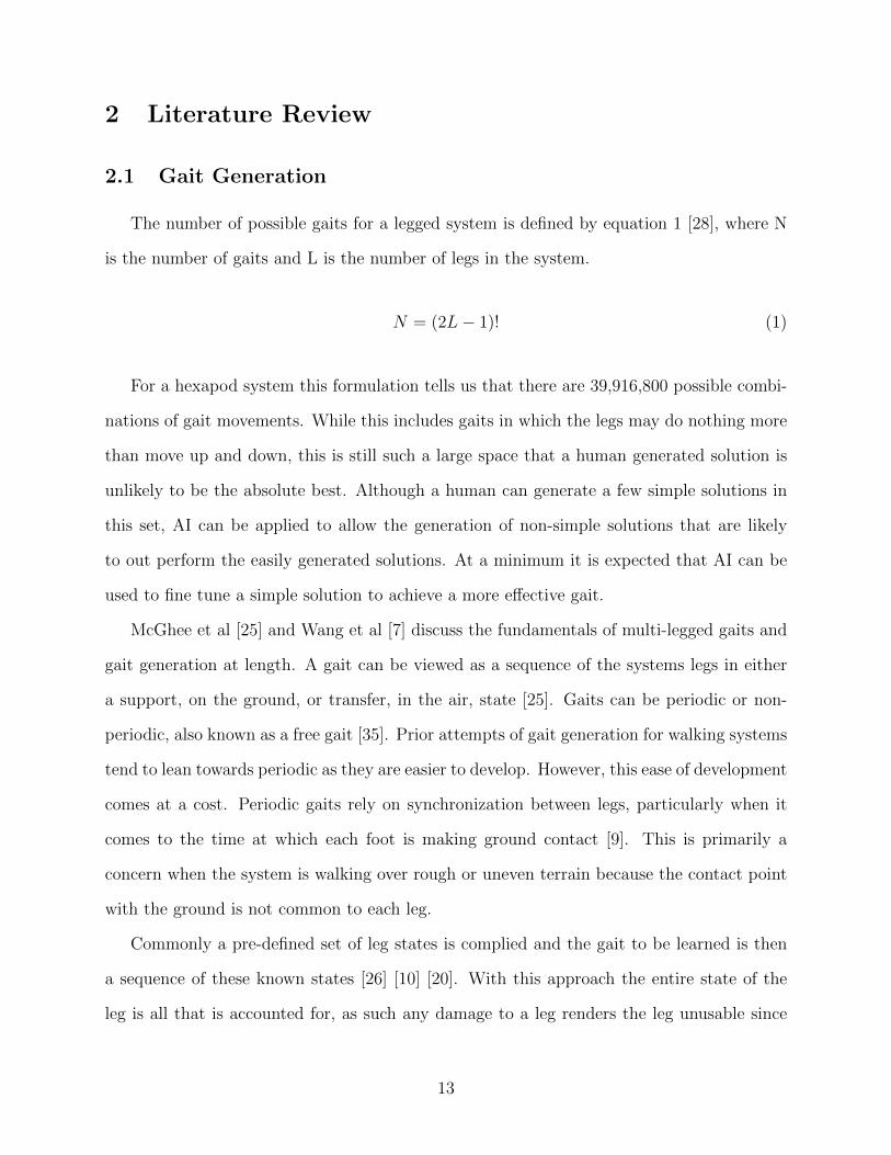
The number of possible gaits for a legged system is defined by equation 1 [28], where N
is the number of gaits and L is the number of legs in the system.
N = (2L− 1)! (1)
For a hexapod system this formulation tells us that there are 39,916,800 possible combi-
nations of gait movements. While this includes gaits in which the legs may do nothing more
than move up and down, this is still such a large space that a human generated solution is
unlikely to be the absolute best. Although a human can generate a few simple solutions in
this set, AI can be applied to allow the generation of non-simple solutions that are likely
to out perform the easily generated solutions. At a minimum it is expected that AI can be
used to fine tune a simple solution to achieve a more effective gait.
McGhee et al [25] and Wang et al [7] discuss the fundamentals of multi-legged gaits and
gait generation at length. A gait can be viewed as a sequence of the systems legs in either
a support, on the ground, or transfer, in the air, state [25]. Gaits can be periodic or non-
periodic, also known as a free gait [35]. Prior attempts of gait generation for walking systems
tend to lean towards periodic as they are easier to develop. However, this ease of development
comes at a cost. Periodic gaits rely on synchronization between legs, particularly when it
comes to the time at which each foot is making ground contact [9]. This is primarily a
concern when the system is walking over rough or uneven terrain because the contact point
with the ground is not common to each leg.
Commonly a pre-defined set of leg states is complied and the gait to be learned is then
a sequence of these known states [26] [10] [20]. With this approach the entire state of the
leg is all that is accounted for, as such any damage to a leg renders the leg unusable since
13

the foot is no longer able to reach the desired position. While this simplifies the problem, it
also means that damage to the system will simply downgrade the robot from a hexapod to
a pentapod and so on. When we sprain our ankle we do not sacrifice the full use of our leg,
and why should a robot?
When compensating for damage there is the major question of what is the the compen-
sation achieving. A gait could be oriented towards stability, speed, energy consumption,
or any other criteria desired [21]. In most cases static stability is the subject of optimiza-
tion [19] [20] [33] [21] [25] [26] [1] [24] [6] [3]. Alternatively Clune et al aims to minimize gait
drift which can be seen as an optimization of the accuracy of the gait [5] . Lastly, Belter
et al aimed to optimize for speed, specifically while on flat terrain [2]. While stability is
an important aspect of gaits, recovery of the system is the aim of this work and as such
speed and accuracy will be the top priorities with stability as the secondary focus. Stability
must still be considered because in a damaged state the robot is more susceptible to further
damage. As such, a gait with higher stability can decrease the chances of further damaging
the system.
Prior works show that modeling of the hexapod system is most commonly achieved
mathematically through the use of forward or inverse kinematics. These equations are used
to obtain the location of the center of mass and the foot positions of the robot. Using
this information polygon stability can be analyzed to determine the static stability of the
robot in each frame of a gait [20] [33] [21] [25] [26] [1] [24] [6] [3]. With the advent of
physics simulation environments a system can be modeled and its behavior simulated. For
the simulation to be meaningful requires the generation of a simulation that is as accurate
to the real world and real system as possible. The importance of simulation accuracy and
the problems associated with simulations are discussed by Chebotar et al [4], and Husbands
et al [14]. While physics simulation environments are by no means new, few examples of
simulations applied to hexapod gait generation were found [11] [5].
The method of compensation is an important aspect of focus when designing a compen-
14

sation generation system as the designer must consider at what level to compensate. If a
single motor is broken, do you sacrifice the entire leg? While doing so may prevent further
damage to an already damaged system [1] [33], this severely limits the number of compen-
sation methods and in general the number of compensation actions available to the system.
The question ultimately draws itself back to the design of the system. If the system is not
well sealed or enclosed, then it is likely much safer for the system to entirely not rely on a
partially damaged limb, this eliminates the possibility of damage to internal systems as well
as further damage to the limb as a whole. However, with sufficient enclosures and shielding
there can be minimal risk to internal devices and structures allowing for less careful use of
the limb. While the system still risks further damage by relying on a partially damaged
limb, there is significantly more room for compensation. This room provides a higher level
of maintained functionality post damage better enabling the system to carry on with its
desired tasks.
2.2 Algorithm
Real et al discuss numerous approaches, and the difficulties faced by each, to using
machine learning for a variety of legged locomotion efforts [32]. This work focuses particularly
on the approach of a hexapod system, which increases the generalized stability of gaits,
walking in a straight path over smooth terrain.
Prior works show a few common approaches to gait generation. One approach is the
application of evolutionary algorithms such as genetic algorithms and particle swarm opti-
mization [26] [8] [24] [15]. Another is the use of central pattern generators [11]. There are
also cases in which multiple approaches are used, such as the use of an evolutionary algo-
rithm used to tune a neural network [15], a not uncommon process in other applications. As
well as applications of reinforcement learning and Q-learning used for the same system in
different situations [18].
For this work an evolutionary approach was desired to learn a gait to compensate for a
15

hexapod system in a damaged state. Two primary methods were considered, Genetic Al-
gorithms and Particle Swarm Optimization. The prime determining factor between these
approaches was the form of the desired generated data. Ultimately, a 54 dimensional indi-
vidual is considered. It is important that each individual is represented accurately and due
to the high dimensionality it was not practical to use particle swarm optimization due to the
inability to properly control the bounds of particles in high dimensional cases. Although it
is possible to simply detect and redefine boundary breaking solutions this approach would
add unnecessary complication to the algorithm due to the high dimensionality of the search
space. When working with high dimensional functions in particle swarm optimization there
is a high probability that every 4th dimension will ignore boundary limitations set by the
user [12]. While there are methods to prevent such errant behavior [16] [29], there are side
effects to some of these common bound handling methods [12]. Most notably, there is a high
probability that the global guide will break boundaries every fourth dimension, this value
is derived from the probability of a particle being generated or initialized near a boundary
on any given dimension [12]. As such, if boundary handling methods are implemented then
the behavior of the bound handling method will influence the behavior of the entire algo-
rithm [12] [13]. This is because the behavior of the global guide directly factors into the
velocity of every particle in the algorithm. As such, the approach of Genetic Algorithms was
chosen to eliminate the possibility of skewing solutions due to boundary handling.
The use of Genetic Algorithms to generate damage compensation gaits is certainly not
a new one. Most prior efforts use a GA or GA variant [30] [24] to discover a sequence of
predetermined leg positions to define a gait.
2.3 Simulation Environment
The robot serving as the design platform for this work, discussed later, makes use of ROS.
As such, the ability to interface ROS with the simulation environment was the first factor
considered when choosing a simulation environment. Other determining factors include:
16

physics engines, 3D visualization, compatible operating systems, and compatible program-
ming languages. A sample of simulation environments are compared as discussed by Noori
et al [27].
1) Virtual Robot Experimentation Platform (V-REP) is a commercial product developed
by Copella Robotics**. VREP supports C++, is available on Linux, supports 3D simulation
and supports multiple physics engines. However, it is not innately interfaceable with ROS.
2) Gazebo is currently maintained by the Open Source Robotics Foundation (OSRF).
Like V-REP, Gazebo supports C++, is available on Linux, supports 3D simulation and
supports multiple physics engines. Gazebo also innately supports ROS interfacing.
3) The Modular Open Robotics Simulation Environment (MORSE) was designed in
France and intended for use with Blender. Morse is supports Python, Linux, 3D simula-
tion, and supports the Bullet physics engine. It is not innately interfaceable with ROS.
4) The United System for Automation and Robot Simulation (USARSim) was designed
with the intent to be used with Unreal Tournament (UT) game engine. It works well with
the Mobility Open Architecture Simulation and Tool Framework (MOAST). USARSim is
available in C++, supports Linux, supports 3D simulation, and supports the Unreal Physics
Engine. But is not innately interfaceable with ROS.
The primary language chosen for this work is C++ due to its general prevalence, and
familiarity with the language. Between familiarity with Gazebo as well as the innate support
in ROS it was the most desirable option.
One significant benefit of the Gazebo environment is the controllers. Within Gazebo
the data generated by controllers is published in shared memory which allows inter-process
communication between robot control software and Gazebo independent of programming lan-
guages [31]. The Gazebo environment also provides access to many high performance physics
engines such as the Open Dynamics Engine, Bullet, Simbody and Dynamic Animation [31].
Gazebo is also a simulation environment that was specifically designed to accurately repro-
duce dynamic environments common in robotic applications [34]. Combined, these factors
17

made Gazebo the choice environment for this work.
3 Hexapod Platform
This work was inspired by the system designed by Pitonyak [23] [22]. His system serves
as the source for the model used throughout this work, and is shown in figure 1. The model
consists of six 3 degree of freedom legs as shown in figure 2. Each joint is controlled by
a singular servo motor, the servos are dynamixel ax-12a and ax-18a. Figure 3 shows the
dynamixel ax-12a motor, the ax-18a motors have the same hardware package with differing
internal components to yield a higher torque. The ax-18a motors control the coxa motion of
the four outer legs, and were used to compensate for the additional weight of fight hardware
in the four outer legs. The remaining fourteen servo motors are all ax-12a. The dynamixel
servos operate on digital packets and can be daisy chained with each motor taking messages
based on its assigned identification number. In this case the coxa, femur and tibia motors
are daisy chained and effect the control of everything downstream of themselves respectively.
This means that if communication is lost with a motor it is likely that all motors downstream
will be lost as well due to communication channels.
18

Figure 1: Hexapod Platform
Figure 2: Hexapod Leg
19

Figure 3: Dynamixel ax-12a motor (a) front (b) back
The coxa motor controls the forward and backwards motion of the entire leg. The femur
motor controls the raising and lowering of the remainder of the leg and the tibia motor
controls the raising and lowering of the foot directly. The four outer legs of the hexapod
system are all alike and the two center legs are alike. The outer legs hold extra hardware
associated with the flight capabilities of the system in the tibia segment and the femur
segments are bifurcated, however the coxa is the same in all legs. While the original system
has flight capabilities, although all hardware is contained in the model flight capabilities
were not added to the system simulation. Only walking procedures are accounted for in this
work.
The dynamixel servos have built in sensing for multiple common motor faults, these faults
are detectable to the overarching system through the digital packet sent by the motor. These
faults include low/high voltage, low/high temperature, out of bounded position, instruction
error, torque overload, and invalid command. Because the dynamixel servos communicate
with the overarching system, a lack of communication can also be detected, this could be
caused by damage rendering a motor inoperable, be it from direct damage to the motor or
20

damage to the communication channels used by the motors. Using this motor state data, a
gait can be generated to compensate for lack of function in specific joints rather than simply
not using a leg as previous works have done.
4 Model Generation
To generate the simulation model of the hexapod-quadcopter system the SOLIDWORKS
to URDF exporter was used. The exporter is an add on available for download that takes a
SOLIDWORKS assembly and generates a mesh URDF. The first step for this process was
to move the existing CAD models from Autodesk Inventor to SOLIDWORKS. A complete
CAD assembly of the hexapod-quadcopter system used in this work can be seen in figure 4.
Figure 4: SOLIDWORKS assembly of complete hexapod quadcopter model
To use the exporter a SOLIDWORKS assembly is made in which all parts are mated
with appropriate constraints. The model should be a digital replica of the real or intended
21

system. For simplicity sub-assemblies can be made, these sub-assemblies should be the
individual links of the intended final URDF model. When making the sub-assemblies the
motion and location of each joint movement should be kept in mind. Although a component
may be a portion of the link, the motion may be such that the component is better located
in a different link. An example of this is the coxa segment. Although the coxa motor is
without a doubt part of the coxa link only the bracket is included in the sub-assembly. This
is done because in the real system the motor remains fixed to the system while rotating the
bracket about the end of the motor. The seven main sub-assemblies used in this model are
the base link or body in figure 5, the shoulder in figure 6, the coxa in figure 7, the center
femur in figure 8, the outer femur in figure 9, the center tibia in figure 10, and the outer
tibia in figure 11.
Figure 5: SOLIDWORKS hexapod quadcopter Base link model
22

Figure 6: SOLIDWORKS hexapod quadcopter shoulder model
Figure 7: SOLIDWORKS hexapod quadcopter coxa model
23

Figure 8: SOLIDWORKS hexapod quadcopter center femur model
Figure 9: SOLIDWORKS hexapod quadcopter outer femur model
24

Figure 10: SOLIDWORKS hexapod quadcopter center tibia model
Figure 11: SOLIDWORKS hexapod quadcopter outer tibia model
Separating the model in to sub-assemblies allows a user to select a singular sub-assembly
as a link in the exporter, shown in figure 12. If sub-assemblies are used the user may not
25

be able to move components of the sub-assembly or the entire sub-assembly upon inserting
the sub-assembly into the full model. This means that the assembly was inserted as rigid
which will cause the exporter to interpret the joints as fixed rather than movable. To re-
enable motion of a sub-assembly the user simply needs to select the part and change to
solve as flexible shown in figure 13. When running the exporter, a link is identified and its
components selected as shown in figure 12. The next step is to select a number of child
links, each child link of a given link generates a joint at the connection of the two links. The
final link tree for the hexapod-quadcopter can be seen in figure 14. For brevity only one
outer and center leg are expanded, however each outer and center leg follow the same format
exchanging the first two characters based on the leg.
Figure 12: SOLIDWORKS Exporter Selection
26

Figure 13: SOLIDWORKS Flexible Component
Figure 14: URDF Link Tree
Finally, the exporter can be run at which point the location of each defined link, location
of each joint and the axis of movement of each joint is generated by the exporter. When
27
choosing links and joints each must be named, it is best to find some sort of naming conven-
tion for both the links and joints. For the hexapod-quadcopter system the links were named
as the base link, which is the only required name, followed by fixed shoulder joints, linked
to the coxas, followed by femurs and finally tibias for the left and right, front, center and
back legs. The outer legs also contain links for the flight motor and two propeller blades.
Although the flight hardware is included in the system model, none of the flight hardware
or flight functionalities are used in this work. A complete diagram of the system can be seen
in figure 14.
It is important to consider the positioning of the system assembly before exporting the
model as the position becomes the zero location for the model. As such, it was desired to
position all legs of the hexapod-quadcopter in a similar way such that the zero or home
position of the model is a uniform position, the home position of the model is shown in
figure 4.
Upon starting the export the user will have the opportunity to review the link and joint
names and have the opportunity to insert numerous other parameters such as moments of
inertia, joint type, joint torque limit, and joint velocity limit as shown in figure 15. Once
the export is complete a ROS ready package is obtained, the user simply needs to insert the
package into a ROS environment and the URDF is ready to be used.
28

Figure 15: URDF Final Configuration
The final URDF is displayed in the gazebo environment in figure 17. After working with
simulation environment the mesh URDF was abandoned for a simplified non-mesh URDF
shown in figure 19. This change allowed the simulation environment to run faster due to
the significant simplification of the physics model. Increased simulation speed was needed
to decrease the training time required for the gait generation algorithm.
29

Figure 16: SOLIDWORKS Mesh URDF Top View
Figure 17: SOLIDWORKS Mesh URDF Side View
30

Figure 18: Non-Mesh Block URDF Top View
Figure 19: Non-Mesh Block URDF Side View
There were a few issues found in using the SOLIDWORKS to URDF exporter. First,
when selecting the components for a link it was found that all components must be selected
31

from the assembly menu shown in figure 20. Second, the selected components must be sin-
gular parts or parts all of which are located in the same sub-assembly. If components in
separate sub-assemblies are chosen the exporter does not properly generate link locations.
The exporter also seems to malfunction if the assembly has been attempted to export pre-
viously, as such it is advised that prior to exporting an assembly that the user save a copy
of the fully made assembly in the event that there is an error of any sort in the exporting
process. The inertial matrices generated by the exporter also seem to generate improperly,
this is simply corrected by the user inserting inertial matrices by hand. Fortunately, SOLID-
WORKS is well equipped to calculate the necessary matrices. To do so, the user must take
the part, or sub-assembly, that makes up the link and insert it into a SOLIDWORKS as-
sembly. The user must then define the coordinate frame of the parts, as generated by the
exporter which is shown in figure 21, by adding reference geometries into the assembly. The
user can then define a part mass manually, this results in an approximation because it is
assumed that the part is of uniform density. The final step is to use the mass properties tab
to obtain the desired inertial matrix, which can then transferred into the generated URDF
file.
Figure 20: URDF Component Selection
32

Figure 21: URDF Inertia Reference Frame
Finally, it is important to consider the use of the generated URDF in a simulation envi-
ronment. In this work, the Gazebo simulation environment is used and details discussed later
on. It was found that the mesh URDF model generated by the SOLIDWORKS exporter
may cause the simulation to run slow due to the complexity of the mesh parts. As such,
it is suggested that the user down sample the mesh files used in the model, these files are
found in the mesh folder of the generated ROS package. The original mesh model caused
the simulation to run with a real time factor of approximately 0.1, after down sampling the
simulation achieved a real time factor of 1. Further depending on the desired usage of the
simulation the complexity of mesh model may make work more difficult and less reliable due
to vibrations in the model beyond real time simulation. While the mesh URDF provides the
most accurate model it is not always practical to use due to computational intensity as was
the case in this work.
5 Gazebo
The simulation environment chosen for this work is Gazebo 7. Gazebo was chosen because
of its built in physics engine as well as built in ROS connectivity. Gazebo 7 was specifically
chosen because it is the version the is fully incorporated with the ROS Kinetic distribution
33

in which the hexapod-quadcopters current software is based. Gazebo also allows for the use
of a variety of joint controllers pre-built into ROS. These controllers can simplify the control
of joints to a basic PID controller.
5.1 PID Tuning
After setting up the joint controllers the PID values needed to be tuned. To aid in PID
tuning the ROS native rqt reconfigure package was used. The rqt plot visualizer is also used
to view the behavior of the desired controller command and the corresponding controller state
ROS topics, by monitoring the behavior of the controller state in relation to the controller
command the desired PID tuning can be achieved. For the purpose of tuning it is easiest to
have periodic movement in the joint such that the overshoot, rise time, settling time, etc.
can be seen in the rqt plot, to do this a simple ROS publisher node can be made to cycle a
joint back and forth between a set of positions.
5.2 Launching Multiple Robots
Initially, the simulation was setup to run with a singular model of the hexapod-quadcopter.
Once the gait generation algorithm was applied, it was found that the time taken to train the
algorithm would be much too long. As such, attempts were made to increase the run speed
of the simulation. The first attempt was to adjust the “real time update rate”. The default
value is 1000 and by increasing the value the real time factor of the simulation increases.
This led to issues with the model behavior however. When the real time factor exceeded
approximately 1.5 the hexapod-quadcopter model generated using the SOLIDWORKS to
URDF exporter would appear to vibrate and move across the environment. This type of be-
haviour ruins the experiment because movement is not well controlled and is not guaranteed
to come from gait movements.
It was found that the moments of inertia were not correct leading to these vibrations,
multiple attempts were made to solve this issue. First, the parts were viewed in SOLID-
34

WORKS which allowed the moments of inertia to be calculated and updated by hand. This
improved the ability of the simulation to run above real time, however the maximum real
time factor was only about 2 times and was still not fast enough to significantly impact the
algorithms overall training time. In attempt to further increase the real time factor, the
mesh model generated by the SOLIDWORKS to URDF exporter was abandoned in favor
of a simplified block URDF model, shown in figure 19. By using a simplified block model,
the geometries of the model become trivial, as do the moments of inertia, by simplifying the
hexapod-quadcopter simulation model a real time factor of 4 was achievable, this ultimately
still proved too slow for a reasonable algorithm training time at approximately 100 genera-
tions in 20 hours of simulation time. This lead to attempts in parallelization of the testing
of gaits by spawning multiple independent hexapod-quadcopter systems.
Spawning multiple models into a Gazebo environment is as simple as defining a unique
model name for the spawning instance. Spawning of the URDF model is achieved using the
gazebo ros package built into ROS. To simplify this process, ROS launch files were used,
this enabled the use of the group tag which can launch a node under a group namespace.
As such, the structure of the launch file is as follows: launch gazebo and sub-launch file that
generates namespaces with a robot name, x coordinate and y coordinate value. The robot
name is unique and is passed to the spawn URDF node as the model name, the x and y
coordinates are passed to the spawning node as well as a custom model reset node to define
the spawn origin and the reset origin of each robot model. The custom node is used with a
reset model message topic that triggers the node to run a ros service call that teleports the
desired model back to its specified origin and set the legs in a default position. This node
was required because publishing to the gazebo topics meant to handle such a task did not
work and because ros service interaction in MATLAB is limited to getting information about
a service. Between each test the model is reset so that its fitness can be determined relative
to the origin making calculation easier. Resetting the model is also done to standardize
the fitness testing process since each test begins with the model in the same position and
35

orientation. When working with multiple models each has its own unique starting position,
the models were spaced out such that there was little to no chance of collision during a gait
test.
Spawning and control of multiple robots was achieved, but this was later abandoned due
to the high computational intensity. While it is possible to spawn numerous, the maximum
tested was fifty, models into gazebo and control each independently the simulations real
time factor dropped significantly and would range from a maximum of approximately 0.2 to
a minimum of 0.02. This again created a scenario in which simulations would take far to
long to be feasible.
In addition to spawning multiple hexapod-quadcopter models, each model needed to have
its own controllers, this allows a different gait to be tested on each robot. To launch multiple
controllers requires careful management of namespaces. To launch the robot controllers, the
my controller spawner node is used from the controller manager package built into ROS. This
node takes in the name of the controllers being launched and checks for parameters loaded
via a yaml file. To properly launch multiple controllers, a yaml file was made containing
the motor PID parameters for each joint in the hexapod-quadcopter, these parameters were
then duplicated with different top level names aligning with the names given to each of the
robot models. This leads to a large, redundant dictionary being loaded by the yaml file, it
is believed that there is a way to load only one copy of the motor parameters and launch
each controller set from one dictionary, but for the sake of time this was achieved by using
the redundant dictionary.
5.3 Torque Limits
While working with the simulation environment, there were initial difficulties in achieving
a proof of concept gait, meaning a gait written in the same form as the algorithm will generate
but with values developed by a human. While it was simple to generate the values for a gait,
the behavior of the system did not well match the expected behaviour. It was determined
36

that the joint torque limit defined in the URDF, although taken from the motor’s data
sheet,was not sufficiently matching the known behavior of the system. In this scenario, there
is benefit from modeling an existing physical system, where as modeling a not yet made
system would suffer potentially unnecessary design changes to compensate. The solution to
this issue was simply to increase the joint torque limit in the URDF until the behavior in
simulation matched that of the known capabilities of the physical system.
5.4 Damage Modeling
To simulate damage to the system multiple paths were considered, the method of damage
simulation could depend upon the specific damage to the system. One consideration is
damage to the system such that the joint is stuck in a fixed position. If the motor can
be communicated with, but not controlled, then the joints position could be known to the
system, this information could be used to lock the joint in simulation in the proper position.
This approach would also imply that the simulation is run in real time when damage occurs
rather than determining the robot state and referencing a look up table of pre-generated
gaits. Alternatively, the joint could remain flexible, unable to be controlled but still able to
move. This is a more likely state in the event that the motor is entirely unresponsive. The
method of simulating a joint in such a state has multiple approaches. One method would
simply be to disable the controller associated with the desired joint in the simulation, this
leaves the joint to swing freely. Upon testing this method it was found that the joint was able
to swing too freely and behaved in an unrealistic manner. As such, rather than removing the
controller the maximum effort of the controller is simply reduced to near zero in the URDF.
This prevents the joint from swinging too freely while removing any capability of function
from the desired leg motor.
37
6 Algorithm
6.1 Theory of Genetic Algorithms
Genetic algorithms are a heuristic search algorithm derived from Darwin’s theory of
natural evolution, relating directly to the idea of natural selection. The algorithm consist of
a population of individuals, each of which is compared against the same characteristics to
determine the individual fitness. Mating pairs are then selected with individuals of higher
fitness having a higher chance of being selected as a parent. These mated pairs produce
offspring, who are then compared against the same characteristics as their parents. Finally,
a new population of individuals is selected from the mated pairs and offspring marking the
end of a generation. The algorithm continues until a desired fitness level is achieved or for
a specified number of generations.
6.2 Algorithm Overview
Figure 22 shows the overarching structure of the algorithm used in this work. After the
first generation is completed, the fitness testing of the population can be skipped. This
is achieved by moving fitness values as well as individuals when the new population is de-
termined. This saves significant time in the overall training process which is particularly
important in this case due to the time needed to evaluate each solution. Using this method,
the algorithm takes approximately twenty hours for two hundred generations. This comes
from fifteen seconds per fitness test for a population of fifty individuals and running gazebo
a real time factor of 1.5.
38

Figure 22: Algorithm Flow Chart
The algorithm takes in an 18-bit binary string associated with the motor states. Each
solution consists of 54 coefficients that are applied to a sinusoidal function for each of the 18
joint controlling servo motors. The sinusoidal function is in the form of shown in equation 2.
A ∗ sin(B(t) + c) (2)
In equation 2 ”A” is the given amplitude of the motors motion profile, ”B” is a time
scaling factor of the motion profile, and ”C” is a phase offset for the motion profile of the
given motor. Each of the 18 leg motors receives its own sinusoidal motion path of the same
generic form mentioned. The motion path was chosen based on 2 factors, the first being that
the sinusoidal function has the potential to cover the entire range of motion of the motor.
39

It is important to specify that the function only provides the capability to cover the entire
range of motion of the motor and does not necessarily actually cover the full range. The
range of motion provided by the function is fully determined by the generated amplitude
of the function, ”A”. It is also important to note that the motor’s motion is restricted by
system parameters. Although the amplitude is allowed to surpass the systems limits the
algorithm will clip the sinusoidal signal to prevent impossible motions from occurring. This
is intended to yield a clipped sinusoidal function as the final motion profile. In the case of
tibia movements, the clipping is actually quite important as it results in the toe of the robot
making longer contact with the ground, whereas a perfect sinusoidal function on the tibia
would yield a singular contact point with the ground per cycle of the motor’s pathing. The
second reason for the use of the sinusoidal motion profile is that the function can be directly
mapped to one of the most common hexapod gaits, the tripod gait. The tripod gait can be
written in the form of Asin(B(t)+0) for coxa 1,3 and 5 and Asin(B(t)+pi) for coxa 2,4 and 6.
The tibias would then need Asin(B(t)+pi/2) and Asin(B(t)+2pi). The femur segments could
act in one of two manners. Either holding a constant value, Asin(0(t)+pi/2), or moving in
sync with the tibia, Asin(B(t)+pi/2) or Asin(B(t)+2pi). In the second case, it is important
to consider the amplitudes ”A” of both the femur and tibias. If too large of amplitudes
are used, the legs will have more travel than necessary, moving further up than needed and
tucking under partially when down. A completed version of this generalized form is shown
in equations 5 and 6.
π
4Sin(2 ∗ t+ π), 0.2Sin(2 ∗ t+
5π
2), 1.3Sin(0 ∗ t+
3π
2) (3)
π
4Sin(2 ∗ t+ 0), 0.2Sin(2 ∗ t+
3π
2), 1.3Sin(0 ∗ t+
3π
2) (4)
40

6.3 Homogeneous Population Check
Due to the size of the search space, it was desired that the algorithm be highly exploratory.
To achieve this the population can be checked for homogeneity every N generations, where
N is defined by the user. When the population is checked, unique solutions can be set aside
and the remaining population randomized. The algorithm then is left to continue as normal.
When choosing a value for N, it should be kept in mind that randomizing the population
too often means that the algorithm will have little time to refine any given answer and will
instead be effectively guessing until a good solution is found. On the other hand, if the value
of N is set too high the algorithm will spend many generations refining a solution that may
be a poor solution. For this work N values of 20, 30 and 50 were attempted. It was observed
that using an N value of 50 was optimal for allowing time for a solution to be significantly
refined while still not wasting too much time in one search space. The results of various
trials can be seen in figures 23 through 28.
Figure 23: Mathematical Fitness Trial - 100 Generations No Homogeneity Test
41

Figure 24: Mathematical Fitness Trial - 100 Generations Homogeneity Check Every Five
Generations
Figure 25: Mathematical Fitness Trial - 100 Generations Homogeneity Check Every Twenty
Generations
42

Figure 26: Mathematical Fitness Trial - 100 Generations Homogeneity Check Every Fifty
Generations
Figure 27: Mathematical Fitness Trial - 100 Generations Homogeneity Check Scaling Fre-
quency
43

Figure 28: Mathematical Fitness Trial - 100 Generations and 100 Population Homogeneity
Check Scaling Frequency
While the homogeneity check proved useful for a randomized initial population, the
results after 200 generations were not to the level desired. Although the desired result
could be achieved by simply increasing the number of generations, the results can also be
improved by giving the algorithm a head start by seeding the initial population with a known
solution. This does not necessarily mean providing the algorithm with a human generated
solution for the robots state. For this work, the algorithm was seeded with the custom
tripod gait, regardless of the robots damage state. By doing this the system is provided
the opportunity to optimize a known solution and adapt the solution to the robots state.
This can significantly decrease training time because the algorithm is looking to tweak a
solution rather than generate a solution from scratch. The extent to which the algorithm
leans towards optimizing a known solution is based upon how pervasive the solution is in the
initial population. If only one entry of the population is the known solution then through
mating and crossover the original solution may work its way out of the set rather quickly.
44

But if the entire initial population is made homogeneous with the known solution then
the algorithm is forced to only seek an optimization of that solution. For this work an
entirely randomized population, seeding with a singular known solution and initializing with
a homogeneous solution were tested.
Ultimately, the homogeneity check was removed from the algorithm because a random-
ized solution is, more often than not, random flailing of the limbs. These random flailings
could often cause the robot to squirm its way further than a traditional gait. Although the
mathematical goal of displacement is achieved in this scenario, the method is not considered
as an acceptable gait for this work.
6.4 Crossover
The crossover method used in this algorithm is a one-point crossover within each of the
54 coefficients generated. This allows the coefficients to be swapped around and changed
simultaneously. A visualization of this process is shown in figure 29.
Figure 29: Crossover Visualization
6.5 Mutation Rate
The mutation process used in this algorithm is a bitwise mutation in which the 540 bit
string is cycled through and each bit has a percent chance to mutate by flipping the bit.
The mutation rate was initially tested at 0.1% , and 0.05%. The final selected rate was 1%,
45

the reasoning for which is discussed later on. Initially it was desired to have a low mutation
rate to limit exploration to the crossover method. By implementing the homogeneity check
mentioned before mutation would serve as a refinement tool more so than exploration tool.
6.6 Example Gait
As mentioned previously the gaits generated by the algorithm are a set of sinusoidal
signals with varying coefficient parameters for each joint. The commonly used tripod gait
is written out in this form and shown in equations 5 and 6. Equation 5 defines the coxa,
femur and tibia sinusoids for legs 1,3 and 5. Equation 6 defines the coxa, femur and tibia
sinusoids for legs 2,4 and 6.
π
4Sin(2 ∗ t+ π), 0.2Sin(2 ∗ t+
5π
2), 1.3Sin(0 ∗ t+
3π
2) (5)
π
4Sin(2 ∗ t+ 0), 0.2Sin(2 ∗ t+
3π
2), 1.3Sin(0 ∗ t+
3π
2) (6)
6.7 Data Structure
The algorithm takes in an eighteen-bit binary string associated with the motor states. A
population of fifty individuals was used, each individual being a 540-bit binary string. The
540 bits represent fifty four decimal values, each decrypted based on its mapped position as
shown in figure ??. The fifty four values are coefficients applied to a sinusoidal function for
each of the eighteen joint controlling servo motors. The sinusoidal function is in the form of
shown in equation 2. The coefficients follow the order of amplitude, frequency scaling and
phase offset for the front, center, and back, left and right legs respectively.
46

Figure 30: Algorithm Data Structure
After some initial work the data was restructured slightly. The overarching structure is
the same, however the number of bits used to represent each coefficient was changed. This
was done to achieve a similar level of precision for each coefficient set. Using the initial
structure the precision was set based on the largest range of values. This led to too much
precision in coefficients with a smaller range. The final format uses eight bits for the coxa
amplitude, nine bits for the femur and tibia amplitudes, six bits for the frequency scaling
coefficients and seven bits for the phase offset coefficients. This results in a 390-bit individual
string that is used in the same manner.
6.8 Development Testing
For initial development, the algorithms performance is tested against a simple mathe-
matical fitness function. The form used for testing is shown in equation 7. Where A is the
generated vector of 54 coefficients, B is a vector containing values 1 to 54 ascending, and X
is an arbitrary value.
Fitness = 1/(A ∗B −X) (7)
The intent is for the algorithm to find any given set of fifty four values such that
A1*1+A2*2+A3*3+..+A54*54 = X. Figure 36 shows the results of the algorithm tested
against the simple fitness function previously defined where X was taken to be 123.456.
This result shows that the algorithm has the expected behavior of a genetic algorithm when
comparing to prior works.
47

Figure 31: URDF Final Configuration
6.9 Fitness Functions
There are numerous factors that could be used to declare an individual fit or unfit. These
factors are entirely up to the user and must be selected based on the desired compensatory
behavior. For example, it may be desired that the robot compensate and be able to traverse
its environment as fast as possible. Or to prevent further damage to the system speed may be
unimportant relative to the stability of the generated gait. For this work, speed and accuracy
are the main goals. The main focus is to generate a gait that walks forward, tweaks to the
fitness function would be necessary to generate gaits for turning, walking sideways and so
on.
Transitioning from mathematical development to the simulation environment requires a
transition in the fitness function as well. The significant challenge faced here is the generation
of a mathematical function that can sufficiently represent the ability of a system to walk.
The simulation environment provides access to the position and orientation data of the entire
hexapod-quadcopter system. For simplicity the only link of the system that is observed is
48
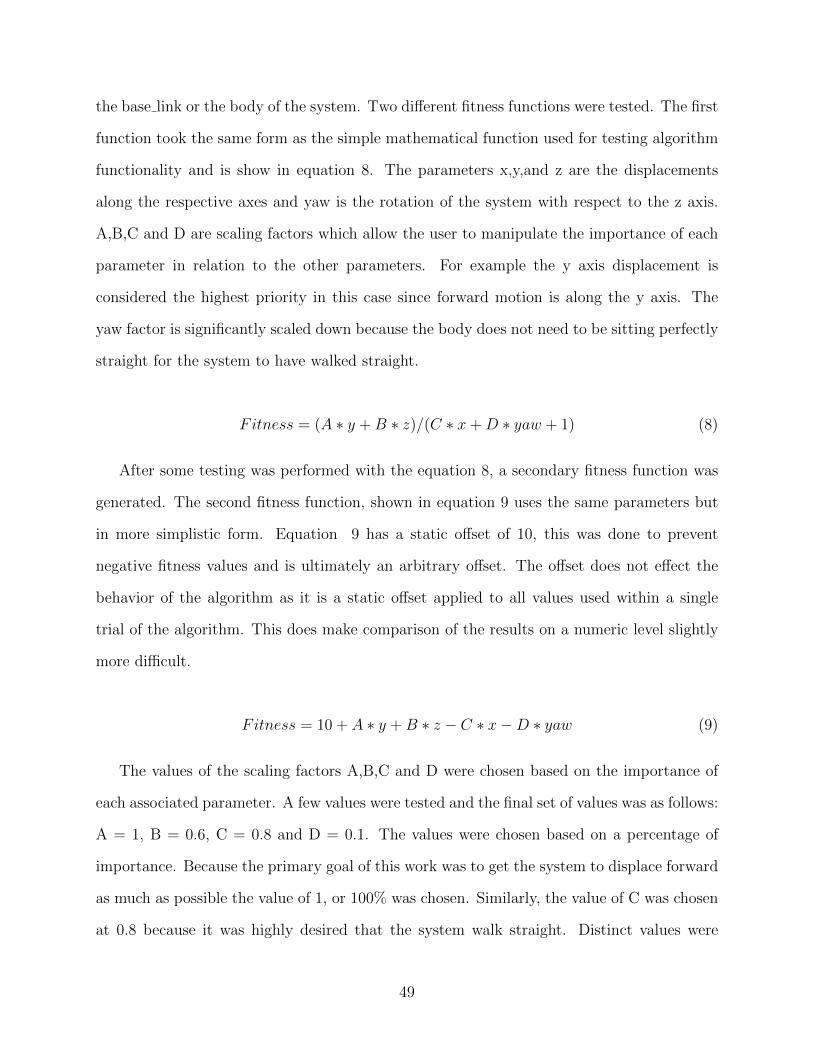
the base link or the body of the system. Two different fitness functions were tested. The first
function took the same form as the simple mathematical function used for testing algorithm
functionality and is show in equation 8. The parameters x,y,and z are the displacements
along the respective axes and yaw is the rotation of the system with respect to the z axis.
A,B,C and D are scaling factors which allow the user to manipulate the importance of each
parameter in relation to the other parameters. For example the y axis displacement is
considered the highest priority in this case since forward motion is along the y axis. The
yaw factor is significantly scaled down because the body does not need to be sitting perfectly
straight for the system to have walked straight.
Fitness = (A ∗ y +B ∗ z)/(C ∗ x+D ∗ yaw + 1) (8)
After some testing was performed with the equation 8, a secondary fitness function was
generated. The second fitness function, shown in equation 9 uses the same parameters but
in more simplistic form. Equation 9 has a static offset of 10, this was done to prevent
negative fitness values and is ultimately an arbitrary offset. The offset does not effect the
behavior of the algorithm as it is a static offset applied to all values used within a single
trial of the algorithm. This does make comparison of the results on a numeric level slightly
more difficult.
Fitness = 10 + A ∗ y +B ∗ z − C ∗ x−D ∗ yaw (9)
The values of the scaling factors A,B,C and D were chosen based on the importance of
each associated parameter. A few values were tested and the final set of values was as follows:
A = 1, B = 0.6, C = 0.8 and D = 0.1. The values were chosen based on a percentage of
importance. Because the primary goal of this work was to get the system to displace forward
as much as possible the value of 1, or 100% was chosen. Similarly, the value of C was chosen
at 0.8 because it was highly desired that the system walk straight. Distinct values were
49

chosen to allow for some wiggle room in solutions. This is to say that although there is no
issue with giving equal weight to multiple parameters, giving the algorithm a highest priority
can increase its chance of succeeding. If everything is prioritise equally, then nothing is truly
prioritised.
6.10 Population
The population size dictates how much of the space can be searched in any given situa-
tion. Based on the shape of the fitness function, coverage of the space can be more or less
important. The most significant factor of spacial coverage is the presence of local maxima.
If there is more than one maxima in the function then poor coverage of the space may lead
to the algorithm becoming stuck at a local maxima rather than the functions true maxima.
While this is not necessarily desirable it is not necessarily detrimental either. In some cases a
local maxima may be a sufficient solution, whereas in other cases a local maxima may not be
a sufficient solution. When testing the algorithm with a simple mathematical function pop-
ulation sizes of 50, 100 and 150 were tested. Results of this testing can be seen in figures 32
through 34. These results show that while larger populations can reach a maxima much
sooner, they may only find a marginally better solution, especially comparing populations
of fifty and one hundred. For this work a final population of 50 was used, this population
size was selected to minimize the computational power and computation time necessary for
simulation.
50

Figure 32: Algorithm Data Structure
Figure 33: Algorithm Data Structure
51

Figure 34: Algorithm Data Structure
6.11 Parent Selection and Child Generation
For the mating process a roulette wheel is used. To generate the roulette wheel each
individuals fitness is measured and summed. This allows each fitness to be measured as a
percentage of the populations total fitness, this ranks individuals in relation to the whole
population and provides a basis for survival of the fittest. The roulette wheel size is variable
to allow for greater precision in the mating process. Individuals are copied into a number of
spaces in the roulette wheel based on the proportion of their fitness to the summed fitness’.
Each individual is guaranteed one space in the wheel, but in general spots are allocated
by rounding the product of the fitness ratio and 1000. This means that there should be
roughly 1000 spots in the roulette wheel, but this value is allowed to vary to ensure that
every individual gets at least one spot. It was desired to ensure a minimum of one spot for
each individual because the algorithm process is random, and while an unfit individual is
unlikely to be selected for mating it should not be made impossible to maintain the level
52

of randomness in the algorithm. To prevent redundant testing of the parent individuals
the fitness value of each individual is stored in a separate array holding the same indices,
such that an individual selected from the roulette wheel can directly reference its fitness
value by looking to the matching index in a separate array. The mating process is achieved
by generating two random numbers, corresponding to the index of the roulette wheel, the
selected individuals are copied into a family array and have their corresponding fitness values
place into a family fitness array. The parents are then passed to the crossover function to
generate children, who can then be tested for fitness. Once tested, the children are copied
into the family array and fitness’ to the family fitness array. This process can be visualized
as shown in figure 1.
Figure 35: Parent Selection, Child Generation and Survivor Selection Process Visualization
6.12 Survivor Selection
At this point it must be decided which individuals will be moved into the next generations
initial population. For this work elitism is used in which the two most fit individuals of
a family are moved into the next population, this helps the algorithm to converge faster
reducing the number of generations necessary to achieve a solution. Changing this method
can lead the algorithm to be exploratory on the basis that a wider variety of individuals is
kept in the mating pool allowing more opportunity for exploration rather than convergence.
In this work exploration is achieved through other methods and as such elitism was chosen
53

for mating.
6.13 Search Time
The total time to generate a gait is dependant upon the exit condition used within the
algorithm. For this work a fixed number of generations was used as the termination condition.
Using an individual simulation time of ten seconds, population of fifty individuals and 200
generations the algorithm takes approximately 21 hours to generate its final solution.
The time taken to generate a solution can be seen to have variable importance when
it comes to implementation. The original concept of this work was for a system to detect
damage, pause what it is doing for a short time, let’s say two minutes, to generate a solution
for the current state, and then continue with it’s tasks. Obviously the time taken to generate
a solution is critical in this case. However, there is not requirement dictating that the system
must compensate on the fly as suggested. Due to the nature of gait generation, there is a
finite set of solutions. Beyond that, in this work individual motors are being compensated
for. This means that we can further bound the solution set based on known viable states.
For example, if all motors are broken there is no reason to attempt a gait generation. This of
course is the extreme case. In the end, any designer can choose their own desired boundaries
for gait generation. This gives a designer the ability to choose how much risk they wish to
take. It is assumed that continuing to operate a system when damaged will lead to further
damage. If the designer wishes to never risk further damage, then an entire leg can be
disabled when damage occurs, as seen in previous works. However, if it an acceptable risk
the designer can choose to allow gait generation for any number of damaged states. In this
design process the gaits can be generated before hand, provided a sufficient simulation and
model is generated. This adds lead time to the system but removes much of the concern for
the time necessary to generate a solution.
54

6.14 Improvements
Further analysis of the algorithm showed one significant place in which the efficiency could
be increased and decrease the total simulation time for training. The algorithm uses elitism
for selecting the members of the next population, this requires the fitness of all individuals to
be known. Originally fitness testing was applied to the population at the beginning of each
generation, however this wastes time after the initial population because each subsequent
population was determined based on known fitness values. As such, if the fitness value used
to determine which individuals are kept is simply kept alongside the individual then the
individual fitness at the beginning of each generation, with the exception of the first, will be
known and the algorithm can skip directly to the creation of the roulette wheel. This halves
the training time and moved this process into a much more manageable time frame. This is
already reflected in the algorithm flowchart shown in figure 22.
7 MATLAB
The simulation framework and proof of functionality of the simulation was achieved
through simple C++ files while the algorithm was developed and tested in MATLAB. For
simplicity, interaction with the simulation was developed in MATLAB rather than generating
a C++ version of the algorithm. This also allowed easier storage of algorithm training data
and results. To implement simulation interaction in MATLAB the Robotics Systems Toolbox
was used for its ROS publishers and subscriber capabilities. This toolbox allows MATLAB
to act as a ROS node that can publish and subscribe to ROS topics. For interaction with
the simulation environment MATLAB was used to publish the sinusoidal signals discussed
previously to be used by the simulation models. MATLAB was also used to subscribe to
the /gazebo/link states topic to retrieve the position of each robot model after testing of the
gait.
55

7.1 Memory leak
Initially, the MATLAB script made significant use of functions, this caused some issues
that tied back to a memory leak cause by a flaw in the Robotics Systems Toolbox. Originally,
the data was generated and sent to a function where the publishing topics were declared, the
data published and then returning to the main script. Upon returning to the main script the
ROS publisher objects created to send the data were supposed to be destroyed, however it
was found that the toolbox does not properly clear the objects such that while the object no
longer exists the memory is not freed. This quickly became an issue in that the system would
run out of memory before completing 40 generations of the algorithm. The fix for this issue
was very simple and was accomplished by removing the publishing function in favor of simply
publishing the data in the main script so that once created the ROS publisher object would
be used for the entirety of the algorithm. Another issue that was found with the Robotics
System Toolbox is that ROS services cannot be used. While functionality exists to read a
ROS service type, there is not support to call a ROS service through the MATLAB node.
This necessitated the custom model reset node previously discussed. This custom node used
a simple C++ file to run the ROS service call and was setup to subscribe to a ROS topic
message that MATLAB could publish to. The custom node subscribes to the topic, when
ready MATLAB publishes the message high, upon completing the reset the node pushes the
node low again. This was done so that MATLAB could subscribe to the topic as well and
be forced to wait until the reset was complete to continue the process of the algorithm. This
prevents MATLAB from sending new gait data to the simulation environment before the
model has a chance to reset and stabilize.
56

8 Results
8.1 Gait Generation
Before attempting to generate gaits for a damaged system the algorithm was tested with
a fully functional system. Although the algorithm was tested mathematically, as discussed
previously, there is a fundamental difference in what is generated by the algorithm in the
simulation and mathematical settings. As such, the algorithm is first tested with a fully
functional system. The results of this testing are shown in figure 36.
Figure 36: Algorithm Verification with Randomized Population
Figure 36 shows that the algorithm is learning however progress stalls around generation
thirty. The gait generated by this trial was not much more than random rapid leg movements.
In attempt to force the generated solution closer to a traditional gait the algorithm was tested
with a single custom gait solution seeding the population and the mutation rate was increased
slightly to aid in the learning process. The result of this can be seen in figure 37.
57

Figure 37: Algorithm Verification with Single Seed Population
Figure 37 showed that the algorithm does not stall out as early in the process. This result
more closely resembles a generic output of a genetic algorithm, much like the results discussed
by Belter et al [2]. However, the final solution was still more spastic than desired. The next
attempt to improve the final solution was to use a homogeneous starting population. The
result of this can be seen in figure 38.
58

Figure 38: Algorithm Verification Homogeneous Seed
In this result the algorithms learning was very minimal and borderline non-apparent.
Because it was already determined that the algorithm is capable of learning it is assumed
that the mutation rate is too low and that the custom solution is a very fit local maxima.
Since the starting population is homogeneous the only room for the algorithm to learn is
by mutation, increasing the mutation rate will also increase the likelihood of the algorithm
escaping the local maxima. The result of increasing the mutation rate for a homogeneous
population can be seen in figure 39.
59

Figure 39: Algorithm Verification with Higher Mutation Rate
By increasing the mutation rate it can be seen that the expected behavior of a genetic
algorithm is once again achieved.
8.2 Damage Compensation
The initial work was all conducted with a fully functional system to prove that the
experimental setup would generate a gait for a fully functional system. If the setup could
not achieve a gait for a fully functional system them it would be very unlikely to achieve
a gait for the same system in a less functional state. After verification of the algorithm in
the simulation environment was completed the fitness functions, shown in equations 9 and 8
were revisited to analyze which approach generated better final solution. Fitness function 1,
equation 10, and fitness function 2, equation 11, are listed below for easier reference.
Fitness = 10 + A ∗ y +B ∗ z − C ∗ x−D ∗ yaw (10)
Fitness = (A ∗ y +B ∗ z)/(C ∗ x+D ∗ yaw + 1) (11)
60

Figures 40 and 41 show the results of a full training set using fitness function 1 and fitness
function 2, respectively, for the system in the same damaged state.
Figure 40: Damage Generation - Left Back Femur Fitness Function 1
61

Figure 41: Damage Generation - Left Back Femur Fitness Function 2
The first thing to point out is the distinct difference between the two fitness levels
achieved. It is very important to consider that fitness function 1 has a static offset of
10, this was done to prevent negative fitness values and is ultimately an arbitrary offset.
The offset does not effect the behavior of the algorithm as it is a static offset applied to all
values used within a single trial of the algorithm. This does make comparison of the results
on a numeric level more difficult. What should be noticed is that in both fitness functions
the same variables are used and ultimately a similar level of progress, fitness at the beginning
and end, is achieved. Although the numeric difference is not as straight forward to compare,
the goal of this work is gait generation in which a stark difference was apparent. When the
generated gait is view fitness function 1 results in a much more spastic gait while fitness
function 2 results in a gait the more closely resembles a tradition gait. This process was
repeated to test if fitness function 2 continued to generate more desirable solutions or if this
was specific to the damaged state.
62

Figure 42: Damage Generation - Right Center Tibia Fitness Function 1
Figure 43: Damage Generation - Right Center Tibia Fitness Function 2
Figures 42 and 43 show the results of the secondary test comparing fitness function 1 and
63

2, in this instance the algorithm was tasked with gait generation for the loss of a missing
right center tibia motor. The results of this test were very similar to the first comparison, in
both cases fitness function 1 and 2 showed similar levels of total learning. More importantly
in both cases fitness function 2 yielded a gait closer resembling a traditional walking method.
As such, fitness function 2 was chosen to work with moving forward.
Numerous damaged states were tested and will be discussed in no particular order. For all
damaged state tests a homogeneous custom solution seed was used alongside fitness function
2, given by equation 11.
8.2.1 Right Center Tibia and Left Center Tibia
The evolution of a gait compensating for the loss of both the right and left center tibia
motors is shown in figure 44. In this case the damage had a bigger impact on the system
from the start resulting in a starting fitness 0.2 lower than the general cases. Interestingly,
in this damaged state the system was able to better compensate than when a singular motor
was damaged. One reason may be the symmetry of the damage. Another reason is that the
tibia motor provides a redundant motion to the femur motor, and as such is not as necessary
to the overall function of the walking gait. It is also possible that the randomness provided
by genetic algorithms simply lead to better ”luck” in this instance.
64

Figure 44: Damage Generation - Right Center Tibia and Left Center Tibia
8.2.2 Left Front Tibia
The evolution of a gait compensating for the loss of the left front tibia motor is shown
in figure 45. This result generated a gait that while usable was not an ideal solution. The
primary issue with the generated solution was drift, this appeared to be an instance in which
the result was good within the analyzed period of the gait. However, the analyzed period
of the gait was shorter than one or more periods of a generated sinusoid. To avoid this the
period used for analyzing a gait should have been greater than or equal to the maximum
period that could be generated by the algorithm.
65

Figure 45: Damage Generation - Right Center Tibia and Left Center Tibia
8.2.3 Left Center Coxa
The evolution of a gait compensating for the loss of the left center coxa motor is shown
in figure 46. This damaged state, specifically damaged coxa motors, was the most difficult to
generate solutions. Although the data shows proper function of the algorithm, the resulting
gait was not usable for a real system. This is because the lack of a coxa motor allowed the
leg to rotate, leading to the leg clipping through the body of the system and acting as a
support, this lead to the generation of a gait that relied on the broken leg in a non-viable
position.
66

Figure 46: Damage Generation - Left Center Coxa
8.2.4 Left Back Coxa and Right Center Femur
The evolution of a gait compensating for the loss of the left back coxa and right center
femur motors is shown in figure 47. In this instance the final result was significantly more
usable on a real system. Although the back left leg was able to rotate into nonviable positions,
as was the case in 8.2.3, it seems that because the leg was in the rear of the system and was
thereby dragged along at times the algorithm did not become dependent on a non-viable
situation.
67

Figure 47: Damage Generation - Left Back Coxa and Right Center Femur
8.2.5 Left Front Femur and Left Center Tibia
The evolution of a gait compensating for the loss of both the left front femur and left
center tibia motors is shown in figure 48. Although the data shows similar learning to many
other results the gait generated for this damaged state was not usable. It seems most likely
that in this instance 200 generations was simply not enough to generate a good solution as
the gait moves the system in a circle.
68

Figure 48: Damage Generation - Left Front Femur and Left Center Tibia
8.2.6 Gait Comparisons
To further compare the algorithms generated solutions the forward displacement, dis-
placement along the Y-axis, of the system in a fixed ten second time frame is listed in
table 1.
69
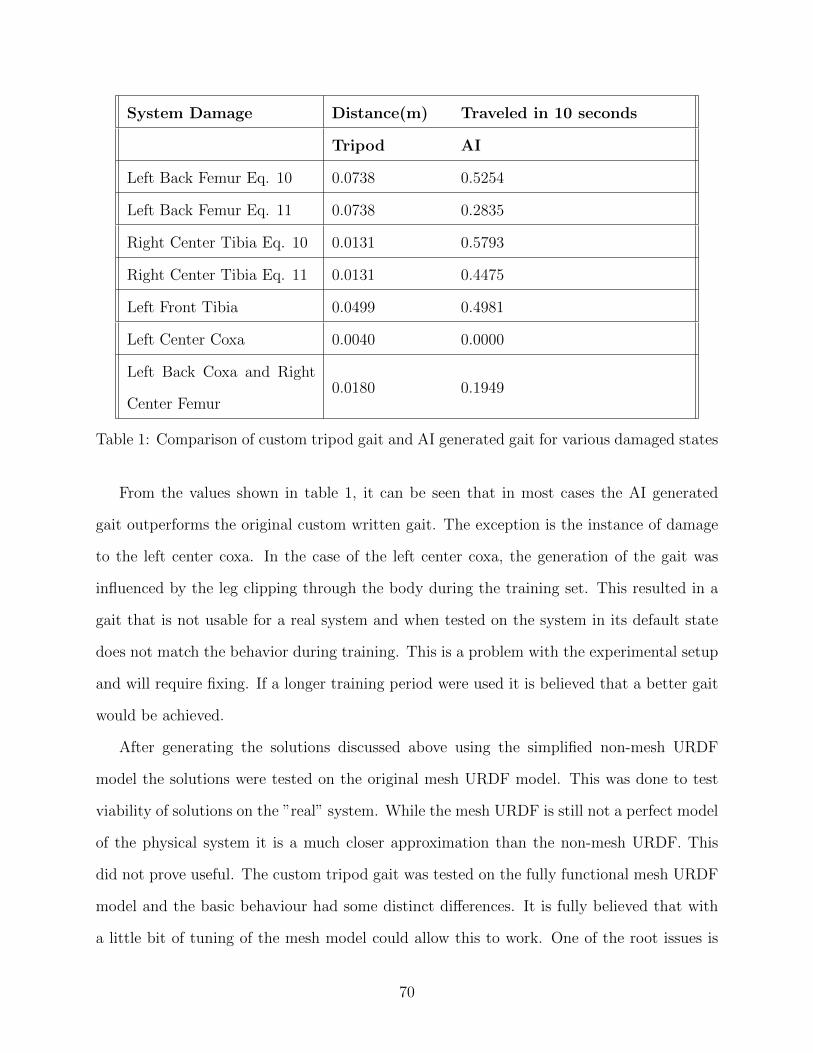
System Damage Distance(m) Traveled in 10 seconds
Tripod AI
Left Back Femur Eq. 10 0.0738 0.5254
Left Back Femur Eq. 11 0.0738 0.2835
Right Center Tibia Eq. 10 0.0131 0.5793
Right Center Tibia Eq. 11 0.0131 0.4475
Left Front Tibia 0.0499 0.4981
Left Center Coxa 0.0040 0.0000
Left Back Coxa and Right
Center Femur0.0180 0.1949
Table 1: Comparison of custom tripod gait and AI generated gait for various damaged states
From the values shown in table 1, it can be seen that in most cases the AI generated
gait outperforms the original custom written gait. The exception is the instance of damage
to the left center coxa. In the case of the left center coxa, the generation of the gait was
influenced by the leg clipping through the body during the training set. This resulted in a
gait that is not usable for a real system and when tested on the system in its default state
does not match the behavior during training. This is a problem with the experimental setup
and will require fixing. If a longer training period were used it is believed that a better gait
would be achieved.
After generating the solutions discussed above using the simplified non-mesh URDF
model the solutions were tested on the original mesh URDF model. This was done to test
viability of solutions on the ”real” system. While the mesh URDF is still not a perfect model
of the physical system it is a much closer approximation than the non-mesh URDF. This
did not prove useful. The custom tripod gait was tested on the fully functional mesh URDF
model and the basic behaviour had some distinct differences. It is fully believed that with
a little bit of tuning of the mesh model could allow this to work. One of the root issues is
70

the home, or zero, position of each joint. Because the mesh model was generated from the
SOLIDWORKS exporter the zero position on the joints do not align with the zero positions
on the non-mesh model used throughout this work. This discrepancy means that even the
custom written tripod solution does not have the same behavior between the non-mesh and
mesh models. With further tuning of the mesh model this difference can be accounted for,
this could also be accounted for in the software by finding the joint offsets and compensating.
This method, although functional would not be suggested because it is more of a band aid
solution. If the mesh model can be made to match the non-mesh model it is expected that
there will still be some difference in behaviour between the two models. This is in part due
to the approximations made in generating the non-mesh model. Although differences are
expected, it is believed that the differences would be relatively minor due to the construction
of the non-mesh model. This would provide a minimally viable solution translating from the
non-mesh to mesh model. It is unknown how accurate the mesh model is to the physical
system and as such there is no estimation of how applicable the solutions generated are to the
real system. This could be tested, at the minor risk of the physical system. It is important
to note that although the solutions generated may not apply to the original system that
inspired this work, the algorithm is independent of the system model. This algorithm is
usable with any system, simply requiring that the user alter the structure of the data to fit
the system or system model.
8.2.7 Damage Gait Summary
In general there were a few common details noticed throughout the testing process. In
general, the algorithm was consistently able to display the expected behavior numerically.
However, the gaits generated were not always good, usable gaits. This is to say that while
the system is able to move itself in accordance with the fitness function the motions often did
not resemble any sort of traditional walking. This primarily shows that the fitness function
used in this work has room for improvement. The generated gaits can easily be sorted into
71

three categories, successful gaits, failed gaits, and gaits that perform well within the window
of testing. To focus in on the last two, some gaits immediately show that it is not a successful
gait. The system may drift significantly, stall in place, or even walk in a circle, ultimately
these solutions are simply no good. Based on the successful results generated it is believed
that these failed cases are the result of short comings in the experimental design as well as
limitations due to time constraints. If the algorithm were run again using the same conditions
but using a longer time per fitness test and a higher number of generations it seems very
likely that a sufficient solution could be achieved. In other cases the gait may start off well
but because the algorithm only analyzes a predefined time window of the gait it is possible
that the generated solution is only good for that window of time. Multiple results were found
to fall into this category to some degree, some solutions would begin to deviate after the
analyzed window indicating that the period of one or more generated sinusoids was likely
larger than the defined window. Other cases showed slight but noticeable deviation from the
start or early on, this simply shows that there was little enough deviation to still succeed
based on the fitness function. To improve the algorithm the window for gait fitness testing
should be greater than or equal to the maximum period generatable by the algorithm. It
was noticed that a number of solutions show little improvement after 100 generations. This
could be a result of the type of damage to the system, however there is not a clear trend from
the current results. Although this is not necessarily a bad behavior the mutation rate could
be increased further to aid in deeper exploration, this could be a static change applied for
the entire algorithm or a change implemented at a threshold level, ie change the mutation
after a number of generations. Such changes would be best determined after changes to the
fitness function are applied as it is believed that the fitness function will have a much more
significant impact on the quality of generated solutions.
72

9 Conclusions
Results have demonstrated that the Genetic Algorithm designed is capable of learning a
gait to compensate for a damaged state as well as optimize a gait for a fully functional system.
Numerically it is clear that the algorithm is capable of learning, however the gaits that are
learned are often not close to a traditional gait. Although it is expected that an AI generates
a solution very dissimilar to a human generated solution, commonly the AI generated gaits
are far too spastic to be considered for use. Improving the generated gaits requires the
generation of a better fitness function and likely an increase in algorithm training time. By
better defining what it means to walk and allowing more time for the algorithm to learn it
is expected that better gaits can be achieved. The total training time also has significant
room for improvement. This could be achieved by spawning and controlling multiple models
within gazebo or by distributing the simulation load across a computer network.
10 Future work
There are numerous areas of improvement and advancement in this work. Beginning with
improvement, it is desirable to use the mesh URDF model generated by the SOLIDWORKS
to URDF exporter rather than the block approximation model. Use of the mesh model is
quite simply a more accurate simulation model and since it is desired that a gait generated
in simulation work in actuality it is important to model the simulation system as close to
reality as possible. Algorithm speed is another obvious space for improvement. Decreasing
training time is key to success in essentially any AI system, with this system particularly the
algorithm is significantly slow due to the complexity of the search and results in an overall
training time that is not truly viable in most instances, although the desired output can be
achieved the time taken to reach said output is simply not practical. The primary bottleneck
in the setup used for this work was the gazebo environment. When testing one gait at a
time the number of tests to be completed causes the training time to become unreasonable
73

quickly. As such the first aim of improvement was to test more than one gait solution at a
time. While this was achieved the gazebo environment slowed down significantly between
simulating one model and simulating 50 models. It is unclear at the moment how best to
solve this bottleneck. Options include using a system with more computing power, using a
different simulation environment or simplifying the testing structure.
In terms of advancement, it is suggested that the basis of the gait be changed. Instead of
the current structure, Asin(Bt+C), it is suggested to us a more complex function of the form
Asin(Bt+C)+Dcos(Et+F). The insertion of a cosine term will allow for more complex motion
profiles of each joint. The wave and ripple gaits were tested using the simple sinusoidal signal
used in this work but a fully function parametization was not generated. While the tripod
gait is a continuous, symmetric motion profile the ripple and wave gaits are not simply
symmetrical, while the addition of a cosine term does not aid in the generation of a non-
symmetric gait, the symmetry available to a sine cosine pair with shifting frequencies and
phases appears in theory to provide enough variability and complexity in the symmetry
to achieve better results than the approach used in this work. Of course this additional
complexity comes at the cost of search space by doubling the number of parameters being
searched for. To aid in limiting the additional complexity the user is able to define bounds
for the additional parameters, the same way that the original parameters are bounded, if the
user is able to define a tight enough bound this will significantly help reduce the complexity
of the search. It is also suggested that future work involve the de-standardizing of coefficients
in terms of their binary representation. In the current form each coefficient is represented
by a 10 bit binary string while the ranges vary from as large as 0-20*PI to as small as 0-2.
The precision achieved in the range of 0-2 is not necessary and the string should likely be
downsized into the range of a 5 bit binary rather than a 10 bit binary.
Beyond the resolution used for each coefficient, the limit of the joint amplitude, or the
clipping point can be further explored. By varying the clipping value the search becomes
much more difficult but has the potential to yield much better gaits. In the current con-
74

figuration of the system, the clipping values are set in accordance with the hand picked
values used when a manual tripod gait was generated. While these values worked well for
a hand written gait, they may not, and are very likely not the ideal values for the algorith-
mic generated gaits. Alteration of the clipping point also provides another means for gait
compensation. For example, rather than compensating by taking steps more frequently, the
system could learn to keep its foot on the ground for a longer portion of time causing a larger
displacement in a singular step. This would be a simple modification to the current work in
that only three parameters need to be added to the current 54 parameter individual. Alter-
natively, a clipping value could be generated for each joint rather than for each joint type,
this would cause an additional eighteen parameters and significantly increase the complexity
of the algorithm search.
The second space for advancement is in the fitness function of the algorithm. For this
work the fitness function was rather simple and could certainly be improved. This will
require further analysis of how six legged agents traverse environments. This also opens up
possibilities to parameterize a gait in different environments based on the generated fitness
function. While a gait to traverse a flat surface may be parameterized as simply as the fitness
functions previously discussed in this work, a gait for traversing rough terrain is likely to be
best parameterized differently. In prior works it was noticed that the time taken to travel
a fixed distance could be used a a fitness evaluation [6]. A preliminary test of this fitness
evaluation proved promising but no significant results were achieved at this time.
The third space for advancement is the inclusion of the clipping limits in the algorithm
itself. In the current state the clipping limits are predefined as hardware parameters. How-
ever, allowing the clipping value to shift, still within the hardware bounds, would open up
more possibilities for compensatory behaviour. In the current form the leg is guaranteed
to have a symmetrical movement, if an upper and lower clipping bound are set, and set
separately this could allow much more complex movements. A leg could act in more of a
support state while still moving only in the front or rear half of its range.
75
Another opportunity for advancement would be to dynamically adjust the individual
used in the algorithm. Currently, the individual remains the same size regardless of damage.
This means that a part of each solution is actually unused, the messages are unsent instead
of removed. By removing excess data from the solutions the algorithm can learn quicker and
better. When excess data is left in the solutions there is no way to distinguish used and
unused data. As such, the algorithm could be lead to believe that unused data is ”good”.
If instead the individual was dynamically sized to only included data that will be used the
learning process becomes straight forward and better enables learning.
One factor that lead to the high computational intensity was the number of ROS topics.
For a singular model there were 74 active topics, these come from 4 topics per joint controller,
the model joint states topic and the model reset topic. This leads to a very high number
of active topics when fifty models are being controlled at the same time. To reduce the
number of topics required a custom controller was attempted, this could collapsed the 4
single input topics per joint into 4 array input topics per model, overall reducing the topics
from 74 to 6. This controller has not actually been implemented but for future work should
be implemented to reduce overhead and speed up all processes.
76

References
[1] Akhlaq, Ammar, et al. “Biologically Inspired Self-Reconfigurable Hexapod with Adap-
tive Locomotion.” 2014 16th International Power Electronics and Motion Control Con-
ference and Exposition, 2014.
[2] Belter, D., Skrzypczynski, P. (2010, 3 1). A biologically inspired approach to feasible
gait learning for a hexapod robot. International Journal of Applied Mathematics and
Computer Science, 20(1), 69-84.
[3] Bunting, M., Sprinkle, J. (n.d.). Rapid Prototyping of Dmitri, a Hexapod Robot
[4] Chebotar, Y., Handa, A., Makoviychuk, V., Macklin, M., Issac, J., Ratliff, N., Fox, D.
(n.d.). Closing the Sim-to-Real Loop: Adapting Simulation Randomization with Real
World Experience.
[5] Cully, A., Clune, J., Tarapore, D., Mouret, J.-B. (2014, 7 13). Robots that can adapt
like animals.
[6] D. Trivun, H. Dindo, and B. Lacevic, “Resilient hexapod robot,” 2017 XXVI Inter-
national Conference on Information, Communication and Automation Technologies
(ICAT), 2017.
[7] Ding, X., Wang, Z., Rovetta, A., Zhu, J. (n.d.). Locomotion analysis of hexapod robot
291 X Locomotion analysis of hexapod robot.
[8] F. Seljanko, “Hexapod walking robot gait generation using genetic-gravitational hybrid
algorithm,” 2011 15th International Conference on Advanced Robotics (ICAR), 2011.
[9] F. Tedeschi and G. Carbone, “Design Issues for Hexapod Walking Robots,” Robotics,
vol. 3, no. 2, pp. 181–206, Oct. 2014.
[10] G. B. Parker, W. T. Tarimo, and M. Cantor, “Quadruped gait learning using cyclic
genetic algorithms,” 2011 IEEE Congress of Evolutionary Computation (CEC), 2011.
77

[11] G. Ren, W. Chen, S. Dasgupta, C. Kolodziejski, F. Worgotter, and P. Manoonpong,
“Multiple chaotic central pattern generators with learning for legged locomotion and
malfunction compensation,” Information Sciences, vol. 294, pp. 666–682, 2015.
[12] Helwig, S., Wanka, R. (n.d.). Particle Swarm Optimization in High-Dimensional
Bounded Search Spaces
[13] Helwig, S., Branke, J., Mostaghim, S. (2013). Experimental analysis of bound han-
dling techniques in particle swarm optimization. IEEE Transactions on Evolutionary
Computation, 17(2), 259-271
[14] Husbands, P., Jakobi, N., Harvey, I. (1995). ”Noise and the Reality Gap: The Use
of Simulation in Evolutionary Robotics,” Noise and The Reality Gap: The Use of
Simulation in Evolutionary Robotics.
[15] Juang, C., Chang, Y., Hsiao, C. (2011, 7). Evolving gaits of a hexapod robot by
recurrent neural networks with symbiotic species-based particle swarm optimization.
IEEE Transactions on Industrial Electronics, 58(7), 3110-3119.
[16] Kaur, A., Kaur, M. (2015). Dealing with Boundary Constraint Violations in Particle
Swarm Optimization with Aging Leader and Challengers (ALC-PSO).
[17] Kon, J., Sahin, F. (2020) Gait Generation for Damaged Hexapods using a Genetic
Algorithm
[18] Kutilek, P. (n.d.). REINFORCEMENT LEARNING IN CONTROL SYSTEMS FOR
WALKING HEXAPOD ROBOTS.
[19] Kutilek, P., Viteckova, S., Hejda, J., Krivanek, V., Doskocil, R., Stefek, A. (n.d.).
Control of Hexapod with Static-stable Walking Using Artificial Intelligence.
[20] Lee, B.-H., Lee, I.-K. (n.d.). The Implementation of the Gaits and Body Structure for
Hexapod Robot.
78

[21] Lopes, A. (2002). Quasi-periodic Gaits in Multi-legged Robots.
[22] M. Pitonyak and F. Sahin, “Locomotion and transitional procedures for a hexapod-
quadcopter robot,” 2017 IEEE International Conference on Systems, Man, and Cyber-
netics (SMC), 2017.
[23] M. Pitonyak and F. Sahin, “A novel hexapod robot design with flight capability,” 2017
12th System of Systems Engineering Conference (SoSE), 2017.
[24] Manglik, Aditya, et al. “Adaptive Gait Generation for Hexapod Robot Using Genetic
Algorithm.” 2016 IEEE 1st International Conference on Power Electronics, Intelligent
Control and Energy Systems (ICPEICES), 2016.
[25] McGHEE, R., Iswandhi, G. (1979). Adaptive Locomotion of a Multilegged Robot over
Rough Terrain.
[26] Moir, T., Massey University (Palmerston North). (n.d.). 15th International Conference
on Mechatronics and Machine Vision in Practice, 2008. IEEE.
[27] Noori, Farzan M., et al. “On 3D Simulators for Multi-Robot Systems in ROS: MORSE or
Gazebo?” 2017 IEEE International Symposium on Safety, Security and Rescue Robotics
(SSRR), 2017
[28] Novitzka, V., Korecko, S., Szakal, A., Technicka univerzita (Kosice, S., IEEE Systems,
M., Institute of Electrical and Electronics Engineers. (n.d.). Informatics 2015 : 2015
IEEE 13th International Scientific Conference on Informatics : proceedings : November
18-20, 2015, Poprad, Slovakia.
[29] Padhye, N., Deb, K., Mittal, P. (2012). Boundary Handling Approaches in Particle
Swarm Optimization.
[30] Parker, G., Braun, D. (n.d.). Evolving Hexapod Gaits Using a Cyclic Genetic Algo-
rithm.
79

[31] Petere, E., Brezovan, M., Institute of Electrical and Electronics Engineers, IEEE Control
Systems Society, International Conference on System Theory and Control (20th : 2016
: Sinaia, R., International Symposium on Automatic Control and Computer Science
(16th : 2016 : Sinaia, R., International Symposium on Modelling, S. (n.d.). 2016
20th International Conference on System Theory, Control and Computing (ICSTCC) :
joint conference of SINTES 20, SACCS 16, SIMSIS 20 : October 13-15, 2016, Sinaia,
Romania.
[32] Real, F., Batou, A., Ritto, T., Desceliers, C. (2019). Stochastic modeling for hysteretic
bit–rock interaction of a drill string under torsional vibrations. Journal of Vibration and
Control, 107754631982824.
[33] Shih, T., Tsai, C., Her, I. (2012, 10 30). Comparison of alternative gaits for multiped
robots with severed legs. International Journal of Advanced Robotic Systems, 9.
[34] W. Qian, Z. Xia, J. Xiong, Y. Gan, Y. Guo, S. Weng, H. Deng, Y. Hu, and J. Zhang,
“Manipulation task simulation using ROS and Gazebo,” 2014 IEEE International Con-
ference on Robotics and Biomimetics (ROBIO 2014), 2014.
[35] X. Duan, W. Chen, S. Yu, and J. Liu, “Tripod gaits planning and kinematics analysis
of a hexapod robot,” 2009 IEEE International Conference on Control and Automation,
2009.
80