gains from trade and the ricardian models of int'l trade
TRANSCRIPT

Dornbusch, Fisher and Samuelson (1977)Eaton and Kortum (2002)
References
Gains from Trade and the Ricardian Models ofint’l Trade
Part 2
Giuseppe De Arcangelis
2016 Fall Term
Giuseppe De Arcangelis GT & Ricardian Models

Dornbusch, Fisher and Samuelson (1977)Eaton and Kortum (2002)
References
DFS – Assumptions1. 2 countries H and F ;2. A continuum of goods normalized on the the unit interval:
z ∈ [0, 1];3. One production factor in quantity L in country H and L∗ in
country F ;4. Fixed labor requirements: a(z) is quantity of labor to produce
good z in country H; same in country F is a∗(z);5. Preferences:
I identical in the two countries;I homotheticI Cobb-Douglas and defined with the fraction of income spent
on each type of good: let b(z) be such that∫ z2
z1b(z)dz is the
fraction of income spent on the good range [z1, z2]; hence,∫ 1
0b(z)dz = 1
6. nominal wages: w in H and w∗ in FGiuseppe De Arcangelis GT & Ricardian Models

Dornbusch, Fisher and Samuelson (1977)Eaton and Kortum (2002)
References
DFS – The Supply SideH exports z if p(z) < p∗(z); hence:
wa(z) < w∗a∗(z)
or
ω ≡ w
w∗<
a∗(z)
a(z)
Let us define
A(z) ≡ a∗(z)
a(z)
and let us order goods z ’s so that A(z) is decreasing.pause Hence, given ω we can determine the range of z-goodsproduced home and exported, as well as imports.
Giuseppe De Arcangelis GT & Ricardian Models

Dornbusch, Fisher and Samuelson (1977)Eaton and Kortum (2002)
References
DFS – The A(z) curve
6
-
A(z)
z
ω
z 1︷ ︸︸ ︷exports of H
︷ ︸︸ ︷imports of H
1
Giuseppe De Arcangelis GT & Ricardian Models

Dornbusch, Fisher and Samuelson (1977)Eaton and Kortum (2002)
References
DFS – The Demand SideIncome in the two countries is given by: Y = wL Y ∗ = w∗L∗
Invert the A(·) function and obtain: z = A−1(ω). Let us define thefraction of income spent on that range of goods, θ(z) according tothe preferences (same in H and F ):
θ(z) =
∫ z
0b(z)dz
Then, given ω, the range of goods [0, z ] is the domestic productionof H, i.e. Y .This has to satisfy world demand for those goods that comes fromHome – θ(z)Y – and from Foreign – θ(z)Y ∗. Hence, equilibriumin the range of products done at Home is:
Y = θ(z)(Y + Y ∗)
Giuseppe De Arcangelis GT & Ricardian Models

Dornbusch, Fisher and Samuelson (1977)Eaton and Kortum (2002)
References
DFS – The Demand SideIncome in the two countries is given by: Y = wL Y ∗ = w∗L∗
Invert the A(·) function and obtain: z = A−1(ω). Let us define thefraction of income spent on that range of goods, θ(z) according tothe preferences (same in H and F ):
θ(z) =
∫ z
0b(z)dz
Then, given ω, the range of goods [0, z ] is the domestic productionof H, i.e. Y .This has to satisfy world demand for those goods that comes fromHome – θ(z)Y – and from Foreign – θ(z)Y ∗. Hence, equilibriumin the range of products done at Home is:
Y = θ(z)(Y + Y ∗)Giuseppe De Arcangelis GT & Ricardian Models

Dornbusch, Fisher and Samuelson (1977)Eaton and Kortum (2002)
References
DFS – The B(z ; L∗
L ) curve
wL = θ(z)(wL + w∗L∗)
ωL = θ(z)(ωL + L∗)
by rearraging:
ω =θ(z)
1− θ(z)
L∗
L≡ B(z ;
L∗
L) ≡ B(z)
L∗
L
Notice that: ∂B∂z > 0, ∂B
∂L∗ > 0 , ∂B∂L < 0
These characteristics of the B(z) assure that it crosses the A(z),hence an equilibrium exists and is unique.
Giuseppe De Arcangelis GT & Ricardian Models

Dornbusch, Fisher and Samuelson (1977)Eaton and Kortum (2002)
References
DFS – The B(z ; L∗
L ) curve
Notice that the B(z) curve represents the equilibrium in the tradebalance:
[1− θ(z)]wL︸ ︷︷ ︸exports of H
= θ(z)w∗L∗︸ ︷︷ ︸imports of F
Giuseppe De Arcangelis GT & Ricardian Models

Dornbusch, Fisher and Samuelson (1977)Eaton and Kortum (2002)
References
DFS – The B(z) curve and Equilibrium
6
-
ω
z
ω′
z′ 1
A(z)
B(z)L∗
L
B(z)L∗′
L
ω
z
1
Giuseppe De Arcangelis GT & Ricardian Models

Dornbusch, Fisher and Samuelson (1977)Eaton and Kortum (2002)
References
DFS – Gains from Trade
Real consumption in autarky of the good z :
c(z) =b(z)wL
p(z)=
b(z)wL
wa(z)=
b(z)L
a(z)∀z
In the free-trade equilibrium imported goods from the foreigncountry cost less:
c(z) =b(z)wL
p(z)=
{b(z)La(z) ∀z < z home goodsb(z)wLp∗(z) = b(z)wL
w∗a∗(z) ∀z > z imports
Giuseppe De Arcangelis GT & Ricardian Models

Dornbusch, Fisher and Samuelson (1977)Eaton and Kortum (2002)
References
DFS – Gains from Trade
c(z) =b(z)wL
p(z)=
{b(z)La(z) ∀z < z home goodsb(z)wLp∗(z) = b(z)wL
w∗a∗(z) ∀z > z imports
The cost of imported goods is lower than before; hence, the valueof the imported consumption bundle is higher than in autarky:
b(z)wL
w∗a∗(z)>
b(z)L
a(z)or
w
w∗>
a∗(z)
a(z)
which holds since for z > z we have A(z) < ω.
Giuseppe De Arcangelis GT & Ricardian Models

Dornbusch, Fisher and Samuelson (1977)Eaton and Kortum (2002)
References
DFS Comparative Statics – Increase in L∗
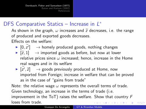
As shown in the graph, ω increases and z decreases, i.e. the rangeof produced and exported goods decreases.Effects on the welfare:
I [0, z ′] → homely produced goods, nothing changes
I [z , 1] → imported goods as before, but now at lowerrelative prices since ω increased; hence, increase in the Homereal wages and in its welfare
I [z ′, z ] → goods previously produced at Home, nowimported from Foreign; increase in welfare that can be provedas in the case of “gains from trade”
Note: the relative wage ω represents the overall terms of trade.Given technology, an increase in the terms of trade (i.e.improvement in the ToT) raises the welfare. Show that country Floses from trade.
Giuseppe De Arcangelis GT & Ricardian Models

Dornbusch, Fisher and Samuelson (1977)Eaton and Kortum (2002)
References
DFS Comparative Statics – Increase in L∗
As shown in the graph, ω increases and z decreases, i.e. the rangeof produced and exported goods decreases.Effects on the welfare:
I [0, z ′] → homely produced goods, nothing changesI [z , 1] → imported goods as before, but now at lower
relative prices since ω increased; hence, increase in the Homereal wages and in its welfare
I [z ′, z ] → goods previously produced at Home, nowimported from Foreign; increase in welfare that can be provedas in the case of “gains from trade”
Note: the relative wage ω represents the overall terms of trade.Given technology, an increase in the terms of trade (i.e.improvement in the ToT) raises the welfare. Show that country Floses from trade.
Giuseppe De Arcangelis GT & Ricardian Models

Dornbusch, Fisher and Samuelson (1977)Eaton and Kortum (2002)
References
DFS Comparative Statics – Neutral TechnologicalImprovement in H
Technological advancement: all a(z) decrease by a factor α:
a′(z) = a(z)α .
Graphically, the A(z) shifts up by the improvement α.Effects:
I the home relative wage ω increases, but less than α
I in this case both countries gain from trade since thetechnology improvement does not raise the relative wageone-to-one
Problem: show that in the range [z ; z ′] both countries gain fromtrade (hint: show that real consumption is higher for bothcountries, or show what happens to the real wage)
Giuseppe De Arcangelis GT & Ricardian Models

Dornbusch, Fisher and Samuelson (1977)Eaton and Kortum (2002)
References
DFS Comparative Statics – Neutral TechnologicalImprovement in H
Technological advancement: all a(z) decrease by a factor α:
a′(z) = a(z)α .
Graphically, the A(z) shifts up by the improvement α.
Effects:
I the home relative wage ω increases, but less than α
I in this case both countries gain from trade since thetechnology improvement does not raise the relative wageone-to-one
Problem: show that in the range [z ; z ′] both countries gain fromtrade (hint: show that real consumption is higher for bothcountries, or show what happens to the real wage)
Giuseppe De Arcangelis GT & Ricardian Models

Dornbusch, Fisher and Samuelson (1977)Eaton and Kortum (2002)
References
DFS Comparative Statics – Neutral TechnologicalImprovement in H
Technological advancement: all a(z) decrease by a factor α:
a′(z) = a(z)α .
Graphically, the A(z) shifts up by the improvement α.Effects:
I the home relative wage ω increases, but less than α
I in this case both countries gain from trade since thetechnology improvement does not raise the relative wageone-to-one
Problem: show that in the range [z ; z ′] both countries gain fromtrade (hint: show that real consumption is higher for bothcountries, or show what happens to the real wage)
Giuseppe De Arcangelis GT & Ricardian Models

Dornbusch, Fisher and Samuelson (1977)Eaton and Kortum (2002)
References
DFS Comparative Statics – Neutral TechnologicalImprovement in H
Technological advancement: all a(z) decrease by a factor α:
a′(z) = a(z)α .
Graphically, the A(z) shifts up by the improvement α.Effects:
I the home relative wage ω increases, but less than α
I in this case both countries gain from trade since thetechnology improvement does not raise the relative wageone-to-one
Problem: show that in the range [z ; z ′] both countries gain fromtrade (hint: show that real consumption is higher for bothcountries, or show what happens to the real wage)
Giuseppe De Arcangelis GT & Ricardian Models

Dornbusch, Fisher and Samuelson (1977)Eaton and Kortum (2002)
References
DFS Comparative Statics – Iceberg Transport Costs: effecton A(z)
Assume that only a fraction g < 1 arrives at destination whendeparts the exporting country. Hence:
H exports z iff: wa(z) < gw∗a∗(z) ⇒ ω < gA(z)H imports z iff: gwa(z) > w∗a∗(z) ⇒ ω > 1
gA(z)
Graphically show that a range of z-goods are not traded.
Giuseppe De Arcangelis GT & Ricardian Models

Dornbusch, Fisher and Samuelson (1977)Eaton and Kortum (2002)
References
DFS Comparative Statics – Iceberg Transport Costs:exogenous effect on the trade balance, B(z)
Let us assume that k is a fraction of income spent on traded goodsand (1− k) on nontraded goods.
If b(z) is still referred only on
traded goods, then∫ 1
0 b(z)dz = k .New trade-balance condition:
[1− θ(z)− (1− k)]wL︸ ︷︷ ︸exports of H
= θ(z)w∗L∗︸ ︷︷ ︸imports of F
Hence, the new B(z) locus will satisfy:
ω =θ(z)
k − θ(z)
L∗
L
where k is exogenously set.
Giuseppe De Arcangelis GT & Ricardian Models

Dornbusch, Fisher and Samuelson (1977)Eaton and Kortum (2002)
References
DFS Comparative Statics – Iceberg Transport Costs:exogenous effect on the trade balance, B(z)
Let us assume that k is a fraction of income spent on traded goodsand (1− k) on nontraded goods. If b(z) is still referred only on
traded goods, then∫ 1
0 b(z)dz = k .
New trade-balance condition:
[1− θ(z)− (1− k)]wL︸ ︷︷ ︸exports of H
= θ(z)w∗L∗︸ ︷︷ ︸imports of F
Hence, the new B(z) locus will satisfy:
ω =θ(z)
k − θ(z)
L∗
L
where k is exogenously set.
Giuseppe De Arcangelis GT & Ricardian Models

Dornbusch, Fisher and Samuelson (1977)Eaton and Kortum (2002)
References
DFS Comparative Statics – Iceberg Transport Costs:exogenous effect on the trade balance, B(z)
Let us assume that k is a fraction of income spent on traded goodsand (1− k) on nontraded goods. If b(z) is still referred only on
traded goods, then∫ 1
0 b(z)dz = k .New trade-balance condition:
[1− θ(z)− (1− k)]wL︸ ︷︷ ︸exports of H
= θ(z)w∗L∗︸ ︷︷ ︸imports of F
Hence, the new B(z) locus will satisfy:
ω =θ(z)
k − θ(z)
L∗
L
where k is exogenously set.Giuseppe De Arcangelis GT & Ricardian Models

Dornbusch, Fisher and Samuelson (1977)Eaton and Kortum (2002)
References
DFS Comparative Statics – Iceberg Transport Costs:endogenous effect on the trade balance, B(z)
Another way of looking at the trade balance condition:
[1− λ(ωg)]wL︸ ︷︷ ︸exports of H
= [1− λ∗(ω/g)]w∗L∗︸ ︷︷ ︸imports of F
where λ is the fraction of income spent on domestically producedgoods (tradeables and nontradeables) in H; λ∗ is the share ofincome spent on the goods produced in the foreign F country.
These fractions are endogenously determined by the relative wageand the transport cost because if each one of these variableschange, then the range of goods produced in each country changes(together with the range of nontradeables) and hence thepurchasing power.
Giuseppe De Arcangelis GT & Ricardian Models

Dornbusch, Fisher and Samuelson (1977)Eaton and Kortum (2002)
References
DFS Comparative Statics – Iceberg Transport Costs:endogenous effect on the trade balance, B(z)
Another way of looking at the trade balance condition:
[1− λ(ωg)]wL︸ ︷︷ ︸exports of H
= [1− λ∗(ω/g)]w∗L∗︸ ︷︷ ︸imports of F
where λ is the fraction of income spent on domestically producedgoods (tradeables and nontradeables) in H; λ∗ is the share ofincome spent on the goods produced in the foreign F country.These fractions are endogenously determined by the relative wageand the transport cost because if each one of these variableschange, then the range of goods produced in each country changes(together with the range of nontradeables) and hence thepurchasing power.
Giuseppe De Arcangelis GT & Ricardian Models

Dornbusch, Fisher and Samuelson (1977)Eaton and Kortum (2002)
References
DFS Comparative Statics – Iceberg Transport Costs:Equilibrium
ω =1− λ∗(ω/g)
1− λ(ωg)
L∗
L= ψ(ω; g ,
L∗
L)
Intuition: pick an ω for which, given transport costs and relativecountry size, it is generated a trade balance equilibrium;
for thesame ω the compatible range of nontraded goods is set from theadjusted A(z) schedules.
Notice: when ω increases the home country produces fewer exportsgoods and some of the previous nontraded domestic goods are nowimported; the opposite for the foreign country.
Giuseppe De Arcangelis GT & Ricardian Models

Dornbusch, Fisher and Samuelson (1977)Eaton and Kortum (2002)
References
DFS Comparative Statics – Iceberg Transport Costs:Equilibrium
ω =1− λ∗(ω/g)
1− λ(ωg)
L∗
L= ψ(ω; g ,
L∗
L)
Intuition: pick an ω for which, given transport costs and relativecountry size, it is generated a trade balance equilibrium; for thesame ω the compatible range of nontraded goods is set from theadjusted A(z) schedules.
Notice: when ω increases the home country produces fewer exportsgoods and some of the previous nontraded domestic goods are nowimported; the opposite for the foreign country.
Giuseppe De Arcangelis GT & Ricardian Models

Dornbusch, Fisher and Samuelson (1977)Eaton and Kortum (2002)
References
DFS Comparative Statics – The Transfer Problem
I Debate between Ohlin and Keynes on the effects of largetransfers from Germany to the Allies after World War I:Keynes envisaged a worsening of the terms of trade forGermany; Ohlin said that it was not sure and depended on thedemand structure
I Effect on the terms of trade of a pure financial transfer from adonor to a recipient: under what conditions the donor is worseoff?
I Effect on the trade balance: fixing the real exchange rate (orterms of trade), is the transfer causing a deficit or a surplus?
Giuseppe De Arcangelis GT & Ricardian Models

Dornbusch, Fisher and Samuelson (1977)Eaton and Kortum (2002)
References
DFS Comparative Statics – The Transfer Problem with NoNontraded Goods
Assume a transfer T of income (measured in foreign labor) from Fto H.
Nothing changes in the trade balance equilibrium sincepreferences are the same:
[1− θ(z)](ωL + T )− T︸ ︷︷ ︸exports of H - Transfer
= θ(z)(L∗ − T )︸ ︷︷ ︸imports of F
ω =θ(z)
1− θ(z)
L∗
L
Giuseppe De Arcangelis GT & Ricardian Models

Dornbusch, Fisher and Samuelson (1977)Eaton and Kortum (2002)
References
DFS Comparative Statics – The Transfer Problem with NoNontraded Goods
Assume a transfer T of income (measured in foreign labor) from Fto H. Nothing changes in the trade balance equilibrium sincepreferences are the same:
[1− θ(z)](ωL + T )− T︸ ︷︷ ︸exports of H - Transfer
= θ(z)(L∗ − T )︸ ︷︷ ︸imports of F
ω =θ(z)
1− θ(z)
L∗
L
Giuseppe De Arcangelis GT & Ricardian Models

Dornbusch, Fisher and Samuelson (1977)Eaton and Kortum (2002)
References
DFS Comparative Statics – The Transfer Problem with NoNontraded Goods
[1− θ(z)](ωL + T )− T︸ ︷︷ ︸exports of H - Transfer
= θ(z)(L∗ − T )︸ ︷︷ ︸imports of F
ω =θ(z)
1− θ(z)
L∗
L
Since resources are fixed, the decrease in the demand for H’s goodsin F (alias F’s imports) matches H’s exports after repaying for thetransfer at the original relative wage. No effect on the relative wageand trade is balanced at the original value of the terms of trade.
Giuseppe De Arcangelis GT & Ricardian Models

Dornbusch, Fisher and Samuelson (1977)Eaton and Kortum (2002)
References
DFS Comparative Statics – The Transfer Problem with NoNontraded Goods
[1− θ(z)](ωL + T )− T︸ ︷︷ ︸exports of H - Transfer
= θ(z)(L∗ − T )︸ ︷︷ ︸imports of F
ω =θ(z)
1− θ(z)
L∗
L
Since resources are fixed, the decrease in the demand for H’s goodsin F (alias F’s imports) matches H’s exports after repaying for thetransfer at the original relative wage.
No effect on the relative wageand trade is balanced at the original value of the terms of trade.
Giuseppe De Arcangelis GT & Ricardian Models

Dornbusch, Fisher and Samuelson (1977)Eaton and Kortum (2002)
References
DFS Comparative Statics – The Transfer Problem with NoNontraded Goods
[1− θ(z)](ωL + T )− T︸ ︷︷ ︸exports of H - Transfer
= θ(z)(L∗ − T )︸ ︷︷ ︸imports of F
ω =θ(z)
1− θ(z)
L∗
L
Since resources are fixed, the decrease in the demand for H’s goodsin F (alias F’s imports) matches H’s exports after repaying for thetransfer at the original relative wage. No effect on the relative wageand trade is balanced at the original value of the terms of trade.
Giuseppe De Arcangelis GT & Ricardian Models

Dornbusch, Fisher and Samuelson (1977)Eaton and Kortum (2002)
References
DFS Comparative Statics – The Transfer Problem withNontraded Goods
As before, assume a fraction (1− k) of income spent on nontradedgoods. The new trade balance condition is:
[1− θ(z)− (1− k)](ωL + T )− T︸ ︷︷ ︸exports of H - Transfer
= θ(z)(L∗ − T )︸ ︷︷ ︸imports of F
ω =1− k
k − θ(z)
T
L+
θ(z)
k − θ(z)
L∗
L
Giuseppe De Arcangelis GT & Ricardian Models

Dornbusch, Fisher and Samuelson (1977)Eaton and Kortum (2002)
References
DFS Comparative Statics – The Transfer Problem withNontraded Goods
ω =1− k
k − θ(z)
T
L+
θ(z)
k − θ(z)
L∗
L
For the same z now ω increases, i.e. the B(z) shifts up,equilibrium ω increases and the range of export goods decreases.
Terms of trade becomes more favorable to the recipient H country.
Giuseppe De Arcangelis GT & Ricardian Models

Dornbusch, Fisher and Samuelson (1977)Eaton and Kortum (2002)
References
DFS Comparative Statics – The Transfer Problem withNontraded Goods
ω =1− k
k − θ(z)
T
L+
θ(z)
k − θ(z)
L∗
L
For the same z now ω increases, i.e. the B(z) shifts up,equilibrium ω increases and the range of export goods decreases.Terms of trade becomes more favorable to the recipient H country.
Giuseppe De Arcangelis GT & Ricardian Models

Dornbusch, Fisher and Samuelson (1977)Eaton and Kortum (2002)
References
DFS Comparative Statics – The Transfer Problem withNontrade Goods: Conclusions
I At the same terms of trade the transfer has increased thedemand for all goods, including the nontradeables, which getresources from the export sector.
Now exports after therepayment of the transfer are lower than the decreased level ofimports by F; H has a trade deficit.
I The increase in domestic real wage – or increase in the termsof trade, i.e. the increase in the relative price of domesticgoods – reduces the range of export goods (reduction in theextensive margin)
I Although same preferences, the presence of nontraded goodsmake home goods always relatively more attractive.
Giuseppe De Arcangelis GT & Ricardian Models

Dornbusch, Fisher and Samuelson (1977)Eaton and Kortum (2002)
References
DFS Comparative Statics – The Transfer Problem withNontrade Goods: Conclusions
I At the same terms of trade the transfer has increased thedemand for all goods, including the nontradeables, which getresources from the export sector. Now exports after therepayment of the transfer are lower than the decreased level ofimports by F;
H has a trade deficit.
I The increase in domestic real wage – or increase in the termsof trade, i.e. the increase in the relative price of domesticgoods – reduces the range of export goods (reduction in theextensive margin)
I Although same preferences, the presence of nontraded goodsmake home goods always relatively more attractive.
Giuseppe De Arcangelis GT & Ricardian Models

Dornbusch, Fisher and Samuelson (1977)Eaton and Kortum (2002)
References
DFS Comparative Statics – The Transfer Problem withNontrade Goods: Conclusions
I At the same terms of trade the transfer has increased thedemand for all goods, including the nontradeables, which getresources from the export sector. Now exports after therepayment of the transfer are lower than the decreased level ofimports by F; H has a trade deficit.
I The increase in domestic real wage – or increase in the termsof trade, i.e. the increase in the relative price of domesticgoods – reduces the range of export goods (reduction in theextensive margin)
I Although same preferences, the presence of nontraded goodsmake home goods always relatively more attractive.
Giuseppe De Arcangelis GT & Ricardian Models

Dornbusch, Fisher and Samuelson (1977)Eaton and Kortum (2002)
References
DFS Comparative Statics – Relationship with the GravityEquation
Recall the balanced trade equation:
Y = θ(z)(Y + Y ∗)
Premultiply by Y ∗ and divide by world income (Y + Y ∗):
YY ∗
(Y + Y ∗)= θ(z)Y ∗
which says that imports by Foreign is described by a sort of gravityequation without the friction of distance.Drawback: the presence of only two countries exclude thegeographical dimension needed for the gravity, but then need amulticountry framework.
Giuseppe De Arcangelis GT & Ricardian Models

Dornbusch, Fisher and Samuelson (1977)Eaton and Kortum (2002)
References
DFS Comparative Statics – Relationship with the GravityEquation
Recall the balanced trade equation:
Y = θ(z)(Y + Y ∗)
Premultiply by Y ∗ and divide by world income (Y + Y ∗):
YY ∗
(Y + Y ∗)= θ(z)Y ∗
which says that imports by Foreign is described by a sort of gravityequation without the friction of distance.
Drawback: the presence of only two countries exclude thegeographical dimension needed for the gravity, but then need amulticountry framework.
Giuseppe De Arcangelis GT & Ricardian Models

Dornbusch, Fisher and Samuelson (1977)Eaton and Kortum (2002)
References
DFS Comparative Statics – Relationship with the GravityEquation
Recall the balanced trade equation:
Y = θ(z)(Y + Y ∗)
Premultiply by Y ∗ and divide by world income (Y + Y ∗):
YY ∗
(Y + Y ∗)= θ(z)Y ∗
which says that imports by Foreign is described by a sort of gravityequation without the friction of distance.Drawback: the presence of only two countries exclude thegeographical dimension needed for the gravity,
but then need amulticountry framework.
Giuseppe De Arcangelis GT & Ricardian Models

Dornbusch, Fisher and Samuelson (1977)Eaton and Kortum (2002)
References
DFS Comparative Statics – Relationship with the GravityEquation
Recall the balanced trade equation:
Y = θ(z)(Y + Y ∗)
Premultiply by Y ∗ and divide by world income (Y + Y ∗):
YY ∗
(Y + Y ∗)= θ(z)Y ∗
which says that imports by Foreign is described by a sort of gravityequation without the friction of distance.Drawback: the presence of only two countries exclude thegeographical dimension needed for the gravity, but then need amulticountry framework.
Giuseppe De Arcangelis GT & Ricardian Models

Dornbusch, Fisher and Samuelson (1977)Eaton and Kortum (2002)
References
AssumptionsTheoretical modelEstimationCounterfactual ExercisesConclusionsReview: Armington Model
Eaton and Kortum (2002)
I A multi-country extension of DFS (1977) with probabilisticproductivities, hence accounting for a special form of countryheterogeneity
I A new empirical framework to account for the relevance ofdistance in int’l trade (i.e. the gravity equation) and fordifferent prices at different locations (i.e. failure of PPP)
I Another empirical regularity to explain: factor rewards aredifferent in various locations
Giuseppe De Arcangelis GT & Ricardian Models

Dornbusch, Fisher and Samuelson (1977)Eaton and Kortum (2002)
References
AssumptionsTheoretical modelEstimationCounterfactual ExercisesConclusionsReview: Armington Model
EK – Assumptions (Supply Side)
1. A series of continuum of goods j ∈ [0, 1]
2. Zi (j): productivity in country i in producing good j with agiven bundle of inputs
3. ciZi (j)
: cost of producing one unit of j in country i where thebundle of inputs costs ci
4. dn,i : (transportation costs) quantity of good that leavescountry i and arrives in country n as 1 unit (same for all j ’s);di ,i = 1 and dn,i ≤ dn,kdk,i (no triangular arbitrage). Note:dn,i is equivalent to 1/g in DFS.
5. Pn,i (j) = dn,i
[ci
Zi (j)
]: c.i.f. price of good j in country n from
country i .
6. Perfect competition implies: Pn(j) = mini [Pn,i (j)]
Giuseppe De Arcangelis GT & Ricardian Models

Dornbusch, Fisher and Samuelson (1977)Eaton and Kortum (2002)
References
AssumptionsTheoretical modelEstimationCounterfactual ExercisesConclusionsReview: Armington Model
EK – Assumptions (Demand Side)
1. CES Utility function: U =(∫ 1
0 Q(j)σ−1σ dj
) σσ−1
2. Recall that σ > 0 is the elasticity of substitution amonggoods:
I 0 < σ < 1 goods are complements (perfect if σ → 0)I σ > 1 goods are substitutes (perfect if σ →∞)I σ → 1 we have the Cobb-Douglas utility function
Giuseppe De Arcangelis GT & Ricardian Models

Dornbusch, Fisher and Samuelson (1977)Eaton and Kortum (2002)
References
AssumptionsTheoretical modelEstimationCounterfactual ExercisesConclusionsReview: Armington Model
EK – TechnologyI Problem: how to compare the various Zi (j) since ratios
cannot help?
I Resorting to a probabilistic view: we can design a distributionfunction for Zi (j) in each country i over the whole range ofgoods
I Notice: a distribution function summarizes with fewparameters the whole range of values. But which distribution?
I We want a distribution that: (1) allows to go fromproductivity to prices (i.e. unaffected by log-lineartransformations); (2) behaves well under the min operatorsince under perfect competition we should always observe thelowest price (i.e. we want an extreme value distribution).
I EK assume the Frechet distribution:
Pr [Zi (j) ≤ z ] = Fi (z) = e−Tiz−θ
Giuseppe De Arcangelis GT & Ricardian Models

Dornbusch, Fisher and Samuelson (1977)Eaton and Kortum (2002)
References
AssumptionsTheoretical modelEstimationCounterfactual ExercisesConclusionsReview: Armington Model
EK – TechnologyI Problem: how to compare the various Zi (j) since ratios
cannot help?I Resorting to a probabilistic view: we can design a distribution
function for Zi (j) in each country i over the whole range ofgoods
I Notice: a distribution function summarizes with fewparameters the whole range of values.
But which distribution?I We want a distribution that: (1) allows to go from
productivity to prices (i.e. unaffected by log-lineartransformations); (2) behaves well under the min operatorsince under perfect competition we should always observe thelowest price (i.e. we want an extreme value distribution).
I EK assume the Frechet distribution:
Pr [Zi (j) ≤ z ] = Fi (z) = e−Tiz−θ
Giuseppe De Arcangelis GT & Ricardian Models

Dornbusch, Fisher and Samuelson (1977)Eaton and Kortum (2002)
References
AssumptionsTheoretical modelEstimationCounterfactual ExercisesConclusionsReview: Armington Model
EK – TechnologyI Problem: how to compare the various Zi (j) since ratios
cannot help?I Resorting to a probabilistic view: we can design a distribution
function for Zi (j) in each country i over the whole range ofgoods
I Notice: a distribution function summarizes with fewparameters the whole range of values. But which distribution?
I We want a distribution that: (1) allows to go fromproductivity to prices (i.e. unaffected by log-lineartransformations); (2) behaves well under the min operatorsince under perfect competition we should always observe thelowest price (i.e. we want an extreme value distribution).
I EK assume the Frechet distribution:
Pr [Zi (j) ≤ z ] = Fi (z) = e−Tiz−θ
Giuseppe De Arcangelis GT & Ricardian Models

Dornbusch, Fisher and Samuelson (1977)Eaton and Kortum (2002)
References
AssumptionsTheoretical modelEstimationCounterfactual ExercisesConclusionsReview: Armington Model
EK – TechnologyI Problem: how to compare the various Zi (j) since ratios
cannot help?I Resorting to a probabilistic view: we can design a distribution
function for Zi (j) in each country i over the whole range ofgoods
I Notice: a distribution function summarizes with fewparameters the whole range of values. But which distribution?
I We want a distribution that: (1) allows to go fromproductivity to prices (i.e. unaffected by log-lineartransformations);
(2) behaves well under the min operatorsince under perfect competition we should always observe thelowest price (i.e. we want an extreme value distribution).
I EK assume the Frechet distribution:
Pr [Zi (j) ≤ z ] = Fi (z) = e−Tiz−θ
Giuseppe De Arcangelis GT & Ricardian Models

Dornbusch, Fisher and Samuelson (1977)Eaton and Kortum (2002)
References
AssumptionsTheoretical modelEstimationCounterfactual ExercisesConclusionsReview: Armington Model
EK – TechnologyI Problem: how to compare the various Zi (j) since ratios
cannot help?I Resorting to a probabilistic view: we can design a distribution
function for Zi (j) in each country i over the whole range ofgoods
I Notice: a distribution function summarizes with fewparameters the whole range of values. But which distribution?
I We want a distribution that: (1) allows to go fromproductivity to prices (i.e. unaffected by log-lineartransformations); (2) behaves well under the min operatorsince under perfect competition we should always observe thelowest price (i.e. we want an extreme value distribution).
I EK assume the Frechet distribution:
Pr [Zi (j) ≤ z ] = Fi (z) = e−Tiz−θ
Giuseppe De Arcangelis GT & Ricardian Models

Dornbusch, Fisher and Samuelson (1977)Eaton and Kortum (2002)
References
AssumptionsTheoretical modelEstimationCounterfactual ExercisesConclusionsReview: Armington Model
EK – TechnologyI Problem: how to compare the various Zi (j) since ratios
cannot help?I Resorting to a probabilistic view: we can design a distribution
function for Zi (j) in each country i over the whole range ofgoods
I Notice: a distribution function summarizes with fewparameters the whole range of values. But which distribution?
I We want a distribution that: (1) allows to go fromproductivity to prices (i.e. unaffected by log-lineartransformations); (2) behaves well under the min operatorsince under perfect competition we should always observe thelowest price (i.e. we want an extreme value distribution).
I EK assume the Frechet distribution:
Pr [Zi (j) ≤ z ] = Fi (z) = e−Tiz−θ
Giuseppe De Arcangelis GT & Ricardian Models

Dornbusch, Fisher and Samuelson (1977)Eaton and Kortum (2002)
References
AssumptionsTheoretical modelEstimationCounterfactual ExercisesConclusionsReview: Armington Model
Extreme value distributions
I Central limit theorem shows that the limit distribution of themean of a sample is a normal distribution with givenparameters
I Similarly, the highest or the lowest value of a sampleconverges to an extreme value distribution.
I Example: the times of runners in a race are usually lognormal;the fastest time then is distributed according to a Type-IIIextreme value distribution, the Weibull distribution.
I The Frechet distribution is a Type-II extreme valuedistribution: when sampling from a Pareto distribution, thehighest (or the lowest) values are distributed as a Frechetdistribution.
Giuseppe De Arcangelis GT & Ricardian Models

Dornbusch, Fisher and Samuelson (1977)Eaton and Kortum (2002)
References
AssumptionsTheoretical modelEstimationCounterfactual ExercisesConclusionsReview: Armington Model
Extreme value distributions
I Central limit theorem shows that the limit distribution of themean of a sample is a normal distribution with givenparameters
I Similarly, the highest or the lowest value of a sampleconverges to an extreme value distribution.
I Example: the times of runners in a race are usually lognormal;
the fastest time then is distributed according to a Type-IIIextreme value distribution, the Weibull distribution.
I The Frechet distribution is a Type-II extreme valuedistribution: when sampling from a Pareto distribution, thehighest (or the lowest) values are distributed as a Frechetdistribution.
Giuseppe De Arcangelis GT & Ricardian Models

Dornbusch, Fisher and Samuelson (1977)Eaton and Kortum (2002)
References
AssumptionsTheoretical modelEstimationCounterfactual ExercisesConclusionsReview: Armington Model
Extreme value distributions
I Central limit theorem shows that the limit distribution of themean of a sample is a normal distribution with givenparameters
I Similarly, the highest or the lowest value of a sampleconverges to an extreme value distribution.
I Example: the times of runners in a race are usually lognormal;the fastest time then is distributed according to a Type-IIIextreme value distribution, the Weibull distribution.
I The Frechet distribution is a Type-II extreme valuedistribution: when sampling from a Pareto distribution, thehighest (or the lowest) values are distributed as a Frechetdistribution.
Giuseppe De Arcangelis GT & Ricardian Models

Dornbusch, Fisher and Samuelson (1977)Eaton and Kortum (2002)
References
AssumptionsTheoretical modelEstimationCounterfactual ExercisesConclusionsReview: Armington Model
Extreme value distributions
I Central limit theorem shows that the limit distribution of themean of a sample is a normal distribution with givenparameters
I Similarly, the highest or the lowest value of a sampleconverges to an extreme value distribution.
I Example: the times of runners in a race are usually lognormal;the fastest time then is distributed according to a Type-IIIextreme value distribution, the Weibull distribution.
I The Frechet distribution is a Type-II extreme valuedistribution: when sampling from a Pareto distribution, thehighest (or the lowest) values are distributed as a Frechetdistribution.
Giuseppe De Arcangelis GT & Ricardian Models

Dornbusch, Fisher and Samuelson (1977)Eaton and Kortum (2002)
References
AssumptionsTheoretical modelEstimationCounterfactual ExercisesConclusionsReview: Armington Model
EK – Technology: Why the Frechet distribution?I The minimum of a series of random variables that are
exponentially distributed is also an exponential distribution
I If ideas arrive according to a Poisson process and the qualityof ideas is Pareto distributed, then the distribution of the bestideas within a certain period is an exponential distributionwhose parameter is related to the rate of arrival of these bestideas and the period length
I When the Pareto distribution of ideas has parameter θ(instead of 1), the resulting exponential distribution is theFrechet distribution
I Recall the Pareto distribution with parameter θ:Pr [Q ≤ q] = 1− q−θ
I Frechet distribution: Pr [X ≤ x ] = e−Tx−θ
x ∈ [1,∞)
Giuseppe De Arcangelis GT & Ricardian Models

Dornbusch, Fisher and Samuelson (1977)Eaton and Kortum (2002)
References
AssumptionsTheoretical modelEstimationCounterfactual ExercisesConclusionsReview: Armington Model
EK – Technology: Why the Frechet distribution?I The minimum of a series of random variables that are
exponentially distributed is also an exponential distributionI If ideas arrive according to a Poisson process and the quality
of ideas is Pareto distributed, then the distribution of the bestideas within a certain period is an exponential distributionwhose parameter is related to the rate of arrival of these bestideas and the period length
I When the Pareto distribution of ideas has parameter θ(instead of 1), the resulting exponential distribution is theFrechet distribution
I Recall the Pareto distribution with parameter θ:Pr [Q ≤ q] = 1− q−θ
I Frechet distribution: Pr [X ≤ x ] = e−Tx−θ
x ∈ [1,∞)
Giuseppe De Arcangelis GT & Ricardian Models

Dornbusch, Fisher and Samuelson (1977)Eaton and Kortum (2002)
References
AssumptionsTheoretical modelEstimationCounterfactual ExercisesConclusionsReview: Armington Model
EK – Technology: Advantages the Frechet distribution
I Being an exponential distribution, it is invariant wrt the maxoperator: it is still Frechet
I Being an exponential distribution, it is invariant to log-lineartransformations (i.e. multiplication, inverse, etc.)
I Differently from the exponential distribution, there are twoparameters T and θ that affect differently mean and variance
Giuseppe De Arcangelis GT & Ricardian Models

Dornbusch, Fisher and Samuelson (1977)Eaton and Kortum (2002)
References
AssumptionsTheoretical modelEstimationCounterfactual ExercisesConclusionsReview: Armington Model
EK – Technology
I EK assume the Frechet distribution:
Pr [Zi (j) ≤ z ] = Fi (z) = e−Tiz−θ
I Interpretation: Ti is more related to absolute advantages(affects especially the mean); the shape parameter θ affectsthe variability and hence to comparative advantages (i.e. thepossibility that different distributions could overlap)
I Note: w.r.t. DFS we substitute the entire range of laborcoefficients a(z) with a probability distribution from whicheach coefficient can be extracted. In this way, given the samedistribution for all countries (and the same parameter θ), eachcountry is only characterized by the technology parameter Ti .
Giuseppe De Arcangelis GT & Ricardian Models

Dornbusch, Fisher and Samuelson (1977)Eaton and Kortum (2002)
References
AssumptionsTheoretical modelEstimationCounterfactual ExercisesConclusionsReview: Armington Model
Frechet Distributions
21.510.50
1
0.75
0.5
0.25
0
x
y
x
y
θ θ θ
Cite as: Pol Antras, course materials for 14.581 International Economics I, Spring 2007. MIT OpenCourseWare(http://ocw.mit.edu/), Massachusetts Institute of Technology. Downloaded on [DD Month YYYY].
Giuseppe De Arcangelis GT & Ricardian Models

Dornbusch, Fisher and Samuelson (1977)Eaton and Kortum (2002)
References
AssumptionsTheoretical modelEstimationCounterfactual ExercisesConclusionsReview: Armington Model
Roadmap of the theoretical modelI From the stochastic characteristics of the Frechet distribution,
we obtain the distribution of import pricesI The distribution of import prices maps one-to-one into the
probability that country i serves country k, hence on theactual spending between i and k, hence on the bilateral trade(preferences help express some unobservable variables asfunctions of price indexes)
I Authors arrives to a form of the gravity equation with explicit“distance-trade costs” (special way of estimating trade costs)
I The model is closed with the determination of input costs (saywages if labor is the only input)
I The model is used to perform counterfactual exercizes: (1) azero-gravity world; (2) autarky; (3) effects of lowering tradebarriers
Giuseppe De Arcangelis GT & Ricardian Models

Dornbusch, Fisher and Samuelson (1977)Eaton and Kortum (2002)
References
AssumptionsTheoretical modelEstimationCounterfactual ExercisesConclusionsReview: Armington Model
EK – Who serves Country n?
I Country i serves country n with good j if its price is thelowest in country n; the probability that it occurs is:
Pr [Pn,i (j) ≤ Pn 6=i (j)]
where Pn 6=i (j) is the minimum price of all the countries otherthan i .
Giuseppe De Arcangelis GT & Ricardian Models
Dornbusch, Fisher and Samuelson (1977)Eaton and Kortum (2002)
References
AssumptionsTheoretical modelEstimationCounterfactual ExercisesConclusionsReview: Armington Model
EK – Prices and QuantitiesTwo results on prices and quantities:
I Probability that country i serves good j to country n, i.e.probability that the price on good j charged by country i isthe lowest:
πn,i =Ti (dn,ici )
−θ
Φn
“Since there are a continuum of goods this is also the fractionof goods that country n buys from i .” (Eaton & Kortum,2002, p. 1748).
I
Xn,i
Xn= πn,i =
Ti (dn,ici )−θ
Φn(1)
i.e. ratio of actual spending of country n on goods from i ,Xn,i , to total spending of country n, Xn
Giuseppe De Arcangelis GT & Ricardian Models

Dornbusch, Fisher and Samuelson (1977)Eaton and Kortum (2002)
References
AssumptionsTheoretical modelEstimationCounterfactual ExercisesConclusionsReview: Armington Model
Solving the model: Wages in the Closed EconomyLet us recall the probability of serving country n from country iand assume that the only input cost is the labor wage wi :
πn,i =Ti (dn,iwi )
−θ
Φn
Use the equation for the general price index to substitute for Φn:
πn,i =Ti (dn,iwi )
−θ
γθP−θn
Let us set n = i , and rearrange to obtain the real wage in i :
wi
Pi= π
−1/θi ,i γ−1T
1/θi
Since πi ,i ≤ 1, there are always gains from trade (since θ ≥ 0).
Giuseppe De Arcangelis GT & Ricardian Models

Dornbusch, Fisher and Samuelson (1977)Eaton and Kortum (2002)
References
AssumptionsTheoretical modelEstimationCounterfactual ExercisesConclusionsReview: Armington Model
Solving the model: Wages in the Closed EconomyLet us recall the probability of serving country n from country iand assume that the only input cost is the labor wage wi :
πn,i =Ti (dn,iwi )
−θ
Φn
Use the equation for the general price index to substitute for Φn:
πn,i =Ti (dn,iwi )
−θ
γθP−θn
Let us set n = i , and rearrange to obtain the real wage in i :
wi
Pi= π
−1/θi ,i γ−1T
1/θi
Since πi ,i ≤ 1, there are always gains from trade (since θ ≥ 0).Giuseppe De Arcangelis GT & Ricardian Models

Dornbusch, Fisher and Samuelson (1977)Eaton and Kortum (2002)
References
AssumptionsTheoretical modelEstimationCounterfactual ExercisesConclusionsReview: Armington Model
Solving the model: Wages
After equilibrium trade flows, factors’ prices are to be determined.
Total income in country i equals domestic expenditure/production(πi ,iXi ) plus exports to all countries n = 1, 2, . . . ,N n 6= i :
wiLi = ΣNn=1Xn,i = ΣN
n=1πn,iXn
by substituting for wnLn = Xn and for πn,i from (1):
wiLi = ΣNn=1
Ti (dn,iwi )−θ
ΦnwnLn ∀i = 1, 2, . . . ,N
This is a system of N equations in the N unknown nominal wageswi . Alvarez and Lucas (JME, 2007) have shown the existence anduniqueness of the equilibrium.
Giuseppe De Arcangelis GT & Ricardian Models

Dornbusch, Fisher and Samuelson (1977)Eaton and Kortum (2002)
References
AssumptionsTheoretical modelEstimationCounterfactual ExercisesConclusionsReview: Armington Model
Solving the model: Wages
After equilibrium trade flows, factors’ prices are to be determined.Total income in country i equals domestic expenditure/production(πi ,iXi ) plus exports to all countries n = 1, 2, . . . ,N n 6= i :
wiLi = ΣNn=1Xn,i = ΣN
n=1πn,iXn
by substituting for wnLn = Xn and for πn,i from (1):
wiLi = ΣNn=1
Ti (dn,iwi )−θ
ΦnwnLn ∀i = 1, 2, . . . ,N
This is a system of N equations in the N unknown nominal wageswi . Alvarez and Lucas (JME, 2007) have shown the existence anduniqueness of the equilibrium.
Giuseppe De Arcangelis GT & Ricardian Models

Dornbusch, Fisher and Samuelson (1977)Eaton and Kortum (2002)
References
AssumptionsTheoretical modelEstimationCounterfactual ExercisesConclusionsReview: Armington Model
Solving the model: Wages under Free Trade (Zero Gravity)
Under free trade dn,i = 1 for all n and i :
wiLi = Tiw−θi ΣN
n=1
wnLnΦn
and it can be shown:
wi ∝(Ti
Li
)1/(1+θ)
Result: under free trade price levels are identical, but wages aredifferent depending on the productivity and on the dimension ofthe country ⇒ an increase in productivity will raise wages more insmaller countries.
Giuseppe De Arcangelis GT & Ricardian Models

Dornbusch, Fisher and Samuelson (1977)Eaton and Kortum (2002)
References
AssumptionsTheoretical modelEstimationCounterfactual ExercisesConclusionsReview: Armington Model
Solving the model: Wages under Free Trade (Zero Gravity)
Under free trade dn,i = 1 for all n and i :
wiLi = Tiw−θi ΣN
n=1
wnLnΦn
and it can be shown:
wi ∝(Ti
Li
)1/(1+θ)
Result: under free trade price levels are identical, but wages aredifferent depending on the productivity and on the dimension ofthe country ⇒
an increase in productivity will raise wages more insmaller countries.
Giuseppe De Arcangelis GT & Ricardian Models

Dornbusch, Fisher and Samuelson (1977)Eaton and Kortum (2002)
References
AssumptionsTheoretical modelEstimationCounterfactual ExercisesConclusionsReview: Armington Model
Solving the model: Wages under Free Trade (Zero Gravity)
Under free trade dn,i = 1 for all n and i :
wiLi = Tiw−θi ΣN
n=1
wnLnΦn
and it can be shown:
wi ∝(Ti
Li
)1/(1+θ)
Result: under free trade price levels are identical, but wages aredifferent depending on the productivity and on the dimension ofthe country ⇒ an increase in productivity will raise wages more insmaller countries.
Giuseppe De Arcangelis GT & Ricardian Models

Dornbusch, Fisher and Samuelson (1977)Eaton and Kortum (2002)
References
AssumptionsTheoretical modelEstimationCounterfactual ExercisesConclusionsReview: Armington Model
Estimation of relevant parameters
Need to obtain the two parameter of interest: θ and the Ti ’s.
Giuseppe De Arcangelis GT & Ricardian Models

Dornbusch, Fisher and Samuelson (1977)Eaton and Kortum (2002)
References
AssumptionsTheoretical modelEstimationCounterfactual ExercisesConclusionsReview: Armington Model
Estimation of θI Divide (1) by the analogous:
Xi,i
Xi= Ti (ci )
−θ
Φiand obtain:
Xn,i
Xn
Xi,i
Xi︸︷︷︸LHS
=Φi
Φn(dn,i )
−θ =
Pidn,iPn︸ ︷︷ ︸RHS
−θ
where LHS is easily measurable, while EK suggest a specialway to obtain a reliable measure of RHS (adjusting foroutliers).
I Then we can recover θ from the regression line of ln LHS tolnRHS .
I Obtain the Ti ’s from the estimation of a gravity equation onthe (normalized) import shares.
Giuseppe De Arcangelis GT & Ricardian Models

Dornbusch, Fisher and Samuelson (1977)Eaton and Kortum (2002)
References
AssumptionsTheoretical modelEstimationCounterfactual ExercisesConclusionsReview: Armington Model
EK – Trade Measure and Geographical Distance1752 J. EATON AND S. KORTUM
0.1~ ~~+
e * . x~~ ~ ... . * 4
A,..Ue * ',. , ..,. .. **
00 v *0 t; t
E 0.0 - * * . . *
0.001 c . . . .v
v .
5 . * ..
0.0001
100 1000 10000 100000
distance (in miles) between countries n and i
FIGURE 1.-Trade and geography.
An obvious, but crude, proxy for dni in equation (12) is distance. Figure 1 graphs normalized import share against distance between the correspond- ing country-pair (on logarithmic scales). The rrelationship is not perfect, and shouldn't be. Imperfections in our proxy for geographic barriers aside, we are ignoring the price indices that appear in equation (12). Nevertheless, the resis- tance that geography imposes on trade comes through clearly.
Since we have no independent information on the extent to which geographic barriers rise with distance, the relationship in Figure 1 confounds the impact of comparative advantage (0) and geographic barriers (dni) on trade flows. The strong inverse correlation could result from geographic barriers that rise rapidly with distance, overcoming a strong force of comparative advantage (a low 0). Alternatively, comparative advantage might exert only a very weak force (a high 0), so that even a mild increase in geographic barriers could cause trade to drop off rapidly with distance.
To identify 0 we turn to price data, which we use to measure the term pid"i/p" on the right-hand side of equation (12). While we used standard data to calculate normalized trade shares, our measure of relative prices, and particularly geo- graphic barriers, requires more explanation. We work with retail prices in each of our 19 countries of 50 manufactured products.24 We interpret these data as
24 The United Nations International Comparison Program 1990 benchmark study gives, for over 100 products, the price in each of our countries relative to the price in the United States. We choose 50 products that are most closely linked to manufacturing outputs.
Giuseppe De Arcangelis GT & Ricardian Models

Dornbusch, Fisher and Samuelson (1977)Eaton and Kortum (2002)
References
AssumptionsTheoretical modelEstimationCounterfactual ExercisesConclusionsReview: Armington Model
EK – Trade Measure and Relative Adjusted PricesTECHNOLOGY, GEOGRAPHY, AND TRADE 1755
0 -
X -2 - *- * -
X -10 - *
0 0.2E0.4 01
E~~~~~ ~FGR 2. Trd an prices
0 u -8 * *%
0M -10 I 0~~~~~~~~~~~~~~~
-12 0 0.2 0.4 0.6 0.8 1 1.2 1.4
price measure: Dni
FIGURE 2.-Trade and prices.
we use this value for 6 in exploring counterfactuals. This value of 6 implies a standard deviation in efficiency (for a given state of technology T) of 15 percent. In Section 5 we pursue two alternative strategies for estimating 6, but we first complete the full description of the model.
4. EQUILIBRIUM INPUT COSTS
Our exposition so far has highlighted how trade flows relate to geography and to prices, taking input costs c1 as given. In any counterfactual experiment, however, adjustment of input costs to a new equilibrium is crucial.
To close the model we decompose the input bundle into labor and intermedi- ates. We then turn to the determination of prices of intermediates, given wages. Finally we model how wages are determined. Having completed the full model, we illustrate it with two special cases that yield simple closed-form solutions.
4.1. Production
We assume that production combines labor and intermediate inputs, with labor having a constant share f3.28 Intermediates comprise the full set of goods
28 We ignore capital as an input to production and as a source of income, although our intermediate inputs play a similar role in the production function. Baxter (1992) shows how a model in which capital and labor serve as factors of production delivers Ricardian implications if the interest rate is common across countries.
Giuseppe De Arcangelis GT & Ricardian Models

Dornbusch, Fisher and Samuelson (1977)Eaton and Kortum (2002)
References
AssumptionsTheoretical modelEstimationCounterfactual ExercisesConclusionsReview: Armington Model
Estimated Values of θ
I In the original article, EK obtain a value of 8.28 (3.60, 12.86).
I Recently Simonovska and Waugh (2013) found a value ofabout 4.
Giuseppe De Arcangelis GT & Ricardian Models

Dornbusch, Fisher and Samuelson (1977)Eaton and Kortum (2002)
References
AssumptionsTheoretical modelEstimationCounterfactual ExercisesConclusionsReview: Armington Model
Estimation of Ti ’sConsider the following:
Xn,i/Xn
Xn,n/Xn= Tiw
−θi T−1
n wθnd−θn,i
In log-terms:
ln
(Xn,i/Xn
Xn,n/Xn
)= Si − Sn − θ ln dn,i
where Sk ≡ lnTk − θ lnwk k = i , n.This equation can be estimated by using:
I country data for the LHSI country dummies for the Sk ’sI traditional covariates for the gravity equations:
ln dn,i = dk + b + l + eh + mn + δn,i
Giuseppe De Arcangelis GT & Ricardian Models

Dornbusch, Fisher and Samuelson (1977)Eaton and Kortum (2002)
References
AssumptionsTheoretical modelEstimationCounterfactual ExercisesConclusionsReview: Armington Model
Estimation of Ti ’sConsider the following:
Xn,i/Xn
Xn,n/Xn= Tiw
−θi T−1
n wθnd−θn,i
In log-terms:
ln
(Xn,i/Xn
Xn,n/Xn
)= Si − Sn − θ ln dn,i
where Sk ≡ lnTk − θ lnwk k = i , n.
This equation can be estimated by using:I country data for the LHSI country dummies for the Sk ’sI traditional covariates for the gravity equations:
ln dn,i = dk + b + l + eh + mn + δn,i
Giuseppe De Arcangelis GT & Ricardian Models

Dornbusch, Fisher and Samuelson (1977)Eaton and Kortum (2002)
References
AssumptionsTheoretical modelEstimationCounterfactual ExercisesConclusionsReview: Armington Model
Estimation of Ti ’sConsider the following:
Xn,i/Xn
Xn,n/Xn= Tiw
−θi T−1
n wθnd−θn,i
In log-terms:
ln
(Xn,i/Xn
Xn,n/Xn
)= Si − Sn − θ ln dn,i
where Sk ≡ lnTk − θ lnwk k = i , n.This equation can be estimated by using:
I country data for the LHS
I country dummies for the Sk ’sI traditional covariates for the gravity equations:
ln dn,i = dk + b + l + eh + mn + δn,i
Giuseppe De Arcangelis GT & Ricardian Models

Dornbusch, Fisher and Samuelson (1977)Eaton and Kortum (2002)
References
AssumptionsTheoretical modelEstimationCounterfactual ExercisesConclusionsReview: Armington Model
Estimation of Ti ’sConsider the following:
Xn,i/Xn
Xn,n/Xn= Tiw
−θi T−1
n wθnd−θn,i
In log-terms:
ln
(Xn,i/Xn
Xn,n/Xn
)= Si − Sn − θ ln dn,i
where Sk ≡ lnTk − θ lnwk k = i , n.This equation can be estimated by using:
I country data for the LHSI country dummies for the Sk ’s
I traditional covariates for the gravity equations:ln dn,i = dk + b + l + eh + mn + δn,i
Giuseppe De Arcangelis GT & Ricardian Models

Dornbusch, Fisher and Samuelson (1977)Eaton and Kortum (2002)
References
AssumptionsTheoretical modelEstimationCounterfactual ExercisesConclusionsReview: Armington Model
Estimation of Ti ’sConsider the following:
Xn,i/Xn
Xn,n/Xn= Tiw
−θi T−1
n wθnd−θn,i
In log-terms:
ln
(Xn,i/Xn
Xn,n/Xn
)= Si − Sn − θ ln dn,i
where Sk ≡ lnTk − θ lnwk k = i , n.This equation can be estimated by using:
I country data for the LHSI country dummies for the Sk ’sI traditional covariates for the gravity equations:
ln dn,i = dk + b + l + eh + mn + δn,iGiuseppe De Arcangelis GT & Ricardian Models

Dornbusch, Fisher and Samuelson (1977)Eaton and Kortum (2002)
References
AssumptionsTheoretical modelEstimationCounterfactual ExercisesConclusionsReview: Armington Model
Estimation of Ti ’s
Hence:
I using θ and wage data we can recover the Tk ’s from the
country dummies coefficients: lnTk ≡ Sk + θ lnwk k = i , n
I Sk ≡ lnTk − θ lnwk k = i , n allows another way to estimateθ with wage data and when approximating lnTk with othervariables (see Section 5.2 in Eaton & Kortum, 2002)
EK use the Tk ’s as measure of competitiveness.
Giuseppe De Arcangelis GT & Ricardian Models

Dornbusch, Fisher and Samuelson (1977)Eaton and Kortum (2002)
References
AssumptionsTheoretical modelEstimationCounterfactual ExercisesConclusionsReview: Armington Model
A model for manufacturingI Labor is employed only in manufacturing, which uses also
intermediates; hence, wiLi is value added in manufacturing;
I Labor enters with the fraction β; intermediates are the sameas final manuf goods; hence, the demand for intermediates is:(1− β)wiLi + (1− β)2wiLi + (1− β)3wiLi + . . .
I Accounting: α is the fraction of final expenditure Yi spent onmanufactures; hence, being Xi total spending onmanufactures:
Xi =1− ββ
wiLi︸ ︷︷ ︸intermediates
+ αYi︸︷︷︸final expenditure
where Yi = YMi + Y O
i and YMi = wiLi is value added in
manufacturing; and Y Oi is nonmanufacturing.
Giuseppe De Arcangelis GT & Ricardian Models

Dornbusch, Fisher and Samuelson (1977)Eaton and Kortum (2002)
References
AssumptionsTheoretical modelEstimationCounterfactual ExercisesConclusionsReview: Armington Model
A model for manufacturingI Labor is employed only in manufacturing, which uses also
intermediates; hence, wiLi is value added in manufacturing;I Labor enters with the fraction β;
intermediates are the sameas final manuf goods; hence, the demand for intermediates is:(1− β)wiLi + (1− β)2wiLi + (1− β)3wiLi + . . .
I Accounting: α is the fraction of final expenditure Yi spent onmanufactures; hence, being Xi total spending onmanufactures:
Xi =1− ββ
wiLi︸ ︷︷ ︸intermediates
+ αYi︸︷︷︸final expenditure
where Yi = YMi + Y O
i and YMi = wiLi is value added in
manufacturing; and Y Oi is nonmanufacturing.
Giuseppe De Arcangelis GT & Ricardian Models

Dornbusch, Fisher and Samuelson (1977)Eaton and Kortum (2002)
References
AssumptionsTheoretical modelEstimationCounterfactual ExercisesConclusionsReview: Armington Model
A model for manufacturingI Labor is employed only in manufacturing, which uses also
intermediates; hence, wiLi is value added in manufacturing;I Labor enters with the fraction β; intermediates are the same
as final manuf goods;
hence, the demand for intermediates is:(1− β)wiLi + (1− β)2wiLi + (1− β)3wiLi + . . .
I Accounting: α is the fraction of final expenditure Yi spent onmanufactures; hence, being Xi total spending onmanufactures:
Xi =1− ββ
wiLi︸ ︷︷ ︸intermediates
+ αYi︸︷︷︸final expenditure
where Yi = YMi + Y O
i and YMi = wiLi is value added in
manufacturing; and Y Oi is nonmanufacturing.
Giuseppe De Arcangelis GT & Ricardian Models

Dornbusch, Fisher and Samuelson (1977)Eaton and Kortum (2002)
References
AssumptionsTheoretical modelEstimationCounterfactual ExercisesConclusionsReview: Armington Model
A model for manufacturingI Labor is employed only in manufacturing, which uses also
intermediates; hence, wiLi is value added in manufacturing;I Labor enters with the fraction β; intermediates are the same
as final manuf goods; hence, the demand for intermediates is:(1− β)wiLi + (1− β)2wiLi + (1− β)3wiLi + . . .
I Accounting: α is the fraction of final expenditure Yi spent onmanufactures;
hence, being Xi total spending onmanufactures:
Xi =1− ββ
wiLi︸ ︷︷ ︸intermediates
+ αYi︸︷︷︸final expenditure
where Yi = YMi + Y O
i and YMi = wiLi is value added in
manufacturing; and Y Oi is nonmanufacturing.
Giuseppe De Arcangelis GT & Ricardian Models
Dornbusch, Fisher and Samuelson (1977)Eaton and Kortum (2002)
References
AssumptionsTheoretical modelEstimationCounterfactual ExercisesConclusionsReview: Armington Model
A model for manufacturingI Labor is employed only in manufacturing, which uses also
intermediates; hence, wiLi is value added in manufacturing;I Labor enters with the fraction β; intermediates are the same
as final manuf goods; hence, the demand for intermediates is:(1− β)wiLi + (1− β)2wiLi + (1− β)3wiLi + . . .
I Accounting: α is the fraction of final expenditure Yi spent onmanufactures; hence, being Xi total spending onmanufactures:
Xi =1− ββ
wiLi︸ ︷︷ ︸intermediates
+ αYi︸︷︷︸final expenditure
where Yi = YMi + Y O
i and YMi = wiLi is value added in
manufacturing; and Y Oi is nonmanufacturing.
Giuseppe De Arcangelis GT & Ricardian Models

Dornbusch, Fisher and Samuelson (1977)Eaton and Kortum (2002)
References
AssumptionsTheoretical modelEstimationCounterfactual ExercisesConclusionsReview: Armington Model
The demand for intermediatesProduction Labor demand Intermediates’ demand
wiLi βwiLi (1− β)wiLi(1− β)wiLi β(1− β)wiLi (1− β)2wiLi(1− β)2wiLi β(1− β)2wiLi (1− β)3wiLi. . . . . . . . .
In order to produce wiLi the total demand for intermediates isthen:
(1− β)wiLi ·∞∑
k=0
(1− β)k =
(1− β)wiLi1
1− (1− β)=
(1− β)
βwiLi
Giuseppe De Arcangelis GT & Ricardian Models

Dornbusch, Fisher and Samuelson (1977)Eaton and Kortum (2002)
References
AssumptionsTheoretical modelEstimationCounterfactual ExercisesConclusionsReview: Armington Model
A model for manufacturing
Revised expressions:
I wiPi
= π−α/βθi ,i γ−1T
α/βθi
I Φn ≡ ΣNk=1Tk
(dn,kw
βk p
1−βk
)−θ
I Pn = γ
[ΣNk=1Tk
(dn,kw
βk p
1−βk
)−θ]−1/θ
I πn,i =Ti
(dn,iw
βi p1−β
i
)−θΦn
=Xn,i
Xn
Giuseppe De Arcangelis GT & Ricardian Models
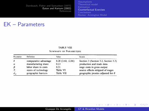
Dornbusch, Fisher and Samuelson (1977)Eaton and Kortum (2002)
References
AssumptionsTheoretical modelEstimationCounterfactual ExercisesConclusionsReview: Armington Model
EK – Parameters
TECHNOLOGY, GEOGRAPHY, AND TRADE 1767
TABLE VIII
SUMMARY OF PARAMETERS
Parameter Definition Value Source
0 comparative advantage 8.28 (3.60, 12.86) Section 3 (Section 5.2, Section 5.3) a manufacturing share 0.13 production and trade data ,B labor share in costs 0.21 wage costs in gross output Ti states of technology Table VI source effects stripped of wages dni geographic barriers Table VII geographic proxies adjusted for 0
To complete the parameterization we calculate a = 0.13, the average demand for final manufactures as a fraction of GDP.39 Table VIII summarizes the structural parameters of the model, their definitions, the values we assign to them, and where we got these numbers.
We can examine counterfactuals according to a number of different criteria. One is overall welfare in country n, measured as real GDP: Wn = Yn/pa. (Since nonmanufactures are numeraire, the price level in country n is pa. Since we hold labor supplies and populations fixed throughout, there is no need to distin- guish between GDP and GDP per worker or GDP per capita.) Decomposing the change in welfare into income and price effects gives
In - -In- aIn- ' __ a In- Wn Yn Pn wn Yn Pn
(Here x' denotes the counterfactual value of a variable xn.) In the case of mobile labor, of course, only the price effect is operative. Aside from looking at welfare, for the case of mobile labor, we ask about manufacturing employment while, for the case of immobile labor, we look at the manufacturing wage wn. We also investigate how trade patterns change.
Since we have data on both manufacturing employment and manufacturing wages, we can look at our model's implications for each given data on the other. Our fit is not perfect since we (i) impose a common manufacturing demand share a across countries and (ii) ignore sources of manufactures from outside our sample of 19 OECD countries.
We wish to distinguish the effects of any of the counterfactuals we examine in the next section from the initial misfit of our model. We therefore compare the various counterfactuals that we examine with a baseline in which wages are
39 Specifically we solve for a from the relationship
X. +IMP,n =
(1-/3)(Xnn +EXP) + ?aYn
summed across our sample (with ,B= .21) in 1990. Here IMPn is manufacturing imports and EXPn is manufacturing exports, and Yn is total GDP, each translated from local currency values into U.S. dollars at the official exchange rate.
Giuseppe De Arcangelis GT & Ricardian Models

Dornbusch, Fisher and Samuelson (1977)Eaton and Kortum (2002)
References
AssumptionsTheoretical modelEstimationCounterfactual ExercisesConclusionsReview: Armington Model
Questions for Counterfactuals (EK 2012)
I What are the gains from trade?
I How much do gains from trade increase if there are fallingtrade costs?
I How much do countries gain from the technologicalimprovement of their partners?
I What are the costs of moving from deficit to balanced trade(similar to the transfer problem)?
New set of parameters in Eaton and Kortum (2012):α = 0.2, β = 0.3, θ = 4
Giuseppe De Arcangelis GT & Ricardian Models

Dornbusch, Fisher and Samuelson (1977)Eaton and Kortum (2002)
References
AssumptionsTheoretical modelEstimationCounterfactual ExercisesConclusionsReview: Armington Model
Gains from Trade
Use: πi ,i = PROD−EXPPROD−(EXP−IMP) .
Expected results:
I In a frictionless world home share should be equal to worldshare
I Large countries should have large home shares (as in reality)
I With the focus on manufacturing, the elasticity of gains fromtrade (i.e. exponent of πi ,i ) is no longer 1/θ, but it is α/(βθ)
Giuseppe De Arcangelis GT & Ricardian Models

Dornbusch, Fisher and Samuelson (1977)Eaton and Kortum (2002)
References
AssumptionsTheoretical modelEstimationCounterfactual ExercisesConclusionsReview: Armington Model
Gains from Trade
Use: πi ,i = PROD−EXPPROD−(EXP−IMP) . Expected results:
I In a frictionless world home share should be equal to worldshare
I Large countries should have large home shares (as in reality)
I With the focus on manufacturing, the elasticity of gains fromtrade (i.e. exponent of πi ,i ) is no longer 1/θ, but it is α/(βθ)
Giuseppe De Arcangelis GT & Ricardian Models

Dornbusch, Fisher and Samuelson (1977)Eaton and Kortum (2002)
References
AssumptionsTheoretical modelEstimationCounterfactual ExercisesConclusionsReview: Armington Model
EK(2012) – Gains from Trade in RealityPutting Ricardo to Work 81
Table 2 reports the home share in 2006 for the 25 countries with data on Table 2 reports the home share in 2006 for the 25 countries with data on gross manufacturing production. The mean value of the home share is just under gross manufacturing production. The mean value of the home share is just under 50 percent. In a world of frictionless trade (all 50 percent. In a world of frictionless trade (all dnini == 1), there is no reason for a 1), there is no reason for a country to spend a larger share of its income on its own goods than any other country to spend a larger share of its income on its own goods than any other country. A country’s home share, in that case, would correspond to its share in country. A country’s home share, in that case, would correspond to its share in world output. As Table 2 makes clear, for each of these countries the home share world output. As Table 2 makes clear, for each of these countries the home share is many times larger than the country’s share in world GDP: three times higher for is many times larger than the country’s share in world GDP: three times higher for the United States, ten times for Germany, 50 times for Denmark, and 100 times for the United States, ten times for Germany, 50 times for Denmark, and 100 times for Greece. Such multiples illustrate the extent to which trade barriers continue to chop Greece. Such multiples illustrate the extent to which trade barriers continue to chop up world markets. Even though countries buy much more of their manufactures up world markets. Even though countries buy much more of their manufactures
Table 2The Home Share of Spending on Manufactures and Gains from Trade
World GDPshare (%) in
2006
Home share of spending Implied gains from trade
CountryLevel in
2006 (%)Change since 1996 (percentage points)
Level in 2006 (%)
Change since 1996 (percentage points)
Austria 0.66 31.4 –16.2 21.3 8.1Canada 2.60 49.1 –1.5 12.6 0.6Czech Republic 0.29 42.6 –14.7 15.3 5.5Denmark 0.56 25.6 –18.1 25.5 10.7Estonia 0.03 2.5 –19.6 85.4 56.7Finland 0.42 58.2 –7.3 9.4 2.1France 4.60 56.9 –10.3 9.9 3.0Germany 5.94 53.7 –16.4 10.9 4.8Greece 0.54 52.7 –11.6 11.3 3.6Hungary 0.23 26.0 –34.5 25.1 16.4Iceland 0.03 27.9 –10.0 23.7 6.2Ireland 0.46 39.6 9.9 16.7 –5.7Italy 3.80 68.9 –7.1 6.4 1.7Japan 8.88 84.9 –5.6 2.8 1.1Korea 1.94 77.2 –0.7 4.4 0.1Mexico 1.94 58.3 –7.9 9.4 2.3New Zealand 0.22 53.6 –8.2 11.0 2.6Norway 0.68 51.9 –2.5 11.6 0.9Poland 0.69 53.4 –15.8 11.0 4.7Portugal 0.41 50.8 –10.2 12.0 3.4Slovenia 0.08 27.2 –15.5 24.3 9.0Spain 2.51 62.8 –10.2 8.1 2.7Sweden 0.81 49.2 –10.0 12.5 3.4Switzerland 0.80 35.3 –20.0 18.9 8.6United States 27.26 73.5 –8.3 5.3 1.9All others 33.62
Source: Authors’ calculations from the OECD STAN (STructural ANalysis) Database, the Economist Intelligence Unit, and a model described in the text.Notes: The home share is the share a country spends on domestic manufactures out of total country spending on manufactures. The last two columns calculate the implications of the level of the home share, and its changes over time, for countries’ gains from trade and how those gains have evolved. We look at the gains from trade only in manufactures.
Giuseppe De Arcangelis GT & Ricardian Models

Dornbusch, Fisher and Samuelson (1977)Eaton and Kortum (2002)
References
AssumptionsTheoretical modelEstimationCounterfactual ExercisesConclusionsReview: Armington Model
Falling Trade Costs
Exercise: a fall of trade barriers by 25%, implemented as adecrease in all dn,i ’s, such that world trade in manufacturesdoubles (it doubled in the past 30 years).
Results:
I Median gain of 10% in real wages
I Larger gains for smaller countries
Giuseppe De Arcangelis GT & Ricardian Models

Dornbusch, Fisher and Samuelson (1977)Eaton and Kortum (2002)
References
AssumptionsTheoretical modelEstimationCounterfactual ExercisesConclusionsReview: Armington Model
Falling Trade Costs
Exercise: a fall of trade barriers by 25%, implemented as adecrease in all dn,i ’s, such that world trade in manufacturesdoubles (it doubled in the past 30 years). Results:
I Median gain of 10% in real wages
I Larger gains for smaller countries
Giuseppe De Arcangelis GT & Ricardian Models

Dornbusch, Fisher and Samuelson (1977)Eaton and Kortum (2002)
References
AssumptionsTheoretical modelEstimationCounterfactual ExercisesConclusionsReview: Armington Model
EK(2012) – Further GlobalizationJonathan Eaton and Samuel Kortum 83
on welfare around the world from a shift in the distribution of technologies in a on welfare around the world from a shift in the distribution of technologies in a particular country particular country i (as refl ected in the parameter (as refl ected in the parameter Aii ). Our particular experiment ). Our particular experiment makes the United States 10 percent more productive, so that makes the United States 10 percent more productive, so that A US == 1.1. 1.1.
The world economy responds in two important ways: First, the U.S. wage rises The world economy responds in two important ways: First, the U.S. wage rises by about 30 percent relative to other countries’ wages. Second, the U.S. real wage by about 30 percent relative to other countries’ wages. Second, the U.S. real wage (in terms of goods and services) rises by about 6 percent, while real wages in other (in terms of goods and services) rises by about 6 percent, while real wages in other countries increase by only a small amount, if at all.countries increase by only a small amount, if at all.
The effects of geography are apparent as the greatest foreign benefi ciaries are The effects of geography are apparent as the greatest foreign benefi ciaries are Canada and Mexico, which experience a real wage gain one-tenth that in the United Canada and Mexico, which experience a real wage gain one-tenth that in the United States. A few countries, if they are initially running a trade surplus in manufactures, States. A few countries, if they are initially running a trade surplus in manufactures, experience a small real wage decline. (If we fi rst eliminate all trade imbalances and experience a small real wage decline. (If we fi rst eliminate all trade imbalances and then increase U.S. technology, all foreign countries experience a real wage gain.)then increase U.S. technology, all foreign countries experience a real wage gain.)
Overall, the increase in U.S. technology raises the GDP-weighted real wage Overall, the increase in U.S. technology raises the GDP-weighted real wage around the world by 1.6 percent, with 8 percent of this gain experienced outside around the world by 1.6 percent, with 8 percent of this gain experienced outside the United States. Foreign countries gain both due to the lower prices of fi nal goods the United States. Foreign countries gain both due to the lower prices of fi nal goods
Figure 3Real Wage Response to a Decrease in Trade Barriers
Source: Authors’ calculations using data from the OECD STAN (STructural Analysis) Database and the Economist Intelligence Unit and a model described in the text.Notes: We consider a uniform proportional 25 percent drop in the costs of trade, a magnitude chosen so that world trade in manufactures approximately doubles relative to world GDP. The fi gure plots the counterfactual change in real wage against each countries’ share of world GDP.
Australia
Austria
Belgium-Luxembourg
Canada
China
Czech Republic
Denmark
Estonia
Finland France
Germany
Greece
Hungary
Iceland
Ireland
Italy
Japan
Korea
Mexico
Netherlands
New Zealand Norway
PolandPortugal
Slovak RepublicSlovenia
Spain
Sweden
Switzerland
Turkey
United States
ROW
Cou
nte
rfac
tual
ch
ange
(%
) in
rea
l wag
e
25
20
15
10
5
0
.001 .01 .1 .5
Share of world GDP
Giuseppe De Arcangelis GT & Ricardian Models

Dornbusch, Fisher and Samuelson (1977)Eaton and Kortum (2002)
References
AssumptionsTheoretical modelEstimationCounterfactual ExercisesConclusionsReview: Armington Model
Technological Improvement
Exercise: An increase in US efficiency by 10%.
Results:
I US real wage increases by 6%; much less in its partners
I Greater beneficiaries are the closer countries (Canada andMexico)
I World’s average real wage increases by 1.6% (8% outside theUS)
I A similar improvement in China: warw ↑ 0.6% (10% outsideChina)
Giuseppe De Arcangelis GT & Ricardian Models

Dornbusch, Fisher and Samuelson (1977)Eaton and Kortum (2002)
References
AssumptionsTheoretical modelEstimationCounterfactual ExercisesConclusionsReview: Armington Model
Technological Improvement
Exercise: An increase in US efficiency by 10%. Results:
I US real wage increases by 6%; much less in its partners
I Greater beneficiaries are the closer countries (Canada andMexico)
I World’s average real wage increases by 1.6% (8% outside theUS)
I A similar improvement in China: warw ↑ 0.6% (10% outsideChina)
Giuseppe De Arcangelis GT & Ricardian Models

Dornbusch, Fisher and Samuelson (1977)Eaton and Kortum (2002)
References
AssumptionsTheoretical modelEstimationCounterfactual ExercisesConclusionsReview: Armington Model
Eliminating Current Account Imbalances
Exercise: international transfers in order to balance all trade inmanufacturing.
Results:
I increase in the real wage of US partners to undo the huge USdeficit
I positive relationship b/w initial position (deficit or surplus)and change in the (relative to the US) real wage
I smaller changes in the real wage
I Importance of the initial dimension of the manufacturingsector (see differences among Iceland, Greece and Ireland)
I large adjustments in the manufacturing shares are required
Giuseppe De Arcangelis GT & Ricardian Models

Dornbusch, Fisher and Samuelson (1977)Eaton and Kortum (2002)
References
AssumptionsTheoretical modelEstimationCounterfactual ExercisesConclusionsReview: Armington Model
Eliminating Current Account Imbalances
Exercise: international transfers in order to balance all trade inmanufacturing. Results:
I increase in the real wage of US partners to undo the huge USdeficit
I positive relationship b/w initial position (deficit or surplus)and change in the (relative to the US) real wage
I smaller changes in the real wage
I Importance of the initial dimension of the manufacturingsector (see differences among Iceland, Greece and Ireland)
I large adjustments in the manufacturing shares are required
Giuseppe De Arcangelis GT & Ricardian Models

Dornbusch, Fisher and Samuelson (1977)Eaton and Kortum (2002)
References
AssumptionsTheoretical modelEstimationCounterfactual ExercisesConclusionsReview: Armington Model
EK(2012) – Effects of Trade Balancing86 Journal of Economic Perspectives
and other activities. In Dekle, Eaton, and Kortum (2008), we introduce rigidities and other activities. In Dekle, Eaton, and Kortum (2008), we introduce rigidities and examine their effect.and examine their effect.
Extending and Improving the Tool
Much recent work has extended this new old Ricardian trade theory in various Much recent work has extended this new old Ricardian trade theory in various ways, sometimes combining elements of it with other theories to address new ques-ways, sometimes combining elements of it with other theories to address new ques-tions. Here we briefl y discuss a few of these contributions.tions. Here we briefl y discuss a few of these contributions.
The fi eld of international trade has traditionally used industry as its unit of The fi eld of international trade has traditionally used industry as its unit of analysis, a natural choice given the heterogeneity of industries and the fact that most analysis, a natural choice given the heterogeneity of industries and the fact that most trade policy is implemented at the industry level. In moving from a small number of trade policy is implemented at the industry level. In moving from a small number of goods, with labor requirements specifi ed in a table, to a continuum of goods, with goods, with labor requirements specifi ed in a table, to a continuum of goods, with labor requirements only described probabilistically, we lose track of this industry labor requirements only described probabilistically, we lose track of this industry dimension. A number of papers have brought industries back into the analysis, dimension. A number of papers have brought industries back into the analysis,
Figure 4Wage Response to Eliminating Current Account Imbalances
Source: Authors’ calculations using data from the OECD STAN (STructural Analysis) Database and the Economist Intelligence Unit and a model described in the text.Notes: We consider the effects of exogenous shifts in manufacturing trade defi cits that would simultaneously balance every country’s current account, holding fi xed any defi cits outside of manufacturing, as in Table 3. The fi gure plots the counterfactual change in wage relative to the United States against the initial current account balance as a share of GDP. “ROW” is “rest of world.”
Australia
AustriaBelgium-Luxembourg
Canada
China
Czech Republic
Denmark
Estonia
Finland
France
Germany
Greece
Hungary
Iceland
IrelandItaly
JapanKorea
Mexico
Netherlands
New Zealand
Norway
Poland
Portugal
Slovak RepublicSlovenia
Spain
SwedenSwitzerland
TurkeyUnited States
ROW
Cou
nte
rfac
tual
ch
ange
(%
) in
wag
e (r
ealt
ive
to U
.S. w
age)
40
20
0
–20
–40
–15 –10 –5 0 5 10 15
Current account (as % of GDP)
Giuseppe De Arcangelis GT & Ricardian Models

Dornbusch, Fisher and Samuelson (1977)Eaton and Kortum (2002)
References
AssumptionsTheoretical modelEstimationCounterfactual ExercisesConclusionsReview: Armington Model
Conclusions
I The EK model offers a simply tractable way of computinggains from trade
where GFT come from comparativespecialization, but not from a discipline effect that increasesaverage productivity – as in Melitz (2003). Actually, averageproductivity in a country can decrease as a consequence ofopening up trade when the country specializes in thelow-productivity sector; however, the country still enjoys GFT(see the example below)
I The model can be easily used for counterfactuals since thechange in the parameters is not subject to the Lucas critique(technology is considered a deep parameter)
Giuseppe De Arcangelis GT & Ricardian Models

Dornbusch, Fisher and Samuelson (1977)Eaton and Kortum (2002)
References
AssumptionsTheoretical modelEstimationCounterfactual ExercisesConclusionsReview: Armington Model
Conclusions
I The EK model offers a simply tractable way of computinggains from trade where GFT come from comparativespecialization, but not from a discipline effect that increasesaverage productivity – as in Melitz (2003).
Actually, averageproductivity in a country can decrease as a consequence ofopening up trade when the country specializes in thelow-productivity sector; however, the country still enjoys GFT(see the example below)
I The model can be easily used for counterfactuals since thechange in the parameters is not subject to the Lucas critique(technology is considered a deep parameter)
Giuseppe De Arcangelis GT & Ricardian Models

Dornbusch, Fisher and Samuelson (1977)Eaton and Kortum (2002)
References
AssumptionsTheoretical modelEstimationCounterfactual ExercisesConclusionsReview: Armington Model
Conclusions
I The EK model offers a simply tractable way of computinggains from trade where GFT come from comparativespecialization, but not from a discipline effect that increasesaverage productivity – as in Melitz (2003). Actually, averageproductivity in a country can decrease as a consequence ofopening up trade when the country specializes in thelow-productivity sector;
however, the country still enjoys GFT(see the example below)
I The model can be easily used for counterfactuals since thechange in the parameters is not subject to the Lucas critique(technology is considered a deep parameter)
Giuseppe De Arcangelis GT & Ricardian Models

Dornbusch, Fisher and Samuelson (1977)Eaton and Kortum (2002)
References
AssumptionsTheoretical modelEstimationCounterfactual ExercisesConclusionsReview: Armington Model
Conclusions
I The EK model offers a simply tractable way of computinggains from trade where GFT come from comparativespecialization, but not from a discipline effect that increasesaverage productivity – as in Melitz (2003). Actually, averageproductivity in a country can decrease as a consequence ofopening up trade when the country specializes in thelow-productivity sector; however, the country still enjoys GFT(see the example below)
I The model can be easily used for counterfactuals since thechange in the parameters is not subject to the Lucas critique(technology is considered a deep parameter)
Giuseppe De Arcangelis GT & Ricardian Models

Dornbusch, Fisher and Samuelson (1977)Eaton and Kortum (2002)
References
AssumptionsTheoretical modelEstimationCounterfactual ExercisesConclusionsReview: Armington Model
Conclusions
I A model of the diffusion of the benefits of technologydiffusion, but without considering special channels (as theliterature on technology diffusion does)
I A central role to the technology parameter θ in explaining thegravity model; previously, the explanation was based only onpreferences (see the Armington model)
Giuseppe De Arcangelis GT & Ricardian Models

Dornbusch, Fisher and Samuelson (1977)Eaton and Kortum (2002)
References
AssumptionsTheoretical modelEstimationCounterfactual ExercisesConclusionsReview: Armington Model
Example: GFT and Decrease in Average CountryProductivity
Labor requirements in the table:
UK P
Cloth 4 6
Wine 8 9
ToT 1/2 2/3
I In autarky average productivity is between 1/4 and 1/8 in UKand between 1/6 and 1/9 in P
I Assume the world ToT is 0.55; hence trade occurs;
I P fully specializes in WineI in P average productivity is 1/9 and has decreased;however, P
gains from trading with the UK
Giuseppe De Arcangelis GT & Ricardian Models

Dornbusch, Fisher and Samuelson (1977)Eaton and Kortum (2002)
References
AssumptionsTheoretical modelEstimationCounterfactual ExercisesConclusionsReview: Armington Model
Example: GFT and Decrease in Average CountryProductivity
Labor requirements in the table:
UK P
Cloth 4 6
Wine 8 9
ToT 1/2 2/3
I In autarky average productivity is between 1/4 and 1/8 in UKand between 1/6 and 1/9 in P
I Assume the world ToT is 0.55; hence trade occurs;I P fully specializes in Wine
I in P average productivity is 1/9 and has decreased;however, Pgains from trading with the UK
Giuseppe De Arcangelis GT & Ricardian Models

Dornbusch, Fisher and Samuelson (1977)Eaton and Kortum (2002)
References
AssumptionsTheoretical modelEstimationCounterfactual ExercisesConclusionsReview: Armington Model
Example: GFT and Decrease in Average CountryProductivity
Labor requirements in the table:
UK P
Cloth 4 6
Wine 8 9
ToT 1/2 2/3
I In autarky average productivity is between 1/4 and 1/8 in UKand between 1/6 and 1/9 in P
I Assume the world ToT is 0.55; hence trade occurs;I P fully specializes in WineI in P average productivity is 1/9 and has decreased;
however, Pgains from trading with the UK
Giuseppe De Arcangelis GT & Ricardian Models

Dornbusch, Fisher and Samuelson (1977)Eaton and Kortum (2002)
References
AssumptionsTheoretical modelEstimationCounterfactual ExercisesConclusionsReview: Armington Model
Example: GFT and Decrease in Average CountryProductivity
Labor requirements in the table:
UK P
Cloth 4 6
Wine 8 9
ToT 1/2 2/3
I In autarky average productivity is between 1/4 and 1/8 in UKand between 1/6 and 1/9 in P
I Assume the world ToT is 0.55; hence trade occurs;I P fully specializes in WineI in P average productivity is 1/9 and has decreased;however, P
gains from trading with the UK
Giuseppe De Arcangelis GT & Ricardian Models

Dornbusch, Fisher and Samuelson (1977)Eaton and Kortum (2002)
References
AssumptionsTheoretical modelEstimationCounterfactual ExercisesConclusionsReview: Armington Model
Armington Preferences
I Armington utility function: U =(∫ 1
0 ϕ(j)1σQ(j)
σ−1σ dj
) σσ−1
where ϕ is a preference parameter
Giuseppe De Arcangelis GT & Ricardian Models

Dornbusch, Fisher and Samuelson (1977)Eaton and Kortum (2002)
References
AssumptionsTheoretical modelEstimationCounterfactual ExercisesConclusionsReview: Armington Model
Gravity in the Armington Model vs EK
I When applying this utility function without specifying theproduction functions and assuming transaction costs as in EK,we obtain the following reduced form for bilateral trade:
Xn,i =ϕn,i
(dn,iPn
)1−σ
ΣNm=1ϕm,i
(dm,iPm
)1−σXm
XnQi
whereas in EK
Xn,i =
(dn,iPn
)−θ
ΣNm=1
(dm,iPm
)−θXm
XnQi
Giuseppe De Arcangelis GT & Ricardian Models

Dornbusch, Fisher and Samuelson (1977)Eaton and Kortum (2002)
References
AssumptionsTheoretical modelEstimationCounterfactual ExercisesConclusionsReview: Armington Model
Gravity in the Armington Model vs EK
Xn,i =ϕn,i
(dn,iPn
)1−σ
ΣNm=1ϕm,i
(dm,iPm
)1−σXm
XnQi
Xn,i =
(dn,iPn
)−θ
ΣNm=1
(dm,iPm
)−θXm
XnQi
I distance plays a role according to the technological parameterθ rather than the preference parameter σ ?see¿Anderson1979
I an increase in the “distance” barriers will decrease the numberof products exported (extensive margin) in EK, rather than areduction in the quantities of all goods (intensive margin) inthe Armington case.
Giuseppe De Arcangelis GT & Ricardian Models

Dornbusch, Fisher and Samuelson (1977)Eaton and Kortum (2002)
References
AssumptionsTheoretical modelEstimationCounterfactual ExercisesConclusionsReview: Armington Model
Other Recent Works
I Rodrıguez-Clare (2010) for offshoring in this framework
I Arkolakis, Costinot, and Rodriguez-Clare (2012) for ageneralization of the computation of welfare within the classof EK models
Giuseppe De Arcangelis GT & Ricardian Models

Dornbusch, Fisher and Samuelson (1977)Eaton and Kortum (2002)
References
References I
Arkolakis, C., Costinot, A., & Rodriguez-Clare, A. (2012,February). New trade models, same old gains? AmericanEconomic Review, 102(1), 94-130.
Eaton, J., & Kortum, S. (2002, September). Technology,geography, and trade. Econometrica, 70(5), 1741-1779.
Eaton, J., & Kortum, S. (2012, Spring). Putting ricardo to work.Journal of Economic Perspectives, 26(2), 65-90.
Melitz, M. J. (2003, November). The impact of trade onintra-industry reallocations and aggregate industryproductivity. Econometrica, 71(6), 1695-1725.
Rodrıguez-Clare, A. (2010, April). Offshoring in a ricardian world.American Economic Journal: Macroeconomics, 2(2), 227-58.
Giuseppe De Arcangelis GT & Ricardian Models

Dornbusch, Fisher and Samuelson (1977)Eaton and Kortum (2002)
References
References II
Simonovska, I., & Waugh, M. E. (2013). The elasticity of trade:Estimates and evidence. Journal of InternationalEconomics(0), -.
Giuseppe De Arcangelis GT & Ricardian Models