ga record template · web viewivreview of hydrofracturing and induced seismicity review of...

$: GA Record Template · Web viewivReview of Hydrofracturing and Induced Seismicity Review of Hydrofracturing and Induced Seismicity91 Review of Hydrofracturing and Induced Seismicityiii$
Review of Hydrofracturing and Induced SeismicityGEOSCIENCE AUSTRALIARECORD 2016/02

Barry Drummond

Department of Industry, Innovation and ScienceMinister for Resources, Energy and Northern Australia: The Hon Josh Frydenberg MPAssistant Minister for Science: The Hon Karen Andrews MPSecretary: Ms Glenys Beauchamp PSM

Geoscience AustraliaChief Executive Officer: Dr Chris PigramThis paper is published with the permission of the CEO, Geoscience Australia

© Commonwealth of Australia (Geoscience Australia) 2016

With the exception of the Commonwealth Coat of Arms and where otherwise noted, this product is provided under a Creative Commons Attribution 4.0 International Licence. (http://creativecommons.org/licenses/by/4.0/legalcode)

Geoscience Australia has tried to make the information in this product as accurate as possible. However, it does not guarantee that the information is totally accurate or complete. Therefore, you should not solely rely on this information when making a commercial decision.

Geoscience Australia is committed to providing web accessible content wherever possible. If you are having difficulties with accessing this document please email [email protected].

ISSN 2201-702X (PDF)

ISBN 978-1-925124-95-8 (PDF)

GeoCat 83880

Bibliographic reference: Drummond, Barry. 2016. Review of Hydrofracturing and Induced Seismicity. Record 2016/02. Geoscience Australia, Canberra. http://dx.doi.org/10.11636/Record.2016.002

http://dx.doi.org/10.11636/Record.2016.002

mailto:[email protected]

http://creativecommons.org/licenses/by/4.0/legalcode

Contents

1 Summary............................................................................................................................................. 1

2 Introduction.......................................................................................................................................... 6

3 What are hydrofracturing and induced seismicity?..............................................................................83.1 Hydrofracturing............................................................................................................................... 83.2 Induced Seismicity......................................................................................................................... 9

3.2.1 Intensity.................................................................................................................................... 93.2.2 Magnitude............................................................................................................................... 10

4 How does hydrofracturing work?.......................................................................................................124.1 An Introduction to Stress..............................................................................................................124.2 Tension Cracks............................................................................................................................ 14

4.2.1 Orientation of Tension Cracks................................................................................................164.3 Shear failure................................................................................................................................. 164.4 Hybrid tension and shear mode failure.........................................................................................174.5 Forming new fractures vs reactivating existing fractures..............................................................174.6 Unintentional Hydrofracturing.......................................................................................................18

5 Australian Stress Field.......................................................................................................................21

6 Monitoring Hydrofracturing................................................................................................................26

7 Fracture Size and Shape................................................................................................................... 30

8 Energy Related Hydrofracturing.........................................................................................................358.1 Intentional Hydrofracturing...........................................................................................................35

8.1.1 Coal Seam Gas......................................................................................................................358.1.2 Shale Gas............................................................................................................................... 428.1.3 Enhanced Geothermal Systems.............................................................................................43

8.2 Unintentional Hydrofracturing.......................................................................................................468.2.1 Carbon Sequestration.............................................................................................................47

9 Issues of Public Concern................................................................................................................... 489.1 Water volumes used during hydrofracturing.................................................................................489.2 Aquifer breaching and loss of water for human use and the agricultural and pastoral industries............................................................................................................................................ 489.3 Contamination of fresh water aquifers by saline formation waters and/or hydrofracturing fluids................................................................................................................................................... 499.4 Environmental issues with disposing of formation waters [volume, contained contaminants]......499.5 Fugitive gas emissions into groundwater used for human and stock consumption, and directly at the surface......................................................................................................................... 499.6 Loss of productive pasture...........................................................................................................509.7 Impact of induced seismicity........................................................................................................50

10 Some Simple Points........................................................................................................................ 51

11 Acknowledgements.......................................................................................................................... 52

12 References...................................................................................................................................... 53

Review of Hydrofracturing and Induced Seismicity

Appendix A How Hydrofracturing Works...............................................................................................56A.1 Introduction.................................................................................................................................. 56A.2 Rock failure through hydrofracture...............................................................................................57

A.2.1 Tensional Cracks....................................................................................................................59A.2.2 Shear Fractures...................................................................................................................... 62A.2.3 Hybrid tension and shear mode failure...................................................................................66

A.3 The interplay between forming new fractures and reactivating existing fractures........................66A.4 Unintentional Hydrofracturing......................................................................................................68A.5 Summary of Intentional and Unintentional Hydrofracturing..........................................................72

A.5.1 Intact Rock............................................................................................................................. 72A.5.2 Rock with a pre-existing fault..................................................................................................72A.5.3 Unintentional Hydrofracturing.................................................................................................72

A.6 References.................................................................................................................................. 73

Appendix B Earthquake Intensity and Magnitude.................................................................................74B.1 Introducing basic earthquake terms.............................................................................................74

B.1.1 Often used nomenclature.......................................................................................................74B.2 Earthquake Intensity.................................................................................................................... 75B.3 Earthquake Magnitude.................................................................................................................77

B.3.1 Relevance to small earthquakes caused by tensional cracking..............................................78B.3.2 Negative Magnitudes..............................................................................................................78

B.4 Intensity–Magnitude Relations.....................................................................................................79B.5 Fault Rupture Parameters............................................................................................................80B.6 Distinguishing between tension cracking and shearing................................................................84

B.6.1 Determining rupture type by the distribution of earthquake size.............................................84B.6.2 Determining rupture type by the spatial and temporal distribution of earthquakes.................86B.6.3 Determining rupture type by waveform analysis.....................................................................86

B.7 Relevance to Hydrofracturing......................................................................................................88B.8 References.................................................................................................................................. 89

Attachment to Appendix B....................................................................................................................91Modified Mercalli (MM) Scale of earthquake intensity (after Eiby 1966).............................................91Categories of non-wooden construction.............................................................................................92

Appendix C Human Induced Seismicity................................................................................................93C.1 Introduction to Human Induced Seismicity...................................................................................93C.2 Causes of Human Induced Seismicity.........................................................................................93C.3 Case Studies............................................................................................................................... 95

C.3.1 Case Study #1: Talbingo Reservoir, NSW, Australia.............................................................95C.3.2 Case Study #2: Rocky Mountains Arsenal.............................................................................96C.3.3 Case Study #3: Rangely Oilfield, Colorado............................................................................98C.3.4 Case Study #4: Oklahoma November 2011 Earthquakes....................................................100

C.4 Discussion................................................................................................................................. 102C.5 References................................................................................................................................ 103

Review of Hydrofracturing and Induced Seismicity

1 Summary

Hydrofracturing is a process whereby the unconventional energy industries produce permeability in rocks in order to release stored energy–oil, gas, heat.

Hydrofracturing has occurred naturally throughout geological time. It is the mechanism by which fluids migrate through the Earth's crust and form ore bodies. Rocks break when they are exposed to high stresses. In natural hydrofracturing, they break at lower stresses if the fluids in the pores of the rock are at high pressure.

The hydrofracturing of rock by manipulating pore fluid pressure in the ambient stress field is used in the energy industries. Water is pumped at high pressures into wells in order to fracture the rocks at specific depths in the well. The directions in which the fractures will propagate is determined by the stress field in rocks. The fractures will propagate horizontally if the minimum principal stress is vertical. They will be vertical if the minimum principal stress is horizontal.

When rocks break, some of the energy that is released is in the form of ground shaking. This is called an earthquake. Small earthquakes occur when rocks are hydrofractured. If the rocks break due to natural causes, the earthquakes are called natural or tectonic earthquakes. If the rocks are hydrofractured by human activity, they are called induced earthquakes.

'Seismicity' refers to the population of earthquakes in a region. If the region has a lot of earthquakes, it is said to have high seismicity. A population of induced earthquakes is called induced seismicity.

Earthquake size is measured in two ways.

Intensity is a measure of how people feel and react to an earthquake, and whether buildings and other infrastructure are damaged. Intensity in Australia is measured on the 12–point Modified Mercalli Scale (which uses Roman numerals). The intensity of an earthquake becomes less with increasing distance from the epicentre of the earthquake; ie., a number of intensities can be assigned to one earthquake. In most cases people will not feel earthquakes if their intensity is MMI I or MMI II. Damage starts at MMI V and gets progressively worse at higher intensities.

Magnitude is a measure of the energy released by the earthquake. Each earthquake has only one magnitude. A number of scales are in use for measuring magnitude. The Richter Magnitude scale is probably the most referred to in the media. Moment magnitude is probably the most widely used scale. It is based on the moment of the earthquake; moment is the product of the shear modulus of the rock, the area of rock that is fractured and the amount of displacement of rock on one side of the fracture relative to the rock on the other side. That is, the moment magnitude scale is linked to the geological parameters of the fracture that causes the ground to shake. If the fracture is large, and/or in rock that is strong (high shear modulus), then the magnitude will be large. If the fracture is small and/or in weak rock, the magnitude will be small.

Earthquake magnitude scales are logarithmic; therefore earthquake magnitude can be negative for very small earthquakes (micro earthquakes).

Because hydrofracturing is both natural and man-made, this report classifies hydrofracturing into:

1. Natural hydrofracturing

Review of Hydrofracturing and Induced Seismicity 1

2. Human induced (usually unintentional) hydrofracturing

3. Energy related hydrofracturing, which includes

a. Intentional hydrofracturing and

b. Unintentional hydrofracturing.

Human induced hydrofracturing is included in this report to distinguish between seismicity and hydrofracturing caused by mining activities and the filling of water storage dams from energy related hydrofracturing.

Energy related hydrofracturing is the subject matter of this report. Hydrofracturing in the coal seam gas, shale gas and enhanced geothermal systems sectors are in scope. The potential for unintentional hydrofracturing of underground storage reservoirs, eg., through injecting large volumes of carbon dioxide, is also in scope. Hydrofracturing for enhanced oil recovery in conventional fields and for tight gas and shale oil are not in scope.

Intentional hydrofracturing is undertaken in order to create new permeability, through

1. creating new fractures in intact rock, and/or

2. re-opening existing fractures, eg., joints, cleats in coal, and/or

3. reactivating existing faults.

Hydrofracturing will create fractures in one of three modes:

1. Tensional fractures open by one side of the fracture moving away from the other without any lateral displacement

2. Shear fractures open by one side of the fracture being displaced laterally with respect to the other

3. Hybrid tensional shear fractures have both types of displacement.

The mode of fracture depends on the differential stress and the physical properties of the rock. The stress field anywhere can be resolved into three orthogonal components, one of which by convention is vertical and the other two horizontal, and differential stress is the difference between the maximum principal stress and the minimum principal stress.

Rocks will fracture in tension when the differential stress is low and the pressure of fluid in the cracks and pores in the rock exceeds the minimum principal stress by an amount equal to the tensional strength of the rock. Tension fractures form perpendicular to the minimum principal stress.

Tension fractures grow by small increments. Therefore the ground shaking that accompanies fracture growth leads to earthquakes with small magnitudes, typically M = -2–0 in shales and coal and enhanced geothermal systems, with occasional M = 3–4 earthquakes from hydrofracturing in enhanced geothermal systems.

As the fractures get larger, the time between growth increments gets longer.

Eventually, growth on large cracks will slow and growth on smaller cracks will dominate. Ultimately the limits on crack size are determined by the volume of cracks that are created and the ability of the pumping system to deliver sufficient volumes of water to the crack system at high enough pressure.

2 Review of Hydrofracturing and Induced Seismicity

Fractures that occur in shear mode in intact rock form at an angle to the maximum principal stress that is around 30 for many common rocks. This is called the optimum angle. Shear fractures require higher differential stresses and lower pore fluid pressures than tension fractures.

The shear direction, ie., normal, reverse or strike-slip, is determined by the orientation of the stress field. Normal faults form at lower differential stresses and/or pore fluid pressures than strike-slip faults, which in turn form at lower values than reverse faults.

Hybrid tensional shear fractures form in intact rock at angles between the direction of the maximum principal stress and the direction of shear fractures, ie, between 0 and about 30 to the maximum principal stress.

If the high pressure fluids intersect an existing fault, the existing fault can be reactivated if it is oriented close to the optimum angle and it is weak. The reactivation of a weak fault requires much lower differential stresses and/or pore fluid pressures than failure in intact rock. However, if the existing fault is strong, or at a high angle to the minimum principal stress, then new fractures will form in nearby intact rock.

Most unintentional hydrofracturing is linked to the reactivation of existing faults through the re-injection of waste fluids, usually mostly water, ie., flow back water from hydrofracturing operations and formation waters pumped from producing parts of reservoirs. The reinjection often happens over long periods of time and builds up pore fluid pressures over large areas, eg., up to 5km from the injection well. Often the induced seismicity does not stop immediately if injection is stopped; the largest earthquakes can happen after injection has stopped. A six-fold increase in seismicity in the mid-continent of the United States of America since 2000 correlates with activities in the energy industries, including the re-injection of waste water. Some earthquake magnitudes exceeded M = 5.

The stress field in and around a well that is to be hydrofractured should be mapped in detail before the hydrofracture operations commence, so that fracture direction can be predicted accurately. Regionally, the stress direction changes from NNE-SSW in northern Australia to E-W in southern Australia. The area of divergence between these two directions is poorly mapped and appears to pass through the south of the Canning Basin, through central Australia and north of the Sydney Basin. In the Cooper Basin, stress directions change at depth. Therefore the fracture direction can change from horizontal to vertical down a well.

Monitoring fracture propagation can be done by monitoring the micro-earthquakes that are caused by the hydrofracturing. In order to gain maximum precision in the location of the micro earthquakes, especially their depth, this is best done with seismometers that are deployed down bore holes to the side of and above and below the rocks being hydrofractured. Tiltmeters deployed on the surface and down boreholes provide information that can be used to estimate the direction of fracture growth.

Factors that affect fracture size are

1. the complexity of the fracture geometry

2. the presence or absence of pre-existing weaknesses in the rock

3. changes in rock type along the length of the fracture

4. changes in stress direction with fracture height if the fracture grows vertically.

Fracture length is probably best known from shale gas operations in the US, where fractures are vertical at most depths but can be horizontal at shallow depths. Fracture lengths where they are


vertical are typically around 30 m, with spikes of around 50 m in length attributed to the reactivation of pre-existing faults. They are shorter at shallower depths where they have a significant horizontal component.

Fewer measurements have been made of fractures in coal seams. Fractures measured in mine-through studies extend up to 250 m from the well. Thicknesses reached 3 cm where the fractures were propped open with sand.

In Australia, deliberate hydrofracturing has been undertaken in the coal seam gas, shale gas and enhanced geothermal systems sectors.

The coal seam gas sector is the biggest user of hydrofracturing. The coal seam gas sector has drilled in excess of 9 500 wells, compared to less than 11 000 in the conventional oil and gas sectors since exploration for oil began in Australia. Between 10 and 40% of coal seam gas wells have to be hydrofractured.

Coal seam gas activities are underway in the Bowen, Surat and Galilee Basins in Queensland, and the southern Surat, Clarence Moreton, Gunnedah, Gloucester and Sydney Basins in New South Wales. Exploration for and production of coal seam gas is complicated by the complex geology of the coal seams, with rapidly changing facies, complex structures and changing stress directions.

Most of these sedimentary basins have very low natural seismicity. Higher levels of seismicity occur in the south western and north eastern Sydney Basin, near where coal seam gas operations are underway near Camden and the Hunter valley, respectively. Although the higher levels of seismicity might be indicative of higher in situ stresses, no correlation has been found between earthquakes recorded by Geoscience Australia's Australian National Seismograph Network (ANSN) and coal seam gas activities.

The coal seam gas industry produces considerable amounts of water–both flow back from hydrofracturing and formation waters–and in some cases this is re-injected into formations below the producing formations. If large volumes are injected over time (years) increased seismicity could occur as has happened in the US. Pressures within the disposal formations must therefore be monitored closely and managed.

The shale gas industry in Australia is in its infancy, with only one production well, unlike in the US where it is now responsible for 30% of gas production. All shale gas wells have to be hydrofractured. Induced earthquakes typically have magnitudes of M = -2–0.

In some case studies from the US, the earthquakes have signatures indicating they are hydrofracture-induced early in the injection period, but more tectonic in their nature either late in the injection period or after shut in of the high pressures, indicating that a pre-existing fault in the hydrofracture zone has been reactivated.

Shale gas does not produce the same amounts of formation waters as coal seam gas. Nevertheless any disposal of waste through re-injection should be modelled and monitored closely to mitigate the likelihood of reactivating existing weak faults through unintentional hydrofracturing.

Enhanced geothermal systems, particularly hot dry rock systems, require hydrofracturing. Earthquake magnitudes are typically M < 0, but sometimes earthquakes with larger magnitudes occur and can be recorded on regional networks like the ANSN. The larger magnitudes may arise because the basement rocks typically hydrofractured in enhanced geothermal systems have shear moduli considerably higher than those of coal and shale, so that a rupture of a certain size will cause an


earthquake up to 2.5 magnitude units larger than the same sized rupture in coal and shale; ie., say, M = 2.5 in granite compared to M = 0 in coal or shale. The larger earthquakes typically occur on pre-existing faults, sometimes late in the hydrofracture process after significant volumes of fluids have been injected. The larger earthquakes do not always stop after injection stops, and they do not always stop completely if the formation pressures are released and artificially lowered.

Enhanced geothermal systems work on a loop system in which cold water is injected into one well and hot water withdrawn from another. A small pressure differential is required to force water to flow from the injection well to the other well. Because there is no build up of water in the system, pressures should not rise above those in the injection well. However, if water is lost into the system, it might be because it is has found its way into a pre-existing fault and the fault could reactivate. Therefore water volumes and pressures should be monitored.

The geological disposal of carbon dioxide in liquid form by injecting it into wells can be considered the same way as the disposal of any other liquid. Experience in the US shows that if the injection of large volumes of liquids is not done with care it can lead to induced earthquakes on re-activated faults. This can happen at pressures below those required to induce tensional hydrofractures in intact rocks. Therefore sites for the geological storage of liquid waste should be thoroughly mapped and modelled to ensure that the conditions under which it could be hydrofractured are known. Those conditions can then be avoided.

Issues of concern flagged by the public can be mitigated through the use of leading industry practice.

The water volumes used during hydrofracturing are typically small compared to other uses in rural and regional areas. The volumes injected during hydrofracturing are insufficient to cause significant earthquakes; indeed the science underpinning hydrofracturing indicates that the earthquakes should be very small, consistent with observations

Hydrofracture directions in Australia and their lengths are such that producing aquifers should not be breached, with consequent loss of water from the aquifers

If hydrofractures do intersect aquifers, the pressure differential between the fractured formation when in production and the aquifer would be such that the aquifer would not be contaminated; rather, water should flow from the aquifer into the gas producing formation

The potential to induce earthquakes through the disposal of formation fluids down wells can be mitigated by proper management of formation pressures

Fugitive gas emissions are not likely to arise from runaway hydrofractures if the hydrofracturing is carefully monitored. Hydrofracturing can be slowed and stopped by controlling the volume, pressure and rate of injection of hydrofracturing water

Environmental issues associated with the surface footprint of hydrofracturing activities are not linked with induced seismicity

Seismicity induced by deliberate hydrofracturing usually has zero or negative magnitudes. It will not be felt and will not be damaging. Larger earthquakes can occur through the reactivation of faults by reinjecting large volumes of waste water. This can be mitigated through management of formation pressures.


2 Introduction

This report on hydrofracturing and induced seismicity was commissioned by Geoscience Australia in order to gather information on the topics and set it out in a logical way that makes the relevant information readily available.

Hydrofracturing is a process whereby the unconventional industries fracture rocks at depth to create permeability pathways through the rocks, or to improve permeability. The report also addresses the potential for unintentional hydrofractures to occur when waste waters are disposed in deep sedimentary formations.

Hydrofracturing is also used in many other parts of the industry, for example, to stimulate reservoirs for enhanced oil recovery. These uses are not in scope for this report.

Hydrofracturing has come to the public's attention in recent years because of the rapid expansion of the Coal Seam Gas industry, particularly in Queensland and New South Wales. It has attracted adverse publicity, to the extent that the Standing Council on Energy and Resources (SCER) commissioned a report: 'The National Harmonised Regulatory Framework-Coal Seam Gas' (SCER, 2013), which is referred to in this report as 'The Harmonised Framework'. The report notes the 'surge of activity has placed pressure on land and water resources and, at times, outraged local communities.'

Issues that have arisen in the public domain from hydrofracturing and induced seismicity include:

concerns that hydrofracturing uses water that can be in short supply in rural and regional communities

concerns that aquifers will be breached with consequent loss of water for human use and the agricultural and pastoral industries

worries that fresh water aquifers could be contaminated by saline formation waters and/or hydrofracturing fluids

the need to dispose of waste waters [volume, contained contaminants] in ways that will not adversely affect the environment

whether fugitive gas emissions might result [into groundwater used for human and stock consumption, and directly at the surface]

whether the size of the footprint will be such that there would be a loss of productive pasture

whether hydrofracturing will induce seismicity and if so what its impacts would be.

Not all of these issues are the direct consequence of hydrofracturing. At the end of this report, each will be addressed in terms of whether and how hydrofracturing might contribute, and how those contributions are mitigated.

Hydrofracturing was first patented in the petroleum industry in 1947 and first used commercially in 1949; since then it has become widely used. The scientific and industry literature contains an estimated 60 000 industry and academic papers on oil and gas operations, written by over 100 000 authors (King, 2012). It contains at least 550 papers on shale fracturing and 3000 papers on horizontal wells.


It was not possible to review all of this literature to determine its relevance, and if it is relevant, to digest and organise the information.

Therefore the approach taken was to review the underpinning science of hydrofracturing, and use it to provide a context to explain how it works. The science was then applied to each of the unconventional energy types that are in scope for the report, using the science as a guide to the relevant literature.

Several major overview documents were also available as a guide and are cited in this document. The publications from which they drew their information were reviewed and where relevant used directly, with the information in them recast into a form relevant to this report.

This report has been set out in two parts.

The main body of the report describes the topics in plain language, although it might still be technical to a person with no scientific background, particularly no geological or geophysical background.

The Appendices contain explanations of some aspects in more mathematical and geophysical terms, and/or in more detail than is provided in the main body of the report.

There is some repetition between the main body of the report and the Appendices so that the main body of the report can be read without having to venture into the Appendices. The Appendices contain references to the literature that can be followed up if further scientific information is required.


3 What are hydrofracturing and induced seismicity?

This section provides a brief overview of the meaning of these terms in order to give introductory context to the sections that follow.

3.1 HydrofracturingRocks break when stressed. They break more easily if the fluid in their pores is under high pressure. Hydrofracturing occurs naturally. It is the mechanism by which fluids migrate through impermeable rocks in the crust. In natural hydrofracturing, rock cracks when the pressure of the pore fluid exceeds the combined effects of the confining pressure, or stress, and the tensile strength of the rock. The conditions under which this happens and the way in which the rock cracks are described in the next section.

The energy industry has adapted this natural process. It pumps fluids, mostly water, into the ground at very high pressure, thereby breaking the rock. This is shown diagrammatically in Figure 3.1.

Figure 3.1 How hydrofracturing works. The two parts of the figure illustrate how vertical (a) and horizontal (b) hydrofractures are produce. Either one or the other but not both will be produced at any depth in a formation, depending on the orientation of the stress field, as discussed below.

Figure 3.1 shows in one diagram the two variations of hydrofracturing geometry. In (a) on the left hand side, a vertical well is deviated to become horizontal and follow the seam to be hydrofractured.


Packers are used to isolate the part of the well to be hydrofractured, the steel casing in the isolated part of the well is perforated, and fluids pumped through the perforations in the isolated part of the well to fracture the rock adjacent to the well. The packers are then moved and another part of the well isolated for hydrofracturing. In the figure, the sections to be progressively isolated and hydrofractured are shown with coloured bands, with the zone at the end of the well hydrofractured first, and the zone closed to the well head treated last.

Whether hydrofractures propagate vertically or horizontally is determined by the stress field in the rocks surrounding the well, as will be discussed below. In Figure 3.1, the direction of the minimum principal stress 3 is shown with arrows for each Scenario.

In (a), because the stress field in this scenario has the direction of minimum stress horizontal, the hydrofractures will be vertical.

In (b), hydrofractures are created from a vertical well using the same procedure. They will be horizontal because in this example the direction of minimum stress is vertical.

The science that underpins hydrofracturing is summarised below and set out more fully in Appendix A.

3.2 Induced SeismicityWhen rocks break, energy is released. Some of the energy that is released manifests as ground shaking. This is called an earthquake; ie., the Earth quakes! The term 'earthquake' refers to the ground shaking, not the breaking of the rock which caused it, although in many instances, the distinction between cause (ground breaking, or faulting) and effect (ground shaking) becomes blurred.

Earthquakes occur naturally when rocks break. Natural earthquakes can be caused by an increase in the stress in the ground or by an increase in the pressure of the fluid in the pores of the rock, or by an increase in both.

When either the stress and/or the fluid pressure is increased by human activity and an earthquake results, the earthquake is called an induced earthquake. That is, the breaking of rock through man-made hydrofracturing causes earthquakes because energy is released when the hydrofracture occurs. The earthquakes induced by hydrofracturing are very small, and are often referred to as micro earthquakes or microseisms. The size of these micro earthquakes is discussed below.

Seismicity is a term that refers to the earthquake population for a region. If the number of earthquakes is high, seismicity is described as high; if the number of earthquakes is low, seismicity is described as low. As will be shown later in this report, when describing seismicity in terms of the number of earthquakes, it also factors in the size or magnitude of earthquakes.

A description of how earthquake size is measured is given in Appendix B and a summary follows. The size of earthquakes is measured in two ways.

3.2.1 Intensity

Earthquake Intensity is a measure of how people see, feel and otherwise experience and react to earthquakes. Intensity is also measured by the amount of damage that is done by an earthquake. Intensity is measured on a scale of 1 to 12 (but in Roman Numerals I to X11).


Because the energy released during an earthquake spreads out with distance from the earthquake (Appendix A has a description of some common earthquake terms), an earthquake can have a number of observed Intensities, from the highest near the epicentre, and decreasing with increasing distance until it is not felt.

3.2.2 Magnitude

Earthquake Magnitude is a measure of the energy released during the earthquake. Estimates of earthquake magnitude are not dependent on the distance of the observer from the epicentre. That is, an earthquake has only one magnitude.

A number of magnitude scales are in use. This report refers to two scales: Richter and Moment Magnitude. Richter Magnitude has the symbol ML and Moment Magnitude uses the symbol Mw. The Richter magnitude scale has a number of limitations which the Moment Magnitude scale has partly overcome. It is commonly used by petroleum industry contractors who provide hydrofracturing services.

Moment Magnitude is based on the moment of an earthquake (See Appendix B, Equations 4 and 5). Earthquake Moment is the product of the shear modulus of the rock, the area of a fault that ruptures during the earthquake, and the average displacement on the fault during rupture. That is, the Moment Magnitude of an earthquake links to the amount of movement on the fault and the physical properties of the rock.

If the rock is 'weak' (ie., it has a low shear modulus) and/or the area of the fault that ruptures is small and/or the amount of displacement on the fault is small, then the moment of the earthquake will be small, and therefore the magnitude will be small. (Conversely, large earthquakes have large rupture areas and displacements).

The equation that describes Moment Magnitude (Appendix B, Equation 4) has a negative term that scales Moment Magnitude to other magnitude scales, and if the Moment of the earthquake is small, the Moment Magnitude can be negative. This is also true for other magnitude scales.

Table 3.1 Indicative widths and displacements in Coal and Shale and in Granite for earthquakes with magnitudes 3, 0 and -1. See Appendix B for the underpinning assumptions, the main one of which was the assumed shear modulus for each rock type. The figures in the table should not be applied in all situations; rather, values should be calculated for shear moduli relevant to the situation being studied.

Magnitude Width Displacement in Coal and Shale Displacement in Granite

3 360 m 13 cm 1 cm

0 11 m 8 mm 1 mm

-1 3.5 m 3 mm 0.1 mm

Appendix B has graphs for the area of a fault rupture (Appendix Figure B.13) and the average displacement during rupture (Appendix Figure B.14) as a function of earthquake magnitude. Note that assumptions were made in deriving the graphs, and that the values shown in the graphs are indicative, order-of-magnitude values; they will not be exact for real earthquakes. Table 3.1 summarises some of the fault rupture widths and displacements for three magnitudes for earthquakes in coal and shale, and in granite.


Note in particular the very small rupture areas and displacements for very small earthquakes, eg., with magnitudes of M = 0 and M = -1. Note also that an earthquake in a rock such as granite will have a much smaller rupture area and displacement than the same magnitude earthquake in shale and coal; conversely, an earthquake in granite will have a magnitude 2.5 units higher than an earthquake that ruptures the same area of shale or coal. That is, an M = 0 magnitude earthquake in coal will have the same rupture area and displacement as a M = 2.5 in granite.


4 How does hydrofracturing work?

The previous section started to make distinctions between natural and man-made hydrofracturing. This distinction is developed further in this section.

Three different kinds of hydrofracturing can be defined; the third type has two sub-types:

1. Natural hydrofracturing

2. Human Induced (usually unintentional)

3. Energy related

a. Intentional

b. Unintentional.

Natural hydrofracturing will not be addressed further in this report.

The second and third types (Human Induced and Energy Related) are both man-made, but a distinction is made between them in this report to separate Human Induced hydrofracturing that is not caused by the energy industry from hydrofracturing that is caused by the energy industry.

The underpinning physics of hydrofracturing applies to both types of man-made hydrofracturing.

In creating new permeability, the energy industry can have one or more of three intentions, to:

1. create new fractures; and/or

2. re-open existing fractures, eg. joint Sets, cleats in coal; and/or

3. create permeability in existing faults.

The following description of the theory behind how cracks are created and then re-stimulated through pore fluid pressure in the presence of an imposed stress field is expanded more fully in Appendix A. It is based on papers of two authors (Secor, 1965, 1968; Cox, 2010).

4.1 An Introduction to StressAny point in the Earth is subject to stress. The stress can be resolved into three orthogonal components. The three orthogonal components can have any orientation, but by convention are usually described as the vertical and two horizontal components. Figure 4.2 provides an example in which the three orthogonal principal stresses are highlighted with arrows.


Figure 4.2 The three directions of principal stress: one vertical and two horizontal. The stresses are named, by convention*, as 1 which is the maximum principal stress, 3 which is the lowest principal stress, and 2 which is the intermediate principal stress. All stresses are shown as compressive. In this figure, 3 is drawn as vertical, and 1 and 2 are drawn as horizontal. As will be seen later, the directions of the principal stresses can be different in nature. This figure has the stress field in an orientation commonly found in Australia. The grey surface represents the plane in which tension cracks would form. In intact rock, shear cracks would form at an angle opt to the maximum principal stress 1 and to the grey tension plane.* This convention is common in the scientific literature. Petroleum industry literature often uses the terms Sv, SH and Sh for the vertical and the maximum and minimum horizontal stresses, respectively. Whereas the convention of 1>2>3 has the advantage of showing immediately the relative sizes of the three principal stresses, it does not imply stress directions, and these have to be stated, eg., which of 1, 2 and 3 is vertical. The convention of Sv, SH and Sh immediately implies the directions of the three principal stresses, and which of the horizontal stresses is the larger, but it does not state the relative values of the vertical and horizontal stresses.

Secor (1965, 1968) and Cox (2010) both differentiated between fractures where the two sides of the fracture move apart without any relative lateral motion, and those where the movement of the two sides is by relative lateral motion. The two types are shown in Figure 4.3

The first type of motion is where the crack opens in tension. In cracks such as these, the new porosity that leads to new permeability is in the form of a new, open crack.

In the second type, the new permeability is in the form of openings caused by the roughness of the rock either side of the crack, for example, at grain scale or due to the fault surface having some form of topography. The gaps between the two faces of the rock may be partially filled with fault gauge material consisting of, for example, sheared rock or fault breccia. Earthquakes caused by cracks that move through shear displacement are sometimes referred to as tectonic earthquakes to distinguish them from hydrofracture earthquakes, but as will be discussed below, populations of earthquakes from some hydrofracture stimulations demonstrably contain both kinds of earthquakes.


Figure 4.3 Mode of opening of tension and shear cracks.

Cracks can also form through a hybrid of tension and shear failure.

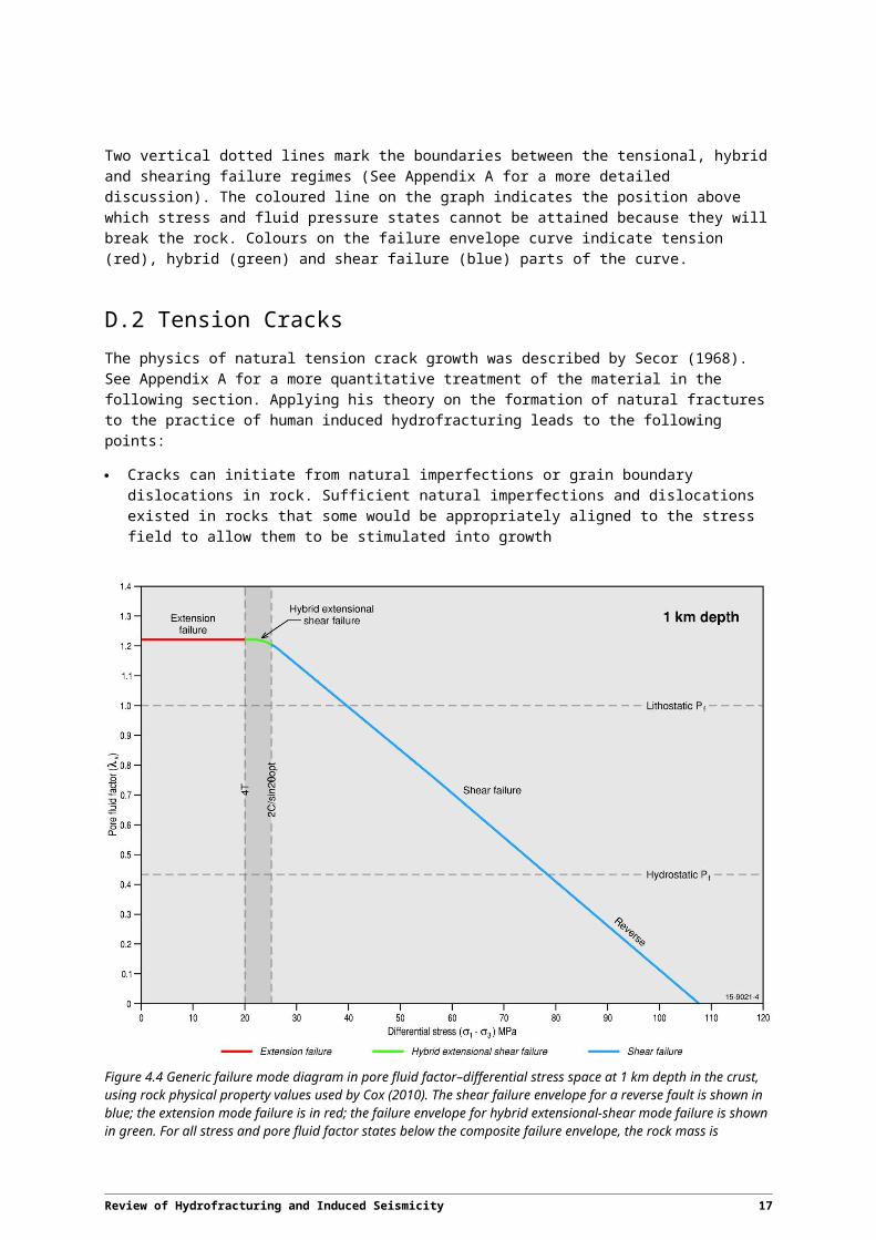
The environments under which tensional, shearing and hybrid failure occur were described by Cox (2010). Figure 4.4 is a failure mode diagram which describes the failure envelope for rock in terms of the differential stress (1-3) on the X-axis, and Pore Fluid Factor (v) on the Y-axis. Pore Fluid Factor is the ratio of the pore fluid pressure and the vertical stress (v) at any depth. Note that v could be any of the three principal stresses shown in Figure 4.2, depending on the orientation of the stress field at that place. When pore fluid pressure follows a hydrostatic pressure gradient, the Pore Fluid Factor would be around 0.4, which is illustrated with a dotted horizontal line ('Hydrostatic Pf'). When Pore Fluid Factor is greater than 1, as illustrated with a second dotted horizontal line ('Lithostatic P f'), in the terms of the petroleum industry, the rock would be overpressured.

Two vertical dotted lines mark the boundaries between the tensional, hybrid and shearing failure regimes (See Appendix A for a more detailed discussion). The coloured line on the graph indicates the position above which stress and fluid pressure states cannot be attained because they will break the rock. Colours on the failure envelope curve indicate tension (red), hybrid (green) and shear failure (blue) parts of the curve.

4.2 Tension CracksThe physics of natural tension crack growth was described by Secor (1968). See Appendix A for a more quantitative treatment of the material in the following section. Applying his theory on the formation of natural fractures to the practice of human induced hydrofracturing leads to the following points:


Cracks can initiate from natural imperfections or grain boundary dislocations in rock. Sufficient natural imperfections and dislocations existed in rocks that some would be appropriately aligned to the stress field to allow them to be stimulated into growth

Figure 4.4 Generic failure mode diagram in pore fluid factor–differential stress space at 1 km depth in the crust, using rock physical property values used by Cox (2010). The shear failure envelope for a reverse fault is shown in blue; the extension mode failure is in red; the failure envelope for hybrid extensional-shear mode failure is shown in green. For all stress and pore fluid factor states below the composite failure envelope, the rock mass is elastically strained, but will not fail in brittle mode. Brittle failure occurs when the stress and pore fluid factor states reach the failure envelope. Stress and fluid pressure states above the failure envelope cannot be attained.

Initially, cracks will not be open and will therefore have no volume. High pressure fluid pumped into the rock during the hydrofracture operations will migrate into the crack and when the fluid pressure in the rock is greater than the tectonic pressure in the rock the crack will expand

The crack will continue to expand until several key failure conditions are met

Firstly, the pressure in the crack exceeds the minimum principal stress 3 by an amount equal to the tensile strength of the rock

Secondly, as the volume of the crack grows and the crack gets wider, it will reach a state where tensional stresses at the ends of the crack are greater than the tensile strength of the rock

When these conditions are met, the rock at the ends of the crack will yield and break

Therefore the parameters that control when a crack will grow are the minimum principal stress 3, the fluid pressure, and the physical properties of the rock, including its tensile strength


When the crack ends fail and the crack gets longer, the volume of the crack increases and the fluid pressure in the crack drops. The fluid pressure in the crack then builds up again until the crack extends at its tips

That is, the crack grows by small increments

Because incremental tensional crack growth is small, the earthquakes that are produced are small

As the length of the crack grows, the time steps between incremental growth of the crack will get longer. This is controlled by both the volume and pressure of fluid required to keep the crack open, and therefore ultimately by the limitations of the pumping equipment

In an environment where impermeable rocks (eg., coal, shale) are juxtaposed against more permeable rock (eg., sandstone), the fractures that would develop in the impermeable rocks would be short and closely spaced, whereas those in less adjacent permeable rock would be longer and more widely spaced

If the crack growth in an impermeable rock reaches a juxtaposed and more permeable formation, for example a coal or shale against a sandstone (eg. See Figure 8.13 below which shows a model of the distribution of rock types within the Walloon Coal Measures of the Surat Basin), then crack growth could be affected because fluid pressures in the cracks would be higher than in the formation, and fluid could leak off into the more permeable formation, rather than from the formation into the cracks as in Secor's theory for natural hydrofractures (see also Rahman & Rahman, 2012). Higher volumes of pumped fluids would be required to overcome this

Eventually, growth on larger cracks will be replaced with growth on nearby smaller cracks. Although Secor's theory does not preclude one crack or even a few cracks continuing to grow to a very large size, a network of smaller cracks is likely to develop

The rate at which fluid pressure is built up in a rock leading to the onset of fracturing may also be important in controlling fracture geometry. If it is slow, fracturing is likely to start with a few long fractures in the rock. When fluid pressure grows faster, fracturing is more likely to start with many small fractures almost simultaneously throughout the rock.

4.2.1 Orientation of Tension Cracks

Tension cracks form orthogonal to the minimum principal stress 3 (see Figure 4.3).

4.3 Shear failureThe yield failure envelope for shear failure is shown by the blue part of the failure mode curve in Figure 4.4. The orientation of a shear that forms in intact rock is determined by the stress directions, as illustrated Figure 4.2.

In Figure 4.2, a piece of rock is shown as a green ellipse. It shows a cross section of the rock, with the principal stresses shown with arrows. Shear zones form at an angle opt to the principal compressive stress 1.

The magnitude of opt is determined by the internal coefficient of friction of intact rock and is typically around 30. Movement on the shear zones is as shown by the half arrows. In this stress orientation, reverse faults form and would lie in and out of the plane of the section. This orientation is different from that of tension fractures that would form in a stress field with this orientation, as shown by the grey surface.


For the orientation of the stress field in Figure 4.2, reverse faults will form (see the block diagram in the upper left of Figure 4.2).

The theory of Cox (2010) allows a number of predictions about shear failure in rock:

Higher differential stresses and/or higher pore fluid factors are required for failure in reverse faulting compared to strike slip, which in turn requires higher values than normal faulting

Much lower differential stresses are required at low pore fluid factors to reach the failure envelope in intact rock as depths decrease, but that higher pore fluid factors are required for tension failure

The reactivation of existing faults can be problematic if the aim of hydrofracturing is to create new fractures within intact rock. It can also be an aim of the hydrofracturing process if existing faults are seen as providing the required permeability

If an existing weak fault is optimally oriented to the stress field, ie., it is close to the angle opt in Figure 4.2, it will be reactivated rather than any new tension, hybrid or shear fractures being created in nearby intact rock

It will be reactivated at lower differential stress and/or pore fluid factors than those required to create fractures in intact rock

It will be reactivated in shear mode irrespective of whether the differential stress is high or low

However, once the angle between the existing fault and 1 increases beyond 2opt, pore fluid factors above 1 are required to re-activate the fault, and ultimately a new fracture will form, through either tension, hybrid or shear failure, rather than the existing fault being reactivated

The form that reactivation would take, ie., as a normal, strike-slip or reverse fault is determined by the orientation of the stresss field at the time of reactivation, not by the original form of the fault

However, even a small amount of healing of the fault will lower the likelihood that the existing fault will be reactivated rather than a new fault created

The case of reactivation of an existing fault can be extended to the reactivation of any other optimally oriented linear feature in a rock, eg., a joint, provided that the rock within the feature is significantly weaker than that in the adjacent intact rock. However, if the existing weak zone is a joint, it will be reactivated in shear mode with relative motions either side of the crack.

4.4 Hybrid tension and shear mode failureFractures formed in the hybrid field of failure can be oriented between the plane of 1 and 2 (shown perpendicular to 3 by the grey surfaces in Figure 4.2) and the conjugate shear zones at an angle of opt to 1, also shown in Figure 4.2 (Cox, 2010).

4.5 Forming new fractures vs reactivating existing fractures

Appendix B gives several examples of earthquakes generated during the hydrofracturing stimulation of impermeable rocks (in the shale gas and hot dry rock geothermal industries), in which the earthquakes generated can be grouped into those related directly to the hydrofracture process, and those that appear to be due to the reactivation of an existing fault (or faults).

The failure mode diagrams of Cox (2010) provide a simple way to consider in systematically the interplay of a hydrofracture and an existing fault. Some examples are set out in Appendix A.


In a hydrofracture operation in a well where differential stresses (1-3) are high, no tension cracks can form. New shear cracks will form at an angle opt to the maximum principal stress. If they intersect an existing weak fault that is at a high angle to the maximum principal stress, the fluids from the new crack could flow into the old fault but it will not be reactivated as a shear fault

At low differential stresses, tension cracks will form during hydrofracture operations. When the tension cracks encounter an existing weak fault, the interaction of the tension cracks with the existing fault is determined by the angle of the existing fault to the direction of 1

If the existing fault is at a high angle, the fault will not be reactivated. Rather, the tension cracks may pass through the fault. If the fault is permeable, hydrofracture fluids can move along it and provided that pore pressures can be maintained at a sufficiently high pore fluid factor, tension cracks can break out of the fault

If, however, the existing fault is at a lower angle (<2opt) to the stress field, the existing fault will fail by shear fracture irrespective of whether the differential stresses are high or low.

4.6 Unintentional HydrofracturingDeliberate hydrofracturing usually involved the injection of fluid at high pressure and over short periods of time. Earthquakes induced this way are mostly small and are unlikely to be felt.

However, previous compilations of human induced seismicity demonstrate that larger earthquakes that can be felt and could be damaging can be induced through increased fluid pressures when fluids are introduced into the upper crust, eg., through natural percolation in the case of water storage reservoirs or deliberately down a well. These earthquakes often occur after high volumes of fluid have been injected into the rocks, and at lower fluid pressures than those required for tensional hydrofracturing. They are particularly prevalent in activities associated with the oil and gas industries (see compilations of Davies et al. (2013a) and The National Academies (2011).

Ellsworth et al. (2012) described a six-fold increase in earthquakes with M 3 in the mid-continent of the US from 2000 to 2012. Ellsworth et al. (2012) noted that the increase began in 2001; this correlated with coal seam gas activities along the Colorado –New Mexico border. A subsequent acceleration in earthquake numbers from 2008 correlates with increased activity in the shale oil and gas industries in Arkansas and Oklahoma and with waste disposal in wells. Ellsworth et al. (2012) considered the increase in earthquakes to be manmade, but did not venture a view on whether they are due to a change in extraction methodologies or to an increase in oil and gas production activities.

Shale gas production in the US accelerated rapidly from 2005 and is predicted to increase to 2040 (USEIA, 2013). Projections of Coal Bed Methane (coal seam gas) production are fairly steady. Irrespective of whether the increase in activities is caused by a change in extraction methodologies or a change in the level of activities, the growth in shale gas production is likely to lead to a continuing increase in earthquake activity for some decades unless the cause of the increased earthquake activity is fully understood and the risk of further earthquakes mitigated.

A high portion of human induced earthquakes are clearly linked to the injection of water into the crust, and are therefore classified in this report as caused by unintentional hydrofracturing.

The larger earthquakes generally have several properties that suggest that they are often associated with the reactivation of existing faults rather than the creation of new hydrofractures. At high differential stresses, they could be caused by the creation of new faults.


They often have a spatial correlation with existing faults, or a linear spatial distribution that suggests they lie on a fault that has not been mapped previously

As a population of earthquakes, they have a b value close to 1, whereas tension hydrofracture earthquakes usually have higher b values (See Appendix B)

Where source signatures can be modelled, they typically have a double couple source signature indicative of shear failure, or a hybrid failure mode, rather than an isotropic source signature (see Appendix B)

Their magnitudes tend to imply rupture sizes significantly larger than might be expected of tension cracks (Appendix A)

If the pore fluid factor in the fault and the differential stress on the fault are close to the failure mode curve, the fault may be reactivated very soon after the injection starts

Otherwise, if the pore fluid factor in the fault and the differential stress on the fault are not close to the failure mode curve, some time may elapse before earthquakes begin

Earthquakes that occur on reactivated faults such as in this scenario often start without any precursor activity

Earthquakes do not always stop immediately the injection is stopped, because of residual high pressures in the formation.

Appendix C summarises results from several case studies, in particular the amount of fluid available to increase pore fluid pressure, in each case over a considerable area, and the amount of time over which it was injected before earthquakes occurred.

Table 4.2 summarises typical parameters for induced earthquakes.


Table 4.2 Parameters for deliberate and unintentional hydrofracturing.

Deliberate Hydrofracturing Fracturing Intact Rock

Number of events 1,000s for each well, and potentially for each hydrofracture treatment in each well.

Time frame Within hours to days of start of fraccing.

Maximum Magnitudes Usually M 0 (Maxwell et al., 2009; Shemeta and Anderson, 2010; Šilneý et al., 2009)

Where Within a few 100s of metres of the well

Spatial Distribution Spread radially with time

Deliberate Hydrofracturing Fault Reactivation

Number of events 100s–1000s

Time frame At the end of fraccing; can be after shut in

Maximum Magnitudes Usually M 0 in shale and coal but can be larger (Maxwell et al., 2009; Rutledge & Phillips, 2003; Šilneý et al., 2009); Can be higher in enhanced geothermal systems (usually M = -2–0 but occasionally M up to 3–4) partly because of the higher shear moduli for basement rocks compared to shale and coal—see text.

Where Typically at the edges of the fractured volume

Spatial Distribution Linear patterns 100s of metres long aligned with existing faults that are usually optimally or near optimally aligned with stress field

Unintentional Hydrofracturing Waste Injection

Number of events 100s–1000s

Time frame Time is required to raise reservoir pressure above the level required to fracture intact rock or reactivate existing fault; this can be years after the injection begins

Maximum Magnitudes M = 5.3 (Davies et al., 2013a); M = 5.0, 5.7 (Keranen et al, 2013)

Where At the edges of the reservoir; usually on faults that are optimally or near optimally aligned with stress field because they will reactivate at lower pressures than intact rock

Spatial Distribution Linear patterns 100s–1000s of metres long aligned with existing faults


5 Australian Stress Field

The preceding sections highlight the significance of the magnitudes of the principal components of the stress field in determining the type of fracture (tensional or shear) and the orientation of the principal components in determining whether the fractures are horizontal or vertical, and whether shear displacement is by normal, strike slip or reverse movement.

The Australian Stress Map is a product of the Australian Stress Map Project at Adelaide University (http://www.asprg.adelaide.edu.au/asm/). It summarises the knowledge about the stress field in the Australian continent. The number of measurements in the database of the Australian Stress Map Project is now (July 2013) 2859, of which 406 are in Irian Jaya and Papua New Guinea which lie on the Australian lithospheric plate.

Early publications describe the various methods by which stress has been measured within the continent (Denham & Windsor, 1991; Hillis et al., 1998; Hillis et al., 1999; Hillis & Reynolds, 2000). Entries in the database have been assigned a quality factor (A–E), of which A, B and C are the best.

Table 5.3 Numbers of stress measurements, by measurement method and quality (A–E), in the Australian continent (including Papua New Guinea and Irian Jaya) as of 17/05/05. Data from http://www.asprg.adelaide.edu.au/asm/statistics.html#summary. Viewed 01/06/2015.

Measurement Method A B C D E Total

Focal Mechanism (FM) 3 79 1815 32 322 2251

Breakouts (BO) 83 101 63 113 36 396

Hydraulic Fracturing (HF) 6 30 25 18 1 80

Overcoring (OC) 0 2 4 51 1 58

Drilling Induced Tension Fractures (DTF) 26 16 9 20 0 71

Geological Indicators (G) 0 0 1 0 2 3

TOTAL 118 229 1916 234 362 2859

Geological areas that have at least 4 good quality measurements with consistent stress directions are classified as stress provinces. With the exception of the Flinders Ranges and the provinces in Papua New Guinea and Irian Jaya, all stress provinces are within sedimentary basins.

Figure 5.5 shows the location and stress directions of all measurements in the stress map project, and Figure 5.6 shows average stress directions in each of the stress provinces. Table 5.4 lists the overall faulting regime (assuming shear failure rather than hydrofracture tension failure) likely to result from the stress regime in the provinces within Australia.


http://www.asprg.adelaide.edu.au/asm/statistics.html#summary

http://www.asprg.adelaide.edu.au/asm/

Figure 5.5 Locations of measurements and directions of horizontal stress within Australia. Stress directions imply: NF normal fault, SS strike slip fault, TF thrust fault, U unknown. Based on the data in http://www.asprg.adelaide.edu.au/asm/images/australasiaa-c.pdf

Unlike other continental masses, such as North America and Europe, the directions of maximum stress do not parallel the N–NNE direction of plate motion (Hillis et al., 2000). The Australian lithospheric plate has a complex boundary, with a mid-ocean ridge in the south, subduction and oblique- and strike-slip motion along its boundary with New Zealand, subduction farther north along the Tonga—Kermadec Trench, oblique convergence near Papua New Guinea and Irian Jaya, and subduction near Indonesia. Hillis et al. (2000) argue that this is reflected in the stress directions in the Australian plate. In the north, stress directions are mostly oriented NNE–SSW, and in the south of the continent they are oriented more towards E–W and SE–NW. The 'area of divergence' between the two zones is marked by a dashed red line in Figure 5.6. Its position and its meaning are unclear. It corresponds with E–W or poorly defined (low horizontal stress anisotropy) regional stress directions in the Cooper, Flinders and Sydney stress provinces.


http://www.asprg.adelaide.edu.au/asm/images/australasiaa-c.pdf

Figure 5.6 Base Map: Average stress directions in the stress provinces in Australia (excluding the onshore Canning Basin) based on http://www.asprg.adelaide.edu.au/asm/regionalorientations.html. Red line represent a zone whose position is uncertain through the continent described by Hillis et al. (2000) where average stress directions change from NNE-SSW in the north of the continent to E-W to SE-NW across the south of the continent.

The methods by which in-situ stress is measured operate at different levels in the crust. Engineering techniques such as overcoring work in the near surface or in mines whereas hydraulic fracturing, borehole breakouts and drilling induced tension fractures are made at depths to 4 km. Earthquake focal mechanisms are usually deeper. In a geological province, stress directions can vary regionally and with depth (Hillis et al., 2000).

In case study #1 in Appendix C, the earthquakes induced by the impoundment of the Talbingo reservoir had a focal mechanism indicating normal faulting in the Lachlan Fold Belt which is otherwise considered to have a reverse faulting stress regime.

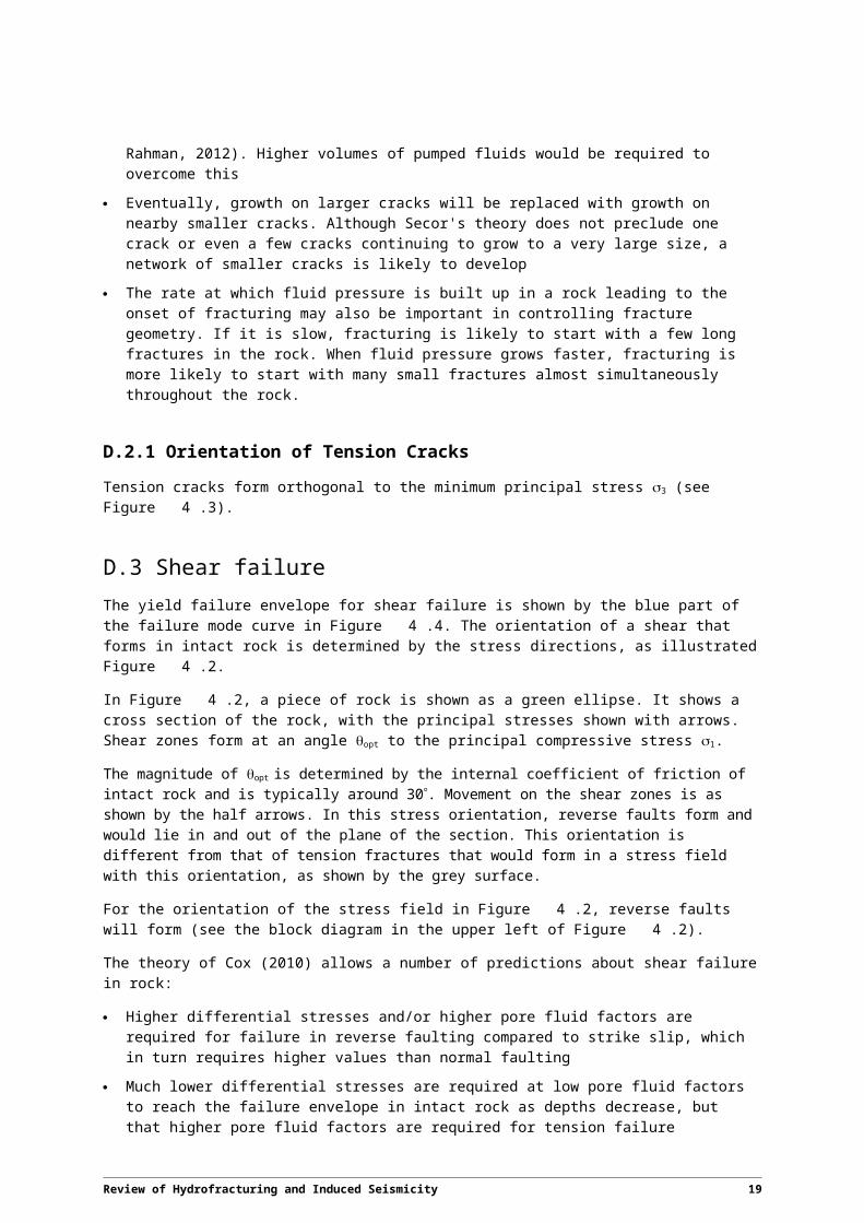
In the Cooper Basin, stress directions can change with depth. Beach (2012) reported that borehole break out data showed a largely E–W maximum horizontal stress direction, consistent with regional stress directions (eg. see Figure 5.6). However, they noted: 'In general, fractures will propagate in the maximum horizontal stress direction and the fracture will open in the minimum stress direction. Geomechanical studies of early exploration wells in the Central Nappamerri Trough as well as recent studies using the Holdfast–1 and Encounter–1 data, indicated the Permian strata within the Central Nappamerri Trough is in a strike-slip stress regime where the vertical stress (Sv) is the intermediate stress. There is a possibility for the stress regime to become a reverse stress regime with depth. In


http://www.asprg.adelaide.edu.au/asm/regionalorientations.html

this instance the vertical stress is the minimum stress. Hydraulic fractures in a strike-slip regime will tend to be vertical whereas a hydraulic fracture in a reverse stress regime will be horizontal.' The complexity of the stress field is demonstrated in Figure 5.7, from Beach (2012).

Table 5.4 Likely faulting regime in stress provinces in Australia for all measurements irrespective of measurement quality. NF–normal faulting; NS–normal faulting with a strike-slip component; SS–strike-slip; TS–thrust faulting with a strike-slip component; TF–thrust faulting; U–unknown. Data from http://www.asprg.adelaide.edu.au/asm/statistics.html#summary. Viewed 01/06/2015.

Province No. A–E Overall Regime NF NS SS TS TF U

Amadeus Basin 28 U 0 0 0 0 0 28

Bonaparte Basin North 103 U 1 0 0 0 0 102

Bonaparte Basin South 9 U 0 0 0 0 0 9

Bowen Basin 44 TF 1 0 7 0 36 0

Browse Basin 18 U 0 0 0 0 0 18

Canning Basin 12 SS 0 0 4 0 0 8

Carnarvon Basin 49 U 0 0 0 0 0 49

Cooper Basin 84 U 0 0 0 0 0 84

Flinders Ranges 10 SS 0 0 7 0 2 1

Gippsland Basin 25 U 0 0 0 0 0 25

Otway Basin 25 U 0 0 0 0 0 25

Perth Basin 37 TF 0 0 1 10 8 18

Sydney Basin 66 TF 0 0 7 0 57 2

In Figure 5.7, the depth interval from 2500–3500 m in the Holdfast–1 well is divided into four zones based on the relative levels of the three principal stresses. In the upper zone between 2550 m and 2825 m depth, vertical stress in the minimum principal stress 3 . The differential stress (1-3) is about 40 MPa. This part of the well would fail by either horizontal tension fractures or by reverse (thrust) displacement on shear cracks oriented at opt to the horizontal, depending on where the differential stress falls in the failure mode diagram of the form shown in Figure 4.4 for this depth. In the next zone between 2825 m and 2975 m, the vertical stress is 2. Tension fractures would be vertical and the shear displacement would be by vertical strike slip movement. Vertical stress is the minimum stress at most depths between 2975 m and 3375 m, therefore horizontal tension cracks and reverse shear cracks should dominate. In the lowermost between 3375 m and 3425 m, the three principal stresses are equal. Cracks could grow in any direction, but if the rock has a strong fabric with anisotropic physical properties, anisotropic rock strength might control crack direction.

The need is apparent to understand the stress directions in detail down a well before embarking on a program of hydrofracturing.


http://www.asprg.adelaide.edu.au/asm/statistics.html#summary

Figure 5.7 Logs and calculated horizontal and vertical stresses in Holdfast–1 in the Nappamerri Trough, Cooper Basin, from Beach (2012), Figure 12. Vertical stress is shown as a smooth green line in the right hand part of the figure; maximum and minimum horizontal stresses are in blue and red.


6 Monitoring Hydrofracturing

Good industry practice includes the use of models to predict hydrofracture behaviour before initial hydrofracturing is undertaken, and preferably before each subsequent well in a field is hydrofractured. As data are then gathered from each hydrofracturing treatment in a well, or more wells in a field are hydrofractured, additional data can be input to improve the predictive capabilities of the model. Ultimately, however, hydrofracture treatments should be monitored.

Hydrofracturing in the unconventional energy industries is monitored for a number of purposes:

to monitor the growth of the hydrofractures in order to ensure that they are being done efficiently and effectively

to ensure that the hydrofractures remain within the formations being hydrofractured

to ensure that any induced seismicity stays below a pre-set threshold and is not damaging to built infrastructure or alarming to nearby residents

to allow an assessment of the nature of the hydrofractures in order to better understand sub-surface conditions

This not only allows better engineering of the production stages of the well but also gathers data to improve future hydrofracture exercises in the well and nearby wells.

The following table, from USEPA (2004) lists the techniques available for monitoring hydrofracturing according to the parameters (fracture height, fracture length and fracture azimuth) that each technique can be used to monitor, and indicates the limitations in the use of the technique in monitoring that parameter.

Table 6.5 Limitations of Fracture Diagnostic Techniques (From USEPA, 2004, Chapter 3, originally derived from a US Department of Energy publication).

Parameter Measured Technique Limitation

Fracture Height Tracer Logs Shallow depth of investigation; shows height only near the wellbore

Fracture Height Temperature Logs

Difficult to interpret; shallow depth of investigation; shows height only near wellbore

Fracture Height Stress profiling Does not measure fracture directly; must be calibrated with in-situ stress tests

Fracture Height Pseudo 3D Models

Does not measure fracture directly; estimates vary depending on which model is used

Fracture Height Microseismic Monitoring

Optimally requires nearby offset well; difficult to interpret; expensive

Fracture Height Tiltmeters Difficult to interpret; expensive and difficult to conduct in the field

Fracture Length Pseudo 3D Models

Length inferred, not measured; estimates vary greatly depending on which model is used

Fracture Length Well Testing Large uncertainties depending upon assumptions and lack of pre-fracture well test data


Parameter Measured Technique Limitation

Fracture Length Microseismic Monitoring

Optimally requires nearby offset well; difficult to interpret; expensive

Fracture Length Tiltmeters Difficult to interpret; expensive and difficult to conduct in the field

Fracture Azimuth Core Techniques

Expensive to cut core and run tests; multiple tests must be run to assure accuracy

Fracture Azimuth Log Techniques Requires open hole logs to be run; does not work if natural fractures are not present

Fracture Azimuth Microseismic Monitoring

Analysis intensive; expensive for determination of azimuth

Fracture Azimuth Tiltmeters Useful only to a depth of 5,000 feet; requires access to large area; expensive

Of all the techniques listed in Table 6.5 microseismic monitoring, tiltmeter monitoring, and the monitoring of chemical, radioactive and/or dye tracers in nearby monitoring wells provide the most direct, real–time or near real-time evidence for fracture geometry.

Seismic arrays are used to locate the hydrofractures using the seismic energy released with each fracture. Abercrombie (1995) discussed the comparative efficacy of downhole and surface recording of very small earthquakes. Microseismic monitoring is best conducted by seismometers deployed down wells because the weathered zone near the surface severely attenuates high frequency seismic energy which makes up most of the signal from very small earthquakes. However, although seismometers can sometimes be used if the hydrofracturing is very shallow (Fisher and Warpinski, 2012).

The use of seismic recording during hydrofracture exercises in demonstrated diagrammatically in Figure 6.8.

In Figure 6.8, the textured horizontal layer represents the formation being hydrofractured. The column on the left represents the well being hydrofractured; black dots are perforations through the casing in the well that allow hydrofracturing fluids to enter the formation being hydrofractured. The red dots are the hypocentres of earthquakes (See Appendix B for a definition of hypocentre).

Straight red lines represent the ray paths of seismic energy travelling from each earthquake hypocentre to 12 seismometers down the well on the right.

Note that for downhole seismometer deployments, each hydrofracture process requires at least two wells—the well being hydrofractured and the well with the monitoring equipment. Optimally, two monitoring wells would be used.

The green waveforms on the right represent the recorded seismic signals from one earthquake at the twelve seismometers. Each waveform has two arrivals: a P-wave and an S-wave. The difference in the times at which these two phases arrive at the seismometer tell the distance from the earthquake to that seismometer, provided that the velocity of seismic waves in the rock is known accurately. Therefore an accurate velocity model must be developed for each field to be hydrofractured using information, for example, from seismic surveys and downhole velocity logs.


Figure 6.8 Microseismic monitoring of hydrofractures in the well on the left, using an array of 12 seismometers down the well on the left. Based on and simplified from Beach (2012) Figure 8.

If each seismometer has three components measuring ground shaking in orthogonal directions (usually Up, North and East), the direction of the earthquake from the seismometer can be calculated by the direction of the first motion of the P-phase on the three components. Technically, the earthquake can be located by combining the distance and direction of the earthquake from one seismometer. However, this location will have an error. The error could be reduced when the locations based on the distances and directions calculated from all 12 seismometers are combined; it will be reduced even further if seismometers are deployed down two wells at different azimuths from the well that is being hydrofractured.

In a study of a hydrofracturing operation in Texas, Rutledge and Phillips (2003) described the monitoring of earthquakes to the east of an injection well using a seismometer array down a well approximately 350 m to the north east of the injection well and another array down a well approximately 350 m to the east of the injection well. Earthquakes were recorded sufficiently well for their locations to be calculated for about 400 m to the ENE of the injection well.

Very few earthquakes were located to the west of the injection well. This is because the very small earthquakes to the west of the wells were too far from the downhole seismometer arrays and their recorded waveforms were therefore below the threshold where they could be used for accurate analysis and event location. The spatial orientation of the earthquakes as a narrow cloud trending ENE combined with focal mechanisms calculated for groups of larger earthquakes indicated that the fractures formed by the reactivation by both left-lateral and right-lateral strike-slip shear movement on pre-existing vertical faults.

A number of earthquakes were located above and below the hydrofractured interval; error ellipses where available for these earthquakes showed that the earthquake locations were indeed outside the hydrofractured zone. This would be consistent with the reactivation of vertical or near vertical strike


slip faults, where the vertical extent of hydrofractures would be difficult to constrain in a hydrofracturing environment in which hydrofractures had horizontal lateral extents of up to 400 m.

Tiltmeters are used to measure the minute amounts of deformation caused by the generation of a fracture, which constitutes an increase in the volume of rock. They can therefore be used to measure a number of geometric properties of the hydrofracture network (Fisher and Warpinski, 2012). Vertical, dipping and horizontal fractures cause different patterns of surface deformation. Data from tiltmeters deployed at the surface can be used to identify which of these patterns has occurred, and therefore, for example, whether the fractures are horizontal, vertical or dipping, including the dip and azimuth of dipping hydrofracture zones. The amplitude and width of the surface deformation also provides a measure of the volume of fractures that have been created; this can be cross checked against the volume of hydrofracturing fluid that has been injected minus any that subsequently flowed back out the injection well when the pumping pressure is released. Tiltmeters deployed down monitoring wells can be used to measure fracture height if they are deployed either side of the zone of hydrofractures.

The detection of chemical, radioactive or dye tracers in monitoring wells is confirmation that the hydrofractures have reached the monitoring well. However, this technique cannot be used to monitor the progress of the hydrofracture from the injection well to the monitoring well.


7 Fracture Size and Shape

Hydrofractures have three dimensional shapes: they have length, width and thickness. The length is the distance that the hydrofracture extends from the well (this is in the direction of 1). As the hydrofracture grows, it expands in the direction orthogonal to the direction in which it is growing – ie., it expands in the direction of 2. This gives it width. Thickness refers to the amount that the hydrofracture opens (orthogonal to 3), as shown by the amount that the top block on the left in Figure 4.3 moves relative to the bottom block.

Usually only the length is reported in the open literature. However, several publications provide statistics on fracture size, although not always in a way that is universal for all applications. The main issue is that much of the literature is based on examples from the US, where the stress regime is such that hydrofractures are mostly vertical, and most data in the public domain are from the shale gas industry.

Fisher and Warpinski (2012) compiled data from many hundred hydrofracture treatments from a number of shale plays in the US. Their Figure 2 is shown here as Figure 7.9, and illustrates the heights to which hydrofractures propagated in the Barnett Shale. They gave similar plots for other shale gas plays.

Figure 7.9 Heights (lengths) of hydrofractures from the Barnett Shale in the US (coloured curves). The upward trend from left to right reflects both variation in depths geographically of the Barnett Shale and different depths of each stage of hydrofracture treatment in the shale. Water bores are shown at the top as blue vertical lines. Y-axis is in feet. (Fisher & Warpinski, 2012, Figure 2, © Society of Petroleum Engineers, reproduced with permission).


Fisher & Warpinski (2012) were focussed on demonstrating that the hydrofractures in the Barnett Shale were unlikely to intersect aquifers tapped by water bores. Therefore they plotted fracture height. In the stress field in the Barnett Shale, fractures grow vertically. Therefor height corresponds to the length of the fractures. The fracture depths for each hydrofracture treatment lie on an orange line at the centre of the fracture height curves.

The curves for fracture height have three significant features. Firstly, most fractures are not very long (high) and plot as a band of fractures about 500 ft (150 m) either side of the point of hydrofracturing. Secondly, the curves have spikes that are up to about 1000 ft (300 m) high. Fisher and Warpinski (2012) attribute these spikes to the hydrofractures meeting existing faults and reactivating the faults. They base this on the seismic characteristics of the earthquakes that correlate with those spikes.

Finally, the heights of the hydrofractures become less at the shallower depths (right hand end of the graph). Fisher and Warpinski argue that fractures at shallower depths are more likely to be horizontal than vertical because the vertical stress decreases and will become less than the maximum horizontal stress. Their discussion is qualitative but they provide a diagram in which they used tiltmeter data from several thousand hydrofracture treatments to show that fractures are more likely to have significant horizontal components above around 2000 ft (600 m).

Fisher and Warpinski (2012) then used both a simple theoretical approach and examples from hydrofractures from mine-through studies to examine the form of hydrofractures (mine-through studies examine hydrofractures by first hydrofracturing the rock and then mining away the rock to study the form of the hydrofractures).

Fisher and Warpinski (2012) demonstrated that the most critical factor restricting the length of a hydrofracture is the availability of injected fluid. Secor (1968) demonstrated this theoretically but Fisher and Warpinski (2012) brought a practical approach to the issue by demonstrating how much fluid would need to be delivered to produce a very long hydrofracture, and how unlikely the volumes could be delivered in real-life field applications.

Davies et al. (2013b) reached a similar conclusion. They studied the statistics of fracture height both in the data of Fisher and Warpinski (2012) and in new data from shale gas hydrofractures, and compared the induced hydrofracture heights with those of naturally occurring hydrofractures.

Naturally occurring hydrofractures take a number of forms; the example in Davies et al. (2013b) resembles the hydrocarbon-related diagenetic zones (HRDZs) identified by Geoscience Australia on the Northwest Shelf (O'Brien et al., 2001). HDRZs occur when hydrocarbons under pressure fracture the seal over a reservoir and propagate up through the sedimentary column. The reaction of the hydrocarbons, including gas, with the overlying sedimentary column around the upgoing fracture causes diagenesis which makes the HDRZ visible in seismic images.

Davies et al. (2013) measured the heights of 1170 naturally occurring hydrofractures from the west coast of Africa and offshore Norway. The greatest measured height (ie. length) is ~1106 m; the probability that a natural hydrofracture length will exceed 350 m is 33%. Fracture height populations in the shales in the US reported by Fisher and Warpinski (2012) vary from shale to shale. The greatest fracture height is ~588 m but most hydrofracture heights are much less. The probability of a stimulated hydrofracture exceeding 350 m is 1%.

Davies et al. (2013b) found no correlation between fracture height and the time duration of pumping during hydraulic fracture treatment of gas reservoirs. Pumping for 5.5 months at an injection well offshore from Norway stimulated hydrofractures that reached the sea floor from the injection point at 900 m depth.


The volumes pumped down the well were considerably more than those injected to stimulate a gas play. The volumes of fluid (gas, oil, water) available in a reservoir to propagate a natural hydrofracture are orders of magnitude higher than those injected in stimulated hydrofracture treatments, and explain why natural hydrofractures have greater heights (lengths) than stimulated hydrofractures.

Other factors that affect the shape and height of vertical hydrofractures include:

the complexity of the fractures

the presence or absence of pre-existing weaknesses (faults, joints, cleats in coal)

changes in rock type with fracture height

changes in stress state with fracture height, eg. in the Cooper Basin (Figure 5.7).

The complexity of hydrofractures can affect their length. Various forms of increasing complexity are shown in Figure 7.10. More complex forms of fracture have higher volumes that simple forms. This limits the ability of the pumping system to keep the pressure of the injected fluid above that required for continued fracture growth. Complex fractures also have high surface areas, and when the injected hydrofracturing fluid is at a higher pressure than the surrounding rock, loss of the injected fluid to the surrounding rock can occur if the fracture passes through rocks with reasonable permeability. This reduces the pressure of the injected fluid below that required to continue the hydrofracture process. Increasing complexity also produces increasing resistance to deformation and displacement in rocks where conditions for shear failure exist.

High concentrations of weak zones, such as faults, joints and cleats in coal, can act as pre-existing porosity and permeability. The porosity accommodates large volumes of injected fluid that reduces the pressure of the injected fluid. The orientation of face and butt cleats in coal (Figure 7.10) to the flow of injected fluid is important; face cleats provide more efficient pathway for injected fluids to pass through the coal and into butt joints, than the reverse.

Bedding in the rocks being hydrofractured affects hydrofracture geometry. Beds in layered sequences have different lithologies, permeabilities, tensile and cohesive strengths and shear moduli. The principal stresses can also change direction through a sequence (eg., Figure 5.7). Fractures can terminate at layer boundaries, change directions, or propagate through the boundaries. Layering of the rocks can therefore lead to a variety of hydrofracture geometries, including simple fractures that terminate or change direction at boundaries, through-going fractures, and complex dendritic networks of vertical and horizontal fractures (Figure 7.10). Dendritic networks of hydrofractures provide a greater fracture volume for a given height (ie., length) than simple, through going fractures, thereby reducing the fluid pressure at the crack tip. This will restrict fracture length, as will the bleed off of injected fluid to any of the surrounding rocks that have reasonable permeability.

All of the statistics provided by Fisher and Warpinski (2012) and Davies et al. (2013b) were collected in areas where the fractures grow vertically. No compilations of comparable numbers of horizontal hydrofracture are available. In intact homogeneous isotropic rocks, cracks that grow horizontally should reach the same dimensions as those that grow vertically, provided that the stress directions do not change with fracture height and the pore fluid factor remains constant, which might not be a valid assumption since vertical stress changes with height. Most of the factors that affect fracture length in vertically growing hydrofractures also apply in horizontal fractures. As will be discussed below, laterally changing physical properties are a real likelihood in coal seams and perhaps also at a different scale in shales. Therefore, horizontal fracture length could just as likely be affected by variable geological conditions as vertical hydrofracture growth.


Figure 7.10(a) fracture complexity, from simple (top left) to complex networks (bottom right). (Based on Fisher and Warpinski, 2012, Figure 10).(b) Schematic geometry of face (F) and butt (B) cleats in coal. (Based on USEPA, 2004, Figure 3-3).(c) forms that fractures can take in layered sequences. (Based on Fisher and Warpinski, 2012), Figure 17).

Very little information is provided on fracture width. Fisher and Warpinski (2012) state that fracture width will be less than fracture length, but they do not state by how much. Where clouds of hydrofractures are published in map view (eg., Rutledge and Phillips, 2003), they are often elongate and are therefore controlled by pre-existing weaknesses in the rocks rather than having grown in intact homogeneous rock. The widths of individual hydrofractures may be similarly affected. Whereas many of the earthquakes might come from the incremental growth of individual hydrofractures, the precision of earthquake locations is likely limit the ability to map each earthquake to a specific hydrofracture to determine the shape of the hydrofracture, particularly if a number of fractures are propagating at the same time.

Very little information is available on the thickness of hydrofractures in shale plays. Their depth does not allow for mine-through examination, although fracture thickness might be determined by drilling.


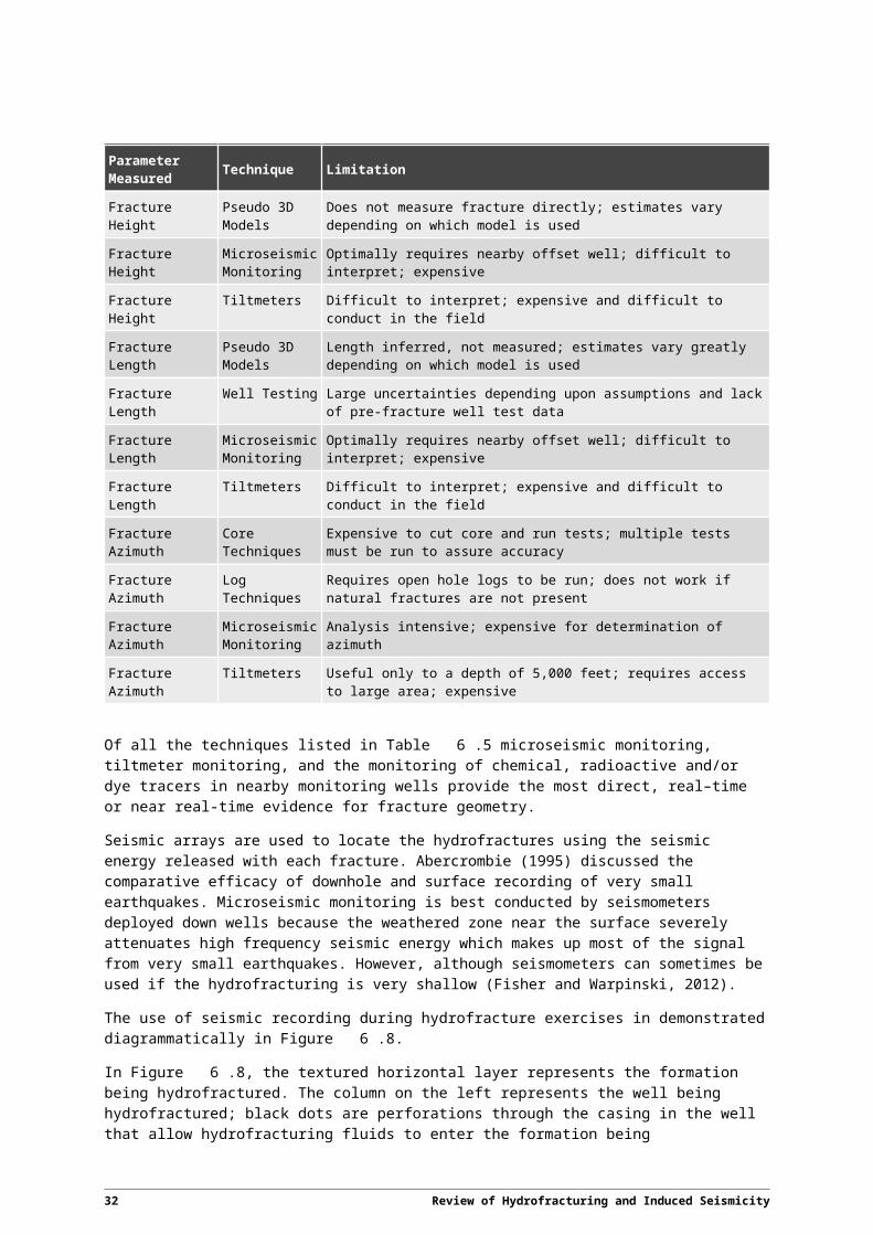
Hydrofractures exposed in mine-through studies in coal showed thicknesses of 0.1 inch (2-3 mm) (USEPA 2004 quoting Steidl (1991)), and up to 3 cm (Diamond and Oyler (1987). Not all fractures are filled with proppant and remain open for measurement in mine-through studies. USEPA also quotes Diamond (1987a, b) and Diamond and Oyler (1987) who showed that hydrofracturing fluids injected into coal seams can travel considerable distances beyond the parts of the fractures that are propped and remain open after the injecting pressure has been removed, after which the fractures would close. Steidl's (1991) measurements were of propped fractures between 2 and 526 feet from the well but paint filled fractures extend up to 870 feet (0.6 m, 160 m and 265 m, respectively). Diamond (1987a, b) gave lengths from one borehole of 95 feet for sand filled cracks but 630 feet for paint filled fractures (29 m and 192 m, respectively).

The implications of these measurements are significant when estimating the area of coal formation that would effectively be in gas production after hydrofracturing. Using Steidl's (1991) results, the area of fractured rock with propped cracks would be only 36% of the area that was actually fractured. Diamond's (1987a, b) results show only 2% of the hydrofractured area might have fractures that remained open for production.

(Note: The papers of Diamond (1987 a, b), and Steidl (1991) are in publications that are not readily accessible, and the original manuscripts have not been sighted. Diamond and Oyler (1987) has been sighted as preprint #85-332 released by the Society of Engineers of the American Institute of Mining, Metallurgical and Petroleum Engineers (AIME) in 1985).


8 Energy Related Hydrofracturing

8.1 Intentional Hydrofracturing

8.1.1 Coal Seam Gas

Coal seam gas (CSG) is also known as coal bed methane (CBM). Miyazaki (2005) reviewed coal seam gas exploration, development and resources in Australia in 2005. Since then the industry has grown significantly. SCER (2013) notes in its Appendix A that the advances in exploration technology and the onset of more successful exploration strategies have seen Australia's CSG resources double since 2010 – ie., a doubling of resources in only 3 years. Note therefore that many of the statistics on the CSG industry in this report will be rapidly out of date. Sedimentary basins that are prospective for CSG are shown in Figure 8.11.

Figure 8.11 Sedimentary basins prospective for coal seam gas.

Production of CSG to date in Australia is from the Bowen, Surat and Sydney Basins. The Gunnedah and Gloucester Basins are also being explored, with prospects in the Gloucester Basin likely to move into production in 2015 or 2016 (AGL, 2015a). Exploration has been undertaken in the Clarence Moreton Basin and is continuing in the Galilee Basin. The comparative size of the CSG industry in


Queensland and New South Wales is shown by the number of CSG wells in each state (Table 8.6). Figure 8.12 shows the locations of the wells. Table 8.6 also shows that the number of CSG wells in Australia is now comparable to the total oil and gas wells drilled in Australia since exploration for oil and gas began.

Table 8.6 Number of CSG wells in Queensland and New South Wales compared to the total drilled for conventional oil and gas in Australia since exploration began. Number of CSG wells includes exploration, production, plugged and abandoned wells.

State # of CSG Wells Source

Queensland 8917 Read from a Google Earth (.KMZ) file downloaded 1 June 2015 from a Queensland Government Web Site*1

New South Wales 639 Number of wells in a data file downloaded 5 May 2015 from the NSW Government Web Site*2

Total CSG Wells (in 2 States) 9556

Conventional wells in Australia (Onshore and Offshore)

<11 000 Geoscience Australia

*1 http://qldspatial.information.qld.gov.au/catalogue/custom/detail.page?fid={C45038EB-BB83-4B16-9231-1905ED753D77}*2 http://dwh.minerals.nsw.gov.au/CI/warehouse

CSG is produced from coal seams typically at depths of 200–1000 m. The first exploration for and attempts at production of CSG were in the Bowen Basin. Early explorers discovered that strategies used overseas did not work there and over time exploration and production strategies that would work were developed (Riley, 2004).

Similarly Johnson et al. (2010) reported that exploration strategies had to be tailored to the complexities encountered in the Surat Basin: understanding stress patterns, immature cleat development and the complex geology in which coal seams are interbedded with fining upward sequences of sandstone with a clay matrix, siltstones and mudstones, leading to variations in permeability throughout the basin.

A sense of the complexity of the geology is given in Figure 8.13, which shows diagrammatically the distribution of coal and non-coal facies in a cross section of the Walloon Coal Measures. The Walloon Coal Measures are the CSG-producing formations accessed in the Surat Basin. Note that the coal seams are discontinuous and are only around 10% of the vertical section (Ryan et al., 2012).

Coal is also only a fraction of the section in other basins, eg., the Sydney Basin (Wang et al., 2004). Issues in the Sydney Basin include geological complexity resulting from a diverse fracture development, particularly in the southern Sydney Basin (Wang et al., 2004). These are most likely a result of the complex stress patterns (Figure 5.5 above and Hillis et al., 2000).

No datasets or reports of earthquake size distribution induced during hydrofracturing stimulations have been found in the available literature on the CSG industry in Australia. The Australian National Seismograph Network operated by Geoscience Australia will not detect events caused by deliberate hydrofracturing, which are likely to have magnitudes M 0 (see references in 'Deliberate Hydrofracturing' in Table 4.2).


http://dwh.minerals.nsw.gov.au/CI/warehouse

http://qldspatial.information.qld.gov.au/catalogue/custom/detail.page?fid=%7BC45038EB-BB83-4B16-9231-1905ED753D77%7D

Figure 8.12 CSG wells (yellow) and earthquakes with magnitudes ≥M3 since 1970 (red).


Figure 8.13 Diagrammatic cross section of part of the Walloon Coal Measures in the Surat Basin in Queensland. Coal seams are shown in green; clastic sedimentary rocks are in yellow. (Based on Ryan et al., 2012, Figure 11).

Frogtech (2013) estimate between 10 and 40% of CSG wells in Australia require hydrofracture treatment. AGL (2015b) state that 117 out of 144 wells in its Camden Project have been hydrofractured, and 4 and 2 wells in its Gloucester and Hunter projects have been hydrofractured. AGL reported to a New South Wales Legislative Council review of CSG that it has ceased using hydrofractured vertical wells and is now using horizontal wells that give sufficient production that they do not require hydrofracturing (NSW, 2012a).

USEPA (2004) reported that when coal is hydrofractured, the cleats in the coal are more likely to be re-activated than fresh fractures formed in intact coal. The separation of coal cleats is a function of the thickness of the coal – thin coal beds will have closer cleats than thick coal. Because the gas producing coals in Australian basins are mostly thin stringers in thicker clastic rocks, the cleats are likely to be tightly spaced and their reactivation should produce only small earthquakes because of the small surface areas involved. Hydrofracturing of the clastic rocks surrounding the coal is likely to be less predictable because of the heterogeneities in physical properties including permeability. More complex forms of fractures may result (Figure 7.10).

Naturally occurring earthquakes in the areas surrounding CSG exploration and production in eastern Australia are shown in Figure 8.12. All earthquakes recorded since 1970 with M 3 are shown. The ability of the Australian National Seismograph Network (ANSN) to record earthquakes with enough seismographs for an accurate location and magnitude to be determined is dependent on the magnitude of the earthquake and the distribution of seismograph stations near the earthquake epicentre. The seismic record for eastern Australia where CSG exploration and production are undertaken should be complete for earthquakes with magnitudes M3 recorded since 1970 (Burbidge, 2012). The earthquakes plotted in Figure 8.12 should therefore be representative of the distribution of earthquakes in the area and not a function of sampling inhomogeneities.


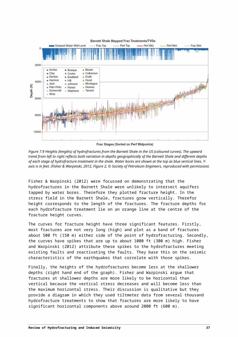
Earthquakes lie outside the area of CSG activities in the Galilee, Bowen, Surat, Clarence Moreton and northern Gunnedah Basins. Any ground shaking caused by hydrofracture operations in those areas must have been below the detection threshold of the ANSN of M = 3 for those areas because no recent earthquakes have been reported from there. M = 3 is also the threshold where people would have begun to feel the ground shaking. It is also a level that will not cause damage to infrastructure.

Earthquakes surround and in some cases lie within the southern Gunnedah and Sydney Basins (Figure 8.12). These areas are more prone to natural tectonic earthquakes than the CSG basins farther north. The largest historic earthquakes in the area occurred in the headwaters of the Warragamba dam near Picton in 1973 and Newcastle in 1989.

The earthquake near Warragamba dam on 9 March, 1973 had a magnitude of M5.5, which is sufficient to cause damage to local built infrastructure (Figure 8.14).

Simpson (1976) and Gibson (1997) attributed this earthquake to the impoundment of the Warragamba reservoir (see Appendix C for a brief discussion on reservoir induced seismicity) but Mills and Fitch (1977) thought it unlikely. The earthquake has a good spatial correlation with the filling of the Warragamba dam by occurring on a linear river valley which downstream forms one arm of the dam. However, the earthquake occurred at depths of 10–20 km in the crust 11 years after the filling of the reservoir, and therefore does not have a good depth or time correlation with the filling of the reservoir. Experience overseas indicates that large earthquakes can be triggered in the upper crust after decades of liquid waste disposal (See Appendix C), so the time lag between reservoir filling and the earthquake may not be a discriminator between a natural stress-initiated or fluid-induced rupture.

The earthquake has a focal mechanism indicating a thrust fault under the influence of an approximate NE-SW regional compressive stress field, consistent with the stress field reported for the Sydney Basin by Hillis et al. (2000) (Figure 8.14). Other earthquakes have occurred in the southern Sydney Basin, some with magnitudes up to M4.

The earthquake near Newcastle in 1989 had a magnitude of M5.6, and it epicentre was 11km deep. Its epicentre was 15 km south of the Newcastle business district. The focal mechanism could be interpreted as either a very shallow-dipping thrust or a normal fault (McCue, et al.,1990). These focal mechanism would imply that either 1 or 3 is oriented NE–SW. McCue et al. (1990) preferred a thrust mechanism consistent with the former; this is also consistent the average stress direction for the basin (Hillis, et. al., 2000).

The occurrence of earthquakes in the area over a number of years, and their magnitudes indicate that stresses are sufficient to create significant earthquakes in the mid-to upper crust; particularly around the margins of the basin.

The earthquakes in the southern Sydney Basin occur close to CSG activities in the Camden area. CSG activities in the Hunter region are in the area of high stress implied by the Newcastle earthquake. No evidence has been found that hydrofracturing activities in the area have caused earthquakes of M 3; they would be detected by the ANSN and would be felt by people locally.


Figure 8.14 Coal seam gas wells and earthquakes in the Camden area of the southern Sydney Basin, with the M5.5 earthquake of 9 March 1973 highlighted. Earthquakes – red circles; CSG wells – yellow circles with cross. The focal mechanism solution from Mills and Fitch (1977) and the average stress direction for the Sydney Basin from Hillis et al., (2000) are also shown.

Figure 8.15 Diagrammatic description of a CSG operation. Blue arrows show fluid movement (water, gas) down and up wells.


The production of CSG generates large volumes of waste water. Options for the disposal of water are shown in Figure 8.15. Central to all options is the need to ensure that the water quality is appropriate for the disposal method. This may require a treatment plant in which salt and other unwanted chemicals are extracted. Options for the disposal of waste water include on site storage in evaporation ponds, reinjection into a producing aquifer as part of a managed aquifer recharge process, discharge to a river, sale to a nearby industry, agricultural development and for potable water supply. Brines left after water is treated can be held on-site in evaporation ponds or injected into deep wells, usually below the depth of producing gas seams and deep aquifers.

Disposal methods vary from state to state. In New South Wales, the storage of waste water on the surface is not allowed; reinjection is permitted (NSW, 2012b). In other jurisdictions elsewhere in Australia, eg., Queensland, treated waste water can be released into river systems. South Australia allows only evaporation ponds.

When discussing the reinjection of waste water SCER (2013) notes: 'There may be information that is applicable from the experience of the offshore petroleum sector or from current research on the sequestration of carbon dioxide in similar systems.' This sentence implies that insufficient consideration has been given by regulators to the management of waste water re-injection. The experience of the US industry is summarised above and in Appendix C.

SCER (2013) reports: 'The volume of water produced in gas operations is variable and unpredictable over time, and also variable between gas wells. In general, the level of water production will unavoidably diminish over time. … For example, over the life of a well, the typical water production in the Surat Basin has been assessed at 0.4 ML/day to 0.8 ML/day before decreasing to 0.1 ML/day, compared with the Camden field in the Sydney Basin, which produced 0.20 ML/day before decreasing to 0.02 ML/day …'. Even at the lower ends of these estimates, each CSG well will produce many millions of litres of water over an estimated 15–20 year production life. Even if the water is treated and much of it re-used, the volume of residual brines collected and re-injected from many wells into only one disposal well, as implied in Figure 8.15, over time could approach the volumes in the case studies in Appendix C where significant earthquakes were induced. The re-injection of waste may therefore result in a risk from induced seismicity.

Therefore, if long term re-injection is to be used,

1. The physical properties of the reservoirs used for waste disposal must be known in advance; ie. a reservoir assessment should be undertaken. However, unlike reservoir assessments undertaken before fluids are withdrawn and fluid pressures drop, it should consider what will happen when fluids are injected and pressures rise. It should take into consideration the distribution (number, separation and direction relative to the stress field) and weakness of existing faults and fractures, many of which could be below the threshold of resolution of the seismic method, assuming that seismic data are available (Ryan et al., 2012). The Harmonised Framework (SCER, 2013) calls for studies such as this before hydrofracturing is undertaken; they would be efficacious if also undertaken before long term injection of waste water. Otherwise, if the faults are strong and a barrier to fluid migration long term injection of large volumes of water could cause formation pressures to build within fault compartments rather than dissipate regionally; if the faults are weak and suitably oriented, they may be reactivated. The magnitudes of earthquakes induced in this way are summarised in 'Unintentional Hydrofracturing Injection' in Table 4.2.

Formation pressures have to be monitored and not exceed the critical pressures that will create new fractures in intact rock, and more importantly, the lower formation pressures that would be required for


the reactivation of existing weak faults and fractures. If these critical pressures are exceeded, earthquakes could start to occur. Even if disposal is discontinued immediately, some time may still elapse before the reservoir pressures equilibrate to a new stable state and seismicity ceases.

8.1.2 Shale Gas

The shale gas industry is in its infancy in Australia. However, a number of basins in Australia are prospective for shale gas (Figure 8.16), and industry interest is growing (eg. Medd, 2012). The sector is likely to expand rapidly as it has done in recent years in the US (USEIA, 2013)

Figure 8.16 Basins with current shale gas and shale oil activity, and basins with potential for shale oil and gas (Source: Geoscience Australia).

Unlike conventional gas accumulations, shale gas is trapped in the rocks where it formed; ie., the shale is both the source and the reservoir. It cannot escape because of the very low permeability of the rocks. To extract the gas, companies have to hydrofracture the shale.

Particular attention needs to be given to the detailed stress orientation down wells (Figure 5.7) so that fracture direction can be predicted accurately.

Insufficient data exists from hydrofracturing for shale gas in Australia to characterise populations of induced earthquake magnitudes likely to be encountered in Australia. They are unlikely to be different in overall form from those in the shale gas industry in the US, where shale gas is produced from similar depths but possibly different stress regimes in some areas.

Maxwell et al. (2009) presented a case study from Western Canada in which microseismicity was used to map the development of hydrofractures. The well that was hydrofractured intersected a system of low angle reverse faults. Earthquakes that were induced during the fluid injection phase of the


hydrofracture process had a Gutenberg-Richter b value around 2, implying that the earthquake population contained more smaller than larger events compared to a population of natural (tectonic) earthquakes. The earthquakes induced during the injection phase were clustered near the well and aligned in a north east to south west direction.

Later earthquakes, including after the fluid injection had stopped and the high injection pressures were shut in, had a b value less than 1, which is closer to the value expected for natural earthquakes. These earthquakes also had different ratios of P-wave to S-wave energy, suggesting a different rupture process. The later population of earthquakes was farther from the well, and was also oriented north east to south west and co-linear with the first population of earthquakes.

The two populations were interpreted to be due to the hydrofracture of intact rock (earlier population with b ≈ 2) and the post fracture reactivation of an existing fault (later population b ≈ 1).

The earthquakes recorded in the study of Maxwell et al (2009) all had magnitudes less than M = 0 and would not have been felt. An important implication of this work is that if the hydrofracture process does start to induce larger earthquakes that would be unacceptable to a nearby community, the operators should not only cease or lower the rate of pumping of fluids but they should also bleed off the high pressures from the injection. Otherwise the high pressure fluids could continue to flow into natural faults and induce earthquakes.

Several of the issues that arise from CSG hydrofracturing are unlikely to arise in hydrofractures for shale gas:

1. Shale gas formations are at much greater depths (2000–3,000 m) than those from which CSG is produced (200–1000 m). Because of the variations of stress directions with depth in the Cooper Basin, for example, hydrofractures could break vertically out of the formation being hydrofractured. The depth resolution of real-time seismic and tiltmeter monitoring techniques may be insufficient to indicate whether this has happened, although post processing of the seismic data may be able to resolve the depths more accurately. If the hydrofractures do break vertically out of the formation being stimulated, they are unlikely to reach the shallower levels from which groundwater is being produced; experience in the US shows that fractures would not be long enough (Section 7, Fisher and Warpinski, 2012; Davies et al., 2013b)

2. Shale gas production does not produce as much waste water as CCG. However the waste water that is produced has to be disposed of. Much of the increase in induced seismicity in the US is associated with the re-injection of waste fluids from the shale gas industry (Appendix C). In South Australia, re-injection is not permitted and most water is disposed of in evaporation ponds. Should the shale gas industry expand in other states, careful attention will need to be given to reservoir modelling if re-injection is to be used, as discussed above for CSG. However, at the greater depths at which the shale gas industry operates, the ability of the seismic reflection method to resolve offsets on faults, and therefore the faults themselves, is very much less than it is at the depths at which the CSG industry operates, so even more care will be needed in resolving the distribution of pre-existing weak faults.

8.1.3 Enhanced Geothermal Systems

Geothermal energy has attracted a significant but varying amount of attention from the unconventional energy industry in the last decade, partly because it is a non-carbon producing source of energy, and partly because the development of a number of mineral prospects in remote parts of Australia, particularly South Australia, requires access to power, preferably from local sources that do not require


significant investment in transmission lines from the power grid. Figure 8.17 shows the distribution of geothermal energy prospects in Australia in 2013 and 2015.

The prospects in Figure 8.17 consist of a number of geothermal energy types. Those dependent on naturally occurring steam tapped from hot water at depth, for example, around Mt Gambier sometime require hydrofracturing to improve steam production. They are not considered further in this report. Enhanced geothermal (Hot Dry Rock) systems always require the hydrofracturing of the rocks that contain the heat source.

Figure 8.18 shows a schematic of how an enhanced geothermal system works. Explorers look for a rock that will be a suitable source of heat, typically a granite with high amounts of heat producing elements. The rock should be buried under a blanket of other rocks, for example, sedimentary rocks, that restrict the heat from escaping, thereby allowing the temperature at depth to increase.

Figure 8.17 Geothermal energy activity in Australia in 2013 (a) and June 2015 (b) (Source: Ed Gerner, Geoscience Australia).

Holes are drilled into the hot rock and the country rock hydrofractured. Water is then pumped down one well into the hot rock, allowed to flow through the porosity created by the hydrofractures, and then pumped out of a second well. Pressure at the injection well is kept higher than at the out-flow well to ensure that the water will flow through the reservoir. As the water flows from the injection well to the extraction well, it becomes hot. The heat is extracted at the surface and used to generate electricity.

Only one prospect in Australia has reached the stage of an initial production test of a hydrofracture stimulated hot dry rock geothermal energy source—that of Geodynamics Pty Ltd in the Cooper Basin in South Australia. Baisch et al. (2006) describe the seismicity generated by a fracture stimulation initiated at a depth of 4250 m in the Habanero–1 well in 2003, and Baisch et al. (2009) describe the seismicity from a second fracture stimulation in 2005.


Figure 8.18 Schematic of an enhanced geothermal (hot dry rock) geothermal energy system. (Source, Geoscience Australia fact sheet).

Downhole seismometers were used to locate the earthquakes caused by the hydrofractures. The first earthquakes were located where the injection fluid exited the well and entered the rock. Subsequent earthquakes were progressively further away. The earthquakes from the 2005 stimulation were mostly located beyond the extremities of the 2003 stimulation, suggesting that the subsequent injection opened new fractures at the ends of old fractures rather than causing new fractures in intact rock near the well.. The earthquakes define a flat lying fracture with a lateral extent up to 2500 m. After errors in the estimate of the depths of the earthquakes were considered, the fracture was estimated to be about a metre thick. This was consistent with the estimated thickness of a fracture zone intersected in a new well drilled after the 2003 stimulation.

The earthquakes had composite focal plane solutions indicative of a flat lying thrust and a Gutenberg-Richter value of 0.83 (for magnitudes between -0.8 and 1.5) also consistent with a shear rupture rather than a tension rupture. Baisch et al. (2009) conservatively estimated that although the displacement for each earthquake would have been very small, (0.03–0.21 mm), cumulative average slip would have been around 3 cm, and slip may have reached 9 mm in places. Baisch et al. (2006) believed it to be a pre-existing structure that was reactivated by the hydrofracture stimulation.

The magnitudes of some earthquakes were larger than recorded in hydrofractures in other energy sectors, eg., shale gas. The Geoscience Australia national seismograph network registered a number of events with magnitudes up to M3.7. Baisch et al. (2006) noted this but did not provide an explanation. As noted above and in Appendix B, fault rupture in granite that causes an earthquake of M = 3.7 would produce an earthquake of M = 1.2 if the same rupture size happened in coal or shale. This is because of the different shear moduli in granite, shale and coal.

Seismicity continued after the hydrofracture stimulation, although it was not monitored continuously. One of these events occurred when the monitoring system was operating and was located at the edge of the 2003 earthquake cloud several months after the injection was completed. It may have resulted from pressure diffusion in the fractured rock, in which pressures had not been deflated after the injection. It was followed by up to 80 aftershocks which may have been triggered by stress migration caused by the larger earthquake. This phenomenon of earthquake populations occurring after the


hydrofracture process is similar to that for shale gas operations reported by Maxwell et al. (2009) and summarised above.

The stimulation of hydrofractures at the Geodynamics Ltd geothermal prospect in the Cooper Basin therefore generated earthquakes that could be recorded on the regional seismograph network operated by Geoscience Australia, and would have been felt by people nearby. They would not have caused damage to built infrastructure, but might have been disconcerting to bystanders.

Similar sized earthquakes were induced during the development of a geothermal prospect in a more populated area near Basel in Switzerland in 2006 and 2007 (Deichmann and Giardini, 2009). The well had been drilled through sedimentary cover rocks into crystalline basement, reaching 5,000m. Stimulation of the well began on 2 December 2006 and on 8 December a M2.6 earthquake occurred. It exceeded the safety threshold set in advance of the hydrofracture stimulation of the well and the injection was shut down. Later that day, two events of magnitude M2.7 and M3.4 occurred. The well was opened and the injected water allowed to flow out to relieve the pressure. Despite the drop in pressure, some seismicity continued in the stimulated volume after two years; three of the four strongest events occurred one to two months after the stimulation had stopped and the water pressure gradient at the well lowered to hydrostatic.

Most of the earthquake focal mechanisms are consistent with shear failure on pre-existing faults (See Appendix B for a discussion of focal mechanisms and the differences for shear and tension failure). The largest earthquake (M3.4) has a focal mechanism indicating strike-slip failure on a pre-existing fault oriented almost optimally (30–40) to the ambient stress field. Most of the induced seismicity occurred before formation pressures reached those required for tension hydrofractures or after peak pressures had dropped. This would be consistent with the reactivation of a weak pre-existing fault (see Appendix Figure A.9 and its accompanying discussion).

Some earthquakes had focal mechanism analyses that showed evidence of a change in volume at the hypocentre, consistent with tension fractures. These earthquakes also occurred when pressures were lower than those expected to cause tension or hybrid tension and shear cracks. The nature of these focal mechanisms was not well developed and would be the subject of further work (Deichmann and Giardini, 2009).

The need for a positive pressure gradient between the injection and out-flow wells requires higher pressures to be maintained at the injection well. The triggering of earthquakes at pressures below those required for tension hydrofractures in the study at Basel (and in some cases at what is believed to be hydrostatic pressure gradients) should be an indicator that seismic monitoring must be continued for some time after geothermal projects go into production, especially if there is any evidence that the fracture system has re-activated a pre-existing fault. Loss of well head pressure might also be an indicator that water is being lost from the hydrofracture network, so that new hydrofractures might be triggered at the periphery of the network.

8.2 Unintentional HydrofracturingMany of the causes of unintentional hydrofracturing are un-related to the unconventional energy industry. Others that are related to the unconventional energy industry are due to the disposal of waste fluids rather than the exploration and production phases per se. Unintentional hydrofracturing is included for completeness in this report in Appendix C—Human Induced Seismicity.


Australia has no known examples of seismicity induced by carbon sequestration; a brief discussion of the potential for induced seismicity from carbon sequestration follows.

8.2.1 Carbon Sequestration

Zoback and Gorelick (2012) predicted that the injection of large volumes of CO2 into storage reservoirs has the potential to induce seismicity. Zoback and Zoback (1981) and Zoback et al. (2002) had earlier hypothesised that the continental lithosphere in the conterminous US is critically stressed. In simple terms, everything that can break under the present-day stress field has broken leaving some other rocks that are stressed just below the yield threshold. A drop in crustal strength, through heat, an increase in the regional stress, or a change in the effective stress, for example., by an increase in pore fluid pressure, could lead critically stressed rocks to break. The injection of CO2 could change the fluid pressure and therefore the effective stress.

If this occurs, an induced fracture in a CO2 reservoir could lead to fracture porosity and a pathway for CO2 to leak from the reservoir in which it had been stored, presumably with the original intention of it staying there for aeons.

Their hypothesis is no different from the principles of unintentional hydrofracturing that are discussed above and in Appendix C, that the injection of large volumes of liquid waste over long periods of time can lead to the reactivation of existing faults. Indeed, Zoback and Gorelick (2012) used the case studies of the Rocky Mountain Arsenal and the Rangeley field set out as Case Studies #2 and #3 in Appendix C in their arguments.

In the Rocky Mountain Arsenal case study, the earthquakes were unexpected. In the Rangeley field case study, the earthquakes were deliberately triggered to test the theories about critical formation pressures required to induce seismicity that had been developed as a result of the Rock Mountain Arsenal earthquakes. The lessons learned at the Rocky Mountains Arsenal and Rangeley seem to have been forgotten if the increasing levels of seismicity induced in the US midcontinent in recent years are being caused by waste injection. Case Study #4 in Appendix C of large induced earthquakes in Oklahoma is an example.

A lesson that can be reinforced from the two examples of seismicity induced by hydrofracturing of geothermal heat reservoirs is that hydrofracturing can re-activate pre-existing faults that were unknown before the hydrofracture stimulation. The faults do not have to have large displacements that can be mapped with, say, seismic reflection profiling. They only have to be weak faults. Indeed the youngest fault are likely to be the weakest faults, and they are also likely to have the smallest displacements and therefore be the most difficult to detect.

Therefore, the storage of anything in the Earth, whether waste water from unconventional energy systems, chemical waste, or CO2, requires a full understanding of the properties of the storage reservoir before anything is injected. Particular attention should be paid to locating pre-existing faults and fractures, especially those optimally oriented to the prevailing stress directions.


9 Issues of Public Concern

The issues of concern to the public were flagged in the Introduction:

concerns that hydrofracturing uses water that can be in short supply in rural and regional communities

concerns that aquifers will be breached with consequent loss of water for human use and the agricultural and pastoral industries

worries that fresh water aquifers could be contaminated by saline formation waters and/or hydrofracturing fluids

the need to dispose of waste waters [volume, contained contaminants] in ways that will not adversely affect the environment

whether fugitive gas emissions might result [into groundwater used for human and stock consumption, and directly at the surface]

whether the size of the footprint is such that there wold be a loss of productive pasture

whether hydrofracturing can induce seismicity and what would its impact be.

9.1 Water volumes used during hydrofracturingThis issue is raised by the community in the context of shortages of fresh water for people in rural areas and towns and for farming and livestock. In that context it is not an issue related to seismicity.

It would become an issue related to seismicity if hydrofractures of very large areas were attempted, leading to high fluid pressures away from the well and no means of reducing those pressures over time. This would increase the likelihood of the high pressure fluids encountering an unmapped fault and re-activating it.

9.2 Aquifer breaching and loss of water for human use and the agricultural and pastoral industriesHydrofracturing in the shale gas and geothermal sectors is performed at great depths and is unlikely to produce fractures long enough to reach the shallower freshwater aquifers, even if the stress fields locally allow vertical fractures to form.

Hydrofracturing in the coal seam gas sector is undertaken at shallower depths and therefore very much closer to fresh water aquifers. The general belief is that hydrofractures in the CSG sector will be horizontal because the vertical stress will be the lowest of the principal stresses. R. Jeffrey (CSIRO, Personal Communication with the Author on 11 July, 2013) wrote that of 9 mine-out experiments in New South Wales and Queensland, 7 of the 9 fractures were contained in the coal or did not grow vertically to any extent. Two, at the German Creek Colliery in Queensland, did grow into the roof because of anomalously low stress in the roof. Another produced a T-shaped hydrofracture near the top of the coal seam. Jeffrey et al. (1993) described the fractures at the German Creek Colliery.


If hydrofractures break into the overlying strata, then that section of the coal will no longer be impermeable. If effective aquitards do not exist between the fresh water aquifers and the coal, the potential exists for hydraulic connections between the aquifers and the fractured zone in the coal. Because the coal is de-watered to produce gas, the coal seam would have a lowered fluid pressure and water would be lost from the aquifer to the coal seam and subsequently through pumping from the well.

The Harmonised Framework (SCER , 2013) addresses this through recommending very detailed geological mapping before hydrofracturing and close monitoring of both the hydrofracturing process and subsequently the water levels in nearby wells.

9.3 Contamination of fresh water aquifers by saline formation waters and/or hydrofracturing fluids

Contamination of shallow aquifers in the shale gas and geothermal sectors should not happen through hydrofracturing because of the significant vertical separation compared to the likely length of hydrofractures even if they grow vertically. Contamination is only likely to happen through well failure, allowing waters to flow in the annulus surrounding the casing and the rock. This is also the finding of the UK enquiry into shale gas (The Royal Societies, 2012).

In the coal seam gas sector, contamination of fresh water aquifers should not happen because the coal seams are dewatered to release the gas, so groundwater is likely to flow into the coal rather from the coal into overlying sequences—see the previous Section.

9.4 Environmental issues with disposing of formation waters [volume, contained contaminants]

Formation waters can be treated to remove unwanted chemicals.

The main concern is the potential for unintentional hydrofractures , particularly fault reactivation, caused by the injection of large volumes of waste in underground storage. This is most likely to occur through the reactivation of pre-existing weak faults that were not previously mapped, or whose physical properties and strength are not understood. It could happen in any of the sectors where significant volumes of liquid are disposed of, including steadily over time: shale gas, geothermal, coal seam gas and CO2 disposal.

Mitigating strategies are discussed above and include undertaking a comprehensive reservoir engineering study and then monitoring formation pressures to ensure they stay below the critical pressures likely to trigger the reactivation of pre-existing faults.

9.5 Fugitive gas emissions into groundwater used for human and stock consumption, and directly at the surface

Fugitive gas emissions are more likely to occur around a failed well than through run-away hydrofractures, provided that the hydrofracturing process is carefully monitored and shut down if necessary.


The coal seam gas sector is the most developed of the sectors covered in this report. Both Queensland and New South Wales where CSG production is presently underway have comprehensive codes of practice for the drilling, hydrofracturing, operation and decommissioning of CSG wells. Their codes of practice are reflected in the Harmonised Framework (SCER, 2013).

9.6 Loss of productive pastureHydrofracturing operations can have a foot print covering a number of hectares because of the need to have hydrofracturing water (and added chemicals and proppant) and the recovered flow-back hydrofracturing water stored on site. State regulators and landholders require rehabilitation of the sites after wells go into production.

Production wells after hydrofracturing have a small footprint. Once wells are de-commissioned, the sites surrounding them are also rehabilitated.

However, this is not an issue related to induced seismicity.

9.7 Impact of induced seismicity

The case studies accessed in the preparation of this report indicate that for hydrofracturing for shale gas and coal seam gas, the earthquakes induced by hydrofracturing are small, mostly with negative magnitudes. They should not be felt, but if they are they would be more of a discomfort than an indication of likely damage to infrastructure.

The case studies accessed for geothermal energy reported larger earthquakes, up to M3.8, which were recorded on regional seismograph networks operating beyond the local networks set up to monitor the hydrofracturing. Public concern and an exceedance of the pre-agreed shut down threshold for induced earthquake magnitude caused the Basel project to stop.

The largest reported induced earthquakes from the unconventional energy sectors discussed in this report were caused by long term disposal of waste water down wells. Most were caused by the reactivation of pre-existing faults, some of which were previously unknown, and often some distance from the injection well (see Appendix C).


10 Some Simple Points

Hydrofracturing breaks rock. When rocks break, energy is released, and some of the energy is in the form of ground shaking. Ground shaking is called an earthquake. Earthquakes caused by hydrofracturing are called induced earthquakes.

The vast majority of induced earthquakes caused by hydrofracturing are so small they will not be felt. However, some earthquakes can be large enough to be felt and some of those that are unintentionally induced could be damaging.

As much should be known about the geology as possible before the hydrofracturing begins. A detailed geological model should inform a hydrofracturing plan, and the plan should be updated as new information becomes available during hydrofracture operations. The hydrofracture process should be monitored with as many techniques as possible. Thresholds for parameters that are monitored should be set in advance, and the hydrofracturing plan modified or the hydrofracturing stopped if the pre-set thresholds are exceeded.

To mitigate the effects of induced seismicity, earthquake magnitudes should be kept as small as possible. This means that hydrofractures should be grown slowly through many small ruptures rather than by a few larger ruptures. The theory of tension fracture indicates that this can be done by controlling the volume and pressure of water made available to the growing hydrofracture and the rates at which water is pumped into the hydrofracture. If the process is monitored closely, varying these parameters can speed up, slow down or stop the process.


11 Acknowledgements

This Record constitutes the publication of a report commissioned in 2013 by Clinton Foster, Chief Scientist for Geoscience Australia. The 2013 report was intended only for internal use in Geoscience Australia. In preparing the original report for publication as a Record, several figures were removed, others replaced, and some re-drafted. Some data tables and maps of earthquakes and wells have been updated to mid-2015. However, the essence of the original report remains unchanged.

The main body of the original report was peer reviewed by Clinton Foster and Andrew Stacey. Appendices A and B were peer reviewed by Clinton Foster, Andrew Stacey, David Burbidge and Mark Leonard. Appendix C was peer reviewed by Clinton Foster.

Clive Collins converted the formats of some 2013 data from the Queensland Government web site. He is acknowledged in several places particularly in the Appendices for specific input to this study. Daniel Jaksa helped convert some 2015 well data from Queensland.

Jingbo Wang provided a copy of her early-2013 seminar on hydrofracturing. Robert Langford provided access to his extensive digital library of scientific publications on coal seam gas. Eric Tenthorey provided advice on the Australian stress field early in the writing of the original internal report. Ken Lawrie drew early attention to the growing incidence of induced seismicity in the US. Ron Hackney pointed to critical parts of the scientific literature. Ed Gerner provided the maps of past (2013) and current (2015) geothermal systems projects in Australia. Rebecca Norman wrote a review paper on the water used during hydrofracturing.

Dr Des Fitzgerald of Intrepid Geophysics provided literature and other information on the Geodynamics Ltd hydrofracture program.

The figures in this Record were prepared by the Products and Promotions team at Geoscience Australia. Silvio Mezzomo led the drafting work. Daniel Rawson helped with document formatting and production.

Elizabeth Fredericks arranged for copyright permission to use previously published figures.


12 References

Abercrombie, Rachel E., 1995. Earthquake source scaling relationships from -1 to 5 ML using seismograms recorded at 2.5-km depth. Journal of Geophysical Research, 100(B12), 24,015–24, 036.

AGL, 2015a. The Gloucester Gas Project. http://www.agl.com.au/~/media/AGL/About%20AGL/Documents/How%20We%20Source%20Energy/Gloucester%20Document%20Repository/Fact%20Sheets/20130101_Fact%20Sheet%20GGP%20%20%20Gloucester%20Gas%20Project.pdf Accessed 20 July, 2013.

AGL, 2015b. AGL’s New South Wales hydraulic fracturing fact sheet and frequently asked questions. http://www.agl.com.au/~/media/AGL/About%20AGL/Documents/How%20We%20Source%20Energy/Hunter%20Document%20Repository/Fact%20Sheets/20130213_AGL%20Fact%20Sheet%20%20%20Hydraulic%20Fracturing.pdf Accessed 20 July 2015

Baisch, S., Weidler, R., Vörös, R., Wyborn, D. and de Graaf, L., 2006. Induced seismicity during the stimulation of a geothermal HFR reservoir in the Cooper Basin, Australia. Bulletin of the Seismological Society of America, 96(6), 2242–2256.

Baisch, S., Vörös, R., Weidler, R. and Wyborn, D., 2009. Investigation of fault mechanisms during geothermal reservoir stimulation experiments in the Cooper Basin, Australia. Bulletin of the Seismological Society of America, 99(1), 148–158.

Beach, 2012. Fracture stimulation of deep shale gas and tight gas targets in the Nappamerri Trough (Cooper Basin), South Australia. Environmental Impact Report. http://www.pir.sa.gov.au/petroleum/environment/register/seo,_eir_and_esa_reports/drilling_activity_reports.

Burbidge, D. (Ed), 2012. The 2012 Australian Earthquake Hazard Map. Geoscience Australia, Record, 2012/71.

Cox, S.F., 2010. The application of failure mode diagrams for exploring the roles of fluid pressure and stress states in controlling styles of fracture-controlled permeability enhancement in faults and shear zones. Geofluids, 10, 217–233.

Davies, R., Foulger, G., Bindley, A. and Styles, P., 2013a. Induced Seismicity and Hydraulic Fracturing for the Recovery of Hydrocarbons. Marine and Petroleum Geology, 45, 171–185.

Davies, R.J., Mathias, S.A., Moss, J., Hustoft, S. and Newport, L., 2013b. Hydraulic fractures: How far can they go? Marine and Petroleum Geology, 37, 1–6.

Deichmann, N and Giardini, D., 2009. Earthquakes induced by the stimulation of an enhanced geothermal system below Basel (Switzerland). Seismological Research Letters, 80(5), 784–798.

Denham, D. and Windsor C.R., 1991. The crustal stress pattern in the Australian continent. Exploration Geophysics, 22, 101–105.

Diamond, W.P. 1987a. Underground observations of mined-through stimulation treatments of coalbeds. Quarterly Review of Methane from Coal Seams Technology. 4(4), 19–29.

Diamond, W.P. 1987b. Characterization of Fracture Geometry and Roof Penetration Associated with Stimulation Treatments in Coalbeds. Proceedings of the 1987 Coalbed Methane Symposium, University of Alabama (Tuscaloosa), pp 243.

Diamond, W.P. and Oyler, D.C.. 1987. Effects of stimulation treatments on coalbeds and surrounding strata, evidence from underground observations. US Department of Interior, RI9083, USBM, 1–47.

Ellsworth, W.L., Hickman, S.H., Lleons, A.L., McGarr, A., Michael, A.J., and Rubenstein, J.L., 2012 Are elasticity rate changes in the midcontinent natural or manmade? Seismological Society of America, Abstract, 12–137.

Fisher, K. and Warpinski, N., 2012. Hydraulic-fracture height growth: real data. Society of Petroleum Engineers (SPE) Production and Operations, February, 8–19, SPE 145949.


http://www.pir.sa.gov.au/petroleum/environment/register/seo,_eir_and_esa_reports/drilling_activity_reports

http://www.pir.sa.gov.au/petroleum/environment/register/seo,_eir_and_esa_reports/drilling_activity_reports

http://www.agl.com.au/~/media/AGL/About%20AGL/Documents/How%20We%20Source%20Energy/Hunter%20Document%20Repository/Fact%20Sheets/20130213_AGL%20Fact%20Sheet%20%20%20Hydraulic%20Fracturing.pdf



http://www.agl.com.au/~/media/AGL/About%20AGL/Documents/How%20We%20Source%20Energy/Gloucester%20Document%20Repository/Fact%20Sheets/20130101_Fact%20Sheet%20GGP%20%20%20Gloucester%20Gas%20Project.pdf



Frogtech, 2013. Potential Geological Risks Associated with Shale Gas Production in Australia. Frogtech Project Code AAS801. http://www.acola.org.au/PDF/SAF06FINAL/Frogtech_Shale_Gas_Geology_and_Risks%20Jan2013.pdf.

Gibson, Gary, 1997. Earthquakes and dams in Australia. Australian Earthquake Engineering Society, Conference Proceedings, Paper 08.

Healy, J.H., Rubey W.W., Griggs D.T. and Raleigh C.B., 1968. The Denver earthquakes. Science, 161, 1301–1310.

Hillis, R.R., Meyer, J.M. and Reynolds, S.D., 1998. The Australian Stress Map. Exploration Geophysics, 29, 420–427.

Hillis, R.R., Enever, J.R. and Reynolds, S.D., 1999. In situ stress field of eastern Australia. Australian Journal of Earth Sciences, 46, 813–825.

Hillis, R.R. and Reynolds, S.D., 2000. The Australian Stress Map. Journal of the Geological Society of London, 157, 915–921.

Jeffrey, R.G., Enever, J.R., Ferguson, T., Bride, J., Phillips, R. and Davidson S. 1993. Small-scale hydraulic fracturing and mineback experiments in coal seams. Proceedings of the 1993 International Coalbed Methane Symposium. University of Alabama (Tuscaloosa). May 17-21, 1993. 79–88.

Johnson, Raymond L.Jr, Glassborow, Brent, Scott, Michael P., Pallikathekathil, Zachariah John, Datey, Ashish, Meyer, Jeremy, 2010. Utilizing current technologies to understand permeability, stress azimuths and magnitudes and their impact on hydraulic fracturing success in a coal seam gas reservoir. Society of Petroleum Engineers, SPE 133066.

Keranen, K.M., Savage, H.M., Abers, G.A. and Cochran, E.S., 2013. Potentially induced earthquakes in Oklahoma, USA: Links between wastewater injection and the 2011 Mw 5.7 earthquake sequence. Geology, Doi: 10.1130/G34045.1.

King, 2012. Hydraulic fracturing 101: What every representative, environmentalist, regulator, reporter, investor, university researcher, neighbor and engineer should know about estimating frac risk and improving frac performance in unconventional gas and oil wells. Society of Petroleum Engineers, SPE 152596.

Maxwell, S.C., Jones, M., Parkes, R., Miong, S., Leaney, S., Dorval, D., D’Amico, D., Logel, J, Anderson, E. and Hammermaster, K., 2009. Fault activation during hydraulic fracturing. SEG Houston International Exposition and Annual Meeting, Abstracts, 1552–1556.

McCue, K., Wesson, V. and Gibson, G., 1990. The Newcastle, New South Wales, earthquake of 28 December 1989. BMR Journal of Australian Geology and Geophysics, 11, 559–567.

Medd, J., 2012. Shale – a new energy dawn? Petroleum in Western Australia, May, 34–35.Mills, J.M. and Fitch, T.J., 1977. Thrust faulting and crust-upper mantle structure in eastern Australia.

Geophysical Journal of the Royal Astronomical Society, 48, 351–384.Miyazaki, S., 2005. Coal seam gas exploration, development and resources in Australia: a national

perspective. APPEA Journal, 45, 131–142NSW, 2012a. General Purpose Standing Committee No. 5. Report of an Inquiry into Coal seam gas.

http://www.parliament.nsw.gov.au/Prod/parlment/committee.nsf/0/318A94F2301A0B2FCA2579F1001419E5?open&refnavid=CO5_1. Downloaded 03/04/2013

NSW, 2012b. General Purpose Standing Committee No. 5. Report of an Inquiry into Coal seam gas – Government Response. http://www.parliament.nsw.gov.au/Prod/parlment/committee.nsf/0/318A94F2301A0B2FCA2579F1001419E5?open&refnavid=CO5_1. Downloaded 03/04/2013

O'Brien, G.W., Lawrence, G.M., Williams, A.K., Webster, M., Lee, J., Cowley, R. and Burns, S., 2001. Hydrocarbon migration and seepage in the Timor Sea and Northern Browse Basin North-West Shelf, Australia: An Integrated SAR, geological and geochemical study. AGSO–Geoscience Australia, Record 2001/11.

Rahman, M.M. and Rahman, S.S., 2012. Induced and natural fracture interaction in tight-gas reservoirs. The APPEA Journal, 52, 611–626.


http://www.parliament.nsw.gov.au/Prod/parlment/committee.nsf/0/318A94F2301A0B2FCA2579F1001419E5?open&refnavid=CO5_1




http://www.acola.org.au/PDF/SAF06FINAL/Frogtech_Shale_Gas_Geology_and_Risks%20Jan2013.pdf

http://www.acola.org.au/PDF/SAF06FINAL/Frogtech_Shale_Gas_Geology_and_Risks%20Jan2013.pdf

Riley, J.M., 2004. The rise and rise of coal seam gas in the Bowen basin. APPEA Journal, 44, 647–652.

Rutledge, James T and Phillips, W. Scott, 2003. Hydraulic stimulation of natural fractures as revealed by induced microearthquakes, Carthage Cotton Valley gas field, east Texas. Geophysics, 68(2), 441–452.

Ryan, D.J., Hall, A., Erriah, L. and Wilson, P.B., 2012. The Walloon coal seam gas play, Surat Basin, Queensland. The APPEA Journal, 52, 273–289

SCER, 2013. The National Harmonised Regulatory Framework for Natural Gas from Coal Seams 2013. http://scer.govspace.gov.au/files/2013/06/National-Harmonised-Regulatory-Framework-for-Natural-Gas-from-Coal-Seams.pdf Downloaded 02/07/2013

Secor, Donald T. Jr, 1965. Role of fluid pressure in jointing. American Journal of Science, 263, 633–646.

Secor, Donald T. Jr, 1968. Mechanics of natural extension fracturing at depth in the Earth's crust. In A.J. Baer and D.K. Norris (Eds). Proceedings, Conference on Research in Tectonics (Kink Bands and Brittle Deformation), Ottawa, March 1968. Geological Survey of Canada Paper 68-52, 3–48.

Simpson, David W., 1976. Seismicity changes associated with reservoir loading. Engineering Geology, 10, 123–150.

Steidl, P.F. 1991. Inspection of induced fractures intercepted by mining in the Warrior basin, Alabama. Proceedings 1991 Coalbed Methane Symposium, University of Alabama (Tuscaloosa), 181–191.

Šilneý, Jan, Hill, David P., Eisner, Leo and Cornet, Francois H., 2009. Non-double couple mechanism of microearthquakes induced by hydraulic fracture. Journal of Geophysical Research, 114(B08), doi:10.1029/2008JB0054987.

The National Academies, 2011. Induced seismicity potential in energy technologies. The National Academies Press. http://www.nap.edu/catalog.php?record_id=13355.

The Royal Societies, 2012. Shale gas extraction in the UK: a review of hydraulic fracturing. The Royal Society and the Royal Academy of Engineering. http://www.royalsociety.org/policy/projects/shale-gas-extraction.

USEIA, 2013. U.S. Annual Energy Outlook 2013 with projections to 2040. US Energy Information Administration. http://www.eia.gov/forecasts/aeo/pdf/0383%282013%29.pdf

USEPA, 2004. Evaluation of Impacts to Underground Sources of Drinking Water by Hydraulic Fracturing of Coalbed Methane Reservoirs, Chapter 3. http://water.epa.gov/type/groundwater/uic/class2/hydraulicfracturing/wells_coalbedmethanestudy.cfm. Downloaded on 1 June 2015

Wang, I., Choudhury, J., Barker, W. and McNally, S., 2004. Developing coal seam methane in the Sydney Basin. APPEA Journal, 44, 625–638.

Zoback, M.D., and Gorelick, S.M., 2012. Earthquake triggering and large-scale storage of carbon dioxide. PNAS Early edition, http://www.pnas.org/cgi/doi/10.1073/pnas.1202473109.

Zoback, M.D., Townend, J., and Grollimund, B., 2002. Steady-state failure equilibrium and deformation of intraplate lithosphere. International Geology Review, 44, 383–401.

Zoback, M.D. and Zoback, M.L., 1981. State of stress and intraplate earthquakes in the United States. Science, 313, 3 July, 96–104.


http://www.pnas.org/cgi/doi/10.1073/pnas.1202473109

http://water.epa.gov/type/groundwater/uic/class2/hydraulicfracturing/wells_coalbedmethanestudy.cfm

http://water.epa.gov/type/groundwater/uic/class2/hydraulicfracturing/wells_coalbedmethanestudy.cfm

http://www.eia.gov/forecasts/aeo/pdf/0383(2013).pdf

http://www.royalsociety.org/policy/projects/shale-gas-extraction

http://www.royalsociety.org/policy/projects/shale-gas-extraction

http://www.nap.edu/catalog.php?record_id=13355

http://onlinelibrary.wiley.com/doi/10.1029/2008JB005987/full

http://scer.govspace.gov.au/files/2013/06/National-Harmonised-Regulatory-Framework-for-Natural-Gas-from-Coal-Seams.pdf

http://scer.govspace.gov.au/files/2013/06/National-Harmonised-Regulatory-Framework-for-Natural-Gas-from-Coal-Seams.pdf

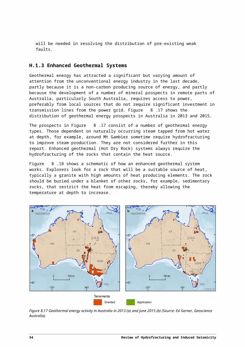
Appendix A How Hydrofracturing Works

A.1 IntroductionRocks break when subjected to stress. The ease and manner with which they break are also controlled by the presence or absence of pore fluids under pressure.

This discussion relies heavily on the work of Secor (1965, 1968) and Cox (2010) who distinguished between (See Appendix Figure A.1)

tensional fracture, in which the rocks break by the opening of cracks which have no lateral displacement of one side of the crack relative to the other

cracks that occur by shear failure, where one side of the crack (or fault zone) is displaced laterally relative to the other

hybrid tensional shear failure, which is a combination of both.

Appendix Figure A.1 Mode of opening of tensional and shear cracks.

Note that cracking in the context of both authors is by Mohr-Coulomb failure (ie., in simple terms, brittle failure) and not ductile deformation. Secor (1968) applied his theory to the production of joints in rocks, and therefore to brittle failure. Cox (2010) explicitly assumed Mohr-Coulomb failure in his analysis. He concentrated on rocks at depths mostly greater than those typically encountered in deliberate hydrofracturing exercises. Although the types of sedimentary rocks typically subjected to hydrofracturing for coal seam gas and shale gas can deform rather than break at slow strain rates,


they will break by brittle fracture at the high rates of change of fluid pressure as demonstrated during deliberate hydrofracturing.

The quantitative models of Cox were mostly derived for depths of 10 km. Therefore his models were recalculated for shallower depths; however, in the absence of rock property values specific to the areas where the kinds of hydrofracturing covered in this report are undertaken, Cox's values of rock properties were used. Where Cox gave ranges of values for any rock property, he used values in the middle of the ranges; they are for weak to moderately weak rock

A.2 Rock failure through hydrofractureThe stress at which rocks break is affected by the pressure of fluids in pore spaces in the rocks. Note that the theory probably applies equally to any fluid that is liquid (water, brine, oil). Cox (2010) used failure mode diagrams to explore the environments in which tensional and shear mode failure occurs. He plotted his failure mode diagram in terms of Pore Fluid Factor v, which is the ratio of (Pore Fluid Pressure Pf / Vertical Stress v), and differential stress ( 1-3), where 1 is the maximum compressive stress in the rock, and 3 is the least compressive stress. A failure mode diagram is shown in Appendix Figure A.2. Initially, the following discussion is about the behaviour of a homogeneous isotropic rock under varying conditions of stress and pore fluid pressure. Heterogeneities (eg., pre-existing cracks and faults and changes in lithology) are introduced later.

For the analysis of rock behaviour at a particular depth in the upper crust, pore fluid factor , which is plotted on the vertical axis in Appendix Figure A.2, is a dimensionless quantity that needs to be calculated for that depth; ie., the vertical axis does not represent a range of depths in the crust but rather the depth of the rock of interest. However, in an environment of active tectonics where the rock is being uplifted or moved to greater depths, v would need to be recalculated for every depth along the rock's journey.

At any depth in a layered Earth, the vertical stress v can be calculated as

σ v=∑i=1

n

ρi g zi (1)

where I = the density in layer i

g = acceleration due to gravity,

zi = thickness of layer i and

n = the number of layers down to the depth of interest.

Pore fluid pressure at any depth can be calculated similarly if the pressure gradient is hydrostatic, using the appropriate density of the fluid in the pores. For the rest of this Appendix, water is assumed to be the pore fluid.

In Appendix Figure A.2, the dashed line marked 'Hydrostatic Pf ', shows where plots when fluid pressure follows a hydrostatic pressure gradient. Where fluid pressures are greater than hydrostatic will plot above this line. When v is greater than 1, fluid pressure exceeds lithostatic pressure; ie., the fluid is overpressured.

Secor (1965) demonstrated that tensional fracture can occur only when the differential stress (1-3) is less than 4T, where T is the tensile strength of the rock. Therefore tensional cracking can only occur


under low differential stress conditions to the left of the dotted line in the diagram marked 4T, and in conditions where the fluid is overpressured (>1). Tensional cracks are discussed in the following section.

Appendix Figure A.2 Generic failure mode diagram in pore fluid factor–differential stress space at 1 km depth in the crust, using rock physical property values used by Cox (2010). The shear failure envelope for a reverse fault is shown in blue; the extension mode failure is in red; the failure envelope for hybrid extensional-shear mode failure is shown in green. For all stress and pore fluid factor states below the composite failure envelope, the rock mass is elastically strained, but will not fail in brittle mode. Brittle failure occurs when the stress and pore fluid factor states reach the failure envelope. Stress and fluid pressure states above the failure envelope cannot be attained.

At differential stresses greater than the vertical dotted line marked 2C/sin(2opt), the rock will break through shear failure and not tensional failure. C is the cohesive strength of the rock, and opt is the angle of failure between the fault that forms and the maximum compressive stress 1.

At stresses between 4T and 2C/sin(2opt), failure will be by a hybrid of tensional and shear failure.

Under any given stress regime, only one of tensional, shear or hybrid failure can occur in intact rock.

A.2.1 Tensional Cracks

A.2.1.1 Growing a Tensional Crack

Secor (1968) described the physics of tensional cracking in the crust in order to explain the growth of joints. He acknowledged earlier workers who noted that the cohesive strength of materials is often less


than predicted by theory by one to two orders of magnitude, and that they are probably weakened by the presence of internal and surface cracks. Premature failure is caused by high stress concentrations near crack tips. These natural cracks provide the seed from which larger cracks can grow.

Cracks open under effective tensional stress, with the crack orthogonal to the minimum principal stress 3. The distribution of internal and surface cracks in natural rock is such that some cracks would be optimally oriented, or oriented such that the component of forces in the direction of 3 would be sufficient for his analysis to be valid. He used an oblate ellipsoid as a mathematical description of the crack geometry, with the major axis orthogonal to 3 and the semi-minor axis parallel to 3. Secor then studied the behaviour of cracks when subjected to high fluid pressures.

The behaviour of cracks can be described in three stages, as illustrated in Appendix Figure A.3.

Appendix Figure A.3 Three stages of crack development, based on Figure 1 of Secor (1968). (a) crack exists but is not filled with fluid and therefore has no finite volume; (b) crack has filled with fluid and expanded under the influence of fluid pressure to the point where it is ready to fail at its tips; and (c) crack has failed at its tips and has become longer.

When the pressure of fluid in a crack is less than the minimum principal stress 3, the crack will remain closed and the volume of the crack will effectively be zero. This is illustrated in Appendix Figure A.3(a)

As fluid pressure in the crack builds through the percolation of fluid from the country rock into the crack, the crack will be wedged open. It will then have a finite volume (V1 in Appendix Figure A.3(b)). The conditions under which a crack with internal pore pressure will fracture under tension are, using the nomenclature of Cox (2010) where it differs from that of Secor (1968):

σ e=σ3−P>−T=−√ πEγ2 r (1−❑2)

(2)

and

V 1=16 r

52

3 √ πγ (1−❑2)2 E

(3)

where

e = effective stress


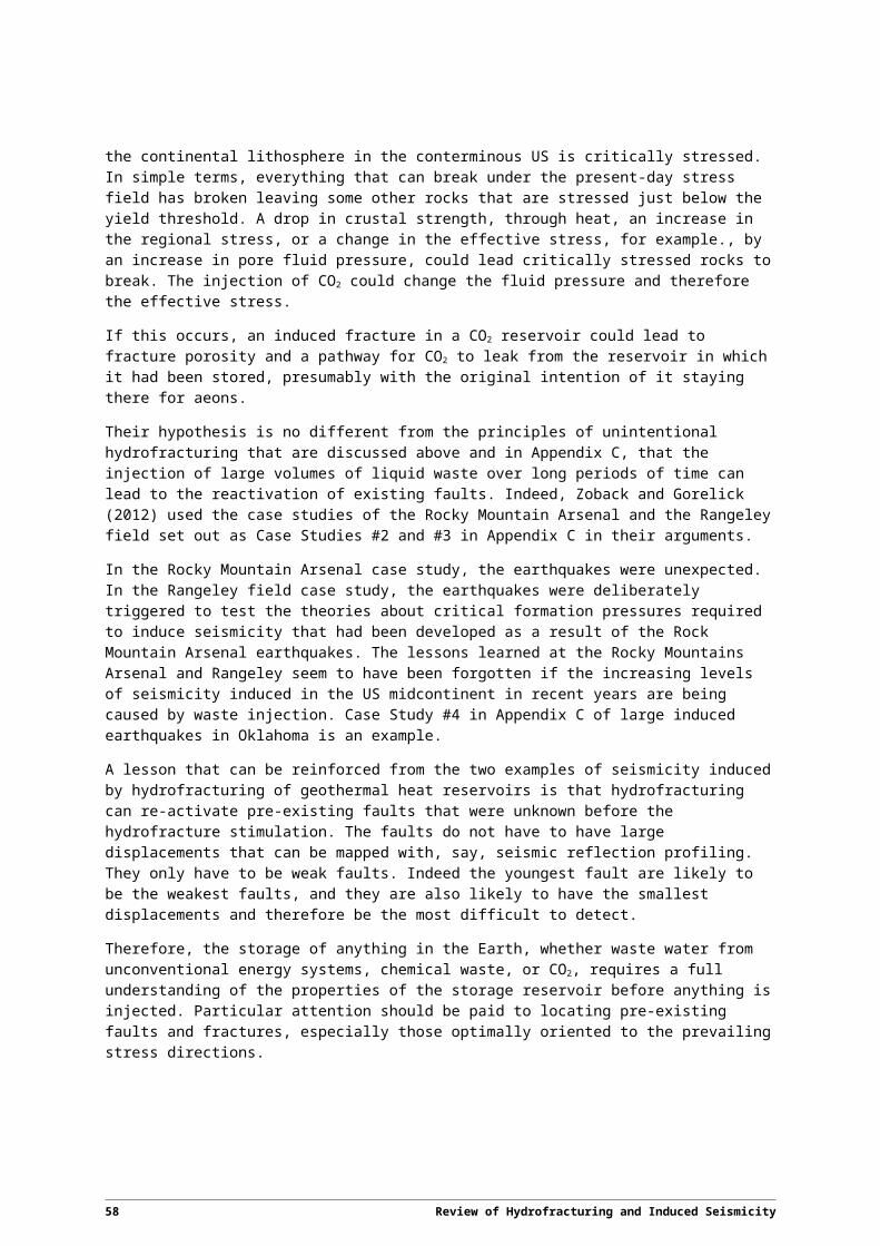
3 = minimum principal stress

P = fluid pressure

T = the tensile strength of the rock (tension considered negative)

E = Young's Modulus of the rock

= Poisson's Ratio

= the Specific Energy of the rock

V1 = the volume of the crack just before it fractures at the ends and expands;

V2 is the volume of the crack after it has expanded, and

r = the half length of the cracks; ie., the radius of the major axis of the oblate ellipsoid.

When the fluid pressure rises, the crack will open when the fluid pressure exceeds the minimum principal stress.

Once the stresses have exceeded the effective stress (Equation 2), and the volume of the crack has reached that defined in Equation 3, the crack will grow by brittle failure at its tips. In Appendix Figure A.2, this would be equivalent to increasing with no change in differential stress ie., moving parallel to the vertical axis, to where it reaches the failure envelope.

Therefore the parameters that control the further expansion of the crack are the physical properties of the rock that define its tensile strength, the effective pressure, and the volume of fluid at pressure in the crack (Equation 3).

When the crack widens, the volume of the crack increases (to V2), the fluid is decompressed and expands, and the pressure of the fluid in the crack drops (to P2) (Appendix Figure A.3(c)). The crack will stop extending at its tips. The pressure in the crack (P2) is then lower than that in the surrounding country rock, so fluid will percolate into the crack from the country rock until the conditions of Equations 2 and 3 are met again, and the crack will grow in another cycle.

The rate at which a crack will grow is controlled by the supply of fluid. Two factors are important. Firstly, fluid flow from the country rock into the crack is determined by the porosity and permeability of the rock. Secondly, the volume of fluid required in Equation 3 rises as the power of 5/2 of the radius of the crack, whereas the surface area of the crack through which fluids can percolate from the country rock into the crack rises as the power of 2 of the radius. Therefore crack growth (through episodic cycles) will slow as the crack gets larger because fluids will take longer to re-pressurise the crack.

Secor used energy balance calculations to consider how much a crack can expand in each cycle. He included the energy both outside and inside the crack: the external forces, the strain energy in the rock, the energy in the compressed fluid and the surface energy of the crack. The critical consideration is that after a cycle of crack extension, the energy must be lower than before the crack extension. The energy balance showed that the crack will expand by only a small amount relative to the existing size of the crack in each cycle.

Theoretically a crack in an ideal elastic medium can continue to propagate but two factors control how big it will become. Firstly, as the crack grows but growth rate slows, ductile creep at the crack tip during slow growth will relieve the stresses that accumulate there before the volume and pressure of fluid can rise sufficiently for brittle failure to occur. Secondly, in a heterogeneous medium such as a


rock with its many textural flaws and cracks, Secor believed that multiple cracks would form rather than one crack. Each would be subject to the same fluid pressures and lithospheric stresses, and another, smaller crack would then start to grow at a faster rate that the larger crack. The fluid volume budget would lead to the smaller crack growing at the expense of the larger crack. That is, the development of multiple cracks would limit the size of any one crack.

All cracks will cease growing when the rock is sufficiently fractured and contains enough fracture porosity for the cracks to contain all the fluids at pressures lower than that required by Equation 2.

Secor found that it was possible to calculate the porosity required to create a fracture set of a known geometry, but he could not predict the geometry of a fracture set for a given value of porosity. He was, however, able to draw some qualitative conclusions.

Because the final length (radius in Appendix Figure A.3) of a crack is dependent on how easy it is for fluids to percolate from the country rock into the crack, in an environment where impermeable rocks (eg., coal, shale) are juxtaposed against more permeable rock (eg., sandstone), he predicted that the fractures that would develop in the impermeable rocks would be short and closely spaced, whereas those in the more permeable rock would be longer and more widely spaced. This was consistent with his field observations.

The rate at which the effective stress (e, see Equation 2) drops leading to the onset of fracturing may also be important in controlling fracture geometry. Effective stress e can drop because (i) tectonic processes lead to a drop in 3, or (ii) because P increases. If the drop is slow, fracturing is likely to start with a few long fractures in the rock. When the effective stress drops sufficiently, numerous smaller fractures will start to develop. However, if the drop in effective stress is rapid, fracturing is more likely to start with many small fractures almost simultaneously throughout the rock.

A.2.1.2 Implications for Deliberate Hydrofracturing

The process of deliberate hydrofracturing in energy systems is based on a number of fundamental requirements for tensional cracking of rocks as outlined by Secor.

When wells are initially hydraulically fractured, the puncturing of the country rock immediately adjacent to the well provides cracks or fractures that can grow. They would probably be larger than the natural cracks and imperfections in the nearby rock, and ultimately growth on them might be overtaken by growth of the smaller cracks. However, the delivery of fraccing fluids directly into them would mean that initial hydrofracturing would start immediately adjacent to the well and not rely on the propagation of fluids from the well through the country rock to a natural crack.

The pressures of the fluids used in hydrofracturing are raised to greater than 3 until the effective pressure e is both negative and exceeds the tensile strength of the rock (Equation 2). In Appendix Figure A.2, v > 1 for (1-3) < 4T.

Once a crack is open, the fluid pressure can be maintained by pumping and the volume criterion (Equation 3) can be met while ever there is connectivity between the well and the expanding crack, so that the crack can be propagated at rates faster than the growth of natural cracks that would otherwise rely on fluid percolating from the country rock. Nevertheless, crack growth should be episodic with many small increments in growth. This is consistent with the observation of thousands of very small earthquakes rather than fewer larger earthquakes during hydrofracturing exercises.


Facture propagation can be slowed or stopped by reducing the pressure and volume of fluid that is pumped into the well, because this will stop the volume of fluid in the crack (V1 in Equation 3) from reaching the required critical value for tensional failure, and because it will lower both e and .

Because intentional hydrofracturing raises the fluid pressure in the vicinity of the well rapidly rather than slowly, fracturing is likely to spread out from the well through numerous small fractures, rather than by stimulating a few long fractures in the rock. Multiple small fractures would be preferable to a few long fractures for the purpose of effectively reducing the permeability of the bulk of the rock volume being stimulated.

Should the fracturing reach the limit of the impermeable rock that is being stimulated along a boundary with a more permeable rock, any fractures that propagate into the more permeable rock could be longer and less well constrained if the fluid transfer to the crack is in part through the porosity of the rock as well as or instead of through the fracture pattern. In this context, 'boundary' is used as a general term. If the cracks are propagating horizontally, the boundary could be a faulted one or a facies change. If the cracks are propagating vertically, it could be a formation top or bottom. However, this effect of meeting a boundary will be offset by the bleeding off of fraccing fluids into the more permeable rock, with a subsequent loss of fluid pressure unless the pumping system can sustain the required volumes of fraccing fluids at high pressure.

Repeated cycles of intentional hydrofracturing tend to break new rock rather than re-stimulate old hydrofractures, subject to a continued supply of fraccing fluids, the sustaining of the required pressures, and the maintenance of porosity in the earlier hydrofractures by propants. This is analogous to the situation described by Secor in which large cracks reach a certain size, beyond which new cracks are more likely to grow at the expense of old larger cracks.

A.2.2 Shear Fractures

The failure envelope for shear failure is shown by the blue curve in Appendix Figure A.2. The orientation of a shear that forms in intact rock is determined by the stress directions, as illustrated in Appendix Figure A.4.

In Appendix Figure A.4, a piece of rock is shown as a green ellipse. Appendix Figure A.4(a) shows a cross section of the rock, with the principal stresses shown with arrows. Shear zones form at an angle opt to the principal compressive stress 1. The magnitude of opt is determined by the internal coefficient of friction in intact rock and is typically around 30. Movement on the shears is as shown by the pairs of half arrows. In this stress orientation, reverse faults form and would lie in and out of the plane of the section. This orientation is different from that of tensional fractures. In a stress field with this orientation, they would form in the plane of the grey surface.

Appendix Figure A.4(b) is also a cross section view of the rock, and shows the stress field rotated so that 1 is vertical. This has been emphasised by rotating the green ellipse. In this stress orientation, the shear fractures would form normal faults that extend in-and-out of the plane of the section. Tension fractures would be vertical and in-and-out of the plane of the section orthogonal to 3, coincident with the grey surface.

Appendix Figure A.4(c) shows the rock in map view. In this orientation, 2 is vertical and 1 and 3 are horizontal. The shear fractures that form in this stress orientation form vertical strike slip faults and the tension fractures would be vertical and in the plane of 1 and 2, and along the line between the arrows labelled 1.


Appendix Figure A.4 Tension and shear failure directions relative to principal stress directions. (a) and (b) are drawn in cross section. The grey surfaces in (a) and (b) show the planes where tension cracks would form. In (a) the cracks would be horizontal and in (b) they would be vertical. (c) is drawn in map view; the crack would be vertical and in-and-out of the plane of the page and co-linear with the line between the arrows marked 1. Shear failure occurs along conjugate faults at an angle opt to the maximum principal stress 1. In (a) and (b) the faults that form have reverse and normal movement, respectively. (c) is a map view, and the faults that form are strike slip and vertical to the page.

A.2.2.1 Shear Failure in Intact Rock

In Appendix Figure A.5, the failure envelopes for reverse, strike-slip and normal shear faulting in intact rock are shown for 3 depths: 2 km, 1 km and 500 m, which are depths typical of the hydrofracturing operations covered in this report.

Appendix Figure A.5 shows the failure mode curves at all depths for stress orientations that will lead to reverse, strike-slip and normal shear faulting.

Note that in all three parts of Appendix Figure A.5 the curves for reverse faulting are similar in shape to that shown in Appendix Figure A.2: ie., the red part of the curve for tensional cracks has zero slope (it is parallel to the X axis) and plots at pore fluid factors greater than 1. For reverse failure, the minimum Principal Stress (3) is the same as the vertical stress (v), and at the failure envelope (red curve) the minimum effective stress (3-P) exceeds the tensile strength of the rock.


Appendix Figure A.5 Failure envelopes for normal, strike slip and reverse shear failure in intact rock at 2km, 1 km and 500m depths. Red, green and blue parts of the curves are for tensional, hybrid and shear failure, respectively, as in Appendix Figure A.2.

However, for strike-slip and normal faults the red parts of the curves have negative slopes, and extend to pore fluid factors lower than 1. This is because for strike-slip and normal faulting, 2 and 1 respectively are the vertical stresses. Higher differential stresses and/or higher pore fluid factors are required for failure in reverse faulting compared to strike slip, which in turn requires higher values than normal faulting.

The diagrams in Appendix Figure A.5 also demonstrate that much lower differential stresses are required at low pore fluid factors to reach the failure envelope in intact rock as depths decrease, but that higher pore fluid factors are required for tensional failure.


A.2.2.2 Reactivation of an existing shear fault

The reactivation of existing faults can be problematic if the aim of hydrofracturing is to create new fractures within intact rock. It can also be an aim of the hydrofracturing process if existing faults are seen as providing the required permeability.

Appendix Figure A.6 Failure envelopes for an incohesive reverse fault (ie., one that has not repaired and regained any strength) at 1 km depth, at different angles to the maximum compressive stress.

In Appendix Figure A.6, the failure envelopes are shown for an existing fault at 1 km depth.

The blue line labelled opt is the failure envelope for an incohesive reverse fault oriented optimally with respect to 1, as in Appendix Figure A.4(a). The red, green and blue failure envelope for intact rock is also shown, labelled 'Intact Rock'. Note that the failure envelope of the existing fault (labelled opt) parallels the blue part of the failure envelope for Intact Rock, however, it does not have green and red segments representing the fields for tensional and hybrid failure. That is, if the existing fault is optimally oriented, it will be reactivated in shear mode failure rather than any new tensional, hybrid or shear fractures being created. It will be reactivated at lower differential stress and/or pore fluid factors than those required to create fractures in intact rock.

However, as the angle between the existing fault and 1 increases beyond opt, the gradient of the failure mode curve becomes less negative and moves to higher differential stresses and pore fluid factors. The failure envelopes for a number of angles are shown as black lines between the failure envelope for the reactivation of the existing fault and that for the creation of a new fracture in neighbouring intact rock.

Once the angle between the existing fault and 1 increases beyond 2opt, pore fluid factors above 1 are required to re-activate the fault, and ultimately a new fracture will form, through either tensional, hybrid or shear failure, rather than the existing fault being reactivated.

Note that the example in Appendix Figure A.6 is for a reverse fault. This is the form that reactivation would take in a situation where the minimum principal stress 3 is vertical, irrespective of whether the fault was originally a normal, strike-slip or reverse fault; ie., the reactivation direction is a result of the stress field at the time of reactivation, not at the time the fault initially formed.


Note also that the existing fault is modelled as incohesive; that is, it has not regained any of its strength since the previous failure. The modelling of Cox (2010) showed that even a small amount of healing of the fault will cause its failure envelope for reactivation to move to higher differential stresses and/or pore fluid factors, with a lower likelihood that the existing fault will be reactivated and a higher likelihood that a new fault will be created.

The case of reactivation of an existing fault can be extended to the reactivation of any other optimally oriented linear weakness in a rock, eg., a joint, provided that the rock within the feature is significantly weaker than that in the adjacent intact rock. However, if the existing weak zone is a joint, it will be reactivated in shear mode with relative motions either side of the new crack determined by the ambient stress field, as in Appendix Figure A.4.

A.2.3 Hybrid tension and shear mode failure

Fractures formed in the hybrid tensional shear field of failure can be oriented between the plane of 1 and 2 (shown by the grey surfaces perpendicular to 3 in Appendix Figure A.4) and the conjugate shear zones at an angle to 1 of opt, also shown in Appendix Figure A.4 (Cox, 2010).

A.3 The interplay between forming new fractures and reactivating existing fractures

Appendix B gives several examples of earthquakes generated during the hydrofracture stimulation of impermeable rocks (in the shale gas and hot dry rock geothermal industries), in which the earthquakes generated can be grouped into those related directly to the hydrofracture process, and those that appear to be due to the reactivation of an existing fault (or faults).

The behaviour of a hydrofracture that approaches a natural fracture was studied by Rahman & Rahman (2012). Their explanation of what happens when a hydrofracture approaches an existing natural fracture is not systematic:

it will cross the natural fracture if the angle of approach is high and the differential stress is high;

however, if the fluid injection rate is low, the hydrofracture will be arrested by the natural fracture.

at low angles of approach and low differential stress, the hydrofracture is likely to be arrested by and then extend again from the far end of the natural fracture.

The hydrofracture will be captured by and pass along the natural fracture at low angles of approach and low injection rates.

The failure mode diagrams of Cox (2010), and particularly Appendix Figure A.6 above, provide a simpler basis for systematically considering the interplay of a hydrofracture and an existing fault. Some examples are set out in Appendix Figure A.7 below. In Appendix Figure A.7, the stress field is oriented to produce horizontal tensional fractures and reverse shear faults, as is the stress field for Appendix Figure A.4(a).

In Cox's diagrams, Rahman and Rahman's (2012) reference to high pumping rates would translate to high pore fluid factor (v), because high pumping rates would be required to maintain high fluid pressure in the hydrofractures, especially as the hydrofractures grow both in size and number.


Appendix Figure A.7(a) illustrates a tension crack forming at a well and extending into intact rock under a stress regime where 3 is vertical. The inset at the top right shows the failure envelopes from Appendix Figure A.6; the thick red line shows the failure envelope for the case of a tension crack in intact rock. The crack would be horizontal, and would form when the pore fluid factor v > 1 (for the model in Appendix Figure A.7, v would be greater than 1.2) and differential stress 1-3 < 4T.

At higher differential stresses (> 2C/sinopt), a shear fault will form rather than a horizontal tension crack. In Appendix Figure A.7(b), the failure envelope is a thick blue line corresponding to the envelope for a shear fault in intact rock. The shear crack will form an angle of opt to the direction of 1.

Appendix Figure A.7(b), (c) and (d) show three examples of the interaction (or lack of interaction) between new fractures and existing faults.

The conditions in Appendix Figure A.7(b) correspond to the thick blue line in the failure envelope diagram in the top right. A new shear fault will form and the existing fault will remain untouched because the angle between the existing fault and the stress field is high. Note that no tension cracks can form because the differential stresses are high.

Appendix Figure A.7(c) has the same pore fluid factors and differential stresses as Appendix Figure A.7(a), in which a tension crack has formed. When the tension crack encounters an existing fault, the interaction of the tension crack with the existing fault is determined by the angle of the existing fault to the direction of 1. If the existing fault is at a high angle, the failure envelope will be similar to that shown in the thick line–from [v = 1, (1-3) = 0] along a black failure envelope with a positive slope until it encounters the thick red tension failure envelope, then along the failure envelope for intact rock. The fault will not be reactivated. Rather, the tension crack may pass through the fault. If the fault is permeable, fluids can move along it and provided that pore pressures can be maintained at a sufficiently high pore fluid factor, tension cracks can break out of the fault. Fisher and Warpinski's (2012) Figure 8 may be an example of this.

If, however, the existing fault is at a lower angle (< 2opt) to the stress field, the fluid from the tension crack can enter the fault, and the failure envelope will be that for a cohensionless fault (thick blue line in Appendix Figure A.7(d)). This will occur at all levels of differential stress (ie., 1-3 0) Note that for the scenario in Appendix Figure A.7(d) pore fluid factors greater than 1 cannot be reached at any level of differential stress because the fault will fail at lower values. Note also that only shear failure will occur. In the stress field relevant to Appendix Figure A.7, the fault will be reactivated as a reverse fault irrespective of its original form.


Appendix Figure A.7 Interaction (or lack of interaction) of hydrofractures with existing faults. In each part of (a) to (d), the body of the figure shows a cross section through a well (not to scale) in which the angle of the existing fault is labelled as r and its value relative to opt is shown; the relevant part of the failure envelope is marked with a thick line in the graph in the top right; the pore fluid factor and differential stress conditions are shown in a box in the bottom right. The style of the failure envelope graphs is as for Appendix Figure A.6.

A.4 Unintentional HydrofracturingDeliberate hydrofracturing usually involves the injection of fluid, usually water, at high pressure and over short periods of time. Earthquakes induced this way are mostly small and are unlikely to be felt.

In contrast, larger earthquakes that can be felt and are sometimes damaging can be induced through increased fluid pressures when fluids are introduced into the upper crust over long periods of time, eg., through natural percolation in the case of water storage reservoirs or when waste fluids are injected down a well. These earthquakes often occur after high volumes of fluid have been injected into the rocks, and occur at lower fluid pressures than those required for deliberate hydrofracturing. They are common in activities associated with the oil and gas industries (see compilations of Davies et al., 2013 and The National Academies, 2011 summarised in Appendix C).


Appendix Figure A.8 Number of earthquakes with M3 in the US Mid-Continent from 1 January 1970 to 31 December 2014 (USGS Preliminary Determination of Epicentres online data base). The blue bars are absolute numbers each year. The additional red bar for 2012 has the aftershocks of several M 5 earthquakes removed (Ellsworth et al., 2012). Dotted lines AA', BB' and CC' mark time periods flagged by Ellsworth et al. (2012) as representative of traditional levels of seismicity, increased seismicity correlate with increased coal seam gas activities, and increased activities in the shale gas industries particularly in Oklahoma and Arkansas, respectively.

Ellsworth et al. (2012) described a six-fold increase in earthquakes with M 3 in the mid-continent of the US from 2000 to 2012. The earthquake numbers are shown in Appendix Figure A.8. An average of 217.6 earthquakes were recorded between 1980 and 2000. Between 2001 and 2008 this increased to 293.5 earthquakes. Since then, the numbers have been much larger, from 50 in 2009 to 178 in 2014. This increase in seismicity cannot be explained as a natural variation in earthquake numbers.

Ellsworth et al. (2012) noted that the increase that began in 2001 (BB' in Appendix Figure A.8 correlates with coal seam gas activities along the Colorado–New Mexico border. The subsequent acceleration in earthquake numbers (CC') correlates with increased activity in the oil and gas industries in Arkansas and Oklahoma and with waste disposal in wells. Ellsworth et al. (2012) considered the increase in earthquakes to be manmade, but did not venture a view on whether they are due to a change in extraction methodologies or to an increase in oil and gas production activities.

Shale gas production in the US accelerated rapidly from 2005 and is predicted to increase to 2040 (USEIA, 2013). Projections of Coal Bed Methane (coal seam gas) production are fairly steady. Irrespective of whether the increase in earthquakes is caused by a change in extraction methodologies or a change in the level of oil and gas activities, the growth in shale gas production is likely to lead to a continuing increase in earthquake activity for some decades unless the cause of the increased earthquake activity is fully understood and the risk of further earthquakes mitigated.

A high portion of human induced earthquakes is clearly linked to the injection of water into the crust, and are therefore classified in this report as caused by unintentional hydrofracturing.


The larger earthquakes generally have several properties that suggest that they are often associated with the reactivation of existing faults rather than the creation of new tensional hydrofractures. At high differential stresses, they could be caused by the creation of new faults.

They often have a spatial correlation with existing faults, or a linear spatial distribution that suggests they lie on a fault that has not been mapped previously. The faults are generally optimally or near-optimally oriented to the ambient stress regime

As a population of earthquakes, they have a b value close to 1, whereas deliberate hydrofracture earthquakes usually have higher b values (See Appendix B)

Where source signatures can be modelled, they typically have a double couple source signature indicative of shear failure, or a hybrid failure mode, rather than an isotropic source signature (see Appendix B)

Their magnitudes tend to imply a rupture sizes significantly larger than might be expected during deliberate hydrofracturing (See above in this Appendix).

Several scenarios for this kind of unintentional hydrofracture-related earthquake are shown in Appendix Figure A.9. Appendix Figure A.9 was derived from concepts illustrated by Healy et al. (1968) and Keranen et al. (2013).

Appendix Figure A.9(a) shows a well, represented as a small red circle, with concentric circles representing the growth of a pressure front away from the well as fluids are injected and formation pressures increase in time with distance from the well. Appendix Figure A.9(b) shows the growth of formation pressure in the well at the depth where fluid is injected as a function of time (in Steps labelled 1–5, pressure values are not to scale) between the well and the fault. The dashed horizontal line represents the formation pressure before injection was started; the thin solid horizontal line at the top of the grey zone represents the pressure for a pore fluid factor (v) of 1 at the depth of injection. Formation pressures raised by the injection are highest near the well. Through time, as the pressure at the well is kept constant, the pressure front spreads out from the well, and pressures increase with distance from the well (steps 1–5). Higher pressures eventually reach and continue to rise at the fault.

Appendix Figure A.9(c) (based on Appendix Figure A.6) shows a failure mode diagram for this scenario. The rocks at the well are intact, and because pressures at the well exceed those required for tensional hydrofracturing (above the value of v=1) horizontal tension cracks (for this orientation of stress field) will open near the well. The red arrows marked T show the corresponding parts of Appendix Figure A.9(b) and (c).

If pressures at the fault reach the point marked with the blue arrow (F) in Appendix Figure A.9(b), the fault will be reactivated. This will happen at a lower pressure than that required for hydrofracture tension cracks in intact rock at the well. In the failure mode diagram in Appendix Figure A.9(c), this is illustrated with a blue arrow that illustrates the pore fluid factor increasing parallel to the Y-axis until it reaches the failure envelope for the reactivation of the fault.

Appendix Figure A.9(d) shows how a fault can be reactivated when no deliberate hydrofracturing is being undertaken. This would be the situation when disposal of fluids down wells reactivate faults, such as in Case Studies 2 & 4 in Appendix C. In this scenario, fluids are injected into wells but the formation pressures at the well are lower than those required for tensional hydrofracturing in intact rock. However, a cohesionless fault optimally oriented to the stress field will be reactivated at lower pressures than those at the well (Appendix Figure A.9(c)).


Appendix Figure A.9 Scenarios for explaining the reactivation of a fault through the injection of fluid down a well. (a) the well is shown as a small red circle (near A), with concentric circles illustrating the movement of the pressure front away from the well towards a fault over time. The fault is oriented to the maximum principal stress at an angle r which is less than or equal to 2opt (see above). (b) graph along the line of section AA' showing the evolution of pressure through time (time steps shown as numbers from 1–5) between the well and the fault. This scenario is for a fault that is reactivated after tensional hydrofractures occur near the well. Dotted line represents formation pressure before injection. Thin horizontal line at the top of the grey zone shows v = 1 at the depth of injection. T and F show the pressures corresponding to the red (tensional) and blue (shear) parts of the failure mode curve in (c). (c) failure mode diagram for the reactivation of an existing cohesionless fault as a reverse fault. See Appendix Figure A.6 for details. (d) Pressure curves as for (b) but for a scenario where the fault is reactivated when pressures at the well are less than those required for tensional hydrofractures near the well. This scenario would apply in the case of disposal wells. (e) as for (b) and (d) but for a scenario in which earthquakes continue to occur after the injection has stopped.

Earthquakes that occur on reactivated faults such as in this scenario often happen without any precursor activity. If the pore fluid factor in the fault and the differential stress on the fault are close to the failure mode curve, the fault may be reactivated very soon after the injection starts provided that


the fluid has permeable connectivity between the injection well and the fault. However, if the fluid connectivity between the well and the fault is poor, and/or the fault pore fluid factor and/or differential stress are not close to the failure mode curve, some time may elapse before earthquakes begin. Two of the common factors in the Case Studies in Appendix C were the amount of fluid available to increase pore fluid pressure, in each case over a considerable area, and in several cases the amount of time over which it was injected before earthquakes occurred.

In some examples of unintentional hydrofracturing (eg., Case Study 2 in Appendix C), earthquakes continue after injection stops. This is illustrated in Appendix Figure A.9(e). The steps in the fluid pressure evolution are shown in solid black lines during the injection. They show the pressure increasing with time between the well and the fault. Injection stops at Step 4, shown as a dotted line. Steps in the pressure evolution after injection has stopped are shown as red curves. After injection stops, pressure at the well is higher than it is near the fault. It will start to find a new equilibrium by dropping at the well and increasing near the fault (Step 5 and then Step 6). If the new equilibrium pressure at the fault is above the failure mode curve for reactivating the fault, the fault will rupture. If a large segment of the fault experiences the new, higher pressure the earthquake could be large.

A.5 Summary of Intentional and Unintentional Hydrofracturing

A.5.1 Intact Rock

When pore fluid pressure is increased, intentional hydrofracturing will create tensional cracks, hybrid tensional shear cracks or shear cracks in intact rock at increasing levels of differential stress. The positions of the boundaries between the different modes of failure are determined by the physical properties of the rock. Only one kind of crack can be formed in intact rock in a given stress regime.

Intentional hydrofracturing in tensional mode should create only small incremental steps in crack growth, leading to small earthquakes. This is consistent with populations of earthquakes observed in hydrofracturing in the coal seam and shale gas industries (see Appendix B).

Intentional hydrofracturing in hybrid or shear mode should also cause small increments in crack growth because of the limited amounts of fluid pumped during intentional hydrofracturing operations. This is consistent with observations in the coal seam and shale gas industries (see Appendix C).

A.5.2 Rock with a pre-existing fault

If a pre-existing fault exists and it is weak, it would be reactivated in shear mode if it is optimally or near optimally oriented to the stress field. If it is severely mis–oriented, tensional, hybrid or shear cracks would form in adjacent intact rock, depending on the differential stress, if pore fluid pressures are high enough.

A.5.3 Unintentional Hydrofracturing

Appendix C discusses a range of instances in which human activities have unintentionally induced hydraulic fracturing. They all have in common a change in the pore fluid regime, eg., by the filling of storage dams or the reinjection of waste fluids into wells.


Some earthquakes induced by the long term injection of waste water into wells are large. This implies a significant amount of the fault ruptures. Sometimes the earthquakes occur years or decades after the injection begins and at distances kilometres from the injection well. This is because time is required to raise the pore fluid pressures in the rocks at a distance from the well to levels where faults can be reactivated. These pressures do not have to be above the levels for tensional failure if the faults are optimally or near optimally oriented to the stress field.

Earthquakes unintentionally induced by the injection of waste water do not always stop occurring when injection is stopped. This is because fluid pressures away from the well have been raised and take time to drop naturally, even though the pressures at the well might be dropped rapidly, eg., by pumping out the well.

A.6 ReferencesCox, S.F., 2010. The application of failure mode diagrams for exploring the roles of fluid pressure and

stress states in controlling styles of fracture-controlled permeability enhancement in faults and shear zones. Geofluids, 10, 217–233.

Davies, R., Foulger, G., Bindley, A. and Styles, P., 2013. Induced Seismicity and Hydraulic Fracturing for the Recovery of Hydrocarbons. Marine and Petroleum Geology, 45, 171–185.

Ellsworth, W.L., Hickman, S.H., Lleons, A.L., McGarr, A., Michael, A.J., and Rubenstein, J.L., 2012 Are elasticity rate changes in the midcontinent natural or manmade? Seismological Society of America, Abstract, 12–137.

Fisher, K. and Warpinski, N., 2012. Hydraulic-fracture height growth: real data. Society of Petroleum Engineers (SPE) Production and Operations, February, 8–19, SPE 145949.

Keranen, K.M., Savage, H.M., Abers, G.A. and Cochran, E.S., 2013. Potentially induced earthquakes in Oklahoma, USA: Links between wastewater injection and the 2011 Mw 5.7 earthquake sequence. Geology, doi:10.1130/G34045.1.

Rahman, M.M. and Rahman, S.S., 2012. Induced and natural fracture interaction in tight-gas reservoirs. The APPEA Journal, 52, 611–626.

Secor, Donald T. Jr, 1965. Role of fluid pressure in jointing. American Journal of Science, 263, 633–646.





http://geology.gsapubs.org/content/41/6/699.full.pdf+html?sid=a1d04bd5-4bcc-456d-90bb-a3a90f0ac5f1

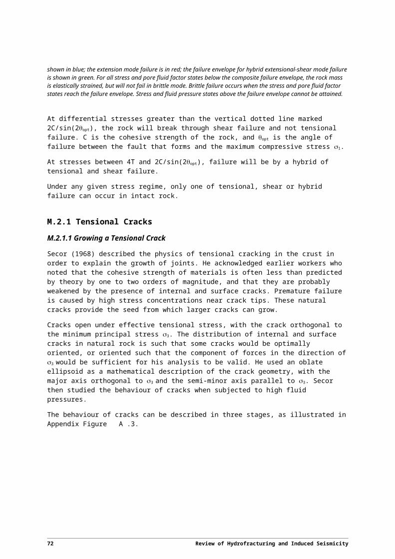
Appendix B Earthquake Intensity and Magnitude

B.1 Introducing basic earthquake termsThis Appendix aims to describe earthquake magnitude and intensity in order to introduce the most common earthquake terms. It seeks to explain how earthquake size relates to both what people feel and see, and to geological parameters, particularly fault rupture size and displacement.

In Appendix A, a distinction was made between the fracturing of rocks by tension cracking, in which the sides of the crack separate in a dilatational sense with no lateral displacement of one side relative to the other, and shear fracture, where the two sides are displaced laterally relative to each other. The first form of cracking is what most geologists would cause jointing, whereas the latter term is faulting. Earthquake seismologists often refer to earthquakes that occur by shearing on faults as tectonic earthquakes.

The terms used to describe earthquakes were derived for large earthquakes, and refer to fracturing by faulting, and therefore fracture by shearing (shearing in the context of Appendix A). The same earthquake terms are used to describe earthquakes caused by hydrofracturing, ie., mostly small earthquakes that are caused by tension fracture. As will be discussed below in this Appendix, some adjustment of terminology is probably needed for micro earthquakes. For example, the measure of displacement used for large earthquakes does not apply to tension cracks, because there is no lateral displacement but rather dilation. This adjustment to earthquake terminology has not happened yet, and can lead some confusion. For example, Shemeta and Anderson (2010) wrote: 'The microseismic events are thought to be shear failure that occur around the opening of a tension hydraulic fracture as it grows.' (this author's underlining)

In this Appendix, therefore, the traditional terms for describing all earthquakes will be used throughout for all earthquakes no matter which mode of cracking applies, but a section below discusses briefly what substitutions probably need to be made in the key formulae for measuring earthquakes.

B.1.1 Often used nomenclature

The following nomenclature for earthquakes is used throughout this Record:

Earthquakes occur when stresses break (rupture) rock, forming a new fault or re-activating an old fault

Earthquakes are the signature of the release of energy stored in rocks that are under stress

The point where the Earth starts to rupture is called the hypocentre. The hypocentre is also called the focus of the earthquake. When seismologists calculate the location of the earthquake, they calculate the position (latitude, longitude, depth) of the hypocentre because this is where the seismic energy is first released

The epicentre is the point on the surface of the Earth directly above the hypocentre or focus

The depth of the earthquake is the vertical distance between the hypocentre (or focus) and the epicentre

The rupture area is small for small earthquakes and large for larger earthquakes (see later)


Larger earthquakes will normally displace the rock on either side of the rupture by larger amounts than smaller earthquakes (see later). In this Appendix, attention is given mostly to earthquakes at the smaller end of the scale because most hydraulically induced earthquakes are small

The Moment of an earthquake is the product of the area of the fault that ruptures, the amount of displacement on the fault, and the shear modulus of the rock that ruptures

The Magnitude of an earthquake is related to the logarithm of the Moment by several scalar values that are derived empirically from observed data (see later).

B.2 Earthquake IntensityEarthquake size can be assessed in two ways: what people feel and observe, and what a seismograph registers.

What people feel and observe are important because they determine how people respond. Measurements made this way are called measures of the Intensity of the earthquake.

In Australia Intensity is measured on a scale called the Modified Mercalli Scale. The Modified Mercalli Scale quantifies the effects of earthquakes into 12 levels, called MM I to MM XII (ie., the Modified Mercalli Scale uses Roman numbers). They are listed in the Attachment at the end of this Appendix.

MM I earthquakes are the smallest—they would not normally be felt by humans, unless perhaps they are, for example, high in a multi-storey building. Note however, that people may feel nausea and dizziness, but not recognise why because they are not conscious that an earthquake has happened.

People start to become conscious of earthquakes around MM II, and certainly MM III, provided they are close enough to the earthquake’s hypocentre.

As the waves of seismic energy propagate from the hypocentre, the level of seismic energy at any point decreases, for two reasons: 1) the geometrical spreading of the wave front means that the energy is spread over a larger area, and 2) the Earth attenuates and scatters the energy, until ultimately at greater distances it is all absorbed, or at least its level falls below the natural ground shaking caused by people moving around, traffic, tree roots shaking the ground because of wind, etc.

This means that the Intensity with which people feel earthquakes decrease with distance from the earthquake. Therefore, near the epicentre, people might report effects that are consistent with, say, MM V, but further away they might report effects more consistent with MM IV and then MM III. People are unlikely to report effects consistent with MM II and MM I because they will not feel and therefore be conscious of the earthquake.

The map in Appendix Figure B.10 shows contours of MM Intensity reported for the Newcastle earthquake of 1989.

In Australia Intensity is mapped by what people feel and observe and report to Geoscience Australia via a web reporting tool. The reported Intensity may be affected by a number of factors, such as whether the observer is standing on solid ground or on earth fill, which has the potential to amplify the ground shaking, and on building standards—more damage will be sustained by a non-engineered structure than an engineered structure. It can also be affected by the time of day—whether people are out and about, indoors or outdoors, in a high rise office or at home, awake or asleep, and therefore whether they are able to observe the effects of the ground shaking and report them.


The Modified Mercalli Scale accounts for this with descriptors, such as the building type, for which definitions are given at the end of the scale. The Modified Mercalli Scale therefore has to be adapted for local conditions—Australian building codes are different from those in say, central Africa. Australia uses the form of the Modified Mercalli Scale from New Zealand; New Zealand has similar building codes to Australia and it has far more earthquakes whose effects can be used to calibrate the scale. Some of the history of the Modified Mercalli Scale and its universal uniformity or lack of uniformity, at least in the early days of its application, is given by Eiby (1966).

Appendix Figure B.10 Isoseismal map for the Newcastle earthquake of 27 December 1989. The Geoscience Australia website report for the earthquake says: 'One of Australia's most serious natural disasters occurred on 28 December 1989 when an earthquake shook Newcastle in New South Wales, leaving 13 people dead and more than 160 injured. The damage bill has been estimated at A$4 billion, including an insured loss of more than A$1 billion. The earthquake had a magnitude of 5.6 with an epicentre about 15 km south of the Newcastle central business district at an estimated depth of 11 km. Only one aftershock, magnitude 2.1, was recorded. The effects were felt over 200 000 square kilometres with isolated reports of movement up to 800 kilometres from Newcastle. Damage to buildings and facilities was reported over an area extending 9000 square kilometres. The earthquake caused damage to more than 35 000 homes, 147 schools, and 3000 commercial and other buildings. At the height of the crisis, between 300 and 400 people were placed in temporary accommodation. In the month following the earthquake, the Disaster Welfare Recovery Centre assisted almost 14 000 people.'(http://www.ga.gov.au/hazards/earthquakes/ earthquake-basics/historic.html.)

In some countries, such as Japan which has many thousand seismographs in a much smaller area than Australia, Intensity maps are produced automatically from instrumental recordings of ground shaking that have been calibrated to the Intensity scale used there.


http://www.ga.gov.au/hazards/earthquakes/

B.3 Earthquake MagnitudeWhereas earthquake intensity varies with distance from the hypocentre, earthquake magnitude is a single number designed to quantify the size of the earthquake. Measurements of magnitude are made with seismographs. It is not a number that depends on how far the observer or seismograph is from the earthquake; distance and attenuation, as well as the response of the seismograph, are factored into the magnitude calculation.

Geoscience Australia uses a number of magnitude scales. The scales use different parts of the seismic waveform (eg., body waves [Mb scale], which are amongst the first to arrive and surface waves [MS] which arrive much later). Some are easier than others to program into computers for the automatic calculation of magnitude. In a well-established earthquake monitoring centre, the various scales will have been calibrated against each other so that for all but the smallest and largest earthquakes any scale is likely to produce a magnitude that can be compared with the magnitude on any other scale.

The Richter magnitude (symbol is ML) is probably the most commonly known. It was originally developed for earthquakes in California, but has several shortcomings. Firstly, it was developed for earthquakes in California, which at the time mostly fell between magnitudes 3 (where people start to feel the ground shaking) and 7, which were amongst the largest known in California then. Secondly, it does not give accurate magnitudes for earthquakes over about magnitude 7 and underestimates magnitudes for much larger earthquakes. Third, it was developed for local earthquakes (hence the suffix 'L' in its symbol), and has to be scaled appropriately for more distant earthquakes. Finally, it was measured using the excursion of the pen on a particular type of seismograph: those seismographs are no longer in service, and seismologists now use digital instruments rather than analogue instruments with pens.

The Moment Magnitude scale (designated Mw) was designed to address these inadequacies in the Richter magnitude scale. Moment Magnitude was defined by Hanks and Kanamori (1979) as

Mw=23l ogM 0−6.07 (4)

where M0 is the seismic moment of the earthquake. M0 is defined by

M 0=μSd (5)

Where

µ = the shear modulus of the rocks that are faulted,

S = the area of the fault that ruptures, and

d = the average displacement on the fault during the rupture.

In these equations M0 is in Newton metres (Nm). In their original formulation, Hanks & Kanamori used cgs units and therefore their scalars in Equation 4 were different.

Therefore the Moment Magnitude is a function of the shear strength of the rock broken by the earthquake, the area of it that ruptures, and the amount of displacement that occurs when it ruptures.


The constants ('2/3'and '6.07') are scalars that match the Moment Magnitude of an earthquake to other magnitudes.

B.3.1 Relevance to small earthquakes caused by tensional cracking

The magnitude of an earthquake is estimated from waveforms in seismograms recorded on calibrated seismographs, taking into account the amplitudes and phases of the waveforms, and the distances of the seismographs from the hypocentre. Radiation patterns of seismic energy representative of the type of source mechanism are not considered for very small earthquakes.

Mw is a convenient scale to use for many reasons, but especially because of the simple relationship between the magnitude and Moment of the earthquake (Equation 4), and because Moment can be related directly to parameters which are essentially geological in their nature (Equation 5).

The description of earthquake magnitude above expects that the earthquake occurred on a fault that fractured through shear failure. In earthquakes caused by tension failure, the formulation for the Moment of a tensional fault that would replace Equation 5 is not given here. It takes the form of three equations and requires an understanding of the stress tensor; a description of the stress tensor is beyond the scope of this Paper. In simple terms, Equation 5 for the moment of an earthquake is replaced by a more complex formulation in which S remains the area of the fault that fails, the displacement d is the amount by which the two sides of the fault are moved apart relative to each other (Figure 4.3a), and the shear modulus is replaced by a combination of the shear modulus µ and the bulk modulus (usually denoted by the letter K) (Julian et al., 1998).

Despite this, the Hanks & Kanamori (1979) version of Moment Magnitude is used by a majority of geophysical contractors who undertake hydrofracturing in the US (Shemeta and Anderson, 2010), and therefore by assumption in Australia.

B.3.2 Negative Magnitudes

Magnitude scales represent the size of earthquakes on a logarithmic scale. Very small earthquakes can therefore have negative magnitudes.

For example, using Equations 4 and 5 above, if an earthquake has a very small Moment, eg., because the fault is weak (low shear modulus µ), or has a small rupture area (S) and /or a small displacement (d), then the magnitude can be negative.

Natural earthquakes with negative or very small positive magnitudes are common but seldom catalogued because they are not felt and not well recorded on regional seismograph networks such as the Australian National Seismograph Network (ANSN) operated by Geoscience Australia. When an earthquake of significance is detected by the ANSN in Australia, Geoscience Australia often deploys a small temporary network of portable seismographs around the epicentre to record the sequence of small aftershock earthquakes. The Glossary of terms for earthquakes on the Geoscience Australia website describes a Significant Earthquake as: 'Any earthquake that was felt in Australia or with a magnitude of 3.5 or greater. Also, any global earthquake with a magnitude of 6 or greater, but occurring at a depth of 100 km or less.'1 Data from the portable instruments are used to locate the aftershocks, which map the rupture area of the main earthquake, because many of the aftershocks are the result of the stress field in the area of the rupture readjusting after the main earthquake.

1 http://www.ga.gov.au/earthquakes/staticPageController.do?page=glossary


http://www.ga.gov.au/earthquakes/staticPageController.do?page=glossary

Earthquakes with very small magnitudes are particularly common in hydraulic stimulation (hydrofracturing) of oil, gas and geothermal energy reservoirs, where the aim is to fracture rock in a controlled way, and therefore usually slowly and systematically. This would be consistent with the results of Secor (1968) that cracks, and therefore hydrofractures, grow by many small increments in crack size rather than by large amounts of crack size (See Appendix A for a discussion).

Early attempts to scale magnitudes for very small earthquakes were inconclusive. However, Abercrombie (1995) was able to demonstrate using earthquakes recorded in a deep bore hole that the scaling of magnitudes of small earthquakes was affected by the attenuation of high frequency energy recorded on seismographs deployed at the Earth's surface. Small earthquakes generate relatively greater amounts of high frequency energy than larger earthquakes, and high frequency energy is scattered and attenuated more than low frequency energy. She was able to demonstrate that Richter magnitudes as low as -1, with rupture areas as small as 30 m2 were recorded.

B.4 Intensity–Magnitude RelationsBecause an earthquake can have a range of intensity estimates with distance from the epicentre (actually, distance from the hypocentre—if the hypocentre is very deep, the intensity at the surface could be much less because of the vertical distance), comparison of intensity with magnitude is usually based on the intensity at the epicentre, designated I0 by Greenhalgh, et al. (1988). Greenhalgh et al. derived the relation

M L=1.2+0.6 I 0 (6)

for shallow earthquakes in Australia, where ML is the Richter magnitude.

This is shown graphically in Appendix Figure B.11. It is close to the relation for the Western United States where much of the early work on the relationship was done.

Appendix Figure B.11shows that apart from exceptional circumstances, people are unlikely to feel earthquakes of Richter magnitude 2 or less because they correspond to MM I and MM II. Yet appropriately placed seismographs can detect very small earthquakes. Appendix Figure B.12 shows data recorded Geoscience Australia's seismograph stations at Toolangi and Arapiles in Victoria. A larger M2.7 earthquake that was felt locally was followed by two aftershocks with unconfirmed magnitudes around 2.3, which were not felt.


Appendix Figure B.11 Richter magnitude vs intensity at the epicentre (for shallow earthquakes; ie, effectively near the hypocentre) for Australian earthquakes. Based on the relation in Equation 3, from Greenhalgh et al. (1988).

Appendix Figure B.12 Three earthquakes at Rye, Victoria on 14 April 2013 recorded on Geoscience Australia seismographs at Toolangi and Arapiles. The first earthquake was felt; the smaller aftershocks (perhaps magnitude 2.3, but not well constrained) were not felt.

B.5 Fault Rupture ParametersIn the following discussion, estimates of fault rupture area and displacement are made for earthquakes with a range of magnitudes assuming that the rupture is by shearing. The physical parameters that might be used to describe rupture by tensional cracking are more complex. Tensional cracks are unlikely to cause large earthquakes because incremental crack extension is by small amounts rather than by large amounts. For very small earthquakes caused by tensional cracking, the increase in the


size of cracks might be assumed to be of the same order of magnitude as the area of displacement for a fault cracked through shearing. Therefore the treatment of very small earthquakes in the following sections is provided in order to give an order of magnitude estimate of crack growth through either mechanism.

Earthquakes are a manifestation of the energy released when stresses cause rocks to break. The earthquakes studied by Abercrombie, ranging from ML -1–5.5 (she estimates Mw 0–4.6) plot between lines of stress drop ranging from 0.1 MPa to 100 MPa (her Figure 11), with most falling between 1 MPa and 10 MPa. Earthquakes from other studies that she considered also fall between these boundaries.

Leonard ( 2010) developed scaling relations between the rupture length of an earthquake and its width, average displacement and Moment release. For small earthquakes, he determined that their lengths and widths can be scaled as equal. This would be consistent with the treatment by Eshelby (1957), in which the rupture area is approximated by a circle. Earthquakes with magnitudes > M5.0–5.6, depending of fault mechanism, scale more reliably when their lengths are greater than their widths. This might be expected because the rupture of larger earthquakes is likely to be affected by the layering of a more brittle upper crust over a more ductile lower crust, and by the crust overlying the mantle for great earthquakes. It is consistent with the treatment of rupture areas as ellipsoidal in structural geology studies.

Eshleby's (1957) equation for stress drop for small earthquakes is

∆ σ=7M 0

16 r3(7)

where:

= the stress drop during the earthquake, and

r = the source radius, assuming a circular rupture.

The four lines in Appendix Figure B.13 show the relationship between Mw and rupture area for stress drops of 0.1, 1.0, 10 and 100 MPa.

For representative stress drops, the rupture area for a Mw = 0 earthquake would be around 50–100 m2, ie, a length and width of around 6–10 m. For lower stress drops, the rupture area would have to be larger to produce a similar sized earthquake, and for a higher stress drop, the dimensions would be smaller. For smaller earthquakes, around Mw = -2, the rupture area could be as small as a few square metres, with a width of 40–60 cm.

Earthquake magnitudes larger than 6 are not shown in Appendix Figure B.13, firstly because the scaling relations between length and width would be different from a circle, and secondly, because earthquakes larger than that are unlikely in intentional hydrofracturing programs, although larger earthquakes have been reported from other kinds of human induced (ie., unintentional) seismicity (see Appendix C).

Appendix Figure B.14 is an attempt to relate the amount of displacement that will occur on a fault during rupture to the size of the earthquake. A number of factors need to be assumed to create this diagram. Firstly, the rupture is assumed to be circular, as for Appendix Figure B.13; ie. the earthquake will be small. Secondly, the shear modulus of the fault material has to be determined; for a well


annealed old fault, this is assumed to be the same as the shear modulus of the country rock. If the fault is not completely annealed, then the shear modulus would be less (Cox, 2010). Finally, there is an implicit assumption that the fault material or country rock is homogeneous, which would not be the case for many rock types, particularly shale and coal, and especially for modelling larger earthquakes with significant rupture areas. Given these caveats, the estimated displacement for a given stress drop can then be calculated from a combination of Equations 4, 5 and 7.

Appendix Figure B.13 Relationship between rupture area and moment magnitude for a range of stress drops across the part of the fault that ruptures causing the earthquake.

In Appendix Figure B.14, two stress drops are modelled. Leonard (2010) estimated a mean stress drop of 5.8 MPa for earthquakes with Mw > ~5, which was consistent with a mean determined by Johnson (1994) (cited by Leonard) of 8.3 MPa. These values are also consistent with where the earthquakes studied by Abercrombie (1995) plot relative to lines of constant stress drop, including very small earthquakes (her Figure 11, for example). In Appendix Figure B.14, a stress drop of 8 MPa is taken as representative of tectonic earthquakes.

Abercrombie (1995) and Abercrombie and Leary (1993) noted that induced earthquakes have lower reported stress drops than tectonic earthquakes. In Appendix Figure B.14, a stress drop of 1 MPa was modelled representing hydraulically induced earthquakes. However, the smaller stress drops for hydraulically induced earthquakes compared to tectonic earthquakes were not altogether certain to Abercrombie (1995) and Abercrombie and Leary (1993). The difference may be because small events typically do not contain high frequency seismic signals if they are recorded at or near the surface above the zone where high frequencies are preferentially attenuated, although Abercrombie (1995) had attempted to take attenuation into account. It might also be due the scaling relationship of stress drop to earthquake rupture size represented above by Equation 7 not being entirely valid.


In Appendix Figure B.14, curves are drawn for each stress drop for shale, coal and granite (representing the types of rocks hydrofractured for shale gas, coal seam gas and hot dry rock geothermal energy). The value of shear modulus of each rock type is given in Table B.1.

Appendix Figure B.14 Displacement across a fault as a function of earthquake magnitude for shale, coal and granite. Displacements for a stress drop of 8 MPa are shown as solid lines. A stress drop of 8 MPa is representative of tectonic earthquakes. Displacements for a stress drop of 1 MPa are shown as dashed lines; some reports of hydraulically stimulated earthquakes list lower stress drops than tectonic earthquakes.

Table B.1 Shear modulus for shale, coal and granite used to calculate the curves in Appendix Figure B.14. Where measured values for a number of samples were available, a representative value was used.

Rock Type Shear Modulus (GPa) Source

Shale 1.6 Birch (1966), Table 7-15; Tieyuan Zhu, Stanford University:http://www.stanford.edu/~tyzhu/Documents/Some%20Useful%20Numbers.pdf sighted 11/09/2013

Coal 2.0 Greenhalgh & Emerson (1986)

Granite 24 Birch (1966), table 7-15; Tieyuan Zhu, Stanford University:http://www.stanford.edu/~tyzhu/Documents/Some%20Useful%20Numbers.pdf sighted 11/09/2013

The amounts of displacement typical of earthquakes vary significantly with stress drop and the shear strength of the rocks being ruptured. For Mw = 2 tectonic earthquakes (ie., a stress drop around 8 MPa, solid lines in Appendix Figure B.14), the displacement could be up to 100 cm for shale and coal and 5–10 cm for granite. For a Mw = 0 tectonic earthquake, displacements of 5–10 cm for shale and coal and an order of magnitude less for granite would be likely. For smaller earthquakes, eg.,


http://www.stanford.edu/~tyzhu/Documents/Some%20Useful%20Numbers.pdf




Mw = -2, displacements for shale and coal would be around 1 mm for shale and coal, and an order of magnitude less for granite.

For stress drops of 1 MPa (dashed lines in Appendix Figure B.14), perhaps more representative of hydraulically induced earthquakes, the amounts of displacements would be half an order of magnitude less: for Mw = 2, around 10 cm for shale and coal and 1 cm for granite, for Mw = 0, 3–5 cm for shale and coal and around 1 mm for granite, and for Mw = -2, around 1 mm for shale and coal and less for granite.

B.6 Distinguishing between tension cracking and shearing

B.6.1 Determining rupture type by the distribution of earthquake size

For every large earthquake there are many smaller earthquakes. Gutenberg and Richter (1944) used empirical evidence to derive Equation 8 to describe the relationship between the numbers of earthquakes of various sizes:

log (N )=a−b(8−M L) (8)

where

N = number of earthquakes

A = a constant that describes the amount of seismicity; Gutenberg and Richter determined a value of -0.65±0.09 empirically for the World's population of earthquakes;

B = a constant that relates the magnitude of the earthquake to the number of earthquakes; Gutenberg and Richter determined a value of 0.97±0.15 empirically for the World's population of earthquakes; and

ML = Richter Magnitude.


Appendix Figure B.15 Graphical representation of the Gutenberg–Richter relation for earthquake size distribution.

Gutenberg and Richter's relation is shown graphically in Appendix Figure B.15. Note that the Y axis, representing the number of earthquakes, has a logarithmic scale. Gutenberg and Richter developed their relationship for earthquakes of ML 3.5-4 and larger that were caused by shear failure on faults. The X-axis in Appendix Figure B.15 (representing ML) has been extended down to ML -2.0 on the basis of Abercrombie (1995) being able to quantify earthquakes of that size using a deep bore hole seismometer. In most populations of earthquakes recorded using surface seismometers, the graph would tend to flatten to the left towards smaller magnitudes, due to the difficulty detecting extremely small earthquakes with surface seismometers and calculating accurate magnitudes.

In simple terms, the Gutenberg–Richter relation implies that for every earthquake of magnitude, say, ML = 5, there will be around 10 earthquakes of size ML = 4, 100 earthquakes of size ML = 3, and 1000 earthquakes of size ML = 2.

Another way of interpreting this relation is that if an earthquake of ML = 3 were to occur, which is not uncommon in Australia, it would probably be felt by people nearby, and there would likely be several hundred aftershocks most of which would not be felt by people nearby.

A much better catalog of earthquakes exists now for the World since the early work of Gutenberg and Richter, but a value of 'b' around 1 persists for larger earthquakes in many subsequent studies of global earthquake populations. Values of b can also be calculated for specific areas of interest. Generally values are around 1.

Values of b can also be calculated for sets of earthquakes caused by hydrofracturing, and these suggest that populations of hydrofractures caused by tension cracking can be distinguished from those that could also be caused by hydrofracturing but occur on reactivated faults. The former often have values of b significantly higher than 1. A higher b value means that there are proportionally more smaller events in the earthquake population.

For example, Wessels (2011) determined a value of ~2.2 for one set of earthquakes and ~1 for another set in a population of events from a hydrofracture stimulation. He assigned the set with the higher b value to tension fracturing and the one with the lower b value to the reactivation of existing


faults. Maxwell et al. (2009) made similar findings. Both of these studies were of shale gas well stimulations. Similar observations have been made of earthquake populations from enhanced geothermal energy hydrofracture operations in Australia (Dr Des Fitzgerald, Intrepid Geophysics, Personal Communication April 2013).

B.6.2 Determining rupture type by the spatial and temporal distribution of earthquakes

The simplest form of discrimination of rupture type is by the spatial and temporal distribution of earthquakes. The earthquakes have to be very accurately located for this kind of analysis. Hydrofractures that are uniformly distributed spatially in the fractured rock are likely to be from tension cracking, particularly if they occur during the hydrofracturing process. Fractures that are spatially related to a known fault, or have a geometry in their spatial distribution that corresponds with that of faults in the area (eg. similar strike and dip), could be on re-activated faults. Fault related earthquakes can also occur late in the hydrofracturing process, including after the initial hydrofracturing and while proppants are being pumped into the new fractures (eg., Maxwell et al., 2009), and after the high injection pressures have been shut in.

B.6.3 Determining rupture type by waveform analysis

The analysis of waveforms to determine the style of rupturing (normal, strike slip or reverse) is common in the analysis of large earthquakes. It can also be applied to very small earthquakes for which good quality seismograms are recorded. If suitable data are available is likely to be the most reliable discriminant of earthquake rupture type. It requires multiple down-hole seismometers to avoid the attenuation of the high frequency components of the waveforms in the near surface layers.

Simple observations of the ratios of P- and S-wave amplitudes can assist in the discrimination of fracture mechanisms. The use of ground motion directions to determine the type of earthquake source is illustrated in Appendix Figure B.16.


Appendix Figure B.16(a) Stylised tension crack expanding at one of its tips for which the ground motion is outwards from the crack in all directions. The amplitudes of ground motion will be smallest away from the crack tips in the direction of the long axis of the crack, and largest orthogonal to the long axis of the crack. (b) shear cracks form on one of two nodal planes marked with double arrows either side of the maximum compressive stress 1. For a shear crack ground motion is both outwards from and inwards towards the crack; amplitudes will be smallest near the nodal planes where the direction changes from inwards to outwards. (c & d) when the directions of the ground motion are plotted on a lower hemisphere stereographic projection, they can be used to identify the type of earthquake focal mechanism. (c) for tension cracks, ground motion is up almost everywhere (grey) and small or indeterminate near the point marked P (white). This is called an isotropic focal mechanism, and is typical of a tensional crack source. (d) for shear cracks, ground motion at seismographs is both up (black zones) and down (white zones). This is indicative of a double-couple source. Double couple sources are caused by shear failure on faults. Solid lines in (c) and the boundaries between black and white in (d) indicate positions of the nodal planes for the ambient stress field. Red line in right hand side indicates which of the nodal planes is the fault plane. In (c) the Tension Axis T (corresponds to the direction of the minimum principal stress 3) is in the middle of the shaded area between the nodal planes. In (d) it would be in a similar position in the black SE quadrant. The examples in (c) and (d) are for a stress field in which a normal fault would form in shear mode.

However, more robust determinations can be made using the inversion of the recorded waveforms to estimate the rupture mechanism. This has the advantage over using the directions of first ground motions that fewer seismic recording stations are required, provided that they have sufficient azimuthal and distance distribution from the hypocentre. Šilneý et al. (2009) gives examples of inversions for a number of earthquakes in which he identified those caused by tension cracking, a few formed by shearing on a fault, and some that he believed were caused by a hybrid mechanism of both types of cracking.

Analyses to determine the focal mechanism of earthquakes, either by an examination of the directions first ground motions or by waveform inversion, are time consuming and complex. Therefore they are not routinely undertaken, particularly in real time in the field during hydrofracturing exercises.


B.7 Relevance to HydrofracturingEarthquake seismologists often do not discriminate between rupture that creates new faults and rupture that re–activates pre-existing faults. All rupture is assumed to be fault related; fluid pressure is seldom considered; and the fault is assumed to be either normal, thrust or strike slip, perhaps with some component of one type in what is essentially another type, eg., an oblique slip normal fault. Earthquake seismology seldom considers creating cracks with fluid pressure, with the cracks perhaps being purely a tensional opening of the rock with no movement of one side of the crack relative to the other. This Appendix has briefly tried to pay attention to the fracture mechanisms during hydrofracturing by considering how Equation 5 that describes the earthquake Moment might adopt different terms to describe tensional fractures. Wherever possible, qualitative correlations between crack properties have been made, for example, on fracture size for tensional cracks compared to shear cracks.

The seismicity caused by deliberate hydrofracturing mostly has very low magnitudes (typically M = -2–0 but occasionally up to M = 3–4 in hydrofracturing in enhanced geothermal systems; Maxwell et al., 2009; Rutledge & Phillips, 2003; Šilneý et al., 2009). This Appendix therefore focusses on magnitudes at the low end of the magnitude scale. Many of the relationships upon which seismology is based were derived from empirical evidence. Empirical evidence is limited for very small earthquakes because of the difficulty in recording the high frequency energy from very small earthquakes with surface seismometers. Therefore many of the relationships on which seismology is based were derived from much larger earthquakes. In this Appendix, those relationships, such as the scaling relationships between moment, magnitude, rupture area and displacement, and the Gutenberg–Richter relation have been extrapolated to very small magnitudes. This also appears to be the practice in the unconventional energy industry.

Because intentional hydrofracturing usually causes very small earthquakes, it is unlikely to cause damage to infrastructure; most of the earthquake magnitudes correlate with intensities that indicate they are unlikely to be felt and will not cause infrastructure damage. Wells drilled for hydrofracturing are engineered structures designed to withstand the stresses and strains during hydrofracturing.

The likelihood of deliberate hydrofracturing breaking out of the formations being hydraulically stimulated and disrupting groundwater systems is dealt with elsewhere. The difficulty in monitoring hydrofracturing using the locations of very small earthquakes increases as their size decreases, especially if mainly surface seismometers are used; hence deep, downhole seismometers should be used wherever possible.

Unintentional hydrofracturing can and does occur. This is the subject of Appendix C. Earthquakes caused by unintentional hydrofracturing can be considerably larger than those caused by deliberate hydrofracturing. However, the reported magnitudes mostly fall within the magnitude ranges in the figures used in this Appendix, and the orders of magnitude estimates of parameters are likely to be valid, with the following caveat.

The estimated values of any parameter, such as fault rupture area and displacement are based on extrapolated relations, and on physical properties that are not site specific for any hydrofracturing exercise. The estimated parameters should therefore be taken as indicative, order-of-magnitude values. Relative orders of magnitude between the values for shale and coal on the one hand and granite on the other are useful for comparing hydrofracturing in different regimes.

The popular media report that people suffer high levels of stress when they have been traumatised by large destructive earthquakes and then exposed to ongoing sequences of felt aftershock. This may be


because aftershocks conjure up memories of the effects of the main earthquake. However, although the earthquakes caused by deliberate hydrofracturing are unlikely to cause damage and many may not even be felt, the Modified Mercalli Scale notes that for Intensity MM I that 'Dizziness or nausea may be experienced.' The effects on people who experience dizziness and nausea due to prolonged exposure to many very small earthquakes are not known.

B.8 ReferencesAbercrombie, Rachel E., 1995. Earthquake source scaling relationships from -1 to 5 ML using

seismograms recorded at 2.5-km depth. Journal of Geophysical research, 100(B12), 24,015–24,036.

Abercrombie, Rachel, and Leary, Peter, 1993. Source Parameters of small earthquakes recorded at 2.5 km depth, Cajon Pass, southern California: Implications for earthquake scaling. Geophysical Research letters, 20(14), 1511–1514.

Birch, Francis, 1966. Section 7 Compressibility; Elastic Constants. In S.P. Clark Jr (Ed), Handbook of Physical Constants – Revised Edition. The Geological Society of America, Memoir 97.

Cox, S.F., 2010. The application of failure mode diagrams for exploring the roles of fluid pressure and stress states in controlling styles of fracture-controlled permeability enhancement in faults and shear zones. Geofluids, 10, 217–233,

Eiby, G.A., 1966. The Modified Mercllli Scale of earthquake Intensity and its use in New Zealand. N.Z. Journal of Geology and Geophysics, 9, 122–129.

Eshelby, J.D., 1957. The determination of the elastic field of an ellipsoidal inclusion and related problems. Proceedings of the Royal Society of London A, 241, 376–396.

Greenhalgh, S.A., Denham, D., McDougall, R. and Rynn, J.M.W, 1988. Magnitude-intensity relations for Australian Earthquakes. Bulletin of the Seismological Society of Australia, 78(1), 374–379.

Greenhalgh, S.A. and Emerson, D.W., 1986. Elastic properties of coal measure rocks from the Sydney Basin, New South Wales. Exploration Geophysics, 17, 157–163.

Gutenberg, B. and Richter, C.F., 1944. Frequency of earthquakes in California. Bulletin of the Seismological Society of America,34(4) , 185–188.

Hanks, Thomas C. and Kanamori, Hiroo, 1979. A Moment Magnitude scale. Journal of Geophysical Research, 84(B5), 2348–2350.

Johnson, A.C., 1994. Seismotectonic interpretations and conclusions from the stable continental region seismicity database. In A.C. Johnson, K.J Coppersmith, L.R. Kanter and C.A. Cornell (Eds), The Earthquake of Stable Continental Regions. Volume 1: Assessment of Large Earthquake Potential. Electric Power Research Institute.

Julian, B.R., Miller, A.D. and Foulger, G.R., 1998. Non-double-couple earthquakes 1. Theory. Reviews of Geophysics, 36(4), 525–549.

Leonard, Mark, 2010. Earthquake fault scaling: self-consistent relating of rupture length, width, average displacement, and moment release. Bulletin of the Seismological Society of America, 100(5A), 1971–2010.

Maxwell, S.C., Jones, M., Parkes, R., Miong, S., Leaney, S., Dorval, D., D’Amico, D., Logel, J, Anderson, E. and Hammermaster, K., 2009. Fault activation during hydraulic fracturing. SEG Houston International Exposition and Annual Meeting, Abstracts, 1552–1556.

Rutledge, James T and Phillips, W. Scott, 2003. Hydraulic stimulation of natural fractures as revealed by induced microearthquakes, Carthage Cotton Valley gas field, east Texas. Geophysics, 68(2), 441 – 452.Secor, Donald T. Jr, 1965. Role of fluid pressure in jointing. American Journal of Science, 263, 633–646.



Shemeta, Julie and Anderson, Paul, 2010. It's a matter of size: Magnitude and moment estimates for microseismic data. The Leading Edge, March, 296–302.

Šilneý, Jan, Hill, David P., Eisner, Leo and Cornet, Francois H., 2009. Non-double couple mechanism of microearthquakes induced by hydraulic fracture. Journal of Geophysical Research, 114(B08), doi:10.1029/2008JB0054987.

Wessels, S.A., De La Pena, A., Kratz, M., William-Stroud, S. and Jbeili, T., 2011. Identifying faults and fractures in unconventional reservoirs through microseismic monitoring. First Break, 29(7), 99–104.


Attachment to Appendix B

Modified Mercalli (MM) Scale of earthquake intensity (after Eiby 1966)

MM I Not felt by humans, except in especially favourable circumstances, but birds and animals may be disturbed. Reported mainly from the upper floors of buildings more than ten storeys high. Dizziness or nausea may be experienced. Branches of trees, chandeliers, doors, and other suspended systems of long natural period may be seen to move slowly. Water in ponds, lakes, reservoirs, etc., may be set into seiche oscillation.

MM II Felt by a few persons at rest indoors, especially by those on upper floors or otherwise favourably placed. The long-period effects listed under MMI may be more noticeable.

MM III Felt indoors, but not identified as an earthquake by everyone. Vibrations may be likened to the passing of light traffic. It may be possible to estimate the duration, but not the direction. Hanging objects may swing slightly. Standing motorcars may rock slightly.

MM IV Generally noticed indoors, but not outside. Very light sleepers may be awakened. Vibration may be likened to the passing of heavy traffic, or to the jolt of a heavy object falling or striking the building. Walls and frame of building are heard to creak. Doors and windows rattle. Glassware and crockery rattle. Liquids in open vessels may be slightly disturbed. Standing motorcars may rock, and the shock can be felt by their occupants.

MM V Generally felt outside, and by almost everyone indoors. Most sleepers awakened. A few people frightened. Direction of motion can be estimated. Small unstable objects are displaced or upset. Some glassware and crockery may be broken. Some windows crack. A few earthenware toilet fixtures crack. Hanging pictures move. Doors and shutters swing. Pendulum clocks stop, start, or change rate.

MM VI Felt by all. People and animals alarmed. Many run outside. Difficulty experienced in walking steadily. Slight damage to masonry D. Some plaster cracks or falls. Isolated cases of chimney damage. Windows and crockery broken. Objects fall from shelves, and pictures from walls. Heavy furniture moves. Unstable furniture overturns. Small school bells ring. Trees and bushes shake, or are heard to rustle. Material may be dislodged from existing slips, talus slopes, or slides.

MM VII General alarm. Difficulty experienced in standing. Noticed by drivers of motorcars. Trees and bushes strongly shaken. Large bells ring. Masonry D cracked and damaged. A few instances of damage to Masonry C. Loose brickwork and tiles dislodged. Unbraced parapets and architectural ornaments may fall. Stone walls crack. Weak chimneys break, usually at the roof-line. Domestic water tanks burst. Concrete irrigation ditches damaged. Waves seen on ponds and lakes. Water made turbid by stirred-up mud. Small slips, and caving-in of sand and gravel banks.

MM VIII Alarm may approach panic. Steering of motor cars affected. Masonry C damaged, with partial collapse. Masonry B damaged in some cases. Masonry A undamaged. Chimneys, factory stacks, monuments, towers, and elevated tanks twisted or brought down. Panel walls thrown out of frame structures. Some brick veneers damaged. Decayed wooden piles break. Frame houses not secured to


the foundation may move. Cracks appear on steep slopes and in wet ground. Landslips in roadside cuttings and unsupported excavations. Some tree branches may be broken off.

MM IX General panic. Masonry D destroyed. Masonry C heavily damaged, sometimes collapsing completely. Masonry B seriously damaged. Frame structures racked and distorted. Damage to foundations general. Frame houses not secured to the foundations shift off. Brick veneers fall and expose frames. Cracking of the ground conspicuous. Minor damage to paths and roadways. Sand and mud ejected in alluviated areas, with the formation of earthquake fountains and sand craters. Underground pipes broken. Serious damage to reservoirs.

MM X Most masonry structures destroyed, together with their foundations. Some well-built wooden buildings and bridges seriously damaged. Dams, dykes, and embankments seriously damaged. Railway lines slightly bent. Cement and asphalt roads and pavements badly cracked or thrown into waves. Large landslides on river banks and steep coasts. Sand and mud on beaches and flat land moved horizontally. Large and spectacular sand and mud fountains. Water from rivers, lakes, and canals thrown up on the banks.

MM XI Wooden frame structures destroyed. Great damage to railway lines. Great damage to underground pipes.

MM XII Damage virtually total. Practically all works of construction destroyed or greatly damaged. Large rock masses displaced. Lines of slight and level distorted. Visible wave-motion of the ground surface reported. Objects thrown upwards into the air.

Categories of non-wooden constructionMasonry A Structures designed to resist lateral forces of about 0.1g, such as those satisfying the New Zealand Model Building By-law, 1955. Typical buildings of this kind are well reinforced by means of steel or ferro-concrete bands, or are wholly of ferro-concrete construction. All mortar is of good quality and the design and workmanship are good. Few buildings erected prior to 1935 can be regarded as Masonry A.

Masonry B Reinforced buildings of good workmanship and with sound mortar, but not designed in detail to resist lateral forces.

Masonry C Buildings of ordinary workmanship, with mortar of average quality. No extreme weakness, such as inadequate bonding of the corners, but neither designed nor reinforced to resist lateral forces.

Masonry D Buildings with low standards of workmanship, poor mortar, or constructed of weak materials like mud brick and rammed earth. Weak horizontally.

Source: http://www.ga.gov.au/scientific-topics/hazards/earthquake/basics/what/modified-mercalli-scale


Appendix C Human Induced Seismicity

C.1 Introduction to Human Induced SeismicityDeliberate hydrofracturing in the unconventional energy industries causes earthquakes, although usually with very small magnitudes, typically M < 2 and often M < 0 (Appendix B). Human induced seismicity from other causes has been recognised for many decades, and can result in earthquakes up to M = 7. Recent reviews of human induced seismicity were provided by The National Academies (2011) and Davies et al. (2013), who in turn cite earlier reviews. Despite the usefulness of these reviews for informing the reader of the extent of human induced seismicity, the catalogues of events in the reviews appear to be inconsistent and incomplete, partly because many events were documented in journals that are not circulated internationally and therefore not visible to the reviewers, and partly because of the uncertainty that some events were human induced rather than natural earthquakes.

The reviews also list only earthquakes that were instrumentally recorded or felt and reported by observers.

This Appendix does not try to correct the omissions and dissimilarities of previous reviews. Rather, it presents an overview of human induced seismicity that is not caused directly by deliberate hydrofracturing. It aims to provide a backdrop for that part of the report that deals with unintentional hydrofracturing.

C.2 Causes of Human Induced Seismicity

Appendix Figure C.17 subdivides the number of earthquakes believed to have been caused by human activity into seven industry categories (Davies et al., 2013). The statistics in the references from which this figure was derived pre-date the significant increase in seismicity in the US mid-continent attributed largely to the coal seam and shale gas industries by Ellsworth et al (2012)

Earthquakes attributed to mining activities are caused by the removal of rock mass from within the mine and the creation of stress discontinuities in the rock adjacent to the mine void. Mining-related earthquakes are not considered further because they are not caused by fluid pressure.

Of the remaining earthquakes documented in Appendix Figure C.17, the greatest numbers appear to be from reservoir impoundment and the depletion of oil and gas fields. Waste water injection and flowback of water are also contributing causes, although with fewer earthquakes. These earthquakes were caused unintentionally by activities that in some way modified the fluid pressure in the area around the hypocentre of the earthquake.

Hydraulic fracturing is a minor contributor in Appendix Figure C.17. This is probably because the minimum magnitude of earthquakes recorded in the figure is M = 1; hydraulic fracturing probably causes many orders of magnitude more earthquakes than all of the other sources in Appendix Figure C.17 combined, but they are mostly very small, less than M = 1. A conclusion of Davies et al. was that hydrofracturing does not in itself create a risk from earthquakes; rather, the risk comes from other parts of the petroleum industry where the magnitudes of the earthquakes can be much higher than during hydrofracturing.


Appendix Figure C.17 Number of induced earthquakes by industry sector. The statistics in the references from which this graph was derived pre-date the significant increase in seismicity in the US mid-continent attributed largely to the coal seam and shale gas industries by Ellsworth et al (2012).

Davis and Frohlich (1993) erected a set of questions in an attempt make more objective assessments of whether earthquakes are human induced or natural.

1. Are these events the first known earthquakes of this character in the region?

2. Is there a clear correlation between injection and seismicity?

3. Are epicentres near wells (within 5 km)?

4. Do some earthquakes occur at or near injection depths?

5. If not, are there known geologic structures that may channel flow to sites of earthquakes?

6. Are changes in fluid pressures at well bottoms sufficient to encourage seismicity?

7. Are changes in fluid pressures at hypocentral distances sufficient to encourage seismicity?

Subsequent authors have applied these criteria, although some, eg. Keranen et al., (2013), have suggested some modification, particularly to Question 2, because not all apparently induced earthquakes have an immediate correlation in time with the injection of fluids. The questions were to apply to earthquakes that might be created by energy-related activities, but are equally applicable with some modification to reservoir-related seismicity (eg., Question 3 could refer to a reservoir rather than a well).

Note that some seismologists call many of the human induced earthquakes 'triggered' earthquakes. They would distinguish between triggered earthquakes caused by heightened fluid pressure gradients, such as those following the impoundment of reservoirs, and those caused by hydrofracturing operations in the unconventional energy industries. This report considers all to be hydrofractured, but some are unintentional and some are deliberate.


C.3 Case StudiesThe following four case studies of human induced seismicity have been chosen from a wide range of available case studies to illustrate a number of observations that can be made about unintentional human induced hydrofracturing. The observations are summarised in the Discussion at the end of this Appendix.

C.3.1 Case Study #1: Talbingo Reservoir, NSW, Australia

The case study of the Talbingo reservoir in New South Wales is included as an example of reservoir-induced seismicity. It is perhaps one of the best documented and most convincing cases of reservoir-induced seismicity in Australia, although other reservoirs have caused induced seismicity during the initial filling and subsequent low level seismicity since then. Gibson (1997) gives a review of reservoir-induced seismicity in Australia.

Earthquakes began occurring close to the Talbingo Reservoir in New South Wales almost immediately after impoundment (Muirhead, 1981; Appendix Figure C.18). Previously, no earthquakes had been recorded in the area in the thirteen years that earthquake monitoring had been undertaken before the filling of the reservoir.

Appendix Figure C.18 Incidence of earthquakes, plotted as bars showing energy release, and the timing of filling of the Talbingo Reservoir (curved line). Re-drawn from the original Figure 3 of Muirhead (1981) by Geoscience Australia 2015; Original copyright © Geological Society of Australia, reprinted by permission of Taylor & Francis Ltd, www.tandfonline.com on behalf of Geological Society of Australia.

The earthquakes tended to occur in clusters, with each cluster containing earthquakes up to M3.8. The first earthquakes occurred in the area of the dam wall, but over a period of time the earthquake activity


migrated 5km downstream from the dam wall, and sporadic seismicity has continued in both areas since then. All earthquakes are believed to have occurred above 3 km depth.

Muirhead (1981) derived fault plane solutions for the earthquakes, and they indicated normal faulting along the line of the reservoir; ie., a strike just east of north, implying that the minimum principal stress 3 is oriented approximately E–W. Measurements of stress elsewhere in the region show that regionally 1 is oriented E–W, ie., reverse faulting rather than normal faulting would be expected. Muirhead (1981) invoked variations in the local geology as the cause of the difference between local stress implied by the earthquake activity and regional measurements of stress. In determining the cause of the earthquakes, he could not differentiate between the effects of loading of the crust by the extra mass of water in the reservoir and increased pore fluid pressure caused by the additional 162m* depth of water in the dam.

* Note: In his abstract Muirhead says that the dam is 162 m high, but his Figure 3 (reproduced above as Appendix Figure C.18) shows the depth of water to be only 60m with a peak water level near 540 m. Snowy Hydro, the owner of the dam, lists the dam at Talbingo as 161.5m (http://www.snowyhydro.com.au/energy/hydro/dams/), therefore the water level graph in Appendix Figure C.18 must show only the top part of the growth in water height. With an embankment volume of 14,488,000 m3, the dam is the largest in the Snowy scheme. It was completed in 1970, and was filled in about a year, which would be a rapid increase in crustal loading.

C.3.1.1 Further reading on reservoir induced seismicity

Allen, T., Gibson, G. and Hill, C., 2000. The Thomson Reservoir-triggered earthquakes. Australian Earthquake Engineering Society, Conference Proceedings, Paper 8, 8.0–8.7.

Simpson, David W., 1976. Seismicity changes associated with reservoir loading. Engineering Geology, 10, 123–150.

Withers, R.J. & Nyland, E., 1978. Time evolution of stress under an artificial lake and its implications for induced seismicity. Canadian Journal of Earth Sciences, 15, 1526–1534.

C.3.2 Case Study #2: Rocky Mountains Arsenal

Human induced seismicity at the Rocky Mountains Arsenal is one of the earliest well-documented cases of seismicity caused by the ongoing injection (rather than short term injection) of fluids into the crust through a well (The National Academies, 2011). The Rocky Mountains Arsenal was the site of chemical weapons development and disposal from 1942 to 1985. In 1961 the army drilled a well 12,045 feet (3671 m) deep through the sedimentary rocks of the Denver Basin and 75 feet (23 m) into crystalline basement. The well was then used for the disposal of chemical waste from 1962 until 1965, with the fluids variously gravity fed and then pressure injected at pressures up to 72 bars (7.2 MPa). A total of 638 megalitres of fluid was disposed of in the well.

Earthquakes began to be felt and recorded shortly after injection began (Evans, 1966), and continued through the injection periods. The history of fluid disposal in the well and earthquake occurrence is shown in Appendix Figure C.19.

Evans cites 710 earthquakes in the area near the well, with the majority having epicentres within 5 km of the well. The earthquake occurrences decreased (but continued sporadically) during a pause in fluid disposal between October 1963 and April 1964, and began again after disposal resumed. When fluid injection under gravity feed was replaced by fluid injection by pumping under pressure in April 1965, the number of earthquakes increased significantly (Appendix Figure C.19).


http://www.snowyhydro.com.au/energy/hydro/dams/

In a later publication Healy et al. (1968) reported 1584 earthquakes up to and including 1967; earthquakes with magnitudes below the recording threshold would not have been included. At that stage fluid disposal had ceased because of concerns that with the disposal well near the city of Denver the fluid disposal might trigger larger, damaging earthquakes . Between April 1967 and November 1967, between 18 months and two years after fluid disposal ceased, three earthquakes with magnitudes greater than M5 occurred within the area where earlier, smaller earthquakes had occurred. The three large earthquakes released more stress than all other earthquakes combined since fluid injection began. They were not predicted by previously held estimates of the Gutenberg-Richter b value for the earthquakes in the area (see Appendix B for a discussion of b values), and this was considered evidence that something other than natural tectonic processes was at work.

Appendix Figure C.19 Histograms showing relation between volume of waste injected into the Rocky Mountain Arsenal well (top graph) and earthquake frequency (bottom graph). This figure was redrawn from The National Academies (2011), Page 22, which cites the following sources: Adapted from Evans (1966); Healy et al. (1968); McClain (1970); Hsieh and Bredehoeft (1981).

The three >M5 earthquakes and their aftershock swarms fell on a linear trend, which Healy et al. (1968) interpreted to be a pre-existing strike slip fault that was optimally oriented for reactivation by the


ambient tectonic stress regime after the increase in pore fluid pressure from the fluid disposal reduced the effective stress on the fault. They estimated that the increase in pore fluid pressure within the reservoir would have reduced the frictional resistance to fracture by around 6.9 MPa, with fluid moving from the well into the fault through tension cracks formed as hydrofractures.

Healy et al. (1968) noted that although the earthquakes initially showed a net migration of epicentres away from the well as fluid injection began and then continued, earthquakes continued to occur within the zone. Moreover, the earthquakes that occurred late in the sequence, after injection had ceased, were at the edge of the earthquake area, and they were the largest.

Of particular concern was their estimate that fluid pressure within the fluid reservoir had not reached a new equilibrium below the effective strength of the rocks there, and that further earthquakes could happen. They recommended that attempts be considered to lower pore fluid pressures in the reservoir through the removal of fluid.

A reservoir analysis of the earthquake zone was eventually published in 1981 (Hseith and Bredehoeft, 1981). It defined the lateral and vertical extents of the fluid reservoir, its fluid transmissivity and its storage coefficient. They showed that earthquakes were confined to the part of the reservoir where pore pressure build up exceeded 3.2 MPa. This work was not done before fluid disposal down the well into the reservoir was undertaken.

C.3.3 Case Study #3: Rangely Oilfield, Colorado

The study of induced earthquakes at the Rangley oilfield in Colorado was described by Raleigh et al. (1976).

The occurrence of earthquakes at the Rocky Mountain Arsenal site thought to be caused by fluid injection (Case Study #2) led the United States Geological Survey (USGS) to develop theories on the role of fluid pressures in triggering earthquakes. They needed a site where they could test their theories; they could not do it at the Rocky Mountain Arsenal site because of concerns that experiments that might trigger earthquakes should not be conducted near large cities such as Denver.

A swarm of earthquakes had been reported from the Rangely oil field in Colorado. The oil field began production in 1945, and in 1957 was prepared for water flooding for enhanced oil recovery. By 1962, reservoir pressures had been raised in some areas to pre-production levels of 17 MPa, and by 1967 when earthquakes were first accurately located in the oil field, bottom-hole pressures as high as 29 MPa had been recorded.

Most earthquakes epicentres lie in the west of the field in two clusters trending ENE–WSW, and are co-linear with a fault mapped in the field (Appendix Figure C.20(a)). The width of the zone of earthquakes indicates that in that area the fault has several parallel fractures rather than one. The earthquakes that were studied had magnitudes (ML) ranging from -0.5 to 3.1. Focal mechanisms were derived for a large number of the earthquakes and indicated that most movement on the faults was by right lateral strike slip faulting (Appendix Figure C.20(b)). The earthquake magnitude distribution has a b value (see Appendix B) of 0.81 for earthquakes in the SW and 0.96 for earthquakes in the NW of the cluster. These values are consistent with earthquakes caused by shearing (tectonic earthquakes).

The USGS entered into an arrangement with Chevron Oil Company as the operator of the field and the US Department of Defense (because of their concerns about earthquake activity at the Rocky Mountain Arsenal) to conduct an experiment at Rangely to test their theory about the role of pore fluid pressure in triggering earthquakes.


Studies were undertaken of the stress field at the site, and of the physical properties of rocks in the reservoir. The study estimated that earthquakes should be triggered at reservoir pressures exceeding a 'critical pressure' of 25.7 MPa.

Appendix Figure C.20(a) Location of earthquakes at Rangely between October 1969 and November 1970 (x), experimental wells () and seismic stations ().The contours are bottom-hole 3-day shut-in pressures as of September 1969; the interval is 70 bars. Heavier dashed line is a fault mapped in the subsurface; lighter dashed line is the boundary of the oil field. This is Figure 1(b) of Raleigh et al. (1976). (b) Focal mechanisms for larger earthquakes. Dashed line is the boundary of the oil field. Inset rose diagram shows distribution of azimuths of right lateral strike-slip faults. This is Figure 3 of Raleigh et al. (1976).Both (a) and (b) American Association for the Advancement of Science, reproduced with permission.

During the next phase of the experiment, fluid pressures in the reservoir were cycled above and below the predicted pressure for the onset of earthquakes. They were raised by injection and lowered either by water withdrawal or by oil and gas production from adjacent wells.

The results are shown in Appendix Figure C.21. When reservoir fluid pressures were raised above the predicted critical pressure, greater numbers of earthquakes occurred, and earthquake numbers decreased when pressures were lowered below the predicted critical pressure.

This led Raleigh et al. (1976) to postulate that earthquakes could be controlled in situations where fluid injection was occurring by managing reservoir pressures. Pressures could be raised above pre-production levels (in the case of enhanced oil recovery) and pre-injection levels (in the case of waste disposal wells), but had to be kept below a critical pressure above which earthquakes would occur. In the case of the Rangely field, this would mean that reservoir pressures could be maintained between 17 and 25.7 MPa with a low risk of triggering earthquakes.

Raleigh et al. (1976) also postulated that naturally occurring earthquakes on fault systems such as the San Andreas Fault could be controlled by managing in a systematic way pore fluid pressures in and around the fault.


Appendix Figure C.21 Frequency of earthquakes at Rangely. Stippled bars indicate earthquakes within I km of experimental wells. The clear areas indicate all others. Pressure history in well Fee 69 is shown by the heavy line; predicted critical pressure is shown by the dashed line. Originally Figure 7 of Raleigh et al. (1976) © American Association for the Advancement of Science, published with permission and redrawn for clarity.

C.3.4 Case Study #4: Oklahoma November 2011 Earthquakes

A series of earthquakes in the Wilzetta oil field near Prague in Oklahoma began in February 2010 with a Mw 4.1 earthquake. Whether small earthquakes occurred in or near the Wilzetta oil field prior to 2010 is unknown, because few seismographs were located nearby at the time. No felt reports of earthquakes had been recorded. The November 2010 earthquake was followed in November 2011 by three earthquakes with magnitudes Mw 5.0, 5.7 and 5.0 in a 4 day period. These earthquakes and their numerous aftershocks were analysed by Keranen et al. (2013).

The Wilzetta oil field is compartmentalised by internal and bounding faults, with oil in structural traps caused by porous limestone abutting steep faults. Depleted reservoirs in the oil field are used for waste fluid disposal. The earthquake sequence began in the Wilzetta North oil field. Most oil production in the North Wilzetta field occurred in the 1950s and 1960s, and limited production continues today.

Three wells in the field have been used for waste disposal since 1993. Initially, waste fluids were fed into a well at zero well head pressure and flowed into the reservoir under gravity, implying that the field had been significantly de-pressurised. Subsequently, well head pressure in one well was increased in steps from 2001, reaching 3.6 MPa in 2006. The increase in well head pressure coincided with the


introduction of a second, deep waste disposal well, and with the volume of waste fluid injected into the well reaching the amount of oil that had been extracted from multiple wells into the reservoir.

Appendix Figure C.22 A. Map showing the spatial relationship between the disposal wells (inverted triangles (red wells are within the Wilzetta North oil field); the main earthquakes (with focal mechanism circles) labelled A, B and C; aftershocks colour coded by the times relevant to earthquakes A, B, C and C plus 1 hour; and faults. Grey areas are oil fields. B and C show earthquakes distribution at depth in cross sections, D shows the earthquakes in a longitudinal section. This is Figure 1 of Keranen et al. (2013), © the Geological Society of America, reproduced with permission.

Keranen et al. (2013) located a subset of 1183 earthquakes using a network of portable seismographs deployed in the area after the first Mw5 earthquake to complement regional seismograph stations. The earthquakes lie in linear, steeply dipping bands that correlate with mapped faults. Focal mechanism solutions for the three Mw 5 earthquakes indicate strike slip movement on the faults. Three separate segments of the fault system were ruptured.

Aftershocks of a large earthquake are interpreted to map out the area of the fault that ruptured during the large earthquake. The northern tip of the aftershock zone for the first Mw 5 earthquake in the Wilzetta oil field lies within 200 m of one of the disposal wells. The earthquakes occurred both within the sedimentary section into which fluids were injected and at greater depths (83% were at depths <5 km).

The Mw 5 earthquakes met many of the criteria set by Davis and Frohlich (1993) for induced earthquakes. The spatial correlation of the first Mw5 earthquake with an injection well was particularly compelling evidence. Aftershocks of the first earthquake deepened away from the well, and could imply downward pressure migration into basement (Keranen et al., 2013). Stress migration after the first Mw5 earthquake is believed to have triggered the next earthquake (Mw5.7), which in turn caused stress migration that triggered the third (Mw5) earthquake. That is, the first earthquake was believed to be triggered by fluid injection; the second earthquake was triggered by the first earthquake, and it in turn triggered the third earthquake.


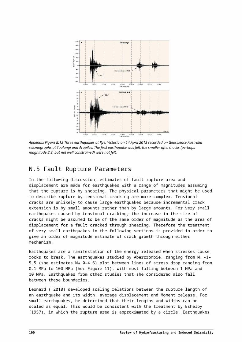
Four key findings of this case study are:

1. The depleted oil field into which waste fluids were being injected consisted of fault bounded (and fault sealed) compartments, which allowed the fluid pressures to build up in a spatially limited fault block rather than be dissipated over a wider area of the oil field.

2. Sparse records mean that pre-production reservoir pressures are unknown. However, Keranen et al. (2013) noted that earthquakes started to occur after the amount of fluid injected into the depleted reservoir reached the amount of oil that had previously produced. This means that the reservoir must have been close to critical pressure (see Case Study #3) prior to production.

3. Changes in pore fluid pressure in a part of the crust that was already highly stressed can trigger a large earthquake, and this in turn can cause stress transfers that cause more large earthquakes.

4. One of the Davis and Frohlich (1993) criteria that was not met in the case of the Oklahoma earthquakes was the time between when fluid injection began and when the first earthquakes happened—17 years rather than almost immediately as in the case of the three Case Studies presented above—and 5 years after a substantial increase in well head pressure was needed to maintain injection into the reservoir. However, the correlation in time between when the injected volume reached the produced volume and the onset of earthquake activity is significant.

C.4 DiscussionCase Study #1 was included in this Appendix for two reasons: (i) it demonstrates that stresses locally can differ from regional stresses, which is discussed in Section 5 of the body of the report, and (ii) although it is not a case study related to the unconventional energy industry it demonstrates that an increase in pore fluid pressure by any means can induce earthquakes. The 162 m of water in the dam represents 1.6 MPa in additional pore fluid pressure added to the hydrostatic pressure gradient; this is the same order of magnitude (although lower) than the additional 3.6 MPa in well head pressure in Oklahoma before earthquakes began to occur. The lessons to be learned from studying earthquakes induced by reservoir loading are relevant to a study of earthquakes induced by increased pore pressure of fluid pumped down a well. The only difference is whether the fluids have to percolate down from the surface through joints and faults, or are injected directly into the rocks where earthquakes occur.

Whereas earthquakes in the first three case studies had both a temporal and spatial correlation with the injection of fluid into the crust, the Oklahoma earthquakes (Case Study #4) had only a spatial correlation. They demonstrated that earthquakes can happen a considerable time after injection begins. The time lag in Oklahoma can be explained partly by time taken to inject enough fluids for the low formation pressures before injection to build beyond pre-production levels. The time lag may be a contributing factor to the larger earthquake magnitudes – it allowed fluid pressures to build up on long segments of the faults, therefore allowing the earthquakes to have larger fault rupture areas, larger Moments (See Appendix B), and therefore larger magnitudes than in the other case studies.

The four case studies have a number of points in common:

1. The volumes of fluids available for increasing pore fluid pressure are large in all cases compared to deliberate hydrofracturing exercises:

a. the largest reservoir in the Snowy Mountains Hydroelectricity Scheme at Talbingo;

b. 638 megalitres at the Rocky Mountains Arsenal;

c. 10 Years (1957–1967) of pumping for enhanced oil recovery at Rangely oil field;


d. 17 years of waste disposal at the Wilzetta oil field in Oklahoma, 5 of them at increased well head pressures.

2. The areas affected in all case studies covered many square kilometres:

a. the earthquakes at Talbingo migrated 5 km downstream;

b. the earthquakes at the Rocky Mountain Arsenal were up to 5 km of the well;

c. the majority of earthquakes at Rangely lie in a linear belt 4–5 km long by 1–2 km wide;

d. the Oklahoma earthquakes lie in a linear belt over 15 km long and 2–3 km wide, although this includes the second and third Mw 5 earthquakes which were tectonic and triggered by the first Mw5 earthquake which was induced.

3. The largest earthquakes in all case studies have larger magnitudes (Mw3–Mw5.7) than those of earthquakes caused by intentional hydrofracturing, which are typically M 2.

C.5 ReferencesDavies, R., Foulger, G., Bindley, A. and Styles, P., 2013. Induced Seismicity and Hydraulic Fracturing

for the Recovery of Hydrocarbons. Marine and Petroleum Geology, 45, 171–185.Davis, S.D., Frohlich, C., 1993. Did (or will) fluid injection cause earthquakes?: Criteria for a rational

assessment. Seismological Research Letters 64, 207–224.Ellsworth, W.L., Hickman, S.H., Lleons, A.L., McGarr, A., Michael, A.J., and Rubenstein, J.L., 2012

Are elasticity rate changes in the midcontinent natural or manmade? Seismological Society of America, Abstract, 12-137.

Evans, D.M. 1966. The Denver area earthquakes and the Rocky Mountain Arsenal disposal well. The Mountain Geologist 3(1), 23–26.

Gibson, Gary, 1997. Earthquakes and dams in Australia. Australian Earthquake Engineering Society, Conference Proceedings, Paper 08.

Healy, J.H., Rubey W.W., Griggs D.T. and Raleigh C.B., 1968. The Denver earthquakes. Science, 161, 1301–1310.

Hsieh, P.A., and J.S. Bredehoeft, 1981. A reservoir analysis of the Denver earthquakes: A case of induced seismicity. Journal of Geophysical Research 86(B2), 903–920.

Keranen, K.M., Savage, H.M., Abers, G.A. and Cochran, E.S., 2013. Potentially induced earthquakes in Oklahoma, USA: Links between wastewater injection and the 2011 Mw 5.7 earthquake sequence. Geology, Doi: 10.1130/G34045.1.

King, G.E., 2012. Hydraulic fracturing 101: what every representative, environmentalist, regulator, reporter, investor, university researcher, neighbor and engineer should know about estimating frac risk and improving frac performance in unconventional gas wells. Society of Petroleum Engineers, SPE-152596. http://dx.doi.org/10.2118/152595-MS.

McClain, W.C., 1970. On Earthquakes Induced by Underground Fluid Injection. ORNL-TM-3154. Oak Ridge, TN. Oak Ridge National Laboratory.

Muirhead, K.J., 1981. Seismicity induced by the filling of the Talbingo reservoir. Journal of the Geological Society of Australia, 28(3-4), 291–298.

Raleigh, C. B., Healy, J. H. and Bredehoeft, J. D., 1976. An Experiment in Earthquake Control at Rangely, Colorado. Science, 191, 1230–1237.




http://dx.doi.org/10.2118/152595-MS