g9 lab project report -injection molding

0

FACULTY OF ENGINEERING AND BUILD ENVIRONMENT

DEPARTMENT OF MECHANICAL AND MATERIAL ENGINEERING

KKKP 3024 Manufacturing Process II

Design And Experiment Project Laboratory Report:

Influence Of Injection Molding Parameter On The Mechanical And

Physical Properties of Polymer ( PP 50% + PE 50% )

GROUP 9

1. HOW YONG CHIAN ( A123700 )

2. CHAN KIEN HO ( A125070 )

3. MUHAMMAD ANWAR BIN RAMLEE ( A124429 )

Lecturer:

1. DR. ABU BAKAR SULONG

2. PROF. DR. NORHAMIDI BIN MUHAMAD

Due Date : 18 October 2010

1

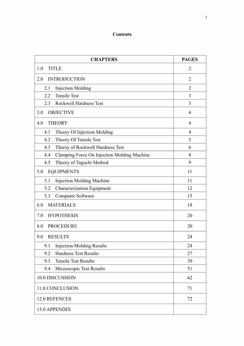
Contents

CHAPTERS PAGES

1.0 TITLE 2

2.0 INTRODUCTION 2

2.1 Injection Molding 2

2.2 Tensile Test 3

2.3 Rockwell Hardness Test 3

3.0 OBJECTIVE 4

4.0 THEORY 4

4.1 Theory Of Injection Molding 4

4.2 Theory Of Tensile Test 5

4.3 Theroy of Rockwell Hardness Test 6

4.4 Clamping Force On Injection Molding Machine 8

4.5 Theory of Taguchi Method 9

5.0 EQUIPMENTS 11

5.1 Injection Molding Machine 11

5.2 Characterization Equipment 12

5.3 Computer Software 15

6.0 MATERIALS 18

7.0 HYPOTHESIS 20

8.0 PROCEDURE 20

9.0 RESULTS 24

9.1 Injection Molding Results 24

9.2 Hardness Test Results 27

9.3 Tensile Test Results 39

9.4 Microscopic Test Results 51

10.0 DISCUSSION 62

11.0 CONCLUSION 71

12.0 REFENCES 72

13.0 APPENDIX

2

1.0 TITLE

Influence of injection molding parameter on the mechanical and physical properties of

polymer ( Polypropylene 50% + Polyethylene 50 % )

2.0 INTRODUCTION

2.1 Injection Molding

Injection molding is a process in which polymer is heated to highly plastic state and

forced to flow under high pressure into mold cavity, where it solidifies. The molded

part called is molding, is then removed from the cavity.

The process produces discrete components that are almost always net shape.

Complex and intricate shapes are possible with injection molding the limitation being

the ability to fabricate a mold whose cavity is the same geometry as the part. In

additional, the mold must be provided for part removal. Injection molding is the most

widely used molding process for thermoplastic.

3

2.2 Tensile Test

Tesnsile test also known as tension test, is probably the most fundamental type of

mechanical test can perform on material. Tensile tests are simple, relatively

inexpensive, and fully standardized. By pulling on something, very quickly determine

how the material will react to forces being applied in tension. As the material is being

pulled, the elongation distance will assist in determine the strength of material such as

yield strength, ultimate strength and breaking strength.

2.3 Rockwell Hardness Test

The Rockwell scale is a hardness scale based on the indentation hardness of a material.

The Rockwell test determines the hardness by measuring the depth of penetration of

an indenter under a large load compared to the penetration made by a preload. There

are different scales, which are denoted by a single letter, that use different loads or

indenters. The result, which is a dimensionless number, is noted by HRX where X is

the scale letter. The indenter is either the Diamond Cone or the Hardened Steel Ball.

The hardness values obtained are useful indicators of a material’s properties and

expected service behavior.

4

3.0 OBJECTIVE

( I ) To analyse the physical and mechanical property of “dog bone” shape

polystyrene product depending on variation of injection molding parameter

such as Injection Pressure, Injection Temperature and Injection Speed.

( II ) To investigate the fracture mechanism of the “dog bone” shape polymer

product after tensile test.

4.0 THEORY

4.1 Theory Of Injection Molding

The theory of injection molding can be reduced to five simple individual steps:

Plasticizing, Injection, Packing, Chilling, and Ejection. Each step is distinct from the

others and correct control of each is essential to the success of the total process.

Plasticizing - the conversion of the polymer material from its normal hard

granular form at room temperatures, to the liquid consistency

necessary for injection at its correct melt temperature.

Injection - the stage during which this melt is introduced into a mold to

completely fill a cavity or cavities.

Packing - additional polymer is melted and packed into the cavity at a higher

pressure to compensate the expected shrinkage as the polymer

solidifies

Chilling - the action of removing heat from the melt to convert it from a

liquid consistency back to its original rigid state. As the material

cools, it also shrinks.

Ejection - the removal of the cooled, molded part from the mold cavity and

from any cores or inserts.

5

4.2 Theory Of Tensile Test

For most tensile testing of materials, the relationship between the applied force and

the elongation the specimen exhibits is linear. In this linear region, the line obeys the

relationship defined as "Hooke's Law" where the ratio of stress to strain is a constant,

or E

. E is the slope of the line in this region where stress (σ) is proportional to

strain (ε) and is called the "Modulus of Elasticity" or "Young's Modulus".

The modulus of elasticity is a measure of the stiffness of the material, only

applicable in the linear region of the curve. Loading within this linear region, the

material will return to its exact same condition if the load is removed. Hooke's Law no

longer applies and some permanent deformation occurs in the specimen when the

curve is no longer linear. This point is called the "elastic, or proportional, limit". From

this point on in the tensile test, the material reacts plastically to any further increase in

load or stress. It will not return to its original condition if the load were removed.

6

4.3 Theroy of Rockwell Hardness Test

The Rockwell hardness test method consists of indenting the test material with a

diamond cone or hardened steel ball indenter. The indenter is forced into the test

material under a preliminary minor load F0 (Fig. 1A) usually 10 kgf. When equilibrium

has been reached, an indicating device, which follows the movements of the indenter

and so responds to changes in depth of penetration of the indenter is set to a datum

position.

While the preliminary minor load is still applied an additional major load is

applied with resulting increase in penetration (Fig. 1B). When equilibrium has again

been reach, the additional major load is removed but the preliminary minor load is still

maintained.

Removal of the additional major load allows a partial recovery, so reducing the

depth of penetration (Fig. 1C). The permanent increase in depth of penetration,

resulting from the application and removal of the additional major load is used to

calculate the Rockwell hardness number.

HR = E - e

F0 = preliminary minor load in kgf

F1 = additional major load in kgf

F = total load in kgf

e = permanent increase in depth of penetration due to major load F1 measured in

units of 0.002 mm

E = a constant depending on form of indenter: 100 units for diamond indenter, 130

units for steel ball indenter

HR = Rockwell hardness number

D = diameter of steel ball

7

Figure 1A, 1B, 1C

8

4.4 Clamping Force On Injection Molding Machine

Clamping force refers to the force applied to a mold by the clamping unit of an

injection molding machine. In order to keep the mold close, this force must oppose

the separating force, caused by the injection of molten plastic into the mold. The

required clamping force can be calculated from the cavity pressure inside the mold

and the shot projected area, on which this pressure is acting. The calculated tonnage

can be used to select a capable machine that will prevent part defects, such as

excessive flash.

Clamping Force, F = Injection pressure, P active area in the separation plane of mold,

A safety coefficient (≥ 1.5)

Active area, A = 2( 35.00 24.00) + [ 78.00 (24.00 – 10.00)]

= 2772 mm2

= 2.77210-3 m2

Injection Pressure, P = vary on each experiment ( 50 bar, 100 bar, 150 bar )

Safety coefficient = 1.5

The approximate shape and dimension of the mold

Thickness = 3.15mm, all units in mm

9

4.5 Theory of Taguchi Method

The Taguchi method involves reducing the variation in a process through robust

design of experiments. The overall objective of the method is to produce high quality

product at low cost to the manufacturer. The Taguchi method was developed by Dr.

Genichi Taguchi of Japan who maintained that variation. Taguchi developed a method

for designing experiments to investigate how different parameters affect the mean and

variance of a process performance characteristic that defines how well the process is

functioning.

The experimental design proposed by Taguchi involves using orthogonal arrays

( OA ) to organize the parameters affecting the process and the levels at which they

should be varies. Instead of having to test all possible combinations like the factorial

design, the Taguchi method tests pairs of combinations. This allows for the collection

of the necessary data to determine which factors most affect product quality with a

minimum amount of experimentation, thus saving time and resources.

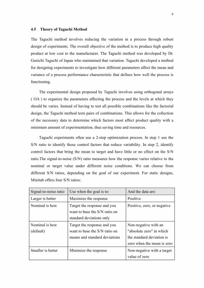
Taguchi experiments often use a 2-step optimization process. In step 1 use the

S/N ratio to identify those control factors that reduce variability. In step 2, identify

control factors that bring the mean to target and have little or no effect on the S/N

ratio.The signal-to-noise (S/N) ratio measures how the response varies relative to the

nominal or target value under different noise conditions. We can choose from

different S/N ratios, depending on the goal of our experiment. For static designs,

Minitab offers four S/N ratios:

Signal-to-noise ratio Use when the goal is to: And the data are:

Larger is better Maximize the response Positive

Nominal is best Target the response and you

want to base the S/N ratio on

standard deviations only

Positive, zero, or negative

Nominal is best

(default)

Target the response and you

want to base the S/N ratio on

means and standard deviations

Non-negative with an

"absolute zero" in which

the standard deviation is

zero when the mean is zero

Smaller is better Minimize the response Non-negative with a target

value of zero

10

4.5.1 Methodology

Step 1 : Designing the Experiment

- Three controllable factors for a plastic injection molding process has been

identified to determine the optimum combination of levels of these factors towards

the contibution of product quality.

- The Levels and Factors which has been identified are summarized as table below:

Levels Factors

1 Pressure ( bar ) 50 100 150

2 Temperature ( °C ) 230 250 270

3 Speed ( rpm ) 60 72 84

Level 1 ( A ) Level 2 ( B ) Level 3 ( C )

Step 2 : Setup the values of parameter

- Using OA ( L9 ) Taguchi Methods, the injection molding parameters ( factors )

are pressure, temperature and injection speed of the reciprocating screw.

The A, B and C represent the values to be tested for each parameters

where A = level 1 (low), B = level 2 (medium), and C = level 3 (high )

- The Taguchi’s L9 Orthoganal Array ( OA ) is shown as the table below:

No. of Order Pressure ( bar ) Temperature ( °C ) Speed ( rpm )

1 A1 = 50 A2 = 230 A3 = 60

2 A1 = 50 B2 = 250 B3 = 72

3 A1 = 50 C2 = 270 C3 = 84

4 B1 = 100 A2 = 230 B3 = 72

5 B1 = 100 B2 = 250 C3 = 84

6 B1 = 100 C2 = 270 A3 = 60

7 C1 = 150 A2 = 230 C3 = 84

8 C1 = 150 B2 = 250 A3 = 60

9 C1 = 150 C2 = 270 B3 = 72

Step 3 : Perform Taguchi Analysis

- Calculate or obtain the mean value, standard deviation value, Ln of standard

deviation value and S/N ratio value from the Minitab V15 software

- Analyse the plotted graph and select the optimum response value.

- Calculate the Sum of Squares, Mean Square, F-ratio and Percentange Contribution

11

5.0 EQUIPMENTS

5.1 Injection Molding Machine ( Arburg 850-210 ALLROUNDER 320 )

Functions:

Perform the injection molding process through heating a plastic to its glass

temperature and forced the polymer flow under high pressure into a mold cavity.

When the polymer solidified, the molding is then being removed from cavity where it

is usually a net shape

Specification:

Machine Properties

( I ) Screw Diameter : 22 mm

( II ) Lock : 25 tonnes

( III ) Plate Size : 250 221 mm

( IV ) Distance Between Tie Bars : 221 mm

( V ) Tool Height : 150-300 mm

( VI ) Location Ring Diameter : 110 mm

12

5.2 Characterization Equipment

5.2.1 Universal Testing Machine ( INSTRON 5567 )

Function:

The Universal Tensile Tester – INSTRON is uesd to deform the specimen with

applied tensile forces in order to determine the stress-strain relation of the material

Specification:

Electrical Power Requirements / Environmental Conditions

( I ) Single Phase Voltage : 100/120/220/240, Vac ±10%

( II ) Frequency : 47-63 Hz

( III ) Operating Temperature : 10 – 38 °C

( IV ) Storage Temperature : - 40 – 60 °C

( V ) Humudity : 10% - 90% ( non-condensing)

Frame Specification

( I ) Height : 1597 mm

( II ) Width : 909 mm

( III ) Depth : 700 mm

( IV ) Weight : 182 kg

( V ) Load Capacity : 30 kN

( VI ) Max Power Requirement : 600 VA

13

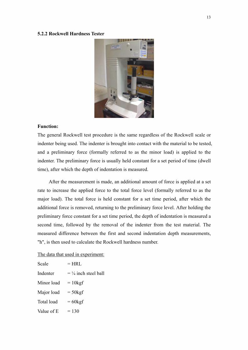
5.2.2 Rockwell Hardness Tester

Function:

The general Rockwell test procedure is the same regardless of the Rockwell scale or

indenter being used. The indenter is brought into contact with the material to be tested,

and a preliminary force (formally referred to as the minor load) is applied to the

indenter. The preliminary force is usually held constant for a set period of time (dwell

time), after which the depth of indentation is measured.

After the measurement is made, an additional amount of force is applied at a set

rate to increase the applied force to the total force level (formally referred to as the

major load). The total force is held constant for a set time period, after which the

additional force is removed, returning to the preliminary force level. After holding the

preliminary force constant for a set time period, the depth of indentation is measured a

second time, followed by the removal of the indenter from the test material. The

measured difference between the first and second indentation depth measurements,

"h", is then used to calculate the Rockwell hardness number.

The data that used in experiment:

Scale = HRL

Indenter = ¼ inch steel ball

Minor load = 10kgf

Major load = 50kgf

Total load = 60kgf

Value of E = 130

14

5.2.3 Scanning Electron Microscope ( Hitachi TM-1000 )

Function:

The Scanning Electron Mircoscope is capable to produce high resolution image of a

sample surface by probing the specimen with a focused electron beam that is scanned

across a rectangular area of the specimen or named “ Raster Scanning ”.

Specification:

( I ) Magnification : 20~10,000X (digital zoom: 2X, 4X)

( II ) Accelerating voltage : 5kV

( III ) Observation mode : Standard mode, Charge-up reduction mode

( IV ) Sample stage traverse : X:15mm, Y:18mm

( V ) Maximum sample size : 70mm in diameter

( VI ) Maximum sample height : 20mm

( VII ) Electron gun : Pre-centered cartridge filament

( VIII ) Signal detection system : High-sensitive semiconductor BSE detector

( IX ) Auto image adjustment

function

: Auto start, auto focus,

auto brightness/contrast

( X ) Frame memory : 640 × 480 pixels, 1,280 × 960 pixels

( XI ) Image data memory : HDD of PC and other removal media

( XII ) Image format : BMP, TIFF, JPEG

( XIII ) Data display : Micron marker, micron value, date and time,

image number and comments

( XIV ) Evacuation system

(vacuum pump)

: Turbomolecular pump: 30L/s × 1 unit,

Diaphragm pump: 1m3/h × 1 unit

( XV ) Safety device Over-current protection function

15

5.3 Computer Software - Minitab V15 ( English )

Minitab is a statistic package which able to create a Taguchi Experimental design.

Data being inserted can be converted into graph and undergo varies of analysis.

Utilization Guideline :

1. Open Minitab V15 English > Stat > DOE > Taguchi > Create Taguchi Design

( Command Box Appear )

2. Select Type of Design > 3-level Design ( 2 to 13 factors )

- Number of factors > ( 3 )

- Display Avaailable Designs > ( Single level , 2-3 )

- Designs > ( L9 , 3**3 )

16

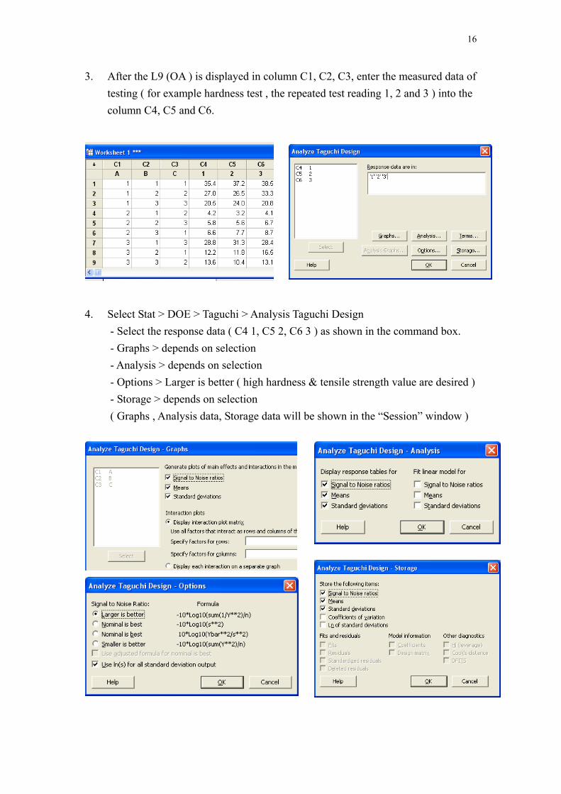
3. After the L9 (OA ) is displayed in column C1, C2, C3, enter the measured data of

testing ( for example hardness test , the repeated test reading 1, 2 and 3 ) into the

column C4, C5 and C6.

4. Select Stat > DOE > Taguchi > Analysis Taguchi Design

- Select the response data ( C4 1, C5 2, C6 3 ) as shown in the command box.

- Graphs > depends on selection

- Analysis > depends on selection

- Options > Larger is better ( high hardness & tensile strength value are desired )

- Storage > depends on selection

( Graphs , Analysis data, Storage data will be shown in the “Session” window )

17

5. Select Stat > DOE > Taguchi > Predict Taguchi Results

- Predict > depends on selection

- Levels > choose ( Coded units , Select levels from a list )

6. All the diagram shown is a sample. For Levels, choose the number of most

optimum level of each factor ( observe from graphs )

7. The record in “Session” and “ Worksheet “window can be used to obtain the

analysed data.

S/N Ratio Ln S

Std Deviation, S

Mean

18

6.0 MATERIALS

During experiment, combination of Polyproplene (PP) and Polyethylene (PE) are used.

The mixture ratio between Polystyrene and Polyethylene is 50:50.

6.1 Polypropylene (PP)

Polypropylene (PP), also known as polypropene, is a thermoplastic polymer, made by

the chemical industry and used in a wide variety of applications, including packaging,

textiles (e.g. ropes, thermal underwear and carpets), stationery, plastic parts and

reusable containers of various types, laboratory equipment, loudspeakers, automotive

components, and polymer banknotes. An addition polymer made from the monomer

propylene, it is rugged and unusually resistant to many chemical solvents, bases and

acids.

Mechanical Properties

( I ) Density : 900 kg/m3

( II ) Young Modulus : 1.22 GPa

( III ) Shear Modulus : 0.43 GPa

( IV ) Bulk modulus : 2.60 GPa

( V ) Hardness - Vickers : 8.70 HV

( VI ) Elastic Limit : 29.00 MPa

( VII ) Tensile Strength : 34.50 MPa

Thermal Properties

( I ) Thermal Conductivity : 0.140 W/m.K

( II ) Thermal Expansion : 150 µ_strain/°C

( III ) Specific Heat : 1910 J/kg.K

( IV ) Melting Temperature : 160 °C

( V ) Max Service Temperature : 90.0 °C

( VI ) Max Service Temperature : -100.0 °C

19

6.1.2 Polyethylene(PE)

Polyethylene is an inexpensive and versatile polymer with numerous applications.

Control of the molecular structure leads to low density (LDPE), linear low density

(LLDPE) and high density (HDPE) products with corresponding differences in the

balance of properties.

Mechanical Properties

( VIII ) Density : 960 kg/m3

( IX ) Young Modulus : 0.75 GPa

( X ) Shear Modulus : 0.30 GPa

( XI ) Bulk modulus : 2.20 GPa

( XII ) Hardness - Vickers : 7.00 HV

( XIII ) Elastic Limit : 24.00 MPa

( XIV ) Tensile Strength : 32.5 MPa

Thermal Properties

( VII ) Thermal Conductivity : 0.425 W/m.K

( VIII ) Thermal Expansion : 160.5 µ_strain/°C

( IX ) Specific Heat : 1840 J/kg.K

( X ) Melting Temperature : 128 °C

( XI ) Max Service Temperature : 115.0 °C

( XII ) Max Service Temperature : -100 °C

20

7.0 HYPOTHESIS

( I ) High Injection pressure will create flashing

( II ) Low Injection pressure will lead to Shrinkage voids, Internal Voids, Poor weld

and flow lines.

( III ) High Injection Temperature will cause Burning or Scorching of molded

Parts, Surface imperfection, Flashing, Shrinkage voids and Internal voids.

( IV ) Low Injection Temperature will result in Poor weld and flow lines, Unmelted

particles in molding, Brittleness of molded parts.

( V ) High Injection Speed will give rise in Surface imperfection, Shrinkage voids,

Flashing, Brittleness of molded parts.

( VI ) Low Injection Speed will produce internal voids

8.0 PROCEDURE

( I ) Injection moulding to get the dumbbell shape product.

( II ) Micro hardness test for the specimen after injection moulding.

( III ) Doing the tensile test by using Universal Testing Machine (UTM)

( IV ) Perform a microscopic test and capture the microstructure view of the failure

position of specimen after the tensile test by using Scanning Electron Mircoscope.

( V ) Each set of parameter, we will produce 8 specimens. The usage of the

specimens are 1 for micro hardness test, 5 for tensile test with 40mm/min

and the other 2 are reserved for any replacement purpose during experiment

( VI ) Repeat the experiment below for 9 set of parameters.

21

8.1 Injection Molding :

( I ) Switch on the injection molding machine and heat around one hour before the

experiment. Follow the instruction from technician, listen carefully and

try to understand the function of machine

( II ) Use the default settings, only vary the input parameter for Injection pressure

Injection temperature and Injection speed of the recipocating screw.

( III ) Insert the input parameters for Set 1 into the machine’s CPU as shown below

( IV ) Insert certain amount of raw material into the feed hopper under technician’s

instruction.

( V ) Make sure two halves of mould in proper alignment with each other.

( VI ) Inject the melted raw material into the mould.

( VII ) Waiting for the mould open and eject the product.

( VIII ) Acquire 8 specimens by repeating the injection process

( IX ) Repeat the experiment for the other set of parameter. The value of each set of

parameter is shown in the results table.

22

8.2 Rockwell Hardness Test

( I ) The Rockwell Hardness unit that used in experiment is HRL.

( II ) Make sure the indenter used is ¼ inch steel ball.

( III ) Keep the product surface clean and finish.

( IV ) The surface of product must be perpendicular to the indenter.

( V ) Apply the force slowly until reach “green” light status and record the value.

( VI ) Repeat the experiment 3 times with different indent area and get the average

value for same specimen.

( VII ) Repeat the step 1 until 6 with other different specimen.

( VIII ) Record the data in the result table.

8.3 Tensile Test

( I ) Use the sand paper to clean the burr at the side of specimens.

( II ) Measure the cross-sectional area and thickness of product before experiments.

( III ) Input the cross-sectional area and thickness to the computer.

( IV ) Use the sand paper to clean the burr at the side of specimens.

( V ) Clamp the both side of product by grip tightly.

( VI ) In the tensile test experiment, the elongation speed using is 5mm/min for all

specimens.

( VII ) For each set of parameter, 5 specimens are tested.

( VIII ) Repeat the step 1 until 7 by different specimens.

Take the data from UTM’s computer after experiment. Find out Young’s

modulus, Ultimate tensile strength, Rupture strength.

23

8.4 Microscopic Test

( I ) By using Scanning Electron Microscope, check out the structure of product at

the failure cross-sectional area.

( II ) The failure area of highest and lowest tensile strength specimens for every set

of parameters are checked out.

( III ) Cut down the failure cross-sectional area with around 3-4mm height from

specimens so that can put at the plate of SEM machine.

( IV ) The failure’s figure of 100X and 300X magnification are taken for each

specimen.

( V ) Discuss and comment about the failure area of each specimen and relation

between failure and parameters of temperature, pressure and injection speed

Figure 8.4 Example of the software being utilized to oeprate the Hitachi TM-1000

24

9.0 RESULTS

9.1 Injection Molding Results

( I ) The Parameter being set for experiment:

LevelsParameters

1 Pressure ( bar ) 50 100 150

2 Temperature ( °C ) 230 250 270

3 Speed ( rpm ) 60 72 84


( II ) The Adjustment of Parameters is required before being insert the functional

panels of injection molding machine. From technician, given that the

injection pressure and speed are (100% = 200bar) and ( 50 % = 300 rpm ).

Thus, the adjustment is shown in the table below.

LevelsParameters

1 Pressure ( bar ) 25% 50% 75%

2 Temperature ( °C ) 230 250 270

3 Speed ( rpm ) 10% 12% 14%


( III ) The input value of each set of parameter :

Set No. Pressure ( bar ) Temperature ( °C ) Speed ( rpm )

1 50 230 60

2 50 250 72

3 50 270 84

4 100 230 72

5 100 250 84

6 100 270 60

7 150 230 84

8 150 250 60

9 150 270 72

25

( IV ) The picture and properties of specimen for each set is shown as below:

Set No. 1

( P=50bar, T=230C, v=60rpm )

* No flash

Set No. 2

( P=50bar, T=250C, v=72rpm )

* No flash

Set No. 3

( P=50bar, T=270C, v=84rpm )

*No flash

*Screw Slip Occur

Set No. 4

( P=100bar, T=230C, v=72rpm )

* Flash start to occur

Set No. 5

( P=100bar, T=250C, v=84rpm )


Set No. 6

( P=100bar, T=270C, v=60rpm )


* Screw Slip Occur

Set No. 7

( P=150bar, T=230C, v=84rpm )

* Large amount of Flash

Set No. 8

( P=150bar, T=250C, v=60rpm )


Set No. 9

( P=150bar, T=270C, v=72rpm )


*Screw Slip Occur

26

9.2 Hardness Test Results

Set

No.

Hardness ( HRL ) Mean,

μ

Standard

Deviation, S Ln S

S/N

Ratio Test 1, x1 Test 2, x2 Test 3, x3

1 35.4 37.2 38.5 37.0333 1.55671 0.44257 31.3564

2 27.0 26.5 33.3 28.9333 3.78990 1.33234 29.0921

3 20.5 24.0 20.8 21.7667 1.93993 0.66265 26.6911

4 4.2 3.2 4.1 3.8333 0.55076 -0.59646 11.4704

5 5.8 5.6 6.7 6.0333 0.58595 -0.53453 15.5341

6 6.6 7.7 8.7 7.6667 1.05040 0.04917 17.5256

7 28.8 31.2 28.4 29.5000 1.57162 0.45211 29.3727

8 12.2 11.8 16.5 13.5000 2.60576 0.95773 22.3226

9 13.6 10.4 13.1 12.3667 1.72143 0.54316 21.6581

Example of Calculation ( For Set No. 1 ):

Number of sampel, n =3

( I ) Mean, μ =

3321 xxx

3

5.382.374.3537.0333 #

( II ) Standard Deviation, S =

1

2

n

x

=

13

033.375.38033.372.37033.374.35 222

= 1.55671 #

( III ) Natural Logarithm of Standard Deviation, ln S = ln ( 1.55671 ) = 0.192208 #

( IV ) S/N Ratio =

nx 2

10

1

log10 =

3

5.38

1

2.37

1

4.35

1

log10222

10 = 31.3564 #

27

9.2.1 Mean of Means Value against Level of factor

Parameter Mean of Means

Range Level 1 (A) Level 2 ( B) Level 3 ( C )

Pressure, bar 29.244 5.844 18.456 23.400

Temperature, o C 23.456 16.156 13.933 9.523

Speed, rpm 19.400 15.044 19.100 4.356

Table 9.21 Response Table for Means – Hardness

Example of Calculation:

Pressure Temperature Speed ( Bar ) ( °C ) ( rpm )

1 A A A = 37.0333

2 A B B = 28.9333

3 A C C = 21.7667

4 B A B = 3.8333

5 B B C = 6.0333

6 B C A = 7.6667

7 C A C = 29.5000

8 C B A = 13.5000

9 C C B = 12.3667

Set No. Mean,

( I ) For Pressure,

Mean of Means Value of Level 1 = ( 29.244 #



( II ) For Temperature,




( III ) For Speed,

Mean of Means Value Value of Level 1 = ( 19.400 #



( IV ) Range for Pressure = ( Max – Min ) = ( 29.244 - 5.844 ) = 23.400 #

Range for Temperature = ( Max – Min ) = ( 23.456 - 13.933 ) = 9.523 #

Range for Speed = ( Max – Min ) = ( 19.400 - 15.044 ) = 4.356 #

28

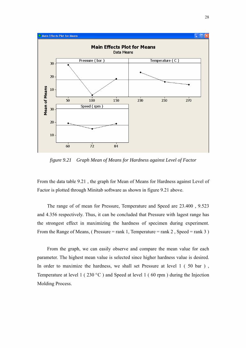
figure 9.21 Graph Mean of Means for Hardness against Level of Factor

From the data table 9.21 , the graph for Mean of Means for Hardness against Level of

Factor is plotted through Minitab software as shown in figure 9.21 above.

The range of of mean for Pressure, Temperature and Speed are 23.400 , 9.523

and 4.356 respectively. Thus, it can be concluded that Pressure with lagest range has

the strongest effect in maximizing the hardness of specimen during experiment.

From the Range of Means, ( Pressure = rank 1, Temperature = rank 2 , Speed = rank 3 )

From the graph, we can easily observe and compare the mean value for each

parameter. The highest mean value is selected since higher hardness value is desired.

In order to maximize the hardness, we shall set Pressure at level 1 ( 50 bar ) ,

Temperature at level 1 ( 230 C ) and Speed at level 1 ( 60 rpm ) during the Injection

Molding Process.

29

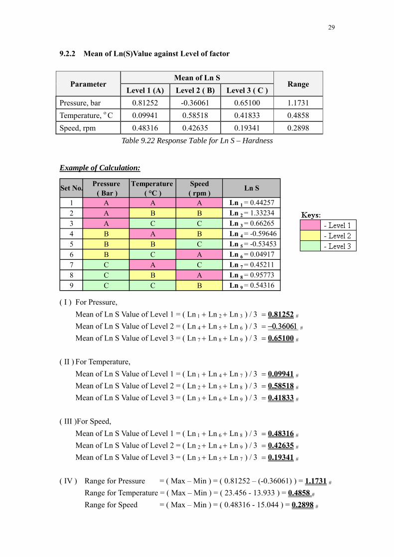
9.2.2 Mean of Ln(S)Value against Level of factor

Parameter Mean of Ln S


Pressure, bar 0.81252 -0.36061 0.65100 1.1731

Temperature, o C 0.09941 0.58518 0.41833 0.4858

Speed, rpm 0.48316 0.42635 0.19341 0.2898

Table 9.22 Response Table for Ln S – Hardness



1 A A A Ln 1 = 0.44257

2 A B B Ln 2 = 1.33234

3 A C C Ln 3 = 0.66265

4 B A B Ln 4 = -0.59646

5 B B C Ln 5 = -0.53453

6 B C A Ln 6 = 0.04917

7 C A C Ln 7 = 0.45211

8 C B A Ln 8 = 0.95773

9 C C B Ln 9 = 0.54316

Set No. Ln S

( I ) For Pressure,

Mean of Ln S Value of Level 1 = ( LnLnLn0.81252 #

Mean of Ln S Value of Level 2 = ( LnLnLn #






( III )For Speed,




( IV ) Range for Pressure = ( Max – Min ) = ( 0.81252 – (-0.36061) ) = 1.1731 #



30

figure 9.22 Graph Mean of Ln Std Deviation for hardness against Level of Factor

From data table 9.22 , the graph for Mean of Natural Logarithm ( Ln ) Standard

Deviation for Hardness against Level of Factor is plotted through Minitab software as

shown in figure 9.22 above.

The range of Ln Standard Deviation for Pressure, Temperature and Speed are

1.1731 , 0.4858 and 0.2898 respectively. Thus, it can be concluded that Pressure has

the strongest effect in minimizing the hardness variability since the range difference is

the largest. From the range of Ln ( S ) : ( Pressure = rank 1, Temperature = rank 2 ,

Speed = rank 3 )

From the graph, we can easily observe and compare the Ln Standard Deviation

value for each parameter. The lowest Ln Standard Deviation value is selected since it

has a smaller hardness variability. In order to minimize the hardness variability, we

shall set Pressure at level 2 ( 100 bar ) , Temperature at level 1 ( 230 C ) and Speed at

level 3 ( 84 rpm ) during the Injection Molding Process.

31

9.2.3 Mean S/N- Ratio against Level of factor

Parameter Mean of S/N ratio


Pressure, bar 29.05 14.84 24.45 14.21

Temperature, o C 24.07 22.32 21.96 2.11

Speed, rpm 23.73 20.74 23.87 3.13

Table 9.23 Response Table for S/N Ratio – Hardness



1 A A A SN 1 = 31.3564

2 A B B SN 2 = 29.0921

3 A C C SN 3 = 26.6911

4 B A B SN 4 = 11.4704

5 B B C SN 5 = 15.5341

6 B C A SN 6 = 17.5256

7 C A C SN 7 = 29.3727

8 C B A SN 8 = 22.3226

9 C C B SN 9 = 21.6581

Set No. S/N Ratio

( I ) For Pressure,

Mean of S/N ratio of Level 1 = ( SN SNSN 29.05 #

Mean of S/N ratio of Level 2 = ( SNSN SN #

Mean of S/N ratio of Level 3 = ( SN SNSN24.45 #


Mean of S/N ratio of Level 1 = ( SNSNSN24.07 #



( III ) For Speed,







32

figure 9.23 Graph Mean of S/N Ratio for hardness against Level of Factor

From data table 9.23 , the graph for Mean of S/N Ratio for Hardness against Level of

Factor is plotted through Minitab software as shown in figure 9.23 above.

An improvement in the process is signified by an increase in the Signal-to-Noise

Ratio ( S/N Ratio ). Optimal injection parameters could be obtained by selecting the

highest value of S/N ratio for each parameter ( Larger-is-better ) . Hence, the selected

parameters are Pressure = 50 bar ( Level 1) , Temperature = 230 C ( Level 1) and

Speed = 84 rpm ( Level 3 )

Regarding to the range of mean S/N ratio for each parameter, Pressure once

again has the largest difference of 14.21, followed by speed with difference of 3.13 and

temperature has the smallest difference of 2.11. This means that Pressure gives the

strongest effect on S/N ratio where as the temperature gives the lowest effect on S/N

ratio. From the range of S/N ratio : (Pressure = rank 1, Temperature = rank 3 , Speed =

rank 2)

33

9.2.4 F-ratio and Percentage Contribution

Source of Degree of Sum of Square Mean Square PercentageVariation Freedom SSp Contribution

Pressure 2 315.4362 157.7181 7.9241 82.65

Temperature 2 7.6443 3.8222 0.192 2.00

Speed 2 18.7566 9.3783 0.4712 4.91

Error 2 39.8073 19.9037 - 10.44

Total 8 381.6444 100

F-Ratio

Table 9.24 Summary of Calculation for F-Ratio & Percentage Contribution

Example of Calculation

Set No. i12 ∑(n) 205.0231

3 N 9

456789

Total ∑n = 205.0231 ∑n2 = 5052.1412

15.5341

= 22.78034 = =

17.525629.372722.322621.6581

307.1466554862.7555053498.2984708469.0732956

31.3564

S/N Ratio , n ( S/N Ratio )2 , n2

983.223821

Number of Sampel , N = 9

Total Mean S/N Ratio , m

29.0921

26.691111.4704

846.3502824

712.4148192131.5700762241.3082628

Using the formula to obtain Total Sum of Square (Sum of Squared Deviation), SST

2

1

2

1

2 0231.2059

11412.5052

1m

i

m

iiiT n

mnSS 381.6444

Formula : SST = SSP + SSe SSP = 3(mP1 – m)2 + 3(mP2 – m)2 + 3(mP3 – m)2

34

From the previous calculated data,

Total Mean S/N ratio , m = 22.78

Mean S/N ratio of Pressure Level 1 , mP1 = 29.05



Mean S/N ratio of Temperature Level 1 , mP1’ = 24.07



Mean S/N ratio of Speed Level 1 , mP1’’ = 23.73



( A ) Sum of Square :

( I ) For Pressure, SSP1 = 3(mP1 – m)2 + 3(mP2 – m)2 + 3(mP3 – m)2

= 3( 29.05 - 22.78 )2 + 3( 14.84 – 22.78 )2 + 3( 24.45 –22.78 )2

= 315.4362 #

( II ) For Temperature, SSP2 = 3(mP1

’ – m)2 + 3(mP2’ – m)2 + 3(mP3

’ – m)2

= 3( 24.07 - 22.78 )2 + 3( 22.32 – 22.78 )2 +3( 21.96 –22.78 )2

= 7.6443 #

( III ) For Speed, SSP3 = 3(mP1

’’ – m)2 + 3(mP2’’ – m)2 + 3(mP3

’’ – m)2

= 3( 23.73 - 22.78 )2 + 3( 20.74 – 22.78 )2 + 3( 23.87 – 22.78 )2

= 18.7566 #

( IV ) For Error, SSe = SST - SSP

= SST – ( SSP1 + SSP2 + SSP3 )

= 381.6444 – ( 315.4362 + 7.6443 + 18.7566 )

= 39.8073 #

35

( B ) Mean Square :

Degree of Freedom, D = (Number of level) -1 = 3 -1 = 2

( I ) Mean Square of Pressure, 1 = 2

315.43621

D

SSP 157.7181 #

( II ) Mean Square of Temperature 2 = 2

7.64432

D

SSP 3.8222 #

( III ) Mean Square of Speed , 3 = 2

18.75663

D

SSP 9.3783 #

( IV ) Mean Square of Error, e = 2

39.8073

D

SSe 19.9037 #

( C ) F-ratio :

( I ) For Pressure, F1 = 19.9037

7181.1571

e

7.9241 #

( II ) For Temperature, F2 = 19.9037

8222.32

e

0.1920 #

( III ) For Speed, F3 = 19.9037

3783.93

e

0.4712 #

( D ) Percentage Contribution :

( I ) Percentage Contribution of Pressure, %100381.6444

315.4362%1001

T

P

SS

SS

( II ) Percentage Contribution of Temperature, %100381.6444

7.6443%1002

T

P

SS

SS

( III ) Percentage Contribution of Speed, %100381.6444

18.7566%1003

T

P

SS

SS

( IV ) Percentage Contribution of Error, e 1 2 3

= 100 – 82.65 – 2.00 – 4.91

= 10.44 %

36

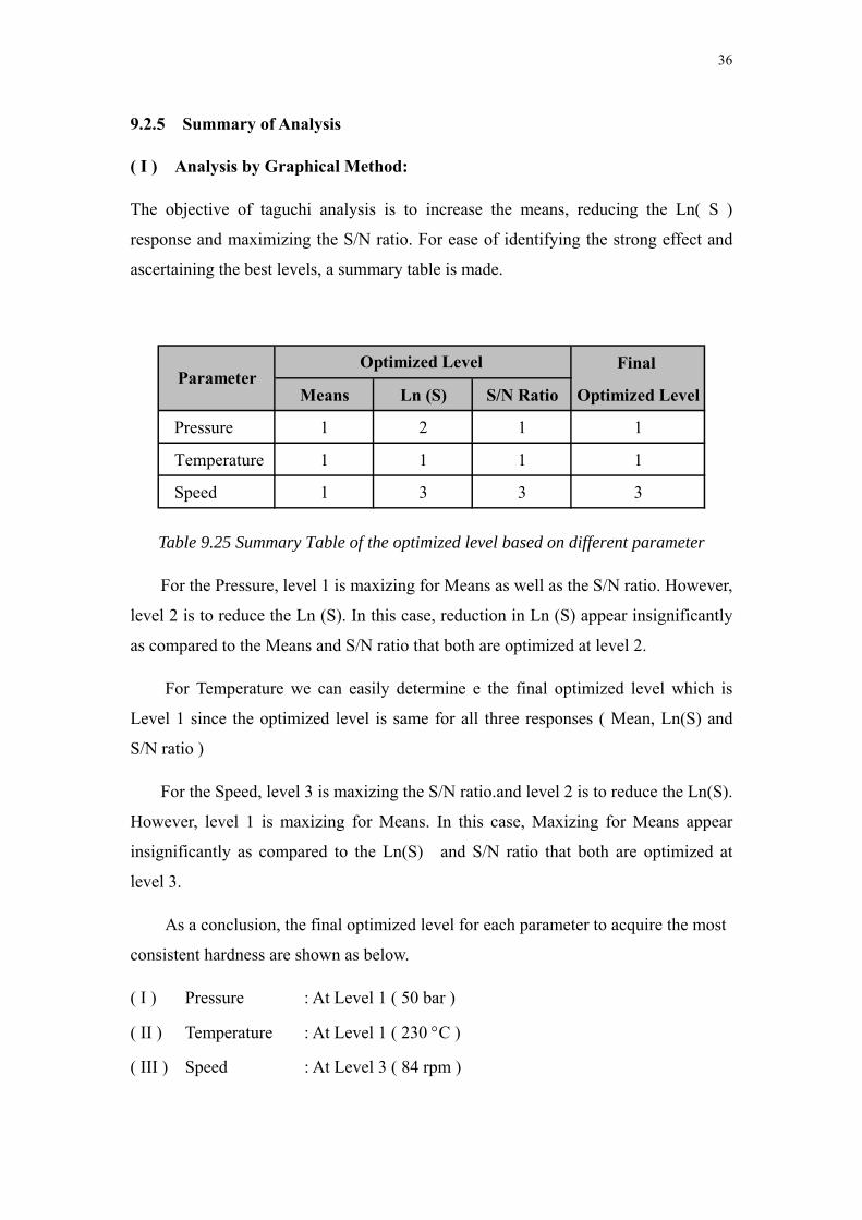
9.2.5 Summary of Analysis

( I ) Analysis by Graphical Method:

The objective of taguchi analysis is to increase the means, reducing the Ln( S )

response and maximizing the S/N ratio. For ease of identifying the strong effect and

ascertaining the best levels, a summary table is made.

Final

Means Ln (S) S/N Ratio Optimized Level

Pressure 1 2 1 1

Temperature 1 1 1 1

Speed 1 3 3 3

ParameterOptimized Level

Table 9.25 Summary Table of the optimized level based on different parameter

For the Pressure, level 1 is maxizing for Means as well as the S/N ratio. However,

level 2 is to reduce the Ln (S). In this case, reduction in Ln (S) appear insignificantly

as compared to the Means and S/N ratio that both are optimized at level 2.

For Temperature we can easily determine e the final optimized level which is

Level 1 since the optimized level is same for all three responses ( Mean, Ln(S) and

S/N ratio )

For the Speed, level 3 is maxizing the S/N ratio.and level 2 is to reduce the Ln(S).

However, level 1 is maxizing for Means. In this case, Maxizing for Means appear

insignificantly as compared to the Ln(S) and S/N ratio that both are optimized at

level 3.

As a conclusion, the final optimized level for each parameter to acquire the most

consistent hardness are shown as below.

( I ) Pressure : At Level 1 ( 50 bar )

( II ) Temperature : At Level 1 ( 230 C )

( III ) Speed : At Level 3 ( 84 rpm )

37

( I I ) Analysis by Manual Calculations:

Percentage OverallContribution Means Ln ( S ) S/N ratio Ranking

Pressure 7.9241 82.65 1 1 1 1

Temperature 0.192 2.00 2 2 3 2

Speed 0.4712 4.91 3 3 2 3

F-RatioRank ( based on the range )

Parameter

* Larger range will have higher rank

Table 9.26 Summary Table of the rank,F-ratio and %Contribution against parameters

The F-ratio test is a ratio of mean square of each parameter and mean square of error

term. It is an indicator which show which process parameter have a significant effect

on performance characteristic. F-ratio is larger if the parameter has greater

performance characteristic We can note that the highest performance characteristic is

Pressure with the ratio of 7.9241, while 0.4712 for Speed and the lowest is

Temperature which gives a ratio of 0.192.

Meanwhile, Percentage Contribution is to show how big the effects of control

factor or parameter to degrade the work. Form the table above, the highest

contribution is Pressure which stands 82.65% , followed by speed which is 4.91% and

the least contribution is Temperature which is only 2.00%.

However, from Table 9.26, the higest overall ranking is Pressure, the second is

Temperature and the lowest is speed. It has a different ranking because F-ratio and

Percentage Contribution had included the Error which is more accurate.

38

9.3 Tensile Test Results

x1 x2 x3 x4 x5

1 20.119 19.275 19.310 20.271 19.005 19.596 0.56197687 -0.57629 25.83486

2 24.344 25.077 24.674 25.159 24.634 24.7776 0.33707165 -1.08746 27.87925

3 24.759 24.606 24.431 24.125 23.504 24.285 0.49613355 -0.70091 27.70233

4 44.110 30.523 30.272 - - 34.9683 7.91791023 2.069127 32.7107

5 33.746 34.283 34.692 33.071 32.863 33.731 0.77741141 -0.25179 30.55506

6 34.244 45.442 32.827 34.502 33.468 36.0966 5.26571931 1.661218 30.97144

7 27.596 28.762 27.368 30.598 31.207 29.1062 1.73632837 0.551773 29.24309

8 28.609 27.969 31.217 28.268 31.072 29.427 1.58495221 0.460554 29.34533

9 29.383 29.271 27.876 27.99 28.218 28.5476 0.72315303 -0.32413 29.10477

Ln S S/N RatioSetNo.

Tensile Strength ( MPa )Mean, μ

Standard

Deviation, S

Example of Calculation ( For Set No. 1 ):

Number of sampel, n =5

( I ) Mean, μ=

554321 xxxxx

3

005.19271.20310.19275.19119.2019.596 #

( II ) Standard Deviation, S =

1

2

n

x

= 15

19.596005.19 19.596271.20 19.596310.19 19.596275.19 19.596119.20 22222

= 0.56197687 #

( III ) Natural Logarithm of Standard Deviation, ln S = ln ( 0.56197687 ) = -0.57629 #

( IV ) S/N Ratio =

nx 2

10

1

log10

=

5

005.19

1

217.20

1

310.19

1

275.19

1

119.20

1

log1022222

10

39

= 25.83486 #

9.3.1 Mean of Means Value against Level of factor

Parameter Mean of Means


Pressure, bar 22.89 34.93 29.03 12.05

Temperature, o C 27.89 29.31 29.64 1.75

Speed, rpm 28.37 29.43 29.04 1.06

Table 9.31 Response Table for Means – Tensile Strength



1 A A A = 19.596

2 A B B = 24.778

3 A C C = 24.285

4 B A B = 34.968

5 B B C = 33.731

6 B C A = 36.097

7 C A C = 29.106

8 C B A = 29.427

9 C C B = 28.548

Set No. Mean,

( I ) For Pressure,








( III ) For Speed,





40



figure 9.31 Graph Mean of Means for Tensile Strength against Level of Factor

From the data table 9.31 , the graph for Mean of Means for Tensile Strength against

Level of Factor is plotted through Minitab software as shown in figure 9.31 above.

The range of of mean for Pressure, Temperature and Speed are 12.05 , 1.75 and

1.06 respectively. Thus, it can be concluded that Pressure with lagest range has the

strongest effect in maximizing the tensile strength of specimen during experiment.

From the Range of Means, ( Pressure = rank 1, Temperature = rank 2 , Speed = rank 3 )

From the graph, we can easily observe and compare the mean value for each

parameter. The highest mean value is selected since higher tensile strength value is

desired. In order to maximize the hardness, we shall set Pressure at level 2 ( 100 bar ) ,

Temperature at level 3 ( 270 C ) and Speed at level 2 ( 72 rpm ) during the Injection

Molding Process.

41

9.3.2 Mean of Ln(S) Value against Level of factor

Parameter Mean of Ln S


Pressure, bar -0.7882 1.1595 0.2294 1.9477

Temperature, o C 0.6815 -0.2929 0.2121 0.9744

Speed, rpm 0.5152 0.2192 -0.1336 0.6488

Table 9.32 Response Table for Ln S –Tensile Strength



1 A A A Ln 1 = -0.57629

2 A B B Ln 2 = -1.08746

3 A C C Ln 3 = -0.70091

4 B A B Ln 4 = -2.06913

5 B B C Ln 5 = -0.25179

6 B C A Ln 6 = 1.66122

7 C A C Ln 7 = 0.55177

8 C B A Ln 8 = 0.46055

9 C C B Ln 9 = -0.32413

Set No. Ln S

( I ) For Pressure,

Mean of Ln S Value of Level 1 = ( LnLnLn-0.7882 #







( III )For Speed,




42

( IV ) Range for Pressure = ( Max – Min ) = ( 0.81252 – (-0.36061) ) = 1.9477 #



figure 9.32 Graph Mean of Ln Std Deviation for tensile strength against Level of Factor

From data table 9.32 , the graph for Mean of Natural Logarithm ( Ln ) Standard

Deviation for Tensile Strength against Level of Factor is plotted through Minitab

software as shown in figure 9.32 above.

The range of Ln Standard Deviation for Pressure, Temperature and Speed are

1.9477 , 0.9744 and 0.6488 respectively. Thus, it can be concluded that Pressure has

the strongest effect in minimizing the hardness variability since the range difference is

the largest. From the range of Ln ( S ) : ( Pressure = rank 1, Temperature = rank 2 ,

Speed = rank 3 )

From the graph, we can easily observe and compare the Ln Standard Deviation

value for each parameter. The lowest Ln Standard Deviation value is selected since it

has a smaller tensile stress variability. In order to minimize the tensile stress

variability, we shall set Pressure at level 1 ( 50 bar ) , Temperature at level 2 ( 250 C )

43

and Speed at level 3 ( 84 rpm ) during the Injection Molding Process.

9.3.3 Mean S/N- Ratio against Level of factor

Parameter Mean of S/N ratio


Pressure, bar 27.14 31.41 29.23 4.27

Temperature, o C 29.26 29.26 29.26 0.00

Speed, rpm 28.72 29.90 29.17 1.18

Table 9.33 Response Table for S/N Ratio – Tensile Strength



1 A A A SN 1 = 25.8349

2 A B B SN 2 = 27.8793

3 A C C SN 3 = 27.7023

4 B A B SN 4 = 32.7107

5 B B C SN 5 = 30.5551

6 B C A SN 6 = 30.9714

7 C A C SN 7 = 29.2431

8 C B A SN 8 = 29.3453

9 C C B SN 9 = 29.1048

Set No. S/N Ratio

( I ) For Pressure,

Mean of S/N ratio of Level 1 = ( SN SNSN 27.14 #

Mean of S/N ratio of Level 2 = ( SNSN SN31.41 #






( III ) For Speed,




44




figure 9.33 Graph Mean of S/N Ratio for tensile strength against Level of Factor

From data table 9.33 , the graph for Mean of S/N Ratio for Tensile Strength against

Level of Factor is plotted through Minitab software as shown in figure 9.33 above.

An improvement in the process is signified by an increase in the Signal-to-Noise

Ratio ( S/N Ratio ). Optimal injection parameters could be obtained by selecting the

highest value of S/N ratio for each parameter ( Larger-is-better ) . Hence, the selected

parameters are Pressure = 100 bar ( Level 2 ) and Speed = 72 rpm ( Level 2 ). Level

of Temperature has no effect on S/N ratio, selecting either one level.

Regarding to the range of mean S/N ratio for each parameter, Pressure once

again has the largest difference of 4.27, and speed has the smallest difference of 1.18.

This means that Pressure gives the strongest effect on S/N ratio where as the speed

gives the lowest effect on S/N ratio. From the range of S/N ratio : (Pressure = rank 1,

45

Temperature = rank 3 , Speed = rank 2)

9.3.4 F-ratio and Percentage Contribution

Source of Degree of Sum of Square Mean Square PercentageVariation Freedom SSp Contribution

Pressure 2 27.353 13.677 8.739 83.88

Temperature 2 0 0 0 0.00

Speed 2 2.128 1.064 1.025 6.53

Error 2 3.129 1.565 - 9.59

Total 8 32.61 100

F-Ratio

Table 9.34 Summary of Calculation for F-Ratio & Percentage Contribution

Example of Calculation

Set No. i12 ∑(n) 263.34682

3 N 9

456789

Total ∑n = 263.3468 ∑n2 = 7738.337

30.5551

= 29.26076 = =

30.971429.243129.345329.1048

959.2299638855.1580605861.1482074847.0875792

25.8349

S/N Ratio , n ( S/N Ratio )2 , n2

667.439941

Number of Sampel , N = 9

Total Mean S/N Ratio , m

27.879327.702332.7107

777.2528441

767.41889991069.990053933.6114446

Using the formula to obtain Total Sum of Square (Sum of Squared Deviation), SST

2

1

2

1

2 3468.2639

1337.7738

1m

i

m

iiiT n

mnSS 32.610

Formula :

46

SST = SSP + SSe SSP = 3(mP1 – m)2 + 3(mP2 – m)2 + 3(mP3 – m)2

From the previous calculated data,

Total Mean S/N ratio , m = 29.26










( A ) Sum of Square :

( I ) For Pressure, SSP1 = 3(mP1 – m)2 + 3(mP2 – m)2 + 3(mP3 – m)2

= 3(27.14 - 29.26 )2 + 3( 31.41 – 29.26 )2 + 3( 29.23 – 29.26 )2

= 27.353 #

( II ) For Temperature, SSP2 = 3(mP1

’ – m)2 + 3(mP2’ – m)2 + 3(mP3

’ – m)2

= 3( 29.26 - 29.26 )2 + 3(29.26 – 29.26 )2 +3( 29.26 – 29.26 )2

= 0 #

( III ) For Speed, SSP3 = 3(mP1

’’ – m)2 + 3(mP2’’ – m)2 + 3(mP3

’’ – m)2

= 3( 28.72 - 29.26 )2 + 3( 29.90 – 29.26 )2 + 3( 29.17 – 29.26 )2

= 2.128 #

( IV ) For Error, SSe = SST - SSP

= SST – ( SSP1 + SSP2 + SSP3 )

47

= 32.610 – ( 27.353 + 0 + 2.128 )

= 3.129 #

( B ) Mean Square :

Degree of Freedom, D = (Number of level) -1 = 3 -1 = 2

( I ) Mean Square of Pressure, 1 = 2

27.3531

D

SSP 13.677 #

( II ) Mean Square of Temperature 2 = 2

02

D

SSP 0 #

( III ) Mean Square of Speed , 3 = 2

2.1283

D

SSP 1.064 #

( IV ) Mean Square of Error, e = 2

3.129

D

SSe 1.565 #

( C ) F-ratio :

( I ) For Pressure, F1 = 1.565

677.131

e

8.739 #

( II ) For Temperature, F2 = 1.565

02

e

0 #

( III ) For Speed, F3 = 1.565

064.13

e

1.025 #

( D ) Percentage Contribution :

( I ) Percentage Contribution of Pressure, %10032.610

27.353%1001

T

P

SS

SS

( II ) Percentage Contribution of Temperature, %10032.610

0%1002

T

P

SS

SS

48

( III ) Percentage Contribution of Speed, %10032.610

2.128%1003

T

P

SS

SS

( IV ) Percentage Contribution of Error, e 1 2 3

= 100 – 83.88 – 0 – 6.53

= 9.59 %

9.3.5 Summary of Analysis

( I ) Analysis by Graphical Method:

The objective of taguchi analysis is to increase the means, reducing the Ln( S )

response and maximizing the S/N ratio. For ease of identifying the strong effect and

ascertaining the best levels, a summary table is made.

Final

Means Ln (S) S/N Ratio Optimized Level

Pressure 2 1 2 2

Temperature 3 2 - 3

Speed 2 3 2 2

ParameterOptimized Level

Table 9.35 Summary Table of the optimized level based on different parameter

For the Pressure, level 2 is maxizing for means as well as the S/N ratio. However,



For the Temperature, level 3 is maxizing for means but level 2 is to reduce the Ln

(S) . There is no optimized level since all the levels have similar mean of S/N ratio .

In this case, We decide to choose level 3 as final optimized level since means is more

significant than Ln (S).

For the Speed, level 2 is maxizing for means as well as the S/N ratio. However,



As a conclusion, the final optimized level for each parameter to acquire the most

49

consistent tensile strength are shown as below.




( I I ) Analysis by Manual Calculations:

Percentage OverallContribution Means Ln ( S ) S/N ratio Ranking

Pressure 8.739 83.88 1 1 1 1

Temperature 0 0.00 2 2 3 2

Speed 1.025 6.53 3 3 2 3

F-RatioRank ( based on the range )

Parameter

* Larger range will have higher rank

Table 9.36 Summary Table of the rank,F-ratio and %Contribution against parameters

The F-ratio test is a ratio of mean square of each parameter and mean square of error

term. It is an indicator which show which process parameter have a significant effect

on performance characteristic. F-ratio is larger if the parameter has greater

performance characteristic We can note that the highest performance characteristic is

Pressure with the ratio of 8.739, while 1.025 for Speed and the lowest is Temperature

which gives a ratio of 0.

Meanwhile, Percentage Contribution is to show how big the effects of control

factor or parameter to degrade the work. Form the table above, the highest

contribution is Pressure which stands 83.88% , followed by speed which is 6.53% and

no contribution from Temperature which is only 0%.

However, from Table 9.36, the higest overall ranking is Pressure, the second is

Temperature and the lowest is speed. It has a different ranking because F-ratio and

Percentage Contribution had included the Error which is more accurate.

50

9.4 Microscopic Test Results

( I ) Specimen Set No 1

Specimen 1-4 ,Magnification 100


51

( II ) Specimen Set No 2



52

( III ) Specimen Set No 3



53

( IV ) Specimen Set No 4



54

( V ) Specimen Set No 5



55

( VI ) Specimen Set No 6



56

( VII ) Specimen Set No 7

Specimen 7-5 , Magnification 100


57

( VIII ) Specimen Set No 8



58

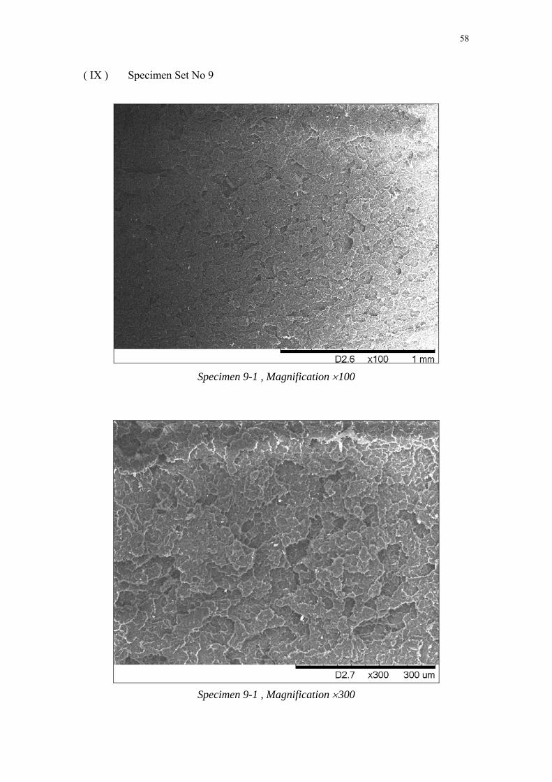
( IX ) Specimen Set No 9



59

9.4.1 Microstructure Of Failure Surface Of Specimen

( A ) Brittle Specimen

Sample 9.1, 300X

The microstructure show that the structure of the specimen does not deform during

fracture and the surface is flat and smooth. The crack is propagated across the surface

structure and break. This type of microstructure is belonging to brittle specimen.

( B ) Ductile Specimen

Sample 1.4, 300X

The microstructure show the structure of the specimen try to deform during fracture

and this cause the specimen try to elongate before fracture. This type of

microstructure is belonging to ductile specimen

60

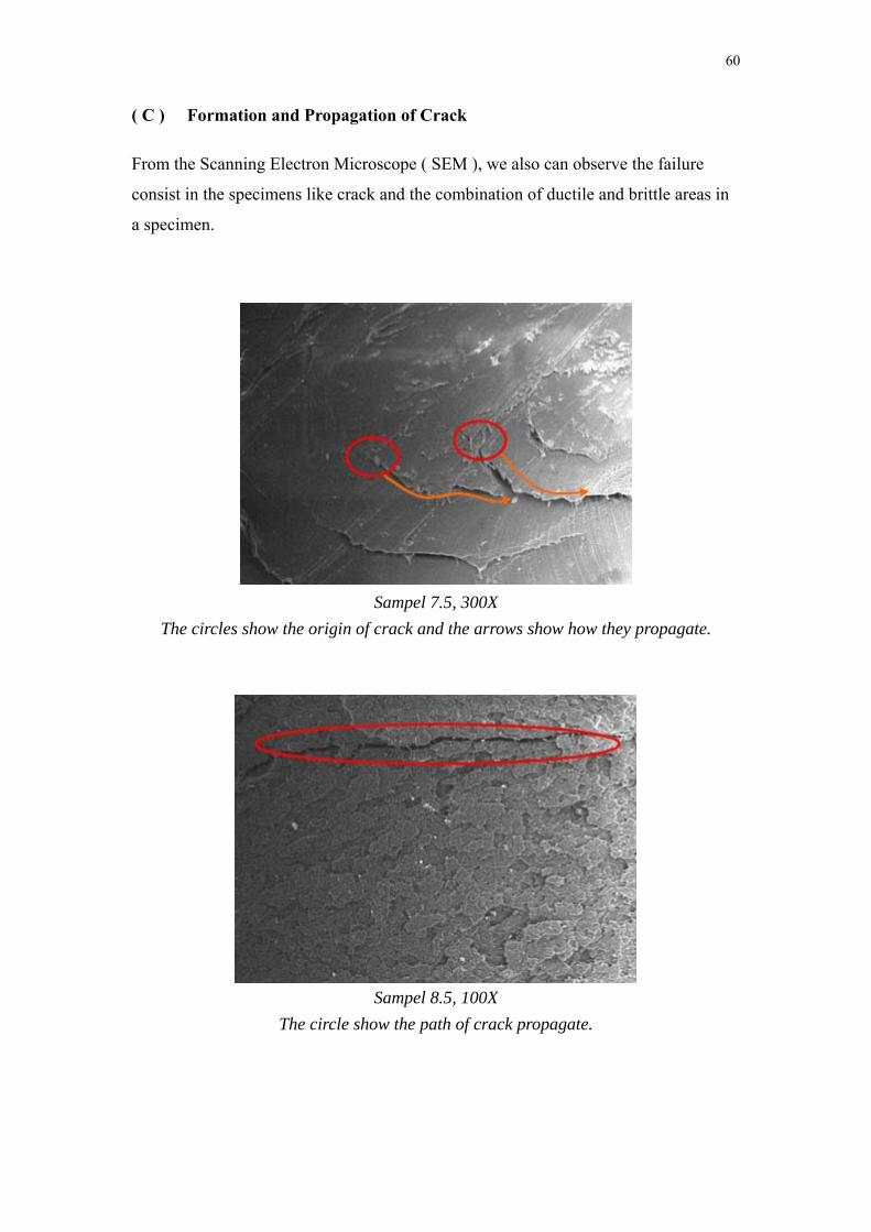
( C ) Formation and Propagation of Crack

From the Scanning Electron Microscope ( SEM ), we also can observe the failure

consist in the specimens like crack and the combination of ductile and brittle areas in

a specimen.

Sampel 7.5, 300X

The circles show the origin of crack and the arrows show how they propagate.

Sampel 8.5, 100X

The circle show the path of crack propagate.

61

(D) Summary of Microscopic Test

1. Combination of Brittle and Ductile area

The Green circle is Brittle area, while the Red circle is Ductile area.

2. From the theory of Tensile Test at 4.2, we can conclude that the specimens at Set

9 are more brittle than specimen at Set 1 due to elongation before break, tensile

strength at maximum load and the microstructure.

3. For the comparison in Young’s Modulus, the highest average value is specimens

Set 4 (1049.71MPa) and lowest value is specimens Set 1 (512.885MPa).

4. From the microstructure of specimen 9.1, 300X and specimen 1.5 ,300X.,we also

can conclude the Young’s modulus of brittle specimen is always higher than

ductile specimen.

62

10.0 DISCUSSION

10.1 General Errors and Precautions

( I ) Error in instrument and equipment

Old or damaged equipments and instruments will cause error. The reading

from the error although very small but it affects the readings toward inaccurate

calculation. To avoid this, we should make sure that equipment in a good condition

before using it. We have to report to the lab assistant or technician if the equipment is

not in good condition.

The reasons of why the Tool and Instrument error occur are:

The machine is already functioned for a long time period and without

maintenance like lubrication system and cooling fan system.

The setting of the machine is always changed and sometimes technicians are

forget to change to the customize setting.

The scale of the machine is not changed to the required standard. For example, the

Rockwell hardness unit for polymer should be HRL.

The wear of the tool is not recognized by students or technician. For example, the

indenter ball of Rockwell hardness Test.

The clamping area of the specimen during tensile test is not tightly or unbalanced

in position will cause the un-consistent elongation due to the pulling force loose.

( II ) Parallax error

Parallax error occur during measuring where it is caused by students during

the experiment. Parallax error occur when the eye position of the observer is not

directly parallel to the scale on instruments. To avoid parallax error, the eyes of

observer should directly perpendicular to the measuring scale while taking readings

from the instruments being used.

63

( III ) Measurement error

It is either random error or systematic error, which are happen frequently

during experiment.

Systematic errors are errors that produce a result that differs from the true

value by a fixed amount. These errors are caused by imperfect calibration of

measurement instruments or imperfect methods of observation, or interference of the

environment with the measurement process.

For example, the condition of injection molding is very hot, while the

condition of tensile test, hardness test and microstructure test all are under cool room.

Although the difference of temperature is not very high, shrinkage and change of

properties still occur.

The zero error which is one of the systematic error is due to the calibration on

the measure instrument such as digital vernier caliper and Rockwell hardness tester.

The reading need to be set back to zero when specimen is changing. If the cause of the

systematic error can be identified, then it can usually be eliminated.

Random error is caused by unpredictable fluctuations in the readings of a

measurement apparatus, or in the experimenter's interpretation of the instrumental

reading. The concept of random error is closely related to the concept of precision. It

can be reduced by taking the average of the readings.

64

10.2 Precaution for Tensile test

When testing the specimens during the tensile test, strains are usually too small to be

measured by using testing machine crosshead or piston displacement methods.

Measuring small strains typical of a high-strength metals test—0.0001 inch or less—is

the task of an extensometer. If yield values are incorrect, review the stress-strain

diagram, the extensometer may have slipped on the specimen during the test. To help

prevent extensometer slippage, the clamping force and the zero point should be

checked regularly and worn knife edges replaced.

Wedge action grips are the most common style used in specimens testing. As the

axial load increases, the wedge acts to increase the squeezing pressure applied to the

specimen. Wedge grips are manually, pneumatically or hydraulically actuated. For

high-volume testing, it is recommended that pneumatic or hydraulic actuated grips be

used. Worn or dirty grip faces can result in specimen slippage, which often renders the

stress-strain diagram useless. The grip faces should be inspected periodically. Worn

inserts should be replaced and dirty inserts cleaned.

Correct alignment of the grips and the specimen, when clamped in the grips, is

important. Offsets in alignment will create bending stresses and lower tensile stress

readings. It may even cause the specimen to fracture outside the gage length.

Most American Society for Testing and Materials (ASTM) or similar test

methods require a shaped specimen that will concentrate the stress within the gage

length. If the specimen is incorrectly machined, fracture could occur outside the gage

length and result in strain errors. Incorrect reading of specimen dimensions will create

stress measurement errors. Worn micrometers or calipers should be replaced and care

should be taken when recording specimen dimensions. Some computer based test

systems will read the micrometer or caliper directly, thus eliminating data entry errors.

65

10.3 Precaution for Hardness Test

It is no surprise that operators often can be the source of problems in hardness

testing. Training operators to be competent in the discipline means that they should

understand the theory of the test method, the proper operation of the instruments they

are responsible for running and the surface preparation requirements and fixturing

techniques for the parts they are responsible for testing. By gaining an understanding

of these areas, the operator will acquire sensitivity to the test method and the abstract

thinking required to prevent some of these problems from occurring. In most cases,

training operators properly once will eliminate rework, and will help to protect the

investment made in the testing instrument.

Dirt and vibration are without a doubt the most often encountered causes of

errors in hardness testing. Unless your hardness tester has “test surface

referencing” — the ability to establish and maintain a referencing relationship

between the indenter, the indenter shroud, and the test surface — dirt in the elevating

screw nut, in bearings, or under the anvil can wreak havoc with all but a few machines.

As mentioned previously, the deflection caused by dirt typically will result in low

readings.

Rough surfaces cause rough results. If we are only interested in knowing

roughly how hard a part is, a rough surface will work. Nevertheless, if we are

interested in accurate, consistent test results, always test a shiny surface. Even though

this method begins its hardness measurement beneath the surface of the part, the

inherent variability of a rough surface can and will cause inconsistent results. Surface

coatings or hardened layers also can provide deceptive results. If we want to test the

hardness of a coating or surface layer, use a load/indenter combination that will ensure

that the measurement is taken in the coating or layer. Remember the 10_ rule: the

thickness of a part or coating must be 10_ greater than the maximum depth of

penetration. On the other hand, if we are interested only in the hardness of the

substrate and not that of the coating, the coating or surface layer must be removed

using a suitable surface preparation technique. Scale and decarburized surfaces also

will deliver erroneous results. In these cases, it is imperative to remove all of the scale,

and to grind to below the decarb layer before conducting a hardness test.

66

10.4 Injection Molding Major Parameter, Defects and Solutions

In the injection molding process, the 3 parameters should be controlled and adjusted

to prevent any failure in the properties and appearances of the specimens.

a) Injection Pressure

The injection pressure should be high enough so that the molten polymer can fully

fill up the cavity and shorten the cycle time. The other advantage of increase the

injection pressure is the density of molded/specimen will be high and increase the

mechanical properties likes hardness and tensile strength. If the injection pressure

is too high, flash will be occurred surrounding the molded and another trimming

process is needed.

b) Injection Temperature

The melt temperature of polymer cannot be too low because the viscosity

decreases when temperature increase. The low melt temperature will disturb the

ability of flow and the cavity cannot be fully filled if the injection pressure is not

increase. If the melt temperature is too high, polymer will degraded and burned

during injection process. High melt temperature also cause resin decomposition

and gas evolution (bubbles) which leads to surface imperfections. More time

required for cool down the molded if the melt temperature is too high and increase

the cycle time.

c) Injection Speed

The high injection speed will shorten the cycle time and fully filled the molten

into the cavity before plastic is freezing at the nozzle. When the injection speed is

too high, the shear rate of the molten polymer will increase simultaneously and

increase the temperature.

67

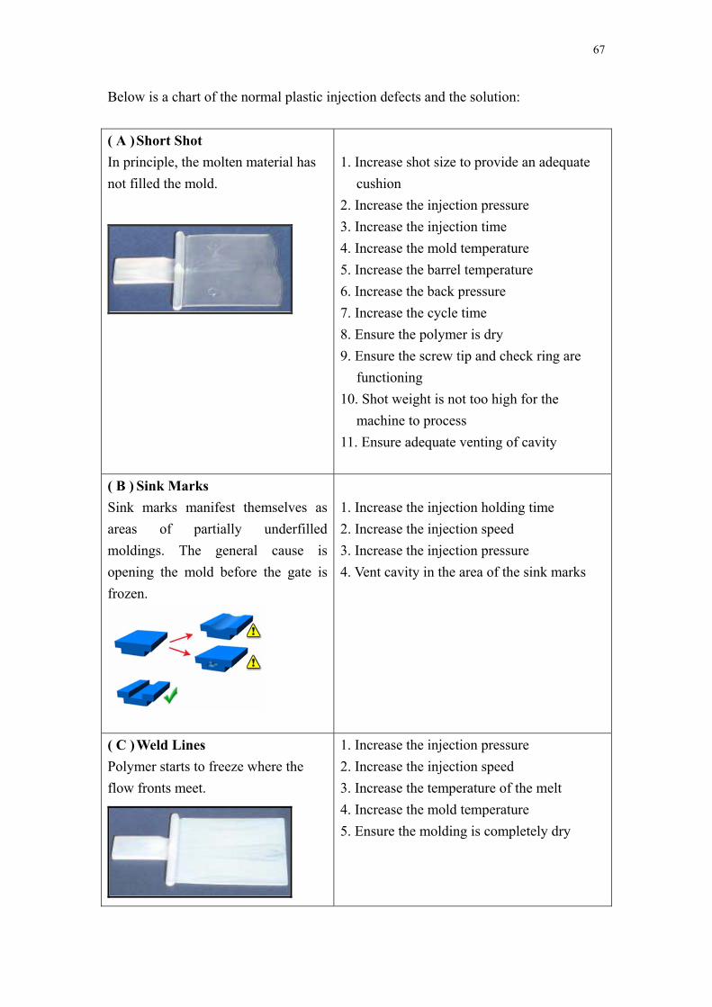
Below is a chart of the normal plastic injection defects and the solution:

( A ) Short Shot

In principle, the molten material has

not filled the mold.

1. Increase shot size to provide an adequate

cushion

2. Increase the injection pressure

3. Increase the injection time

4. Increase the mold temperature

5. Increase the barrel temperature

6. Increase the back pressure

7. Increase the cycle time

8. Ensure the polymer is dry

9. Ensure the screw tip and check ring are

functioning

10. Shot weight is not too high for the

machine to process

11. Ensure adequate venting of cavity

( B ) Sink Marks

Sink marks manifest themselves as

areas of partially underfilled

moldings. The general cause is

opening the mold before the gate is

frozen.

1. Increase the injection holding time

2. Increase the injection speed


4. Vent cavity in the area of the sink marks

( C ) Weld Lines

Polymer starts to freeze where the

flow fronts meet.


2. Increase the injection speed

3. Increase the temperature of the melt

4. Increase the mold temperature

5. Ensure the molding is completely dry

68

( D ) Flashing

Caused when material escapes from

the mold due to the material viscosity

or poor clamping.

1. Reduce the injection pressure

2. Reduce the injection speed

3. Reduce the melt temperature

4. Increase the size of gate

5. Ensure mold closes and seals satisfactory

6. Ensure machine has sufficient mold lock

7. Increase the clamping force.

( E ) Unmelted Particles

1. Increase the cycle time to allow the

polymer to melt

2. Increase the barrel temperature


4. Preheat the granules

( F ) Inconsistent Shot

A problem normally associated with

the machine or due to inconsistent

cycle times .

1. Examine the machine capacity against shot

weight ensuring there is a cushion

2. Stabilize the cycle time reducing delays

with insert loading by automation

3. Check there is no screw slip

4. Check the nozzle hole for damage or

blockage

5. Examine the check ring to ensure its

working properly

( G ) Bubbles & Voids

If the hot compressed air inside the

mold cannot escape, it may lead to

incomplete filling and leave burn

mark on the part.

1. Ensure the resin/pellet is dry

2. Check the screw is feeding regularly


4. Reduce the melt temperature

5. Reduce the screw speed to lessen the

shearing effect on the GPPS

6. Reduce the injection speed

7. Increase cavity venting

8. Ensure mold has not over heated

69

( H ) Screw Slip

1. Ensure the hopper and feed throat are free

from obstructions

2. Reduce melt temperature

3. Reduce screw charging speed

4. Ensure water cooling to hopper feed throat

( I ) Screw Stall

This is common when using low

powered machines

1. Increase the melt temperature

2. Check for cold areas of barrel

3. Reduce the screw back pressure

( J ) Flow marks

If molten plastic does not properly

flow as it fills the cavity, flow marks

may result.

1.Adjusting the mold by changing the gate

location or size

2. Increase the melt temperature.

70

10.5 Safety consideration

1) Wear the lab coat, covered shoe, apron, safety glasses/goggles or ear-plug if

needed.

2) Understand and read through the specification of machine and understand the

function of each button and controller before experiment.

3) Waiting at the outside the laboratory until receive the permission to enter.

4) Do not touch any machine and electrical switch without attendance of technician

or demonstrator.

5) Stand behind the yellow/caution line during the injection molding experiment.

This is want to prevent students are injured/burned because molten material might

be flash out from the machine when nozzle is blocked by freezing material. The

molten material will caused any fire accident due to high temperature.

6) Make sure the transparent shield window is closed before the injection molding

start. Do not simply open it without the permission of demonstrator.

7) Try to be careful and slowly during cutting or trimming of the flash on the

specimens. Make sure there is not people getting close to prevent any injure by

the cutting tool.

8) Do not stand closely to the Universal Tensile machine when it is operated. Some

particles will break out with high velocity from the specimen when the fracture is

happened.

9) Keep the hand dry during experiment to prevent electrical shock.

10) Let the technician/lab assistant change all the equipments/tools and setting. Do not

make any adjust to the machine/tooling setting without technicians.

11) Shut down/switch off the machine/computer/electrical switches before leaving the

laboratory.

12) For Scanning Electron Microscope ( SEM ), students are not allowed to operate

due to expensive price/maintenance, easy to break down and hardly to control. All

the steps will be done by technician under any request of students.

71

11.0 CONCLUSION

From the Design And Experiment Project Laboratory, we have done four major

experiment such as Injection Molding Process, Rockwell Hardness Test, Tensile Test

and Microscopic Test.

Taguchi Analysis Method has been adopted and being adapted to this lab project.

It provides a simple, systematic, and efficient methodology for the optimization of the

injection parameters. Taguchi analysis was carried out to find the optimization of the

process parameter values in order to improve performance characteristics.Besides, the

analysis and calculation of data can be easily done with the aid of software, Minitab

V15.

For the Hardness Test, the overall 1st ranking is Pressure which is the strongest

effect in maximizing the hardness of specimen during experiment. Whereas, the final

optimized level for each parameter to acquire the most consistent hardness are shown

as below.




For the Tensile Test, the overall 1st ranking is Pressure which is the strongest

effect in maximizing the tensile strength of specimen during experiment. Whereas, the

final optimized level for each parameter to acquire the most consistent tensile strength

are shown as below.




72

12.0 REFERENCE

1. William D. Callister, Jr. Material Science and Enginnering: An Introduction.

John Wiley & Sons ( Asia ) Pte Ltd, 2007.

2. Richard S.Figliola, Donald E.Beasley. Theory and Design for Mechanical

Measurements, 4th Edition. John Wiley & Sons ( Asia ) Pte Ltd, 2006.

3. Ferdinand P. Beer, E.Russell johnston,Jr. , John T.DeWolf & david F.Mazurek.

Mechanics Of Materials, 5th Edition. McGrow-Hill Companies, Inc.

4. Mikell P.Groover. Fundamentals Of Modern Manufacturing, 3rd Edition.

John Wiley & Sons ( Asia ) Pte Ltd, 2007.

5. Mechanical Properties Of Materials.

http://www.physchem.co.za/OB12-mat/hooke.htm

6. Tensile Property Testing of Plastics.

http://www.matweb.com/reference/tensilestrength.aspx

7. Handbook of Analytical Methods For Materials. http://mee-inc.com/microhar.html

8. Injection molding defects.

http://viewmold.com/Injection%20Mold%20Management/Injection%20molding%20de

fects.html

9. Introduction To Taguchi Method.

http://www.ee.iitb.ac.in/~apte/CV_PRA_TAGUCHI_INTRO.htm

10. Injection Molding. http://www.custompartnet.com/wu/InjectionMolding#tooling

g9 lab project report -injection molding

Documents