fuzzy logic system for intermixed biogas and...
TRANSCRIPT

FUZZY LOGIC SYSTEM FOR INTERMIXED BIOGAS AND PHOTOVOLTAICS
MEASUREMENT AND CONTROL
by
LISTON MATINDIFE
submitted in accordance with the requirements for the degree of
MAGISTER TECHNOLOGIAE
In the subject
ELECTRICAL ENGINEERING
at the
University of South Africa
Supervisor: PROF Z WANG
DECEMBER 2016

ii
DECLARATION
Name: LISTON MATINDIFE
Student number: 57478295 ______________________________________________________________
Degree: MAGISTER TECHNOLOGIAE IN ELECTRICAL ENGINEERING
Exact wording of the title of the dissertation or thesis as appearing on the copies submitted
for examination:
FUZZY LOGIC SYSTEM FOR INTERMIXED BIOGAS AND PHOTOVOLTAICS
MEASUREMENT AND CONTROL
I declare that the above dissertation/thesis is my own work and that all the sources that I have
used or quoted have been indicated and acknowledged by means of complete references.
SIGNATURE
07 – 12 – 2016 DATE

iii
ABSTRACT
The major contribution of this dissertation is the development of a new integrated measurement
and control system for intermixed biogas and photovoltaic systems to achieve safe and optimal
energy usage. Literature and field studies show that existing control methods fall short of
comprehensive system optimization and fault diagnosis, hence the need to re-look these control
methods. The control strategy developed in this dissertation is a considerable enhancement on
existing strategies as it incorporates intelligent fuzzy logic algorithms based on C source codes
developed on the MPLABX programming environment. Measurements centered on the
PIC18F4550 microcontroller were carried out on existing biogas and photovoltaic installations.
The designed system was able to accurately predict digester stability, quantify biogas output and
carry out biogas fault detection and control. Optimized battery charging and photovoltaic fault
detection and control was also successfully implemented. The system optimizes the operation
and performance of biogas and photovoltaic energy generation.
Key terms: Fuzzy logic system; Fuzzy logic algorithms; Biogas fault detection; Photovoltaic
fault detection; Intermixed biogas and photovoltaics; Renewable energy on-line monitoring;
Biogas measurement and control; Photovoltaic measurement and control; Biogas and
photovoltaic sensors; MPLABX C source codes.

iv
ACKNOWLEDGEMENTS
To GOD is all the glory.
I would like to thank my supervisor Professor Zenghui Wang for his invaluable guidance
throughout this study, without which I would not have progressed much.
Thanks also to the management and personnel of the rural electrification fund (REF) for availing
the facilities to implement the research project designed measurement and control unit and for
taking time out of their busy schedule to respond to the interview sessions.
A special thanks to my wife, son and daughter for allowing me to attend to my studies without
disturbance when instead I was supposed to spend time with them.
Last but not least I would like to thank my fellow work colleagues and management at Kwekwe
Polytechnic for their unwavering support during my studies.

v
TABLE OF CONTENTS
ABSTRACT……………………………………………………………………………………...iii
ACKNOWLEDGEMENTS………………………………………………………………………iv
LIST OF TABLES……………………………………………………………………………….xii
LIST OF FIGURES……………………………………………………………………………..xiv
LIST OF ACRONYMS AND ABBREVIATIONS…………………………………………….xix
CHAPTER 1 INTRODUCTION………………………………………………………………..1
1.1 INTRODUCTION…………………………………………………………………….1
1.2 BACKGROUND TO THE STUDY………………………………………………......2
1.3 STATEMENT OF THE PROBLEM………………………………………………….3
1.4 RESEARCH QUESTIONS AND OBJECTIVES…………………………………… 4
1.5 SCOPE (DELIMITATIONS) AND LIMITATIONS…………………………………5
1.6 RESEARCH DESIGN AND METHODOLOGY…………………………………….6
1.7 RESEARCH ETHICS…………………………………………………………………6
1.8 SIGNIFICANCE OF STUDY………………………………………………………...7
1.9 LAYOUT OF CHAPTERS……………………………………………………….......7
CHAPTER 2 REVIEW OF RELATED LITERATURE………………………………….....9
2.1 INTRODUCTION………………………………………………………………….....9
2.2 MECHANISM OF ENERGY GENERATION PROCESS…………………………..9
2.2.1 BIOGAS GENERATION…………………………………………………………...9
2.2.1.1 HYDROLYSIS………………………………………………………………........9
2.2.1.2 ACIDOGENESIS………………………………………………………………..11
2.2.1.3 ACETOGENESIS………………………………………………………...……...11
2.2.1.4 METHANOGENESIS…………………………………………………………...12
2.2.2 OPTIMISATION OF BIOGAS DIGESTERS OUTPUT………………………….12
2.2.2.1 FIRST LEVEL ANAEROBIC DIGESTER PARAMETERS…………………...13
2.2.2.2 SECOND LEVEL ANAEROBIC DIGESTER PARAMETERS……………......14
2.2.2.3 FIRST LEVEL OPERATIONAL PARAMETERS……………………………..14
2.2.2.4 SECOND LEVEL OPERATIONAL PARAMETERS........................................14

vi
2.2.3 PHOTOVOLTAIC GENERATION………………………………………………15
2.2.4 OPTIMISATION OF PHOTOVOLTAICS OUTPUT…………………………….16
2.3 FUZZY LOGIC ALGORITHMS……………………………………………………17
2.3.1 MEMBERSHIP FUNCTIONS AND FUZZIFICATION…………….…………...17
2.3.2 RULES.....................................................................................................................18
2.3.3 INFERENCE……………………………………………………………………….20
2.3.3.1 PURPOSE FOR INFERENCE..............................................................................20
2.3.3.2 RULE FIRING STRENGTH.................................................................................21
2.3.3.3 OUTPUT COMBINATION OF THE RULES......................................................22
2.3.3.3.1 COMBINED RULE FIRING STRENGTH USING MAX-MIN METHOD..23
2.3.3.3.2 SUMMATION OF COMBINED RULE FIRING STRENGTH
MEMBERSHIP FUNCTIONS...........................................................................24
2.3.4 DEFUZZIFICATION...............................................................................................24
2.3.4.1 DIGESTER OPERATION ACTUAL OUTPUT..................................................25
2.4 REVIEW OF THE RESEARCH……………………………………………..……...25
2.5 CONCLUSION………………………………………………………………………27
CHAPTER 3 RESEARCH DESIGN AND METHODOLOGY…………………………….28
3.1 INTRODUCTION…………………………………………………………………...28
3.2 INTERVIEW PROCESS…………………………………………………………….28
3.3 RESEARCH DESIGN……………………………………………………………….31
3.3.1 RESEARCH PARADIGM..……………………………………….………………31
3.3.2 RESEARCH METHODS……………………………………………………….....33
3.4 HYPOTHESIS AND RESEARCH QUESTIONS………..........................................34
3.5 DATA COLLECTION………………………………………………………………35
3.5.1 HISTORICAL/LITERATURE REVIEW…………………………………………35
3.5.2 FIELD INTERVIEWS………………………………………………………….....36
3.5.3 EXPERIMENTS…………………………………………………………………..36
3.5.4 FIELD MEASUREMENTS………………………………………………...……..36
3.5.5 FIELD OBSERVATIONS…………………………………………….…………..36
3.6 DATA ANALYSIS……...…………………………………………………………..36
3.6.1 HISTORICAL DATA ANALYSIS……………..…………………………….…..36

vii
3.6.2 INTERVIEW DATA ANALYSIS………………………………………………...37
3.6.3 EXPERIMENTALLY BASED DATA ANALYSIS………………………………37
3.6.4 FIELD BASED DATA ANALYSIS………………………………………………37
3.7 RESEARCH ETHICS……………………………………………………………......37
3.7 CONCLUSION………………………………………………………………………38
CHAPTER 4 FUZZY LOGIC ALGORITHMS AND SYSTEM FLOWCHART
DESIGN……………………………………………………………………………..39
4.1 INTRODUCTION……………………………………………………………….......39
4.2 DIGESTER SYTEM STABILITY TEST…………………………………………...39
4.2.1 FUZZY LOGIC ALGORITHM 1…………………………………………………39
4.2.2 EVALUATION OF ALKALINITY FROM SOFT SENSORS …………………..39
4.2.3 DIGESTER SYSTEM IMBALANCE EARLY WARNING FLOWCHART
DESCRIPTION........................................................................................................41
4.3 BIOGAS AMOUNT (OUTPUT)…………………………………………………….44
4.3.1 FUZZY LOGIC ALGORITHM 2…………………………………………………44
4.3.1.1 CALCULATION OF RETENTION TIME AND ORGANIC LOADING
RATE FOR REF 50M3 DIGESTERS...................................................................44
4.3.1.2 BIOGAS AMOUNT ORGANIC LOADING RATE BASED RULES…………45
4.3.2 BIOGAS AMOUNT FLOWCHART DESCRIPTION……………………………46
4.4 BIOGAS SYSTEM FAULT DETECTION………………………………………….48
4.4.1 FUZZY LOGIC ALGORITHM 3............................................................................48
4.4.1.1 BIOGAS PRESSURE AND LEAKS CONSIDERATIONS................................48
4.4.1.1.1 METHANE LEAK AT END USER...................................................................49
4.4.1.1.2 OXYGEN INGRESS INTO THE DIGESTER..................................................49
4.4.1.2 SLURRY LEVEL CONSIDERATIONS..............................................................49
4.4.2 BIOGAS SYSTEM FAULT/STATUS FLOWCHART DESCRIPTION................51
4.5 SOLAR BATTERY CHARGING/DISCHARGING.................................................53
4.5.1 FUZZY LOGIC ALGORITHM 4............................................................................53
4.5.1.1 BATTERY STATE OF CHARGE.......................................................................53
4.5.1.2 BATTERY CHARGING STRATEGY................................................................54

viii
4.5.2 SOLAR BATTERY CHARGING/DISCHARGING FLOWCHART
DESCRIPTION........................................................................................................57
4.6 SOLAR SYSTEM FAULT DETECTION AND STATUS........................................58
4.6.1 FUZZY LOGIC ALGORITHM 5............................................................................58
4.6.1.1 ARRAY SHADING..............................................................................................58
4.6.1.2 USER LOAD CONTROL.....................................................................................60
4.6.1.3 PV PANEL, CHARGE CONTROLLER, BATTERY AND INVERTER
FAULT DETECTION............................................................................................61
4.6.2 OVERALL FLOWCHART FOR SOLAR FAULT DETECTION AND
STATUS.................................................................................................................61
4.7 CONCLUSION...........................................................................................................64
CHAPTER 5 INPUT SENSOR, CONTROL SPECIFICATION AND CIRCUIT
DESIGN…..................................................................................................................65
5.1 INTRODUCTION…………………………………………………………………...65
5.2 INPUTS SENSORS AND CIRCUITS………………………………………………65
5.2.1 pH…………………………………………………………………………...……...65
5.2.1.1 pH SENSOR CALIBRATION………………………………………………......66
5.2.1.2 PH AMPLIFIER....................................................................................................68
5.2.2 CONDUCTIVITY…………………………………………………………………71
5.2.3 REDOX ( OXIDATION-REDUCTION POTENTIAL (ORP))…………………...75
5.2.4 BUFFER CAPACITY MEASUREMENT BY TITRATION…………………......77
5.2.4.1 VOLATILE FATTY ACIDS AND ALKALINITY……………………………..77
5.2.4.2 TITRATION PROCEDURE…………………………………………………….77
5.2.5 TEMPERATURE…………………………………………………………...……..78
5.2.6 METHANE………………………………………………………………………...80
5.2.7 CARBON DIOXIDE………………………………………………………………82
5.2.8 PRESSURE………………………………………………………………………...84
5.2.9 LEVEL…………………………………………………………………...………...86
5.2.10 OXYGEN.……………………………………………………………...…………87
5.2.11 VOLTAGE DETECTION IN PV SYSTEM…………………………………......88
5.2.12 CURRENT DETECTION IN PV SYSTEM..........................................................89

ix
5.2.13 STATE OF CHARGE (SOC) OF PV BATTERY................................................90
5.2.14 PV FAULT DETECTION CURRENTS...............................................................90
5.3 OUTPUTS……………………………………………………………………….......91
5.3.1 STANDARD OUTPUT DEVICES……………………………………………….91
5.3.2 PULSE WIDTH MODULATION…………………………………………….......92
5.4 BASELINE MEASUREMENTS……………………………………………………92
5.4.1 TITRATION BASELINE MEASUREMENTS…………………………………..92
5.5 CONCLUSION……………………………………………………………………..93
CHAPTER 6 SOFTWARE DEVELOPMENT AND SIMULATION…………………….94
6.1 INTRODUCTION…………………………………………………………………..94
6.2 UNIVERSAL DEGREE OF MEMBERSHIP CALCULATION METHOD……....94
6.3 DIGESTER SYSTEM IMBALANCE EARLY WARNING SOFTWARE
CODING AND SIMULATION..................................................................................96
6.3.1 STABILITY ROUTINE SOFTWARE....................................................................96
6.3.2 STABILITY SIMULATION RESULTS.................................................................97
6.4 BIOGAS OUTPUT AMOUNT SOFTWARE CODING AND SIMULATION…...100
6.4.1 BIOGAS AMOUNT ROUTINE SOFTWARE......................................................100
6.4.2 BIOGAS AMOUNT SIMULATION RESULTS………………………………...100
6.5 BIOGAS SYSTEM FAULT DETECTION AND STATUS SOFTWARE
CODING AND SIMULATION……………………………………………………105
6.5.1 BIOGAS SYSTEM FAULT DETECTION AND STATUS ROUTINE
SOFTWARE……………………………………………………………………...105
6.5.2 BIOGAS SYSTEM FAULT DETECTION AND STATUS SIMULATION
RESULTS………………………………………………………………………...105
6.6 SOLAR BATTERY CHARGING/DISCHARGING SOFTWARE
CODING AND SIMULATION…………………………………………………..106
6.6.1 SOLAR BATTERY CHARGING/DISCHARGING ROUTINE
SOFTWARE……………………………………………………………………..106
6.6.2 SOLAR BATTER CHARGING/DISCHARGING SIMULATION RESULTS..107
6.7 SOLAR SYSTEM FAULT DETECTION AND STATUS SOFTWARE
CODING AND SIMULATION…………………………………………………...108

x
6.7.1 SOLAR SYSTEM FAULT DETECTION AND STATUS ROUTINE
SOFTWARE……………………………………………………………………...108
6.7.2 SOLAR SYSTEM FAULT DETECTION AND STATUS SIMULATION
RESULTS………………………………………………………………………...108
6.8 CONCLUSION…………………………………………………………………….108
CHAPTER 7 EMBEDDED SYSTEM DESIGN……………………………………………109
7.1 INTRODUCTION………………………………………………………………….109
7.2 HARDWARE STRUCTURE....................................................................................109
7.2.1 INTEGRATED CIRCUIT (I.C) PIN DESIGNATION..........................................109
7.2.2 CLOCK SIGNAL...................................................................................................112
7.3 PIC18F4550 PROGRAMMING USING MPLABXIDE..........................................112
7.4 POWER SUPPLIES AND OVERALL EMBEDDED SYSTEM.............................114
7.5 CONCLUSION..........................................................................................................115
CHAPTER 8 RESERCH FINDINGS……………………………………………………….116
8.1 INTRODUCTION………………………………………………………………….116
8.2 THREE MONTH PERIOD DIGESTER READINGS..............................................116
8.2.1 GRAPHS OF DIGESTER OUTPUTS...................................................................117
8.3 PHOTOVOLTAIC BASED MEASUREMENTS....................................................121
8.4 TITRATION RESULTS............................................................................................124
CHAPTER 9 CONCLUSIONS AND RECOMMENDATIONS………………………….125
LIST OF PUBLICATIONS: PEER REVIEWED INTERNATIONAL CONFERENCE
PROCEEDINGS………………………………………………………………………………126
REFERENCES………………………………………………………………………………..127

xi
LIST OF APPENDICES
APPENDIX A: UNISA ETHICAL CLEARANCE APPROVAL……………………………137
APPENDIX B: SAMPLE INTERVIEW PROTOCOL………………………………………..138
APPENDIX C: SAMPLE OF SIGNED INFORMED CONSENT FORM……………………141
APPENDIX D: EXCEL BASED MULTIPLE LINEAR REGRESSION COEFFICIENTS
FOR ALKALINITY SOFT SENSOR…………………………………………142
APPENDIX E: SAMPLE MPLABXIDE XC8 COMPILER BASED C – SOURCE
CODES………………………………………………………………………..143
APPENDIX E1: LISTING ONE………………………………………………………………143
APPENDIX E2: LISTING TWO………………………………………………………………162
APPENDIX F: CONDUCTIVITY SENSOR CIRCUIT………………………………………178
APPENDIX G: OUTPUT CIRCUITS…………………………………………………………179
APPENDIX H: SAMPLE RESEARCH PHOTOGRAPHS……………………………………181
APPENDIX I: PIC18F4550 EMBEDDED SYSTEM LAYOUT……………………………...185

xii
LIST OF TABLES
TABLE 2.1: THE RESULTS OF FERMENTATION PROCESS………………………………11
TABLE 2.2: METHANOGENESIS BREAKDOWN PROCESS……………………………….12
TABLE 2.3: RULE MATRIX FOR THE DIGESTER OPERATION…………………………..20
TABLE 2.4: DEGREE OF MEMBERSHIPS FOR EXAMPLE GIVEN IN FIGURE 2.7……...21
TABLE 3.1: SUMMARIZED INTERVIEW RESULTS RELATED TO BIOGAS
GENERATION.........................................................................................................29
TABLE 3.2: SUMMARIZED INTERVIEW RESULTS RELATED TO PHOTOVOLTAIC
GENERATION........................................................................................................30
TABLE 3.3: RESEARCH PARADIGMS AND ASSOCIATED ASSUMPTIONS…………….32
TABLE 3.4: MAPPING OF RESEARCH QUESTIONS INTO RESEARCH METHODS……35
TABLE 4.1: DATA FOR DEVELOPING A GENERAL REGRESSION ANALYSIS
MODEL……………………………………………………………………………40
TABLE 4.2: RULE MATRIX FOR BIOGAS OUTPUT………………………………………..46
TABLE 4.3: RULE MATRIX FOR PRESSURE AND LEVEL STATUS OF DIGESTER……50
TABLE 4.4: STATE OF CHARGE AS RELATED TO SPECIFIC GRAVITY AND OPEN
CIRCUIT VOLTAGE...............................................................................................53
TABLE 4.5: RULE BASE TABLE FOR SOLAR BATTERY
CHARGING/DISCHARGING.................................................................................56
TABLE 4.6: SUNLIGHT SHADING LEVELS VERSUS PHOTOCELL RESISTANCE..........60
TABLE 5.1: MEASURED VALUES OF PH FOR SENSOR DFROBOT SEN0161
CAILBRATION.......................................................................................................67
TABLE 5.2: CONDUCTIVITY VALUES OF COMMON ELECTROLYTES AT 25OC...........71
TABLE 5.3: CALIBRATION OF PRESSURE SENSOR USING BICYCLE
PUMP........................................................................................................................85
TABLE 5.4: FIELD TITRATION RESULTS…………………………………………………..93
TABLE 6.1: STRUCTURE OF THE USED FOR PH AND ALKALINITY
DEGREE OF MEMBERSHIP VALUES................................................................97
TABLE 6.2: DIGESTER STABILITY OUTPUT FOR THE TWO INPUTS OF PH
AND ALKALINITY..............................................................................................100

xiii
TABLE 6.3: METHANE GAS PPM READINGS WITH RESPECT TO RATIO RS/RO
FOR THE MQ2 SENSOR………………………………………………………..102
TABLE 6.4: NATURAL LOGARITHM METHANE GAS PPM READINGS WITH
RESPECT TO RATIO RS/RO FOR THE MQ2 SENSOR………………………102
TABLE 6.5: TABULATED EMF VALUES FOR THE MG811 SENSOR AGAINST
COMMON LOGARITHM CARBON DIOXIDE CONCENTRATION IN
PARTS PER MILLION…………………………………………………………..104
TABLE 7.1: UTILIZATION OF PINS ON THE PIC18F4550 MICROCONTROLLER .........111
TABLE 8.1: THREE MONTHS DIGESTER STATUS READINGS………............................116
TABLE 8.2: INTERNAL DIGESTER DANGER STATUS…………………………………..120
TABLE 8.3: BIOGAS SYSTEM FAULT CAUSES AND CORRECTION…………………..121
TABLE 8.4: BATTERY CHARGING VOLTAGE AND CURRENT MEASUREMENTS…122

xiv
LIST OF FIGURES
FIG. 1.1: BIOGAS DIGESTER OF SIZE 50 m3 UNDER CONSTRUCTION ……………........2
FIG. 1.2: INSTALLED HOUSEHOLD DOME DIGESTER SHOWING MANHOLE AND
GAS OUTLET………………………………………………………………………….3
FIG. 1.3: TYPICAL INSTALLATIONS IN RURAL INSTITUTIONS FOR THE SOLAR
MINI GRID……………………………………………………………………………3
FIG. 1.4: LAYOUT OF THE DISSERTATION CHAPTERS…………………………………..8
FIG. 2.1: A BRIEF DESCRIPTION OF THE ANAEROBIC DIGESTION PROCESS………..10
FIG. 2.2: A TYPICAL LAYOUT OF A PHOTOVOLTAIC SYSTEM………………………...15
FIG. 2.3: PV-CURVES OF A SOLAR CELL AT DIFFERENT IRRADIANCE………………16
FIG. 2.4: BLOCK DIAGRAM OF FUZZY LOGIC IMPLEMENTATION PROCESS…..........17
FIG. 2.5: TYPES OF MEMBERSHIP FUNCTIONS……………………………………...........18
FIG. 2.6: MEMBERSHIP FUNCTIONS UoD OF pH, ALKALINITY AND DIGESTER
OPERATION STATUS INCORPORATING THE LINGUISTIC TERMS…………..19
FIG. 2.7: DEGREE OF MEMBERSHIP OF REAL (CRISP) INPUTS REPRESENTED
BY pH = 5.7 AND ALKALINITY = 3900 MG/L INTO THE FUZZY LOGIC
CONTROLLER..............................................................................................................21
FIG. 2.8: OVERALL FUZZY OUTPUT MEMBERSHIP FUNCTION......................................24
FIG. 2.9: BLOCK DIAGRAM OF PROPOSSED BIOGAS SYSTEM.......................................26
FIG. 2.10: BLOCK DIAGRAM OF PROPOSSED PHOTOVOLTAIC SYSTEM.....................27
FIG. 3.1: RELATIVE NUMBER OF INSTALLATIONS THAT WHERE ACCESSED...........28
FIG. 4.1: DIGESTER SYSTEM IMBALANCE EARLY WARNING FLOWCHART..............43
FIG. 4.2: MEMBERSHIP FUNCTIONS FOR BIOGAS AMOUNT FOR REF 50m3
DIGESTERS..................................................................................................................45
FIG. 4.3: BIOGAS OUTPUT AMOUNT FLOWCHART...........................................................47
FIG. 4.4: FIXED DOME BIODIGESTER VOLUME COMPONENTS.....................................49
FIG. 4.5: MEMBERSHIP FUNCTIONS FOR PRESSURE AND LEVEL STATUS OF
DIGESTER.....................................................................................................................51
FIG. 4.6: BIOGAS SYSTEM FAULT/STATUS DETECTION FLOWCHART........................52
FIG. 4.7: CONSTANT CURRENT AND CONSTANT VOLTAGE BATTERY
CHARGING PROFILE.................................................................................................54

xv
FIG. 4.8: MEMBERSHIP FUNCTIONS FOR SOLAR BATTERY
CHARGING/DISCHARGING....................................................................................55
FIG. 4.9: SOLAR BATTERY CHARGING/DISCHARGING FLOWCHART.........................57
FIG. 4.10: LIGHT DEPENDENT RESISTOR RESISTANCE OF 143.9 Ω READING IN
DIRECT SUNLIGHT...................................................................................................58
FIG. 4.11: CIRCUIT CONFIGURATION FOR PHOTOCELL CONNECTION TO
MICROCONTROLLER...............................................................................................59
FIG. 4.12: MEMBERSHIP FUNCTIONS FOR (A) & (B) SOLAR PANEL SHADING
LEVEL AND (C) & (D) USER LOAD CONTROL...................................................60
FIG. 4.13: OVERALL SOLAR SYSTEM FAULT DETECTION AND STATUS
FLOWCHART.............................................................................................................63
FIG. 5.1: SENSITIVITY OF A PH SENSOR.............................................................................66
FIG. 5.2: SENSITIVITY PLOT FOR THE LUTRON PE-21 PH ELECTRODE......................67
FIG. 5.3: PH SENSOR CALIBRATION SETUP........................................................................68
FIG. 5.4: PH AMPLIFIER AND VOLTAGE LEVEL SHIFTER SECTION.............................69
FIG. 5.5: PH PROBE VOLTAGE OUTPUT FOR THE RANGE 0 PH TO14 PH FOR
A 1V/PH SLOPE..........................................................................................................69
FIG. 5.6: ACTUAL VOLTAGE ALLOCATION FOR PH MEMBERSHIP FUNCTION
FROM PH12 TO PH2.............................................................................................69
FIG. 5.7: BIFET OP-AMP PRINTED CIRCUIT BOARD INCORPORATING A
CURRENT LEAKAGE SHIELD (GUARD).........................................................70
FIG. 5.8: CONDUCTIVITY MEASUREMENT PRINCIPLE.....................................................72
FIG. 5.9: BLOCK DIAGRAM OF CONDUCTIVITY MEASUREMENT SYSTEM.................73
FIG. 5.10: A) WEIN BRIDGE OSCILLATOR FOR THE ELECTRICAL
CONDUCTIVITY SENSOR CIRCUIT, AND B) OUTPUT WAVEFORM.......73
FIG. 5.11: CONDUCTANCE AMPLIFIER .................................................................................74
FIG. 5.12: CONDUCTIVITY VS VOLTAGE.............................................................................75
FIG. 5.13: PH AND REDOX TL082CP OP AMP BASED AMPLIFIER CIRCUIT...................76
FIG. 5.14: THE TITRATION SETUP...........................................................................................78
FIG. 5.15: RESISTANCE-TEMPERATURE PLOT FOR A PT100 TEMPERATURE

xvi
PROBE………………………………………………………………………….........79
FIG. 5.16: PT100 TEMPERATURE MEASUREMENT CIRCUIT WITH PHOTOGRAPH
OF PRINTED CIRCUIT BOARD AMPLIFIER SHOWN IN APPENDIX H.2…….79
FIG. 5.17: MQ-2 BASIC MEASURING CIRCUIT......................................................................81
FIG. 5.18: FLYING FISH MH MQ2 GAS SENSOR MODULE.................................................81
FIG. 5.19: SENSITIVITY CHARACTERISTICS OF THE MQ-2 GAS SENSOR ……………82
FIG. 5.20: MG811 CARBON DIOXIDE SENSOR MODULE....................................................83
FIG. 5:21: MG811 BASIC MEASURING CIRCUIT...................................................................83
FIG. 5.22: SENSITIVITY CHARACTERISTICS OF THE MG811 GAS SENSOR..................83
FIG. 5.23: LINEAR RELATIONSHIP BETWEEN PRESSURE AND SENSOR OUTPUT…..84
FIG. 5.24: CIRCUIT DIAGRAM OF THE 4-20 MA TO 1-5 V CONVERTER FOR THE
ANALOGUE TO DIGITAL CONVERTER (ADC) INPUT TO THE
MICROCONTROLLER..............................................................................................85
FIG. 5.25: CALIBRATION OF PRESSURE SENSOR ...............................................................86
FIG. 5.26: LEVEL FLOAT SWITCHES CONNECTED TO MICROCONTROLLER..............86
FIG. 5.27: OXYGEN SENSOR SIGNAL AMPLIFIER...............................................................88
FIG. 5.28: BATTERY CHARGING VOLTAGE MEASURING CIRCUIT FOR
MICROCONTROLLER INPUT.................................................................................89
FIG. 5.29: LM324 CHARGING CURRENT SENSING CIRCUIT FOR
MICROCONTROLLER...............................................................................................89
FIG. 5.30: CURRENT TRANSFORMER AMPLIFIER...............................................................91
FIG. 6.1: (I).TRAPEZOIDAL FUNCTION,(II). TRIANGULAR FUNCTION,
(III). MONOTONICALLY DECREASING FUNCTION, AND
(IV). MONOTONICALLY INCREASING FUNCTION............................................94
FIG. 6.2: DISCRIMINATION BETWEEN OVERLAPPING MEMBERSHIP FUNCTIONS..96
FIG. 6.3: PH, REDOX AND ELECTRICAL CONDUCTIVITY ANALOGUE
VOLTAGE INPUTS……………………………………………………………...........97
FIG. 6.4: PERCENT DIGESTER STABILITY OUTPUT ON LCD............................................98
FIG. 6.5: TYPICAL PH AND ALKALINITY VALUES FROM ANALOGUE INPUTS……..98
FIG. 6.6: POOR DIGESTER STABILITY ALARM SOUNDER................................................99
FIG. 6.7: INFORMATION ON LCD ABOUT DIGESTER STABILITY STATUS...................99

xvii
FIG. 6.8: TEMPERATURE, HYDRAULIC RETENTION TIME (HRT) AND
ORGANIC LOADING RATE (OLR), LCD READINGS……………………..........101
FIG. 6.9: METHANE AND CARBON DIOXIDE (CO2) OUTPUTS IN
THOUSANDS OF LITRES………………………………………………………….101
FIG. 6.10: RATIO LNRS/RO AGAINST METHANE CONCENTRATION IN LNPPM……103
FIG. 6.11: TYPICAL METHANE AND CARBON DIOXIDE CONCENTRATIONS IN
PPM READINGS ON LCD………………………………………………………...103
FIG. 6.12: CARBON DIOXIDE CONCENTRATION IN LOGPPM AGAINST SENSOR
EMF VOLTAGE…………………………………………………………………...104
FIG. 6.13: OXYGEN CONCENTRATION AS PERCENTAGE AGAINST SENSOR
OUTPUT VOLTAGE……………………………………………………………….106
FIG. 6.14: DIGESTER DANGER LEVEL LCD READING………………………………….106
FIG. 6.15: TYPICAL VALUES OF DUTY CYCLE, CHARGING VOLTAGE,
CHARGING CURRENT AND BATTERY‟S STATE OF CHARGE......................107
FIG. 6.16: A) SHADING LEVEL OF SOLAR PANEL, AND B) LOAD CURRENT
AS A PERCENTAGE OF ALLOWED AMPERAGE...............................................108
FIG. 7.1: PIN STRUCTURES OF THE A) LM324N, AND B) TL082CP
OPERATIONAL AMPLIFIERS.................................................................................109
FIG. 7.2: PIN STRUCTURE OF THE TL061CP OPERATIONAL AMPLIFIER....................110
FIG. 7.3: PIN STRUCTURE OF THE PIC18F4550 MICROCONTROLLER..........................110
FIG. 7.4: PIC18F4550 EXTERNAL OSCILLATOR CIRCUIT...............................................112
FIG. 7.5: PICKIT3 PROGRAMMER……………………………………………………..........113
FIG. 7.6: PHOTOGRAPH OF PICKIT3 PROGRAMMING......................................................114
FIG. 8.1: THREE MONTH INTERVAL STABILITY...............................................................117
FIG. 8.2: THREE MONTHS METHANE OUTPUT………......................................................117
FIG. 8.3: THREE MONTHS METHANE PPM CONCENTRATION......................................118
FIG. 8.4: THREE MONTHS CARBON DIOXIDE OUTPUT……….......................................118
FIG. 8.5: THREE MONTHS CARBON DIOXIDE PPM CONCENTRATION………………119
FIG. 8.6: THREE MONTHS PERCENT (%) DIGESTER DANGER LEVEL..........................120
FIG. 8.7: CHARGING VOLTAGE CHARACTERISTICS.......................................................123
FIG. 8.8: CHARGING CURRENT CHARACTERISTICS........................................................123
xviii
FIG. F.1: CONDUCTIVITY SENSOR CIRCUIT……………………………………….........178
FIG. G.1: BUCK REGULATOR………………………………………………………………179
FIG. G.2: SOLENOID VALVE DRIVER……………………………………………………..180
FIG. H.1: PH AND REDOX SENSOR AMPLIFIERS………………………………..............181
FIG. H.2: THREE (3) WIRE PT100 TEMPERATURE MEASUREMENT PRINTED
CIRCUIT- BOARD AMPLIFIER……………………………………………..........181
FIG. H.3: BOARD INCORPORATING PRESSURE, OXYGEN AND CHARGING
CURRENT ON A SINGLE SUPPLY QUAD LM324 OP-AMP……………..........182
FIG. H.4: PH, REDOX AND ELECTRICAL CONDUCTIVITY SENSORS
MOUNTED ON 6M 19MM PVC CONDUITS……………………………….........183
FIG. H.5: 24 V 30 VA BATTERY BANK WITH 10W AND 20W SERIES CONNECTED
PANELS FOR THE EXPERIMENT……………………………………………….183
FIG. H6: 30 A PRINTED CIRCUIT- BOARD TRANSFORMER…………………………...184
FIG. I.1: SAMPLE PIC18F4550 MICROCONTROLLER INPUTS & OUTPUTS…………..185
xix
LIST OF ACRONYMS AND ABBREVIATIONS
CAD COMPUTER AIDED DESIGN
CH4 METHANE
CO2 CARBON DIOXIDE
COD CHEMICAL OXYGEN DEMAND
COG CENTRE OF GRAVITY
DS DRY SOLIDS
H2 HYDROGEN
HRT HYDRAULIC RETENTION TIME
ICD3 IN-CIRCUIT DEBUGGER
IDE INTEGRATED DEVELOPMENT ENVIRONMENT
LED LIGHT EMITTING DIODE
LDR LIGHT DEPENDENT RESISTOR (PHOTOCELL)
MPLABX SOFTWARE APPLICATION FOR PROGRAMMINING
MICROCONTROLLERS
MPP MAXIMUM POWER POINT
NH3 AMMONIA
PCB PRINTED CIRCUIT BOARD
pH POTENTIAL FOR HYDROGEN
PIC PERIPHERAL INTERFACE CONTROLLER/PROGRAMMABLE
INTERFACE CONTROLLER
PICKIT3 IN-CIRCUIT DEBUGGING PROGRAMMER
PPM PARTS PER MILLION
PV PHOTOVOLTAIC
PWM PULSE –WIDTH-MODULATION
REA RURAL ELECTRIFICATION AGENCY
REF RURAL ELECTRIFICATION FUND
SCADA SUPERVISORY CONTROL AND DATA ACQUISITION
SOC STATE OF CHARGE
SDD SOLID STATE DIGESTER
xx
TDS TOTAL DRY SOLIDS
TS TOTAL SOLIDS
UNISA UNIVERSITY OF SOUTH AFRICA
UoD UNIVERSE OF DISCOURSE
VFA VOLATILE FATTY ACIDS
VLA VENTILATED LEAD ACID
VLRA VALVE-REGULATED-LEAD-ACID
VS VOLATILE SOLIDS

1
CHAPTER 1
INTRODUCTION
1.1 INTRODUCTION
This dissertation looks at developing and applying fuzzy logic algorithms (Zadeh, 1965; Singh et
al., 2013), to the measurement and control of intermixed1 biogas and photovoltaic systems.
However the fuzzy logic algorithms are often incorporated into a broader software framework to
address each measurement and control aspect of the intermixed system at hand. The system that
incorporates fuzzy logic algorithms and integrates independent biogas and photovoltaic on-line
monitoring2 into a single unit is a unique design of this dissertation. Prior to this dissertation no
on-line monitoring system existed for the small to medium scale intermixed biogas and
photovoltaic systems. Based on the biogas generation, photovoltaic generation and embedded
system application it is established that this study falls within the field of renewable energy
measurement and control.
Rural households have since time immemorial been obtaining most of their energy from
firewood. These same households have now been introduced to biogas and photovoltaic energy.
The main challenge is that of very limited appreciation of the extent these energy systems can
actually provide all the energy requirements of the rural households. Biogas is mainly used for
heating and cooking, whilst the photovoltaic system is mainly used for electricity for electrical
gadgets. Hence a measurement and control system to maximize on these biogas and photovoltaic
systems needs to be developed. The system should be low cost, reliable and user friendly.
Any renewable energy generation system is designed to operate within certain limits and to
produce maximum output based on certain system conditions. Hence, by setting performance
criteria3 of the intermixed biogas and photovoltaic system, as is in this dissertation a monitoring
system is designed to compel the renewable energy system set up under consideration to meet
these performance criteria and to operate within the required limits. The expected system
performance criteria is arrived at based on literature from existing biogas and photovoltaic
systems of the same design specifications, system design data and feedback from field
measurements and observations of the intermixed biogas and photovoltaic system being
monitored in this study.
This dissertation also addresses the selection of the critical components and the design of some
circuits of the hardware. The hardware is made up of various sensors, sensor circuits, various
output devices and a microcontroller which is the heart of the hardware. The algorithms are
implemented using in-house developed C source codes. The development of the whole
embedded system is centered on MPLABX (Microchip, 2015a), which is an Integrated
Development Environment (IDE).
1 Intermixed in this situation simply refers to a situation where both biogas and photovoltaic installations exist at a
single site. 2 On-line monitoring means automatic measurement and control.
3 Performance criteria are the inputs, outputs, stability requirements, fault levels and normal operation parameters.

2
The use of fuzzy logic algorithms in the formulation of a measurement and control strategy for
intermixed biogas and photovoltaic systems will provide improved process operation, increased
system output capability, simplified system fault detection and increased confidence/ ease of use
by non skilled rural people.
1.2 BACKGROUND TO THE STUDY
Fixed dome biogas digesters as shown in Figs. 1.1 & 1.2 are the common type installed in
Zimbabwean rural establishments (Hivos & Snv, 2012; Southern, 2015). For establishments such
as rural clinics, schools and indeed very small villages the medium scale bio digesters that range
between fifty and eighty cubic metres are the norm. On the other hand small scale bio digesters
that range between four and twenty cubic metres suffice for the single household. For even
bigger establishments the large scale bio digesters that range from one hundred cubic metres and
above are used. However this research focuses on the medium scale bio digesters which are
normally installed by the Rural Electrification Fund (REF), formerly the Rural Electrification
Agency (REA) as depicted in Fig. 1.1. These biogas digesters are basic installed, and normally
without any form of instrumentation as shown in Fig. 1.2.
The electrical demands for the rural establishments mentioned above and not connected to the
national grid are met by photovoltaic systems that are normally installed by REF and by a limited
number of non-governmental organizations. The REF photovoltaic systems such as the ones
shown in Fig. 1.3 (solar panels with an adjacent control room housing the inverter, charge
controller, circuit breakers, measuring and indication instruments), come with a minimum power
rating of one thousand watts comprising twelve solar arrays, a twenty four volt twelve battery
set, an inverter and a simple charge controller. It is observed that the battery charging method is
simple and the equipment protection strategy used is based on a simple fuse.
Fig. 1.1: Biogas digester of size 50 m3 under construction
(Rural Electrification Fund, 2015)

3
Fig. 1.2: Installed household dome digester showing the manhole and gas outlet
(Hivos & Snv, 2012)
a. Lower Gweru Administrative Office b. Lower Gweru Clinic
Fig. 1.3: Typical installations in rural institutions for the solar mini grid
(Rural Electrification Fund, 2015)
1.3 STATEMENT OF THE PROBLEM
In Zimbabwe biogas digesters have been installed since 1979 with an intended output of 7400
domestic units by the year 2017 (Hivos & Snv, 2012). However some of the bio digesters are no
longer functioning or have totally collapsed. On existing structures sometimes gas is being
produced in very little quantities or is not available at all when needed. The reasons for low or no
output capability are not normally apparent or will not be determined at all. Bio digester
installations that use cow dung as primary feed are sometimes connected to sewer lines
exhausting hospital or industrial waste with the intention of seeding, that is increasing population

4
of fermentation and methanogenesis (Teodorita et al., 2008) bacteria but it is observed that the
output instead continues to decrease.
To mitigate the low output capability it is required to evolve an approach to aggrandize the
output capability of the biogas digester. The average rural household lacks the expertise to use or
maintain digester systems relying on external expensive and sometimes unavailable technical
experts. This approach when implemented will also act in addition to giving constant high output
supply as an affordable intermediary expert to globally aid the user in various digester aspects
including enabling known gas leaks, safe pressure levels, raw material feeding interval,
feedstock quality and quantity which is not the case at present. According to Business (2013):
‘One of the major challenges facing the country is that of lack of capacity in designing,
construction and management of large biogas installations in both the private and public
sectors.‟
Some of the 300 REA photovoltaic installations exhibit low power output even when there is
abundant sun shine. There is no immediate way to tell if the problem is due to solar cells (dirt or
black spots due to trees), battery, power module, connected loads, charging system or the
principle of battery charging. The average rural householder lacks the technical expertise in
photovoltaic systems. It is required to evolve an approach to aggrandize the output capability and
aid in the use of rural household photovoltaic arrangement. Operability and system performance
issues are then clearly articulated.
The increased adoption of renewable energy systems at rural household level has put more
scrutiny on process operation and adoption of better technologies (Karimov, 2012) to evolve an
affordable monitoring approach to aggrandize the output capability and aid in the ability to use
the arrangements (Bernhard, 2013; Kanokwan, 2006). The aspects addressed in the preceding
paragraphs form a gap in the use and operation of small to medium scale intermixed biogas and
photovoltaic systems.
1.4 RESEARCH QUESTIONS AND OBJECTIVES
The main research question for this study is:
How can fuzzy logic algorithms be developed and implemented in the design of a measurement
and control system for intermixed biogas and photovoltaic systems?
To be able to answer the main research question the following six sub-questions need to be
answered:
1) What are the parameters and mechanisms that define the energy generation processes for
each of the biogas and photovoltaic systems?

5
2) What are the established aspects required to optimize system4 output?
3) What is/are the shortfalls in the current method/s, if any, used to optimize system output?
4) Can fuzzy logic algorithms be developed and implemented in the measurement and control
strategy for intermixed biogas and photovoltaic systems?
5) What hardware is to be specified, both for sensing and control?
6) Can microcontroller based embedded technique be suitably applied to the measurement and
control of intermixed biogas and photovoltaic systems?
The aim of this research is to achieve the following objectives by addressing the sub-questions
above:
1) To identify from literature and design specifications the parameters and mechanisms that
define the energy generation processes.
2) To identify from literature and design specifications the established aspects required to
optimize system output.
3) To identify the gap in the current method/s used to optimize system output.
4) To develop, code in C source codes and implement suitable fuzzy logic algorithms in the
measurement and control of intermixed biogas and photovoltaic systems.
5) To design sensor and control circuits based on suitably selected sensors and output devices.
6) To design an embedded measurement and control system complete with inputs, outputs and
in-house developed C source codes software based on MPLABX Microchip‟s Integrated
Development Environment (IDE).
1.5 SCOPE (DELIMITATIONS) AND LIMITATIONS
Field implementation of the photovoltaic system will not be done, but will be restricted to a
laboratory5 setup, however fully addressing the aspects of fuzzy logic algorithms measurement
and control of battery charging/discharging and fault detection (including shading of solar
panels). This is because the terms of agreement with REF do not allow tampering with already
existing photovoltaic circuitry such that the researchers cannot (not allowed to) modify the
system charge controller circuit to incorporate pulse width modulation (PWM), nor induce over
loading and under loading on the inverter that is supplying critical equipment, to make
measurements. However REF has agreed to incorporate the photovoltaic monitoring strategy into
their subsequent new installations. On the other hand the biogas fuzzy logic algorithms
measurement and control system is fully implementable on site and will be restricted to system
imbalance early warning notification (from buffering capacity which will be validated by making
manual titration measurements), biogas output level, fault detection and control.
For the conventional fixed dome small to medium scale biogas digesters that are naturally stirred
and heated, expensive online monitoring instruments/analyzers, automatic stirring, automatic
4 System is either the biogas or photovoltaic energy generation.
5 Laboratory is not strictly „laboratory‟ in the sense since the specifications that will be used are 24V dc supply,
0 to 6A variable load current, REF single panel specification, simple constructed inverter and charge controller.

6
loading of feedstock and acid neutralizing agents will be excluded from the study. Whilst for
photovoltaic systems motorized and maximum power point (MPP) tracking systems will not be
treated either in this study.
The choice of sensors and output devices will be restricted to simple inexpensive types with all
relevant circuits developed in-house. Subsystem and complete system simulation will be
restricted to the use of MPLABX and Labcenter Electronics Proteus. Cabling is exclusively used
to connect the various units of the embedded system.
1.6 RESEARCH DESIGN AND METHODOLOGY
This research is based on the mixed qualitative and quantitative research methods. The bias
however is towards the quantitative positivistic research paradigm (Jerry, 2007; O‟Leary, 2007a)
that involves the collection and interpretation of data.
The qualitative research method which is the beginning stage involves a literature study on the
mechanisms of energy generation process with a view of determining the methods that have been
developed or need to be developed to optimize system output and the conducting of field based
consultations/interviews to establish the user‟s (experts and non-experts) perceptions on existing
biogas and photovoltaic systems.
The second stage involves the design of the fuzzy logic algorithms, module6 flowcharting,
software and hardware structure comprising the data acquisition plus control. This second stage
with elevated, quantitative data collection (measurement) by using the designed measuring
circuits, software simulation and experimentation indicates a high degree of empirical positivistic
approach (O‟Leary, 2007c).
The final stage involves the analysis of the data which is a two-fold process. The first case is the
processing and interpretation of the data by the designed algorithms to give the desired control
outputs. In the second case the data is analyzed using descriptive statistics which allows
presentation of the research findings in the form of calculations, graphs or tables. A detailed
report of the aspects mentioned in this section will be given in Chapter 3.
1.7 RESEARCH ETHICS
The requirements for research ethics guided by the UNISA revised policy on research ethics
(2013) were duly met, and are tabulated below:
1) Ethical clearance (Appendix A) was obtained from the College of Science, Engineering and
Technology‟s (CSET) Research and Ethics Committee at the University of South Africa
(UNISA).
2) Permission was sought and obtained from the administrators of the biogas and photovoltaic
installations to conduct interviews where the interviewees were free to accept or decline to
6 Module refers to sub parts of the complete software program.
7
participate. To this end, a sample of a signed informed consent form is provided in
Appendix B.
3) The research was implemented without interfering neither with the constructional designs nor
the operation status of the existing biogas and photovoltaic systems.
4) Permission was sought and obtained from REF to implement the monitoring system on their
installations provided the conditions in 3) above are observed.
5) Information from any other consultations done was treated in the strictest confidence and the
anonymity of the participants maintained.
1.8 SIGNIFICANCE OF THE STUDY
The increased use of renewable energy systems in rural establishments has put more scrutiny on
process operation and the need to develop an affordable monitoring system to increase the output
capability and assist in the ability to use these energy systems. In the current biogas and
photovoltaic installations very basic independent monitoring is done and in some cases is not
done at all.
In this research a comprehensive integrated intelligent monitoring system for intermixed biogas
and photovoltaic systems is developed. This is new to approach altogether for renewable energy
monitoring and control that has not been done before at the mentioned user level. The application
of this approach to large scale national renewable energy installations has not been investigated,
nor is it known to exist.
The successful implementation of fuzzy logic algorithms in the measurement and control of
intermixed biogas and photovoltaic systems addresses part of the knowledge gap in renewable
energy monitoring and control. Whilst a self contained online-monitoring and control system
easily used and understood by the layman has been developed.
1.9 LAYOUT OF THE CHAPTERS
The dissertation is made-up of nine chapters as shown in Fig. 1.4. Chapter 1 is the introduction
which gives the background to the study, scope (delimitations) and limitations, significance of
the study and a brief description of the research design and methodology. Chapter 2 gives a
review of the related literature to cover the mechanisms of energy generation process, established
aspects to optimize system output, fuzzy logic algorithms and a review of this research with
emphasis on addressing the shortfall in the currently used method/s to improve system
performance. Chapter 3 details the research design and methodology. Chapters 4 and 5 address
the initial system development stages pertaining to fuzzy logic algorithms, module flowcharting,
the measuring and control circuits design. Chapter 6 details the software development process
that is made up of C source programming and simulation in Microchips‟ MPLABX and
Labcenters‟ Proteus software packages. In Chapter 7 the coherent hardware structure (embedded
system design) which represents the result of all the circuits, supporting software and
PIC18F4550 microcontroller is elaborated on. The research findings are given in Chapter 8 and
appropriately presented. Chapter 9 gives the conclusion pertaining to the research objectives and
findings. Future work and recommendations are also given in Chapter 9.

8
Fig. 1.4: Layout of the Dissertation chapters
Chapter 1 Introduction
Chapter 3 Research Design and Methodology
Chapter 2
Review of Related Literature
Initial System Development Stage
Chapter 4 Fuzzy Logic Algorithms and System
Flowchart Design
Chapter 5
Input Sensor, Control Specification and
Circuit Design
Chapter 6 Software Development and
Simulation
Chapter 7
Embedded System Design
Chapter 8 Research Findings
Chapter 9 Conclusion and Recommendations

9
CHAPTER 2
REVIEW OF RELATED LITERATURE
2.1 INTRODUCTION
As a basis for the argument for this research there is need to consider what other researchers
have done in the area of measurement and control of biogas and photovoltaic systems. Situations
where the monitoring strategy is independently done or is in integrated form if any will be
researched on. It is necessary to consider the mechanism of energy generation as a starting point
and to determine the methods that have been developed to improve system performance. These
aspects are considered in this chapter together with a detailed review of fuzzy logic algorithms
and comprehensive review of this research itself.
2.2 MECHANISM OF ENERGY GENERATION PROCESS
2.2.1 BIOGAS GENERATION
The by-products of anaerobic (oxygen free) digestion process shown in Fig. 2.1 are mainly
carbon dioxide (CO2) and methane (CH4) gases. However to a lesser extent hydrogen sulphide
(NH3) and hydrogen (H2) are also produced. A brief explanation of the mechanisms involved in
biogas generation is done in the following sections.
2.2.1.1 Hydrolysis
According to Bharathiraja et al. (2016), carbohydrates, proteins and lipids7 which are polymers
are degraded into smaller units called monomers and oligomers. These constitute the amino
acids, sugars and long chain fatty acids (LFAC). The breakdown process is achieved through
exoenzymes8 produced by the microorganisms present in the material. The next fermentation
9
stage in the process is only possible pending successful hydrolysis since fermentation bacteria
cannot directly take in carbohydrates, proteins or lipids into their cells. Hydrolysis is a multi-
valued dependent process where the independent values are defined by the shape of the organic material, effective surface area of organic material, concentration of the feedstock and enzyme
manufacture process.
7 Lipids are molecules that include fat, waxes, sterols etc and they occur naturally.
8 Exoenzyme, also called extracellular defines an enzyme that operates outside the cell that produces it.
9 Fermentation is bacteria or yeast based chemical breaking down of sugar to alcohol, gasses and acids.

10
Fig. 2.1: A Brief description of the anaerobic digestion process
(Falk, 2011; Kanokwan, 2006; Labatut & Gooch, 2015; Teodorita et al., 2008)
Hydrolysis
-due to exoenzymes produced by micro-organisms
Carbohydrates Proteins Lipids
Sugars Amino acids Long Chain Fatty acids (LFAC)
Acidogenesis
-due to fermentation bacteria
Hydrogen (H2) + Carbon dioxide (CO2) Acetate Carbon acids (VFAs) + Alcohols
Acetogenesis
-oxidation of VFAs & Alcohols
--partial H2 pressure increase
Methanogenesis
-due to methanogenic bacteria
42-35% Carbon Dioxide (CO2) 58-65% Methane (CH4)
Acetic acid H2 O2

11
2.2.1.2 Acidogenesis
Acidogenesis which is the fermentation stage involves the chemical breakdown of the products
of hydrolysis by fermentation bacteria. The result of the fermentation process is composed of
acetate, carbon dioxide (CO2), hydrogen (H2), alcohols and volatile fatty acids (VFAs). This
process which depends on pH, dissolved feedstock and hydrogen concentrations, produces the
following relative amounts of the products, fifty one percent acetate, nineteen percent hydrogen
and thirty percent higher VFAs and alcohols. According to Labatut & Gooch (2015), the VFAs
are made up of the following components:
„acetic acid/acetate, propionic acid/propionate, butyric acid/butyrate, valeric acid/valerate,
caproic acid/caproate, and enanthic acid/enanthate, from which acetate is predominant‟.
The results of fermentation are shown in Table 2.1, where the expression represents
the chemical symbol for glucose. To prevent „killing‟ the anaerobic process due to too much
acidity the concentration of VFAs acetic acid by volume should be low and this should typically
be less than five hundred milligrams of acetic acid per litre of feedstock solution (500mg/L)
(Labatut & Gooch, 2015]).
Table 2.1: The results of fermentation process (Kanokwan, 2006)
Products Reaction
Acetate
Propionate + Acetate
Butyrate
Lactate
Ethanol
2.2.1.3 Acetogenesis
VFAs and alcohols cannot be directly acted upon by methanogenesis bacteria. The VFAs and
alcohols are made compatible to methanogenesis through the acetogenesis stage which converts
these to acetate , hydrogen and carbon dioxide. The VFAs and alcohols that are made up of
carbon chains longer than two units (atoms) and longer than one unit (atom) (Teodorita et al.,
2008), respectively, are oxidized into acetate and hydrogen. This has the overall effect of
increasing the hydrogen partial pressure which can have a negative effect on acetogenesis.
However an increase in temperature favors the mechanisms in this stage.

12
2.2.1.4 Methanogenesis This is the final but slowest stage in the biogas generation process. Methanogenesis bacteria
acting on acetic acid, hydrogen and carbon dioxide will produce methane as detailed in the Table
2.2, Methanogenesis breakdown process.
Table 2.2: Methanogenesis breakdown process (Deublein & Steinhauser, 2008)
Substrate type Chemical reaction Gf ‘10
(kJ mol− 1
)
Methanogic
species
CO2 − Type -135.4 All species
-131.0
CO2 − Type
-130.4 Many species
Acetate -30.9 Some species
Methyl type -314.3 One species
Methyl type -13.0
e.g. Methyl type:
ethanol -116.3
In this stage the bacteria is very sensitive to pH and temperature changes. The methanogenesis
mechanism which normally runs parallel to the acetogenesis process is also severely affected by
the feeding rate and composition of the feedstock.
2.2.2 OPTIMISATION OF BIOGAS DIGESTERS OUTPUT
As described in section 2.2.1, the biogas generation process is inherently complex and sensitive,
hence justifying the need for intelligent control and optimization. There are many published
techniques and many commercially available ways to generate and monitor biogas. Previuos
work from other researchers and designers has identified the following issues that need to be
considered for process and perfomance evaluation of biogas generation:
10
This is the Gibbs free energy that signifies how readily a reaction will take place. This shows that methanogenesis
reaction on hydrogen and carbon dioxide takes place more easily than on acetate.

13
2.2.2.1 First level anaerobic digester parameters
We would like to term the parameters described in this section as first level type. This term has
come about since these are the parameters required to define a comprehensive monitoring system
as a starting point. The type of parameter and the prescribed limits of operation according to
literature review are described hence forth.
It has been established that a pH value of between 5 and 6.5 will facilitate the hydrolysis stage in
the anaerobic digester, whilst in methanogenesis the pH is required to be neutral and in the
ranges of 6.8 to 8 (Eu-agrobiogas, 2009). With regards to temperature, the requirements are such
that existing industrial anaerobic digesters operate at 43 to 55oC (Thermophilic) to give a
minimum time for biogas production of fifteen to twenty days. Domestic anaerobic digesters
would normally operate at 30 to 42oC (Mesophilic) with retention
11 times between thirty to forty
days (Teodarita et al., 2008).
The concentration of volatile fatty acids should not exceed 1,500-2,000 mg/L as acetic acid
since this would imply a definite stoppage of the process in the anaerobic digester process and
hence it is paramount to monitor this parameter (Labatut & Gooch, 2015). The other parameters
that can be used to monitor the stability of the anaerobir digester process are total ammonia
nitrogen and alkalinity or buffer capacity. Total ammonia nitrogen levels greater than 1,500
mg/L of ammonia at pH values greater than neutral will destroy the anaerobic process however
biodigesters can operate at moderate ammonium nitrogen concentrations without completely
destroying anaerobic digetion process (Bernhard,2013; Labatut & Gooch, 2015). Buffer capacity
is a measure of the tendency of the substrate to avoid change in pH which is a requirement in
digesters. Typical alkalinity values in biodigesters range from 2000 – 5500mgl-1
bicarbonate and
normally values above 4000mgL-1
bicarbonate means a good buffering capacity (Eu-agrobiogas
,2009; Labatut & Gooch, 2015; Wisconsin, 1992).
Anaerobic digester process is not fully defined if the intended biogas output is not quantified.
For methane gas, which is the required product it is recommended to monitor the gas production
on a daily basis ”(L–CH4/day)” as an “online” indicator of bio digester performance
(Kanokwan, 2006, p.19). Carbon dioxide level monitoring is very important as it complements
methane level monitoring since a rise in carbon dioxide level implies less methane is being
produced, and therefore there must be a problem in the digester process.
With regards to digester system protection and safe operating status the following observations
are made:
1) Composite gas pressure needs to be measured so that it does not reach abnormal levels. In
fixed dome type digesters too much un checked pressure would push active feedstock out
through the exhaust affecting the balance of materials.
2) Level measurement is also important as it gives indication of the digester fill level both
during feedstock inputting and during operation over the retention time.
11
Retention is the time taken before a usable amount of biogas is produced.

14
3) It is important to monitor oxygen levels as this would indicate a leak in the system
structure. Presence of oxygen would effectively stop the anaerobic process.
4) The output gas should be monitored of hydrogen sulphide and moisture concentrations as an
increase in these would form sulphuric acid which can be corrosive to internal sensors, metal
regulators and pipe work.
2.2.2.2 Second level anaerobic digester parameters
This section describes second level type parameters. The parameters described here are only
considered when designing an advanced monitoring system. The observations made by
considering incorporating these parameters in monitoring are:
1) Electrical conductivity (EC) gives a measure of the effective decomposition of the effective
feed in abiodigester (Eu-agrobiogas, 2009).
2) A negative redox potential for the raw material solution/slurry ( less than -300mV) is a much
required and necessary condition for any anaerobic digestion to occur (Bernhard, 2013, p.20).
3) Hydrogen and carbon monoxide measurements are more complex but can also be considered
for bio digester process monitoring (Giovannini et al., 2016).
2.2.2.3 First level operational parameters
One important operational parameter is the hydraulic retention rate (HRT) which is defined as
the time period that the feedstock remains inside the digester. An elevated organic loading rate
will reduce the HRT as space needs to be created for the incoming feedstock. The HRT is
expressed as the effective digester volume (m3) divided by organic loading per day (m
3/day).
The organic loading can be on hourly or daily basis whilst the HRT takes a number of days. Too
low a HRT will result in low gas output whilst too high a HRT will result result temporily in
good gas output. However, if the HRT remains too high the gas output will eventually decrease
since fresh input feedstock takes a longer time to come into the digester. Hence a balance has to
be struck between gas yeild and HRT.
In the operation of the digester, process monitoring is best done at a point in the earlier stages of
the digetser whilst the overall measurement of the by products constituents and gas composition
is best done at the output stage of the digester (Labatut & Gooch, 2015). The measurement of
feedstock composition is to be made at the input of the digester and this involves input feedstock
amount, pH and volatile solids (VS)12
weight. It has also been established that liquid feedstocks
(waste water) require a chemical oxygen demand (COD) measurement instead of VS or TS as
these contain undefined volatile substances such as acetic acid and ethanol (Bernhard, 2013).
2.2.2.4 Second level operational parameters
What we term second level operational parameters are described below. This is because basic
digester operation can take place without taking into consideration these parameters. However,
fine tuning and system enhancement can occur if we do implement these.
12
Volatile solids is the organic matter in the solution used to produce methane, and this is approximately equal to
the total solids (TS).

15
The first observation is that toxic materials that take the form of soluble salts of zinc, nickel,
chromium, mercury and copper in the feedstock can reduce biogas production and these have to
be removed or reduced. Enhancement of biogas generation and dilution of toxic substances to
mention but a few can be achieved by having a combined (Co-digestion) feedstock of cow dung
and vegetable or agricultural waste (Bharathiraja et al., 2016; Corro et al., 2013; Kanokwan,
2006; Shah et al., 2015).
The other oberservations are:
1) Normal operational intervention parameters are the increase or decrease of temperature, stir
and acid dosage (Biró et al., 2012).
2) Too much „‟mixing‟‟ in the digester as a contributary factor to anaerobic process interruption
or complete destruction (Kanokwan, 2006 p.15).
2.2.3 PHOTOVOLTAIC GENERATION
Fig. 2.2 gives a typical photovoltaic layout incorporating solar panel, charge controller,
battery/bank inverter and alternating current based load.
Fig. 2.2: A typical layout of photovoltaic system
The battery whether it is the ventilated-lead-acid (VLA) or the valve-regulated-lead-acid
(VRLA) commonly known as the wet and sealed batteries respectively is the most important
component of a photovoltaic system for constant load current. A depleted lead-acid battery will
initially accommodate a relatively large charging current. However, further up the charging
ladder the battery chemical makeup changes requiring a different charging strategy altogether
since at seventy to eighty percent (Daoud & Midoun, 2005) level of charging the battery water
breaks down to hydrogen and oxygen if the large charging current is maintained. This
decomposition process is unwelcome in battery charging as it causes “dryout” (Byrne, 2010).
Parameters such as the charging rate, upper limit of charging current, battery internal resistance,
terminal voltage, temperature and moisture vary continuously during the charging and
discharging process (Cinar & Akarslan; 2012) resulting in a non-linear (Yong et al., 2008)
battery charging and discharging control mechanism. For lead acid batteries both overcharging
and under charging are undesirable (Byrne, 2010; Reddy, 2011). To this end it is required to
design a charging strategy that effectively addresses all of these issues. These issues coupled
with the inability of formulating an exact mathematical model of the battery (Daoud & Midoun,
Charge
Controller
Battery
Bank
Inverter AC
Load/s
Solar Array

16
2005) renders traditional control methods ineffective and the adoption of a fuzzy logic control
strategy for the battery charging and discharging (Rekha & Kavitha 2014) would be more
appropriate.
2.2.4 OPTIMISATION OF PHOTOVOLTAICS OUTPUT
The power (Watts) and voltage (Volts) output of a typical photovoltaic cell at constant
temperature varies as the solar radiation level (W/m2) as shown in Fig. 2.3. Clearly to obtain
maximum power as the day progresses a maximum power point tracking strategy would be
appropriate. Advanced charge control modules incorporate this control strategy as one way of
optimizing system output.
On the other hand, the battery needs to be kept at an acceptable output voltage level under load
and the state-of-charge (SOC) monitored. The SOC (Achaibou, Haddadi & Malek, 2012; Burgos
et al., 2015) gives a representation of the usable capacity of a battery as a function of time. At
manufacture a battery is capable of providing ideally one hundred percent of its capacity but over
time the maximum capacity it can give decreases. The photovoltaic batteries‟ SOC which is
given as the ratio of present capacity (Q(t)) to the theoretical capacity (Qn) (Achaibou et al.,
2012; Chang, 2013) will affect the overall charging mechanism. Hence it is very necessary for
photovoltaic system to incorporate SOC measurement. Depending on the level of estimation
required, different methods of obtaining the SOC are available and originally these included the
specific gravity, open circuit voltage and coulomb counting methods. While more advanced
methods include adaptive and hybrid systems (Chang, 2013; Tseng & Lin, 2005).
Fig. 2.3: P-V curves of a solar cell at different irradiance
(Hasan & Parida, 2016)
Different charging methods exist and these include the constant-current (one-current rate),
constant-current (multiple decreasing-current steps), modified constant current, constant
potential, modified constant potential with constant initial current, modified constant potential

17
with a constant finish rate, modified constant potential with a constant start and finish rate, taper
charge, pulse charging, trickle charging, float charging and rapid charging (Reddy, 2011) .
2.3 FUZZY LOGIC ALGORITHMS
2.3.1 Membership Functions and Fuzzification
Fuzzy logic (Zadeh, 1965), is a linguistic based computing system that possess non-linear
dynamics problem solving capabilities. In biogas and photovoltaic systems the energy generation
processes involved are complex and the measurement information generated is imprecise and
fragmented. The use of fuzzy logic algorithms has the overall effect of reducing the complexity
(Singh et al., 2013) and cost of measurement and control equipment used.
The first step in developing a fuzzy logic based monitoring system is to specify the required
input and output values (crisp data) and their ranges. Secondly to convert the crisp data to
membership values (fuzzification), thirdly to synthesize output membership values based on
developed fuzzy rules (fuzzy inference) and finally to convert the output membership values to
crisp output values (defuzzification). The block diagram of the whole process is as shown in
Fig. 2.4.
Fig. 2.4: Block diagram of fuzzy logic implementation process
As opposed to classical set theory where an entity either belongs or does not belong to a set,
fuzzy set theory accommodates partial membership of the entity in the set. Indeed the fuzzy set is
described by Zadeh (1965) as a „class with a continuum of grades of membership‟. This is
interpreted to mean that an entities‟ degree of belonging in a set can be on a sliding scale from
zero(0) to unity(1). Furthermore the rules that govern operation on classical set theory are
extended and adapted to fuzzy set theory.
A fuzzy set A according to Klir (2003) is related to a membership function μA by
μA : U [0,1] where U is a classical set such that when x ϵ U , μA(x) gives degree of
membership of x in A and the case where μA(x) =0 or μA(x)=1 for all x ϵ U is known as a crisp
Fuzzification Block
Rules
Inference Block
Defuzzification Block
Real Input
Real Output

18
set. A single membership function whose different characteristics are shown in Fig. 2.5 is related
to a single fuzzy set. The membership functions in Fig. 2.5 are defined as a. Monotonically
increasing linear-function, b. Monotonically increasing sigmoidal-function, c. Monotonically
decreasing linear- function, d. Triangular function, e. Gaussian function, and f. Trapezoidal
function. However, the most extensively used membership functions are the monotonically
increasing linear, monotonically decreasing linear and triangular functions (Cirstea et al., 2002).
In the case were the bio digester process has to be evaluated such that pH and alkalinity
(buffering capacity) are input parameters and digester status is the output, the membership
Fig. 2.5: Types of membership functions:
(Cirstea et al., 2002; Pappis & Siettos, 2005)
functions showing the Universe of Discourse (UoD)13
are formulated as shown in Fig. 2.6. These
membership functions incorporate a variable (word based term) to describe the respective
membership function. As an example the pH can either be quite acidic (Q.acd), moderate acidic
(M.acid), neutral (Neutral), moderate alkalinity (M.alkaline) or high alkaline (H.akaline). The
Alkalinity value can be low (L), medium (M) or high (H). Whilst the digester operation status
(Stability) could either have failed (F), be failing (FL) or is operating at Optimum (O).
2.3.2 Rules
Fuzzy rules can be implemented on decision trees. Predictive models that are tree-like describe
decision trees. Observations are mapped onto several levels of a tree until final result is obtained.
Hence fuzzy rules are not necessarily decision trees.
13
Universe of Discourse (UoD) is the total range of influence of that parameter.
μ(x)
μ(x) μ(x)
a. b. c.
0 0 0
μ(x) μ(x) μ(x)
0 0 0
d. e. f.
x x x
x x x

19
IF-THEN rules that relate the input to output linguistic variables and can include the following
fuzzy logic operators AND, OR and NOT are structured as follows:
IF condition (premise or antecedent) THEN conclusion (consequent) (Carr & Shearer, 2007). It
should also be noted that the IF-THEN rules can also be realized in the form of a fuzzy rule base
or rule matrix).
Fig. 2.6: Membership functions UoD of pH, Alkalinity and Digester operation status
incorporating the linguistic terms
An example of a fuzzy rule is given below as:
IF pH is Quite Acidic AND Alkalinity is Low THEN Digester Operation is Failed.
From which pH, Alkalinity and Digester Operation are defined as fuzzy variables and Quite
Acidic, Low and Failed as linguistic terms (values or states) (Salmoladas & Petrou, 1994). A rule
base or rule matrix for the fuzzy control showing all the possible combinations of input and out
is formulated as shown in Table 2.3.
Q.acid M.acid Nuetral M.alkaline Q.alkaline μ
1.0
0
0 5.5 6 7 8 8.5 14
pH (UoD)
a.
1500 3500 4000 4500 5500 0% 30% 50% 70% 100%
μ
1.0
0
L M H μ
1.0
0
F FL O
Alkalinity in mg/L Bicarbonate (UoD)
b.
Digester Stability (UoD)
as % efficiency
c.

20
Table 2.3: Rule Matrix for the digester operation
pH Alkalinity
H
M
L
Q.acid F F F
M.acid
N
M.alkaline
Q.alkaline
O
O
O
F
O
O
O
F
FL
FL
FL
F
From Table 2.3, it is realized that the number of possible rules is given by the number of first
inputs (inputs1) multiplied by the number of second inputs (inputs2), that is 5 x 3 =15 in this
case. A few rules are shown below.
1) Rule 1: IF pH is Q.acid AND Alkalinity is H THEN Digester Operation is Failed.
2) Rule 2: IF pH is Q.acid AND Alkalinity is M THEN Digester Operation is Failed.
3) Rule 3: IF pH is Q.acid AND Alkalinity is L THEN Digester Operation is Failed.
4) Rule 4: IF pH is M.acid AND Alkalinity is H THEN Digester Operation is Optimum.
5) Rule 5: IF pH is M.acid AND Alkalinity is M THEN Digester Operation is Optimum.
6) Rule 6: IF pH is M.acid AND Alkalinity is L THEN Digester Operation is Failing,
Etc.
2.3.3 Inference
2.3.3.1 Purpose for inference
This is the part that performs fuzzy reasoning or decision making and is made up of the
Mamdani inference (Iancu, 2012; Iancu & Gabroveanu, 2010) method to evaluate:
1) Each rule‟s firing level based on the input
2) Output of each rule and
3) Summation of the results of each rule to realize the fuzzy output.
Taking the sample rules given above for our system, the actual degree of membership of each
rule can be evaluated say for the two inputs where pH =5.7 and Alkalinty = 3900 mgl-1
bicarbonate as shown in Fig. 2.7.

21
Fig. 2.7: Degree of membership of real (crisp) inputs represented by pH = 5.7 and
Alkalinity = 3900 mg/L into the fuzzy logic controller
In this example the following degrees of membership for the UoD of pH and Alkalinity are given
in Table 2.4.
Table 2.4: Degree of memberships for example given in Figure 2.7
Degree of membership
Membership function Q.acid M.acid Nuetral M.alkaline Q.alkaline L M H
Input 1 0.2 0.8 0.0 0.0 0.0 N/A N/A N/A
Input 2 N/A N/A N/A N/A N/A 0.17 0.86 0.0
2.3.3.2 Rule firing strength
The inference process, mainly revolves around either the Max-Min or the Max-Product (Dot)
methods (Pappis & Siettos, 2005). For degree of membership values μA(x) and μB(x) of sets A
and B, typically these processes are given as:
μA(x) AND μB(x) = min[μA(x) , μB(x)] for the Max-Min where the minimum value of the premise
is considered, and
μA(x) AND μB(x) = μA(x)μB(x) for the Max–Product where the product of the premise is
considered.
μ
1.0
0.8
0.2
5.5 6
Input 1: pH =5.9
μ
1.0
0.86
0.17
1500 3500 4000 4500
Input 2: Alkalinity = 3900mg/L bicarbonate
Q.acid M.acid L M

22
To elaborate further consider the case where μA(x) = 0.5 and μB(x) = 0.8 for two triangular
membership functions. Then for the Max-Min method the resultant degree of membership is
[ ] giving a truncated triangular function that forms a trapezium. Whilst for the
Max- Product method the resultant degree of membership is giving a scaled down
version of an un-truncated triangular function whose peak is 0.4.
The firing strengths for the complete rule matrix in Table 2.3, considering the degree of
membership values in Table 2.4 are given below:
1) IF pH is Q.acid (0.2) AND Alkalinity is H(0.0) THEN Digester Operation is Failed(0.0)
2) IF pH is Q.acid (0.2) AND Alkalinity is M (0.86) THEN Digester Operation is Failed(0.2)
3) IF pH is Q.acid(0.2) AND Alkalinity is L(0.17) THEN Digester Operation is Failed(0.17)
4) IF pH is M.acid(0.8) AND Alkalinity is H(0.0) THEN Digester Operation is Optimum(0.0)
5) IF pH is M.acid(0.8) AND Alkalinity is M(0.86) THEN Digester Operation is
Optimum(0.8)
6) IF pH is M.acid(0.8) AND Alkalinity is L(0.17) THEN Digester Operation is Failing(0.17)
7) IF pH is Neutral(0.0) AND Alkalinity is H(0.0) THEN Digester Operation is Optimum(0.0)
8) IF pH is Neutral(0.0) AND Alkalinity is M(0.86) THEN Digester Operation is
Optimum(0.0)
9) IF pH is Neutral(0.0) AND Alkalinity is L(0.17) THEN Digester Operation is Failing(0.0)
10) IF pH is M.alkaline(0.0) AND Alkalinity is H(0.0) THEN Digester Operation is
Optimum(0.0)
11) IF pH is M.alkaline(0.0) AND Alkalinity is M(0.86) THEN Digester Operation is
Optimum(0.0)
12) IF pH is M.alkaline(0.0) AND Alkalinity is L(0.17) THEN Digester Operation is
Failing(0.0)
13) IF pH is Q.alkaline(0.0) AND Alkalinity is H(0.0) THEN Digester Operation is Failed(0.0)
14) IF pH is Q.alkaline(0.0) AND Alkalinity is M(0.86) THEN Digester Operation is
Failed(0.0)
15) IF pH is Q.alkaline(0.0) AND Alkalinity is L(0.17) THEN Digester Operation is Failed(0.0)
2.3.3.3 Output combination of the rules
Preceding the defuzzification process it is required to combine same like (conclusion) rule
outputs whose single firing strengths has been obtained, so as to find their effective combined
firing strength. The combination of the rule outputs can be achieved by adopting the Max-Min,
Max-Dot (Max-Product),Averaging or Root-Sum-Square methods (Gopal & Raol, 2012).
According to Gopal & Raol (2012) each of the methods used for combining rule outputs as
stated above can be briefly described as:

23
1) Max-Min method: Measure relative magnitudes of the respective rules and take note of the
most significant one. Then evaluate the centre of mass (centroid) whose horizontal coordinate
will give you the output, of the area under this most significant function. However this method
seemingly uninvolved mathematically excludes all the other smaller rule magnitudes in deciding
the output.
2) Max-Dot method: From the product process the membership function peak is effectively
reduced (as illustrated in 2.3.3.2 above) from its previous height while maintaining a common
horizontal base as the original membership function. From all contributing membership functions
the centre of mass (centroid) is evaluated whose horizontal coordinate will give you the output.
In this method all firing rules are catered for to provide a contiguous output.
3) Averaging method: The average membership value of the same logical outputs is calculated
whose resultant becomes the new membership value of that logical output and the centroid can
then be calculated. The main shortcoming of this method is its inability to increase the average
value for an increase in the rules that give the same membership value.
4) Root-Sum-Square method: This method considers the influence of all the relevant rules and
includes scaling of heights with sum of squares, after which the centroid is obtained from the
resultant area. All firing rules are duly recognized.
The Max-Min method is used in this project as it is easier to calculate and it provides a
continuous output without scaling of heights. The Max-Min (which is associative) method passes
through the smaller value. Out of a number of possible outcomes, the smaller value is most likely
to be stable, hence a better representation of the output. The actual value obtained represents the
overall degree of membership of the linguistic term within acceptable tolerance.
2.3.3.3.1 Combined rule firing strength using Max-Min method
The maximum possible degree of membership value present for any rule is adopted as the valid
degree of membership for the output linguistic term.
Output “Failed” is represented by the following rules:
Rule 1 degree of membership = 0, Rule 2 degree of membership = 0.2, Rule 3 degree of
membership = 0, Rule 13 degree of membership = 0, Rule 14 degree of membership = 0, Rule 15
degree of membership = 0,
Hence overall “Failed” degree of membership =0.2.
Output “Failing” is represented by the following rules:
Rule 6 degree of membership = 0.17, Rule 9 degree of membership = 0, Rule 12 degree of
membership = 0,
Hence overall “Failing” degree of membership =0.17.
Output “Optimum” is represented by the following rules:
Rule 4 degree of membership = 0, Rule 5 degree of membership = 0.8, Rule 7 degree of
membership = 0, Rule 8 degree of membership = 0, Rule 10 degree of membership = 0, Rule 11
degree of membership = 0,
Hence overall “Optimum” degree of membership =0.8.

24
2.3.3.3.2 Summation of Combined rule firing strength membership functions
The final overall fuzzy output membership function in Fig. 2.8 is obtained from the union of the
resultant membership functions obtained in 2.3.3.3.1 above. In this case this would be:
Overall fuzzy output membership function =
Fig. 2.8: Overall fuzzy output membership function
2.3.4 Defuzzification
Many defuzzification techniques abound and the use of a specific technique depends on the
nature of the membership functions defining the system (including symmetrical nature). For this
particular digester stability test, the output membership functions are symmetrical and the
commonly used continuous centre of gravity (COG) also known as the centre of area (COA) or
centroid method (Pappis & Siettos, 2005) is applied. For other algorithms for my project suitable
techniques can be used. The equation for the COG method is given by Vas (1999) as:
rout = ∫ ( )
∫ ( ) for continuous systems where μ(r) is resultant membership function from (1)
combination with r defining output member, and
rout = ∑ ( )
∑ ( )
for discrete systems where μ(rk) are the sampled resultant membership (2)
functions for k =1,2,3,….n..
μ 1.0 0.9 0.8 0.7 0.6 0.5 0.4 0.3 0.2 0.1 0.0
0% 10% 20% 30% 40% 50% 60% 70% 80% 90% 100% Digester operation Status
Failed Failing Optimum
35% 45% 55% 65%
0.17

25
2.3.4.1 Digester operation actual output
The output membership functions are normally modified after rule combination to give
trapeziums as shown in Fig. 2.8. The COG defuzzification method then makes use of the area of
each trapezium and the horizontal axis centroid points (Viot, 1993; Ross et al., 2002; Ross, 2004)
to come up with the final output result. The resultant degree of membership from combination is
taken as the height of the respect trapezium .With reference to Fig. 2.8 areas bounded by thick
green lines:
) ( )
) ( )
) ( )
The crisp output is then given as:
rout =
( )
= ( ) ( ) ( )
( )
=
=
This result is interpreted from Fig. 2.8, to mean that the digester is operating approximately at
. It is important to note that this makes sense since
our input alkalinity (3900mg/L bicarbonate) is almost equal to that required of 4000mg/L
bicarbonate for good buffering capacity (Eu-agrobiogas, 2009; Labatut & Gooch, 2015;
Wisconsin, 1992). Furthermore our pH input of 5.9 will facilitate hydrolysis stage and falls 0.2
units shy of neutrality which is a required condition for methanogenesis (Eu-agrobiogas, 2009).
2.4 REVIEW OF THE RESEARCH
The measurement and control strategies investigated in this dissertation are shown in Figs. 2.9 &
2.10 for the biogas and photovoltaic systems respectively. Redox (ORP), conductivity (EC),
composite gas pressure, feedstock level, oxygen (O2), carbon dioxide (CO2), methane gas
concentration (CH4), temperature (Temp.) and pH sensors monitored the biogas system.
The photovoltaic system, not incorporating maximum power point tracking (MPPT) algorithm
was monitored by two current sensors (one for battery charging and the other for load overload
protection), a voltage divider sensing circuit and two photocells attached to diagonal ends of the
solar panels for prolonged shading detection. With typical array efficiencies that vary between
6% and 30% (Welch, 2010), the solar panels outputted reasonable power even without the

26
inclusion of MPPT as long as there was sunshine. The incorporation of photocells in the design
sought to identify prolonged partial shading of the solar panels that could occur due to physical
objects (leaves, cloth, paper, feathers, tree shadow etc). Photocells were used because current
produced by a photocell is related to the sunlight available on it. This principle was used to
detect partial shading of the solar panels and fuzzy algorithm would be most suitable as a
significant number of shading levels could be quantified.
The fuzzy logic controller algorithm was to be embedded into an 8-bit enhanced mid-range or
advanced architecture for microchip (Microchip, 2015b) microcontroller whilst simulation would
be implemented in MPLABX IDE (Microchip, 2015a). Pre-amplification and signal scaling
circuits were designed and incorporated into the measurements.
The expected outputs from the fuzzy logic controller included biogas digester stability status,
emergency main gas pipe close valve, methane gas output amount, oxygen leak detection,
feedstock low level detection and operating temperature status. Since the biogas digesters under
consideration are naturally stirred and heated the main intervention was to be feedstock
amount/composition loading rate and the addition of pH changing agent. The system did not
have automatic stirring nor automatic loading of feedstock and acid/neutralizing agents. For the
photovoltaic system the expected outputs included a sufficiently charged battery, detection of a
break in the power flow, abnormal overload detection and prolonged partial or full shading of the
solar panels during normal daylight.
Fig. 2.9: Block diagram of proposed biogas system
ORP EC Pressure Level O2 CO2 CH4 Temp. pH
Biogas digester
Fuzzy logic controller
Fault Alarms/LEDS Emergency pressure close
valve
Status LCD/ Data
record
User pressure
Methane leak
sensor
CH4
output
Loading
rate
HRT
pH changing agent
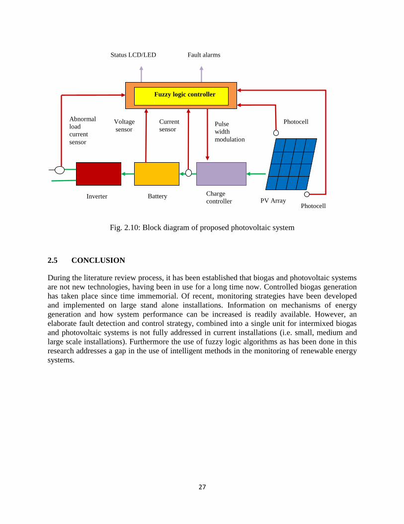
27
Fig. 2.10: Block diagram of proposed photovoltaic system
2.5 CONCLUSION
During the literature review process, it has been established that biogas and photovoltaic systems
are not new technologies, having been in use for a long time now. Controlled biogas generation
has taken place since time immemorial. Of recent, monitoring strategies have been developed
and implemented on large stand alone installations. Information on mechanisms of energy
generation and how system performance can be increased is readily available. However, an
elaborate fault detection and control strategy, combined into a single unit for intermixed biogas
and photovoltaic systems is not fully addressed in current installations (i.e. small, medium and
large scale installations). Furthermore the use of fuzzy logic algorithms as has been done in this
research addresses a gap in the use of intelligent methods in the monitoring of renewable energy
systems.
Fuzzy logic controller
Inverter Battery Charge
controller
Current
sensor
Voltage
sensor Pulse
width
modulation
Photocell
Photocell PV Array
Abnormal
load
current
sensor
Status LCD/LED Fault alarms

28
CHAPTER 3
RESEARCH DESIGN AND METHODOLOGY
3.1 INTRODUCTION
This chapter gives a detailed discussion of the research design and methodology. Section 3.2
details the interview process, whilst, in section 3.3 the research paradigms and research methods
used in this study are discussed. Section 3.4 is about the hypothesis and the translation (mapping)
of research questions into their research methodology equivalents. The data collection process
pertaining to the study is described in detail in section 3.5 which begins by giving a detailed
discussion of data collection principle. The method of data analysis is described in section 3.6,
whilst the research ethics and the conclusion to chapter 3 are given in section 3.7 and section 3.8
respectively.
3.2. INTERVIEW PROCESS
The results of the interviews carried out in rural establishments that have REF digesters and
photovoltaic systems installed are given in Tables 3.1 and 3.2 respectively. A large percentage of
the biogas and photovoltaic systems that where considered for the interview exist alone, as such
interviews done on site were either only for biogas or only for the photovoltaic system.
Furthermore it was observed that the number of biogas systems outweigh the number of
photovoltaic installations of the said capacity, as even some rural establishments with grid
electricity do also have biogas systems installed so as to reduce their electricity bill and to
counteract on grid outages that are caused by faults and load shedding. The pie chart in Fig. 3.1
shows the relative nature of the biogas and photovoltaic installations at which interviews where
done.
Fig. 3.1: Relative number of installations that where accessed
Available installations
Biogas
Solar

29
Table 3.1: Summarized interview results related to biogas generation
Main questions Sub questions Interviewee’s response
1) is your bio digester for a single
household or for a small
community?
OR
-what size is your bio digester?
- how many people use this
digester?
- are there school going children
among the users?
- is the gas output tap turned on
continuously?
- are there times when the gas
supply is fully closed?
-small community, less than
five hundred people
-many school children
-mains always turned on
-no
2) does your bio digester supply
enough biogas?
-for what purpose is the gas used?
-do you always obtain gas output
as and when you need it?
-what are your gas storage
facilities?
-what can you say about the
pressure of the gas coming out of
the pipe?
-how far are the gas storage and
digester from the house?
-firewood also used
- cooking and heating
-just for functions at schools
-continuous use for small
foods
-some always, others not
enough gas sometimes
-high „‟ layman‟s response‟‟
-generally high
-250m to 400m
3) Do you troubleshoot gas
related issues?
- How do you rectify continuous
low biogas output from the
digester?
-What is the effect of gas leakage in
the house?
-what biogas pressure irregularities
are of concern?
-always refer faults to REF
-explosions occur with
furniture burnt and injury to
people usually at homesteads
(few or no leakages at
schools or clinics)
-some times gas takes long to
come
4) what type of waste is used in
the bio digester?
-what are the daily solids (dry
matter) to liquid (water) ratio input
to the digester?
- how do you know which solids to
liquid ratio will give the best biogas
output?
- do you know the toxicity and pH
of the feedstock?
-difficult to say (REF knows
better), only lots of water
required
-1) human sewerage based
2) some piggery waste
3) some cow waste
(also add hides, dead
chickens, dead pigs in 2) and
3) above)
-no way to tell

30
5) how do you monitor internal
bio digester process?
-is feedstock level in the bio
digester important?
-what parameters are critical to bio
digester sustained process
operation?
-no internal monitoring
-do not know
6) how is the used up waste from
the bio digester removed?
-what is the typical retention time
(i.e time between inputting waste
and discharging it)?
- how is the waste material used?
-minimum of about 21 days
-( solids removed as fertilizer
after 2 years)
-waste water for garden pond
- digester near vegetable
garden
7) are there written down
instructions on how to operate
the biogas system?
-what are your observations and
recommendations?
-not sure if they exist, never
seen any instructions
Table 3.2: Summarized interview results related to photovoltaic generation
Main questions Sub questions Interviewee’s response
1) is your photovoltaic system for
a single household or for a small
community?
OR
-what size is your photovoltaic
system?
- how many people use this
photovoltaic system?
- are there users who need
continuous electrical supply?
-small community (single
household up to 500 people)
-some important establishments
also have stand-by generators
2) does your photovoltaic system
supply enough electricity?
-for what purpose is the
electricity used?
-do you always obtain electricity
when you need it?
-how reliable is your battery
bank?
-what can you say about the
power generated versas that
taken by the users?
-how far are the battery bank and
inverter from the house?
-lighting, entertainment,
computers, business equipment,
small refrigerators
-reliable
-not enough for all user
requirements
-depends on intended installation
3) Do you troubleshoot electrical
generation related issues?
- How do you rectify continuous
low electrical output from the
photovoltaic system?
-How do you maintain the
different components of the
photovoltaic system from solar
panel to inverter?
- we call REF
- clean solar panels
31
-what electrical generation
irregularities are of concern?
-what load conditions interfere
with system operation?
-none, only low power during
heavy clouds and rainy season
-people trying to connect two
plate stoves and electric irons
4) how do you monitor internal
photovoltaic process?
-what aspects are critical to
photovoltaic sustained process
operation?
-do not know
5) are there written down
instructions on how to operate
the photovoltaic system?
-what are your observations and
recommendations?
-some (including battery
maintenance)
These interviews were done and concluded as per attached interview protocol in Appendix B and
signed informed consent form in Appendix C. The interview results clearly consolidate the initial
idea of designing a measurement and control system for intermixed biogas and photovoltaic
systems. Existing systems also totally lack any forms of fault detection and control. The users of
these renewable energies are heavily dependent on external expertise for solving serious issues
that can arise during the operation of biogas and photovoltaic systems. The design of a fuzzy
logic measurement and control system for intermixed biogas and photovoltaic systems will
reduce or totally eliminate the external expert on a wide range of operational issues.
The study established that solar energy for most rural households is used for entertainment and
lighting, while for public establishments that include clinics, hospitals and schools the use of
solar power is more elaborate. In these establishments in addition to those uses similar to rural
households the solar energy is required for equipment such as communication systems,
refrigerators, computers and other critical electrical equipment. On the other hand biogas is
heavily used for cooking and heating by both households and public establishments.
3.3 RESEARCH DESIGN
3.3.1 Research Paradigm
A paradigm14
is defined by Chalmers 1982, p. 90 (cited in Jerry 2007) as being “made up of the
general theoretical assumptions and laws, and techniques for their application that the members
of a particular scientific community adopt”. Chalmers 1982, p. 91 (cited in Jerry 2007) also
states that a paradigm is made up of the following components:
1) “Explicitly stated laws and theoretical assumptions”.
2) “Standard ways of applying the fundamental laws to a variety of situations”.
3) “Instrumentation and instrumental techniques that bring the laws of the paradigm to bear
on the real world”.
4) “General metaphysical15
principles that guide work within the paradigm”.
14
A paradigm can also be looked at as a world view or framework for that particular study. 15
Metaphysics is a branch of philosophy that asks two questions and according to Jerry (2007) these are: 1. “What
are the characteristics of existence?” and, 2. “How can we know the things that exist?”

32
5) “General methodological prescriptions about how to conduct work within the paradigm”.
Research assumptions that are made by researchers include those known as ontological,
epistemological, methodological and axiological. Ontological assumptions address the nature of
reality of the system being studied while epistemological assumptions define the nature of the
connection (knowledge) between the researcher and the system being studied. On the other hand
methodological assumptions address the ways taken by the researcher to investigate and acquire
knowledge on the system being studied. Finally, the axiological assumption seeks to identify any
information that could be of importance to the study (Aliyu et al., 2014).
The research paradigms are mainly identified as positivism, post-positivism (interpretation) and
constructivism and these are related to the research assumptions as shown in Table 3.3
Table 3.3: Research paradigms and associated assumptions (Aliyu et al., 2014)
Issue Positivism Post positivism Constructivism
Ontology naïve realism-
“real”
critical realism-
“real”
relativism- local and
specific constructed
reality but
apprehendable
reality but
only imperfectly
and probabilistically
apprehendable
realities
Epistemology dualist/objectivist;
findings true
modified
dual/objectivist;
critical tradition/
community ;findings
probably true
Transactional/
subjectivist; created
findings
Methodology experimental/
manipulative;
verification of
hypothesis; chiefly
quantitative methods
Modified
experimental/
manipulative; critical
multiplism;
falsification of
hypothesis; may
include qualitative
methods
Hermeneutic/
dialectical
Axiology propositional knowing
about the world is an
end in itself, is
intrinsically valuable
propositional
knowing about the
world is an end in
itself, is intrinsically
valuable
propositional,
transactional
knowing is
instrumentally
valuable as a means
to social
emancipation, which
is an end itself, is
intrinsically valuable

33
As far as positivism is concerned, knowledge is obtained by employing scientifically based
measurements and observations on systems in the real world (O‟Leary, 2007a; Payne, 2004). In
the positivist attitude by considering the ontological, epistemological and methodological
assumptions in Table 3.3, the system under research is definitely real, findings are objective/true,
and the experimental based quantitative research can be done.
On the other hand the post-positivist believe in a complex, highly disordered world that is left to
interpretation and cannot be measured directly (Aliyu et al., 2014; O‟Leary, 2007b). In the
ontological assumption, a number of realities exist and the epistemological findings that are
observer based are probably true. The methodology in the interpretive paradigm can be
qualitative with little reliance on the experimentation method.
Constructivism and participatory (not mentioned here) are both paradigms of inquiry (Howell,
2013) where knowledge is solely based on humans, either as individuals or as society. According
to Howell (2013):
„Constructivism understands reality as being locally constructed and based on shared
experiences and, because groups/individuals are changeable, identifies it as „relativist realism‟
or „relative ontology‟. Epistemologically, constructivism is similar to critical theory, however
research results are created through consensus and individual constructions, including the
constructions of the investigator. Theory in this paradigm is relative and changeable, reliability
and prediction almost impossible and cause and effect difficult to identify.‟
In this scenario any research to be done cannot be separated from the human construct. The
positivistic research paradigm (Jerry, 2007; O‟Leary, 2007a) is adopted in this research since
positivist attitude clearly accommodates the relevant assumptions that are required. In this study
the energy generation processes in both the biogas and photovoltaic systems, though multi-
parameter dependent do follow pre-defined steps. The state of each process which can be
successfully assessed by the scientifically based measurement procedure lies within the
positivistic research paradigm. This dissertation will include design and programming
experiments, which indicates a high degree of empirical positivistic approach. Empiricism
(O‟Leary, 2007c) explains that valid results are only obtained from measuring, testing and
making observations. However this study will also involve post-positivistic (interpretative)
research approach in the form of qualitative literature and field study.
3.3.2 Research methods
Research methods are basically ways to get information that the researcher has to use. The type
of method used is attributed to the source of information, how the information is acquired and
the data collection instruments used. Research methods are globally indentified as either
qualitative (Denzin, 2007) or quantitative (Salkind, 2010).
The qualitative research process involves the study of systems in their natural setup (Bloor &
Wood, 2006) and attempts to provide relevant human based interpretation of the findings. The

34
methods used in qualitative research include case study, personal experience, interactional,
historical, interview and observational (Denzin, 2007).
Quantitative research method is based on sound data investigation that has no bias. The results
can be statistically or numerically used to describe the system population under study. The
scientific research method (positivism), which is based on measurement (including
experimentation) is the hallmark of the quantitative research method (Salkind, 2010). The
descriptive form can also be used to represent the findings in quantitative research. Based on the
nature of this study, the quantitative research method will be mainly used.
The overall research methodology strategy is to include both the qualitative and quantitative
research methods in this research in what is termed the „mixed method‟ research method. Mixed
methods research according to Jupp (2006), is:
„The combined use of both quantitative and qualitative methodologies within the same study in
order to address a single research question.‟
However, this does not imply the use of multiple quantitative nor qualitative methods in any
research question. One method can be used before the other, or both methods can be used at the
same time between quantitative and qualitative research. In this research, established (historical)
data from literature review is first used to test the accuracy of the algorithm and software
development process with the aid of simulation software.
After this initial process of verification, the algorithms are then passed and implemented on the
real system that measures and collects real time data. Immediately after development and
verification of the algorithms, and before hardware implementation the results of the
interviews/consultations that are qualitative in nature are considered. The interviews seek to
establish the user‟s (experts and non-experts) perceptions on existing biogas and photovoltaic
systems. Although the interviews are meant to be done earlier on in the study, their results are
only considered after the initial measurement and control system simulation has passed since it
becomes easy to make specific adjustments if any in the design. Hence the interviews can still be
performed way into the study. The design of the sensor circuits, output circuits and embedded
system is based on literature study and expert knowledge of the researcher.
The mixed research method is a triangulation16
process that seeks to establish the functionality
and accuracy of the designed algorithms from the simulation and implementation angles.
3.4 HYPOTHESIS AND RESEARCH QUESTIONS
The hypothesis for this dissertation is given as:
The measurement and control for intermixed biogas and photovoltaic systems is successfully
implemented by the use of fuzzy logic algorithms.
16
In triangulation a number of different approaches are taken to address a single research question issue.

35
The data used was obtained from an already installed and working biogas digester and
photovoltaic system. Software and performance as given in Appendix E1 & E2, and Chapter 8,
show that the hypothesis is true.
In this section, the research questions in this study are all translated (mapped) into their research
methodology equivalents. For this study, Table 3.4 gives the relationship between a research
question and the most suitable research method that can be used. An X indicates a
correspondence between a research question and a data collection method that can be used.
Table 3.4 shows a bias towards the quantitative research method as depicted by the pronounced
measurement and experiment methods. High levels of the design and historical methods are also
noted. The observation method is relatively significant, with the interview method contributing
the least in this study. The positivism approach is hence consolidated within a mixed method
situation. With this perspective in mind, the data collection methods are fully described in the
following sections.
Table 3.4: Mapping of research questions into research methods
Data Collection Method
Research
Question
Number
(See Page 4)
Measurement Experiment Design Historical/
Literature
Observation Interview
1) X X
2) X X X
3) X X X
4) X X X X
5) X X X X
6) X X X X
3.5 DATA COLLECTION
3.5.1 Historical/Literature Review
A detailed literature study was done to obtain existing information on the biogas and
photovoltaic energy generation process with a view of determining the critical parameters
required to improve system performance. A literature study on fuzzy logic concepts, relevant
instrument sensors, output devices, suitable microcontroller and existing methods used to
improve/optimize system performance was also been done. The literature was obtained from
books, journals, conference papers, white papers, system design specifications and from the
internet (mainly UNISA library).

36
3.5.2 Field Interviews
The interviews provided an opportunity for us to look at the biogas and photovoltaic systems
from the „eyes „, of the day to day users of these energy establishments. The users were free to
participate in the interviews and to provide any kind or amount of information they so wished
pertaining to the operation of the biogas and photovoltaic systems. Depending on the interview
outcomes, the information so provided by the interviewees was ether considered or not
considered for modification of the designed program flowcharts.
3.5.3 Experiments
Initially the experiments took the form of simulations in this research. The writing of fuzzy logic
algorithms was undertaken using various approaches. Flowcharts where developed followed by
C language based source codes writing in the MPLABX IDE development software. The
hardware simulation and development of circuit schematics were performed in the Labcenter‟s
Proteus (Labcenter, 2012) and National Instrument‟s Multisim (National, 2013 software
packages.
3.5.4 Field Measurements
Measurements were performed using the specified sensors and sensor circuits. Firstly, data was
acquired from the real system using the sensors and sensor circuits not yet connected to program
bearing microcontroller and the readings noted. Manual titration method was performed on a
given sample of the digester substrate to determine the value of the buffering capacity. Secondly
data was acquired by using the complete hardware and software based data acquisition system.
The sensors were installed inside the digester, at the user end premises (Figure 2.9 page 26) and
on the photovoltaic system points as per design (Figure 2.10 page 27).
3.5.5 Field Observations
The field observations entail observing the behavior and nature of the outputs that are the result
of the implementation of the complete measurement and control system. The on-line outputs
were observed to see if the system behaved as per design.
3.6 DATA ANALYSIS
3.6.1 Historical Data Analysis
From the literature review, we were able to provide a detailed breakdown of the energy process
mechanism in biogas and photovoltaic systems. We were able to show how the different stages
are linked together and how each stage affects the overall system output. With the knowledge of
the role each stage, by product and/or parameter plays in achieving the desired output we could
confidently design a monitoring system which was able to guide us to the successful production
of biogas or photovoltaic energy. This review also assisted in showing that quite a number
approaches of standalone system optimization have been developed and implemented, however
the „gap‟ that exists in the intelligent measurement and control of intermixed biogas and
photovoltaic systems was further consolidated through the literature study. The initial stages of

37
the fuzzy logic algorithms development process and the embedded system hardware design were
successfully done by incorporating the results of the literature review.
3.6.2 Interview Data Analysis
The interviews were performed using the interview protocol that was designed for this research.
The numbers of the interviews were limited mainly due to the sparsely distributed nature of the
energy installations in the rural areas. However, those who did participate provided invaluable
information on the operation of the biogas and photovoltaic systems. The actual responses are
given in the findings (Section 3.2), but it serves to mention here that no modification in the
measurement and control system design was necessary as the initial design process had globally
considered most aspects ( from literature review and observation).
3.6.3 Experimental Based Data Analysis
The simulations were used to verify the proper functionality of the developed algorithms and
whether the outputs generated are realistic when given specific input data, first from established
literature sources and secondly from system measured data. The written software modules were
continuously modified or fine tuned until they effectively addressed the flowchart with the least
number of program lines. In summary, the outcome of the experimental data was to identify the
best working fuzzy logic and control algorithms that addressed the problem at hand and to
provide written code that was working without errors. Chapter 6 gives the complete simulation
behavior of the programs to given input data, while chapter 7 gives the overall data acquisition
and control system (designed and experimentally validated) ready to be directly installed in the
field.
3.6.4 Field Based Measurement Data Analysis
The readings that were obtained by using the sensors and sensor circuits not yet connected to the
microcontroller were used as data input for the simulation routines. The results of the simulation,
so produced were used to cross-check the overall field measurement and control system
response, since the same data range and type was used in each case. The results for the
simulation are given in chapter 5, while the field based results/findings are given in chapter 8.
The buffering capacity value obtained from manual titration was used in the multiple regression
analysis formulation of the alkalinity prediction equation. The soft sensor routine and
corresponding results are given in chapter 4, section 4.2.2.
3.7 RESEARCH ETHICS
According to Thomas & Hodges (2010) a research is supposed to be ethically undertaken. We
were, required for our research to conform to a moral, transparent, original and above board way
of dealing. In the strictest way possible we endeavored not to hurt or prejudice any individual as
we carried out my research, nor where existing biogas and photovoltaic installations unduly
negatively affected. Furthermore, due acknowledgement of all work and information which was
not our own was made.

38
The requirements for research ethics guided by the UNISA revised policy on research ethics
(2013) were duly met, and are tabulated below:
1) Ethical clearance (Appendix A) was obtained from the College of Science, Engineering and
Technology‟s (CSET) Research and Ethics Committee at the University of South Africa
(UNISA).
2) Human subjects were not directly used in this research.
3) Permission was sought and obtained from the administrators of the biogas and photovoltaic
installations to conduct interviews where the interviewees were free to accept or decline to
participate. To this end, a sample of a signed informed consent form is provided in
Appendix B.
4) The research was implemented without interfering neither with the constructional designs nor
the operation status of the existing biogas and photovoltaic systems.
5) Permission was sought and obtained from REF to implement the monitoring system on their
installations provided the conditions in 3) above are observed.
6) Information from any other consultations done was treated in the strictest confidence and the
anonymity of the participants maintained.
3.8 CONCLUSION
In chapter 3, we detailed the research paradigms and research methods used in this study. The
translation (mapping) of the research questions into research methods was done and the relative
contributions of each research method to the research questions was given (Table 3.3 page 32).
The data collection methods, the data analysis procedure and the ethical considerations according
to UNISA requirements are also fully explained in this chapter.

39
CHAPTER 4
FUZZY LOGIC ALGORITHMS AND SYSTEM FLOWCHART
DESIGN
4.1 INTRODUCTION
In this chapter the fuzzy logic algorithms and module flowcharts are developed. The fuzzy logic
algorithm and module flowchart for digester system stability test are developed in section 4.2.
Section 4.3 looks at the development of the fuzzy logic algorithm and flowchart for biogas
amount output. Section 4.4 develops the fuzzy logic algorithm and flowchart for biogas system
fault detection and status, while the design of solar battery charging/discharging fuzzy logic
algorithm and flowchart are detailed in section 4.5. Solar system fault detection and status fuzzy
logic algorithm and flowchart are treated in section 4.6, with section 4.7 concluding this chapter.
4.2 DIGESTER SYSTEM STABILITY TEST
4.2.1 Fuzzy logic algorithm 1
The algorithm procedure given as an example in the literature review section (Section 2.3 FUZZY
LOGIC ALGORITHMS), was the adopted fuzzy logic algorithm for digester stability. This is made
up of a two input and one output fuzzy logic controller with a total number of fifteen rules as
shown. The inputs are pH and buffering capacity (Alkalinity), whilst the output is the stability
status of the digester as a percentage. A high percentage value, of stability implies a greater
confidence level in the digesters‟ capability to continually produce biogas. The pH parameter is
directly measured by a pH sensor, whilst the alkalinity is inferred by the combined
measurements of pH, redox and electrical conductivity of the digester substrate. The alkalinity
prediction procedure and the overall stability test flowchart are given in the following sections.
4.2.2 Evaluation of alkalinity from soft sensors
The buffering capacity (Alkalinity) value that forms one of the inputs to the fuzzy logic routine
was obtained by prediction from a soft sensor algorithm using multiple linear regression analysis
(MLRA) of a number of independent bio digester parameters. This value of alkalinity could have
been measured directly by using very expensive instruments which are however beyond the
scope of this study. An alternative cheaper on-line method to measure alkalinity based on soft
sensor method was considered.
A software sensor algorithm that uses pH, conductivity and redox (Eu-agrobiogas, 2009; Ward
et al., 2008; Ward et al., 2011) was proposed and used. This method is supposed to produce a
reasonable good prediction of alkalinity. However, as an alternative to the method just
mentioned above, other software algorithms (Argyropoulos, 2013; Pham et al., 2014; Turkdogan,
2010) that may use only pH and gas production in its simplest form as the independent variables,
as a way of reducing the number of probes and circuitry can be proposed.
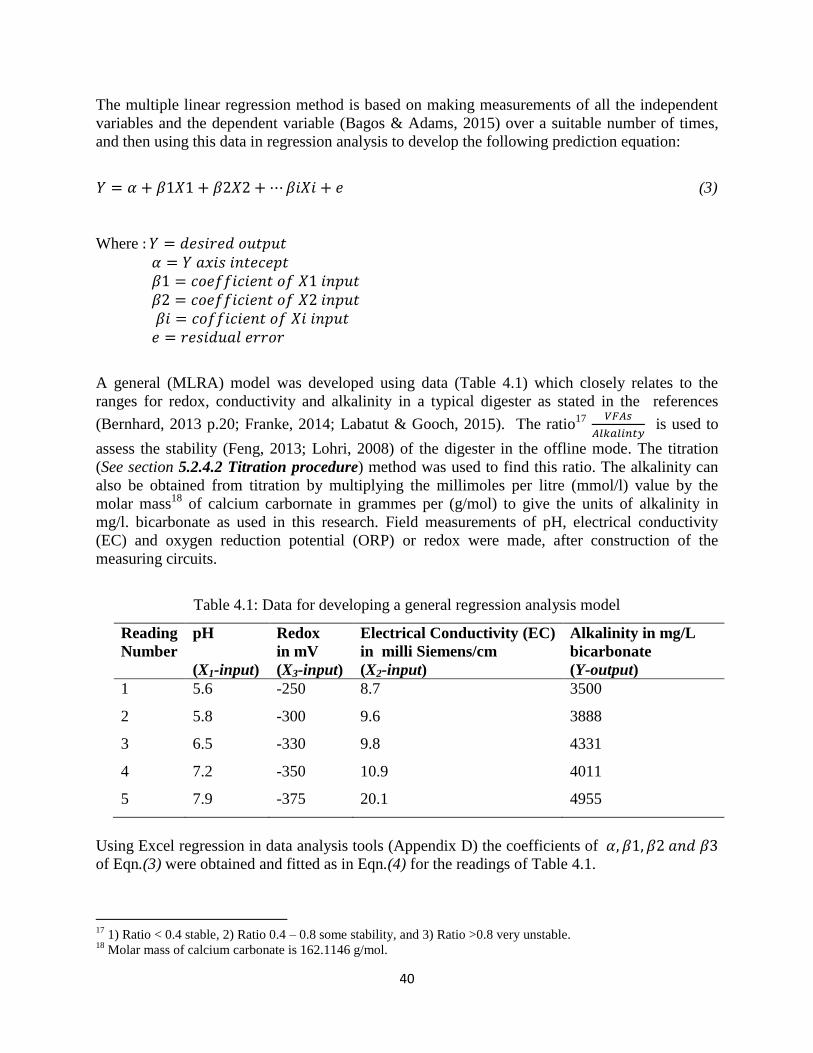
40
The multiple linear regression method is based on making measurements of all the independent
variables and the dependent variable (Bagos & Adams, 2015) over a suitable number of times,
and then using this data in regression analysis to develop the following prediction equation:
(3)
Where
A general (MLRA) model was developed using data (Table 4.1) which closely relates to the
ranges for redox, conductivity and alkalinity in a typical digester as stated in the references
(Bernhard, 2013 p.20; Franke, 2014; Labatut & Gooch, 2015). The ratio17
is used to
assess the stability (Feng, 2013; Lohri, 2008) of the digester in the offline mode. The titration
(See section 5.2.4.2 Titration procedure) method was used to find this ratio. The alkalinity can
also be obtained from titration by multiplying the millimoles per litre (mmol/l) value by the
molar mass18
of calcium carbornate in grammes per (g/mol) to give the units of alkalinity in
mg/l. bicarbonate as used in this research. Field measurements of pH, electrical conductivity
(EC) and oxygen reduction potential (ORP) or redox were made, after construction of the
measuring circuits.
Table 4.1: Data for developing a general regression analysis model
Reading
Number
pH
(X1-input)
Redox
in mV
(X3-input)
Electrical Conductivity (EC)
in milli Siemens/cm
(X2-input)
Alkalinity in mg/L
bicarbonate
(Y-output)
1 5.6 -250 8.7 3500
2 5.8 -300 9.6 3888
3 6.5 -330 9.8 4331
4 7.2 -350 10.9 4011
5 7.9 -375 20.1 4955
Using Excel regression in data analysis tools (Appendix D) the coefficients of
of Eqn.(3) were obtained and fitted as in Eqn.(4) for the readings of Table 4.1.
17
1) Ratio < 0.4 stable, 2) Ratio 0.4 – 0.8 some stability, and 3) Ratio >0.8 very unstable. 18
Molar mass of calcium carbonate is 162.1146 g/mol.

41
(4)
Eqn.(4) gives the most likely output for alkalinity for specific values of pH, redox and electrical
conductivity where the Adjusted R Square value of 0.696504 shows a reasonable good fit for
the equation to predict the output alkalinity. Low values of P-value (P < 0.05) eliminate the
possibility of any independent variable (pH, EC, Redox) having a value of zero (“the null
hypothesis”) in our prediction equation thereby consolidating its nature (Zaman & Alakus, 2005).
Likewise should be greater than the obtained in Excel for us
to eliminate the “null hypothesis”. However the data we have used says otherwise as hence it is imperative for our
measurements to be done accurately and the preceding tests done to establish a reliable
prediction.
The software coding for Eqn. (4) was incorporated into Listing one (Appendix E1) which is the
software code for the whole digester stability routine also known as the digester system
imbalance early warning routine. The flowchart for the digester system imbalance early warning
routine is shown in Fig. 4.1.
4.2.3 Digester System Imbalance Early Warning Flowchart Description
The digester system imbalance early warning routine starts by measuring the values of pH, redox
and electrical conductivity (EC) of the digester substrate. These values are input to the soft
sensor algorithm, whose output is the value of the buffering capacity (alkalinity). The value of
the alkalinity so outputted is input together with the pH value read before into the fuzzy logic
algorithm where the percentage level of the stability is evaluated.
Based on the fuzzy logic algorithm the digester system will either be stable or unstable. If the
system is stable the program returns control back to the beginning to make a new sweep of the
measurements. However, if the system is not stable, a failing or failed stability alarm will be
activated. When this does occur, the program goes on to establish which between the pH and
alkalinity is out of range and to give the remedial action to be taken by the user.
A liquid crystal display (LCD) is used to communicate instructions to the user on what remedial
action has to be taken to return the pH or alkalinity value to an acceptable value. The pH can be
increased by adding an acid reducing agent such as calcium carbonate (lime). Lime is good at
suddenly increasing the value of the pH but unfortunately this does not translate to an equivalent
increase in alkalinity. Hence, the addition of lime should be complemented by the addition of
bicarbonate or carbonate salts such as sodium and potassium that will substantially increase
alkalinity and fine tune the pH value to the required level. On the other hand the pH can be
decreased by adding some form of pH reducing agent such as acetic acid or ferric chloride.
It should be noted that the addition of any chemical into the digester substrate should be gradual
so as not to „shock „ , the bacteria involved in the anaerobic process. Furthermore too often the
addition of elevated chemical levels is not recommended as this can cause unwanted solids build-
up inside the digester.

42
Yes
No
(continued on the next page)
Initialise μ-controller
Measure –pH , Redox and Electrical conductivity (EC)
Fuzzification
Is bio-digester stable ?
-Alarm -Status output
-LCD
Begin
Inference Rules
Defuzzification
A-11
Soft sensor algorithm
pH plus Buffering capacity (Alkalinity)

43
Yes
No
No
Yes
Yes
No
Fig. 4.1: Digester System Imbalance Early Warning Flowchart
Is 5.5≤ pH ≤8.5?
Is alkalinity ≥ 3500 mg/L bicarbonate?
Increase alkalinity
Exit
-Reset alarm -clear displays
Is pH < 5.5
Add acid reducing agent
Add alkalinity Reducing agent
Then pH > 8.5
A-10
44
4.3 BIOGAS AMOUNT (OUTPUT)
4.3.1 Fuzzy Logic Algorithm 2
The amount of biogas produced depends to a large extent on the organic loading rate (OLR) and
digester temperature. Industrial bio digesters will operate at 43 to 55oC (Thermophilic) as this
gives minimum hydraulic retention time (HRT) of about 15 to 20 days for yield production,
whilst domestic digesters will normally operate at 30 to 42oC (Mesophilic) with HRT between 30
to 40 days (Teodarita et al., 2008). From this it is established that temperature affects the point at
which biogas production starts and hence the amount of biogas produced in a given situation.
The fuzzy logic controller for biogas amount will be a two input controller of OLR and
temperature. The biogas output amount consists of 58 to 65% methane by volume and 42 to 35%
carbon dioxide by volume (Labatut & Gooch, 2015), hence a measurement of the ratio of
methane/carbon dioxide from the sensors should be 1.38 to 1.86. For the REF 50m3 biogas
digesters under consideration the gas storage capacity is 7m3
(7000 litres) and the exhausted
slurry is 6m3 per day.
The normally unheated and unmixed domestic digesters will have a loading rate (OLR) of 0.481
to 1.6kg of volatile solids (VS) per cubic meter per day whilst commercial digesters that are
continuously fed normally have a loading rate (OLR) of 1.6 to 6.41 kg of volatile solids (VS) per
cubic meter per day. However, too low an OLR will reduce biogas output potential while too
high an OLR greater than 4.0kg.VS/m3 day will result in too much feed for the bacteria to
operate on thereby effectively reducing biogas output potential The daily intake of the volatile
solids in kilograms over the usable biogas digester volume in m3 will give the value of the
organic loading rate in the units of kg.VS/m3 day (Bioenergy, 2016; Winsconsin, 1992 pp.3).
4.3.1.1 Calculation of retention time and organic loading rate for REF 50m3 Digesters
( ) ( ) ( ) (5)
Digester effective volume = 50 m3
Feedstock(slurry) per day = 2.1875 m3 /day of piggery and sewer waste
= 22.85 days (A high level of bacteria already exists in the slurry)
[ ]
( )

45
(
)
=2.975 kgVS/m3 day
Biogas output for these digesters ranges from 15 to 20 m3
(1500 to 20000 litres), hence
secondary gas storage facilities, input slurry regulation and continuous gas usage are required
since the internal digester storage capacity is 7 m3
(7000 litres).
4.3.1.2 Biogas amount organic loading rate based rules
From Fig. 4.2, the number of possible rules is 3 x 2 = 6 from the inputs. The linguistic variables
are OLR ={ Low organic loading rate (OLRL), Good organic loading rate (OLRG), High organic
loading rate (ORLH)} , Temperature ={Low temperature (TL), Optimum temperature (TO)} and
Biogas output ={Gas low (GL), Gas average (GA), Gas high (GH)}.
(1) IF Organic loading is OLRL AND Temperature is TL THEN Biogas Output is Gas low
(2) IF Organic loading is OLRL AND Temperature is TO THEN Biogas Output is Gas low
(3) IF Organic loading is OLRG AND Temperature is TL THEN Biogas Output is Gas average
(4) IF Organic loading is OLRG AND Temperature is TO THEN Biogas Output is Gas High
0 0.5 1.5 2 3 4 7 Organic Loading Rate in kg.VS/m3 day
pH
0 3 7 15 20
Biogas output in 1000 Litres/day
Digester stability status
GL GA GH μ
1
1
Fig. 4.2: Membership functions for biogas amount for REF 50m3 digesters
0 15 30 55 Digester temperature in oC
TL TO OLRL OLRG OLRH μ
1
μ
1
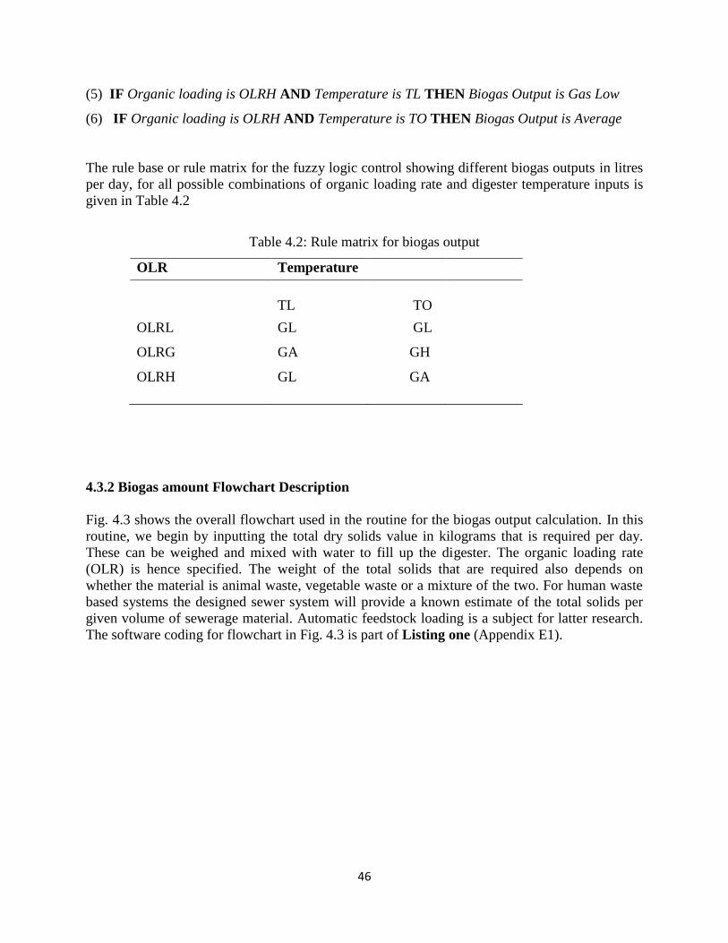
46
(5) IF Organic loading is OLRH AND Temperature is TL THEN Biogas Output is Gas Low
(6) IF Organic loading is OLRH AND Temperature is TO THEN Biogas Output is Average
The rule base or rule matrix for the fuzzy logic control showing different biogas outputs in litres
per day, for all possible combinations of organic loading rate and digester temperature inputs is
given in Table 4.2
Table 4.2: Rule matrix for biogas output
OLR Temperature
TL
TO
OLRL
OLRG
OLRH
GL
GA
GL
GL
GH
GA
4.3.2 Biogas amount Flowchart Description
Fig. 4.3 shows the overall flowchart used in the routine for the biogas output calculation. In this
routine, we begin by inputting the total dry solids value in kilograms that is required per day.
These can be weighed and mixed with water to fill up the digester. The organic loading rate
(OLR) is hence specified. The weight of the total solids that are required also depends on
whether the material is animal waste, vegetable waste or a mixture of the two. For human waste
based systems the designed sewer system will provide a known estimate of the total solids per
given volume of sewerage material. Automatic feedstock loading is a subject for latter research.
The software coding for flowchart in Fig. 4.3 is part of Listing one (Appendix E1).

47
Fig. 4.3: Biogas output amount flowchart
Begin
Input –TDS & Temperature
Fuzzy algorithm
Biogas output in Litres.
Calculate quantity of CH4 & CO2
From ratio value of 1.5. Measure concentrations of CH4 & CO2 in ppm.
CH4 sensor
sensor CO2 sensor
LCD
Calculate OLR & HRT
LCD
Concentration of CH4 in ppm > Minimum value ?
Increase OLR and increase HRT
No
Yes
Exit

48
The calculated OLR and measured digester temperature are input into the fuzzy logic algorithm
to give the expected biogas output in litres. From literature study the ratio of methane gas to
carbon dioxide gas has an average range of 1.5 (See page 44), hence we can calculate the relative
expected quantities of methane and carbon dioxide gases in our system. Methane and carbon
dioxide sensors are also incorporated into the digester to make concentration measurements of
the actual methane and carbon dioxide gases. Recommended19
values of concentrations are
compared with the measured values, and if the measured value of methane is less than the
recommended value the system will either increase the organic load rate or the hydraulic
retention times depending on which is most appropriate. If the measured methane value is equal
to or greater than the recommended value the system will exit to go to the next routine.
4.4 BIOGAS SYSTEM FAULT DETECTION AND STATUS
4.4.1 Fuzzy Logic Algorithm 3
4.4.1.1 Biogas pressure and leaks considerations
The properties of methane are 1) non-poisonous to people, 2) colorless gas, 3) odorless gas
(assuming hydrogen sulfide20
has been filtered off), and 4) highly flammable. However,
prolonged exposure to methane will lead to symptoms associated with lake of oxygen as the
methane normally displaces oxygen bearing air due to its lower density. When biogas is mixed
with air in certain proportions an explosive mixture is formed (Wisconsin, 1992; Zlochower &
Green, 2016). Hence it is imperative that biogas is not unnecessarily exposed to air.
Situations that can contribute air mixing with biogas include gas leaks at user end confined space
and gas storage facility, purging of gas from the gas reservoir for maintenance purposes or
opening of the biogas digester for cleaning purposes. Another very important situation that
deserves mention here is that of biogas storage compartment pressure. According to Marchaim
(1992), in a well designed dome digester atmospheric pressure forces the total water body to
occupy 95% of the total digester volume, leaving 5% as the dead volume. Dome type gas
pressures are usually less than or equal to 120cm of water (11.77 KPa). Consequently the REF
50m3 digesters operate at around 15 KPa biogas pressure. The biogas digester should always be
operated at a gas pressure greater than the external gas pressures above atmospheric value, since
a lower pressure in the gas storage compartment would imply suction of air into it. If this where
to happen the oxygen in the air would combine with the biogas to form either a combustible
mixture or would incapacitate the anaerobic process, completely shutting down the gas
production process. Hence gas usage should not be greater than that required to maintain a higher
pressure in the gas storage compartment. Conversely too high a gas pressure will cause bubbles
to appear at the outlet liberating methane to the ambient which can result an explosive mixture.
An emergency close valve is incorporated into the main gas outlet line to serve the dual purpose
of mitigating against the possibility of air suction into the biogas digester (valve shuts off when
pressure goes below a certain point and opens above this point) and also shuts off when there is a
gas leak at user end.
19
Carbon dioxide concentrations should be less than methane concentrations by a factor of 1.5 or more. 20
Hydrogen sulphide smells like a typical rotten egg.

49
Signs of gas leakage include a rotten egg smell at end user side or an above normal gas pressure
reduction rate from the gas storage compartment.
4.4.1.1.1 Methane leak at end user
According to Zlochower & Green (2016) methane has lower explosive limit (LEL) of 5.0% and
an upper explosive limit (UEL) of 15.8%. This range defines the lowest and highest
concentrations of the gas as a percentage by volume in air (oxygen) that will easily ignite and
cause an explosion. However, this research will not carry out calculations for the exact
concentration levels of methane in air but will design a system to sound an alarm while
activating an emergency gas line solenoid close valve once methane is detected within the room
far from the stove or lamp.
4.4.1.1.2 Oxygen ingress into the digester
Any increase in the concentration of oxygen within the gas storage compartment in the digester
has both the potential of causing a explosion or killing the anaerobic process. Hence once there is
any detectable oxygen in the digester an alarm will sound and the emergency close solenoid
valve closed again activated to prevent dangerous gas mixture being transferred to the end user.
4.4.1.2 Slurry level considerations
The three components that make up the total volume of a fixed dome digester are the dead
storage (Vd), the effective gas storage (Vg) and the effective slurry storage (Vs) as shown in
Fig. 4.4
Fig. 4.4: Fixed dome biodigester volume components
(Rural Electrification Fund (REF), 2015)

50
In the fixed dome digester the level of the feedstock (slurry) decreases in direct relationship to
the pressure or amount of biogas produced. The minimum recommended level of the feedstock
in this case should just be above the digester outlet to prevent unnecessary loss of biogas through
the outlet. According to Wafler (2008) it is established that the minimum feedstock level
(P-line) represented by the lowest slurry level corresponds to the highest recommended gas
pressure while the maximum feedstock level (zero line) represented by the highest slurry level
corresponds to the minimum or no gas pressure. Hence it is necessary to monitor the feedstock
level in the digester both as compliment to safe pressure operation and availability of adequate
feedstock in the digester.
The fuzzy logic controller for Biogas System Fault/Status Detection is a two input
controller of pressure and feedstock level. From Fig. 4.5 the number of possible rules is
3 x 3 = 9 from the inputs. The linguistic variables are pressure ={Low pressure (LP), Good
pressure (GP), High pressure (HP)}, feedstock level ={Low level P-line (LL), Between P-line &
Zero-line level (BPO), High level Zero line (HL)} and Digester Danger status output ={No
danger (ND), Low danger (LD), High danger (HD)}. A few rules are shown below.
(1) IF Gas pressure is LP AND Feedstock level is LL THEN Output is High danger
(2) IF Gas pressure is LP AND Feedstock level is BPO THEN Output is Low danger
(3) IF Gas pressure is LP AND Feedstock level is HL THEN Output is No danger
(4) IF Gas pressure is GP AND Feedstock level is LL THEN Output is Low danger
(5) IF Gas pressure is GP AND Feedstock level is BPO THEN Output is No danger
(6) IF Gas pressure is GP AND Feedstock level is HL THEN Output is Low danger
The rule matrix for pressure and level status is given in Table 4.3.
Pressure Level
LDIS
MDIS
HDIS
LP
GP
HP
ND
LD
HD
LD
ND
ND
HD
LD
ND

51
4.4.2 Biogas system fault/status detection flowchart description
Fig. 4.6 gives the overall flowchart for the biogas system fault detection and control. In this
routine the integrity of the system is evaluated by detection of unwanted methane or oxygen
outside the digester or inside the digester respectively. If a methane leak occurs especially at the
enclosed premises of the user an alarm comes on. If oxygen ingress into the digester occurs an
alarm is also activated. In both cases a line valve is closed until the problem is rectified. If there
are no leaks, the routine goes on to digester danger status level with respect to biogas pressure
and slurry levels. The software coding for flowchart in Fig. 4.6 is incorporated in Listing one
(Appendix E1).
0 6 10 15 19 25 Biogas pressure in KPa
pH
0 0.25 0.5 0.75 1
Internal digester danger level referenced to unity
Digester stability status
ND LD HD μ
1
1
Fig. 4.5: Membership functions for pressure and level status of digester
0 0.125 0.25 0.375 0.5 Slurry displacement in metres
LL BPO HL
TO
LP GP HP μ
1
μ
1

52
Fig. 4.6: Biogas system fault/status detection flowchart
Begin
Measure methane and oxygen
Methane leak
in room? Oxygen inside the digester?
Alarm
Alarm
Close line valve
Measure pressure and slurry level
Fuzzy Logic Algorithm
Digester danger status
Fix fault and reset alarms
No No
Yes
Yes

53
4.5 SOLAR BATTERY CHARGING/DISCHARGING
4.5.1 Fuzzy Logic Algorithm 4
4.5.1.1 Battery state of charge
The simplest methods for SOC estimation are the open circuit voltage and the specific gravity
(hydrometer) tests, the ranges of which are shown in Table 4.4, for the flooded batteries that are
used by the Rural Electrification Fund (REF) formerly REA. Open circuit voltage measurement
will give reasonable estimation whilst the specific gravity test will give a very good estimation of
the SOC by following the procedures in the REF document, though both methods are not on-line
implementable. An on-line SOC estimation method then, based on terminal voltage and
charging/discharging current is most plausible (Saravanan et al., 2013) for this research. The
static SOC methods are then used to verify the accuracy of the on-line SOC estimation method.
Table 4.4: State of charge as related to specific specific gravity and open circuit voltage
(Rural Electrification Fund, 2015)
Percentage of
Charge
Specific
Gravity
Corrected to
26.70C
Open-Circuit Voltage
6V 8V 12V 24V 36V 48V
100 1.277 6.37 8.49 12.73 25.46 38.20 50.93
90 1.258 6.31 8.41 12.62 25.24 37.85 50.47
80 1.238 6.25 8.33 12.50 25.00 37.49 49.99
70 1.217 6.19 8.25 12.37 24.74 37.12 49.49
60 1.195 6.12 8.16 12.24 24.48 36.72 48.96
50 1.172 6.05 8.07 12.10 24.20 36.31 48.41
40 1.148 5.98 7.97 11.96 23.92 35.87 47.83
30 1.124 5.91 7.88 11.81 23.63 35.44 47.26
20 1.098 5.83 7.77 11.66 23.32 34.97 46.63
10 1.073 5.75 7.67 11.51 23.02 34.52 46.03

54
4.5.1.2 Battery charging strategy
In this research the preferred method of battery charging as shown in Fig. 4.7, will be constant
current at first followed by constant voltage later (Byrne, 2010).
Fig. 4.7: Constant current and constant voltage battery charging profile
The buck regulator which steps down the supply (solar panel) voltage to a given load (the
battery) of lower voltage is adopted in the formulation of the rules.
According to Rashid (2003), for the buck regulator with pulse-width modulation (PWM) duty
cycle D, the output average voltage Va is related to the supply voltage Vs by the equation:
(6)
and the output average current Ia to the supply current Is by
(7)
Clearly applying equations (6) and (7) to the profile in Fig. 4.7, it is established that for high duty
cycle Va approaches Vs whilst Ia approaches Is an overall condition for high SOC. On the other
hand a low SOC condition is characterized by a low duty cycle where Va is far less than Vs and
Ia is far higher than Is.
The fuzzy logic controller for Solar Charging/Discharging is a three input controller of
SOC, charging voltage and charging current. From Fig. 4.8, the number of possible rules is
3 x 3 x 3 = 27 from the inputs. The linguistic variables are SOC ={Low SOC (LSOC), Medium
SOC (MSOC), High SOC (HSOC)}, Charging voltage ={Low voltage (LV), Average voltage
(AV), High voltage (HV)}, Charging current={Low current (LC), Average current (AC), High
current (HC)}, and Charge controller PWM output ={Low duty cycle (LD), Medium duty cycle
(MD, High duty cycle (HD)}. A few rules are shown below.

55
(1) IF SOC is LSOC AND Charging voltage is LV AND Charging current is LC THEN Duty
cycle is Low
(2) IF SOC is LSOC AND Charging voltage is AV AND Charging current is LC THEN Duty
cycle is Medium
(3) IF SOC is LSOC AND Charging voltage is HV AND Charging current is LC THEN Duty
cycle is Medium
(4) IF SOC is LSOC AND Charging voltage is LV AND Charging current is AC THEN Duty
cycle is Medium
The software coding for flowchart in Fig. 4.9 is shown in Listing two (Appendix E2).
It is important to note that normally the charging current in amperes, is not allowed to exceed
1/10 of the battery‟s rated capacity in ampere-hours (Ah). The 50 Ah battery used here should
be charged at maximum of 5.0 amperes. However prior to electrolyte decomposition, this
charging current can be momentarily higher. From this observation the UoD of the current
membership function is defined.
10 20 30 40 50 60 70 80 90 100 State of charge as %
pH
0 0.5 4 5 7 Charging current in A
Digester stability status
μ
1
1
Fig. 4.8: Membership functions for solar battery charging/discharging
0 5 10 15 20 25 30 Charging voltage in V
μ
1
μ
1 LSOC MSOC HSOC LV AV HV
LC AC HC
0 10 20 30 40 50 60 70 80 90 100 PWM Duty cycle as %
LD MD HD

56
Table 4.5: Rule base table for solar battery charging/discharging
Rule number State of charge
(%)
Charging
voltage
(V)
Charging
current
(A)
Duty cycle
(%)
1 LSOC LV LC LD
2 LSOC AV LC MD
3 LSOC HV LC MD
4 LSOC LV AC MD
5 LSOC AV AC MD
6 LSOC HV AC MD
7 LSOC LV HC LD
8 LSOC AV HC LD
9 LSOC HV HC MD
10 MSOC LV LC LD
11 MSOC AV LC LD
12 MSOC HV LC LD
13 MSOC LV AC MD
14 MSOC AV AC MD
15 MSOC HV AC MD
16 MSOC LV HC HD
17 MSOC AV HC HD
18 MSOC HV HC HD
19 HSOC LV LC MD
20 HSOC AV LC LD
21 HSOC HV LC LD
22 HSOC LV AC HD
23 HSOC AV AC MD
24 HSOC HV AC MD
25 HSOC LV HC HD
26 HSOC AV HC HD
27 HSOC HV HC HD
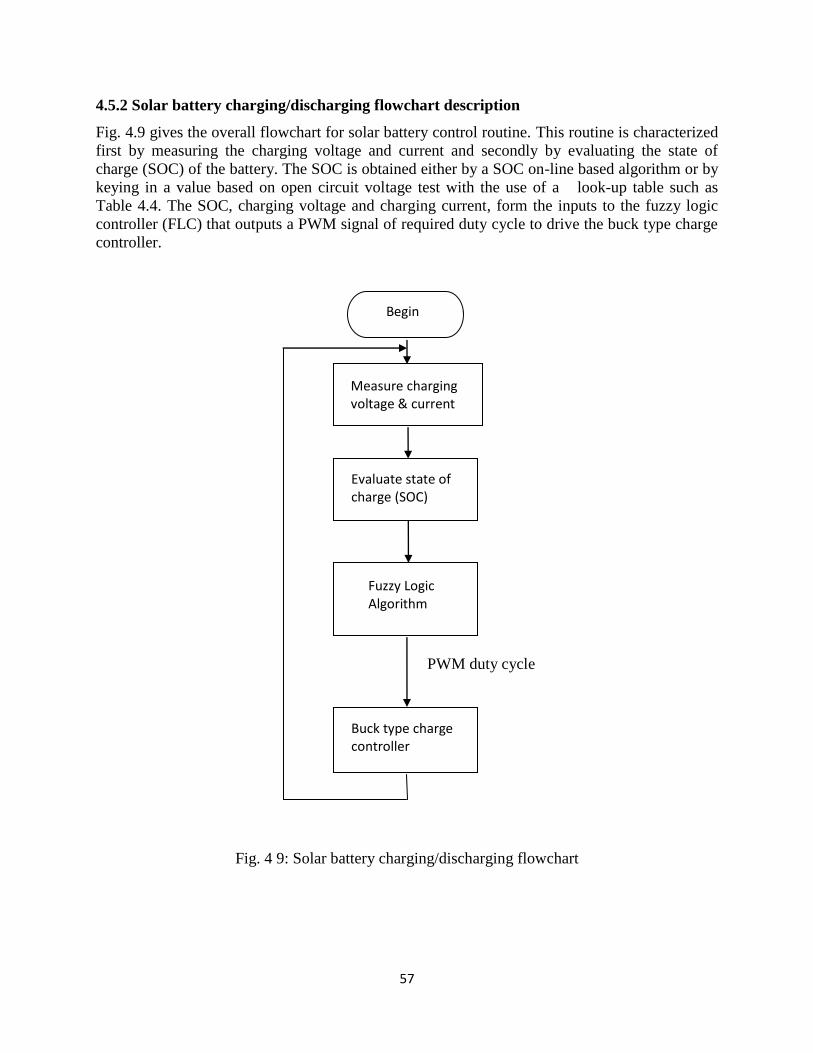
57
4.5.2 Solar battery charging/discharging flowchart description
Fig. 4.9 gives the overall flowchart for solar battery control routine. This routine is characterized
first by measuring the charging voltage and current and secondly by evaluating the state of
charge (SOC) of the battery. The SOC is obtained either by a SOC on-line based algorithm or by
keying in a value based on open circuit voltage test with the use of a look-up table such as
Table 4.4. The SOC, charging voltage and charging current, form the inputs to the fuzzy logic
controller (FLC) that outputs a PWM signal of required duty cycle to drive the buck type charge
controller.
Fig. 4 9: Solar battery charging/discharging flowchart
Begin
Measure charging voltage & current
Evaluate state of charge (SOC)
Fuzzy Logic Algorithm
Buck type charge controller
PWM duty cycle

58
4.6 SOLAR SYSTEM FAULT DETECTION AND STATUS
4.6.1 Fuzzy Logic Algorithm 5
4.6.1.1 Array shading
With respect to the solar panels reasonable output without the inclusion of maximum power
point tracking algorithm can be obtained as long as there is sunshine even though typical solar
panel array efficiencies vary between 6% and 30% (Welch, 2010). The incorporation of
photocells in the design seeks to identify prolonged partial shading of the solar panels that can
occur due to physical objects (leaves, cloth, paper, feathers, tree shadow etc). The resistance of
the photocell is related to the sunlight available on it. This can be used to detect partial shading
of the solar panels and fuzzy algorithm would be the most suitable as a significant number of
shading levels can be quantified. The control output is in the form of status indication (LEDs) to
inform the user on prolonged solar panel shading/obstruction.
Fig. 4.10, shows the reading of the light dependent resistor resistance of 143.9 Ω in direct
sunlight, while Fig. 4.11 gives the circuit configuration for obtaining an analogue signal to the
microcontroller from the photocell. The supply voltage is naturally 5V and the pull down
resistance is chosen to be 4.7 KΩ so that we do not reach saturation of 5V early, getting a
balanced tradeoff between the very dark and very bright light scales (The resistance of the
photocell used in this research varies from 4.0 MΩ to 144 Ω in complete darkness to direct
sunlight respectively).
Fig. 4.10: Light dependent resistor resistance of 143.9 Ω reading in direct sunlight

59
(8)
Hence for complete darkness.
(9)
Hence for sunlight.
For the photocell type that is used in this research, Table 4.6 gives measured values of the
photocell resistance, pull down resistor and the potential difference across the pull down resistor
for various solar panel shading situations. The procedure involves measuring the photocell
resistance and voltage across pull down resistor when photocell is completely covered in
darkness, under a shadow in daylight, covered by slightly transparent paper and finally in broad
daylight uncovered. The fuzzy logic controller for panel shading is a single input controller
of LDR voltage pull down resistor. From Fig. 4.12 (a) & (b) the number of possible rules is 4
from the input. The linguistic variables are Potential difference across pull down resistor ={Low
voltage (LVadc), Lower Medium voltage (LMVadc), Upper Medium voltage, High voltage
(HVadc)}, and Panel shading level output ={Total shading (TS)21
, Heavy shading (HS), Partial
shading (PS), No shading (NS)}. The rules are shown below.
(1) IF Potential across pull down resistor is LVadc THEN Total shading of panels is TS
(2) IF Potential across pull down resistor is LMVadc THEN Total shading of panels is HS
(3) IF Potential across pull down resistor is UMVadc THEN Total shading of panels is PS
(4) IF Potential across pull down resistor is HVadc THEN Total shading of panels is NS
21
Total shading (TS) in photovoltaic systems is not to be confused with total solids (TS) in biogas systems.
+5V supply
Vadc
Microcontroller input
Pull down resistor R p = 4.7KΩ
Fig. 4.11: Circuit configuration for photocell connection to microcontroller
Photocell (LDR)

60
Table 4.6: Sunlight shading levels versus photocell resistance
Panel shading
situation
Photocell resistance
(KΩ)
Photocell plus Rp
(KΩ)
Potential across Rp
(V)
Total darkness 4000 4004.7 0.00585
Room passageway 12.00 16.7 1.4072
Day light room
average
5.09 9.79 2.4004
Outside leaf shadow 0.4 5.1 4.60785
Newsprint shadow 0.302 5.002 4.6981
Direct sunlight 0.144 4.844 4.85135
4.6.1.2 User load control
The loads that are supplied by the photovoltaic stations include domestic and institutional users.
For institutional users, some loads will need to be constantly connected requiring some form of
priority load scheduling. Priority load scheduling fuzzy logic systems based on particle swarm
optimization (Welch, 2010) algorithms have been studied. However, this research will develop a
simpler algorithm to monitor the overall load current where its ceiling is limited to 5,43A for the
0.1 1 2 4.5 4.8 5 (a) Vadc in V
pH
0 1 2 3 4 5 5.5 6 (c) Load current in A
Digester stability status
μ
1
1
Fig. 4.12: Membership functions for (a) & (b) solar panel shading level and (c) &
(d) user load control
control
0 10 20 30 40 50 60 70 80 90 100 (b) Shading level as a %
μ
1
μ
1
AC RL TH
0 10 20 30 40 50 60 70 80 90 100 (d) Overload warning level as %
NW FLED A
LVadc LMVadc UMVadc HVadc NS PS HS TS

61
1250W, 230V, 50Hz inverter. The control output is in the form of alarms and status indicator to
alert on increasing load condition.
The fuzzy logic controller for user load control is a single input controller of Load current.
From Fig. 4.12 (c) & (d) the number of possible rules is 3 from the input. The linguistic variables
are Load current ={Acceptable (AC), Reaching limit (RL), Too high (TH)}, and Overload
warning level output ={No warning (NW), Approaching limit Flashing LED (FLED), Alarm
(A)}. The rules are shown below.
(1) IF Load current is acceptable (AC) THEN All overload indicators off (NW)
(2) IF Load current is reaching limit (RL) THEN Activate flashing LED (FLED)
(3) IF Load current is too high (TH) THEN Activate load overload alarm (A)
4.6.1.3 PV panel, charge controller, battery and inverter fault detection
At first the battery and charge controller input currents are measured whose control output is to
identify which between the solar panels and the charge controller is at fault. Secondly current
into and out of the inverter is measured whose control output is to determine whether the battery
or inverter is at fault.
4.6.2 Overall Flowchart for Solar Fault Detection and Status
The routine depicted by the flowchart in Fig. 4.13, begins by detecting the current from the
photovoltaic (pv) array that goes into the charge controller, the output current of the charge
controller which is the input to the battery, the output current from the battery which forms the
input to the inverter and finally the inverter output current which is the load current. The output
voltages at the photocells (LDRs), is also detected. The next stage in the flowchart, involves the
pv array panel shading algorithm that determines the status of any shading that is available on the
solar cells if any. The cases where total shading and prolonged shading of the solar panels occur
are investigated and rectified. As the routine is further executed, the electrical functionality of the
solar panels, charge controller, battery and inverter is also accessed. In the final stages, the
routine addresses the situation where the current drawn from the inverter (load current) is greater
than the permissible value.
The C-source codes software coding for the flowchart shown in Fig. 4.13 is included in Listing
two (Appendix E2).

62
(continued on the next page)
Begin
Measure output I from pv array, charge controller,
battery, inverter and V across photocells
Prolonged
shading ?
Solar panel shading status
Yes
No
Panel I good ?
Battery input I good ?
Attend to faulty PV
Array
Attend to faulty Charge Controller
No
No
Yes
Yes
B-39
B-39
A-39 C-39
Panel shading Fuzzy Logic Algorithm

63
Fig. 4.13: Overall solar system fault detection and status flowchart
A-38
Inverter input I good ?
Attend to faulty Battery supply
Inverter output I good ?
Attend to Faulty inverter
Load overload Fuzzy Logic Algorithm
Overload ?
Reaching Limit ?
LED
Alarm
C-38
Exit
B-38
No
No
Yes
Yes
Yes
No
Yes
Yes

64
4.7 CONCLUSION
This chapter detailed the fuzzy logic algorithms and module flowcharts for 1) digester system
imbalance early warning, 2) biogas output amount, 3) biogas system fault/status detection,
4) solar battery charging/discharging, and 5) solar fault/status detection which were successfully
developed. The measurements for the inputs to the algorithms are achieved by the sensors
specified in the next chapter, chapter 5.
65
CHAPTER 5
INPUT SENSOR, CONTROL SPECIFICATION AND CIRCUIT
DESIGN
5.1 INTRODUCTION
In this chapter the input sensors and control output devices are specified and the respective
circuits designed. Section 5.2 looks at the sensors and their circuits to include buffer capacity
measurement by titration, while the outputs are treated in section 5.3 and finally the conclusion
in section 5.4. These sensor and output device circuits are designed in such a way that they meet
the input and output requirements22
the PIC18F4550 microcontroller.
5.2 INPUT SENSORS AND CIRCUITS
5.2.1 pH
A pH value between 5 to 6.5, will facilitate the hydrolysis stage which is the first stage in
anaerobic digestion, whilst in methanogenesis the pH is required to be neutral and in the range
6.5 to 7.6 (Eu-agrobiogas, 2009; Labatut & Gooch, 2015).
An ionized water solution contains a combination of hydrogen (H+) and hydroxyl (OH
-) ions. On
the basis of the relative concentrations of these ions we can either have an acidic or alkaline
(base) solution where the hydrogen ions can be represented “from a scale of 1(100) via 10
-7 to
10-14
mole/litre” (Springer, 2014) and the hydroxyl ions are represented on an inverted scale
from the previous one. High concentrations of (H+) ions imply a strong acidic solution whilst
those for (HO-) imply a strong alkaline solution. Conversely acids in aqueous solution form
hydrogen ions whilst bases form hydroxyl ions as illustrated in the equations below.
( ) ( ) ( ) and (10)
( ) ( ) ( ) (11)
According to Springer (2014) the “active” hydrogen ion scale is more conveniently represented
as a pH scale between 1 (most acidic), through 7 (neutral) to 14 (most alkaline) given by the
following equation:
(
) (12)
22
The requirements include the microcontroller input and output voltages (analogue or digital), frequency
consideration and the output sink currents.

66
An e.m.f (NERST‟s potential) is generated in the solution for every unit change in pH
(Figure 5.1) where this e.m.f has a value of approximately 58.10 mV/pH at 20oC (Rosemount,
2010; Springer, 2014).
The slope presented in Fig. 5.1, which is temperature dependent defines the sensitivity of the pH
sensor and is given by:
( )
(13)
Fig. 5.1: Sensitivity of a pH sensor
5.2.1.1 pH sensor calibration
The initial pH measurement experiments where done using the DFRobot SEN0161 analogue pH
sensor as shown in Fig. 5.3 (a), which was the replaced by the much robust Lutron PE-21
industrial in line pH electrode (Fig. 5.3 (b)), that lasts a longer time in the digester effluent. At
least eight repeated measurements are made at each buffer solution as shown in Table 5.1, and
the average value of the voltage calculated.

67
Table 5.1: Measured values of pH for sensor Lutron PE-21 cailbration
pH
buffer
1
(mV)
2
(mV)
3
(mV)
4
(mV)
5
(mV)
6
(mV)
7
(mV)
8
(mV)
Average
(mV)
solution
4 150 140 147 144 153 158.3 151 152.1 149.4
7 7.1 9.5 3.0 6.1 9.2 8.7 1.5 14.5 7.45
10 -142 -153 -137 -149 -150 -138 -156.7 -144 -146.2
The time interval (5 minutes) between each measurement was determined when the reading from
the sensor has stabilized within the specified tolerance value. The average readings are then used
to provide the sensitivity plot (Fig. 5.2), of the Lutron PE-21 pH electrode so that:
(14)
where
(i)
( ) ( ) and
( )
Equation (14) which will be used in the software pH scaling process then simplifies for this
sensor to .It is required to design a circuit to first amplify the small
signal( ) to acceptable levels and then to scale the whole amplified signal range from negative
to positive to between 0V and 5 V for microcontroller ADC input compatibility.
Fig. 5.2: Sensitivity plot for the Lutron PE-21 pH electrode
y = -49.886x + 351.33 -400
-300
-200
-100
0
100
200
300
400
0 2 4 6 8 10 12 14 16
PE-
21
ele
ctro
de
(m
V)
pH
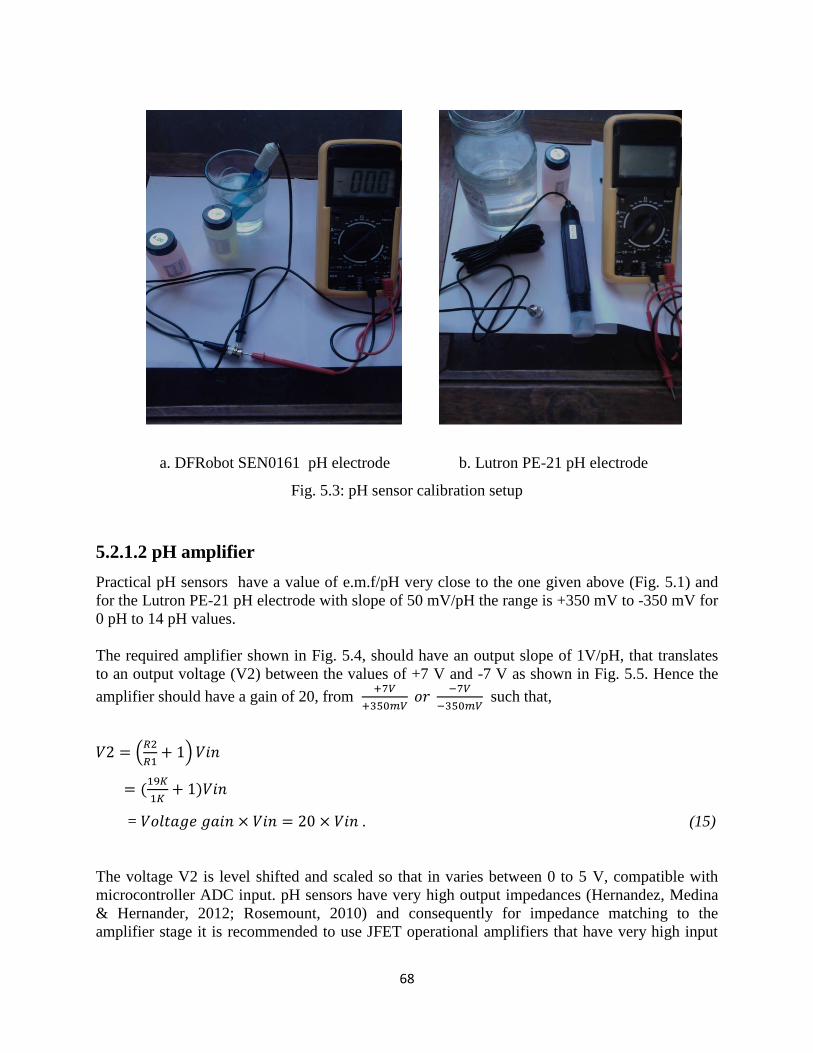
68
a. DFRobot SEN0161 pH electrode b. Lutron PE-21 pH electrode
Fig. 5.3: pH sensor calibration setup
5.2.1.2 pH amplifier
Practical pH sensors have a value of e.m.f/pH very close to the one given above (Fig. 5.1) and
for the Lutron PE-21 pH electrode with slope of 50 mV/pH the range is +350 mV to -350 mV for
0 pH to 14 pH values.
The required amplifier shown in Fig. 5.4, should have an output slope of 1V/pH, that translates
to an output voltage (V2) between the values of +7 V and -7 V as shown in Fig. 5.5. Hence the
amplifier should have a gain of 20, from
such that,
(
)
(
)
= . (15)
The voltage V2 is level shifted and scaled so that in varies between 0 to 5 V, compatible with
microcontroller ADC input. pH sensors have very high output impedances (Hernandez, Medina
& Hernander, 2012; Rosemount, 2010) and consequently for impedance matching to the
amplifier stage it is recommended to use JFET operational amplifiers that have very high input

69
impedances such as the TL082CP Dual Bifet op-amp (TL082, 2000). Leakage current that would
otherwise severely affect accuracy of the amplifier circuit is reduced by incorporation of a guard
ring (Kumen, 2009) around the input signal paths of the amplifier on the printed circuit board as
depicted in Fig. 5.6.
Fig. 5.4: pH amplifier and voltage level shifter section
pH=0 pH=7 pH=14
+7V 0 V -7V
Fig. 5.5: pH probe voltage output for the range 0 pH to14 pH for a 1V/pH slope
Fig. 5.6: Actual voltage allocation for pH membership function from pH12 to pH2

70
Fig. 5.7: BIFET OP-AMP printed circuit board incorporating a current leakage shield (guard)
( https://www.qrz.ru/reference/micro/analog/ad712.pdf)
The voltage level shifter is designed for pH ranges between 2 and 12, corresponding to a V2
voltage range of +5V to-5V since digesters operating outside these ranges are not realistic.
From this assertion it can be shown that:
(i) For pH12 and amplifier output V2 = -5 V,
( )
( )
( )
(16)
(ii) For pH7 and amplifier output V2 = 0 V,
(17)
(iii) For pH2 and amplifier output V2 = +5 V,

71
( )
(18)
5.2.2 Conductivity
This defines the ability of an aqueous solution to pass electricity, relative to the amount of ions in
that solution. The more ions that are present in the solution the more conductive the solution is as
depicted in Table 5.2. With reference to biogas digesters the concentration of dissolved salts in
the total dissolved solids (TDS) will define how conductive that feedstock solution is, since salts
readily form conducting ions. In addition to the total number of ions present the conductivity of
the feedstock solution increases with temperature. The interpretation of high conductivity then,
due to too much acidity or too much alkalinity is to indicate failing digester operation in-terms of
the depletion of the micro-organisms that produce methane gas. This is related to a high organic
loading rate and the presents of toxic soluble salts (Eu-agrobiogas, 2009; Kanokwan, 2006;
McCarty & McKinney, 1961).The basic principle of conductivity measurements whose units are
Siemens per cm (S/cm) is shown in Fig. 5.8.
Table 5.2: Conductivity values of common electrolytes at 25oC
(http://www.analyticalchemistry.uoc.gr/files/items/6/618/agwgimometria_2.pdf)
Common electrolyte Conductivity value
Pure water 0.055 μS/cm
Deionised water 1 μS/cm
Rainwater 50 μS/cm
Drinking water 500 μS/cm
Industrial wastewater 5 mS/cm
Seawater 50 mS/cm
1 mol/l NaCL 85 mS/cm
1 mol/l HCL 332 mS/cm

72
Let ( )
and ( )
(19)
(
) (
)
An ac voltage is used instead of a dc voltage to minimize the build-up of one specific polarity of
ion that would otherwise accumulate on either electrode thereby affecting the current drawn from
the supply and severely affecting the accuracy of measurement. The conductivity sensor will
need to be calibrated against a solution of known conductivity. This calibration normally seeks to
make correction for the cell constant.
Fig. 5.8: Conductivity measurement principle
(http://www.analyticalchemistry.uoc.gr/files/items/6/618/agwgimometria_2.pdf)
Variations of the conductivity sensor include the two electrode, four electrode or the inductive
type. The accuracy of measurement increases with adoption of the four electrode or the inductive
types. The block diagram for the measurement circuit is shown in Fig. 5.9. The two electrode
208DH conductivity electrode with a measuring range of was used.

73
Fig. 5.9: Block diagram of conductivity measurement system
The oscillator was the typical Wein Bridge designed to give a 20 Vpeak-peak waveform of
frequency 7.1 KHz as shown in Fig. 5.10. Fig. 5.11 shows the diagram for the conductance
amplifier incorporating the range selector.
Fig. 5.10: a) Wein Bridge oscillator for the electrical conductivity sensor circuit, and b) output
waveform

74
The complete circuit diagram is shown in Appendix F, where the conductivity probe was
connected to pin 6 of the LM324N quad operational amplifier (LM 324, 2001). From Tables
(4.1) & (5.2), a reasonable range of conductivity to select was 5 ~ 25 mS/cm. Now the
electrolyte resistance expression is given as (
), that translates to
value range of 200 ~ 40 Ω. The output of this circuit varied from 0 to 5 V as the value of the
electrolytes‟ electrical conductivity varied from very low to very high and a suitable range
scaling resistor (RR) was found to be 820 Ω.
Calibration was performed using two sodium chloride solutions pre-paired in-house at 25oC to
give conductivities of 10 mS/cm and 20 mS/cm respectively. The voltage output at each of these
solutions was measured and recorded. A plot shown in Fig. 5.12, of conductivity against output
voltage was done. From the plot the equation that relates electrical conductivity (EC) to final
output voltage (Vecadc) is formulated and this equation is given as:
(20)
Equation (20), gives the actual value of electrical conductivity in mS/cm directly from the sensor
immersed in the digester slurry. This equation is then incorporated into the software for use by
the alkalinity prediction equation (4).
-
+
LM324
+VDD
-VDD
Fig. 5.11: Conductance amplifier
Conductivity range selector (RR) Conductivity probe (RP)
Vout from Wein Bridge oscillator
20Vpp 100K
1K
0.2Vpp
To rectifier section

75
Fig. 5.12: Conductivity vs Voltage
5.2.3 Redox (Oxidation-reduction potential (ORP))
When an ion or atom releases an electron we term the process as oxidation of that ion or atom,
whilst the acceptance of an electron by the same is termed reduction.
Consider the equation:
(21)
is in a reduced state whilst is in an oxidized state.
Redox pontential(ORP) standardized against the hydrogen equation,
(22)
is a measure of the inclination of a substance(compound) to receive electrons. A high (positive)
ORP then implies a gain in oxygen, whilst a low (negative) ORP implies a loss of oxygen. This
is the voltage between the electron givers and the electron receivers that are present in the
feedstock (Bernhard, 2013). By definition anaerobic bacteria operates when there is no oxygen,
implying a low ORP. According to Bernhard (2013) an ORP of less than -300mV has been found
to be ideal for anaerobic microbes to function optimally. The output voltage specification of the
201DH ORP probe to be used in this project is specified . The same amplifier and
level shifter configuration as for the pH probe (See page 69) will be used where the required
amplifier should have an output voltage, corresponding to a V2 between the values of +5V and
-5V compatible for level shifting for microcontroller ADC. Hence the amplifier should have a
gain of 2½, from
such that,
y = 0.0049x - 0.3837
-5
0
5
10
15
20
25
30
0 1000 2000 3000 4000 5000 6000
EC (mS/cm)
Vceadc (mV)
Conductivity vs Voltage

76
(
)
(
)
= . (23)
Fig. 5.13, gives the complete schematic incorporating both pH redox sensors.
a.
b.
Fig. 5.13: pH and redox TL082CP OP AMP based amplifier circuit

77
For an oxygen reduction potential (redox) , the value of V2 from equation (23)
is and substituting this value of V2 into the expression ( ( ))
( ( ))
,
Vshift (VADC) is obtained as Likewise with , Vshift is obtained as
. To supply the correct value of redox in the prediction equation c source code, software
scaling of the analogue voltage at the input of the microcontroller is done. This is basically a
reverse process to obtain the value of from Vshift.
The constructed printed circuit board amplifier picture for pH and redox (ORP) is given in
Appendix H.1.
.
5.2.4 Buffer capacity measurement by titration
5.2.4.1 Volatile fatty acids and Alkalinity
The carbon acids called volatile fatty acids (VFA) are a result of the acidogenesis process in the
digester material. An increase in the concentration of the VFA between 1500 and 2000 mg/L will
significantly suppress the biogas production process. Hence being able to monitor this parameter
we can determine how stable the system is. Similarly alkalinity (buffer capacity) which is a
measure of the tendency to avoid pH change can also be used to determine how stable the
digestion process is. Typical alkalinity values in biodigesters range from 2000 – 5500 mg/L
bicarbonate and above 4000 mg/L bicarbonate means a good buffering capacity (Eu-agrobiogas,
2009; Labatut & Gooch, 2015; Wisconsin, 1992).
For this research titration measurements to determine23
the ratio of VFAs to Alkalinity (also
known as TIC (Total Inorganic Carbon)) (Lohri, 2008) and to evaluate the actual value of
alkalinity (can be used to formulate a much more accurate prediction equation) in
mg/l.bicarbonate are performed.
5.2.4.2 Titration24
procedure
(1) The sample is filtered through a fine membrane (order of 0.45μm) so as to remain with a
solution with no solid particles.
(2) Capture between 20 to 50 ml of the filtered sample in a glass or transparent container.
(3) Titrate (add) carefully 0.1 N sulphuric acid until pH 5.0 is reached. Write down the added
volume h1[ml] of titrant.
(4) Add more acid to get a pH 4.3 and write down the added volume h2[ml] of titrant.
(5) Add more acid to get a pH 4.0 and write down the added volume h3[ml] of titrant.
(6) During all these steps the resultant solution is constantly mixed as addition of acid is done.
(7) Calculate (Lohri, 2008) the values of alkalinity and volatile fatty acids as shown below.
23
Assess digester stability in the off-line mode. 24
Was done on-site and the results given in Chapter 8.

78
*
+ (24)
d1 = Sulphuric acid (H2SO4, 0.1N) used to change from pH 5.0 to pH 4.3 in ml
( )
N= Normality[mmol/l]
Sv=Initial sample volume [ml]
*
+ [
] (25)
d2 = Sulphuric acid (H2SO4, 0.1N) used to change from pH 5.0 to pH 4.0 in ml due to
HCO3/CO2 buffer
( )
N= Normality[mmol/l]
Sv=Initial sample volume [ml]
Alkalinity = Alkalinity [mmol/l]
Fig. 5.14: The titration setup
5.2.5 Temperature
The temperature of the digester slurry is measured by using a PT100 platinum resistance
temperature detector (RTD) that has the temperature resistance characteristics shown in
Fig. 5.15. From the PT100 resistance table (Thermocouple, 1999), probe resistances at various
temperatures are noted. However in this research the aspects considered when designing the
circuit of Fig. 5.16 based on the TL06125
operational amplifiers (TL061, 2004) are maximum
permissible RTD current, maximum possible ground temperatures in the digester vicinity and the
microcontroller voltage. A current of 1mA will cause some self-heating of 100 μW
( R), however this current will cause a small measurable voltage change.
25
The TL061CP operational amplifier is pin compatible with the 741 traditional operational amplifier.
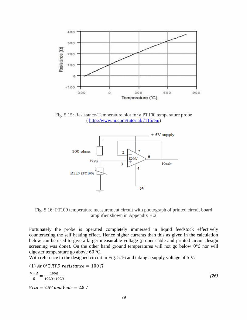
79
Fig. 5.15: Resistance-Temperature plot for a PT100 temperature probe
( http://www.ni.com/tutorial/7115/en/)
Fig. 5.16: PT100 temperature measurement circuit with photograph of printed circuit board
amplifier shown in Appendix H.2
Fortunately the probe is operated completely immersed in liquid feedstock effectively
counteracting the self heating effect. Hence higher currents than this as given in the calculation
below can be used to give a larger measurable voltage (proper cable and printed circuit design
screening was done). On the other hand ground temperatures will not go below nor will
digester temperature go above With reference to the designed circuit in Fig. 5.16 and taking a supply voltage of 5 V:
( )
(26)

80
( )
(27)
( )
(28)
The voltage output was then calibrated to give temperature readings and the expression
(obtained from MS-Excel plot) used in the software
development process.
5.2.6 Methane
In this research methane gas detection is made by use of the Flying Fish MH MQ2 gas sensor.
The basic structure of this sensor as shown in Fig. 5.17, comprises of tin dioxide (SnO2), the
material of which decreases in conductivity as the air becomes cleaner. As the gas concentration
increases the sensor‟s conductivity also increases. The sensor element (Rs) is heated to a
specified temperature for it to operate, hence it gets uncomfortably hot when powered on.
The sensor used here (Fig. 5.18), incorporates an electronics (amplifier) circuit board with the
following pins:
GND
+5 V
Do (Digital out) and
Ao (Analog out varying from 0 – 5 V)
The sensor module detects methane in the concentration ranges of 5000 ppm -20000 ppm.
Calibration of the sensor module is done by measuring a gas of known concentration (for
example 1000 ppm liquefied petroleum gas) and making the necessary adjustment on the module
potentiometer. However, the sensor module is factory calibrated. Fig. 5.19, gives a plot of the
sensitivity characteristics of the MQ2 sensor for different gas measurements.
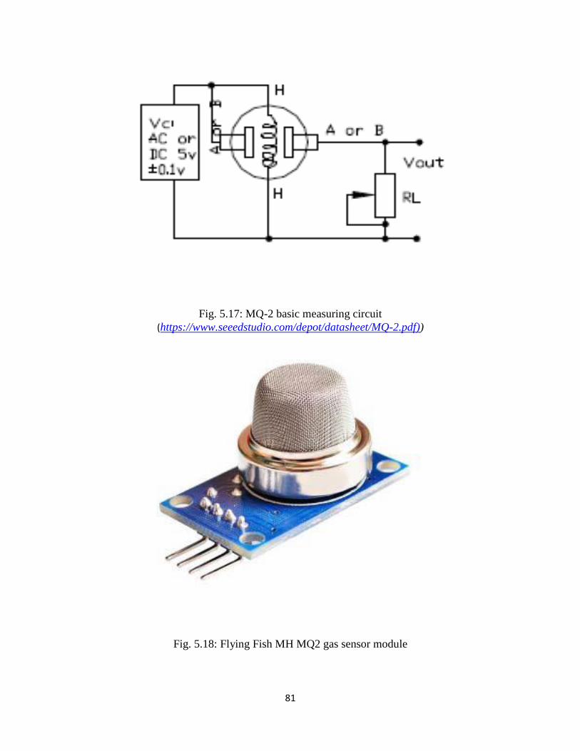
81
Fig. 5.17: MQ-2 basic measuring circuit
(https://www.seeedstudio.com/depot/datasheet/MQ-2.pdf))
Fig. 5.18: Flying Fish MH MQ2 gas sensor module

82
Fig. 5.19: Sensitivity characteristics of the MQ-2 gas sensor
(https://www.seeedstudio.com/depot/datasheet/MQ-2.pdf)
5.2.7 Carbon dioxide
For carbon dioxide measurement an MG811 carbon dioxide sensor module (Fig. 5.20) has the
same constructional structure as for the methane module is used. The module has the following
specifications:
Four pins comprising +6 V supply, analog output (AO), digital output (DO) and GND
LM393 and carbon dioxide sensor circuit board
An output voltage range of
0 to 10000ppm carbon dioxide detection concentration range.
Just like in the methane sensor the carbon dioxide sensor material is also heated to operating
temperature. The carbon dioxide sensor material made up of polymer will produce an
electromotive force (EMF) that is proportional to the carbon dioxide concentration as depicted in
Fig. 5:22. The sensor module is factory calibrated.
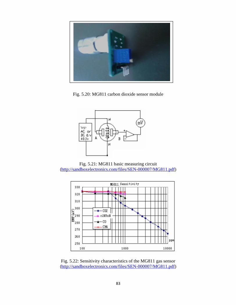
83
Fig. 5.20: MG811 carbon dioxide sensor module
Fig. 5.21: MG811 basic measuring circuit
(http://sandboxelectronics.com/files/SEN-000007/MG811.pdf)
Fig. 5.22: Sensitivity characteristics of the MG811 gas sensor
(http://sandboxelectronics.com/files/SEN-000007/MG811.pdf)

84
5.2.8 Pressure
The gas pressure sensor specified here is of the type that is used on flammable gases. Since the
normal accepted methane gas pressures in the digester are limited to 15 KPa (0.15 bar or 2.17557
psi), the pressure sensor used should measure at least 30 KPa (0.3 bar or 4.35113 psi). For this
research use is made of the model RC 300 Liyuan Electronic 1MPa 4-20 mA 24 V gas pressure
sensor. The pressure sensor supplied by the photovoltaic 24 V Dc supply directly provides an
output between the limits of 4 to 20 mA as depicted in Fig. 5.23.
Fig. 5.23: Linear relationship between pressure and sensor output
( http://www.wika.us/upload/BR_CAT_Electronic_Pressure_en_us_17801.pdf)
Fig. 5.24 gives the circuit diagram of the 4-20mA to 1-5V converter for the analogue to digital
converter (ADC) input to the microcontroller. From Fig. 5.24, it can be shown that:
(1) For 20 mA,
( )
and (29)
(2) For 4mA,
( )
(30)

85
Calibration of the pressure transmitter module is done by using a bicycle pump that has a
calibrated pressure gauge connected to it. The procedure involves the measurement of voltage
output (Vadc) at different pressures up to 20 KPa and the resulting software equation (Fig. 5.25)
of obtaining pressure at various voltage levels formulated. The constructed printed circuit board
amplifier is shown in Appendix H.3.
Fig. 5.24 Circuit diagram of the 4-20 mA to 1-5 V converter for the analogue to digital converter
(ADC) input to the microcontroller
Table 5.3: Calibration of pressure sensor using bicycle pump
Pressure (KPa) Voltage (V)
0
2
4
6
1.28
1.73
2.21
2.47
8
10
12
14
16
18
2.64
2.85
3.11
3.46
3.89
4.39

86
Fig. 5.25: Calibration of pressure sensor
The equation on Fig. 5.25, directly gives the value of biogas pressure (KPa) in the digester, and
is used in the software coding of the pressure routine.
5.2.9 Level
Level is monitored by the use of two stainless steel sealed vertical float switches. One switch
(SW1) is positioned to be at the highest slurry level point whilst the other switch (SW2) is
positioned at the lowest slurry level point. The switching current of
is small
enough not to cause any danger in the digester due to arcing. Fig. 5.26, shows how the switches
are connected to the microcontroller.
y = -0.1612x2 + 7.2031x - 9.7921
-5
0
5
10
15
20
0 1 2 3 4 5
Pre
ssu
re (
KP
a)
Voltage (V)
Fig. 5.26: Level float switches connected to microcontroller
10 KΩ
SW1
SW2
10 KΩ
10 KΩ
D0
D1
Microcontroller 10 KΩ
+5V

87
5.2.10 Oxygen
The trace oxygen sensor module is made up of a “galvanic fuel cell” (electro-chemical in nature)
and an electronics circuit board housing a resistive network that includes resistors and an NTC
for current to voltage conversion and temperature compensation respectively. Initially no output
is produced by the oxygen cell until it is placed in the presence of oxygen. Oxygen initiates a
chemical reaction after which the oxygen cell produces an electrical current. This electrical
current is converted to a voltage by placing a resistor across the cell terminals. The sensor
voltage output that typically ranges from 8-13 mV in air to 175 mV in one hundred percent
oxygen (Gurr, 2013) is directly proportional to the oxygen concentration. Calibration of the
sensor is then easily done by measuring the voltage output of the known concentration of oxygen
air which is 20.945 % (Lauer, 2016).
The oxygen cell is normally made up of a lead anode, a platinum cathode and a potassium
electrolyte to give the following reaction breakdown:
(31)
(32)
(33)
Equation (32) clearly shows that electrons will flow from the anode to the cathode if an external
path is provided, hence the current nature of the generated signal. Furthermore from the same
equation it is noted that lead is depleted to form lead oxide which implies that the oxygen sensor
will eventually run out of lead leading to its death. According to Gurr (2013) the average lifetime
of this type of oxygen sensor is three years.
By the time the oxygen reaches 30 % the alarm system should have already come on. This
corresponds to a voltage of
, which is taken as the upper limit in the design.
To scale up the sensor signal to 0-5V the circuit of Fig. 5.27, with a gain of
is
used. A gain of 91 instead giving a voltage range of 0-4.78 V was used. The voltage output in air
is 0.73-1.18 V.
The constructed printed circuit board amplifier is shown in Appendix H.3, where it shares the
quad LM324 operational amplifier with the pressure sensor.

88
5.2.11 Voltage detection in PV system
In coming up with the voltage divider measurement circuit for converting the 24V photovoltaic
battery value to 0-5V it was required to take into consideration the maximum allowable source
impedance of the microchip microcontrollers. The recommended maximum source impedances
for microchip 8/10 bits microcontrollers is 10KΩ and for 12bits its‟ 2.5 KΩ (Microchip, 2015b).
With reference to Fig. 5.28, let:
and (34)
, then
.
The standard values of are taken as respectively where the
parallel combination (source impedance) of the resistors yields
.
The calculated source impedance is clearly less than the maximum allowable value. Furthermore
the normal output of a 100 % SOC battery during charging about 26 V, implying that the current
at this point through the resistors is
Therefore the maximum output to the
microcontroller is given as
The photocell output at the PV panel is measured by the sensing circuit as shown in Chapter 4,
Fig. 4.11.
430 Ω
39 KΩ
-
+ 0-4.78V adc input
Fig. 5.27: Oxygen sensor signal amplifier
LM324

89
5.2.12 Current detection in PV system
For the dc charging current which is limited to 5 A the current measurement system is as shown
in Fig. 5.29, where the following observations are made: A series resistance of 0.05 Ω is used to give a maximum power output of
voltage drop across series resistor is Vs , where:
is scaled up to 5 V by multiplying by the gain factor. (35)
Gain of op-amp circuit is 20.
Fig. 5.29: LM324 Charging current sensing circuit for microcontroller
+
_
Charge + Controller _
+
Battery
_
Vs
0.05Ω 2W
dc charging current
Rf
Rin
+5V
Fig. 5.28: Battery charging voltage measuring circuit for microcontroller input
+24V from battery bank
R1
R2
(Vadc ) 0-5 V microcontroller
input
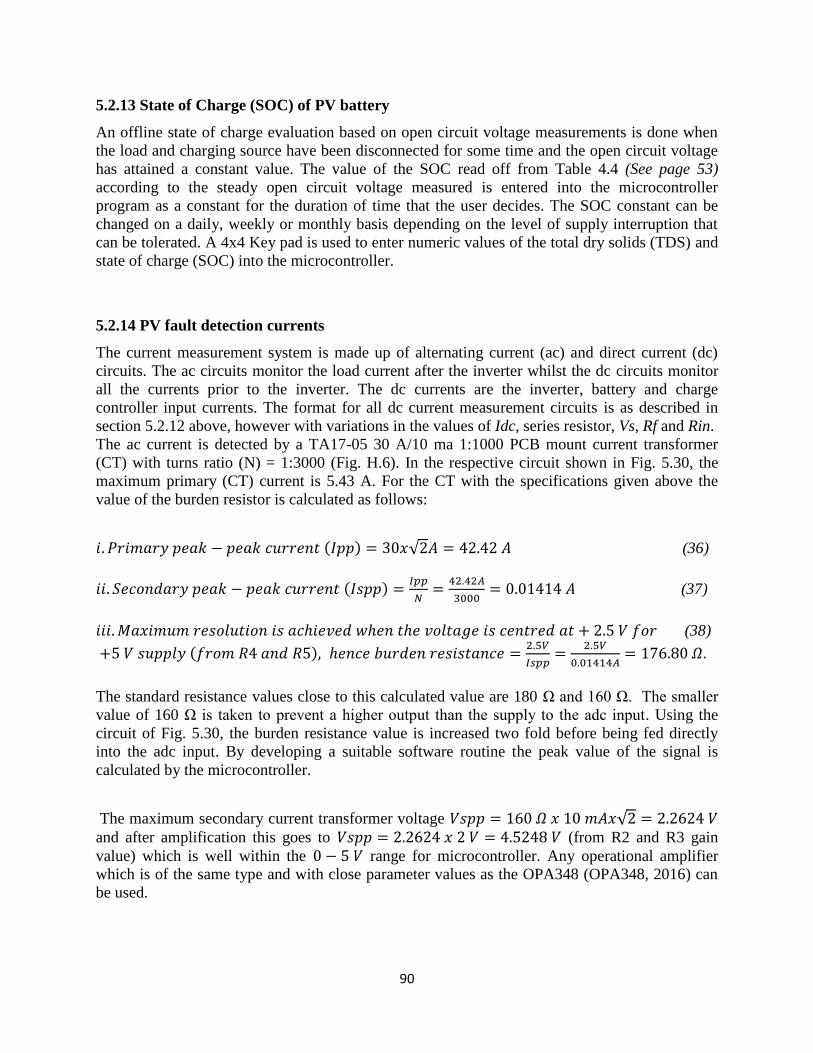
90
5.2.13 State of Charge (SOC) of PV battery
An offline state of charge evaluation based on open circuit voltage measurements is done when
the load and charging source have been disconnected for some time and the open circuit voltage
has attained a constant value. The value of the SOC read off from Table 4.4 (See page 53)
according to the steady open circuit voltage measured is entered into the microcontroller
program as a constant for the duration of time that the user decides. The SOC constant can be
changed on a daily, weekly or monthly basis depending on the level of supply interruption that
can be tolerated. A 4x4 Key pad is used to enter numeric values of the total dry solids (TDS) and
state of charge (SOC) into the microcontroller.
5.2.14 PV fault detection currents
The current measurement system is made up of alternating current (ac) and direct current (dc)
circuits. The ac circuits monitor the load current after the inverter whilst the dc circuits monitor
all the currents prior to the inverter. The dc currents are the inverter, battery and charge
controller input currents. The format for all dc current measurement circuits is as described in
section 5.2.12 above, however with variations in the values of Idc, series resistor, Vs, Rf and Rin.
The ac current is detected by a TA17-05 30 A/10 ma 1:1000 PCB mount current transformer
(CT) with turns ratio (N) = 1:3000 (Fig. H.6). In the respective circuit shown in Fig. 5.30, the
maximum primary (CT) current is 5.43 A. For the CT with the specifications given above the
value of the burden resistor is calculated as follows:
( ) √ (36)
( )
(37)
(38)
( )
The standard resistance values close to this calculated value are 180 Ω and 160 Ω. The smaller
value of 160 Ω is taken to prevent a higher output than the supply to the adc input. Using the
circuit of Fig. 5.30, the burden resistance value is increased two fold before being fed directly
into the adc input. By developing a suitable software routine the peak value of the signal is
calculated by the microcontroller.
The maximum secondary current transformer voltage √
and after amplification this goes to (from R2 and R3 gain
value) which is well within the range for microcontroller. Any operational amplifier
which is of the same type and with close parameter values as the OPA348 (OPA348, 2016) can
be used.

91
5.3 OUTPUT CIRCUITS
5.3.1 Standard output devices
For the audio alarms, status LEDs, solenoid close valve driver and LCD display, standard output
interfacing circuits have been used. The following is the connection breakdown:
(1) An LED with a current limiting resistor in series is directly driven by one of the
microcontroller output ports.
(2) A Piezo buzzer also driven directly at resonance by one the microcontroller output ports.
(3) A solenoid coil in parallel with a freewheeling diode connected to the collector of a transistor
driven by one of the microcontroller output ports as shown in Appendix G.
(4) A 16x2 LCD display directly connected to six microcontroller output ports.
Fig. 5.30: Current transformer amplifier
( https://e2e.ti.com/support/amplifiers/precision_amplifiers/f/14/t/108187)

92
5.3.2 Pulse width modulation
The varying duty cycle which is the result of the charging/discharging fuzzy logic algorithm is
used to control the output through the charge controller. The charge controller used in this study
is the buck type. The design method and circuit diagram (Appendix G) for this charge controller
is as detailed by Ejury (2013) and by Rashid (2003).
5.4 BASELINE MEASUREMENTS
Baseline measurements are those measurements made with the sensor circuits as standalone and
not connected to the embedded system (offline measurements). These measurements assist in
sensor calibration or in developing equations to be incorporated into the software development
process prior to the simulations.
5.4.1 Titration baseline measurements
In addition to providing alkalinity value, titrations also allow for the calculation of volatile fatty
acids (VFA) as a periodical offline compliment to access the stability of the digester in biogas
generation. This includes the evaluation of the ratio of VFAs to Alkalinity given in equation
(39) to complement the on line stability measurements. Using the titration procedure above (See
page 77), a sample of the results are shown in Table 5.4. At the same time, when the value of
alkalinity was being calculated from titration, the other measurements of pH, redox and electrical
conductivity where also done. The measurement results in this section are distributed over a
number of days.
Table 5.4: Field titration results
Slurry
pH
sv[ml] h1[ml] h2[ml] h3[ml] d1[ml] d2[ml] Alkalinity
[mg/L
bicarbonate]
VFAs [mg/L
acetic acid
equivalents]
6.9 20 4.5 0.8 0.13 5.3 0.93 2148.01845 518.211
*
+
*
+
*
+
*
+ (39)
Where A= Acids
TIC= Total Inorganic Carbon
VFA and Alkalinity are defined as before.
According to Lohri (2008), ‘Alkalinity [mmol/l] needs to be converted to TIC [mg/l CaCO3] by
multiplying it with half the molecular weight of CaCO3 (100.084/2=50.042), as each molecule of
CaCO3 can take up (
) ‘.
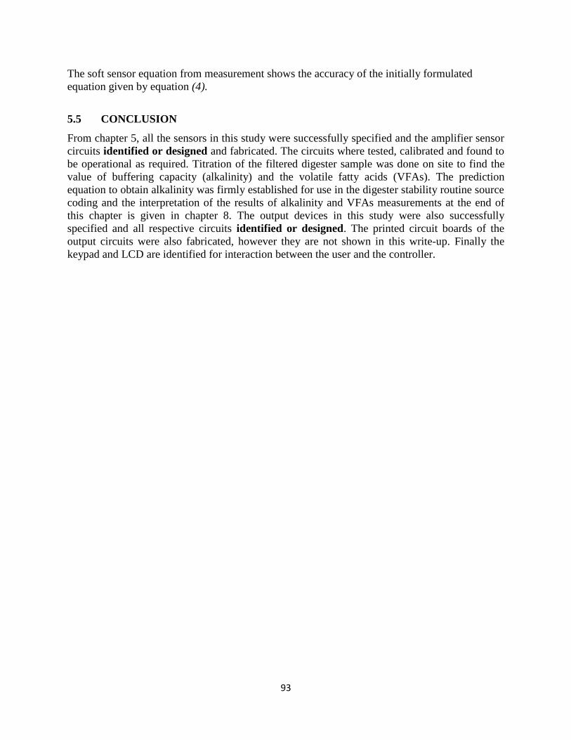
93
The soft sensor equation from measurement shows the accuracy of the initially formulated
equation given by equation (4).
5.5 CONCLUSION
From chapter 5, all the sensors in this study were successfully specified and the amplifier sensor
circuits identified or designed and fabricated. The circuits where tested, calibrated and found to
be operational as required. Titration of the filtered digester sample was done on site to find the
value of buffering capacity (alkalinity) and the volatile fatty acids (VFAs). The prediction
equation to obtain alkalinity was firmly established for use in the digester stability routine source
coding and the interpretation of the results of alkalinity and VFAs measurements at the end of
this chapter is given in chapter 8. The output devices in this study were also successfully
specified and all respective circuits identified or designed. The printed circuit boards of the
output circuits were also fabricated, however they are not shown in this write-up. Finally the
keypad and LCD are identified for interaction between the user and the controller.

94
CHAPTER 6
SOFTWARE DEVELOPMENT AND SIMULATION
6.1 INTRODUCTION
In this chapter, detailed software coding in C source codes is proposed to execute the fuzzy logic
algorithms and module flowcharts. Simulation of the written programs that will be „burnt‟ into
the PIC18F4550 microcontroller is performed using both microchip‟s MPLABXIDE and
Labcenter‟s Proteus software packages. Section 6.2 details the general procedure of calculating
the degree of membership of the commonly used membership functions adopted in this study.
Digester system stability test software coding development and simulation is done in section 6.3,
while the development of the software code and simulation of the biogas output amount is
performed in section 6.4. Section 6.5 details the biogas fault detection software development and
simulation process. Software coding and simulation of the battery charging/discharging and solar
system fault detection and status modules are detailed in section 6.6 and section 6.7 respectively,
while section 6.8 covers the conclusion of this chapter.
6.2 UNIVERSAL DEGREE OF MEMBERSHIP CALCULATION METHOD
The common trapezoidal membership function shown in Fig. 6.1 (i) , can be reduced or
modified either to a triangular function Fig. 6.1 (ii), a monotonically decreasing linear- function
Fig. 6.1 (iii), or monotonically increasing linear- function Fig. 6.1 (iv) (See page 18) by
appropriate shifting of the positions of b and c on the diagram.
Fig. 6.1: (i).Trapezoidal function,(ii). Triangular function,(iii). Monotonically decreasing
function and (iv). Monotonically increasing function

95
It is required to find the actual degree of membership for any value of input. This is done by
establishing the slopes and lower/upper limits to be incorporated into the software development
process for the particular membership function (Viot, 1993). In the Fig. 6.1, the lower limit is
given by a, whilst the upper limit in given by d.
Universal degree of membership of the above membership functions subroutines whose
expressions are given below are then easily developed (Nhivekar et al., 2011).
( ) {
(40)
for monotonically decreasing linear-function membership function,
( )
{
(41)
For triangular membership function, and
( ) {
(42)
for monotonically increasing linear-function.
In the special case (which I have adopted in my project for simplicity of calculation) points 2
will directly be above points 1 as shown in Fig. 6.2. Discrimination between these special case,
though not symmetrical membership functions is achieved by selecting the calculation of degree
of membership (μ) between say points 1 and 2 for C as shown below (Vuong et al., 2006). The
respective degree of membership for B between point 1 and point 2 as defined for C is then given
as (1-μ).

96
Fig. 6.2: Discrimination between overlapping membership functions
6.3 DIGESTER SYSTEM IMBALANCE EARLY WARNING SOFTWARE CODING
AND SIMULATION
6.3.1 Stability routine software
The routine shown as Listing one, in Appendix E1, successfully calculates the degree of
membership for both pH and Alkalinity membership functions for any given input and outputs
these values onto a for latter retrieval (this is a dynamic system). The listing also
shows the inference process that includes calculation of the firing strength of each rule by use of
the data stored in the and simultaneous reference to the rule matrix for digester
operation given in Table 6.1. The rule matrix is dynamically mapped onto a
(digesterop[5][3] as shown in the listing.
The routine also calculates the output combination of the rules, defuzzification using the centre
of gravity (COG) method, activates alarms and finds out whether the cause for poor digester
stability is due to too low a pH value,too high a pH value or too low a buffering capacity.

97
Table 6.1: Structure of the used for pH and alkalinity degree of
membership values
Q.acid degree of membership value
Array position [0][0]
M.acid degree of membership value
Array position [0][1]
Nuetral degree of membership value
Array position [0][2]
M.alkaline degree of membership value
Array position [0][3]
Q.alkaline degree of membership value
Array position [1][0]
Low degree of membership value
Array position [1][1]
Medium degree of membership value
Array position [1][2]
High degree of membership value
Array position [1][3]
6.3.2 Stability simulation results
Fig. 6.3 gives a representation of the analogue inputs of pH, redox and conductivity from the
sensor circuits. The potentiometers given in the diagram vary the voltage from 0 to +5V in
exactly the same way as the input sensor circuits would. The +2V shown, say for the
potentiometer labeled pH corresponds to a pH value of 8, as read from the diagram in Fig. 5.6
(See page 69). This is exactly the pH value given in Fig. 6.5.
Fig. 6.3: pH, redox and electrical conductivity analogue voltage inputs

98
A sample reading of the percentage digester stability value reading is shown in Fig. 6.4. This
value, including the values of pH and buffering capacity values given in Fig. 6.5 will
momentarily appear on the LCD for the user, before the diagnostic information shown in Fig. 6.6
is given.
Fig. 6.4: Percent digester stability output on LCD
Fig. 6.5: Typical pH and alkalinity values from analogue inputs

99
Fig. 6.6: Poor digester stability alarm sounder
Fig. 6.7: Information on LCD about digester stability status
In the digester stability routine, the alarm takes the form of an audio sounder shown connected to
the microcontroller in Fig. 6.6. These simulations provide successful activation of the digester
failed alarm system. With respect to Fig. 6.7, the information given here is very important as in
tells the user directly what the problem is, and what action he/she should take to address the
problem at hand. From Table 6.2, the percentage stability status for various values of pH and
alkalinity are observed. The defuzzified digester operation status is shown as a percentage for a
specific pair of inputs of pH and alkalinity. From the output membership functions of Figure 2.8
(See page 24), it is then established that any defuzzified output above 60 % is stable, between
40 % and 60 % is failing whilst that below 40 % is not stable.
As given by the MPLABXIDE clean and build option, the PIC18F4550 program memory used is
58.2 % and data memory used is 17.0% used by this routine which is part of Listing one.

100
Table 6.2: Digester stability output for the two inputs of pH and Alkalinity
Input 1
Input 2 (Alkalinity in mg/L bicarbonate)
(pH) 3499 3600 3800 4200 4400 4600 4.9 25% 25% 25% 25% 25% 25% 5.59 29% 49.1% 39.4% 37.4% 35.3% 35% 5.75 35% 50% 50% 50% 50% 50% 5.8 37% 50% 53.5% 54.5% 54.5% 54.5% 6 50% 58.3% 66.8% 75% 75% 75% 6.1 50% 58.3% 66.8% 75% 75% 75% 6.3 50% 58.6% 66.8% 75% 75% 75% 6.75 50% 58.5% 62% 75% 75% 75% 6.8 50% 58.3% 60.7% 75% 75% 75% 7 50% 58.3% 66.8% 75% 75% 75% 7.3 50% 58.6% 66.8% 75% 75% 75% 7.6 50% 60.7% 64.7% 75% 75% 75% 7.8 50% 64.3% 64.3% 75% 75% 755% 8.2 36.9% 50% 53.5% 50% 54.5% 54.5% 8.4 29.4% 50% 40.3% 42.1% 36.1% 36.1% 8.7 25% 25% 25% 25% 25% 25%
6.4 BIOGAS OUTPUT AMOUNT SOFTWARE CODING
AND SIMULATION
6.4.1 Biogas amount routine software
The routine that is part of Listing one in Appendix E1, successfully measures digester
temperature and calculates the OLR, HRT and the expected biogas quantity in litres. It also gives
the actual quantities of methane and carbon dioxide in litres present in the biogas.
6.4.2 Biogas amount simulation results
The simulation results for this module are given in Figs. 6.8 & 6.9. The user of the digester reads
real time temperature, hydraulic retention time, the organic loading rate and the actual amounts
of methane and carbon dioxide produced.
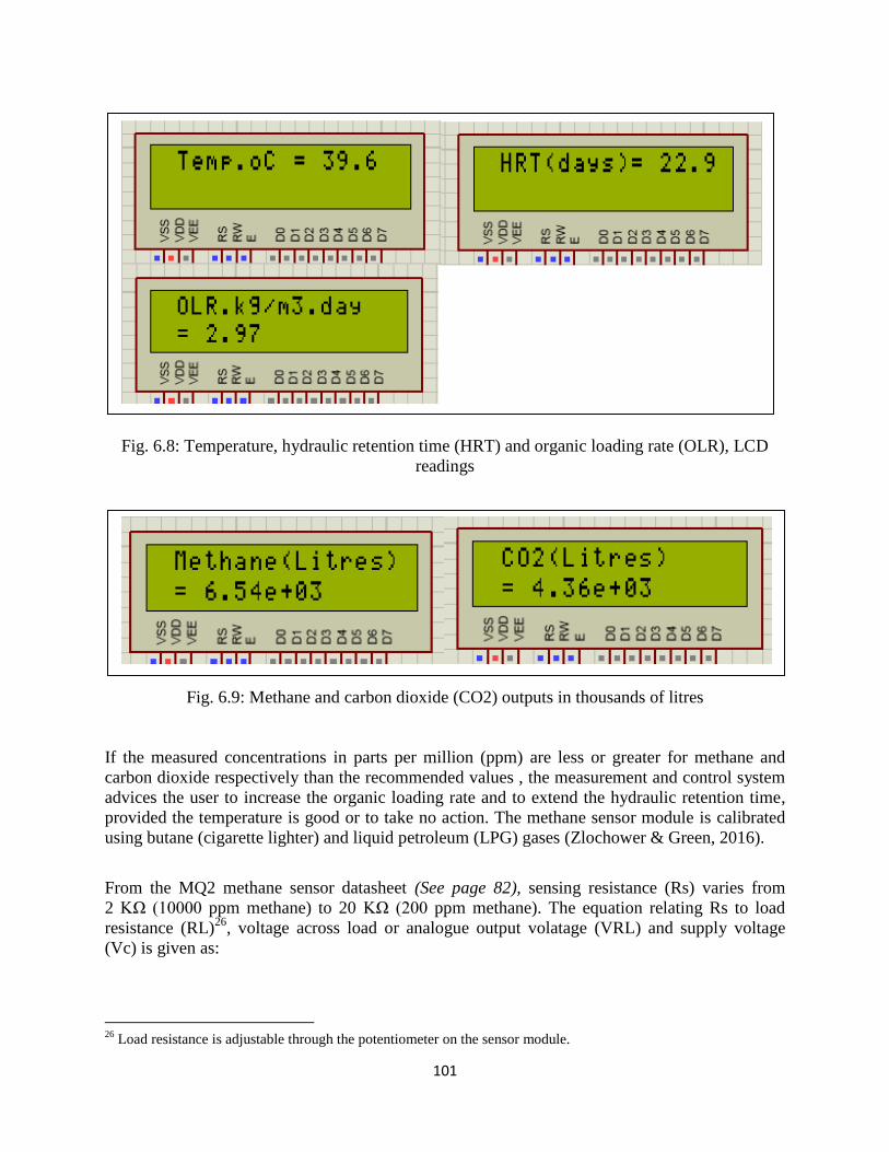
101
Fig. 6.8: Temperature, hydraulic retention time (HRT) and organic loading rate (OLR), LCD
readings
Fig. 6.9: Methane and carbon dioxide (CO2) outputs in thousands of litres
If the measured concentrations in parts per million (ppm) are less or greater for methane and
carbon dioxide respectively than the recommended values , the measurement and control system
advices the user to increase the organic loading rate and to extend the hydraulic retention time,
provided the temperature is good or to take no action. The methane sensor module is calibrated
using butane (cigarette lighter) and liquid petroleum (LPG) gases (Zlochower & Green, 2016).
From the MQ2 methane sensor datasheet (See page 82), sensing resistance (Rs) varies from
2 KΩ (10000 ppm methane) to 20 KΩ (200 ppm methane). The equation relating Rs to load
resistance (RL)26
, voltage across load or analogue output volatage (VRL) and supply voltage
(Vc) is given as:
26
Load resistance is adjustable through the potentiometer on the sensor module.

102
( )
, (43)
Where the ratio value of
is used in the software coding.
From Fig. 5.20 (See page 83), with respect to the methane gas (CH4), corresponding values of
ppm for different ratio values of Rs/Ro are obtained and shown in Table 6.3.
Table 6.3: Methane gas PPM readings27
with respect to ratio Rs/Ro for the MQ2 sensor
PPM Rs/Ro
200 3
500 2.25
800 2
1000 1.85
2000 1.6
3000 1.5
5000 1.1
10000 0.7
To obtain a linear equation for ppm calculation the natural logarithms of the values in Table 6.3
are used instead. These are tabulated in Table 6.4, and plotted as in Fig. 6.10. The resultant
equation28
is used in the software development process for ppm calculation. Fig. 6.11 shows
typical ppm reading on the LCD.
Table 6.4: Natural logarithm methane gas PPM readings with respect to ratio Rs/Ro for the MQ2
sensor
lnPPM
lnRs/Ro
5.298317 1.098612
6.214608 0.81093
6.684612 0.693147
6.907755 0.615186
7.600902 0.470004
8.006368 0.405465
8.517193 0.09531 9.21034 -0.35667
27
These values when plotted will result in an exponential equation for ppm calculation. 28
It is necessary to convert the natural logarithms to common logarithms in the software process.
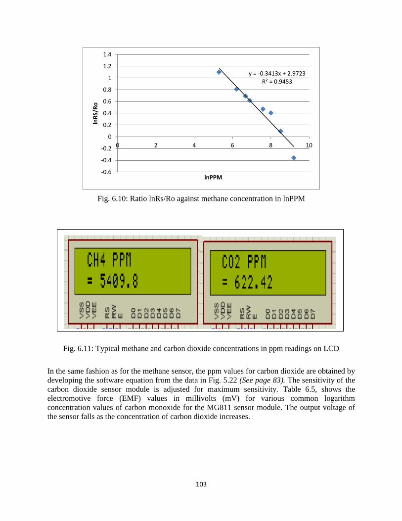
103
Fig. 6.10: Ratio lnRs/Ro against methane concentration in lnPPM
Fig. 6.11: Typical methane and carbon dioxide concentrations in ppm readings on LCD
In the same fashion as for the methane sensor, the ppm values for carbon dioxide are obtained by
developing the software equation from the data in Fig. 5.22 (See page 83). The sensitivity of the
carbon dioxide sensor module is adjusted for maximum sensitivity. Table 6.5, shows the
electromotive force (EMF) values in millivolts (mV) for various common logarithm
concentration values of carbon monoxide for the MG811 sensor module. The output voltage of
the sensor falls as the concentration of carbon dioxide increases.
y = -0.3413x + 2.9723 R² = 0.9453
-0.6
-0.4
-0.2
0
0.2
0.4
0.6
0.8
1
1.2
1.4
0 2 4 6 8 10
lnR
S/R
o
lnPPM

104
Table 6.5: Tabulated EMF values for the MG811 sensor against common logarithm carbon
dioxide concentration in parts per million
EMF (mV) PPM Log10 PPM
324 400 2.60206
314 600 2.778151
308 800 2.90309
303 1000 3
298 1500 3.176091
293 2000 3.30103
290 2500 3.39794
286 3000 3.477121
281 4000 3.60206
275 6000 3.778151
269 8000 3.90309
265 10000 4
Fig. 6.12: Carbon dioxide concentration in logPPM against sensor EMF voltage
From Fig. 6.12, the equation used in the calculation29
of the ppm for carbon dioxide is given by:
( ) . (44)
29
The anti-log of equation (44) gives the value of the ppm for carbon dioxide gas.
y = -0.0247x + 10.55 R² = 0.9957
0
0.5
1
1.5
2
2.5
3
3.5
4
4.5
0 50 100 150 200 250 300 350
logP
PM
EMF (mV)

105
6.5 BIOGAS SYSTEM FAULT DETECTION AND STATUS SOFTWARE CODING
AND SIMULATION
6.5.1 Biogas system fault detection and status routine software
The routine that is part of Listing one in Appendix E1, successfully performs biogas fault
detection and informs about the safety status of the digester.
6.5.2 Biogas system fault detection and status simulation results
A methane leak (greater than 1000 ppm) in the room activates a leak alarm and switches on a
yellow LED, while oxygen ingress (greater than 15%) into the digester is represented by a green
LED coming on and activation of the same alarm which is common to both situations.
Furthermore, in both cases of methane leak and oxygen ingress, an emergency solenoid valve is
successfully activated to cut off the main line supplying the user until the problem is rectified30
.
The simulation also successfully monitors the biogas pressure and slurry level in the digester.
An additional float switch (SW12) to those in Fig. 5.26 (See page 86), is placed between SW1
and SW2 where:
1) SW1 is placed at P-line (will activate exactly at 0.13m above P-Line).
2) SW12 is placed between P-line and Zero-line (will activate at 0.25m above P-line).
3) SW2 is placed at Zero-line (will activate at 0.45m above P-line, just below Zero-line).
4) SW1 (OFF) - slurry too low (activate alarm).
5) SW1 (ON) – minimum slurry level (alarm off).
6) SW1 (ON) & SW12 (OFF) - take displacement as 0.13m (LL).
7) SW12 (ON) – take displacement as 0.25m (BPO).
8) SW2 (ON) – take displacement as 0.45m (HL).
It is important to note that, to obtain a finely tuned level measurement system for a large
number of varying slurry displacement levels, a moving gauge needs to be used instead. This
gauge will produce varying analogue voltages calibrated to give displacement values (not
implemented in this study).
The equation from Fig. 5.25 (See page 86), gives the value of the pressure of the biogas in KPa,
while the equation in Fig. 6.13, is used in the software coding to find the concentration of oxygen
in the digester.
30
When solenoid valve closes the program waits until reset button is pressed (MCLR pin 1 on PIC18F4550)

106
Fig. 6.13: Oxygen concentration as percentage against sensor output voltage
Fig. 6.14, shows a typical LCD output of the digester danger level as a percentage. The higher
the percentage, the more compromised is the operation of the digester.
Fig. 6.14: Digester danger level LCD reading
6.6 SOALAR BATTERY CHARGING/DISCHARGING SOFTWARE CODING
AND SIMULATION
6.6.1 Solar battery charging/discharging routine software
The routine given as Listing two in Appendix E2, successfully calculates the duty cycle that
drives the buck charge controller. The duty cycle is based on the charging voltage, charging
current and SOC of the battery.
The charging voltage is obtained from direct measurement as shown in Fig. 5.28 (See page 89).
The standard resistor values of R1 and R2 give a charging voltage of:
( ( ) , (45)
y = 0.4791x + 16.154
0
20
40
60
80
100
120
0 50 100 150 200
% O
xyge
n
Sensor output (mV)

107
which this simplifies to .
With respect to charging current measurement, taking equation (35) and considering Fig. 5.29
(See page 89), the voltage drop across the series resistor (0.05 Ω 2 W) is given by:
. (46)
From equation (46), the expression of the voltage drop simplifies to , and
consequently the charging current is given by:
(47)
The expressions of the charging voltage, charging current and SOC are used in the fuzzy logic
controller software coding for battery charging/discharging.
6.6.2 Solar batter charging/discharging simulation results
The routine written for battery charging was successfully simulated. The routine sensed the
charging voltage and charging current, adjusting the duty cycle accordingly in the process to
obtain optimum battery charging. Fig. 6.15, shows typical values of duty cycle, charging voltage,
charging current and battery‟s state of charge.
Fig. 6.15: Typical values of duty cycle, charging voltage, charging current and
battery‟s state of charge
108
6.7 SOLAR SYSTEM FAULT DETECTION AND STATUS SOFTWARE CODING
AND SIMULATION
6.7.1 Solar system fault detection and status routine software
The routine that is part of Listing two in Appendix E2, successfully identifies any faulty piece of
equipment that makes up the photovoltaic system and performs overload protection of the
inverter system from the users where an alarm is activated if the current limit is breached. The
software also successfully notifies about the status of the solar panel shading levels to include
partial, prolonged or very high31
shading levels
6.7.2 Solar system fault detection and status simulation results
Fig. 6.16 (a), shows typical solar panel shading level. A high percentage reading as shown in
Fig. 6.16 (a), implies a high shading level. Using the information given in section 5.2.14 (See
page 90), the analogue current transformer (CT) voltage from the CT amplifier in the
microcontroller was converted to provide the value of the alternating load current being drawn
from the inverter. Fig. 6.16 (b), shows the status of the load current being drawn by the user as
percentage (%) of the maximum allowable value. With respect to user load current, the routine
also successfully activates a flashing LED when this percentage becomes high and eventually
activates an alarm when the current being drawn becomes too high.
a. b.
Fig. 6.16: a) Shading level of solar panel, and b) load current as a percentage of allowed
amperage
6.8 CONCLUSION
In chapter 6, all the software routines in this study were successfully coded in C source codes
and all the simulations done. The simulations behaved as expected, however there was need to
improve on the coding to make the programs smaller (consider coding in less memory occupying
assemble language) so that they occupied less PIC18F4550 microcontroller memory. The PWM
(duty cycle) output signal derived from the simulation software will be implemented in the CCP
(compare capture pwm) registers and output through microcontroller pins RC1, RC2 or RB3 to
switch on and off the charge controller. In Chapter 7, all the developed programs without further
modification where uploaded (“burnt”) into the microcontroller.
31
These are shading levels higher than normal shadows in day light.

109
CHAPTER 7
EMBEDDED SYSTEM DESIGN
7.1 INTRODUCTION
In this chapter the complete hardware for the measurement and control system was realized. The
hardware structure is dealt with in section 7.2, to include integrated circuit (i.c) pin designation
and clock signal derivation. Section 7.3, details the procedure for programming PIC18F4550
microcontroller, while section 7.4 shows how the respective power supplies were obtained.
Section 7.5, which is the conclusion, gives a description of how the different circuits of the
embedded system were constructed.
7.2 HARDWARE STRUCTURE
7.2.1 Integrated circuit (i.c) pin designation
Fig. 7.1 shows the pin structures of the LM324N and TL082CP operational amplifiers (OP-
AMP). From the analysis of these pin structures it is shown that one LM324N OP-AMP (LM
324, 2001) can accommodate up to four different inputs and the TL082CP (TL082CP, 2000) up
to two different inputs. Specifically, the conductance amplifier used one complete LM324N OP-
AMP, while one TL082CP was used for the pH and redox sensors.
Fig. 7.1: Pin structures of the a) LM324N, and b) TL082CP operational amplifiers
The pressure, oxygen and photovoltaic current charging sensor amplifiers were accommodated in
a second LM324N OP-AMP, while the temperature and CT sensors were incorporated in two
TL061CP OP-AMPs whose pin structure is depicted in Fig. 7.2. The CT sensor used the TL061
OP AMP in single supply mode. The pin structure of the PIC18F4550 microcontroller which is

110
the heart of the embedded system is shown in Fig. 7.3. Table 7.1, shows how each pin on this
microcontroller was used in this study.
Fig. 7.2: Pin structure of the TL061CP operational amplifier
(http://datasheet.octopart.com/TL061CP-Texas-Instruments-datasheet-77091.pdf)
Fig. 7.3: Pin structure of the PIC18F4550 microcontroller
(http://ww1.microchip.com/downloads/en/devicedoc/39632c.pdf)

111
Table 7.1: Utilization of pins on the PIC18F4550 microcontroller
Pin number
Pin Designation & Type Circuit/Device Name
Circuit/Device Type
1 MCLR/Vpp/RE3 Reset/ programming Input 2 RA0/AN0
pH sensor Input
3 RA1/AN1 Redox Input 4 RA2/AN2 Electrical conductivity Input 5 RA3/AN3 Temperature Input 6 RA4 Flashing PV LED Output 7 RA5/AN4 Methane inside digester Input 8 RE0/AN5 Carbon dioxide Input 9 RE1/AN6 Pressure Input
10 RE2/AN7 LDR Input 11 VDD +5V Supply 12 VSS 0V Ground 13 OSC1/CLKI 14 OSC2/CLK2/RA6 15 RC0/T1OSO/T1CK1 Biogas and Solar systems
shared alarm Output
16 RC1 Level sensor low (SW1) Input 17 RC2 PWM to solar regulator Output 18 VUSB 19 RD0/SPP0 LCD D4 Outpt 20 RD1/SPP1 LCD D5 Output 21 RD2/SPP2 LCD D6 Output 22 RD3/SPP3 LCD D7 Output 23 RC4
24 RC5 Level sensor middle (SW12) Input 25 RC6 Solenoid drive Output 26 RC7 Level sensor high (SW2) Input 27 RD4/SPP4 LCD E Output 28 RD5/SPP5/PIB LCD RS Output 29 RD6 Green LED (CH4 leak) Output 30 RD7 Yellow LED (O2 ingress) Output 31 VSS 0V Ground 32 VDD +5V Supply 33 RB0/AN12 CT amplifier voltage Input 34 RB1/AN10 Charging current Input 35 RB2/AN8 Methane leak in house Input 36 RB3/AN9 Oxygen in digester Input 37 RB4/AN11 Charging voltage Input 38 RB5 39 RB6/PGC Pickit 3 programming 40 RB7/PGD Pickit 3 programming

112
7.2.2 Clock signal
The PICF184550 microcontroller uses an external oscillator32
comprising of a 20MHz crystal
and two 22pF capacitors as shown in Fig. 7.4 connected to pin 13 (OSC1) and pin 14 (OSC2) of
the microcontroller.
Fig. 7.4: PIC18F4550 external oscillator circuit
(http://ww1.microchip.com/downloads/en/devicedoc/39632c.pdf)
7.3 PIC18F4550 PROGRAMMING USING MPLABXIDE
The HEX file obtained from compilation of the overall routine in MPLABXIDE XC8 compiler
was uploaded into the PIC18F4550 microcontroller through the use of the Pickit3 in-circuit
debugger/programmer (PICkit™ 3, 2013). Fig. 7.5, shows how the pickit3 was connected to the
microcontroller, while Fig. 7.6, shows a photograph of the pickit3 based PIC18F4550
programming setup. The pickit3 was connected between the personal computer and the
microcontroller as shown.
32
The oscillator setting in the header file is FOSC = HSPLL_HS // Oscillator Selection bits (HS oscillator, PLL
enabled (HSPLL)) and #define _XTAL_FREQ 20000000

113
Fig. 7.5: Pickit3 programmer
1
2
3
4
5
6
(Arrow) 6 Pin Header From Pickit3
MCLR*/Vpp RB7/PGD
RB6/PGC
PIC18F4550
Vdd Vdd
Vss Vss
10K
+5V
+5V
NOTE: ENABLE MCLR*/Vpp in CONFIG header file
+5V

114
Fig. 7.6: Photograph of pickit3 programming
7.4 POWER SUPPLIES AND OVERALL EMBEDDED SYSTEM
The power supplies for the respective hardware modules were all derived from the solar battery
bank. For the positive polarity levels, use was made of the LM78xx positive terminal voltage
regulators whose xx value was selected based on the specifications of the device to be supplied.
The negative polarity levels were obtained from the LM79xx negative terminal voltage
regulators. The 24V dc supply for the pressure sensor was obtained from an LM7824 positive
terminal voltage regulator supplied by the 24V solar battery bank. The methane and carbon
dioxide sensors have heater elements that consume (drain) a large amount of heating power.
However the power supply system was large enough to make this current drain insignificant.
Basic equipment protection to excessive voltages and currents was based on module fuses, zener
and power diodes.

115
7.5 CONCLUSION
The hardware was successfully designed and implemented. The sensor circuits, regulated power
supply circuits, solenoid valve driver and buck regulator were constructed on printed circuit
board33
, while the microcontroller and LCD connections was implemented on bread board due to
the complexity of the printed circuit that would otherwise be required for the complete embedded
system. Sample inputs and outputs connected to the PIC18F4550 microcontroller for the
constructed embedded system designed for this study are given in Appendix I.
33
The standard procedures for printed circuit board development where applied.

116
CHAPTER 8
RESEARCH FINDINGS
8.1 INTRODUCTION
This chapter gives a detailed presentation and analysis of the research findings of this study. The
biogas field measurements were obtained from a REF digester of size 50 m3 that used a
combination of human and cow dung as feedstock. Due to ethical considerations the photovoltaic
measurements were performed on a laboratory scale system with scaled down versions of the
same specifications as that for the REF photovoltaic installations.
8.2 THREE MONTH PERIOD DIGESTER READINGS
Table 8.1, shows the readings over three months, of percent stability, methane quantity34
in litres,
carbon dioxide quantity in litres, methane ppm, carbon dioxide ppm and percent digester danger
level. These are the derived outputs that provide information on the overall status of the digester
and are indicated on the LCD. The pH, redox and electrical conductivity probes were
submerged35
into the digester slurry. The measurements were performed at around the same time
in the afternoons where temperature was fairly constant. The organic loading rate was assumed
to remain constant during the three month period under consideration.
Table 8.1: Three months digester status readings
Required
output
Date/ Period
9/30/16 10/12/16 10/21/16 10/31/16 11/7/16 11/15/16 11/18/16
% Stability 67.9 67.1 67.4 66.1 70.1 50 58
Methane
(x103 litres)
7.2 7.5 7.7 7.83 7.65 7.6 7.45
Methane
(ppm)
3678 4501 4877 4999 3589 4770 4004
Carbon
Dioxide
(x103 litres)
3.7 3.75 3.89 3.9 3.86 3.85 3.82
Carbon
Dioxide
(ppm)
1200 1444 1905 2178 2033 1588 1334
% Digester
danger level
25 25 27 25 33 26 25
34
Quantities are based on the calculations from the actual measurements for an ORL of 2.975 Kg.VS/m3.day which
is the standard for this digester. 35
The three probes were each secured by waterproof tape to the ends of long PVC electrical conduits and the probe
cabling ran through the conduit to the outside control unit.

117
8.2.1 Graphs of digester outputs
In this section the graphs of all the outputs over a three month period as shown in Table 8.1 are
given. The graph in Fig. 8.1, shows that the stability of the digester under observation is fairly
constant over the three months in question. A dip in stability does occur on the sixth
measurement and this was due to a massive increase in the amount of feedstock added prior to
that and this upset the balance in the pH, redox and electrical conductivity. The stability started
to rebound as seen after the seventh measurement.
Fig. 8.1: Three month interval stability
Fig. 8.2: Three months methane output
0
10
20
30
40
50
60
70
80
% Digester stability
Period/Date
6.86.9
77.17.27.37.47.57.67.77.87.9
Methane (1000L)
Period/Date

118
Fig. 8.2, shows how methane output is distributed over a three month period. The graph shows
that biogas methane use peaked sometime towards the end of October 2016 with a dip on the
sixth measurement. A dip in the methane level can be attributed to the instability issue at this
point or increased user use. Fig. 8.3, gives the variation of methane concentration in the digester
with time, giving an average concentration of about 4500 ppm.
Fig. 8.3: Three months methane ppm concentration
Fig. 8.4: Three months carbon dioxide output
0
1000
2000
3000
4000
5000
6000
CH4 (ppm)
3.63.65
3.73.75
3.83.85
3.93.95
Carbon dioxide (1000L)
Period/Date
119
Fig. 8.5: Three months carbon dioxide ppm concentration
Figs. 8.4 & 8.5, give the variation of carbon dioxide in litres and ppm respectively. From the 10th
of October 2016, an increase in the output of carbon dioxide is noted. This is to be expected
since the amount of methane has also relatively increased, which implies an overall increase in
the bulk biogas produced at this time. The concentration of carbon dioxide peaks between the
28th
of October 2016 and the 4th
of November 2016. It should be noted that the sensors for
methane and carbon dioxide concentration were momentarily36
exposed to the biogas just outside
the digester through a conduit due to fear of explosion. From this observation, the concentration
levels are only approximate, however, the readings do show the trend of concentrations involved
with time.
Fig. 8.6 shows that the digester danger level due to abnormal pressures and slurry levels is very
low during this period. Under normal37
operating conditions, a dome type digester is
self-regulating and will function with a relatively high level of safety as long as there is normal
use of the output biogas as per design specification.
36
These sensors contain heating elements, and a faulty sensor could cause serious accident. Industrial type sensors
are recommended. 37
These are operating conditions without gas blockages, leaks and continuous input and output flow of feedstock.
0
500
1000
1500
2000
2500
CO2 (ppm)

120
Fig. 8.6: Three months percent (%) digester danger level
To validate the digester danger status routine that was used online, there was need to record
down specific values of biogas pressure, slurry level and percent danger status and to perform an
analysis of these results. Table 8.2, shows these results of the internal digester danger status of
the digester as a percentage based on measured inputs of biogas pressure and slurry
displacement. A high percentage danger status value implied a high system breach. The results
show that the danger status was elevated both at very low and very high pressures. At mid
pressures the danger status was low as would be expected. However, the results failed to
appreciably differentiate varying slurry displacements. The fuzzy algorithm and the direct
proportional relationship concept between slurry displacement and pressure needed to be revised
to take into consideration the varying densities of feedstock. However, the designed system
shows a reasonable level of predicting the digester danger level as given in Fig. 8.6.
Table 8.2: Internal digester danger status
Biogas
pressure
(KPa)
Slurry displacement (m)
0.13 0.25 0.45
4 41.96% 43.10% 40.09%
9 33.26% 31.93% 37.84%
11 25% 25% 25%
12 25% 25% 25%
16 33.26% 31.93% 37.84%
19.5 41.11% 40.91% 41.67%
% Danger level
Column10
5
10
15
20
25
30
35
% Danger level

121
Table 8.3: Biogas system fault causes and correction
Type of fault Causes Corrective action
Significance
with respect to
system danger
Too low pressure
Biogas over use,
leak, low hydraulic
retention tme, little
gas produced
Reduce usage rate,
Check for leak at
dome top, increase
organic loading
rate
Serious will
cause negative
pressure
Too High
pressure
Low gas uasge, gas
line blockage
Increase usage,
purge system,
reduce organic
loading rate
Not very serious
but gas loss
through output
Too low slurry
displacement
Too low gas
pressure, high
feeding, gas over
use
Reduce usage rate,
increase hydraulic
retention time,
reduce feeding
Not serious but
little gas out
Too high slurry
displacement
Too high gas
pressure, low
feeding
Increase gas
usage, increase
feeding
Serious can
cause negative
pressure
Methane leak Broken pipe, taps
left open
Check integrity of
pipe work, close
all valves and taps
Very serious
Oxygen ingress
Negative digester
pressure, dome top
not air tight
Increase digester
pressure above low
limit, check
integrity of dome
top, high slurry
displacement from
zero line
Very serious will
kill process and
cause explosion
Table 8.3 shows the possible causes and corrective actions that needed to be taken when a given fault condition or biogas system abnormality was observed. On the other hand, when tested the methane leak detector activated the sound alarm with the yellow light emitting diode (LED) coming on, simultaneously energizing the solenoid coil. The oxygen sensor responded to atmospheric oxygen levels. However, both sensors especially the oxygen sensor required detailed calibration to give accurate readings.
8.3 PHOTOVOLTAIC BASED MEASUREMENTS
The laboratory scale photovoltaic system was implemented by using two ten watt (2 x 10Watt)
solar panels connected in series and two 12Volt 15Ah batteries also connected in series. This
brings the test voltage to the level that is used in the full scale photovoltaic system, save for the
current rating. To obtain valid current charging and voltage charging characteristics, the 24Volt

122
battery bank is first completely discharged through a 24Volt load, preferably a parallel
combination of 24V vehicle indicator lamps and then connected to the 24V solar panel through
the buck regulator. During the charging process, the charging voltage and charging currents are
recorded at thirty minute time intervals from the beginning until full charge is obtained.
Each 10W solar panel has the following specifications:
Peak Power (Pmax) of 10 Wp
Maximum Power Current (Imp) of 0.58 A
Maximum Power Voltage (Vmp) of 17.2 V
Short-Circuit Current (Isc) of 0.65 A
Open-Circuit Voltage (Voc) of 21.6 V
Hence two series connected solar panels have the following specifications:
Peak Power (Pmax) of 20 Wp
Maximum Power Current (Imp) of 0.58 A
Maximum Power Voltage (Vmp) of 34.4 V
Short-Circuit Current (Isc) of 0.65 A
Open-Circuit Voltage (Voc) of 43.2 V
Table 8.4: Battery charging voltage and current measurements
Time (minutes) Charging voltage (V) Charging current (I)
0 21.2 0.942
30 21.3 0.937
60 21.8 0.915
90 22.6 0.883
120 23.8 0.838
150 24.7 0.808
180 25.81 0.773
210 25.87 0.771
240 25.9 0.770
123
Fig. 8.7: Charging voltage characteristics
Fig. 8.8: Charging current characteristics
From Figs. 8.7 & 8.8, at the beginning of the charging process, the current is large, while the
charging voltage is low. As the process progresses, after about one hundred and seventy
minutes38
the charging voltage becomes high, while the charging current becomes low.
With respect to solar panel shading, the designed system responds to various shading levels to
inform the user through the LCD. An increased shading level significantly reduces the output of
38
Which corresponds to about seventy percent state of charge the charging current decreases while the charging
voltage increases.
0
5
10
15
20
25
30
0 50 100 150 200 250 300
Time (minutes)
Voltage
Voltage
0
0.1
0.2
0.3
0.4
0.5
0.6
0.7
0.8
0.9
1
0 50 100 150 200 250 300
Time (minutes)
Current
Current

124
the solar panels. However, most of the solar installations are in open space where trees will
minimally impose any shading. The users are also encouraged to remove any litter in the form of
paper or cloth near the solar panels and to occasionally clean the panels.
8.4 TITRATION RESULTS
The results obtained from titration of VFAs and alkalinity done on-site confirm that digester was
stable during the period of observation from the 30th
of October 2016 to the 18th
of November
2016. Titrations are more accurate than the online measurement system and they do provide a
reference point to improve the accuracy of the online measurements. The main disadvantage of
titration method is its difficulty in direct online implementation and the fact that it is not
advisable39
for the average user to perform titration measurements without the presence of an
expert. Hence titrations are to be used only by the designer or expert to validate the accuracy of
the online system.
39
The user is exposed to corrosive acid and danger of explosion if acid mixing method is wrongly followed.

125
CHAPTER 9
CONCLUSION AND RECOMMENDATIONS
The designed measurement and control system for intermixed biogas and photovoltaic systems
functioned as intended. The system was able to successfully monitor the stability of the biogas
system, to predict and measure the amount and concentrations of the main components of biogas
in-terms of litres and parts per million (ppm) respectively. Biogas fault detection and status were
also successfully performed. Due to ethical reasons pertaining to equipment modification
(incorporation of pwm on solar charge controller) only the biogas system was fully implemented
on the full scale installation, while the solar system was designed and tested on a laboratory scale
version to carry out battery charging and solar fault detection and status. However the software
routines where all incorporated into the same microcontroller and run as one program.
The success of the measurement and control system was considerably enhanced by the use of
fuzzy logic algorithms as the basis for all the routines. The fuzzy logic algorithms are powerful
at solving non-linear based problems, which constituted a great part of this research. The design
and testing of the fuzzy logic algorithms including simulation took a considerable amount of
time of this research. Measurements had to be done over and over again due sensor amplifier
generated electrical noise. These sensor amplifiers are simple types prone to error, hence due
care had to be taken (this is one major weakness of the system). Another weakness is due to the
use of limited type of membership functions. For best results, a careful selection of the most
suitable membership function for each measured parameter is required. The system also needs to
be robust (existing systems outperform our design in this respect). However the overall
monitoring ability is superior to existing systems.
The contributions of this paper include; 1) a new biogas system fault detection and control
strategy which can used on any size of digester, 2) a comprehensive photovoltaic system fault
detection and control strategy, and 2) a biogas and photovoltaic system easily and quickly fixed
by persons with no expertise at all in the respective fields.
Based on this research, we recommend the use of the designed fuzzy logic based measurement
and control system to be used on mixed biogas and photovoltaic systems. The system needs
further development, especially on identifying cheaper hardware and improving on the accuracy
of the fuzzy logic algorithms. The future plan involves the reduction in the number of sensors
and parameters to be measured by developing better algorithms so as to obtain the same level or
even better biogas fault detection and control. The development of an integrated system model
(of whole system) with simulations done using type-2 fuzzy logic algorithms that address the
uncertainty of the membership functions as a way of considerably improving the accuracy of the
fuzzy logic controller is a possible future research area. Continued use of MPLABXIDE is
recommended as this is a very powerful and authentic platform for developing software.

126
LIST OF PUBLICATIONS: PEER REVIEWED INTERNATIONAL
CONFERENCE PROCEEDINGS
1. L. Matindife and Z. Wang, Biogas System Fault Detection and Control, THE SECOND IEEE
INTERNATIONAL CONFERENCE ON ADVANCES IN COMPUTING,
COMMUNICATION AND ENGINEERING, pp. 231-235, 28 – 29 NOVEMBER 2016,
DURBAN, SOUTH AFRICA.
2. L. Matindife and Z. Wang, Fuzzy Logic Algorithms Based Measurement and Control System
Design for Intermixed Biogas and Photovoltaic System, Accepted by THE FIRST
INTERNATIONAL CONFERENCE ON SUSTAINABLE MATERIALS PROCESSING
AND MANUFACTURING, 23 - 25 JANUARY 2017, KRUGER NATIONAL PARK,
SOUTH AFRICA.
3. L. Matindife and Z. Wang, Fuzzy logic SOLAR Panel and Battery Control system design,
submitted to 2017 IEEE FUTURE OF ELECTRONIC POWER PROCESSING AND
CONVERSION (FEPPCON).

127
REFERENCES
ACHAIBOU, N., HADDADI, M. & MALEK, A. 2012, "Modeling of Lead Acid Batteries in PV
Systems", Energy Procedia, vol. 18, no. 0, pp. 538-544. Available from:
http://0-www.sciencedirect.com.oasis.unisa.ac.za/science/article/pii/S1876610212008351
Last access date: 24 June 2015
ALIYU, A.A., BELLO, M.U., KASIM, R., & MARTIN, D., 2014, “Positivist and Non-Positivist
Paradigm in Social Science Research: Conflicting Paradigms or Perfect Partners?”, Journal of Management
and Sustainability; Vol. 4, No. 3, pp. 79-95, Canadian Centre for Science and Education. Available from:
http://dx.doi.org/10.5539/jms.v4n3p79. Last access date: 13 October 2016
ARGYROPOULOS A. 2013, Soft sensor development and process control of anaerobic
digestion, PhD Thesis, University of Exeter. Available from:
https://ore.exeter.ac.uk/repository/bitstream/handle/10871/15068/ArgyropoulosA.pdf?sequence=1&isAllo
wed=y. Last access date: 5 April 2016
BAGOS P.G. AND ADAM M. 2015,On the Covariance of Regression Coefficients. Open
Journal of Statistics, Vol.5,pp. 680-701. Available from: http://dx.doi.org/10.4236/ojs.2015.57069.
Last access date: 6 April 2016
BERNHARD DROUSG 2013, Process monitoring in biogas plants, IEA Bioenergy.
Available from: http://www.iea-biogas.net/technical-brochure-process_monitoring.pdf.
Last access date: 26 January 2015
BHARATHIRAJA, B., SUDHARSANAA, T., BHARGHAVI, A., JAYAMUTHUNAGAI, J. &
PRAVEENKUMAR, R. 2016, "Biohydrogen and Biogas – An overview on feedstocks and enhancement
process", Fuel, vol. 185, pp. 810-828. Available from:
http://0-www.sciencedirect.com.oasis.unisa.ac.za/science/article/pii/S0016236116307682
Last access date: 26 September 2016
BIOENERGY. 2016, How to calculate the retention time and the organic loading rate,
Sunstainable Energy Authority of Ireland. Available from:
http://www.seai.ie/Renewables/Bioenergy/Bioenergy_Technologies/Anaerobic_Digestio
n/The_Process_and_Techniques_of_Anaerobic_Digestion/How_to_calculate_the_retention_time_and_the_
organic_loading_rate.pdf. Last access date: 4 June 2016
BIRÓ GYÖRGYI, LILI MÉZES, JÁNOS BORBÉLY, JÁNOS TAMÁS 2012, Automation and
Control Developing Solutions of Anaerobic Fermentation Process, Institute of Water and
Environmental Management, University of Debrecen, Hungary, pp. 307–315.
BLOOR, M & WOOD, F 2006, 'Naturalism', in Keywords in qualitative methods, SAGE
Publications Ltd, pp. 123-125. Available from:
http://0-methods.sagepub.com.oasis.unisa.ac.za/book/keywords-in-qualitative-methods/n60.xml.
Last access date: 16 October 2016

128
BURGOS, C., SÁEZ, D., ORCHARD, M.E. & CÁRDENAS, R. 2015, "Fuzzy modelling for the
state-of-charge estimation of lead-acid batteries", Journal of Power Sources, vol. 274, no. 0, pp. 355-366.
Available from:
http://0-www.sciencedirect.com.oasis.unisa.ac.za/science/article/pii/S0378775314016450
Last access date: 24 June 2015
BUSINESS REPORTER 2013,‟REA to roll out 64 biogas digesters‟, NewsDay, 24 July.
Available from:
https://www.newsday.co.zw/2013/07/24/rea-to-roll-out-64-biogas-digesters/.
Last access date: 17 February 2015
CARR DAVE & SHEARER JEFF. 2007,‟Nonlinear control and decision making using fuzzy
logic in Logix‟, Rockwell Automation. Available from:
https://www.isa.org/WorkArea/DownloadAsset.aspx?id=123309.
Last access date: 15 July 2015
CHANG WEN-YEAU. 2013, “The State of Charge Estimating Methods for Battery: A
Review,” Applied Mathematics, vol. 2013. Available from:
http://www.hindawi.com/journals/isrn/2013/953792/. Last access date: 25 July 2016
ÇINAR,S.M.& AKARSLAN,E. 2012,‟ Research Article On the Design of an Intelligent Battery
Charge Controller for PV Panels‟, Journal of Engineering Science and Technology Review5(4),pp. 30 -34.
Available on: http://www.jestr.org. Last access date: 5 October 2014
CIRSTEA, M.N., DINU, A., KHOR, J.G. & McCORMICK, M. 2002, "6 - Fuzzy logic fundamentals" in Neural
and Fuzzy Logic Control of Drives and Power Systems, eds. M.N. CIRSTEA, A. DINU, J.G. KHOR & M.
McCORMICK, Newnes, Oxford, pp. 113-122. Available from:
http://ac.els-cdn.com/B9780750655583500064/3-s2.0-B9780750655583500064-main.pdf?_tid=a7270e50-
c4c3-11e4-90df-00000aab0f27&acdnat=1425730713_4722050b561e0b05f7676aa5bfebbbd7.
Last access date: 7 March 2015
CORRO, G., PANIAGUA, L., PAL, U., BAÑUELOS, F. & ROSAS, M. 2013, "Generation of
biogas from coffee-pulp and cow-dung co-digestion: Infrared studies of postcombustion
emissions", Energy Conversion and Management, vol. 74, pp. 471-481. Available
http://0-www.sciencedirect.com.oasis.unisa.ac.za/science/article/pii/S0196890413003889
Last access date: 26 September 2016
DAOUD,A., MIDOUN, A. 2005, „Fuzzy Control of a Lead Acid Battery Charger‟, J. Electrical
Systems 1-1, pp. 52-59.
DENZIN,N, & RYAN,K 2007,‟Qualitative Methodology (Including Focus Groups)‟, in W
Outhwaite, & Stephen P. Turner (eds), SAGE Publications Ltd, London, England,
pp. 578-95. Available from:
http://0-dx.doi.org.oasis.unisa.ac.za/10.4135/9781848607958.n32.
Last access date: 15 March 2015

129
DEUBLEIN, D. & STEINHAUSER, A., (EDS). 2008, „Biogas from Waste and Renewable
Resources‟, John Wiley & Sons Inc., Germany.
EJURY JENS. 2013, „Buck converter design‟, Design Note, V1.0, Infineon Technologies.
Available on: http://www.mouser.com/pdfdocs/BuckConverterDesignNote.pdf.
Last access date: 03 December 2016
EU-AGRO-BIOGAS 2009, European Biogas Initiative to improve the yield of agricultural
biogas plants, Partner N° 2, North Wyke Research, (Rothamsted Research). Available on:
http://rtd-services.com/euagrobiogas/images/d18.pdf.
Last access date: 5 April 2016
FALK HARRY MICHAEL 2011, Monitoring the anaerobic digestion process, PhD Thesis,
Jacobs University. Available from:
http://www.jacobs-university.de/phd/files/phd20111213_falk-harry.pdf.
Last access date: 5 February 2015
FENG LU. 2013, Biochemical Methane Potential (BMP) of Vinegar Residue and the Influence
of Feed to Inoculum Ratios on Biogas Production. Available from:
https://www.researchgate.net/publication/273221251.
Last access date: 12 November 2016
FRANKE-WHITTLE I.H., WALTER A., EBNER, C. & INSAM, H. 2014, "Investigation into
the effect of high concentrations of volatile fatty acids in anaerobic digestion on methanogenic
communities", Waste Management, vol. 34, no. 11, pp. 2080-2089.
Available from: http://www.sciencedirect.com/science/article/pii/S0956053X14003250.
Last access date: 6 April 2016
GIOVANNINI, G., DONOSO-BRAVO, A., JEISON, D., CHAMY, R., RUÍZ-FILIPPI, G. &
VANDE WOUWER, A. 2016, "A review of the role of hydrogen in past and current modelling approaches
to anaerobic digestion processes", International Journal of Hydrogen Energy, vol. 41, no. 39, pp. 17713-
17722. Available from:
http://0-www.sciencedirect.com.oasis.unisa.ac.za/science/article/pii/S0360319916320201
Last access date: 26 September 2016
GOPAL A.K, RAOL J.R. 2012, ‘Mobile Intelligent Autonomous Systems‟, Technology &
Engineering, CRC Press, pp. 16. Available from:
https://books.google.co.zw/books?id=HaS91phGuRQC&pg=PA106&dq=gopal+and+Raol&hl=en&sa=X&
ved=0ahUKEwjpysXOu_PLAhWJYZoKHbhLD9YQuwUIHTAA#v=onepage&q=gopal%20and%20Raol
&f=false. Last access date: 2 April 2016
GURR KEVIN. 2013, Oxygen sensors and their use within Rebreathers. Available from:
http://rebreatherpro.typepad.com/Oxygen%20Sensors%20for%20use%20in%20rebreathers%20-
%20release%20V1.pdf.
Last access date: 08 August 2016

130
HASAN, M.A. & PARIDA, S.K. 2016, "An overview of solar photovoltaic panel modeling
based on analytical and experimental viewpoint", Renewable and Sustainable Energy Reviews, vol. 60, pp.
75-83. Available from:
http://0-www.sciencedirect.com.oasis.unisa.ac.za/science/article/pii/S1364032116001179
Last access date: 26 September 2016
HERNANDEZ, J, MEDINA ,R, HERNANDER ,M 2012, „Instrumentation and Design of a
Supervisory System for an Anaerobic Biodigestor‟, IEEE Conference, International
Symposium on Alternative Energies and Energy Quality(SIFAE) IEEE, pp. 1- 6. Available from:
http://0-ieeexplore.ieee.org.oasis.unisa.ac.za/stamp/stamp.jsp?tp=&arnumber=6478900.
Last access date: 13 February 2015
HOWELL, KE 2013, 'Constructivist and participatory paradigms of inquiry: introducing action
research', in An introduction to the philosophy of methodology, SAGE Publications Ltd, London, , pp. 88-
100. Available from:
http://0-methods.sagepub.com.oasis.unisa.ac.za/book/an-introduction-to-the-philosophy-of-
methodology/n6.xml. Last access date: 15 October 2016
HIVOS & SNV 2012,‟ Feasibility on a national domestic biogas programme in Zimbabwe‟.
Available from:
https://www.academia.edu/9075196/Feasibility_on_a_national_domestic_biogas_programme_in_Zimbabw
e. Last access date: 18 February 2015
IANCU ION ,ELMER DADIOS (Ed.). 2012, A Mamdani Type Fuzzy Logic Controller, Fuzzy
Logic - Controls, Concepts, Theories and Applications, InTech, Available from:
http://www.intechopen.com/books/fuzzy-logic-controls-concepts-theories-and-applications/a-mamdani-
typefuzzy-logic-controller. Last access date: 19 July 2015
IANCU ION & GABROVEANU MIHAI.2010,‟ Fuzzy Logic Controller Based on Association
Rules‟, Mathematics and Computer Science Series, Vol. 37 no.3, 2010, pp. 12-21
http://www.researchgate.net/publication/265201384_Fuzzy_Logic_Controller_Based_on_Association_Rul
es. Last access date: 19 July 2015
JERRY, W. WILLIS 2007,‟Chapter 1.World Views, Paradigms, and the Practice of Social
Science Research‟, SAGE Publications, Inc., Thousand Oaks, CA, pp. 1-27. Available from: http://0-
dx.doi.org.oasis.unisa.ac.za/10.4135/9781452230108.n1. Last access date: 15 March 2015
JUPP, V. 2006. The SAGE dictionary of social research methods : SAGE Publications Ltd.
Available from:
http://0-methods.sagepub.com.oasis.unisa.ac.za/base/download/ReferenceEntry/the-sage-dictionary-of-
social-research-methods/n120.xml. Last access date: 16 October 2016
KANOKWAN, BOE 2006, Online monitoring and control of the biogas process. Ph.D. Thesis
Institute of Environment & Resources Technical University of Denmark. Available from:
http://www2.er.dtu.dk/./MR2006-055.pdf. Last access date: 5 October 2014

131
KARIMOV, Kh.S., MUHAMMAD ABID, UMAROV,S.U.2012, „Designs of Some Low Power
Renewable Energies Installations‟, Proceedings of the 2012 International Conference on
Industrial Engineering and Operations Management Istanbul, Turkey, pp. 317-325.
Available from: http://iieom.org/ieom2012/pdfs/85.pdf. Last access date: 26 September 2016
KLIR, G.J. 2003, "Chapter 2 Fuzzy logic", Developments in Petroleum Science, vol. 51, no. 0,
pp. 33-49. Available from:
http://ac.els-cdn.com/S0376736103800067/1-s2.0-S0376736103800067-main.pdf?_tid=fddaebbe-c4c2-
11e4-b0cc-00000aab0f6b&acdnat=1425730429_7990aad4d4760c232437b58b1b5c4c5f.
Last access date: 27 June 2015
KUMEN BLAKE. 2009, Op Amp Precision Design: PCB Layout Techniques,Microchip
Technology Inc. Available from: http://ww1.microchip.com/downloads/cn/AppNotes/cn540604.pdf.
Last access date: 2 May 2016
LABCENTER ELECTRONICS. 2012, PROTEUS DESIGN SUITE 8.0 [Software package].
LABATUT R. A. and GOOCH C. A. 2015, MONITORING OF ANAEROBIC DIGESTION
PROCESS TO OPTIMIZE PERFORMANCE AND PREVENT SYSTEM FAILURE,
Department of Biological and Environmental Engineering Cornell University, Ithaca, NY.
Available from:
https://dspace.library.cornell.edu/bitstream/1813/36531/1/21.Rodrigo.Labatut.pdf.
Last access date: 13 June 2015
LM 324. 2001, Low power quad operational amplifiers. Available from:
http://pdf.datasheetcatalog.com/datasheet/stmicroelectronics/2156.pdf. Last access date: 27 October 2016
LOHRI CHRISTIA. 2008, TITRATION METHODOLOGY ACCORDING TO KAPP FOR
MONITORING OF ANAEROBIC DIGESTION: VFA, alkalinity and A/TIC-ratio, Zurich University of
Applied Sciences (ZHAW), Switzerland. Available from:
https://www.eawag.ch/fileadmin/Domain1/Abteilungen/sandec/publikationen/SWM/Anaerobic_Digestion/
Lohri_2009_Appendix.pdf. Last access date: 30 July 2016
McCARTY, P.L. & McKINNEY, R.E. 1961, "Salt Toxicity in Anaerobic Digestion", Journal
(Water Pollution Control Federation), vol. 33, no. 4, pp. 399-415. Available from:
http://www.jstor.org/stable/25034396?seq=1#page_scan_tab_contents.
Last access date: 14 May 2016
MARCHAIM, U., 1992, Biogas processes for sustainable development, Rome. Available from:
https://books.google.co.zw/books?id=NLDRTXyp0IcC&pg=PA63&lpg=PA63&dq=total+pressure+in+a+f
ixed+dome+digester&source=bl&ots=jEVqdulBXO&sig=W8Kc8I3s6j4sMOZGqUNPAqO_ESQ&hl=en&
sa=X&ved=0ahUKEwiRuu6vqozOAhVFCMAKHaS_DAAQ6AEILTAD#v=onepage&q=total%20pressur
e%20in%20a%20fixed%20dome%20digester&f=false.
Last access date: 24 July 2016
MICROCHIP 2015a, MPLAB XDE (Version: 3.00) [Computer program]. Available from:

132
http://www.microchip.com/pagehandler/en-us/family/mplabx/. Last access date: 20 May 2015
MICROCHIP 2015b,‟Products-PIC microcontrollers 8 bit‟. Available from:
http://www.microchip.com/. Last access date: 29 March 2015
NATIONAL INSTRUMENTS. 2013, NI CIRCUIT DESIGN SUITE 13.0 PROFESSIONAL EDITION
[Software package].
NHIVEKAR G.S., NIRMALE S.S, MUDHOLKER R.R. 2011, Implementation of fuzzy logic
control algorithm in embedded microcomputers for dedicated application, International Journal of
Engineering, Science and Technology Vol. 3, No. 4, pp. 276-283, MultiCraft. Available from:
http://www.ijest-ng.com/vol3_no4/ijest-ng-vol3-no4-pp276-283.pdf. Last access date: 24 February 2015
O‟LEARY, Z 2007a,‟Positivism‟, SAGE Publications Ltd, London, England, pp. 197-9.
Available from: http://0-dx.doi.org.oasis.unisa.ac.za/10.4135/9780857020147.n98.
Last access date: 15 March 2015
O‟LEARY ,Z 2007b,‟Post-positivism‟, SAGE Publications Ltd, London, England, pp. 203-5.
Available from: http://0-dx.doi.org.oasis.unisa.ac.za/10.4135/9780857020147.n101.
Last access date: 15 March 2015
O‟LEARY, Z 2007c,‟Empiricism‟, SAGE Publications Ltd, London, England, pp. 75-6.
Available from: http://0-dx.doi.org.oasis.unisa.ac.za/10.4135/9780857020147.n37.
Last access date: 15 March 2015
OPA348. 2016, Operational Amplifier, Texas Instruments. Available from:
http://www.ti.com/lit/ds/symlink/opa348-q1.pdf. Last access date: 27 October 2016
PAPPIS COSTAS P. & SIETTOS CONSTANTINOS I .2005,‟‟Fuzzy reasoning‟‟, in Search
Methodologies Introductory Tutorials in Optimization and Decision Support Techniques,
eds. E. K. Burke, G. Kendall , Springer US, pp. 437 – 474. Available from:
http://0-link.springer.com.oasis.unisa.ac.za/chapter/10.1007/0-387-28356-0_15.
Last access date: 25 March 2016
PAYNE, G, & PAYNE, J 2004, „Positivism and realism‟, in Key concepts in social research,
The SAGE key concepts series, SAGE Publications, Ltd, London, England, pp. 171-5.
Available from: http://0-dx.doi.org.oasis.unisa.ac.za/10.4135/9781849209397.n36
Last access date: 15 March 2015
PICkit™ 3. 2013, In-Circuit Debugger/Programmer User‟s Guide For MPLAB® X IDE,
Microchip Technology Inc. Available from:
http://ww1.microchip.com/downloads/en/DeviceDoc/52116A.pdf
Last access date: 16 November 2016
RASHID M.H. 2003, Power Electronics Circuits and Devices, 3rd
edition, Prentice Hall
REDDY THOMAS B. 2011, Linden‟s Handbook of Batteries, 4th
edition, McGraw-Hill
Education. Available from:

133
http://0-accessengineeringlibrary.com.oasis.unisa.ac.za/browse/lindens-handbook-of-batteries-fourth-
edition/p2001c2f299716_1001?subject=%23DISCIPLINE%23Energy+%26+petroleum+engineering%23B
atteries+%2F+Fuel+Cells&q=lead+acid+battery+charging+methods.
Last access date: 18 June 2015
REKHA, B. R. & KAVITHA, D.,2014, „Simulation and Digital Implementation of Fuzzy Logic
Controller for Solar Maximum Power Tracker Application‟, International Journal of Digital &
Contemporary research Application , Volume 2, Issue 9, April 2014. Available from:
http://www.ijdar.com . Last access date: 07 August 2014
ROSEMOUNT ANALYTICAL INC. 2010, The theory of pH measurement, Application Data
Sheet, Emerson Process Management. Available from:
http://www2.emersonprocess.com/siteadmincenter/PM%20Rosemount%20Analytical%20Documents/Liq_
ADS_43-002.pdf.
Last access date: 24 April 2016
ROSS TIMOTHY.J., BOOKER JANE.M, PARKINSON W.JERRY (Eds). 2002, Fuzzy Logic
and Probability Applications: Bridging the Gap, ASA SIAM.
ROSS T.J. 2004, Fuzzy Logic with Engineering Applications, USA, Second edition: John Wiley
& Sons Ltd.
RURAL ELECTRIFICATION AGENCY. 2015, “Solar Mini grid System Project”, Design,
Installation and Maintenance Manual.
SALKIND, NJ 2010, Encyclopedia of research design, SAGE Publications, Inc., Thousand
Oaks, CA. Available from:
http://0-methods.sagepub.com.oasis.unisa.ac.za/base/download/ReferenceEntry/encyc-of-research-
design/n352.xml. Last access date: 16 October 2016
SAMOLADAS, V. & PETROU, L. 1994, "Special-purpose architectures for fuzzy logic
controllers", Microprocessing and Microprogramming, vol. 40, no. 4, pp. 275-289. Available on:
http://ac.els-cdn.com/016560749490135X/1-s2.0-016560749490135X-
main.pdf?_tid=4e67cf2c-c4bc-11e4-a7fa-
00000aacb360&acdnat=1425727557_2920ed7efcff9d5b44a9627bf92468ff.
Last access date: 7 March 2015
SARAVANAN S., VIDYHA R., THANGAVEL S. 2013, “Online SOC estimation and
Intelligent Battery Charger for Solar PV System”, International Journal of Engineering and Advanced
Technology (IJEAT), Volume. 2, Issue-4, pp. 2249 – 8958.
Available from:
http://citeseerx.ist.psu.edu/viewdoc/download?doi=10.1.1.681.2551&rep=rep1&type=pdf
Last access date: 26 July 2016
SHAH, F.A., MAHMOOD, Q., RASHID, N., PERVEZ, A., RAJA, I.A. & SHAH, M.M. 2015,

134
"Co-digestion, pretreatment and digester design for enhanced methanogenesis", Renewable and
Sustainable Energy Reviews, vol. 42, pp. 627-642. Available from:
http://www.sciencedirect.com/science/article/pii/S1364032114008788.
Last access date: 19 October 2016
SINGH HARPREET, GUPTA MADAN M. , MEITZLER THOMAS, HOU ZENG-GUANG,
GARG KUM KUM, SOLO ASHU M. G. AND, ZADEH LOTFI A, (Eds) 2013, „Real-
Life Applications of Fuzzy Logic‟, Advances in Fuzzy Systems Vol. 2013, 3 pages. Available from:
http://www.hindawi.com/journals/afs/2013/581879/. Last access date: 8 March 2015
SOUTHERN BIOPOWER LTD 2015, „National Biogas Programme Zimbabwe‟, Zambia.
Available from :http://www.southernbiopower.com/?page_id=34. Last access date: 1 February 2015
SPRINGER ERICH K. 2014,pH Measurement Guide, Hamilton Bonduz AG.
Available from: www.hamiltoncompany.com/~/.../pH%20Measurement%20Guide.ashx
Last access date: 24 April 2016
TEODORITA AL SEADI, DOMINIK RUTZ, HEINZ PRASSL, MICHAEL KÖTTNER,
TOBIAS FINSTERWALDER, SILKE VOLK, RAINER JANSSENBIOGAS 2008,
biogas HANDBOOK, University of Southern Denmark. Available from:
http://www.lemvigbiogas.com/ . Last access date: 1 July 2014
THERMOCOUPLE 1999, Temperature measurement: PT100 resistance table. Available from:
http://www.micropik.com/PDF/pt100.pdf. Last access date: 24 October 2016
THOMAS, DR, & HODGES, ID 2010, „Research ethics and ethics reviews‟, in Designing and
managing your research project: Core skills for social and health research, SAGE Publications Ltd,
London, pp. 83-105. Available from:
http://0-dx.doi.org.oasis.unisa.ac.za/10.4135/9781446289044.n6.
Last access date: 10 May 2015
TL061. 2004. Low-Power JFET-Input Operational Amplifiers, Texas Instruments. Available
from: http://datasheet.octopart.com/TL061CP-Texas-Instruments-datasheet-77091.pdf.
Last access date: 16 November 2016
TL082. 2000, Wide Bandwidth Dual JFET Input Operational Amplifier, National
Semiconductor. Available from:
www.mantech.co.za/Datasheets/Products/TL082.pdf.
Last access date: 2 May 2016
TSENG CHYUAN-YOW , LIN CHIU-FENG 2005, “Estimation of the state-of-charge of
lead–acid batteries used in electric scooters”, Journal of Power Sources, Vol. 147, no. 1–2, pp.282-
287. Available from:
http://0-
www.sciencedirect.com.oasis.unisa.ac.za/science/article/pii/S0378775305001485?np=y
Last access date: 24 June 2015

135
VAS PETER. 1999, Artificial-Intelligence-based Electrical Machines and Drives:
Application of Fuzzy, Neural, Fuzzy-neural, and Genetic-algorithm-based Techniques, OUP Oxford.
Available from:
https://books.google.co.zw/books?id=16Ai4r7qjuIC&pg=PA207&lpg=PA207&dq=max-
dot++fuzzy+rule++inference+example&source=bl&ots=sfbcp2l6am&sig=pR5WMjZICiSNHuLd5penOD
Ga0wM&hl=en&sa=X&ved=0ahUKEwj248ej-KvJAhXM7xQKHQVuA-
wQ6AEIMzAE#v=onepage&q=maxdot%20%20fuzzy%20rule%20%20inference%20example&f=false.
Last access date: 25 November 2015
VIOT GREGORY. 1993, Fuzzy Logic in C, Dr Dobb‟s Journal Vol.18, No. 2, pp. 40-49, CMP
Media, Inc., USA. Available from:
http://www.drdobbs.com/cpp/fuzzy-logic-in-c/184408940.
Last access date: 24 February 2016
WAFLER MARTIN. 2008, “Capacity Building for Ecological Sanitation in Bhutan”, Training
Material on Anaerobic Wastewater Treatment, Ecosan ecological sanitation, seecon gmbh. Availble from:
http://www.sswm.info/sites/default/files/reference_attachments/WAFLER%202008%20Training%20Mater
ial%20on%20Anaerobic%20Wastewater%20Treatment.pdf.
Last access date: 23 July 2016
WARD A, HOBBS P,HOLLIMAN P , RAVELLA S.R,1 , PARDO G, WILLIAMS J AND
RETTER A . 2008.‟ Software sensor monitoring and expert control of biogas production. Available from:
http://www.ramiran.net/doc08/RAMIRAN_2008/Ward.pdf.
Last access date: 5 April 2016
WARD A.J, HOBBS P.J, Peter J. HOLLIMAN P.J , JONES D.L. 2011, “Evaluation of near
infrared spectroscopy and software sensor methods for determination of total alkalinity in anaerobic
digesters”, Bioresource Technology, Elsevier, pp. 4083 – 4090.
Available from:
https://www.researchgate.net/publication/49748387_Evaluation_of_near_infrared_spectroscopy_and_softw
are_sensor_methods_for_determination_of_total_alkalinity_in_anaerobic_digesters. Last access date: 5
April 2016
WELCH RICHARD L.,VENAYAGAMOORTHY GANESH KUMAR 2010,‟ Energy dispatch
fuzzy controller for a grid-independent photovoltaic system‟, Energy Conversion and Management,
Vol.51,Issue 5, pp. 928 – 937. Available from:
http://0-www.sciencedirect.com.oasis.unisa.ac.za/science/article/pii/S0196890409004816
Last access date: 23 June 2015
WISCONSIN DEPARTMENT OF NATURAL RESOURCES 1992,‟ Advanced Anaerobic
Digestion Study Guide‟, Madison. Available from:
http://dnr.wi.gov/regulations/opcert/documents/wwsganaerobdigadv.pdf.
Last access date: 17 July 2015

136
YONG YIN, XING LUO, SHEN GUO, ZUDE ZHOU AND JIHONG WANG 2008, „A Battery
Charging Control Strategy for Renewable Energy Generation Systems‟, Proceedings of the World Congress
on Engineering Vol. 1, July 2 - 4 , London, U.K. Available from:
ww.iaeng.org/publication/WCE2008/WCE2008_pp356-361.pdf.
Last access date: 19 October 2016
ZADEH, L.A.1965, ‟ Fuzzy Sets.‟, Information and Control, vol.8, no.3, pp. 338-353.
Available from: http://www.cs.berkeley.edu/~zadeh/papers/Fuzzy%20Sets-
Information%20and%20Control-1965.pdf. Last access date: 8 March 2015
ZAMAN T. and ALAKUS K. 2015, Analysis of the Invariance and Generalizability of Multiple
Linear Regression Model Results Obtained from Maslach Burnout Scale through Jackknife Method. Open
Journal of Statistics, Vol.5, pp. 645-651.Available from: http://dx.doi.org/10.4236/ojs.2015.57065. Last
access date: 6 April 2016
ZLOCHOWER ISAAC A. & GREEN GREGORY M. 2016, “The limiting oxygen concentration
and flammability limits of gases and gas mixtures”, Pittsburgh Research Laboratory,
National Institute for Occupational Safety and Health, Pittsburgh, USA.
Available from:
https://www.cdc.gov/niosh/mining/UserFiles/works/pdfs/tloca.pdf.
Last access date: 24 July 2016

137
Appendix A: UNISA ethical clearance approval

138
Appendix B: Sample interview protocol
Interview number: ………
Date: ……………………………….
INTERVIEW PROTOCOL
(Semi-structured )
A. How you operate the bio digester
Main questions Sub questions Sub-sub questions
-is your bio digester for a single
household or for a small
community?
OR
-what size is your bio digester?
- how many people use this
digester?
- are there school going children
among the users?
- is the gas output tap turned on
continuously?
- are there times when the gas
supply is fully closed?
- can you elaborate?
- can you explain?
-Do you troubleshoot gas
related issues?
- How do you rectify continuous
low biogas output from the
digester?
-What is the effect of gas leakage in
the house?
-what biogas pressure irregularities
are of concern?
- can you explain how
this is done?
-can you expand on the
biogas‟ undesirable
properties and whether any
measures if any are taken to
counter this?
-would you recommend an
automatic system of
troubleshooting?
-what type of waste is used in the
bio digester?
-what are the daily solids(dry
matter) to liquid(water) ratio input
to the digester?
- how do you know which solids to
liquid ratio will give the best biogas
output?
- do you know the toxicity and pH
of the feedstock?
- can you give figures of
actual quantities (kgs,
buckets etc)?
-can you elaborate?
-how do you monitor internal bio
digester process?
-is feedstock level in the bio
digester important?
-what parameters are critical to bio
digester sustained process
operation?
-can you elaborate?
-can you explain how
tracking of these may be
important?
-how best can you implement
a tracking system?
-how is the used up waste from the
bio digester removed?
-what is the typical retention time
(i.e time between inputting waste
and discharging it)?
- how is the waste material used?
-can you explain further?

139
-are there written down
instructions on how to operate the
biogas system?
-what are your observations and
recommendations?
-can you explain further?
B. How you operate your photovoltaic system
Main questions Sub questions Sub-sub questions
-is your photovoltaic system for a
single household or for a small
community?
OR
-what size is your photovoltaic
system?
- how many people use this
photovoltaic system?
- are there users who need
continuous electrical supply?
-can you elaborate?
-can you explain?
-does your photovoltaic system
supply enough electricity?
-for what purpose is the
electricity used?
-do you always obtain electricity
when you need it?
-how reliable is your battery
bank?
-what can you say about the
power generated versas that
taken by the users?
-how far are the battery bank and
inverter from the house?
-can you elaborate to include
cloudy conditions and night
time?
-Do you troubleshoot electrical
generation related issues?
- How do you rectify continuous
low electrical output from the
photovoltaic system?
-How do you maintain the
different components of the
photovoltaic system from solar
panel to inverter?
-what electrical generation
irregularities are of concern?
-what load conditions interfere
with system operation?
-can you explain how this is
done?
-can you elaborate?
-how do you rectify them?
-would you recommend an
automatic system of
troubleshooting?
-how can these be rectified?
-how do you monitor internal
photovoltaic process?
-what aspects are critical to
photovoltaic sustained process
operation?
-can you elaborate?
-can you explain how tracking of
these may be important?
-how best can you implement a
tracking system?
-are there written down
instructions on how to operate
the photovoltaic system?
-what are your observations and
recommendations?
-can you explain further?

140
C. Conclusion of Interview
1. Do you feel we have exhausted the most important aspects on how to operate a bio digester
and photovoltaic system in which case you may want to make additions?
OR
Have we left anything else on how to operate a bio digester and photovoltaic system?
2. I would like to express my profound appreciation of the time you took for this interview.
Once again thank you.

141
Appendix C: Sample of signed informed consent form
INFORMED CONSENT FORM
Interviewer:
Good morning/afternoon sir/madam, my name is Liston Matindife and I am undertaking a master of
technology (MTech) degree in electrical engineering research project with the University of South Africa
(UNISA). My research area is on designing a measurement and control system for both biogas and
photovoltaic systems with a view of increasing output efficiency.
I would like to interview you on the following topics: how you operate your bio digester from waste
material feeding, process monitoring, methane gas collection (including low output troubleshooting) up to
effluent discharge and how you operate, monitor and troubleshoot your photovoltaic set up from solar
panels up to the inverter and load.
With these topics in mind and my assurance of your anonymity in the interview as I will assign numbers
to the interviews may I take about thirty to forty minutes of your precious time for you to answer the
following few questions if you are available. Your responses will only be used in assisting to improve the
monitoring system I am developing and will in no way be taken as final. You may withdraw from
participation at any time if you so wish.
Interviewee:
I acknowledge that I have sufficiently understood the nature of the intended research and I freely give my
consent to be interviewed. Furthermore I am free now and I have sole authority or have sought permission
from my superiors to be interviewed for no remuneration.
place of interview: ……………………………………………………………………………
name of interviewee: ………………………………………………
signature of interviewee:…………………………………………. Date:…………………...
name of interviewer: ………………………………………………
signature of interviewer:…………………………………………. Date:…………

142
Appendix D: Excel based multiple linear regression coefficients for alkalinity soft sensor
SUMMARY OUTPUT
Regression Statistics
Multiple R 0.961315
R Square 0.924126
Adjusted R
Square 0.696504
Standard
Error 300.5343
Observations 5
ANOVA
df SS MS F
Significance
F
Regression 3 1100085 366695 4.059914 0.34623
Residual 1 90320.89 90320.89
Total 4 1190406
Coefficients
Standard
Error t Stat P-value Lower 95%
Upper
95%
Lower
95.0%
Upper
95.0%
Intercept 2148.33 1414.918 1.518343 0.370771 -15829.9 20126.57
-
15829.9 20126.57
pH -392.01 610.5598 -0.64205 0.636639 -8149.91 7365.887
-
8149.91 7365.887
EC -11.0743 9.587449 -1.15508 0.454267 -132.894 110.7458
-
132.894 110.7458
Redox 86.38605 63.56982 1.358916 0.403874 -721.345 894.1172
-
721.345 894.1172
prob 5%
0.116117 EqualsTDIST(x,degree_freedom,tails)
t -critical 2.776445 equalsTINV(prob.,degree_freedom)
equalsTINV(0.05,N-1)

143
Appendix E: Sample MPLABXIDE XC8 complier based C- source codes
E1: Listing one
/*File: BIOGAS SYSTEM.c
* Author: L.Matindife: University of south Africa (UNISA)
*/
/*Listing one*/
/* THIS LISTING COVERS 1)DIGESTER STABILITY, 2) BIOGAG OUTPUT AMOUNT , AND
3}BIOGAS SYSTEM FAULT DETECTION AND STATUS*/
#include "Old3_1.h"
#include <math.h>
#include <stdio.h>
#include <stdlib.h>
#include <plib/delays.h>
#include <plib/xlcd.h>
#include <plib/adc.h>
void init_ADC1(void); //Initialize ADC
void init_XLCD(void); //Initialize LCD display
void DelayFor18TCY( void ); //18 cycles delay
void DelayPORXLCD (void); // Delay of 15ms
void DelayXLCD (void); // Delay of 5ms
float d_membershipmd(float k,float a,float b,float c,float d);/*Subroutine to
calculate
degree of membership of any monotonically decreasing function.In this case
this is the Q.acid membership function*/
float d_membershiptr(float k,float a,float b,float c,float d);/*Subroutine to
calculate
degree of membership of any triangular function.In this case these are the
M.acid,Nuetral
and M.alkaline membership functions*/
float d_membershipmi(float k,float a,float b,float c,float d);/*Subroutine to
calculate
degree of membership of any monotonically increasing function.In this case
this is the Q.alkaline membership function*/
float d_membershipmda(float xa,float a,float b,float c,float d);/*Subroutine
to calculate
degree of membership of the Low buffering capacity membership function*/
float d_membershiptra(float xa,float a,float b,float c,float d);/*Subroutine
to calculate
degree of membership of High buffering capacity membership function*/
float d_membershipmia(float xa,float a,float b,float c,float d);/*Subroutine
to calculate
degree of membership of the High buffering capacity membership function*/
//**************Declare Global
Varaibles**************************************
unsigned int ADCResult[9]=0;
unsigned char ResultStr[10];
unsigned char Buffer[20];
//int i;//integer value for screen display

144
float
voltage1,voltage2,voltage3,voltage4,voltage5,voltage6,voltage7,voltage8;
float
voltage9,Vrll,k,ec,orp,xa,dmf,a,b,c,d,V21,V22,V23,V24,pHs;
float degreestore[2][4]={{0},{0}};/*Array to store all degrees
of membership
at specific memory locations for latter retrieval*/
float digesterop[5][3]={{0},{0}};/*Rule matrix of digester
operation*/
float firingcomb[3]={0};/*Array to store values of overall
combined firing
strengths of the rules*/
float a1,a2,a3,b1,b2,b3,area1,area2,area3;
float top1,top2,top3,crispout;
float ts,fsd,hrt,ots,CH4,CO2,Vrl,Vrl2,V7,V8,Pressure,Oxygen;//..
double lgPPM,logPPM,PPMCO2,PPM,Ratio,Ratio1,lgPPM1,PPM1;
void main(void)
{
TRISCbits.RC0=0;//Stability alarm out
TRISDbits.RD6=0;//Green methane leak LED output
TRISDbits.RD7=0;//Yellow oxygen ingress LED output
TRISCbits.RC1=1;//Level sensor SW1
TRISCbits.RC2=1;//Level sensor SW12
TRISCbits.RC6=0;//Soleniod valve drive
TRISCbits.RC7=1;//Level sensor SW2
//OSCCON=0x70; //Configure to use 8MHz internal
oscillator.
init_XLCD(); //Call the Initialize LCD display function
init_ADC1(); //Call the Initialize ADC function
putrsXLCD(" DIGESTER "); //Display "DIGESTER"
SetDDRamAddr(0x40); //shift cursor to beginning of second line
putrsXLCD("STABILITY"); //Display "STABILITY"
for (int i=0; i<=100;i++) __delay_ms(10); // 1 second delay
WriteCmdXLCD(0x01); //Clear Screen
while(1)
{
//---sample and convert----
for (unsigned char m=0; m<=8; m++)
{
ADCON0bits.CHS = m;
DelayFor18TCY();
ConvertADC(); //Start conversion
while(BusyADC()); //Wait here until conversion is finished
ADCResult[m] = (unsigned int)ReadADC(); //Read the converted
data
// convert the converted data into voltage
//we divide by 1024 because its a 10-bit converted data
voltage1 = (ADCResult[0]*5.0)/1024;//From pH sensor
voltage2 = (ADCResult[1]*5.0)/1024;//From Redox sensor

145
voltage3 = (ADCResult[2]*5.0)/1024;// From Electrical conductivity
sensor
voltage4 = (ADCResult[3]*5.0)/1024;//Temperature sensor
voltage5 = (ADCResult[4]*5.0)/1024;//Methane sensor
voltage6 = (ADCResult[5]*5.0)/1024;//Carbon dioxide sensor
voltage7 = (ADCResult[6]*5.0)/1024;//Pressure sensor
voltage8 = (ADCResult[7]*5.0)/1024;//Oxygen sensor
voltage9 = (ADCResult[8]*5.0)/1024;//Methane leak sensor
}
V21=2*voltage1 - 5;//Scale back pH value
pHs = V21*1000/20;
k = (350.0 - pHs)/50.0;//pH
V22=2*voltage2 - 5;//Scale back Redox reading
orp = (2*V22/5)*1000;//Redox
V23= (4.9*voltage3)- 0.3837;//Scale conductivity input multiply
eqn. (25) *1000
ec=V23;//Electrical conductivity mS/cm
V24=(200.33*voltage4)-500.33;//.. Temperature
ts=175;//..Total solids
xa = (2148.33 - 392.01*k + 86.39*ec - 11.07*orp); // Alkalinity
prediction equation
Vrl = voltage5;//Methane analogue voltage
Ratio = (5-Vrl)/Vrl;//Ratio = Rs/Ro
lgPPM = (log10(Ratio)*-2.6) + 2.7;//MQ2 sensor equation
PPM = pow(10,lgPPM);//Methane ppm
Vrl2=voltage6;//Carbon dioxide analogue voltage
logPPM= (-0.0247*Vrl2*1000)+10.55;//MG811 sensor equation
PPMCO2=pow(10,logPPM);//Carbon dioxide ppm
if (k>=0 && k<=5.5){//Select Q.acid membership function
a=0;//Limits for the Q.acid membership function
b=0;
c=5.5f;
d=6;
dmf=d_membershipmd( k, a, b, c, d);//Degree of membership from
subroutine
degreestore[0][0]=dmf;//Q.acid degree of membership for this
input
degreestore[0][1]=(1-dmf);}//M.acid degree of membership for
this input
else if(k>5.5 && k<=6)//Select M.acid membership function
{a=5.5f;//Limits for the M.acid membership function
b=6;
c=6;
d=7;
146
dmf=d_membershiptr( k, a, b, c, d);//Degree of membership from
subroutine
degreestore[0][1]=dmf;//M.acid degree of membership
degreestore[0][0]=(1-dmf);}//Q.acid degree of membership
else if(k>6 && k<=7)//Select Nuetral membership function
{a=6;//Limits for the Nuetral membership function
b=7;
c=7;
d=8;
dmf=d_membershiptr( k, a, b, c, d);//Degree of membership from
subroutine
degreestore[0][2]=dmf;//Nuetral degree of membership
degreestore[0][1]=(1-dmf);}//M.acid degree of membership
else if(k>7 && k<=8)//Select M.alkaline membership function
{a=7;//Limits for the M.alkaline membership function
b=8;
c=8;
d=8.5f;
dmf=d_membershiptr( k, a, b, c, d);//Degree of membership from
subroutine
degreestore[0][3]=dmf;//M.alkaline degree of membership
degreestore[0][2]=(1-dmf);}//Nuetral degree of membership
else {//Select Q.alkaline membership function
a=8;//Limits for the Q.alkaline membership function
b=8.5f;
c=14;
d=14;
dmf=d_membershipmi( k, a, b, c, d);//Degree of membership from
subroutine
degreestore[1][0]=dmf;//Q.alkaline degree of membership
degreestore[0][3]=(1-dmf);}//M.alkaline degree of membership
if (xa>=1500 && xa<=3500){//Select LOW buffer capacity membership
function
a=1500;//Limits for LOW buffer capacity membership function
b=1500;
c=3500;
d=4000;
dmf=d_membershipmda( xa, a, b, c, d);//Degree of membership
from subroutine
degreestore[1][1]=dmf;//LOW degree of membership
degreestore[1][2]=(1-dmf);}//MEDIUM degree of membership
else if(xa>3500 && xa<=4000)//Select MEDIUM buffer capacity
membership function
{a=3500;//Limits for the MEDIUM alkalinity membership function
b=4000;
c=4000;
d=4500;
dmf=d_membershiptra( xa, a, b, c, d);//Degree of membership
from subroutine
degreestore[1][2]=dmf;//MEDIUM degree of membership
degreestore[1][1]=(1-dmf);}//LOW degree of membership
else {//Select HIGH buffer capacity membership function
a=4000;//Limits for HIGH buffer capacity membership function
b=4500;
c=5500;
d=5500;

147
dmf=d_membershipmia( xa, a, b, c, d);//Degree of membership
from subroutine*/
degreestore[1][3]=dmf;//HIGH degree of membership
degreestore[1][2]=(1-dmf);}//MEDIUM degree of membership
/*Evaluate the firing strengths of the fifteen (15) rules for the required
digester operation status*/
/*The results according to the Max-Min method are stored in an array
digesterop*/
if((degreestore[0][0])>(degreestore[1][3])){//Rule 1 (Failed
output)
digesterop[0][0]=degreestore[1][3];}
else
{digesterop[0][0]=degreestore[0][0];}
if((degreestore[0][0])>(degreestore[1][2])){//Rule 2 (Failed
ouput)
digesterop[0][1]=degreestore[1][2];}
else
{digesterop[0][1]=degreestore[0][0];}
if((degreestore[0][0])>(degreestore[1][1])){//Rule 3 (Failed ouput)
digesterop[0][2]=degreestore[1][1];}
else
{digesterop[0][2]=degreestore[0][0];}
if((degreestore[0][1])>(degreestore[1][3])){//Rule 4 (Optimum
ouput)
digesterop[1][0]=degreestore[1][3];}
else
{digesterop[1][0]=degreestore[0][1];}
if((degreestore[0][1])>(degreestore[1][2])){//Rule 5 (Optimum
ouput)
digesterop[1][1]=degreestore[1][2];}
else
{digesterop[1][1]=degreestore[0][1];}
if((degreestore[0][1])>(degreestore[1][1])){//Rule 6 (Failing
ouput)
digesterop[1][2]=degreestore[1][1];}
else
{digesterop[1][2]=degreestore[0][1];}
if((degreestore[0][2])>(degreestore[1][3])){//Rule 7 (Optimum
ouput)
digesterop[2][0]=degreestore[1][3];}
else
{digesterop[2][0]=degreestore[0][2];}
if((degreestore[0][2])>(degreestore[1][2])){//Rule 8 (Optimum
ouput)
digesterop[2][1]=degreestore[1][2];}
else
{digesterop[2][1]=degreestore[0][2];}
if((degreestore[0][2])>(degreestore[1][1])){//Rule 9 (Failing
ouput)
digesterop[2][2]=degreestore[1][1];}
else
{digesterop[2][2]=degreestore[0][2];}
if((degreestore[0][3])>(degreestore[1][3])){//Rule 10 (Optimum
ouput)
digesterop[3][0]=degreestore[1][3];}

148
else
{digesterop[3][0]=degreestore[0][3];}
if((degreestore[0][3])>(degreestore[1][2])){//Rule 11 (Optimum
ouput)
digesterop[3][1]=degreestore[1][2];}
else
{digesterop[3][1]=degreestore[0][3];}
if((degreestore[0][3])>(degreestore[1][1])){//Rule 12 (Failing
ouput)
digesterop[3][2]=degreestore[1][1];}
else
{digesterop[3][2]=degreestore[0][3];}
if((degreestore[1][0])>(degreestore[1][3])){//Rule 13 (Failed
ouput)
digesterop[4][0]=degreestore[1][3];}
else
{digesterop[4][0]=degreestore[1][0];}
if((degreestore[1][0])>(degreestore[1][2])){//Rule 14 (Failed
ouput)
digesterop[4][1]=degreestore[1][2];}
else
{digesterop[4][1]=degreestore[1][0];}
if((degreestore[1][0])>(degreestore[1][1])){//Rule 15 (Failed
ouput)
digesterop[4][2]=degreestore[1][1];}
else
{digesterop[4][2]=degreestore[1][0];}
/*Max-Min method for output combination of the rules, by
measuring relative
magnitudes of the respective firing strengths of the rules and
taking note
of the most significant one*/
if ((digesterop[0][0])<(digesterop[0][1])){ /* Degree of
membership*/
firingcomb[0]=digesterop[0][1];} /* of Failed
status of */
else if ((digesterop[0][1])<(digesterop[0][2])){ /* digester
operation */
firingcomb[0]=digesterop[0][2];}
else if ((digesterop[0][2])<(digesterop[4][0])){
firingcomb[0]=digesterop[4][0];}
else if ((digesterop[4][0])<(digesterop[4][1])){
firingcomb[0]=digesterop[4][1];}
else if ((digesterop[4][1])<(digesterop[4][2])){
firingcomb[0]=digesterop[4][2];}
else {
firingcomb[0]=digesterop[0][0];}
if ((digesterop[1][2])<(digesterop[2][2])){ /* Degree of
membership*/
firingcomb[1]=digesterop[2][2];} /* of
Failing status of */
else if ((digesterop[2][2])<(digesterop[3][2])){ /* digester
operation */

149
firingcomb[1]=digesterop[3][2];}
else {
firingcomb[1]=digesterop[1][2];}
if ((digesterop[1][0])<(digesterop[1][1])){ /* Degree of
membership*/
firingcomb[2]=digesterop[1][1];} /* of
Optimum status of */
else if ((digesterop[1][1])<(digesterop[2][0])){ /* digester
operation */
firingcomb[2]=digesterop[2][0];}
else if ((digesterop[2][0])<(digesterop[2][1])){
firingcomb[2]=digesterop[2][1];}
else if ((digesterop[2][1])<(digesterop[3][0])){
firingcomb[2]=digesterop[3][0];}
else if ((digesterop[3][0])<(digesterop[3][1])){
firingcomb[2]=digesterop[3][1];}
else {
firingcomb[2]=digesterop[1][0];}
/*DEFUZZIFICATION using CENTER OF GRAVITY(COG) method*/
a1=0; //slope1 of Failed =0
a2=firingcomb[1]*20;//height x slope1 of Failing trapezium
a3=firingcomb[2]*20;//height x slope1(slope2=0) of optimum
trapezium
b1=firingcomb[0]*20;//height x slope2 of Failed
b2=firingcomb[1]*20;//height x slope 2 of Failing
b3=0;
top1=50-a1-b1;
top2=40-a2-b2;
top3=50-a3-b3;
area1=firingcomb[0]*((50+top1)/2);//Area of Failed
area2=firingcomb[1]*((40+top2)/2);//Area of Failing
area3=firingcomb[2]*((50+top3)/2);//Area of Optimum
crispout=((area1*25)+(area2*50)+(area3*75))/(area1+area2+area3);
WriteCmdXLCD(0x01);
putrsXLCD("% Stability = "); //Display "Stability" on the screen
sprintf(Buffer, "%.3g", crispout ); // Convert stability to string
putsXLCD(Buffer); //Display the Stability on the screen
putrsXLCD(" "); // Clear after comma
WriteCmdXLCD(0x02); //Home position on LCD
for (int i=0; i<=100;i++) __delay_ms(10); //// 1 second delay
WriteCmdXLCD(0x01); ///Clear Screen
putrsXLCD(" pH = "); ////Display "pH" on the screen
sprintf(Buffer, "%.3g", k ); //// Convert pH to string
putsXLCD(Buffer); ////Display the pH on the screen
putrsXLCD(" "); //// Clear after comma
WriteCmdXLCD(0x02); ////Home position on LCD
for (int i=0; i<=100;i++) __delay_ms(10); //// 1 second delay
WriteCmdXLCD(0x01); ///Clear Screen
putrsXLCD(" Alk. = "); ////Display "Alkalinity" on the screen
sprintf(Buffer, "%.3g", xa ); //// Convert Alkalinity to string
putsXLCD(Buffer); ////Display the Alkalinity on the screen

150
putrsXLCD(" "); //// Clear after comma
WriteCmdXLCD(0x02); ////Home position on LCD
for (int i=0; i<=100;i++) __delay_ms(10); //// 1 second delay
/////////////////////////////////////////////////
/*Find out whether the cause for poor digester stability is due to too
low a pH value,
too high a pH value or too low a buffering capacity*/
// RESTORE SYSTEM TO STABILITY and Reset Alarms and Clear displays\n");
if((k>=5.5) && (k<=8.5) && (xa<3500)){
WriteCmdXLCD(0x01);
LATCbits.LATC0=1;//Activate Stability Alarm
putrsXLCD(" pH Good,Low Alk."); //Display "pH Good, Low
Alk."
SetDDRamAddr(0x40); //shift cursor to beginning of second line
putrsXLCD("Increase Alk. "); //Display "Increase Alk."
WriteCmdXLCD(0x02);
for (int i=0; i<=100;i++) __delay_ms(10); // 1 second delay
LATCbits.LATC0=0;//Clear Alarm
}
else if(k<5.5 && xa>=3500){
WriteCmdXLCD(0x01);
LATCbits.LATC0=1;//Activate Stability Alarm
putrsXLCD(" pH too Low"); //Activate failed alarm
SetDDRamAddr(0x40); //shift cursor to beginning of second line
putrsXLCD("Add lime "); //Display "Add lime"
WriteCmdXLCD(0x02);
for (int i=0; i<=100;i++) __delay_ms(10); // 1 second delay
LATCbits.LATC0=0;//Clear Alarm
}
else if(k<5.5 && xa<3500){
WriteCmdXLCD(0x01);
putrsXLCD(" pH low, Alk."); //Display "pH low, Alk."
SetDDRamAddr(0x40); //shift cursor to beginning of second line
putrsXLCD(" low, correct "); //Display " low correct"
WriteCmdXLCD(0x02);
for (int i=0; i<=100;i++) __delay_ms(10); // 1 second delay
}
else if(k>8.5 && xa>=3500){
WriteCmdXLCD(0x01);
putrsXLCD(" pH high, add"); //Display "pH high, add"
SetDDRamAddr(0x40); //shift cursor to beginning of second line
putrsXLCD(" acetic acid"); //Display "acetic acid"
WriteCmdXLCD(0x02);
for (int i=0; i<=100;i++) __delay_ms(10); // 1 second delay
}
else if(k>8.5 && xa<3500){
WriteCmdXLCD(0x01);
putrsXLCD(" pH high, Alk."); //Display "pH high, Alk."
SetDDRamAddr(0x40); //shift cursor to beginning of second line

151
putrsXLCD("low, correct "); //Display " low correct"
WriteCmdXLCD(0x02);
for (int i=0; i<=100;i++) __delay_ms(10); // 1 second delay
}
else {
WriteCmdXLCD(0x01);
putrsXLCD(" Digester is"); //Display " Digester is"
SetDDRamAddr(0x40); //shift cursor to beginning of second line
putrsXLCD("Failing"); //Display "Failing"
WriteCmdXLCD(0x02);
for (int i=0; i<=100;i++) __delay_ms(10); // 1 second delay
}
/////////////////////////////////////////////////////////////////////////////
//////////////////
// BIOGAS AMOUNT
CALCULATION..............................................................
//degreestore[2][4]={{0},{0}};//..
//digesterop[5][3]={{0},{0}};//..
//firingcomb[3]={0};//..
k=0;
xa=0;
crispout=0;
fsd=(ts/80);//..Feedstock(slurry) per day
hrt=50/fsd;//..Hyraulic retention time
ots=ts*0.85f;//Organic total solids
k=ots/50;//Organic loading rate
xa=V24;
if (k>=0 && k<=0.5){//Select OLRL membership function
a=0;//Limits for the OLRL membership function
b=0;
c=0.5f;
d=1.5f;
dmf=d_membershipmd( k, a, b, c, d);//Degree of membership from
subroutine
degreestore[0][0]=dmf;//OLRL degree of membership for this
input
degreestore[0][1]=(1-dmf);}//OLRG degree of membership for this
input
else if(k>0.5 && k<=4)//Select OLRG membership function
{a=0.5f;//Limits for the OLRG membership function
b=1.5f;
c=3;
d=4;
dmf=d_membershiptr( k, a, b, c, d);//Degree of membership from
subroutine
degreestore[0][1]=dmf;//OLRG degree of membership
degreestore[0][0]=(1-dmf);}//OLRL degree of membership
else {//Select OLRH membership function
a=3;//Limits for the OLRH membership function
b=4;
c=7;

152
d=7;
dmf=d_membershipmi( k, a, b, c, d);//Degree of membership from
subroutine
degreestore[1][0]=dmf;//OLRH degree of membership
degreestore[0][1]=(1-dmf);}//OLRG degree of membership
if (xa>=0 && xa<=15){//Select LOW Temperature membership function
a=0;//Limits for LOW Temperature membership function
b=0;
c=15;
d=30;
dmf=d_membershipmda( xa, a, b, c, d);//Degree of membership
from subroutine
degreestore[1][1]=dmf;//LOW Temperature degree of membership
degreestore[1][2]=(1-dmf);}//Optimum Temperature degree of
membership
else {//Select Optimum Temperature membership function
a=15;//Limits for HIGH buffer capacity membership function
b=30;
c=55;
d=55;
dmf=d_membershipmia( xa, a, b, c, d);//Degree of membership
from subroutine*/
degreestore[1][2]=dmf;//Optimum Temperature degree of
membership
degreestore[1][1]=(1-dmf);}//Low Temperature degree of
membership
/*Evaluate the firing strengths of the fifteen (15) rules for the required
digester operation status*/
/*The results according to the Max-Min method are stored in an array
digesterop*/
if((degreestore[0][0])>(degreestore[1][1])){//Rule 1 (Biogas
Low output)
digesterop[0][0]=degreestore[1][1];}
else
{digesterop[0][0]=degreestore[0][0];}
if((degreestore[0][0])>(degreestore[1][2])){//Rule 2 (Biogas
Low ouput)
digesterop[0][1]=degreestore[1][2];}
else
{digesterop[0][1]=degreestore[0][0];}
if((degreestore[0][1])>(degreestore[1][1])){//Rule 3 (Biogas
Average ouput)
digesterop[0][2]=degreestore[1][1];}
else
{digesterop[0][2]=degreestore[0][1];}
if((degreestore[0][1])>(degreestore[1][2])){//Rule 4 (Biogas High
ouput)
digesterop[1][0]=degreestore[1][2];}
else
{digesterop[1][0]=degreestore[0][1];}
if((degreestore[1][0])>(degreestore[1][1])){//Rule 5 (Biogas
Low ouput)
digesterop[1][1]=degreestore[1][1];}
else
{digesterop[1][1]=degreestore[1][0];}

153
if((degreestore[1][0])>(degreestore[1][2])){//Rule 6 (Biogas
Average ouput)
digesterop[1][2]=degreestore[1][2];}
else
{digesterop[1][2]=degreestore[1][0];}
/*Max-Min method for output combination of the rules, by
measuring relative
magnitudes of the respective firing strengths of the rules and
taking note
of the most significant one*/
if ((digesterop[0][0])<(digesterop[0][1])){ /* Degree of
membership*/
firingcomb[0]=digesterop[0][1];} /* of Gas
low of */
else if ((digesterop[0][1])<(digesterop[1][1])){ /* biogas
output */
firingcomb[0]=digesterop[1][1];}
else {
firingcomb[0]=digesterop[0][0];}
if ((digesterop[0][2])<(digesterop[1][2])){ /* Degree of
membership*/
firingcomb[1]=digesterop[1][2];} /* of Gas
Average of */
else if ((digesterop[1][2])<(digesterop[1][0])){ /* biogas
output */
firingcomb[1]=digesterop[1][0];}
else {
firingcomb[1]=digesterop[0][2];} /*
Degree of membership*/
firingcomb[2]=digesterop[1][0];
/* of Gas High of */
/* biogas output*/
/*DEFUZZIFICATION using CENTER OF GRAVITY(COG) method*/
a1=0; //slope1 of Failed =0
a2=firingcomb[1]*4;//height x slope1 of Failing trapezium
a3=firingcomb[2]*8;//height x slope1(slope2=0) of optimum
trapezium
b1=firingcomb[0]*4;//height x slope2 of Failed
b2=firingcomb[1]*8;//height x slope 2 of Failing
b3=0;
top1=7-a1-b1;
top2=12-a2-b2;
top3=13-a3-b3;
area1=firingcomb[0]*((7+top1)/2);//Area of Failed
area2=firingcomb[1]*((12+top2)/2);//Area of Failing
area3=firingcomb[2]*((13+top3)/2);//Area of Optimum
crispout=((area1*3.5)+(area2*7)+(area3*13.5))/(area1+area2+area3);

154
//printf("Biogas output in 1000litres/day = %.2f\n
",crispout);//Print Array
//while(crispout>=60)/*If digester stability is greater or equal to 60%
then system is
//stable , go back to start of program else
flag alarm*/
//goto label;
CH4=crispout*0.6*1000;
CO2=crispout*0.4*1000;
WriteCmdXLCD(0x01);
putrsXLCD(" Temp.oC = "); //Display "Temp.oC" on the screen
sprintf(Buffer, "%.3g", xa ); // Convert Temperature to string
putsXLCD(Buffer); //Display the Temperature on the screen
putrsXLCD(" "); // Clear after comma
WriteCmdXLCD(0x02); //Home position on LCD
for (int i=0; i<=100;i++) __delay_ms(10); //// 1 second delay
WriteCmdXLCD(0x01); ///Clear Screen
putrsXLCD(" HRT(days)= "); ////Display "HRT" on the screen
sprintf(Buffer, "%.3g", hrt ); //// Convert HRT to string
putsXLCD(Buffer); ////Display the HRT on the screen
putrsXLCD(" "); //// Clear after comma
WriteCmdXLCD(0x02); ////Home position on LCD
for (int i=0; i<=100;i++) __delay_ms(10); //// 1 second delay
WriteCmdXLCD(0x01);
putrsXLCD(" OLR.kg/m3.day "); //Display "OLR" on the screen
SetDDRamAddr(0x40);
putrsXLCD(" = ");
sprintf(Buffer, "%.3g", k ); // Convert OLR to string
putsXLCD(Buffer); //Display the OLR on the screen
putrsXLCD(" "); // Clear after comma
WriteCmdXLCD(0x02); //Home position on LCD
for (int i=0; i<=100;i++) __delay_ms(10); //// 1 second delay
WriteCmdXLCD(0x01);
putrsXLCD(" Methane(Litres)"); //Display "Stability" on the
screen
SetDDRamAddr(0x40);
putrsXLCD(" = ");
sprintf(Buffer, "%.3g", CH4 ); // Convert stability to string
putsXLCD(Buffer); //Display the Stability on the screen
putrsXLCD(" "); // Clear after comma
WriteCmdXLCD(0x02); //Home position on LCD
for (int i=0; i<=100;i++) __delay_ms(10); //// 1 second delay
WriteCmdXLCD(0x01); ///Clear Screen
putrsXLCD(" CO2(Litres)"); ////Display "CO2 (Litres)" on the screen
SetDDRamAddr(0x40);
putrsXLCD(" = ");
sprintf(Buffer, "%.3g", CO2 ); //// Convert CO2 to string
putsXLCD(Buffer); ////Display the CO2 on the screen
putrsXLCD(" "); //// Clear after comma
WriteCmdXLCD(0x02); ////Home position on LCD
for (int i=0; i<=100;i++) __delay_ms(10); //// 1 second delay
WriteCmdXLCD(0x01); ///Clear Screen
putrsXLCD(" CH4 PPM"); ////Display "CH4 PPM" on the screen
SetDDRamAddr(0x40);
155
putrsXLCD(" = ");
sprintf(Buffer, "%.5g", PPM ); //// Convert PPM to string
putsXLCD(Buffer); ////Display the PPM on the screen
putrsXLCD(" "); //// Clear after comma
WriteCmdXLCD(0x02); ////Home position on LCD
for (int i=0; i<=100;i++) __delay_ms(10); //// 1 second delay
// degreestore[2][4]={{0},{0}};//..
//digesterop[5][3]={{0},{0}};//..
//firingcomb[3]={0};//..
k=0;
xa=0;
crispout=0;
//...........................................................................
.......
//xxxxxxxxxxxxxxxxxxxxxxxxxxxxxxxxxxxxxxxxxxxxxxxxxxxxxxxxxxxxxxxxxxxxxxxxxxx
xxxxxxxxxxxx
//DIGESTER FAULT DETECTION AND STATUS INDICATION
V7=voltage7;//Analogue pressure voltage
V8=voltage8;//Analogue oxygen voltage
Pressure = (-0.1612*V7*V7)+ 7.203*V7-9.7921;//Pressure equation
k=Pressure;
//k=9;
Vrll = voltage9;//Methane leak analogue voltage
Ratio1 = (5-Vrll)/Vrll;//Ratio = Rs/Ro
lgPPM1 = (log10(Ratio1)*-2.6) + 2.7;//MQ2 sensor equation
PPM1 = pow(10,lgPPM1);//Methane leak ppm
Oxygen=(0.479*V8/91)*1000+16.54;
if (Oxygen>=15){
LATDbits.LATD7=1;//Yellow LED On
LATCbits.LATC0=1;//Activate Oxygen Alarm
LATCbits.LATC6=1;//Solenoid ON until MCLR reset
for (int i=0; i<=100;i++) __delay_ms(10); // 1 second delay
LATCbits.LATC0=0;//Switch off Low level Alarm
LATDbits.LATD7=0;//Yellow LED Off
}
if (PPM1>=1000){
LATDbits.LATD6=1;//Green LED On
LATCbits.LATC0=1;//Activate methane leak Alarm
LATCbits.LATC6=1;//Solenoid ON until MCLR reset
for (int i=0; i<=100;i++) __delay_ms(10); // 1 second delay
LATCbits.LATC0=0;//Switch off Low level Alarm
LATDbits.LATD6=0;//Green LED Off
}
if (k>=0 && k<=10){//Select LP biogas pressure membership function
a=0;//Limits for the LP membership function
b=0;
c=0;
d=10;
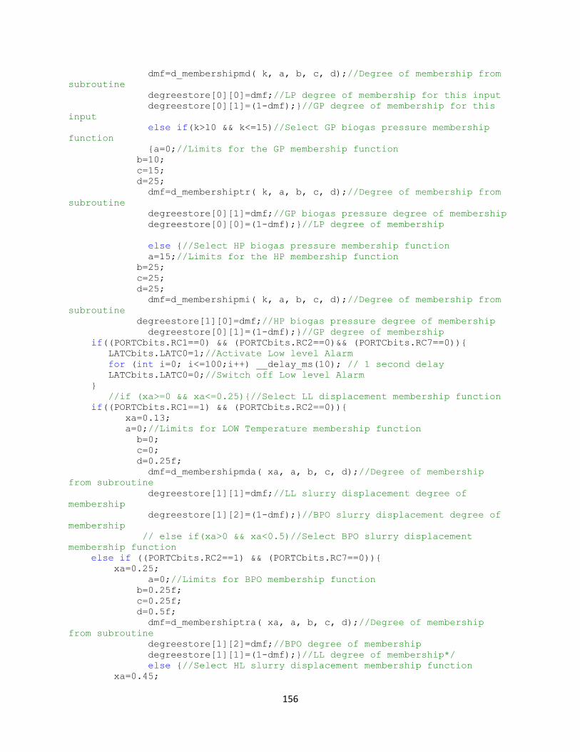
156
dmf=d_membershipmd( k, a, b, c, d);//Degree of membership from
subroutine
degreestore[0][0]=dmf;//LP degree of membership for this input
degreestore[0][1]=(1-dmf);}//GP degree of membership for this
input
else if(k>10 && k<=15)//Select GP biogas pressure membership
function
{a=0;//Limits for the GP membership function
b=10;
c=15;
d=25;
dmf=d_membershiptr( k, a, b, c, d);//Degree of membership from
subroutine
degreestore[0][1]=dmf;//GP biogas pressure degree of membership
degreestore[0][0]=(1-dmf);}//LP degree of membership
else {//Select HP biogas pressure membership function
a=15;//Limits for the HP membership function
b=25;
c=25;
d=25;
dmf=d_membershipmi( k, a, b, c, d);//Degree of membership from
subroutine
degreestore[1][0]=dmf;//HP biogas pressure degree of membership
degreestore[0][1]=(1-dmf);}//GP degree of membership
if((PORTCbits.RC1==0) && (PORTCbits.RC2==0)&& (PORTCbits.RC7==0)){
LATCbits.LATC0=1;//Activate Low level Alarm
for (int i=0; i<=100;i++) __delay_ms(10); // 1 second delay
LATCbits.LATC0=0;//Switch off Low level Alarm
}
//if (xa>=0 && xa<=0.25){//Select LL displacement membership function
if((PORTCbits.RC1==1) && (PORTCbits.RC2==0)){
xa=0.13;
a=0;//Limits for LOW Temperature membership function
b=0;
c=0;
d=0.25f;
dmf=d_membershipmda( xa, a, b, c, d);//Degree of membership
from subroutine
degreestore[1][1]=dmf;//LL slurry displacement degree of
membership
degreestore[1][2]=(1-dmf);}//BPO slurry displacement degree of
membership
// else if(xa>0 && xa<0.5)//Select BPO slurry displacement
membership function
else if ((PORTCbits.RC2==1) && (PORTCbits.RC7==0)){
xa=0.25;
a=0;//Limits for BPO membership function
b=0.25f;
c=0.25f;
d=0.5f;
dmf=d_membershiptra( xa, a, b, c, d);//Degree of membership
from subroutine
degreestore[1][2]=dmf;//BPO degree of membership
degreestore[1][1]=(1-dmf);}//LL degree of membership*/
else {//Select HL slurry displacement membership function
xa=0.45;

157
a=0.25f;//Limits for HL slurry displacement membership function
b=0.5f;
c=0.5f;
d=0.5f;
dmf=d_membershipmia( xa, a, b, c, d);//Degree of membership
from subroutine*/
degreestore[1][3]=dmf;//HL slurry displacement degree of
membership
degreestore[1][2]=(1-dmf);}//BPO degree of membership
/*Evaluate the firing strengths of the nine (9) rules for the required
digester danger status*/
/*The results according to the Max-Min method are stored in an array
digesterop*/
if((degreestore[0][0])>(degreestore[1][1])){//Rule 1 (No danger
output)
digesterop[0][0]=degreestore[1][1];}
else
{digesterop[0][0]=degreestore[0][0];}
if((degreestore[0][0])>(degreestore[1][2])){//Rule 2 (Low
danger ouput)
digesterop[0][1]=degreestore[1][2];}
else
{digesterop[0][1]=degreestore[0][0];}
if((degreestore[0][0])>(degreestore[1][3])){//Rule 3 (High danger
output)
digesterop[0][2]=degreestore[1][3];}
else
{digesterop[0][2]=degreestore[0][0];}
if((degreestore[0][1])>(degreestore[0][0])){//Rule 4 (Low danger
ouput)
digesterop[1][0]=degreestore[0][0];}
else
{digesterop[1][0]=degreestore[0][1];}
if((degreestore[0][1])>(degreestore[1][2])){//Rule 5 (No danger
ouput)
digesterop[1][1]=degreestore[1][2];}
else
{digesterop[1][1]=degreestore[0][1];}
if((degreestore[0][1])>(degreestore[1][3])){//Rule 6 (Low danger
ouput)
digesterop[1][2]=degreestore[1][3];}
else
{digesterop[1][2]=degreestore[0][1];}
if((degreestore[1][0])>(degreestore[0][0])){//Rule 7 (High
danger ouput)
digesterop[2][0]=degreestore[0][0];}
else
{digesterop[2][0]=degreestore[1][0];}
if((degreestore[1][0])>(degreestore[1][2])){//Rule 8 (Low
danger ouput)
digesterop[2][1]=degreestore[1][2];}
else
{digesterop[2][1]=degreestore[1][0];}
if((degreestore[1][0])>(degreestore[1][3])){//Rule 9 (No danger
ouput)
digesterop[2][2]=degreestore[1][3];}

158
else
{digesterop[2][2]=degreestore[1][0];}
/*Max-Min method for output combination of the rules, by
measuring relative
magnitudes of the respective firing strengths of the rules and
taking note
of the most significant one*/
if ((digesterop[0][0])<(digesterop[1][1])){ /* Degree of
membership*/
firingcomb[0]=digesterop[1][1];} /* of No
danger */
else if ((digesterop[1][1])<(digesterop[2][2])){ /* digester
output */
firingcomb[0]=digesterop[2][2];}
else {
firingcomb[0]=digesterop[0][0];}
if ((digesterop[0][1])<(digesterop[1][0])){ /* Degree of
membership*/
firingcomb[1]=digesterop[1][0];} /* of Low
danger */
else if ((digesterop[1][0])<(digesterop[1][2])){ /* digester
output */
firingcomb[1]=digesterop[1][2];}
else if ((digesterop[1][2])<(digesterop[2][1])){
firingcomb[1]=digesterop[2][1];}
else {
firingcomb[1]=digesterop[0][1];}
if ((digesterop[0][2])<(digesterop[2][0])){ /* Degree of
membership*/
firingcomb[2]=digesterop[2][0];} /* of High
danger */
else {
firingcomb[2]=digesterop[0][0];}
/*DEFUZZIFICATION using CENTER OF GRAVITY(COG) method*/
a1=0; // +ve slope1 of No danger =0
a2=firingcomb[1]*50;//height x +ve slope1 of Low danger
trapezium
a3=firingcomb[2]*50;//height x +ve slope1(slope2=0) of high
danger trapezium
b1=firingcomb[0]*50;//height x -ve slope2 of No danger
b2=firingcomb[1]*50;//height x -ve slope 2 of Low danger
b3=0;// -ve slope of No danger
top1=50-a1-b1;//varying top1 width from maximum to minimum
top2=100-a2-b2;
top3=50-a3-b3;
area1=firingcomb[0]*((50+top1)/2);//Area of No danger
area2=firingcomb[1]*((100+top2)/2);//Area of Low danger
area3=firingcomb[2]*((50+top3)/2);//Area of High danger

159
crispout=((area1*25)+(area2*50)+(area3*75))/(area1+area2+area3);
WriteCmdXLCD(0x01); ///Clear Screen
putrsXLCD(" %Digest.Danger ");////Display "%Digest.Danger" on the screen
SetDDRamAddr(0x40);
putrsXLCD(" Level = ");
sprintf(Buffer, "%.3g", crispout ); //// Convert %Digest.Danger to string
putsXLCD(Buffer); ////Display the %Digest.Danger on the screen
putrsXLCD(" "); //// Clear after comma
WriteCmdXLCD(0x02); ////Home position on LCD
for (int i=0; i<=100;i++) __delay_ms(10); //// 1 second delay
k=0;
xa=0;
crispout=0;
//XXXXXXXXXXXXXXXXXXXXXXXXXXXXXXXXXXXXXXXXXXXXXXXXXXXXXXXXXXXXXXXXXXXXXXXXXXx
xXXXXXXXXXXXXXXXXXXXX
}
}
void init_XLCD(void) //Initialize LCD display
{
OpenXLCD(FOUR_BIT&LINES_5X7); //configure LCD in 4-bit Data Interface
mode
//and 5x7 characters, multiple line
display
while(BusyXLCD()); //Check if the LCD controller is not busy
//before writing some commands?
WriteCmdXLCD(0x06); // move cursor right, don?t shift display
WriteCmdXLCD(0x0C); //turn display on without cursor
}
void init_ADC1(void) //Initialize ADC
{
/**** ADC configured for:
* FOSC/2 as conversion clock
* Result is right justified
* Aquisition time of 2 AD
* Channel 1 for sampling
* ADC interrupt off
* ADC reference voltage from VDD & VSS
*/
OpenADC(ADC_FOSC_2 & ADC_RIGHT_JUST & ADC_2_TAD,
ADC_CH0 & ADC_INT_OFF & ADC_REF_VDD_VSS,
ADC_9ANA);
}
void DelayFor18TCY( void ) //18 cycles delay
{
Delay10TCYx(2);
return;
}
void DelayPORXLCD (void) // Delay of 15ms
{

160
Delay1KTCYx(60); // Cycles=(Time Delay*Fosc)/4
//__delay_ms(15); // Cycles =(15ms*16MHz)/4
// Cycles =60000
}
void DelayXLCD (void) // Delay of 5ms
{
Delay1KTCYx(20); // Cycles = 20000
//__delay_ms(5);
}
float d_membershipmd(float k,float a,float b,float c,float d) /*x is input
value
from sensor into subroutine*/
{
//float dmf;
if (k>c && k<d)
{ dmf=(d-k)/(d-c); }
else if (k>=b && k<=c)
{dmf=1.0; }
else
{ dmf=0; }
return dmf;//Return value from subroutine into main program
}
float d_membershiptr(float k,float a,float b,float c,float d) /*k is
input value
from sensor into subroutine*/
{
//float dmf;
if (k >a && k <b)
{ dmf=(k-a)/(b-a);}
else if (k>c && k<d)
{ dmf=(d-k)/(d-c); }
else if (k>=b && k<=c)
{dmf=1.0; }
else
{ dmf=0; }
return dmf;//Return value from subroutine into main program
}
float d_membershipmi(float k,float a,float b,float c,float d) /*x is
input value
from sensor into subroutine*/
{
//float dmf;
if (k >a && k <b)
{ dmf=(k-a)/(b-a);}
else if (k>=b && k<=c)
{dmf=1.0; }
else
{ dmf=0; }
return dmf;//Return value from subroutine into main program
}
float d_membershipmda(float xa,float a,float b,float c,float d) /*xa is
input value
from sensor into subroutine*/
{

161
//float dmf;
if (xa>c && xa<d)
{ dmf=(d-xa)/(d-c); }
else if (xa>=b && xa<=c)
{dmf=1.0; }
else
{ dmf=0; }
return dmf;//Return value from subroutine into main program
}
float d_membershiptra(float xa,float a,float b,float c,float d) /*xa is
input value
from sensor into subroutine*/
{
//float dmf;
if (xa >a && xa <b)
{ dmf=(xa-a)/(b-a);}
else if (xa>c && xa<d)
{ dmf=(d-xa)/(d-c); }
else if (xa>=b && xa<=c)
{dmf=1.0; }
else
{ dmf=0; }
return dmf;//Return value from subroutine into main program
}
float d_membershipmia(float xa,float a,float b,float c,float d) /*xa is
input value
from sensor into subroutine*/
{
//float dmf;
if (xa >a && xa <b)
{ dmf=(xa-a)/(b-a);}
else if (xa>=b && xa<=c)
{dmf=1.0; }
else
{ dmf=0; }
return dmf;//Return value from subroutine into main program
}

162
E2: Listing two
/*File: PHOTOVOLTAIC SYSTEM.c
* Author: L.Matindife: University of south Africa (UNISA)
*/
/*Listing two*/
//THIS LISTING COVERS 1) SOLAR BATTERY CHARGING/DISCHARGING, AND 2) SOLAR
FAULT DETECTION AND STATUS
#include "Old3_1.h"
#include <stdio.h>
#include <stdlib.h>
#include <plib/delays.h>
#include <plib/xlcd.h>
#include <plib/adc.h>
void init_ADC1(void); //Initialize ADC
void init_XLCD(void); //Initialize LCD display
void DelayFor18TCY( void ); //18 cycles delay
void DelayPORXLCD (void); // Delay of 15ms
void DelayXLCD (void); // Delay of 5ms
float d_membershipmd(float k,float a,float b,float c,float d);/*Subroutine to
calculate
degree of membership of any monotonically decreasing function.In this case
this is charging voltage membership function*/
float d_membershiptr(float k,float a,float b,float c,float d);/*Subroutine to
calculate degree of membership of charging voltage triangular function*/
float d_membershipmi(float k,float a,float b,float c,float d);/*Subroutine to
calculate
degree of membership of monotonically increasing charging voltage function*/.
float d_membershipmda(float xa,float a,float b,float c,float d);/*Subroutine
to calculate degree of membership of the Charging current membership
function*/
float d_membershiptra(float xa,float a,float b,float c,float d);/*Subroutine
to calculate degree of membership of charging current membership function*/
float d_membershipmia(float xa,float a,float b,float c,float d);/*Subroutine
to calculate degree of membership of charging current membership function*/
float d_membershipmdSOC(float SOC,float a,float b,float c,float d);
/*Subroutine to calculate degree of membership of the SOC membership
function*/
float d_membershiptrSOC(float SOC,float a,float b,float c,float d);
/*Subroutine to calculate
degree of membership of SOC membership function*/
float d_membershipmiSOC(float SOC,float a,float b,float c,float d);
/*Subroutine to calculate
degree of membership of the SOC membership function*/
//**************Declare Global
Varaibles**************************************
unsigned int ADCResult[4]=0;
unsigned char ResultStr[10];
unsigned char Buffer[20];

163
float voltage10,voltage11,voltage12,voltage13;
float k,ec,orp,xa,dmf,a,b,c,d,V21,V22,V23,pHs,Ich,Irms;
float degreestore[4][4]={{0},{0}};/*Array to store all degrees
of membership
at specific memory locations for latter retrieval*/
float digesterop[27][1]={{0},{0}};/*Rule matrix of digester
operation*/
float firingcomb[3]={0};/*Array to store values of overall
combined firing
strengths of the rules*/
float firing[7]={0};
float a1,a2,a3,a4,b1,b2,b3,b4,area1,area2,area3,area4;
float SOC,top1,top2,top3,top4,crispout;
void main(void)
{
TRISCbits.RC0=0;//Combined Photovoltaic and Biogas Alarm
TRISAbits.RA4=0;//User PV current Flashing LED (FLED)
//OSCCON=0x70; //Configure to use 8MHz internal
oscillator.
init_XLCD(); //Call the Initialize LCD display function
init_ADC1(); //Call the Initialize ADC function
putrsXLCD(" SOLAR "); //Display "SOLAR"
SetDDRamAddr(0x40); //shift cursor to beginning of second line
putrsXLCD(" SYSTEM "); //Display "SYSTEM"
for (int i=0; i<=100;i++) __delay_ms(10); // 1 second delay
WriteCmdXLCD(0x01); //Clear Screen
while(1)
{
//---sample and convert----
for (unsigned char m=0; m<=2; m++)
{
ADCON0bits.CHS = m;
DelayFor18TCY();
ConvertADC(); //Start conversion
while(BusyADC()); //Wait here until conversion is finished
ADCResult[m] = (unsigned int)ReadADC(); //Read the converted
data
// convert the converted data into voltage
//we divide by 1024 because its a 10-bit converted data
voltage10 = (ADCResult[0]*5.0)/1024;//From voltage charging sensor
voltage11 = (ADCResult[1]*5.0)/1024;//From current charging sensor
voltage12 = (ADCResult[2]*5.0)/1024;//Solar photocell voltage
voltage13 = (ADCResult[3]*5.0)/1024;//Load voltage sensor
}
V21=5.27*voltage10;//Charging voltage
k = V21;
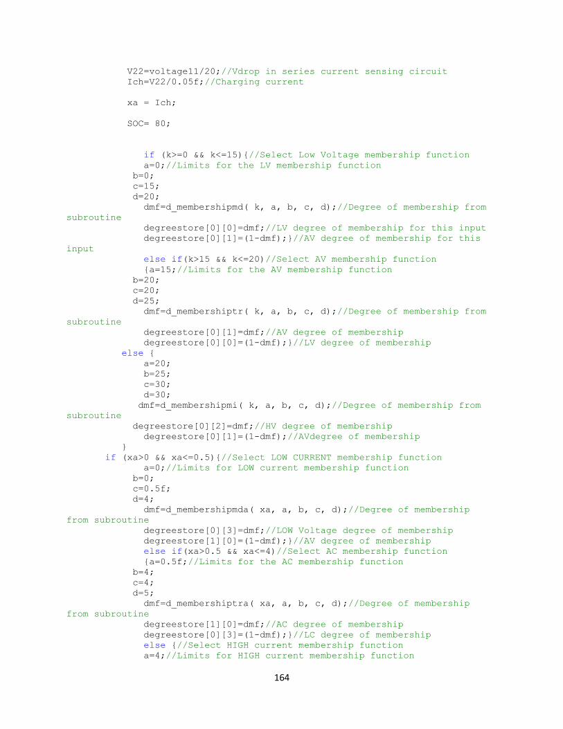
164
V22=voltage11/20;//Vdrop in series current sensing circuit
Ich=V22/0.05f;//Charging current
xa = Ich;
SOC= 80;
if (k>=0 && k<=15){//Select Low Voltage membership function
a=0;//Limits for the LV membership function
b=0;
c=15;
d=20;
dmf=d_membershipmd( k, a, b, c, d);//Degree of membership from
subroutine
degreestore[0][0]=dmf;//LV degree of membership for this input
degreestore[0][1]=(1-dmf);}//AV degree of membership for this
input
else if(k>15 && k<=20)//Select AV membership function
{a=15;//Limits for the AV membership function
b=20;
c=20;
d=25;
dmf=d_membershiptr( k, a, b, c, d);//Degree of membership from
subroutine
degreestore[0][1]=dmf;//AV degree of membership
degreestore[0][0]=(1-dmf);}//LV degree of membership
else {
a=20;
b=25;
c=30;
d=30;
dmf=d_membershipmi( k, a, b, c, d);//Degree of membership from
subroutine
degreestore[0][2]=dmf;//HV degree of membership
degreestore[0][1]=(1-dmf);//AVdegree of membership
}
if (xa>0 && xa<=0.5){//Select LOW CURRENT membership function
a=0;//Limits for LOW current membership function
b=0;
c=0.5f;
d=4;
dmf=d_membershipmda( xa, a, b, c, d);//Degree of membership
from subroutine
degreestore[0][3]=dmf;//LOW Voltage degree of membership
degreestore[1][0]=(1-dmf);}//AV degree of membership
else if(xa>0.5 && xa<=4)//Select AC membership function
{a=0.5f;//Limits for the AC membership function
b=4;
c=4;
d=5;
dmf=d_membershiptra( xa, a, b, c, d);//Degree of membership
from subroutine
degreestore[1][0]=dmf;//AC degree of membership
degreestore[0][3]=(1-dmf);}//LC degree of membership
else {//Select HIGH current membership function
a=4;//Limits for HIGH current membership function

165
b=5;
c=7;
d=7;
dmf=d_membershipmia( xa, a, b, c, d);//Degree of membership from
subroutine*/
degreestore[1][1]=dmf;//HC degree of membership
degreestore[1][0]=(1-dmf);}//AC degree of membership
if(SOC>10 && SOC<=50)//Select LSOC membership function
{a=10;//Limits for the LSOC membership function
b=10;
c=50;
d=70;
dmf=d_membershiptrSOC( SOC, a, b, c, d);//Degree of membership
from subroutine
degreestore[1][2]=dmf;//LSOC degree of membership
degreestore[1][3]=(1-dmf);}//MSOC degree of membership
else if(SOC>50 && SOC<=70)//Select MSOC membership function
{a=50;//Limits for the M.alkaline membership function
b=70;
c=70;
d=80;
dmf=d_membershiptrSOC( SOC, a, b, c, d);//Degree of membership
from subroutine
degreestore[1][3]=dmf;//MSOC degree of membership
degreestore[1][2]=(1-dmf);}//LSOC degree of membership
else {//Select HSOC membership function
a=70;//Limits for the HSOC membership function
b=80;
c=100;
d=100;
dmf=d_membershipmiSOC( SOC, a, b, c, d);//Degree of membership from
subroutine
degreestore[2][0]=dmf;// HSOCdegree of membership
degreestore[1][3]=(1-dmf);}//MSOC degree of membership
/*Evaluate the firing strengths of the fifteen (15) rules for the required
digester operation status*/
/*The results according to the Max-Min method are stored in an array
digesterop*/
if((degreestore[1][2])>(degreestore[0][0])){//Rule 1 LD
digesterop[0][0]=degreestore[0][0];}
else if((degreestore[1][2])>(degreestore[0][3]))
{digesterop[0][0]=degreestore[0][3];}
else
{digesterop[0][0]=degreestore[1][2];}
if((degreestore[1][2])>(degreestore[0][1])){//Rule 2 MD
digesterop[1][0]=degreestore[0][1];}
else if((degreestore[1][2])>(degreestore[0][3]))
{digesterop[1][0]=degreestore[0][3];}
else
{digesterop[1][0]=degreestore[1][2];}
if((degreestore[1][2])>(degreestore[0][2])){//Rule 3 MD
digesterop[2][0]=degreestore[0][2];}
else if((degreestore[1][2])>(degreestore[0][3]))
{digesterop[2][0]=degreestore[0][3];}
else

166
{digesterop[2][0]=degreestore[1][2];}
if((degreestore[1][2])>(degreestore[0][0])){//Rule 4 MD
digesterop[3][0]=degreestore[0][0];}
else if((degreestore[1][2])>(degreestore[1][0]))
{digesterop[3][0]=degreestore[1][0];}
else
{digesterop[3][0]=degreestore[1][2];}
if((degreestore[1][2])>(degreestore[0][1])){//Rule 5 MD
digesterop[4][0]=degreestore[0][1];}
else if((degreestore[1][2])>(degreestore[1][0]))
{digesterop[4][0]=degreestore[1][0];}
else
{digesterop[4][0]=degreestore[1][2];}
if((degreestore[1][2])>(degreestore[0][2])){//Rule 6 MD
digesterop[5][0]=degreestore[0][2];}
else if((degreestore[1][2])>(degreestore[1][0]))
{digesterop[5][0]=degreestore[1][0];}
else
{digesterop[5][0]=degreestore[1][2];}
if((degreestore[1][2])>(degreestore[0][0])){//Rule 7 LD
digesterop[6][0]=degreestore[0][0];}
else if((degreestore[1][2])>(degreestore[1][1]))
{digesterop[6][0]=degreestore[1][1];}
else
{digesterop[6][0]=degreestore[1][2];}
if((degreestore[1][2])>(degreestore[0][1])){//Rule 8 LD
digesterop[7][0]=degreestore[0][1];}
else if((degreestore[1][2])>(degreestore[1][1]))
{digesterop[7][0]=degreestore[1][1];}
else
{digesterop[7][0]=degreestore[1][2];}
if((degreestore[1][2])>(degreestore[0][2])){//Rule 9 MD
digesterop[8][0]=degreestore[0][2];}
else if((degreestore[1][2])>(degreestore[1][1]))
{digesterop[8][0]=degreestore[1][1];}
else
{digesterop[8][0]=degreestore[1][2];}
//zzzzzzzzzzzzzzzzzzzzzzzzzzzzzzzzzzzzzzzzzzzzzzzzzzzzzzzzz
if((degreestore[1][3])>(degreestore[0][0])){//Rule 10 LD
digesterop[9][0]=degreestore[0][0];}
else if((degreestore[1][3])>(degreestore[0][3]))
{digesterop[9][0]=degreestore[0][3];}
else
{digesterop[9][0]=degreestore[1][3];}
if((degreestore[1][3])>(degreestore[0][1])){//Rule 11 LD
digesterop[10][0]=degreestore[0][1];}
else if((degreestore[1][3])>(degreestore[0][3]))
{digesterop[10][0]=degreestore[0][3];}
else

167
{digesterop[10][0]=degreestore[1][3];}
if((degreestore[1][3])>(degreestore[0][2])){//Rule 12 LD
digesterop[11][0]=degreestore[0][2];}
else if((degreestore[1][3])>(degreestore[0][3]))
{digesterop[11][0]=degreestore[0][3];}
else
{digesterop[11][0]=degreestore[1][3];}
if((degreestore[1][3])>(degreestore[0][0])){//Rule 13 MD
digesterop[12][0]=degreestore[0][0];}
else if((degreestore[1][3])>(degreestore[1][0]))
{digesterop[12][0]=degreestore[1][0];}
else
{digesterop[12][0]=degreestore[1][3];}
if((degreestore[1][3])>(degreestore[0][1])){//Rule 14 MD
digesterop[13][0]=degreestore[0][1];}
else if((degreestore[1][3])>(degreestore[1][0]))
{digesterop[13][0]=degreestore[1][0];}
else
{digesterop[13][0]=degreestore[1][3];}
if((degreestore[1][3])>(degreestore[0][2])){//Rule 15 MD
digesterop[14][0]=degreestore[0][2];}
else if((degreestore[1][3])>(degreestore[1][0]))
{digesterop[14][0]=degreestore[1][0];}
else
{digesterop[14][0]=degreestore[1][3];}
if((degreestore[1][3])>(degreestore[0][0])){//Rule 16 HD
digesterop[15][0]=degreestore[0][0];}
else if((degreestore[1][3])>(degreestore[1][1]))
{digesterop[15][0]=degreestore[1][1];}
else
{digesterop[15][0]=degreestore[1][3];}
if((degreestore[1][3])>(degreestore[0][1])){//Rule 17 HD
digesterop[16][0]=degreestore[0][1];}
else if((degreestore[1][3])>(degreestore[1][1]))
{digesterop[16][0]=degreestore[1][1];}
else
{digesterop[16][0]=degreestore[1][3];}
if((degreestore[1][3])>(degreestore[0][2])){//Rule 18 HD
digesterop[17][0]=degreestore[0][2];}
else if((degreestore[1][3])>(degreestore[1][1]))
{digesterop[17][0]=degreestore[1][1];}
else
{digesterop[17][0]=degreestore[1][3];}
//yyyyyyyyyyyyyyyyyyyyyyyyyyyyyyyyyyyyyyyyyyyyyyyyyyyyyyyyyyyyyyyyyyyyyyyyyyy
yy
if((degreestore[2][0])>(degreestore[0][0])){//Rule 19 MD
digesterop[18][0]=degreestore[0][0];}
else if((degreestore[2][0])>(degreestore[0][3]))
{digesterop[18][0]=degreestore[0][3];}
168
else
{digesterop[18][0]=degreestore[2][0];}
if((degreestore[2][0])>(degreestore[0][1])){//Rule 20 LD
digesterop[19][0]=degreestore[0][1];}
else if((degreestore[2][0])>(degreestore[0][3]))
{digesterop[19][0]=degreestore[0][3];}
else
{digesterop[19][0]=degreestore[2][0];}
if((degreestore[2][0])>(degreestore[0][2])){//Rule 21 LD
digesterop[20][0]=degreestore[0][2];}
else if((degreestore[2][0])>(degreestore[0][3]))
{digesterop[20][0]=degreestore[0][3];}
else
{digesterop[20][0]=degreestore[2][0];}
if((degreestore[2][0])>(degreestore[0][0])){//Rule 22 HD
digesterop[21][0]=degreestore[0][0];}
else if((degreestore[2][0])>(degreestore[1][0]))
{digesterop[21][0]=degreestore[1][0];}
else
{digesterop[21][0]=degreestore[2][0];}
if((degreestore[2][0])>(degreestore[0][1])){//Rule 23 MD
digesterop[22][0]=degreestore[0][1];}
else if((degreestore[2][0])>(degreestore[1][0]))
{digesterop[22][0]=degreestore[1][0];}
else
{digesterop[22][0]=degreestore[1][3];}
if((degreestore[2][0])>(degreestore[0][2])){//Rule 24 MD
digesterop[23][0]=degreestore[0][2];}
else if((degreestore[2][0])>(degreestore[1][0]))
{digesterop[23][0]=degreestore[1][0];}
else
{digesterop[23][0]=degreestore[2][0];}
if((degreestore[2][0])>(degreestore[0][0])){//Rule 25 HD
digesterop[24][0]=degreestore[0][0];}
else if((degreestore[2][0])>(degreestore[1][1]))
{digesterop[24][0]=degreestore[1][1];}
else
{digesterop[24][0]=degreestore[2][0];}
if((degreestore[2][0])>(degreestore[0][1])){//Rule 26 HD
digesterop[25][0]=degreestore[0][1];}
else if((degreestore[2][0])>(degreestore[1][1]))
{digesterop[25][0]=degreestore[1][1];}
else
{digesterop[25][0]=degreestore[2][0];}
if((degreestore[2][0])>(degreestore[0][2])){//Rule 27 HD
digesterop[26][0]=degreestore[0][2];}
else if((degreestore[2][0])>(degreestore[1][1]))
{digesterop[26][0]=degreestore[1][1];}
else
{digesterop[26][0]=degreestore[2][0];}

169
/*Max-Min method for output combination of the rules, by measuring relative
magnitudes of the respective firing strengths of the rules and taking note
of the most significant one*/
if ((digesterop[0][0])<(digesterop[6][0])) /* Degree of membership*/
firingcomb[0]=digesterop[6][0];} /* of Low DUTY */
else if ((digesterop[6][0])<(digesterop[7][0])){ /* CYCLE LD */
firingcomb[0]=digesterop[7][0];}
else if ((digesterop[7][0])<(digesterop[9][0])){
firingcomb[0]=digesterop[9][0];}
else if ((digesterop[9][0])<(digesterop[10][0])){
firingcomb[0]=digesterop[10][0];}
else if ((digesterop[10][0])<(digesterop[11][0])){
firingcomb[0]=digesterop[11][0];}
else if ((digesterop[11][0])<(digesterop[19][0])){
firingcomb[0]=digesterop[19][0];}
else if ((digesterop[19][0])<(digesterop[20][0])){
firingcomb[0]=digesterop[20][0];}
else {
firingcomb[0]=digesterop[0][0];}
if ((digesterop[1][0])<(digesterop[2][0])){ /* Degree of membership*/
firingcomb[1]=digesterop[2][0];} /* of MEDIUM DUTY */
else if ((digesterop[2][0])<(digesterop[3][0])){ /* CYCLE MD */
firingcomb[1]=digesterop[3][0];}
else if ((digesterop[3][0])<(digesterop[4][0])){
firingcomb[1]=digesterop[4][0];}
else if ((digesterop[4][0])<(digesterop[5][0])){
firingcomb[1]=digesterop[5][0];}
else if ((digesterop[5][0])<(digesterop[8][0])){
firingcomb[1]=digesterop[8][0];}
else if ((digesterop[8][0])<(digesterop[12][0])){
firingcomb[1]=digesterop[12][0];}
else if ((digesterop[12][0])<(digesterop[13][0])){
firingcomb[1]=digesterop[13][0];}
else if ((digesterop[13][0])<(digesterop[14][0])){
firingcomb[1]=digesterop[14][0];}
else if ((digesterop[14][0])<(digesterop[18][0])){
firingcomb[1]=digesterop[18][0];}
else if ((digesterop[18][0])<(digesterop[22][0])){
firingcomb[1]=digesterop[22][0];}
else if ((digesterop[22][0])<(digesterop[23][0])){
firingcomb[1]=digesterop[23][0];}
else {
firingcomb[1]=digesterop[1][0];}
if ((digesterop[15][0])<(digesterop[16][0])){/* Degree of membership*/
firingcomb[2]=digesterop[16][0];} /* of HIGH DUTY */
else if ((digesterop[16][0])<(digesterop[17][0])){ /* CYCLE HD */
firingcomb[2]=digesterop[17][0];}
else if ((digesterop[17][0])<(digesterop[21][0])){
firingcomb[2]=digesterop[21][0];}
else if ((digesterop[21][0])<(digesterop[24][0])){
firingcomb[2]=digesterop[24][0];}
else if ((digesterop[24][0])<(digesterop[25][0])){
firingcomb[2]=digesterop[25][0];}
else if ((digesterop[25][0])<(digesterop[26][0])){
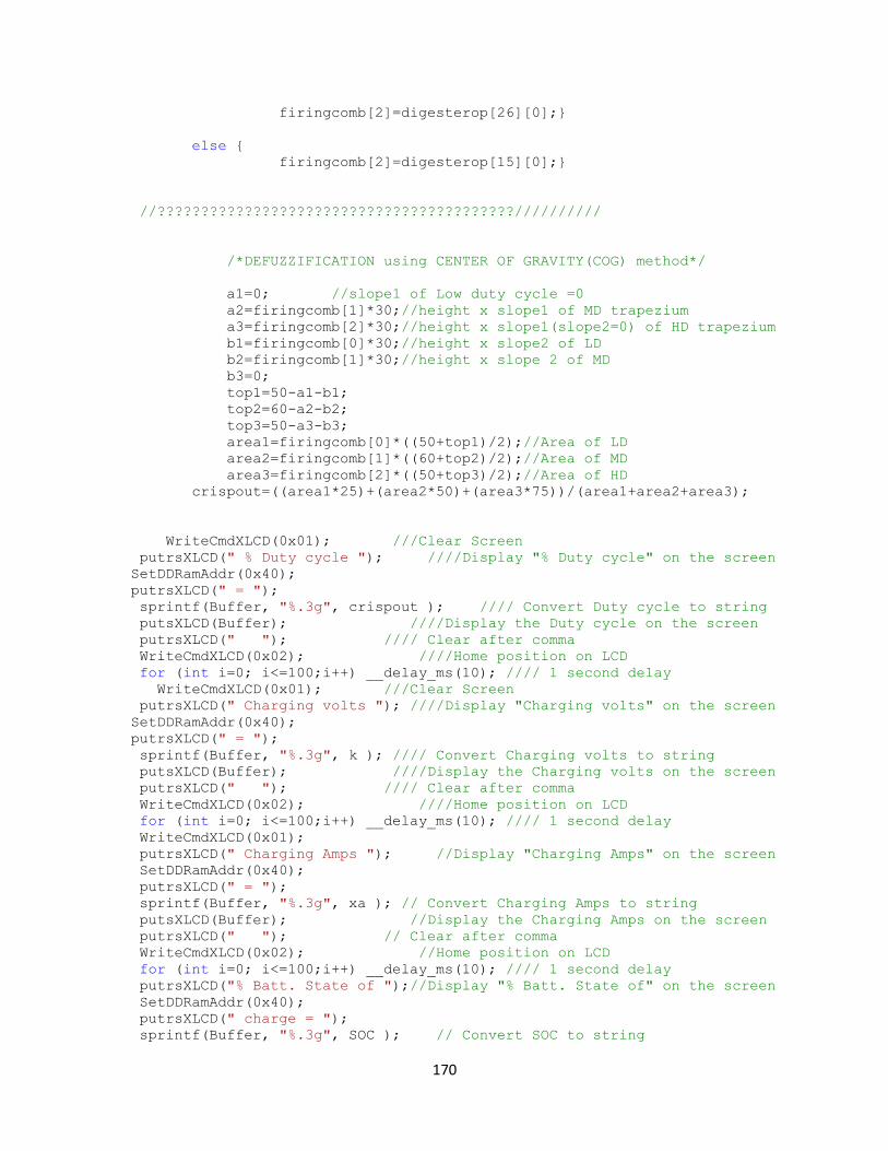
170
firingcomb[2]=digesterop[26][0];}
else {
firingcomb[2]=digesterop[15][0];}
//?????????????????????????????????????????//////////
/*DEFUZZIFICATION using CENTER OF GRAVITY(COG) method*/
a1=0; //slope1 of Low duty cycle =0
a2=firingcomb[1]*30;//height x slope1 of MD trapezium
a3=firingcomb[2]*30;//height x slope1(slope2=0) of HD trapezium
b1=firingcomb[0]*30;//height x slope2 of LD
b2=firingcomb[1]*30;//height x slope 2 of MD
b3=0;
top1=50-a1-b1;
top2=60-a2-b2;
top3=50-a3-b3;
area1=firingcomb[0]*((50+top1)/2);//Area of LD
area2=firingcomb[1]*((60+top2)/2);//Area of MD
area3=firingcomb[2]*((50+top3)/2);//Area of HD
crispout=((area1*25)+(area2*50)+(area3*75))/(area1+area2+area3);
WriteCmdXLCD(0x01); ///Clear Screen
putrsXLCD(" % Duty cycle "); ////Display "% Duty cycle" on the screen
SetDDRamAddr(0x40);
putrsXLCD(" = ");
sprintf(Buffer, "%.3g", crispout ); //// Convert Duty cycle to string
putsXLCD(Buffer); ////Display the Duty cycle on the screen
putrsXLCD(" "); //// Clear after comma
WriteCmdXLCD(0x02); ////Home position on LCD
for (int i=0; i<=100;i++) __delay_ms(10); //// 1 second delay
WriteCmdXLCD(0x01); ///Clear Screen
putrsXLCD(" Charging volts "); ////Display "Charging volts" on the screen
SetDDRamAddr(0x40);
putrsXLCD(" = ");
sprintf(Buffer, "%.3g", k ); //// Convert Charging volts to string
putsXLCD(Buffer); ////Display the Charging volts on the screen
putrsXLCD(" "); //// Clear after comma
WriteCmdXLCD(0x02); ////Home position on LCD
for (int i=0; i<=100;i++) __delay_ms(10); //// 1 second delay
WriteCmdXLCD(0x01);
putrsXLCD(" Charging Amps "); //Display "Charging Amps" on the screen
SetDDRamAddr(0x40);
putrsXLCD(" = ");
sprintf(Buffer, "%.3g", xa ); // Convert Charging Amps to string
putsXLCD(Buffer); //Display the Charging Amps on the screen
putrsXLCD(" "); // Clear after comma
WriteCmdXLCD(0x02); //Home position on LCD
for (int i=0; i<=100;i++) __delay_ms(10); //// 1 second delay
putrsXLCD("% Batt. State of ");//Display "% Batt. State of" on the screen
SetDDRamAddr(0x40);
putrsXLCD(" charge = ");
sprintf(Buffer, "%.3g", SOC ); // Convert SOC to string

171
putsXLCD(Buffer); //Display the SOC on the screen
putrsXLCD(" "); // Clear after comma
WriteCmdXLCD(0x02); //Home position on LCD
for (int i=0; i<=100;i++) __delay_ms(10); //// 1 second delay
//0000000000000000000000000000000000000000000000000000000000000
//SOLAR PANEL SHADING ROUTINE
k=0;
crispout=0;
k=voltage12;
if (k>=0.1f && k<=1){//Select LVadc membership function
a=0,1f;//Limits for the LV membership function
b=0.1f;
c=1;
d=2;
dmf=d_membershipmd( k, a, b, c, d);//Degree of membership from
subroutine
degreestore[0][0]=dmf;//LVadc degree of membership for this
input
degreestore[0][1]=(1-dmf);}//LMVadc degree of membership for
this input
else if(k>1 && k<=2)//Select AV membership function
{a=1;//Limits for the AV membership function
b=2;
c=2;
d=4.5f;
dmf=d_membershiptr( k, a, b, c, d);//Degree of membership from
subroutine
degreestore[0][2]=dmf;//LMVadc degree of membership
degreestore[0][3]=(1-dmf);}//LVadc degree of membership
else if(k>2 && k<=4.5f)//Select AV membership function
{a=2;//Limits for the AV membership function
b=4.5f;
c=4.5f;
d=4.8f;
dmf=d_membershiptr( k, a, b, c, d);//Degree of membership from
subroutine
degreestore[1][0]=dmf;//UMVadc degree of membership
degreestore[1][1]=(1-dmf);}//LMVadc degree of membership
else {
a=4;
b=4.8f;
c=5;
d=5;
dmf=d_membershipmi( k, a, b, c, d);//Degree of membership from
subroutine
degreestore[1][2]=dmf;//HVadc degree of membership
degreestore[1][3]=(1-dmf);//UMVdegree of membership
}
if((degreestore[0][0])<(degreestore[0][3])){//Rule 1 LVadc (TS)
firing[0]=degreestore[0][3];}
else
{firing[0]=degreestore[0][0];}

172
if((degreestore[0][1])<(degreestore[0][2])){//Rule 2 LMVadc (HS))
firing[1]=degreestore[0][2];}
else if((degreestore[0][2])<(degreestore[1][1]))
{firing[1]=degreestore[1][1];}
else
{firing[1]=degreestore[0][1];}
if((degreestore[1][0])<(degreestore[1][3])){//Rule 3 UMVadc (PS)
firing[2]=degreestore[1][3];}
else
{ firing[2]=degreestore[1][0];}
{firing[3]=degreestore[1][2];}
/*DEFUZZIFICATION using CENTER OF GRAVITY(COG) method*/
a1=0; //slope1 of NS =0
a2=firing[2]*20;//height x slope1 of PS trapezium
a3=firing[1]*10;//height x slope1(slope2=0) of HS trapezium
a4=firing[0]*15;//TS
b1=firing[3]*20;//height x slope2 of NS
b2=firing[2]*10;//height x slope 2 of PS
b3=firing[1]*15;//HS
b4=0;
top1=60-a1-b1;
top2=30-a2-b2;
top3=25-a3-b3;
top4=30-a4-b4;
area1=firing[3]*((60+top1)/2);//Area of NS
area2=firing[2]*((30+top2)/2);//Area of PS
area3=firing[1]*((25+top3)/2);//Area of HS
area4=firing[0]*((30+top4)/2);//Area of TS
crispout=((area1*30)+(area2*55)+(area3*72.5)+(area4*85))/(area1+area2+area3+a
rea4);
WriteCmdXLCD(0x01); ///Clear Screen
putrsXLCD(" % Solar Shading ");////Display "% Solar Shading" on the screen
SetDDRamAddr(0x40);
putrsXLCD(" = ");
sprintf(Buffer, "%.3g", crispout ); //// Convert Solar shading to string
putsXLCD(Buffer); ////Display the Solar shading on the screen
putrsXLCD(" "); //// Clear after comma
WriteCmdXLCD(0x02); ////Home position on LCD
for (int i=0; i<=100;i++) __delay_ms(10); //// 1 second delay
k=0;// Reset values for next routine
crispout=0;
//SOLAR USER LOAD CONTROL
//Vspp=Vadc/2 (secondar peak to peak voltage)
//Ispp(secondary peak to peak current)=Vspp/(160*1.414)
//Ippp (primary peak to peak current)=N*Ispp =3000*Ispp
Irms = 1.172*voltage13;
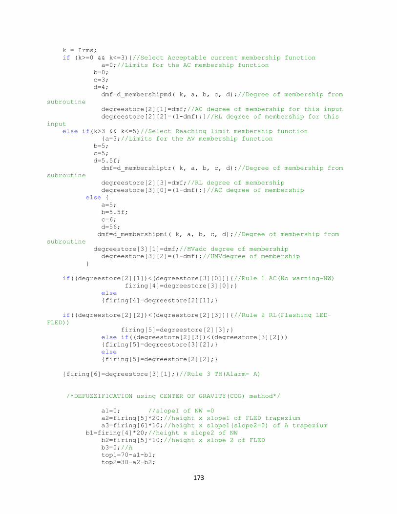
173
k = Irms;
if (k>=0 && k<=3){//Select Acceptable current membership function
a=0;//Limits for the AC membership function
b=0;
c=3;
d=4;
dmf=d_membershipmd( k, a, b, c, d);//Degree of membership from
subroutine
degreestore[2][1]=dmf;//AC degree of membership for this input
degreestore[2][2]=(1-dmf);}//RL degree of membership for this
input
else if(k>3 && k<=5)//Select Reaching limit membership function
{a=3;//Limits for the AV membership function
b=5;
c=5;
d=5.5f;
dmf=d_membershiptr( k, a, b, c, d);//Degree of membership from
subroutine
degreestore[2][3]=dmf;//RL degree of membership
degreestore[3][0]=(1-dmf);}//AC degree of membership
else {
a=5;
b=5.5f;
c=6;
d=56;
dmf=d_membershipmi( k, a, b, c, d);//Degree of membership from
subroutine
degreestore[3][1]=dmf;//HVadc degree of membership
degreestore[3][2]=(1-dmf);//UMVdegree of membership
}
if((degreestore[2][1])<(degreestore[3][0])){//Rule 1 AC(No warning-NW)
firing[4]=degreestore[3][0];}
else
{firing[4]=degreestore[2][1];}
if((degreestore[2][2])<(degreestore[2][3])){//Rule 2 RL(Flashing LED-
FLED))
firing[5]=degreestore[2][3];}
else if((degreestore[2][3])<(degreestore[3][2]))
{firing[5]=degreestore[3][2];}
else
{firing[5]=degreestore[2][2];}
{firing[6]=degreestore[3][1];}//Rule 3 TH(Alarm- A)
/*DEFUZZIFICATION using CENTER OF GRAVITY(COG) method*/
a1=0; //slope1 of NW =0
a2=firing[5]*20;//height x slope1 of FLED trapezium
a3=firing[6]*10;//height x slope1(slope2=0) of A trapezium
b1=firing[4]*20;//height x slope2 of NW
b2=firing[5]*10;//height x slope 2 of FLED
b3=0;//A
top1=70-a1-b1;
top2=30-a2-b2;
174
top3=30-a3-b3;
area1=firing[4]*((70+top1)/2);//Area of NW
area2=firing[5]*((30+top2)/2);//Area of FLED
area3=firing[6]*((30+top3)/2);//Area of A
crispout=((area1*35)+(area2*65)+(area3*85))/(area1+area2+area3);
if(Irms>3 && Irms<5.5){//Flashing load current LED
LATAbits.LATA4=1;//Put a high on RA4
for (int i=0; i<=100;i++) __delay_ms(10); //// 1 second delay
LATAbits.LATA4=0;//Put a low on RA4
LATAbits.LATA4=1;//Put a high on RA4
for (int i=0; i<=100;i++) __delay_ms(10); //// 1 second delay
LATAbits.LATA4=0;//Put a low on RA4
LATAbits.LATA4=1;//Put a high on RA4
for (int i=0; i<=100;i++) __delay_ms(10); //// 1 second delay
LATAbits.LATA4=0;//Put a low on RA4
}
if(Irms>=5.5){
LATCbits.LATC0=1;//Put pv current breach alarm ON
for (int i=0; i<=100;i++) __delay_ms(10); //// 1 second delay
LATCbits.LATC0=0;//Switch off alarm
}
WriteCmdXLCD(0x01); ///Clear Screen
putrsXLCD(" % Safe current ");////Display "% Safe current" on the screen
SetDDRamAddr(0x40);
putrsXLCD(" being used = ");
sprintf(Buffer, "%.3g", crispout ); //// Convert % Safe current to string
putsXLCD(Buffer); ////Display the % Safe current on the screen
putrsXLCD(" "); //// Clear after comma
WriteCmdXLCD(0x02); ////Home position on LCD
for (int i=0; i<=100;i++) __delay_ms(10); //// 1 second delay
k=0;
crispout=0;
}
/////////////////////////////////////////////////////////////////////////////
//////////////////
}
// }
void init_XLCD(void) //Initialize LCD display
{
OpenXLCD(FOUR_BIT&LINES_5X7); //configure LCD in 4-bit Data Interface
mode
//and 5x7 characters, multiple line
display
while(BusyXLCD()); //Check if the LCD controller is not busy
//before writing some commands?
WriteCmdXLCD(0x06); // move cursor right, don?t shift display
WriteCmdXLCD(0x0C); //turn display on without cursor
}
void init_ADC1(void) //Initialize ADC

175
{
/**** ADC configured for:
* FOSC/2 as conversion clock
* Result is right justified
* Aquisition time of 2 AD
* Channel 1 for sampling
* ADC interrupt off
* ADC reference voltage from VDD & VSS
*/
OpenADC(ADC_FOSC_2 & ADC_RIGHT_JUST & ADC_2_TAD,
ADC_CH0 & ADC_INT_OFF & ADC_REF_VDD_VSS,
ADC_4ANA);
}
void DelayFor18TCY( void ) //18 cycles delay
{
Delay10TCYx(2);
return;
}
void DelayPORXLCD (void) // Delay of 15ms
{
Delay1KTCYx(60); // Cycles=(Time Delay*Fosc)/4
//__delay_ms(15); // Cycles =(15ms*16MHz)/4
// Cycles =60000
}
void DelayXLCD (void) // Delay of 5ms
{
Delay1KTCYx(20); // Cycles = 20000
//__delay_ms(5);
}
float d_membershipmd(float k,float a,float b,float c,float d) /*x is input
value
from sensor into subroutine*/
{
//float dmf;
if (k>c && k<d)
{ dmf=(d-k)/(d-c); }
else if (k>=b && k<=c)
{dmf=1.0; }
else
{ dmf=0; }
return dmf;//Return value from subroutine into main program
}
float d_membershiptr(float k,float a,float b,float c,float d) /*k is
input value
from sensor into subroutine*/
{
//float dmf;
if (k >a && k <b)
{ dmf=(k-a)/(b-a);}
else if (k>c && k<d)
{ dmf=(d-k)/(d-c); }
else if (k>=b && k<=c)

176
{dmf=1.0; }
else
{ dmf=0; }
return dmf;//Return value from subroutine into main program
}
float d_membershipmi(float k,float a,float b,float c,float d) /*x is
input value
from sensor into subroutine*/
{
//float dmf;
if (k >a && k <b)
{ dmf=(k-a)/(b-a);}
else if (k>=b && k<=c)
{dmf=1.0; }
else
{ dmf=0; }
return dmf;//Return value from subroutine into main program
}
float d_membershipmda(float xa,float a,float b,float c,float d) /*xa is
input value
from sensor into subroutine*/
{
//float dmf;
if (xa>c && xa<d)
{ dmf=(d-xa)/(d-c); }
else if (xa>=b && xa<=c)
{dmf=1.0; }
else
{ dmf=0; }
return dmf;//Return value from subroutine into main program
}
float d_membershiptra(float xa,float a,float b,float c,float d) /*xa is
input value
from sensor into subroutine*/
{
//float dmf;
if (xa >a && xa <b)
{ dmf=(xa-a)/(b-a);}
else if (xa>c && xa<d)
{ dmf=(d-xa)/(d-c); }
else if (xa>=b && xa<=c)
{dmf=1.0; }
else
{ dmf=0; }
return dmf;//Return value from subroutine into main program
}
float d_membershipmia(float xa,float a,float b,float c,float d) /*xa is
input value
from sensor into subroutine*/
{
//float dmf;
if (xa >a && xa <b)
{ dmf=(xa-a)/(b-a);}
else if (xa>=b && xa<=c)
{dmf=1.0; }
else
{ dmf=0; }

177
return dmf;//Return value from subroutine into main program
}
float d_membershipmdSOC(float SOC,float a,float b,float c,float d) /*x is
input value
from sensor into subroutine*/
{
//float dmf;
if (SOC>c && SOC<d)
{ dmf=(d-SOC)/(d-c); }
else if (SOC>=b && SOC<=c)
{dmf=1.0; }
else
{ dmf=0; }
return dmf;//Return value from subroutine into main program
}
float d_membershiptrSOC(float SOC,float a,float b,float c,float d) /*k
is input value
from sensor into subroutine*/
{
//float dmf;
if (SOC >a && SOC <b)
{ dmf=(SOC-a)/(b-a);}
else if (SOC>c && SOC<d)
{ dmf=(d-k)/(d-c); }
else if (SOC>=b && SOC<=c)
{dmf=1.0; }
else
{ dmf=0; }
return dmf;//Return value from subroutine into main program
}
float d_membershipmiSOC(float SOC,float a,float b,float c,float d) /*x
is input value
from sensor into subroutine*/
{
//float dmf;
if (SOC >a && SOC <b)
{ dmf=(SOC-a)/(b-a);}
else if (SOC>=b && SOC<=c)
{dmf=1.0; }
else
{ dmf=0; }
return dmf;//Return value from subroutine into main program
}
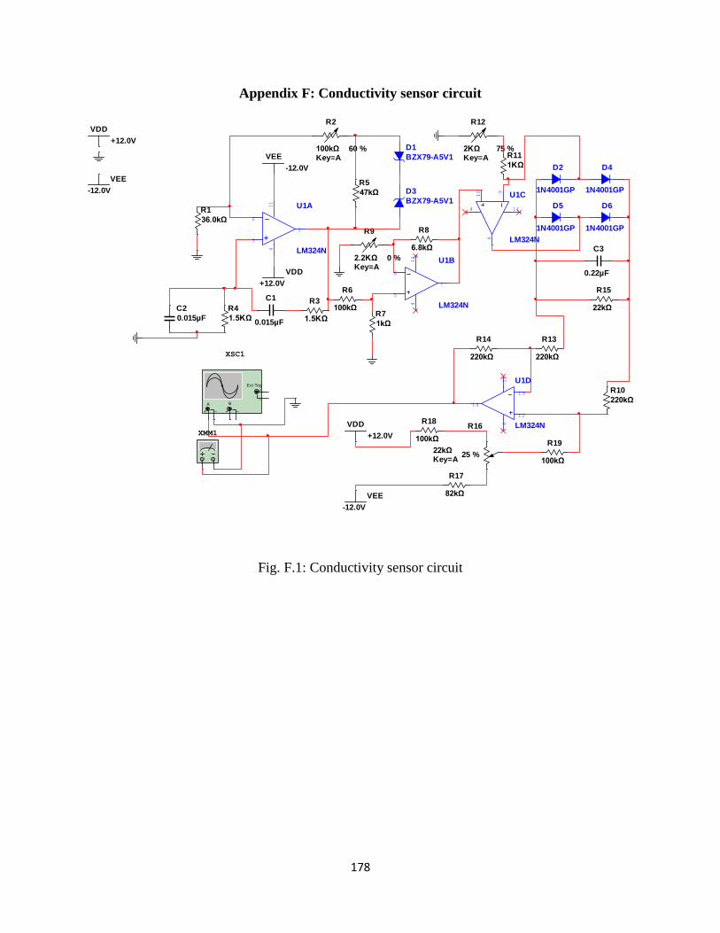
178
Appendix F: Conductivity sensor circuit
Fig. F.1: Conductivity sensor circuit
VDD
+12.0V
VEE
-12.0V
VEE
-12.0V
VDD
+12.0V
R1
36.0kΩ
R2
100kΩKey=A
60 %
R3
1.5KΩ
R4
1.5KΩ
C1
0.015µF
C2
0.015µF
U1A
LM324N
3
2
11
4
1
R5
47kΩ D3
BZX79-A5V1
D1
BZX79-A5V1
U1B
LM324N
5
6
11
4
7
R6
100kΩR7
1kΩ
R8
6.8kΩ
R9
2.2KΩKey=A
0 %
U1C
LM324N
10 9
114
8
R11
1KΩ
R12
2KΩKey=A
75 %
D2
1N4001GP
D4
1N4001GP
D5
1N4001GP
D6
1N4001GP
U1D
LM324N
12
13
11
4
14
R10
220kΩ
R13
220kΩ
R14
220kΩ
R15
22kΩ
VDD
+12.0V
VEE
-12.0V
R16
22kΩKey=A
25 %
R17
82kΩ
R18
100kΩR19
100kΩ
XSC1
A B
Ext Trig+
+
_
_ + _
C3
0.22µF
XMM1

179
Appendix G: Output circuits
Fig. G.1: Buck regulator
With reference to Figure H.1:
Vin = 34.4V (series connected solar panels)
Vout = 26.2V (Maximum charging voltage)
Iload = 0.56A (Maximum current rating of single 10W solar panel)
F = 25KHz (fixed frequency of converter operation)
(ripple current< 30% of Iload maximum)
Vripple = 50mV (Maximum ripple voltage).
pic pin RC2
180
From Rashid (2003), the following expressions of L1 and C3 are obtained:
(( ) )) , and
( )
20μF
Fig. G.2: Solenoid valve driver

181
Appendix H: Sample research photographs
a. PCB track layout b. Constructed board
Fig. H.1: pH and redox sensor amplifiers
Fig. H.2: Three (3) wire PT100 temperature measurement constructed board amplifier

182
a. PCB track layout
b. Constructed board
Fig. H.3: Board incorporating pressure, oxygen and charging current on a single supply quad LM324
OP-AMP

183
Fig. H.4: pH, redox and electrical conductivity sensors mounted on 6m 19mm PVC conduits
Fig. H.5: 24V 30VA battery bank with 10W and 20W series connected panels for the experiment
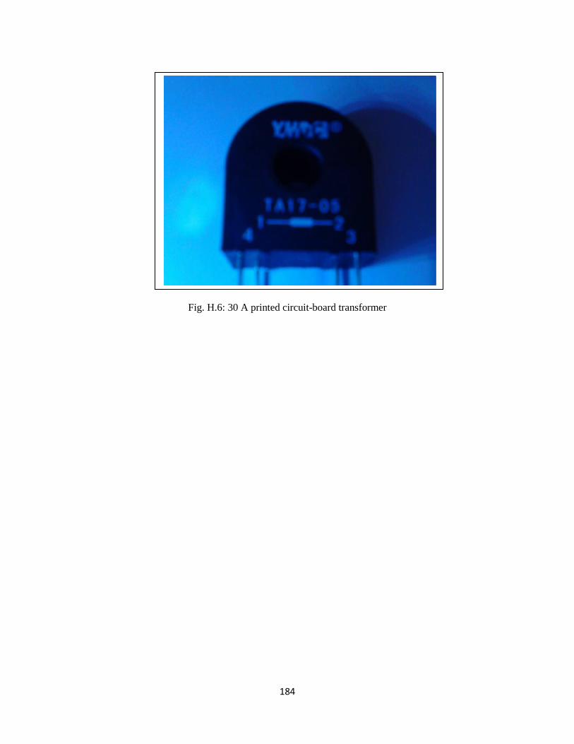
184
Fig. H.6: 30 A printed circuit-board transformer
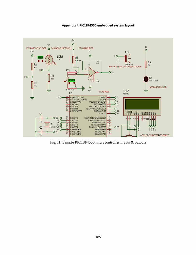
185
Appendix I: PIC18F4550 embedded system layout
Fig. I1: Sample PIC18F4550 microcontroller inputs & outputs