fuzzy logic based control of a two rotor aero-dynamical...
TRANSCRIPT

Tallinn University of Technology
Faculty of Information Technology
Department of Computer Control
Víctor Tarcha Muñoz
Fuzzy Logic Based Control of a Two RotorAero-Dynamical System
Bachelor’s Thesis
Supervisor: Juri Belikov,
Department of Computer Control,
Tallinn University of Technology
Tallinn 2014

Declaration: I hereby declare that this Bachelor’s thesis, my original investigation and
achievement, submitted for the Bachelor’s degree at Tallinn University of Technology,
has not been submitted for any degree or examination.
Declaración: Por la presente declaro que este Trabajo Fin de Grado, mi investigación
y la consecución original, presentado para el título de grado en “Tallinn University of
Technology”, no se ha presentado a ningún grado o examen con anterioridad.
Víctor Tarcha Muñoz
Date . . . . . . . . . . . . . . . . . . . . . . . . . . . . . . . . . . . . . . .
Signature . . . . . . . . . . . . . . . . . . . . . . . . . . . . . . . . . . . . . . .

Contents
Abstract 4
Resumen 5
Acknowledgments 6
1 Introduction 7
1.1 State of the art . . . . . . . . . . . . . . . . . . . . . . . . . . . . . . 8
1.2 Goals of the thesis . . . . . . . . . . . . . . . . . . . . . . . . . . . . 9
1.3 Outline of the thesis . . . . . . . . . . . . . . . . . . . . . . . . . . . 9
2 Theoretical Background 10
2.1 Brief overview of the fuzzy systems . . . . . . . . . . . . . . . . . . 10
2.2 Fuzzy logic . . . . . . . . . . . . . . . . . . . . . . . . . . . . . . . 11
2.3 Fuzzy controller . . . . . . . . . . . . . . . . . . . . . . . . . . . . . 11
2.4 Advantages of fuzzy control . . . . . . . . . . . . . . . . . . . . . . 13
3 TRAS Model 14
3.1 Mathematical model derivation . . . . . . . . . . . . . . . . . . . . . 14
3.1.1 Block diagram . . . . . . . . . . . . . . . . . . . . . . . . . 15
3.1.2 Physical parameters . . . . . . . . . . . . . . . . . . . . . . 17
3.1.3 Nonlinear model . . . . . . . . . . . . . . . . . . . . . . . . 18
3.1.3.1 Moment of the forces and moments of inertia ap-
plied to the horizontal axis . . . . . . . . . . . . . 19
1

3.1.3.2 Moment of the forces and moments of inertia ap-
plied to the vertical axis . . . . . . . . . . . . . . . 20
4 Design 22
4.1 Fuzzy Controller Design . . . . . . . . . . . . . . . . . . . . . . . . 22
4.2 Azimuth Angle Scenario . . . . . . . . . . . . . . . . . . . . . . . . 23
4.2.1 Controller Task Definition for Azimuth Angle . . . . . . . . . 23
4.2.2 Rule-Base Design . . . . . . . . . . . . . . . . . . . . . . . . 24
4.2.2.1 Controller Inputs and Outputs . . . . . . . . . . . . 24
4.2.2.2 Language Description and Value of a Variable . . . 25
4.2.2.3 Rules . . . . . . . . . . . . . . . . . . . . . . . . . 26
4.2.2.4 Rule-Base Tabulation . . . . . . . . . . . . . . . . 27
4.2.3 Inference Mechanism Design . . . . . . . . . . . . . . . . . 28
4.2.3.1 Membership Functions . . . . . . . . . . . . . . . 28
4.2.3.2 Inference Mechanism . . . . . . . . . . . . . . . . 31
4.2.3.3 Defuzzification . . . . . . . . . . . . . . . . . . . 31
4.3 Pitch Angle Scenario . . . . . . . . . . . . . . . . . . . . . . . . . . 32
4.3.1 Controller Task Definition for Pitch Angle . . . . . . . . . . . 32
4.3.2 Rule-Base Design . . . . . . . . . . . . . . . . . . . . . . . . 33
4.3.2.1 Controller Inputs and Outputs . . . . . . . . . . . . 33
4.3.2.2 Language Description and Value of a Variable . . . 33
4.3.2.3 Rules . . . . . . . . . . . . . . . . . . . . . . . . . 34
4.3.2.4 Rule-Base Tabulation . . . . . . . . . . . . . . . . 35
4.3.3 Inference Mechanism Design . . . . . . . . . . . . . . . . . 35
4.3.3.1 Membership Functions . . . . . . . . . . . . . . . 35
4.4 Cross Angles Scenario . . . . . . . . . . . . . . . . . . . . . . . . . 37
2

5 Implementation and improvement of the controller 39
5.1 Azimuth angle . . . . . . . . . . . . . . . . . . . . . . . . . . . . . . 39
5.1.1 Implementation of the Premises . . . . . . . . . . . . . . . . 39
5.2 Pitch Angle . . . . . . . . . . . . . . . . . . . . . . . . . . . . . . . 43
5.3 Cross Angles . . . . . . . . . . . . . . . . . . . . . . . . . . . . . . 48
Discussion 53
Conclusions 55
Future Plans 57
Bibliography 59
3

Abstract
In this thesis an implementation of a fuzzy logic based controller for a Twin Rotor
Aero-dynamical System (TRAS) is presented and discussed. The TRAS consists of a
beam with two propellers placed on the ends. The beam can pivot on its base in such a
way that it can rotate freely both in the horizontal and vertical planes. The control goal
is to provide an accurate control of the beam of the TRAS.
The device is controlled in the real time. Three different scenarios are presented: az-
imuth angle, pitch angle and both of them. For the first two cases 1-DOF model is
derived and used, while to cover the final scenario 2-DOF model is implemented. The
fuzzy controller has been chosen in order to deal with the high nonlinearities of the
system, trying to improve the performance of the classical controllers and their capa-
bilities. The controllers are first designed and implemented separately without taking
into account the cross-couplings effects between the two axes due to the moment of the
forces of the propellers. Then, both designs are put together in a 2-DOF TRAS model.
Numerical experiments are done within the MATLAB/Simulink environment. The cor-
responding figures and simulation results are presented. The performance of suggested
fuzzy controllers is discussed and analyzed.
4
Resumen
En este trabajo fin de grado se presenta y estudia la implementación de lógica difusa
en un sistema aerodinámico con doble motor (TRAS) haciendo uso de un controlador
fuzzy. Este sistema (TRAS) consiste en un eje principal el cual tiene dos motores en
sus extremos, teniendo un eje para pivotar que permite el movimiento en dos grados de
libertad, horizontal y vertical. El objetivo de control es conseguir de una forma rápida
y precisa la posición deseada.
El dispositivo es controlado en tiempo real. Se presentan 3 diferentes situaciones; án-
gulo horizontal, ángulo vertical y ambos al mismo tiempo. Para los ángulos vertical
y horizontal se usa un modelo de 1 grado de libertad, mientras que para el escena-
rio en el que ambos movimientos están involucrados, el modelo diseñado contempla
los 2 grados de libertad. Se elige usar un controlador fuzzy para poder trabajar con
un sistema no lineal, intentando mejorar el rendimiento de los controladores clásicos
y sus capacidades. Los controladores se diseñan por separado sin tener en cuenta los
efectos de acoplamiento provocados por los momentos de las fuerzas que se producen
entre ambos ejes, después se implementan en tiempo real para comprobar su funcio-
namiento. En el último escenario se unen ambos diseños en el modelo de dos grados
de libertad, y así poder estudiar cómo afectan los acoplamientos cruzados provocados
por los momentos de las fuerzas de ambos ejes y cómo el controlador difuso es capaz
de gestionarlos.
Los experimentos son llevados a cabo en el entorno de MATLAB/Simulink. Se pre-
sentan los experimentos llevados a cabo, así como los modelos y los diseños del con-
trolador obtenidos. Por último, se analiza y discute el rendimiento obtenido por el
controlador fuzzy.
5

Acknowledgments
I would like to express my gratitude to the Alpha Control Lab of the Tallinn University
of Technology and specially to my supervisor Juri Belikov, without their help would
not have been possible to accomplish my final bachelor thesis. I am very grateful with
Tallinn University of Technology for giving me the opportunity of realizing this project
here, using its installations and resources. In addition, I want to thanks to Carlos III
University of Madrid which gave me the chance to participate in the Erasmus program.
I cannot forget my girlfriend Ruth Yuste, who has helped me during this course in
the distance, and last, but not least, I also want to thank to my family and friends,
particularly to my parents who supported this year abroad in Tallinn.
6

Chapter 1
Introduction
Two Rotor Aero-dynamical System (TRAS) is a laboratory set-up designed for con-
trol experiments. In certain aspects its behavior resembles that of a helicopter. From
the control point of view it exemplifies a high order nonlinear system with significant
cross-couplings. TRAS consists of a beam pivoted on its base in such a way that the
beam can rotate freely both in the horizontal and vertical planes. At both ends of
the beam there are rotors (the main and tail ones) driven by DC motors. A counter-
balance arm with a weight at its end is fixed to the beam at the pivot. The state of
the beam is described by four process variables: horizontal and vertical angles mea-
sured by encoders fitted at the pivot, and two corresponding angular velocities. Two
additional state variables are the angular velocities of the rotors, measured by speed
sensors coupled with the driving DC motors. In a real helicopter the aerodynamic
force is controlled by changing the angle of attack. In the laboratory set-up the angle
of attack is fixed. The aerodynamic force is controlled by varying the speed of rotor.
Significant cross couplings are observed between actions of the rotors. Each rotor in-
fluences both position angles. The TRAS system has been designed to operate with an
external, PC-based digital controller. The control computer communicates with the po-
sition, speed sensors and motors by a dedicated I/O board and power interface. The I/O
board is controlled by the real-time software which operates in the MATLAB/Simulink
RTW/RTWT environment.
7

1.1 State of the art
The modern control theory starts in the early 19th century, when the first prototypes
PID controllers were developed by Nicolás Minorsk in 1922. Such controllers are the
most spread ones due to their inherit simplicity. The computers era made them even
more and more popular. The need in automation of process was growing with the
increase of industry. That is why a variety of alternatives to PID controllers started to
appear. Fuzzy logic or genetic algorithms are the particular examples of the alternatives
that showed up in the earlier 1960s. In this moment, the computers were grew up and
assisted in development of the industry. In 1980 the first industrial application of the
fuzzy controller was developed by Sugeno [1], who expanded the control of a Fuji
Electric water purification plant.
Nowadays PID controllers are mostly spread in all industries which require automati-
zation of a process. However, fuzzy controllers are also used in the consumer electron-
ics such as washing machines, image stabilizers, cars or even in the subway control [1].
The fuzzy theory is becoming more important, where the complexity of the processes
is demanding new approaches.
From the point of view of research, in the last years the research of fuzzy control theory
are focused on systems in which a model of the process is not possible to obtain, such as
glass industry or cement kilns [1]. In this kind of plants a new approach of controlling
has to be applied, since from the control point of view one has to deal with a black box
model. The industrial applications of the fuzzy control can be divided in three main
fields: control system with Mamdani fuzzy controllers, control systems with Takagi-
Sugeno fuzzy controllers, adaptive and predictive control systems [2].
The latest studies with the Twin Rotor Aero-dynamical System are carried out in the
direction of combining classical controllers with the novel control theories. some ex-
amples can be found in [3, 4] developed in this field, where the fuzzy control theory
is intended help to improve the PID controllers already implemented in the plant. In
addition to the fuzzy systems, also genetic algorithms [5, 6] and radial basis functions
network [7] may be seen as examples of the approach used to improve the control in
TRAS. Another approach consists in using fuzzy systems to develop an observer to
obtain the necessary variables instead of deriving the current inputs of the controller to
obtain more state variables, see [8, 9, 10].
8

1.2 Goals of the thesis
The information discussed in Section 1.1 and the fact that there is no a previous imple-
mentation of a unique fuzzy controller for a Twin Rotor Aero-dynamical System, gave
us the motivation for trying to implement and tune a fuzzy controller for the TRAS.
The next steps are followed for the growth of this thesis:
• Analysis of the system’s properties;
• Analysis of a mathematical model of the system;
• Fuzzy logic based controller design;
• Execution of real-time experiments and analysis of the results.
1.3 Outline of the thesis
In Chapter 2 the reader is presented with the theoretical introduction of the fuzzy the-
ory. It is followed by a brief explanation of a typical fuzzy controller design. Moreover,
several advantages, that have to be taken into account in specific control cases, are dis-
cussed.
In Chapter 3 the model of the TRAS system is described. Its physical parameters and
dynamical properties are explained. In addition, the used demo tape and the interface
are presented.
In Chapter 4 the control design process is presented. The steps and the mechanisms
used in each task are also provided. A brief description of three different scenario is
given, where the differences are explained.
The implementation of the fuzzy controller is shown in Chapter 5. The results of
each experiment are described together, with brief explanations and comparisons. Also
different variants of experiments are presented, in order to compare different situations.
9

Chapter 2
Theoretical Background
The development of the fuzzy control theory begins in the earlier 1960s by Zadeh [1],
and since that moment fuzzy logic based approach infiltrated into control theory and
practice. The reason of such success is very simple – its inherently very simple due
to linguistic component allowing to a less familiar user to write relatively complex
control algorithms without being an expert. In the case of fuzzy control system one
has the option to use the knowledge about how the plant works and what has to be
controlled. This knowledge is introduced into the controller by means of a set of
linguistic statements such as “The speed is very high”, [11].
2.1 Brief overview of the fuzzy systems
The Fuzzy Systems were developed as an alternative to the classical controllers meth-
ods using instead of the analytic control theory, the decision-making logic originated
by artificial intelligence. In addition to other decision-making techniques like neural
networks or genetic algorithms, fuzzy logic provides a more intuitive way to tune a
controller [12]. Even if the name “fuzzy” associates with a something imprecisely
defined, using the rule-base technique, it becomes a rigorous and established theory.
Using the “IF-THEN” statements and the fuzzy controllers it is possible to achieve a
very good control for nonlinear dynamical systems [1,12]. The strong point of design-
ing fuzzy controller is that it can be easily synthesized using natural language.
10

Figure 2.1: Blocks of a fuzzy controller
2.2 Fuzzy logic
A fuzzy controller is a control method based on fuzzy logic. This means that a
fuzzy controller can be described simply as “control with sentences rather than equa-
tions” [13]. The fuzzy logic provides a reasonable way to design a controller. It is an
approximation or quantification of the knowledge in which we are not dealing with 1
or 0 logic, but with a degree of membership of a statement. In the fuzzy logic the im-
plication of each premise can be modeled in many different ways using computational
techniques [14]. The fuzzy logic defines a decision as the best feasible choice of an
action. Hence, the fuzzy logic is seeking for the optimal solution for which the utility
function is maximized.
2.3 Fuzzy controller
A fuzzy controller consists of four common steps: “Fuzzification”, “Rule-Base”, “In-
ference System” and “Defuzzification” [13, 15, 16] as it is shown in Figure 2.1. The
sentences, used for controlling the plant, are the rules of the controller, which repre-
sents the knowledge of the expert. These steps are described in more detail as follows:
Fuzzification: This is the procedure where the controller converts the inputs in a set of
fuzzy variables. This kind of classification is done by giving values to each value of a
set of membership functions. A very common fuzzy classifier splits the input signal in
five levels giving to the input a degree of membership [16]:
• Large positive;
11

• Medium positive;
• Small;
• Medium negative;
• Large negative.
In the fuzzy controller you have to define the constraints on each input in such a
way that the fuzzification mechanism is able to determine the corresponding degree
of membership function for each value.
The Rule-Base defines the rules that quantify the knowledge of the expert of how best
to control the plant in some natural language. This rules are usually given in the “IF-
THEN” format. Using this representation the number of rules will increase exponen-
tially with the number of inputs, for instance, with 3 inputs divided in 5 levels each one,
there are 53 = 125 rules all together. Hence, in general, it is quite tedious procedure
to define all the possible rules. Thus, the expert has to choose the number of inputs as
less as possible. Note that when there are more than 2 rules involved we have to use
connectives as in a normal conversation. The most spread connector is the “AND” but
it is also possible to use “OR”, “NOT” “IF AND ONLY IF” and so on [13].
The Inference Mechanism carries out decision-making procedure. Here the fuzzy con-
troller tries to imitate the behavior of a controller designed by a human in a plant. The
inference mechanism is divided in 2 phases. The first phase is matching in which the
premises of the rules are compared to the inputs. This process entails to determine
the degree of membership. The second phase is devoted to deriving the conclusion
from the inputs. After conclusion is done by the inference mechanism, the last step is
Defuzzification.
The Defuzzification process is the opposite to the fuzzification. Here the controller
translates (also using a set of rules) the conclusions taken by the inference mechanism
and put them in numerical values available for the plant. This step gives the input to
the plant – the signal that will determine the behavior of the procedure available. There
are various methods for this process we proposed, but the only “Center of gravity” is
used in this thesis, see Subsection 4.2.3.3 and [13, 15] for more details.
12

2.4 Advantages of fuzzy control
As it was already mentioned the majority of the industrial plants and processes are
nonlinear, and the classical control approach, for instance PID, is able to perform an
accurate control, but around some working point. Nowadays we are still studying with
a great effort linear systems [1], because we always try to model these systems.In addi-
tion, the PID controllers have a big liability with the noise of the signal, because these
controllers cannot deal with the noise of a signal [17]. Moreover, the fuzzy controllers
are able to put together the knowledge of an expert engineer and the information mea-
sured by sensors. These are the main reasons why are the fuzzy controllers increasing
its place in the industry [1]. Another approach to understand the advantages of the
fuzzy controller is the easy implement of the rule sets. The engineer is able to trans-
late his knowledge through the rules without being an expert on fuzzy control systems,
because it is used the natural language, for instance English. These non analytical
methods allows to the expert to put his knowledge about the plant. In the classical
controllers the model of the plant has to be developed for an expert engineer in that
area, then the controller has to be developed using the classical mathematical theo-
ries [1,12,15]. In addition, we have to imagine the industrial processes where the wear
of engines is present. With the fuzzy control we do not create any model, that means
the controller does not need to change with the engine wear because the sensors are
giving new information (including wear) even when the time is going. Conversely,
when we are dealing with classical controller, we create a model with a given condi-
tions. Over time the wear is not taken into account, and the precision of the classical
controller decrease [17, 18].
13

Chapter 3
TRAS Model
This chapter will serve as a brief introduction of Twin Rotor Aero-dynamical System
(TRAS), and we refer the interested reader to the user’s manual [19] for more details.
Throughout the thesis we consider f(t) = f omitting the time variable t to make the
mathematical expressions visually more compact.
3.1 Mathematical model derivation
The TRAS model was derived by the INTECO company which is placed in Poland.
This device was developed as a laboratory set-up designed for control experiments.
In certain aspects its behavior resembles that of a helicopter. The system consists of
a device controlled from a PC. The system is controlled in real time using software.
TRAS has also its own power supply and the interface with the PC and the dedicated
RT-DAC/PCI I/O board configured in the Xilinx® technology. The overall system
can be seen as a nonlinear MIMO control system, which is very suitable to illustrate
complex control algorithms [19].
The device consists of a beam pivoted on its base in such a way that it can rotate freely
both in the horizontal and vertical planes as shown in Figure 3.1. The beam has two
DC rotors at both ends, the tail rotor allows the azimuth movement (horizontal plane)
and the main rotor allows the pitch movement (vertical plane). A counter-weight arm
is fixed to the beam in the pivoting point. The TRAS has two encoders at the pivot
to measure angles in the horizontal and vertical planes, respectively. It also has two
tacho-generators to measure the velocity of the DC rotors. Therefore, we can use up
14

to six variables to determine the state of the beam; two angles and their velocities, and
two velocities of the rotors. The inputs of the system are the supply voltages of our DC
rotors, which determine the aerodynamic force by varying the speed of rotors. That
change in the supply voltage of the rotor cause a change in the speed of the propeller
and results in a change of the beam position.
Figure 3.1: Picture of the TRAS device [19]
3.1.1 Block diagram
Here, we represent the mathematical model via a block diagram, that provides a con-
venient way to be used within MATLAB/Simulink environment. The block diagram
of the device is shown below in Figure 3.2. The notations of the physical parameters
are as follows:
αh is horizontal position (azimuth position) of TRAS beam [rad]
Ωh is angular velocity (azimuth velocity) of TRAS beam [rad/s]
Uh is rotational speed of tail rotor [rad/s]
15

Fh is aerodynamic force from tail rotor [N]
lh is effective arm of aerodynamical force from tail rotor [m]
Jh is nonlinear function of moment of inertia with respect to vertical axis
[Kgm2]
Mh is horizontal turning torque [Nm]
Kh is horizontal angular momentum [Nms]
fh is moment of friction force in vertical axis [Nm]
αv is vertical position (pitch position) of TRAS beam [rad]
Ωv is angular velocity (pitch velocity) of TRAS beam [rad/s]
Uv is vertical DC-motor PWM voltage control input
ωv is rotational speed of main rotor [rad/s]
Fv is aerodynamic force from main rotor [N]
lv is arm of aerodynamic force from main rotor [m]
Jv is moment of inertia with respect to horizontal axis [Kgm2]
Mv is vertical turning momentum [Nm]
Kv is vertical angular momentum [Nms]
fv is moment of friction force in horizontal axis [Nm]
Rv is vertical returning momentum [Nm]
Jhv is vertical angular momentum from tail rotor [Nms]
Jvh is horizontal angular momentum from main rotor [Nms]
Gv is aerodynamical damping torque from main rotor
Gh is aerodynamical damping torque from tail rotor
16

Figure 3.2: Block diagram of the system
In the above notations h and v correspond to horizontal and vertical directions, re-
spectively. The block diagram shown in Figure 3.2 is a mathematical representation
of the beam. The block is a simplification of the nonlinear cross-coupled system. It
was obtained using classical modeling methods, in particular, Lagrange equations. The
control voltages Uh and Uv are inputs to the DC-motors which drive the rotors. A ro-
tation of the propeller generates an angular momentum which, according to the law of
conservation of angular momentum, must be compensated by the remaining body of
the TRAS beam. This results in the interaction between two transfer functions, rep-
resented by the moment of inertia of the motors with propellers Khv and Kvh. This
interaction directly influences the velocities of the beam in both planes. The forces Fh
and Fv multiplied by the arm lengths lh and lv are equal to the torques acting on the
arm.
3.1.2 Physical parameters
The numerical values for the physical parameters are taken from [19] and given below:
lt = 0.216 [m] is the length of the tail part of the beam;
lm = 0.202 [m] is the length of the main part of the beam;
lb = 0.145 [m] is the length of the counter-weight beam;
lcb = 0.15 [m] is the distance between the counter-weight and the joint;
rms = 0.145 [m] is the radius of the main shield;
rts = 0.10 [m] is the radius of the tail shield;
17

mtr = 0.225 [kg] is the mass of the tail motor with tail rotor;
mmr = 0.252 [kg] is the mass of the main DC-motor with main rotor;
mcb = 0.0256 [kg] is the mass of the counter-weight;
mt = 0.032 [kg] is the mass of the tail part of the beam;
mm = 0.03 [kg] is the mass of the main part of the beam;
mb = 0.01 [kg] is the mass of the counter-weight beam;
mts = 0.061 [kg] is the mass of the tail shield;
mms = 0.083 [kg] is the mass of the main shield.
Most of these parameters are presented in Figure 3.3.
Figure 3.3: Gravity forces corresponding with the returning torque
3.1.3 Nonlinear model
In order to reach a proper description of the nonlinear model several assumptions have
to be done. These assumptions allow us to achieve an accurate model having a similar
behavior to that of the real device:
1. The dynamics of the propeller subsystem can be described by the first order
differential equations.
2. It is assumed that the friction in the system is of the viscous type.
18

3. It is assumed that the subsystem propeller-air could be described in accord with
postulates of the flow theory.
3.1.3.1 Moment of the forces and moments of inertia applied to the horizontal
axis
Using the second Newton law we have:
Mv = Jvd2αv
dt2,
where Mv is total moment of forces in the vertical plane, i.e., Mv =∑
Mvi, Jv is
the sum of moments of inertia relative to the horizontal axis, i.e., J =∑Jvi, αv is
the pitch angle of the beam. Next, consider the situation shown in Figure 3.3, which
represents the gravity forces that are involved in the beam when it is rotated around the
horizontal axis. Then, one obtains the the next equation of the moment of forces:
Mv1 = g
[(mt
2+mtr +mts
)lt −
(mm
2+mmr +mms
)lm
]cosαv
−[mb
2lb +mcdlcb
]sinαv
,
where g is the gravitational acceleration assumed to be 9.8 m/s2 and
A =(mt
2+mtr +mts
)lt, B =
(mm
2+mmr +mms
)lm, C =
mb
2lb +mcdlcb.
Using the expressions above (A,B and C) we obtain Mv1 in a more compact form:
Mv1 = g (A−B) cosαv − C sinαv .
We get the others moments of forces as follows:
Mv2 = lmFv (ωm) ,
whereωm is angular velocity of the main rotor and Fv(ωm) denotes the dependence
of the propulsive force on the angular velocity of the rotor. It should be measured
experimentally. Then,
19

Mv3 = −Ω2h(A+B + C) sinαv cosαv,
where Ωh = dαh
dt, and Mv3 is the moment of centrifugal forces corresponding to the
motion of the beam around the vertical axis.
Mv4 = −dαh
dtfv is the moment of friction depending on the angular velocity of the
beam around the horizontal axis, where fv is a constant.
Mv5 is the cross moment from Uh,v5 = Uhkhv, where khv is a constant.
Mv6 is the damping torque from rotating propeller Mv6 = −a1Ωva|ωv|, where a1 is a
constant.
Finally, we obtain the equations of the moment of inertia:
Jv1 = mmrl2m, Jv2 = mm
l2m3, Jv3 = mcbl
2cb,
Jv4 = mbl2b3, Jv5 = mtrl
2t , Jv6 = mt
l2t3,
Jv7 =mms
2r2ms +mmsl
2m, Jv8 = mtsr
2ts +mtsl
2t ,
where rms is the radius of the main shield and rts is the radius of the tail shield. After
the analysis of the physical features the value of Jv is 0.0307 Kgm2
3.1.3.2 Moment of the forces and moments of inertia applied to the vertical axis
Using the same principles as in the horizontal axis we can describe the moments of
inertia and the moments of the forces in the vertical axis. In Figure 3.4 below an
example of this forces is shown. We have the formula:
Mh = Jhd2αh
dt2,
whereMh is the sum of the moments of the forces in the vertical axis (horizontal plane)
and Jh is the sum of the moments of inertia relative to the vertical axis. This situation
is described in Figure 3.4, where the pitch angle is shown. The moment induced by the
tail rotor:
Mh1 = ltFh(ωt) cosαv,
20

where ωt is angular speed of the tail rotor, Ft(ωt) denotes the dependence of the propul-
sive force on the angular speed of the tail rotor, which has to be determined experimen-
tally. The others moments of forces are obtained as following:
Mh2 = −dαh
dtfh is the moment of the friction depending on the angular velocity of the
beam around the vertical axis, where fh is a constant.
Mh3 = Uvkvh is the cross moment from Uv with kvh being a constant.
Mh4 = −a2Ωh|ωh| is the damping torque from rotating propeller, where a2 is a con-
stant.
The moment of inertia relative to vertical axis can be obtained as:
Jh = E cos2 αv +D sin2 αv + F ,
where D = mb
3l2b +mcbl
2cb, E =
(mm
3+mmr +mms
)l2ms +
(mt
3+mtr +mts
)l2t , and
F = mmsr2ms + mts
2r2ts.
Figure 3.4: Gravity forces for the horizontal axis
After this analysis, we can conclude with the sum of the values of the moments of
inertia in the horizontal axis using the values of the length and weight given in the
manual [19],
Jh = 0.0279 cos2 αv + 0.0013 sin2 αv + 0.0021Kgm2.
21

Chapter 4
Design
In this chapter we will proceed with the preliminary design of the controller using the
fuzzy logic techniques. We follow the classical procedure given in [15].
4.1 Fuzzy Controller Design
A fuzzy design is based on the understanding of how to control a process. Then the ob-
tained knowledge can be used to synthesize the controller. While the classical ideas of
controlling, as for instance PID controller, usually use an analytical method to develop
the controller, with Fuzzy the process of developing the controller exploits a natural
language, becoming easier to set the controller for a non expert control engineer. In this
case, it is more important to know how the plant works, and what is the desired control.
Fuzzy controllers have four main components: “Rule-Base”, “Inference Mechanism”,
“Fuzzification Interface” and “Defuzzification Interface”. All this parts are described
in Figure 4.1, where the process outputs are denoted by y, its inputs are denoted by
u, and the reference input to the fuzzy controller is denoted by r, see [15] for more
details.
22

Figure 4.1: Convention fuzzy controller architecture [15]
In the “Rule-Base” the knowledge of the expert, who is going to control the plant,
is given by a set of a rules of how to control the process designed after knowing the
behavior of the plant. In the “Inference Mechanism” fuzzy controller evaluates which
rules are important at the current time in order to decide what input of the plant should
be, while the “Fuzzification Interface” modifies the inputs of the controller so that they
can be interpreted and compared to the rules in the “Rule-Base”. The “Defuzzification
Interface” is the opposite to the “Fuzzification Interface”, converts the conclusions of
the “Inference Mechanism” into the inputs of the plant. Thus, we can see why the
process is natural, and how the fuzzy controller imitate the expert decision making in
such a way that the control of the plant is proportional to the expert knowledge.
In this project we are dealing with the TRAS device, which has 2 main angles of
movement – azimuth and pitch. Three fuzzy controllers have to be developed: one for
the azimuth angle, another for the pitch angle, and the last one for both of them.
4.2 Azimuth Angle Scenario
4.2.1 Controller Task Definition for Azimuth Angle
First, we should know the tasks that our controller has to do. The tasks can be formu-
lated as follows:
• The TRAS model has to be brought to a desired position in a finite time.
• The TRAS model has to reach the desired position given any reasonable values
of initial position.
23

• In case of disturbances at any moment, the TRAS has to reach the desired posi-
tion in a finite time.
• TRAS controlling has to be developed without exceeding the velocities and the
angle position constraints.
For this section we assume that only the azimuth angle is taken into consideration, and
the moments of inertia given by the pitch angle are not present.
4.2.2 Rule-Base Design
The first main controller task. All the steps for the Rule-Base design are described in
the next subsections, following the main steps to get the optimal design.
4.2.2.1 Controller Inputs and Outputs
The selection of the inputs and outputs is one of the main tasks. It determines how
many membership functions we will have, and the choice of the proper inputs and
outputs will give us the best control. Furthermore, if we choose too many inputs our
controller will be slow. Thus, the number of inputs has to be as small as possible, but
sufficient to have a good control of the plant. It can be see in Figure 4.1 that the input
for our controller y is the error given by the difference between the desired position
and the current position. We will use also the velocity of the beam in such a way to be
more precise with our controller. The output of the controller is the input of our plant.
For this project the inputs are:
eΘ Position error between the desired position and the current position.
eΘ Velocity of the beam in the current moment.
Hence we have two inputs. Furthermore there is also an output (the normalized voltage
[−1, 1]) which is the input to the device. Thus, we have a MISO type controller with
two inputs and one output.
These inputs are the same for the three different scenario, the movement in the azimuth
angle, pitch, and both of them.
24

4.2.2.2 Language Description and Value of a Variable
Since the description of how to control the plant is given by a person, it has to use a
natural language [12]. The fuzzy controller has to interpret this natural language using
the fuzzification process, and we have to implement these variables for the controller
in an understandable language. It has been decided to use the next language for the
variables:
eΘ position error;
eΘ change in error;
u voltage.
The values of the variables are assigned in a form of linguistic values, which will be
later assigned to numerical values. We will use five linguistic values for the “position
error” input and for the output, and only three linguistic values for the input change in
error. In such a way we indicate the importance of each variable using one of these five
values. Every variable with five values is assigned with one of the following linguistic
values:
• “neglarge” negative large in size
• “negsmall” negative small in size
• “zero” zero
• “possmall” positive small in size
• “poslarge” positive large in size
Again here we try to mimic as much as possible the name of the variables for having
a comfortable work later, that is why we write “negative large in size” as “neglarge”
which gives us enough information about its value. For the input “change in error” the
following names are used:
• “neglarge”
• “zero”
25

• “poslarge”
After the linguistic values are given we can abbreviate them, using integer values. The
numerical values are not assigned to a specific value of the radians of the error or to a
specific value of the input voltage. The use of the numbers for linguistic descriptions
simply indicates the size in relation to other linguistic values [15]. As an example of
quantification of values of statements we can have:
• Position error neglarge is when the beam is quite far away from the desired
position in the azimuth angle angle of the horizontal position.
Assigning the numerical values for the linguistic values, we obtain the following result:
• “neglarge” is −2
• “negsmall” is −1
• “zero” is 0
• “possmall” is 1
• “poslarge” is 2
4.2.2.3 Rules
Once we have determined the inputs and the outputs, and we have quantified the lin-
guistic and numeric values of the variables, we have to implement the rules. Doing
this, we are imitating the expert knowledge, that will be reflected in the “rule base”.
The normal form of a linguistic rule is as follows:
• If premise Then consequent
This is the general case for one input and one output, but we can use the operators And,
Or and Not to consider more than one premises. In the example above the operator
“And” was used. In the specific case described in this project, we are dealing with at
most 15 rules (all possible combination of the premises for our two inputs). In this case
the physics of the system are quite basics, however in other cases it is very important to
have a deep knowledge about the process, that is why it is necessary to use the expert.
As an example of this linguistic statements we can use the next:
26

• IF error position is negsmall AND change in error is negsmall THEN voltage is
negsmall
As we can imagine here, the situation is as follows. The beam is close to the desired
position, but the velocity shows us that it is moving in the wrong direction. Hence, we
need to change the direction of the beam switching the direction of the propeller, but
taking into account that the beam is near to the desired position and we have to use low
voltage to reach the desired position.
These are the linguistic rules that give us understanding about the plant and how the
controller has to work. These linguistic rules are not completely precises, they are only
an abstract idea about how to do a proper control. For a better implementation of the
fuzzy controller and for a more compact form, it is common to use the numeric values
in the table representation.
4.2.2.4 Rule-Base Tabulation
The Rule-Base is the set of rules specified by the expert. The set of rules has to be
wide enough to provide a good control of the plant. Moreover, we have to bear in mind
all the possible combinations involved in the behavior of the device, always knowing
that the number of inputs will be critical in the performance of the control. Thus, it is
necessary to implement the minimum number of inputs providing enough information
to the controller.
The most common way to represent the Rule-Base is the table representation. As it was
only chosen two inputs, we will deal with one table (see Table 4.1 below), where we
will use the numerical values for the representation of all the possible situations in the
Rule-Base. In this case, the table will be symmetric, logically because the dynamics
in the azimuth angle are totally symmetric. In the case of the pitch angle, we will see
that it is not symmetric, which will complicate the setting up of the table more than it
was expected.
27

Table 4.1: Design for azimuth angle
Design for the azimuth angle control
VoltageError
−2 −1 0 1 2
Change in error−2 −2 −2 −1 −2 20 −2 −1 0 1 22 −2 2 1 2 2
4.2.3 Inference Mechanism Design
We have to apply the inference system in order to implement the Rule-Base meaning.
The linguistic rules are abstract descriptions of how to control the plant and we have to
implement this knowledge with the fuzzy controller through the Inference mechanism.
4.2.3.1 Membership Functions
The membership functions are the way to quantify the degree of certainty of each
rule. We will use for this specific case the triangle and the trapezoidal shapes. It is
important to note that the shapes of the membership function have to be finite because
the inference system will be used to determine how much important is each rule for
every working moment. As we decided to have five different values for the each input
and output, we will have five membership functions, i.e., one for each value. The
triangle function is defined as:
f(a, b, c, d) =
0, x ≤ a
x−ab−a , a ≤ x ≤ b
c−xc−b , b ≤ x ≤ c
0, c ≤ x
and the trapezoidal function is defined by:
28

f(a, b, c, d) =
0, x < a or x > d
x−ab−a , a ≤ x ≤ b
1, b ≤ x ≤ c
d−xd−c , c ≤ x ≤ d
Using the heuristic knowledge of the system we create the membership functions that
are suitable for changes in the future. For the design purposes we use the triangle
shape, being this the simplest one providing simple calculations compared to the other
shapes. To define our membership functions we use [15] as the expert knowledge:
• the error input [3,−3],
• the change in error input [10,−10],
• the normalized output signal [1,−1],
and the final design for every membership function is as follows.
• Input Position Error:
−3 −2 −1 0 1 2 3
0
0.2
0.4
0.6
0.8
1
error
Deg
ree
of m
embe
rshi
p
neglarge zero poslargenegsmall possmall
Figure 4.2: First design of the input position error
• Input Change in Error:
29

−10 −5 0 5 10
0
0.2
0.4
0.6
0.8
1
change
Deg
ree
of m
embe
rshi
p
mf1 mf2 mf3
Figure 4.3: First design for input change in error
• Output Normalized Voltage:
−1 −0.5 0 0.5 1
0
0.2
0.4
0.6
0.8
1
voltage
Deg
ree
of m
embe
rshi
p
mf1 mf2 mf3mf4 mf5
Figure 4.4: First design of the output
The fuzzification interface is responsible for taking a value from the inputs. We use
the simplest and more spread fuzzification function, called singleton, defined by
30

µ(x) =
1, x = ui
0, x 6= ui,
where ui denotes a single value for a set.
4.2.3.2 Inference Mechanism
The Inference Mechanism process can be divided in two subprocesses:
a) The matching process. In this process the fuzzy controller compares all the premises
of the rules with the controller inputs, in order to decide which inputs apply at each
moment.
b) The process of making conclusions is based on the rules that have to be applied in
the current situation.
In the matching process the "And" method is used for composing the premises, and
to quantify the certainty µ of each premise is used the minimum definitions [15]. For
instance, consider the situation with the next statement:
“error is zero and change-in-error is possmall”
To quantify the “And” operation in the premise suppose that µzero = 0.25 and µchange−in−error =
0.35, the minimum definition means:
µpremise = min0.25, 0.35 = 0.25, that is, using the minimum of two membership
values to quantify the certainty of the premise.
Based on the premises the rules that apply to the current situation can be determined.
A rule is considered to be “on” if its premise is greater than zero. The decision making
process follows the values of the rules that are “on” and the degree of certainty of the
consequent is determined by the degree of certainty of the premise.
4.2.3.3 Defuzzification
This process provides the way to choose a single crisp output that is denoted by ycrispq .
In this case there are a lot of solutions for this process and we will choose the most
common and spread one: The Center Of Gravity Defuzzification Technique [1, 15].
31

The following formula shows us how the Fuzzy controller proceed with the defuzzifi-
cation process:
ycrispq =∑R
i=1 bqi
∫yqµBıq(yq)dyq∑R
i=1
∫yqµBıq(yq)dyq
,
where R is the number of rules, biq is the center of area of the membership function
of Bpq associated with the constructed fuzzy set Bq
i for the ith rule (j, k, ..., l; p, q)i,
and∫yqµBıq(yq)dyq denotes the area under µBıq(yq). It is important to notice that the
area under each implied fuzzy set cannot be infinite, since it has to be computable. In
addition the denominator must be nonzero.
4.3 Pitch Angle Scenario
In this scenario we follow the same steps as in the case of azimuth angle. The main
difference here is that the system is not symmetrical. The gravity force is not the same
for different pitch angles. This situation generates a more complex control for the
plant.
4.3.1 Controller Task Definition for Pitch Angle
First, we should know the tasks that our controller has to do. The tasks are formulated
as in Section 4.2 :
• The TRAS model has to be brought to a desired position in a finite time.
• The TRAS model has to reach the desired position given any reasonable values
of initial position.
• In case of disturbances at any moment, the TRAS has to reach the desired posi-
tion in a finite time.
• TRAS controlling has to be developed without exceeding the velocities and the
angle position constraints.
For this section we assume that only the pitch angle is taken into consideration, and
the moments of inertia given by the azimuth angle are not present.
32

4.3.2 Rule-Base Design
In the pitch scenario we are dealing also with the same inputs and outputs, but for a
different propeller.
4.3.2.1 Controller Inputs and Outputs
The selection of the inputs and outputs is:
eΘ Position error between the desired position and the current position.
eΘ Velocity of the beam in the current moment.
Furthermore there is also an output (the normalized voltage [−1, 1]) which is the input
to the device:
u Output of the fuzzy controller
Thus, we have a MISO type controller with two inputs and one output.
4.3.2.2 Language Description and Value of a Variable
In order to have an easy interpretation of the controller tasks the name given in the pich
scenario are the same as in the azimuth.
eΘ position error;
eΘ change in error;
u voltage.
The values of the variables are assigned in a form of linguistic values, which will be
later assigned to numerical values. We will use five linguistic values for the “position
error” input and for the output, and only three linguistic values for the input change in
error following the azimuth design:
• “neglarge” negative large in size
• “negsmall” negative small in size
33

• “zero” zero
• “possmall” positive small in size
• “poslarge” positive large in size
Again here we try to mimic as much as possible the name of the variables for having a
comfortable work later. For the input “change in error” the following names are used:
• “neglarge”
• “zero”
• “poslarge”
The last step in the description is to give numerical values for the linguistic values, we
obtain the following result:
• “neglarge” is −2
• “negsmall” is −1
• “zero” is 0
• “possmall” is 1
• “poslarge” is 2
4.3.2.3 Rules
Again in this step we have to put the expert knowledge into the fuzzy controller. The
technique used is as follows:
• If premise 1 and premise 2 Then consequent
This case is used for out 2 inputs (premises) and 1 output. In the example above the
operator “And” was used. In the specific case described in this project, we are dealing
with at most 15 rules (all possible combination of the premises for our two inputs). The
physics in the pitch scenario are more complex than in the azimuth one, because of the
gravity force. We are dealing with a more complex case, so we have to pay attention to
the differences between the azimuth angle and pitch such as in azimuth was the same
going from left to right and vise versa, but the propeller in pitch angle is almost always
going in the same direction with more power or less depending on the desired position.
34

4.3.2.4 Rule-Base Tabulation
The most common and compact way to represent the set of rules is the table represen-
tation. In this case the table is not symmetrical, and the set of rules is totally different
from the azimuth angle. Starting from the azimuth table a design is developed to avoid
the gravity forces, which will be changed in the implementation section to improve
this preliminary design.
Table 4.2: Design for pitch angle
Design for the pitch angle control
VoltageError
−2 −1 0 1 2
Change in error−2 −2 −2 −2 −1 20 −2 −2 −1 0 22 −2 −1 2 2 2
4.3.3 Inference Mechanism Design
Following the common steps described in [15] the inference system is the responsible
for the decision making, also described in the case of azimuth angle above.
4.3.3.1 Membership Functions
The membership functions are the way to quantify the degree of certainty of each rule.
We will use for this specific case the triangle and the trapezoidal shapes described in
Subsection 4.2.3.1. Again we have 5 membership functions in the case of the input
“error” and the output “voltage” and 3 in the input “change in error”, i.e., one for each
value.
Using the heuristic knowledge of the system we create the membership functions, that
are suitable for changes in the future, with the following bounds:
• the error input [3,−3],
• the change in error input [10,−10],
• the normalized output signal [0.8,−0.8],
35

and the final design for every membership function in the pitch scenario is as follows.
• Input Position Error
−3 −2 −1 0 1 2 3
0
0.2
0.4
0.6
0.8
1
error
Deg
ree
of m
embe
rshi
p
negsmall zero possmallneglarge poslarge
Figure 4.5: First design of the input position error
• Input Change in Error
−10 −5 0 5 10
0
0.2
0.4
0.6
0.8
1
derivative
Deg
ree
of m
embe
rshi
p
neglarge zero poslarge
Figure 4.6: First design of the input change in error
36

• Output Voltage
−0.8 −0.6 −0.4 −0.2 0 0.2 0.4 0.6 0.8
0
0.2
0.4
0.6
0.8
1
control
Deg
ree
of m
embe
rshi
p
mf1 zero mf3mf4mf5
Figure 4.7: First design of the output
4.4 Cross Angles Scenario
In this section we are mixing both angles at the same time. The TRAS system will
work with both angles at the same time. As we have used fuzzy systems we are able to
use the same design as for the individual cases. That is one of the most useful features
of this sort of designs, in this case we obtain good results without designing anything
new.
For this scenario a new model has to be created:
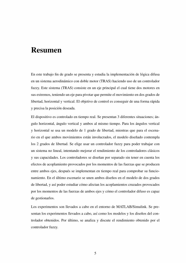
37
Figure 4.8: Model for the cross angles scenario
After the model is developed, we only have to load the fis files used in azimuth and
pitch angles into the model, using the fuzzy toolbox provided by MATLAB/Simulink.
38
Chapter 5
Implementation and improvement of
the controller
To implement and improve the controller we used the Simulink tool provided with
MATLAB. In this particular case the version MATLAB R2012b is used, which is in-
stalled in the computers of the laboratory. We use the given circuit with the device as
a basis for the design of the circuit in Simulink. Further, we will include the premises
using the toolbox given in Simulink for this purpose, and also the defined rules.
5.1 Azimuth angle
Following the same steps as in the previous chapter, we divide the implementation in
three different scenario starting with the azimuth angle.
5.1.1 Implementation of the Premises
In the command row of MATLAB we introduce the command:
“fuzzy” or:
“fuzzy (NameOfTheFisFile)”
and we get the interface for the implementation of the premises and the rules. The final
set of rules is shown in the following table:
39

Table 5.1: Final design for azimuth angle
Final design for the azimuth angle control
VoltageError
−2 −1 0 1 2
Change in error−2 −2 −2 −1 −2 20 −2 −1 0 1 22 −2 2 1 2 2
Later we will save all the information in a fis file, which will be used by the Simulink
model. After several attempts, we obtain the final design of the input “Error Position”
as in the following figure:
−2.5 −2 −1.5 −1 −0.5 0 0.5 1 1.5 2 2.5
0
0.2
0.4
0.6
0.8
1
error[rad]
De
gre
e o
f m
em
be
rsh
ip
neglarge zero poslargenegsmall possmall
Figure 5.1: Premises of the input error
Here, it is easy to see that the shape is not symmetrically looking at the premises
“neglarge” and “negsmall”. That is because the physics of the system are not exactly
as it was supposed. A lot of involved parameters, for instance, the wires which read
the information of the tachometers, are constraining the free movements of the beam.
That could seem simple to solve, but during the improving process this was one of the
most difficult steps, because it was not working as it was supposed to and we had to
figure out what was the problem and we had to spent a lot of time for this purpose. The
following figure is the Input Change in Error:
40

−1 −0.5 0 0.5 1
0
0.2
0.4
0.6
0.8
1
derivative
Deg
ree
of m
embe
rshi
p
zeronegsmall possmall
Figure 5.2: Premises of the input change in error
Output Normalized Voltage:
−0.6 −0.4 −0.2 0 0.2 0.4 0.6
0
0.2
0.4
0.6
0.8
1
control
Deg
ree
of m
embe
rshi
p
neglarge zero poslargenegsmall possmall
Figure 5.3: Premises in the output of the controller
In this case the constraints of the output are [−0.6, 0.6]. The TRAS device has the
input normalized between −1 and 1, but with this constraints the control of the device
was very hard to achieve, that is why we dropped this restriction.
41

Fuzzy process is done by the computer, and we only have to say to the computer
through the Fuzzy toolbox interface our preferences. In this case the main preferences
are:
1. It will be used “And” method for composing the premises in the inference mech-
anism.
2. It will be used “COG” process for the defuzzification mechanism.
Proceeding this way we create a fis file for the azimuth angle that is to be implemented
in the model. With the fis file ready, the last step of the implementation is to prepare the
model. The fuzzy toolbox provided by Simulink is used to create the new model with
the fuzzy controller. We also have to implement a derivative tool, in order to get the
“Change in Error” input for the controller. Finally, the model is completed as shown
in the next figure:
Figure 5.4: Model for the azimuth movement
After tuning the name and the parameters in the “Scope” set the time of the simulation
as 30 seconds, we obtain the next output signal depicted in Figure 5.5:
42

0 5 10 15 20 25 30−1
−0.8
−0.6
−0.4
−0.2
0
0.2
0.4
0.6
0.8
Time [s]
Pos
ition
[rad
]
desired positionPosition
Figure 5.5: Output of the TRAS device with fuzzy controller
From Figure 5.5 we can see a quite good response of the system. The desired position
(the solid one) changes every 10 seconds from −0.8 to 0.8 radians. The device reacts
quite fast before the stabilization, which means a good control response.
5.2 Pitch Angle
In this case in order to be more efficient we have created the model of the pitch scenario
in MATLAB/Simulink at the beginning of the process, yielding Figure 5.6:
43

Figure 5.6: Model for the pitch movement
After the model is prepared the fuzzy interface is opened. The final design of the set
of rules is as follows:
Table 5.2: Final design for pitch angle
Final design for the pitch angle control
VoltageError
−2 −1 0 1 2
Change in error−2 −2 −1 −2 −1 20 −2 −1 −1 2 22 −2 1 2 2 2
In this case, after several different implementations we have 2 options for the pitch
implementation. The first fis file is developed as follows:
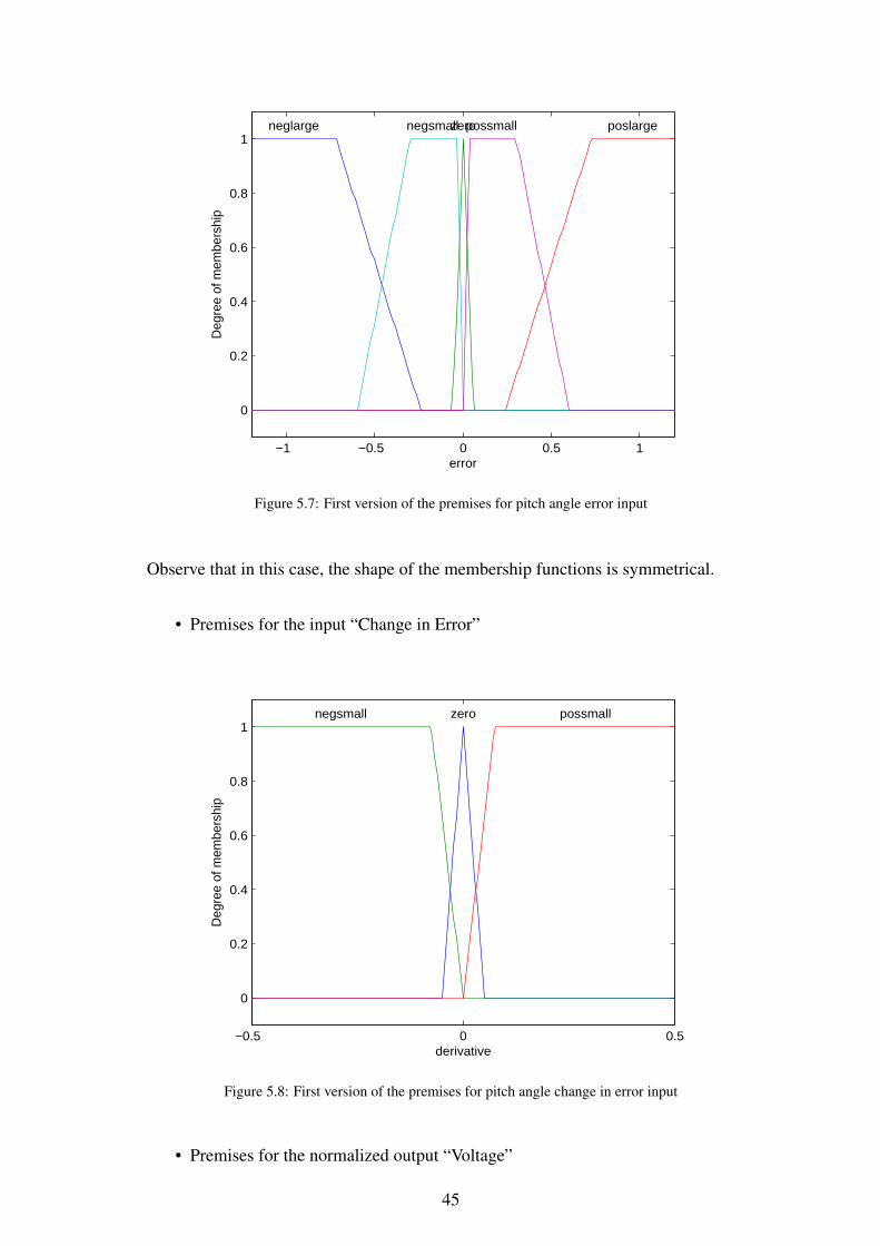
• Premises for the input “Error”
44
−1 −0.5 0 0.5 1
0
0.2
0.4
0.6
0.8
1
error
Deg
ree
of m
embe
rshi
p
neglarge zero poslargenegsmall possmall
Figure 5.7: First version of the premises for pitch angle error input
Observe that in this case, the shape of the membership functions is symmetrical.
• Premises for the input “Change in Error”
−0.5 0 0.5
0
0.2
0.4
0.6
0.8
1
derivative
Deg
ree
of m
embe
rshi
p
zeronegsmall possmall
Figure 5.8: First version of the premises for pitch angle change in error input
• Premises for the normalized output “Voltage”
45

−0.5 0 0.5
0
0.2
0.4
0.6
0.8
1
control
Deg
ree
of m
embe
rshi
p
neglarge zero poslargenegsmall possmall
Figure 5.9: First version of the premises for pitch angle voltage output
With this we are able to see the final design for the pitch movement in this first option.
The results are shown in Figure 5.10, where we can see the static error of 0.08 radians
when the beam has reached steady-state.
0 10 20 30 40 50 60−0.1
0
0.1
0.2
0.3
0.4
0.5
0.6
Time [s]
Pos
ition
[rad
]
desired positionPosition
Figure 5.10: First case of the output in the pitch angle
Trying to fix the static error the second option it is implemented. In this case we have
46

changed the shape of the premises in the input “Error”, given a nonsymmetrical shape,
trying to fix the static error. The error input in the fis file was designed as follows:
−1 −0.5 0 0.5 1
0
0.2
0.4
0.6
0.8
1
error
Deg
ree
of m
embe
rshi
pneglarge zero poslargenegsmallpossmall
Figure 5.11: Second version of the premises for pitch angle error input
And the price that we have to pay for eliminating the static error are small oscillations
near the desired position, as is shown in the next figure:
0 10 20 30 40 50 600
0.05
0.1
0.15
0.2
0.25
0.3
0.35
0.4
0.45
0.5
Time [s]
Position [rad]
desired positionPosition
Figure 5.12: Second case of the output in the pitch angle
47

5.3 Cross Angles
In this scenario the implementation was simpler, because we have already developed
separate controllers for the azimuth and pitch angles. As in the pitch experiment we
analyze two different variants, we are doing the same in the cross angle case. We im-
plement the premises shown in Figures 5.1, 5.2 and 5.3 for azimuth movement and for
pitch angle Figures 5.7, 5.8 and 5.9. The implemented controller yields the following
results:
Azimuth response:
0 10 20 30 40 50 60 70 80 90−1
−0.8
−0.6
−0.4
−0.2
0
0.2
0.4
0.6
0.8
1Azimuth response for Cross control
Time [s]
Pos
ition
[rad
]
Reference PositionPosition
Figure 5.13: Azimuth response in the cross angle scenario
Azimuth response in the cross angle scenario. Here we can see how fast is the control
in the azimuth angle with this frequency.
Pitch response:
48

0 10 20 30 40 50 60 70 80 90−0.1
0
0.1
0.2
0.3
0.4
0.5
0.6Pitch response for Cross control
Time [s]
Pos
ition
[rad
]
Reference PositionPosition
Figure 5.14: Pitch response in the cross angle scenario
In this case we still observe the static error as in the pitch scenario. As the azimuth
control was very fast, we tried to increase the azimuth frequency, in such a way that
the azimuth frequency of change is two times higher than that of the pitch, getting the
following results for azimuth and pitch angles respectively:
0 10 20 30 40 50 60 70 80 90−1
−0.8
−0.6
−0.4
−0.2
0
0.2
0.4
0.6
0.8
1Azimuth response for Cross control
Time [s]
Pos
ition
[rad
]
Reference PositionPosition
Figure 5.15: Azimuth response in the cross angle scenario with double frequency
49

0 10 20 30 40 50 60 70 80 90−0.1
0
0.1
0.2
0.3
0.4
0.5
0.6Pitch response for Cross control
Time [s]
Pos
ition
[rad
]
Reference PositionPosition
Figure 5.16: Pitch response in the cross angle scenario with double frequency
In this case we see the control for azimuth angle is still acceptable, however the con-
trol for the pitch angle becomes oscillating. Changing the pitch error premises to the
second variant as shown in the Figure 5.11 and having the same frequency in both
movements, the following results are obtained for azimuth angle:
0 10 20 30 40 50 60 70 80 90−1
−0.8
−0.6
−0.4
−0.2
0
0.2
0.4
0.6
0.8
1Azimuth response for Cross control
Time [s]
Pos
ition
[rad
]
Reference PositionPosition
Figure 5.17: Azimuth response in the cross angle scenario with the second pitch variant
50

For the pitch angle:
0 10 20 30 40 50 60 70 80 90−0.1
0
0.1
0.2
0.3
0.4
0.5
0.6Pitch response for Cross control
Time [s]
Pos
ition
[rad
]
Reference PositionPosition
Figure 5.18: Azimuth response in the cross angle scenario with the second pitch variant
Here there is not almost any change comparing with the previous experiment, again
we have the static error. In this case again we modify the frequency in the azimuth
movement:
0 10 20 30 40 50 60 70 80 90−1
−0.8
−0.6
−0.4
−0.2
0
0.2
0.4
0.6
0.8
1Azimuth response for Cross control
Time [s]
Pos
ition
[rad
]
Reference PositionPosition
Figure 5.19: Azimuth response in the cross angle scenario with the second pitch variant and doubledfrequency
51

0 10 20 30 40 50 60 70 80 90−0.1
0
0.1
0.2
0.3
0.4
0.5
0.6Pitch response for Cross control
Time [s]
Pos
ition
[rad
]
Reference PositionPosition
Figure 5.20: Pitch response in the cross angle scenario with the second pitch variant and doubled fre-quency
The azimuth and pitch responses are shown above respectively. In this analysis, the
pitch control does not have high oscillations even increasing the frequency in the az-
imuth angle, something that is very interesting for the control purpose.
In all this experiments we can observe how even with significant cross couplings be-
tween actions of the rotors, using the same fuzzy designs as in the individual cases,
where the cross couplings actions were not presented, the fuzzy controller works with
acceptable tolerance.
52

Discussion
The control of the TRAS has been achieved using the fuzzy logic with some important
differences compared to a PID controller. The response in the azimuth angle is faster
than that obtained using the PID controller. In addition, a stable and accurate outcome,
even with a big range of input error is obtained, without the need to fix a working
point. The results can be compared in details in Figure 5.21. The PID controller gives
a stable response, however, is slower. In addition, with the PID controller for the
azimuth movement we can see a small static error, which is bigger than the static error
produced by the fuzzy controller.
0 5 10 15 20 25 30−0.8
−0.6
−0.4
−0.2
0
0.2
0.4
0.6
0.8Comparison fuzzy and PID controllers pitch angle
Time [s]
Po
sitio
n [ra
d]
Fuzzy positionPID position
Figure 5.21: Comparison between the fuzzy and PID responses in azimuth scenario
The response in the case of pitch angle is also faster using fuzzy controller than using
PID controller, but in this case we have to deal with a small static error induced by the
gravity force.This error is shown in Figure 5.22 below. In this case, the model provided
for the PID controller is accurate enough to take into account the gravity forces, that is
53

why the PID controller do not show that error in its response. However, if we need to
change the input signal range, the PID controller is not able to accomplish the control
adequately, and we would have to change the model. Conversely, the fuzzy controller
is able to adapt to a new input signal range conditions.
0 10 20 30 40 50 600
0.1
0.2
0.3
0.4
0.5
0.6
0.7Comparison fuzzy and PID controllers pitch angle
Time [s]
Posi
tion [ra
d]
Fuzzy positionPID position
Figure 5.22: Comparison between the fuzzy and PID responses in azimuth scenario
In the case of cross angles the fuzzy controller provides the same results without mod-
ifying the designs of the decoupled angles scenarios. It was able to obtain due to a
design based on the knowledge of the plant (fuzzy point of view) and not on the math-
ematical model of the system as in the classical control point of view. In general, the
fuzzy system is capable to deal with uncertainties and impressions. Moreover, fuzzy
systems are able to work with nonlinear systems with a big range of input signal. Some
classical methods (in particular PID) do not allow to take into account a big range of
input signal because they have to fix a linearized working point in case of nonlinear-
ities and imprecise system. Accuracy of the model determines the proper control in
classical control theories, which do not allow to hold changes in the operation and
environment.
54

Conclusions
Nowadays the main purpose of advanced theories, such as fuzzy theory, is to provide
alternative and complementary (to the classical) methods to study nonlinear control
systems. Usually, classical techniques do not take into account the knowledge of the
real process and the possible changes in the environment in long-term. Thus, the fuzzy
controller can provide an additional functionality to deal with the most spread systems
in the industry.
In the thesis the corresponding mathematical models of the azimuth, pitch and both
of them were derived. The (Twin Rotor Aero-dynamical System) TRAS works as a
(multi-input single-output) MISO system for the azimuth and pitch angles, while for
the cross angles it can be understood as a (multi-input multi-output) MIMO system.
The mathematical block model is shown in Figure 2.1, where the physical parameters
are presented and discussed.
The main part is divided in three scenarios: control of the azimuth angle, pitch angle
and cross angles. First, the azimuth control design is carried out and implemented in
MATLAB/Simulink environment. Using as a basis the model and controller design
for azimuth part, the pitch scenario was developed following the same idea. After the
separate design of the pitch and azimuth angles is carried out, the coupled model for
both angles is developed. The same control design, used for the individual angles, is
implemented for the cross angle variation.
Once the design process is finished, the implementation in real-time is carried out.
Taking into account the real parameters and conditions of the room, the proper modifi-
cations in the first control design are performed and the results are shown in Chapter 5.
Next, the improved results (obtained after some modifications in control). This results
are given for the three different scenarios separately. In Chapter 5 the results are dis-
cussed paying particular attention to the pitch variant, where the gravity forces cause a
55

challenge for the case in study.
To conclude, fuzzy theory allowed us to try an alternative to the classical control ideas,
in the cases where a classical controller is not suitable using the Twin Rotor Aero-
dynamical System as an example of these control problems. Such cases are: imprecise
models, when the nonlinearities prevent us to have a large range of input signal, or
when changes in the operation or environment are present.
56

Future plans
It is necessary to improve the operation behavior with variant dynamics, such as the
gravity forces or changing conditions of the environment. It is necessary to developed
a systematic fashion to achieve the fuzzy control, in order to avoid all the problems
given by the controller adjustment and design. In this particular case, it becomes very
tedious to deal with the gravity forces, and at the end means a lot of time waste to
adjust the controller features.
In further researchers may be developed a fuzzy observer [8] in order to avoid the
necessity to derive to have a second input for the fuzzy controller. In addition, it should
be improve the static error due to the gravity force. This thesis was developed in a
laboratory set-up with 2-DOF, when a real helicopter has 3-DOF. Thus, the elevation
movement should be studied also to have a proper knowledge on how to use the fuzzy
logic in a real device, and achieve the implementation in real helicopters.
Regarding controller desing procedure for TRAS we have several options to be done
in mind. First, the fuzzy theory provides the reduction of the number of the rules, in
order to achieve better computation processes. When the simplification is done the
interpretability of the system properties improves adressing a better design for further
modifications [20]. Second, it also possible to implement and compare another infer-
ence system. In this thesis, Mamdani inference system was used. The most common
alternative to the Mamdani inference system is the Takagi-Sugeno inference system.
There are several differences between this two inference systems. Mamdani is able
to work either with Multi-Input Single-Output (MISO) systems and with Multi-Input
Multi-Output (MIMO) systems, while Takagi-Sugeno inference system is able to deal
only with MISO systems. Both systems have some advantages. in particular, the defi-
nition of rules is more intuitive and easily understandable in case of Mamdani system.
However, the Takagi-Sugeno inference system is more robust in the sense that the noise
presented in the input does not have any effect on the functioning of the object, and it
57

has a faster response in the plant [21, 22]. Finally, to avoid the static error (observed
in pitch angle, see Figure 5.10 ) some experiments can be done. It is possible to try
different shapes for the fuzzy sets of rules trying to achieve a better response. Also it is
possible to inplement another controller only for this static error, which should assist
to the main controller in this particular task.
58

Bibliography
[1] L.-X. Wang, A Course in Fuzzy Systems and Control. Upper Saddle River, NJ,
USA: Prentice-Hall, Inc., 1997.
[2] R.-E. Precup and H. Hellendoorn, “A survey on industrial applications of fuzzy
control,” Computers in Industry, vol. 62, no. 3, pp. 213–226, 2011.
[3] C.-S. Liu, L.-R. Chen, B.-Z. Li, S.-K. Chen, and Z.-S. Zeng, “Improvement of
the twin rotor MIMO system tracking and transient response using fuzzy control
technology,” in Industrial Electronics and Applications, 2006 1ST IEEE Confer-
ence on. IEEE, 2006, pp. 1–6.
[4] J.-G. Juang, W.-K. Liu, and C.-Y. Tsai, “Intelligent control scheme for twin rotor
MIMO system,” in Mechatronics, 2005. ICM’05. IEEE International Conference
on. IEEE, 2005, pp. 102–107.
[5] W.-Y. Wang, T.-T. Lee, and H.-C. Huang, “Evolutionary design of pid controller
for twin rotor multi-input multi-output system,” in Intelligent Control and Au-
tomation, 2002. Proceedings of the 4th World Congress on, vol. 2. IEEE, 2002,
pp. 913–917.
[6] J.-G. Juang, M.-T. Huang, and W.-K. Liu, “Pid control using presearched genetic
algorithms for a MIMO system,” Systems, Man, and Cybernetics, Part C: Appli-
cations and Reviews, IEEE Transactions on, vol. 38, no. 5, pp. 716–727, 2008.
[7] S. Ahmad, M. Shaheed, A. Chipperfield, and M. Tokhi, “Nonlinear modelling
of a twin rotor MIMO system using radial basis function networks,” in National
Aerospace and Electronics Conference, 2000. NAECON 2000. Proceedings of the
IEEE 2000. IEEE, 2000, pp. 313–320.
59

[8] A. MEZA, “Observadores difusos y control adaptable difuso basado en obser-
vadores,” Ph.D. dissertation, Tesis de maestría, Instituto Politecnico Nacional,
México DF Octubre de, 2003.
[9] B. Pratap and S. Purwar, “Neural network observer for twin rotor MIMO system:
an LMI based approach,” in Modelling, Identification and Control (ICMIC), The
2010 International Conference on. IEEE, 2010, pp. 539–544.
[10] F. A. Shaik and S. Purwar, “A nonlinear state observer design for 2-dof twin rotor
system using neural networks,” in Advances in Computing, Control, & Telecom-
munication Technologies, 2009. ACT’09. International Conference on. IEEE,
2009, pp. 15–19.
[11] S. Kouro and R. Musalem, “Control mediante lógica difusa,” Técnicas Modernas
en Automática, pp. 15–26.
[12] E. Mamdani, “Twenty years of fuzzy control: experiences gained and lessons
learnt,” in Fuzzy Systems, 1993., Second IEEE International Conference on,
1993, pp. 339–344 vol.1.
[13] J. Jantzen, “Design of fuzzy controllers,” Technical University of Denmark, De-
partment of Automation, Bldg, vol. 326, pp. 362–367, 1998.
[14] H.-J. Zimmermann, “Fuzzy set theory,” Wiley Interdisciplinary Reviews: Com-
putational Statistics, vol. 2, no. 3, pp. 317–332, 2010.
[15] K. M. Passino and S. Yurkovich, Fuzzy Control, Addison-Wesley, Ed. Menlo
Park, California: Addison-Wesley Longman, 1998, vol. 1.
[16] D. Sharma, “Designing and modeling fuzzy control systems,” International Jour-
nal of Computer Applications, vol. 16, no. 1, pp. 46–53, 2011.
[17] M. A. P. L. Medina, M. G. H. Saba, M. E. L. de Guevara Durán, and M. J. H.
Silva, “Controladores PID y controladores difusos.”
[18] M. S. Ballal, Z. J. Khan, H. M. Suryawanshi, and R. L. Sonolikar, “Adaptive neu-
ral fuzzy inference system for the detection of inter-turn insulation and bearing
wear faults in induction motor,” Industrial Electronics, IEEE Transactions on,
vol. 54, no. 1, pp. 250–258, 2007.
60

[19] Two Rotor Aero-dynamical System, User’s Manual. Poland: INTECO.
[20] M. Setnes, “Simplification and reduction of fuzzy rules,” in Interpretability issues
in fuzzy modeling. Springer, 2003, pp. 278–302.
[21] Y. Piolet, “Comparison of mamdani and sugeno fuzzy inference systems.”
[22] A. Hamam and N. D. Georganas, “A comparison of mamdani and sugeno fuzzy
inference systems for evaluating the quality of experience of hapto-audio-visual
applications,” in Haptic Audio visual Environments and Games, 2008. HAVE
2008. IEEE International Workshop on. IEEE, 2008, pp. 87–92.
61