futuregenerationcomputersystems - ali asghar heidari
TRANSCRIPT
FUTURE: 4781 Model 5G pp. 1–23 (col. fig: NIL)
Please cite this article as: A.A. Heidari, S. Mirjalili, H. Faris et al., Harris hawks optimization: Algorithm and applications, Future Generation Computer Systems (2019),https://doi.org/10.1016/j.future.2019.02.028.
Future Generation Computer Systems xxx (xxxx) xxx
Contents lists available at ScienceDirect
Future Generation Computer Systems
journal homepage: www.elsevier.com/locate/fgcs
Harris hawks optimization: Algorithm and applications, Seyedali Mirjalili b, Hossam Faris c, Ibrahim Aljarah c, Majdi Mafarja d,
Huiling Chen e,∗
a School of Surveying and Geospatial Engineering, University of Tehran, Tehran, Iranb School of Information and Communication Technology, Griffith University, Nathan, Brisbane, QLD 4111, Australiac King Abdullah II School for Information Technology, The University of Jordan, Amman, Jordand Department of Computer Science, Birzeit University, POBox 14, West Bank, Palestinee Department of Computer Science, Wenzhou University, Wenzhou 325035, China
h i g h l i g h t s
• A mathematical model is proposed to simulate the hunting behavior of Harris’ Hawks.• An optimization algorithm is proposed using the mathematical model.• The proposed HHO algorithm is tested on several benchmarks.• The performance of HHO is also examined on several engineering design problems.• The results show the merits of the HHO algorithm as compared to the existing algorithms.
a r t i c l e i n f o
Article history:Received 2 June 2018Received in revised form 29 December 2018Accepted 18 February 2019Available online xxxx
Keywords:Nature-inspired computingHarris hawks optimization algorithmSwarm intelligenceOptimizationMetaheuristic
a b s t r a c t
In this paper, a novel population-based, nature-inspired optimization paradigm is proposed, whichis called Harris Hawks Optimizer (HHO). The main inspiration of HHO is the cooperative behaviorand chasing style of Harris’ hawks in nature called surprise pounce. In this intelligent strategy,several hawks cooperatively pounce a prey from different directions in an attempt to surprise it.Harris hawks can reveal a variety of chasing patterns based on the dynamic nature of scenariosand escaping patterns of the prey. This work mathematically mimics such dynamic patterns andbehaviors to develop an optimization algorithm. The effectiveness of the proposed HHO optimizer ischecked, through a comparison with other nature-inspired techniques, on 29 benchmark problems andseveral real-world engineering problems. The statistical results and comparisons show that the HHOalgorithm provides very promising and occasionally competitive results compared to well-establishedmetaheuristic techniques.
© 2019 Published by Elsevier B.V.
1. Introduction1
Many real-world problems in machine learning and artificial2
intelligence have generally a continuous, discrete, constrained or3
unconstrained nature [1,2]. Due to these characteristics, it is hard4
to tackle some classes of problems using conventional mathe-5
matical programming approaches such as conjugate gradient, se-6
quential quadratic programming, fast steepest, and quasi-Newton7
methods [3,4]. Several types of research have verified that these8
methods are not efficient enough or always efficient in dealing9
with many larger-scale real-world multimodal, non-continuous,10
∗ Corresponding author.E-mail addresses: [email protected] (A.A. Heidari),
[email protected] (S. Mirjalili), [email protected](H. Faris), [email protected] (I. Aljarah), [email protected] (M. Mafarja),[email protected] (H. Chen).
and non-differentiable problems [5]. Accordingly, metaheuristic 11
algorithms have been designed and utilized for tackling many 12
problems as competitive alternative solvers, which is because of 13
their simplicity and easy implementation process. In addition, 14
the core operations of these methods do not rely on gradient 15
information of the objective landscape or its mathematical traits. 16
However, the common shortcoming for the majority of meta- 17
heuristic algorithms is that they often show a delicate sensitivity 18
to the tuning of user-defined parameters. Another drawback is 19
that the metaheuristic algorithms may not always converge to the 20
global optimum. [6] 21
In general, metaheuristic algorithms have two types [7]; single 22
solution based (i.g. Simulated Annealing (SA) [8]) and population- 23
based (i.g. Genetic Algorithm (GA) [9]). As the name indicates, 24
in the former type, only one solution is processed during the 25
optimization phase, while in the latter type, a set of solutions 26
(i.e. population) are evolved in each iteration of the optimization 27
https://doi.org/10.1016/j.future.2019.02.0280167-739X/© 2019 Published by Elsevier B.V.
Ali Asghar Heidari
Department of Computer Science, School of Computing, National University of Singapore, Singaporee-Mail: [email protected], [email protected] (Singapore): [email protected], [email protected]
Source codes of HHO are publicly available at (1) http://www.alimirjalili.com/HHO.html(2) http://www.evo-ml.com/2019/03/02/hho
https://aliasgharheidari.com/HHO.html
FUTURE: 4781
Please cite this article as: A.A. Heidari, S. Mirjalili, H. Faris et al., Harris hawks optimization: Algorithm and applications, Future Generation Computer Systems (2019),https://doi.org/10.1016/j.future.2019.02.028.
2 A.A. Heidari, S. Mirjalili, H. Faris et al. / Future Generation Computer Systems xxx (xxxx) xxx
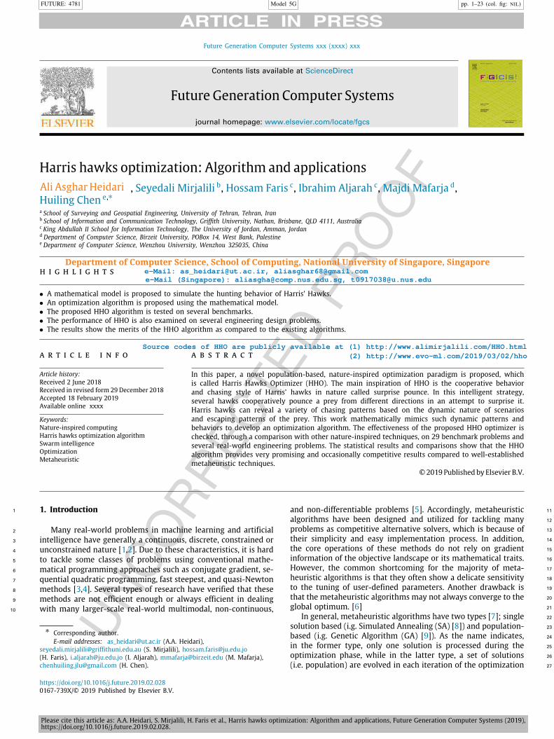
Fig. 1. Classification of meta-heuristic techniques (meta-heuristic diamond).
process. Population-based techniques can often find an optimal or1
suboptimal solution that may be same with the exact optimum2
or located in its neighborhood. Population-based metaheuris-3
tic (P-metaheuristics) techniques mostly mimic natural phenom-4
ena [10–13]. These algorithms start the optimization process5
by generating a set (population) of individuals, where each in-6
dividual in the population represents a candidate solution to7
the optimization problem. The population will be evolved itera-8
tively by replacing the current population with a newly generated9
population using some often stochastic operators [14,15]. The op-10
timization process is proceeded until satisfying a stopping criteria11
(i.e. maximum number of iterations) [16,17].12
Based on the inspiration, P-metaheuristics can be categorized13
in four main groups [18,19] (see Fig. 1): Evolutionary Algorithms14
(EAs), Physics-based, Human-based, and Swarm Intelligence (SI)15
algorithms. EAs mimic the biological evolutionary behaviors such16
as recombination, mutation, and selection. The most popular EA is17
the GA that mimics the Darwinian theory of evolution [20]. Other18
popular examples of EAs are Differential Evolution (DE) [21],19
Genetic Programming (GP) [20], and Biogeography-Based Opti-20
mizer (BBO) [22]. Physics-based algorithms are inspired by the21
physical laws. Some examples of these algorithms are Big-Bang22
Big-Crunch (BBBC) [23], Central Force Optimization (CFO) [24],23
and Gravitational Search Algorithm (GSA) [25]. Salcedo-Sanz [26]24
has deeply reviewed several physic-based optimizers. The third25
category of P-metaheuristics includes the set of algorithms that26
mimic some human behaviors. Some examples of the human-27
based algorithms are Tabu Search (TS) [27], Socio Evolution and28
Learning Optimization (SELO) [28], and Teaching Learning Based29
Optimization (TLBO) [29]. As the last class of P-metaheuristics,30
SI algorithms mimic the social behaviors (e.g. decentralized, self-31
organized systems) of organisms living in swarms, flocks, or32
herds [30,31]. For instance, the birds flocking behaviors is the33
main inspiration of the Particle Swarm Optimization (PSO) pro-34
posed by Eberhart and Kennedy [32]. In PSO, each particle in35
the swarm represents a candidate solution to the optimization36
problem. In the optimization process, each particle is updated37
with regard to the position of the global best particle and its38
own (local) best position. Ant Colony Optimization (ACO) [33],39
Cuckoo Search (CS) [34], and Artificial Bee Colony (ABC) are other40
examples of the SI techniques.41
Regardless of the variety of these algorithms, there is a com-42
mon feature: the searching steps have two phases: exploration43
(diversification) and exploitation (intensification) [26]. In the ex- 44
ploration phase, the algorithm should utilize and promote its 45
randomized operators as much as possible to deeply explore 46
various regions and sides of the feature space. Hence, the ex- 47
ploratory behaviors of a well-designed optimizer should have 48
an enriched-enough random nature to efficiently allocate more 49
randomly-generated solutions to different areas of the problem 50
topography during early steps of the searching process [35]. The 51
exploitation stage is normally performed after the exploration 52
phase. In this phase, the optimizer tries to focus on the neigh- 53
borhood of better-quality solutions located inside the feature 54
space. It actually intensifies the searching process in a local region 55
instead of all-inclusive regions of the landscape. A well-organized 56
optimizer should be capable of making a reasonable, fine balance 57
between the exploration and exploitation tendencies. Otherwise, 58
the possibility of being trapped in local optima (LO) and immature 59
convergence drawbacks increases. 60
We have witnessed a growing interest and awareness in the 61
successful, inexpensive, efficient application of EAs and SI al- 62
gorithms in recent years. However, referring to No Free Lunch 63
(NFL) theorem [36], all optimization algorithms proposed so- 64
far show an equivalent performance on average if we apply 65
them to all possible optimization tasks. According to NFL theo- 66
rem, we cannot theoretically consider an algorithm as a general- 67
purpose universally-best optimizer. Hence, NFL theorem encour- 68
ages searching for developing more efficient optimizers. As a 69
result of NFL theorem, besides the widespread studies on the 70
efficacy, performance aspects and results of traditional EAs and SI 71
algorithms, new optimizers with specific global and local search- 72
ing strategies are emerging in recent years to provide more 73
variety of choices for researchers and experts in different fields. 74
In this paper, a new nature-inspired optimization technique 75
is proposed to compete with other optimizers. The main idea 76
behind the proposed optimizer is inspired from the cooperative 77
behaviors of one of the most intelligent birds, Harris’ Hawks, in 78
hunting escaping preys (rabbits in most cases) [37]. For this pur- 79
pose, a new mathematical model is developed in this paper. Then, 80
a stochastic metaheuristic is designed based on the proposed 81
mathematical model to tackle various optimization problems. 82
The rest of this research is organized as follows. Section 2 83
represents the background inspiration and info about the coop- 84
erative life of Harris’ hawks. Section 3 represents the mathemat- 85
ical model and computational procedures of the HHO algorithm. 86
The results of HHO in solving different benchmark and real- 87
world case studies are presented in Section 4 Finally, Section 6 88
concludes the work with some useful perspectives. 89
2. Background 90
In 1997, Louis Lefebvre proposed an approach to measure 91
the avian ‘‘IQ’’ based on the observed innovations in feeding 92
behaviors [38]. Based on his studies [38–41], the hawks can be 93
listed amongst the most intelligent birds in nature. The Harris’ 94
hawk (Parabuteo unicinctus) is a well-known bird of prey that 95
survives in somewhat steady groups found in southern half of 96
Arizona, USA [37]. Harmonized foraging involving several animals 97
for catching and then, sharing the slain animal has been persua- 98
sively observed for only particular mammalian carnivores. The 99
Harris’s hawk is distinguished because of its unique cooperative 100
foraging activities together with other family members living 101
in the same stable group while other raptors usually attack to 102
discover and catch a quarry, alone. This avian desert predator 103
shows evolved innovative team chasing capabilities in tracing, 104
encircling, flushing out, and eventually attacking the potential 105
quarry. These smart birds can organize dinner parties consisting 106
of several individuals in the non-breeding season. They are known 107
https://aliasgharheidari.com/HHO.html
FUTURE: 4781
Please cite this article as: A.A. Heidari, S. Mirjalili, H. Faris et al., Harris hawks optimization: Algorithm and applications, Future Generation Computer Systems (2019),https://doi.org/10.1016/j.future.2019.02.028.
A.A. Heidari, S. Mirjalili, H. Faris et al. / Future Generation Computer Systems xxx (xxxx) xxx 3
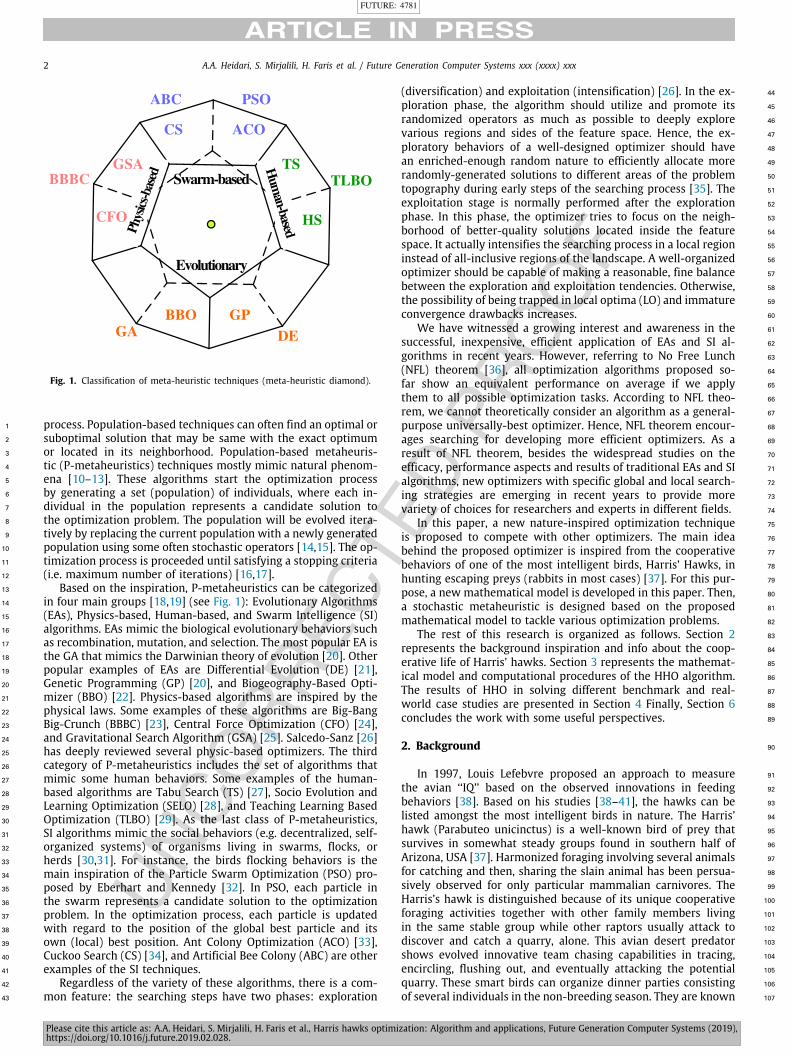
Fig. 2. Harris’s hawk and their behaviors.2
as truly cooperative predators in the raptor realm. As reported1
by Bednarz [37] in 1998, they begin the team mission at morning2
twilight, with leaving the rest roosts and often perching on giant3
trees or power poles inside their home realm. They know their4
family members and try to be aware of their moves during the5
attack. When assembled and party gets started, some hawks one6
after the other make short tours and then, land on rather high7
perches. In this manner, the hawks occasionally will perform a8
‘‘leapfrog’’ motion all over the target site and they rejoin and split9
several times to actively search for the covered animal, which is10
usually a rabbit.111
The main tactic of Harris’ hawks to capture a prey is ‘‘surprise12
pounce’’, which is also known as ‘‘seven kills’’ strategy. In this in-13
telligent strategy, several hawks try to cooperatively attack from14
different directions and simultaneously converge on a detected15
escaping rabbit outside the cover. The attack may rapidly be16
completed by capturing the surprised prey in few seconds, but17
occasionally, regarding the escaping capabilities and behaviors18
of the prey, the seven kills may include multiple, short-length,19
quick dives nearby the prey during several minutes. Harris’ hawks20
can demonstrate a variety of chasing styles dependent on the21
dynamic nature of circumstances and escaping patterns of a prey.22
A switching tactic occurs when the best hawk (leader) stoops at23
the prey and get lost, and the chase will be continued by one of24
the party members. These switching activities can be observed25
in different situations because they are beneficial for confusing26
the escaping rabbit. The main advantage of these cooperative27
tactics is that the Harris’ hawks can pursue the detected rabbit28
to exhaustion, which increases its vulnerability. Moreover, by29
perplexing the escaping prey, it cannot recover its defensive30
capabilities and finally, it cannot escape from the confronted team31
besiege since one of the hawks, which is often the most powerful32
and experienced one, effortlessly captures the tired rabbit and33
shares it with other party members. Harris’ hawks and their main34
behaviors can be seen in nature, as captured in Fig. 2.35
3. Harris hawks optimization (HHO)36
In this section, we model the exploratory and exploitative37
phases of the proposed HHO inspired by the exploring a prey, sur-38
prise pounce, and different attacking strategies of Harris hawks.39
HHO is a population-based, gradient-free optimization technique;40
hence, it can be applied to any optimization problem subject to41
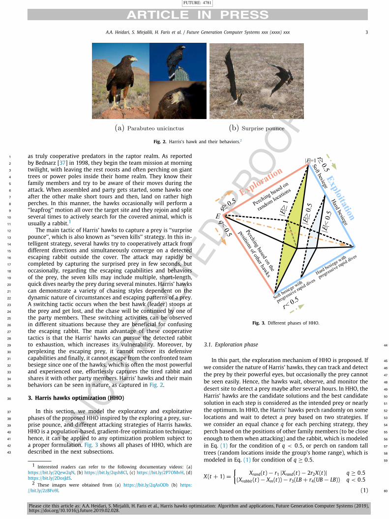
a proper formulation. Fig. 3 shows all phases of HHO, which are42
described in the next subsections.43
1 Interested readers can refer to the following documentary videos: (a)https://bit.ly/2Qew2qN, (b) https://bit.ly/2qsh8Cl, (c) https://bit.ly/2P7OMvH, (d)https://bit.ly/2DosJdS.2 These images were obtained from (a) https://bit.ly/2qAsODb (b) https:
//bit.ly/2zBFo9l.
Fig. 3. Different phases of HHO.
3.1. Exploration phase 44
In this part, the exploration mechanism of HHO is proposed. If 45
we consider the nature of Harris’ hawks, they can track and detect 46
the prey by their powerful eyes, but occasionally the prey cannot 47
be seen easily. Hence, the hawks wait, observe, and monitor the 48
desert site to detect a prey maybe after several hours. In HHO, the 49
Harris’ hawks are the candidate solutions and the best candidate 50
solution in each step is considered as the intended prey or nearly 51
the optimum. In HHO, the Harris’ hawks perch randomly on some 52
locations and wait to detect a prey based on two strategies. If 53
we consider an equal chance q for each perching strategy, they 54
perch based on the positions of other family members (to be close 55
enough to them when attacking) and the rabbit, which is modeled 56
in Eq. (1) for the condition of q < 0.5, or perch on random tall 57
trees (random locations inside the group’s home range), which is 58
modeled in Eq. (1) for condition of q ≥ 0.5. 59
X(t + 1) =
{Xrand(t) − r1 |Xrand(t) − 2r2X(t)| q ≥ 0.5
(Xrabbit (t) − Xm(t)) − r3(LB + r4(UB − LB)) q < 0.5
(1) 60
https://aliasgharheidari.com/HHO.html

FUTURE: 4781
Please cite this article as: A.A. Heidari, S. Mirjalili, H. Faris et al., Harris hawks optimization: Algorithm and applications, Future Generation Computer Systems (2019),https://doi.org/10.1016/j.future.2019.02.028.
4 A.A. Heidari, S. Mirjalili, H. Faris et al. / Future Generation Computer Systems xxx (xxxx) xxx
where X(t + 1) is the position vector of hawks in the next1
iteration t , Xrabbit (t) is the position of rabbit, X(t) is the current2
position vector of hawks, r1, r2, r3, r4, and q are random numbers3
inside (0,1), which are updated in each iteration, LB and UB show4
the upper and lower bounds of variables, Xrand(t) is a randomly5
selected hawk from the current population, and Xm is the average6
position of the current population of hawks.7
We proposed a simple model to generate random locations8
inside the group’s home range (LB, UB). The first rule generates9
solutions based on a random location and other hawks. In second10
rule of Eq. (1), we have the difference of the location of best so11
far and the average position of the group plus a randomly-scaled12
component based on range of variables, while r3 is a scaling13
coefficient to further increase the random nature of rule once14
r4 takes close values to 1 and similar distribution patterns may15
occur. In this rule, we add a randomly scaled movement length16
to the LB. Then, we considered a random scaling coefficient for17
the component to provide more diversification trends and explore18
different regions of the feature space. It is possible to construct19
different updating rules, but we utilized the simplest rule, which20
is able to mimic the behaviors of hawks. The average position of21
hawks is attained using Eq. (2):22
Xm(t) =1N
N∑i=1
Xi(t) (2)23
where Xi(t) indicates the location of each hawk in iteration t and24
N denotes the total number of hawks. It is possible to obtain the25
average location in different ways, but we utilized the simplest26
rule.27
3.2. Transition from exploration to exploitation28
The HHO algorithm can transfer from exploration to exploita-29
tion and then, change between different exploitative behaviors30
based on the escaping energy of the prey. The energy of a prey31
decreases considerably during the escaping behavior. To model32
this fact, the energy of a prey is modeled as:33
E = 2E0(1 −tT) (3)34
where E indicates the escaping energy of the prey, T is the maxi-35
mum number of iterations, and E0 is the initial state of its energy.36
In HHO, E0 randomly changes inside the interval (−1, 1) at each37
iteration. When the value of E0 decreases from 0 to −1, the rabbit38
is physically flagging, whilst when the value of E0 increases from39
0 to 1, it means that the rabbit is strengthening. The dynamic40
escaping energy E has a decreasing trend during the iterations.41
When the escaping energy |E| ≥1, the hawks search different42
regions to explore a rabbit location, hence, the HHO performs the43
exploration phase, and when |E| <1, the algorithm try to exploit44
the neighborhood of the solutions during the exploitation steps.45
In short, exploration happens when |E| ≥1, while exploitation46
happens in later steps when |E| <1. The time-dependent behavior47
of E is also demonstrated in Fig. 4.48
3.3. Exploitation phase49
In this phase, the Harris’ hawks perform the surprise pounce50
(seven kills as called in [37]) by attacking the intended prey51
detected in the previous phase. However, preys often attempt to52
escape from dangerous situations. Hence, different chasing styles53
occur in real situations. According to the escaping behaviors of54
the prey and chasing strategies of the Harris’ hawks, four possible55
strategies are proposed in the HHO to model the attacking stage.56
The preys always try to escape from threatening situations.57
Suppose that r is the chance of a prey in successfully escaping58
Fig. 4. Behavior of E during two runs and 500 iterations.
(r < 0.5) or not successfully escaping (r ≥0.5) before surprise 59
pounce. Whatever the prey does, the hawks will perform a hard 60
or soft besiege to catch the prey. It means that they will encircle 61
the prey from different directions softly or hard depending on 62
the retained energy of the prey. In real situations, the hawks get 63
closer and closer to the intended prey to increase their chances 64
in cooperatively killing the rabbit by performing the surprise 65
pounce. After several minutes, the escaping prey will lose more 66
and more energy; then, the hawks intensify the besiege process 67
to effortlessly catch the exhausted prey. To model this strategy 68
and enable the HHO to switch between soft and hard besiege 69
processes, the E parameter is utilized. 70
In this regard, when |E| ≥0.5, the soft besiege happens, and 71
when |E| <0.5, the hard besiege occurs. 72
3.3.1. Soft besiege 73
When r ≥ 0.5 and |E| ≥ 0.5, the rabbit still has enough 74
energy, and try to escape by some random misleading jumps but 75
finally it cannot. During these attempts, the Harris’ hawks encircle 76
it softly to make the rabbit more exhausted and then perform the 77
surprise pounce. This behavior is modeled by the following rules: 78
79
X(t + 1) = ∆X(t) − E |JXrabbit (t) − X(t)| (4) 80
81
∆X(t) = Xrabbit (t) − X(t) (5) 82
where ∆X(t) is the difference between the position vector of 83
the rabbit and the current location in iteration t , r5 is a random 84
number inside (0,1), and J = 2(1 − r5) represents the random 85
jump strength of the rabbit throughout the escaping procedure. 86
The J value changes randomly in each iteration to simulate the 87
nature of rabbit motions. 88
3.3.2. Hard besiege 89
When r ≥0.5 and |E| <0.5, the prey is so exhausted and it 90
has a low escaping energy. In addition, the Harris’ hawks hardly 91
encircle the intended prey to finally perform the surprise pounce. 92
In this situation, the current positions are updated using Eq. (6): 93
X(t + 1) = Xrabbit (t) − E |∆X(t)| (6) 94
A simple example of this step with one hawk is depicted in 95
Fig. 5. 96
https://aliasgharheidari.com/HHO.html
FUTURE: 4781
Please cite this article as: A.A. Heidari, S. Mirjalili, H. Faris et al., Harris hawks optimization: Algorithm and applications, Future Generation Computer Systems (2019),https://doi.org/10.1016/j.future.2019.02.028.
A.A. Heidari, S. Mirjalili, H. Faris et al. / Future Generation Computer Systems xxx (xxxx) xxx 5
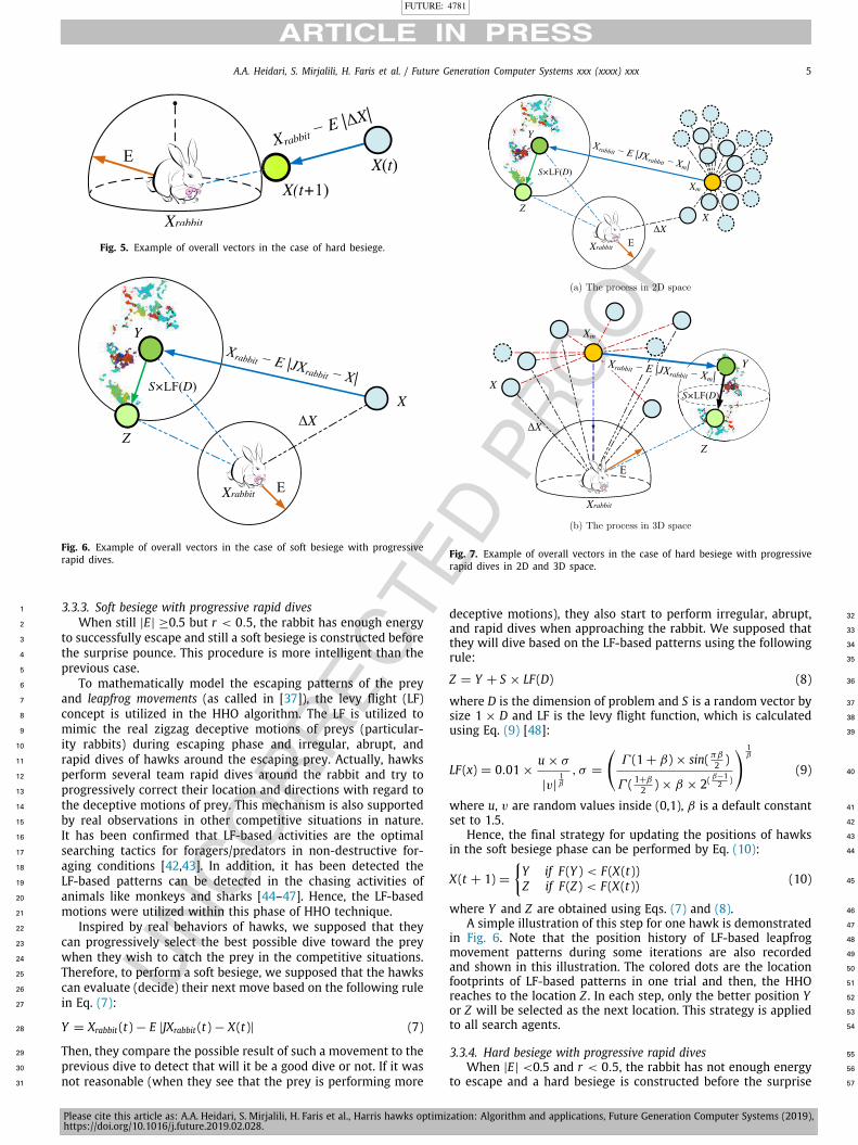
Fig. 5. Example of overall vectors in the case of hard besiege.
Fig. 6. Example of overall vectors in the case of soft besiege with progressiverapid dives.
3.3.3. Soft besiege with progressive rapid dives1
When still |E| ≥0.5 but r < 0.5, the rabbit has enough energy2
to successfully escape and still a soft besiege is constructed before3
the surprise pounce. This procedure is more intelligent than the4
previous case.5
To mathematically model the escaping patterns of the prey6
and leapfrog movements (as called in [37]), the levy flight (LF)7
concept is utilized in the HHO algorithm. The LF is utilized to8
mimic the real zigzag deceptive motions of preys (particular-9
ity rabbits) during escaping phase and irregular, abrupt, and10
rapid dives of hawks around the escaping prey. Actually, hawks11
perform several team rapid dives around the rabbit and try to12
progressively correct their location and directions with regard to13
the deceptive motions of prey. This mechanism is also supported14
by real observations in other competitive situations in nature.15
It has been confirmed that LF-based activities are the optimal16
searching tactics for foragers/predators in non-destructive for-17
aging conditions [42,43]. In addition, it has been detected the18
LF-based patterns can be detected in the chasing activities of19
animals like monkeys and sharks [44–47]. Hence, the LF-based20
motions were utilized within this phase of HHO technique.21
Inspired by real behaviors of hawks, we supposed that they22
can progressively select the best possible dive toward the prey23
when they wish to catch the prey in the competitive situations.24
Therefore, to perform a soft besiege, we supposed that the hawks25
can evaluate (decide) their next move based on the following rule26
in Eq. (7):27
Y = Xrabbit (t) − E |JXrabbit (t) − X(t)| (7)28
Then, they compare the possible result of such a movement to the29
previous dive to detect that will it be a good dive or not. If it was30
not reasonable (when they see that the prey is performing more31
Fig. 7. Example of overall vectors in the case of hard besiege with progressiverapid dives in 2D and 3D space.
deceptive motions), they also start to perform irregular, abrupt, 32
and rapid dives when approaching the rabbit. We supposed that 33
they will dive based on the LF-based patterns using the following 34
rule: 35
Z = Y + S × LF (D) (8) 36
where D is the dimension of problem and S is a random vector by 37
size 1 × D and LF is the levy flight function, which is calculated 38
using Eq. (9) [48]: 39
LF (x) = 0.01 ×u × σ
|v|1β
, σ =
(Γ (1 + β) × sin( πβ
2 )
Γ ( 1+β
2 ) × β × 2( β−12 )
) 1β
(9) 40
where u, v are random values inside (0,1), β is a default constant 41
set to 1.5. 42
Hence, the final strategy for updating the positions of hawks 43
in the soft besiege phase can be performed by Eq. (10): 44
X(t + 1) =
{Y if F (Y ) < F (X(t))Z if F (Z) < F (X(t)) (10) 45
where Y and Z are obtained using Eqs. (7) and (8). 46
A simple illustration of this step for one hawk is demonstrated 47
in Fig. 6. Note that the position history of LF-based leapfrog 48
movement patterns during some iterations are also recorded 49
and shown in this illustration. The colored dots are the location 50
footprints of LF-based patterns in one trial and then, the HHO 51
reaches to the location Z . In each step, only the better position Y 52
or Z will be selected as the next location. This strategy is applied 53
to all search agents. 54
3.3.4. Hard besiege with progressive rapid dives 55
When |E| <0.5 and r < 0.5, the rabbit has not enough energy 56
to escape and a hard besiege is constructed before the surprise 57
https://aliasgharheidari.com/HHO.html
FUTURE: 4781
Please cite this article as: A.A. Heidari, S. Mirjalili, H. Faris et al., Harris hawks optimization: Algorithm and applications, Future Generation Computer Systems (2019),https://doi.org/10.1016/j.future.2019.02.028.
6 A.A. Heidari, S. Mirjalili, H. Faris et al. / Future Generation Computer Systems xxx (xxxx) xxx
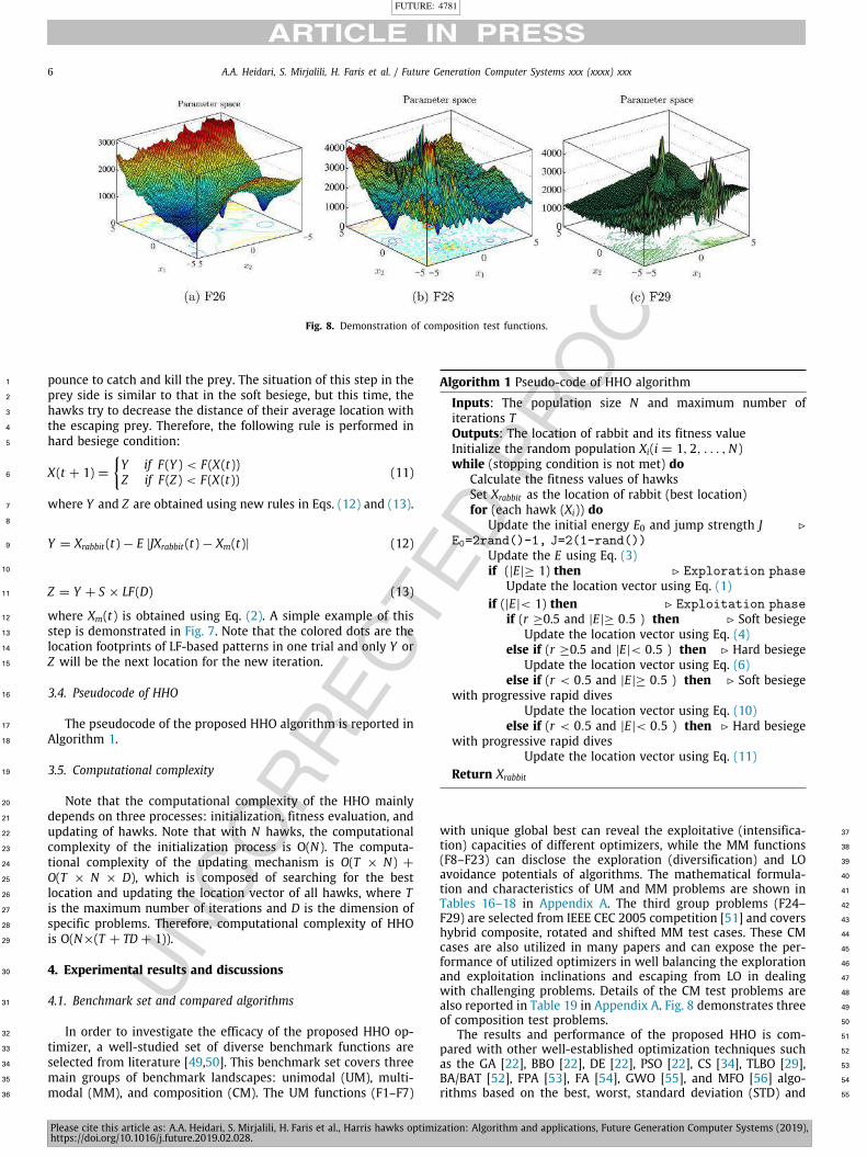
Fig. 8. Demonstration of composition test functions.
pounce to catch and kill the prey. The situation of this step in the1
prey side is similar to that in the soft besiege, but this time, the2
hawks try to decrease the distance of their average location with3
the escaping prey. Therefore, the following rule is performed in4
hard besiege condition:5
X(t + 1) =
{Y if F (Y ) < F (X(t))Z if F (Z) < F (X(t)) (11)6
where Y and Z are obtained using new rules in Eqs. (12) and (13).7
8
Y = Xrabbit (t) − E |JXrabbit (t) − Xm(t)| (12)9
10
Z = Y + S × LF (D) (13)11
where Xm(t) is obtained using Eq. (2). A simple example of this12
step is demonstrated in Fig. 7. Note that the colored dots are the13
location footprints of LF-based patterns in one trial and only Y or14
Z will be the next location for the new iteration.15
3.4. Pseudocode of HHO16
The pseudocode of the proposed HHO algorithm is reported in17
Algorithm 1.18
3.5. Computational complexity19
Note that the computational complexity of the HHO mainly20
depends on three processes: initialization, fitness evaluation, and21
updating of hawks. Note that with N hawks, the computational22
complexity of the initialization process is O(N). The computa-23
tional complexity of the updating mechanism is O(T × N) +24
O(T × N × D), which is composed of searching for the best25
location and updating the location vector of all hawks, where T26
is the maximum number of iterations and D is the dimension of27
specific problems. Therefore, computational complexity of HHO28
is O(N×(T + TD + 1)).29
4. Experimental results and discussions30
4.1. Benchmark set and compared algorithms31
In order to investigate the efficacy of the proposed HHO op-32
timizer, a well-studied set of diverse benchmark functions are33
selected from literature [49,50]. This benchmark set covers three34
main groups of benchmark landscapes: unimodal (UM), multi-35
modal (MM), and composition (CM). The UM functions (F1–F7)36
Algorithm 1 Pseudo-code of HHO algorithm
Inputs: The population size N and maximum number ofiterations TOutputs: The location of rabbit and its fitness valueInitialize the random population Xi(i = 1, 2, . . . ,N)while (stopping condition is not met) do
Calculate the fitness values of hawksSet Xrabbit as the location of rabbit (best location)for (each hawk (Xi)) do
Update the initial energy E0 and jump strength J ▷
E0=2rand()-1, J=2(1-rand())Update the E using Eq. (3)if (|E|≥ 1) then ▷ Exploration phase
Update the location vector using Eq. (1)if (|E|< 1) then ▷ Exploitation phase
if (r ≥0.5 and |E|≥ 0.5 ) then ▷ Soft besiegeUpdate the location vector using Eq. (4)
else if (r ≥0.5 and |E|< 0.5 ) then ▷ Hard besiegeUpdate the location vector using Eq. (6)
else if (r < 0.5 and |E|≥ 0.5 ) then ▷ Soft besiegewith progressive rapid dives
Update the location vector using Eq. (10)else if (r < 0.5 and |E|< 0.5 ) then ▷ Hard besiege
with progressive rapid divesUpdate the location vector using Eq. (11)
Return Xrabbit
with unique global best can reveal the exploitative (intensifica- 37
tion) capacities of different optimizers, while the MM functions 38
(F8–F23) can disclose the exploration (diversification) and LO 39
avoidance potentials of algorithms. The mathematical formula- 40
tion and characteristics of UM and MM problems are shown in 41
Tables 16–18 in Appendix A. The third group problems (F24– 42
F29) are selected from IEEE CEC 2005 competition [51] and covers 43
hybrid composite, rotated and shifted MM test cases. These CM 44
cases are also utilized in many papers and can expose the per- 45
formance of utilized optimizers in well balancing the exploration 46
and exploitation inclinations and escaping from LO in dealing 47
with challenging problems. Details of the CM test problems are 48
also reported in Table 19 in Appendix A. Fig. 8 demonstrates three 49
of composition test problems. 50
The results and performance of the proposed HHO is com- 51
pared with other well-established optimization techniques such 52
as the GA [22], BBO [22], DE [22], PSO [22], CS [34], TLBO [29], 53
BA/BAT [52], FPA [53], FA [54], GWO [55], and MFO [56] algo- 54
rithms based on the best, worst, standard deviation (STD) and 55
https://aliasgharheidari.com/HHO.html
FUTURE: 4781
Please cite this article as: A.A. Heidari, S. Mirjalili, H. Faris et al., Harris hawks optimization: Algorithm and applications, Future Generation Computer Systems (2019),https://doi.org/10.1016/j.future.2019.02.028.
A.A. Heidari, S. Mirjalili, H. Faris et al. / Future Generation Computer Systems xxx (xxxx) xxx 7
Table 1The parameter settings.Algorithm Parameter Value
DE Scaling factor 0.5Crossover probability 0.5
PSO Topology fully connectedInertia factor 0.3c1 1c2 1
TLBO Teaching factor T 1, 2GWO Convergence constant a [2 0]MFO Convergence constant a [−2 −1]
Spiral factor b 1CS Discovery rate of alien solutions pa 0.25BA Qmin Frequency minimum 0
Qmax Frequency maximum 2A Loudness 0.5r Pulse rate 0.5
FA α 0.5β 0.2γ 1
FPA Probability switch p 0.8BBO Habitat modification probability 1
Immigration probability limits [0, 1]Step size 1Max immigration (I) and Max emigration (E) 1Mutation probability 0.005
average of the results (AVG). These algorithms cover both recently1
proposed techniques such as MFO, GWO, CS, TLBO, BAT, FPA, and2
FA and also, relatively the most utilized optimizers in the field3
like the GA, DE, PSO, and BBO algorithms.4
As recommended by Derrac et al. [57], the non-parametric5
Wilcoxon statistical test with 5% degree of significance is also6
performed along with experimental assessments to detect the7
significant differences between the attained results of different8
techniques.9
4.2. Experimental setup10
All algorithms were implemented under Matlab 7.10 (R2010a)11
on a computer with a Windows 7 64-bit professional and 64 GB12
RAM. The swarm size and maximum iterations of all optimizers13
are set to 30 and 500, respectively. All results are recorded and14
compared based on the average performance of optimizers over15
30 independent runs.16
The settings of GA, PSO, DE and BBO algorithms are same with17
those set by Dan Simon in the original work of BBO [22], while18
for the BA [52], FA [58], TLBO [29], GWO [55], FPA [53], CS [34],19
and MFO [56], the parameters are same with the recommended20
settings in the original works. The used parameters are also21
reported in Table 1.22
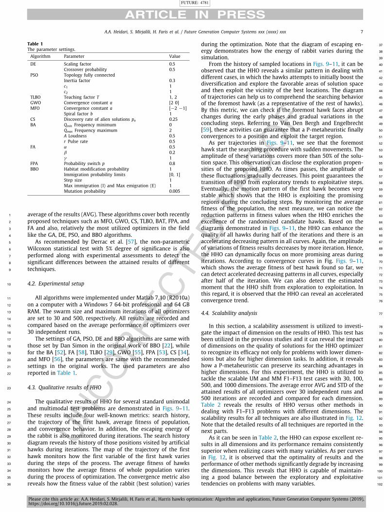
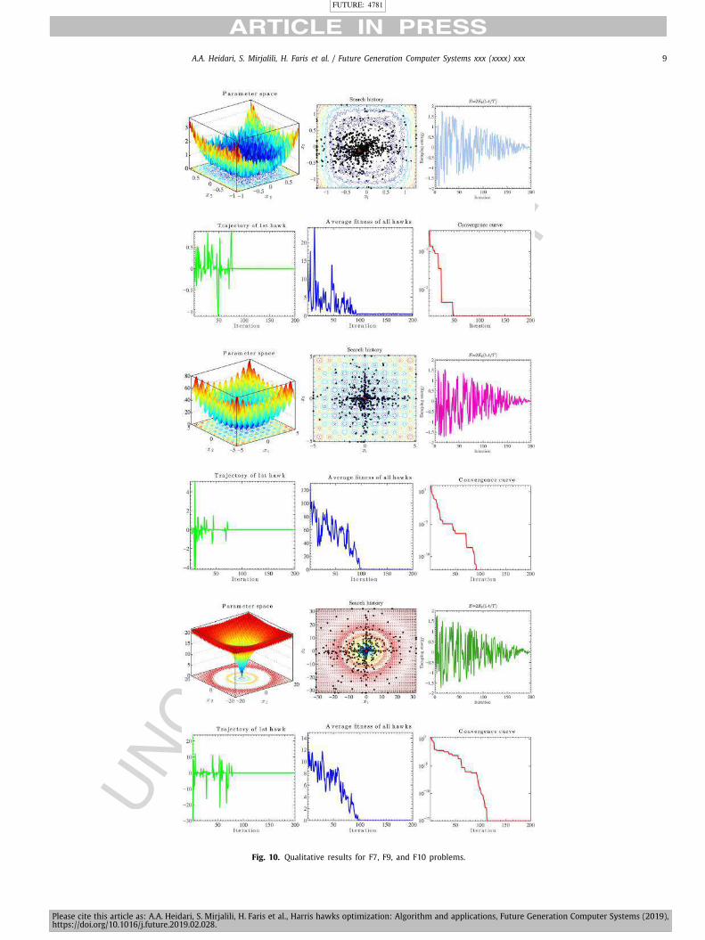
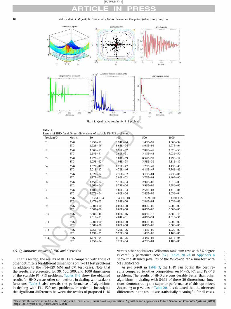
4.3. Qualitative results of HHO23
The qualitative results of HHO for several standard unimodal24
and multimodal test problems are demonstrated in Figs. 9–11.25
These results include four well-known metrics: search history,26
the trajectory of the first hawk, average fitness of population,27
and convergence behavior. In addition, the escaping energy of28
the rabbit is also monitored during iterations. The search history29
diagram reveals the history of those positions visited by artificial30
hawks during iterations. The map of the trajectory of the first31
hawk monitors how the first variable of the first hawk varies32
during the steps of the process. The average fitness of hawks33
monitors how the average fitness of whole population varies34
during the process of optimization. The convergence metric also35
reveals how the fitness value of the rabbit (best solution) varies36
during the optimization. Note that the diagram of escaping en- 37
ergy demonstrates how the energy of rabbit varies during the 38
simulation. 39
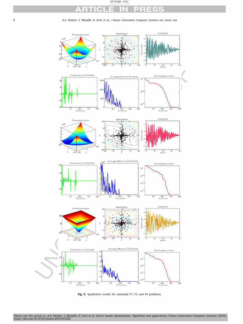
From the history of sampled locations in Figs. 9–11, it can be 40
observed that the HHO reveals a similar pattern in dealing with 41
different cases, in which the hawks attempts to initially boost the 42
diversification and explore the favorable areas of solution space 43
and then exploit the vicinity of the best locations. The diagram 44
of trajectories can help us to comprehend the searching behavior 45
of the foremost hawk (as a representative of the rest of hawks). 46
By this metric, we can check if the foremost hawk faces abrupt 47
changes during the early phases and gradual variations in the 48
concluding steps. Referring to Van Den Bergh and Engelbrecht 49
[59], these activities can guarantee that a P-metaheuristic finally 50
convergences to a position and exploit the target region. 51
As per trajectories in Figs. 9–11, we see that the foremost 52
hawk start the searching procedure with sudden movements. The 53
amplitude of these variations covers more than 50% of the solu- 54
tion space. This observation can disclose the exploration propen- 55
sities of the proposed HHO. As times passes, the amplitude of 56
these fluctuations gradually decreases. This point guarantees the 57
transition of HHO from exploratory trends to exploitative steps. 58
Eventually, the motion pattern of the first hawk becomes very 59
stable which shows that the HHO is exploiting the promising 60
regions during the concluding steps. By monitoring the average 61
fitness of the population, the next measure, we can notice the 62
reduction patterns in fitness values when the HHO enriches the 63
excellence of the randomized candidate hawks. Based on the 64
diagrams demonstrated in Figs. 9–11, the HHO can enhance the 65
quality of all hawks during half of the iterations and there is an 66
accelerating decreasing pattern in all curves. Again, the amplitude 67
of variations of fitness results decreases by more iteration. Hence, 68
the HHO can dynamically focus on more promising areas during 69
iterations. According to convergence curves in Fig. Figs. 9–11, 70
which shows the average fitness of best hawk found so far, we 71
can detect accelerated decreasing patterns in all curves, especially 72
after half of the iteration. We can also detect the estimated 73
moment that the HHO shift from exploration to exploitation. In 74
this regard, it is observed that the HHO can reveal an accelerated 75
convergence trend. 76
4.4. Scalability analysis 77
In this section, a scalability assessment is utilized to investi- 78
gate the impact of dimension on the results of HHO. This test has 79
been utilized in the previous studies and it can reveal the impact 80
of dimensions on the quality of solutions for the HHO optimizer 81
to recognize its efficacy not only for problems with lower dimen- 82
sions but also for higher dimension tasks. In addition, it reveals 83
how a P-metaheuristic can preserve its searching advantages in 84
higher dimensions. For this experiment, the HHO is utilized to 85
tackle the scalable UM and MM F1–F13 test cases with 30, 100, 86
500, and 1000 dimensions. The average error AVG and STD of the 87
attained results of all optimizers over 30 independent runs and 88
500 iterations are recorded and compared for each dimension. 89
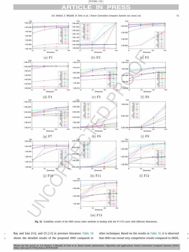
Table 2 reveals the results of HHO versus other methods in 90
dealing with F1–F13 problems with different dimensions. The 91
scalability results for all techniques are also illustrated in Fig. 12. 92
Note that the detailed results of all techniques are reported in the 93
next parts. 94
As it can be seen in Table 2, the HHO can expose excellent re- 95
sults in all dimensions and its performance remains consistently 96
superior when realizing cases with many variables. As per curves 97
in Fig. 12, it is observed that the optimality of results and the 98
performance of other methods significantly degrade by increasing 99
the dimensions. This reveals that HHO is capable of maintain- 100
ing a good balance between the exploratory and exploitative 101
tendencies on problems with many variables. 102
https://aliasgharheidari.com/HHO.html
FUTURE: 4781
Please cite this article as: A.A. Heidari, S. Mirjalili, H. Faris et al., Harris hawks optimization: Algorithm and applications, Future Generation Computer Systems (2019),https://doi.org/10.1016/j.future.2019.02.028.
8 A.A. Heidari, S. Mirjalili, H. Faris et al. / Future Generation Computer Systems xxx (xxxx) xxx
Fig. 9. Qualitative results for unimodal F1, F3, and F4 problems.
https://aliasgharheidari.com/HHO.html
FUTURE: 4781
Please cite this article as: A.A. Heidari, S. Mirjalili, H. Faris et al., Harris hawks optimization: Algorithm and applications, Future Generation Computer Systems (2019),https://doi.org/10.1016/j.future.2019.02.028.
A.A. Heidari, S. Mirjalili, H. Faris et al. / Future Generation Computer Systems xxx (xxxx) xxx 9
Fig. 10. Qualitative results for F7, F9, and F10 problems.
https://aliasgharheidari.com/HHO.html
FUTURE: 4781
Please cite this article as: A.A. Heidari, S. Mirjalili, H. Faris et al., Harris hawks optimization: Algorithm and applications, Future Generation Computer Systems (2019),https://doi.org/10.1016/j.future.2019.02.028.
10 A.A. Heidari, S. Mirjalili, H. Faris et al. / Future Generation Computer Systems xxx (xxxx) xxx
Fig. 11. Qualitative results for F13 problem.
Table 2Results of HHO for different dimensions of scalable F1–F13 problems.Problem/D Metric 30 100 500 1000
F1 AVG 3.95E−97 1.91E−94 1.46E−92 1.06E−94STD 1.72E−96 8.66E−94 8.01E−92 4.97E−94
F2 AVG 1.56E−51 9.98E−52 7.87E−49 2.52E−50STD 6.98E−51 2.66E−51 3.11E−48 5.02E−50
F3 AVG 1.92E−63 1.84E−59 6.54E−37 1.79E−17STD 1.05E−62 1.01E−58 3.58E−36 9.81E−17
F4 AVG 1.02E−47 8.76E−47 1.29E−47 1.43E−46STD 5.01E−47 4.79E−46 4.11E−47 7.74E−46
F5 AVG 1.32E−02 2.36E−02 3.10E−01 5.73E−01STD 1.87E−02 2.99E−02 3.73E−01 1.40E+00
F6 AVG 1.15E−04 5.12E−04 2.94E−03 3.61E−03STD 1.56E−04 6.77E−04 3.98E−03 5.38E−03
F7 AVG 1.40E−04 1.85E−04 2.51E−04 1.41E−04STD 1.07E−04 4.06E−04 2.43E−04 1.63E−04
F8 AVG −1.25E+04 −4.19E+04 −2.09E+05 −4.19E+05STD 1.47E+02 2.82E+00 2.84E+01 1.03E+02
F9 AVG 0.00E+00 0.00E+00 0.00E+00 0.00E+00STD 0.00E+00 0.00E+00 0.00E+00 0.00E+00
F10 AVG 8.88E−16 8.88E−16 8.88E−16 8.88E−16STD 4.01E−31 4.01E−31 4.01E−31 4.01E−31
F11 AVG 0.00E+00 0.00E+00 0.00E+00 0.00E+00STD 0.00E+00 0.00E+00 0.00E+00 0.00E+00
F12 AVG 7.35E−06 4.23E−06 1.41E−06 1.02E−06STD 1.19E−05 5.25E−06 1.48E−06 1.16E−06
F13 AVG 1.57E−04 9.13E−05 3.44E−04 8.41E−04STD 2.15E−04 1.26E−04 4.75E−04 1.18E−03
4.5. Quantitative results of HHO and discussion1
In this section, the results of HHO are compared with those of2
other optimizers for different dimensions of F1–F13 test problems3
in addition to the F14–F29 MM and CM test cases. Note that4
the results are presented for 30, 100, 500, and 1000 dimensions5
of the scalable F1–F13 problems. Tables 3–6 show the obtained6
results for HHO versus other competitors in dealing with scalable7
functions. Table 8 also reveals the performance of algorithms8
in dealing with F14–F29 test problems. In order to investigate9
the significant differences between the results of proposed HHO10
versus other optimizers, Wilcoxon rank-sum test with 5% degree 11
is carefully performed here [57]. Tables 20–24 in Appendix B 12
show the attained p-values of the Wilcoxon rank-sum test with 13
5% significance. 14
As per result in Table 3, the HHO can obtain the best re- 15
sults compared to other competitors on F1–F5, F7, and F9–F13 16
problems. The results of HHO are considerably better than other 17
algorithms in dealing with 84.6% of these 30-dimensional func- 18
tions, demonstrating the superior performance of this optimizer. 19
According to p-values in Table 20, it is detected that the observed 20
differences in the results are statistically meaningful for all cases. 21
https://aliasgharheidari.com/HHO.html

FUTURE: 4781
Please cite this article as: A.A. Heidari, S. Mirjalili, H. Faris et al., Harris hawks optimization: Algorithm and applications, Future Generation Computer Systems (2019),https://doi.org/10.1016/j.future.2019.02.028.
A.A. Heidari, S. Mirjalili, H. Faris et al. / Future Generation Computer Systems xxx (xxxx) xxx 11
Table 3Results of benchmark functions (F1–F13), with 30 dimensions.Benchmark HHO GA PSO BBO FPA GWO BAT FA CS MFO TLBO DE
F1 AVG 3.95E−97 1.03E+03 1.83E+04 7.59E+01 2.01E+03 1.18E−27 6.59E+04 7.11E−03 9.06E−04 1.01E+03 2.17E−89 1.33E−03STD 1.72E−96 5.79E+02 3.01E+03 2.75E+01 5.60E+02 1.47E−27 7.51E+03 3.21E−03 4.55E−04 3.05E+03 3.14E−89 5.92E−04
F2 AVG 1.56E−51 2.47E+01 3.58E+02 1.36E−03 3.22E+01 9.71E−17 2.71E+08 4.34E−01 1.49E−01 3.19E+01 2.77E−45 6.83E−03STD 6.98E−51 5.68E+00 1.35E+03 7.45E−03 5.55E+00 5.60E−17 1.30E+09 1.84E−01 2.79E−02 2.06E+01 3.11E−45 2.06E−03
F3 AVG 1.92E−63 2.65E+04 4.05E+04 1.21E+04 1.41E+03 5.12E−05 1.38E+05 1.66E+03 2.10E−01 2.43E+04 3.91E−18 3.97E+04STD 1.05E−62 3.44E+03 8.21E+03 2.69E+03 5.59E+02 2.03E−04 4.72E+04 6.72E+02 5.69E−02 1.41E+04 8.04E−18 5.37E+03
F4 AVG 1.02E−47 5.17E+01 4.39E+01 3.02E+01 2.38E+01 1.24E−06 8.51E+01 1.11E−01 9.65E−02 7.00E+01 1.68E−36 1.15E+01STD 5.01E−47 1.05E+01 3.64E+00 4.39E+00 2.77E+00 1.94E−06 2.95E+00 4.75E−02 1.94E−02 7.06E+00 1.47E−36 2.37E+00
F5 AVG 1.32E−02 1.95E+04 1.96E+07 1.82E+03 3.17E+05 2.70E+01 2.10E+08 7.97E+01 2.76E+01 7.35E+03 2.54E+01 1.06E+02STD 1.87E−02 1.31E+04 6.25E+06 9.40E+02 1.75E+05 7.78E−01 4.17E+07 7.39E+01 4.51E−01 2.26E+04 4.26E−01 1.01E+02
F6 AVG 1.15E−04 9.01E+02 1.87E+04 6.71E+01 1.70E+03 8.44E−01 6.69E+04 6.94E−03 3.13E−03 2.68E+03 3.29E−05 1.44E−03STD 1.56E−04 2.84E+02 2.92E+03 2.20E+01 3.13E+02 3.18E−01 5.87E+03 3.61E−03 1.30E−03 5.84E+03 8.65E−05 5.38E−04
F7 AVG 1.40E−04 1.91E−01 1.07E+01 2.91E−03 3.41E−01 1.70E−03 4.57E+01 6.62E−02 7.29E−02 4.50E+00 1.16E−03 5.24E−02STD 1.07E−04 1.50E−01 3.05E+00 1.83E−03 1.10E−01 1.06E−03 7.82E+00 4.23E−02 2.21E−02 9.21E+00 3.63E−04 1.37E−02
F8 AVG −1.25E+04 −1.26E+04 −3.86E+03 −1.24E+04 −6.45E+03 −5.97E+03 −2.33E+03 −5.85E+03 −5.19E+19 −8.48E+03 −7.76E+03 −6.82E+03STD 1.47E+02 4.51E+00 2.49E+02 3.50E+01 3.03E+02 7.10E+02 2.96E+02 1.16E+03 1.76E+20 7.98E+02 1.04E+03 3.94E+02
F9 AVG 0.00E+00 9.04E+00 2.87E+02 0.00E+00 1.82E+02 2.19E+00 1.92E+02 3.82E+01 1.51E+01 1.59E+02 1.40E+01 1.58E+02STD 0.00E+00 4.58E+00 1.95E+01 0.00E+00 1.24E+01 3.69E+00 3.56E+01 1.12E+01 1.25E+00 3.21E+01 5.45E+00 1.17E+01
F10 AVG 8.88E−16 1.36E+01 1.75E+01 2.13E+00 7.14E+00 1.03E−13 1.92E+01 4.58E−02 3.29E−02 1.74E+01 6.45E−15 1.21E−02STD 4.01E−31 1.51E+00 3.67E−01 3.53E−01 1.08E+00 1.70E−14 2.43E−01 1.20E−02 7.93E−03 4.95E+00 1.79E−15 3.30E−03
F11 AVG 0.00E+00 1.01E+01 1.70E+02 1.46E+00 1.73E+01 4.76E−03 6.01E+02 4.23E−03 4.29E−05 3.10E+01 0.00E+00 3.52E−02STD 0.00E+00 2.43E+00 3.17E+01 1.69E−01 3.63E+00 8.57E−03 5.50E+01 1.29E−03 2.00E−05 5.94E+01 0.00E+00 7.20E−02
F12 AVG 2.08E−06 4.77E+00 1.51E+07 6.68E−01 3.05E+02 4.83E−02 4.71E+08 3.13E−04 5.57E−05 2.46E+02 7.35E−06 2.25E−03STD 1.19E−05 1.56E+00 9.88E+06 2.62E−01 1.04E+03 2.12E−02 1.54E+08 1.76E−04 4.96E−05 1.21E+03 7.45E−06 1.70E−03
F13 AVG 1.57E−04 1.52E+01 5.73E+07 1.82E+00 9.59E+04 5.96E−01 9.40E+08 2.08E−03 8.19E−03 2.73E+07 7.89E−02 9.12E−03STD 2.15E−04 4.52E+00 2.68E+07 3.41E−01 1.46E+05 2.23E−01 1.67E+08 9.62E−04 6.74E−03 1.04E+08 8.78E−02 1.16E−02
Table 4Results of benchmark functions (F1–F13), with 100 dimensions.Benchmark HHO GA PSO BBO FPA GWO BAT FA CS MFO TLBO DE
F1 AVG 1.91E−94 5.41E+04 1.06E+05 2.85E+03 1.39E+04 1.59E−12 2.72E+05 3.05E−01 3.17E−01 6.20E+04 3.62E−81 8.26E+03STD 8.66E−94 1.42E+04 8.47E+03 4.49E+02 2.71E+03 1.63E−12 1.42E+04 5.60E−02 5.28E−02 1.25E+04 4.14E−81 1.32E+03
F2 AVG 9.98E−52 2.53E+02 6.06E+23 1.59E+01 1.01E+02 4.31E−08 6.00E+43 1.45E+01 4.05E+00 2.46E+02 3.27E−41 1.21E+02STD 2.66E−51 1.41E+01 2.18E+24 3.74E+00 9.36E+00 1.46E−08 1.18E+44 6.73E+00 3.16E−01 4.48E+01 2.75E−41 2.33E+01
F3 AVG 1.84E−59 2.53E+05 4.22E+05 1.70E+05 1.89E+04 4.09E+02 1.43E+06 4.65E+04 6.88E+00 2.15E+05 4.33E−07 5.01E+05STD 1.01E−58 5.03E+04 7.08E+04 2.02E+04 5.44E+03 2.77E+02 6.21E+05 6.92E+03 1.02E+00 4.43E+04 8.20E−07 5.87E+04
F4 AVG 8.76E−47 8.19E+01 6.07E+01 7.08E+01 3.51E+01 8.89E−01 9.41E+01 1.91E+01 2.58E−01 9.31E+01 6.36E−33 9.62E+01STD 4.79E−46 3.15E+00 3.05E+00 4.73E+00 3.37E+00 9.30E−01 1.49E+00 3.12E+00 2.80E−02 2.13E+00 6.66E−33 1.00E+00
F5 AVG 2.36E−02 2.37E+07 2.42E+08 4.47E+05 4.64E+06 9.79E+01 1.10E+09 8.46E+02 1.33E+02 1.44E+08 9.67E+01 1.99E+07STD 2.99E−02 8.43E+06 4.02E+07 2.05E+05 1.98E+06 6.75E−01 9.47E+07 8.13E+02 7.34E+00 7.50E+07 7.77E−01 5.80E+06
F6 AVG 5.12E−04 5.42E+04 1.07E+05 2.85E+03 1.26E+04 1.03E+01 2.69E+05 2.95E−01 2.65E+00 6.68E+04 3.27E+00 8.07E+03STD 6.77E−04 1.09E+04 9.70E+03 4.07E+02 2.06E+03 1.05E+00 1.25E+04 5.34E−02 3.94E−01 1.46E+04 6.98E−01 1.64E+03
F7 AVG 1.85E−04 2.73E+01 3.41E+02 1.25E+00 5.84E+00 7.60E−03 3.01E+02 5.65E−01 1.21E+00 2.56E+02 1.50E−03 1.96E+01STD 4.06E−04 4.45E+01 8.74E+01 5.18E+00 2.16E+00 2.66E−03 2.66E+01 1.64E−01 2.65E−01 8.91E+01 5.39E−04 5.66E+00
F8 AVG −4.19E+04 −4.10E+04 −7.33E+03 −3.85E+04 −1.28E+04 −1.67E+04 −4.07E+03 −1.81E+04 −2.84E+18 −2.30E+04 −1.71E+04 −1.19E+04STD 2.82E+00 1.14E+02 4.75E+02 2.80E+02 4.64E+02 2.62E+03 9.37E+02 3.23E+03 6.91E+18 1.98E+03 3.54E+03 5.80E+02
F9 AVG 0.00E+00 3.39E+02 1.16E+03 9.11E+00 8.47E+02 1.03E+01 7.97E+02 2.36E+02 1.72E+02 8.65E+02 1.02E+01 1.03E+03STD 0.00E+00 4.17E+01 5.74E+01 2.73E+00 4.01E+01 9.02E+00 6.33E+01 2.63E+01 9.24E+00 8.01E+01 5.57E+01 4.03E+01
F10 AVG 8.88E−16 1.82E+01 1.91E+01 5.57E+00 8.21E+00 1.20E−07 1.94E+01 9.81E−01 3.88E−01 1.99E+01 1.66E−02 1.22E+01STD 4.01E−31 4.35E−01 2.04E−01 4.72E−01 1.14E+00 5.07E−08 6.50E−02 2.55E−01 5.23E−02 8.58E−02 9.10E−02 8.31E−01
F11 AVG 0.00E+00 5.14E+02 9.49E+02 2.24E+01 1.19E+02 4.87E−03 2.47E+03 1.19E−01 4.56E−03 5.60E+02 0.00E+00 7.42E+01STD 0.00E+00 1.05E+02 6.00E+01 4.35E+00 2.00E+01 1.07E−02 1.03E+02 2.34E−02 9.73E−04 1.23E+02 0.00E+00 1.40E+01
F12 AVG 4.23E−06 4.55E+06 3.54E+08 3.03E+02 1.55E+05 2.87E−01 2.64E+09 4.45E+00 2.47E−02 2.82E+08 3.03E−02 3.90E+07STD 5.25E−06 8.22E+06 8.75E+07 1.48E+03 1.74E+05 6.41E−02 2.69E+08 1.32E+00 5.98E−03 1.45E+08 1.02E−02 1.88E+07
F13 AVG 9.13E−05 5.26E+07 8.56E+08 6.82E+04 2.76E+06 6.87E+00 5.01E+09 4.50E+01 5.84E+00 6.68E+08 5.47E+00 7.19E+07STD 1.26E−04 3.76E+07 2.16E+08 3.64E+04 1.80E+06 3.32E−01 3.93E+08 2.24E+01 1.21E+00 3.05E+08 8.34E−01 2.73E+07
From Table 4, when we have a 100-dimensional search space, the1
HHO can considerably outperform other techniques and attain2
the best results for 92.3% of F1–F13 problems. It is observed3
that the results of HHO are again remarkably better than other4
techniques. With regard to p-values in Table 21, it is detected that5
the solutions of HHO are significantly better than those realized6
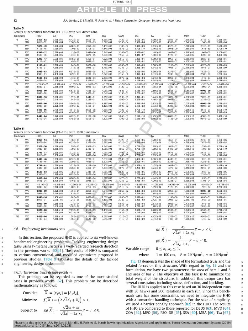
by other techniques in almost all cases. From Table 5, we see that7
the HHO can attain the best results in terms of AVG and STD in8
dealing with 12 test cases with 500 dimensions. By considering p-9
values in Table 22, it is recognized that the HHO can significantly10
outperform other optimizers in all cases. As per results in Table 6,11
similarly to what we observed in lower dimensions, it is detected12
that the HHO has still a remarkably superior performance in13
dealing with F1–F13 test functions compared to GA, PSO, DE, BBO,14
CS, GWO, MFO, TLBO, BAT, FA, and FPA optimizers. The statistical15
results in Table 23 also verify the significant gap between the16
results of HHO and other optimizers in almost all cases. It is seen17
that the HHO has reached the best global optimum for F9 and F1118
cases in any dimension.19
In order to further check the efficacy of HHO, we recorded20
the running time taken by optimizers to find the solutions for21
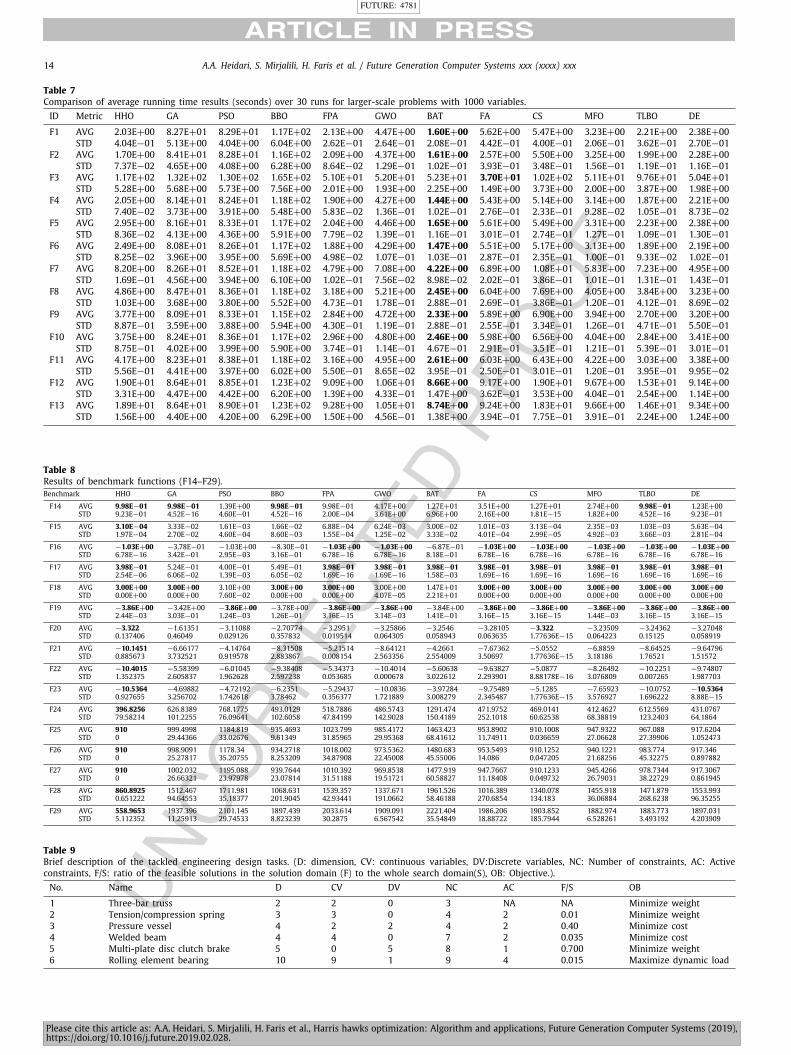
F1–F13 problems with 1000 dimensions and the results are ex- 22
posed in Table 7. As per results in Table 7, we detect that the 23
HHO shows a reasonably fast and competitive performance in 24
finding the best solutions compared to other well-established 25
optimizers even for high dimensional unimodal and multimodal 26
cases. Based on average running time on 13 problems, the HHO 27
performs faster than BBO, PSO, GA, CS, GWO, and FA algorithms. 28
These observations are also in accordance with the computational 29
complexity of HHO. 30
The results in Table 8 verify that HHO provides superior and 31
very competitive results on F14–F23 fixed dimension MM test 32
cases. The results on F16–F18 are very competitive and all al- 33
gorithms have attained high-quality results. Based on results in 34
Table 8, the proposed HHO has always achieved to the best re- 35
sults on F14–F23 problems in comparison with other approaches. 36
Based on results for F24–F29 hybrid CM functions in Table 8, 37
the HHO is capable of achieving to high-quality solutions and 38
outperforming other competitors. The p-values in Table 24 also 39
confirm the meaningful advantage of HHO compared to other 40
optimizers for the majority of cases. 41
https://aliasgharheidari.com/HHO.html
FUTURE: 4781
Please cite this article as: A.A. Heidari, S. Mirjalili, H. Faris et al., Harris hawks optimization: Algorithm and applications, Future Generation Computer Systems (2019),https://doi.org/10.1016/j.future.2019.02.028.
12 A.A. Heidari, S. Mirjalili, H. Faris et al. / Future Generation Computer Systems xxx (xxxx) xxx
Table 5Results of benchmark functions (F1–F13), with 500 dimensions.Benchmark HHO GA PSO BBO FPA GWO BAT FA CS MFO TLBO DE
F1 AVG 1.46E−92 6.06E+05 6.42E+05 1.60E+05 8.26E+04 1.42E−03 1.52E+06 6.30E+04 6.80E+00 1.15E+06 2.14E−77 7.43E+05STD 8.01E−92 7.01E+04 2.96E+04 9.76E+03 1.32E+04 3.99E−04 3.58E+04 8.47E+03 4.93E−01 3.54E+04 1.94E−77 3.67E+04
F2 AVG 7.87E−49 1.94E+03 6.08E+09 5.95E+02 5.13E+02 1.10E−02 8.34E+09 7.13E+02 4.57E+01 3.00E+08 2.31E−39 3.57E+09STD 3.11E−48 7.03E+01 1.70E+10 1.70E+01 4.84E+01 1.93E−03 1.70E+10 3.76E+01 2.05E+00 1.58E+09 1.63E−39 1.70E+10
F3 AVG 6.54E−37 5.79E+06 1.13E+07 2.98E+06 5.34E+05 3.34E+05 3.37E+07 1.19E+06 2.03E+02 4.90E+06 1.06E+00 1.20E+07STD 3.58E−36 9.08E+05 1.43E+06 3.87E+05 1.34E+05 7.95E+04 1.41E+07 1.88E+05 2.72E+01 1.02E+06 3.70E+00 1.49E+06
F4 AVG 1.29E−47 9.59E+01 8.18E+01 9.35E+01 4.52E+01 6.51E+01 9.82E+01 5.00E+01 4.06E−01 9.88E+01 4.02E−31 9.92E+01STD 4.11E−47 1.20E+00 1.49E+00 9.05E−01 4.28E+00 5.72E+00 3.32E−01 1.73E+00 3.03E−02 4.15E−01 2.67E−31 2.33E−01
F5 AVG 3.10E−01 1.79E+09 1.84E+09 2.07E+08 3.30E+07 4.98E+02 6.94E+09 2.56E+07 1.21E+03 5.01E+09 4.97E+02 4.57E+09STD 3.73E−01 4.11E+08 1.11E+08 2.08E+07 8.76E+06 5.23E−01 2.23E+08 6.14E+06 7.04E+01 2.50E+08 3.07E−01 1.25E+09
F6 AVG 2.94E−03 6.27E+05 6.57E+05 1.68E+05 8.01E+04 9.22E+01 1.53E+06 6.30E+04 8.27E+01 1.16E+06 7.82E+01 7.23E+05STD 3.98E−03 7.43E+04 3.29E+04 8.23E+03 9.32E+03 2.15E+00 3.37E+04 8.91E+03 2.24E+00 3.48E+04 2.50E+00 3.28E+04
F7 AVG 2.51E−04 9.10E+03 1.43E+04 2.62E+03 2.53E+02 4.67E−02 2.23E+04 3.71E+02 8.05E+01 3.84E+04 1.71E−03 2.39E+04STD 2.43E−04 2.20E+03 1.51E+03 3.59E+02 6.28E+01 1.12E−02 1.15E+03 6.74E+01 1.37E+01 2.24E+03 4.80E−04 2.72E+03
F8 AVG −2.09E+05 −1.31E+05 −1.65E+04 −1.42E+05 −3.00E+04 −5.70E+04 −9.03E+03 −7.27E+04 −2.10E+17 −6.29E+04 −5.02E+04 −2.67E+04STD 2.84E+01 2.31E+04 9.99E+02 1.98E+03 1.14E+03 3.12E+03 2.12E+03 1.15E+04 1.14E+18 5.71E+03 1.00E+04 1.38E+03
F9 AVG 0.00E+00 3.29E+03 6.63E+03 7.86E+02 4.96E+03 7.84E+01 6.18E+03 2.80E+03 2.54E+03 6.96E+03 0.00E+00 7.14E+03STD 0.00E+00 1.96E+02 1.07E+02 3.42E+01 7.64E+01 3.13E+01 1.20E+02 1.42E+02 5.21E+01 1.48E+02 0.00E+00 1.05E+02
F10 AVG 8.88E−16 1.96E+01 1.97E+01 1.44E+01 8.55E+00 1.93E−03 2.04E+01 1.24E+01 1.07E+00 2.03E+01 7.62E−01 2.06E+01STD 4.01E−31 2.04E−01 1.04E−01 2.22E−01 8.66E−01 3.50E−04 3.25E−02 4.46E−01 6.01E−02 1.48E−01 2.33E+00 2.45E−01
F11 AVG 0.00E+00 5.42E+03 5.94E+03 1.47E+03 6.88E+02 1.55E−02 1.38E+04 5.83E+02 2.66E−02 1.03E+04 0.00E+00 6.75E+03STD 0.00E+00 7.32E+02 3.19E+02 8.10E+01 8.17E+01 3.50E−02 3.19E+02 7.33E+01 2.30E−03 4.43E+02 0.00E+00 2.97E+02
F12 AVG 1.41E−06 2.79E+09 3.51E+09 1.60E+08 4.50E+06 7.42E−01 1.70E+10 8.67E+05 3.87E−01 1.20E+10 4.61E−01 1.60E+10STD 1.48E−06 1.11E+09 4.16E+08 3.16E+07 3.37E+06 4.38E−02 6.29E+08 6.23E+05 2.47E−02 6.82E+08 2.40E−02 2.34E+09
F13 AVG 3.44E−04 8.84E+09 6.82E+09 5.13E+08 3.94E+07 5.06E+01 3.17E+10 2.29E+07 6.00E+01 2.23E+10 4.98E+01 2.42E+10STD 4.75E−04 2.00E+09 8.45E+08 6.59E+07 1.87E+07 1.30E+00 9.68E+08 9.46E+06 1.13E+00 1.13E+09 9.97E−03 6.39E+09
Table 6Results of benchmark functions (F1–F13), with 1000 dimensions.Benchmark HHO GA PSO BBO FPA GWO BAT FA CS MFO TLBO DE
F1 AVG 1.06E−94 1.36E+06 1.36E+06 6.51E+05 1.70E+05 2.42E−01 3.12E+06 3.20E+05 1.65E+01 2.73E+06 2.73E−76 2.16E+06STD 4.97E−94 1.79E+05 6.33E+04 2.37E+04 2.99E+04 4.72E−02 4.61E+04 2.11E+04 1.27E+00 4.70E+04 7.67E−76 3.39E+05
F2 AVG 2.52E−50 4.29E+03 1.79E+10 1.96E+03 8.34E+02 7.11E−01 1.79E+10 1.79E+10 1.02E+02 1.79E+10 1.79E+10 1.79E+10STD 5.02E−50 8.86E+01 1.79E+10 2.18E+01 8.96E+01 4.96E−01 1.79E+10 1.79E+10 3.49E+00 1.79E+10 1.79E+10 1.79E+10
F3 AVG 1.79E−17 2.29E+07 3.72E+07 9.92E+06 1.95E+06 1.49E+06 1.35E+08 4.95E+06 8.67E+02 1.94E+07 8.61E−01 5.03E+07STD 9.81E−17 3.93E+06 1.16E+07 1.48E+06 4.20E+05 2.43E+05 4.76E+07 7.19E+05 1.10E+02 3.69E+06 1.33E+00 4.14E+06
F4 AVG 1.43E−46 9.79E+01 8.92E+01 9.73E+01 5.03E+01 7.94E+01 9.89E+01 6.06E+01 4.44E−01 9.96E+01 1.01E−30 9.95E+01STD 7.74E−46 7.16E−01 2.39E+00 7.62E−01 5.37E+00 2.77E+00 2.22E−01 2.69E+00 2.24E−02 1.49E−01 5.25E−31 1.43E−01
F5 AVG 5.73E−01 4.73E+09 3.72E+09 1.29E+09 7.27E+07 1.06E+03 1.45E+10 2.47E+08 2.68E+03 1.25E+10 9.97E+02 1.49E+10STD 1.40E+00 9.63E+08 2.76E+08 6.36E+07 1.84E+07 3.07E+01 3.20E+08 3.24E+07 1.27E+02 3.15E+08 2.01E−01 3.06E+08
F6 AVG 3.61E−03 1.52E+06 1.38E+06 6.31E+05 1.60E+05 2.03E+02 3.11E+06 3.18E+05 2.07E+02 2.73E+06 1.93E+02 2.04E+06STD 5.38E−03 1.88E+05 6.05E+04 1.82E+04 1.86E+04 2.45E+00 6.29E+04 2.47E+04 4.12E+00 4.56E+04 2.35E+00 2.46E+05
F7 AVG 1.41E−04 4.45E+04 6.26E+04 3.84E+04 1.09E+03 1.47E−01 1.25E+05 4.44E+03 4.10E+02 1.96E+05 1.83E−03 2.27E+05STD 1.63E−04 8.40E+03 4.16E+03 2.91E+03 3.49E+02 3.28E−02 3.93E+03 4.00E+02 8.22E+01 6.19E+03 5.79E−04 3.52E+04
F8 AVG −4.19E+05 −1.94E+05 −2.30E+04 −2.29E+05 −4.25E+04 −8.64E+04 −1.48E+04 −1.08E+05 −9.34E+14 −9.00E+04 −6.44E+04 −3.72E+04STD 1.03E+02 9.74E+03 1.70E+03 3.76E+03 1.47E+03 1.91E+04 3.14E+03 1.69E+04 2.12E+15 7.20E+03 1.92E+04 1.23E+03
F9 AVG 0.00E+00 8.02E+03 1.35E+04 2.86E+03 1.01E+04 2.06E+02 1.40E+04 7.17E+03 6.05E+03 1.56E+04 0.00E+00 1.50E+04STD 0.00E+00 3.01E+02 1.83E+02 9.03E+01 1.57E+02 4.81E+01 1.85E+02 1.88E+02 1.41E+02 1.94E+02 0.00E+00 1.79E+02
F10 AVG 8.88E−16 1.95E+01 1.98E+01 1.67E+01 8.62E+00 1.88E−02 2.07E+01 1.55E+01 1.18E+00 2.04E+01 5.09E−01 2.07E+01STD 4.01E−31 2.55E−01 1.24E−01 8.63E−02 9.10E−01 2.74E−03 2.23E−02 2.42E−01 5.90E−02 2.16E−01 1.94E+00 1.06E−01
F11 AVG 0.00E+00 1.26E+04 1.23E+04 5.75E+03 1.52E+03 6.58E−02 2.83E+04 2.87E+03 3.92E−02 2.47E+04 1.07E−16 1.85E+04STD 0.00E+00 1.63E+03 5.18E+02 1.78E+02 2.66E+02 8.82E−02 4.21E+02 1.78E+02 3.58E−03 4.51E+02 2.03E−17 2.22E+03
F12 AVG 1.02E−06 1.14E+10 7.73E+09 1.56E+09 8.11E+06 1.15E+00 3.63E+10 6.76E+07 6.53E−01 3.04E+10 6.94E−01 3.72E+10STD 1.16E−06 1.27E+09 6.72E+08 1.46E+08 3.46E+06 1.82E−01 1.11E+09 1.80E+07 2.45E−02 9.72E+08 1.90E−02 7.67E+08
F13 AVG 8.41E−04 1.91E+10 1.58E+10 4.17E+09 8.96E+07 1.21E+02 6.61E+10 4.42E+08 1.32E+02 5.62E+10 9.98E+01 6.66E+10STD 1.18E−03 4.21E+09 1.56E+09 2.54E+08 3.65E+07 1.11E+01 1.40E+09 7.91E+07 1.48E+00 1.76E+09 1.31E−02 2.26E+09
4.6. Engineering benchmark sets1
In this section, the proposed HHO is applied to six well-known2
benchmark engineering problems. Tackling engineering design3
tasks using P-metaheuristics is a well-regarded research direction4
in the previous works [60,61]. The results of HHO is compared5
to various conventional and modified optimizers proposed in6
previous studies. Table 9 tabulates the details of the tackled7
engineering design tasks.8
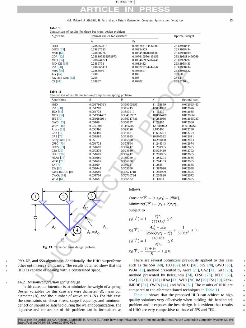
4.6.1. Three-bar truss design problem9
This problem can be regarded as one of the most studiedcases in previous works [62]. This problem can be describedmathematically as follows:
Consider−→X = [x1x2] = [A1A2],
Minimize f (−→X ) =
(2√2X1 + X2
)× 1,
Subject to g1(−→X ) =
√2x1 + x2
√2x21 + 2x1x2
P − σ ≤ 0,
g2(−→X ) =
x2√2x21 + 2x1x2
P − σ ≤ 0,
g3(−→X ) =
1√2x2 + x1
P − σ ≤ 0,
Variable range 0 ≤ x1, x2 ≤ 1,
where 1 = 100 cm, P = 2 KN/cm2, σ = 2 KN/cm2
Fig. 13 demonstrates the shape of the formulated truss and the 10
related forces on this structure. With regard to Fig. 13 and the 11
formulation, we have two parameters: the area of bars 1 and 3 12
and area of bar 2. The objective of this task is to minimize the 13
total weight of the structure. In addition, this design case has 14
several constraints including stress, deflection, and buckling. 15
The HHO is applied to this case based on 30 independent runs 16
with 30 hawks and 500 iterations in each run. Since this bench- 17
mark case has some constraints, we need to integrate the HHO 18
with a constraint handling technique. For the sake of simplicity, 19
we used a barrier penalty approach [82] in the HHO. The results 20
of HHO are compared to those reported for DEDS [63], MVO [64], 21
GOA [62], MFO [56], PSO–DE [65], SSA [60], MBA [66], Tsa [67], 22
https://aliasgharheidari.com/HHO.html
FUTURE: 4781
Please cite this article as: A.A. Heidari, S. Mirjalili, H. Faris et al., Harris hawks optimization: Algorithm and applications, Future Generation Computer Systems (2019),https://doi.org/10.1016/j.future.2019.02.028.
A.A. Heidari, S. Mirjalili, H. Faris et al. / Future Generation Computer Systems xxx (xxxx) xxx 13
Fig. 12. Scalability results of the HHO versus other methods in dealing with the F1–F13 cases with different dimensions.
Ray and Sain [68], and CS [34] in previous literature. Table 101
shows the detailed results of the proposed HHO compared to2
other techniques. Based on the results in Table 10, it is observed 3
that HHO can reveal very competitive results compared to DEDS, 4
https://aliasgharheidari.com/HHO.html
FUTURE: 4781
Please cite this article as: A.A. Heidari, S. Mirjalili, H. Faris et al., Harris hawks optimization: Algorithm and applications, Future Generation Computer Systems (2019),https://doi.org/10.1016/j.future.2019.02.028.
14 A.A. Heidari, S. Mirjalili, H. Faris et al. / Future Generation Computer Systems xxx (xxxx) xxx
Table 7Comparison of average running time results (seconds) over 30 runs for larger-scale problems with 1000 variables.ID Metric HHO GA PSO BBO FPA GWO BAT FA CS MFO TLBO DE
F1 AVG 2.03E+00 8.27E+01 8.29E+01 1.17E+02 2.13E+00 4.47E+00 1.60E+00 5.62E+00 5.47E+00 3.23E+00 2.21E+00 2.38E+00STD 4.04E−01 5.13E+00 4.04E+00 6.04E+00 2.62E−01 2.64E−01 2.08E−01 4.42E−01 4.00E−01 2.06E−01 3.62E−01 2.70E−01
F2 AVG 1.70E+00 8.41E+01 8.28E+01 1.16E+02 2.09E+00 4.37E+00 1.61E+00 2.57E+00 5.50E+00 3.25E+00 1.99E+00 2.28E+00STD 7.37E−02 4.65E+00 4.08E+00 6.28E+00 8.64E−02 1.29E−01 1.02E−01 3.93E−01 3.48E−01 1.56E−01 1.19E−01 1.16E−01
F3 AVG 1.17E+02 1.32E+02 1.30E+02 1.65E+02 5.10E+01 5.20E+01 5.23E+01 3.70E+01 1.02E+02 5.11E+01 9.76E+01 5.04E+01STD 5.28E+00 5.68E+00 5.73E+00 7.56E+00 2.01E+00 1.93E+00 2.25E+00 1.49E+00 3.73E+00 2.00E+00 3.87E+00 1.98E+00
F4 AVG 2.05E+00 8.14E+01 8.24E+01 1.18E+02 1.90E+00 4.27E+00 1.44E+00 5.43E+00 5.14E+00 3.14E+00 1.87E+00 2.21E+00STD 7.40E−02 3.73E+00 3.91E+00 5.48E+00 5.83E−02 1.36E−01 1.02E−01 2.76E−01 2.33E−01 9.28E−02 1.05E−01 8.73E−02
F5 AVG 2.95E+00 8.16E+01 8.33E+01 1.17E+02 2.04E+00 4.46E+00 1.65E+00 5.61E+00 5.49E+00 3.31E+00 2.23E+00 2.38E+00STD 8.36E−02 4.13E+00 4.36E+00 5.91E+00 7.79E−02 1.39E−01 1.16E−01 3.01E−01 2.74E−01 1.27E−01 1.09E−01 1.30E−01
F6 AVG 2.49E+00 8.08E+01 8.26E+01 1.17E+02 1.88E+00 4.29E+00 1.47E+00 5.51E+00 5.17E+00 3.13E+00 1.89E+00 2.19E+00STD 8.25E−02 3.96E+00 3.95E+00 5.69E+00 4.98E−02 1.07E−01 1.03E−01 2.87E−01 2.35E−01 1.00E−01 9.33E−02 1.02E−01
F7 AVG 8.20E+00 8.26E+01 8.52E+01 1.18E+02 4.79E+00 7.08E+00 4.22E+00 6.89E+00 1.08E+01 5.83E+00 7.23E+00 4.95E+00STD 1.69E−01 4.56E+00 3.94E+00 6.10E+00 1.02E−01 7.56E−02 8.98E−02 2.02E−01 3.86E−01 1.01E−01 1.31E−01 1.43E−01
F8 AVG 4.86E+00 8.47E+01 8.36E+01 1.18E+02 3.18E+00 5.21E+00 2.45E+00 6.04E+00 7.69E+00 4.05E+00 3.84E+00 3.23E+00STD 1.03E+00 3.68E+00 3.80E+00 5.52E+00 4.73E−01 1.78E−01 2.88E−01 2.69E−01 3.86E−01 1.20E−01 4.12E−01 8.69E−02
F9 AVG 3.77E+00 8.09E+01 8.33E+01 1.15E+02 2.84E+00 4.72E+00 2.33E+00 5.89E+00 6.90E+00 3.94E+00 2.70E+00 3.20E+00STD 8.87E−01 3.59E+00 3.88E+00 5.94E+00 4.30E−01 1.19E−01 2.88E−01 2.55E−01 3.34E−01 1.26E−01 4.71E−01 5.50E−01
F10 AVG 3.75E+00 8.24E+01 8.36E+01 1.17E+02 2.96E+00 4.80E+00 2.46E+00 5.98E+00 6.56E+00 4.04E+00 2.84E+00 3.41E+00STD 8.75E−01 4.02E+00 3.99E+00 5.90E+00 3.74E−01 1.14E−01 4.67E−01 2.91E−01 3.51E−01 1.21E−01 5.39E−01 3.01E−01
F11 AVG 4.17E+00 8.23E+01 8.38E+01 1.18E+02 3.16E+00 4.95E+00 2.61E+00 6.03E+00 6.43E+00 4.22E+00 3.03E+00 3.38E+00STD 5.56E−01 4.41E+00 3.97E+00 6.02E+00 5.50E−01 8.65E−02 3.95E−01 2.50E−01 3.01E−01 1.20E−01 3.95E−01 9.95E−02
F12 AVG 1.90E+01 8.64E+01 8.85E+01 1.23E+02 9.09E+00 1.06E+01 8.66E+00 9.17E+00 1.90E+01 9.67E+00 1.53E+01 9.14E+00STD 3.31E+00 4.47E+00 4.42E+00 6.20E+00 1.39E+00 4.33E−01 1.47E+00 3.62E−01 3.53E+00 4.04E−01 2.54E+00 1.14E+00
F13 AVG 1.89E+01 8.64E+01 8.90E+01 1.23E+02 9.28E+00 1.05E+01 8.74E+00 9.24E+00 1.83E+01 9.66E+00 1.46E+01 9.34E+00STD 1.56E+00 4.40E+00 4.20E+00 6.29E+00 1.50E+00 4.56E−01 1.38E+00 3.94E−01 7.75E−01 3.91E−01 2.24E+00 1.24E+00
Table 8Results of benchmark functions (F14–F29).Benchmark HHO GA PSO BBO FPA GWO BAT FA CS MFO TLBO DE
F14 AVG 9.98E−01 9.98E−01 1.39E+00 9.98E−01 9.98E−01 4.17E+00 1.27E+01 3.51E+00 1.27E+01 2.74E+00 9.98E−01 1.23E+00STD 9.23E−01 4.52E−16 4.60E−01 4.52E−16 2.00E−04 3.61E+00 6.96E+00 2.16E+00 1.81E−15 1.82E+00 4.52E−16 9.23E−01
F15 AVG 3.10E−04 3.33E−02 1.61E−03 1.66E−02 6.88E−04 6.24E−03 3.00E−02 1.01E−03 3.13E−04 2.35E−03 1.03E−03 5.63E−04STD 1.97E−04 2.70E−02 4.60E−04 8.60E−03 1.55E−04 1.25E−02 3.33E−02 4.01E−04 2.99E−05 4.92E−03 3.66E−03 2.81E−04
F16 AVG −1.03E+00 −3.78E−01 −1.03E+00 −8.30E−01 −1.03E+00 −1.03E+00 −6.87E−01 −1.03E+00 −1.03E+00 −1.03E+00 −1.03E+00 −1.03E+00STD 6.78E−16 3.42E−01 2.95E−03 3.16E−01 6.78E−16 6.78E−16 8.18E−01 6.78E−16 6.78E−16 6.78E−16 6.78E−16 6.78E−16
F17 AVG 3.98E−01 5.24E−01 4.00E−01 5.49E−01 3.98E−01 3.98E−01 3.98E−01 3.98E−01 3.98E−01 3.98E−01 3.98E−01 3.98E−01STD 2.54E−06 6.06E−02 1.39E−03 6.05E−02 1.69E−16 1.69E−16 1.58E−03 1.69E−16 1.69E−16 1.69E−16 1.69E−16 1.69E−16
F18 AVG 3.00E+00 3.00E+00 3.10E+00 3.00E+00 3.00E+00 3.00E+00 1.47E+01 3.00E+00 3.00E+00 3.00E+00 3.00E+00 3.00E+00STD 0.00E+00 0.00E+00 7.60E−02 0.00E+00 0.00E+00 4.07E−05 2.21E+01 0.00E+00 0.00E+00 0.00E+00 0.00E+00 0.00E+00
F19 AVG −3.86E+00 −3.42E+00 −3.86E+00 −3.78E+00 −3.86E+00 −3.86E+00 −3.84E+00 −3.86E+00 −3.86E+00 −3.86E+00 −3.86E+00 −3.86E+00STD 2.44E−03 3.03E−01 1.24E−03 1.26E−01 3.16E−15 3.14E−03 1.41E−01 3.16E−15 3.16E−15 1.44E−03 3.16E−15 3.16E−15
F20 AVG −3.322 −1.61351 −3.11088 −2.70774 −3.2951 −3.25866 −3.2546 −3.28105 −3.322 −3.23509 −3.24362 −3.27048STD 0.137406 0.46049 0.029126 0.357832 0.019514 0.064305 0.058943 0.063635 1.77636E−15 0.064223 0.15125 0.058919
F21 AVG −10.1451 −6.66177 −4.14764 −8.31508 −5.21514 −8.64121 −4.2661 −7.67362 −5.0552 −6.8859 −8.64525 −9.64796STD 0.885673 3.732521 0.919578 2.883867 0.008154 2.563356 2.554009 3.50697 1.77636E−15 3.18186 1.76521 1.51572
F22 AVG −10.4015 −5.58399 −6.01045 −9.38408 −5.34373 −10.4014 −5.60638 −9.63827 −5.0877 −8.26492 −10.2251 −9.74807STD 1.352375 2.605837 1.962628 2.597238 0.053685 0.000678 3.022612 2.293901 8.88178E−16 3.076809 0.007265 1.987703
F23 AVG −10.5364 −4.69882 −4.72192 −6.2351 −5.29437 −10.0836 −3.97284 −9.75489 −5.1285 −7.65923 −10.0752 −10.5364STD 0.927655 3.256702 1.742618 3.78462 0.356377 1.721889 3.008279 2.345487 1.77636E−15 3.576927 1.696222 8.88E−15
F24 AVG 396.8256 626.8389 768.1775 493.0129 518.7886 486.5743 1291.474 471.9752 469.0141 412.4627 612.5569 431.0767STD 79.58214 101.2255 76.09641 102.6058 47.84199 142.9028 150.4189 252.1018 60.62538 68.38819 123.2403 64.1864
F25 AVG 910 999.4998 1184.819 935.4693 1023.799 985.4172 1463.423 953.8902 910.1008 947.9322 967.088 917.6204STD 0 29.44366 33.02676 9.61349 31.85965 29.95368 68.41612 11.74911 0.036659 27.06628 27.39906 1.052473
F26 AVG 910 998.9091 1178.34 934.2718 1018.002 973.5362 1480.683 953.5493 910.1252 940.1221 983.774 917.346STD 0 25.27817 35.20755 8.253209 34.87908 22.45008 45.55006 14.086 0.047205 21.68256 45.32275 0.897882
F27 AVG 910 1002.032 1195.088 939.7644 1010.392 969.8538 1477.919 947.7667 910.1233 945.4266 978.7344 917.3067STD 0 26.66321 23.97978 23.07814 31.51188 19.51721 60.58827 11.18408 0.049732 26.79031 38.22729 0.861945
F28 AVG 860.8925 1512.467 1711.981 1068.631 1539.357 1337.671 1961.526 1016.389 1340.078 1455.918 1471.879 1553.993STD 0.651222 94.64553 35.18377 201.9045 42.93441 191.0662 58.46188 270.6854 134.183 36.06884 268.6238 96.35255
F29 AVG 558.9653 1937.396 2101.145 1897.439 2033.614 1909.091 2221.404 1986.206 1903.852 1882.974 1883.773 1897.031STD 5.112352 11.25913 29.74533 8.823239 30.2875 6.567542 35.54849 18.88722 185.7944 6.528261 3.493192 4.203909
Table 9Brief description of the tackled engineering design tasks. (D: dimension, CV: continuous variables, DV:Discrete variables, NC: Number of constraints, AC: Activeconstraints, F/S: ratio of the feasible solutions in the solution domain (F) to the whole search domain(S), OB: Objective.).No. Name D CV DV NC AC F/S OB
1 Three-bar truss 2 2 0 3 NA NA Minimize weight2 Tension/compression spring 3 3 0 4 2 0.01 Minimize weight3 Pressure vessel 4 2 2 4 2 0.40 Minimize cost4 Welded beam 4 4 0 7 2 0.035 Minimize cost5 Multi-plate disc clutch brake 5 0 5 8 1 0.700 Minimize weight6 Rolling element bearing 10 9 1 9 4 0.015 Maximize dynamic load
https://aliasgharheidari.com/HHO.html
FUTURE: 4781
Please cite this article as: A.A. Heidari, S. Mirjalili, H. Faris et al., Harris hawks optimization: Algorithm and applications, Future Generation Computer Systems (2019),https://doi.org/10.1016/j.future.2019.02.028.
A.A. Heidari, S. Mirjalili, H. Faris et al. / Future Generation Computer Systems xxx (xxxx) xxx 15
Table 10Comparison of results for three-bar truss design problem.Algorithm Optimal values for variables Optimal weight
x1 x2HHO 0.788662816 0.408283133832900 263.8958434DEDS [63] 0.78867513 0.40824828 263.8958434MVO [64] 0.78860276 0.408453070000000 263.8958499GOA [62] 0.788897555578973 0.407619570115153 263.895881496069MFO [56] 0.788244771 0.409466905784741 263.8959797PSO–DE [65] 0.7886751 0.4082482 263.8958433SSA [60] 0.788665414 0.408275784444547 263.8958434MBA [66] 0.7885650 0.4085597 263.8958522Tsa [67] 0.788 0.408 263.68Ray and Sain [68] 0.795 0.395 264.3CS [34] 0.78867 0.40902 263.9716
Table 11Comparison of results for tension/compression spring problem.Algorithms d D N Optimal cost
HHO 0.051796393 0.359305355 11.138859 0.012665443SSA [60] 0.051207 0.345215 12.004032 0.0126763TEO [69] 0.051775 0.3587919 11.16839 0.012665MFO [56] 0.051994457 0.36410932 10.868422 0.0126669SFS [70] 0.051689061 0.356717736 11.288966 0.012665233GWO [55] 0.05169 0.356737 11.28885 0.012666WOA [18] 0 .051207 0 .345215 12 .004032 0 .0126763Arora [71] 0.053396 0.399180 9.185400 0.012730GA2 [72] 0.051480 0.351661 11.632201 0.012704GA3 [73] 0.051989 0.363965 10.890522 0.012681Belegundu [74] 0.05 0.315900 14.250000 0.012833CPSO [75] 0.051728 0.357644 11.244543 0.012674DEDS [63] 0.051689 0.356717 11.288965 0.012665GSA [25] 0.050276 0.323680 13.525410 0.012702DELC [76] 0.051689 0.356717 11.288965 0.012665HEAA [77] 0.051689 0.356729 11.288293 0.012665WEO [78] 0.051685 0.356630 11.294103 0.012665BA [79] 0.05169 0.35673 11.2885 0.012665ESs [80] 0.051643 0.355360 11.397926 0.012698Rank-iMDDE [81] 0.051689 0.35671718 11.288999 0.012665CWCA [14] 0.051709 0.35710734 11.270826 0.012672WCA [61] 0.05168 0.356522 11.30041 0.012665
Fig. 13. Three-bar truss design problem.
PSO–DE, and SSA algorithms. Additionally, the HHO outperforms1
other optimizers significantly. The results obtained show that the2
HHO is capable of dealing with a constrained space.3
4.6.2. Tension/compression spring design4
In this case, our intention is to minimize the weight of a spring.Design variables for this case are wire diameter (d), mean coildiameter (D), and the number of active coils (N). For this case,the constraints on shear stress, surge frequency, and minimumdeflection should be satisfied during the weight optimization. Theobjective and constraints of this problem can be formulated as
follows:
Consider−→z = [z1z2z3] = [dDN],
Minimizef (−→z ) = (z3 + 2)z2z21 ,
Subject to
g1(−→z ) = 1 −
z32z371785z41
≤ 0,
g2(−→z ) =
4z22 − z1z212566(z2z31 − z41 )
+1
5108z21≤ 0,
g3(−→z ) = 1 −
140.45z1z22z3
≤ 0
g4(−→z ) =
z1 + z21.5
− 1 ≤ 0,
There are several optimizers previously applied to this case 5
such as the SSA [60], TEO [69], MFO [56], SFS [70], GWO [55], 6
WOA [18], method presented by Arora [71], GA2 [72], GA3 [73], 7
method presented by Belegundu [74], CPSO [75], DEDS [63], 8
GSA [25], DELC [76], HEAA [77], WEO [78], BA [79], ESs [80], Rank- 9
iMDDE [81], CWCA [14], and WCA [61]. The results of HHO are 10
compared to the aforementioned techniques in Table 11. 11
Table 11 shows that the proposed HHO can achieve to high 12
quality solutions very effectively when tackling this benchmark 13
problem and it exposes the best design. It is evident that results 14
of HHO are very competitive to those of SFS and TEO. 15
https://aliasgharheidari.com/HHO.html
FUTURE: 4781
Please cite this article as: A.A. Heidari, S. Mirjalili, H. Faris et al., Harris hawks optimization: Algorithm and applications, Future Generation Computer Systems (2019),https://doi.org/10.1016/j.future.2019.02.028.
16 A.A. Heidari, S. Mirjalili, H. Faris et al. / Future Generation Computer Systems xxx (xxxx) xxx
Fig. 14. Pressure vessel problem.
Fig. 15. Welded beam design problem.
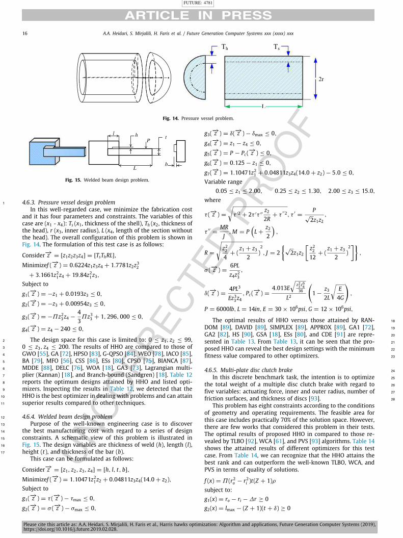
4.6.3. Pressure vessel design problem1
In this well-regarded case, we minimize the fabrication costand it has four parameters and constraints. The variables of thiscase are (x1 - x4): Ts (x1, thickness of the shell), Th (x2, thickness ofthe head), r (x3, inner radius), L (x4, length of the section withoutthe head). The overall configuration of this problem is shown inFig. 14. The formulation of this test case is as follows:
Consider−→z = [z1z2z3z4] = [TsThRL],
Minimizef (−→z ) = 0.6224z1z3z4 + 1.7781z2z32+ 3.1661z21z4 + 19.84z21z3,
Subject to
g1(−→z ) = −z1 + 0.0193z3 ≤ 0,
g2(−→z ) = −z3 + 0.00954z3 ≤ 0,
g3(−→z ) = −Πz23z4 −
43Πz33 + 1, 296, 000 ≤ 0,
g4(−→z ) = z4 − 240 ≤ 0,
The design space for this case is limited to: 0 ≤ z1, z2 ≤ 99,2
0 ≤ z3, z4 ≤ 200. The results of HHO are compared to those of3
GWO [55], GA [72], HPSO [83], G-QPSO [84], WEO [78], IACO [85],4
BA [79], MFO [56], CSS [86], ESs [80], CPSO [75], BIANCA [87],5
MDDE [88], DELC [76], WOA [18], GA3 [73], Lagrangian multi-6
plier (Kannan) [18], and Branch-bound (Sandgren) [18]. Table 127
reports the optimum designs attained by HHO and listed opti-8
mizers. Inspecting the results in Table 12, we detected that the9
HHO is the best optimizer in dealing with problems and can attain10
superior results compared to other techniques.11
4.6.4. Welded beam design problem12
Purpose of the well-known engineering case is to discover13
the best manufacturing cost with regard to a series of design14
constraints. A schematic view of this problem is illustrated in15
Fig. 15. The design variables are thickness of weld (h), length (l),16
height (t), and thickness of the bar (b).17
This case can be formulated as follows:
Consider−→z = [z1, z2, z3, z4] = [h, l, t, b],
Minimizef (−→z ) = 1.10471z21z2 + 0.04811z3z4(14.0 + z2),Subject to
g1(−→z ) = τ (−→z ) − τmax ≤ 0,
g2(−→z ) = σ (−→z ) − σmax ≤ 0,
g3(−→z ) = δ(−→z ) − δmax ≤ 0,
g4(−→z ) = z1 − z4 ≤ 0,
g5(−→z ) = P − Pc(
−→z ) ≤ 0,
g6(−→z ) = 0.125 − z1 ≤ 0,
g7(−→z ) = 1.10471z21 + 0.04811z3z4(14.0 + z2) − 5.0 ≤ 0,
Variable range0.05 ≤ z1 ≤ 2.00, 0.25 ≤ z2 ≤ 1.30, 2.00 ≤ z3 ≤ 15.0,
where
τ (−→z ) =
√τ ′2 + 2τ ′τ ′′
z22R
+ τ′′2, τ ′
=P
√2z1z2
,
τ ′′=
MRJ
,M = P(L +
z22
),
R =
√z224
+ (z1 + z3
2)2, J = 2
{√2z1z2
[z2212
+ (z1 + z3
2)2]}
,
σ (−→z ) =6PLz4z23
,
δ(−→z ) =4PL3
Ez33z4, Pc(
−→z ) =4.013E
√z23 z
64
36
L2
(1 −
z32L
√E4G
),
P = 6000lb, L = 14in, E = 30 × 106psi,G = 12 × 106psi,
The optimal results of HHO versus those attained by RAN- 18
DOM [89], DAVID [89], SIMPLEX [89], APPROX [89], GA1 [72], 19
GA2 [82], HS [90], GSA [18], ESs [80], and CDE [91] are repre- 20
sented in Table 13. From Table 13, it can be seen that the pro- 21
posed HHO can reveal the best design settings with the minimum 22
fitness value compared to other optimizers. 23
4.6.5. Multi-plate disc clutch brake 24
In this discrete benchmark task, the intention is to optimize 25
the total weight of a multiple disc clutch brake with regard to 26
five variables: actuating force, inner and outer radius, number of 27
friction surfaces, and thickness of discs [93]. 28
This problem has eight constraints according to the conditionsof geometry and operating requirements. The feasible area forthis case includes practically 70% of the solution space. However,there are few works that considered this problem in their tests.The optimal results of proposed HHO in compared to those re-vealed by TLBO [92], WCA [61], and PVS [93] algorithms. Table 14shows the attained results of different optimizers for this testcase. From Table 14, we can recognize that the HHO attains thebest rank and can outperform the well-known TLBO, WCA, andPVS in terms of quality of solutions.
f (x) = Π (r2o − r2i )t(Z + 1)ρsubject to:g1(x) = ro − ri − ∆r ≥ 0g2(x) = lmax − (Z + 1)(t + δ) ≥ 0
https://aliasgharheidari.com/HHO.html
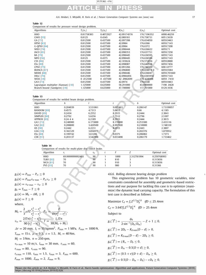
FUTURE: 4781
Please cite this article as: A.A. Heidari, S. Mirjalili, H. Faris et al., Harris hawks optimization: Algorithm and applications, Future Generation Computer Systems (2019),https://doi.org/10.1016/j.future.2019.02.028.
A.A. Heidari, S. Mirjalili, H. Faris et al. / Future Generation Computer Systems xxx (xxxx) xxx 17
Table 12Comparison of results for pressure vessel design problem.Algorithms Ts(x1) Th(x2) R(x3) L(x4) Optimal cost
HHO 0.81758383 0.4072927 42.09174576 176.7196352 6000.46259GWO [55] 0.8125 0.4345 42.089181 176.758731 6051.5639GA [72] 0.812500 0.437500 42.097398 176.654050 6059.9463HPSO [83] 0.812500 0.437500 42.0984 176.6366 6059.7143G-QPSO [84] 0.812500 0.437500 42.0984 176.6372 6059.7208WEO [78] 0.812500 0.437500 42.098444 176.636622 6059.71IACO [85] 0.812500 0.437500 42.098353 176.637751 6059.7258BA [79] 0.812500 0.437500 42.098445 176.636595 6059.7143MFO [56] 0.8125 0.4375 42.098445 176.636596 6059.7143CSS [86] 0.812500 0.437500 42.103624 176.572656 6059.0888ESs [80] 0.812500 0.437500 42.098087 176.640518 6059.7456CPSO [75] 0.812500 0.437500 42.091266 176.746500 6061.0777BIANCA [87] 0.812500 0.437500 42.096800 176.6580 0 0 6059.9384MDDE [88] 0.812500 0.437500 42.098446 176.636047 6059.701660DELC [76] 0.812500 0.437500 42.0984456 176.6365958 6059.7143WOA [18] 0 .812500 0 .437500 42 .0982699 176 .638998 6059 .7410GA3 [73] 0.812500 0.437500 42.0974 176.6540 6059.9463Lagrangian multiplier (Kannan) [18] 1.125000 0.625000 58.291000 43.6900000 7198 .0428Branch-bound (Sandgren) [18] 1.125000 0.625000 47.700000 117.701000 8129.1036
Table 13Comparison of results for welded beam design problem.Algorithm h l t b Optimal cost
HHO 0.204039 3.531061 9.027463 0.206147 1.73199057RANDOM [89] 0.4575 4.7313 5.0853 0.66 4.1185DAVID [89] 0.2434 6.2552 8.2915 0.2444 2.3841SIMPLEX [89] 0.2792 5.6256 7.7512 0.2796 2.5307APPROX [89] 0.24 4 4 6.2189 8.2915 0.2444 2.3815GA1 [72] 0.248900 6.173000 8.178900 0.253300 2.433116GA2 [82] 0.208800 3.420500 8.997500 0.210000 1.748310HS [90] 0.2442 6.2231 8.2915 0.2443 2.3807GSA [18] 0.182129 3.856979 10 0.202376 1.879952ESs [80] 0.199742 3.61206 9.0375 0.206082 1.7373CDE [91] 0.203137 3.542998 9.033498 0.206179 1.733462
Table 14Comparison of results for multi-plate disc clutch brake.Algorithm ri r0 t F Z Optimal cost
HHO 69.9999999992493 90 1 1000 2.312781994 0.259768993TLBO [92] 70 90 1 810 3 0.313656WCA [61] 70 90 1 910 3 0.313656PVS [93] 70 90 1 980 3 0.31366
g3(x) = Pmax − Prz ≥ 0
g4(x) = Pmaxvsr max − Przνsr ≥ 0
g5(x) = vsr max − vsr ≥ 0
g6 = Tmax − T ≥ 0
g7(x) = Mh − sMs ≥ 0
g8(x) = T ≥ 0
where,
Mh =23µFZ
r3o − r2ir2o − r3i
, Prz =F
Π (r2o − r2i ),
vrz =2Πn(r3o − r3i )90(r2o − r2i
) , T =IzΠn
30(Mh + Mf )
∆r = 20 mm, Iz = 55 kgmm2, Pmax = 1 MPa, Fmax = 1000N,
Tmax = 15 s, µ = 0.5, s = 1.5, Ms = 40Nm,
Mf = 3Nm, n = 250 rpm,
vsr max = 10 m/s, lmax = 30 mm, rimin = 60,
rimax = 80, romin = 90,
romax = 110, tmin = 1.5, tmax = 3, Fmin = 600,
Fmax = 1000, Zmin = 2, Zmax = 9,
4.6.6. Rolling element bearing design problem 1
This engineering problem has 10 geometric variables, nineconstraints considered for assembly and geometric-based restric-tions and our purpose for tackling this case is to optimize (maxi-mize) the dynamic load carrying capacity. The formulation of thistest case is described as follows:
Maximize Cd = fcZ2/3D1.8b ifD ≤ 25.4mm
Cd = 3.647fcZ2/3D1.4b ifD > 25.4mm
Subject to
g1(−→z ) =
φ0
2 sin−1(Db/Dm)− Z + 1 ≤ 0,
g2(−→z ) = 2Db − KDmin(D − d) > 0,
g3(−→z ) = KDmax(D − d) − 2Db ≥ 0,
g4(−→z ) = ζBw − Db ≤ 0,
g5(−→z ) = Dm − 0.5(D + d) ≥ 0,
g6(−→z ) = (0.5 + e)(D + d) − Dm ≥ 0,
g7(−→z ) = 0.5(D − Dm − Db) − ϵDb ≥ 0,
https://aliasgharheidari.com/HHO.html
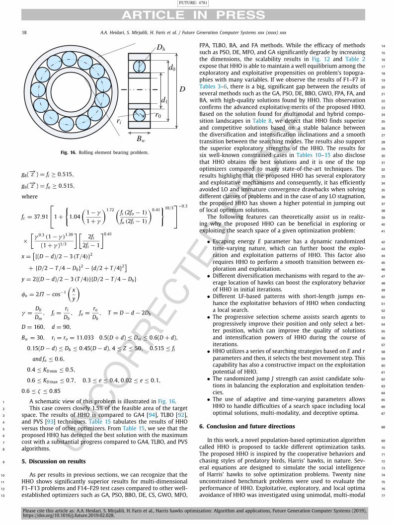
FUTURE: 4781
Please cite this article as: A.A. Heidari, S. Mirjalili, H. Faris et al., Harris hawks optimization: Algorithm and applications, Future Generation Computer Systems (2019),https://doi.org/10.1016/j.future.2019.02.028.
18 A.A. Heidari, S. Mirjalili, H. Faris et al. / Future Generation Computer Systems xxx (xxxx) xxx
Fig. 16. Rolling element bearing problem.
g8(−→z ) = fi ≥ 0.515,
g9(−→z ) = fo ≥ 0.515,
where
fc = 37.91
⎡⎣1 +
{1.04
(1 − γ
1 + γ
)1.72 ( fi (2fo − 1)fo (2fi − 1)
)0.41}10/3
⎤⎦−0.3
×
[γ 0.3 (1 − γ )1.39
(1 + γ )1/3
][2fi
2fi − 1
]0.41x =
[{(D − d)/2 − 3 (T/4)}2
+ {D/2 − T/4 − Db}2− {d/2 + T/4}2
]y = 2{(D − d)/2 − 3 (T/4)}{D/2 − T/4 − Db}
φo = 2Π − cos−1(xy
)γ =
Db
Dm, fi =
riDb
, fo =roDb
, T = D − d − 2Db
D = 160, d = 90,
Bw = 30, ri = ro = 11.033 0.5(D + d) ≤ Dm ≤ 0.6(D + d),
0.15(D − d) ≤ Db ≤ 0.45(D − d), 4 ≤ Z ≤ 50, 0.515 ≤ fi
and fo ≤ 0.6,
0.4 ≤ KDmin ≤ 0.5,
0.6 ≤ KDmax ≤ 0.7, 0.3 ≤ e ≤ 0.4, 0.02 ≤ e ≤ 0.1,
0.6 ≤ ζ ≤ 0.85
A schematic view of this problem is illustrated in Fig. 16.1
This case covers closely 1.5% of the feasible area of the target2
space. The results of HHO is compared to GA4 [94], TLBO [92],3
and PVS [93] techniques. Table 15 tabulates the results of HHO4
versus those of other optimizers. From Table 15, we see that the5
proposed HHO has detected the best solution with the maximum6
cost with a substantial progress compared to GA4, TLBO, and PVS7
algorithms.8
5. Discussion on results9
As per results in previous sections, we can recognize that the10
HHO shows significantly superior results for multi-dimensional11
F1–F13 problems and F14–F29 test cases compared to other well-12
established optimizers such as GA, PSO, BBO, DE, CS, GWO, MFO,13
FPA, TLBO, BA, and FA methods. While the efficacy of methods 14
such as PSO, DE, MFO, and GA significantly degrade by increasing 15
the dimensions, the scalability results in Fig. 12 and Table 2 16
expose that HHO is able to maintain a well equilibrium among the 17
exploratory and exploitative propensities on problem’s topogra- 18
phies with many variables. If we observe the results of F1–F7 in 19
Tables 3–6, there is a big, significant gap between the results of 20
several methods such as the GA, PSO, DE, BBO, GWO, FPA, FA, and 21
BA, with high-quality solutions found by HHO. This observation 22
confirms the advanced exploitative merits of the proposed HHO. 23
Based on the solution found for multimodal and hybrid compo- 24
sition landscapes in Table 8, we detect that HHO finds superior 25
and competitive solutions based on a stable balance between 26
the diversification and intensification inclinations and a smooth 27
transition between the searching modes. The results also support 28
the superior exploratory strengths of the HHO. The results for 29
six well-known constrained cases in Tables 10–15 also disclose 30
that HHO obtains the best solutions and it is one of the top 31
optimizers compared to many state-of-the-art techniques. The 32
results highlight that the proposed HHO has several exploratory 33
and exploitative mechanisms and consequently, it has efficiently 34
avoided LO and immature convergence drawbacks when solving 35
different classes of problems and in the case of any LO stagnation, 36
the proposed HHO has shown a higher potential in jumping out 37
of local optimum solutions. 38
The following features can theoretically assist us in realiz- 39
ing why the proposed HHO can be beneficial in exploring or 40
exploiting the search space of a given optimization problem: 41
• Escaping energy E parameter has a dynamic randomized 42
time-varying nature, which can further boost the explo- 43
ration and exploitation patterns of HHO. This factor also 44
requires HHO to perform a smooth transition between ex- 45
ploration and exploitation. 46
• Different diversification mechanisms with regard to the av- 47
erage location of hawks can boost the exploratory behavior 48
of HHO in initial iterations. 49
• Different LF-based patterns with short-length jumps en- 50
hance the exploitative behaviors of HHO when conducting 51
a local search. 52
• The progressive selection scheme assists search agents to 53
progressively improve their position and only select a bet- 54
ter position, which can improve the quality of solutions 55
and intensification powers of HHO during the course of 56
iterations. 57
• HHO utilizes a series of searching strategies based on E and r 58
parameters and then, it selects the best movement step. This 59
capability has also a constructive impact on the exploitation 60
potential of HHO. 61
• The randomized jump J strength can assist candidate solu- 62
tions in balancing the exploration and exploitation tenden- 63
cies. 64
• The use of adaptive and time-varying parameters allows 65
HHO to handle difficulties of a search space including local 66
optimal solutions, multi-modality, and deceptive optima. 67
6. Conclusion and future directions 68
In this work, a novel population-based optimization algorithm 69
called HHO is proposed to tackle different optimization tasks. 70
The proposed HHO is inspired by the cooperative behaviors and 71
chasing styles of predatory birds, Harris’ hawks, in nature. Sev- 72
eral equations are designed to simulate the social intelligence 73
of Harris’ hawks to solve optimization problems. Twenty nine 74
unconstrained benchmark problems were used to evaluate the 75
performance of HHO. Exploitative, exploratory, and local optima 76
avoidance of HHO was investigated using unimodal, multi-modal 77
https://aliasgharheidari.com/HHO.html
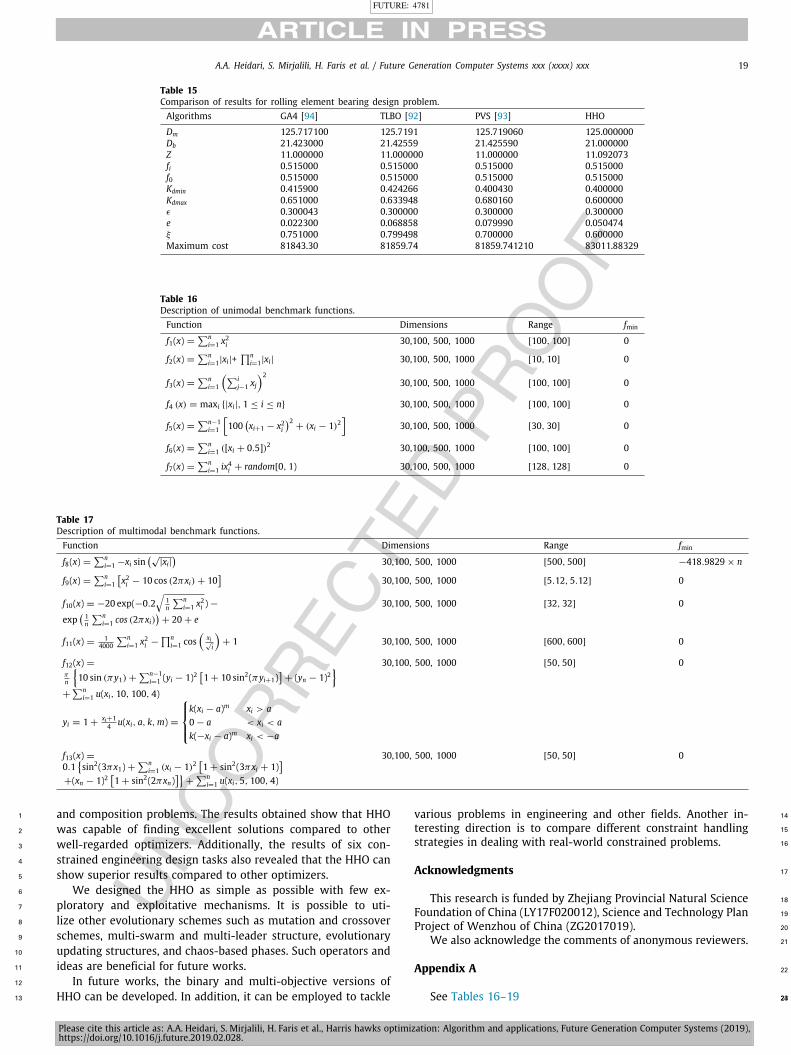
FUTURE: 4781
Please cite this article as: A.A. Heidari, S. Mirjalili, H. Faris et al., Harris hawks optimization: Algorithm and applications, Future Generation Computer Systems (2019),https://doi.org/10.1016/j.future.2019.02.028.
A.A. Heidari, S. Mirjalili, H. Faris et al. / Future Generation Computer Systems xxx (xxxx) xxx 19
Table 15Comparison of results for rolling element bearing design problem.Algorithms GA4 [94] TLBO [92] PVS [93] HHO
Dm 125.717100 125.7191 125.719060 125.000000Db 21.423000 21.42559 21.425590 21.000000Z 11.000000 11.000000 11.000000 11.092073fi 0.515000 0.515000 0.515000 0.515000f0 0.515000 0.515000 0.515000 0.515000Kdmin 0.415900 0.424266 0.400430 0.400000Kdmax 0.651000 0.633948 0.680160 0.600000ϵ 0.300043 0.300000 0.300000 0.300000e 0.022300 0.068858 0.079990 0.050474ξ 0.751000 0.799498 0.700000 0.600000Maximum cost 81843.30 81859.74 81859.741210 83011.88329
Table 16Description of unimodal benchmark functions.Function Dimensions Range fmin
f1(x) =∑n
i=1 x2i 30,100, 500, 1000 [100, 100] 0
f2(x) =∑n
i=1|xi|+∏n
i=1|xi| 30,100, 500, 1000 [10, 10] 0
f3(x) =∑n
i=1
(∑ij−1 xj
)230,100, 500, 1000 [100, 100] 0
f4 (x) = maxi {|xi|, 1 ≤ i ≤ n} 30,100, 500, 1000 [100, 100] 0
f5(x) =∑n−1
i=1
[100
(xi+1 − x2i
)2+ (xi − 1)2
]30,100, 500, 1000 [30, 30] 0
f6(x) =∑n
i=1 ([xi + 0.5])2 30,100, 500, 1000 [100, 100] 0
f7(x) =∑n
i=1 ix4i + random[0, 1) 30,100, 500, 1000 [128, 128] 0
Table 17Description of multimodal benchmark functions.Function Dimensions Range fmin
f8(x) =∑n
i=1 −xi sin(√
|xi|)
30,100, 500, 1000 [500, 500] −418.9829 × n
f9(x) =∑n
i=1
[x2i − 10 cos (2πxi) + 10
]30,100, 500, 1000 [5.12, 5.12] 0
f10(x) = −20 exp(−0.2√
1n
∑ni=1 x
2i ) −
exp( 1n
∑ni=1 cos (2πxi)
)+ 20 + e
30,100, 500, 1000 [32, 32] 0
f11(x) =1
4000
∑ni=1 x
2i −
∏ni=1 cos
(xi√i
)+ 1 30,100, 500, 1000 [600, 600] 0
f12(x) =
πn
{10 sin (πy1) +
∑n−1i=1 (yi − 1)2
[1 + 10 sin2(πyi+1)
]+ (yn − 1)2
}+∑n
i=1 u(xi, 10, 100, 4)
yi = 1 +xi+14 u(xi, a, k,m) =
⎧⎪⎨⎪⎩k(xi − a)m xi > a0 − a < xi < ak(−xi − a)m xi < −a
30,100, 500, 1000 [50, 50] 0
f13(x) =
0.1{sin2(3πx1) +
∑ni=1 (xi − 1)2
[1 + sin2(3πxi + 1)
]+(xn − 1)2
[1 + sin2(2πxn)
]}+∑n
i=1 u(xi, 5, 100, 4)
30,100, 500, 1000 [50, 50] 0
and composition problems. The results obtained show that HHO1
was capable of finding excellent solutions compared to other2
well-regarded optimizers. Additionally, the results of six con-3
strained engineering design tasks also revealed that the HHO can4
show superior results compared to other optimizers.5
We designed the HHO as simple as possible with few ex-6
ploratory and exploitative mechanisms. It is possible to uti-7
lize other evolutionary schemes such as mutation and crossover8
schemes, multi-swarm and multi-leader structure, evolutionary9
updating structures, and chaos-based phases. Such operators and10
ideas are beneficial for future works.11
In future works, the binary and multi-objective versions of12
HHO can be developed. In addition, it can be employed to tackle13
various problems in engineering and other fields. Another in- 14
teresting direction is to compare different constraint handling 15
strategies in dealing with real-world constrained problems. 16
Acknowledgments 17
This research is funded by Zhejiang Provincial Natural Science 18
Foundation of China (LY17F020012), Science and Technology Plan 19
Project of Wenzhou of China (ZG2017019). 20
We also acknowledge the comments of anonymous reviewers. 21
Appendix A 22
23See Tables 16–19 24
https://aliasgharheidari.com/HHO.html

FUTURE: 4781
Please cite this article as: A.A. Heidari, S. Mirjalili, H. Faris et al., Harris hawks optimization: Algorithm and applications, Future Generation Computer Systems (2019),https://doi.org/10.1016/j.future.2019.02.028.
20 A.A. Heidari, S. Mirjalili, H. Faris et al. / Future Generation Computer Systems xxx (xxxx) xxx
Table 18Description of fixed-dimension multimodal benchmark functions.Function Dimensions Range fmin
f14(x) =
(1
500 +∑25
j=11
j+∑2
i=1(xi−aij)6
)−1
2 [−65, 65] 1
f15(x) =∑11
i=1
[ai −
x1(b2i +bix2
)b2i +bix3+x4
]24 [−5, 5] 0.00030
f16(x) = 4x21 − 2.1x41 +13 x
61 + x1x2 − 4x22 + 4x42 2 [−5, 5] −1.0316
f17 (x) =
(x2 −
5.14π2 x21 +
5πx1 − 6
)2+ 10
(1 −
18π
)cos x1 + 10 2 [−5, 5] 0.398
f18(x) =[1 + (x1 + x2 + 1)2
(19 − 14x1 + 3x21 − 14x2 + 6x1x2 + 3x22
)]×[30 + (2x1 − 3x2)2 ×
(18 − 32x1 + 12x21 + 48x2 − 36x1x2 + 27x22
)] 2 [−2, 2] 3
f19(x) = −∑4
i=1 ci exp(−∑3
j=1 aij(xj − pij
)2) 3 [1, 3] −3.86
f20(x) = −∑4
i=1 ci exp(−∑6
j=1 aij(xj − pij
)2) 6 [0, 1] −3.32
f21(x) = −∑5
i=1
[(X − ai) (X − ai)T + ci
]−14 [0, 10] −10.1532
f22(x) = −∑7
i=1
[(X − ai) (X − ai)T + ci
]−14 [0, 10] −10.4028
f23(x) = −∑10
i=1
[(X − ai) (X − ai)T + ci
]−14 [0.10] −10.5363
Table 19Details of hybrid composition functions F24–F29 (MM: Multi-modal, R: Rotated, NS: Non-Separable, S: Scalable, D: Dimension).ID (CEC5-ID) Description Properties D Range
F24 (C16) Rotated Hybrid Composition Function MM, R, NS, S 30 [−5, 5]D
F25 (C18) Rotated Hybrid Composition Function MM, R, NS, S 30 [−5, 5]D
F26 (C19) Rotated Hybrid Composition Function with narrow basin global optimum MM, NS, S 30 [−5, 5]D
F27 (C20) Rotated Hybrid Composition Function with Global Optimum on the Bounds MM, NS, S 30 [−5, 5]D
F28 (C21) Rotated Hybrid Composition Function MM, R, NS, S 30 [−5, 5]D
F29 (C25) Rotated Hybrid Composition Function without bounds MM, NS, S 30 [−5, 5]D
Table 20P-values of the Wilcoxon rank-sum test with 5% significance for F1–F13 with 30 dimensions (p-values ≥ 0.05 are shown in bold face, NaN means ‘‘Not a Number’’returned by the test).
GA PSO BBO FPA GWO BAT FA CS MFO TLBO DE
F1 2.85E−11 2.88E−11 2.52E−11 3.02E−11 3.02E−11 3.02E−11 3.02E−11 3.02E−11 3.02E−11 3.02E−11 3.02E−11F2 2.72E−11 2.52E−11 4.56E−11 3.02E−11 3.02E−11 3.02E−11 3.02E−11 3.02E−11 3.02E−11 3.02E−11 3.02E−11F3 2.71E−11 2.63E−11 2.79E−11 3.02E−11 3.02E−11 3.02E−11 3.02E−11 3.02E−11 3.02E−11 3.02E−11 3.02E−11F4 2.62E−11 2.84E−11 2.62E−11 3.02E−11 3.02E−11 3.02E−11 3.02E−11 3.02E−11 3.02E−11 3.02E−11 3.02E−11F5 2.62E−11 2.52E−11 2.72E−11 3.02E−11 3.02E−11 3.02E−11 3.02E−11 3.02E−11 3.02E−11 3.02E−11 3.02E−11F6 2.72E−11 2.71E−11 2.62E−11 3.02E−11 3.02E−11 3.02E−11 3.02E−11 3.02E−11 3.02E−11 2.25E−04 3.02E−11F7 2.52E−11 2.71E−11 9.19E−11 3.02E−11 3.69E−11 3.02E−11 3.02E−11 3.02E−11 3.02E−11 3.02E−11 3.02E−11F8 7.83E−09 2.71E−11 7.62E−09 3.02E−11 3.02E−11 3.02E−11 3.02E−11 3.02E−11 3.02E−11 3.02E−11 3.02E−11F9 9.49E−13 1.00E−12 NaN 1.21E−12 4.35E−12 1.21E−12 1.21E−12 1.21E−12 1.21E−12 4.57E−12 1.21E−12F10 1.01E−12 1.14E−12 1.05E−12 1.21E−12 1.16E−12 1.21E−12 1.21E−12 1.21E−12 1.21E−12 4.46E−13 1.21E−12F11 9.53E−13 9.57E−13 9.54E−13 1.21E−12 2.79E−03 1.21E−12 1.21E−12 1.21E−12 1.21E−12 NaN 1.21E−12F12 2.63E−11 2.51E−11 2.63E−11 3.02E−11 3.02E−11 3.02E−11 3.02E−11 1.01E−08 3.02E−11 1.07E−06 3.02E−11F13 2.51E−11 2.72E−11 2.61E−11 3.02E−11 3.02E−11 3.02E−11 5.49E−11 3.02E−11 3.02E−11 2.00E−06 3.02E−11
Table 21p-values of the Wilcoxon rank-sum test with 5% significance for F1–F13 with 100 dimensions (p-values ≥ 0.05 are shown in bold face).
GA PSO BBO FPA GWO BAT FA CS MFO TLBO DE
F1 2.98E−11 2.52E−11 2.52E−11 3.01E−11 3.02E−11 3.02E−11 3.02E−11 3.02E−11 3.02E−11 3.02E−11 3.02E−11F2 2.88E−11 2.72E−11 2.72E−11 3.02E−11 3.02E−11 3.02E−11 3.02E−11 3.02E−11 3.02E−11 3.02E−11 3.02E−11F3 2.72E−11 2.72E−11 2.52E−11 3.02E−11 3.02E−11 3.02E−11 3.02E−11 3.02E−11 3.02E−11 3.02E−11 3.02E−11F4 2.40E−11 2.52E−11 2.51E−11 3.02E−11 3.02E−11 3.02E−11 3.02E−11 3.02E−11 3.02E−11 3.01E−11 3.02E−11F5 2.72E−11 2.62E−11 2.84E−11 3.02E−11 3.02E−11 3.02E−11 3.02E−11 3.02E−11 3.02E−11 3.02E−11 3.02E−11F6 2.52E−11 2.52E−11 2.52E−11 3.02E−11 3.02E−11 3.02E−11 3.02E−11 3.02E−11 3.02E−11 3.02E−11 3.02E−11F7 2.71E−11 2.79E−11 2.52E−11 3.02E−11 3.02E−11 3.02E−11 3.02E−11 3.02E−11 3.02E−11 4.20E−10 3.02E−11F8 2.72E−11 2.51E−11 2.83E−11 3.02E−11 3.02E−11 3.02E−11 3.02E−11 5.57E−10 3.02E−11 3.02E−11 3.02E−11F9 1.06E−12 9.57E−13 9.54E−13 1.21E−12 1.21E−12 1.21E−12 1.21E−12 1.21E−12 1.21E−12 3.34E−01 1.21E−12F10 9.56E−13 9.57E−13 1.09E−12 1.21E−12 1.21E−12 1.21E−12 1.21E−12 1.21E−12 1.21E−12 4.16E−14 1.21E−12F11 1.06E−12 9.55E−13 9.56E−13 1.21E−12 1.21E−12 1.21E−12 1.21E−12 1.21E−12 1.21E−12 NaN 1.21E−12F12 2.72E−11 2.52E−11 2.52E−11 3.02E−11 3.02E−11 3.02E−11 3.02E−11 3.02E−11 3.02E−11 3.02E−11 3.02E−11F13 2.72E−11 2.72E−11 2.52E−11 3.02E−11 3.02E−11 3.02E−11 3.02E−11 3.02E−11 3.02E−11 3.02E−11 3.02E−11
https://aliasgharheidari.com/HHO.html
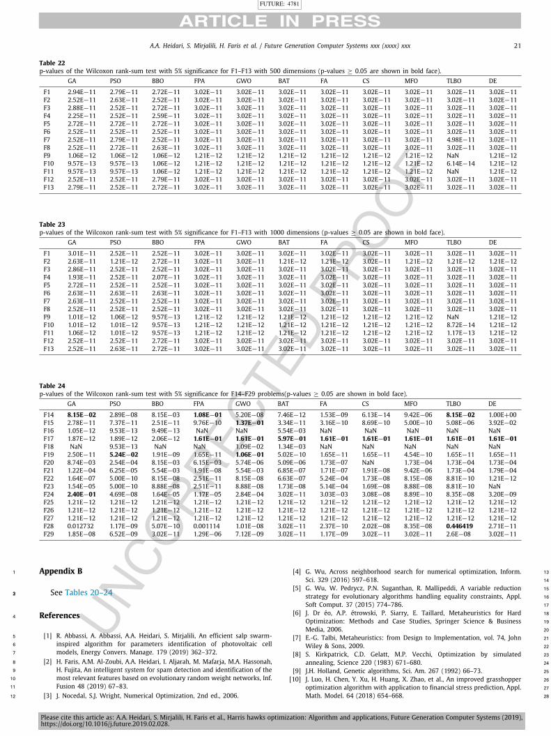
FUTURE: 4781
Please cite this article as: A.A. Heidari, S. Mirjalili, H. Faris et al., Harris hawks optimization: Algorithm and applications, Future Generation Computer Systems (2019),https://doi.org/10.1016/j.future.2019.02.028.
A.A. Heidari, S. Mirjalili, H. Faris et al. / Future Generation Computer Systems xxx (xxxx) xxx 21
Table 22p-values of the Wilcoxon rank-sum test with 5% significance for F1–F13 with 500 dimensions (p-values ≥ 0.05 are shown in bold face).
GA PSO BBO FPA GWO BAT FA CS MFO TLBO DE
F1 2.94E−11 2.79E−11 2.72E−11 3.02E−11 3.02E−11 3.02E−11 3.02E−11 3.02E−11 3.02E−11 3.02E−11 3.02E−11F2 2.52E−11 2.63E−11 2.52E−11 3.02E−11 3.02E−11 3.02E−11 3.02E−11 3.02E−11 3.02E−11 3.02E−11 3.02E−11F3 2.88E−11 2.52E−11 2.72E−11 3.02E−11 3.02E−11 3.02E−11 3.02E−11 3.02E−11 3.02E−11 3.02E−11 3.02E−11F4 2.25E−11 2.52E−11 2.59E−11 3.02E−11 3.02E−11 3.02E−11 3.02E−11 3.02E−11 3.02E−11 3.02E−11 3.02E−11F5 2.72E−11 2.72E−11 2.72E−11 3.02E−11 3.02E−11 3.02E−11 3.02E−11 3.02E−11 3.02E−11 3.02E−11 3.02E−11F6 2.52E−11 2.52E−11 2.52E−11 3.02E−11 3.02E−11 3.02E−11 3.02E−11 3.02E−11 3.02E−11 3.02E−11 3.02E−11F7 2.52E−11 2.79E−11 2.52E−11 3.02E−11 3.02E−11 3.02E−11 3.02E−11 3.02E−11 3.02E−11 4.98E−11 3.02E−11F8 2.52E−11 2.72E−11 2.63E−11 3.02E−11 3.02E−11 3.02E−11 3.02E−11 3.02E−11 3.02E−11 3.02E−11 3.02E−11F9 1.06E−12 1.06E−12 1.06E−12 1.21E−12 1.21E−12 1.21E−12 1.21E−12 1.21E−12 1.21E−12 NaN 1.21E−12F10 9.57E−13 9.57E−13 1.06E−12 1.21E−12 1.21E−12 1.21E−12 1.21E−12 1.21E−12 1.21E−12 6.14E−14 1.21E−12F11 9.57E−13 9.57E−13 1.06E−12 1.21E−12 1.21E−12 1.21E−12 1.21E−12 1.21E−12 1.21E−12 NaN 1.21E−12F12 2.52E−11 2.52E−11 2.79E−11 3.02E−11 3.02E−11 3.02E−11 3.02E−11 3.02E−11 3.02E−11 3.02E−11 3.02E−11F13 2.79E−11 2.52E−11 2.72E−11 3.02E−11 3.02E−11 3.02E−11 3.02E−11 3.02E−11 3.02E−11 3.02E−11 3.02E−11
Table 23p-values of the Wilcoxon rank-sum test with 5% significance for F1–F13 with 1000 dimensions (p-values ≥ 0.05 are shown in bold face).
GA PSO BBO FPA GWO BAT FA CS MFO TLBO DE
F1 3.01E−11 2.52E−11 2.52E−11 3.02E−11 3.02E−11 3.02E−11 3.02E−11 3.02E−11 3.02E−11 3.02E−11 3.02E−11F2 2.63E−11 1.21E−12 2.72E−11 3.02E−11 3.02E−11 1.21E−12 1.21E−12 3.02E−11 1.21E−12 1.21E−12 1.21E−12F3 2.86E−11 2.52E−11 2.52E−11 3.02E−11 3.02E−11 3.02E−11 3.02E−11 3.02E−11 3.02E−11 3.02E−11 3.02E−11F4 1.93E−11 2.52E−11 2.07E−11 3.02E−11 3.02E−11 3.02E−11 3.02E−11 3.02E−11 3.02E−11 3.02E−11 3.02E−11F5 2.72E−11 2.52E−11 2.52E−11 3.02E−11 3.02E−11 3.02E−11 3.02E−11 3.02E−11 3.02E−11 3.02E−11 3.02E−11F6 2.63E−11 2.63E−11 2.63E−11 3.02E−11 3.02E−11 3.02E−11 3.02E−11 3.02E−11 3.02E−11 3.02E−11 3.02E−11F7 2.63E−11 2.52E−11 2.52E−11 3.02E−11 3.02E−11 3.02E−11 3.02E−11 3.02E−11 3.02E−11 3.02E−11 3.02E−11F8 2.52E−11 2.52E−11 2.52E−11 3.02E−11 3.02E−11 3.02E−11 3.02E−11 3.02E−11 3.02E−11 3.02E−11 3.02E−11F9 1.01E−12 1.06E−12 9.57E−13 1.21E−12 1.21E−12 1.21E−12 1.21E−12 1.21E−12 1.21E−12 NaN 1.21E−12F10 1.01E−12 1.01E−12 9.57E−13 1.21E−12 1.21E−12 1.21E−12 1.21E−12 1.21E−12 1.21E−12 8.72E−14 1.21E−12F11 1.06E−12 1.01E−12 9.57E−13 1.21E−12 1.21E−12 1.21E−12 1.21E−12 1.21E−12 1.21E−12 1.17E−13 1.21E−12F12 2.52E−11 2.52E−11 2.72E−11 3.02E−11 3.02E−11 3.02E−11 3.02E−11 3.02E−11 3.02E−11 3.02E−11 3.02E−11F13 2.52E−11 2.63E−11 2.72E−11 3.02E−11 3.02E−11 3.02E−11 3.02E−11 3.02E−11 3.02E−11 3.02E−11 3.02E−11
Table 24p-values of the Wilcoxon rank-sum test with 5% significance for F14–F29 problems(p-values ≥ 0.05 are shown in bold face).
GA PSO BBO FPA GWO BAT FA CS MFO TLBO DE
F14 8.15E−02 2.89E−08 8.15E−03 1.08E−01 5.20E−08 7.46E−12 1.53E−09 6.13E−14 9.42E−06 8.15E−02 1.00E+00F15 2.78E−11 7.37E−11 2.51E−11 9.76E−10 1.37E−01 3.34E−11 3.16E−10 8.69E−10 5.00E−10 5.08E−06 3.92E−02F16 1.05E−12 9.53E−13 9.49E−13 NaN NaN 5.54E−03 NaN NaN NaN NaN NaNF17 1.87E−12 1.89E−12 2.06E−12 1.61E−01 1.61E−01 5.97E−01 1.61E−01 1.61E−01 1.61E−01 1.61E−01 1.61E−01F18 NaN 9.53E−13 NaN NaN 1.09E−02 1.34E−03 NaN NaN NaN NaN NaNF19 2.50E−11 5.24E−02 1.91E−09 1.65E−11 1.06E−01 5.02E−10 1.65E−11 1.65E−11 4.54E−10 1.65E−11 1.65E−11F20 8.74E−03 2.54E−04 8.15E−03 6.15E−03 5.74E−06 5.09E−06 1.73E−07 NaN 1.73E−04 1.73E−04 1.73E−04F21 1.22E−04 6.25E−05 5.54E−03 1.91E−08 5.54E−03 6.85E−07 1.71E−07 1.91E−08 9.42E−06 1.73E−04 1.79E−04F22 1.64E−07 5.00E−10 8.15E−08 2.51E−11 8.15E−08 6.63E−07 5.24E−04 1.73E−08 8.15E−08 8.81E−10 1.21E−12F23 1.54E−05 5.00E−10 8.88E−08 2.51E−11 8.88E−08 1.73E−08 5.14E−04 1.69E−08 8.88E−08 8.81E−10 NaNF24 2.40E−01 4.69E−08 1.64E−05 1.17E−05 2.84E−04 3.02E−11 3.03E−03 3.08E−08 8.89E−10 8.35E−08 3.20E−09F25 1.21E−12 1.21E−12 1.21E−12 1.21E−12 1.21E−12 1.21E−12 1.21E−12 1.21E−12 1.21E−12 1.21E−12 1.21E−12F26 1.21E−12 1.21E−12 1.21E−12 1.21E−12 1.21E−12 1.21E−12 1.21E−12 1.21E−12 1.21E−12 1.21E−12 1.21E−12F27 1.21E−12 1.21E−12 1.21E−12 1.21E−12 1.21E−12 1.21E−12 1.21E−12 1.21E−12 1.21E−12 1.21E−12 1.21E−12F28 0.012732 1.17E−09 5.07E−10 0.001114 1.01E−08 3.02E−11 2.37E−10 2.02E−08 8.35E−08 0.446419 2.71E−11F29 1.85E−08 6.52E−09 3.02E−11 1.29E−06 7.12E−09 3.02E−11 1.17E−09 3.02E−11 3.02E−11 2.6E−08 3.02E−11
Appendix B1
2 See Tables 20–243
References4
[1] R. Abbassi, A. Abbassi, A.A. Heidari, S. Mirjalili, An efficient salp swarm-5
inspired algorithm for parameters identification of photovoltaic cell6
models, Energy Convers. Manage. 179 (2019) 362–372.7
[2] H. Faris, A.M. Al-Zoubi, A.A. Heidari, I. Aljarah, M. Mafarja, M.A. Hassonah,8
H. Fujita, An intelligent system for spam detection and identification of the9
most relevant features based on evolutionary random weight networks, Inf.10
Fusion 48 (2019) 67–83.11
[3] J. Nocedal, S.J. Wright, Numerical Optimization, 2nd ed., 2006.12
[4] G. Wu, Across neighborhood search for numerical optimization, Inform. 13
Sci. 329 (2016) 597–618. 14
[5] G. Wu, W. Pedrycz, P.N. Suganthan, R. Mallipeddi, A variable reduction 15
strategy for evolutionary algorithms handling equality constraints, Appl. 16
Soft Comput. 37 (2015) 774–786. 17
[6] J. Dr éo, A.P. étrowski, P. Siarry, E. Taillard, Metaheuristics for Hard 18
Optimization: Methods and Case Studies, Springer Science & Business 19
Media, 2006. 20
[7] E.-G. Talbi, Metaheuristics: from Design to Implementation, vol. 74, John 21
Wiley & Sons, 2009. 22
[8] S. Kirkpatrick, C.D. Gelatt, M.P. Vecchi, Optimization by simulated 23
annealing, Science 220 (1983) 671–680. 24
[9] J.H. Holland, Genetic algorithms, Sci. Am. 267 (1992) 66–73. 25
[10] J. Luo, H. Chen, Y. Xu, H. Huang, X. Zhao, et al., An improved grasshopper 26
optimization algorithm with application to financial stress prediction, Appl. 27
Math. Model. 64 (2018) 654–668. 28
https://aliasgharheidari.com/HHO.html
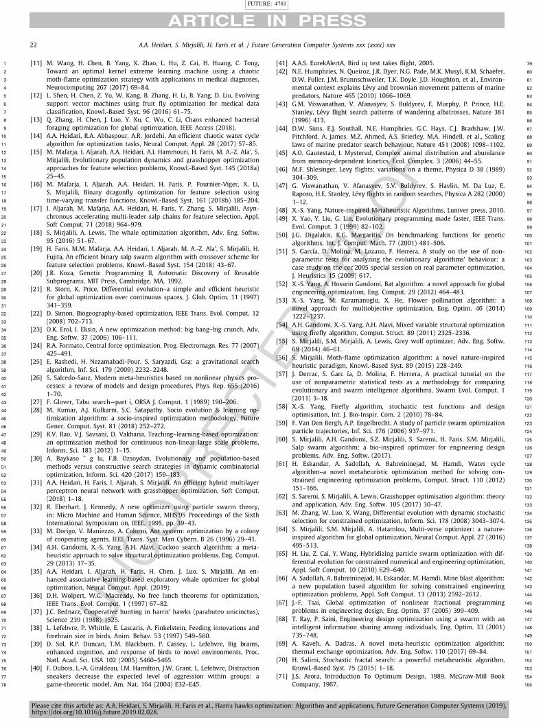
FUTURE: 4781
Please cite this article as: A.A. Heidari, S. Mirjalili, H. Faris et al., Harris hawks optimization: Algorithm and applications, Future Generation Computer Systems (2019),https://doi.org/10.1016/j.future.2019.02.028.
22 A.A. Heidari, S. Mirjalili, H. Faris et al. / Future Generation Computer Systems xxx (xxxx) xxx
[11] M. Wang, H. Chen, B. Yang, X. Zhao, L. Hu, Z. Cai, H. Huang, C. Tong,1
Toward an optimal kernel extreme learning machine using a chaotic2
moth-flame optimization strategy with applications in medical diagnoses,3
Neurocomputing 267 (2017) 69–84.4
[12] L. Shen, H. Chen, Z. Yu, W. Kang, B. Zhang, H. Li, B. Yang, D. Liu, Evolving5
support vector machines using fruit fly optimization for medical data6
classification, Knowl.-Based Syst. 96 (2016) 61–75.7
[13] Q. Zhang, H. Chen, J. Luo, Y. Xu, C. Wu, C. Li, Chaos enhanced bacterial8
foraging optimization for global optimization, IEEE Access (2018).9
[14] A.A. Heidari, R.A. Abbaspour, A.R. Jordehi, An efficient chaotic water cycle10
algorithm for optimization tasks, Neural Comput. Appl. 28 (2017) 57–85.11
[15] M. Mafarja, I. Aljarah, A.A. Heidari, A.I. Hammouri, H. Faris, M. A.-Z. Ala’, S.12
Mirjalili, Evolutionary population dynamics and grasshopper optimization13
approaches for feature selection problems, Knowl.-Based Syst. 145 (2018a)14
25–45.15
[16] M. Mafarja, I. Aljarah, A.A. Heidari, H. Faris, P. Fournier-Viger, X. Li,16
S. Mirjalili, Binary dragonfly optimization for feature selection using17
time-varying transfer functions, Knowl.-Based Syst. 161 (2018b) 185–204.18
[17] I. Aljarah, M. Mafarja, A.A. Heidari, H. Faris, Y. Zhang, S. Mirjalili, Asyn-19
chronous accelerating multi-leader salp chains for feature selection, Appl.20
Soft Comput. 71 (2018) 964–979.21
[18] S. Mirjalili, A. Lewis, The whale optimization algorithm, Adv. Eng. Softw.22
95 (2016) 51–67.23
[19] H. Faris, M.M. Mafarja, A.A. Heidari, I. Aljarah, M. A.-Z. Ala’, S. Mirjalili, H.24
Fujita, An efficient binary salp swarm algorithm with crossover scheme for25
feature selection problems, Knowl.-Based Syst. 154 (2018) 43–67.26
[20] J.R. Koza, Genetic Programming II, Automatic Discovery of Reusable27
Subprograms, MIT Press, Cambridge, MA, 1992.28
[21] R. Storn, K. Price, Differential evolution–a simple and efficient heuristic29
for global optimization over continuous spaces, J. Glob. Optim. 11 (1997)30
341–359.31
[22] D. Simon, Biogeography-based optimization, IEEE Trans. Evol. Comput. 1232
(2008) 702–713.33
[23] O.K. Erol, I. Eksin, A new optimization method: big bang–big crunch, Adv.34
Eng. Softw. 37 (2006) 106–111.35
[24] R.A. Formato, Central force optimization, Prog. Electromagn. Res. 77 (2007)36
425–491.37
[25] E. Rashedi, H. Nezamabadi-Pour, S. Saryazdi, Gsa: a gravitational search38
algorithm, Inf. Sci. 179 (2009) 2232–2248.39
[26] S. Salcedo-Sanz, Modern meta-heuristics based on nonlinear physics pro-40
cesses: a review of models and design procedures, Phys. Rep. 655 (2016)41
1–70.42
[27] F. Glover, Tabu search—part i, ORSA J. Comput. 1 (1989) 190–206.43
[28] M. Kumar, A.J. Kulkarni, S.C. Satapathy, Socio evolution & learning op-44
timization algorithm: a socio-inspired optimization methodology, Future45
Gener. Comput. Syst. 81 (2018) 252–272.46
[29] R.V. Rao, V.J. Savsani, D. Vakharia, Teaching–learning-based optimization:47
an optimization method for continuous non-linear large scale problems,48
Inform. Sci. 183 (2012) 1–15.49
[30] A. Baykaso ˘ g lu, F.B. Ozsoydan, Evolutionary and population-based50
methods versus constructive search strategies in dynamic combinatorial51
optimization, Inform. Sci. 420 (2017) 159–183.52
[31] A.A. Heidari, H. Faris, I. Aljarah, S. Mirjalili, An efficient hybrid multilayer53
perceptron neural network with grasshopper optimization, Soft Comput.54
(2018) 1–18.55
[32] R. Eberhart, J. Kennedy, A new optimizer using particle swarm theory,56
in: Micro Machine and Human Science, MHS’95 Proceedings of the Sixth57
International Symposium on, IEEE, 1995, pp. 39–43.58
[33] M. Dorigo, V. Maniezzo, A. Colorni, Ant system: optimization by a colony59
of cooperating agents, IEEE Trans. Syst. Man Cybern. B 26 (1996) 29–41.60
[34] A.H. Gandomi, X.-S. Yang, A.H. Alavi, Cuckoo search algorithm: a meta-61
heuristic approach to solve structural optimization problems, Eng. Comput.62
29 (2013) 17–35.63
[35] A.A. Heidari, I. Aljarah, H. Faris, H. Chen, J. Luo, S. Mirjalili, An en-64
hanced associative learning-based exploratory whale optimizer for global65
optimization, Neural Comput. Appl. (2019).66
[36] D.H. Wolpert, W.G. Macready, No free lunch theorems for optimization,67
IEEE Trans. Evol. Comput. 1 (1997) 67–82.68
[37] J.C. Bednarz, Cooperative hunting in harris’ hawks (parabuteo unicinctus),69
Science 239 (1988) 1525.70
[38] L. Lefebvre, P. Whittle, E. Lascaris, A. Finkelstein, Feeding innovations and71
forebrain size in birds, Anim. Behav. 53 (1997) 549–560.72
[39] D. Sol, R.P. Duncan, T.M. Blackburn, P. Cassey, L. Lefebvre, Big brains,73
enhanced cognition, and response of birds to novel environments, Proc.74
Natl. Acad. Sci. USA 102 (2005) 5460–5465.75
[40] F. Dubois, L.-A. Giraldeau, I.M. Hamilton, J.W. Grant, L. Lefebvre, Distraction76
sneakers decrease the expected level of aggression within groups: a77
game-theoretic model, Am. Nat. 164 (2004) E32–E45.78
[41] A.A.S. EurekAlertA, Bird iq test takes flight, 2005. 79
[42] N.E. Humphries, N. Queiroz, J.R. Dyer, N.G. Pade, M.K. Musyl, K.M. Schaefer, 80
D.W. Fuller, J.M. Brunnschweiler, T.K. Doyle, J.D. Houghton, et al., Environ- 81
mental context explains Lévy and brownian movement patterns of marine 82
predators, Nature 465 (2010) 1066–1069. 83
[43] G.M. Viswanathan, V. Afanasyev, S. Buldyrev, E. Murphy, P. Prince, H.E. 84
Stanley, Lévy flight search patterns of wandering albatrosses, Nature 381 85
(1996) 413. 86
[44] D.W. Sims, E.J. Southall, N.E. Humphries, G.C. Hays, C.J. Bradshaw, J.W. 87
Pitchford, A. James, M.Z. Ahmed, A.S. Brierley, M.A. Hindell, et al., Scaling 88
laws of marine predator search behaviour, Nature 451 (2008) 1098–1102. 89
[45] A.O. Gautestad, I. Mysterud, Complex animal distribution and abundance 90
from memory-dependent kinetics, Ecol. Complex. 3 (2006) 44–55. 91
[46] M.F. Shlesinger, Levy flights: variations on a theme, Physica D 38 (1989) 92
304–309. 93
[47] G. Viswanathan, V. Afanasyev, S.V. Buldyrev, S. Havlin, M. Da Luz, E. 94
Raposo, H.E. Stanley, Lévy flights in random searches, Physica A 282 (2000) 95
1–12. 96
[48] X.-S. Yang, Nature-inspired Metaheuristic Algorithms, Luniver press, 2010. 97
[49] X. Yao, Y. Liu, G. Lin, Evolutionary programming made faster, IEEE Trans. 98
Evol. Comput. 3 (1999) 82–102. 99
[50] J.G. Digalakis, K.G. Margaritis, On benchmarking functions for genetic 100
algorithms, Int. J. Comput. Math. 77 (2001) 481–506. 101
[51] S. García, D. Molina, M. Lozano, F. Herrera, A study on the use of non- 102
parametric tests for analyzing the evolutionary algorithms’ behaviour: a 103
case study on the cec’2005 special session on real parameter optimization, 104
J. Heuristics 15 (2009) 617. 105
[52] X.-S. Yang, A. Hossein Gandomi, Bat algorithm: a novel approach for global 106
engineering optimization, Eng. Comput. 29 (2012) 464–483. 107
[53] X.-S. Yang, M. Karamanoglu, X. He, Flower pollination algorithm: a 108
novel approach for multiobjective optimization, Eng. Optim. 46 (2014) 109
1222–1237. 110
[54] A.H. Gandomi, X.-S. Yang, A.H. Alavi, Mixed variable structural optimization 111
using firefly algorithm, Comput. Struct. 89 (2011) 2325–2336. 112
[55] S. Mirjalili, S.M. Mirjalili, A. Lewis, Grey wolf optimizer, Adv. Eng. Softw. 113
69 (2014) 46–61. 114
[56] S. Mirjalili, Moth-flame optimization algorithm: a novel nature-inspired 115
heuristic paradigm, Knowl.-Based Syst. 89 (2015) 228–249. 116
[57] J. Derrac, S. Garc ía, D. Molina, F. Herrera, A practical tutorial on the 117
use of nonparametric statistical tests as a methodology for comparing 118
evolutionary and swarm intelligence algorithms, Swarm Evol. Comput. 1 119
(2011) 3–18. 120
[58] X.-S. Yang, Firefly algorithm, stochastic test functions and design 121
optimisation, Int. J. Bio-Inspir. Com. 2 (2010) 78–84. 122
[59] F. Van Den Bergh, A.P. Engelbrecht, A study of particle swarm optimization 123
particle trajectories, Inf. Sci. 176 (2006) 937–971. 124
[60] S. Mirjalili, A.H. Gandomi, S.Z. Mirjalili, S. Saremi, H. Faris, S.M. Mirjalili, 125
Salp swarm algorithm: a bio-inspired optimizer for engineering design 126
problems, Adv. Eng. Softw. (2017). 127
[61] H. Eskandar, A. Sadollah, A. Bahreininejad, M. Hamdi, Water cycle 128
algorithm–a novel metaheuristic optimization method for solving con- 129
strained engineering optimization problems, Comput. Struct. 110 (2012) 130
151–166. 131
[62] S. Saremi, S. Mirjalili, A. Lewis, Grasshopper optimisation algorithm: theory 132
and application, Adv. Eng. Softw. 105 (2017) 30–47. 133
[63] M. Zhang, W. Luo, X. Wang, Differential evolution with dynamic stochastic 134
selection for constrained optimization, Inform. Sci. 178 (2008) 3043–3074. 135
[64] S. Mirjalili, S.M. Mirjalili, A. Hatamlou, Multi-verse optimizer: a nature- 136
inspired algorithm for global optimization, Neural Comput. Appl. 27 (2016) 137
495–513. 138
[65] H. Liu, Z. Cai, Y. Wang, Hybridizing particle swarm optimization with dif- 139
ferential evolution for constrained numerical and engineering optimization, 140
Appl. Soft Comput. 10 (2010) 629–640. 141
[66] A. Sadollah, A. Bahreininejad, H. Eskandar, M. Hamdi, Mine blast algorithm: 142
a new population based algorithm for solving constrained engineering 143
optimization problems, Appl. Soft Comput. 13 (2013) 2592–2612. 144
[67] J.-F. Tsai, Global optimization of nonlinear fractional programming 145
problems in engineering design, Eng. Optim. 37 (2005) 399–409. 146
[68] T. Ray, P. Saini, Engineering design optimization using a swarm with an 147
intelligent information sharing among individuals, Eng. Optim. 33 (2001) 148
735–748. 149
[69] A. Kaveh, A. Dadras, A novel meta-heuristic optimization algorithm: 150
thermal exchange optimization, Adv. Eng. Softw. 110 (2017) 69–84. 151
[70] H. Salimi, Stochastic fractal search: a powerful metaheuristic algorithm, 152
Knowl.-Based Syst. 75 (2015) 1–18. 153
[71] J.S. Arora, Introduction To Optimum Design, 1989, McGraw-Mill Book 154
Company, 1967. 155
https://aliasgharheidari.com/HHO.html
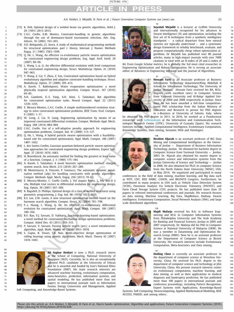
FUTURE: 4781
Please cite this article as: A.A. Heidari, S. Mirjalili, H. Faris et al., Harris hawks optimization: Algorithm and applications, Future Generation Computer Systems (2019),https://doi.org/10.1016/j.future.2019.02.028.
A.A. Heidari, S. Mirjalili, H. Faris et al. / Future Generation Computer Systems xxx (xxxx) xxx 23
[72] K. Deb, Optimal design of a welded beam via genetic algorithms, AIAA J.1
29 (1991) 2013–2015.2
[73] C.A.C. Coello, E.M. Montes, Constraint-handling in genetic algorithms3
through the use of dominance-based tournament selection, Adv. Eng.4
Inform. 16 (2002) 193–203.5
[74] A.D. Belegundu, J.S. Arora, A study of mathematical programming methods6
for structural optimization. part i: theory, Internat. J. Numer. Methods7
Engrg. 21 (1985) 1583–1599.8
[75] Q. He, L. Wang, An effective co-evolutionary particle swarm optimization9
for constrained engineering design problems, Eng. Appl. Artif. Intell. 2010
(2007) 89–99.11
[76] L. Wang, L.-p. Li, An effective differential evolution with level comparison12
for constrained engineering design, Struct. Multidiscip. Optim. 41 (2010)13
947–963.14
[77] Y. Wang, Z. Cai, Y. Zhou, Z. Fan, Constrained optimization based on hybrid15
evolutionary algorithm and adaptive constraint-handling technique, Struct.16
Multidiscip. Optim. 37 (2009) 395–413.17
[78] A. Kaveh, T. Bakhshpoori, Water evaporation optimization: a novel18
physically inspired optimization algorithm, Comput. Struct. 167 (2016)19
69–85.20
[79] A.H. Gandomi, X.-S. Yang, A.H. Alavi, S. Talatahari, Bat algorithm21
for constrained optimization tasks, Neural Comput. Appl. 22 (2013)22
1239–1255.23
[80] E. Mezura-Montes, C.A.C. Coello, A simple multimembered evolution strat-24
egy to solve constrained optimization problems, IEEE Trans. Evol. Comput.25
9 (2005) 1–17.26
[81] W. Gong, Z. Cai, D. Liang, Engineering optimization by means of an27
improved constrained differential evolution, Comput. Methods Appl. Mech.28
Engrg. 268 (2014) 884–904.29
[82] C.A.C. Coello, Use of a self-adaptive penalty approach for engineering30
optimization problems, Comput. Ind. 41 (2000) 113–127.31
[83] Q. He, L. Wang, A hybrid particle swarm optimization with a feasibility-32
based rule for constrained optimization, Appl. Math. Comput. 186 (2007)33
1407–1422.34
[84] L. dos Santos Coelho, Gaussian quantum-behaved particle swarm optimiza-35
tion approaches for constrained engineering design problems, Expert Syst.36
Appl. 37 (2010) 1676–1683.37
[85] H. Rosenbrock, An automatic method for finding the greatest or least value38
of a function, Comput. J. 3 (1960) 175–184.39
[86] A. Kaveh, S. Talatahari, A novel heuristic optimization method: charged40
system search, Acta Mech. 213 (2010) 267–289.41
[87] M. Montemurro, A. Vincenti, P. Vannucci, The automatic dynamic penal-42
isation method (adp) for handling constraints with genetic algorithms,43
Comput. Methods Appl. Mech. Engrg. 256 (2013) 70–87.44
[88] E. Mezura-Montes, C. Coello Coello, J. Vel ázquez Reyes, L. Mu ñoz-D á45
vila, Multiple trial vectors in differential evolution for engineering design,46
Eng. Optim. 39 (2007) 567–589.47
[89] K. Ragsdell, D. Phillips, Optimal design of a class of welded structures using48
geometric programming, J. Eng. Ind. 98 (1976) 1021–1025.49
[90] K.S. Lee, Z.W. Geem, A new structural optimization method based on the50
harmony search algorithm, Comput. Struct. 82 (2004) 781–798.51
[91] F.-z. Huang, L. Wang, Q. He, An effective co-evolutionary differential52
evolution for constrained optimization, Appl. Math. Comput. 186 (2007)53
340–356.54
[92] R.V. Rao, V.J. Savsani, D. Vakharia, Teaching–learning-based optimization:55
a novel method for constrained mechanical design optimization problems,56
Comput. Aided Des. 43 (2011) 303–315.57
[93] P. Savsani, V. Savsani, Passing vehicle search (pvs): a novel metaheuristic58
algorithm, Appl. Math. Model. 40 (2016) 3951–3978.59
[94] S. Gupta, R. Tiwari, S.B. Nair, Multi-objective design optimisation of60
rolling bearings using genetic algorithms, Mech. Mach. Theory 42 (2007)61
1418–1443.62
63
Ali Asghar Heidari is now a Ph.D. research intern64
at the School of Computing, National University of65
Singapore (NUS). Currently, he is also an exceptionally66
talented Ph.D. candidate at the University of Tehran67
and he is awarded and funded by Iran’s National Elites68
Foundation (INEF). His main research interests are69
advanced machine learning, evolutionary computation,70
meta-heuristics, prediction, information systems, and71
spatial modeling. He has published more than ten72
papers in international journals such as Information73
Fusion, Energy Conversion and Management, Applied74
Soft Computing, and Knowledge-Based Systems.75
76
Seyedali Mirjalili is a lecturer at Griffith University 77
and internationally recognized for his advances in 78
Swarm Intelligence (SI) and optimization, including the 79
first set of SI techniques from a synthetic intelligence 80
standpoint – a radical departure from how natural 81
systems are typically understood – and a systematic 82
design framework to reliably benchmark, evaluate, and 83
propose computationally cheap robust optimization al- 84
gorithms. Dr Mirjalili has published over 80 journal 85
articles, many in high-impact journals with over 7000 86
citations in total with an H-index of 29 and G-index of 87
84. From Google Scholar metrics, he is globally the 3rd most cited researcher in 88
Engineering Optimization and Robust Optimization. He is serving an associate 89
editor of Advances in Engineering Software and the journal of Algorithms. 90
91
Hossam Faris is an Associate professor at Business 92
Information Technology department/King Abdullah II 93
School for Information Technology/ The University of 94
Jordan (Jordan). Hossam Faris received his BA, M.Sc. 95
degrees (with excellent rates) in Computer Science 96
from Yarmouk University and Al-Balqa‘ Applied Uni- 97
versity in 2004 and 2008 respectively in Jordan. Since 98
then, he has been awarded a full-time competition- 99
based PhD scholarship from the Italian Ministry of 100
Education and Research to peruse his PhD degrees 101
in e-Business at University of Salento, Italy, where 102
he obtained his PhD degree in 2011. In 2016, he worked as a Postdoctoral 103
researcher with GeNeurateam at the Information and Communication Tech- 104
nologies Research Center (CITIC), University of Granada (Spain). His research 105
interests include: Applied Computational Intelligence, Evolutionary Computation, 106
Knowledge Systems, Data mining, Semantic Web and Ontologies. 107
108
Ibrahim Aljarah is an assistant professor of BIG Data 109
Mining and Computational Intelligence at the Univer- 110
sity of Jordan — Department of Business Information 111
Technology, Jordan. He obtained his bachelor degree in 112
Computer Science from Yarmouk University — Jordan, 113
2003. Dr. Aljarah also obtained his master degree in 114
computer science and information systems from the 115
Jordan University of Science and Technology — Jordan 116
in 2006. He also obtained his Ph.D. In computer Science 117
from the North Dakota State University (NDSU), USA, 118
in May 2014. He organized and participated in many 119
conferences in the field of data mining, machine learning, and Big data such 120
as NTIT, CSIT, IEEE NABIC, CASON, and BIGDATA Congress. Furthermore, he 121
contributed in many projects in USA such as Vehicle Class Detection System 122
(VCDS), Pavement Analysis Via Vehicle Electronic Telemetry (PAVVET), and 123
Farm Cloud Storage System (CSS) projects. He has published more than 35 124
papers in refereed international conferences and journals. His research focuses 125
on data mining, Machine Learning, Big Data, MapReduce, Hadoop, Swarm 126
intelligence, Evolutionary Computation, Social Network Analysis (SNA), and large 127
scale distributed algorithms. 128
129
Majdi Mafarja received his B.Sc in Software Engi- 130
neering and M.Sc in Computer Information Systems 131
from Philadelphia University and The Arab Academy 132
for Banking and Financial Sciences, Jordan in 2005 and 133
2007 respectively. Dr. Mafarja did his PhD in Computer 134
Science at National University of Malaysia (UKM). He 135
was a member in Datamining and Optimization Re- 136
search Group (DMO). Now he is an assistant professor 137
at the Department of Computer Science at Birzeit 138
University. His research interests include Evolutionary 139
Computation, Meta-heuristics and Data mining. 140
141
Huiling Chen is currently an associate professor in 142
the department of computer science at Wenzhou Uni- 143
versity, China. He received his Ph.D. degree in the 144
department of computer science and technology at Jilin 145
University, China. His present research interests center 146
on evolutionary computation, machine learning, and 147
data mining, as well as their applications to medical 148
diagnosis and bankruptcy prediction. He has published 149
more than 100 papers in international journals and 150
conference proceedings, including Pattern Recognition, 151
Expert Systems with Applications, Knowledge-Based 152
Systems, Soft Computing, Neurocomputing, Applied Mathematical Modeling, IEEE 153
ACCESS, PAKDD, and among others. 154
https://aliasgharheidari.com/HHO.html
A brief description of the HHO algorithm
1. Harris hawks optimization (HHO)
1.1. Exploration phase
In HHO, the Harris’ hawks perch randomly on some locations and wait to detect a prey based on twostrategies.
X(t+ 1) =
{Xrand(t)− r1 |Xrand(t)− 2r2X(t)| q ≥ 0.5
(Xrabbit(t)−Xm(t))− r3(LB + r4(UB − LB)) q < 0.5(1)
where X(t + 1) is the position vector of hawks in the next iteration t, Xrabbit(t) is the position of rabbit,X(t) is the current position vector of hawks, r1, r2, r3, r4, and q are random numbers inside (0,1), whichare updated in each iteration, LB and UB show the upper and lower bounds of variables, Xrand(t) isa randomly selected hawk from the current population, and Xm is the average position of the currentpopulation of hawks. The average position of hawks is attained using Eq. (2):
Xm(t) =1
N
N∑i=1
Xi(t) (2)
where Xi(t) indicates the location of each hawk in iteration t and N denotes the total number of hawks.
1.2. Transition from exploration to exploitation
To model this step, the energy of a rabbit is modeled as:
E = 2E0(1−t
T) (3)
where E indicates the escaping energy of the prey, T is the maximum number of iterations, and E0 is theinitial state of its energy.
1.3. Exploitation phase
1.3.1. Soft besiege
This behavior is modeled by the following rules:
X(t+ 1) = ∆X(t)− E |JXrabbit(t)−X(t)| (4)
∆X(t) = Xrabbit(t)−X(t) (5)
where ∆X(t) is the difference between the position vector of the rabbit and the current location in iterationt, r5 is a random number inside (0,1), and J = 2(1−r5) represents the random jump strength of the rabbitthroughout the escaping procedure. The J value changes randomly in each iteration to simulate the natureof rabbit motions.
1.3.2. Hard besiege
In this situation, the current positions are updated using Eq. (6):
X(t+ 1) = Xrabbit(t)− E |∆X(t)| (6)
1
https://aliasgharheidari.com/HHO.html
1.3.3. Soft besiege with progressive rapid dives
To perform a soft besiege, we supposed that the hawks can evaluate (decide) their next move based onthe following rule in Eq. (7):
Y = Xrabbit(t)− E |JXrabbit(t)−X(t)| (7)
We supposed that they will dive based on the LF-based patterns using the following rule:
Z = Y + S × LF (D) (8)
where D is the dimension of problem and S is a random vector by size 1 × D and LF is the levy flightfunction, which is calculated using Eq. (9):
LF (x) = 0.01× u× σ|v|
1β
, σ =
(Γ(1 + β)× sin(πβ
2)
Γ(1+β2
)× β × 2(β−12
))
) 1β
(9)
where u, v are random values inside (0,1), β is a default constant set to 1.5.Hence, the final strategy for updating the positions of hawks in the soft besiege phase can be performed
by Eq. (10):
X(t+ 1) =
{Y ifF (Y ) < F (X(t))Z ifF (Z) < F (X(t))
(10)
where Y and Z are obtained using Eqs.(7) and (8).
1.3.4. Hard besiege with progressive rapid dives
The following rule is performed in hard besiege condition:
X(t+ 1) =
{Y ifF (Y ) < F (X(t))Z ifF (Z) < F (X(t))
(11)
where Y and Z are obtained using new rules in Eqs.(12) and (13).
Y = Xrabbit(t)− E |JXrabbit(t)−Xm(t)| (12)
Z = Y + S × LF (D) (13)
where Xm(t) is obtained using Eq. (2).
1.4. Pseudocode of HHO
The pseudocode of the proposed HHO algorithm is reported in Algorithm 1.
References
Harris Hawks Optimization: Algorithm and Applications, Ali Asghar Heidari and SeyedaliMirjalili and Hossam Faris and Ibrahim Aljarah and Majdi Mafarja and Huiling Chen, FutureGeneration Computer Systems, 2019.
2
https://aliasgharheidari.com/HHO.html
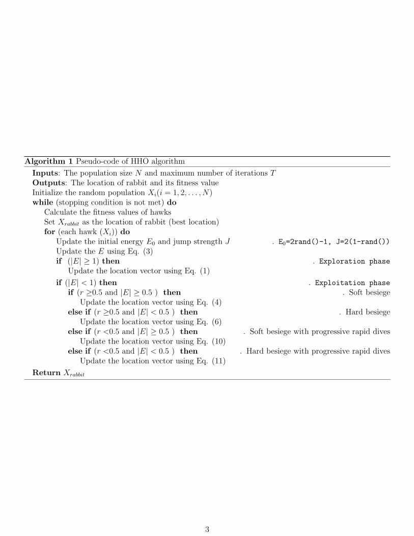
Algorithm 1 Pseudo-code of HHO algorithm
Inputs: The population size N and maximum number of iterations TOutputs: The location of rabbit and its fitness valueInitialize the random population Xi(i = 1, 2, . . . , N)while (stopping condition is not met) do
Calculate the fitness values of hawksSet Xrabbit as the location of rabbit (best location)for (each hawk (Xi)) do
Update the initial energy E0 and jump strength J . E0=2rand()-1, J=2(1-rand())
Update the E using Eq. (3)if (|E| ≥ 1) then . Exploration phase
Update the location vector using Eq. (1)
if (|E| < 1) then . Exploitation phase
if (r ≥0.5 and |E| ≥ 0.5 ) then . Soft besiegeUpdate the location vector using Eq. (4)
else if (r ≥0.5 and |E| < 0.5 ) then . Hard besiegeUpdate the location vector using Eq. (6)
else if (r <0.5 and |E| ≥ 0.5 ) then . Soft besiege with progressive rapid divesUpdate the location vector using Eq. (10)
else if (r <0.5 and |E| < 0.5 ) then . Hard besiege with progressive rapid divesUpdate the location vector using Eq. (11)
Return Xrabbit
3
https://aliasgharheidari.com/HHO.html

Accepted Manuscript
Harris hawks optimization: Algorithm and applications
Ali Asghar Heidari, Seyedali Mirjalili, Hossam Faris, Ibrahim Aljarah,Majdi Mafarja, Huiling Chen
PII: S0167-739X(18)31353-0DOI: https://doi.org/10.1016/j.future.2019.02.028Reference: FUTURE 4781
To appear in: Future Generation Computer Systems
Received date : 2 June 2018Revised date : 29 December 2018Accepted date : 18 February 2019
Please cite this article as: A.A. Heidari, S. Mirjalili, H. Faris et al., Harris hawks optimization:Algorithm and applications, Future Generation Computer Systems (2019),https://doi.org/10.1016/j.future.2019.02.028
This is a PDF file of an unedited manuscript that has been accepted for publication. As a service toour customers we are providing this early version of the manuscript. The manuscript will undergocopyediting, typesetting, and review of the resulting proof before it is published in its final form.Please note that during the production process errors may be discovered which could affect thecontent, and all legal disclaimers that apply to the journal pertain.
https://aliasgharheidari.com/HHO.html
Harris Hawks Optimization: Algorithm and Applications
Ali Asghar Heidaria, Seyedali Mirjalilib, Hossam Farisc, Ibrahim Aljarahc, Majdi Mafarjad,Huiling Chen ∗e
aSchool of Surveying and Geospatial Engineering, University of Tehran, Tehran, Iranas [email protected]
bSchool of Information and Communication Technology, Griffith University, Nathan, Brisbane, QLD 4111,Australia
[email protected] Abdullah II School for Information Technology, The University of Jordan, Amman, Jordan
{i.aljarah,hossam.faris}@ju.edu.jodDepartment of Computer Science, Birzeit University, POBox 14, West Bank, Palestine
[email protected] of Computer Science, Wenzhou University, Wenzhou 325035, China
Abstract
In this paper, a novel population-based, nature-inspired optimization paradigm is proposed, whichis called Harris Hawks Optimizer (HHO). The main inspiration of HHO is the cooperative behaviorand chasing style of Harris’ hawks in nature called surprise pounce. In this intelligent strategy,several hawks cooperatively pounce a prey from different directions in an attempt to surprise it.Harris hawks can reveal a variety of chasing patterns based on the dynamic nature of scenariosand escaping patterns of the prey. This work mathematically mimics such dynamic patterns andbehaviors to develop an optimization algorithm. The effectiveness of the proposed HHO optimizeris checked, through a comparison with other nature-inspired techniques, on 29 benchmark problemsand several real-world engineering problems. The statistical results and comparisons show thatthe HHO algorithm provides very promising and occasionally competitive results compared towell-established metaheuristic techniques.
Keywords:Nature-inspired computing, Harris hawks optimization algorithm, Swarm intelligence,Optimization, Metaheuristic
1 Introduction
Many real-world problems in machine learning and artificial intelligence have generally a con-1
tinuous, discrete, constrained or unconstrained nature [1, 2]. Due to these characteristics, it is2
hard to tackle some classes of problems using conventional mathematical programming approaches3
such as conjugate gradient, sequential quadratic programming, fast steepest, and quasi-Newton4
methods [3, 4]. Several types of research have verified that these methods are not efficient enough5
or always efficient in dealing with many larger-scale real-world multimodal, non-continuous, and6
non-differentiable problems [5]. Accordingly, metaheuristic algorithms have been designed and7
utilized for tackling many problems as competitive alternative solvers, which is because of their8
∗Corresponding author: Huiling Chen ([email protected])
Preprint submitted to Future Generation Computing Systems December 29, 2018
https://aliasgharheidari.com/HHO.html

simplicity and easy implementation process. In addition, the core operations of these methods do9
not rely on gradient information of the objective landscape or its mathematical traits. However,10
the common shortcoming for the majority of metaheuristic algorithms is that they often show11
a delicate sensitivity to the tuning of user-defined parameters. Another drawback is that the12
metaheuristic algorithms may not always converge to the global optimum. [6]13
In general, metaheuristic algorithms have two types [7]; single solution based (i.g. Simulated14
Annealing (SA) [8]) and population-based (i.g. Genetic Algorithm (GA) [9]). As the name indi-15
cates, in the former type, only one solution is processed during the optimization phase, while in16
the latter type, a set of solutions (i.e. population) are evolved in each iteration of the optimiza-17
tion process. Population-based techniques can often find an optimal or suboptimal solution that18
may be same with the exact optimum or located in its neighborhood. Population-based meta-19
heuristic (P-metaheuristics) techniques mostly mimic natural phenomena [10, 11, 12, 13]. These20
algorithms start the optimization process by generating a set (population) of individuals, where21
each individual in the population represents a candidate solution to the optimization problem. The22
population will be evolved iteratively by replacing the current population with a newly generated23
population using some often stochastic operators [14, 15]. The optimization process is proceeded24
until satisfying a stopping criteria (i.e. maximum number of iterations) [16, 17].25
Based on the inspiration, P-metaheuristics can be categorized in four main groups [18, 19] (see26
Fig. 1): Evolutionary Algorithms (EAs), Physics-based, Human-based, and Swarm Intelligence27
(SI) algorithms. EAs mimic the biological evolutionary behaviors such as recombination, mutation,28
and selection. The most popular EA is the GA that mimics the Darwinian theory of evolution [20].29
Other popular examples of EAs are Differential Evolution (DE) [21], Genetic Programming (GP)30
[20], and Biogeography-Based Optimizer (BBO) [22]. Physics-based algorithms are inspired by the31
physical laws. Some examples of these algorithms are Big-Bang Big-Crunch (BBBC) [23], Central32
Force Optimization (CFO) [24], and Gravitational Search Algorithm (GSA) [25]. Salcedo-Sanz33
[26] has deeply reviewed several physic-based optimizers. The third category of P-metaheuristics34
includes the set of algorithms that mimic some human behaviors. Some examples of the human-35
based algorithms are Tabu Search (TS) [27], Socio Evolution and Learning Optimization (SELO)36
[28], and Teaching Learning Based Optimization(TLBO) [29]. As the last class of P-metaheuristics,37
SI algorithms mimic the social behaviors (e.g. decentralized, self-organized systems) of organisms38
living in swarms, flocks, or herds [30, 31]. For instance, the birds flocking behaviors is the main39
inspiration of the Particle Swarm Optimization (PSO) proposed by Eberhart and Kennedy [32].40
In PSO, each particle in the swarm represents a candidate solution to the optimization problem.41
In the optimization process, each particle is updated with regard to the position of the global best42
particle and its own (local) best position. Ant Colony Optimization (ACO) [33], Cuckoo Search43
(CS) [34], and Artificial Bee Colony (ABC) are other examples of the SI techniques.44
Regardless of the variety of these algorithms, there is a common feature: the searching steps45
have two phases: exploration (diversification) and exploitation (intensification) [26]. In the ex-46
ploration phase, the algorithm should utilize and promote its randomized operators as much as47
possible to deeply explore various regions and sides of the feature space. Hence, the exploratory48
behaviors of a well-designed optimizer should have an enriched-enough random nature to effi-49
ciently allocate more randomly-generated solutions to different areas of the problem topography50
during early steps of the searching process [35]. The exploitation stage is normally performed after51
the exploration phase. In this phase, the optimizer tries to focus on the neighborhood of better-52
quality solutions located inside the feature space. It actually intensifies the searching process in53
a local region instead of all-inclusive regions of the landscape. A well-organized optimizer should54
be capable of making a reasonable, fine balance between the exploration and exploitation tenden-55
2
https://aliasgharheidari.com/HHO.html
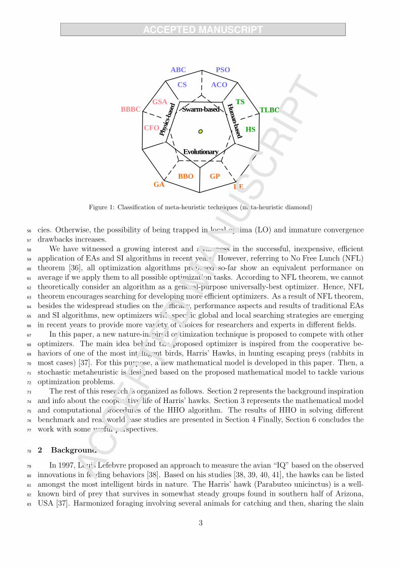
A
B
C
D
E
F
A1
O
B1
C1
D1
E1
F1
G1
H1
I1
J1
G
H
I
J
BBBC
GA DE
GPBBO
PSOABC
CS ACO
HS
TLBOTS
Phys
ics-bas
ed Swarm-based
Evolutionary
Hum
an-b
ased
GSA
CFO
Figure 1: Classification of meta-heuristic techniques (meta-heuristic diamond)
cies. Otherwise, the possibility of being trapped in local optima (LO) and immature convergence56
drawbacks increases.57
We have witnessed a growing interest and awareness in the successful, inexpensive, efficient58
application of EAs and SI algorithms in recent years. However, referring to No Free Lunch (NFL)59
theorem [36], all optimization algorithms proposed so-far show an equivalent performance on60
average if we apply them to all possible optimization tasks. According to NFL theorem, we cannot61
theoretically consider an algorithm as a general-purpose universally-best optimizer. Hence, NFL62
theorem encourages searching for developing more efficient optimizers. As a result of NFL theorem,63
besides the widespread studies on the efficacy, performance aspects and results of traditional EAs64
and SI algorithms, new optimizers with specific global and local searching strategies are emerging65
in recent years to provide more variety of choices for researchers and experts in different fields.66
In this paper, a new nature-inspired optimization technique is proposed to compete with other67
optimizers. The main idea behind the proposed optimizer is inspired from the cooperative be-68
haviors of one of the most intelligent birds, Harris’ Hawks, in hunting escaping preys (rabbits in69
most cases) [37]. For this purpose, a new mathematical model is developed in this paper. Then, a70
stochastic metaheuristic is designed based on the proposed mathematical model to tackle various71
optimization problems.72
The rest of this research is organized as follows. Section 2 represents the background inspiration73
and info about the cooperative life of Harris’ hawks. Section 3 represents the mathematical model74
and computational procedures of the HHO algorithm. The results of HHO in solving different75
benchmark and real-world case studies are presented in Section 4 Finally, Section 6 concludes the76
work with some useful perspectives.77
2 Background78
In 1997, Louis Lefebvre proposed an approach to measure the avian “IQ” based on the observed79
innovations in feeding behaviors [38]. Based on his studies [38, 39, 40, 41], the hawks can be listed80
amongst the most intelligent birds in nature. The Harris’ hawk (Parabuteo unicinctus) is a well-81
known bird of prey that survives in somewhat steady groups found in southern half of Arizona,82
USA [37]. Harmonized foraging involving several animals for catching and then, sharing the slain83
3
https://aliasgharheidari.com/HHO.html
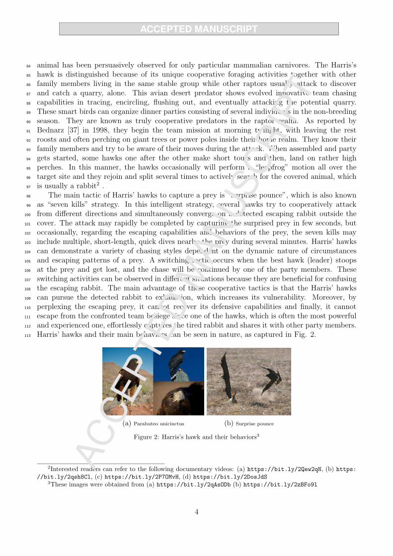
animal has been persuasively observed for only particular mammalian carnivores. The Harris’s84
hawk is distinguished because of its unique cooperative foraging activities together with other85
family members living in the same stable group while other raptors usually attack to discover86
and catch a quarry, alone. This avian desert predator shows evolved innovative team chasing87
capabilities in tracing, encircling, flushing out, and eventually attacking the potential quarry.88
These smart birds can organize dinner parties consisting of several individuals in the non-breeding89
season. They are known as truly cooperative predators in the raptor realm. As reported by90
Bednarz [37] in 1998, they begin the team mission at morning twilight, with leaving the rest91
roosts and often perching on giant trees or power poles inside their home realm. They know their92
family members and try to be aware of their moves during the attack. When assembled and party93
gets started, some hawks one after the other make short tours and then, land on rather high94
perches. In this manner, the hawks occasionally will perform a “leapfrog” motion all over the95
target site and they rejoin and split several times to actively search for the covered animal, which96
is usually a rabbit2 .97
The main tactic of Harris’ hawks to capture a prey is “surprise pounce”, which is also known98
as “seven kills” strategy. In this intelligent strategy, several hawks try to cooperatively attack99
from different directions and simultaneously converge on a detected escaping rabbit outside the100
cover. The attack may rapidly be completed by capturing the surprised prey in few seconds, but101
occasionally, regarding the escaping capabilities and behaviors of the prey, the seven kills may102
include multiple, short-length, quick dives nearby the prey during several minutes. Harris’ hawks103
can demonstrate a variety of chasing styles dependent on the dynamic nature of circumstances104
and escaping patterns of a prey. A switching tactic occurs when the best hawk (leader) stoops105
at the prey and get lost, and the chase will be continued by one of the party members. These106
switching activities can be observed in different situations because they are beneficial for confusing107
the escaping rabbit. The main advantage of these cooperative tactics is that the Harris’ hawks108
can pursue the detected rabbit to exhaustion, which increases its vulnerability. Moreover, by109
perplexing the escaping prey, it cannot recover its defensive capabilities and finally, it cannot110
escape from the confronted team besiege since one of the hawks, which is often the most powerful111
and experienced one, effortlessly captures the tired rabbit and shares it with other party members.112
Harris’ hawks and their main behaviors can be seen in nature, as captured in Fig. 2.113
(a) Parabuteo unicinctus (b) Surprise pounce
Figure 2: Harris’s hawk and their behaviors3
2Interested readers can refer to the following documentary videos: (a) https://bit.ly/2Qew2qN, (b) https://bit.ly/2qsh8Cl, (c) https://bit.ly/2P7OMvH, (d) https://bit.ly/2DosJdS
3These images were obtained from (a) https://bit.ly/2qAsODb (b) https://bit.ly/2zBFo9l
4
https://aliasgharheidari.com/HHO.html
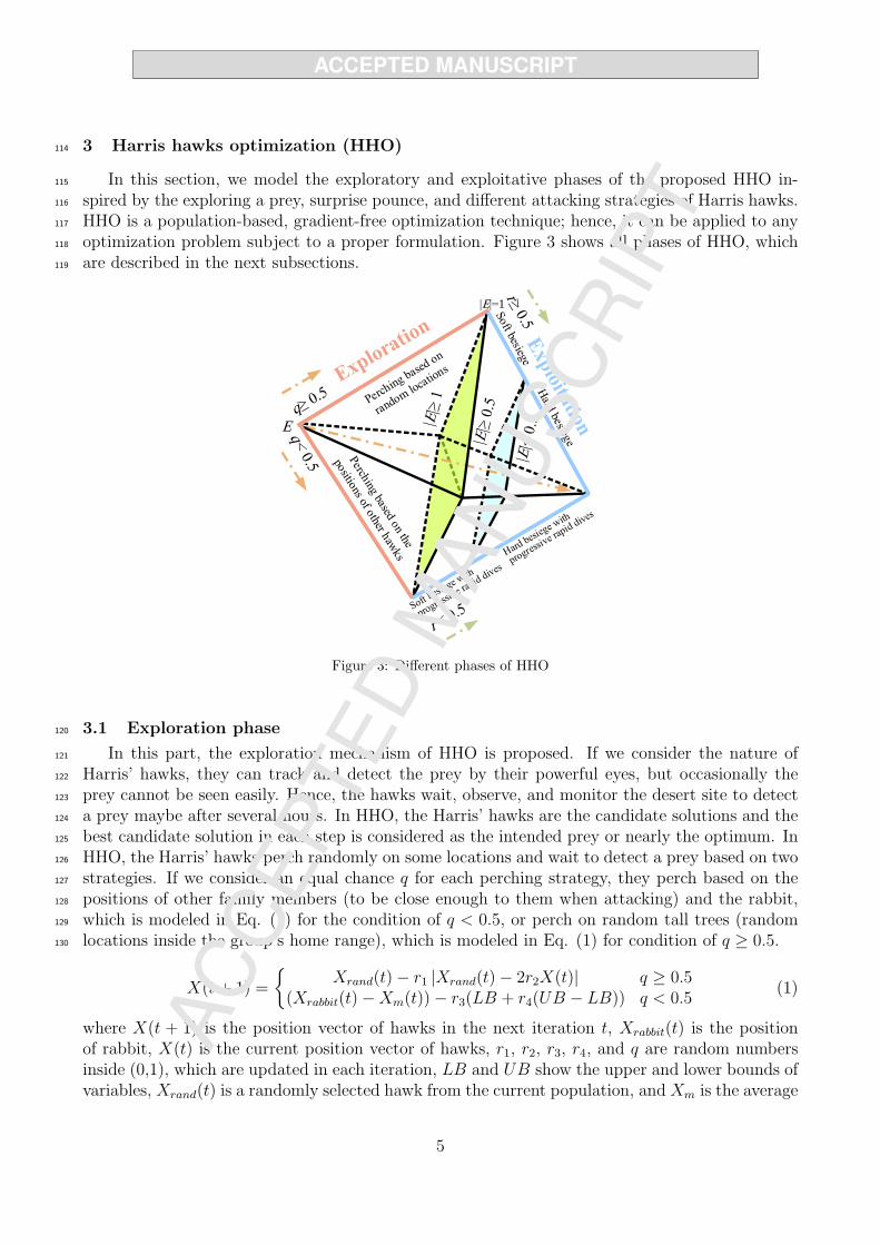
3 Harris hawks optimization (HHO)114
In this section, we model the exploratory and exploitative phases of the proposed HHO in-115
spired by the exploring a prey, surprise pounce, and different attacking strategies of Harris hawks.116
HHO is a population-based, gradient-free optimization technique; hence, it can be applied to any117
optimization problem subject to a proper formulation. Figure 3 shows all phases of HHO, which118
are described in the next subsections.119
|E 1=|
E
Figure 3: Different phases of HHO
3.1 Exploration phase120
In this part, the exploration mechanism of HHO is proposed. If we consider the nature of121
Harris’ hawks, they can track and detect the prey by their powerful eyes, but occasionally the122
prey cannot be seen easily. Hence, the hawks wait, observe, and monitor the desert site to detect123
a prey maybe after several hours. In HHO, the Harris’ hawks are the candidate solutions and the124
best candidate solution in each step is considered as the intended prey or nearly the optimum. In125
HHO, the Harris’ hawks perch randomly on some locations and wait to detect a prey based on two126
strategies. If we consider an equal chance q for each perching strategy, they perch based on the127
positions of other family members (to be close enough to them when attacking) and the rabbit,128
which is modeled in Eq. (1) for the condition of q < 0.5, or perch on random tall trees (random129
locations inside the group’s home range), which is modeled in Eq. (1) for condition of q ≥ 0.5.130
X(t+ 1) =
{Xrand(t)− r1 |Xrand(t)− 2r2X(t)| q ≥ 0.5
(Xrabbit(t)−Xm(t))− r3(LB + r4(UB − LB)) q < 0.5(1)
where X(t + 1) is the position vector of hawks in the next iteration t, Xrabbit(t) is the positionof rabbit, X(t) is the current position vector of hawks, r1, r2, r3, r4, and q are random numbersinside (0,1), which are updated in each iteration, LB and UB show the upper and lower bounds ofvariables, Xrand(t) is a randomly selected hawk from the current population, and Xm is the average
5
https://aliasgharheidari.com/HHO.html
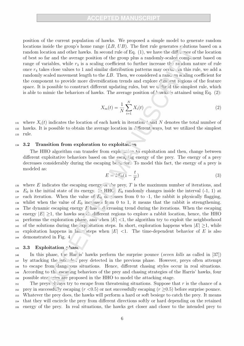
position of the current population of hawks. We proposed a simple model to generate randomlocations inside the group’s home range (LB, UB). The first rule generates solutions based on arandom location and other hawks. In second rule of Eq. (1), we have the difference of the locationof best so far and the average position of the group plus a randomly-scaled component based onrange of variables, while r3 is a scaling coefficient to further increase the random nature of ruleonce r4 takes close values to 1 and similar distribution patterns may occur. In this rule, we add arandomly scaled movement length to the LB. Then, we considered a random scaling coefficient forthe component to provide more diversification trends and explore different regions of the featurespace. It is possible to construct different updating rules, but we utilized the simplest rule, whichis able to mimic the behaviors of hawks. The average position of hawks is attained using Eq. (2):
Xm(t) =1
N
N∑
i=1
Xi(t) (2)
where Xi(t) indicates the location of each hawk in iteration t and N denotes the total number of131
hawks. It is possible to obtain the average location in different ways, but we utilized the simplest132
rule.133
3.2 Transition from exploration to exploitation134
The HHO algorithm can transfer from exploration to exploitation and then, change betweendifferent exploitative behaviors based on the escaping energy of the prey. The energy of a preydecreases considerably during the escaping behavior. To model this fact, the energy of a prey ismodeled as:
E = 2E0(1−t
T) (3)
where E indicates the escaping energy of the prey, T is the maximum number of iterations, and135
E0 is the initial state of its energy. In HHO, E0 randomly changes inside the interval (-1, 1) at136
each iteration. When the value of E0 decreases from 0 to -1, the rabbit is physically flagging,137
whilst when the value of E0 increases from 0 to 1, it means that the rabbit is strengthening.138
The dynamic escaping energy E has a decreasing trend during the iterations. When the escaping139
energy |E| ≥1, the hawks search different regions to explore a rabbit location, hence, the HHO140
performs the exploration phase, and when |E| <1, the algorithm try to exploit the neighborhood141
of the solutions during the exploitation steps. In short, exploration happens when |E| ≥1, while142
exploitation happens in later steps when |E| <1. The time-dependent behavior of E is also143
demonstrated in Fig. 4.144
3.3 Exploitation phase145
In this phase, the Harris’ hawks perform the surprise pounce (seven kills as called in [37])146
by attacking the intended prey detected in the previous phase. However, preys often attempt147
to escape from dangerous situations. Hence, different chasing styles occur in real situations.148
According to the escaping behaviors of the prey and chasing strategies of the Harris’ hawks, four149
possible strategies are proposed in the HHO to model the attacking stage.150
The preys always try to escape from threatening situations. Suppose that r is the chance of a151
prey in successfully escaping (r <0.5) or not successfully escaping (r ≥0.5) before surprise pounce.152
Whatever the prey does, the hawks will perform a hard or soft besiege to catch the prey. It means153
that they will encircle the prey from different directions softly or hard depending on the retained154
energy of the prey. In real situations, the hawks get closer and closer to the intended prey to155
6
https://aliasgharheidari.com/HHO.html
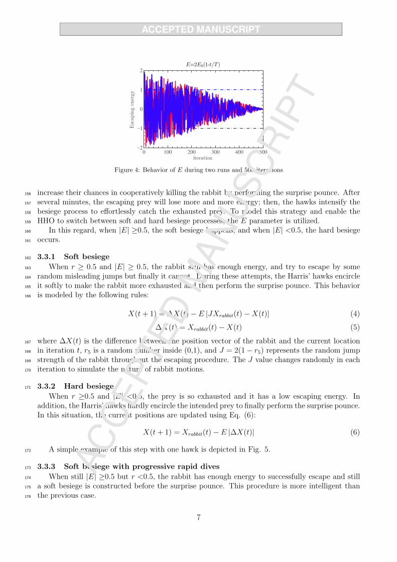
0 100 200 300 400 500−2
−1
0
1
2
E=2E0(1-t/T)
iteration
Escap
ingenergy
Figure 4: Behavior of E during two runs and 500 iterations
increase their chances in cooperatively killing the rabbit by performing the surprise pounce. After156
several minutes, the escaping prey will lose more and more energy; then, the hawks intensify the157
besiege process to effortlessly catch the exhausted prey. To model this strategy and enable the158
HHO to switch between soft and hard besiege processes, the E parameter is utilized.159
In this regard, when |E| ≥0.5, the soft besiege happens, and when |E| <0.5, the hard besiege160
occurs.161
3.3.1 Soft besiege162
When r ≥ 0.5 and |E| ≥ 0.5, the rabbit still has enough energy, and try to escape by some163
random misleading jumps but finally it cannot. During these attempts, the Harris’ hawks encircle164
it softly to make the rabbit more exhausted and then perform the surprise pounce. This behavior165
is modeled by the following rules:166
X(t+ 1) = ∆X(t)− E |JXrabbit(t)−X(t)| (4)
∆X(t) = Xrabbit(t)−X(t) (5)
where ∆X(t) is the difference between the position vector of the rabbit and the current location167
in iteration t, r5 is a random number inside (0,1), and J = 2(1− r5) represents the random jump168
strength of the rabbit throughout the escaping procedure. The J value changes randomly in each169
iteration to simulate the nature of rabbit motions.170
3.3.2 Hard besiege171
When r ≥0.5 and |E| <0.5, the prey is so exhausted and it has a low escaping energy. Inaddition, the Harris’ hawks hardly encircle the intended prey to finally perform the surprise pounce.In this situation, the current positions are updated using Eq. (6):
X(t+ 1) = Xrabbit(t)− E |∆X(t)| (6)
A simple example of this step with one hawk is depicted in Fig. 5.172
3.3.3 Soft besiege with progressive rapid dives173
When still |E| ≥0.5 but r <0.5, the rabbit has enough energy to successfully escape and still174
a soft besiege is constructed before the surprise pounce. This procedure is more intelligent than175
the previous case.176
7
https://aliasgharheidari.com/HHO.html
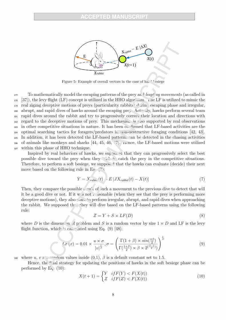
X(t)
Xrabbit − E |ΔX|
X(t+1)
E
Xrabbit
A
B
OO1
B
ΔXFigure 5: Example of overall vectors in the case of hard besiege
To mathematically model the escaping patterns of the prey and leapfrog movements (as called in177
[37]), the levy flight (LF) concept is utilized in the HHO algorithm. The LF is utilized to mimic the178
real zigzag deceptive motions of preys (particularity rabbits) during escaping phase and irregular,179
abrupt, and rapid dives of hawks around the escaping prey. Actually, hawks perform several team180
rapid dives around the rabbit and try to progressively correct their location and directions with181
regard to the deceptive motions of prey. This mechanism is also supported by real observations182
in other competitive situations in nature. It has been confirmed that LF-based activities are the183
optimal searching tactics for foragers/predators in non-destructive foraging conditions [42, 43].184
In addition, it has been detected the LF-based patterns can be detected in the chasing activities185
of animals like monkeys and sharks [44, 45, 46, 47]. Hence, the LF-based motions were utilized186
within this phase of HHO technique.187
Inspired by real behaviors of hawks, we supposed that they can progressively select the bestpossible dive toward the prey when they wish to catch the prey in the competitive situations.Therefore, to perform a soft besiege, we supposed that the hawks can evaluate (decide) their nextmove based on the following rule in Eq. (7):
Y = Xrabbit(t)− E |JXrabbit(t)−X(t)| (7)
Then, they compare the possible result of such a movement to the previous dive to detect that willit be a good dive or not. If it was not reasonable (when they see that the prey is performing moredeceptive motions), they also start to perform irregular, abrupt, and rapid dives when approachingthe rabbit. We supposed that they will dive based on the LF-based patterns using the followingrule:
Z = Y + S × LF (D) (8)
where D is the dimension of problem and S is a random vector by size 1×D and LF is the levyflight function, which is calculated using Eq. (9) [48]:
LF (x) = 0.01× u× σ
|v| 1β, σ =
(Γ(1 + β)× sin(πβ
2)
Γ(1+β2)× β × 2(
β−12
))
) 1β
(9)
where u, v are random values inside (0,1), β is a default constant set to 1.5.188
Hence, the final strategy for updating the positions of hawks in the soft besiege phase can beperformed by Eq. (10):
X(t+ 1) =
{Y ifF (Y ) < F (X(t))Z ifF (Z) < F (X(t))
(10)
8
https://aliasgharheidari.com/HHO.html
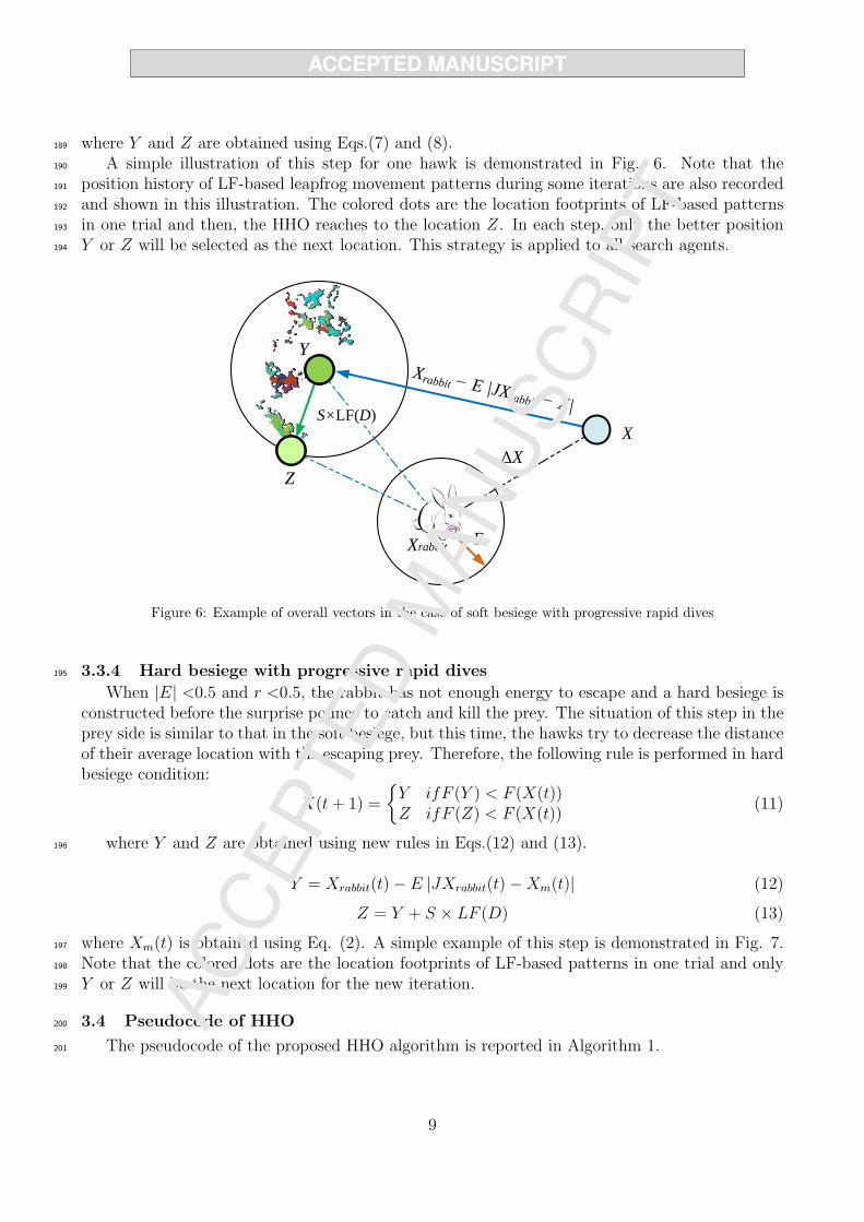
where Y and Z are obtained using Eqs.(7) and (8).189
A simple illustration of this step for one hawk is demonstrated in Fig. 6. Note that the190
position history of LF-based leapfrog movement patterns during some iterations are also recorded191
and shown in this illustration. The colored dots are the location footprints of LF-based patterns192
in one trial and then, the HHO reaches to the location Z. In each step, only the better position193
Y or Z will be selected as the next location. This strategy is applied to all search agents.194
E
Z
X
ΔX
Xrabbit
Xrabbit − E |JXrabbit − X|S×LF(D)
Y
Figure 6: Example of overall vectors in the case of soft besiege with progressive rapid dives
3.3.4 Hard besiege with progressive rapid dives195
When |E| <0.5 and r <0.5, the rabbit has not enough energy to escape and a hard besiege isconstructed before the surprise pounce to catch and kill the prey. The situation of this step in theprey side is similar to that in the soft besiege, but this time, the hawks try to decrease the distanceof their average location with the escaping prey. Therefore, the following rule is performed in hardbesiege condition:
X(t+ 1) =
{Y ifF (Y ) < F (X(t))Z ifF (Z) < F (X(t))
(11)
where Y and Z are obtained using new rules in Eqs.(12) and (13).196
Y = Xrabbit(t)− E |JXrabbit(t)−Xm(t)| (12)
Z = Y + S × LF (D) (13)
where Xm(t) is obtained using Eq. (2). A simple example of this step is demonstrated in Fig. 7.197
Note that the colored dots are the location footprints of LF-based patterns in one trial and only198
Y or Z will be the next location for the new iteration.199
3.4 Pseudocode of HHO200
The pseudocode of the proposed HHO algorithm is reported in Algorithm 1.201
9
https://aliasgharheidari.com/HHO.html
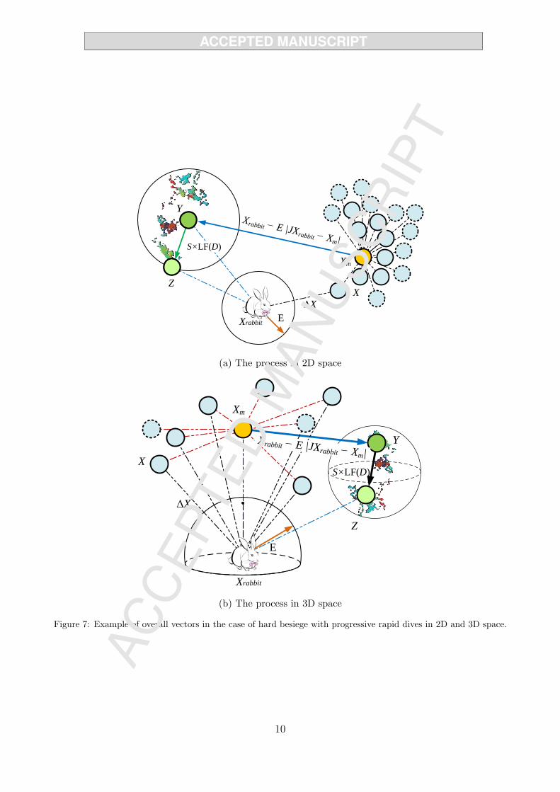
E
ZX
ΔX
Xrabbit
Xrabbit − E |JXrabbit − Xm|S×LF(D)
Y
Xm
(a) The process in 2D space
E
Xrabbit
X
A
B
OO1
B
ΔX
Xm
Z
S×LF(D)
YXrabbit − E |JXrabbit − Xm|
(b) The process in 3D space
Figure 7: Example of overall vectors in the case of hard besiege with progressive rapid dives in 2D and 3D space.
10
https://aliasgharheidari.com/HHO.html
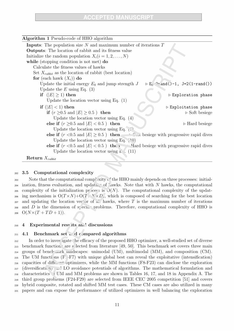
Algorithm 1 Pseudo-code of HHO algorithm
Inputs: The population size N and maximum number of iterations TOutputs: The location of rabbit and its fitness valueInitialize the random population Xi(i = 1, 2, . . . , N)while (stopping condition is not met) do
Calculate the fitness values of hawksSet Xrabbit as the location of rabbit (best location)for (each hawk (Xi)) do
Update the initial energy E0 and jump strength J ▷ E0=2rand()-1, J=2(1-rand())
Update the E using Eq. (3)if (|E| ≥ 1) then ▷ Exploration phase
Update the location vector using Eq. (1)
if (|E| < 1) then ▷ Exploitation phase
if (r ≥0.5 and |E| ≥ 0.5 ) then ▷ Soft besiegeUpdate the location vector using Eq. (4)
else if (r ≥0.5 and |E| < 0.5 ) then ▷ Hard besiegeUpdate the location vector using Eq. (6)
else if (r <0.5 and |E| ≥ 0.5 ) then ▷ Soft besiege with progressive rapid divesUpdate the location vector using Eq. (10)
else if (r <0.5 and |E| < 0.5 ) then ▷ Hard besiege with progressive rapid divesUpdate the location vector using Eq. (11)
Return Xrabbit
3.5 Computational complexity202
Note that the computational complexity of the HHOmainly depends on three processes: initial-203
ization, fitness evaluation, and updating of hawks. Note that with N hawks, the computational204
complexity of the initialization process is O(N). The computational complexity of the updat-205
ing mechanism is O(T×N)+O(T×N×D), which is composed of searching for the best location206
and updating the location vector of all hawks, where T is the maximum number of iterations207
and D is the dimension of specific problems. Therefore, computational complexity of HHO is208
O(N×(T + TD + 1)).209
4 Experimental results and discussions210
4.1 Benchmark set and compared algorithms211
In order to investigate the efficacy of the proposed HHO optimizer, a well-studied set of diverse212
benchmark functions are selected from literature [49, 50]. This benchmark set covers three main213
groups of benchmark landscapes: unimodal (UM), multimodal (MM), and composition (CM).214
The UM functions (F1-F7) with unique global best can reveal the exploitative (intensification)215
capacities of different optimizers, while the MM functions (F8-F23) can disclose the exploration216
(diversification) and LO avoidance potentials of algorithms. The mathematical formulation and217
characteristics of UM and MM problems are shown in Tables 16, 17, and 18 in Appendix A. The218
third group problems (F24-F29) are selected from IEEE CEC 2005 competition [51] and covers219
hybrid composite, rotated and shifted MM test cases. These CM cases are also utilized in many220
papers and can expose the performance of utilized optimizers in well balancing the exploration221
11
https://aliasgharheidari.com/HHO.html
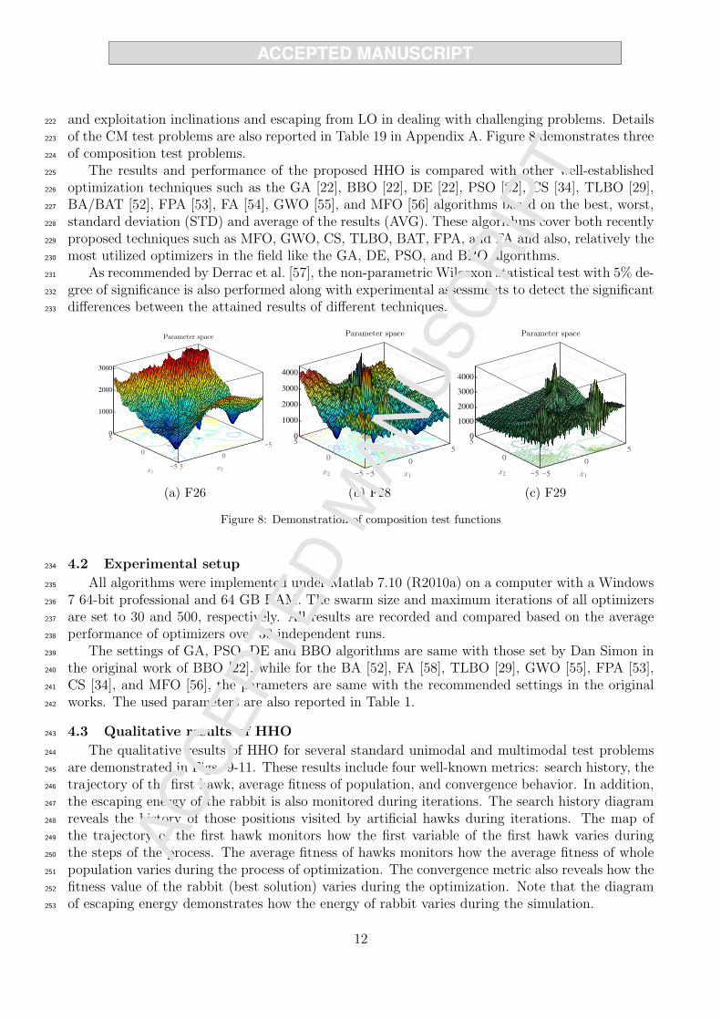
and exploitation inclinations and escaping from LO in dealing with challenging problems. Details222
of the CM test problems are also reported in Table 19 in Appendix A. Figure 8 demonstrates three223
of composition test problems.224
The results and performance of the proposed HHO is compared with other well-established225
optimization techniques such as the GA [22], BBO [22], DE [22], PSO [22], CS [34], TLBO [29],226
BA/BAT [52], FPA [53], FA [54], GWO [55], and MFO [56] algorithms based on the best, worst,227
standard deviation (STD) and average of the results (AVG). These algorithms cover both recently228
proposed techniques such as MFO, GWO, CS, TLBO, BAT, FPA, and FA and also, relatively the229
most utilized optimizers in the field like the GA, DE, PSO, and BBO algorithms.230
As recommended by Derrac et al. [57], the non-parametric Wilcoxon statistical test with 5% de-231
gree of significance is also performed along with experimental assessments to detect the significant232
differences between the attained results of different techniques.233
−5
0
5
−5
0
5
0
1000
2000
3000
x2
Parameter space
x1
(a) F26
−5
0
5
−5
0
50
1000
2000
3000
4000
x1
Parameter space
x2
(b) F28
−5
0
5
−5
0
50
1000
2000
3000
4000
x1
Parameter space
x2
(c) F29
Figure 8: Demonstration of composition test functions
4.2 Experimental setup234
All algorithms were implemented under Matlab 7.10 (R2010a) on a computer with a Windows235
7 64-bit professional and 64 GB RAM. The swarm size and maximum iterations of all optimizers236
are set to 30 and 500, respectively. All results are recorded and compared based on the average237
performance of optimizers over 30 independent runs.238
The settings of GA, PSO, DE and BBO algorithms are same with those set by Dan Simon in239
the original work of BBO [22], while for the BA [52], FA [58], TLBO [29], GWO [55], FPA [53],240
CS [34], and MFO [56], the parameters are same with the recommended settings in the original241
works. The used parameters are also reported in Table 1.242
4.3 Qualitative results of HHO243
The qualitative results of HHO for several standard unimodal and multimodal test problems244
are demonstrated in Figs. 9-11. These results include four well-known metrics: search history, the245
trajectory of the first hawk, average fitness of population, and convergence behavior. In addition,246
the escaping energy of the rabbit is also monitored during iterations. The search history diagram247
reveals the history of those positions visited by artificial hawks during iterations. The map of248
the trajectory of the first hawk monitors how the first variable of the first hawk varies during249
the steps of the process. The average fitness of hawks monitors how the average fitness of whole250
population varies during the process of optimization. The convergence metric also reveals how the251
fitness value of the rabbit (best solution) varies during the optimization. Note that the diagram252
of escaping energy demonstrates how the energy of rabbit varies during the simulation.253
12
https://aliasgharheidari.com/HHO.html
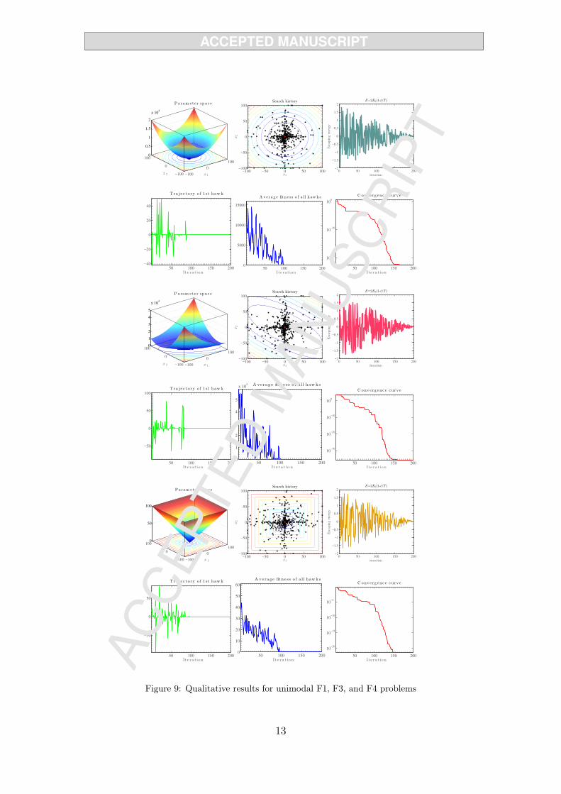
−100
0
100
−100
0
1000
0.5
1
1.5
2
x 104
x 1
P a ram e te r spa c e
x 2−100 −50 0 50 100
−100
−50
0
50
100
Search history
x1
x2
0 50 100 150 200−2
−1.5
−1
−0.5
0
0.5
1
1.5
2
E=2E0(1-t/T)
iteration
Escapingenergy
50 100 150 200
−40
−20
0
20
40
Tra je c to ry o f 1 st haw k
Ite ra t io n50 100 150 200
0
5000
10000
15000
A ve ra g e fitn e ss o f a ll h aw k s
Ite ra t io n50 100 150 200
10−40
10−20
100
C onve rg e n c e c u rv e
Ite ra t io n
−100
0
100
−100
0
1000
1
2
3
4
5
x 104
x 1
P a ram e te r spa c e
x 2−100 −50 0 50 100
−100
−50
0
50
100
Search history
x1
x2
0 50 100 150 200−2
−1.5
−1
−0.5
0
0.5
1
1.5
2
E=2E0(1-t/T)
iteration
Escapingenergy
50 100 150 200
−50
0
50
100
Tra je c to ry o f 1 st haw k
Ite ra t io n50 100 150 200
0
1
2
3
4
5
x 105 A ve ra g e fitn e ss o f a ll h aw k s
Ite ra t io n50 100 150 200
10−30
10−20
10−10
100
C onve rg e n c e c u rv e
Ite ra t io n
−100
0
100
−100
0
1000
50
100
x 1
P a ram e te r spa c e
x 2−100 −50 0 50 100
−100
−50
0
50
100
Search history
x1
x2
0 50 100 150 200−2
−1.5
−1
−0.5
0
0.5
1
1.5
2
E=2E0(1-t/T)
iteration
Escapingenergy
50 100 150 200
−50
0
50
Tra je c to ry o f 1 st haw k
Ite ra t io n50 100 150 200
0
10
20
30
40
50
60
A ve ra g e fitn e ss o f a ll h aw k s
Ite ra t io n50 100 150 200
10−20
10−15
10−10
10−5
C onve rg e n c e c u rv e
Ite ra t io n
Figure 9: Qualitative results for unimodal F1, F3, and F4 problems
13
https://aliasgharheidari.com/HHO.html
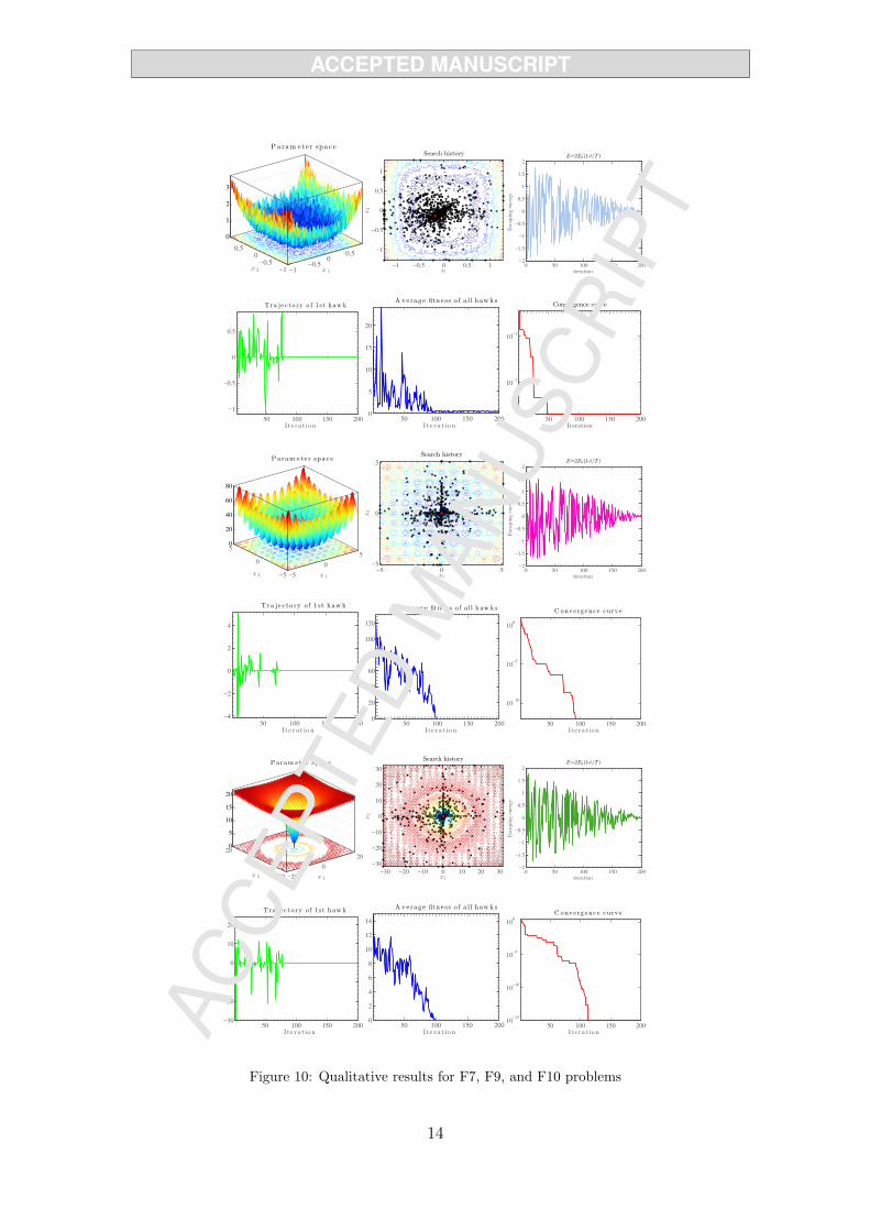
−1−0.5
00.5
−1
−0.5
0
0.5
0
1
2
3
x 1
P a ram e te r spa c e
x 2−1 −0.5 0 0.5 1
−1
−0.5
0
0.5
1
Search history
x1
x2
0 50 100 150 200−2
−1.5
−1
−0.5
0
0.5
1
1.5
2
E=2E0(1-t/T)
iteration
Escapingenergy
50 100 150 200
−1
−0.5
0
0.5
Tra je c to ry o f 1 st haw k
Ite ra t io n50 100 150 200
0
5
10
15
20
A ve ra g e fitn e ss o f a ll h aw k s
Ite ra t io n50 100 150 200
10−2
10−1
Convergence curve
Iteration
−5
0
5
−5
0
50
20
40
60
80
x 1
P a ram e te r spa c e
x 2−5 0 5
−5
0
5
Search history
x1
x2
0 50 100 150 200−2
−1.5
−1
−0.5
0
0.5
1
1.5
2
E=2E0(1-t/T)
iteration
Escapingenergy
50 100 150 200
−4
−2
0
2
4
Tra je c to ry o f 1 st haw k
Ite ra t io n50 100 150 200
0
20
40
60
80
100
120
A ve ra g e fitn e ss o f a ll h aw k s
Ite ra t io n50 100 150 200
10−10
10−5
100
C onve rg e n c e c u rv e
Ite ra t io n
−20
0
20
−20
0
200
5
10
15
20
x 1
P a ram e te r spa c e
x 2−30 −20 −10 0 10 20 30
−30
−20
−10
0
10
20
30
Search history
x1
x2
0 50 100 150 200−2
−1.5
−1
−0.5
0
0.5
1
1.5
2
E=2E0(1-t/T)
iteration
Escapingenergy
50 100 150 200−30
−20
−10
0
10
20
Tra je c to ry o f 1 st haw k
Ite ra t io n50 100 150 200
0
2
4
6
8
10
12
14
A ve ra g e fitn e ss o f a ll h aw k s
Ite ra t io n50 100 150 200
10−15
10−10
10−5
100
C onve rg e n c e c u rv e
Ite ra t io n
Figure 10: Qualitative results for F7, F9, and F10 problems
14
https://aliasgharheidari.com/HHO.html
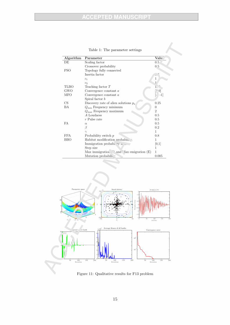
Table 1: The parameter settings
Algorithm Parameter ValueDE Scaling factor 0.5
Crossover probability 0.5PSO Topology fully connected
Inertia factor 0.3c1 1c2 1
TLBO Teaching factor T 1, 2GWO Convergence constant a [2 0]MFO Convergence constant a [-2 -1]
Spiral factor b 1CS Discovery rate of alien solutions pa 0.25BA Qmin Frequency minimum 0
Qmax Frequency maximum 2A Loudness 0.5r Pulse rate 0.5
FA α 0.5β 0.2γ 1
FPA Probability switch p 0.8BBO Habitat modification probability 1
Immigration probability limits [0,1]Step size 1Max immigration (I) and Max emigration (E) 1Mutation probability 0.005
−5
0
5
−5
0
50
5
10
x1
Parameter space
x2−50 0 50
−50
0
50
Search history
x1
x2
0 50 100 150 200−2
−1.5
−1
−0.5
0
0.5
1
1.5
2
E=2E0(1-t/T)
iteration
Escapingenergy
50 100 150 200−50
0
50
Trajectory of 1st hawk
Iteration50 100 150 200
0
1
2
3
4
5
6
x 108 Average fitness of all hawks
Iteration50 100 150 200
10−1
100
Convergence curve
Iteration
Figure 11: Qualitative results for F13 problem
15
https://aliasgharheidari.com/HHO.html
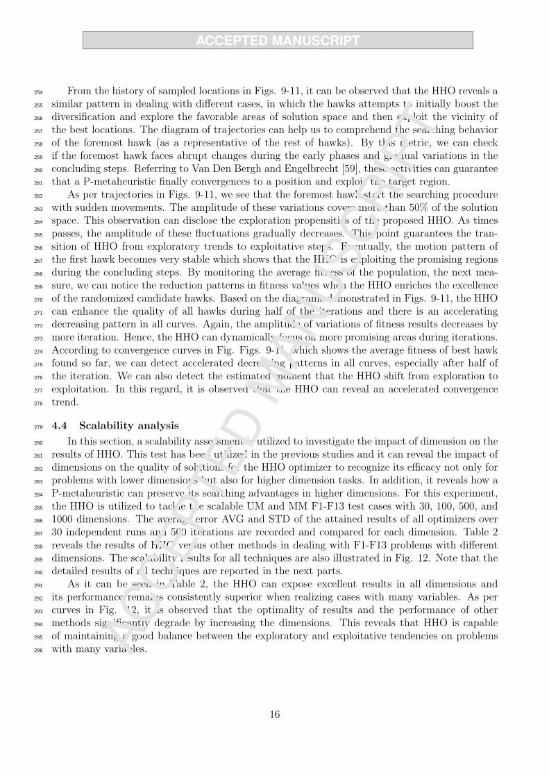
From the history of sampled locations in Figs. 9-11, it can be observed that the HHO reveals a254
similar pattern in dealing with different cases, in which the hawks attempts to initially boost the255
diversification and explore the favorable areas of solution space and then exploit the vicinity of256
the best locations. The diagram of trajectories can help us to comprehend the searching behavior257
of the foremost hawk (as a representative of the rest of hawks). By this metric, we can check258
if the foremost hawk faces abrupt changes during the early phases and gradual variations in the259
concluding steps. Referring to Van Den Bergh and Engelbrecht [59], these activities can guarantee260
that a P-metaheuristic finally convergences to a position and exploit the target region.261
As per trajectories in Figs. 9-11, we see that the foremost hawk start the searching procedure262
with sudden movements. The amplitude of these variations covers more than 50% of the solution263
space. This observation can disclose the exploration propensities of the proposed HHO. As times264
passes, the amplitude of these fluctuations gradually decreases. This point guarantees the tran-265
sition of HHO from exploratory trends to exploitative steps. Eventually, the motion pattern of266
the first hawk becomes very stable which shows that the HHO is exploiting the promising regions267
during the concluding steps. By monitoring the average fitness of the population, the next mea-268
sure, we can notice the reduction patterns in fitness values when the HHO enriches the excellence269
of the randomized candidate hawks. Based on the diagrams demonstrated in Figs. 9-11, the HHO270
can enhance the quality of all hawks during half of the iterations and there is an accelerating271
decreasing pattern in all curves. Again, the amplitude of variations of fitness results decreases by272
more iteration. Hence, the HHO can dynamically focus on more promising areas during iterations.273
According to convergence curves in Fig. Figs. 9-11, which shows the average fitness of best hawk274
found so far, we can detect accelerated decreasing patterns in all curves, especially after half of275
the iteration. We can also detect the estimated moment that the HHO shift from exploration to276
exploitation. In this regard, it is observed that the HHO can reveal an accelerated convergence277
trend.278
4.4 Scalability analysis279
In this section, a scalability assessment is utilized to investigate the impact of dimension on the280
results of HHO. This test has been utilized in the previous studies and it can reveal the impact of281
dimensions on the quality of solutions for the HHO optimizer to recognize its efficacy not only for282
problems with lower dimensions but also for higher dimension tasks. In addition, it reveals how a283
P-metaheuristic can preserve its searching advantages in higher dimensions. For this experiment,284
the HHO is utilized to tackle the scalable UM and MM F1-F13 test cases with 30, 100, 500, and285
1000 dimensions. The average error AVG and STD of the attained results of all optimizers over286
30 independent runs and 500 iterations are recorded and compared for each dimension. Table 2287
reveals the results of HHO versus other methods in dealing with F1-F13 problems with different288
dimensions. The scalability results for all techniques are also illustrated in Fig. 12. Note that the289
detailed results of all techniques are reported in the next parts.290
As it can be seen in Table 2, the HHO can expose excellent results in all dimensions and291
its performance remains consistently superior when realizing cases with many variables. As per292
curves in Fig. 12, it is observed that the optimality of results and the performance of other293
methods significantly degrade by increasing the dimensions. This reveals that HHO is capable294
of maintaining a good balance between the exploratory and exploitative tendencies on problems295
with many variables.296
16
https://aliasgharheidari.com/HHO.html
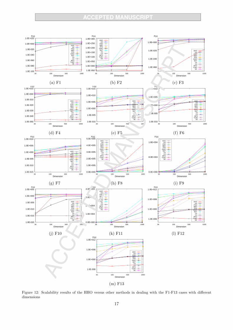
1.0E-100
1.0E-080
1.0E-060
1.0E-040
1.0E-020
1.0E+000
1.0E+020
30 100 500 1000
F(x)
Dimension
HHOGA
PSOBBOFPA
GWOBAT
FACS
MFOTLBO
DE
(a) F1
1.0E-050
1.0E+000
1.0E+050
1.0E+100
1.0E+150
1.0E+200
1.0E+250
1.0E+300
30 100 500 1000
F(x)
Dimension
HHOGA
PSOBBOFPA
GWOBAT
FACS
MFOTLBO
DE
(b) F2
1.0E-060
1.0E-040
1.0E-020
1.0E+000
30 100 500 1000
F(x)
Dimension
HHOGA
PSOBBOFPA
GWOBAT
FACS
MFOTLBO
DE
(c) F3
1.0E-050
1.0E-040
1.0E-030
1.0E-020
1.0E-010
1.0E+000
1.0E+010
30 100 500 1000
F(x)
Dimension
HHOGA
PSOBBOFPA
GWOBAT
FACS
MFOTLBO
DE
(d) F4
1.0E-010
1.0E-005
1.0E+000
1.0E+005
1.0E+010
1.0E+015
30 100 500 1000
F(x)
Dimension
HHOGA
PSOBBOFPA
GWOBAT
FACS
MFOTLBO
DE
(e) F5
1.0E-010
1.0E-005
1.0E+000
1.0E+005
1.0E+010
30 100 500 1000
F(x)
Dimension
HHOGA
PSOBBOFPA
GWOBAT
FACS
MFOTLBO
DE
(f) F6
1.0E-015
1.0E-010
1.0E-005
1.0E+000
1.0E+005
1.0E+010
30 100 500 1000
F(x)
Dimension
HHOGA
PSOBBOFPA
GWOBAT
FACS
MFOTLBO
DE
(g) F7
-5.0E+005
-4.0E+005
-3.0E+005
-2.0E+005
-1.0E+005
0.0E+00030 100 500 1000
F(x)
Dimension
HHOGA
PSOBBOFPA
GWOBAT
FACS
MFOTLBO
DE
(h) F8
0.0E+000
8.0E+003
1.6E+004
30 100 500 1000
F(x)
Dimension
HHOGA
PSOBBOFPA
GWOBAT
FACS
MFOTLBO
DE
(i) F9
1.0E-020
1.0E-015
1.0E-010
1.0E-005
1.0E+000
1.0E+005
30 100 500 1000
F(x)
Dimension
HHOGA
PSOBBOFPA
GWOBAT
FACS
MFOTLBO
DE
(j) F10
0.0E+000
1.0E+004
2.0E+004
3.0E+004
4.0E+004
30 100 500 1000
F(x)
Dimension
HHOGA
PSOBBOFPA
GWOBAT
FACS
MFOTLBO
DE
(k) F11
1.0E-006
1.0E+000
1.0E+006
1.0E+012
30 100 500 1000
F(x)
Dimension
HHOGA
PSOBBOFPA
GWOBAT
FACS
MFOTLBO
DE
(l) F12
1.0E-006
1.0E+000
1.0E+006
1.0E+012
30 100 500 1000
F(x)
Dimension
HHOGA
PSOBBOFPA
GWOBAT
FACS
MFOTLBO
DE
(m) F13
Figure 12: Scalability results of the HHO versus other methods in dealing with the F1-F13 cases with differentdimensions
17
https://aliasgharheidari.com/HHO.html
Table 2: Results of HHO for different dimensions of scalable F1-F13 problems
Problem/D Metric 30 100 500 1000
F1AVG 3.95E-97 1.91E-94 1.46E-92 1.06E-94STD 1.72E-96 8.66E-94 8.01E-92 4.97E-94
F2AVG 1.56E-51 9.98E-52 7.87E-49 2.52E-50STD 6.98E-51 2.66E-51 3.11E-48 5.02E-50
F3AVG 1.92E-63 1.84E-59 6.54E-37 1.79E-17STD 1.05E-62 1.01E-58 3.58E-36 9.81E-17
F4AVG 1.02E-47 8.76E-47 1.29E-47 1.43E-46STD 5.01E-47 4.79E-46 4.11E-47 7.74E-46
F5AVG 1.32E-02 2.36E-02 3.10E-01 5.73E-01STD 1.87E-02 2.99E-02 3.73E-01 1.40E+00
F6AVG 1.15E-04 5.12E-04 2.94E-03 3.61E-03STD 1.56E-04 6.77E-04 3.98E-03 5.38E-03
F7AVG 1.40E-04 1.85E-04 2.51E-04 1.41E-04STD 1.07E-04 4.06E-04 2.43E-04 1.63E-04
F8AVG -1.25E+04 -4.19E+04 -2.09E+05 -4.19E+05STD 1.47E+02 2.82E+00 2.84E+01 1.03E+02
F9AVG 0.00E+00 0.00E+00 0.00E+00 0.00E+00STD 0.00E+00 0.00E+00 0.00E+00 0.00E+00
F10AVG 8.88E-16 8.88E-16 8.88E-16 8.88E-16STD 4.01E-31 4.01E-31 4.01E-31 4.01E-31
F11AVG 0.00E+00 0.00E+00 0.00E+00 0.00E+00STD 0.00E+00 0.00E+00 0.00E+00 0.00E+00
F12AVG 7.35E-06 4.23E-06 1.41E-06 1.02E-06STD 1.19E-05 5.25E-06 1.48E-06 1.16E-06
F13AVG 1.57E-04 9.13E-05 3.44E-04 8.41E-04STD 2.15E-04 1.26E-04 4.75E-04 1.18E-03
4.5 Quantitative results of HHO and discussion297
In this section, the results of HHO are compared with those of other optimizers for different298
dimensions of F1-F13 test problems in addition to the F14-F29 MM and CM test cases. Note299
that the results are presented for 30, 100, 500, and 1000 dimensions of the scalable F1-F13 prob-300
lems. Tables 3-6 show the obtained results for HHO versus other competitors in dealing with301
scalable functions. Table 8 also reveals the performance of algorithms in dealing with F14-F29302
test problems. In order to investigate the significant differences between the results of proposed303
HHO versus other optimizers, Wilcoxon rank-sum test with 5% degree is carefully performed here304
[57]. Tables 20, 21, 22, 23, and 24 in Appendix B show the attained p-values of the Wilcoxon305
rank-sum test with 5% significance.306
As per result in Table 3, the HHO can obtain the best results compared to other competitors307
on F1-F5, F7, and F9-F13 problems. The results of HHO are considerably better than other308
algorithms in dealing with 84.6% of these 30-dimensional functions, demonstrating the superior309
performance of this optimizer. According to p-values in Table 20, it is detected that the observed310
differences in the results are statistically meaningful for all cases. From Table 4, when we have a311
100-dimensional search space, the HHO can considerably outperform other techniques and attain312
the best results for 92.3% of F1-F13 problems. It is observed that the results of HHO are again313
remarkably better than other techniques. With regard to p-values in Table 21, it is detected that314
the solutions of HHO are significantly better than those realized by other techniques in almost315
all cases. From Table 5, we see that the HHO can attain the best results in terms of AVG and316
STD in dealing with 12 test cases with 500 dimensions. By considering p-values in Table 22, it is317
recognized that the HHO can significantly outperform other optimizers in all cases. As per results318
in Table 6, similarly to what we observed in lower dimensions, it is detected that the HHO has319
still a remarkably superior performance in dealing with F1-F13 test functions compared to GA,320
PSO, DE, BBO, CS, GWO, MFO, TLBO, BAT, FA, and FPA optimizers. The statistical results321
in Table 23 also verify the significant gap between the results of HHO and other optimizers in322
18
https://aliasgharheidari.com/HHO.html
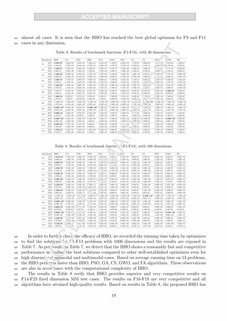
almost all cases. It is seen that the HHO has reached the best global optimum for F9 and F11323
cases in any dimension.324
Table 3: Results of benchmark functions (F1-F13), with 30 dimensions.
Benchmark HHO GA PSO BBO FPA GWO BAT FA CS MFO TLBO DE
F1AVG 3.95E-97 1.03E+03 1.83E+04 7.59E+01 2.01E+03 1.18E-27 6.59E+04 7.11E-03 9.06E-04 1.01E+03 2.17E-89 1.33E-03STD 1.72E-96 5.79E+02 3.01E+03 2.75E+01 5.60E+02 1.47E-27 7.51E+03 3.21E-03 4.55E-04 3.05E+03 3.14E-89 5.92E-04
F2AVG 1.56E-51 2.47E+01 3.58E+02 1.36E-03 3.22E+01 9.71E-17 2.71E+08 4.34E-01 1.49E-01 3.19E+01 2.77E-45 6.83E-03STD 6.98E-51 5.68E+00 1.35E+03 7.45E-03 5.55E+00 5.60E-17 1.30E+09 1.84E-01 2.79E-02 2.06E+01 3.11E-45 2.06E-03
F3AVG 1.92E-63 2.65E+04 4.05E+04 1.21E+04 1.41E+03 5.12E-05 1.38E+05 1.66E+03 2.10E-01 2.43E+04 3.91E-18 3.97E+04STD 1.05E-62 3.44E+03 8.21E+03 2.69E+03 5.59E+02 2.03E-04 4.72E+04 6.72E+02 5.69E-02 1.41E+04 8.04E-18 5.37E+03
F4AVG 1.02E-47 5.17E+01 4.39E+01 3.02E+01 2.38E+01 1.24E-06 8.51E+01 1.11E-01 9.65E-02 7.00E+01 1.68E-36 1.15E+01STD 5.01E-47 1.05E+01 3.64E+00 4.39E+00 2.77E+00 1.94E-06 2.95E+00 4.75E-02 1.94E-02 7.06E+00 1.47E-36 2.37E+00
F5AVG 1.32E-02 1.95E+04 1.96E+07 1.82E+03 3.17E+05 2.70E+01 2.10E+08 7.97E+01 2.76E+01 7.35E+03 2.54E+01 1.06E+02STD 1.87E-02 1.31E+04 6.25E+06 9.40E+02 1.75E+05 7.78E-01 4.17E+07 7.39E+01 4.51E-01 2.26E+04 4.26E-01 1.01E+02
F6AVG 1.15E-04 9.01E+02 1.87E+04 6.71E+01 1.70E+03 8.44E-01 6.69E+04 6.94E-03 3.13E-03 2.68E+03 3.29E-05 1.44E-03STD 1.56E-04 2.84E+02 2.92E+03 2.20E+01 3.13E+02 3.18E-01 5.87E+03 3.61E-03 1.30E-03 5.84E+03 8.65E-05 5.38E-04
F7AVG 1.40E-04 1.91E-01 1.07E+01 2.91E-03 3.41E-01 1.70E-03 4.57E+01 6.62E-02 7.29E-02 4.50E+00 1.16E-03 5.24E-02STD 1.07E-04 1.50E-01 3.05E+00 1.83E-03 1.10E-01 1.06E-03 7.82E+00 4.23E-02 2.21E-02 9.21E+00 3.63E-04 1.37E-02
F8AVG -1.25E+04 -1.26E+04 -3.86E+03 -1.24E+04 -6.45E+03 -5.97E+03 -2.33E+03 -5.85E+03 -5.19E+19 -8.48E+03 -7.76E+03 -6.82E+03STD 1.47E+02 4.51E+00 2.49E+02 3.50E+01 3.03E+02 7.10E+02 2.96E+02 1.16E+03 1.76E+20 7.98E+02 1.04E+03 3.94E+02
F9AVG 0.00E+00 9.04E+00 2.87E+02 0.00E+00 1.82E+02 2.19E+00 1.92E+02 3.82E+01 1.51E+01 1.59E+02 1.40E+01 1.58E+02STD 0.00E+00 4.58E+00 1.95E+01 0.00E+00 1.24E+01 3.69E+00 3.56E+01 1.12E+01 1.25E+00 3.21E+01 5.45E+00 1.17E+01
F10AVG 8.88E-16 1.36E+01 1.75E+01 2.13E+00 7.14E+00 1.03E-13 1.92E+01 4.58E-02 3.29E-02 1.74E+01 6.45E-15 1.21E-02STD 4.01E-31 1.51E+00 3.67E-01 3.53E-01 1.08E+00 1.70E-14 2.43E-01 1.20E-02 7.93E-03 4.95E+00 1.79E-15 3.30E-03
F11AVG 0.00E+00 1.01E+01 1.70E+02 1.46E+00 1.73E+01 4.76E-03 6.01E+02 4.23E-03 4.29E-05 3.10E+01 0.00E+00 3.52E-02STD 0.00E+00 2.43E+00 3.17E+01 1.69E-01 3.63E+00 8.57E-03 5.50E+01 1.29E-03 2.00E-05 5.94E+01 0.00E+00 7.20E-02
F12AVG 2.08E-06 4.77E+00 1.51E+07 6.68E-01 3.05E+02 4.83E-02 4.71E+08 3.13E-04 5.57E-05 2.46E+02 7.35E-06 2.25E-03STD 1.19E-05 1.56E+00 9.88E+06 2.62E-01 1.04E+03 2.12E-02 1.54E+08 1.76E-04 4.96E-05 1.21E+03 7.45E-06 1.70E-03
F13AVG 1.57E-04 1.52E+01 5.73E+07 1.82E+00 9.59E+04 5.96E-01 9.40E+08 2.08E-03 8.19E-03 2.73E+07 7.89E-02 9.12E-03STD 2.15E-04 4.52E+00 2.68E+07 3.41E-01 1.46E+05 2.23E-01 1.67E+08 9.62E-04 6.74E-03 1.04E+08 8.78E-02 1.16E-02
Table 4: Results of benchmark functions (F1-F13), with 100 dimensions.
Benchmark HHO GA PSO BBO FPA GWO BAT FA CS MFO TLBO DE
F1AVG 1.91E-94 5.41E+04 1.06E+05 2.85E+03 1.39E+04 1.59E-12 2.72E+05 3.05E-01 3.17E-01 6.20E+04 3.62E-81 8.26E+03STD 8.66E-94 1.42E+04 8.47E+03 4.49E+02 2.71E+03 1.63E-12 1.42E+04 5.60E-02 5.28E-02 1.25E+04 4.14E-81 1.32E+03
F2AVG 9.98E-52 2.53E+02 6.06E+23 1.59E+01 1.01E+02 4.31E-08 6.00E+43 1.45E+01 4.05E+00 2.46E+02 3.27E-41 1.21E+02STD 2.66E-51 1.41E+01 2.18E+24 3.74E+00 9.36E+00 1.46E-08 1.18E+44 6.73E+00 3.16E-01 4.48E+01 2.75E-41 2.33E+01
F3AVG 1.84E-59 2.53E+05 4.22E+05 1.70E+05 1.89E+04 4.09E+02 1.43E+06 4.65E+04 6.88E+00 2.15E+05 4.33E-07 5.01E+05STD 1.01E-58 5.03E+04 7.08E+04 2.02E+04 5.44E+03 2.77E+02 6.21E+05 6.92E+03 1.02E+00 4.43E+04 8.20E-07 5.87E+04
F4AVG 8.76E-47 8.19E+01 6.07E+01 7.08E+01 3.51E+01 8.89E-01 9.41E+01 1.91E+01 2.58E-01 9.31E+01 6.36E-33 9.62E+01STD 4.79E-46 3.15E+00 3.05E+00 4.73E+00 3.37E+00 9.30E-01 1.49E+00 3.12E+00 2.80E-02 2.13E+00 6.66E-33 1.00E+00
F5AVG 2.36E-02 2.37E+07 2.42E+08 4.47E+05 4.64E+06 9.79E+01 1.10E+09 8.46E+02 1.33E+02 1.44E+08 9.67E+01 1.99E+07STD 2.99E-02 8.43E+06 4.02E+07 2.05E+05 1.98E+06 6.75E-01 9.47E+07 8.13E+02 7.34E+00 7.50E+07 7.77E-01 5.80E+06
F6AVG 5.12E-04 5.42E+04 1.07E+05 2.85E+03 1.26E+04 1.03E+01 2.69E+05 2.95E-01 2.65E+00 6.68E+04 3.27E+00 8.07E+03STD 6.77E-04 1.09E+04 9.70E+03 4.07E+02 2.06E+03 1.05E+00 1.25E+04 5.34E-02 3.94E-01 1.46E+04 6.98E-01 1.64E+03
F7AVG 1.85E-04 2.73E+01 3.41E+02 1.25E+00 5.84E+00 7.60E-03 3.01E+02 5.65E-01 1.21E+00 2.56E+02 1.50E-03 1.96E+01STD 4.06E-04 4.45E+01 8.74E+01 5.18E+00 2.16E+00 2.66E-03 2.66E+01 1.64E-01 2.65E-01 8.91E+01 5.39E-04 5.66E+00
F8AVG -4.19E+04 -4.10E+04 -7.33E+03 -3.85E+04 -1.28E+04 -1.67E+04 -4.07E+03 -1.81E+04 -2.84E+18 -2.30E+04 -1.71E+04 -1.19E+04STD 2.82E+00 1.14E+02 4.75E+02 2.80E+02 4.64E+02 2.62E+03 9.37E+02 3.23E+03 6.91E+18 1.98E+03 3.54E+03 5.80E+02
F9AVG 0.00E+00 3.39E+02 1.16E+03 9.11E+00 8.47E+02 1.03E+01 7.97E+02 2.36E+02 1.72E+02 8.65E+02 1.02E+01 1.03E+03STD 0.00E+00 4.17E+01 5.74E+01 2.73E+00 4.01E+01 9.02E+00 6.33E+01 2.63E+01 9.24E+00 8.01E+01 5.57E+01 4.03E+01
F10AVG 8.88E-16 1.82E+01 1.91E+01 5.57E+00 8.21E+00 1.20E-07 1.94E+01 9.81E-01 3.88E-01 1.99E+01 1.66E-02 1.22E+01STD 4.01E-31 4.35E-01 2.04E-01 4.72E-01 1.14E+00 5.07E-08 6.50E-02 2.55E-01 5.23E-02 8.58E-02 9.10E-02 8.31E-01
F11AVG 0.00E+00 5.14E+02 9.49E+02 2.24E+01 1.19E+02 4.87E-03 2.47E+03 1.19E-01 4.56E-03 5.60E+02 0.00E+00 7.42E+01STD 0.00E+00 1.05E+02 6.00E+01 4.35E+00 2.00E+01 1.07E-02 1.03E+02 2.34E-02 9.73E-04 1.23E+02 0.00E+00 1.40E+01
F12AVG 4.23E-06 4.55E+06 3.54E+08 3.03E+02 1.55E+05 2.87E-01 2.64E+09 4.45E+00 2.47E-02 2.82E+08 3.03E-02 3.90E+07STD 5.25E-06 8.22E+06 8.75E+07 1.48E+03 1.74E+05 6.41E-02 2.69E+08 1.32E+00 5.98E-03 1.45E+08 1.02E-02 1.88E+07
F13AVG 9.13E-05 5.26E+07 8.56E+08 6.82E+04 2.76E+06 6.87E+00 5.01E+09 4.50E+01 5.84E+00 6.68E+08 5.47E+00 7.19E+07STD 1.26E-04 3.76E+07 2.16E+08 3.64E+04 1.80E+06 3.32E-01 3.93E+08 2.24E+01 1.21E+00 3.05E+08 8.34E-01 2.73E+07
In order to further check the efficacy of HHO, we recorded the running time taken by optimizers325
to find the solutions for F1-F13 problems with 1000 dimensions and the results are exposed in326
Table 7. As per results in Table 7, we detect that the HHO shows a reasonably fast and competitive327
performance in finding the best solutions compared to other well-established optimizers even for328
high dimensional unimodal and multimodal cases. Based on average running time on 13 problems,329
the HHO performs faster than BBO, PSO, GA, CS, GWO, and FA algorithms. These observations330
are also in accordance with the computational complexity of HHO.331
The results in Table 8 verify that HHO provides superior and very competitive results on332
F14-F23 fixed dimension MM test cases. The results on F16-F18 are very competitive and all333
algorithms have attained high-quality results. Based on results in Table 8, the proposed HHO has334
19
https://aliasgharheidari.com/HHO.html
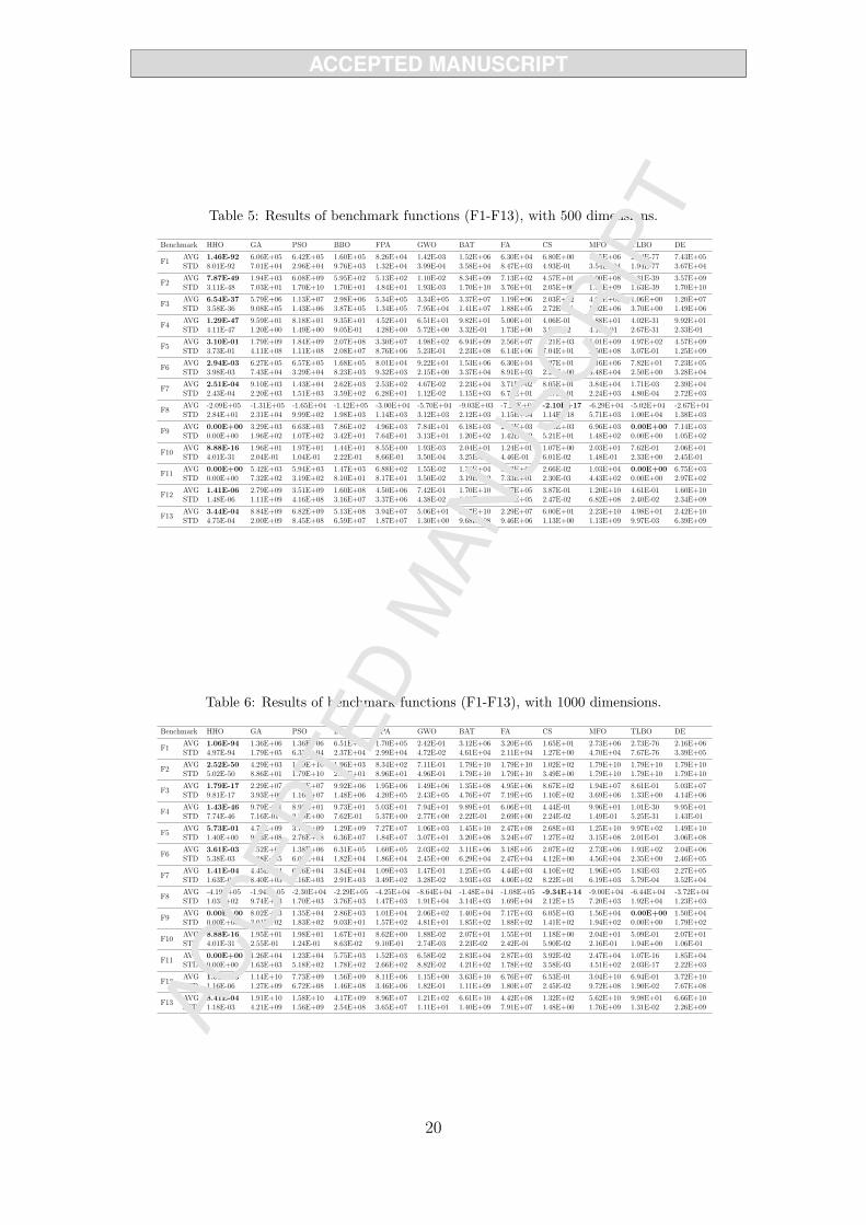
Table 5: Results of benchmark functions (F1-F13), with 500 dimensions.
Benchmark HHO GA PSO BBO FPA GWO BAT FA CS MFO TLBO DE
F1AVG 1.46E-92 6.06E+05 6.42E+05 1.60E+05 8.26E+04 1.42E-03 1.52E+06 6.30E+04 6.80E+00 1.15E+06 2.14E-77 7.43E+05STD 8.01E-92 7.01E+04 2.96E+04 9.76E+03 1.32E+04 3.99E-04 3.58E+04 8.47E+03 4.93E-01 3.54E+04 1.94E-77 3.67E+04
F2AVG 7.87E-49 1.94E+03 6.08E+09 5.95E+02 5.13E+02 1.10E-02 8.34E+09 7.13E+02 4.57E+01 3.00E+08 2.31E-39 3.57E+09STD 3.11E-48 7.03E+01 1.70E+10 1.70E+01 4.84E+01 1.93E-03 1.70E+10 3.76E+01 2.05E+00 1.58E+09 1.63E-39 1.70E+10
F3AVG 6.54E-37 5.79E+06 1.13E+07 2.98E+06 5.34E+05 3.34E+05 3.37E+07 1.19E+06 2.03E+02 4.90E+06 1.06E+00 1.20E+07STD 3.58E-36 9.08E+05 1.43E+06 3.87E+05 1.34E+05 7.95E+04 1.41E+07 1.88E+05 2.72E+01 1.02E+06 3.70E+00 1.49E+06
F4AVG 1.29E-47 9.59E+01 8.18E+01 9.35E+01 4.52E+01 6.51E+01 9.82E+01 5.00E+01 4.06E-01 9.88E+01 4.02E-31 9.92E+01STD 4.11E-47 1.20E+00 1.49E+00 9.05E-01 4.28E+00 5.72E+00 3.32E-01 1.73E+00 3.03E-02 4.15E-01 2.67E-31 2.33E-01
F5AVG 3.10E-01 1.79E+09 1.84E+09 2.07E+08 3.30E+07 4.98E+02 6.94E+09 2.56E+07 1.21E+03 5.01E+09 4.97E+02 4.57E+09STD 3.73E-01 4.11E+08 1.11E+08 2.08E+07 8.76E+06 5.23E-01 2.23E+08 6.14E+06 7.04E+01 2.50E+08 3.07E-01 1.25E+09
F6AVG 2.94E-03 6.27E+05 6.57E+05 1.68E+05 8.01E+04 9.22E+01 1.53E+06 6.30E+04 8.27E+01 1.16E+06 7.82E+01 7.23E+05STD 3.98E-03 7.43E+04 3.29E+04 8.23E+03 9.32E+03 2.15E+00 3.37E+04 8.91E+03 2.24E+00 3.48E+04 2.50E+00 3.28E+04
F7AVG 2.51E-04 9.10E+03 1.43E+04 2.62E+03 2.53E+02 4.67E-02 2.23E+04 3.71E+02 8.05E+01 3.84E+04 1.71E-03 2.39E+04STD 2.43E-04 2.20E+03 1.51E+03 3.59E+02 6.28E+01 1.12E-02 1.15E+03 6.74E+01 1.37E+01 2.24E+03 4.80E-04 2.72E+03
F8AVG -2.09E+05 -1.31E+05 -1.65E+04 -1.42E+05 -3.00E+04 -5.70E+04 -9.03E+03 -7.27E+04 -2.10E+17 -6.29E+04 -5.02E+04 -2.67E+04STD 2.84E+01 2.31E+04 9.99E+02 1.98E+03 1.14E+03 3.12E+03 2.12E+03 1.15E+04 1.14E+18 5.71E+03 1.00E+04 1.38E+03
F9AVG 0.00E+00 3.29E+03 6.63E+03 7.86E+02 4.96E+03 7.84E+01 6.18E+03 2.80E+03 2.54E+03 6.96E+03 0.00E+00 7.14E+03STD 0.00E+00 1.96E+02 1.07E+02 3.42E+01 7.64E+01 3.13E+01 1.20E+02 1.42E+02 5.21E+01 1.48E+02 0.00E+00 1.05E+02
F10AVG 8.88E-16 1.96E+01 1.97E+01 1.44E+01 8.55E+00 1.93E-03 2.04E+01 1.24E+01 1.07E+00 2.03E+01 7.62E-01 2.06E+01STD 4.01E-31 2.04E-01 1.04E-01 2.22E-01 8.66E-01 3.50E-04 3.25E-02 4.46E-01 6.01E-02 1.48E-01 2.33E+00 2.45E-01
F11AVG 0.00E+00 5.42E+03 5.94E+03 1.47E+03 6.88E+02 1.55E-02 1.38E+04 5.83E+02 2.66E-02 1.03E+04 0.00E+00 6.75E+03STD 0.00E+00 7.32E+02 3.19E+02 8.10E+01 8.17E+01 3.50E-02 3.19E+02 7.33E+01 2.30E-03 4.43E+02 0.00E+00 2.97E+02
F12AVG 1.41E-06 2.79E+09 3.51E+09 1.60E+08 4.50E+06 7.42E-01 1.70E+10 8.67E+05 3.87E-01 1.20E+10 4.61E-01 1.60E+10STD 1.48E-06 1.11E+09 4.16E+08 3.16E+07 3.37E+06 4.38E-02 6.29E+08 6.23E+05 2.47E-02 6.82E+08 2.40E-02 2.34E+09
F13AVG 3.44E-04 8.84E+09 6.82E+09 5.13E+08 3.94E+07 5.06E+01 3.17E+10 2.29E+07 6.00E+01 2.23E+10 4.98E+01 2.42E+10STD 4.75E-04 2.00E+09 8.45E+08 6.59E+07 1.87E+07 1.30E+00 9.68E+08 9.46E+06 1.13E+00 1.13E+09 9.97E-03 6.39E+09
Table 6: Results of benchmark functions (F1-F13), with 1000 dimensions.
Benchmark HHO GA PSO BBO FPA GWO BAT FA CS MFO TLBO DE
F1AVG 1.06E-94 1.36E+06 1.36E+06 6.51E+05 1.70E+05 2.42E-01 3.12E+06 3.20E+05 1.65E+01 2.73E+06 2.73E-76 2.16E+06STD 4.97E-94 1.79E+05 6.33E+04 2.37E+04 2.99E+04 4.72E-02 4.61E+04 2.11E+04 1.27E+00 4.70E+04 7.67E-76 3.39E+05
F2AVG 2.52E-50 4.29E+03 1.79E+10 1.96E+03 8.34E+02 7.11E-01 1.79E+10 1.79E+10 1.02E+02 1.79E+10 1.79E+10 1.79E+10STD 5.02E-50 8.86E+01 1.79E+10 2.18E+01 8.96E+01 4.96E-01 1.79E+10 1.79E+10 3.49E+00 1.79E+10 1.79E+10 1.79E+10
F3AVG 1.79E-17 2.29E+07 3.72E+07 9.92E+06 1.95E+06 1.49E+06 1.35E+08 4.95E+06 8.67E+02 1.94E+07 8.61E-01 5.03E+07STD 9.81E-17 3.93E+06 1.16E+07 1.48E+06 4.20E+05 2.43E+05 4.76E+07 7.19E+05 1.10E+02 3.69E+06 1.33E+00 4.14E+06
F4AVG 1.43E-46 9.79E+01 8.92E+01 9.73E+01 5.03E+01 7.94E+01 9.89E+01 6.06E+01 4.44E-01 9.96E+01 1.01E-30 9.95E+01STD 7.74E-46 7.16E-01 2.39E+00 7.62E-01 5.37E+00 2.77E+00 2.22E-01 2.69E+00 2.24E-02 1.49E-01 5.25E-31 1.43E-01
F5AVG 5.73E-01 4.73E+09 3.72E+09 1.29E+09 7.27E+07 1.06E+03 1.45E+10 2.47E+08 2.68E+03 1.25E+10 9.97E+02 1.49E+10STD 1.40E+00 9.63E+08 2.76E+08 6.36E+07 1.84E+07 3.07E+01 3.20E+08 3.24E+07 1.27E+02 3.15E+08 2.01E-01 3.06E+08
F6AVG 3.61E-03 1.52E+06 1.38E+06 6.31E+05 1.60E+05 2.03E+02 3.11E+06 3.18E+05 2.07E+02 2.73E+06 1.93E+02 2.04E+06STD 5.38E-03 1.88E+05 6.05E+04 1.82E+04 1.86E+04 2.45E+00 6.29E+04 2.47E+04 4.12E+00 4.56E+04 2.35E+00 2.46E+05
F7AVG 1.41E-04 4.45E+04 6.26E+04 3.84E+04 1.09E+03 1.47E-01 1.25E+05 4.44E+03 4.10E+02 1.96E+05 1.83E-03 2.27E+05STD 1.63E-04 8.40E+03 4.16E+03 2.91E+03 3.49E+02 3.28E-02 3.93E+03 4.00E+02 8.22E+01 6.19E+03 5.79E-04 3.52E+04
F8AVG -4.19E+05 -1.94E+05 -2.30E+04 -2.29E+05 -4.25E+04 -8.64E+04 -1.48E+04 -1.08E+05 -9.34E+14 -9.00E+04 -6.44E+04 -3.72E+04STD 1.03E+02 9.74E+03 1.70E+03 3.76E+03 1.47E+03 1.91E+04 3.14E+03 1.69E+04 2.12E+15 7.20E+03 1.92E+04 1.23E+03
F9AVG 0.00E+00 8.02E+03 1.35E+04 2.86E+03 1.01E+04 2.06E+02 1.40E+04 7.17E+03 6.05E+03 1.56E+04 0.00E+00 1.50E+04STD 0.00E+00 3.01E+02 1.83E+02 9.03E+01 1.57E+02 4.81E+01 1.85E+02 1.88E+02 1.41E+02 1.94E+02 0.00E+00 1.79E+02
F10AVG 8.88E-16 1.95E+01 1.98E+01 1.67E+01 8.62E+00 1.88E-02 2.07E+01 1.55E+01 1.18E+00 2.04E+01 5.09E-01 2.07E+01STD 4.01E-31 2.55E-01 1.24E-01 8.63E-02 9.10E-01 2.74E-03 2.23E-02 2.42E-01 5.90E-02 2.16E-01 1.94E+00 1.06E-01
F11AVG 0.00E+00 1.26E+04 1.23E+04 5.75E+03 1.52E+03 6.58E-02 2.83E+04 2.87E+03 3.92E-02 2.47E+04 1.07E-16 1.85E+04STD 0.00E+00 1.63E+03 5.18E+02 1.78E+02 2.66E+02 8.82E-02 4.21E+02 1.78E+02 3.58E-03 4.51E+02 2.03E-17 2.22E+03
F12AVG 1.02E-06 1.14E+10 7.73E+09 1.56E+09 8.11E+06 1.15E+00 3.63E+10 6.76E+07 6.53E-01 3.04E+10 6.94E-01 3.72E+10STD 1.16E-06 1.27E+09 6.72E+08 1.46E+08 3.46E+06 1.82E-01 1.11E+09 1.80E+07 2.45E-02 9.72E+08 1.90E-02 7.67E+08
F13AVG 8.41E-04 1.91E+10 1.58E+10 4.17E+09 8.96E+07 1.21E+02 6.61E+10 4.42E+08 1.32E+02 5.62E+10 9.98E+01 6.66E+10STD 1.18E-03 4.21E+09 1.56E+09 2.54E+08 3.65E+07 1.11E+01 1.40E+09 7.91E+07 1.48E+00 1.76E+09 1.31E-02 2.26E+09
20
https://aliasgharheidari.com/HHO.html
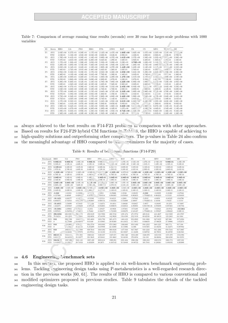
Table 7: Comparison of average running time results (seconds) over 30 runs for larger-scale problems with 1000variables
ID Mertic HHO GA PSO BBO FPA GWO BAT FA CS MFO TLBO DE
F1 AVG 2.03E+00 8.27E+01 8.29E+01 1.17E+02 2.13E+00 4.47E+00 1.60E+00 5.62E+00 5.47E+00 3.23E+00 2.21E+00 2.38E+00STD 4.04E-01 5.13E+00 4.04E+00 6.04E+00 2.62E-01 2.64E-01 2.08E-01 4.42E-01 4.00E-01 2.06E-01 3.62E-01 2.70E-01
F2 AVG 1.70E+00 8.41E+01 8.28E+01 1.16E+02 2.09E+00 4.37E+00 1.61E+00 2.57E+00 5.50E+00 3.25E+00 1.99E+00 2.28E+00STD 7.37E-02 4.65E+00 4.08E+00 6.28E+00 8.64E-02 1.29E-01 1.02E-01 3.93E-01 3.48E-01 1.56E-01 1.19E-01 1.16E-01
F3 AVG 1.17E+02 1.32E+02 1.30E+02 1.65E+02 5.10E+01 5.20E+01 5.23E+01 3.70E+01 1.02E+02 5.11E+01 9.76E+01 5.04E+01STD 5.28E+00 5.68E+00 5.73E+00 7.56E+00 2.01E+00 1.93E+00 2.25E+00 1.49E+00 3.73E+00 2.00E+00 3.87E+00 1.98E+00
F4 AVG 2.05E+00 8.14E+01 8.24E+01 1.18E+02 1.90E+00 4.27E+00 1.44E+00 5.43E+00 5.14E+00 3.14E+00 1.87E+00 2.21E+00STD 7.40E-02 3.73E+00 3.91E+00 5.48E+00 5.83E-02 1.36E-01 1.02E-01 2.76E-01 2.33E-01 9.28E-02 1.05E-01 8.73E-02
F5 AVG 2.95E+00 8.16E+01 8.33E+01 1.17E+02 2.04E+00 4.46E+00 1.65E+00 5.61E+00 5.49E+00 3.31E+00 2.23E+00 2.38E+00STD 8.36E-02 4.13E+00 4.36E+00 5.91E+00 7.79E-02 1.39E-01 1.16E-01 3.01E-01 2.74E-01 1.27E-01 1.09E-01 1.30E-01
F6 AVG 2.49E+00 8.08E+01 8.26E+01 1.17E+02 1.88E+00 4.29E+00 1.47E+00 5.51E+00 5.17E+00 3.13E+00 1.89E+00 2.19E+00STD 8.25E-02 3.96E+00 3.95E+00 5.69E+00 4.98E-02 1.07E-01 1.03E-01 2.87E-01 2.35E-01 1.00E-01 9.33E-02 1.02E-01
F7 AVG 8.20E+00 8.26E+01 8.52E+01 1.18E+02 4.79E+00 7.08E+00 4.22E+00 6.89E+00 1.08E+01 5.83E+00 7.23E+00 4.95E+00STD 1.69E-01 4.56E+00 3.94E+00 6.10E+00 1.02E-01 7.56E-02 8.98E-02 2.02E-01 3.86E-01 1.01E-01 1.31E-01 1.43E-01
F8 AVG 4.86E+00 8.47E+01 8.36E+01 1.18E+02 3.18E+00 5.21E+00 2.45E+00 6.04E+00 7.69E+00 4.05E+00 3.84E+00 3.23E+00STD 1.03E+00 3.68E+00 3.80E+00 5.52E+00 4.73E-01 1.78E-01 2.88E-01 2.69E-01 3.86E-01 1.20E-01 4.12E-01 8.69E-02
F9 AVG 3.77E+00 8.09E+01 8.33E+01 1.15E+02 2.84E+00 4.72E+00 2.33E+00 5.89E+00 6.90E+00 3.94E+00 2.70E+00 3.20E+00STD 8.87E-01 3.59E+00 3.88E+00 5.94E+00 4.30E-01 1.19E-01 2.88E-01 2.55E-01 3.34E-01 1.26E-01 4.71E-01 5.50E-01
F10 AVG 3.75E+00 8.24E+01 8.36E+01 1.17E+02 2.96E+00 4.80E+00 2.46E+00 5.98E+00 6.56E+00 4.04E+00 2.84E+00 3.41E+00STD 8.75E-01 4.02E+00 3.99E+00 5.90E+00 3.74E-01 1.14E-01 4.67E-01 2.91E-01 3.51E-01 1.21E-01 5.39E-01 3.01E-01
F11 AVG 4.17E+00 8.23E+01 8.38E+01 1.18E+02 3.16E+00 4.95E+00 2.61E+00 6.03E+00 6.43E+00 4.22E+00 3.03E+00 3.38E+00STD 5.56E-01 4.41E+00 3.97E+00 6.02E+00 5.50E-01 8.65E-02 3.95E-01 2.50E-01 3.01E-01 1.20E-01 3.95E-01 9.95E-02
F12 AVG 1.90E+01 8.64E+01 8.85E+01 1.23E+02 9.09E+00 1.06E+01 8.66E+00 9.17E+00 1.90E+01 9.67E+00 1.53E+01 9.14E+00STD 3.31E+00 4.47E+00 4.42E+00 6.20E+00 1.39E+00 4.33E-01 1.47E+00 3.62E-01 3.53E+00 4.04E-01 2.54E+00 1.14E+00
F13 AVG 1.89E+01 8.64E+01 8.90E+01 1.23E+02 9.28E+00 1.05E+01 8.74E+00 9.24E+00 1.83E+01 9.66E+00 1.46E+01 9.34E+00STD 1.56E+00 4.40E+00 4.20E+00 6.29E+00 1.50E+00 4.56E-01 1.38E+00 3.94E-01 7.75E-01 3.91E-01 2.24E+00 1.24E+00
always achieved to the best results on F14-F23 problems in comparison with other approaches.335
Based on results for F24-F29 hybrid CM functions in Table 8, the HHO is capable of achieving to336
high-quality solutions and outperforming other competitors. The p-values in Table 24 also confirm337
the meaningful advantage of HHO compared to other optimizers for the majority of cases.338
Table 8: Results of benchmark functions (F14-F29)
Benchmark HHO GA PSO BBO FPA GWO BAT FA CS MFO TLBO DE
F14AVG 9.98E-01 9.98E-01 1.39E+00 9.98E-01 9.98E-01 4.17E+00 1.27E+01 3.51E+00 1.27E+01 2.74E+00 9.98E-01 1.23E+00STD 9.23E-01 4.52E-16 4.60E-01 4.52E-16 2.00E-04 3.61E+00 6.96E+00 2.16E+00 1.81E-15 1.82E+00 4.52E-16 9.23E-01
F15AVG 3.10E-04 3.33E-02 1.61E-03 1.66E-02 6.88E-04 6.24E-03 3.00E-02 1.01E-03 3.13E-04 2.35E-03 1.03E-03 5.63E-04STD 1.97E-04 2.70E-02 4.60E-04 8.60E-03 1.55E-04 1.25E-02 3.33E-02 4.01E-04 2.99E-05 4.92E-03 3.66E-03 2.81E-04
F16AVG -1.03E+00 -3.78E-01 -1.03E+00 -8.30E-01 -1.03E+00 -1.03E+00 -6.87E-01 -1.03E+00 -1.03E+00 -1.03E+00 -1.03E+00 -1.03E+00STD 6.78E-16 3.42E-01 2.95E-03 3.16E-01 6.78E-16 6.78E-16 8.18E-01 6.78E-16 6.78E-16 6.78E-16 6.78E-16 6.78E-16
F17AVG 3.98E-01 5.24E-01 4.00E-01 5.49E-01 3.98E-01 3.98E-01 3.98E-01 3.98E-01 3.98E-01 3.98E-01 3.98E-01 3.98E-01STD 2.54E-06 6.06E-02 1.39E-03 6.05E-02 1.69E-16 1.69E-16 1.58E-03 1.69E-16 1.69E-16 1.69E-16 1.69E-16 1.69E-16
F18AVG 3.00E+00 3.00E+00 3.10E+00 3.00E+00 3.00E+00 3.00E+00 1.47E+01 3.00E+00 3.00E+00 3.00E+00 3.00E+00 3.00E+00STD 0.00E+00 0.00E+00 7.60E-02 0.00E+00 0.00E+00 4.07E-05 2.21E+01 0.00E+00 0.00E+00 0.00E+00 0.00E+00 0.00E+00
F19AVG -3.86E+00 -3.42E+00 -3.86E+00 -3.78E+00 -3.86E+00 -3.86E+00 -3.84E+00 -3.86E+00 -3.86E+00 -3.86E+00 -3.86E+00 -3.86E+00STD 2.44E-03 3.03E-01 1.24E-03 1.26E-01 3.16E-15 3.14E-03 1.41E-01 3.16E-15 3.16E-15 1.44E-03 3.16E-15 3.16E-15
F20AVG -3.322 -1.61351 -3.11088 -2.70774 -3.2951 -3.25866 -3.2546 -3.28105 -3.322 -3.23509 -3.24362 -3.27048STD 0.137406 0.46049 0.029126 0.357832 0.019514 0.064305 0.058943 0.063635 1.77636E-15 0.064223 0.15125 0.058919
F21AVG -10.1451 -6.66177 -4.14764 -8.31508 -5.21514 -8.64121 -4.2661 -7.67362 -5.0552 -6.8859 -8.64525 -9.64796STD 0.885673 3.732521 0.919578 2.883867 0.008154 2.563356 2.554009 3.50697 1.77636E-15 3.18186 1.76521 1.51572
F22AVG -10.4015 -5.58399 -6.01045 -9.38408 -5.34373 -10.4014 -5.60638 -9.63827 -5.0877 -8.26492 -10.2251 -9.74807STD 1.352375 2.605837 1.962628 2.597238 0.053685 0.000678 3.022612 2.293901 8.88178E-16 3.076809 0.007265 1.987703
F23AVG -10.5364 -4.69882 -4.72192 -6.2351 -5.29437 -10.0836 -3.97284 -9.75489 -5.1285 -7.65923 -10.0752 -10.5364STD 0.927655 3.256702 1.742618 3.78462 0.356377 1.721889 3.008279 2.345487 1.77636E-15 3.576927 1.696222 8.88E-15
F24AVG 396.8256 626.8389 768.1775 493.0129 518.7886 486.5743 1291.474 471.9752 469.0141 412.4627 612.5569 431.0767STD 79.58214 101.2255 76.09641 102.6058 47.84199 142.9028 150.4189 252.1018 60.62538 68.38819 123.2403 64.1864
F25AVG 910 999.4998 1184.819 935.4693 1023.799 985.4172 1463.423 953.8902 910.1008 947.9322 967.088 917.6204STD 0 29.44366 33.02676 9.61349 31.85965 29.95368 68.41612 11.74911 0.036659 27.06628 27.39906 1.052473
F26AVG 910 998.9091 1178.34 934.2718 1018.002 973.5362 1480.683 953.5493 910.1252 940.1221 983.774 917.346STD 0 25.27817 35.20755 8.253209 34.87908 22.45008 45.55006 14.086 0.047205 21.68256 45.32275 0.897882
F27AVG 910 1002.032 1195.088 939.7644 1010.392 969.8538 1477.919 947.7667 910.1233 945.4266 978.7344 917.3067STD 0 26.66321 23.97978 23.07814 31.51188 19.51721 60.58827 11.18408 0.049732 26.79031 38.22729 0.861945
F28AVG 860.8925 1512.467 1711.981 1068.631 1539.357 1337.671 1961.526 1016.389 1340.078 1455.918 1471.879 1553.993STD 0.651222 94.64553 35.18377 201.9045 42.93441 191.0662 58.46188 270.6854 134.183 36.06884 268.6238 96.35255
F29AVG 558.9653 1937.396 2101.145 1897.439 2033.614 1909.091 2221.404 1986.206 1903.852 1882.974 1883.773 1897.031STD 5.112352 11.25913 29.74533 8.823239 30.2875 6.567542 35.54849 18.88722 185.7944 6.528261 3.493192 4.203909
4.6 Engineering benchmark sets339
In this section, the proposed HHO is applied to six well-known benchmark engineering prob-340
lems. Tackling engineering design tasks using P-metaheuristics is a well-regarded research direc-341
tion in the previous works [60, 61]. The results of HHO is compared to various conventional and342
modified optimizers proposed in previous studies. Table 9 tabulates the details of the tackled343
engineering design tasks.344
21
https://aliasgharheidari.com/HHO.html
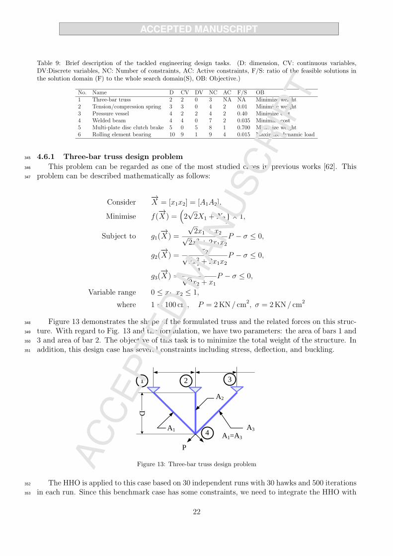
Table 9: Brief description of the tackled engineering design tasks. (D: dimension, CV: continuous variables,DV:Discrete variables, NC: Number of constraints, AC: Active constraints, F/S: ratio of the feasible solutions inthe solution domain (F) to the whole search domain(S), OB: Objective.)
No. Name D CV DV NC AC F/S OB1 Three-bar truss 2 2 0 3 NA NA Minimize weight2 Tension/compression spring 3 3 0 4 2 0.01 Minimize weight3 Pressure vessel 4 2 2 4 2 0.40 Minimize cost4 Welded beam 4 4 0 7 2 0.035 Minimize cost5 Multi-plate disc clutch brake 5 0 5 8 1 0.700 Minimize weight6 Rolling element bearing 10 9 1 9 4 0.015 Maximize dynamic load
4.6.1 Three-bar truss design problem345
This problem can be regarded as one of the most studied cases in previous works [62]. This346
problem can be described mathematically as follows:347
Consider−→X = [x1x2] = [A1A2],
Minimise f(−→X ) =
(2√2X1 +X2
)× 1,
Subject to g1(−→X ) =
√2x1 + x2√
2x21 + 2x1x2
P − σ ≤ 0,
g2(−→X ) =
x2√2x2
1 + 2x1x2
P − σ ≤ 0,
g3(−→X ) =
1√2x2 + x1
P − σ ≤ 0,
Variable range 0 ≤ x1, x2 ≤ 1,
where 1 = 100 cm, P = 2KN/ cm2, σ = 2KN/ cm2
Figure 13 demonstrates the shape of the formulated truss and the related forces on this struc-348
ture. With regard to Fig. 13 and the formulation, we have two parameters: the area of bars 1 and349
3 and area of bar 2. The objective of this task is to minimize the total weight of the structure. In350
addition, this design case has several constraints including stress, deflection, and buckling.351
A1 A3
A2
P
A1=A3
D
1 2 3
4
Figure 13: Three-bar truss design problem
The HHO is applied to this case based on 30 independent runs with 30 hawks and 500 iterations352
in each run. Since this benchmark case has some constraints, we need to integrate the HHO with353
22
https://aliasgharheidari.com/HHO.html

a constraint handling technique. For the sake of simplicity, we used a barrier penalty approach354
[63] in the HHO. The results of HHO are compared to those reported for DEDS [64], MVO [65],355
GOA [62], MFO [56], PSO-DE [66], SSA [60], MBA [67], Tsa [68], Ray and Sain [69], and CS [34]356
in previous literature. Table 10 shows the detailed results of the proposed HHO compared to other357
techniques. Based on the results in Table 10, it is observed that HHO can reveal very competitive358
results compared to DEDS, PSO-DE, and SSA algorithms. Additionally, the HHO outperforms359
other optimizers significantly. The results obtained show that the HHO is capable of dealing with360
a constrained space.361
Table 10: Comparison of results for three-bar truss design problem.
Algorithm Optimal values for variables Optimal weightx1 x2
HHO 0.788662816 0.408283133832900 263.8958434DEDS [64] 0.78867513 0.40824828 263.8958434MVO [65] 0.78860276 0.408453070000000 263.8958499GOA [62] 0.788897555578973 0.407619570115153 263.895881496069MFO [56] 0.788244771 0.409466905784741 263.8959797PSO-DE [66] 0.7886751 0.4082482 263.8958433SSA [60] 0.788665414 0.408275784444547 263.8958434MBA [67] 0.7885650 0.4085597 263.8958522Tsa [68] 0.788 0.408 263.68Ray and Sain [69] 0.795 0.395 264.3CS [34] 0.78867 0.40902 263.9716
4.6.2 Tension/compression spring design362
In this case, our intention is to minimize the weight of a spring. Design variables for this363
case are wire diameter (d), mean coil diameter (D), and the number of active coils (N). For this364
case, the constraints on shear stress, surge frequency, and minimum deflection should be satisfied365
during the weight optimization. The objective and constraints of this problem can be formulated366
as follows:367
Consider−→z = [z1z2z3] = [dDN ],
Minimizef(−→z ) = (z3 + 2)z2z21 ,
Subject to
g1(−→z ) = 1− z32z3
71785z41≤ 0,
g2(−→z ) = 4z22 − z1z2
12566(z2z31 − z41)+
1
5108z21≤ 0,
g3(−→z ) = 1− 140.45z1
z22z3≤ 0
g4(−→z ) = z1 + z2
1.5− 1 ≤ 0,
There are several optimizers previously applied to this case such as the SSA [60], TEO [70],368
MFO [56], SFS [71], GWO [55], WOA [18], method presented by Arora [72], GA2 [73], GA3 [74],369
method presented by Belegundu [75], CPSO [76], DEDS [64], GSA [25], DELC [77], HEAA [78],370
WEO [79], BA [80], ESs [81], Rank-iMDDE [82], CWCA [14], and WCA [61]. The results of HHO371
are compared to the aforementioned techniques in Table 11.372
23
https://aliasgharheidari.com/HHO.html
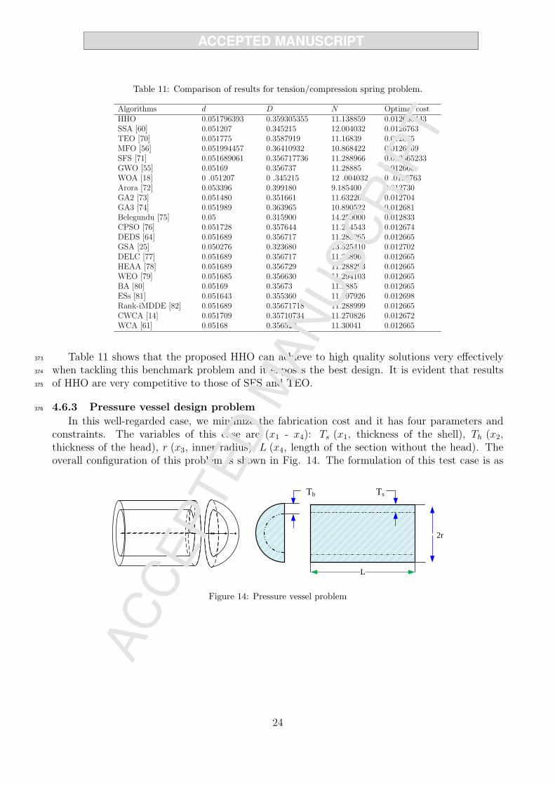
Table 11: Comparison of results for tension/compression spring problem.
Algorithms d D N Optimal costHHO 0.051796393 0.359305355 11.138859 0.012665443SSA [60] 0.051207 0.345215 12.004032 0.0126763TEO [70] 0.051775 0.3587919 11.16839 0.012665MFO [56] 0.051994457 0.36410932 10.868422 0.0126669SFS [71] 0.051689061 0.356717736 11.288966 0.012665233GWO [55] 0.05169 0.356737 11.28885 0.012666WOA [18] 0 .051207 0 .345215 12 .004032 0 .0126763Arora [72] 0.053396 0.399180 9.185400 0.012730GA2 [73] 0.051480 0.351661 11.632201 0.012704GA3 [74] 0.051989 0.363965 10.890522 0.012681Belegundu [75] 0.05 0.315900 14.250000 0.012833CPSO [76] 0.051728 0.357644 11.244543 0.012674DEDS [64] 0.051689 0.356717 11.288965 0.012665GSA [25] 0.050276 0.323680 13.525410 0.012702DELC [77] 0.051689 0.356717 11.288965 0.012665HEAA [78] 0.051689 0.356729 11.288293 0.012665WEO [79] 0.051685 0.356630 11.294103 0.012665BA [80] 0.05169 0.35673 11.2885 0.012665ESs [81] 0.051643 0.355360 11.397926 0.012698Rank-iMDDE [82] 0.051689 0.35671718 11.288999 0.012665CWCA [14] 0.051709 0.35710734 11.270826 0.012672WCA [61] 0.05168 0.356522 11.30041 0.012665
Table 11 shows that the proposed HHO can achieve to high quality solutions very effectively373
when tackling this benchmark problem and it exposes the best design. It is evident that results374
of HHO are very competitive to those of SFS and TEO.375
4.6.3 Pressure vessel design problem376
In this well-regarded case, we minimize the fabrication cost and it has four parameters andconstraints. The variables of this case are (x1 - x4): Ts (x1, thickness of the shell), Th (x2,thickness of the head), r (x3, inner radius), L (x4, length of the section without the head). Theoverall configuration of this problem is shown in Fig. 14. The formulation of this test case is as
L
Th Ts
2rB
O 1 OA
ABO
O1
B
BO 1 OA
ABO
O1
B
Figure 14: Pressure vessel problem
24
https://aliasgharheidari.com/HHO.html
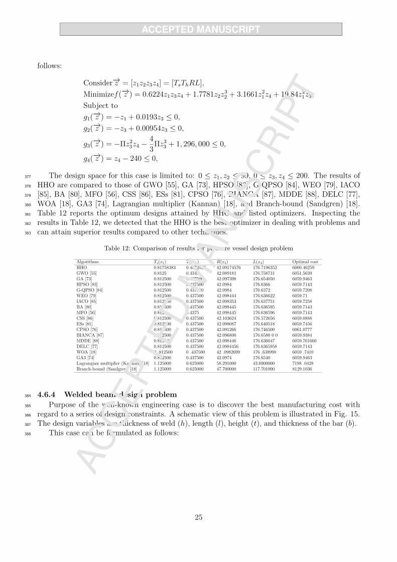
follows:
Consider−→z = [z1z2z3z4] = [TsThRL],
Minimizef(−→z ) = 0.6224z1z3z4 + 1.7781z2z32 + 3.1661z21z4 + 19.84z21z3,
Subject to
g1(−→z ) = −z1 + 0.0193z3 ≤ 0,
g2(−→z ) = −z3 + 0.00954z3 ≤ 0,
g3(−→z ) = −Πz23z4 −
4
3Πz33 + 1, 296, 000 ≤ 0,
g4(−→z ) = z4 − 240 ≤ 0,
The design space for this case is limited to: 0 ≤ z1, z2 ≤ 99, 0 ≤ z3, z4 ≤ 200. The results of377
HHO are compared to those of GWO [55], GA [73], HPSO [83], G-QPSO [84], WEO [79], IACO378
[85], BA [80], MFO [56], CSS [86], ESs [81], CPSO [76], BIANCA [87], MDDE [88], DELC [77],379
WOA [18], GA3 [74], Lagrangian multiplier (Kannan) [18], and Branch-bound (Sandgren) [18].380
Table 12 reports the optimum designs attained by HHO and listed optimizers. Inspecting the381
results in Table 12, we detected that the HHO is the best optimizer in dealing with problems and382
can attain superior results compared to other techniques.383
Table 12: Comparison of results for pressure vessel design problem
Algorithms Ts(x1) Th(x2) R(x3) L(x4) Optimal costHHO 0.81758383 0.4072927 42.09174576 176.7196352 6000.46259GWO [55] 0.8125 0.4345 42.089181 176.758731 6051.5639GA [73] 0.812500 0.437500 42.097398 176.654050 6059.9463HPSO [83] 0.812500 0.437500 42.0984 176.6366 6059.7143G-QPSO [84] 0.812500 0.437500 42.0984 176.6372 6059.7208WEO [79] 0.812500 0.437500 42.098444 176.636622 6059.71IACO [85] 0.812500 0.437500 42.098353 176.637751 6059.7258BA [80] 0.812500 0.437500 42.098445 176.636595 6059.7143MFO [56] 0.8125 0.4375 42.098445 176.636596 6059.7143CSS [86] 0.812500 0.437500 42.103624 176.572656 6059.0888ESs [81] 0.812500 0.437500 42.098087 176.640518 6059.7456CPSO [76] 0.812500 0.437500 42.091266 176.746500 6061.0777BIANCA [87] 0.812500 0.437500 42.096800 176.6580 0 0 6059.9384MDDE [88] 0.812500 0.437500 42.098446 176.636047 6059.701660DELC [77] 0.812500 0.437500 42.0984456 176.6365958 6059.7143WOA [18] 0 .812500 0 .437500 42 .0982699 176 .638998 6059 .7410GA3 [74] 0.812500 0.437500 42.0974 176.6540 6059.9463Lagrangian multiplier (Kannan) [18] 1.125000 0.625000 58.291000 43.6900000 7198 .0428Branch-bound (Sandgren) [18] 1.125000 0.625000 47.700000 117.701000 8129.1036
4.6.4 Welded beam design problem384
Purpose of the well-known engineering case is to discover the best manufacturing cost with385
regard to a series of design constraints. A schematic view of this problem is illustrated in Fig. 15.386
The design variables are thickness of weld (h), length (l), height (t), and thickness of the bar (b).387
This case can be formulated as follows:388
25
https://aliasgharheidari.com/HHO.html
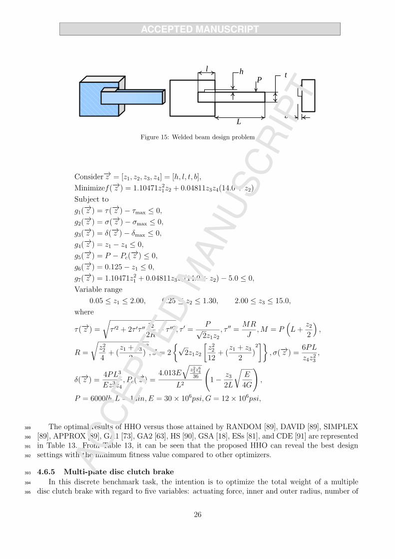
P
l h
L
t
b
Figure 15: Welded beam design problem
Consider−→z = [z1, z2, z3, z4] = [h, l, t, b],
Minimizef(−→z ) = 1.10471z21z2 + 0.04811z3z4(14.0 + z2),
Subject to
g1(−→z ) = τ(−→z )− τmax ≤ 0,
g2(−→z ) = σ(−→z )− σmax ≤ 0,
g3(−→z ) = δ(−→z )− δmax ≤ 0,
g4(−→z ) = z1 − z4 ≤ 0,
g5(−→z ) = P − Pc(
−→z ) ≤ 0,
g6(−→z ) = 0.125− z1 ≤ 0,
g7(−→z ) = 1.10471z21 + 0.04811z3z4(14.0 + z2)− 5.0 ≤ 0,
Variable range
0.05 ≤ z1 ≤ 2.00, 0.25 ≤ z2 ≤ 1.30, 2.00 ≤ z3 ≤ 15.0,
where
τ(−→z ) =√
τ ′2 + 2τ ′τ ′′z22R
+ τ ′′2, τ ′ =P√2z1z2
, τ ′′ =MR
J,M = P
(L+
z22
),
R =
√z224
+ (z1 + z3
2)2
, J = 2
{√2z1z2
[z2212
+ (z1 + z3
2)2]}
, σ(−→z ) = 6PL
z4z23,
δ(−→z ) = 4PL3
Ez33z4, Pc(
−→z ) =4.013E
√z23z
64
36
L2
(1− z3
2L
√E
4G
),
P = 6000lb, L = 14in, E = 30× 106psi,G = 12× 106psi,
The optimal results of HHO versus those attained by RANDOM [89], DAVID [89], SIMPLEX389
[89], APPROX [89], GA1 [73], GA2 [63], HS [90], GSA [18], ESs [81], and CDE [91] are represented390
in Table 13. From Table 13, it can be seen that the proposed HHO can reveal the best design391
settings with the minimum fitness value compared to other optimizers.392
4.6.5 Multi-plate disc clutch brake393
In this discrete benchmark task, the intention is to optimize the total weight of a multiple394
disc clutch brake with regard to five variables: actuating force, inner and outer radius, number of395
26
https://aliasgharheidari.com/HHO.html

Table 13: Comparison of results for welded beam design problem
Algorithm h l t b Optimal costHHO 0.204039 3.531061 9.027463 0.206147 1.73199057RANDOM [89] 0.4575 4.7313 5.0853 0.66 4.1185DAVID [89] 0.2434 6.2552 8.2915 0.2444 2.3841SIMPLEX [89] 0.2792 5.6256 7.7512 0.2796 2.5307APPROX [89] 0.24 4 4 6.2189 8.2915 0.2444 2.3815GA1 [73] 0.248900 6.173000 8.178900 0.253300 2.433116GA2 [63] 0.208800 3.420500 8.997500 0.210000 1.748310HS [90] 0.2442 6.2231 8.2915 0.2443 2.3807GSA [18] 0.182129 3.856979 10 0.202376 1.879952ESs [81] 0.199742 3.61206 9.0375 0.206082 1.7373CDE [91] 0.203137 3.542998 9.033498 0.206179 1.733462
friction surfaces, and thickness of discs [92].396
This problem has eight constraints according to the conditions of geometry and operating re-397
quirements. The feasible area for this case includes practically 70% of the solution space. However,398
there are few works that considered this problem in their tests. The optimal results of proposed399
HHO in compared to those revealed by TLBO [93], WCA [61], and PVS [92] algorithms. Table400
14 shows the attained results of different optimizers for this test case. From Table 14, we can401
recognize that the HHO attains the best rank and can outperform the well-known TLBO, WCA,402
and PVS in terms of quality of solutions.403
f(x) = Π(r2o − r2i )t(Z + 1)ρ
subject to:
g1(x) = ro − ri −∆r ≥ 0
g2(x) = lmax − (Z + 1)(t+ δ) ≥ 0
g3(x) = Pmax − Prz ≥ 0
g4(x) = Pmaxvsrmax − Przνsr ≥ 0
g5(x) = vsrmax − vsr ≥ 0
g6 = Tmax − T ≥ 0
g7(x) = Mh − sMs ≥ 0
g8(x) = T ≥ 0
where,
Mh =2
3µFZ
r3o − r2ir2o − r3i
, Prz =F
Π(r2o − r2i ),
vrz =2Πn(r3o − r3i )
90 (r2o − r2i ), T =
IzΠn
30(Mh +Mf )
∆r = 20mm, Iz = 55 kgmm2, Pmax = 1MPa, Fmax = 1000N,
Tmax = 15 s, µ = 0.5, s = 1.5, Ms = 40Nm, Mf = 3Nm, n = 250 rpm,
vsrmax = 10m/s, lmax = 30mm, rimin = 60, rimax = 80, romin = 90,
romax = 110, tmin = 1.5, tmax = 3, Fmin = 600, Fmax = 1000, Zmin = 2, Zmax = 9,
27
https://aliasgharheidari.com/HHO.html
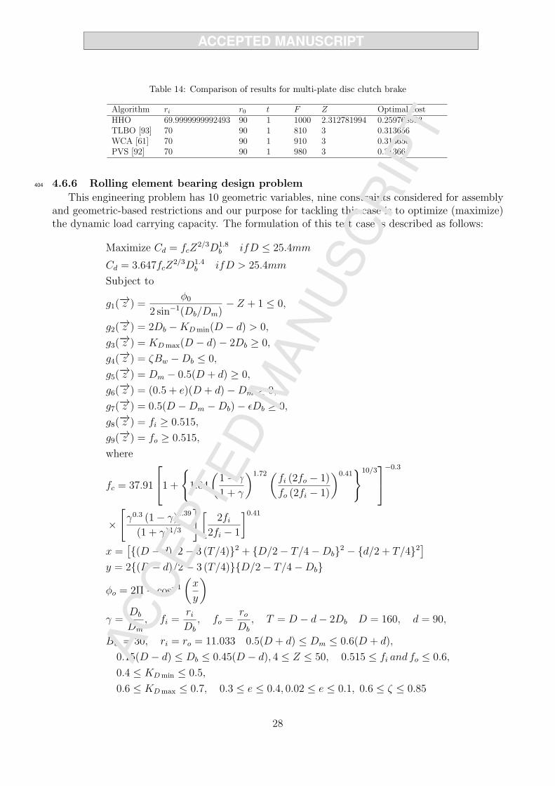
Table 14: Comparison of results for multi-plate disc clutch brake
Algorithm ri r0 t F Z Optimal costHHO 69.9999999992493 90 1 1000 2.312781994 0.259768993TLBO [93] 70 90 1 810 3 0.313656WCA [61] 70 90 1 910 3 0.313656PVS [92] 70 90 1 980 3 0.31366
4.6.6 Rolling element bearing design problem404
This engineering problem has 10 geometric variables, nine constraints considered for assemblyand geometric-based restrictions and our purpose for tackling this case is to optimize (maximize)the dynamic load carrying capacity. The formulation of this test case is described as follows:
Maximize Cd = fcZ2/3D1.8
b ifD ≤ 25.4mm
Cd = 3.647fcZ2/3D1.4
b ifD > 25.4mm
Subject to
g1(−→z ) = ϕ0
2 sin−1(Db/Dm)− Z + 1 ≤ 0,
g2(−→z ) = 2Db −KDmin(D − d) > 0,
g3(−→z ) = KDmax(D − d)− 2Db ≥ 0,
g4(−→z ) = ζBw −Db ≤ 0,
g5(−→z ) = Dm − 0.5(D + d) ≥ 0,
g6(−→z ) = (0.5 + e)(D + d)−Dm ≥ 0,
g7(−→z ) = 0.5(D −Dm −Db)− ϵDb ≥ 0,
g8(−→z ) = fi ≥ 0.515,
g9(−→z ) = fo ≥ 0.515,
where
fc = 37.91
1 +
{1.04
(1− γ
1 + γ
)1.72(fi (2fo − 1)
fo (2fi − 1)
)0.41}10/3
−0.3
×[γ0.3 (1− γ)1.39
(1 + γ)1/3
] [2fi
2fi − 1
]0.41
x =[{(D − d)/2− 3 (T/4)}2 + {D/2− T/4−Db}2 − {d/2 + T/4}2
]
y = 2{(D − d)/2− 3 (T/4)}{D/2− T/4−Db}
ϕo = 2Π− cos−1
(x
y
)
γ =Db
Dm
, fi =riDb
, fo =roDb
, T = D − d− 2Db D = 160, d = 90,
Bw = 30, ri = ro = 11.033 0.5(D + d) ≤ Dm ≤ 0.6(D + d),
0.15(D − d) ≤ Db ≤ 0.45(D − d), 4 ≤ Z ≤ 50, 0.515 ≤ fi and fo ≤ 0.6,
0.4 ≤ KDmin ≤ 0.5,
0.6 ≤ KDmax ≤ 0.7, 0.3 ≤ e ≤ 0.4, 0.02 ≤ e ≤ 0.1, 0.6 ≤ ζ ≤ 0.85
28
https://aliasgharheidari.com/HHO.html
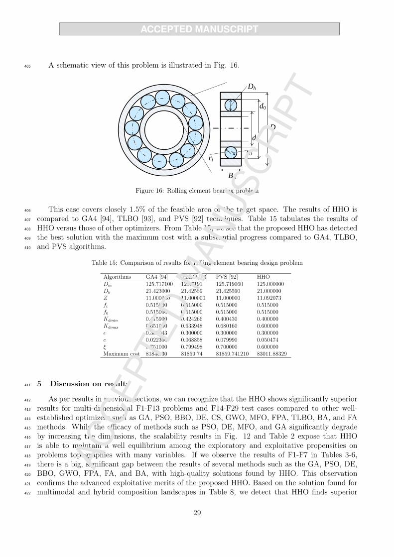
A schematic view of this problem is illustrated in Fig. 16.405
d0
d1
Dh
Bw
D
r0ri
Figure 16: Rolling element bearing problem
This case covers closely 1.5% of the feasible area of the target space. The results of HHO is406
compared to GA4 [94], TLBO [93], and PVS [92] techniques. Table 15 tabulates the results of407
HHO versus those of other optimizers. From Table 15, we see that the proposed HHO has detected408
the best solution with the maximum cost with a substantial progress compared to GA4, TLBO,409
and PVS algorithms.410
Table 15: Comparison of results for rolling element bearing design problem
Algorithms GA4 [94] TLBO [93] PVS [92] HHODm 125.717100 125.7191 125.719060 125.000000Db 21.423000 21.42559 21.425590 21.000000Z 11.000000 11.000000 11.000000 11.092073fi 0.515000 0.515000 0.515000 0.515000f0 0.515000 0.515000 0.515000 0.515000Kdmin 0.415900 0.424266 0.400430 0.400000Kdmax 0.651000 0.633948 0.680160 0.600000ϵ 0.300043 0.300000 0.300000 0.300000e 0.022300 0.068858 0.079990 0.050474ξ 0.751000 0.799498 0.700000 0.600000Maximum cost 81843.30 81859.74 81859.741210 83011.88329
5 Discussion on results411
As per results in previous sections, we can recognize that the HHO shows significantly superior412
results for multi-dimensional F1-F13 problems and F14-F29 test cases compared to other well-413
established optimizers such as GA, PSO, BBO, DE, CS, GWO, MFO, FPA, TLBO, BA, and FA414
methods. While the efficacy of methods such as PSO, DE, MFO, and GA significantly degrade415
by increasing the dimensions, the scalability results in Fig. 12 and Table 2 expose that HHO416
is able to maintain a well equilibrium among the exploratory and exploitative propensities on417
problems topographies with many variables. If we observe the results of F1-F7 in Tables 3-6,418
there is a big, significant gap between the results of several methods such as the GA, PSO, DE,419
BBO, GWO, FPA, FA, and BA, with high-quality solutions found by HHO. This observation420
confirms the advanced exploitative merits of the proposed HHO. Based on the solution found for421
multimodal and hybrid composition landscapes in Table 8, we detect that HHO finds superior422
29
https://aliasgharheidari.com/HHO.html
and competitive solutions based on a stable balance between the diversification and intensification423
inclinations and a smooth transition between the searching modes. The results also support the424
superior exploratory strengths of the HHO. The results for six well-known constrained cases in425
Tables 10-15 also disclose that HHO obtains the best solutions and it is one of the top optimizers426
compared to many state-of-the-art techniques. The results highlight that the proposed HHO has427
several exploratory and exploitative mechanisms and consequently, it has efficiently avoided LO428
and immature convergence drawbacks when solving different classes of problems and in the case429
of any LO stagnation, the proposed HHO has shown a higher potential in jumping out of local430
optimum solutions.431
The following features can theoretically assist us in realizing why the proposed HHO can be432
beneficial in exploring or exploiting the search space of a given optimization problem:433
• Escaping energy E parameter has a dynamic randomized time-varying nature, which can434
further boost the exploration and exploitation patterns of HHO. This factor also requires435
HHO to perform a smooth transition between exploration and exploitation.436
• Different diversification mechanisms with regard to the average location of hawks can boost437
the exploratory behavior of HHO in initial iterations.438
• Different LF-based patterns with short-length jumps enhance the exploitative behaviors of439
HHO when conducting a local search.440
• The progressive selection scheme assists search agents to progressively improve their position441
and only select a better position, which can improve the quality of solutions and intensifica-442
tion powers of HHO during the course of iterations.443
• HHO utilizes a series of searching strategies based on E and r parameters and then, it selects444
the best movement step. This capability has also a constructive impact on the exploitation445
potential of HHO.446
• The randomized jump J strength can assist candidate solutions in balancing the exploration447
and exploitation tendencies.448
• The use of adaptive and time-varying parameters allows HHO to handle difficulties of a449
search space including local optimal solutions, multi-modality, and deceptive optima.450
6 Conclusion and future directions451
In this work, a novel population-based optimization algorithm called HHO is proposed to452
tackle different optimization tasks. The proposed HHO is inspired by the cooperative behaviors453
and chasing styles of predatory birds, Harris’ hawks, in nature. Several equations are designed454
to simulate the social intelligence of Harris’ hawks to solve optimization problems. Twenty nine455
unconstrained benchmark problems were used to evaluate the performance of HHO. Exploitative,456
exploratory, and local optima avoidance of HHO was investigated using unimodal, multi-modal457
and composition problems. The results obtained show that HHO was capable of finding excellent458
solutions compared to other well-regarded optimizers. Additionally, the results of six constrained459
engineering design tasks also revealed that the HHO can show superior results compared to other460
optimizers.461
30
https://aliasgharheidari.com/HHO.html
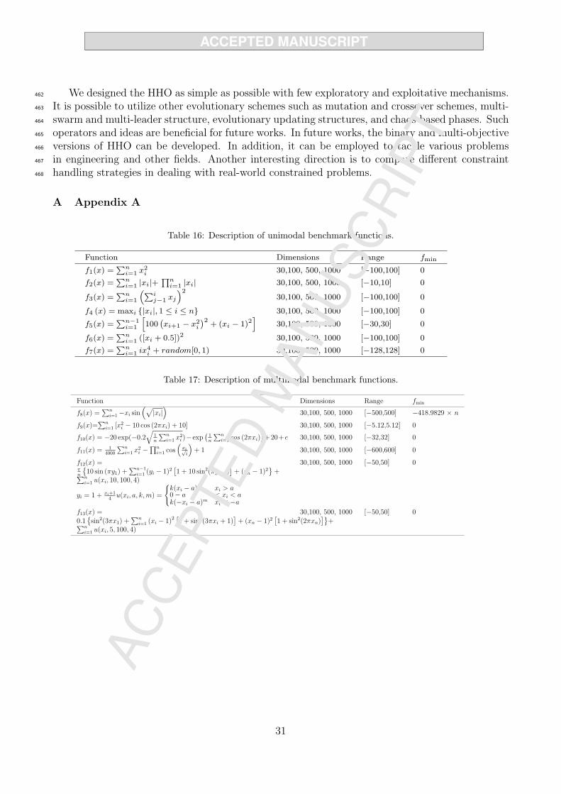
We designed the HHO as simple as possible with few exploratory and exploitative mechanisms.462
It is possible to utilize other evolutionary schemes such as mutation and crossover schemes, multi-463
swarm and multi-leader structure, evolutionary updating structures, and chaos-based phases. Such464
operators and ideas are beneficial for future works. In future works, the binary and multi-objective465
versions of HHO can be developed. In addition, it can be employed to tackle various problems466
in engineering and other fields. Another interesting direction is to compare different constraint467
handling strategies in dealing with real-world constrained problems.468
A Appendix A
Table 16: Description of unimodal benchmark functions.
Function Dimensions Range fmin
f1(x) =∑n
i=1 x2i 30,100, 500, 1000 [−100,100] 0
f2(x) =∑n
i=1 |xi|+∏n
i=1 |xi| 30,100, 500, 1000 [−10,10] 0
f3(x) =∑n
i=1
(∑ij−1 xj
)230,100, 500, 1000 [−100,100] 0
f4 (x) = maxi {|xi|, 1 ≤ i ≤ n} 30,100, 500, 1000 [−100,100] 0
f5(x) =∑n−1
i=1
[100
(xi+1 − x2
i
)2+ (xi − 1)2
]30,100, 500, 1000 [−30,30] 0
f6(x) =∑n
i=1 ([xi + 0.5])2 30,100, 500, 1000 [−100,100] 0
f7(x) =∑n
i=1 ix4i + random[0, 1) 30,100, 500, 1000 [−128,128] 0
Table 17: Description of multimodal benchmark functions.
Function Dimensions Range fmin
f8(x) =∑n
i=1−xi sin(√
|xi|)
30,100, 500, 1000 [−500,500] −418.9829 × n
f9(x)=∑n
i=1 [x2i − 10 cos (2πxi) + 10] 30,100, 500, 1000 [−5.12,5.12] 0
f10(x) = −20 exp(−0.2√
1n
∑ni=1 x
2i )−exp
(1n
∑ni=1 cos (2πxi)
)+20+e 30,100, 500, 1000 [−32,32] 0
f11(x) =1
4000
∑ni=1 x
2i −
∏ni=1 cos
(xi√i
)+ 1 30,100, 500, 1000 [−600,600] 0
f12(x) =πn
{10 sin (πy1) +
∑n−1i=1 (yi − 1)2
[1 + 10 sin2(πyi+1)
]+ (yn − 1)2
}+∑n
i=1 u(xi, 10, 100, 4)
yi = 1 + xi+14
u(xi, a, k,m) =
{k(xi − a)m xi > a0− a < xi < ak(−xi − a)m xi < −a
30,100, 500, 1000 [−50,50] 0
f13(x) =0.1{sin2(3πx1) +
∑ni=1 (xi − 1)2
[1 + sin2(3πxi + 1)
]+ (xn − 1)2
[1 + sin2(2πxn)
]}+∑n
i=1 u(xi, 5, 100, 4)
30,100, 500, 1000 [−50,50] 0
31
https://aliasgharheidari.com/HHO.html
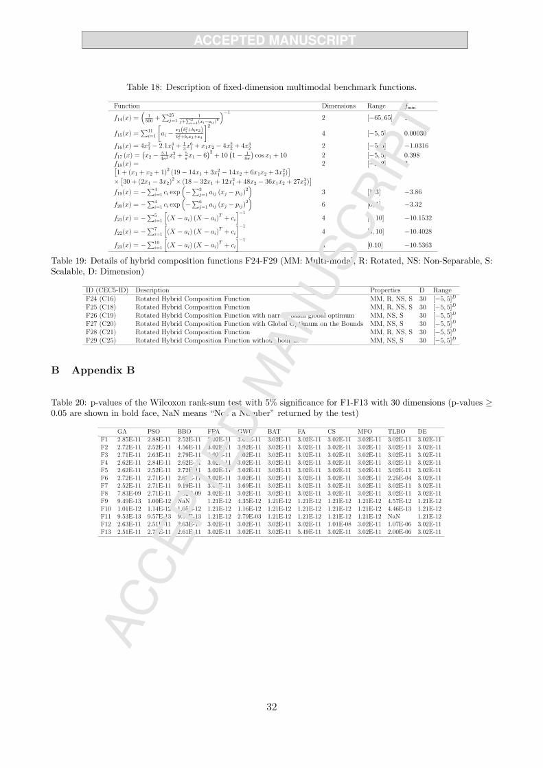
Table 18: Description of fixed-dimension multimodal benchmark functions.
Function Dimensions Range fmin
f14(x) =(
1500
+∑25
j=11
j+∑2
i=1(xi−aij)6
)−1
2 [−65, 65] 1
f15(x) =∑11
i=1
[ai −
x1(b2i+bix2)b2i+bix3+x4
]24 [−5, 5] 0.00030
f16(x) = 4x21 − 2.1x4
1 +13x61 + x1x2 − 4x2
2 + 4x42 2 [−5, 5] −1.0316
f17 (x) =(x2 − 5.1
4π2x21 +
5πx1 − 6
)2+ 10
(1− 1
8π
)cosx1 + 10 2 [−5, 5] 0.398
f18(x) =[1 + (x1 + x2 + 1)2 (19− 14x1 + 3x2
1 − 14x2 + 6x1x2 + 3x22)]
×[30 + (2x1 − 3x2)
2 × (18− 32x1 + 12x21 + 48x2 − 36x1x2 + 27x2
2)]
2 [−2, 2] 3
f19(x) = −∑4i=1 ci exp
(−∑3
j=1 aij (xj − pij)2)
3 [1, 3] −3.86
f20(x) = −∑4i=1 ci exp
(−∑6
j=1 aij (xj − pij)2)
6 [0, 1] −3.32
f21(x) = −∑5i=1
[(X − ai) (X − ai)
T + ci
]−1
4 [0, 10] −10.1532
f22(x) = −∑7i=1
[(X − ai) (X − ai)
T + ci
]−1
4 [0, 10] −10.4028
f23(x) = −∑10i=1
[(X − ai) (X − ai)
T + ci
]−1
4 [0.10] −10.5363
Table 19: Details of hybrid composition functions F24-F29 (MM: Multi-modal, R: Rotated, NS: Non-Separable, S:Scalable, D: Dimension)
ID (CEC5-ID) Description Properties D RangeF24 (C16) Rotated Hybrid Composition Function MM, R, NS, S 30 [−5, 5]D
F25 (C18) Rotated Hybrid Composition Function MM, R, NS, S 30 [−5, 5]D
F26 (C19) Rotated Hybrid Composition Function with narrow basin global optimum MM, NS, S 30 [−5, 5]D
F27 (C20) Rotated Hybrid Composition Function with Global Optimum on the Bounds MM, NS, S 30 [−5, 5]D
F28 (C21) Rotated Hybrid Composition Function MM, R, NS, S 30 [−5, 5]D
F29 (C25) Rotated Hybrid Composition Function without bounds MM, NS, S 30 [−5, 5]D
B Appendix B
Table 20: p-values of the Wilcoxon rank-sum test with 5% significance for F1-F13 with 30 dimensions (p-values ≥0.05 are shown in bold face, NaN means “Not a Number” returned by the test)
GA PSO BBO FPA GWO BAT FA CS MFO TLBO DEF1 2.85E-11 2.88E-11 2.52E-11 3.02E-11 3.02E-11 3.02E-11 3.02E-11 3.02E-11 3.02E-11 3.02E-11 3.02E-11F2 2.72E-11 2.52E-11 4.56E-11 3.02E-11 3.02E-11 3.02E-11 3.02E-11 3.02E-11 3.02E-11 3.02E-11 3.02E-11F3 2.71E-11 2.63E-11 2.79E-11 3.02E-11 3.02E-11 3.02E-11 3.02E-11 3.02E-11 3.02E-11 3.02E-11 3.02E-11F4 2.62E-11 2.84E-11 2.62E-11 3.02E-11 3.02E-11 3.02E-11 3.02E-11 3.02E-11 3.02E-11 3.02E-11 3.02E-11F5 2.62E-11 2.52E-11 2.72E-11 3.02E-11 3.02E-11 3.02E-11 3.02E-11 3.02E-11 3.02E-11 3.02E-11 3.02E-11F6 2.72E-11 2.71E-11 2.62E-11 3.02E-11 3.02E-11 3.02E-11 3.02E-11 3.02E-11 3.02E-11 2.25E-04 3.02E-11F7 2.52E-11 2.71E-11 9.19E-11 3.02E-11 3.69E-11 3.02E-11 3.02E-11 3.02E-11 3.02E-11 3.02E-11 3.02E-11F8 7.83E-09 2.71E-11 7.62E-09 3.02E-11 3.02E-11 3.02E-11 3.02E-11 3.02E-11 3.02E-11 3.02E-11 3.02E-11F9 9.49E-13 1.00E-12 NaN 1.21E-12 4.35E-12 1.21E-12 1.21E-12 1.21E-12 1.21E-12 4.57E-12 1.21E-12F10 1.01E-12 1.14E-12 1.05E-12 1.21E-12 1.16E-12 1.21E-12 1.21E-12 1.21E-12 1.21E-12 4.46E-13 1.21E-12F11 9.53E-13 9.57E-13 9.54E-13 1.21E-12 2.79E-03 1.21E-12 1.21E-12 1.21E-12 1.21E-12 NaN 1.21E-12F12 2.63E-11 2.51E-11 2.63E-11 3.02E-11 3.02E-11 3.02E-11 3.02E-11 1.01E-08 3.02E-11 1.07E-06 3.02E-11F13 2.51E-11 2.72E-11 2.61E-11 3.02E-11 3.02E-11 3.02E-11 5.49E-11 3.02E-11 3.02E-11 2.00E-06 3.02E-11
32
https://aliasgharheidari.com/HHO.html
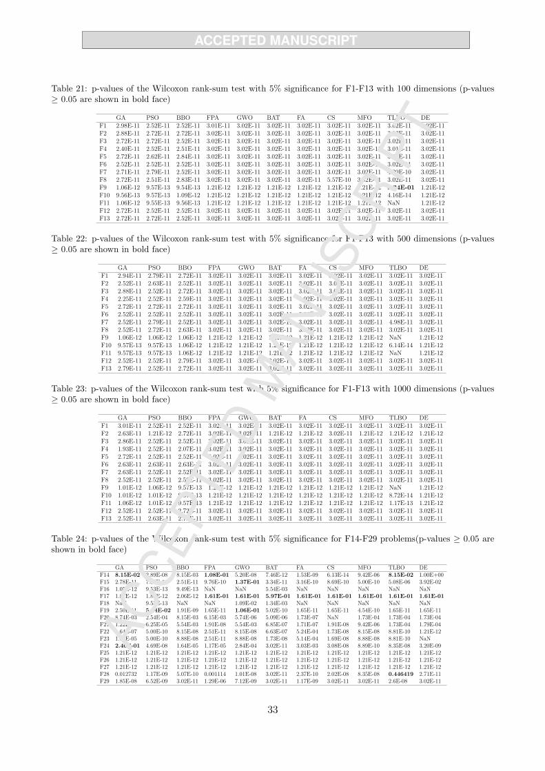
Table 21: p-values of the Wilcoxon rank-sum test with 5% significance for F1-F13 with 100 dimensions (p-values≥ 0.05 are shown in bold face)
GA PSO BBO FPA GWO BAT FA CS MFO TLBO DEF1 2.98E-11 2.52E-11 2.52E-11 3.01E-11 3.02E-11 3.02E-11 3.02E-11 3.02E-11 3.02E-11 3.02E-11 3.02E-11F2 2.88E-11 2.72E-11 2.72E-11 3.02E-11 3.02E-11 3.02E-11 3.02E-11 3.02E-11 3.02E-11 3.02E-11 3.02E-11F3 2.72E-11 2.72E-11 2.52E-11 3.02E-11 3.02E-11 3.02E-11 3.02E-11 3.02E-11 3.02E-11 3.02E-11 3.02E-11F4 2.40E-11 2.52E-11 2.51E-11 3.02E-11 3.02E-11 3.02E-11 3.02E-11 3.02E-11 3.02E-11 3.01E-11 3.02E-11F5 2.72E-11 2.62E-11 2.84E-11 3.02E-11 3.02E-11 3.02E-11 3.02E-11 3.02E-11 3.02E-11 3.02E-11 3.02E-11F6 2.52E-11 2.52E-11 2.52E-11 3.02E-11 3.02E-11 3.02E-11 3.02E-11 3.02E-11 3.02E-11 3.02E-11 3.02E-11F7 2.71E-11 2.79E-11 2.52E-11 3.02E-11 3.02E-11 3.02E-11 3.02E-11 3.02E-11 3.02E-11 4.20E-10 3.02E-11F8 2.72E-11 2.51E-11 2.83E-11 3.02E-11 3.02E-11 3.02E-11 3.02E-11 5.57E-10 3.02E-11 3.02E-11 3.02E-11F9 1.06E-12 9.57E-13 9.54E-13 1.21E-12 1.21E-12 1.21E-12 1.21E-12 1.21E-12 1.21E-12 3.34E-01 1.21E-12F10 9.56E-13 9.57E-13 1.09E-12 1.21E-12 1.21E-12 1.21E-12 1.21E-12 1.21E-12 1.21E-12 4.16E-14 1.21E-12F11 1.06E-12 9.55E-13 9.56E-13 1.21E-12 1.21E-12 1.21E-12 1.21E-12 1.21E-12 1.21E-12 NaN 1.21E-12F12 2.72E-11 2.52E-11 2.52E-11 3.02E-11 3.02E-11 3.02E-11 3.02E-11 3.02E-11 3.02E-11 3.02E-11 3.02E-11F13 2.72E-11 2.72E-11 2.52E-11 3.02E-11 3.02E-11 3.02E-11 3.02E-11 3.02E-11 3.02E-11 3.02E-11 3.02E-11
Table 22: p-values of the Wilcoxon rank-sum test with 5% significance for F1-F13 with 500 dimensions (p-values≥ 0.05 are shown in bold face)
GA PSO BBO FPA GWO BAT FA CS MFO TLBO DEF1 2.94E-11 2.79E-11 2.72E-11 3.02E-11 3.02E-11 3.02E-11 3.02E-11 3.02E-11 3.02E-11 3.02E-11 3.02E-11F2 2.52E-11 2.63E-11 2.52E-11 3.02E-11 3.02E-11 3.02E-11 3.02E-11 3.02E-11 3.02E-11 3.02E-11 3.02E-11F3 2.88E-11 2.52E-11 2.72E-11 3.02E-11 3.02E-11 3.02E-11 3.02E-11 3.02E-11 3.02E-11 3.02E-11 3.02E-11F4 2.25E-11 2.52E-11 2.59E-11 3.02E-11 3.02E-11 3.02E-11 3.02E-11 3.02E-11 3.02E-11 3.02E-11 3.02E-11F5 2.72E-11 2.72E-11 2.72E-11 3.02E-11 3.02E-11 3.02E-11 3.02E-11 3.02E-11 3.02E-11 3.02E-11 3.02E-11F6 2.52E-11 2.52E-11 2.52E-11 3.02E-11 3.02E-11 3.02E-11 3.02E-11 3.02E-11 3.02E-11 3.02E-11 3.02E-11F7 2.52E-11 2.79E-11 2.52E-11 3.02E-11 3.02E-11 3.02E-11 3.02E-11 3.02E-11 3.02E-11 4.98E-11 3.02E-11F8 2.52E-11 2.72E-11 2.63E-11 3.02E-11 3.02E-11 3.02E-11 3.02E-11 3.02E-11 3.02E-11 3.02E-11 3.02E-11F9 1.06E-12 1.06E-12 1.06E-12 1.21E-12 1.21E-12 1.21E-12 1.21E-12 1.21E-12 1.21E-12 NaN 1.21E-12F10 9.57E-13 9.57E-13 1.06E-12 1.21E-12 1.21E-12 1.21E-12 1.21E-12 1.21E-12 1.21E-12 6.14E-14 1.21E-12F11 9.57E-13 9.57E-13 1.06E-12 1.21E-12 1.21E-12 1.21E-12 1.21E-12 1.21E-12 1.21E-12 NaN 1.21E-12F12 2.52E-11 2.52E-11 2.79E-11 3.02E-11 3.02E-11 3.02E-11 3.02E-11 3.02E-11 3.02E-11 3.02E-11 3.02E-11F13 2.79E-11 2.52E-11 2.72E-11 3.02E-11 3.02E-11 3.02E-11 3.02E-11 3.02E-11 3.02E-11 3.02E-11 3.02E-11
Table 23: p-values of the Wilcoxon rank-sum test with 5% significance for F1-F13 with 1000 dimensions (p-values≥ 0.05 are shown in bold face)
GA PSO BBO FPA GWO BAT FA CS MFO TLBO DEF1 3.01E-11 2.52E-11 2.52E-11 3.02E-11 3.02E-11 3.02E-11 3.02E-11 3.02E-11 3.02E-11 3.02E-11 3.02E-11F2 2.63E-11 1.21E-12 2.72E-11 3.02E-11 3.02E-11 1.21E-12 1.21E-12 3.02E-11 1.21E-12 1.21E-12 1.21E-12F3 2.86E-11 2.52E-11 2.52E-11 3.02E-11 3.02E-11 3.02E-11 3.02E-11 3.02E-11 3.02E-11 3.02E-11 3.02E-11F4 1.93E-11 2.52E-11 2.07E-11 3.02E-11 3.02E-11 3.02E-11 3.02E-11 3.02E-11 3.02E-11 3.02E-11 3.02E-11F5 2.72E-11 2.52E-11 2.52E-11 3.02E-11 3.02E-11 3.02E-11 3.02E-11 3.02E-11 3.02E-11 3.02E-11 3.02E-11F6 2.63E-11 2.63E-11 2.63E-11 3.02E-11 3.02E-11 3.02E-11 3.02E-11 3.02E-11 3.02E-11 3.02E-11 3.02E-11F7 2.63E-11 2.52E-11 2.52E-11 3.02E-11 3.02E-11 3.02E-11 3.02E-11 3.02E-11 3.02E-11 3.02E-11 3.02E-11F8 2.52E-11 2.52E-11 2.52E-11 3.02E-11 3.02E-11 3.02E-11 3.02E-11 3.02E-11 3.02E-11 3.02E-11 3.02E-11F9 1.01E-12 1.06E-12 9.57E-13 1.21E-12 1.21E-12 1.21E-12 1.21E-12 1.21E-12 1.21E-12 NaN 1.21E-12F10 1.01E-12 1.01E-12 9.57E-13 1.21E-12 1.21E-12 1.21E-12 1.21E-12 1.21E-12 1.21E-12 8.72E-14 1.21E-12F11 1.06E-12 1.01E-12 9.57E-13 1.21E-12 1.21E-12 1.21E-12 1.21E-12 1.21E-12 1.21E-12 1.17E-13 1.21E-12F12 2.52E-11 2.52E-11 2.72E-11 3.02E-11 3.02E-11 3.02E-11 3.02E-11 3.02E-11 3.02E-11 3.02E-11 3.02E-11F13 2.52E-11 2.63E-11 2.72E-11 3.02E-11 3.02E-11 3.02E-11 3.02E-11 3.02E-11 3.02E-11 3.02E-11 3.02E-11
Table 24: p-values of the Wilcoxon rank-sum test with 5% significance for F14-F29 problems(p-values ≥ 0.05 areshown in bold face)
GA PSO BBO FPA GWO BAT FA CS MFO TLBO DEF14 8.15E-02 2.89E-08 8.15E-03 1.08E-01 5.20E-08 7.46E-12 1.53E-09 6.13E-14 9.42E-06 8.15E-02 1.00E+00F15 2.78E-11 7.37E-11 2.51E-11 9.76E-10 1.37E-01 3.34E-11 3.16E-10 8.69E-10 5.00E-10 5.08E-06 3.92E-02F16 1.05E-12 9.53E-13 9.49E-13 NaN NaN 5.54E-03 NaN NaN NaN NaN NaNF17 1.87E-12 1.89E-12 2.06E-12 1.61E-01 1.61E-01 5.97E-01 1.61E-01 1.61E-01 1.61E-01 1.61E-01 1.61E-01F18 NaN 9.53E-13 NaN NaN 1.09E-02 1.34E-03 NaN NaN NaN NaN NaNF19 2.50E-11 5.24E-02 1.91E-09 1.65E-11 1.06E-01 5.02E-10 1.65E-11 1.65E-11 4.54E-10 1.65E-11 1.65E-11F20 8.74E-03 2.54E-04 8.15E-03 6.15E-03 5.74E-06 5.09E-06 1.73E-07 NaN 1.73E-04 1.73E-04 1.73E-04F21 1.22E-04 6.25E-05 5.54E-03 1.91E-08 5.54E-03 6.85E-07 1.71E-07 1.91E-08 9.42E-06 1.73E-04 1.79E-04F22 1.64E-07 5.00E-10 8.15E-08 2.51E-11 8.15E-08 6.63E-07 5.24E-04 1.73E-08 8.15E-08 8.81E-10 1.21E-12F23 1.54E-05 5.00E-10 8.88E-08 2.51E-11 8.88E-08 1.73E-08 5.14E-04 1.69E-08 8.88E-08 8.81E-10 NaNF24 2.40E-01 4.69E-08 1.64E-05 1.17E-05 2.84E-04 3.02E-11 3.03E-03 3.08E-08 8.89E-10 8.35E-08 3.20E-09F25 1.21E-12 1.21E-12 1.21E-12 1.21E-12 1.21E-12 1.21E-12 1.21E-12 1.21E-12 1.21E-12 1.21E-12 1.21E-12F26 1.21E-12 1.21E-12 1.21E-12 1.21E-12 1.21E-12 1.21E-12 1.21E-12 1.21E-12 1.21E-12 1.21E-12 1.21E-12F27 1.21E-12 1.21E-12 1.21E-12 1.21E-12 1.21E-12 1.21E-12 1.21E-12 1.21E-12 1.21E-12 1.21E-12 1.21E-12F28 0.012732 1.17E-09 5.07E-10 0.001114 1.01E-08 3.02E-11 2.37E-10 2.02E-08 8.35E-08 0.446419 2.71E-11F29 1.85E-08 6.52E-09 3.02E-11 1.29E-06 7.12E-09 3.02E-11 1.17E-09 3.02E-11 3.02E-11 2.6E-08 3.02E-11
33
https://aliasgharheidari.com/HHO.html

Acknowledgments
This research is funded by Zhejiang Provincial Natural Science Foundation of China(LY17F020012), Science and Technology Plan Project of Wenzhou of China (ZG2017019).
We also acknowledge the comments of anonymous reviewers.
References
[1] R. Abbassi, A. Abbassi, A. A. Heidari, S. Mirjalili, An efficient salp swarm-inspired algorithm for parameters identification ofphotovoltaic cell models, Energy Conversion and Management 179 (2019) 362–372.
[2] H. Faris, A. M. Al-Zoubi, A. A. Heidari, I. Aljarah, M. Mafarja, M. A. Hassonah, H. Fujita, An intelligent system for spamdetection and identification of the most relevant features based on evolutionary random weight networks, Information Fusion 48(2019) 67 – 83.
[3] J. Nocedal, S. J. Wright, Numerical optimization 2nd, 2006.[4] G. Wu, Across neighborhood search for numerical optimization, Information Sciences 329 (2016) 597–618.[5] G. Wu, W. Pedrycz, P. N. Suganthan, R. Mallipeddi, A variable reduction strategy for evolutionary algorithms handling equality
constraints, Applied Soft Computing 37 (2015) 774–786.[6] J. Dreo, A. Petrowski, P. Siarry, E. Taillard, Metaheuristics for hard optimization: methods and case studies, Springer Science &
Business Media, 2006.[7] E.-G. Talbi, Metaheuristics: from design to implementation, volume 74, John Wiley & Sons, 2009.[8] S. Kirkpatrick, C. D. Gelatt, M. P. Vecchi, Optimization by simulated annealing, science 220 (1983) 671–680.[9] J. H. Holland, Genetic algorithms, Scientific american 267 (1992) 66–73.
[10] J. Luo, H. Chen, Y. Xu, H. Huang, X. Zhao, et al., An improved grasshopper optimization algorithm with application to financialstress prediction, Applied Mathematical Modelling 64 (2018) 654–668.
[11] M. Wang, H. Chen, B. Yang, X. Zhao, L. Hu, Z. Cai, H. Huang, C. Tong, Toward an optimal kernel extreme learning machineusing a chaotic moth-flame optimization strategy with applications in medical diagnoses, Neurocomputing 267 (2017) 69–84.
[12] L. Shen, H. Chen, Z. Yu, W. Kang, B. Zhang, H. Li, B. Yang, D. Liu, Evolving support vector machines using fruit fly optimizationfor medical data classification, Knowledge-Based Systems 96 (2016) 61–75.
[13] Q. Zhang, H. Chen, J. Luo, Y. Xu, C. Wu, C. Li, Chaos enhanced bacterial foraging optimization for global optimization, IEEEAccess (2018).
[14] A. A. Heidari, R. A. Abbaspour, A. R. Jordehi, An efficient chaotic water cycle algorithm for optimization tasks, Neural Computingand Applications 28 (2017) 57–85.
[15] M. Mafarja, I. Aljarah, A. A. Heidari, A. I. Hammouri, H. Faris, A.-Z. AlaM, S. Mirjalili, Evolutionary population dynamics andgrasshopper optimization approaches for feature selection problems, Knowledge-Based Systems 145 (2018) 25 – 45.
[16] M. Mafarja, I. Aljarah, A. A. Heidari, H. Faris, P. Fournier-Viger, X. Li, S. Mirjalili, Binary dragonfly optimization for featureselection using time-varying transfer functions, Knowledge-Based Systems 161 (2018) 185 – 204.
[17] I. Aljarah, M. Mafarja, A. A. Heidari, H. Faris, Y. Zhang, S. Mirjalili, Asynchronous accelerating multi-leader salp chains forfeature selection, Applied Soft Computing 71 (2018) 964–979.
[18] S. Mirjalili, A. Lewis, The whale optimization algorithm, Advances in Engineering Software 95 (2016) 51–67.[19] H. Faris, M. M. Mafarja, A. A. Heidari, I. Aljarah, A.-Z. AlaM, S. Mirjalili, H. Fujita, An efficient binary salp swarm algorithm
with crossover scheme for feature selection problems, Knowledge-Based Systems 154 (2018) 43–67.[20] J. R. Koza, Genetic Programming II, Automatic Discovery of Reusable Subprograms, MIT Press, Cambridge, MA, 1992.[21] R. Storn, K. Price, Differential evolution–a simple and efficient heuristic for global optimization over continuous spaces, Journal
of global optimization 11 (1997) 341–359.[22] D. Simon, Biogeography-based optimization, IEEE transactions on evolutionary computation 12 (2008) 702–713.[23] O. K. Erol, I. Eksin, A new optimization method: big bang–big crunch, Advances in Engineering Software 37 (2006) 106–111.[24] R. A. Formato, Central force optimization, progress in Electromagnetic Research77 (2007) 425–491.[25] E. Rashedi, H. Nezamabadi-Pour, S. Saryazdi, Gsa: a gravitational search algorithm, Information sciences 179 (2009) 2232–2248.[26] S. Salcedo-Sanz, Modern meta-heuristics based on nonlinear physics processes: A review of models and design procedures, Physics
Reports 655 (2016) 1–70.[27] F. Glover, Tabu searchpart i, ORSA Journal on computing 1 (1989) 190–206.[28] M. Kumar, A. J. Kulkarni, S. C. Satapathy, Socio evolution & learning optimization algorithm: A socio-inspired optimization
methodology, Future Generation Computer Systems 81 (2018) 252–272.[29] R. V. Rao, V. J. Savsani, D. Vakharia, Teaching–learning-based optimization: an optimization method for continuous non-linear
large scale problems, Information Sciences 183 (2012) 1–15.[30] A. Baykasoglu, F. B. Ozsoydan, Evolutionary and population-based methods versus constructive search strategies in dynamic
combinatorial optimization, Information Sciences 420 (2017) 159–183.[31] A. A. Heidari, H. Faris, I. Aljarah, S. Mirjalili, An efficient hybrid multilayer perceptron neural network with grasshopper
optimization, Soft Computing (2018) 1–18.[32] R. Eberhart, J. Kennedy, A new optimizer using particle swarm theory, in: Micro Machine and Human Science, 1995. MHS’95.,
Proceedings of the Sixth International Symposium on, IEEE, pp. 39–43.[33] M. Dorigo, V. Maniezzo, A. Colorni, Ant system: optimization by a colony of cooperating agents, IEEE Transactions on Systems,
Man, and Cybernetics, Part B (Cybernetics) 26 (1996) 29–41.[34] A. H. Gandomi, X.-S. Yang, A. H. Alavi, Cuckoo search algorithm: a metaheuristic approach to solve structural optimization
problems, Engineering with computers 29 (2013) 17–35.[35] X.-S. Yang, Review of meta-heuristics and generalised evolutionary walk algorithm, International Journal of Bio-Inspired Com-
putation 3 (2011) 77–84.
34
https://aliasgharheidari.com/HHO.html
[36] D. H. Wolpert, W. G. Macready, No free lunch theorems for optimization, IEEE transactions on evolutionary computation 1(1997) 67–82.
[37] J. C. Bednarz, Cooperative hunting in harris’ hawks (parabuteo unicinctus), Science 239 (1988) 1525.[38] L. Lefebvre, P. Whittle, E. Lascaris, A. Finkelstein, Feeding innovations and forebrain size in birds, Animal Behaviour 53 (1997)
549–560.[39] D. Sol, R. P. Duncan, T. M. Blackburn, P. Cassey, L. Lefebvre, Big brains, enhanced cognition, and response of birds to novel
environments, Proceedings of the National Academy of Sciences of the United States of America 102 (2005) 5460–5465.[40] F. Dubois, L.-A. Giraldeau, I. M. Hamilton, J. W. Grant, L. Lefebvre, Distraction sneakers decrease the expected level of aggression
within groups: a game-theoretic model, The American Naturalist 164 (2004) E32–E45.[41] EurekAlertAAAS, Bird iq test takes flight, 2005.[42] N. E. Humphries, N. Queiroz, J. R. Dyer, N. G. Pade, M. K. Musyl, K. M. Schaefer, D. W. Fuller, J. M. Brunnschweiler, T. K.
Doyle, J. D. Houghton, et al., Environmental context explains levy and brownian movement patterns of marine predators, Nature465 (2010) 1066–1069.
[43] G. M. Viswanathan, V. Afanasyev, S. Buldyrev, E. Murphy, P. Prince, H. E. Stanley, Levy flight search patterns of wanderingalbatrosses, Nature 381 (1996) 413.
[44] D. W. Sims, E. J. Southall, N. E. Humphries, G. C. Hays, C. J. Bradshaw, J. W. Pitchford, A. James, M. Z. Ahmed, A. S.Brierley, M. A. Hindell, et al., Scaling laws of marine predator search behaviour, Nature 451 (2008) 1098–1102.
[45] A. O. Gautestad, I. Mysterud, Complex animal distribution and abundance from memory-dependent kinetics, ecological complexity3 (2006) 44–55.
[46] M. F. Shlesinger, Levy flights: Variations on a theme, Physica D: Nonlinear Phenomena 38 (1989) 304–309.[47] G. Viswanathan, V. Afanasyev, S. V. Buldyrev, S. Havlin, M. Da Luz, E. Raposo, H. E. Stanley, Levy flights in random searches,
Physica A: Statistical Mechanics and its Applications 282 (2000) 1–12.[48] X.-S. Yang, Nature-inspired metaheuristic algorithms, Luniver press, 2010.[49] X. Yao, Y. Liu, G. Lin, Evolutionary programming made faster, IEEE Transactions on Evolutionary computation 3 (1999) 82–102.[50] J. G. Digalakis, K. G. Margaritis, On benchmarking functions for genetic algorithms, International journal of computer mathe-
matics 77 (2001) 481–506.[51] S. Garcıa, D. Molina, M. Lozano, F. Herrera, A study on the use of non-parametric tests for analyzing the evolutionary algorithms
behaviour: a case study on the cec2005 special session on real parameter optimization, Journal of Heuristics 15 (2009) 617.[52] X.-S. Yang, A. Hossein Gandomi, Bat algorithm: a novel approach for global engineering optimization, Engineering Computations
29 (2012) 464–483.[53] X.-S. Yang, M. Karamanoglu, X. He, Flower pollination algorithm: a novel approach for multiobjective optimization, Engineering
Optimization 46 (2014) 1222–1237.[54] A. H. Gandomi, X.-S. Yang, A. H. Alavi, Mixed variable structural optimization using firefly algorithm, Computers & Structures
89 (2011) 2325–2336.[55] S. Mirjalili, S. M. Mirjalili, A. Lewis, Grey wolf optimizer, Advances in Engineering Software 69 (2014) 46–61.[56] S. Mirjalili, Moth-flame optimization algorithm: A novel nature-inspired heuristic paradigm, Knowledge-Based Systems 89 (2015)
228–249.[57] J. Derrac, S. Garcıa, D. Molina, F. Herrera, A practical tutorial on the use of nonparametric statistical tests as a methodology
for comparing evolutionary and swarm intelligence algorithms, Swarm and Evolutionary Computation 1 (2011) 3–18.[58] X.-S. Yang, Firefly algorithm, stochastic test functions and design optimisation, International Journal of Bio-Inspired Computation
2 (2010) 78–84.[59] F. Van Den Bergh, A. P. Engelbrecht, A study of particle swarm optimization particle trajectories, Information sciences 176
(2006) 937–971.[60] S. Mirjalili, A. H. Gandomi, S. Z. Mirjalili, S. Saremi, H. Faris, S. M. Mirjalili, Salp swarm algorithm: A bio-inspired optimizer
for engineering design problems, Advances in Engineering Software (2017).[61] H. Eskandar, A. Sadollah, A. Bahreininejad, M. Hamdi, Water cycle algorithm–a novel metaheuristic optimization method for
solving constrained engineering optimization problems, Computers & Structures 110 (2012) 151–166.[62] S. Saremi, S. Mirjalili, A. Lewis, Grasshopper optimisation algorithm: Theory and application, Advances in Engineering Software
105 (2017) 30–47.[63] C. A. C. Coello, Use of a self-adaptive penalty approach for engineering optimization problems, Computers in Industry 41 (2000)
113–127.[64] M. Zhang, W. Luo, X. Wang, Differential evolution with dynamic stochastic selection for constrained optimization, Information
Sciences 178 (2008) 3043–3074.[65] S. Mirjalili, S. M. Mirjalili, A. Hatamlou, Multi-verse optimizer: a nature-inspired algorithm for global optimization, Neural
Computing and Applications 27 (2016) 495–513.[66] H. Liu, Z. Cai, Y. Wang, Hybridizing particle swarm optimization with differential evolution for constrained numerical and
engineering optimization, Applied Soft Computing 10 (2010) 629–640.[67] A. Sadollah, A. Bahreininejad, H. Eskandar, M. Hamdi, Mine blast algorithm: A new population based algorithm for solving
constrained engineering optimization problems, Applied Soft Computing 13 (2013) 2592–2612.[68] J.-F. Tsai, Global optimization of nonlinear fractional programming problems in engineering design, Engineering Optimization
37 (2005) 399–409.[69] T. Ray, P. Saini, Engineering design optimization using a swarm with an intelligent information sharing among individuals,
Engineering Optimization 33 (2001) 735–748.[70] A. Kaveh, A. Dadras, A novel meta-heuristic optimization algorithm: Thermal exchange optimization, Advances in Engineering
Software 110 (2017) 69 – 84.[71] H. Salimi, Stochastic fractal search: a powerful metaheuristic algorithm, Knowledge-Based Systems 75 (2015) 1–18.[72] J. S. Arora, Introduction to optimum design, 1989, McGraw-Mill Book Company (1967).[73] K. Deb, Optimal design of a welded beam via genetic algorithms, AIAA journal 29 (1991) 2013–2015.[74] C. A. C. Coello, E. M. Montes, Constraint-handling in genetic algorithms through the use of dominance-based tournament
selection, Advanced Engineering Informatics 16 (2002) 193–203.
35
https://aliasgharheidari.com/HHO.html
[75] A. D. Belegundu, J. S. Arora, A study of mathematical programming methods for structural optimization. part i: Theory,International Journal for Numerical Methods in Engineering 21 (1985) 1583–1599.
[76] Q. He, L. Wang, An effective co-evolutionary particle swarm optimization for constrained engineering design problems, EngineeringApplications of Artificial Intelligence 20 (2007) 89–99.
[77] L. Wang, L.-p. Li, An effective differential evolution with level comparison for constrained engineering design, Structural andMultidisciplinary Optimization 41 (2010) 947–963.
[78] Y. Wang, Z. Cai, Y. Zhou, Z. Fan, Constrained optimization based on hybrid evolutionary algorithm and adaptive constraint-handling technique, Structural and Multidisciplinary Optimization 37 (2009) 395–413.
[79] A. Kaveh, T. Bakhshpoori, Water evaporation optimization: a novel physically inspired optimization algorithm, Computers &Structures 167 (2016) 69–85.
[80] A. H. Gandomi, X.-S. Yang, A. H. Alavi, S. Talatahari, Bat algorithm for constrained optimization tasks, Neural Computing andApplications 22 (2013) 1239–1255.
[81] E. Mezura-Montes, C. A. C. Coello, A simple multimembered evolution strategy to solve constrained optimization problems,IEEE Transactions on Evolutionary computation 9 (2005) 1–17.
[82] W. Gong, Z. Cai, D. Liang, Engineering optimization by means of an improved constrained differential evolution, ComputerMethods in Applied Mechanics and Engineering 268 (2014) 884–904.
[83] Q. He, L. Wang, A hybrid particle swarm optimization with a feasibility-based rule for constrained optimization, Appliedmathematics and computation 186 (2007) 1407–1422.
[84] L. dos Santos Coelho, Gaussian quantum-behaved particle swarm optimization approaches for constrained engineering designproblems, Expert Systems with Applications 37 (2010) 1676–1683.
[85] H. Rosenbrock, An automatic method for finding the greatest or least value of a function, The Computer Journal 3 (1960)175–184.
[86] A. Kaveh, S. Talatahari, A novel heuristic optimization method: charged system search, Acta Mechanica 213 (2010) 267–289.[87] M. Montemurro, A. Vincenti, P. Vannucci, The automatic dynamic penalisation method (adp) for handling constraints with
genetic algorithms, Computer Methods in Applied Mechanics and Engineering 256 (2013) 70–87.[88] E. Mezura-Montes, C. Coello Coello, J. Velazquez-Reyes, L. Munoz-Davila, Multiple trial vectors in differential evolution for
engineering design, Engineering Optimization 39 (2007) 567–589.[89] K. Ragsdell, D. Phillips, Optimal design of a class of welded structures using geometric programming, Journal of Engineering for
Industry 98 (1976) 1021–1025.[90] K. S. Lee, Z. W. Geem, A new structural optimization method based on the harmony search algorithm, Computers & structures
82 (2004) 781–798.[91] F.-z. Huang, L. Wang, Q. He, An effective co-evolutionary differential evolution for constrained optimization, Applied Mathematics
and computation 186 (2007) 340–356.[92] P. Savsani, V. Savsani, Passing vehicle search (pvs): A novel metaheuristic algorithm, Applied Mathematical Modelling 40 (2016)
3951–3978.[93] R. V. Rao, V. J. Savsani, D. Vakharia, Teaching–learning-based optimization: a novel method for constrained mechanical design
optimization problems, Computer-Aided Design 43 (2011) 303–315.[94] S. Gupta, R. Tiwari, S. B. Nair, Multi-objective design optimisation of rolling bearings using genetic algorithms, Mechanism and
Machine Theory 42 (2007) 1418–1443.
36
View publication statsView publication stats
https://aliasgharheidari.com/HHO.html