fundamentals of plasma physics - paul m
TRANSCRIPT

Fundamentals of Plasma Physics
Paul M. Bellan

to my parents


Contents
Preface xi
1 Basic concepts 11.1 History of the term “plasma” 11.2 Brief history of plasma physics 11.3 Plasma parameters 31.4 Examples of plasmas 31.5 Logical framework of plasma physics 41.6 Debye shielding 71.7 Quasi-neutrality 91.8 Small v. large angle collisions in plasmas 111.9 Electron and ion collision frequencies 141.10 Collisions with neutrals 161.11 Simple transport phenomena 171.12 A quantitative perspective 201.13 Assignments 22
2 Derivation of fluid equations: Vlasov, 2-fluid, MHD 302.1 Phase-space 302.2 Distribution function and Vlasov equation 312.3 Moments of the distribution function 332.4 Two-fluid equations 362.5 Magnetohydrodynamic equations 462.6 Summary of MHD equations 522.7 Sheath physics and Langmuir probe theory 532.8 Assignments 58
3 Motion of a single plasma particle 623.1 Motivation 623.2 Hamilton-Lagrange formalism v. Lorentz equation 623.3 Adiabatic invariant of a pendulum 663.4 Extension of WKB method to general adiabatic invariant 683.5 Drift equations 733.6 Relation of Drift Equations to the Double Adiabatic MHD Equations 913.7 Non-adiabatic motion in symmetric geometry 953.8 Motion in small-amplitude oscillatory fields 1083.9 Wave-particle energy transfer 1103.10 Assignments 119

viii
4 Elementary plasma waves 1234.1 General method for analyzing small amplitude waves 1234.2 Two-fluid theory of unmagnetized plasma waves 1244.3 Low frequency magnetized plasma: Alfvén waves 1314.4 Two-fluid model of Alfvén modes 1384.5 Assignments 147
5 Streaming instabilities and the Landau problem 1495.1 Streaming instabilities 1495.2 The Landau problem 1535.3 The Penrose criterion 1725.4 Assignments 175
6 Cold plasma waves in a magnetized plasma 1786.1 Redundancy of Poisson’s equation in electromagnetic mode analysis 1786.2 Dielectric tensor 1796.3 Dispersion relation expressed as a relation betweenn2
x andn2z 193
6.4 A journey through parameter space 1956.5 High frequency waves: Altar-Appleton-Hartree dispersion relation 1976.6 Group velocity 2016.7 Quasi-electrostatic cold plasma waves 2036.8 Resonance cones 2046.9 Assignments 208
7 Waves in inhomogeneous plasmas and wave energy relations 2107.1 Wave propagation in inhomogeneous plasmas 2107.2 Geometric optics 2137.3 Surface waves - the plasma-filled waveguide 2147.4 Plasma wave-energy equation 2197.5 Cold-plasma wave energy equation 2217.6 Finite-temperature plasma wave energy equation 2247.7 Negative energy waves 2257.8 Assignments 228
8 Vlasov theory of warm electrostatic waves in a magnetized plasma 2298.1 Uniform plasma 2298.2 Analysis of the warm plasma electrostatic dispersion relation 2348.3 Bernstein waves 2368.4 Warm, magnetized, electrostatic dispersion with small, but finitek‖ 2398.5 Analysis of linear mode conversion 2418.6 Drift waves 2498.7 Assignments 263
9 MHD equilibria 2649.1 Why use MHD? 2649.2 Vacuum magnetic fields 265

ix
9.3 Force-free fields 2689.4 Magnetic pressure and tension 2689.5 Magnetic stress tensor 2719.6 Flux preservation, energy minimization, and inductance 2729.7 Static versus dynamic equilibria 2749.8 Static equilibria 2759.9 Dynamic equilibria:flows 2869.10 Assignments 295
10 Stability of static MHD equilibria 29810.1 The Rayleigh-Taylor instability of hydrodynamics 29910.2 MHD Rayleigh-Taylor instability 30210.3 The MHD energy principle 30610.4 Discussion of the energy principle 31910.5 Current-driven instabilities and helicity 31910.6 Magnetic helicity 32010.7 Qualitative description of free-boundary instabilities 32310.8 Analysis of free-boundary instabilities 32610.9 Assignments 334
11 Magnetic helicity interpreted and Woltjer-Taylor relaxation 33611.1 Introduction 33611.2 Topological interpretation of magnetic helicity 33611.3 Woltjer-Taylor relaxation 34111.4 Kinking and magnetic helicity 34511.5 Assignments 357
12 Magnetic reconnection 36012.1 Introduction 36012.2 Water-beading: an analogy to magnetic tearing and reconnection 36112.3 Qualitative description of sheet current instability 36212.4 Semi-quantitative estimate of the tearing process 36412.5 Generalization of tearing to sheared magnetic fields 37112.6 Magnetic islands 37612.7 Assignments 378
13 Fokker-Planck theory of collisions 38213.1 Introduction 38213.2 Statistical argument for the development of the Fokker-Planck equation 38413.3 Electrical resistivity 39313.4 Runaway electric field 39513.5 Assignments 395
14 Wave-particle nonlinearities 39814.1 Introduction 39814.2 Vlasov non-linearity and quasi-linear velocity space diffusion 399

x
14.3 Echoes 41214.4 Assignments 426
15 Wave-wave nonlinearities 42815.1 Introduction 42815.2 Manley-Rowe relations 43015.3 Application to waves 43515.4 Non-linear dispersion formulation and instability threshold 44415.5 Digging a hole in the plasma via ponderomotive force 44815.6 Ion acoustic wave soliton 45415.7 Assignments 457
16 Non-neutral plasmas 46016.1 Introduction 46016.2 Brillouinflow 46016.3 Isomorphism to incompressible 2D hydrodynamics 46316.4 Near perfect confinement 46416.5 Diocotron modes 46516.6 Assignments 476
17 Dusty plasmas 48317.1 Introduction 48317.2 Electron and ion currentflow to a dust grain 48417.3 Dust charge 48617.4 Dusty plasma parameter space 49017.5 LargeP limit: dust acoustic waves 49117.6 Dust ion acoustic waves 49417.7 The strongly coupled regime: crystallization of a dusty plasma 49517.8 Assignments 504
Bibliography and suggested reading 507
References 509
Appendix A: Intuitive method for vector calculus identities 515
Appendix B: Vector calculus in orthogonal curvilinear coordinates 518
Appendix C: Frequently used physical constants and formulae 524
Index 528

Preface
This text is based on a course I have taught for many years to first year graduate andsenior-level undergraduate students at Caltech. One outcome of this teaching has been therealization that although students typically decide to study plasma physics as a means to-wards some larger goal, they often conclude that this study has an attraction and charmof its own; in a sense the journey becomes as enjoyable as the destination. This conclu-sion is shared by me and I feel that a delightful aspect of plasma physics is thefrequenttransferability of ideas between extremely different applications so,for example, a conceptdeveloped in the context of astrophysics might suddenly become relevant to fusion researchor vice versa.
Applications of plasma physics are many and varied. Examples include controlled fu-sion research, ionospheric physics, magnetospheric physics, solar physics,astrophysics,plasma propulsion, semiconductor processing, and metals processing. Because plasmaphysics is rich in both concepts and regimes, it has also often served asan incubator fornew ideas in applied mathematics. In recent years there has been an increased dialog re-garding plasma physics among the various disciplines listed above and it is my hope thatthis text will help to promote this trend.
The prerequisites for this text are a reasonable familiarity with Maxwell’s equa-tions, classical mechanics, vector algebra, vector calculus, differential equations, and com-plex variables – i.e., the contents of a typical undergraduate physics or engineering cur-riculum. Experience has shown that because of the many different applications for plasmaphysics, students studying plasma physics have a diversity of preparation and not all areproficient in all prerequisites. Brief derivations of many basic concepts are included to ac-commodate this range of preparation; these derivations are intended to assist those studentswho may have had little or no exposure to the concept in question and to refresh the mem-ory of other students. For example, rather than just invoke Hamilton-Lagrange methods orLaplace transforms, there is a quick derivation and then a considerable discussion showinghow these concepts relate to plasma physics issues. These additional explanations makethe book more self-contained and also provide a close contact with first principles.
The order of presentation and level of rigor have been chosen to establish a firmfoundation and yet avoid unnecessary mathematical formalism or abstraction. In particular,the variousfluid equations are derived from first principles rather than simply invoked andthe consequences of the Hamiltonian nature of particle motion are emphasized early onand shown to lead to the powerful concepts of symmetry-induced constraint and adiabaticinvariance. Symmetry turns out to be an essential feature of magnetohydrodynamic plasmaconfinement and adiabatic invariance turns out to be not only essential for understandingmany types of particle motion, but also vital to many aspects of wave behavior.
The mathematical derivations have been presented with intermediate steps shownin as much detail as is reasonably possible. This occasionally leads to daunting-lookingexpressions, but it is my belief that it is preferable to see all the details rather than havethem glossed over and then justified by an “it can be shown" statement.
xi

xii Preface
The book is organized as follows: Chapters 1-3 lay out the foundation of the subject.Chapter 1 provides a brief introduction and overview of applications, discusses the logicalframework of plasma physics, and begins the presentation by discussing Debyeshieldingand then showing that plasmas are quasi-neutral and nearly collisionless. Chapter 2 intro-duces phase-space concepts and derives the Vlasov equation and then, by taking momentsof the Vlasov equation, derives the two-fluid and magnetohydrodynamic systems of equa-tions. Chapter 2 also introduces the dichotomy between adiabatic and isothermal behaviorwhich is a fundamental and recurrent theme in plasma physics. Chapter 3 considers plas-mas from the point of view of the behavior of a single particle and develops both exactand approximate descriptions for particle motion. In particular, Chapter3 includes a de-tailed discussion of the concept of adiabatic invariance with the aim of demonstrating thatthis important concept is a fundamental property of all nearly periodic Hamiltonian sys-tems and so does not have to be explained anew each time it is encountered ina differentsituation. Chapter 3 also includes a discussion of particle motion in fixedfrequency oscil-latory fields; this discussion provides a foundation for later analysis of cold plasma wavesand wave-particle energy transfer in warm plasma waves.
Chapters 4-8 discuss plasma waves; these are not only important in many practical sit-uations, but also provide an excellent way for developing insight about plasma dynamics.Chapter 4 shows how linear wave dispersion relations can be deduced from systems of par-tial differential equations characterizing a physical system and thenpresents derivations forthe elementary plasma waves, namely Langmuir waves, electromagnetic plasma waves, ionacoustic waves, and Alfvén waves. The beginning of Chapter 5 shows that when a plasmacontains groups of particles streaming at different velocities, freeenergy exists which candrive an instability; the remainder of Chapter 5 then presents Landau damping and instabil-ity theory which reveals that surprisingly strong interactions between waves and particlescan lead to either wave damping or wave instability depending on the shape of the velocitydistribution of the particles. Chapter 6 describes cold plasma waves in abackground mag-netic field and discusses the Clemmow-Mullaly-Allis diagram, an elegant categorizationscheme for the large number of qualitatively different types of cold plasma waves that existin a magnetized plasma. Chapter 7 discusses certain additional subtleand practical aspectsof wave propagation including propagation in an inhomogeneous plasma and how the en-ergy content of a wave is related to its dispersion relation. Chapter 8 begins by showingthat the combination of warm plasma effects and a background magnetic fieldleads to theexistence of the Bernstein wave, an altogether different kind of wave which has an infinitenumber of branches, and shows how a cold plasma wave can ‘mode convert’ into a Bern-stein wave in an inhomogeneous plasma. Chapter 8 concludes with a discussion of driftwaves, ubiquitous low frequency waves which have important deleterious consequencesfor magnetic confinement.
Chapters 9-12 provide a description of plasmas from the magnetohydrodynamicpointof view. Chapter 9 begins by presenting several basic magnetohydrodynamic concepts(vacuum and force-free fields, magnetic pressure and tension, frozen-influx, and energyminimization) and then uses these concepts to develop an intuitive understanding for dy-namic behavior. Chapter 9 then discusses magnetohydrodynamic equilibria and derives theGrad-Shafranov equation, an equation which depends on the existence of symmetry andwhich characterizes three-dimensional magnetohydrodynamic equilibria. Chapter 9 ends
Preface xiii
with a discussion on magnetohydrodynamicflows such as occur in arcs and jets. Chap-ter 10 examines the stability of perfectly conducting (i.e., ideal) magnetohydrodynamicequilibria, derives the ‘energy principle’ method for analyzing stability, discusses kink andsausage instabilities, and introduces the concepts of magnetic helicity and force-free equi-libria. Chapter 11 examines magnetic helicity from a topological point of view and showshow helicity conservation and energy minimization leads to the Woltjer-Taylor model formagnetohydrodynamic self-organization. Chapter 12 departs from the ideal models pre-sented earlier and discusses magnetic reconnection, a non-ideal behavior which permitsthe magnetohydrodynamic plasma to alter its topology and thereby relax to a minimum-energy state.
Chapters 13-17 consist of various advanced topics. Chapter 13 considers collisionsfrom a Fokker-Planck point of view and is essentially a revisiting of the issues in Chapter1 using a more sophisticated point of view; the Fokker-Planck model is used to derive amore accurate model for plasma electrical resistivity and also toshow the failure of Ohm’slaw when the electric field exceeds a critical value called the Dreicer limit. Chapter 14considers two manifestations of wave-particle nonlinearity: (i) quasi-linear velocity spacediffusion due to weak turbulence and (ii) echoes, non-linear phenomena whichvalidate theconcepts underlying Landau damping. Chapter 15 discusses how nonlinear interactions en-able energy and momentum to be transferred between waves, categorizesthe large numberof such wave-wave nonlinear interactions, and shows how these various interactions are allbased on a few fundamental concepts. Chapter 16 discusses one-component plasmas (pureelectron or pure ion plasmas) and shows how these plasmas have behaviors differing fromconventional two-component, electron-ion plasmas. Chapter 17 discusses dusty plasmaswhich are three component plasmas (electrons, ions, and dust grains) and showshow theaddition of a third component also introduces new behaviors, including the possibility ofthe dusty plasma condensing into a crystal. The analysis of condensation involves revisit-ing the Debye shielding concept and so corresponds, in a sense to having the bookend onthe same note it started on.
I would like to extend my grateful appreciation to Professor Michael Brown atSwarthmore College for providing helpful feedback obtained from using a draft version ina seminar course at Swarthmore and to Professor Roy Gould at Caltech for providing usefulsuggestions. I would also like to thank graduate students Deepak Kumar and GunsuYun forcarefully scrutinizing the final drafts of the manuscript and pointing out both ambiguitiesin presentation and typographical errors. I would also like to thank the many students who,over the years, provided useful feedback on earlier drafts of this workwhen it was in theform of lecture notes. Finally, I would like to acknowledge and thank my ownmentors andcolleagues who have introduced me to the many fascinating ideas constitutingthe disciplineof plasma physics and also the many scientists whose hard work over many decades hasled to the development of this discipline.
Paul M. BellanPasadena, CaliforniaSeptember 30, 2004


1
Basic concepts
1.1 History of the term “plasma”
In the mid-19th century the Czech physiologist Jan Evangelista Purkinje introduced useof the Greek word plasma (meaning “formed or molded”) to denote the clearfluid whichremains after removal of all the corpuscular material in blood. Half acentury later, theAmerican scientist Irving Langmuir proposed in 1922 that the electrons, ions and neutralsin an ionized gas could similarly be considered as corpuscular material entrained in somekind offluid medium and called this entraining medium plasma. However it turned outthatunlike blood where there really is afluid medium carrying the corpuscular material, thereactually is no “fluid medium” entraining the electrons, ions, and neutrals in an ionized gas.Ever since, plasma scientists have had to explain to friends and acquaintances that theywere not studying blood!
1.2 Brief history of plasma physics
In the 1920’s and 1930’s a few isolated researchers, each motivated by a specific practi-cal problem, began the study of what is now called plasma physics. This workwas mainlydirected towards understanding (i) the effect of ionospheric plasma on longdistanceshort-wave radiopropagation and (ii)gaseous electron tubesused for rectification, switchingand voltage regulation in the pre-semiconductor era of electronics. In the1940’s HannesAlfvén developed a theory of hydromagnetic waves (now called Alfvén waves) and pro-posed that these waves would be important in astrophysical plasmas. In the early 1950’slarge-scale plasma physics basedmagnetic fusion energyresearch started simultaneouslyin the USA, Britain and the then Soviet Union. Since this work was an offshoot of ther-monuclear weapon research, it was initially classified but because of scant progress in eachcountry’s effort and the realization that controlled fusion research was unlikely to be of mil-itary value, all three countries declassified their efforts in 1958 andhave cooperated since.Many other countries now participate in fusion research as well.
Fusion progress was slow through most of the 1960’s, but by the end of that decade the
1

2 Chapter 1. Basic concepts
empirically developed Russiantokamakconfiguration began producing plasmas with pa-rameters far better than the lackluster results of the previous two decades. By the 1970’sand 80’s many tokamaks with progressively improved performance were constructed andat the end of the 20th century fusion break-even had nearly been achieved in tokamaks.International agreement was reached in the early 21st century to build theInternationalThermonuclear Experimental Reactor (ITER), a break-even tokamak designed to produce500 megawatts of fusion output power. Non-tokamak approaches to fusion have also beenpursued with varying degrees of success; many involve magnetic confinement schemesrelated to that used in tokamaks. In contrast to fusion schemes based on magnetic con-finement, inertial confinement schemes were also developed in which high power lasers orsimilarly intense power sources bombard millimeter diameter pellets of thermonuclear fuelwith ultra-short, extremely powerful pulses of strongly focused directed energy. The in-tense incident power causes the pellet surface to ablate and in so doing, act like a rocketexhaust pointing radially outwards from the pellet. The resulting radially inwards forcecompresses the pellet adiabatically, making it both denser and hotter; with sufficient adia-batic compression, fusion ignition conditions are predicted to be achieved.
Simultaneous with the fusion effort, there has been an equally important andextensivestudy of space plasmas. Measurements of near-Earth space plasmas suchas the auroraand the ionosphere have been obtained by ground-based instruments since the late 19thcentury. Space plasma research was greatly stimulated when it became possible to usespacecraft to make routinein situ plasma measurements of the Earth’smagnetosphere, thesolar wind, and the magnetospheres of other planets. Additional interest has resulted fromground-based and spacecraft measurements of topologically complex, dramaticstructuressometimes having explosive dynamics in thesolar corona.Using radio telescopes, opticaltelescopes, Very Long Baseline Interferometry and most recently the Hubble and Spitzerspacecraft, large numbers ofastrophysical jetsshooting out from magnetized objects suchas stars, active galactic nuclei, and black holes have been observed. Space plasmas oftenbehave in a manner qualitatively similar to laboratory plasmas, but have a much granderscale.
Since the 1960’s an important effort has been directed towards using plasmas forspacepropulsion. Plasma thrusters have been developed ranging from smallion thrustersforspacecraft attitude correction to powerfulmagnetoplasmadynamic thrustersthat –given anadequate power supply – could be used for interplanetary missions. Plasmathrusters arenow in use on some spacecraft and are under serious consideration for new and more am-bitious spacecraft designs.
Starting in the late 1980’s a new application of plasma physics appeared –plasmaprocessing– a critical aspect of the fabrication of the tiny, complex integrated circuitsused in modern electronic devices. This application is now of great economic importance.
In the 1990’s studies began ondusty plasmas. Dust grains immersed in a plasma canbecome electrically charged and then act as an additional charged particle species. Be-cause dust grains are massive compared to electrons or ions and can be charged to varyingamounts, new physical behavior occurs that is sometimes an extension of what happensin a regular plasma and sometimes altogether new. In the 1980’s and 90’s therehas alsobeen investigation ofnon-neutral plasmas; these mimic the equations of incompressiblehydrodynamics and so provide a compelling analog computer for problems in incompress-ible hydrodynamics. Both dusty plasmas and non-neutral plasmas can also form bizarrestrongly coupled collective states where the plasma resembles a solid (e.g., forms quasi-crystalline structures). Another application of non-neutral plasmas is as a means to store
1.4 Examples of plasmas 3
large quantities of positrons.In addition to the above activities there have been continuing investigations of indus-
trially relevant plasmas such asarcs, plasma torches, and laser plasmas.In particular,approximately 40% of the steel manufactured in the United States is recycled in huge elec-tric arc furnaces capable of melting over 100 tons of scrap steel in a fewminutes. Plasmadisplays are used forflat panel televisions and of course there are naturally-occurring ter-restrial plasmas such aslightning.
1.3 Plasma parameters
Three fundamental parameters1 characterize a plasma:1. the particle densityn (measured in particles per cubic meter),
2. the temperatureT of each species (usually measured in eV, where 1 eV=11,605 K),
3. the steady state magnetic fieldB (measured in Tesla).A host of subsidiary parameters (e.g., Debye length, Larmor radius, plasmafrequency,
cyclotron frequency, thermal velocity) can be derived from these three fundamental para-meters. For partially-ionized plasmas, the fractional ionization and cross-sections of neu-trals are also important.
1.4 Examples of plasmas
1.4.1 Non-fusion terrestrial plasmas
It takes considerable resources and skill to make a hot, fully ionized plasma and so, ex-cept for the specialized fusion plasmas, most terrestrial plasmas (e.g., arcs, neon signs,fluorescent lamps, processing plasmas, welding arcs, and lightning) have electron tem-peratures of a few eV, and for reasons given later, have ion temperatures that are colder,often at room temperature. These ‘everyday’ plasmas usually have no imposed steady statemagnetic field and do not produce significant self magnetic fields. Typically,these plas-mas are weakly ionized and dominated by collisional and radiative processes. Densities inthese plasmas range from1014 to 1022m−3 (for comparison, the density of air at STP is2.7× 1025m−3).
1.4.2 Fusion-grade terrestrial plasmas
Using carefully designed, expensive, and often large plasma confinement systems togetherwith high heating power and obsessive attention to purity, fusion researchers have suc-ceeded in creating fully ionized hydrogen or deuterium plasmas which attain temperatures
1In older plasma literature, density and magnetic fields are often expressed in cgs units, i.e., densities are givenin particles per cubic centimeter, and magnetic fields are given in Gauss. Since the 1990’s there has been generalagreement to use SI units when possible. SI units have the distinct advantage that electrical units are in terms offamiliar quantities such as amps, volts, and ohms and so a model prediction in SI units can much more easily becompared to the results of an experiment than a prediction given in cgs units.

4 Chapter 1. Basic concepts
in the range from 10’s of eV totens of thousandsof eV. In typical magnetic confinementdevices (e.g., tokamaks, stellarators, reversed field pinches, mirror devices) an externallyproduced 1-10 Tesla magnetic field of carefully chosen geometry is imposedon the plasma.Magnetic confinement devices generally have densities in the range1019−1021m−3. Plas-mas used in inertial fusion are much more dense; the goal is to attain for a brief instantdensities one or two orders of magnitude larger than solid density (∼ 1027m−3).
1.4.3 Space plasmas
The parameters of these plasmas cover an enormous range. For example the density ofspace plasmas vary from106 m−3 in interstellar space, to1020 m−3 in the solar atmosphere.Most of the astrophysical plasmas that have been investigated have temperatures in therange of 1-100 eV and these plasmas are usually fully ionized.
1.5 Logical framework of plasma physics
Plasmas are complex and exist in a wide variety of situations differing bymany orders ofmagnitude. An important situation where plasmas do not normally exist isordinary humanexperience. Consequently, people do not have the sort of intuition for plasma behavior thatthey have for solids, liquids or gases. Although plasma behavior seems non- or counter-intuitive at first, with suitable effort a good intuition for plasma behavior can be developed.This intuition can be helpful for making initial predictions about plasma behavior inanew situation, because plasmas have the remarkable property of being extremelyscalable;i.e., the same qualitative phenomena often occur in plasmas differing by many orders ofmagnitude. Plasma physics is usually not a precise science. It is rather a web of overlappingpoints of view, each modeling a limited range of behavior. Understanding of plasmasisdeveloped by studying these various points of view, all the while keeping in mind thelinkages between the points of view.
Lorentz equation
(givesxj , vj for each particle from knowledge ofEx, t,Bx, t)
Maxwell equations
(givesEx, t, Bx, t from knowledge ofxj , vj for each particle)
Figure 1.1: Interrelation between Maxwell’s equations and the Lorentzequation
Plasma dynamics is determined by theself-consistent interaction between electromag-netic fields and statistically large numbers of charged particlesas shown schematically in

1.5 Logical framework of plasma physics 5
Fig.1.1. In principle, the time evolution of a plasma can be calculatedas follows:1. given the trajectoryxj(t) and velocityvj(t) of each and every particlej, the electric
fieldE(x,t) and magnetic fieldB(x,t) can be evaluated using Maxwell’s equations,
and simultaneously,
2. given the instantaneous electric and magnetic fieldsE(x,t) andB(x,t), the forces oneach and every particlej can be evaluated using the Lorentz equation and then usedto update the trajectoryxj(t) and velocityvj(t) of each particle.
While this approach is conceptually easy to understand, it is normally impractical to im-plement because of the extremely large number of particles and to a lesserextent, becauseof the complexity of the electromagnetic field. To gain a practical understanding, we there-fore do not attempt to evaluate the entire complex behavior all at once but, instead, studyplasmas by considering specific phenomena. For each phenomenon under immediate con-sideration, appropriate simplifying approximations are made, leading toa more tractableproblem and hopefully revealing the essence of what is going on. A situation where a cer-tain set of approximations is valid and provides a self-consistent description is called aregime. There are a number of general categories of simplifying approximations, namely:
1. Approximations involving the electromagnetic field:
(a) assuming the magnetic field is zero (unmagnetized plasma)
(b) assuming there are no inductive electric fields (electrostatic approximation)
(c) neglecting the displacement current in Ampere’s law (suitable for phenomenahaving characteristic velocities much slower than the speed of light)
(d) assuming that all magnetic fields are produced by conductors external to theplasma
(e) various assumptions regarding geometric symmetry (e.g., spatially uniform, uni-form in a particular direction, azimuthally symmetric about an axis)
2. Approximations involving the particle description:
(a) averaging of the Lorentz force over some sub-group of particles:i. Vlasov theory: average over all particles of a given species (electrons or
ions) having the same velocity at a given location and characterize theplasma using the distribution functionfσ(x,v, t) which gives the densityof particles of speciesσ having velocityv at positionx at timet
ii. two-fluid theory: average velocities over all particles of a given speciesat a given location and characterize the plasma using the species densitynσ(x, t), mean velocityuσ(x, t), and pressurePσ(x, t) defined relative tothe species mean velocity
iii. magnetohydrodynamic theory: average momentum over all particles of allspecies and characterize the plasma using the center of mass densityρ(x, t),center of mass velocityU(x, t), and pressureP (x, t) defined relative to thecenter of mass velocity
(b) assumptions about time (e.g., assume the phenomenon under consideration isfast or slow compared to some characteristic frequency of the particles such asthe cyclotron frequency)

6 Chapter 1. Basic concepts
(c) assumptions about space (e.g., assume the scale length of the phenomenon underconsideration is large or small compared to some characteristic plasmalengthsuch as the cyclotron radius)
(d) assumptions about velocity (e.g., assume the phenomenon under considerationis fast or slow compared to the thermal velocityvTσ of a particular speciesσ)
The large number of possible permutations and combinations that can be constructedfrom the above list means that there will be a large number of regimes.Since developing anintuitive understanding requires making approximations of the sort listed above and sincethese approximations lack an obvious hierarchy, it is not clear where tobegin. In fact,as sketched in Fig.1.2, the models for particle motion (Vlasov, 2-fluid, MHD) involve acircular argument. Wherever we start on this circle, we are always forced to take at leastone new concept on trust and hope that its validity will be established later. The reader isencouraged to refer to Fig.1.2 as its various components are examined sothat the logic ofthis circle will eventually become clear.
Debyeshielding
nearlycollisionlessnatureof plasmas
Vlasovequation
Rutherfordscattering
randomwalk statistics
slowphenomena fastphenomena
plasmaoscillations
magnetohydrodynamics two-fluid equations
Figure 1.2: Hierarchy of models of plasmas showing circular nature of logic.
Because the argument is circular, the starting point is at the author’s discretion, and forgood (but not overwhelming reasons), this author has decided that the optimum startingpoint on Fig.1.2 is the subject ofDebye shielding. Debye concepts, the Rutherford modelfor how charged particles scatter from each other, and some elementary statistics will becombined to construct an argument showing that plasmas areweakly collisional. We willthen discussphase-spaceconcepts and introduce theVlasov equationfor the phase-spacedensity. Averages of the Vlasov equation will providetwo-fluid equationsand also themagnetohydrodynamic(MHD) equations. Having established this framework, we will thenreturn to study features of these points of view in more detail, often tying up loose ends that

1.6 Debye shielding 7
occurred in our initial derivation of the framework. Somewhat separate from the study ofVlasov, two-fluid and MHD equations (which all attempt to give a self-consistent picture ofthe plasma) is the study ofsingle particle orbits in prescribed fields. This provides usefulintuition on the behavior of a typical particle in a plasma, and can provide important inputsor constraints for the self-consistent theories.
1.6 Debye shielding
We begin our study of plasmas by examining Debye shielding, a concept originating fromthe theory of liquid electrolytes (Debye and Huckel 1923). Consider a finite-temperatureplasma consisting of a statistically large number of electrons and ions and assume that theion and electron densities are initially equal and spatially uniform. Aswill be seen later,the ions and electrons need not be in thermal equilibrium with each other, and so the ionsand electrons will be allowed to have separate temperatures denoted byTi, Te.
Since the ions and electrons have random thermal motion, thermally induced perturba-tions about the equilibrium will cause small, transient spatial variations of the electrostaticpotentialφ. In the spirit of circular argument the following assumptions are now invokedwithout proof:
1. The plasma is assumed to be nearly collisionless so that collisions between particlesmay be neglected to first approximation.
2. Each species, denoted asσ, may be considered as a ‘fluid’ having a densitynσ, atemperatureTσ, a pressurePσ = nσκTσ (κ is Boltzmann’s constant), and a meanvelocityuσ so that the collisionless equation of motion for eachfluid is
mσduσdt = qσE− 1
nσ∇Pσ (1.1)
wheremσ is the particle mass,qσ is the charge of a particle, andE is the electric field.Now consider a perturbation with a sufficientlyslow time dependence to allow the fol-
lowing assumptions:1. The inertial term∼ d/dt on the left hand side of Eq.(1.1) is negligible and may be
dropped.
2. Inductive electric fields are negligible so the electric field is almost entirely electrosta-tic, i.e.,E ∼ −∇φ.
3. All temperature gradients are smeared out by thermal particle motionso that the tem-perature of each species is spatially uniform.
4. The plasma remains in thermal equilibrium throughout the perturbation (i.e., can al-ways be characterized by a temperature).
Invoking these approximations, Eq.(1.1) reduces to
0 ≈ −nσqe∇φ− κTσ∇nσ, (1.2)
a simple balance between the force due to the electrostatic electric field and the force dueto the isothermal pressure gradient. Equation (1.2) is readily solved to give theBoltzmannrelation
nσ = nσ0 exp(−qσφ/κTσ) (1.3)

8 Chapter 1. Basic concepts
wherenσ0 is a constant. It is important to emphasize that the Boltzmann relationresultsfrom the assumption that the perturbation isvery slow; if this is not the case, then inertialeffects, inductive electric fields, or temperature gradient effects will cause the plasma tohave a completely different behavior from the Boltzmann relation. Situationsexist wherethis ‘slowness’ assumption is valid for electron dynamics but not for ion dynamics, inwhich case the Boltzmann condition will apply only to the electrons but not to the ions(the converse situation does not normally occur, because ions, being heavier,are alwaysmore sluggish than electrons and so it is only possible for a phenomena to appear slow toelectrons but not to ions).
Let us now imagine slowly inserting a single additional particle (so-called “test” par-ticle) with chargeqT into an initially unperturbed, spatially uniform neutral plasma. Tokeep the algebra simple, we define the origin of our coordinate system to be at the locationof the test particle. Before insertion of the test particle, the plasmapotential wasφ = 0everywhere because the ion and electron densities were spatially uniform and equal, butnow the ions and electrons will be perturbed because of their interaction with the test par-ticle. Particles having the same polarity asqT will be slightly repelled whereas particles ofopposite polarity will be slightly attracted. The slight displacements resulting from theserepulsions and attractions will result in a small, but finite potential in the plasma. This po-tential will be the superposition of the test particle’s own potential andthe potential of theplasma particles that have moved slightly in response to the test particle.
This slight displacement of plasma particles is calledshieldingor screeningof the testparticle because the displacement tends to reduce the effectiveness of thetest particle field.To see this, suppose the test particle is a positively charged ion. Whenimmersed in theplasma it will attract nearby electrons and repel nearby ions; the net result is an effectivelynegative charge cloud surrounding the test particle. An observer located far from the testparticle and its surrounding cloud would see the combined potential of the test particle andits associated cloud. Because the cloud has the opposite polarity of the test particle, thecloud potential will partially cancel (i.e.,shieldor screen) the test particle potential.
Screening is calculated using Poisson’s equation with the source terms being the testparticle and its associated cloud. The cloud contribution is determined usingthe Boltz-mann relation for the particles that participate in the screening. Thisis a ‘self-consistent’calculation for the potential because the shielding cloud is affected by its self-potential.
Thus, Poisson’s equation becomes
∇2φ = − 1ε0
[
qT δ(r) +∑
σnσ(r)qσ
]
(1.4)
where the termqT δ(r) on the right hand side represents the charge density due to the testparticle and the term
∑nσ(r)qσ represents the charge density of all plasma particles thatparticipate in the screening (i.e., everything except the test particle). Before the test particlewas inserted
∑
σ=i,e nσ(r)qσ vanished because the plasma was assumed to be initiallyneutral.
Since the test particle was inserted slowly, the plasma response will be Boltzmann-likeand we may substitute fornσ(r) using Eq.(1.3). Furthermore, because the perturbationdue to a single test particle is infinitesimal, we can safely assume that |qσφ| << κTσ, inwhich case Eq.(1.3) becomes simplynσ ≈ nσ0(1 − qσφ/κTσ). The assumption of initial

1.7 Quasi-neutrality 9
neutrality means that∑
σ=i,e nσ0qσ = 0 causing the terms independent ofφ to cancel inEq.(1.4) which thus reduces to
∇2φ− 1λD2φ = −qT
ε0 δ(r) (1.5)
where the effective Debye length is defined by
1λ2D
= ∑
σ
1λ2σ
(1.6)
and the species Debye lengthλσ is
λ2σ = ε0κTσn0σq2σ . (1.7)
The second term on the left hand side of Eq.(1.5) is just the negative of the shieldingcloud charge density. The summation in Eq.(1.6) is over all species that participate in theshielding. Since ions cannot move fast enough to keep up with an electron test chargewhich would be moving at the nominal electron thermal velocity, the shielding of electronsis only by other electrons, whereas the shielding of ions is by both ions and electrons.
Equation (1.5) can be solved using standard mathematical techniques (cf. assignments)to give
φ(r) = qT4πǫ0r e−r/λD . (1.8)
For r << λD the potentialφ(r) is identical to the potential of a test particle in vacuumwhereas forr >> λD the test charge is completely screened by its surrounding shieldingcloud. The nominal radius of the shielding cloud isλD . Because the test particle is com-pletely screened forr >> λD, the total shielding cloud charge is equal in magnitude to thecharge on the test particle and opposite in sign. This test-particle/shielding-cloud analy-sis makes sense only if there is a macroscopically large number of plasma particles in theshielding cloud; i.e., the analysis makes sense only if4πn0λ3D/3 >> 1. This will be seenlater to be the condition for the plasma to be nearly collisionless and so validate assumption#1 in Sec.1.6.
In order for shielding to be a relevant issue, the Debye length must be small comparedto the overall dimensions of the plasma, because otherwise no point in the plasma could beoutside the shielding cloud. Finally, it should be realized thatanyparticle could have beenconstrued as being ‘the’ test particle and so we conclude that the time-averaged effectivepotential of any selected particle in the plasma is given by Eq. (1.8) (from a statistical pointof view, selecting a particle means that it no longer is assumed to have a random thermalvelocity and its effective potential is due to its own charge and to the time average of therandom motions of the other particles).
1.7 Quasi-neutrality
The Debye shielding analysis above assumed that the plasma was initiallyneutral, i.e., thatthe initial electron and ion densities were equal. We now demonstratethat if the Debye

10 Chapter 1. Basic concepts
length is a microscopic length, then it is indeed an excellent assumption that plasmas re-main extremely close to neutrality, while not being exactly neutral. It is found that theelectrostatic electric field associated with any reasonable configuration is easily producedby having only a tiny deviation from perfect neutrality. This tendency to bequasi-neutraloccurs because a conventional plasma does not have sufficient internal energy to becomesubstantially non-neutral for distances greater than a Debye length (theredo exist non-neutral plasmas which violate this concept, but these involve rotation ofplasma in a back-ground magnetic field which effectively plays the neutralizing role of ionsin a conventionalplasma).
To prove the assertion that plasmas tend to be quasi-neutral, we consider an initiallyneutral plasma with temperatureT and calculate the largest radius sphere that could spon-taneously become depleted of electrons due to thermalfluctuations. Letrmax be the radiusof this presumed sphere. Complete depletion (i.e., maximum non-neutrality) would occurif a random thermalfluctuation caused all the electrons originally in the sphere to vacatethe volume of the sphere and move to its surface. The electrons would have tocome to reston the surface of the presumed sphere because if they did not, they would still have avail-able kinetic energy which could be used to move out to an even larger radius, violating theassumption that the sphere was the largest radius sphere which could become fully depletedof electrons. This situation is of course extremely artificial and likely to be so rare as to beessentially negligible because it requires all the electrons to be moving radially relative tosome origin. In reality, the electrons would be moving in random directions.
When the electrons exit the sphere they leave behind an equal number of ions. Theremnant ions produce a radial electric field which pulls the electronsback towards thecenter of the sphere. One way of calculating the energy stored in this system is to calculatethe work done by the electrons as they leave the sphere and collect on the surface, but asimpler way is to calculate the energy stored in the electrostatic electric field produced bythe ions remaining in the sphere. This electrostatic energy did not exist when the electronswere initially in the sphere and balanced the ion charge and so it must be equivalent to thework done by the electrons on leaving the sphere.
The energy density of an electric field isε0E2/2 and because of the spherical symmetryassumed here the electric field produced by the remnant ions must be in the radial direction.The ion charge in a sphere of radiusr isQ = 4πner3/3 and so after all the electrons havevacated the sphere, the electric field at radiusr is Er = Q/4πε0r2 = ner/3ε0. Thusthe energy stored in the electrostatic field resulting from completelack of neutralization ofions in a sphere of radiusrmax is
W =∫ rmax
0ε0E2r
2 4πr2dr = πr5max2n2ee245ε0 . (1.9)
Equating this potential energy to the initial electron thermal kinetic energyWkineticgives
πr5max2n2ee245ε0 = 3
2nκT × 43πr
3max (1.10)
which may be solved to give
r2max = 45ε0κTnee2 (1.11)

1.8 Small v. large angle collisions in plasmas 11
so thatrmax ≃ 7λD.Thus, the largest spherical volume that could spontaneously become fully depleted of
electrons has a radius of a few Debye lengths, but this would require the highly unlikelysituation of having all the electrons initially moving in the outward radial direction. Weconclude thatthe plasma is quasi-neutral over scale lengths much larger than the Debyelength. When a biased electrode such as a wire probe is inserted into a plasma, the plasmascreens the field due to the potential on the electrode in the same way that the test chargepotential was screened. The screening region is called thesheath,which is a region ofnon-neutrality having an extent of the order of a Debye length.
1.8 Small v. large angle collisions in plasmas
We now consider what happens to the momentum and energy of a test particle of chargeqT and massmT that is injected with velocityvT into a plasma. This test particle willmake a sequence of random collisions with the plasma particles (called “field” particlesand denoted by subscriptF ); these collisions will alter both the momentum and energy ofthe test particle.
bπ/2
smallanglescattering
crosssectionπbπ/22
for largeanglescattering
π/2 scattering
b
θ
differential crosssection2πbdbfor small anglescattering
Figure 1.3: Differential scattering cross sections for large and small deflections
Solution of the Rutherford scattering problem in the center of mass frame shows (see

12 Chapter 1. Basic concepts
assignment 1, this chapter) that the scattering angleθ is given by
tan(θ
2)
= qT qF4πε0bµv20 ∼ Coulomb interaction energy
kinetic energy (1.12)
whereµ−1 = m−1T + m−1
F is the reduced mass,b is the impact parameter, andv0 is theinitial relative velocity. It is useful to separate scattering events (i.e., collisions) into twoapproximate categories, namely (1) large angle collisions whereπ/2 ≤ θ ≤ π and (2)small angle (grazing) collisions whereθ << π/2.
Let us denotebπ/2 as the impact parameter for 90 degree collisions; from Eq.(1.12) thisis
bπ/2 = qT qF4πε0µv20 (1.13)
and is the radius of the inner (small) shaded circle in Fig.1.3. Large angle scatterings willoccur if the test particle is incident anywhere within this circle andso the total cross sectionfor all large angle collisions is
σlarge ≈ πb2π/2= π
( qT qF4πε0µv20
)2. (1.14)
Grazing (small angle) collisions occur when the test particle impingesoutsidethe shadedcircle and sooccur much more frequentlythan large angle collisions. Although each graz-ing collision does not scatter the test particle by much, there are far more grazing collisionsthan large angle collisions and so it is important to compare thecumulativeeffect of graz-ing collisions with thecumulativeeffect of large angle collisions.
To make matters even more complicated, the effective cross-section of grazing colli-sions depends on impact parameter, since the largerb is, the smaller the scattering. To takethis weighting of impact parameters into account, the area outside the shaded circle is sub-divided into a set of concentric annuli, called differential cross-sections. If the test particleimpinges on the differential cross-section having radii betweenb andb + db, then the testparticle will be scattered by an angle lying betweenθ(b) andθ(b + db) as determined byEq.(1.12). The area of the differential cross-section is2πbdbwhich is therefore the effec-tive cross-section for scattering betweenθ(b) andθ(b + db). Because the azimuthal angleabout the direction of incidence is random, the simple average ofN small angle scatteringsvanishes, i.e.,N−1 ∑N
i=1 θi = 0 whereθi is the scattering due to theith collision andNis a large number.
Random walk statistics must therefore be used to describe the cumulativeeffect ofsmall angle scatterings and so we will use thesquareof the scattering angle, i.e.θ2i , as thequantity for comparing the cumulative effects of small (grazing) and largeangle collisions.Thus, scattering is a diffusive process.
To compare the respective cumulative effects of grazing and large angle collisions wecalculate how many small angle scatterings must occur to be equivalentto a single largeangle scattering (i.e.θ2l arg e ≈ 1); here we pick the nominal value of the large angle scat-
tering to be 1 radian. In other words, we ask what mustN be in order to have∑N
i=1 θ2i ≈ 1where eachθi represents an individual small angle scattering event. Equivalently,we may

1.8 Small v. large angle collisions in plasmas 13
ask what timet do we have to wait for the cumulative effect of the grazing collisions on atest particle to give an effective scattering equivalent to a single large angle scattering?
To calculate this, let us imagine we are “sitting” on the test particle.In this test particleframe the field particles approach the test particle with the velocityvrel and so the apparentflux of field particles isΓ = nF vrel wherevrel is the relative velocity between the test andfield particles. The number of small angle scattering events in timet for impact parametersbetweenb andb+db is Γt2πbdb and so the time required for the cumulative effect of smallangle collisions to be equivalent to a large angle collision is given by
1 ≈N∑
i=1θ2i = Γt
∫
2πbdb[θ(b)]2. (1.15)
The definitions of scattering theory show (see assignment 9) thatσΓ = t−1 whereσ is thecross section for an event andt is the time one has to wait for the event to occur. Substitutingfor Γt in Eq.(1.15) gives the cross-sectionσ∗ for the cumulative effect of grazing collisionsto be equivalent to a single large angle scattering event,
σ∗ =∫
2πbdb[θ(b)]2. (1.16)
The appropriate lower limit for the integral in Eq.(1.16) isbπ/2, since impact parameterssmaller than this value produce large angle collisions. What should the upper limit of theintegral be? We recall from our Debye discussion that the field of the scattering centeris screened outfor distances greater thanλD. Hence, small angle collisions occuronlyfor impact parameters in the rangebπ/2 < b < λD because the scattering potential isnon-existent for distances larger thanλD.
For small angle collisions, Eq.(1.12) gives
θ(b) = qT qF2πε0µv20b . (1.17)
so that Eq. (1.7.3) becomes
σ∗ =∫ λD
bπ/2
2πbdb( qT qF
2πε0µv20b)2
(1.18)
or
σ∗ = 8 ln( λDbπ/2
)
σlarge. (1.19)
Thus, if λD/bπ/2 >> 1 the cross sectionσ∗ will significantly exceedσlarge. Sincebπ/2 = 1/2nλ2D, the conditionλD >> bπ/2 is equivalent tonλ3D >> 1, which is justthe criterion for there to be a large number of particles in a sphere having radiusλD (aso-calledDebye sphere). This was the condition for the Debye shielding cloud argument tomake sense. We conclude that the criterion for an ionized gas to behave as a plasma (i.e.,Debye shielding is important and grazing collisions dominate large angle collisions) is thecondition thatnλ3D >> 1. For most plasmasnλ3D is a large number with natural logarithmof order 10; typically, when making rough estimates ofσ∗, one usesln(λD/bπ/2) ≈ 10.The reader may have developed a concern about the seeming arbitrary nature ofthe choiceof bπ/2 as the ‘dividing line’ between large angle and grazing collisions. This arbitrariness

14 Chapter 1. Basic concepts
is of no consequence since the logarithmic dependence means that any other choicehavingthe same order of magnitude for the ‘dividing line’ would give essentially the same result.
By substituting forbπ/2 the cross section can be re-written as
σ∗ = 12π
( qT qfε0µv20
)2ln( λDbπ/2
)
. (1.20)
Thus,σ∗ decreases approximately as the fourth power of the relative velocity. In a hotplasma wherev0 is large,σ∗ will be very smalland so scattering by Coulomb collisions isoften much less important than other phenomena. A useful way to decide whetherCoulombcollisions are important is to compare the collision frequencyν = σ∗nv with the frequencyof other effects, or equivalently the mean free path of collisionslmfp = 1/σ∗n with thecharacteristic length of other effects. If the collision frequency is small, or the mean freepath is large (in comparison to other effects) collisions may be neglected to first approx-imation, in which case the plasma under consideration is called a collisionless or “ideal”plasma. The effective Coulomb cross sectionσ∗and its related parametersν andlmfp canbe used to evaluate transport properties such as electrical resistivity, mobility, and diffusion.
1.9 Electron and ion collision frequencies
One of the fundamental physical constants influencing plasma behavior is the ion to elec-tron mass ratio. The large value of this ratio often causes electrons and ions to experiencequalitatively distinct dynamics. In some situations, one species may determine the essen-tial character of a particular plasma behavior while the other species has little or no effect.Let us now examine how mass ratio affects:
1. Momentum change (scattering) of a given incident particle due to collision between
(a) like particles (i.e., electron-electron or ion-ion collisions, denotedee or ii),(b) unlike particles (i.e., electrons scattering from ions denotedei or ions scattering
from electrons denotedie),2. Kinetic energy change (scattering) of a given incident particle due to collisions be-
tween like or unlike particles.Momentum scattering is characterized by the time required for collisions to deflect the
incident particle by an angleπ/2 from its initial direction, or more commonly, by theinverse of this time, called the collision frequency. The momentum scattering collisionfrequencies are denoted asνee, νii, νei, νie for the various possible interactions betweenspecies and the corresponding times asτ ee, etc. Energy scattering is characterized by thetime required for an incident particle to transfer all its kinetic energy to the target particle.Energy transfer collision frequencies are denoted respectively byνEee, νE ii, νEei, νE ie.
We now show that these frequencies separate into categories havingthree distinct ordersof magnitudehaving relative scalings1 : (mi/me)1/2 : mi/me. In order to estimate theorders of magnitude of the collision frequencies we assume the incident particle is ‘typical’for its species and so take its incident velocity to be the species thermal velocityvTσ =(2κTσ/mσ)1/2. While this is reasonable for a rough estimate, it should be realizedthat,because of thev−4 dependence inσ∗, a more careful averaging over all particles in the

1.9 Electron and ion collision frequencies 15
thermal distribution will differ somewhat. This careful averagingis rather involved andwill be deferred to Chapter 13.
We normalize all collision frequencies toνee, and for further simplification assume thatthe ion and electron temperatures are of the same order of magnitude. First considerνei: thereduced mass forei collisions is the same as foree collisions (except for a factor of 2 whichwe neglect), the relative velocity is the same — hence, we conclude thatνei ∼ νee. Nowconsiderνii: because the temperatures were assumed equal,σ∗ii ≈ σ∗ee and so the collisionfrequencies will differ only because of the different velocities in the expressionν = nσv.The ion thermal velocity is lower by an amount(me/mi)1/2 giving νii ≈ (me/mi)1/2νee.
Care is required when calculatingνie. Strictly speaking, this calculation should be donein the center of mass frame and then transformed back to the lab frame, but an easy wayto estimateνie using lab-frame calculations is to note that momentum is conserved in acollision so that in the lab framemi∆vi = −me∆ve where∆ means the change in aquantity as a result of the collision. If the collision of an ion head-on with a stationaryelectron is taken as an example, then the electron bounces off forwardwith twice the ion’svelocity (corresponding to a specular reflection of the electron in a frame where the ionis stationary); this gives∆ve = 2vi and|∆vi| / |vi| = 2me/mi.Thus, in order to have|∆vi| / |vi| of order unity, it is necessary to havemi/me head-on collisions of an ion withelectrons whereas in order to have|∆ve|/ |ve| of order unity it is only necessary to haveone collision of an electron with an ion. Henceνie ∼ (me/mi)νee.
Now consider energy changes in collisions. If a moving electron makes a head-oncollision with an electron at rest, then the incident electron stops (loses all its momentumand energy) while the originally stationary electronflies off with the same momentum andenergy that the incident electron had. A similar picture holds for an ion hitting an ion.Thus, like-particle collisions transfer energy at the same rate asmomentum soνEee ∼ νeeandνEii ∼ νii.
Inter-species collisions are more complicated. Consider an electron hitting a stationaryion head-on. Because the ion is massive, it barely recoils and the electron reflects with avelocity nearly equal in magnitude to its incident velocity. Thus, the change in electronmomentum is−2meve. From conservation of momentum, the momentum of the recoilingion must bemivi = 2meve. The energy transferred to the ion in this collision ismiv2i /2 =4(me/mi)mev2e/2. Thus, an electron has to make∼ mi/me such collisions in order totransfer all its energy to ions. Hence,νEei = (me/mi)νee.
Similarly, if an incident ion hits an electron at rest the electronwill fly off with twicethe incident ion velocity (in the center of mass frame, the electronis reflecting from theion). The electron gains energymev2i /2 so that again∼mi/me collisions are required forthe ion to transfer all its energy to electrons.
We now summarize the orders of magnitudes of collision frequencies in the table below.
∼ 1 ∼ (me/mi)1/2 ∼ me/miνee νii νieνei νEii νEeiνEee νEie
Although collisions are typically unimportant for fast transient processes, they mayeventually determine many properties of a given plasma. The wide disparity of collision

16 Chapter 1. Basic concepts
frequencies shows that one has to be careful when determining which collisional process isrelevant to a given phenomenon. Perhaps the best way to illustrate how collisions must beconsidered is by an example, such as the following:
Suppose half the electrons in a plasma initially have a directed velocityv0 while theother half of the electrons and all the ions are initially at rest. This maybe thought of as ahigh density beam of electrons passing through a cold plasma. On the fast (i.e.,νee) timescale the beam electrons will:
(i) collide with the stationary electrons and share their momentum and energy so thatafter a time of orderν−1ee the beam will become indistinguishable from the backgroundelectrons. Since momentum must be conserved, the combined electrons will have a meanvelocityv0/2.
(ii) collide with the stationary ions which will act as nearly fixedscattering centers sothat the beam electrons will scatter in direction but not transfer significant energy to theions.
Both the above processes will randomize the velocity distribution of theelectrons untilthis distribution becomes Maxwellian (the maximum entropy distribution); the Maxwellianwill be centered about the average velocity discussed in (i) above.
On the very slowνEei time scale (down by a factormi/me) the electrons will trans-fer momentum to the ions, so on this time scale the electrons will share their momentumwith the ions, in which case the electrons will slow down and the ions will speed up untileventually electrons and ions have the same momentum. Similarly the electrons will shareenergy with the ions in which case the ions will heat up while the electrons will cool.
If, instead, a beam of ions were injected into the plasma, the ion beam would thermalizeand share momentum with the background ions on the intermediateνii time scale, and thenonly share momentum and energy with the electrons on the very slowνEie time scale.
This collisional sharing of momentum and energy and thermalization of velocity dis-tribution functions to make Maxwellians is the process by which thermodynamic equilib-rium is achieved. Collision frequencies vary asT−3/2 and so, for hot plasmas, collisionprocesses are often slower than many other phenomena. Since collisions are the means bywhich thermodynamic equilibrium is achieved, plasmas are typicallynot in thermodynamicequilibrium, although some components of the plasma may be in a partial equilibrium (forexample, the electrons may be in thermal equilibrium with each other but not with the ions).Hence, thermodynamically based descriptions of the plasma are often inappropriate. It isnot unusual, for example, to have a plasma where the electron and ion temperatures dif-fer by more than an order of magnitude. This can occur when one species or the otherhas been subject to heating and the plasma lifetime is shorter than the interspecies energyequilibration time∼ ν−1
Eei.
1.10 Collisions with neutrals
If a plasma is weakly ionized then collisions with neutrals must be considered. Thesecollisions differ fundamentally from collisions between charged particles because now theinteraction forces are short-range (unlike the long-range Coulomb interaction) and so theneutral can be considered simply as a hard body with cross-section of the order of its actualgeometrical size. All atoms have radii of the order of10−10m so the typical neutral cross

1.11 Simple transport phenomena 17
section isσneut ∼ 3 × 10⁻²⁰ m2. When a particle hits a neutral it can simply scatter withno change in the internal energy of the neutral; this is calledelastic scattering.It can alsotransfer energy to the structure of the neutral and so cause an internal change in the neutral;this is calledinelastic scattering. Inelastic scattering includes ionization and excitation ofatomic level transitions (with accompanying optical radiation).
Another process can occur when ions collide with neutrals — the incident ion can cap-ture an electron from the neutral and become neutralized while simultaneously ionizing theoriginal neutral. This process, calledcharge exchangeis used for producing energetic neu-tral beams. In this process a high energy beam of ions is injected into a gas of neutrals,captures electrons, and exits as a high energy beam of neutrals.
Because ions have approximately the same mass as neutrals, ions rapidly exchangeenergy with neutrals and tend to be in thermal equilibrium with the neutrals if the plasmais weakly ionized. As a consequence, ions are typically cold in weakly ionizedplasmas,because the neutrals are in thermal equilibrium with the walls of the container.
1.11 Simple transport phenomena
1. Electrical resistivity- When a uniform electric fieldE exists in a plasma, the electronsand ions are accelerated in opposite directions creating a relative momentum betweenthe two species. At the same time electron-ion collisions dissipate this relative mo-mentum so it is possible to achieve a steady state where relative momentum creation(i.e., acceleration due to theE field) is balanced by relative momentum dissipation dueto interspecies collisions (this dissipation of relative momentum is knownas ‘drag’).The balance of forces on the electrons gives
0 = − eme
E− υeiurel (1.21)
since the drag is proportional to therelativevelocityurel between electrons and ions.However, the electric current is justJ = −neeurel so that Eq.(1.21) can be re-writtenas
E = ηJ (1.22)where
η = meυeinee2 (1.23)
is the plasma electrical resistivity. Substitutingυei = σ∗nivTe and noting from quasi-neutrality thatZni = ne the plasma electrical resistivity is
η = Ze22πmeε20v3Te ln
( λDbπ/2
)
(1.24)
from which we see that resistivity is independent of density, proportional toT−3/2e ,and also proportional to the ion chargeZ. This expression for the resistivity is onlyapproximate since we did not properly average over the electron velocity distribution(a more accurate expression, differing by a factor of order unity, will bederived inChapter 13). Resistivity resulting from grazing collisions between electrons and ionsas given by Eq.(1.24) is known as Spitzer resistivity (Spitzer and Harm 1953). It
18 Chapter 1. Basic concepts
should be emphasized that although this discussion assumes existence of auniformelectric field in the plasma, a uniform field will not exist in what naively appears tobe the most obvious geometry, namely a plasma between two parallel plates chargedto different potentials. This is because Debye shielding will concentrate virtually allthe potential drop into thin sheaths adjacent to the electrodes, resulting in near-zeroelectric field inside the plasma. A practical way to obtain a uniform electric field is tocreate the field by induction so that there are no electrodes that can be screened out.
2. Diffusion and ambipolar diffusion- Standard random walk arguments show that parti-cle diffusion coefficients scale asD ∼ (∆x)2 /τ where∆x is the characteristic stepsize in the random walk andτ is the time between steps. This can also be expressedasD ∼ v2T /ν whereν = τ−1 is the collision frequency andvT = ∆x/τ = ν∆x isthe thermal velocity. Since the random step size for particle collisionsis the mean freepath and the time between steps is the inverse of the collision frequency, the electrondiffusion coefficient in an unmagnetized plasma scales as
De = νel2mfp,e = κTemeνe (1.25)
whereνe = νee + νei ∼ νee is the 900 scattering rate for electrons andlmfp,e =√κTe/meν2e is the electron mean free path. Similarly, the ion diffusion coefficient inan unmagnetized plasma is
Di = νil2mfp,i = κTimiνi (1.26)
whereνi = νii + νie ∼ νii is the effective ion collision frequency. The electrondiffusion coefficient is typically much larger than the ion diffusioncoefficient in anunmagnetized plasma (it is the other way around for diffusion across a magneticfieldin a magnetized plasma where the step size is the Larmor radius). However, if theelectrons in an unmagnetized plasma did in fact diffuse across a densitygradient ata rate two orders of magnitude faster than the ions, the ions would be left behindand the plasma would no longer be quasi-neutral. What actually happens is that theelectrons try to diffuse faster than the ions, but an electrostaticelectric field is es-tablished which decelerates the electrons and accelerates the ionsuntil the electronand ionfluxes become equalized. This results in an effective diffusion, called theambipolar diffusion, which is less than the electron rate, but greater than the ion rate.Equation (1.21) shows that an electric field establishes an average electron momentummeue = −eE/υe whereυe is the rate at which the average electron loses momen-tum due to collisions with ions or neutrals. Electron-electron collisionsare excludedfrom this calculation because the average electron under consideration here cannotlose momentum due to collisions with other electrons, because the other electronshave on average the same momentum as this average electron. Since the electric fieldcannot impart momentum to the plasma as a whole, the momentum imparted to ionsmust be equal and opposite somiui = eE/υe. Because diffusion in the presence ofa density gradient produces an electronflux−De∇ne, the net electronflux resultingfrom both an electric field and a diffusion across a density gradient is
Γe = neµeE−De∇ne (1.27)

1.11 Simple transport phenomena 19
whereµe = − e
meυe (1.28)
is called the electron mobility. Similarly, the net ionflux is
Γi = niµiE−Di∇ni (1.29)
whereµi = e
miυi (1.30)
is the ion mobility. In order to maintain quasineutrality, the electricfield automaticallyadjusts itself to giveΓe = Γi = Γambipolar andni = ne = n; this ambipolar electricfield is
Eambipolar = (De −Di)(µe − µi) ∇ lnn
≃ Deµe
∇ lnn
= κTee ∇ lnn (1.31)
Substitution forE gives the ambipolar diffusion to be
Γambipolar = −(µeDi −Deµi
µe − µi
)
∇n (1.32)
so the ambipolar diffusion coefficient is
Dambipolar = µeDi −Deµiµe − µi
=Diµi
− Deµe1
µi− 1
µe
=Di
miυie + De
meυeemiυi
e + meυee
= κ (Ti + Te)miυi (1.33)
where Eqs.(1.25) and (1.26) have been used as well as the relationυi ∼ (me/mi)1/2υe.If the electrons are much hotter than the ions, then for a given ion temperature, theambipolar diffusion scales asTe/mi. The situation is a little like that of a small childtugging on his/her parent (the energy of the small child is like the electron temperature,the parental mass is like the ion mass, and the tension in the arm which acceleratesthe parent and decelerates the child is like the ambipolar electric field); the resultingmotion (parent and child move together faster than the parent would like and slowerthan the child would like) is analogous to electrons being retarded and ions being ac-celerated by the ambipolar electric field in such a way as to maintain quasineutrality.

20 Chapter 1. Basic concepts
1.12 A quantitative perspective
Relevant physical constants are
e = 1.6 × 10⁻¹⁹ Coulombsme = 9.1 × 10⁻³¹ kgmp/me = 1836ε0 = 8.85 × 10⁻¹² Farads/meter.
The temperature is measured in units of electron volts, so thatκ = 1.6×10⁻¹⁹Joules/volt;i.e.,κ = e. Thus, the Debye length is
λD =√ε0κT
ne2=
√ε0e√TeV
n= 7.4 × 10³
√TeVn meters. (1.34)
We will assume that the typical velocity is related to the temperatureby
12mv2 = 3
2κT. (1.35)
For electron-electron scatteringµ = me/2 so that the small angle scattering cross-sectionis
σ∗ = 12π
( e2ε0mv2/2
)2ln (λD/bπ/2)
= 12π
( e23ε0κT
)2ln Λ (1.36)
where
Λ = λDbπ/2
=√ε0κT
ne24πε0mv2/2
e2= 6πnλ3D (1.37)
is typically a very large number corresponding to there being a macroscopically large num-ber of particles in a sphere having a radius equal to a Debye length; different authors willhave slightly different numerical coefficients, depending on how they identifyvelocity withtemperature. This difference is of no significance because one is taking thelogarithm.

1.12 A quantitative perspective 21
The collision frequency isν = σ∗nv so
νee = n2π
( e23ε0κT
)2 √3κTme
ln Λ
= e5/22 × 33/2πε20m1/2e
n ln ΛT 3/2eV
= 4 × 10⁻¹²n ln ΛT 3/2eV
. (1.38)
Typically ln Λ lies in the range 8-25 for most plasmas.
Table 1.1 lists nominal parameters for several plasmas of interest andshows these plas-mas have an enormous range of densities, temperatures, scale lengths, mean free paths, andcollision frequencies. The crucial issue is the ratio of the mean free path to the characteris-tic scale length.
Arc plasmas and magnetoplasmadynamic thrusters are in the category of denselab plas-mas; these plasmas are very collisional (the mean free path is much smaller than the char-acteristic scale length). The plasmas used in semiconductor processing and many researchplasmas are in the diffuse lab plasma category; these plasmas are collisionless. It is possi-ble to make both collisional and collisionless lab plasmas, and in fact ifthere is are largetemperature or density gradients it is possible to have both collisional andcollisionlessbehavior in the same device.
n T λD nλD3 lnΛ νee lmfp Lunits m−3 eV m s−1 m m
Solar corona 1015 100 10−3 107 19 102 105 108(loops)Solar wind 107 10 10 109 25 10−5 1011 1011(near earth)Magnetosphere 104 10 102 1011 28 10−8 1014 108(tail lobe)Ionosphere 1011 0.1 10−2 104 14 102 103 105Mag. fusion 1020 104 10−4 107 20 104 104 10(tokamak)Inertial fusion 1031 104 10−10 102 8 1014 10−7 10−5(imploded)Lab plasma 1020 5 10−6 103 9 108 10−2 10−1(dense)Lab plasma 1016 5 10−4 105 14 104 101 10−1(diffuse)
Table 1.1: Comparison of parameters for a wide variety of plasmas
22 Chapter 1. Basic concepts
1.13 Assignments
θ
b
v iv f
α
φr
x
y
trajectory
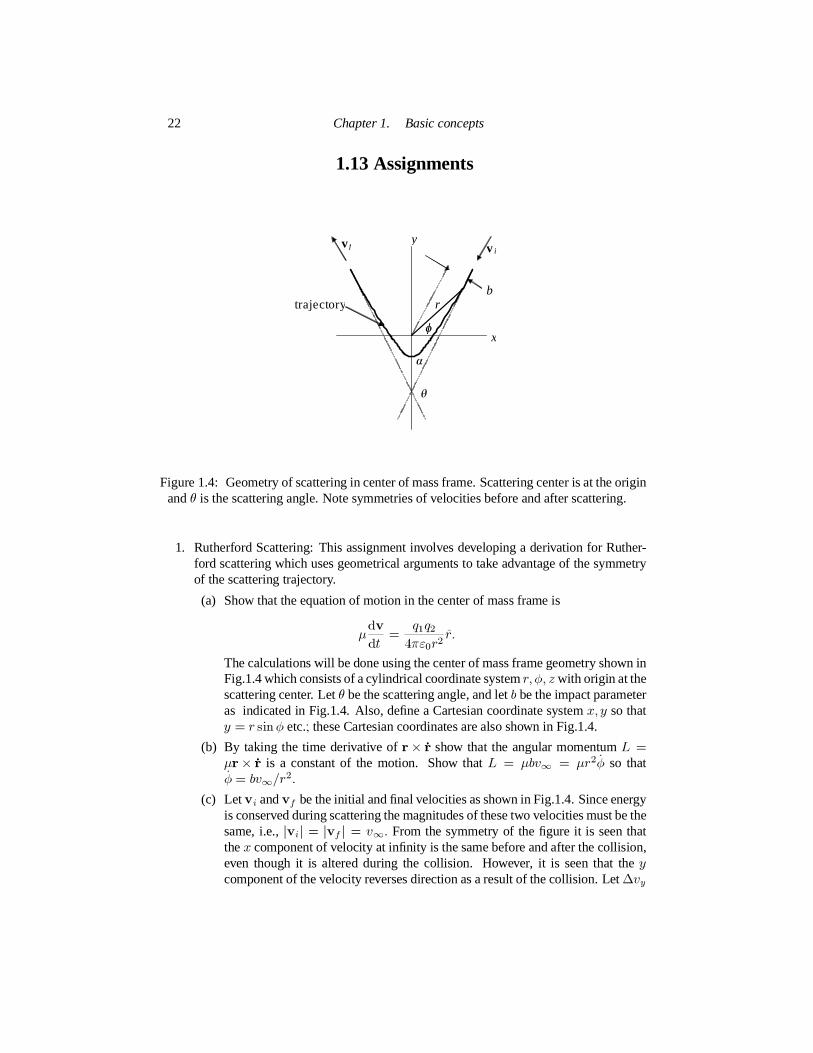
Figure 1.4: Geometry of scattering in center of mass frame. Scattering center is at the originandθ is the scattering angle. Note symmetries of velocities before and after scattering.
1. Rutherford Scattering: This assignment involves developing a derivation for Ruther-ford scattering which uses geometrical arguments to take advantage of the symmetryof the scattering trajectory.
(a) Show that the equation of motion in the center of mass frame is
µdvdt = q1q2
4πε0r2 r.The calculations will be done using the center of mass frame geometry shown inFig.1.4 which consists of a cylindrical coordinate systemr,φ, z with origin at thescattering center. Letθ be the scattering angle, and letb be the impact parameteras indicated in Fig.1.4. Also, define a Cartesian coordinate systemx, y so thaty = r sinφ etc.; these Cartesian coordinates are also shown in Fig.1.4.
(b) By taking the time derivative ofr× r show that the angular momentumL =µr× r is a constant of the motion. Show thatL = µbv∞ = µr2φ so thatφ = bv∞/r2.
(c) Letvi andvf be the initial and final velocities as shown in Fig.1.4. Since energyis conserved during scattering the magnitudes of these two velocities must be thesame, i.e.,|vi| = |vf | = v∞. From the symmetry of the figure it is seen thatthex component of velocity at infinity is the same before and after the collision,even though it is altered during the collision. However, it is seen thatthe ycomponent of the velocity reverses direction as a result of the collision. Let∆vy

1.13 Assignments 23
be the net change in they velocity over the entire collision. Express∆vy interms ofvyi, they component ofvi.
(d) Using they component of the equation of motion, obtain a relationship betweendvy andd cosφ. (Hint: it is useful to use conservation of angular momentum toeliminatedt in favor of dφ.) Let φi andφf be the initial and final values ofφ.By integratingdvy, calculate∆vy over the entire collision. How isφf related toφi and toα (refer to figure)?
(e) How isvyi related toφi andv∞? How isθ related toα? Use the expressionsfor ∆vy obtained in parts (c) and (d) above to obtain the Rutherford scatteringformula
tan(θ
2)
= q1q24πε0µbv2∞
What is the scattering angle for grazing (small angle collisions) andhow doesthis small angle scattering relate to the initial center of mass kinetic energy andto the potential energy at distanceb? For grazing collisions how doesb relateto the distance of closest approach? What impact parameter gives 90 degreescattering?
2. One-dimensional Scattering relations:The separation of collision types according tome/mi can also be understood by considering how the combination of conservation ofmomentum and of energy together constrain certain properties of collisions. Supposethat a particle with massm1 and incident velocityv1 makes a head-on collision with astationary target particle having massm2. The conservation equations for momentumand energy can be written as
m1v1 = m1v′1 + m2v′212m1v21 = 1
2m1v′21 + 12m2v′22 .
where prime refers to the value after the collision. By eliminatingv′1 between thesetwo equations obtainv′2 as a function ofv1. Use this to construct an expression show-ing the ratiom2v′22 /m1v21 , i.e., the fraction of the incident particle energy is trans-ferred to the target particle per collision. How does this fraction depend onm1/m2whenm1/m2 is equal to unity, very large, or very small? Ifm1/m2 is very largeor very small how many collisions are required to transfer approximately all of theincident particle energy to target particles?
3. Some basic facts you should know:Memorize the value ofε0 (or else arrange for thevalue to be close at hand). What is the value of Boltzmann’s constant when tempera-tures are measured in electron volts? What is the density of the air you arebreathing,measured in particles per cubic meter? What is the density of particles in solid copper,measured in particles per cubic meter? What is room temperature, expressed in elec-tron volts? What is the ionization potential (in eV) of a hydrogen atom? What is themass of an electron and of an ion (in kilograms)? What is the strength of the Earth’smagnetic field at your location, expressed in Tesla? What is the strength ofthe mag-netic field produced by a straight wire carrying 1 ampere as measured byan observerlocated 1 meter from the wire and what is the direction of the magnetic field? What

24 Chapter 1. Basic concepts
is the relationship between Tesla and Gauss, between particles per cubiccentimeterand particles per cubic meter? What is magneticflux? If a circular loop of wire witha break in it links a magneticflux of 29.83 Weber which increases at a constant rate toaflux of 30.83 Weber in one second, what voltage appears across the break?
4. Solve Eq.(1.5) the ‘easy’ way by first proving using Gauss’ law to show thatthe solu-tion of
∇2φ = − 1ε0 δ(r)
is
φ = 14πε0r .
Show that this implies
∇2 14πr = −δ(r) (1.39)
is a representation for the delta function. Then, use spherical polar coordinates andsymmetry to show that the Laplacian reduces to
∇2φ = 1r2
∂∂r
(
r2 ∂φ∂r)
.
Explicitly calculate∇2(1/r) and then reconcile your result with Eq.(1.39). Usingthese results guess that the solution to Eq.(1.5) has the form
φ = g(r)4πε0r .
Substitute this guess into Eq.(1.5) to obtain a differential equation forg which is trivialto solve.
5. Solve Eq.(1.5) forφ(r) using a more general method which illustrates several im-portant mathematical techniques and formalisms. Begin by defining the 3D Fouriertransform
φ(k) =∫
drφ(r)e−ik·r (1.40)
in which case the inverse transform is
φ(r) = 1(2π)3
∫
dkφ(k)eik·r (1.41)
and note that the Dirac delta function can be expressed as
δ(r) = 1(2π)3
∫
dkeik·r. (1.42)
Now multiply Eq.(1.5) byexp(−ik · r) and then integrate over allr, i.e. operate with∫ dr. The term involving∇2 is integrated by parts, which effectively replaces the∇operator withik.
Show that the Fourier transform of the potential is
φ(k) = qTǫ0(k2+λ−2
D ) . (1.43)

1.13 Assignments 25
and use this in Eq. (1.41).
Because of spherical symmetry use spherical polar coordinates for thek space integral.The only fixed direction is ther direction so choose the polar axis of thek coordinatesystem to be parallel tor. Thusk · r = krα whereα = cosθ andθ is the polar angle.Also, dk = −dφk2dαdk whereφ is the azimuthal angle. What are the limits of therespectiveφ, α, andk integrals? In answering this, you should first obtain an integralof the form
φ(r) ∼∫ ?
φ=?dφ
∫ ?
α=?dα
∫ ?
k=?k2dk × (?) (1.44)
where the limits and the integrand with appropriate coefficients are specified (i.e.,replace all the question marks and∼ by the correct quantities). Upon evaluation oftheφ andα integrals Eq.(1.44) becomes an even function ofk so that the range ofintegration can be extended to−∞ providing the overall integral is multiplied by1/2.Realizing thatsin kr =Im[eikr ], derive an expression of the general form
φ(r) ∼ Im∫ ∞
−∞kdk eikr
f(k2) . (1.45)
but specify the coefficient and exact form off(k2). Explain why the integration con-tour (which is along the realk axis) can be completed in the upper half complexkplane. Complete the contour in the upper half plane and show that the integrand has asingle pole in the upper half plane atk =? Use the method of residues to obtainφ(r).
6. Make sure you know how to evaluate quicklyA× (B×C) and(A×B)×C. A use-ful mnemonic which works for both cases is: “Both variations = Middle (dot othertwo) - Outer (dot other two)”, where outer refers to the outer vector of the parentheses(furthest from the center of the triad), and middle refers to the middle vector in thetriad of vectors.
7. Particle Integrator scheme (Birdsall and Langdon 1985)-In this assignment you willdevelop a simple, but powerful “leap-frog” numerical integration scheme. This is atype of “implicit” numerical integration scheme. This numerical scheme can laterbe used to evaluate particle orbits in time-dependent fields having complex topology.These calculations can be considered as numerical experiments used in conjunctionwith the analytic theory we will develop. This combined analytical/numerical ap-proach provides a deeper insight into charged particle dynamics than does analysisalone.
Brief note on Implicit v. Explicit numerical integration schemesSuppose it is desired use numerical methods to integrate the equation
dydt = f(y(t), t)
Unfortunately, sincey(t) is the sought-after quantity , we do not know what to use inthe right hand side fory(t). A naive choice would be to use the previous value ofy inthe RHS to get a scheme of the form
ynew − yold∆t = f(yold, t)

26 Chapter 1. Basic concepts
which may be solved to give
ynew = yold + ∆t f(yold, t)Simple and appealing as this is, it does not work since it is numerically unstable.
However, if we use the following scheme we will get a stable result:
ynew − yold∆t = f((ynew + yold)/2, t) (1.46)
In other words, we have used the average of the new and the old values ofy in theRHS. This makes sense because the RHS is a function evaluated at timet whereasynew = y(t+∆t/2) andyold = y(t−∆t/2). If Taylor expand these last quantities areTaylor expanded, it is seen that to lowest ordery(t) = [y(t+∆t/2)+y(t−∆t/2)]/2.
Sinceynew occurs on both sides of the equation we will have to solve some sort ofequation, or invert some sort of matrix to getynew.
Start with
m dvdt = q(E + v ×B).
Define, the angular cyclotron frequency vectorΩ =qB/m and the normalized electricfieldΣ = qE/m so that the above equation becomes
dvdt = Σ + v ×Ω (1.47)
Using the implicit scheme of Eq.(1.46), show that Eq. (1.47) becomes
vnew + A× vnew= CwhereA = Ω∆t/2 andC = vold+∆t (Σ + vold ×Ω/2). By first dotting the aboveequation withA and then crossing it withA show that the new value of velocity isgiven by
vnew = C+ AA ·C−A×C1+A2 .
The new position is simply given by
xnew = xold + vnewdtThe above two equations can be used to solve charged particle motion in complicated,3D, time dependent fields. Use this particle integrator to calculatethe trajectory ofan electron moving in crossed electric and magnetic fields where the non-vanishingcomponents areEx = 1 volt/meter andBz = 1 Tesla. Plot your result graphically onyour computer monitor. Try varying the field strengths, polarities, and alsotry ionsinstead of electrons.
8. Use the leap-frog numerical integration scheme to demonstrate the Rutherford scat-tering problem:
(i) Define a characteristic length for this problem to be the impact parameter for a90degree scattering angle,bπ/2. A reasonable choice for the characteristic velocity isv∞. What is the characteristic time?

1.13 Assignments 27
(ii) Define a Cartesian coordinate system such that thez axis is parallel to the incidentrelative velocity vectorv∞ and goes through the scattering center. Let the impactparameter be in they direction so that the incident particle is traveling in they − zplane. Make the graphics display span−50 ≤ z/bπ/2 ≤ 50 and−50 ≤ y/bπ/2 ≤ 50.
(iii) Set the magnetic field to be zero, and let the electric field be
E = −∇φwhereφ =? soEx =? etc.
(iv) By usingr2 = x2 + y2 + z2 calculate the electric field at each particle position,and so determine the particle trajectory.
(v) Demonstrate that the scattering is indeed at 90 degrees whenb = bπ/2. Whathappens whenb is much larger or much smaller thanbπ/2? What happens whenq1,q2have the same or opposite signs?
(vi) Have your code draw the relevant theoretical scattering angleθs and show that thenumerical result is in agreement.
9. Collision relations- Show thatσntlmfp = 1 whereσ is the cross-section for a colli-sion,nt is the density of target particles andlmfp is the mean free path. Show alsothat the collision frequency is given byυ = σntv wherev is the velocity of the in-cident particle. Calculate the electron-electron collision frequency for the followingplasmas: fusion (n ∼ 1020m−3, T ∼ 10 keV), partially ionized discharge plasma(n ∼ 1016m−3, T ∼ 10 eV). At what temperature does the conductivity of plasmaequal that of copper, and of steel? Assume thatZ = 1.
10. Cyclotron motion- Suppose that a particle is immersed in a uniform magneticfieldB = Bz and there is no electric field. Suppose that att = 0 the particle’s initialposition is atx = 0 and its initial velocity isv = v0x. Using the Lorentz equation,calculate the particle position and velocity as a function of time (be sure to take initialconditions into account). What is the direction of rotation for ions and for electrons(right handed or left handed with respect to the magnetic field)? If you had tomakeup a mnemonic for the sense of ion rotation, would it be Lions or Rions? Now, repeatthe analysis but this time with an electric fieldE = xE0 cos(ωt). What happens in thelimit whereω → Ω whereΩ = qB/m is the cyclotron frequency? Assume that theparticle is a proton and thatB = 1 Tesla,v0 = 105m/s, and compare your results withdirect numerical solution of the Lorentz equation. UseE0 = 104 V/m for the electricfield.
11. Space charge limited current- When a metal or metal oxide is heatedto high tem-peratures it emits electrons from its surface. This process calledthermionic emissionis the basis of vacuum tube technology and is also essential when high currentsaredrawn from electrodes in a plasma. The electron emitting electrode is called acath-odewhile the electrode to which the electronsflow is called ananode.An idealizedconfiguration is shown in Fig.1.5.

28 Chapter 1. Basic concepts
cathode anode
spacecharge
d
V
− +
electronsemittedfrom cathodesurface
Figure 1.5: Electron cloud accelerated from cathode to anode encounters space charge ofpreviously emitted electrons.
This configuration can operate in two regimes: (i) thetemperature limitedregimewhere the current is determined by the thermionic emission capability of the cathode,and (ii) thespace charge limitedregime, where the current is determined by a buildupof electron density in the region between cathode and anode (inter-electrode region).Let us now discuss this space charge limited regime: If the current is small then thenumber of electrons required to carry the current is small and so the inter-electroderegion is nearly vacuum in which case the electric field in this region will be nearlyuniform and be given byE = V/dwhereV is the anode-cathode potential differenceandd is the anode cathode separation. This electric field will accelerate the electronsfrom anode to cathode. However, if the current is large, there will be a significantelectron density in the inter-electrode region. This space charge will create a localizeddepression in the potential (since electrons have negative charge). Theresult is thatthe electric field will be reduced in the region near the cathode. If the space charge issufficiently large, the electric field at the cathode vanishes. In this situation attemptingto increase the current by increasing the number of electrons ejected by the cathodewill not succeed because an increase in current (which will give an increase in spacecharge) will produce a repulsive electric field which will prevent the additional elec-trons from leaving the cathode. Let us now calculate the space charge limited currentand relate it to our discussion on Debye shielding. The current density in thissystemis
J = −n(x)ev(x) = a negative constantSince potential is undefined with respect to a constant, let us choose this constant so
1.13 Assignments 29
that the cathode potential is zero, in which case the anode potential isV0. Assumingthat electrons leave the cathode with zero velocity, show that the electron velocity asa function of position is given by
v(x) =√
2eV (x)me
.Show that the above two equations, plus Poisson’s equation, can be combined to givethe following differential equation for the potential
d2Vdx2 − λV −1/2 = 0
whereλ = ǫ−10 |J |√me/2e. By multiplying this equation with the integrating factor
dV/dx and using the space charge limited boundary condition thatE = 0 at x = 0,solve forV (x). By rearranging the expression forV (x) show that the space chargelimited current is
J = 49ǫ0
√ 2eme
V 3/2d2 .
This is called the Child-Langmuir space charge limited current. For reference thetemperature limited current is given by the Richardson-Dushman law,
J = AT 2e−φ0/κT
where coefficientA and thework functionφ0 are properties of the cathode mate-rial, while T is the cathode temperature. Thus, the actual cathode current will bewhichever is the smaller of the above two expressions. Show there is a close relation-ship between the physics underlying the Child-Langmuir law and Debye shielding(hint-characterize the electron velocity as being a thermal velocity and its energy asbeing a thermal energy, show that the inter-electrode spacing correspondsto ?). Sup-pose that a cathode was operating in the space charge limited regime and thatsomepositively charged ions were placed in the inter-electrode region. What would happento the space charge-would it be possible to draw more or less current from thecath-ode? Suppose the entire inter-electrode region were filled with plasma with electrontemperatureTe. What would be the appropriate value ofd and how much current couldbe drawn from the cathode (assuming it were sufficiently hot)? Does this giveyou anyideas on why high current switch tubes (called ignitrons) use plasma to conduct thecurrent?

2
Derivation offluid equations: Vlasov, 2-fluid,MHD
2.1 Phase-space
Consider a particle moving in a one-dimensional space and let its positionbe describedasx = x(t) and its velocity asv = v(t). A way to visualize thex and v trajectoriessimultaneously is to plot them on a 2-dimensional graph where the horizontal coordinate isgiven byx(t) and the vertical coordinate is given byv(t). Thisx−v plane is calledphase-space.The trajectory (or orbit) of several particles can be represented as aset of curvesin phase-space as shown in Fig.2.1. Examples of a few qualitatively different phase-spaceorbits are shown in Fig.2.1.
passing particleorbit(positive velocity)
passing particleorbit(negativevelocity)
quasi-periodicorbit periodicorbit
particle phase-spacepositionat timet
x
v
Figure 2.1: Phase space showing different types of possible particle orbits.
Particles in the upper half plane always move to the right since they havea positivevelocity while those in the lower half plane always move to the left.Particles having exactperiodic motion [e.g.,x = A cos(ωt), v = −ωA sin(ωt)] alternate between moving to theright and the left and so describe an ellipse in phase-space. Particles with nearly periodic(quasi-periodic) motions will have near-ellipses or spiral orbits. A particle that does not
30
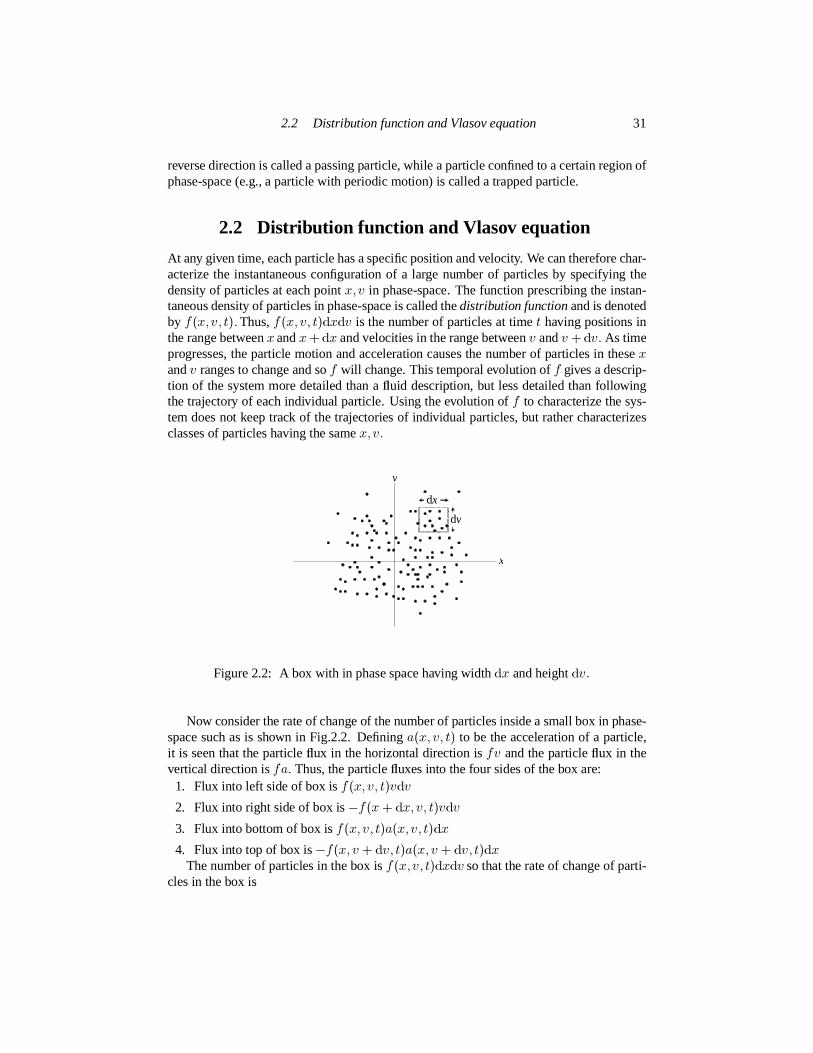
2.2 Distribution function and Vlasov equation 31
reverse direction is called a passing particle, while a particle confined to a certain region ofphase-space (e.g., a particle with periodic motion) is called a trapped particle.
2.2 Distribution function and Vlasov equation
At any given time, each particle has a specific position and velocity. We can therefore char-acterize the instantaneous configuration of a large number of particles byspecifying thedensity of particles at each pointx, v in phase-space. The function prescribing the instan-taneous density of particles in phase-space is called thedistribution functionand is denotedby f(x, v, t).Thus,f(x, v, t)dxdv is the number of particles at timet having positions inthe range betweenx andx + dx and velocities in the range betweenv andv + dv. As timeprogresses, the particle motion and acceleration causes the number of particles in thesexandv ranges to change and sof will change. This temporal evolution off gives a descrip-tion of the system more detailed than afluid description, but less detailed than followingthe trajectory of each individual particle. Using the evolution off to characterize the sys-tem does not keep track of the trajectories of individual particles, but rather characterizesclasses of particles having the samex, v.
x
v
dx
dv
Figure 2.2: A box with in phase space having widthdx and heightdv.
Now consider the rate of change of the number of particles inside a small boxin phase-space such as is shown in Fig.2.2. Defininga(x, v, t) to be the acceleration of a particle,it is seen that the particleflux in the horizontal direction isfv and the particleflux in thevertical direction isfa. Thus, the particlefluxes into the four sides of the box are:
1. Flux into left side of box isf(x, v, t)vdv2. Flux into right side of box is−f(x + dx, v, t)vdv3. Flux into bottom of box isf(x, v, t)a(x, v, t)dx4. Flux into top of box is−f(x, v + dv, t)a(x, v + dv, t)dx
The number of particles in the box isf(x, v, t)dxdv so that the rate of change of parti-cles in the box is

32 Chapter 2. Derivation offluid equations: Vlasov, 2-fluid, MHD
∂f(x, v, t)∂t dxdv = −f(x + dx, v, t)vdv + f(x, v, t)vdv
−f(x, v + dv, t)a(x, v + dv, t)dx+f(x, v, t)a(x, v, t)dx
(2.1)
or, on Taylor expanding the quantities on the right hand side, we obtain the one dimensionalVlasov equation,
∂f∂t + v ∂f∂x + ∂
∂v (af) = 0. (2.2)
It is straightforward to generalize Eq.(2.2) to three dimensions and soobtain the three-dimensional Vlasov equation
∂f∂t + v·∂f∂x + ∂
∂v · (af) = 0. (2.3)
Becausex,v are independent quantities in phase-space, the spatial derivative term has thecommutation property:
v·∂f∂x = ∂∂x · (vf) . (2.4)
The particle acceleration is given by the Lorentz force
a = qm (E+ v ×B) . (2.5)
Because(v ×B)i = vjBk−vkBj is independent ofvi, the term∂(v ×B)i/∂vi vanishesso that even though the accelerationa is velocity-dependent, it nevertheless commutes withthe vector velocity derivative as
a·∂f∂v = ∂∂v · (af) . (2.6)
Because of this commutation property the Vlasov equation can also be written as
∂f∂t + v·∂f∂x + a·∂f∂v = 0 . (2.7)
If we “sit on top of” a particle moving in phase-space with trajectory x = x(t),v = v(t)and measure the distribution function as we are carried along by the particle, the ob-served rate of change of the distribution function will bedf(x(t),v(t), t)/dt where thed/dt means that the derivative is measured in the moving frame. Becausedx/dt = v anddv/dt = a, this observed rate of change is(df(x(t),v(t), t)
dt)
orbit = ∂f∂t + v·∂f∂x + a·∂f∂v = 0. (2.8)
Thus, the distribution function as measured when moving along a particletrajectory (orbit)is aconstant.This gives a powerful method for finding solutions to the Vlasov equation.Since the distribution function is a constant when measured in the frame following an orbit,we can choose it to depend onany quantitythat is constant along the orbit (Jeans 1915,Watson 1956).

2.3 Moments of the distribution function 33
For example, if the energyE of particles is constant along their orbits thenf = f(E) isa solution to the Vlasov equation. On the other hand, if both the energy and the momen-tum p are constant along particle orbits, then any distribution function with thefunctionaldependencef = f(E,p) is a solution to the Vlasov equation. Depending on the situationat hand, the energy and/or canonical momentum may or may not be constant along an or-bit and so whether or notf = f(E,p) is a solution to the Vlasov equation depends on thespecific problem under consideration. However, there always exists at least one constant ofthe motion for any trajectory because, just like every human being has an invariant birth-day, the initial conditions of a particle trajectory are invariant alongits orbit. As a simpleexample, consider a situation where there is no electromagnetic field sothata =0 in whichcase the particle trajectories are simplyx(t) = x0+v0t, v(t) = v0 wherex0,v0 are theinitial position and velocity. Let us check to see whetherf(x0) is indeed a solution to theVlasov equation. Writex0= x(t) − v0t sof(x0) = f(x(t) − v0t) and observe that
∂f∂t + v·∂f∂x + a·∂f∂v = −v0·∂f∂x + v·∂f∂x = 0. (2.9)
x
v
Figure 2.3: Moments give weighted averages of the particles in the shaded vertical strip
2.3 Moments of the distribution function
Let us count the particles in the shaded vertical strip in Fig.2.3. The number of particles inthis strip is the number of particles lying betweenx andx + dx wherex is the location ofthe left hand side of the strip andx + dx is the location of the right hand side. The numberof particles in the strip is equivalently defined asn(x, t)dx wheren(x) is thedensityof

34 Chapter 2. Derivation offluid equations: Vlasov, 2-fluid, MHD
particles atx. Thus we see that∫ f(x, v)dv = n(x); the transition from a phase-space
description (i.e.,x, v are dependent variables) to a normal space description (i.e.,x is adependent variable) involves “integrating out” the velocity dependence to obtain a quantity(e.g., density) depending only on position. Since the number of particles is finite, and sincef is a positive quantity, we see thatf must vanish asv → ∞.
Another way of viewingf is to consider it as the probability that a randomly selectedparticle at positionx has the velocityv.Using this point of view, we see that averaging overthe velocities of all particles atx gives the mean velocityu(x) determined byn(x)u(x) =∫ vf(x, v)dv. Similarly, multiplying f by v2 and integrating over velocity will give anexpression for the mean energy of all the particles. This procedure of multiplying f byvarious powers ofv and then integrating over velocity is calledtaking moments of thedistribution function.
It is straightforward to generalize this “moment-taking” to three dimensional problemssimply by taking integrals over three-dimensional velocity space. Thus, in three dimensionsthe density becomes
n(x) =∫
f(x,v)dv (2.10)
and the mean velocity becomes
u(x) =∫ vf(x,v)dv
n(x) . (2.11)
x
vinitially fastparticlemovingto right
initially slowparticlemovingto right
apparentannihilation
suddenchangein vdueto collision
apparentcreation
Figure 2.4: Detailed view of collisions causing ‘jumps’ in phase space
2.3.1 Treatment of collisions in the Vlasov equation
It was shown in Sec. 1.8 that the cumulative effect of grazing collisions dominates the

2.3 Moments of the distribution function 35
cumulative effect of the more infrequently occurring large angle collisions. In order tosee how collisions affect the Vlasov equation, let us now temporarily imagine that thegrazing collisions are replaced by an equivalent sequence of abrupt large scattering angleencounters as shown in Fig.2.4. Two particles involved in a collision donot significantlychange their positions during the course of a collision, but they do substantially change theirvelocities. For example, a particle making a head-on collision with anequal mass stationaryparticle will stop after the collision, while the target particle will assume the velocity ofthe incident particle. If we draw the detailed phase-space trajectories characterized by acollision between two particles we see that each particle has a sudden change in its verticalcoordinate (i.e., velocity) but no change in its horizontal coordinate (i.e.,position). Thecollision-induced velocity jump occurs very fast so that if the phase-space trajectories wererecorded with a “movie camera” having insufficient framing rate to catch the details of thejump the resulting movie would show particles being spontaneously created orannihilatedwithin given volumes of phase-space (e.g., within the boxes shown in Fig.2.4).
The details of these individual jumps in phase-space are complicated and yet of littleinterest since all we really want to know is the cumulative effectof many collisions. Itis therefore both efficient and sufficient to follow the trajectories on the slow time scalewhile accounting for the apparent “creation” or “annihilation” of particles byinserting acollision operatoron the right hand side of the Vlasov equation. In the example shownhere it is seen that when a particle is apparently “created” in one box, another particle mustbe simultaneously “annihilated” in another box at the samex coordinate but a differentv coordinate (of course, what is actually happening is that a single particleis suddenlymoving from one box to the other). This coupling of the annihilation and creationrates indifferent boxes constrains the form of the collision operator. We will not attempt to derivecollision operators in this chapter but will simply discuss the constraints on these operators.From a more formal point of view, collisions are characterized by constrained sources andsinks for particles in phase-space and inclusion of collisions in the Vlasov equation causesthe Vlasov equation to assume the form
∂fσ∂t + ∂
∂x · (vfσ) + ∂∂v · (afσ) = ∑
αCσα(fσ) (2.12)
whereCσα(fσ) is the rate of change offσ due to collisions of speciesσ with speciesα.Let us now list the constraints which must be satisfied by the collision operatorCσα(fσ)
are as follows:
• (a) Conservation of particles – Collisions cannot change the total number of par-ticles at a particular location so∫
dvCσα(fσ) = 0. (2.13)
(b) Conservation of momentum – Collisions between particles of the samespeciescannot change the total momentum of that species so∫
dvmσvCσσ(fσ) = 0 (2.14)

36 Chapter 2. Derivation offluid equations: Vlasov, 2-fluid, MHD
while collisions between different species must conserve the total momentumof both species together so∫
dvmivCie(fi) +∫
dvmevCei(fe) = 0. (2.15)
(c) Conservation of energy –Collisions between particles of the same species can-not change the total energy of that species so∫
dvmσv2Cσσ(fσ) = 0 (2.16)
while collisions between different species must conserve the total energy ofboth species together so∫
dvmiv2Cie(fi) +∫
dvmev2Cei(fe) = 0. (2.17)
2.4 Two-fluid equations
Instead of just taking moments of the distribution functionf itself, moments will nowbe taken of the entire Vlasov equation to obtain a set of partial differential equations re-lating the mean quantitiesn(x),u(x), etc. We begin by integrating the Vlasov equation,Eq.(2.12), over velocity for each species. This first and simplest step in the procedure isoften called taking the “zeroth” moment, since we are multiplying by unity which for con-sistency with later “moment-taking”, can be considered as multiplying theentire Vlasovequation byv raised to the power zero. Multiplying the Vlasov equation by unity and thenintegrating over velocity gives∫ [∂fσ
∂t + ∂∂x · (vfσ) + ∂
∂v · (afσ)]
dv = ∑α
∫Cσα(fσ)dv. (2.18)
The velocity integral commutes with both the time and space derivativeson the left handside becausex,v, andt are independent variables, while the third term on the left hand sideis the volume integral of a divergence in velocity space. Gauss’s theorem[i.e.,
∫vol dx∇ ·
Q = ∫sfc ds · Q] givesfσ evaluated on a surface atv = ∞. However, becausefσ → 0
asv → ∞, this surface integral in velocity space vanishes. Using Eqs.(2.10), (2.11), and(2.13), we see that Eq.(2.18) becomes the speciescontinuity equation
∂nσ∂t + ∇ · (nσuσ) = 0. (2.19)
Now let us multiply Eq.(2.12) byv and integrate over velocity to take the “first moment”,∫v[∂fσ
∂t + ∂∂x · (vfσ) + ∂
∂v · (afσ)]
dv = ∑α
∫vCσα(fσ)dv. (2.20)
This may be re-arranged in a more tractable form by:

2.4 Two-fluid equations 37
(i) “pulling” both the time and space derivatives out of the velocity integral,
(ii) writing v = v′(x, t) +u(x,t) wherev′(x,t) is therandompart of a given velocity,i.e., that part of the velocity which differs from the mean (note thatv is independentof bothx andt butv′ is not; alsodv =dv′),
(iii) integrating by parts in 3-D velocity space on the acceleration term and using(∂v∂v
)ij
= δij .
After performing these manipulations, the first moment of the Vlasovequation be-comes ∂ (nσuσ)
∂t + ∂∂x ·
∫(v′v′ + v′uσ+uσv′ +uσuσ) fσdv′
− qσmσ
∫(E + v ×B) fσdv′ = − 1
mσRσα
(2.21)
whereRσα is the net frictional drag force due to collisions of speciesσ with speciesα.Note thatRσσ = 0 since a species cannot exert net drag on itself (e.g., the totality ofelectrons cannot cause frictional drag on the totality of electrons). The frictional termshave the form
Rei = νeimene(ue −ui) (2.22)
Rie = νiemini(ui − ue) (2.23)so that in the ion frame the drag on electrons is simply the total electronmomentummeneue measured in this frame multiplied by the rateνei at which this momentum isdestroyed by collisions with ions. This form for frictional drag has the following proper-ties: (i)Rei +Rie = 0 showing that the plasma cannot have a frictional drag on itself, (ii)friction causes the faster species to be slowed down by the slower species, and (iii) there isno friction between species if both have the same mean velocity.
Equation (2.21) can be further simplified by factoringu out of the velocity integralsand recalling that by definition
∫ v′fσdv′ =0 . Thus, Eq. (2.21) reduces to
mσ[∂ (nσuσ)
∂t + ∂∂x · (nσuσuσ)
]=nσqσ (E +uσ×B)− ∂
∂x · ←→P σ−Rσα (2.24)
where thepressure tensor←→P is defined by
←→P σ = mσ∫
v′v′fσdv′.If fσ is an isotropic function ofv′, then the off-diagonal terms in
←→P σ vanish and the threediagonal terms are identical. In this case, it is useful to define the diagonal terms to be thescalar pressurePσ, i.e.,
Pσ = mσ∫ v′xv′xfσdv′ = mσ
∫ v′yv′yfσdv′ = mσ∫ v′zv′zfσdv′
= mσ3
∫ v′ · v′fσdv′.(2.25)
38 Chapter 2. Derivation offluid equations: Vlasov, 2-fluid, MHD
Equation (2.25) defines pressure for a three-dimensional isotropic system.However, wewill often deal with systems of reduced dimensionality, i.e., systems with just one or twodimensions. Equation (2.25) can therefore be generalized to these other cases by introduc-ing the generalN-dimensional definition for scalar pressure
Pσ = mσN
∫v′ · v′fσdNv′ =mσ
N∫ N∑
j=1v′ 2j fσdNv′ (2.26)
wherev′ is theN -dimensional random velocity.It is important to emphasize that assuming isotropy is done largely for mathematical
convenience and that in real systems the distribution function is often quite anisotropic.Collisions, being randomizing, drive the distribution function towards isotropy, while com-peting processes simultaneously drive it towards anisotropy. Thus, eachsituation must beconsidered individually in order to determine whether there is sufficient collisionality tomakef isotropic. Because fully-ionized hot plasmas often have insufficient collisions tomakef isotropic, the oft-used assumption of isotropy is an oversimplification which mayor may not be acceptable depending on the phenomenon under consideration.
On expanding the derivatives on the left hand side of Eq.(2.24), it is seen that two ofthe terms combine to giveu times Eq. (2.19). After removing this embedded continuityequation, Eq.(2.24) reduces to
nσmσduσdt =nσqσ (E + uσ×B)−∇Pσ −Rσα (2.27)
where the operatord/dt is defined to be theconvective derivative
ddt = ∂
∂t + uσ · ∇ (2.28)
which characterizes the temporal rate of change seen by an observermoving with the meanfluid velocityuσ of speciesσ.An everyday example of the convective term would be theapparent temporal increase in density of automobiles seen by a motorcyclist who enters atraffic jam of stationary vehicles and is not impeded by the traffic jam.
At this point in the procedure it becomes evident that a certain pattern recurs for eachsuccessive moment of the Vlasov equation. When we took the zeroth moment, an equationfor the density
∫ fσdv resulted, but this also introduced a term involving the next highermoment, namely the mean velocity∼ ∫ vfσdv. Then, when we took the first moment toget an equation for the velocity, an equation was obtained containing a term involving thenext higher moment, namely the pressure∼ ∫ vvfσdv. Thus, each time we take a momentof the Vlasov equation, an equation for the moment we want is obtained, but because of thev ·∇f term in the Vlasov equation, a next higher moment also appears. Thus, moment-taking never leads to a closed system of equations; there is always be a “loose end”, ahighest moment for which there is no determining equation. Some sort of ad hoc closureprocedure must always be invoked to terminate this chain (as seen below,typical closuresinvolve invoking adiabatic or isothermal assumptions). Another feature of taking momentsis that each higher moment has embedded in it a term which contains completelowermoment equations multiplied by some factor. Algebraic manipulation can identify theselower moment equations and eliminate them to give a simplified higher moment equation.

2.4 Two-fluid equations 39
Let us now take the second moment of the Vlasov equation. Unlike the zeroth andfirst moments, here the dimensionality of the system enters explicitlyso the more generalpressure definition given by Eq. (2.26) will be used. Multiplying the Vlasov equation bymσv2/2 and integrating over velocity gives
∂∂t
∫ mσv22 fσdNv
+ ∂∂x ·
∫ mσv22 vfσdNv
+qσ∫ v2
2∂∂v · (E + v ×B) fσdNv
= ∑α
∫mσ
v22 CσαfσdNv. (2.29)
We now consider each term of this equation separately as follows:1. The time derivative term becomes
∂∂t
∫ mσv22 fσdNv = ∂
∂t∫ mσ (v′+uσ)2
2 fσdNv′= ∂∂t
(NPσ2 + mσnσu2σ
2)
.
2. Again usingv = v′ +uσ the space derivative term becomes
∂∂x ·
∫ mσv22 vfσdNv =∇·
(Qσ + 2 + N
2 Pσuσ + mσnσu2σ2 uσ
).
whereQσ =∫ mσv′2
2 v′fσdNv is called theheatflux.
3. On integrating by parts, the acceleration term becomes
qσ∫ v2
2∂∂v · [(E + v ×B) fσ ] dNv = −qσ
∫v ·Efσdv = −qσnσuσ ·E.
4. The collision term becomes (using Eq.(2.16))
∑α
∫mσ
v22 Cσαfσdv =
∫α=σ
mσv22 Cσαfσdv = −
(∂W∂t
)Eσα
.where(∂W/∂t)Eσα is the rate at which speciesσ collisionally transfers energy tospeciesα.
Combining the above four relations, Eq.(2.29) becomes
∂∂t
(NPσ2 + mσnσu2σ
2)
+ ∇·(Qσ + 2 + N
2 Pσuσ + mσnσu2σ2 uσ
)− qσnσuσ ·E
= −(∂W
∂t)Eσα
.(2.30)
This equation can be simplified by invoking two mathematical identities, the first of whichis
∂∂t
(mσnσu2σ2
)+∇·
(mσnσu2σ2 uσ
)= nσ
( ∂∂t +uσ · ∇
) mσu2σ2 = nσ d
dt(mσu2σ
2)
.(2.31)

40 Chapter 2. Derivation offluid equations: Vlasov, 2-fluid, MHD
The second identity is obtained by dotting the equation of motion withuσ and is
nσmσ[ ∂∂t
(u2σ2)
+uσ ·(∇
(u2σ2)− uσ ×∇× uσ
)]= nσqσuσ ·E−uσ·∇Pσ−Rσα ·uσ
or
nσ ddt
(mσu2σ2
)= nσqσuσ ·E− uσ·∇Pσ−Rσα · uσ . (2.32)
Inserting Eqs. (2.31) and (2.32) in Eq.(2.30) gives the energy evolution equation
N2
dPσdt + 2 + N
2 P∇ · uσ = −∇ ·Qσ + Rσα · uσ −(∂W
∂t)Eσα
. (2.33)
The first term on the right hand side represents the heatflux, the second term gives thefrictional heating of speciesσ due to frictional drag on speciesα, while the last term onthe right hand side gives the rate at which speciesσ collisionally transfers energy to otherspecies. Although Eq.(2.33) is complicated, two important limiting situations become ev-ident if we lett be the characteristic time scale for a given phenomenon andl be its char-acteristic length scale. A characteristic velocityVph ∼ l/t may then be defined for thephenomenon and so, replacing temporal derivatives byt−1 and spatial derivatives byl−1in Eq.(2.33), it is seen that the two limiting situations are:
1. Isothermal limit – The heatflux term dominates all other terms in which case thetemperature becomes spatially uniform. This occurs if (i)vTσ >> Vph since the ratioof the left hand side terms to the heatflux term is∼ Vph/vTσ and (ii) the collisionalterms are small enough to be ignored.
2. Adiabatic limit –The heatflux terms and the collisional terms are small enough tobe ignored compared to the left hand side terms; this occurs whenVph >> vTσ .Adiabatic is a Greek word meaning ‘impassable’, and is used here to denote that noheat isflowing.
Both of these limits make it possible to avoid solving forQσ which involves the thirdmoment and so both the adiabatic and isothermal limit provide a closure tothe momentequations.
The energy equation may be greatly simplified in the adiabatic limit by re-arranging thecontinuity equation to give
∇ ·uσ = − 1nσ
dnσdt (2.34)
and then substituting this expression into the left hand side of Eq.(2.33) to obtain
1Pσ
dPσdt = γ
nσdnσdt (2.35)
where
γ = N + 2N . (2.36)
Equation (2.35) may be integrated to give the adiabatic equation of state
Pσnγσ = constant; (2.37)
this can be considered a derivation of adiabaticity based on geometry and statistical me-chanics rather than on thermodynamic arguments.

2.4 Two-fluid equations 41
2.4.1 Entropy of a distribution function
Collisions cause the distribution function to tend towards a simple final state characterizedby having the maximum entropy for the given constraints (e.g., fixed total energy). Tosee this, we provide a brief discussion of entropy and show how it relates toa distributionfunction.
Suppose we throw two dice, labeledA andB, and letR denote the result of a throw.ThusR ranges from 2 through 12. The complete set of(A,B) combinations that give theseR’s are listed below:
R =2⇐⇒(1,1)
R =3⇐⇒(1,2),(2,1)
R =4⇐⇒(1,3),(3,1),(2,2)
R =5⇐⇒(1,4),(4,1),(2,3),(3,2)
R =6⇐⇒(1,5),(5,1),(2,4),(4,2),(3,3)
R =7⇐⇒(1,6),(6,1),(2,5),(5,2),(3,4),(4,3)
R =8⇐⇒(2,6),(6,2),(3,5),(5,3),(4,4)
R =9⇐⇒(3,6),(6,3),(4,5),(5,4)
R =10⇐⇒(4,6),(6,4),(5,5)
R =11⇐⇒(5,6),(6,5)
R =12⇐⇒(6,6)
There are six(A,B) pairs that giveR =7, but only one pair forR =2 and only one pairfor R =12. Thus, there are six microscopic states [distinct(A,B) pairs] corresponding toR =7 but only one microscopic state corresponding to each ofR =2 or R =12. Thus,we know moreabout the microscopic state of the system ifR = 2 or 12 than ifR = 7.We define the entropyS to be thenatural logarithm of the number of microscopic statescorresponding to a given macroscopic state.Thus for the dice, the entropy would be thenatural logarithm of the number of(A,B) pairs that correspond to a giveR. The entropyfor R = 2 or R = 12 would be zero sinceS = ln(1) = 0, while the entropy forR = 7would beS = ln(6) since there were six different ways of obtainingR = 7.
If the dice were to be thrown a statistically large number of times themost likely resultfor any throw isR = 7; this is the macroscopic state with the most number of microscopicstates. Since any of the possible microscopic states is an equally likely outcome, the mostlikely macroscopic state after a large number of dice throws is the macroscopic state withthe highest entropy.
Now consider a situation more closely related to the concept of a distribution function.In order to do this we first pose the following simple problem: Suppose we have a pegboardwith N holes, labeledh1, h2, ...hN and we also haveN pegs labeled byp1, p2, ..., pN .What are the number of ways of putting all the pegs in all the holes? Starting with holeh1, we have a choice ofN different pegs, but when we get to holeh2 there are now onlyN − 1 pegs remaining so that there are now onlyN − 1 choices. Using this argument for

42 Chapter 2. Derivation offluid equations: Vlasov, 2-fluid, MHD
subsequent holes, we see there areN ! ways of putting all the pegs in all the holes.Let us complicate things further. Suppose that we arrange the holes inM groups, say
groupG1 has the first 10 holes, groupG2 has the next 19 holes, groupG3 has the next 4holes and so on, up to groupM. We will usef to denote the number of holes in a group,thusf(1) = 10, f(2) = 19, f(3) = 4, etc. The number of ways of arranging pegs withina group is just the factorial of the number of pegs in the group, e.g., the number of waysof arranging the pegs within group 1 is just10! and so in general the number of ways ofarranging the pegs in thejth group is[f(j)]!.
Let us denoteC as the number of ways for putting all the pegs in all the groupswithoutcaring about the internal arrangement within groups. The number of ways of putting thepegs in all the groupscaringabout the internal arrangements in all the groups isC×f(1)!×f(2)!× ...f(M)!, but this is just the number of ways of putting all the pegs in all the holes,i.e.,
C × f(1)! × f(2)! × ...f(M)! = N !or
C = N !f(1)! × f(2)!× ...f(M)! .
Now C is just the number of microscopic states corresponding to the macroscopic stateof the prescribed groupingf(1) = 10, f(2) = 19, f(3) = 4, etc. so the entropy is justS = lnC or
S = ln( N !f(1)!× f(2)!× ...f(M)!
)
= lnN ! − ln f(1)!− ln f(2)! − ...− ln f(M)!(2.38)
Stirling’s formula shows that the large argument asymptotic limit of the factorial functionis
limk→largeln k! = k ln k − k. (2.39)
Noting thatf(1) + f(2) + ...f(M) = N the entropy becomes
S = N lnN − f(1) ln f(1) − f(2) ln f(2) − ...− f(M) ln f(M)= N lnN −
M∑j=1
f(j) ln f(j) (2.40)
The constantN lnN is often dropped, giving
S = −M∑j=1
f(j) ln f(j). (2.41)
If j is made into a continuous variable say,j → v so thatf(v)dv is the number of items inthe group labeled byv, then the entropy can be written as
S = −∫
dvf(v) ln f(v). (2.42)

2.4 Two-fluid equations 43
By now, it is obvious thatf could be the velocity distribution function in which casef(v)dvis just the number of particles in the group having velocity betweenv andv+dv. Since thepeg groups correspond to different velocity ranges coordinates, having more dimensionsjust means having more groups and so for three dimensions the entropy generalizes to
S = −∫
dv f(v) ln f(v). (2.43)
If the distribution function depends on position as well, this corresponds to still more peggroups, and so a distribution function which depends on both velocity and position willhave the entropy
S = −∫
dx∫
dv f(x,v) ln f(x,v). (2.44)
2.4.2 Effect of collisions on entropy
The highest entropy state is the most likely state of the system because the highest entropystate has the most number of microscopic states corresponding to the macroscopic state.Collisions (or other forms of randomization) will take some prescribed initial microscopicstate where phase-space positions of all particles are individually specified and scramblethese positions to give a new microscopic state. The new scrambled statecould be anymicroscopic state, but is most likely to be a member of the class of microscopic statesbelonging to the highest entropy macroscopic state. Thus, any randomization process suchas collisions will cause the system to evolve towards the maximum entropy macroscopicstate.
An important shortcoming of this argument is that it neglects any conservation rela-tions that have to be satisfied. To see this, note that the expression for entropy could bemaximized if all the particles are put in one group, in which caseC = N !, which is thelargest possible value forC. Thus, the maximum entropy configuration ofN plasma parti-cles corresponds to all the particles having the same velocity. However, this would assigna specific energy to the system which would in general differ from the energy of the initialmicrostate. This maximum entropy state is therefore not accessible inisolated system, be-cause energy would not be conserved if the system changed from its initialmicrostate tothe maximum entropy state.
Thus, a qualification must be added to the argument. Randomizing processeswillscramble the system to attain the state of maximum entropy stateconsistentwith any con-straints placed on the system. Examples of such constraints would be the requirements thatthe total system energy and the total number of particles must be conserved. Wethereforere-formulate the problem as: given an isolated system withN particles in a fixed volumeVand initial average energy per particle〈E〉 , what is the maximum entropy state consistentwith conservation of energy and conservation of number of particles? Thisis a variationalproblem because the goal is to maximizeS subject to the constraint that bothN andN 〈E〉are fixed. The method of Lagrange multipliers can then be used to take into account theseconstraints. Using this method the variational problem becomes
δS − λ1δN − λ2 δ(N 〈E〉) = 0 (2.45)
whereλ1 andλ2 are as-yet undetermined Lagrange multipliers. The number of particles

44 Chapter 2. Derivation offluid equations: Vlasov, 2-fluid, MHD
is
N = V∫
fdv. (2.46)
The energy of an individual particle isE = mv2/2 wherev is the velocity measured inthe rest frame of the center of mass of the entire collection ofN particles. Thus, the totalkinetic energy of all the particles in this rest frame is
N 〈E〉 = V∫ mv2
2 f(v)dv (2.47)
and so the variational problem becomes
δ∫
dv(f ln f − λ1V f − λ2V mv2
2 f)
= 0. (2.48)
Incorporating the volumeV into the Lagrange multipliers, and factoring out the coefficientδf this becomes ∫
dv δf(
1 + ln f − λ1 − λ2mv2
2)
= 0. (2.49)
Sinceδf is arbitrary, the integrand must vanish, giving
ln f = λ2mv2
2 − λ1 (2.50)
where the ‘1’ has been incorporated intoλ1.The maximum entropy distribution function of an isolated, energy and particle conserv-
ing system is therefore
f = λ1 exp(−λ2mv2/2); (2.51)
this is called a Maxwellian distribution function. We will often assume that the plasma islocally Maxwellian so thatλ1 = λ1(x, t) andλ2 = λ(x, t). We define the temperature tobe
κTσ(x, t) = 1λ2(x, t) (2.52)
where Boltzmann’s factorκ allows temperature to be measured in various units. The nor-malization factor is set to be
λ1(x, t) = n(x, t)( mσ
2πκTσ(x, t))N/2
(2.53)
whereN is the dimensionality (1, 2, or 3) so that∫ fσ(x,v,t)dNv =nσ(x,t). Because the
kinetic energy of individual particles was defined in terms of velocities measured in the restframe of the center of mass of the complete system of particles, if this center of mass ismoving in the lab frame with a velocityuσ, then in the lab frame the Maxwellian will havethe form
fσ(x,v,t) = nσ( mσ
2πκTσ)N/2
exp(−mσ(v − uσ)2/2κTσ). (2.54)

2.4 Two-fluid equations 45
2.4.3 Relation between pressure and Maxwellian
The scalar pressure has a simple relation to the generalized Maxwellian as seen by recastingEq.(2.26) as
Pσ = −nσmσN
(βπ)N/2 d
dβ∫
e−βv′2dv
= −nσmσN
(βπ)N/2 d
dβ(βπ)−N/2
= nσκTσ ,
(2.55)
which is just the ideal gas law. Thus, the definitions that have been proposed forpressureand temperature are consistent with everyday notions for these quantities.
Clearly, neither the adiabatic nor the isothermal assumption will beappropriate whenVph ∼ vTσ. Thefluid description breaks down in this situation and the Vlasov descriptionmust be used. It must also be emphasized that the distribution function is Maxwellianonly if there are sufficient collisions or some other randomizing process. Because of theweak collisionality of a plasma, this is often not the case. In particular, since the collisionfrequency scales asv−3, fast particles take much longer to become Maxwellian than slowparticles. It is not at all unusual for a plasma to be in a state where the low velocity particleshave reached a Maxwellian distribution whereas the fast particles form a non-Maxwellian“tail”.
We now summarize the two-fluid equations:
• continuity equation for each species
∂nσ∂t + ∇ · (nσuσ) = 0 (2.56)
• equation of motion for each species
nσmσduσdt =nσqσ (E + uσ×B)−∇Pσ −Rσα (2.57)
• equation of state for each species
Regime Equation of state NameVph >> vTσ Pσ ∼ nγσ adiabaticVph << vTσ Pσ = nσκTσ , Tσ=constant isothermal
• Maxwell’s equations
∇×E = −∂B∂t (2.58)
∇×B =µ0∑σ
nσqσuσ + µ0ε0 ∂E∂t (2.59)
∇ ·B = 0 (2.60)
∇ ·E = 1ε0
∑σ
nσq (2.61)

46 Chapter 2. Derivation offluid equations: Vlasov, 2-fluid, MHD
2.5 Magnetohydrodynamic equations
Particle motion in the two-fluid system was described by the individual species mean veloc-itiesue,ui and by the pressures
←→P e,←→P i which gave information on the random deviationof the velocity from its mean value. Magnetohydrodynamics is an alternate description ofthe plasma where instead of usingue,ui to describe mean motion, two new velocity vari-ables that are a linear combination ofue,ui are used. As will be seen below, this means aslightly different definition for pressure must also be used.
The new velocity-like variables are (i) the current density
J =∑σ
nσqσuσ (2.62)
which is essentially the relative velocity between ions and electrons, and (ii) the center ofmass velocity
U = 1ρ∑σ
mσnσuσ. (2.63)
whereρ = ∑
σmσnσ (2.64)
is the total mass density. Magnetohydrodynamics is primarily concerned with low fre-quency, long wavelength,magneticbehavior of the plasma.
2.5.1 MHD continuity equation
Multiplying Eq.(2.19) bymσ and summing over species gives the MHD continuity equa-tion ∂ρ
∂t + ∇ · (ρU) = 0. (2.65)
2.5.2 MHD equation of motion
To obtain an equation of motion, we take the first moment of the Vlasov equation, thenmultiply by mσ and sum over species to obtain
∂∂t
∑σ
mσ∫
vfσdv+ ∂∂x ·∑
σ
∫mσvvfσdv+∑
σqσ
∫v ∂∂v · [(E + v ×B) fσ ] = 0;
(2.66)the right hand side is zero sinceRei +Rie = 0, i.e., the total plasma cannot exert drag onitself. We now define random velocities relative toU (rather than touσ as was the case forthe two-fluid equations) so that the second term can be written as
∑σ
∫mσvvfσdv =∑
σ
∫mσ(v′ + U)(v′ +U)fσdv =∑
σ
∫mσv′v′fσdv+ρUU
(2.67)where
∑σ∫ mσv′fσdv = 0 has been used to eliminate terms linear inv′. The MHD
pressure tensor is now defined in terms of the random velocities relative toU and is given
2.5 Magnetohydrodynamic equations 47
by ←→P MHD =∑σ
∫mσv′v′fσdv. (2.68)
We insert Eqs.(2.67) and (2.68) in Eq.(2.66), integrate by parts on the acceleration term,and perform the summation over species to obtain the MHD equation of motion
∂(ρU)∂t + ∇ · (ρUU) =
(∑σ
nσqσ)E+ J×B−∇·←→P MHD . (2.69)
MHD is typically used to describe phenomena with large spatial scales where the plasmais essentially neutral, so that
∑σ nσqσ ≈ 0. Just as in the two-fluid situation, the left hand
side of Eq.(2.69) contains a factor times the MHD continuity equation,
∂(ρU)∂t + ∇ · (ρUU) =
[∂ρ∂t + ∇ · (ρU)
]U + ρ∂U∂t + ρU∇ ·U. (2.70)
Using Eq.(2.65) leads to the standard form for the MHD equation of motion
ρDUDt = J×B−∇·←→P MHD (2.71)
where DDt = ∂
∂t + U·∇ (2.72)
is the convective derivative using the MHD center of mass velocity. Scalar approximationsof the MHD pressure tensor will be postponed until after discussing implications of theMHD Ohm’s law.
2.5.3 MHD Ohm’s law
Equation (2.71) provides one equation relatingJ andU; let us now find the other one. Inorder to find this second relation betweenJ andU consider the two-fluid electron equationof motion:
meduedt = −e (E+ ue×B) − 1
ne∇ (neκTe) − υeime(ue −ui). (2.73)
In MHD we are interested in low frequency phenomena with large spatial scales. If thecharacteristic time scale of the phenomenon is long compared to the electron cyclotronmotion, then the electron inertia termmedue/dt can be dropped since it is small comparedto the magnetic force term−e(ue×B). This assumption is reasonable for velocities per-pendicular toB, but can be a poor approximation for the velocity component parallel toB,since parallel velocities do not provide a magnetic force. Sinceue − ui = −J/nee andui ≃ U, Eq.(2.73) reduces to the generalized Ohm’s law
E+ U×B− 1neeJ×B + 1
nee∇ (neκTe) = ηJ. (2.74)
The term−J×B/nee on the left hand side of Eq.(2.74) is called theHall termand can beneglected in either of the following two cases:

48 Chapter 2. Derivation offluid equations: Vlasov, 2-fluid, MHD
1. The pressure term in the MHD equation of motion, Eq.(2.71) is negligible comparedto the other two terms which therefore must balance giving
|J| ∼ωρ|U|/|B|;hereω ∼ D/Dt is the characteristic frequency of the phenomenon. In this case com-parison of the Hall term with theU×B term shows that the Hall term is small bya factor∼ ω/ωci whereωci = qiB/mi is the ion cyclotron frequency. Thus drop-ping the Hall term is justified for phenomena having characteristic frequencies smallcompared toωci.
2. The electron-ion collision frequency is large compared to the electron cyclotron fre-quencyωce = qeB/me in which case the Hall term may be dropped since it is smallby a factorωce/υei compared to the right hand side resistive termηJ =(meνei/nee2)J.
From now on, when using MHD it will be assumed that one of these conditions is trueand Hall terms will be dropped (if Hall terms are retained, the systemis called Hall MHD).Typically, Eq. (2.74) will not be used directly; instead its curl will be used to provide theinductionequation
−∂B∂t + ∇× (U×B) − 1
nee∇ne ×∇κTe = ∇×( ηµ0
∇×B)
. (2.75)
Usually the density gradient is parallel to the temperature gradient so that the thermal elec-tromotive force term(nee)−1 ∇ne ×∇κTe can be dropped, in which case the inductionequation reduces to
−∂B∂t + ∇× (U×B) = ∇×
( ηµ0
∇×B)
. (2.76)
The thermal term is often simply ignored in the MHD Ohm’s law, which is written as
E + U×B = ηJ; (2.77)
this is only acceptable providing we intend to take the curl and providing∇ne×∇κTe ≃ 0.2.5.4 Ideal MHD and frozen-in flux
If the resistive termηJ is small compared to the other terms in Eq.(2.77), then the plasmais said to beidealor perfectly conducting. From the Lorentz transformation of electromag-netic theory we realize thatE + U×B = E′ whereE′ is the electric field observed inthe frame moving with velocityU. This implies that the magneticflux in ideal plasmasis time-invariant in the frame moving with velocityU, because otherwise Faraday’s lawwould imply the existence of an electric field in the moving frame. In order to have themagneticflux invariant in the moving frame, the magnetic field lines must convectwiththe velocityU, i.e., the magnetic field lines arefrozeninto the plasma andmove with theplasma. The frozen-in field concept is the essential “bed-rock” concept underlying idealMHD. While this concept is often an excellent approximation, it must be keptin mindthat the concept becomes invalid in situations when any one of the electron inertia, electronpressure, or Hall terms become important and lead to different, more complex behavior.

2.5 Magnetohydrodynamic equations 49
A formal proof of this frozen-influx property will now be established by direct calcula-tion of the rate of change of the magneticflux through a surfaceS(t) bounded by a materialline C(t), i.e., a closed contour which moves with the plasma. This magneticflux is
Φ(t) =∫S(t)
B(x, t)·ds (2.78)
and theflux changes with respect to time due to either (i) the explicit time dependenceofB(t) or (ii) changes in the surfaceS(t) resulting from plasma motion. The rate of changeof flux is thus
DΦDt = limδt→0
(∫S(t+δt) B(x, t + δt)·ds−∫
S(t) B(x, t)·dsδt
). (2.79)
The displacement of a segmentdl of the bounding contourC isUδt whereU is the velocityof this segment. The incremental change in surface area due to this displacement is∆S =Uδt× dl. The rate of change offlux can thus be expressed as
DΦDt = limδt→0
∫S(t+δt)
(B(x, t) + δt∂B∂t
)·ds−
∫S(t)
B(x, t)·dsδt
= limδt→0
∫S(t)
(B(x, t) + δt∂B∂t
)·ds+
∮CB(x, t) ·Uδt× dl−
∫S(t)
B(x, t)·dsδt
=∫S(t)
∂B∂t ·ds+
∮CB(x, t) ·U× dl
=∫S(t)
[∂B∂t +∇× (B ×U)
]·ds . (2.80)
Thus, if ∂B∂t =∇× (U×B) (2.81)
then DΦDt = 0 (2.82)
so that the magneticflux linked by any closed material line is constant. Therefore, magneticflux is frozen into an ideal plasma because Eq.(2.76) reduces to Eq.(2.81) if η = 0.Equation(2.81) is called the ideal MHD induction equation.
2.5.5 MHD equations of state
Double adiabatic laws A procedure analogous to that which led to Eq.(2.35) gives theMHD adiabatic relation PMHD
ργ = const. (2.83)
where againγ = (N + 2)/N andN is the number of dimensions of the system. Itwas shown in the previous section that magneticflux is conserved in the plasma frame.

50 Chapter 2. Derivation offluid equations: Vlasov, 2-fluid, MHD
This means that, as shown in Fig.2.5, a tube of plasma initially occupying the same vol-ume as a magneticflux tube is constrained to evolve in such a way that
∫ B·ds stays con-stant over the plasma tube cross-section. For aflux tube of infinitesimal cross-section, themagnetic field is approximately uniform over the cross-section and we may write this asBA = const.whereA is the cross-sectional area. Let us define two temperatures for thismagnetized plasma, namelyT⊥ the temperature corresponding to motions perpendicular tothe magnetic field, andT‖ the temperature corresponding to motions parallel to the mag-netic field. If for some reason (e.g., anisotropic heating or compression) the temperaturedevelops an anisotropy such thatT⊥ = T‖ and if collisions are infrequent, this anisotropywill persist for a long time, since collisions are the means by which thetwo temperaturesequilibrate. Thus, rather than assuming that the MHD pressure is fullyisotropic, we con-sider the less restrictive situation where the MHD pressure tensoris given by
←→P MHD = P⊥ 0 0
0 P⊥ 00 0 P‖
= P⊥
←→I + (P‖ − P⊥)BB. (2.84)
The first two coordinates(x, y-like) in the above matrix refer to the directions perpendic-ular to the local magnetic fieldB and the third coordinate(z-like) refers to the direction
parallel toB. The tensor expression on the right hand side is equivalent (here←→I is the unit
tensor) but allows for arbitrary, curvilinear geometry. We now developseparate adiabaticrelations for the perpendicular and parallel directions:
• Parallel direction- Here the number of dimensions isN = 1 so thatγ = 3 and sothe adiabatic law gives
P 1D‖ρ31D = const. (2.85)
whereρ1D is theone-dimensionalmass density; i.e., ρ1D ∼ 1/LwhereL is thelength along the one-dimension, e.g. along the length of theflux tube in Fig.2.5. Thethree-dimensional mass densityρ, which has been used implicitly until now has theproportionalityρ ∼ 1/LA whereA is the cross-section of theflux tube; similarlythe three dimensional pressure has the proportionalityP‖ ∼ ρT‖. However, we mustbe careful to realize thatP 1D‖ ∼ ρ1DT‖ so, usingBA = const., Eq. (2.85) can berecast as
const. = P 1D‖ρ31D ∼ ρ1DT‖
ρ31D ∼ T‖L2 ∼( 1LA
)T‖︸ ︷︷ ︸
P‖
(LA)3︸ ︷︷ ︸ρ−3
B2. (2.86)
or P‖B2
ρ3 = const. (2.87)
• Perpendicular direction- Here the number of dimensions isN = 2 so thatγ = 2and the adiabatic law gives
P 2D⊥ρ22D = const. (2.88)

2.5 Magnetohydrodynamic equations 51
whereP 2D⊥ is the 2-D perpendicular pressure, and has dimensions of energy perunit area, whileρ2D is the 2-D mass density and has dimensions of mass per unitarea. Thus,ρ2D ∼ 1/A so thatP 2D⊥ ∼ ρ2DT⊥ ∼ T⊥/A in which case Eq.(2.88)can be re-written as
const. = P 2D⊥ρ22D ∼ T⊥A ∼
( 1LA
)T⊥
LAB (2.89)
or P⊥ρB = const. (2.90)
Equations (2.87) and (2.90) are called the double adiabatic or CGL laws afterChew,Goldberger and Low (1956) who first developed them using a Vlasov analysis).
B
LA
Figure 2.5: Magneticflux tube withflux Φ = BA.
Single adiabatic law If collisions are sufficiently frequent to equilibrate the perpen-dicular and parallel temperatures, then the pressure tensor becomes fullyisotropic and thedimensionality of the system isN = 3 so thatγ = 5/3. There is now just one pressure andtemperature and the adiabatic relation becomes
Pρ5/3 = const. (2.91)
2.5.6 MHD approximations for Maxwell’s equations
The various assumptions contained in MHD lead to a simplifying approximation ofMaxwell’sequations. In particular, the assumption of charge neutrality in MHD makes Poisson’sequation superfluous because Poisson’s equation prescribes the relationship between non-neutrality and the electrostatic component of the electric field. The assumption of chargeneutrality has implications for the current density also. To see this, the2-fluid continuity

52 Chapter 2. Derivation offluid equations: Vlasov, 2-fluid, MHD
equations is multiplied byqσ and then summed over species to obtain the charge conserva-tion equation
∂∂t
(∑nσqs)
+∇ · J = 0. (2.92)
Thus, charge neutrality implies∇ · J = 0. (2.93)
Let us now consider Ampere’s law
∇×B =µ0J+µ0ε0 ∂E∂t . (2.94)
Taking the divergence gives
∇ · J+ε0 ∂∇ ·E∂t = 0
which is equivalent to Eq.(2.92) if Poisson’s equation is invoked.Finally, MHD is restricted to phenomena having characteristic velocitiesVph slow com-
pared to the speed of light in vacuumc = (ε0µ0)−1/2. Again t is assumed to represent thecharacteristic time scale for a given phenomenon andl is assumed to represent the cor-responding characteristic length scale so thatVph ∼ l/t. Faraday’s equation gives thescaling
∇×E = − ∂B∂t =⇒ E ∼ Bl/t. (2.95)
On comparing the magnitude of the displacement current term in Eq.(2.94) tothe left handside it is seen that
µ0ε0∣∣∣∣∂E∂t
∣∣∣∣|∇ ×B| ∼ c−2E/t
B/l ∼(Vph
c)2
. (2.96)
Thus, if Vph << c the displacement current term can be dropped from Ampere’s lawresulting in the so-called “pre-Maxwell” form
∇×B =µ0J. (2.97)
The divergence of Eq. (2.97) gives Eq.(2.93) so it is unnecessary to specifyEq.(2.93)separately.
2.6 Summary of MHD equations
We may now summarize the MHD equations:1. Mass conservation ∂ρ
∂t + ∇ · (ρU) = 0. (2.98)
2. Equation of state and associated equation of motion
(a) Single adiabatic regime, collisions equilibrate perpendicular and parallel tem-peratures so that both pressure and temperature are isotropic
Pρ5/3 = const. (2.99)

2.7 Sheath physics and Langmuir probe theory 53
and the equation of motion is
ρDUDt = J×B−∇P. (2.100)
(b) Double adiabatic regime, the collision frequency is insufficient to equilibrateperpendicular and parallel temperatures so that
P‖B2ρ3 = const., P⊥
ρB = const. (2.101)
and the equation of motion is
ρDUDt = J×B−∇·
[P⊥
←→I + (P‖−P⊥)BB]. (2.102)
3. Faraday’s Law
∇×E =− ∂B∂t . (2.103)
4. Ampere’s Law∇×B =µ0J. (2.104)
5. Ohm’s LawE + U×B = ηJ. (2.105)
These equations provide a self-consistent description of phenomena that satisfy all thevarious assumptions we have made, namely:
(i) The plasma is charge-neutral since characteristic lengths are much longer than aDebye length;
(ii) The characteristic velocity of the phenomenon under consideration isslow com-pared to the speed of light;
(iii) The pressure and density gradients are parallel, so there is no electrothermal EMF;(iv) The time scale is long compared to both the electron and ion cyclotron periods.Even thought these assumptions are self-consistent, they may not accurately portray a
real plasma and so MHD models, while intuitively appealing, must be used with caution.
2.7 Sheath physics and Langmuir probe theory
Let us now turn attention back to Vlasov theory and discuss an immediatepractical ap-plication of this theory. The properties of collisionless Vlasov equilibria can be combinedwith Poisson’s equation to develop a model for the potential in the steady-state transitionregion between a plasma and a conducting wall; this region is known as a sheath and isimportant in many situations. The sheath is non-neutral and its width is of the order of aDebye length. The exact sheath potential profile must be solved numerically because ofthe transcendental nature of the relevant equations, but a useful approximate solution canbe obtained by a simple analytic argument which will now be discussed. Sheath physics isof particular importance for interpreting the behavior of Langmuir probes whichare small

54 Chapter 2. Derivation offluid equations: Vlasov, 2-fluid, MHD
metal wires used to diagnose low temperature plasmas. Biasing a Langmuir probe at a se-quence of voltages and then measuring the resulting current provides a simple way to gaugeboth the plasma density and the electron temperature.
x = 0
φplasma
Langmuirprobe(or metalwall)
φprobe
−∞ < x < 0
potentialwith convexcurvature
plasma sheath
Figure 2.6: Sketch of sheath. Ions are accelerated in sheath to probe (wall) atx = 0 whereaselectrons are repeled. Convex curvature of sheath requiresni(x) to always be greater thanne(x).
The model presented here is the simplest possible model for sheaths and Langmuirprobes and is one-dimensional. The geometry, sketched in Fig.2.6, idealizes the Langmuirprobe as a metal wall located atx = 0 and biased to a potentialφprobe.; this geometrycould also be used to describe an actual biased metal wall atx = 0 in a two-dimensionalplasma. The plasma is assumed to be collisionless and unmagnetized and tohave an am-bipolar potentialφplasma which differs from the laboratory reference potential (so-calledground potential) because of a difference in the diffusion rates of electrons and ions outof the plasma. The plasma is assumed to extend into the semi-infinite left-hand half-plane−∞ < x < 0. If φprobe = φplasma, then neither electrons nor ions will be accelerated ordecelerated on leaving the plasma and so each species will strikethe probe (or wall) at arate given by its respective thermal velocity. Sinceme << mi, the electron thermal veloc-ity greatly exceeds the ion thermal velocity. Thus, forφprobe = φplasma the electronfluxto the probe (or wall) greatly exceeds the ionflux and so the current collected by the probe(or wall) will be negative.
Now consider what happens to this electronflow if the probe (or wall) is biasednegativewith respect to the plasma as shown in Fig.2.6. To simplify the notation, a bar will be used

2.7 Sheath physics and Langmuir probe theory 55
to denote a potential measured relative to the plasma potential, i.e.,
φ(x) = φ(x) − φplasma. (2.106)
The bias potential imposed on the probe (or wall) will be shielded out by the plasma withina distance of the order of the Debye length; this region is the sheath. The relative potentialφ(x) varies within the sheath and has the two limiting behaviors:
limx→0 φ(x) = φprobe − φplasmalim|x|>>λD
φ(x) = 0. (2.107)
Inside the plasma, i.e., for|x| >> λD, it is assumed that the electron distribution function isMaxwellian with temperatureTe. Since the distribution function depends only on constantsof the motion, the one-dimensional electron velocity distribution function must depend onlyon the electron energymv2/2 + qeφ(x), a constant of the motion, and so must be of theform
fe(v, x) = n0√π2κTe/meexp
(−(mv2/2 + qeφ(x)
κTe))
(2.108)
in order to be Maxwellian whenx >> λD .The electron density is
ne(x) =∫ ∞
−∞dvfe(v,0) = n0e−qeφ(x)/κTe . (2.109)
When the probe is biased negative with respect to the plasma, only those electrons withsufficient energy to overcome the negative potential barrier will be collected by the probe.
The ion dynamics is not a mirror image of the electron dynamics. This is because arepulsive potential prevents passage of particles having insufficient initial energy to climbover a potential barrier whereas an attractive potential allows passage of all particles en-tering a region of depressed potential. Particle density is reduced compared to the inletdensity for both repulsive and attractive potentials but for different reasons. As shown inEq.(2.109) a repulsive potential reduces the electron density exponentially (this is essen-tially the Boltzmann analysis developed in the theory of Debye shielding). Suppose theions are cold and enter a region of attractive potential with velocityu0. Flux conservationshows thatn0u0 = ni(x)ui(x) and since the ions accelerate to higher velocity when fallingdown the attractive potential, the ion density must also decrease. Thusthe electron den-sity scales asexp(− ∣∣qeφ∣∣ /κTe) and so decreases upon approaching the wall in responseto what is a repulsive potential for electrons whereas the ion density scales as1/ui(x) andalso decreases upon approaching the wall in response to what is an attractive potential forions.
Suppose the probe is biased negatively with respect to the plasma. Since quasi-neutralitywithin the plasma mandates that the electric field must vanish inside the plasma, the po-tential must have a downward slope on going from the plasma to the probe and the deriv-ative of this slope must also be downward. This means that the potentialφ must have aconvex curvature and a negative second derivative as indicated in Fig.2.6. However, the

56 Chapter 2. Derivation offluid equations: Vlasov, 2-fluid, MHD
one-dimensional Poisson’s equation
d2φdx2 = − e
ε0 (ni(x) − ne(x)) (2.110)
shows that in order forφ to have convex curvature, it is necessary to haveni(x) > ne(x)everywhere. This condition will now be used to estimate the inflow velocity of the ions atthe location where they enter the sheath from the bulk plasma.
Ion energy conservation gives
12miu2(x) + eφ(x) = 1
2miu20 (2.111)
which can be solved to give
u(x) =√
u20 − 2eφ(x)/mi. (2.112)
Using the ionflux conservation relationn0u0 = ni(x)ui(x) the local ion density is foundto be
ni(x) = n0(1 − 2eφ(x)/mu20)1/2 . (2.113)
The convexity requirementni(x) > ne(x) implies(1 − 2eφ(x)/miu20)−1/2 > eeφ(x)/κTe . (2.114)
Bearing in mind thatφ(x) is negative, this can be re-arranged as
1 + 2e|φ(x)|miu20
< e2e|φ(x)|/κTe (2.115)
or2e|φ(x)|miu20
< 2e|φ(x)|κTe + 1
2(2e|φ(x)|
κTe)2
+ 13!
(2e|φ(x)|κTe
)3+ ... (2.116)
which can only be satisfied for arbitrary|φ(x)| if
u20 > 2κTe/mi . (2.117)
Thus, in order to be consistent with the assumption that the probe is more negative thanthe plasma to keepd2φ/dx2 negative and henceφ convex, it is necessary to have theions enter the region of non-neutrality with a velocity slightly larger than the so-called “ionacoustic” velocitycs = √κTe/mi.
The ion current collected by the probe is given by the ionflux times the probe area, i.e.,
Ii = n0u0qiA= n0cseA. (2.118)
The electron current density incident on the probe is
Je(x) =∫ ∞
0dvqevfe(v,0)
= n0qee−qeφ(x)/κTe√π2κTe/me
∫ ∞
0dv ve−mv2/2κTe
= n0qe√ κTe
2πmee−e|φ(x)|/κTe (2.119)

2.7 Sheath physics and Langmuir probe theory 57
and so the electron current collected at the probe is
Ie = −n0eA√ κTe
2πmee−e|φ(x)|/κTe . (2.120)
Thus, the combined electron and ion current collected by the probe is
I = Ii + Ie (2.121)
= n0cseA− n0eA√ κTe
2πmee−e|φ(x)|/κTe .
The electron and ion currents cancel each other when√2κTemi
=√ κTe
2πmee−e|φ(x)|/κTe (2.122)
i.e., when
e|φprobe|/κTe = ln√ mi
4πme= 2.5 for hydrogen. (2.123)
This can be expressed as
φprobe = φplasma − κTee ln
√ mi4πme
(2.124)
and shows that when the probe potential is more negative than the plasma potential byan amountTe ln√mi/4πme whereTe is expressed in electron volts, then no currentflows to the probe. This potential is called thefloating potential, because an insulatedobject immersed in the plasma will always charge up until it reaches thefloating potentialat which point no net currentflows to the object.
These relationships can be used as simple diagnostic for the plasma density and tem-perature. If a probe is biased with a large negative potential, then no electrons are collectedbut an ionflux is collected. The collected current is called the ion saturation currentandis given byIsat = n0cseA. The ion saturation current is then subtracted from all subse-quent measurements giving the electron currentIe = I − Isat = n0eA (κTe/2πme)1/2exp (−e|φ(x)|/κTe) . The slope of a logarithmic plot ofIe versusφ gives1/κTe and canbe used to measure the electron temperature. Once the electron temperature is known,cscan be calculated. The plasma density can then be calculated from the ion saturation cur-rent measurement and knowledge of the probe area. Langmuir probe measurements aresimple to implement but are not very precise, typically having an uncertainty of a factor oftwo or more.

58 Chapter 2. Derivation offluid equations: Vlasov, 2-fluid, MHD
2.8 Assignments
1. Prove Stirling’s formula. To do this first show
lnN ! = ln 1 + ln 2 + ln 3 + ... lnN=
N∑j=1
ln j
Now assumeN is large and, using a graphical argument, show that the above expres-sion can be expressed as an integral
lnN ! ≈∫ ?
?h(x)dx
where the form ofh(x) and the limits of integration are to be provided. Evaluate theintegral and obtain Stirling’s formula
lnN ! ≃ N lnN −N for largeNwhich is a way of calculating the values of factorials of large numbers.Check theaccuracy of Stirling’s formula by evaluating the left and right hand sides of Stirling’sformula numerically and plot the results forN = 1, 10, 100,1000, 104 and higher ifpossible.
2. Variational calculus and Lagrange multipliers- The entropy associated with a distrib-ution function is
S =∫ ∞
−∞f(v) ln f(v) dv.
(a) Sincef(v) measures the number of particles that have velocityv, use physicalarguments to explain what valuef(±∞) must have.
(b) Suppose thatfME(v) is the distribution function having the maximum entropyout of all distribution functions allowed for the problem at hand. Letδf(v) besome small arbitrary deviation fromfME(v). What is the entropyS + δS asso-ciated with the distribution functionfME(v) + δf(v)? What is the differentialof entropyδS between the two situations?
(c) Each particle in the distribution function has a kinetic energymv2/2 and sup-pose that there are no external forces acting on the system of particles so thatthe potential energy of each particle is zero. LetE be the total energy of allthe particles. How doesE depend on the distribution function? If the system isisolated and the system changes from having a distribution functionfME(v) tohaving the distribution functionfME(v) + δf(v) what is the change in energyδE between these two cases?
(d) By now you should have integral expressions forδS and forδE. Both of theseintegrals should have what value? Make a rough sketch showing any possi-ble, nontrivialv dependence of the integrands of these expressions (i.e., showwhether the integrands are positive definite or not).
(e) Sinceδf was assumed to be arbitrary, what can you say about the ratio of theintegrand in the expression forδS to the integrand in the expression forδE? Is
2.8 Assignments 59
this ratio constant or not (explain your answer)? Let this ratio be denoted byλ(this is called a Lagrange multiplier).
(f) Show that the conclusion reached in ‘e’ above lead to thefME (v) having to bea Maxwellian.
3. Suppose that a group ofN particles with chargeqσ and massmσ are located in anelectrostatic potentialφ(x). What is the maximum entropy distribution function forthis situation (give a derivation)?
4. Prove that ∫ ∞
−∞dx e−ax2 =
√πa (2.125)
Hint: Consider the integral∫ ∞
−∞dx e−x2
∫ ∞
−∞dy e−y2 =
∫ ∞
−∞
∫ ∞
−∞dxdy e−(x2+y2),
and note thatdxdy is an element of area. Then instead of using Cartesian coordinatesfor the integral over area, use cylindrical coordinates and express allquantities in thedouble integral in cylindrical coordinates.
5. Evaluate the integrals∫ ∞
−∞dxx2e−ax2 ,
∫ ∞
−∞dxx4e−ax2 .
Hint: Take the derivative of both sides of Eq.(2.125) with respect toa.6. Suppose that a particle starts at timet = t0 with velocity v0 at locationx0 and is
located in a uniform, constant magnetic fieldB =Bz. There is no electric field. Cal-culate its position and velocity as a function of time. Make sure that your solutionsatisfies the initial conditions on both velocity and position. Be careful totreat mo-tion parallel to the magnetic field as well as perpendicular. Express your answer invector form as much as possible; use the subscripts‖,⊥ to denote directions paralleland perpendicular to the magnetic field, and useωc = qB/m to denote the cyclotronfrequency. Show thatf(x0) is a solution of the Vlasov equation.
7. Thermal force (Braginskii 1965)- If there is a temperature gradient then because ofthe temperature dependence of collisions, there turns out to be an additional subtledrag force proportional to∇T . To find this force, suppose a temperature gradientexists in thex direction, and consider the frictional drag on electrons passing a pointx = x0. The electrons moving to the right (positive velocity) atx0 have travelledwithout collision from the pointx0 − lmfp, where the temperature wasT (x0 − lmfp),while those moving to the left (negative velocity) will have come collisionlessly fromthe pointx0+lmfp where the temperature isT (x0+lmfp). Suppose that both electronsand ions have no mean velocity atx0; i.e.,ue = ui = 0. Show that the total drag forceon all the electrons atx0 is
Rthermal = −2menelmfp ∂∂x (νeivTe) .

60 Chapter 2. Derivation offluid equations: Vlasov, 2-fluid, MHD
Normalize the collision frequency, thermal velocity, and mean free paths to theirvalues atx = x0 whereT = T0; e.g. vTe(T ) = vTe0(T/T0)1/2. By writing∂/∂x = (∂T/∂x) ∂/∂T and using these normalized values show that
Rthermal = −2neκ∇Te.A more accurate treatment which does a proper averaging over velocities gives
Rthermal = −0.71neκ∇Te.8. MHD with neutrals- Suppose a plasma is partially (perhaps weakly) ionized so that
besides moment equations for ions and electrons there will also be moment equationsfor neutrals. Now the constraints will be different since ionization andrecombinationwill genuinely produce creation of plasma particles and also of neutrals.Construct aset of constraint equations on the collision operators which will now include ionizationand recombination as well as scattering. Take the zeroth and first moment of thethree Vlasov equations for ions, electrons, and neutrals and show that the continuityequation is formally the same as before, i.e.,
∂ρ∂t + ∇ · (ρU) = 0
providing ρ refers to the total mass density of the entirefluid (electrons, ions andneutrals) andU refers to the center of mass velocity of the entirefluid. Show also thatthe equation of motion is formally the same as before, provided the pressurerefers tothe pressure of the entire configuration:
ρDUDt = −∇P + J×B.
Show that Ohm’s law will be the same as before, providing the plasma is sufficientlycollisional so that the Hall term can be dropped, and so Ohm’s law is
E +U×B =ηJExplain how the neutral component of the plasma gets accelerated by theJ×B force— this must happen since the inertial part of the equation of motion (i.e.,ρDU/Dt)includes the acceleration on neutrals. Assume that electron temperature gradients areparallel to electron density gradients so that the electro-thermalforce can be ignored.
9. MHD Heat Transport Equation- Define the MHDN−dimensional pressure
P = 1N
∑σ
mσ∫
v′ · v′fσdNv
wherev′ = v −U andN is the number of dimensions of motion (e.g., if only motionin one dimensions is considered, thenN = 1, andv,U are one dimensional, etc.).Also define the isotropic MHD heatflux
q = ∑σ
mσ∫
v′ v′22 fdNv

2.8 Assignments 61
(i) By taking the second moment of the Vlasov equation for each species (i.e., usev2/2) and summing over species show that
N2
DPDt + N + 2
2 P∇ ·U = −∇ · q + J · (E + U×B)Hints:
(a) Prove thatU· (mσ∑∫ v′v′fσdNv)=PU assuming thatfσ is isotropic.
(b) What happens to∑σ mσ
∫ v2CσαfσdNv ?
(c) Prove using the momentum and continuity equations that
∂∂t
(ρU22
)+ ∇ ·
(ρU22 U
)= −U·∇P + U · (J×B) .
(ii) Using the continuity equation and Ohm’s law show that
N2
DPDT − N + 2
2Pρ
DρDt = −∇ · q + ηJ2
Show that if both the heatflux term−∇ · q and the Ohmic heating termηJ2 can beignored, then the pressure and density are related by the adiabatic condition P ∼ ργwhereγ = (N + 2)/N.By assuming thatD/Dt ∼ ω and that∇ ∼ k show that thedropping of these two right hand terms is equivalent to assuming thatω >> νei andthatω/k >> vT. Explain why the phenomenon should be isothermal ifω/k << vT.
10. Sketch the current collected by a Langmuir probe as a function of the bias voltageand indicate the ion saturation current, the exponentially changing electron current,thefloating potential, and the plasma potential. Calculate the ion saturation currentcollected by a 1 cm long, 0.25 mm diameter probe immersed in a 5 eV argon plasmawhich has a densityn = 1016 m−3. Calculate the electron saturation current also (i.e.,the current when the probe is at the plasma potential). What is the offset of thefloatingpotential relative to the plasma potential?

3
Motion of a single plasma particle
3.1 Motivation
As discussed in the previous chapter, Maxwellian distributions resultwhen collisions havemaximized the local entropy. Since collisions occur infrequently in hot plasmas, many im-portant phenomena have time scales much shorter than the time required for the plasmato relax to a Maxwellian. A collisionless model of the plasma is thus required to charac-terize these fast phenomena. Since randomization does not occur in collisionless plasmas,entropy is conserved and the distribution function is typically non-Maxwellian. Such aplasma is not in thermodynamic equilibrium and so thermodynamic concepts do not ingeneral apply.
In Sect.2.2 it was shown that any function constructed from constants of theparticlemotion is a solution of the collisionless Vlasov equation. It is therefore worthwhile todevelop a ‘repertoire’ of constants of the motion which can then be used to construct solu-tions to the Vlasov equation appropriate for various circumstances. Furthermore, the studyof single particle motion is a worthy endeavor because it:
(i) develops valuable intuition,(ii) highlights unusual situations requiring special treatment,(iii) gives valuable insight intofluid motion.
3.2 Hamilton-Lagrange formalism v. Lorentz equation
Two mathematically equivalent formalisms describe charged particle dynamics; these are(i) the Lorentz equation
mdvdt = q(E + v ×B) (3.1)
and (ii) Hamiltonian-Lagrangian dynamics.The two formalisms are complementary: the Lorentz equation is intuitive and suitable
for approximate methods, whereas the more abstract Hamiltonian-Lagrange formalism ex-ploits time and space symmetries. A brief review of the Hamiltonian-Lagrangian formalismfollows, emphasizing aspects relevant to dynamics of charged particles.
The starting point is to postulate the existence of a functionL, called the Lagrangian,which:
62

3.2 Hamilton-Lagrange formalism v. Lorentz equation 63
1. containsall information about the particle dynamics for a given situation,
2. depends only on generalized coordinatesQi(t), Qi(t) appropriate to the problem,
3. possibly has an explicit dependence on timet.If such a functionL(Qi(t), Qi (t), t) exists, then information on particle dynamics is
retrieved by manipulation of theaction integral
S =∫ t2
t1L(Qi(t), Qi (t), t)dt. (3.2)
This manipulation is based on d’Alembert’s principle of least action.According to thisprinciple, one considers the infinity of possible trajectories a particlecould follow to getfrom its initial positionQi(t1) to its final positionQi(t2), and postulates that the trajectoryactually followed is the one which results in theleast value ofS. Thus, the value ofSmust be minimized (note thatS here is action, and not entropy as in the previous chapter).Minimizing S does not give the actual trajectory directly, but rather gives equations ofmotion which can be solved to give the actual trajectory.
Minimizing S is accomplished by considering an arbitrary nearbyalternativetrajectoryQi(t) + δQi(t) having thesamebeginning and end points as the actual trajectory, i.e.,δQi(t1) = δQi(t2) = 0. In order to make the variational argument more precise,δQi isexpressed as
δQi(t) = ǫηi(t) (3.3)whereǫ is an arbitrarily adjustable scalar assumed to be small so thatǫ2 < ǫ andηi(t) is afunction oft which vanishes whent = t1 or t = t2 but is otherwise arbitrary. CalculatingδS to second order inǫ gives
δS =∫ t2
t1L(Qi + δQi, Qi + δQi , t)dt −
∫ t2
t1L(Qi, Qi , t)dt
=∫ t2
t1L(Qi + ǫηi, Qi + ǫηi , t)dt−
∫ t2
t1L(Qi, Qi , t)dt
=∫ t2
t1
(ǫηi ∂L∂Qi
+ (ǫηi)22
∂2L∂Q2i
+ ǫηi ∂L∂Qi+ (ǫηi)2
2∂2L∂Q2i
)dt. (3.4)
Suppose that the trajectoryQi(t) is the one that minimizesS. Any other trajectory mustlead to a higher value ofS and soδS must be positive for any finite value ofǫ. If ǫ ischosen to be sufficiently small, then the absolute values of the terms oforderǫ2 in Eq.(3.4)will be smaller than the absolute values of the terms linear inǫ. The sign ofǫ could thenbe chosen to makeδS negative, but this would violate the requirement thatδS must bepositive. The only way out of this dilemma is to insist that the sum of the terms linear inǫin Eq.(3.4) vanishes so thatδS ∼ ǫ2 and is therefore always positive as required. Insistingthat the sum of terms linear inǫ vanishes implies
0 =∫ t2
t1
(ηi ∂L∂Qi + ηi ∂L∂Qi
)dt. (3.5)
Using ηi = dηi/dt the above expression may be integrated by parts to obtain
0 =∫ t2
t1
(ηi ∂L∂Qi
+ dηidt
∂L∂Qi
)dt
=[ηi ∂L∂Qi
]t2t1
+∫ t2
t1
ηi ∂L∂Qi − ηi d
dt( ∂L∂Qi
)dt. (3.6)

64 Chapter 3. Motion of a single plasma particle
Sinceηi(t1,2) = 0 the integrated term vanishes and sinceηi was an arbitrary function oft,the coefficient ofηi in the integrand must vanish, yieldingLagrange’s equation
dPidt = ∂L
∂Qi(3.7)
where thecanonical momentumPi is defined as
Pi = ∂L∂Qi
. (3.8)
Equation (3.7) shows that ifL doesnot depend on a particular generalized coordinateQj thendPj/dt = 0 in which case the canonical momentumPj is aconstant of the motion;the coordinateQj is called acyclic or ignorablecoordinate. This is a very powerful andprofound result. Saying that the Lagrangian function does not depend on a coordinateis equivalent to saying that the system issymmetricin that coordinate or translationallyinvariant with respect to that coordinate. The quantitiesPj andQj are called conjugateand action has the dimensions of the product of these quantities.
Hamilton extended this formalism by introducing a new function related tothe La-grangian. This new function, called the Hamiltonian, provides further usefulinformationand is defined as
H ≡(∑
iPiQi
)− L. (3.9)
Partial derivatives ofH with respect toPi and toQi give Hamilton’s equations
Qi = ∂H∂Pi Pi = − ∂H
∂Qi(3.10)
which are equations of motion having a close relation to phase-space concepts.The timederivative of the Hamiltonian is
dHdt = ∑
i
dPidt Qi +∑
iPi dQi
dt −(∑
i
∂L∂Qi
Q +∑i
∂L∂Qi
dQidt + ∂L
∂t)
= −∂L∂t .(3.11)
This shows that ifL does not explicitly depend on time, i.e.,∂L/∂t = 0, the HamiltonianH is aconstant of the motion.As will be shown later,H corresponds to the energy of thesystem, so if∂L/∂t = 0, the energy is a constant of the motion. Thus, energy is conjugateto time in analogy to canonical momentum being conjugate to position (note that energy×time also has the units of action). If the Lagrangian does not explicitly dependon time, thenthe system can be thought of as being ‘symmetric’ with respect to time, or ‘translationally’invariant with respect to time.
The Lagrangian for a charged particle in an electromagnetic field is
L = mv22 + qv ·A(x, t) − qφ(x, t); (3.12)
the validity of Eq.(3.12) will now be established by showing that it generatesthe Lorentzequation when inserted into Lagrange’s equation. Since no symmetry is assumed, there isno reason to use any special coordinate system and so ordinary Cartesian coordinates will

3.2 Hamilton-Lagrange formalism v. Lorentz equation 65
be used as the canonical coordinates in which case Eq.(3.8) gives the canonical momentumas
P =mv + qA(x,t). (3.13)The left hand side of Eq.(3.7) becomes
dPdt = mdv
dt + q(∂A
∂t + v·∇A)
(3.14)
while the right hand side of Eq.(3.7) becomes
∂L∂x = q∇ (v ·A) − q∇φ = q (v·∇A + v×∇×A) − q∇φ
= q (v·∇A+ v ×B) − q∇φ. (3.15)
Equating the above two expressions gives the Lorentz equation where the electric field isdefined asE = −∂A/∂t −∇φ in accord with Faraday’s law. This proves that Eq.(3.12)is mathematically equivalent to the Lorentz equation when used with the principle of leastaction.
The Hamiltonian associated with this Lagrangian is, in Cartesian coordinates,
H = P · v−L= mv2
2 + qφ
= (P−qA(x,t))22m + qφ(x,t) (3.16)
where the last line is the form more suitable for use with Hamilton’s equations, i.e.,H =H(x,P,t). Equation (3.16) also shows thatH is, as promised, the particle energy. Ifgeneralized coordinates are used, the energy can be written in a general form asE =H(Q,P, t). Equation (3.11) showed that even though bothQ andP depend on time, theenergy depends on time only ifH explicitly depends on time. Thus, in a situation whereHdoes not explicitly depend on time, the energy would have the formE = H(Q(t), P (t)) =const.
It is important to realize that both canonical momentum and energy depend on thereference frame. For example, a bullet fired in an airplane in the direction opposite tothe airplane motion and with a speed equal to the airplane’s speed, hasa large energy asmeasured in the airplane frame, but zero energy as measured by an observer on the ground.A more subtle example (of importance to later analysis of waves and Landaudamping)occurs whenA and/orφ have a wave-like dependence, e.g.φ(x,t) = g(x−Vpht) whereVph is the wave phase velocity. This potential istime-dependentin the lab frame andso the associated Lagrangian has an explicit dependence on time in the lab frame, whichimplies thatenergy is not a constant of the motion in the lab frame. In contrast,φ is time-independentin the wave frame and so the energy is aconstant of the motion in the waveframe. Existence of a constant of the motion reduces the complexity of the system ofequations and typically makes it possible to integrate at least one equation in closed form.Thus it is advantageous to analyze the system in the frame having the most constants of themotion.

66 Chapter 3. Motion of a single plasma particle
3.3 Adiabatic invariant of a pendulum
Perfect symmetry is never attained in reality. This leads to the practical question of howconstants of the motion behave when space and/or time symmetries are ‘good’,but notperfect. Does the utility of constants of the motion collapse abruptly when the slightestnon-symmetrical blemish rears its ugly head, does the utility decay gracefully, or doessomething completely different happen? To answer these questions, we begin byconsid-ering the problem of a small-amplitude pendulum having a time-dependent, butslowlychangingresonant frequencyω(t). Sinceω2 = g/l, the time-dependence of the frequencymight result from either a slow change in the gravitational acceleration g or else from aslow change in the pendulum lengthl. In both cases the pendulum equation of motion willbe d2x
dt2 + ω2(t)x = 0. (3.17)
This equation cannot be solved exactly for arbitraryω(t) but for if a modest restriction is putonω(t) the equation can be solvedapproximatelyusing the WKB method (Wentzel 1926,Kramers 1926, Brillouin 1926). This method is based on the hypothesis that the solutionfor a time-dependent frequency is likely to be a generalization of the constant-frequencysolution
x = Re [A exp(iωt)] , (3.18)where this generalization is guessed to be of the form
x(t) = Re[A(t)ei ∫ t ω(t′)dt′] . (3.19)
HereA(t) is an amplitude function determined as follows: calculate the first derivative ofEq. (3.19),
dxdt = Re
[iωAei ∫ t ω(t′)dt′ + dA
dt ei ∫ t ω(t′)dt′], (3.20)
then the second derivative
d2xdt2 = Re
[(idωdt A + 2iωdA
dt − ω2A + d2Adt2
)ei ∫ t ω(t′)dt′
], (3.21)
and insert this last result into Eq. (3.17) which reduces to
idωdt A + 2iωdAdt + d2A
dt2 = 0, (3.22)
since the terms involvingω2 cancel exactly. To proceed further, we make an assumption– the validity of which is to be checked later – that the time dependence of dA/dt issufficiently slowto allow dropping the last term in Eq. (3.22) relative to the middle term.The two terms that remain in Eq. (3.22) can then be re-arranged as
1ω
dωdt = − 2
AdAdt (3.23)
which has the exact solution
A(t) ∼ 1√ω(t) . (3.24)
3.3 Adiabatic invariant of a pendulum 67
The assumption of slowness is thus at least self-consistent, for ifω(t) is indeed slowlychanging, Eq.(3.24) shows thatA(t) will also be slowly changing and the dropping of thelast term in Eq.(3.22) is justified. The slowness requirement can be quantified by assumingthat the frequency has an exponential dependence
ω(t) = ω0eαt. (3.25)
Thus
α = 1ω
dωdt (3.26)
is a measure of how fast the frequency is changing compared to the frequency itself. Hencedropping the last term in Eq.(3.22) is legitimate if
α << 4ω0 (3.27)
or 1ω
dωdt << 4ω. (3.28)
In other words, if Eq.(3.28) is satisfied, then the fractional change of thependulum periodper period is small.
Equation (3.24) indicates that whenω is time-dependent, the pendulum amplitude is notconstant and so the pendulum energy isnot conserved. It turns out that whatis conservedis theaction integral
S =∮
vdx (3.29)
where the integration is over one period of oscillation. This integral can also be written interms of time as
S =∫ t0+τ
t0v dx
dt dt (3.30)
wheret0 is a time whenx is at an instantaneous maximum andτ, the period of a completecycle, is defined as the interval between two successive times whendx/dt = 0 andd2x/dt2has the same sign (e.g., for a pendulum,t0 would be a time when the pendulum has swungall the way to the right and so is reversing its velocity whileτ is the time one has to waitfor this to happen again). To show that action is conserved, Eq. (3.29) can be integrated byparts as
S =∫ t0+τ
t0
[ ddt
(xdx
dt)− xd2x
dt2]
dt
=[xdx
dt]t0+τt0
−∫ t0+τ
t0xd2x
dt2 dt
=∫ t0+τ
t0ω2x2dt (3.31)
where (i) the integrated term has vanished by virtue of the definitions oft0 andτ ,and (ii)Eq.(3.17) has been used to substitute ford2x/dt2. Equations (3.19) and (3.24) can becombined to give
x(t) = x(t0)√
ω(t0)ω(t) cos
(∫ t
t0ω(t′)dt′
)(3.32)

68 Chapter 3. Motion of a single plasma particle
so Eq.(3.31) becomes
S =∫ t0+τ
t0ω(t′)2
x(t0)
√ω(t0)ω(t′) cos
(∫ t′t0 ω(t′′ )dt′′
)2dt′
= [x(t0)]2 ω(t0)∫ t0+τ
t0ω(t′) cos 2(∫ t′t0 ω(t′′)dt′′)dt′
= [x(t0)]2 ω(t0)∫ 2π
0dξ cos 2ξ = π [x(t0)]2 ω(t0) = const.
(3.33)
whereξ = ∫ t′t0 ω(t′′)dt′′ anddξ = ω(t′)dt′. Equation (3.29) shows thatS is the area in
phase-space enclosed by the trajectoryx(t), v(t) and Eq.(3.33) shows that for a slowlychanging pendulum frequency,this area is a constant of the motion. Since the averageenergy of the pendulum scales as∼[ω(t)x(t)]2 , we see from Eq.(3.24) that the ratio
energyfrequency ∼ ω(t)x2(t) ∼ S ∼ const. (3.34)
The ratio in Eq.(3.34) is the classical equivalent of the quantum numberN of a simpleharmonic oscillator because in quantum mechanics the energyE of a simple harmonicoscillator is related to the frequency by the relationE/hω = N + 1/2.
This analysis clearly applies toanydynamical system having an equation of motion ofthe form of Eq.(3.17). Hence, if the dynamics of plasma particles happens to be of thisform, thenS can be added to our repertoire of constants of the motion.
3.4 Extension of WKB method to general adiabaticinvariant
Action has the dimensions of (canonical momentum)× (canonical coordinate) so we mayanticipate that for general Hamiltonian systems, the action integralgiven in Eq.(3.29) is notan invariant becausev is not, in general, proportional toP . We postulate that the generalform for the action integral is
S =∮
PdQ (3.35)
where the integral is over one period of the periodic motion andP,Q are the relevantcanonical momentum-coordinate conjugate pair. The proof of adiabatic invariance used forEq.(3.29) does not work directly for Eq.(3.35); we now present a slightly more involvedproof to show that Eq.(3.35) is indeed the more general form of adiabatic invariant.
Let us define the radius vector in theQ − P plane to beR = (Q,P ) and define unitvectors in theQ andP directions byQandP ; these definitions are shown in Fig.3.1. Fur-thermore we define thez direction as being normal to theQ−P plane; thus the unit vectorz is ‘out of the paper’, i.e.,z = Q× P . Hamilton’s equations [i.e.,P = −∂H/∂Q, Q =∂H/∂P ] may be written in vector form as
dRdt = −z ×∇H (3.36)

3.4 Extension of WKB method to general adiabatic invariant 69
where
∇ = Q ∂∂Q + P ∂
∂P (3.37)
is the gradient operator in theQ − P plane. Equation (3.36) shows that the phase-space‘velocity’ dR/dt is orthogonalto ∇H. Hence,R stays on a level contour ofH. If H isconstant, then, in order for the motion to be periodic, the path along this level contour mustcircle around and join itself, like a road ofconstant elevationaround the rim of a mountain(or a crater). IfH is not constant, but slowly changing in time, the contour will circlearound andnearlyjoin itself.
P
Q
R = Q,PconstantHcontour
P
Q
Figure 3.1: Q-P plane
Equation (3.36) can be inverted by crossing it withz to give
∇H = z × dRdt . (3.38)
For periodic and near-periodic motions,dR/dt is always in the same sense (always clock-wise or always counterclockwise). Thus, Eq. (3.38) shows that an “observer” followingthe path would always see thatH is increasing on the left hand side of the path and de-creasing on the right hand side (or vice versa). For clarity, the origin oftheQ − P planeis re-defined to be at a local maximum or minimum ofH. Hence, near the extremumHmust have the Taylor expansion
H(P,Q) = Hextremum + P 22
[∂2H∂P 2
]P=0,Q=0
+ Q22
[∂2H∂Q2
]P=0,Q=0
(3.39)
where[∂2H/∂P 2]
P=0,Q=0 and[∂2H/∂Q2]
P=0,Q=0 are either both positive (valley) orboth negative (hill). SinceH is assumed to have a slow dependence on time, these secondderivatives will be time-dependent so that Eq.(3.39) has the form
H = α(t)P 22 + β(t)Q2
2 (3.40)

70 Chapter 3. Motion of a single plasma particle
whereα(t) andβ(t) have the same sign. The termHextremum in Eq.(3.39) has beendropped because it is just an additive constant to the energy and does not affect Hamilton’sequations. From Eq. (3.36) the direction of rotation ofR is seen to be counterclockwise ifthe extremum ofH is a hill, and clockwise if a valley.
Hamilton’s equations operating on Eq.(3.40) give
dPdt = −βQ, dQ
dt = αP. (3.41)
These equations do not directly generate the simple harmonic oscillator equation becauseof the time dependence ofα, β. However, if we define the auxiliary variable
τ =∫ t
β(t′)dt′ (3.42)
then ddt = dτ
dtd
dτ = β ddτ
so Eq.(3.41) becomesdPdτ = −Q, dQ
dτ = αβP. (3.43)
Taking theτ derivative of the left equation above, and substituting the right hand equationgives
d2Pdτ 2 + α
βP = 0 (3.44)
which now is a simple harmonic oscillator withω2(τ) = α(τ )/β(τ ). The action integralmay be rewritten as
S =∫
P dQdτ dτ (3.45)
where the integral is over one period of the motion. Using Eqs.(3.43) and following thesame procedure as was used with Eqs.(3.32) and Eq.(3.33), this becomes
S =∫
P 2αβ dτ = λ2
∫ [(α(τ ′)β(τ ′)
)1/2cos 2
(∫ τ ′
(α/β)1/2dτ ′′
)]dτ ′ (3.46)
whereλ is a constant dependent on initial conditions. By introducing the orbit phaseφ =∫ τ (α/β)1/2dτ , Eq.(3.46) becomes
S = λ2∫ 2π
0dφ cos 2φ = const. (3.47)
Thus, the general action integral is indeed an adiabatic invariant. This proof is of courseonly valid in the vicinity of an extremum ofH, i.e., only whereH can be adequatelyrepresented by Eq.(3.40).
3.4.1 General Proof for the General Adiabatic Invariant
We now develop a proof for the general adiabatic invariant. This proof is not restrictedto small oscillations (i.e., being near an extremum ofH) as was the previous discussion.

3.4 Extension of WKB method to general adiabatic invariant 71
Let the Hamiltonian depend on time via a slowly changing parameterλ(t), so thatH =H(P,Q, λ(t)). From Eq.(3.16) the energy is given by
E(t) = H(P,Q, λ(t)) (3.48)
and, in principle, this relation can be inverted to giveP = P (E(t),Q, λ(t)). Suppose aparticle is executing nearly periodic motion in theQ − P plane. We define the turningpoint Qtp as a position wheredQ/dt = 0. SinceQ is oscillating there will be a turningpoint associated withQ having its maximum value and a turning point associated withQhaving its minimum value. From now on let us only consider turning points whereQ hasits maximum value, that is we only consider the turning points on the right hand side of thenearly periodic trajectories in theQ− P plane shown in Fig.3.2.
Q
P
Qtpt
Figure 3.2: Nearly periodic phase space trajectory for slowly changing Hamiltonian. TheturningQtp(t) point is whereQ is at its maximum.
If the motion is periodic, then the turning point for theN + 1th period will be the sameas the turning point for theN th period, but if the motion is only nearly periodic, there willbe a slight difference as shown in Fig.3.2. This difference can be characterized by makingthe turning point a function of time soQtp = Qtp(t). This function is only defined for thetimes whendQ/dt = 0. When the motion is not exactly periodic, this turning point is suchthatQtp(t + τ ) = Qtp(t) whereτ is the time interval required for the particle to go fromthe first turning point to the next turning point. The action integral is over one entire periodof oscillation starting from a right hand turning point and then going to the next right handturning point (cf. Fig. 3.2) and so can be written as
S =∮
PdQ
=∫ Qtp(t+τ )
Qtp(t)PdQ. (3.49)

72 Chapter 3. Motion of a single plasma particle
From Eq.(3.16) it is seen thatP/m is not, in general, the velocity and so the velocitydQ/dt is not, in general, proportional toP. Thus, the turning points are not necessarilyat the locations whereP vanishes, and in factP need not change sign during a period.However,S still corresponds to the area of phase-space enclosed by one period of thephase-space trajectory.
We can now calculate
dSdt = d
dt∮
PdQ = ddt
∫ Qtp(t+τ )
Qtp(t)P (E(t),Q,λ(t))dQ
=[P dQ
dt]Qtp(t+τ )
Qtp(t)+
∫ Qtp(t+τ)
Qtp(t)
(∂P∂t
)Q
dQ
=∫ Qtp(t+τ )
Qtp(t)
[(∂P∂E
)Q,λ
dEdt +
(∂P∂λ
)Q,E
dλdt
]dQ.
(3.50)
BecausedQ/dt = 0 at the turning point, the integrated term vanishes and so there is nocontribution from motion of the turning point. From Eq.(3.48) we have
1 = ∂H∂P
(∂P∂E
)Q,λ
(3.51)
and
0 = ∂H∂P
(∂P∂λ
)Q,E
+ ∂H∂λ (3.52)
so that Eq.(3.50) becomes
dSdt =
∮ (∂H∂P
)−1 [dE
dt − ∂H∂λ
dλdt
]dQ. (3.53)
From Eq.(3.48) we have
dEdt = ∂H
∂PdPdt + ∂H
∂QdQdt + ∂H
∂λdλdt = ∂H
∂λdλdt (3.54)
since the first two terms cancelled due to Hamilton’s equations. Substitution of Eq.(3.54)into Eq.(3.53) givesdS/dt = 0, completing the proof of adiabatic invariance. No assump-tion has been made here thatP,Q are close to the values associated with an extremum ofH.
This proof seems too neat, because it has established adiabatic invariance simply bycareful use of the chain rule, and by taking partial derivatives. However, this observationreveals the underlying essence of adiabaticity, namely it is the differentiability of H,Pwith respect toλ from one period to the next and the Hamilton nature of the system whichtogether provide the conditions for the adiabatic invariant to exist. Ifthe motion had beensuch that after one cycle the motion had changed so drastically that taking a derivative ofHor P with respect toλ would not make sense, then the adiabatic invariant would not exist.

3.5 Drift equations 73
3.5 Drift equations
We show in this section that it is possible to deduce intuitive and quite accurate analyticsolutions for the velocity (drift) of charged particles in arbitrarily complicated electric andmagnetic fields provided the fields areslowly changing in both space and time(this re-quirement is essentially the slowness requirement for adiabatic invariance). Drift solutionsare obtained by solving the Lorentz equation
mdvdt = q (E + v ×B) (3.55)
iteratively, taking advantage of the assumed separation of scales between fast and slowmotions.
3.5.1 SimpleE ×B and force drifts
Before developing the general method for analyzing drifts, a simple example illustratingthe basic idea will now be discussed. This example consists of an ion starting at rest in aspatially uniform magnetic fieldB =Bz and a spatially uniform electric fieldE = Ey.The origin is defined to be at the ion’s starting position and both electric and magnetic fieldsare constant in time. The assumed spatial uniformity and time-independenceof the fieldsrepresent the extreme limit of assuming that the fields are slowly changing in space andtime.
Because the magnetic forceqv ×B is perpendicular tov, the magnetic force does nowork and so only the electric field can change the ion’s energy (this can be seen by dottingEq.(3.55) withv). Also, because all fields are uniform and static the electric field can beexpressed asE =−∇φ whereφ = −Ey is an electrostatic potential. Since the ion lowersits potential energyqφ on moving to largery, motion in the positivey direction correspondsto the ion “falling downhill”. Since the ion starts from rest aty = 0 whereφ = 0, the totalenergyW = mv2/2 + qφ is initially zero. Furthermore, the time-independence of thefields implies thatW must remain zero for all time. Because the kinetic energymv2/2is positive-definite, the ion can only attain finite kinetic energy if itfalls downhill, i.e.,moves into regions of positivey. If for any reason the iony-coordinate becomes zero atsome later time, then at such a time the ion would again have to havev = 0 becauseW = mv2 − qEy = 0.
When the ion begins moving, it will initially experience mainly the electric forceqEybecause the magnetic forceqv ×B, being proportional to velocity, is negligible. Theelectric force accelerates the ion in they direction so the ion develops a positivevy andalso moves towards larger positivey as it “falls downhill” in the potential. As it developsa positivevy, the ion starts to experience a magnetic forceqvyy × Bz = vyqBx whichaccelerates the ion in the positivex−direction causing the ion to develop a positivevxin addition. The trajectory now becomes curved as the ion veers in thex direction whilemoving towards largery. The positivevx continues to increase and as a consequence a newmagnetic forceqvxx×Bz = −vx qBy develops and, being in the negativey direction, thisincreasing magnetic force counteracts the steady electric force, eventually causing the ionto decelerate in they direction. The velocityvy now decreases and ultimately reverses sothat the ion starts to head in the negativey direction back towardsy = 0. As a consequenceof the reversal ofvy, the magnetic forceqvyy×Bz will become negative and so the ion

74 Chapter 3. Motion of a single plasma particle
will also decelerate in thex-direction. Moving with negativevy means the ion is goinguphill in the electrostatic potential and when it reachesy = 0, its potential energy mustgo back to zero. As noted above, the ion must come to rest at this point, because its totalenergy is always zero. Because thex velocity was never negative, the result of all this isthat the ion makes a net positive displacement in thex direction. The whole process thenrepeats with the result that the ion keeps advancing inx while making a sequence of semi-circles in whichvy oscillates in polarity whilevx is never negative. The ion consequentlymoves like a leap-frog which bounces up and down in they direction while continuouslyadvancing in thex direction. If an electron had been used instead of an ion, the sign ofboth the electric and magnetic forces would have reversed and the electronwould havebeen confined to regions wherey ≤ 0. However, the net displacement would also be in thepositivex direction (this is easily seen by repeating the above argument using an electron).
ion
electron
B =Bz
E =Ey^
Figure 3.3: E x B drifts for particles having finite initial energy
If an ion starts with a finite rather than a zero velocity, it will execute cyclotron (alsocalled Larmor) orbits which take the ion into regions of both positive andnegativey. How-ever, the ion will have a larger gyro-radius in itsy > 0 orbit segment than in itsy < 0 orbitsegment resulting again in an average drift to the right as shown in Fig.3.3. Electrons havelarger gyro-radii in they < 0 portions of their orbit, but have a counterclockwise rotationso electronsalsodrift to the right. The magnitude of this steady drift is easily calculated byassuming the existence of a constant perpendicular drift velocity in theLorentz equation,and then averaging out the cyclotron motion:
0 = E+ 〈v〉 ×B. (3.56)
3.5 Drift equations 75
This may be solved to give the average drift velocity
vE ≡ 〈v〉 = E×BB2 . (3.57)
This steady ‘E crossB’ drift is independent of both the particle’s polarity and initial ve-locity. One way of interpreting this behavior is to recall that according to the theoryof special relativity the electric fieldE′ observed in a frame moving with velocityu isE′ = E +u×B and so Eq. (3.56) is simply a statement that a particle drifts in such away to ensure that the electric field seen in its own frame vanishes. The ‘E crossB’ driftanalysis can be easily generalized to describe the effect on a charged particle of any forceorthogonal toB by simply making the replacementE → F/q in the Lorentz equation.Thus, any spatially uniform, temporally constant force orthogonal toB will cause a drift
vF ≡ 〈v〉 = F×BqB2 . (3.58)
Equations (3.57) and (3.58) lead to two counter-intuitive and important conclusions:1. A steady-state electric field perpendicular to a magnetic field does not drive currents
in a plasma, but instead causes a bulk motion of the entire plasma acrossthe magneticfield with the velocityvE .
2. A steady-stateforce (e.g., gravity, centrifugal force, etc.) perpendicular to the mag-netic field causes oppositely directed motions for electrons and ions and so drives across-field current
JF=∑σ
nσF×BB2 . (3.59)
3.5.2 Drifts in slowly changing arbitrary fields
We now consider charged particle motion in arbitrarily complicated butslowly changingfields subject to the following restrictions:
1. The time variation is so slow that the fields can be considered as approximately con-stant during each cyclotron period of the motion.
2. The fields vary sogradually in space that they are nearly uniform over the spatialextent of any single complete cyclotron orbit.
3. The electric and magnetic fields are related by Faraday’s law∇×E = −∂B/∂t.4. E/B << c so that relativistic effects are unimportant (otherwise there would be a
problem withvE becoming faster thanc).In this more general situation a charged particle will gyrate aboutB, stream parallel to
B, have ‘E×B’ drifts acrossB, and may also have force-based drifts. The analysis is basedon the assumption that all these various motions are well-separated (easily distinguishablefrom each other); this assumption is closely related to the requirement that the fieldsvaryslowly and also to the concept of adiabatic invariance.
The assumed separation of scales is expressed by decomposing the particle motioninto a fast, oscillatory component – the gyro-motion – and a slow component obtained by

76 Chapter 3. Motion of a single plasma particle
averaging out the gyromotion. As sketched in Fig.3.4, the particle’s positionand velocityare each decomposed into two terms
x(t) = xgc(t) + rL(t), v(t) = dxdt = vgc(t) + vL(t) (3.60)
whererL(t) ,vL(t) give thefast gyration of the particle in a cyclotron orbit andxgc(t),vgc(t) are theslowlychanging motion of theguiding centerobtained after averaging outthe cyclotron motion. Ignoring any time dependence of the fields for now, the magneticfield seen by the particle can be written as
B(x(t)) = B(xgc(t) + rL(t))= B(xgc(t)) + (rL(t) · ∇)B. (3.61)
BecauseB was assumed to be nearly uniform over the cyclotron orbit, it is sufficient tokeep only the first term in the Taylor expansion of the magnetic field. The electric fieldmay be expanded in a similar fashion.
r Lt
xgctxt
B
guidingcentertrajectory
particleactualtrajectory
Figure 3.4: Drift in an arbitrarily complicated field
After insertion of these Taylor expansions for the non-uniform electric and magnetic

3.5 Drift equations 77
fields, the Lorentz equation becomes
md [vgc(t) + vL(t)]dt = q
[E(xgc(t)) + (rL(t) · ∇)E
]
+q [vgc(t) + vL(t)] ×[B(xgc(t)) + (rL(t) · ∇)B
].
(3.62)The gyromotion (i.e., the fast cyclotron motion) is defined to be the solution of the equa-tion
mdvL(t)dt = qvL(t)×B(xgc(t)); (3.63)
subtracting this fast motion equation from Eq.(3.62) leaves
mdvgc(t)dt = q
[E(xgc(t)) + (rL(t) · ∇)E
]+q
vgc(t) ×
[B(xgc(t)) + (rL(t) · ∇)B
]+ vL(t) × (rL(t) · ∇)B
.
(3.64)Let us now average Eq.(3.64) over one gyroperiod in which case termslinear in gyromotionaverage to zero. What remains is an equation describing the slow quantities, namely
mdvgc(t)dt = q
E(xgc(t))+vgc(t) ×B(xgc(t)) + 〈vL(t) × (rL(t) · ∇)B〉
(3.65)
where〈〉 means averaged over a cyclotron period. The guiding center velocity cannow bedecomposed into components perpendicular and parallel toB,
vgc(t) = v⊥gc(t) + v‖gc(t)B (3.66)
so that
dvgc(t)dt = dv⊥gc(t)
dt + d(v‖gc(t)B
)dt = dv⊥gc(t)
dt + dv‖gc(t)dt B + v‖gc(t)dB
dt . (3.67)
Denoting the distance along the magnetic field bys, the derivative of the magnetic fieldunit vector can be written, to lowest order, as
dBdt = ∂B
∂sdsdt = v‖gcB · ∇B, (3.68)
so Eq.(3.65) becomes
m[dv⊥gc(t)
dt + dv‖gc(t)dt B + v2‖gcB · ∇B
]= qE(xgc(t))
+qvgc(t) ×B(xgc(t))+q 〈vL(t) × (rL(t) · ∇)B〉 .(3.69)
The component of this equation alongB is
mdv‖gc(t)dt = q
[E‖(xgc(t)) + 〈vL(t) × (rL(t) · ∇)B〉‖
](3.70)

78 Chapter 3. Motion of a single plasma particle
while the component perpendicular toB is
m[dv⊥gc(t)
dt + v2‖gcB · ∇B]
= q E⊥(xgc(t))+vgc(t) ×B(xgc(t))+ 〈vL(t) × (rL(t) · ∇)B〉⊥
. (3.71)
Equation (3.71) is of the generic form
mdv⊥gcdt = F⊥+qvgc ×B (3.72)
whereF⊥ = q
[E⊥(xgc(t)) + 〈vL(t) × (rL(t) · ∇)B〉⊥
]−mv2‖gcB · ∇B. (3.73)
Equation (3.72) is solved iteratively based on the assumption thatv⊥gc has a slow timedependence. In the first iteration, the time dependence is neglected altogether so that theLHS of Eq.(3.72) is set to zero to obtain the ‘first guess’ for the perpendicular drift to be
v⊥gc ≃ vF ≡ F⊥ ×BqB2 .
Next, vp is defined to be a correction to this first guess, wherevp is assumed small andincorporates effects due to any time dependence ofv⊥gc. To determinevp, we writev⊥gc = vF + vP so, to second order Eq. (3.72) becomes,
md (vF + vP )dt = F⊥+q (vF + vP ) ×B. (3.74)
In accordance with the slowness condition, it is assumed that|dvP/dt| << |dvF/dt| soEq.(3.74) becomes
0 = −mdvFdt +qvP ×B. (3.75)
Crossing this equation withB gives the generalpolarization drift
vP = − mqB2
dvFdt ×B. (3.76)
The most important example of the polarization drift is whenvF is theE × B drift in auniform, constant magnetic field so that
vP = − mqB2
ddt
(E×BB2
)×B (3.77)
= mqB2
dEdt .
To calculate the middle term on the RHS of Eq.(3.73), it is necessary toaverage overcyclotron orbits (also called gyro-orbits or Larmor orbits). This middleterm is defined asthe ‘gradB’ force
F∇ B =q 〈vL(t) × (rL(t) · ∇)B〉 . (3.78)

3.5 Drift equations 79
To simplify the algebra for the averaging, a local Cartesian coordinate system is used withx axis in the direction of the gyrovelocity att = 0 and z axis in the direction of themagnetic fieldat the gyrocenter.Thus, the Larmor orbit velocity has the form
vL(t) = vL0 [x cosωct − y sinωct] (3.79)
where
ωc = qBm (3.80)
is called the cyclotron frequency and the Larmor orbit position has the form
rL(t) = vL0ωc
[x sinωct + y cosωct] . (3.81)
Inserting the above two expressions in Eq.(3.78) gives
F∇ B =q v2L0ωc
〈[x cosωct− y sinωct] × ([x sinωct + y cosωct] · ∇)B〉 . (3.82)
Noting that⟨sin 2ωct⟩ = ⟨cos 2ωct⟩ = 1/2 while 〈sin (ωct) cos (ωct)〉 = 0, this reduces
to
F∇ B = qv2L02ωc
[x× ∂B
∂y − y × ∂B∂x
]
= mv2L02B
[x× ∂ (Byy + Bzz)
∂y − y × ∂ (Bxx + Bzz)∂x
]
= mv2L02B
[z(∂By
∂y + ∂Bx∂x
)− y ∂Bz
∂y − x∂Bz∂x
]. (3.83)
But from∇ ·B = 0, it is seen that∂By∂y + ∂Bx
∂x = −∂Bz∂z so the ‘gradB’ force is
F∇B = −mv2L02B ∇B (3.84)
where the approximationBz ≃ B has been used since the magnetic field direction is mainlyin the z direction.
Let us now defineFc = −mv2‖gcB · ∇B (3.85)
and consider this force. Suppose that the magnetic field lines have curvature and considera particular point on a specific field line. Define, as shown in Fig.3.5, a two-dimensionalcylindrical coordinate system(R,φ) with origin at the field line center of curvature for thisspecific point and lying in the plane of the field line at this point. Then, the radial positionof the chosen point in this cylindrical coordinate system is the local radius of curvature ofthe field line and, sinceφ= B, it is seen thatB · ∇B = φ·∇ φ= −R/R. Thus, the forceassociated with curvature of a field line
Fc = mv2‖gcRR (3.86)
is just the centrifugal force resulting from the motion along the curve ofthe particle’sguiding center.
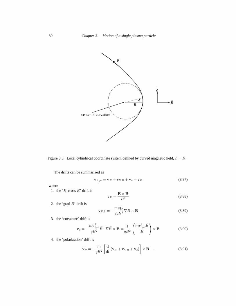
80 Chapter 3. Motion of a single plasma particle
φ
RR
φ
B
centerof curvature
Figure 3.5: Local cylindrical coordinate system defined by curved magnetic field,φ = B.
The drifts can be summarized as
v⊥gc = vE + v∇B + vc + vP (3.87)
where1. the ‘E crossB’ drift is
vE = E×BB2 (3.88)
2. the ‘gradB’ drift is
v∇B = −mv2L02qB3 ∇B ×B (3.89)
3. the ‘curvature’ drift is
vc = −mv2‖gcqB2 B · ∇B ×B = 1
qB2
(mv2‖gcRR
)×B (3.90)
4. the ‘polarization’ drift is
vP = − mqB2
[ ddt (vE + v∇B + vc)
]×B . (3.91)

3.5 Drift equations 81
3.5.3 µ conservation
We now imagine being in a frame moving with the velocityv⊥gc; in this frame the onlyperpendicular velocity is the cyclotron velocity (Larmor motion).Sincev⊥gc is orthogonalto B, the parallel equation of motion is not affected by this change of frame and usingEqs.(3.70) and (3.84) can be written as
mdv‖dt = qE‖ − mv2L0
2B∂B∂s (3.92)
where as before,s is the distance along the magnetic field. Multiplication byv‖ gives anenergy relation
ddt
(mv2‖2
)= qE‖v‖ − mv2L0
2B v‖ ∂B∂s . (3.93)
The perpendicular force defined in Eq.(3.73) does not exist in this moving framebecause ithas been ‘transformed away’ by the change of frames. Also, recall that it was assumed thatthe characteristic scale lengths ofE andB are large compared to the gyro radius (Larmorradius). However, if the magnetic field has anabsolute time derivative, Faraday’s law statesthat there must be an inductive electric field, i.e., an electric field for which
∮E·dl = 0.
This is distinct from the static electric field that has been previously assumed and so itsconsequences must be explicitly taken into account.
To understand the effect of an inductive electric field, consider a specific particle, anddot the Lorentz equation withv to obtain
ddt
(mv2‖2 + mv2LO
2)
= qv‖E‖ + qv⊥ ·E⊥ (3.94)
wherev⊥ is the vector Larmor orbit velocity. Subtracting Eq.(3.93) from (3.94) gives
ddt
(mv2L02
)= qv⊥ ·E⊥+mv2L0
2B v‖ ∂B∂s . (3.95)
Integration of Faraday’s law over the cross-section of the Larmor orbit gives
∫ds ·∇×E = −
∫ds·∂B∂t (3.96)
or ∮dl ·E = −πr2L ∂B
∂t (3.97)
where it has been assumed that the magnetic field is changing sufficientlyslowly for theorbit radius to be approximately constant during each orbit.
Equation (3.95) involves the local electric fieldE⊥ but Eq.(3.97) only gives the lineintegral of the electric field. This line integral can still be used if Eq.(3.95) is averaged overa cyclotron period. The critical term is the time average over the Larmororbit of qv⊥ ·E⊥

82 Chapter 3. Motion of a single plasma particle
(which gives the rate at which the perpendicular electric field does workon the particle),
< qv⊥ ·E⊥ >orbit = ωc2π
∫dt qv⊥ ·E⊥
= −qωc2π
∮dl ·E⊥
= qωc2 r2L ∂B
∂t .
(3.98)
The substitutionv⊥dt = −dl has been used and the minus sign is invoked because particlemotion is diamagnetic (e.g., ions have a left-handed orbit, whereas in Stokes’ theoremdlis assumed to be a right handed line element). Averaging of Eq. (3.95) gives⟨ d
dt(mv2L0
2)⟩
= mv2L02B
∂B∂t +mv2L0
2B v‖ ∂B∂s = mv2L02B
dBdt (3.99)
wheredB/dt = ∂B/∂t + v‖∂B/∂s is thetotal derivativeof the average magnetic fieldexperienced by the particle over a Larmor orbit. Defining the Larmor orbit kinetic energyasW⊥ = mv2L0/2, Eq.(3.99) can be rewritten as
1W⊥
dW⊥dt = 1
BdBdt (3.100)
which has the solution W⊥B ≡ µ = const. (3.101)
for magnetic fields that can be changing inbothtime and space. In plasma physics terminol-ogy,µ is called the ‘first adiabatic’ invariant, and the invariance ofµ shows that the ratio ofthe kinetic energy of gyromotion to gyrofrequency is a conserved quantity. The derivationassumed the magnetic field changed sufficiently slowly for the instantaneous field strengthB(t) during an orbit to differ only slightly from the orbit-averaged field strength 〈B〉 theorbit, i.e.,|B(t) − 〈B〉 | << 〈B〉 .
3.5.4 Relation of µ conservation to other conservation relations
µ conservation is both of fundamental importance and a prime example of the adiabaticinvariance of the action integral associated with a periodic motion. Theµ conservationconcept unites together several seemingly disparate points of view:
1. Conservation of magnetic moment of a particle- According to electromagnetic theorythe magnetic momentm of a current loop ism = IA whereI is the current carried inthe loop andA is the area enclosed by the loop. Because a gyrating particle traces outa circular orbit at the frequencyωc/2π and has a chargeq, it effectively constitutesa current loop havingI = qωc/2π and cross-sectional areaA = πr2L. Thus, themagnetic moment of the gyrating particle is
m =(qωc
2π)πr2L = mv2L0
2B = µ (3.102)
and so the magnetic momentm is an adiabatically conserved quantity.

3.5 Drift equations 83
2. Conservation of magneticflux enclosed by gyro-orbit- Because the magneticflux Φenclosed by the gyro-orbit is
Φ = Bπr2L =(2mπ
q)
µ, (3.103)
µ conservation further implies conservation of the magneticflux enclosed by a gyro-orbit. This is consistent with the concept that the magneticflux is frozen into theplasma, since if the field is made stronger, the field lines squeeze together such thatthe density of field lines per area increases proportional to the field strength.As shownin Fig.3.6, the particle orbit area contracts in inverse proportion to the field strength sothat after a compression of field, the particle orbit links the same numberof field linesas before the compression.
3. Hamiltonian point of view (cylindrical geometry with azimuthal symmetry)- Definea cylindrical coordinate system(r, θ, z) with z axis along the axis of rotation of thegyrating particle. SinceBz = r−1∂(rAθ)/∂r the vector potential isAθ = rBz/2.The velocity vector isv =rr + rθθ + zz and the Lagrangian is
L = m2(r2 + r2θ2 + z2
)+ qrθAθ − qφ (3.104)
so that the canonical angular momentum is
Pθ = mr 2θ + qrAθ = mr2θ + qr2Bz/2. (3.105)
Since particles are diamagnetic,θ = −ωc. Because of the azimuthal symmetry,Pθwill be a constant of the motion and so
const. = Pθ = −mr2ωc + qr2B/2 = −mv2θ2ωc
= −mq µ. (3.106)
This shows that constancy of canonical angular momentum is equivalent toµ conser-vation. It is important to realize that constancy of angular momentum due to perfectaxisymmetry is a much more restrictive assumption than the slowness assumptionused for adiabatic invariance.
4. Adiabatic gas law- The pressure associated with gyrating particles has dimensionalityN = 2, i.e.,P = (m/2) ∫ v′ · v′fd2v wherev′ =vxx + vyy and thex − y plane isthe plane of the gyration. Also the density for a two dimensional system has units ofparticles/area, i.e.n ∼ 1/A. Hence, the pressure will scale asP ∼ v2T⊥/A. Sinceγ = (N + 2)/N = 2, the adiabatic law, Eq.(2.37), gives
const. ∼ Pn2 ∼ v2T⊥
A A2; (3.107)
but from theflux conservation property of orbitsA ∼ 1/B so Eq.(3.107) becomes
Pn2 ∼ v2T⊥
B (3.108)
which is again proportional toµ sincev2T⊥ is proportional to the mean perpendicularthermal energy, i.e., the average of the gyrational energies of the individualparticlesmaking up thefluid.

84 Chapter 3. Motion of a single plasma particle
particleorbit areacontractsin inverse proportionto the field strength
after compressionof field,particle orbit links same numberof field linesasbefore
field lines oftime-dependentmagneticfield Bzt
Larmor orbittwo particlesat sameposition,but havingdifferentgyrocenters
increasemagneticfield strength
EE
Figure 3.6: Illustration showing how conservation offlux linked by an orbit is equivalent tofrozen-in field; also increasing magnetic field results in magnetic compression.
3.5.5 Magnetic mirrors- a consequence ofµ conservation
Consider a charged particle moving in a static, but spatially nonuniform magnetic field.The non-uniformity is such that the field strength varies in the direction of the field line sothat∂B/∂s = 0 wheres is the distance along a field line. Such a field cannot be straightbecause if it were and so had the formB =Bz(z)z, it would necessarily have a non-zerodivergence, i.e., it would have∇ ·B = ∂Bz/∂z = 0. Because magnetic fields must havezero divergence there must be another component besidesBz and this other componentmust be spatially non-uniform also in order to contribute to the divergence.Hence the fieldmust be curved if the field strength varies along the direction of the field.
This curvature is easy to see by sketching field lines, as shown in Fig.3.7. The densityof field lines is proportional to the strength of the magnetic field and so a gradient of fieldstrength along the field means that the field lines squeeze together as the field becomesstronger. Because magnetic field lines have zero divergence they are endless and so mustbend as they squeeze together. This means that if∂Bz/∂z = 0 there must also be a field
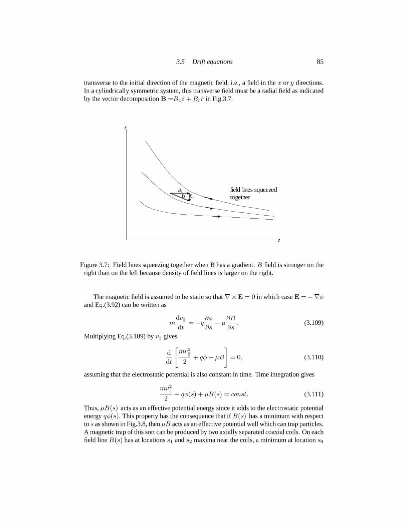
3.5 Drift equations 85
transverse to the initial direction of the magnetic field, i.e., a field in thex or y directions.In a cylindrically symmetric system, this transverse field must be a radial field as indicatedby the vector decompositionB =Bzz + Br r in Fig.3.7.
BBz
Br
r
z
field linessqueezedtogether
Figure 3.7: Field lines squeezing together when B has a gradient.B field is stronger on theright than on the left because density of field lines is larger on the right.
The magnetic field is assumed to be static so that∇×E = 0 in which caseE =−∇φand Eq.(3.92) can be written as
mdv‖dt = −q∂φ∂s − µ∂B
∂s . (3.109)
Multiplying Eq.(3.109) byv‖ gives
ddt
[mv2‖2 + qφ + µB
]
= 0, (3.110)
assuming that the electrostatic potential is also constant in time. Time integration gives
mv2‖2 + qφ(s) + µB(s) = const. (3.111)
Thus,µB(s) acts as an effective potential energy since it adds to the electrostatic potentialenergyqφ(s). This property has the consequence that ifB(s) has a minimum with respecttos as shown in Fig.3.8, thenµB acts as an effective potential well which can trap particles.A magnetic trap of this sort can be produced by two axially separated coaxialcoils. On eachfield lineB(s) has at locationss1 ands2 maxima near the coils, a minimum at locations0
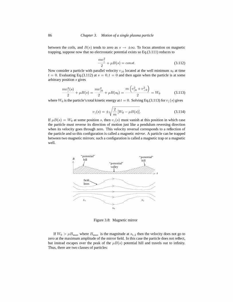
86 Chapter 3. Motion of a single plasma particle
between the coils, andB(s) tends to zero ass → ±∞. To focus attention on magnetictrapping, suppose now that no electrostatic potential exists so Eq.(3.111) reduces to
mv2‖2 + µB(s) = const. (3.112)
Now consider a particle with parallel velocityv‖0 located at the well minimums0 at timet = 0. Evaluating Eq.(3.112) ats = 0, t = 0 and then again when the particle is at somearbitrary positions gives
mv2‖(s)2 + µB(s) = mv2‖0
2 + µB(s0) = m(
v2‖0 + v2⊥0
)
2 = W0 (3.113)
whereW0 is the particle’s total kinetic energy att = 0. Solving Eq.(3.113) forv‖(s) gives
v‖(s) = ±√ 2
m [W0 − µB(s)]. (3.114)
If µB(s) = W0 at some positions, thenv‖(s) must vanish at this position in which casethe particle must reverse its direction of motion just like a pendulum reversing directionwhen its velocity goes through zero. This velocity reversal corresponds to a reflection ofthe particle and so this configuration is called a magneticmirror. A particle can be trappedbetween two magnetic mirrors; such a configuration is called a magnetic trap or a magneticwell.
B
s0
s1 s2
fieldlines
“potential”hill
“potential”hill
“potential”valley
z
Figure 3.8: Magnetic mirror
If W0 > µBmax whereBmax is the magnitude ats1,2 then the velocity does not go tozero at the maximum amplitude of the mirror field. In this case the particle does not reflect,but instead escapes over the peak of theµB(s) potential hill and travels out to infinity.Thus, there are two classes of particles:

3.5 Drift equations 87
1. trapped particles – these haveW0 < µBmax and bounce back and forth between themirrors of the magnetic well,
2. untrapped (or passing) particles – these haveW0 > µBmax and are retarded at thepotential hills but not reflected.
Sinceµ = mv2⊥0/2Bmin andW0 = mv20/2, the criterion for trapping can be writtenas
BminBmax
< v2⊥0v20 . (3.115)
Let us defineθ as the angle the velocity vector makes with respect to the magnetic field ats0, i.e.,sin θ = v⊥0/v0 and also define
θtrap = sin −1√Bmin
Bmax. (3.116)
Thus, as shown in Fig.3.9 all particles withθ > θtrap are trapped, while all particles withθ < θtrap are untrapped. Suppose att = 0 the particle velocity distribution ats0 isisotropic. After a long time interval long enough for all untrapped particles to have escapedthe trap, there will be no particles in theθ < θtrap region of velocity space. The velocitydistribution will thus be zero forθ < θtrap; such a distribution function is called aloss-conedistribution function.
mirrortrapped
losscone
θ
vθtrap
Figure 3.9: Loss-cone velocity distribution. Particles with velocity angleθ > θtrap aremirror trapped, others are lost.
3.5.6 J , the Second Adiabatic Invariant
Trapped particles have periodic motion in the magnetic well, and so applying the concept

88 Chapter 3. Motion of a single plasma particle
of adiabatic invariance presented in Sec.3.4.1, the quantity
J =∮
P‖ds =∮
(mv‖ + qA‖)ds (3.117)
will be an invariant if1. any time dependence of the well shape is slow compared to the bounce frequency of
the trapped particle,
2. any spatial inhomogeneities of the well magnetic field are so gradual that the particle’sbounce trajectory changes by only a small amount from one bounce to the next.
To determine the circumstances whereA‖ = 0, we use Coulomb gauge (i.e., assume∇·A =0) and at any given location define a local Cartesian coordinate system with z axisparallel to the local field. From Ampere’s law it is seen that
[∇× (∇×A)] z = −∇2Az = µ0Jz (3.118)
soAz is finite only if there is acurrent parallel to the magnetic field. BecauseJz acts asthe source term in a Poisson-like partial differential equation forAz , the parallel currentneed not be at the same location asAz. If there are no currents parallel to the magneticfield anywhere thenA‖ = 0, and in this case the second adiabatic invariant reduces to
J = m∮
v‖ds. (3.119)
Having a currentflow along the magnetic field corresponds to a more complicated magnetictopology. The axial current produces an associated azimuthal magnetic fieldwhich linksthe axial magnetic field resulting in a helical twist. This more complicated situation offinite magnetic helicity will be discussed in a later chapter.
3.5.7 Consequences ofJ -invariance
Just asµ invariance was related to the perpendicular CGL adiabatic invariant discussedin Sec.(2.101),J -invariance is closely related to the parallel CGL adiabatic invariant alsodiscussed in Sec.(2.101). To see this relation, recall that density in a one dimensionalsystem has dimensions of particles per unit length, i.e.,n1D ∼ 1/L, and pressure in a onedimensional system has dimensions of kinetic energy per unit length, i.e.,P1D ∼ v2‖/L.For parallel motion the number of dimensions isN = 1 so thatγ = (N + 2)/N = 3 andthefluid adiabatic relation is
const. ∼ P1Dn31D
∼ v2‖/LL−3 ∼ (v‖L)2 (3.120)
which is a simplified form of Eq.(3.119) since Eq.(3.119) has the scalingJ ∼v‖L = const.J -invariance combined with mirror trapping/detrapping is the basis of an accelerationmechanism proposed by Fermi (1954) as a means for accelerating cosmic ray particles toultra-relativistic velocities. The Fermi mechanism works as follows: Consider a particleinitially trapped in a magnetic mirror. This particle has an initial angle in velocity spaceθ > θtrap; bothθ andθtrap are measured when the particle is at the mirror minimum. Nowsuppose the distance between the magnetic mirrors is slowly reduced so thatthe bounce

3.5 Drift equations 89
distanceL of the mirror-trapped particle slowly decreases. This would typically occur byreducing the axial separation between the coils producing the magnetic mirror field. Be-causeJ ∼ v‖L is invariant, the particle’s parallel velocity increases on each successivebounce asL slowly decreases. This steady increase inv‖ means that the velocity angleθ decreases. Eventually,θ becomes smaller thanθtrap whereupon the particle becomesdetrapped and escapes from one end of the mirror with a large parallel velocity. This mech-anism provides a slow pumping to very high energy, followed by a sudden and automaticejection of the energetic particle.
3.5.8 The third adiabatic invariant
Consider a particle bouncing back and forth in either of the two geometries shown inFig.3.10. In Fig.3.10(a), the magnetic field is produced by a single magnetic dipole andthe field lines always have convex curvature, i.e. the radius of curvature is always on theinside of the field lines. The field decreases in magnitude with increasing distance from thedipole.
(a) (b)
Figure 3.10: Magnetic field lines relevant to discussion of third adiabatic invariant: (a) fieldlines always have same curvature (dipole field), (b) field lines have both concave and con-vex curvature (mirror field).
In Fig.3.10(b) the field is produced by two coils and has convex curvature near themirror minimum and concave curvature in the vicinity of the coils. On defining a cylindrical

90 Chapter 3. Motion of a single plasma particle
coordinate system(r, θ, z) with z axis coaxial with the coils, it is seen that in the regionbetween the two coils where the field bulges out, the field strength is a decreasing functionof r, i.e. ∂B/∂r < 0, whereas in the plane of each coil the opposite is true. Thus, in themirror minimum, both the centrifugal and gradB forces are radially outward, whereas theopposite is true near the coils.
In both Figs. 3.10(a) and (b) a particle moving along the field line can be mirror-trapped because in both cases the field has a minimumflanked by two maxima. However,for Fig.3.10(a), the particle will have gradB and curvature drifts always in the same az-imuthal sense, whereas for Fig.3.10(b) the azimuthal direction of these drifts will dependon whether the particle is in a region of concave or convex curvature. Thus, in addition tothe mirror bouncing motion, much slower curvature and gradB drifts also exist, directedalong the field binormal (i.e. the direction orthogonal to both the field and its radius ofcurvature). These higher-order drifts may alternate sign during the mirror bouncing. Thebinormally directed displacement made by a particle during itsith complete periodτ ofmirror bouncing is
δrj =∫ τ
0vdt (3.121)
whereτ is the mirror bounce period andv is the sum of the curvature and gradB driftsexperienced in the course of a mirror bounce. This displacement is due to thecumulativeeffect of the curvature and gradB drifts experienced during one complete period of bounc-ing between the magnetic mirrors. The average velocity associated with this slow driftingmay be defined as
〈v〉=1τ∫ τ
0vdt. (3.122)
Let us calculate the action associated with a sequence ofδrj. This action is
S = ∑
j[m 〈v〉 + qA]j · δrj (3.123)
where the quantity in square brackets is evaluated on the line segmentδrj. If the δrj aresmall then this can be converted into an action ‘integral’ for the pathtraced out by theδrj. If the δrj are sufficiently small to behave as differentials, then we may writethem asdrbounce and express the summation as an action integral
S =∫
[m 〈v〉 + qA] · drbounce (3.124)
where it must be remembered that〈v〉 is the bounce-averagedvelocity. The quantitym 〈v〉 + qA is just the canonical momentum associated with the effective motion alongthe sequence of line segmentsδrj . The vectorrbounce is a vector pointing from the originto the particle’s location at successive bounces and so is the generalized coordinate asso-ciated with the bounce averaged velocity. If the motion resulting from〈v〉 is periodic, weexpectS to be an adiabatic invariant. The first term in Eq.(3.124) will be of the order ofmvdrift2πr wherer is the radius of the trajectory described by theδrj .The second term isjust qΦ whereΦ is the magneticflux enclosed by the trajectory. Let us compare the ratioof these two terms
∫ m 〈v〉 · dr∫ qA · dr ∼ mvdrift2πr
qBπr2 ∼ vdriftωcr ∼ r2L
r2 (3.125)

3.6 Relation of Drift Equations to the Double Adiabatic MHD Equations 91
where we have usedv∇B ∼ vc ∼ v2⊥/ωcr ∼ ωcr2L/r. Thus, if the Larmor radius is muchsmaller than the characteristic scale length of the field, the magneticflux term dominatesthe action integral and adiabatic invariance corresponds to the particlestaying on a constantflux surfaceas its orbit evolves following the various curvature and gradB drifts. This thirdadiabatic invariant is much more fragile thanJ , which in turn was more fragile thanµ,because the analysis here is based on the rather strong assumption that thecurvature andgradB drifts are small enough for theδrj to trace out a nearly periodic orbit.
3.6 Relation of Drift Equations to the Double AdiabaticMHD Equations
The derivation of the MHD Ohm’s law involved dropping the Hall term (see p. 48)andthe basis for dropping this term was assuming thatω << ωci whereω is the characteris-tic rate of change of the electromagnetic field. The derivation of the singleparticle driftequations involved essentially the same assumption (i.e., the motion was slow compared toωcσ). Thus, if the characteristic rate of change of the electromagnetic fieldis slow com-pared toωci both the MHD and the single particle drift equations ought to be equally validdescriptions of the plasma dynamics. If so, then there also ought to be somesort of a cor-respondence relation between these two points of view. Some evidence supporting thishypothesis was the observation that the single particle adiabatic invariantsµ andJ wererespectively related to the perpendicular and parallel double adiabaticMHD equations. Itthus seems reasonable to expect additional connections between the drift equations andthe double adiabatic MHD equations.
In fact, an approximate derivation of the double adiabatic MHD equations canbe ob-tained by summing the currents associated with the various particle drifts — providing oneadditional effect,diamagnetic current,is added to this sum. Diamagnetic current is a pe-culiar concept because it is a consequence of the macroscopic phenomenon of pressuregradients and so has no meaning in the context of a single particle description.
In order to establish this microscopic-macroscopic relationship we begin by recallingfrom electromagnetic theory2 that a magnetic material with densityM of magnetic dipolemoments per unit volume has an associated magnetization current
JM = ∇×M. (3.126)
The magnitude of the magnetic moment of a charged particle in a magnetic field was shownin Sec.3.5.4 to beµ. The magnetic moment of a magnetic dipole is a vector pointing inthe direction of the magnetic field produced by the dipole. The vector magnetic momentof a charged particle gyrating in a magnetic field ism = −µB where the minus signcorresponds to cyclotron motion being diamagnetic, i.e., the magnetic field resulting fromcyclotron rotation opposes the original field in which the particle is rotating. For example,an individual ion placed in a magnetic fieldB =Bz rotates in the negativeθ direction, andso the current associated with the ion motion creates a magnetic field pointing in the−zdirection inside the ion orbit.
2For example, see p. 192 of (Jackson 1998).

92 Chapter 3. Motion of a single plasma particle
Suppose there exists a large number or ensemble of particles with densitynσ and meanmagnetic momentµσ . The density of magnetic moments, or magnetization density, of thisensemble is
M = −∑
σnσµσB = −∑
σnσ
⟨mσv2⊥2B
⟩
B = −P⊥BB (3.127)
where〈〉 denotes averaging over the velocity distribution and Eq.(2.26) has been used.Inserting Eq.(3.127) into Eq.(3.126) shows that this ensemble of charged particles in amagnetic field has adiamagnetic current
JM = −∇×(P⊥B
B)
. (3.128)
Figure 3.11: Gradient of magnetized particles gives apparent current as observed on dashedline.
Figure 3.11 shows the physical origin ofJM . Here, a collection of ions all rotate clock-wise in a magnetic field pointing out of the page. The azimuthally directed current on thedashed curve is the sum of contributions from (i) particles with guiding centers locatedone Larmor radiusinside the dashed curve and (ii) particles with guiding centers locatedone Larmor radiusoutsidethe dashed curve. From the point of view of an observer lo-cated on the dashed curve, the inside particles [group (i)] constitute a clockwise current,whereas the outside [group (ii)] particles constitute a counterclockwise current. If there areunequal numbers of inside and outside particles (indicated here by concentriccircles inside
3.6 Relation of Drift Equations to the Double Adiabatic MHD Equations 93
the dashed curve), then the two opposing currents do not cancel and a net macroscopic cur-rent appears toflow around the dashed curve, even thoughno actual particlesflow aroundthe dashed curve. Inequality of the numbers of inside and outside particles corresponds toa density gradient and so we see that a radial density gradient of gyrating particles gives anet macroscopic azimuthal current. Similarly, if there is a radial temperature gradient, thevelocities of the inner and outer groups differ, resulting again in an apparent macroscopicazimuthal current. The combination of density and temperature gradients is such that thenet macroscopic current depends on the pressure gradient as given by Eq.(3.128).
Taking diamagnetic current into account is critical for establishing acorrespondencebetween the single particle drifts and the MHD equations, and having recognized this,we are now in a position to derive this correspondence. In order for the derivation to betractable yet non-trivial, it will be assumed that the magnetic field is time-independent, butthe electric field will be allowed to depend on time. It is also assumed that thedominantcross-field particle motion is thevE = E×B/B2 drift; this assumption is consistent withthe hierarchy of particle drifts (i.e., polarization drift is a higher-order correction tovE) .
Because both species have the samevE , no macroscopic current results fromvE , andso all cross-field currents must result from the other, smaller drifts, namelyv∇B, vc, andvp. Let us now add the magnetization current to the currents associated withv∇B, vc, andvp to obtain the total macroscopic current
Jtotal = JM + J∇B + Jc + Jp = JM + ∑
σnσqσ (u∇B,σ + uc,σ + up,σ) (3.129)
whereJ∇B,Jc, Jp are currents due to gradB, curvature, and polarization drifts respec-tively andu∇B,σ, uc,σ andup,σ are the mean (i.e.,fluid) velocities associated with thesedrifts. These currents are explicitly:
1. gradB current
J∇B = ∑
σ nσqσu∇B,σ
= −∑
σmσnσqσ ⟨v2⊥σ
⟩
2B∇B ×BqσB2 = −P⊥
∇B ×BB3
(3.130)
2. curvature current
Jc = ∑
σ nσqσuc,σ
= −∑
σ nσqσmσ⟨
v2‖σ⟩ B · ∇B ×B
qσB2 = −P‖B · ∇B ×B
B2(3.131)
3. polarization current
Jp = ∑
σnσqσup,σ = ∑
σnσqσ
( mσqσB2
dE⊥dt
)
= ρB2
dE⊥dt . (3.132)
Because the magnetic field was assumed to be constant, the time derivative of vE is theonly contributor to the polarization drift current.

94 Chapter 3. Motion of a single plasma particle
The total magnetic force is
Jtotal ×B = (JM + J∇B + Jc + JP ) ×B
=
−∇×(P⊥B
B)
−P⊥∇B ×B
B3
−P‖B · ∇B ×B
B2 + ρB2
dEdt
×B.(3.133)
The gradB current cancelspart of the magnetization current as follows:
∇×(P⊥B
B)
+ P⊥∇B ×B
B3 =[∇( 1
B)×P⊥B + 1
B∇× (
P⊥B)
]
+P⊥∇B ×B
B3
= 1B∇× (
P⊥B)
= P⊥B ∇× B + ∇P⊥ × B
B(3.134)
so that
Jtotal ×B = −[
P⊥∇× B +∇P⊥ × B + P‖B · ∇B × B − ρB
dEdt
]× B. (3.135)
The first term can be recast using the vector identity
∇( B · B
2)
= 0 = B · ∇B + B ×∇× B (3.136)
while the electric field can be replaced usingE = −U×B to give
Jtotal ×B = − (P⊥ −P‖) B · ∇B +∇⊥P⊥ − ρ
Bd (U×B)
dt × B. (3.137)
Here the relation[
B · ∇B]
⊥ = B · ∇B has been used; this relation follows from Eq.
(3.136). Finally, it is observed that[∇ · (BB
)]
⊥ =[(∇ · B)
B + B · ∇B]
⊥ = B · ∇B (3.138)
so(P⊥ −P‖
) B·∇B = (P⊥ − P‖)
[∇ · (BB)]
⊥ =[∇ · (P⊥ − P‖
) BB]
⊥ . (3.139)
Furthermore, ρB
d (U×B)dt × B ≃ −[
ρdUdt
]
⊥(3.140)
since it has been assumed that the magnetic field is time-independent. Inserting these lasttwo results in Eq.(3.137) gives
Jtotal ×B =[∇ · (P⊥ − P‖
) BB]
⊥ + ∇⊥P⊥ +[
ρdUdt
]
⊥(3.141)

3.7 Non-adiabatic motion in symmetric geometry 95
or[
ρdUdt
]
⊥=
[
Jtotal ×B−∇ · P⊥←→I + (P⊥ − P‖
) BB]
⊥ (3.142)
which is just the perpendicular component of the double adiabatic MHD equation of mo-tion. This demonstrates that if diamagnetic current is taken into account, the drift equationsfor phenomena with characteristic frequenciesω much smaller thanωci and the double adi-abatic MHD equations are equivalent descriptions of plasma dynamics. Thisanalysis alsoshows that one has to be extremely careful when invoking single particle concepts to ex-plain macroscopic behavior, because if diamagnetic effects are omitted, erroneous conclu-sions can result.
The reason for the name polarization current can now be addressed by comparing thiscurrent to the currentflowing through a parallel plate capacitor with dielectricε. The ca-pacitance of the parallel plate capacitor isC = εA/d whereA is the cross-sectional areaof the capacitor plates andw is the gap between the plates. The charge on the capacitoris Q = CV whereV is the voltage across the capacitor plates. The current through thecapacitor isI = dQ/dt so
I = C dVdt = εA
ddVdt . (3.143)
However the electric field between the plates isE = V/d and the current density isJ =I/A so this can be expressed as
J = εdEdt (3.144)
which gives the alternating current density in a medium with dielectric ε. If this is comparedto the polarization current
Jp = ρB2
dE⊥dt (3.145)
it is seen that the plasma acts like a dielectric medium in the direction perpendicular to themagnetic field and has an effective dielectric constant given byρ/B2.
3.7 Non-adiabatic motion in symmetric geometry
Adiabatic behavior occurs when temporal or spatial changes in the electromagnetic fieldfrom one cyclical orbit to the next are sufficiently gradual to be effectively continuousand differentiable (i.e., analytic). Thus, adiabatic behavior corresponds to situations wherevariations of the electromagnetic field are sufficiently gradual to be characterized by thetechniques of calculus (differentials, limits, Taylor expansions, etc.).
Non-adiabatic particle motion occurs when this is not so. It is therefore nosurprise thatit is usually not possible to construct analytic descriptions of non-adiabaticparticle motion.However, there exist certain special situations where non-adiabatic motion can be describedanalytically. Using these special cases as a guide, it is possible to develop an understandingfor what happens when motion is non-adiabatic.
One special situation is where the electromagnetic field isgeometrically symmetricwithrespect to some coordinateQj in which case the symmetry makes it possible to developanalytic descriptions of non-adiabatic motion. This is because symmetry in Qj causes thecanonical momentumPj to be an exact constant of the motion. The critical feature is thatPj remains constant no matter how drastically the field changes in time or space because

96 Chapter 3. Motion of a single plasma particle
Lagrange’s equationPj = −∂L/∂Qj has no limitations on the rate at which changes canoccur. In effect, being geometrically symmetric trumps being non-analytic. The absoluteinvariance ofPj when∂L/∂Qj = 0 reduces the number of equations and allows a partialor sometimes even a complete solution of the motion. Solutions to symmetricproblemsgive valuable insight regarding the more general situation of being both non-adiabatic andasymmetric.
Two closed related examples of non-adiabatic particle motion will now be analyzed: (i)sudden temporal and (ii) sudden spatial reversal of the polarity of an azimuthally symmetricmagnetic field having no azimuthal component. The most general form of such a fieldcanbe written in cylindrical coordinates(r, θ, z) as
B = 12π∇ψ(r, z, t) ×∇θ; (3.146)
a field of this form is called poloidal. Rather than usingθ explicitly, the form∇θ has beenused because∇θ is better suited for use with the various identities of vector calculus (e.g.,∇×∇θ = 0) and leads to greater algebraic clarity. The relationship between∇θ andθ isseen by simply taking the gradient:
∇θ =(
r ∂∂r + θ
r∂∂θ + z ∂
∂z)
θ = θr . (3.147)
Equation(3.146) automatically satisfies∇ · B = 0 [by virtue of the vector identity∇ · (G×H) = H·∇×G−G·∇×H], has noθ component, and is otherwise arbitrarysinceψ is arbitrary. As shown in Fig.3.12, the magneticflux linking a circle of radiusrwith center at axial positionz is
∫
B·ds =∫ r
02πrdrz · [ 1
2π∇ψ(r, z, t) ×∇θ]
=∫ r
0dr∂ψ(r, z, t)
∂r = ψ(r, z, t) −ψ(0, z, t).(3.148)
However,
Br(r, z, t) = − 12πr
∂ψ∂z (3.149)
and since∇ ·B =0, Br must vanish atr = 0, and so∂ψ/∂z = 0 on the symmetry axisr = 0.

3.7 Non-adiabatic motion in symmetric geometry 97
Bz
ψr,z is fluxlinked bythiscircle
Figure 3.12: Azimuthally symmetricflux surface
Thusψ is constant along the symmetry axisr = 0; for convenience we choose thisconstant to be zero. Hence,ψ(r, z, t) is precisely the magneticflux enclosed by a circle ofradiusr at axial locationz. We can also use the vector potentialA to calculate the magneticflux through the same circle and obtain
∫
B·ds =∫ ∇×A·ds =
∮
A·dl =∫ 2π
0Aθrdθ = 2πrAθ. (3.150)
This shows that thefluxψ and the vector potentialAθ are related by
ψ(r, z, t) = 2πrAθ. (3.151)
No other component of vector potential is required to determine the magnetic field and sowe may setA =Aθ(r, z, t)θ.
The currentJ =µ−10 ∇×B producing this magnetic field is purely azimuthal as can beseen by considering ther andz components of∇×B. The actual current density is
Jθ = µ−10 r∇θ · ∇ ×B= µ−10 r∇ · (B×∇θ)= − r
2πµ0∇ ·( 1
r2∇ψ)
= − r2πµ0
[ ∂∂r
( 1r2
∂ψ∂r
)
+ 1r2
∂2ψ∂z2
]
(3.152)

98 Chapter 3. Motion of a single plasma particle
a Poisson-like equation. Since no current loops can exist at infinity, the field prescribedby Eq.(3.146) must be produced by a set of coaxial coils having various finite radiir andvarious finite axial positionsz.
The axial magnetic field is
Bz = 12πr
∂ψ∂r . (3.153)
Nearr = 0, ψ can always be Taylor expanded as
ψ(r, z) = 0 + r∂ψ(r = 0, z)∂r + r2
2∂2ψ(r = 0, z)
∂r2 + ... (3.154)
Suppose that∂ψ/∂r is non-zero atr = 0, i.e.,ψ ∼ r nearr = 0. If this were the case,then the first term in the right hand side of the last line of Eq.(3.152) would become infiniteand so lead to an infinite current density atr = 0. Such a result is non-physical and so werequire that the first non-zero term in the Taylor expansion ofψ aboutr = 0 to be ther2term.
Every field line that loops through the inside of a current loop also loops back in thereverse direction on the outside, so there is no net magneticflux at infinity. This meansthatψ must vanish at infinity and so asr increases,ψ increases from its value of zero atr = 0 to some maximum valueψmax atr = rmax, and then slowly decreases back to zeroasr → ∞. As seen from Eq.(3.153) this behavior corresponds toBz being positive forr < rmax and negative forr > rmax. A contour plot of theψ(r, z) flux surfaces and a plotof ψ(r, z = 0) versusr is shown in Fig.3.13.
ψr,0
r
rB
ψr,z = const.
z
Figure 3.13: Contour plot offlux surfaces

3.7 Non-adiabatic motion in symmetric geometry 99
In this cylindrical coordinate system the Lagrangian, Eq.(3.12), has the form
L = m2
(
r2 + r2θ2 + z2)
+ qrθAθ − qφ(r, z, t). (3.155)
Sinceθ is an ignorable coordinate, the canonical angular momentum is a constant of themotion, i.e.
Pθ = ∂L∂θ = mr2θ + qrAθ = const. (3.156)
or, in terms offlux,
Pθ = mr2θ + q2πψ(r, z, t) = const. (3.157)
Thus, the Hamiltonian is
H = m2
(
r2 + r2θ2 + z2)
+ φ(r, z, t)
= m2
(r2 + z2) + (Pθ − qψ(r, z, t)/2π)22mr2 + φ(r, z, t)
= m2
(r2 + z2) + χ(r, z, t)
(3.158)
where
χ(r, z, t) = 12m
[Pθ − qψ(r, z, t)/2πr
]2(3.159)
is aneffectivepotential. For purposes of plotting, the effective potential can be writtenin adimensionless form as
χ(r, z, t)χ0
=
2πPθqψ0
− ψ(r, z, t)ψ0
r/L
2
(3.160)
whereL is some reference scale length,ψ0 is some arbitrary reference value for theflux,andχ0 = qψ20/8π2L2m. For simplicity we have setφ(r, z, t) = 0, since this term givesthe motion of a particle in a readily understood, two-dimensional electrostatic potential.
Suppose that for timest < t1 the coil currents are constant in which case the associatedmagnetic field andflux are also constant. Since the Lagrangian does not explicitly dependon time, the energyH is a constant of the motion. Hence there are two constants of themotion,H andPθ. Consider now a particle located initially on the midplanez = 0 withr < rmax. The particle motion depends on the sign ofqψ/Pθ and so we consider eachpolarity separately.

100 Chapter 3. Motion of a single plasma particle
Figure 3.14: Specific example (withz dependence suppressed) showingψ and χ rela-tionship: top is plot of functionψ(r)/ψ0 = (r/L)2 /(1 + (r/L)6), middle and bot-tom plots show corresponding normalized effective potential for2πPθ/qψ0 = +0.2 and2πPθ/qψ0 = −0.2. Both middle and bottom plots have a minimum atr/L ≃ 0.45; mid-dle plot also has a minimum atr/L ≃ 1.4. The two minima in the middle plot occur whenχ(r)/χ0 = 0 but the single minimum in the bottom plot occurs at a finite value ofχ(r)/χ0indicating that an axis-encircling particle must have finite energy.
1. qψ/Pθ is positive. If 2π|Pθ| < |qψmax| there exists a location insidermax where
Pθ = q2πψ (3.161)
and there exists a location outsidermax where this equality holds as well.χ vanishesat these two points which are also local minima ofχ becauseχ is positive-definite.The top plot in Fig.3.14 shows a nominalψ(r)/ψ0 flux profile and the middle plotshows the correspondingχ(r)/χ0 ; the z andt dependence are suppressed from thearguments for clarity. There exists a maximum ofχ between the two minima. Weconsider a particle initially located in one of the two minima ofχ. If H < χmax theparticle will be confined to an effective potential well centered about theflux surface

3.7 Non-adiabatic motion in symmetric geometry 101
defined by Eq.(3.161). From Eq.(3.157) the angular velocity is
θ = 1mr2
(
Pθ − qψ2π
)
. (3.162)
The sign ofθ reverses periodically as the particle bounces back and forth in theχpotential well. This corresponds to localized gyromotion as shown in Fig.3.15.
non-axis-encircling axis-encircling
Figure 3.15: Localized gyro motion associated with particle bouncing in effective potentialwell.
2. qψ/Pθ is negative. In this caseχ can never vanish, becausePθ − qψ/2π nevervanishes. Nevertheless, it is still possible forχ to have a minimum and hence apotential well. This possibility can be seen by setting∂χ/∂r = 0 which occurswhen
(
Pθ − q2πψ
) ∂∂r
(Pθ − qψ/2πr
)
= 0. (3.163)
Equation (3.163) can be satisfied by having
∂∂r
Pθ − q2πψ
r
= 0 (3.164)
which implies
Pθ = −qr22π
∂∂r
(ψr)
. (3.165)
Recall thatψ had a maximum, thatψ ∼ r2 nearr = 0, and also thatψ → 0 asr → ∞. Thusψ/r ∼ r for small r andψ/r → 0 for r → ∞ so thatψ/r alsohas a maximum; this maximum is located at anr somewhat inside of the maximumof ψ. Thus Eq.(3.165) can only be valid at points inside of this maximum; other-wise the assumption of opposite signs forPθ andψ would be incorrect. Furthermore

102 Chapter 3. Motion of a single plasma particle
Eq.(3.165) can only be satisfied if|Pθ | is not too large, because the right hand side ofEq.(3.165) has a maximum value. If all these conditions are satisfied, thenχwill havea non-zero minimum as shown in the bottom plot of Fig.3.14.
A particularly simple example of this behavior occurs if Eq.(3.165) is satisfied near ther = 0 axis (i.e., whereψ ∼ r2) so that this equation becomes simply
Pθ = − q2πψ (3.166)
which is just the opposite of Eq.(3.161). Substituting in Eq.(3.162) we see thatθ nowneverchanges sign; i.e., the particle isaxis-encircling. The Larmor radius of this axis-encircling particle is just the radius of the minimum of the potential well, the radius whereEq.(3.165) holds. The azimuthal kinetic energy of the particle corresponds to the height ofthe minimum ofχ in the bottom plot of Fig.3.14.
3.7.1 Temporal Reversal of Magnetic Field - Energy Gain
Armed with this information about axis-encircling and non-axis encircling particles, wenow examine the strongly non-adiabatic situation where a coil current startsat I = I0,is reduced to zero, and then becomesI = −I0, so that all fields andfluxes reverse sign.The particle energy will not stay constant for this situation because the Lagrangian dependsexplicitly on time. However, since symmetry is maintained,Pθ mustremain constant. Thus,a non-axis encircling particle (with radial location determined by Eq. (3.161)) will changeto an axis-encircling particle if a minimum exists forχwhen the sign ofψ is reversed. Ifsuch a minimum does exist and if the initial radius was near the axis whereψ ∼ r2, thencomparison of Eqs.(3.161) and (3.166) shows that the particle will have the sameradiusafter the change of sign as before. The particle will gain energy during thefield reversal byan amount corresponding to the finite value of the minimum ofχ for the axis-encirclingcase.
This process can also be considered from the point of view of particle drifts: Initially,the non-axis-encircling particle is frozen to a constantψ surface (flux surface). When thecoil current starts to decrease, the maximum value of theflux correspondingly decreases.The constantψ contours on theinside of ψmax move outwards towards the location ofψmax where they are annihilated. Likewise, the contours outside ofψmax move inwardstoψmax where they are also annihilated.
To the extent that theE×Bdrift is a valid approximation, its effect is to keep theparticle attached to a surface of constantflux. This can be seen by integrating Faraday’slaw over the area of a circle of radiusr to obtain
∫ ds ·∇×E = −∫ ds · ∂B/∂t and theninvoking Stoke’s theorem to give
Eθ2πr = − ∂ψ∂t . (3.167)
The theta component ofE+ v ×B = 0 is
Eθ + vzBr − vrBz = 0 (3.168)
and from (3.146),Br = − (2πr)−1 ∂ψ/∂z andBz = − (2πr)−1 ∂ψ/∂r. Combination ofEqs.(3.167) and (3.168) thus gives
∂ψ∂t + vr ∂ψ∂r + vz ∂ψ∂z = 0 . (3.169)

3.7 Non-adiabatic motion in symmetric geometry 103
Becauseψ(r(t), z(t), t) is theflux measured in the frame of a particle moving with trajec-tory r(t) andz(t), Eq.(3.169) shows that theE×Bdrift maintains the particle on a surfaceof constantψ, i.e., theE×Bdrift is such as to maintaindψ/dt = 0 whered/dt meanstime derivative as measured in the particle frame.
The implication of this attachment of the particle to a surface of constantψ can beappreciated by making an analogy to the motion of people initially located on the beachof a volcanic island which is slowly sinking into the sea. In order toavoid being drownedas the island sinks, the people will move towards the mountain top to stay at aconstantheight above the sea. The location ofψmax here corresponds to the mountain top and theparticles trying to stay on surfaces of constantψ correspond to people trying to stay atconstant altitude. A particle initially located at some location away from the “mountaintop” ψmax moves towardsψmax if the overall level of all theψ surfaces is sinking. Thereduction ofψ as measured at a fixed position will create the azimuthal electric field givenby Eq.(3.167) and this electric field will, as shown by Eqs.(3.168) and (3.169), causeanE×Bdrift which convects each particle in just such a way as to stay on a constantψcontour.
TheE×Bdrift approximation breaks down whenB becomes zero, i.e., whenψ changespolarity. This breakdown corresponds to a breakdown of the adiabatic approximation. Ifψ changes polarity before a particle reachesψmax, the particle becomes axis-encircling.The extra energy associated with being axis-encircling is obtained whenψ ≃ 0 but∂ψ/∂t =0 so that there is an electric fieldEθ, but no magnetic field. FiniteEθ and no magneticfield results in a simple theta acceleration of the particle. Thus, whenψ reverses polarity theparticle is accelerated azimuthally and develops finite kinetic energy. Afterψ has changedpolarity the magnitude ofψ increases and the adiabatic approximation again becomes valid.Because the polarity is reversed, increase of the magnitude ofψ is now analogous to creat-ing an ever deepening crater. Particles again try to stay on constant flux surfaces as dictatedby Eq.(3.169) and as the crater deepens, the particles have to move awayfrom ψmin tostay at the same altitude. When the reversedflux attains the same magnitude as the origi-nal flux, theflux surfaces have the same shape as before. However, the particles arenowaxis-encircling and have the extra kinetic energy obtained at field reversal.
3.7.2 Spatial reversal of field - cusps
Suppose two solenoids with constant currents are arranged coaxially withtheir magneticfields opposing each other as shown in Fig.3.16(a). Since the solenoid currents are constant,the Lagrangian does not depend explicitly on time in which case energy is a constant of themotion. Because of the geometrical arrangement, theflux function is anti-symmetric inzwherez = 0 defines the midplane between the two solenoids.
Consider a particle injected with initial velocityv =vz0z at z = −L, r = a. Sincethis particle has no initialv⊥, it simply streams along a magnetic field line. However,when the particle approaches the cusp region, the magnetic field lines startto curve causingthe particle to develop both curvature and gradB drifts perpendicular to the magneticfield. When the particle approaches thez = 0 plane, the drift approximation breaks downbecauseB → 0 and so the particle’s motion becomes non-adiabatic [cf. Fig.3.16(a)].
Although the particle trajectory is very complex in the vicinity of the cusp, it is stillpossible to determine whether the particle will cross into the positivez half-plane, i.e.,
104 Chapter 3. Motion of a single plasma particle
cross the cusp. Such an analysis is possible because two constants of the motion exist,namelyPθ andH. The energy
H = P 2r2m + P 2z
2m +(
Pθ − q2πψ(r, z)
)2
2mr2 = const. (3.170)
can be evaluated using
Pθ =[
mr2θ + q2πψ
]
initial= q
2πψ0 (3.171)
since initiallyθ = 0. Here
ψ0 = ψ(r = a, z = −L) (3.172)
is the flux at the particle’s initial position. Inserting initial values of all quantities inEq.(3.170) gives
H = mv2z02 (3.173)
and so Eq.(3.170) becomes
mv2z02 = mv2r
2 + mv2z2 +
( q2π
)2 (ψ0 −ψ(r, z))22mr2
= mv2r2 + mv2z
2 + mv2θ2 .
(3.174)
The extent to which a particle penetrates the cusp can be easily determined if the particlestarts close enough tor = 0 so that theflux may be approximated asψ ∼ r2. Specifically,theflux will be ψ = Bz0πr2 whereBz0 is the on-axis magnetic field in thez << 0 region.The canonical momentum is simplyPθ = qψ/2π = qBz0a2/2 since the particle started asnon-axis encircling.

3.7 Non-adiabatic motion in symmetric geometry 105
(a)
(b)
particlev =vz0z
B
adiabatic adiabaticnon-adiabaticregion
solenoidcoils
flux surface
cusp-trappedparticle cuspcusp
Figure 3.16: (a) Cusp field showing trajectory for particle with sufficient initial energy topenetrate the cusp; (b) two cusps used as magnetic trap to confine particles.
Suppose the particle penetrates the cusp and arrives at some region whereagainψ ∼ r2.Since the particle is now axis-encircling, the relation between canonical momentum andflux isPθ = −qψ/2π = −q(−Bz0πr2)/2π = qBz0r2/2 from which it is concluded thatr = a. Thus,if the particle is able to move across the cusp, it becomes an axis-encirclingparticle with thesameradiusr = a it originally had when it was non-axis-encircling. Theminimum energy an axis-encircling particle can have is when it is purely axis encircling,i.e., hasvr = 0 andvz = 0. Thus, for the particle to cross the cusp and reach a locationwhere it becomes purely axis-encircling, the particle’s initial energy must satisfy
mv2z02 ≥ m(ωca)2
2 (3.175)
or simplyvz0 ≥ ωca. (3.176)
If vz0 is too small to satisfy this relation, the particle reflects from the cusp and returnsback to the negativez half-plane. Plasma confinement schemes have been designed basedon particles reflecting from cusps as shown in Fig.3.16(b). Here a particle is trapped be-tween two cusps and so long as its parallel energy is insufficient to violate Eq.(3.176), the

106 Chapter 3. Motion of a single plasma particle
particle is confined between the two cusps.Cusps have also been used to trap relativistic electron beams in mirror fields (Hudgings,
Meger, Striffler, Destler, Kim, Reiser and Rhee 1978, Kribel, Shinksky, Phelps and Fleischmann1974). In this scheme an additional opposing solenoid is added to one end of a magneticmirror so as to form a cusp outside the mirror region. A relativistic electron beam is in-jected through the cusp into the mirror. The beam changes from non-axis-encircling intoaxis-encircling on passing through the cusp as in Fig.3.16(a). If energy is conserved, thebeam is not trapped because the beam will reverse its trajectory and bounceback out of themirror. However, if axial energy is removed from the beam once it is in the mirror, then themotion will not be reversible and the beam will be trapped. Removal of beam axial energyhas been achieved by having the beam collide with neutral particles or by having the beaminduce currents in a resistive wall.
3.7.3 Stochastic motion in large amplitude, low frequency waves
The particle drifts (E×B, polarization, etc.) were derived using an iteration scheme whichwas based on the assumption that spatial changes in the electric and magnetic fields are suf-ficiently gradual to allow Taylor expansions of the fields about their values at the gyrocen-ter.
We now examine a situation where the fields change gradually in space relative to theinitial gyro-orbit dimensions, but the fields also pump energy into the particle motion sothat eventually the size of the gyro-orbit increases to the point that the smallness assumptionfails. To see how this might occur consider motion of a particle in an electrostatic wave
E = ykφ sin(ky − ωt) (3.177)
which propagates in a plasma immersed in a uniform magnetic fieldB =Bz. The wavefrequency is much lower than the cyclotron frequency of the particle in question. Thisω << ωc condition indicates that the drift equations in principle can be used and so ac-cording to these equations, the charged particle will have both anE×B drift
vE = E×BB2 =x kφ
B2 sin(ky − ωt). (3.178)
and a polarization drift
vp = mqB2
dE⊥dt = y mkφ
qB2ddt sin(ky − ωt). (3.179)
If the wave amplitude is infinitesimal, the spatial displacements associated withvE andvp are negligible and so the guiding center value ofy may be used in the right hand side ofEq.(3.179) to obtain
vp = −y ωmkφqB2 cos(ky − ωt). (3.180)
Equations (3.178) and (3.180) show that the combinedvE andvp particle drift motionresults in an elliptical trajectory.
Now suppose that the wave amplitude becomes so large that the particle is displacedsignificantly from its initial position. Since the polarization drift is in they direction, therewill be a substantial displacement in they direction. Thus, the right side of Eq.(3.179)

3.7 Non-adiabatic motion in symmetric geometry 107
should be construed assin [ky(t) − ωt] so that, taking into account the time dependenceof y on the right hand sided, Eq.(3.179) becomes
vp = y mkφqB2
ddt sin(ky − ωt) = y mkφ
qB2
(
kdydt − ω
)
cos(ky − ωt). (3.181)
However,dy/dt = vp sincevp is the motion in they direction. Equation (3.181) becomesan implicit equation forvp and may be solved to give
vp = −y ωmkφqB2
cos(ky − ωt)[1 − α cos(ky − ωt)] (3.182)
where
α = mk2φqB2 (3.183)
is a non-dimensional measure of the wave amplitude (McChesney, Stern and Bellan 1987,White, Chen and Lin 2002).
If α > 1, the denominator in Eq.(3.182) vanishes whenky − ωt = cos−1 α−1 andthis vanishing denominator would result in an infinite polarization drift. However, thederivation of the polarization drift was based on the assumption that thetime derivativeof the polarization drift was negligible compared to the time derivative ofvE , i.e., it wasexplicitly assumeddvp/dt << dvE/dt. Clearly, this assumption fails whenvp becomesinfinite and so the iteration scheme used to derive the particle driftsfails. What is happeningis that whenα ∼ 1, the particle displacement due to polarization drift becomes∼ k−1.Thus the displacement of the particle from its gyrocenter is of the order of a wavelength. Insuch a situation it is incorrect to represent the its actual location by its gyrocenter becausethe particle experiences the wave field at the particle’s actual location, not at its gyrocenter.Because the wave field is significantly different at two locations separated by∼ k−1, it isessential to evaluate the wave field evaluated at the actual particle location rather than atthe gyrocenter.
Direct numerical integration of the Lorentz equation in this large-amplitude limit showsthat whenα exceeds unity, particle motion becomes chaotic and cannot be described byanalytic formulae. Onset of chaotic motion resembles heating of the particles since chaosand heating both broaden the velocity distribution function. However, chaotic heating isnot a true heating because entropy is not increased — the motion is deterministic and notrandom. Nevertheless, this chaotic (or stochastic) heating is indistinguishable for practicalpurposes from ordinary collisional thermalization of directed motion.
An alternate way of looking at this issue is to consider the Lorentz equations for twoinitially adjacent particles, denoted by subscripts 1 and 2 which arein a wave electric fieldand a uniform, steady-state magnetic field (Stasiewicz, Lundin and Marklund 2000). Therespective Lorentz equations of the two particles are
dv1dt = q
m [E(x1, t)+v1×B]dv2dt = q
m [E(x2, t)+v1×B] . (3.184)
Subtracting these two equations gives an equation for the difference between thevelocitiesof the two particles,δv = v1−v2 in terms of the differenceδx = x1−x2 in their positions,

108 Chapter 3. Motion of a single plasma particle
i.e., dδvdt = q
m [δx ·∇E+ δv ×B] . (3.185)
The difference velocity is related to the difference in positions bydδx/dt=δv. Let y bethe direction in which the electric field is non-uniform, i.e., with this choice of coordinatesystemE depends only on they direction. To simplify the algebra, defineEx = qEx/mandEy = qEy/m so the components of Eq.(3.185) transverse to the magnetic field are
δx = δy ∂Ex∂y +ωcδy
δy = δy ∂Ey∂y −ωcδx. (3.186)
Now take the time derivative of the lower equation to obtain
δ...y = δy ∂Ey∂y + δy ∂
∂y(dEy
dt)−ωcδx (3.187)
and then substitute forδx giving
δ...y = δy ∂Ey∂y + δy ∂
∂y(dEy
dt)−ωc
(
δy ∂Ex∂y +ωcδy
)
. (3.188)
This can be re-arranged as
δ...y + ω2c(
1 − 1ωc
∂Ey∂y
)
δy = ωcδy ∂Ex∂y − δy ∂
∂y(dEy
dt)
. (3.189)
Consider the right hand side of the equation as being a forcing term for the lefthand side.If ω−1c ∂Ey/∂y < 1, then the left hand side is a simple harmonic oscillator equation inthe variableδy. However, ifω−1c ∂Ey/∂y exceeds unity, then the left hand side becomesan equation with solutions that grow exponentially in time. If two particles are initiallyseparated by the infinitesimal distanceδy and ifω−1c ∂Ey/∂y < 1 the separation distancebetween the two particles will undergo harmonic oscillations, but ifω−1c ∂Ey/∂y > 1 theseparation distance will exponentially diverge with time. It is seen thatα corresponds toω−1c ∂Ey/∂y for a sinusoidal wave. Exponential growth of the separation distance betweentwo particles that are initially arbitrarily close together is called stochastic behavior.
3.8 Motion in small-amplitude oscillatory fields
Suppose a small-amplitude electromagnetic field exists in a plasma which in addition has alarge uniform, steady-state magnetic field and no steady-state electric field. The fields canthus be written as
E = E1(x, t)B = B0 + B1(x, t) (3.190)
where the subscript 1 denotes the small amplitude oscillatory quantities and the subscript 0denotes large, uniform equilibrium quantities. A typical particle in this plasma will developan oscillatory motion
x(t) = 〈x(t)〉+δx(t) (3.191)

3.8 Motion in small-amplitude oscillatory fields 109
where〈x(t)〉 is the particle’s time-averaged position andδx(t) is the instantaneous devia-tion from this average position. If the amplitudes ofE1(x, t) andB1(x, t) are sufficientlysmall, then the fields at the particle position can be approximated as
E(〈x(t)〉+δx(t), t) ≃ E1(〈x(t)〉 , t)B(〈x(t)〉+δx(t), t) ≃ B0 +B1(〈x(t)〉 , t) (3.192)
This is the opposite limit from what was considered in Section 3.7.3. TheLorentz equationreduces in this small-amplitude limit to
mdvdt = q [E1(〈x〉 ,t) + v× (B0 + B1(〈x(t)〉 , t))] . (3.193)
Since the oscillatory fields are small, the resulting particle velocity will also be small(unless there is a resonant response as would happen at the cyclotron frequency).If theparticle velocity is small, then the termv ×B1(x,t) is of second order smallness, whereasE1 andv ×B0 are of first-order smallness. Thev ×B1(x,t) is thus insignificant com-pared to the other two terms on the right hand side and therefore can be discarded so thatthe Lorentz equation reduces to
mdvdt = q [E1(〈x〉 ,t) + v ×B0] , (3.194)
a linear differential equation forv. Sinceδx is assumed to be so small that it can beignored, the average brackets will be omitted from now on and the first order electric fieldwill simply be written asE1(x,t) wherex can be interpreted as being either the actual orthe average position of the particle.
The oscillatory electric field can be decomposed into Fourier modes, each having timedependence∼ exp(−iωt) and since Eq.(3.194) is linear, the particle response to a fieldE1(x,t) is just the linear superposition of its response to each Fourier mode. Thus it isappropriate to consider motion in a single Fourier mode of the electric field, say
E1(x,t) = E(x,ω) exp(−iωt). (3.195)
If initial conditions are ignored for now, the particle motion can be found by simply assum-ing that the particle velocity also has the time dependenceexp(−iωt) in which case theLorentz equation becomes
−iωmv = q[
E(x) + v ×B0]
(3.196)
where a factorexp(−iωt) is implicitly assumed for all terms and also anω argument isimplicitly assumed forE. Equation (3.196) is a vector equation of the form
v + v ×A = C (3.197)
whereA =ωc
iω z
ωc=qB0m
C = iqωm E(x)
(3.198)

110 Chapter 3. Motion of a single plasma particle
and thez axis has been chosen to be in the direction ofB0. Equation (3.197) can be solvedfor v by first dotting withA to obtain
A · v = C ·A (3.199)
and then crossing withA to obtain
v ×A +AA · v − vA2 = C×A. (3.200)
Substituting forA · v using Eq.(3.199) and forv ×Ausing Eq.(3.197) gives
v = C +AA ·C−C×A1 + A2 = C‖z + C⊥
1 + A2 + A×C1 + A2 (3.201)
whereC has been split into parallel and perpendicular parts relative toB0 andAA ·C=A2C‖z has been used. On substituting forA andC this becomes
v = iqωm
[
E‖(x)z + E⊥(x)1 − ω2c/ω2 − iωc
ωz × E(x)1− ω2c/ω2
]
e−iωt. (3.202)
The third term on the right hand side is a generalization of theE×B drift, since forω << ωc this term reduces to theE×B drift. Similarly, the middle term on the right handside is a generalization of the polarization drift, since forω << ωc this term reduces to thepolarization drift. The first term on the right hand side, the parallel quiver velocity, doesnot involve the magnetic fieldB0. This non-dependence on magnetic field is to be expectedbecause no magnetic force results from motion parallel to a magnetic field. In fact, if themagnetic field were zero, then the second term would add to the first and thethird termwould vanish, giving a three dimensional unmagnetized quiver velocityv = iqE(x)/ωm.
If the electric field is in addition decomposed into spatial Fourier modes with depen-dence∼ exp(ik · x), then the velocity for a typical mode will be
v(x,t)= iqωm
[
E‖z + E⊥1 − ω2c/ω2 − iωc
ωz × E
1 − ω2c/ω2
]
eik·x−iωt. (3.203)
The convention of a negative coefficient forω and a positive coefficient fork has beenadopted to give waves propagating in the positivex direction. Equation (3.203) will laterbe used as the starting point for calculating wave-generated plasma currents.
3.9 Wave-particle energy transfer
3.9.1 ‘Average velocity’
Anyone who has experienced delay in a traffic jam knows that it is usually impossible tomake up for the delay by going faster after escaping from the traffic jam.To see why,defineα as the fraction of the total trip length in the traffic jam,vs as the slow (traffic jam)

3.9 Wave-particle energy transfer 111
speed, andvf as the fast speed (out of traffic jam). It is tempting, but wrong, to say that theaverage velocity is(1 −α)vf + αvs because
average velocity of a trip= total distancetotal time
. (3.204)
Since the fast-portion duration istf = (1 −α)L/vf while the the slow-portion duration ists = αL/vs, the average velocity of the complete trip is
vavg = L(1 −α)L/vf + αL/vs = 1
(1 −α)/vf + α/vs . (3.205)
Thus, ifvs << vf thenvavg ≃ vs/α which (i) is not the weighted average of the fast andslow velocities and (ii) is almost entirely determined by the slow velocity.
3.9.2 Motion of particles in a sawtooth potential
The exact motion of a particle in a sinusoidal potential can be solved using elliptic integrals,but the obtained solution is implicit, i.e., the solution is expressed in the form of timeas a function of position. While exact, the implicit nature of this solution obscures theessential physics. In order to shed some light on the underlying physics, we willfirstconsider particle motion in the contrived, but analytically tractable, situation of the periodicsawtooth-shaped potential shown in Fig.3.17 and then later will consider particle motion ina more natural, but harder to analyze, sinusoidal potential.
When in the downward-sloping portion of the sawtooth potential, a particleexperiencesa constant acceleration+a and when in the upward portion it experiences a constant accel-eration−a. Our goal is to determine the average velocity of a group of particles injectedwith an initial velocityv0 into the system. Care is required when using the word ‘average’because this word has two meanings depending on whether one is referring to the averagevelocity of a single particle or the average velocity of a group of particles. The average ve-locity of a single particle is defined by Eq.(3.204) whereas the average velocity of a groupof particles is defined as the sum of the velocities of all the particles in the group dividedby the number of particles in the group.
The average velocity of any given individual particle depends on where the particlewas injected. Consider the four particles denoted asA,B, C, andD in Fig.3.17 as rep-resentatives of the various possibilities for injection location. Particle A is injected at apotential maximum, particleC at a potential minimum, particleB is injected half way onthe downslope, and particleD is injected half way on the upslope.
B
A
C
D
Figure 3.17: Initial positions of particlesA,B,C, andD. All are injected with same initialvelocity v0, moving to the right.

112 Chapter 3. Motion of a single plasma particle
The average velocity for each of these four representative particles will now be evalu-ated:
ParticleA– Let the distance between maximum and minimum potential bed. Letx = 0be the location of the minimum so the injection point is atx = −d. Thus the trajectory onthe downslope is
x(t) = −d + v0t + at2/2 (3.206)and the time for particleA to go from its injection point to the potential minimum is foundby settingx(t) = 0 giving
tAdown = v0a
(−1 + √1 + 2δ)
(3.207)
whereδ = ad/v20 is the normalized acceleration. When particleA reaches the next poten-tial peak, it again has velocityv0 and if the time and space origins are re-set to be at thenew peak, the trajectory will be
x(t) = v0t− at2/2. (3.208)
The negative time when the particle is at the preceding potential minimum is found from
−d = v0t− at2/2. (3.209)
Solving for this negative time and then calculating the time increment to go from the mini-mum to the maximum shows that this time is the same as going from the maximum to theminimum, i.e.,tAdown = tAup. Thus the average velocity for particleA is
vAavg = da/v0−1 + √1 + 2δ . (3.210)
The average velocity of particleA is thus alwaysfasterthan its injection velocity.ParticleC – Now letx = 0 be the location of maximum potential andx = −d be the
point of injection so the particle trajectory is
x(t) = −d + v0t − at2/2 (3.211)
and the time to get tox = 0 is
tCup = v0a
(
1 −√1 − 2δ)
. (3.212)
From symmetry it is seen that the time to go from the maximum to the minimum will bethe same so the average velocity will be
vCavg = ad/v01 −√1 − 2δ . (3.213)
Because particleB is always on a potential hill relative to its injection position, its averagevelocity is alwaysslowerthan its injection velocity.
ParticlesB andD- ParticleB can be considered as first traveling in a potential well andthen in a potential hill, while the reverse is the case for particleD. For the potential well

3.9 Wave-particle energy transfer 113
portion, the forces are the same, but the distances are half as much, so the time to traversethe potential well portion is
twell = 2v0a
(−1 + √1 + δ)
. (3.214)
Similarly, the time required to traverse the potential hill portion will be
thill = 2v0a
(
1 −√1 − δ)
(3.215)
so the average velocity for particlesB andD will be
vB,Davg = ad/v0√1 + δ − √1 − δ . (3.216)
These particles moveslowerthan the injection velocity, but the effect is second order inδ.The average velocity of the four particles will be
vavg = 14(vAavg + vBavg + vCavg + vDavg
)
(3.217)
= ad4v0
[ 1−1 + √1 + 2δ + 11 −√1 − 2δ + 2√1 + δ − √1 − δ
]
.If δ is small this expression can be approximated as
vavg ≃ ad4δv0
[ 11− δ/2 + δ2/2 + 1
1 + δ/2 + δ2/2 + 21 + δ2/8
]
(3.218)
= ad2δv0
[ 1 + δ2/21 + 3δ2/4 + 1
1 + δ2/8]
≃ v0 [ 1 − 3δ2/16 ]
so that the average velocity of the four representative particles issmallerthan the injectionvelocity. This effect is second order inδ and shows that a group of particles injectedat random locations with identical velocities into a sawtooth periodic potential will, onaverage, be slowed down.
3.9.3 Slowing down, energy conservation, and average velocity
The sawtooth potential analysis above shows that is necessary to be very careful about whatis meant by energy and average velocity. Each particle individually conserves energy andregains its injection velocity when it returns to the phase at which it was injected. However,the average velocities of the particles are not the same as the injection velocities. ParticleAhas an average velocity higher than its injection velocity whereas particlesB,C andD haveaverage velocities smaller than their respective injection velocities. The average velocity ofall the particles is less than the injection velocity so that the average kinetic energy of theparticles is reduced relative to the injection kinetic energy. Thus the average velocity of agroup of particles slows down in a periodic potential, yet paradoxically individual particlesdo not lose energy. The energy that appears to be missing is contained in the instantaneouspotential energy of the individual particles.

114 Chapter 3. Motion of a single plasma particle
3.9.4 Wave-particle energy transfer in a sinusoidal wave
The calculation will now redone for the physically more relevant situationwhere a groupof particles interact with a sinusoidal wave. As a prerequisite for doingthis calculation itmust first be recognized that two distinct classes of particles exist, namely those which aretrapped in the wave and those which are not. The trajectories of trapped particles differsin a substantive way from untrapped particles, but for low amplitude waves the number oftrapped particles is so small as to be of no consequence. It therefore will be assumed thatthe wave amplitude is sufficiently small that the trapped particles can be ignored.
Particle energy is conserved in the wave frame but not in the lab frame because theparticle Hamiltonian is time-independent in the wave frame but not inthe lab frame. Sinceeach additional conserved quantity reduces the number of equations to be solved, itisadvantageous to calculate the particle dynamics in the wave frame, and then transformback to the lab frame.
The analysis in Sec.3.9.2 of particle motion in a sawtooth potential showed that ran-domly phased groups of particles have their average velocity slow down, i.e., the averagevelocity of the group tends towards zero as observed in the frame of the sawtooth potential.If the sawtooth potential were moving with respect to the lab frame, the sawtooth poten-tial would appear as a propagating wave in the lab frame. A lab-frame observer would seethe particle velocities tending to come to rest in the sawtooth frame,i.e., the lab-frame av-erage of the particle velocities would tend to converge towards the velocity with which thesawtooth frame moves in the lab frame.
The quantitative motion of a particle in a one-dimensional wave potentialφ(x, t) =φ0 cos(kx − ωt) will now be analyzed in some detail. This situation corresponds to aparticle being acted on by a wave traveling in the positivex direction with phase velocityω/k. It is assumed that there is no magnetic field so the equation of motionis simply
dvdt = qkφ0
m sin(kx− ωt) . (3.219)
At t = 0 the particle’s position isx = x0 and its velocity isv = v0. The wave phase at theparticle location is defined to beψ = kx − ωt. This is a more convenient variable thanxand so the differential equations forx will be transformed into a corresponding differentialequation forψ. Usingψ as the dependent variable corresponds to transforming to the waveframe, i.e., the frame moving with the phase velocityω/k, and makes it possible to takeadvantage of the wave-frame energy being a constant of the motion. The equations are lesscluttered with minus signs if a slightly modified phase variableθ = kx− ωt− π is used.
The first and second derivatives ofθ are
dθdt = kv − ω (3.220)
and d2θdt2 = kdv
dt . (3.221)
Substitution of Eq.(3.221) into Eq.(3.219) gives
d2θdt2 + k2qφ0
m sin θ = 0. (3.222)

3.9 Wave-particle energy transfer 115
By defining thebouncefrequency
ω2b = k2qφ0m (3.223)
and the dimensionless bounce-normalized time
τ = ωbt, (3.224)
Eq. (3.222) reduces to the pendulum-like equation
d2θdτ 2 + sin θ = 0. (3.225)
Upon multiplying by the integrating factor2dθ/dτ , Eq.(3.225) becomes
ddτ
[
(dθdτ
)2 − 2 cos θ]
= 0. (3.226)
This integrates to give(dθ
dτ)2 − 2 cosθ = λ = const. (3.227)
which indicates the expected energy conservation in the wave frame. Thevalue ofλ isdetermined by two initial conditions, namely the wave-frame injection velocity
(dθdτ
)
τ=0= 1
ωb
(dθdt
)
t=0= kv0 − ω
ωb≡ α (3.228)
and the wave-frame injection phase
θτ=0 = kx0 − π ≡ θ0. (3.229)
Inserting these initial values in the left hand side of Eq. (3.227) gives
λ = α2 − 2 cos θ0. (3.230)
Except for a constant factor,
• λ is the total wave-frame energy
• (dθ/dτ )2 is the wave-frame kinetic energy
• −2 cos θ is the wave-frame potential energy.
If −2 < λ < 2, then the particle is trapped in a specific wave trough and oscillatesback and forth in this trough. However, ifλ > 2, the particle is untrapped and travelscontinuously in the same direction, speeding up when traversing a potential valley andslowing down when traversing a potential hill.
Attention will now be restricted to untrapped particles with kineticenergy greatly ex-ceeding potential energy. For these particles
α2 >> 2 (3.231)

116 Chapter 3. Motion of a single plasma particle
which corresponds to considering small amplitude waves sinceα ∼ ω−1b andωb ∼ √φ0.
We wish to determine how these untrapped particles exchange energy with the wave.To accomplish this the lab-frame kinetic energy must be expressed in terms of wave-framequantities. From Eqs.(3.220) and (3.224) the lab-frame velocity is
v = 1k(
ω + dθdt
)
= ωbk
( ωωb
+ dθdτ
)
(3.232)
so that the lab-frame kinetic energy can be expressed as
W = 12mv2 = mω2b
2k2[
( ωωb
)2+ 2 ω
ωbdθdτ +
(dθdτ
)2]. (3.233)
Substituting for(dθ/dτ)2 using Eq.(3.227) gives
W = mω2b2k2
[
( ωωb
)2+ 2 ω
ωbdθdτ + λ + 2 cos θ
]
. (3.234)
Since wave-particle energy transfer is of interest, attention is nowfocused on thechangesin the lab-frame particle kinetic energy and so we consider
dWdt = mω3b
k2
[ ωωb
d2θdτ2 − dθ
dτ sin θ]
= −mω3bk2 sin θ
[ ωωb
+ dθdτ
]
(3.235)
where Eq.(3.225) has been used. To proceed further, it is necessary to obtain the timedependence of bothsin θ anddθ/dt.
Solving Eq.(3.227) fordθ/dτ and assumingα >> 1 (corresponding to untrapped par-ticles) gives dθ
dτ = ±√λ + 2 cosθ
= ±√α2 + 2(cosθ − cosθ0)
= α(
1 + 2(cosθ − cosθ0)α2
)1/2
≃ α + cosθ − cosθ0α .
(3.236)
This expression is valid for both positive and negativeα, i.e. for particles going in eitherdirection in the wave frame. The first term in the last line of Eq. (3.236) gives the velocitythe particle would have if there wereno wave (unperturbed orbit) while the second termgives theperturbationdue to the small amplitude wave. The particle orbitθ(τ ) is nowsolved for iteratively. To lowest order (i.e., dropping terms of orderα−2) the particlevelocity is dθ
dτ = α (3.237)

3.9 Wave-particle energy transfer 117
and so the rate at which energy is transferred from the wave to the particles is
dWdt = −mω3b
k2 sin θ[ ωωb
+ α]
≃ −mω2bv0k sin θ (3.238)
Integration of Eq.(3.237) gives the unperturbed orbit solution
θ(τ ) = θ0 + ατ. (3.239)
This first approximation is then substituted back into Eq.(3.236) to get the corrected form
dθdτ = α + cos(θ0 + ατ ) − cosθ0
α (3.240)
which may be integrated to give the corrected phase
θ(τ ) = θ0 + ατ + sin(θ0 + ατ ) − sin θ0α2 − τ
α cosθ0. (3.241)
From Eq.(3.241) we may write
sin θ = sin[(θ0 + ατ ) + ∆(τ)] (3.242)
where
∆(τ ) = sin(θ0 + ατ ) − sin θ0α2 − τ
α cos θ0 (3.243)
is the ‘perturbed-orbit’ correction to the phase. If consideration is restricted to times whereτ << |α|, the phase correction∆(τ ) will be small. This restriction corresponds to
(ωbt)2 << |kv0 − ω|t (3.244)
which means that the number of wave peaks the particle passes greatly exceeds the numberof bounce times. Since bounce frequency is proportional to wave amplitude, thisconditionwill be satisfied for all finite times for an infinitesimal amplitude wave. Because∆ isassumed to be small, Eq.(3.242) may be expanded as
sin θ = sin(θ0+ατ ) cos ∆+sin ∆ cos(θ0+ατ ) ≃ sin(θ0+ατ )+∆cos(θ0+ατ ) (3.245)
so that Eq. (3.238) becomes
dWdt = −mω2bv0
k [sin(θ0 + ατ ) + ∆cos(θ0 + ατ )] . (3.246)
The wave-to-particle energy transfer rate depends on the particle initial position. Thisis analogous to the earlier sawtooth potential analysis where it was shownthat whetherparticles gain or lose average velocity depends on their injection phase.It is now assumedthat there exist many particles withevenly spacedinitial positions and then an averagingwill be performed over all these particles which corresponds to averaging over all initialinjection phases. Denoting such averaging by〈〉 gives
⟨dWdt
⟩
= −mω2bv0k 〈∆cos(θ0 + ατ )〉
= −mω2bv0k
⟨[sin(θ0 + ατ ) − sin θ0α2 − τ
α cosθ0]
cos(θ0 + ατ )⟩
(3.247)

118 Chapter 3. Motion of a single plasma particle
Using the identities 〈sin(θ0 + ατ ) cos(θ0 + ατ)〉 = 0〈sin θ0 cos(θ0 + ατ)〉 = −12 sinατ〈cosθ0 cos(θ0 + ατ)〉 = 1
2 cosατ(3.248)
the wave-to-particle energy transfer rate becomes⟨dW
dt⟩
= −mω2bv02k
(sinατα2 − τ
α cosατ)
= mω2bv02k
ddα
(sinατα
)
. (3.249)
At this point it is recalled that one representation for a delta function is
δ(z) = limN→∞sin(Nz)
πz (3.250)
so that for|ατ | >> 1 Eq.(3.249) becomes⟨dW
dt⟩
= πmω2bv02k
ddαδ(α). (3.251)
Sinceδ(z) has an infinite positive slope just to the left ofz = 0 and an infinite negativeslope just to the right ofz = 0, the derivative of the delta function consists of a positivespike just to the left ofz = 0 and a negative spike just to the right ofz = 0. Furthermoreα = (kv0 − ω)/ωb is slightly positive for particles moving a little faster than the wavephase velocity and slightly negative for particles moving a little slower. Thus〈dW/dt〉is large and positive for particles moving slightly slower than the wave, while it is largeand negative for particles moving slightly faster. If the number of particles moving slightlyslower than the wave equals the number moving slightly faster, the energygained by theslightly slower particles is equal and opposite to that gained by the slightly faster particles.
However, if the number of slightly slower particlesdiffers from the number of slightlyfaster particles, there will be a net transfer of energy from wave to particles or vice versa.Specifically, if there are more slow particles than fast particles, there will be a transfer ofenergy to the particles. This energy must come from the wave and a more complete analysis(cf. Chapter 5) will show that the wavedamps. The direction of energy transfer dependscritically on the slope of the distribution function in the vicinity ofv = ω/k, since thisslope determines the ratio of slightly faster to slightly slower particles.
We now consider a large number of particles with an initial one-dimensional distributionfunctionf(v0) and calculate the net wave-to-particle energy transfer rate averaged overall particles. Sincef(v0)dv0 is the probability that a particle had its initial velocity betweenv0 andv0 + dv0, the energy transfer rate averaged over all particles is
⟨dWtotaldt
⟩
=∫
dv0f(v0)πmω2bv02k
ddαδ(α)
= πmω3b2k2
∫
dv0f(v0)v0 ddv0 δ
(kv0 − ωωb
)
= πmω4b2k3
∫
dv0f(v0)v0 ddv0 δ
(
v0 − ωk)
= −πmω4b2k3
[ddv0 (f(v0)v0)
]
v0=ω/k. (3.252)

3.10 Assignments 119
If the distribution function has the Maxwellian formf ∼ exp(−v20/2v2T ) wherevT is thethermal velocity, and ifω/k >> vT then
[ ddv0 (f(v0)v0)
]
v0=ω/k=
[
v0 ddv0 (f(v0)) + f(v0)
]
v0=ω/k
=[−2 v20
v2T f(v0) + f(v0)]
v0=ω/k(3.253)
showing that the derivative off is the dominant term. Hence, Eq.(3.252) becomes⟨dWtotal
dt⟩
= −πmω4bω2k4
[ ddv0 (f(v0))
]
v0=ω/k. (3.254)
Substituting for the bounce frequency using Eq.(3.223) this becomes
⟨dWtotaldt
⟩
= −πmω2k2
(qkφ0m
)2 [ ddv0 (f(v0))
]
v0=ω/k. (3.255)
Thus particlesgain kinetic energy at the expense of the wave if the distribution functionhas negative slope in the rangev ∼ ω/k. This process is called Landau damping and willbe examined in the Chapter 5 from the wave viewpoint.
3.10 Assignments
1. A charged particle starts fromrestin combined static fieldsE = Ey andB =Bz whereE/B << c andc is the speed of light. Calculate and plot its exact trajectory (do thisboth analytically and numerically).
2. Calculate (qualitatively and numerically) the trajectory of a particle starting from restatx = 0, y = 5a in combinedE andB fields whereE =E0x andB =zB0y/a. Whathappens toµ conservation on the liney = 0? Sketch the motion showing both theLarmor motion and the guiding center motion.
3. Calculate the motion of a particle in the steady state electric field produced by a linechargeλ along thez axis and a steady state magnetic fieldB =B0z.Obtain an approx-imate solution using drift theory and also obtain a solution using Hamilton-Lagrangetheory. Hint -for the drift theory show that the electric field has the formE =rλ/2πr.Assume thatλ is small for approximate solutions.
4. Consider the magnetic field produced by a toroidal coil system; this coil consists ofa single wire threading the hole of a torus (donut)N times with theN turns evenlyarranged around the circumference of the torus. Use Ampere’s law to show that themagnetic field is in the toroidal direction and has the formB = µNI/2πr whereNis the total number of turns in the coil andI is the current through the turn. What arethe drifts for a particle having finite initial velocities both parallel and perpendicularto this toroidal field.

120 Chapter 3. Motion of a single plasma particle
5. Show that of all the standard drifts (E×B, ∇B, curvature, polarization) only thepolarization drift causes a change in the particle energy. Hint: consider what happenswhen the following equation is dotted withv:
mdvdt = F + v ×B
6. Use the numerical Lorentz solver to calculate the motion of a charged particle in auniform magnetic fieldB = Bz and an electric field given by Eq.(3.177). Comparethe motion to the predictions of drift theory (E×B, polarization). Describe the motionfor cases whereα << 1, α ≃ 1, andα >> 1 whereα = mk2φ/qB2. Describe whathappens whenα becomes of order unity.
7. A “magnetic mirror” field in cylindrical coordinatesr, θ, z can be expressed asB =(2π)−1∇ψ ×∇θ whereψ = B0πr2(1 + (z/L)2) whereL is a characteristic length.Sketch by hand the field line pattern in ther, z plane and write out the components ofB. What are appropriate characteristic lengths, times, and velocities for an electronin this configuration? User = (x2 + y2)1/2 and numerically integrate the orbit of anelectron starting atx = 0, y = L, z = 0 with initial velocity vx = 0 and initialvy, vzof the order of the characteristic velocity (try different values).Simultaneously plotthe motion in thez, y plane and in thex, y plane. What interesting phenomena can beobserved (e.g., reflection)? Does the electron stay on a constantψ contour?
8. Consider the motion of a charged particle in the magnetic field
B = 12π∇ψ(r, z, t) ×∇θ
where
ψ(r, z, t) = Bminπr2[
1 + 2λ ζ2ζ4 + 1
]
andζ = z
L(t) .Show by explicit evaluation of theflux derivatives and also by plotting contours ofconstantflux that this is an example of a magnetic mirror field with minimum axialfield Bmin whenz = 0 and maximum axial fieldλBmin at z = L(t). By makingL(t) a slowly decreasing function of time show that the magnetic mirrors slowly movetogether. Using numerical techniques to integrate the equation of motion, demonstrateFermi acceleration of a particle when the mirrors move slowly together. Do not forgetthe electric field associated with the time-changing magnetic field (this electric fieldis closely related to the time derivative ofψ(r, z, t); use Faraday’s law). Plot thevelocity space angle atz = 0 for each bounce between mirrors and show that theparticle becomes detrapped when this angle decreases belowθtrap = sin −1(λ−1).
9. Consider a point particle bouncing with nominal velocityv between a stationary walland a second wall which is approaching the first wall with speedu.Calculate thechange in speed of the particle after it bounces from the moving wall (hint: do this firstin the frame of the moving wall, and then translate back to the lab frame). Calculateτ b

3.10 Assignments 121
the time for the particle to make one complete bounce between the walls if thenomi-nal distance between walls isL. Calculate∆L, the change inL during one completebounce and show that ifu << v, thenLv is a conserved quantity. By consideringcollisionless particles bouncing in a cube which is slowly shrinking self-similarly inthree dimensions show thatPV 5/3 is constant whereP = nκT , n is the density ofthe particles andT is the average kinetic energy of the particles. What happens if theshrinking is not self-similar (hint: consider the effect of collisions and see discussionin Bellan (2004a)).
10. Using numerical techniques to integrate the equation of motion illustratehow a chargedparticle changes from being non-axis-encircling to axis-encircling when a magneticfield B =(2π)−1∇ψ(r, z, t) ×∇θ reverses polarity att = 0.For simplicity useψ =B(t)πr2, i.e., a uniform magnetic field. To make the solution as general as possi-ble, normalize time to the cyclotron frequency by definingτ = ωct, and setB(τ ) =tanh τ to represent a polarity reversing field. Normalize lengths to some referencelengthL and normalize velocities toωcL. Show that the canonical angular momen-tum is conserved. Hint - do not forget about the inductive electric field associated witha time-dependent magnetic field.
11. Consider a cusp magnetic field given byB =(2π)−1∇ψ(r, z) × ∇θ where thefluxfunction
ψ(r, z) = Bπr2 z√1 + z2/a2 .
is antisymmetric inz. Plot the surfaces of constantflux. Using numerical techniques tointegrate the equation of motion demonstrate that a particle incident atz << −a andr = r0 with incident velocityv =vz0z will reflect from the cusp ifvz0 < r0ωc whereωc = qB/m.
12. Consider the motion of a charged particle starting from rest in a simpleone dimen-sional electrostatic wave field:
md2xdt2 = −q∇φ(x, t)
whereφ(x, t) = φ cos(kx − ωt). How large doesφ have to be to give trapping ofparticles that start from rest. Demonstrate this trapping threshold numerically.
13. Prove Equation (3.218).
14. Prove that
δ(z) = limN→∞sin(Nz)
πzis a valid representation for the delta function.
15. As sketched in Fig.3.18, a current loop (radiusr, currentI) is located in thex − yplane; the loop’s axis defines thez axis of the coordinate system, so that the centerof the loop is at the origin. The loop is immersed in a non-uniform magnetic fieldB produced by external coils and oriented so that the magnetic field lines convergesymmetrically about thez-axis. The currentI is small and does not significantlymodify B. Consider the following three circles: the current loop, a circle of radiusb coaxial with the loop but with center atz = −L/2 and a circle of radiusa with

122 Chapter 3. Motion of a single plasma particle
center atz = +L/2. The radiia andb are chosen so as to intercept the field lines thatintercept the current loop (see figure). Assume the figure is somewhat exaggerated sothatBz is approximately uniform over each of the three circular surfaces andso onemay ignore the radial dependence ofBz and therefore expressBz = Bz(z).
(a) Note thatr = (a + b)/2. What is the force (magnitude and direction) on the currentloop expressed in terms ofI, Bz(0), a, b andL only? [Hint- use the field line slope to givea relationship betweenBr andBz at the loop radius.]
(b) For each of the circles and the current loop, express the magneticflux enclosed interms ofBz at the respective entity and the radius of the entity. What is the relationshipbetween theBz ’s at these three entities?
(c) By combining the results of parts (a) and (b) above and taking the limitL → 0,show that the force on the loop can be expressed in terms of a derivative ofBz.
circle(edgeview)
circlez axis
y axis
currentloop
B
Br ab
L/2 L/2
magneticfieldline
Figure 3.18: Non-uniform magnetic field acting on a current loop.

4
Elementary plasma waves
4.1 General method for analyzing small amplitude waves
All plasma phenomena can be described by combining Maxwell’s equations with the Lorentzequation where the Lorentz equation is represented by the Vlasov, two-fluid or MHD ap-proximations. The subject of linear plasma waves provides a good introduction to the studyof plasma phenomena because linear waves are relatively simple to analyze and yet demon-strate many of the essential features of plasma behavior.
Linear analysis, a straightforward method applicable to any set of partial differentialequations describing a physical system, reveals the physical system’s simplest non-trivial,self-consistent dynamical behavior. In the context of plasma dynamics, themethod is asfollows:
1. By making appropriate physical assumptions, the general Maxwell-Lorentz system ofequations is reduced to the simplest set of equations characterizing the phenomenaunder consideration.
2. An equilibrium solution is determined for this set of equations. The equilibrium mightbe trivial such that densities are uniform, the plasma is neutral, andall velocities arezero. However, less trivial equilibria could also be invoked wherethere are densitygradients orflow velocities. Equilibrium quantities are designated by the subscript 0,indicating ‘zero-order’ in smallness.
3. If f, g, h ,etc. represent the dependent variables and it is assumed that a specificpertur-bation is prescribed for one of these variables, then solving the system ofdifferentialequations will give the responses of all the other dependent variables to this prescribedperturbation. For example, suppose that a perturbationǫf1 is prescribed for the depen-dent variablef so thatf becomes
f = f0 + ǫf1. (4.1)
The system of differential equations gives the functional dependence of the othervariables onf, and for example, would giveg = g(f) = g(f0 + ǫf1). Sincethe functional dependence ofg on f is in general nonlinear, Taylor expansion givesg = g0 + ǫg1 + ǫ2g2 + ǫ3g3 + .... Theǫ’s are, from now on, considered implicit and
123

124 Chapter 4. Elementary plasma waves
so the variables are written as
f = f0 + f1g = g0 + g1 + g2 + ....h = h0 + h1 + h2 + .... (4.2)
and it is assumed that the order of magnitude off1 is smaller than the magnitude off0by a factorǫ, etc. The smallness of the perturbation is an assumption which obviouslymust be satisfied in the real situation being modeled. Note that there is nof2 or higherf terms because the perturbation tof was prescribed as beingf1.
4. Each partial differential equation is re-written with all dependent quantities expandedto first order as in Eq.(4.2). For example, the twofluid continuity equation becomes
∂(n0 + n1)∂t +∇ · [(n0 + n1)(u0 +u1)] = 0. (4.3)
By assumption, equilibrium quantities satisfy
∂n0∂t + ∇ · (n0u0) = 0. (4.4)
The essence of linearization consists of subtracting the equilibrium equation (e.g.,Eq.(4.4)) from the expanded equation (e.g., Eq.(4.3)). For this example such a sub-traction yields ∂n1
∂t + ∇ · [n1u0 + n0u1 + n1u1] = 0. (4.5)
The nonlinear termn1u1 which is a product oftwo first order quantities is discardedbecause it is of orderǫ2 whereas all the other terms are of orderǫ. What remainsis called the linearized equation, i.e., the equation which consists ofonly first-orderterms. For the example here, the linearized equation would be
∂n1∂t + ∇ · [n1u0 + n0u1] = 0.
The linearized equation is in a sense the differential of the original equation.Before engaging in a methodical study of the large variety of waves that canpropagate
in a plasma, a few special cases of fundamental importance will first beexamined.
4.2 Two-fluid theory of unmagnetized plasma waves
The simplest plasma waves are those described by two-fluid theory in an unmagnetizedplasma, i.e., a plasma which has no equilibrium magnetic field. The theory for these wavesalso applies to magnetized plasmas in the special situation where all fluid motions arestrictly parallel to the equilibrium magnetic field becausefluid flowing along a magneticfield experience nou×B force and so behaves as if there were no magnetic field.
The two-fluid equation of motion corresponding to an unmagnetized plasma is
mσnσ duσdt = qσnσE−∇Pσ (4.6)
and these simple plasma waves are found by linearizing about an equilibriumwhereuσ0 =0, E0 = 0, andPσ0 are all constant in time and uniform in space. The linearized form of

4.2 Two-fluid theory of unmagnetized plasma waves 125
Eq. (4.6) is then
mσnσ0 ∂uσ1∂t = qσnσ0E1 −∇Pσ1. (4.7)
The electric field can be expressed as
E = −∇φ− ∂A∂t , (4.8)
a form that automatically satisfies Faraday’s law. The vector potentialA is undefined withrespect to a gauge sinceB = ∇×(A+∇ψ) = ∇×A. It is convenient to chooseψ so as tohave∇·A = 0. This is called Coulomb gauge and causes the divergence of Eq.(4.8) to givePoisson’s equation so that charge density provides the only source term for the electrostaticpotentialφ. Since Eq. (4.8) is linear to begin with, its linearized form is just
E1 = −∇φ1 − ∂A1∂t . (4.9)
4.2.1 Electrostatic (compressional caves)
These waves are characterized by having finite∇ · u1 and are variously called compres-sional, electrostatic, or longitudinal waves. The first step in the analysis is to take thedivergence of Eq.(4.7) to obtain
mσnσ0 ∂∇ · uσ1∂t = −qσnσ0∇2φ1 −∇2Pσ1. (4.10)
Because Eq.(4.10) involves three variables (i.e.,uσ1, φ1, Pσ1) two more equations are re-quired to provide a complete description. One of these additional equations is the linearizedcontinuity equation
∂nσ1∂t + n0∇ · uσ1 = 0 (4.11)
which, after substitution into Eq.(4.10), gives
mσ∂2nσ1∂t2 = qσnσ0∇2φ1 +∇2Pσ1. (4.12)
For adiabatic processes the pressure and density are related by
Pσnγσ = const. (4.13)
whereγ = (N + 2)/N andN is the dimensionality of the system, whereas for isothermalprocesses
Pσnσ = const. (4.14)
The same formalism can therefore be used for both isothermal and adiabaticprocessesby using Eq. (4.13) for both and then simply settingγ = 1 if the process is isothermal.Linearization of Eq.(4.13) gives
Pσ1Pσ0
= γnσ1nσ0 (4.15)

126 Chapter 4. Elementary plasma waves
so Eq. (4.12) becomes
mσ∂2nσ1∂t2 = qσnσ0∇2φ1 + γκTσ0∇2nσ1 (4.16)
wherePσ0 = nσ0κTσ0 has been used.Although this system of linear equations could be solved by the formal method of
Fourier transforms, we instead take the shortcut of making the simplifying assumptionthat the linear perturbation happens to be a single Fourier mode. Thus, it is assumed thatall linearized dependent variables have the wave-like dependence
nσ1 ∼ exp(ik · x−iωt), φ1 ∼ exp(ik · x−iωt), etc. (4.17)
so that∇ → ik and∂/∂t → −iω. Equation (4.16) therefore reduces to the algebraicequation
mσω2nσ1 = qσnσ0k2φ1 + γκTσ0k2nσ1 (4.18)which may be solved fornσ1 to give
nσ1 = qσnσ0mσ
k2φ1(ω2 − γk2κTσ0/mσ) . (4.19)
Poisson’s equation provides another relation betweenφ1 andnσ1, namely
−k2φ1 = 1ǫ0
∑
σnσ1qσ. (4.20)
Equation (4.19) is substituted into Poisson’s equation to give
k2φ1 = ∑
σ
nσ0q2σǫ0mσ
k2φ1(ω2 − γk2κTσ0/mσ) (4.21)
which may be re-arranged as[
1 −∑
σ
ω2pσ(ω2 − γk2κTσ0/mσ)
]
φ1 = 0 (4.22)
where
ω2pσ ≡ nσ0q2σε0mσ
(4.23)
is the square of theplasma frequencyof speciesσ. A useful way to recast Eq.(4.22) is
(1 + χe + χi)φ1 = 0 (4.24)
where
χσ = − ω2pσ(ω2 − γk2κTσ0/mσ) (4.25)
is called the susceptibility of speciesσ. In Eq.(4.24) the “1” comes from the “vacuum” partof Poisson’s equation (i.e., the LHS term∇2φ) while the susceptibilities give the respectivecontributions of each species to the right hand side of Poisson’s equation. This formalismfollows that of dielectrics where the displacement vector isD =εE and the dielectric con-stant isε = 1 + χ whereχ is a susceptibility.

4.2 Two-fluid theory of unmagnetized plasma waves 127
Equation (4.24) shows that ifφ1 = 0, the quantity1 + χe + χi must vanish. In otherwords, in order to have a non-trivial normal mode it is necessary to have
1 + χe + χi = 0. (4.26)
This is called a dispersion relation and prescribes a functional relationbetweenω andk.The dispersion relation can be considered as the determinant-like equation for the eigen-valuesω(k) of the system of equations.
The normal modes can be identified by noting that Eq.(4.25) has two limiting behaviorsdepending on how the wave phase velocity compares to
√κTσ0/mσ , a quantity which isof the order of the thermal velocity. These limiting behaviors are
1. Adiabatic regime:ω/k >> √κTσ0/mσ andγ = (N + 2)/N. Because plane wavesare one-dimensional perturbations (i.e., the plasma is compressed in thek directiononly),N = 1 so thatγ = 3. Hence the susceptibility has the limiting form
χσ = − ω2pσω2(1 − γk2κTσ0/mσω2)
≃ −ω2pσω2
(
1 + 3 k2ω2
κTσ0mσ
)
= − 1k2λ2Dσ
k2ω2
κTσmσ
(
1 + 3 k2ω2
κTσ0mσ
)
. (4.27)
2. Isothermal regime:ω/k << √κTσ0/mσ andγ = 1. Here the susceptibility has thelimiting form
χσ = ω2pσk2κTσ0/mσ
= 1k2λ2Dσ
. (4.28)
Figure 4.1 shows a plot ofχσk2λ2Dσ versusω/k√κTσ0/mσ. The isothermal and adia-batic susceptibilities are seen to be substantially different and, in particular, do not coalescewhenω/k√κTσ0/mσ → 1. This non-coalescence asω/k√κTσ0/mσ → 1 indicates thatthe fluid description, while valid in both the adiabatic and isothermal limits, fails in thevicinity of ω/k ∼ √κTσ0/mσ. As will be seen later, the more accurate Vlasov descrip-tion must be used in theω/k ∼ √κTσ0/mσ regime.

128 Chapter 4. Elementary plasma waves
1 2 3ω/k κTσ0/mσ
χ ≈ 1k2λDσ
2
χ ≈ −ωpσ
2
ω2
Figure 4.1: Susceptibilityχ as a function ofω/k√κTσ0/mσ.
Since the ion-to-electron mass ratio is large, ions and electrons typically have thermalvelocities differing by at least one and sometimes two orders of magnitude. Furthermore,ion and electron temperatures often differ, again allowing substantially different electronand ion thermal velocities. Three different situations can occur in atypical plasma de-pending on how the wave phase velocity compares to thermal velocities. These situationsare:
1. Case whereω/k >>√κTe0/me,√κTi0/miHere both electrons and ions are adiabatic and the dispersion relationbecomes
1− ω2peω2
(1 + 3 k2
ω2κTe0me
)− ω2piω2
(1 + 3 k2
ω2κTi0mi
)= 0. (4.29)
Sinceω2pe/ω2pi = mi/me the ion contribution can be dropped, and the dispersionbecomes
1− ω2peω2
(1 + 3 k
2
ω2κTe0me
)= 0. (4.30)
To lowest order, the solution of this equation is simplyω2 = ω2pe. An iterative solutionmay be obtained by substituting this lowest order solution into the thermal term which,by assumption, is a small correction becauseω/k >> √κTe0/me. This gives the

4.2 Two-fluid theory of unmagnetized plasma waves 129
standard form for the high-frequency, electrostatic, unmagnetized plasma wave
ω2 = ω2pe + 3k2κTe0me
. (4.31)
This most basic of plasma waves is called the electron plasma wave, the Langmuirwave (Langmuir 1928), or the Bohm-Gross wave (Bohm and Gross 1949).
2. Case whereω/k <<√κTe0/me,√κTi0/miHere both electrons and ions are isothermal and the dispersion becomes
1 +∑σ
1k2λ2Dσ
= 0. (4.32)
This has no frequency dependence, and is just the Debye shielding derived in Chapter1. Thus, whenω/k << √κTe0/me,√κTi0/mi the plasma approaches the steady-state limit and screens out any applied perturbation. This limit shows why ions cannotprovide Debye shielding for electrons, because if the test particle were chosen to bean electron then its nominal speed would be the electron thermal velocityand fromthe point of view of an ion the test particle motion would constitute a disturbancewith phase velocityω/k ∼ vTe which would then violate the assumptionω/k <<√κTi0/mi.
3. Case where√κTi0/mi << ω/k <<√κTe0/me
Here the ions act adiabatically whereas the electrons act isothermally so that the dis-persion becomes
1 + 1k2λ2De
− ω2piω2
(1 + 3 k2
ω2κTi0mi
)= 0. (4.33)
It is conventional to define the ‘ion acoustic’ velocity
c2s = ω2piλ2De = κTe/mi (4.34)
so that Eq.(4.33) can be recast as
ω2 = k2c2s1 + k2λ2De
(1 + 3 k
2
ω2κTi0mi
). (4.35)
Sinceω/k >> √κTi0/mi, this may be solved iteratively by first assumingTi0 =0 giving
ω2 = k2c2s1 + k2λ2De
. (4.36)
This is the most basic form for theion acoustic wavedispersion and in the limitk2λ2De >> 1, becomes simplyω2 = c2s/λ2De = ω2pi. To obtain the next higherorder of precision for the ion acoustic dispersion, Eq.(4.36) may be used to eliminatek2/ω2 from the ion thermal term of Eq.(4.35) giving
ω2 = k2c2s1 + k2λ2De
+3k2 κTi0mi
. (4.37)
130 Chapter 4. Elementary plasma waves
For self-consistency, it is necessary to havec2s >> κTi0/mi; if this were not true,the ion acoustic wave would becomeω2 = 3k2κTi0/mi which would violate theassumption thatω/k >> √κTi0/mi.The conditionc2s >> κTi0/mi is the sameasTe >> Ti so ion acoustic waves can only propagate when the electrons are muchhotter than the ions. This issue will be further explored when ion acousticwaves arere-examined from the Vlasov point of view.
4.2.2 Electromagnetic (incompressible) waves
The compressional waves discussed in the previous section were obtained bytaking thedivergence of Eq. (4.7). An arbitrary vector fieldV can always be decomposed into agradient of a potential and a solenoidal part, i.e., it can always be written asV =∇ψ+∇×Q whereψ andQ can be determined fromV. The potential gradient∇ψ has zerocurl and so describes a conservative field whereas the solenoidal term∇ × Q has zerodivergence and describes a non-conservative field. Because Coulomb gauge is being used,the−∇φ term on the right hand side of Eq.(4.8) is the only conservative field; the−∂A/∂tterm is the solenoidal or non-conservative field.
Waves involving finiteA have coupled electric and magnetic fields and are a generaliza-tion of vacuum electromagnetic waves such as light or radio waves. Thesefinite A wavesare variously called electromagnetic, transverse, or incompressible waves. Since no elec-trostatic potential is involved,∇ · E =0 and the plasma remains neutral. BecauseA =0,these waves involve electric currents.
Since the electromagnetic waves are solenoidal, the−∇φ term in Eq. (4.7) is superflu-ous and can be eliminated by taking the curl of Eq. (4.7) giving
∂∂t∇× (mσnσuσ1) = −qσnσ
∂B1∂t . (4.38)
To obtain an equation involving currents, Eq.(4.38) is integrated with respect to time, mul-tiplied byqσ/mσ , and then summed over species to give
∇× J1 = −ε0ω2pB1 (4.39)
whereω2p =∑
σω2pσ. (4.40)
However, Ampere’s law can be written in the form
J1 = 1µ0
∇×B1 − ε0 ∂E1∂t (4.41)
which, after substitution into Eq. (4.39), gives
∇×(∇×B1 − 1c2
∂E1∂t)= −ω2p
c2 B1. (4.42)
Using the vector identity∇× (∇×Q) = ∇ (∇ ·Q)−∇2Q and Faraday’s law this be-comes
∇2B1 = 1c2
∂2B1∂t2 + ω2p
c2 B1. (4.43)

4.3 Low frequency magnetized plasma: Alfvén waves 131
In the limit of no plasma so thatω2p → 0, Eq.(4.43) reduces to the standard vacuum elec-tromagnetic wave. If it is assumed thatB1 ∼ exp(ik · x − iωt), Eq.(4.43) becomes theelectromagnetic, unmagnetized plasma wave dispersion
ω2 = ω2p + k2c2. (4.44)
Waves satisfying Eq. (4.44) are often used to measure plasma density. Sucha measurementcan be accomplished two ways:
1. Cutoff method
If ω2 < ω2p thenk2 becomes negative, the wave does not propagate, and only expo-nentially growing or decaying spatial behavior occurs (such behavior is called evanes-cent). If the wave is excited by an antenna driven by a fixed-frequency oscillator, theboundary condition that the wave field does not diverge at infinity means that onlywaves that decay away from the antenna exist. Thus, the field is localized near theantenna and there is no wave-like behavior. This is calledcutoff. When the oscillatorfrequency is raised aboveωp, the wave starts to propagate so that a receiver locatedsome distance away will abruptly start to pick up the wave. By scanning thetrans-mitter frequency and noting the frequency at which the wave starts to propagateω2p isdetermined, giving a direct, unambiguous measurement of the plasma density.
2. Phase shift method
Here the oscillator frequency is set to be well above cutoff so that the wave is alwayspropagating. The dispersion relation is solved fork and the phase delay∆φ of thewave through the plasma is measured by interferometric fringe-counting. The totalphase delay through a lengthL of plasma is
φ =∫ L
0kdx = 1
c∫ L
0
[ω2 − ω2p]1/2 dx ≃ ω
c∫ L
0
[1− ω2p
2ω2
]dx (4.45)
so that the phase delay due to the presence of plasma is
∆φ = − 12ωc
∫ L
0ω2pe
dx = − e22ωcmeε0
∫ L
0ndx. (4.46)
Thus, measurement of the phase shift∆φ due to the presence of plasma can be used tomeasure the average density alongL; this density is called theline-averaged density.
4.3 Low frequency magnetized plasma: Alfvén waves
4.3.1 Overview of Alfvén waves
We now consider low frequency waves propagating in amagnetizedplasma, i.e. a plasmaimmersed in a uniform, constant magnetic fieldB = B0z. By low frequency, it is meantthat the wave frequencyω is much smaller than the ion cyclotron frequencyωci. Severaltypes of waves exist in this frequency range; certain of these involve electric fields having apurely electrostatic character (i.e.,∇×E = 0), whereas others involve electric fields having

132 Chapter 4. Elementary plasma waves
an inductive character (i.e.,∇ × E = 0). Faraday’s law∇ × E = −∂B/∂t shows thatif the electric field is electrostatic the magnetic field must be constant, whereas inductiveelectric fields must have an associated time-dependent magnetic field.
We now further restrict attention to a specific category of theseω << ωci modes. Thiscategory, called Alfvén waves are the normal modes of MHD, involve magnetic perturba-tions and have characteristic velocities of the order of the Alfvén velocity vA = B/√µ0ρ.The existence of such modes is not surprising if one considers that ordinary sound waveshave a velocitycs = √γP/ρ and the magnetic stress tensor scales as∼ B2/µ0ρ sothat Alfvén-type velocities will result ifP is replaced byB2/2µ0. Two distinct kinds ofAlfvén modes exist and to complicate matters these are called a variety of names by dif-ferent authors. One mode, variously called the fast mode, the compressional mode, orthe magnetosonic mode resembles a sound wave and involves compression and rarefac-tion of magnetic field lines; this mode has a finiteBz1. The other mode, variously calledthe Alfvén mode, the shear mode, the torsional mode, or the slow mode, involves twisting,shearing, or plucking motions; this mode hasBz1 = 0. This latter mode appears in twodistinct versions when modeled using two-fluid or Vlasov theory depending on the plasmaβ; these are respectively called the inertial Alfvén wave and the kinetic Alfvén wave.
4.3.2 Zero-pressure MHD model
In order to understand the basic structure of these modes, the pressure will temporarilyassumed to be zero so that all MHD forces are magnetic. The fundamental dynamicsof both MHD modes comes from the polarization drift associated with a time-dependentperpendicular electric field, namely
uσ,polarization = mσqσB2
dE⊥dt ; (4.47)
this was discussed in the derivation of Eq.(3.77). The polarizationdrift results in a polar-ization current
J⊥ = ∑nσqσuσ,polarization
= ρB2
dE⊥dt (4.48)
whereρ =∑nσmσ is the mass density. This can be recast as
dE⊥dt = B2
µ0ρµ0J= v2A (∇×B1)⊥ (4.49)
where
v2A = B2
µ0ρ (4.50)
is the Alfvén velocity. Linearization and combining with Faraday’s lawgives the two basiccoupled equations underlying these modes,
∂E⊥1∂t = v2A (∇×B1)⊥∂B1∂t = −∇×E1. (4.51)

4.3 Low frequency magnetized plasma: Alfvén waves 133
The fields and gradient operator can be written as
E1 = E⊥1
B1 = B⊥1 +Bz1z∇ = z ∂
∂z +∇⊥ (4.52)
sinceEz1 = 0 in the MHD limit as obtained from the linearized ideal Ohm’s law
E1+U1×B = 0. (4.53)
The curl operators can be expanded as
∇×E1 =(z ∂∂z +∇⊥
)×E⊥1
= z × ∂E⊥1∂z +∇⊥ ×E⊥1 (4.54)
and
(∇×B1)⊥ =((
z ∂∂z +∇⊥
)× (B⊥1 +Bz1z))
⊥= z × ∂B⊥1
∂z +∇⊥Bz1 × z (4.55)
where it should be noted that both∇⊥ ×E⊥1 and∇⊥ ×B⊥1 are in thez direction.
Slow or Alfvén mode (mode whereBz1 = 0) In this caseB1 = B⊥1 and Eqs.(4.51)become
∂E⊥1∂t = v2Az × ∂B⊥1
∂z∂B⊥1∂t = −z × ∂E⊥1
∂z . (4.56)
This can be re-written as
∂∂t (z ×E⊥1) = −v2A ∂B⊥1
∂z∂B⊥1∂t = − ∂
∂z (z ×E⊥1) (4.57)
which gives a wave equation in the coupled variablesz ×E⊥1 andB⊥1. Taking a secondtime derivative of the bottom equation and then substituting the top equation gives the waveequation for the slow mode (Alfvén mode),
∂2B⊥1∂t2 = v2A ∂2B⊥1
∂z2 . (4.58)
This is the mode originally derived by Alfven (1943).

134 Chapter 4. Elementary plasma waves
4.3.3 Fast mode (mode whereBz1 = 0)
In this case only thez component of Faraday’s law is used and after crossing the top equa-tion with z, Eqs.(4.51) become
∂∂tE⊥1 × z = v2A
(z × ∂B⊥1
∂z +∇⊥Bz1 × z)× z = v2A
( ∂B⊥1∂z −∇⊥Bz1
)
∂B1z∂t = −z · ∇⊥ ×E⊥1 = −∇ · (E⊥1 × z) . (4.59)
Taking a time derivative of the bottom equation and then substituting forE⊥1 × z gives
∂2B1z∂t2 = −v2A∇ ·( ∂B⊥1
∂z −∇⊥Bz1). (4.60)
However, using∇ ·B1 = 0 it is seen that
∇ ·B⊥1 = −∂Bz1∂z (4.61)
and so the fast wave equation becomes
∂2B1z∂t2 = −v2A
( ∂∇ ·B⊥1∂z −∇2⊥Bz1
)
= −v2A(− ∂2Bz1
∂z2 −∇2⊥Bz1)
= v2A∇2Bz1. (4.62)
4.3.4 Comparison of the two modes
The slow mode Eq.(4.58) involvesz only derivatives and so has a dispersion relation
ω2 = k2zv2A (4.63)
whereas the fast mode involves the∇2 operator and so has the dispersion relation
ω2 = k2v2A. (4.64)
The slow mode hasBz1 = 0 and so its perturbed magnetic field is entirely orthogonal tothe equilibrium field. Thus the slow mode magnetic perturbation is entirely perpendicularto the equilibrium field and corresponds to a twisting or plucking of the equilibrium field.The fast mode hasBz1 = 0 which corresponds to a compression of the equilibrium field asshown in Fig.4.2.

4.3 Low frequency magnetized plasma: Alfvén waves 135
directionof propagationofcompressionalAlfven wave
compressedfield lines
rarified field lines
Figure 4.2: Compressional Alfvén waves
4.3.5 Finite-pressure analysis of MHD waves
If the pressure is allowed to be finite, then the two modes become coupled and an acousticmode appears. Using the vector identity∇B2 = 2(B·∇B+B×∇×B) theJ×B forcein the MHD equation of motion can be written as
J×B = −∇( B2
2µ0
)+ 1
µ0B·∇B . (4.65)
The MHD equation of motion thus becomes
ρDUDt = −∇(P + B2
2µ0
)+ 1
µ0B·∇B. (4.66)
Linearizing this equation about a stationary equilibrium where the pressure and the densityare uniform and constant, gives
ρ∂U1∂t = −∇(P1 + B ·B1
µ0
)+ 1
µ0B · ∇B1. (4.67)
The curl of the linearized ideal MHD Ohm’s law,
E1 +U1 ×B = 0, (4.68)
gives the induction equation
∂B1∂t = ∇× (U1 ×B) , (4.69)

136 Chapter 4. Elementary plasma waves
while the linearized continuity equation
∂ρ1∂t + ρ∇ ·U1 = 0 (4.70)
together with the equation of state P1P = γ ρ1
ρ (4.71)
give ∂P1∂t = −γP∇ ·U1. (4.72)
To obtain an equation involvingU1 only, we take the time derivative of Eq.(4.67) and useEqs.(4.69) and (4.72) to eliminate the time derivatives ofP1 andB1. This gives
ρ∂2U1∂t2 = −∇(−γP∇ ·U1 + 1
µ0B · ∇ × (U1 ×B)
)
+ 1µ0
(B · ∇)∇× (U1 ×B) .(4.73)
This can be simplified using the identity∇ · (a× b) = b·∇× a− a·∇× b so that
B · ∇× (U1 ×B) = ∇ · [(U1 ×B)×B] = −B2∇ ·U1⊥. (4.74)
Furthermore,
B · ∇ = B ∂∂z = ikzB. (4.75)
Using these relations Eq. (4.73) becomes
∂2U1∂t2 = ∇ (c2s∇ ·U1 + v2A∇ ·U1⊥
)+ ikzv2A∇× (U1 × z) . (4.76)
To proceed further we take either the divergence or the curl of this equation to obtainexpressions for compressional or incompressible motions.
4.3.6 MHD compressional (fast) mode
Here we take the divergence of Eq. (4.76) to obtain
∂2∇·U1∂t2 = ∇2 (c2s∇ ·U1 + v2A∇ ·U1⊥
)(4.77)
orω2∇·U1 = (k2⊥ + k2z
) (c2s∇ ·U1 + v2A∇ ·U1⊥) . (4.78)
On the other hand if Eq.(4.76) is operated on with∇⊥ = ∇− ikzz we obtain
∂2∇⊥ ·U1∂t2 = ∇2⊥
(c2s∇ ·U1 + v2A∇ ·U1⊥)+ k2zv2Az · ∇× (U1⊥ × z) . (4.79)
Using ∇× (U1 × z) = z · ∇U1⊥ − z∇ ·U1 = ikzU1⊥ − z∇ ·U1 (4.80)Eq.(4.79) becomes
ω2∇⊥ ·U1 = k2⊥(c2s∇ ·U1 + v2A∇ ·U1⊥
) + k2zv2A∇ ·U1⊥. (4.81)
4.3 Low frequency magnetized plasma: Alfvén waves 137
Equations (4.78) and (4.81) constitute two coupled equations in the variables∇ · U1and∇⊥ ·U1⊥, namely
(ω2 − k2c2s)∇·U1 − k2v2A∇⊥ ·U1⊥ = 0
k2⊥c2s∇ ·U1 + (k2v2A − ω2)∇⊥ ·U1⊥ = 0. (4.82)
These coupled equations have the determinant
(ω2 − k2c2s) (k2v2A − ω2)+ k2v2Ak2⊥c2s = 0 (4.83)
which can be re-arranged as a fourth order polynomial inω,ω4 − ω2k2 (v2A + c2s
)+ k2k2zv2Ac2s = 0 (4.84)
having roots
ω2 = k2 (v2A + c2s)± √
k4 (v2A + c2s)2 − 4k2k2zv2Ac2s2 . (4.85)
Thus, according to the MHD model, the compressional mode dispersion relation has thefollowing limiting forms
ω2 = k2⊥(v2A + c2s
)if kz = 0 (4.86)
ω2 = k2zv2Aorω2 = k2zc2s
if k2⊥ = 0. (4.87)
4.3.7 MHD shear (slow) mode
It is now assumed that∇ ·U1 = 0 and taking the curl of Eq.(4.76) gives
∂2∇×U1∂t2 = v2A∇×∇×(∂U1
∂z × z)
= v2A∇×
∂U1∂z ∇ · z︸︷︷︸
zero
+ z · ∇∂U1∂z − z∇ · ∂U1
∂z︸ ︷︷ ︸zero
− ∂U1∂z · ∇z︸︷︷︸
zero
= v2A ∂2
∂z2∇×U1 (4.88)
where the vector identity∇× (F×G) = F∇·G+G·∇F −G∇·F−F·∇G has beenused.
Equation (4.88) reduces to the slow wave dispersion relation Eq.(4.63). The associatedspatial behavior is such that∇ × U1 = 0, and the mode is unaffected by existence offinite pressure. The perturbed magnetic field is orthogonal to the equilibrium field, i.e.,B1 ·B = 0, since it has been assumed that∇·U1 = 0 and since finiteB1 ·B correspondsto finite∇ ·U1.
138 Chapter 4. Elementary plasma waves
4.3.8 Limitations of the MHD model
The MHD model ignores parallel electron dynamics and so has a shear mode dispersionω2 = k2zv2A that has no dependence onk⊥. Some authors interpret this as a license to allowarbitrarily largek⊥ in which case a shear mode could be localized to a single field line.However, the two-fluid model of the shear mode does have a dependence onk⊥ whichbecomes important when eitherk⊥c/ωpe or k⊥ρs become of order unity (whether to usec/ωpe or ρs depends on whetherβmi/me is small or large compared to unity). Sincec/ωpe andρs are typically small lengths, the MHD point of view is acceptable providedthe characteristic length of perpendicular localization is much larger thanc/ωpe or ρs.
MHD also predicts a sound wave which is identical to the ordinary hydrodynamicsoundwave of an unmagnetized gas. The perpendicular behavior of this sound wave isconsistentwith the two-fluid model because both two-fluid and MHD perpendicular motions involvecompressional behavior associated with having finiteBz1. However, the parallel behaviorof the MHD sound wave is problematical becauseEz1 is assumed to be identically zeroin MHD. According to the two-fluid model, any parallel acceleration requires a parallelelectric field. The two-fluid Bz1 mode is decoupled from the two-fluid Ez1 mode so thatthe two-fluid Bz1 mode is both compressional and has no parallel motion associated withit.
The MHD analysis makes no restriction on the electron to ion temperature ratio andpredicts that a sound wave would exist forTe = Ti. In contrast, the two-fluid model showsthat sound waves can only exist whenTe >> Ti because only in this regime is it possibleto haveκTi/mi << ω2/k2z << κTe/me and so have inertial behavior for ions and kineticbehavior for electrons.
Various paradoxes develop in the MHD treatment of the shear mode but not in thetwo-fluid description. These paradoxes illustrate the limitations of the MHDdescription of aplasma and shows that MHD results must be treated with caution for theshear (slow) mode.MHD provides an adequate description of the fast (compressional) mode.
4.4 Two-fluid model of Alfvén modes
We now examine these modes from a two-fluid point of view. The two-fluid point of viewshows that the shear mode occurs as one of two distinct modes, only one of which canexistfor given plasma parameters. Which of these shear modes occurs depends upon the ratio ofhydrodynamic pressure to magnetic pressure. This ratio is defined for each speciesσ as
βσ = nκTσB2/µ0
; (4.89)
the subscriptσ is not used if electrons and ions have the same temperature.βi measuresthe ratio of ion thermal velocity to the Alfvén velocity since
v2Tiv2A = κTi/mi
B2/nmiµ0= βi. (4.90)
Thus, vTi << vA corresponds toβi << 1. Magnetic forces dominate hydrodynamicforces in a lowβ plasma, whereas in a highβ plasma the opposite is true.

4.4 Two-fluid model of Alfvén modes 139
The ratio of electron thermal velocity to Alfvén velocity is also ofinterest and is
v2Tev2A = κTe/me
B2/nmiµ0= mi
meβe. (4.91)
Thus,v2Te >> v2A whenβe >> me/mi andv2Te << v2A whenβe << me/mi. ShearAlfvén wave physics is different in theβe >> me/mi andβe << me/mi regimes whichtherefore must be investigated separately. MHD ignores thisβe dependence, an oversim-plification which leads to the paradoxes.
Both Faraday’s law and the pre-Maxwell Ampere’s law are fundamental to Alfvén wavedynamics. The system of linearized equations thus is
∇×E1 = −∂B1∂t (4.92)
∇×B1 = µ0J1. (4.93)
If the dependence ofJ1 on E1 can be determined, then the combination of Ampere’slaw and Faraday’s law provides a complete self-consistent description of thecoupled fieldsE1,B1 and hence describes the normal modes. From a mathematical point of view, speci-fying J1(E1) means that there are as many equations as dependent variables in the pair ofEqs.(4.92),(4.93). The relationship betweenJ1 andE1 is determined by the Lorentz equa-tion or some generalization thereof (e.g., drift equations, Vlasov equation, fluid equationof motion). The MHD derivation used the polarization drift to give a relationship betweenJ1⊥ andE1⊥ but leaves ambiguous the relationship betweenJ1‖ andE1‖.
The two-fluid equations provide a definite description of the relationship betweenJ1‖andE1‖. At frequencies well below the cyclotron frequency, decoupling of modes alsooccurs in the two-fluid description, and this decoupling is more clearly defined and moresymmetric than in MHD. The decoupling in a uniform plasma results because the depen-dence ofJ1 onE1 has the property thatJ1z ∼ E1z andJ1⊥ ∼ E1⊥. Thus, forω << ωcithere is a simple linear relation between parallel electric fieldand parallel current and an-other distinct simple linear relation between perpendicular electric field and perpendicularcurrent; these two linear relations mean that the tensor relatingJ1 to E1 is diagonal (athigher frequencies this is not the case). The decoupling can be seen by supposing that allfirst order quantities have the dependenceexp(ik⊥ · x + ikzz) wherek⊥ = kxx + kyy.Herek⊥ is the unit vector in the direction ofk⊥ andz × k⊥ is the binormal unit vector sothat the setk⊥, z× k⊥, z form a right-handed coordinate system. Mode decoupling can beseen by examining the table below which lists the electric and magnetic field componentsin this coordinate system:
E components B components
k⊥ ·E1 k⊥ ·B1
z × k⊥ ·E1 z × k⊥ ·B1
z ·E1 z ·B1
Because of the property thatJ1z ∼ E1z andJ1⊥ ∼ E1⊥ the terms in boxes are decoupledfrom the terms not in boxes. Hence, one mode consists solely of interrelationships between

140 Chapter 4. Elementary plasma waves
the boxed terms (this mode is called theEz mode since it has finiteEz) and the otherdistinct mode consists solely of interrelationships between the unboxed terms (this modeis called theBz mode since it has finiteBz). Since the modes are decoupled, it is possibleto “turn off” the Ez mode when considering theBz mode and vice versa. If the plasma isnon-uniform, theEz andBz modes can become coupled.
The ideal MHD formalism sidesteps discussion of theEz mode. Instead, two discon-nected assumptions are invoked in ideal MHD, namely (i) it is assumed thatEz1 = 0 and(ii) the parallel currentJz1 is assumed to arrange itself spontaneously in such a way asto always satisfy∇ · J1 = 0. This pair of assumptions completes the system of equa-tions, but omits the parallel dynamics associated with theEz mode and instead replacesthis dynamics with an assumption thatJz1 is determined by some unspecified automaticfeedback mechanism. In contrast, the two-fluid equations describe how particle dynamicsdetermines the relationship betweenJz1 andEz1. Thus, while MHD is both simpler andself-consistent, it omits some vital physics.
The two-fluid model is based on the linearized equations of motion
mσn∂uσ1∂t = nqσ (E1 + uσ1 ×B)−∇ ·Pσ1. (4.94)
Charge neutrality is assumed so thatni = ne = n. Also, the pressure term is
∇ ·Pσ1 = ∇ ·
Pσ⊥1 0 00 Pσ⊥1 00 0 Pσz1
= ∇⊥Pσ⊥1 + z ∂Pσz1∂z . (4.95)
Assumingω << ωci implies ω << ωce also and so perpendicular motion can bedescribed by drift theory for both ions and electrons. However, here the drift approximationis used for thefluid equations, rather than for a single particle. Following the drift methodof analysis, the left hand side of Eq.(4.94) is neglected to first approximation, resulting in
uσ1 ×B ≃ −E1⊥ +∇⊥Pσ⊥1/nqσ (4.96)
which may be solved foruσ⊥1 to give
uσ⊥1 = E1 ×BB2 − ∇Pσ⊥1 ×B
nqσB2 . (4.97)
The first term is the single-particleE × B drift and the second term is called thediamagnetic drift, afluid effect that does not exist for single-particle motion. Becauseuσ⊥1 is time-dependent there is also a polarization drift. Recalling that the form of thesingle-particle polarization drift for electric field only isvp = mE1⊥/qB2 and usingE1⊥ −∇⊥Pσ⊥1/nqσ for thefluid model instead of justE1⊥ for single particles (cf. righthand side of Eq.(4.96)) thefluid polarization drift is obtained. With the inclusion of thishigher order correction, the perpendicularfluid motion becomes
uσ⊥1 = E1 ×BB2 − ∇Pσ⊥1 ×B
nqσB2 + mσqσB2 E1⊥ − mσ
nq2σB2∇⊥Pσ⊥1. (4.98)
The last two terms are smaller than the first two terms by the ratio ω/ωcσ and so maybe ignored when the electron and ionfluid velocities are considered separately. However,

4.4 Two-fluid model of Alfvén modes 141
when the perpendicular current, i.e.,J1⊥ =∑nqσuσ⊥1 is considered, the electron and ionE×B drift terms cancel so that the polarization terms become the leading terms involvingthe electric field. Because of the mass in the numerator, the ion polarization drift is muchlarger than the electron polarization drift. Thus, the perpendicular current comes from ionpolarization drift and diamagnetic current
µ0J⊥1 = µ0nmiE⊥B2 −∑
σ
∇Pσ⊥1 ×BB2 = 1
v2A E⊥1 − µ0∇P⊥1 ×BB2 (4.99)
whereP⊥1 = ∑Pσ⊥1. The term involvingP⊥1 has been dropped because it is small byω/ωc compared to theP⊥1 term.
The center of mass perpendicular motion is
U⊥1 =∑mσnuσ⊥1∑mσn ≈ ui⊥1 (4.100)
An important issue for the perpendicular motion is whetheruσ⊥1 is compressible or incom-pressible. Let us temporarily ignore parallel motion and consider the continuity equation
∂n1∂t + n∇ · uσ⊥1 = 0. (4.101)
If ∇ · uσ⊥1 = 0, the mode does not involve any density perturbation, i.e.,n1 = 0, andis said to be an incompressible mode. On the other hand, if∇ · uσ⊥1 = 0 then there arefluctuations in density and the mode is said to be compressible.
To proceed further, consider the vector identity
∇ · (F×G) = G·∇ ×F−F·∇ ×G.If G is spatially uniform, this identity reduces to∇ · (F×G) = G·∇×F which in turnvanishes ifF is the gradient of a scalar (since the curl of a gradient is always zero). Takingthe divergence of Eq.(4.98) and ignoring the polarization terms (they are of order ω/ωciand are only important when calculating the current which we are not interested in rightnow) gives
∇ · uσ⊥1 = 1B2B·∇ ×E1 = 1
B z·∇ ×E1 (4.102)
to lowest order. SettingE1 = −∇φ (i.e., assuming that the electric field is electrostatic)would cause the right hand side of Eq.(4.102) to vanish, but such an assumption is overlyrestrictive because all that matters here is thez-component of∇×E1. The z-componentof ∇×E1 involves only the perpendicular component of the electric field (i.e., onlythexandy components of the electric field) and so the least restrictive assumption for the righthand side of Eq.(4.102) to vanish is to haveE1⊥ = −∇⊥φ. Thus, one possibility is to haveE1⊥ = −∇⊥φ in which case the perpendicular electric field is electrostatic in nature andthe mode is incompressible.
The other possibility is to havez·∇×E1 = 0. In this case, invoking Faraday’s lawreduces Eq.(4.102) to
∇ ·uσ⊥1 = − 1B z·∂B1
∂t= − 1
B∂Bz1∂t . (4.103)

142 Chapter 4. Elementary plasma waves
Combining Eqs.(4.103) and (4.101) and then integrating in time gives
n1n = Bz1
B (4.104)
which shows that compression/rarefaction is associated with having finite Bz1.In summary, there are two general kinds of behavior:
1. Modes with incompressible behavior; these are theshear modesand haven1 = 0,∇ · uσ⊥1 = 0, E1⊥ = −∇⊥φ andBz1 = 0,2. Modes with compressible behavior; these are thecompressible modesand haven1 =
0,∇ · uσ⊥1 = 0,∇×E1⊥ = 0, andBz1 = 0.Equation (4.99) provides a relationship between the perpendicular electric field and the
perpendicular current. A relationship between the parallel electric field and the parallelcurrent is now required. To obtain this, all vectors are decomposed into components par-allel and perpendicular to the equilibrium magnetic field, i.e.,E1= E⊥1 +Ez1z etc. The∇ operator is similarly decomposed into components parallel to and perpendicular to theequilibrium magnetic field, i.e.,∇ = ∇⊥ + z∂/∂z and all quantities are assumed to beproportional tof(x, y) exp(ikzz − iωt). Thus, Faraday’s law can be written as
∇⊥ ×E⊥1 +∇⊥ ×Ez1z + z ∂∂z ×E⊥1= −∂
∂t (B⊥1 +Bz1z) (4.105)
which has a parallel component
z · ∇⊥ ×E⊥1 = iωBz1 (4.106)
and a perpendicular component
(∇⊥Ez1 − ikzE⊥1)× z = iωB⊥1. (4.107)
Similarly Ampere’s law can be decomposed into
z · ∇⊥ ×B⊥1 = µ0Jz1 (4.108)
and
(∇⊥Bz1 − ikzB⊥1)× z = µ0J⊥1. (4.109)
Substituting Eq.(4.99) into Eq.(4.109) gives
(∇⊥Bz1 − ikzB⊥1) × z = − iωv2A E⊥1 − µ0∇P1 × z
B (4.110)
or, after re-arrangement,
∇⊥(Bz1 + µ0P⊥1
B)× z − ikzB⊥1 × z = − iω
v2A E⊥1. (4.111)
The slow (shear) and fast (compressional modes) are now considered separately.

4.4 Two-fluid model of Alfvén modes 143
4.4.1 Two-fluid slow (shear) modes
As discussed above these modes haveBz1 = 0,E⊥1 = −∇φ1, and∇·uσ⊥1 = 0. We firstconsider the parallel component of the linearized equation of motion, namely
nmσ∂uσz1∂t = nqσEz1 − ∂Pσ1
∂z (4.112)
wherePσ1 = γσnσ1κTσ andγ = 1 if the motion is isothermal andγσ = 3 if the motionis adiabatic and the compression is one-dimensional. The isothermal case corresponds toω2/k2z << κTσ/mσ and vice versa for the adiabatic case.
The continuity equation is
∂n1∂t +∇ · (nuσ1) = 0. (4.113)
Because the shear mode is incompressible in the perpendicular direction, the continuityequation reduces to ∂n1
∂t + ∂∂z (n0uσz1) = 0. (4.114)
Taking the time derivative of Eq.(4.112) gives
∂2uσz1∂t2 − γσ
κTσmσ
∂2uσz1∂z2 = qσ
mσ∂Ez1∂t (4.115)
which is similar to electron plasma wave and ion acoustic wave dynamics except it hasnotbeen assumed thatEz1 is electrostatic.
Invoking the assumption that all quantities are of the formf(x, y) exp(ikzz − iωt)Eq.(4.115) can be solved to give
uσz1 = iωqσmσ
Ez1ω2 − γσk2zκTσ/mσ
(4.116)
and so the relation between parallel current and parallel electricfield is
µ0Jz1 = iωc2 Ez1
∑
σ
ω2pσω2 − γσk2zκTσ/mσ
. (4.117)
Usingz ·∇×B1=∇· (B1 × z) = ∇· (B⊥1 × z) the parallel component of Ampere’slaw becomes for the shear wave
∇⊥ · (B⊥1 × z) = iωc2 Ez1
∑
σ
ω2pσω2 − γσk2zκTσ/mσ
. (4.118)
Ion acoustic wave physics is embedded in Eq.(4.118) as well as shear Alfvén physics.The ion acoustic mode can be retrieved by assuming that the electric field is electrostaticin which caseB⊥1 vanishes. For the special case where the electric field is just in thez direction, and assuming thatκTi/mi << ω2/k2z << κTe/me the right hand side ofEq.(4.118) becomes (ω2pi
ω2 − 1k2zλ2De
)Ez1 = 0 (4.119)

144 Chapter 4. Elementary plasma waves
which gives the ion acoustic waveω2 = k2zκTe/mi discussed in Sec.4.2.1. This shows thatthe acoustic wave is associated with having finiteEz1 and also requiresTe >> Ti in orderto exist.
Returning to shear waves, we now assume that the electric field is not electrostatic soB⊥1 does not vanish and Eq.(4.118) has to be considered in its entirety. For shearwavesthe character of the parallel current changes depending on whether the waveparallel phasevelocity is faster or slower than the electron thermal velocity. Theω2/k2z >> κTe/mecase is called the inertial limit while theω2/k2z << κTe/me case is called the kineticlimit. The perpendicular component of Faraday’s law is
∇⊥Ez1 × z − ikzE⊥1 × z = iωB⊥1. (4.120)
Substitution ofE⊥1 as determined from Eq.(4.111) into Eq.(4.120) gives
− iωv2A∇⊥Ez1 × z − ikz
(µ0∇P⊥1B × z − ikzB⊥1 × z
)× z = ω2
v2A B⊥1 (4.121)
which may be solved forB⊥1 to give
B⊥1 = 1ω2 − k2zv2A
(−iω∇⊥Ez1 × z + ikzv2Aµ0∇⊥P⊥1B
)(4.122)
and
B⊥1 × z = 1ω2 − k2zv2A
(iω∇⊥Ez1 + ikzv2Aµ0∇⊥P⊥1
B × z). (4.123)
Substitution ofB⊥1 × z into Eq.(4.118) gives
∇⊥ ·( 1ω2 − k2zv2A
(∇⊥Ez1 + kzv2Aµ0∇⊥P⊥1ωB × z
))= Ez1
∑
σ
ω2pσ/c2ω2 − γσk2zκTσ/mσ
.(4.124)
However, because∇⊥ · (∇⊥P⊥1 × z) = ∇· (∇P⊥1 × z) = 0 the term involving pressurevanishes, leaving an equation involvingEz1 only, namely
∇⊥ ·( 1(ω2 − k2zv2A)∇⊥Ez1
)−Ez1∑
σ
ω2pσ/c2ω2 − γσk2zκTσ/mσ
= 0. (4.125)
This is the fundamental equation for shear waves. On replacing∇⊥ → ik⊥, Eq.(4.125)becomes
k2⊥ω2 − k2zv2A + ω2pe
c21
ω2 − γek2zκTe/me+ ω2pi
c21
ω2 − γik2zκTi/mi= 0. (4.126)
In the situation whereω2/k2z >> κTe/me, the second term dominates the third termsinceω2pe >> ω2pi and so Eq.(4.126) can be recast as
ω2 = k2zv2A1 + k2⊥c2/ω2pe
(4.127)

4.4 Two-fluid model of Alfvén modes 145
which is called the inertial Alfvén wave (IAW). Ifk2⊥c2/ω2pe is not too large, thenω/kzis of the order of the Alfvén velocity and the conditionω2 >> k2zκTe/me corresponds tov2A >> κTe/me or
βe = nκTeB2/µ0
<< memi
. (4.128)
Thus, inertial Alfvén wave shear modes exist only in the ultra-lowβ regime whereβe <<me/mi.
In the situation whereκTi/mi << ω2/k2z << κTe/me, Eq.(4.126) can be recast as
k2⊥(ω2 − k2zv2A) −
ω2pec2
1k2zκTe/me
+ ω2pic2
1ω2 = 0. (4.129)
Becauseω2 appears in the respective denominators of two distinct terms, Eq.(4.129) isfourth order inω2 and so describes two distinct modes. Let us suppose that the mode inquestion is much faster than the acoustic velocity, i.e.,ω2/k2z >> κTe/mi. In this case theion term can be dropped and the remaining terms can be re-arranged to give
ω2 = k2zv2A(1 + k2⊥
v2AκTeme
c2ω2pe
); (4.130)
this is called the kinetic Alfvén wave (KAW).
ρ2s = 1v2A
κTeme
c2ω2pe
= 1ω2ci
κTemi
(4.131)
as a fictitious ion Larmor radius calculated using the electron temperature instead of theion temperature, the kinetic Alfvén wave (KAW) dispersion relationcan be expressed moresuccinctly as
ω2 = k2zv2A(1 + k2⊥ρ2s
) . (4.132)If k2⊥ρ2s is not too large, thenω/kz is again of the order ofvA and so the conditionω2 <<k2zκTe/me corresponds to havingβe >> me/mi. The conditionω2/k2z >> κTe/miwhich was also assumed corresponds to assuming thatβe << 1. Thus, the KAW dispersionrelation Eq.(4.132) is valid in the regimeme/mi << βe << 1.
Let us now consider the situation whereω2/k2z << κTi/mi, κTe/me. In this caseEq.(4.126) again reduces to
ω2 = k2zv2A(1 + k2⊥ρ2s
)(4.133)
but this time
ρ2s = κ (Te + Ti)miω2ci
. (4.134)
This situation would describe shear modes in a highβ plasma (ion thermal velocity fasterthan Alfvén velocity).
To summarize: the shear mode hasBz1 = 0, Ez1 = 0, Jz1 = 0, E⊥1 = −∇φ1and exists in the form of the inertial Alfvén wave forβe << me/mi and in the formof the kinetic Alfvén wave forβe >> me/mi. The shear mode involves incompressibleperpendicular motion, i.e.,∇·uσ⊥1 = ik⊥ ·uσ⊥1 = 0, which means thatk⊥ is orthogonaltouσ⊥1. For example, in Cartesian geometry, this means that ifuσ⊥1 is in thex direction,

146 Chapter 4. Elementary plasma waves
thenk⊥ must be in they direction while in cylindrical geometry, this means that ifuσ⊥1 isin theθ direction, thenk⊥ must be in ther direction. The inertial Alfvén wave is known asa cold plasma wave because its dispersion relation does not depend on temperature (sucha mode would exist even in the limit of a cold plasma). The kinetic Alfvénwave dependson the plasma having finite temperature and is therefore called a warm plasma wave. Theshear mode can be coupled to ion acoustic modes since both shear and ion acoustic modesinvolve finiteEz1.
4.4.2 Two-fluid compressional modes
The compressional mode involves assuming thatBz1 is finite and thatEz1 = 0. HavingEz1 = 0 means that there is no parallel motion and, in particular, implies thatJz1 = 0.Thus, for the compressional mode Faraday’s law has the form
∇⊥ · (E⊥1 × z) = iωBz1 (4.135)−ikzE⊥1 × z = iωB⊥1. (4.136)
Using Eq.(4.136) to substitute forB⊥1 in Eq.(4.111) and then solving forE⊥1 gives
E⊥1 = iωv2Aω2 − k2zv2A∇⊥
(Bz1 + µ0P⊥1
B)× z. (4.137)
Since
E⊥1 × z = − iωv2Aω2 − k2zv2A∇⊥
(Bz1 + µ0P⊥1
B)
(4.138)
Eq.(4.135) becomes
∇⊥ ·( v2Aω2 − k2zv2A∇⊥
(Bz1 + µ0P⊥1
B))
+Bz1 = 0. (4.139)
If we assume that the perpendicular motion is adiabatic, then
P⊥1P = γn1
n = γBz1B . (4.140)
Substitution forP⊥1 in Eq.(4.139) gives
∇⊥ ·( (v2A + c2s
)
ω2 − k2zv2A∇⊥Bz1
)+Bz1 = 0 (4.141)
where
c2s = γκTe + Timi
. (4.142)
On replacing∇⊥ → ik⊥, Eq.(4.141) becomes the dispersion relation
−k2⊥(v2A + c2s
)
ω2 − k2zv2A + 1 = 0 (4.143)
orω2 = k2v2A + k2⊥c2s (4.144)
wherek2 = k2z + k2⊥. Since∇ · uσ⊥1 = ik⊥ · uσ⊥1 = 0, the perpendicular wave vectork⊥ is at least partially co-aligned with the perpendicular velocity.
4.5 Assignments 147
4.4.3 Differences between the two-fluid and MHD descriptions
The two-fluid description shows that the slow mode (finiteEz) appears as either an inertialor a kinetic Alfvén wave depending on the plasmaβ; the MHD description assumes thatEz = 0 for this mode and does not distinguish between inertial and kinetic modes. Thetwo-fluid description also shows that finiteEz will give ion acoustic modes in the paralleldirection which are decoupled. The MHD description predicts a so-called sound wavewhich differs from the ion acoustic wave because the MHD sound wave doesnot have therequirement thatTe >> Ti; the MHD sound wave is an artifact for parallel propagationin a plasma with low collisionality (if the collisions are sufficiently large, then the plasmawould behave like a neutral gas). Then MHD description predicts a coupling betweenoblique sound waves via a square root relation (see Eq.(4.85)) which does not exist in thetwo-fluid model.
4.5 Assignments
1. Plot frequency versus wavenumber for the electron plasma wave and the ion acousticwave in an unmagnetized Argon plasma which hasn = 1018 m−3, Te = 10 eV, andTi = 1 eV.
2. Let ∆φ be the difference between the phase shift a Helium-Neon laser beam expe-riences on traversing a given length of vacuum and on traversing the same length ofplasma. What is∆φ when the laser beam passes through 10 cm of plasma having adensity ofn = 1022m3? How could this be used as a density diagnostic?
3. Prove that the electrostatic plasma waveω2 = ω2pe +3k2κTe/me can also be writtenas
ω2 = ω2pe(1 + 3k2λ2De)and show over what range ofk2λ2De the dispersion is valid. Plot the dispersionω(k)versusk for both negative and positivek. Next plot on the same graph the electromag-netic dispersionω2 = ω2pe+k2c2 and show the limits of validity. Plot the ion acousticdispersionω2 = k2c2s/(1 + k2λ2De) on this graph showing its region of validity. Fi-nally plot the ion acoustic dispersion with a finite ion temperature. Showthe limits ofvalidity of the ion acoustic dispersion.
4. Physical picture of plasma oscillations: Suppose that a plasma is cold and initiallyneutral. Consider a spherical volume of this plasma and imagine that a thin shellof electrons at spherical radiusr having thicknessδr moves radially outward by adistance equal to its thickness. Suppose further that the ions are infinitely massiveand cannot move. What is the total ion charge acting on the electrons (consider thecharge density and volume of the ions left behind when the electron shell is movedout)? What is the electric field due to these ions. By considering the force dueto thiselectric field on an individual electron in the shell, show that the entire electron shellwill execute simple harmonic motion at the frequencyωpe. If the ions had finite masshow would you expect the problem to be modified (hint-consider the reduced mass)?
5. Suppose that an MHD plasma immersed in a uniform magnetic fieldB = B0z has

148 Chapter 4. Elementary plasma waves
an oscillating electric fieldE⊥ where⊥ means in the direction perpendicular toz.What is the polarization current associated withE⊥? By substituting this polarizationcurrent into the MHD approximation of Ampere’s law, find a relationship between∂E⊥/∂tand a spatial operator onB.Use Faraday’s law to obtain a similar relationshipbetween∂B⊥/∂t and a spatial operator onE. Consider a mode whereEx(z, t) andBy(z, t) are the only finite components and derive a wave equation. Do the same forthe pairEy(z, t) andBz(z, t). Which mode is the compressional mode and which isthe shear mode?

5
Streaming instabilities and the Landauproblem
5.1 Streaming instabilities
The electrostatic dispersion relation for a zero-temperature plasma is simply
1−∑σ
ω2pσω2 = 0 (5.1)
indicating that aspatially-independentoscillation at the plasma frequency
ωp =√
ω2pe + ω2pi (5.2)
is a normal mode of a cold plasma. Once started, such an oscillation wouldpersist in-definitely because no dissipative mechanism exists to quench it. On the other hand, theoscillation would have to be initiated by some source, because no availablefree energyexists from which the oscillation could draw to start spontaneously.
We now consider a slightly different situation where instead of being at rest in equilib-rium, cold electrons or ions stream at some spatially-uniform initial velocity. In the specialsituation where electrons and ions have the same initial velocity, the center of mass wouldalso move at this initial velocity and one could simply move to the centerof mass framewhere both species are stationary and so, as argued in the previous paragraph, an oscillationwould not start spontaneously. However, in the more general situation where the electronsand ions stream atdifferentvelocities, then both species have kinetic energy in the centerof mass frame. This free energy could drive an instability.
In order to determine the conditions where such an instability could occur, thesituationwhere each species has the equilibrium streaming velocityuσ0 will now be examined. Thelinearized equation of motion, the linearized continuity equation, and Poisson’s equationbecome respectively
∂uσ1∂t + uσ0 · ∇uσ1 = − qσ
mσ∇φ1, (5.3)
∂nσ1∂t +uσ0 · ∇nσ1 = −nσ0∇ · uσ1, (5.4)
149

150 Chapter 5. Streaming instabilities and the Landau problem
and ∇2φ1 = − 1ε0∑
σqσnσ1. (5.5)
As before, all first-order dependent variables are assumed to vary as exp(ik · x−iωt).Combining the equation of motion and the continuity equation gives
nσ1 = nσ0k2
(ω − k ·uσ0)2qσmσ
φ1. (5.6)
Substituting this into Eq.(5.5) gives the dispersion relation
1−∑σ
ω2pσ(ω − k · uσ0)2 = 0 (5.7)
which is just like the susceptibility for stationary cold species except that hereω is replacedby the Doppler-shifted frequencyωDoppler = ω − k ·uσ0.
Two examples of streaming instability will now be considered: (i) equal densities ofpositrons and electrons streaming past each other with equal and opposite velocities, and(ii) electrons streaming past stationary ions.
Positron-electron streaming instabilityThe positron/electron example, while difficult to realize in practice, is worth analyzing
because it reveals the essential features of the instability with aminimum of mathematicalcomplexity. The equilibrium positron and electron densities are assumed equal so as tohave charge neutrality. Since electrons and positrons have identical mass,the positronplasma frequencyωpp is the same as the electron plasma frequencyωpe. Let u0 be theelectron stream velocity and−u0 be the positron stream velocity. Definingz = ω/ωpeandλ = k · u0/ωpe, Eq. (5.7) reduces to
1 = 1(z − λ)2 + 1
(z + λ)2 , (5.8)
a quartic equation inz.Because of the symmetry, no odd powers ofz appear and Eq.(5.8)becomes
z4 − 2z2(λ2 + 1) + λ4 − 2λ2 = 0 (5.9)which may be solved forz2 to give
z2 = (λ2 + 1) ±√4λ2 + 1. (5.10)
Each choice of the± sign gives two roots forz. If z2 > 0 then the two roots are real, equalin magnitude, and opposite in sign. On the other hand, ifz2 < 0, then the two roots arepure imaginary, equal in magnitude, and opposite in sign. Recalling thatω = ωpez andthat the perturbation varies asexp(ik · x−iωt), it is seen that the positive imaginary rootz = +i|z| corresponds to instability; i.e., to a perturbation whichgrowsexponentially intime.
Hence the condition for instability isz2 < 0. Only the choice of minus sign in Eq.(5.10)allows this possibility, so choosing this sign, the condition for instability is
√4λ2 + 1 > λ2 +1 (5.11)
which corresponds to0 < λ <√2. (5.12)

5.1 Streaming instabilities 151
The maximum growth rate is found by maximizing the right hand side of Eq.(5.10) withthe minus sign chosen. Taking the derivative with respect toλ and settingdz/dλ = 0 tofind the maximum, gives
2z dzdλ = 2λ− 4λ√4λ2 + 1 = 0
or λ = √3/2.Substituting this most unstableλ back into Eq.(5.10) (with the minus sign,since this is the potentially unstable root) gives the maximum growth rate to bey = 1/2wherez = x+ iy.
Changing back to physical variables, it is seen that onset of instability occurs when
ku0 < √2ωpe,and the maximum growth rate occurs when
ku0 =√32 ωpe
in which caseω = iωpe
2 .Figure 5.1 plots the normalized instability growth rate Imz as a function ofλ; both on-set and maximum growth rate are indicated. Since the instability has a pure imaginaryfrequency it is called a purely growing mode. Because the growth rate is ofthe order ofmagnitude of the plasma frequency, the instability grows extremely quickly.
ymax = 0.5
y
λ0
0.5
1.0
1.0 2.032
2
Figure 5.1: Normalized growth rate v. normalized wavenumber
Electron-ion streaming instability
152 Chapter 5. Streaming instabilities and the Landau problem
Now consider the more realistic situation where electrons stream withvelocity v0through a background of stationary neutralizing ions. The dispersion relation here is
1− ω2piω2 − ω2pe
(ω − k · u0)2 = 0 (5.13)
which can be recast in non-dimensional form by definingz = ω/ωpe, ǫ = me/mi, andλ = k · u0/ωpe, giving
1 = ǫz2 + 1
(z − λ)2 . (5.14)
The value ofλ at which onset of instability occurs can be seen by plotting the right handside of Eq.(5.14) versusz. The first termǫ/z2 diverges atz = 0, while the second termdiverges atz = λ. Betweenz = 0 andz = λ, the right hand side of Eq.(5.14) has aminimum. If the value of the right hand side at this minimum is below unity, there will betwo places betweenz = 0 andz = λ where the right hand side of Eq.(5.14) equals unity.For z > λ, there is always one and only one place where the right hand side equals unityand similarly forz < 0 there is one and only one place where the right hand side equalsunity. If the minimum of the right hand side drops below unity, then Eq.(5.14) has fourrealroots, but if the minimum of the right hand side is above unity there are only tworeal roots(those in the regionsz > λ andz < 0). In this latter case the other two roots of this quarticequation must be complex.
Because a quartic equation must be expressible in the form
(z − z1)(z − z2)(z − z3)(z − z4) = 0 (5.15)
and because the coefficients of Eq.(5.14) are real, the two complex roots must be complexconjugates of each other. To see this, suppose the complex roots arez1 andz2 and the realroots arez3 andz4.The product of the first two factors in Eq.(5.15) isz2−(z1+z2)z+z1z2;if the complex roots are not complex conjugates of each other then this product will containcomplex coefficients and, when multiplied with the product of the terms involving the realroots, will result in an equation that contains complex coefficients.However, Eq.(5.14) hasonly real coefficients so the two complex roots must be complex conjugates ofeach other.The complex root with positive imaginary part will give rise to instability.
Thus, when the minimum of the right hand side of Eq.(5.14) is greater than unity, twoof the roots become complex, and one of these complex roots gives instability. The on-set of instability occurs when the minimum of the right hand side Eq.(5.14) equals unity.Straightforward analysis (cf. assignments) shows this occurs when
λ = (1 + ǫ1/3)3/2, (5.16)
i.e., instability starts when
k · u0 = ωpe
[
1 +(memi
)1/3]3/2. (5.17)
The maximum growth rate of the instability may be found by solving Eq.(5.14)for λ andthen simplifying the resulting expression usingǫ as a small parameter. The details of this

5.2 The Landau problem 153
are worked out in the assignments showing that the maximum growth rate is
max ωi ≃√32
( me2mi
)1/3ωpe (5.18)
which occurs whenk ·u0 ≃ ωpe. (5.19)
Again this is a very fast growing instability, about one order of magnitude smaller than theelectron plasma frequency.
Streaming instabilities are a reason why certain simple proposed methods for attainingthermonuclear fusion will not work. These methods involve shooting an energetic deu-terium beam at an oppositely directed energetic tritium beam with theexpectation thatcollisions between the two beams would produce fusion reactions. However, such a systemis extremely unstable with respect to the two-stream instability. This instability typicallyhas a growth rate much faster than the fusion reaction rate and so will destroy the beamsbefore significant fusion reactions can occur.
5.2 The Landau problem
A plasma wave behavior that is both of great philosophical interest and great practicalimportance can now be investigated. Before doing so, three seemingly disconnected resultsobtained thus far should be mentioned, namely:
1. When the exchange of energy between charged particles and a simple one-dimensionalwave having dependence∼ exp(ikx− iωt) was considered, the particles were catego-rized into two general classes, trapped and untrapped, and it was found that untrappedparticles tended to be dragged toward the wave phase velocity. Thus, untrapped par-ticles moving slower than the wave gain kinetic energy, whereas those moving fasterlose kinetic energy. This has the consequence that if there are more slow than fastparticles, the particles gain net kinetic energy overall and this gain presumably comesat the expense of the wave. Conversely if there are more fast than slowparticles, netenergyflows from the particles to the wave.
2. When electrostatic plasma waves in an unmagnetized, uniform, stationary plasmawere considered it was found that wave behavior is characterized by a dispersion re-lation1+χe(ω,k)+χi(ω,k) = 0, whereχσ(ω,k) is the susceptibility of each speciesσ.These susceptibilities had simple limiting forms whenω/k << √κTσ0/mσ (isother-mal limit) and whenω/k >> √κTσ0/mσ (adiabatic limit), but thefluid analysisfailed whenω/k ∼√κTσ0/mσ and the susceptibilities became undefined.
3. When the behavior of interacting beams of particles was considered, itwas found thatunder certain conditions a fast growing instability would develop.
These three results will be tied together by the analysis of the Landau problem.
5.2.1 Attempt to solve the linearized Vlasov-Poisson system of equations usingFourier analysis
The method for manipulatingfluid equations to find wave solutions was as follows: (i)
154 Chapter 5. Streaming instabilities and the Landau problem
the relevantfluid equations were linearized, (ii) a perturbation∼ exp(ik · x − iωt) wasassumed, (iii) the system of partial differential equations was transformed into a systemof algebraic equations, and then finally (iv) the roots of the determinant of the system ofalgebraic equations provided the dispersion relations which characterizedthe various wavesolutions.
It seems reasonable to use this method again in order to investigate waves from theVlasov point of view. However, it will be seen that this approachfails and that instead, amore complicated Laplace transform technique must be used in the Vlasovcontext. How-ever, once the underlying difference between the Laplace and Fourier transform techniqueshas been identified, it is possible to go back and “patch up” the Fourier technique. Al-though perhaps not entirely elegant, this patching approach turns out to be a reasonablecompromise that incorporates both the simplicity of the Fourier method andthe correctmathematics/physics of the Laplace method.
The Fourier method will now be presented and, to highlight how this method fails, thesimplest relevant example will be considered, namely a one dimensional, unmagnetizedplasma with a stationary Maxwellian equilibrium. The ions are assumedto be so massiveas to be immobile and the ion density is assumed to equal the electron equilibrium density.The electrostatic electric fieldE = −∂φ/∂x is therefore zero in equilibrium because thereis charge neutrality in equilibrium. Since ions do not move there is no need to track iondynamics. Thus, all perturbed quantities refer to electrons and so it is redundant to labelthese with a subscript “e”. In order to have a well-defined, physicallymeaningful problem,the equilibrium electron velocity distribution is assumed to be Maxwellian, i.e.,
f0(v) = n01
π1/2vT e−v2/v2T (5.20)
wherevT ≡√2κT/m.The one dimensional, unmagnetized Vlasov equation is
∂f∂t + v∂f∂x − q
m∂φ∂x
∂f∂v = 0 (5.21)
and linearization of this equation gives
∂f1∂t + v∂f1∂x − q
m∂φ1∂x
∂f0∂v = 0. (5.22)
Because the Vlasov equation describes evolution in phase-space,v is anindependentvari-able just likex andt. Assuming a normal mode dependence∼ exp(ikx− iωt), Eq.(5.22)becomes
−i(ω − kv)f1 − ikφ1qm
∂f0∂v = 0 (5.23)
which gives
f1 = − k(ω − kv)
qm
∂f0∂v φ1. (5.24)
The electron density perturbation is
n1 =∫ ∞
−∞f1dv = − q
mφ1∫ ∞
−∞
k(ω − kv)
∂f0∂v dv, (5.25)

5.2 The Landau problem 155
a relationship betweenn1 andφ1. Another relationship betweenn1 andφ1 is Poisson’sequation
∂2φ1∂x2 = −n1q
ε0 . (5.26)
Replacing∂/∂x by ik, Eq.(5.26) becomes
k2φ1 = n1qε0 . (5.27)
Combining Eqs.(5.25) and (5.27) gives the dispersion relation
1 + q2k2mε0
∫ ∞
−∞
k(ω − kv)
∂f0∂v dv = 0. (5.28)
This can be written more elegantly by substituting forf0 using Eq.(5.20), defining the non-dimensional particle velocityξ = v/vT , and the non-dimensional phase velocityα =ω/kvT to give
1− 12k2λ2D
1π1/2
∫ ∞
−∞dξ 1
(ξ − α)∂∂ξ e
−ξ2 = 0. (5.29)
or1 + χ = 0 (5.30)
where the electron susceptibility is
χ = − 12k2λ2D
1π1/2
∫ ∞
−∞dξ 1
(ξ −α)∂∂ξ e
−ξ2 . (5.31)
In contrast to the earlier two-fluid wave analysis where in effect the zeroth, first, and secondmoments of the Vlasov equation were combined (continuity equation, equation of motion,and equation of state), here only the Vlasov equation is involved. Thus theVlasov equa-tion contains all the information of the moment equations and more. The Vlasov methodtherefore seems a simpler and more direct way for calculating the susceptibilities than thefluid method, except for a serious difficulty: the integral in Eq.(5.31) is mathematicallyill-defined because the denominator vanishes whenξ = α (i.e., whenω = kvT ). Be-cause it is not clear how to deal with this singularity, theζ integral cannot be evaluated andthe Fourier method fails. This is essentially the same as the problem encountered influidanalysis whenω/k became comparable to
√κT/m.5.2.2 Landau method: Laplace transforms
Landau (1946) argued that the Fourier problem as presented above is ill-posed and showedthat the linearized Vlasov-Poisson problem should be treated as aninitial value problem,rather than as a normal mode problem. The initial value point of view is conceptually re-lated to the analysis of single particle motion in sawtooth or sine waves.Before presentingthe Landau analysis of the linearized Vlasov-Poisson problem, certain important featuresof Laplace transforms will now be reviewed.
The Laplace transform of a functionψ(t) is defined as
ψ(p) =∫ ∞
0ψ(t)e−ptdt (5.32)

156 Chapter 5. Streaming instabilities and the Landau problem
and can be considered as a “half of a Fourier transform” since the time integration starts att = 0 rather thant = −∞. Caution is required regarding the convergence of this integralfor situations whereψ(t) contains exponentially growing terms.
Suppose such exponentially growing terms exist. Ast → ∞, the fastest growing term,sayexp(γt), will dominate all other terms contributing toψ(t). The integral in Eq.(5.32)will then diverge ast → ∞, unless arestriction is imposed on the real part ofp. In partic-ular, if it is required thatRep > γ, then the decayingexp(−pt) factor will always over-whelm the growingexp(γt) factor so that the integral in Eq.(5.32) will converge. Theseissues of convergence are ignored in Fourier transforms where it is implicitly assumed thatthe function being transformed has neither exponentially growing terms (which diverge att =∞) nor exponentially decaying terms (which diverge att = −∞).
Thus, the integral transform in Eq.(5.32) is definedonly for Rep > γ. To emphasizethis restriction, Eq.(5.32) is re-written as
ψ(p) =∫ ∞
0ψ(t)e−ptdt, Re p > γ (5.33)
whereγ is the fastest growing exponential term contained inψ(t). Sincep is typicallycomplex, Eq.(5.33) means thatψ(p) is only defined in that part of the complexpplanelying to the right of γ as sketched in Fig.5.2(a). Wheneverψ(p) is used, one must bevery careful to avoid venturing outside the region inp−space whereψ(p) is defined (thisrestriction will later become an important issue).
To construct an inverse transform, consider the integral
g(t) =∫
Cdp ψ(p)ept. (5.34)
This integral is ambiguously defined for now because the integration contourC is unspec-ified. However, whatever integration contour is ultimately selectedmust not venture intoregions whereψ(p) is undefined. Thus, an allowed integration path must haveRe p > γ.Substitution of Eq.(5.33) into Eq.(5.34) and interchanging the order of integration gives
g(t) =∫ ∞
0dt′
∫
Cdpψ(t′)ep(t−t′), Re p > γ. (5.35)
A useful integration pathC for thep integral will now be determined. Recall from thetheory of Fourier transforms that the Dirac delta function can be expressed as
δ(t) = 12π
∫ ∞
−∞dω eiωt (5.36)
which is an integral along the realω axis so thatω is always real. The integration pathfor Eq.(5.35) will now be chosen such that the real part ofp stays constant, say at a valueβ which is larger thanγ, while the imaginary part ofp goes from−∞ to ∞.This path isshown in Fig.5.2(b), and is called the Bromwich contour.

5.2 The Landau problem 157
(a)
(b)
(c)
Imp
Imp
Imp
Rep
Rep
Rep
complexp plane
complexp plane
γ
γ
ψpdefinedthis regiononly
ψpdefinedthis regiononly
ψpdefinedthis regiononly
analyticcontinuationof ψp
leastdampedmodepj
β − i∞
β + i∞
Figure 5.2: Contours in complex p-plane
For this choice of path, Eq.(5.35) becomes
g(t) =∞∫
0dt′
β+i∞∫
β−i∞d(pr + ipi)ψ(t′)e(pr+ipi)(t−t′)
= i∞∫
0dt′eβ(t−t′)ψ(t′)
∞∫
−∞
dpi eipi(t−t′)
= 2πi∞∫
0dt′eβ(t−t′)ψ(t′)δ(t− t′)
= 2πiψ(t) (5.37)
where Eq.(5.36) has been used. Thus,ψ(t) = (2πi)−1g(t) and so the inverse of theLaplace transform is
ψ(t) = 12πi
∫ β+i∞
β−i∞dpψ(p)ept, β > γ. (5.38)

158 Chapter 5. Streaming instabilities and the Landau problem
Before returning to physics, recall another peculiarity of Laplace transforms, namelythe transformation procedure for derivatives. The Laplace transform of dψ/dt; may besimplified by integrating by parts to give
∫ ∞
0dt dψdt e
−pt = [ψ(t)e−pt]∞0 + p
∫ ∞
0dt ψ(t)e−pt = pψ(p)− ψ(0). (5.39)
Unlike Fourier transforms, here theinitial value forms part of the transform. Thus, Laplacetransforms contain information about the initial value and so should be better suited thanFourier transforms for investigating initial value problems. The importance of initial valuewas also evident in the Chapter 3 analysis of particle motion in sawtoothor sine wavepotentials.
The requisite mathematical tools are now in hand for investigating the Vlasov-Poissonsystem and its dependence on initial value. To obtain extra insights with little additionaleffort the analysis is extended to the more general situation of a three dimensional plasmawhere ions are allowed to move. Again electrostatic waves are considered and it is assumedthat the equilibrium plasma is stationary, spatially uniform, neutral, and unmagnetized.
The equilibrium velocity distribution of each species is assumed to be a three dimen-sional Maxwellian distribution function
fσ0(v) = nσ0( mσ2πκTσ
)3/2exp(−mσv2/2κTσ). (5.40)
The equilibrium electric field is assumed to be zero so that the equilibrium potential isa constant chosen to be zero. It is further assumed that att = 0 there exists a smallperturbation of the distribution function and that this perturbation evolves intime so that atlater times
fσ(x,v,t) = fσ0(v) + fσ1(x,v,t). (5.41)
The linearized Vlasov equation for each species is therefore
∂fσ1∂t + v · ∇fσ1 − qσ
mσ∇φ1 · ∂fσ0∂v = 0. (5.42)
All perturbed quantities are assumed to have the spatial dependence∼ exp(ik · x); this isequivalent to Fourier transforming in space. Equation (5.42) becomes
∂fσ1∂t + ik · vfσ1 − qσ
mσφ1ik · ∂fσ0∂v = 0. (5.43)
Laplace transforming in time gives
(p+ ik · v)fσ1(v,p)− fσ1(v, 0) − qσmσ
φ1(p)ik · ∂fσ0∂v = 0 (5.44)
which may be solved forfσ1(v,p) to give
fσ1(v,p) = 1(p + ik · v)
[
fσ1(v,0) + qσmσ
φ1(p)ik · ∂fσ0∂v]
. (5.45)
5.2 The Landau problem 159
This is similar to Eq.(5.24), except that now the Laplace variablep occurs instead of theFourier variable−iω and also the initial valuefσ1(v,0) appears. As before, Poisson’sequation can be written as
∇2φ1 = − 1ε0
∑
σqσnσ1 = − 1
ε0∑
σqσ
∫
d3vfσ1(x,v, t). (5.46)
Replacing∇ → ik and Laplace transforming with respect to time, Poisson’s equationbecomes
k2φ1(p) = 1ε0
∑
σqσ
∫
d3vfσ1(v,p). (5.47)
Substitution of Eq.(5.45) into the right hand side of Eq. (5.47) gives
k2φ1(p) = 1ε0
∑
σqσ
∫
d3v
fσ1(v,0) + qσmσ
φ1(p)ik · ∂fσ0∂v(p+ ik · v)
(5.48)
which is similar to Eq.(5.28) except that−iω → p and the initial value appears. Equation(5.48) may be solved forφ1(p) to give
φ1(p) = N(p)D(p) (5.49)
where the numerator is
N(p) = 1k2ε0
∑
σqσ
∫
d3v fσ1(v,0)(p+ ik · v) (5.50)
and the denominator is
D(p) = 1− 1k2
∑
σ
q2σε0mσ
∫
d3vik · ∂fσ0∂v(p+ ik · v) . (5.51)
Note that the denominator is similar to Eq.(5.28). All that has to be done now is take theinverse Laplace transform of Eq.(5.49) to obtain
φ1(t) = 12πi
∫ β+i∞
β−i∞dp N(p)D(p) e
pt (5.52)
whereβ is chosen to be larger than the fastest growing exponential term inN(p)/D(p).This is an exact formal solution to the problem. However, because of the complexity of
N(p)andD(p) it is impossible to evaluate the integral in Eq.(5.52). Nevertheless, it turnsout to be feasible to evaluate the long-time asymptotic limit of this integral and for practicalpurposes, this is a sufficient answer to the problem.

160 Chapter 5. Streaming instabilities and the Landau problem
5.2.3 The relationship between poles, exponential functions, and analyticcontinuation
Before evaluating Eq.(5.52), it is useful to examine the relationship between exponentiallygrowing/decaying functions, Laplace transforms, poles, residues, and analytic continua-tion. This relationship is demonstrated by considering the exponential function
f(t) = eqt (5.53)
whereq is a complex constant. If the real part ofq is positive, then the amplitude off(t)is exponentially growing, whereas if the real part ofq is negative, the amplitude off(t) isexponentially decaying. Now, calculate the Laplace transform off(t); it is
f(p) =∫ ∞
0e(q−p)tdt = 1
p − q , defined only for Rep > Re q. (5.54)
Let us examine the Bromwich contour integral forf(p) and temporarily call this integralF (t); evaluation ofF (t) ought to yieldF (t) = f(t).Thus, we define
F (t) = 12πi
∫ β+i∞
β−i∞dpf(p)ept, β > Re q. (5.55)
If the Bromwich contour could be closed in the left handp plane, the integral could easilybe evaluated using the method of residues but closure of the contour to the left is forbiddenbecause of the restriction thatβ > Re q. This annoyance may be overcome by constructinga new functionf(p) which
1. equalsf(p) in the regionβ > Re q,2. isalsodefined in the regionβ < Re q , and
3. is analytic.Integration off(p)along the Bromwich contour gives the same result as does inte-
gration off(p)along the same contour because the two functions areidenticalalong thiscontour [cf. stipulation (1) above]. Thus, it is seen that
F (t) = 12πi
∫ β+i∞
β−i∞dpf(p)ept, (5.56)
but now there is no restriction on which part of thep plane may be used. So long as theend points are kept fixed and no poles are crossed, the path of integration of an analyticfunction can be arbitrarily deformed. This is because the difference between the originalpath and a deformed path is a closed contour which integrates to zero if itdoes not encloseany poles. Becausef(p) → 0 at the endpointsβ ±∞, the integration path off(p) can bedeformed into the left hand plane as long asf(p) remains analytic (i.e., does not jump overany poles or branch cuts). How can this magic functionf(p) be constructed?
The answer is simple; wedefinea functionf(p) having the identical functional form asf(p), butwithout the restriction thatRep > Re q. Thus, the analytic continuation of
f(p) = 1p− q , defined only for Rep > Req (5.57)

5.2 The Landau problem 161
is simply
f(p) = 1p− q , defined for all p provided f(p) remains analytic. (5.58)
The Bromwich contour can now be deformed into the left hand plane as shown in Fig.5.3. Becauseexp(pt)→ 0 for positivet and negativeRe p, the integration contour can beclosed by an arc that goes to the left (cf. Fig.5.3) into the region whereRe p→ −∞. Theresulting contour encircles the pole atp = q and so the integral can be evaluated using themethod of residues as follows:
F (t) = 12πi
∮ 1p− q e
ptdp = limp→q 2πi(p− q)[ 12πi(p− q) e
pt]
= eqt. (5.59)
closureofdeformedcontour
deformedcontour
Imp originalBromwichcontour
complexp plane
β + i∞
β − i∞
fp, fpbothdefinedin thisregion
only fpdefinedin this region
Rep
Figure 5.3: Bromwich contour
This simple example shows that while the Bromwich contour formally givesthe inverseLaplace inverse transform off(p), the Bromwich contour by itself does not allow use ofthe method of residues, since the poles of interest are located precisely in the left handcomplexp plane wheref(p) is undefined. However, analytic continuation off(p) allowsdeformation of the Bromwich contour into the formerly forbidden area, and then the inversetransform may be easily evaluated using the method of residues.

162 Chapter 5. Streaming instabilities and the Landau problem
5.2.4 Asymptotic long time behavior of the potential oscillation
We now return to the more daunting problem of evaluating Eq.(5.52). As in the simpleexample above, the goal is to close the contour to the left, but because the functionsN(p)andD(p) are not defined for Rep < γ, this is not immediately possible. It is first necessaryto construct analytic continuations ofN(p) andD(p) that extend the definition of thesefunctions into regions of negativeRep. As in the simple example, the desired analyticcontinuations may be constructed by taking the same formal expressions as obtained before,but now extending the definition to the entirep plane with the proviso thatthe functionsremain analyticas the region of definition is pushed leftwards in thep plane.
Consider first construction of an analytic continuation for the functionN(p). This func-tion can be written as
N(p) = 1k2ε0
∑σqσ
∫ ∞
−∞dv‖Fσ1(v‖,0)
(p+ ikv‖) =1
ik3ε0∑σqσ
∫ ∞
−∞dv‖ Fσ1(v‖, 0)
(v‖−ip/k) . (5.60)
Here,‖ means in thek direction, and the parallel component of the initial value of theperturbed distribution function has been defined as
Fσ1(v‖,0) =∫d2v⊥fσ1(v,0). (5.61)
The integrand in Eq.(5.50) has a pole atv‖ = ip/k. Let us assume thatk > 0 (thegeneral case wherek can be of either sign will be left as an assignment). Before weconstruct an analytic continuation, Rep is restricted to be greater thanγ so that the polev‖ = ip/k is in theupper halfof the complexv‖ plane as shown in Fig.5.4(a). WhenN(p)is analytically continued to the left hand region, the definition ofN(p) is extended to allowRep to become less thanγ and even negative. As shown in Figs. 5.4(b), decreasing Repmeans that the pole atv‖ = ip/k in Eq.(5.50) drops from its initial location in the upperhalf v‖ plane toward the lower halfv‖ plane. A critical question now arises: how shouldwe arrange this construction when Rep passes through zero? If the pole is allowed tojump from being above the path ofv‖ integration (which is along the realv‖ axis) to beingbelow, the functionN(p) will notbe analytic because it will have a discontinuous jump of2πi times the residue associated with the pole. Since it was stipulated that N(p) must beanalytic, the pole cannot be allowed to jump over thev‖ contour of integration. Instead,the prescription proposed by Landau will be used which is todeformthev‖ contour as Repbecomes negative so that the contouralwayslies below the pole; this deformation is shownin Figs.5.4(c).

5.2 The Landau problem 163
dropping pole,
v∥ =ipk
(a)
(b)
(c)
integrationcontour
integrationcontour
integrationcontour
pole,v∥ =ipk
droppingpole,
v∥ =ipk
Imv∥
Imv∥
Imv∥
Rev∥
Rev∥
Rev∥
complexv∥ plane
complexv∥ plane
complexv∥ plane
Figure 5.4: Complexv plane
D(p) involves a similar integration along the realv‖ axis. It also has a pole that isinitially in the upper half plane whenRep > 0, but then drops to being below the axis asRep is allowed to become negative. Thus analytic continuation ofD(p) is also constructedby deforming the path of thev‖ integration so that the contour always lies below the pole.
Equipped with these suitably constructed analytic continuations ofN(p) andD(p)into the left-handp plane, evaluation of Eq.(5.52) can now be undertaken. As shown inthe simple example, it is computationally advantageous to deform the Bromwich contourinto the left handp-plane. The deformed contour evaluates to the same result as the orig-inal Bromwich contour (provided the deformation does not jump over any poles) and thisevaluation may be accomplished via the method of residues. In the general case whereN(p)/D(p) has several poles in the left handp plane, then as shown in Fig.5.2(c), the

164 Chapter 5. Streaming instabilities and the Landau problem
contour may be deformed so that the vertical portion is pushed to the far left, exceptwhere there is a polepj ; the contour “snags” around each polepj as shown in Fig.5.2(c).For Rep → −∞, the numeratorN(p) → 0, while the denominatorD(p) → 1. Sinceexp(pt)→ 0 for Rep→ −∞ and positivet, the left hand vertical line does not contributeto the integral and Eq.(5.52) simply consists of the sum of the residues of all the poles,i.e.
φ1(t) =∑
jlimp→pj
[
(p− pj) N(p)D(p) ept]
. (5.62)
Where do the polespj come from? Upon examining Eq.(5.62), it is clear that poles couldcome either from (i)N(p) having an explicit pole, i.e.N(p) contains a term∼ 1/(p−pj),or (ii) from D(p) containing a factor∼ (p− pj), i.e.,pj is a root of the equationD(p) =0. The integrand in Eq. (5.60) has a pole in thev‖ plane; this pole is “used up” as aresidue upon performing thev‖ integration, and so does not contribute a pole toN(p).The only other possibility is that the initial valueFσ1(v‖,0) somehow provides a pole, butFσ1(v‖,0) is a physical quantity with a bounded integral [i.e.,
∫ Fσ1(v‖,0)dv‖ is finite] andso cannot contribute a pole inN(p). It is therefore concluded that all poles inN(p)/D(p)must come from the roots (also called zeros) ofD(p).
The problem can be simplified by deciding to be content with alessthan complete so-lution. Instead of attempting to calculateφ1(t) for all positive times (i.e., all the polespj contribute to the solution), we restrict ourselves to the less burdensome problem of find-ing the long time asymptotic behavior ofφ1(t).Because each term in Eq.(5.62) has a factorexp(ipjt), the least damped term [i.e., the term with pole furthest to the right in Fig.5.2(c)],will dominate all the other terms at larget. Hence, in order to find the long-term asymptoticbehavior, all that is required is to find the rootpj having the largest real part.
The problem is thus reduced to finding the roots ofD(p); this requires performing thev‖ integration sketched in Fig.5.4. Before doing this, it is convenient to integrate out theperpendicular velocity dependence fromD(p) so that
D(p) = 1− 1k2
∑
σ
q2σε0mσ
∫
d3vik · ∂fσ0∂v(p + ik · v)
= 1− 1k2
∑
σ
q2σε0mσ
∫ ∞
−∞dv‖
∂Fσ0∂v‖
(v‖ − ip/k) . (5.63)
Thus, the relationD(p) = 0 can be written in terms of susceptibilities as
D(p) = 1 + χi + χe = 0 (5.64)
since the quantities being summed in Eq.(5.63) are essentially the electron and ion pertur-bations associated with the oscillation, andD(p) is the Laplace transform analog of thethe Fourier transform of Poisson’s equation. In the special case where the equilibrium dis-tribution function is Maxwellian, the susceptibilities can be written in a standardized form

5.2 The Landau problem 165
as
χσ = − 12k2λ2Dσ
1π1/2
∞∫
−∞dξ 1(ξ − ip/kvTσ)
∂∂ξ exp(−ξ
2)
= 1k2λ2Dσ
1π1/2
∞∫
−∞dξ (ξ − ip/kvTσ + ip/kvTσ)
(ξ − ip/kvTσ) exp(−ξ2)
= 1k2λ2Dσ
1 + 1π1/2α
∞∫
−∞dξ exp(−ξ
2)(ξ − α)
= 1k2λ2Dσ
[1 +αZ(α)] (5.65)
whereα = ip/kvTσ , and the last line introduces theplasma dispersionfunctionZ(α)defined as
Z(α) ≡ 1π1/2
∞∫
−∞dξ exp(−ξ
2)(ξ − α) (5.66)
where theξ integration path is under the dropped pole.
5.2.5 Evaluation of the plasma dispersion function
If the pole corresponding to the fastest growing (i.e., least damped) mode turns out to havedropped well below the real axis (corresponding toRe p being large and negative), thefastest growing mode would be highly damped. We argue that this does not happen be-cause there ought to be a correspondence between the Vlasov andfluid models in regimeswhere both are valid. Since thefluid model indicated the existence of undamped plasmawaves whenω/k was much larger than the thermal velocity, the Vlasov model should pre-dict nearly the same wave in this regime. Thefluid wave model had no damping andso any damping introduced by the Vlasov model should be weak in order to maintain anapproximate correspondence betweenfluid and Vlasov models. The Vlasov solution cor-responding to thefluid mode can therefore have a pole only slightly below the real axis,i.e., only slightly negative. In this case, it is only necessary to analytically continue the de-finition of N(p)/D(p) slightly into the negativep plane. Thus, the pole in Eq.(5.66) dropsonly slightly below the real axis as shown in Fig.5.5.
Theξ integration contour can therefore be divided into three portions, namely (i)fromξ =−∞ to ξ = α − δ, just to the left of the pole; (ii) a counterclockwise semicircle ofradiusδ half way around andunder the pole [cf. Fig.5.5]; and (iii) a straight line fromα+δ to+∞. The sum of the straight line segments (i) and (iii) in the limitδ→ 0 is calledtheprinciple partof the integral and is denoted by a ‘P’ in front of the integral sign. Thesemicircle portion ishalf a residue and so makes a contribution that is justπi times theresidue (rather than the standard2πi for a complete residue). Hence, the plasma dispersionfunction for a pole slightly below the real axis is

166 Chapter 5. Streaming instabilities and the Landau problem
Z(α) = 1π1/2
P∞∫
−∞dξ exp(−ξ
2)(ξ −α)
+ iπ1/2 exp(−α2) (5.67)
whereP means principle part of the integral. Equation (5.67) prescribes how to evaluateill-defined integrals of the type we first noted in Eq.(5.28).
integrationcontour
Imξ
Reξ
α2δ
complexξ plane
Figure 5.5: Contour for evaluating plasma dispersion function
There are two important limiting situations forZ(α), namely|α| >> 1 (correspond-ing to the adiabaticfluid limit sinceω/k >> vTσ) and|α| << 1 (corresponding to theisothermalfluid limit sinceω/k << vTσ). Asymptotic evaluations ofZ(α) are possible inboth cases and are found as follows:
1. α >> 1 case.
Here, it is noted that the factorexp(−ξ2) contributes significantly to the integralonly whenξ is of order unity or smaller. In the important part of the integral wherethis exponential term is finite,|α| >> ξ. In this region ofξ the other factor in theintegrand can be expanded as
1(ξ − α) = − 1α
(
1− ξα)−1
= − 1α[
1 + ξα +
( ξα)2
+( ξα)3
+( ξα)4
+ ...]
.(5.68)
The expansion is carried to fourth order because of numerous cancellations that elim-inate several of the lower order terms. Substitution of Eq.(5.68) into the integral inEq.(5.67) and noting that all odd terms in Eq.(5.68) do not contribute to the integralbecause the rest of the integrand is even gives
P 1π1/2
∞∫
−∞dξ exp(−ξ
2)(ξ −α) = − 1α
1π1/2
∞∫
−∞dξ exp(−ξ2)
[
1 +( ξα)2
+( ξα)4
+ ...]
.(5.69)

5.2 The Landau problem 167
The ‘P’ has been dropped from the right hand side of Eq.(5.69) because there is nolonger any problem with a singularity. These Gaussian-type integrals may be evalu-ated by taking successive derivatives with respect toa of the Gaussian
1π1/2
∫
dξ exp(−aξ2) = 1a1/2 (5.70)
and then settinga = 1. Thus,
1π1/2
∫
dξ ξ2 exp(−ξ2) = 12 ,
1π1/2
∫
dξ ξ4 exp(−ξ2) = 34 (5.71)
so Eq.(5.69) becomes
P 1π1/2
∞∫
−∞dξ exp(−ξ
2)(ξ −α) = − 1α
[
1 + 12α2 +
34α4 + ...
]
. (5.72)
In summary, for|α| >> 1, the plasma dispersion function has the asymptotic form
Z(α) = − 1α[
1 + 12α2 +
34α4 + ...
]
+ iπ1/2 exp(−α2). (5.73)
2. |α| << 1 case.
In order to evaluate the principle part integral in this regime the variableη = ξ −α isintroduced so thatdη = dξ. The integral may be evaluated as follows:
P 1π1/2
∫ ∞
−∞dξ exp(−ξ
2)(ξ − α) = 1
π1/2∫ ∞
−∞dη e−η2−2αη−α2
η
= e−α2
π1/2∫ ∞
−∞dη e−η2
η
1− 2αη + (−2α)22!
+(−2α)3
3! + ...
= −2αe−α2
π1/2∫ ∞
−∞dη e−η2
[
1 + 2η2α2
3 + ...]
= −2α (1−α2 + ...)(
1 + α2
3 + ...)
= −2α(
1− 2α2
3 + ...)
(5.74)where in the third line all odd terms from the second line integrated to zero due totheir symmetry. Thus, forα << 1, the plasma dispersion function has the asymptoticlimit
Z(α) = −2α(
1− 2α2
3 + ...)
+ iπ1/2 exp(−α2). (5.75)

168 Chapter 5. Streaming instabilities and the Landau problem
5.2.6 Landau damping of electron plasma waves
The plasma susceptibilities given by Eq.(5.65) can now be evaluated. For|α| >> 1,usingEq.(5.73), and introducing the “frequency”ω = ip so thatα = ω/kvTσ andαi = ωi/kvTσthe susceptibility is seen to be
χσ = 1k2λ2Dσ
1 +α[
− 1α(
1 + 12α2 +
34α4 + ...
)
+ iπ1/2 exp(−α2)]
= 1k2λ2Dσ
−( 12α2 +
34α4 + ...
)
+ iαπ1/2 exp(−α2)
= −ω2pσω2
(
1 + 3 k2ω2κTσmσ
+ ...)
+ i ωkvTσ
π1/2
k2λ2Dσexp(−ω2/k2v2Tσ) .
(5.76)Thus, if the root is such that|α| >> 1, the equation for the polesD(p) = 1+χi+χe = 0becomes
1− ω2peω2
(
1 + 3 k2ω2κTeme
+ ...)
+ i ωkvTe
π1/2
k2λ2Deexp(−ω2/k2v2Te)
− ω2piω2
(
1 + 3 k2ω2κTimi
+ ...)
+ i ωkvTi
π1/2
k2λ2Diexp(−ω2/k2v2Ti) = 0. (5.77)
This expression is similar to the previously obtainedfluid dispersion relation, Eq. (4.31),but contains additional imaginary terms that did not exist in thefluid dispersion. Further-more, Eq.(5.77) is not actually a dispersion relation. Instead, it is tobe understood as theequation for the roots ofD(p). These roots determine the poles inN(p)/D(p) producingthe least damped oscillations resulting from some prescribed initialperturbation of the dis-tribution function. Sinceω2pe/ω2pi =mi/me and in generalvT i << vTe, both the real andimaginary parts of the ion terms are much smaller than the corresponding electron terms.On dropping the ion terms, the expression becomes
1− ω2peω2
(
1 + 3 k2
ω2κTeme
+ ...)
+ i ωkvTe
π1/2
k2λ2Deexp(−ω2/k2v2Te) = 0. (5.78)
Recalling thatω = ip is complex, we writeω = ωr + iωi and then proceed to find thecomplexω that is the root of Eq.(5.78). Although it would not be particularly difficulttosimply substituteω = ωr + iωi into Eq.(5.78) and then manipulate the coupled real andimaginary parts of this equation to solve forωr andωi, it is better to take this analysis asan opportunity to introduce a more general way for solving equations of this sort.
Equation (5.78) can be written as
D(ωr + iωi) = Dr(ωr + iωi) + iDi(ωr + iωi) = 0 (5.79)
whereDr is the part ofD that does not explicitly containi andDi is the part that doesexplicitly containi. Thus
Dr = 1− ω2peω2
(
1 + 3 k2ω2κTeme
+ ...)
, Di = ωkvTe
π1/2
k2λ2Deexp(−ω2/k2v2Te). (5.80)

5.2 The Landau problem 169
Since the oscillation has been assumed to be weakly damped,ωi << ωr and so Eq.(5.79)can be Taylor expanded in the small quantityωi,
Dr(ωr) + iωi(dDrdω
)
ω=ωr+ i
[
Di(ωr) + iωi(dDidω
)
ω=ωr
]
= 0. (5.81)
Sinceωi << ωr, the real part of Eq.(5.81) is
Dr(ωr) ≃ 0. (5.82)
Balancing the two imaginary terms in Eq.(5.81) gives
ωi = −Di(ωr)dDrdω
. (5.83)
Thus, Eqs.(5.82) and (5.80) give the real part of the frequency as
ω2r = ω2pe(
1 + 3 k2ω2rκTeme
)
≃ ω2pe(1 + 3k2λ2De
)
(5.84)
while Eqs.(5.83) and (5.80) give the imaginary part of the frequency which is called theLandau dampingas
ωi = −√π8
ωpek3λ3De
exp (−ω2/k2v2Tσ)
= −√π8
ωpek3λ3De
exp [− (1 + 3k2λ2De) /2k2λ2De
] .(5.85)
Since the least damped oscillation goes asexp(pt) = exp(−iωt) = exp(−i(ωr +iωi)t) = exp(−iωrt+ωit) and Eq.(5.85) gives a negativeωi , this is indeed a damping. Itis interesting to note that while Landau damping was proposed theoretically by Landau in1949, it took sixteen years before Landau damping was verified experimentally(Malmbergand Wharton 1964).
What is meant by weak damping v. strong damping? In order to calculateωi it wasassumed thatωi is small compared toωr suggesting perhaps thatωi is unimportant. How-ever, even though small,ωi can be important, because the factor2π affects the real andimaginary parts of the wave phase differently. Suppose for example that the imaginary partof the frequency is1/2π ∼ 1/6 the magnitude of the real part. This ratio is surely smallenough to justify the Taylor expansion used in Eq.(5.81) and also to justify theassumptionthat the polepj corresponding to this mode is only slightly to the left of the imaginarypaxis. Let us calculate how much the wave is attenuated in one periodτ = 2π/ωr. Thisattenuation will beexp(−|ωi|τ ) = exp(−2π/6) ∼ exp(−1) ∼ 0.3. Thus, the wave ampli-tude decays to one third its original value in just one period, which is certainly important.
5.2.7 Power relationships
It is premature to calculate the power associated with wave damping, because we do not yetknow how to add up all the energy in the wave. Nevertheless, if we are willing to assumetemporarily that the wave energy is entirely in the wave electric field (it turns out there is

170 Chapter 5. Streaming instabilities and the Landau problem
also energy in coherent particle motion - to be discussed in Chapter 14), itis seen that thepower being lost from the wave electric field is
Pwavelost ∼ ddt
⟨ε0E2wave2
⟩
∼ ddt
[ε0|E2wave|4 exp (−2|ωi|t)
]
= −|ωi|ε0E2wave2
=√π8
ωpe2k3λ3De
exp (−ω2/k2v2Tσ) ε0E2wave
(5.86)where
⟨E2wave⟩ = |Ewave|2 〈cos(kx− ωt)〉 = |Ewave|2/2 has been used. However, in
Sec.3.8, it was shown that the energy gained by untrapped resonant particles in a wave is
Ppartgain = −πmω2k2
(qEwavem
)2 [ ddv0 f(v0)
]
v0=ω/k
= −πmω2k2
(qEwavem
)2 [ ddv0
( m2πκT
)1/2 n0 exp(
−mv22κT) ]
v0=ω/k
= πmω2k2
(qEwavem
)2 ( m2πκT
)1/2 ( mκT
ωk)
n0 exp(
− ω2
k2v2Tσ
)
;(5.87)
usingω ∼ ωpe this is seen to be the same as Eq.(5.86) except for a factor of two. We shallsee later that this factor of two comes from the fact that the wave electric field actuallycontainshalf the energy of the electron plasma wave, with the other half in coherent particlemotion, so the true power loss rate is really twice that given in Eq.(5.86).
5.2.8 Landau damping for ion acoustic waves
Ion acoustic waves resulted from a two-fluid analysis in the regime where the wave phasevelocity was intermediate between the electron and ion thermal velocities. In this situationthe electrons behave isothermally and the ions behave adiabatically.This suggests theremight be another root ofD(p) if |αe| << 1 and |αi| >> 1 or equivalentlyvTi <<ω/k << vTe. From Eqs.(5.65) and (5.75), the susceptibility for|α| << 1 is found to be
χσ = 1k2λ2Dσ
[1 + αZ(α)]
= 1k2λ2Dσ
1− 2α2(
1− 2α2
3 + ...)
+ iαπ1/2 exp(−α2)
≃ 1k2λ2Dσ
+ i αk2λ2Dσ
π1/2 exp(−α2).
(5.88)
Using Eq.(5.88) for the electron susceptibility and Eq.(5.76) for the ion susceptibilitygives
D(ω) = 1 + 1k2λ2De
+ i ωkvTe
π1/2
k2λ2Deexp(−ω2/k2v2Te)
−ω2piω2
(
1 + 3 k2ω2κTimi
+ ...)
+ i ωkvTi
π1/2
k2λ2Diexp(−ω2/k2v2Ti).
(5.89)

5.2 The Landau problem 171
On applying the Taylor expansion technique discussed in conjunction with Eqs.(5.82) and(5.83) we find thatωr is the root of
Dr(ωr) = 1 + 1k2λ2De
− ω2piω2r
(
1 + 3 k2ω2κTimi
)
= 0, (5.90)
i.e.,
ω2r = k2c2s1 + k2λ2De
(
1 + 3 k2ω2rκTimi
)
≃ k2c2s1 + k2λ2De
+ 3k2κTimi. (5.91)
Here, as in the two-fluid analysis of ion acoustic waves,c2s = ω2piλ2De = κTe/mi has beendefined. The imaginary part of the frequency is found to be
ωi ≃ − Di(ωr)dDr/dω
= −ωπ1/2k3
1λ2DevTe
exp(−ω2/k2v2Te) + 1λ2DivTi
exp(−ω2/k2v2Ti)2ω2pi/ω3
= − ω4
k3c3s√π8[
√memi
+(TeTi
)3/2exp(−ω2/k2v2Ti)
]
= − |ωr |(1 + k2λ2De
)3/2
√π8[
√memi
+(TeTi
)3/2exp
(
− Te/2Ti1 + k2λ2De
− 32)
]
.(5.92)
The dominant Landau damping comes from the ions, since the electron Landau dampingterm has the small factor
√me/mi. If Te >> Ti the ion term also becomes small becausex3/2 exp(−x) → 0 asx becomes large. Hence, strong ion Landau damping occurs whenTi approachesTe and so ion acoustic waves can only propagate without extreme attenu-ation if the plasma hasTe >> Ti. Landau damping of ion acoustic waves was observedexperimentally by Wong, Motley and D’Angelo (1964).
5.2.9 The Plemelj formula
The Landau method showed that the correct way to analyze problems that lead to ill-definedintegrals such as Eq.(5.31) is to pose the problem as an initial value problemrather than asa steady-state situation. The essential result of the Landau method can besummarized bythe Plemelj formula
limε→0
1ξ − a∓ i|ε| = P 1
ξ − a ± iπδ(ξ − a) (5.93)
which is a prescription showing how to deal with singular integrands of the form appearingin the plasma dispersion function. From now on, instead of repeating the lengthy Laplacetransform analysis, we instead will use the less cumbersome, but formally incorrect Fouriermethod and then invoke Eq.(5.93) as a ‘patch’ to resolve any ambiguities regarding inte-gration contours.

172 Chapter 5. Streaming instabilities and the Landau problem
5.3 The Penrose criterion
The analysis so far showed that electrostatic plasma waves are subject to Landau damping,a collisionless attenuation proportional to[∂f/∂v]v=ω/k , and that this damping is con-sistent with the calculation of power input to particles by an electrostatic wave. Since aMaxwellian distribution function has a negative slope, its associated Landau damping is al-ways a true wave damping. This is consistent with the physical picture developed in thesingle particle analysis which showed that energy is transferred from wave to particles ifthere are more slow than fast particles in the vicinity of the wavephase velocity. Whathappens if there is a non-Maxwellian distribution function, in particular one where thereare more fast particles than slow particles in the vicinity of the wave phase velocity, i.e.,[∂f/∂v]v=ω/k > 0? Becausef(v) → 0 asv → ∞, f can only have a positive slope fora finite range of velocity; i.e., positive slopes of the distribution function must always belocated to the left of a localized maximum inf(v). A localized maximum inf(v) corre-sponds to a beam of fast particles superimposed on a (possible) background of particleshaving a monotonically decreasingf(v). Can the Landau damping process be run in re-verse and so provide Landau growth, i.e., wave instability? The answer isyes. We willnow discuss a criterion due to Penrose (1960) that shows how strong a beam mustbe togive Landau instability.
The procedure used to derive Eq.(5.28) is repeated, giving
1 + q2k2mε0
∫ ∞
−∞k
(ω − kv)∂f0∂v dv = 0 (5.94)
which may be recast ask2 = Q(z) (5.95)
where
Q(z) = q2mε0
∫ ∞
−∞1
(v − z)∂f0∂v dv (5.96)
is a complex function of the complex variablez = ω/k. The wavenumberk is assumed tobe a positive real quantity and the Plemelj formula will be used to resolvethe ambiguitydue to the singularity in the integrand.
The left hand side of Eq.(5.95) is, by assumption, always real and positive for any choiceof k. A solution of this equation can therefore always be found ifQ(z) is simultaneouslypure real and positive. The actual magnitude ofQ(z) does not matter, since the magnitudeof k2 can be adjusted to match the magnitude ofQ(z).
The functionQ(z) may be interpreted as a mapping from the complexz plane to thecomplexQ plane. Because solutions of Eq.(5.95) giving instability are those for whichImω > 0, the upper half of the complexz plane corresponds to instability and the realzaxis represents the dividing line between stability and instability. Letus consider a straight-line contourCz parallel to the realz axis, and slightly above. As shown in Fig.5.6(a) thiscontour can be prescribed asz = zr + iδ whereδ is a small constant andzr ranges rangesfrom−∞ to+∞.
The functionQ(z) → 0 whenz → ±∞ and so, asz is moved along theCz contour,the corresponding pathCQ traced in theQ plane must start at the origin and end at theorigin. Furthermore, sinceQ can be evaluated using the Plemelj formula, it is seen thatQ is finite for all z on the pathCz. Thus,CQ is a continuous finite curve starting at the

5.3 The Penrose criterion 173
Q-plane origin and ending at this same origin as shown by the various possible mappingssketched in Figs.5.6(b), (c) and (d).
complexzplane
(a)
(b)
(c)
(d)
(e)
complexQ plane
complexQ plane
complexQ plane
upper halfzplanecorresponds toinstability
Imz
ImQ
ImQ
ImQ
ReQ
ReQ
ReQ
mapping ofupperhalf of zplaneinto Q plane
Rez
Cz
CQ
ReQ > 0, ImQ = 0
positive contributiontoinstabilitycriterion
negativecontribution negativecontribution
fv
vvmin
fvmindistributionfunction
Figure 5.6: Penrose criterion: (a)-(d) mappings, (e) instability criterion.
The upper halfz plane maps to the area inside the curveCQ. If CQ is of the formshown in Fig.5.6(b), thenQ(z) never takes on a positive real value forz being in the upperhalf z plane; thus a curve of this form cannot give a solution to Eq.(5.95) corresponding

174 Chapter 5. Streaming instabilities and the Landau problem
to an instability. However, curves of the form sketched in Figs.5.6(c) and (d) do haveQ(z) taking on positive real values and so do correspond to unstable solutions. Marginallyunstable situations correspond to whereCQ crosses the positive realQ axis, sinceCQ is amapping ofCz which was the set of marginally unstable frequencies.
Let us therefore focus attention on what happens whenCQ crosses the positive realQaxis. Using the Plemelj formula on Eq.(5.96) it is seen that
ImQ = q2mε0π
[∂f0∂v
]
v=ωr/k(5.97)
and, on moving alongCQ from a point just below the realQ axis to just above the realQ axis, ImQ goes from being negative to positive. Thus,[∂f0/∂v]v=ωr/k changes frombeing negative to positive, so that on the positive realQ axisf0 is aminimumat some valuev = vmin (here the subscript “min” means the value ofv for whichf0 is at a minimum andnotv itself is at a minimum). A Taylor expansion about this minimum gives
f(v) = f [vmin + (v − vmin)] = f(vmin) + 0 + (v − vmin)22 f ′′(vmin) + ... (5.98)
Sincef(vmin) is a constant, it is permissible to write
∂f0∂v = ∂
∂v [f0(v) − f0(vmin)] . (5.99)
This innocuous insertion off(vmin) makes it easy to integrate Eq. (5.96) by parts
Q(z = vmin) = q2mε0
P∞∫
−∞
dv∂∂v [f(v)− f(vmin)]
(v − vmin) + iπ[ ∂∂vf(v)
]
v=vmin
= q2mε0P
∫ ∞
−∞dv 1
(v − vmin)2 [f(v)− f(vmin)]
= q2mε0
∫ ∞
−∞dv 1
(v − vmin)2[
0 + (v − vmin)22 f ′′(vmin) + ...
]
;(5.100)
in the second line advantage has been taken of the fact that the imaginary partis zero byassumption, and in the third line the ‘P’ for principle part has been dropped because thereis no longer a singularity atv = vmin. In fact, since the leading term off(v)− f(vmin) isproportional to(v − vmin)2, this qualifying ‘P’ can also be dropped from the second line.The requirement for marginal instability can be summarized as:f(v) has a minimum atv = vmin, and the value ofQ is positive, i.e.,
Q(vmin) = q2mε0
∫ ∞
−∞dv
[f(v)− f(vmin)(v − vmin)2
]
> 0. (5.101)
This is just a weighted measure of the strength of the bump inf located to the right of theminimum as shown in Fig.5.6(e). The hatched areas with horizontal linesmake positivecontributions toQ, while the hatched areas with vertical lines make negative contributions.

5.4 Assignments 175
These contributions are weighted according to how far they are fromvmin by the factor(v − vmin)−2.
The Penrose criterion extends the 2-stream instability analysis to an arbitrary distribu-tion function containing finite temperature beams.
5.4 Assignments
1. Show that the electrostatic dispersion relation for electrons streaming through ionswith velocityv0 through stationary ions is
1− ω2piω2 − ω2pe
(ω − k · v0)2 = 0.(a) Show that instability begins when
(
k · v0ωpe
)2<
[
1 +(memi
)1/3]3
(b) Split the frequency into its real and imaginary parts so thatω = ωr + iωi. Showthat the instability has maximum growth rate
ωiωpe
=√32
( me2mi
)1/3.
What is the value ofkv0/ωpe when the instability has maximum growth rate.Sketch the dependence ofωi/ωpe on kv0/ωpe.(Hint- define non-dimensionalvariablesǫ = me/mi, z = ω/ωpe, andλ = kv0/ωpe. Let z = x + iy andlook for the maximumy satisfying the dispersion. A particularly neat way tosolve the dispersion is to solve the dispersion for the imaginary part ofλ whichof course is zero, since by assumptionk is real. Take advantage of the fact thatǫ << 1 to find a relatively simple expression involvingy. Maximizey withrespect tox and then find the respective values ofx, y, andλ at this point ofmaximumy.
2. Prove the Plemelj formula.
3. Suppose that
E(x,t) =∫
E(k)eik·x−iω(k)tdk (5.102)
whereω = ωr(k) + iωi(k)
is determined by an appropriate dispersion relation. Assuming thatE(x,t) is a realquantity, show by comparing Eq.(5.102) to its complex conjugate, thatωr(k) mustalways be an odd function ofk while ωi must always be an even function ofk.(Hint- Note that the left hand side of Eq.(5.102) is real by assumption, and sothe righthand side must also be real. Take the complex conjugate of both sides and replace

176 Chapter 5. Streaming instabilities and the Landau problem
the dummy variable of integrationk by−k so thatdk → −dk and the±∞ limits ofintegration are also interchanged).
4. Plot the real and imaginary parts of the plasma dispersion function. Plotthe real andimaginary parts of the susceptibilities.
5. Is it possible to have electrostatic plasma waves withkλDe >> 1. Hint, considerLandau damping.
6. Plot the potential versus time in units of the real period of an electron plasma wave forvarious values ofω/k√κTe/me showing the onset of Landau damping.
7. Plotωi/ωr for ion acoustic waves for various values ofTe/Ti and show that thesewaves have strong Landau damping when the ion temperature approaches the electrontemperature.
8. Landau instability for ion acoustic waves- Plasmas withTe > Ti support propagationof ion acoustic waves; these waves are Landau damped by both electrons and ions.However, if there is a sufficiently strong currentJ flowing in the plasma giving arelative streaming velocityu0 = J/ne between the ions and electrons, the Landaudamping can operate in reverse, and give a Landau growth. This can be seen bymoving to the ion frame in which case the electrons appear as an offset Gaussian. Ifthe offset is large enough it will be possible to have[∂fe/∂v]v∼cs > 0, giving morefast than slow particles at the wave phase velocity. Now, sincefe is a Gaussian withits center shifted to be atu0, show that ifu0 > ω/k the portion offe immediatelyto the left ofu0 will have positive slope and so lead to instability. These qualitativeideas can easily be made quantitative, by considering a 1-D equilibrium where the iondistribution is
fi0 = n0π1/2vTi
e−v2/v2Ti
and the drifting electron distribution is
fe0 = n0π1/2vTe
e−(v−u0)2/v2Te .
The ion susceptibility will be the same as before, but to determine the electron sus-ceptibility we must reconsider the linearized Vlasov equation
∂fe1∂t + v ∂fe1x − qe
me∂φ1∂x
∂∂v
[ n0π1/2vTe
e−(v−u0)2/v2Te
]
= 0.This equation can be simplified by definingv′ = v − u0. Show that the electronsusceptibility becomes
χe = 1k2λ2De
[1 +αZ(α)]where nowα = (ω − ku0)/kvTe. SupposeTe >> Ti so that the electron Landaudamping term dominates. Show that ifu0 > ωr/k the electron imaginary term willreverse sign and give instability.
9. Suppose a currentI flows in a long cylindrical plasma of radiusa, densityn, ion massmi for whichTe >> Ti. Write a criterion for ion acoustic instability in terms of an

5.4 Assignments 177
appropriate subset of these parameters. Suppose a cylindrical mercury plasma withTe = 1 − 2 eV, Ti = 0.1 eV, diameter 2.5 cm, carries a current ofI = 0.35 amps.At what density would an ion acoustic instability be expected to develop. Does thisconfiguration remind you of an everyday object? Hint: there are several hanging fromthe ceiling of virtually every classroom.
6
Cold plasma waves in a magnetized plasma
Chapter 4 showed that finite temperature is responsible for the lowest order dispersiveterms in both electron plasma waves [dispersionω2 = ω2p +3k2κTe/me] and ion acousticwaves [dispersionω2 = k2c2s/(1 + k2λ2De)]. Furthermore, finite temperature was shownin Chapter 5 to be essential to Landau damping and instability.
Chapter 4 also contained a derivation of the electromagnetic plasma wave [dispersionω2 = ω2pe+k2c2] and of the inertial Alfvén wave [dispersionω2 = k2zv2A/(1+k2xc2/ω2pe)],both of which had no dependence on temperature. To distinguish waves which dependon temperature from waves which do not, the terminology “cold plasma wave” and “hotplasma wave” is used. A cold plasma wave is a wave having a temperature-independentdispersion relation so that the temperature could be set to zero without changing the wave,whereas a hot plasma wave has a temperature-dependent dispersion relation.Thus hotand cold do not refer to a ‘temperature’ of the wave, but rather to the wave’s dependenceor lack thereof on plasma temperature. Generally speaking, cold plasma waves are justthe consequence of a large number of particles having identical Hamiltonian-Lagrangiandynamics whereas hot plasma waves involve different groups of particleshaving differentdynamics because they have different initial velocities. Thus hot plasma waves involvestatistical mechanical or thermodynamic considerations. The generaltheory of cold plasmawaves in a uniformly magnetized plasma is presented in this chapter and hot plasma waveswill be discussed in later chapters.
6.1 Redundancy of Poisson’s equation in electromagneticmode analysis
When electrostatic waves were examined in Chapter 4 it was seen thatthe plasma responseto the wave electric field could be expressed as a sum of susceptibilities where the sus-ceptibility of each species was proportional to the density perturbation of that species.Combining the susceptibilities with Poisson’s equation gave a dispersion relation. How-ever, because electric fields can also be generated inductively, electrostatic waves are notthe only type of wave. Inductive electric fields result from time-dependent currents, i.e.,from charged particle acceleration, and do not involve density perturbations. As an exam-ple, the electromagnetic plasma wave involved inductive rather thanelectrostatic electricfields. The inertial Alfvén wave involved inductive electric fields in the parallel directionand electrostatic electric fields in the perpendicular direction.
178

6.2 Dielectric tensor 179
One might expect that a procedure analogous to the previous derivation of electrostaticsusceptibilities could be used to derive inductive “susceptibilities” which would then beused to construct dispersion relations for inductive modes. It turns out that such a procedurenot only gives dispersion relations for inductive modes, but also includes the electrostaticmodes. Thus, it turns out to be unnecessary to analyze electrostatic modes separately. Themain reason for investigating electrostatic modes separately as done earlier is pedagogical– it is easier to understand a simpler system. To see why electrostatic modes are auto-matically included in an electromagnetic analysis, consider the interrelationship betweenPoisson’s equation, Ampere’s law, and a charge-weighted summation of thetwo-fluid con-tinuity equation, ∇ ·E = − 1
ε0∑
σnσqσ, (6.1)
∇×B = µ0J+ ε0µ0 ∂E∂t , (6.2)
∑
σqσ
[∂nσ∂t +∇ · (nσvσ)
]
=[ ∂∂t
∑
σnσqσ
]
+∇ · J = 0. (6.3)
The divergence of Eq.(6.2) gives
∇ · J+ ε0 ∂∂t∇ ·E = 0 (6.4)
and substituting Eq.(6.3) gives
∂∂t
[
−∑
σnσqσ + ε0∇ ·E
]
= 0 (6.5)
which is just the time derivative of Poisson’s equation. Integrating Eq.(6.5) shows that
−∑
σnσqσ + ε0∇ ·E =const. (6.6)
Poisson’s equation, Eq.(6.1), thus provides aninitial condition which fixes the value ofthe constant in Eq.(6.6). Since all small-amplitude perturbations are assumed to have thephase dependenceexp(ik · x − iωt) and therefore behave as a single Fourier mode, the∂/∂t operator in Eq. (6.5) is replaced by−iω in which case the constant in Eq.(6.6) isautomatically set to zero, making a separate consideration of Poisson’s equation redundant.In summary, the Fourier-transformed Ampere’s law effectively embeds Poisson’s equationand so a discussion of waves based solely on currents describes inductive, electrostaticmodes and also contains modes involving a mixture of inductive and electrostatic electricfields such as the inertial Alfvén wave.
6.2 Dielectric tensor
Section 3.8 showed that a single particle immersed in a constant, uniform equilibrium mag-netic fieldB =B0z and subject to asmall-amplitudewave with electric field∼ exp(ik · x−iωt) has the velocity
vσ = iqσωmσ
[
Ezz + E⊥1− ω2cσ/ω2 − iωcσ
ωz × E
1− ω2cσ/ω2
]
eik·x−iωt. (6.7)

180 Chapter 6. Cold plasma waves in a magnetized plasma
The tilde ˜ denotes a small-amplitude oscillatory quantity with space-time dependenceexp(ik · x−iωt); this phase factor may or may not be explicitly written, but should alwaysbe understood to exist for a tilde-denoted quantity.
The three terms in Eq.(6.7) are respectively:1. The parallel quiver velocity-this quiver velocity is the same as the quiver velocity of
an unmagnetized particle, but is restricted to parallel motion. Because the magneticforceq(v ×B) vanishes for motion along the magnetic field, motion parallel toB ina magnetized plasma is identical to motion in an unmagnetized plasma .
2. The generalized polarization drift- this motion has a resonance at the cyclotron fre-quency but at low frequencies such thatω << ωcσ, it reduces to the polarization driftvpσ =mσE⊥/qσB2 derived in Chapter 3.
3. The generalizedE ×B drift- this also has a resonance at the cyclotron frequency andfor ω << ωcσ reduces to the driftvE = E×B/B2 derived in Chapter 3.
The particle velocities given by Eq.(6.7) produce a plasma current density
J = ∑
σ n0σqσ vσ
= iε0 ∑σω2pσω
[
Ezz + E⊥1− ω2cσ/ω2 − iωcσ
ωz × E
1− ω2cσ/ω2
]
eik·x−iωt.. (6.8)
If these plasma currents are written out explicitly, then Ampere’slaw has the form
∇× B = µ0J+µ0ε0 ∂E∂t= µ0
(
iε0∑
σ
ω2pσω
[
Ezz + E⊥1− ω2cσ/ω2 − iωcσ
ωz × E
1− ω2cσ/ω2
]
− iωε0E)
(6.9)
where a factorexp (ik · x− iωt) is implicit.The cold plasma wave equation is established by combining Ampere’s and Faraday’s
law in a manner similar to the method used for vacuum electromagnetic waves. However,before doing so, it is useful to define the dielectric tensor
←→K . This tensor contains the
information in the right hand side of Eq.(6.9) so that this equation is written as
∇×B= µ0ε0 ∂∂t(←→K ·E)
(6.10)
where
←→K ·E = E− ∑
σ=i,e
ω2pσω2
[
Ezz + E⊥1− ω2cσ/ω2 − iωcσ
ωz × E
1− ω2cσ/ω2
]
=
S −iD 0iD S 00 0 P
·E (6.11)

6.2 Dielectric tensor 181
and the elements of the dielectric tensor are
S = 1− ∑
σ=i,e
ω2pσω2 − ω2cσ
, D = ∑
σ=i,e
ωcσω
ω2pσω2 − ω2cσ
, P = 1− ∑
σ=i,e
ω2pσω2 . (6.12)
The nomenclatureS,D,P for the matrix elements was introduced by Stix (1962) and isa mnemonic for “Sum”, “Difference”, and “Parallel”. The reasoningbehind “Sum” and“Difference” will become apparent later, but for now it is clear that the P element cor-responds to the cold-plasma limit of the parallel dielectric, i.e.,P = 1 + χi + χe whereχσ = −ω2pσ
/ω2. This is just the cold limit of the unmagnetized dielectric because behaviorinvolving parallel motions in a magnetized plasma is identical to that in an unmagnetizedplasma. In the limit of no plasma,
←→K becomes the unit tensor and describes the effect of
the vacuum displacement current only.This definition of the dielectric tensor means that Maxwell’s equations, theLorentz
equation, and the plasma currents can now be summarized in just two coupled equations,namely
∇×B = 1c2∂∂t
(←→K ·E) (6.13)
∇×E = −∂B∂t . (6.14)
The cold plasma wave equation is obtained by taking the curl of Eq.(6.14) and thensubsti-tuting for∇×B using (6.13) to obtain
∇× (∇×E)=− 1c2∂2∂t2
(←→K ·E) . (6.15)
Since a phase dependenceexp(ik · x − iωt) is assumed, this can be written in algebraicform as
k× (k×E) = −ω2c2
←→K ·E. (6.16)
It is now convenient to define the refractive indexn = ck/ω, a renormalization of thewavevectork arranged so that light waves have a refractive index of unity. Using thisdefinition Eq.(6.16) becomes
nn ·E−n2E+←→K ·E = 0, (6.17)
which is essentially a set of three homogeneous equations in the three componentsof E.The refractive indexn = ck/ω can be decomposed into parallel and perpendicular
components relative to the equilibrium magnetic fieldB =B0z. For convenience, thex axisof the coordinate system is defined to lie along the perpendicular component ofn so thatny = 0 by assumption. This simplification is possible for a spatially uniform equilibriumonly; if the plasma is non-uniform in thex−y plane, there can be a real distinction betweenx andy direction propagation and the refractive index in they-direction cannot be simplydefined away by choice of coordinate system.
To set the stage for obtaining a dispersion relation, Eq.(6.17) is written inmatrix formas
S − n2z −iD nxnziD S − n2 0nxnz 0 P − n2x
·
ExEyEz
= 0 (6.18)
182 Chapter 6. Cold plasma waves in a magnetized plasma
where, for clarity, the tildes have been dropped. It is now useful to introduce asphericalcoordinate system ink-space (or equivalently refractive index space) withz defining theaxis andθ the polar angle. Thus, the Cartesian components of the refractive index arerelated to the spherical components by
nx = n sin θnz = n cos θn2 = n2x + n2z (6.19)
and so Eq.(6.18) becomes
S − n2 cos2 θ −iD n2 sin θ cosθiD S − n2 0n2 sin θ cosθ 0 P − n2 sin2 θ
·
ExEyEz
= 0. (6.20)
6.2.1 Mode behavior atθ = 0Non-trivial solutions to the set of three coupled equations forEx,Ey,Ez prescribed byEq.(6.20) exist only if the determinant of the matrix vanishes. For arbitrary values ofθ,this determinant is complicated. Rather than examining the arbitrary-θ determinant im-mediately, two simpler limiting cases will first be considered, namely the situations whereθ = 0 (i.e.,k ‖ B0) andθ = π/2 (i.e.,k ⊥ B0). These special cases are simpler than thegeneral case because the off-diagonal matrix elementsn2 sin θ cosθ vanish for bothθ = 0andθ = π/2.
Whenθ = 0 Eq.(6.20) becomes
S − n2 −iD 0iD S − n2 00 0 P
·
ExEyEz
= 0 . (6.21)
The determinant of this system is[
(S − n2)2 −D2]P = 0 (6.22)
which has rootsP = 0 (6.23)
andn2 − S = ±D. (6.24)
Equation (6.24) may be rearranged in the form
n2 = R, n2 = L (6.25)
whereR = S +D, L = S −D (6.26)
have the mnemonics “right” and “left”. The rationale behind the nomenclature“S(um)”and “D(ifference)” now becomes apparent since
S = R+L2 , D = R− L
2 . (6.27)

6.2 Dielectric tensor 183
What does all this algebra mean? Equation (6.25) states that forθ = 0 the dispersion re-lation has two distinct roots, each corresponding to a natural mode (or characteristic wave)constituting a self-consistent solution to the Maxwell-Lorentz system. The definitions inEqs.(6.12) and (6.26) show that
R = 1−∑
σ
ω2pσω(ω + ωcσ) , L = 1−∑
σ
ω2pσω(ω − ωcσ) (6.28)
so thatR diverges whenω = −ωcσ whereasL diverges whenω = ωcσ . Sinceωcσ =qσB/mσ, the ion cyclotron frequency is positive and the electron cyclotron frequencyisnegative. Hence,R diverges at the electron cyclotron frequency, whereasL diverges at theion cyclotron frequency. Whenω → ∞, bothR,L→ 1. In the limit ω → 0, evaluation ofR,Lmust be done very carefully, since
ω2pσωcσ
= nσq2σε0mσ
mσqσB
= nσqσε0B (6.29)
so that
ω2piωci
= −ω2peωce
. (6.30)
Thus
limω→0R,L = 1− 1ω[ ω2pi(ω ± ωci) +
ω2pe(ω ± ωce)
]
= 1− ω2pi + ω2peωciωce
≃ 1− neq2eε0me
miqiB
meqeB
= 1+ ω2piω2ci
= 1+ c2v2A (6.31)
wherev2A = B2/µ0ρ is the Alfvén velocity. Thus, at low frequency, bothR andL arerelated to Alfvén modes. Then2 = L mode is the slow mode (largerk) and then2 = Rmode is the fast mode (smallerk). Figure 6.1 shows the frequency dependence of then2 = R,Lmodes.

184 Chapter 6. Cold plasma waves in a magnetized plasma
1 + c2
vA2
n2 = L
n2 = R
1
ωci
ω
|ωce|
n2
Figure 6.1: Propagation parallel to the magnetic field.
Having determined the eigenvalues forθ = 0, the associated eigenvectors can nowbe found. These are obtained by substituting the eigenvalueback into the original set ofequations; for example, substitution ofn2 = R into Eq.(6.21) gives
−D −iD 0iD −D, 00 0 P
·
ExEyEz
= 0, (6.32)
so that the eigenvector associated withn2 = R is
ExEy = −i, for eigenvalue n2 = R. (6.33)
The implication of this eigenvector can be seen by considering the rootn = +√R so that

6.2 Dielectric tensor 185
the electric field in the plane orthogonal toz has the form
E⊥ = ReE⊥ (x+ iy) exp(ikzz − iωt)= |E⊥| x cos(kzz − ωt+ δ) − y sin(kzz − ωt+ δ) (6.34)
whereE⊥ = |E⊥|eiδ. This is aright-handcircularly polarized wave propagating in thepositivez direction; hence the nomenclatureR.Similarly, then2 = L root gives a left-handcircularly polarized wave. Linearly polarized waves may be constructed from appropriatesums and differences of these left- and right-hand circularly polarizedwaves.
In summary, two distinct modes exist when the wavevector happens to be exactly par-allel to the magnetic field (θ = 0): a right-hand circularly polarized wave with dispersionn2 = R with n → ∞ at the electron cyclotron resonance and a left-hand circularly polar-ized mode with dispersionn2 = L with n→ ∞ at the ion cyclotron resonance. Since ioncyclotron motion is left-handed (mnemonic ‘Lion’) it is reasonable thata left-hand circu-larly polarized wave resonates with ions, and vice versa for electrons. At low frequencies,these modes become Alfvén modes with dispersionn2z = 1 + c2/v2A for θ = 0. In theChapter 4 discussion of Alfvén modes the dispersions of both compressional and shearmodes were found to reduce toc2k2z/ω2 = n2z = c2/v2A for θ = 0. One one may ask whya ‘1’ term did not appear in the Chapter 4 dispersion relations? The answer isthat the ‘1’term comes from displacement current, a quantity neglected in the Chapter4 derivations.The displacement current term shows that if the plasma density is so low (orthe magneticfield is so high) thatvA becomes larger thanc, then Alfvén modes become ordinary vac-uum electromagnetic waves propagating at nearly the speed of light. In orderfor a plasmato demonstrate significant Alfvenic (i.e., MHD behavior) it must satisfy B/√µ0ρ << c orequivalently haveωci << ωpi.
6.2.2 Cutoffs and resonances
The general situation wheren2 → ∞ is called aresonanceand corresponds to the wave-length going to zero. Any slight dissipative effect in this situation will cause large wavedamping. This is because if wavelength becomes infinitesimal and the fractional attenua-tion per wavelength is constant, there will be a near-infinite number of wavelengths and thewave amplitude is reduced by the same fraction for each of these. Figure6.1 also showsthat it is possible to have a situation wheren2 = 0. The general situation wheren2 = 0 iscalled acutoff and corresponds to wave reflection, sincen changes from being pure real topure imaginary. If the plasma is non-uniform, it is possible for layers to exist in the plasmawhere eithern2 → ∞ or n2 = 0; these are called resonance or cutoff layers. Typically, ifa wave intercepts a resonance layer, it is absorbed whereas if it intercepts a cutoff layer itis reflected.
6.2.3 Mode behavior atθ = π/2Whenθ = π/2 Eq.(6.20) becomes
S −iD 0iD S − n2 00 0 P − n2
·
ExEyEz
= 0 (6.35)

186 Chapter 6. Cold plasma waves in a magnetized plasma
and again two distinct modes appear. The first mode has as its eigenvector the conditionthatEz = 0. The associated eigenvalue equation isP − n2 = 0 or
ω2 = k2c2 +∑σω2pσ (6.36)
which is just the dispersion for an electromagnetic plasma wave in an unmagnetized plasma.This is in accordance with the prediction that modes involving particlemotion strictly par-allel to the magnetic field are unaffected by the magnetic field. This mode is called theordinarymode because it is unaffected by the magnetic field.
The second mode involves bothEx andEy and has the eigenvalue equationS(S −n2)−D2 = 0 which gives the dispersion relation
n2 = S2 −D2S = 2 RL
R+ L. (6.37)
Cutoffs occur here when eitherR = 0 orL = 0 and a resonance occurs whenS = 0. Sincethis mode depends on the magnetic field, it is called theextraordinarymode.TheS = 0resonance is called a hybrid resonance because it depends on a hybrid ofω2cσ andω2pσterms (note thatω2cσ terms depend on single-particle physics whereasω2pσ terms dependon collective motion physics). BecauseS is quadratic inω2, the equationS = 0 has twodistinct roots and these are found by explicitly writing
S = 1− ω2piω2 − ω2ci
− ω2peω2 − ω2ce
= 0. (6.38)
A plot of this expression shows that the two roots are well separated. The large root maybe found by assuming thatω ∼ O(ωce) in which case the ion term becomes insignificant.Dropping the ion term shows that the large root ofS is simply
ω2uh = ω2pe + ω2ce (6.39)
which is called theupper hybrid frequency. The small root may be found by assuming thatω2 << ω2ce which gives thelower hybrid frequency
ω2lh = ω2ci + ω2pi
1 + ω2peω2ce
. (6.40)
6.2.4 Very low frequency modes whereθ is arbitrary
Equation (6.31) shows that forω << ωciS ≃ R ≃ L ≃ 1 + c2/v2AD ≃ 0 (6.41)
so the cold plasma dispersion simplifies to
S − n2z 0 nxnz0 S − n2 0nxnz 0 P − n2x
·
ExEyEz
= 0. (6.42)

6.2 Dielectric tensor 187
BecauseD = 0 the determinant factors into two modes, one where
(S − n2)Ey = 0 (6.43)and the other where
[ S − n2z nxnznxnz P − n2x] · [ ExEz
]
= 0. (6.44)
The former gives the dispersion relation
n2 = S (6.45)
with Ey = 0 as the eigenvector. This mode is the fast or compressional mode, since in thelimit where the displacement current can be neglected, Eq.(6.45) becomesω2 = k2v2A. Thelatter mode involves finiteEx andEy and has the dispersion
n2x = PS(S − n2z) (6.46)
which is the inertial Alfvén waveω2 = k2zv2A/(1 + k2xc2/ω2pe
)
in the limit that the dis-placement current can be neglected.
6.2.5 Modes whereω and θ are arbitrary
The respective behaviors atθ = 0 and atθ = π/2 and the low frequency Alfvén modesgave a useful introduction to the cold plasma modes and, in particular, showed how modescan be subject to cutoffs or resonances. We now evaluate the determinant of thematrix inEq.(6.20) for arbitraryθ and arbitraryω; after some algebra this determinant can be writtenas
An4 −Bn2 +C = 0 (6.47)where A = S sin 2θ+ P cos 2θ
B = (S2 −D2) sin 2θ + PS(1 + cos 2θ)C = P (S2 −D2) = PRL.
(6.48)
Equation (6.47) is quadratic inn2 and has the two roots
n2 = B ±√B2 − 4AC2A . (6.49)
Thus, the two distinct modes in the special cases of (i)θ = 0, π/2 or (ii) ω << ωci werejust particular examples of the more general property that a cold plasma supports two dis-tinct types of modes. Using a modest amount of algebraic manipulation (cf. assignments) itis straightforward to show that for realθ the quantityB2−4AC is positive definite, since
B2 − 4AC = (S2 −D2 − SP )2 sin 4θ +4P 2D2 cos 2θ. (6.50)
Thusn is either pure real (corresponding to a propagating wave) or pure imaginary (corre-sponding to an evanescent wave).
From Eqs.(6.47) and (6.48) it is seen that cutoffs occur whenC = 0 which happens ifP = 0,L = 0, orR = 0. Also, resonances correspond to havingA→ 0 in which case
S sin 2θ+ P cos 2θ ≃ 0. (6.51)

188 Chapter 6. Cold plasma waves in a magnetized plasma
6.2.6 Wave normal surfaces
The information contained in a dispersion relation can be summarized in a qualitative,visual manner by awave normal surfacewhich is a polar plot of the phase velocity of thewave normalized toc. Sincen = ck/ω, a wave normal surface is just a plot of1/n(θ) v.θ. The most basic wave normal surface is obtained by considering the equation fora lightwave in vacuum,
( ∂2∂t2 − c2∇2
)
E = 0, (6.52)
which has the simple dispersion relation
1n2 =
ω2k2c2 = 1. (6.53)
Thus the wave normal surface of a light wave in vacuum is just a sphere of radius unitybecauseω/k = 1/nc is independent of direction. Wave normal surfaces of plasma wavesare typically more complicated becausen usually depends onθ. The radius of the wavenormal surface goes to zero at a resonance and goes to infinity at a cutoff (since1/n → 0at a resonance,1/n→ ∞ at a cutoff).
6.2.7 Taxonomy of modes – the CMA diagram
Equation (6.49) gives the general dispersion relation for arbitraryθ. While formally correct,this expression is of little practical value because of the complicated chain of dependence ofn2 on several variables. The CMA diagram (Clemmow and Mullaly (1955), Allis (1955))provides an elegant method for revealing and classifying the large number ofqualitativelydifferent modes embedded in Eq.(6.49).
In principle, Eq. (6.49) gives the dependence ofn2 on the six parametersθ, ω, ωpe,ωpi, ωce, andωci.However,ωpi andωpe are not really independent parameters and neitherareωci andωce becauseω2ce/ω2ci = (mi/me)2 andω2pe/ω2pi = mi/me for singly chargedions. Thus, once the ion species has been specified, the only free parameters are the densityand the magnetic field. Once these have been specified, the plasma frequencies and thecyclotron frequencies are determined. It is reasonable to normalize these frequencies tothe wave frequency in question since the quantitiesS, P,D depend only on the normalizedfrequencies. Thus,n2 is effectively just a function ofθ, ω2pe/ω2 andω2ce/ω2. Pushing thissimplification even further, we can say that for fixedω2pe/ω2 andω2ce/ω2, the refractiveindexn is just a function ofθ. Then, oncen = n(θ) is known, it can be used to plot awave normal surface, i.e.,ω/kc plotted v.θ.
The CMA diagram is developed by first constructing a chart where the horizontal axis isln (ω2pe/ω2 + ω2pi/ω2) and the vertical axis isln (ω2ce/ω2) .For a givenω any point on thischart corresponds to a unique density and a unique magnetic field. If we were ambitious,we could plot the wave normal surfaces1/n v. θ for a very large number of points on thischart, and so have plots of dispersions for a large set of cold plasmas. While conceivable,such a thorough examination of all possible combinations of density and magnetic fieldwould require plotting an inconveniently large number of wave normal surfaces.

6.2 Dielectric tensor 189
ω
ωce2
ω2
ωpe2 + ωpi
2
ω2
Figure 6.2: CMA diagram.
It is actually unnecessary to plot this very large set of wave normal surfaces becauseit turns out that the qualitative shape (i.e., topology) of the wave normal surfaces changesonly at specific boundaries in parameter space and away from the these boundaries thewave normal surface deforms, but does not change its topology. Thus, the parameter spaceboundaries enclose regions of parameter space where the qualitative shape (topology) ofwave normal surfaces does not change. The CMA diagram, shown in Fig.6.2 charts theseparameter space boundaries and so provides a powerful method for classifying cold plasma

190 Chapter 6. Cold plasma waves in a magnetized plasma
modes. Parameter space is divided up into a finite number of regions, called bounded vol-umes, separated by curves in parameter space, called bounding surfaces,across which themodes changequalitatively. Thus, within a bounded volume, modes change quantitativelybut not qualitatively. For example, if Alfvén waves exist at one point in aparticular boundedvolume, they must exist everywhere in that bounded volume, although the dispersion maynot be quantitatively the same at different locations in the volume.
The appropriate choice of bounding surfaces consists of:1. Theprinciple resonanceswhich are the curves in parameter space wheren2 has a
resonance at eitherθ = 0 or θ = π/2. Thus, the principle resonances are the curvesR = ∞ (i.e., electron cyclotron resonance),L = ∞ (i.e., ion cyclotron resonance),andS = 0 (i.e., the upper and lower hybrid resonances).
2. The cutoffsR = 0, L = 0, andP = 0.The behavior of wave normal surfaces inside a bounded volume and when crossing a
bounded surface can be summarized in five theorems (Stix 1962), each a simpleconse-quence of the results derived so far:
1. Inside a bounded volumen cannot vanish. Proof:n vanishes only whenPRL = 0,butP = 0, R = 0 andL = 0 have been defined to be bounding surfaces.
2. If n2 has a resonance (i.e., goes to infinity) atanypoint in a bounded volume, thenfor everyother point in the same bounded volume, there exists a resonance at someunique angleθres and its associated mirror angles, namely−θres, π − θres, and− (π − θres) but atno other angles. Proof: Ifn2 → ∞ thenA → 0 in which casetan 2θres = −P/S determines the uniqueθres. Now tan 2(π − θres) = tan 2θresso there is also a resonance at the supplementθ = π − θres. Also, since the squareof the tangent is involved, bothθres andπ − θres may be replaced by their negatives.NeitherP norS can change sign inside a bounded volume and both are single valuedfunctions of their location in parameter space. Thus,−P/S can only change sign ata bounding surface. In summary, if a resonance occurs at any point in a boundingsurface, then a resonance exists at some unique angleθres and its associated mirrorangles at every point in the bounding surface. Resonances only occur whenP andS have opposite signs. Since1/n goes to zero at a resonance, the radius of a wavenormal surface goes to zero at a resonance.
3. At any point in parameter space, for a given interval inθ in whichn is finite,n iseither pure real or pure imaginary throughout that interval. Proof:n2 is always realand is a continuous function ofθ. The only situation wheren can change from beingpure real to being pure imaginary is whenn2 changes sign. This occurs whenn2passes through zero, but because of the definition for bounding surfaces,n2 does notvanish inside a bounded volume. Althoughn2 may change sign when going throughinfinity, this situation is not relevant because the theorem was restrictedto finiten.
4. n is symmetric aboutθ = 0 andθ = π/2. Proof: n is a function ofsin 2θ and ofcos 2θ, both of which are symmetric aboutθ = 0 andθ = π/2.
5. Except for the special case where the surfacesPD = 0 andRL = PS intersect, thetwo modes may coincide only atθ = 0 or atθ = π/2. Proof: For0 < θ < π/2 the

6.2 Dielectric tensor 191
square root in Eq.(6.49) is
√B2 − 4AC =√
(RL− SP )2 sin 4θ+ 4P 2D2 cos 2θ (6.54)
and can only vanish ifPD = 0 andRL = PS simultaneously.
(a) (b) (c)
(d) (e)
z z z
z z
ellipsoid dumbell wheel
Figure 6.3: (a), (b), (c) show types of wave normal surfaces; (d) and (e) show permissibleoverlays of wave normal surfaces.
These theorems provide sufficient information to characterize the morphologyof wavenormal surfaces throughout all of parameter space. In particular, the theorems show thatonly three types of wave normal surfaces exist. These are ellipsoid, dumbbell, and wheelas shown in Fig.6.3(a,b,c) and each is a three-dimensional surface symmetric about thezaxis.
We now discuss the features and interrelationships of these three types of wave normalsurfaces. In this discussion, each of the two modes in Eq.(6.49) is considered separately;i.e., either the plus or the minus sign is chosen. The convention is used that a mode isconsidered to exist (i.e., has a wave normal surface) only ifn2 > 0 for at least some rangeof θ; if n2 < 0 for all angles, then the mode is evanescent (i.e., non-propagating) for allangles and is not plotted. The three types of wave normal surfaces are:

192 Chapter 6. Cold plasma waves in a magnetized plasma
1. Bounded volume with no resonance andn2 > 0 at some point in the bounded volume.Sincen2 = 0 occurs only at the bounding surfaces andn2 → ∞ only at resonances,n2 must be positive and finite at everyθ for each location in the bounded volume.The wave normal surface is thus ellipsoidal with symmetry about bothθ = 0 andθ = π/2.The ellipse may deform as one moves inside the bounded volume, but willalways have the morphology of an ellipse. This type of wave normal surface is shownin Fig.6.3(a). The wave normal surface is three dimensional and is azimuthally sym-metric about thez axis.
2. Bounded volume having a resonance at some angleθres where0 < θres < π/2 andn2(θ) positive forθ < θres. At θres, n→ ∞ so the radius of the wave normal surfacegoes to zero. Forθ < θres, the wave normal surface exists (n is pure real sincen2 > 0) and is plotted. At resonancesn2(θ)passes from−∞ to +∞ or vice versa.This type of wave normal surface is a dumbbell type as shown in Fig. 6.3(b).
3. Bounded volume having a resonance at some angleθres where0 < θres < π/2 andn2(θ) positive forθ > θres. This is similar to case 2 above, except that now the wavenormal surface exists only for angles greater thanθres resulting in the wheel typesurface shown in Fig.6.3(c).
Consider now the relationship between the two modes (plus and minus sign) given byEq.(6.49). Because the two modes cannot intersect (cf. theorem 5) at angles other thanθ = 0, π/2 and mirror angles, if one mode is an ellipsoid and the other has a resonance(i.e., is a dumbbell or wheel), the ellipsoid must be outside the other dumbbell or wheel;for if not, the two modes would intersect at an angle other thanθ = 0 or θ = π/2). This isshown in Figs. 6.3(d) and (e).
Also, only one of the modes can have a resonance, so at most one mode in a boundedvolume can be a dumbbell or wheel. This can be seen by noting that a resonance occurswhenA→ 0. In this caseB2 >> |4AC| in Eq.(6.49) and the two roots arewell-separated.This means that the binomial expansion can be used on the square root in Eq.(6.49)to obtain
n2 ≃ B ± (B − 2AC/B)2A
n2+ ≃ BA, n2− ≃ C
B (6.55)
where|n2+| >> |n2−| sinceB2 >> |4AC|. The rootn2+ has the resonance and the rootn2− has no resonance. Since the wave normal surface of the minus root has no resonance,its wave normal surface must be ellipsoidal (if it exists). Because the ellipsoidal surfacemust always lie outside the wheel or dumbbell surface, the ellipsoidal surface will have alarger value ofω/kc than the dumbbell or wheel at everyθ and so the ellipsoidal modewill always be thefast mode. The mode with the resonance will be a dumbbell or wheel,will lie inside the ellipsoidal surface, and so will always be theslowmode. This conceptof well-separated roots is quite useful and, if the roots are well-separated, then Eq.(6.47)can be solved approximately for the large root (slow mode) by balancing the first two termswith each other, and for the small root (fast mode) by balancing the last two terms witheach other.
Parameter space is subdivided into thirteen bounded volumes, each potentially con-

6.3 Dispersion relation expressed as a relation betweenn2x andn2z 193
taining two normal modes corresponding to two qualitatively distinct propagating waves.However, since two modes do not exist in all bounded volumes, the actual number of modesis smaller than twenty-six. As an example of a bounded volume with two waves, the wavenormal surfaces of the fast and slow Alfvén waves are in the upper right hand corner of theCMA diagram since this bounded volume corresponds toω << ωci andω << ωpe, i.e.,aboveL = 0 and to the right ofP = 0.
6.2.8 Use of the CMA diagram
The CMA diagram can be used in several ways. For example it can be used to(i) identifyall allowed cold plasma modes in a given plasma for various values ofω or (ii) investigatehow a given mode evolves as it propagates through a spatially inhomogeneous plasmaandpossibly intersects resonances or cutoffs due to spatial variation of density or magneticfield.
Let us consider the first example. Suppose the plasma is uniform and has a prescribeddensity and magnetic field. Sinceln [(ω2pe + ω2pi
)/ω2] andln [ω2ce/ω2] are the coordi-nates of the CMA diagram, varyingω corresponds to tracing out a line having a slopeof 450 and an offset determined by the prescribed density and magnetic field. Highfre-quencies correspond to the lower left portion of this line and low frequencies to the upperright. Since the allowed modes lie along this line, if the line does not pass through a givenbounded volume, then modes inside that bounded volume do not exist in the specifiedplasma.
Now consider the second example. Suppose the plasma is spatially non-uniform in sucha way that both density and magnetic field are a function of position. To be specific, supposethat density increases as one moves in thex direction while magnetic field increases as onemoves in they direction. Thus, the CMA diagram becomes a map of the actual plasma. Awave with prescribed frequencyω is launched at some positionx, y and then propagatesalong some trajectory in parameter space as determined by its local dispersion relation.The wave will continuously change its character as determined by the local wave normalsurface. Thus a wave which is injected with a downward velocity as a fast Alfvén mode inthe upper-right bounded volume will pass through theL = ∞ bounding surface and willundergo only a quantitative deformation. In contrast, a wave which is launched as a slowAlfvén mode (dumbbell shape) from the same position will disappear when it reaches theL = ∞ bounding surface, because the slow mode does not exist on the lower side (highfrequency side) of theL = ∞ bounding surface. The slow Alfvén wave undergoes ioncyclotron resonance at theL =∞ bounding surface and will be absorbed there.
6.3 Dispersion relation expressed as a relation betweenn2xand n2z
The CMA diagram is very useful for classifying waves, but is often notso useful in practicalsituations where it is not obvious how to specify the angleθ. In a practical situation a waveis typically excited by an antenna that lies in a plane and the geometry ofthe antennaimposes the component of the wavevector in the antenna plane. The transmitterfrequencydeterminesω.
194 Chapter 6. Cold plasma waves in a magnetized plasma
For example, consider an antenna located in thex = 0 plane and having some specifiedz dependence. When Fourier analyzed inz, such an antenna would excite a characteristickz spectrum. In the extreme situation of the antenna extending to infinity in thex = 0 planeand having the periodic dependenceexp(ikzz), the antenna would excite just a singlekz.Thus, the antenna-transmitter combination in this situation would imposekz andω butleavekx undetermined. The job of the dispersion relation would then be to determinekx. Itshould be noted that antennas which are not both infinite and perfectly periodic will excitea spectrum ofkz modes rather than just a singlekz mode.
By writing n2x = n2 sin2 θ andn2z = n2 cos2 θ, Eqs. (6.47) and (6.48) can be expressedas a quadratic equation forn2x, namely
Sn4x − [S(S +P ) −D2]n2x + P [S2 −D2] = 0 (6.56)
whereS = S − n2z. (6.57)
If the two roots of Eq.(6.56) are well-separated, the large root is found bybalancing thefirst two terms to obtain
n2x ≃ S(S + P ) −D2S , (large root) (6.58)
or in the limit of largeP (i.e., low frequencies),
n2x ≃ SPS , (large root). (6.59)
The small root is found by balancing the last two terms of Eq.(6.56) to obtain
n2x ≃ P [S2 −D2][S(S +P )−D2] , (small root) (6.60)
or in the limit of largeP ,
n2x ≃ (n2z −R)(n2z − L)S − n2z (small root). (6.61)
Thus, any givenn2z always has an associated largen2x mode and an associated smalln2xmode. Because the phase velocity is inversely proportion to the refractive index, the rootwith largen2x is called the slow mode and the root with smalln2x is called the fast mode.
Using the quadratic formula it is seen that the exact form of these two roots of Eq.(6.56)is given by
n2x =S(S +P )−D2 ±√[S(S − P )−D2]2 + 4PD2n2z
2S . (6.62)
It is clear thatn2x can become infinite only whenS = 0. Situations wheren2x is complex(i.e., neither pure real or pure imaginary) can occur whenP is large and negative in whichcase the argument of the square root can become negative. In these cases,θ also becomescomplex and is no longer a physical angle. This shows that considering real angles between0 < θ < 2π does not account for all possible types of wave behavior. The regions where

6.4 A journey through parameter space 195
n2x becomes complex is called a region of inaccessibility and is a region where Eq.(6.56)does not have real roots. If a plasma is non-uniform in thex direction so thatS, P, andDare functions ofx andω2 < ω2pe + ω2pi so thatP is negative, the boundaries of a region ofinaccessibility (if such a region exists) are the locations where thesquare root in Eq.(6.62)vanishes, i.e., where there is a solution forS(S − P )−D2 = ±√−4PD2n2z.
6.4 A journey through parameter space
Imagine an enormous plasma where the density increases in thex direction and the mag-netic field points in thez direction but increases in they direction. Suppose further that aradio transmitter operating at a frequencyω is connected to a hypothetical antenna whichemitsplane waves, i.e. waves with spatial dependenceexp(ik · x). These assumptions aresomewhat self-contradictory because, in order to excite plane waves, an antenna must beinfinitely long in the direction normal tok and if the antenna is infinitely long it cannot belocalized. To circumvent this objection, it is assumed that the plasma is so enormous thatthe antenna at any location is sufficiently large compared to the wavelength in question toemit waves that are nearly plane waves.
The antenna is located at some pointx, y in the plasma and the emitted plane wavesare detected by a phase-sensitive receiver. The positionx, y corresponds to a point in CMAspace. The antenna is rotated through a sequence of anglesθ and as the antenna is rotated,an observer walks in front of the antenna staying exactly one wavelengthλ = 2π/k fromthe face of the antenna. Sinceλ is proportional to1/n = ω/kc at fixed frequency, thelocus of the observer’s path will have the shape of a wave normal surface, i.e., a plot of1/nversusθ.
Because of the way the CMA diagram was constructed, the topology of one of the twocold plasma modes always changes when a bounding surface is traversed. Which mode isaffected and how its topology changes on crossing a bounding surface can be determinedby monitoring the polarities of the four quantitiesS,P,R,L within each bounded volume.P changes polarity only at theP = 0 bounding surface, butR andL change polarity whenthey go through zero and also when they go through infinity. Furthermore,S = (R+L)/2changes sign not only whenS = 0 but also atR =∞ and atL =∞.
A straightforward way to establish how the polarities ofS,P,R,L change as boundingsurfaces are crossed is to start in the extreme lower left corner of parameter space, corre-sponding toω2 >> ω2pe, ω2ce. This is the limit of having no plasma and no magnetic fieldand so corresponds to unmagnetized vacuum. The cold plasma dispersion relation in thislimit is simply n2 = 1; i.e., vacuum electromagnetic waves such as ordinary light wavesor radio waves. HereS = P = R = L = 1 because there are no plasma currents. ThusS,P,R,L are allpositivein this bounded volume, denoted as Region 1 in Fig.6.2 (regionsare labeled by boxed numbers). To keep track of the respective polarities, a small cross issketched in each of the 13 bounded volumes. The signs ofL andR are noted on the leftand right of the cross respectively, while the sign ofS is shown at the top and the sign ofP is shown at the bottom.
In traversing from region 1 to region 2,R passes through zero and so reverses polar-ity but the polarities ofL,S,P are unaffected. Going from region 2 to region 3,S passesthrough zero so the sign ofS reverses. By continuing from region to region in this manner,

196 Chapter 6. Cold plasma waves in a magnetized plasma
the plus or minus signs on the crosses in each bounded volume are established. It is impor-tant to remember thatS changes sign at bothS = 0 and the cyclotron resonancesL =∞andR =∞, but at all other bounding surfaces, only one quantity reverses sign.
Modes with resonances (i.e., dumbbells or wheels) only occur ifS andP have oppositesign which occurs in regions 3, 7, 8, 10, and 13. The ordinary mode (i.e.,θ = π/2, n2 = P )exists only ifP > 0 and so exists only in those regions to the left of theP = 0 boundingsurface. Thus, to the right of theP = 0 bounding surface only extraordinary modes exist(i.e., only modes wheren2 = RL/S at θ = π/2). Extraordinary modes exist only ifRL/S > 0 which cannot occur if an odd subset of the three quantitiesR,L andS isnegative. For example, in region 5 all three quantities are negative so extraordinary modesdo not exist in region 5. The parallel modesn2 = R,L do not exist in region 5 becauseR andL are negative there. Thus, no modes exist in region 5, because if a mode weretoexist there, it would need to have a limiting behavior of either ordinary orextraordinary atθ = π/2 and of either right or left circularly polarized atθ = 0.
When crossing a cutoff bounding surface (R = 0, L = 0, or P = 0), the outer (i.e.,fast) mode has its wave normal surface become infinitely large,ω2/k2c2 =1/n2 → ∞.Thus, immediately to the left of theP = 0 bounding surface, the fast mode (outer mode)is always the ordinary mode, because by definition this mode has the dispersionn2 = P atθ = π/2 and so has a cutoff atP = 0. As one approaches theP = 0 bounding surface fromthe left, all the outer modes are ordinary modes and all disappear on crossing theP = 0line so that to the right of theP = 0 line there are no ordinary modes.
In region 13 where the modes are Alfvén waves, the slow mode is then2 = L modesince this is the mode which has the resonance atL = ∞. The slow Alfvén mode is theinertial Alfvén mode while the fast Alfvén mode is the compressionalAlfvén mode. Goingdownwards from region 13 to region 11, the slow Alfvén wave undergoes ion cyclotronresonance and disappears, but the fast Alfvén wave remains. Similar arguments can bemade to explain other boundary crossings in parameter space.
A subtle aspect of this taxonomy is the division of region 6 into two sub-regions 6a,and6b. This subtlety arises because the dispersion atθ = π/2 has the form
n2 = RL+ PS ± |RL− PS|2S = P,RL/S. (6.63)
In region 6, bothS andP are positive. IfRL−PS is also positive, then the plus sign givesthe extraordinary mode which is the slow mode (biggern, inner of the two wave normalsurfaces). On the other hand, ifRL − PS is negative, then the absolute value operatorinverts the sign ofRL− PS and the minus sign now gives the extraordinary mode whichwill be the fast mode (smallern, outer of the two wave normal surfaces). Region 8 canalso be divided into two regions (omitted here for clarity) separated by theRL = PS line.In region 8 the ordinary mode does not exist, but the extraordinary mode will be given byeither the plus or minus sign in Eq.(6.63) depending on which side of theRL = PS lineone is considering.
For a given plasma density and magnetic field, varying the frequency corresponds tomoving along a ‘mode’ line which has a 45 degree slope on the log-log CMA diagram. Ifthe plasma density is increased, the mode line moves to the right whereas if the magneticfield is increased, the mode line moves up. Since any single mode line cannot pass throughall 13 regions of parameter space only a limited subset of the 13 regions of parameter space

6.5 High frequency waves: Altar-Appleton-Hartree dispersion relation 197
can be accessed for any given plasma density and magnetic field. Plasmaswith ω2pe > ω2ceare often labelled ‘overdense’ and plasmas withω2pe < ω2ce are correspondingly labeled‘underdense’.For overdense plasmas, the mode line passes to the rightof the intersectionof theP = 0, R = ∞ bounding surfaces while for underdense plasmas the mode linepasses to the left of this intersection. Two different plasmas will beself-similar if they havesimilar mode lines. For example if a lab plasma has the same mode line as a space plasmait will support the same kind of modes, but do so in a scaled fashion. Becausethe CMAdiagram is log-log the bounding surface curves extend infinitely to the left and right of thefigure and also infinitely above and below it; however no new regions exist outside of whatis sketched in Fig.6.2.
The weakly-magnetized case corresponds to the lower parts of regions 1-5,while thelow-density case corresponds to the left parts of regions 1, 2, 3, 6, 9, 10, and 12. TheCMA diagram provides a visual way for categorizing a great deal of useful information. Inparticular, it allows identification of isomorphisms between modes indifferent regions ofparameter space so that understanding developed about the behavior for one kind of modecan be readily adapted to explain the behavior of a different, but isomorphicmode locatedin another region of parameter space.
6.5 High frequency waves: Altar-Appleton-Hartreedispersion relation
Examination of the dielectric tensor elementsS,P,andD shows that while both ion andelectron terms are of importance for low frequency waves, for high frequencywaves (ω >>ωci, ωpi) the ion terms are unimportant and may be dropped. Thus, for high frequencywaves the dielectric tensor elements simplify to
S = 1− ω2peω2 − ω2ce
P = 1− ω2peω2
D = ωceω
ω2pe(ω2 − ω2ce)
(6.64)
and the correspondingR andL terms are
R = 1− ω2peω (ω + ωce)
L = 1− ω2peω (ω − ωce) .
(6.65)
The development of long distance short-wave radio communication in the 1930’s motivatedinvestigations into how radio waves bounce from the ionosphere. Because the bouncinginvolves aP = 0 cutoff and because the ionosphere hasω2pe of orderω2ce but usually larger,the relevant frequencies must be of the order of the electron plasma frequency and so aremuch higher than both the ion cyclotron and ion plasma frequencies. Thus, ion effects areunimportant and so all ion terms may be dropped in order to simplify the analysis.

198 Chapter 6. Cold plasma waves in a magnetized plasma
Perhaps the most important result of this era was a peculiar, but useful, reformulationby Appleton, Hartree, and Altar3 (Appleton 1932) of theω >> ωpi, ωci limit of Eq.(6.49).The intent of this reformulation was to expressn2 in terms of its deviation from the vacuumlimit, n2 = 1. An obvious way to do this is to defineξ = n2−1 and then re-write Eq.(6.47)as an equation forξ,namely
A(ξ2 +2ξ + 1)−B(ξ +1) +C = 0 (6.66)
or, after regrouping,Aξ2 + ξ(2A−B) +A−B +C = 0. (6.67)
Unfortunately, when this expression is solved forξ, the leading term is−1 and so thisattempt to find the deviation ofn2 from its vacuum limit fails. However, a slight rewritingof Eq.(6.67) as
A−B +Cξ2 + 2A−B
ξ +A = 0 (6.68)
and then solving for1/ξ, gives
ξ = 2(A−B +C)B − 2A±√B2 − 4AC . (6.69)
This expression does not have a leading term of−1 and so allows the solution of Eq.(6.49)to be expressed as
n2 = 1+ 2(A−B +C)B − 2A±√B2 − 4AC . (6.70)
In theω >> ωci, ωpi limit whereS, P,D are given by Eq.(6.64), algebraic manipulation ofEq.(6.70) (cf. assignments) shows that there exists a common factor in thenumerator anddenominator of the second term. After cancelling this common factor, Eq.(6.70) reducesto
n2 = 1−
2ω2peω2
(
1− ω2peω2
)
2(
1− ω2peω2
)
− ω2ceω2 sin 2θ ± Γ
(6.71)
where
Γ =√
√
√
√ω4ceω4 sin 4θ+ 4ω2ce
ω2
(
1− ω2peω2
)2cos 2θ. (6.72)
Equation (6.71) is called the Altar-Appleton-Hartree dispersion relation (Appleton 1932)and has the desired property of showing the deviation ofn2 from the vacuum dispersionn2 = 1.
We recall that the cold plasma dispersion relation simplified considerably when eitherθ = 0 or θ = π/2. A glance at Eq.(6.71) shows that this expression reduces indeed ton2 = R,L for θ = 0. Somewhat more involved manipulation shows that Eq.(6.71) alsoreduces ton2+ = P andn2− = RL/S for θ = π/2.
3See discussion by Swanson (1989) regarding the recent addition of Altar to this citation

6.5 High frequency waves: Altar-Appleton-Hartree dispersion relation 199
Equation (6.71) can be Taylor-expanded in the vicinity of the principle anglesθ = 0andθ = π/2 to give dispersion relations for quasi-parallel or quasi-perpendicular propaga-tion. The terms quasi-longitudinal and quasi-transverse are commonly used to denote thesesituations. The nomenclature is somewhat unfortunate because of the possible confusionwith the traditional convention that longitudinal and transverse refer tothe orientation ofk relative to the wave electric field. Here, longitudinal meansk is nearly parallel to the sta-tic magnetic field while transverse meansk is nearly perpendicular to the static magneticfield.
6.5.1 Quasi-transverse modes (θ ≃ π/2)For quasi-transverse propagation, the first term inΓ dominates, that is
ω4ceω4 sin 4θ >> 4ω2ce
ω2
(
1− ω2peω2
)2cos 2θ. (6.73)
In this case a binomial expansion ofΓ gives
Γ = ω2ceω2 sin 2θ
1 + 4 ω2ω2ce
(
1− ω2peω2
)2 cos 2θsin 4θ
1/2
≃ ω2ceω2 sin 2θ + 2
(
1− ω2peω2
)2cot 2θ . (6.74)
Substitution ofΓ into Eq.(6.71) shows that the generalization of the ordinary mode disper-sion to angles in the vicinity ofπ/2 is
n2+ =1− ω2pe
ω2
1− ω2peω2 cos 2θ
. (6.75)
The subscript+ here means that the positive sign has been used in Eq.(6.71). This modeis called the QTO mode as an acronym for ‘quasi-transverse-ordinary’.
Choosing the− sign in Eq.(6.71) gives the quasi-transverse-extraordinary mode orQTX mode. After a modest amount of algebra (cf. assignments) the QTX dispersion isfound to be
n2− =
(
1− ω2peω2
)2 − ω2ceω2 sin 2θ
1− ω2peω2 − ω2ce
ω2 sin 2θ. (6.76)
Note that the QTX mode has a resonance near the upper hybrid frequency.
6.5.2 Quasi-longitudinal dispersion (θ ≃ 0)Here, the term containingcos 2θ dominates in Eq.(6.72). Because there are no cancellationsof the leading terms inΓ with any remaining terms in the denominator of Eq.(6.71), it

200 Chapter 6. Cold plasma waves in a magnetized plasma
suffices to keep only the leading term ofΓ.Thus, in this limit
Γ ≃ 2∣
∣
∣
∣
∣
ωceω(
1− ω2peω2
)
cosθ∣
∣
∣
∣
∣
= −2(
1− ω2peω2
)
∣
∣
∣
ωceω cos θ
∣
∣
∣ (6.77)
sinceP = 1−ω2pe/ω2 is assumed to be negative. Upon substitution forΓ in Eq.(6.71) andthen simplifying one obtains
n2+ = 1− ω2pe/ω2
1− ∣∣∣ωceω cosθ∣
∣
∣
, QLR mode (6.78)
and
n2− = 1− ω2pe/ω2
1 +∣
∣
∣
ωceω cosθ
∣
∣
∣
, QLL mode. (6.79)
These simplified dispersions are based on the implicit assumption that|P | is large, becauseif P → 0 the presumption that Eq.(6.77) gives the leading term inΓwould be inappropriate.Whenω <|ωce cos θ| the QLR mode (quasi-longitudinal, right-hand circularly polarized)is called the whistler or helicon wave. This wave is distinguished by having a descendingwhistling tone which shows up at audio frequencies on sensitive amplifiers connected tolong wire antennas. Whistlers may have been heard as early as the late 19thcentury by tele-phone linesmen installing long telephone lines. They become a subject of some interest inthe trenches of the First World War when German scientist H. Barkhausen heard whistlerson a sensitive audio receiver while trying to eavesdrop on British military communications;the origin of these waves was a mystery at that time. After the war Barkhausen (1930) andEckersley (1935) proposed that the descending tone was due to a dispersive propagationsuch that lower frequencies traveled more slowly, but did not explain the source locationor propagation trajectory. The explanation had to wait over two more decades until Storey(1953) finally solved the mystery by showing that whistlers were caused by lightning boltsand identified two main types of propagation. The first type, called a short whistler re-sulted from a lightning bolt in the opposite hemisphere exciting a wave which propagateddispersively along the Earth’s magnetic field to the observer. The second type, called along whistler, resulted from a lightning bolt in the vicinity of the observer exciting a wavewhich propagated dispersively along field lines to the opposite hemisphere, then reflected,and traveled back along the same path to the observer. The dispersion wouldbe greater inthis round trip situation and also there would be a correlation with a click from the locallightning bolt. Whistlers are routinely observed by spacecraftflying through the Earth’smagnetosphere and the magnetospheres of other planets.
The reason for the whistler’s descending tone can be seen by representingeach lightningbolt as a delta function in time
δ(t) = 12π∫
e−iωtdω. (6.80)
A lightning bolt therefore launches a very broad frequency spectrum. Because the ionosphericelectron plasma frequency is in the range 10-30 MHz, audio frequenciesare much lowerthan the electron plasma frequency, i.e.,ωpe >> ω and so|P | >> 1. The electron cy-clotron frequency in the ionosphere is of the order of 1 MHz soωce >> ω also. Thus, the

6.6 Group velocity 201
whistler dispersion for acoustic (a few kHz) waves in the ionosphere is
n2− = ω2pe∣
∣
∣
ωceω cos θ
∣
∣
∣
(6.81)
or
k = ωpec√ ω|ωce cos θ| . (6.82)
Each frequencyω in Eq.(6.80) has a correspondingk given by Eq.(6.82) so that the distur-banceg(x, t) excited by a lightning bolt has the form
g(x, t) = 12π∫
eik(ω)x−iωtdω (6.83)
wherex = 0 is the location of the lightning bolt. Because of the strong dependence ofkonω, contributions to the phase integral in Eq.(6.83) at adjacent frequencies will in generalhave substantially different phases. The integral can then be considered as the sum ofcontributions having all possible phases. Since there will be approximately equal amountsof positive and negative contributions, the contributions will cancel each other out whensummed; this cancelling is called phase mixing.
Suppose there exists some frequencyω at which the phasek(ω)x − ωt has a localmaximum or minimum with respect to variation ofω. In the vicinity of this extremum,the phase is independent of frequency and so the contributions from adjacent frequenciesconstructively interfere and produce a finite signal. Thus, an observer located at somepositionx = 0 will hear a signal only at the time when the phase in Eq.(6.83) is at anextrema. The phase extrema is found by setting to zero the derivative of thephase withrespect to frequency, i.e. setting ∂k
∂ωx− t = 0. (6.84)
From Eq.(6.82) it is seen that
∂k∂ω = ωpe
2c1
√ω|ωce cosθ| (6.85)
so that the time at which a frequencyω is heard by an observer at locationx is
t = ωpe2c
x√ω|ωce cosθ| . (6.86)
This shows that lower frequencies are heard at later times, resultingin the descending tonecharacteristic of whistlers.
6.6 Group velocity
Suppose that at timet = 0 the electric field of a particular fast or slow mode is decomposedinto spatial Fourier modes, each varying asexp(ik · x). The total wave field can then bewritten as
E(x) =∫
dkE(k) exp(ik · x) (6.87)

202 Chapter 6. Cold plasma waves in a magnetized plasma
whereE(k) is the amplitude of the mode with wavenumberk. The dispersion relationassigns anω to eachk, so that at later times the field evolves as
E(x, t) =∫
dkE(k) exp(ik · x − iω(k)t) (6.88)
whereω(k) is given by the dispersion relation. The integration overk may be viewed as asummation of rapidly oscillatory waves, each having different rates of phase variation. Ingeneral, this sum vanishes because the waves add destructively or “phase mix”. However,if the waves add constructively, a finiteE(x,t)will result. Denoting the phase by
φ(k) = k · x− ω(k)t (6.89)
it is seen that the Fourier components add constructively at extrema (minima or maxima)of φ(k), because in the vicinity of an extrema, the phase is stationary with respect to k,that is, the phase does not vary withk. Thus, the trajectoryx = x(t) along whichE(x, t)is finite is the trajectory along which the phase is stationary. At timet the stationary phaseis the place where∂φ(k)/∂k vanishes which is where
∂φ∂k = x −∂ω∂k t = 0. (6.90)
The trajectory of the points of stationary phase is therefore
x(t) = vgt (6.91)
wherevg = ∂ω/∂k is called the group velocity. The group velocity is the velocity atwhich a pulse propagates in a dispersive medium and is also the velocity at which energypropagates.
The phase velocity for a one-dimensional system is defined asvph = ω/k. In threedimensions this definition can be extended to bevph = kω/k, i.e. a vector in the directionof k but with the magnitudeω/k.
Group and phase velocities are the same only for the special case whereω is linearlyproportional tok, a situation which occurs only if there is no plasma. For example, thephase velocity of electromagnetic plasma waves (dispersionω2 = ω2pe + k2c2) is
vph = k
√
ω2pe + k2c2k (6.92)
which is faster than the speed of light. However, no paradox results because informationand energy travel at the group velocity, not the phase velocity. The group velocity for thiswave is evaluated by taking the derivative of the dispersion with respect tok giving
2ω ∂ω∂k = 2kc (6.93)
or ∂ω∂k = kc
√
ω2pe + k2c2(6.94)
which is less than the speed of light.This illustrates an important property of the wave normal surface concept – awave
normal surface is a polar plot of thephase velocityand should not be confused with thegroup velocity.

6.7 Quasi-electrostatic cold plasma waves 203
6.7 Quasi-electrostatic cold plasma waves
Another useful way of categorizing waves is according to whether the wave electric fieldis:
1. electrostatic so that∇×E =0 andE =−∇φor
2. inductive so that∇ · E = 0 and in Coulomb gauge,E = −∂A/∂t, whereA is thevector potential.
An electrostatic electric field is produced by net charge density whereas an inductivefield is produced by time-dependent currents. Inductive electric fields are always associatedwith time-dependent magnetic fields via Faraday’s law.
Waves involving purely electrostatic electric fields are called electrostatic waves, whereaswaves involving inductive electric fields are called electromagnetic waves because thesewaves involve both electric and magnetic wave fields. In actuality, electrostatic waves mustalways have some slight inductive component, because there must always be a small cur-rent which establishes the net charge density. Thus, strictly speaking, the condition forelectrostatic modes is∇×E ≃0 rather than∇×E = 0.
In terms of Fourier modes where∇ is replaced byik, electrostatic modes are thosefor which k ×E =0 so thatE is parallel tok; this means that electrostatic waves arelongitudinal waves. Electromagnetic waves havek ·E = 0 and so are transverse waves.Here, we are using the usual wave terminology where longitudinal and transverse refer towhetherk is parallel or perpendicular toE.
The electron plasma waves and ion acoustic waves discussed in the previous chapterwere electrostatic, the compressional Alfvén wave was inductive, and the inertial Alfvénwave was both electrostatic and inductive. We now wish to show that ina magnetizedplasma, the wheel and dumbbell modes in the CMA diagram always have electrostaticbehavior in the region where the wave normal surface comes close to the origin, i.e., nearthe cross-over in the figure-eight pattern of these wave normal surfaces.For these waves,whenn becomes large (i.e., near the cross-over of the figure-eight pattern ofthe wheelor dumbbell),n becomes nearly parallel toE and the magnetic part of the wave becomesunimportant. We now prove this assertion and also take care to distinguish this situationfrom another situation wheren becomes infinite, namely at cyclotron resonances.
When the two roots of the dispersionAn4 − Bn2 + C = 0 are well-separated (i.e.,B2 >> 4AC) the slow mode is found by assuming thatn2 is large. In this case thedispersion can be approximated asAn4 − Bn2 ≃ 0 which gives the slow mode asn2 ≃B/A. Resonance (i.e.,n2 → ∞) can thus occur either from
1. A = S sin 2θ + P cos 2θ vanishing, or
2. B = RL sin 2θ +PS(1 + cos 2θ) becoming infinite.These two cases are different. In the first caseS andP remain finite and the vanishing
of A determines a critical angleθres = tan−1√−P/S; this angle is the cross-over angleof the figure-eight pattern of the wheel or dumbbell. In the second case eitherR orLmustbecome infinite, a situation occurring only at theR orL bounding surfaces.
The first case results in quasi-electrostatic cold plasma waves, whereas the second casedoes not. To see this, the electric field is first decomposed into its longitudinal and trans-

204 Chapter 6. Cold plasma waves in a magnetized plasma
verse parts
El = nn·EEt = E−El (6.95)
wheren = k = n/n is a unit vector in the direction ofn. The cold plasma wave equation,Eq. (6.17) can thus be written as
nn· (Et +El)− n2 (Et +El
)+←→K · (Et +El)=0. (6.96)
Sincen ·Et = 0 andnn ·El = n2El this expression can be recast as
(←→K − n2←→I ) ·Et+←→K ·El=0 (6.97)
where←→I is the unit tensor. If the resonance is such that
n2 >>Kij (6.98)
whereKij are the elements of the dielectric tensor, then Eq.(6.97) may be approximatedas −n2Et+←→K ·El≃0. (6.99)This shows that the transverse electric field is
Et = 1n2
←→K ·El (6.100)
which is much smaller in magnitude than the longitudinal electric field by virtue of Eq.(6.98).An easy way to obtain the dispersion relation (determinant of this system) is to dot
Eq.(6.100) withn to obtain
n · ←→K · n = n2(S sin 2θ +P cos 2θ) ≃ 0 (6.101)
which is just the first case discussed above. This argument is self-consistent because forthe first case (i.e.,A → 0) the quantitiesS, P,D remain finite so the condition given byEq.(6.98) is satisfied.
The second case,B → ∞, occurs at the cyclotron resonances whereS andD divergeso the condition given by Eq.(6.98) is not satisfied. Thus, for the second case the electricfield is not quasi-electrostatic.
6.8 Resonance cones
The situationA → 0 corresponds to Eq.(6.101) which is a dispersion relation having thesurprising property of depending onθ, but not on the magnitude ofn. This limiting formof dispersion has some bizarre aspects which will now be examined.
The group velocity in this situation can be evaluated by writing Eq.(6.101)as
k2xS + k2zP = 0 (6.102)
6.8 Resonance cones 205
and then taking the vector derivative with respect tok to obtain
2kxxS +2kz zP +(
k2x ∂S∂ω + k2z ∂P∂ω) ∂ω∂k = 0 (6.103)
which may be solved to give
∂ω∂k = −2
kxxS + kzzPk2x ∂S∂ω + k2z ∂P∂ω
. (6.104)
If Eq.(6.104) is dotted withk the surprising result
k· ∂ω∂k = 0, (6.105)
is obtained which means that the group velocity isorthogonalto the phase velocity. Thesame result may also be obtained in a quicker but more abstract way by using sphericalcoordinates ink space in which case the group velocity is just
∂ω∂k = k∂ω∂k + θ
k∂ω∂θ . (6.106)
Applying this to Eq.(6.101), it is seen that the first term on the right hand side vanishesbecause the dispersion relation is independent of the magnitude ofk. Thus, the groupvelocity is in theθ direction, so the group and phase velocities are againorthogonal, sincek is orthogonal toθ. Thus, energy and information propagate at right angles to the phasevelocity.
A more physically intuitive interpretation of this phenomenon may be developed by“un-Fourier” analyzing the cold plasma wave equation, Eq.(6.17) giving
∇×∇×E− ω2c2
←→K ·E =0. (6.107)
The modes corresponding toA→ 0 were obtained by dotting the dispersion relation withn, an operation equivalent to taking the divergence in real space, and then arguing thatthe wave is mainly longitudinal. Let us therefore assume thatE ≃ −∇φ and take thedivergence of Eq.(6.107) to obtain
∇ · (←→K · ∇φ) = 0 (6.108)
which is essentially Poisson’s equation for a medium having dielectric tensor←→K . Equation
(6.108) can be expanded to give
S∂2φ∂x2 +P∂2φ∂z2 = 0. (6.109)
If S andP have the same sign, Eq.(6.109) is an elliptic partial differential equation and sois just a distorted form of Poisson’s equation. In fact, by defining the stretched coordinatesξ = x/√|S| andη = z/√|P |, Eq.(6.109) becomes Poisson’s equation inξ − η space.

206 Chapter 6. Cold plasma waves in a magnetized plasma
Suppose now that waves are being excited by a line sourceqδ(x)δ(z)exp(− iωt), i.e., awire antenna lying along they axis oscillating at the frequencyω. In this case Eq.(6.109)becomes
∂2φ∂ξ2 +
∂2φ∂η2 = q|SP |3/2ε0 δ(ξ)δ(η) (6.110)
so that the equipotential contours excited by the line source are just static concentric circlesin ξ, η or equivalently, static concentric ellipses inx, z.
However, ifS andP haveopposite signs, the situation is entirely different, becausenow the equation is hyperbolic and has the form
∂2φ∂x2 =
∣
∣
∣
∣
PS∣
∣
∣
∣
∂2φ∂z2 . (6.111)
Equation (6.111) is formally analogous to the standard hyperbolic wave equation
∂2ψ∂t2 = c2 ∂2ψ∂z2 (6.112)
which has solutions propagating along the characteristicsψ = ψ(z ± ct). Thus, the solu-tions of Eq.(6.111) also propagate along characteristics, i.e.,
φ = φ(z ±√−P/Sx) (6.113)
which are characteristics in thex − z plane rather than thex − t plane. For a line source,the potential is infinite at the line, and this infinite potential propagates from the sourcefollowing the characteristics
z = ±√
−PS x. (6.114)
If the source is a point source, then the potential has the form
φ(r, z) ∼ q4πε0
(r2S + z2
P)1/2 (6.115)
which diverges on the conical surface having cone angletan θcone = r/z = ±√−S/Pas shown in Fig.6.4. These singular surfaces are called resonance cones and were firstobserved by Fisher and Gould (1969). The singularity results because the cold plasma ap-proximation allowsk to be arbitrarily large (i.e., allows infinitesimally short wavelengths).However, whenk is made larger thanω/vT , the cold plasma assumptionω/k >> vT be-comes violated and warm plasma effects need to be taken into account. Thus, instead ofbecoming infinite on the resonance cone, the potential is large and finite and has afinestructure determined by thermal effects (Fisher and Gould 1971).

6.8 Resonance cones 207
oscillatingpointsource
resonance cone‘infinite’ potentialonthissurface
B
Figure 6.4: Resonance cone excited by oscillating point source in magnetized plasma.
Resonance cones exist in the following regions of parameter space
(i) Region 3, where they are called upper hybrid resonance cones; hereS < 0, P > 0,(ii) Regions 7 and 8, where they are a limiting form of the whistler wave and are also called
lower hybrid resonance cones since they are affected by the lower hybrid resonance(Bellan and Porkolab 1975). Forωci <<ω << ωpe, ωce theP andS dielectrictensor elements become
P ≃ −ω2peω2 , S ≃ 1− ω2pi
ω2 + ω2peω2ce
(6.116)
so that the cone angleθcone = tan−1r/z is
θcone = tan−1√
−SP = tan−1√
(ω2 − ω2lh)(ω−2pe + ω−2ce
). (6.117)
If ω >> ωlh, the cone depends mainly on the smaller ofωpe, ωce. For example, ifωce << ωpe then the cone angle is simply
θcone ≃ tan−1ω/ωce (6.118)
whereas ifωce >> ωpe then
θcone ≃ tan−1ω/ωpe. (6.119)
For low density plasmas this last expression can be used as the basis for asimple,accurate plasma density diagnostic.
(iii) Regions 10 and 13. The Alfvén resonance cones in region 13 have a cone angleθcone = ω/√|ωceωci| and are associated with the electrostatic limit of inertialAlfvén waves (Stasiewicz, Bellan, Chaston, Kletzing, Lysak, Maggs,Pokhotelov,Seyler, Shukla, Stenflo, Streltsov and Wahlund 2000). To the best of the author’sknowledge, cones have not been investigated in region 10 which corresponds to anunusual mix of parameters, namelyωpe is the same order of magnitude asωci.

208 Chapter 6. Cold plasma waves in a magnetized plasma
6.9 Assignments
1. Prove that the cold plasma dispersion relation can be written as
An4 −Bn2 +C = 0where A = S sin 2θ + P cos 2θ
B = (S2 −D2 ) sin 2θ + SP (1 + cos 2θ)C = P (S2 −D2)
so that the dispersion is
n2 = B ±√B2 − 4AC2A
Prove thatRL = S2 −D2.
2. Prove thatn2 is always real ifθ is real, by showing that
B2 − 4AC = [S2 −D2 − SP ]2 sin 4θ + 4P 2D2 cos 2θ.3. Plot the bounding surfaces of the CMA diagram, by definingme/mi = λ, x =(ω2pe + ω2pi
) /ω2, and y = ω2ce/ω2. Show that
ω2peω2 = x
1 + λso that
P = 1− xandS,R,L are functions ofx andy with λ as a parameter. Hint– it is easier to plotxversusy for some of the functions.
4. Plotn2 versusω for θ = π/2, showing the hybrid resonances.
5. Starting in region 1 of the CMA diagram, establish the signs ofS,P,R,L in all theregions.
6. Plot the CMA mode lines for plasmas havingω2pe >> ω2ce and vice versa.
7. Consider a plasma with two ion species.By plottingS versusω show that there is anion-ion hybrid resonance located between the two ion cyclotron frequencies. Give anapproximate expression for the frequency of this resonance in terms of the ratios ofthe densities of the two ion species. Hint– compare the magnitude of the electron termto that of the two ion terms. Using quasineutrality, obtain an expression that dependsonly on the fractional density of each ion species.
8. Consider a two-dimensional plasma with an oscillatory delta function source at theorigin. Suppose that slow waves are being excited which satisfy the electrostatic dis-persion
k2xS + k2zP = 0

6.9 Assignments 209
whereSP < 0. By writing the source on thez axis as
f(z) = 12π∫
eikzz−iωtdkzand by solving the dispersion to givekx = kx(kz) show that the potential excited inthe plasma is singular along the resonance cone surfaces. Explain why thishappens.Draw the group and phase velocity directions.
9. What is the polarization (i.e., relative magnitude ofEx, Ey, Ez ) of the QTO, QTX,and the two QL modes? How should a microwave horn be oriented (i.e., in which wayshould theE field of the horn point) when being used for (i) a QTO experiment, (ii) aQTX experiment. Which experiment would be best suited for heating the plasma andwhich best suited for measuring the density of the plasma?
10. Show that there is a simple factoring of the cold plasma dispersionrelation in the lowfrequency limitω << ωci. Hint - first find approximate forms ofS,P, andD in thislimit and then show that the cold plasma dielectric tensor becomes diagonal.Considera mode which has onlyEy finite and a mode which only hasEx andEz finite. Whatare the dispersion relations for these two modes, expressed in terms of ω as a functionof k. Assume that the Alfvén velocity is much smaller than the speed of light.

7
Waves in inhomogeneous plasmas and waveenergy relations
7.1 Wave propagation in inhomogeneous plasmas
Thus far in our discussion of wave propagation it has been assumed that the plasma is spa-tially uniform. While this assumption simplifies analysis, the real world is usually not soaccommodating and it is plausible that spatial nonuniformity might modify wave propaga-tion. The modification could be just a minor adjustment or it could be profound. Spatialnonuniformity might even produce entirely new kinds of waves. As will be seen, all thesepossibilities can occur.
To determine the effects of spatial nonuniformity, it is necessary to re-examine the orig-inal system of partial differential equations from which the wave dispersion relation wasobtained. This is because the technique of substitutingik for ∇ is, in essence, a shortcutfor spatial Fourier analysis, and so is mathematically validonly if the equilibrium is spa-tially uniform. This constraint on replacing∇ by ik can be appreciated by consideringthe simple example of a high-frequency electromagnetic plasma wave propagating in anunmagnetized three-dimensional plasma having a gentle density gradient. The plasma fre-quency will be a function of position for this situation. To keep matters simple, the densitynon-uniformity is assumed to be in one direction only which will be labeled thex direction.The plasma is thus uniform in they andz directions, but non-uniform in thex direction.Because the frequency is high, ion motion may be neglected and the electron motion isjust
v1 = − qeiωmeE1. (7.1)
The current density associated with electron motion is therefore
J1 = −ne(x)q2eiωme E1 = −ε0 ω2pe(x)iω E1. (7.2)
Inserting this current density into Ampere’s law gives
∇×B1 = −ω2pe(x)iωc2 E1 − iω
c2 E1 = − iωc2(
1− ω2pe(x)ω2
)
E1. (7.3)
210

7.1 Wave propagation in inhomogeneous plasmas 211
Substituting Ampere’s law into the curl of Faraday’s law gives
∇×∇×E1 = ω2c2(
1− ω2pe(x)ω2
)
E1. (7.4)
Attention is now restricted to waves for which∇ · E1 = 0; this is a generalization ofthe assumption that the waves are transverse (i.e., haveik ·E = 0) or equivalently areelectromagnetic, and so involve no density perturbation. In this case, expansion of the lefthand side of Eq.(7.4) yields
( ∂2∂x2 +
∂2∂y2 +
∂2∂z2)
E1 + ω2c2(
1− ω2pe(x)ω2
)
E1 = 0. (7.5)
It should be recalled that Fourier analysis is restricted to equationswith constant coeffi-cients, so Eq.(7.5) can only be Fourier transformed in they andz directions. It cannot beFourier transformed in thex direction because the coefficientω2pe(x) depends onx. Thus,after performing only the allowed Fourier transforms, the wave equationbecomes
( ∂2∂x2 − k2y − k2z
)
E1(x, ky, kz) + ω2c2(
1− ω2pe(x)ω2
)
E1(x, ky, kz) = 0 (7.6)
whereE1(x, ky, kz) is the Fourier transform in they andz directions. This may be rewrit-ten as
( ∂2∂x2 + κ
2(x))
E1(x, ky, kz) = 0 (7.7)
where
κ2(x) = ω2c2(
1− ω2pe(x)ω2
)
− k2y − k2z . (7.8)
We now realize that Eq. (7.7) is just the spatial analog of the WKB equation for a pendulumwith slowly varying frequency, namely Eq.(3.17); the only difference is that the indepen-dent variablet has been replaced by the independent variablex. Since changing the nameof the independent variable is of no consequence, the solution here is formally the same asthe previously derived WKB solution, Eq.(3.24). Thus the approximate solution to Eq.(7.8)is
E1(x, ky, kz) ∼ 1√κ(x) exp(i
∫ xκ(x′)dx′). (7.9)
Equation (7.9) shows that both the the wave amplitude and effective wavenumber changeas the wave propagates in thex direction, i.e. in the direction of the inhomogeneity. Itis clear that if the inhomogeneity is in thex direction, the wavenumbersky andkz do notchange as the wave propagates. This is because, unlike for thex direction, it was possibleto Fourier transform in they andz directions and soky andkz are just coordinates inFourier space. The effective wavenumber in the direction of the inhomogeneity, i.e.,κ(x),is not a coordinate in Fourier space because Fourier transformation was not allowed in thex direction. The spatial dependence of the effective wavenumberκ(x) defined by Eq.(7.8)and the spatial dependence of the WKB amplitude together provide the means by whichthe system accommodates the spatial inhomogeneity. The invarianceof the wavenumbersin the homogeneous directions is called Snell’s law. An elementary example ofSnell’slaw is the situation where light crosses an interface between two media having differentdielectric constants and the refractive index parallel to the interface remains invariant.

212 Chapter 7. Waves in inhomogeneous plasmas and wave energy relations
One way of interpreting this result is to state that the WKB method gives qualifiedpermission to Fourier analyze in thex direction. To the extent that such anx-directionFourier analysis is allowed,κ (x) can be considered as the effective wavenumber in thexdirection, i.e.,κ(x) = kx(x). The results in Chapter 3 imply that the WKB approximatesolution, Eq.(7.9), is valid only when the criterion
1kx
dkxdx << kx (7.10)
is satisfied. Inequality (7.10) is not satisfied whenkx → 0, i.e., at a cutoff. At a resonancethe situation is somewhat more complicated. According to cold plasma theory, kx simplydiverges at a resonance; however when hot plasma effects are taken into account, it is foundthat instead of havingkx going to infinity, the resonant cold plasma mode coalesces witha hot plasma mode as shown in Fig.7.1. At the point of coalescencedkx/dx → ∞ whileall the other terms in Eq.(7.9) remain finite, and so the WKB method also breaks down at aresonance.
An interesting and important consequence of this discussion is the very realpossibilitythat inequality (7.10) could be violated in a plasma having only the mildest ofinhomo-geneities. This breakdown of WKB in an apparently benign situation occurs because thecritical issue is howkx(x) changes and not how plasma parameters change. For example,kx could go through zero at some critical plasma density and, no matter how gentle thedensity gradient is, there will invariably be a cutoff at the critical density.
kx
S = 0x
coldplasmawave
hot plasmawave
cold plasmawaveresonance
Figure 7.1: Example of coalescence of a cold plasma wave and a hot plasma wave near theresonance of the cold plasma wave. Here a hybrid resonance causes the cold resonance.

7.2 Geometric optics 213
7.2 Geometric optics
The WKB method can be generalized to a plasma that is inhomogeneous in more thanone dimension. In the general case of inhomogeneity in all three dimensions, the threecomponents of the wavenumber will be functions of position, i.e.,k = k(x). How is thefunctional dependence determined? The answer is to write the dispersion relation as
D(k,x) = 0. (7.11)
Thex-dependence ofD denotes an explicit spatial dependence of the dispersion relationdue to density or magnetic field gradients. This dispersion relation is now presumed tobe satisfied at some initial pointx and then it is further assumed that all quantities evolvein such a way to keep the dispersion relation satisfied at other positions. Thus, at somearbitrary nearby positionx+δx, the dispersion relation is also satisfied so
D(k+δk,x+δx) = 0 (7.12)
or, on Taylor expanding,
δk·∂D∂k +δx·∂D∂x = 0. (7.13)
The general condition for satisfying Eq.(7.13) can be established by assumingthat bothkandx depend on some parameter which increases monotonically along the trajectory ofthe wave, for example the distances along the wave trajectory. The wave trajectory itselfcan also be parametrized as a function ofs. Then using bothk = k(s) andx = x(s), it isseen that moving a distanceδs corresponds to respective incrementsδk = δs dk/ds andδx = δs dx/ds. This means that Eq. (7.13) can be expressed as
[dkds · ∂D∂k +dxds · ∂D∂x
]
δs = 0. (7.14)
The general solution to this equation are the two coupled equations
dkds = −∂D∂x , (7.15)
dxds = ∂D
∂k . (7.16)
These are just Hamilton’s equations with the dispersion relationD acting as the Hamil-tonian, the path lengths acting like the time,x acting as the position, andk acting as themomentum. Thus, given the initial momentum at an initial position, the wavenumber evo-lution and wave trajectory can be calculated using Eqs.(7.15) and (7.16) respectively. Theclose relationship between wavenumber and momentum fundamental to quantummechan-ics is plainly evident here. Snell’s law states that the wavenumber in a particular directionremains invariant if the medium is uniform in that direction; this is clearly equivalent (cf.Eq.(7.15)) to the Hamilton-Lagrange result that the canonical momentum in a particulardirection is invariant if the system is uniform in that direction.
This Hamiltonian point of view provides a useful way for interpreting cutoffs and reso-nances. Suppose thatD is the dispersion relation for a particular mode and suppose thatDcan be written in the form
D(k,x) =∑ijαijkikj + g(ω, n(x), B(x)) = 0. (7.17)

214 Chapter 7. Waves in inhomogeneous plasmas and wave energy relations
If D is construed to be the Hamiltonian, then the first term in Eq.(7.17) can be identified asthe ‘kinetic energy’ while the second term can be identified as the ‘potential energy’. As anexample, consider the simple case of an electromagnetic mode in an unmagnetized plasmawhich has nonuniform density, so that
D(k,x) = c2k2ω2 − 1 + ω2pe(x)
ω2 = 0. (7.18)
The wave propagation can be analyzed in analogy to the problem of a particle in a poten-tial well. Here the kinetic energy isc2k2/ω2, the potential energy is−1+ω2pe(x)/ω2, andthe total energy is zero. This is a ‘wave-particle’ duality formallylike that of quantum me-chanics since there is a correspondence between wavenumber and momentum and betweenenergy and frequency. Cutoffs give wave reflection in analogy to the reflection of a particlein a potential well at points where the potential energy equals the total energy. As shownin Fig.7.2(a), when the potential energy has a local minimum, waves willbe trapped inthe potential well associated with this minimum. Electrostatic plasma waves can also ex-hibit wave trapping between two reflection points; these trapped waves are called cavitons(the analysis is essentially the same; one simply replacesc2 by 3ω2peλ2De). The bouncingof short wave radio waves from the ionospheric plasma can be analyzed using Eq.(7.18) to-gether with Eqs.(7.15) and (7.16). As shown in Fig.7.2(b) a wave resonance (i.e.,k2 → ∞)would correspond to a deep crevice in the potential energy. One must be careful to use geo-metric optics only when the plasma is weakly inhomogeneous, so that the waves changesufficiently gradually as to satisfy the WKB criterion.
(a) (b)
totalenergytotalenergy
‘potentialenergy’
‘potentialenergy’
‘kineticenergy’ ‘kineticenergy’
waveresonance
Figure 7.2: (a) Effective potential energy for trapped wave; (b) for wave resonance.
7.3 Surface waves - the plasma-filled waveguide
An extreme form of plasma inhomogeneity occurs when there is an abrupt transition from

7.3 Surface waves - the plasma-filled waveguide 215
plasma to vacuum – in other words, the plasma has an edge or surface. A qualitatively newmode, called a surface wave, appears in this circumstance. The physical basis of surfacewaves is closely related to the mechanism by which light waves propagate in an opticalfiber.
Using the same analysis that led to Eq.(7.3), Maxwell’s equations in an unmagnetizedplasma may be expressed as
∇×B = − iωc2 PE, ∇×E = iωB (7.19)
whereP is the unmagnetized plasma dielectric function
P = 1− ω2peω2 . (7.20)
We consider a plasma which is uniform in thez direction but non-uniform in the direc-tions perpendicular toz. The electromagnetic fields and gradient operator can be separatedinto axial components (i.e.z direction) and transverse components (i.e., perpendicular toz) as follows:
B = Bt +Bzz, E = Et +Ezz, ∇ = ∇t + z ∂∂z . (7.21)
Using these definitions Eqs.(7.19) become(∇t + z ∂∂z
)× (Bt +Bz z) = − iωc2 P (Et +Ezz) ,(∇t + z ∂∂z
)× (Et +Ezz) = iω (Bt +Bzz) .(7.22)
Since the curl of a transverse vector is in thez direction, these equations can be separatedinto axial and transverse components,
z · ∇t ×Bt = − iωc2 PEz, (7.23)
z · ∇t ×Et = iωBz, (7.24)
z × ∂Bt∂z +∇tBz × z = − iωc2 PEt, (7.25)
z × ∂Et∂z +∇tEz × z = iωBt. (7.26)
The transverse electric field on the left hand side of Eq.(7.26) can be replaced using Eq.(7.25)to give
iωBt = z × ∂∂z
z × ∂Bt∂z +∇tBz × z− iωc2P
+∇tEz × z. (7.27)
It is now assumed that all quantities have axial dependence∼ exp(ikz) so that Eq.(7.27)can be solved to giveBt solely in terms ofEz andBz, i.e.,
Bt =(ω2c2 P − k2)−1 [∇t ∂Bz∂z − iω
c2 P∇tEz × z]
. (7.28)

216 Chapter 7. Waves in inhomogeneous plasmas and wave energy relations
This result can also be used to solve for the transverse electric fieldby interchanging−iωP/c2 ←→ iω andE ←→ B to obtain
Et =(ω2c2 P − k2)−1 [∇t ∂Ez∂z + iω∇tBz × z] . (7.29)
Except for the plasma-dependent factorP, these are the standard waveguide equations. Animportant feature of these equations is that the transverse fieldsEt,Bt are functions of theaxial fieldsEz, Bz only and so all that is required is to construct wave equations charac-terizing the axial fields. This is an enormous simplification because, instead of having toderive and solve six wave equations in the six components ofE,B as might be expected, itsuffices to derive and solve wave equations for justEz andBz.
The sought-after wave equations are determined by eliminatingEt andBt from Eqs.(7.23)and (7.24) to obtain
z · ∇t ×
(ω2c2 P − k2
)−1 [ik∇tBz − iω
c2 P∇tEz × z]
= − iωc2PEz, (7.30)
z · ∇t ×
(ω2c2 P − k2
)−1[ik∇tEz + iω∇tBz × z]
= iωBz . (7.31)
In the special situation where∇tP ×∇tBz = ∇tP ×∇tEz = 0, the first terms in thesquare brackets of the above equations vanish. This simplification would occurfor examplein an azimuthally symmetric plasma having an azimuthally symmetricperturbation so that∇tP, ∇tEz and∇tBz are all in ther direction. It is now assumed that both the plasmaand the mode have this azimuthal symmetry so that Eqs.(7.30) and (7.31) reduce to
z · ∇t ×
(ω2c2 P − k2
)−1(P∇tEz × z)
= PEz, (7.32)
z · ∇t ×
(ω2c2 P − k2
)−1(∇tBz × z)
= Bz (7.33)
or equivalently
∇t · PP − k2c2/ω2∇tEz
+ ω2c2 PEz = 0, (7.34)
∇t · 1P − k2c2/ω2∇tBz
+ ω2c2 Bz = 0. (7.35)
The assumption that both the plasma and the modes are azimuthally symmetric hasthe important consequence of decoupling theEz andBz modes so there are two distinctpolarizations. These are (i) a mode whereBz is finite, butEz = 0 and (ii) the reverse. Case(i) is called a transverse electric (TE) mode while case (ii) iscalled a transverse magneticmode (TM) since in the first case the electric field is purely transverse while in the secondcase the magnetic field is purely transverse.

7.3 Surface waves - the plasma-filled waveguide 217
We now consider an azimuthally symmetric TM mode propagating in a uniform cylin-drical plasma of radiusa surrounded by vacuum. SinceBz = 0 for a TM mode, thetransverse fields are the following functions ofEz:
Bt =(ω2c2 P − k2)−1 [− iωc2 P∇tEz × z
]
, (7.36)
Et =(ω2c2 P − k2)−1 ∇t ∂Ez∂z . (7.37)
Additionally, because of the assumed symmetry, the TM mode Eq.(7.34) simplifies to
1r∂∂r( rPP − k2c2/ω2
∂Ez∂r)
+ ω2c2 PEz = 0. (7.38)
SinceP is uniform within the plasma region and within the vacuum region, but has differentvalues in these two regions, separate solutions to Eq.(7.38) must be obtained in the plasmaand vacuum regions respectively and then matched at the interface. Thejump in P isaccommodated by defining distinct radial wave numbers
κ2p = k2 − ω2c2 P, (7.39)
κ2v = k2 − ω2c2 (7.40)
for the respective plasma and vacuum regions. The solutions to Eq.(7.38) in the respectiveplasma and vacuum regions are linear combinations of Bessel functions of order zero. Ifboth ofκ2p andκ2v are positive then the TM mode has the peculiar property of being radiallyevanescent inboth the plasma and vacuum regions. In this case both the vacuum andplasma region solutions consist of modified Bessel functionsI0,K0. These solutions areconstrained by physics considerations as follows:
1. Because the parallel electric field is a physical quantity it must be finite. In particular,Ez must be finite atr = 0 in which case only theI0(κpr) solution is allowed in theplasma region (theK0 solution diverges atr = 0). Similarly, becauseEz must befinite asr → ∞, only theK0(κvr) solution is allowed in the vacuum region (theI0(κvr) solution diverges atr =∞).
2. The parallel electric fieldEz must be continuous across the vacuum-plasma interface.This constraint is imposed by Faraday’s law and can be seen by integrating Faraday’slaw over an area in ther − z plane of axial lengthL and infinitesimal radial width.The inner radius of this area is atr− and the outer radius is atr+ wherer− < a < r+.Integrating Faraday’s law over this area gives
limr−→r+
∫
ds·∇ ×E =∮
E·dl = − limr−→r+
∫
ds·∂B∂tor
Evacz L−Eplasmaz L = 0showing thatEz must be continuous at the plasma-vacuum interface.

218 Chapter 7. Waves in inhomogeneous plasmas and wave energy relations
3. Integration of Eq.(7.38) across the interface shows that the quantity
P (P − k2c2/ω2)−1 ∂Ez/∂rmust be continuous across the interface.
In order to satisfy constraint #1 the parallel electric field in the plasma must be
Ez(r) = Ez(a) I0(κpr)I0(κpa) (7.41)
and the parallel electric field in the vacuum must be
Ez(r) = Ez(a)K0(κvr)K0(κva) . (7.42)
The normalization has been set so thatEz is continuous across the interface as required byconstraint #2.
Constraint #3 gives[
(ω2c2 P − k2)−1
P ∂Ez∂r]
r=a−=[
(ω2c2 − k2
)−1 ∂Ez∂r]
r=a+. (7.43)
Inserting Eqs. (7.41) and (7.42) into the respective left and right hand sides of the aboveexpression gives
(ω2c2 P − k2)−1
P κpI′0(κpa)I0(κpa) =(ω2c2 − k2)−1 κvK ′0(κva)
K0(κva) (7.44)
where a prime means a derivative with respect to the argument of the function. This expres-sion is effectively a dispersion relation since it prescribes a functional relationship betweenω andk. It is qualitatively different from the previously discussed uniform plasma disper-sion relations, because of the dependence on the plasma radiusa, a physical dimension.This dependence indicates that this mode requires the existence of the plasma-vacuum in-terface. The mode amplitude is strongest in the vicinity of the interfacebecause both theplasma and vacuum fields decay exponentially on moving away from the interface.
The surface wave dispersion depends on a combination of Bessel functions and the par-allel dielectricP. However, a limit exists for which the dispersion relation reduces to asimpler form, and this limit illustrates important features of these surface waves. Specifi-cally, if the axial wavelength is sufficiently short fork2 to be much larger than bothω2P/c2andω2/c2 then it is possible to approximatek2 ≃ κ2v ≃ κ2p so that the dispersion simplifiesto
P I ′0(ka)I0(ka) ≃ K′0(ka)K0(ka) . (7.45)
If, in addition, the axial wavelength is sufficiently long to satisfyka << 1, then the small-argument limits of the modified Bessel functions can be used, namely,
limξ→0 I0(ξ) = 1 + ξ24 , (7.46)
limξ→0K0(ξ) = − ln ξ. (7.47)

7.4 Plasma wave-energy equation 219
Thus, in the limitω2P/c2, ω2/c2 << k2 << 1/a2, Eq.(7.45) simplifies to
(
1− ω2peω2
) ka2 ≃ 1
ka ln(ka) . (7.48)
Becauseka << 1, the logarithmic term is negative. Hence, to satisfy Eq.(7.48) it is neces-sary to haveω << ωpe so that the dispersion further becomes
ωωpe = ka
√
12 ln
( 1ka)
. (7.49)
On the other hand, ifka >> 1, then the large argument limit of the Bessel functionscan be used, namely,
I0(ξ) = eξ , K0(ξ) = e−ξ (7.50)so that the dispersion relation becomes
1− ω2peω2 = −1 (7.51)
orω = ωpe√2 . (7.52)
This provides the curious result that a finite-radius plasma cylinder resonates at a lowerfrequency than a uniform plasma if the axial wavelength is much shorter than thecylinderradius.
These surface waves are slow waves sinceω/k << c has been assumed. They werefirst studied by Trivelpiece and Gould (1959) and are seen in cylindrical plasmas sur-rounded by vacuum. Forka << 1 the phase velocity isω/k ∼ O(ωpea) and forka >> 1the phase velocity goes to zero sinceω is a constant at largeka. More complicated varia-tions of the surface wave dispersion are obtained if the vacuum region is offinite extent andis surrounded by a conducting wall, i.e., if there is plasma forr < a, vacuum fora < r < band a conducting wall atr = b. In this case the vacuum region solution consists of a linearcombination ofI0(κvr) andK0(κvr) terms with coefficients chosen to satisfy constraints#2 and #3 discussed earlier and also a new, additional constraint thatEz must vanish at thewall, i.e., atr = b.
7.4 Plasma wave-energy equation
The energy associated with a plasma wave is related in a subtle way to the dispersive prop-erties of the wave. Quantifying this relation requires starting fromfirst principles regardingthe electromagnetic field energy density and taking into account specific features of dis-persive waves. The basic equation characterizing electromagnetic energy density, calledPoynting’s theorem, is obtained by subtractingB dotted with Faraday’s law fromE dottedwith Ampere’s law,
E ·∇×B−B·∇ ×E = E·(µ0J+ε0µ0 ∂E∂t)
+B·∂B∂t

220 Chapter 7. Waves in inhomogeneous plasmas and wave energy relations
and expressing this result as ∂w∂t +∇ ·P = 0 (7.53)
where ∂w∂t = E · J+ε0E·∂E∂t + 1
µ0B·∂B∂t (7.54)
and
P =E×Bµ0 (7.55)
is called the Poyntingflux. The quantitiesP and∂w/∂t are respectively interpreted as theelectromagnetic energyflux into the system and the rate of change of energy density of thesystem. The energy density is obtained by time integration and is
w(t) = w(t0) +∫ t
t0dt
E · J+ε0E·∂E∂t + 1µ0B·∂B∂t
= w(t0) +∫ t
t0dtE · J+[ε02 E2 + B2
2µ0]t
t0(7.56)
wherew(t0) is the energy density at some reference timet0.The quantityE · J is the rate of change of kinetic energy density of the particles. This
can be seen by first dotting the Lorentz equation withv to obtain
mv · dvdt = qv· (E+ v ×B) (7.57)
or ddt(12mv
2)
= qE · v. (7.58)
Since this is the rate of change of kinetic energy of a single particle, the rate of change ofthe kinetic energy density of all the particles, found by summing over all theparticles, is
ddt (kinetic energy density) = ∑
σ
∫
dvfσqσE · v= ∑
σnσqσE · uσ
= E · J . (7.59)
This shows that positiveE · J corresponds to work going into the particles (increaseof particle kinetic energy) whereas negativeE · J corresponds to work coming out of theparticles (decrease of the particle kinetic energy). The latter situation is obviously possibleonly if the particles start with a finite initial kinetic energy. SinceE · J accounts for changesin the particle kinetic energy density,wmust be the sum of the electromagnetic field densityand the particle kinetic energy density.
The time integration of Eq.(7.59) must be done with great care ifE andJ are wavefields. This is because writing a wave field asψ = ψ exp(ik · x− iωt) must always be un-derstood as a notational convenience which should never be taken to mean thatthe actualphysical wave field is complex. The physical wave field is always real and soit is always
understood that the physically meaningful variable isψ = Re[
ψ exp(ik · x− iωt)]
. This

7.5 Cold-plasma wave energy equation 221
taking of the real part is often not explicitly stated in linear relationships where its omissiondoes not affect the mathematical logic. However, taking the real part isa critical step innonlinear relationships, because for nonlinear relationships omitting thisstep causes seri-ous errors. In particular, when dealing with a product of two oscillating physical quantities,
sayψ(t) = Re[
ψe−iωt]
and χ(t) = Re [χe−iωt] , it is essential to write the productas
ψ(t)χ(t) = Re[
ψe−iωt]×Re [χe−iωt] ; (7.60)
that is the real part of the factors must always be establishedbeforecalculating the product.If ω = ωr + iωi is a complex frequency, then the product in Eq.(7.60) assumes the form
ψ(t)χ(t) =( ψe−iωt + ψ∗eiω∗t
2)
( χe−iωt + χ∗eiω∗t2
)
= 14[
ψχe−2iωt + ψ∗χ∗e2iω∗t+ψχ∗e−i(ω−ω∗)t + ψ∗χe−i(ω−ω∗)t
]
. (7.61)
When considering the energy density of a wave, we are typically interested in time-average quantities, not rapidlyfluctuating quantities. Thus the time average of the productψ(t)χ(t) over one wave period will be considered. Theψχ andψ∗χ∗ terms oscillate atthe fast second harmonic of the frequency and vanish upon time-averaging. In contrast, theψχ∗ andψ∗χ terms survive time-averaging because these terms have no oscillatory factorsinceω − ω∗ = 2iωi. Thus, the time average (denoted by〈〉) of the product is
〈ψ(t)χ(t)〉 = 14(ψχ
∗ + ψ∗χ)e2ωit;= 1
2 Re(
ψχ∗) e2ωit; (7.62)
this is the desired rule for time-averaging products of oscillating quantities.
7.5 Cold-plasma wave energy equation
The current densityJ in Ampere’s law consists of the explicit plasma currents which arefrequency-dependent. This frequency dependence means that care is required wheninte-gratingE · J. In order to arrange for this integration we express Eq.(6.9) and Eq.(6.10)as
1µ0∇× B = ε0 ∂∂t
(←→K (ω)·Ee−iωt)
= Je−iωt+ε0 ∂∂t(
Ee−iωt) (7.63)
whereJ consists of the plasma currents and the time dependence is shown explicitly.

222 Chapter 7. Waves in inhomogeneous plasmas and wave energy relations
Integration of Eq.(7.56) taking into account the prescription given by Eq.(7.60)has theform
w(t) = w(−∞) +∫ t
−∞dt⟨ E(x,t)·(J(x,t)+ε0 ∂E(x,t)∂t
)
+ 1µ0B(x,t)·
∂B(x,t)∂t
⟩
= w(−∞) + 14∫ t
−∞dt⟨ Ee−iωt·ε0 ∂∂t
(←→K (ω)·Ee−iωt)∗
+ 1µ0 Be
−iωt· ∂∂t(
Be−iωt)∗ + c.c.
⟩
(7.64)
where c.c. means complex conjugate. The term containing the rates of changeof theelectric field and the particle kinetic energy can be written as
⟨
E·(J+ε0 ∂E∂t) ⟩
= ε04
Ee−iωt · (iω∗←→K ∗ · E∗eiω∗t)
+ c.c.
= ε04
E · iω∗←→K ∗ · E∗ − E∗ · iω←→K · E e2ωit
= ε04
iωr[
E · ←→K ∗ · E∗ − E∗ · ←→K · E]+ωi
[
E · ←→K ∗ · E∗ + E∗ ·←→K · E]
e2ωit.(7.65)
To proceed further it is noted that
E · ←→K ∗E∗ =∑pqEpK∗pqE∗q =
∑
pqEpK∗tqpE∗q = E∗ · ←→K † · E (7.66)
where the superscriptt means transpose and the dagger superscript† means Hermitianconjugate, i.e., the complex conjugate of the transpose. Thus, Eq.(7.65) can be re-writtenas⟨
E·(J+ε0 ∂E∂t) ⟩
=ε04[
iωrE∗ · (←→K †−←→K) · E+ωiE∗ · (←→K †+←→K) · E] e2ωit.(7.67)
Both the Hermitian part of the dielectric tensor,
←→K h = 12(←→K +←→K †) , (7.68)
and the anti-Hermitian part,
←→K ah = 1
2(←→K −←→
K †) , (7.69)
occur in Eq. (7.67). The cold plasma dielectric tensor is a function ofω via the functionsS, P, andD,
←→K (ω) =
S(ω) −iD(ω) 0iD(ω) S(ω) 00 0 P (ω)
. (7.70)

7.5 Cold-plasma wave energy equation 223
If ωi = 0 thenS, P , andD are all pure real. In this case←→K (ω) is Hermitian so that←→
K h = ←→K and
←→K ah = 0. However, ifωi is finite but small, then
←→K (ω) will have a small
non-Hermitian part. This non-Hermitian part is extracted using a Taylor expansion in termsof ωi, i.e., ←→
K (ωr + iωi) =←→K (ωr) + iωi
[ ∂∂ω
←→K (ω)
]
ω=ωr
. (7.71)
The transpose of the complex conjugate of this expansion is
[←→K (ωr + iωi)]† =←→K (ωr)− iωi
[ ∂∂ω
←→K (ω)]
ω=ωr
(7.72)
since←→K is non-Hermitian only to the extent thatωi is finite. Substituting Eqs.(7.71) and
(7.72) into Eqs.(7.68) and (7.69) and assuming smallωi gives←→K h =←→
K (ωr) (7.73)
and ←→K ah = iωi
[ ∂∂ω
←→K (ω)
]
ω=ωr
. (7.74)
Inserting Eqs. (7.73) and (7.74) in Eq.(7.67) yields
⟨
E·(J+ε0 ∂E∂t)⟩
= 2ε0ωi4[
ωrE∗·[ ∂∂ω←→K (ω)]
ω=ωr
·E+ E∗·←→K (ωr)·E]
e2ωit
= 2ε0ωi4 E∗· [ ∂∂ωω←→K (ω)
]
ω=ωr
·Ee2ωit.(7.75)
Similarly, the rate of change of the magnetic energy density is⟨ 1µ0B·∂B∂t
⟩
= 14µ0
[
2ωiB∗ · B] e2ωit. (7.76)
Using Eqs.(7.75) and (7.76) in Eq.(7.64) gives
w = w(−∞)+ε04 E∗ · [ ∂∂ω
(
ω←→K (ω))
]
ω=ωr
· E+ 14µ0
[
B∗ · B]
∫ t
−∞dt 2ωie2ωit
(7.77)which now may be integrated in time to give the total energy densityassociated with bring-ing the wave into existence
w = w −w(−∞)=
ε04 E∗·[ ∂∂ω
(
ω←→K (ω))
]
ω=ωr
·E+ 14µ0
[
B∗ · B]
e2ωit. (7.78)
In the limit ωi → 0 this reduces to
w = ε04 E∗· ∂∂ω
[
ω←→K (ω)] ·E+ |B|2
4µ0 . (7.79)

224 Chapter 7. Waves in inhomogeneous plasmas and wave energy relations
Since the energy density stored in the vacuum electric field is
wE = ε0|E|24 (7.80)
and the energy density stored in the vacuum magnetic field is
wB = |B|24µ0 (7.81)
the change in particle kinetic energy density associated with bringingthe wave into exis-tence is
wpart = ε04 E∗· [ ∂∂ω
(
ω←→K (ω))−←→I ] ·E. (7.82)
Although this result has been established for the general case of the dielectric ten-sor
←→K (ω) of a cold magnetized plasma, in order to appreciate its meaning it is use-
ful to consider the simple example of high frequency electrostatic oscillations in an un-magnetized plasma. In this simplest caseS = P = 1 − ω2pe/ω2 andD = 0 so that←→K (ω) = (1− ω2pe/ω2)←→I . Since the oscillations are electrostatic,wB = 0. The energydensity of the particles is therefore
wpart = ε0|E|24
[ ∂∂ω
ω(
1− ω2peω2
)
− 1]
= ε0|E|24
[
2ω2peω2 − 1
]
= ε0|E|24
(7.83)
where the dispersion relation1 − ω2pe/ω2 = 0 has been used. Thus, for this simple case,half of the average wave energy density is contained in the electric fieldwhile the other halfis contained in the coherent particle motion associated with the wave.
7.6 Finite-temperature plasma wave energy equation
The dielectric tensor does not depend on the wavevectork in a cold plasma, but doesin a finite temperature plasma. For example, the electrostatic unmagnetized cold plasmadielectricP (ω) = 1 − ω2pe/ω2 becomesP (ω,k) = 1 − (1 + 3k2λ2De)ω2pe/ω2 in a warmplasma. The analysis of the previous section will now be generalized to allow for thepossibility that the dielectric tensor depends onk as well as onω. In analogy to the methodused in the previous section for treating complexω, herek will also be assumed to havea small imaginary part. In this case, Taylor expansion of the dielectric tensor and thenextracting the anti-Hermitian part shows that the anti-Hermitian part is
←→K ah = iωi[ ∂∂ω
←→K (ω,k)]
ω=ωr,k=kr
+ iki · [ ∂∂k←→K (ω,k)]
ω=ωr,k=kr
(7.84)

7.7 Negative energy waves 225
while the Hermitian part remains the same. There is now a new term involving ki.With theincorporation of this new term, Eq.(7.75) becomes
⟨
E·(J+ε0 ∂E∂t)⟩
=
2ε0ωi4 E∗ · [ ∂∂ωω←→K (ω)
]
ω=ωr
· E+ε04 E∗ · [2ωki · ∂∂k←→K (ω,k)
]
ω=ωr,k=kr
· E
e−2ki·x+2ωit
(7.85)where we have explicitly written the exponential space-dependent factorexp (−2ki · x) .
What is the meaning of this new term involvingki? The answer to this question may befound by examining the Poyntingflux for the situation whereki is finite. Using the productrule to allow for finiteki shows that
〈∇ ·P〉 = 〈∇ · (E×H)〉= 1
4∇ · [(E∗ × H+ E× H∗) e−2ki·x+2ωit]
= 14(−2ki · (E∗ × H+ E× H∗)) e−2ki·x+2ωit. (7.86)
Comparison of Eqs.(7.85) and (7.86) show that the factor−2ki· acts as a divergence andso the second term in Eq.(7.85) represents anenergyflux. Since the Poynting vectorP isthe energyflux associated with the electromagnetic field, this additional energyflux mustbe identified as the energyflux associated with particle motion due to the wave. Definingthisflux asT it is seen that
Tj= −ωε04 E∗ · [ ∂∂kj
←→K (ω,k)] · E (7.87)
in the limit ki → 0. For small but finiteki, ωi the generalized Poynting theorem can bewritten as −2ki · (P+T) + 2ωi(wE +wB + wpart) = 0. (7.88)
We now define the generalized group velocityvg to be the velocity with which waveenergy is transported. This velocity is the total energyflux divided by the total energydensity, i.e.,
vg = P+TwE +wB + wpart . (7.89)
The bar in the particle energy represents the fact that this is the difference between theparticle energy with the wave and the particle energy without the wave andit should berecalled that this difference can be negative.
7.7 Negative energy waves
A curious consequence of this analysis is that a wave can have anegativeenergy density.While the field energy densitieswE andwB are positive definite, the particle energy den-sity wpart can have either sign and in certain circumstances can be sufficientlynegativeto make the total wave energy density negative. This surprising possibility can occur be-cause, as was shown in Eq.(7.78), the wave energy density is actually thechangein the

226 Chapter 7. Waves in inhomogeneous plasmas and wave energy relations
total system energy density in going from a situation where there is no wave to a situationwhere there is a wave. Typically, negative energy waves occur when the equilibrium has asteady-stateflow velocity and there exists a mode which causes the particles to develop aslower mean velocity than in steady state. Wave growth taps free energy from theflow.
As an example of a negative energy wave, we consider the situation where unmagne-tized cold electrons stream with velocityv0 through a background of infinitely massiveions. As shown earlier, the electrostatic dispersion for this simple1D situation withflowinvolves a parallel dielectric involving a Doppler shifted frequency,i.e., the dispersion re-lation is
P (ω,k) = 1− ω2pe(ω − kv0)2 = 0. (7.90)
Since the plasma is unmagnetized, its dielectric tensor is simply←→K (ω,k) = P (ω, k)←→I .
Using Eq.(7.79), the wave energy density is
w = ε0|E|24
∂∂ω (ωP (ω, k)) =
ε0|E|22
ωω2pe(ω − kv0)3 . (7.91)
However, the dispersion relation, Eq.(7.90), shows that
ω = kv0 ± ωpe (7.92)
so that Eq.(7.91) can be recast as
w = ε0|E|22
(
1± kv0ωpe)
. (7.93)
Thus, ifkv0 > ωpe and the minus sign is selected, the wave hasnegativeenergy density.This result can be verified by direct calculation of the change in system energy density
due to growth of the wave. When there is no wave, the electric field iszero and the systemenergy densitywsys is simply the beam kinetic energy density
wsys0 = 12n0mev
20 . (7.94)
Now consider a one dimensional electrostatic wave with electric fieldE=Re(
Eeikx−iωt)
.The system average energy density with this wave is
wsyswave = ε0|E|24 +
⟨12n(x, t)mev(x, t)
2⟩
(7.95)
so that the change in system energy density due to the wave is
wsys = wsyswave−wsys0 = ε0|E|24 +
⟨12 [n0 + n1(x, t)]me [v0 + v1(x, t)]
2⟩− 1
2n0mev20
(7.96)where
n1(x, t) = Re (neikx−iωt) , v1(x, t) = Re (veikx−iωt) . (7.97)

7.7 Negative energy waves 227
Since odd powers of oscillating quantities vanish upon time averaging, Eq.(7.96) becomes
wsys = ε0|E|24 + n0me
⟨12v
21 + n1n0 v1v0
⟩
= ε0|E|24 + 1
2n0me⟨v21⟩+ mev0 〈n1v1〉 . (7.98)
The linearized continuity equation gives
−i(ω − kv0)n+ n0ikv = 0 (7.99)
or nn0 =
kvω − kv0 . (7.100)
Thefluid quiver velocity in the wave is
v = qE−i(ω − kv0)me (7.101)
so that⟨v21⟩ = 1
2q2E2
(ω − kv0)2m2e(7.102)
and
〈n1v1〉 = k2
n0q2E2(ω − kv0)3m2e
. (7.103)
We may now evaluate Eq.(7.98) to obtain
wsys = ε0|E|24 + n0me
[ q2E24(ω − kv0)2m2e
+ kv02
q2E2(ω − kv0)3m2e
]
= ε0|E|24
[
1 + ω2pe(ω − kv0)2 +
2ω2pekv0(ω − kv0)3
]
= ε0|E|22
[
1± kv0ωpe]
(7.104)
where Eq.(7.92) has been invoked repeatedly. This is the same as Eq. (7.93). The energyflux associated with this wave shows is also negative (cf. assignments). However, the groupvelocity is positive (cf. assignments) because the group velocity is the ratio of a negativeenergyflux to a negative energy density.
Dissipation acts on negative energy waves in a manner opposite to the way it actson positive energy waves. This can be seen by Taylor-expanding the dispersion relationP (ω,k) = 0 as done in Eq.(5.83)
ωi = − Pi[∂Pr/∂ω]ω=ωr
. (7.105)
Expanding Eq.(7.91) gives
w = ε0ω|E|24
∂P∂ω (7.106)

228 Chapter 7. Waves in inhomogeneous plasmas and wave energy relations
so a negative energy wave hasω∂P/∂ω < 0. If the dissipative termPi is the same for bothpositive and negative waves, then for a given sign ofω , the critical difference betweenpositive and negative waves is due to the sign of∂P/∂ω. Equation (7.105) shows thatωiwill have opposite signs for positive and negative energy waves. Hence, dissipation tendsto drive negative energy waves unstable. Since there is usually some dissipation in any realsystem, a negative energy wave will generally spontaneously develop if it isan allowablemode and will grow at the expense of the free energy in the system (e.g., thefree energy inthe streaming particles).
7.8 Assignments
1. Consider the problem of short wave radio transmission. Letx be the horizontal di-rection andz be the vertical direction. A short wave radio antenna is designed insuch a way that it radiates most of the transmitter power into a specifiedkx andkzat the antenna. This is determined essentially by the Fourier transformof the antennageometry.
(i) What is the frequency range of short wave radio communications?
(ii) For ionospheric parameters, and the majority of the short wave band should theionospheric plasma be considered magnetized or unmagnetized?
(iii)What is the appropriate dispersion for short wave radio waves (hint-it is very sim-ple)
(iv) Using Snell’s law and geometric optics, sketch the trajectory of a radio waveshowing what happens at the ionosphere.
2. Using geometric optics discuss qualitatively with sketches how a low frequency wavecould act as a lens for a high frequency wave.
3. For the example of an electrostatic electron plasma wave [dispersionω2 = ω2pe(1 +3k2λ2de)] show that the generalized group velocity as defined in Eq.(7.89) gives thesame group velocity as found using the previous definition based on∂ω/∂k.
4. Calculate the wave energy density, wave energyflux, and group velocity for the elec-trostatic wave that can exist when a beam of cold electrons having velocity v0 streamsthrough a neutralizing background of infinitely massive ions. Discuss the signs ofthese three quantities.

8
Vlasov theory of warm electrostatic waves ina magnetized plasma
8.1 Uniform plasma
It has been tacitly assumed until now that the wave phase experienced by a particle isjust what would have been experienced if the particle had not deviated from its initialpositionx0. This means that the particle trajectory used when determining the wave phaseexperienced by the particle isx = x0 instead of the actual trajectoryx = x(t). Thus thewave phase seen by the particle was approximated as
k · x(t)− ωt = k · x0 − ωt. (8.1)
This approximation is fine provided the deviation of the actual trajectory from the assumedtrajectory satisfies the condition
|k· (x(t)− x0) | << π/2 (8.2)
so any phase error due to the deviation is insignificant. Two situations exist where thisassumption fails:
1. the wave amplitude is so large that the particle displacement due to the wave is signif-icant compared to a wavelength,
2. the wave amplitude is small, but the particle has a large initial velocity so that it movessubstantially during one wave period.
The first case results in chaotic particle motion as discussed in Sec.3.7.3 while thesecond case, the subject of this chapter, occurs when the particles have significant thermalmotion. If the motion is parallel to the magnetic field, significant thermal motion meansthat vT is non-negligible compared toω/k‖, a regime already discussed in Sec.5.2 forunmagnetized plasmas. Thermal motion in the perpendicular direction becomes an issuewhenk⊥rL ∼ π/2, i.e., when the Larmor orbitrL becomes comparable to the wavelength.In this situation, the particle samples different phases of the wave as the particle traces outits Larmor orbit. The subscript‖ is used here to denote the direction along the magneticfield. If the magnetic field is straight and given byB =Bz, ‖ would simply be thezdirection, but in a more general situation the‖ component of a vector would be obtainedby dotting the vector withB.
229
230 Chapter 8. Vlasov theory of warm electrostatic waves in a magnetized plasma
Consider an electrostatic wave with potential
φ1(x, t) = φ1 exp(ik · x−iωt). (8.3)
As before the convention will be used that a tilde refers to the amplitude of aperturbedquantity; if there is no tilde, then the exponential phase factor is understood to be included.Because the wave is electrostatic, Poisson’s equation is the relevant Maxwell’s equationrelating particle motion to fields, i.e.,
k2φ1 = 1ε0∑
σnσ1qσ (8.4)
wherenσ1 is the density perturbation for each speciesσ. Since the density perturbation isjust the zeroth moment of the perturbed distribution function,
nσ1 =∫
fσ1d3v, (8.5)
the problem reduces to determining the perturbed distribution functionfσ1.In the presence of a uniform magnetic field the linearized Vlasov equation is
∂fσ1∂t + v·∂fσ1∂x + qσ
mσ (v ×B) · ∂fσ1∂v = qσmσ∇φ1 · ∂fσ0∂v (8.6)
where the subscript 0 refers to equilibrium quantities and the subscript 1 tofirst-order per-turbations (no0 has been used for the magnetic field, because the wave has been assumedto be electrostatic and so does not have any perturbed magnetic field, thusB is the equilib-rium magnetic field).
Consider an arbitrary pointx,v in phase space at timet. All particles at this pointx,vat timet have identical phase-space trajectories in both the future and the pastbecause theparticles are subject to the same forces and have the same temporal initial condition. Byintegrating the equation of motion starting from this point in phase space,the phase-spacetrajectoryx(t′),v(t′) can be determined. The boundary conditions on such a phase-spacetrajectory are simply
x(t) = x, v(t) = v. (8.7)Instead of treatingx,v as independent variables denoting a point in phase space, let usthink of these quantities as temporal boundary conditions for particles with phase-spacetrajectoriesx(t), v(t) that happen to be at locationx,v at timet. Thus, the velocity distri-bution function for all particles that happen to be at phase-space locationx,v at timet isfσ1 = fσ1(x(t),v(t), t) and sincex andv were arbitrary, this expression is valid for allparticles. The time derivative of this function is
ddtfσ1(x(t),v(t), t) =
∂fσ1∂t + ∂fσ1
∂x · dxdt + ∂fσ1∂v · dvdt . (8.8)
In principle, one ought to take into account the wave force on the particles when calculatingtheir trajectories. However, if the wave amplitude is small enough, the particle trajectorywill not be significantly affected by the wave and so will be essentially the same as theunperturbed trajectory, namely the trajectory the particle would have had if there were nowave. Since the unperturbed particle trajectory equations are
dxdt = v, dv
dt =qσmσ (v ×B) (8.9)

8.1 Uniform plasma 231
it is seen that Eq.(8.8) is identical to the left hand side of Eq.(8.6). Equation (8.6) can thusbe rewritten as
( ddtfσ1(x(t),v(t), t)
)
unperturbed trajectory
= qσmσ∇φ1 · ∂fσ0∂v (8.10)
where the left hand side is the derivative of the distribution function that would be mea-sured by an observer sitting on a particle having theunperturbedphase-space trajectoryx(t),v(t). Equation (8.10) may be integrated to give
fσ1(x,v, t) = qσmσ
t∫
−∞dt′[∇φ1 · ∂fσ0∂v
]
x=x(t′),v=v(t′). (8.11)
If the right hand side of Eq.(8.10) is considered as a ‘force’ acting to changethe perturbeddistribution function, then Eq.(8.11) is effectively a statement that the perturbed distribu-tion function atx,v for time t is a result of the sum of all the ‘forces’ acting over timesprior tot calculated along the unperturbed trajectory of the particle. “Unperturbedtrajecto-ries” refers to the solution to Eqs.(8.9); these equations neglect any wave-induced changesto the particle trajectory and simply give the trajectory of a thermal particle. The ‘force’in Eq.(8.11) must be evaluated along thepastphase-space trajectory becausethat is wherethe particles atx,v were located at previous times and so that is where the particles ‘felt’the ‘force’. This is called “integrating along theunperturbedorbits” and is only valid whenthe unperturbed orbits (trajectories) are a good approximation to the particles’ actual or-bits. Mathematically speaking, these unperturbed orbits are the characteristics of the lefthand side of Eq.(8.6), a homogeneous hyperbolic partial differential equation. The solu-tions of this homogeneous equation are constant along the characteristics. The right handside is the inhomogeneous or forcing term and acts to modify the homogeneous solution;the cumulative effect of this force is found by integrating along the characteristics of thehomogeneous part.
The problem is now formally solved; all that is required is an explicit evaluation of theintegrals. The functional form of the equilibrium distribution function is determined by thespecific physical problem under consideration. Often the plasma has a uniform Maxwelliandistribution
fσ0(v) = nσ0π3/2v3Tσ e
−v2/v2Tσ (8.12)
wherevTσ =
√2κTσ/mσ. (8.13)It must be understood that Eq.(8.12) represents one of an infinity of possiblechoices forthe equilibrium distribution function —anyother function of the constants of the motionwould also be valid. In fact, functions differing from Eq.(8.12) will later be used to modeldrifting plasmas and plasmas with density gradients.
Substitution of Eq.(8.12) into the orbit integral gives
fσ1(x,v, t) = − 2nσ0qσφ1π3/2mσv3Tσ exp
[−v2/v2Tσ]×∫ t
−∞dt′ ik · v(t′)
v2Tσ exp [ik · x(t′)− iωt′]
.(8.14)
232 Chapter 8. Vlasov theory of warm electrostatic waves in a magnetized plasma
Since the kinetic energymv2/2 of the unperturbed orbits is a constant of the motion, thequantityexp [−v2/v2Tσ] has been factored out of the time integral. This orbit integral maybe simplified by noting
ddt′ exp [ik · x(t′)] = ik · v(t′) exp [ik · x(t′)] (8.15)
so that Eq.(8.14) becomes
fσ1(x,v, t) = − qσκTσ φ1fσ0
∫ t
−∞dt′
exp [−iωt′] ddt′ exp [ik · x(t′)]
= − qσκTσ φ1fσ0
[exp (ik · x(t′) − iωt′)]t−∞ + iωIphase(x, t)
(8.16)where the phase-history integral is defined as
Iphase(x, t) =t∫
−∞dt′ exp (ik · x(t′)− iωt′) .
Evaluation ofIphase requires knowledge of the unperturbed orbit trajectoryx(t′). Thistrajectory, determined by solving Eqs.(8.9) with boundary conditions specified by Eq.(8.7),has the velocity time-dependence
v(t′) = v‖B+ v⊥ cos [ωcσ(t′ − t)]− B× v⊥ sin [ωcσ(t′ − t)] . (8.17)
Equation (8.17) satisfies both the dynamics and the boundary conditionv(t) = v and sogives the correct helical ‘unwinding’ into the past for a particle at itspresent position inphase space. The position trajectory, found by integrating Eq.(8.17), is
x(t′) = x+v‖ (t′ − t) B+ 1ωcσ
v⊥ sin [ωcσ(t′ − t)] + B× v⊥ (cos [ωcσ(t′ − t)]− 1) (8.18)
which satisfies the related boundary conditionx(t) = x.To proceed further, we defineϕ to be the velocity-space angle between the fixed quan-
tity k⊥ and the dummy variablev⊥ so thatk⊥ · v⊥ =k⊥v⊥ cosϕ andk⊥ · B× v⊥ =k⊥v⊥ sinϕ .Using this definition, the time history of the spatial part of the phase can bewritten as
k · x(t′) = k · x+k‖v‖ (t′ − t) + k⊥v⊥ωcσ sin [ωcσ(t′ − t) +ϕ]− sinϕ . (8.19)
The phase integral can now be expanded
Iphase(x,t) = e−iωt∫ t
−∞dt′eik·x(t′)−iω(t′−t)
= eik·x−iωt∫ 0
−∞dτ exp
i
(k‖v‖ − ω) τ+k⊥v⊥ωcσ sin [ωcστ +ϕ]− sinϕ
(8.20)

8.1 Uniform plasma 233
whereτ = t′ − t. Certain Bessel function relations are now of use. The first of these is theintegral representation of theJn Bessel function, namely
Jn(z) = 12π∫ 2π
0eiz sin θ−inθdθ. (8.21)
The inverse of this relation is
eiz sin θ =∞∑
n=−∞Jn(z)einθ (8.22)
which may be validated by taking theθ Fourier transform of both sides over the intervalfrom 0 to 2π.
The phase integral can be evaluated using Eq.(8.22) in Eq.(8.20) to obtain
Iphase(x,t) = eik·x−iωt∞∑
n=−∞Jn(k⊥v⊥ωcσ
)
e− ik⊥v⊥ sinϕωcσ
0∫
−∞dτei(k‖v‖−ω)τ+in(ωcστ+ϕ)
= eik·x−iωte− ik⊥v⊥ sinϕωcσ
∞∑
n=−∞Jn(k⊥v⊥ωcσ
)
[
ei(k‖v‖−ω)τ+in(ωcστ+ϕ)]0−∞−i (ω − k‖v‖ − nωcσ) .
(8.23)
In Eqs. (8.16) and (8.23) there is a lower limit att = −∞; this limit corresponds to thephase in the distant past and is essentially the information regarding theinitial condition ofthe system in the distant past. We saw in our previous discussion of the Landau problemthat initial value problems are properly discussed using a Laplace transform approach andthat Fourier transforms do not work properly when there is an initial valueproblem. How-ever, if we ignore the initial conditions and use the Plemelj formula with Fourier transformsthe same result as the Laplace method is obtained. This short-cut procedurewill now be fol-lowed and so any reference to the initial conditions will be dropped andFourier transformswill be used with invocation of the Plemelj formula whenever it is necessary to resolve anysingularities in the integrations. Hence, terms evaluated att = −∞ in Eqs. (8.16) and(8.23) are dropped since these are initial values. After making these simplifications, theperturbed distribution function becomes
fσ1(x,v, t) = −qσ φ1fσ0eik·x−iωtκTσ
1− e− ik⊥v⊥ sinϕωcσ
∑
n
Jn(k⊥v⊥ωcσ )ωeinϕ(ω − k‖v‖ − nωcσ)
.
(8.24)The next step is to evaluate the density perturbation Eq.(8.5), an operation which involvesintegrating the perturbed distribution function over velocity; the velocity integrals are eval-uated using the Bessel identity (Watson 1922)
∫ ∞
0zJ2n(βz)e−α2z2dz = 1
2α2 e−β2/2α2In( β2
2α2 ). (8.25)
234 Chapter 8. Vlasov theory of warm electrostatic waves in a magnetized plasma
Using this identity, substitution of Eq.(8.24) into Eq.(8.5) gives
nσ1 = − qσκTσ φ1nσ0
1− ωπ3/2v3Tσ
∑
n
∫ ∞
−∞dv‖∫ 2π
0dϕ∫ ∞
0v⊥dv⊥
e−i k⊥v⊥ωcσsinϕ+inϕJn(k⊥v⊥ωcσ
)e−(v2‖+v2⊥)/v2Tσ
(ω − k‖v‖ − nωcσ)
= −qσφ1nσ0κTσ
1− 2ω√πv3Tσ∑
n
∫ ∞
−∞dv‖∫ ∞
0v⊥dv⊥
J2n(k⊥v⊥ωcσ )e−v2‖+v2⊥v2Tσ
(ω − k‖v‖ − nωcσ)
= − qσκTσ φ1nσ0
[
1 +α0σe−k2⊥r2Lσ∑
n
In (k2⊥r2Lσ)
π1/2∫∞−∞ dξ e−ξ2
ξ − αnσ]
= − qσκTσ φ1nσ0
[
1 +α0σe−k2⊥r2Lσ∑
nIn (k2⊥r2Lσ
)Z(αnσ)]
(8.26)where
αnσ = ω − nωcσk‖vTσ , (8.27)
the Larmor radius is
rLσ =√κTσ/mσ
ωcσ , (8.28)
andZ is the plasma dispersion function. Finally, Eq.(8.26) is substituted into Eq.(8.4) toobtain the warm magnetized plasma electrostatic dispersion relation
D(ω,k) = 1 +∑σ
1k2λ2Dσ
[
1 +α0σe−k2⊥r2Lσ
∞∑
n=−∞In (k2⊥r2Lσ
)Z(αnσ)]
= 0. (8.29)
Note thatD(ω,k) refers to the dispersion relation and should not be confused withDthe off-diagonal term of the cold-plasma dielectric tensor, nor withD the displacementvector. A similar, but more involved calculation using unperturbed orbit phase integralsfor the perturbed current density gives the hot plasma version of the full electromagneticdispersion, i.e., the finite temperature generalization of the cold plasmadielectric tensor←→K . Although the calculation is essentially similar, it is considerably more tedious, andthe interested reader is referred to specialized texts on plasmawaves such as those by Stix(1992) or Swanson (2003).
8.2 Analysis of the warm plasma electrostatic dispersionrelation
Equation (8.29) generalizes the unmagnetized warm plasma electrostatic dispersion rela-

8.2 Analysis of the warm plasma electrostatic dispersion relation 235
tion Eq.(5.51) derived in Chapter 4 to the situation of a magnetized warm plasma. Thismeans that Eq.(8.29) should revert to Eq.(5.51) in the limit thatB → 0. The Bessel iden-tity
∞∑
n=−∞In(λ) = eλ (8.30)
together with the conditionαn → α0 if B → 0 show that this is indeed the case.Furthermore, Eq.(8.29) should also be the warm-plasma generalization of the cold,
magnetized plasma, electrostatic dispersion
k2xS + k2zP = 0; (8.31)
demonstration of this correspondence will be presented later. Equation (8.30)can be usedto recast Eq.(8.29) as
D(ω,k) = 1 +∑σ
e−k2⊥r2Lσ
k2λ2Dσ∞∑
n=−∞In (k2⊥r2Lσ
) [1 + α0σZ(αnσ)] = 0. (8.32)
UsingI−n(z) = In(z), the summation overn can be rearranged to give
D(ω, k) = 1 +∑σ
e−k2⊥r2Lσ
k2λ2Dσ
I0 (k2⊥r2Lσ) (1 +α0σZ(α0σ))
+∞∑
n=1In (k2⊥r2Lσ
) [2 + α0σ Z(αnσ) + Z(α−nσ)]
.
(8.33)In order to obtain the lowest order thermal correction, it is assumed thatα0 = ω/k‖vTσ >>1 in which case the large argument expansion Eq.(5.73) can be used to evaluateZ(α0). In-voking this expansion and keeping only lowest order terms, shows that
1+ α0Z(α0) = 1 +α0− 1
α0
[
1 + 12α20
+ ...]
+ iπ1/2 exp(−α20)
= − 12α20
+ iα0π1/2 exp(−α20). (8.34)
It is additionally assumed that|αn| = |(ω − nωcσ)/k‖vTσ | >> 1 for n = 0; this cor-responds to assuming that the wave frequency is not too close to a cyclotron resonance.With this assumption the large argument expansion of the plasma dispersion function isalso appropriate for then = 0 terms, and so one can write
2 +α0 [Z(αn) + Z(α−n)] = 2 +α0[− 1
αn − 1α−n
+ i√π (e−α2n + e−α2−n
)
]
= 2− ωω − nωcσ − ω
ω + nωcσ + iα0√π (e−α2
n + e−α2−n
)
= − 2n2ω2cσω2 − n2ω2cσ
+ iα0√π (e−α2
n + e−α2−n
)
(8.35)

236 Chapter 8. Vlasov theory of warm electrostatic waves in a magnetized plasma
where the subscriptσ has been omitted from theαn to keep the algebra uncluttered. Sub-stitution of these expansions back into the dispersion relation gives
D(ω,k) = 1 +∑σ
e−k2⊥r2Lσ
k2λ2Dσ
I0 (k2⊥r2Lσ)
(− 12α20σ
+ iα0σ√π exp(−α20σ)
)
+∞∑
n=1In (k2⊥r2Lσ
)
− 2n2ω2cσω2 − n2ω2cσ
+iα0σ√π(
e−α2n
+e−α2−n
)
= 0. (8.36)
Equation (8.36) generalizes the magnetized cold plasma electrostatic dispersion to finitetemperature and shows how Landau damping appears both at the wave frequencyω andalso at cyclotron harmonics, i.e., in the vicinity ofnωcσ . Two important limits of Eq.(8.36)are discussed in the following sections.
8.3 Bernstein waves
Suppose the wave phase is uniform in the direction along the magnetic field. Such a situa-tion would occur if the antenna exciting the wave is an infinitely long wire aligned parallelto a magnetic field line (in reality, the antenna would have to be sufficiently long to be-have as if infinite). This situation corresponds to havingk‖ → 0 in which case the Landaudamping terms and the1/2α20σ term vanish. The dispersion relation Eq.(8.36) consequentlyreduces to
1 =∑σ
e−λσ
λσ∞∑
n=1
2n2ω2pσω2 − n2ω2cσ
In (λσ) (8.37)
whereλσ = k2⊥r2Lσ (8.38)
and
r2Lσ = ω2pσλ2Dσω2cσ
= κTσmσω2cσ
(8.39)
is the Larmor radius. The waves resulting from this dispersion were first derived by Bern-stein (1958) and are called Bernstein waves or cyclotron harmonic waves; these wavesare often called hot plasma waves because their existence depends on the plasma havinga finite temperature. Both electron and ion Bernstein waves exist; early measurements ofelectron Bernstein waves in laboratory experiments were reported byCrawford (1965) andby Leuterer (1969) and of ion Bernstein waves were reported by Schmitt (1973). Thesewaves have also been routinely observed by spacecraft and fitting of the measurements tothe wave dispersion has been used, for example by Moncuquet, Meyervernet and Hoang(1995), to infer the electron temperature in the magnetized plasma of Jupiter’s moon Io.Electron Bernstein waves involveω being in the vicinity of an electron cyclotron harmonic,i.e.,ω2 ∼ O(n2ω2ce),while for ion wavesω is in the vicinity of an ion cyclotron harmonic.

8.3 Bernstein waves 237
(a) (b)
1
2
3
4
ωωc
λ
ωp2 << ωc
2ωp
2 >> ωc2
vgr > 0 vgr < 0
ωuhωc
λ
1
2
3
4
ωωc
Figure 8.1: Electron Bernstein wave dispersion relations
The Bernstein wave dispersion relation, Eq. (8.37), provides a transcendental relationbetweenω andk⊥ and for any givenk⊥has an infinite number of rootsω . This is becauseasω is varied, the factor
(ω2 − n2ω2cσ)−1
in each term of the summation takes on all valuesfrom−∞ to∞ so that there are an infinite number of ways for the right hand side to equalthe left hand side. In particular, it should be noted that the right hand side becomes largeand positive wheneverω is just slightly larger thannωcσ for anyn.
We now consider electron Bernstein waves and so drop the ion terms from thesumma-tion (the analysis for ion Bernstein waves is similar). The subscriptσ will now be droppedand it will be understood that all quantities refer to electrons. On keepingthe electronterms only, Eq.(8.37) reduces to
1 = 2e−λλ
∞∑
n=1
n2ω2pω2 − n2ω2c
In (λ) (8.40)
which has the following limiting forms whenω2p << ω2c and vice versa.1. ω2p << ω2c case:
Here the term2n2ω2p/(ω2−n2ω2c) is negligible compared to unity except whenω2 ∼O(n2ω2ce). Thus, for a givenω only one term in the summation is near resonance andthe dispersion relation is satisfied by this one term on the right hand side ofEq.(8.40)balancing the left hand side. This results in a spectrum waves that are slightly abovethe cyclotron harmonics, namely
ω2 = n2ω2c + 2e−λλ n2ω2pIn (λ) , for n = 1, 2, ...,∞. (8.41)
238 Chapter 8. Vlasov theory of warm electrostatic waves in a magnetized plasma
The small and largeλ limits of this expression are determined using the asymptoticvalues of theIn Bessel function, namely forn ≥ 1,
limλ<<1 In(λ) = 1n!
(λ2)n
limλ>>1 In(λ) = eλ (8.42)
to give
ω2 = n2ω2c + (1 − λ)n2ω2p1n!
(λ2)n−1
for λ << 1,ω2 = n2ω2c for λ >> 1.
(8.43)
Then = 1 mode differs slightly from then > 1 modes because then = 1 mode hasthe smallλ dispersion
ω2 = ω2uh − λω2p (8.44)showing that this mode is the warm plasma generalization of the upper hybridreso-nance. The modes for whichn > 1 start atω2 = n2ω2c whenλ = 0, have a maximumfrequency at some finiteλ, and then revert toω2 = n2ω2c asλ → ∞. To the leftof the frequency maximum the group velocity∂ω/∂k⊥is positive and to the right ofthe maximum the group velocity is negative. This system of modes is sketchedinFig.8.1(a).
2. ω2p >> ω2cFor largeλ, the product of the exponential factor and the modified Bessel functionin Eq.(8.40) is unity, leaving one more factor ofλ in the denominator, so again thedispersion reduces to cyclotron harmonics,ω2 = n2ω2c asλ → ∞. For smallλ thesituation is more involved because to lowest order, then = 1 term is independent ofλ and so must always be retained when approximating Eq.(8.40). Let us suppose thatsome other term, say the(n + 1)th term is near resonance, i.e.,ω2 ∼ (n + 1)2ω2c.Then, keeping the left hand side, then = 1 term and the(n+ 1)th term, expansion ofEq.(8.40) results in
1 ≃ ω2p[
(n+ 1)2 − 1]
ω2c+ (n+ 1)ω2p
[
ω2 − (n+ 1)2 ω2c]
n!(λ
2)n
(8.45)
which may be solved forω to give
ω = (n+ 1)ωc
1 − ω2p[
(n+ 1)2 − 1]
(
ω2p − [
(n+ 1)2 − 1]
ω2c)
λn2n+1 (n+ 1)!
. (8.46)
Thus, for smallλ the nth mode starts atω ≃ (n+ 1)ωc and then asλ → ∞ thefrequency decreases towards the asymptotic limitnωc. This dispersion is sketched inFig.8.1(b).
Excitation of Bernstein waves requiresk‖ = 0 which is a quite stringent requirement.The antenna must be absolutely uniform in the direction along the magnetic field becauseotherwise a finitek‖ will be excited which will result in the waves being subject to strongLandau damping.

8.4 Warm, magnetized, electrostatic dispersion with small, but finitek‖ 239
8.4 Warm, magnetized, electrostatic dispersion with small,but finite k‖
An alternate limit for Eq.(8.36) would be to allowk‖ to be finite but also havek2⊥r2L << 1so that only the lowest-order finite Larmor radius terms are retained. Tokeep matters simpleand also to relate to cold plasma theory,k‖ will be assumed to be sufficiently small thatω/k‖ >> vTe
, vTi. Sincer2Lσ/λ2Dσ = ω2pσ/ω2cσ, the lowest-order perpendicular thermalterms will beO(k4⊥) and so perpendicular quantities up to fourth order must be retained.This means that both then = 1 and then = 2 terms must be retained in the summationovern.With these approximations and using1/2λ2Dσα20 = ω2p/ω2, Eq.(8.36) becomes
k2‖ + k2⊥ + ∑
σ
(1 − k2⊥r2L)
(
1 + k4⊥r4L4
)
(
−ω2pσω2 + iα0
√πλ2Dσ e−α2
0
)
+ k2⊥ω2pσ2ω2cσ
− 2ω2cσω2 − ω2cσ
+iα0√π
(
e−α21
+e−α2−1
)
+ k4⊥r2Lω2pσ8ω2cσ
− 8ω2cσω2 − 4ω2cσ
+iα0√π
(
e−α22
+e−α2−2
)
= 0.
(8.47)
The Landau damping terms will be assumed to be negligible to keep matters simple and theequation will now be grouped according to powers ofk2⊥. Retaining only the lowest-orderfinite-temperature perpendicular terms gives
k2‖(
1 −∑
σ
ω2pσω2
)
+k2⊥(
1 −∑
σ
ω2pσω2 − ω2cσ
)
−k4⊥ ∑
σ
( 3ω4pσλ2Dσ(ω2 − ω2cσ) (ω2 − 4ω2cσ)
)
= 0.(8.48)
This is of the form −k4⊥ǫth + k2⊥S + k2‖P = 0 (8.49)
where the perpendicular fourth-order thermal coefficient is
ǫth = ∑
σ
( 3ω4pσλ2Dσ(ω2 − ω2cσ) (ω2 − 4ω2cσ)
)
. (8.50)
Equation (8.49) is a quadratic equation ink2⊥. The cold-plasma model used earlier in effectsetǫth = 0 so that a wave propagating through an inhomogeneous plasma towards a hybridresonance whereS → 0 would havek2⊥ → ∞. This non-physical prediction is resolvedby the warm plasma theory becauseǫth, while small, is finite and so preventsk2⊥ → ∞from occurring. What happens instead is that Eq. (8.49) has two qualitatively distinct roots,

240 Chapter 8. Vlasov theory of warm electrostatic waves in a magnetized plasma
namely
k2⊥ =S ±√
S2 + 4ǫthk2‖P2ǫth . (8.51)
hot wavegoingout
cold wavegoingin
modecoalescence
S = 0x
kx2
Figure 8.2: Linear mode conversion of cold mode into hot mode near hybrid resonance
Far from the hybrid resonanceS is large so that the two modes are well separated andgiven by
k2⊥ = −PS k2‖, cold plasma wavek2⊥ = S
ǫth , hot plasma wave (8.52)
but asS → 0 these two modes coalesce. The hot plasma wave results from balancing thefirst and middle terms in Eq. (8.49) and the cold plasma wave results frombalancing themiddle and last terms. The actual mode coalescence occurs where the square root term inEq.(8.51) vanishes, i.e., where
S2 = −4ǫthk2‖P. (8.53)
The WKB approximation fails at the mode coalescence, because heredk⊥/dx = ∞ andso a more sophisticated analysis is required. This analysis, which will bediscussed in thenext section, shows that the hot and cold waves are strongly coupled at the coalescenceregion. In particular, it will be demonstrated that a cold wave propagating towards thehybrid resonance, as shown in Fig.8.2, will be linearly converted into a hot wave whichthen propagates back out from the resonance.

8.5 Analysis of linear mode conversion 241
8.5 Analysis of linear mode conversion
8.5.1 Airy equation
The procedure for analyzing linear mode conversion was developed by Stix (1965)and isan extension of the standard method for connecting solutions of the Airy equation
y′′ + xy = 0 (8.54)
from thex < 0 region to thex > 0 region. The Airy problem involves a second orderordinary differential equation with a coefficient which goes through zero. Themode con-version problem involves a fourth order equation which also has a coefficientgoing throughzero. The Airy connection method will first be examined to introduce the relevant conceptsand then these will be applied to the actual mode conversion problem.
The sequence of steps for developing the solution to the Airy problem are asfollows:1. Laplace transform the equation: Equation (8.54) cannot be Fourier transformed be-
cause of the non-constant coefficientx in the second term; however it can be Laplacetransformed by make use of the relation that the Laplace transform ofxy(x) is−dy(p)/dp.Thus, the Laplace transform of Eq.(8.54) is
p2y(p) − dy(p)dp = 0. (8.55)
Strictly speaking, Laplace transform ofy′′ will also bring in terms involving initialconditions, but these will be ignored for now and this issue will be addressed later.Equation (8.55) is easily solved to give
y(p) = A exp(p3/3) (8.56)
whereA is a constant. The formal solution to Eq.(8.54) is the inverse transform
y(x) = (2πi)−1∫
Cy(p)epxdp = a
∫
Cef(p)dp (8.57)
wherea = A/2πi, f(p) = p3/3 + px, andC is some contour in the complex plane.By appropriate choice of this contour Eq.(8.57) is shown to be a valid solution to theoriginal differential equation. In particular, if the endpointsp1 andp2 of the contourC are chosen to satisfy
[
ef (p)]p2p1
= 0 (8.58)
then Eq.(8.57) is a valid solution to Eq.(8.54). The reason for this may beseen byexplicitly calculatingy′′ andxy using Eq.(8.57) to obtain
y′′ = d2dx2 a
∫
Cep3/3+pxdp = a
∫
Cp2ep3/3+pxdp (8.59)

242 Chapter 8. Vlasov theory of warm electrostatic waves in a magnetized plasma
and
xy = a ∫C ep3/3( d
dpepx)
dp
= a[
ep3/3+px]p2p1
− a ∫C ddp
(
ep3/3)
epxdp
= −a ∫C p2ep3/3+pxdp .
(8.60)
Addition of these results corresponds to Eq.(8.54).
2. Suppose the integrand is analytic in some region and consider two different contoursin this region having thesamepair of endpoints. We can take one of these contours anddeform it into the other. Thus, the two contours give the same result and so correspondto the same solution.
3. Independence of contours: Since Eq. (8.54) is a second order ordinary differentialequation it must have two linearly independent solutions. This means theremust betwo linearly independent contours since a choice of contour corresponds to a solution.Linear independence of the contours means that one cannot be deformed into the other.One possible way for the two contours to be linearly independent is for them tohavedifferent pairs of end points. In this case, one contour can only be deformed intothe other if the end points can be moved without changing the integral. If movingthe end points changes the integral, then the two contours are independent. Anotherpossibility is a situation where the two contours have the same pairs of endpoints, butthe integrand is not analytic in the region between the two contours. For examplethere could be a pole or branch cut between the contours. Then, one contour couldnot be deformed into the other because of the non-analytic region separating the twocontours. The two contours would then be linearly independent.
8.5.2 Steepest descent contour
The solution to the Airy equation is thus
y(x) =∫
Cef (p,x)dp (8.61)
whereC satisfies the conditions listed above and the solution can be multiplied by anarbitrary constant. In order to evaluate the integral it is useful tofirst separate the complexfunctionf(p,x) into its real and imaginary parts,
f(p, x) = fr(p,x) + ifi(p,x). (8.62)
Also, it should be remembered that for the purposes of thep integration,x can be consid-ered as a fixed parameter. Thus, when performing thep integration,x need not be writtenexplicitly and so we may simply writef(p) = fr(p) + ifi(p) wherep = u + iv andu, vare the coordinates in the complexp plane. For an arbitrary contour in thep plane, bothfrandfi will vary. The variation of phase means that there will be alternatingpositive andnegative contributions to the integral in Eq.(8.61), making evaluation of this integral verydelicate. However, evaluation of the integral can be made almost trivialif the contour isdeformed to follow a certain optimum path.

8.5 Analysis of linear mode conversion 243
To see this, it should first be recalled that the theory of complex variables shows thatany function of a complex variable must satisfy the Cauchy-Riemann conditions, whichmeans thatfr andfi satisfy
∂fr∂u = ∂fi
∂v ,∂fr∂v = −∂fi∂u . (8.63)
Also, on defining the gradient operator in theu, v plane∇ = u∂/∂u + v∂/∂v it is seenthat
∇fr · ∇fi = ∂fr∂u
∂fi∂u + ∂fr
∂v∂fi∂v = 0. (8.64)
This means that contours of constantfr are everywhere orthogonal to contours of constantfi.
Sincefi corresponds to the phase ofexp(fr(p) + ifi(p)) andfr corresponds to theamplitude, Eq.(8.64) shows that a path in the complexp plane which is arranged to followthe gradient offr will automatically be a contour of constantfi, i.e., a contour of constantphase. Thus, the optimum path is to follow∇fr because on this pathfi will be constantand so there will not be any alternating positive and negative contributions as on any otherpath. In fact, because it is constant, the phase can be factored from the integral when usingthis optimum path, giving
y(x) = eifi∫
C‖∇frefr(p)dp. (8.65)
Clearly, the maximum contribution to this integral comes from the vicinity of wherefr assumes its maximum value. Since the maximum occurs where∇fr = 0, most of thecontribution to the integral comes from the vicinity of where∇fr = 0. The extrema off are always saddle points because the Cauchy-Reimann conditions imply∂2fr,i/∂u2 +∂2fr,i/∂v2 = 0. Thus, the vicinity of∇fr = 0 must be a saddle point.
The discussion in the previous paragraph implies that once the endpoints of the contourhave been chosen, for purposes of evaluation it is advantageous to deform the contour sothat it follows the gradient offr ; this called the steepest ascent/descent path (usually justcalled steepest descent). This optimum choice of path ensures that (i) there is a localizedregion wherefr assumes a maximum value and (ii) the phase does not vary along the path.The contribution to the integral is concentrated into a small region of the complexp−planein the vicinity of wherefr has its maximum value. Simple integration techniques may beused to evaluate the integral in this vicinity, and the contribution from this region dominatesother contributions becauseexp(fr(p)) at the maximum offr is exponentially larger thanat other places. Furthermore if the contour is chosen so thatfr → −∞ at the endpointsthen Eq.(8.58) will be satisfied and the chosen contour will be a solutionof the originaldifferential equation.
The saddle points are located wheref ′(p) = 0. For the Airy function,
f(p) = p3/3 + pxf ′(p) = p2 + xf′′(p) = 2p (8.66)
244 Chapter 8. Vlasov theory of warm electrostatic waves in a magnetized plasma
so the saddle points (denoted by subscripts) are located atps = ±(−x)1/2. In the vicinityof the saddle point,f can be Taylor expanded as
f(p) ≃ f(ps) + (p− ps)22 f ′′(ps). (8.67)
It is now convenient to define the origin of the coordinate system to be at the saddle pointand also use cylindrical coordinates,r, θ so thatp − ps = r exp(iθ) and for fixedθ, dp =dreiθ. Also, phasor notation is used forf ′′ sof ′′ = |f ′′| exp(iψ) whereψ is the phase off ′′. Thus, in the vicinity of the saddle point we write
f(p) ≃ f(ps) + r2 |f ′′(ps)|2 exp(2iθ + iψ). (8.68)
Choosing the contour to follow the path of steepest descent corresponds to choosingθ suchthat2θ + ψ = ±π in which case
f(p) ≃ f(ps) − r2 |f′′(ps)|2 (8.69)
and so Eq.(8.61) becomes
y(x) ≃ ∫ ∞
−∞ef(ps)− 1
2 r2|f ′′(ps)|dreiθ (8.70)
where the approximation has been made that nearly all the contribution to the integralcomes from smallr; it is not necessary to worry about errors in the Taylor expansionat larger, since the contributions from larger are negligible because of the exponentialbehavior. Thusfr is maximum at the saddle pointr = 0 and the main contribution tothe integral comes from the contour going over the ridge of the saddle. Ther integral is aGaussian integral
∫ exp(−ar2)dr =√π/a so
y(x) ≃ ∫ ∞
−∞ef(ps)−r2|f ′′(ps)|/2dreiθ
= ef(ps)+iθ∫ ∞
−∞e−r2|f ′′(ps)|/2dr
= ef(ps)+iθ√
2π|f ′′(ps)|= ef(ps)
√
2πei2θ|f′′(ps)|= ef(ps)
√
πei(±π−ψ)|f ′′(ps)|= ef(ps)
√
− 2πf ′′(ps) . (8.71)
Sincef(ps) = p (p2/3 + x) = ±√−x (2x/3) = ∓2(−x)3/2/3 andf ′′(ps) = ±2√−x itis seen that
∫
vicinityof saddle
ef (p)dp ≃√ ∓π
(−x)1/2 e∓2(−x)3/2/3. (8.72)

8.5 Analysis of linear mode conversion 245
Providingx is not too close to zero, the two saddle points determined by the± signs arewell-separated and do not perturb each other; the integral will then be a summation overwhichever saddle points the contour happens to pass over. The polarity of a saddlepoint isdetermined by the sense in which the contour passes through the saddle point.
8.5.3 Relationship between saddle point solutions and WKB modes
For large|x|Eq. (8.54) can be solved approximately using the WKB method, in which caseit is assumed thaty(x) = A(x) exp(i ∫ x k(x′)dx′). The wavevectork(x) is determinedfrom the dispersion relation associated with the original differential equation andA(x) is afunction ofk(x). At large|x| the dispersion relation associated with Eq.(8.54) obtained byassumingd/dx→ ik is
k2 = x (8.73)
sok(x) = ±x1/2 andA(x) ∼ (±x)−1/4. The WKB solution is thus
yWKB ∼ 1(±x)1/4 e ±i ∫ x x′1/2dx′ = 1
(±x)1/4 e ±i2x3/2/3 (8.74)
which is the same as the saddle point solution. Thuseach saddle point solution correspondsto a WKB mode, and in particular to a propagating wave ifx > 0 and to an evanescent modeif x < 0.
8.5.4 Using boundary conditions to choose contours
The choice of contour is determined by the boundary conditions which in turn are deter-mined by the physical considerations. In this Airy equation problem, the boundarycondi-tion would typically be the physical constraint that no exponentially growing solutions areallowed forx < 0. This forces choice of a contour which doesnot pass through the saddlepoint having the plus sign in Eq.(8.74) whenx < 0. This condition together with Eq.(8.58)uniquely determines the contour. Choosing a contourC is equivalent to specifying a par-ticular solution to Eq.(8.57); this chosen solution can be evaluated forx > 0. Forx > 0the saddle points become reshuffled and different and so for purposes of evaluation alongthe steepest descent path, the chosen contour must be deformed to pass through the saddlepoints as they exist forx > 0. The sum of the contributions of these saddle points gives theform of the solution forx > 0. The important point here is that thesamecontour is used forbothx > 0 andx < 0 because the linearly independent solution is determined by the con-tour. The contour is determined by its endpoints, but may be deformed provided analyticityis preserved. Thus, the endpoints are the same for both thex > 0 andx < 0 evaluations,but the deformations of the contour differ in order to pass through the respectivex > 0 orx < 0 saddle points. The sign ofx determines the character of the saddle points and soforpurposes of evaluationthe contour is deformed differently forx > 0 andx < 0.
This completes the discussion of the Airy problem and we now return to the linearmode conversion problem (Stix 1965). A comparison of Eqs.(6.108) and (8.49) shows thatif Eq.(8.49) is “un-Fourier” analyzed in thex-direction, it becomes
ddx
(
ǫth d3dx3 + S d
dx)
φ− k2‖Pφ = 0 (8.75)

246 Chapter 8. Vlasov theory of warm electrostatic waves in a magnetized plasma
where it is assumed thatǫth is approximately constant. To prove this is the correct form,consider the following two statements: (i) ifǫth → 0, Eq.(8.75) reverts to Eq.(6.108)(Fourier-analyzed in thez direction, but not thex direction), (ii) if ǫth is finite andS andP are assumed uniform, then Fourier analysis inx restores Eq.(8.49).
We now suppose that the plasma is non-uniform such thatS(x) = 0 at some particularvalue ofx.Thex origin is defined to be at this location and so corresponds to the locationof the hybrid resonance. In order to be specific, we assume that we are dealing with a modewhereS > 0 andP < 0, sinceS andP must have opposite signs for the cold plasma waveto propagate. Then, in the vicinity ofx = 0 Taylor expansion ofS givesS = S′x so thatEq.(8.75) becomes
ǫth d4φdx4 + S′ dφ
dx + S′xd2φdx2 − k2‖Pφ = 0 (8.76)
which has a coefficient which vanishes atx = 0 just like the Airy equation. AlthoughEq.(8.76) could be analyzed as it stands, it is better to clean it up somewhat bychanging toa suitably chosen dimensionless coordinate. This is done by first defining
ξ = xλ (8.77)
whereλ is a yet-undetermined characteristic length which will be chosen to provide maxi-mum simplification of the coefficients. Replacingx by ξ in Eq.(8.76) gives
ǫthλ4
d4φdξ4 + S′
λdφdξ + S′
λ ξd2φdξ2 − k2‖Pφ = 0. (8.78)
This becomes d4φdξ4 + dφ
dξ + ξ d2φdξ2 + µφ = 0 (8.79)
if λ is chosen to haveǫth/S′λ3 = 1 and we setµ = −k2‖λP/S′. These choices imply
λ =(ǫthS′)1/3 , µ = −k2‖Pǫ1/3th
(S′)4/3 . (8.80)
Equation (8.79) describes a boundary layer problem having complicated behavior in theinner|ξ| < 1 region in the vicinity of the hybrid resonance and, presumably, simple WKB-like behavior in the outer|ξ| >> 1 region away from the hybrid resonance. To solve thisproblem the technique discussed for the Airy equation will now be applied and generalized:
1. Laplace Transform: While Eq.(8.79) cannot be Fourier analyzed in theξ direction, itcan be Laplace transformed giving
p4φ(p) + pφ(p) − ddp
[
p2φ(p)]
+ µφ(p) = 0 (8.81)
or equivalently 1[
p2φ(p)]
ddp
[
p2φ(p)]
= p2 + 1p + µ
p2 . (8.82)
This has the solution
φ(p) = A exp(p3/3 − µ/p− ln p) (8.83)

8.5 Analysis of linear mode conversion 247
whereA is a constant. The inverse transform is
φ(ξ) = A∫
Cef (p)dp (8.84)
where
f(p) = p33 − µ
p − ln (p) + pξ. (8.85)
2. Boundary conditions: Since Eq.(8.79) is a fourth-order ordinary differential equation,four independent solutions must exist with four associated independent choices for thecontourC in Eq.(8.84). The appropriate contour is determined by the imposed physi-cal boundary conditions which must be equal in number to the order of the equation.We consider a specific physical problem where an external antenna located atξ >> 0generates a cold plasma wave propagating to the left. This physical prescription im-poses the following four boundary conditions:
(a) To the right ofξ = 0 there is a cold plasma wave withenergypropagatingto the left (i.e., towards the hybrid layer). It is important to take into accountthe fact that the group velocity is orthogonal to the phase velocity for thesewaves in which case the wave is backwards in either thex or thez direction.The dispersion of these waves is given in Eq.(6.102) and the group velocity inEq.(6.104). A plot ofS(ω) andP (ω) shows that∂S/∂ω > 0 and∂P/∂ω > 0.Thus, for the situation whereS > 0 andP < 0 thex component of the wavephase and group velocities have opposite sign. Hence, the cold wave phasevelocity must propagate to theright to be consistent with the boundary conditionthat cold wave energy is propagating to theleft.
(b) To the right ofξ = 0 there isno warm plasma wave propagating to the left (forthe hot wave, energy and phase propagate in the same direction).
(c) To the left ofξ = 0 the cold plasma evanescent mode vanishes asξ → −∞.(d) To the left ofξ = 0 the hot plasma evanescent mode vanishes asξ → −∞.
The question is: what happens at the hybrid layer? Possibilities include absorption ofthe incoming cold plasma wave (unlikely since there is no dissipation in this problem),reflection of the incoming cold plasma wave at the hybrid layer, or mode conversion.
3. Calculation of saddle points: The saddle points are the roots of
f′(p) = p2 + ξ + µp2 − 1
p = 0. (8.86)
For largeξ, these roots separate into two large roots (hot mode) given when the firsttwo terms in Eq.(8.86) are balanced with each other and two small roots (cold mode)given by balancing the second and third terms. The large roots satisfyp2 = −ξ whilethe small roots satisfyp2 = −µ/ξ. For largeξ, the fourth term is small compared tothe dominant terms for both large and small roots. The quantityf can be approximated

248 Chapter 8. Vlasov theory of warm electrostatic waves in a magnetized plasma
for largep as
f(p) ≃ p33 + pξ − ln p
= p(p2
3 + ξ)− ln p
= 23pξ − ln p (8.87)
while for smallp it can be approximated as
f(p) ≃ pξ − µp − ln p
= p(
ξ − µp2)− ln p
= p(
ξ − µp2)− ln p
= 2pξ − ln p. (8.88)
Forξ > 0 and large roots, the quantitiespl, f(pl) andf ′′(pl) are respectively
pl = ±(−ξ)1/2, f(pl) = ∓23 (−ξ)3/2 − ln pl, f ′′(pl) = ±2(−ξ)1/2. (8.89)
Forξ > 0 the corresponding quantities for the small roots are
ps = ±(−µ/ξ)1/2, f(ps) = ±2(−ξµ)1/2 − ln ps, f ′′(ps) = ∓2(−ξ)3/2µ1/2 . (8.90)
The Gaussian integrals corresponding to steepest descent paths over theseξ > 0 sad-dle points are
large roots:∫
vicinityof saddle
ef (p)dp =√ ∓π
(−ξ)3/2 e∓ 23 (−ξ)3/2 (8.91)
small roots :∫
vicinityof saddle
ef(p)dp =√ ±π
(−µξ)1/2 e±2(−ξµ)1/2 (8.92)
where the logarithmic term inf(p) has been taken into account. Forξ < 0, the largeroot quantities are
pl = ±|ξ|1/2, f(pl) = ∓23 |ξ|3/2 − ln pl, f′′(pl) = ±2|ξ|1/2 (8.93)
and the small root quantities are
ps = ±( µ/|ξ|)1/2, f(ps) = ∓2( |ξ|µ)1/2 − ln ps, f ′′(ps) = ∓2 |ξ|3/2µ1/2 . (8.94)

8.6 Drift waves 249
4. Choice of contour path: Forξ < 0 and assumingµ > 0 the saddle points givingsolutions that vanish whenξ → −∞ are the saddle points with the upper (i.e., minus)sign chosen in the argument of the exponential. Hence, forξ < 0 a contour must bechosen that passes through one or both of these saddle points. Forξ > 0 the upper signcorresponds to waves propagating to the left (i.e., towards the hybrid layer). Hence,we allow the upper sign (minus) for the small root (i.e., cold mode), but not for thelarge root since one of the boundary conditions was that there is no inward propagatinghot plasma wave. To proceed further it is necessary to look at the topography of thereal part off(p) for both signs ofξ; see assignments.
From these plots it is seen that the correct joining is given by
i exp(−23 |ξ|3/2)|ξ|3/4
+exp[−2µ|ξ|1/2](|ξ|µ)1/4
⇐⇒
exp[ 23 (iξ)3/2]i1/2ξ3/4
+i1/2 exp[2i(µξ)1/2](ξµ)1/4
evanescent side, ξ < 0 propagating side, ξ > 0
(8.95)
which shows that a cold wave with energy propagating into theS = 0 layer is con-verted into a hot wave that propagates back out.
5. WKB connection: The quantities in Eq.(8.95) can be expressed as integrals having thesame form as WKB solutions. For example, the cold propagating term can be writtenas
exp[2i(µξ)1/2](ξµ)1/4 = √2exp[i ∫ ξ0 (µ/ξ′)1/2dξ′]
√
∫ ξ0 (µ/ξ′)1/2dξ′
= √2exp[i ∫ x0 (−k2zP/S)1/2dx′]√
∫ x0 (−k2zP/S)1/2dx′]
(8.96)
where the last form is clearly the WKB solution. A similar identification exists forthe hot plasma mode, so that Eq. (8.95) can also be written in terms of the WKBsolutions.
This is just one example of mode conversion; other forms also occur in different con-texts but a similar analysis may be used and similar joining conditions are obtained. Acurious feature of the mode conversion analysis is that the differential equation is neverexplicitly solved nearξ = 0; all that is done is match asymptotic solutions for the regionwhereξ is large and positive to the solutions for the region whereξ is large and negative.
8.6 Drift waves
Only textbook plasmas are uniform — real plasmas have both finite extent and pressuregradients. As an example, consider an azimuthally symmetric cylindrical plasma immersedin a strong axial magnetic field as sketched in Fig.8.3. Particles stream freely in the axial

250 Chapter 8. Vlasov theory of warm electrostatic waves in a magnetized plasma
direction but are constrained to make Larmor orbits in the perpendicular direction. Sincethe concept of pressure gradient has no meaning for an individual particle, consideration ofthe effect of pressure gradients requires afluid or Vlasov point of view. This will be donefirst using a two-fluid analysis, then using a Vlasov analysis.
From the two-fluid point of view, the radial pressure gradient implies an equilibriumforce balance
0 = qσuσ ×B−n−1σ ∇ (nσκTσ) . (8.97)
Solving Eq.(8.97) foruσ shows that each species has a steady-state perpendicular motionat thediamagnetic drift velocity
udσ = −∇ (nσκTσ) ×BqσnσB2 (8.98)
which is in the azimuthal direction. The corresponding diamagnetic drift current is
Jd = ∑
σnσqσudσ
= − 1B2
∑
σ∇ (nσκTσ) ×B
= − 1B2∇P ×B (8.99)
which is just the azimuthal current associated with the MHD equilibrium equationJ×B =∇P whereP = Pi +Pe.The electron and ion diamagnetic drift velocities thus provide the current needed to
establish the magnetic force which balances the MHD pressure gradient. It turns out thatmagnetized plasmas with pressure gradients are unstable to a class of electrostatic modescalled ‘drift’ waves. These modes exist in the same frequency regime as MHD but do notappear in standard MHD models, since standard MHD models do not provide enough detailon the difference between electron and ion dynamics.
From the particle point of view, the diamagnetic velocity is entirelyfictitious becauseno particle actually moves at such a velocity. The diamagnetic drift velocity is neverthelessquite genuine from thefluid point of view and so afluid-based wave analysis must linearizeabout an equilibrium that includes this equilibrium drift. As will be seen later, the Vlasovpoint of view confirms and extends the conclusions of thefluid theory, providing care istaken to start with an equilibrium velocity distribution function which is both valid andconsistent with existence of a pressure gradient.

8.6 Drift waves 251
cylindricalmagnetizedplasma
typicalparticleorbit
typicalfield line
radialdensityprofile
z
r
Figure 8.3: Cylindrical magnetized plasma with radial density gradient
Drift waves will be examined using three progressively more realisticpoints of view.These are:
1. A collisionless two-fluid model where ions are assumed to be cold and electrons areassumed to be hot. This model establishes existence of the mode and provides aderivation for the intrinsic frequency, but provides no information regarding stability.
2. A collisional two-fluid model which shows thatcollisionsdestabilize drift waves.
3. A Vlasov model including both finite ion temperature and net axial current.Thismodel shows that both Landau damping and axial currents destabilize driftwaves.
Drift waves involve physically distinctive ion and electron motions, three-dimensionalgeometry, magnetized warm plasma effects, pressure gradients, collisionality, and Landaudamping/instability. Drift waves are often of practical importance because they are so eas-ily driven unstable. While real plasmas have geometry resembling Fig.8.3,the cylindricalgeometry will now be replaced by Cartesian geometry to make the analysismore straight-forward.
Using Cartesian geometry, the equilibrium magnetic field is assumed tobe in thezdirection and the new feature, an exponential density gradient in thex direction, representsthe pressure gradient. Thex direction thus corresponds to ther direction of cylindricalgeometry, and theydirection corresponds to theθ direction. They andz directions, but notthex direction, are ignorable coordinates, and so the governing equations may beFourier-transformed in they andz directions, but not in thex direction.

252 Chapter 8. Vlasov theory of warm electrostatic waves in a magnetized plasma
8.6.1 Simple two-fluid model of drift waves
The plasma is assumed to have the exponential density gradient
n ∼ exp(−x/L) (8.100)
whereL is called the density-gradient scale length. We consider electrostatic, extremelylow frequency (ω << ωci) waves having the potential perturbation
φ1 = φ exp(ikyy + ikzz − iωt). (8.101)
The parallel phase velocity is assumed to lie in the rangevTi << ω/kz << vTe so thations are adiabatic and electrons are isothermal (this is the same regime as ion acousticwaves). The parallel and perpendicular wavelengths are both assumed to be much longerthan the electron Debye length, so that the plasma may be considered quasi-neutral and sohaveni ≃ ne. Sinceω/kz << vTe, the parallel component of the electron equation ofmotion is simply
0 ≃ −qe ∂φ1∂z − 1ne
∂∂z (neκTe) (8.102)
which leads to a Boltzmann electron density,
ne = ne0 exp(−qeφ1/κTe). (8.103)
Assumingφ1 is small, linearization of this Boltzmann electron density gives the first-orderelectron density ne1
ne0 = −qeφ1κTe . (8.104)
Sinceω/kz >> vT i, ions may be considered cold to first approximation and the zero-pressure limit of the ion equation of motion characterizes ion dynamics. Furthermore,sinceω << ωci the lowest-order perpendicular ion motion is just theE×B drift so
ui1 = −∇φ1 ×BB2 = − ikyφ1
B x. (8.105)
Since theE ×B drift is in thex direction, it isin the direction of the density gradientandso this drift leads to an ion density perturbation because of a convective interaction withthe equilibrium density gradient. The ion density perturbation is found by linearizing theion continuity equation
∂ni1∂t +ui1 · ∇ni0 + ni1∇ · ui1 = 0. (8.106)
After noting that∇ · ui1 = 0, substitution forui1 in the convective term gives
ni1ni0 = kyφ1
ωLB. (8.107)
The density perturbation results from the ionE×B drift causing the ions with their densitygradient to slosh back and forth in thex direction so that a stationary observer at a fixedpointx sees oscillations of the ion density.
Quasi-neutrality means that the electron and ion density perturbations densities must bealmost exactly equal although electrons and ions are governed by entirely different physics.

8.6 Drift waves 253
Equating the electron and ion perturbed densities, respectively given by Eqs.(8.104) and(8.107), provides the most basic form of the drift wave dispersion relation,
ω = −kyκTeqeLB = kyude, (8.108)
whereude = −κTe/qeLB (8.109)
is the electron diamagnetic drift velocity given by Eq.(8.97). Equation (8.108) describes anormal mode where Boltzmann electron density perturbations caused by isothermal elec-tron motion along field lines neutralize ion density perturbations causedby ion E×Bmotion sloshing thex-dependent equilibrium density profile in thex direction. This ba-sic dispersion relation provides no information about the mode stabilitybecause collisionsand Landau damping have not yet been considered. The wave phase velocityω/ky is equalto the electron diamagnetic drift velocity given by Eq.(8.98). This dispersion relation hasthe interesting feature that it does not depend on the mass of either species; this is becauseneither the electron Boltzmann dependence nor the ionE ×B drift depend on mass. Thisbasic dispersion is the building block for the more complicated models to be consideredlater, and it is conventional to define the ‘drift frequency’
ω∗ = kyude (8.110)
which will appear repeatedly in the more complicated models. The basic dispersion istherefore simplyω = ω∗ (the asterisk should not be confused with complex conjugate).
8.6.2 Two-fluid drift wave model with collisions
The next level of sophistication involves assuming that the plasma is mildly collisional sothat the electron equation of motion is now
meduedt = qe (−∇φ+ ue ×B) − 1
ne∇ (neκTe) − νeime(ue − ui). (8.111)
The collision frequency is assumed to be small compared to the electron cyclotron fre-quency. Becauseω/kz << vTe, the electron inertia term on the left hand side is negligiblecompared to the electron pressure gradient term on the right hand side and sothe parallelcomponent of the electron equation reduces to
0 = −qe ∂φ∂z − κTene
∂ne∂z − νeimeuez; (8.112)
the ion parallel velocity has been dropped since it is negligible compared to the electronparallel velocity. After linearization and assuming perturbed quantities have a space-timedependence given by Eq.(8.101), Eq.(8.112) can be solved to give the parallel electronvelocity
uez = − ikzκTeνeime
(qeφ1κTe + ne1
ne0)
. (8.113)
It is seen that in the limit of no collisions, this reverts to the Boltzmann result, Eq.(8.104).As in the previous section, quasi-neutrality is invoked so that the dispersion relation is
obtained by equating the perturbed electron and ion densities. Equation (8.113) together

254 Chapter 8. Vlasov theory of warm electrostatic waves in a magnetized plasma
with the continuity equation gives the perturbed electron density, provided the electronperpendicular velocity is also known. Since it has been assumed thatωce >> νei, themagnetic force term in Eq.(8.111) is much greater than the perpendicular component ofthe collision term. The perpendicular component of the electron equation of motion istherefore
0 = qe (−∇⊥φ+ ue ×B) − 1ne∇⊥ (neκTe) . (8.114)
In previous derivations the continuity equation was typically linearized right away, buthere it turns out to be computationally advantageous to postpone linearizationand insteadsolve Eq.(8.114) as it stands for the perpendicular electronflux to obtain
Γe⊥ = neue⊥ = −ne∇φ×BB2 − 1
qeB2∇ (neκTe) ×B. (8.115)
Using the vector identities∇ · (∇φ×B) = 0 and∇ · [∇ (neκTe) ×B] = 0 it is seen thatthe divergence of the perpendicular electronflux is
∇ · Γe⊥ = −∇ne · ∇φ×BB2 . (8.116)
The electron continuity equation can be expressed as
∂ne∂t + ∂
∂z (neuez) + ∇ · Γe⊥ = 0, (8.117)
and, after substitution for the perpendicular electronflux, this becomes
∂ne∂t + ∂
∂z (neuez) −∇ne · ∇φ×BB2 = 0. (8.118)
At this stage of the derivation it is now appropriate to linearize the continuity equationwhich becomes ∂ne
∂t + ne0 ∂uez1∂z − dne0dx x · ∇φ1 ×B
B2 = 0. (8.119)
Substituting forφ1 using Eq.(8.101), and using Eq.(8.113) foruz1 gives
ne1ne0
(−iω + k2zκTeνeime
)
+ qeφ1Te
(k2zκTeνeime
+ ikyTeqeBL
)
= 0 (8.120)
which may be solved to give the sought-after electron density perturbation
ne1ne0 = −qeφ1Te
(−iω∗ + 1τ‖)
(−iω + 1τ‖) . (8.121)
Hereτ‖ = νeime/k2zTe (8.122)
is the nominal time required for electrons to diffuse a distance of the orderof a parallelwavelength. This is because the parallel collisional diffusion coefficient scales asD‖ ∼(random step)2/ (collision period) ∼Te/νeime and according to the diffusion equation

8.6 Drift waves 255
the distance diffused in timet is given byz2 ∼ 4D‖t. Equation (8.121) shows that in thelimit τ‖ → 0, the electron density perturbation reverts to being Boltzmann, but for finiteτ‖, a phase lag occurs betweenne1 andφ1.
The next step is to calculate the ion density perturbation. The ion equation ofmotionis
miduidt = qi (−∇φ+ui ×B) − νiemi(ui −ue); (8.123)
because the ions are heavy, the left hand side inertial term must now be retained. The ionsare assumed to be cold and the ion inertial term is assumed to be much larger than thecollisional term so that the parallel component of the linearized Eq.(8.123) is
uiz1 = kzqiφ1ωmi
= kzc2sω
qiφ1κTe . (8.124)
Again assuming that the inertial term is much larger than the collisionalterm, the linearizedperpendicular ion equation becomes
midui1dt = qi (−∇φ1 +ui1 ×B) (8.125)
which can be solved to give the perpendicular velocity as a sum of anE×B drift and apolarization drift, i.e.,
ui⊥ = −∇φ×BB2 + mi
qiB2ddt (−∇φ) . (8.126)
The polarization drift is retained in the ion but not the electron equation, because polariza-tion drift is proportional to mass. The perpendicular ionflux is
Γi⊥ = −ni∇φ×BB2 +nimi
qiB2ddt (−∇⊥φ) (8.127)
which has a divergence
∇ · Γi⊥ = −∇ni · ∇φ×BB2 −∇·(nimi
qiB2ddt (∇⊥φ)
)
. (8.128)
Substitution of Eq.(8.128) and (8.124) into the ion continuity equation, linearizing, andsolving for the ion density perturbation gives
ni1ni0 =
[k2zc2sω2 + qe
qikyκTeωqeLB − miκTe
q2iB2 k2y] qiφ1Te
=[k2zc2sω2 − qe
qiω∗ω − k2yρ2s
] qiφ1Te
(8.129)
whereρ2s ≡ κTe/miω2ci is a fictitious ion Larmor orbit defined using the electron insteadof ion temperature. The fictitious lengthρ2s is analogous to the fictitious velocityc2s =κTe/mi that occurred in the analysis of ion acoustic waves.
256 Chapter 8. Vlasov theory of warm electrostatic waves in a magnetized plasma
Since the plasma is quasi-neutral, the normalized electron and ion density perturbationsmust be the same. Equating the normalized density perturbations obtained from Eq.(8.121)and (8.129) gives
(−iω∗ + 1τ‖)
(−iω + 1τ‖) = ω∗
ω + k2zc2sω2 − k2yρ2s. (8.130)
For simplicity it is assumed here thatqi/qe = −1, which is the situation for low tem-perature plasmas where the ions are too cold to be multiply ionized (qi/qe = −1 is, ofcourse, always true for hydrogen plasmas). It is also assumed that the collision frequencyis sufficiently small to haveωτ‖ = ωνeime/k2zTe << 1 and thatω is of the order ofω∗; the self-consistency of these assumptions will be checked later. The left hand side ofEq.(8.130) can now be expanded using the binomial theorem to obtain the collisional driftwave dispersion relation
D(ω,ky, kz) = 1 − ω∗ω + k2yρ2s − k2zc2s
ω2 + i(ω − ω∗)τ‖ = 0. (8.131)
This dispersion relation shows that drift waves have an association with ion acoustic wavessince in the limitk2yρ2s → 0, the real part of the dispersion becomes
1 − ω∗ω − k2zc2s
ω2 = 0 (8.132)
which becomes an ion-acoustic wave in the limit of no equilibrium pressure gradient. Equa-tion (8.132) has two roots
ω = ω∗ ±√
(ω∗)2 + 4k2zc2s2 (8.133)
which for smallkzcs are1. ω = ω∗ andω = −|kzcs| if ω∗ > 02. ω = ω∗ andω = |kzcs| if ω∗ < 0.
Thus, the drift mode is a distinct mode compared to the ion acoustic wave andits parallelphase velocity is much faster than the ion acoustic wave since the drift wave occurs in thelimit ω/kz >> cs.
We now address the important question of the stability properties of Eq.(8.131). Todo this,kz is assumed to be sufficiently small to havekzcs << ω so that the dispersiondescribes the drift mode and not the ion acoustic mode. The real part of the dispersion isthen set to zero to obtain the real part of the frequency
ωr = ω∗1 + k2yρ2s (8.134)
showing that the actual frequency of the collisional drift wave is smaller thanω∗, but asassumed is of the same order, providedk2yρ2s is not larger than order unity. Thek2yρ2sdependence results from ion polarization drift, an effect which was neglected in the initialsimple model. The assumptionωτ‖ = ωνeime/k2zTe << 1 implieskyνei/k2zLωce << 1
8.6 Drift waves 257
which is true provided the ratioνei/ωce is sufficiently small for a given geometric factorky/k2zL. The imaginary part of the frequency is
ωi = − Di(∂Dr/∂ω)ω=ωr
= − (ω − ω∗)τ‖ω∗/ω2r
= ω∗ k2yρ2sω∗τ‖(1 + k2yρ2s
)3 (8.135)
and has several important features:1. ωi is positive so collisional drift waves arealways unstable.
2. ωi is proportional toτ‖ so that modes with the smallestkz and hence the fastest par-allel phase velocities are the most unstable, subject to the provisothatωτ‖ << 1 ismaintained. This increase of growth rate withk−1z or equivalently parallel wavelengthmeans that drift waves typically have the longest possible parallel wavelength consis-tent with boundary conditions. For example, a linear plasma of finite axialextent withgrounded conducting end walls has the boundary condition thatφ1 = 0 at both endwalls; the longest allowed parallel wavenumber isπ/h whereh is the axial length ofthe plasma (i.e., half a wavelength is the minimum number of waves that can be fittedsubject to the boundary condition).
3. Collisions make the wave unstable sinceτ‖ ∼ νei.4. ωi is proportional to the factork2yρ2s/(1+k2yρ2s)3 which has its maximum value when
kyρs is of order unity.
5. ωi is proportional toL−2 ; for a realistic cylindrical plasma (cf. Fig.8.3) the densityis uniform near the axis and has a gradient near the edge (e.g., a Gaussian densityprofile wheren(r) ∼ exp(−r2/L2)). The density gradient is localized near the edgeof the plasma and so drift waves should have the largest growth rate near the edge.Drift waves in real plasmas are typically observed to have maximum amplitude in theregion of maximum density gradient.
The free energy driving drift waves is the pressure gradient and so the driftwaves mightbe expected tend to deplete their energy source byflattening out the pressure gradient.This indeed happens and in particular, the nonlinear behavior of drift waves reduces thepressure gradient. Drift waves pump plasma from regions of high pressure to regions oflow pressure. This pumping can be calculated by considering the time-averaged, nonlinear,x-directed particleflux associated with drift waves, namely
Γx = 〈Ren1Reu1x〉 = 12Re (n1u∗1x). (8.136)
The species subscriptσ has been omitted here, because to lowest order both species havethe sameu1x given by theE ×B drift, i.e.,
u1x = x · −∇φ1 ×BB2 = −ikyφ1/B. (8.137)
Being careful to remember thatω∗ is a real quantity (this is a conventional, but confus-ing notation), Eqs.(8.121) and (8.137) are substituted into Eq.(8.136) to obtain the wave-induced particleflux
258 Chapter 8. Vlasov theory of warm electrostatic waves in a magnetized plasma
Γx = 12Re
[−n0qeTe(1 − i(ω∗ − ω)τ‖) iky|φ1|2
B]
= −12Re
[n0qeTe (ω∗ − ω)τ‖ ky|φ1|2B
]
=( k2yρ2s
1 + k2yρ2s
) k2y|φ1|22LB2
νein0mek2zTe
= −Dnldn0dx .
(8.138)
Thus, it is seen that collisional drift waves cause an outward diffusion of plasma with anonlinear wave-induced diffusion coefficient
Dnl =( k2yρ2s
1 + k2yρ2s
) k2y|φ1|22B2
νeimek2zTe . (8.139)
This diffusion coefficient has a proportionality similar toωi.The drift wave thus has thefollowing properties: (i) the pressure gradient provides free energy andalso an equilib-rium where drift waves are a normal mode, (ii) collisions allow the drift wave to feed onthe available free energy and grow, (iii) nonlinear diffusionflattens the pressure gradientthereby depleting the free energy and also undermining the confining effectof the mag-netic field. A nonlinear saturated amplitude can result if some external source continuouslyreplenishes the pressure gradient.
It was shown earlier that the most unstable drift waves are those havingkyρs of orderunity. This property can be adapted to the more physically realistic situation of a cylindricalplasma by realizing that in a cylindrical plasmaky is replaced bym/r where m is theazimuthal mode number. Periodicity inθ forces m to be an integer. If the most unstablem is a small integer, then the drift waves tend to be coherent, but ifm is a large integer,many azimuthal wavelengths fit into the circumference of the cylinder. In this case, theperiodicity condition is only a weak constraint and the waves typically become turbulent.Largem corresponds to smallρs which occurs when the magnetic field is strong. Thus,plasmas with strong magnetic fields tend to have turbulent, short perpendicular wavelengthdrift waves, whereas plasmas with weak magnetic fields have coherent, long perpendicularwavelength drift waves.
Drift wave turbulence has been found to be the main reason why the radial diffusion intokamak magnetic plasma confinement devices is much worse than can be explained bysimple random walks due to particle collisions.
8.6.3 Vlasov theory of drift waves: collisionless drift waves
Drift waves also exist when the plasma is so hot that the collision frequency becomesinsignificant and the plasma can be considered collisionless. The previous section showedthat a collision-induced phase lag between the density and potentialfluctuations producesa destabilizing imaginary term in the dispersion relation. The analysis of collisionlessplasma waves showed that Landau damping also causes a phase shift between thedensity
8.6 Drift waves 259
and potentialfluctuations resulting in an imaginary term in the dispersion relation.Also,since Vlasov analysis showed that a relative motion between electrons and ions (i.e., anet current) destabilizes ion acoustic waves, it is reasonable to expect that current-drivendestabilization could occur for drift waves.
The Vlasov analysis of drift waves is less intuitive than thefluid analysis, but the rewardfor abstraction is a more profound model. As in thefluid analysis, the plasma is assumed tohave a uniform equilibrium magnetic fieldB = Bz, anx-directed density gradient givenby Eq.(8.100), and a perturbed potential given by Eq.(8.101). In a sense the Vlasovanalysisis simpler than thefluid analysis, because the Vlasov analysis involves a modest extensionof the warm plasma electrostatic Vlasov model discussed in Section 8.1. As before, theperturbed distribution function is evaluated by integrating along the unperturbed orbits,i.e.,
fσ1(x,v, t) =t∫
−∞dt′
[ qσmσ
∇φ1 · ∂fσ0∂v]
x=x(t′),v=v(t′). (8.140)
The new feature here is that the equilibrium distribution function must incorporate theassumed density gradient.
A first instinct would be to accomplish this by simply multiplying the Maxwellian dis-tribution function of Section 8.1 by the factorexp(−x/L) so that the assumed equilibriumdistribution function would befσ0(x,v) = (πvτσ)−3/2 exp(−v2/v2Tσ − x/L). This ap-proach turns out to be wrong becausefσ0(x,v) = (πvτσ)−3/2 exp(−v2/v2Tσ − x/L) isnot a function of the constants of the motion and so is not a solution of the equilibriumVlasov equation.
What is needed is some constant of the motion which includes the parameter x. Theequilibrium distribution function could then be constructed from this constant of the motionand arranged to have the desiredx−dependence. The appropriate constant of the motion isthe canonical momentum in they direction, namely
Py = mσvy + qσAy = mσvy + qσBzx =( vyωcσ + x
)
qσBz (8.141)
sinceBz = ∂Ay/∂x.Multiplying the original Maxwellian by the factorexp[−(vy/ωcσ +x)/L] produces the desired spatial dependence while simultaneously satisfying the require-ment that the distribution function depends only on constants of the motion. Note thatPyis a constant of the motion becausey is an ignorable coordinate.
It turns out thatz-directed currents can also destabilize collisionless drift waves, muchlike currents provide free energy which can destabilize ion-acousticwaves. Since it takeslittle additional effort to include this possibility, az-directed current will also be assumedso that electrons and ions are assumed to have distinct mean velocitiesuσz . In a framemoving with velocityuσz the speciesσ is thus assumed to have a distribution function∼ exp[−mv′2/2 − (vy/ωcσ + x)/L] wherev′ = v−uσz z is the velocity in the movingframe. This is a valid solution to the equilibrium Vlasov equation, since both the energymv′2/2 and they-direction canonical momentum(vy/ωcσ + x)/L are constants of the

260 Chapter 8. Vlasov theory of warm electrostatic waves in a magnetized plasma
motion. The appropriately normalized lab frame distribution function is
fσ0(x,v) = n0σπ3/2v3Tσ exp
[
− (v − uσz z)2 /v2Tσ − (vy/ωcσ + x)/L−( vT2ωcL
)2]
(8.142)
where the normalization factorexp(− (vT/2ωcL)2
)
has been inserted so that the zeroth
moment offσ0 gives the density. The necessity of this factor is made evident by completingthe squares for the velocities and writing Eq.(8.142) in the equivalent form
f(x,v)= n0π3/2v3T exp
−
v2x +(
vy + v2T2ωcL
)2+ (vz − uσz)2
v2T
− xL
. (8.143)
The termvy/ωcσ which crept into Eq.(8.142) because of the seemingly abstract require-ment of having the distribution function depend on the constant of the motionPy cor-responds to thefluid theory equilibrium diamagnetic drift. This correspondence is easilyseen by calculating the meany-direction velocity (i.e. first moment of Eq.(8.142)) and find-ing that thevy/ωcσ term results in afluid velocityuy which is precisely the diamagneticvelocity given by Eq.(8.98).
We now insert Eq.(8.142) in Eq.(8.140) to calculate the perturbed distributionfunction.The unperturbed particle orbits are the same as in Section 8.1 because the concepts of bothdensity gradient and axial current result from averaging over a distribution of many parti-cles and so have no meaning for an individual particle. The integration over unperturbedorbits is thus identical to that of Section 8.1, except that a different equilibrium distributionfunction is used.
The essence of the calculation is in the term
∇φ1 · ∂fσ0∂v = iφ1k·∂fσ0∂v
= −iφeik·x(t)−iωt[2k · vv2Tσ − 2kzuσz
v2Tσ + kyωcσL
]
fσ0(8.144)

8.6 Drift waves 261
which causes Eq.(8.140) to become
fσ1(x,v, t) = −qσφfσ0mσ
t∫
−∞dt′eik·x(t′)−iωt′
[2ik · vv2Tσ − 2ikzuσz
v2Tσ + ikyωcσL
]
= −qσφfσ0mσ
t∫
−∞dt′
2e−iωt′
v2Tσ[ d
dt′ eik·x(t′)
]−(2ikzuσz
v2Tσ − ikyωcσL
)
eik·x(t′)−iωt′
= −2qσ φfσ0mσvTσ 2
eik·x(t)−iωt + i (ω − kzuσz − ω∗σ)t∫
−∞dt′eik·x(t′)−iωt′
;
(8.145)
here kyv2Tσ2ωcσL = kyκT
qBL = −ω∗σ (8.146)
has been used as a generalization of Eq.(8.110). The rest of the analysis is as before andgives the dispersion relation
1 +∑
σ
1k2λ2Dσ
[
1 + (ω − kzuσz − ω∗σ)kzvTσ
∞∑
n=−∞In(Λσ)e−ΛσZ(αnσ)
]
= 0 (8.147)
where as beforeΛσ = k2⊥r2Lσ andαnσ = (ω − nωcσ)/kzvTσ. It is seen that the densitygradient and the axial current both provide a Doppler shift in theα0σ term. In both casesthe Doppler shift is given by the wavenumber in the appropriate directiontimes the meanfluid velocity in that direction.
Because Eq.(8.147) contains so much detailed physics in addition to the sought-aftercollisionless drift wave4, some effort and guidance is required to disentangle the drift waveinformation from all the other information. This is done by taking appropriate asymptoticlimits of Eq.(8.147) and guidance is obtained using the results from the two-fluid analysis.These results showed that drift waves exist in the regime where:
1. vTi << ω/kz << vTe so that the ions are adiabatic and the electrons are isothermal,
2. ω ∼ ω∗e << ωci, ωce,3. k2⊥r2Le ∼ 0 because the extremely small electron mass means that the electron Larmor
orbit radius is negligible compared to the perpendicular wavelength even though theelectrons are warm,
4. k2⊥r2Li < 1 since the ions were assumed cold,
5. k2⊥ρ2s ∼ 1,6. k2λ2De << 1 so that the waves are quasi-neutral,
4Eq.(8.147) also describes Bernstein waves, the electrostatic limit of magnetized cold plasma waves, and modeconversion.

262 Chapter 8. Vlasov theory of warm electrostatic waves in a magnetized plasma
7. |uzi| << |uze| since the parallel equilibrium velocities satisfymeuez +miuiz = 0;there is no parallelflow, just a parallel current.
BecauseΛe ∼ 0, all electron terms in the summation overn vanish except for then = 0 term. Sinceω/kz << vTe, the small-argument limit of the plasma dispersionfunction is used for electrons and it is seen that the imaginary term isthe dominant termfor the electrons. In contrast sincevTi << ω/kz , the large-argument limit of the plasmadispersion function is used for the ions and also equilibrium parallel motionis neglected forions because of the large ion mass. For then = 0 harmonics the termsZ(α1)+Z(α−1) →−kzvTi[1/(ω − nωci) + 1/(ω + nωci)] and hence cancel each other sinceω << ωci. Onmaking these approximations, Eq.(8.147) reduces to
1 + TeTi[1 − e−ΛiI0(Λi)]− ω∗e
ω e−ΛiI0(Λi) + iπ1/2 (ω − kzuze − ω∗e)kzvTe = 0. (8.148)
The real part of this dispersion gives
ωr = ω∗e
e−ΛiI0(Λi)1 + Te
Ti [1 − e−ΛiI0(Λi)]
(8.149)
or in the limit of smallΛiωr = ω∗e
1 −Λi1 + k2⊥ρ2s
; (8.150)
this corresponds to thefluid dispersion and moreover shows how finite ion temperatureaffects the dispersion. Using the method of Eq.(8.135), the imaginary part of the frequencyis obtained from Eq.(8.148) as
ωi = − ω2π1/2ω∗ee−ΛiI0(Λi)
(ωr − kzuze0 − ω∗e)kzvTe
= π1/2 (ω∗e)2kzvTe
(1 − Υ) (1 + Te/Ti) + kzuze0Υ/ωr[1 + (1 − Υ)Te/Ti]3
(8.151)
whereΥ = e−ΛiI0(Λi). In the limit Λi → 0, it is seen thatΥ → 1 − Λi so that theimaginary part of the frequency becomes
ωi = π1/2 (ω∗e)2kzvTe [1 + k2⊥ρ2s]3
k2⊥(ρ2s + r2Li) + kzuze0/ω . (8.152)
The imaginary part of the frequency is therefore always positive so there is always in-stability. Two collisionless destabilization mechanisms are seen to exist,normal Landaudampingrepresented by the term involvingk2⊥(ρ2s+r2Li) in the curly brackets, andcurrent,represented bykzuz0/ω. Since collisions can also destabilize drift waves there are at leastthree mechanisms by which drift waves can be destabilized. Comparisonof Eq.(8.152)with Eq.(8.135) shows which of these mechanisms will be dominant in a given plasma.Modes with long parallel wavelengths are the most unstable for drift waves driven unstableby Landau damping, just as for collisional drift waves.

8.7 Assignments 263
There are many more varieties of drift waves besides the basic versionsdiscussed here.The common feature is that the gradient of pressure perpendicular to the magnetic fieldprovides a new mode and free energy from the pressure gradient or from parallelcurrentcan be tapped by this mode so that the mode is spontaneously unstable.
8.7 Assignments
1. Electrostatic ion cyclotron waves: Using the electrostatic hot plasma dispersion rela-tion show that there exists a mode in the vicinity of the ion cyclotron frequency havingthe dispersion
ω2 = ω2ci + k2⊥c2s (8.153)Show that this mode can be driven unstable by an axial current.
2. Mode conversion: Work through the algebra of the linear mode conversion problemand plot the contours of Ref(p) for both positive and negativeξ. Hint: It is easier toplot the contours off(p) if one uses polar coordinates in the complexp plane so thatp = reiθ . Then the real part of the termp3 is just Re(r3e3iθ) = r3 cos(3θ). Choosea set of contour paths forξ < 0 which satisfy the boundary condition that there are nomodes growing exponentially with increasing distance fromξ = 0. Then determinewhich combination of these contours does not give an inward propagating hot plasmawave whenξ > 0 (this was another boundary condition).
3. Prove that the distribution function
fσ0(x,v) = n0σπ3/2v3Tσ exp
[
− (v − uσz z)2 /v2Tσ − (vy/ωcσ + x)/L−( vT2ωcL
)2]
provides a mean drift in they direction corresponding to the diamagnetic drift.

9
MHD equilibria
9.1 Why use MHD?
Of the three levels of plasma description – Vlasov, two-fluid, and MHD – Vlasov is themost accurate and MHD is the least accurate. So, why use MHD? The answer is thatbecause MHD is a more macroscopic point of view, it is more efficient to use MHDinsituations where the greater detail and accuracy of the Vlasov or two-fluid models areunnecessary. MHD is particularly suitable for situations having complex geometry becauseit is very difficult to model such situations using the microscopically oriented Vlasov or2-fluid approaches and because geometrical complexities are often most important at theMHD level of description. The equilibrium and gross stability of three-dimensional, finite-extent plasma configurations are typically analyzed using MHD. Issues requiring a 2-fluidor a Vlasov point of view can exist and be important, but these more subtle questions canbe addressed after an approximate understanding has first been achieved using MHD. TheMHD point of view is especially relevant to situations where magneticforces are usedto confine or accelerate plasmas. Examples of such situations include magnetic fusionconfinement plasmas, solar and astrophysical plasmas, planetary and stellar dynamos, arcs,and magnetoplasmadynamic thrusters. Although molten metals are not plasmas, they aredescribed by MHD and in fact, the MHD description is actually more appropriate and moreaccurate for molten metals than it is for plasmas.
We begin our discussion by examining certain general properties of magnetic fields inorder to develop an intuitive understanding of the various stresses governing MHD equilib-rium and stability. The MHD equation of motion,
ρ[∂U∂t + U·∇U
]
= J ×B−∇P, (9.1)
is a generalization of the equation of motion for an ordinaryfluid because it includes theJ ×B magnetic force. Plasma viscosity is normally very small and is usually omittedfrom the MHD equation of motion. However, when torques exist, a viscous damping termneeds to be included if one wishes to consider equilibria. This is because sucha damping isrequired to balance any torque; otherwise the plasma will spin up without limit. Such situ-ations will be discussed in Section 9.9; until then, viscosity will assumed to be negligibleand will be omitted from Eq.(9.1).
264

9.2 Vacuum magnetic fields 265
9.2 Vacuum magnetic fields
The simplest non-trivial magnetic field results when the magnetic field is produced byelectric currents located outside the volume of interest and there are no currents in thevolume of interest. This type of magnetic field is called a vacuum field sinceit could existin a vacuum. Because there are no local currents, a vacuum field satisfies
∇×Bvac=0. (9.2)
Since the curl of a gradient is always zero, a vacuum field must be the gradientof somescalar potentialψ, i.e., the vacuum field can always be expressed asBvac = ∇ψ. Forthis reason vacuum magnetic fields are also called potential magnetic fields. Because allmagnetic fields must satisfy∇ ·B =0, the potentialψ satisfies Laplace’s equation,
∇2ψ = 0. (9.3)
Hence the entire mathematical theory of vacuum electrostatic fields canbe brought intoplay when studying vacuum magnetic fields. Vacuum electrostatic theory showsthat if ei-therψ or its normal derivative is specified on the surfaceS bounding a volumeV, thenψ is uniquely determined inV . Also, if an equilibrium configuration has symmetry insome direction so that the coefficients of the relevant linearized partial differential equa-tions do not depend on this direction, the linearized equations may be Fourier transformedin this ‘ignorable’ direction. Vacuum is automatically symmetric in all directions and Pois-son’s equation reduces to Laplace’s equation which is intrinsically linear. The linearity andsymmetry causes Laplace’s equation to reduce to one of the standard equations of math-ematical physics. For example, consider a cylindrical configuration with coordinatesr, θ,andz and suppose that this configuration is axially and azimuthally uniform so that both θandz are ignorable coordinates; i.e., the coefficients of the partial differential equation donot depend onθ or onz. Fourier analysis of Eq.(9.3) implies thatψ can be expressed asthe linear superposition of modes varying asexp(imθ+ikz). For each choice ofm andk,Eq. (9.3) becomes
∂2ψ∂r2 + 1
r∂ψ∂r −(m2
r2 + k2)
ψ = 0. (9.4)
Definings = kr, this can be recast as
∂2ψ∂s2 + 1
s∂ψ∂s −(
1 + m2s2)
ψ = 0, (9.5)
a modified Bessel’s equation. The solutions of Eq.(9.5) are the modified BesselfunctionsIm(kr) andKm(kr). Thus, the general solution of Laplace’s equation here is
ψ(r, θ, z) =∞∑
m=−∞
∫
[am(k)Im(kr) + bm(k)Km(kr)] eimθ+ikzdk (9.6)
where the coefficientsam(k), bm(k) are determined by specifying eitherψ or its normalderivative on the bounding surface. Analogous solutions can be found in geometries havingother symmetries.
This behavior can be viewed in a more general way. Equation (9.3) states thatthe sumof partial second derivatives in two or three different directions is zero, so at least one ofthese terms must be negative and at least one term must be positive. Since negativeψ′′/ψcorresponds to oscillatory (harmonic) behavior and positiveψ′′/ψ corresponds to exponen-tial (non-harmonic) behavior, any solution of Laplace’s equation must be oscillatory in one

266 Chapter 9. MHD equilibria
or two directions (theθ andz directions for the cylindrical example here), and exponen-tially growing or decaying in the remaining direction or directions (ther direction for thecylindrical example here).
Non-vacuum magnetic fields are more complicated than vacuum fields, and unlike vac-uum fields, are not uniquely determined by the surface boundary conditions. This is be-cause non-vacuum fields are determined by both the current distribution within the volumeand the surface boundary conditions. Vacuum fields are distinguished from non-vacuumfields because vacuum fields are the lowest energy fields satisfying given boundary condi-tions on the surfaceS of a volumeV . Let us now prove this statement.
Consider a volumeV bounded by a surfaceS over which boundary conditions arespecified. LetBmin(r) be the magnetic field having theloweststored magnetic energy ofall possible magnetic fields satisfying the prescribed boundary conditions.We use methodsof variational calculus to prove that this lowest energy field is the vacuum field.
Bmin
B
δB
W
Figure 9.1: Magnetic field energy for different configurations,Bmin is the configurationwith minimum magnetic energy for a given boundary condition.
Consider some slightly different field denoted asB(r) which satisfies the same bound-ary conditions asBmin. This slightly different field can be expressed asB(r) = Bmin(r) +δB(r) whereδB(r) is a small arbitrary variation aboutBmin. This situation is sketched in aqualitative fashion in Fig.9.1 where the horizontal axis represents a continuumof differentallowed choices for the vector functionB(r). SinceB(r) satisfies the same boundary con-ditions asBmin, δB(r) must vanish onS. The magnetic energyW associated withB(r)can be evaluated as
2µ0W =∫
V(Bmin + δB)2 d3r
=∫
VB2mind3r + 2
∫
VδB ·Bmind3r +
∫
V(δB)2 d3r. (9.7)
If the middle term does not vanish,δB could always be chosen to be antiparallel toBmininsideV so thatδB ·Bmin would be negative. SinceδB is assumed small,δB ·Bminwould be larger in magnitude than(δB)2. Such a choice forδB would makeW lower thanthe energy of the assumed lowest energy field, thus contradicting the assumption thatBmin

9.2 Vacuum magnetic fields 267
is in fact the lowest energy field. Thus, the only way to ensure thatBmin is indeed the trueminimum is to require
∫
vδB ·Bmind3r = 0 (9.8)
no matter howδB is chosen. UsingδB =∇× δA and the vector identity∇ · (A×B) =B·∇ ×A−A·∇×B, Eq. (9.8) can be integrated by parts to obtain
∫
V[∇ · (δA×Bmin) + δA ·∇×Bmin] d3r = 0. (9.9)
The first term can be transformed into a surface integral overS using Gauss’s theorem.This surface integral vanishes becauseδA must vanish on the bounding surface (recall thatthe variation satisfies the same boundary condition as the minimum energy field). BecauseδB is arbitrary withinV , δA must also be arbitrary withinV and so the only way for thesecond term in Eq. (9.9) to vanish is to have∇×Bmin = 0. Thus,Bmin must be a vacuumfield.
An important corollary is as follows: Suppose boundary conditions are specified on thesurface enclosing some volume. These boundary conditions can be considered as “rules”which must be satisfied by any solution to the equations. All configurations satisfying theimposed boundary condition and having finite current within the volume arenot in thelowest energy state. Thus, non-vacuum fields can, in principle, have freeenergy availablefor driving boundary-condition-preserving instabilities.
magneticenergy
vacuumfield
force-freefield (typical)
configuration
Figure 9.2: Sketch of magnetic energy dependence on configuration of a system withfixed,specified boundary conditions. The variation of the configuration would correspond todifferent internal current profiles. The force-free configurations are local energy minimawhile the vacuum configuration has the absolute lowest minimum.

268 Chapter 9. MHD equilibria
9.3 Force-free fields
Although the vacuum field is the lowest energy configuration satisfying prescribed bound-ary conditions, non-vacuum configurations do not always ‘decay’ to this lowest energystate. This is because there also exists a family of higher energy configurations to whichthe system may decay; these are the so-called force-free states. The current is not zero ina force-free state but the magnetic force is zero because the current density is everywhereparallel to the magnetic field. ThusJ×B vanishes even though bothJ andB are finite.If a plasma initially in a non-force-free state evolves toward a force-free state it becomes‘stuck’ in the force-free state because there are no forces acting to change the equilibrium.The magnetic energy of a force-free field is not the absolute minimum energy forthe spec-ified boundary conditions, but it is a local minimum in configuration space as sketched inFig.9.2. This hierarchy of states is somewhat analogous to the states of a quantum system– the vacuum field is the analog of the ground state and the force-free states are the analogsof higher energy quantum states.
magnetic fielddue to first wire
first wire
secondwire
force
force
I
force due to magneticfieldof second wire acting oncurrentof first wire
force due to magneticfieldof first wire acting oncurrent of second wire
B
I
Figure 9.3: Parallel currents attract each other
9.4 Magnetic pressure and tension
Much useful insight can be obtained by considering the force between two parallelcurrent-carrying wires as shown in Fig.9.3. Calculation of the fieldB observed at one wire due tocurrent in the other shows that theJ×B force is such as to push the wires together; i.e.,
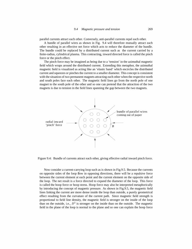
9.4 Magnetic pressure and tension 269
parallel currents attract each other. Conversely, anti-parallel currents repel each other.A bundle of parallel wires as shown in Fig. 9.4 will therefore mutuallyattract each
other resulting in an effective net force which acts to reduce the diameter of the bundle.The bundle could be replaced by a distributed current such as the current carried by afinite-radius, cylindrical plasma. This contracting, inward directedforce is called the pinchforce or the pinch effect.
The pinch force may be imagined as being due to a ‘tension’ in the azimuthalmagneticfield which wraps around the distributed current. Extending this metaphor, the azimuthalmagnetic field is visualized as acting like an ‘elastic band’ which encircles the distributedcurrent and squeezes or pinches the current to a smaller diameter. This concept is consistentwith the situation of two permanent magnets attracting each other when the respective northand south poles face each other. The magnetic field lines go from the north pole ofonemagnet to the south pole of the other and so one can pretend that the attraction of the twomagnets is due to tension in the field lines spanning the gap between the two magnets.
bundleof parallelwirescomingout of paper
radial inward‘pinch’ force B
Figure 9.4: Bundle of currents attract each other, giving effective radial inward pinch force.
Now consider a current-carrying loop such as is shown in Fig.9.5. Becausethe currentson opposite sides of the loopflow in opposing directions, there will be a repulsive forcebetween the current element at each point and the current element on the opposite side ofthe loop. The net result is a force directed to expand the diameter of the loop. This forceis called the hoop force or hoop stress. Hoop force may also be interpreted metaphoricallyby introducing the concept of magnetic pressure. As shown in Fig.9.5, the magnetic fieldlines linking the current are more dense inside the loop than outside, a purelygeometricaleffect resulting from the curvature of the current path. Since magnetic field strength isproportional to field line density, the magnetic field is stronger on the insideof the loopthan on the outside, i.e.,B2 is stronger on the inside than on the outside. The magneticfield in the plane of the loop is normal to the plane and so one can explain the hoop force
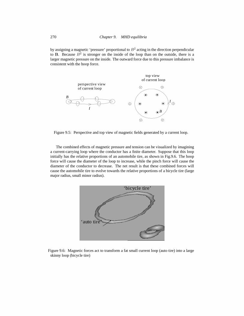
270 Chapter 9. MHD equilibria
by assigning a magnetic ‘pressure’ proportional toB2 acting in the direction perpendicularto B. BecauseB2 is stronger on the inside of the loop than on the outside, there is alarger magnetic pressure on the inside. The outward force due to this pressure imbalance isconsistent with the hoop force.
perspectiveviewof currentloop
top viewof currentloop
B
B
I
I
Figure 9.5: Perspective and top view of magnetic fields generated by a current loop.
The combined effects of magnetic pressure and tension can be visualized byimagininga current-carrying loop where the conductor has a finite diameter. Suppose that this loopinitially has the relative proportions of an automobile tire, as shown inFig.9.6. The hoopforce will cause the diameter of the loop to increase, while the pinch force will cause thediameter of the conductor to decrease. The net result is that these combined forces willcause the automobile tire to evolve towards the relative proportions of a bicycle tire (largemajor radius, small minor radius).
‘ autotire’
‘ bicycle tire’
Figure 9.6: Magnetic forces act to transform a fat small current loop (autotire) into a largeskinny loop (bicycle tire)

9.5 Magnetic stress tensor 271
9.5 Magnetic stress tensor
The existence of magnetic pressure and tension shows that the magnetic force is differ-ent in different directions, and so the magnetic force ought to be characterized by ananisotropic stress tensor. To establish this mathematically, the vector identity∇B2/2 =B·∇B+B×∇×B is invoked so that the magnetic force can be expressed as
J ×B = 1µ0 (∇×B) ×B
= 1µ0
[−∇(B22)
+B·∇B]
= − 1µ0∇ · [B22 I−BB
]
(9.10)
whereI is the unit tensor and the relation∇ · (BB) = (∇ ·B)B+B·∇B =B·∇B hasbeen used. At any pointr a local Cartesian coordinate system can be defined withz axisparallel to the local value ofB so that Eq.(9.1) can be written as
ρ[∂U∂t +U·∇U
]
= −∇ ·
P + B22µ0
P + B22µ0
P − B22µ0
(9.11)
showing again that the magnetic field acts like a pressure in the directions transverse toB(i.e.,x, y directions in the local Cartesian system) and like a tension in the direction paralleltoB.
While the above interpretation is certainly useful, it can be somewhat misleading be-cause it might be interpreted as implying the existence of a force in the direction ofBwhen in fact no such force exists becauseJ×B clearly does not have a component in theB direction. A more accurate way to visualize the relation between magnetic pressure andtension is to rearrange the second line of Eq.(9.10) as
J ×B = 1µ0[−∇(B2
2)
+B2B·∇B + BB·∇(B22
)]
= 1µ0
[−∇⊥
(B22)
+B2κ]
(9.12)or
J ×B = 1µ0
[−∇⊥
(B22)
+B2κ]
. (9.13)
Here
κ =B · ∇B= − RR (9.14)
is a measure of the curvature of the magnetic field at a selected point on a field line and, inparticular,R is the local radius of curvature vector. The vectorR goes from the center ofcurvature to the selected point on the field line. Theκ term in Eq.(9.13) describes a forcewhich tends to straighten out magnetic curvature and is a more precise way for character-izing field line tension (recall that tension similarly acts to straighten out curvature). The
272 Chapter 9. MHD equilibria
term involving∇⊥B2 portrays a magnetic force due to pressure gradients perpendicularto the magnetic field and is a more precise expression of the hoop force.
In our earlier discussion it was shown that the vacuum magnetic field is the lowestenergy state of all fields satisfying prescribed boundary conditions. A vacuum field mightbe curved for certain boundary conditions (e.g., a permanent magnet with finite dimensions)and, in such a case, the two terms in Eq.(9.13) are both finite but exactly cancel eachother. We can think of the minimum-energy state for given boundary conditions as beinganalogous to the equilibrium state of a system of stiff rubber hoses which have been pre-formed into shapes having the morphology of the vacuum magnetic field and which havetheir ends fixed at the bounding surface. Currents will cause the morphology of this systemto deviate from the equilibrium state, but since any deformation requires work to be doneon the system, currents invariably cause the system to be in a higher energystate.
9.6 Flux preservation, energy minimization, andinductance
Another useful way of understanding magnetic field behavior relates to theconcept ofelectric circuit inductance. The self-inductanceL of a circuit component is defined asthe magneticflux Φ linking the component divided by the currentI flowing through thecomponent, i.e.
L = ΦI . (9.15)
Consider an arbitrary short-circuited coil with currentI located in an infinite volumeVand letC denote the three-dimensional spatial contour traced out by the wire constitutingthe coil. The total magneticflux linked by the turns of the coil can be expressed as
Φ =∫
B·ds =∫ ∇×A·ds = ∮
CA · dl (9.16)
where the surface integral is over the area elements linked by the coil turns. The energycontained in the magnetic field produced by the coil is
W =∫
V
B22µ0 d
3r
= 12µ0
∫
VB·∇×Ad3r. (9.17)
However, using the vector identity∇ · (A×B) = B·∇×A−A·∇×B this magneticenergy can be expressed as
W = 12µ0
∫
VA·∇×Bd3r + 1
2µ0∫
S∞
ds ·A×B (9.18)
where Gauss’s law has been invoked to obtain the second term, an integral over the surfaceat infinityS∞. This surface integral vanishes because (i) at infinity the magnetic field mustfall off at least as fast as a dipole, i.e.,B ∼ R−3 whereR is the distance to the origin,(ii) the vector potential magnitudeA scales as the integral ofB soA ∼ R−2, and (iii) thesurface at infinity scales asR2.

9.6 Flux preservation, energy minimization, and inductance 273
Using Ampere’s law, Eq.(9.18) can thus be rewritten as
W = 12∫
VA · Jd3r. (9.19)
However,J is only finite in the coil wire and so the integral reduces to an integral over thevolume of the wire. A volume element of wire can be expressed asd3r = ds·dl wheredlis an element of length along the wire, andds is the cross-sectional area of the wire. SinceJ anddl are parallel, they can be interchanged in Eq.(9.19) which becomes
W = 12∫
Vcoil
A·dl J·ds= I
2∮
A·dl= IΦ
2= Φ2
2L= 1
2LI2 (9.20)
whereJ·ds =I is the currentflowing through the wire. Thus, the energy stored in themagnetic field produced by a coil is just the inductive energy of the coil.
If the coil is perfectly short-circuited, then it must beflux conserving, for if there werea change influx, a voltage would appear across the ends of the coil. A closed currentflowing in a perfectly conducting plasma is thus equivalent to a short-circuited current-carrying coil and so the perfectly conducting plasma can be considered as aflux-conserver.If flux is conserved, i.e.Φ = const., the second from last line in Eq.(9.20) shows thatthemagnetic energy of the system will be lowered by any rearrangement of circuittopologythat increases self-inductance.
Hot plasmas are reasonably goodflux conservers because of their high electrical con-ductivity. Thus, any inductance-increasing change in the topology of plasma currents willrelease free energy which could be used to drive an instability. Since forces act so as to re-duce the potential energy of a system, magnetic forces due to currentflowing in a plasmawill always act so as to increase the self-inductance of the configuration. One can thereforewrite the forceF due to aflux-conserving change in inductanceL as
F = −Φ22 ∇( 1
L)
. (9.21)
The pinch force is consistent with this interpretation since the inductance of a conductordepends inversely on its radius. The hoop force is also consistent with thisinterpretationsince inductance of a current loop increases with the major radius of the loop. Morecomplicated behavior can also be explained, especially the kink instability to be discussedlater. In the kink instability, current initiallyflowing in a straight line develops an instabilitythat causes the current path to become helical. Since a coil (helix) has more inductance thana straight length of the same wire, the effect of the kink instabilityalso acts so as to increasethe circuit self-inductance.

274 Chapter 9. MHD equilibria
9.7 Static versus dynamic equilibria
We define (i) a static equilibrium to be a time-independent solution to Eq.(9.1) having noflow velocity and (ii) a dynamic equilibrium as a solution with steady-stateflow velocities.ThusU = 0 for a static equilibrium whereasU is finite and steady-state for a dynamicequilibrium. For a static equilibrium the MHD equation of motion reduces to
∇P = J ×B. (9.22)
For a dynamic equilibrium the MHD equation of motion reduces to
ρU·∇U+∇P = J ×B+νρ∇2U (9.23)
where the last term represents a viscous damping andν is the kinematic viscosity. By tak-ing the curl of these last two equations we see that for static equilibria the magnetic forcemust be conservative i.e.,∇× (J ×B) = 0 whereas for dynamic equilibria the magneticforce is typically not conservative since in general∇ × (J ×B) = 0. Thus, the charac-ter of the magnetic field is quite different for the two cases. Static equilibria are relevant toplasma confinement devices such as tokamaks, stellarators, reversed field pinches, spher-omaks while dynamic equilibria are mainly relevant to arcs, jets, magnetoplasmadynamicthrusters, but can also be relevant to tokamaks, etc., if there areflows. Both static anddynamic equilibria occur in space plasmas.
z
r
finite pressurein cylinder
magneticforce pinchesinhydrodynamicpressurepushesout
cylindrical plasmawithaxial currentdensityJzr
Figure 9.7: Geometry of Bennett pinch.

9.8 Static equilibria 275
9.8 Static equilibria
9.8.1 Static equilibria in two dimensions: the Bennett pinch
The simplest static equilibrium was first investigated by Bennett (1934) and is called theBennett pinch orz-pinch (herez refers to the direction of the current). This configuration,sketched in Fig.9.7, consists of an infinitely long axisymmetric cylindrical plasma withaxial current densityJz = Jz(r) and no other currents.
The axial currentflowing within a circle of radiusr is
I(r) =∫ r
02πr′Jz(r′)dr′ (9.24)
and the axial current density is related to this integrated current by
Jz(r) = 12πr
∂I∂r . (9.25)
Since Ampere’s law gives
Bθ(r) = µ0I(r)2πr , (9.26)
Eq.(9.22) can be written
r2 ∂P∂r = − µ08π2
∂I2∂r . (9.27)
Integrating Eq. (9.27) fromr = 0 to r = a, wherea is the outer radius of the cylindricalplasma, gives the relation
∫ a
0r2 ∂P∂r dr =
[r2P (r)]a0 − 2∫ a
0rP (r)dr = −µ0I2(a)8π2 . (9.28)
The integrated term vanishes at bothr = 0 andr = a sinceP (a) = 0 by definition. If thetemperature is uniform, the pressure can be expressed asP (r) = n(r)κT and so Eq.(9.28)can be expressed as
I2 = 8πNκTµ0 (9.29)
whereN = ∫ a0 n(r)2πrdr is the number of particles per axial length. Equation (9.29),
called the Bennett relation, shows that the current required to confine a givenN andT isindependent of the details of the internal density profile. This relation describes the sim-plest non-trivial MHD equilibrium and suggests that quite modest currents couldcontainsubstantial plasma pressures. This relation motivated the design of early magnetic fusionconfinement devices but, as will be seen, it is overly optimistic because simple z-pinchequilibria turn out to be highly unstable.
Confinement using currents thatflow in the azimuthal direction is also possible, butthis configuration, known as aθ-pinch, is fundamentally transient. In aθ-pinch a rapidlychanging azimuthal current in a coil going around a cylindrical plasma creates a transientBz field as shown in Fig. 9.8. Because the conducting plasma conserves magneticflux,the transientBz field cannot penetrate the plasma and so is confined to the vacuum regionbetween the plasma and the coil. This exclusion of theBz field by the plasma requires

276 Chapter 9. MHD equilibria
the existence in the plasma surface of an induced azimuthal current which creates a mag-netic field in the plasma interior that exactly cancels the coil-producedtransientBz field.The radial confining force results from a radially inward forceJ×B =Jθθ × Bzz whereBz is the magnetic field associated with the current in the coil andJθ is the plasma surfacecurrent. An alternative but equivalent point of view is to invoke the concept that oppositecurrents repel and argue that the azimuthal current in the coil repels theoppositely directedazimuthal current in the plasma surface, thereby pushing the plasma inwards and so bal-ancing the outwards force due to plasma pressure. Theθ-pinch configuration is necessarilytransient, because the induced surface current cannot be sustained in steady-state.
plasma
coil current
plasmasurfacecurrentBz
Bz
Bz
Bz
Bz
Bz
Bz
Bz
Bz Bz
Figure 9.8: Theta pinch configuration. Rapidly changing azimuthal coil current inducesequal and opposite azimuthal current in plasma surface. Pressure ofBz between these twocurrents pushes in on plasma and provides confinement.
9.8.2 Impossibility of self-confinement of current-carrying plasma in threedimensions: the virial theorem
The Bennett analysis showed that axial currentsflowing in an infinitely long cylindricalplasma generate a pinch force which confines a finite pressure plasma. The inward pinchforce balances the outward force associated with the pressure gradient. Thequestion now iswhether this two-dimensional result can be extended to three dimensions; i.e., is it possibleto have a finite-pressure three-dimensional plasma, as shown in Fig.9.9, which is confinedentirely by currents circulating within the plasma? To be more specific, is it possible tohave a finite-radius plasma sphere surrounded by vacuum where the confinement of thefinite plasma pressure is entirely provided by the magnetic force of currents circulating inthe plasma; i.e., can the plasma hold itself together by its own ‘bootstraps’? The answer,

9.8 Static equilibria 277
a resounding ‘no’, is provided by a virial theorem due to Shafranov (1966). A virial isa suitably weighted integral over the entirety of a system and contains information abouthow an extensive property such as energy is partitioned in the system. For example, inmechanics the virial can be the time average of the potential or of the kinetic energy.
ball of plasmasurroundedby vacuum
x
y
z
Figure 9.9: Plasma sphere with finite pressure surrounded by vacuum
The MHD virial theorem is obtained by supposing that a self-confining configurationexists and then showing this leads to a contradiction.
We therefore postulate the existence of a spherical plasma with the following properties:1. the plasma has finite radiusa and is surrounded by vacuum,
2. the plasma is in static MHD equilibrium,
3. the plasma has finite internal pressure and the pressure gradient is entirely balancedby magnetic forces due to currents circulating in the plasma; i.e. there are no currentsin the surrounding vacuum region.
Using Eqs.(9.10) and (9.11) the static MHD equilibrium can be expressed as
∇ ·T =0 (9.30)
where the tensorT is defined as
T =(
P + B22µ0
)
I− 1µ0BB. (9.31)
Letr =xx+yy+zz be the vector from the center of the plasma to the point of observation.

278 Chapter 9. MHD equilibria
Consider the virial expression
∇ · (T · r) = ∑
jk∂∂xj (Tjkxk)
= (∇ ·T) · r +∑
jkTjk ∂
∂xj xk
= TraceT
(9.32)
whereTraceT =∑
jk Tjkδjk. From Eq.(9.31) (or, equivalently from the matrix form inEq.(9.11)) it is seen that
TraceT =3P +B2/2µ0is positive definite.
We now integrate both sides of Eq.(9.32) over all space. Since the right hand side ofEq.(9.32) is positive definite, the integral of the right hand side over all space is finite andpositive. The integral of the left hand side can be transformed to a surface integral at infinityusing Gauss’ theorem
∫
d3r∇ · (T · r) = ∫
S∞
ds ·T · r=
∫
S∞
ds· [(P + B22µ0
)
I− 1µ0BB
] ·r .
(9.33)
Since the plasma is assumed to have finite extent,P is zero on the surface at infinity.The magnetic field can be expanded in multipoles with the lowest order multipole beinga dipole. The magnetic field of a dipole scales asr−3 for larger while the surface area∫ ds scales asr2. Thus the left hand side term scales as
∫ dsB2r∼r−3 and so vanishesasr→∞. This is in contradiction to the right hand side being positive definite and so theset of initial assumptions must be erroneous. Thus, any finite extent, three-dimensional,static plasma equilibrium must involve at least some currents external to the plasma. Afinite extent, three-dimensional static plasma can therefore only be in equilibrium if at leastsome of the magnetic field is produced by currents in coils that are external to the plasmaand that are held in place by some mechanical structure. If the coils werenot supportedby a mechanical structure, then the current in the coils could be considered as part of theMHD plasma and the virial theorem would be violated. In summary, a finite extent three-dimensional plasma in static equilibrium with a finite internal hydrodynamic pressurePmust ultimately have some tangible exterior object to “push against”. The buttressing isprovided by magnetic forces acting between currents in external coils and currents in theplasma.
9.8.3 Three-dimensional static equilibria: the Grad-Shafranov equation
Despite the simple appearance of Eq.(9.22), its three-dimensional solution is far from triv-ial. Before even attempting to find a solution, it is important to decide the appropriate wayto pose the problem, i.e., it must be decided which quantities are prescribed and which areto be solved for. For example, one might imagine prescribing a pressure profileP (r) and

9.8 Static equilibria 279
then using Eq.(9.22) to determine a correspondingB(r)with associated currentJ(r); alter-natively one could imagine prescribingB(r) and then using Eq.(9.22) to determineP (r).Unfortunately, neither of these approaches work in general because solutions to Eq.(9.22)only exist for a very limited set of functions.
The reason why an arbitrary magnetic field cannot be specified is that∇ ×∇P = 0is always true by virtue of a mathematical identity whereas∇ × (J×B) = 0 is trueonly for certain types ofB(r). It is also true that an arbitrary equilibrium pressure profileP (r) cannot be prescribed (see assignment #2 where it is demonstrated that noJ×Bexists which can confine a spherically symmetric pressure profile). Equilibria thus existonly for certain specific situations, and these situations typically require symmetry in somedirection. We shall now examine a very important example, namely static equilibria whichare azimuthally symmetric about an axis (typically defined as thez axis). This symmetryapplies to a wide variety of magnetic confinement devices used in magnetic fusion research,for example tokamaks, reversed field pinches, spheromaks, and field reversed theta pinches.
We start the analysis by assuming azimuthal symmetry about thez axis of a cylindri-cal coordinate systemr, φ, z so that any physical quantityf has the property∂f/∂φ = 0.Because of the identity∇×∇φ = 0, algebraic manipulations become considerably sim-plified if vectors in theφ direction are expressed in terms of∇φ = φ/r rather than in termsof φ. As sketched in Fig.9.10 the term toroidal denotes vectors in theφ direction (long wayaround a torus) and the term poloidal denotes vectors in ther − z plane.
z
toroidalvector
poloidalvector
Figure 9.10: Toroidal vectors and poloidal vectors.
The most general form for an axisymmetric magnetic field is
B = 12π (∇ψ ×∇φ+ µ0I∇φ) . (9.34)
ψ(r, z) is called the poloidalflux andI(r, z) is the current linked by a circle of radiusrwith center on the axis at axial locationz. The toroidal magnetic field then is
Btor = Bφφ = µ0I2π ∇φ = µ0I
2πr φ (9.35)

280 Chapter 9. MHD equilibria
showing that the functional form of Eq.(9.34) is consistent with Ampere’s law∮ B·dl =µ0I.
The poloidal magnetic field is
Bpol = 12π (∇ψ ×∇φ) . (9.36)
Integration of the poloidal magnetic field over the area of a circle of radiusr with center ataxial locationz gives
∫ r
0Bpol · ds = ∫ r
012π∇ψ ×∇φ · z2πr′dr′ = ψ(r, z); (9.37)
thusψ(r, z) is the poloidalflux at locationr, z. The concept of poloidalflux depends onthe existence of axisymmetry so that a circle of radiusr can always be associated with alocationr, z.
Axisymmetry also provides a useful relationship between toroidal and poloidal vectors.In particular, the curl of a toroidal vector is poloidal since
∇×Btor = µ02π∇I ×∇φ (9.38)
and similarly the curl of a poloidal vector is toroidal since
∇×Bpol =∇× (Br r +Bzz) = φ(∂Br∂z − ∂Bz
∂r)
. (9.39)
The curl of the poloidal magnetic field is a Laplacian-like operator onψ since
∇φ ·∇×Bpol = ∇·(Bpol ×∇φ) = ∇·( 12π [∇ψ ×∇φ]×∇φ) = − 12π∇·( 1r2∇ψ)
,(9.40)
a relationship established using the vector identity∇· (F×G) =G·∇×F−F·∇×G.Because∇×Bpol is purely toroidal andφ = r∇φ, one can write
∇×Bpol = − r22π∇ ·( 1r2∇ψ)∇φ. (9.41)
Ampere’s law states that∇×B =µ0J. Thus, from Eqs. (9.38) and (9.41) the respectivetoroidal and poloidal currents are
Jtor = − r22πµ0∇ ·( 1r2∇ψ
)∇φ (9.42)
and
Jpol = 12π∇I ×∇φ. (9.43)
We are now in a position to evaluate the magnetic force in Eq.(9.22). After decomposingthe magnet field and current into toroidal and poloidal components, Eq.(9.22)becomes
∇P = Jpol ×Btor + Jtor ×Bpol + Jpol ×Bpol. (9.44)
TheJpol ×Bpol term is in the toroidal direction and is the only toroidally directed term onthe right hand side of the equation. However∂P/∂φ = 0 because all physical quantitiesare independent ofφ and soJpol ×Bpol must vanish. This implies
(∇I ×∇φ)× (∇ψ ×∇φ) = 0 (9.45)

9.8 Static equilibria 281
which further implies that∇I must be parallel to∇ψ. An arbitrary displacementdr resultsin respective changes in current and poloidalflux dI = dr·∇I anddψ = dr·∇ψ so that
dIdψ =
dr·∇Idr·∇ψ ;
since∇I is parallel to∇ψ, the derivativedI/dψ is always defined. ThusI must be afunction ofψ and it is always possible to write
∇I(ψ) = I′(ψ)∇ψ (9.46)
where prime means derivative with respect to the argument. The poloidal current can there-fore be expressed in terms of the poloidalflux function as
Jpol = I ′2π∇ψ ×∇φ. (9.47)
Substitution for the currents and magnetic fields in Eq.(9.44) gives the expression
∇P = I′2π (∇ψ ×∇φ) × µ0I
2π ∇φ−∇φ r22πµ0∇ ·( 1r2∇ψ
)× 12π [∇ψ ×∇φ]
= −[ µ0II′(2πr)2 +
1(2π)2µ0∇ ·( 1r2∇ψ
)]∇ψ.(9.48)
This gives the important result that∇P must also be parallel to∇ψ which in turn impliesthatP = P (ψ) so that∇P = P ′∇ψ. Equation (9.48) now has a common vector factor∇ψ which may be divided out, so that the original vector equation reduces to thescalarequation
∇ ·( 1r2∇ψ)
+ 4π2µ0P ′ + µ20r2 II
′ = 0. (9.49)
This equation, known as the Grad-Shafranov equation (Grad and Rubin 1958, Shafranov1966), has the peculiarity thatψ shows up as both an independent variable and as a de-pendent variable, i.e., there are both derivatives ofψ and derivatives with respect toψ.Axisymmetry has made it possible to transform a three-dimensional vectorequation into aone-dimensional scalar equation. It is not surprising that axisymmetry would transform athree dimensional system into a two dimensional system, but the transformation of a threedimensional system into a one dimensional system suggests more profound physics is in-volved than just geometrical simplification.
The Grad-Shafranov equation can be substituted back into Eq.(9.42) to give
Jtor =(
2πr2P ′ + µ02πII
′)∇φ (9.50)
so that the total current can be expressed as
J = Jpol+Jtor = I′2π∇ψ×∇φ+(
2πr2P ′ + µ02πII
′)∇φ = 2πr2P ′∇φ+I ′B. (9.51)
The last term is called the ‘force-free’ current because it is parallel to the magnetic fieldand so provides no force. The first term on the right hand side is the diamagnetic current.

282 Chapter 9. MHD equilibria
The Grad-Shafranov equation is a non-linear equation inψ and, in general, cannotbe solved analytically. It does not in itself determine the equilibrium because it involvesthree independent quantities,ψ,P (ψ), andI(ψ). Thus, use of the Grad-Shafranov equationinvolves specifying two of these functions and then solving for the third. Typically P (ψ)andI(ψ) are specified (either determined from other equations or from experimental data)and then the Grad-Shafranov equation is used to determineψ.
Although the Grad-Shafranov equation must in general be solved numerically, thereexist a limited number of analytic solutions. These can be used as idealized examples thatdemonstrate typical properties of axisymmetric equilibria. We shall now examine one suchanalytic solution, the Solov’ev solution (Solovev 1976).
The Solov’ev solution is obtained by invoking two assumptions: first, the pressure isassumed to be a linear function ofψ,
P = P0 + λψ (9.52)
and second,I is assumed to be constant within the plasma so
I′ = 0. (9.53)
The second assumption corresponds to having all thez-directed currentflowing on thez-axis, so that away from thez-axis, the toroidal field is a vacuum field (cf. Eq.(9.35)).This arrangement is equivalent to having a zero-radius current-carrying wire going up thez axis acting as the sole source for the toroidal magnetic field. The region over which theSolev’ev solution applies excludes thez−axis and so the problem is analogous to a centralforce problem where the source of the central force is a singularity at theorigin. Theexcluded region of thez−axis corresponds to the ‘hole in the doughnut’ of a tokamak. Inthe more general case whereI′ is finite, the plasma is either diamagnetic (toroidal field isweaker than the vacuum field) or paramagnetic (toroidal field is stronger than the vacuumfield).
Using these two simplifying assumptions the Grad-Shafranov equation reduces to
r ∂∂r(1r∂ψ∂r
)
+ ∂2ψ∂z2 + 4π
2r2µ0λ = 0 (9.54)
which has the exact solution (Solov’ev solution)
ψ(r, z) = ψ0r2r40
(2r20 − r2 − 4α2z2) (9.55)
whereψ0, r0, andα are constants. Figure 9.11 shows a contour plot ofψ as a functionof r/r0 andz/z0 for the caseα = 1. Note that there are three distinct types of curves inFig.9.11, namely (i) open curves going toz = ±∞, (ii) concentric closed curves, and (iii)a single curve called the separatrix which separates the first two types of curves.

9.8 Static equilibria 283
Figure 9.11: Contours of constantflux of Solov’ev solution to Grad-Shafranov equation.
Even though it is an idealization, the Solov’ev solution illustrates manyimportant fea-tures of three-dimensional, static MHD equilibria. Let us now examine some of thesefeatures. The constants in Eq.(9.55) have been chosen so thatψ = ψ0 at r = r0, z = 0(in the figure this point corresponds tor = 1, z = 0 since lengths in the figure have beennormalized tor0). The locationr = r0, z = 0 is called themagnetic axisbecause it is theaxis linked by the closed contours of poloidalflux.
Let us temporarily assume thatψ0 is positive. Examination of Eq.(9.55) shows thatif ψ is positive, then the quantity2r20 − r2 − 4α2z2 is positive and vice versa. For anynegative value ofψ, Eq.(9.55) can be satisfied by makingr very small andz very large. Inparticular, ifr is infinitesimal thenz must become infinite. Thus, all contours for whichψis negative go toz = ±∞; these contours are the open or type (i) contours.
On the other hand, ifψ is positive then it has a maximum value ofψ0 which occurs onthe magnetic axis and if0 < ψ < ψ0 thenψ must be located at some point outside themagnetic axis, but inside the curve2r20 − r2 − 4α2z2 = 0. Hence all contours of positiveψ must lie inside the curve2r20 − r2 − 4α2z2 = 0 and correspond to field lines that do notgo to infinity. These contours are the closed or type (ii) contours, since they form closedcurves in ther, z plane.
The contour separating the closed contours from the contours going to infinity isthe

284 Chapter 9. MHD equilibria
separatrixand is given by the ellipse
r2 + 4α2z2 = 2r20 . (9.56)
On the magnetic axisψ is a local maximum ifψ0 is positive or a local minimum ifψ0is negative (the sign depends on the sense of the toroidal current). Thus, one can imaginethat a hill (or valley) of poloidalflux exists with apex (or bottom) at the magnetic axisand in the vicinity of the apex (bottom) the contours of constantψ are circles or ellipsesenclosing the magnetic axis. The degree of ellipticity of these surfaces is determined bythe value ofα. These closedflux surfaces are a set of nested toroidal surfaces sharing thesame magnetic axis. The projection of the total magnetic field lies in aflux surface sinceEq.(9.34) shows
B · ∇ψ = 0,i.e., the magnetic field does not have a component in the direction normal to theflux surface.
Direct substitution of Eq.(9.55) into Eq.(9.54) gives
λ = 2ψ0π2r40µ0
(1 +α2) (9.57)
so that the pressure is
P (ψ) = P0 + 2ψ0π2r40µ0
(1 +α2)ψ. (9.58)
Pressure vanishes at the plasma edge so ifψedge is the poloidalflux at the edge, then theconstantP0 is determined and Eq.(9.58) becomes
P (ψ) = 2ψ0π2r40µ0
(1 + α2) [ψ − ψedge] . (9.59)
In the earlier discussion of single particle motion it was shown that particles were at-tached toflux surfaces. Particles that start on a particularflux surface always stay on thatflux surface, although they may travel to any part of thatflux surface. The equilibrium pre-scribed by Eq.(9.55) is essentially a three-dimensional vortex with pressure peaking on themagnetic axis and then falling monotonically to zero at the edge.
This is a particularly simple solution to the Grad-Shafranov equation, butneverthelessdemonstrates several important features:
1. Three dimensional equilibria can incorporate closed nested poloidalflux surfaceswhich are concentric about a magnetic axis and correspond to local maxima orminimaof thefluxψ.
2. There can also be openflux surfaces; i.e.,flux surfaces which go to infinity.
3. Theflux surface separating closed and openflux surfaces is called a separatrix.
4. The total magnetic field projects into theflux surfaces sinceB · ∇ψ = 0.5. Finite pressure corresponds to a depression (or elevation) of the poloidal flux. The
pressure maximum andflux extrema are located at the magnetic axis.
6. The poloidal magnetic field and associated poloidalfluxψ are responsible for plasmaconfinement and result from the toroidal current. Thustoroidal current is essential forconfinement in an axisymmetric geometry. For a givenP (ψ) the toroidal magnetic
9.8 Static equilibria 285
field does not contribute to confinement ifI ′ = 0. If I ′ is finite, plasma diamagnetismor paramagnetism will affectP (ψ). Although the toroidal field does not directly pro-vide confinement, it can affect the rate of cross-field particle and energy diffusion andhence the functional form ofP (ψ). For example, the frequency of drift waves willbe a function of the toroidal field and drift waves can cause an outward diffusion ofplasma acrossflux surfaces, thereby affectingP (ψ).
7. The poloidalflux surfaces are related to the surfaces of constant canonical angular
momentum sinceBpol = ∇× (ψ∇φ/2π) = ∇ × (
ψφ/2πr)
= ∇× Aφφ implies
Aφ = ψ/2πr. Thus, the canonical angular momentum can be expressed as
pφ = mr2φ+ qrAφ
= mrvφ + qψ2π . (9.60)
Surfaces of constant canonical angular momentum correspond to surfacesof constantpoloidalflux in the limitm→ 0.Because the system is toroidally symmetric (axisym-metric) the canonical angular momentum of each particle is a constant of the motionand so, to the extent that the particles can be approximated as having zero mass, parti-cle trajectories are constrained to lie on surfaces of constantψ.Sincepφ is a conservedquantity, the maximum excursion a finite-mass particle can make from a poloidalfluxsurface can be estimated by writing
δpφ = δ (mrvφ + qrAφ) = 0. (9.61)
Thus,vφr δr + δvφ + q
mδr1r∂∂r (rAφ) = 0 (9.62)
or
δr = − rδvφvφ + rωc,pol
(9.63)
whereωc,pol = qBpol/m is the cyclotron frequency measured using the poloidalmagnetic field. Sincevφ is of the order of the thermal velocity or smaller, if thepoloidal field is sufficiently strong that the poloidal Larmor radiusrlpol ∼ vφ/ωc,pol ismuch smaller than the radiusr, then the first term in the denominator may be dropped.Sinceδvφ is also of the order of the thermal velocity or smaller, the particle cannotdeviate from its initialflux surface by more than a poloidal Larmor radius. Sincepoloidal field is produced by toroidal current, it is clear that particle confinement toaxisymmetricflux surfaces requires the existence of a toroidal current.
Tokamaks, reverse field pinches, spheromaks, and field reversed configurations are allmagnetic confinement configurations having three dimensional axisymmetric equilibriasimilar to this Solov’ev solution and all involve a toroidal current to produce a set of nested,closed poloidalflux surfaces which link a magnetic axis. Stellarators are non-axisymmetricconfigurations which have poloidalflux surfaces without toroidal currents; the advantageof current-free operation is offset by the complexity of non-axisymmetry.

286 Chapter 9. MHD equilibria
9.9 Dynamic equilibria: flows
The basic mechanism driving MHDflows will first be discussed using the simplified as-sumptions of incompressibility and self-field only. This situation isrelevant to simple arcs,basic concepts of magnetoplasmadynamic thrusters, and to currents driven inmolten met-als. The more general situation where the plasma is compressible and where there areexternal, applied magnetic fields in addition to the self-field will then be addressed.
9.9.1 Incompressible plasma with self-field only
MHD-drivenflows involve situations where∇×(J×B) is non-zero. This means the MHDforceJ×B is non-conservative in which case its finite curl acts as torque or equivalently asa source for hydrodynamic vorticity. When the MHD force is non-conservative a closed lineintegral
∮ dl · J×B will be finite, whereas in contrast a closed line integral of a pressuregradient
∮ dl·∇P is always zero. Since a pressure gradient cannot balance the torqueproduced by a non-conservativeJ×B, it is necessary to include a vorticity-damping term(viscosity term) to allow for the possibility of balancing this torque. Plasma viscosity ismainly due to ion-ion collisions and is typically very small. With theaddition of viscosity,the MHD equation of motion becomes
ρ(∂U∂t +U · ∇U
)
= J×B−∇P + ρυ∇2U (9.64)
whereυ is the kinematic viscosity. To focus attention on vorticity generation,transport,and decay the following simplifying assumptions are made:
1. The motion is incompressible so thatρ = const.
This is an excellent assumption for a molten metal, but is questionable for aplasma.However, this assumption could be at least locally reasonable for aplasma if the regionof vorticity generation is smaller in scale than regions of compressionor rarefactionor is spatially distinct from these regions. The consequences of compressibility willbe discussed later.
2. The system is cylindrically symmetric.
A cylindrical coordinate systemr, φ, z can then be used andφ is ignorable. Thisgeometry corresponds to magnetohydrodynamic thrusters and arcs.
3. Theflow velocitiesU and the current densityJ are in the poloidal direction (r and zplane). Restricting the current to be poloidal means that the magnetic fieldis purelytoroidal (see Fig.9.10).
The most general poloidal velocity for a constant-density, incompressiblefluid hasthe form
U = 12π∇ψ ×∇φ (9.65)
whereψ(r, z) is theflux offluid through a circle of radiusr at locationz.Note the analogyto the poloidal magneticflux function used in Eqs.(3.146) and (9.34). SinceU lies entirelyin the r, z plane and since the system is axisymmetric, the curl ofU will be in the φdirection. It is thus useful to define a scalar cylindrical “vorticity”χ = rφ · ∇ ×U; this

9.9 Dynamic equilibria:flows 287
definition differs slightly from the conventional definition of vorticity (curl of velocity)because it includes an extra factor ofr. This slight change of definition is essentially amatter of semantics, but makes the algebra more transparent.
Since∇φ = φ/r it is seen that
∇×U = φr rφ · ∇ ×U =χ∇φ (9.66)
and so
∇×( 12π∇ψ ×∇φ) =χ∇φ. (9.67)
Dotting Eq.(9.67) with∇φ and using the vector identity∇φ · ∇ × Q = ∇ · (Q×∇φ)gives
∇ ·( 12π (∇ψ ×∇φ)×∇φ) = χr2 (9.68)
or
r2∇ ·( 1r2∇ψ)
= −2πχ (9.69)
which is a Poisson-like relation between the vorticity and the stream function. The vorticityplays the role of the source (charge-density) and the stream function plays the role of thepotential function (electrostatic potential). However, the ellipticoperator is not exactly aLaplacian and when expanded has the form
r2∇ ·( 1r2∇ψ)
= r ∂∂r(1r∂ψ∂r
)
+ ∂2ψ∂z2 (9.70)
which is just the operator in the Grad-Shafranov equation.Since the current was assumed to be purely poloidal, the magnetic field must be
purely toroidal and so can be written as
B =µ02πI∇φ (9.71)
whereI is the current through a circle of radiusr at locationz. This is consistent with theintegral form of Ampere’s law,
∮ B·dl =µ0I. The curl of Eq.(9.71) gives
∇×B = µ02π∇I ×∇φ (9.72)
showing thatI acts like a stream-function for the magnetic field.

288 Chapter 9. MHD equilibria
z
Ir ,z = const.
Figure 9.12: Current channelI(r, z).
The magnetic force is therefore
J×B = 12π (∇I ×∇φ)× µ02πI∇φ = − µ0
(2πr)2∇(I22)
. (9.73)
It is seen that there is an axial force ifI2 depends onz; this is the essential condition thatproduces axialflows in MHD arcs (Maecker 1955) and plasma guns(Marshall 1960).
Using the identities∇U2/2 =U·∇U+U×∇×U and∇×∇×U = −∇2U =∇χ×∇φ the equation of motion Eq.(9.64) becomes
ρ(∂U∂t +∇U2
2 −U× χ∇φ) = − µ0(2πr)2∇
(I22)−∇P − ρυ∇χ ×∇φ (9.74)
or
ρ(∂U∂t +∇U2
2 −U× χ∇φ) = − µ0(2π)2∇
( I22r2
)
+ µ0I2(2π)2 ∇( 1
2r2)
− ∇P − ρυ∇χ×∇φ. (9.75)
Every term in this equation is either a gradient of a scalar or else can be expressed as across-product involving∇φ. The equation can thus be regrouped as
∇(ρU22 + µ0
(2π)2I22r2 +P
)
+( ρ2π∇∂ψ∂t − ρUχ− µ0I2
(2πr)2 z + ρυ∇χ)
×∇φ = 0.(9.76)
Similarly, the MHD Ohm’s lawE+U×B = ηJ can be written as
−∂A∂t −∇V +U× µ02πI∇φ = η
2π∇I ×∇φ (9.77)
whereV is the electrostatic potential. SinceB is purely toroidal,A is poloidal and so isorthogonal to∇φ. Thus, both the equation of motion and Ohm’s law are equations of the

9.9 Dynamic equilibria:flows 289
form ∇g +Q×∇φ = 0. (9.78)
which is the most general form of an axisymmetric partial differential equation involving apotential. Two distinct scalar partial differential equations can be extracted from Eq.(9.78)by (i) operating with∇φ · ∇× and (ii) taking the divergence. Doing the former it is seenthat Eq.(9.78) becomes ∇φ · ∇ × (Q×∇φ) = 0 (9.79)
or
∇ ·( 1r2Qpol)
= 0. (9.80)
Applying this procedure to Eq.(9.76) gives
ρ2π
∂∂t
(∇ · 1r2∇ψ)−ρ∇·( 1r2Uχ
)−∇·( µ0I2(2πr2)2 z
)
+ρυ∇·( 1r2∇χ)
= 0 (9.81)
or
∂∂t
( χr2
)
+ ∇ · (U χr2
)
= − µ04π2ρr4
∂I2∂z + υ∇ ·( 1r2∇χ
)
. (9.82)
Since∇ ·U = 0, this can also be written as
∂∂t
( χr2
)
+ U·∇( χr2
)
= − µ04π2ρr4
∂I2∂z + υ∇ · 1r2∇χ (9.83)
which shows that if there is no viscosity and if∂I2/∂z = 0, then the scaled vorticityχ/r2convects with thefluid; i.e., is frozen into thefluid. The viscous term on the right handside describes a diffusive-like dissipation of vorticity. The remaining termr−4∂I2/∂z actsas avorticity sourceand is finite only ifI2 is non-uniform in thez direction. The vortic-ity source has a strongr−4 weighting factor so that axial non-uniformities ofI nearr = 0dominate. Positiveχ corresponds to a clockwise rotation in ther, z plane. IfI2 is an in-creasing function ofz then the source term is negative, implying that a counterclockwisevortex is generated and vice versa. Suppose as shown in Fig.9.12 that the current channelbecomes wider with increasingz corresponding to a fanning out of the current with in-creasingz. In this case∂I2/∂z will be negative and a clockwise vortex will be generated.Fluid will flow radially inwards at smallz, thenflow vertically upwards, and finally radi-ally outwards at largez. Thefluid flow produced by the vorticity source will convect thevorticity along with theflow until it is dissipated by viscosity.
Operating on Ohm’s law, Eq.(9.77), with∇φ · ∇× gives
∂∂t
( Ir2
)
+U·∇( Ir2
)
= ηµ0∇ · ( 1
r2∇I)
(9.84)
showing thatI/r2 is similarly convected with thefluid and also has a diffusive-like term,this time with coefficientη/µ0.

290 Chapter 9. MHD equilibria
Thus, the system of equations can be summarized as (Bellan 1992)
∂∂t
( χr2
)
+ U·∇( χr2
)
= υ∇ · 1r2∇χ− µ04π2ρr4
∂I2∂z (9.85)
∂∂t
( Ir2
)
+U·∇( Ir2
)
= ηµ0∇ · ( 1
r2∇I)
(9.86)
r2∇ ·( 1r2∇ψ)
= −2πχ (9.87)
U = 12π∇ψ ×∇φ . (9.88)
This system cannot be solved analytically, but its general behavior can be described in aqualitative manner. The system involves three scalar variables,χ,ψ, andI all of which arefunctions ofr andz. Boundary conditions must be specified in order to have a well-posedproblem. If a recirculatingflow is driven, thefluid flux ψ will be zero on the boundarywhereasI will be finite on electrodes at the boundary. In particular, the currentI willtypically flow from the anode into the plasma and then from the plasma into the cathode.The vorticity χ will usually have the boundary condition of vanishing on the boundingsurface.
Initially, there is noflow soψ is zero everywhere. An initial solution of Eq.(9.86) inthis no-flow situation will establish a current profile between the two electrodes. For anyreasonable situation, thisI(r, z) profile will have∂I2/∂z = 0 so that a vorticity sourcewill be created. The source will be quite localized because of ther−4 coefficient. Oncevorticity χ is created as determined by Eq.(9.85), the vorticity acts as a source term for thefluid flux ψ in Eq.(9.87), and so a finiteψ will be developed. Thus aflow U(r, z) will becreated as specified by Eq.(9.88), and thisflow will convect bothχ/r2 andI/r2.
A good analogy is to think of ther−4∂I2/∂z term as constituting a toroidally sym-metric centrifugal pump which acceleratesfluid radially from large to smallr. This radialacceleration takes place atz locations where the current channel radius is constricted. Thepump then accelerates the ingestedfluid up or down thez axis, in a direction away from thecurrent constriction. This vortex generation can also be seen by drawing vectors showingthe magnitude and orientation of theJ×B force in the vicinity of a current constriction.It is seen that theJ×B force is non-conservative and provides a centrifugal pumping asdescribed above.
An arc or magnetoplasmadynamic thruster can thus be construed as a pump whichsucksfluid radially inward towards the smaller radius electrode and then shoots thefluidaxially away from the smaller electrode towards the larger radius electrode. The sign of thecurrent does not matter, since the pumping action depends only on thez derivative ofI2. Ifthe equations are put in dimensionless form, it is seen that the characteristic flow velocityis of the order of the Alfvén velocity.

9.9 Dynamic equilibria:flows 291
Onceχ,ψ and I have been determined, it is possible to determine the pressure andelectrostatic potential profiles. This is done by taking the divergence of Eq.(9.78) to obtain
∇2g = −∇φ · ∇ ×Q. (9.89)
The pressure and electrostatic potential are contained within theg term, whereas theQterm involves onlyχ,ψ andI or functions ofχ, ψ andI (e.g., the velocity). Thus, the righthand side of Eq.(9.89) is known and so can be considered as the source for a Poisson-likeequation for the left hand side. For the equation of motion
gmotion = ρU22 + µ0
(2π)2I22r2 +P (9.90)
so that
P = gmotion − ρU22 − µ0
(2π)2I22r2 . (9.91)
Regions wheregmotion is constant satisfy an extended form of the Bernoulli theorem,namely
ρU22 + B2
2µ0 +P = const. (9.92)
Similarly, taking the divergence of Eq.(9.77) gives an equation for the electrostatic po-tential (using Coulomb gauge so that∇·A = 0). Thus, a complete solution for incompress-ible flow is obtained by first solving forχ,ψ andI using prescribed boundary conditions,and then solving for the pressure and electrostatic potential.
9.9.2 Compressible plasma and applied poloidal field
The previous discussion assumed that the plasma was incompressible and the magneticfield was purely toroidal (i.e., generated by the prescribed poloidal current). The moregeneral situation involves having a pre-existing poloidal magnetic field such as would begenerated by external coils and also allowing for plasma compressibility. This situationwill now be discussed qualitatively making reference to the sketch provided in Fig.9.13 (amore thorough discussion is provided in Bellan (2003)).
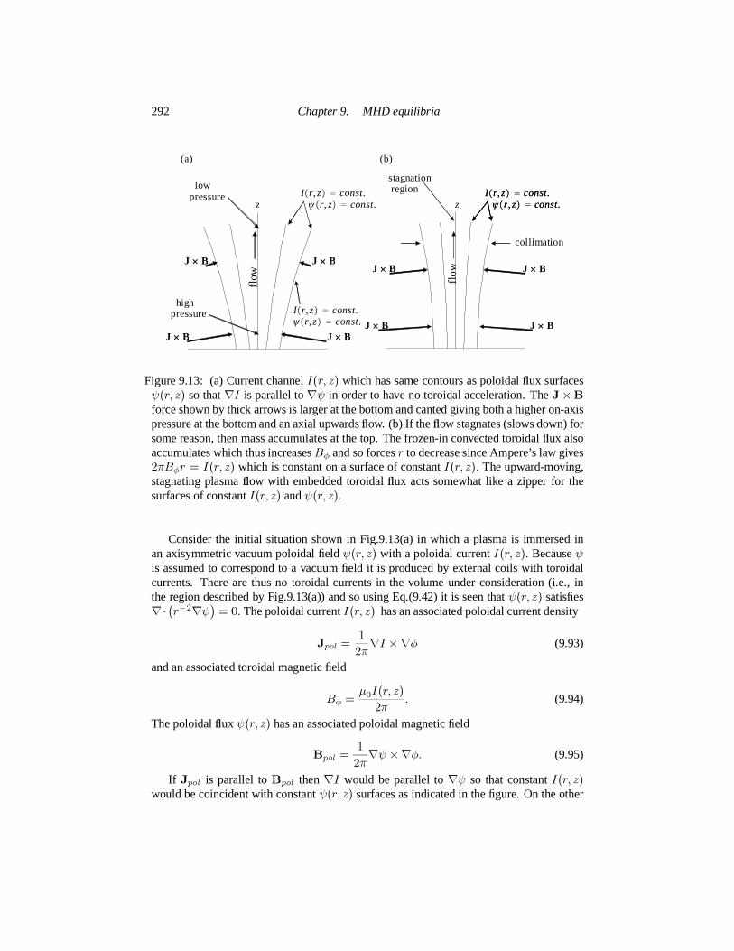
292 Chapter 9. MHD equilibria
stagnationregion
Ir ,z = const.ψr ,z = const.
z zIr ,z = const.ψr ,z = const.
highpressure
lowpressure
collimationflo
w
flow
J × BJ × B J × B
J × B
(a) (b)
J × BJ × BJ × BJ × B
Ir ,z = const.ψr ,z = const.
Ir ,z = const.ψr ,z = const.
Figure 9.13: (a) Current channelI(r, z) which has same contours as poloidalflux surfacesψ(r, z) so that∇I is parallel to∇ψ in order to have no toroidal acceleration. TheJ×Bforce shown by thick arrows is larger at the bottom and canted giving both a higher on-axispressure at the bottom and an axial upwardsflow. (b) If theflow stagnates (slows down) forsome reason, then mass accumulates at the top. The frozen-in convected toroidalflux alsoaccumulates which thus increasesBφ and so forcesr to decrease since Ampere’s law gives2πBφr = I(r, z) which is constant on a surface of constantI(r, z). The upward-moving,stagnating plasmaflow with embedded toroidalflux acts somewhat like a zipper for thesurfaces of constantI(r, z) andψ(r, z).
Consider the initial situation shown in Fig.9.13(a) in which a plasma is immersed inan axisymmetric vacuum poloidal fieldψ(r, z) with a poloidal currentI(r, z). Becauseψis assumed to correspond to a vacuum field it is produced by external coils with toroidalcurrents. There are thus no toroidal currents in the volume under consideration (i.e., inthe region described by Fig.9.13(a)) and so using Eq.(9.42) it is seen thatψ(r, z) satisfies∇·(r−2∇ψ) = 0. The poloidal currentI(r, z) has an associated poloidal current density
Jpol = 12π∇I ×∇φ (9.93)
and an associated toroidal magnetic field
Bφ = µ0I(r, z)2π . (9.94)
The poloidalfluxψ(r, z) has an associated poloidal magnetic field
Bpol = 12π∇ψ ×∇φ. (9.95)
If Jpol is parallel toBpol then∇I would be parallel to∇ψ so that constantI(r, z)would be coincident with constantψ(r, z) surfaces as indicated in the figure. On the other

9.9 Dynamic equilibria:flows 293
hand ifJpol were not parallel toBpol, these surfaces would not be coincident and therewould be a forceJpol ×Bpol in the toroidal direction would tend to cause a change in thetoroidal velocity, i.e., an acceleration or deceleration ofUφ.We argue thatJpol×Bpol mustbe a transient force with zero time average because any current whichflows perpendicularto the poloidalflux surfaces must be the polarization current as given by Eq.(3.145). Thispolarization current results from the time derivative of the electricfield perpendicular tothe poloidalflux surfaces and this electric field in turn is proportional to the timerate ofchange of the poloidal current as determined from Faraday’s law. Thus, once thecurrentis in steady state, it is necessary to haveI = I(ψ) and so the surfaces of constantI(r, z)in Fig.9.12 can also be considered as surfaces of constantψ(r, z). Another way to see this,is to realize that a steady current perpendicular toflux surfaces would cause a continuouselectrostatic charging of theflux surfaces which would then violate the stipulation that theplasma is quasi-neutral.
The initial magnetic force is thus the same as for the situation of a purely toroidalmagnetic field since
J×B = Jtor︸︷︷︸zero
×Bpol + Jpol ×Btor. (9.96)
The remaining forceJpol×Btor = (Jr r + Jzz)×Bφφ = JrBφz−JzBφr has componentsin both ther andz directions. If the plasma axial length is much larger than its radius (i.e.,it is long and skinny) then the plasma will develop a local radial pressure balance
(−∇P + Jpol ×Btor) · r = 0. (9.97)
However, this local radial pressure balance precludes the possibility ofan axial pressurebalance if ∂ψ/∂z = 0 because, as discussed earlier,∇P cannot balanceJ×B if thelatter has a finite curl. Suppose that the radius of the current channel and the poloidalfluxare both given bya = a(z) and sinceI = I(ψ) let us assume a simple linear dependencewhere µ0I(r, z) = λψ(r, z). Thus,∇I is parallel to∇ψ andI is just the current perflux.We assume a parabolic poloidalflux
ψ(r, z)ψ0
=( ra(z)
)2(9.98)
for r ≤ a(z) andψ0 is theflux atr = a; this is the simplest allowed form for theflux (ifψ depended linearly onr, there would be infinite fields atr = 0). The local radial pressurebalance is essentially a local version of the Bennett pinch relation
∂P∂r = −JzBφ
= − λ28π2µ0r2
∂ψ2
∂r . (9.99)
On substitution of Eq.(9.98) this becomes
∂P∂r = −µ0λ2ψ2
08π2r2
∂∂r
( ra(z)
)4
= − λ2ψ20 r
2π2 µ0 a4 . (9.100)

294 Chapter 9. MHD equilibria
Integration and using the boundary condition thatP = 0 atr = a gives
P (r) = λ2ψ20
4π2 µ0 a2(1− r2
a2)
(9.101)
which shows that the on-axis pressure is larger wherea(z) is smaller as indicated inFig.9.13(a). The axial component of the equation of motion is thus
Fz = z · (−∇P + Jpol ×Btor)= −∂P∂z + JrBφ
= − λ2ψ20
4π2 µ0∂∂z
( 1a2 − r2
a4)− 1
µ0Bφ∂Bφ∂z
= − λ2ψ20
π2 µ0(− 12a3 +
r2a5
) ∂a∂z − 1
2µ0∂∂z
( λψ2πr
)2
= λ2ψ20
π2a3 µ0( 12 − r2
a2) ∂a∂z − λ2ψ2
08π2r2µ0
∂∂z
( ra)4
= µ0I202π2a3
(1− r2
a2) ∂a
∂z (9.102)
which shows that there is an axial force which peaks on axis. This forceis proportional tocurrentflowing along theflux tube and to the axial non-uniformity of theflux tube, i.e., to∂a/∂z and accelerates plasma away from regions wherea is small to regions wherea islarge.
If the flow stagnates, i.e., is such that the axial velocity is non-uniform so that∇ ·U isnegative, then there will be a net inflow of matter into the stagnation region and hence anincrease of mass density at the locations where∇·U is negative. Because magneticflux isfrozen to the plasma, there will be a corresponding accumulation of toroidalmagneticfluxat the locations where∇·U is negative. IfUφ is zero (as assumed on the basis of there beingno steady toroidal acceleration and zero initial toroidal velocity), then the accumulation oftoroidalflux will increase the toroidal field. This can be seen by considering the toroidalcomponent of the induction equation
∂Bφ∂t = rBpol · ∇(Uφ
r)− rUpol · ∇(Bφ
r)−Bφ∇ ·Upol (9.103)
or DBφDt = −Bφ∇ ·Upol (9.104)
whereD/DT = ∂/∂t +U ·∇ andUφ = 0 has been assumed. Thus, it is seen thatBφwill increase in the frame of the plasma when∇ · Upol is negative. However, Ampere’slaw givesµ0I = 2πrBφ and sinceI = I0 at the outer radius of the current channel, it isseen that ifBφ increases, then the radius of the current channel has to decrease in order tokeeprBφ fixed. The result is that stagnation of theflow tends to collimate theflux tube,i.e., make it axially uniform as shown in Fig.9.13(b). The plasma accelerated upwards inFig.9.12 will then squeeze together theψ and thusI surfaces so that these surfaces willbe become vertical lines; very roughly stagnation of an upward moving plasma in Fig.9.12

9.10 Assignments 295
can be imagined as a sort of “zipper” which collimates theflux surfaces. Collimation isoften seen in current-carrying magneticflux tubes (e.g., see Hansen and Bellan (2001) andis an important property of solar coronal loops (Klimchuk 2000) and of astrophysical jets(Livio 1999)).
9.10 Assignments
1. Show that if a Bennett pinch equilibrium has aJz independent ofr, then the az-imuthal magnetic field is of the formBθ(r) = Bθ(a)r/a. Then show that if thetemperature is uniform, the pressure will be of the formP = P0(1 − r2/a2) whereP0 = µ0I2/4π2a2. Show that this result is consistent with Eq.(9.29).
2. Show that it is impossible to confine a spherically symmetric pressure profile usingmagnetic forces alone and therefore show that three dimensional magnetostatic equi-libria cannot be found for arbitrarily specified pressure profiles. To do thissupposethere exists a magnetic field that satisfiesJ×B = ∇P whereP = P (r) andr is theradius in spherical coordinatesr, θ, φ.(a) Show that neitherJ norB can have a component in ther direction. Hint: assume
thatBr is finite and write out the three components ofJ×B = ∇P in spher-ical coordinates. By eliminating eitherJr or Br from the equations resultingfrom theθ andφ components, obtain equations of the formJr∂P/∂r = 0 andBr∂P/∂r = 0. Then use the fact that∂P/∂r is finite to develop a contradictionregarding the original assumption regardingJr orBr.
(b) By calculatingJθ andJφ from Ampere’s law (use the curl in spherical coordi-nates as given on p.523), show thatJ×B = ∇P impliesB2θ+B2φ = B2(r).Ar-
gue that this means that the magnitude ofB =Bθθ+Bφφmust be independentof θ andφ and thereforeBθ andBφ must be of the formBθ = B sin [η(θ,φ, r)]andBφ = B cos [η(θ,φ, r)] whereη is some arbitrary function.
(c) UsingJr = 0, Br = 0 and∇ ·B = 0 (see p. 523 for the latter) derive a pairof coupled equations for∂η/∂θ and∂η/∂φ. Solve these coupled equations for∂η/∂θ and∂η/∂φ using the method of determinants (the solutions for∂η/∂θand∂η/∂φ should be very simple). Integrate the∂η/∂φ equation to obtainη andshow that this solution forη is inconsistent with the requirements of the solutionfor ∂η/∂θ, thereby demonstrating that the original assumption of existence of aspherically symmetric equilibrium must be incorrect.
3. Using numerical methods solve for the motion of charged particles in the Solov’evfield, B = ∇ψ × ∇φ whereψ = B0r2(2a2 − r2 − 4(αz)2)/a4 whereB0, a andα are constants. Plot the surfaces of constantψ and show there are open and closedsurfaces. Select appropriate characteristic times, lengths, and velocities and chooseappropriate time steps, initial conditions, and graph windows. Plot thex, y plane andthex, z plane. What interesting features are observed in the orbits. How do theyrelateto theflux surfacesψ = const.What can be said aboutflux conservation?
4. Grad-Shafranov equation for a current-carryingflux tube:The Grad-

296 Chapter 9. MHD equilibria
Shafranov equation describes axisymmetric equilibria and so can be used to charac-terize an axisymmetric magneticflux tube. Suppose thatψ = ψ(r, z) and thatψ is amonotonically increasing function ofr. Assume that both the currentI and pressureP are linear functions ofψ so that
µ0I = λψP = P0(1−ψ/ψ0)
whereψ0 is theflux surface at whichP vanishes andP0 is the pressure on thez axis.Show that the Grad-Shafranov equation can be written in the form
r2∇ ·( 1r2∇ψ)+ µ20λ2ψ = 4π
2r2µ0P0ψ20
whereψ = ψ(r, z)/ψ0. Show that if
P0 = µ20λ2ψ2
04π2µ0a2
wherea is the radius at which the pressure vanishes atz = 0, the flux tube mustbe axially uniform, i.e.,ψ cannot have anyz dependence. Express this condition interms of the pitch angle of the magnetic fieldBφ/Bz measured atr = a. Hint: notethat the Grad-Shafranov equation has a both homogeneous part (left hand side) andinhomogeneous part (right hand side). Show thatψ = r2/a2 is a particular solutionand then consider the form of the general solution (homogenous plus inhomogeneoussolution).
5. Lawson Criterion: Of the many possible thermonuclear reactions, the deuterium-tritium (DT) reaction stands out as being most attractive because ithas the largestreaction cross-section at accessible temperatures. The DT reactionhas the form
D+T −→ n +He4 +17.6 MeV.The output energy consists of 3.5 MeV neutron kinetic energy and 14.1 MeV alphaparticle kinetic energy. Fusion reaction cross-sections have a very strong dependenceon the impact energy of the reacting ions because of the Coulomb barrier. In order fora controlled fusion reaction to be economically useful, more energy must begeneratedthan is invested. The break-even condition is determined by equating theenergy inputper volume to the energy output for the reaction duration. The time duration that thiscondition is maintained is called theenergy confinementtimeτE of the configuration,a measure of the insulating capability of the plasma confinement device. Let all tem-peratures and energies be measured in kilovolts (keV) so that the Boltzmann constantis κ = 1.6× 10⁻¹⁶ and consider a volumeV of reacting deuterium, tritium and asso-ciated neutralizing electrons (the plasma needs to be overall neutral,otherwise therewill be enormous electrostatic forces).
(a) Show that if the electrons and ions have the same temperatureT the energyrequired to heat this volume isEin ∼ 3neV κT wherene is the electron densityand equal densities of deuterium and tritium are assumed so thatnD = nT =

9.10 Assignments 297
ne/2.(Hint: the mean energy per degree of freedom isκT/2 so the mean energyof a particle moving in three dimensional space is3κT/2).
(b) What is the fusion reaction rateR for a single incident ion of velocityv pass-ing through stationary target ions whereσ(v) is the fusion reaction rate cross-section andnt is the density of the target ions (assumed stationary). If<σ(v)v > denotes the velocity average ofσ(v)v what is the velocity-averagedreaction rate?
(c) Assume that the reaction of hot tritium with hot deuterium can be approximatedas the sum of hot deuterium interacting with stationary tritium and hot tritiuminteracting with stationary deuterium. Show that the fusion output powerin thevolume is
P = nDnT < σ(v)v > V EreactionwhereEreaction = 17.6× 10³ keV.
(d) Show that the ratioQ of the fusion output energy to the input energy satisfies therelation
neτE ∼ 6.8 × 10⁻⁴TkeV< σ(v)v > Q
At break-evenQ = 1.(e) For a thermal ion distribution and the experimentally measured reaction cross-
sectionσ(v) the velocity averaged rate integral has the following values
Temperature in keV < σ(v)v > inm3/s neτE1 5.5× 10⁻²⁷
2 2.6× 10⁻²⁵
5 1.3× 10⁻²³
10 1.1× 10⁻²²
20 4.2× 10⁻²²
50 8.7× 10⁻²²
100 8.5× 10⁻²²
Calculate theneτE required for break-even at the listed temperatures (i.e. fill inthe last column).
(f) The Joint European Tokamak (JET) located in Culham, UK (in operationduringthe latter 20th and early 21st century) has a plasma volume of approximately 80cubic meters. Suppose JET has an energy confinement time ofτE ∼ 0.3 s atne ∼ 1020 m−3 andT ∼ 10 keV. If the plasma is a 50%-50% mixture of D-Thow much fusion power would be produced in JET and what isQ? What is theweight of the plasma? How much does the confinement time have to be scaledup to achieve break-even? How much does the volume have to be scaled up toachieve 2000 MWt power output at breakeven? In order to achieve this volumescale-up, how much does the linear dimension have to be scaled up?

10
Stability of static MHD equilibria
Solutions to Eq.(9.49), the Grad-Shafranov equation, (or to some more complicated coun-terpart in the case of non-axisymmetric geometry) provide a static MHD equilibrium. Thequestion now arises whether the equilibrium is stable. This issue was forced upon earlymagnetic fusion researchers who found that plasma which was expected to be well-confinedin a static MHD equilibrium configuration would instead became violently unstable andcrash destructively into the wall in a few microseconds.
The difference between stable and unstable equilibria is shown schematically in Fig.10.1.Here a ball, representing the plasma, is located at either the bottom of a valley or the top ofa hill. If the ball is at the bottom of a valley, i.e., a minimum in the potential energy, then aslight lateral displacement results in a restoring force which pushes the ball back. The ballthen overshoots and oscillates about the minimum with a constant amplitude because en-ergy is conserved. On the other hand, if the ball is initially located at the top of a hill, thena slight lateral displacement results in a force that pushes the ball further to the side so thatthere is an increase in the velocity. The perturbed force is not restoring, but rather the op-posite. The velocity is always in the direction of the original displacement; i.e., there is nooscillation in velocity.
stableequilibrium
unstableequilibrium
Figure 10.1: Stable and unstable equilibria
298

10.1 The Rayleigh-Taylor instability of hydrodynamics 299
The equation of motion for this system is
md2xdt2 = ±κx (10.1)
whereκ is assumed positive, the plus sign is chosen for the ball on hill case, andthe minussign is chosen for the ball in valley case. This equation has a solutionx ∼ exp(−iωt)whereω = ±√κ/m for the valley case andω = ±i√κ/m for the hill case. The hillsolutionω = −i√κ/m is unstable and corresponds to the ball accelerating down the hillwhen perturbed from its initial equilibrium position.
If this configuration is extended to two dimensions, then stability would require anabsolute minimum in both directions. However, a saddle point potential would suffice forinstability, since the ball could always roll down from the saddle point. Thus, a multi-dimensional system can only be stable if the equilibrium potential energy corresponds toan absolute minimum with respect to all possible displacements.
The problem of determining MHD stability is analogous to having a ball on a multi-dimensional hill. If the potential energy of the system increases for any allowed perturba-tion of the system, then the system is stable. However, if there existseven a single allowedperturbation that decreases the system’s potential energy, then the system is unstable.
10.1 The Rayleigh-Taylor instability of hydrodynamics
An important subset of MHD instabilities is formally similar to the Rayleigh-Taylor in-stability of hydrodynamics; it is therefore useful to put aside MHD for the moment andexamine this classical problem. As any toddler learns from stacking building blocks, it ispossible to construct an equilibrium whereby a heavy object is supported by a light ob-ject, but such an equilibrium is unstable. The corresponding hydrodynamic situationhasa heavyfluid supported by a lightfluid as shown in Fig.10.2(a); this situation is unstablewith respect to the rippling shown in Fig.10.2(b). The ripples are unstable because theyeffectively interchange volume elements of heavyfluid with equivalent volume elementsof light fluid. Each volume element of interchanged heavyfluid originally had its centerof mass a distance∆ above the interface while each volume element of interchanged lightfluid originally had its center of mass a distance∆ below the interface. Since the potentialenergy of a massm at heighth in a gravitational fieldg ismgh the respective changes inpotential energy of the heavy and lightfluids are,
δWh = −2ρhV∆g, δWl = +2ρlV∆g (10.2)
whereV is the volume of the interchangedfluid elements andρh andρl are the massdensities of the heavy and lightfluids. The net change in the total system potential energyis
δW = −2 (ρh − ρl)V∆g (10.3)which is negative so that the systemlowersits potential energy by forming ripples. This isanalogous to the ball falling off the top of the hill.
A well-known example of this instability is the situation of an inverted glass of wa-ter. The heavyfluid in this case is the water and the lightfluid is the air. The system isstable when a piece of cardboard is located at the interface betweenthe water and the air,but when the cardboard is removed the system becomes unstable and the water falls out.The function of the cardboard is to prevent ripple interchange from occurring. Thesys-tem is in stable equilibrium when ripples are prevented because atmospheric pressure is
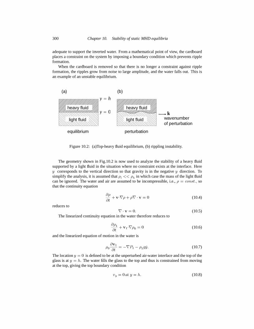
300 Chapter 10. Stability of static MHD equilibria
adequate to support the inverted water. From a mathematical point of view, the cardboardplaces a constraint on the system by imposing a boundary condition which prevents rippleformation.
When the cardboard is removed so that there is no longer a constraint against rippleformation, the ripples grow from noise to large amplitude, and the water falls out. This isan example of an unstable equilibrium.
light fluid light fluid
heavy fluid heavy fluid
perturbation equilibrium
(a) (b)
wavenumberof perturbation
ky = 0
y = h
Figure 10.2: (a)Top-heavyfluid equilibrium, (b) rippling instability.
The geometry shown in Fig.10.2 is now used to analyze the stability of a heavy fluidsupported by a lightfluid in the situation where no constraint exists at the interface. Herey corresponds to the vertical direction so that gravity is in the negativey direction. Tosimplify the analysis, it is assumed thatρl << ρh in which case the mass of the lightfluidcan be ignored. The water and air are assumed to be incompressible, i.e.,ρ = const., sothat the continuity equation
∂ρ∂t + v·∇ρ+ ρ∇ · v = 0 (10.4)
reduces to ∇ · v = 0. (10.5)The linearized continuity equation in the water therefore reduces to
∂ρ1∂t + v1·∇ρ0 = 0 (10.6)
and the linearized equation of motion in the water is
ρ0 ∂v1∂t = −∇P1 − ρ1gy. (10.7)
The locationy = 0 is defined to be at the unperturbed air-water interface and the top of theglass is aty = h. The water fills the glass to the top and thus is constrained from movingat the top, giving the top boundary condition
vy = 0at y = h. (10.8)

10.1 The Rayleigh-Taylor instability of hydrodynamics 301
The perturbation is assumed to have the form
v1 = v1(y)eγt+ik·x (10.9)
wherek lies in thex − z plane and positiveγ implies instability. The incompressibilitycondition, Eq.(10.5), can thus be written as
∂v1y∂y + ik · v1⊥ = 0 (10.10)
where⊥ means perpendicular to they direction. They and⊥components of Eq.(10.7)become respectively
γρ0v1y = −∂P1∂y − ρ1g (10.11)
γρ0v1⊥ = −ikP1. (10.12)The system is solved by dotting Eq.(10.12) withik and then using Eq. (10.10) to eliminatek · v1⊥ and so obtain
−γρ0 ∂v1y∂y = k2P1. (10.13)
The perturbed density, as given by Eq.(10.6), is
γρ1 = −v1y ∂ρ0∂y . (10.14)
Next,ρ1 andP1 are substituted for in Eq. (10.11) to obtain the eigenvalue equation
∂∂y
[
γ2ρ0 ∂v1y∂y]
=[
γ2ρ0 − g ∂ρ0∂y]
k2v1y. (10.15)
This equation is solved by considering the interior and the interface separately:1. Interior: Here∂ρ0/∂y = 0 andρ0 = const. in which case Eq.(10.15) becomes
∂2v1y∂y2 = k
2v1y . (10.16)
The solution satisfying the boundary condition given by Eq.(10.8) is
v1y = A sinh(k(y − h)). (10.17)
2. Interface: To find the properties of this region, Eq.(10.15) is integrated across theinterface fromy = 0− to y = 0+ to obtain
[
γ2ρ0 ∂v1y∂y]0+
0−= − [gρ0k2v1y
]0+0− (10.18)
or
γ2 ∂v1y∂y = −gk2v1y (10.19)
where all quantities refer to the upper (water) side of the interface, since by assumptionρ0(y = 0−) ≃ 0.

302 Chapter 10. Stability of static MHD equilibria
Substitution of Eq.(10.17) into Eq.(10.19) gives the dispersion relation
γ2 = kg tanh(k⊥h) (10.20)
which shows that the configuration is always unstable sinceγ2 > 0. Equation (10.20)furthermore shows that short wavelengths are most unstable, but a more detailed analysistaking into account surface tension (which is stronger for shorter wavelengths) would showthatγ2 has a maximum at some wavelength. Above this most unstable wavelength, surfacetension would decrease the growth rate.
10.2 MHD Rayleigh-Taylor instability
We define a ‘magnetofluid’ as afluid which satisfies the MHD equations. A given plasmamay or may not behave as a magnetofluid, depending on the validity of the MHD approx-imation for the circumstances of the given plasma. The magnetofluid concept providesa legalism which allows consideration of the implications of MHD without necessarilyaccepting that these implications are relevant to a specific actual plasma. In effect, themagnetofluid concept can be considered as a tentative model of plasma.
Let us now replace the water in the Rayleigh-Taylor instability by magnetofluid. Wefurther suppose that instead of atmospheric pressure supporting the magnetofluid, a verticalmagnetic field gradient balances the downwards gravitational force, i.e., at eachy the up-ward force of−∇B2/2µ0 supports the downward force of the weight of the plasma above.Although gravity is normally unimportant in actual plasmas, the gravitational model is nev-ertheless quite useful for characterizing situations of practical interest, because gravity canbe considered as a proxy for the actual forces which typically have a more complex struc-ture. An important example is the centrifugal force associated with thermal particle motionalong curved magnetic field lines acting like a gravitational force in the direction of the ra-dius of curvature of these field lines. The curved field with associated centrifugal force dueto parallel thermal motion is replaced by a Cartesian geometry model having straight fieldlines and, perpendicular to the field lines, a gravitational force is invokedto represent theeffect of the centrifugal force. They direction corresponds to the direction of the radius ofcurvature.
In order for−∇B2 to point upwards in they direction, the magnetic field must dependon y such that its magnitude decreases with increasingy. Furthermore it is required thatBy = 0 so that∇B2 is perpendicular to the magnetic field and the field can be consideredas locally straight (field line curvature has already been taken into account by introducingthe fictitious gravity). Thus, the equilibrium magnetic field is assumed to be of the generalform
B0 = Bx0(y)x+Bz0(y)z. (10.21)The unit vector associated with the equilibrium field is
B0 = Bx0(y)x+Bz0(y)z√Bx0(y)2 +Bz0(y)2 . (10.22)
For the special case whereBx0(y) andBz0(y) are proportional to each other, the field linedirection is independent ofy, but in the more general case where this is not so,B0 depends

10.2 MHD Rayleigh-Taylor instability 303
ony and thus rotates as a function ofy. In this latter case, the magnetic field lines are saidto be sheared, since adjacenty-layers of field lines are not parallel to each other.
The magnetofluid is assumed incompressible and so using Eq.(9.10) the linearizedequation of motion becomes
ρ0 ∂v1∂t = −∇P1 + B0 · ∇B1 +B1 · ∇B0
µ0 − ρ1gy (10.23)
where
P1 = P1 + B0 ·B1µ0
is the perturbation of the combined hydrodynamic and magnetic pressure, i.e., the perturba-tion ofP +B2/2µ0. It is again assumed that all quantities vary in the manner of Eq.(10.9)so Eq.(10.23) has the respectivey and⊥components
γρ0v1y = −∂P1∂y +
i (k ·B0)B1yµ0 − ρ1g (10.24)
γρ0v1⊥ = −ikP1 + 1µ0[
i (k ·B0)B1⊥ +B1y∂B0∂y
]
. (10.25)
In analogy to the glass of water problem, Eq.(10.25) is dotted withik and Eq.(10.10) isinvoked to obtain
−γρ0 ∂v1y∂y = k2P1 + 1µ0
[− (k ·B0)k ·B1⊥ + iB1y∂ (k ·B0)
∂y]
. (10.26)
Because∇ ·B1 = 0, the perturbed perpendicular field is
ik ·B1⊥ = −∂B1y∂y (10.27)
so that Eq.(10.26) can be recast as
k2P1 = −γρ0 ∂v1y∂y − 1µ0
[−i (k ·B0) ∂B1y∂y + iB1y
∂ (k ·B0)∂y
]
. (10.28)
Following a procedure analogous to that used in the inverted glass of waterproblem,P1 iseliminated in Eq.(10.24) by substitution of Eq. (10.28) to obtain
γρ0v1y = − 1k2 ∂∂y−γρ0 ∂v1y∂y − 1
µ0[− (ik ·B0) ∂B1y
∂y +B1y∂ (ik ·B0)
∂y]
+i (k ·B0)B1yµ0 − ρ1g.
(10.29)To proceed further, it is necessary to knowB1y. The complete vectorB1 is found by firstlinearizing the MHD Ohm’s law to obtain
E1 + v1 ×B0 = 0, (10.30)
then taking the curl, and finally using Faraday’s law to obtain
γB1 = ∇× [v1 ×B0] . (10.31)

304 Chapter 10. Stability of static MHD equilibria
They component is found by dotting withy and then using the vector identity∇·(F×G) =G · ∇×F−F · ∇×G to obtain
γB1y = y · ∇× [v1 ×B0] = ∇ · [(v1 ×B0)× y] =∇ · [v1yB0] = ik ·B0v1y. (10.32)
Substituting into Eq.(10.29) using Eq.(10.32) and Eq.(10.14) and rearranging the ordergives
∂∂y
[
γ2ρ0 + 1µ0 (k ·B0)2] ∂v1y∂y
= k2
γ2ρ0 − g ∂ρ0∂y + (k ·B0)2µ0
v1y (10.33)
which is identical to the inverted glass of water problem ifk ·B0 = 0.Rather than have an abrupt interface between a heavy and lightfluid as in the glass
of water problem, it is assumed that the magnetofluid fills the container betweeny = 0andy = h and that there is a density gradient in they direction. This situation is moreappropriate for a plasma which would typically have a continuous density gradient.It isassumed that rigid boundaries exist at bothy = 0 andy = h so thatv1y = 0 at bothy = 0 andy = h. These boundary conditions mean that rippling is not allowed aty = 0, hbut could occur in the interior,0 < y < h. Equation (10.33) is now impossible to solveanalytically because all the coefficients are functions ofy. However, an approximateunderstanding for the behavior predicted by this equation can be found by multiplying theequation byv1y and integrating fromy = 0 to y = h to obtain
[
γ2ρ0 + 1µ0 (k ·B0)2
v1y ∂v1y∂y]h
0− ∫ h
0
[
γ2ρ0 + 1µ0 (k ·B0)2](∂v1y
∂y)2dy
= k2∫ h
0
γ2ρ0 − g∂ρ0∂y +(k ·B0)2
µ0
v21ydy.(10.34)
The integrated term vanishes because of the boundary conditions (which could also havebeen∂v1y/∂y = 0). Solving forγ2 gives
γ2 =
∫ h
0dy
[
k2g ∂ρ0∂y v21y − (k ·B0)2
µ0
(
k2v21y +(∂v1y∂y
)2)]
∫ h
0dy ρ0
[
k2v21y +(∂v1y∂y
)2] . (10.35)
If k ·B0 = 0 and the density gradient is positive everywhere thenγ2 > 0 so thereis instability. If the density gradient is negative everywhere except at onestratum withthickness∆y, then the system will be unstable with respect to an interchange at that one‘top-heavy’ stratum. The velocity will be concentrated at this unstable stratum and sothe integrands will vanish everywhere except at the unstable stratumgiving a growth rateγ2 ∼ g∆y ρ−1
0 ∂ρ0/∂y where∂ρ0/∂y is the value in the unstable region. This MHDversion of the Rayleigh-Taylor instability is called the Kruskal-Schwarzschild instability(Kruskal and Schwarzschild 1954).

10.2 MHD Rayleigh-Taylor instability 305
Finitek ·B0 opposes the effect of the destabilizing positive density gradient, reducingthe growth rate toγ2 ∼ g∆y ρ−1
0 ∂ρ0/∂y − (k ·B0)2 /µ0. A sufficiently strong fieldwill stabilize the system. However, thermally excited noise excites modes with all possiblevalues ofk and those modes aligned such thatk ·B0 = 0will not be stabilized. A shear inthe magnetic field has the effect of making it possible to havek ·B0(y) = 0 at only a singlevalue ofy. The lack of any spatial dependence ofk results from the translational invarianceof the plasma with respect to bothx andz implying thatk =kxx+ kzz is independent ofposition. Thus, magnetic shear constrains the instability to a narrowy stratum.
The stabilizing effect of finitek ·B0 can be understood by considering Eq.(10.32)which shows that the amount ofB1y associated with a givenv1y is proportional tok ·B0.Since the original equilibrium field had noy component, introducing a finiteB1y corre-sponds to ‘plucking’ the equilibrium field. The plucking varies sinusoidally alongthe equi-librium field and stretches the equilibrium field like a plucked violin string.The pluckedfield has a restoring force which pulls the field back to its equilibrium position. If the energyassociated with plucking the magnetic field exceeds the energy liberated by the interchangeof heavy upper magnetofluid with light lower magnetofluid, the mode is stable.
‘good’ curvature ‘bad’ curvature
lastfluxsurface
lastfluxsurface plasma
vacuum vacuumplasma
Figure 10.3: Good and bad curvature of the plasma-vacuum interface.
As discussed earlier, the gravitational force in the magnetofluid model represents thecentrifugal force resulting from guiding center motion along curved field lines. This leadsto the concept of ‘good’ and ‘bad’ curvature illustrated in Fig.10.3. A plasma has badcurvature if the field lines at the plasma-vacuum boundary have a convex shape as seenby an observer outside the plasma since in this case the centrifugal force is outwards fromthe plasma. Bad curvature gives a centrifugal force that can drive interchange instabilitieswhereas good curvature corresponds to a concave shape so that the centrifugal force isalways inwards. Mirror magnetic fields as sketched in Fig.10.4 havegood curvature inthe vicinity of the mirrors and bad curvature in the vicinity of the mirror minimum so thata detailed analysis of interchange instabilities requires averaging the‘goodness/badness’along the portion of theflux tube experienced by the particle. Cusp magnetic fields (cf.Fig.10.4) have good curvature everywhere, but have singular behavior at the cusps. Plasmaswith internal currents such as tokamaks have significant shear everywhere since∂Bx/∂y ∼

306 Chapter 10. Stability of static MHD equilibria
Jz and∂Bz/∂y ∼ Jx; this shear inhibits interchange instabilities. However, as will beshown later this current can be the source for another class of instability called a current-driven instability.
goodcurvaturegoodcurvaturebadcurvature
mirror field cuspfield
Figure 10.4: Mirror fields have bad curvature at the mirror minimum, good curvature nearthe maximum; cusp fields have good curvature everywhere.
10.3 The MHD energy principle
Suppose a system initially in equilibrium is subject to a small perturbationinstigated byrandom thermal noise. The perturbation will affect all the various dependent variables ina way which must be consistent with all the relevant equations and boundary conditions.Thus, the perturbation may be considered as a low-level excitation of someallowed normalmode of the system. The mode will be unstable if it reduces the potential energy ofthe sys-tem and, if unstable, the mode growth rate will be proportional to the amount by which thepotential energy is reduced. In order to investigate whether a given system is stable, it suf-fices to show that no modes exist which reduce the system potential energy. DemonstratingMHD stability this way was first done by Bernstein, Frieman, Kruskal andKuslrud (1958)and the method is called the MHD energy principle.
Each mode has its own specific pattern for displacing the magnetofluid volume elementsfrom their equilibrium positions. The pattern of displacements can be represented by avector function of positionξ(x) that prescribes how afluid volume element originallyat locationx is displaced. Thus, the mode involves moving afluid element initially atx to the positionx+ ξ(x). The displacement of a magnetofluid element initially at thesurface is shown in Fig. 10.5, a sketch of a two-dimensional cut of a three dimensionalmagnetofluid (plasma) surrounded by a vacuum region in turn bounded by a conductingwall. The wall could be brought right up to the magnetofluid to eliminate the vacuumregion or, alternatively, the wall could be placed at infinity to represent a system having nowall and surrounded by vacuum.

10.3 The MHD energy principle 307
perfectlyconductingwall
Gaussianpillbox
equilibriumsurface
ξx
x
perturbedsurface
vacuum
origin
ds
magnetofluid
vacuum
Figure 10.5: Two-dimensional cut of three-dimensional plasma equilibrium and perturba-tion; Gaussian pillbox is used to relate quantities in vacuum to quantitiesin plasma. Eachvolume element at a positionx is displaced by an amountξ(x). The displacement of avolume element at the surface is illustrated.
10.3.1Energy equation for a magnetofluid
The energy content of a magnetofluid can be obtained from the ideal MHD equations if it isassumed that all motions are sufficiently fast to be adiabatic but slowenough for collisionsto keep the pressure isotropic. The ideal MHD equations are
ρ(∂U∂t +U · ∇U
)
= J×B−∇P (10.36)
E+U×B =0 (10.37)
∇×E = −∂B∂t (10.38)
∇×B =µoJ (10.39)

308 Chapter 10. Stability of static MHD equilibria
∂ρ∂t +∇ · (ρU) = 0 (10.40)
P ∼ ργ . (10.41)Ohm’s law, Eq.(10.37), and Faraday’s law, Eq. (10.38), are combined to give theinductionequation ∂B
∂t = ∇× (U×B) (10.42)
which prescribes the magnetic field evolution and, as discussed in the contextof Eq.(2.82),shows that the magneticflux is frozen into the magnetofluid. Equation (10.41), the adi-abatic relation, implies the following relationships for spatial and temporal derivatives ofdensity and pressure ∇P
P = γ∇ρρ ,1P∂P∂t = γ
ρ∂ρ∂t . (10.43)
Combining these relationships with the continuity equation, Eq.(10.40), gives the pressureevolution equation
∂P∂t +U·∇P + γP∇ ·U = 0 (10.44)
which can also be written as
∂P∂t + ∇ · (PU) + (γ − 1)P∇ ·U = 0. (10.45)
An expression for the overall energy can be derived by first writing the equation of motion,Eq.(10.36), as
ρ∂U∂t + ρ∇( U2
2)
− ρU×∇×U = J×B −∇P (10.46)
and then dotting Eq.(10.46) withU to obtain
ρ ∂∂t( U2
2)
+ ρU ·∇( U2
2)
= J×B ·U−U·∇P . (10.47)
Multiplying the entire continuity equation byU2/2 and adding the result gives
∂∂t
(ρU2
2)
+ ∇ ·( ρU2
2 U)
= −J · U×B − ∇ · (PU) +P∇ ·U. (10.48)
Using Ampere’s law, Eq.(10.39), to eliminateJ, then Ohm’s law, Eq.(10.37), to eliminateU×B, and the pressure evolution equation, Eq.(10.45), to eliminateP∇ ·U, this energyequation becomes
∂∂t
(ρU2
2)
+∇·( ρU2
2 U)
= (∇×B)µ0 ·E− ∇·(PU)− 1
(γ − 1)(∂P∂t + ∇ · (PU)
)
.(10.49)
Finally, using the vector identity
∇ · (E×B) = B · ∇×E−E · ∇×B
= −B · ∂B∂t −E · ∇×B (10.50)

10.3 The MHD energy principle 309
Eq.(10.49) can be written as
∂∂t
(ρU2
2 + Pγ − 1 + B2
2µ0)
+∇ ·(
ρU2
2 U+E×Bµ0 + γ
γ − 1PU)
= 0. (10.51)
This is a conservation equation relating energy density and energyflux. The time deriva-tive operates on the magnetofluid energy density and the divergence operates on the energyflux. The energy density is comprised of kinetic energy densityρU2/2, thermal energydensityP/(γ−1), and magnetic energyB2/2µ0. The energyflux is comprised of convec-tion of kinetic energyρU2U/2, the Poynting vectorE×B/µ0, and convection of thermalenergy densityγPU/(γ − 1).
The pressure and density both vanish at the magnetofluid surface, but the Poyntingflux E×B can be finite. However, if the tangential electric field vanishes at the surface,then the Poyntingflux normal to the surface will be zero. This situation occurs if themagnetofluid is bounded by a perfectly conducting wall with no vacuum region between themagnetofluid and the wall. On the other hand, if a vacuum region bounds the magnetofluid,then a tangential electric field can exist at the vacuum-magnetofluid interface and allowa Poyntingflux normal to the surface. Energy could thenflow back and forth betweenthe magnetofluid and the vacuum region. For example, if the magnetofluid were to movetowards the wall thereby reducing the volume of the vacuum region, any vacuum regionmagnetic field would be compressed and so raise the energy contained inthis vacuummagnetic field. Thisflow of energy into the vacuum region would require a Poyntingfluxfrom the magnetofluid into the vacuum region.
Let us now consider the energy properties of the vacuum region between the mag-netofluid and a perfectly conducting wall. The equations characterizing the vacuum regionare Faraday’s law
∇×E = −∂B∂t (10.52)
and Ampere’s law∇×B = 0. (10.53)
Dotting Faraday’s law withB, Ampere’s law withE and subtracting gives
∂∂t
( B2
2µ0)
+∇ ·(
E×Bµ0
)
= 0 (10.54)
which is just the limit of Eq.(10.51) for zero density and zero pressure. Thus,Eq. (10.51)characterizes not only the magnetofluid, but also the surrounding vacuum region. As men-tioned earlier, the Poyntingflux is the means by which electromagnetic energyflows be-tween the magnetofluid and the vacuum region.
If the vacuum region is bounded by a conducting wall, then the tangential electric fieldmust vanish on the wall. The integral of the energy equation over the volume of both themagnetofluid and the surrounding vacuum region then becomes
∂∂t
∫
d3r(ρU2
2 + Pγ − 1 + B2
µ0)
= 0 (10.55)
since on the wallds ·E×B = 0 whereds is a surface element of the wall. If the wall isbrought right up to the magnetofluid so there is no vacuum region, then Eq.(10.55) will also

310 Chapter 10. Stability of static MHD equilibria
result with the additional stipulation that the normal component of the velocity vanishes atthe wall (i.e., the wall is impermeable).
A system consisting of a magnetofluid surrounded by a vacuum region enclosed by animpermeable perfectly conducting wall will therefore have its total internal energy con-served, that is
∫
Vmfd3r
(ρU2
2 + Pγ − 1 + B2
µ0)
+∫
Vvacd3rB2
µ0 = const. (10.56)
whereVmf is the volume of the magnetofluid andVvac is the volume of the vacuum regionbetween the magnetofluid and the wall.
This total system energy can be split into a kinetic energy term
T =∫
d3rρU2
2 (10.57)
and a potential energy term
W =∫
Vd3r
( Pγ − 1 + B2
µ0)
(10.58)
so thatT +W = E (10.59)
where the total energyE is a constant. HereV includes the volume of both the magnetofluidand any vacuum region between the magnetofluid and the wall.
We will now consider a static equilibrium (i.e., an equilibrium withU0 = 0) so that
0 = J0 ×B0 −∇P0. (10.60)
Dotting with eitherB0 or J0 shows that
B0 · ∇P0 = 0, J0 · ∇P0 = 0 (10.61)
so that∇P0 is normal to the surface defined by theJ0 andB0 vectors.
10.3.2Self-adjointness of potential energy as a consequence of energy integral
From Eq.(10.57) it is seen that in static equilibriumT0 = 0. This means that all the internalenergy must be in the form of stored potential energy, i.e.,
W0 = E . (10.62)
It is now supposed that thermal noise causes a small motion of orderǫ to develop ateach point in the magnetofluid. This means there is a first-order velocity
U1 ∼ ǫ. (10.63)
The displacement of afluid element is obtained by time integration to be
ξ =∫ t
0U1dt′; (10.64)

10.3 The MHD energy principle 311
becauseǫ is small the spatial dependence ofU1 can be ignored when evaluating the timeintegral, i.e., terms of orderξ·∇U1 are ignored since these are of orderǫ2.
The kinetic energy associated with the mode is
δT =∫
d3rρ0U21
2 (10.65)
which clearly is of orderǫ2. Since total energy is conserved it is necessary to have
δT + δW = 0 (10.66)
leading to the important conclusion that the perturbed potential energyδW must also beof orderǫ2.
The perturbed pressure and magnetic field can be found to first-order inǫ by integratingEqs.(10.42) and (10.44) respectively to obtain
B1 =∇× (ξ ×B0) (10.67)
andP1 = −ξ·∇P0 − γP0∇ · ξ (10.68)
showing that the first-order pressure and first-order magnetic fields are linear functions ofξ. However, since it was shown above thatδW scales asǫ2, only terms second-order inξcan contribute toδW , and so all first-order terms must average to zero when integratingover the volume. To specify thatδW depends only to second-order inξ, we write
δW = δW (ξ, ξ) (10.69)
where the double argument means thatδW is a bilinear function, i.e., δW (aξ,bη) =abδW (ξ,η) for arbitraryξ,η. The time derivative ofδW is thus
δW = δW (ξ, ξ) + δW (ξ, ξ). (10.70)
Sinceξ is algebraically independent ofξ, Eq.(10.70) means thatδW is self-adjoint (i.e.,δW is invariant when its two arguments are interchanged). Self-adjointness is a directconsequence of the existence of an energy integral.
10.3.3Formal solution for perturbed potential energy
The self-adjointness property can be exploited by explicitly calculatingthe time derivativeof the perturbed potential energy. This is done using the linearized equation ofmotion
ρ0 ∂2ξ∂t2 = F1 (10.71)
whereF1 = J0 ×B1+J1 ×B0 −∇P1 (10.72)
results from linear operations onξ sinceB1, µ0J1 = ∇×B1 andP1 are all result fromlinear operations onξ.

312 Chapter 10. Stability of static MHD equilibria
Multiplying Eq.(10.71) by the perturbed velocityξ and integrating over the volume ofthe magnetofluid and vacuum region gives
∫
d3rρ0 ∂∂t(
ξ22)
=∫
d3rξ ·F1(ξ). (10.73)
Although the integration includes the vacuum region, both the right and left hand sides ofthis equation vanish in the vacuum region because no density, current, or pressure existthere.
The left hand side of Eq.(10.73) is just the time derivative of the kinetic energy δT .SinceδT + δW = 0, it is seen that
δW = −∫
d3rξ ·F1(ξ). (10.74)
However, sinceδW was shown to be self-adjoint, Eq.(10.74) can also be written asδW =−∫ d3rξ ·F1(ξ).Combining these last two equations provides an integrable form forδW ,namely
δW = −12(∫
d3rξ ·F1(ξ) +∫
d3rξ ·F1(ξ))
= −12∂∂t
(∫
d3rξ ·F1(ξ))
. (10.75)
Performing the time integration gives the desired result, namely thechange in system po-tential energy as a function of thefluid displacement is
δW = −12∫
d3rξ ·F1(ξ). (10.76)
Standard techniques of normal mode analysis can be invoked by assuming that thedis-placement has the form
ξ = Re(
ξe−iωt)(10.77)
so the equation of motion can be written as
−ω2ρξ = F1(ξ). (10.78)
Multiplication by ξ∗ and integrating over the volume gives
−ω2∫
d3rρ|ξ|2=∫
d3r ξ∗ ·F1(ξ). (10.79)
In the earlier discussion of self-adjointness, it was noted thatξ is essentially an arbitraryfunction for a givenξ, i.e., anyξ could be obtained by choosing a suitable time dependencefor ξ. Thus, ξ could be chosen to be proportional toξ∗ and so the right hand side ofEq.(10.79) is also self-adjoint. Equation (10.79) can therefore be recast as
−ω2∫
d3rρ|ξ|2=12[∫
d3r ξ∗ ·F1(ξ) +∫
d3r ξ ·F1(ξ∗)]
(10.80)

10.3 The MHD energy principle 313
which shows thatω2 must be pure real. Negativeω2 corresponds to instability.
Equation (10.78) can be considered as an eigenvalue problem whereω2 is the eigen-value andξ is the eigenvector. As in the usual linear algebra sense, eigenvectors havingdifferent eigenvalues are orthogonal and so, in principle, a basis set ofnormalized orthog-onal eigenvectorsζm can be constructed where
F1(ζm) = −ω2mρζm. (10.81)
Thus any arbitrary displacement can be expressed as a suitably weighted sum of eigenvec-tors,
ξ =∑
mαmζm. (10.82)
The orthogonality of the basis set gives the relation∫
d3rζm·F(ζn) = −ω2m∫
d3rρζm·ζn = 0 if m = n. (10.83)
Instability will result if there exists some perturbation that makesδW negative. Con-versely, if all possible perturbations result in positiveδW for a given equilibrium, then theequilibrium is MHD stable.
10.3.4Evaluation of δWSinceF1 consists of three terms involvingJ0, B1 andP1 respectively,δW can be decom-posed into three terms,
δW = δWJ0 + δWB1 + δWP1 . (10.84)Using Eqs. (10.72), (10.67), (10.68) in Eq.(10.76) shows that these terms are
δWJ0 = −12∫
d3rξ · J0 ×B1, (10.85)
δWB1 = − 12µ0
∫
d3rξ · (∇×B1) ×B0, (10.86)
δWP 1 = 12∫
d3rξ · ∇P1. (10.87)
Although the above three right hand sides are in principle integrated over the volumes ofboth the magnetofluid and the vacuum regions, in fact, the integrands vanish in the vacuumregion for all three cases and so the integration is effectively overthe magnetofluid volumeonly. The second two integrals can be simplified using the vector identities∇· (C×D) =D·∇ ×C−C·∇ ×D and∇ · (fa) = a·∇f +f∇ · a to obtain
δWB1 = 12µ0
∫
Vmfd3r (ξ ×B0) · ∇ ×B1
= 12µ0
∫
Vmfd3r B2
1 + 12µ0
∫
Smfds ·B1 × (ξ ×B0) (10.88)

314 Chapter 10. Stability of static MHD equilibria
and
δWP1 = −12
∫
Vmf
d3rξ·∇ [ξ · ∇P0 + γP0∇ · ξ]
= 12
∫
Vmf
d3r[
−ξ·∇ (ξ · ∇P0) + γP0 (∇ · ξ)2]
− 12
∫
Smf
ds · ξγP0∇ · ξ.
(10.89)
Since bothJ×B and∇P are perpendicular toB at the surface of the magnetofluid,the force acting on the magnetofluid at the surface is perpendicular toB and so the dis-placementξ of the magnetofluid at the surface is perpendicular toB, i.e., at the surfaceξ = ξ⊥.The surface integral in Eq.(10.88) can be expanded
12µ0
∫
Smfds ·B1 × (ξ ×B0) = 1
2µ0∫
Smfds · ξ⊥ B0 ·B1 (10.90)
sinceds ·B0 = 0 on the magnetofluid surface. This latter condition is true because themagnetic field was initially tangential to the magnetofluid surface (i.e.,J0 ×B0 = ∇P0implies∇P0 is perpendicular toB0) and must remain so since the field is frozen into themagnetofluid.
Recombining and re-ordering these separate contributions gives
δW = 12∫
Vmfd3r
γP0 (∇ · ξ)2 + B21µ0 − ξ · [J0 ×B1 +∇ (ξ · ∇P0)]
+ 12µ0
∫
Smfds · ξ⊥ [B0 ·B1 − µ0γP0∇ · ξ] . (10.91)
The substitutionds · ξ =ds · ξ⊥ has been made for the pressure contribution to the surfaceterm on the grounds thatds must be perpendicular toB0. Further simplification is obtainedby considering the dot product withB0 of the term in square brackets in Eq.(10.91), namely
B0 · [J0 ×B1 +∇ (ξ · ∇P0)] = −∇P0 ·B1 +B0 · ∇ (ξ · ∇P0)= −∇P0 · ∇ × (ξ ×B0) +B0 · ∇ (ξ · ∇P0)= ∇ · ∇P0 × (ξ ×B0) + (ξ · ∇P0)B0= ∇ · [ξB0 · ∇P0]= 0 (10.92)
where Eq.(10.61) has been used to obtain the last line. Thus,ξ·[J0 ×B1 +∇ (ξ · ∇P0)] =ξ⊥ · [J0 ×B1 +∇ (ξ · ∇P0)] since Eq.(10.92) shows that the factor in square brackets hasno component parallel to the equilibrium magnetic field.
The potential energy variationδW is now decomposed into its magnetofluid volumeand surface components,
δWF ′ = 12∫
Vmfd3r
γP0 (∇ · ξ)2 + B21⊥µ0 + B2
1‖µ0−ξ⊥ · J0 ×B1 − ξ⊥ · ∇⊥ (ξ⊥·∇P0)
(10.93)

10.3 The MHD energy principle 315
and
δWS′ = 12µ0
∫
Smfds · ξ⊥ (B0 ·B1 − µ0γP0∇ · ξ) . (10.94)
At this point it is useful to examine the parallel and perpendicular componentsof B1.Finite B1⊥ corresponds to changing the curvature of field lines (twanging or plucking)whereas finiteB1‖ corresponds to compressing or rarefying the density of field lines. Theequilibrium force balance can be written as
µ0∇P0 = −∇⊥B2
02 +κB2
0 (10.95)
whereκ =B0 · ∇B0 is related to the local curvature of the equilibrium magnetic field.Applying the vector identity∇ (C ·D) = C ·∇D+D ·∇C+D×∇×C+C×∇×Dgives
κ =− B0 ×∇× B0, (10.96)
a relation which will be used when evaluatingB1‖. From Eq.(10.67) it is seen that theparallel component of the perturbed magnetic field is
B1‖ = B0 · ∇ × (ξ⊥ ×B0)= (ξ⊥ ×B0) · ∇ × B0 +∇ ·
[
(ξ⊥ ×B0)× B0
]
= −B0ξ⊥ · κ − ∇ · (B0ξ⊥)= −B0ξ⊥ · κ − B0 (∇ · ξ⊥) − ξ⊥
B0·∇B2
02
= −B0 [2ξ⊥ ·κ +∇ · ξ⊥] + µ0B0
ξ⊥·∇P0. (10.97)
The term involvingJ0 in Eq.(10.93) can be expanded to give
ξ⊥ · J0 ×B1 = ξ⊥ · J0⊥ × B0B1‖ + ξ⊥ · J0‖B0 ×B1⊥
= (ξ⊥ · ∇P0) B1‖B0
+ ξ⊥ · J0‖B0 ×B1⊥. (10.98)
Substituting for this term in Eq.(10.93), factoring out one power ofB1‖, and then sub-

316 Chapter 10. Stability of static MHD equilibria
stituting Eq.(10.97) gives
δWF ′ = 12
∫
Vmf
d3r
γP0 (∇ · ξ)2 + B21⊥µ0
+ B21‖µ0 − (ξ⊥ · ∇P0) B1‖
B0−ξ⊥ · J0‖B0 ×B1⊥ − ξ⊥ · ∇⊥ (ξ⊥·∇P0)
= 12
∫
Vmf
d3r
γP0 (∇ · ξ)2 + B21⊥µ0
+ B1‖µ0
(
B1‖ − µ0ξ⊥ · ∇P0B0
)
−ξ⊥ · J0‖B0 ×B1⊥ − ξ⊥ · ∇⊥ (ξ⊥·∇P0)
= 12
∫
Vmf
d3r
γP0 (∇ · ξ)2 + B21⊥µ0 +
(B20µ0 [2ξ⊥ · κ +∇ · ξ⊥]− ξ⊥·∇P0
)
[2ξ⊥ · κ +∇ · ξ⊥]−ξ⊥ · J0‖B0 ×B1⊥ + (ξ⊥·∇P0)∇ · ξ⊥−∇ · [ξ⊥ (ξ⊥·∇P0)]
= 12
∫
Vmf
d3r
γP0 (∇ · ξ)2 + B21⊥µ0 + B2
0µ0 [2ξ⊥ · κ +∇ · ξ⊥]2
− (ξ⊥·∇P0) (2ξ⊥ · κ) − ξ⊥ · J0‖B0 ×B1⊥−∇ · [ξ⊥ (ξ⊥·∇P0)]
= 12µ0
∫
Vmfd3r
γµ0P0 (∇ · ξ)2 +B21⊥ +B2
0 [2ξ⊥ · κ +∇ · ξ⊥]2−2µ0 (ξ⊥·∇P0) (ξ⊥ · κ) + ξ⊥ ×B1⊥ ·
(
µ0J0‖B0
)
−12∫
Smfds · ξ⊥ (ξ⊥ · ∇P0) . (10.99)
A new surface term has appeared because of an integration by parts; this new term isabsorbed into the previous surface term and thefluid and surface terms are redefined byremoving the primes; thus
δWF = 12µ0
∫
Vmfd3r
γµ0P0 (∇ · ξ)2 + B21⊥ + B2
0 [2ξ⊥ · κ +(∇ · ξ⊥)]2−2µ0 (ξ⊥·∇P0) (ξ⊥ · κ) + ξ⊥ ×B1⊥ ·
(
µ0J0‖B0
)
(10.100)and
δWS = 12µ0
∫
Smfds · ξ⊥ B0 ·B1 − µ0 (γP0∇ · ξ + ξ⊥ · ∇P0)
= 12µ0
∫
Smfds · ξ⊥ B0 ·B1 + µ0P1 (10.101)
whereB0 ·ds = 0 and Eq.(10.68) have been used to simplify the surface integral. The sur-face integral can be further re-arranged by considering the relationship between the vacuum

10.3 The MHD energy principle 317
and magnetofluid fields at the perturbed surface. If the equilibrium force balance is inte-grated over the volume of the small Gaussian pillbox located at the perturbed magnetofluidsurface in Fig.10.5, it is seen that
0 =∫
Vpillbox,psd3r∇ ·
[(
P + B2
2µ0)
I− 1µ0BB
]
=∫
S,psds
[
P + B2
2µ0]vac
magnetof luid(10.102)
sinceds ·B =0 at the perturbed surface. The subscriptsps indicate that the volume andsurface integrals are at the perturbed surface.
Quantities evaluated at the perturbed surface are of the form
fpert sfc = f0 + f1 + ξ · ∇f0; (10.103)
i.e., both absolute and convective first-order terms must be included. Since the pillboxextent was arbitrary in Eq.(10.102), the integrand
[P +B2/2µ0]vacmagnetofluid must vanish
at each point on the perturbed surface, giving the relation(
P1 + B0 ·B1µ0
)
magnetofluid
+ξ·∇(
P + B2
2µ0)
magnetof luid
=(
B0 ·B1µ0
)
vac+ξ·∇
( B2
2µ0)
vac(10.104)
which can be rewritten as(
P1 + B0 ·B1µ0
)
magnetofluid= ξ · ∇
[
P + B2
2µ0]vac
magnetof luid+
(
B0 ·B1µ0
)
vac.
(10.105)Thus the surface integral Eq.(10.101) can be rewritten as
δWS = 12∫
Smfds · ξ⊥ ξ⊥·∇
[
P + B2
2µ0]vac
magnetofluid+ 12µ0
∫
Smfds · ξ⊥ (B0 ·B1)vac .
(10.106)The volume integral in Eq.(10.100) is over the magnetofluid volume and the direction ofds in Eq.(10.106) is outwards from the magnetofluid volume. The energy stored in thevacuum region between the magnetofluid and wall is
δWvac = 12µ0
∫
Vvacd3rB2
1v
= 12µ0
∫
Vvacd3rB1v · ∇×A1v
= 12µ0
∫
Vvacd3r∇ · (A1v ×B1v)
= 12µ0
∫
Svacds · (A1v ×B1v) (10.107)
whereds pointsout from the vacuum region and∇×B1v = 0 has been used when inte-grating by parts. At the conducting wall (which might be at infinity) the integrandvanishessince it contains the factords×A1v which is proportional to the tangential electric fieldand the tangential electric field vanishes at a conductor. Thus, only the surface integral over

318 Chapter 10. Stability of static MHD equilibria
the magnetofluid-vacuum interface remains. Since an element of surfaceds pointing outof the vacuum points into the magnetofluid, usingds to mean out of the magnetofluid (asbefore), this becomes
δWvac = − 12µ0
∫
Smfds · (A1v ×B1v) (10.108)
whereSmf has been used instead ofSvac to indicate thatds points out of the magnetofluid.The tangential component of the electric field must be continuous at the magnetofluid-
vacuum interface. This field is not necessarily zero. The electric field inside the mag-netofluid is determined by Ohm’s law, Eq.(10.37). Thus the electric field on the mag-netofluid side of the magnetofluid-vacuum interface is
E1p = −v1 ×B0 (10.109)
while on the vacuum side of this interface the electric field is simply
E1v = −∂A1v∂t (10.110)
whereA1v is the vacuum vector potential. Defining the surface normal unit vectorn andintegrating both electric fields with respect to time, the condition that the tangential electricfield is continuous is seen to be
n×A1v = n× (ξ ×B0) = −n·ξB0 (10.111)
wheren·B0 = 0 has been used. Thus, the second surface integral in Eq.(10.106) can bewritten as
12µ0
∫
Sds n·ξ⊥B0 ·B1v. = − 1
2µ0∫
Sds n×A1v ·B1v = δWvac. (10.112)
These results are now summarized. The perturbed potential energy can be expressedas
δW = δWF + δWint + δWvac (10.113)where the contribution from thefluid volume interior is
δWF = 12µ0
∫
Vmfd3r
γµ0P0 (∇ · ξ)2 +B21⊥ +B2
0 [2ξ⊥ · κ +(∇ · ξ⊥)]2+ξ⊥ ×B1⊥ · B0µ0J0‖ − 2µ0 (ξ⊥ · κ) (ξ⊥·∇P0)
(10.114)the contribution from the vacuum-magnetofluid interface is
δWint = 12µ0
∫
Smfds · ξ⊥ ξ⊥ · ∇
[
µ0P + B2
2]vac
magnetof luid(10.115)
and the contribution from the vacuum region is
δWvac = 12µ0
∫
vacd3r B2
1v. (10.116)

10.5 Current-driven instabilities and helicity 319
10.4 Discussion of the energy principle
The terms in the integrands ofδWF , δWint, andδWvac are of two types: those that arepositive-definite and those that are not. Positive-definite terms always increaseδW andare therefore stabilizing whereas terms that could be negative are potentially destabilizing.Consideration ofδWF in particular shows that magnetic perturbations interior to the mag-netofluid and perpendicular to the equilibrium field are always stabilizing, since these per-turbations appear in the formB2
1⊥. It is also seen that a positive-definite term∼ (∇ · ξ)2
exists indicating that a compressible magnetofluid is always more stable than an otherwiseidentical incompressible magnetofluid. Hence, incompressible instabilities are more vio-lent than compressible ones. It is also seen that two types of destabilizing terms exist. Onegives instability if
(κ · ξ⊥) (ξ⊥·∇P0) > 0; (10.117)
this is a generalization of the good curvature/bad curvature result obtained in the ear-lier Rayleigh-Taylor analysis. In the vicinity of the magnetofluid surface all quantitiesin Eq.(10.117) point in the same direction and so Eq.(10.117) can be written as
κ·∇P0 > 0 =⇒ instability (10.118)
which gives instability for bad curvature (κ parallel to∇P0) and stability for good curva-ture (κ antiparallel to∇P0). A Bennett pinch has bad curvature and is therefore grosslyunstable to Rayleigh-Taylor interchange modes. Instabilities associated with Eq.(10.117)are called pressure-driven instabilities, and are important in plasmas where there is signifi-cant energy stored in the pressure (highβ whereβ = 2µ0P0/B2
0 ).The other type of destabilizing term depends on the existence of a force-freecurrent
(i.e.,J0‖ = 0) and leads to internal kink instabilities. These sorts of instabilitiesare calledcurrent-driven instabilities (although strictly speaking, only the parallel component of thecurrent is involved).
There also exist instabilities associated with the magnetofluid-vacuum interface. TheenergyδWint can be thought of as the change in potential energy of a stretched membraneat the magnetofluid-vacuum interface where the stretching force is given by the differencebetween the vacuum and magnetofluid forces pushing on the membrane surface; instabilitywill occur if δWint < 0. When investigating these surface instabilities it is convenient tosetδWF to zero by idealizing the plasma to being incompressible, having uniform internalpressure, and no internal currents. Surface instabilities can exist onlyif the surface canmove, and so require a vacuum region between the wall and the plasma. Thus, moving aconducting wall right up to the surface of a conducting plasma prevents surface instabilities.These surface instabilities will be investigated in detail laterin this chapter.
10.5 Current-driven instabilities and helicity
We shall now discuss current driven instabilities and show that these are helical in natureand are driven by gradients inJ0///B0. To simplify the analysisP → 0 is assumed so thatpressure-driven instabilities can be neglected since they have already been discussed. Onmaking this simplification, Eq.(10.97) shows that the parallel component of the perturbed

320 Chapter 10. Stability of static MHD equilibria
magnetic field reduces to
B1‖ = −B0 [2ξ⊥ · κ +∇ · ξ⊥] . (10.119)
Thus, we may identify
B21 = B2
1⊥ +B21‖ = B2
1⊥ +B20 [2ξ⊥ · κ +∇ · ξ⊥]2 (10.120)
and so the perturbed potential energy of the magnetofluid volume reduces to
δWF = 12µ0
∫
d3r
B21 + ξ⊥ ×B1⊥ ·B0
µ0J0‖B0
. (10.121)
Equation (10.67) shows that the perturbed vector potential can be identified as
A1 = ξ ×B0 (10.122)
so that Eq.(10.121) can be recast as
δWF = 12µ0
∫
d3r
B21 −A1 ·B1
µ0J0‖B0
. (10.123)
We now show that finiteA1 · B1 corresponds to a helical perturbation. Consider thesimplest situation whereA1 ·B1 is simply a constant and define a local Cartesian coordinatesystem withz axis parallel to the localB0. Equation (10.122) shows thatA1 = A1x x +A1y y so
A1 ·B1 = −A1x∂A1y∂z +A1y
∂A1x∂z . (10.124)
Suppose both components ofA1 are non-trivial functions ofz and, in particular, assumeA1x = ReA1x exp(ikz)andA1y = ReA1y exp(ikz). In this case
A1 ·B1 = 12Re
[
−A∗1x∂A1y∂z +A∗
1y∂A1x∂z
]
= −k2Re[i (A∗
1xA1y −A∗1yA1x
)]
(10.125)which can be finite only ifA∗
1xA1y is not pure real. The simplest such case is whereA1y = iA1x so
A1 ·B1 = k|A1x|2 (10.126)and
A1 = Re [A1x (x+ i y) exp(ikz)] (10.127)which is a helically polarized field sinceA1x ∼ coskz andA1y ∼ sin kz.
10.6 Magnetic helicity
Since finiteA1 · B1 corresponds to the local helical polarization of the perturbed fields,it is reasonable to defineA ·B as the density of magnetic helicity and to define the totalmagnetic helicity in a volume as
K =∫
Vd3rA ·B . (10.128)

10.6 Magnetic helicity 321
The question immediately arises whether this definition makes sense, i.e., is it reasonableto defineA · B as an intensive property andK as an extensive property. An obviousproblem is thatA is undefined with respect to a gauge, sinceA can be redefined to beA′ = A+∇f wheref is an arbitrary scalar function without affecting the magnetic field,because∇×A =∇× (A+∇f) . The above definition for magnetic helicity would be oflittle use ifK depended on choice of gauge. However, if no magnetic field penetrates thesurfaceS enclosing the volumeV, the proposed definition ofK is gauge-independent. Thisis becauseB·ds = 0 everywhere on the surface if no magnetic field penetrates the surface.If this is so, then
∫
Vd3r (A+∇f) ·B =
∫
Vd3rA ·B +
∫
Vd3r∇ · (fB)
=∫
Vd3rA ·B +
∫
Sds · (fB)
=∫
Vd3rA ·B (10.129)
and so the helicity is gauge-independent even though the helicity density is gauge-dependent.Let us consider the situation where there is no vacuum region between the plasma and
an impermeable wall. Thus the normalfluid velocityu1⊥ must vanish at the wall. FromOhm’s law the component of the perturbed electric field tangential to the wallE1t is just
E1t = −u1⊥ ×B0 = 0 (10.130)
sinceB0 lies in the plane of the wall. Thus, an impermeable wall is equivalentto a con-ducting wall. If the magnetic field initially does not penetrate the wall,i.e. B·ds = 0initially, then the field will always remain tangential to the wall and the helicityK in thevolume enclosed by the wall will always be a well-defined quantity (i.e., will always begauge-invariant).
The time derivative of the magnetic helicity density together with Faraday’s law givesa conservation equation for helicity density. This is seen by direct calculation:
− ∂∂t (A ·B) = −∂A∂t ·B−A · ∂B∂t= (E+∇ϕ) ·B+A · ∇ ×E
= 2E ·B+∇ · (ϕB+E×A)
(10.131)
whereϕ is the electrostatic potential. Since the ideal MHD Ohm’s law givesE ·B =0,Eq. (10.131) can be rearranged in the form of a helicity conservation equation
∂∂t (A ·B) +∇ · (ϕB+E×A) = 0. (10.132)
Integration of Eq.(10.132) over the entire magnetofluid volume gives a global helicity con-servation relation
∂∂t
[∫
d3rA ·B]
+∫
dsn· (ϕB +E×A) = 0. (10.133)

322 Chapter 10. Stability of static MHD equilibria
Since bothB·n=0 andEt = 0 at the wall, this reduces to
K =∫
d3rA ·B =const.; (10.134)
i.e., the total helicity (integral of the helicity density) is conserved for an ideal plasmasurrounded by a rigid or conducting wall.
Now recall thatA1 is a linear function ofξ as given in Eq.(10.122) and thatξ wasassumed to be of orderǫ. Consider the implications of this result for perturbed magneticfields. We writeB = B0 +B1 andA = A0 +A1 so that the total magnetic helicity, aconstant, is
K = ∫ d3rA0 · ∇ ×A0 = ∫ d3r (A0 +A1 ) · ∇ × (A0 +A1 )
=∫ d3rA0 · ∇×A0 + ∫ d3rA1 · ∇ ×A0
+∫ d3rA0 · ∇ ×A1 + ∫ d3rA1 · ∇ ×A1.(10.135)
Thus, to first-order in the perturbation (i.e., to orderǫ),∫
d3rA1 · ∇×A0 +∫
d3rA0 · ∇ ×A1 = 0 (10.136)
and to second-order (i.e., to orderǫ2 which is what is relevant for the energy principle),∫
d3rA1 · ∇ ×A1 =∫
d3rA1 ·B1 = 0. (10.137)
This can be compared to Eq.(10.123); the second term is almost the same as Eq.(10.137)except for a factor−µ0J0‖/B0 which, in general, is some complicated function of position.However, in the special case whereµ0J0‖/B0 = const., it is possible to factorµ0J0‖/B0out of the integral and obtain, using Eq.(10.137),
δWF = 12µ0
∫
d3r B21 (10.138)
which is positive-definite and therefore gives absolute stability. Thus, equilibria which haveµ0J0‖/B0 = λ whereλ = const. are stable against current-driven modes. Since theseequilibria are helical or kinked, they may be considered as being the final relaxed stateassociated with a kink instability –once a system attains this state no free energy remainsto drive further instability. Since pressure has been assumed to be negligible, Eq.(10.60)implies that the equilibrium current must be parallel to the equilibriummagnetic field,but does not specify the proportionality factor. What has been shown here is that if theproportionality factor is spatially uniform, i.e.,
µ0J0=λB0 (10.139)
whereλ does not depend on position, then the system is stable against any further helicalperturbations. This gives rise to the relation
∇×B0 = λB0 (10.140)

10.7 Qualitative description of free-boundary instabilities 323
whereλ is spatially uniform. This equation is called the force-free equilibrium and itssolutions are helical vector fields, namely fields where the curl of the field is parallel tothe field itself. If a field is confined to a plane, then its curl will be normal to the planeand so a field confined to a plane cannot be a solution to Eq.(10.140). The field must bethree-dimensional.
To summarize, it has been shown that current-driven instabilities arehelical and drivethe plasma towards a force-free equilibrium as prescribed by Eq.(10.140). Current-driveninstabilities are energized by the gradient ofJ0‖/B0 and become stabilized whenJ0‖/B0becomes spatially uniform. Gradients inJ0‖/B0 can therefore be considered as the freeenergy for driving kink modes. When all the free energy is consumed, the kinks are stabi-lized and the plasma assumes a force-free equilibrium with spatially uniformJ0‖/B0.
This tendency to coil up or kink is a means by which the plasma increases its inductance.However, when the plasma coils up into a state satisfying Eq.(10.140) it is in a stableequilibrium. This stable equilibrium represents a local minimum in potential energy. Theremight be several such local minima, each of which has a different value assketched inFig.9.2. As mentioned earlier this set of discrete energy levels is somewhat analogousto the ground and excited states of a quantum system. Here, the vacuum magnetic fieldis analogous to the ground state, while the various force-free equilibria (i.e., solutions ofEq.(10.140)) are analogous to higher energy states.
10.7 Qualitative description of free-boundary instabilities
The previous section considered internal instabilities of a magnetofluid bounded by a rigidwall so that no vacuum region existed between the magnetofluid and the wall. Let usnow consider the other extreme, namely a situation where not only does a vacuum regionexist external to the magnetofluid, but in addition, the location of the vacuum-magnetofluidinterface is not fixed and can move around. To focus attention on the effect of surfacemotions, the simplest non-trivial configuration will be considered, namely a configurationwhere the interior pressure is both uniform and finite. This corresponds to having∇P =0 in the interior so that the entire pressure gradient and therefore the entireJ×B force isconcentrated in an infinitesimally thin surface layer.
The MHD energy principle showed that compressibility, manifested by having finite∇ · ξ, is stabilizing. Therefore, if a given system is stable with respect to incompressiblemodes, it will be even more stable with respect to compressible modes, or equivalently, withrespect to modes having finite∇·ξ. Thus by assuming∇·ξ =0, the worst-case scenario isconsidered and, in addition, the analysis is simplified. Finally, it isassumed that the plasmais cylindrical and uniform in thez direction (axially uniform). For example, the Bennettpinch would satisfy these assumptions if all the current were concentrated on the plasmasurface. The physical basis of the two main types of current-driven instability, sausage andkink, will first be discussed before engaging in a detailed mathematical analysis.
10.7.1Qualitative examination of the sausage instability
Consider a Bennett pinch (z-pinch), that is an axially uniform cylindrical plasma with anaxial current and an associated azimuthal magnetic field. In addition, asdiscussed above

324 Chapter 10. Stability of static MHD equilibria
the pressure is assumed to be (i) uniform in the interior regionr < a wherea is the plasmaradius and (ii) zero in the exterior regionr > a. In equilibrium, the radially inwardJ×Bpinch force balances the radially outward force associated with the pressure gradient sothat−Jz0Bθ0 = ∂P0/∂r where both sides of this equation are finite only in an infinitesi-mal surface layer atr = a.We now suppose that thermal noise causes the incompressibleplasma to develop axially periodic constrictions and bulges as shown in Fig.10.6. At theconstrictions the azimuthal magnetic fieldBθ = µ0I/2πr becomes larger than in equilib-rium becauser < a at a constriction whereasI is fixed. Thus, at the constriction the pinchforce∼ B2θ/r is greater than its equilibrium value and so exceeds the outward force fromthe internally uniform pressure. The resulting net force will be inwards and will cause aradial inwards motion which will enhance the constriction. Because the configuration isassumed incompressible, any plasma squeezed inwards at constrictions must flow into theinterspersed bulges shown in Fig.10.6. The azimuthal magnetic field at a bulge is weakerthan its equilibrium value becauser > a at a bulge so the tables are now turned in thecompetition between outward pressure and inward pinch force — at a bulge the pressureexceeds the weakened pinch force and this force imbalance causes the bulge to increase.Hence any initial perturbed combination of constrictions and bulges willtend to grow andso the system is unstable. This behavior is called the ‘sausage’ instability because whatresults is a plasma resembling a string of sausages.
current
bulge
constriction
Figure 10.6: Sausage instability, current is axial, magnetic field is azimuthal

10.7 Qualitative description of free-boundary instabilities 325
weaker azimuthalmagneticfield
stronger azimuthalmagneticfield
surfacecurrent
Figure 10.7: Kink instability can occur when the equilibrium magnetic fieldis helical
The sausage instability can be prevented by surrounding the plasma with aperfectlyconducting wall or by immersing the plasma in a strong axial vacuum magnetic field gen-erated by currents in external solenoid coils coaxial with the plasma. Ifa plasma withembedded axial field attempts to sausage, the axial rippling of the plasma would have tobend the embedded axial field since this axial field is frozen into the plasma.Any bendingof a magnetic field requires work and so the free energy available to drive the sausage insta-bility would also have to do work to bend the axial field. If bending the axial magnetic fieldabsorbs more energy than liberated by the sausaging motion, the plasma is stabilized. Theaxial field stabilizes the plasma in a manner analogous to a steel reinforcing rod embeddedin concrete. The other method for stabilization, a close-fitting conductingwall, works be-cause image currents induced in the wall by the sausage motion produce a magneticfieldwhich interacts with the plasma current in such a way as to repel the plasma away from thewall.
10.7.2Qualitative examination of the kink instability
The axial magnetic fieldBz combined with the azimuthal magnetic fieldBθ produced bythe plasma current results in a magnetic field that is helical. This helical magnetic field issusceptible to the helical kink instabilities sketched in Fig.10.7. At the concave parts ofthe plasma surface there is a concentration of the azimuthal field resulting in a magneticpressure that increases the concavity. Similarly, at the convex portions of the surface, the
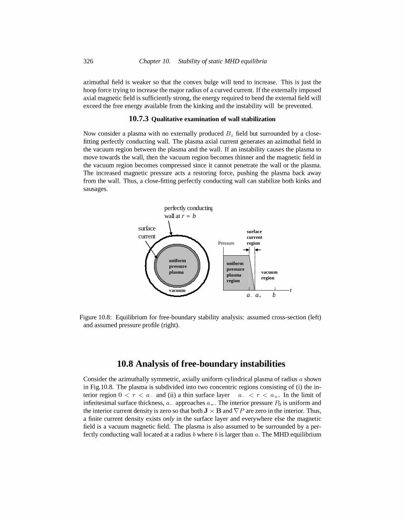
326 Chapter 10. Stability of static MHD equilibria
azimuthal field is weaker so that the convex bulge will tend to increase.This is just thehoop force trying to increase the major radius of a curved current. If the externally imposedaxial magnetic field is sufficiently strong, the energy required to bend the external field willexceed the free energy available from the kinking and the instability will be prevented.
10.7.3Qualitative examination of wall stabilization
Now consider a plasma with no externally producedBz field but surrounded by a close-fitting perfectly conducting wall. The plasma axial current generatesan azimuthal field inthe vacuum region between the plasma and the wall. If an instability causes the plasma tomove towards the wall, then the vacuum region becomes thinner and the magneticfield inthe vacuum region becomes compressed since it cannot penetrate the wall or the plasma.The increased magnetic pressure acts a restoring force, pushing the plasma back awayfrom the wall. Thus, a close-fitting perfectly conducting wall can stabilize both kinks andsausages.
surfacecurrent
perfectlyconductingwall at r = b
a− a+ b
uniform pressureplasma
vacuum
uniformpressureplasma region
vacuumregion
Pressure
surfacecurrentregion
r
Figure 10.8: Equilibrium for free-boundary stability analysis: assumed cross-section (left)and assumed pressure profile (right).
10.8 Analysis of free-boundary instabilities
Consider the azimuthally symmetric, axially uniform cylindrical plasma of radiusa shownin Fig.10.8. The plasma is subdivided into two concentric regions consisting of(i) the in-terior region0 < r < a− and (ii) a thin surface layer a− < r < a+. In the limit ofinfinitesimal surface thickness,a− approachesa+. The interior pressureP0 is uniform andthe interior current density is zero so that bothJ×B and∇P are zero in the interior. Thus,a finite current density existsonly in the surface layer and everywhere else the magneticfield is a vacuum magnetic field. The plasma is also assumed to be surrounded by a per-fectly conducting wall located at a radiusbwhereb is larger thana. The MHD equilibrium

10.8 Analysis of free-boundary instabilities 327
can be written as
0 = −µ0∇P0 −∇(B202)
+B0 · ∇B0. (10.141)
Because∇ ·B0 = r−1∂/∂r (rB0r) = 0 for an azimuthally symmetric, axially uni-form system and becauseBr cannot be singular,B0r must be zero everywhere. Since allequilibrium quantities depend only onr, the third term in Eq.(10.141) can be expanded
B0 · ∇B0 =(
B0θ(r)θ +B0z(r)z)
· ∇(
B0θ(r)θ +B0z(r)z)
= B20θθ · ∇θ = −B20θr r.
(10.142)
Thus, Eq.(10.141) has onlyr components and reduces to the relation
0 = −µ0 ∂P0∂r − ∂
∂r(B202)
− B20θr . (10.143)
On integrating across the surface layer, this becomes
P0 + B20pz2µ0 = B20vθ +B20vz
2µ0 (10.144)
where the subscriptp refers to being at the inner radius (plasma side) of the surface layer andthe subscriptv refers to the outer radius (vacuum side). The reason there is noB20pθterm on the left hand side is that there are no interior plasma currents (from Ampere’slaw 2πaB0pθ = µ0Iz = 0).
The equilibrium surface can be described by the functionr = a or equivalently, thesurface-defining equation
S0(r) = r − a = 0. (10.145)The incompressible perturbation is characterized by a harmonic deformation of the plasmasurface such thatr = a + ξeimθ+ikz. The surface equation for the perturbed surface isthus
S(r, θ, z) = r − a− ξeimθ+ikz = 0 (10.146)where without loss of generality it is assumed thatξ > 0 . The equilibrium magnetic fieldhadB0r = 0, i.e., had no component normal to the surface, and so the equilibrium magneticfield lines at the surface lie in the surface. This is equivalent to stating thatB0 · ∇S0 = 0which implies that the equilibrium magnetic field is tangential to the surface. Since themagnetic field is assumed frozen into the plasma, the magnetic field must continueto betangential to the surface even when the surface becomes deformed from its equilibriumshape. Thus, the condition
B · ∇S = 0 (10.147)must be satisfied at all times where∇S is in the direction normal to the surface; this isessentially a statement that no magnetic field line penetrates the surface.
A quantity f at the perturbed surface (denoted by the subscript ps) can be expressedas
fps = f0 + f1 + ξ·∇f0 (10.148)where the the middle term is the absolute first-order change and the last termis the convec-tive term due to the motion of the surface.

328 Chapter 10. Stability of static MHD equilibria
If a configuration is to be stable, any perturbation must generate a restoring force whichpushes the perturbed surface back to its equilibrium location. The competition betweendestabilizing and restoring forces is found by integrating Eq.(10.141) across the perturbedsurface. This integration gives Eq.(10.144) evaluated at the perturbed surface, i.e., usingEq.(10.148) to take into account the effect of the perturbation of the surface.Sinceξwasassumed positive (outward bulge atθ = 0, z = 0) the perturbed system will be stable if theeffective pressure on the outside of the perturbed surface exceeds the effective pressure onthe inside, i.e., if
[B2vθ +B2vz2µ0
]
perturbed sfc>
[
P + B2pz
2µ0
]
perturbed sfc=⇒ stable. (10.149)
In this case, the restoring force pushes back the bulge and makes the system revert to itsequilibrium condition. Subtracting the equilibrium pressure balance relation, Eq.(10.144),this becomes
B0vθB1vθ +B0vzB1vzµ0 + ξ ∂∂r
[B20vθ +B20vz2µ0
]
> P1 + B0pzB1pzµ0 + ξ ∂∂r
[
P0 + B20pz2µ0
]
(10.150)where all quantities are evaluated atr = a.
Equation (10.150) can be simplified considerably because of the following relation-ships:
1. There are no currents in either the plasma interior or the external vacuum so
∂B0pz∂r = ∂B0vz
∂r = 0. (10.151)
2. The adiabatic pressure equation gives
P1 + ξ·∇P0 + γP0∇ · ξ = 0. (10.152)
Since incompressibility∇ · ξ = 0has been assumed, the adiabatic relation reducesto
P1 + ξ ∂P0/∂r = 0 . (10.153)
3. From Ampere’s law it is seen thatB20vθ ∼ r−2 so[∂B20vθ/∂r
]
r=a = −2B20vθ/a; thusEq.(10.150) simplifies to
B0vθB1vθ +B0vzB1vz − ξaB
20vθ > B0pzB1pz =⇒ stable (10.154)
where again all fields are evaluated atr = a.To simplify the algebra all fields are now normalized toB0vθ(a).The normalized fields
are denoted by a bar on top and are
B0vz = B0vzB0vθ(a) , B0pz = B0pz
B0vθ(a) ,B1vz = B1vz
B0vθ(a) , B1vθ = B1vθB0vθ(a) , B1pz = B1pz
B0vθ(a)(10.155)

10.8 Analysis of free-boundary instabilities 329
so that, when expressed as a relationship between normalized fields, Eq.(10.154) becomes
B1vθ + B0vzB1vz − ξa > B0pzB1pz =⇒ stable. (10.156)
What remains to be done is express all first-order magnetic fields in terms of ξ. This isrelatively easy because the current is confined to the surface layer sothe magnetic field isa vacuum magnetic field everywhere but exactly on the surface.
SinceB is a vacuum magnetic field for both0 < r < a anda < r < b, it must be of theform B =∇χ where∇2χ = 0 in both regions, but there could be a jump discontinuity atr = a. Because the perturbed fields were assumed to have anexp(imθ+ikz) dependence,the Laplacian becomes
∇2χ = d2χ(r)dr2 + 1
rdχ(r)dr −
(m2
r2 + k2)
χ(r) = 0 (10.157)
which is just the equation for modified Bessel functions,I|m|(|k|r) andK|m|(|k|r). Ab-solute value signs have been used to avoid possible confusion later for situationswheremork could be negative. TheI|m|(|k|r) function is finite atr = 0 but diverges atr =∞whilethe opposite is true forK|m|(|k|r).
The surface current causes a discontinuity in the tangential components of the perturbedmagnetic field. Hence, different solutions must be used in the respective plasma and vac-uum regions and then these solutions must be related to each other in such a way as tosatisfy the requirements of this discontinuity. The forms of the plasma and vacuum solu-tions are, in addition, constrained by the respective boundary conditions atr = 0 and atr = b. In particular, theK|m|(|k|r) solution is not allowed in the plasma because of theconstraint that the magnetic field must be finite atr = 0; thus inside the plasma the solutionis of the form
χ = αI|m|(|k|r) in plasma region 0 < r < a− . (10.158)On the other hand, both theI|m|(|k|r) andK|m|(|k|r) solutions are permissible in thevacuum region and so the vacuum region solution is of the general form
χ = β1I|m|(|k|r) + β2K|m|(|k|r) in vacuum regiona+ < r < b . (10.159)
The objective now is to express the coefficientsα, β1, andβ2 in terms ofξ so that allcomponents of the perturbed magnetic field can be expressed as a function ofξ, both in theplasma and in the vacuum.
The functional dependence of these coefficients is determined by considering boundaryconditions at the wall and then at the plasma-vacuum interface:
1. Wall: Since the wall is perfectly conducting it is aflux conserver. There is no radialmagnetic field initially and so there is noflux linking each small patch of the wall.ThusB1vr(b) must vanish at the wall in order to maintain zeroflux at each patch ofthe wall. Using Eq.(10.159) to calculate the perturbed radial magnetic field at the wall,this condition means that
β1I ′|m|(|k|b) + β2K′|m|(|k|b) = 0 (10.160)
which may be solved forβ2 to give
β2 = −β1I′|m|K′|m|
; (10.161)

330 Chapter 10. Stability of static MHD equilibria
here the circumflex means the modified Bessel function is evaluated at the wall, i.e.,with its argument set to|k|b.Equation (10.159) can then be recast as
χ = β[
I|m|(|k|r)K′|m| − I ′|m|K|m|(|k|r)]
(10.162)
whereβ = β1/K ′|m|. The wall boundary condition has reduced the number of inde-pendent coefficients by one.
2. Vacuum side of plasma-vacuum interface: Here Eq.(10.147) is linearized to obtain
B1 · ∇S0 +B0 · ∇S1 = 0 (10.163)
or using Eqs.(10.145) and (10.146)
B1vr − i(ma + kB0vz)ξ = 0. (10.164)
On the vacuum side Eq.(10.162) gives
B1vr = |k|β[
I′|m|K′|m| − I ′|m|K′|m|]
(10.165)
where omission of the argument means that the modified Bessel function is evaluatedatr = a. Substitution of Eq.(10.165) into Eq.(10.164) gives
β =i(ma + kB0z
)
|k|[
I′|m|K′|m| − I ′|m|K′|m|]ξ (10.166)
so the complete vacuum field can now be expressed in terms ofξ.3. Plasma side of plasma-vacuum interface: The plasma-side version of Eq.(10.163)
givesB1pr − ikB0pzξ = 0 (10.167)
sinceB0pθ vanishes inside the plasma. From Eq.(10.158) the perturbed radial mag-netic field on the plasma side of the interface is
B1pr = |k|αI ′|m|. (10.168)
The plasma side version of Eq.(10.164) is thus
α = ikB0pz|k|I ′|m|
ξ (10.169)
and so the plasma fields can now also be expressed in terms ofξ.The stability condition, Eq.(10.156), can be written in terms ofα andβ to obtain
β( ima + ikB0vz
)
(
I|m|K ′|m| − I′|m|K|m|)
− ξa > αB0pzikI|m|. (10.170)
Substituting forα andβ and re-arranging the order gives
|k|aB20pz
[I|m|I ′|m|
]
− (m+ kaB0vz)2|k|a
[ I|m|K′|m| − I ′|m|K|m|I′|m|K′|m| − I ′|m|K′|m|
]
> 1 =⇒ stable. (10.171)

10.8 Analysis of free-boundary instabilities 331
If we introduce the normalized pressure
P0 = 2µ0P0B20vθ(a) (10.172)
the MHD equilibrium, Eq.(10.144), can be written in normalized form as
P0 + B20pz = 1+ B20vz. (10.173)Substitution forB20pz into Eq.(10.171) and rearranging the order of the second term gives
|k|a [1 + B20vz − P0]
[I|m|I ′|m|
]
+ (m+ kaB0vz)2|k|a
[−I|m|K′|m| + I ′|m|K|m|I′|m|K′|m| − I ′|m|K′|m|
]
> 1(10.174)
which is the general requirement for stability of a configuration having a specified internalpressure, vacuum axial field, plasma radius, and wall radius.
Conditions for sausage and kink instability Let us now examine the effect of thevarious factors in Eq.(10.174). For large argument, the modified Bessel functions have theasymptotic form
lims→∞ I|m|(s)→ es; lims→∞ K|m|(s)→ e−s (10.175)
so if the wall radius goes to infinity, the factor
[−I|m|K ′|m| + I′|m|K|m|I′|m|K′|m| − I ′|m|K′|m|
]
→ −K|m|K′|m|
= positive definite. (10.176)
Since bringing the wall closer is stabilizing, the factor
−I|m|K′|m| + I′|m|K|m|I′|m|K′|m| − I ′|m|K′|m|
will always be positive-definite. In particular, ifb→ a thenI ′|m|K′|m| → I ′|m|K′|m| so thatthe wall stabilization becomes arbitrarily large.
As |k|a → ∞ the left hand side of Eq.(10.174) becomes infinite. Thus, the configura-tion is stable with respect to modes having short axial wavelengths. The reason for this isthat short wavelength perturbations cause more bending of the magnetic fieldthan a longwavelength perturbation and so require more energy.
We therefore focus attention on modes with alongaxial wavelength (i.e., modes with asmallk) since these offer the only possibility of instability. The analysis can besubdividedinto specific cases, such asm = 0, |m| = 1, |m| > 1, close-fitting wall, no wall, lowpressure, high pressure, etc. Before getting into the details let us take a broader look at theeffect of the various terms in Eq. (10.174). SinceI|m|/I ′|m| > 0 we see that increasingP0is destabilizing, while increasingB20vz is stabilizing. Also, ifm+ kaB0vz = 0 the secondterm vanishes, leading toreducedstability; by defining the wavevector ask = (m/a)θ+kzit is seen thatm+ kaB0vz = 0 corresponds to havingk ·B0 = 0 at the surface.

332 Chapter 10. Stability of static MHD equilibria
Sausage modesThem = 0modes are the sausage instabilities and here Eq. (10.174) reduces to
[1 + B20vz − P0
]
[I0I ′0
]
+ B20vz
[−I0K′0 + I ′0K0I′0K′0 − I ′0K′0
]
> 1|k|a =⇒ stable. (10.177)
For a given normalized plasma pressure and normalized wall radiusb/a, this expressioncan be used to make a stability plot ofB20vz versus|k|a. Since the wall always providesstabilization if brought in close enough, let us consider situations where there is no wall(i.e.,b→ ∞) in which case the stability condition reduces to
[1 + B20vz − P0
]
[I0I′0
]
+ B20vz
[−K0K′0
]
> 1|k|a =⇒ stable. (10.178)
For small arguments, the modified Bessel functions of order zero have the asymptotic val-ues
I0(s) ≃ 1 + s24 ; K0(s) ≃ − ln s (10.179)
so the stability criterion becomes
B20vz[1− k2a2 ln(|k|a)] > P0 =⇒ stable . (10.180)
This gives a simple criterion for how muchB20vz is required to stabilize a given plasmapressure against sausage instabilities. The logarithmic term is stabilizing for |k|a < 1but is destabilizing for|k|a > 1; however this region of instability is limited because weshowed that very large|k|a is stable.
Kink modesThe finitemmodes are the kink modes. It was shown earlier that large|k|a is stable so
again we confine attention to small|k|a. In addition, we again let the wall location go toinfinity to simplify the analysis. The stability condition now reduces to
|k|a [1 + B20vz − P0
]
[I|m|I ′|m|
]
+ (m+ kaB0vz)2|k|a
[−K|m|K′|m|
]
> 1 =⇒ stable. (10.181)
Form = 0 the small argument asymptotic asymptotic limits of the modified Besselfunc-tions are
I|m|(s) ≃ 1|m|!
(s2)|m| ; K|m|(s) ≃ |m− 1|!
2(s2)−|m|
(10.182)
so the stability condition becomes
k2a2 [1 + B20vz − P0
]+ (m+ kaB0vz)2 > |m| =⇒ stable (10.183)
which is a quadratic equation inka. Let us consider plasmas whereB20vz >> 1 andB20vz >> P0; this corresponds to a low beta plasma where the externally imposed axialfield is much stronger than the field generated by the internal plasma currents (tokamaksare in this category). Let us define
x = kaB0vz (10.184)

10.8 Analysis of free-boundary instabilities 333
so the stability condition becomes
x2 + (m+ x)2 > |m| =⇒ stable. (10.185)
Without loss of generalityx can assumed to be positive, in which case instability occursonly whenm is negative. Thus, Eq.(10.185) can be written as
2x2 − 2|m|x+m2 − |m| > 0 =⇒ stable. (10.186)
The threshold for instability occurs when the left hand side of Eq. (10.186) vanishes, i.e.,at the roots of the left hand side. These roots are
x = |m| ±√2|m| −m22 . (10.187)
Since the left hand side of Eq.(10.186) goes to positive infinity for|x| → ∞, the left handside is negative only in the region between the two roots. Thus, the plasmais unstable onlyif |x| lies between the two roots. The stability condition is that|x| must lie outside theregion between the two roots, i.e., for stability we must have
x > |m|+√2|m| −m2
2 orx < |m| −√2|m| −m2
2 .(10.188)
Form = −1 modes this gives the stability condition
x > 1. (10.189)
In un-normalized quantities and usingk = 2π/L whereL is the length of the system, thestability condition is
2πaLB0zB0θ
> 1;this is known as the Kruskal-Shafranov stability criterion (Kruskal,Johnson, Gottlieb andGoldman 1958, Shafranov 1958).
Form = −2 modes, the two roots coalesce atx = 1 and so Eq.(10.189) also givesstability. Form ≥ 3 the argument of the square root in Eq.(10.187) is negative so there isno region of instability.
In toroidal devices such as tokamaks, the axial wavenumber corresponds to the toroidalwavenumber since the dominant magnetic field is in the toroidal direction,i.e.B0z → B0φwhereφ is the toroidal angle. The axial wavenumberk becomesn/R wheren is thetoroidal mode number. Since we saw that long axial wavelengths are the most unstable wetaken = 1. The Kruskal-Shafranov kink stability condition becomes
q = aB0φRB0θ
> 1 (10.190)
whereq is called the safety factor. Typical tokamaks operate withq ∼ 3 at the wall; thisq condition is one of the most important design criteria for tokamaks since it dictates themagnitude of the large and expensive toroidal field system.

334 Chapter 10. Stability of static MHD equilibria
10.9 Assignments
1. Interchange instabilities and volume per unitflux- Another way to consider inter-change instabilities is to calculate the consequence of interchanging twoflux tubeshaving the same magneticflux. Doing so will not change the magnetic energy sincethe magnetic field is unchanged by this interchange. However, if theflux tubes con-tain finite-pressure plasma and the volumes of the twoflux tubes differ, then the inter-change will result in compression of the plasma in theflux tube which initially had thelarger volume and expansion of plasma in theflux tube which initially had the smallervolume. The former requires work on the plasma and the latter involves workby theplasma. If the net work must be done on the plasma to effect the interchange, thenthe interchange is stable and vice versa. In a magnetic confinement configuration, thehigh pressure is by assumption on the inside of the configuration and the low pressureis on the outside. Thus, the question is whether interchanging a high pressure,innerregionflux tube with a low pressure out regionflux tube requires positive or negativework.
(a) Show that the volume per unitflux in aflux tube is given by
V ′ =∮ dlB
where the contour is over the length of theflux tube. Hint: Consider thatBA =const. on aflux tube.
(b) Show that instability corresponds toV ′ increasing on going outwards.
(c) Consider the magnetic field external to a current-carrying straight wire. HowdoesV ′ scale with distance from the wire and would a plasma confined by sucha magnetic field be stable or unstable to interchanges. Is this result consistentwith the concepts of good and bad curvature?
2. Work through the algebra of the magnetic energy principle and verify Eqs.(10.113),(10.114), (10.115), and (10.116).
3. Show that the force on a plasma in anarched magnetic fieldwith fixed ends tendsto push the plasma towards the shape of a vacuum magnetic field arch havingthesame boundary conditions. Under what circumstances will the force (i) increase themagnetic field arch major radius, (ii) decrease the magnetic field archmajor radius,(iii) leave the magnetic field arch major radius unchanged. Show that, incontrast, theforce on a plasma containing anarched currentalways tends to increase the majorradius of the arched current.
4. Show that if the wall radiusb→ ∞, then Eq.(10.174) reduces to the condition
F (x, B0vz, P0) = xB2pvz[Im(x)I′m(x)
]
− (m+ xB0vz)2x
Km(x)K′m(x) − 1 > 0 for stability
wherex = ka.Assume thatBpvz = B0vz and use a computer to evaluate the modifiedBessel functions numerically. Make a plot of this expression in a parameter spacewhere the vertical axis isx and the horizontal axis isB0vθ/B0vz = 1/B0vz and in

10.9 Assignments 335
particular, indicate by shading regions whereF < 0. Do this for bothm = 0 and form = −1 so as to show the regions of the parameter space where kinks and sausagesare unstable. For a givenk show on the plot how raising the axial current would leadto kink or sausage instability. Which happens first (kink or sausage)?
5. Are kink instabilities diamagnetic or paramagnetic with respect to the axial field?To find this, consider the kinked current as a solenoid and determine whether theorientation of the solenoid is such as to add or subtract from the initialBz field.
6. According to Eq.(10.139) current driven instabilities cause the plasma to relax to asituation whereµ0J = λB.
(a) Show that a class of solutions to this can be found if it is assumed thatB has theform
B =λ∇ψ × z+∇× (∇ψ × z)provided∇2ψ + λ2ψ = 0.
(b) Suppose thatψ(x, z) = f(z) cos(kx). What is the form off(z)? Show thatsolutions which decay inz are only possible for a certain range ofλ2.
(c) Consider a two dimensional force-free solar coronal loop. Let thez = 0 planedenote the solar surface. Calculate the functional form ofBx andBz using thesolution in part (a) above.
(d) Sketch the shape of the field line going fromx = −π/k to x = +π/k in thez = 0 plane. Do this for a sequence of increasing values ofλ2.What happens tothe shape of the field line asλ2 is increased? How is current related toλ?

11
Magnetic helicity interpreted andWoltjer-Taylor relaxation
11.1 Introduction
The previous chapter introduced the concept of magnetic helicity by using arguments de-riving from the energy principle and showed that global helicityK = ∫ d3rA ·B is aconserved quantity in an ideal plasma. We show in this chapter that magnetic helicity hasan important topological interpretation and furthermore that the conservation property ofglobal helicity is more robust than magnetic energy conservation. By robust,it is meantthat when some dissipation exists and the plasma is no longer ideal, helicity conservationholds up much better than magnetic energy conservation, i.e., helicity isnearly conservedeven though energy is not conserved. This difference in the relative loss rates of energy andhelicity provides the basis for the Woltjer-Taylor theory which predicts a minimum-energy,conserved-helicity final state which any arbitrary initial state will always relax towards.Relaxation theory has been very successful for predicting the general behavior of manylaboratory, space, and astrophysical plasmas. Finally, it will be shown that helicity can bemanifested in more than one way and in particular that the kink instabilitycan be consid-ered as a conversion of helicity from one form (twist) to another form (writhe).
11.2 Topological interpretation of magnetic helicity
11.2.1Linkage helicity
Consider the two thin linked untwistedflux tubes labeled asflux tube #1 andflux tube #2shown in Fig. 11.1. The respectivefluxes areΦ1 andΦ2 and the tube axes follow thecontoursC1 andC2. and the tube volumes areV1 andV2. The magnetic field is assumed tovanish outside of theflux tubes.
The helicity of the volumeV containing the two linkedflux tubes is
K =∫
VA ·Bd3r. (11.1)
336

11.2 Topological interpretation of magnetic helicity 337
BecauseB vanishes outside of the twoflux tubes, the helicity integral is finite only in thevolumesV1 andV2 of the two tubes and so the helicity can be expressed as (Moffatt 1978)
K =∫
V1
A ·Bd3r +∫
V2
A ·Bd3r. (11.2)
The contribution to the helicity from integrating over the volume offlux tube #1 is
K1 =∫
V1
A ·Bd3r. (11.3)
In order to evaluate this integral it is recalled that the magneticflux through a surfaceSwith perimeterC can be expressed as
Φ =∫
SB·ds =
∮
CA·dl. (11.4)
In flux tube #1,d3r = dl·B∆S,where∆S is the cross-sectional area offlux tube #1 anddlis an element of length alongC1. It is therefore possible to recast the integrand in Eq.(11.3)as
A ·Bd3r = A ·B dl·B∆S= A·dlΦ1 (11.5)
sincedl is parallel toB andB∆S = Φ1. BecauseΦ1 is by definition constant along thelength offlux tube #1, it may be factored from theK1 integral, giving
K1 = Φ1∫
C1
A·dl. (11.6)
However, theflux linked by contourC1 is precisely theflux in tube #2, i.e.,∫
C1A·dl = Φ2
and soK1 = Φ1Φ2. (11.7)
The same analysis applied toflux tube#1 leads toK2 = Φ1Φ2 and so the helicity contentof the linkedflux tubes is therefore
K = K1 +K2 = 2Φ1Φ2. (11.8)
flux Φ1
contourC1
volumeV1
flux Φ 2
contourC2
volumeV2
B B
Figure 11.1: Two linked thin untwistedflux tubes. Magnetic field is zero outside thefluxtubes.
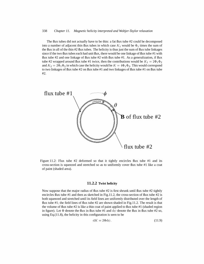
338 Chapter 11. Magnetic helicity interpreted and Woltjer-Taylor relaxation
Theflux tubes did not actually have to be thin: a fatflux tube #2 could be decomposedinto a number of adjacent thinflux tubes in which caseK1 would beΦ1 times the sum oftheflux in all of the thin #2flux tubes. The helicity is thus just the sum offlux tube linkagessince if the twoflux tubes each had unitflux, there would be one linkage offlux tube #1 withflux tube #2 and one linkage offlux tube #2 withflux tube #1. As a generalization, iffluxtube #2 wrapped aroundflux tube #1 twice, then the contributions would beK1 = 2Φ1Φ2andK2 = 2Φ1Φ2 in which case the helicity would beK = 4Φ1Φ2. This would correspondto two linkages offlux tube #2 onflux tube #1 and two linkages offlux tube #1 onflux tube#2.
flux tube#1
B of flux tube#2
φθB
flux tube#2
Figure 11.2: Flux tube #2 deformed so that it tightly encirclesflux tube #1 and itscross-section is squeezed and stretched so as to uniformly coverflux tube #1 like a coatof paint (shaded area).
11.2.2Twist helicity
Now suppose that the major radius offlux tube #2 is first shrunk untilflux tube #2 tightlyencirclesflux tube #1 and then as sketched in Fig.11.2, the cross-section offlux tube #2 isboth squeezed and stretched until its field lines are uniformly distributedover the length offlux tube #1; the field lines offlux tube #2 are shown shaded in Fig.11.2. The result is thatthe volume offlux tube #2 is like a thin coat of paint applied toflux tube #1 (shaded regionin figure). LetΦ denote theflux in flux tube #1 anddψ denote theflux in flux tube #2 so,using Eq.(11.8), the helicity in this configuration is seen to be
dK = 2Φdψ. (11.9)

11.2 Topological interpretation of magnetic helicity 339
We next add another layer of ‘paint’ with more embeddedψ flux, and also with embed-dedΦ flux so that bothψ andΦ increase. The value ofΦ can be used to label the layersof ‘paint’ so thatΦ is the amount offlux in flux tube #1 up to the layer of ‘paint’ labeledbyΦ. Furthermore, sinceψ increases with added layers of ‘paint’,ψ must be a function ofthe layer of ‘paint’ and soψ = ψ(Φ). It is therefore possible to writedψ = ψ′dΦ whereψ′ = dψ/dΦ. Thus, the amount of helicity added with each layer of ‘paint’ is
dK = 2Φ ψ′dΦ (11.10)
and so the sum of the helicity contributions from all the layers of ‘paint’ is
K = 2∫ Φ
0Φ ψ′dΦ. (11.11)
We now show thatψ′ represents the twist of the embedded magnetic field. Letφ be theangle the long way aroundflux tube #1 andθ be the angle the long way aroundflux tube#2 as shown in Fig.11.2. Thus increasingφ is in the direction of contourC1 and increasingθ is in the direction of contourC2. The perimeter of a cross-section offlux tube #1 is in theθ direction and the perimeter of a cross-section offlux tube #2 is in theφ direction. Themagnetic field influx tube #1 can be written as
B1 = 12π∇Φ ×∇θ = 1
2π∇× Φ∇θ (11.12)
which is in theφ direction since∇Φ is orthogonal to∇θ. HereΦ is theflux linked by acontour going in the direction of∇θ. To verify that this is the appropriate expression forB1, theflux through the cross sectionS1 of flux tube #1 is calculated as follows:
flux throughS1 =∫
S1
ds ·B1
= 12π
∫
S1
ds·∇ ×Φ∇θ
= 12π
∫
C2
dl·Φ∇θ
= Φ2π
∫
C2
dl·∇θ
= Φ2π
∮
dθ= Φ. (11.13)
Theflux Φ can be factored from the integral in the third line above, becauseΦ is thefluxlinked by contourC2 which goes in the direction of∇θ. Similarly, it is possible to write
B2 = 12π∇ψ ×∇φ = 1
2π∇× ψ∇φ (11.14)
which is in theθ direction since∇ψ is orthogonal to∇φ. SinceB1 is in theφ direction andB2 is in theθ direction, the total magnetic field can be written asB =B1φ+B2θ which ishelical.

340 Chapter 11. Magnetic helicity interpreted and Woltjer-Taylor relaxation
The twist of the magnetic field is defined as the number of times a field line goesaroundin theθ direction for one circuit in theφ direction. Ifdlφ is a displacement in theφ directionthen
dφ = |∇φ|dlφ (11.15)
and similarly
dθ = |∇θ|dlθ. (11.16)
The trajectory of a magnetic field line is parallel to the magnetic field so if dl is an incrementalong a magnetic field line thenB×dl =0 or
dlθBθ
= dlφBφ. (11.17)
This means thatdθ
|∇θ|Bθ= dφ
|∇φ|Bφ. (11.18)
HoweverBθ = |∇ψ| |∇φ| /2π andBφ = |∇Φ| |∇θ| /2π so
dθdφ = |∇θ|Bθ
|∇φ|Bφ
= |∇θ| |∇ψ| |∇φ|/2π|∇φ| |∇Φ| |∇θ| /2π
= |∇ψ||∇Φ| . (11.19)
Finally, if ψ = ψ(Φ) then∇ψ = ψ′∇Φ whereψ′ = dψ/dΦ and so
dθdφ = ψ
′. (11.20)
Thus,θ increasesψ′ times faster than doesφ and so ifφ makes one complete circuit (i.e.,goes from0 to 2π), thenθ makesψ′ circuits (i.e.,θ goes from0 to 2πψ′). The numberof times the field line goes around in theθ direction for each time it goes around in theφdirection is called the twist
T (Φ) = ψ′. (11.21)
Hence Eq. (11.11), which gave the helicity when theψ flux is embedded in theΦ flux, canbe expressed in terms of the twist as
K = 2∫
ΦT (Φ)dΦ. (11.22)
and if the twist is a constant (i.e.,T ′ = 0) then
K = TΦ2. (11.23)

11.3 Woltjer-Taylor relaxation 341
11.2.3Conservation of magnetic helicity during magnetic reconnection
Ideal MHD constrains magneticflux to be frozen into the frame of the plasma. Thismeans that the topology (connectedness) of magnetic field lines in a perfectlyconductingplasma cannot change. As will be shown in Chapter 12, introduction of a small amountof resistivity allows the frozen-in condition to be violated at locations where the velocitymust vanish due to symmetry. At these locations, the approximation of the resistive MHDOhm’s lawE+U×B = ηJ to the ideal formE+U×B = 0 necessarily fails. In-stead, Ohm’s law has the formE = ηJ so that magnetic field lines can diffuse across theplasma and reconnect with each other. Even though the reconnection is localized to a smallregion in the vicinity of whereU vanishes, it nevertheless changes the overall magneticfield topology. As will be shown below, reconnection destroys individual linkages betweenflux tubes, but creates a replacement linkage for every destroyed linkage so that the totalsystem helicity is conserved. The result is that the ideal MHD constraint of having per-fectflux conservation everywhere is replaced by the somewhat weaker constraint that totalmagnetic helicity is conserved. Reconnection necessarily involvesenergy dissipation sincereconnection requires finite resistivity. Thus reconnection dissipates magnetic field energywhile conserving magnetic helicity.
Conservation of helicity during reconnection is demonstrated in Fig. 11.3. Two linkeduntwisted ribbons of magneticflux are shown in 11.3(a). If each ribbon is imagined to bea magnetic field line bundle having nominalfluxΦ, then according to Eq.(11.8) this initialconfiguration has helicityK = 2Φ2. The ribbons are then cut at their line of overlap asin Fig.11.3(b) and reconnected as in Fig.11.3(c) to form one long ribbon. This long ribbonin Fig.11.3(c) may then be continuously deformed until in the shape shown in Fig.11.3(f),a long ribbon havingtwo twists. Thus, the twist parameter for Fig.11.3(f) isT = 2 andso according to Eq.(11.23) this two-twist ribbon has a helicityK = TΦ2 = 2Φ2. Hence,magnetic helicity is conserved by the reconnection. Since the magnetic equivalent of cut-ting ribbons with scissors involves the dissipative process of resistive diffusion of magneticfield across the plasma, it can be concluded that magnetic reconnection conserves helicity,but dissipates magnetic energy.
11.3 Woltjer-Taylor relaxation
Woltjer (1958) provided a mathematical proof that the lowest energy state ofa magneticsystem with a fixed amount of magnetic helicity was a certain kind of force-free state, butdid not provide any detailed explanation on how the system would attain this state. Taylor(1974) argued that because reconnection conserves helicity while dissipating magnetic en-ergy, reconnection events will provide the mechanism by which an isolatedplasma relaxestowards a state having the lowest magnetic energy consistent with conservation of helicity.The discussion of Eq.(10.133) showed that the isolation requirement corresponds to havingno field lines penetrate the surface bounding the plasma and also arrangingfor this surfaceto be an electrostatic equipotential. It will therefore be assumed that the plasma is boundedby a perfectly conducting wall and that no magnetic field lines penetrate this wall. Thetangential electric field and hence the tangential component of the vector potential musttherefore vanish at the wall.

342 Chapter 11. Magnetic helicity interpreted and Woltjer-Taylor relaxation
(a) (b) (c)
(d) (e) (f)
Figure 11.3: (a) Two linked, untwistedflux tube squeezed to be ribbons, magnetic fielddirections shown by arrows; (b) cut at overlay of two ribbons; (c) reconnection at cut; (d)deformation; (e) more deformation; (f) more deformation showing there are two completetwists of magnetic field.

11.3 Woltjer-Taylor relaxation 343
The relaxation process involves minimizing the magnetic energy
W = 12µ0
∫
B2d3r (11.24)
subject to the constraint that the magnetic helicity
K =∫
A ·Bd3r (11.25)
is conserved (Woltjer 1958, Taylor 1974). The minimum-energy magnetic field for thegiven helicity is calledBME and its associated magnetic energy is
WME = 12µ0
∫
B2MEd3r. (11.26)
In order to determineBME , we consider an arbitrary variationB = BME + δB satis-fying the same boundary conditions; by assumption, this variation has a higher associ-ated magnetic energy thanBME . The magnetic fieldB has an associated vector potentialA =AME+δA and because the tangential electric field must vanish at the wall to preventhelicity flux across the wall, the tangential component ofδA must also vanish at the wall.A naive solution for minimizingWME would be to setBME to zero, but this is forbiddenbecause it would makeK vanish and violate the helicity conservation requirement. ThusW must be minimized subject to the constraint thatK remains constant. The variation ofthe magnetic energy about the minimum energy state is
δW = 12µ0
∫
[
(BME + δB)2 −B2ME]
d3r
= 1µ0
∫
BME ·δBd3r
= 1µ0
∫
BME ·∇×δAd3r
= 1µ0
∫
[∇ · (BME × δA) + δA·∇×BME ] d3r
= 1µ0
∫
ds ·BME × δA+∫
δA·∇×BMEd3r
=∫
δA·∇×BMEd3r (11.27)
sinceds ·BME × δA =0 everywhere on the wall. The variation of the helicity is
δK =∫
(δA ·BME +AME ·δB) d3r
=∫
(δA ·BME +AME ·∇ × δA) d3r
=∫
(δA ·BME + δA·∇×AME) +∇ · (δA×AME) d3r= 2
∫
δA ·BME d3r. (11.28)

344 Chapter 11. Magnetic helicity interpreted and Woltjer-Taylor relaxation
Minimization of δW subject to the constraint thatK remains constant is characterizedusing a Lagrange multiplierλ so that the constrained variational equation is
δW = λδK. (11.29)
Substitution forδW andδK gives∫
δA· ∇ ×BMEd3r = 2λ∫
δA ·BME d3r (11.30)
or, after re-defining the arbitrary parameterλ,∫
δA· (∇×BME − λBME ) d3r = 0. (11.31)
SinceδA is arbitrary, the quantity in parentheses must vanish and so
∇×BME = λBME . (11.32)
It is clear thatλ is a spatially uniform constant because the Lagrange multiplier is a con-stant. Thus, relaxation leads to the same force-free state as predicted by Eq.(10.140). Thesestates are a good approximation to many solar and astrophysical plasmas as well as certainlaboratory plasmas such as spheromaks and reversed field pinches.
The energy per helicity of a minimum energy state can be written as
WK =
∫ B2MEd3r2µ0
∫
AME ·BMEd3r=
∫
BME ·∇ ×AMEd3r2µ0
∫
AME ·BMEd3r=
∫ [AME ·∇ ×B+∇· (AME ×BME)] d3r2µ0
∫
A ·Bd3r . (11.33)
However, Eq. (11.32) can be integrated to give
BME = λAME +∇f (11.34)
wheref is an arbitrary scalar function of position. This can be used to show
∇·(AME ×BME) = ∇· (AME ×∇f) = ∇f ·∇×AME =BME ·∇f = ∇· (fBME)(11.35)
so that∫
∇· (AME ×BME) d3r =∫
ds · (fBME) = 0 (11.36)
sinceBME · ds = 0 by assumption. Thus, Eq.(11.33) reduces to
WK = λ
2µ0 (11.37)
indicating that the minimum energy state must have the lowest value ofλ consistent withthe prescribed boundary conditions.

11.4 Kinking and magnetic helicity 345
11.4 Kinking and magnetic helicity
Magnetic helicity can be manifested in various forms and plasma dynamics cause this formto be altered. We now discuss an important example of helicity-conserving, morphology-altering dynamics, namely the situation where kink instability causes thetwist of a straight-axisflux tube to be transformed into the writhe of the axis of an untwistedflux tube (Bergerand Field 1984, Moffatt and Ricca 1992).
Consider a volumeV bounded by a surfaceS where no magnetic field lines penetratethe surfaceS so thatB·ds = 0 over all ofS. It is assumed here thatV extends to infinity,but the analysis would equally apply for a finite-extent volumeV so long as no magneticfield lines penetrate its bounding surfaceS. The helicity contained inV is
KV =∫
VA ·Bd3r. (11.38)
Equation (10.129) showed thatKV is gauge-independent because no field lines penetrateS.
The volumeV is now decomposed into two subvolumes which haveB·ds = 0 at alllocations on their mutual interface. Thus, any specific field line inV is entirely in one orthe other of the two subvolumes.
1. The first subvolume, calledVtube, is a closedflux tube of minor radiusa with a pos-sibly helical axis as shown in Fig. 11.4. The length of the axis of thisflux tube isdenotedlaxis and the variableξ denotes the distance along this axis from some fixedreference pointx0 on the axis. Incrementingξ from 0 to laxis thus corresponds togoing once around theflux tube axis. A pseudo-angular coordinateφ is defined as
φ = 2π ξlaxis (11.39)
so that going once around the axis corresponds to incrementingφ from 0 to 2π andφdefines the local direction of the axis. Because the axis of theflux tube has the complexcurvature of a helix, everywhere along the axis there exists a radius of curvature vectorκ = φ · ∇φ which is at right angles toφ. The local radius of curvature of the axis
is rcurve =∣
∣
∣φ · ∇φ∣
∣
∣
−1(see discussion of Eq.(3.85)). From the point of view of
an observer inside theflux tube, theflux tube appears as a long curved tunnel thateventually closes upon itself. Theflux tube minor radiusa must always be smallerthanrcurve which corresponds locally to the condition that by definition the majorradius of a torus must exceed the minor radius. Theflux tube interior volume is nowimagined to be filled with fiduciary lines all of which are parallel to theflux tube axis;the lengths of these fiduciary lines will vary according to their location relative to theaxis. We defineξ′ as the distance along a fiduciary line of lengthl′ from a planeperpendicular to theflux tube axis at the reference pointx0. The meaning ofφ canthen be extended to indicate the distance along any fiduciary line using the relationξ′ = φl′/2π. Incrementingφ from 0 to 2π thus corresponds to going once around anyor all of these fiduciary lines and soφ provides an unambiguous measure of fractionaldistance along theflux tube for any point within theflux tube even though thefluxtube may be curved, twisted, or helical.

346 Chapter 11. Magnetic helicity interpreted and Woltjer-Taylor relaxation
axis of helix
helical flux tube,volume Vtube
linked external flux ψext
Figure 11.4: Subvolume #1 is aflux tube with a possibly helical axis and volumeVtube.Subvolume #2 is all space external to subvolume #1. All field lines in subvolume #2 whichlink subvolume #1 are represented by the verticalflux tube in figure labeledψext.
2. The second subvolume in this decomposition is the remaining volume ofV and islabeled asVext. There might be field lines in this second subvolume which link theflux tubeVtube and theflux due to all these linkages is labeledψext. This externalfluxlinkage is represented by the verticalflux tube labeledψext in Fig. 11.4.
If the dynamics within the volumeV are governed by ideal MHD, then the helicityKVin V must be conserved and, sinceKV is a volume integral, the volume of integration canbe subdivided into theflux tube volume and the volume external to theflux tube,
KV = KVtube +KVext .

11.4 Kinking and magnetic helicity 347
11.4.1KVtube , helicity content of theflux tube
We now consider the helicity content of the possibly helicalflux tube,
KVtube=∫Vtube
A ·Bd3r . (11.40)
The magnetic field in theflux tube is decomposed into a componentBaxis parallel to theflux tube axis and an orthogonal componentBazimuthal which goes the short way aroundthe axis; thus the magnetic field inside theflux tube is
B = Baxis +Bazimuthal. (11.41)
The field lines in theflux tube are assumed to lie in successive layers (magnetic surfaces)wrapped around theflux tube axis. The axial and azimuthal magnetic fields are derivedfrom respective vector potentialsAaxis andAazimuthal such that
Baxis = ∇×AaxisBazimuthal = ∇×Aazimuthal. (11.42)
It should be emphasized that these definitions say nothing about the direction ofAaxis orAazimuthal and so, unlike axisymmetric situations, here neitherAaxis nor Aazimuthalshould be construed to be in a particular direction because of the possibility that thefluxtube is helical. All that can be said is that the curl ofAaxis gives theflux tube axialmagnetic field and the curl ofAazimuthal gives the azimuthal field.
The helicity content of theflux tube is thus
KVtube=∫Vtube
(Aaxis +Aazimuthal) · (Baxis +Bazimuthal) d3r (11.43)
and this is true even though the axis of theflux tube could be helical.
By definition, each layer of field lines constituting a magnetic surface encloses afluxΦ. An equivalent definition is to state thatΦ is the magneticflux linked by a contour in themagnetic surface going the short way around theflux tube axis. The magnetic surface is la-beled byΦ and soΦ can be considered to be a coordinate having its gradient always normalto theflux surface. In effectΦ is a re-scaled minor radius, sinceΦ increases monotonicallywith minor radius.
These definitions are sufficiently general to allow for the axis of theflux tube to be ahelix, a knot, or a simple closed curve lying in a plane. If the axis is just a simple closedcurve lying in a plane, then∇× φ is normal to the plane and therefore normal toφ . In theslightly more general case where the axis is not in a plane butφ·∇×φ = 0, the path tracedout by φ can be considered to be the perimeter of a some bumpy surface. However, in themost general case whereφ · ∇× φ is finite, the path traced out byφ is not the perimeter ofeven a bumpy surface (Barnes 1977). There might also be situations whereφ ·∇× φ = 0but the sign ofφ · ∇ × φ alternates. If the average ofφ · ∇ × φ over the length of the axisis zero, then the situation would be similar to the case whereφ · ∇ × φ = 0 everywhere,because twists in the axis could be squeezed together axially until mutually cancelling out.

348 Chapter 11. Magnetic helicity interpreted and Woltjer-Taylor relaxation
axial segment of helicalflux tube surface
helical axisof flux tube
cut ribbon surfacefrom helical axisto flux tube surface
axis of helix
linked external flux ψext
φ
φ = 0
φ = 2π
Figure 11.5: Ribbon surface extending from helical axis of helicalflux tube to surface offlux tube with normal toφ× κ
Because any magnetic field line in theflux tube lies in some magnetic surface labeledbyΦ, any field line in theflux tube has a component parallel to the axis and possibly alsoa component perpendicular to the axis, but never a component in the∇Φ direction. Thissuggests introduction of an azimuthal coordinateθ which is defined as the angular distancearound the axis in the direction given by∇φ×∇Φ, i.e.,θ is defined such that
∇θ|∇θ| =
∇φ×∇Φ|∇φ×∇Φ| . (11.44)
The local direction of∇θ depends on bothφ andθ; furthermore, forθ to denote somedefinite position,θ must be measured with respect to some unambiguous origin. An unam-biguousθ origin can be defined by using as a reference the negative of the direction of thelocal radius of curvature vectorκ of theflux tube axis. Theθ = 0 surface is then a ribbonsurface, as shown in Fig.11.5, that extends from theflux tube axis to theflux tube outer sur-face so thatφ× κ is normal to the ribbon surface. The ribbon is considered to have a cutatφ = 0 so that the ribbon ends atφ = 0 andφ = 2π are distinct.

11.4 Kinking and magnetic helicity 349
Figure 11.6 shows a cross-section of this system. Theflux tube has minor radiusa andthe helical axis of theflux tube traces out a trajectory with minor radiusb about an axiswhich has major radiusR. Representative magnetic surfaces (surfaces of constantΦ), theribbon surface, and the angleθ are also shown.
axis of flux tube
2b
2a
R
flux tubesurface
ribbonsurface
θ
magnetic surface,constant Φ
axis of helix
Figure 11.6: Cross-section showingflux tube of minor radiusa, with its axis making a helixof radiusb. Interiorflux surfaces withΦ = const. and the ribbon surface definingθ = 0are also shown.
The flux Φ was a generalization of the toroidalflux of an axisymmetric system. Wenow define a corresponding generalization of the poloidalflux ψ(Φ) as the magneticfluxpenetrating a sub-ribbon extending inwards from the outer surface of the possibly helicalflux tube to some given interior magnetic surfaceΦ. This subribbon is shown in Fig.11.7and the definition is such that
ψ =∫subribbon
ds ·B
=∫subribbon
ds ·∇×A
=∮Cdl ·A (11.45)
where the contourC follows the perimeter of the subribbon and specifically follows the

350 Chapter 11. Magnetic helicity interpreted and Woltjer-Taylor relaxation
two ends atφ = 0 andφ = 2π. This definition implies thatψ = 0 on the outer surface oftheflux tube because the sub-ribbon area will be zero in this case.
We define the vector potential
Aazimuthal = ψ(Φ)2π ∇φ (11.46)
and note that this definition is valid only in the range0 ≤ φ < 2π. The appropriateness ofthis definition is established by integrating following the contourC around the subribbonto obtain
∮Cdl ·Aazimuthal =
∮Cdl·ψ(Φ)2π ∇φ
= ψ(Φ)2π
∫cΦdl·∇φ
= ψ(Φ) (11.47)
wheredl·∇φ = dφ. As seen in Fig.11.7, the contourC consists of four segments, namely asegment following the outside edge of the sub-ribbon (this segment lies in theouter surfaceof theflux tube whereψ = 0), the segment labeledCΦ on the inside edge of the sub-ribbon,a segment at theφ = 0 end, and an oppositely directed segment at theφ = 2π− end. OnlytheCΦ segment contributes to the integral because (i)dl·∇φ = 0 on the endsφ = 0 andφ = 2π− sinceφ is constant on both these ends and (ii)ψ = 0 on the outside edge of thesub-ribbon.
The magnetic field inside theflux tube can thus be written as
B = Baxis + ∇ × ψ(Φ)2π ∇φ (11.48)
whereBaxis is the magnetic field component parallel to theflux tube axis. This decom-position of the magnetic field is valid even for a twisted or knotted axis provided it is usedonly for situations where0 ≤ φ < 2π.

11.4 Kinking and magnetic helicity 351
subribbon lying betweenflux tube outer surfaceand magnetic surface Φ
ψ is flux throughthis subribbon
location of magnetic surface Φ
Figure 11.7:ψ is flux through cut subribbon located between magnetic surfaceΦ and outersurface offlux tube.
The vector potential for the entire field can be written as
A =Aaxis + ψ(Φ)2π ∇φ. (11.49)
These results can be used in Eq.(11.43) to give the helicity content of theflux tube as
KVtube =∫
Vtube
d3r(
Aaxis + ψ(Φ)2π ∇φ)
·(
Baxis + 12π∇ψ ×∇φ
)
=∫
Vtube
d3r(
Aaxis ·Baxis + ψ(Φ)2π ∇φ ·Baxis +Aaxis · 12π∇ψ ×∇φ)
(11.50)
and this may be decomposed into writhe and twist terms,
KVtube = Kwrithe +Ktwistrespectively defined as
Kwrithe =∫
Vtube
d3rAaxis ·Baxis (11.51)

352 Chapter 11. Magnetic helicity interpreted and Woltjer-Taylor relaxation
and
Ktwist =∫
Vtube
d3r(ψ(Φ)2π ∇φ ·Baxis +Aaxis · 12π∇ψ ×∇φ
)
. (11.52)
As will be shown below,Ktwist depends onψ being finite whereasKwrithe depends on theextent to which theflux tube axis is helical. Theflux tube helicity can thus be entirely duetoKwrithe, entirely due toKtwist, or due to some combination of these types of helicity.
.11.4.2Evaluation ofKtwist
Since theKtwist integral is avolumeintegral, theflux tube may be cut atφ = 0 withoutaffecting this integral. Making such a cut means thatφ is restricted to the range0 ≤ φ <2π and therefore does not make a complete circuit around the axis of theflux tube. Theevaluation of this integral is insensitive to the connectivity of the axis because connectivityis a concept which makes sense only after making a complete circuit of theaxis. The axialmagnetic field within the cut volume may be expressed as
Baxis = 12π∇× Φ∇θ (11.53)
whereθ is the angular distance on a contourCθ encircling theflux tube axis and lies in amagnetic surface. This representation for the axial magnetic field is appropriate here sinceat eachφ for 0 ≤ φ < 2π we may write
Φ =∫
ds ·Baxis
= 12π
∫
ds·∇ ×Φ∇θ
= 12π
∮
Cθ
dl· Φ∇θ
= Φ2π
∮
Cθ
dl· ∇θ
= Φ2π
∮
Cθ
dθ. (11.54)
By uncurling Eq.(11.53) it is seen that vector potential associated with theaxial magneticfield may be represented in the cutflux tube as
Aaxis = Φ2π∇θ, 0 ≤ φ < 2π (11.55)
so that
Ktwist = 14π2
∫
Vtube
d3r (ψ∇φ · ∇Φ × ∇θ +Φ∇θ · ∇ψ ×∇φ)
= 14π2
∫
Vtube
d3r (ψ∇φ · ∇Φ× ∇θ +Φψ′∇θ · ∇Φ×∇φ)
= 14π2
∫
Vtube
d3r (−ψ +Φψ′)∇θ · ∇Φ×∇φ. (11.56)

11.4 Kinking and magnetic helicity 353
The three direction gradients∇θ,∇Φ, and∇φ form an orthonormal coordinate systemand an element of volume in this system is given by
d3r = dlΦdlθdlφ = dΦdθdφ∇θ · ∇Φ × ∇φ (11.57)
sincedθ = dlθ |∇θ|, dφ = dlφ |∇φ| , anddΦ = dlΦ |∇Φ|. Thus,
Ktwist = 14π2
∫ Φ
0dΦ
∫ 2π
θ=0dθ
∫ (2π)−
φ=0dφ (−ψ +Φψ′)
= −∫ Φ
0ψdΦ +
∫ Φ
0ψ′ΦdΦ
= 2∫ Φ
0ΦdψdΦdΦ. (11.58)
where the integration limit(2π)− corresponds to being infinitesimally less than2π. The lastline has been obtained using the relationship
∫ d(ψΦ) = [ψΦ]surfaceaxis = ∫ Φdψ + ∫ ψdΦand noting that the integrated term vanishes sinceψ = 0 in theflux tube surface andΦ = 0on theflux tube axis.
11.4.3Evaluation ofKwrithe
Connectivity of theflux tube is now the important issue. In order to evaluate theKwritheintegral the volume element is expressed as
d3r = dl·ds (11.59)
wheredl is an increment of length along the axis andds is an element of surface in the planeperpendicular to the axis so thatBaxis·ds = dΦ. Because the line integral will involve acomplete circuit of theflux tube axis, in contrast to the earlier evaluation ofKtwist, we nowavoid using the gradient of a scalar to denote distance along the axis. Using Eq.(11.59) thewrithe helicity may therefore be expressed as
Kwrithe =∫
Caxis
Aaxis · dlaxis∫
dΦ
= Φ∫
Caxis
Aaxis · dlaxis. (11.60)
This integral differs topologically from the integrals of the previous section, because herethe contour is acomplete circuit, i.e.,φ varies from0 to 2π, and not from0 to 2π−.
A contour pathC of an integral∫
C A·dl may be continuously deformed into a newcontour pathC ′ without changing the value of the integral provided no magneticflux islinked by the surfaceS bounded byC andC ′; this behavior is a three dimensional analogto the concept of analyticity for a contour integral in the complex plane. The validity ofthis assertion is established by the relation
0 =∫
SB·ds =
∮
A · dl =∫
CA · dl−
∫
C′
A · dl. (11.61)

354 Chapter 11. Magnetic helicity interpreted and Woltjer-Taylor relaxation
It should be noted that the ability forC to be continuously deformed intoC ′ imposes therequirement that a surfaceS exists betweenC andC ′; this is only true ifC does not linkC ′.
We now consider some limiting cases forKwrithe and to aid in visualization it shouldbe recalled that theflux tube axis is assumed to have a helical trajectory with helix majorradiusR and helix minor radiusb as shown in Fig.11.6.
Limiting case whereflux tube axis not helicalThis situation corresponds to havingb = 0 in which case theflux tube axis lies in
a plane. The contourCaxis in Eq.(11.60) can thus be slipped from its original positionthrough theBaxis field lines to the surface of theflux tube without crossing anyBaxisfield lines. This is topologically possible because by definition, allBaxis field lines in theflux tube are parallel to theflux tube axis. Thus, here
Kwrithe = Φ∫
C′Aaxis · dlaxis (11.62)
whereC ′ lies on theflux tube surface. The line integralC ′ encircles the externalflux linkedby theflux tube and so
Kwrithe = Φψext, when theflux tube axis is not helical (11.63)
helical axisof flux tube
slit cut in flux tubeparallel to flux tubeaxis, faces helical axisof flux tube
axis of helix
Figure 11.8: Helical axis offlux tube may be slipped throughBaxis field lines offlux tubesto coincide of axis of helix (note that open slit influx tube always faces axis of helix).

11.4 Kinking and magnetic helicity 355
Case where axis is helical andb > aBecause the helix minor radiusb exceeds theflux tube minor radiusa, the entireflux
tube revolves around the axis of the helix as shown in Fig.11.8. Becausethe helical axiscloses upon itself, it must have an integral number of periods and we letN be the numberof helix periods. However, becauseBaxis is everywhere parallel to theflux tube axis, theflux tube axis may again be slipped through theBaxis field lines and in this case movedtowards the helix axis until it coincides with the helix axisChelix. The writhe helicity canthus be expressed as
Kwrithe = Φ∫
Chelix
Aaxis · dlaxis. (11.64)
However, theflux tube links the helix axisN times and so
∫
Chelix
Aaxis · dlaxis = NΦ +ψext. (11.65)
Thus,
Kwrithe = NΦ2 +Φψext if b > a. (11.66)
Case whereflux tube axis is helical buta > bIn this situation theflux tube may be subdivided into an inner core with minor radius
r < b and associatedflux Φb2/a2 and an outer annular region withb < r < a withthe remainder ofΦ. We again slip theflux tube axis through the parallelBaxis field linesto be coincident with the helix axis. However, now only the inner core of theflux tube(r < baxis) rotates around the helix axis. The outer annular region of theflux tube merelywobbles around the helix axis and does not link the helix axis. Thus, the linkedflux is
∫
Chelix
Aaxis · dlaxis =NΦb2/a2 + ψext (11.67)
and so the writhe helicity is
Kwrithe = NΦ2b2/a2 +Φψext if a > b. (11.68)
Hence, the helicity of theflux tube is
KVtube = Ktwist +Kwrithe
= 2∫
ΦdψdΦdΦ +NΦ2b2/a2 +Φψext if a > b. (11.69)
The distinction between thea < b anda > b cases is sketched in Fig.11.9.

356 Chapter 11. Magnetic helicity interpreted and Woltjer-Taylor relaxation
a < b
a > b
flux tubesurface
flux tubesurface
a
b
b
a
axis of helix
coreregion0 ≤ r < b
outerregionb ≤ r ≤ a
Figure 11.9: Top: case whereflux tube radiusa is less than radiusb of helix traced out byflux tube axis. Bottom: Case wherea > b; the core region0 ≤ r < b rotates around theaxis of the helix whereas the outer region withb < r < a wobbles about the axis of thehelix.
11.4.4Twist and writhe exchange in a kink instability
A kink instability is governed by ideal MHD and so must be helicity-conserving. Thenumber of turns of the kink is defined by the initial twist conditionk ·B =kφBφ+kθBθ =0 so if kθ = 1/a andkφ = n/R then the kink will result in a helix withN = n. Sincehelicity is conserved, it is seen that as the amplitude of the kink increases(i.e.,b increases),theflux tube twistdψ/dΦ will have to decrease. In particular if the twist is uniform so thatψ = TΦ where twistT is independent ofΦ, then as in Section 11.2.2 we may write
2∫
ΦdψdΦdΦ = TΦ2 (11.70)
and so from conservation of helicity we may conclude that
T +Nb2/a2 = const. for b < a; (11.71)
this is an example of the Calugareanu theorem (Calugareanu 1959).
11.5 Assignments 357
A kink instability which starts withb = 0 and an initial twistTinitial = n will growuntil at b = a the twist vanishes and all helicity is contained by anN-turn writhe whereN = Tinitial. Thus, a kink will convert twist into writhe so that forb > a , T = 0 andN = Tinitial. This property can be confirmed by taking a length of garden hose with astripe running along the length and connecting the two ends together to form a closedfluxtube with a stripe running along the axis. Initially,N + T = 0 because the stripe is nottwisted and the hose axis is not helical. If the hose is deformed into a right-handed helix,then the stripe will make a left-handed helix about the hose axis to keepN +T = 0. If thestripe is initially a right-handed helix when the hose is not a helix, then deformation of thehose into a right handed helix will result in the stripe becoming parallel to the hose axis.
11.5 Assignments
1. Derive the helicity conservation equation for a resistive plasma
dKdt +
∫
Sds· (ϕB +E×A) = −2∫ d3r ηJ ·B (11.72)
and express it in the form
dKdt +
∫
Sds·(2ϕB +A× ∂A∂t
)
= −2 ∫ d3r ηJ ·B (11.73)
whereϕ is the electrostatic potential. What happens to the surface integral when thesurface is a perfectly conducting wall? Hint: Start by evaluating−∂ (A ·B) /∂t andmake repeated use of Faraday’s law∇×E = −∂B/∂t, the electric field expressed asE = −∇ϕ − ∂B/∂t and the resistive MHD Ohm’s lawE+U×B =ηJ.
2. Alternative explanation for why helicity is conserved better than magnetic energy:
(a) By subtractingE dotted with Ampere’s law fromB dotted with Faraday’s lawderive the MHD limit of Poynting’s theorem:
∂∂t
( B2
2µ0)
+∇ ·(E×Bµ0
)
= −E · J (11.74)
(b) Consider a plasma in a perfectly conducting chamber with no vacuum gap be-tween the plasma and the chamber wall. Show that integration of Eq.(11.72) andEq.(11.74) over the entire volume give respectively
dKdt = −2 ∫ d3rηJ ·B (11.75)
and dWdt = − ∫
d3rηJ2. (11.76)
whereW = ∫ d3rB2/2µ0 is the magnetic energy.
(c) Show that the right hand side of Eq. (11.76) is proportional to higher orderspatial derivatives ofB than is the right hand side of Eq. (11.75). Use this

358 Chapter 11. Magnetic helicity interpreted and Woltjer-Taylor relaxation
property to argue that the rate of dissipation of magnetic energy greatly exceedsthat of magnetic helicity when the dynamics is spatially complex so that most ofthe spectral power is in short characteristic scale lengths.
(d) Explain why this difference in dissipation rates could be approximated byas-suming that magnetic helicity remains constant while magnetic energy decaysin the presence of dynamics having fine scales. Argue that the decay of mag-netic energy is thereby constrained by the requirement that helicity is conserved.
3. Show that the minimum energy state given by Eq.(11.32) is a force-free configuration.Is λ spatially uniform? Is this the same result as given in Eqs.(10.139) and (10.140)?Take the curl again to obtain
∇2B+ λ2B = 0.What are the components of this equation in axisymmetric cylindrical geometry? Becareful when evaluating the components of∇2B to take into account derivatives op-
erating on unit vectors (e.g.,∇2(
Bφφ) = φ∇2Bφ).
(a) Show that for axisymmetric cylindrical geometry the minimum-energy stateshave the magnetic field components
Bz(r) = BJ0(λr)Bφ(r) = BJ1(λr).
SketchBz(r) andBφ(r). This is called the Bessel function model or Lundquistsolution (Lundquist 1950) to the force-free equation and is often a good firstguess representation for nearly force-free equilibria such as spheromaks,re-versed field pinches, and solar coronal loops.
4. For a cylindrical system with coordinates r, φ, z show that ifχ satisfies the Helmholtzequation ∇2χ+ λ2χ = 0then
B =λ∇χ ×∇z +∇× (∇χ×∇z)is a solution of the force-free equationµ0J =λB. By assuming thatχ is independentof φ and is of the formχ ∼ f(r) coskz find f(r) and then determine the componentsof B. Show that ifλ satisfies an eigenvalue condition, it is possible to have a finiteforce-free field having no normal component on the walls of a cylinder of lengthhand radiusa. Give the magnetic field components for this situation. Calculate thepoloidal flux ψ(r, z) by direct integration ofBz(r, z). Hint: the answers will be interms of Bessel functionsJ0 andJ1.
5. Obtain a ribbon such as is used in gift-wrapping, make one complete twistin thisribbon and tape the ends together. By manipulating the twisted ribbon show the fol-lowing:
(a) If the ribbon is manipulated to have no twists, then it has a figure-eight patternwith a cross-over. If theflux through the ribbon isΦ, show that the helicity ofone full twist isΦ2, show that the helicity of one cross-over is also .

11.5 Assignments 359
(b) Cut the ribbon all the way along its length so that it becomes two interlinkedribbons of unequal width. Assuming that the original ribbon had afluxΦ, calcu-late the helicity of the configuration taking into account the helicity due to bothtwists and linkages and show that helicity is conserved.
(c) Demonstrate that the sum of twist plus writhe is conserved using a bundle offlexible wires (or ropes) that are initially twisted about a straight axis and thenmanipulated into a kink where the wires are parallel to the locus of the kink.Theends of the bundle should be fixed. Similarly, start with a bundle of untwistedwires that are parallel to a straight axis and manipulate the wiresinto a helix.Show that the sense of the twist of the wires about their local axis is oppositetothe sense of the helix so that a condition of zero helicity is maintained.
12
Magnetic reconnection
12.1 Introduction
Section 2.5.4 established the fundamental concept underlying ideal MHD, namely thatmagneticflux is frozen into the plasma. Chapter 10 showed that ideal MHD plasmasare susceptible to two distinct types of instabilities, pressure-driven and current-driven.Pressure-driven modes draw on free energy associated with heavyfluids stacked on topof light fluids in an effective gravitational field whereas current-driven instabilities drawon free magnetic energy and involve the plasma attempting to increase its inductance in aflux-conserving manner. Both of these instabilities occur on the Alfvén time scale definedas some characteristic distance divided byvA.
It is possible for an MHD equilibrium to be stable to all ideal MHD modes and yet notbe in a lowest energy state. Free energy is therefore available to drive an instability but thisenergy cannot be tapped by ideal MHD modes. Magnetic tearing and associated reconnec-tion is a non-ideal instability where the plasma is effectively ideal everywhereexcept at avery thin boundary layerwhere the ideal assumption breaks down and magnetic fields candiffuse across the plasma. Even though the boundary layer is thin, the tearing/reconnectioncauses the overall topology of the magnetic field to change. It is the changing of the topol-ogy (the local unfreezing of the magnetic field from the plasma) that allows the configura-tion to relax to a lower energy state. Because ideal MHD does not allow the topology tochange, the lower energy state cannot be accessed via ideal MHD instabilities. The non-ideal resistive modes are much slower than ideal modes because the non-ideal mode relieson a diffusion or leakage of magnetic field across the plasma in some verylimited spatialregion where ideal MHD breaks down.
Magnetic tearing is an intrinsically complicated boundary layer phenomenon becausetwo very different length scales mutually interact; the mathematical description has to rec-oncile behavior in a microscopic thin diffusion layer with behavior in a macroscopic outerideal layer. We shall begin the discussion with an analogy drawn from everyday experienceand use this analogy to show why it is energetically favorable for a sheet current to breakup into filaments. The time scale for this process will be estimated and shown to be muchslower than ideal MHD. Finally, the tearing and reconnection concept will be generalizedto sheared magnetic fields and helical equilibria.
360

12.2 Water-beading: an analogy to magnetic tearing and reconnection361
longthindrop
(a) (b) (c)
contractiontosingle largedropof same area(energeticallyunfavorable)
beading(energeticallyfavorable)
substrate
Figure 12.1: (a) Initial long thin drop, (b) contraction into big round drop (too much scrap-ing on substrate), (c) beading into chain of little drops.
12.2 Water-beading: an analogy to magnetic tearing andreconnection
Since magnetic tearing and reconnection is not a simple process, it is helpful to start byconsidering the dynamics of a somewhat analogous instability known from everyday ex-perience, namely the process of water beading. The initial condition in waterbeading isshown in Fig.12.1(a) and consists of a long, thin, two-dimensional, incompressible drop ofwater (approximate analog to the magnetic field) frictionally attached to a substrate (ap-proximate analog to the plasma). The long thin drop has surface tension ‘trying’ to reducethe perimeter of the drop (this is analogous to the pinch force being interpreted as fieldline “tension” squeezing on a current channel). If the drop were not attached tothe sub-strate, then as shown in Fig.12.1(b), the surface tension would simply collapse the long thinincompressible drop into a circular drop having area equal to that of the initial long thindrop. Because of the frictional work involved in dragging the water over the substrate, thiswholesale collapse is not energetically favorable and does not occur. On the other hand,if as shown in Fig.12.1(c) the long thin drop breaks up into a line of discrete segments(which does not involve significant dragging of water across the substrate), thesurface ten-sion of each line segment causes each discrete segment to contract inlength and bulge in

362 Chapter 12. Magnetic reconnection
width until circular. Because only modest frictional dragging of water across the substrateis required to do this, the process can be energetically favorable, and so result in waterbeading.
12.3 Qualitative description of sheet current instability
Suppose an infinite-extent plasma has a thin sheet of currentflowing in thez directionas shown in Fig.12.2(a). The sheet current is centered atx = 0 and extends fromy =−∞ to y = +∞. The current is uniform in both they and thez directions and roughlycorresponds to the initial long thin water drop. This somewhat artificial situation can beconsidered as the Cartesian analog of a cylindrical shell currentflowing in thez direction,localized at some radiusr = r0 and azimuthally symmetric. Thus, we identifyr with xandy with θ.
(a) (b) (c)
sheetcurrent
By0
y
gap
typical barself field
filamentationof currentinto barcross-sections
detail of barsshowing fluidflow patterns
centeroftypicalfluidvortex
fluidflowvector
Figure 12.2: (a) Initial sheet current; (b) breaking up into bar cross-section filaments; (c)detail showingfluid flow consists of set of small vortices which are antisymmetric inx.
Since all quantities depend onx only, Ampere’s law reduces to
µ0Jz(x) = ∂By∂x (12.1)

12.3 Qualitative description of sheet current instability 363
which integrates to give
By(x) = By(0) +∫ x
0µ0Jz(x′)dx′. (12.2)
On the basis of symmetry the sheet current cannot generate a magnetic fieldatx = 0 so thefieldBy(0) must entirely due to external currents. Let us assume for now that no externalcurrents exist and setBy(0) = 0; the situation of finiteBy(0) will be treated later inSec.12.5. ThusBy(x) is a sheared magnetic field which is positive forx > 0 and negativefor x < 0. The magnitude ofBy(x) changes rapidly inside the current layer and becomesconstant for|x| → ∞.
This situation can be characterized analytically by using a magneticfield
By(x) = B tanh(x/L) (12.3)
whereL is the scale width of the current layer. Substituting in Eq.(12.1) gives
Jz(x) = Bµ0L cosh
−2(x/L) (12.4)
which is sharply peaked in the neighborhood ofx = 0.Suppose that the perturbation shown in Fig.12.2(b) is introduced so that thecurrent
sheet cross-section is broken up into a number of bar-shaped structures each with currentIbar separated by small gaps in they direction; these bars are roughly analogous to the wa-ter beads discussed above. Each bar’s self magnetic field acts like an elastic band wrappedaround the bar (analogous to the surface tension of a drop). This tension contracts theydimension of the bar, and if the bar is incompressible, thex dimension will then have togrow, as shown in Fig.12.2(c). As the bar deforms from a rectangle into a circle havingthe same area, its perimeter becomes shorter giving rise to a strongerfield (and effectivesurface tension) since
∫
perimeterB·dl =µ0Ibar . (12.5)
Hence, this deformation feeds upon itself and is unstable. Note that the inductance of thesystem increases as the current breaks into filaments, consistent withthe earlier observationthat the plasma is always ‘trying’ to increase its inductance.
This energetically allowed filamentation instability is forbidden inideal MHD becausethe topology of the magnetic field changes at the gaps between the bars. Beforethe gapsform, the magnetic field lines are open and straight, stretching fromy = −∞ to y = +∞whereas after the gaps form, some field lines circle the current filaments; these field linesare finite in length and curved. In order to go from the initial state to thefilamented state,some magnetic field lines must move across plasma in violation of ideal MHD(this changein topology is approximately analogous to dragging the water drops across the substrate inthe water beading problem). The field lines have an ‘X’ shape at the center of the gaps andthe change in topology occurs at these X-points. The center of the bar is called an O-pointsince the field around this point has an O-shape.
If some mechanism exists that allows X-points to develop, instability can occur. Sincefinite resistivity allows magnetic field to diffuse across plasma, aresistive plasma will besusceptible to this instability at locations where the magnetic field attachment to the plasma

364 Chapter 12. Magnetic reconnection
is weakest. The location of the weak spot can be deduced by examining Ohm’s law for anearly ideal plasma (i.e., small but finite resistivity),
E+U×B = ηJ. (12.6)
At most locations in the plasma, the two left hand side terms are both much larger than theright hand side resistive term and so plasma behavior is determined by these two left handterms balancing each other. This balancing causes the electric field in the plasma frame tobe zero, which corresponds to the magnetic field being frozen into the plasma.However,if there exists a point, line or plane of symmetry where eitherU orB vanishes, then in thevicinity of this special region, Eq.(12.6) reduces to
E ≈ ηJ. (12.7)
The curl of Eq.(12.7) gives∂B∂t =
ηµ0∇2B (12.8)
a diffusion equationfor the magnetic field. Thus, in thisspecial regionthe magnetic fieldis not frozen to the plasma and diffuses across the plasma.
Let us now examine thefluid flow pattern associated with the bars as they contract inthe y direction and expand in thex direction. As shown in Fig. 12.2(c), each bar hasy-directed velocities pointing from the gap toward the bar center andx-directed velocitiespointing out from the center of the bar. To complete the incompressibleflow there mustalso be oppositely directedx andy velocities just outside the bar with the net result thatthere is a set of smallfluid vortices which are anti-symmetric inx and in addition havea y-dependence which is 900 out of phase with respect to the current bary−directionperiodicity. In particular, there is an outwardx-directed velocity at they location of theO-points and an inwardx-directed at they location of the X-points. Thefluid motion insummary consists of a spatially periodic set of vortices that are antisymmetric with respectto x = 0. Each bar has a pair of opposite vortices for positivex and a mirror image pair ofvortices for negativex so that there are four vortices for each bar.
12.4 Semi-quantitative estimate of the tearing process
An exact, self-consistent description of tearing and reconnection is beyond the capabilityof standard analytic methods because of the multi-scale nature of this process. However,the essential features (geometry, critical parameters, growth rate) and a reasonable physicalunderstanding can be deduced using a semi-quantitative analysis which outlines the basicphysics and determines the relevant orders of magnitude. The starting point for this analysisinvolves solving for the vector potential associated with the magnetic field in Eq.(12.3),obtaining
Az(x) = − ∫ xBy(x′)dx′ = −BL ln [cosh(x/L)] + const. (12.9)
The constant is chosen to giveAz = 0 atx = 0 so
Az(x) = −BL ln [cosh(x/L)] . (12.10)

12.4 Semi-quantitative estimate of the tearing process 365
For |x| << L, cosh(x/L) ≃ 1+x2/L2 while for |x| >> L, cosh(x/L) ≃ exp(|x|/L)/2.Thus, the limiting forms of the vector potential are
lim|x|<<LAz(x) = −Bx2L (12.11)
andlim|x|>>LAz(x) = −BL (|x| − ln 2) . (12.12)
Nearx = 0, Az is parabolic with a maximum value of zero, while far fromx = 0, Az islinear and becomes more negative with increasing displacement fromx = 0. This behav-ior of the vector potential is consistent with the field being uniform farfrom x = 0, butreversing sign on going acrossx = 0. The behavior is also consistent with the relationshipbetween the current density and the second derivative of the vector potential,
µ0Jz = ∂By∂x = −∂2Az
∂x2 . (12.13)
Thus, current density is associated with curvature inAz(x) or, in more extreme form, witha discontinuity in the first derivative ofAz(x). Specifying the vector potential is sufficientto characterize the problem since the magnetic field and currents are respectively the firstand second derivatives ofAz(x). This general idea can be extended to more complicatedgeometries if there is sufficient symmetry so that specification of an equilibrium flux profileuniquely gives both the equilibrium field and the current distribution.
The reconnection process is characterized by the MHD equation of motion
ρdUdt = J×B−∇P, (12.14)
Faraday’s law expressed as
E =− ∂A∂t , (12.15)
Ampere’s law ∇×B = µ0J, (12.16)and the resistive Ohm’s law
E+U×B =ηJ. (12.17)The analysis involves relating the velocity vortices to the linearized Ohm’s law, and inparticular to itsz component
E1z + U1xB0y = ηJ1z. (12.18)
The sense of the vortices sketched in Fig.12.2(c) indicate that the velocity perturbationis uniform in thez direction andU1x is antisymmetricwith respect tox. Also, since themotion consists of vortices, there is no net divergence of thefluid velocity and so it isreasonable and appropriate to stipulate that theflow is incompressiblewith ∇ · U = 0.Since the perturbed current density is in thez direction, and since for straight geometriesthe vector potential is parallel to the current density, the perturbed vector potential mayalso be assumed to be in thez direction. Hence, both equilibrium and perturbed vectorpotentials are in thez direction and so the total magnetic field is related to the total vectorpotential by
B =∇×Azz = ∇Az × z. (12.19)

366 Chapter 12. Magnetic reconnection
Equation (12.18) can be recast using Eqs.(12.15) and (12.19) as aninduction equation,
−∂A1z∂t − U1x
∂A0z∂x = ηJ1z. (12.20)
The current has the form
µ0Jz = z · ∇ ×B = z · ∇× (∇×Azz) = z · ∇ × (∇Az × z) = −∇2⊥Az (12.21)
where the subscript⊥ means perpendicular toz. Thus, the induction equation becomes
∂A1z∂t + U1x
∂A0z∂x = η
µ0∇2⊥A1z. (12.22)
To proceed, it is necessary to express the perturbed velocityU1x in terms ofA1z; thisrelation is obtained from the equation of motion.
While we could just plow ahead and manipulate the equation of motion to obtainU1xin terms ofA1z , it is more efficient to exploit the incompressibility relation. In two-dimensional hydrodynamics, incompressibility simplifiesflow dynamics so thatflow isdescribed by two related scalars, the stream-functionf and the vorticityΩ. For two-dimensional motion in thex−y plane of interest here, the general incompressible velocitycan be expressed as
U =∇f × z (12.23)since ∇ ·U = ∇ · (∇f × z) = z · ∇ ×∇f = 0. (12.24)The vorticity is the curl of the velocity and because the velocity lies inthex− y plane, thevorticity vector is in thez direction. The vorticity magnitudeΩ is given by
Ω = z · ∇ ×U = z · ∇ × (∇f × z) = ∇ · [(∇f × z)× z] = −∇2⊥f (12.25)
where⊥ means perpendicular with respect toz. Given the vorticity,f can be found bysolving the Poisson-like Eq.(12.25), and then knowingf, the velocity can be evaluatedusing Eq.(12.23). Appropriate boundary conditions must be specified for bothf andΩ;these boundary conditions are that the vorticity is antisymmetric inxand is only large inthe vicinity ofx = 0 as indicated in Fig.12.2(c).
The curl of the equation of motion provides the vorticity evolution and also annihilates∇P ; this elimination ofP from consideration is why the vorticity/stream-line method is amore efficient approach rather than direct solution of the equation of motion.
Let us now solve forU1x following this procedure. The linearized equation of motionis
ρ0 ∂U1∂t = (J×B)1 −∇P1; (12.26)
taking the curl and dotting withz gives
ρ0 ∂Ω1∂t = z · ∇ × (J×B)1
= z · ∇ × [Jzz × (∇Az × z)]1= z · ∇ × (Jz∇Az)1= z · (∇Jz ×∇Az)1 . (12.27)

12.4 Semi-quantitative estimate of the tearing process 367
Using Eq.(12.21) this can be written as
∂Ω1∂t = 1
µ0ρ0 z ·[∇Az ×∇ (∇2⊥Az
)]
1 . (12.28)
From Fig.12.2(c) it is expected that the vortices have significant amplitude only in thevicinity of where the current bars are deforming and that at large|x| there will be negli-gible vorticity. Thus, it is assumed that the vorticity evolution equation has the followingbehavior:
1. Inner (tearing/reconnection) region: Here it is assumed that the perturbation has muchsteeper gradients than the equilibrium so
|∇ (∇2⊥Az0) ||∇Az0| << |∇ (∇2⊥Az1
) ||∇Az1| . (12.29)
This allows Eq.(12.28) to be approximated as
∂Ω1∂t ≃ 1
µ0ρ0 z ·[∇Az0 ×∇ (∇2⊥Az1
)]
= 1µ0ρ0
dAz0dx
∂∂y
(∇2⊥Az1)
(12.30)
which shows thatJ1z crossed withBy0 generates vorticity. SinceBy0 is antisym-metric with respect tox, the vortices have the assumed antisymmetry. Furthermore,becauseJ1z is symmetric with respect tox and localized in the vicinity ofx = 0 thevortices are localized to the vicinity ofx = 0.
2. Outer (ideal) region: Here it is assumed thatΩ1 ≃ 0, so Eq.(12.28) becomes
dAz0dx
∂∂y
(∇2⊥Az1)− ∂Az1
∂yd3Az0dx3 = 0 (12.31)
which is a specification forAz1 in the outer region for a givenAz0. Thus, it is effec-tively assumed that the outer perturbed field is force-free, i.e.,(J×B)1 = 0 so thatno vorticity is generated in the outer region.
The perturbed quantities will now be assumed to have the space-time dependence
Az1 = Az1(x)eiky+γtΩ1 = Ω1(x)eiky+γt (12.32)
so that Eq.(12.30) gives the inner region vorticity as
Ω1 = 1µ0γρ0
dAz0dx ik (∇2⊥Az1
) = − 1γρ0
dAz0dx ikJz1. (12.33)
This satisfies all the geometric conditions noted earlier, namely the antisymmetric depen-dence onx, the localization nearx = 0 and, consistent with Fig.12.2(c), a periodicity inythat is 900 out of phase with the periodicity ofJ1z.
Using Eq. (12.23), it is seen that
U1x = ∂f1∂y = ikf1. (12.34)

368 Chapter 12. Magnetic reconnection
The stream-functionf1 is a solution of the Poisson-like system Eq.(12.25) and Eq.(12.33),
∂2f1∂x2 − k2f1 = 1
γρ0dAz0dx ikJz1. (12.35)
Since the perturbed current peaks atx = 0 and has a width of the order ofǫ, it may becharacterized by the Gaussian profile
Jz1 ≃ λǫ√π e−x2/ǫ2 (12.36)
where
λ =∫
layerJz1dx (12.37)
is the total perturbed current in the tearing layer. The gradient of the vectorpotential canbe written as
dAz0dx = −By0(x) ≃ −xLB′y0. (12.38)
Assuming that the tearing layer is very narrow gives
∂2f1∂x2 >> k
2f1 (12.39)
so that Eq.(12.35) becomes
∂2f1∂x2 = − B′y0
γLρ0 ikλǫ√πxe−x2/ǫ2 = ikB′y0
2γLρ0λǫ√π ddxe
−x2/ǫ2 . (12.40)
The profiles ofJz1, By0(x) and their product (right hand side of Eq.(12.40)) are shown inFig.12.3.
Integrating Eq.(12.40) with respect tox gives
∂f1∂x = ikB′y0
2γLρ0λǫ√π e−x2/ǫ2 (12.41)
which incidentally givesU1y = −∂f1/∂x. Since it is desired to find the magnitude ofU1xin the regionx ∼ ǫ, a rough ‘order of magnitude’ integration of Eq.(12.41) in this regiongives
f1 ∼ ikB′yoλǫ22γL√πρ0 sign(x) for x ∼ ǫ (12.42)
and so
U1x ∼ − k2Bλǫ22γL√πρ0 sign(x) for x ∼ ǫ. (12.43)
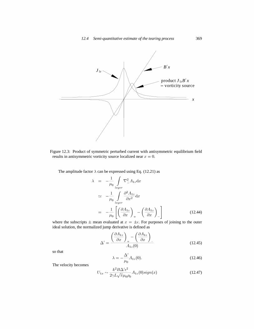
12.4 Semi-quantitative estimate of the tearing process 369
productJ1zB′ x= vorticity source
J1zB′x
x
Figure 12.3: Product of symmetric perturbed current with antisymmetricequilibrium fieldresults in antisymmetric vorticity source localized nearx = 0.
The amplitude factorλ can be expressed using Eq. (12.21) as
λ = − 1µ0
∫
layer∇2⊥A1zdx
≃ − 1µ0
∫
layer
∂2A1z∂x2 dx
= − 1µ0
[
(∂A1z∂x
)
+−(∂A1z
∂x)
−
]
(12.44)
where the subscripts± mean evaluated atx = ±ǫ. For purposes of joining to the outerideal solution, the normalized jump derivative is defined as
∆′ =
(∂A1z∂x
)
+−(∂A1z
∂x)
−A1z(0) (12.45)
so that
λ = −∆′µ0A1z(0). (12.46)
The velocity becomes
U1x ∼ k2B∆′ǫ22γL√πµ0ρ0A1z(0)sign(x) (12.47)

370 Chapter 12. Magnetic reconnection
and using Eq.(12.36), the current density becomes
J1z ∼ − ∆′ǫµ0√πA1z(0). (12.48)
We now repeat the induction equation, Eq.(12.20),
−∂A1z∂t − U1x
∂A0z∂x = ηJ1z (12.49)
and substitute forU1x, J1z and assume that∂A0z/∂x = −By0 ≃ −Bǫ/L in the tearinglayer. This gives
γ − k2B2∆′ǫ32γL2√πµ0ρ0 = η∆′
ǫµ0√π#1 #2 #3(12.50)
where the terms have been numbered for reference in the following discussion.In the ideal plasma limit, terms #1 and #2 balance each other while term #3 is small;
this gives the frozen-in condition. At exactlyx = 0, term #2 vanishes and so terms #1and #3must balance each other, resulting in diffusion of the magnetic field. At the edge ofthe tearing layer, which is the transition from the ideal limit to the diffusive limit all threeterms are of the same size.Thus, the three terms may be equated; this gives two equationswhich may be solved forγ andǫ with∆′ as a parameter. Equating terms #1 and #3 gives
γ = η∆′ǫµ0√π (12.51)
while equating terms #2 and #3 gives
γ = (kB′)2 ǫ42ηρ0 (12.52)
whereB′ = B/L is the derivative of the equilibrium field atx = 0. Equating these lasttwo equations to eliminateγ gives the width of the tearing layer to be
ǫ ≃[ 2η2ρ0∆′
µ0√π (kB′)2]1/5
. (12.53)
Substitutingǫ back into Eq.(12.51) gives
γ = 0.55 (∆′)4/5[ ηµ0
]3/5 [ (kB′)2ρ0µ0
]1/5. (12.54)
This result can be put in a more transparent form by defining characteristic times for idealprocesses and for resistive processes. The characteristic time forideal processes is theAlfvén time τA, defined as the time to move the characteristic lengthL when traveling atthe Alfvén velocity, i.e.,
τ−1A = vA
L =√B2/ρ0µ0
L =√
(B′)2ρ0µ0 . (12.55)

12.5 Generalization of tearing to sheared magnetic fields 371
The Alfvén time is the characteristic time of ideal MHD and is typically a very fast time.The characteristic time for resistive processes is the timeτR, defined as the time to diffuseresistively a distanceL,
τ−1R = η
L2µ0 . (12.56)
For nearly ideal plasmas the resistive time scale is very slow. Using these definitions,Eq.(12.54) can be written as (Furth, Killeen and Rosenbluth 1963)
γ = 0.55 (∆′L)4/5 (kL)2/5 τ−3/5R τ−2/5
A (12.57)
All that is needed now is∆′ . This jump condition is found from Eq.(12.31) which givesthe form ofAz1 in the ideal region outside the tearing layer. This can be expressed as
∇2⊥Az1 +[
B−1y0d2By0dx2
]
Az1 = 0 (12.58)
which shows that the equilibrium magnetic field acts like a ‘potential’ for the perturbedvector potential ‘wavefunction’. If boundary conditions are specified at large |x| for theperturbed vector potential, then in general, there will be a discontinuityin the first derivativeof Az1 at x = 0; this discontinuity gives∆′. The jump depends on the existence of alocalized equilibrium current since
d2By0dx2 = µ0 dJz0dx . (12.59)
In general the outer equation must be solved numerically.The main result, as given by Eq.(12.57), is that if∆′ > 0 an instability develops having
a growth rateintermediatebetween the fast Alfvén time scale and the slow resistive timescale. Since a nearly ideal plasma is being considered,η is extremely small. The widthof the tearing layer is therefore very narrow, since as shown by Eq.(12.53), this width isproportional toη2/5.
12.5 Generalization of tearing to sheared magnetic fields
The sheet current discussed above can occur in real situations but is a special case of themore general situation where the equilibrium magnetic field does not have anull, but in-stead is simply sheared. This means that the equilibrium magnetic field is straight, hascomponents in both they andz directions, and has direction that is a varying function ofx. The sheared situation thus has a uniform magnetic field in thez direction and insteadof the current being concentrated in a sheet, there is simply a non-uniformBy0(x). In thismore general situation the equilibrium magnetic field has the form
B0 = By0(x)y +Bz0z. (12.60)
A nontrivial feature of this situation is that unlike the previously considered sheet currentequilibrium, hereBy0(x) does not vanish at any particularx. Instead, as will be seen later,what counts is the vanishing ofk ·B0. Equation (12.60) can be used as a slab representa-tion of the straight cylindrical geometry equilibrium field
B0 = ∇ψ0(r) ×∇z +Bz0z; (12.61)

372 Chapter 12. Magnetic reconnection
which in turn can be thought of as the straight cylindrical approximationof a toroid withzcorresponding to the toroidal angle.
k
x = 0 planeonly
B ζ
z
y.
Figure 12.4: Tilted coordinate system for general sheared field.
Figure 12.4 shows the magnetic field given by Eq.(12.60) as viewed in thex = 0 plane.In the sheet current analysis discussed in the previous section, the perturbed vector potentialpointed in thez direction and was periodic in they direction. This corresponded to havingk ·A1 = 0 so that the wavevector was orthogonal to the vector potential and both wereorthogonal tox. Other important properties were thatk ·B vanished at the reconnectionlayer, thefluid vorticity vector was pointed in thez direction, the perturbed currents andperturbed magnetic fields were such thatJ1/J0 >> B1/B0 in the reconnection layer, andJ1/J0 ∼ B1/B0 in the exterior region.
These relationships and approximations are generalized here and, in particular, it isassumed that all perturbed quantities have functional dependence∼ g(x) exp(ikyy+ikzz+γt). As before, the vorticity equation is the curl of the linearized equationof motion, i.e.
ρ∂Ω1∂t = ∇× (J1×B0+J0×B1) (12.62)
and in the reconnection layer whereJ1/J0 >> B1/B0 this becomes
ρ∂Ω1∂t = ∇× (J1×B0)
= B0 · ∇J1 − J1 · ∇B0 (12.63)
since∇ ·B0 = 0 and∇ · J1 = 0.An essential feature of the reconnection topology is that the vorticity must be anti-
symmetric about the reconnection layer, as can be seen from examination of thefluid flowvectors in Fig.12.2(c). Since the vorticity is created by the torque (i.e., the curl of the force),it is clear that the torque must be antisymmetric about the reconnectionlayer. As will beseen in the next paragraphs, the condition that the torque is antisymmetric doesnot implythat eitherB0 or J1 are antisymmetric, but rather implies some more subtle conditions.

12.5 Generalization of tearing to sheared magnetic fields 373
Thus, if x = 0 is defined to be the location of the reconnection layer, thenΩ1 mustbe an odd function ofx and therefore must vanish atx = 0. Hence the right hand side ofEq.(12.63) must vanish atx = 0 and since there need be no particular functional relation-ship betweenB0 and its gradient, the two terms on the right hand side of Eq.(12.63) mustseparately vanish. Therefore one of the requirements is to choose the origin of thex axissuch thatB0 · ∇J1 = 0 atx = 0 or, equivalently,
k ·B0 = 0 at x = 0 (12.64)
so thatkyBy0(0) + kzBz0 = 0. (12.65)
Havingk ·B vanish at the reconnection layer is physically reasonable, since finitek ·Bimplies a periodic bending of the equilibrium field; such a bending absorbs energy and sois stabilizing. Havingk ·B vanish is like letting the instability cleave the system at a weakpoint so that the instability can develop without requiring much free energy.
The second requirement for the right hand side of Eq.(12.63) to vanish is to haveJ1 · ∇B0 = 0. If the flow is incompressible, then the perturbed magnetic field mustbe orthogonal to the equilibrium magnetic field and since the perturbed current is the curlof the perturbed magnetic field, the perturbed current must be parallel to theequilibriummagnetic field. SinceB0 is assumed straight,B0 ·∇B0 = 0 and sinceJ1 is parallel toB0,it is seen thatJ1 · ∇B0 = (J1/B0)B0 · ∇B0 = 0. BecauseJ1 is parallel toB0, J1 mustalso be straight and so a Coulomb gauge vector potential will be parallel toJ1, since
µ0J1 = ∇×∇×A1= ∇∇ ·A1 −∇2A1= −∇2A1 (12.66)
= −ζ∇2A1 (12.67)
can be satisfied by having bothJ1 andA1 in the direction ofζ whereζ = B0(0)/B0(0)does not depend on position.
It is therefore assumed thatA1 is parallel toB0(0) and so
A1(x, y, z, t) = A1ζ(x)ζeikyy+ikzz+γt. (12.68)
Thus,k ·A1 = 0 in this tilted coordinate system and also∇·A1 = 0 so that the Coulombgauge assumption is satisfied.
Reconsideration of the right hand side of Eq. (12.63) shows that although the two termsboth vanish atx = 0 there is a difference in the geometrical dependence of these terms. Inparticular
J1 · ∇B0 = 0is true for allx becauseJ1 is in theζ direction andB0 is a function ofx only. Thus, Eq.(12.63) reduces to
ρ∂Ω1∂t = B0 · ∇J1
= i (k ·B0)J1 (12.69)
where, by assumption,k ·B0 vanishes atx = 0.

374 Chapter 12. Magnetic reconnection
Continuing this discussion of the ramifications of the antisymmetry ofk ·B0 aboutx = 0, we now define an artificial reference magnetic fieldB that is parallel to the realfield atx = 0, but has no shear (i.e. has nox dependence). The reference field thereforehas the form
B =By0(0)y +Bz0z = B0(0)ζ for all values of x. (12.70)We now defineb0 as the difference between the real field andB so that
B0(x) = B +b0(x) (12.71)
andb0(x) has the samex-dependence as theBy0 field used for the sheet current instabilityin the previous section in that (i) it is antisymmetric aboutx and (ii) is in they direction.One way of thinking about this is to realize thatb0(x) is the component ofB0(x) which isantisymmetric aboutx = 0.With this definition
k ·B0 = k · b0(x) = kyb0 (12.72)
and so Eq.(12.69) becomesγρΩ1ζ = ikyb0J1ζ . (12.73)
This equation provides the essence of the dynamics. It shows how the componentof themagnetic field that is antisymmetric aboutx = 0 createsfluid vortices that are antisymmet-ric with respect tox. In particular, sinceb0(x) is an odd function ofx andJ1ζ is an evenfunction ofx, Ω1ζ is an odd function ofx.
The complete self-consistent description is obtained by in addition taking into accountthe induction equation which shows howfluid motion acts to create perturbations of theelectromagnetic field.
Since we are working with vector potentials, Ohm’s law provides the induction equa-tion. In the sheet current case the component of Ohm’s law in the direction ofsymmetryof the perturbation was considered, i.e., the component in thez direction. Here, the cor-responding symmetry direction for the perturbation is theζ direction and so the relevantcomponent of Ohm’s law is theζ component,
ζ · [E1 +U1 ×B0(x)] = ζ · ηJ1 (12.74)
which becomes −∂A1ζ∂t +
(
y × ζ ·U1)
b0(x) = ηJ1ζ . (12.75)
Since the vorticity vector lies alongζ the incompressible velocity must be orthogonal toζand so has the form
U1 = ∇f1 × ζ. (12.76)Thus
y × ζ ·U1 =(
y × ζ) · (∇f1 × ζ) = ikyf1. (12.77)
Again, taking into account the fact that the vorticity points in theζ direction it is seen thatΩ1 = Ω1ζ ζ where
Ω1ζ = ζ · ∇ ×U1 = −∇2⊥f1 (12.78)
and now⊥ means perpendicular toζ.Substituting forΩ1ζ in Eq.(12.73) using Eq. (12.78) gives
∇2⊥f1 = − ikyb0(x)J1ζγρ0 ; (12.79)

12.5 Generalization of tearing to sheared magnetic fields 375
this equation provides the essential dynamics offluid vortices that are antisymmetric withrespect tox and driven by the torque associated with the non-conservative nature, i.e., curl,of theJ×B force. This is essentially the same as Eq.(12.35) and the rest of the analysis isthe same as for the sheet current problem except that nowky is used instead ofk andb′0 isused instead ofB′0y. Sinceb0(x) only differs fromBy0(x) by a constant,b′0 = B′y0. Thus,using Eq.(12.54) the growth rate will be
γ = 0.55 (∆′)4/5[ ηµ0
]3/5 [(kyB′y0)2
ρ0µ0
]1/5. (12.80)
The global system has to be periodic in both they andz direction in order for well-definedky andkz to exist. In particular, the physical arrangement and dimensions of the globalsystem determine the quantized spectra ofky andkz and so determine the allowed planeswherek ·B0 can vanish. As suggested earlier, the allowed planes can be consideredas ‘cleavage’ planes where the magnetic field can most easily become unglued from theplasma.
Let us express this result in the context of toroidal geometry such as that of atokamak.This is done by lettingBz0 correspond to the toroidal fieldBφ andBy correspond toBθthe poloidal field. The Alfvén time is now defined in terms ofBφ as
τ−1A = Bφ
a√ρ0µ0 (12.81)
wherea is the minor radius. The safety factor, a measure of the twist, is definedas
q = aBφRBθ
(12.82)
so that
Bθ = aBφRq (12.83)
and
B′y0 → −aBφRq2 q
′. (12.84)
Thus it is possible to replaceky →m/a and
(kyB′y0)2
ρ0µ0 → (maRq2 q
′)2 1τA . (12.85)
At the tearing layerk ·B = 0 or
ma Bθ + n
RBφ = 0 (12.86)
soq = −mn (12.87)
and Eq.(12.85) becomes(kyB′y0
)2
ρ0µ0 → (naRq′q)2 1τA . (12.88)
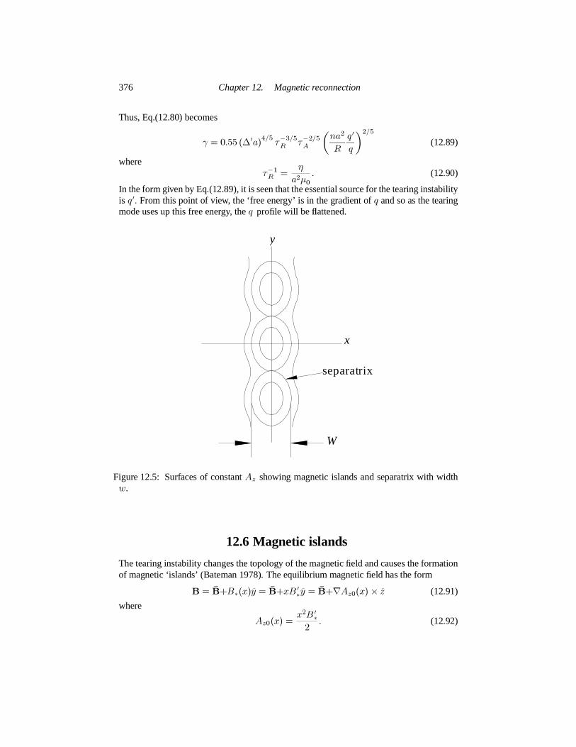
376 Chapter 12. Magnetic reconnection
Thus, Eq.(12.80) becomes
γ = 0.55 (∆′a)4/5 τ−3/5R τ−2/5
A(na2Rq′q)2/5
(12.89)
whereτ−1R = η
a2µ0 . (12.90)
In the form given by Eq.(12.89), it is seen that the essential source for thetearing instabilityis q′. From this point of view, the ‘free energy’ is in the gradient ofq and so as the tearingmode uses up this free energy, theq profile will beflattened.
x
y
W
separatrix
Figure 12.5: Surfaces of constantAz showing magnetic islands and separatrix with widthw.
12.6 Magnetic islands
The tearing instability changes the topology of the magnetic field and causes the formationof magnetic ‘islands’ (Bateman 1978). The equilibrium magnetic field has the form
B = B+B∗(x)y = B+xB′∗y = B+∇Az0(x) × z (12.91)
where
Az0(x) = x2B′∗
2 . (12.92)

12.6 Magnetic islands 377
It is seen that
B⊥ · ∇Az0 = 0 (12.93)
whereB⊥ is the component perpendicular toz. Thus, the surfacesAz = const. give theprojection of the field lines in the plane perpendicular toz; these projections correspond tothe poloidalflux surfaces in toroidal geometry.
If it is assumed thatkz << ky, so thatζ is very nearly parallel toz, then it is seen thatthe tearing instability adds a perturbation toAz so that now
Az(x, y) = x2B′∗
2 +Az1 coskyy. (12.94)
A sketch of a set of surfaces of constantAz(x, y) is shown in Fig.12.5. These surfacesconsist of (i) closed curves called islands, (ii) a separatrix which passes through thex point,and (iii) open outer surfaces. The widthw of the separatrix can be calculated, by notingthat at thex−point
Asep = 0+Az1 (12.95)
while at the point of maximum width,x = w/2,
Asep = (w/2)2 B′∗
2 −Az1. (12.96)
Equating these gives
w = 4√
Az1B′
∗= 4
√
∣
∣
∣
∣
Bx1kyB′
∗
∣
∣
∣
∣
(12.97)
usingBx1 = ikyAz. In tokamak terminology we identifyBx1 → Br1 wherer is the minorradius, and using Eq.(12.84), (12.87) andky →m/a this becomes
w = 4√
∣
∣
∣
∣
Rqnq′
Br1Bφ
∣
∣
∣
∣
. (12.98)
It is important to realize that the width of the island is much larger than the width of thetearing layer. Since particles tend to be attached to magneticflux surfaces, the formationof islands means that particles can circulate around the island, therebycausing aflatteningof the pressure gradient because the pressure is constant along a magnetic field line.

378 Chapter 12. Magnetic reconnection
12.7 Assignments
(a) (b)
(c)
zz
poloidalflux surface
currentloop
12
34
5
1 23
4 5
U in
U in
UoutUout δ
currentsheet
L
X-point X-point
Figure 12.6: (a) Two identical coaxial current loops; (b) current loops approaching eachother; (c) detail of X-point region of (b) showing inflows/outflows and current-sheet(shaded region) having nominal lengthL and thicknessδ.
1. Sweet-Parker type reconnection(Sweet 1958, Parker 1957): Consider the two identicalflux-conserving current loops shown in Fig. 12.6(a). Becausethe system is axisym-metric, the magnetic field can be expressed as
B = 12π∇ψ ×∇φ.
(a) Explain why there is an attractive force between the current loops (hint: considerthe force between parallel currents or between north and south poles of twomagnets).

12.7 Assignments 379
(b) Define privateflux to be aflux surface that links only one of the current loops(examples are theflux surfaces labeled 1 and 2 in Fig.12.6(a)). Define publicflux to be aflux surface that links both of the current loops (examples arefluxsurfaces 3,4,5 in Fig.12.6(a)). Define the X-point to be the location in thez = 0plane where there is a field null as shown in Fig.12.6(a); let r0 be the radiusof the X-point. Show by sketching that as the two current loops approach eachother in vacuum, a privateflux surface above the midplane will merge with aprivateflux surface below to form a publicflux surface.
(c) Show that theflux linked by a circle in thez = 0 plane with radiusr0 (i.e.,the circle follows the locus of the X-point) is the publicflux. Argue that if thecurrent loops approach each other, this publicflux will increase at the rate thatprivate flux is converted into publicflux. By integrating Faraday’s law overthe surface of this circle in thez plane with radiusr0, show that there exists atoroidal electric field at the X-point,
Eφ = − 12πr0
∂ψpublic∂t
where∂ψpublic/∂t is the rate of increase of publicflux.
(d) Now suppose that the vacuum is replaced by perfectly conducting plasma sothatplasma is frozen to field lines. Show from symmetry that the plasma velocity atthex point must vanish. What isEφ at the X-point if the two current loops areimmersed in a plasma which satisfies the ideal Ohm’s law,
E+U×B = 0.Can there be any conversion of privateflux into publicflux in an ideal plasma?Sketch contours of private and publicflux when two current loops approach eachother in an ideal plasma.
(e) Now suppose the two current loops are immersed in a non-ideal plasma whichsatisfies the resistive Ohm’s law
E+U×B =ηJ.Can privateflux be converted into publicflux in this situation, and if so, what isthe relationship between the rate of increase of publicflux and the resistivity?
(f) By writing Eφ, Br ,Bz, andJφ in terms of the poloidalflux function show thatthe toroidal component of the resistive Ohm’s law can be expressed as
∂ψ∂t +U·∇ψ = r2∇ ·( η
µ0r2∇ψ)
.Show that this equation implies thatflux convects with the plasma ifη = 0, butdiffuses across the plasma ifU = 0.Show that the diffusion increases ifψ devel-ops a steep gradient at the location whereU = 0. By considering your responseto (d) above, discuss how theflux gradient in thez direction might steepen in thevicinity of the X-point. Taking into account the relationship betweenJ andψ,show that this corresponds to developing a thin sheet of current in the midplane

380 Chapter 12. Magnetic reconnection
(current-sheet) as shown in Fig.12.6(c). Show that in order to have an X-pointgeometry and also satisfy Faraday’s law, theflux function must have the form
ψ(r, z, t) =(
1 + z22δ2 − (r − r0)2
2L2
)
ψ0 − 2πrEφtin the vicinity of the X-point; hereψ0 is theflux at the X-point att = 0 andr0is the radial location of the X-point. What is the relationship betweenδ andL invacuum and in a resistive plasma? Isδ larger or smaller thanL if the two currentloops are approaching each other? Ifδ < L is there a current in the vicinity ofthe X-point? What is the direction of this current with respect to the currents inthe two current loops? Will the force on the current loops from the current inthe current sheet accelerate or retard the motion of the two current loops towardseach other? What is the direction ofEφ? Isψ increasing or decreasing at theX-point?
(g) Suppose that the current sheet has a nominal thickness ofδ in the z directionand a nominal width ofL in the r direction as shown in Fig.12.6(c). LetUinbe the nominal vertical velocity with which the plasma approaches thex pointand letUout be the nominal horizontal velocity with which the plasma leaves thex point region as shown in Fig.12.6(c). If the plasma motion is incompressibleshow that
UinL ≃ Uoutδ. (12.99)
(h) Consider the transition from the ideal MHD form of Ohm’s law to the form atthe X-point. Argue that in the region of this transition the termsU×B andηJshould have the same order of magnitude (this is essentially the same argumentthat was used to analyze Eq.(12.49)). Use this result and Ampere’s law to find arelationship betweenηJ, Bin andδ. Use this to show
Uin ∼ η /µ0δ (12.100)
and explain this result in terms of the convective velocity for motion offluxsurfaces outside the current sheet and the "diffusive velocity" for motion offluxsurfaces inside the current sheet.
(i) Using Eq.(9.42) show that the MHD force acting on the plasma is
FMHD=− ∇ψ(2π)2 µ0
∇ ·( 1r2∇ψ
)
Sketch the direction of this force and indicate where this force is finite (hint:consider whereJ is finite). Estimate the work
∫
F·dl done on plasma acceleratedthrough the current sheet by using relationships involvingBin, Bout, δ, andL.Use this estimate to show that
Uout ≃ vA,in (12.101)
wherevA,in = Bin/√µ0ρis the Alfvén velocity at the input. (Hint: Let∆ψ bethe jump influx experienced by afluid element as it moves across the current

12.7 Assignments 381
sheet. Note thatBout ∼ ∆ψ/2πrL andBin ∼ ∆ψ/2πrδ; also note that∇ ·(r−2∇ψ) can be expressed in terms ofBin andδ.)
(j) By eliminatingUin andUout between Eqs.(12.99), (12.100), and (12.101) showthat δ
L = Uinva,in = 1√Sin
where the inflow region Lundquist numberSin is defined as
Sin = µ0va,inLη
(k) If the initial separation between the two current loops is also of the order ofL, how much time is required for the two loops to merge, thus completing thereconnection process? Structures in the solar corona have scale lengthsL ∼1-100 megameters (108 m) and it is observed that Alfvén wave disturbancespropagate with velocitiesvA ∼ 106 m/s. The temperature of these structures is10-100 eV. Assuming a nominal temperature of 50 eV, use Spitzer resistivitytocalculate the nominal value ofSin.How long would it take for two solar currentloops to merge if they are governed by the mechanism discussed here (what isthe appropriate time unit to use seconds, days, weeks, years, ...?). Actual currentloops change topology on time scales ranging from minutes to hours – how doesthis compare with the predictions of this model?

13
Fokker-Planck theory of collisions
13.1 Introduction
Logically, this chapter ought to be located at the beginning of Chapter 2, just after phase-space concepts had been introduced. The reason this chapter is not located there is thatthe theory in this chapter is too involved to be at the beginning of the book and would havedelayed the introduction of important other topics that do not need the detail of thischapter.
The discussion of collisions in Chapter 1 was very approximate. Collisions were shownto scale as an inverse power of temperature, but this was based on a “one size fits all”analysis since it was assumed that the collision frequency of both slow andfast particleswere nominally the same as that of a particle going at the thermal velocity. Because thecollision frequency scales asv−3, it is dubious to assume that the collision rates of bothsuper-thermal and subthermal particles can be reasonably represented by a single collisionfrequency. A more careful averaging over velocities is clearly warranted. This is providedby a Fokker-Planck analysis due to Rosenbluth, Macdonald and Judd (1957) but ifallthis analysis provided was more accuracy for collision calculations, itwould not be worththe considerable effort except possibly for exceptional situations wherehigh accuracy isimportant. However, it turns out that more than increased accuracy results from this theory,because some new and important phenomena become evident from the analysis.
We begin the analysis by reviewing collisions between two particles. Suppose a testparticle having massmT and chargeqT collides with a field particle having massmF andchargeqF . Since the electric field associated with a chargeq is E = rq/4πε0r2 whereris the distance from the charge, the equations of motion for the respective test and fieldparticles are
mT rT = qT qF4πε0|rT − rF |3 (rT − rF ) (13.1a)
mF rF = qT qF4πε0|rT − rF |3 (rF − rT ) . (13.1b)
The center of mass vector is defined to be
R = mT rT +mF rFmT +mF
. (13.2)
382

13.1 Introduction 383
Adding Eqs.(13.1a) and (13.1b) gives
(mT +mF )R =mT rT +mF rF = 0 (13.3)
showing that the center of mass velocityR is a constant of the motion and so does notchange as a result of the collision. If∆rT and∆rF are defined as the change in respectivevelocities of the two particles during a collision, then it is seen that these changes are notindependent, but are related by
(mT +mF )∆R = 0 =mT∆rT +mF∆rF . (13.4)
It is useful to define the relative position vector
r = rT − rF (13.5)
and the reduced mass 1µ = 1
mT+ 1mF
. (13.6)
Then, dividing Eqs.(13.1a) and (13.1b) by their respective masses and taking the differencebetween the resulting equations gives an equation of motion for the relativevelocity
µr = qT qF4πε0r2 r. (13.7)
Solving Eqs.(13.2) and (13.5) forrT andrF gives
rF = R− µmF
r (13.8)
rT = R+ µmT
r
and so the respective test and field velocities are
rF = R− µmF
r (13.9)
rT = R+ µmT
r. (13.10)
Since∆R = 0 the change of the test and field particle velocities as measured in the labframe can be related to the change in the relative velocity by
∆rF = − µmF
∆r (13.11)
∆rT = + µmT
∆r. (13.12)
The collision problem is first solved in the center of mass frame to find the change inthe relative velocity and then the center of mass result is transformed to the lab-frame todetermine the change in the lab-frame velocity of the particles.
Let us now consider a many-particle point of view. Suppose a mono-energetic beam ofparticles impinges upon a background plasma. Several effects are expected to occur dueto collisions between the beam and the background plasma. First, there willbe a slowingdown of the beam as it loses momentum due to collisions. Second, there should be aspreading out of the velocity distribution of the particles in the beam since collisions willtend to diffuse the velocity of the particles in the beam. Meantime, the background plasmashould be heated and also should gain momentum due to the collisions. Eventually, thebeam should be so slowed down and so spread out that it becomes indistinguishablefromthe background plasma which will be warmer because of the energy transferred from thebeam.

384 Chapter 13. Fokker-Planck theory of collisions
13.2 Statistical argument for the development of theFokker-Planck equation
The Fokker-Planck theory (Rosenbluth et al. 1957) is based on a logical argument on how adistribution function attains its present form due to collisions at someearlier time. Considera particle with velocityv at timet that is subject to random collisions which change itsvelocity. We defineF (v,∆v) as the conditional probability that if a particle has a velocityv at timet, then at some later timet+∆t, collisions will have caused the particle to havevelocityv +∆v.
Clearly at timet + ∆t the particle must have some velocity, so the sum of all theconditional probabilities must be unity, i.e.,F must be normalized such that
∫
F (v,∆v)d∆v = 1. (13.13)
This definition of conditional probability can be used to show how a present distributionfunctionf(v, t) comes to be the way it is because of the way it was at timet −∆t. Thiscan be expressed as
f(v, t) =∫
f(v−∆v, t −∆t)F (v−∆v,∆v)d∆v (13.14)
which sums up all the possible ways for obtaining a given present velocity weighted bythe probability of each of these ways occurring. This analysis presumes that the presentstatus depends only on what happened during the previous collision and is independentof all events before that previous collision. A partial differential equation for f can beconstructed by Taylor expanding the integrand as follows:
f(v−∆v, t−∆t)F (v−∆v,∆v) = f(v, t)F (v,∆v)−∆t∂f∂t F (v,∆v)−∆v· ∂∂v (f(v, t)F (v,∆v))+12∆v∆v : ∂∂v
∂∂v (f(v, t)F (v,∆v)) .
(13.15)Substitution of Eq.(13.15) into Eq.(13.14) gives
f(v, t) = f(v, t) ∫ F (v,∆v)d∆v−∆t∂f∂t∫ F (v,∆v)d∆v
− ∫ ∆v· ∂∂v (f(v, t)F (v,∆v)) d∆v
+12∫ ∆v∆v : ∂∂v
∂∂v (f(v, t)F (v,∆v)) d∆v
(13.16)
where in the top line advantage has been taken off(v, t) not depending on∆v. Upon

13.2 Statistical argument for the development of the Fokker-Planck equation385
invoking Eq.(13.13) this can be recast as
∂f∂t =
− ∂∂v ·(∫ ∆vF (v,∆v)d∆v
∆t f(v, t))
+12∂∂v
∂∂v :
(∫ ∆v∆vF (v,∆v)d∆v∆t f(v, t)
)
. (13.17)
By defining⟨∆v
∆t⟩
=∫ ∆vF (v,∆v)d∆v
∆t (13.18)
and⟨∆v∆v
∆t⟩
=∫ ∆v∆vF (v,∆v)d∆v
∆t (13.19)
the standard form of the Fokker-Planck equation is obtained,
∂f∂t = − ∂
∂v ·(⟨∆v∆t
⟩
f(v, t))
+ 12∂∂v
∂∂v :
(⟨∆v∆v∆t
⟩
f(v, t))
. (13.20)
The first term gives the slowing down of a beam and is called the frictional term while thesecond term gives the spreading out of a beam and is called the diffusive term.
The goal now is to compute〈∆v/∆t〉 and〈∆v∆v/∆t〉. To do this, it is necessaryto consider all possible ways there can be a change in velocity∆v in time ∆t and thenaverage all values of∆v and∆v∆v weighted according to their respective probability ofoccurrence. We will first evaluate〈∆v/∆t〉 and then later use the same method to evaluate〈∆v∆v/∆t〉. The problem will first be solved in the center of mass frame and so involvesa particle with reduced massµ, speedvrel = |vT − vF |, and impact parameterb collidingwith a stationary scattering center at the origin. This was discussed inChapter 1 and thegeometry was sketched in Fig.1.3. The deflection angleθ for small angle scattering wasshown to be
θ = qT qF2πε0bµv2rel . (13.21)
The averaging procedure is done in two stages:1. The effect of collisions in time∆t is calculated. The functional dependence of∆v on
the scattering angleθ is determined and then used to calculate the weighted average∆v for all possible impact parameters and all possible azimuthal angles of incidence.This result is then used to calculate the weighted average change in target particlevelocity in the lab frame.
2. An averaging is then performed over all possible field particle velocities weightedaccording to their probability, i.e., weighted according to the field particle distributionfunctionfF (vF ).
Energy is conserved in the center of mass frame and since the energy before and afterthe collision is entirely composed of kinetic energy, the magnitude ofv2rel must be the samebefore and after the collision. The collision thus has the effect of causing a simple rotationof the relative velocity vector by the angleθ. Let z be the direction of the relative velocitybefore the collision and letb be the direction of the impact parameter. Ifvrel1,vrel2 are

386 Chapter 13. Fokker-Planck theory of collisions
the respective relative velocities before and after the collision, then
vrel1 = vrelzvrel2 = vrel cosθz + vrel sin θb. (13.22)
Thus
∆vrel = vrel2 − vrel1= vrel (cosθ − 1) z + vrel sin θb≃ −vrelθ22 z + vrelθ(x cosφ+ y sinφ) (13.23)
whereφ is the angle between the impact parameter and thex axis and the scattering angleθ is assumed to be small. The fact that thez component is negative reflects the slowingdown of the particle in its initial direction of motion.
The cross section associated with impact parameterb and the range of azimuthal impactangledφ is bdφdb. In time∆t the incident particle moves a distancev∆t and so the vol-ume swept out for this cross-section isbdφdbv∆t. The number of relevant field particlesencountered in time∆t will be the densityfF (vF )dvF of relevant field particles multi-plied by this volume, i.e.,fF (vF )dvF bdφdbv∆t and so the change in relative velocity forall possible impact parameters and all possible azimuthal angles for agivenvF will be
∆v|all b, all φ = v∆tfF (vF )dvF∫
dφ∫
∆vbdb. (13.24)
The limits of integration for the azimuthal angle are from0 to 2π and the limits of integra-tion of the impact parameter are from the 900 impact parameter to the Debye length. Onwriting ∆v in component form, this becomes
∆vrel|all b, all φ = vrel∆tfF (vF )dvF∫ 2π
0dφ
∫ λD
bπ/2vrel (θ cosφ, θ sinφ,−θ2/2) bdb.
(13.25)Thex andy integrals vanish upon integration overφ and so
∆vrel|all b, all φ = −zv2rel∆tfF (vF )dvFπ∫ λD
bπ/2θ2bdb
= −zv2rel∆tfF (vF )dvFπ∫ λD
bπ/2
( qT qF2πε0bµv2rel
)2bdb
= −z∆tfF (vF )dvFq2T q2F
4πε20µ2v2rel ln Λ (13.26)
whereΛ = λD/bπ/2.Using Eq.(13.12) the above expression can be transformed to give the test particle ve-
locity change to be
∆vT |all b, all φ = −z∆tfF (vF )dvFq2T q2F
4πε20µmT v2rel ln Λ
= −∆t q2T q2F ln Λ
4πε20µmT(vT − vF )|vT − vF |3 fF (vF )dvF . (13.27)

13.2 Statistical argument for the development of the Fokker-Planck equation387
This result was for a particular value ofvF and summing over all possiblevF weightedaccording to their probability, gives
∆vT |all b, all φ, all vF = −∆t q2T q2F ln Λ4πε20µmT
∫ vrelv3rel fF (vF )dvF . (13.28)
The integrand can be expressed in a simpler form by considering that
∂r∂r =
(
x ∂∂x + y ∂∂y + z ∂∂z)
√x2 + y2 + z2 = rr (13.29)
and also∂/∂vT = ∂/∂vrel. Thus
∂vrel∂vT
= vrelvrel (13.30)
and∂∂vT
1vrel = − 1
v2relvrelvrel . (13.31)
Equation (13.28) can therefore be written as
∆vT |all b, all φ, all vF = ∆t q2T q2F ln Λ
4πε20µmT∂∂vT
∫ 1vrel fF (vF )dvF . (13.32)
The ∂/∂vT has been factored out of the integral becausevT is independent ofvF , thevariable of integration. SincevF is a dummy variable, it can be replaced byv′ and sincevT is the velocity of the given incident particle, the subscriptT can be dropped. Aftermaking these re-arrangements we obtain the desired result,
⟨∆v∆t
⟩
= q2T q2F ln Λ4πε20µmT
∂∂v
∫ fF (v′)|v − v′|dv′. (13.33)
The averaging procedure for∆v∆v is performed in a similar manner, starting by notingthat
∆v∆v = (θ cosφ, θ sinφ,−θ2/2) (θ cosφ, θ sinφ,−θ2/2) (13.34)
and so Eq.(13.25) is replaced by
∆vrel∆vrel|all b, all φ = vrel∆tfF (vF )dvF∫ 2π
0dφ
∫ λD
bπ/2bdb×
v2rel(θ cosφ, θ sinφ,−θ2/2) (θ cosφ, θ sinφ,−θ2/2) .
(13.35)
The terms linear insinφ or cosφ vanish upon performing theφ integration. Also, thezzterm scales asθ4 and so may be neglected relative to thexx andyy terms which scale as
388 Chapter 13. Fokker-Planck theory of collisions
θ2. Thus, we obtain
∆vrel∆vrel|all b,φ = v3rel∆tfF (vF )dvF2π∫
0
dφλD∫
bπ/2
θ2 (xx cos2 φ+ yy sin2 φ) bdb
= v3rel∆tfF (vF )dvF π (xx+ yy)∫ λD
bπ/2θ2bdb
= ∆tfF (vF )dvF (xx+ yy) q2T q2F ln Λ4πε20µ2vrel . (13.36)
Sincevrel defines thez direction, we may write
xx+ yy = I−vrelvrelv2rel (13.37)
whereI is the unit tensor. Thus,
∆vrel∆vrel|all b, all φ = ∆tq2T q2F ln Λ4πε20µ2 fF (vF )dvF
(v2relI − vrelvrelv3rel
)
. (13.38)
Using Eq.(13.12) this can be transformed to give
∆vT∆vT |all b, all φ =∆tq2T q2F ln Λ4πε20m2T
fF (vF )dvF(v2relI− vrelvrel
v3rel)
. (13.39)
The tensor may be expressed in a simpler form by noting
∂∂vT
∂vrel∂vT
= ∂∂vT
vrelvrel
= Ivrel − vrel
v2relvrelvrel
= v2relI− vrelvrelv3rel . (13.40)
Inserting Eq.(13.40) in Eq.(13.39) and then integrating over all the field particles showsthat
⟨∆vT∆vT∆t
⟩
= q2T q2F ln Λ4πε20m2T
∫
fF (vF )dvF∂∂vT
∂∂vT
|vT − vF |. (13.41)
However,vT is constant in the integrand and so∂/∂vT may be factored from the integral.Dropping the subscriptT from the velocity and changingvF to be the integration variablev′ this can be re-written as
⟨∆v∆v∆t
⟩
= q2T q2F ln Λ4πε20m2T
∂∂v
∂∂v
∫ |v − v′|fF (v′)dv′. (13.42)
It is convenient to define the Rosenbluth potentials
gF (v) =∫ |v − v′|fF (v′)dv′ (13.43)
hF (v) = mTµ
∫ fF (v′)|v − v′|dv′ (13.44)
13.2 Statistical argument for the development of the Fokker-Planck equation389
in which case⟨∆v∆t
⟩
= q2T q2F ln Λ4πε20m2T
∂hF∂v
⟨∆v∆v∆t
⟩
= q2T q2F ln Λ4πε20m2T
∂2gF∂v∂v . (13.45)
The Fokker-Planck equation, Eq.(13.20) thus becomes
∂fT∂t = ∑
F=i,e
q2T q2F ln Λ4πε20m2T
[− ∂∂v ·(fT ∂hF∂v
)
+ 12∂∂v
∂∂v :
(
fT ∂2gF∂v∂v
)]
. (13.46)
The first term on the right hand side is a friction term which slows downthe mean velocityassociated withfT while the second term is an isotropization term which spreads out (i.e.,diffuses) the velocity distribution described byfT . The right hand side of Eq.(13.46) thusgives the rate of change of the distribution function due to collisions and sois the correctquantity to put on the right hand side of Eq.(2.12).
13.2.1Slowing down
Mean velocity is defined by
u =∫
vfdvn (13.47)
wheren = ∫ fdv. The rate of change of the mean velocity of speciesT is thus found bytaking the first velocity moment of Eq.(13.46). Integration by parts on the right hand sideterms respectively give
−∫
v ∂∂v ·(fT ∂hF∂v)
dv=∫
fT ∂hF∂v dv (13.48)
and∫
v ∂∂v∂∂v :
(
fT ∂2gF∂v∂v
)
dv =−∫ ∂∂v ·(fT ∂2gF∂v∂v
)
dv = 0 (13.49)
where Gauss’s theorem has been used in Eq.(13.49). The first velocity momentof Eq.(13.46)is therefore ∂uT
∂t = ∑
F=i,e
q2T q2F ln Λ4πε20nTm2T
∫
fT ∂hF∂v dv. (13.50)
Let us now suppose that the test particles consist of a mono-energetic beam so that
fT (v) = nT δ(v −u0). (13.51)
In this case Eq.(13.50) becomes
∂uT∂t = ∑
F=i,e
q2T q2F ln Λ4πε20m2T
(∂hF∂v
)
v=u0
. (13.52)
Let us further suppose that the field particles have a Maxwellian distribution so that
fF (v) = nF( mF2πκTF
)3/2exp (−mF v2/2κTF ) (13.53)
390 Chapter 13. Fokker-Planck theory of collisions
and so, using Eq.(13.44),
hF (v) = nFmTµ
( mF2πκTF
)3/2 ∫ exp (−mF v′2/2κTF )|v − v′| dv′. (13.54)
The velocity integral in Eq.(13.54) can be evaluated using standard means (see assign-ments) to obtain
hF (v) = nFmTµv erf
(√ mF2κTF v
)
(13.55)
where
erf (x) = 2√π∫ x
0exp(−w2)dw (13.56)
is the Error Function.Thus, Eq.(13.52) becomes
∂uT∂t = niq2T q2i ln Λ
4πε20m2TmTµi
∂∂v
[
v−1 erf(√ mi
2κTi v)]
v=u0
+neq2T q2e ln Λ4πε20m2TmTµe
∂∂v
[
v−1 erf(√ me
2κTev)]
v=u0
(13.57)
whereµ−1i,e =m−1i,e +m−1T .
This can be further simplified by noting (i) quasi-neutrality implies
niZqi + neqe = 0 (13.58)
whereZ is the charge of the ions, (ii) the masses are related by
mTµi,e = 1+ mT
mi,e, (13.59)
and (iii) the velocity gradient of the Error Function must be in the direction ofu0 becausethat is the only direction there is in the problem. Using these relationships and realizingthat both the left and right sides are in the direction ofu, Eq.(13.57) becomes
∂u∂t = nee2 ln Λ
4πε20q2Tm2T
Z(
1 + mTmi
) ddu
erf(√ mi
2κTiu)
u
+(
1 + mTme
) ddu
erf(√ me
2κTeu)
u
. (13.60)
Let us define
ξi,e =√ mi,e
2κTi,eu (13.61)
13.2 Statistical argument for the development of the Fokker-Planck equation391
which is the ratio of the beam velocity to the thermal velocity of the ionsor electrons. Theslowing down relationship can then be expressed as
∂u∂t = nee2 ln Λ
4πε20q2Tm2T
[
Z(
1 + mTmi
) mi2κTi
ddξi
(erf (ξi)ξi
)
+(
1 + mTme
) me2κTe
ddξe
(erf (ξe)ξe
)]
. (13.62)
53.752.51.250
0.4
0.3
0.2
0.1
−ddx
erfxx
x
limx<<1 −ddx
erfxx =
4x3 π
limx>>1 −ddx
erfxx =
1x2
Figure 13.1: Plot of−(x−1 erf x)′ v. x.
Figure 13.1 plots− (erf(x)/x)′ as a function ofx; this quantity has a maximum whenx = 0.9 indicating that the friction increases with respect tox whenx is less than0.9 butdecreases with respect tox whenx exceeds this value. Examination of this figure suggeststhat the function has a linear dependence forx well to the left of the maximum and variesas some inverse power ofx well to the right of the maximum.
This conjecture is verified by noting that Eq.(13.56) has the limiting values
limx<<1 erf(x) ≃ 2√π∫ x
0(1−w2)dw = 2√π
(
x− x33)
limx>>1 erf(x) ≃ 1 (13.63)
and so
limx<<1
(−ddx
erf xx
)
= 4x3√π (13.64a)
limx>>1
(−ddx
erf xx
)
= 1x2 (13.64b)
which is consistent with the figure.The existence of these two different asymptotic limits according to the ratio of the test
particle velocity (i.e., beam velocity) to the thermal velocity indicates three distinct regimescan occur, namely:

392 Chapter 13. Fokker-Planck theory of collisions
1. Test particle is much faster than both ion and electron thermal velocities, that isξi, ξe >> 1.
2. Test particle is much slower than both ion and electron thermal velocities, that isξi, ξe << 1.
3. Test particle is much faster than the ion thermal velocity, but muchslower than theelectron thermal velocity, i.e.,ξi >> 1 andξe << 1.
A nominal slowing down time can be defined by writing the generic slowingdownequation
∂u∂t = − u
τs (13.65)
so
τ s = − u∂u/∂t (13.66)
this can be used to compare slowing down of test particles in the three situations listedabove.
Test particle faster than both electrons, ionsHere the limit given by Eq.(13.64b) is used for both electrons and ions so that the
slowing down becomes
∂u∂t = −nee2 ln Λ4πε20
q2Tm2T
Z(
1 + mTmi
)
+(
1 + mTme
)
u2 (13.67)
and so
τ s ≃ 4πε20nee2 ln Λ
m2Tq2T
u3Z +1+ mT
me
(13.68)
since1/me >> 1/mi. Equation (13.67) shows that if the test particle beam is composedof electrons, the ion friction scales asZ/(Z + 2) of the total friction while the electronfriction scales as2/(2 + Z) of the total friction. In contrast, if the test particle is an ion,the friction is almost entirely from collisions with electrons.The slowing down time isinsensitive to the plasma temperature except for the weakln Λ dependence. The slowingdown time for ions is of the order ofmi/me times longer than the slowing down time forelectrons having the same velocity.
Test particle slower than both electrons, ionsHere the limit given by Eq.(13.64a) is used for both electrons and ions so that the
slowing down equation becomes
∂u∂t = − u
3√π nee2 ln Λπε20
q2Tm2T
(
Z(
1 + mTmi
)( mi2κTi
)3/2+(
1 + mTme
)( me2κTe
)3/2)
(13.69)

13.3 Electrical resistivity 393
and the slowing down time becomes
τs = 3√ππε20nee2 ln Λ
m2Tq2T
1(
Z(
1 + mTmi
)( mi2κTi
)3/2+(
1 + mTme
)( me2κTe
)3/2) .
(13.70)The temperature terms scale as the inverse cube of the thermal velocity and so if the
ion and electron temperatures are the same order of magnitude, then the ion contributiondominates. Thus, the slowing down is mainly done by collisions with ions and the slowingdown time is
τ s ≃ 3√ππε20nee2 ln Λ
m2Tq2T
(2κTi/mi)3/2Z(
1 + mTmi
) . (13.71)
The beam takes a longer time to slow down in hotter plasmas.Intermediate case: beam faster than ions, slower than electronsIn this case, the slowing down equation becomes
∂u∂t = −nee2 ln Λ4πε20
q2Tm2T
(
Z(
1 + mTmi
) 1u2 +
(
1 + mTme
)( me2κTe
)3/2 4u3√π
)
(13.72)
and the slowing down time is
τ s = 4πε20m2T
neq2T e2 ln Λ(
Z(
1 + mTmi
)
1u3 + 4
3√π(
1 + mTme
)( me2κTe
)3/2) . (13.73)
13.3 Electrical resistivity
If a uniform steady electric field is imposed on a plasma this electric field will acceleratethe ions and electrons in opposite directions. The accelerated particles will collide withother particles and this frictional drag will oppose the acceleration so that a steady statemight be achieved where the accelerating force balances the drag force. The electric fieldcauses equal and opposite momentum gains by the electrons and ions and therefore does notchange the net momentum of the entire plasma. Furthermore, electron-electron collisionscannot change the total momentum of all the electrons and ion-ion collisions cannotchangethe momentum of all the ions. The only wave for the entirety of electrons to lose momentumis by collisions with ions.
Let us assume that an equilibrium is attained where the electrons and ionshave shiftedMaxwellian distribution functions
fi(v) = niπ3/2(2κTi/mi)3/2 exp
(−mi (v −ui)2 /2κTi)
fe(v) = neπ3/2(2κTe/me)3/2 exp
(−me (v −ue)2 /2κTe)
. (13.74)

394 Chapter 13. Fokker-Planck theory of collisions
The current density will be
J = niqiui + neqeue. (13.75)
It is convenient to transform to a frame moving with the electrons, i.e., with the velocityue. In this frame the electron mean velocity will be zero and the ion meanvelocity will beurel = ui − ue. The current density remains the same because it is proportional tourelwhich is frame-independent. The distribution functions in this frame willbe
fi(v) = niπ3/2(2κTi/mi)3/2 exp
(−mi (v − urel)2 /2κTi)
fe(v) = neπ3/2(2κTe/me)3/2 exp (−mev2/2κTe) . (13.76)
Since the ion thermal velocity is much smaller than the electron thermal velocity, theion distribution function is much narrower than the electron distributionfunction and theions can be considered as a mono-energetic beam impinging upon the electrons. UsingEq.(13.57), the net force on this ion beam due to the combination of frictional drag onelectrons and acceleration due to the electric field is
mi∂urel∂t = neq2i q2e ln Λ
4πε20µe ∂∂v
[
v−1 erf(√ me
2κTe v)]
v=urel
+ qiE. (13.77)
In steady-state the two terms on the right hand side balance each other inwhich case
E = −neqie2 ln Λ4πε20µe ∂∂v
[
v−1 erf(√ me
2κTe v)]
v=urel
. (13.78)
If urel is much smaller than the electron thermal velocity, then Eq.(13.64a) canbe used toobtain
E = neqie2 ln Λ3√ππε20me
urel(2κTe/me)3/2
= Ze2m1/2e ln Λ3√ππε20
J(2κTe)3/2
(13.79)
whereurel = J/nee andµ−1e = 1/mi+1/me ≃ 1/me have been used. Equation (13.79)can be used to define the electrical resistivity
η = Ze2m1/2e3√ππε20
ln Λ(2κTe)3/2
(13.80)
so that
E =ηJ. (13.81)
If the temperature is expressed in terms of electron volts thenκ = e and the resistivity is
η = 1.03× 10⁻⁴Z ln ΛT 3/2e
Ohm-m. (13.82)

13.5 Assignments 395
13.4 Runaway electric field
The evaluation of the error function in Eq.(13.78) involved the assumptionthaturel, therelative drift between the electron and ion mean velocities, is much smaller than the electronthermal velocity. This assumption implies that−(x−1 erf x)′ ≃ 4x/3√π, so thatx lieswell to the left of 0.9 in the curve plotted in Fig.13.1. Consideration of Fig.13.1 shows that−(x−1 erf x)′ has a maximum value of0.43 which occurs whenx = 0.9 so that Eq.(13.78)cannot be satisfied if (Drecier 1959)
E > max−neqie2 ln Λ4πε20me
∂∂v
[
v−1 erf(√ me
2κTe v)]
= 0.43neZe3 ln Λ8πε20κTe . (13.83)
If the electron temperature is expressed in terms of electron volts, attaining a balance be-tween the acceleration due to the electric field and frictional dragdue becomes impossibleif
E > EDreicer (13.84)where the Dreicer electric field is defined by
EDreicer = 0.43neZe3 ln Λ8πε20κTe= 5.6× 10⁻¹⁸neZ ln Λ
Te V/m . (13.85)
If the electric field exceedsEDreicer then the frictional drag lies to the right of the max-imum in Fig. 13.1. No equilibrium is possible in this case as can be seen by considering thesequence of collisions of a nominal particle. The acceleration due toE between collisionscauses the particle to go faster, but since it is to the right of the maximum,the particle hasless drag when it goes faster. If the particle has less drag, then it will have a longer meanfree path between collisions and so be accelerated to an even higher velocity. The particlevelocity will therefore increase without bound if the system is infinite and uniform. In real-ity, the particle might exit the system if the system is finite or it might radiate energy. Veryhigh, even relativistic velocities can easily develop in runaway situations.
13.5 Assignments
1. Evaluate the integral in Eq.(13.54) and show that it leads to Eq.(13.55).Hint: Sincevis a fixed parameter in the integral, let the direction ofv define the axis of a sphericalpolar coordinate system. Letξ = v′−v and letθ be the angle betweenξ andv. Thennote that(v′)2 = ξ2 + 2ξ · v + v2 and thatdv′ = dξ. Expressdξ in spherical polarcoordinates and letx = cosθ.
2. Interaction of a low density, fast electron beam with a cold background plasma. As-sume that the velocity of a beam of electrons impinging on a plasma is much fasterthan the velocities of the background electrons and ions. The ions have chargeZ sothat, ignoring the beam density, the quasineutrality condition isZni = ne.

396 Chapter 13. Fokker-Planck theory of collisions
(a) Show that the Rosenbluthh potential can be approximated as
hF (v) = mTµ
∫ fF (v′)|v − v′|dv′
≃ menFvµ
where 1µ = 1
me+ 1mF
.What is the form ofhF (v) for beam electrons interacting with backgroundplasma (i) electrons and (ii) ions?
(b) By approximating
(v2−2v · v′ + v′2)1/2 = v(
1−v · v′
v2 + v′22v2
)
where the beam velocityv is much larger than the background species velocityv′, show that the Rosenbluthg potential can be approximated as
gF (v) =∫ |v − v′|fF (v′)dv′
≃ (
v + 1v
3κTF2mF
)
nF .Hint: use symmetry arguments when considering the term involvingv · v′.
(c) Assume that the beam velocity isz-directed and letFT = ∫ d2v⊥fT so thatFTdescribes the projection of the 3-D beam distribution onto thez axis of velocityspace. Sincev = vz andvy = vx ≈ 0 show that it is possible to write
hF (v) ≃ menFvzµ
gF (v) ≃ (
vz + 1vz
3κTF2mF
)
nF .Show that the Fokker-Planck equation can be written as
∂FT∂t ≃ ∑
F=i,e
nF q2T q2F ln Λ4πε20m2T
∂∂vz
(
FT mTµv2z
)
+12∂2∂v2z
(
FT ∂2∂v2z
(
vz + 3κTF2mF vz
))
≃ ∑
F=i,e
nF q2T q2F ln Λ4πε20m2T
∂∂vz
[
FT mTµv2z + 3
2v3zκTFmF
∂FT∂vz
]
.
(d) Taking into account charge neutrality andvz >> vTi show that this can be recastas
∂FT∂t ≃ nee4 ln Λ
4πε20m2e∂∂vz
[
FT 2 + Zv2z + 3
2v3zκTeme
∂FT∂vz
]

13.5 Assignments 397
(e) Show that a steady-state equilibrium can develop where, because of collisionswith background electrons and ions, the fast beam distribution has the form
FT ∼ exp(−(2 + Z)mev2z
3κTe)
.Is this consistent with the original assumption that the beam is fast compared tothe background plasma?
3. An axisymmetric plasma has a magnetic field which can be expressed as
B = 12π (∇ψ ×∇φ+ µ0I∇φ)
where /φ is the toroidal angle,ψ(r, z) is the poloidalflux, andI is the currentflowingthrough a circle of radiusr at axial positionz.(a) Show that the toroidal component of the vector potential is
Aφ(r, z, t) = 12πrψ(r, z, t)
(b) Assume that the plasma obeys the resistive Ohm’s law
E+U×B = ηJand assume that the plasma is stationary so that the toroidal componentis simply
Eφ = ηJφ.and Eq.(9.42) to show that
Jφ = − r2πµ0
∇ ·( 1r2∇ψ
)
so that the toroidal component of Ohm’s law is
Eφ = − rη2πµ0
∇ ·( 1r2∇ψ
)
.
(c) Assuming classical resistivityη ∼ T−3/2e sketch the temperature dependenceof |Eφ| as given above and also sketch the temperature dependence ofEDreiceras given by Eq.(13.85). For a plasma with givenψ and physical dimensions,in what electron temperature limit do runaway electrons develop (high or lowtemperature)? For a given temperature, do runaways develop with highψ or lowψ? For a given temperature andflux, do runaways develop in a large device orin a small device? If the plasma density decays, will runaways develop?

14
Wave-particle nonlinearities
14.1 Introduction
Linear models are straightforward and rich in descriptive power becausethey are basedon a powerful, integrated set of concepts and tools consisting of eigenmodes, eigenvalues,eigenvectors, orthogonality, and integral transforms. These concepts and tools ultimatelydepend on the very essence of linearity, namely the principle of superposition.
While many important phenomena are well characterized by linear models there never-theless exist other important phenomena where the principle of superposition breaks downeither partially or completely. The phenomenon in question becomes amplitude-dependentabove some critical amplitude threshold and then nonlinearity becomes important. Break-down of the superposition principle means that modes with different eigenvalues (to theextent eigenvalues still exist) are no longer orthogonal and start to interact with each other.These interactions result from non-linear terms in the system of equations, i.e., terms in-volving products of dependent variables. As an example of this, consider the product oftwo modes having respective frequenciesω1 andω2. This product can be decomposed intosum and difference frequencies according to standard trigonometric identities, e.g.,
cosω1t cosω2t = cos [(ω1 + ω2)t] + cos [(ω1 − ω2)t]2 . (14.1)
The beat waves at frequenciesω1 ± ω2 can act as source terms driving oscillations atω1 ± ω2. In the special case whereω1 = ω2, the difference frequency is zero and the non-linear product can act as a source term which modulates equilibrium parameters and therebychanges the mode dynamics. In particular, feedback loops can develop where modes affecttheir own stability properties. Another possibility occurs when the nonlinear product is verysmall, but happens to resonantly drive a linear mode. In this case even a weak non-linearcoupling between two modes can resonantly drive another linear mode to large amplitude.Similar beating can occur with spatial factors∼ exp(ik · x) so that the non-linear productof modes with wavevectorsk1 andk2 drive spatial oscillations with wavevectorsk1 ± k2.In analogy to quantum mechanics the momentum associated with a wave is foundto beproportional tok and the energy proportional toω. The beating together of two waves withrespective space-time dependenceexp(ik1 · x−iω1t) andexp(ik2 · x−iω2t) can then be
398

14.2 Vlasov non-linearity and quasi-linear velocity space diffusion 399
interpreted in terms of conservation of wave energy and momentum,
ω3 = ω1 + ω2k3 = k1 + k2 (14.2)
where wave3 is what results from beating together waves1 and2.Because of the large variety of possible nonlinear effects, there are many ways to cat-
egorize nonlinear behavior. For example, one categorization is according to whether thenon-linearity involves velocity space (Vlasov non-linearity) or position space (fluid non-linearity). Vlasov nonlinearities are characterized by energy exchange between wave elec-tric fields, resonant particles, and non-resonant particles. Fluid instabilities involve non-linear mixing of two or morefluid modes and can be interpreted as one wave modulatingthe equilibrium seen by another wave. Another categorization is according to whether thenon-linearity is weak or strong. In weak nonlinear situations, linear theory is invoked as areasonable first approximation and then used as a building block for developing the non-linear model. In strong non-linear situations, linear assumptions fail completely and thenon-linear behavior must be addressed directly without any help from linear theory. Weaknon-linear theories can be further categorized into (i) mode-coupling models where a smallnumber of modes mutually interact in a coherent manner and (ii) weak turbulence modelswhere a statistically large number of modes mutually interact with random phase so thatsome sort of averaging is required.
An important feature of non-nonlinear theory concerns energy. Because energy is aquadratic function of amplitude, energy does not satisfy the principle of superposition andso energy cannot be properly accounted for in linear models. Thus, non-linearmodels areessential for tracking theflow of energy between modes and also between modes and theequilibrium.
14.2 Vlasov non-linearity and quasi-linear velocity spacediffusion
14.2.1Derivation of the quasilinear diffusion equation
Quasilinear theory(Vedenov, Velikhov and Sagdeev 1962, Drummond and Pines1962,Bernstein and Engelmann 1966), a surprisingly complete extension to the Landau model ofplasma waves, shows how plasma waves can alter the equilibrium velocity distribution. Inorder to focus attention on the most essential features of this theory, a simplified situationwill be considered where the plasma is assumed to be one dimensional, uniform, and un-magnetized. Furthermore, only electrostatic modes will be considered and ion motion willbe neglected. Thus the plasma is characterized by the coupled Vlasov and Poisson equa-tions for electrons and the only role for the ions is to provide a static, uniform neutralizingbackground. It is assumed that the electron velocity distribution function can be decom-posed into (i) a spatially independent equilibrium term which is allowed to have a slowtemporal variation and (ii) a small, high frequency perturbation having a space-time depen-dence and which is associated with a spectrum of linear plasma waves of the sort discussedin Section 5.2. Thus, it is assumed that the electron velocity distribution has the form
f(x, v, t) = f0(v, t) + f1(x, v, t) + f2(x, v, t) + ... (14.3)

400 Chapter 14. Wave-particle nonlinearities
where it is implicit that the magnitude of terms with subscriptn is of order ǫn whereǫ << 1. At t = 0, the termsfn wheren ≥ 2 all vanish because the perturbation wasprescribed to bef1 at t = 0. Other variables such as the electric field will have some kindof nonlinear dependence on the distribution function and so, for example, the electric fieldwill have the form
E = E0 +E1 +E2 +E3 + ...where it is implicit that thenth term is of orderǫn.
nonresonantparticles
f 0v
v
Ek, t(a) t = 0
kkmin kmax
resonantparticles
initialwaveenergyspectrum
nonresonantparticles
f 0v
v
(b) t → ∞Ek, t
kkmin kmax
resonantparticles
finalwaveenergyspectrum
plateau
“ colder”
vresmin = ω/kmax vres
max = ω/kmin
vresmax = ω/kminvres
min = ω/kmax
Figure 14.1: (a) Att = 0 the equilibrium distribution functionf0(v) is monotonically de-creasing resulting in Landau damping of any waves and there is a wave spectrum (insert)with wave energy in the spectral rangekmin < k < kmax. Resonant particles are shown asshaded in distribution function and lie in velocity rangevminres < v < vmaxres . (b) As t → ∞the resonant particles develop a plateau (corresponding to absorbing energy from the wave),the wave spectrum goes to zero, and the non-resonant particles appear to become colder.
Since by assumption,f0(v, t) does not depend on position, it is convenient to define avelocity-normalized order zero distribution function
f0(v, t) = n0f0(v, t) (14.4)

14.2 Vlasov non-linearity and quasi-linear velocity space diffusion 401
so that ∫f0(v, t)dv = 1. (14.5)
This definition causesn0 to show up explicitly so that terms such as(e2/mε0) ∂f0/∂v can
be written asω2p∂f0/∂v. A possible initial condition forf0(v, t), namely a monotonicallydecreasing velocity distribution, is shown in Fig.14.1(a).
Spatial averaging will be used in the mathematical procedure to filter out some types ofterms while retaining others. This averaging will be denoted by〈〉 so that, for example, theaverage off1 is
〈f1(x, v, t)〉 = 1L∫
dxf1(x, t) (14.6)
whereL is the length of the one-dimensional system and the integration is over this length.The spatial average of a quantity is independent ofx and so, sincef0 is assumed to beindependent of position,〈f0〉 = f0. (In an alternate version of the theory, the averaging isinstead understood to be over a statistically large ensemble of systems containing turbulentwaves and in this version, the averaged quantity can be position-dependent.)
The 1-D electron Vlasov equation is
∂∂t (f0 + f1 + f2 + ...) + v ∂∂x (f1 + f2 + ...)− em (E1 +E2 + ...) ∂∂v (f0 + f1 + f2 + ...) = 0; (14.7)
note that there is no∂f0/∂x term becausef0 is assumed to be spatially independent andalso there is noE0 term because the system is assumed to be neutral in equilibrium. Thelinear portion of this equation
∂f1∂t + v ∂f1∂x − e
mE1∂f0∂v = 0, (14.8)
forms the basis for the linear Landau theory of plasma waves discussed in Section 4.5.Subtracting Eq.(14.8) from Eq.(14.7) leaves the remainder equation
∂∂t (f0 + f2 + ...) + v ∂∂x (f2 + ...)− e
m (E2 + ...) ∂∂v (f0 + f1 + f2 + ...)− emE1
∂∂v (f1 + f2 + ...) = 0.
(14.9)
We assume that the quantities with subscriptsn ≥ 1 are waves and therefore have spatialaverages which vanish, i.e.,〈f1〉 = 0, 〈E1〉 = 0, etc. Also, sincef0 is independent ofposition, it is seen that〈E2f0〉 = f0 〈E2〉 = 0, etc. Spatial averaging of Eq.(14.9) thusannihilates many terms, leaving
∂f0∂t − e
m∂∂v [〈E1f1〉+ 〈E2f1〉+ ...] (14.10)
where∂/∂v has been factored out of the spatial averaging becausev is an independentvariable in phase-space. The term〈E1f1〉 is of orderǫ2 whereas〈E2f1〉 is of orderǫ3 andthe terms represented by the+... are of still higher order. The essential postulate of quasi-linear theory is that all terms of orderǫ3 and higher may be neglected becauseǫ is small.

402 Chapter 14. Wave-particle nonlinearities
On applying this postulate, Eq.(14.10) reduces to thequasi-linear velocity-space diffusionequation ∂f0
∂t = em
∂∂v 〈E1f1〉 . (14.11)
This implies that even thoughf0 is of orderǫ0, the time derivative off0 is of orderǫ2 sothatf0 is a very slowly changing equilibrium.
The nonlinear term〈E1f1〉 can be explicitly calculated by first expressing the perturba-tions as a sum (i.e., integral) over spatial Fourier modes, for example the first order electricfield can be expressed as
E1(x, t) = 12π∫
dk E1(k, t)eikx. (14.12)
This allows the product on the right hand side of Eq.(14.11) to be evaluated as
〈E1f1〉 = 1L∫
dx[( 1
2π∫
dk E1(k, t)eikx)( 1
2π∫
dk′ f1(k′, v, t)eik′x)]
= 12πL
∫dk∫
dkE1(k, t) f1(k′, v, t) 12π∫
dxei(k+k′)x (14.13)
where the order of integration has been changed in the second line. Then, invoking therepresentation of the Dirac delta function
δ(k) = 12π∫
dx eikx, (14.14)
Eq.(14.13) reduces to
〈E1f1〉 = 12πL
∫dk E1(−k, t) f1(k, v, t). (14.15)
The linear perturbationsE1 andf1 are governed by the system of linear equations discussedin Section 4.5. This means that associated with each wavevectork there is a complexfrequencyω(k) which is determined by the linear dispersion relationD(ω(k), k) = 0. Thisgives the explicit time dependence of the modes,
E1(k, t) = E1(k)e−iω(k)t (14.16a)
f1(k, v, t) = f1(k, v)e−iω(k)t. (14.16b)
Furthermore, Eq.(14.8) provides a relationship betweenE1(k) and f1(k, v) since the spa-tial Fourier transform of this equation is
−iωf1 + ikvf1 − emE1
∂f0∂v = 0 (14.17)
which leads to the familiar linear relationship
f1(k, v) = i emE1(k) ∂f0/∂vω − kv . (14.18)
Inserting Eqs.(14.18) and (14.16a) into Eq.(14.15) shows that
〈E1f1〉 = i2πL
em∫
dk E1(−k)E1(k) ∂f0/∂vω − kv e−i[ω(−k)+ω(k)]t. (14.19)

14.2 Vlasov non-linearity and quasi-linear velocity space diffusion 403
This expression can be further evaluated by invoking the parity properties ofE1(k) andω(k). These parity properties are established by writing
E1(x, t) = 12π∫
dk E1(k)eikx−iω(k)t (14.20)
and noting that the left hand side is real because it describes a physical quantity. Taking thecomplex conjugate of Eq.(14.20) gives
E1(x, t) = 12π∫
dk E∗1 (k)e−ikx+iω∗(k)t. (14.21)
The parity properties are determined by defining a temporary new integration variablek′ =−k and noting that∫∞−∞ dk corresponds to
∫∞−∞ dk′ sincedk′ = −dk and the k limits
(−∞,∞) correspond to thek′ limits (∞,−∞). Thus Eq.(14.21) can be recast as
E1(x, t) = 12π∫
dk′ E∗1 (−k′)eik′x+iω∗(−k′)t
= 12π∫
dk E∗1 (−k)eikx+iω∗(−k)t (14.22)
where the primes have now been removed in the second line. Since Eq.(14.20)and (14.22)have the same left hand sides, the right hand sides must also be the same. BecauseE1(k)andω(k) are arbitrary, they must individually satisfy the respective parity conditions
E1(k) = E∗1 (−k)ω(k) = −ω∗(−k) (14.23)
or equivalently
E1(−k) = E∗1 (k)ω(−k) = −ω∗(k). (14.24)
If the complex frequency is written in terms of explicit real and imaginary partsω(k) =ωr(k) + iωi(k) then the frequency parity condition becomes
ωr(−k) + iωi(−k) = − [ωr(k) + iωi(k)]∗= −ωr(k) + iωi(k) (14.25)
from which it can be concluded that
ωr(−k) = −ωr(k)ωi(−k) = ωi(k). (14.26)
The real part ofω is therefore an odd function ofk whereas the imaginary part is an evenfunction ofk.
Application of the parity conditions gives
E1(−k)E1(k) = E∗1 (k)E1(k) =∣∣∣E1(k)
∣∣∣2 (14.27)

404 Chapter 14. Wave-particle nonlinearities
andω(−k) + ω(k) = 2iωi(k) (14.28)
in which case Eq.(14.19) reduces to
〈E1f1〉 = i2πL
em∫
dk∣∣∣E1(k)
∣∣∣2 e2ωi(k)t
ω − kv∂f0∂v . (14.29)
Substitution of〈E1f1〉 into Eq.(14.10) gives the time evolution of the equilibrium distrib-ution function,
∂f0∂t = i
2πLe2m2
∂∂v∫
dk∣∣∣E1(k)
∣∣∣2 e2ωi(k)t
ω − kv∂f0∂v . (14.30)
The quantity∣∣∣E1(k)
∣∣∣2 has a physical meaning that is made evident by considering the
volume average of the electric field energy
〈WE〉 =⟨ε0E21
2⟩
= ε02L∫
dx( 12π∫
dk E1(k)eikx−iω(k)t)( 1
2π∫
dk′ E1(k′)eik′x−iω(k′)t)
= ε04πL
∫dk∫
dk′ E1(k)E1(k′)e−i[ω(k)+ω(k′)]t 12π∫
dx ei(k+k′)x. (14.31)
However, using Eq.(14.14) this can be written as
〈WE〉 = ε04πL
∫dk E1(k)E1(−k)e−i[ω(k)+ω(−k)]t
=∫
dk E(k,t) (14.32)
where E(k,t) = ε04πL
∣∣∣E1(k)∣∣∣2 e2ωi(k)t (14.33)
is the time-dependent electric field energy density associated withthe wavevectork. Apossible initial condition for the distribution function and wave energy spectrum is shownin Fig.14.1(a); the wave energy spectrum is shown in the insert and is finite in the rangekmin < k < kmax and the distribution function is monotonically decreasing so as to causeLandau damping of the waves.
Combination of Eqs.(14.30) and (14.33) shows that the evolution of the equilibriumdistribution function is given by
∂f0∂t = 2i
ε0e2m2
∂∂v∫
dk E(k,t)ω − kv
∂f0∂v . (14.34)
This can be summarized as a velocity space-diffusion equation
∂f0∂t = ∂
∂v(DQL
∂f0∂v)
(14.35)
14.2 Vlasov non-linearity and quasi-linear velocity space diffusion 405
where thequasi-linear velocity space diffusion coefficientis
DQL = 2ie2ε0m2
∫dk E(k,t)
ω − kv . (14.36)
The factori in the velocity diffusion tensor seems surprising at first becausef0 is a realquantity. However, thei factor is entirely appropriate and is intimately related to the parityproperties ofω(k) since
iω(k) − kv = i [ωr(k) − kv] + ωi(k)
[ωr(k) − kv]2 + ω2i (k). (14.37)
The denominator in this expression is an even function ofk, the term[ωr(k) − kv] in thenumerator is an odd function ofk, andωi(k) is an even function ofk. SinceE(k,t) is aneven function ofk, integration overk in Eq.(14.36) annihilates the imaginary component(this component is an odd function ofk) and so
DQL = e2ε0m2
∫dk 2ωi(k)E(k,t)
[ωr(k) − kv]2 + ω2i (k). (14.38)
In summary, the self-consistent coupled system of equations for the non-linear evolutionof the equilibrium consists of Eq.(14.35), (14.38), and
∂∂tE(k,t) = 2ωi(k)E(k,t) (14.39)
which is obtained from Eq.(14.33). The real and imaginary parts of the frequencyωr(k),ωi(k) appear as parameters in these equations and are determined from the linear wavedispersion relation which in turn depends onf0. This linear wave dispersion relation isobtained as in Section 4.5 by writingE1 = −∂φ1/∂x and then combining Eq.(14.18) withPoisson’s equation
k2φ1(k) = − eε0∫
dv f1 (14.40)
to obtain
k2φ1(k) = − e2ε0m
∫dv ∂fσ0∂v
kφ1(k)ω − kv (14.41)
which can be expressed as
1 + ω2pk∫
dv ∂f0/∂vω − kv = 0 (14.42)
using Eq.(14.4). Thus, given the instantaneous value off0(v, t) = n0f0(v, t), the complexfrequency is determined from Eq.(14.42) and then, given the instantaneous value of thewave spectral energy, both the evolution off0 and the wave spectral energy are determinedfrom Eqs.(14.35) and (14.39).

406 Chapter 14. Wave-particle nonlinearities
14.2.2Conservation properties of the quasilinear diffusion equation
Conservation of particlesConservation of particles occurs automatically because Eq.(14.35) has theform of a
derivative in velocity space. Thus, the zeroth moment of Eq.(14.35) issimply
∂∂t∫
dvf0 =∫
dv ∂∂v(DQL
∂f0∂v)
=[DQL
∂f0∂v]v=∞
v=−∞= 0 (14.43)
and so the quasi-linear diffusion equation conserves the densityn = ∫ dvf0.Conservation of momentumExamination of momentum conservation requires taking the first moment of Eq.(14.35),
∂∂t (nmu) =m
∫dv v ∂∂v
(DQL
∂f0∂v)
= −m∫ dvDQL∂f0∂v . (14.44)
Using Eq.(14.36) this becomes
∂∂t (nmu) = −m∫ dv 2ie2
ε0m2∫
dk E(k,t)ω − kv
∂f0∂v
= − 2iω2p∫
dkE(k,t) ∫ dv 1ω − kv
∂f0∂v . (14.45)
However, the linear dispersion relation Eq.(14.41) shows that
ω2p∫
dv 1ω − kv
∂f0∂v = −k (14.46)
and so ∂∂t (nmu) = 2i
∫dkE(k,t)k = 0 (14.47)
which vanishes because the integrand is an odd function ofk. Thus, the constraint providedby the linear dispersion relation shows that the quasi-linear velocity diffusion equation alsoconserves momentum.
Conservation of energyConsideration of energy conservation starts out in a similar manner but leads to some
interesting, non-trivial results. The mean particle kinetic energy is defined to be
WP =∫
dvmv2
2 f0. (14.48)
The time evolution ofWP is obtained by taking the second moment of the quasi-lineardiffusion equation, Eq.(14.35),
∂WP∂t =
∫dvmv22
∂∂vDQL
∂f0∂v
= −∫ dvmvDQL∂f0∂v . (14.49)

14.2 Vlasov non-linearity and quasi-linear velocity space diffusion 407
Using Eq.(14.36) gives
∂WP∂t = −∫ dvmv 2ie2
ε0m2∫
dk E(k,t)ω − kv
∂f0∂v
= 2iω2p∫
dk E(k,t)k
∫dv ω − kv − ω
ω − kv∂f0∂v
= −ω2p∫
dk 2iω(k)E(k,t)k
∫dv 1
ω − kv∂f0∂v . (14.50)
Invoking Eq.(14.42) to substitute for the velocity integral results in
∂WP∂t =
∫dk 2i [ωr(k) + iωi(k)] E(k,t). (14.51)
Sinceωr(k) is an odd function ofk andωi(k) is an even function ofk, only the terminvolvingωi survives thek integration and so
∂WP∂t +
∫dk 2ωi(k)E(k,t) = 0. (14.52)
Using Eq.(14.39) this becomes
∂∂t[WP +
∫dk E(k,t)] = 0 (14.53)
which can now be integrated to give
WP +∫
dk E(k,t) =WP +WE = const.showing that the sum of the particle and electric field energies is conserved. The particleenergy and the electric field energy therefore need not be individually conserved – onlythe sum of these two types of energy is conserved. This result allows for energyexchangebetween the particles and the electric field.
14.2.3Energy exchange with resonant particles
More detailed insight is obtained by considering the role of resonant particles, i.e., thoseparticles having velocityv ≈ ω/k as indicated by the shaded region in Fig.14.1. This isdone by using Eq.(14.37) to re-write the top line of Eq.(14.50) as
∂WP∂t = − 2 e2
ε0m∫
dk E(k,t) ∫ dv v i [ωr(k)− kv] + ωi(k)[ωr(k)− kv]2 + ω2i (k)
∂f0∂v
= −2ω2p∫
dk E(k,t) ∫ dv vωi(k)[ωr(k)− kv]2 + ω2i (k)
∂f0∂v (14.54)
where becauseωr(k)−kv is an odd function ofk, only theωi(k) numerator term survivesthek integration. The velocity integral can be decomposed into a resonant portionwhichis the velocity range whereωr ≃ kv and the remaining or non-resonant portion. In theresonant portion, it is possible to approximate
ωi(ωr − kv)2 + ω2i
≃ πδ(ωr − kv) = πk δ(v − ωr
k ) (14.55)

408 Chapter 14. Wave-particle nonlinearities
while the non-resonant portion can be written as a principle-part integral.Thus, Eq.(14.54)becomes
∂WP∂t = −ω2p
∫dk 2E(k,t)
[P∫
dv vωi(k)(ωr − kv)2
∂f0∂v + πωrk2
(∂f0∂v)v=ωr/k
].
(14.56)A relationship between the principle part and resonant terms in this expression can
be constructed by similarly decomposing Eq.(14.42) into a resonant portion and anon-resonant or principle part. The principle part is Taylor expanded as a function of ωr + iωiwhereωi is assumed to be much smaller thanωr . This procedure is essentially the schemediscussed in the development of Eq.(5.81), but to emphasize the details the expansion ofthe principle part is written explicitly here. Thus, the linear dispersion relation Eq.(14.42)can be expanded as
0 = 1− ω2pk2∫
dv ∂f0/∂vv − ωr
k − iωik
= 1− ω2pk2
P ∫ dv ∂f0/∂v
v − ωrk − iωi
k+ iπ
(∂f0∂v)v=ωr/k
= 1− ω2pk2P ∫ dv ∂f0/∂vv − ωr
k+ iωi
k∂∂(ωk )
P∫
dv∂f0/∂vv − ωk
+ iπ(∂f0∂v)v=ωr/k
= 1− ω2pk2
P ∫ dv ∂f0/∂vv − ωr
k+ iωi
k P∫
dv ∂f0/∂v(v − ω
k)2 + iπ
(∂f0∂v)v=ωr/k
.
(14.57)
The imaginary part of the last line must vanish and so
ωik P
∫dv ∂f0/∂v
(v − ωr/k)2 + π(∂f0∂v)v=ωr/k
= 0 (14.58)
which leads to the usual expression for Landau damping.If it is assumed thatωr/k >> vT then the principle part integral in Eq. (3.238) can be
approximated as
P∫
dv v(ωr − kv)2
∂f0∂v ≃ 1
ω2r
∫dv v ∂f0∂v = − 1
ω2r
∫dv f0 = − 1
ω2r(14.59)

14.2 Vlasov non-linearity and quasi-linear velocity space diffusion 409
and the principle part integral in Eq.(14.58) can similarly be approximatedas
P∫
dv ∂f0/∂v(v − ωr/k)2 = −∫ dvf0 ∂∂v
1(v − ωr/k)2
= 2∫
dv f0(v − ωr/k)3
≃ −2 k3ω3r. (14.60)
Using Eq.(14.59), Eq. (14.56) becomes
∂WP∂t = −ω2p
∫dk 2E(k,t)
[−ωi(k)ω2r
+ ωrk2 π
(∂f0∂v)v=ωr/k
](14.61)
and using Eq.(14.60), Eq. (14.58) becomes
− 2ωi k2ω3r
+ π(∂f0∂v)v=ωr/k
= 0. (14.62)
Comparison of the above two expressions shows that the second term in the square bracketsof Eq.(14.61) has twice the magnitude of the first term and is of the opposite sign. Sinceω2r ≃ ω2p, this means that Eq.(14.61) is of the form
∂WP∂t = ∂
∂tWP,non−resonant + ∂∂tWP,resonant =
∫d3kE(k,t) [2ωi − 4ωi] (14.63)
where the2ωi term prescribes the rate of change of the kinetic energy of the non-resonantparticles, and the−4ωi term prescribes the rate of change of the kinetic energy of theresonant particles. On the other hand, Eq.(14.52) showed that the rate of change ofthe totalparticle kinetic energy was equal and opposite to the total rate of change of the electric fieldenergy. These two statements can be reconciled by asserting that the wave energy consistsof equal parts of non-resonant particle kinetic energy and electric field energy and that theresonant particles act as a source or sink for this wave energy. This energy budgeting isshown schematically as∫
d3k2ωi(k)E(k,t)︸ ︷︷ ︸kinetic energy
of non-resonant particles
+∫
d3k2ωi(k)E(k,t)︸ ︷︷ ︸energy stored in
electric field︸ ︷︷ ︸waveenergy
⇐⇒ ∫d3k4ωi(k)E(k,t)︸ ︷︷ ︸kinetic energy
of resonant particles
.
(14.64)Behavior of the resonant particlesWe definefres as the velocity distribution of the resonant particles, i.e., the particles
with velocitiesv ≃ ω/k for which E(k,t) is finite. Since the velocity rangev = ω(k)/kof the resonant particles maps to the spectrumE(k,t), the upper and lower bounds of the
410 Chapter 14. Wave-particle nonlinearities
resonant particle velocity range respectively map to the lower and upper bounds of thevalues ofk for whichE(k,t) is finite. For these particles, the delta function approximationEq.(14.55) can be used to evaluate the quasilinear diffusion coefficient given by Eq.(14.38)and obtain
DQL,res(v) ≃ 2πe2ε0m2
∫dk δ(ωr − kv) E(k,t)
= 2πe2ε0m2
∫dk δ(ωr/v − k) E(k,t)v
= 2πe2ε0m2
E(ωr/v,t)v . (14.65)
Using this coefficient the quasilinear velocity diffusion for the resonant particles is
∂f0,res∂t = 2πe2
ε0m2∂∂v(E(ωr/v,t)
v∂f0,res∂v
). (14.66)
It is seen from Eq.(14.62), the generalized formula for Landau damping, that
π(∂f0∂v)v=ωr/k
= 2ωi k2ω3rn0 (14.67)
and so Eq.(14.66) becomes
∂f0,res∂t = 2 e2
ε0m2∂∂v(E(ωr/v,t)
v 2ωi k2ω3rn0)
≃ 2ωpm
∂∂v(E(ωr/v,t)
v3 2ωi)
= 2ωpm
∂∂t
∂∂v(E(ωr/v,t)
v3)
(14.68)
whereωr ≃ ωp =√n0e2/ε0m has been used and also, because the particles are resonant,v ≃ ωr/k. This can be integrated with respect to time to obtain
f0,res(v, t)− f0,res(v,0) = 2ωpm
∂∂v(E(ωr/v,t)− E(ωr/v,0)
v3). (14.69)
By definitionE(ωr/v,t) vanishes forv lying outside the resonant particle velocity rangevminres < v < vmaxres because outside this range there is no wave energy with which theparticles can resonate (see Fig.14.1). Hence, integration of Eq.(14.69) over the velocityrangevminres < v < vmaxres of the resonant particles gives∫ vmax
res
vminres
dv f0,res(v, t) =∫ vmax
res
vminres
dv f0,res(v,0) (14.70)
which shows that the number of resonant particles is conserved.Equation (14.64) showed that the resonant particle energy is not conserved and can be
exchanged with the wave energy. Thus, the zeroth moment of the resonant particles is

14.2 Vlasov non-linearity and quasi-linear velocity space diffusion 411
conserved, but the second moment is not. Change of the resonant particle energy whileconserving their number is achieved by adjusting the number of resonant particles thatare slightly slower and slightly faster thanω/k. For example, if there is a decrease in thenumber of resonant particles havingv ≃ (ω/k)− there must be a corresponding increase inthe number of resonant particles havingv ≃ (ω/k)+. This process provides a net transferof energy from the wave to the resonant particles, involves wave Landau damping, andrequires having∂f0,res/∂v < 0. The result, increasing the number of resonant particleshavingv ≃ (ω/k)+ while decreasing the number havingv ≃ (ω/k)− flattensf0,res(v)and so makes it plateau-like as indicated in Fig.14.1(b).
Behavior of the non-resonant particlesThe quasi-linear diffusion coefficient for the non-resonant particles comes from the
principle part of the integral in Eq.(14.38), i.e.,
DQL,non−res = e2ε0m2 P
∫dk 2ωi(k)E(k,t)
[ωr(k)− kv]2 + ω2i (k). (14.71)
The vast majority of the non-resonant particles have velocities much slowerthan the wave,so for the non-resonant particles it can be assumedv << ωr/k in which case
DQL,non−res ≃ e2ε0m2
∫dk 2ωi(k)E(k,t)
ω2r(k)≃ 1
mn0
∫dk 2ωi(k)E(k,t) . (14.72)
Since this non-resonant particle velocity space diffusion coefficient is velocity-independent,it can be factored from velocity integrals or derivatives. Equation (14.11) showed that thechange inf0 is orderǫ2 whereǫ << 1. This means that changes inf0 are small comparedto f0. On the other hand, there is no zero-order wave energy since the wave energy scalesasE21 and so is entirely constituted of terms which are orderǫ2. Thus, the wave energyspectrum can change substantially (for example, disappear altogether) whereas there is aonly slight corresponding change tof0. Thus, Eq.(14.35), becomes
∂f0,non−res∂t = 1
mn0∂∂v∫
dk 2ωi(k)E(k,t)∂f0,non−res∂v≃ 1
mn0
( ddt∫
dk E(k,t)) ∂2f0,non−res∂v2 (14.73)
which can be integrated to give
f0,non−res(v, t) − f0,non−res(v,0) = 1mn0
(∫dk [E(k,t) −E(k,0)]) ∂2f0,non−res
∂v2 .(14.74)
Since the number of resonant particles is conserved, the number of non-resonant particlesmust also be conserved.
If an initial wave spectrum becomes damped att = ∞ then it is possible to write
f0,non−res(v, ∞) = f0,non−res(v,0)− 1mn0
[∫dk E(k,0)] ∂2f0,non−res(v, 0)∂v2 .
(14.75)

412 Chapter 14. Wave-particle nonlinearities
In the range of velocities where∂2f0,non−res/∂v2 > 0 there will be a decrease in thenumber of non-resonant particles and vice versa in the range where∂2f0,non−res/∂v2 < 0.An initially Maxwellian distribution (which has∂2f0,non−res/∂v2 < 0 for very smallvelocities and vice versa for very large velocities) will develop a double-plateau shape(high plateau at low velocities and low plateau at high velocities) with a sharp gradientbetween the two plateaus. The lower plateau will merge smoothly with the plateau of theresonant particles. The non-resonant portion of the velocity distribution will appear tobecome colder as the waves damp as indicated in Fig.14.1(b).
This apparent cooling can be quantified by introducing an effective temperatureTeffwhich is defined to have the time derivative
ddt (κTeff ) =
2n0
ddt∫
dk E(k,t). (14.76)
This expression can be integrated to obtain
κTeff (t) = κT0 + 2n0
∫dk E(k,t) (14.77)
whereT0 is the temperature for the situation where there are no waves.Using Eq.(14.76), Eq.(14.73) can be written as
∂∂tf0,non−res =
ddt(κTeff
2m) ∂2f0,non−res
∂v2 . (14.78)
If f0,non−res is considered a function ofκTeff instead oft, Eq.(14.78) can be written as
∂∂(κTeff )f0,non−res =
12m
∂2f0,non−res∂v2 (14.79)
which has the appropriately normalized solution
f0,non−res = n0√ m
2πκTeff (t) exp(− mv2
2κTeff (t))
= n0
√√√√√ m/2πκT0 + 2
n0∫ dk E(k,t) exp
− mv2/2
κT0 + 2n0∫ dk E(k,t)
.
(14.80)
Thus wave damping [i.e., the reduction ofE(k,t)] corresponds to an effective cooling ofthe non-resonant particles. As shown in Eq.(14.64) this kinetic energy reduction is accom-panied by an equal reduction in the electric field energy and all this energy is transferred tothe resonant particles.
14.3 Echoes
Plasma wave echoes (Gould, O’Neil and Malmberg 1967, Malmberg, Wharton, Gould andO’Neil 1968) are a nonlinear effect that provide some very useful insights intothe Landau

14.3 Echoes 413
damping mechanism and raises some interesting questions about how Landau dampingre-lates to entropy. This arises from consideration of the following two apparently conflictingobservations:
1. Wave damping should destroy the information content of the wave by converting or-dered motion into heat. Thus, wave damping should increase the entropy of the sys-tem.
2. The collisionless Vlasov equation conserves entropy. This is because collisions arethe agent that increases randomness and hence entropy. A collisionless system is inprinciple completely deterministic, so that the future of the system can be predictedwith complete precision simply by integrating the system of equations forward in time.This entropy-conserving property of the collisionless Vlasov equation can be seen bydirect calculation of the rate of change of the entropy,
dSdt = d
dt∫
dx∫
dv f(x, v, t) ln f(x, v, t)
=∫
dx∫
dv (ln f + 1) ∂f∂t= −∫ dx
∫dv (ln f +1)
(v∂f∂x + q
mE∂f∂v)
= −∫ dx∫
dv(v ∂∂x + q
mE ∂∂v)(f ln f − f)
= 0 (14.81)
since ∫dv ∂f∂v = 0,
∫dx∂f∂x = 0∫
dv ∂∂v (f ln f − f) = 0,∫
dx ∂∂x (f ln f − f) = 0. (14.82)
So, what really happens– does Landau damping increase entropy or not? The answergoes right to the heart of what is meant by entropy. In particular, it should be recalledthat entropy is defined as the natural logarithm of the number of microscopicstates corre-sponding to a given macroscopic state. The concept “macroscopic state”presumes thereexist macroscopic states which are (i) composed of different microscopic states and (ii) forall intents and purposes indistinguishable. Collisions would cause the systemto continu-ously evolve through all the various microscopic states and an observer of the macroscopicsystem would not be able to distinguish one of these microscopic states from another.
The paradox is resolved because the concept of many microscopic states mapping toasingle macroscopic state fails for Landau damping since the physical system for the Landaudamping problem is actually in just one well-defined state which can be calculated. Themacroscopic state therefore maps to just one microscopic state and so thesystem does notcontinuously and randomly evolve through a sequence of microscopic states.
Landau damping does not involve turning ordered information into heat. Instead, macro-scopically ordered information is turned into microscopically ordered information. The in-formation is still there, but is encoded in a macroscopically invisible form. A good analogy

414 Chapter 14. Wave-particle nonlinearities
to this situation is the process of making a holographic image of an object. The hologramlooks blank unless illuminated in such a way to provide the proper decoding. If anobserverdoes not know how to do the decoding, the information is lost to the observer, and theen-tropy content of the hologram is high compared to a regular photograph. However, if theobserver knows how to decode the microscopically stored information, then noinformationis lost.
The Landau damping process scrambles the phase of the macroscopic information andencodes this as microscopic information which is normally irretrievable. If one does notknow the appropriate trick for unscrambling the microscopically encoded information, itwould be tempting to state that entropy has increased. However, the appropriate trick existsand has been demonstrated in laboratory experiments. Information that appeared to havebeen lost is retrieved and so entropy is not increased. The trick involvesunscrambling theinformation encoded in the well-defined microscopic state.
To get an idea for the issues involved, we first consider the simple problem ofa one di-mensional beam of electrons having initial velocityv0. The beam is transiently acceleratedby an externally generated, spatially periodic electric field pulseE = E cos(kx)δ(t) whereE is considered to be infinitesimal. The equation of motion for the electron beam is
m(∂v∂t + v ∂v∂x
)= −eE cos(kx)δ(t) (14.83)
and linearization of this equation gives
m(∂v1∂t + v0 ∂v1∂x
)= −eE cos(kx)δ(t). (14.84)
It is convenient to use complex notation so thatcos kx → eikx and it is understood thateventually, the real part of a complex solution will be used to give the physical solution. Itis therefore assumed thatv1 ∼ eikx and so the linearized equation becomes
m(∂v1∂t + ikv0v1
)= −eEδ(t). (14.85)
Next it is argued that since the delta function can be considered as thesuperposition of aninfinite spectrum of harmonic oscillations, i.e.,
δ(t) = 12π∫
e−iωtdω (14.86)
the response of the beam to each frequency component can be considered. Thus, we con-sider the equation
∂v1∂t + ikv0v1 = −eEm e−iωt, (14.87)
so that the net velocity is
v1(t) = 12π∫v1(ω, t)dω. (14.88)
Note thatv1(ω, t) is not a Fourier transform because it contains the explicit time depen-dence.
Sincev0 is the initial beam velocity,v1(t) must vanish att = 0 providing a boundarycondition for Eq.(14.87) att = 0. One way to solve this equation is to first assume that

14.3 Echoes 415
v1(ω, t) consists of a particular solution satisfying the inhomogeneous part of the equation(i.e., balances the driving term on the right hand side) and a homogeneous solution (i.e., asolution of the homogeneous equation (left hand side of Eq.(14.87))). The coefficient of thehomogeneous solution is chosen to satisfy the boundary condition att = 0. The particularsolution is assumed to vary aseikx−iωt and so is the solution of the equation
(−iω + ikv0) v1 = −eEm e−iωt. (14.89)
The homogenous solution is the solution of
∂v1∂t + ikv0v1 = 0 (14.90)
and has the formvh1 = λ exp(−ikv0t) whereλ is a constant to be determined. Adding theparticular and homogeneous solutions together gives the general solution
v1 = −eEm ie−iωt(ω − kv0) + λe−ikv0t (14.91)
whereλ is chosen to satisfy the initial condition. The initial conditionv1 = 0 at t = 0determinesλ and gives
v1(ω, t) = − ieEm(e−iωt − e−ikv0t)
(ω − kv0) (14.92)
as the solution which satisfies both Eq.(14.87) and the initial condition. The term involvinge−ikvt is called the ballistic term. This term contains information about the initial condi-tions, is a solution of the homogeneous equation, is missed by Fourier treatments, is incor-porated by Laplace transform treatments, and keepsv1 from diverging whenω − kv → 0.
If we wished to revert to the time domain, then the contributions of all the harmonicswould have to be summed, giving
v1(t) = − ieE2πm
∫dω(e−iωt − e−ikv0t)
(ω − kv0) . (14.93)
14.3.1Ballistic terms and Laplace transforms
The discussion above used an approach related to Fourier transforms, but added additionalstructure to account for the initial condition thatv1 = 0 att = 0. This suggests that Laplacetransforms ought to be used, since Laplace transforms automatically take into account ini-tial conditions. Let us therefore Laplace transform Eq.(14.87) to see ifindeed the particularand ballistic terms are appropriately characterized. The Laplace transform of Eq.(14.85)gives
pv1 + ikv0v1 = −eEm∫ ∞
0dt e−iωt−pt
= −eEm 1iω + p (14.94)

416 Chapter 14. Wave-particle nonlinearities
so
v1 = − eE/m(p+ iω) (p+ ikv0) . (14.95)
The inverse Laplace transform gives
v1 = − 12πi
eEm∫ b+i∞
b−i∞ept
(p+ iω) (p+ ikv0) dp. (14.96)
Analytic continuation allows the contour to be completed on the left hand side andit isseen that there are two poles, one atp = −iω and the other atp = −ikv. Evaluation of theresidues for the two poles gives
v1 = − 12πi
eEm
2πi limp→−iω (p+ iω)[ ept(p + iω) (p+ ikv0)
]+ 2πi limp→−ikv (p+ ikv)
[ ept(p+ iω) (p+ ikv0)
]
= − eEm
e−iωt(−iω + ikv0) + e−ikv0t
(−ikv0 + iω)
(14.97)
which is the same as Eq.(14.92). The ballistic term∼ e−ikv0t thus results from a poleoriginating from the Laplace transform of the source term, whereas the homogeneous term∼ e−iωt results from the pole originating from the factor(p+ ikv0) that appeared in theleft hand side of Eq.(14.94).
14.3.2Phase mixing of the ballistic term for multiple beams
Now suppose that instead of just one electron beam, there are multiple beams wherethe density of each beam is proportional toexp(−v20/v2T ); this would be one way ofcharacterizing a Maxwellian velocity distribution. Superposition of the ballistic terms fromall these beams leads to a vanishing sum, because the ballistic terms each have a velocity-dependent phase and so the superposition would give destructive interference dueto phasemixing. In particular, the superposition would involve integrals of the form∫
dv0e−v20/v2
T+ikv0t = e−k2v2T t2/4∫
dv0e−(v0/vT+ikvT t/2)2 = √πvT e−k2v2T t2/4
(14.98)which would quickly become extremely small. This suggests the ballisticterm has no en-during macroscopic physical importance and, in fact, this is true for linear problems wherethe ballistic term is typically ignored. However, the ballistic term can assume importancewhen nonlinearities are considered.
14.3.3Beam echoes
The linearized continuity equation corresponding to Eq.(14.84) is
∂n1∂t + v0 ∂n1
∂x + n0∂v1∂x = 0 (14.99)
and so, invoking the assumedeikx dependence, this becomes
∂n1∂t + ikv0n1 + ikn0v1 = 0. (14.100)

14.3 Echoes 417
In analogy to Eq.(14.88) the linearized density can be expressed as
n1(t) = 12π∫n1(ω, t)dω (14.101)
where againn1(ω, t) is not a Fourier transform becausen1(ω, t) contains a ballistic termincorporating information about initial conditions. The equation for eachfrequency com-ponent thus is
∂n1∂t + ikv0n1 + ikn0v1 = 0 (14.102)
which may be Laplace transformed to give
(p+ ikv0) n1 + ikn0v1 = 0 (14.103)
or, using Eq.(14.95),
n1(p,ω) = ikn0eE/m(p+ iω) (p+ ikv0)2 . (14.104)
There is now a second-order pole atp = ikv0 and so there will be a ballistic term∼exp(ikv0t) associated with the density perturbation. This ballistic term will also phase mixaway if there is a Gaussian velocity distribution of beams.
In order to consider non-linear consequences, we consider the second-order continuityequation
∂n2∂t + v0 ∂n2
∂t + v1 ∂n1∂x + ∂
∂x(n1v1) = 0 (14.105)
which has inhomogeneous (forcing) terms such asn1v1 involving products of linear quanti-ties. Suppose that in addition to the original pulse with spatial wavenumber k at timet = 0an additional pulse is also imposed with wavenumberk′ at timet = τ . This additional pulsewould introduce ballistic terms having a time dependence∼ exp(ik′v0 (t− τ )). Thus thenonlinear productn1v1 has a dependence
n1v1 ∼ Reexp(ikv0t)×Reexp(ik′v0 (t − τ )) (14.106)
which contains terms of the formexp(ikv0t − k′v0 (t− τ )). In general, this product ofballistic terms would phase mix away if there were a Gaussian distribution of beams, justas for the linear ballistic term. However, at the special time given by
kt − k′ (t− τ ) = 0 (14.107)
the phase of the nonlinear ballistic term would be zero for all velocities, and so no phasemixing would occur when the velocity contributions are summed. Thus, at the special time
t = k′τk′ − k (14.108)
the non-linear product is not subject to phase-mixing and the superposition of the non-linearballistic terms of a Gaussian distribution of beams gives a macroscopic signal. The timeat which the phase of the non-linear ballistic term becomes stationary can greatly exceedτ and so a macroscopic nonlinear signal would appear long after both initial pulses havegone. This ghost-like non-linear signal is called thefluid echo.

418 Chapter 14. Wave-particle nonlinearities
14.3.4The self-consistent non-linear Vlasov-Poisson problem
These ideas carry over into the Vlasov-Poisson analysis of plasma waves, but several ad-ditional issues occur which complicate and obscure matters. First, the problem takes placein phase-space so instead of having a pair of coupled equations for velocity and density,there is only the Vlasov equation. The Vlasov equation not only contains a convectiveterm analogous to thefluid convective terms but also incorporates an acceleration termwhich describes how the velocity distribution function is modified when particles undergoacceleration and change their velocity. As in thefluid equations there is a coupling withPoisson’s equation. This coupling not only provides the self-consistent interaction giv-ing plasma waves, but it also provides for Landau damping. Landau damping is essen-tially a phase mixing of the Fourier-like driven terms, each of which scales as
∫ dv(ω −kv)−1 exp(−iωt)∂f0/∂v. However, linear ballistic terms must also be excited in order tosatisfy initial conditions. These ballistic terms scale as
∫ dv(ω−kv)−1 exp(−ikvt)∂f0/∂vand also phase mix away because of theexp(−ikvt) factor.
If there are two successive pulses, then the non-linear ballistic termwill again have a sta-tionary phase (i.e., phase independent of velocity) at the special time given byEq.(14.108).This time could be arranged to be long after the linear plasma responsesto the two pulseshave Landau damped away so that the echo would seem to appear from nowhere. Thus,the Vlasov-Poisson analysis contains essentially similar echo physics, but in addition has aself-consistent treatment of the plasma waves and their associated Landau damping.
To proceed with the Vlasov-Poisson analysis, we begin by considering Eq.(14.7) again,which is rewritten below for convenience
∂∂t (f0 + f1 + f2 + ...) + v ∂∂x (f0 + f1 + f2 + ...)− em (E0 +E1 +E2 + ..) ∂∂v (f0 + f1 + f2 + ...) = 0. (14.109)
Equilibrium is defined as the solution obtained by balancing all the zeroth orderterms,i.e., ∂f0
∂t + v∂f0∂x − emE0
∂f0∂v = 0. (14.110)
This is trivially satisfied by havingE0 = 0, ∂f0/∂t = 0, ∂f0/∂x = 0 andf0(v) arbitrary;we will make these assumptions here. This equilibrium solution is then subtracted fromEq.(14.109) leaving
∂∂t (f1 + f2 + ..) + v ∂∂x (f1 + f2 + ..)− e
mE1∂∂v (f0 + f1 + f2 + ..)
− em (E2 + ..) ∂∂v (f0 + f1 + ..) = 0.
(14.111)
The first-order solution is defined as the solution to
∂∂tf1 + v ∂f1∂x − e
mE1∂f0∂v = 0, (14.112)
the equation obtained by retaining all the first-order terms. The first-order solution is thensubtracted from Eq.(14.111) and what remains are second and higher order terms. Drop-

14.3 Echoes 419
ping terms higher than second-order gives the second-order equation
∂f2∂t + v ∂f2∂x − eE2
m∂f0∂v − e
mE1∂f1∂v = 0. (14.113)
The special case whereE1f1 has a zero frequency component was discussed in the previoussection on quasilinear diffusion and so here only the situation whereE1f1 has a finitefrequency will be considered. Since the first-order system has been solved, the last term inEq.(14.113) can be considered as a source term and so we re-arrange the equationto be
∂f2∂t + v ∂f2∂x − eE2
m∂f0∂v = e
m∂∂v (E1f1) (14.114)
whereE1 andf1 are known andf2 is to be determined. The specification thatf = f0 + f1at t = 0 provides the boundary conditionf2 = 0 at timet = 0. Because Eq. (14.114)has both a self-consistent electric field contribution (E2 term on the left hand side) and aprescribed electric field term (E1 term on the right hand side), it has aspects of both theself-consistent problem and of the problem where the electric field is prescribed.
The linear problem Suppose periodic grids are inserted into a plasma and the grids aretransiently pulsed thereby creating the potentialφext(x, t). The charged particles will movein response to this applied potential and the resulting displacement produces aperturbationof the plasma charge density. Poisson’s equation must therefore take intoaccount both thecharge density on the grid and the resulting plasma charge density and so has the form
∇2φ1 = − 1ε0 (grid charge density+ plasma charge density) . (14.115)
Since the grid charge density is related to the grid potential by
∇2φext = − 1ε0 (grid charge density) (14.116)
Poisson’s equation can be recast as
∇2φ1 = ∇2φext + eε0∫f1dv. (14.117)
A Fourier-Laplace transform operation is then applied to Eq.(14.117) to obtain
−k2φ1 = −k2φext + eε0∫f1dv. (14.118)
However, usingE1 = −∇φ1 the Fourier Laplace transform of Eq.(14.112) gives
f1 = −i emk φ1
p+ ikv∂f0∂v (14.119)
so that Eq.(14.118) becomes
φ1(p, k) = φext(p, k)D(p, k) (14.120)
where
D(p, k) = 1− i e2k2mε0
∫ kp+ ikv
∂f0∂v dv (14.121)

420 Chapter 14. Wave-particle nonlinearities
is the usual self-consistent linear dielectric response function. Thus, the driven first-ordervelocity distribution function can be written as
f1 = −i emk
p+ ikvφext(p, k)D(p, k)
∂f0∂v . (14.122)
If an inverse transform were to be performed onf1, then three issues would have to betaken into account. These are (i) a ballistic term∼ exp(ikvt) associated with the poledue top + ikv in the denominator, (ii) a Landau-damped plasma oscillation due to theroot ofD(p, k) in the denominator, and (iii) the direct inverse transform of the numeratorφext(p, k) which by itself would reproduce the original imposed potential, but which willbe modified due to the other factors.
Fourier-Laplace transform of the non-linear equation As discussed in Eq.(14.1)nonlinear quantities provide sum and difference frequencies. For example, anoscillation atfrequencyω would result from the nonlinear product of a term oscillating atω − ω′ and aterm oscillating atω′ since(ω − ω′) + ω′ = ω. This can be written in a more formal andmore general way using convolution integrals for both Fourier and Laplace transforms.
Since Laplace transforms will be used for the temporal dependence and since therighthand side of Eq.(14.114) involves a product term, it is necessary to considerthe Laplacetransform of a product,
L (g(t)h(t)) =∫ ∞
0g(t)h(t)e−ptdt
=∫ ∞
0
[ 12πi∫ b+i∞
b−i∞g(p′)ep′tdp′
]h(t)e−ptdt
= 12πi∫ b+i∞
b−i∞g(p′)
(∫ ∞
0h(t)e(p′−p)tdt
)dp′
= 12πi∫ b+i∞
b−i∞g(p′)h(p− p′)dp′. (14.123)
This means that the Laplace transform with argumentp results from all possible productsof g(p′) with h(p− p′). If exp(α1t) is the fastest growing term ing(t) andexp(α2t) is thefastest growing term inh(t) thenb > α1 is required in order for the Laplace transform ofg(t) to be defined. Furthermore, in order for the Laplace transform ofh(t) to be defined, itis necessary to have Rep−Re p′ > α2 orRep > Rep′+α2 which impliesRe p > b+α2.These requirements can be summarized asRep− α2 > b > α1.
Using
g(k) =∫ ∞
−∞g(x) e−ikxdx (14.124a)
g(x) = 12π∫ ∞
−∞g(k) e+ikxdk, (14.124b)

14.3 Echoes 421
a similar procedure for Fourier transforms gives
F (g(x)h(x)) =∫ ∞
−∞g(x)h(x)eikxdx
=∫ ∞
−∞
[ 12π∫ ∞
−∞g(k′)e−ik′x dk′
]h(x)eikxdx
= 12π∫ ∞
−∞dk′g(k′)
∫ ∞
−∞h(x)ei(k−k′)xdx
= 12π∫ ∞
−∞dk′g(k′)h(k − k′). (14.125)
Thus, the Fourier-Laplace transform of Eq.(14.114) gives
(p+ ikv) f2(p, k) + ik em∂f0∂v φ2(p, k)
= − em∂∂v[∫ ∞
−∞
dk′2π∫ b+i∞
b−i∞dp′2π k′φ1(p′, k′)f1(p− p′, k − k′)
]. (14.126)
Because the convolution integrals are notationally unwieldy, to clarifythe notation wedefine the new dummy variables
k′ = k − k′p′ = p− p′ (14.127)
so that Eq.(14.126) becomes
(p+ ikv) f2(p, k) + ik em∂f0∂v φ2(p, k)
= − em∂∂v[∫ ∞
−∞
dk′2π∫ b+i∞
b−i∞dp′2π k
′φ1(p′, k′)f1(p′, k′)]. (14.128)
The factors in the convolution integral can be expressed in terms of the original drivingpotential using Eqs.(14.120) and (14.122) to obtain
(p+ ikv) f2(p, k) + ik em∂f0∂v φ2(p, k) = ∂
∂vχ(p, k, v) (14.129)
where the non-linear convolution term is
χ(p, k, v) =( em)2 ∫ ∞
−∞
dk′2π∫ b+i∞
b−i∞dp′2πk′ φext(p′, k′)D(p′, k′) ×
ik′p′ + ik′v
φext(p′, k′)D(p′, k′)∂f0∂v. (14.130)

422 Chapter 14. Wave-particle nonlinearities
Equation (14.129) may be solved forf2(p, k) to give
f2(p, k) = −i emk
(p+ ikv)∂f0∂v φ2(p, k) + 1
(p+ ikv)∂∂vχ(p, k, v). (14.131)
However, the Fourier-Laplace transform of the second-order Poisson’s equation gives
−k2φ2(p, k) = eε0∫f2(p, k)dv (14.132)
and so substituting forf2(p, k) gives
−k2φ2(p, k) = eε0∫ [−i em
k(p+ ikv)
∂f0∂v φ2(p, k) + 1
(p+ ikv)∂χ∂v]dv (14.133)
or
φ2(p, k) = − ek2ε0D(p, k)
∫ 1(p+ ikv)
∂χ∂v dv
= ek2ε0D(p, k)
∫ ikχ(p+ ikv)2 dv. (14.134)
Substitution forχ and using the velocity-normalized distribution functionf0 = f0/n0discussed in Eq.(14.4) gives
φ2(p, k) = ω2pk2D(p, k)
em∫
dv∫ ∞
−∞
dk′2π∫ b+i∞
b−i∞dp′2π ik
(p+ ikv)2k′φext(p′, k′)D(p′, k′)
i k′p′ + ik′v
φext(p′, k′)D(p′, k′)∂f0∂v.(14.135)
Double-impulse source function and its transformIn order to proceed further, the form of the external source must be specified. We
assume that the external source consists of two sets of periodic grids whichare pulsedsequentially. The first set of grids has wavenumberka and is pulsed att = 0 whereas thesecond set of grids has wavenumberkb and is pulsed after a delayτ . Thus, the externalsource has the form
φext(x, t) = φa cos (kax) δ(ωpt) + φb cos (kbx) δ(ωp(t − τ )). (14.136)The Fourier-Laplace transform of this source function gives
φext(p, k) =∫ ∞
−∞
∫ ∞
0φext(x, t) e−ikx−ptdxdt
= πωp∑±
φaδ(k ± ka) + φbδ(k ± kb) e−pτ . (14.137)
Since we are interested in the non-linear interaction between thea andb pulses, onlythe contribution from thea pulse in the firstφext factor in Eq.(14.135) and the contribution

14.3 Echoes 423
from theb pulse in the secondφext factor in Eq.(14.135) will be considered. We thereforesubstitute thea contribution in Eq.(14.137) for the firstφext factor in Eq.(14.135) to obtain
φ2(p, k) = ωpπφak2D(p, k)
em∫
dv∫ ∞
−∞
dk′2π∫ b+i∞
b−i∞dp′2π
ikk′δ(k′ ± ka)(p+ ikv)2 D(p′, k′)
× i k′(p− p′) + ik′v
φext((p− p′) , k′)D(p− p′, k′)∂f0∂v . (14.138)
The effect of theδ(k′ ± ka) factor when evaluating thek′ integral is to forcek′ → ±kaand alsok′ → k ∓ ka so that
φ2(p, k) = ωpk2D(p, k)
eφa2m
∑±
∫dv∫ b+i∞
b−i∞dp′2π
(∓ikka)(p+ ikv)2 D(p′,∓ka) ×
i (k ∓ ka)p′ + i (k ∓ ka) v
φext(p′, (k ∓ ka))D(p′, k ∓ ka)∂f0∂v . (14.139)
Now let us substitute for the secondφext factor using the contribution from theb pulse toobtain
φ2(p, k) = π2k2D(p, k)
em φaφb
∑±
∑±
∫dv∫ b+i∞
b−i∞dp′2π
(∓ikka)(p+ ikv)2 D(p′,∓ka)
× i (k ∓ ka)p′ + i (k ∓ ka) v
δ(k ∓ ka ± kb) e−p′τD(p′, k ∓ ka)∂f0∂v . (14.140)
The upper choice of the± and∓ signs is selected and the inverse Fourier transform per-formed to obtain
φupper2 (p, x) = φaφb4k2D(p, k)
em∫ ∞
−∞dk∫
dv∫ b+i∞
b−i∞dp′2π
(−ikka)(p+ ikv)2 D(p′,−ka)
× i (k − ka)p′ + i (k − ka) v
δ(k − ka + kb) e−p′τ+ikxD(p′, k − ka)
∂f0∂v
= φaφb4 (ka − kb)2 D(p, ka − kb)
em∫
dv∫ b+i∞
b−i∞dp′2π ×
i (ka − kb)(p+ i (ka − kb) v)2
kaD(p′,−ka) i kbp′ − ikbv
e−p′τ+i(ka−kb)xD(p′,−kb) ∂f0
∂v .(14.141)
The lower choice of the± and∓ signs means thatka → −ka andkb → −kb and so at
the end of the calculationφlower2 (p,x) can also be determined by simply lettingka → −ka

424 Chapter 14. Wave-particle nonlinearities
andkb → −kb. The inverse Laplace transform gives
φupper2 (t, x) = φaφb4 (ka − kb)2
em∫ b+i∞
b−i∞dp2πi
1D(p, ka − kb)∫
dv∫ b+i∞
b−i∞dp′2π
× ka(p+ i (ka − kb) v)2 D(p′,−ka)
i kbp− p′ − ikbv
× ept−(p−p′)τ+i(ka−kb)xD(p− p′,−kb) ∂f0
∂v . (14.142)
We first consider thep′ integral and only retain the ballistic term due to the pole(p− p′)−ikbv. Evaluating the residue associated with this pole givesp′ = p− ikbv so
φupper2 (t, x) = − φaφb4 (ka − kb)2
em∫ b+i∞
b−i∞dp 1D(p, ka − kb)
∫dv
i (ka − kb)(p+ i (ka − kb) v)2
i kakbD(p − ikbv,−ka) ept−ikbvτ+i(ka−kb)xD(ikbv,−kb) ∂f0
∂v .(14.143)
The pole at(p+ i (ka − kb) v)2 is second-order and so the rule for a second-order residueshould be used, i.e., ∮
dp 1(p− p0)2 g(p) = πi limp→p0
ddpg(p). (14.144)
Thus, we obtain
φ2(t, x) = − φaφbπi4 (ka − kb)2
em∫
dv limp→i(kb−ka)vddp( i (ka − kb)D(p, ka − kb)
i kakbD(p− ikbv,−ka) ept−ikbvτ+i(ka−kb)xD(ikbv,−kb) ∂f0
∂v).
(14.145)
The strongest dependence onp is in the exponentialept and so retaining only the contribu-tion of this term to thed/dp operator gives
φupper2 (t, x) = − πiφaφb4 (ka − kb)2
em∫
dv limp→i(kb−ka)v( ti (ka − kb)D(p, ka − kb)i kakbD(p− ikbv,−ka) ept−ikbvτ+i(ka−kb)x
D(ikbv,−kb) ∂f0∂v)
= π4
kakb(ka − kb)2
eφaφbm ei(ka−kb)x
∫dv
i (ka − kb) tD(i(kb − ka)v, ka − kb)D(−ikav,−ka) ei(kb−ka)vt−ikbvτD(ikbv,−kb) ∂f0
∂v .(14.146)

14.3 Echoes 425
Theφlower(t, x) term is obtained by lettingka − kb → −(ka − kb) and so
φ2(t, x) = φupper2 (t, x) + φlower(t, x). (14.147)
If it is assumed thatf0 = (πvT )−1/2 exp(−v2/v2T ) then the velocity integrals in the upperand lower terms will be
1√π∫
dve−v2/v2T±i[(kb−ka)t−kbτ ]v = exp(− [(kb − ka)t− kbτ ]2 v2T/4
)
= exp(−[t − kb
kb − ka τ]2 (kb − ka)2v2T
4).
(14.148)
Phase mixing due to the extreme velocity dependence of theexp(i(kb − ka)vt − ikbvτ )factor will cause the velocity integral to vanish except at the special time
techo = kbkb − ka τ (14.149)
when there is no phase mixing and so a finiteφ2(t, x) signal results. This is the echo. Thehalf-width of the echo can be determined by writing Eq.(14.148) as
1√π∫
dve−v2/v2T±i[(kb−ka)t−kbτ ]v = e−(t−techo)2/(∆t)2 (14.150)
where
∆t = 2|kb − ka|vT (14.151)
is the width of the echo.
14.3.5Spatial echoes
Creating spatially periodic sources with temporal delta functions is experimentally moredifficult than creating temporally periodic sources with spatial delta functions. In the latterarrangement, two spatially separated grids are placed in a plasma and each grid is excited ata different frequency. This system is then characterized by a Fourier transform in time anda Laplace transform in space so that the convective derivative in the linearized Vlasov equa-tion has the form−iωf1+v∂f1∂x giving ballistic terms proportional toexp(iωx/v) insteadof proportional toexp(−ikvt). Thus, if two grids separated by a distanceL are excited atrespective frequenciesω1 andω2, one grid will excite a ballistic term∼ exp(iω1(x−L)/v)and the other will excite a ballistic term∼ exp(iω2x/v) and so the non-linear product ofthese two ballistic terms will include a factor∼ exp(iω1(x − L)/v − iω2x/v)which willphase mix to zero except at the spatial location
xecho = ω1Lω1 − ω2
. (14.152)
If the spatial Landau damping length of the two linear modes is much less thanxecho,then the linear modes will appear to damp away spatially and then the echo will appearat x = xecho which will be much further away. This sort of arrangement was used todemonstrate echoes in lab experiments by Malmberg et al. (1968)

426 Chapter 14. Wave-particle nonlinearities
14.3.6Higher order echoes
If one expands the Vlasov equation to higher than second-order, then higher order productsof ballistic terms can result. For spatial echoes high order products of the form
[eiω1(x−L)/v]N × [e−iω2x/v
]M(14.153)
will appear and will phase mix away except at locations where
Nω1(x− L) =Mω2x (14.154)
so there will be a higher order echo at the location
xecho = Mω2LNω1 −Mω2
.
14.4 Assignments
1. Competition between collisions and quasilinear diffusion
(a) Let vTe = √2κTe/me andw = vz/vTe and show that the Fokker-Planckequation in problem 1 of Chapter 13 can be written in dimensionless form as
∂FT∂τ ≃ ∂
∂w(FT 2 +Z
w2 + 34w3
∂FT∂w).
whereτ = νt and
ν = nee4 ln Λ4πε20m2ev3Te
is an effective collision frequency.
Now show that the quasilinear diffusion equation can similarly be writtenindimensionless form as
∂FT∂τ = ∂
∂wDQL∂FT∂w
where
DQL(w) = DQLDcol
and
Dcol = 2νκTeme
is an effective collisional velocity-space diffusion coefficient.
(b) Suppose that both collisions and quasilinear diffusion are operative sothat
∂FT∂τ = ∂
∂w(DQL
∂FT∂w + FT 2 + Z
w2 + 34w3
∂FT∂w).

14.4 Assignments 427
Show that the steady-state solution to this equation has the form (Fisch1978)
FT ∼ exp−∫ w
dw (2 + Z)w(w3DQL + 3
4)
SketchFT for the cases where (i)DQL >> 1 over a certain range of velocities(i.e., where wave spectrum is resonant with particles) and (ii)DQL << 1. Howcould this be used to drive a toroidal current in a tokamak? Using the appro-priate form ofDQL show that the normalized quasilinear diffusion for resonantparticles is
DQL(w) = 8π2 E(ωr/v,t)wmeω2pe ln Λ .
If the wave is electrostatic then show that
E(ωr/v,t) ∼ k|φ|2wherek is the wavenumber of the waves resonantly interacting with the particlesso that
DQL(w) ∼ 8π2 k|φ|2mewω2pe ln Λ .
What sort of waves would be most efficient at driving current, large or small k?Would this current drive work best in high or low density plasmas?

15
Wave-wave nonlinearities
15.1 Introduction
Wave non-linearity is a vast subject that is not particularly specific to plasma physics be-cause similar non-nonlinear behavior can occur in any medium that supports wavepropa-gation. However, because of the enormous variety of plasma waves, there is usually at leastone plasma context where any given type of wave nonlinearity is an important issue.
Wave nonlinearity occurs when non-linear terms become sufficiently largethat theycannot be ignored. Three general types of non-linear wave behavior will be discussed:mode-mode coupling instabilities, self-modulation, and solitons. Before discussing thesevarious behaviors in detail, a qualitative overview will first be presented showing how cer-tain wave nonlinearities typically present themselves.
Mode-mode coupling instabilitiesSuppose a linear wave is made to propagate in a plasma by inserting in the plasmaan
antenna connected to a sine wave generator tuned to an appropriate frequency.As a spe-cific example, suppose the plasma frequency isωpe/2π =100 MHz and the generator istuned toω/2π =500 MHz so as to excite an electromagnetic plasma wave with dispersionrelationω2 = ω2pe + k2c2. The wave propagates through the plasma and is detected bya distant receiving probe. Instead of connecting the receiving probe to a radioreceiver oran oscilloscope, the receiving probe is connected to a spectrum analyzer, adevice whichprovides a graphic display of signal amplitude versus frequency. The signal showsup onthis display as a sharp peak at 500 MHz as sketched in Fig.15.1(a). If the signal gener-ator amplitude is increased or decreased, the spectrum analyzer peak goes up or down inproportion, thereby indicating the signal strength.
An odd behavior is observed when the generator amplitude is increased above somecritical threshold. At generator amplitudes below this threshold, the spectrum analyzerdisplays just the single peak at 500 MHz, but above this threshold, two additional peaksabruptly appear at two different frequencies and these new peaks have amplitudes consider-ably lower than the 500 MHz peak. These two additional peaks are typically at frequencieswhich sum to 500 MHz and the frequencies of the two additional peaks are typically verydifferent from each other. For example, one of the two additional peaks might be at 1 MHzand the other at 499 MHz. These two peaks are called daughter waves and their spectrumis usually broader and their amplitude “springier” than the 500 MHz “pump” wave. If the
428

15.1 Introduction 429
generator amplitude is increased further, the pump wave amplitude no longer increases inproportion to the generator amplitude, and instead the daughter wave amplitudes increase.One gets the impression that the plasma does not like to have too much power in the pumpwave and when the above-mentioned threshold is exceeded, excess power spills into thedaughter waves at the expense of the pump wave. If the power is increased still more, thedaughters become quite large, and then at another threshold, the upper daughter might sud-denly spawn its own pair of low and high frequency daughters. The spectrum becomesquite complicated and the amplitudes of the various spectral components dependsensi-tively on the generator amplitude and on plasma parameters. One gets the impression thatenergy is sloshing around between the pump wave and the daughter waves.
(a) (b) (c)
amplitude amplitude amplitude
ff
500MHz
500MHz
500MHz 499
MHz
f
1MHz
Figure 15.1: Frequency spectrum showing onset of decay instability at high power when a500 MHz sine wave generator excites a wave in plasma. Low and intermediategeneratorpower as in (a),(b) provide linear response, but high generator power as in (c)results indecay instability with daughter modes appearing at 1 MHz and 499 MHz.
This behavior can occur at surprisingly modest generator power levels where it mighthave reasonably been expected that nonlinear behavior would be negligible. The springi-ness of the daughter wave amplitudes suggests that some kind of resonant effect makesthe nonlinearities more important than would be expected. The behavior sketched hereis sometimes called a parametric decay instability (Silin 1965) because the pump wave isconsidered as decaying into the daughter waves. It has analogies to photon decay and in asense can be considered as the classical limit of photon decay. Whether this sort of insta-bility is good or bad depends on the context. If the goal is to propagate a large amplitudewave through a plasma and the wave decays into daughters, then the instabilitywould bebad and efforts would be required to avoid it. On the other hand, if one of the daughterwaves is normally difficult to excite and has some beneficial aspects, thenthe decay insta-bility provides a means to access the desired daughter wave. Another possibility is that theonset of the decay could be used as a diagnostic to provide information about the plasma.
Self-modulationA closely related situation is where the low-frequency daughter wave is at zero fre-
quency. In this case the pump wave beats with itself and so modulates the equilibrium viaa ponderomotive non-linear pressure which acts to expel plasma. If this happens, increas-ing the generator amplitude above the nonlinear threshold causes the pump wave to dig a
430 Chapter 15. Wave-wave nonlinearities
hole in the plasma density. The pump wave can dig itself a channel in the plasma and thenthis channel can guide, focus, and even trap the pump wave.
SolitonsPlasma waves are dispersive in general so, after propagating some distance, an initially
sharp pulse will become less sharp because the various components of the Fourier spec-trum constituting the pulse propagate at different phase velocities. However, it is found incertain situations that pulses with an amplitude exceeding some critical value will prop-agate indefinitely without broadening even though the medium is nominally dispersive.This high amplitude non-dispersive pulse is called a soliton and its existence results fromnonlinearities competing against dispersion in a way such that the two effects cancel eachother.
15.2 Manley-Rowe relations
Before investigating wave-wave nonlinearities, it is instructive toexamine a closelyrelated, but simpler system consisting of three non-linearly coupled harmonic oscillators(Manley and Rowe 1956). This simple system consists of a particle of massm moving ina three dimensional space with dynamics governed by the Hamiltonian
H = 12m(P 21 + P 22 +P 23
) + 12(κ1Q21 + κ2Q22 + κ3Q23
) + λQ1Q2Q3. (15.1)
In theλ → 0 limit this Hamiltonian describes three independent harmonic oscillatorshav-ing respective frequenciesω1 =√κ1/m, ω2 =√κ2/m andω3 =√κ3/m. In the moregeneral case of finiteλ, Hamilton’s equations for theP1,Q1 conjugate coordinates are
P1 = − ∂H∂Q1
= −κ1Q1 − λQ2Q3, (15.2a)
Q1 = ∂H∂P1
= P1/m (15.2b)
with similar equations for theP2,Q2 andP3,Q3 conjugates. Using relationships such asQ1 = P1/m, three coupled oscillator equations result, namely
Q1 + ω21Q1 = − λmQ2Q3
Q2 + ω22Q2 = − λmQ1Q3
Q3 + ω23Q3 = − λmQ1Q2. (15.3)
For smallλ, each oscillator may be assumed to oscillate nearly independently so that duringeach cycle of a given oscillator, the oscillator experiences only slight amplitude and phasechanges due to the nonlinear coupling with the other two oscillators. Thus,approximatesolutions for the oscillators can be written as
Q1(t) = A1(t) cos [ω1t+ δ1(t)]Q2(t) = A2(t) cos [ω2t+ δ2(t)]Q3(t) = A3(t) cos [ω3t+ δ3(t)] (15.4)

15.2 Manley-Rowe relations 431
where it is assumed that AjAj
<< ωj andδj << ωj. (15.5)
Each oscillator is considered as a linear mode of the system and, from now on,the termmode will be used interchangeably with oscillator. The energy associated with each modeis
Wj = 12mP 2j + 1
2κjQ2j = m
2 Q2j + 1
2κjQ2j = m
2 ω2jA2j (15.6)
and the associated action is
S =∮PjdQj =m
∮QjdQj = −mωjA2j
∫ 2π
0sinψjd cosψj
= mωjA2j∫ 2π
0sin2 ψj dψj = m
2 ωjA2j (15.7)
whereψj = ωjt+ δj(t) is the phase of the mode.SinceAj andδj are small compared toωjAj andωj δj respectively, the former terms
may be dropped when calculating the second derivative ofQj which is therefore
Qj = −ω2jAj cos(ωjt+δj)−2ωjAj sin(ωjt+δj)−2ωjAj δj cos(ωjt+δj). (15.8)
When the above expression is inserted into Eqs.(15.3) the terms involving ω2j cancel andwhat remains is[ 2ωjAj sin(ωjt+ δj)
+2ωjAj δj cos(ωjt + δj)]
= λmAkAl cos(ωkt+ δk) cos(ωlt+ δl)
= λ2mAkAl
[ cos((ωk + ωl) t+ δk + δl)+cos((ωk − ωl) t+ δk − δl)].
(15.9)
It is necessary to write out the three coupled equations explicitly becausethe couplingterms on the right hand side are not fully symmetric. To identify resonant interactions it isassumed that
ω3 = ω1 + ω2 (15.10)
θ(t) = δ1 + δ2 − δ3 (15.11)
in which case the coupled mode equations can be written
[ A1 sin(ω1t+ δ1)+ A1 δ1 cos(ω1t+ δ1)
]= λA2A3
4mω1
cos((ω2 + ω3) t+ δ2 + δ3)
+cos((ω2 − ω3) t+ δ2 − δ3)︸ ︷︷ ︸resonant at−ω1
[ A2 sin(ω2t+ δ2)+ A2 δ2 cos(ω2t+ δ2)
]= λA1A3
4mω2
cos((ω1 + ω3) t+ δ1 + δ3)+cos((ω1 − ω3) t+ δ1 − δ3)︸ ︷︷ ︸
resonant at−ω2
[ A3 sin(ω3t+ δ3)+ A3 δ3 cos(ω3t+ δ3)
]= λA1A2
4mω3
resonant at+ω3︷ ︸︸ ︷
cos((ω1 + ω2) t+ δ1 + δ2)+ cos((ω1 − ω2) t+ δ1 − δ2)
.(15.12)

432 Chapter 15. Wave-wave nonlinearities
Usingω2 − ω3 = −ω1, δ2 − δ3 = θ − δ1, ω1 − ω3 = −ω2, δ1 − δ3 = θ − δ2 anddiscarding non-resonant terms, these become
A1 sin(ω1t+ δ1) + A1 δ1 cos(ω1t+ δ1) = λA2A34mω1
cos(θ − ω1t− δ1)A2 sin(ω2t+ δ2) + A2 δ2 cos(ω2t+ δ2) = λA1A3
4mω2cos(θ − ω2t− δ2)
A3 sin(ω3t+ δ3) + A3 δ3 cos(ω3t+ δ3) = λA1A24mω3
cos(θ + ω3t+ δ3 )(15.13)
or [ A1 sin(ω1t+ δ1)+ A1δ1 cos(ω1t+ δ1)
]= λA2A3
4mω1
[ cosθ cos(ω1t+ δ1)+ sin θ sin(ω1t+ δ1)
][ A2 sin(ω2t+ δ2)
+ A2δ2 cos(ω2t+ δ2)]
= λA1A34mω2
[ cosθ cos(ω2t+ δ2)+ sin θ sin(ω2t+ δ2)]
[ A3 sin(ω3t+ δ3)+ A3δ3 cos(ω3t+ δ3)
]= λA1A2
4mω3
[ cosθ cos(ω3t+ δ3)− sin θ sin(ω3t+ δ3)].
(15.14)
Matching the time-dependent sine and cosine terms on both sides gives
A1 = λA2A34mω1
sin θ (15.15a)
A2 = λA1A34mω2
sin θ (15.15b)
A3 = −λA1A24mω3
sin θ (15.15c)
and
A1δ1 = λA2A34mω1
cosθA2δ2 = λA1A3
4mω2cosθ
A3δ3 = λA1A24mω3
cosθ. (15.16)
These equations can be used to establish various conservation relations. MultiplyingEqs.(15.15) byω2jAj , and summing gives
12ddt(ω21A21 + ω22A22 + ω23A23
) = (ω1 + ω2 − ω3)λA1A2A34m sin θ = 0
soω21A21 + ω22A22 + ω23A23 = const. (15.17)
This shows that the sum of the energies of the three modes is constant, but allows for energytransfer back and forth between the three modes.

15.2 Manley-Rowe relations 433
A corresponding set of relations for the action can be obtained by multiplying pairsof equations in Eq.(15.15) byωjAj and then either adding or subtracting. For example,multiplying the first pair byωjAj and subtracting gives
12ddt(ω1A21 − ω2A22
) = 0. (15.18)
Appropriate adding and subtracting in this manner gives
ω1A21 − ω2A22 = const.ω1A21 + ω3A23 = const.ω2A22 + ω3A23 = const. (15.19)
These relationships can be expressed in a manner analogous to quantum principles by defin-ing the effective “quantum number” of a mode as its ratio of energy to frequency,
Nj = Wjωj = m
2 ωjA2j . (15.20)
It is clear thatNj is the same as the action except for an unimportant constant factor. Thus,the action conservation rules can be recast as
N1 −N2 = const.N1 +N3 = const.N2 +N3 = const. (15.21)
or if changes in action are considered
∆N1 = +∆N2∆N1 = −∆N3∆N2 = −∆N3. (15.22)
This provides an action accounting scheme such that a change∆N3 = −1 can be consid-ered as a mode 3 "photon" decaying (or equivalently disintegrating) into a mode 1 photon(∆N1 = +1) and a mode 2 photon (∆N2 = +1), all the while satisfying conservation ofenergy; this is sketched in Fig. 15.2.

434 Chapter 15. Wave-wave nonlinearities
Figure 15.2: Photon at frequencyω3 decaying into a photon at frequencyω1 and a photonat frequencyω2.
An additional conservation equation can be obtained by subtracting the last ofEqs.(15.16) from the sum of the first two to obtain
θ = δ1 + δ2 − δ3=( λA2A34mA1ω1
+ λA1A34mA2ω2
− λA1A24mA3ω3
)cosθ
=( A1A1
+ A2A2
+ A3A3
) cosθsin θ (15.23)
and then integrating to findA1A2A3 cosθ = const. (15.24)
We now consider some solutions to the system of equations given by Eqs.(15.15b)-(15.15c). Suppose thatA3 >> A2, A1 initially. In this case Eq.(15.15c) givesA3 ≃ const.Solving Eq.(15.15b) forA1 and substituting the result in Eq.(15.15a) gives
1sin θ
ddt( 1
sin θdA2dt)
= λ2A2316m2ω1ω2
A2 (15.25)
which has exponentially growing solutions ifω1ω2 > 0. By defining
τ =∫ t
0dt′ sin θ(t′) (15.26)
15.3 Application to waves 435
it is seen that dA2dt = dτ
dtdA2dτ = sin θdA2
dτ (15.27)
and so d2A2dτ 2 = λ2A23
16m2ω1ω2A2. (15.28)
Sinceω1ω2 > 0 andω1 + ω2 = ω3, if ω3 is chosen to be positive, then bothω1 andω2must both be positive and thereforeω3 > ω1, ω2. If A2 grows, then because of the actionrules,A1 must grow in the same proportion. Furthermore, asA1 andA2 grow,A3 mustdecrease until the approximationA3 >> A1, A3 fails. This process can be considered asa high energy “photon” with frequencyω3 decaying into anω1 photon and anω2 photonwhere the latter two photons have lower energy thanω1. Equation (15.28) shows that thedecay of the mode 3 photon into mode 1,2 photons can be characterized by an exponentialgrowth of the mode 2 amplitude,
A2 ∼ eγτ (15.29)where
γ = λA34m√ω1ω2
(15.30)
is the instability growth rate. Mode 3 is called the pump mode since it supplies the energyfor the instability. Modes 1 and 2 are called the daughter modes.
15.3 Application to waves
Nonlinearities in wave equations give rise to coupled systems of equations similar to Eqs.(15.3).SupposeQ now refers to a plasma parameter, say density, and that the plasma can supportthree distinct waves (modes) having respective linear densityfluctuations
Q1(x,t) = A1(t) cos(k1 · x − ω1t− δ1(t))Q2(x,t) = A2(t) cos(k2 · x − ω2t− δ2(t))Q3(x,t) = A3(t) cos(k3 · x − ω3t− δ3(t)); (15.31)
the densityQ therefore has the functional form
Q(x,t) = Q1(x,t) +Q2(x,t) +Q3(x,t). (15.32)
This situation is mathematically analogous to the coupled oscillator system discussed inSec.15.2 if the amplitudeQj of each of the three waves is considered to be an effectivecanonical coordinate. Each wave satisfies a linear dispersion relationωj = ωj(k) and non-linearities in the wave equations provide a mutual coupling between the modesanalogousto the coupling between the different directions of motion for the oscillatingmass discussedin Sec.15.2. Theexp(ik · x) dependence of the waves suggests the need for a wavenumberselection rule
k3 = k1 + k2 (15.33)analogous to the frequency selection rule Eq.(15.10). Using the wavenumber selection ruleand generalizing the phase offset definition to beδ′j(t) = δj(t) − kj · x, it is seen thatthe coupled wave equations become identical to the coupled oscillator equations with δ′j

436 Chapter 15. Wave-wave nonlinearities
replacingδj . Hence, so long as the selection rulesω3 = ω1 + ω2 andk3 = k1 + k2 aresatisfied, a high frequency waveω3 should decay spontaneously into two low frequencywavesω1, ω2 providing there is a suitable coupling coefficient.
15.3.1Examples of nonlinearities
Nonlinearities can be divided into two general types: (1) two high frequency waves beatingtogether to give a low frequency driving term and (2) a high frequency wave beating with alow frequency wave to give a high frequency driving term. As shown below, the first typeof nonlinearity has the form of a radiation pressure (also known as a ponderomotive force)while the second type of nonlinearity has the form of a density modulation.
1. Beat of two high-frequency waves driving a low frequency wave (ponderomotive force).Since ion motion is negligible in a high frequency wave, all that is requiredwhen con-sidering nonlinearities is the electron equation of motion,
∂ue∂t = −ue · ∇ue + qe
me(E+ue ×B) − 1
mene∇Pe. (15.34)
For simplicity, it is assumed no equilibrium magnetic field exists, so theonly magneticfield is the wave magnetic field. Tildes are used to denote linear quantities to avoidconfusion with the subscripts1,2,3 which denote the low frequency daughter, highfrequency daughter and pump wave respectively. Because the pressuregradient termin the electron equation of motion provides only a small correction at highfrequencies,the linear motion for either the pump or the high frequency daughter must thus be asolution of ∂ue
∂t = qeme
E. (15.35)
The electron quiver velocity is defined to be
uhe = qeme
∫ tEdt′ (15.36)
which is the solution to Eq.(15.35) for both electron plasma waves and electromag-
netic waves. The main non-linear terms in Eq.(15.34) are−ue·∇ue+qe(ue × B
)/me;
non-linearity in the pressure gradient is ignored because, by assumption, this term isalready small. In order to obtainB, Faraday’s law is integrated with respect to timegiving
B = −∇× ∫ tEdt′ = −me
qe ∇× uhe . (15.37)
The two nonlinear terms can be combined using Eq.(15.37) to form what is called theponderomotive force or radiation pressure,
−ue · ∇ue + qeme
(ue × B
)= −uhe · ∇uhe − (uhe ×∇× uhe
)= −1
2∇ (uhe)2 . (15.38)
If only one high frequency mode exists and beats with itself, then the ponderomotiveforce−∇ (uhe )2 /2 is at zero frequency but if the beating is between two distinct high
15.3 Application to waves 437
frequency modes, then the ponderomotive force contains a term at the difference (i.e.,beat) frequency between the frequencies of the two modes. Thus, at low frequenciesthe electron equation of motion, Eq.(15.34) becomes
∂ue∂t = qe
meE− 1
men∇Pe − 12 ∇ (uhe )2 (15.39)
where only the beat frequency component in(uhe)2 is used. The ponderomotive force
provides a mechanism for high-frequency waves to couple to low frequency waves.It acts as an effective pressure scaling asmen (uhe)2 /2 and so in a sense, the quivervelocity uhe acts as a thermal velocity. The ratio of ion radiation pressure to the ionpressure is smaller than the corresponding ratio for electrons by a factorof me/mibecause the ion quiver velocity is smaller by this factor. Thus, ion ponderomotiveforce is ignored since it is so small.
2. Beating of a low frequency wave with a high frequency wave to drive another highfrequency wave (modulation).By writing Ampere’s law as
∇× B = µ0∑σ
(nσqσuσ + n0qσuσ) + µ0ε0 ∂E∂t (15.40)
it is seen that densityfluctuations provide a nonlinear component to the current den-sity. The nonlinear term can be put on the right hand side to emphasize its role as anonlinear driving term so that Ampere’s law becomes
∇× B−µ0ε0 ∂E∂t − µ0∑σn0qσuσ = −µ0
∑σnσqσuσ. (15.41)
The nonlinear term is assumed to be a product of a high frequency wave and a lowfrequency wave. The linearized continuity equation gives
∂nσ∂t = −nσ∇ · uσ (15.42)
showing thatnσ ∼ uσ/ω so that the productnlσuhσ is much larger than the productnhσulσ wherel andh refer to low and high frequency waves. Thus, the dominant effectof a low frequency wave is to modulate the density profile seen by a high frequencywave.
15.3.2Possible types of wave interaction
As discussed in Sec.4.2, three distinct types of waves can propagate in anunmagne-tized uniform plasma and these waves have the dispersion relations:
ω2 = ω2pe + k2c2, electromagnetic wave
ω2 = ω2pe(1 + 3k2λ2de
) , electron plasma wave
ω2 = k2c2s1 + k2λ2De
, ion acoustic wave. (15.43)

438 Chapter 15. Wave-wave nonlinearities
If three waves satisfy the selection rules
ω3 = ω1 + ω2 (15.44)
k3 = k1 + k2, (15.45)
they can only have thesamedispersion relation ifω2 depends linearly onk2 so that themagnitude ofk is linearly proportional to the magnitude ofω. This is not so for the modeslisted in Eq.(15.43) except for thek2λ2De << 1 limit of the ion acoustic wave; applyingthe selection rules to thisω2 = k2c2s limit of ion acoustic waves gives nonlinear inter-actions between various sound wave harmonics, e.g., the first and second harmonic caninteract with the third harmonic. Since this limit corresponds to the well-known nonlinearsteepening of ordinary sound waves it will not be discussed further.
The situations which are of particular relevance to plasmas are wheremodes satisfyingdifferent types of dispersion relations interact with each other, forexample an electromag-netic wave interacting with an electron plasma wave and an ion acoustic wave. The variouspossibilities for non-linear interactions of the three types of plasma waves are the follow-ing:
pump hf daughter lf daughter common nameω3 ω2 ω1em em Langmuir stimulated Raman backscatterem em acoustic stimulated Brillouin backscatterem em zero frequency self-focusingem Langmuir Langmuir two-plasmon decayem Langmuir acoustic parametric decay instabilityLangmuir Langmuir acoustic electron decay instabilityLangmuir Langmuir zero frequency caviton
Here the abbreviations em, Langmuir, and acoustic stand for electromagnetic wave,electron plasma wave, and ion acoustic wave respectively and the ordering is by progres-sively lower frequency, column by column taking into account thatω3 > ω2 > ω1 andelectromagnetic waves have higher frequencies than Langmuir waves which inturn havehigher frequency than ion acoustic waves.
In each case the low frequency daughter modulates the density and beats with either thepump or the high frequency daughter to provide a high frequency nonlinear current as givenby Eq.(15.41) while the pump and the high frequency daughter beat together to provideaponderomotive force that couples to the low frequency wave. Becausec2 >> v2Te >> c2sthe electromagnetic wave has a stronger dependence onk2 than does the electron plasmawave which in turn has a stronger dependence onk2 than does the ion acoustic wave.This means that ifk1, k2, andk3 are all in the same direction and Eq.(15.45) is satisfied,Eq.(15.44) cannot be satisfied sinceω3(|k3|) = ω3(|k1| + |k2|) > ω1(|k1|) + ω2(|k2|).Thus, the frequency and wavenumber selection rules can only be satisfied ifk1, k2, andk3are not all in the same direction. The pump wave direction is taken todefine the positivedirection, i.e.,k3 defines the positive direction so one of the daughter waves must propagatein the direction opposite to the pump.
The electromagnetic wave in a given plasma always has a higher frequency than theelectron plasma or ion acoustic waves. As a consequence, the low frequency daughter can-

15.3 Application to waves 439
not be an electromagnetic wave because then all three waves would haveto be electromag-netic waves which would then violate the requirement that the dispersion relations cannotall be the same. The low frequency daughter must therefore be either an ionacoustic waveor an electron plasma wave. Similarly, the high frequency wave (pump orhigh frequencydaughter) cannot be an ion acoustic wave and so must be either an electromagnetic wave oran electron plasma wave. Thus, the various interactions tabulated above can be accountedfor by establishing the appropriate coupling equations for the following four possibilities:high frequency wave is an electromagnetic wave or a Langmuir wave, low frequency waveis a Langmuir wave or an ion acoustic wave.
Low frequency wave is an ion acoustic wave On assuming quasi-neutrality whichcorresponds to assumingk2λ2De << 1, the low frequency electron and ion equations ofmotion may be approximated as
∂ue∂t = qe
meE− κTe
men∇n− 12∇ (uhe)2 (15.46)
∂ui∂t = qi
miE; (15.47)
here only the low frequency beat component of(uhe )2 is used. Also, as shown earlier, the
ion ponderomotive force is negligible and therefore ignored. Because the electron mass isvery small, the left hand side of the electron equation of motion is dropped in which casethis equation reduces to the simple force balance relation
qeme
E− κTemen∇n− 1
2∇ (uhe)2 ≃ 0. (15.48)
Using Eq.(15.48) to eliminateE from the ion equation gives
∂ui∂t = − κTe
min∇n− 12memi
∇ (uhe )2 . (15.49)
Because quasi-neutrality is assumedni = ne = n, and so the time derivative of the ioncontinuity equation can be written as
∂2n∂t2 + n∇ · ∂ui∂t = 0. (15.50)
Substituting for∂ui/∂t, the above equation becomes
∂2n∂t2 − n∇ ·( κTe
min∇n+ 12memi
∇ (uhe)2)= 0 (15.51)
which can be written as an ion acoustic wave equation with a non-linearcoupling term dueto the electron ponderomotive force,
∂2n∂t2 − c2s∇2n = n
2memi
∇2 (uhe)2 . (15.52)
If the electron quiver velocity is considered to behave as an effective thermal velocity, then

440 Chapter 15. Wave-wave nonlinearities
the low frequency beat component of(uhe )2 can be considered as modulating the effective
electron temperature. Specifically,
neκTe + nκTe = neκTe + nme(uhe )22 (15.53)
and so
nc2s → nc2s + n(c2s) = nc2s + nκTemi= nc2s + nme
(uhe)22mi
(15.54)
which is consistent with Eq.(15.52).
Low frequency wave is an electron plasma wave In this case the low frequency wavefrequency is aboveωpe so that the ions form a stationary background. Now only theelectron dynamic response matters and the density perturbation is not quasi-neutral. Theelectron equation of motion for the low frequency wave is
∂ue∂t = qe
meE− 3κTe
men∇ne − 12∇ (uhe)2 (15.55)
where the3 comes from the adiabatic pressure perturbation. Combining this with thetimederivative of the electron continuity equation,
∂2ne∂t2 + n∇ ·(∂ue∂t
)= 0, (15.56)
gives∂2ne∂t2 + n∇ ·( qe
meE− 3κTe
men∇ne − 12∇ (uhe)2
)= 0. (15.57)
This may be simplified by invoking Poisson’s equation
∇ · E = 1ε0 neqe (15.58)
to obtain ∂2ne∂t2 + ω2pene − 3κTe
me∇2ne = n
2 ∇2 (uhe)2 . (15.59)
The left hand side is the electron plasma wave equation (Langmuir wave) and the righthand side provides the nonlinear drive (or coupling) due to ponderomotive force. Again,using Eq.(15.53) it is seen that the ponderomotive force term acts like a modulation of theelectron temperature such thatnκTe → nκTe+nκTe whereTe is due to the high frequencyelectron quiver velocity.
High frequency wave is an electron plasma wave In this case the wave is electro-static and so there is no high frequency oscillating magnetic field. The non-linear continuityequation is ∂ne
∂t + n ∇ · ue = −∇ · (neue) (15.60)
and taking a time derivative this becomes
∂2ne∂t2 + n ∇ · ∂ue∂t = − ∂
∂t∇ · (neue) . (15.61)

15.3 Application to waves 441
However, the high frequency linear electron equation of motion is
∂ue∂t = qe
meE− 3κTe
men∇ne (15.62)
so Eq.(15.61) becomes
∂2ne∂t2 + ω2pene − 3κTe
me∇2ne = − ∂
∂t∇ · (neue) . (15.63)
In principle, there are two possible components in the right hand side nonlinear term sinceneue = nleuhe + nhe ule wherel andh refer to low and high frequency waves. If both highand low frequency waves are electrostatic, thenue ∼ E = −ikφ and∇·ue = ik· ue = ik·ue ∼ k2φ whereφ is the electrostatic potential. The linearized continuity equation gives
nen = −k · ue
ω ∼ k2φω (15.64)
and so ∣∣∣∣ nleuhenhe ule∣∣∣∣ =
k2l φlωl khφhk2hφhωh klφl
= ωh/khωl/kl >> 1 (15.65)
since the phase velocity of the high frequency mode is much higher than the phasevelocityof the low frequency mode. Thus, thenleuhe term dominates and the other term can bediscarded. If the high frequency wave associated withuhe is an electromagnetic wave, thenthe electric field is transverse so∇ · uhe ∼ ∇ · Eh = 0 in which case there is no highfrequency densityfluctuation, i.e.,nhe = 0. Again, only thenleuhe term is to be retained.Hence, the high frequency wave equation becomes
∂2ne∂t2 + ω2pene − 3κTe
me∇2ne = − ∂
∂t∇ · (nleuhe ) . (15.66)
If the high frequency wave is electromagnetic, then∇·(nleuhe) = uhe ·∇nle showing that thenon-linearity consists of a density modulation due to the high frequency motion across thedensity ripples of the low frequency mode. For purposes of consistency, it isworthwhile toexpress Eq.(15.66) in terms of electric field using
∇ · E = 1ε0 neqe (15.67)
so
∇ ·(∂2E∂t2 + ω2peE − 3κTe
me∇2E
)= − ∂
∂t1ε0∇ · (nleqeuhe ) (15.68)
which can be integrated in space to give the general expression for a high frequency electronplasma wave with nonlinear coupling term,
∂2E∂t2 + ω2peE − 3κTe
me∇2E =− 1
ε0∂∂t(nleqeuhe ) . (15.69)
442 Chapter 15. Wave-wave nonlinearities
High frequency wave is an electromagnetic wave Here the wave is transverse so∇ · E = 0 and the curl of Faraday’s law becomes
∇2E = ∂∇× B∂t . (15.70)
Substituting Eq.(15.41) and using the linear equation of motion gives the general expressionfor a high frequency electromagnetic wave with non-linear coupling term,
∂2E∂t2 + ω2peE−c2∇2E = − 1
ε0∂∂t(nleqeuhe) ; (15.71)
the termnhe qeule has been dropped for the reasons given in the previous paragraph.
Summary of mode interactions Examination of the various combinations consid-ered above shows that the non-linear coupling acting on high frequency modes (either pumpand high frequency daughter) is an effective modulation of the density experienced by thehigh frequency wave, i.e.,ω2pe → ω2pe + ω2penl/n. On the other hand the non-linear cou-pling acting on the low frequency daughter comes from the electron ponderomotive forcewhich effectively modulates the electron temperature experienced bythe low frequencymode, i.e.,nκTe → nκTe + nκ (uhe )2 /2.Coupled oscillator formulation To see how the coupled wave equations can be ex-pressed in terms of coupled oscillators, the specific situation of an electromagnetic waveinteracting with a Langmuir wave and an ion acoustic wave is now considered. In this case,the three coupled equations are
∂2E3∂t2 + ω2peE3 − c2∇2E3 = −qeε0 ∂
∂t (n1u2)∂2E2∂t2 + ω2peE2 − 3κTe
me∇2E2 = −qeε0 ∂∂t (n1u3)
∂2n1∂t2 − c2s∇2n1 = nme
mi∇2 (u2 · u3) (15.72)
where the relation(12(uhe)2
)ω1,k1
= 12 〈(u2 + u3) · (u2 + u3)〉 = 〈u2 · u3〉 (15.73)
has been used and the angle brackets refer to the component oscillating at thebeat fre-quencyω1 = ω3 − ω2 and having the beat wavevectork1 = k3 − k2.
The subscripte has been dropped from all dependent variables because they all referto electrons. Since the acoustic wave frequency is much smaller thanωpe, it is possible toapproximate ∂
∂t (n1u2) ≃ n1∂u2∂t = n1
qeme
E2. (15.74)
Using the quiver relation Eq.(15.36), the product of the high frequency velocities can beexpressed as
〈u2 · u3〉 = q2em2eω2ω3
⟨E2 · E3
⟩. (15.75)

15.3 Application to waves 443
Although the two velocities are oscillating 900 out of phase relative to their respective elec-tric fields, the non-linear product of the velocities has the same phase behavioras the elec-tric fields. This is because the nonlinear product of the velocities scales as〈cosω2t cosω3t〉and the nonlinear product of the electric fields scales as〈sinω2t sinω3t〉 so that the dif-ference between these scalings is〈cosω2t cosω3t − sinω2t sinω3t〉 = 〈cos(ω2 + ω3)t〉which vanishes becauseω2 + ω3 is non-resonant. The system of equations thus becomes( ∂2
∂t2+ ω2pe−c2∇2)E3 = −ω2pe
n1n E2(∂2
∂t2 + ω2pe − 3κTeme
∇2)E2 = −ω2pe
n1n E3( ∂2
∂t2 − c2s∇2) n1n = q2e
mimeω2ω3∇2 (E2 · E3
). (15.76)
If different modes are used, e.g., a Langmuir mode decaying into another Langmuir modeor if the low frequency mode is a Langmuir wave, the left hand side wave terms will bechanged accordingly, but the right hand coupling terms will stay the same exceptif the lowfrequency wave is a Langmuir wave in which case the productmime must be replaced bym2e in the denominator of the right hand side of the third equation.
The right hand coupling terms can be made identical by defining a renormalized densityperturbation
ψ = αn1n (15.77)
so that the equations become
( ∂2∂t2+ ω2pe−c2∇2
)E3 = −ω2pe
ψα E2(∂2
∂t2 + ω2pe − 3κTeme
∇2)E2 = −ω2pe
ψα E3( ∂2
∂t2 − c2s∇2)ψ = − αq2ek21
mimeω2ω3E2 · E3. (15.78)
Equating the coefficients of the second and third terms gives
α = ωpe√mimeω2ω3
qek1 (15.79)
so the equations become( ∂2∂t2+ ω2pe−c2∇2
)E3 = −λψ E2(∂2
∂t2 + ω2pe − 3κTeme
∇2)E2 = −λψ E3( ∂2
∂t2 − c2s∇2)ψ = −λE2 · E3. (15.80)

444 Chapter 15. Wave-wave nonlinearities
where
λ = ωpeqek1√mimeω2ω3. (15.81)
Defining the mode frequencies as
ω23 = ω2pe + k23c2ω22 = ω2pe +3k23κTe/meω21 = k21c2s (15.82)
the coupled equations become( ∂2∂t2+ ω23
)E3 = −λψ E2( ∂2
∂t2+ ω22)E2 = −λψ E3( ∂2
∂t2 + ω21)ψ = −λE2 · E3 (15.83)
which is identical to the coupled oscillator system described by Eq.(15.3) ifm is set tounity in Eq.(15.3) andE2 is parallel toE3. Using Eq.(15.30), the nonlinear growth rate isfound to be
γ = λE34√ω1ω2
= 14ωpiω2
√ω3ω1k1 qeE3
meω3. (15.84)
15.4 Non-linear dispersion formulation and instabilitythreshold
An equivalent way of considering the effect of nonlinearity is to derive a so-called nonlin-ear dispersion relation (Nishikawa 1968b, Nishikawa 1968a). This method has the virtuethat both wave damping and frequency mismatches can easily be incorporated. To see howdamping can be introduced, consider an electrical circuit consisting of an inductor, capaci-tor and resistor all in series. The circuit equation is
Ld2Qdt2 +RdQdt + Q
C = 0 (15.85)
whereQ is the charge stored in the capacitor and the current isI = dQ/dt. The generalsolution isQ ∼ e−iωt whereω satisfies
ω2 + iωRL − 1LC = 0. (15.86)
Solving forω gives the usual damped harmonic oscillator solution
ω = − iR2L ±
√ 1LC − R2
4L2 . (15.87)

15.4 Non-linear dispersion formulation and instability threshold 445
Thus, if 1/LC >> R/L the imaginary part of the frequency isωi = −R/2L and thereal part of the frequency isωr = ±1/√LC. This means that the resistor can be identifiedwith damping by the relationR→ −2ωiL. InterpretingQj now as the dependent variablefor oscillation modej, the appropriate differential equation for the damped mode can bewritten as d2Qj
dt2 +2Γj dQjdt + ω2jQj = 0 (15.88)
whereΓj = |Imωj| is the linear damping rate for modej. Modej therefore has the timedependenceexp(±iωjt− Γjt) where bothωj andΓj are positive quantities.
Thus, when dissipation is included, the typical system given by Eq.(15.83) generalizesto ( ∂2
∂t2+2Γ3∂∂t + ω23
)E3 = −λψ E2( ∂2
∂t2+2Γ2∂∂t + ω22
)E2 = −λψ E3( ∂2
∂t2+2Γ1∂∂t + ω21
)ψ = −λE2 · E3. (15.89)
Let us now consider again the situation where the pump waveE3 is very large and somay be considered as having approximately constant amplitude. The decay waves then donot grow to sufficient amplitude to deplete the pump energy and so only the last two of thethree coupled equations have to be considered. We defines2 as a unit vector in the directionof E2 so that
E2 = s2 · E2 (15.90)and so the last two of the three coupled equations become( ∂2
∂t2 + 2Γ2∂∂t + ω22
)E2 = −λψs2 · E3( ∂2
∂t2 + 2Γ1∂∂t + ω21
)ψ = −λE2s2 · E3. (15.91)
The wavevector selection rules are assumed to be satisfied but a slight mismatching in thefrequency selection rules will be allowed. The pump wave is now writtenas
s2 · E3 = Z3 cosω3t (15.92)
whereZ3 is the effective pump wave amplitude. The coupled daughter equations thenbecome ( ∂2
∂t2+2Γ2∂∂t + ω22
)E2 = −λZ3
2(eiω3t + e−iω3t) ψ( ∂2
∂t2+2Γ1∂∂t + ω21
)ψ = −λZ3
2(eiω3t + e−iω3t) E2. (15.93)
The Fourier transform of a quantityf(t) is defined as
f(ω) =∫
dtf(t)eiωt (15.94)

446 Chapter 15. Wave-wave nonlinearities
where the sign of the exponent is chosen to be consistent with the convention that a singleFourier mode has the formexp(−iωt). The Fourier transform off(t)e±iω3t will thereforebe ∫
dt (f(t)e±iω3t) eiωt = f(ω ± ω3) (15.95)
and the Fourier transform of∂f/∂t will be∫dt( ∂∂tf(t)
)eiωt = −iω
∫dtf(t)eiωt = −iωf(ω). (15.96)
Application of Eqs.(15.95) and (15.96) to Eqs.(15.93) gives
(−ω2−2iωΓ2 + ω22) E2(ω) = −λZ3
2[ψ (ω + ω3) + ψ (ω − ω3)
](−ω2−2iωΓ1 + ω21
) ψ(ω) = −λZ32[E2 (ω + ω3) + E2 (ω − ω3)
].(15.97)
By defining a generic linear dispersion relation
εj(ω) = −ω2−2iωΓj + ω2j , (15.98)
these equations can be written as
ε2(ω)E2(ω) = −λZ32[ψ (ω + ω3) + ψ (ω − ω3)
](15.99)
ε1(ω)ψ(ω) = −λZ32[E2 (ω + ω3) + E2 (ω − ω3)
]. (15.100)
The frequencyω in Eq.(15.100) can be replaced byω ± ω3 so that
ψ(ω ± ω3) = − λZ32ε1(ω ± ω3)
[E2 (ω) + E2 (ω ± 2ω3)
]which is then substituted into Eq.(15.99) to obtain
ε2(ω)E2(ω) =(λZ3
2)2 [ E2 (ω) + E2 (ω + 2ω3)
ε1(ω + ω3) + E2 (ω) + E2 (ω − 2ω3)ε1(ω − ω3)
].
(15.101)The termsE2 (ω ± 2ω3) can be discarded since they are non-resonant and therefore ofinsignificant amplitude. What remains is
ε2(ω) =(λZ3
2)2 [ 1
ε1(ω + ω3) +1
ε1(ω − ω3)]
(15.102)
which is called thenon-linear dispersion relation(Nishikawa 1968b, Nishikawa 1968a).The non-linear dispersion relation is investigated by first writing
ω = x+ iy (15.103)
where it is assumed thatx ≃ ω2 (15.104)

15.4 Non-linear dispersion formulation and instability threshold 447
and alsoω − ω3 = x+ iy − ω3 ≃ −ω1. (15.105)
These assumptions and definitions have been made so thatε1(ω − ω3) is close to zero,ε1(ω+ω3) is not close to zero, and positivey corresponds to instability. The term1/ε1(ω+ω3) can therefore be discarded as being non-resonant and the nonlinear dispersion relationsimplifies to
ε2(ω)ε1(ω − ω3) =(λZ3
2)2
. (15.106)
The linear dispersion relationsε2 andε1 on the left hand side are each Taylor-expanded togive
ε2(ω) = ε2(ω2 + x− ω2 + iy)≃ ε2(ω2) + (x− ω2 + iy) dε2
dω∣∣∣∣ω=ω2
= −2iω2Γ2 − 2ω2 (x− ω2 + iy) (15.107)
and
ε1(ω − ω3) = ε1(−ω1 + x+ iy + ω1 − ω3)≃ ε2(−ω1) + (x+ iy + ω1 − ω3) dε1
dω∣∣∣∣ω=−ω1
= 2iω1Γ1 + 2ω1 (x+ iy + ω1 − ω3) . (15.108)
Using these expansions, the nonlinear dispersion relation becomes
−i (Γ2 + y) − (x− ω2) i (Γ1 + y) + (x+ ω1 − ω3) = 1ω1ω2
(λZ34)2
(15.109)or, in more compact form,
(x+ i (Γ2 + y)) (x −∆+ i (Γ1 + y)) = − 1ω1ω2
(λZ34)2
(15.110)
wherex = x− ω2 (15.111)
and∆ = ω3 − (ω1 + ω2) (15.112)
is the frequency mismatch.The real and imaginary parts of Eq.(15.110) are
(x−∆) x− (Γ2 + y) (Γ1 + y) = − 1ω1ω2
(λZ34)2
(15.113)
x (Γ1 + y) + (x −∆) (Γ2 + y) = 0. (15.114)
Solving Eq.(15.114) gives
x = (Γ2 + y)(2y +Γ1 + Γ2)∆, x−∆ = − ( Γ1 + y )
(2y + Γ1 + Γ2)∆ (15.115)

448 Chapter 15. Wave-wave nonlinearities
and substitution forx andx − ∆ in Eq.(15.113) results in the expression for the growthrate
(Γ2 + y) (Γ1 + y)(1 + ∆2
(2y + Γ1 + Γ2)2)
= 1ω1ω2
(λZ34)2
. (15.116)
Onset of instability onset corresponds toy being close to zero and at marginal stabilityEq.(15.116) becomes
(Γ2 + Γ1) y +Γ1 Γ2 = λ2Z23
16ω1ω2
(1 + ∆2
(Γ2 +Γ1 )2) . (15.117)
The growth rate near threshold therefore is
y = 1(Γ2 + Γ1)
λ2Z23
16ω1ω2
(1 + ∆2
(Γ2 +Γ1 )2) − Γ1 Γ2
. (15.118)
This shows that the pump amplitude threshold for instability is
Z3 = 4√ω1ω2 Γ1 Γ2λ
√1 + ∆2
(Γ2 +Γ1 )2 ; (15.119)
this threshold is proportional to the geometric mean of the linear damping rate of the twomodes. If the pump amplitude is below threshold then the nonlinear instability does notoccur. The lowest threshold occurs when∆ = 0, i.e., when the frequency selection ruleis exactly satisfied. Instability when the pump amplitude exceeds a threshold is routinelyobserved in actual experimental situations as was discussed earlier, i.e., decay instability ofa pump wave is observed to begin only when the pump wave amplitude exceeds threshold(for example, see Stenzel and Wong (1972)). For a pump amplitude well above threshold,Eq.(15.116) becomes
y =√
1ω1ω2
(λZ34)2 − ∆2
4 (15.120)
which shows that frequency mismatch reduces the growth rate. The situation reduces toEqs.(15.84) and (15.30) when∆ = 0. Thus the non-linear dispersion relation formalismextends the Manley-Rowe coupled oscillator model to include the effects of both dissipa-tion and frequency mismatch.
15.5 Digging a hole in the plasma via ponderomotive force
If the low frequency daughter mode is at zero frequency, then the ion acoustic mode ceasesto be a wave. Instead, it becomes a density depletion caused by the ponderomotive force

15.5 Digging a hole in the plasma via ponderomotive force 449
and so Eq.(15.49) reduces to
1n∇n = −1
2meκTe∇
(uhe )2 (15.121)
which can be integrated to give a Boltzmann-like relation
nn = −1
2me⟨(uhe )2⟩κTe . (15.122)
Since the high frequency daughter wave is the same as the pump wave there is now only onehigh frequency wave and so there is no need to have subscripts distinguishing themodes.The consequence is that the high frequency wave propagates in a plasma having adensitydepletion dug out by the ponderomotive force. For example the Langmuir wave equationin this case would become
∂2∂t2+ 2Γ ∂∂t + ω2pe
1− 1
2me⟨(uhe)2⟩κTe
−3κTe
me∇2 uhe = 0 (15.123)
whereuhe has been used as the linear variable instead ofE and a linear damping terminvolvingΓ, the linear damping rate has been introduced.
An undamped linear Langmuir wave in a uniform plasma satisfies the dispersion rela-tion ω2 = ω2pe(1 + 3k2λ2De) where kλDe << 1 so that the wave frequency is very closeto ωpe. It is reasonable to presume that the nonlinear wave also oscillates at a frequencyvery close toωpe and so what is important is the deviation of the frequency fromωpe. Toinvestigate this, the electronfluid velocity is assumed to be of the form
uhe (x,t) = Re [A(x, t)e−iωpet]= 1
2A(x, t)e−iωpet +A∗(x, t)eiωpet (15.124)
in which case ⟨(uhe)2⟩ = 12 |A|2 (15.125)
and the time dependence ofA(x, t) characterizes the extent to which the wave frequencydeviates fromωpe. Because this deviation is small,A changes slowly compared toωpe,and so in analogy to Eq.(3.22) it is possible to approximate
∂2∂t2[A(x, t)e−iωpet] ≃ −ω2peA(x, t)e−iωpet − 2iωpe ∂A∂t e
−iωpet (15.126)
and
2Γ ∂∂t[A(x, t)e−iωpet] ≈ −i2ωpeΓAe−iωpet.
Substitution of Eq. (15.126) into Eq.(15.123) gives
2iωpe ∂A∂t + i2ωpeΓA+ ω2pe4me |A|2κTe A+c2∇2A = 0. (15.127)

450 Chapter 15. Wave-wave nonlinearities
By defining the normalized variables
τ = ωpet/2χ = A
2√κTe/meξ = xωpe/cη = 2Γ/ωpe (15.128)
Eq.(15.127) can be put in the standardized form
i∂χ∂τ + iηχ+ |χ|2 χ+∇2ξχ = 0; (15.129)
this is called a non-linear Schrödinger equation since ifη = 0, this equation resembles aSchrödinger equation where|χ|2 plays the role of a potential energy.
In order to exploit this analogy, we recall the relationship between the Schrödingerequation and the classical conservation of energy relation for a particle in a potential wellV (x). According to classical mechanics, the sum of the kinetic and potential energies givesthe total energy, i.e.,
p22m + V (x) = E. (15.130)
However, in quantum mechanics, the momentum and the energy are expressed as spatialand temporal operators,p = −i∇ andE = i∂/∂t which act on a wave functionψ sothat Eq.(15.130) becomes
− 22m∇2ψ + V ψ = i∂ψ∂t (15.131)
or, after re-arrangement,
i∂ψ∂t − V ψ + 22m∇2ψ = 0. (15.132)
Equation (15.130) shows that a particle will be trapped in a potential well if V (±∞) >E > Vmin whereVmin is the minimum value ofV. From the quantum mechanical pointof view, |ψ|2 is the probability of finding the particle at positionx. Thus, existence ofsolutions to Eq.(15.132) localized to the vicinity ofVmin is the quantum mechanical way ofstating that a particle can be trapped in a potential well. Comparison of Eqs.(15.129) and(15.132) shows that− ∣∣A∣∣2 plays the role ofV and so a local maximum of
∣∣A∣∣2 should actas an effective potential well. This makes physical sense because Langmuir waves reflectfrom regions of high density and the amplitude-dependent ponderomotive force digsa holein the plasma. Thus, regions of high wave amplitude create a density depression and theLangmuir wave reflects from the high density regions surrounding this density depression.The Langmuir wave then becomes trapped in a depression of its own making. Formation ofthis depression can be an unstable process because if a wave is initiallytrapped in a shallowwell, its energy|χ|2 will concentrate at the bottom of this well, but this concentration of|χ|2 will make the well deeper and so concentrate the wave energy into a smaller region,making|χ|2 even larger, and so on.
15.5 Digging a hole in the plasma via ponderomotive force 451
Caviton instabilityThe instability outlined above can be described in a quantitative manner usingthe 1-D
version of Eq.(15.129), namely
i∂χ∂τ + iηχ + |χ|2 χ+ ∂2χ∂ξ2 = 0. (15.133)
It is assumed that a stable solutionχ0(x, t) exists initially and satisfies
i∂χ0∂τ + iηχ0 + |χ0|2 χ0+ ∂2χ0
∂ξ2 = 0 (15.134)
where|χ0(x, t)| is bounded in both time and space. Next, a slightly different solution isconsidered,
χ(x, t) = χ0(x, t) + χ(x, t) (15.135)where the perturbationχ(x, t) is assumed to be very small compared toχ0(x, t). The equa-tion forχ(x, t) is thus
i ∂∂τ (χ0 + χ) + iη (χ0 + χ) + |χ0 + χ|2 (χ0 + χ)+ ∂2∂ξ2 (χ0 + χ) = 0. (15.136)
Subtracting Eq.(15.134) from (15.136) yields
i ∂∂τ χ+ iηχ + |χ0 + χ|2 (χ0 + χ)− |χ0|2 χ0+ ∂2∂ξ2 χ = 0. (15.137)
Expansion of the potential-energy-like terms while keeping only terms linearin theperturbation gives
|χ0 + χ|2 (χ0 + χ)− |χ0|2 χ0 ≈ χ20χ∗ +2 |χ0|2 χ (15.138)
so Eq.(15.137) becomes
i ∂∂τ χ + iηχ+ χ20χ∗ +2 |χ0|2 χ+ ∂2∂ξ2 χ = 0. (15.139)
It is now assumed that the perturbation is unstable and has the space-time dependence
χ ∼ eikξ+γt (15.140)
in which case Eq.(15.139) becomes(iγ + iη +2 |χ0|2 −k2) χ = − χ20χ∗ (15.141)
which has the complex conjugate(−iγ − iη +2 |χ0|2 −k2) χ∗ = − χ∗20 χ. (15.142)
Combining the above two equations gives a dispersion relation for the growth rate
(γ + η)2 = −k4 +4k2 |χ0|2 − 3 |χ0|4 . (15.143)

452 Chapter 15. Wave-wave nonlinearities
The maximumγ is found by taking the derivative of both sides with respect tok2 andsetting this derivative to zero, obtaining
k2max = 2 |χ0|2 (15.144)
as the value ofk2 giving the maximum forγ. Substitution ofk2max into Eq.(15.143) gives
γmax = −η + |χ0|2 . (15.145)
Thus, the configuration is unstable when|χ0|2 > η or in terms of the original variableswhen (
uhe√κTe/me
)2> Γωpe . (15.146)
This is called a caviton instability and it tends to dig a sharp hole. Thisis because eachsuccessive stage of growth can be considered a quasi-equilibrium which is destabilizedand from Eq.(15.144) it is seen that the most unstablek becomes progressively larger asthe amplitude increases. Another way of seeing this hole-digging tendency isto note thatEqs.(15.141) and (15.142) are coupled by their respective right hand terms and these termsare proportional to the amplitude of the original wave. It is this coupling which leads toinstability of the perturbation and so the perturbation is most unstable wherethe amplitudeof the original wave was largest. The digging of a density cavity in a plasma by a Langmuirwave was observed experimentally by Kim, Stenzel and Wong (1974); the density cavitywas called a caviton.
Stationary Envelope SolitonA special, fully nonlinear solution of Eq.(15.133) can be found in the limit wheredamp-
ing is sufficiently small to be neglected so that the non-linear Schrödinger equation reducesto
i∂χ∂τ + |χ|2 χ+ ∂2χ∂ξ2 = 0. (15.147)
We now search for a solution that vanishes at infinity, propagates at some fixed velocity,and oscillates so that
χ = g(ξ)eiΩτ . (15.148)With this assumption, Eq.(15.147) becomes
−Ωg + g3 + g′′ = 0. (15.149)
After multiplying by the integrating factorg′, this becomes
ddξ(−Ω
2 g2 + 1
4g4 + 1
2 (g′)2)
= 0. (15.150)
Since the solution is assumed to vanish at infinity, integration with respect toξ from ξ =−∞ gives
(g′)2 = Ωg2 − 12g
4 (15.151)or dg
g√Ω − 12g2
= dξ. (15.152)

15.5 Digging a hole in the plasma via ponderomotive force 453
By letting
g =√2Ωcosh θ (15.153)
it is seen that
dg = − √2Ωcosh2 θ sinh θdθ (15.154)
in which caseθ = −√Ωξ + δ (15.155)
whereδ is an arbitrary constant. Thus, the solution is
χ(ξ, τ ) =√2ΩeiΩτ
cosh(√Ωξ − δ
) (15.156)
which is localized in space. For largeΩ the oscillation frequency and amplitude bothincrease, and the localization is more pronounced.
Propagating envelope solitonOne may ask whether the above solution can be generalized to a propagatingsolution,
i.e., canξ be replaced byξ − vt wherev is a velocity? Making only this replacement isclearly inadequate and so a solution of the form
χ = g(ξ − vt)eiΩτ+ih(ξ,τ ) (15.157)
is assumed whereh(ξ, τ ) is an unknown function to be determined. Substitution of thisassumed solution into Eq.(15.147) gives
−ivg′ −Ωg − g∂h∂τ + g3 + g′′ + 2i∂h∂ξ g′ −(∂h∂ξ
)2g = 0. (15.158)
Setting the imaginary part to zero gives
v = 2∂h∂ξ (15.159)
which can be integrated to give
h = vξ2 + f(τ ) (15.160)
wheref(τ ) is to be determined. The real part of the equation becomes
−Ωg − g∂h∂τ + g3 + g′′ − v24 g = 0. (15.161)
If we set ∂h∂τ = −v24 (15.162)
then the terms linear ing vanish,f(τ ) = −v2τ/4 and so
h(ξ, τ) = vξ2 − v2
4 τ. (15.163)
Thus, Eq.(15.161) reverts to Eq.(15.149) which is solved as in Eqs.(15.150)-(15.156) togive the propagating envelope soliton
χ(ξ, τ ) =√2Ω exp (iΩτ + ivξ/2− iv2τ/4)
cosh(√Ω(ξ − vt) − δ
) . (15.164)

454 Chapter 15. Wave-wave nonlinearities
15.6 Ion acoustic wave soliton
The ion acoustic wave dispersion relation is
ω2 = k2c2s1 + k2λ2D (15.165)
which has the forward propagating solution
ω = kcs (1 + k2λ2D)−1/2
(15.166)
or, for smallkλD,ω = kcs − k3λ2Dcs/2 (15.167)
where the last term is small. Since∂/∂x → ik and∂/∂t → −iω the reverse substitutionk → −i∂/∂x andω → i∂/∂t can be invoked so that the forward propagating ion acousticwave can be written as a partial differential equation for say, the ion velocity
i∂ui∂t = −i∂ui∂x cs − (−i)3 ∂3ui∂x3λ2Dcs2 . (15.168)
After multiplying by−i, this gives the dispersive forward propagating wave equation
∂ui∂t = − cs ∂ui∂x − λ2Dcs
2∂3ui∂x3 . (15.169)
This wave equation was derived using a linearized version of the ionfluid equation ofmotion, namely
mi∂ui∂t = qiE. (15.170)
If the complete nonlinear ion equation had been used instead, the ionfluid equation ofmotion would contain a convective nonlinear term and be
mi(∂ui∂t + ui ∂ui∂x
)= qiE. (15.171)
This suggests that inclusion of convective ion nonlinearity corresponds to making the gen-eralization ∂ui
∂t → ∂ui∂t + ui∂ui∂x (15.172)
and so the forward propagating ion acoustic wave equation with inclusion of ion convectivenonlinearity is
∂ui∂t + (ui + cs) ∂ui∂x + λ2Dcs
2∂3ui∂x3 = 0. (15.173)
This suggests defining a new variable
U = ui + cs (15.174)
which differs only by a constant from the ionfluid velocity. The forward propagatingnonlinear ion acoustic wave equation can thus be re-written as
∂U∂t + U ∂U∂x + λ2Dcs
2∂3U∂x3 = 0. (15.175)

15.6 Ion acoustic wave soliton 455
We now introduce dimensionless variables by normalizing lengths to the Debye length,velocities tocs and time toωpi = cs/λde. In this case
χ = Ucs , ξ =
xλD τ = ωpit (15.176)
so the wave equation becomes
∂χ∂τ + χ∂χ∂ξ + 1
2∂3χ∂ξ3 = 0; (15.177)
this is called the (KdV) equation (Korteweg 1895) and modern interest in this equationwas stimulated with the discovery of a general solution to the soliton problem by Gardner,Greene, Kruskal and Miura (1967).
Because the linear wave is forward traveling with unity velocity inthese dimensionlessvariables, it is reasonable to postulate that the nonlinear solution has theforward propagat-ing form
χ = χ(ξ − V τ ) (15.178)whereV is of order unity. A special solution can be found by introducing the wave-frameposition variable
η = ξ − V τ (15.179)so the lab frame space and time derivatives can be written as
∂∂ξ = ∂
∂η∂∂τ = −V ∂
∂η . (15.180)
Substitution of these into the wave equation gives an ordinary differentialequation in thewave-frame,
−V dχdη + 1
2dχ2dη + 1
2d3χdη3 = 0 (15.181)
whered has been used instead of∂ because the equation is an ordinary differential equation.A solution is now sought that vanishes at both plus and minus infinity; such a solution iscalled a solitary wave. To find this solution, Eq.(15.181) is integrated using the boundarycondition thatχ vanishes at infinity to obtain
−V χ + χ22 + 1
2d2χdη2 = 0. (15.182)
Multiplying by the integration factordχ/dη allows this to be recast as
ddη(−V χ2
2 + χ36 + 1
4(dχdη)2)
= 0 (15.183)
and then integrating gives
dχdη = χ
√(2V − 2
3χ)
(15.184)

456 Chapter 15. Wave-wave nonlinearities
where the boundary condition at infinity has been used again. This can be written as
d (χ/3)21/2 χ3
√V − χ
3= dη. (15.185)
The substitution χ3 = V
cosh2 θ (15.186)
allows simplification of Eq.(15.185) to
d(χ3)= −2V sinh θ
cosh3 θ dθ. (15.187)
Thus, Eq.(15.185) becomes
−2V sinh θcosh3 θ dθ
21/2 Vcosh2 θ
√V − V
cosh2 θ= dη (15.188)
or
−√ 2V dθ = dη
which can be integrated to give
θ =√V
2 (ξ0 − η) (15.189)
whereξ0 is a constant. The propagating solitary wave solution to Eq. (15.177) is therefore
χ(η) = 3Vcosh2
(√V2 (ξ0 − η)
) (15.190)
or
χ(ξ, τ) = 3Vcosh2
(√V2 (ξ0 − (ξ − V τ))
) . (15.191)
This solution, called a soliton, has the following properties:1. It vanishes when|ξ| → ∞ as required.
2. The spatial profile consists of a solitary pulse centered around the position ξ = ξ0+V τ3. The pulse width scales asV −1/2 and the pulse height scales asV so that larger am-
plitudes are sharper and propagate faster.An important property of solitons is that they obey a form of superposition principle
even though they are essentially nonlinear. In particular, a fast soliton can overtake a slowsoliton such that after the collision or interaction, both the fast andslow solitons retaintheir identity. The underlying mathematical theory explaining this surprising behavior isso complex as to be beyond the scope of this text (the interested reader shouldconsult

15.7 Assignments 457
Drazin and Johns (1989)). This theory is called inverse scattering (Gardner et al. 1967)and involves mapping the non-linear equation to a special linear equation which is thensolved and then mapped back again to give the time evolution of the nonlinear solution.The special linear equation describes a quantum mechanical particle trapped in a potentialwell whereχ(ξ, t) plays the role of the potential. In particular, the linear equation is ofthe form∂2ψ/∂ξ2 + (λ − χ(ξ, t))ψ = 0 whereλ is an eigenvalue and timet is treatedas a parameter. When this linear equation is solved forχ(ξ, t) and the solution is insertedin the KdV equation it is found that∂λ/∂t = 0. This invariance of the eigenvalues is akey feature which makes possible the nonlinear→linear and then linear→nonlinearmappings required to construct the solution.
15.7 Assignments
1. Pump depletion for a system of three coupled oscillators.
(a) SupposeA1 = 0 at t = 0 butA2 andA3 are finite. What is the value of theconstant in Eq.(15.24)?
(b) Suppose thatsin θ is not zero. WillA1 become finite at timest > 0? If A1becomes finite, what constraint does Eq.(15.24) put on the value of cosθ andhence onsin θ?
(c) Use Eqs.(15.21) to writeA21(t) andA22(t) in terms ofA23(t) and the initial con-ditionsA20(0), A21(0), andA23(0).
(d) Square both sides of Eq.(15.15c) and use the results in (b) (c) above to obtainanequation of the form
12(dA3dt)2
+U(A3) = E (15.192)
whereE is a constant. Sketch the dependence ofU(A3) onA3 indicating thelocations of maxima and minima.
(e) Consider Eq.(15.192) as the energy equation for a pseudo-particle with veloc-ity dA3/dt in a potential wellU(A3). What is the total energy of this pseudo-particle in terms ofA20(0), A21(0), andA23(0)? What does the position of thepseudo-particle in the potential well correspond to?
(f) Considering the initial conditions given in (a), where is the pseudo-particle ini-tially located in its potential well? Sketch the qualitative time dependence ofA3and indicate how features of this time dependence correspond to the locationofthe pseudo-particle in its potential well.
(g) Give an integral expression for the time required forA3 to go to its first zero.
(h) Solve Eqs.(15.15a)-(15.15c) numerically for the initial conditions given in (a)and use the numerical results to show that the time dependence ofA3 can beinterpreted as the position of a pseudo-particle in a potential well prescribed byEq.(15.192). Note: The reduction of the pump wave amplitude as it transfers en-ergy to the daughter waves is called pump depletion; the mathematical behavior

458 Chapter 15. Wave-wave nonlinearities
discussed in this problem can be expressed in terms of Jacobi elliptic functions(Sagdeev and Galeev 1969).
2. Stimulated Raman scattering in laser fusion: Laser fusion is a proposed method forattaining a controlled fusion reaction. This method involves illuminating a millimeterradius pellet with intense laser light so as to ablate the outer layer of the pellet. Theradial outflow of the ablating material constitutes a radial outflow of momentum andso, in order to conserve radial momentum, the rest of the pellet accelerates inwardsin rocket-like fashion. An important issue is the decay of the incident laser lightinto other waves because such a decay would reduce the power available todrivethe ablation process. For example there could be stimulated Raman scattering wherethe incident laser light decays into a outward propagating electromagneticwave (thebackscattered light) and an inward propagating Langmuir wave.
(a) Let the incident laser beam be denoted by subscript 3, the outward propagat-ing electromagnetic wave be denoted by subscript 2 and the inward propagatingLangmuir wave be denoted by subscript 1. Assume that the laser wavelength ismuch shorter than the characteristic density scale length. Show that if the back-ward scattered electromagnetic wave has a frequency only slightly above ωpethen it is possible to satisfy the frequency and wavenumber matching conditionsat a location where the density is approximately 1/4 of the density where theincident wave would reflect.
(b) Draw a sketch ofω versusk for the incident em wave, the backscattered emwave, and the Langmuir wave. Note thatvTe << c so that if this plot is scaled toshow the dispersion of the electromagnetic waves, the Langmuir wave dispersionis almost a horizontal line.
(c) Draw vectors on the sketch in (a) with coordinatesk, ω so that the incidentelectromagnetic wave is a vectorv3 = k3, ω3, the backscattered wave is avectorv2 = k2, ω2 and the Langmuir wave is a vectorv1 = k1, ω1. Showon the sketch how the vectors can add up in a manner consistent with the selec-tion rulesv3 = v1 + v2.
3. Parametric decay instability: The minimum pump amplitude for the parametric decayinstability (electromagnetic wave decays into a Langmuir wave and anion acousticwave) is given by Eq.(15.119) to be
E3 = 4√ω1ω2Γ1Γ2
λwhere the coupling parameter was defined in Eq.(15.81) to be
λ = ωpeqk1√mimeω2ω3.
(a) How do the Langmuir wave frequencyω2 and the ion acoustic wave frequencyω1 compare toωpe (nearly same, much larger, or much smaller)?
(b) Taking into account the selection rules, how does the pump frequencyω3 com-pare toωpe? What does this imply fork3 and hencek1 andk2?
15.7 Assignments 459
(c) Using the results from (a) express the instability threshold in a form whereε0E2/nκTe is a function ofΓ1/ω1 andΓ2/ω2.
(d) Suppose a pump wave with frequencyω3 propagates into a plasma with a monoton-ically increasing density. Show the relative locations of stimulated Brillouin andstimulated Raman backscattering in terms of a criterion for the local density.Assume that the wavelengths of the waves are much shorter than the densitygradient scale length.
(e) The National Ignition Facility at the Lawrence Livermore National Lab in theUSA, nearing completion in 2004, has an array of 351 nm wavelength laserswhich are designed to apply5 × 1014 watts over the surface of a target withinitial radius of 1 mm. If these lasers are considered the pump electromagneticwave with frequencyω3, at what density doesω3 = ωpe occur. AssumingTe = 300 eV, what is the value ofε0E2/nκTe at the location whereω3 = ωpe?If Γ1/ω1 = Γ2/ω2 = 0.1will this plasma be susceptible to the parametric decayinstability?

16
Non-neutral plasmas
16.1 Introduction
Conventional plasmas, the main topic of this book, consist of a quasi-neutral collectionof mutually interacting ions and electrons. This description appliesto the vast majorityof entities called plasma (e.g., fusion, industrial, propulsion, ionospheric,magnetospheric,interplanetary, solar, and astrophysical plasmas). Non-neutral plasmas are an exceptionto this taxonomy and not surprisingly, have certain behaviors which differfrom conven-tional plasmas (Malmberg 1992, Davidson 2001). Applications of non-neutral plasmasinclude microwave oscillators and amplifiers, simulating the vortex dynamics of ideal two-dimensional hydrodynamics, testing basic non-linear concepts, and confining anti-particles.
16.2 Brillouin flow
Using a cylindrical coordinate system r,θ, z we first consider the forces acting on aninfinitely long, azimuthally symmetric cylindrical cloud of cold charged particles all havingthesamepolarity. Because of the mutual electrostatic repulsion of the same-sign chargedparticles, the cloud of particles will expand continuously in ther direction and so willnot be in radial equilibrium. The cloud would be even further from equilibrium if, inaddition, it were to rotate with azimuthal velocityu = uθθ, because rotation would providea centrifugal forcemu2θ/r which would add to the radially outwards electrostatic force andso increase the rate of radially outward expansion.
However, if this rotating cloud of same-sign charged particles were immersed in a uni-form axial magnetic fieldB = Bz, then the magnetic force∼ qu×B would push thecharged particles radially inwards, counteracting both the electrostatic repulsion and thecentrifugal force. This situation is shown in Fig.16.1 for the situation where the cloud con-sists of electrons (Malmberg and de Grassie 1975). Negatively biased electrodes are usedat the ends to prevent cloud expansion in thez direction; if the cloud were made of ions,then the end electrodes would be biased positively.
460

16.2 Brillouinflow 461
negativelybiasedelectrode
negativelybiasedelectrode
cylindrical electroncloud
coils to makeaxial magneticfield B
perfectlyconductingwall
Figure 16.1: Pure electron plasma configuration. Magnetic fieldB = Bz produced by coils,electrodes on ends prevent axial expansion.
Because there is only one charge species, there is no frictional drag due to collisionswith a species of opposite polarity, and because the plasma is cold, the pressure is zero.The radial component of thefluid equation of motion Eq.(2.27) thus reduces to a simplecompetition between the electrostatic, magnetic, and centrifugal forces, namely
0 = q (Er+uθBz) + mu2θr . (16.1)
Because of the assumed cylindrical and azimuthal symmetry, Poisson’s equation reducesto 1
r∂∂r (rEr) = n(r)q
ε0 (16.2)
which can be integrated to give
Er = qε0
1r∫ r
0n(r′)r′dr′. (16.3)
In the special case of uniform density up to the plasma radiusrp, which by assumption isless than the wall radiusa , Eq.(16.3) may be evaluated to give
Er =
nq2ε0 r for r ≤ rpnq2ε0
r2pr for rp ≤ r ≤ a
(16.4)
so that inside the plasma Eq.(16.1) becomes
u2θ + uθrωc + ω2pr22 = 0. (16.5)
This is a quadratic equation foruθ and it is convenient to express the two roots in terms ofangular velocitiesω0 = uθ/r so
ω0 =−ωc ±√ ω2c − 2ω2p
2 . (16.6)
Sinceω0 is independent ofr, the cloud rotates as a rigid body; this is a special case resultingfrom the assumption of a uniform density profile (in the more general caseof a non-uniformdensity profile which will be discussed later, the rotation velocity is sheared so thatω0 is afunction ofr). The two roots in Eq.(16.6) coalesce atω2p = ω2c/2; this point of coalescence

462 Chapter 16. Non-neutral plasmas
is called the and it is seen that real rootsω0 exist only if the density is sufficiently low forω2p to be below this limit.
We will consider the situation, typical for non-neutral plasma experiments, where thedensity is well below the Brillouin limit so that the two roots are well-separated and givenby
ω0− ≃ −ωc (1 + ω2p /2ω2c)
(16.7)
ω0+ ≃ ω2p /2ωc; (16.8)
the plus and minus signs refer to the choice of signs in Eq.(16.6). The large rootω0− is nearthe cyclotron frequency and the small rootω0+ is much smaller than the plasma frequencysinceωp << ωc. The small root is called the diocotron frequency.
The rotation in the magnetic field provides an inward force balancing the outward radialelectrostatic force of the non-neutral plasma. There also exist axial electrostatic forcesdue to the mutual electrostatic repulsion between the same-sign charges and these forceswould cause the plasma to expand axially. Since these axial forces cannot be balancedmagnetically, the axial forces are balanced by biased electrodes at the ends of the plasma.The electrodes have the same polarity as the plasma, thereby providing a potential well inthe axial direction. Any particle which tries to escape axially isrepelled by forces due tothe repulsive bias of the end electrode and reflects before reaching the end electrode.
The fast motion of the charged particles in the axial direction smears out axial structureso that the non-neutral plasma can be considered axially uniform to first approximation.A pair of deceptively simple-looking coupled equations relating the electrostatic potentialφ and the densityn govern not only the equilibrium but also the surprisingly rich low-frequency dynamics of a non-neutral plasma. An important feature of these equations isthat theE ×B drift
u =−∇φ×BB2 (16.9)
describes an incompressibleflow, so that when this drift is inserted into the continuityequation ∂n
∂t +u·∇n+n∇ · u = 0, (16.10)
the∇ · u term vanishes and the density time dependence results from convection only, sothat ∂n
∂t = ∇φ×BB2 · ∇n. (16.11)
Equation (16.11) and Poisson’s equation
∇2φ = −nqε0 (16.12)
provide two coupled equations inn andφ and are the governing equations for the configu-ration. Although Eqs.(16.11) and (16.12) appear simple, they actually allow quite complexbehavior which will be discussed in the remainder of this chapter. An interesting featureof these equations is that they have no mass dependence, a consequence of ignoring thecentrifugal force term which affects only the high frequency branch, Eq.(16.7).Thus, thelow frequency dynamics described by Eqs.(16.11) and (16.12) can be thought of as the dy-namics of a massless, incompressiblefluid governed by a combination ofE ×B drifts andPoisson’s equation.

16.3 Isomorphism to incompressible 2D hydrodynamics 463
16.3 Isomorphism to incompressible 2D hydrodynamics
Consider now the equations governing an incompressible two-dimensionalfluid with ve-locityu =ur(r, θ)r+uθ(r, θ)θ. Incompressibility means that the mass densityρ is constantand uniform so that the continuity equation reduces to
∇ · u = 0. (16.13)
Using the vector identityu·∇u =∇u2/2 − u×∇×u thefluid equation of motion can bewritten as
ρ(∂u∂t + 1
2∇u2 −u×∇×u)
= −∇P. (16.14)
Taking the curl of this equation and defining the vorticity vectorΩ =∇× u gives
∂Ω∂t =∇ × (u×Ω) (16.15)
which has the same form as the ideal MHD induction equation, Eq.(2.81), and socan beinterpreted as indicating that the vorticity being frozen into the convecting fluid (Kelvinvorticity theorem). Because
∇× u =z(1r∂∂r (ruθ)− 1
r∂ur∂θ)
(16.16)
the vorticity vector lies in thez direction and may be written as
Ω =Ωz. (16.17)
Thez component of Eq.(16.15) is
∂Ω∂t = z · ∇ × (u×Ωz)
= ∇ · ((u×Ωz)× z)= −∇ · (uΩ)= −u·∇Ω. (16.18)
The incompressibility condition Eq.(16.13) means that the velocity can be written in termsof a stream-functionψ,
u = −∇ψ × z (16.19)so Eq.(16.18) can be written as
∂Ω∂t = ∇ψ × z · ∇Ω. (16.20)
Furthermore, thez component of the curl of Eq.(16.19) can also be expressed in terms ofψ since
Ω = z · ∇ ×u= −z · ∇ × (∇ψ × z)= −∇ · ((∇ψ × z) × z)= ∇2ψ. (16.21)

464 Chapter 16. Non-neutral plasmas
There is thus an exact isomorphism between the non-neutral plasma equations and theequations describing a 2D incompressiblefluid; this isomorphism is tabulated below:
Non-neutral plasma Incompressible 2Dfluid
∂n∂t = ∇φ× z
B · ∇n ∂Ω∂t = ∇ψ × z · ∇Ω
∇2φ = −nqε0 ∇2ψ = ΩThese sets of equations can be made identical by setting
ψ = φB, Ω = − nq
ε0B . (16.22)
Thus density corresponds to vorticity and electrostatic potential corresponds to stream-function.
A non-neutral plasma can therefore be used as an analog computer for investigating thebehavior of an inviscid incompressible 2Dfluid. This is quite useful because it is difficultto make a realfluid act in a truly two dimensional inviscid fashion whereas it is relativelyeasy to make a non-neutral plasma. While realfluids are three dimensional, it is neverthe-less important to understand 2D dynamics since this understanding can be of considerablehelp for understanding three dimensional dynamics. The plasma analog contains allthenonlinearities of vortex interactions that characterize the 2Dfluid problem. Besides serv-ing as an analog computer for investigations of 2Dfluid dynamics, non-neutral plasmashave also been successfully used as a method for trapping antimatter (Surko, Leventhal andPassner 1989).
16.4 Near perfect confinement
An curious feature of non-neutral plasmas is that collisions do not degrade confinementso long as axisymmetry is maintained (O’Neil 1995). Thus, in a pure electron plasma,electron-electron collisions do not cause leakage of the plasma out of thetrap (loss ofconfinement comes only from collisions with neutrals and this can be minimized by usinggood vacuum techniques). To see this, consider the canonical angular momentum oftheith particle
Pθi =mrivθi + qriAθi. (16.23)
A collision between two identical charged particles will conserve the total angular momen-tum of the two particles and so the total angular momentum of all the particles is
N∑i=1
Pθi =N∑i=1
(mrivθi + qriAθi) = const. (16.24)
even when there are electron-electron collisions. The vector potential for the magnetic fieldB = Bz is A = θBr/2, and if the magnetic field is sufficiently strong, the inertial termin Eq.(16.24) can be dropped, so that conservation of total canonical angular momentum
16.5 Diocotron modes 465
reduces to the simple relationship
Pθ =N∑i=1
Pθi ≃ qeB2
N∑i=1
r2i = const. (16.25)
Equation (16.25) constrains the plasma from moving radially outwards in an axisymmetricfashion. Thus, interparticle collisions cannot make the plasma diffuse to the wall and so acollisional plasma is perfectly confined so long as axisymmetry is maintained.
An alternative interpretation can be developed by considering how collisions cause ax-isymmetric outward diffusion in a conventional (i.e., electron-ion) plasma. The effect ofcollisions in this situation can be seen by considering the steady-state azimuthal componentof the resistive MHD Ohm’s law. This azimuthal component is
−UrB = ηJθ =(meνeine2
)ne(uiθ − uθ) = meνei
e (uiθ − uθ) (16.26)
and shows that axisymmetric radialflow to the wall results from collisions between unlikeparticles since
Ur = −meνeieB (uiθ − uθ). (16.27)
Thus, radial transport requires momentum exchange between unlike species and this ex-change occurs at a rate dictated by the collision frequencyνei and by the difference be-tween electron and ion azimuthal velocities. If only one species exists, it is clearly impos-sible for momentum to be exchanged between unlike species and so there cannot bea netradial motion. A practical consequence of this result is that electron confinement in pureelectron plasmas is orders of magnitude larger than confinement in quasi-neutral plasmas(hours/weeks compared to microseconds/seconds).
16.5 Diocotron modes
Non-neutral plasmas support linear waves that differ from those of a quasi-neutral plasma(Gould 1995). The theory of low frequency linear waves in cylindrical non-neutral plasmascan be developed by linearizing the continuity equation Eq.(16.11) to obtain
∂n1∂t + u0 · ∇n1 +u1 · ∇n0 = 0. (16.28)
Using Eq.(16.9) to giveu0,u1 and Poisson’s equation Eq.(16.12) to given0, n1 results inthe wave equation
∂∇2φ1∂t − ∇φ0 ×B
B2 · ∇∇2φ1 − ∇φ1 ×BB2 · ∇∇2φ0 = 0. (16.29)
Because of the cylindrical geometry, it is convenient to decompose the perturbed poten-tial into azimuthal Fourier modes
φ1(r, θ, t) =∞∑
l=−∞φl(r, t)eilθ (16.30)
where
φl(r, t) = 12π∫ 2π
0dθφ1(r, θ, t)e−ilθ. (16.31)

466 Chapter 16. Non-neutral plasmas
Thelth azimuthal mode is assumed to have a time dependenceexp(−iωlt) so that
φ1(r, θ, t) =∑lφl(r)eilθ−iωlt (16.32)
and the Fourier coefficient is given by
φl(r) = 12π∫ 2π
0dθφ1(r, θ, t)e−ilθ+iωlt . (16.33)
Using the equilibrium azimuthal velocity
uθ0(r) = −∇φ0 ×BB2 ·θ (16.34)
the temporal-azimuthal Fourier transform of Eq.(16.29) can be written as(ωl − luθ0(r)
r)∇2φl + lφl
rBddr∇2φ0 = 0. (16.35)
Using the relations
∇2φl = 1rddr(rdφldr
)− l2r2 φl (16.36)
∇2φ0 = 1rddr(rdφ0dr)
(16.37)
this temporal-azimuthal Fourier transform of Eq.(16.29) can be expanded as
(ωl − luθ0(r)
r)(1
rddr(rdφldr
)− l2r2 φl
)+ lφl
rBddr(1rddr(rdφ0dr))
= 0 (16.38)
The equilibrium angular velocity is
ω0(r) = uθ0(r)r = 1
rBdφ0dr (16.39)
and so Eq.(16.38) can be expressed as
(ω − lω0(r))(1rddr(rdφldr
)− l2r2 φl
)+ lφl
rddr(1rddr(r2ω0(r))) = 0 (16.40)
where thel subscript has been dropped fromω.Since Eq.(16.37) gives
dφ0dr = − q
ε0r∫ r
0n0(r′)r′dr′, (16.41)
the equilibrium angular velocity can be evaluated in terms of the equilibrium density toobtain
ω0(r) = − qε0Br2
∫ r
0n0(r′)r′dr′. (16.42)

16.5 Diocotron modes 467
Equation (16.42) reduces to the special case of rigid body rotation when the density isuniform, but in the more general case there is a shear in the angular velocity. It is seen fromEq.(16.39) that
1rddr(r2ω0(r)) = 1
Brddr(rdφ0dr)
= − nqε0B = −ω2p(r)
ωc . (16.43)
Furthermore, sinceddr(1rdr2dr)= 0 (16.44)
an arbitrary constant can be added toω0(r) in the last term in Eq.(16.40), which conse-quently can be written as
[ω − lω0(r)]( ddr(rdφldr
)− l2r φl)− φl ddr
(1rddr[r2 (ω − lω0)]) = 0; (16.45)
this is called the diocotron wave equation.The dioctron wave equation can be written in a more symmetric form by defining
Φ = rφlG = r2 (ω − lω0(r)) (16.46)
and usingddr(rdφldr
)= r d
dr(1rdΦdr)+ Φ
r2 (16.47)
to obtain
r ddr(1rdΦdr)+ (1− l2)Φ − Φ r
Gddr(1rdGdr)
= 0. (16.48)
16.5.1Wall boundary condition
While the wall boundary condition does not affect the equilibrium of a non-neutral plasma,it plays a critical role for the diocotron modes since these modes are non-axisymmetric. Be-cause the wall is perfectly conducting, the azimuthal electric field must vanish at the wall,i.e.,Eθ(a) = 0. This is trivially satisfied for the equilibrium because the equilibrium is ax-isymmetric andEθ = −r−1∂φ/∂θ vanishes everywhere for an axisymmetric field. How-ever, for a non-axisymmetric perturbation, the azimuthal electric field is Eθ,l = −ilφl/rwhich is, in general, finite. Thus, in order to have the azimuthal electric field vanish at thewall, each finitel mode must satisfy the wall boundary conditionφl(a) = 0.
16.5.2The l = 1 diocotron mode: a special case
Thel = 1 mode is a special case and has the exact solution
Φ = λG (16.49)
whereλ is an arbitrary constant. In terms of the original variables, thissolution is (White,Malmberg and Driscoll 1982)
φl=1(r) = ω − ω0(r)2ω Sr (16.50)

468 Chapter 16. Non-neutral plasmas
whereS is a constant. Since Eq.(16.48) is a second-order ordinary differential equation, itmust have two independent solutions and Eq.(16.50) must be one of these solutions. Theother solution has a singularity atr = 0 and is discarded as being non-physical (this othersolution can be found by assuming it is of the formΦ = FG and substituting this intoEq.(16.48) to findF ). It is now evident that rigid body rotation corresponds to havingG = 0 for all r sinceω0(r) is a constant andω = ω0(a) for a rigid body; if G = 0 thenEq.(16.48) shows that the form ofΦ is unrestricted and so rigid body rotation can haveany perturbation profile. On the other hand, if the rotation has even the slightest amount ofshear, thenG must be non-zero and the solution is restricted to be of the form specified byEq.(16.50).
The perfectly conducting wall boundary conditionEθ = 0 implies thatφl=1(a) = 0and so Eq.(16.50) gives thel = 1 mode frequency to be
ω = ω0(a)= − q
ε0Ba2∫ rp
0n0(r′)r′dr′
= −Er(a)Ba (16.51)
which has the interesting feature of depending only onEr(a), the equilibrium radial fieldat the wall. SinceEr(a) depends only on the total charge per length, thel = 1 modefrequency depends only on the total charge per length and not on the radial profile of thecharge density. The coefficientS has been chosen so that theperturbedradial electric fieldat the wall is
Er(a) = −Sa2ω( dω0(r)
dr)r=a
. (16.52)
Sincen0(a) = 0 by assumption, Eq.(16.42) shows that( dω0(r)dr
)r=a
=(−2
rω0(r))r=a
= −2ωa (16.53)
and so
S = Er(a). (16.54)
16.5.3Energy analysis of diocotron modes
The linearized current density of a diocotron mode is
J1 = n1qu0 + n0qu1= n1qrω0(r)θ + n0qE1 ×B
B2 (16.55)
and then1qrω0(r)θ equilibriumflow term enables the wave energy to become negative.The wave is electrostatic so Eq.(7.56) gives the wave energy density to be (Briggs, Daugh-

16.5 Diocotron modes 469
erty and Levy 1970)
w =∫ t
−∞dt⟨E1·(J1+ε0 ∂E1
∂t) ⟩
= ε02 E
21 +∫ t
−∞dt 〈E1·J1〉 . (16.56)
Unlike the uniform plasma analysis in Section 7.4, here both plasma non-uniformity andwall boundary conditions must be taken into account. The change in system energyW dueto establishment of the diocotron wave is found by integratingw over volume and is
W =∫
d3r(ε0
2(∇ · φ1∇φ1 − φ1∇2φ1
) +∫ t
−∞dt n1qrω0(r)E1θ
)
= q∫
d3r(12n1φ1 + rω0(r)
∫ t
−∞dt n1E1θ
)(16.57)
where Eq.(16.55) and the perfectly conducting wall boundary conditionφ1(a) = 0 havebeen used. Using Eq.(7.62) and (16.32), the energy for a givenl mode can be written as
Wl = q2 Re
∫d3r(12 nlφ
∗l e2ωit + rω0(r)
∫ t
−∞dt nlE∗lθ e2ωit
)(16.58)
In order to evaluate this expression, it is necessary to express allfluctuating quantitiesin terms of the oscillating potentialφl. Using Poisson’s equation in Eq.(16.35) it is seenthat
nl = − lφlrB(ω − lω0(r))
dn0dr (16.59)
and the complex conjugate of the linearized azimuthal electric field is
E∗1θ =(−i lφlr
)∗
= i lφ∗1r . (16.60)
The wave energy is thus
δWl = − ql2B Re
∫d3r
∣∣∣φl∣∣∣22r(ω − lω0(r))
dn0dr e2ωit
+rω0(r) ∫ t−∞ dt il∣∣∣φl∣∣∣2 e2ωit
r2(ω − lω0(r))dn0dr
= − qL4B Re
∫ 2π
0dθ∫ a
0dr
e2ωit(ω − lω0(r))
+ ω0(r) ∫ t−∞2ile2ωitdt
(ω − lω0(r))
dn0
dr l∣∣∣φl∣∣∣2
(16.61)

470 Chapter 16. Non-neutral plasmas
whereL is the axial length of the plasma. The second term above can be directly evaluatedas
Re∫ t
−∞dt 2il
∣∣∣φl∣∣∣2 e2ωit
(ω − lω0(r)) = Re∫ t
−∞dt 2il(ωr − lω0(r) − iωi)
(ωr − lω0(r))2 + ω2i
∣∣∣φl∣∣∣2 e2ωit
=∫ t
−∞dt l2ωi
(ωr − lω0(r))2 + ω2i
∣∣∣φl(t = 0)∣∣∣2 e2ωit
= l(ωr − lω0(r))2 + ω2i
∣∣∣φl∣∣∣2 e2ωit
→ l(ωr − lω0(r))2
∣∣∣φl∣∣∣2 asωi → 0 (16.62)
Thus, in the limitωi → 0,
δWl = − qL4B∫ 2π
0dθ∫ a
0dr[( 1
(ω − lω0(r)) + l ω0(r)(ω − lω0(r))2
) dn0dr l
∣∣∣φl∣∣∣2]
= −πqL2B∫ a
0dr ω
(ω − lω0(r))2dn0dr l
∣∣∣φl∣∣∣2 . (16.63)
For thel = 1 mode this can be evaluated using Eq. (16.50) to give
ω = − qε0Ba2
∫ rp
0n0(r′)r′dr′
δWl=1 = −πqL2B∫ a
0dr ω
(ω − ω0(r))2dn0dr
[Sr(ω − ω0(r)
2ω)]2
= −πqLS28ωB
∫ a
0dr dn0
dr r2
= −πqLS28ωB
∫ a
0dr(−2rn0(r) + d
dr[r2n0(r)] )
= πqLS24ωB
∫ rp
0rn0(r)dr (16.64)
wheren0(r) = 0 for rp < r ≤ a has been used. Finally, using the middle line ofEq.(16.51) this becomes
δWl=1 = −ε0πLa2S24 (16.65)
and so thel = 1 dioctron mode is seen to be a negative energy mode. This result canalso be derived by considering the change in system energy which results when the non-neutral plasma is attracted to a fictitious image charge chosen to maintain the wall as anequipotential when the plasma moves off axis (see assignments).
For l ≥ 2, the negative energy nature of the diocotron mode can be understood byconsidering the change in the electrostatic energy stored in an isolatedparallel platecapacitor when the distance between the parallel plates is varied. The stored energy isW = CV 2/2 = Q2/2C andQ is constant because the capacitor is isolated. Increasing the

16.5 Diocotron modes 471
capacitance at constantQ reducesW, so bringing the plates together makes available freeenergy which could be used to move the plates even closer together. The system is there-fore unstable with respect to perturbations that tend to increase the capacitance. This is theelectrostatic analog of the ideal magnetohydrodynamicflux-conserving situation where theenergy isW = Φ2/2L andΦ is the magneticflux linked by an isolated inductorL; anyflux-conserving perturbation which increases inductance makes availablefree energy fordriving an instability.
If all the charge of a non-neutral plasma is assumed to be located at the radius rp,then the combination of the non-neutral plasma and the wall at radiusa is effectivelya coaxial capacitor. Gauss’ law shows that the radial electric fieldis 2πrε0Er = λwhereλ is the charge per length. The voltage difference between the plasma and the wallis thereforeV = −∫ arp Erdr = λ(2πε0)−1 ln(a/rp) and the capacitance per length is
C ′ = 2πε0 [ln(a/rp)]−1. Thus, increasingrp increases the capacitance and decreases theelectrostatic energy associated with the fixed amount of charge. However, such an az-imuthally symmetric increase ofrp is forbidden because it would rarefy the plasma, animpossibility since the only allowed motion is anE×B drift which is incompressible foran electrostatic electric field.
The plasma can circumvent this constraint by undergoing an azimuthally periodic in-compressible motion that, on average, increases the capacitance. This could be arranged bysplitting the system into an even number of equally spaced azimuthally periodic segmentsand arranging for an incompressible motion where even-numbered segments move towardsthe wall and odd-numbered segments move away from the wall. The volume between thewall and the plasma would thus be conserved so the system would be incompressible, butbecause capacitance scales as the inverse of the distance between a segment and the wall,the increase in capacitance due to the segments moving towards the wallwould exceed thedecrease of the segments moving away from the wall. Thus, the electrostatic energy of thesystem would decrease and free energy would be available to drive an instability.
16.5.4Resistive wall
Let us now assume that the conducting wall has an insulated segment of lengthLs andangular extent∆ which is connected to ground via a small resistorR. The remainder of thewall is directly connected to ground; this is sketched in Fig.16.2. The wall is thus at or nearground potential and so there are no electric fields exterior to the wall, and in particularthere is no radial electric field just outside the wall.
In order for the radial electric field to vanish outside the wall, the wall must have asurface charge density that creates a radial electric field equal and opposite to the radialelectric field produced by the plasma so
−S = σlε0 . (16.66)

472 Chapter 16. Non-neutral plasmas
The surface chargeflows back and forth between the wall segments and ground. The chargeon the segment extending fromθ = −∆/2 to∆/2 is
Qs = Ls∫ ∆/2
−∆/2adθσleilθ
= Lsa σl eil∆/2 − e−il∆/2
il= − 2
l Lsaε0S sin ∆2 . (16.67)
The electric currentI flowing through the resistor is the rate of change of this surfacecharge, i.e., for thel = 1 mode this current is
I = 2iωLsaε0S sin ∆2 . (16.68)
R
pureelectronplasma
perfectlyconductingwall
wall segmentpure
electronplasma
Figure 16.2: Arrangement for resistive wall instability of a non-neutral plasma. ResistorR is connected between ground and an isolated segment of azimuthal extent∆ and axialextentLs. Remainder of wall is connected directly to ground.
The rate at which energy is dissipated in the resistor is
⟨I2R⟩ = 12(2ωLsaε0S sin ∆
2)2
R. (16.69)
If the mode frequency is allowed to have a small imaginary part then the rate of change ofelectrostatic energy will be
P = 2ωiδW. (16.70)

16.5 Diocotron modes 473
Since the sum of the thermal energy in the resistor and the electrostatic energy in the plasmaconstitutes the total energy in the system, conservation of this sum gives
2ωiδW + ⟨I2R⟩ = 0 (16.71)
or
ωi = −⟨I2R⟩2δW . (16.72)
Because the mode has negative energy,ωi is positive corresponding to instability.Substitution into the RHS gives
ωi =4ω2RL2sε0 sin2 ∆
2πL (16.73)
whereL is the axial length of the wall andLs ≤ L is the axial length of the segment.This dependence of the growth rate on resistance has been observed in experiments (Whiteet al. 1982). If the resistorR is replaced by a parallel resonant circuit, then the instabilitywill occur at the resonant frequency of this circuit, because the effective resistance seenby the non-neutral plasma wall segment will be at a maximum at the resonant frequency.This is the basis of the magnetron tube used in radar transmitters and microwave ovens (seeassignments).
16.5.5Diocotron modes withl ≥ 2The analysis ofl ≥ 2 diocotron modes resembles the Landau analysis of electron plasmawaves but is not exactly the same. In generall ≥ 2 diocotron modes must be consideredusing numerical methods because their behavior depends on the equilibrium density profilevia coefficients of both the first and last terms in Eq.(16.38). However, some indication ofthe general behavior can be obtained analytically. An important condition can be obtained(Davidson 2001) by assuming thatω = ωr + iωi and writing Eq.(16.38) as
1rddr(rdφldr
)− l2r2 φl − (ωr − lω0(r))− iωi
(ωr − lω0(r))2 + ω2ilrB
n′0qε0 φl = 0. (16.74)
After multiplying through byrφ∗l , integrating fromr = 0 to r = a, and using the perfectly
conducting boundary conditionφl(a) = 0 when integrating the first term by parts, thefollowing integral relation is found:
∫ a
0drr∣∣∣∣∣dφldr
∣∣∣∣∣2+ l2r∣∣∣φl∣∣∣2 + (ωr − lω0(r))− iωi
(ωr − lω0(r))2 + ω2i
∣∣∣φl∣∣∣2 lrB
n′0qε0
= 0. (16.75)
The imaginary part of this expression is
−ωi lqε0rB
∫ rp
0dr
∣∣∣φl∣∣∣2(ωr − lω0(r))2 + ω2i
dn0dr
= 0; (16.76)

474 Chapter 16. Non-neutral plasmas
the upper limit has been changed torp becausen0(r) anddn0/dr are by assumption zeroin the regionrp < r ≤ a. If dn0/dr has the same sign throughout the radial interval0 ≤ r ≤ rp, then the integral would have to be non-zero since the integrand always hasthe same sign, and soωi would have to be zero. Thus, a necessary condition forωi to befinite is fordn0/dr to change signs in the interval0 ≤ r ≤ rp. This necessary conditioncorresponds ton0(r) having a maximum in the interval0 ≤ r ≤ rp. This sort of profile iscommonly called hollow, becausen0(r) starts at some finite value atr = 0, increases to amaximum at some finiter < rp, and then decreases to zero atr = rp.
Further progress can be made by expressing the diocotron equations as a pair of coupledequations for the density and potential perturbations, i.e.,
nl = − lφlrB(ω − lω0(r))
dn0dr (16.77)
1rddr(rdφldr
)− l2r2 φl = − nlqε0 . (16.78)
Rather than substitute fornl in order to obtain Eq.(16.38), instead Eq.(16.78) is solvedfor φl using a Green’s function method (Schecter, Dubin, Cass, Driscoll, Lansky andO’Neil 2000). This approach has the virtue of imposing the perfectly conducting wallboundary condition onφl at an earlier stage of the analysis before the entire wave equationis developed. The set of solutions to Eq.(16.78) are then effectively restricted to those satis-fying the wall boundary condition, and only this restricted set is used when later combiningEqs.(16.78) and (16.77) to form a wave equation.
The Green’s function solution to Eq.(16.78) is obtained by first recasting Eq.(16.78)as
1rddr(rdφldr
)− l2r2 φl = − q
ε0∫ a
0ds δ(r − s)nl(s). (16.79)
Thus, ifψ(s, r) is the solution of
1rddr(r ddrψ(r, s)
)− l2r2ψ(r, s) = −δ(r − s) (16.80)
where0 ≤ s ≤ a then
φl(r) = qε0∫ a
0dsψ(r, s)nl(s) (16.81)
is the solution of Eq.(16.78). The spatial boundary conditions are accounted forwhensolving Eq.(16.80) for the Green’s functionψ(r, s) and so are independent of the form ofnl.
Equation (16.80) is solved by finding separate solutions to its homogeneous counter-part
1rddr(rdψdr
)− l2r2ψ = 0 (16.82)
for the inner interval0 ≤ r < s and for the outer intervals < r ≤ a and then appropriatelymatching these two distinct homogeneous solutions atr = s where they meet. The innersolution must satisfy the regularity conditionψ(0) = 0 and the outer solution must satisfy

16.5 Diocotron modes 475
the wall boundary conditionψ(a) = 0. Since the solutions of Eq.(16.82) areψ ∼ r±l, theinner solution must be
ψ = α( ra)l
for 0 ≤ r < s (16.83)
and the outer solution must be
ψ = β( ( r
a)l − ( ra
)−l)for s < r ≤ a (16.84)
where the coefficientsα andβ are to be determined.Integration of Eq.(16.80) across the delta function fromr = s− to r = s+ gives the
jump condition [ ddrψ(r, s)
]s+s−
= −1 (16.85)
and integrating a second time shows thatψ must be continuous atr = s. These jump andcontinuity conditions give two coupled equations inα andβ,
βla( ( s
a)l−1 +
( sa)−l−1)− αl
a( sa)l−1 = −1 (16.86)
β( ( s
a)l − ( sa
)−l)− α( sa)l = 0. (16.87)
Solving forα andβ gives the Green’s function,
ψ(r, s) =
− a2l( sa)l+1 ( ( r
a)l − ( ra
)−l)for r > s
− a2l( ra)l( ( s
a)l+1 − ( s
a)− l+1)
for r < s;(16.88)
this satisfies Eq.(16.80) and also the boundary conditions atr = 0 andr = a. Using theGreen’s function in Eq.(16.81) gives
φl(r) = qε0[∫ r
0dsψ(r, s)nl(s) +
∫ a
rdsψ(r, s)nl(s)
]
= − a2lqε0
∫ r0 ds
(( sa)l+1( ( r
a)l − ( ra
)−l) ) nl(s)+∫ ar ds
( ( ra)l( ( s
a)l+1 − ( s
a)− l+1)) nl(s)
.(16.89)
Finally, using Eq.(16.77) to substitute fornl(s) gives
φl(r) = q2ε0B
∫ r
0dsslal
( rlal − al
rl) φl(s)
ω − lω0(s)dn0ds
+∫ a
rds r
lal( slal − al
sl) φl(s)ω − lω0(s)
dn0ds
. (16.90)
This integral equation forφl(r) not only prescribes the mode dynamics, but also explic-itly incorporates the spatial boundary conditions. The resonant denominatorsω− lω0(s) in

476 Chapter 16. Non-neutral plasmas
thes integrals are reminiscent of the resonant denominators occurring in the velocity spaceintegrals of the Landau problem. Stability depends on the sign ofdn0/ds at the locationwhereω = lω0(s) in analogy to the dependence of Landau stability on the sign ofdf0/dvwherev = ω/k. Because these equations are isomorphic to the 2D incompressible hy-drodynamic equations, it is seen that phenomena similar to Landau damping or instabilityshould occur in 2D incompressible hydrodynamics.
16.5.6Phase mixing and relation to Landau damping
The behavior of a localized infinitesimal bump or patch of increased density which is ini-tially off-center provides insight into vortex dynamics. If the equilibrium angular velocityis sheared, then the patch will become sheared because the inner and outer portions of thepatch will rotate at different angular velocities. Thus the angular position of different radialpositions of the patch will have trajectories scaling asθ(r) = tω0(r). The angular separa-tion between two points in the patch starting at respective radiir andr + δr will scaleasδθ = tδrdω0/dr and this separation will eventually exceed2π at sufficiently larget.This gives a sort of spatial phase mixing (Gould 1995), because a localized density patch ofincreased density will eventually be stretched out to become a multi-turn thin spiral of in-creased density. The number of turns in the spiral increases linearly with time. The patch isthus smeared out over all angles and so is no longer azimuthally localized. Since the patchis stretched azimuthally and yet is incompressible, the thickness of each turn in the spi-ral must decrease as the number of turns in the spiral increases. Specifically, the length ofthe spiral increases witht and the radial thickness of each turn decreases as1/t so that thearea remains constant. A graphic demonstration of this stretching and thinning has beenobtained by Bachman and Gould (1996) by direct numerical integration of the dynamicalequations with an initial condition consisting of a prescribed density patch. Since the de-cay and eventual disappearance of the patch as it deforms into a nearly infinitely long andnearly infinitely thin spiral is a spatial analog to the velocity space phase mixing underly-ing Landau damping, it might be expected that the non-linear mixing of two such patchesinitiated at two successive times might give rise to a spatial echo effect (Gould 1995). Thisspatial echo effect involving the nonlinear beating of two spatial spirals has been seen ex-perimentally (Yu and Driscoll 2002). In this experiment anl = 2 perturbation is appliedand then decays as it is stretched into a nearly infinitely long, nearly infinitely thin spiral.Then anl = 4 perturbation is applied which similarly decays. Finally, after bothof the per-turbations have decayed a nonlinearl = 2 echo is observed because of nonlinear mixing ofthe two spirals associated with the respective initial perturbations.
If the patch has a finite amplitude, then its self-electric field willaffect the dynamics.This is the non-linear regime and will cause a sigmoidal curling of the patch since azimuthalelectric fields associated with the patch will give radial motions inaddition to the azimuthalmotions.
16.6 Assignments
1. Relationship between non-neutral and conventional plasma equilibria:
Compare the following two plasmas, both of which have cylindrical symmetry, axial

16.6 Assignments 477
uniformity, the same radial electron density profilene(r), and are in equilibrium:
(a) a cylindrical pure electron plasma immersed in a strong magnetic fieldB =Bzwhereω2pe << ω2ce
(b) anunmagnetizedquasi-neutral electron-ion plasma which has infinitely massiveions.
What is the ion density in the quasi-neutral plasma and what electric field is producedby this ion density? How does the force associated with the electric field produced bythe ions in the quasi-neutral plasma compare to the magnetic force associated withelectron rotation (finiteueθ) in the pure electron plasma? What is the net equilibriumforce on the electrons in the two cases? Assuming that the electrons have zero mass,which plasma has more free energy?
2. Free energy associated with sheared velocity profile in slab approximation:Supposea non-neutral plasma does not rotate as a rigid body and instead has a sheared angularvelocity. An observer rotating with the plasma at some radiusrobs would conclude thatthe plasma has positive angular velocity forr > robs and a negative angular velocityfor r < robs. Since the rotational velocity is due to anE×B drift, this means thatthe effective radial electric field measured in the observer frame must change sign atr = robs.
(a) Show that this means that there is an effective charge sheet atr = robs.
(b) Consider the limiting situation where the above situation is modeled using slabgeometry so thatr → x andθ → y,B =Bz and the non-neutral plasma initiallycentered aboutx = 0, has widthw and a uniform densityn for |x| < w/2. Thisequilibrium is sketched in Fig.16.3. There is vacuum in the region betweentheplasma and perfectly conducting walls atx = ±awherea > w/2. What are theelectric field and the plasmaflow velocity forx > 0 and forx < 0?
(c) Now suppose that the location of the non-neutral plasma charge sheet is per-turbed so that instead of being centered atx = 0, the location of the centerbecomes a function ofy and is given byx = ∆(y) = ∆ cosky wherekd << 1so that the wavelength in they direction is very long. What is the boundarycondition onEy and hence onφ at the walls?

478 Chapter 16. Non-neutral plasmas
non-neutralplasma
equilibriumconfiguration
perturbedconfiguration
x
y
z
−a +a −a +ax x
perfectlyconducting
wall
0 0
Figure 16.3: Left: equilibrium configuration for non-neutral plasma of widthw, centeredbetween pair of perfectly conducting walls atx = ±a. Right: perturbed configurationwhere position ofx-midpoint of plasma is located at∆ = ∆ cosky.
(d) Since there is vacuum between the plasma and the wall andkd << 1, what isthe limiting form of Poisson’s equation in the regions between the plasmaandthe walls?
(e) Assume thatw is small, so that the non-neutral plasma can be approximatedas being a thin sheet of charge. Being perfectly conducting, the walls must beequipotentials, and so without loss of generality, this potential can be defined tobe zero. Show that the potential to the right of the charge sheet must be of theform
φr = α(a − x) (16.91)and the potential to the left of the charge sheet must be of the form
φl = β(a+ x) (16.92)
whereα andβ are coefficients to be determined by considering the jump inelectric field at the charge sheet.
(f) Taking into account the jump in the potential at the charge sheet and the continu-ity in the potential at the charge sheet, solve forα andβ. Assume thatw << aconsistent with the assumption that the non-neutral plasma can be considered asa thin charge sheet. Which ofE2y , E2x is larger?
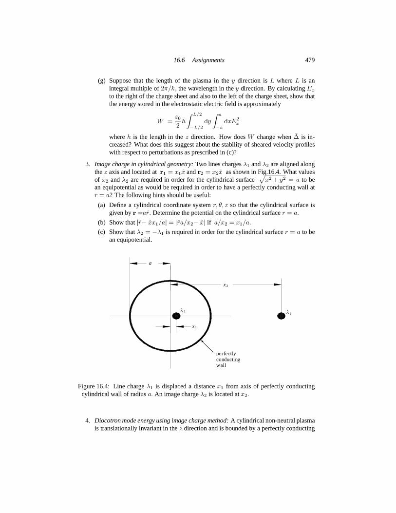
16.6 Assignments 479
(g) Suppose that the length of the plasma in they direction isL whereL is anintegral multiple of2π/k, the wavelength in they direction. By calculatingExto the right of the charge sheet and also to the left of the charge sheet, show thatthe energy stored in the electrostatic electric field is approximately
W = ε02 h
∫ L/2
−L/2dy
∫ a
−adxE2x
whereh is the length in thez direction. How doesW change when∆ is in-creased? What does this suggest about the stability of sheared velocity profileswith respect to perturbations as prescribed in (c)?
3. Image charge in cylindrical geometry:Two lines chargesλ1 andλ2 are aligned alongthez axis and located atr1 = x1x andr2 = x2x as shown in Fig.16.4. What valuesof x2 andλ2 are required in order for the cylindrical surface
√x2 + y2 = a to bean equipotential as would be required in order to have a perfectly conductingwall atr = a? The following hints should be useful:
(a) Define a cylindrical coordinate systemr, θ, z so that the cylindrical surface isgiven byr =ar. Determine the potential on the cylindrical surfacer = a.
(b) Show that|r− xx1/a| = |ra/x2− x| if a/x2 = x1/a.(c) Show thatλ2 = −λ1 is required in order for the cylindrical surfacer = a to be
an equipotential.
perfectlyconductingwall
x1
λ1 λ2
x2
a
Figure 16.4: Line chargeλ1 is displaced a distancex1 from axis of perfectly conductingcylindrical wall of radiusa. An image chargeλ2 is located atx2.
4. Diocotron mode energy using image charge method:A cylindrical non-neutral plasmais translationally invariant in thez direction and is bounded by a perfectly conducting

480 Chapter 16. Non-neutral plasmas
wall atr = a. The plasma has an equilibrium density profilen = n(r) for 0 ≤ r < rpandn = 0 for rp < r ≤ a so there is a finite-size vacuum region between the edgeof the plasmarp and the wall radiusa. Calculate the change in system energy if theplasma axis is shifted off the wall axis and compare this result to Eq.(16.65). Hintsare given below:
(a) Show that the electric field outside the plasma is the same as the electric field ofa line charge located on the plasma axis.
(b) Suppose thatx denotes the distance the plasma is shifted off the wall axis. Whatis the location and strength of the image charge required for the wall to be anequipotential? Is the force between the plasma and the image charge attractiveor repulsive. How does the image charge move asx increases from zero to somefinite value?
(c) Calculate the force on the image charge. What is the force on the plasma? Whatwork is done by the plasma in order to be displaced by a finite amountx? Ex-press this work in terms of the radial electric field perturbation at thewall.
d d d
d
d + x d + xd − x
d − x
Q
Q
Q
Q
(a) (b) (c)
capacitorplates
Figure 16.5:
5. Negative energy in terms of two capacitors with fixed charge:Consider two situationswhere a chargeQ is stored on the two parallel plate capacitorsC1 andC2 that de-form in such a way as to conserve total system volume; these situations are shown in

16.6 Assignments 481
Fig.16.5(a) and (b).
(a) Here the center plate is displaced off center by an amountx so that the volumeoccupied by the two capacitors is conserved. What is the change in the systemenergy when the center plate is displaced? Assume that the value of eachcapac-itor is C1,2 = ε0A/d1,2 whered1,2 is the distance between the parallel platesand initiallyd1 = d2.
(b) Show that the configuration in Fig.16.5(b) is electrically equivalent to the con-figuration in Fig.16.5(a). Discuss how the system shown in Fig.16.5(c) wouldrelate to anl = 4 diocotron mode (recall that any perturbations to the plasmamust be incompressible).
6. Magnetrons as a generalization of non-neutral plasmas undergoing a resistive wallinstability: The magnetron vacuum tube used in radar transmitters and in microwaveovens can be considered as a non-neutral plasma undergoing a negative energy dio-cotron instability. These tubes are simple, rugged, and efficient. The relation betweenthe non-neutral plasma resistive wall instability and the magnetron is shown in the se-quence of sketches Figs.16.6(a)-(d). The magnetron has a cylindrical geometry withan electron emitting filament (cathode) on thez axis, a segmented cylindrical wall(anode) and az-directed magnetic field produced by permanent magnets. Instead ofhaving a resistorR connected across the gap of a segmented wall as in Fig.16.6(a),the magnetron has a set of cavities connected across the gap as in Fig.16.6(d). Thecavities function as a resonant circuit and the output circuit loading provides an effec-tive resistance at the cavity resonant frequency. From the point of view of the plasma,the power appears to be dissipated in a resistor across the wall gap. However, sincethe cavity is coupled to an output waveguide, the power is actually transported awayfrom the magnetron via a waveguide to some external location where the power isused to transmit a radar pulse or cook a meal. If the cavities in Fig.16.6(d) are phased0, π then the ten cavities provide five complete azimuthal wave periods orl = 5. Ifthe electrons have near Brillouinflow, andl = 5, what axial magnetic field shouldbe used in order to have an output frequencyf =2450 MHz, the frequency used in ahome microwave oven. Why would the electron density increase to the point that theflow is nearly Brillouin, and why is the electron density not higher than thisvalue?If the voltage drop between anode and cathode is4 kV and the electron density isuniform, what nominal wall radius (distance between cathode and anode) should beused? Show that a parallel resonant circuit with a small resistance in series with thecoil as 16.6(b) has an effective resistance which peaks at the resonant frequency; whydoes one want the effective resistance to peak at the resonant frequency?
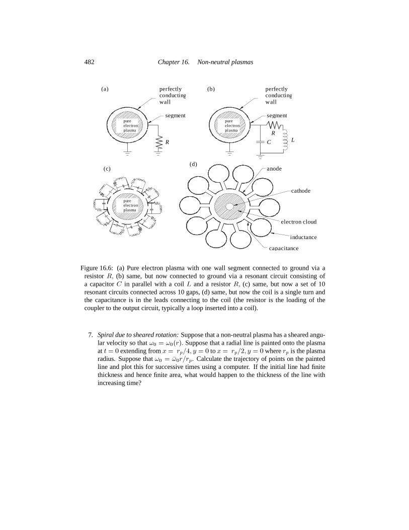
482 Chapter 16. Non-neutral plasmas
perfectlyconductingwall
perfectlyconductingwall
(a) (b)
(c)(d)
pureelectronplasma
pureelectronplasma
pureelectronplasma
segment segment
R
RLC
anode
cathode
inductance
capacitance
electroncloud
Figure 16.6: (a) Pure electron plasma with one wall segment connected to ground via aresistorR, (b) same, but now connected to ground via a resonant circuit consisting ofa capacitorC in parallel with a coilL and a resistorR, (c) same, but now a set of 10resonant circuits connected across 10 gaps, (d) same, but now the coil is a single turn andthe capacitance is in the leads connecting to the coil (the resistor is the loading of thecoupler to the output circuit, typically a loop inserted into a coil).
7. Spiral due to sheared rotation:Suppose that a non-neutral plasma has a sheared angu-lar velocity so thatω0 = ω0(r). Suppose that a radial line is painted onto the plasmaat t = 0 extending fromx = rp/4, y = 0 tox = rp/2, y = 0 whererp is the plasmaradius. Suppose thatω0 = ω0r/rp. Calculate the trajectory of points on the paintedline and plot this for successive times using a computer. If the initial linehad finitethickness and hence finite area, what would happen to the thickness of the linewithincreasing time?

17
Dusty plasmas
17.1 Introduction
Non-neutral plasmas had one less species than a conventional plasma (one species insteadof two); dusty plasmas have one more species (three species instead of two). Not sur-prisingly, the addition of another species provides new freedoms which giverise to newbehaviors.
The third species in a dusty plasma, electrically charged dust grains, typically have acharge to mass ratio quite different from that of electrons or ions. Several methods forcharging dust grains are possible. Electron bombardment is the usual means forcharginglaboratory dusty plasmas, but photoionization or radioactive decay could also be operativemechanisms and may be important for certain space and astrophysical situations. Photoion-ization would make dust grains positive because photoionization causes electrons to leavedust grains. Radioactive decay of dust grains would make the dust grains develop apolar-ity opposite to that of the particle emitted in the decay process, e.g., alpha particle emissionby dust grains would make the dust grains negative.
We shall consider here only the typical laboratory dusty plasma situation where theplasma is weakly ionized and dust grain charging is due to electron bombardment. Negativecharging occurs because the electrons, being much lighter than the ions andusually muchhotter, have a much larger thermal velocity than the ions. As a result, when a dust grainis inserted into the plasma, it is initially subject to a greaterflux of impacting electronsthan impacting ions, thereby causing the dust grain to become negatively charged. Thisnegative charge eventually becomes sufficiently large to repel incident electrons and thusattenuate the incoming electronflux. On the other hand, the negative charge of the dustgrain accelerates incident ions thereby increasing the ionflux to the dust grain. The netcharge on the dust grain reaches equilibrium when the electron and ionfluxes interceptingthe dust grain become equal. This is a dynamic equilibrium because it involvesa continuousflow of plasma to the dust grain. Some kind of external source is thus required to replenishthe plasma electrons and ions continuously, because otherwise all the plasma electrons andions would eventually collect on the dust grain. The dust grain charging process is quitesimilar to the development of afloating potential on an insulated probe immersed in aplasma (see Eq.(2.124)).
483

484 Chapter 17. Dusty plasmas
Debyeradius
ion trajectory
b r d
dustgrain
l mfp
Figure 17.1: Electrons and ions may be considered as being collisionless inside asphere ofdiameterlmfp surrounding a dust grain. The trajectory an ion making a grazing collisionis shown; this ion has an impact parameterb.
17.2 Electron and ion currentflow to a dust grain
Because an individual dust grain is much heavier than an electron or an ion, itcan beapproximated as an infinitely massive scattering center for the electrons and ions collidingwith it. In typical dusty plasma laboratory experiments the collisional mean free pathlmfpgreatly exceeds the Debye length. This situation is sketched in Fig.17.1 where a dust grainwith radiusrd is surrounded by an imaginary sphere with diameterlmfp and the Debyeradius is much smaller thanlmfp. Electrons and ions are collisionless inside thelmfpsphere and so have Keplerian orbits associated with the electrostaticcentral force producedby the charge on the dust grain. Because the dust grain is shielded by other particles,the electrons and ions only experience the central force when inside a sphere having thenominal Debye radius.
Dust grain charging involves calculating effective collision cross-sections for the elec-trons and ions colliding with the dust grain. A useful benchmark reference for thiscalcu-lation is the cross-section of charged particles colliding with a neutral dust grain. Becausecharged particles incident on a neutral dust grain have straight line trajectories, the cross-section of a neutral dust grain is just the geometrical area it projectsonto a plane, i.e.,σgeometric = πr2d. The cross-section of achargeddust grain differs fromσgeometric be-cause incident electrons and ions are deflected from straight line trajectories by the electro-static central force produced by the charge on the dust grain. The respectivecross-sectionsfor ions and electrons will now be calculated and related toσgeometric.
Fig.17.1 shows the impact parameterb and trajectory of an ion colliding with a nega-

17.2 Electron and ion currentflow to a dust grain 485
tively charged dust grain; the corresponding trajectory of an electron would curl outwardsinstead of inwards and so the electron would require a much smaller impact parameterbin order to hit the dust grain. We definev to be the initial velocity of an incident particlehaving massm and chargeq, and definevimpact as the velocity of this particle at the in-stant it makes a grazing impact with the dust grain. Using these definitions it is seen thatconservation of angular momentum imposes the requirement
vb = vimpactrd (17.1)
and conservation of energy impose the requirement
12mv
2 = 12mv
2impact + qφd (17.2)
whereφd is the potential on the surface of the dust grain. Figure 17.1 shows thatb is largerthanrd for an ion. Because the repulsive force between the negatively charged dust grainand an electron causes the trajectory of an electron to swerve in the opposite sense from anion, b is smaller thanrd for an electron; that is the electron has to be more ‘on-target’ thana neutral particle to hit the dust grain whereas an ion can be less ‘on-target’ than a neutralparticle to hit the dust grain.
Eliminatingvimpact between Eqs.(17.1) and (17.2) gives
12mv
2 = 12mv
2 b2r2d + qφd (17.3)
so the effective scattering cross-section is (Allen, Boyd and Reynolds 1957)
σ(v) = πb2 =(1− 2qφd
mv2)σgeometric. (17.4)
For qφd > 0 the interaction is repulsive and the cross-section is smaller thanσgeometric,whereas forqφd < 0 the interaction is attractive and the cross-section is larger thanσgeometric. The former case applies to electrons and the latter case applies to ions.
The total currentflowing to the dust grain for attractive interactions is
Iattractive = q∫ ∞
0σ(v)vf(v)4πv2dv. (17.5)
However, because in the repulsive situation incident particles havingv < √2qφd/m arereflected and do not hit the dust grain, the repulsive situation cross-section is zero for allparticles havingv <√2qφd/m. Thus, the total current for repulsive interactions is
Irepulsive = q∫ ∞√2qφd/m
σ(v)vf(v)4πv2dv. (17.6)
Since the region outside thelmfp sphere sketched in Fig.17.1 extends to infinity, particlescan be considered to have made many collisions before entering thelmfp sphere, and so thevelocity distribution of particles incident upon thelmfp sphere will be Maxwellian, i.e.,
f(v) = n0π3/2v3T e−v2/v2
T (17.7)

486 Chapter 17. Dusty plasmas
wherevT = √2κT/m is the thermal velocity. The incident particles will be collisionlessas they travel inside thelmfp sphere. Integration of Eqs.(17.5) and (17.6) gives
Iattractive = q∫ ∞
0πr2d
(1− 2qφd
mv2)vf(v)4πv2dv
= 2π1/2r2dn0qvT∫ ∞
0
(1− 2qφd
mv2Tx)
e−xxdx
= 2π1/2
(1− qφd
κT)n0qvTσgeometric (17.8)
and
Irepulsive = 2π1/2 r2dn0qvT∫ ∞
qφd/κT
(1− qφd
κTx)
e−xxdx
= 2π1/2 e−qφd/κTn0qvTσgeometric. (17.9)
17.3 Dust charge
As discussed above, a neutral dust grain inserted into a plasma will become negativelycharged becausevTe >> vTi. The electron currentIe is thus a repulsive-type current andthe ion currentIi is an attractive-type current. As the dust grain becomes more negativelycharged,|Ie| decreases and|Ii| increases untilIi+Ie = 0 at which time dust grain chargingceases.
The presence of negatively charged dust grains affects the quasi-neutrality condition.Assuming singly charged ions and a charge ofZd on the negatively charged dust grains,the quasineutrality condition generalizes to
ni0 = ne0 +Zdnd0. (17.10)
Since the ion density is unaffected by the charging process, it is convenient to normalize alldensities to the ion density and define
α = Zdnd0ni0 (17.11)
so that ne0ni0 = 1− α (17.12)
wherene0, ni0, andnd0 are the volume-averaged electron, ion, and dust grain densities.Furthermore, ifrd is small compared to the effective shielding lengthλd, then the dustgrain chargeZd is related to the dust grain surface potential and the dust grain radiusrd viathe vacuum Coulomb relationship, i.e.,
φd = −Zde exp(−rd/λd)4πε0rd≃ − Zde
4πε0rd if rd << λd. (17.13)

17.3 Dust charge 487
Equation (17.11) can then be written in terms of the dust grain surface potential as
α = −4πε0rdnd0ni0e φd. (17.14)
It is now convenient to introduce the dimensionless variable
ψ = − eφκTi (17.15)
so thatα becomesα = 4πnd0rdλ2diψd (17.16)
where
λdi =√ε0κTini0e2 (17.17)
is the ion Debye length. Largeψd means that ions fall into a potential energy well muchdeeper than their thermal energy.
It is also useful to introduce the Wigner-Seitz radiusa, a measure of the nominal spacingbetween adjacent dust grains. This spacing is defined by dividing the total volume of thesystemV by the total number of dust grainsN to find a nominal volume surrounding eachdust grain. It is then imagined that this nominal volume is spherical with radiusa so that
N 4πa33 = V (17.18)
in which case
nd0 = 34πa3 (17.19)
and
α = 3rdλ2dia3 ψd. (17.20)
It is also convenient to normalize lengths to the ion Debye length so
α = Pψd (17.21)
whereP = 3 rda3 (17.22)
and the bar means normalized to an ion Debye length.The dust charge can also be expressed in a non-dimensional fashion using Eq.(17.13)
to give Zd4πni0λ3di
= rdψd . (17.23)
Thefloating conditionIi + Ie = 0 shows that the equilibrium dust potential is givenby
0 = ni0vTi
(1− eφd
κTi)− ne0vTe exp(eφd/κTe) (17.24)
which can be re-arranged as
(1 + ψd)√meTimiTe exp(ψdTi/ Te) = 1−α. (17.25)

488 Chapter 17. Dusty plasmas
However, using Eq.(17.21) this becomes
(1 + ψd)√meTimiTe exp(ψdTi/ Te) = 1 − Pψd, (17.26)
a transcendental equation relatingψd andP.Equation (17.26) shows that, for a given temperature ratioTi/Te and given mass ratio
me/mi, the normalized dust grain surface potentialψd is a function ofP, a dimension-less parameter incorporating the geometrical information characterizing the dust grains inthe dusty plasma. Becauseψd appears non-algebraically in Eq.(17.26), it is not possible tosolve forψd(P ) without resorting to numerical methods. However, solving the inverse rela-tion, namelyP (ψd), is straightforward becauseP occurs only once in Eq.(17.26). Solvingfor P gives (Havnes, Goertz, Morfill, Grun and Ip 1987)
P = 1ψd −(
1 + 1ψd
)√meTimiTe exp(ψdTi/ Te). (17.27)
Figure 17.2: Plots oflogP andα v. logψd for Te = 100Ti andTe = Ti. Logarithms arebase 10 and ion mass is 40 amu. SinceP is proportional to the dust grain density the righthand side of these curves, i.e., smallP, corresponds to the limit of low dust grain density.

17.3 Dust charge 489
The upper plot in Fig. 17.2 showslogP plotted versus logψd for two cases correspond-ing to two typical laboratory configurations where dusty plasma experiments have beenconducted; the lower plot shows the corresponding dependence ofα onψd. The Te = Ticonfiguration corresponds to a potassium Q-machine plasma while theTe = 100Ti con-figuration corresponds to an argon rf discharge. An ion of 40 atomic mass units has beenassumed for both cases. Figure 17.2 shows thatP varies inversely withψd up to somecritical value and then, forψd above this critical value,P heads sharply to zero for mod-est increases inψd. The lower plot shows thatα is near unity to the left of the knee andthen drops sharply to zero to the right of the knee. Comparison of the solid and dashedcurves shows that the saturated value ofψd is an increasing function ofTe/Ti. The satura-tion value ofψd is 2.5 for the Q-machine parameters whereas the saturated value ofψd forthe rf discharge is∼ 2 × 10². SinceP is proportional toa−3 and hence to the dust graindensity, the right hand side of these plots (i.e., whereP is small) correspond to the limit ofsmall dust grain density. Also, comparison of the solid and dashed plots shows thatψd in-creases withTe/Ti. Since Eq.(17.23) shows thatZd is proportional toψd, it is seen thatZdalso saturates on moving to the right in the plots and largestZd occurs at highTe/Ti andsmall dust grain density.
The downward sloping segment on the left of Fig. 17.2 corresponds to theα ≃ 1regime which is the situation where the dust grain density is large, nearlyall the electronsare attached to the dust grains, and the plasma has almost no free electrons. On the otherhand, the saturated limit ofψd on the right of Fig. 17.2 corresponds to theα << 1 regimewhich is where there is minimal depletion of free electrons, the dust grain density is low,and there is a very high charge on each of the relatively small number of dust grains.
There are thus three regimes:1. The regime well to the left of the knee in the curves.Hereα ≃ 1 and nearly all
electrons are attached to the dust grains. To the extent thatα approaches unity, thedust grains replace the electrons as the negative charge carriers.
2. The regime to the right of the knee in the curves.Hereα << 1, most electrons arefree, and the potential of an individual dust grain is very high and near at itssaturationvalue (right hand side of plots). This regime corresponds to smallP and a very smalldust grain density.
3. The regime in the vicinity of the knee in the curves.If Te >> Ti then it is possible tohave both α of order unity andψd large even thoughψd is not quite at its saturationlevel. In this regime the majority of electrons reside on the dust grains, the dust grainsare highly charged, and the dust grain density is appreciable. Crystallization of thedust grains can occur in this regime since crystallization requires a combination ofhigh dust grain charge and small separation between dust grains.

490 Chapter 17. Dusty plasmas
Figure 17.3: Dusty plasma parameter space showing contours of constantψd, α, andZd/4πni0λ3Di for an argon plasma withTe/Ti = 100. The experimental line correspondsto the density range of the Chu and I experiment (Chu and I 1994); these plots are fromBellan (2004).
17.4 Dusty plasma parameter space
A dusty plasma is characterized by its normalized dust radiusrd and normalized dust in-terparticle spacinga. These quantities determineP and, givenP, the normalized dustsurface potentialψd is obtained by solving Eq.(17.27). KnowingP andψd givesα usingEq.(17.21). The consequence of this logical chain of argument is thatα can be consideredto be a function ofrd anda.
A dusty plasma parameter space can thus be constructed wherea is the horizontal com-

17.5 LargeP limit: dust acoustic waves 491
ponent andrd is the vertical component so that a given dusty plasma would correspond toa point in this parameter space. The quantitiesψd, α, andZd/4πni0λ3di are all functionsof a andrd and so contours of these three quantities can be drawn in thea, rd parameterspace for specifiedme/mi andTe/Ti. Examples of these contours are shown in Fig.17.3for an argon plasma withTe = 100Ti. An actual experiment would have specific values ofa andrd and so would be represented as a point in this parameter space. Variationof theion density in the experiment would change the value ofλdi while keeping the ratiord/afixed and so would correspond to moving along a sloped line in parameter space. The shortsloped line in Fig.17.3 represents the density in the dusty plasma experimentby Chu and I(1994) to be discussed later (the finite length of this line corresponds to the error bars forthe density measurement).
17.5 LargeP limit: dust acoustic waves
The large P limit (i.e., regime 1 discussed above) has nearly all the electrons attachedto the dust grains so that the plasma effectively consists of negatively charged dust grainsand positive ions. A wave similar to the conventional ion acoustic wave can propagate inthis regime, but the role played by positive and negative particles isreversed: here the ionsare the light species and the dust grains are the heavy species. In order to appreciate theconsequence of this role reversal, consider the conventional ion acoustic wave from themost simplistic point of view. The wave phase velocityω/k is assumed to be much fasterthan the ion thermal velocityvTi (i.e., cold ion regime) but much slower than the electronthermal velocityvTe (i.e., isothermal electron regime) so the respective approximations ofthe electron and ion equations of motion are
0 = −neeE−∇ (neκTe) (17.28)
nimiduidt = niZeE. (17.29)
Adding the electron and ion equations and assuming quasineutralityne ≃ niZ, gives
nimiduidt = −∇ (neκTe) (17.30)
showing that the effective force acting on the ions is the electron pressure gradient. Thisforce is coupled to the ions via the electric field. In effect, the electron pressure gradientpushes against the electric field which in turn pushes the ions. Linearizing Eq.(17.30) givesa result similar to a conventional sound wave, except that the system is isothermal withrespect to the electron temperature (in a normal neutral gas sound wave, the gas temperaturewould appear in the right hand side, the gas would be adiabatic, and so aγ would appearupon linearizing the gas pressure). Linearization of Eq.(17.30) and invokingthe linearizedquasineutrality relationne1 ≃ ni1Z, gives
ni0mi∂ui1∂t = −ZκTe∇ni1. (17.31)
The linearized ion equation of continuity is
∂ni1∂t + ni0∇ · ui1 = 0. (17.32)

492 Chapter 17. Dusty plasmas
The equations are combined by taking the divergence of Eq.(17.31) and then substitutingEq.(17.32) to obtain
∂2ni1∂t2 = ZκTe
mi∇2ni1 (17.33)
which is a wave equation with wave velocityc2s = ZκTe/mi.This method can now be generalized to a plasma consisting of ions with charge+e,
free electrons with charge−e, and dust grains with charge−Zde. The free electron densityis assumed to be small so thatP >> 1 in which case the configuration is on the left ofFig.17.2. The wave phase velocity is assumed to be much faster than the dust grain thermalvelocity, but much slower than the ion/electron thermal velocities so the respective electron,ion and dust grain equations of motion are
0 = −neeE−∇ (neκTe) (17.34)
0 = +nieE−∇ (niκTi) (17.35)
ndmdduddt = −ndZdeE. (17.36)
Adding the above three equations and invoking quasineutrality (i.e.,ni = ndZd + ne)results in
ndmdduddt = −∇ (niκTi + neκTe) . (17.37)
In analogy to the conventional ion acoustic wave, here the ion and electron pressures coupleto the dust via the electric field. Linearization of Eq.(17.37) gives
nd0md∂ud1∂t = −κTi∇ni1 − κTe∇ne1 (17.38)
while linearization of Eqs.(17.34) and (17.35) gives
0 = −ne0eE1−κTe∇ne1 (17.39)
0 = +ni0eE1−κTi∇ni1. (17.40)
EliminatingE1 between these last two equations shows that
κTe∇ne1 = −ne0ni0 κTi∇ni1 (17.41)
which can be integrated to give
ne1 = −ne0Tini0Teni1. (17.42)
Inserting Eq.(17.42) into the linearized quasineutrality expressionni1 = nd1Zd + ne1gives
ni1 = 11 + ne0Ti
ni0TeZdnd1 (17.43)
and hence
ne1 = − ne0Ti/ni0Te1 + ne0Ti
ni0TeZdnd1. (17.44)
17.5 LargeP limit: dust acoustic waves 493
Substitution forni1 andne1 in Eq.(17.38) gives
nd0md∂ud1∂t = −κTi 1− ne0/ni0
1 + ne0Tini0Te
Zd∇nd1≃ −κTiZd∇nd1 (17.45)
sincene0 << ni0 and typicallyTi/Te << ni0/ne0.The linearized dust continuity equation is
∂nd1∂t + nd0∇ ·ud1 = 0 (17.46)
so taking the divergence of Eq.(17.45) and substituting Eq.(17.46) gives
∂2nd1∂t2 = ZdκTi
md∇2nd1 (17.47)
which is a wave with phase velocity
c2da = ZdκTimd
. (17.48)
This wave is called the dust acoustic wave and its phase velocity is extremely low becauseof the large dust grain mass.
This analysis could be extended to include finitekλD terms as obtained by using thefull Poisson’s equation instead of making the simplifying assumption of perfectneutrality.A Vlasov approach could also be invoked to demonstrate the effect of Landau damping.Rather than work through the details of these extensions, one can argue that theα ≃ 1 dustyplasma is effectively a two-component plasma where the heavy particles are the negativelycharged dust grains and the light particles are the positively charged ions. Thepreviouslyderived results from both two-fluid theory and Vlasov theory could then be invoked bysimply identifying the heavy and light particles in the manner stated above. Thus by makingthe identification,
ion acoustic wave dust acoustic waveinertia provided by ions dust grainsrestoring force provided by electron pressure ion pressure
taking into account finitek2λ2D terms will result in a dispersive dust acoustic wave
ω2 = k2c2da1 + k2λ2Di
. (17.49)
Similarly, just as an electronflow velocity faster than the ion acoustic phase velocity woulddestabilize ion acoustic waves via inverse Landau damping, a Landau analysis would showthat an ionflow velocity faster than the dust acoustic phase velocity would destabilize dustacoustic waves.
Destabilized dust acoustic waves have been observed in an experiment byBarkan, Mer-lino and D’Angelo (1995). The phase velocity of these waves was of the order of 10 cm/swhich is an order of magnitude less than a human walking speed.

494 Chapter 17. Dusty plasmas
17.6 Dust ion acoustic waves
The presence of dust grains can also substantially modify the propagationproperties ofconventional ion acoustic waves. In a conventional electron-ion plasma, ion acoustic wavescan propagate only ifTe >> Ti. This is because strong ion Landau damping occurs whenthe wave phase velocity is of the order of the ion thermal velocity and this is impossibleto avoid unlessTe >> Ti since the conventional ion acoustic phase velocity scales asc2s = (γκTi + κTe)/mi.
As in the conventional ion acoustic wave, the derivation of dust ion acoustic wavesinvolves the linearized electron and ion equations
0 = −ne0eE1−κTe∇ne1 (17.50)
ni0mi∂ui∂t = +ni0eE1−γκTi∇ni1 (17.51)
but here the possibility of finiteTi has been retained in order to allow consideration oftheTe ∼ Ti regime. The wave frequency is assumed to be sufficiently high so that thedust grains are unable to respond to the wave; the dust grains are effectively consideredas being infinitely massive and therefore stationary. In this limit the dust grains contributeto the equilibrium quasineutrality conditionni0 = ne0 + Zdnd0 but since the dust grainsare assumed stationary their density cannot change and so the linearized quasi-neutralitycondition isni1 = ne1. Thus, infinitely massive dust grains affect the equilibrium electrondensity, but not the perturbed electron density.
EliminatingE1 between Eqs.(17.50) and (17.51) gives
ni0mi∂ui∂t = −ni0ne0 κTe∇ne1−γκTi∇ni1. (17.52)
Sinceni1 = ne1 andni0/ne0 = ni0/(ni0 −Zdnd0), Eq.(17.52) becomes
nimi∂ui∂t = − 1
1−Zdnd0/ni0 κTe∇ni−γκTi∇ni. (17.53)
Taking the divergence and using Eqs. (17.11) and (17.32) gives
mi∂2ni1∂t2 =
( 11−ακTe+γκTi
)∇2ni1 (17.54)
which gives the dust ion acoustic wave (Shukla and Silin 1992), a wave with phase velocity
c2DIA = 11−α
κTemi
+γ κTimi. (17.55)
As α approaches unity, the dust ion acoustic wave phase velocity becomes muchgreaterthan the ion thermal velocity even in a plasma havingTi = Te. The dust ion acoustic wavethus propagates without being attenuated by ion Landau damping in aTi = Te plasmahavingα ≃ 1, which corresponds to the left side of Fig.17.2. Thus, the presence of a largedust grain density enables the propagation of ion acoustic waves that normally would bedamped in aTe = Ti plasma; this has been observed in experiments by Barkan, D’Angeloand Merlino (1996).

17.7 The strongly coupled regime: crystallization of a dusty plasma 495
17.7 The strongly coupled regime: crystallization of a dustyplasma
The mutual repulsive force between two negatively charged dust grains scales asZ2d andso will be very large for highly charged dust grains. In the extreme limit ofthis situa-tion the electrostatic potential energy between dust grains might exceed their kinetic en-ergy so that the grains would tend to form an ordered, crystallized state. The possibil-ity that dust grains might crystallize was first suggested by Ikezi (1986)and has sincebeen demonstrated in a number of experiments (Chu and I 1994, Melzer, Trottenberg andPiel 1994, Thomas, MorfillL, Demmel, Goree, Feuerbacher and Mohlmann 1994, Hayashiand Tachibana 1994, Nefedov, Morfill, Fortov, Thomas, Rothermel, Hagl, Ivlev, Zuzic,Klumov, Lipaev, Molotkov, Petrov, Gidzenko, Krikalev, Shepherd, Ivanov, Roth, Binnen-bruck, Goree and Semenov 2003, Morfill, Annaratone, Bryant, Ivlev, Thomas, Zuzic andFortov 2002). The threshold criterion for crystallization will be discussed in this sectionfollowing a model by Bellan (2004b). The threshold is determined by considering certainissues relating to the validity of the conventional Debye shielding model andthe Boltzmannrelation.
LargeZd corresponds to largeψd which in turn corresponds to operating towards theright of Fig. 17.2. Since the location of the saturation value ofψd increases withTe/Ti,very largeψd can occur ifTe >> Ti. The repulsive force also scales inversely with thesquare of the distance separating the two dust grains, i.e., the repulsiveforce also scalesasn2/3
d0 . SinceP is proportional tond0, the maximum repulsive force would be obtainedaround the knee in theTe >> Ti curves in Fig. 17.2 since at this location it is possible tohave largeψd withoutndo becoming infinitesimal.
The repulsive electrostatic force between two dust grains is attenuated by Debye shield-ing. This shielding can be calculated by considering a single dust grain to be a test particleimmersed in a plasma consisting of electrons, ions, and other dust grains which will be re-ferred to as “field” dust grains. The test particle will be completely shielded beyond somecritical radius. A field dust grain located beyond this critical radius will experience no in-teraction with the test particle dust grain whereas if the field dust grain is located within theshielding radius, it will experience an enormous repulsive force. The test particle dust grainthus acts like a finite-radius hard sphere in its interactions with field particle dust grains.
A quantitative model for these interactions between dust grains can be developed byconsidering Poisson’s equation for a dusty plasma,
∇2φ = − 1ε0 (nie− nee−Zdnde) . (17.56)
The usual test-particle argument (see p.8) involves linearization of theBoltzmann relationfor each species to obtain a linearized density for each species. These linearized densitiesare then substituted into Poisson’s equation resulting in the Yukawa-type solution,
φ = − qt4πε0r exp(−r/λD) (17.57)
whereλ−2D = ∑ λ−2
Dσ . However, this linearization is based on the assumption|qtφ/κTσ|<< 1 which is clearly not true in the vicinity of a highly charged dust grain. This inconsis-

496 Chapter 17. Dusty plasmas
tency cannot be resolved influid theory and it is necessary to revert to the more fundamentalVlasov description.
Particles are characterized by a velocity distribution functionf(r,v) in the Vlasov de-scription and the Vlasov equation describes the time evolution off. The test particle loca-tion is defined to be at the origin of a spherical coordinate system and the system is assumedto be spherically symmetric so that the only spatial dependence ofφ andf is on the spheri-cal radiusr. The nominal location of the last collision made by a particle incident uponthetest particle is the collision mean free pathλmfp and since any particle incident upon thetest particle will have traveled many mean free paths, the velocity distribution of particlesentering a sphere of orderlmfp will be Maxwellian. Because the incident particles are col-lisionless within theλmfp sphere, their velocity distribution function must be a solution tothe collisionless Vlasov equation inside the sphere. The boundary condition this solutionmust satisfy is that its larger limit should correspond to the collisional (i.e., Maxwellian)distribution.
Solutions to the collisionless Vlasov equation are functions of constants of themotionas was shown in Sec.2.2 and the appropriate constant of the motion here is the particleenergyW =mσv2/2+ qσφ(r). Hence the distribution function in the collisionless regionnear the test particle must be
fσ (r,v) = nσ0( mσ2πκTσ
)3/2exp
(−mσv2/2 + qσφ(r)κTσ
)(17.58)
since this maps to a Maxwellian distribution at large distancesr whereφ(r) → 0.A negatively charged particle such as a dust grain or an electron experiences a repulsive
force upon approaching the dust grain test particle and so slows down. Some approachingnegatively charged particles reflect and so the minimum velocity of electrons or dust grainsapproaching the dust grain test particle is zero. The density of these particles will thus be
nσ =∫ ∞
0fσ (r,v) d3v
= nσ0 exp(−qσφ(r)κTσ
)(17.59)
which is the same as thefluid theory Boltzmann relation. It is useful at this point to changeover to the non-dimensional scalarψ defined in Eq.(17.15). Since the dust grains are neg-atively charged,ψ is large and positive in the vicinity of a dust grain. The respectivenormalized electron and field dust grain densities are thus
nene0 = exp (−ψTi/Te) (17.60)
ndnd0 = exp (−Zψ) (17.61)
whereZ = ZdTi/Td. (17.62)
Both the electron and field dust grain densities decrease in the vicinity of the dust grain testparticle. However, becauseZ is typically very large andTi/Te is assumed to be very small,the field dust density scale length is much shorter than the electron density scale length.

17.7 The strongly coupled regime: crystallization of a dusty plasma 497
Ion dynamics are qualitatively different because all ions approaching the dustgrain areaccelerated, leading to the situation that no zero velocity ions exist near the dust grain. Inparticular, an ion starting with infinitesimal inward velocity at infinity whereψ = 0 hasnearly zero energy, i.e.,W ≃ 0. The energy conservation equation for this slowest ion is
miv2/2 + eφ(r) = 0 (17.63)
and so the velocity for this slowest ion has the spatial dependence
vmin =√
−2eφ(r)mi
. (17.64)
The ion density is thus
ni(r) =∫ ∞
vmin
fi (r,v) d3v
= ni0( mi2πκTi
)3/2exp
(− qiφ(r)κTi
)∫ ∞
vmin
exp(−mv2/2κTi
)d3v
= ni0 4√π exp (ψ)∫ ∞√ψ
exp (−ξ2) ξ2dξ. (17.65)
This can be expressed in terms of the Error Function
erf z = 2√π∫ z
0exp(−ξ2)dξ (17.66)
and, in particular, using the identity
4√π∫ ∞
zexp (−ξ2) ξ2dξ = 2√π
∫ ∞
zdξ exp(−ξ2) − 2√π
∫ ∞
zdξ d
dξ(ξ exp(−ξ2))
(17.67)it is seen that (Laframboise and Parker 1973)
nini0 = exp (ψ)
(1− erf√ψ
)+ 2√π
√ψ . (17.68)
The error function has the small-argument limit
limz→0 erf z ≃ 2z√π (17.69)
and so forψ << 1 nini0 = 1+ ψ (17.70)
which is identical to the Boltzmann result given byfluid theory.However, because
limz→∞ e−z2 (1− erf z) = 0, (17.71)
whenψ >> 1 the ion density has a non-Boltzmann dependence
nini0 = 2√π
√ψ (17.72)

498 Chapter 17. Dusty plasmas
which is much smaller than theexp(ψ) dependence predicted by the Boltzmann relation.Poisson’s equation can be written non-dimensionally as
1r2
∂∂r
(r2 ∂ψ∂r
)= ni
ni0 − neni0 − Zdnd
ni0= ni
ni0 − (1− α) nene0 − α ndnd0 (17.73)
where, following the normalization convention introduced earlier,r = r/λdi.Upon substi-tuting for the normalized densities, Poisson’s equation becomes
1r2
∂∂r
(r2 ∂ψ∂r
)
︸ ︷︷ ︸vacuum
= eψ(1− erf
(√ψ))
+ 2√π√ψ
︸ ︷︷ ︸ions
−(1− α) exp(−ψTiTe
)
︸ ︷︷ ︸electrons−α exp (−Zψ)
︸ ︷︷ ︸dust
. (17.74)
Becauseψ becomes large near the dust grain, this equation is highly non-linear and sothe linearization technique used on p. 8 for the conventional Debye shieldingderivationcannot be invoked. Instead, an approximate solution to Poisson’s equation is obtained byseparating the collisionless region around the dust grain test particleinto three concentriclayers (regions) according to the magnitude ofψ :
Region 1 Region 2 Region 3Definition ψd > ψ > 1 1 > ψ > 1/Z 1/Z > ψLocation adjacent to dust grain middle spherical layer outer layerIons non-Boltzmann, fast Boltzmann BoltzmannElectrons Boltzmann Boltzmann BoltzmannDust zero density zero density BoltzmannDependence vacuum-like w/const. growing/decaying Yukawa decaying Yukawa
Poisson’s equation has the following approximations in the three regions
Region 1 :1r2
∂∂r
(r2 ∂ψ∂r
)= 0 (17.75)
Region 2 :1r2
∂∂r
(r2 ∂ψ∂r
)= ψ + α (17.76)
Region 3 :1r2
∂∂r
(r2 ∂ψ∂r
)= (1 + αZ)ψ . (17.77)
The reasons for these approximations are as follows:

17.7 The strongly coupled regime: crystallization of a dusty plasma 499
In region 1,ψ >> 1 so that the ion density is given in principle by Eq.(17.72) whichwould give a right hand side scaling as
√ψ. This ion term would dominate the electron anddust terms since the latter are always less than unity in this region. Thus,keeping just theion term on the right hand side, Poisson’s equation in region 1 reduces to
1r2
∂∂r
(r2 ∂ψ∂r
)
︸ ︷︷ ︸vacuum
≃ 2√πψψ︸ ︷︷ ︸ion
; (17.78)
however, the ion term above can be neglected compared to the vacuum termbecause√ψ >> 1 sinceψ >> 1. Thus Poisson’s equation can be approximated in region 1 byjust the vacuum term. This assumption is quite good near the dust grainsurface whereψ isindeed very large compared to unity, but becomes marginal whenψ approaches unity at theouter limit of region 1.
In region 2, the ions have a Boltzmann distribution soni/ne0 = 1+ψ.SinceTi/Te <<1, the normalized electron density isne/ne0 = exp(−ψTi/Te) ≃ 1. BecauseZψ>> 1,the dust density is nearly zero in this region.
In region 3, Eq.(17.74) approximates to
1r2
∂∂r
(r2 ∂ψ∂r
)
︸ ︷︷ ︸vacuum
≃ 1 + ψ︸ ︷︷ ︸ions
− (1− α)(1− ψTi
Te)
︸ ︷︷ ︸electrons
− (1− Zψ)α︸ ︷︷ ︸
dust
≃ (1 + αZ)ψ (17.79)
whereTi/Te << 1 has been used. For finiteα, the dust term dominates becauseαZ >> 1.The system has two boundary conditions, one at the dust grain surface and the other at
infinity. The former occurs in region 1 and is set by the radial electric field on the dust grainsurface. This boundary condition is obtained from Gauss’ law which relates∂ψ/∂r at thedust grain surface to the dust grain charge and radius. The boundary condition atinfinitycan be considered as the larger limit for region 3 and requiresψ to vanish asr goes toinfinity.
If the same form of Poisson’s equation were to characterize regions 1, 2, and 3, thenthe system would be governed by a single second-order ordinary differential equation andthe two boundary conditions described in the previous paragraph would suffice to givea unique solution. However, the equations in regions 1, 2, and 3 differ from each otherand so must be solved separately with appropriate matching at the two interfaces betweenthese three regions. The criteria for matching at the interfaces, determined by integratingPoisson’s equation twice across each interface, are that bothψ and its radial derivative mustbe continuous at each interface. An important feature of this analysis is thatthe locationsof the two interfaces are unknowns to be determined by solving the matching problem.Since regions 1 and 2 are of finite extent, both decaying and non-decayingψ solutions areallowed in these regions. However, only a decaying solution is allowed inregion 3.
Region 1, which is governed by Eq.(17.75), has vacuum-like solutions of the formψ ∼ cr−1 + d wherec andd are constants. The constantc is chosen to give the correctradial electric field at the surface of the dust grain test charge andd is chosen so thatψ = 1at ri which is the as-yet undetermined location of the interface between regions1 and 2.

500 Chapter 17. Dusty plasmas
Using Gauss’s law to prescribe the radial electric field at the dust grain surface and alsochoosingd so thatψ = 1 at r = ro gives
ψ1(r) =αa33 +
(1− 1
riαa33
)r
r . (17.80)
In region 2, which is governed by Eq.(17.76), the effective dependent variable isψ+αwhich has growing and decaying Yukawa-like solutions∼ exp(±r)/r. It is convenient towrite the region 2 solution as
ψ2(r) =ro
( 1Z +α
)cosh (r − ro) +B sinh (r − ro) −αr
r (17.81)
where the coefficients have been chosen so thatψ = 1/Z at ro, the as-yet undeterminedlocation of the interface between regions 2 and 3. The coefficientB is also undeterminedfor now, and it should be noted thatψ is independent ofB at r = ro.
Region 3, governed by Eq.(17.77), has a solution which can be expressed as
ψ3(r) = r0Zr exp
(−√αZ + 1 (r − r0))
(17.82)
where the coefficients have been chosen to giveψ = 1/Z at ro, the interface betweenregions 2 and 3.
The condition that∂ψ/∂r is continuous atro gives
B = α− roZ√αZ +1 (17.83)
and this result completes the matching process atro since bothψ and∂ψ/∂r have nowbeen arranged to be continuous atro. Sinceψ1 = 1 has already been arranged atri, inorder to have continuity ofψ at ri it is necessary to setψ2 = 1 at ri, i.e.,
ri = ro( 1Z + α
)cosh (ri − ro) +B sinh (ri − ro)− αri. (17.84)
All that remains to be done is to arrange for continuity of∂ψ/∂r at r = ri. Sinceψhas already been arranged to be continuous atr = ri, continuity of∂ (rψ) /∂r at r = riimplies continuity of∂ψ/∂r. This means that continuity of∂ψ/∂r at r = ri is attainedby equating the derivatives of the numerators of the right hand sides of Eqs.(17.80) and(17.81) at ri, i.e., continuity of∂ψ/∂r at r = ri is attained by setting
1− 1riαa33 = ro
( 1Z + α
)sinh (ri − ro) +B cosh (ri − ro)− α . (17.85)
SinceZ >> 1 andα is of order unity, Eqs.(17.84) and (17.85) can be approximated as
(1 +α) ri = αro cosh (ri − ro) +α sinh (ri − ro) (17.86)
1 +α− 1riαa33 = αro sinh (ri − ro) +α cosh (ri − ro) . (17.87)

17.7 The strongly coupled regime: crystallization of a dusty plasma 501
These constitute two coupled nonlinear equations in the unknownsri and ro and canbe solved numerically. Since the parametersα and a in these equations are functions ofposition in dusty plasma parameter space, Eqs.(17.86) and (17.87) can be solved for riand ro at any point in dusty plasma parameter space. Because a different solutionsetri, ro exists at each point in dusty plasma parameter space,ri andro may be consideredas functions of position in dusty plasma parameter space, i.e.,ri = ri(a, rd) and ro =ro(a, rd).
Now consider the density of the field dust grains in the vicinity ofr = ro. For r > rothe normalized potential is prescribed by Eq.(17.82) and decays at the dust Debye lengthwhich is an extremely short length becauseZ >> 1. This precipitous spatial attenuationof ψ for r > ro means that dust grains are completely shielded from each other when theirseparation distance slightly exceedsro. If this is the case, then the dust grains will notinteract with each other; i.e., they can be considered as a gas of non-interacting particles.On the other hand, ifr < ro, the normalized potentialψ then exceeds1/Z and the dustgrains will experience a strong mutual repulsion. This abrupt change-over is implicit inEq.(17.61) which indicates thatnd/nd0 is near unity whenψ << 1/Z (i.e., just outsider = ro) but near zero whenψ becomes significantly larger than1/Z (i.e., just insider = ro). Hence, a dust grain test particle can be considered as a hard sphere of radiusrowhen interacting with field dust grains.
Since the nominal separation between dust grains isa, if a > ro then each dust grain iscompletely shielded from its neighbors in which case the dust grains behave asan ideal gasof non-interacting particles. However, ifa < ro is attempted, each dust grain experiencesthe full, unshielded repulsive force of its neighbors. This extreme repulsiveforce meansthat it is not possible fora to become less thanro. In effect, each dust grain sees its neighboras a hard sphere of radiusr0. Thus, whena = ro the collection of pressed-together dustgrains should form a regularly spaced lattice structure with lattice spacing of ordera = ro.The dusty plasma has thus crystallized.
The condition for crystallization of a dusty plasma is thus
a ≤ ro(a, rd) (17.88)
which defines a curve in dusty plasma parameter space. Figure 17.4 shows a plot of con-tours ofro/a in dusty plasma parameter space; for reference the region in parameter spaceassociated with the Chu and I dusty plasma crystallization experimentis indicated as a boldline (as mentioned before, the finite length of this line corresponds to the density measure-ment error bars). The contourro(a, rd)/a = 1 gives the crystallization condition; abovethis contour the dust grains are crystallized. It is also necessaryto haverd small as wasspecified in Eq.(17.13) so thatψd is not attenuated from its vacuum value by the effect ofthe shielding cloud.
Figure 17.5 shows plots oflog10 ψ, ψ, 104ψ, ne/ne0, ni/ni0, andnd/nd0 as functionsof r for a dusty plasma on the verge of condensation. The functional form ofψ is obtainedfrom the ri and ro values determined by solving Eqs.(17.86) and (17.87). The extremelyrapid cutoff of the potential atro, the interface between regions 2 and 3 is evident; thecharacteristic scale of this cut-off is the dust Debye length. The normalized densities areplotted using Eqs.(17.60), (17.68), and (17.61). The field dust grain density vanishes forr

502 Chapter 17. Dusty plasmas
insidero, consistent with the hard-sphere behavior of the dust grain test particle. Althoughψ is tiny at the interface between regions 2 and 3, it nevertheless affects the average dustgrain density profile at this location because of the extremely largecharge on the dustgrains.
Figure 17.4: Contours ofro/a as determined from solution to matching problem. Conden-sation (crystallization) is predicted to occur above thero/a = 1 line. Chu and I (1994)crystallization experiment, shown as bold line, is seen to lie in the condensation region.

17.7 The strongly coupled regime: crystallization of a dusty plasma 503
Figure 17.5: Plots oflog10 ψ, ψ, 104ψ, ne/ne0, ni/ni0, andnd/nd0 as functions ofr fora dusty plasma on the verge of condensation. Dust grain radius is at left of region1,parameters are from Bellan (2004b).

504 Chapter 17. Dusty plasmas
17.8 Assignments
1. AssumingTe = 3 eV,Ti = 0.03 eV, andni = 109 cm−3, estimate to within an orderof magnitude how long it would take for5 µm dust grains with densitynd = 105cm−3 to become fully charged. Hint- estimate the initial electron current impingingon a dust grain and compare this to the final charge on the dust grain. Use Fig. 17.3to estimateZd.
2. Orbital motion limit and angular momentum: The (OML) approximation ignores theeffective potential resulting from centrifugal force. The validity ofthis approxima-tion is examined here for the cases of an algebraically decaying central force and anexponentially decaying central force.
(a) Show that when centrifugal force is taken into account, the radial equation ofmotion for a particle in a spherically symmetric electrostatic potential φ(r) is
mr = −∂χ∂rwhere the effective potentialχ is given by
χ = qφ(r) + mb2v22r2
andm,b, andv are defined as in Sec. 17.2.
(b) Show that ifqφ is negative, a local minimum of the effective potential exists atsome radial positionr1; compare this situation to planetary motion in the solarsystem.
(c) Show that ifqφ ∼ −r−n there can also be a local maximum at a radiusr2 wherer2 > r1 providingn satisfies a certain condition. What is this condition forn?Plotχ(r) for the situation where there is a local maximum. Can a particle inci-dent from infinity reachr1 if its energy is less thanχ(r2). What sort of conditiondoes this placem, v, andb. Under what circumstances is the OML approxima-tion valid? Plot trajectories for the situations where the OML approximation isvalid and situations where it fails. Comment on whether OML is a reasonableapproximation for dust charging.
(d) Repeat (c) above for the situation whereqφ ∼ − exp(−r/λ).3. Assume the OML approximation is valid so that the effective potential can be consid-
ered to have a minimum in the vicinity of a negatively charged dust particle. Showthat, if an incident ion does not hit the dust grain, it will reflect back to infinity. Showthat a collision could cause an incident ion to be trapped in the effective potential wellatr1 as discussed in problem 1b. Once an ion becomes trapped how long would it staytrapped?
4. Dust Alfvén waves: Show that for waves with frequency below the dust grain cy-clotron frequency, a dusty plasma will support MHD Alfvén waves with dispersionω2 = k2zv2A wherev2A = B2/ndmd.

17.8 Assignments 505
5. Dust whistler waves: Show that a dusty plasma withα ≃ 1 will support whistler-likewaves with dispersionω ≃ ωci cosθ whereωcd << ω << ωci.
6. Make a plot like Fig. 17.3 for a dusty plasma withTe = Ti and discuss whether sucha plasma could condense and form crystals.
7. Consider a methane plasma consisting of CH4 ions and electrons. Assume that thereexist some infinitesimal dust nuclei att = 0 and that these become negatively chargedas discussed in Sec. 17.2.Further assume that any methane ion hitting the dust grain sticks to the dust grain sothat the mass of the dust grain increases with time. Plot the dust grain radius as afunction of time. How long would it take for the dust grains to become sufficientlylarge to form a crystal (assume thatnd = 105 cm−3, Te/Ti = 100, λdi = 100 µm)?
8. Consider a weakly ionized dusty plasma with 5µm diameter dust grains, 3 eV elec-trons and room temperature (0.025 eV) argon ions. The dusty plasma is located abovea horizontal metal plate lying in thez = 0 plane. Because electrons move faster thanions and dust grains, the electronflux to the metal plate is initially much larger thanthe ion or dust grainflux. The faster rate of loss for electrons causes the dusty plasmato become positively charged so that an electric field develops which tends to retardthe electrons and accelerate the ions towards the metal plate. Thus, theplasma poten-tial is positive with respect to the metal plate and if the plasma potential is defined tobe zero, then the metal plate has a negative potential, sayφplate. The electronflux tothe plate will thus be
Γe = nvTe exp(−qeφplate/κTe)and, using a sheath analysis as in Section 2.7, the ionflux to the plate is
Γi = ncswherecs = √κTe/miis the ion acoustic velocity. In equilibrium, the electron andion fluxes will balance so that
exp(−qeφplate/κTe) =√memi
or
φplate = −Te2 ln mime
where the temperature is expressed in electron volts. The change in potential willoccur over a distance of the order of the electron Debye length going from the plate tothe bulk plasma so that
φ(z) = −Te2 exp(−z/λDe) ln mime
wherez is the distance above the metal plate. By considering the combined effectof the vertical electric field associated with this potential and ofgravity acting on adust grain show that dust grains will tend to levitate above the metal plate. Plot thepotential energy of dust grains in the combination of the electrostatic and gravitational

506 Chapter 17. Dusty plasmas
potential fields. Assume thatZd = 104 and that the dust grains are made of a materialwhich has a mass density of1 gm/cc.
9. Suppose a negatively charged dust grain has a chargeZd and a radiusrd.Show that thepotential on the surface of the dust grain is much less thanZd/4πε0rd if rd >> λDwhereλD is the nominal shielding length for the shielding cloud around the dust grain.What implication does this have for dust charging theory and why do interesting dustyplasmas typically haverd << λD?

Bibliography and suggested reading
Bateman G 1978MHD instabilitiesMIT Press Cambridge, Mass.
Bellan P M 2000Spheromaks : a practical application of magnetohydrodynamic dynamos andplasma self-organizationImperial College Press London.
Birdsall C K & Langdon A B 1985Plasma physics via computer simulationMcGraw Hill NewYork.
Boyd T J M & Sanderson J J 2003The physics of plasmasCambridge University Press Cam-bridge, U.K.; New York.
Chen F F 1984Introduction to plasma physics and controlled fusion2nd edn: Plenum PressNew York.
Cramer N F 2001The physics of Alfven wavesWiley-VCH Berlin; New York.
Davidson R C 1972Methods in nonlinear plasma theoryAcademic Press New York,.
Davidson R C 2001Physics of nonneutral plasmasImperial College Press; World ScientificLondon Singapore; River Edge, NJ.
Drazin P & Johns R 1989Solitons: an IntroductionCambridge University Press Cambridge[England].
Freidberg J P 1987Ideal magnetohydrodynamicsPlenum Press New York.
Goldston R J & Rutherford P H 1995Introduction to plasma physicsInstitute of Physics Pub-lishing.
Hasegawa A & Uberoi C 1982The Alfven WaveNational Technical Information Service, U.S.Department of Commerce, 1982 Oak Ridge, Tenn.
Hutchison I H 2002Principles of plasma diagnostics2nd edn Cambridge University PressCambridge [England]; New York.
Kadomtsev B B 1965Plasma turbulenceAcademic Press London, New York,.Kivelson M G & Russell C T 1995Introduction to space physicsCambridge University Press
Cambridge [England]; New York.
Krall N A & Trivelpiece A W 1973Principles of plasma physicsMcGraw-Hill New York.
Landau L D & Lifshits E M 1989MechanicsTeoreticheskaia fizika (Izd. 3-e). v. 1. 3rd rev.english , repr. with corrections. edn Pergamon Press Oxford; New York.
Mathews J & Walker R L 1965Mathematical methods of physicsW.A. Benjamin New York.
Melrose D B 1986Instabilities in space and laboratory plasmasCambridge University PressCambridge [England]; New York.
Miyamoto K 1989Plasma physics for nuclear fusionrev. edn MIT Press Cambridge, Mass.
Moffatt H K 1978Magnetic field generation in electrically conductingfluidsCambridge Uni-versity Press Cambridge [England]; New York.
Nicholson D R 1992Introduction to plasma theoryKrieger Pub. Co. Malabar, Fla.
Sagdeev R Z & Galeev A 1969Nonlinear plasma theoryFrontiers in physics; v. 34. W. A.Benjamin New York,.
507

508 Bibliography and suggested reading
Schmidt G 1979Physics of high temperature plasmasAcademic Press New York.
Shukla P K & Mamun A A 2002Introduction to dusty plasma physicsInstitute of PhysicsPublishing Bristol.
Stix T H 1992Waves in plasmasAmerican Institute of Physics New York.
Storey L R O 1956Scientific American194, 34.
Sturrock P A 1994Plasma physics : an introduction to the theory of astrophysical, geophysi-cal, and laboratory plasmasCambridge University Press Cambridge [England]; New York.
Swanson D G 2003Plasma wavesSeries in plasma physics. 2nd edn Institute of Physics Pub-lishing Bristol; Philadelphia.

References
Alfven, H.: 1943, On the existence of electromagnetic-hydrodynamic waves,Arkiv Mat. As-tron. FysikB29, 2.
Allen, J., Boyd, R. and Reynolds, P.: 1957, The collection of positive ions by a probe immersedin a plasma,Proceedings of the Physical Society of London Section B70, 297.
Allis, W. P.: 1955, Waves in a plasma,MIT Res. Lab Electronics Quarterly Report, Vol. 54,p. 5.
Appleton, E. V.: 1932, Wireless studies of the ionosphere,J. Inst. Elec. Engrs.71, 642.
Bachman, D. and Gould, R.: 1996, Landau-like damping in rotating pure electron plasmas,IEEE Trans. Plasma Science24, 14.
Barkan, A., D’Angelo, N. and Merlino, R.: 1996, Experiments on ion-acoustic waves in dustyplasmas,Planetary and Space Science44, 239.
Barkan, A., Merlino, R. and D’Angelo, N.: 1995, Laboratory observation of thedust-acousticwave mode,Physics of Plasmas2, 3563.
Barkhausen, H.: 1930, Whistling tones from the Earth,Proc. Inst. Radio Engrs.18, 1115.
Barnes, A.: 1977, Geometrical meaning of curl operation whenA· curlA =0, American Jour-nal of Physics45, 371.
Bateman, G.: 1978,MHD Instabilities, MIT Press, Cambridge, Mass.
Bellan, P.: 1992, Vorticity model offlow driven by purely poloidal currents,Physical ReviewLetters69, 3515.
Bellan, P. M.: 2003, Why current-carrying magneticflux tubes gobble up plasma and becomethin as a result,Physics of Plasmas10, 1999.
Bellan, P. M.: 2004a, A microscopic, mechanical derivation of the adiabatic gas relation,Amer-ican Journal of Physics72, 679.
Bellan, P. M.: 2004b, A model for the condensation of a dusty plasma,Physics of Plasmas11, 3368.
Bellan, P. and Porkolab, M.: 1975, Excitation of lower-hybrid waves by a slow-wave structure,Physical Review Letters34, 124.
Bennett, W. H.: 1934, Magnetically self-focussing streams,Physical Review45, 890.
Berger, M. and Field, G.: 1984, The topological properties of magnetic helicity, Journal ofFluid Mechanics147, 133.
Bernstein, I.: 1958, Waves in a plasma in a magnetic field,Physical Review109, 10.
Bernstein, I. B. and Engelmann, F.: 1966, Quasi-linear theory of plasma waves,Physics ofFluids9, 937.
Bernstein, I., Frieman, E., Kruskal, M. and Kuslrud, R.: 1958, An energy principle for hy-dromagnetic stability problems,Proceedings of the Royal Society of London Series A-Mathematical and Physical Sciences244, 17.
509

510 References
Birdsall, C. K. and Langdon, A. B.: 1985,Plasma physics via computer simulation, McGrawHill, New York.
Bohm, D. and Gross, E.: 1949, Theory of plasma oscillations. A. Originof medium-like be-havior,Physical Review75, 1851.
Braginskii, S. I.: 1965, Transport processes in a plasma,Reviews of Plasma Physics1, 205.
Briggs, R. J., Daugherty, J. and Levy, R.: 1970, Role of Landau damping in crossed-fieldelectron beams and inviscid shearflow, Physics of Fluids13, 421.
Brillouin, L.: 1926, La mecanique ondulatoire de Schrodinger, une methode generale de reso-lution par approximations successives,Compt. Rend.183, 24.
Calugareanu, G.: 1959, L’intégrale de Gauss et l’analyse des nuds tridimensionnels,Rev. Math.Pures Appl.4, 5.
Chew, G., Goldberger, M. and Low, F.: 1956, The Boltzmann equation and the one-fluidhydromagnetic equations in the absence of particle collisions,Proceedings of the RoyalSociety of London Series A-Mathematical and Physical Sciences236, 112.
Chu, J. and I, L.: 1994, Direct observation of Coulomb crystals and liquids in strongly coupledrf dusty plasmas,Physical Review Letters72, 4009.
Clemmow, P. C. and Mullaly, R. F.: 1955, Dependence of the refractive index in magneto-ionictheory on the direction of the wave normal,Physics of the ionosphere: Report of Phys. Soc.Conf. Cavendish Lab., Physical Society, London, p. 340.
Crawford, F.: 1965, Cyclotron harmonic waves in warm plasmas,Journal of Research of theNational Bureau of Standards, Section D- Radio ScienceD 69, 789.
Davidson, R. C.: 2001,Physics of nonneutral plasmas, Imperial College Press; World Scien-tific, London Singapore; River Edge, NJ.
Debye, P. and Huckel, E.: 1923,Physik. Zeits.24, 185.
Drazin, P. and Johns, R.: 1989,Solitons: an Introduction, Cambridge University Press, Cam-bridge.
Drecier, H.: 1959, Electron and ion runaway in a fully ionized gas. 1.,Physical Review115, 238.
Drummond, W. and Pines, D.: 1962, Non-linear stability of plasma oscillations,Nuclear Fu-sionp. 1049.
Eckersley, T. L.: 1935, Musical atmospherics,Nature135, 104.
Fermi, E.: 1954, Galactic magnetic fields and the origin of cosmic radiation,AstrophysicalJournal119, 1.
Fisch, N.: 1978, Confining a tokamak plasma with rf-driven currents,Physical Review Letters41, 873.
Fisher, R. and Gould, R.: 1969, Resonance cones in field pattern of a short antennain ananisotropic plasma,Physical Review Letters22, 1093.
Fisher, R. and Gould, R.: 1971, Resonance cones in field pattern of a radio frequency probe ina warm anisotropic plasma,Physics of Fluids14, 857.
Furth, H., Killeen, J. and Rosenbluth, M.: 1963, Finite-resistivity instabilities of a sheet pinch,Physics of Fluids6, 459.
Gardner, C., Greene, J., Kruskal, M. and Miura, R.: 1967, Method for solving Korteweg-deVries equation,Physical Review Letters19, 1095.
Gould, R.: 1995, Dynamics of nonneutral plasmas,Physics of Plasmas2, 2151.

References 511
Gould, R., O’Neil, T. and Malmberg, J.: 1967, Plasma wave echo,Physical Review Letters19, 219.
Grad, H. and Rubin, H.: 1958, MHD equilibrium in an axisymmetric toroid,Proceedings ofthe 2nd U.N. Conf. on the Peaceful uses of Atomic Energy, Vol. 31, IAEA, Vienna, p. 190.
Hansen, J. F. and Bellan, P. M.: 2001, Experimental demonstration of how strapping fields caninhibit solar prominence eruptions,Astrophysical Journal563, L183.
Havnes, O., Goertz, C., Morfill, G., Grun, E. and Ip, W.: 1987, Dust charges, cloud potential,and instabilities in a dust cloud embedded in a plasma,Journal of Geophysical Research -Space Physics92, 2281.
Hayashi, Y. and Tachibana, K.: 1994, Observation of Coulomb-crystal formation from carbonparticles grown in a methane plasma,Japanese Journal of Applied Physics Part 2 - Letters33, L804.
Hudgings, D., Meger, R., Striffler, C., Destler, W., Kim, H., Reiser, M. and Rhee, M.: 1978,Trapping of cusp-injected, nonneutral, electron- rings with resistive walls and static mirrorcoils,Physical Review Letters40, 764.
Ikezi, H.: 1986, Coulomb solid of small particles in plasmas,Physics of Fluids29, 1764.
Jackson, J.: 1998,Classical Electrodynamics, Wiley, New York. Third Edition.
Jeans, J. H.: 1915,Monthly Notices of the Royal Astronomical Society76, 70.
Kim, H., Stenzel, R. and Wong, A.: 1974, Development of cavitons and trappings ofrf field,Physical Review Letters33, 886.
Klimchuk, J.: 2000, Cross-sectional properties of coronal loops,Solar Physics193, 53.
Korteweg, D.: 1895, On the change of form of long waves advancing in a rectangular canaland on a new type of long stationary waves,Philos. Mag.39, 422.
Kramers, H. A.: 1926, Wellenmechanik und halbzahlige quantisierung,Z. Physik.39, 828.
Kribel, R., Shinksky, K., Phelps, D. and Fleischmann, H.: 1974, Generationof field-reversingelectron rings by neutralized-cusp injection into a magnetic-mirror trap, Plasma Physicsand Controlled Fusion16, 113.
Kruskal, M. D. and Schwarzschild, M.: 1954, Some instabilities of a completely ionizedplasma,Proceedings of the Royal Society of London. Series A, Mathematical and Phys-ical Sciences223, 348.
Kruskal, M., Johnson, J., Gottlieb, M. and Goldman, L.: 1958, Hydromagneticinstability in astellarator,Physics of Fluids1, 421.
Laframboise, J. and Parker, L.: 1973, Probe design for orbit-limited current collection,Physicsof Fluids16, 629.
Landau, L.: 1946, On the vibrations of the electronic plasma,J. Physics (U.S.S.R.)10, 25.
Langmuir, I.: 1928, Oscillations in ionized gases,Proceedings of the National Academy ofSciences14, 627.
Leuterer, F.: 1969, Foward and backward Bernstein waves,Plasma Physics11, 615.
Livio, M.: 1999, Astrophysical jets: a phenomenological examination of acceleration andcollimation,Physics Reports - Review Section of Physics Letters311, 225.
Lundquist, S.: 1950, A,Arkiv for FysikB2, 361.
512 References
Maecker, H.: 1955, Plasmastromungen in lichtbogen infolge eigenmagnetischer kompression,Z. Physik141, 198.
Malmberg, J.: 1992, Some recent results with nonneutral plasmas,Plasma Physics and Con-trolled Fusion34, 1767.
Malmberg, J. and de Grassie, J.: 1975, Properties of nonneutral plasma,Physical ReviewLetters35, 577.
Malmberg, J. and Wharton, C.: 1964, Collisionless damping of electrostatic plasma waves,Physical Review Letters13, 184.
Malmberg, J., Wharton, C., Gould, R. and O’Neil, T.: 1968, Plasma wave echo experiment,Physical Review Lettersp. 95.
Manley, J. and Rowe, H.: 1956, Some general properties of nonlinear elements .1. Generalenergy relations,Proceedings of the Institute of Radio Engineers44, 904.
Marshall, J.: 1960, Performance of a hydromagnetic plasma gun,Physics of Fluids3, 134.
McChesney, J., Stern, R. and Bellan, P.: 1987, Observations of fast stochastic ion heating bydrift waves,Physical Review Letters59, 1436.
Melzer, A., Trottenberg, T. and Piel, A.: 1994, Experimental-determination of the charge ondust particles forming Coulomb lattices,Physics Letters A191, 301.
Moffatt, H. K.: 1978,Magnetic field generation in electrically conductingfluids, CambridgeUniversity Press, Cambridge.
Moffatt, H. and Ricca, R.: 1992, Helicity and the Calugareanu invariant, Proceedings ofthe Royal Society of London Series A-Mathematical Physical and Engineering Sciences439, 411.
Moncuquet, M., Meyervernet, N. and Hoang, S.: 1995, Dispersion of electrostatic-waves inthe Io plasma torus and derived electron-temperature,Journal of Geophysical Research -Space Physics100, 21697.
Morfill, G., Annaratone, B., Bryant, P., Ivlev, A., Thomas, H., Zuzic, M.and Fortov, V.: 2002,A review of liquid and crystalline plasmas - new physical states of matter?,Plasma Physicsand Controlled Fusion44, B263.
Nefedov, A., Morfill, G., Fortov, V., Thomas, H., Rothermel, H., Hagl, T., Ivlev, A., Zuzic, M.,Klumov, B., Lipaev, A., Molotkov, V., Petrov, O., Gidzenko, Y., Krikalev, S., Shepherd, W.,Ivanov, A., Roth, M., Binnenbruck, H., Goree, J. and Semenov, Y.: 2003, PKE-Nefedov:plasma crystal experiments on the International Space Station,New Journal of Physics5, art. no.–33.
Nishikawa, K.: 1968a, Parametric excitation of coupled waves .2. Parametric plasmon-photoninteraction,Journal of the Physical Society of Japan24, 1152.
Nishikawa, K.: 1968b, Parametric excitation of coupled waves .I. General formulation,Journalof the Physical Society of Japan24, 916.
O’Neil, T.: 1995, Plasmas with a single sign of charge (an overview),Physica ScriptaT59, 341.
Parker, E. N.: 1957, Sweet’s mechanism for merging magnetic fields in conducting fluids,Journal of Geophys. Research62, 509.
Penrose, O.: 1960, Electrostatic instabilities of a uniform non-maxwellian plasma,Physics ofFluids3, 258.
Rosenbluth, M., Macdonald, W. and Judd, D.: 1957, Fokker-Planck equation for an inverse-

References 513
square force,Physical Review107, 1.
Sagdeev, R. Z. and Galeev, A.: 1969,Nonlinear plasma theory, W. A. Benjamin, New York,.
Schecter, D., Dubin, D., Cass, A., Driscoll, C., Lansky, I. and O’Neil, T.: 2000, Invisciddamping of asymmetries on a two-dimensional vortex,Physics of Fluids12, 2397.
Schmitt, J.: 1973, Dispersion and cyclotron damping of pure ion Bernstein waves,PhysicalReview Letters31, 982.
Shafranov, V. D.: 1958, On magnetohydrodynamical equilibrium configurations,Soviet Physics- JETP6, 545.
Shafranov, V. D.: 1966, Plasma equilibrium in a magnetic field,Reviews of Plasma Physics,Vol. 2, Consultants Bureau, New York, p. 103.
Shukla, P. and Silin, V.: 1992, Dust ion-acoustic-wave,Physica Scripta45, 508.
Silin, V.: 1965, Parametric resonance in a plasma,Soviet Physics- JETP21, 1127.
Solovev, L. S.: 1976,Reviews of Plasma Physics6, 239.
Spitzer, L. and Harm, R.: 1953, Transport phenomena in a completely ionized gas,PhysicalReview89, 977.
Stasiewicz, K., Bellan, P., Chaston, C., Kletzing, C., Lysak, R., Maggs, J., Pokhotelov, O.,Seyler, C., Shukla, P., Stenflo, L., Streltsov, A. and Wahlund, J.: 2000, Small scale Alfvenicstructure in the aurora,Space Science Reviews92, 423.
Stasiewicz, K., Lundin, R. and Marklund, G.: 2000, Stochastic ion heatingby orbit chaotiza-tion on electrostatic waves and nonlinear structures,Physica ScriptaT84, 60.
Stenzel, R. and Wong, A.: 1972, Threshold and saturation of parametric decay instability,Physical Review Letters28, 274.
Stix, T.: 1965, Radiation and absorption via mode conversion in an inhomogeneouscollision-free plasma,Physical Review Letters15, 878.
Stix, T. H.: 1962,The theory of plasma waves, McGraw-Hill, New York.
Stix, T. H.: 1992,Waves in plasmas, American Institute of Physics, New York.
Storey, L. R. O.: 1953, An investigation of whistling atmospherics,Philosophical transactionsof the Royal Society of London.246, 113.
Surko, C., Leventhal, M. and Passner, A.: 1989, Positron plasma in the laboratory,PhysicalReview Letters62, 901.
Swanson, D. G.: 1989,Plasma waves, Academic Press, San Diego. see p.24 for discussionregarding Altar.
Swanson, D. G.: 2003,Plasma waves, Series in plasma physics., 2nd edn, Institute of PhysicsPublishing, Bristol.
Sweet, P. A.: 1958, The neutral point theory of solarflares,in B. Lehnert (ed.),ElectromagneticPhenomena in Cosmical Physics, Cambridge University Press.
Taylor, J. B.: 1974, Relaxation of toroidal plasma and generation of reverse magnetic-fields,Physical Review Letters33, 1139.
Thomas, H., MorfillL, G., Demmel, V., Goree, J., Feuerbacher, B. and Mohlmann, D.: 1994,Plasma crystal - Coulomb crystallization in a dusty plasma,Physical Review Letters73, 652.
Trivelpiece, A. and Gould, R.: 1959, Space charge waves in cylindrical plasma columns,J.

514 References
Applied Phys.30, 1784.
Vedenov, A., Velikhov, E. and Sagdeev, R.: 1962, Quasi-linear theory of plasma oscillations,Nuclear Fusionp. 465.
Watson, G. N.: 1922,A Treatise on the Theory of Bessel Functions, Cambridge UniversityPress, Cambridge.
Watson, K.: 1956, Use of the Boltzmann equation for the study of ionized gases of low density.1.,Physical Review102, 12.
Wentzel, G.: 1926, Eine verallgemeinerung der quantenbedingungen fur die zwecke der wellen-mechanik,Z. Physik.38, 518.
White, R., Chen, L. and Lin, Z.: 2002, Resonant plasma heating below the cyclotron frequency,Physics of Plasmas9, 1890.
White, W., Malmberg, J. and Driscoll, C.: 1982, Resistive-wall destabilization of diocotronwaves,Physical Review Letters49, 1822.
Woltjer, L.: 1958, A theorem on force-free magnetic fields,Proceedings of the National Acad-emy of Sciences44, 489.
Wong, A., Motley, R. and D’Angelo, N.: 1964, Landau damping of ion acoustic wavesinhighly ionized plasmas,Physical Review A133, A436.
Yu, J. H. and Driscoll, C.: 2002, Diocotron wave echoes in a pure electron plasma,IEEE Trans.Plasma Science30, 24.

Appendix AIntuitive method for vector calculus
identities
Instead of providing the traditional ‘back of the book’ list of vector calculus identities, anintuitive method5 for deriving these identities will now be presented.
The building blocks for this are the rules for the vector algebra triple product and forthe dot-cross product. These two vector rules will first be reviewed and then the methodfor combining the vector rules with the rules of calculus will be presented.
Vector algebra triple productThere are two forms for the vector triple product, depending on the location ofthe
parenthesis on the left hand side, namely:
A×
B︸︷︷︸middle
× C︸︷︷︸outer
= B︸︷︷︸middle
A ·C︸ ︷︷ ︸
other twodotted together
− C︸︷︷︸
outer
A ·B︸ ︷︷ ︸
other twodotted together
(A.1)
A︸︷︷︸outer
× B︸︷︷︸middle
×C = B︸︷︷︸middle
A ·C︸ ︷︷ ︸
other twodotted together
− A︸︷︷︸
outer
B ·C︸ ︷︷ ︸
other twodotted together
. (A.2)
Both of these distinct forms can be remembered by the two-word mnemonic “middle-outer”. The words middle and outer are defined with reference to the left hand side ofboth equations; middle refers to the middle vector in the group of three and outer refers tothe outer vector in the parentheses. The first term on the right hand side is inthe vector di-rection of the “middle” vector with the other two vectors dotted together; the second termon the right hand side is in the direction of the “outer” vector with the other twovectorsdotted together.
Dot-Cross productNow consider the combination of dot and cross,A ·B×C. Here the rules are that
the dot and cross can be interchanged without changing the result and the order can becyclically permuted without changing the result, but if the cyclic order is changed then the
5This method was explained to the author by the late C. Oberman.
515
516 Appendix A
sign changes. Thus
A ·B×C = A×B ·C interchange dot and cross, (A.3)
A ·B×C = B×C ·A permutation maintaining cyclic order, (A.4)
A ·B×C = −A ·C×B permutation changing cyclic order. (A.5)
Derivation of the vector calculus identitiesThe basic idea is to replace one of the vectors by the∇ operator and then rearrange
terms and if necessary add terms. The criterion for these maneuvers is that, just like gettingthe right piece placed in a jigsaw puzzle, here all applicable rules of vector algebra and ofcalculus must be simultaneously satisfied. The simple example
∇ · (ψQ) = ψ∇ ·Q+Q·∇ψ (A.6)
illustrates this principle of satisfying the vector algebra and the calculus rules simultane-ously. Here the dot always goes between the∇ and theQ in order to satisfy the rules ofvector algebra and the∇ operates once onQ and once onψ in order to satisfy the productrule (ab)′ = ab′ + a′b of calculus.
A less trivial example is∇ · (B×C) . Here the∇ must operate on bothB andCaccording to the product rule so, neglecting vector issues for now, the result must be of theform B∇C +C∇B. This basic product rule result is then adjusted to satisfy the vectordot-cross rules. In particular, the dots and crosses may be interchanged atwill and the signis plus if the cyclic order is∇BC,BC∇, orC∇B and the sign is minus if the cyclic orderis∇CB,CB∇, orB∇C. Since the∇ is supposed to operate on only one vector at a time,we pick the arrangement where the∇ is in the middle and eitherB or C is to its rightso that each ofB or C has a turn at being acted on by the∇ operator. The arrangementsof interest are thusC·∇ ×B and−B·∇ ×C where the minus sign has been inserted toaccount for the change in cyclic order. The result is
∇ · (B ×C) = C·∇ ×B −B·∇×C (A.7)
which satisfies both the vector algebra dot-cross rule and the product rule of calculus.Next consider the triple productA× (∇×C) . Here the∇ operates only on theC and
the vector triple product generates two terms as indicated by Eq.(A.1).Expanding the tripleproduct according to Eq.(A.1) while arranging an ordering of terms where the∇ operatesonly onC gives
A×
∇︸︷︷︸middle
× C︸︷︷︸outer
=
∇︸︷︷︸middle
C︸︷︷︸outer
·A−
A· ∇︸︷︷︸middle
C︸︷︷︸outer
. (A.8)
Thus, the first term on the right hand side has its vector direction determined by∇ with theother two terms dotted together, and the parenthesis indicates that the∇ operates only onC. The second term on the right hand side has its vector direction determined byC withthe other two terms dotted together and again the∇ operates only onC.
This can be rearranged as
(∇C) ·A = A× (∇×C) +A · ∇C. (A.9)
InterchangingA andC gives
(∇A) ·C = C× (∇×A) +C · ∇A. (A.10)
Adding these last two expressions gives
(∇C) ·A+(∇A) ·C = A× (∇×C) +A · ∇C+C× (∇×A) +C · ∇A. (A.11)

Appendix A 517
However, using the same arguments about maintaining the dot and satisfying theprod-uct rule shows that
∇ (A ·C) = ∇ (C ·A)= (∇A) ·C+(∇C) ·A. (A.12)
Here the∇ operates once on theA and once on theC according to the product rule andthe dot is always between theA and theC. Combining Eqs.(A.11) and (A.12) gives thestandard vector identity
∇ (A ·C) = A× (∇×C) +A · ∇C+C× (∇×A) +C · ∇A. (A.13)
Finally, the triple product with two∇’s can be expressed as
∇×
∇︸︷︷︸middle
× A︸︷︷︸outer
= ∇︸︷︷︸middle
∇ ·A︸ ︷︷ ︸
other twodotted together
− ∇2
︸︷︷︸other two
dotted together
A︸︷︷︸outer
(A.14)
or, without the labeling, as
∇×∇×A =∇∇ ·A−∇2A. (A.15)
The relationships∇ · ∇ ×A = 0 and∇ ×∇ψ = 0 can be proved by direct evaluationusing Cartesian coordinates.
Summary of vector identities
A× (B×C) = B (A ·C)−C (A ·B)(A×B)×C = B (A ·C)−A (B ·C)
A ·B×C = A×B ·C, interchange dot and cross
A ·B×C = B ×C ·A, cyclic permutation, cyclic order maintained
A ·B×C = −A ·C×B, cyclic permutation, cyclic order changed∇ · (ψA) = ψ∇ ·A+A·∇ψ∇ · (A×B) = B·∇ ×A−A·∇ ×B(∇B) ·A = A× (∇×B) +A · ∇B∇ (A ·B) = A× (∇×B) +A · ∇B+B× (∇×A) +B · ∇A∇×∇×A = ∇ (∇ ·A)−∇2A∇ · ∇×A = 0∇×∇ψ = 0
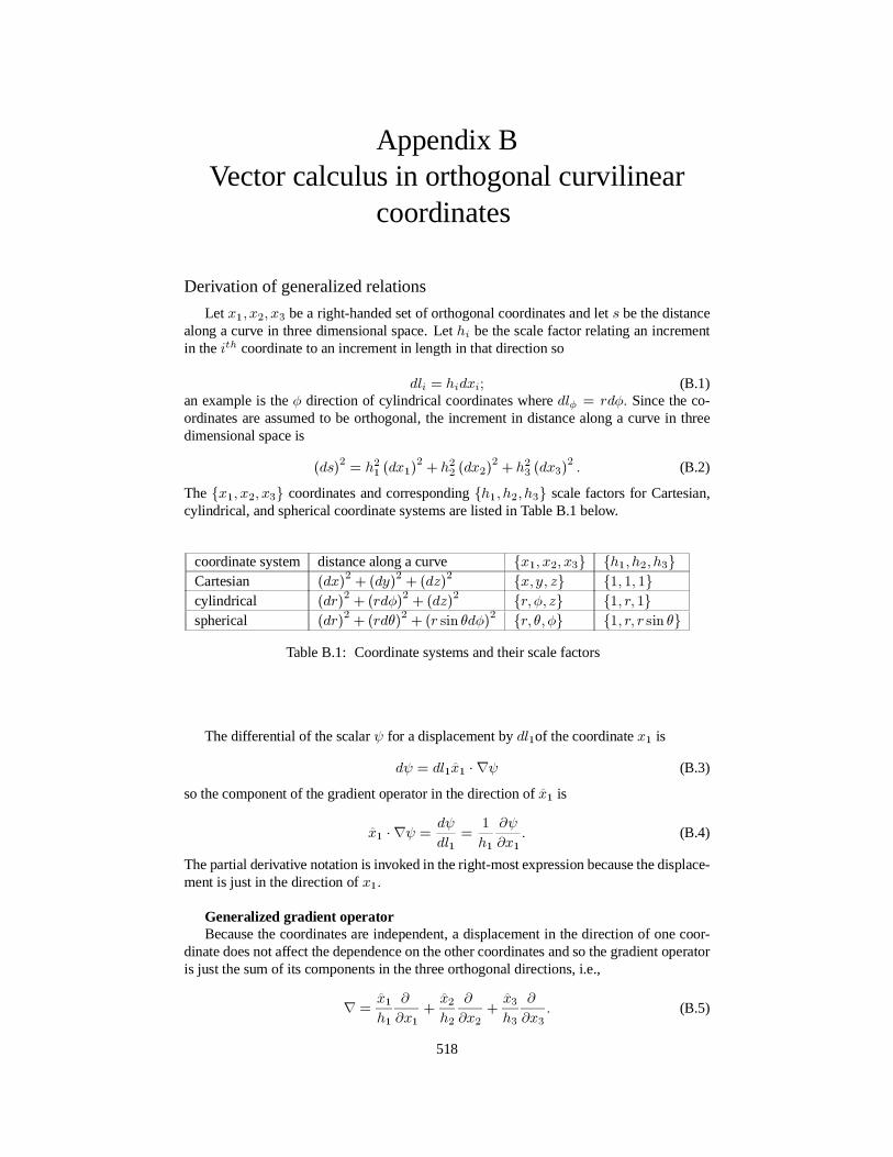
Appendix BVector calculus in orthogonal curvilinear
coordinates
Derivation of generalized relations
Let x1, x2, x3 be a right-handed set of orthogonal coordinates and lets be the distancealong a curve in three dimensional space. Lethi be the scale factor relating an incrementin theith coordinate to an increment in length in that direction so
dli = hidxi; (B.1)an example is theφ direction of cylindrical coordinates wheredlφ = rdφ. Since the co-ordinates are assumed to be orthogonal, the increment in distance along a curve in threedimensional space is
(ds)2 = h21 (dx1)2 + h22 (dx2)2 + h23 (dx3)2 . (B.2)
Thex1, x2, x3 coordinates and correspondingh1, h2, h3 scale factors for Cartesian,cylindrical, and spherical coordinate systems are listed in Table B.1 below.
coordinate system distance along a curve x1, x2, x3 h1, h2, h3Cartesian (dx)2 + (dy)2 + (dz)2 x, y, z 1, 1, 1cylindrical (dr)2 + (rdφ)2 + (dz)2 r,φ, z 1, r, 1spherical (dr)2 + (rdθ)2 + (r sin θdφ)2 r, θ, φ 1, r, r sin θ
Table B.1: Coordinate systems and their scale factors
The differential of the scalarψ for a displacement bydl1of the coordinatex1 is
dψ = dl1x1 · ∇ψ (B.3)
so the component of the gradient operator in the direction ofx1 is
x1 · ∇ψ = dψdl1 = 1
h1∂ψ∂x1 . (B.4)
The partial derivative notation is invoked in the right-most expression because the displace-ment is just in the direction ofx1.
Generalized gradient operatorBecause the coordinates are independent, a displacement in the direction of one coor-
dinate does not affect the dependence on the other coordinates and so the gradient operatoris just the sum of its components in the three orthogonal directions, i.e.,
∇ = x1h1
∂∂x1 + x2
h2∂∂x2 + x3
h3∂∂x3 . (B.5)
518

Appendix B 519
Since∇x1 = x1/h1, the unit vector in thex1 direction is
x1 = h1∇x1. (B.6)
Also, because the coordinates form a right-handed orthogonal system the unit vectorsare related by
x1 × x2 = x3, x2 × x3 = x1, x3 × x1 = x2. (B.7)
Generalized divergence and curlLetV be an arbitrary vector
V=V1x1 + V2x2 + V3x3 (B.8)
and consider the divergence of the first term,
∇ · (V1x1) = ∇ · (V1x2 × x3)= ∇ · (V1h2∇x2 × h3∇x3)= ∇ (h2h3V1) · ∇x2 ×∇x3= ∇ (h2h3V1) · x2 × x3
h2h3= x1
h2h3 · ∇ (h2h3V1)= 1
h1h2h3∂∂x1 (h2h3V1) . (B.9)
Extending this to all three terms gives the general form for the divergence to be
∇ ·V = 1h1h2h3
( ∂∂x1 (h2h3V1) + ∂
∂x2 (h1h3V2) + ∂∂x3 (h1h2V3)
). (B.10)
Now consider the curl of the first term of the arbitrary vector, namely
∇× (V1x1) = ∇× (V1h1∇x1)= ∇ (V1h1)×∇x1= 1
h1∇ (V1h1) × x1 (B.11)
and so
∇×V = 1h1∇ (V1h1) × x1 + 1
h2∇ (V2h2)× x2 + 1h3∇ (V3h3) × x3. (B.12)
The component in the direction ofx1 is
x1 · ∇ ×V = 1h2∇ (V2h2)× x2 · x1 + 1
h3∇ (V3h3)× x3 · x1= 1
h2∇ (V2h2) · x2 × x1 + 1h3∇ (V3h3) · x3 × x1
= 1h3 x2 · ∇ (V3h3) − 1
h2 x3 · ∇ (V2h2)= 1
h2h3∂∂x2 (V3h3)− 1
h2h3∂∂x3 (V2h2) (B.13)
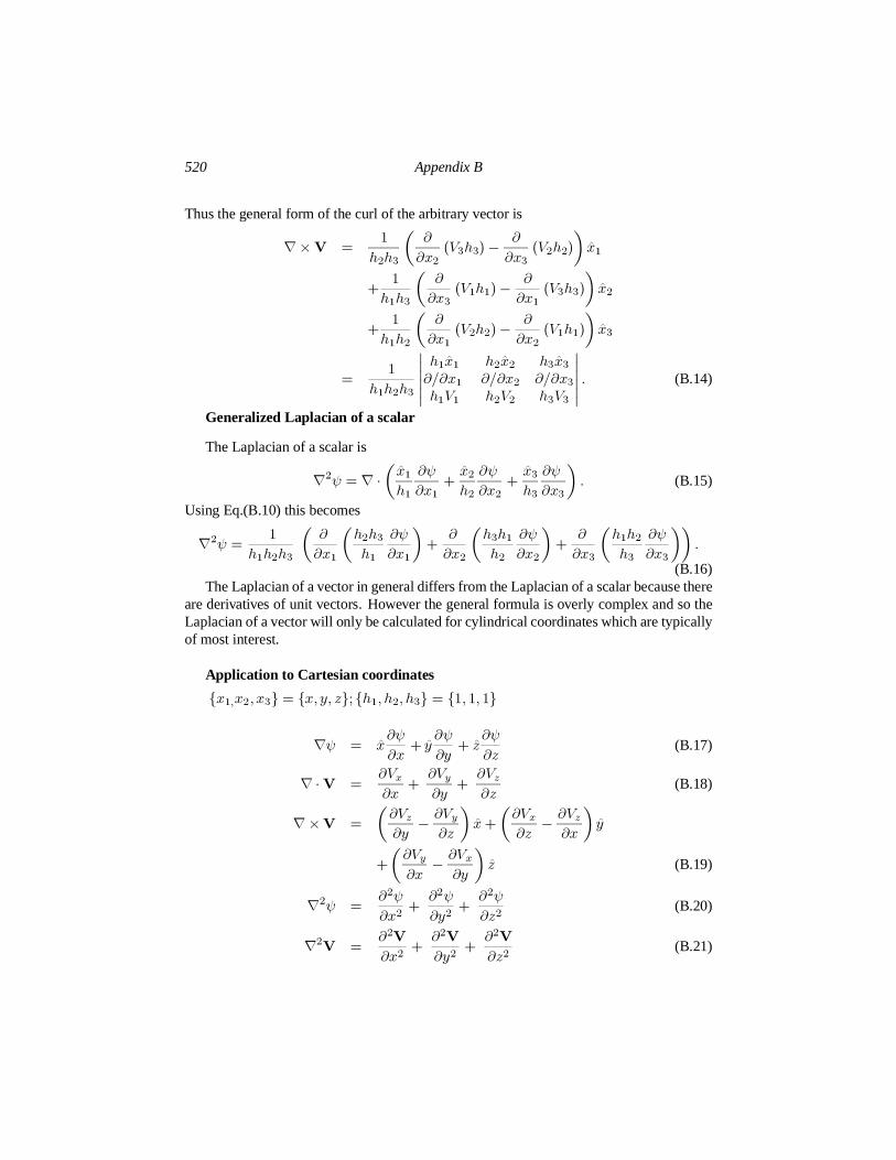
520 Appendix B
Thus the general form of the curl of the arbitrary vector is
∇×V = 1h2h3
( ∂∂x2 (V3h3) − ∂
∂x3 (V2h2))x1
+ 1h1h3
( ∂∂x3 (V1h1)− ∂
∂x1 (V3h3))x2
+ 1h1h2
( ∂∂x1 (V2h2)− ∂
∂x2 (V1h1))x3
= 1h1h2h3
∣∣∣∣∣∣
h1x1 h2x2 h3x3∂/∂x1 ∂/∂x2 ∂/∂x3h1V1 h2V2 h3V3
∣∣∣∣∣∣. (B.14)
Generalized Laplacian of a scalar
The Laplacian of a scalar is
∇2ψ = ∇ ·( x1h1 ∂ψ∂x1 + x2h2∂ψ∂x2 + x3
h3∂ψ∂x3
). (B.15)
Using Eq.(B.10) this becomes
∇2ψ = 1h1h2h3
( ∂∂x1
(h2h3h1
∂ψ∂x1
)+ ∂∂x2
(h3h1h2
∂ψ∂x2
)+ ∂∂x3
(h1h2h3
∂ψ∂x3
)).
(B.16)The Laplacian of a vector in general differs from the Laplacian of a scalar because there
are derivatives of unit vectors. However the general formula is overly complex and so theLaplacian of a vector will only be calculated for cylindrical coordinates which are typicallyof most interest.
Application to Cartesian coordinates
x1,x2, x3 = x, y, z;h1, h2, h3 = 1, 1, 1∇ψ = x∂ψ∂x + y ∂ψ∂y + z ∂ψ∂z (B.17)
∇ ·V = ∂Vx∂x + ∂Vy
∂y + ∂Vz∂z (B.18)
∇×V =(∂Vz∂y − ∂Vy
∂z)x+
(∂Vx∂z − ∂Vz
∂x)y
+(∂Vy∂x − ∂Vx
∂y)z (B.19)
∇2ψ = ∂2ψ∂x2 + ∂2ψ
∂y2 + ∂2ψ∂z2 (B.20)
∇2V = ∂2V∂x2 + ∂2V
∂y2 + ∂2V∂z2 (B.21)
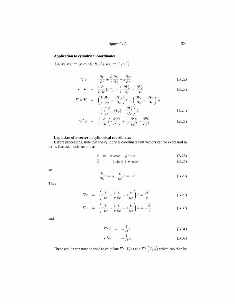
Appendix B 521
Application to cylindrical coordinates
x1,x2, x3 = r,φ, z; h1, h2, h3 = 1, r,1
∇ψ = r ∂ψ∂r + φr∂ψ∂φ + z ∂ψ∂z (B.22)
∇ ·V = 1r∂∂r (rVr) + 1
r∂Vφ∂φ + ∂Vz
∂z (B.23)
∇×V =(1r∂Vz∂φ − ∂Vφ
∂z)r +
(∂Vr∂z − ∂Vz
∂r)φ
+1r( ∂∂r (rVφ) − ∂Vr
∂φ)z (B.24)
∇2ψ = 1r∂∂r
(r∂ψ∂r
)+ 1r2∂2ψ∂φ2 + ∂2ψ
∂z2 (B.25)
Laplacian of a vector in cylindrical coordinatesBefore proceeding, note that the cylindrical coordinate unit vectors can be expressed in
terms Cartesian unit vectors as
r = x cosφ+ y sinφ (B.26)
φ = −x sinφ+ y cosφ (B.27)
so∂∂φ r = φ, ∂
∂φφ = −r. (B.28)
Thus
∇r =(r ∂∂r + φ
r∂∂φ + z ∂∂z
)r = φφ
r (B.29)
∇φ =(r ∂∂r + φ
r∂∂φ + z ∂∂z
)φ = − φrr (B.30)
and
∇2 r = − 1r2 r (B.31)
∇2φ = − 1r2 φ. (B.32)
These results can now be used to calculate∇2 (Vr r) and∇2 (Vφφ)
which can then be

522 Appendix B
used to construct the full Laplacian. The first calculation gives
∇2 (Vr r) = ∇ · ∇ (Vr r)= ∇ · ((∇Vr) r + Vr∇r)= r∇2Vr + (∇Vr) · ∇r +∇ · (Vr∇r)= r∇2Vr + 2∇Vr · ∇r + Vr∇2 r= r∇2Vr + 2φφ
r · ∇Vr + Vrr2
∂2∂φ2 r
= r∇2Vr + 2φr2
∂Vr∂φ − Vr
r2 r (B.33)
while the second calculation gives
∇2 (Vφφ)
= ∇ · ∇(Vφφ
)
= ∇ · ((∇Vφ) φ+ Vφ∇φ)= φ∇2Vφ + 2∇Vφ · ∇φ+ Vφ∇2φ= φ∇2Vφ − 2r
r2∂Vφ∂φ − Vφ
r2 φ. (B.34)
Since∇2 (Vzz) = z∇2Vz it is seen that the Laplacian of a vector in cylindrical coordi-nates is
∇2V = r(∇2Vr − 2
r2∂Vφ∂φ − Vr
r2)
+φ(∇2Vφ + 2
r2∂Vr∂φ − Vφ
r2)
+z∇2Vz. (B.35)
Equation (B.28) can also be used to calculateV·∇V giving
V·∇V =(Vr ∂∂r + Vφ
r∂∂φ + Vz
∂∂z
)(Vr r + Vφφ+ Vzz
)
= r(Vr ∂Vr∂r + Vφ
r∂Vr∂φ + Vz
∂Vr∂z − V 2φ
r)
+φ(Vr ∂Vφ∂r + Vφ
r∂Vφ∂φ + Vz ∂Vφ
∂z + VφVrr
)
+z(Vr ∂Vz∂r + Vφ
r∂Vz∂φ + Vz ∂Vz∂z
). (B.36)

Appendix B 523
Application to spherical coordinatesx1,x2, x3 = r, θ, φ;h1, h2, h3 = 1, r, r sinθ∇ψ = r ∂ψ∂r + θ
r∂ψ∂θ + φ
r sin θ∂ψ∂φ (B.37)
∇ ·V = 1r2
∂∂r
(r2Vr) + 1r sin θ
∂∂θ (sin θ Vθ) +
1r sin θ
∂∂φ (Vφ) (B.38)
∇×V = 1r sin θ
( ∂∂θ (Vφ sin θ)− ∂Vθ
∂φ)r
+ 1r sin θ
(∂Vr∂φ − ∂
∂r (Vφr sin θ))θ
+1r( ∂∂r (Vθr) − ∂Vr
∂φ)φ (B.39)
∇2ψ = 1r2∂∂r
(r2 ∂ψ∂r
)+ 1r2 sin θ
∂∂θ
(sin θ∂ψ∂θ
)+ 1r2 sin2 θ
∂2ψ∂φ2 (B.40)

Appendix CFrequently used physical constants and
formulae
Physical constants (to 3 significant figures)symbol value unit
electron mass me 9.11× 10⁻³¹ kgproton mass mp 1.67× 10⁻²⁷ kgvacuum permeability µ0 4π × 10−7 N A−2vacuum permittivity ε0 8.85× 10⁻¹² F m−1speed of light c 3.00× 10⁸ m s−1electron charge e 1.60× 10⁻¹⁹ CAvogadro’s number 6.02× 10²³ mol−1Boltzmann constant κ 1.60× 10⁻¹⁹ J eV−1
Formulae(all quantities in SI units, temperatures in eV,A is ion atomic mass number)Lengths
Debye length (p.7)
1λ2D
= ∑
σ
1λ2σ
whereσ is over all species participating in shielding and
λσ =√ε0κTσn0σq2σ = 7.4× 10³
√Tσn0σ
m
Electron Larmor radius (p.234)
rLe =√κTe/me|ωce| = 2.4× 10⁻⁶
√TeB m
Ion Larmor radius (p.234)
rLi =√κTi/mi|ωci| = 1. 0× 10−4
√ATiB√Z m
whereA is atomic mass andZ is ion charge.Electron collisionless skin depth (p.145)
cωpe
= 5.3× 10⁶√nem
524

Appendix C 525
Ion collisionless skin depth (assuming quasi-neutral plasma soniZ = necωpi
= 2. 3× 10⁸√ AZne
m
Frequencies
Electron plasma frequency (p.126)
fpe = ωpe2π = 1
2π√nee2ε0me
= 9√ne Hz
Ion plasma frequency (p.126)
fpi = ωpi = 12π
√niq2iε0mi
= 0.21√Zne
A Hz
Electron cyclotron frequency (p.79)
fce = 12π |ωce| = eB
2πme= 2. 8× 10¹⁰B Hz
Ion cyclotron frequency (p.79)
fci = 12π |ωci| = ZeB
2πmi= 1.55× 10⁷ZBA Hz
Upper hybrid frequency (p.186)
fuh =√f2pe + f2ce
Lower hybrid frequency (p.186)
flh =√√√√√f2ci +
f2pi
1 + f2pef2ce
Diocotron frequency (pure electron plasma, p.462)
fdioc ≃ f2pe /2fceVelocities
Electron thermal velocity (p.154)
vTe =√2κTe
me= 5. 9× 10⁵√Te m s−1
Ion thermal velocity (p.154)
vTi =√2κTi
mi= 1.4× 10⁴
√TiAm s−1
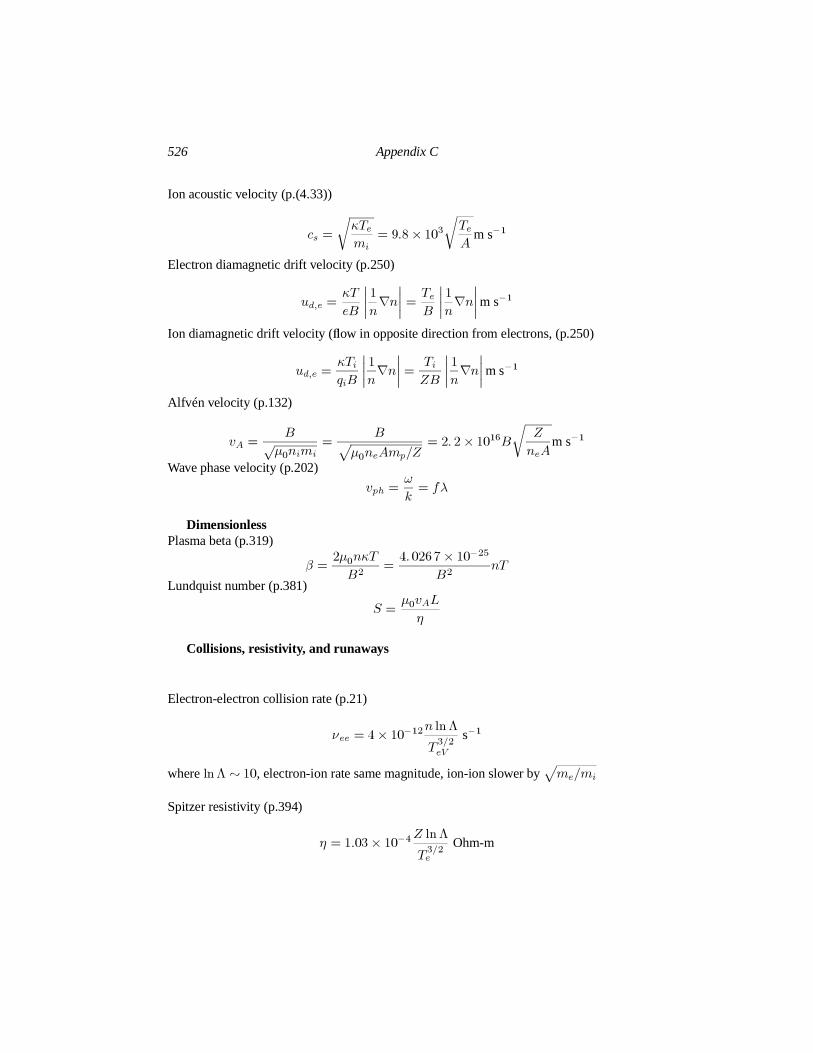
526 Appendix C
Ion acoustic velocity (p.(4.33))
cs =√κTemi
= 9.8× 10³√TeA m s−1
Electron diamagnetic drift velocity (p.250)
ud,e = κTeB
∣∣∣∣1n∇n
∣∣∣∣ = TeB
∣∣∣∣1n∇n
∣∣∣∣m s−1
Ion diamagnetic drift velocity (flow in opposite direction from electrons, (p.250)
ud,e = κTiqiB
∣∣∣∣1n∇n
∣∣∣∣ = TiZB
∣∣∣∣1n∇n
∣∣∣∣m s−1
Alfvén velocity (p.132)
vA = B√µ0nimi= B√µ0neAmp/Z = 2. 2× 10¹⁶B
√ ZneAm s−1
Wave phase velocity (p.202)
vph = ωk = fλ
DimensionlessPlasma beta (p.319)
β = 2µ0nκTB2 = 4.0267× 10⁻²⁵
B2 nTLundquist number (p.381)
S = µ0vALη
Collisions, resistivity, and runaways
Electron-electron collision rate (p.21)
νee = 4× 10⁻¹²n ln ΛT 3/2eV
s−1
whereln Λ ∼ 10, electron-ion rate same magnitude, ion-ion slower by√me/mi
Spitzer resistivity (p.394)
η = 1.03× 10⁻⁴Z ln ΛT 3/2e
Ohm-m
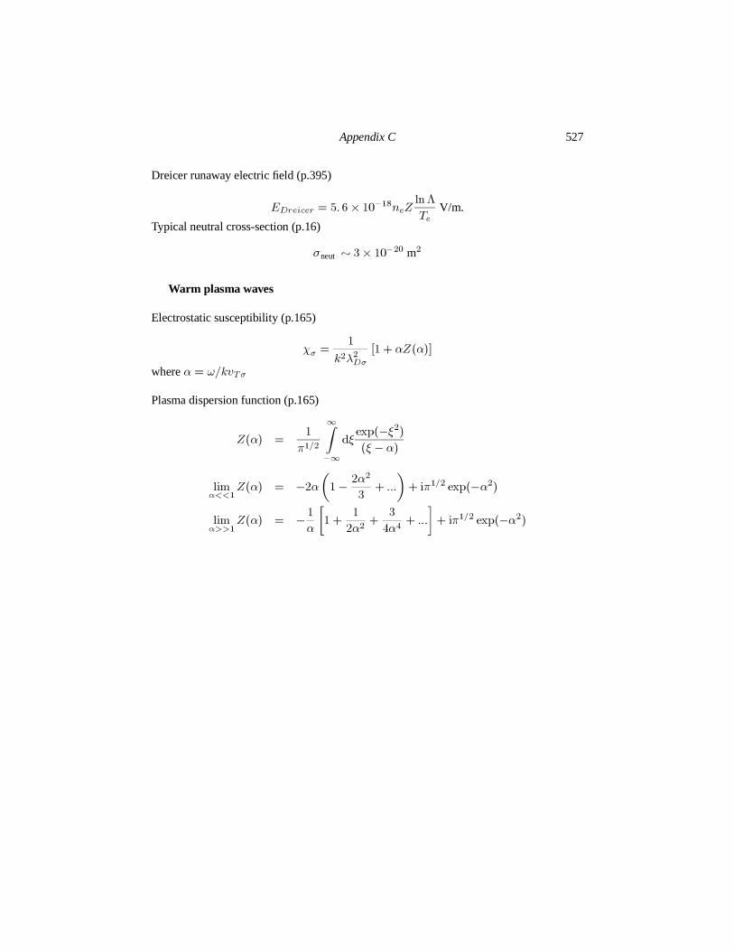
Appendix C 527
Dreicer runaway electric field (p.395)
EDreicer = 5.6× 10⁻¹⁸neZ ln ΛTe V/m.
Typical neutral cross-section (p.16)
σneut ∼ 3× 10⁻²⁰ m2
Warm plasma waves
Electrostatic susceptibility (p.165)
χσ = 1k2λ2Dσ
[1 + αZ(α)]whereα = ω/kvTσ
Plasma dispersion function (p.165)
Z(α) = 1π1/2
∞∫
−∞dξ exp(−ξ2)(ξ −α)
limα<<1Z(α) = −2α(1− 2α2
3 + ...)+ iπ1/2 exp(−α2)
limα>>1Z(α) = − 1α[1 + 1
2α2 + 34α4 + ...
]+ iπ1/2 exp(−α2)

Index
actionintegral in Lagrangian formalism,
63in wave-wave coupling, 433relation to quantum number, 433
action integral, 67adiabatic invariance
breakdown of, 95pendulum, 66
adiabatic invariantgeneral proof for Hamiltonian sys-
tem, 70J, second adiabatic invariant, 88mu conservation, 81relation to quantum number, 68third adiabatic invariant, 89
adiabatic limit of energy equation, 40Airy equation, 241Alfven time, 370Alfven velocity, 183Alfven wave, 131
compressional (fast), 134, 136in parameter space, 196inertial Alfven wave, 187, 207shear (slow), 137two-fluid model, 138
compressional mode, 146inertial Alfven wave, 144kinetic Alfven wave, 145
alpha particle, 296Altar-Appleton-Hartree dispersion
relation, 197ambipolar diffusion, 18analytic continuation, 160antenna, 193Appleton-Hartree dispersion relation,
197
arc, 290astrophysical jet, 295axisymmetry, 280
bad curvature, 305ballistic term, 415beam echo, 416beat waves, 398Bennett pinch, 275, 295Bernstein waves, 236Bessel function model, 358Bessel relationships, 233beta, 319bilinear function, 311Bohm-Gross wave, 129Boltzmann relation
difficulties with, 498in Debye shielding, 7limitations of, 495
bounded volume, 190bounding surface, 190break-even
fusion, 297break-even, fusion, 296Brillouin backscatter, 438Brillouin flow, 460Brillouin limit, 462Bromwich contour, 156
Calugareanu theorem, 356canonical angular momentum, 99
in non-neutral plasma, 464toroidal confinement, 285
canonical momentum, 259definition of, 64
cathode emission, 27caviton, 214, 451center of mass frame dynamics, 382
528

Child-Langmuir space charge limitedemission, 29
CMA diagram, 188coalescence
mode, 240coalescence, mode, 212cold plasma wave energy equation,
221collimation, 294collision
frequencies, 14relations between cross-section,
mean-free-path, 27collisions
and quasi-linear diffusion, 426Coulomb, 11Fokker-Planck model, 389qualitative treatment in Vlasov
equation, 34with neutrals, 16
condensationof dusty plasma, 495
confinement time, 296constant of the motion
definition of, 64convective derivative
definition of, 38coronal loop, 295correspondence of drift equations
with MHD, 91coupled oscillator, 442cross-section
effective, for dust grain charging,484
fusion, 297neutral, 17small-angle scattering, 13
crystallization, 495crystallization criterion, dusty
plasma, 501current
curvature, 93diamagnetic, 91, 250force-free in Grad-Shafranov
equation, 281
grad B, 93parallel, 268polarization, 93poloidal, 280sheet, 362sheet, in Sweet-Parker reconnec-
tion, 380toroidal, 280
curvaturegood v. bad, 305, 318magnetic field, 271
curvature current, 93curvature drift, 80curved magnetic field, 79cusp field, 103cutoff, 131, 185, 190cyclotron motion
sense of rotation, 29
daughter wave, 429Debye shielding, 129
derivation of, 7solution of pde for, 24
decay instability, 428, 438delta W
in MHD energy principle, 313destructive interference, 202deuterium, 296diamagnetic, 282
current, 91drift velocity, 250
dielectric constant, 95dielectric tensor, 179dielectric tensor elements, 181
right, left hand polarization, 183diffusion
ambipolar, 18magnetic, 364quasi-linear velocity space, 405
diocotron mode, 465resistive wall, image charge
method, 479distribution function
definition of, 31for collisionless drift wave, 260moments of, 33
529
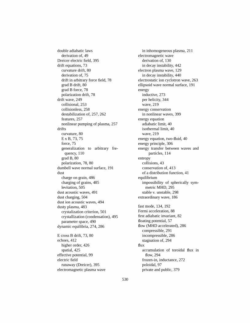
double adiabatic lawsderivation of, 49
Dreicer electric field, 395drift equations, 73
curvature drift, 80derivation of, 75drift in arbitrary force field, 78grad B drift, 80grad B force, 78polarization drift, 78
drift wave, 249collisional, 253collisionless, 258destabilization of, 257, 262features, 257nonlinear pumping of plasma, 257
driftscurvature, 80E x B, 73, 75force, 75generalization to arbitrary fre-
quency, 110grad B, 80polarization, 78, 80
dumbell wave normal surface, 191dust
charge on grain, 486charging of grains, 485levitation, 505
dust acoustic waves, 491dust charging, 504dust ion acoustic waves, 494dusty plasma, 483
crystalization criterion, 501crystallization (condensation), 495parameter space, 490
dynamic equilibria, 274, 286
E cross B drift, 73, 80echoes, 412
higher order, 426spatial, 425
effective potential, 99electric field
runaway (Dreicer), 395electromagnetic plasma wave
in inhomogeneous plasma, 211electromagnetic wave
derivation of, 130in decay instability, 442
electron plasma wave, 129in decay instability, 440
electrostatic ion cyclotron wave, 263ellipsoid wave normal surface, 191energy
inductive, 273per helicity, 344wave, 219
energy conservationin nonlinear waves, 399
energy equationadiabatic limit, 40isothermal limit, 40wave, 219
energy equation, two-fluid, 40energy principle, 306energy transfer between waves and
particles, 114entropy
collisions, 43conservation of, 413of a distribution function, 41
equilibriumimpossibility of spherically sym-
metric MHD, 295stable v. unstable, 298
extraordinary wave, 186
fast mode, 134, 192Fermi acceleration, 88first adiabatic invariant, 82floating potential, 57flow (MHD accelerated), 286
compressible, 291incompressible, 286stagnation of, 294
fluxaccumulation of toroidalflux inflow, 294
frozen-in, inductance, 272poloidal, 97private and public, 379
530

relation to vector potential, 97volume per unit, 334
flux linkage, 346flux preservation, 272flux surface, 96
in mirror, 91flux tube
Grad-Shafranov solution for, 295Fokker-Planck theory, 382force
axial MHD force, 287between parallel currents, 268centrifugal, 79flux-conserving, 273hoop, 270non-conservative, 286pinch, 269
force-freemagnetic field, 344
force-free equilibrium, 322, 335Bessel function model, 358Lundquist solution, 358
force-free magnetic field, 268free-energy
in sheared non-neutral plasma, 477frequently used formulae, 524frictional drag, 391
qualitative derivation of, 37frozen-influx
proof of, 48fusion
break-even, 297criteria for, 296
Gaussian integrals, 59geometric optics, 213good curvature, 305grad B
current, 93drift, 80force, 78
Grad-Shafranov equation, 278Green’s function in diocotron mode,
474group velocity, 201guiding center
definition of, 76
Hall term, 48Hamilton-Lagrange
formalism, 62Hamiltonian, 64, 65
coupled harmonic oscillator, 430geometric optics, 213
Helmholtz equation, 358Hermitian part, 223hollow profile, 474hoop force, 270
ignitron, 29ignorable coordinate, 64image charge, line, 479inductance, 272induction equation, 49
in magnetic reconnection, 366inhomogeneous plasmas, 210initial condition
Poisson’s equation as, 179initial value, 158instability
caviton, 451decay, 428free-boundary, 323, 326kink, 325, 331parametric, 428positron-electron streaming, 150Rayleigh-Taylor, 299resistive wall, 471sausage, 323, 331streaming, 149
ion acoustic velocityin sheath, 56
ion acoustic wave, 129in decay instability, 439Landau damping of, 170Landau instability, 176
ion saturation current, 56ion-ion resonance, 208isothermal limit of energy equation,
40
J, second adiabatic invariant, 87
531

jetastrophysical, 295
joining, in mode conversion, 249
kappamagnetic curvature, 271
Kelvin vorticity theorem, 463kink, 323kink instability, 325, 331
diamagnetic or paramagnetic?, 335Korteweg-de Vries equation, 455Kruskal-Shafranov stability criterion,
333
Lagrange multipliers, 58Lagrange’s equation, 64Lagrangian
electromagnetic, 64Landau damping, 169
and entropy, 413Landau problem, 153Langmuir probe, 56Langmuir wave, 129Laplace transform, 155
and ballistic term, 415Laplace’s equation, 265Larmor radius
poloidal, 285laser fusion, 458Lawson criterion, 296leap-frog numerical integration, 25lightning bolt, 200line-averaged density, 131linear mode conversion, 241linearization, general method, 123loss-cone, 87lower hybrid frequency, 186Lundquist number, 381Lundquist solution, 358
magneticaxis, 283diffusion, 364islands, 376reconnection, 360shear, 305
magnetic fieldforce-free, 268minimum energy, 343most general axisymmetric, 279pressure, 268reconnection in sheared field, 371Solov’ev solution, 282tension, 268vacuum, 265
magnetic field curvature, 271magnetic helicity, 320, 336, 345
association with current-driven in-stability, 319
conservation equation, 321, 357conservation of, 341global, 322linkage, 336linked ribbons, 358twist, 338
magnetic mirror, 84magnetic moments
density of, 92magnetic pressure, 268magnetic stress tensor, 271magnetic tension, 268magnetization, 92magnetofluid, definition of, 306magnetoplasmadynamic thruster, 290magnetron, 481Manley-Rowe relations, 430Maxwellian distribution
definition of, 44MHD equations
derivation of, 46Ohm’s law, derivation of, 47
MHD with neutrals, 60minimum energy
frozen-influx, 272minimum energy magnetic field, 343moments of distribution function, 33momentum conservation
in nonlinear waves, 399mu conservation, 81mu, definition of, 82
National Ignition Facility, 459
532

negative energy wave, 225neutron, 296nominal plasma parameters, 21non-adiabatic motion, 95non-linear dispersion relation, 444non-neutral plasma, 460
relation to Landau damping, 476non-resonant particles
in quasilinear velocity space diffu-sion, 411
numerical integration of particle tra-jectory, 25
orbital motion limited model, 485,504
ordinary wave, 186orthogonal curvilinear coordinates,
518overdense, 197
parallel current, 268paramagnetic, 282parameter space, 195parametric decay instability, 428, 458Parker reconnection model, 378Penrose criterion, 172phase integral, 232phase mixing, 202
and echoes, 416phase space, 30physical constants, 524pinch
Bennett, 295pinch force, 269plasma dispersion function
definition of, 165large argument limit of, 167small argument limit of, 167
plasma frequencydefinition of, 126
plateau velocity distribution, 412Plemelj formula, 171polarization current, 93
relation to capacitance, 95polarization drift, 78, 80
change in particle energy, 120
in Alfven wave, 132relation to MHD equation of mo-
tion, 93stochastic motion, 106
poles, 160poloidal
definition of, 279poloidalflux, 279poloidal Larmor radius, 285poloidal magnetic field, 280ponderomotive force, 436, 448Poyntingflux, 220, 309Poynting theorem, 357pressure
magnetic, 268pressure tensor, definition of, 37principal resonances, 190privateflux, 379product rule for oscillating physical
quantities, 221publicflux, 379pump
MHD acceleration offluid, 290pump depletion, 457pump wave, 429pure electron plasma, 460
QL modes, 199QT modes, 199quantum mechanics, 323quantum mechanics, correspondence
to, 214quasi-linear velocity space diffusion,
399quasi-neutrality, 9quasilinear diffusion
and collisions, 426quiver velocity, 436
radiation pressure, 436radius of curvature, 79Raman backscatter, 438random velocity, 37reduced mass, 383redundancy of Poisson’s equation,
178
533

refractive indexdefinition of, 181
relaxation, 341relaxed state, 344residues, 160resistive mode, 360resistive time, 371resistive wall instability, 471, 479resistivity
Fokker-Planck model, 393simple derivation of, 17
resonance, 185, 190ion cyclotron, 193ion-ion, 208
resonance cones, 204resonant particles
in quasilinear velocity space diffu-sion, 407, 409
reversal of magnetic fieldspatial (cusp), 103temporal, 102
reversed field pinch, 285, 344ribbon, gift-wrapping, 358Richardson-Dushman temperature
limited emission, 29Rosenbluth potentials, 388, 395runaway electric field, 395, 397Rutherford scattering
derivation, 22
saddle point, 243safety factor, 333
tokamak, 375sausage instability, 323, 331scale factor, 518scattering
energy transfer, 23large angle, 12Rutherford, 11, 22small angle, 13
second adiabatic invariant, 87self-adjointness, 310self-confinement
impossibility of, 276self-focusing, 438separatrix, 284
sheath physics, 53sheet current, 362short wave radio transmission, 228slow mode, 192slow wave, 133Snell’s law, 211solar corona loop, 295, 381soliton
interaction, 456ion acoustic wave, 454propagating envelope, 453stationary envelope, 452
Solov’ev solution, 282orbits in, 295
space-charge-limited current, 27spheromak, 285, 344stagnation offlow, 294static equilibria, 274steepest-descent contour, 242stellarator, 285stimulated Raman scattering, 458Stirling’s formula, 58stochastic motion, 106streaming instability, 149stress tensor
magnetic, 271strongly-coupled plasma, 495surface wave, 214susceptibility
definition of, 126Sweet-Parker
reconnection, 378symmetry
assumption in MHD jet, 286canonical angular momentum &
toroidal confinement, 285in Grad-Shafranov equation, 280in Lagrangian formalism, 64in solution of Grad-Shafranov
equation, 280
taxonomy of cold plasma waves, 188Taylor relaxation, 341TE mode, 216tearing, 364temperature limited current, 27
534

tensionmagnetic, 268
thermal force, 59third adiabatic invariant, 89thruster, 290TM mode, 216tokamak, 285, 333topology
minimum energy, 273torque, 286trapped particle
in mirror, 87tritium, 296twist and writhe, 351, 356two-fluid equations
derivation of, 36
underdense, 197unperturbed orbit, 232untrapped particle
in mirror, 87upper hybrid frequency, 186
vacuum magnetic field, 265vector calculus identities, 515vector potential, 320
relation toflux, 97velocity
Alfven, 132, 183bounce-averaged, 90definitions of ‘average’ velocity,
110diamagnetic drift, 250group, 201in sawtooth wave, 111in small amplitude oscillatory
field, 108quiver, 436
virial theorem, 276viscosity, 274, 286Vlasov equation
derivation of, 31moments of, 34treatment of collisions, 34
volume per unitflux, 334vortices
magnetic reconnection, 364vorticity, 286
source for, 289
wall stabilization, 326warm plasma dispersion relation
(electrostatic), 234water beading, 362wave
Alfven, 131beating, 398Bernstein, 236definition of cold plasma wave,
178drift, 249dust acoustic, 491dust Alfven, 504dust ion acoustic, 494dust whistler, 505electron-plasma, 129electrostatic ion cyclotron, 263energy equation, 219, 221energy, finite temperature wave,
224extraordinary, 186frequency dispersion, 201ion acoustic, 129magnetized cold plasma disper-
sion, 181negative energy, 225ordinary, 186quasi-electrostatic cold plasma,
203surface, 214whistler, 200
wave energyin diocotron mode, 468
wave normal surface, 188, 191wave-wave nonlinearity, 428waveguide, plasma, 214wheel wave normal surface, 191whistler wave, 200, 207Wigner-Seitz radius, 487WKB approximation, 66WKB criterion, 212WKB mode
535

correspondence to saddle point,245
WKB solution, 211WKB solutions
of mode conversion problem, 249Woltjer-Taylor relaxation, 341
work function, 29writhe and twist, 351, 356
X-point, 379
Yukawa solution, 9, 24, 495, 498
536