fundamentals of image processing -...
TRANSCRIPT


0. Mathematical Foundations . . . . . . . . . . . . . . . . . . . . . . . . . . . . . . . . . . . . . . . . . . . . . 30.1: Vectors0.2: Matrices0.3: Vector Spaces0.4: Basis0.5: Inner Products and Projections [*]0.6: Linear Transforms [*]
1. Discrete-Time Signals and Systems . . . . . . . . . . . . . . . . . . . . . . . . . . . . . . . . . . . .141.1: Discrete-Time Signals1.2: Discrete-Time Systems1.3: Linear Time-Invariant Systems
2. Linear Time-Invariant Systems . . . . . . . . . . . . . . . . . . . . . . . . . . . . . . . . . . . . . . . . 172.1: Space: Convolution Sum2.2: Frequency: Fourier Transform
3. Sampling: Continuous to Discrete (and back) . . . . . . . . . . . . . . . . . . . . . . . . . 293.1: Continuous to Discrete: Space3.2: Continuous to Discrete: Frequency3.3: Discrete to Continuous
4. Digital Filter Design . . . . . . . . . . . . . . . . . . . . . . . . . . . . . . . . . . . . . . . . . . . . . . . . . . 344.1: Choosing a Frequency Response4.2: Frequency Sampling4.3: Least-Squares4.4: Weighted Least-Squares
5. Photons to Pixels . . . . . . . . . . . . . . . . . . . . . . . . . . . . . . . . . . . . . . . . . . . . . . . . . . . . . 395.1: Pinhole Camera5.2: Lenses5.3: CCD
6. Point-Wise Operations . . . . . . . . . . . . . . . . . . . . . . . . . . . . . . . . . . . . . . . . . . . . . . . . 436.1: Lookup Table6.2: Brightness/Contrast6.3: Gamma Correction6.4: Quantize/Threshold6.5: Histogram Equalize
7. Linear Filtering . . . . . . . . . . . . . . . . . . . . . . . . . . . . . . . . . . . . . . . . . . . . . . . . . . . . . . . 477.1: Convolution7.2: Derivative Filters7.3: Steerable Filters7.4: Edge Detection7.5: Wiener Filter
8. Non-Linear Filtering . . . . . . . . . . . . . . . . . . . . . . . . . . . . . . . . . . . . . . . . . . . . . . . . . . 608.1: Median Filter8.2: Dithering
9. Multi-Scale Transforms [*] . . . . . . . . . . . . . . . . . . . . . . . . . . . . . . . . . . . . . . . . . . . . 6310. Motion Estimation . . . . . . . . . . . . . . . . . . . . . . . . . . . . . . . . . . . . . . . . . . . . . . . . . . .64
10.1: Differential Motion10.2: Differential Stereo
11. Useful Tools . . . . . . . . . . . . . . . . . . . . . . . . . . . . . . . . . . . . . . . . . . . . . . . . . . . . . . . . . 6911.1: Expectation/Maximization11.2: Principal Component Analysis [*]11.3: Independent Component Analysis [*]
[*] In progress
0. Mathematical Foundations
0.1 Vectors
0.2 Matrices
0.3 Vector Spaces
0.4 Basis
0.5 Inner Products
andProjections
0.6 Linear Trans-
forms
0.1 Vectors
From the preface of Linear Algebra and its Applications:
“Linear algebra is a fantastic subject. On the one hand
it is clean and beautiful.” – Gilbert Strang
This wonderful branch of mathematics is both beautiful and use-ful. It is the cornerstone upon which signal and image processing
is built. This short chapter can not be a comprehensive surveyof linear algebra; it is meant only as a brief introduction and re-
view. The ideas and presentation order are modeled after Strang’shighly recommended Linear Algebra and its Applications.
x
y
x+y=5
2x−y=1
(x,y)=(2,3)
Figure 0.1 “Row” solu-
tion
(2,1)(−1,1)
(1,5)
(4,2)
(−3,3)
Figure 0.2 “Column”
solution
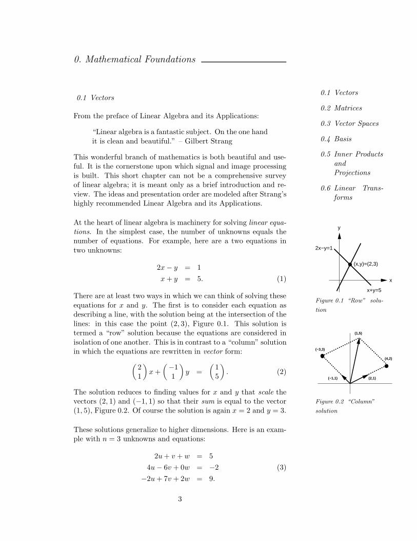
At the heart of linear algebra is machinery for solving linear equa-tions. In the simplest case, the number of unknowns equals thenumber of equations. For example, here are a two equations in
two unknowns:
2x− y = 1
x + y = 5. (1)
There are at least two ways in which we can think of solving these
equations for x and y. The first is to consider each equation asdescribing a line, with the solution being at the intersection of the
lines: in this case the point (2, 3), Figure 0.1. This solution istermed a “row” solution because the equations are considered in
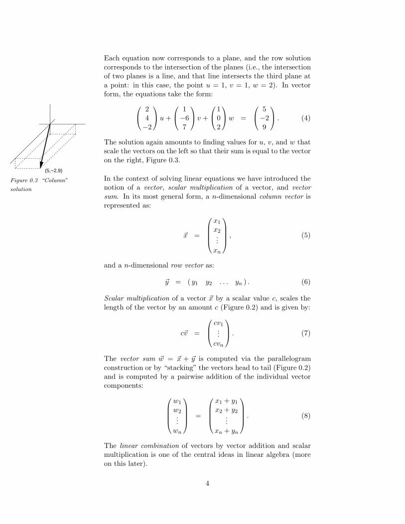
isolation of one another. This is in contrast to a “column” solutionin which the equations are rewritten in vector form:
(
21
)
x +
(−11
)
y =
(
15
)
. (2)
The solution reduces to finding values for x and y that scale thevectors (2, 1) and (−1, 1) so that their sum is equal to the vector(1, 5), Figure 0.2. Of course the solution is again x = 2 and y = 3.
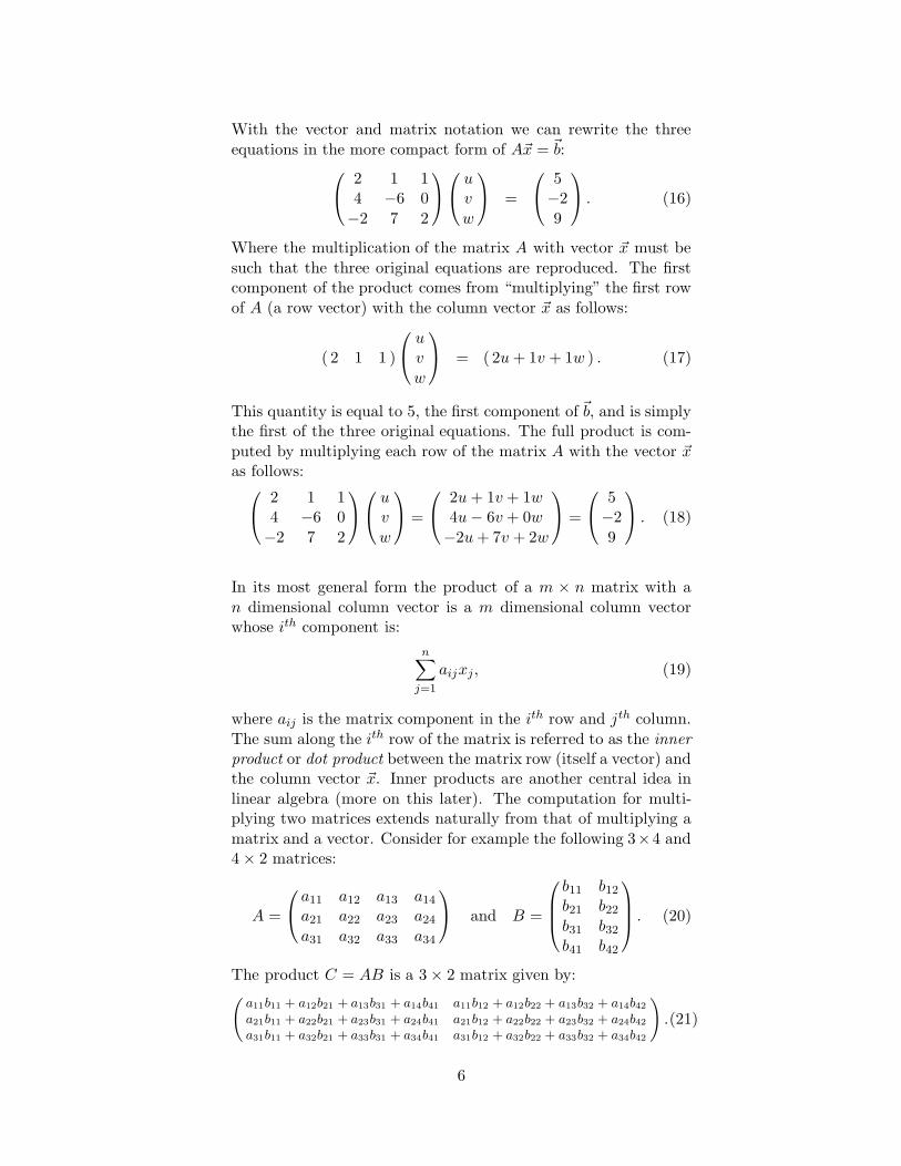
These solutions generalize to higher dimensions. Here is an exam-ple with n = 3 unknowns and equations:
2u + v + w = 5
4u− 6v + 0w = −2 (3)
−2u + 7v + 2w = 9.
3
Each equation now corresponds to a plane, and the row solution
corresponds to the intersection of the planes (i.e., the intersectionof two planes is a line, and that line intersects the third plane at
a point: in this case, the point u = 1, v = 1, w = 2). In vectorform, the equations take the form:
(5,−2,9)
Figure 0.3 “Column”
solution
24
−2
u +
1−6
7
v +
10
2
w =
5−2
9
. (4)
The solution again amounts to finding values for u, v, and w thatscale the vectors on the left so that their sum is equal to the vector
on the right, Figure 0.3.
In the context of solving linear equations we have introduced thenotion of a vector, scalar multiplication of a vector, and vector
sum. In its most general form, a n-dimensional column vector isrepresented as:
~x =
x1
x2...
xn
, (5)
and a n-dimensional row vector as:
~y = ( y1 y2 . . . yn ) . (6)
Scalar multiplication of a vector ~x by a scalar value c, scales the
length of the vector by an amount c (Figure 0.2) and is given by:
c~v =
cv1...
cvn
. (7)
The vector sum ~w = ~x + ~y is computed via the parallelogram
construction or by “stacking” the vectors head to tail (Figure 0.2)and is computed by a pairwise addition of the individual vectorcomponents:
w1
w2...
wn
=
x1 + y1
x2 + y2...
xn + yn
. (8)
The linear combination of vectors by vector addition and scalarmultiplication is one of the central ideas in linear algebra (more
on this later).
4

0.2 Matrices
In solving n linear equations in n unknowns there are three quan-
tities to consider. For example consider again the following set ofequations:
2u + v + w = 5
4u− 6v + 0w = −2 (9)
−2u + 7v + 2w = 9.
On the right is the column vector:
5
−29
, (10)
and on the left are the three unknowns that can also be writtenas a column vector:
u
vw
. (11)
The set of nine coefficients (3 rows, 3 columns) can be written inmatrix form:
2 1 14 −6 0
−2 7 2
(12)
Matrices, like vectors, can be added and scalar multiplied. Notsurprising, since we may think of a vector as a skinny matrix: a
matrix with only one column. Consider the following 3×3 matrix:
A =
a1 a2 a3
a4 a5 a6
a7 a8 a9
. (13)
The matrix cA, where c is a scalar value, is given by:
cA =
ca1 ca2 ca3
ca4 ca5 ca6
ca7 ca8 ca9
. (14)
And the sum of two matrices, A = B + C, is given by:
a1 a2 a3
a4 a5 a6
a7 a8 a9
=
b1 + c1 b2 + c2 b3 + c3
b4 + c4 b5 + c5 b6 + c6
b7 + c7 b8 + c8 b9 + c9
. (15)
5
With the vector and matrix notation we can rewrite the three
equations in the more compact form of A~x = ~b:
2 1 14 −6 0
−2 7 2
uv
w
=
5−2
9
. (16)
Where the multiplication of the matrix A with vector ~x must be
such that the three original equations are reproduced. The firstcomponent of the product comes from “multiplying” the first row
of A (a row vector) with the column vector ~x as follows:
( 2 1 1 )
uv
w
= (2u + 1v + 1w ) . (17)
This quantity is equal to 5, the first component of ~b, and is simplythe first of the three original equations. The full product is com-
puted by multiplying each row of the matrix A with the vector ~xas follows:
2 1 14 −6 0
−2 7 2
uv
w
=
2u + 1v + 1w4u− 6v + 0w
−2u + 7v + 2w
=
5−2
9
. (18)
In its most general form the product of a m × n matrix with a
n dimensional column vector is a m dimensional column vectorwhose ith component is:
n∑
j=1
aijxj , (19)
where aij is the matrix component in the ith row and jth column.
The sum along the ith row of the matrix is referred to as the innerproduct or dot product between the matrix row (itself a vector) andthe column vector ~x. Inner products are another central idea in
linear algebra (more on this later). The computation for multi-plying two matrices extends naturally from that of multiplying a
matrix and a vector. Consider for example the following 3×4 and4× 2 matrices:
A =
a11 a12 a13 a14
a21 a22 a23 a24
a31 a32 a33 a34
and B =
b11 b12
b21 b22
b31 b32
b41 b42
. (20)
The product C = AB is a 3× 2 matrix given by:(
a11b11 + a12b21 + a13b31 + a14b41 a11b12 + a12b22 + a13b32 + a14b42a21b11 + a22b21 + a23b31 + a24b41 a21b12 + a22b22 + a23b32 + a24b42a31b11 + a32b21 + a33b31 + a34b41 a31b12 + a32b22 + a33b32 + a34b42
)
.(21)
6
That is, the i, j component of the product C is computed from
an inner product of the ith row of matrix A and the jth columnof matrix B. Notice that this definition is completely consistent
with the product of a matrix and vector. In order to multiplytwo matrices A and B (or a matrix and a vector), the columndimension of A must equal the row dimension of B. In other words
if A is of size m× n, then B must be of size n× p (the product isof size m× p). This constraint immediately suggests that matrix
multiplication is not commutative: usually AB 6= BA. Howevermatrix multiplication is both associative (AB)C = A(BC) and
distributive A(B + C) = AB + AC.
The identity matrix I is a special matrix with 1 on the diagonal
and zero elsewhere:
I =
1 0 . . . 0 0
0 1 . . . 0 0...
. . ....
0 0 . . . 0 1
. (22)
Given the definition of matrix multiplication, it is easily seen that
for any vector ~x, I~x = ~x, and for any suitably sized matrix, IA = Aand BI = B.
In the context of solving linear equations we have introduced thenotion of a vector and a matrix. The result is a compact notation
for representing linear equations, A~x = ~b. Multiplying both sidesby the matrix inverse A−1 yields the desired solution to the linear
equations:
A−1A~x = A−1~b
I~x = A−1~b
~x = A−1~b (23)
A matrix A is invertible if there exists 1 a matrix B such that
BA = I and AB = I , where I is the identity matrix. The ma-trix B is the inverse of A and is denoted as A−1. Note that this
commutative property limits the discussion of matrix inverses tosquare matrices.
Not all matrices have inverses. Let’s consider some simple exam-ples. The inverse of a 1 × 1 matrix A = (a ) is A−1 = (1/a );
but the inverse does not exist when a = 0. The inverse of a 2× 2
1The inverse of a matrix is unique: assume that B and C are both theinverse of matrix A, then by definition B = B(AC) = (BA)C = C, so that Bmust equal C.
7
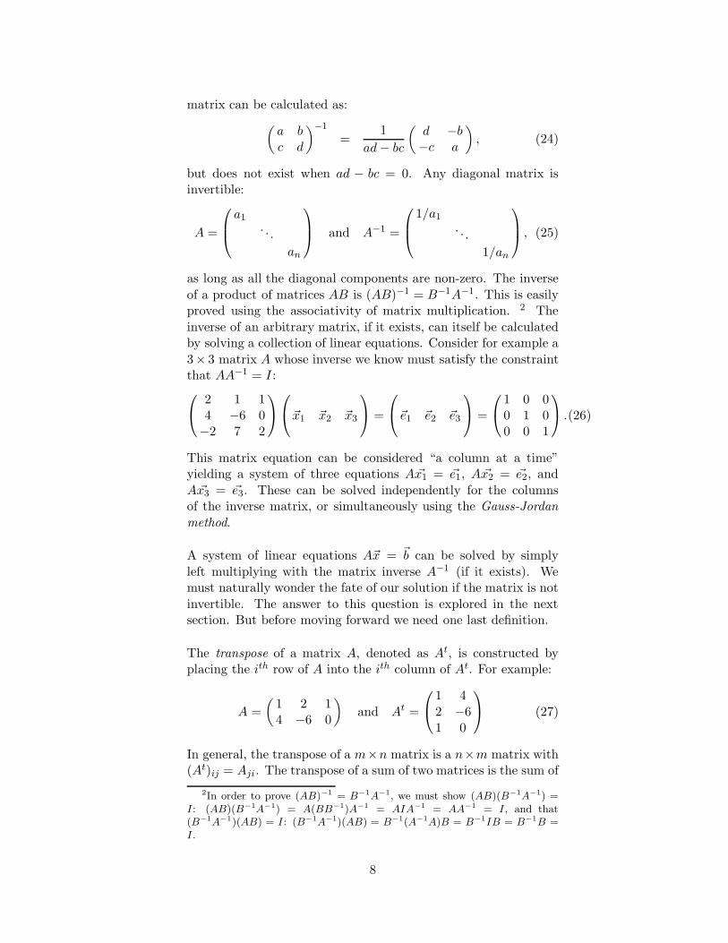
matrix can be calculated as:
(
a bc d
)−1
=1
ad− bc
(
d −b−c a
)
, (24)
but does not exist when ad − bc = 0. Any diagonal matrix isinvertible:
A =
a1. . .
an
and A−1 =
1/a1
. . .
1/an
, (25)
as long as all the diagonal components are non-zero. The inverse
of a product of matrices AB is (AB)−1 = B−1A−1. This is easilyproved using the associativity of matrix multiplication. 2 The
inverse of an arbitrary matrix, if it exists, can itself be calculatedby solving a collection of linear equations. Consider for example a
3× 3 matrix A whose inverse we know must satisfy the constraintthat AA−1 = I :
2 1 14 −6 0−2 7 2
~x1 ~x2 ~x3
=
~e1 ~e2 ~e3
=
1 0 00 1 00 0 1
.(26)
This matrix equation can be considered “a column at a time”yielding a system of three equations A ~x1 = ~e1, A ~x2 = ~e2, and
A ~x3 = ~e3. These can be solved independently for the columnsof the inverse matrix, or simultaneously using the Gauss-Jordan
method.
A system of linear equations A~x = ~b can be solved by simply
left multiplying with the matrix inverse A−1 (if it exists). Wemust naturally wonder the fate of our solution if the matrix is not
invertible. The answer to this question is explored in the nextsection. But before moving forward we need one last definition.
The transpose of a matrix A, denoted as At, is constructed byplacing the ith row of A into the ith column of At. For example:
A =
(
1 2 14 −6 0
)
and At =
1 4
2 −61 0
(27)
In general, the transpose of a m×n matrix is a n×m matrix with(At)ij = Aji. The transpose of a sum of two matrices is the sum of
2In order to prove (AB)−1 = B−1A−1, we must show (AB)(B−1A−1) =I: (AB)(B−1A−1) = A(BB−1)A−1 = AIA−1 = AA−1 = I, and that(B−1A−1)(AB) = I: (B−1A−1)(AB) = B−1(A−1A)B = B−1IB = B−1B =I.
8
the transposes: (A+B)t = At +Bt. The transpose of a product of
two matrices has the familiar form (AB)t = BtAt. And the trans-pose of the inverse is the inverse of the transpose: (A−1)t = (At)−1.
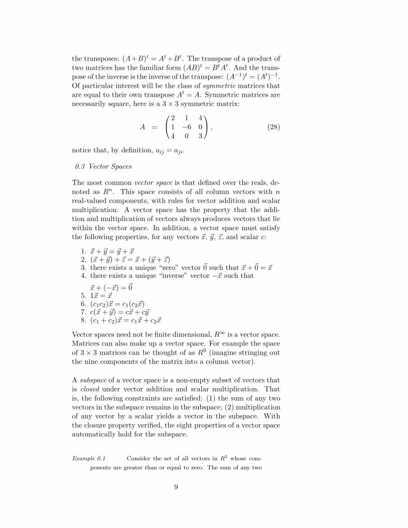
Of particular interest will be the class of symmetric matrices thatare equal to their own transpose At = A. Symmetric matrices arenecessarily square, here is a 3× 3 symmetric matrix:
A =
2 1 41 −6 0
4 0 3
, (28)
notice that, by definition, aij = aji.
0.3 Vector Spaces
The most common vector space is that defined over the reals, de-
noted as Rn. This space consists of all column vectors with nreal-valued components, with rules for vector addition and scalar
multiplication. A vector space has the property that the addi-tion and multiplication of vectors always produces vectors that lie
within the vector space. In addition, a vector space must satisfythe following properties, for any vectors ~x, ~y, ~z, and scalar c:
1. ~x + ~y = ~y + ~x2. (~x + ~y) + ~z = ~x + (~y + ~z)3. there exists a unique “zero” vector ~0 such that ~x + ~0 = ~x4. there exists a unique “inverse” vector −~x such that
~x + (−~x) = ~05. 1~x = ~x6. (c1c2)~x = c1(c2~x)7. c(~x + ~y) = c~x + c~y8. (c1 + c2)~x = c1~x + c2~x
Vector spaces need not be finite dimensional, R∞ is a vector space.Matrices can also make up a vector space. For example the space
of 3 × 3 matrices can be thought of as R9 (imagine stringing outthe nine components of the matrix into a column vector).
A subspace of a vector space is a non-empty subset of vectors thatis closed under vector addition and scalar multiplication. That
is, the following constraints are satisfied: (1) the sum of any twovectors in the subspace remains in the subspace; (2) multiplicationof any vector by a scalar yields a vector in the subspace. With
the closure property verified, the eight properties of a vector spaceautomatically hold for the subspace.
Example 0.1 Consider the set of all vectors in R2 whose com-
ponents are greater than or equal to zero. The sum of any two
9
vectors in this space remains in the space, but multiplication of,
for example, the vector
(
12
)
by −1 yields the vector
(
−1−2
)
which is no longer in the space. Therefore, this collection of
vectors does not form a vector space.
Vector subspaces play a critical role in understanding systems of
linear equations of the form A~x = ~b. Consider for example thefollowing system:
u1 v1
u2 v2
u3 v3
(
x1
x2
)
=
b1
b2
b3
(29)
Unlike the earlier system of equations, this system is over-constrained,
there are more equations (three) than unknowns (two). A solu-tion to this system exists if the vector ~b lies in the subspace of thecolumns of matrix A. To see why this is so, we rewrite the above
system according to the rules of matrix multiplication yielding anequivalent form:
x1
u1
u2
u3
+ x2
v1
v2
v3
=
b1
b2
b3
. (30)
In this form, we see that a solution exists when the scaled columns
of the matrix sum to the vector ~b. This is simply the closureproperty necessary for a vector subspace.
The vector subspace spanned by the columns of the matrix A iscalled the column space of A. It is said that a solution to A~x = ~bexists if and only if the vector ~b lies in the column space of A.
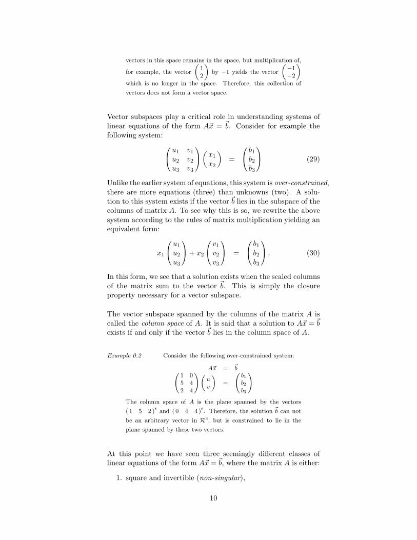
Example 0.2 Consider the following over-constrained system:
A~x = ~b(
1 05 42 4
)
(
uv
)
=
(
b1b2b3
)
The column space of A is the plane spanned by the vectors
( 1 5 2 )t and ( 0 4 4 )t. Therefore, the solution ~b can not
be an arbitrary vector in R3, but is constrained to lie in the
plane spanned by these two vectors.
At this point we have seen three seemingly different classes oflinear equations of the form A~x = ~b, where the matrix A is either:
1. square and invertible (non-singular),
10
2. square but not invertible (singular),3. over-constrained.
In each case solutions to the system exist if the vector ~b lies in thecolumn space of the matrix A. At one extreme is the invertible
n×n square matrix whose solutions may be any vector in the wholeof Rn. At the other extreme is the zero matrix A = 0 with only
the zero vector in it’s column space, and hence the only possiblesolution. In between are the singular and over-constrained cases,
where solutions lie in a subspace of the full vector space.
The second important vector space is the nullspace of a matrix.
The vectors that lie in the nullspace of a matrix consist of allsolutions to the system A~x = ~0. The zero vector is always in thenullspace.
Example 0.3 Consider the following system:
A~x = ~0(
1 0 15 4 92 4 6
)(
uvw
)
=
(
000
)
The nullspace of A contains the zero vector (u v w )t = ( 0 0 0 )t.
Notice also that the third column of A is the sum of the first two
columns, therefore the nullspace of A also contains all vectors of
the form (u v w )t = ( c c −c )t (i.e., all vectors lying on a
one-dimensional line in R3).
(2,2)
(−1,−1)
(2,2)
(−2,0)
(2,2)
(−2,0)
(−1,2)
Figure 0.4 Linearly de-
pendent
(top/bottom) and inde-
pendent (middle).
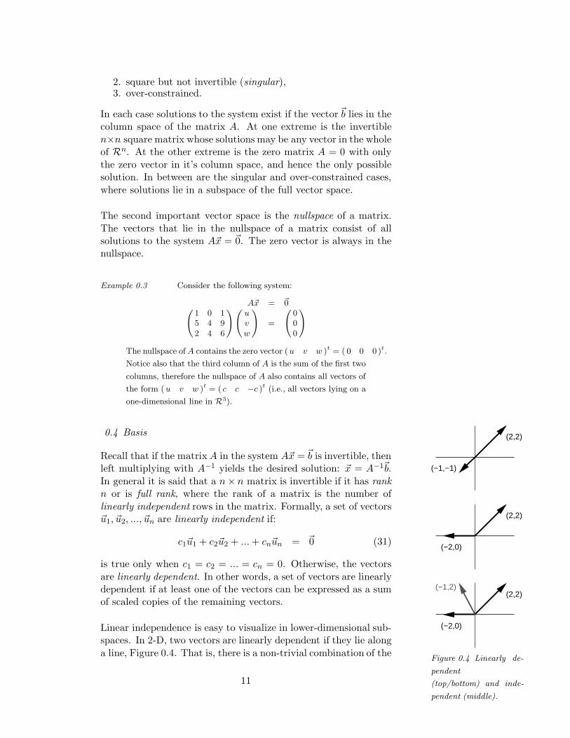
0.4 Basis
Recall that if the matrix A in the system A~x = ~b is invertible, thenleft multiplying with A−1 yields the desired solution: ~x = A−1~b.
In general it is said that a n× n matrix is invertible if it has rankn or is full rank, where the rank of a matrix is the number of
linearly independent rows in the matrix. Formally, a set of vectors~u1, ~u2, ..., ~un are linearly independent if:
c1~u1 + c2~u2 + ... + cn~un = ~0 (31)
is true only when c1 = c2 = ... = cn = 0. Otherwise, the vectors
are linearly dependent. In other words, a set of vectors are linearlydependent if at least one of the vectors can be expressed as a sumof scaled copies of the remaining vectors.
Linear independence is easy to visualize in lower-dimensional sub-spaces. In 2-D, two vectors are linearly dependent if they lie along
a line, Figure 0.4. That is, there is a non-trivial combination of the
11
vectors that yields the zero vector. In 2-D, any three vectors are
guaranteed to be linearly dependent. For example, in Figure 0.4,the vector (−1 2 ) can be expressed as a sum of the remaining
linearly independent vectors: 32 (−2 0 ) + ( 2 2 ). In 3-D, three
vectors are linearly dependent if they lie in the same plane. Alsoin 3-D, any four vectors are guaranteed to be linearly dependent.
Linear independence is directly related to the nullspace of a ma-trix. Specifically, the columns of a matrix are linearly independent
(i.e., the matrix is full rank) if the matrix nullspace contains onlythe zero vector. For example, consider the following system of
linear equations:
u1 v1 w1
u2 v2 w2
u3 v3 w3
x1
x2
x3
=
0
00
. (32)
Recall that the nullspace contains all vectors ~x such that x1~u +x2~v + x3 ~w = 0. Notice that this is also the condition for linear
independence. If the only solution is the zero vector then thevectors are linearly independent and the matrix is full rank and
invertible.
Linear independence is also related to the column space of a ma-
trix. If the column space of a n × n matrix is all of Rn, then thematrix is full rank. For example, consider the following system of
linear equations:
u1 v1 w1
u2 v2 w2
u3 v3 w3
x1
x2
x3
=
b1
b2
b3
. (33)
If the the matrix is full rank, then the solution ~b can be any vectorin R3. In such cases, the vectors ~u, ~v, ~w are said to span the space.
Now, a linear basis of a vector space is a set of linearly independentvectors that span the space. Both conditions are important. Givenan n dimensional vector space with n basis vectors ~v1, ..., ~vn, any
vector ~u in the space can be written as a linear combination ofthese n vectors:
~u = a1 ~v1 + ... + an ~vn. (34)
In addition, the linear independence guarantees that this linear
combination is unique. If there is another combination such that:
~u = b1 ~v1 + ... + bn ~vn, (35)
12
then the difference of these two representations yields
~0 = (a1 − b1)~v1 + ... + (an − bn) ~vn
= c1 ~v1 + ... + cn ~vn (36)
which would violate the linear independence condition. While
the representation is unique, the basis is not. A vector space hasinfinitely many different bases. For example in R2 any two vectors
that do not lie on a line form a basis, and in R3 any three vectorsthat do not lie in a common plane or line form a basis.
Example 0.4 The vectors ( 1 0 ) and ( 0 1 ) form the canonical
basis for R2. These vectors are both linearly independent and
span the entire vector space.
Example 0.5 The vectors ( 1 0 0 ), ( 0 1 0 ) and (−1 0 0 )
do not form a basis for R3. These vectors lie in a 2-D plane and
do not span the entire vector space.
Example 0.6 The vectors ( 1 0 0 ), ( 0 −1 0 ), ( 0 0 2 ),
and ( 1 −1 0 ) do not form a basis. Although these vectors
span the vector space, the fourth vector is linearly dependent on
the first two. Removing the fourth vector leaves a basis for R3.
0.5 Inner Products and Projections
0.6 Linear Transforms
13
1. Discrete-Time Signals and Systems
1.1 Discrete-TimeSignals
1.2 Discrete-TimeSystems
1.3 Linear Time-
Invariant Sys-tems
1.1 Discrete-Time Signals
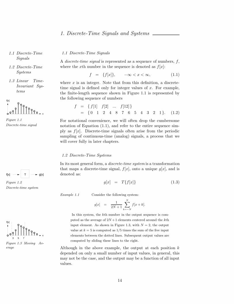
A discrete-time signal is represented as a sequence of numbers, f ,
where the xth number in the sequence is denoted as f [x]:
f = {f [x]}, −∞ < x < ∞, (1.1)
where x is an integer. Note that from this definition, a discrete-time signal is defined only for integer values of x. For example,
the finite-length sequence shown in Figure 1.1 is represented by
f[x]
x
Figure 1.1
Discrete-time signal
the following sequence of numbers
f = { f [1] f [2] ... f [12]}= { 0 1 2 4 8 7 6 5 4 3 2 1 }. (1.2)
For notational convenience, we will often drop the cumbersomenotation of Equation (1.1), and refer to the entire sequence sim-
ply as f [x]. Discrete-time signals often arise from the periodicsampling of continuous-time (analog) signals, a process that we
will cover fully in later chapters.
1.2 Discrete-Time Systems
In its most general form, a discrete-time system is a transformation
f[x] g[x]T
Figure 1.2
Discrete-time system
that maps a discrete-time signal, f [x], onto a unique g[x], and is
denoted as:
g[x] = T{f [x]} (1.3)
Example 1.1 Consider the following system:
g[x] =1
2N + 1
N∑
k=−N
f [x + k].
In this system, the kth number in the output sequence is com-
f[x]
x3 5 7
Figure 1.3 Moving Av-erage
puted as the average of 2N +1 elements centered around the kth
input element. As shown in Figure 1.3, with N = 2, the output
value at k = 5 is computed as 1/5 times the sum of the five input
elements between the dotted lines. Subsequent output values are
computed by sliding these lines to the right.
Although in the above example, the output at each position k
depended on only a small number of input values, in general, thismay not be the case, and the output may be a function of all input
values.
14
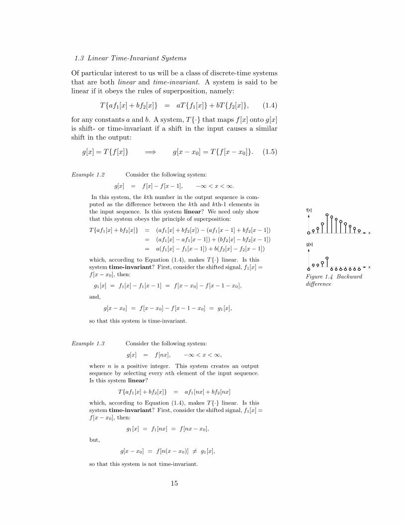
1.3 Linear Time-Invariant Systems
Of particular interest to us will be a class of discrete-time systems
that are both linear and time-invariant. A system is said to belinear if it obeys the rules of superposition, namely:
T{af1[x] + bf2[x]} = aT{f1[x]}+ bT{f2[x]}, (1.4)
for any constants a and b. A system, T{·} that maps f [x] onto g[x]is shift- or time-invariant if a shift in the input causes a similarshift in the output:
g[x] = T{f [x]} =⇒ g[x− x0] = T{f [x− x0]}. (1.5)
Example 1.2 Consider the following system:
g[x] = f [x]− f [x− 1], −∞ < x < ∞.
In this system, the kth number in the output sequence is com-
f[x]
x
x
g[x]
Figure 1.4 Backwarddifference
puted as the difference between the kth and kth-1 elements inthe input sequence. Is this system linear? We need only showthat this system obeys the principle of superposition:
T{af1[x] + bf2[x]} = (af1[x] + bf2[x])− (af1[x− 1] + bf2[x− 1])
= (af1[x]− af1[x− 1]) + (bf2[x]− bf2[x− 1])
= a(f1[x]− f1[x− 1]) + b(f2[x]− f2[x− 1])
which, according to Equation (1.4), makes T{·} linear. Is thissystem time-invariant? First, consider the shifted signal, f1[x] =f [x− x0], then:
g1[x] = f1[x]− f1[x− 1] = f [x− x0]− f [x− 1 − x0],
and,
g[x − x0] = f [x− x0]− f [x− 1− x0] = g1[x],
so that this system is time-invariant.
Example 1.3 Consider the following system:
g[x] = f [nx], −∞ < x < ∞,
where n is a positive integer. This system creates an outputsequence by selecting every nth element of the input sequence.Is this system linear?
T{af1[x] + bf2[x]} = af1[nx] + bf2[nx]
which, according to Equation (1.4), makes T{·} linear. Is thissystem time-invariant? First, consider the shifted signal, f1[x] =f [x− x0], then:
g1[x] = f1[nx] = f [nx− x0],
but,
g[x − x0] = f [n(x− x0)] 6= g1[x],
so that this system is not time-invariant.
15
The precise reason why we are particularly interested in linear
time-invariant systems will become clear in subsequent chapters.But before pressing on, the concept of discrete-time systems is
reformulated within a linear-algebraic framework. In order to ac-complish this, it is necessary to first restrict ourselves to considerinput signals of finite length. Then, any discrete-time linear sys-
tem can be represented as a matrix operation of the form:
~g = M ~f, (1.6)
where, ~f is the input signal, ~g is the output signal, and the matrix
M embodies the discrete-time linear system.
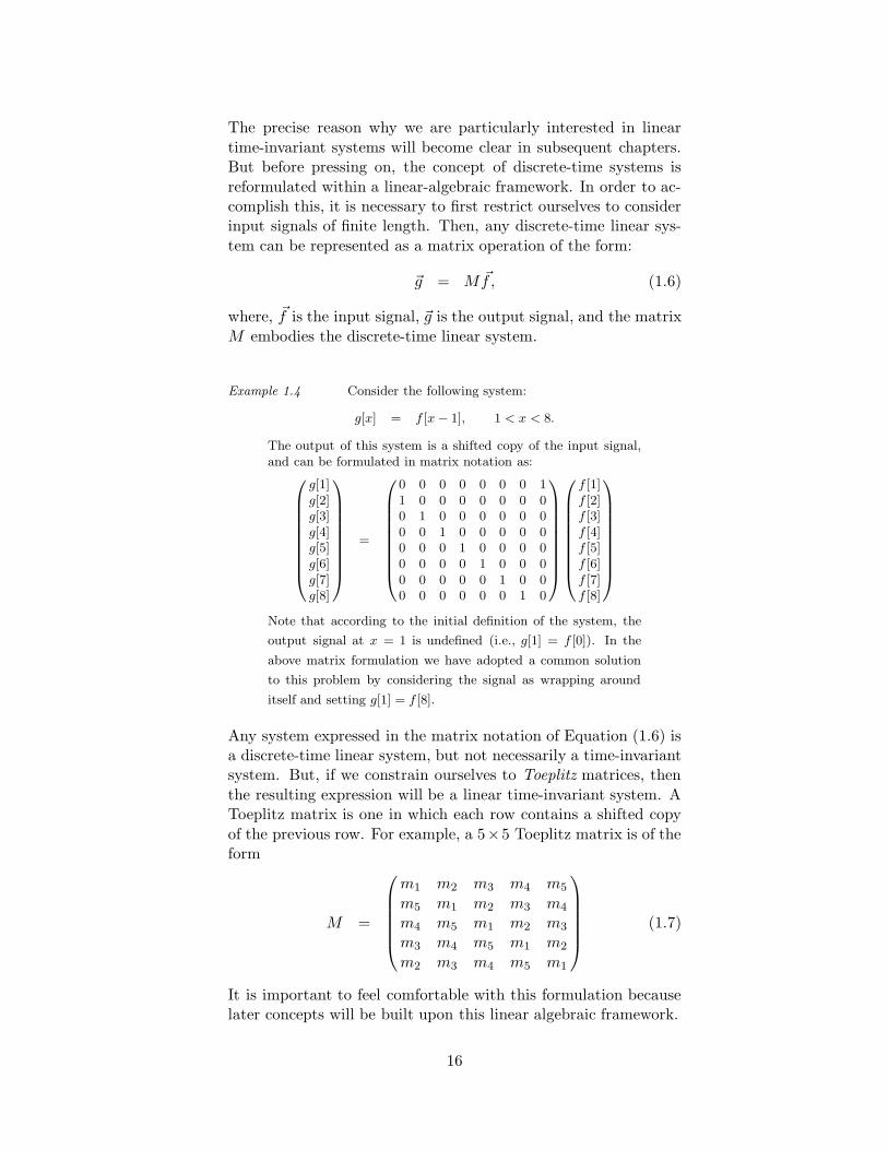
Example 1.4 Consider the following system:
g[x] = f [x− 1], 1 < x < 8.
The output of this system is a shifted copy of the input signal,and can be formulated in matrix notation as:
g[1]g[2]g[3]g[4]g[5]g[6]g[7]g[8]
=
0 0 0 0 0 0 0 11 0 0 0 0 0 0 00 1 0 0 0 0 0 00 0 1 0 0 0 0 00 0 0 1 0 0 0 00 0 0 0 1 0 0 00 0 0 0 0 1 0 00 0 0 0 0 0 1 0
f [1]f [2]f [3]f [4]f [5]f [6]f [7]f [8]
Note that according to the initial definition of the system, the
output signal at x = 1 is undefined (i.e., g[1] = f [0]). In the
above matrix formulation we have adopted a common solution
to this problem by considering the signal as wrapping around
itself and setting g[1] = f [8].
Any system expressed in the matrix notation of Equation (1.6) isa discrete-time linear system, but not necessarily a time-invariantsystem. But, if we constrain ourselves to Toeplitz matrices, then
the resulting expression will be a linear time-invariant system. AToeplitz matrix is one in which each row contains a shifted copy
of the previous row. For example, a 5×5 Toeplitz matrix is of theform
M =
m1 m2 m3 m4 m5
m5 m1 m2 m3 m4
m4 m5 m1 m2 m3
m3 m4 m5 m1 m2
m2 m3 m4 m5 m1
(1.7)
It is important to feel comfortable with this formulation becauselater concepts will be built upon this linear algebraic framework.
16
2. Linear Time-Invariant Systems
2.1 Space: Convo-lution Sum
2.2 Frequency:Fourier Trans-
form
Our interest in the class of linear time-invariant systems (LTI) is
motivated by the fact that these systems have a particularly con-venient and elegant representation, and this representation leads
us to several fundamental tools in signal and image processing.
2.1 Space: Convolution Sum
In the previous section, a discrete-time signal was represented asa sequence of numbers. More formally, this representation is in
x
1
Figure 2.1 Unit impulse
terms of the discrete-time unit impulse defined as:
δ[x] =
{
1, x = 00, x 6= 0.
(2.1)
Any discrete-time signal can be represented as a sum of scaled andshifted unit-impulses:
f [x] =∞∑
k=−∞
f [k]δ[x− k], (2.2)
where the shifted impulse δ[x − k] = 1 when x = k, and is zero
elsewhere.
Example 2.1 Consider the following discrete-time signal, cen-tered at x = 0.
f [x] = ( . . . 0 0 2 −1 4 0 0 . . . ) ,
this signal can be expressed as a sum of scaled and shifted unit-impulses:
f [x] = 2δ[x + 1] − 1δ[x] + 4δ[x− 1]
= f [−1]δ[x + 1] + f [0]δ[x] + f [1]δ[x− 1]
=
1∑
k=−1
f [k]δ[x− k].
Let’s now consider what happens when we present a linear time-invariant system with this new representation of a discrete-time
signal:
g[x] = T{f [x]}
= T
∞∑
k=−∞
f [k]δ[x− k]
. (2.3)
17
By the property of linearity, Equation (1.4), the above expression
may be rewritten as:
g[x] =∞∑
k=−∞
f [k]T{δ[x− k]}. (2.4)
Imposing the property of time-invariance, Equation (1.5), if h[x] isthe response to the unit-impulse, δ[x], then the response to δ[x−k]
is simply h[x−k]. And now, the above expression can be rewrittenas:
g[x] =∞∑
k=−∞
f [k]h[x− k]. (2.5)
Consider for a moment the implications of the above equation.
The unit-impulse response, h[x] = T{δ[x]}, of a linear time-invariantsystem fully characterizes that system. More precisely, given the
unit-impulse response, h[x], the output, g[x], can be determinedfor any input, f [x].
The sum in Equation (2.5) is commonly called the convolutionsum and may be expressed more compactly as:
g[x] = f [x] ? h[x]. (2.6)
A more mathematically correct notation is (f ?h)[x], but for later
notational considerations, we will adopt the above notation.
Example 2.2 Consider the following finite-length unit-impulseresponse:
h[x]0
f[x]0
g[−2]
Figure 2.2 Convolution:g[x] = f [x] ? h[x]
h[x] = (−2 4 −2 ) ,
and the input signal, f [x], shown in Figure 2.2. Then the outputsignal at, for example, x = −2, is computed as:
g[−2] =
−1∑
k=−3
f [k]h[−2− k]
= f [−3]h[1] + f [−2]h[0] + f [−1]h[−1].
The next output sum at x = −1, is computed by “sliding” the
unit-impulse response along the input signal and computing a
similar sum.
Since linear time-invariant systems are fully characterized by con-volution with the unit-impulse response, properties of such sys-
tems can be determined by considering properties of the convolu-tion operator. For example, convolution is commutative:
f [x] ? h[x] =∞∑
k=−∞
f [k]h[x− k], let j = x− k
18
=∞∑
j=−∞
f [x− j]h[j] =∞∑
j=−∞
h[j]f [x− j]
= h[x] ? f [x]. (2.7)
Convolution also distributes over addition:
f [x] ? (h1[x] + h2[x]) =∞∑
k=−∞
f [k](h1[x− k] + h2[x− k])
=∞∑
k=−∞
f [k]h1[x− k] + f [k]h2[x− k]
=∞∑
k=−∞
f [k]h1[x− k] +∞∑
k=−∞
f [k]h2[x− k]
= f [x] ? h1[x] + f [x] ? h2[x]. (2.8)
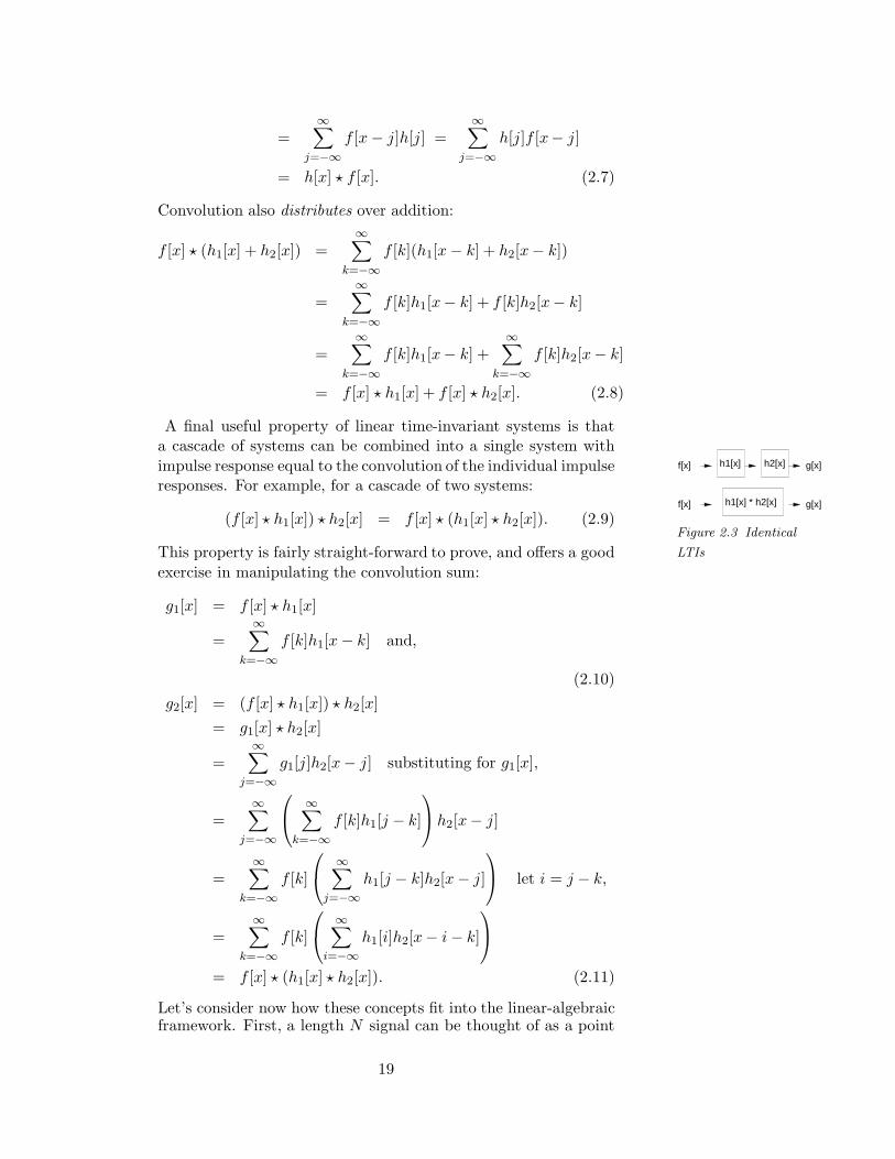
A final useful property of linear time-invariant systems is that
f[x] g[x]h1[x] h2[x]
f[x] g[x]h1[x] * h2[x]
Figure 2.3 Identical
LTIs
a cascade of systems can be combined into a single system with
impulse response equal to the convolution of the individual impulseresponses. For example, for a cascade of two systems:
(f [x] ? h1[x]) ? h2[x] = f [x] ? (h1[x] ? h2[x]). (2.9)
This property is fairly straight-forward to prove, and offers a good
exercise in manipulating the convolution sum:
g1[x] = f [x] ? h1[x]
=∞∑
k=−∞
f [k]h1[x− k] and,
(2.10)
g2[x] = (f [x] ? h1[x]) ? h2[x]
= g1[x] ? h2[x]
=∞∑
j=−∞
g1[j]h2[x− j] substituting for g1[x],
=∞∑
j=−∞
∞∑
k=−∞
f [k]h1[j − k]
h2[x− j]
=∞∑
k=−∞
f [k]
∞∑
j=−∞
h1[j − k]h2[x− j]
let i = j − k,
=∞∑
k=−∞
f [k]
∞∑
i=−∞
h1[i]h2[x− i− k]
= f [x] ? (h1[x] ? h2[x]). (2.11)
Let’s consider now how these concepts fit into the linear-algebraicframework. First, a length N signal can be thought of as a point
19
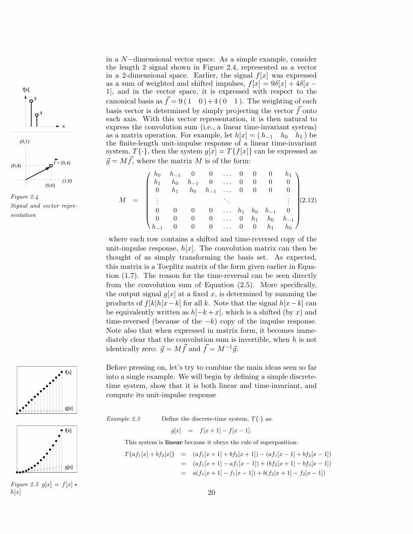
in a N−dimensional vector space. As a simple example, considerthe length 2 signal shown in Figure 2.4, represented as a vectorin a 2-dimensional space. Earlier, the signal f [x] was expressed
f[x]
x
9
4
(0,1)
(1,0)(9,0)
(0,4)f = (9,4)
Figure 2.4
Signal and vector repre-
sentation
as a sum of weighted and shifted impulses, f [x] = 9δ[x] + 4δ[x−1], and in the vector space, it is expressed with respect to the
canonical basis as ~f = 9 ( 1 0 )+4 ( 0 1 ). The weighting of each
basis vector is determined by simply projecting the vector ~f ontoeach axis. With this vector representation, it is then natural toexpress the convolution sum (i.e., a linear time-invariant system)as a matrix operation. For example, let h[x] = (h−1 h0 h1 ) bethe finite-length unit-impulse response of a linear time-invariantsystem, T{·}, then the system g[x] = T{f [x]} can be expressed as
~g = M ~f , where the matrix M is of the form:
M =
h0 h−1 0 0 . . . 0 0 0 h1
h1 h0 h−1 0 . . . 0 0 0 0
0 h1 h0 h−1 . . . 0 0 0 0
.... . .
...0 0 0 0 . . . h1 h0 h
−1 00 0 0 0 . . . 0 h1 h0 h
−1
h−1 0 0 0 . . . 0 0 h1 h0
,(2.12)
where each row contains a shifted and time-reversed copy of the
unit-impulse response, h[x]. The convolution matrix can then bethought of as simply transforming the basis set. As expected,
this matrix is a Toeplitz matrix of the form given earlier in Equa-tion (1.7). The reason for the time-reversal can be seen directly
from the convolution sum of Equation (2.5). More specifically,the output signal g[x] at a fixed x, is determined by summing the
products of f [k]h[x−k] for all k. Note that the signal h[x−k] canbe equivalently written as h[−k +x], which is a shifted (by x) andtime-reversed (because of the −k) copy of the impulse response.
Note also that when expressed in matrix form, it becomes imme-diately clear that the convolution sum is invertible, when h is not
identically zero: ~g = M ~f and ~f = M−1~g.
Before pressing on, let’s try to combine the main ideas seen so far
into a single example. We will begin by defining a simple discrete-time system, show that it is both linear and time-invariant, and
compute its unit-impulse response
Example 2.3 Define the discrete-time system, T{·} as:
f[x]
g[x]
f[x]
g[x]
Figure 2.5 g[x] = f [x] ?h[x]
g[x] = f [x + 1]− f [x− 1].
This system is linear because it obeys the rule of superposition:
T{af1[x] + bf2[x]} = (af1[x + 1] + bf2[x + 1])− (af1[x− 1] + bf2[x− 1])
= (af1[x + 1] − af1[x− 1]) + (bf2[x + 1] − bf2[x− 1])
= a(f1[x + 1] − f1[x− 1]) + b(f2[x + 1]− f2[x− 1])
20
This system is also time-invariant because a shift in the input,f1[x] = f [x− x0], leads to a shift in the output:
g1[x] = f1[x + 1] − f1[x− 1]
= f [x + 1 − x0]− f [x− 1 − x0] and,
g[x − x0] = f [x + 1 − x0]− f [x− 1 − x0]
= g1[x].
The unit-impulse response is given by:
h[x] = T{δ[x]}
= δ[x + 1] − δ[x− 1]
= ( . . . 0 1 0 −1 0 . . . ) .
So, convolving the finite-length impulse response h[x] = ( 1 0 −1 )with any input signal, f [x], gives the output of the linear time-invariant system, g[x] = T{f [x]}:
g[x] =
∞∑
k=−∞
f [k]h[x− k] =
x+1∑
k=x−1
f [k]h[x− k].
And, in matrix form, this linear time-invariant system is givenby ~g = M ~f , where:
M =
0 1 0 0 . . . 0 0 0 −1−1 0 1 0 . . . 0 0 0 00 −1 0 1 . . . 0 0 0 0...
. . ....
0 0 0 0 . . . −1 0 1 00 0 0 0 . . . 0 −1 0 11 0 0 0 . . . 0 0 −1 0
.
2.2 Frequency: Fourier Transform
−1
0
1
−1
0
1
−1
0
1
Figure 2.6
f [x] = A cos[ωx + φ]
In the previous section the expression of a discrete-time signal as
a sum of scaled and shifted unit-impulses led us to the convolutionsum. In a similar manner, we will see shortly how expressing asignal in terms of sinusoids will lead us to the Fourier transform,
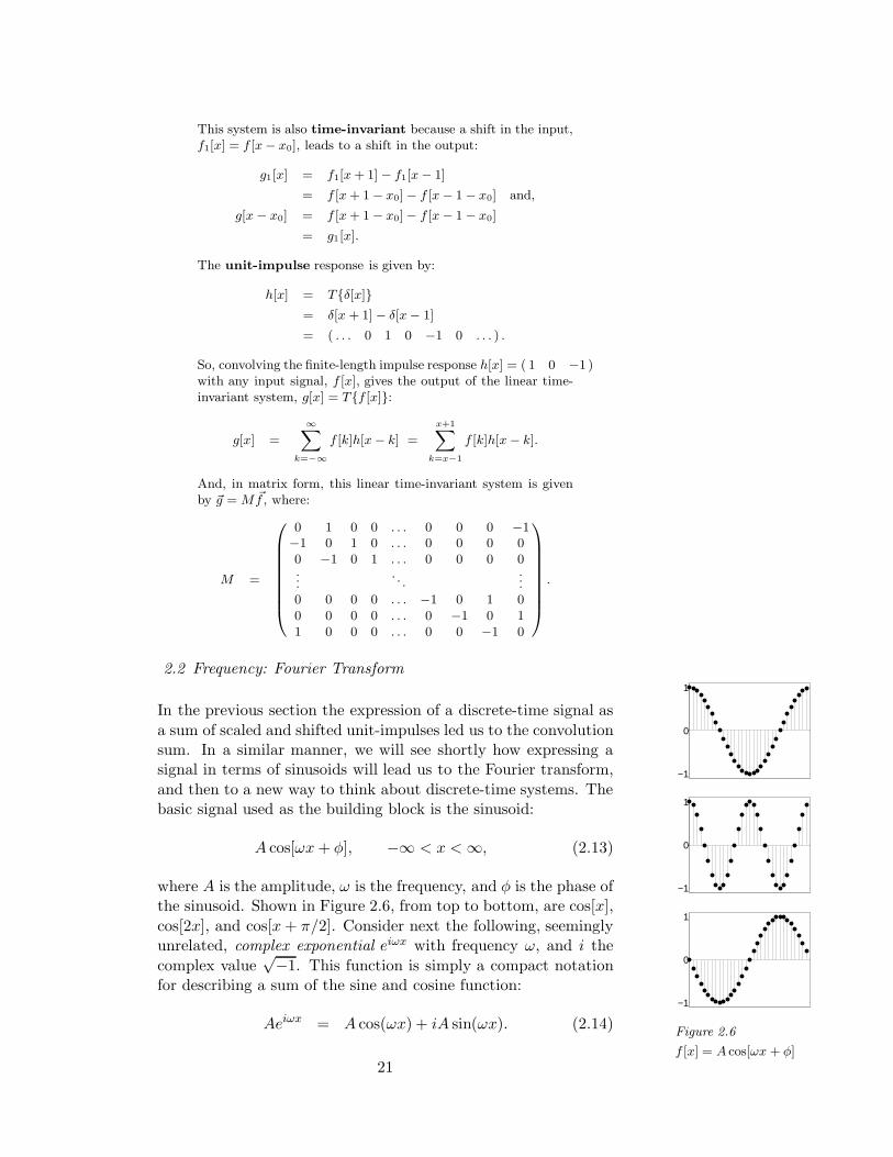
and then to a new way to think about discrete-time systems. Thebasic signal used as the building block is the sinusoid:
A cos[ωx + φ], −∞ < x < ∞, (2.13)
where A is the amplitude, ω is the frequency, and φ is the phase ofthe sinusoid. Shown in Figure 2.6, from top to bottom, are cos[x],
cos[2x], and cos[x + π/2]. Consider next the following, seeminglyunrelated, complex exponential eiωx with frequency ω, and i the
complex value√−1. This function is simply a compact notation
for describing a sum of the sine and cosine function:
Aeiωx = A cos(ωx) + iA sin(ωx). (2.14)
21
The complex exponential has a special relationship with linear
time-invariant systems - the output of a linear time-invariant sys-tem with unit-impulse response h[x] and a complex exponential as
input is:
g[x] = eiωx ? h[x]
=∞∑
k=−∞
h[k]eiω(x−k)
= eiωx∞∑
k=−∞
h[k]e−iωk (2.15)
Defining H [ω] to be the summation component, g[x] can be ex-
pressed as:
g[x] = H [ω]eiωx, (2.16)
that is, given a complex exponential as input, the output of a
Real
Imaginary
H = R + I
H
| H |
Figure 2.7 Magnitude
and phase
linear time-invariant system is again a complex exponential of the
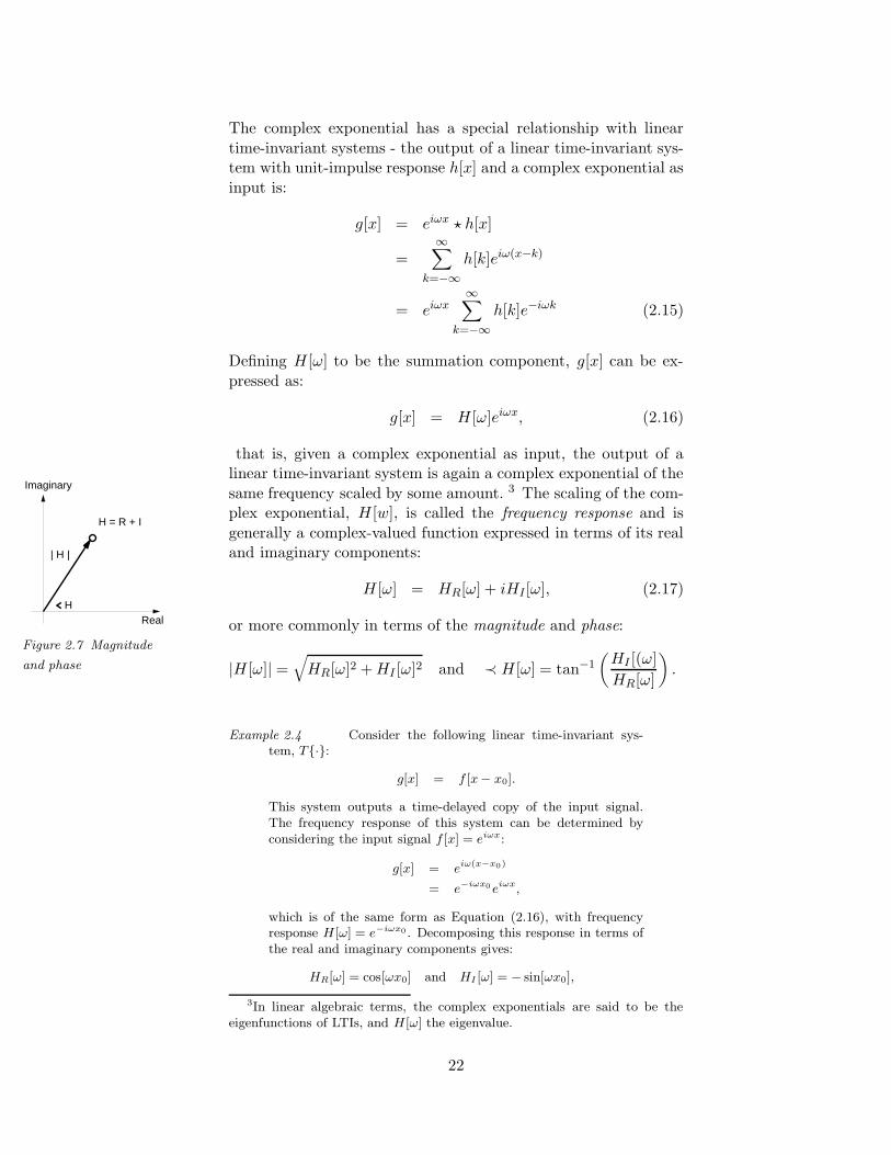
same frequency scaled by some amount. 3 The scaling of the com-plex exponential, H [w], is called the frequency response and is
generally a complex-valued function expressed in terms of its realand imaginary components:
H [ω] = HR[ω] + iHI [ω], (2.17)
or more commonly in terms of the magnitude and phase:
|H [ω]| =√
HR[ω]2 + HI [ω]2 and ≺ H [ω] = tan−1(
HI [(ω]
HR[ω]
)
.
Example 2.4 Consider the following linear time-invariant sys-tem, T{·}:
g[x] = f [x− x0].
This system outputs a time-delayed copy of the input signal.The frequency response of this system can be determined byconsidering the input signal f [x] = eiωx:
g[x] = eiω(x−x0)
= e−iωx0eiωx,
which is of the same form as Equation (2.16), with frequencyresponse H[ω] = e−iωx0 . Decomposing this response in terms ofthe real and imaginary components gives:
HR[ω] = cos[ωx0] and HI [ω] = − sin[ωx0],
3In linear algebraic terms, the complex exponentials are said to be theeigenfunctions of LTIs, and H[ω] the eigenvalue.
22
or in terms of the magnitude and phase:
|H[ω]| =√
cos2[ωx0] + − sin2[ωx0]
= 1
≺ H[ω] = tan−1
(
− sin[ωx0]
cos[ωx0]
)
= −ωx0.
Intuitively, this should make perfect sense. This system simply
takes an input signal and outputs a delayed copy, therefore, there
is no change in the magnitude of each sinusoid, while there is a
phase shift proportional to the delay, x0.
So, why the interest in sinusoids and complex exponentials? As
we will show next, a broad class of signals can be expressed as alinear combination of complex exponentials, and analogous to the
impulse response, the frequency response completely characterizesthe system.
Let’s begin by taking a step back to the more familiar sinusoids,and then work our way to the complex exponentials. Any periodic
discrete-time signal, f [x], can be expressed as a sum of scaled,phase-shifted sinusoids of varying frequencies:
f [x] =1
2π
π∑
k=−π
ck cos [kx + φk] −∞ < x < ∞, (2.18)
For each frequency, k, the amplitude is a real number, ck ∈ R,
and the phase, φk ∈ [0, 2π]. This expression is commonly referredto as the Fourier series.
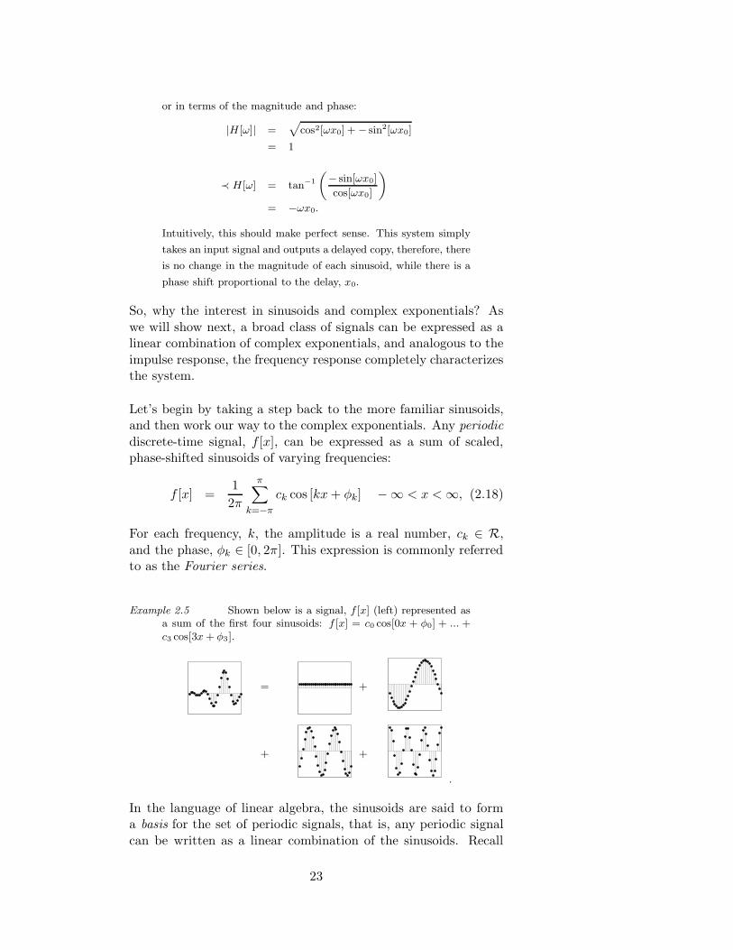
Example 2.5 Shown below is a signal, f [x] (left) represented asa sum of the first four sinusoids: f [x] = c0 cos[0x + φ0] + ... +c3 cos[3x + φ3].
= c0 + c1
+ c2 + c3
.
In the language of linear algebra, the sinusoids are said to forma basis for the set of periodic signals, that is, any periodic signal
can be written as a linear combination of the sinusoids. Recall
23
that in deriving the convolution sum, the basis consisted of shifted
copies of the unit-impulse. But note now that this new basis isnot fixed because of the phase term, φk . It is, however, possible
to rewrite the Fourier series with respect to a fixed basis of zero-phase sinusoids. With the trigonometric identity cos(A + B) =cos(A) cos(B)−sin(A) sin(B), the Fourier series of Equation (2.18)
may be rewritten as:
f [x] =1
2π
π∑
k=−π
ck cos[kx + φk]
=1
2π
π∑
k=−π
ck cos[φk] cos[kx] + ck sin[φk] sin[kx]
=1
2π
π∑
k=−π
ak cos[kx] + bk sin[kx] (2.19)
In this expression, the constants ak and bk are the Fourier coef-ficients and are determined by the Fourier transform. In other
words, the Fourier transform simply provides a means for express-ing a signal in terms of the sinusoids. The Fourier coefficients are
given by:
ak =∞∑
j=−∞
f [j] cos[kj] and bk =∞∑
j=−∞
f [j] sin[kj] (2.20)
Notice that the Fourier coefficients are determined by projectingthe signal onto each of the sinusoidal basis. That is, consider both
the signal f [x] and each of the sinusoids as T -dimensional vectors,~f and ~b, respectively. Then, the projection of ~f onto ~b is:
f0b0 + f1b1 + ... =∑
j
fjbj, (2.21)
where the subscript denotes the jth entry of the vector.
Often, a more compact notation is used to represent the Fourier
series and Fourier transform which exploits the complex exponen-tial and its relationship to the sinusoids:
eiωx = cos(ωx) + i sin(ωx), (2.22)
where i is the complex value√−1. Under the complex exponential
notation, the Fourier series and transform take the form:
f [x] =1
2π
π∑
k=−π
ckeikx and ck =
∞∑
j=−∞
f [j]e−ikj , (2.23)
24
where ck = ak − ibk. This notation simply bundles the sine and
cosine terms into a single expression. A more common, but equiv-alent, notation is:
f [x] =1
2π
π∑
ω=−π
F [ω]eiωx and F [ω] =∞∑
k=−∞
f [k]e−iωk. (2.24)
d[x]
h[x]
LTI
g[x]=f[x]*h[x] G[w]=F[w]H[w]
LTI
Fourier
Transform
exp(iwx)
H[w]exp(iwx)
Figure 2.8 LTI: space
and frequency
Comparing the Fourier transform (Equation (2.24)) with the fre-quency response (Equation (2.16)) we see now that the frequency
response of a linear time-invariant system is simply the Fouriertransform of the unit-impulse response:
H [ω] =∞∑
k=−∞
h[k]e−iωk . (2.25)
In other words, linear time-invariant systems are completely char-acterized by their impulse response, h[x], and, equivalently, by
their frequency response, H [ω], Figure 2.8.
Example 2.6 Consider the following linear time-invariant sys-tem, T{·}:
g[x] =1
4f [x− 1] +
1
2f [x] +
1
4f [x + 1].
The output of this system at each x, is a weighted average ofthe input signal centered at x. First, let’s compute the impulse
response:
h[x] =1
4δ[x− 1] +
1
2δ[x] +
1
4δ[x + 1]
= ( . . . 0 0 14
12
14
0 0 . . . ) .
Then, the frequency response is the Fourier transform of thisimpulse response:
H[ω] =
∞∑
k=−∞
h[k]e−iωk
=
1∑
k=−1
h[k]e−iωk
=1
4eiω +
1
2e0 +
1
4e−iω
=1
4(cos(ω) + i sin(ω)) +
1
2+
1
4(cos(ω) − i sin(ω))
= |1
2+
1
2cos(ω) |.
In this example, the frequency response is strictly real (i.e., HI[ω] =0) and the magnitude and phase are:
|H[ω]| =√
HR[ω]2 + HI [ω]2
=1
2+
1
2cos(ω)
≺ H[ω] = tan−1
(
HI[ω]
Hr[ω]
)
= 0
25
Both the impulse response and the magnitude of the frequencyresponse are shown below, where for clarity, the frequency re-sponse was drawn as a continuous function.
Space (h[x]) Frequency (|H[ω]|)
−1 0 10
0.25
0.5
−pi 0 pi0
1
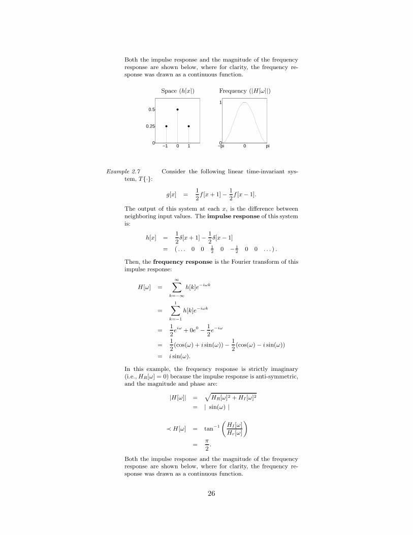
Example 2.7 Consider the following linear time-invariant sys-tem, T{·}:
g[x] =1
2f [x + 1]−
1
2f [x− 1].
The output of this system at each x, is the difference betweenneighboring input values. The impulse response of this systemis:
h[x] =1
2δ[x + 1]−
1
2δ[x− 1]
= ( . . . 0 0 12 0 − 1
2 0 0 . . . ) .
Then, the frequency response is the Fourier transform of thisimpulse response:
H[ω] =
∞∑
k=−∞
h[k]e−iωk
=
1∑
k=−1
h[k]e−iωk
=1
2eiω + 0e0 −
1
2e−iω
=1
2(cos(ω) + i sin(ω))−
1
2(cos(ω) − i sin(ω))
= i sin(ω).
In this example, the frequency response is strictly imaginary(i.e., HR[ω] = 0) because the impulse response is anti-symmetric,and the magnitude and phase are:
|H[ω]| =√
HR[ω]2 + HI [ω]2
= | sin(ω) |
≺ H[ω] = tan−1
(
HI[ω]
Hr[ω]
)
=π
2.
Both the impulse response and the magnitude of the frequencyresponse are shown below, where for clarity, the frequency re-sponse was drawn as a continuous function.
26
Space (h[x]) Frequency (|H[ω]|)
−1 0 1
−0.5
0
0.5
−pi 0 pi0
1
This system is an (approximate) differentiator, and can be seenfrom the definition of differentiation:
df(x)
dx= lim
ε→0
f(x + ε)− f(x− ε)
ε,
where, in the case of the system T{·}, ε is given by the dis-
tance between samples of the discrete-time signal f [x]. Let’s
see now if we can better understand the frequency response of
this system, recall that the magnitude was given by | sin(ω)| and
the phase by π
2 . Consider now the derivative of a fixed fre-
quency sinusoid sin(ωx), differentiating with respect to x gives
ω cos(ωx) = ω sin(ωx − π/2). Note that differentiation causes a
phase shift of π/2 and a scaling by the frequency of the sinusoid.
Notice that this is roughly in-line with the Fourier transform, the
difference being that the amplitude is given by | sin(ω)| instead
of ω. Note though that for small ω, | sin(ω)| ≈ ω. This dis-
crepancy makes the system only an approximate, not a perfect,
differentiator.
Linear time-invariant systems can be fully characterized by theirimpulse, h[x], or frequency responses, H [ω], both of which may beused to determine the output of the system to any input signal,
f [x]:
g[x] = f [x] ? h[x] and G[ω] = F [ω]H [ω], (2.26)
where the output signal g[x] can be determined from its Fouriertransform G[ω], by simply applying the inverse Fourier transform.
This equivalence illustrates an important relationship between thespace and frequency domains. Namely, convolution in the space
domain is equivalent to multiplication in the frequency domain.This is fairly straight-forward to prove:
g[x] = f [x] ? h[x] Fourier transforming,∞∑
k=−∞
g[k]e−iωk =∞∑
k=−∞
(f [k] ? h[k])e−iωk
G[ω] =∞∑
k=−∞
∞∑
j=−∞
f [j]h[k− j]
e−iωk
27
=∞∑
j=−∞
f [j]∞∑
k=−∞
h[k − j]e−iωk let l = k − j,
=∞∑
j=−∞
f [j]∞∑
l=−∞
h[l]e−iω(l+j)
=∞∑
j=−∞
f [j]e−iωj∞∑
l=−∞
h[l]e−iωl
= F [ω]H [ω]. (2.27)
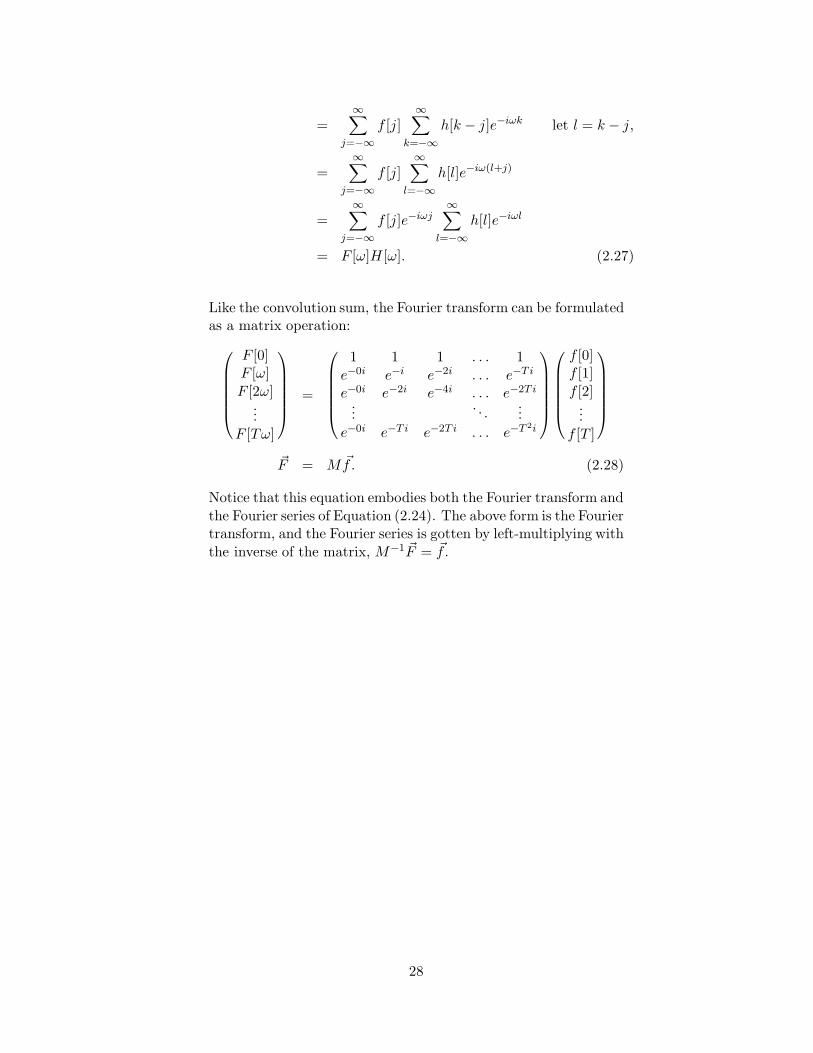
Like the convolution sum, the Fourier transform can be formulatedas a matrix operation:
F [0]F [ω]
F [2ω]...
F [Tω]
=
1 1 1 . . . 1
e−0i e−i e−2i . . . e−T i
e−0i e−2i e−4i . . . e−2T i
.... . .
...
e−0i e−T i e−2T i . . . e−T 2i
f [0]f [1]
f [2]...
f [T ]
~F = M ~f. (2.28)
Notice that this equation embodies both the Fourier transform and
the Fourier series of Equation (2.24). The above form is the Fouriertransform, and the Fourier series is gotten by left-multiplying with
the inverse of the matrix, M−1 ~F = ~f .
28
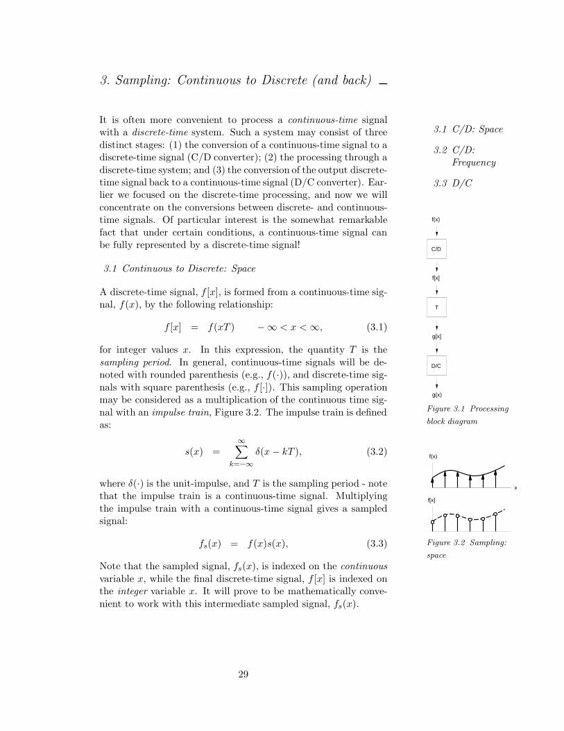
3. Sampling: Continuous to Discrete (and back)
3.1 C/D: Space
3.2 C/D:Frequency
3.3 D/C
f[x]
f(x)
C/D
T
g[x]
D/C
g(x)
Figure 3.1 Processing
block diagram
It is often more convenient to process a continuous-time signalwith a discrete-time system. Such a system may consist of three
distinct stages: (1) the conversion of a continuous-time signal to adiscrete-time signal (C/D converter); (2) the processing through a
discrete-time system; and (3) the conversion of the output discrete-time signal back to a continuous-time signal (D/C converter). Ear-lier we focused on the discrete-time processing, and now we will
concentrate on the conversions between discrete- and continuous-time signals. Of particular interest is the somewhat remarkable
fact that under certain conditions, a continuous-time signal canbe fully represented by a discrete-time signal!
3.1 Continuous to Discrete: Space
A discrete-time signal, f [x], is formed from a continuous-time sig-nal, f(x), by the following relationship:
f [x] = f(xT ) −∞ < x < ∞, (3.1)
for integer values x. In this expression, the quantity T is the
sampling period. In general, continuous-time signals will be de-noted with rounded parenthesis (e.g., f(·)), and discrete-time sig-
nals with square parenthesis (e.g., f [·]). This sampling operation
x
f(x)
f[x]
Figure 3.2 Sampling:
space
may be considered as a multiplication of the continuous time sig-
nal with an impulse train, Figure 3.2. The impulse train is definedas:
s(x) =∞∑
k=−∞
δ(x− kT ), (3.2)
where δ(·) is the unit-impulse, and T is the sampling period - notethat the impulse train is a continuous-time signal. Multiplying
the impulse train with a continuous-time signal gives a sampledsignal:
fs(x) = f(x)s(x), (3.3)
Note that the sampled signal, fs(x), is indexed on the continuous
variable x, while the final discrete-time signal, f [x] is indexed onthe integer variable x. It will prove to be mathematically conve-
nient to work with this intermediate sampled signal, fs(x).
29
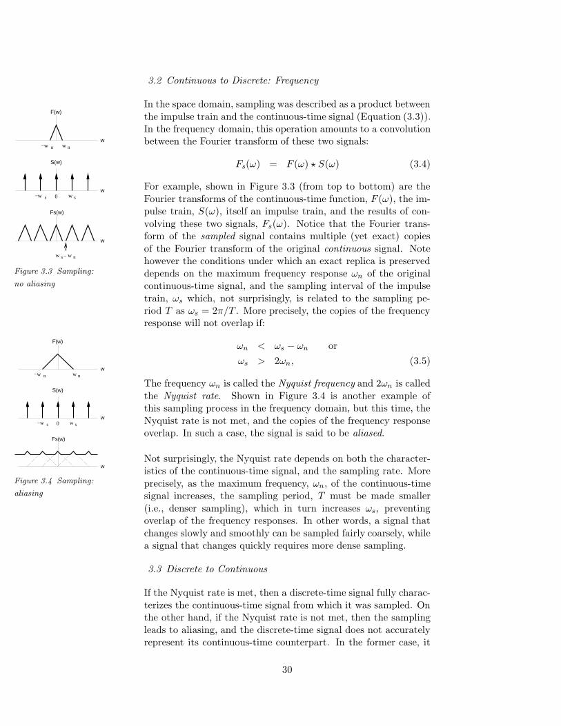
3.2 Continuous to Discrete: Frequency
w
S(w)
w ss−w 0
w
F(w)
−w n w n
w
Fs(w)
w s− w n
Figure 3.3 Sampling:
no aliasing
In the space domain, sampling was described as a product between
the impulse train and the continuous-time signal (Equation (3.3)).In the frequency domain, this operation amounts to a convolutionbetween the Fourier transform of these two signals:
Fs(ω) = F (ω) ? S(ω) (3.4)
For example, shown in Figure 3.3 (from top to bottom) are the
Fourier transforms of the continuous-time function, F (ω), the im-pulse train, S(ω), itself an impulse train, and the results of con-
volving these two signals, Fs(ω). Notice that the Fourier trans-form of the sampled signal contains multiple (yet exact) copies
of the Fourier transform of the original continuous signal. Notehowever the conditions under which an exact replica is preserved
depends on the maximum frequency response ωn of the originalcontinuous-time signal, and the sampling interval of the impulse
train, ωs which, not surprisingly, is related to the sampling pe-riod T as ωs = 2π/T . More precisely, the copies of the frequencyresponse will not overlap if:
w
S(w)
w ss−w 0
w
Fs(w)
w
F(w)
−w n w n
Figure 3.4 Sampling:
aliasing
ωn < ωs − ωn or
ωs > 2ωn, (3.5)
The frequency ωn is called the Nyquist frequency and 2ωn is called
the Nyquist rate. Shown in Figure 3.4 is another example ofthis sampling process in the frequency domain, but this time, the
Nyquist rate is not met, and the copies of the frequency responseoverlap. In such a case, the signal is said to be aliased.
Not surprisingly, the Nyquist rate depends on both the character-istics of the continuous-time signal, and the sampling rate. More
precisely, as the maximum frequency, ωn, of the continuous-timesignal increases, the sampling period, T must be made smaller
(i.e., denser sampling), which in turn increases ωs, preventingoverlap of the frequency responses. In other words, a signal that
changes slowly and smoothly can be sampled fairly coarsely, whilea signal that changes quickly requires more dense sampling.
3.3 Discrete to Continuous
If the Nyquist rate is met, then a discrete-time signal fully charac-
terizes the continuous-time signal from which it was sampled. Onthe other hand, if the Nyquist rate is not met, then the samplingleads to aliasing, and the discrete-time signal does not accurately
represent its continuous-time counterpart. In the former case, it
30
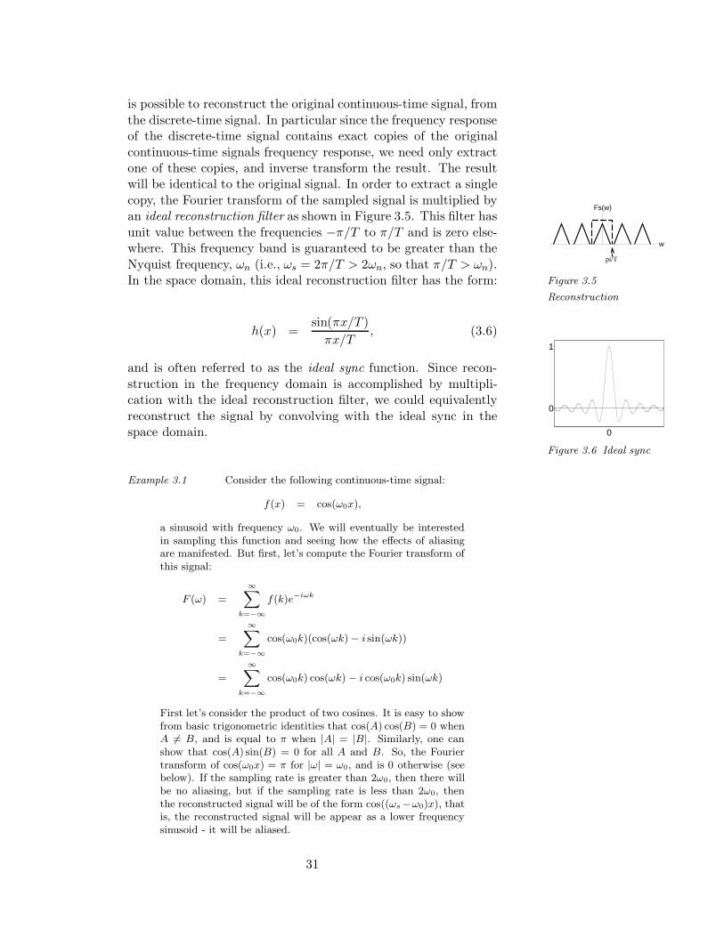
is possible to reconstruct the original continuous-time signal, from
the discrete-time signal. In particular since the frequency responseof the discrete-time signal contains exact copies of the original
continuous-time signals frequency response, we need only extractone of these copies, and inverse transform the result. The resultwill be identical to the original signal. In order to extract a single
w
Fs(w)
pi/T
Figure 3.5
Reconstruction
copy, the Fourier transform of the sampled signal is multiplied byan ideal reconstruction filter as shown in Figure 3.5. This filter has
unit value between the frequencies −π/T to π/T and is zero else-where. This frequency band is guaranteed to be greater than the
Nyquist frequency, ωn (i.e., ωs = 2π/T > 2ωn, so that π/T > ωn).In the space domain, this ideal reconstruction filter has the form:
0
0
1
Figure 3.6 Ideal sync
h(x) =sin(πx/T )
πx/T, (3.6)
and is often referred to as the ideal sync function. Since recon-
struction in the frequency domain is accomplished by multipli-cation with the ideal reconstruction filter, we could equivalently
reconstruct the signal by convolving with the ideal sync in thespace domain.
Example 3.1 Consider the following continuous-time signal:
f(x) = cos(ω0x),
a sinusoid with frequency ω0. We will eventually be interestedin sampling this function and seeing how the effects of aliasingare manifested. But first, let’s compute the Fourier transform ofthis signal:
F (ω) =
∞∑
k=−∞
f(k)e−iωk
=
∞∑
k=−∞
cos(ω0k)(cos(ωk)− i sin(ωk))
=
∞∑
k=−∞
cos(ω0k) cos(ωk) − i cos(ω0k) sin(ωk)
First let’s consider the product of two cosines. It is easy to showfrom basic trigonometric identities that cos(A) cos(B) = 0 whenA 6= B, and is equal to π when |A| = |B|. Similarly, one canshow that cos(A) sin(B) = 0 for all A and B. So, the Fouriertransform of cos(ω0x) = π for |ω| = ω0, and is 0 otherwise (seebelow). If the sampling rate is greater than 2ω0, then there willbe no aliasing, but if the sampling rate is less than 2ω0, thenthe reconstructed signal will be of the form cos((ωs−ω0)x), thatis, the reconstructed signal will be appear as a lower frequencysinusoid - it will be aliased.
31
w
F(w)
−w 0 w 0
Sampling
No Aliasing
w
Fs(w)
−w 0 w 0
Aliasing
w
Fs(w)
−w 0 w 0
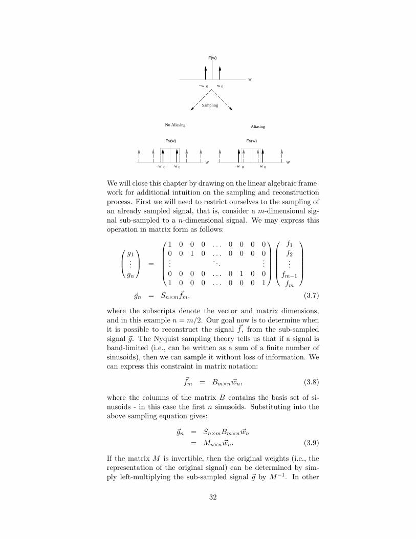
We will close this chapter by drawing on the linear algebraic frame-work for additional intuition on the sampling and reconstruction
process. First we will need to restrict ourselves to the sampling ofan already sampled signal, that is, consider a m-dimensional sig-
nal sub-sampled to a n-dimensional signal. We may express thisoperation in matrix form as follows:
g1...
gn
=
1 0 0 0 . . . 0 0 0 00 0 1 0 . . . 0 0 0 0...
. . ....
0 0 0 0 . . . 0 1 0 01 0 0 0 . . . 0 0 0 1
f1
f2...
fm−1
fm
~gn = Sn×m~fm, (3.7)
where the subscripts denote the vector and matrix dimensions,
and in this example n = m/2. Our goal now is to determine whenit is possible to reconstruct the signal ~f , from the sub-sampled
signal ~g. The Nyquist sampling theory tells us that if a signal isband-limited (i.e., can be written as a sum of a finite number of
sinusoids), then we can sample it without loss of information. Wecan express this constraint in matrix notation:
~fm = Bm×n ~wn, (3.8)
where the columns of the matrix B contains the basis set of si-
nusoids - in this case the first n sinusoids. Substituting into theabove sampling equation gives:
~gn = Sn×mBm×n ~wn
= Mn×n ~wn. (3.9)
If the matrix M is invertible, then the original weights (i.e., therepresentation of the original signal) can be determined by sim-
ply left-multiplying the sub-sampled signal ~g by M−1. In other
32

words, Nyquist sampling theory can be thought of as simply a
matrix inversion problem. This should not be at all surprising,the trick to sampling and perfect reconstruction is to simply limit
the dimensionality of the signal to at most twice the number ofsamples.
33
4. Digital Filter Design
4.1 Choosing a
Frequency Re-sponse
4.2 FrequencySampling
4.3 Least-Squares
4.4 Weighted
Least-Squares
Recall that the class of linear time-invariant systems are fully char-acterized by their impulse response. More specifically, the output
of a linear time-invariant system to any input f [x] can be deter-mined via a convolution with the impulse response h[x]:
g[x] = f [x] ? h[x]. (4.1)
Therefore the filter h[x] and the linear-time invariant system are
synonymous. In the frequency domain, this expression takes onthe form:
G[ω] = F [ω]H [ω]. (4.2)
In other words, a filter modifies the frequencies of the input signal.
It is often the case that such filters pass certain frequencies andattenuate others (e.g., a lowpass, bandpass, or highpass filters).
The design of such filters consists of four basic steps:
1. choose the desired frequency response
2. choose the length of the filter
3. define an error function to be minimized
4. choose a minimization technique and solve
The choice of frequency response depends, of course, on the design-
ers particular application, and its selection is left to their discre-tion. We will however provide some general guidelines for choosing
a frequency response that is amenable to a successful design. Inchoosing a filter size there are two conflicting goals, a large filter al-
lows for a more accurate match to the desired frequency response,however a small filter is desirable in order to minimize computa-
tional demands 4. The designer should experiment with varyingsize filters until an equitable balance is found. With a frequency
response and filter size in hand, this chapter will provide the com-putational framework for realizing a finite length filter that “best”approximates the specified frequency response. Although there are
numerous techniques for the design of digital filters we will coveronly two such techniques chosen for their simplicity and generally
good performance (see Digital Filter Design by T.W. Parks andC.S. Burrus for a full coverage of many other approaches).
4In multi-dimensional filter design, separability is also a desirable property.
34
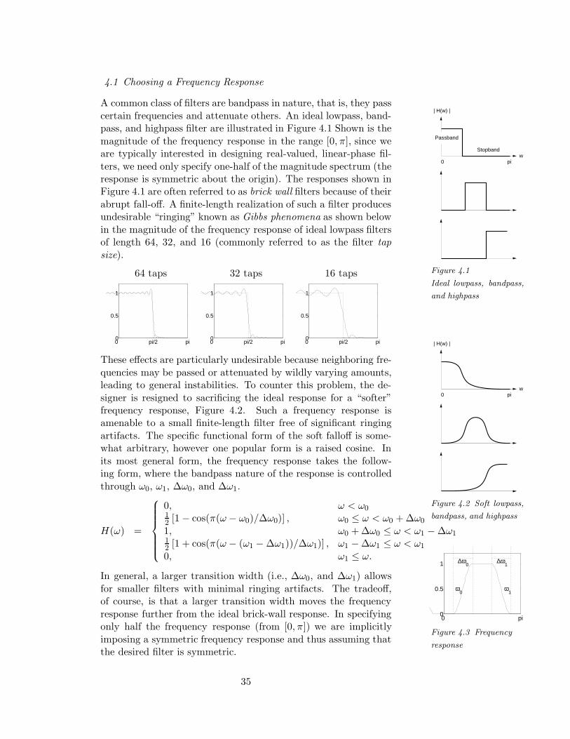
4.1 Choosing a Frequency Response
w
| H(w) |
Stopband
Passband
0 pi
Figure 4.1
Ideal lowpass, bandpass,
and highpass
A common class of filters are bandpass in nature, that is, they pass
certain frequencies and attenuate others. An ideal lowpass, band-pass, and highpass filter are illustrated in Figure 4.1 Shown is the
magnitude of the frequency response in the range [0, π], since weare typically interested in designing real-valued, linear-phase fil-
ters, we need only specify one-half of the magnitude spectrum (theresponse is symmetric about the origin). The responses shown inFigure 4.1 are often referred to as brick wall filters because of their
abrupt fall-off. A finite-length realization of such a filter producesundesirable “ringing” known as Gibbs phenomena as shown below
in the magnitude of the frequency response of ideal lowpass filtersof length 64, 32, and 16 (commonly referred to as the filter tap
size).
64 taps 32 taps 16 taps
0 pi/2 pi 0
0.5
1
0 pi/2 pi 0
0.5
1
0 pi/2 pi 0
0.5
1
w
| H(w) |
0 pi
Figure 4.2 Soft lowpass,
bandpass, and highpass
These effects are particularly undesirable because neighboring fre-
quencies may be passed or attenuated by wildly varying amounts,leading to general instabilities. To counter this problem, the de-
signer is resigned to sacrificing the ideal response for a “softer”frequency response, Figure 4.2. Such a frequency response isamenable to a small finite-length filter free of significant ringing
artifacts. The specific functional form of the soft falloff is some-what arbitrary, however one popular form is a raised cosine. In
its most general form, the frequency response takes the follow-ing form, where the bandpass nature of the response is controlled
through ω0, ω1, ∆ω0, and ∆ω1.
0 pi0
0.5
1
ω0
ω1
∆ω0
∆ω1
Figure 4.3 Frequency
response
H(ω) =
0, ω < ω012 [1− cos(π(ω − ω0)/∆ω0)] , ω0 ≤ ω < ω0 + ∆ω0
1, ω0 + ∆ω0 ≤ ω < ω1 −∆ω112 [1 + cos(π(ω − (ω1 −∆ω1))/∆ω1)] , ω1 −∆ω1 ≤ ω < ω1
0, ω1 ≤ ω.
In general, a larger transition width (i.e., ∆ω0, and ∆ω1) allows
for smaller filters with minimal ringing artifacts. The tradeoff,of course, is that a larger transition width moves the frequency
response further from the ideal brick-wall response. In specifyingonly half the frequency response (from [0, π]) we are implicitly
imposing a symmetric frequency response and thus assuming thatthe desired filter is symmetric.
35
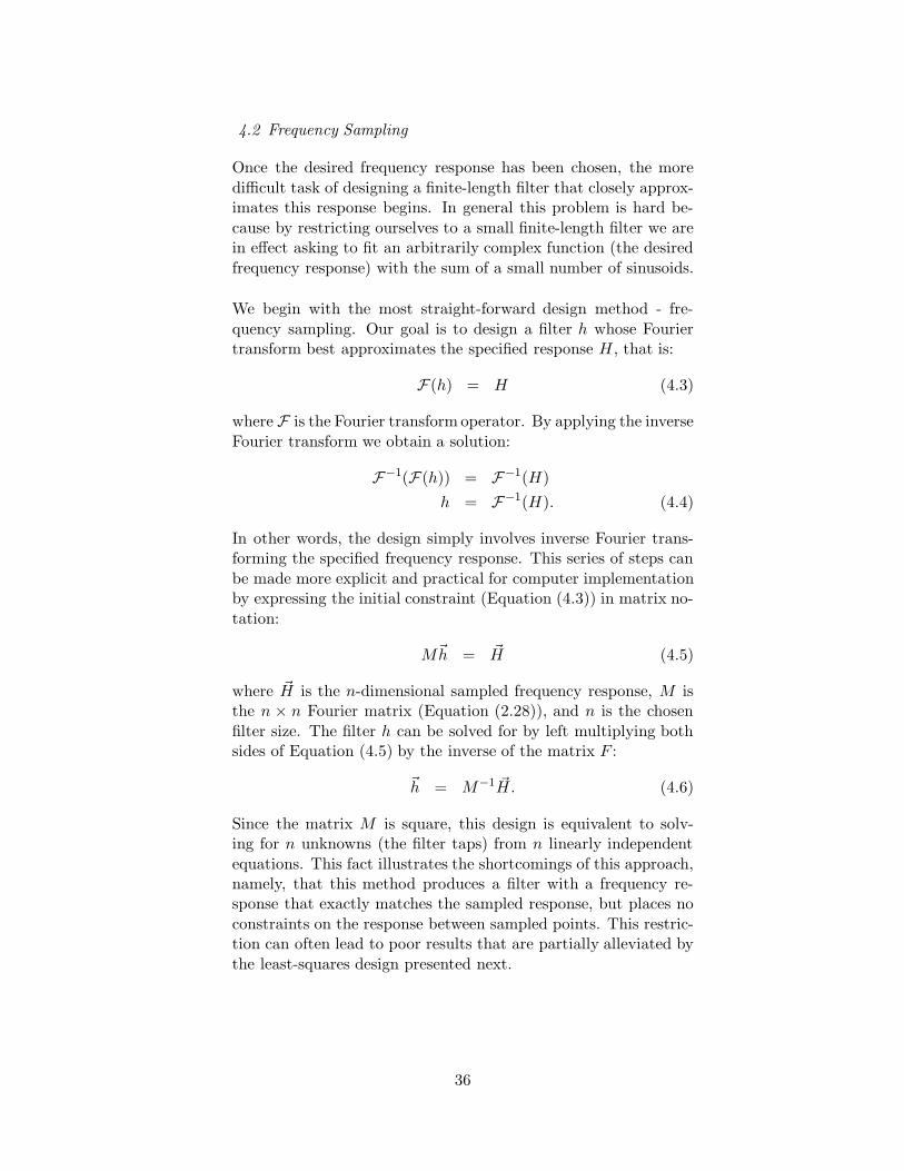
4.2 Frequency Sampling
Once the desired frequency response has been chosen, the more
difficult task of designing a finite-length filter that closely approx-imates this response begins. In general this problem is hard be-
cause by restricting ourselves to a small finite-length filter we arein effect asking to fit an arbitrarily complex function (the desired
frequency response) with the sum of a small number of sinusoids.
We begin with the most straight-forward design method - fre-
quency sampling. Our goal is to design a filter h whose Fouriertransform best approximates the specified response H , that is:
F(h) = H (4.3)
where F is the Fourier transform operator. By applying the inverse
Fourier transform we obtain a solution:
F−1(F(h)) = F−1(H)
h = F−1(H). (4.4)
In other words, the design simply involves inverse Fourier trans-forming the specified frequency response. This series of steps can
be made more explicit and practical for computer implementationby expressing the initial constraint (Equation (4.3)) in matrix no-
tation:
M~h = ~H (4.5)
where ~H is the n-dimensional sampled frequency response, M isthe n × n Fourier matrix (Equation (2.28)), and n is the chosen
filter size. The filter h can be solved for by left multiplying bothsides of Equation (4.5) by the inverse of the matrix F :
~h = M−1 ~H. (4.6)
Since the matrix M is square, this design is equivalent to solv-ing for n unknowns (the filter taps) from n linearly independent
equations. This fact illustrates the shortcomings of this approach,namely, that this method produces a filter with a frequency re-sponse that exactly matches the sampled response, but places no
constraints on the response between sampled points. This restric-tion can often lead to poor results that are partially alleviated by
the least-squares design presented next.
36
4.3 Least-Squares
Our goal is to design a filter ~h that “best” approximates a specifiedfrequency response. As before this constraint can be expressed as:
M~h = ~H, (4.7)
where M is the N × n Fourier matrix (Equation (2.28)), ~H is theN sampled frequency response, and the filter size is n. Note that
unlike before, this equation is over constrained, having n unknownsin N > n equations. We can solve this system of equations in aleast-squares sense by first writing a squared error function to be
minimized:
E(~h) = | M~h− ~H |2 (4.8)
In order to minimize 5, we differentiate with respect to the un-known ~h:
dE(~h)
d~h= 2M t| M~h − ~H |
= 2M tM~h − 2M t ~H, (4.9)
then set equal to zero, and solve:
0 pi/2 pi0
0.5
1
0 pi/2 pi0
0.5
1
0 pi/2 pi0
0.5
1
Figure 4.4 Least-
squares: lowpass, band-
pass, and highpass
~h = (M tM)−1M t ~H (4.10)
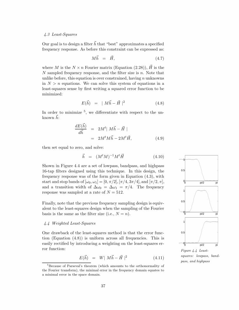
Shown in Figure 4.4 are a set of lowpass, bandpass, and highpass
16-tap filters designed using this technique. In this design, thefrequency response was of the form given in Equation (4.3), withstart and stop bands of [ω0, ω1] = [0, π/2], [π/4, 3π/4], and [π/2, π],
and a transition width of ∆ω0 = ∆ω1 = π/4. The frequencyresponse was sampled at a rate of N = 512.
Finally, note that the previous frequency sampling design is equiv-alent to the least-squares design when the sampling of the Fourier
basis is the same as the filter size (i.e., N = n).
4.4 Weighted Least-Squares
One drawback of the least-squares method is that the error func-tion (Equation (4.8)) is uniform across all frequencies. This is
easily rectified by introducing a weighting on the least-squares er-ror function:
E(~h) = W | M~h− ~H |2 (4.11)
5Because of Parseval’s theorem (which amounts to the orthonormality ofthe Fourier transform), the minimal error in the frequency domain equates toa minimal error in the space domain.
37
where W is a diagonal weighting matrix. That is, the diagonal
of the matrix contains the desired weighting of the error acrossfrequency. As before, we minimize by differentiating with respect
to ~h:
dE(~h)
d~h= 2M tW | M~h− ~H |
= 2M tWM~h − 2WM t ~H, (4.12)
then set equal to zero, and solve:
0 pi/2 pi0
0.5
1
0 pi/2 pi0
0.5
1
Figure 4.5
Least-squares and
weighted least squares
~h = (M tWM)−1M tW ~H. (4.13)
Note that this solution will be equivalent to the original least-squares solution (Equation (4.10)) when W is the identity matrix
(i.e., uniform weighting).
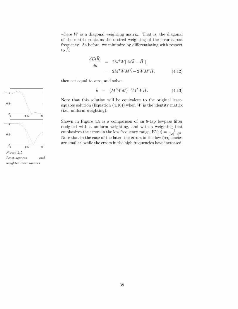
Shown in Figure 4.5 is a comparison of an 8-tap lowpass filter
designed with a uniform weighting, and with a weighting thatemphasizes the errors in the low frequency range, W (ω) = 1
(|ω|+1)8.
Note that in the case of the later, the errors in the low frequenciesare smaller, while the errors in the high frequencies have increased.
38
5. Photons to Pixels
5.1 Pinhole Cam-era
5.2 Lenses
5.3 CCD
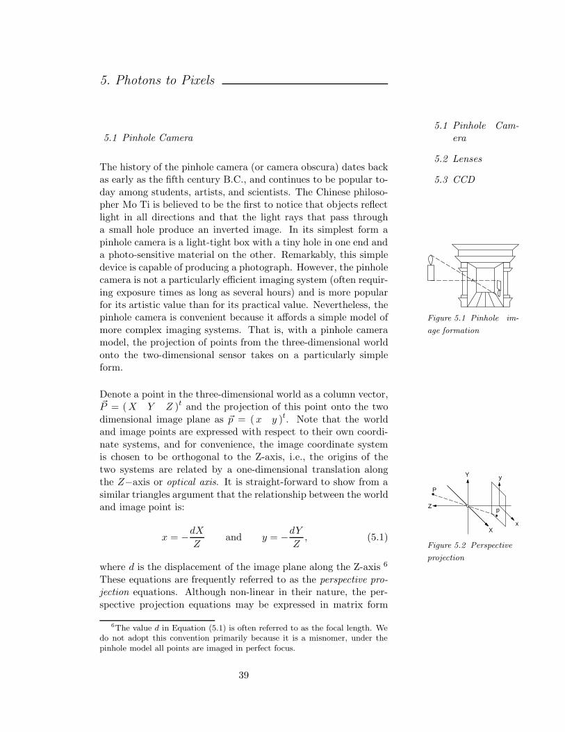
5.1 Pinhole Camera
The history of the pinhole camera (or camera obscura) dates backas early as the fifth century B.C., and continues to be popular to-
day among students, artists, and scientists. The Chinese philoso-pher Mo Ti is believed to be the first to notice that objects reflect
light in all directions and that the light rays that pass througha small hole produce an inverted image. In its simplest form a
Figure 5.1 Pinhole im-
age formation
pinhole camera is a light-tight box with a tiny hole in one end anda photo-sensitive material on the other. Remarkably, this simple
device is capable of producing a photograph. However, the pinholecamera is not a particularly efficient imaging system (often requir-
ing exposure times as long as several hours) and is more popularfor its artistic value than for its practical value. Nevertheless, thepinhole camera is convenient because it affords a simple model of
more complex imaging systems. That is, with a pinhole cameramodel, the projection of points from the three-dimensional world
onto the two-dimensional sensor takes on a particularly simpleform.
Denote a point in the three-dimensional world as a column vector,~P = (X Y Z )t and the projection of this point onto the two
dimensional image plane as ~p = ( x y )t. Note that the worldand image points are expressed with respect to their own coordi-
nate systems, and for convenience, the image coordinate systemis chosen to be orthogonal to the Z-axis, i.e., the origins of the
Y
X
Z
x
y
P
p
Figure 5.2 Perspective
projection
two systems are related by a one-dimensional translation alongthe Z−axis or optical axis. It is straight-forward to show from a
similar triangles argument that the relationship between the worldand image point is:
x = −dX
Zand y = −dY
Z, (5.1)
where d is the displacement of the image plane along the Z-axis 6
These equations are frequently referred to as the perspective pro-jection equations. Although non-linear in their nature, the per-
spective projection equations may be expressed in matrix form
6The value d in Equation (5.1) is often referred to as the focal length. Wedo not adopt this convention primarily because it is a misnomer, under thepinhole model all points are imaged in perfect focus.
39
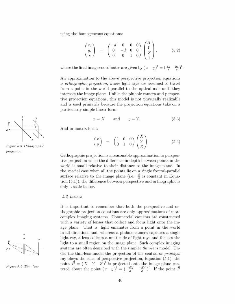
using the homogeneous equations:
xs
ys
s
=
−d 0 0 0
0 −d 0 00 0 1 0
XY
Z1
, (5.2)
where the final image coordinates are given by (x y )t = ( xs
sys
s )t.
An approximation to the above perspective projection equationsis orthographic projection, where light rays are assumed to travel
from a point in the world parallel to the optical axis until theyintersect the image plane. Unlike the pinhole camera and perspec-
tive projection equations, this model is not physically realizableand is used primarily because the projection equations take on a
particularly simple linear form:
Y
X
Z
x
y
Pp
Figure 5.3 Orthographic
projection
x = X and y = Y. (5.3)
And in matrix form:
(
x
y
)
=
(
1 0 0
0 1 0
)
X
YZ
(5.4)
Orthographic projection is a reasonable approximation to perspec-tive projection when the difference in depth between points in the
world is small relative to their distance to the image plane. Inthe special case when all the points lie on a single frontal-parallel
surface relative to the image plane (i.e., dZ is constant in Equa-
tion (5.1)), the difference between perspective and orthographic is
only a scale factor.
5.2 Lenses
It is important to remember that both the perspective and or-
thographic projection equations are only approximations of morecomplex imaging systems. Commercial cameras are constructed
with a variety of lenses that collect and focus light onto the im-age plane. That is, light emanates from a point in the world
Y
Z
Py
Figure 5.4 Thin lens
in all directions and, whereas a pinhole camera captures a singlelight ray, a lens collects a multitude of light rays and focuses the
light to a small region on the image plane. Such complex imagingsystems are often described with the simpler thin-lens model. Un-
der the thin-lens model the projection of the central or principalray obeys the rules of perspective projection, Equation (5.1): thepoint ~P = (X Y Z )t is projected onto the image plane cen-
tered about the point (x y )t = ( −dXZ
−dYZ )t. If the point ~P
40
is in perfect focus, then the remaining light rays captured by the
lens also strike the image plane at the point ~p. A point is imagedin perfect focus if its distance from the lens satisfies the following
thin-lens equation:
1
Z+
1
d=
1
f, (5.5)
where d is the distance between the lens and image plane along theoptical axis, and f is the focal length of the lens. The focal lengthis defined to be the distance from the lens to the image plane such
that the image of an object that is infinitely far away is imagedin perfect focus. Points at a depth of Zo 6= Z are imaged onto a
small region on the image plane, often modeled as a blurred circlewith radius r:
r =R
1f − 1
Zo
∣
∣
∣
∣
(
1
f− 1
Zo
)
− 1
d
∣
∣
∣
∣
, (5.6)
where R is the radius of the lens. Note that when the depth of a
point satisfies Equation (5.5), the blur radius is zero. Note alsothat as the lens radius R approaches 0 (i.e., a pinhole camera),the blur radius also approaches zero for all points independent of
its depth (referred to as an infinite depth of field).
Alternatively, the projection of each light ray can be described in
the following more compact matrix notation:(
l2α2
)
=
(
1 0− 1
R
(
n2−n1n2
)
n1n2
)(
l1α1
)
, (5.7)
where R is the radius of the lens, n1 and n2 are the index ofrefraction for air and the lens material, respectively. l1 and l2 arethe height at which a light ray enters and exits the lens (the thin
lens idealization ensures that l1 = l2). α1 is the angle between theentering light ray and the optical axis, and α2 is the angle between
the exiting light ray and the optical axis. This formulation isparticularly convenient because a variety of lenses can be described
in matrix form so that a complex lens train can then be modeledas a simple product of matrices.
Y
X
Z
x
y
p
P1 P2 P3
Figure 5.5
Non-invertible projection
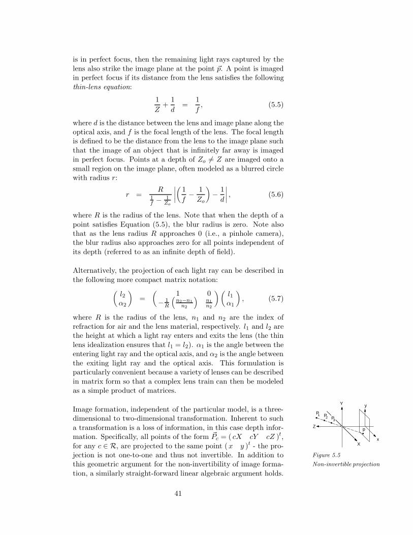
Image formation, independent of the particular model, is a three-dimensional to two-dimensional transformation. Inherent to such
a transformation is a loss of information, in this case depth infor-mation. Specifically, all points of the form ~Pc = ( cX cY cZ )t,
for any c ∈ R, are projected to the same point (x y )t - the pro-jection is not one-to-one and thus not invertible. In addition tothis geometric argument for the non-invertibility of image forma-
tion, a similarly straight-forward linear algebraic argument holds.
41
In particular, we have seen that the image formation equations
may be written in matrix form as, ~p = Mn×m~P , where n < m
(e.g., Equation (5.2)). Since the projection is from a higher di-
mensional space to a lower dimensional space, the matrix M isnot invertible and thus the projection is not invertible.
5.3 CCD
To this point we have described the geometry of image formation,
how light travels through an imaging system. To complete the im-age formation process we need to discuss how the light that strikes
the image plane is recorded and converted into a digital image.The core technology used by most digital cameras is the charge-
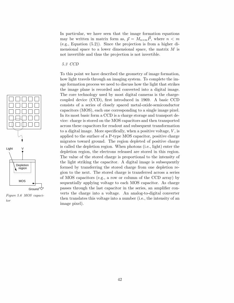
coupled device (CCD), first introduced in 1969. A basic CCD
Depletion region
Ground
VLight
MOS
Figure 5.6 MOS capaci-
tor
consists of a series of closely spaced metal-oxide-semiconductor
capacitors (MOS), each one corresponding to a single image pixel.In its most basic form a CCD is a charge storage and transport de-
vice: charge is stored on the MOS capacitors and then transportedacross these capacitors for readout and subsequent transformation
to a digital image. More specifically, when a positive voltage, V , isapplied to the surface of a P-type MOS capacitor, positive chargemigrates toward ground. The region depleted of positive charge
is called the depletion region. When photons (i.e., light) enter thedepletion region, the electrons released are stored in this region.
The value of the stored charge is proportional to the intensity ofthe light striking the capacitor. A digital image is subsequently
formed by transferring the stored charge from one depletion re-gion to the next. The stored charge is transferred across a series
of MOS capacitors (e.g., a row or column of the CCD array) bysequentially applying voltage to each MOS capacitor. As charge
passes through the last capacitor in the series, an amplifier con-verts the charge into a voltage. An analog-to-digital converterthen translates this voltage into a number (i.e., the intensity of an
image pixel).
42
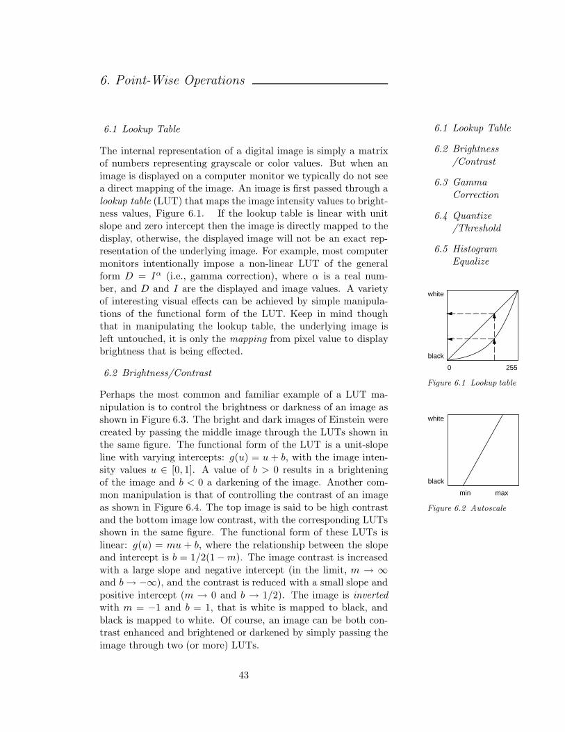
6. Point-Wise Operations
6.1 Lookup Table
6.2 Brightness
/Contrast
6.3 Gamma
Correction
6.4 Quantize/Threshold
6.5 HistogramEqualize
6.1 Lookup Table
The internal representation of a digital image is simply a matrixof numbers representing grayscale or color values. But when an
image is displayed on a computer monitor we typically do not seea direct mapping of the image. An image is first passed through a
lookup table (LUT) that maps the image intensity values to bright-ness values, Figure 6.1. If the lookup table is linear with unit
0 255
white
black
Figure 6.1 Lookup table
white
black
min max
Figure 6.2 Autoscale
slope and zero intercept then the image is directly mapped to the
display, otherwise, the displayed image will not be an exact rep-resentation of the underlying image. For example, most computer
monitors intentionally impose a non-linear LUT of the generalform D = Iα (i.e., gamma correction), where α is a real num-
ber, and D and I are the displayed and image values. A varietyof interesting visual effects can be achieved by simple manipula-
tions of the functional form of the LUT. Keep in mind thoughthat in manipulating the lookup table, the underlying image is
left untouched, it is only the mapping from pixel value to displaybrightness that is being effected.
6.2 Brightness/Contrast
Perhaps the most common and familiar example of a LUT ma-
nipulation is to control the brightness or darkness of an image asshown in Figure 6.3. The bright and dark images of Einstein were
created by passing the middle image through the LUTs shown inthe same figure. The functional form of the LUT is a unit-slope
line with varying intercepts: g(u) = u + b, with the image inten-sity values u ∈ [0, 1]. A value of b > 0 results in a brightening
of the image and b < 0 a darkening of the image. Another com-mon manipulation is that of controlling the contrast of an image
as shown in Figure 6.4. The top image is said to be high contrastand the bottom image low contrast, with the corresponding LUTsshown in the same figure. The functional form of these LUTs is
linear: g(u) = mu + b, where the relationship between the slopeand intercept is b = 1/2(1−m). The image contrast is increased
with a large slope and negative intercept (in the limit, m → ∞and b → −∞), and the contrast is reduced with a small slope and
positive intercept (m → 0 and b → 1/2). The image is invertedwith m = −1 and b = 1, that is white is mapped to black, and
black is mapped to white. Of course, an image can be both con-trast enhanced and brightened or darkened by simply passing the
image through two (or more) LUTs.
43
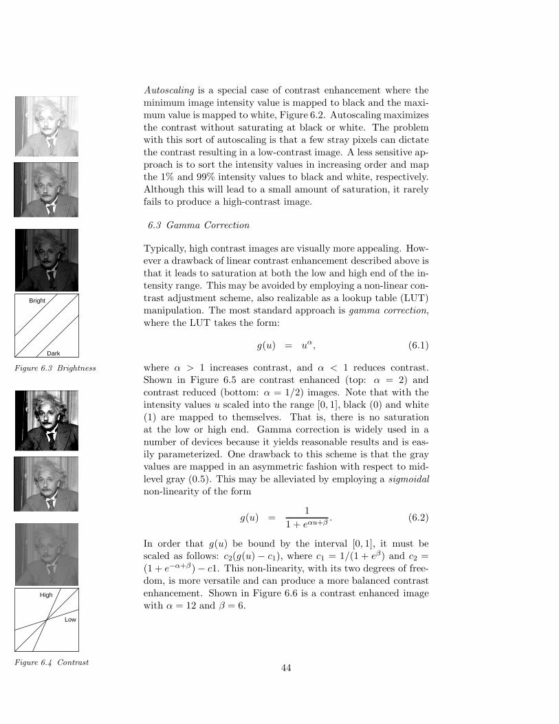
Dark
Bright
Figure 6.3 Brightness
High
Low
Figure 6.4 Contrast
Autoscaling is a special case of contrast enhancement where the
minimum image intensity value is mapped to black and the maxi-mum value is mapped to white, Figure 6.2. Autoscaling maximizes
the contrast without saturating at black or white. The problemwith this sort of autoscaling is that a few stray pixels can dictate
the contrast resulting in a low-contrast image. A less sensitive ap-proach is to sort the intensity values in increasing order and mapthe 1% and 99% intensity values to black and white, respectively.
Although this will lead to a small amount of saturation, it rarelyfails to produce a high-contrast image.
6.3 Gamma Correction
Typically, high contrast images are visually more appealing. How-ever a drawback of linear contrast enhancement described above is
that it leads to saturation at both the low and high end of the in-tensity range. This may be avoided by employing a non-linear con-
trast adjustment scheme, also realizable as a lookup table (LUT)manipulation. The most standard approach is gamma correction,
where the LUT takes the form:
g(u) = uα, (6.1)
where α > 1 increases contrast, and α < 1 reduces contrast.Shown in Figure 6.5 are contrast enhanced (top: α = 2) and
contrast reduced (bottom: α = 1/2) images. Note that with theintensity values u scaled into the range [0, 1], black (0) and white
(1) are mapped to themselves. That is, there is no saturationat the low or high end. Gamma correction is widely used in a
number of devices because it yields reasonable results and is eas-ily parameterized. One drawback to this scheme is that the grayvalues are mapped in an asymmetric fashion with respect to mid-
level gray (0.5). This may be alleviated by employing a sigmoidalnon-linearity of the form
g(u) =1
1 + eαu+β. (6.2)
In order that g(u) be bound by the interval [0, 1], it must bescaled as follows: c2(g(u)− c1), where c1 = 1/(1 + eβ) and c2 =
(1 + e−α+β)− c1. This non-linearity, with its two degrees of free-dom, is more versatile and can produce a more balanced contrast
enhancement. Shown in Figure 6.6 is a contrast enhanced imagewith α = 12 and β = 6.
44
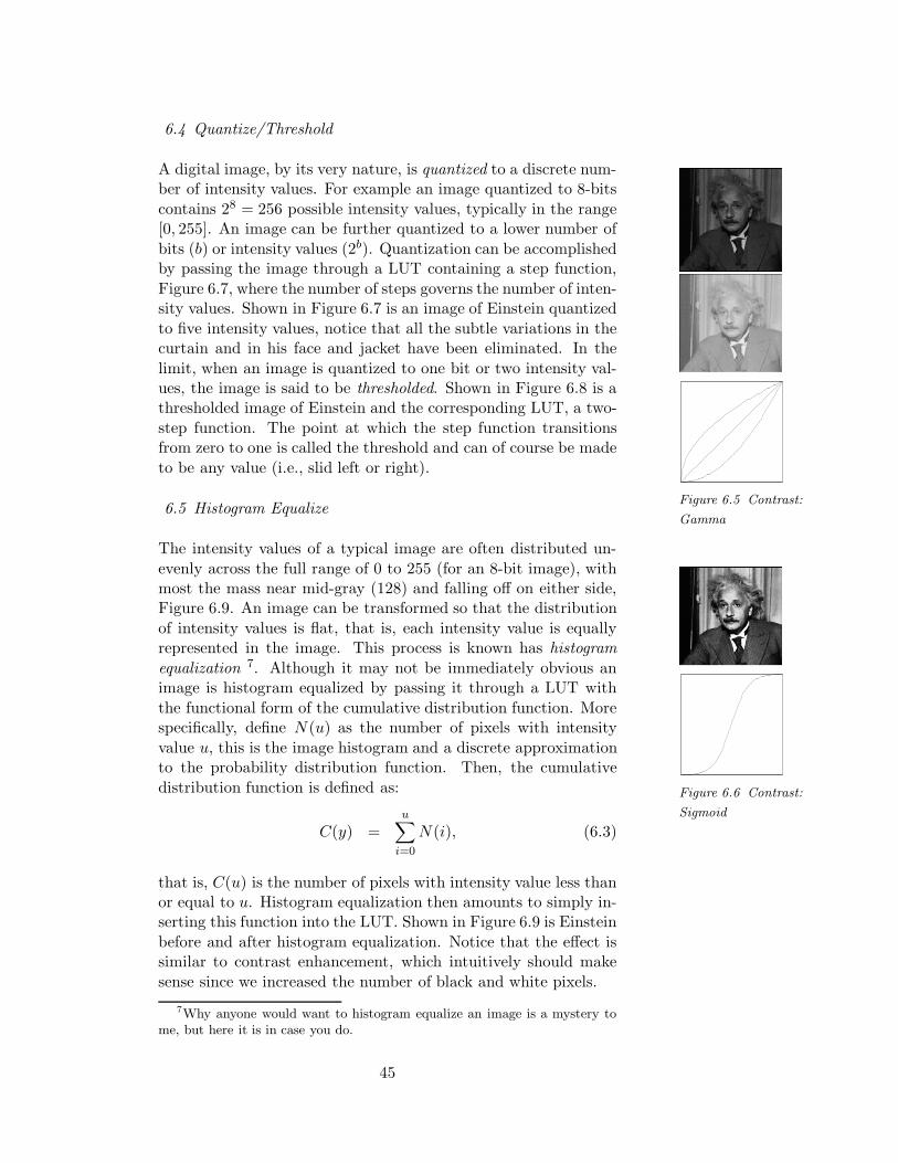
6.4 Quantize/Threshold
A digital image, by its very nature, is quantized to a discrete num-ber of intensity values. For example an image quantized to 8-bits
contains 28 = 256 possible intensity values, typically in the range[0, 255]. An image can be further quantized to a lower number of
bits (b) or intensity values (2b). Quantization can be accomplishedby passing the image through a LUT containing a step function,
Figure 6.7, where the number of steps governs the number of inten-sity values. Shown in Figure 6.7 is an image of Einstein quantized
to five intensity values, notice that all the subtle variations in thecurtain and in his face and jacket have been eliminated. In the
limit, when an image is quantized to one bit or two intensity val-ues, the image is said to be thresholded. Shown in Figure 6.8 is athresholded image of Einstein and the corresponding LUT, a two-
step function. The point at which the step function transitionsfrom zero to one is called the threshold and can of course be made
to be any value (i.e., slid left or right).
Figure 6.5 Contrast:
Gamma
Figure 6.6 Contrast:
Sigmoid
6.5 Histogram Equalize
The intensity values of a typical image are often distributed un-
evenly across the full range of 0 to 255 (for an 8-bit image), withmost the mass near mid-gray (128) and falling off on either side,Figure 6.9. An image can be transformed so that the distribution
of intensity values is flat, that is, each intensity value is equallyrepresented in the image. This process is known has histogram
equalization 7. Although it may not be immediately obvious animage is histogram equalized by passing it through a LUT with
the functional form of the cumulative distribution function. Morespecifically, define N(u) as the number of pixels with intensity
value u, this is the image histogram and a discrete approximationto the probability distribution function. Then, the cumulative
distribution function is defined as:
C(y) =u∑
i=0
N(i), (6.3)
that is, C(u) is the number of pixels with intensity value less thanor equal to u. Histogram equalization then amounts to simply in-serting this function into the LUT. Shown in Figure 6.9 is Einstein
before and after histogram equalization. Notice that the effect issimilar to contrast enhancement, which intuitively should make
sense since we increased the number of black and white pixels.
7Why anyone would want to histogram equalize an image is a mystery tome, but here it is in case you do.
45
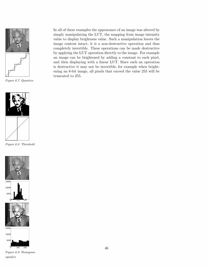
In all of these examples the appearance of an image was altered by
simply manipulating the LUT, the mapping from image intensityvalue to display brightness value. Such a manipulation leaves the
image content intact, it is a non-destructive operation and thuscompletely invertible. These operations can be made destructiveby applying the LUT operation directly to the image. For example
an image can be brightened by adding a constant to each pixel,and then displaying with a linear LUT. Since such an operation
is destructive it may not be inveritble, for example when bright-ening an 8-bit image, all pixels that exceed the value 255 will be
truncated to 255.Figure 6.7 Quantize
Figure 6.8 Threshold
0 100 2000
5000
10000
15000
0 100 2000
5000
10000
15000
Figure 6.9 Histogram
equalize
46
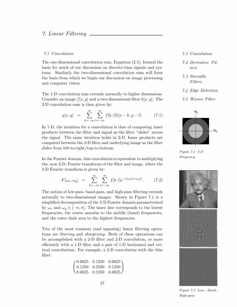
7. Linear Filtering
7.1 Convolution
7.2 Derivative Fil-
ters
7.3 Steerable
Filters
7.4 Edge Detection
7.5 Wiener Filter
7.1 Convolution
ωx
ωy
Figure 7.1 2-D
Frequency
Figure 7.2 Low-, Band-,
High-pass
The one-dimensional convolution sum, Equation (2.5), formed the
basis for much of our discussion on discrete-time signals and sys-tems. Similarly the two-dimensional convolution sum will form
the basis from which we begin our discussion on image processingand computer vision.
The 1-D convolution sum extends naturally to higher dimensions.Consider an image f [x, y] and a two-dimensional filter h[x, y]. The
2-D convolution sum is then given by:
g[x, y] =∞∑
k=−∞
∞∑
l=−∞
f [k, l]h[x− k, y − l]. (7.1)
In 1-D, the intuition for a convolution is that of computing innerproducts between the filter and signal as the filter “slides” across
the signal. The same intuition holds in 2-D. Inner products arecomputed between the 2-D filter and underlying image as the filter
slides from left-to-right/top-to-bottom.
In the Fourier domain, this convolution is equivalent to multiplying
the, now 2-D, Fourier transforms of the filter and image, where the2-D Fourier transform is given by:
F [ωx, ωy] =∞∑
k=−∞
∞∑
l=−∞
f [k, l]e−i(ωxk+ωyl). (7.2)
The notion of low-pass, band-pass, and high-pass filtering extends
naturally to two-dimensional images. Shown in Figure 7.1 is asimplified decomposition of the 2-D Fourier domain parameterized
by ωx and ωy ∈ [−π, π]. The inner disc corresponds to the lowestfrequencies, the center annulus to the middle (band) frequencies,
and the outer dark area to the highest frequencies.
Two of the most common (and opposing) linear filtering opera-
tions are blurring and sharpening. Both of these operations canbe accomplished with a 2-D filter and 2-D convolution, or more
efficiently with a 1-D filter and a pair of 1-D horizontal and ver-tical convolutions. For example, a 2-D convolution with the blur
filter:
0.0625 0.1250 0.0625
0.1250 0.2500 0.12500.0625 0.1250 0.0625
47
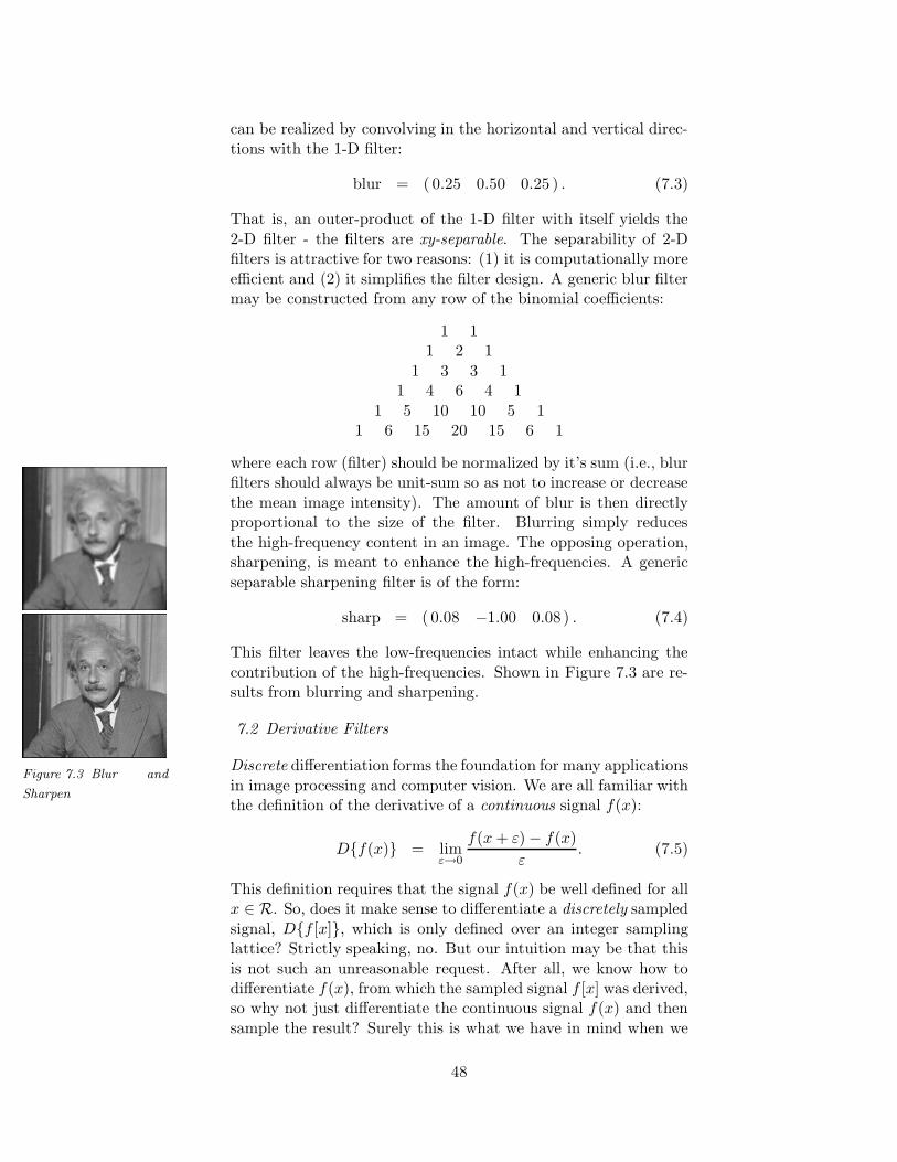
can be realized by convolving in the horizontal and vertical direc-
tions with the 1-D filter:
blur = ( 0.25 0.50 0.25 ) . (7.3)
That is, an outer-product of the 1-D filter with itself yields the
2-D filter - the filters are xy-separable. The separability of 2-Dfilters is attractive for two reasons: (1) it is computationally more
efficient and (2) it simplifies the filter design. A generic blur filtermay be constructed from any row of the binomial coefficients:
1 11 2 1
1 3 3 11 4 6 4 1
1 5 10 10 5 11 6 15 20 15 6 1
Figure 7.3 Blur and
Sharpen
where each row (filter) should be normalized by it’s sum (i.e., blurfilters should always be unit-sum so as not to increase or decrease
the mean image intensity). The amount of blur is then directlyproportional to the size of the filter. Blurring simply reduces
the high-frequency content in an image. The opposing operation,sharpening, is meant to enhance the high-frequencies. A generic
separable sharpening filter is of the form:
sharp = ( 0.08 −1.00 0.08) . (7.4)
This filter leaves the low-frequencies intact while enhancing the
contribution of the high-frequencies. Shown in Figure 7.3 are re-sults from blurring and sharpening.
7.2 Derivative Filters
Discrete differentiation forms the foundation for many applications
in image processing and computer vision. We are all familiar withthe definition of the derivative of a continuous signal f(x):
D{f(x)} = limε→0
f(x + ε)− f(x)
ε. (7.5)
This definition requires that the signal f(x) be well defined for allx ∈ R. So, does it make sense to differentiate a discretely sampled
signal, D{f [x]}, which is only defined over an integer samplinglattice? Strictly speaking, no. But our intuition may be that this
is not such an unreasonable request. After all, we know how todifferentiate f(x), from which the sampled signal f [x] was derived,so why not just differentiate the continuous signal f(x) and then
sample the result? Surely this is what we have in mind when we
48
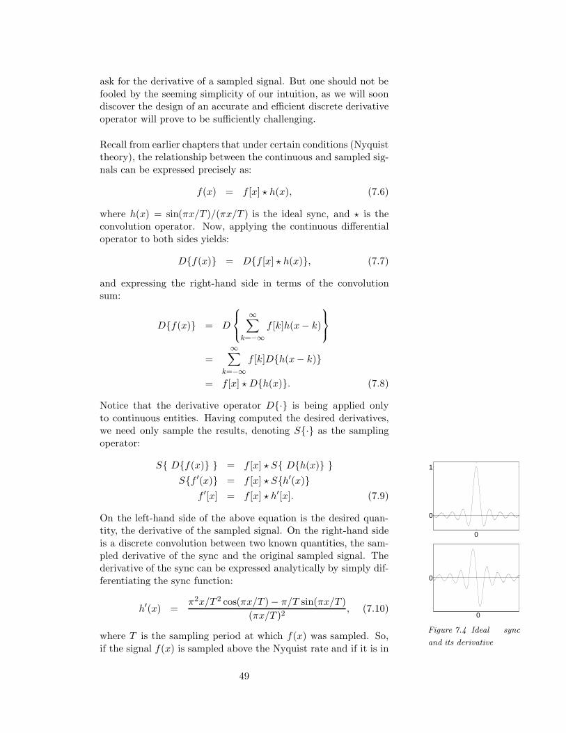
ask for the derivative of a sampled signal. But one should not be
fooled by the seeming simplicity of our intuition, as we will soondiscover the design of an accurate and efficient discrete derivative
operator will prove to be sufficiently challenging.
Recall from earlier chapters that under certain conditions (Nyquisttheory), the relationship between the continuous and sampled sig-
nals can be expressed precisely as:
f(x) = f [x] ? h(x), (7.6)
where h(x) = sin(πx/T )/(πx/T ) is the ideal sync, and ? is theconvolution operator. Now, applying the continuous differential
operator to both sides yields:
D{f(x)} = D{f [x] ? h(x)}, (7.7)
and expressing the right-hand side in terms of the convolutionsum:
D{f(x)} = D
∞∑
k=−∞
f [k]h(x− k)
=∞∑
k=−∞
f [k]D{h(x− k)}
= f [x] ? D{h(x)}. (7.8)
Notice that the derivative operator D{·} is being applied only
to continuous entities. Having computed the desired derivatives,we need only sample the results, denoting S{·} as the sampling
operator:
0
0
1
0
0
Figure 7.4 Ideal sync
and its derivative
S{ D{f(x)} } = f [x] ? S{ D{h(x)} }S{f ′(x)} = f [x] ? S{h′(x)}
f ′[x] = f [x] ? h′[x]. (7.9)
On the left-hand side of the above equation is the desired quan-tity, the derivative of the sampled signal. On the right-hand side
is a discrete convolution between two known quantities, the sam-pled derivative of the sync and the original sampled signal. Thederivative of the sync can be expressed analytically by simply dif-
ferentiating the sync function:
h′(x) =π2x/T 2 cos(πx/T )− π/T sin(πx/T )
(πx/T )2, (7.10)
where T is the sampling period at which f(x) was sampled. So,
if the signal f(x) is sampled above the Nyquist rate and if it is in
49
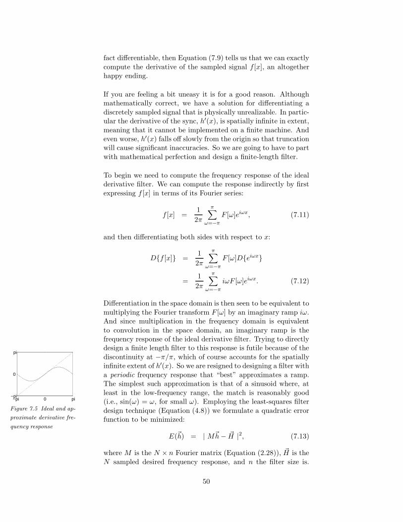
fact differentiable, then Equation (7.9) tells us that we can exactly
compute the derivative of the sampled signal f [x], an altogetherhappy ending.
If you are feeling a bit uneasy it is for a good reason. Althoughmathematically correct, we have a solution for differentiating a
discretely sampled signal that is physically unrealizable. In partic-ular the derivative of the sync, h′(x), is spatially infinite in extent,
meaning that it cannot be implemented on a finite machine. Andeven worse, h′(x) falls off slowly from the origin so that truncationwill cause significant inaccuracies. So we are going to have to part
with mathematical perfection and design a finite-length filter.
To begin we need to compute the frequency response of the idealderivative filter. We can compute the response indirectly by first
expressing f [x] in terms of its Fourier series:
f [x] =1
2π
π∑
ω=−π
F [ω]eiωx, (7.11)
and then differentiating both sides with respect to x:
D{f [x]} =1
2π
π∑
ω=−π
F [ω]D{eiωx}
=1
2π
π∑
ω=−π
iωF [ω]eiωx. (7.12)
Differentiation in the space domain is then seen to be equivalent to
multiplying the Fourier transform F [ω] by an imaginary ramp iω.And since multiplication in the frequency domain is equivalent
to convolution in the space domain, an imaginary ramp is thefrequency response of the ideal derivative filter. Trying to directly
−pi 0 pi−pi
0
pi
Figure 7.5 Ideal and ap-
proximate derivative fre-
quency response
design a finite length filter to this response is futile because of the
discontinuity at −π/π, which of course accounts for the spatiallyinfinite extent of h′(x). So we are resigned to designing a filter with
a periodic frequency response that “best” approximates a ramp.The simplest such approximation is that of a sinusoid where, at
least in the low-frequency range, the match is reasonably good(i.e., sin(ω) = ω, for small ω). Employing the least-squares filter
design technique (Equation (4.8)) we formulate a quadratic errorfunction to be minimized:
E(~h) = | M~h− ~H |2, (7.13)
where M is the N × n Fourier matrix (Equation (2.28)), ~H is the
N sampled desired frequency response, and n the filter size is.
50
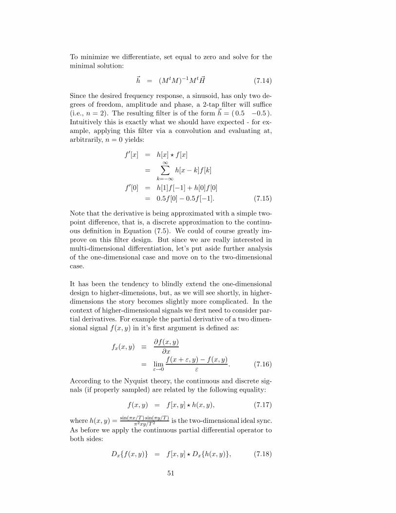
To minimize we differentiate, set equal to zero and solve for the
minimal solution:
~h = (M tM)−1M t ~H (7.14)
Since the desired frequency response, a sinusoid, has only two de-grees of freedom, amplitude and phase, a 2-tap filter will suffice(i.e., n = 2). The resulting filter is of the form ~h = (0.5 −0.5 ).
Intuitively this is exactly what we should have expected - for ex-ample, applying this filter via a convolution and evaluating at,
arbitrarily, n = 0 yields:
f ′[x] = h[x] ? f [x]
=∞∑
k=−∞
h[x− k]f [k]
f ′[0] = h[1]f [−1] + h[0]f [0]
= 0.5f [0]− 0.5f [−1]. (7.15)
Note that the derivative is being approximated with a simple two-
point difference, that is, a discrete approximation to the continu-ous definition in Equation (7.5). We could of course greatly im-
prove on this filter design. But since we are really interested inmulti-dimensional differentiation, let’s put aside further analysisof the one-dimensional case and move on to the two-dimensional
case.
It has been the tendency to blindly extend the one-dimensional
design to higher-dimensions, but, as we will see shortly, in higher-dimensions the story becomes slightly more complicated. In the
context of higher-dimensional signals we first need to consider par-tial derivatives. For example the partial derivative of a two dimen-
sional signal f(x, y) in it’s first argument is defined as:
fx(x, y) ≡ ∂f(x, y)
∂x
= limε→0
f(x + ε, y)− f(x, y)
ε. (7.16)
According to the Nyquist theory, the continuous and discrete sig-nals (if properly sampled) are related by the following equality:
f(x, y) = f [x, y] ? h(x, y), (7.17)
where h(x, y) = sin(πx/T ) sin(πy/T )π2xy/T 2 is the two-dimensional ideal sync.
As before we apply the continuous partial differential operator toboth sides:
Dx{f(x, y)} = f [x, y] ? Dx{h(x, y)}, (7.18)
51
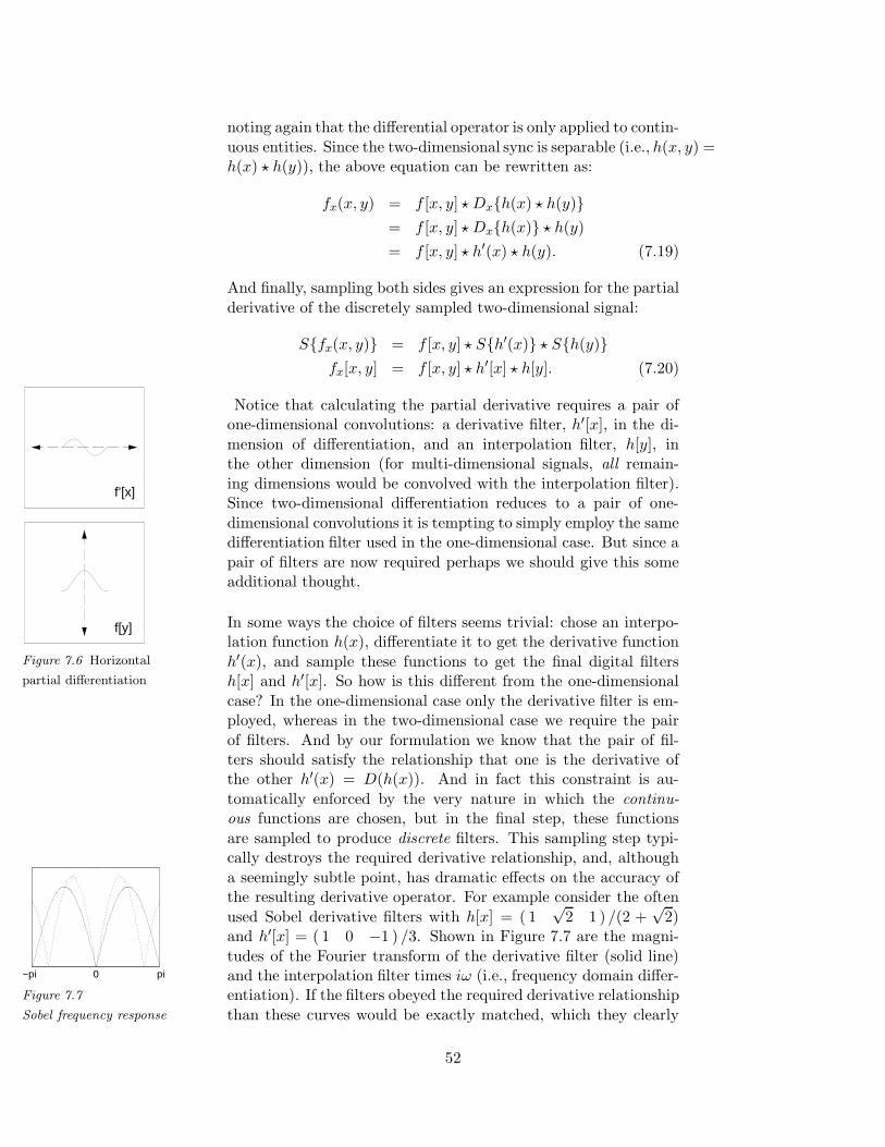
noting again that the differential operator is only applied to contin-
uous entities. Since the two-dimensional sync is separable (i.e., h(x, y) =h(x) ? h(y)), the above equation can be rewritten as:
fx(x, y) = f [x, y] ? Dx{h(x) ? h(y)}= f [x, y] ? Dx{h(x)} ? h(y)
= f [x, y] ? h′(x) ? h(y). (7.19)
And finally, sampling both sides gives an expression for the partial
derivative of the discretely sampled two-dimensional signal:
S{fx(x, y)} = f [x, y] ? S{h′(x)} ? S{h(y)}fx[x, y] = f [x, y] ? h′[x] ? h[y]. (7.20)
Notice that calculating the partial derivative requires a pair of
f’[x]
f[y]
Figure 7.6 Horizontal
partial differentiation
one-dimensional convolutions: a derivative filter, h′[x], in the di-
mension of differentiation, and an interpolation filter, h[y], inthe other dimension (for multi-dimensional signals, all remain-
ing dimensions would be convolved with the interpolation filter).Since two-dimensional differentiation reduces to a pair of one-
dimensional convolutions it is tempting to simply employ the samedifferentiation filter used in the one-dimensional case. But since a
pair of filters are now required perhaps we should give this someadditional thought.
In some ways the choice of filters seems trivial: chose an interpo-lation function h(x), differentiate it to get the derivative function
h′(x), and sample these functions to get the final digital filtersh[x] and h′[x]. So how is this different from the one-dimensional
case? In the one-dimensional case only the derivative filter is em-ployed, whereas in the two-dimensional case we require the pair
of filters. And by our formulation we know that the pair of fil-ters should satisfy the relationship that one is the derivative ofthe other h′(x) = D(h(x)). And in fact this constraint is au-
tomatically enforced by the very nature in which the continu-ous functions are chosen, but in the final step, these functions
are sampled to produce discrete filters. This sampling step typi-
−pi 0 pi
Figure 7.7
Sobel frequency response
cally destroys the required derivative relationship, and, although
a seemingly subtle point, has dramatic effects on the accuracy ofthe resulting derivative operator. For example consider the often
used Sobel derivative filters with h[x] = ( 1√
2 1 ) /(2 +√
2)and h′[x] = ( 1 0 −1 ) /3. Shown in Figure 7.7 are the magni-
tudes of the Fourier transform of the derivative filter (solid line)and the interpolation filter times iω (i.e., frequency domain differ-entiation). If the filters obeyed the required derivative relationship
than these curves would be exactly matched, which they clearly
52
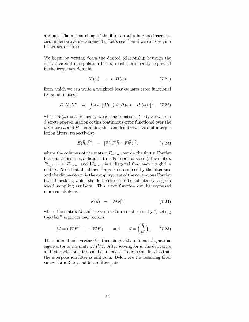
are not. The mismatching of the filters results in gross inaccura-
cies in derivative measurements. Let’s see then if we can design abetter set of filters.
We begin by writing down the desired relationship between thederivative and interpolation filters, most conveniently expressedin the frequency domain:
H ′(ω) = iωH(ω), (7.21)
from which we can write a weighted least-squares error functionalto be minimized:
E(H, H ′) =
∫
dω[
W (ω)(iωH(ω)−H ′(ω))]2
, (7.22)
where W (ω) is a frequency weighting function. Next, we write a
discrete approximation of this continuous error functional over then-vectors ~h and ~h′ containing the sampled derivative and interpo-lation filters, respectively:
E(~h, ~h′) = |W (F ′~h− F ~h′)|2, (7.23)
where the columns of the matrix Fm×n contain the first n Fourierbasis functions (i.e., a discrete-time Fourier transform), the matrix
F ′m×n = iωFm×n, and Wm×m is a diagonal frequency weighting
matrix. Note that the dimension n is determined by the filter size
and the dimension m is the sampling rate of the continuous Fourierbasis functions, which should be chosen to be sufficiently large toavoid sampling artifacts. This error function can be expressed
more concisely as:
E(~u) = |M~u|2, (7.24)
where the matrix M and the vector ~u are constructed by “packing
together” matrices and vectors:
M = ( WF ′ | −WF ) and ~u =
( ~h~h′
)
. (7.25)
The minimal unit vector ~u is then simply the minimal-eigenvalue
eigenvector of the matrix M tM . After solving for ~u, the derivativeand interpolation filters can be “unpacked” and normalized so that
the interpolation filter is unit sum. Below are the resulting filtervalues for a 3-tap and 5-tap filter pair.
53
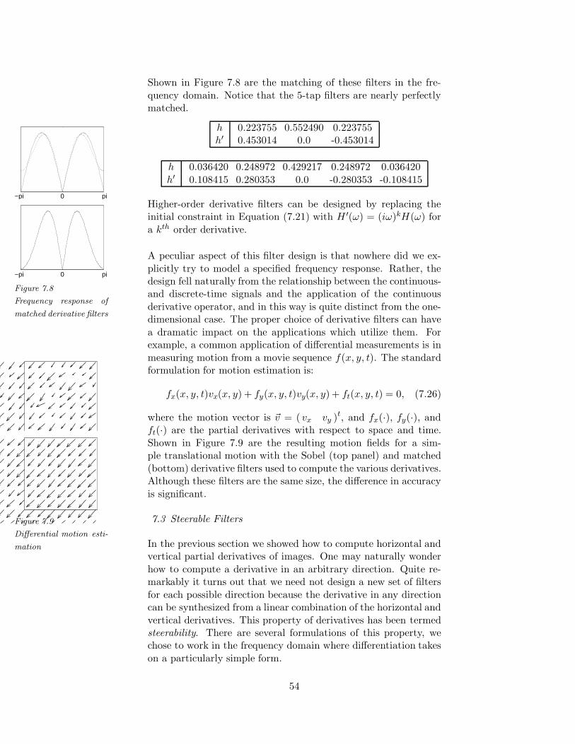
Shown in Figure 7.8 are the matching of these filters in the fre-
quency domain. Notice that the 5-tap filters are nearly perfectlymatched.
−pi 0 pi
−pi 0 pi
Figure 7.8
Frequency response of
matched derivative filters
h 0.223755 0.552490 0.223755h′ 0.453014 0.0 -0.453014
h 0.036420 0.248972 0.429217 0.248972 0.036420
h′ 0.108415 0.280353 0.0 -0.280353 -0.108415
Higher-order derivative filters can be designed by replacing theinitial constraint in Equation (7.21) with H ′(ω) = (iω)kH(ω) for
a kth order derivative.
A peculiar aspect of this filter design is that nowhere did we ex-
plicitly try to model a specified frequency response. Rather, thedesign fell naturally from the relationship between the continuous-and discrete-time signals and the application of the continuous
derivative operator, and in this way is quite distinct from the one-dimensional case. The proper choice of derivative filters can have
a dramatic impact on the applications which utilize them. For
Figure 7.9
Differential motion esti-
mation
example, a common application of differential measurements is in
measuring motion from a movie sequence f(x, y, t). The standardformulation for motion estimation is:
fx(x, y, t)vx(x, y) + fy(x, y, t)vy(x, y) + ft(x, y, t) = 0, (7.26)
where the motion vector is ~v = ( vx vy )t, and fx(·), fy(·), andft(·) are the partial derivatives with respect to space and time.
Shown in Figure 7.9 are the resulting motion fields for a sim-ple translational motion with the Sobel (top panel) and matched
(bottom) derivative filters used to compute the various derivatives.Although these filters are the same size, the difference in accuracy
is significant.
7.3 Steerable Filters
In the previous section we showed how to compute horizontal andvertical partial derivatives of images. One may naturally wonder
how to compute a derivative in an arbitrary direction. Quite re-markably it turns out that we need not design a new set of filters
for each possible direction because the derivative in any directioncan be synthesized from a linear combination of the horizontal and
vertical derivatives. This property of derivatives has been termedsteerability. There are several formulations of this property, wechose to work in the frequency domain where differentiation takes
on a particularly simple form.
54
To begin, we express a two-dimensional image with respect to its
Fourier series:
f(x, y) =π∑
ωx=−π
π∑
ωy=−π
F (ωx, ωy)e−j(ωxx+ωyy). (7.27)
Differentiating 8 both sides with respect to x gives:
fx(x, y) =π∑
ωx=−π
π∑
ωy=−π
−jωxF (ωx, ωy)e−j(ωxx+ωyy).(7.28)
That is, in the frequency domain differentiation in the horizon-tal direction u is equivalent to multiplying the Fourier transform
F (ωx, ωy) by an imaginary horizontal ramp, −jωx. Similarly, thevertical partial derivative in v is:
fy(x, y) =π∑
ωx=−π
π∑
ωy=−π
−jωyF (ωx, ωy)e−j(ωxx+ωyy).(7.29)
Now, differentiation in the vertical direction v is equivalent to
multiplying the Fourier transform by an imaginary vertical ramp.This trend generalizes to arbitrary directions, that is, the partialderivative in any direction α can be computed by multiplying the
Fourier transform by an imaginary oriented ramp −jωα:
fα(x, y) =π∑
ωx=−π
π∑
ωy=−π
−jωαF (ωx, ωy)e−j(ωxx+ωyy),(7.30)
where the oriented ramp can be expressed in terms of the horizon-tal and vertical ramps:
ωα = cos(α)ωx + sin(α)ωy . (7.31)
Substituting this definition back into the partial derivative in α,
Equation (7.30), gives:
fα(x, y) =π∑
ωx=−π
π∑
ωy=−π
−j[cos(α)ωx + sin(α)ωy]F (ωx, ωy)e−j(ωxx+ωyy)
= cos(α)π∑
ωx=−π
π∑
ωy=−π
−jωxF (ωx, ωy)e−j(ωxx+ωyy)
+ sin(α)π∑
ωx=−π
π∑
ωy=−π
−jωyF (ωx, ωy)e−j(ωxx+ωyy)
= cos(α)fx(x, y) + sin(α)fy(x, y). (7.32)
8Recall that the derivative of an exponential is an exponential, so thataccording to the chain rule, Dx{e
ax} = aeax.
55
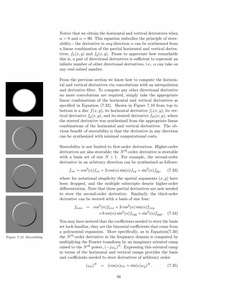
Notice that we obtain the horizontal and vertical derivatives when
α = 0 and α = 90. This equation embodies the principle of steer-ability - the derivative in any direction α can be synthesized from
a linear combination of the partial horizontal and vertical deriva-tives, fx(x, y) and fy(x, y). Pause to appreciate how remarkablethis is, a pair of directional derivatives is sufficient to represent an
infinite number of other directional derivatives, i.e., α can take onany real-valued number.
Figure 7.10 Steerability
From the previous section we know how to compute the horizon-tal and vertical derivatives via convolutions with an interpolation
and derivative filter. To compute any other directional derivativeno more convolutions are required, simply take the appropriate
linear combinations of the horizontal and vertical derivatives asspecified in Equation (7.32). Shown in Figure 7.10 from top to
bottom is a disc f(x, y), its horizontal derivative fx(x, y), its ver-tical derivative fy(x, y), and its steered derivative f45(x, y), wherethe steered derivative was synthesized from the appropriate linear
combinations of the horizontal and vertical derivatives. The ob-vious benefit of steerability is that the derivative in any direction
can be synthesized with minimal computational costs.
Steerability is not limited to first-order derivatives. Higher-order
derivatives are also steerable; the N th-order derivative is steerablewith a basis set of size N + 1. For example, the second-order
derivative in an arbitrary direction can be synthesized as follows:
fαα = cos2(α)fxx + 2 cos(α) sin(α)fxy + sin2(α)fyy , (7.33)
where for notational simplicity the spatial arguments (x, y) have
been dropped, and the multiple subscripts denote higher-orderdifferentiation. Note that three partial derivatives are now needed
to steer the second-order derivative. Similarly, the third-orderderivative can be steered with a basis of size four:
fααα = cos3(α)fxxx + 3 cos2(α) sin(α)fxxy
+3 cos(α) sin2(α)fxyy + sin3(α)fyyy . (7.34)
You may have noticed that the coefficients needed to steer the basis
set look familiar, they are the binomial coefficients that come froma polynomial expansion. More specifically, as in Equation(7.30)
the N th-order derivative in the frequency domain is computed bymultiplying the Fourier transform by an imaginary oriented ramp
raised to the N th power, (−jωα)N . Expressing this oriented rampin terms of the horizontal and vertical ramps provides the basis
and coefficients needed to steer derivatives of arbitrary order:
(ωα)N = (cos(α)ωx + sin(α)ωy)N . (7.35)
56
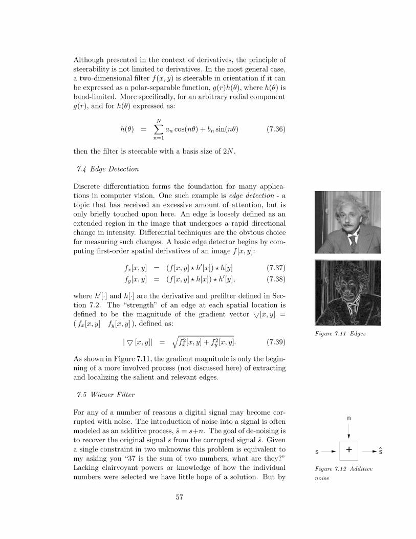
Although presented in the context of derivatives, the principle of
steerability is not limited to derivatives. In the most general case,a two-dimensional filter f(x, y) is steerable in orientation if it can
be expressed as a polar-separable function, g(r)h(θ), where h(θ) isband-limited. More specifically, for an arbitrary radial componentg(r), and for h(θ) expressed as:
h(θ) =N∑
n=1
an cos(nθ) + bn sin(nθ) (7.36)
then the filter is steerable with a basis size of 2N .
7.4 Edge Detection
Figure 7.11 Edges
Discrete differentiation forms the foundation for many applica-tions in computer vision. One such example is edge detection - a
topic that has received an excessive amount of attention, but isonly briefly touched upon here. An edge is loosely defined as an
extended region in the image that undergoes a rapid directionalchange in intensity. Differential techniques are the obvious choice
for measuring such changes. A basic edge detector begins by com-puting first-order spatial derivatives of an image f [x, y]:
fx[x, y] = (f [x, y] ? h′[x]) ? h[y] (7.37)
fy [x, y] = (f [x, y] ? h[x]) ? h′[y], (7.38)
where h′[·] and h[·] are the derivative and prefilter defined in Sec-tion 7.2. The “strength” of an edge at each spatial location isdefined to be the magnitude of the gradient vector 5[x, y] =
( fx[x, y] fy [x, y] ), defined as:
| 5 [x, y]| =√
f2x [x, y] + f2
y [x, y]. (7.39)
As shown in Figure 7.11, the gradient magnitude is only the begin-ning of a more involved process (not discussed here) of extracting
and localizing the salient and relevant edges.
7.5 Wiener Filter
+
n
s s
Figure 7.12 Additive
noise
For any of a number of reasons a digital signal may become cor-rupted with noise. The introduction of noise into a signal is often
modeled as an additive process, s = s+n. The goal of de-noising isto recover the original signal s from the corrupted signal s. Given
a single constraint in two unknowns this problem is equivalent tomy asking you “37 is the sum of two numbers, what are they?”Lacking clairvoyant powers or knowledge of how the individual
numbers were selected we have little hope of a solution. But by
57
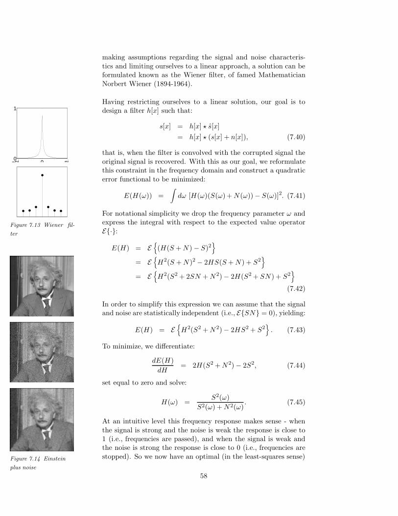
making assumptions regarding the signal and noise characteris-
tics and limiting ourselves to a linear approach, a solution can beformulated known as the Wiener filter, of famed Mathematician
Norbert Wiener (1894-1964).
−pi 0 pi 0
1
Figure 7.13 Wiener fil-
ter
Figure 7.14 Einstein
plus noise
Having restricting ourselves to a linear solution, our goal is todesign a filter h[x] such that:
s[x] = h[x] ? s[x]
= h[x] ? (s[x] + n[x]), (7.40)
that is, when the filter is convolved with the corrupted signal the
original signal is recovered. With this as our goal, we reformulatethis constraint in the frequency domain and construct a quadratic
error functional to be minimized:
E(H(ω)) =
∫
dω [H(ω)(S(ω)+ N(ω))− S(ω)]2. (7.41)
For notational simplicity we drop the frequency parameter ω andexpress the integral with respect to the expected value operator
E{·}:
E(H) = E{
(H(S + N)− S)2}
= E{
H2(S + N)2 − 2HS(S + N) + S2}
= E{
H2(S2 + 2SN + N2)− 2H(S2 + SN) + S2}
(7.42)
In order to simplify this expression we can assume that the signaland noise are statistically independent (i.e., E{SN} = 0), yielding:
E(H) = E{
H2(S2 + N2)− 2HS2 + S2}
. (7.43)
To minimize, we differentiate:
dE(H)
dH= 2H(S2 + N2)− 2S2, (7.44)
set equal to zero and solve:
H(ω) =S2(ω)
S2(ω) + N2(ω). (7.45)
At an intuitive level this frequency response makes sense - when
the signal is strong and the noise is weak the response is close to1 (i.e., frequencies are passed), and when the signal is weak andthe noise is strong the response is close to 0 (i.e., frequencies are
stopped). So we now have an optimal (in the least-squares sense)
58

frequency response in terms of the signal and noise characteris-
tics, but of course we don’t typically know what those are. Butwe can instantiate them by making assumptions about the general
statistical nature of the signal and noise, for example a commonchoice is to assume white noise, N(ω) is constant for all ω, and,for natural images, to assume that S(ω) = 1/ωp. The frequency
response in the top panel of Figure 7.13 was constructed underthese assumptions. Shown in the bottom panel is a 7-tap filter
derived from a least-squares design. This one-dimensional formu-lation can easily be extended to two or more dimensions. Shown
in Figure 7.14 from top to bottom, is Einstein, Einstein plus noise,and the results of applying a 7 × 7 Wiener filter. Note that the
noise levels are reduced but that much of the sharp image struc-ture has also been lost, which is an unfortunate but expected side
effect given that the Wiener filter is low-pass in nature.
59
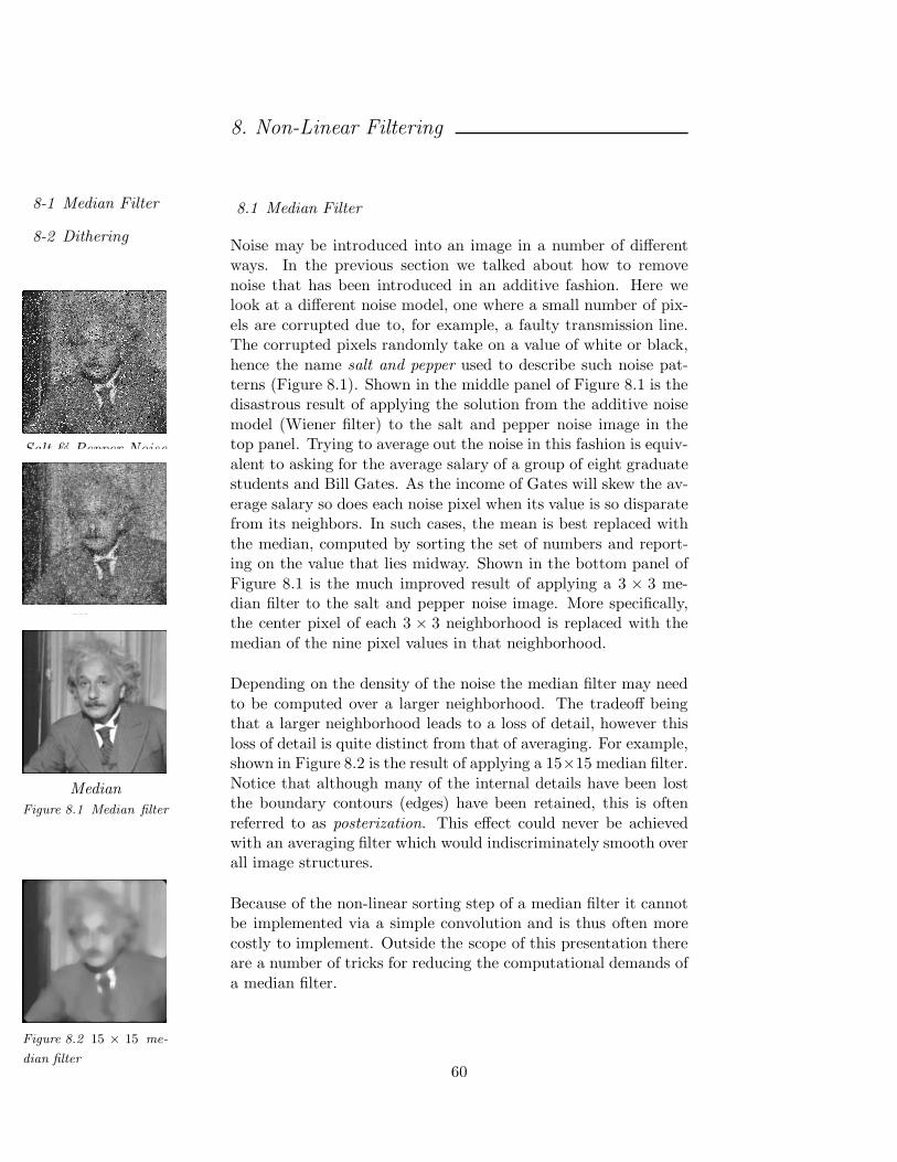
8. Non-Linear Filtering
8-1 Median Filter
8-2 Dithering
8.1 Median Filter
Salt & Pepper Noise
Wiener
Median
Figure 8.1 Median filter
Noise may be introduced into an image in a number of differentways. In the previous section we talked about how to remove
noise that has been introduced in an additive fashion. Here welook at a different noise model, one where a small number of pix-
els are corrupted due to, for example, a faulty transmission line.The corrupted pixels randomly take on a value of white or black,
hence the name salt and pepper used to describe such noise pat-terns (Figure 8.1). Shown in the middle panel of Figure 8.1 is thedisastrous result of applying the solution from the additive noise
model (Wiener filter) to the salt and pepper noise image in thetop panel. Trying to average out the noise in this fashion is equiv-
alent to asking for the average salary of a group of eight graduatestudents and Bill Gates. As the income of Gates will skew the av-
erage salary so does each noise pixel when its value is so disparatefrom its neighbors. In such cases, the mean is best replaced with
the median, computed by sorting the set of numbers and report-ing on the value that lies midway. Shown in the bottom panel of
Figure 8.1 is the much improved result of applying a 3 × 3 me-dian filter to the salt and pepper noise image. More specifically,the center pixel of each 3 × 3 neighborhood is replaced with the
median of the nine pixel values in that neighborhood.
Figure 8.2 15 × 15 me-
dian filter
Depending on the density of the noise the median filter may need
to be computed over a larger neighborhood. The tradeoff beingthat a larger neighborhood leads to a loss of detail, however this
loss of detail is quite distinct from that of averaging. For example,shown in Figure 8.2 is the result of applying a 15×15 median filter.
Notice that although many of the internal details have been lostthe boundary contours (edges) have been retained, this is often
referred to as posterization. This effect could never be achievedwith an averaging filter which would indiscriminately smooth overall image structures.
Because of the non-linear sorting step of a median filter it cannotbe implemented via a simple convolution and is thus often more
costly to implement. Outside the scope of this presentation thereare a number of tricks for reducing the computational demands of
a median filter.
60
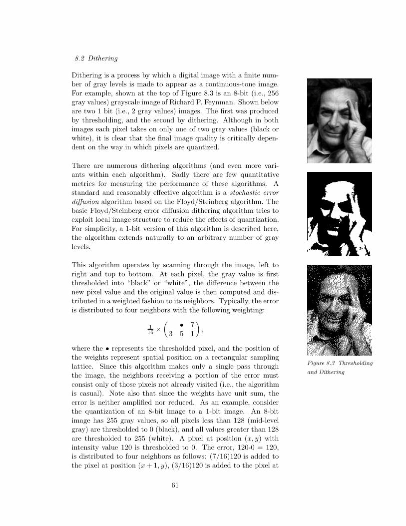
8.2 Dithering
Figure 8.3 Thresholding
and Dithering
Dithering is a process by which a digital image with a finite num-ber of gray levels is made to appear as a continuous-tone image.
For example, shown at the top of Figure 8.3 is an 8-bit (i.e., 256gray values) grayscale image of Richard P. Feynman. Shown beloware two 1 bit (i.e., 2 gray values) images. The first was produced
by thresholding, and the second by dithering. Although in bothimages each pixel takes on only one of two gray values (black or
white), it is clear that the final image quality is critically depen-dent on the way in which pixels are quantized.
There are numerous dithering algorithms (and even more vari-ants within each algorithm). Sadly there are few quantitative
metrics for measuring the performance of these algorithms. Astandard and reasonably effective algorithm is a stochastic error
diffusion algorithm based on the Floyd/Steinberg algorithm. Thebasic Floyd/Steinberg error diffusion dithering algorithm tries toexploit local image structure to reduce the effects of quantization.
For simplicity, a 1-bit version of this algorithm is described here,the algorithm extends naturally to an arbitrary number of gray
levels.
This algorithm operates by scanning through the image, left to
right and top to bottom. At each pixel, the gray value is firstthresholded into “black” or “white”, the difference between the
new pixel value and the original value is then computed and dis-tributed in a weighted fashion to its neighbors. Typically, the error
is distributed to four neighbors with the following weighting:
116 ×
( • 73 5 1
)
,
where the • represents the thresholded pixel, and the position ofthe weights represent spatial position on a rectangular sampling
lattice. Since this algorithm makes only a single pass throughthe image, the neighbors receiving a portion of the error must
consist only of those pixels not already visited (i.e., the algorithmis casual). Note also that since the weights have unit sum, the
error is neither amplified nor reduced. As an example, considerthe quantization of an 8-bit image to a 1-bit image. An 8-bit
image has 255 gray values, so all pixels less than 128 (mid-levelgray) are thresholded to 0 (black), and all values greater than 128
are thresholded to 255 (white). A pixel at position (x, y) withintensity value 120 is thresholded to 0. The error, 120-0 = 120,is distributed to four neighbors as follows: (7/16)120 is added to
the pixel at position (x + 1, y), (3/16)120 is added to the pixel at
61
position (x− 1, y + 1), (5/16)120 to pixel (x, y + 1) and (1/16)120
to pixel (x + 1, y + 1). The intuition behind this algorithm isthat when the pixel value of 120 is thresholded to 0 that pixel is
made darker. By propagating this error the surrounding pixels arebrightened making it more likely that they will be thresholded tosomething brighter. As a result the local neighborhood maintains
it’s average gray value.
Qualitatively, the error diffusion algorithm reduces the effects of
quantization via simple thresholding. However this algorithm doesintroduce correlated artifacts due to the deterministic nature of
the algorithm and scanning order. These problems may be par-tially alleviated by introducing a stochastic process in a variety
of places. Two possibilities include randomizing the error beforedistributing it to its neighbors (e.g., randomly scaling the error
in the range 0.9 to 1.1), and alternating the scanning direction(e.g., odd lines are scanned left to right, and even lines from rightto left).
62

9. Multi-Scale Transforms
63
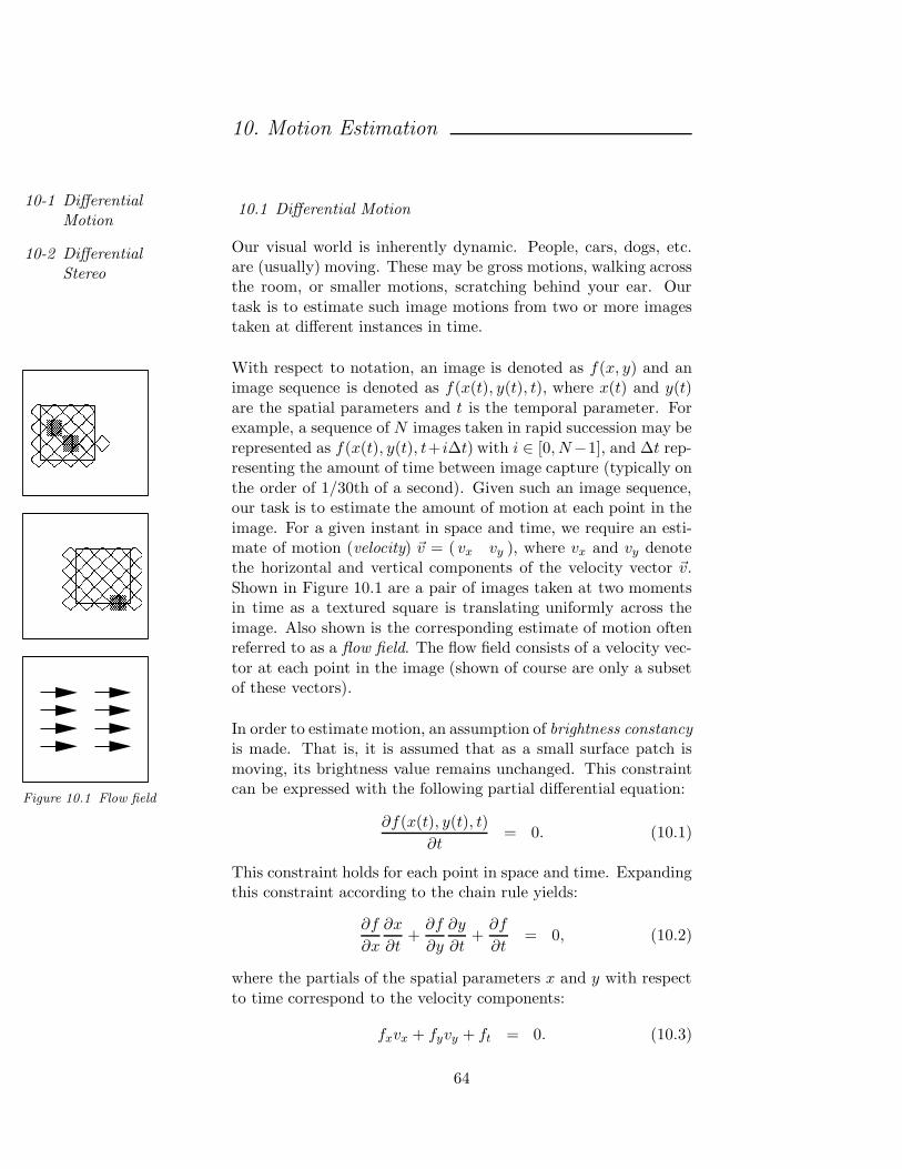
10. Motion Estimation
10-1 DifferentialMotion
10-2 DifferentialStereo
10.1 Differential Motion
Our visual world is inherently dynamic. People, cars, dogs, etc.are (usually) moving. These may be gross motions, walking acrossthe room, or smaller motions, scratching behind your ear. Our
task is to estimate such image motions from two or more imagestaken at different instances in time.
��
�
����������������������������
��
������������������������������������
Figure 10.1 Flow field
With respect to notation, an image is denoted as f(x, y) and animage sequence is denoted as f(x(t), y(t), t), where x(t) and y(t)
are the spatial parameters and t is the temporal parameter. Forexample, a sequence of N images taken in rapid succession may be
represented as f(x(t), y(t), t+ i∆t) with i ∈ [0, N−1], and ∆t rep-resenting the amount of time between image capture (typically on
the order of 1/30th of a second). Given such an image sequence,our task is to estimate the amount of motion at each point in the
image. For a given instant in space and time, we require an esti-mate of motion (velocity) ~v = ( vx vy ), where vx and vy denotethe horizontal and vertical components of the velocity vector ~v.
Shown in Figure 10.1 are a pair of images taken at two momentsin time as a textured square is translating uniformly across the
image. Also shown is the corresponding estimate of motion oftenreferred to as a flow field. The flow field consists of a velocity vec-
tor at each point in the image (shown of course are only a subsetof these vectors).
In order to estimate motion, an assumption of brightness constancyis made. That is, it is assumed that as a small surface patch is
moving, its brightness value remains unchanged. This constraintcan be expressed with the following partial differential equation:
∂f(x(t), y(t), t)
∂t= 0. (10.1)
This constraint holds for each point in space and time. Expandingthis constraint according to the chain rule yields:
∂f
∂x
∂x
∂t+
∂f
∂y
∂y
∂t+
∂f
∂t= 0, (10.2)
where the partials of the spatial parameters x and y with respect
to time correspond to the velocity components:
fxvx + fyvy + ft = 0. (10.3)
64
The subscripts on the function f denote partial derivatives. Note
again that this constraint holds for each point in space and timebut that for notational simplicity the spatial/temporal parameters
are dropped. This transformed brightness constancy constraint isrewritten by packing together the partial derivatives and velocitycomponents into row and column vectors.
( fx fy )
(
vx
vy
)
+ ft = 0
~f ts~v + ft = 0. (10.4)
The space/time derivatives ~fs and ft are measured quantities, leav-ing us with a single constraint in two unknowns (the two compo-nents of the velocity vector, ~v). The constraint can be solved by
assuming that the motion is locally similar, and integrating thisconstraint over a local image neighborhood. A least-squares error
function takes the form:
E(~v) =
[
∑
x,y
~f ts~v +
∑
x,y
ft
]2
, (10.5)
To solve for the motion this error function is first differentiated
∂E(~v)
∂~v= 2
∑
~fs
[
∑
~f ts~v +
∑
ft
]
= 2∑
~fs~f ts~v + 2
∑
~fsft. (10.6)
Setting equal to zero and recombining the terms into matrix form
yields:
(∑
fx∑
fy
)
(∑
fx∑
fy )
(
vx
vy
)
= −(∑
fxft∑
fyft
)
( ∑
f2x
∑
fxfy∑
fxfy∑
f2y
)(
vx
vy
)
= −(∑
fxft∑
fyft
)
M~v = −~b. (10.7)
If the matrix M is invertible (full rank), then the velocity can be
estimated by simply left multiplying by the inverse matrix:
~v = −M−1~b (10.8)
The critical question then is, when is the matrix M invertible?
Generally speaking the matrix is rank deficient, and hence notinvertible, when the intensity variation in a local image neighbor-
hood varies only one-dimensionally (e.g., fx = 0 or fy = 0) orzero-dimensionally (fx = 0 and fy = 0). These singularities aresometimes referred to as the aperture and blank wall problem.
The motion at such points simply can not be estimated.
65
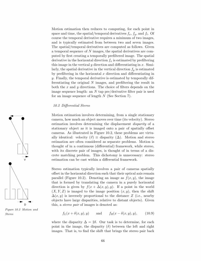
Motion estimation then reduces to computing, for each point in
space and time, the spatial/temporal derivatives fx, fy , and ft. Ofcourse the temporal derivative requires a minimum of two images,
and is typically estimated from between two and seven images.The spatial/temporal derivatives are computed as follows. Givena temporal sequence of N images, the spatial derivatives are com-
puted by first creating a temporally prefiltered image. The spatialderivative in the horizontal direction fx is estimated by prefiltering
this image in the vertical y direction and differentiating in x. Simi-larly, the spatial derivative in the vertical direction fy is estimated
by prefiltering in the horizontal x direction and differentiating iny. Finally, the temporal derivative is estimated by temporally dif-
ferentiating the original N images, and prefiltering the result inboth the x and y directions. The choice of filters depends on the
image sequence length: an N tap pre/derivative filter pair is usedfor an image sequence of length N (See Section 7).
10.2 Differential Stereo
V
D
Figure 10.2 Motion and
Stereo
Motion estimation involves determining, from a single stationarycamera, how much an object moves over time (its velocity). Stereo
estimation involves determining the displacement disparity of astationary object as it is imaged onto a pair of spatially offset
cameras. As illustrated in Figure 10.2, these problems are virtu-ally identical: velocity (~v) ≡ disparity (∆). Motion and stereoestimation are often considered as separate problems. Motion is
thought of in a continuous (differential) framework, while stereo,with its discrete pair of images, is thought of in terms of a dis-
crete matching problem. This dichotomy is unnecessary: stereoestimation can be cast within a differential framework.
Stereo estimation typically involves a pair of cameras spatially
offset in the horizontal direction such that their optical axis remainparallel (Figure 10.2). Denoting an image as f(x, y), the image
that is formed by translating the camera in a purely horizontaldirection is given by f(x + ∆(x, y), y). If a point in the world
(X, Y, Z) is imaged to the image position (x, y), then the shift∆(x, y) is inversely proportional to the distance Z (i.e., nearbyobjects have large disparities, relative to distant objects). Given
this, a stereo pair of images is denoted as:
fL(x + δ(x, y), y) and fR(x− δ(x, y), y), (10.9)
where the disparity ∆ = 2δ. Our task is to determine, for eachpoint in the image, the disparity (δ) between the left and right
images. That is, to find the shift that brings the stereo pair back
66
into register. To this end, we write a quadratic error function to
be minimized:
E(δ(x, y)) = [fL(x + δ(x, y), y)− fR(x− δ(x, y), y)]2. (10.10)
In this form, solving for δ is non-trivial. We may simplify thingsby expressing the image pair in terms of their truncated first-order
Taylor series expansion:
f(x + δ(x, y), y) = f(x, y) + δ(x, y)fx(x, y), (10.11)
where fx(x, y) denotes the partial derivative of f with respect to
x. With this first-order approximation, the error function to beminimized takes the form:
E(δ) = [(fL + δ(fL)x)− (fR − δ(fR)x)]2
= [(fL − fR) + δ(fL + fR)x]2, (10.12)
where for notational convenience, the spatial parameters have been
dropped. Differentiating, setting the result equal to zero and solv-ing for δ yields:
dE(δ)
dδ= 2(fL + fR)x[(fL − fR) + δ(fL + fR)x]
= 0
δ = − fL − fR
(fL + fR)x(10.13)
Stereo estimation then reduces to computing, for each point in theimage, spatial derivatives and the difference between the left and
right stereo pair (a crude derivative with respect to viewpoint).
Why, if motion and stereo estimation are similar, do the math-
ematical formulations look so different? Upon closer inspectionthey are in fact quite similar. The above formulation amounts to
a constrained version of motion estimation. In particular, becauseof the strictly horizontal shift of the camera pair, the disparity
was constrained along the horizontal direction. If we reconsiderthe motion estimation formulation assuming motion only alongthe horizontal direction, then the similarity of the formulations
becomes evident. Recall that in motion estimation the brightnessconstancy assumption led to the following constraint:
∂f
∂x
∂x
∂t+
∂f
∂y
∂y
∂t+
∂f
∂t= 0, (10.14)
Constraining the motion along the vertical y direction to be zeroyields:
∂f
∂x
∂x
∂t+
∂f
∂t= 0, (10.15)
67
where the partial derivative of the spatial parameter x with re-
spect to time correspond to the motion (speed) in the horizontaldirection:
fxvx + ft = 0. (10.16)
Unlike before, this leads to a single constraint with a single un-
known which can be solved for directly:
vx = − ft
fx. (10.17)
This solution now looks very similar to the solution for differential
stereo in Equation 10.13. In both solutions the numerator is aderivative, in one case with respect to time (motion) and in theother with respect to viewpoint (stereo). Also in both solutions,
the denominator is a spatial derivative. In the stereo case, thedenominator consists of the spatial derivative of the sum of the
left and right image pair. This may seem odd, but recall thatdifferentiation of a multi-dimensional function requires differenti-
ating along the desired dimension and prefiltering along all otherdimensions (in this case the viewpoint dimension).
In both the differential motion and stereo formulations there existssingularities when the denominator (spatial derivative) is zero. As
with the earlier motion estimation this can be partially alleviatedby integrating the disparities over a local image neighborhood.
However, if the spatial derivative is zero over a large area, corre-sponding to a surface in the world with no texture, then disparitiesat these points simply can not be estimated.
68
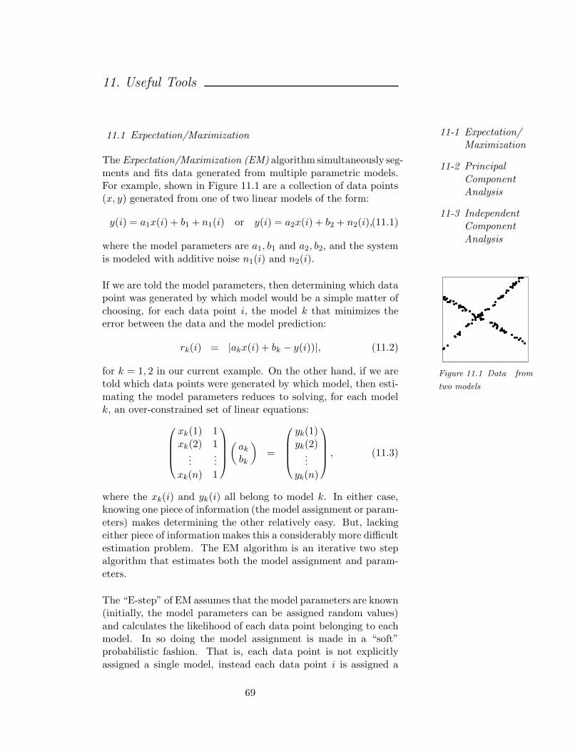
11. Useful Tools
11-1 Expectation/Maximization
11-2 Principal
ComponentAnalysis
11-3 IndependentComponent
Analysis
11.1 Expectation/Maximization
The Expectation/Maximization (EM) algorithm simultaneously seg-
ments and fits data generated from multiple parametric models.For example, shown in Figure 11.1 are a collection of data points(x, y) generated from one of two linear models of the form:
Figure 11.1 Data from
two models
y(i) = a1x(i) + b1 + n1(i) or y(i) = a2x(i) + b2 + n2(i),(11.1)
where the model parameters are a1, b1 and a2, b2, and the system
is modeled with additive noise n1(i) and n2(i).
If we are told the model parameters, then determining which datapoint was generated by which model would be a simple matter of
choosing, for each data point i, the model k that minimizes theerror between the data and the model prediction:
rk(i) = |akx(i) + bk − y(i))|, (11.2)
for k = 1, 2 in our current example. On the other hand, if we aretold which data points were generated by which model, then esti-
mating the model parameters reduces to solving, for each modelk, an over-constrained set of linear equations:
xk(1) 1
xk(2) 1...
...
xk(n) 1
(
ak
bk
)
=
yk(1)
yk(2)...
yk(n)
, (11.3)
where the xk(i) and yk(i) all belong to model k. In either case,knowing one piece of information (the model assignment or param-
eters) makes determining the other relatively easy. But, lackingeither piece of information makes this a considerably more difficult
estimation problem. The EM algorithm is an iterative two stepalgorithm that estimates both the model assignment and param-
eters.
The “E-step” of EM assumes that the model parameters are known(initially, the model parameters can be assigned random values)
and calculates the likelihood of each data point belonging to eachmodel. In so doing the model assignment is made in a “soft”probabilistic fashion. That is, each data point is not explicitly
assigned a single model, instead each data point i is assigned a
69
probability of it belonging to each model k. For each model the
residual error is first computed as:
rk(i) = akx(i) + bk − y(i) (11.4)
from which the likelihoods are calculated. We ask, what is the
likelihood of point i belonging to model k given the residual error.For our two model example:
P (ak , bk|rk(i)) =P (rk(i)|ak, bk)P (ak , bk)
P (rk(i))
=P (rk(i)|ak, bk)
P (r1(i)|ak, bk) + P (r2(i)|ak, bk), (11.5)
for k = 1, 2. The expansion of the conditional probability is from
Bayes rule: P (B|Ak) = P (Ak |B)P (B)∑
lP (Al |B)P (B)
. If we assume a Gaussian
probability distribution, then the likelihood takes the form:
wk(i) =e−rk(i)2/σN
e−r1(i)2/σN + e−r2(i)2/σN(11.6)
where, σN is proportional to the amount of noise in the data, andfor each data point i,
∑
k wk(i) = 1.
The “M-step” of EM takes the likelihood of each data point be-longing to each model, and re-estimates the model parameters
using weighted least-squares. That is, the following weighted errorfunction on the model parameters is minimized:
Ek(ak, bk) =∑
i
wk(i)[akx(i) + bk − y(i)]2. (11.7)
The intuition here is that each data point contributes to the esti-
mation of each model’s parameters in proportion to the belief thatit belongs to that particular model. This quadratic error function
is minimized by computing the partial derivatives with respect tothe model parameters, setting the result equal to zero and solving
for the model parameters. Differentiating:
∂Ek(ak, bk)
∂ak=
∑
i
2wk(i)x(i)[akx(i) + bk − y(i)]
∂Ek(ak, bk)
∂bk=
∑
i
2wk(i)[akx(i) + bk − y(i)], (11.8)
setting both equal to zero yields the following set of linear equa-
tions:
ak
∑
i
wk(i)x(i)2 + bk
∑
i
wk(i)x(i) =∑
i
wk(i)x(i)y(i)(11.9)
ak
∑
i
wk(i)x(i) + bk
∑
i
wk(i) =∑
i
wk(i)y(i). (11.10)
70
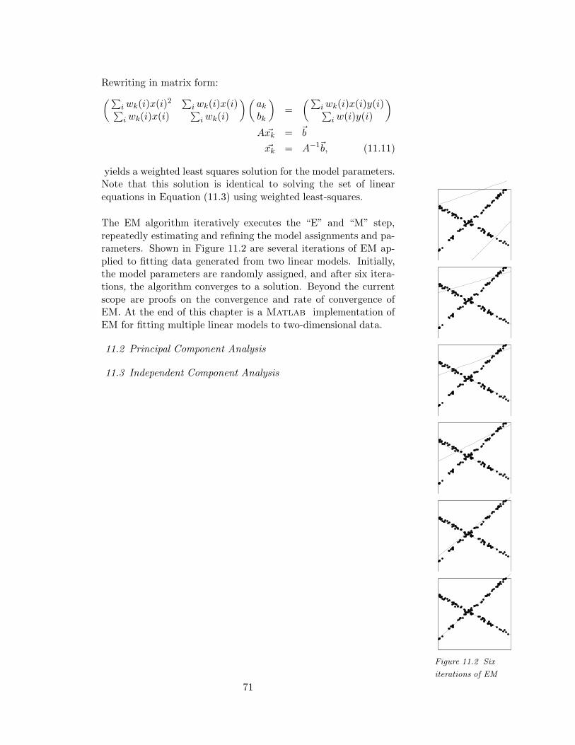
Rewriting in matrix form:
(∑
i wk(i)x(i)2∑
i wk(i)x(i)∑
i wk(i)x(i)∑
i wk(i)
)(
ak
bk
)
=
(∑
i wk(i)x(i)y(i)∑
i w(i)y(i)
)
A ~xk = ~b
~xk = A−1~b, (11.11)
yields a weighted least squares solution for the model parameters.
Figure 11.2 Six
iterations of EM
Note that this solution is identical to solving the set of linear
equations in Equation (11.3) using weighted least-squares.
The EM algorithm iteratively executes the “E” and “M” step,
repeatedly estimating and refining the model assignments and pa-rameters. Shown in Figure 11.2 are several iterations of EM ap-
plied to fitting data generated from two linear models. Initially,the model parameters are randomly assigned, and after six itera-tions, the algorithm converges to a solution. Beyond the current
scope are proofs on the convergence and rate of convergence ofEM. At the end of this chapter is a Matlab implementation of
EM for fitting multiple linear models to two-dimensional data.
11.2 Principal Component Analysis
11.3 Independent Component Analysis
71

%%% THE EM ALGORITHM
clear;
NumModel = 2;
NumData = 64;
Sigma = 0.1; % IN E-STEP
Noise = 0.1; % IN DATA
NIterate = 10;
%%% MAKE SYNTHETIC DATA
A = 2*rand(1,NumModel) - 1;
B = 2*rand(1,NumModel) - 1;
X = [];
Y = [];
for i = 1 : NumModel
x = 2*rand(1,NumData) - 1;
y = A(i) * x + B(i) + Noise*(rand(1,NumData)-0.5);
X = [X x];
Y = [Y y];
end
%%% INITIALIZE MODEL
a = 2*rand(1,NumModel) - 1;
b = 2*rand(1,NumModel) - 1;
for j = 1 : NIterate
%%% E-STEP
for i = 1 : NumModel
r(i,:) = a(i)*X + b(i) - Y;
end
den = sum( exp( -(r.^2)/Sigma^2 ) );
for i = 1 : NumModel
w(i,:) = exp( (-(r(i,:).^2)/Sigma^2) ) ./ (den+eps);
end
%%% M-STEP
for i = 1 : NumModel
M = [ sum(w(i,:).*X.^2) sum(w(i,:).*X) ; sum(w(i,:).*X) sum(w(i,:)) ];
V = [ sum(w(i,:).*X.*Y) ; sum(w(i,:).*Y) ];
U = pinv(M) * V;
a(i) = U(1);
b(i) = U(2);
end
%%% SHOW MODEL FIT AND ASSIGNMENT
xc = [-1 : 0.1 : 1];
subplot(2,1,1); cla; hold on;
plot( X, Y, ’bo’ );
for i = 1 : NumModel
yc = a(i)*xc + b(i);
plot( xc, yc, ’r’ );
end
hold off;
subplot(2,1,2); cla; imagesc(w); colormap gray; pause(1);
end
72