fundamentals of digital image processing - r-5.org · image processing and pattern recognition...

Fundamentals of DigitalImage Processing

A Practical Approachwith Examples in Matlab

Chris SolomonSchool of Physical Sciences, University of Kent, Canterbury, UK

Toby BreckonSchool of Engineering, Cranfield University, Bedfordshire, UK


A Practical Approachwith Examples in Matlab

Chris SolomonSchool of Physical Sciences, University of Kent, Canterbury, UK

Toby BreckonSchool of Engineering, Cranfield University, Bedfordshire, UK

This edition first published 2011, � 2011 by John Wiley & Sons, Ltd

Wiley Blackwell is an imprint of John Wiley & Sons, formed by the merger of Wiley’s global Scientific,Technical and Medical business with Blackwell Publishing.

Registered office: John Wiley & Sons Ltd, The Atrium, Southern Gate, Chichester,West Sussex, PO19 8SQ, UK

Editorial Offices:9600 Garsington Road, Oxford, OX4 2DQ, UK

111 River Street, Hoboken, NJ 07030 5774, USA

For details of our global editorial offices, for customer services and for information about how toapply for permission to reuse the copyright material in this book please see our website atwww.wiley.com/wiley blackwell

The right of the author to be identified as the author of this work has been asserted in accordance withthe Copyright, Designs and Patents Act 1988.

All rights reserved. No part of this publication may be reproduced, stored in a retrieval system, ortransmitted, in any form or by any means, electronic, mechanical, photocopying, recording or otherwise,except as permitted by the UK Copyright, Designs and Patents Act 1988, without the prior permissionof the publisher.

Wiley also publishes its books in a variety of electronic formats. Some content that appears inprint may not be available in electronic books.

Designations used by companies to distinguish their products are often claimed as trademarks. All brandnames and product names used in this book are trade names, service marks, trademarks or registeredtrademarks of their respective owners. The publisher is not associated with any product or vendor mentionedin this book. This publication is designed to provide accurate and authoritative information in regard tothe subject matter covered. It is sold on the understanding that the publisher is not engaged in renderingprofessional services. If professional advice or other expert assistance is required, the services of acompetent professional should be sought.

MATLAB� is a trademark of TheMathWorks, Inc. and is usedwith permission. TheMathWorks does notwarrantthe accuracy of the text or exercises in this book. This book’s use or discussion of MATLAB� software or relatedproducts does not constitute endorsement or sponsorship by The MathWorks of a particular pedagogicalapproach or particular use of the MATLAB� software.

Library of Congress Cataloguing in Publication Data

Solomon, Chris and Breckon, TobyFundamentals of digital image processing : a practical approach with examples in Matlab / Chris Solomon and

Toby Breckonp. cm.

Includes index.Summary: �Fundamentals of Digital ImageProcessing is an introductory text on the science of image processing

and employs the Matlab programming language to illustrate some of the elementary, key concepts in modernimage processing and pattern recognition drawing on specific examples from within science, medicine andelectronics� Provided by publisher.ISBN 978 0 470 84472 4 (hardback) ISBN 978 0 470 84473 1 (pbk.)1. Image processing Digital techniques. 2. Matlab. I. Breckon, Toby. II. Title.TA1637.S65154 2010621.36’7 dc22

2010025730

This book is published in the following electronic formats: eBook 9780470689783; Wiley Online Library9780470689776

A catalogue record for this book is available from the British Library.

Set in 10/12.5 pt Minion by Thomson Digital, Noida, India

1 2011

Contents

Preface xi

Using the book website xv

1 Representation 1

1.1 What is an image? 11.1.1 Image layout 11.1.2 Image colour 2

1.2 Resolution and quantization 31.2.1 Bit-plane splicing 4

1.3 Image formats 51.3.1 Image data types 61.3.2 Image compression 7

1.4 Colour spaces 91.4.1 RGB 10

1.4.1.1 RGB to grey-scale image conversion 111.4.2 Perceptual colour space 12

1.5 Images in Matlab 141.5.1 Reading, writing and querying images 141.5.2 Basic display of images 151.5.3 Accessing pixel values 161.5.4 Converting image types 17

Exercises 18

2 Formation 21

2.1 How is an image formed? 212.2 The mathematics of image formation 22

2.2.1 Introduction 222.2.2 Linear imaging systems 232.2.3 Linear superposition integral 242.2.4 The Dirac delta or impulse function 252.2.5 The point-spread function 28

2.2.6 Linear shift-invariant systems and the convolutionintegral 29

2.2.7 Convolution: its importance and meaning 302.2.8 Multiple convolution: N imaging elements

in a linear shift-invariant system 342.2.9 Digital convolution 34

2.3 The engineering of image formation 372.3.1 The camera 382.3.2 The digitization process 40

2.3.2.1 Quantization 402.3.2.2 Digitization hardware 422.3.2.3 Resolution versus performance 43

2.3.3 Noise 44Exercises 46

3 Pixels 49

3.1 What is a pixel? 493.2 Operations upon pixels 50

3.2.1 Arithmetic operations on images 513.2.1.1 Image addition and subtraction 51

3.2.1.2 Multiplication and division 533.2.2 Logical operations on images 543.2.3 Thresholding 55

3.3 Point-based operations on images 573.3.1 Logarithmic transform 573.3.2 Exponential transform 593.3.3 Power-law (gamma) transform 61

3.3.3.1 Application: gamma correction 623.4 Pixel distributions: histograms 63

3.4.1 Histograms for threshold selection 653.4.2 Adaptive thresholding 663.4.3 Contrast stretching 673.4.4 Histogram equalization 69

3.4.4.1 Histogram equalization theory 693.4.4.2 Histogram equalization theory: discrete case 703.4.4.3 Histogram equalization in practice 71

3.4.5 Histogram matching 733.4.5.1 Histogram-matching theory 733.4.5.2 Histogram-matching theory: discrete case 743.4.5.3 Histogram matching in practice 75

3.4.6 Adaptive histogram equalization 763.4.7 Histogram operations on colour images 79

Exercises 81

vi CONTENTS

4 Enhancement 85

4.1 Why perform enhancement? 854.1.1 Enhancement via image filtering 85

4.2 Pixel neighbourhoods 864.3 Filter kernels and the mechanics of linear filtering 87

4.3.1 Nonlinear spatial filtering 904.4 Filtering for noise removal 90

4.4.1 Mean filtering 914.4.2 Median filtering 924.4.3 Rank filtering 944.4.4 Gaussian filtering 95

4.5 Filtering for edge detection 974.5.1 Derivative filters for discontinuities 974.5.2 First-order edge detection 99

4.5.2.1 Linearly separable filtering 1014.5.3 Second-order edge detection 102

4.5.3.1 Laplacian edge detection 1024.5.3.2 Laplacian of Gaussian 1034.5.3.3 Zero-crossing detector 104

4.6 Edge enhancement 1054.6.1 Laplacian edge sharpening 1054.6.2 The unsharp mask filter 107

Exercises 109

5 Fourier transforms and frequency-domain processing 113

5.1 Frequency space: a friendly introduction 1135.2 Frequency space: the fundamental idea 114

5.2.1 The Fourier series 1155.3 Calculation of the Fourier spectrum 1185.4 Complex Fourier series 1185.5 The 1-D Fourier transform 1195.6 The inverse Fourier transform and reciprocity 1215.7 The 2-D Fourier transform 1235.8 Understanding the Fourier transform: frequency-space filtering 1265.9 Linear systems and Fourier transforms 1295.10 The convolution theorem 1295.11 The optical transfer function 1315.12 Digital Fourier transforms: the discrete fast Fourier transform 1345.13 Sampled data: the discrete Fourier transform 1355.14 The centred discrete Fourier transform 136

6 Image restoration 141

6.1 Imaging models 1416.2 Nature of the point-spread function and noise 142

CONTENTS vii

6.3 Restoration by the inverse Fourier filter 1436.4 The Wiener–Helstrom Filter 1466.5 Origin of the Wiener–Helstrom filter 1476.6 Acceptable solutions to the imaging equation 1516.7 Constrained deconvolution 1516.8 Estimating an unknown point-spread function or optical transfer

function 1546.9 Blind deconvolution 1566.10 Iterative deconvolution and the Lucy–Richardson algorithm 1586.11 Matrix formulation of image restoration 1616.12 The standard least-squares solution 1626.13 Constrained least-squares restoration 1636.14 Stochastic input distributions and Bayesian estimators 1656.15 The generalized Gauss–Markov estimator 165

7 Geometry 169

7.1 The description of shape 1697.2 Shape-preserving transformations 1707.3 Shape transformation and homogeneous coordinates 1717.4 The general 2-D affine transformation 1737.5 Affine transformation in homogeneous coordinates 1747.6 The Procrustes transformation 1757.7 Procrustes alignment 1767.8 The projective transform 1807.9 Nonlinear transformations 1847.10 Warping: the spatial transformation of an image 1867.11 Overdetermined spatial transformations 1897.12 The piecewise warp 1917.13 The piecewise affine warp 1917.14 Warping: forward and reverse mapping 194

8 Morphological processing 197

8.1 Introduction 1978.2 Binary images: foreground, background and connectedness 1978.3 Structuring elements and neighbourhoods 1988.4 Dilation and erosion 2008.5 Dilation, erosion and structuring elements within Matlab 2018.6 Structuring element decomposition and Matlab 2028.7 Effects and uses of erosion and dilation 204

8.7.1 Application of erosion to particle sizing 2078.8 Morphological opening and closing 209

8.8.1 The rolling-ball analogy 2108.9 Boundary extraction 2128.10 Extracting connected components 213

viii CONTENTS

8.11 Region filling 2158.12 The hit-or-miss transformation 216

8.12.1 Generalization of hit-or-miss 2198.13 Relaxing constraints in hit-or-miss: ‘don’t care’ pixels 220

8.13.1 Morphological thinning 2228.14 Skeletonization 2228.15 Opening by reconstruction 2248.16 Grey-scale erosion and dilation 2278.17 Grey-scale structuring elements: general case 2278.18 Grey-scale erosion and dilation with flat structuring elements 2288.19 Grey-scale opening and closing 2298.20 The top-hat transformation 2308.21 Summary 231Exercises 233

9 Features 235

9.1 Landmarks and shape vectors 2359.2 Single-parameter shape descriptors 2379.3 Signatures and the radial Fourier expansion 2399.4 Statistical moments as region descriptors 2439.5 Texture features based on statistical measures 2469.6 Principal component analysis 2479.7 Principal component analysis: an illustrative example 2479.8 Theory of principal component analysis: version 1 2509.9 Theory of principal component analysis: version 2 2519.10 Principal axes and principal components 2539.11 Summary of properties of principal component analysis 2539.12 Dimensionality reduction: the purpose of principal

component analysis 2569.13 Principal components analysis on an ensemble of digital images 2579.14 Representation of out-of-sample examples using principal

component analysis 2579.15 Key example: eigenfaces and the human face 259

10 Image Segmentation 263

10.1 Image segmentation 26310.2 Use of image properties and features in segmentation 26310.3 Intensity thresholding 265

10.3.1 Problems with global thresholding 26610.4 Region growing and region splitting 26710.5 Split-and-merge algorithm 26710.6 The challenge of edge detection 27010.7 The Laplacian of Gaussian and difference of Gaussians filters 27010.8 The Canny edge detector 271

CONTENTS ix

10.9 Interest operators 27410.10 Watershed segmentation 27910.11 Segmentation functions 28010.12 Image segmentation with Markov random fields 286

10.12.1 Parameter estimation 28810.12.2 Neighbourhood weighting parameter un 28910.12.3 Minimizing U(x | y): the iterated conditional

modes algorithm 290

11 Classification 291

11.1 The purpose of automated classification 29111.2 Supervised and unsupervised classification 29211.3 Classification: a simple example 29211.4 Design of classification systems 29411.5 Simple classifiers: prototypes and minimum distance

criteria 29611.6 Linear discriminant functions 29711.7 Linear discriminant functions in N dimensions 30111.8 Extension of the minimum distance classifier and the

Mahalanobis distance 30211.9 Bayesian classification: definitions 30311.10 The Bayes decision rule 30411.11 The multivariate normal density 30611.12 Bayesian classifiers for multivariate normal distributions 307

11.12.1 The Fisher linear discriminant 31011.12.2 Risk and cost functions 311

11.13 Ensemble classifiers 31211.13.1 Combining weak classifiers: the AdaBoost method 313

11.14 Unsupervised learning: k-means clustering 313

Further reading 317

Index 319

x CONTENTS

Preface

Scope of this book

This is an introductory text on the science (and art) of image processing. The book also

employs the Matlab programming language and toolboxes to illuminate and consolidate

some of the elementary but key concepts in modern image processing and pattern

recognition.

The authors are firmbelievers in the old adage, �Hear and forget. . . , See and remember. . .,Do and know�. For most of us, it is through good examples and gently guided experimenta-

tion that we really learn. Accordingly, the book has a large number of carefully chosen

examples, graded exercises and computer experiments designed to help the reader get a real

grasp of the material. All the program code (.m files) used in the book, corresponding to the

examples and exercises, are made available to the reader/course instructor and may be

downloaded from the book’s dedicated web site – www.fundipbook.com.

Who is this book for?

For undergraduate and graduate students in the technical disciplines, for technical

professionals seeking a direct introduction to the field of image processing and for

instructors looking to provide a hands-on, structured course. This book intentionally

starts with simple material but we also hope that relative experts will nonetheless find some

interesting and useful material in the latter parts.

Aims

What then are the specific aims of this book ? Two of the principal aims are –

. To introduce the reader to some of the key concepts and techniques of modern image

processing.

. To provide a framework within which these concepts and techniques can be understood

by a series of examples, exercises and computer experiments.

These are, perhaps, aims which one might reasonably expect from any book on a technical

subject. However, we have one further aim namely to provide the reader with the fastest,

most direct route to acquiring a real hands-on understanding of image processing.We hope

this book will give you a real fast-start in the field.

Assumptions

We make no assumptions about the reader’s mathematical background beyond that

expected at the undergraduate level in the technical sciences – ie reasonable competence

in calculus, matrix algebra and basic statistics.

Why write this book?

There are already a number of excellent and comprehensive texts on image processing and

pattern recognition and we refer the interested reader to a number in the appendices of this

book. There are also some exhaustive and well-written books on theMatlab language.What

the authors felt was lacking was an image processing book which combines a simple exposition

of principles with ameans to quickly test, verify and experiment with them in an instructive and

interactive way.

In our experience, formed over a number of years, Matlab and the associated image

processing toolbox are extremely well-suited to help achieve this aim. It is simple but

powerful and its key feature in this context is that it enables one to concentrate on the image

processing concepts and techniques (i.e. the real business at hand) while keeping concerns

about programming syntax and data management to a minimum.

What is Matlab?

Matlab is a programming language with an associated set of specialist software toolboxes.

It is an industry standard in scientific computing and used worldwide in the scientific,

technical, industrial and educational sectors. Matlab is a commercial product and

information on licences and their cost can be obtained direct by enquiry at the

web-site www.mathworks.com. Many Universities all over the world provide site licenses

for their students.

What knowledge of Matlab is required for this book?

Matlab is very much part of this book and we use it extensively to demonstrate how

certain processing tasks and approaches can be quickly implemented and tried out in

practice. Throughout the book, we offer comments on the Matlab language and the best

way to achieve certain image processing tasks in that language. Thus the learning of

concepts in image processing and their implementation within Matlab go hand-in-hand

in this text.

xii PREFACE

Is the book any use then if I don’t know Matlab?

Yes. This is fundamentally a book about image processing which aims to make the subject

accessible and practical. It is not a book about theMatlab programming language. Although

some prior knowledge of Matlab is an advantage and will make the practical implementa-

tion easier, we have endeavoured to maintain a self-contained discussion of the concepts

which will stand up apart from the computer-based material.

If you have not encountered Matlab before and you wish to get the maximum from

this book, please refer to the Matlab and Image Processing primer on the book website

(http://www.fundipbook.com). This aims to give you the essentials on Matlab with a

strong emphasis on the basic properties and manipulation of images.

Thus, you do not have to be knowledgeable in Matlab to profit from this book.

Practical issues

To carry out the vastmajority of the examples and exercises in the book, the reader will need

access to a current licence for Matlab and the Image Processing Toolbox only.

Features of this book and future support

This book is accompanied by a dedicated website (http://www.fundipbook.com). The site is

intended to act as a point of contact with the authors, as a repository for the code examples

(Matlab .m files) used in the book and to host additional supportingmaterials for the reader

and instructor.

About the authors

Chris Solomon gained a B.Sc in theoretical physics fromDurhamUniversity and a Ph.D in

Medical imaging from the Royal Marsden Hospital, University of London. Since 1994, he

has been on the Faculty at the School of Physical Sciences where he is currently a Reader in

Forensic Imaging. He has broad research interests focussing on evolutionary and genetic

algorithms, image processing and statistical learning methods with a special interest in the

human face. Chris is also Technical Director of Visionmetric Ltd, a company he founded in

1999 and which is now the UK’s leading provider of facial composite software and training

in facial identification to police forces. He has received a number of UK and European

awards for technology innovation and commercialisation of academic research.

Toby Breckon holds a Ph.D in Informatics and B.Sc in Artificial Intelligence and

Computer Science from the University of Edinburgh. Since 2006 he has been a lecturer in

image processing and computer vision in the School of Engineering at CranfieldUniversity.

His key research interests in this domain relate to 3D sensing, real-time vision, sensor

fusion, visual surveillance and robotic deployment. He is additionally a visiting member

of faculty at Ecole Sup�erieure des Technologies Industrielles Avanc�ees (France) and has

held visiting faculty positions in China and Japan. In 2008 he led the development of

PREFACE xiii

image-based automatic threat detection for the winning Stellar Team system in the UK

MoD Grand Challenge. He is a Chartered Engineer (CEng) and an Accredited Imaging

Scientist (AIS) as an Associate of the Royal Photographic Society (ARPS).

Thanks

The authors would like to thank the following people and organisations for their various

support and assistance in the production of this book: the authors families and friends for

their support and (frequent) understanding, Professor Chris Dainty (National University of

Ireland), Dr. Stuart Gibson (University of Kent), Dr. Timothy Lukins (University of

Edinburgh), The University of Kent, Cranfield University, VisionMetric Ltd and Wiley-

Blackwell Publishers.

For further examples and exercises see http://www.fundipbook.com

xiv PREFACE

Using the book website

There is an associated website which forms a vital supplement to this text. It is:

www.fundipbook.com

The material on the site is mostly organised by chapter number and this contains –

EXERCISES: intended to consolidate and highlight concepts discussed in the text. Some of

these exercises are numerical/conceptual, others are based on Matlab.

SUPPLEMENTARY MATERIAL: Proofs, derivations and other supplementary material

referred to in the text are available from this section and are intended to consolidate,

highlight and extend concepts discussed in the text.

Matlab CODE: The Matlab code to all the examples in the book as well as the code used to

create many of the figures are available in the Matlab code section.

IMAGE DATABASE: The Matlab software allows direct access and use to a number of

images as an integral part of the software. Many of these are used in the examples presented

in the text.

We also offer amodest repository of images captured and compiled by the authors which

the readermay freely download andworkwith. Please note that some of the exampleMatlab

code contained on the website and presented in the text makes use of these images.Youwill

therefore need to download these images to run some of the Matlab code shown.

We strongly encourage you tomake use of the website and the materials on it. It is a vital

link to making your exploration of the subject both practical and more in-depth. Used

properly, it will help you to get much more from this book.

1Representation

In this chapter we discuss the representation of images, covering basic notation and

information about images together with a discussion of standard image types and image

formats.We endwith a practical section, introducingMatlab’s facilities for reading, writing,

querying, converting and displaying images of different image types and formats.

1.1 What is an image?

Adigital image can be considered as a discrete representation of data possessing both spatial

(layout) and intensity (colour) information. As we shall see in Chapter 5, we can also

consider treating an image as a multidimensional signal.

1.1.1 Image layout

The two-dimensional (2-D) discrete, digital image Iðm; nÞ represents the response of some

sensor (or simply a value of some interest) at a series of fixed positions

(m ¼ 1; 2; . . . ;M; n ¼ 1; 2; . . . ;N) in 2-D Cartesian coordinates and is derived from the

2-D continuous spatial signal Iðx; yÞ through a sampling process frequently referred to as

discretization. Discretization occurs naturally with certain types of imaging sensor (such as

CCD cameras) and basically effects a local averaging of the continuous signal over some

small (typically square) region in the receiving domain.

The indices m and n respectively designate the rows and columns of the image. The

individual picture elements or pixels of the image are thus referred to by their 2-D ðm; nÞindex. Following the Matlab� convention, Iðm; nÞ denotes the response of the pixel

located at the mth row and nth column starting from a top-left image origin (see

Figure 1.1). In other imaging systems, a column–row convention may be used and the

image origin in use may also vary.

Although the images we consider in this book will be discrete, it is often theoretically

convenient to treat an image as a continuous spatial signal: Iðx; yÞ. In particular, this

sometimes allows us to make more natural use of the powerful techniques of integral and

differential calculus to understand properties of images and to effectively manipulate and

Fundamentals of Digital Image Processing A Practical Approach with Examples in Matlab

Chris Solomon and Toby Breckon

� 2011 John Wiley & Sons, Ltd

process them. Mathematical analysis of discrete images generally leads to a linear algebraic

formulation which is better in some instances.

The individual pixel values in most images do actually correspond to some physical

response in real 2-D space (e.g. the optical intensity received at the image plane of a camera

or the ultrasound intensity at a transceiver). However, we are also free to consider images in

abstract spaces where the coordinates correspond to something other than physical space

and we may also extend the notion of an image to three or more dimensions. For example,

medical imaging applications sometimes consider full three-dimensional (3-D) recon-

struction of internal organs and a time sequence of such images (such as a beating heart) can

be treated (if we wish) as a single four-dimensional (4-D) image in which three coordinates

are spatial and the other corresponds to time. When we consider 3-D imaging we are often

discussing spatial volumes represented by the image. In this instance, such 3-D pixels are

denoted as voxels (volumetric pixels) representing the smallest spatial location in the 3-D

volume as opposed to the conventional 2-D image.

Throughout this book we will usually consider 2-D digital images, but much of our

discussion will be relevant to images in higher dimensions.

1.1.2 Image colour

An image contains one or more colour channels that define the intensity or colour at a

particular pixel location Iðm; nÞ.In the simplest case, each pixel location only contains a single numerical value

representing the signal level at that point in the image. The conversion from this set of

numbers to an actual (displayed) image is achieved through a colour map. A colour map

assigns a specific shade of colour to each numerical level in the image to give a visual

representation of the data. The most common colour map is the greyscale, which assigns

all shades of grey from black (zero) to white (maximum) according to the signal level. The

Figure 1.1 The 2-D Cartesian coordinate space of an M x N digital image

2 CH 1 REPRESENTATION

greyscale is particularly well suited to intensity images, namely images which express only

the intensity of the signal as a single value at each point in the region.

In certain instances, it can be better to display intensity images using a false-colour map.

One of the main motives behind the use of false-colour display rests on the fact that the

human visual system is only sensitive to approximately 40 shades of grey in the range from

black to white, whereas our sensitivity to colour is much finer. False colour can also serve to

accentuate or delineate certain features or structures, making them easier to identify for the

human observer. This approach is often taken in medical and astronomical images.

Figure 1.2 shows an astronomical intensity image displayed using both greyscale and a

particular false-colour map. In this example the jet colour map (as defined in Matlab) has

been used to highlight the structure andfiner detail of the image to the human viewer using a

linear colour scale ranging from dark blue (low intensity values) to dark red (high intensity

values). The definition of colour maps, i.e. assigning colours to numerical values, can be

done in any way which the user finds meaningful or useful. Although the mapping between

the numerical intensity value and the colour or greyscale shade is typically linear, there are

situations inwhich a nonlinearmapping between them ismore appropriate. Such nonlinear

mappings are discussed in Chapter 4.

In addition to greyscale images where we have a single numerical value at each

pixel location, we also have true colour images where the full spectrum of colours can

be represented as a triplet vector, typically the (R,G,B) components at each pixel

location. Here, the colour is represented as a linear combination of the basis colours or

values and the image may be considered as consisting of three 2-D planes. Other

representations of colour are also possible and used quite widely, such as the (H,S,V)

(hue, saturation and value (or intensity)). In this representation, the intensity V of the

colour is decoupled from the chromatic information, which is contained within the H

and S components (see Section 1.4.2).

1.2 Resolution and quantization

The size of the 2-D pixel grid together with the data size stored for each individual image

pixel determines the spatial resolution and colour quantization of the image.

Figure 1.2 Example of grayscale (left) and false colour (right) image display (See colour plate section

for colour version)

1.2 RESOLUTION AND QUANTIZATION 3

The representational power (or size) of an image is defined by its resolution. The

resolution of an image source (e.g. a camera) can be specified in terms of three quantities:

. Spatial resolution The column (C) by row (R) dimensions of the image define the

numberofpixels used to cover the visual space capturedby the image.This relates to the

sampling of the image signal and is sometimes referred to as the pixel or digital

resolution of the image. It is commonly quoted as C�R (e.g. 640� 480, 800� 600,

1024� 768, etc.)

. Temporal resolution For a continuous capture system such as video, this is the number of

images captured in a given time period. It is commonly quoted in frames per second

(fps), where each individual image is referred to as a video frame (e.g. commonly

broadcast TV operates at 25 fps; 25–30 fps is suitable for most visual surveillance; higher

frame-rate cameras are available for specialist science/engineering capture).

. Bit resolution This defines the number of possible intensity/colour values that a pixel

may have and relates to the quantization of the image information. For instance a binary

image has just two colours (black or white), a grey-scale image commonly has 256

different grey levels ranging from black to white whilst for a colour image it depends on

the colour range in use. The bit resolution is commonly quoted as the number of binary

bits required for storage at a given quantization level, e.g. binary is 2 bit, grey-scale is 8 bit

and colour (most commonly) is 24 bit. The range of values a pixel may take is often

referred to as the dynamic range of an image.

It is important to recognize that the bit resolution of an image does not necessarily

correspond to the resolution of the originating imaging system. A common feature ofmany

cameras is automatic gain, in which the minimum andmaximum responses over the image

field are sensed and this range is automatically divided into a convenient number of bits (i.e.

digitized into N levels). In such a case, the bit resolution of the image is typically less than

that which is, in principle, achievable by the device.

By contrast, the blind, unadjusted conversion of an analog signal into a given number of

bits, for instance 216¼ 65 536 discrete levels, does not, of course, imply that the true

resolution of the imaging device as a whole is actually 16 bits. This is because the overall level

of noise (i.e. random fluctuation) in the sensor and in the subsequent processing chain may

be of a magnitude which easily exceeds a single digital level. The sensitivity of an imaging

system is thus fundamentally determined by the noise, and this makes noise a key factor in

determining the number of quantization levels used for digitization. There is no point in

digitizing an image to a high number of bits if the level of noise present in the image sensor

does not warrant it.

1.2.1 Bit-plane splicing

The visual significance of individual pixel bits in an image can be assessed in a subjective but

useful manner by the technique of bit-plane splicing.

To illustrate the concept, imagine an 8-bit image which allows integer values from 0 to

255. This can be conceptually divided into eight separate image planes, each corresponding


Figure 1.3 An example of bit-plane slicing a grey-scale image

to the values of a given bit across all of the image pixels. The first bit plane comprises the first

and most significant bit of information (intensity¼ 128), the second, the second most

significant bit (intensity¼ 64) and so on. Displaying each of the bit planes in succession, we

may discern whether there is any visible structure in them.

In Figure 1.3, we show the bit planes of an 8-bit grey-scale image of a car tyre descending

from the most significant bit to the least significant bit. It is apparent that the two or three

least significant bits do not encode much useful visual information (it is, in fact, mostly

noise). The sequence of images on the right in Figure 1.3 shows the effect on the original

image of successively setting the bit planes to zero (from the first andmost significant to the

least significant). In a similar fashion, we see that these last bits do not appear to encode any

visible structure. In this specific case, therefore, we may expect that retaining only the five

most significant bits will produce an image which is practically visually identical to the

original. Such analysis could lead us to amore efficientmethod of encoding the image using

fewer bits – a method of image compression. We will discuss this next as part of our

examination of image storage formats.

1.3 Image formats

From amathematical viewpoint, anymeaningful 2-D array of numbers can be considered

as an image. In the real world, we need to effectively display images, store them (preferably

1.3 IMAGE FORMATS 5

compactly), transmit them over networks and recognize bodies of numerical data as

corresponding to images. This has led to the development of standard digital image

formats. In simple terms, the image formats comprise a file header (containing informa-

tion on how exactly the image data is stored) and the actual numeric pixel values

themselves. There are a large number of recognized image formats now existing, dating

back over more than 30 years of digital image storage. Some of the most common 2-D

image formats are listed in Table 1.1. The concepts of lossy and lossless compression are

detailed in Section 1.3.2.

As suggested by the properties listed in Table 1.1, different image formats are generally

suitable for different applications. GIF images are a very basic image storage format limited

to only 256 grey levels or colours, with the latter defined via a colourmap in the file header as

discussed previously. By contrast, the commonplace JPEG format is capable of storing up to

a 24-bit RGB colour image, and up to 36 bits for medical/scientific imaging applications,

and ismost widely used for consumer-level imaging such as digital cameras. Other common

formats encountered include the basic bitmap format (BMP), originating in the develop-

ment of the Microsoft Windows operating system, and the new PNG format, designed as a

more powerful replacement for GIF. TIFF, tagged image file format, represents an

overarching and adaptable file format capable of storing a wide range of different image

data forms. In general, photographic-type images are better suited towards JPEG or TIF

storage, whilst images of limited colour/detail (e.g. logos, line drawings, text) are best suited

to GIF or PNG (as per TIFF), as a lossless, full-colour format, is adaptable to the majority of

image storage requirements.

1.3.1 Image data types

The choice of image format used can be largely determined by not just the image contents,

but also the actual image data type that is required for storage. In addition to the bit

resolution of a given image discussed earlier, a number of distinct image types also exist:

. Binary images are 2-D arrays that assign one numerical value from the set f0; 1g to eachpixel in the image. These are sometimes referred to as logical images: black corresponds

Table 1.1 Common image formats and their associated properties

Acronym Name Properties

GIF Graphics interchange format Limited to only 256 colours (8 bit); lossless

compression

JPEG Joint Photographic Experts Group In most common use today; lossy

compression; lossless variants exist

BMP Bit map picture Basic image format; limited (generally)

lossless compression; lossy variants exist

PNG Portable network graphics New lossless compression format; designed

to replace GIF

TIF/TIFF Tagged image (file) format Highly flexible, detailed and adaptable

format; compressed/uncompressed variants

exist


to zero (an ‘off’ or ‘background’ pixel) and white corresponds to one (an ‘on’ or

‘foreground’ pixel). As no other values are permissible, these images can be represented

as a simple bit-stream, but in practice they are represented as 8-bit integer images in the

common image formats. A fax (or facsimile) image is an example of a binary image.

. Intensity or grey-scale images are 2-D arrays that assign one numerical value to each

pixel which is representative of the intensity at this point. As discussed previously, the

pixel value range is bounded by the bit resolution of the image and such images are

stored as N-bit integer images with a given format.

. RGB or true-colour images are 3-D arrays that assign three numerical values to each

pixel, each value corresponding to the red, green and blue (RGB) image channel

component respectively. Conceptually, we may consider them as three distinct, 2-D

planes so that they are of dimension C by R by 3, where R is the number of image rows

and C the number of image columns. Commonly, such images are stored as sequential

integers in successive channel order (e.g. R0G0B0, R1G1B1, . . .) which are then accessed

(as in Matlab) by IðC;R; channelÞ coordinates within the 3-D array. Other colour

representations which we will discuss later are similarly stored using the 3-D array

concept, which can also be extended (starting numerically from 1withMatlab arrays) to

four or more dimensions to accommodate additional image information, such as an

alpha (transparency) channel (as in the case of PNG format images).

. Floating-point images differ from the other image types we have discussed. By defini-

tion, they do not store integer colour values. Instead, they store a floating-point number

which, within a given range defined by the floating-point precision of the image bit-

resolution, represents the intensity. They may (commonly) represent a measurement

value other than simple intensity or colour as part of a scientific or medical image.

Floating point images are commonly stored in the TIFF image format or a more

specialized, domain-specific format (e.g. medical DICOM). Although the use of

floating-point images is increasing through the use of high dynamic range and stereo

photography, file formats supporting their storage currently remain limited.

Figure 1.4 shows an example of the different image data types we discuss with an example

of a suitable image format used for storage. Although the majority of images we will

encounter in this text will be of integer data types, Matlab, as a general matrix-based data

analysis tool, can of course be used to process floating-point image data.

1.3.2 Image compression

The other main consideration in choosing an image storage format is compression. Whilst

compressing an image can mean it takes up less disk storage and can be transferred over a

network in less time, several compression techniques in use exploit what is known as lossy

compression.Lossycompressionoperatesbyremovingredundant informationfromthe image.

As the example of bit-plane slicing in Section 1.2.1 (Figure 1.3) shows, it is possible to

remove some information from an image without any apparent change in its visual

1.3 IMAGE FORMATS 7

appearance. Essentially, if such information is visually redundant then its transmission is

unnecessary for appreciation of the image. The formof the information that can be removed

is essentially twofold. Itmay be in terms of fine image detail (as in the bit-slicing example) or

it may be through a reduction in the number of colours/grey levels in a way that is not

detectable by the human eye.

Some of the image formats we have presented, store the data in such a compressed form

(Table 1.1). Storage of an image in one of the compressed formats employs various

algorithmic procedures to reduce the raw image data to an equivalent image which appears

identical (or at least nearly) but requires less storage. It is important to distinguish between

compressionwhich allows the original image to be reconstructed perfectly from the reduced

data without any loss of image information (lossless compression) and so-called lossy

compression techniques which reduce the storage volume (sometimes dramatically) at

the expense of some loss of detail in the original image as shown in Figure 1.5, the lossless

and lossy compression techniques used in common image formats can significantly reduce

the amount of image information that needs to be stored, but in the case of lossy

compression this can lead to a significant reduction in image quality.

Lossy compression is also commonly used in video storage due to the even larger volume

of source data associated with a large sequence of image frames. This loss of information,

itself a form of noise introduced into the image as compression artefacts, can limit the

effectiveness of later image enhancement and analysis.

Figure 1.4 Examples of different image types and their associated storage formats


In terms of practical image processing inMatlab, it should be noted that an imagewritten

to file fromMatlab in a lossy compression format (e.g. JPEG) will not be stored as the exact

Matlab image representation it started as. Image pixel values will be altered in the image

output process as a result of the lossy compression. This is not the case if a lossless

compression technique is employed.

An interesting Matlab exercise is posed for the reader in Exercise 1.4 to illustrate this

difference between storage in JPEG and PNG file formats.

1.4 Colour spaces

Aswasbrieflymentioned inour earlier discussionof image types, the representationof colours

in an image is achievedusing a combinationofoneormore colour channels that are combined

to form the colour used in the image.The representationweuse to store the colours, specifying

the number and nature of the colour channels, is generally known as the colour space.

Considered as a mathematical entity, an image is really only a spatially organized set of

numbers with each pixel location addressed as IðC;RÞ. Grey-scale (intensity) or binary

images are 2-D arrays that assign one numerical value to each pixel which is representative of

Figure 1.5 Example image compressed using lossless and varying levels of lossy compression (See

colour plate section for colour version)

1.4 COLOUR SPACES 9

Figure 1.6 Colour RGB image separated into its red (R), green (G) and blue (B) colour channels (See

colour plate section for colour version)

the intensity at that point. They use a single-channel colour space that is either limited to a

2-bit (binary) or intensity (grey-scale) colour space. By contrast, RGB or true-colour images

are 3-D arrays that assign three numerical values to each pixel, each value corresponding to

the red, green and blue component respectively.

1.4.1 RGB

RGB (or true colour) images are 3-D arrays that we may consider conceptually as three

distinct 2-D planes, one corresponding to each of the three red (R), green (G) and blue (B)

colour channels. RGB is the most common colour space used for digital image representa-

tion as it conveniently corresponds to the three primary colours which aremixed for display

on a monitor or similar device.

We can easily separate and view the red, green and blue components of a true-colour

image, as shown in Figure 1.6. It is important to note that the colours typically present in a

real image are nearly always a blend of colour components from all three channels. A

common misconception is that, for example, items that are perceived as blue will only

appear in the blue channel and so forth. Whilst items perceived as blue will certainly appear

brightest in the blue channel (i.e. they will contain more blue light than the other colours)

they will also have milder components of red and green.

If we consider all the colours that can be representedwithin the RGB representation, then

we appreciate that the RGB colour space is essentially a 3-D colour space (cube) with axes R,

G and B (Figure 1.7). Each axis has the same range 0! 1 (this is scaled to 0–255 for the

common1byte per colour channel, 24-bit image representation). The colour black occupies

the origin of the cube (position ð0; 0; 0Þ), corresponding to the absence of all three colours;white occupies the opposite corner (position ð1; 1; 1Þ), indicating themaximum amount of

all three colours. All other colours in the spectrum lie within this cube.

The RGB colour space is based upon the portion of the electromagnetic spectrum visible

to humans (i.e. the continuous range of wavelengths in the approximate range


Figure 1.7 An illustration of RGB colour space as a 3-D cube (See colour plate section for colour version)

400–700 nm). The human eye has three different types of colour receptor over which it has

limited (and nonuniform) absorbency for each of the red, green and blue wavelengths. This

is why, as we will see later, the colour to grey-scale transform uses a nonlinear combination

of the RGB channels.

In digital image processing we use a simplified RGB colour model (based on the CIE

colour standard of 1931) that is optimized and standardized towards graphical displays.

However, the primary problem with RGB is that it is perceptually nonlinear. By this we

mean that moving in a given direction in the RGB colour cube (Figure 1.7) does not

necessarily produce a colour that is perceptually consistent with the change in each of the

channels. For example, starting at white and subtracting the blue component produces

yellow; similarly, starting at red and adding the blue component produces pink. For this

reason, RGB space is inherently difficult for humans to work with and reason about because

it is not related to the natural way we perceive colours. As an alternative we may use

perceptual colour representations such as HSV.

1.4.1.1 RGB to grey-scale image conversionWe can convert from an RGB colour space to a grey-scale image using a simple transform.

Grey-scale conversion is the initial step in many image analysis algorithms, as it essentially

simplifies (i.e. reduces) the amount of information in the image. Although a grey-scale

image contains less information than a colour image, the majority of important, feature-

related information is maintained, such as edges, regions, blobs, junctions and so on.

Feature detection and processing algorithms then typically operate on the converted grey-

scale version of the image. As we can see from Figure 1.8, it is still possible to distinguish

between the red and green apples in grey-scale.

An RGB colour image, Icolour, is converted to grey scale, Igrey-scale, using the following

transformation:

Igrey-scaleðn;mÞ ¼ aIcolourðn;m; rÞþbIcolourðn;m; gÞþ gIcolourðn;m; bÞ ð1:1Þ

1.4 COLOUR SPACES 11

Figure 1.8 An example of RGB colour image (left) to grey-scale image (right) conversion (See colour

plate section for colour version)

where ðn;mÞ indexes an individual pixel within the grey-scale image and ðn;m; cÞ the

individual channel at pixel location ðn;mÞ in the colour image for channel c in the red r, blue

b and green g image channels. As is apparent from Equation (1.1), the grey-scale image is

essentially a weighted sum of the red, green and blue colour channels. The weighting

coefficients (a,b and g) are set in proportion to the perceptual response of the human eye to

each of the red, green and blue colour channels and a standardized weighting ensures

uniformity (NTSC television standard,a¼ 0.2989,b¼ 0.5870 and g ¼ 0.1140). The human

eye is naturally more sensitive to red and green light; hence, these colours are given higher

weightings to ensure that the relative intensity balance in the resulting grey-scale image is

similar to that of the RGB colour image. An example of performing a grey-scale conversion

in Matlab is given in Example 1.6.

RGB to grey-scale conversion is a noninvertible image transform: the true colour

information that is lost in the conversion cannot be readily recovered.

1.4.2 Perceptual colour space

Perceptual colour space is an alternative way of representing true colour images in amanner

that is more natural to the human perception and understanding of colour than the RGB

representation. Many alternative colour representations exist, but here we concentrate on

the Hue, Saturation and Value (HSV) colour space popular in image analysis applications.

Changes within this colour space follow a perceptually acceptable colour gradient. From

an image analysis perspective, it allows the separation of colour from lighting to a greater

degree. An RGB image can be transformed into an HSV colour space representation as

shown in Figure 1.9.

Each of these three parameters can be interpreted as follows:

. H (hue) is the dominant wavelength of the colour, e.g. red, blue, green

. S (saturation) is the ‘purity’ of colour (in the sense of the amount of white light mixed

with it)

. V (value) is the brightness of the colour (also known as luminance).


The HSV representation of a 2-D image is also as a 3-D array comprising three channels

ðh; s; vÞ and each pixel location within the image, Iðn;mÞ, contains an ðh; s; vÞ triplet

that can be transformed back into RGB for true-colour display. In the Matlab HSV

implementation each of h, s and v are bounded within the range 0! 1. For example, a

blue hue (top of cone, Figure 1.9) may have a value of h¼ 0.9, a saturation of s¼ 0.5 and a

value v¼ 1 making it a vibrant, bright sky-blue.

By examining the individual colour channels of images in the HSV space, we can see

that image objects are more consistently contained in the resulting hue field than in the

channels of the RGB representation, despite the presence of varying lighting conditions

over the scene (Figure 1.10). As a result, HSV space is commonly used for colour-based

Figure 1.9 HSV colour space as a 3-D cone (See colour plate section for colour version)

Figure 1.10 Image transformed and displayed in HSV colour space (See colour plate section for colour

version)

1.4 COLOUR SPACES 13

image segmentation using a technique known as colour slicing. A portion of the hue

colour wheel (a slice of the cone, Figure 1.9) is isolated as the colour range of interest,

allowing objects within that colour range to be identified within the image. This ease of

colour selection in HSV colour space also results in its widespread use as the preferred

method of colour selection in computer graphical interfaces and as a method of adding

false colour to images (Section 1.1.2).

Details of RGB to HSV image conversion in Matlab are given in Exercise 1.6.

1.5 Images in Matlab

Having introduced the basics of image representation, we now turn to the practical

aspect of this book to investigate the initial stages of image manipulation using Matlab.

These are presented as a number of worked examples and further exercises for the

reader.

1.5.1 Reading, writing and querying images

Reading and writing images is accomplished very simply via the imread and imwrite

functions. These functions support all of the most common image formats and create/

export the appropriate 2-D/3-D image arrays within theMatlab environment. The function

imfinfo can be used to query an image and establish all its important properties, including

its type, format, size and bit depth.

Example 1.1

Matlab code What is happening?

imfinfo(‘cameraman.tif ’) %Query the cameraman image that

%is available with Matlab

%imfinfo provides information

%ColorType is gray scale, width is 256 . . . etc.

I1¼imread(‘cameraman.tif ’); %Read in the TIF format cameraman image

imwrite(I1,’cameraman.jpg’,’jpg’); %Write the resulting array I1 to

%disk as a JPEG image

imfinfo(‘cameraman.jpg’) %Query the resulting disk image

%Note changes in storage size, etc.

Comments

. Matlab functions: imread, imwrite and iminfo.

. Note the change in file size when the image is stored as a JPEG image. This is due to the

(lossy) compression used by the JPEG image format.


1.5.2 Basic display of images

Matlab provides two basic functions for image display: imshow and imagesc. Whilst

imshow requires that the 2-D array specified for display conforms to an image data type

(e.g. intensity/colour images with value range 0–1 or 0–255), imagesc accepts input

arrays of any Matlab storage type (uint 8, uint 16 or double) and any numerical range.

This latter function then scales the input range of the data and displays it using the

current/default colour map. We can additionally control this display feature using the

colormap function.

Example 1.2


A¼imread(‘cameraman.tif ’); %Read in intensity image

imshow(A); %First display image using imshow

imagesc(A); %Next display image using imagesc

axis image; %Correct aspect ratio of displayed image

axis off; %Turn off the axis labelling

colormap(gray); %Display intensity image in grey scale

Comments

. Matlab functions: imshow, imagesc and colormap.

. Note additional steps required when using imagesc to display conventional images.

In order to show the difference between the two functions we now attempt the display of

unconstrained image data.

Example 1.3


B¼rand(256).�1000; %Generate random image array in range 0 1000

imshow(B); %Poor contrast results using imshow because data

%exceeds expected range

imagesc(B); %imagesc automatically scales colourmap to data

axis image; axis off; %range

colormap(gray); colorbar;

imshow(B,[0 1000]); %But if we specify range of data explicitly then

%imshow also displays correct image contrast

Comments

. Note the automatic display scaling of imagesc.

1.5 IMAGES IN MATLAB 15

If we wish to display multiple images together, this is best achieved by the subplot

function. This function creates a mosaic of axes into which multiple images or plots can be

displayed.

Example 1.4


B¼imread(‘cell.tif ’); %Read in 8 bit intensity image of cell

C¼imread(‘spine.tif ’); %Read in 8 bit intensity image of spine

D¼imread(‘onion.png’); %Read in 8 bit colour image

subplot(3,1,1); imagesc(B); axis image; %Creates a 3� 1 mosaic of plots

axis off; colormap(gray); %and display first image

subplot(3,1,2); imagesc(C); axis image; %Display second image

axis off; colormap(jet); %Set colourmap to jet (false colour)

subplot(3,1,3); imshow(D); %Display third (colour) image

Comments

. Note the specification of different colour maps using imagesc and the combined

display using both imagesc and imshow.

1.5.3 Accessing pixel values

Matlab also contains a built-in interactive image viewer which can be launched using the

imview function. Its purpose is slightly different from the other two: it is a graphical, image

viewer which is intended primarily for the inspection of images and sub-regions within

them.

Example 1.5


B¼imread(‘cell.tif ’); %Read in 8 bit intensity image of cell

imview(B); %Examine grey scale image in interactive viewer

D¼imread(‘onion.png’); %Read in 8 bit colour image.

imview(B); %Examine RGB image in interactive viewer

B(25,50) %Print pixel value at location (25,50)

B(25,50)¼255; %Set pixel value at (25,50) to white

imshow(B); %View resulting changes in image

D(25,50,:) %Print RGB pixel value at location (25,50)

D(25,50, 1) %Print only the red value at (25,50)


D(25,50,:)¼(255, 255, 255); %Set pixel value to RGB white

imshow(D); %View resulting changes in image

Comments

. Matlab functions: imview.

. Note how we can access individual pixel values within the image and change their

value.

1.5.4 Converting image types

Matlab also contains built in functions for converting different image types. Here, we

examine conversion to grey scale and the display of individual RGB colour channels from an

image.

Example 1.6


D¼imread(‘onion.png’); %Read in 8 bit RGB colour image

Dgray¼rgb2gray(D); %Convert it to a grey scale image

subplot(2,1,1); imshow(D); axis image; %Display both side by side

subplot(2,1,2); imshow(Dgray);

Comments

. Matlab functions: rgb2gray.

. Note how the resulting grayscale image array is 2 D while the originating colour

image array was 3 D.

Example 1.7


D¼imread(‘onion.png’); %Read in 8 bit RGB colour image.

Dred¼D(:,:,1); %Extract red channel (first channel)

Dgreen¼D(:,:,2); %Extract green channel (second channel)

Dblue¼D(:,:,3); %Extract blue channel (third channel)

subplot(2,2,1); imshow(D); axis image; %Display all in 2� 2 plot

subplot(2,2,2); imshow(Dred); title(‘red’); %Display and label

subplot(2,2,3); imshow(Dgreen); title(‘green’);

subplot(2,2,4); imshow(Dblue); title(‘blue’);

Comments

. Note how we can access individual channels of an RGB image and extract them as separate

images in their own right.

1.5 IMAGES IN MATLAB 17

Exercises

The following exercises are designed to reinforce and develop the concepts and Matlab

examples introduced in this chapter

Matlab functions: imabsdiff, rgb2hsv.

Exercise 1.1 Using the examples presented for displaying an image in Matlab together

with those for accessing pixel locations, investigate adding and subtracting a scalar value

from an individual location, i.e. Iði; jÞ ¼ Iði; jÞþ 25 or Iði; jÞ ¼ Iði; jÞ�25. Start by using the

grey-scale ‘cell.tif’ example image and pixel location ð100; 20Þ.What is the effect on the grey-

scale colour of adding and subtracting?

Expand your technique to RGB colour images by adding and subtracting to all three of

the colour channels in a suitable example image. Also try just adding to one of the individual

colour channels whilst leaving the others unchanged. What is the effect on the pixel colour

of each of these operations?

Exercise 1.2 Based on your answer to Exercise 1.1, use the for construct inMatlab (see help

for at theMatlab command prompt) to loop over all the pixels in the image and brighten or

darken the image.

Youwill need to ensure that your program does not try to create a pixel value that is larger

or smaller than the pixel canhold. For instance, an 8-bit image can only hold the values 0–255

at each pixel location and similarly for each colour channel for a 24-bit RGB colour image.

Exercise 1.3 Using the grey-scale ‘cell.tif’ example image, investigate using different false

colour maps to display the image. TheMatlab function colormap can take a range of values

to specify different false colour maps: enter help graph3d and look under the Color maps

heading to get a full list. What different aspects and details of the image can be seen using

these false colourings in place of the conventional grey-scale display?

False colour maps can also be specified numerically as parameters to the colormap

command: enter help colormap for further details.

Exercise 1.4 Load an example image into Matlab and using the functions introduced in

Example 1.1 save it once as a JPEG format file (e.g. sample.jpg) and once as a PNG format

image (e.g. sample.png). Next, reload the images from both of these saved files as new

images in Matlab, ‘Ijpg’ and ‘Ipng’.

We may expect these two images to be exactly the same, as they started out as the same

image andwere just saved in different image file formats. If we compare them by subtracting

one from the other and taking the absolute difference at each pixel location we can check

whether this assumption is correct.

Use the imabsdiff Matlab command to create a difference image between ‘Ijpg’ and

‘Ipng’. Display the resulting image using imagesc.

The difference between these two images is not all zeros as one may expect, but a noise

pattern related to the difference in the images introduced by saving in a lossy compression

format (i.e. JPEG) and a lossless compression format (i.e. PNG). The differencewe see is due


to the image information removed in the JPEG version of the file which is not apparent to us

when we look at the image. Interestingly, if we view the difference image with imshow all we

see is a black image because the differences are so small they have very low (i.e. dark) pixel

values. The automatic scaling and false colour mapping of imagesc allows us to visualize

these low pixel values.

Exercise 1.5 Implement a program to perform the bit-slicing technique described in

Section 1.2.1 and extract/display the resulting plane images (Figure 1.3) as separate Matlab

images.

You may wish to consider displaying a mosaic of several different bit-planes from an

image using the subplot function.

Exercise 1.6 Using theMatlab rgb2hsv function, write a program to display the individual

hue, saturation and value channels of a given RGB colour image. You may wish to refer to

Example 1.6 on the display of individual red, green and blue channels.


EXERCISES 19

2Formation

All digital images have to originate from somewhere. In this chapter we consider the issue of

image formation both from amathematical and an engineering perspective. The origin and

characteristics of an image can have a large bearing on how we can effectively process it.

2.1 How is an image formed?

The image formation process can be summarized as a small number of key elements. In

general, a digital image s can be formalized as amathematicalmodel comprising a functional

representation of the scene (the object function o) and that of the capture process (the point-

spread function (PSF) p). Additionally, the image will contain additive noise n. These are

essentially combined as follows to form an image:

Image ¼ PSF � object functionþ noises ¼ p � oþ n

ð2:1Þ

In this process we have several key elements:

. PSF this describes the way information on the object function is spread as a result of

recording the data. It is a characteristic of the imaging instrument (i.e. camera) and is a

deterministic function (that operates in the presence of noise).

. Object function This describes the object (or scene) that is being imaged (its surface or

internal structure, for example) and the way light is reflected from that structure to the

imaging instrument.

. Noise This is a nondeterministic function which can, at best, only be described in terms

of some statistical noise distribution (e.g. Gaussian). Noise is a stochastic function

which is a consequence of all the unwanted external disturbances that occur during the

recording of the image data.

. Convolution operator � A mathematical operation which ‘smears’ (i.e. convolves) one

function with another.




Here, the function of the light reflected from the object/scene (object function) is trans-

formed into the image data representation by convolution with the PSF. This function

characterizes the image formation (or capture) process. The process is affected by noise.

The PSF is a characteristic of the imaging instrument (i.e. camera). It represents the

response of the system to a point source in the object plane, as shown in Figure 2.1, where we

can also consider an imaging system as an input distribution (scene light) to output

distribution (image pixels) mapping function consisting both of the PSF itself and additive

noise (Figure 2.1 (lower)).

From this overview we will consider both the mathematical representation of the image

formation process (Section 2.2), useful as a basis for our later consideration of advanced

image-processing representations (Chapter 5), and from an engineering perspective in

terms of physical camera imaging (Section 2.3).

2.2 The mathematics of image formation

The formation process of an image can be represented mathematically. In our later

consideration of various processing approaches (see Chapters 3–6) this allows us to reason

mathematically using knowledge of the conditions under which the image originates.

2.2.1 Introduction

In a general mathematical sense, we may view image formation as a process which

transforms an input distribution into an output distribution. Thus, a simple lens may be

viewed as a ‘system’ that transforms a spatial distribution of light in one domain (the object

Figure 2.1 An overview of the image formation ‘system’ and the effect of the PSF

22 CH 2 FORMATION

plane) to a distribution in another (the image plane). Similarly, a medical ultrasound

imaging system transforms a set of spatially distributed acoustic reflection values into a

corresponding set of intensity signals which are visually displayed as a grey-scale intensity

image. Whatever the specific physical nature of the input and output distributions, the

concept of amapping between an input distribution (the thing you want to investigate, see

or visualize) and an output distribution (what you actually measure or produce with your

system) is valid. The systems theory approach to imaging is a simple and convenient way of

conceptualizing the imaging process. Any imaging device is a system, or a ‘black box’, whose

properties are defined by the way in which an input distribution is mapped to an output

distribution. Figure 2.2 summarizes this concept.

The process by which an imaging system transforms the input into an output can be

viewed from an alternative perspective, namely that of the Fourier or frequency domain.

From this perspective, images consist of a superposition of harmonic functions of different

frequencies. Imaging systems then act upon the spatial frequency content of the input to

produce an output with a modified spatial frequency content. Frequency-domain methods

are powerful and important in image processing, and we will offer a discussion of such

methods later in Chapter 5. First however, we are going to devote some time to

understanding the basic mathematics of image formation.

2.2.2 Linear imaging systems

Linear systems and operations are extremely important in image processing because the

majority of real-world imaging systems may be well approximated as linear systems.

Moreover, there is a thorough and well-understood body of theory relating to linear

systems. Nonlinear theory is still much less developed and understood, and deviations from

strict linearity are often best handled in practice by approximation techniques which exploit

the better understood linear methods.

An imaging system described by operator S is linear if for any two input distributions X

and Y and any two scalars a and b we have

SfaXþ bYg ¼ aSfXgþ bSfYg ð2:2Þ

In other words, applying the linear operator to a weighted sum of two inputs yields the

same result as first applying the operator to the inputs independently and then combining

the weighted outputs. To make this concept concrete, consider the two simple input

INPUT DISTRIBUTION I OUTPUT DISTRIBUTION OSYSTEM SS(I) = O

Figure 2.2 Systems approach to imaging. The imaging process is viewed as an operator Swhich acts

on the input distribution I to produce the output O

2.2 THE MATHEMATICS OF IMAGE FORMATION 23

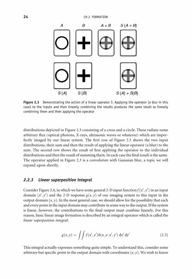
distributions depicted in Figure 2.3 consisting of a cross and a circle. These radiate some

arbitrary flux (optical photons, X-rays, ultrasonic waves or whatever) which are imper-

fectly imaged by our linear system. The first row of Figure 2.3 shows the two input

distributions, their sum and then the result of applying the linear operator (a blur) to the

sum. The second row shows the result of first applying the operator to the individual

distributions and then the result of summing them. In each case the final result is the same.

The operator applied in Figure 2.3 is a convolution with Gaussian blur, a topic we will

expand upon shortly.

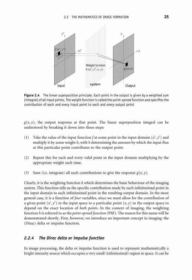
2.2.3 Linear superposition integral

Consider Figure 2.4, in which we have some general 2-D input function f ðx0; y0Þ in an inputdomain ðx0; y0Þ and the 2-D response gðx; yÞ of our imaging system to this input in the

output domain ðx; yÞ. In the most general case, we should allow for the possibility that each

and every point in the input domainmay contribute in someway to the output. If the system

is linear, however, the contributions to the final output must combine linearly. For this

reason, basic linear image formation is described by an integral operator which is called the

linear superposition integral:

gðx; yÞ ¼Z Z

f ðx0; y0Þhðx; y; x0; y0Þ dx0 dy0 ð2:3Þ

This integral actually expresses something quite simple. To understand this, consider some

arbitrary but specific point in the output domain with coordinates ðx; yÞ. We wish to know

Figure 2.3 Demonstrating the action of a linear operator S. Applying the operator (a blur in this

case) to the inputs and then linearly combining the results produces the same result as linearly

combining them and then applying the operator

24 CH 2 FORMATION

gðx; yÞ, the output response at that point. The linear superposition integral can be

understood by breaking it down into three steps:

(1) Take the value of the input function f at some point in the input domain ðx0; y0Þ andmultiply it by some weight h, with h determining the amount by which the input flux

at this particular point contributes to the output point.

(2) Repeat this for each and every valid point in the input domain multiplying by the

appropriate weight each time.

(3) Sum (i.e. integrate) all such contributions to give the response gðx; yÞ.

Clearly, it is the weighting function h which determines the basic behaviour of the imaging

system. This function tells us the specific contribution made by each infinitesimal point in

the input domain to each infinitesimal point in the resulting output domain. In the most

general case, it is a function of four variables, since we must allow for the contribution of

a given point ðx0; y0Þ in the input space to a particular point ðx; yÞ in the output space to

depend on the exact location of both points. In the context of imaging, the weighting

function h is referred to as the point-spread function (PSF). The reason for this name will be

demonstrated shortly. First, however, we introduce an important concept in imaging: the

(Dirac) delta or impulse function.

2.2.4 The Dirac delta or impulse function

In image processing, the delta or impulse function is used to represent mathematically a

bright intensity source which occupies a very small (infinitesimal) region in space. It can be

Figure 2.4 The linear superposition principle. Each point in the output is given by a weighted sum

(integral) of all input points. The weight function is called the point-spread function and specifies the

contribution of each and every input point to each and every output point


modelled in a number of ways,1 but arguably the simplest is to consider it as the limiting

form of a scaled rectangle function as the width of the rectangle tends to zero. The 1-D

rectangle function is defined as

rect

�x

a

�¼ 1 jxj < a=2

¼ 0 otherwise

ð2:4Þ

Accordingly, the 1-D and 2-D delta function can be defined as

dðxÞ ¼ lima! 0

1

arect

�x

a

�in 1-D

dðx; yÞ ¼ lima! 0

1

a2rect

�x

a

�rect

�y

a

�in 2-D

ð2:5Þ

In Figure 2.5 we show the behaviour of the scaled rectangle function as a! 0. We

see that:

As a! 0 the support (the nonzero region) of the function tends to a vanishingly small

region either side of x ¼ 0.

As a! 0 the height of the function tends to infinity but the total area under the function

remains equal to one.

dðxÞ is thus a function which is zero everywhere except at x ¼ 0 precisely. At this point,

the function tends to a value of infinity but retains a finite (unit area) under the function.

aaa

a1 a

1

a

x

δ (x)

δ (x) dx = 1

δ (x) = lim∞

∞

−∞�

1

a1

ax⎛⎛ ⎛⎛rect

Figure 2.5 The Dirac delta or impulse function can be modelled as the limiting form of a scaled

rectangle function as its width tends to zero. Note that the area under the delta function is equal to unity

1 An alternative is the limiting form of a Gaussian function as the standard deviation s! 0.

26 CH 2 FORMATION

Thus:

dðxÞ ¼ ¥ x ¼ 0

¼ 0 x 6¼ 0ð2:6Þ

ð¥

¥

dðxÞ dx ¼ 1 ð2:7Þ

and it follows that a shifted delta function corresponding to an infinitesimal point located at

x ¼ x0 is defined in exactly the same way, as

dðx�x0Þ ¼ ¥ x ¼ x0¼ 0 x 6¼ x0

ð2:8Þ

These results extend naturally to two dimensions and more:

dðx; yÞ ¼ ¥ x ¼ 0; y ¼ 0

¼ 0 otherwiseð2:9Þ

ð¥

¥

ð¥

¥

dðx; yÞ dx dy ¼ 1 ð2:10Þ

However, the most important property of the delta function is defined by its action under

an integral sign, i.e. its so-called sifting property. The sifting theorem states that

ð¥

¥

f ðxÞdðx�x0Þ dx ¼ f ðx0Þ 1-D case

ð¥

¥

ð¥

¥

f ðx; yÞdðx�x0; y�y0Þ dx dy ¼ f ðx0; y0Þ 2-D case

ð2:11Þ

Thismeans that, whenever the delta function appears inside an integral, the result is equal to

the remaining part of the integrand evaluated at those precise coordinates for which the

delta function is nonzero.

In summary, the delta function is formally defined by its three properties of singularity

(Equation (2.6)), unit area (Equation (2.10)) and the sifting property (Equation (2.11)).

Delta functions are widely used in optics and image processing as idealized representa-

tions of point and line sources (or apertures):

f ðx; yÞ ¼ dðx�x0; y�y0Þ ðpoint source located at x0; y0Þf ðx; yÞ ¼ dðx�x0Þ ðvertical line source located on the line x ¼ x0Þf ðx; yÞ ¼ dðy�y0Þ ðhorizontal line source located on the line y ¼ y0Þf ðx; yÞ ¼ dðaxþ byþ cÞ ðsource located on the straight line axþ byþ cÞ

ð2:12Þ


2.2.5 The point-spread function

The point-spread function of a system is defined as the response of the system to an input

distribution consisting of a very small intensity point. In the limit that the point becomes

infinitesimal in size, we can represent the input function as a Dirac delta function

f ðx0; y0Þ ¼ dðx0�x0; y0�y0Þ. For a linear system, we can substitute this into the linear

superposition integral, Equation (2.3), to give

gðx; yÞ ¼Z Z

dðx0�x0; y0�y0Þhðx; y; x0; y0Þ dx0 dy0 ð2:13Þ

By applying the sifting theorem of Equation (2.11) this gives a response gðx; yÞ to the point-like input as

gðx; yÞ ¼ hðx; y; x0; y0Þ ð2:14ÞIn other words, the response to the point-like input (sometimes termed the impulse

response) is precisely equal to h. However, in the context of imaging, the weighting function

in the superposition integral hðx; y; x0; y0Þ is termed the point spread function or PSF

because it measures the spread in output intensity response due to an infinitesimal (i.e.

infinitely sharp) input point.

Why, then, is the PSF an important measure? Consider for a moment that any input

distribution may be considered to consist of a very large (!¥) collection of very small

(! infinitesimal) points of varying intensity. The PSF tells us what each of these points will

look like in the output; so, through the linearity of the system, the output is given by the sum

of the PSF responses. It is thus apparent that the PSF of such a linear imaging system (in the

absence of noise) completely describes its imaging properties and, therefore, is of primary

importance in specifying the behaviour of the system.

It also follows from what we have said so far that an ideal imaging system would possess

a PSF that exactly equalled the Dirac delta function for all combinations of the input and

output coordinates (i.e. all valid combinations of the coordinates ðx; y; x0; y0Þ). Such a

system would map each infinitesimal point in the input distribution to a corresponding

infinitesimal point in the output distribution. There would be no blurring or loss of detail

and the image would be ‘perfect’. Actually, the fundamental physics of electromagnetic

diffraction dictates that such an ideal system can never be achieved in practice, but it

nonetheless remains a useful theoretical concept. By extension then, a good or ‘sharp’

imaging systemwill generally possess anarrowPSF,whereas a poor imaging systemwill have

a broad PSF, which has the effect of considerably overlapping the output responses to

neighbouring points in the input. This idea is illustrated in Figure 2.6, in which a group

of points is successively imaged by systems with increasingly poor (i.e. broader) PSFs.

Figure 2.6 The effect of the system PSF. As the PSF becomes increasingly broad, points in the

original input distribution become broader and overlap

28 CH 2 FORMATION

2.2.6 Linear shift-invariant systems and the convolution integral

So far in our presentation, we have assumed that the systemPSFmay depend on the absolute

locations of the two points in the input and output domains. In other words, by writing

the PSF as a function of four variables in Equation (2.3), we have explicitly allowed for the

possibility that the response at, let us say, point x1; y1 in the output domain due to a point

x01; y01 in the input domainmay be quite different from that at some other output point x2; y2.

If this were the case in practice for all pairs of input and output points, then specification of

the system PSF would be a very cumbersome business. As an example, consider discretizing

both the input and output domains into even amodest number of pixels such as 128� 128.

Since every pixel in the input can in principle contribute to every pixel in the output in a

different way, we would then require 1284� 268.4 million values to fully specify the system

behaviour.

Fortunately, most imaging systems (at least to a very good approximation) possess a

property called shift invariance or isoplanatism. A shift-invariant system is characterized

by a PSF that depends only on the difference between the coordinates in the input and

output domains, not on their absolute values. Thus, a shift-invariant PSF in a 2-D imaging

system has a functional form which makes it dependent not on four variables, but on two

variables only:

hðx; y; x0; y0Þ ¼ hðx00; y

00 Þ ¼ hðx�x0; y�y0Þ ð2:15Þ

Shift invariance has a simple physical interpretation. Consider a source point in the input

domain at coordinates x0; y0. If we move this source point to different locations in the input

domain, changing the values of the coordinates x0; y0, the corresponding response (i.e. itsshape/functional form) in the output domain will remain the same but will simply be

correspondingly translated in the output domain. In other words, shift the input and the

corresponding output just shifts too. Figure 2.72 is a simulation of a photon-limited system

in which photons in the input domain are randomly emitted and imaged by the linear shift-

invariant system. This shows clearly how the image is built as the weighted superposition of

shift-invariant responses to an increasing number of point-like inputs.

When we have a shift-invariant system, the linear superposition integral Equation (2.3)

reduces to a simpler and very important form – a convolution integral:

gðx; yÞ ¼ð¥

¥

ð¥

¥

f ðx0; y0Þhðx�x0; y�y0Þ dx0 dy0 ð2:16Þ

Note that the infinite limits are used to indicate that the integration is to take place over all

values for which the product of the functions is nonzero. The output gðx; yÞ is said to be

given by the convolution of the input f ðx; yÞ with the PSF hðx; yÞ. Note that the

corresponding form for convolution of 1-D functions follows naturally:

gðxÞ ¼ð¥

¥

f ðx0Þhðx�x0Þ dx0 ð2:17Þ

2 The Matlab code which produced Figure 2.7 is available at http://www.fundipbook.com/materials/.


Convolution integrals are so important and common that they are often written in an

abbreviated form:

gðx; yÞ ¼ f ðx; yÞ � � hðx; yÞ ð2-DÞgðxÞ ¼ f ðxÞ � hðxÞ ð1-DÞ ð2:18Þ

where the asterisks denote the operation of convolving the input function f with the

system PSF h. In general, the function h in the convolution integrals above is called the

kernel.

2.2.7 Convolution: its importance and meaning

It would be hard to overstate the importance of convolution in imaging. There are twomain

reasons:

(1) A very large number of image formation processes (and, in fact, measurement

procedures in general) are well described by the process of convolution. In fact, if

a system is both linear and shift invariant, then image formation is necessarily

described by convolution.

(2) The convolution theorem (which we will discuss shortly) enables us to visualize and

understand the convolution process in the spatial frequency domain. This equiva-

lent frequency-domain formulation provides a very powerful mathematical frame-

work to deepen understanding of both image formation and processing.

This framework will be developed in Chapter 5 and also forms a major part of

Chapter 6.

Figure 2.7 Each image in the top row shows arbitrary points in the input domain (increasing

in number from left to right) whilst the images in the bottom row show the response of a LSI

system to the corresponding input. The final image at the bottom right consists of a weighted

superposition of responses to the input points, each of which has a similar mathematical shape or

form

30 CH 2 FORMATION

First, let us try to understand the mechanism of the convolution process. A convolution

integral is a type of ‘overlap’ integral, and Figure 2.8 gives a graphical representation of how

convolutions occur and are calculated. Basically, a flipped version of one of the functions is

systematically displaced and the integral of their product (the overlap area) is calculated at

each shift position. All shift coordinates for which the overlap area is nonzero define the

range of the convolution.

Wemight well still ask, but why then is the physical process of forming an image so often

described by convolution? This is perhaps best understood through a simple example (see

Figure 2.9a–c). Gamma rays are too energetic to be focused, so that the very earliest gamma

ray detectors used in diagnostic radionuclide imaging consisted of a gamma-ray-sensitive

scintillation crystal encapsulated by a thick lead collimatorwith a finite-size aperture to allow

normally incident gamma photons to strike and be absorbed in the crystal. The scan was

acquired by raster-scanning with uniform speed over the patient; in this way, the derived

signal is thus proportional to the gamma activity emanating from that region of the body

lying beneath the aperture. Note that a finite-size aperture is absolutely necessary because

reducing the aperture size to an infinitesimal size would permit a vanishingly small fraction

of emitted photons to actually reach the detector, which is clearly useless for diagnostic

purposes.

Let us first remind ourselves that, in general, the linear superposition integral allows for

the possibility that every point in the input domain f ðx0Þmay in principle contribute to the

detector response at a chosen point x and does this through the PSF hðx; x0Þ; thus, wehave quite generally that gðxÞ ¼ Ð

f ðx0Þhðx; x0Þ dx0. Consider then Figure 2.9a, where for

Figure 2.8 The calculation of a 1-D convolution integral


Detector(delta-like)

Scanning pinhole(delta-like)

(a)

1-D intensity profile

δ (x ′) f (x ′) x ′

x

g (x )

g (x ) = f (x ′) h (x ,x ′)dx ′ = f (x ′) δ (x –x ′)dx ′ = f (x )� �

Detector(delta-like)

Scanning pinhole(finite aperture)

(b)


h (x ′) f (x ′) x ′

x

g (x )

g (x ) = f (x ′) h (x ,x ′)dx ′ = f (x ′) h (x –x ′)dx ′� �

Detector(finite size)

Scanning pinhole(finite aperture)

(c)


h (x ′) I (x ) hd (x ′) f (x ′) x ′

x

I (x ) = g (x ′) hd (x ,x ′)dx ′I (x ) = f (x ′) *h (x ,)*hd (x )

g (x ) = f (x ′) δ (x –x ′)dx ′� �where

Figure 2.9 (a) A delta like detector views a source intensity profile through a delta-like scanning

pinhole. The resulting image is a convolution of the source with the pinhole PSF. In principle, this

replicates the source profile so that gðxÞ ¼ f ðxÞ but this idealized response can never describe a realsystem. (b) Here, a delta like detector views a source intensity profile through a finite-size scanning

pinhole. The resulting image is a convolution of the source with the pinhole PSF. All real systems

exhibit such finite aperture effects. (c) A finite-size detector viewing a source intensity profile through

a finite scanning pinhole. The resulting image is a convolution of the source intensity with both the

pinhole and detector PSFs. In general, if N LSI elements are involved in the image formation process,

the resulting image is described by convolving the source with each corresponding PSF

32 CH 2 FORMATION

simplicity, we depict a 1-D detector and a 1-D intensity source. The idealized pinhole

aperture may be approximated by a delta function dðx0Þ. It is readily apparent that, if thedetector were kept stationary but the pinhole aperture scanned along the x0 axis, wewould only get a nonzero detector response gðxÞ at the detector when the shift

coordinate x ¼ x0. This situation is thus described by the linear superposition

gðxÞ ¼ Ðf ðx0Þdðx�x0Þ dx0.3

If we now consider a finite pinhole aperture, as in Figure 2.9b, it is clear that many points

in the input domain will now contribute to the detector response gðxÞ but some will not.

In fact, it is clear that only those points in the input domain forwhich the difference x�x0 liesbelow a certain threshold can contribute. Note that the PSF of this scanning aperture is

determined by pure geometry and the detector response is thus independent of the absolute

position x0 of the aperture – the dependence on x0 comes only as a result of how the input

f ðx0Þ changes.Finally, consider Figure 2.9c. Here, we depict a finite detector aperture as well as a

finite scanning aperture, and this results in a more complicated situation. However, this

situation is simply described by an additional further convolution such that the actual

recorded intensity at the finite detector is now given by IðxÞ ¼ Ðgðx0Þhdðx�x0Þ dx0,

where gðx0Þ is the intensity at some point on the detector and hdðx0Þ is the detector

response (PSF). The way to understand this situation is depicted in Figure 2.10.

Essentially, we break it down into two parts, first calculating the resulting intensity

Contribution dI to the total intensity overthe detector at point x ′ is the productof the incident intensity g and the responseat that point h

The total recorded intensity is the sum ofall such contributions over the detector-

Detector

x ′

x

hd (x ′)

hd (x – x ′)

I (x ) = �dI = � g(x ′) h (x – x ′) dx ′

dI = g (x ′) h (x –x ′)

–∞

∞

Figure 2.10 The response of a finite detector with response function hdðxÞ to an incident intensityfield gðxÞ is given by their convolution. We consider the contribution to the total intensity recorded

by the detector at some ordinate x0 when the detector is displaced by some amount x. This is

dI ¼ gðx0Þhdðx x0Þ. By integrating all such contributions over the detector surface we obtain the

convolution integral

3 Strictly, this supposes that the effective sensitive area of the detector is infinitesimal and thus also well

approximated by a delta response this will occur either because it is infinitesimally small or because the scanning

aperture lies very close to it.


at a fixed point on the detector and then considering how all such contributions

make up the final recorded intensity. Referring to Figure 2.10, the detector has a response

hdðx0Þ when referred to the origin. We are interested in the total intensity recorded

by this detector IðxÞwhen it is displaced some distance x from the origin. The contribution

to the recorded intensity dI at some precise point with ordinate x0 is given by the

product of the incident intensity at that point gðx0Þ times the shifted response hdðx�x0Þ –thus dI ¼ gðx0Þhdðx�x0Þ. The total recorded intensity at the detector is thus given

by all such contributions dI for which the ordinate x0 lies within the dimensions

of the detector dimension (i.e. for which dI ¼ gðx0Þhdðx�x0Þ 6¼ 0. Thus, we

obtain IðxÞ ¼ ÐdI ¼ Ð ¥

¥ gðx0Þhdðx�x0Þ dx0.

2.2.8 Multiple convolution: N imaging elements in a linear shift-invariantsystem

In Figure 2.9c we effectively have an imaging system in which two aperture functions

describe the imaging properties: hðxÞ and hdðxÞ. Under these circumstances, we have seen

that the recorded intensity IðxÞ is given by successive convolutions of the input f ðxÞwith thePSF of the scanning aperture hðxÞ and the PSF of the detector hdðxÞ. Symbolically, we denote

this by IðxÞ ¼ f ðxÞ � hðxÞ � hdðxÞ. Provided the assumption of linearity and shift invariance

remains valid, this result extends naturally to an arbitrary systemofN imaging elements (e.g.

a sequence of lenses in an optical imaging system). Thus, in general, any processing sequence

in which N linear and shift-invariant system elements act upon the input is described by a

sequence of N convolutions of the input with the respective PSFs of the elements. This is

summarized in Figure 2.11.

2.2.9 Digital convolution

In digital image processing, signals are discrete not continuous. Under these conditions,

convolution of two functions is achieved by discretizing the convolution integral. In the

simple 1-D case, this becomes

PSF 1 PSF 2 PSF N

OutputInput

h1 (x ) h2 (x ) hn (x )

g (x ) = f (x )* h1 (x )* h2 (x )...*h2 (x )

g (x )f (x )

Figure 2.11 The output of an LSI system characterized by N components each having a PSF hiðxÞ isthe repeated convolution of the input with each PSF

34 CH 2 FORMATION

gj ¼Xi

fihj i ð2:19Þ

where the indices j and i correspond to discrete values of x and x0 respectively.In two dimensions, the discrete convolution integral may be written as

gkl ¼Xj

Xi

fijhk i;l j ð2:20Þ

where the indices k and l correspond to x and y and i and j correspond to x0 and y0. Thisequation somewhat belies the simplicity of the mechanism involved. The filter kernel h is

only nonzero when both the shift coordinates k� i and l� j are small enough to lie within

the spatial extent of h (i.e. are nonzero). For this reason, although the image fij has a large

spatial extent, the filter kernel hk i;l j, when it corresponds to a PSF, is typically of much

smaller spatial extent. The convolved or filtered function is thus given by a weighted

combination of all those pixels that lie beneath the filter kernel (see Figure 2.12). A simple

example of 1-D discrete convolution in Matlab� is given in Example 2.1 and some simple

examples of 2-D convolution using Matlab are given in Example 2.2. Note that 2-D

convolution of two functions that are both of large spatial extent is much more computa-

tionally efficient when carried out in the Fourier domain. We will discuss this when we

introduce the convolution theorem later in Chapter 5. Figures 2.13 and 2.14 result from the

code in Examples 2.1 and 2.2.

12

–1 –1 –1

–1 –1 –1

–1

w1 w2 w3

w4 w5 w6

w7 w8 w9

= 8 –1

10

32

40

41

42

12

Image

= (–1x10) + (–1x11) + (–1x8) + (–1x40) + (8x35)

fi = ∑ wkI k (i )

+ (–1x42) + (–1x38) + (–1x36) + (–1x46) = 1410

40

38

89

39

13

11

35

36

39

43

13

8

42

46

42

45

9

13

40

41

39

38

11

8

36

37

36

37

9

i–j

Figure 2.12 Discrete convolution. The centre pixel of the kernel and the target pixel in the image

are indicated by the dark grey shading. The kernel is ‘placed’ on the image so that the centre and

target pixels match. The filtered value of the target pixel is then given by a linear combination of

the neighbourhood pixels, the specific weights being determined by the kernel values. In this

specific case the target pixel of original value 35 has a filtered value of 14


Example 2.2


A¼imread('trui.png'); %Read in image

PSF¼ fspecial('gaussian',[5 5],2); %Define Gaussian convolution kernel

h¼fspecial('motion',10,45); %Define motion filter

B¼conv2(PSF,A); %Convolve image with convolution kernel

C¼imfilter(A,h,'replicate'); %Convolve motion PSF using alternative function

D¼conv2(A,A); %Self convolution motion blurred with original

subplot(2,2,1),imshow(A); %Display original image

subplot(2,2,2),imshow(B,[]); %Display filtered image

subplot(2,2,3),imshow(C,[]); %Display filtered image

subplot(2,2,4),imshow(D,[]); %Display convolution image with

itself (autocorrln)

Comments

Matlab functions: conv2, imfilter.

This example illustrates 2 D convolution. The first two examples show convolution of the

image with a Gaussian kernel using two related Matlab functions. The final image shows the

autocorrelation of the image given by the convolution of the function with itself.

Example 2.1


f¼ones(64,1); f¼f./sum(f); %Define rectangle signal f and normalize

g¼conv(f,f); g¼g./sum(g); %Convolve f with itself to give g and normalize

h¼conv(g,g); h¼h./sum(h); %Convolve g with itself to give h and normalize

j¼conv(h,h); j¼j./sum(j); %Convolve h with itself to give j and normalize

subplot(2,2,1),plot(f,'k '); axis square;

axis off;

subplot(2,2,2),plot(g,‘k ’); axis square;

axis off;

subplot(2,2,3),plot(h,‘k ’); axis square;

axis off;

subplot(2,2,4),plot(j,‘k ’); axis square;

axis off;

Comments

Matlab functions: conv.

This example illustrates the repeated convolution of a 1 D uniform signal with itself. The

resulting signal quickly approaches the formof the normal distribution, illustrating the central

limit theorem of statistics.

36 CH 2 FORMATION

2.3 The engineering of image formation

From our mathematical consideration of the image formation, we now briefly consider the

engineering aspects of this process. It is not possible to consider every eventuality in this

instance, but we instead limit ourselves to the most common and, hence, practical imaging

scenarios.

f (x) g (x) = f (x)* f (x)

j (x) = g (x)* h (x) h (x) = g (x)* g (x)

Figure 2.13 Repeated convolution of a 1-D rectangle signal. The output rapidly approaches the form

of the normal distribution, illustrating the central limit theorem of statistics

Figure 2.14 Top left: original image; top right: after convolution with Gaussian kernel; bottom left:

after convolution with Gaussian kernel; bottom right: convolution of the image with itself

2.3 THE ENGINEERING OF IMAGE FORMATION 37

2.3.1 The camera

In general, let us consider our imaging device to be a camera. A camera image of a

conventional scene is essentially a projection of the 3-D world (i.e. the scene) to a 2-D

representation (i.e. the image). The manner in which this 3-D to 2-D projection occurs is

central to our ability to perform effective analysis on digital images.

If we assume an object/scene is illuminated by a light source (possibly multiple

sources), then some of the light will be reflected towards the camera and captured as a

digital image. Assuming we have a conventional camera, the light reflected into the lens is

imaged onto the camera image plane based on the camera projection model. The camera

projection model transforms 3-D world coordinates ðX;Y ;ZÞ to 2-D image coordinates

ðx; yÞ on the image plane. The spatial quantization of the image plane projection into a

discretized grid of pixels in turn transforms the 2-D image coordinate on the image plane

to a pixel position ðc; rÞ. The majority of scene images we deal with will be captured using

a perspective camera projection.

Perspective projection: In general the perspective projection (Figure 2.15, right) can be

stated as follows:

x ¼ fX

Zy ¼ f

Y

Zð2:21Þ

A position ðX;Y ;ZÞ in the scene (depth Z) is imaged at position ðx; yÞ on the image plane

determined by the focal length of the camera f (lens to image plane distance). The

perspective projection has the following properties (illustrated in Figure 2.16):

. Foreshortening The size of objects imaged is dependent on their distance from the

viewer. Thus, objects farther away from the viewer appear smaller in the image.

. Convergence Lines that are parallel in the scene appear to converge in the resulting

image. This is known as perspective distortion, with the point(s) at which parallel lines

meet termed the vanishing point(s) of the scene.

Scene Co-ordinatesScene Co-ordinates

Image Co-ordinates

Image Co-ordinates

PerspectiveProjection Model

ParallelProjection Model

Z

XY

y

Z

f

Y

X

Z

xy

x

Figure 2.15 Camera projection models: perspective (left) and parallel/affine (right)

38 CH 2 FORMATION

Tobemore precise this is the pin-hole perspective projectionmodel, aswe assume all the light

rays pass through a single point and, hence, the scene is inverted (horizontally and vertically)

on the image plane (Figure 2.15, left). Realistically, we deploy a lens, which further

complicates matters by introducing lens distortion (affecting f), but this optics-related

topic is beyond the scope of this text. With a lens, the scene is still imaged upside down (and

back to front), but this is generally dealt with by the camera and should be ignored for all

applied purposes. It should be noted that the perspective projection is not easily invertible

from an image alone – i.e. given 2-D image position ðx; yÞ and camera focal length f it is not

possible to recover ðX;Y ;ZÞ. However, given knowledge of ðX;YÞ in the scene (measured

relative to the camera position), the recovery of position depth Z may become possible

(subject to noise and distortion). Accurate ðX;YÞ positions, relative to the exact camera

position, are, however, difficult to determine and rarely recorded at time of image capture.

Orthographic projection: An alternative camera projection model to the perspective

projection is the orthographic (or parallel) projection. This is used by some specialist

imaging instruments; for instance, a flat-bed scanner produces an orthographic projection

of a scanned document, a medical scanner produces an orthographic projection of the

human body. The orthographic projection is simply denoted as

x ¼ X y ¼ Y

The orthographic projection is an affine transformation such that relative geometric

relationships are maintained, as the scene to image plane projection is parallel. As such, the

image features are not reversed (Figure 2.15, right), but notably all information relating to

scene depth is lost. In an orthographic projection, size is independent of the distance from

the viewer and parallel lines are preserved. The projection may have a scaling factorm such

that x¼mX and y¼mY, but this relates to regular image zooming or reduction and

maintains these properties. Images captured over a close range (i.e. short focal length,

macro-scale photography) or of a planar target can often be assumed to have an

orthographic camera projection because of the negligible effects of the perspective projec-

tion over this range.

In addition to the projection model, the camera has a number of other characteristics

that determine the final image formed from the scene. Notably any camera is of fixed spatial

Convergence ofparallel lines

Foreshortening

Vanishing Point

Figure 2.16 Effects of the perspective projection model on scene geometry in the image


resolution (number of pixels making up the image) and has a fixed depth per pixel (number

of bits used to represent each pixel) (see Section 2.1). Both of these are discussed in the next

section regarding the image digitization process. In addition, every camera has unique lens

distortion characteristics related to differences in manufacture (referred to as the intrinsic

camera parameters) that together with similar subtle differences in the image sensor itself

make it impossible to capture two identical digital images from a given camera source – thus

no two images are the same.

2.3.2 The digitization process

From our discussion of how our image is formed by the camera as a 3-D to 2-D projective

transform (Section 2.3.1), we now move on to consider the discretization of the image

into a finite-resolution image of individual pixels. The key concept in digitization is that

of quantization: themapping of the continuous signal from the scene to a discrete number

of spatially organized points (pixels) each with a finite representational capacity

(pixel depth).

2.3.2.1 QuantizationQuantization in digital imaging happens in two ways: spatial quantization and colour

quantization.

Spatial quantization corresponds to sampling the brightness of the image at a number

of points. Usually a C�R rectangular grid is used but variations from rectangular do

exist in specialist sensors. The quantization gives rise to a matrix of numbers which

form an approximation to the analogue signal entering the camera. Each element of this

matrix is referred to as a pixel – an individual picture element. The fundamental question

is: How well does this quantized matrix approximate the original analogue signal ? We

note that

(1) If n2 samples are taken at regular intervals (uniform sampling, n� n image) within a

bounding square, then the approximation improves as n increases. As spatial

resolution increases so does image quality in terms of the reduction in approximation

error between the original and the digitized image.

(2) In general, as long as sufficient samples are taken, a spatially quantized image is as good

as the original image (for the purposes required, i.e. at a given level of detail).

The precise answer to our question is provided by the sampling theorem (also referred to as

the Nyquist sampling theorem or Shannon’s sampling theorem). The sampling theorem, in

relation to imaging, states: an analogue image can be reconstructed exactly from its digital

form as long as the sampling frequency (i.e. number of samples per linearmeasure) is at least

twice the highest frequency (i.e. variation per measure) present in the image. Thus we

require:

sampling interval � 1

Nyquist frequencyð2:22Þ

40 CH 2 FORMATION

where

Nyquist frequency ¼ 2� ðMaximum frequency in imageÞThe sampling theorem is concerned with the number of samples needed to recreate the

original image, not with the adequacy of the digitization for any particular type of

processing or presentation. As far as the implementation in digitization hardware is

concerned, the sampling interval is effectively set by:

. Dt (time between samples) in a scanning-based image capture process where a sensor is

being swept over a region or scene (e.g. a desktop flat-bed scanner);

. the spatial distribution of the charge-coupled device (CCD) or complementary metal–

oxide–semiconductor (CMOS) elements on the capture device itself (see Section 2.3.2.2).

Spatial quantization of the image causes aliasing to occur at edges and features within the

image (Figure 2.17, left) and differing spatial quantization can affect the level of detail

apparent within the image (Figure 2.17, right).

In addition to spatial sampling,we also have the colour or intensity sampling to consider –

effectively intensity quantization. For each sample point (pixel) captured at a given spatial

resolution we obtain a voltage reading on the image sensor (i.e. the CCD/CMOS or

analogue-to-digital (A/D) converter) that relates to the amount and wavelength of light

being projected through the camera lens to that point on the image plane. Depending on the

sensitivity of the sensor to particular levels and wavelengths of light, these analogue voltage

signals can be divided (i.e. discretized) into a number of bins each representing a specific level

of intensity – pixel values. For an 8-bit grey-scale sensor this continuous voltage is divided

into 28 bins, giving 256 possible pixel values and thus representing a grey scale ranging from 0

(black) to 255 (white).

Different levels of intensity quantization give different levels of image colour quality, as

shown in Figure 2.18. Notably, a significant reduction in the level of quantization can be

performed (256 ! 16) before any real effects become noticeable. For colour sensors each of

the red, green and blue channels are similarly each quantized into an N-bit representation

(typically 8-bits per channel, giving a 24-bit colour image). In total, 24-bit colour gives 16.7

million possible colour combinations. Although these representations may seem limited,

given current computing abilities, it isworth noting that the humanvisual system can atmost

Figure 2.17 The effects of spatial quantization in digital images


determine between�40 different levels of grey and it is estimated to see around 7–10million

distinct colours. This is illustrated in Figure 2.18, where a perceived difference in colour

quality is only visible after a significant 256 ! 16 level change. This limitation of human

vision has implications for what ‘we can get away with’ in image compression algorithms

(Section 1.3.2). Note that.. although the human visual system cannot determine the

difference between these levels, the same is not always true for image processing. A shallow

colour depth (i.e. low-intensity quantization) can lead to different objects/features appearing

at the same quantization level despite being visually distinct in terms of colour. Again,

aliasing in intensity quantization can occur (e.g. the 16 grey-levels example in Figure 2.18).

2.3.2.2 Digitization hardwareBoth forms of quantization, spatial and intensity, are performed near simultaneously in the

digitization hardware.

Traditionally, image capture was performed based on an analogue video-type camera

connected to a computer system via an analogue to digital (A/D) converter. The converter

required enough memory to store an image and a high-speed interface to the computer

(commonly direct PCI or SCSI interface). When signalled by the computer, the frame

grabber digitized a frame and stored the result in its internal memory. The data stored in the

image memory (i.e. the digital image) can then be read into the computer over the

communications interface. The schematic of such a system would typically be as per

Figure 2.19, where we see an analogue link from the camera to the computer system itself

anddigitization is essentially internal to the hardwareunitwhere the processing is performed.

Figure 2.18 The effects of intensity quantization in digital images

Figure 2.19 Schematic of capture-card-based system

42 CH 2 FORMATION

Such systems are now rarer and predominantly for high-speed industrial or specialist

medical/engineering applications. By contrast, most modern frame-grabbing systems are

directly integrated into the camera, with theA/D conversion being done at the sensor level in

the electronics of the CCD or CMOS sensor inside the camera itself (i.e. digital capture,

Figure 2.20). Here, analogue voltage readings occurring upon the sensor itself, in response

to light being projected through the camera lens onto the sensor surface, are converted into a

digitally sampled form. The digitization is carried out in situ, inside the sensor itself prior, to

a digital transport link to the computer. Modern computer peripheral interfaces such as

USB/FireWire (IEEE 1394)/GigE offer suitable high-speed digital interfaces to make

digitization at sensor level and real-time transmission to the computer system a possibility.

The image capture subsystem in Figure 2.19 is essentially reduced onto the capture device

itself, either retaining only the most recent ‘live’ image to service requests from the

computer (e.g. webcams) or, in the case of storage-based capture devices, retaining up toN

digitized images in internal storage (e.g. digital camera/video). This is conceptually similar

to what is believed to happen in the human eye, where basic ‘processing’ of the image is

thought to occur in the retina before transmission onwards to the brain via the optic nerve.

Increasingly, the advent of embedded processing is facilitating the onboard processing of

images in so-called smart cameras. This trend in image capture and processing looks likely

to continue in the near future.

2.3.2.3 Resolution versus performanceA final note on digitization relates to the spatial resolution of the image. A common

misconception is that a greater resolution is somehow always a good thing. Image

processing is by its very nature a very computationally demanding task. Just as in traditional

computational analysis, where we discuss computational runtime in terms of O(n) for a

given algorithm operating on n items, in image processing we consider an ðn� nÞ image

(which generalizes to the differing R�C case).

With serial processing, any operation upon every image pixel (most common) is

inherently quadratic in runtime, O(n2). Thus, the total number of operations increases

Figure 2.20 Example of CCD sensor in a digital video camera


rapidly as image size increases. Here, we see the limitation of increasing image resolution

to achieve better image-processing results- speed. As a result, efficiency is a major concern

when designing image-processing algorithms and is especially important for systems

requiring the processing of video data with high temporal resolution in real time. In order

to counter this high computational demand and to address the increasing need for real-

time image-processing systems, specialist parallel computing facilities have traditionally

be frequently used in image-processing tasks. Specialist hardware for conventional PCs,

such as image-processing boards, were also commonplace and essentially performed user-

defined image-processing tasks using fast hardware implementations independently of

the PC itself.

With the ongoing increase in consumer-level image-processing power (Moore’s law), the

adaptation of processors to specialist multimedia tasks such as image processing (e.g. Intel

MMX technologies) and now the advent of desktop-level multi-processor systems (e.g. Intel

Core-Duo), the use of such specialist hardware has reduced in the image-processing

industry. Although still used in industrial applications, the advent of embedded PC

technology and robust embedded image-processing-capable operating systems look set to

change this over the coming years. Reconfigurable, programmable hardware such as field-

programmable gate arrays (FPGA) and the use of graphics processing unit (GPU) proces-

sing (image processing on the PC graphics card processor) also offer some of the benefits of a

hardware solution with the additional flexibility of software based development/testing.

Modern PCs can cope well with real-time image-processing tasks and have memory

capacities that realistically exceed any single image. The same is not always true of video

stream processing, and performance evaluation and optimization is still an area of research.

2.3.3 Noise

Themain barrier to effective image processing and signal processing in general is noise. By

noisewemean a variation of the signal from its true value by a small (random) amount due to

external or internal factors in the image-processing pipeline. These factors cannot be (easily)

controlled and thus introduce randomelements into the processing pipeline.Noise is the key

problem in 99 % of cases where image processing techniques either fail or further image

processing is required to achieve the required result. As a result, a large part of the image

processing domain, and any image processing system pipeline, is dedicated to noise

reduction and removal. A robust image processing system must be able to cope with noise.

At each stage of image processing, capture and sampling noise is introduced (Figure 2.21).Noise in digital images can originate from a variety of sources :

. Capture noise can be the result of variations in lighting, sensor temperature, electrical

sensor noise, sensor nonuniformity, dust in the environment, vibration, lens distortion,

focus limitations, sensor saturation (too much light), underexposure (too little light).

. Sampling noise As discussed previously (Section 2.3.2), limitations in sampling and

intensity quantization are a source of noise in the form of representational aliasing.

The sampled digital image is not a true representation of the analogue image, but an

alias of the original.

44 CH 2 FORMATION

. Processing noise Limitations in numerical precision (floating-point numbers), poten-

tial integer overflow and mathematical approximations (e.g. p¼ 3.142. . .) are all

potential sources of noise in the processing itself.

. Image-encoding noise Many modern image compression techniques (e.g. JPEG used

intrinsically by modern digital cameras) are lossy compression techniques. By lossy we

mean that they compress the image by removing visual information that represents

detail not general perceivable to the human viewer. The problem is that this loss of

information due to compression undermines image-processing techniques that rely on

this information. This loss of detail is often referred to by the appearance of compression

artefacts in the image. In general, loss¼ compression artefacts¼ noise. Modern image

formats, such as PNG, offer lossless compression to counter this issue (see Section

1.3.2).

. Scene occlusion In the task of object recognition, objects are frequently obscured by

other objects. This is known as occlusion. Occlusion poses a big problem for computer

vision systems because you don’t know what you cannot see. You may be able to infer

recognition from a partial view of an object, but this is never as robust as full-view

recognition. This limits available image information.

Ignoring systematic noise attributable to a specific cause (e.g. nonuniform lighting), noise in

images can be characterized in a number of ways. Themain twonoise characterizations used

in imaging are:

Figure 2.21 Examples of noise effects in digital imaging


. Salt and pepper noise This is caused by the random introduction of pure white or black

(high/low) pixels into the image (Figure 2.21). This is less common in modern image

sensors, although can most commonly be seen in the form of camera sensor faults (hot

pixels that are always at maximum intensity or dead pixels which are always black). This

type of noise is also known as impulse noise.

. Gaussian noise In this case, the random variation of the image signal around its

expected value follows the Gaussian or normal distribution (Figure 2.21). This is the

most commonly used noise model in image processing and effectively describes most

random noise encountered in the image-processing pipeline. This type of noise is also

known as additive noise.

Ultimately, no digital image is a perfect representation of the original scene: it is limited in

resolution by sampling and contains noise. One of the major goals of image processing is to

limit the effects of these aspects in image visualization and analysis.

Exercises


examples introduced in this chapter. Additional information on all of theMatlab functions

represented in this chapter and throughout these exercises is available in Matlab from the

function help browser (use doc <function name> at the Matlab command prompt, where

<function name> is the function required)

Matlab functions: rand(), fspecial(), filter2(), imresize(), tic(), toc(), imapprox(),

rgb2ind(), gray2ind(), imnoise(), imtool(), hdrread(), tonemap(), getrangefromclass().

Exercise 2.1 Using Example 2.3 we can investigate the construction of a coherent image

from a limited number of point samples via the concept of the PSF introduced in

Section 2.1:

Example 2.3


A¼imread(‘cameraman.tif ’); %Read in an image

[rows dims]¼size(A); %Get image dimensions

Abuild¼zeros(size(A)); %Construct zero image of equal size

%Randomly sample 1% of points only and convolve with Gaussian PSF

sub¼rand(rows.�dims,1)<0.01;Abuild(sub)¼A(sub); h¼fspecial(‘gaussian’,[10 10],2);

B10¼filter2(h,Abuild);

subplot(1,2,1), imagesc(Abuild); axis image; axis off;colormap(gray); title(‘Object points’)

subplot(1,2,2), imagesc(B10); axis image; axis off;colormap(gray); title(‘Response of LSI system’)

46 CH 2 FORMATION

Here, we randomly select 1% (0.01) of the image pixels and convolve them using a

Gaussian-derived PSF (see Section 4.4.4) applied as a 2-D image filter via the filter2()

function. Experiment with this example by increasing the percentage of pixels randomly

selected for PSF convolution to form the output image. At what point is a coherent image

formed? What noise characteristics does this image show? Additionally, investigate the use

of the fspecial() function and experiment with changing the parameters of the Gaussian

filter used to approximate the PSF. What effect does this have on the convergence of the

image towards a coherent image (i.e. shape outlines visible) as we increase the number of

image pixels selected for convolution?

Exercise 2.2 The engineering of image formation poses limits on the spatial resolution

(Section 1.2) of an image through the digitization process. At the limits of spatial resolution

certain image details are lost. Using the Matlab example images ‘football.jpg’ and ‘text.

png’, experiment with the use of the imresize() function both in its simplest form (using a

single scale parameter) and using a specified image width and height (rows and columns).

As you reduce image size, at what point do certain image details deteriorate beyond

recognition/comprehension within the image? You may also wish to investigate the use of

imresize() for enlarging images. Experiment with the effects of enlarging an image using all

three of the available interpolation functions for the Matlab imresize() function. What

differences do you notice? (Also try timing different resizing interpolation options using the

Matlab tic()/toc() functions.)

Exercise 2.3 In addition to spatial resolution, the engineering of image formation also

poses limits on the number of quantization (colour or grey-scale) levels in a given image.

Using the Matlab function imapprox() we can approximate a given image represented in a

given colour space (e.g. RGB or grey scale, Section 1.4.1.1) with fewer colours. This function

operates on an indexed image (essentially an imagewith a reference look-up table for each of

its values known as a colour map) – see ‘indexed images’ in Matlab Help. A conventional

image (e.g. Matlab example ‘peppers.png’) can be converted to an indexed image and

associated look-up table colourmap using theMatlab rgb2ind() function (or gray2ind() for

grey-scale images). Investigate the use of imapprox() and rgb2ind()/gray2ind() to reduce

the number of colours in a colour image example and a greyscale image example.

Experiment with different levels of colour reduction. How do your findings tally with the

discussion of human colour perception in Section 2.3.2.1)?

Exercise 2.4 The Matlab imnoise() function can be used to add noise to images. Refer to

Example 4.3 for details of how to use this function and experiment with its use as suggested

in the associated Exercise 4.1.

Exercise 2.5 The Matlab function imtool() allows us to display an image and perform a

number of different interactive operations upon it. Use this function to load the example

image shown in Figure 2.16 (available as ‘railway.png’) and measure the length in pixels of

the railway sleepers in the foreground (front) and background (rear) of the image. Based on

the discussion of Section 2.3.1, what can we determine about the relative distance of the two

sleepers you have measured to the camera? If we assume the standard length of a railway

EXERCISES 47

sleeper is 2.5 m, what additional information would be need to determine the absolute

distance of these items from the camera? How could this be applied to other areas, such as

estimating the distance of people or cars from the camera?

Exercise 2.6 High dynamic range (HDR) imaging is a new methodology within image

capture (formation) whereby the image is digitized with a much greater range of quantiza-

tion levels (Section 2.3.2.1) between the minimum and maximum colour levels. Matlab

supports HDR imaging through the use of the hdrread() function. Use this function to load

the Matlab example HDR image ‘office.hdr’ and convert it to a conventional RGB colour

representation using the Matlab tonemap() function for viewing (with imshow()). Use the

Matlab getrangefromclass() function and imtool() to explore the value ranges of these two

versions of the HDR image.


48 CH 2 FORMATION

3Pixels

In this chapter we discuss the basis of all digital image processing: the pixel. We cover the

types of tangible information that pixels can contain and discuss operations both on

individual pixels (point transforms) and on distributions of pixels (global transforms).

3.1 What is a pixel?

The word pixel is an abbreviation of ‘picture element’. Indexed as an ðx; yÞ or column-row

ðc; rÞ location from the origin of the image, it represents the smallest, constituent element in

a digital image and contains a numerical value which is the basic unit of information within

the image at a given spatial resolution and quantization level. Commonly, pixels contain the

colour or intensity response of the image as a small point sample of coloured light from the

scene. However, not all images necessarily contain strictly visual information. An image is

simply a 2-D signal digitized as a grid of pixels, the values of which may relate to other

properties other than colour or light intensity. The information content of pixels can vary

considerably depending on the type of image we are processing:

. Colour/grey-scale images Commonly encountered images contain information relat-

ing to the colour or grey-scale intensity at a given point in the scene or image.

. Infrared (IR) The visual spectrum is only a small part of the electromagnetic spectrum.

IR offers us the capability of imaging scenes based upon either the IR light reflectance or

upon the IR radiation they are emitting. IR radiation is emitted in proportion to heat

generated/reflected by an object and, thus, IR imaging is also commonly referred to as

thermal imaging. As IR light is invisible to the naked human eye, IR illumination and

imaging systems offer a useful method for covert surveillance (as such, IR imaging

commonly forms the basis for night-vision systems).

. Medical imaging Many medical images contain values that are proportional to the

absorption characteristics of tissue with respect to a signal projected through the body.

The most common types are computed tomography (CT) and magnetic resonance

imaging (MRI). CT images, like conventional X-rays, represent values that are directly

proportional to the density of the tissue through which the signal passed. By contrast,

magnetic resonance images exhibit greater detail but do not have a direct relationship to




a single quantifiable property of the tissue. In CT and MRI our 2-D image format is

commonly extended to a 3-D volume; the 3-D volume is essentially just a stack of 2-D

images.

. Radar/sonar imaging A radar or sonar image represents a cross-section of a target in

proportion to its distance from the sensor and its associated signal ‘reflectivity’. Radar is

commonly used in aircraft navigation, although it has also been used on road vehicle

projects. Satellite-based radar forweathermonitoring is now commonplace, as is the use

of sonar on most modern ocean-going vessels. Ground-penetrating radar is being

increasingly used for archaeological and forensic science investigations.

. 3-D imaging Using specific 3-D sensing techniques such as stereo photography or 3-D

laser scanning we can capture data from objects in the world around us and represent

them in computer systems as 3-D images. 3-D images often correspond to depth maps

in which every pixel location contains the distance of the imaged point from the sensor.

In this case, we have explicit 3-D information rather than just a projection of 3-D as in

conventional 2-D imaging. Depending on the capture technology, we may have only

3-Ddepth information or both 3-Ddepth and colour for every pixel location. The image

depth map can be re-projected to give a partial view of the captured 3-D object (such

data is sometimes called 21 2= -D).

. Scientific imaging Many branches of science use a 2-D (or 3-D)-based discrete format

for the capture of data and analysis of results. The pixel values may, in fact, correspond

to chemical or biological sample densities, acoustic impedance, sonic intensity, etc.

Despite the difference in the information content, the data is represented in the same

form, i.e. a 2-D image. Digital image processing techniques can thus be applied inmany

different branches of scientific analysis.

Figure 3.1 shows some examples of images with different types of pixel information.

These are just a few examples of both the variety of digital images in use and of the

broad scale of application domains for digital image processing. In the colour/grey-scale

images we will consider in this book the pixels will usually have integer values within a

given quantization range (e.g. 0 to 255, 8-bit images), although for other forms of image

information (e.g.medical, 3-D, scientific) floating-point real pixel values are commonplace.

3.2 Operations upon pixels

The most basic type of image-processing operation is a point transform which maps the

values at individual points (i.e. pixels) in the input image to corresponding points (pixels) in

an output image. In the mathematical sense, this is a one-to-one functional mapping from

input to output. The simplest examples of such image transformations are arithmetic or

logical operations on images. Each is performed as an operation between two images IA and

IB or between an image and a constant value C:

Ioutput ¼ IA þ IB

Ioutput ¼ IA þCð3:1Þ

50 CH 3 PIXELS

In both cases, the values at an individual pixel location ði; jÞ in the output image are

mapped as follows:

Ioutputði; jÞ ¼ IAði; jÞþ IBði; jÞIoutputði; jÞ ¼ IAði; jÞþC

ð3:2Þ

To perform the operation over an entire image of dimension C�R, we simply iterate over

all image indices for ði; jÞ ¼ f0 . . .C�1; 0 . . .R�1g in the general case (N.B. in Matlab�

pixel indices are {1 . .C;1 . .R}).

3.2.1 Arithmetic operations on images

Basic arithmetic operations can be performed quickly and easily on image pixels for a variety

of effects and applications.

3.2.1.1 Image addition and subtractionAdding a value to each image pixel value can be used to achieve the following effects

(Figure 3.2):

. Contrast adjustment Adding a positive constant value C to each pixel location

increases its value and, hence, its brightness.

. Blending Adding images together produces a composite image of both input images.

This can be used to produce blending effects using weighted addition.

Figure 3.1 Differing types of pixel information

3.2 OPERATIONS UPON PIXELS 51

Image addition can be carried out in Matlab, as shown in Example 3.1.

Subtracting a constant value from each pixel (like addition) can also be used as a basic

form of contrast adjustment. Subtracting one image from another shows us the difference

Figure 3.2 Image contrast adjustment and blending using arithmetic addition

Example 3.1


A¼imread(‘cameraman.tif ’); %Read in image

subplot(1,2,1), imshow(A); %Display image

B ¼ imadd(A, 100); %Add 100 to each pixel value in image A

subplot(1,2,2), imshow(B); %Display result image B

Comments

. Generally, images must be of the same dimension and of the same data type (e.g. 8 bit

integer) for addition and subtraction to be possible between them.

. When performing addition operations we must also be aware of integer overflow. An 8 bit

integer image can only hold integer values from 0 to 255. The Matlab functions imadd,

imsubtract and imabsdiff avoid this problem by truncating or rounding overflow values.

52 CH 3 PIXELS

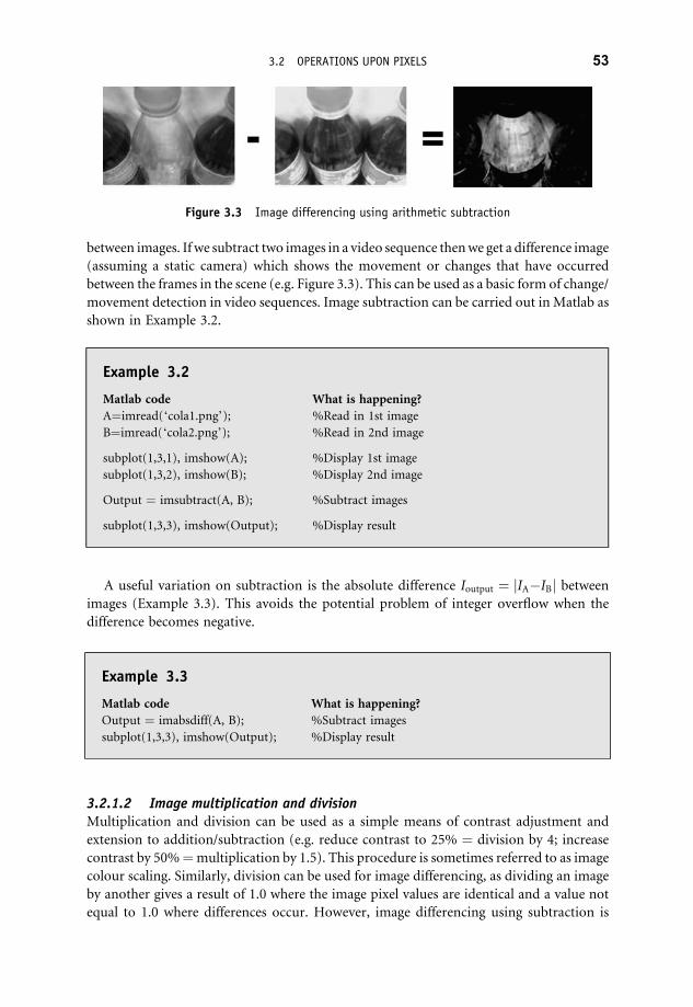
between images. If we subtract two images in a video sequence thenwe get a difference image

(assuming a static camera) which shows the movement or changes that have occurred

between the frames in the scene (e.g. Figure 3.3). This can be used as a basic form of change/

movement detection in video sequences. Image subtraction can be carried out in Matlab as

shown in Example 3.2.

A useful variation on subtraction is the absolute difference Ioutput ¼ jIA�IBj betweenimages (Example 3.3). This avoids the potential problem of integer overflow when the

difference becomes negative.

3.2.1.2 Image multiplication and divisionMultiplication and division can be used as a simple means of contrast adjustment and

extension to addition/subtraction (e.g. reduce contrast to 25% ¼ division by 4; increase

contrast by 50%¼multiplication by 1.5). This procedure is sometimes referred to as image

colour scaling. Similarly, division can be used for image differencing, as dividing an image

by another gives a result of 1.0 where the image pixel values are identical and a value not

equal to 1.0 where differences occur. However, image differencing using subtraction is

Figure 3.3 Image differencing using arithmetic subtraction

Example 3.2


A¼imread(‘cola1.png’); %Read in 1st image

B¼imread(‘cola2.png’); %Read in 2nd image

subplot(1,3,1), imshow(A); %Display 1st image

subplot(1,3,2), imshow(B); %Display 2nd image

Output ¼ imsubtract(A, B); %Subtract images

subplot(1,3,3), imshow(Output); %Display result

Example 3.3


Output ¼ imabsdiff(A, B); %Subtract images



computationally more efficient. Following from the earlier examples, image multiplication

and division can be performed in Matlab as shown in Example 3.4.

For all arithmetic operations between images we must ensure that the resulting pixel

values remain within the available integer range of the data type/size available. For instance,

an 8-bit image (or three-channel 24-bit colour image) can represent 256 values in each pixel

location. An initial pixel value of 25 multiplied by a constant (or secondary image pixel

value) of 12 will exceed the 0–255 value range. Integer overflowwill occur and the value will

ordinarily ‘wrap around’ to a low value. This is commonly known as saturation in the image

space: the value exceeds the representational capacity of the image. A solution is to detect

this overflow and avoid it by setting all such values to the maximum value for the image

representation (e.g. truncation to 255). This method of handling overflow is implemented

in the imadd, imsubtract, immultiply and imdivide Matlab functions discussed here.

Similarly, wemust also be aware of negative pixel values resulting from subtraction and deal

with these accordingly; commonly they are set to zero. For three-channel RGB images (or

other images with vectors as pixel elements) the arithmetic operation is generally performed

separately for each colour channel.

3.2.2 Logical operations on images

We can perform standard logical operations between images such as NOT, OR, XOR and

AND. In general, logical operation is performed between each corresponding bit of the

image pixel representation (i.e. a bit-wise operator).

. NOT (inversion) This inverts the image representation. In the simplest case of a binary

image, the (black) backgroundpixels become (white) foreground and vice versa. For grey-

scale and colour images, the procedure is to replace each pixel value Iinputði; jÞ as follows:

Ioutputði; jÞ ¼ MAX�Iouputði; jÞ ð3:3Þ

whereMAX is themaximumpossible value in the given image representation.Thus, for an

8-bit grey-scale image (or for 8-bit channels within a colour image), MAX¼ 255.

In Matlab this can be performed as in Example 3.5.

Example 3.4


Output ¼ immultiply(A,1.5); %Multiply image by 1.5


Output ¼ imdivide(A,4); %Divide image by 4


Comments

Multiplying different images together or dividing them by one another is not a common

operation in image processing.

54 CH 3 PIXELS

. OR/XOR LogicalOR (andXOR) is useful for processing binary-valued images (0 or 1)

to detect objects which have moved between frames. Binary objects are typically

produced through application of thresholding to a grey-scale image. Thresholding is

discussed in Section 3.2.3.

. AND Logical AND is commonly used for detecting differences in images, highlighting

target regions with a binary mask or producing bit-planes through an image, as

discussed in Section 1.2.1 (Figure 1.3). These operations can be performed in Matlab

as in Example 3.6.

Combined operators, such as NAND, NOR and NXOR, can also be applied in a similar

manner as image-processing operators.

Example 3.5




B ¼ imcomplement(A); %Invert the image


Example 3.6


A=imread(‘toycars1.png’); %Read in 1st image

B=imread(‘toycars2.png’); %Read in 2nd image

Abw=im2bw(A); %convert to binary

Bbw=im2bw(B); %convert to binary

subplot(1,3,1), imshow(Abw); %Display 1st image

subplot(1,3,2), imshow(Bbw); %Display 2nd image

Output = xor(Abw, Bbw); %xor images images


Comments

. note that the images are first converted to binary using the Matlab im2bw function (with an

automatic threshold Section 3.2.3).

. note that the resulting images from the im2bw function and the xor logical operation is of

Matlab type ‘logical’.

. the operators for AND is ‘&’ whilst the operator for OR is ‘|’ and are applied in infix notation

form as A & B, A | B.


3.2.3 Thresholding

Another basic point transform is thresholding. Thresholding produces a binary image from

a grey-scale or colour image by setting pixel values to 1 or 0 depending on whether they are

above or below the threshold value. This is commonly used to separate or segment a region

or object within the image based upon its pixel values, as shown in Figure 3.4.

In its basic operation, thresholding operates on an image I as follows:

for each pixel I(i,j) within the image I

if I(i,j) > threshold

I(i,j) = 1

else

I(i,j) = 0

end

end

InMatlab, this can be carried out using the function im2bw and a threshold in the range 0

to 1, as in Example 3.7.

The im2bw function automatically converts colour images (such as the input in the

example) to grayscale and scales the threshold value supplied (from 0 to 1) according to the

given quantization range of the image being processed. An example is shown in Figure 3.5.

For grey-scale images, whose pixels contain a single intensity value, a single threshold

must be chosen. For colour images, a separate threshold can be defined for each channel (to

Figure 3.4 Thresholding for object identification

Example 3.7


I¼imread(‘trees.tif ’); %Read in 1st image

T¼im2bw(I, 0.1); %Perform thresholding

subplot(1,3,1), imshow(I); %Display original image

subplot(1,3,2), imshow(T); %Display thresholded image

56 CH 3 PIXELS

correspond to a particular colour or to isolate different parts of each channel). In many

applications, colour images are converted to grey scale prior to thresholding for simplicity.

Common variations on simple thresholding are:

. the use of two thresholds to separate pixel values within a given range;

. the use of multiple thresholds resulting in a labelled image with portions labelled 0 toN;

. retaining the original pixel information for selected values (i.e. above/between thresh-

olds) whilst others are set to black.

Thresholding is the ‘work-horse’ operator for the separation of image foreground from

background. One question that remains is how to select a good threshold. This topic is

addressed in Chapter 10 on image segmentation.

3.3 Point-based operations on images

The dynamic range of an image is defined as the difference between the smallest and largest

pixel values within the image.We can define certain functional transforms ormappings that

alter the effective use of the dynamic range. These transforms are primarily applied to

improve the contrast of the image. This improvement is achieved by altering the relation-

ship between the dynamic range of the image and the grey-scale (or colour) values that are

used to represent the values.

In general, wewill assume an 8-bit (0 to 255) grey-scale range for both input and resulting

output images, but these techniques can be generalized to other input ranges and individual

channels from colour images.

3.3.1 Logarithmic transform

The dynamic range of an image can be compressed by replacing each pixel value in a given

image with its logarithm: Ioutputði; jÞ ¼ ln Iinputði; jÞ, where Iði; jÞ is the value of a pixel at alocation ði; jÞ in image I and the function ln() represents the natural logarithm. In practice,

as the logarithm is undefined for zero, the following general form of the logarithmic

Figure 3.5 Thresholding of a complex image

3.3 POINT BASED OPERATIONS ON IMAGES 57

transform is used:Ioutputði; jÞ ¼ c ln½1þðes�1ÞIinputði; jÞ� ð3:4Þ

Note that the scaling factors controls the input range to the logarithmic function, whilst

c scales the output over the image quantization range 0 to 255. The addition of 1 is included

to prevent problems where the logarithm is undefined for Iinputði; jÞ ¼ 0. The level of

dynamic range compression is effectively controlled by the parameter s. As shown in

Figure 3.6, as the logarithmic function is close to linear near the origin, the compression

achieved is smaller for an image containing a low range of input values than one containing a

broad range of pixel values.

The scaling constant c can be calculated based on the maximum allowed output value

(255 for an 8-bit image) and the maximum value maxðIinputði; jÞÞ present in the input:

c ¼ 255

log½1þmaxðIinputði; jÞÞ� ð3:5Þ

The effect of the logarithmic transform is to increase the dynamic range of dark regions in

an image and decrease the dynamic range in the light regions (e.g. Figure 3.7). Thus, the

logarithmic transformmaps the lower intensity values or dark regions into a larger number

of greyscale values and compresses the higher intensity values or light regions in to a smaller

range of greyscale values.

In Figure 3.7 we see the typical effect of being photographed in front of a bright

background (left) where the dynamic range of the film or camera aperture is too small to

capture the full range of the scene. By applying the logarithmic transform we brighten the

foreground of this image by spreading the pixel values over a wider range and revealing

more of its detail whilst compressing the background pixel range.

In Matlab, the logarithmic transform can be performed on an image as in Example 3.8.

From this example,wecan see that increasing themultiplication constant c increases the overall

brightness of the image (as we would expect from our earlier discussion of multiplication

in Section 3.4). A common variant which achieves a broadly similar result is the simple

increasing σ

255

255

Ioutput

Iinput0

Figure 3.6 The Logarithmic Transform: Varying the parameter s changes the gradient of the

logarithmic function used for input to output

58 CH 3 PIXELS

square-root transform (i.e. mapping output pixel values to the square root of the input)which

similarly compresses high-value pixel ranges and spreads out low-value pixel ranges.

3.3.2 Exponential transform

The exponential transform is the inverse of the logarithmic transform. Here, the mapping

function is defined by the given base e raised to the power of the input pixel value:

Ioutputði; jÞ ¼ eIinputði;jÞ ð3:6Þwhere Iði; jÞ is the value of a pixel at a location ði; jÞ in image I.

This transform enhances detail in high-value regions of the image (bright) whilst

decreasing the dynamic range in low-value regions (dark) – the opposite effect to the

logarithmic transform. The choice of base depends on the level of dynamic range

compression required. In general, base numbers just above 1 are suitable for photographic

image enhancement. Thus, we expand our exponential transform notation to include a

variable base and scale to the appropriate output range as before:

Ioutputði; jÞ ¼ c½ð1þaÞIinputði;jÞ�1� ð3:7Þ

Figure 3.7 Applying the logarithmic transform to a sample image

Example 3.8


I¼imread(‘cameraman.tif ’); %Read in image

subplot(2,2,1), imshow(I); %Display image

Id¼im2double(I);

Output1¼2�log(1þ Id);



subplot(2,2,2), imshow(Output1); %Display result images

subplot(2,2,3), imshow(Output2);



Here, ð1þaÞ is the base and c is the scaling factor required to ensure the output lies in anappropriate range. As is apparent when Iinputði; jÞ ¼ 0, this results in Ioutputði; jÞ ¼ c unless

we add in the�1 to counter this potential offset appearing in the output image. The level of

dynamic range compression and expansion is controlled by the portion of the exponential

function curve used for the input to output mapping; this is determined by parameter a. As

shown in Figure 3.8, as the exponential function is close to linear near the origin, the

compression is greater for an image containing a lower range of pixel values than one

containing a broader range.

We can see the effect of the exponential transform (and varying the base) in Figure 3.9 and

Example 3.9. Here, we see that the contrast of the background in the original image can be

improved by applying the exponential transform, but at the expense of contrast in the darker

areas of the image. The background is a high-valued area of the image (bright), whilst the

darker regions have low pixel values. This effect increases as the base number is increased.

increasing α

255

Ioutput

Iinput 2550

Figure 3.8 The Exponential Transform: Varying the parameter a changes the gradient of the

exponential function used for input to output

Figure 3.9 Applying the exponential transform to a sample image

60 CH 3 PIXELS

InMatlab, the exponential transform can be performed on an image as in Example 3.9. In

this example we keep c constant whilst varying the exponential base parameter a, which in

turn varies the effect of the transform on the image (Figure 3.9).

3.3.3 Power-law (gamma) transform

An alternative to both the logarithmic and exponential transforms is the ‘raise to a power’or

power-law transform in which each input pixel value is raised to a fixed power:

Ioutputði; jÞ ¼ cðIinputði; jÞÞg ð3:8Þ

In general, a value of g > 1 enhances the contrast of high-value portions of the image at the

expense of low-value regions, whilst we see the reverse for g < 1. This gives the power-law

transform properties similar to both the logarithmic ðg < 1Þ and exponential ðg > 1Þtransforms. The constant c performs range scaling as before.

InMatlab, this transform can be performed on an image as in Example 3.10. An example

of this transform, as generated by this Matlab example, is shown in Figure 3.10.

Example 3.10




Id¼im2double(I);

Output1¼2�(Id.^0.5);Output2¼2�(Id.^1.5);Output3¼2�(Id.^3.0);




Example 3.9




Id¼im2double(I);

Output1¼4�(((1þ 0.3).^(Id)) 1);

Output2¼4�(((1þ 0.4).^(Id)) 1);

Output3¼4�(((1þ 0.6).^(Id)) 1);





3.3.3.1 Application: gamma correctionA common application of the power-law transform is gamma correction. Gamma correc-

tion is the term used to describe the correction required for the nonlinear output curve of

modern computer displays. When we display a given intensity on a monitor we vary the

analogue voltage in proportion to the intensity required. The problem that all monitors

share is the nonlinear relationship between input voltage and output intensity. In fact, the

monitor output intensity generally varies with the power of input voltage curve, as

approximately g ¼ 2:5 (this varies with type of monitor, manufacturer, age, etc.). This

means that, when you request an output intensity equal to say i, you in fact get an intensity

of i2.5. In order to counter this problem, we can preprocess image intensities using an inverse

power-law transformprior to output to ensure they are displayed correctly. Thus, if the effect

of the display gamma can be characterized as Ioutput ¼ ðIinputÞg where g is the r value for theoutput curve of the monitor (lower right), then pre-correcting the input with the inverse

power-law transform, i.e. ðIinputÞ1=g , compensates to produce the correct output as

Ioutput ¼ ððIinputÞ1=gÞg ¼ Iinput ð3:9Þ

Modern operating systems have built in gamma correction utilities that allow the user to

specify a g value that will be applied in a power-law transform performed automatically on

all graphical output. Generally, images are displayed assuming a g of 2.2. For a specific

monitor, gamma calibration can be employed to determine an accurate g value.

We can perform gamma correction on an image in Matlab using the imadjust function

to perform the power-law transform, as in Example 3.11. An example of the result is shown

in Figure 3.11.

Figure 3.10 Applying the power-law transform to a sample image

62 CH 3 PIXELS

Example 3.11




B¼imadjust(A,[0 1],[0 1],1./3); %Map input grey values of image A in range 0 1 to

%an output range of 0 1 with gamma factor of 1/3

%(i.e. r¼ 3).

%Type � doc imadjust for details of possible syntaxes

subplot(1,2,2), imshow(B); %Display result.

Figure 3.11 Gamma correction on a sample image

3.4 Pixel distributions: histograms

An image histogram is a plot of the relative frequency of occurrence of each of the permitted

pixel values in the image against the values themselves. If we normalize such a frequency plot,

so that the total sumof all frequency entries over the permissible range is one,wemay treat the

image histogram as a discrete probability density function which defines the likelihood of a

given pixel value occurring within the image. Visual inspection of an image histogram can

reveal the basic contrast that is present in the image and anypotential differences in the colour

distribution of the image foreground and background scene components.

For a simple grey-scale image, the histogram can be constructed by simply counting the

number of times each grey-scale value (0–255) occurs within the image. Each ‘bin’ within

the histogram is incremented each time its value is encountered thus an image histogram

can easily be constructed as follows -

initialize all histogram array entries to 0

for each pixel I(i,j) within the image I

histogram(I(i,j)) = histogram(I(i,j)) + 1

end

3.4 PIXEL DISTRIBUTIONS: HISTOGRAMS 63

In Matlab we can calculate and display an image histogram as in Example 3.12. An

example histogram is shown in Figure 3.12, where we see a histogram plot with two

distinctive peaks: a high peak in the lower range of pixel values corresponds to the

background intensity distribution of the image and a lower peak in the higher range of

pixel values (bright pixels) corresponds to the foreground objects (coins).

Following on from Example 3.12, we can also individually query and address the

histogram ‘bin’ values to display the pixel count associated with a selected ‘bin’ within the

first peak; see Example 3.13.

Example 3.12


I¼imread(‘coins.png’); %Read in image


subplot(1,2,2), imhist(I); %Display histogram

Figure 3.12 Sample image and corresponding image histogram

Example 3.13



[counts,bins]¼imhist(I); %Get histogram bin values

counts(60) %Query 60th bin value

64 CH 3 PIXELS

3.4.1 Histograms for threshold selection

In the example shown in Figure 3.12, we essentially see the image histogram plotted as a bar

graph.The x-axis represents the rangeof valueswithin the image (0–255 for 8-bit grayscale) and

the y-axis shows the number of times each value actually occurs within the particular image. By

selecting a threshold value between the two histogram peaks we can successfully separate the

background/foreground of the image using the thresholding approach of Section 3.2.3 (a

thresholdof�120 is suitable for Figure 3.12).Generally, sceneswith clear bimodal distributions

work best for thresholding. For more complex scenes, such as Figure 3.13, a more complex

histogram occurs and simple foreground/background thresholding cannot be applied. In such

cases, we must resort to more sophisticated image segmentation techniques (see Chapter 10).

In Matlab, we can use the image histogram as the basis for calculation of an automatic

threshold value. The function graythresh in Example 3.14 exploits the Otsumethod, which

chooses that threshold value which minimizes the interclass statistical variance of the

thresholded black and white pixels.

Figure 3.13 Sample image and corresponding image histogram

Example 3.14



level¼graythresh(I); %Get OTSU threshold

It¼im2bw(I, level); %Threshold image

imshow(It); %Display it


3.4.2 Adaptive thresholding

Adaptive thresholding is designed to overcome the limitations of conventional, global

thresholding by using a different threshold at each pixel location in the image. This local

threshold is generally determined by the values of the pixels in the neighbourhood of the pixel.

Thus, adaptive thresholding works from the assumption that illuminationmay differ over the

image but can be assumed to be roughly uniform in a sufficiently small, local neighbourhood.

The local threshold value t in adaptive thresholding can be based on several statistics.

Typically, the threshold is chosen to be either t ¼ meanþC, t ¼ medianþC or

floorððmax�minÞ=2ÞþC of the localN�N pixel neighbourhood surrounding each pixel.

The choice ofN is important and must be large enough to cover sufficient background and

foreground pixels at each point but not so large as to let global illumination deficiencies

affect the threshold. When insufficient foreground pixels are present, then the chosen

threshold is often poor (i.e. themean/median or averagemaximum/minimumdifference of

the neighbourhood varies largely with image noise). For this reason, we introduce the

constant offsetC into the overall threshold to set the threshold above the general image noise

variance in uniform pixel areas.

In Example 3.15 we carry out adaptive thresholding in Matlab using the threshold

t ¼ meanþC for a neighbourhood of N¼ 15 and C¼ 20. The result of this example is

shown in Figure 3.14,wherewe see the almost perfect foreground separationof the rice grains

Figure 3.14 Adaptive thresholding applied to sample image

Example 3.15


I¼imread(‘rice.png’); %Read in image

Im¼imfilter(I,fspecial(‘average’,[15 15]),‘replicate’); %Create mean image

It¼I (Imþ 20); %Subtract mean image

(þ constant C¼20)

Ibw¼im2bw(It,0); %Threshold result at 0

(keep þ ve results only)


subplot(1,2,2), imshow(Ibw); %Display result

66 CH 3 PIXELS

despite the presenceof an illumination gradient over the image (contrast this to the bottomof

Figure 3.4 using global thresholding). Further refinement of this result could be performed

using the morphological operations of opening and closing discussed in Chapter 8.

Example 3.15 can also be adapted to use the threshold t ¼ medianþC by replacing the

line of Matlab code that constructs the mean image with one that constructs the median

image; see Example 3.16. Adjustments to the parameters N and C are also required to

account for the differences in the threshold approach used.

3.4.3 Contrast stretching

Image histograms are also used for contrast stretching (also known as normalization) which

operates by stretching the range of pixel intensities of the input image to occupy a larger

dynamic range in the output image.

In order to perform stretching we must first know the upper and lower pixel value limits

over which the image is to be normalized, denoted a and b respectively. These are generally

the upper and lower limits of the pixel quantization range in use (i.e. for an 8-bit image,

a¼ 255 and b¼ 0 – see Section 1.2). In its simplest form, the first part of the contrast stretch

operation then scans the input image to determine the maximum and minimum pixel

values currently present, denoted c and d respectively. Based on these four values (a, b, c and

d), the image pixel range is stretched according to the following formula:

Ioutputði; jÞ ¼ ðIinputði; jÞ�cÞ a�b

c�d

� �þ a ð3:10Þ

for each pixel location denoted ði; jÞ in the input and output images. Contrast stretching is

thus a further example of a point transform, as discussed earlier in this chapter.

In reality, this method of choosing c and d is very naive, as even a single outlier pixel (i.e.

one that is unrepresentative of the general pixel range presentwithin the image – e.g. salt and

pepper noise) will drastically affect the overall enhancement result. We can improve upon

thismethod by ensuring that c and d are truly representative of the image content and robust

to such statistical outliers. Two such methods are presented here.

. Method 1 Compute the histogram of the input image and select c and d as the 5th and

95th percentile points of the cumulative distribution (i.e. 5% of the image pixels will be

less than c and 5% greater than d).

. Method 2 Compute the histogram of the input image and find the most frequently

occurring intensity value within the image. Let us assume that this peak value has a bin

count ofN. Select as a cut-off some fraction ofN (e.g. 5%). Move away from the peak in

either direction (left towards 0 one way, right towards 255) until the last values greater

than the cut-off are reached. These values are c and d (see the histogram in Figure 3.12).

Example 3.16


Im¼medfilt2(I,[N N]); %Create median image


Method 2 is somewhat less robust to complex, multi-peak histograms or histograms that do

not follow typical intensity gradient distributions.

In Example 3.17, we carry out contrast stretching inMatlab usingmethod 1. The result of

Example 3.17 is shown in Figure 3.15, wherewe see that the contrast is significantly improved

(albeit slightly saturated).We can display the histograms before and after contrast stretching

for this example using Example 3.18. These histogramdistributions are shown in Figure 3.16.

We can clearly see the restricted dynamic range of the original image and how the contrast-

stretched histogram corresponds to a horizontally scaled version of the original.

Figure 3.15 Contrast stretch applied to sample image

Example 3.17


I¼imread(‘pout.tif ’); %Read in image

Ics¼imadjust(I,stretchlim(I, [0.05 0.95]),[]); %Stretch contrast using method 1


subplot(1,2,2), imshow(Ics); %Display result

Comments

Here we use the stretchlim() function to identify the c and d pixel values at the 5th and 95th

percentile points of the (normalized) histogram distribution of the image. The imadjust()

function is then used tomap the this range to the (default) maximum quantization range of

the image.

Example 3.18


subplot(1,2,3), imhist(I); %Display input histogram

subplot(1,2,4), imhist(Ics); %Display output histogram

68 CH 3 PIXELS

As is evident in this example (Figure 3.15), image enhancement operations such as this

are highly subjective in their evaluation, and parameter adjustments (i.e. values c and d) can

subsequently make a significant difference to the resulting output.

3.4.4 Histogram equalization

The second contrast enhancement operation based on the manipulation of the image

histogram is histogram equalization. This is one of the most commonly used image

enhancement techniques.

3.4.4.1 Histogram equalization theoryInitially, we will assume a grey-scale input image, denoted IinputðxÞ. If the variable x is

continuous and normalized to lie within the range ½0; 1�, then this allows us to consider the

normalized image histogram as a probability density function (PDF) pxðxÞ, which defines

the likelihood of given grey-scale values occurring within the vicinity of x. Similarly, we can

denote the resulting grey-scale output image after histogram equalisation as IoutputðyÞ withcorresponding PDF pyðyÞ.

The essence of the histogram equalization problem is that we seek some transformation

function y ¼ f ðxÞ that maps between the input and the output grey-scale image values and

which will transform the input PDF pxðxÞ to produce the desired output PDF pyðyÞ. A

Figure 3.16 Before and after histogram distributions for Figure 3.15


standard result from elementary probability theory states that:

pyðyÞ ¼ pxðxÞ�� dxdy

�� ð3:11Þ

which implies that the desired output PDF depends only on the known input PDF and the

transformation function y ¼ f ðxÞ. Consider, then, the following transformation function,

which calculates the area under the input probability density curve (i.e. integral) between 0

and an upper limit x:

yðxÞ ¼ðx

0

pxðx0Þ dx0 ð3:12Þ

This is recognizable as the cumulative distribution function (CDF) of the randomvariable x.

Differentiating this formula, applying Leibniz’s rule1 and substituting into our previous

statement we obtain the following:

pyðyÞ ¼ pxðxÞ�� 1

pxðxÞ�� ð3:13Þ

Finally, because pxðxÞ is a probability density and guaranteed to be positive (0 � pxðxÞ � 1),

we can thus obtain:

pyðyÞ ¼ pxðxÞpxðxÞ ¼ 1 0 � y � 1 ð3:14Þ

The output probability density pyðyÞ is thus constant, indicating that all output intensityvalues y are equally probable and, thus, the histogramof output intensity values is equalized.

The principle of histogram equalization for the continuous case, therefore, is encapsu-

lated by this mapping function y ¼ f ðxÞ between the input intensity x and the output

intensity y, which, as shown, is given by the cumulative integral of the input PDF (the

cumulative distribution in statistics). However, wemust note that the validity of the density

transformation result given above depends on the satisfaction of two conditions. The

function y(x) must be (a) single valued and (b) monotonically increasing, i.e. 0 � yðxÞ � 1

for 0 � x � 1. Condition (a) first ensures that the inverse transformation x 1ðyÞ exists andthat the ascending pixel value order fromblack towhite (dark to light, 0 to 255) is preserved.

Note that, if the function were not monotonically increasing, the inverse transformation

would not be single valued, resulting in a situation in which some output intensities map to

more than one input intensity. The second requirement simply ensures that the output

range maps the input.

3.4.4.2 Histogram equalization theory: discrete caseIntensity values in real digital images can occupy only a finite and discrete number of levels.

We assume that there are S possible discrete intensity values denoted xk, where

k ¼ f0; 1; 2; . . . ; S�1g, and the input probability density for level xk is pxðxkÞ. In this

1 Leibniz’s rule: the derivative of a definite integral with respect to its upper limit is equal to the integrand evaluated

at the upper limit.

70 CH 3 PIXELS

discrete case, the required general mapping y ¼ f ðxÞ can be defined specifically for xk as thefollowing summation:

yðxkÞ ¼Xk

j¼0

pxðxkÞ ð3:15Þ

This is essentially the cumulative histogram for the input image x, where the kth entry yðxkÞis the sum of all the histogram bin entries up to and including k. Assuming, as is normally

the case, that the permissible intensity values in the input and output image can be denoted

simply by discrete integer values k, where k ¼ f0; 1; 2; . . . ; S�1g, this can be written simply

as:

yk ¼Xk

j¼0

pxðjÞ ¼ 1

N

Xk

j¼0

nj ð3:16Þ

where the population of the kth level is given by nk and the total number of pixels in the

image is N.

This definition makes the corresponding, computational procedure of histogram

equalization a simple procedure to implement in practice. Unlike its continuous counter-

part, however, the discrete transformation for y ¼ f ðxÞ cannot in general produce a

perfectly equalized (uniform) output histogram (i.e. in which all intensity values are

strictly equally probable). In practice, it forms a good approximation to the ideal, driven and

adapted to the cumulative histogram of the input image, that spreads the intensity values

more evenly over the defined quantization range of the image.

3.4.4.3 Histogram equalization in practiceThe twomain attractions of histogram equalization are that it is a fully automatic procedure

and is computationally simple to perform. The intensity transformation y ¼ f ðxÞ we

have defined in this section depends only on the readily available histogram of the input

image.

Histogram modelling provides a means of modifying the dynamic range of an image

such that its histogram distribution conforms to a given shape. In histogram equalization,

we employ a monotonic, nonlinear mapping such that the pixels of the input image are

mapped to an output image with a uniform histogram distribution. As shown in

Section 3.4.4.2, this required mapping can be defined as the cumulative histogram C(i)

such that each entry in is the sumof the frequency of occurrence for each grey level up to and

including the current histogram bin entry i. By its very nature C() is a single-valued,

monotonically increasing function. Its gradient will be in proportion to the current

equalization of the image (e.g. a constant gradient of 1 will be a perfectly equalized image,

as the increase at each step is constant).

In the idealized case, the resulting equalized imagewill contain an equal number of pixels

each having the same grey level. For L possible grey levels within an image that hasN pixels,

this equates to the jth entry of the cumulative histogram C(j) having the value jN/L in this

idealized case (i.e. j times the equalized value). We can thus find a mapping between input


pixel intensity values i and output pixel intensity values j as follows:

CðiÞ ¼ jN

Lð3:17Þ

from which rearrangement gives:

j ¼ L

NCðiÞ ð3:18Þ

which represents a mapping from a pixel of intensity value i in the input image to an

intensity value of j in the output image via the cumulative histogram C() of the input

image.

Notably, themaximum value of j from the above is L, but the range of grey-scale values is

strictly j ¼ f0 . . . ðL�1Þg for a given image. In practice this is rectified by adding a�1 to the

equation, thus also requiring a check to ensure a value of j ¼ �1 is not returned:

j ¼ max 0;L

NCðiÞ�1

� �ð3:19Þ

which, in terms of our familiar image-based notation, for 2-D pixel locations i ¼ ðc; rÞ andj ¼ ðc; rÞ transforms to

Ioutputðc; rÞ ¼ max 0;L

NCðIinputðc; rÞ�1

� �ð3:20Þ

whereC() is the cumulative histogram for the input image Iinput,N is the number of pixels in

the input image (C�R) and L is the number of possible grey levels for the images (i.e.

quantization limit, Section 1.2). This effectively provides a compact look-up table for

mapping pixel values in Iinput to Ioutput. As an automatic procedure, this mapping, which

constitutes histogram equalization, can be readily performed as in Example 3.19. The

output result of Example 3.19 is shown in Figure 3.17, which can be compared with the

input dynamic range of the image and corresponding input image histogram of Figures 3.15

(left) and 3.16 (left) respectively. Here (Figure 3.17), we can see the equalization effect on

the dynamic range of the image and the corresponding equalization of the histogram

Example 3.19



Ieq¼histeq(I);


subplot(2,2,2), imshow(Ieq); %Display result

subplot(2,2,3), imhist(I); %Display histogram of image

subplot(2,2,4), imhist(Ieq); %Display histogram of result

72 CH 3 PIXELS

distribution over the full quantization range of the image (in comparison with the inputs

of Figures 3.15 (left) and 3.16 (left)). Notably, the resulting histogram of Figure 3.17

does not contain all equal histogram entries, as discussed in Sections 3.4.4.1 and 3.4.4.2 –

this is a common misconception of histogram equalization.

3.4.5 Histogram matching

Despite its attractive features, histogram equalization is certainly no panacea. There are

many instances in which equalization produces quite undesirable effects. A closely related

technique known as histogram matching (also known as histogram specification) is

sometimes more appropriate and can be employed both as a means for improving visual

contrast and for regularizing an image prior to subsequent processing or analysis.

The idea underpinning histogram matching is very simple. Given the original (input)

image Iinput and its corresponding histogram pxðxÞ, we seek to effect a transformation

f(x) on the input intensity values such that the transformed (output) image Ioutput has a

desired (target) histogram pzðzÞ. Often, the target histogram will be taken from a model or

‘typical’ image of a similar kind.

3.4.5.1 Histogram matching theoryFor the moment, we will gloss over the question of how to obtain the target histogram and

simply assume it to be known. Our matching task, then, can be formulated as follows.

Figure 3.17 Histogram equalization applied to sample image


Let the input intensity levels be denoted by the variable xð0 � x � 1Þ and the PDF

(i.e. the continuous, normalized version of the histogram) of the input image be denoted by

pxðxÞ. Similarly, let the output (matched) intensity levels be denoted by the variable

zð0 � z � 1Þ and the corresponding PDF of the input image be denoted by pzðzÞ. Ourhistogram-matching task can then be formulated as the derivation of a mapping f(x)

between the input intensities x and the output intensities z such that the mapped output

intensity values have the desired PDF pzðzÞ. We can approach this problem as follows.

The cumulative distribution (CDF) CxðxÞ of the input image is, by definition, given by

the integral of the input PDF:

CxðxÞ ¼ðx

0

px0 ðx0Þ dx0 ð3:21Þ

Similarly, the CDF of the output image Cz(z) is given by the integral of the output PDF:

CzðzÞ ¼ðz

0

pz0 ðz0Þ dz0 ð3:22Þ

A key point in our reasoning is the recognition that both of these transforms are invertible.

Specifically, an arbitrary PDF f(x) is related to its CDF p(X) by the relation

pðxÞ ¼ dP

dX

��X¼x

ð3:23Þ

Thus, knowledge of a CDF uniquely determines the PDF; and if the CDF is known, then the

PDF is also known and calculable through this explicit differential. It follows that if we can

define a mapping f(x) between input intensities (x) and output intensities (z) such that the

input andoutputCDFs are identical, we thereby guarantee that the correspondingPDFswill

be the same. Accordingly, we demand that the CDFs defined previously,Cx(x) andCz(z), be

equal for the mapping z ¼ f ðxÞ:

Cz½f ðxÞ� ¼ CxðxÞ ð3:24Þ

from which it follows that the required mapping f() is

f ðxÞ ¼ C 1z ½CxðxÞ� ð3:25Þ

The definition of this mapping is fundamental to the ability to map input Cx(x) to Cz(z)

and, hence, input PDF px(x) to output PDF pz(z).

3.4.5.2 Histogram matching theory: discrete caseIn general, the inverse mapping C 1 defined previously in Section 3.4.5.1 is not an analytic

function andwemust resort to numerical techniques to approximate the requiredmapping.

74 CH 3 PIXELS

To effect a discrete approximation of the matching of two arbitrary image histograms, we

proceed by first calculating the discrete CDF Cx(k) of the input image:

CxðkÞ ¼Xk

j¼0

pxðjÞ ¼ 1

N

Xk

j¼0

xj ð3:26Þ

where xj is the population of the jth intensity level in the input image,N is the total number

of pixels in that image and k ¼ f0; 1; 2; . . . ; L�1g, where L is the number of possible grey

levels for the image.

Second, in a similar manner, we calculate the discrete CDF Cz(l) of the output image:

CzðlÞ ¼Xl

j¼0

pzðjÞ ¼ 1

N

Xl

j¼0

zj ð3:27Þ

where zj is the population of the jth intensity level in the output image,N is the total number

of pixels and l ¼ f0; 1; 2; . . . ; L�1g, where L is the number of possible grey levels for the

image as before. Finally, we effect the discrete version of the earlier transform

f ðxÞ ¼ C 1z ½CxðxÞ� and must find the mapping defined by C 1

z when the input to it is the

CDF of the input image, Cx(). Like the earlier example on histogram equalization

(Section 3.4.4), this mapping effectively defines a look-up table between the input and

output image pixel values which can be readily and efficiently computed.

3.4.5.3 Histogram matching in practiceHistogram matching extends the principle of histogram equalization by generaliz-

ing the form of the target histogram. It is an automatic enhancement technique in

which the required transformation is derived from a (user-) specified target histogram

distribution.

In practice, the target histogram distribution t will be extracted from an existing

reference image or will correspond to a specified mathematical function with the correct

properties. In Matlab, histogram matching can be achieved as in Example 3.20. In this

example, we specify a linearly ramped PDF as the target distribution t and we can see the

resulting output together with the modified image histograms in Figure 3.18.

Example 3.20


I¼imread(‘pout.tif ’);

pz¼0:255; %Define ramp like pdf as desired output histogram

Im¼histeq(I, pz); %Supply desired histogram to perform matching


subplot(2,3,2), imshow(Im); %Display result

subplot(2,3,3), plot(pz); %Display distribution t

subplot(2,3,4), imhist(I); %Display histogram of image

subplot(2,3,5), imhist(Im); %Display histogram of result


It is evident from Figure 3.18 that the desired histogram of the output image (in this case

chosen arbitrarily) does not produce an output with particularly desirable characteristics

above that of the histogram equalization shown in Figure 3.17. In general, choice of an

appropriate target histogram presupposes knowledge of what structures in the input image

are present and need enhancing.One situation inwhich the choice of output histogrammay

be essentially fixed is when the image under consideration is an example of a given class (and

in which the intensity distribution should thus be constrained to a specific form) but has

been affected by extraneous factors. One example of this is a sequence of faces in frontal

pose. The histogram of a given face may be affected by illumination intensity and by

shadowing effects. A face captured under model/ideal conditions could supply the desired

histogram to correct these illumination and shadowing effects prior to subsequent use of the

transformed input image for facial recognition.

3.4.6 Adaptive histogram equalization

Sometimes the overall histogram of an image may have a wide distribution whilst the

histogram of local regions is highly skewed towards one end of the grey spectrum. In such

cases, it is often desirable to enhance the contrast of these local regions, but global histogram

equalization is ineffective. This can be achieved by adaptive histogram equalization. The

term adaptive implies that different regions of the image are processed differently (i.e.

different look-up tables are applied) depending on local properties.

Figure 3.18 Histogram matching applied to sample image

76 CH 3 PIXELS

There are several variations on adaptive histogram equalization, but perhaps the simplest

and most commonplace is the so-called sliding window (or tile-based) approach. In this

method, the underlying image is broken down into relatively small contiguous ‘tiles’ or

local N�M neighbourhood regions (e.g. 16� 16 pixels). Each tile or inner window is

surrounded by a larger, outer window which is used to calculate the appropriate histogram

equalization look-up table for the inner window.

This is generally effective in increasing local contrast, but ‘block artefacts’ can occur as a

result of processing each such region in isolation and artefacts at the boundaries between the

inner windows can tend to produce the impression of an image consisting of a number of

slightly incongruous blocks. The artefacts can generally be reduced by increasing the size of

the outer window relative to the inner window.

An alternativemethod for adaptive histogram equalization (attributed to Pizer) has been

applied successfully, the steps of which are as follows:

. A regular grid of points is superimposed over the image. The spacing of the grid points is

a variable in this approach, but is generally a few tens of pixels.

. For each and every grid point, a rectangular window with twice the grid spacing is

determined. A given window thus has a 50% overlap with its immediate neighbours to

north, south, east and west.

. A histogram-equalized look-up table is calculated for each such window. Owing to the

50% overlap between the windows, every pixel within the image lies within four

adjacent, rectangular windows or four neighbourhoods.

. The transformed value of a given image pixel is calculated as a weighted combination of

the output values from the four neighbourhood look-up tables using the following

bilinear formula:

I ¼ ð1�aÞð1�bÞI1 þ að1�bÞI2 þð1�aÞbI3 þ abI4 ð3:28Þ

for distance weights 0 � a; b � 1 and histogram-equalized look-up table values I1, I2, I3and I4 from each of the four adjacent neighbourhoods. This methodology is illustrated

further in Figure 3.19. Note how this formula gives appropriate importance to the

neighbourhoods to which the point of calculation I most fully belongs; e.g. a pixel

located precisely on a grid point derives its equalized value from its surrounding

neighbourhood only, whereas a point which is equidistant from its four nearest grid

points is an equally weighted combination of all four surrounding neighbourhood

values. It is important to remember the overlapping nature of the neighbourhoodswhen

considering Figure 3.19.

A final extension to this method is the contrast-limited adaptive histogram equalization

approach. In general terms, calculating local region histograms and equalizing the intensity

values within those regions has a tendency to increase the contrast too much and amplify

noise. Some regions within an image are inherently smooth with little real contrast and

blindly equalizing the intensity histogram in the given region can have undesirable results.


The main idea behind the use of contrast limiting is to place a limit l, 0 � l � 1, on the

overall (normalized) increase in contrast applied to any given region.

This extendedmethod of contrast-limited adaptive histogram equalization is available in

Matlab as in Example 3.21. The result of Example 3.21 is shown in Figure 3.20, where we see

the differing effects of the specified contrast limit l and target distribution t on the resulting

adaptively equalized image. Adaptive histogram equalization can sometimes effect signifi-

cant improvements in local image contrast. However, owing to the fundamentally different

nature of one image from the next, the ability to vary the number of tiles into which the

image is decomposed and the specific form of the target probability distribution, there is

little general theory to guide us. Obtaining an imagewith the desired contrast characteristics

is thus, to a considerable degree, an art in which these parameters are varied on an

experimental basis.

Figure 3.19 Adaptive histogram equalization multi-region calculation approach

Example 3.21



I1¼adapthisteq(I,‘clipLimit’,0.02,‘Distribution’,‘rayleigh’);

I2¼adapthisteq(I,‘clipLimit’,0.02,‘Distribution’,‘exponential’);

I3¼adapthisteq(I,‘clipLimit’,0.08,‘Distribution’,‘uniform’);

subplot(2,2,1), imshow(I); subplot(2,2,2), imshow(I2); %Display orig. þ output

subplot(2,2,3), imshow(I2); subplot(2,2,4), imshow(I3); %Display outputs

78 CH 3 PIXELS

3.4.7 Histogram operations on colour images

Until this point, we have only considered the application of our contrast manipulation

operations on single-channel, grey-scale images. Attempting to improve the contrast of

colour images is a slightly more complex issue than for grey-scale intensity images. At first

glance, it is tempting to consider application of histogram equalization or matching

independently to each of the three channels (R,G,B) of the true colour image. However,

the RGB values of a pixel determine both its intensity and its chromaticity (i.e. the subjective

impression of colour). Transformation of the RGB values of the pixels to improve contrast

will, therefore, in general, alter the chromatic (i.e. the colour hue) content of the image.

Comments

. Here we use the adapthisteq() function to perform this operation with a contrast limit l

(parameter ‘clipLimit'¼0.02/0.08) set accordingly. In addition, the Matlab implementation of

adaptive histogram equalization also allows the user to specify a target distribution t for use with

every region in the image (in the style of histogram matching, Section 3.4.5). Standard

equalization is performed with the specification of (the default) uniform distribution.

. By default, the Matlab implementation uses an 8� 8 division of the image into windows/

neighbourhoods for processing. This, like the other parameters in this example, can be

specified as named (‘parameter name’, value) pairs as inputs to the function. Please refer to

theMatlab documentation on adapthisteq() for further details (doc adapthisteq at theMatlab

command prompt).

Figure 3.20 Adaptive histogram equalization applied to a sample image


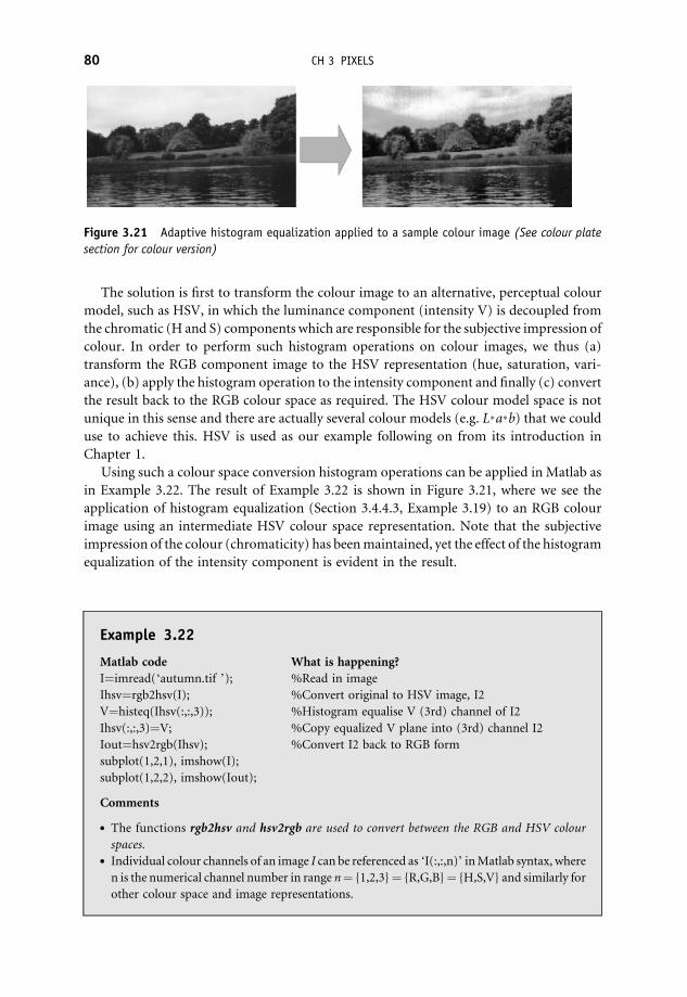
The solution is first to transform the colour image to an alternative, perceptual colour

model, such as HSV, in which the luminance component (intensity V) is decoupled from

the chromatic (H and S) components which are responsible for the subjective impression of

colour. In order to perform such histogram operations on colour images, we thus (a)

transform the RGB component image to the HSV representation (hue, saturation, vari-

ance), (b) apply the histogram operation to the intensity component and finally (c) convert

the result back to the RGB colour space as required. The HSV colour model space is not

unique in this sense and there are actually several colour models (e.g. L�a�b) that we coulduse to achieve this. HSV is used as our example following on from its introduction in

Chapter 1.

Using such a colour space conversion histogram operations can be applied in Matlab as

in Example 3.22. The result of Example 3.22 is shown in Figure 3.21, where we see the

application of histogram equalization (Section 3.4.4.3, Example 3.19) to an RGB colour

image using an intermediate HSV colour space representation. Note that the subjective

impression of the colour (chromaticity) has beenmaintained, yet the effect of the histogram

equalization of the intensity component is evident in the result.

Figure 3.21 Adaptive histogram equalization applied to a sample colour image (See colour plate

section for colour version)

Example 3.22


I¼imread(‘autumn.tif ’); %Read in image

Ihsv¼rgb2hsv(I); %Convert original to HSV image, I2

V¼histeq(Ihsv(:,:,3)); %Histogram equalise V (3rd) channel of I2

Ihsv(:,:,3)¼V; %Copy equalized V plane into (3rd) channel I2

Iout¼hsv2rgb(Ihsv); %Convert I2 back to RGB form

subplot(1,2,1), imshow(I);

subplot(1,2,2), imshow(Iout);

Comments

. The functions rgb2hsv and hsv2rgb are used to convert between the RGB and HSV colour

spaces.. Individual colour channels of an image I can be referenced as ‘I(:,:,n)’ inMatlab syntax, where

n is the numerical channel number in range n¼ {1,2,3}¼ {R,G,B}¼ {H,S,V} and similarly for

other colour space and image representations.

80 CH 3 PIXELS

Exercises


examples introduced in this chapter. Additional information on all of the Matlab functions

represented in this chapter and throughout these exercises is available in Matlab from the

function help browser (use doc <function name> at the Matlab command prompt, where

<function name> is the function required)

Matlab functions: imresize, size, whos, imadd, imsubtract, immultiply, imagesc,

imcomplement, imabsdiff, implay, uint8, horzcat, tic, toc, rgb2ycbcr.

Exercise 3.1 Using the examples presented on arithmetic operations (Examples 3.1–3.4)

we can investigate the use of these operators in a variety of ways. First, load the Matlab

example images ‘rice.png’ and ‘cameraman.tif’. Investigate the combined use of theMatlab

imresize() and size() functions to resize one of the images to be the same size as the other.

The Matlab command whos used in the syntax ‘whos v’ will display information about the

size and type of a given image or other variable v.

Try adding both of these images together using the standard Matlab addition operator

‘þ ’ and displaying the result.What happens?Now add them together by using the imadd()

function but adding a third parameter to the function of ‘uint16’ or ‘double’ with quotes

that forces an output in a 16-bit or floating-point double-precision data type. You will need

to display the output using the imagesc() function. How do these two addition operator

results differ and why do they differ?

Repeat this exercise using the standard Matlab subtraction operator ‘�’ and also by

using the imsubtract() function.

Exercise 3.2 Building upon the logical inversion example presented in Example 3.6,

investigate the application of the imcomplement() function to different image types and

different applications. First load the example image ‘peppers.png’ and apply this operator.

What effect do you see and to what aspect of traditional photography does the resulting

image colouring relate?

Image inversion is also of particular use in medical imaging for highlighting different

aspects of a given image. Apply the operator to the example images ‘mir.tif’, ‘spine.tif’ and

cell image ‘AT3 1m4 09.tif’. What resulting effects do you see in the transformed images

which may be beneficial to a human viewer?

Exercise 3.3 Use the sequence of cell images (‘AT3 1m4 01.tif’, ‘AT3 1m4 02.tif, . . .

‘AT3 1m4 09.tif’, ‘AT3 1m4 10.tif’) provided in combination with the Matlab

imabsdiff() function and a Matlab for loop construct to display an animation of the

differences between images in the sequence.

Youmaywish to use an additional enhancement approach to improve the dynamic range

of difference images that result from the imabsdiff() function. What is result of this

differencing operation? How could this be useful?

Hint. You may wish to set up an array containing each of the image file names 01 to 10.

The animation effect can be achieved by updating the same figure for each set of differences

(e.g. between the kth and (k� 1)th images in the sequence) or by investigating the Matlab

implay() function to play back an array of images.

EXERCISES 81

Exercise 3.4 Using a combination of the Matlab immultiply() and imadd() functions

implement aMatlab function (or sequence of commands) for blending two images A and B

into a single image with corresponding blending weights wA andwB such that output image

C is

C ¼ wAAþwBB ð3:29Þ

Experiment with different example images and also with blending information from a

sequence of images (e.g. cell images from Exercise 3.3). How could such a technique be used

in a real application?

Exercise 3.5 Using the thresholding technique demonstrated in Example 3.7 and with

reference to the histogram display functions of Example 3.12, manually select and apply a

threshold to the example image ‘pillsetc.png’. Compare your result with the adaptive

threshold approaches shown in Examples 3.15 and 3.16. Which is better? (Also, which is

easier?)

Repeat this procedure to isolate the foreground items in example images ‘tape.png’,

‘coins.png’ and ‘eight.tif’. Note that images require to be transformed to grey scale (see

Section 1.4.1.1) prior to thresholding.

Exercise 3.6 Looking back to Examples 3.15 and 3.16, investigate the effects of varying the

constant offset parameter C when applying it to example images ‘cameraman.tif’ and

‘coins.png’. How do the results for these two images differ?

Implement the third method of adaptive thresholding from Section 3.4.2 using the

threshold t ¼ floorððmax�minÞ=2ÞþC method. Compare this approach against the

examples already provided for thresholding the previous two images and other available

example images.

Exercise 3.7 Read in the example images ‘cameraman.tif’ and ‘circles.png’ and convert

the variable resulting from the latter into the unsigned 8-bit type of the former using the

Matlab casting function uint8(). Concatenate these two images into a single image (using

the Matlab function horzcat()) and display it. Why can you not see the circles in the

resulting image? (Try also using the Matlab imagesc function).

Using the logarithmic transform (Example 3.8), adjust the dynamic range of this

concatenated image so that both the outline of the cameraman’s jacket and the outline

of the circles are just visible (parameterC > 10will be required). By contrast, investigate the

use of both histogram equalization and adaptive histogram equalization on this concatenat-

ed image. Which approach gives the best results for overall image clarity and why is this

approach better for this task?

Exercise 3.8 Consider the Matlab example image ‘mandi.tif’, where we can see varying

lighting across both the background and foreground.Where is information not clearly visible

within this image? What are the properties of these regions in terms of pixel values?

Consider the corresponding properties of the logarithmic and exponential transforms

(Sections 3.3.1 and 3.3.2) and associated Examples 3.8 and 3.9. Experiment with both of

82 CH 3 PIXELS

these transforms and determine a suitable choice (with parameters) for enhancing this

image. Note that this is large image example and processingmay take a few seconds (use the

Matlab functions tic and toc to time the operation).

Contrast the results obtained using these two transforms to applying histogram equali-

zation contrast stretch (Section 3.4.4) or adaptive histogram equalization (Section 3.4.6)

to this image.

Exercise 3.9 Based on the grey-scale gamma correction presented in Example 3.11, apply

gamma correction to a colour image using the example ‘autumn.tif’. Why can we (and why

would we) apply this technique directly to the RGB image representation and not an

alternative HSV representation as per the colour image histogram processing of

Example 3.22?

Exercise 3.10 Based on Example 3.22, where we apply histogram equalization to a colour

image, apply contrast stretching (Section 3.4.3, Example 3.17) to the colour example image

‘westconcordaerial.png’ using the same approach. Experiment with different parameter

values to find an optimum for the visualization of this image. Compare the application of

this approachwith histogram equalization and adaptive histogram equalization on the same

image. Which produces the best result? Which approach is more ‘tunable’ and which is

more automatic in nature?

Repeat this for the Matlab image example ‘peppers.png’. Do the results differ signifi-

cantly for this example?

Exercise 3.11 Using the various contrast enhancement and dynamic range manipulation

approaches presented throughout this chapter, investigate and make a selection of trans-

forms to improve the contrast in the example image ‘AT3 1m4 01.tif’. Once you have

achieved a suitable contrast for this example image, extract the corresponding histogram

distribution of the image (Example 3.13) and apply it to the other images in the sequence

(‘AT3 1m4 02.tif’, . . . ‘AT3 1m4 09.tif’, ‘AT3 1m4 10.tif’) using histogram matching

(Example 3.20). Are the contrast settings determined for the initial example image suitable

for all of the others? What if the images where not all captured under the same conditions?

Here, we see the use of histogram matching as a method for automatically setting the

dynamic range adjustment on a series of images based on the initial determination of

suitable settings for one example. Where else could this be applied?

Exercise 3.12 In contrast to the approach shown for colour histogram equalization shown

in Example 3.22, perform histogram equalization on each of the (R,G,B) channels of an

example colour image. Compare the results with that obtained using the approach of

Example 3.22. What is the difference in the resulting images?

Repeat this for the operations of contrast stretching and adaptive histogram equaliza-

tion. Investigate also using the YCbCr colour space (Matlab function rgb2ybcr()) for

performing colour histogram operations on images. Which channel do you need to use?

What else do you need to consider?


EXERCISES 83

4Enhancement

The techniques we introduced at the end of Chapter 3 considered the manipulation of the

dynamic range of a given digital image to improve visualization of its contents. In this

chapter we consider more general image enhancement. We introduce the concept of image

filtering based on localized image subregions (pixel neighbourhoods), outline a range of

noise removal filters and explain how filtering can achieve edge detection and edge

sharpening effects for image enhancement.

4.1 Why perform enhancement?

The basic goal of image enhancement is to process the image so that we can view and assess

the visual information it contains with greater clarity. Image enhancement, therefore, is

rather subjective because it depends strongly on the specific information the user is hoping

to extract from the image.

The primary condition for image enhancement is that the information that you want to

extract, emphasize or restore must exist in the image. Fundamentally, ‘you cannot make

something out of nothing’ and the desired information must not be totally swamped by

noise within the image. Perhaps themost accurate and general statementwe canmake about

the goal of image enhancement is simply that the processed image should be more suitable

than the original one for the required task or purpose. This makes the evaluation of image

enhancement, by its nature, rather subjective and, hence, it is difficult to quantify its

performance apart from its specific domain of application.

4.1.1 Enhancement via image filtering

The main goal of image enhancement is to process an image in some way so as to render it

more visually acceptable or pleasing. The removal of noise, the sharpening of image edges

and the ‘soft focus’ (blurring) effect so often favoured in romantic photographs are all

examples of popular enhancement techniques. These and other enhancement operations

can be achieved through the process of spatial domain filtering. The term spatial domain is

arguably somewhat spurious, but is used to distinguish this procedure from frequency

domain procedures (discussed inChapter 5). Thus, spatial domainfiltering simply indicates

that the filtering process takes place directly on the actual pixels of the image itself.




Therefore, we shall refer simply to filtering in this chapter without danger of confusion.

Filters act on an image to change the values of the pixels in some specified way and are

generally classified into two types: linear and nonlinear. Linear filters aremore common, but

we will discuss and give examples of both kinds.

Irrespective of the particular filter that is used, all approaches to spatial domain filtering

operate in the same simple way. Each of the pixels in an image – the pixel under

consideration at a given moment is termed the target pixel – is successively addressed.

The value of the target pixel is then replaced by a new value which depends only on the value

of the pixels in a specified neighbourhood around the target pixel.

4.2 Pixel neighbourhoods

An important measure in images is the concept of connectivity. Many operations in image

processing use the concept of a local image neighbourhood to define a local area of

influence, relevance or interest. Central to this theme of defining the local neighbourhood

is the notion of pixel connectivity, i.e. deciding which pixels are connected to each other.

When we speak of 4-connectivity, only pixels which are N, W, E, S of the given pixel are

connected. However, if, in addition, the pixels on the diagonals must also be considered,

then we have 8-connectivity (i.e. N, NW, W, NE, SE, E, SW, S are all connected

see Figure 4.1).

In Figure 4.1 (right) we use this concept to determine whether region A and region B are

connected and use a local connectivity model (hereN�N¼ 3� 3) to determine if these are

separate or the same image feature. Operations performed locally in images, such as filtering

and edge detection, all consider a given pixel location ði; jÞ in terms of its local pixel

neighbourhood indexed as an offset ði� k; j� kÞ. The size and, hence, the scale of the

neighbourhood can be controlled by varying the neighbourhood size parameter N from

which an offset k (generally N=2b c) is computed. In general, neighbourhoodsmay beN�M

where N„M for unequal influence of pixels in the horizontal and vertical directions. More

frequently N¼M is commonplace and, hence, N�N neighbourhoods arise. The majority

Figure 4.1 Image neighbourhood connectivity (left) and an example 3� 3 neighbourhood centred

at a specific image pixel location

86 CH 4 ENHANCEMENT

of image processing techniques now use 8-connectivity by default, which for a reasonable

size of neighbourhood is often achievable in real time onmodern processors for themajority

of operations. Filtering operations over a whole image are generally performed as a series of

local neighbourhood operations using a sliding-window-based principle, i.e. each and every

pixel in the image is processed based on an operation performed on its local N�N pixel

neighbourhood (region of influence).

In Matlab� such an operation can be performed as in Example 4.1.

Example 4.1




func¼@(x) max(x(:)); %Set filter to apply

B¼nlfilter(A,[3 3],func); %Apply over 3 � 3 neighbourhood


Comments

Here we specify func() as the max() filter function to apply over each and every 3� 3

neighbourhood of the image. This replaces every input pixel in the output image with the

maximumpixel valueof the inputpixelneighbourhood.Youmaywish toexperimentwith the

effects of varying the neighbourhood dimensions and investigating the Matlab min() and

mean() (for the latter, a type conversion will be required to display the double output type of

theMatlabmean() function as an 8 bit image specify the filter function as uint8(mean())).

4.3 Filter kernels and the mechanics of linear filtering

In linear spatial filters the new or filtered value of the target pixel is determined as some

linear combination of the pixel values in its neighbourhood. Any other type of filter is, by

definition, a nonlinear filter. The specific linear combination of the neighbouring pixels that

is taken is determined by the filter kernel (often called a mask). This is just an array/sub-

image of exactly the same size as the neighbourhood1 containing the weights that are to be

assigned to each of the corresponding pixels in the neighbourhood of the target pixel.

Filtering proceeds by successively positioning the kernel so that the location of its centre

pixel coincides with the location of each target pixel, each time the filtered value being

calculated by the chosen weighted combination of the neighbourhood pixels. This filtering

procedure can thus be visualized as sliding the kernel over all locations of interest in the

original image ði; jÞ, multiplying the pixels underneath the kernel by the corresponding

weights w, calculating the new values by summing the total and copying them to the same

locations in a new (filtered) image f (e.g. Figure 4.2).

The mechanics of linear spatial filtering actually express in discrete form a process called

convolution, an important physical and mathematical phenomenon which we will develop

1A point of detail for the purist. With linear filters it is really the kernel that comes first and thus defines the

neighbourhood. For some nonlinear filters (e.g. order filters) the order is reversed because we must define the

region over which we wish to do the ranking and cannot write down a kernel.

4.3 FILTER KERNELS AND THE MECHANICS OF LINEAR FILTERING 87

further in Chapter 5. For this reason, many filter kernels are sometimes described as

convolution kernels, it then being implicitly understood that they are applied to the image in

the linear fashion described above. Formally, we can express the action of convolution

between a kernel and an image in two equivalent ways. The first addresses the row and

column indices of the image and the kernel:

f ðx; yÞ ¼XImax

i¼Imin

XJmax

j¼Jmin

wði; jÞIðxþ i; yþ jÞ ð4:1Þ

Here, the indices i¼ 0, j¼ 0 correspond to the centre pixel of the kernel which is of size

ðImax�Imin þ 1; Jmax�Jmin þ 1Þ. A second, equivalent approach is to use linear indices:

fi ¼XNk¼1

wkIkðiÞ ð4:2Þ

In this case, IkðiÞ represents the neighbourhood pixels of the ith image pixel, where k is

a linear index running over the neighbourhood region according to a row-wise (as in

Figure 4.2) or column-wise convention. Here,wk are the corresponding kernel values and firepresents the filtered value resulting from original input value IkðiÞ. The former notation is

more explicit, whereas the latter is neater and more compact; but neither is generally

recommended over the other. Figure 4.2 illustrates this basic procedure, where the centre

pixel of the kernel and the target pixel in the image are indicated by the dark grey shading.

The kernel is ‘placed’ on the image so that the centre and target pixels match. The filtered

value of the target pixel fi is then given by a linear combination of the neighbourhood pixel

values, the specific weights being determined by the kernel valueswk. In this specific case the

target pixel value of original value 35 is filtered to an output value of 14.

The steps in linear (convolution) filtering can be summarized as follows:

(1) Define the filter kernel.

(2) Slide the kernel over the image so that its centre pixel coincides with each (target) pixel

in the image.

Figure 4.2 The mechanics of image filtering with an N� N¼ 3� 3 kernel filter

88 CH 4 ENHANCEMENT

(3) Multiply the pixels lying beneath the kernel by the corresponding values (weights) in

the kernel above them and sum the total.

(4) Copy the resulting value to the same locations in a new (filtered) image.

In certain applications, we may apply such a linear filter to a selected region rather than the

entire image; we then speak of region-based filtering. We may also take a slightly more

sophisticated approach in which the filter itself can change depending on the distribution of

pixel values in the neighbourhood, a process termed adaptive filtering (e.g. see adaptive

thresholding, discussed in Section 3.4.2).

Filtering at the boundaries of images also poses challenges. It is reasonable to ask what we

should do when a target pixel lies close to the image boundary such that the convolution

kernel overlaps the edge of the image. In general, there are threemain approaches for dealing

with this situation:

(1) Simply leave unchanged those target pixels which are located within this boundary

region.

(2) Perform filtering on only those pixels which lie within the boundary (and adjust the

filter operation accordingly).

(3) ‘Fill in’ in the missing pixels within the filter operation by mirroring values over the

boundary.

Resulting undesirable edge artefacts are generally difficult to overcome and, in general, (2)

or (3) is the preferred method. In certain instances, it is acceptable to ‘crop’ the image –

meaning that we extract only a reduced-size image in which any edge pixels which have not

been adequately filtered are removed entirely.

In Matlab, linear convolution filtering can be performed as in Example 4.2.

Example 4.2


A¼imread(‘peppers.png’); %Read in image


k¼fspecial(‘motion’, 50, 54); %Create a motion blur convolution kernel

B¼imfilter(A, k, ‘symmetric’); %Apply using symmetric mirroring at edges


Comments

Here we specify the fspecial() function to construct a kernel that will mimic the effect of

motion blur (of specified length and angle) onto the image. Option 3) from our earlier

discussion is used to deal with image edges during filtering. Youmay wish to investigate the

use of other kernel filters that can be generated with the fspecial() function and the edge

region filtering options available with the imfilter() function. Type doc imfilter at theMatlab

prompt for details). How do they effect the image filtering result?

4.3 FILTER KERNELS AND THE MECHANICS OF LINEAR FILTERING 89

4.3.1 Nonlinear spatial filtering

Nonlinear spatial filters can easily be devised that operate through exactly the same basic

mechanism as we described above for the linear case. The kernel mask slides over the image

in the same way as the linear case, the only difference being that the filtered value will be the

result of some nonlinear operation on the neighbourhood pixels. For example, employing

the same notation as before, we could define a quadratic filter:

fi ¼XNk¼1

wk1I2k ðiÞþwk2IkðiÞþwk3 ð4:3Þ

In this case, the action of the filter will be defined by the three weights which specify the

contribution of the second, first- and zeroth-order terms. Nonlinear filters of this kind

are not common in image processing. Much more important are order (or statistical)

filters (discussed shortly), which operate by ranking the pixels in the specified neigh-

bourhood and replacing the target pixel by the value corresponding to a chosen rank. In

this case, we cannot write down a kernel and an equation of the form of our linear

convolution is not applicable. In the following sections, we will present and discuss some

of the more important examples of both linear and nonlinear spatial filters.

4.4 Filtering for noise removal

One of the primary uses of both linear and nonlinear filtering in image enhancement is for

noise removal. We will now investigate the application of a number of different filters for

removing typical noise, such as additive ‘salt and pepper’ and Gaussian noise (first

introduced in Section 2.3.3). However, we first need to consider generation of some

example images with noise added so that we can compare the effectiveness of different

approaches to noise removal.

In Matlab, this can be achieved as in Example 4.3. The results of the noise addition from

Example 4.3 are shown in Figure 4.3. These images will form the basis for our comparison of

noise removal filters in the following sections of this chapter.

Figure 4.3 (a) Original image with (b) ‘salt and pepper’ noise and (c) Gaussian noise added

90 CH 4 ENHANCEMENT

Example 4.3


I¼imread(‘eight.tif ’); %Read in image


Isp¼imnoise(I,‘salt & pepper’,0.03); %Add 3% (0.03) salt and pepper noise

subplot(1,3,2), imshow(Isp); %Display result image Isp

Ig¼imnoise(I,‘gaussian’,0.02); %Add Gaussian noise (with 0.02 variance)

subplot(1,3,3), imshow(Ig); %Display result image Ig

Comments

Here we use the imnoise() function to add both ‘salt and pepper’ noise andGaussian noise to

the input image. The strength is specified using the percentage density and variance (with

zeromean) respectively. The readermaywish to experimentwith the effects of changing these

noise parameters and also explore the other noise effects available using this function (type

doc imnoise at the Matlab prompt for details).

4.4.1 Mean filtering

Themean filter is perhaps the simplest linear filter and operates by giving equal weightwK to

all pixels in the neighbourhood. A weight of WK¼ 1/(NM) is used for an N�M

neighbourhood and has the effect of smoothing the image, replacing every pixel in the

output image with the mean value from its N�M neighbourhood. This weighting scheme

guarantees that the weights in the kernel sum to one over any given neighbourhood size.

Mean filters can be used as a method to suppress noise in an image (although the median

filter which we will discuss shortly usually does a better job). Another common use is as

a preliminary processing step to smooth the image in order that some subsequent

processing operation will be more effective.

In Matlab, the mean filter can be applied as in Example 4.4 with the results as shown

in Figure 4.4.

Figure 4.4 Mean filter (3� 3) applied to the (a) original, (b) ‘salt and pepper’ noise and (c) Gaussian

noise images of Figure 4.3

4.4 FILTERING FOR NOISE REMOVAL 91

Example 4.4


k¼ones(3,3)/9; %Define mean filter

I m¼imfilter(I,k); %Apply to original image

Isp m¼imfilter(Isp,k); %Apply to salt and pepper image

Ig m¼imfilter(Ig,k); %Apply to Gaussian image

subplot(1,3,1), imshow(I m); %Display result image

subplot(1,3,2), imshow(Isp m); %Display result image

subplot(1,3,3), imshow(Ig m); %Display result image

Comments

Here we define a 3� 3 mean filter and apply it to the three images generated in Example 4.3

and shown in Figure 4.3. Experiment with using larger neighbourhood sizes for this filter.

What effect does it have on the resulting image?

We can see that the mean filtering is reasonably effective at removing the Gaussian

noise (Figure 4.4c), but at the expense of a loss of high-frequency image detail (i.e. edges).

Although a significant portion of the Gaussian noise has been removed (compared with

Figure 4.3c), it is still visible within the image. Larger kernel sizes will further suppress the

Gaussian noise but will result in further degradation of image quality. It is also apparent

that mean filtering is not effective for the removal of ‘salt and pepper’ noise (Figure 4.4b).

In this case, the large deviation of the noise values from typical values in the neighbour-

hood means that they perturb the average value significantly and noise is still very

apparent in the filtered result. In the case of ‘salt and pepper’ noise, the noisy high/low

pixel values thus act as outliers in the distribution. For this reason, ‘salt and pepper’ noise

is best dealt with using a measure that is robust to statistical outliers (e.g. a median filter,

Section 4.4.2).

In summary, the main drawbacks of mean filtering are (a) it is not robust to large noise

deviations in the image (outliers) and (b)when themeanfilter straddles an edge in the image

it will cause blurring. For this latter reason, the mean filter can also be used as a general

low-pass filter. A common variation on the filter, which can be partially effective in

preserving edge details, is to introduce a threshold and only replace the current pixel value

with the mean of its neighbourhood if the magnitude of the change in pixel value lies below

this threshold.

4.4.2 Median filtering

Another commonly used filter is the median filter. Median filtering overcomes the main

limitations of the mean filter, albeit at the expense of greater computational cost. As each

pixel is addressed, it is replaced by the statistical median of itsN�M neighbourhood rather

than themean. Themedian filter is superior to themean filter in that it is better at preserving

92 CH 4 ENHANCEMENT

sharp high-frequency detail (i.e. edges) whilst also eliminating noise, especially isolated

noise spikes (such as ‘salt and pepper’ noise).

The medianm of a set of numbers is that number for which half of the numbers are less

than m and half are greater; it is the midpoint of the sorted distribution of values. As the

median is a pixel value drawn from the pixel neighbourhood itself, it is more robust to

outliers and does not create a new unrealistic pixel value. This helps in preventing edge

blurring and loss of image detail.

By definition, the median operator requires an ordering of the values in the pixel

neighbourhood at every pixel location. This increases the computational requirement of the

median operator.

Median filtering can be carried out in Matlab as in Example 4.5. The results of

Example 4.5 are shown in Figure 4.5, where we can now see the effectiveness of median

filtering on the two types of noise (‘salt and pepper’ andGaussian) introduced to the images

in Example 4.3/Figure 4.3.

Example 4.5


I m¼medfilt2(I,[3 3]); %Apply to original image

Isp m¼medfilt2(Isp,[3 3]); %Apply to salt and pepper image

Ig m¼medfilt2(Ig,[3 3]); %Apply to Gaussian image

subplot(1,3,1), imshow(I m); %Display result image



Comments

Here we define a 3� 3 median filtermedfilt2() and apply it to the three images generated in

Example 4.3 and shown in Figure 4.3. Experiment with using larger neighbourhood sizes for

this filter and the effect it has on the resulting image.

Figure 4.5 Median filter (3� 3) applied to the (a) original, (b) ‘salt and pepper’ noise and

(c) Gaussian noise images of Figure 4.3


In this result (Figure 4.5c), we again see the removal of some Gaussian noise at the

expense of a slight degradation in image quality. By contrast, themedian filter is very good at

removing ‘salt and pepper’-type noise (Figure 4.5b), where we see the removal of this high/

low impulse-type noise withminimal degradation or loss of detail in the image. This is a key

advantage of median filtering.

4.4.3 Rank filtering

The median filter is really just a special case of a generalized order (or rank) filter. The

general order filter is a nonlinear filter comprising the following common steps:

(1) Define the neighbourhood of the target pixel (N�N).

(2) Rank them in ascending order (first is lowest value, (N�N)th is highest value).

(3) Choose the order of the filter (from 1 to N).

(4) Set the filtered value to be equal to the value of the chosen rank pixel.

Order filters which select the maximum and minimum values in the defined neigh-

bourhood are (unsurprisingly) called maximum and minimum filters. We can use the

Matlab order-filter function as shown in Example 4.6. The results of Example 4.6 are

shown in Figure 4.6, where we can now see the result of maximum filtering on the two

types of noise (‘salt and pepper’ and Gaussian) introduced to the images in Figure 4.3.

Notably, the Gaussian noise has been largely removed (Figure 4.6c), but at the expense

of image detail quality (notably the lightening of the image background). The nature of

the ‘salt and pepper’-type noise causes its high values to be amplified by the use of

a maximum filter.

Example 4.6


I m¼ordfilt2(I,25,ones(5,5)); %Apply to original image

Isp m¼ordfilt2(Isp,25,ones(5,5)); %Apply to salt and pepper image

Ig m¼ordfilt2(Ig,25,ones(5,5)); %Apply to Gaussian image

subplot(1,3,1), imshow(I m); % %Display result image



Comments

Here we define a 5� 5 max filter and apply it to the three images generated in Example 4.3

and shown in Figure 4.3. Experiment with using larger neighbourhood sizes for this filter,

varying the rank of the filter (second parameter of ordfilt2() function) and the effect it has on

the resulting image.

94 CH 4 ENHANCEMENT

A variation on simple order filtering is conservative smoothing, in which a given

pixel is compared with the maximum and minimum values (excluding itself) in the

surrounding N�N neighbourhood and is replaced only if it lies outside of that range. If

the current pixel value is greater than the maximum of its neighbours, then it is replaced

by the maximum. Similarly, if it is less than the minimum, then it is replaced by the

minimum.

4.4.4 Gaussian filtering

The Gaussian filter is a very important one both for theoretical and practical reasons. Here,

we filter the image using a discrete kernel derived from a radially symmetric form of the

continuous 2-D Gaussian function defined as follows:

f ðx; yÞ ¼ 1

2ps2exp � x2 þ y2

2s2

� �ð4:4Þ

Discrete approximations to this continuous function are specified using two free

parameters:

(1) the desired size of the kernel (as an N�N filter mask);

(2) the value of s, the standard deviation of the Gaussian function.

As is always the case with linear convolution filters (Section 4.3), there is a trade-off between

the accurate sampling of the function and the computational time required to implement it.

Some examples of discreteGaussian filters, with varying kernel and standard deviation sizes,

are shown in Figure 4.7.

Applying the Gaussian filter has the effect of smoothing the image, but it is used in a way

that is somewhat different to themean filter (Section 4.4.1). First, the degree of smoothing is

controlled by the choice of the standard deviation parameter s, not by the absolute value of

the kernel size (which is the case with the mean filter). Second, the Gaussian function has

a rather special property, namely that its Fourier transform is also a Gaussian function,

which makes it very convenient for the frequency-domain analysis of filters (Chapter 5).

Figure 4.6 Order filtering (max, order¼ 25, 5� 5) applied to the (a) original, (b) ‘salt and pepper’

noise and (c) Gaussian noise images of Figure 4.3


A Gaussian function with a large value of s is an example of a so-called low-pass filter in

which the high spatial frequency content (i.e. sharp edge features) of an image is suppressed.

To understand this properly requires a background in the Fourier transform and frequency-

domain analysis, subjects that are developed in Chapter 5.

We can apply the Gaussian filter inMatlab as in Example 4.7. The results of Example 4.7

are shown in Figure 4.8. In all cases, the smoothing effect of the filter degrades high-

frequency (edge) detail as expected (e.g. Figure 4.8a), but it also removes to some degree the

noise present in both Figure 4.8b and c.

Example 4.7


k¼fspecial(‘gaussian’, [5 5], 2); %Define Gaussian filter

I g¼imfilter(I,k); %Apply to original image

Isp g¼imfilter(Isp,k); %Apply to salt and pepper image

Ig g¼imfilter(Ig,k); %Apply to Gaussian image

subplot(1,3,1), imshow(I g); %Display result image

subplot(1,3,2), imshow(Isp g); %Display result image

subplot(1,3,3), imshow(Ig g); %Display result image

Comments

Here we define a 5� 5Gaussian filter kernel withs¼ 2 using theMatlab fspecial() function

and apply it to the three images generated in Example 4.3 and shown in Figure 4.3. The

reader can experiment by trying different kernel sizes and different s values to understand

the effect it has on the resulting image.

Gaussian smoothing (or filtering) commonly forms the first stage of an edge-detection

algorithm (e.g. the Canny edge detector, discussed in Chapter 10), where it is used as a

means of noise suppression.

Figure 4.7 Gaussian filter kernels 3� 3s¼ 1, 11� 11 s¼ 2 and 21� 21 s¼ 4 (The numerical

values shown are unnormalised)

96 CH 4 ENHANCEMENT

4.5 Filtering for edge detection

In addition to noise removal, the other two main uses of image filtering are for (a) feature

extraction and (b) feature enhancement. We will next look at the use of image filtering in

both of these areas through the detection of edges within images. An edge can be considered

as a discontinuity or gradient within the image. As a result, the consideration of derivative

filters is central to edge detection in image processing.

4.5.1 Derivative filters for discontinuities

The mean or averaging filter sums the pixels over the specified neighbourhood and, as we

have seen, this has the effect of smoothing or blurring the image. In effect, this is just

integration in discrete form. By contrast, derivative filters can be used for the detection of

discontinuities in an image and they play a central role in sharpening an image (i.e.

enhancing fine detail). As their name implies, derivative filters are designed to respond (i.e.

return significant values) at points of discontinuity in the image and to give no response in

perfectly smooth regions of the image, i.e. they detect edges.

One of the most important aspects of the human visual system is the way in which it

appears tomake use of the outlines or edges of objects for recognition and the perception of

distance and orientation. This feature has led to one theory for the human visual system

based on the idea that the visual cortex contains a complex of feature detectors that are

tuned to the edges and segments of various widths and orientations. Edge features,

therefore, can play an important role in the analysis of the image.

Edge detection is basically a method of segmenting an image into regions based on

discontinuity, i.e. it allows the user to observe those features of an image where there is a

more or less abrupt change in grey level or texture, indicating the end of one region in the

image and the beginning of another. Enhancing (or amplifying) the presence of these

discontinuities in the image allows us to improve the perceived image quality under certain

conditions. However, like other methods of image analysis, edge detection is sensitive to

noise.

Edge detection makes use of differential operators to detect changes in the gradients of

the grey or colour levels in the image. Edge detection is divided into two main categories:

Figure 4.8 Gaussian filtering (5� 5 with s¼ 2) applied to the (a) original, (b) ‘salt and pepper’

noise and (c) Gaussian noise images of Figure 4.3

4.5 FILTERING FOR EDGE DETECTION 97

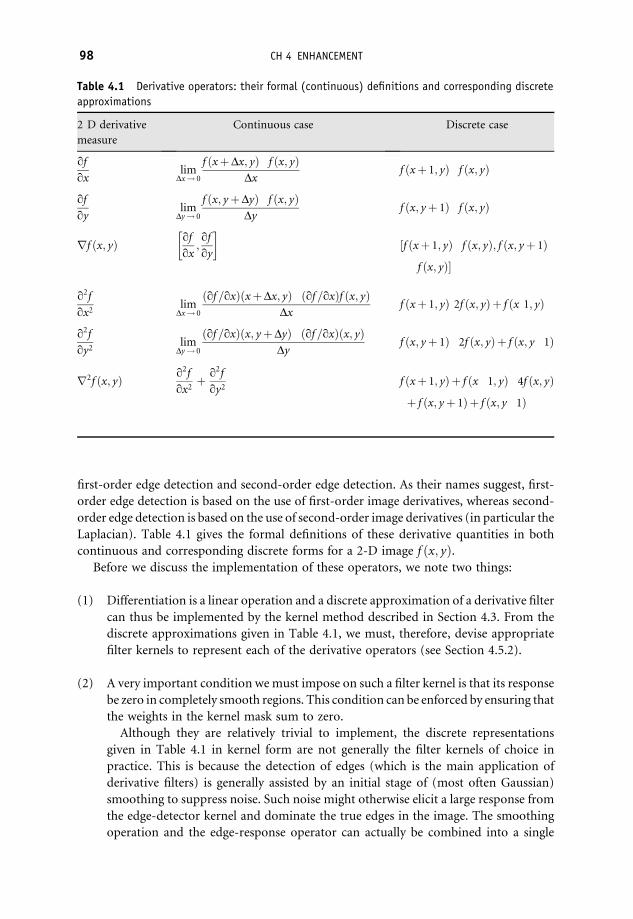
first-order edge detection and second-order edge detection. As their names suggest, first-

order edge detection is based on the use of first-order image derivatives, whereas second-

order edge detection is based on the use of second-order image derivatives (in particular the

Laplacian). Table 4.1 gives the formal definitions of these derivative quantities in both

continuous and corresponding discrete forms for a 2-D image f ðx; yÞ.Before we discuss the implementation of these operators, we note two things:

(1) Differentiation is a linear operation and a discrete approximation of a derivative filter

can thus be implemented by the kernel method described in Section 4.3. From the

discrete approximations given in Table 4.1, we must, therefore, devise appropriate

filter kernels to represent each of the derivative operators (see Section 4.5.2).

(2) A very important condition wemust impose on such a filter kernel is that its response

be zero in completely smooth regions. This condition can be enforced by ensuring that

the weights in the kernel mask sum to zero.

Although they are relatively trivial to implement, the discrete representations

given in Table 4.1 in kernel form are not generally the filter kernels of choice in

practice. This is because the detection of edges (which is the main application of

derivative filters) is generally assisted by an initial stage of (most often Gaussian)

smoothing to suppress noise. Such noise might otherwise elicit a large response from

the edge-detector kernel and dominate the true edges in the image. The smoothing

operation and the edge-response operator can actually be combined into a single

Table 4.1 Derivative operators: their formal (continuous) definitions and corresponding discrete

approximations

2 D derivative

measure

Continuous case Discrete case

qfqx

limDx! 0

f ðxþDx; yÞ f ðx; yÞDx

f ðxþ 1; yÞ f ðx; yÞ

qfqy

limDy! 0

f ðx; yþDyÞ f ðx; yÞDy

f ðx; yþ 1Þ f ðx; yÞ

rf ðx; yÞ qfqx

;qfqy

� �½f ðxþ 1; yÞ f ðx; yÞ; f ðx; yþ 1Þ

f ðx; yÞ�

q2fqx2

limDx! 0

ðqf =qxÞðxþDx; yÞ ðqf =qxÞf ðx; yÞDx

f ðxþ 1; yÞ 2f ðx; yÞþ f ðx 1; yÞ

q2fqy2

limDy! 0

ðqf =qxÞðx; yþDyÞ ðqf =qxÞðx; yÞDy

f ðx; yþ 1Þ 2f ðx; yÞþ f ðx; y 1Þ

r2f ðx; yÞ q2fqx2

þ q2fqy2

f ðxþ 1; yÞþ f ðx 1; yÞ 4f ðx; yÞþ f ðx; yþ 1Þþ f ðx; y 1Þ

98 CH 4 ENHANCEMENT

kernel, an example of which we will see in Section 4.6). More generally, noise

suppression is a key part of more advanced edge-detection approaches, such as the

Canny method (see Chapter 10).

Although a conceptually simple task, effective and robust edge detection is crucial in so

many applications that it continues to be a subject of considerable research activity.Here, we

will examine some basic edge-detection filters derived directly from the discrete derivatives.

4.5.2 First-order edge detection

A number of filter kernels have been proposed which approximate the first derivative of the

image gradient. Three of the most common (their names being taken from their original

authors/designers in the early image-processing literature) are shown in Figure 4.9, where

we see the Roberts, Prewitt and Sobel edge-detector filter kernels. All three are implemented

as a combination of two kernels: one for the x-derivative and one for the y-derivative

(Figure 4.9).

The simple 2� 2 Roberts operators (commonly known as the Roberts cross) were one of

the earliest methods employed to detect edges. The Roberts cross calculates a simple,

efficient, 2-D spatial gradient measurement on an image highlighting regions correspond-

ing to edges. The Roberts operator is implemented using two convolution masks/kernels,

each designed to respond maximally to edges running at�45� to the pixel grid, (Figure 4.9(left)) which return the image x-derivative and y-derivative, Gx and Gy respectively. The

magnitude |G| and orientation u of the image gradient are thus given by:

jGj ¼ G2x þG2

y

q

u ¼ tan 1

�Gy

Gx

�þ 1

4p

ð4:5Þ

Figure 4.9 First-order edge-detection filters


This gives an orientation u¼ 0 for a vertical edgewhich is darker on the left side in the image.

For speed of computation, however, |G| is often approximated as just the sum of the

magnitudes of the x-derivative and y-derivative, Gx and Gy.

The Roberts cross operator is fast to compute (due to theminimal size of the kernels), but

it is very sensitive to noise. The Prewitt and Sobel edge detectors overcome many of its

limitations but use slightly more complex convolution masks (Figure 4.9 (centre and

right)).

The Prewitt/Sobel kernels are generally preferred to the Roberts approach because the

gradient is not shifted by half a pixel in both directions and extension to larger sizes (for

filter neighbourhoods greater than 3� 3) is not readily possible with the Roberts

operators. The key difference between the Sobel and Prewitt operators is that the Sobel

kernel implements differentiation in one direction and (approximate)Gaussian averaging

in the other (see Gaussian kernels, Figure 4.7). The advantage of this is that it smoothes the

edge region, reducing the likelihood that noisy or isolated pixels will dominate the filter

response.

Filtering using these kernels can be achieved inMatlab as shown in Example 4.8. The edge

filter output of Example 4.8 is shown in Figure 4.10, where we can see the different responses

of the three Roberts, Prewitt and Sobel filters to a given sample image. As expected, stronger

and highly similar edge responses are obtained from the more sophisticated Prewitt and

Sobel approaches (Figure 4.10 (bottom)). The Roberts operator is notably susceptible to

image noise, resulting in a noisy and less distinct edgemagnitude response (Figure 4.10 (top

right)).

Example 4.8


I¼imread(‘circuit.tif ’); %Read in image

IEr ¼ edge(I,‘roberts’); %Roberts edges

IEp ¼ edge(I,‘prewitt’); %Prewitt edges

IEs ¼ edge(I,‘sobel’); %Sobel edges


subplot(2,2,2), imshow(IEr); %Display image

subplot(2,2,3), imshow(IEp); %Display image

subplot(2,2,4), imshow(IEs); %Display image

Comments

Here we use the Matlab edge() function to apply the Roberts, Prewitt and Sobel edge

detectors. As an extension, this function also facilitates the use of an additional third,

threshold parameter in the form edge(Image, ‘filter name’, threshold). This exploits the

concept of thresholding to select a subset of edge filter responses based on themagnitude of

the filter response. The edge() function can also be used to return the individualGx andGy

components of a given filter mask and automatically select a magnitude threshold (in a

similar manner to Example 3.15; see doc edge in Matlab command prompt). Experiment

with these parameters and the effects that can be achieved on the example images. Youmay

alsowish to investigate the use of theMatlab tic()/toc() functions for timing different edge

filtering operations.

100 CH 4 ENHANCEMENT

4.5.2.1 Linearly separable filteringThe Sobel and Prewitt filters are examples of linearly separable filters. This means that the

filter kernel can be expressed as the matrix product of a column vector with a row vector.

Thus, the filter kernels shown in Figure 4.9 can be expressed as follows:

1 0 �11 0 �11 0 �1

24

35 ¼

111

24

35 1 0 �1½ � and

1 0 �12 0 �21 0 �1

24

35 ¼

121

24

35 1 0 �1 �½

ð4:6ÞAn important consequence of this is that the 2-D filtering process can actually be carried out

by two sequential 1-D filtering operations. Thus, the rows of the image are first filtered with

the 1-D row filter and the resulting filtered image is then filtered column-wise by the

1-D column filter. This effects a computational saving in terms of reducing the amount of

arithmetic operations required for a given convolution with a filter kernel. The saving is

modest in the 3� 3 case (a reduction to six multiplications/additions compared with nine

for the 2-D version), but is considerably greater if we are considering larger kernel sizes. In

general, linear separable filters result in a saving of order 2N operations as opposed to order

N2 for nonseparable, 2-D convolution.

Figure 4.10 Roberts, Prewitt and Sobel edge-magnitude responses


4.5.3 Second-order edge detection

In general, first-order edge filters are not commonly used as ameans of image enhancement.

Rather, their main use is in the process of edge detection as a step in image segmentation

procedures.Moreover, as we shall see in our discussion of the Cannymethod in Chapter 10,

although the application of a derivative operator is a vital step, there is actually considerably

more to robust edge detection than the simple application of a derivative kernel. A much

more commonmeans of image enhancement is through the use of a second-order derivative

operator:- the Laplacian.

4.5.3.1 Laplacian edge detectionA very popular second-order derivative operator is the Laplacian:

r2f ðx; yÞ ¼ q2fqx2

þ q2fqy2

ð4:7Þ

The discrete form is given from Table 4.1 as:

r2f ¼ f ðxþ 1; yÞþ f ðx�1; yÞ�4f ðx; yÞþ f ðx; yþ 1Þþ f ðx; y�1Þ ð4:8Þ

This can easily be implemented in a 3� 3 kernel filter, as shown in Figure 4.11A.

However, if we explore an image applying this operator locally, then we expect the

response to be greatest (as the Laplacian is a second-order derivative operator) at those

points in the image where the local gradient changes most rapidly. One of the potential

shortcomings of applying the mask in the form given by Figure 4.11A is the relative

insensitivity to features lying in approximately diagonal directions with respect to the

image axes. If we imagine rotating the axes by 45� and superimposing the rotated

Laplacian on the original, then we can construct a filter that is invariant under multiple

rotations of 45� (Figure 4.11B).

Figure 4.12 compares the response of the first-order Sobel and second-order Laplacian

derivative filters. Note how the first-order gradient operator tends to produce ‘thick edges’,

whereas the Laplacian filter tends to produce finer edges in response to the change in

gradient rather than the image gradient itself. The Laplacian operator can be applied in

Matlab as in Example 4.9.

The second-order derivative property that allows the Laplacian to produce a fine edge

response corresponding to a change in gradient, rather than the less isolated response of the

first-order edge filters, makes it suitable as the first stage of digital edge enhancement.

Figure 4.11 Construction of the Laplacian discrete kernel


However, as the Laplacian kernels approximate a second derivative over the image they are

in fact very sensitive to noise.

Example 4.9


I¼rgb2gray(imread(‘peppers.png’)); %Read in image (in grey scale)

k¼fspecial('laplacian'); %Create Laplacian filter

IEl¼imfilter(double(I),k,‘symmetric’); %Laplacian edges

subplot(1,2,1), imagesc(I); %Display image

subplot(1,2,2), imagesc(IEl); %Display image

colormap(‘gray’);

Comments

Herewe first construct the Laplacian filter (in a similarmanner toExample 4.2) and then apply

it to the image using the Matlab imfliter() function. Note the inline use of the rgb2gray()

function to load the (colour) example image as grey scale. In addition, we perform the

Laplacian operation on a floating point version of the input image (function double()) and, as

the Laplacian operator returns both positive and negative values, use function imagesc() and

colormap() to correctly scale and display the image as shown in Figure 4.12.

4.5.3.2 Laplacian of Gaussian

To counter this high noise sensitivity of the Laplacian filter, the standard Laplacian kernel

(Figure 4.11) is commonly combined with the Gaussian kernel (Figure 4.7) to produce

Figure 4.12 Comparison of first-order derivative (Sobel) and second-order (Laplacian) filters


a robust filtering method. These two kernels could be applied sequentially to the image as

two separate convolution operations – first smoothing with the Gaussian kernel and then

with the Laplacian.However, as convolution is associative (Section 4.3), we can combine the

kernels by convolving the Gaussian smoothing operator with the Laplacian operator to

produce a single kernel: the Laplacian of Gaussian (LoG) filter. This single kernel is then

applied to the image in a single pass. This offers a significant computational saving by

approximately halving the calculations required.

The response of the filter will be zero in areas of uniform image intensity, whilst it will be

nonzero in an area of transition. At a given edge, the operator will return a positive response

on the darker side and negative on the lighter side.

We can see this effect in Figure 4.12 and the results of Example 4.9. If we wish to apply the

LoG operator in Matlab, then we can do so by replacing the ‘laplacian’ parameter of the

fspecial() function with ‘log’. The result should be a smoothed version of the result in

Example 4.9. Additional input parameters to the fspecial() function allow the level of

smoothing to be controlled by varying the width of the Gaussian.

4.5.3.3 Zero-crossing detectorThe zero-crossing property of the Laplacian (and LoG) also permits anothermethod of edge

detection: the zero-crossing method. We use a zero-crossing detector to locate pixels at

which the value of the Laplacian passes through zero (i.e. points where the Laplacian

changes sign). This occurs at ‘edges’ in the image where the intensity of the image changes

rapidly (or in areas of intensity change due to noise). It is best to think of the zero-crossing

detector as a type of feature detector rather than as a specific edge detector. The output

from the zero-crossing detector is usually a binary image with single-pixel thickness lines

showing the positions of the zero-crossing points.

The starting point for the zero-crossing detector is an image which has been filtered

using the LoG filter (to overcome the effects of noise). The zero crossings that result are

strongly influenced by the size of the Gaussian used for the smoothing stage of this

operator. As the smoothing is increased, then fewer and fewer zero-crossing contours will

be found, and those that do remain will correspond to features of larger and larger scale in

the image.

We can use a zero-crossing detector with the LoG filter in Matlab as in Example 4.10.

Figure 4.13 shows edge transitions detected using the zero-crossings concept applied to the

LoG filter (from Example 4.10). The effect of noise on the second derivative despite the use

of Gaussian smoothing is evident.

Example 4.10


I¼rgb2gray(imread(‘peppers.png’)); %Read in image (in grey scale)

k¼fspecial(‘log’, [10 10], 3.0); %Create LoG filter

IEzc ¼ edge(I, ‘zerocross’, [], k); %Zero crossing edges (auto thresholded)


subplot(1,2,2), imshow(IEzc); %Display image


Comments

As is evident from Figure 4.13, the results are still quite noisy even with a broad 10� 10

Gaussian (s¼ 3.0) as specified in the above example. The readermay wish to experiment with

different Gaussian parameters (note that the filter k can itself be visualized as an image using

the imagesc() function).

A couple of points to note with this operator are:

. In the general case, all edges detected by the zero-crossing detector are in the form of

closed curves in the same way that contour lines on a map are always closed. In the

Matlab implementation, if a threshold of zero is specified then this is always the case

(NB: Example 4.10 uses an autoselected threshold (parameter specified as ‘[ ]’) onwhich

edges to keep). The only exception to this is where the curve goes off the edge of the

image. This can have advantages for later processing.

. As we have seen, the LoG filter is quite susceptible to noise if the standard deviation of

the smoothing Gaussian is small. One solution to this is to increase Gaussian smoothing

to preserve only strong edges. An alternative is to look at the gradient of the zero crossing

and only keep zero crossings where this is above a certain threshold (i.e. use the third

derivative of the original image). This will tend to retain only stronger edges but as the

third derivative is also highly sensitive to noise this greatly amplifies any high-frequency

noise in the image.

4.6 Edge enhancement

In the final part of this chapter we look at the use of second-order edge detection

(Section 4.5.3) as amethod for edge enhancement (commonly knownas image sharpening).

4.6.1 Laplacian edge sharpening

We have seen that the Laplacian responds only to the fine detail in the image (i.e. those

image regions where the change in gradient is significant) but has a zero response to

Figure 4.13 Edges detected as the zero crossings of the LOG operator

4.6 EDGE ENHANCEMENT 105

constant regions and regions of smooth gradient in the image. If, therefore, we take the

original image and add or subtract the Laplacian, then we may expect to enhance the fine

detail in the image artificially. It is common practice just to subtract it from the original,

truncating any values which exhibit integer overflow in the common 8-bit representation.

Using the Laplacian definition of Section 4.5.3.1, we can define this as follows:

Ioutputðx; yÞ ¼ Iinðx; yÞ�r2Iinðx; yÞ ð4:9Þ

Using Matlab, Laplacian image sharpening can be achieved as in Example 4.11. The

output from Example 4.11 is shown in Figure 4.14, where we can see the original image, the

Laplacian ‘edges’ and the sharpened final output. Note that we can see the enhancement of

edge contrast in this filtering result, but also an increase in image noise in the sharpened

image.

Example 4.11



h¼fspecial(laplacian, [10 0], 3.0); %Generate 3 � 3 Laplacian filter

B¼imfilter(A,h); %Filter image with Laplacian kernel

C¼imsubtract(A,B); %Subtract Laplacian from original.

subplot(1,3,1), imshow(A);

subplot(1,3,2), imagesc(B); axis image; axis off %Display original, Laplacian and

subplot(1,3,3), imshow(C); %enhanced image

Comments

In this example, because the images are not first converted to floating point format (data type

double), the Laplacian filtered image is automatically truncated into the 8 bit form. The

reader may experiment by first converting both images A and B to floating point (double()),

performing the calculation in floating point image arithmetic and displaying such images as

per Example 4.9.

Figure 4.14 Edge sharpening using the Laplacian operator


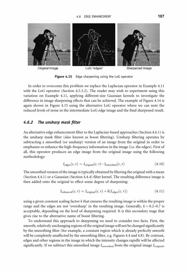
In order to overcome this problem we replace the Laplacian operator in Example 4.11

with the LoG operator (Section 4.5.3.2). The reader may wish to experiment using this

variation on Example 4.11, applying different-size Gaussian kernels to investigate the

difference in image sharpening effects that can be achieved. The example of Figure 4.14 is

again shown in Figure 4.15 using the alternative LoG operator where we can note the

reduced levels of noise in the intermediate LoG edge image and the final sharpened result.

4.6.2 The unsharp mask filter

An alternative edge enhancement filter to the Laplacian-based approaches (Section 4.6.1) is

the unsharp mask filter (also known as boost filtering). Unsharp filtering operates by

subtracting a smoothed (or unsharp) version of an image from the original in order to

emphasize or enhance the high-frequency information in the image (i.e. the edges). First of

all, this operator produces an edge image from the original image using the following

methodology:

Iedgesðc; rÞ ¼ Ioriginalðc; rÞ�Ismoothedðc; rÞ ð4:10ÞThe smoothed version of the image is typically obtained by filtering the original with amean

(Section 4.4.1) or a Gaussian (Section 4.4.4) filter kernel. The resulting difference image is

then added onto the original to effect some degree of sharpening:

Ienhancedðc; rÞ ¼ Ioriginalðc; rÞþ kðIedgesðc; rÞÞ ð4:11Þ

using a given constant scaling factor k that ensures the resulting image is within the proper

range and the edges are not ‘oversharp’ in the resulting image. Generally, k¼ 0.2–0.7 is

acceptable, depending on the level of sharpening required. It is this secondary stage that

gives rise to the alternative name of boost filtering.

To understand this approach to sharpening we need to consider two facts. First, the

smooth, relatively unchanging regions of the original imagewill not be changed significantly

by the smoothing filter (for example, a constant region which is already perfectly smooth

will be completely unaffected by the smoothing filter, e.g. Figures 4.4 and 4.8). By contrast,

edges and other regions in the image in which the intensity changes rapidly will be affected

significantly. If we subtract this smoothed image Ismoothed from the original image Ioriginal,

Figure 4.15 Edge sharpening using the LoG operator

4.6 EDGE ENHANCEMENT 107

then we get a resulting image Iedges with higher values (differences) in the areas affected

significantly (by the smoothing) and low values in the areas where little change occurred.

This broadly corresponds to a smoothed edge map of the image. The result of subtracting

this smoothed image (or some multiple thereof) from the original is an image of higher

value pixels in the areas of high contrast change (e.g. edges) and lower pixel values in the

areas of uniformity Iedges. This resulting image can then be added back onto the original,

using a specified scaling factor k, to enhance areas of rapid intensity changewithin the image

whilst leaving areas of uniformity largely unchanged. It follows that the degree of

enhancement will be determined by the amount of smoothing that is imposed before the

subtraction takes place and the fraction of the resulting difference image which is added

back to the original. Unsharp filtering is essentially a reformulation of techniques referred to

as high boost – we are essentially boosting the high-frequency edge information in the

image.

This filtering effect can be implemented in Matlab as shown in Example 4.12. The result

of Example 4.12 is shown in Figure 4.16, where we see the original image, the edge difference

image (generated by subtraction of the smoothed image from the original) and a range of

enhancement results achieved with different scaling factors k. In the examples shown,

improvement in edge detail (sharpness) is visible but the increasing addition of the edge

image (parameter k) increases both the sharpness of strong edges and noise apparent within

the image. In all cases, image pixels exceeding the 8-bit range 0–255 were truncated.

Example 4.12



Iorig¼imread(‘cameraman.tif ’); %Read in image

g¼fspecial(‘gaussian’,[5 5],1.5); %Generate Gaussian kernel

subplot(2,3,1), imshow(Iorig); %Display original image

Is¼imfilter(Iorig,g); %Create smoothed image by filtering

Ie¼(Iorig Is); %Get difference image

subplot(2,3,2), imshow(Ie); %Display unsharp difference

Iout¼Iorigþ (0.3).�Ie; %Add k � difference image to original








Comments

In this example we perform all of the operations using unsigned 8 bit images (Matlab type

uint8) and we compute the initial smoothed image using a 5� 5 Gaussian kernel (s¼ 1.5).

Try changing the levels of smoothing, using an alternative filter such as the mean for the

smoothing operator and varying the scaling factor k.


Exercises


examples introduced in this chapter. Additional information on all of theMatlab functions

presented in this chapter and throughout these exercises is available in Matlab from the

function help browser (use doc <function name> at the Matlab command prompt where

<function name> is the function required).

Matlab functions: imnoise, plot, tic, toc,min,max,mean, function, imresize, for, colfilt,

roipoly, roifilt, imfilter, fspecial.

Exercise 4.1 Based on Example 4.3, experiment with the Matlab imnoise() function

for adding different levels of ‘salt and pepper’ and Gaussian noise to images. Use the

‘peppers.png’ and ‘eight.tif’ example images as both a colour and grey-scale example to

construct a series of image variables in Matlab with varying levels and types of noise (you

may also wish to investigate the other noise types available from this function, type doc

imnoise at the Matlab prompt). Based on the filtering topics presented in Section 4.4,

investigate the usefulness of each of the mean, median and Gaussian filtering for removing

different types and levels of image noise (see Examples 4.4, 4.5 and 4.7 for help).

Exercise 4.2 Building on Example 4.2, experiment with the use of different neighbour-

hood dimensions and the effect on the resulting image output. Using the plotting functions

of Matlab (function plot()) and the Matlab timing functions tic and toc, create a plot of

Figure 4.16 Edge sharpening using unsharp mask filter

EXERCISES 109

neighbourhood dimensionN against operation run-time for applying themin(),max() and

mean() functions over an example image. Does the timing increase linearly or not? Why is

this?

Exercise 4.3 Building on the local pixel neighbourhood definition described Section 4.2,

write a Matlab function (see Matlab help for details on functions or type doc function at the

Matlab function) to extract the N�N pixel neighbourhood of a given specified pixel

location ðx; yÞ and copy the pixel values to a new smallerN�N image. Youmaywant to take

a look at the syntax for the Matlab for loop function (doc for) in the first instance.

Combine your extraction programwith theMatlab imresize() function to create a region

extraction and magnification program.

Exercise 4.4 TheMatlab colfilt() function utilizes the highly efficientmatrix operations of

Matlab to perform image filtering operations on pixel neighbourhoods. Using the Matlab

timing functions tic()/toc(), time the operation performed in Example 4.2 with andwithout

the use of this optimizing parameter. Vary the size of the neighbourhood over which the

operation is performed (and the operation:min()/max()/mean()). What do you notice? Is

the increase in performance consistent for very small neighbourhoods and very large

neighbourhoods?

Exercise 4.5 Based on Example 4.4 for performingmean filtering on a given image, record

the execution time for this operation (using Matlab timing functions tic()/toc()) over

a range of different neighbourhood sizes in the range 0–25.UseMatlab’s plotting facilities to

present your results as a graph.What do you notice?How does the execution time scale with

the increase in size of the neighbourhood? (Hint. To automate this task you may want to

consider investigating the Matlab for loop constructor).

As an extension you could repeat the exercise for differently sized images (or a range of

image sizes obtained from imresize()) and plot the results. What trends do you notice?

Exercise 4.6 Repeat the first part of Exercise 4.5, but compare the differences between

mean filtering (Example 4.4) and median filtering (Example 4.5). How do the trends

compare? How can any differences be explained?

Exercise 4.7 A region of interest (ROI) within an image is an image sub-region

(commonly rectangular in nature) over which localized image-processing operations can

be performed. In Matlab an ROI can be selected interactively by first displaying an image

(using imshow()) and then using the roipoly() function that returns an image sub-region

defined as a binary image the same size as the original (zero outside the ROI and one outside

the ROI).

Investigate the use of the roifilt() function for selectively applying bothGaussian filtering

(Example 4.7) and mean filtering (Example 4.4) to an isolated region of interest within one

of the available example images.

Youmay also wish to investigate combining the ROI selection functionwith your answer

to Exercise 4.3 to extract a given ROI for histogram equalization (Section 3.4.4) or edge-

detection processing (Section 4.5) in isolation from the rest of the image.


Exercise 4.8 Several of the filtering examples in this chapter make use of the Matlab

imfilter() function (Example 4.2), which itself has a parameter of how to deal with

image boundaries for a given filtering operation. Select one of the filtering operations

from this chapter and experiment with the effect of selecting different boundary options

with the imfilter() function. Does it make a difference to the result? Does it make a

difference to the amount of time the filtering operation takes to execute? (Use tic()/toc()

for timing.)

Exercise 4.9 Implement a Matlab function (doc function) to perform the conservative

smoothing filter operation described towards the end of Section 4.4.3. (Hint. You may

wish to investigate the Matlab for loop constructor.) Test this filter operation on the

noise examples generated in Example 4.3. How does it compare to mean or median

filtering for the different types of noise? Is it slower or faster to execute? (Use tic()/toc()

for timing.)

Exercise 4.10 Considering the Roberts and Sobel edge detectors from Example 4.8, apply

edge detection to three-channel RGB images and display the results (e.g. the ‘peppers.png’

and ‘football.jpg’ images). Display the results as a three-channel colour image and as

individual colour channels (one per figure).

Note how some of the edge responses relate to distinct colour channels or colours within

the image. When an edge is visible in white in the edge-detected three-channel image, what

does this mean? Youmay also wish to consider repeating this task for the HSV colour space

we encountered in Chapter 1. How do the results differ in this case?

Exercise 4.11 Building upon the unsharp operator example (Example 4.12), extend the

use of this operator to colour images (e.g. the ‘peppers.png’ and ‘football.jpg’ images). How

do the areas of image sharpening compare with the areas of edge-detection intensity in

Exercise 4.10?

The unsharp operator can also be constructed by the use of an ‘unsharp’ parameter to the

Matlab fspecial() function for us with imfilter(). Compare the use of this implementation

with that of Example 4.12. Are there any differences?


EXERCISES 111

5Fourier transforms andfrequency-domain processing

5.1 Frequency space: a friendly introduction

Grasping the essentials of frequency-space methods is very important in image processing.

However, if the author’s experience is anything to go by, Fourier methods can prove

something of a barrier to students. Many discussions of the Fourier transform in the

literature simply begin by defining it and then offer a comprehensive but rather formal

mathematical presentation of the related theorems. The significant risk in this approach is

that all but the mathematically inclined or gifted are quickly turned off, either feeling

inadequate for the task or not understanding why it is all worth the trouble of struggling

with. The real significance of Fouriermethods, the small number of really central concepts,

simply gets lost in the mathematical details. We will try to avoid this overly formal

approach. Of course, we cannot simply ignore the mathematics – it is central to the whole

subject – but we will certainly aim to stress the key points and to underline the real

significance of the concepts we discuss.

Frequency-space analysis is a widely used and powerful methodology centred around a

particular mathematical tool, namely the Fourier transform.1 We can begin simply by

saying that the Fourier transform is a particular type of integral transform that enables us

to view imaging and image processing from an alternative viewpoint by transforming the

problem to another space. In image processing, we are usually concerned with 2-D spatial

distributions (i.e. functions) of intensity or colour which exist in real space – i.e. a 2-D

Cartesian space in which the axes define units of length. The Fourier transform operates

on such a function to produce an entirely equivalent form which lies in an abstract space

called frequency space. Why bother? In the simplest terms, frequency space is useful

because it can make the solution of otherwise difficult problemsmuch easier (Figure 5.1).

Fourier methods are sufficiently important that we are going to break the pattern and

digress (for a time) from image processing to devote some time to understanding some of the

key concepts and mathematics of Fourier transforms and frequency space. Once this

1 Strictly, frequency space analysis is not exclusively concerned with the Fourier transform. In its most general

sense, it also covers the use of similar transforms such as the Laplace and Z transform. However, we will use

frequency space and Fourier space synonymously.




Problem infrequency

space

Problem inreal space

Solution inreal space

Solution infrequency

space

InverseTransform

Difficult solution

Easy solution

IntegralTransform

Figure 5.1 Frequency-space methods are used to make otherwise difficult problems easier to solve

foundation has been laid, wewill move on to see how they can be used to excellent effect both

to look at image processing from a new perspective and to carry out a variety of applications.

5.2 Frequency space: the fundamental idea

We will begin our discussion of Fourier methods by summarizing, without any attempt at

rigour, some of the key concepts. To stay general, we will talk for themoment of the Fourier

analysis of signals rather than images.

(1) The harmonic content of signals. The fundamental idea of Fourier analysis is that any

signal, be it a function of time, space or any other variables, may be expressed as a

weighted linear combination of harmonic (i.e. sine and cosine) functions having

different periods or frequencies. These are called the (spatial) frequency components

of the signal.

(2) The Fourier representation is a complete alternative. In the Fourier representation of a

signal as a weighted combination of harmonic functions of different frequencies, the

assigned weights constitute the Fourier spectrum. This spectrum extends (in principle)

to infinity and any signal can be reproduced to arbitrary accuracy. Thus, the Fourier

spectrum is a complete and valid, alternative representation of the signal.

(3) Fourier processing concerns the relation between the harmonic content of the output signal

to the harmonic content of the input signal. In frequency space, signals are considered

as combinations of harmonic signals. Signal processing in frequency space (analysis,

synthesis and transformation of signals) is thus concerned with the constituent

harmonic content and how these components are preserved, boosted or suppressed

by the processing we undertake.

These first three concepts are summarized in Figure 5.2.

(4) The space domain and the Fourier domain are reciprocal. In the Fourier representa-

tion of a function, harmonic termswith high frequencies (short periods) are needed to

construct small-scale (i.e. sharp or rapid) changes in the signal. Conversely, smooth

features in the signal can be represented by harmonic termswith low frequencies (long

periods). The two domains are thus reciprocal – small in the space domain maps to

114 CH 5 FOURIER TRANSFORMS AND FREQUENCY DOMAIN PROCESSING

Figure 5.2 A summary of three central ideas in Fourier (frequency) domain analysis. (1) Input

signals are decomposed into harmonic components. (2) The decomposition is a complete and valid

representation. (3) From the frequency-domain perspective, the action of any linear system on the

input signal is to modify the amplitude and phase of the input components

large in the Fourier domain and large in the space domainmaps to small in the Fourier

domain.

Students often cope with Fourier series quite well but struggle with the Fourier transform.

Accordingly, we make one more key point.

(5) The Fourier series expansion and the Fourier transform have the same basic goal.

Conceptually, the Fourier series expansion and the Fourier transform do the same

thing. The difference is that the Fourier series breaks down a periodic signal into

harmonic functions of discrete frequencies, whereas the Fourier transform breaks

down a nonperiodic signal into harmonic functions of continuously varying frequen-

cies. The maths is different but the idea is the same.

We will expand on these basic ideas in what follows. We begin our discussion in the next

section with Fourier series.

5.2.1 The Fourier series

Key point 1

Any periodic signal may be expressed as a weighted combination of sine and cosine functions

having different periods or frequencies.

5.2 FREQUENCY SPACE: THE FUNDAMENTAL IDEA 115

This is Fourier’s basic hypothesis. The process of breaking down a periodic signal as a sum

of sine and cosine functions is called a Fourier decomposition or Fourier expansion. If the

signal is something that varies with time, such as a voltage waveform or stock-market share

price, the harmonic functions that build the signal are 1-D and have a temporal frequency.

In such a 1-D case, Fourier’s basic theorem says that a periodic signal2VðtÞ having period Tcan be constructed exactly as an infinite sum of harmonic functions, a Fourier series, as

follows:

VðtÞ ¼X1n¼0

an cos

�2pntT

�þX1n¼1

bn sin

�2pntT

�

¼X1n¼0

an cosðvntÞþX1n¼1

bn sinðvntÞð5:1Þ

An arbitrary periodic 1-D function of a spatial coordinate x f(x) having spatial period lcan be represented in exactly the same way:

VðxÞ ¼X1n¼0

an cos

�2pnxl

�þX1n¼1

bn sin

�2pnxl

�

¼X1n¼0

an cosðknxÞþX1n¼1

bn sinðknxÞð5:2Þ

Let us first make some simple observations on the Fourier expansion of the spatial

function f(x) expressed by Equation (5.2).

(1) The infinite series of harmonic functions in the expansion, namely cosðknxÞ and

sinðknxÞ, are called the Fourier basis functions.

(2) We are dealing with a function that varies in space and the (inverse) periodicity,

determined by kn ¼ 2pn=l, is thus called the spatial frequency.

(3) The coefficientsan and bn indicatehowmuchof eachbasis function (i.e. harmonicwave

of the given spatial frequency) is required to build f(x). The complete set of coefficients

fan and bng are said to constitute the Fourier or frequency spectrum of the spatial

function. The function f(x) itself is called the spatial domain representation.

(4) To reproduce the original function f(x) exactly, the expansionmust extend to an infinite

number of terms. In this case, asn!1, the spatial frequencies kn !1 and the number

of coefficients fan and bng describing the Fourier spectrum also approach infinity.

2 Strictly, the signal must satisfy certain criteria to have a valid Fourier expansion. We will not digress into these

details but assume that we are dealing with such functions here.


Key point 2

The Fourier spectrum is a valid and complete alternative representation of a function.

This point is essential, namely that in knowing the coefficients an and bn we have a

complete representation of the function just as valid as f(x) itself. This is so because we

can rebuild f(x) with arbitrary precision by carrying out the summation in Equation (5.2).

Figure 5.3 shows how a simple 1-D periodic function (only one cycle of the function is

shown) – a step function – can be increasingly well approximated by a Fourier series

representation asmore terms in Equation (5.2) are added. If we continue this procedure for

ever, the Fourier spectrum fan; bng can reproduce the function exactly and can thus be

rightly considered an alternative (frequency-domain) representation.

If we examine the synthesis of the periodic square wave in Figure 5.3, we can observe our

key point number 4 in the Fourier decomposition/synthesis of a function. The low spatial

frequencies (corresponding to the lower values of n) build the ‘basic’ smooth shape, whereas

the high spatial frequencies are required to reproduce the sharp transitions in the function

(the edges). The synthesis of a step function by a Fourier series is just one simple example,

Figure 5.3 The synthesis of a step function of period l using a Fourier series. The resulting spectrumis the frequency-domain representation of the spatial function determining the contribution of each

sine wave of frequency sinðknxÞ ¼ sinð2pnx=lÞ

5.2 FREQUENCY SPACE: THE FUNDAMENTAL IDEA 117

but this is in fact a basic ‘ground rule’ of the Fourier representation of any function (true in

one or more dimensions).

It is also worth emphasizing that although the ability to synthesize a given function

exactly requires harmonic (i.e. sine and cosine) frequencies extending to infinite spatial

frequency, it is often the case that a good approximation to a function can be obtained using

a finite and relatively small number of spatial frequencies. This is evident from the synthesis of

the step function. When we approximate a spatial function by a Fourier series containing a

finite number of harmonic terms N, we then effectively define a so-called spatial frequency

cut-off kCO ¼ 2pN=l. The loss of the high spatial frequencies in a signal generally results in

a loss of fine detail.

5.3 Calculation of the Fourier spectrum

Fourier’s basic theorem states that we can synthesize periodic functions using the sinusoidal

basis functions, but we have so far glossed over the question of how we actually calculate the

Fourier spectrum (i.e. the expansion coefficients in Equation (5.2)). Fortunately, this is easy.

By exploiting the orthogonality properties of the Fourier basis,3 we can obtain simple

formulae for the coefficients:

an ¼ 2

l

ðl=2l=2

f ðxÞcosðknxÞ dx

bn ¼ 2

l

ðl=2l=2

f ðxÞsinðknxÞ dxð5:3Þ

where kn ¼ 2pn=l. Note that we get the coefficients in each case by integrating over one fullspatial period of the function.4

5.4 Complex Fourier series

Fourier series can actually be expressed in a more convenient and compact, complex form.

Thus, a periodic, 1-D spatial function f(x) is expressed as a weighted sum of complex

exponential (harmonic) functions:

f ðxÞ ¼X1

n¼ 1cn exp

�i2pnxl

�

¼X1

n¼ 1cn expðiknxÞ

ð5:4Þ

3 A proof of these formulae is offered on the book website http://www.fundipbook.com/materials/.4We can of course add any constant value to our chosen limits of l/2 and l/2. Zero and l are commonly quoted,

but all that matters is that the periodic function is integrated over a full spatial period l.


where nmay assume all integer values from�1 to þ1. In an entirely analogousway to the

real form of the expansion, we may exploit the orthogonality relations between complex

exponential functions to obtain the Fourier expansion coefficients:5

cn ¼ 1

l

ðl=2

l=2

f ðxÞexpðiknxÞ dx ð5:5Þ

Note that the cn are, in general, complex numbers. In using the complex representation we

stress that nothing essential changes. We are still representing f(x) as an expansion in terms

of the real sine and cosine functions. The sines and cosines can actually bemade to reappear

by virtue of grouping the positive and negative exponentials with the same magnitude of

the index n but of opposite sign. A strictly real function can then be constructed from

the complex Fourier basis because the expansion coefficients (the cn) are also, in general,

complex. It is relatively straightforward to show that (see the exercises on the book’s

website6) that the complex coefficients cn are related to the real coefficients an and bn in the

real Fourier series (Equation (5.3)) by

ck ¼ ak þ ibk

c k ¼ ak�ibk for k ¼ 0; 1 . . . !1ð5:6Þ

To expand the discussion of Fourier methods to deal with images, there are two main

differences from the formalism we have presented so far that we must take into account:

(1) images are not, in general, periodic functions.

(2) images are typically 2-D (and sometimes higher dimensional) spatial functions of

finite support.7

The extension of the Fourier hypothesis from periodic functions to deal with non-

periodic functions is really just the extension from a Fourier series to a Fourier transform.

First, we will consider the issue of periodicity and only after extend to two dimensions. In

what follows (just to keep it simple) we will consider a 1-D spatial function f(x), though an

analogous argument can be made for two or more dimensions.

5.5 The 1-D Fourier transform

To move from a Fourier series to a Fourier transform, we first express our function f ðxÞ asa complex Fourier series:

5,6 See http://www.fundipbook.com/materials/.7 The supportof a function is the region overwhich it is nonzero.Obviously, any real digital imagehas finite support.

5.5 THE 1 D FOURIER TRANSFORM 119

f ðxÞ ¼X1

n¼ 1cn expðiknxÞ kn ¼ 2pn

lð5:7Þ

Multiplying top and bottom by l!1, this can also be written as

f ðxÞ ¼ 1

l

X1n¼ 1

ðlcnÞexpðiknxÞ ð5:8Þ

We now let the period of the function l!1. In other words, the trick here is to consider

that a nonperiodic function may be considered as a periodic function having infinite spatial

period. Note that the individual spatial frequencies in the summation expressed by

Equation (5.8) are given by kn ¼ 2pn=l and the frequency interval between them is thus

given by Dk ¼ 2p=l. As the spatial period l!1, the frequency interval Dk becomes

infinitesimally small and lcn tends towards a continuous function FðkxÞ. It is in fact possibleto show8 that the limit of Equation (5.8) as l!1 is the inverse Fourier transform:

f ðxÞ ¼ð1

1FðkxÞexpðikxxÞ dkx ð5:9Þ

Note that:

. the specific weights assigned to the harmonic (complex exponential) functions are given

by the function FðkxÞ;

. the frequencies kx are now continuous and range over all possible values;

. The summation for f(x) becomes an integral and the Fourier spectrum FðkxÞ is nowa function as opposed to a set of discrete values.

The orthogonality properties of the complex Fourier basis (the expðikxxÞ functions)enable us to calculate the weighting function FðkxÞ in Equation (5.9). This is, in fact, the

Fourier transform of f(x):

FðkxÞ ¼ 1

2p

ð1

1f ðxÞexpð�ikxxÞ dx ð5:10Þ

It is vital to emphasize that the essential meaning and purpose of the Fourier transform is

really no different from that of the Fourier series. The Fourier transform of a function also

fundamentally expresses its decomposition into a weighted set of harmonic functions.

Moving from the Fourier series to the Fourier transform, we move from function synthesis

using weighted combinations of harmonic functions having discrete frequencies (a sum-

mation) to weighted, infinitesimal, combinations of continuous frequencies (an integral).

8 See book website http://www.fundipbook.com/materials/ for details.


The synthesis of functions using the real Fourier series, the complex Fourier series and the

Fourier transform are summarized in Table 5.1.

The Fourier transform FðkxÞ is a complex function and we can, therefore, also write the

Fourier spectrum in polar form as the product of the Fouriermodulus and (the exponential

of) the Fourier phase:

where

FðkxÞ ¼ jFðkxÞjexpiwðkxÞjFðkxÞj2 ¼ ½RefFðkxÞg�2 þ ½ImfFðkxÞg�2 wðkxÞ ¼ tan 1

�ImfFðkxÞgRefFðkxÞg

�ð5:11Þ

This form is useful because it helps us to see that the Fourier transform FðkxÞ defines boththe ‘amount’ of each harmonic function contributing to f(x) (through jFðkxÞj) and the

relative placement/position of the harmonic along the axis through the associated

complex phase term expðiwðkxÞÞ. As we shall see in Figure 5.11, most of what we will

loosely call the ‘visual information’ in a Fourier transform is actually contained in the

phase part.

5.6 The inverse Fourier transform and reciprocity

Examination of Equations (5.9) and (5.10) shows that there is a close similarity between the

Fourier transform and its inverse. It is in fact arbitrary whether we define the forward

Fourier transform with the negative form of the exponential function or the positive form,

but the convention we have chosen here is the normal one and we will use this throughout.

There is also a certain freedom with regard to the 2p factor which can be placed on either

the forward or reverse transforms or split between the two.9 The factor of 2p also appears in

Table 5.1 Comparison of the synthesis of spatial functions using the real Fourier series, the complex

Fourier series and the Fourier transform

Real Fourier series Complex Fourier series Fourier transform

Spatial frequencieskn ¼ 2pn

l

n ¼ 1; 2; . . . ;1

kn ¼ 2pnl

n ¼ �1;�2; . . . ;�1kx

1 � kx � 1

Basis functions sin knx; cos knx

n ¼ 1; 2; . . . ;1expðiknxÞ

n ¼ 0;�1;�2; . . . ;�1expðikxxÞ1 � kx � 1

Spectrum Coefficients

fan; bngn ¼ 0; 1; 2; . . . ;1

Coefficients

fcngn ¼ 0;�1;�2; . . . ;�1

Function

FðkxÞ1 � kx � 1

9 Some authors define both forward and reverse transforms with a normalization factor of ð2pÞ�1=2 outside.

5.6 THE INVERSE FOURIER TRANSFORM AND RECIPROCITY 121

the 2-D Fourier transform, which is presented in the next section, but is actually remarkably

unimportant in image processing – it enters simply as an overall scaling factor and thus has no

effect on the spatial structure/content of an image. For this reason, it is quite common to

neglect it entirely.

Rather like the Fourier series expansion of a square wave, the Fourier transform of

the rectangle function is easy to calculate and informative. The 1-D rectangle function is

defined as

rect

�x

a

�¼ 1 jxj � a

2

¼ 0 jxj � a

2

By substituting directly into the definition we can show that its Fourier transform is

given by

FðkxÞ ¼ a

2psinðkxa=2Þkxa=2

¼ a

2psinc

kxa

2

� �

where sinc u ¼ sin u=u. This function is plotted in Figure 5.4 for three values of the

rectangle width a, over a spatial frequency range �8p=a � kx � 8p=a. Note the

reciprocity between the extent of the spatial function and the extent of its Fourier

transform (the scaling factor of 2a/p has been omitted to keep the graphs the same

height).

Note that a decrease in the width of the rectangle in the spatial domain results in the

Fourier transform spreading out in the frequency domain. Similarly, an increase of the

extent of the function in the spatial domain results in the frequency-domain representation

shrinking. This reciprocal behaviour is a central feature of the frequency-domain repre-

sentation of functions.

Important examples of 1-D Fourier transforms and Fourier transform relations are

provided in Tables 5.2 and 5.3. We also offer some exercises (with worked solutions) on the

book’s website10 which we strongly recommend to the reader as a means to consolidate the

basic concepts discussed so far and to gaining further insight into the basic behaviour and

properties of the Fourier transform.

FT for width a FT for width 2a FT for width a/2

Figure 5.4 The Fourier transform of the rectangle function FðkxÞ ¼ ða=2pÞf½sinðkxa=2Þ�=ðkxa=2Þg

10 http://www.fundipbook.com/materials/.


5.7 The 2-D Fourier transform

In an entirely analogous way to the 1-D case, a function of two spatial variables f ðx; yÞ can beexpressed as a weighted superposition of 2-D harmonic functions.11 The basic concept is

Table 5.2 Fourier transforms of some important functions

Function name Space domain f(x) Frequency domain F(k)

f ðxÞFðkÞ ¼

ð1

�1f ðxÞe�ikx dx

Impulse (delta function) dðxÞ 1

Constant 1 dðkÞ

Gaussian expx2

2s2

� �ðs 2p

p Þexp s2k2

2

� �

Rectangle rectx

L

� �¼ Q x

L

� �� 1 jxj � L=2

0 elsewhere

L sinc

kL

2p

� �

Triangle Lx

W

� �� 1 ðjxj=WÞ jxj � W

0 elsewhere

(W sinc2

kW

2p

� �

Sinc sincðWxÞ � sinðWxÞWx

1

Wrect

k

W

� �

Exponential e�ajxj a > 02a

a2 þ k2

Complex exponential expðik0xÞ dðk k0Þ

Decaying exponential expð axÞuðxÞ Refag> 0 1

aþ ik

Impulse trainX1

n �1dðx nxsÞ 2p

xs

X1k �1

d k 12pxs

� ��

Cosine cosðk0xþ uÞ eiudðk k0Þþ e�iudðkþ k0ÞSine sinðk0xþ uÞ i½eiudðk k0Þ e�iudðkþ k0Þ�

Unit step uðxÞ � 1 x � 0

0 x < 0

pdðkÞþ 1

jik

Signum sgnðxÞ � 1 x � 0

1 x < 0

2

ik

Sinc2 sinc2ðBxÞ 1

BL

v

2pB

� �

Linear decay 1=x ipsgnðkÞ

11 Certain functions do not, in the strict sense, possess Fourier transforms, but this is a mathematical detail which

has no real practical importance in image processing and we will fairly assume that we can obtain the Fourier

transform of any function of interest.


graphically illustrated in Figure 5.5, in which examples of 2-D harmonic functions are

combined to synthesize f ðx; yÞ. Mathematically, the reverse or inverse 2-D Fourier

transform is defined as

Table 5.3 Some important properties of the 2-D Fourier transform: f(x, y) has a Fourier transform

F(kx, ky); g(x, y) has a Fourier transform G(kx, ky)

Property Spatial domain Frequency domain Comments

Addition

theorem

f ðx; yÞþ gðx; yÞ Fðkx; kyÞþGðkx; kyÞ Fourier transform of the

sum equals sum of the

Fourier transforms.

Similarity

theorem

f ðax; byÞ 1

jabj Fkxa;ky

b

� �The frequency domain

function scales in

inverse proportion to

the spatial domain

function.

Shift theorem f ðx a; y bÞ exp½ iðkxaþ kybÞ�Fðkx; kyÞ Shift a function in space

and its transform is

multiplied by a pure

phase term.

Convolution

theorem

f ðx; yÞ � gðx; yÞ Fðkx; kyÞGðkx; kyÞ Transform of a

convolution is equal to

the product of the

individual transforms.

Separable

product

f ðx; yÞ ¼ hðxÞgðyÞ Fðkx; kyÞ ¼ HðkxÞGðkyÞ If a 2 D function separates

into two 1 D functions,

then so does its Fourier

transform

Differentiation qqxm

qqyn

f ðx; yÞ ðikxÞmðikyÞnFðkx; kyÞ Calculation of image

derivatives is trivial

using the image Fourier

transform

Rotation f ðxcos uþ y sin u;

x sin uþ y cos uÞFðkx cos uþ ky sin u;

kx sin uþ ky cos uÞRotate a function by u in

the plane and its

Fourier transform

rotates by u

Parseval’s

theorem

ð1

�1

ð1

�1j f ðx; yÞj2 dx dy

ð1

�1

ð1

�1jFðkx; kyÞj2 dkx dky

Fourier transformation

preserves image

‘energy’

Laplacian r2f ðx; yÞ ðk2x þ k2yÞFðkx; kyÞ Calculation of the image

Laplacian is trivial

using the image Fourier

transform

Multiplication f ðx; yÞ gðx; yÞ Fðkx; kyÞ � �Gðkx; kyÞ Product of functions is a

convolution in the

Fourier domain


f ðx; yÞ ¼ 1

2pp

ð1

1

ð1

1Fð fx; fyÞexp½2pið fxxþ fyyÞ� dfx dfy

¼ 1

2pp

ð1

1

ð1

1Fðkx; kyÞexp½iðkxxþ kyyÞ� dkx dky

ð5:12Þ

where the weighting function Fðkx; kyÞ is called the 2-D Fourier transform and is given by

Fð fx; fyÞ ¼ 1

2pp

ð1

1

ð1

1f ðx; yÞexp½�2pið fxxþ fyyÞ� dx dy

Fðkx; kyÞ ¼ 1

2pp

ð1

1

ð1

1f ðx; yÞexp½�iðkxxþ kyyÞ� dx dy

ð5:13Þ

Considering the 2-D Fourier transform purely as an integral to be ‘worked out’, it can at

first appear rather formidable.12 Indeed, the number of functions whose Fourier transform

can be analytically calculated is relatively small and, moreover, they tend to be rather simple

functions (some are listed in Table 5.2). We stress two things, however. First, Fourier

transforms of even very complicated functions can be calculated accurately and quickly on

a computer. In fact, the development and digital implementation of the Fourier transform

for the computer (known as the fast Fourier transform (FFT)) revolutionized the world of

Figure 5.5 The central meaning of the 2-D Fourier transform is that some scaled and shifted

combination of the 2-D harmonic basis functions (some examples are shown) can synthesize an

arbitrary spatial function

12One of the authors freely confesses that he never understood it at all as an undergraduate, despite encountering

it in several different courses at various times.


image processing and indeed scientific computing generally. Second, the real value of

the frequency-domain representation lies not just in the ability to calculate such complex

integrals numerically, but much more in the alternative and complementary viewpoint

that the frequency domain provides on the processes of image formation and image

structure.

Just as for the 1-D case, there are a relatively small number of simple 2-D functions

whose Fourier transform can be analytically calculated (and a number of them are, in

fact, separable into a product of two 1-D functions). It is instructive, however, to work

through some examples, and these are provided with worked solutions on the book’s

website.13

There are a number of theorems relating operations on a 2-D spatial function to their

effect on the corresponding Fourier transform which make working in the frequency

domain and swapping back to the spatial domain much easier. Some of these are listed in

Table 5.3. Again their formal proofs are provided on the book’s website for the interested

reader.

5.8 Understanding the Fourier transform:frequency-space filtering

In spatial-domain image processing, we are basically concerned with how imaging systems

and filters of various kinds affect the individual pixels in the image. In frequency-domain

image processing, however, we consider imaging systems and filtering operations from an

alternative perspective – namely, how they affect the constituent harmonic components that

make up the input. Figure 5.6 depicts the basic ideas of spatial and frequency-space

Figure 5.6 The relation between the space domain and the frequency domain. The value at a point

ðx; yÞ in the space domain specifies the intensity of the image at that point. The (complex) value at

a point ðkx; kyÞ in the frequency domain specifies the contribution of the harmonic function

exp½iðkxx þ kyyÞ� to the image

13 See http://www.fundipbook.com/materials/.


representation. In the spatial domain, we refer to the pixel locations through a Cartesian

ðx; yÞ coordinate system. In the frequency-space representation the value at each coordinate

point in the (kx; ky) system tells us the contribution that the harmonic frequency compo-

nent exp½iðkxxþ kyyÞ� makes to the image.

Figure 5.7 demonstrates the basic idea behind frequency-domain filtering, in which

certain harmonic components are removed from the image. The basic filtering proce-

dure involves three steps: (i) calculate the Fourier transform; (ii) suppress certain

frequencies in the transform through multiplication with a filter function (in this case,

the filter is set to zero at certain frequencies but is equal to one otherwise); and then

(iii) calculate the inverse Fourier transform to return to the spatial domain. In Figure 5.7,

the image and (the modulus) of its corresponding Fourier transform are displayed

alongside the image which results when we remove selected groups of harmonic

frequencies from the input. This removal is achieved by multiplication of the filter

function image (where white is 1, black is 0) with the Fourier transform of the image.

Components of increasing spatial frequency (low to high) are thus transmitted as we

increase the size of the filter function centred on the Fourier image.

Figure 5.7 A basic illustration of frequency-domain filtering. The Fourier transform of the original

image is multiplied by the filters indicated above (white indicates spatial frequency pairs which are

preserved and black indicates total removal). An inverse Fourier transform then returns us to the

spatial domain and the filtered image is displayed to the right. (The Matlab code for this figure can be

found at http://www.fundipbook.com/materials/.)

5.8 UNDERSTANDING THE FOURIER TRANSFORM: FREQUENCY SPACE FILTERING 127

Figure 5.8 shows a real-life example of frequency-domain filtering undertaken by one of

the authors. The InfraredAstronomical Satellite (IRAS)was a joint project of theUSA,UK

and the Netherlands.14 The IRAS mission performed a sensitive all-sky survey at

wavelengths of 12, 25, 60 and 100 mm. As a result of this survey, we were presented with

acquired images which suffered from striping artefacts – a result of the difficulty in

properly aligning and registering the strips recorded as the detector effectively made 1-D

sweeps across the sky. The stripes which are visible in the image can also be clearly seen in

the Fourier transform of the image, where they show up as discrete groups of spatial

frequencies which are enhanced over the background. Note that we show the absolute

value of the Fourier transform on a log scale to render them visible. Clearly, if we can

suppress these ‘rogue’ frequencies in frequency space, then we may expect to largely

remove the stripes from the original image.

Simply setting all the identified rogue frequencies to zero is one option, but is not really

satisfactory. We would expect a certain amount of the rogue frequencies to be naturally

present in the scene and such a tactic will reduce the overall power spectrum of the image.

Figure 5.8 An application of frequency-domain filtering. Proceeding from left to right and top to

bottom, we have: (a) the original image with striping effect apparent; (b) the Fourier modulus of the

image (displayed on log scale); (c) the Fourier modulus of the image after filtering (displayed on log

scale); (d) the filtered image resulting from recombination with the original phase; (e) the difference

between the original and filtered images (See colour plate section for colour version)

14 See http://irsa.ipac.caltech.edu/IRASdocs/iras.html.


The basic approach taken to filtering was as follows:

(1) Calculate the Fourier transform and separate it into its modulus and phase.

(2) Identify the ‘rogue frequencies’. Whilst, in principle, this could be achieved manually

on a single image, we sought an automated approach that would be suitable for

similarly striped images. We must gloss over the details here, but the approach relied

on use of the Radon transform to identify the directionality of the rogue frequencies.

(3) Replace the rogue frequencies in the Fourier modulus with values which were

statistically reasonable based on their neighbouring values.

(4) Recombine the filtered modulus with the original phase and perform an inverse

Fourier transform.

5.9 Linear systems and Fourier transforms

From the frequency-domain perspective, the action of a linear imaging system on an input

can be easily summarized:

Any input image can be decomposed into a weighted sum of harmonic functions. The action

of a linear system in general will be to preserve or alter the magnitude and phase of the input

harmonics.

Broadly speaking, we may thus view a linear imaging system as something that operates

on the constituent input harmonics of the image and can assess its quality by its ability to

(more or less) faithfully transmit the input harmonics to the output. This basic action of

a linear system in the frequency domain is illustrated in Figure 5.9. One measure for

characterizing the performance of a linear, shift-invariant imaging system is through the

optical transfer function (OTF). To understand this fully, we must first introduce the

convolution theorem.

5.10 The convolution theorem

As we showed earlier in this chapter, the importance of the convolution integral originates

from the fact that many situations involving the process of physical measurement with

an imperfect instrument can be accurately described by convolution. The process of

convolution (a rather messy integral in the spatial domain) has a particularly simple

and convenient form in the frequency domain; this is provided by the famous convolu-

tion theorem – probably the single most important theorem in the field of image processing.

Consider two 2-D functions f ðx; yÞ and hðx; yÞ having Fourier transforms respectively

denoted by Fðkx; kyÞ and Hðkx; kyÞ. Symbolically denoting the operation of taking a 2-D

Fourier transform by F, the first form of the convolution theorem states that:

5.10 THE CONVOLUTION THEOREM 129

Ff f ðx; yÞ � � hðx; yÞg ¼ Fðkx; kyÞHðkx; kyÞ ð5:14Þ

The Fourier transform of the convolution of the two functions is equal to the product of the


Thus, the processing of convolving two functions in the spatial domain can be

equivalently carried out by simple multiplication of their transforms in the frequency domain.

This first form of the convolution theorem forms the essential basis for the powerful

methods of frequency-domain filtering. Thus, rather than attempt to operate directly on the

image itself with a chosen spatial-domain filter (e.g. edge detection or averaging), we

alternatively approach the problem by consideringwhat changes we would like to effect on the

spatial frequency content of the image. Filter design is often much easier in the frequency

domain, and the alternative viewpoint of considering an image in terms of its spatial

frequency content often allows a more subtle and better solution to be obtained.

For completeness, we note that there is a second form of the convolution theorem, which

states that

Ff f ðx; yÞhðx; yÞg ¼ Fðkx; kyÞ � �Hðkx; kyÞ ð5:15Þ

The Fourier transform of the product of the two functions is equal to the convolution of their


Figure 5.9 The basic action of a linear system can be understood by how well it transmits to the

output each of the constituent harmonic components that make up the input. In this illustration, the

lower frequencies are faithfully reproduced, but higher frequencies are suppressed.


This formdoes not find quite suchwidespread use in digital image processing as it does not

describe the basic image formation process. However, it finds considerable use in the fields of

Fourieropticsandoptical imageprocessing,whereweareoften interested in theeffectofdevices

(diffraction gratings, apertures, etc.) which act multiplicatively on the incident light field.

The convolution theorem15 lies at the heart of both frequency-domain enhancement

techniques and the important subject of image restoration (a subject we will develop in

more detail in Chapter 6).

5.11 The optical transfer function

Consider for a moment the specific imaging scenario in which f ðx; yÞ corresponds to the

input distribution, hðx; yÞ to the respective systemPSF and gðx; yÞ is the image given by their

convolution:

gðx; yÞ ¼ f ðx; yÞ � � hðx; yÞ ð5:16Þ

Taking the Fourier transform of both sides, we can use the first form of the convolution

theorem to write the right-hand side:

Ffgðx; yÞg ¼ Ff f ðx; yÞ � � hðx; ygGðkx; kyÞ ¼ Fðkx; kyÞHðkx; kyÞ

ð5:17Þ

Thus, the Fourier spectrum of the output image Gðkx; kyÞ is given by the product of the

input Fourier spectrum Fðkx; kyÞ with a multiplicative filter functionHðkx; kyÞ.Hðkx; kyÞ iscalled the OTF. The OTF is the frequency-domain equivalent of the PSF. Clearly, the OTF

derives its name from the fact that it determines how the individual spatial frequency pairs

ðkx; kyÞ are transferred from input to output. This simple interpretationmakes the OTF the

most widely usedmeasure of the quality or fidelity of a linear shift-invariant imaging system.

Fff ðx; yÞ � hðx; yg ¼ Gðkx; kyÞ|fflfflfflffl{zfflfflfflffl}outputFourierspectrum

¼ Fðkx; kyÞ|fflfflfflffl{zfflfflfflffl}inputFourierspectrum

Hðkx; kyÞ|fflfflfflfflffl{zfflfflfflfflffl}OTF

ð5:18Þ

This multiplicative property of the OTF on the input spectrum is particularly convenient

whenever we consider complex imaging systems comprising multiple imaging elements

(e.g. combinations of lenses and apertures in a camera or telescope). If the kth element

is characterized by its PSF hkðx; yÞ, then the overall image is given by a sequence of

convolutions of the input with the PSFs. Taking Fourier transforms and using the

convolution theorem, this can be equivalently expressed by sequential multiplication of

the OTFs in the frequency domain- a much easier calculation:

Ffh1ðx; yÞ � h2ðx; yÞ � hNðx; yÞg ¼ H1ðkx; kyÞH2ðkx; kyÞ HNðkx; kyÞ ð5:19Þ

15 For proof, go to http://www.fundipbook.com/materials/.

5.11 THE OPTICAL TRANSFER FUNCTION 131

A detailed discussion of OTFs and their measurement is outside our immediate scope,

but we stress two key points:

(1) The OTF is normalized to have a maximum transmission of unity. It follows that

an ideal imaging system would be characterized by an OTF given byHðkx; kyÞ ¼ 1 for

all spatial frequencies.

(2) As the Fourier transform of the PSF, the OTF is, in general, a complex function:

Hðkx; kyÞ ¼ jHðkx; kyÞjexp½iwðkx; kyÞ�The squaremodulus of theOTF is a real function known as themodulation transfer

function (MTF); this gives the magnitude of transmission of the spatial frequencies.

However, it is the phase term wðkx; kyÞ which controls the position/placement of the

harmonics in the image plane. Although theMTF is a common and useful measure of

image quality, the phase transmission function wðkx; kyÞ is also crucial for a complete

picture.

Figure 5.10 (generated using the Matlab� code in Example 5.1) shows on the left an

image of the old BBC test card.16 The test card has a number of features designed to allow

Example 5.1


A¼imread('BBC grey testcard.png'); %Read in test card image

FA¼fft2(A); FA¼fftshift(FA); %Take FFT and centre it

PSF¼fspecial('gaussian',size(A),6); %Define PSF

OTF¼fft2(PSF); OTF¼fftshift(OTF); %Calculate corresponding OTF

Afilt¼ifft2(OTF.�FA);Afilt¼fftshift(Afilt);

%Calculate filtered image

subplot(1,4,1);imshow(A,[]);

colormap(gray);

%Display results

subplot(1,4,2); imagesc(log(1þ (PSF)));

axis image; axis off;

subplot(1,4,3); imagesc(log(1þ abs

(OTF))); axis image; axis off;

subplot(1,4,4); imagesc(abs(Afilt)); axis

image; axis off;

PSF¼fspecial('gaussian',size(A),6); %Define PSF

OTF¼fft2(PSF); OTF¼fftshift(OTF); %Calculate corresponding OTF

rlow¼(size(A,1)./2) 3; rhigh¼(size(A,1)./2)þ 3;

%Define range to be altered

clow¼(size(A,2)./2) 3; chigh¼(size(A,2)./2)þ 3;

16 For those readers too young to remember this, the test cardwasdisplayedwhen you switchedonyourTVset before

transmission of programmes had started. This was back in the days when television often did not start until 11 am.


Fphase¼angle(OTF); %Extract Fourier phase

Fphase(rlow:rhigh,clow:chigh)¼Fphase(rlow:rhigh,clow:chigh)þ0.�pi.�rand;

%Add random component to selected phase

OTF¼abs(OTF).�exp(i.�Fphase); %Recombine phase and modulus

Afilt¼ifft2(OTF.�FA);Afilt¼fftshift(Afilt);

%Calculate filtered image

psfnew¼abs(fftshift((otf2psf(OTF)))); %Calculate corresponding PSF

subplot(1,4,2); imagesc(log(1þ psfnew));

axis image; axis off; colormap(gray);

subplot(1,4,3); imagesc(log(1þabs(OTF))); axis image; axis off;

subplot(1,4,4); imagesc(abs(Afilt));

axis image; axis off;

PSF¼fspecial('motion',30,30); %Define motion PSF

OTF¼psf2otf(PSF,size(A));

OTF¼fftshift(OTF);

%Calculate corresponding OTF

Afilt¼ifft2(OTF.�FA); %Calculate filtered image

subplot(1,4,1);imshow(A,[]); %Display results

subplot(1,4,2); imshow(log(1þPSF),[]);

subplot(1,4,3); imshow(log(1þ abs

(OTF)),[])

subplot(1,4,4); imshow(abs(Afilt),[]);

Figure 5.10 The effect of the OTF on the image quality. Column 1: the original image; column 2: the

system PSF; column 3: the corresponding system MTF; column 4: the resulting images after transfer by

the systemOTF. Note the image at bottom right has the sameMTF as that at the top right, but the phase

has been shifted and this has significant consequences on the image quality

5.11 THE OPTICAL TRANSFER FUNCTION 133

assessment of image quality. For example, hard edges, sinusoidal patterns of both low

and high frequency and adjacent patches of slightly different intensities are all evident.

These features allow systematic measurements to be made on the OTF and also the image

contrast to be assessed. The top row shows the effect on the test card image of

transmission through a system with an OTF well approximated by a 2-D Gaussian

function. The PSF (also a Gaussian) corresponding to the OTF is also shown. Note that

the overall effect on the image is an isotropic blurring and most of the fine structures in

the original image are unresolved. The middle row shows the OTF corresponding to a

motion of the source or detector during image acquisition. The corresponding PSF, a

long thin line, is displayed (on a finer scale) indicating a motion of approximately 30

pixels at an angle of 30. Note that the MTF extends to high spatial frequencies in the

direction orthogonal to the motion but drops rapidly in the direction of the motion, and

this substantiates what we have already discussed concerning the reciprocal behaviour in

the space and spatial frequency domain in which short signals in the space domain

become extended in the frequency domain and vice versa. The bottom row shows the

effect of an OTF whose MTF is identical to that in the first row but to which a random

phase term has been added to some of the low-frequency components of the image. The

drastic effect on the image quality is apparent.

5.12 Digital Fourier transforms: the discrete fastFourier transform

In our discussion, we have been a little disingenuous through our silence on a key

computational issue. We commented earlier that Fourier transforms can be carried out

quickly and effectively on a digital computer thanks to the development of a Fourier

transform which works on discrete or digital data – the discrete Fast Fourier Transform

(FFT) – but have offered no discussion of it. For example, we have implicitly assumed in

the examples presented so far that the Fourier transform of an image (which has a finite

number of pixels and thus spatial extent) also has finite extent. Moreover, we have

implicitly made use of the fact that an N�N digital image in the spatial domain will

transform to a corresponding N�N frequency-domain representation. This is true, but

certainly not obvious. In fact, we have already seen that the continuous Fourier

transform of a function having finite spatial extent (e.g. a delta or rectangle function)

generally has infinite extent in the frequency domain. Clearly, then, there are issues to be

resolved. In this chapter we will not attempt to offer a comprehensive treatment of the

discrete FFT. This is outside our immediate concern and many excellent treatments exist

already.17 In the simplest terms, we can say that the discrete FFT is just an adaptation of

the integral transform we have studied which preserves its essential properties when we

deal with discrete (i.e. digital) data. The following section can be considered optional on

a first reading, but it is included to ensure the reader is aware of some practical aspects of

working with the discrete FFT.

17 For example, see The Fast Fourier Transform by E. Oran Brigham or Fourier Analysis and Imaging by Ron

Bracewell.


5.13 Sampled data: the discrete Fourier transform

Digital images are by definition discrete. A digital image which consists of a (typically)

large but finite number of pixels must, by definition, have finite support. This immediately

suggests one potential problem for using Fourier transforms in digital image processing,

namely: how can we possibly represent a Fourier transform having infinite support in a

finite array of discrete pixels? The answer is that we cannot, but there is, fortunately, an

answer to this problem. The discrete Fourier transform (DFT) – and its inverse – calculates

a frequency-domain representation of finite support from a discretized signal of finite

support.

The theorems that we have presented and the concepts of frequency space that we have

explored for the continuous Fourier transform are identical and carry directly over to the

DFT. However, there is one important issue in using the DFT on discrete data that we need

to be fully aware of.18 This relates to the centring of the DFT, i.e. the centre of the Fourier

array corresponding to the spatial frequency pair ð0; 0Þ. Accordingly, we offer a brief

description of the DFT in the following sections.

Consider a function f ðx; yÞ which we wish to represent discretely by anM�N array of

sampled values. In general, the samples are taken at arbitrary but regularly spaced intervals

Dx and Dy along the x and y axes. We will employ the notation f ðx; yÞ for the discrete

representation on the understanding that this actually corresponds to samples at coordi-

nates x0 þ xDx and y0 þ yDy:

f ðx; yÞD�� f ðx0 þ xDx; y0 þ yDyÞ ð5:20Þ

where x0 and y0 are the chosen starting point for the sampling and the indices x and y assume

integer values x ¼ 0; 1; 2; . . . ;M�1 and y ¼ 0; 1; 2; . . . ;N�1 respectively.

The 2-D (forward) DFT of the M�N array f ðx; yÞ is given by the expression

Fðu; vÞ ¼ 1

MNp

XM 1

x¼0

XN 1

y¼0

f ðx; yÞexp �2piux

Mþ vy

N

� �h ið5:21Þ

Note that

. the DFT is also of dimension M�N;

. the spatial frequency indices also assume integer values u ¼ 0; 1; 2; . . . ;M�1 and

v ¼ 0; 1; 2; . . . ;N�1.

The discrete transform Fðu; vÞ actually corresponds to sampling spatial frequency pairs

ðuDu; vDvÞ, i.e. D�� Fðu; vÞFðuDu; vDvÞ, where the sampling intervals in the frequency domain

fDu;Dvg are related to the spatial sampling interval by

Du ¼ 1

MDxDv ¼ 1

NDvð5:22Þ

18 It is easy to be caught out by this issue when using computer FFT routines, including the Matlab functions fft,

fft2 and fftn.

5.13 SAMPLED DATA: THE DISCRETE FOURIER TRANSFORM 135

The inverse DFT (reverse DFT) is defined in a similar manner as

f ðx; yÞ ¼ 1

MNp

XM 1

u¼0

XN 1

v¼0

Fðu; vÞexp þ 2piux

Mþ vy

N

� �h ið5:23Þ

Note that the only difference in the forward and reverse transforms is the sign in the

exponential. It is possible to show that the forward and reverse DFTs are exact inverses of

each other. Equations (5.21) and (5.23) thus represent an exact transform relationship

which maintains finite support in both the spatial and frequency domains as required.

Figure 5.11 illustrates graphically the basic sampling relationship between a 2-D digital

image represented by M�N pixels and its DFT.

5.14 The centred discrete Fourier transform

The definition of the DFT in Equation (5.21) and the diagram in Figure 5.11 indicate that

the spatial frequency coordinates run from the origin at the top left corner of the array,

increasing aswemove across right and down. It is usual practice to centre theDFT by shifting

its origin to the centre of the array.

For clarity, we repeat the definition for the DFT given earlier of the 2-D discrete array

f ðx; yÞ:

Fðu; vÞ ¼ 1

MNp

XM 1

x¼0

XN 1

y¼0

f ðx; yÞexp �2piux

Mþ vy

N

� �h ið5:24Þ

Δy

f (x, y) f (u, v)

Δx

0

0

1

2

...

1 2 ... M -1

x

y

N-1

Δv

Δu

Δu ΔvMΔx NΔy

0

0

1

2

...

1 2 ... M -1

u

v

N-1

1 1==Sampling intervals related by

Figure 5.11 A discretely sampled image f ðx; yÞ and its DFT Fðu; vÞ have the same number of pixels.The relationship between the sampling intervals in the two domains is given in the diagram


We now shift the frequency coordinates to new values u0 ¼ u�ðM=2Þ; v0 ¼ v�ðN=2Þ sothat ðu0; v0Þ ¼ ð0; 0Þ is at the centre of the array. The centred Fourier transform Fðu0; v0Þ isdefined as

Fðu0; v0Þ ¼ F

�u�M

2; v�N

2

�

¼ 1

MNp

XM 1

x¼0

XN 1

y¼0

f ðx; yÞexp��2pi

½u�ðM=2Þ�xM

þ ½v�ðN=2Þ�yN

��

Factoring out the exponential terms which are independent of u and v and using eip ¼ �1,

we have

Fðu0; v0Þ ¼ F

�u�M

2; v�N

2

�

¼ 1

MNp

XM 1

x¼0

XN 1

y¼0

ð�1Þxþ yf ðx; yÞ� exp

��2pi

�ux

Mþ vy

N

�� ð5:25Þ

which is, by definition, the DFT of the product ð�1Þxþ yf ðx; yÞ. Thus, we have one simple

way to achieve a centred Fourier transform:

Centred DFT: method 1

If f ðx; yÞ is an M�N array, then its centred DFT is given by the DFT of ð 1Þxþ yf ðx; yÞ:

Fðu0; v0Þ � F u�M

2; v�N

2

� �¼ FT ð�1Þxþ yf ðx; yÞ� � ð5:26Þ

where FT symbolically represents the DFT operation.

However, rather than premultiply our function by the factor ð�1Þxþ y, we can also

achieve a centred DFT ‘retrospectively’. Assume that we have calculated the DFT Fðu; vÞ off ðx; yÞ using the standard definition. It is possible to show, that the centred DFT is given by

a diagonal swapping of the quadrants in the DFT (Example 5.2, Figure 5.12).

Centred DFT: method 2

If f ðx; yÞ is an M�N array with DFT Fðu; vÞ, its centred DFT is given by swapping the first

quadrant of Fðu; vÞ with the third and swapping the second quadrant with the fourth.

5.14 THE CENTRED DISCRETE FOURIER TRANSFORM 137

Example 5.2


A¼imread('cameraman.tif'); %Read in image

FT¼fft2(A); FT centred¼fftshift(FT); %Take FT, get centred version too


subplot(2,3,2), imshow(log(1þabs(FT)),[]);

%Display FT modulus (log scale)

subplot(2,3,3), imshow(log(1þabs(FT centred)),[]);

%Display centred FT modulus (log scale)

Im1¼abs(ifft2(FT)); subplot(2,3,5),

imshow(Im1,[]);

%Inverse FFT and display

Im2¼abs(ifft2(FT centred));

subplot(2,3,6), imshow(Im1,[]);

%Inverse FFT and display

figure;

[xd,yd]¼size(A); x¼ xd./2:xd./2 1;

y¼ yd./2:yd./2 1;

[X,Y]¼meshgrid(x,y); sigma¼32;

arg¼(X.^2þY.^2)./sigma.^2;

frqfilt¼exp( arg);

%Construct freq domain filter

imfilt1¼abs(ifft2(frqfilt.�FT)); %Centred filter and noncentred spectrum

imfilt2¼abs(ifft2(frqfilt.�FT centred)); %image centred filter on centred spectrum

subplot(1,3,1), imshow(frqfilt,[]); %Display results

subplot(1,3,2), imshow(imfilt1,[]);

subplot(1,3,3), imshow(imfilt2,[]);

Figure 5.12 The centred DFT (right) can be calculated from the uncentred DFT (left) by dividing the

array into four rectangles with two lines through the centre and diagonally swapping the quadrants.

Using the labels indicated, we swap quadrant 1 with quadrant 3 and quadrant 2 with quadrant 4


Why shouldwe centre theDFT? The answer is that we do not have to do this, but there are

two good reasons in its favour. First, shifting the origin to the centre makes the discrete

frequency-space range ð�M=2!M=2�1;�N=2!N=2�1Þmore akin to the continuous

space inwhichwehave an equal distribution of positive andnegative frequency components

ð�1 � kx � 1;�1 � ky � 1Þ. Second, the construction of frequency-domain filters

for suppressing or enhancing groups of spatial frequencies is generally facilitated by using

a centred coordinate system.


Comments

Matlab functions: fft2, ifft2, fftshift.

This example illustrates the role played by fftshift, which centres the Fourier transform such

that the zeroth spatial frequency pair is at the centre of the array.

5.14 THE CENTRED DISCRETE FOURIER TRANSFORM 139

6Image restoration

Building upon our consideration of the Fourier (frequency) domain in the previous chapter,

we now progress to explore a practical use of these methods in the field of image restoration.

6.1 Imaging models

Image restoration is based on the attempt to improve the quality of an image through

knowledge of the physical processes which led to its formation. As we discussed in Chapter 5,

wemay consider image formation as a process which transforms an input distribution into an

output distribution.1 The input distribution represents the ideal, i.e. it is the ‘perfect’ image to

which we do not have direct access but which we wish to recover or at least approximate by

appropriate treatment of the imperfect or corrupted output distribution. Recall that, in 2-D

linear imaging systems, the relationship between the input distribution f ðx0; y0Þ and the

measured output distribution gðx; yÞ is represented as a linear superposition integral. For

linear, shift invariant (LSI) systems, this reduces to the form of a convolution:

gðx; yÞ ¼ðð

f ðx0; y0Þhðx�x0; y�y0Þdx0dy0 þ nðx; yÞgðx; yÞ ¼ f ðx; yÞ � �hðx; yÞþ nðx; yÞ

ð6:1Þ

where �� is used to denote 2-D convolution. In Equation (6.1), the quantity hðx�x0; y�y0Þ isthe Point Spread Function (PSF) or impulse response and nðx; yÞ is an additive noise term.

These two factors are responsible for the imperfect output distribution which is obtained.

The image restoration task is (in principle at least) simple:

Estimate the input distribution f ðx0; y0Þ using the measured output gðx; yÞ and any knowledge

we may possess about the PSF hðx x0; y y0Þ and the noise nðx; yÞ.

Recovery of the input distribution f ðx0; y0Þ from Equation (6.1) is known as deconvolu-

tion. Image restoration has now evolved into a fascinating but quite complex field of

research. The simple observation that any approach to image restoration will be ultimately

1 These are also often referred to as the object and the image.




limited by our explicit or implicit knowledge of the PSF and the noise process is helpful in

establishing firm ground at the beginning.

Equation (6.1) is not the only model which describes image formation – some situations

require amore complexmodel – but it is certainly by far themost important in practice. Some

imaging situationsneed tobedescribedbymore complexmodels, such as spatially variant and

nonlinearmodels. However, these are relatively rare and, in any case, can be best understood

by first developing a clear understanding of approaches to restoration for the LSI model.

Accordingly, Equation (6.1) will form the basis for our discussion of image restoration.

6.2 Nature of the point-spread function and noise

We have said that the quality of our image restoration will be limited by our knowledge of

the PSF and the noise. What, then, are the natures of these two entities? Although

important exceptions do exist in practice,2 the system PSF is typically a fixed or

deterministic quantity that is determined by the physical hardware which constitutes the

overall imaging system and which may, therefore, be considered to be unchanging with

time. For example, in a simple optical imaging system, the overall PSF will be determined

by the physical nature and shape of the lenses; in a medical diagnostic imaging system,

such as the Anger camera (which detects gamma-rays emitted from the body of a patient),

the PSF is determined by a combination of a mechanical collimator and a scintillator–

photomultiplier system which allows the detection of the origin of an emitted gamma

photon with a certain limited accuracy.

Thus, given certain physical limitations relating to the nature of the detected flux in the

imaging system (i.e. optical, infrared, sonar, etc.), the PSF is typically something over which

we initially have some control in principle but which becomes fixed once the system has

been designed and engineered. Precisely because the PSF is the result of a design and

engineering process, it is something of which we can usually expect to have knowledge and

which will assist in approaching the restoration problem.

By contrast, the noise term in Equation (6.1) is typically stochastic in nature and produces

a random and unwanted fluctuation on the detected signal. The key characteristic of noise

processes is that we usually have no control over them and we cannot predict the noise

which will be present in a given instant. Noise originates from the physical nature of

detection processes and has many specific forms and causes. Whatever the specific physical

process that gives rise to the formation of an image, the common characteristic is the

unpredictable nature of the signal fluctuations. However, although we cannot know the

values of a specific realization of the noise, we can often understand andmodel its statistical

properties. The variety of noise models and behaviour are often a major factor in the subtly

different approaches to image restoration. Figure 6.1 summarizes the basic image forma-

tion/restoration model described by Equation (6.1).

Image formation results from convolution of the input with the system PSF and the

addition of random noise. Linear restoration employs a linear filter whose specific form

2The PSF of a telescope system viewing light waves which propagate through atmospheric turbulence is one

important example in astronomical imaging where the PSF may be considered as random in nature and changes

significantly over a short time scale.

142 CH 6 IMAGE RESTORATION

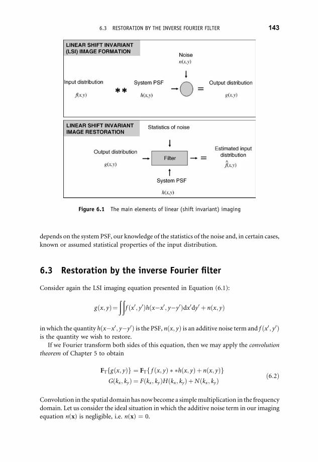
depends on the system PSF, our knowledge of the statistics of the noise and, in certain cases,

known or assumed statistical properties of the input distribution.

6.3 Restoration by the inverse Fourier filter

Consider again the LSI imaging equation presented in Equation (6.1):

gðx; yÞ¼ðð

f ðx0; y0Þhðx�x0; y�y0Þdx0dy0 þ nðx; yÞ

in which the quantity hðx�x0; y�y0Þ is the PSF, nðx; yÞ is an additive noise term and f ðx0; y0Þis the quantity we wish to restore.

If we Fourier transform both sides of this equation, then we may apply the convolution

theorem of Chapter 5 to obtain

FTfgðx; yÞg ¼ FTf f ðx; yÞ � �hðx; yÞþ nðx; yÞgGðkx; kyÞ ¼ Fðkx; kyÞHðkx; kyÞþNðkx; kyÞ

ð6:2Þ

Convolution in the spatial domain has nowbecome a simplemultiplication in the frequency

domain. Let us consider the ideal situation in which the additive noise term in our imaging

equation n(x) is negligible, i.e. n(x) ¼ 0.

Figure 6.1 The main elements of linear (shift invariant) imaging

6.3 RESTORATION BY THE INVERSE FOURIER FILTER 143

In this case a trivial solution results. We simply divide both sides of Equation (6.2) by

HðKx;KyÞ and then take the inverse Fourier transform of both sides. Thus:

Fðkx; kyÞ ¼ Gðkx; kyÞHðkx; kyÞ ¼ Yðkx; kyÞGðkx; kyÞ ð6:3Þ

and so

f ðx; yÞ ¼ F 1fYðkx; kyÞGðkx; kyÞg ð6:4Þ

where F 1 denotes the operation of inverse Fourier transformation. The frequency-domain

filter

Yðkx; kyÞ ¼ 1

Hðkx; kyÞ ð6:5Þ

where H(kx , ky) is the system optical transfer function (OTF) is called the inverse filter.

In practice, the straight inverse filter rarely works satisfactorily and should only ever

be used with extreme caution. The reason for this can be understood by examining

Equation (6.5) and considering the simple fact that the OTF of any imaging system will

generally not extend to the diffraction limit. This means that any attempt to recover spatial

frequency pairs ðkx; kyÞwhichmay exist in the input but at which the OTF of the system has

dropped to an effective value of zero will be disastrous. Themagnitude of themultiplicative

filter Yðkx; kyÞ at these frequencies will then tend to � 1=0!1.

One way round this is to use a truncated inverse filter in which one effectively monitors

the value of the OTF Hðkx; kyÞ and sets the value of the filter function Yðkx; kyÞ to zero

wheneverHðkx; kyÞ falls below a predetermined ‘dangerously low’ value. Technically, this

is an example of a band-pass filter because it allows certain spatial frequency pairs to be

passed into the reconstruction and suppresses others. This is, in fact, how the restoration

was achieved in Figure 6.2 (the Matlab� code used to generate this figure is given in

Example 6.1).

However, whenever noise is present, the use of an inverse filter will have unpredictable

and often disastrous effects. Consider applying the inverse filter in Equation (6.5) to a

situation in which noise is present. We obtain

Fðkx; kyÞ ¼ Yðkx; kyÞGðkx; kyÞ ¼ Gðkx; kyÞHðkx; kyÞ þ

Nðkx; kyÞHðkx; kyÞ

¼ Fðkx; kyÞþ Nðkx; kyÞHðkx; kyÞ

ð6:6Þ

where we use the common ‘hat’ notation (i.e. Fðkx; kyÞ) to denote an estimated quantity.

Equation (6.6) shows that our recovered frequency spectrum has an additional term: the

noise spectrum Nðkx; kyÞ divided by the system OTF Hðkx; kyÞ. Clearly, we would like this

additional term to be as small as possible, since the estimated spectrum will then approach

the true input spectrum.The noise spectrum, however, is an unknown and randomaddition


Example 6.1


A¼imread('trui.png'); B¼fft2(A); B¼fftshift(B); %Read in image and take FT

[x y]¼size(A); [X Y]¼meshgrid(1:x,1:y); %Construct Gaussian PSF

h¼exp( (X x/2).^2./48).�exp( (Y y/2).^2./48); %extending over entire array

H¼psf2otf(h,size(h)); H¼fftshift(H); %Get OTF corresponding to PSF

g¼ifft2(B.�H); g¼abs(g); %Generate blurred image via

%Fourier domain

G¼fft2(g); G¼fftshift(G); %Take FT of image

indices¼find(H>1e 6); %Do inverse filtering AVOIDING

F¼zeros(size(G)); F(indices)¼G(indices)./

H(indices);

%small values in OTF !!

f¼ifft2(F); f¼abs(f); %Inverse FT to get filtered image

subplot(1,4,1), imshow(g,[min(min(g))

max(max(g))]);

%Display �original� blurred image

subplot(1,4,2), imagesc(h); axis square; axis off; %Display PSF

subplot(1,4,3), imagesc(abs(H)); axis square; axis off; %Display MTF

subplot(1,4,4), imagesc(f); axis square; axis tight;

axis off;

%Display filtered image

Comments

New Matlab functions: find, psf2otf.

The first section of code generates a Gaussian blurred image. The second section estimates the

original image using an inverse filter.

to the data to which we ‘do not have access’ andwhich is actually quite inseparable from the

output image spectrum.Moreover, it is characteristic ofmany noise processes that they have

significant high-frequency content; in other words, there is a spatial frequency regime for

which jNðkx; kyÞj � jGðkx; kyÞj. In this case, it is clear that the first term on the right-hand

side in Equation (6.6) (the true spatial frequency content) will be completely dominated

by the second term (the noise). This is the case shown in the Figure 6.3 (theMatlab code used

to generate this figure is given in Example 6.2).

Figure 6.2 Restoration of a blurred but noiseless image through inverse filtering. From left to right

(a) blurred original; (b) Gaussian PSF; (c) corresponding MTF; (d) recovered original

6.3 RESTORATION BY THE INVERSE FOURIER FILTER 145

Figure 6.3 Restoration of a blurred and noisy image through inverse filtering. From left to right:

(a) blurred original with Gaussian white noise (zero mean, 0.2% variance); (b) system PSF;

(c) corresponding MTF; (d) recovered image

Example 6.2


A¼imread('trui.png'); B¼fft2(A); B¼fftshift(B);

[x y]¼size(A); [X Y]¼meshgrid(1:x,1:y);

h¼exp( (X x/2).^2./48).�exp( (Y y/2).^2./48); %CODE SAME AS EXAMPLE 6.1

H¼psf2otf(h,size(h)); H¼fftshift(H); %Get OTF

g¼ifft2(B.�H); g¼mat2gray(abs(g)); %Blur image in Fourier domain

g¼imnoise(g,'gaussian',0,0.002); %Add noise to image

%CODE HEREAFTER SAME AS 6.1

Comments

Matlab functions: imnoise, mat2gray.

Similar to Example 6.1 except that white noise is added to the image.

6.4 The Wiener–Helstrom filter

As Example 6.2 and the corresponding Figure 6.3 show, whenever noise is present in an

image we require a more sophisticated approach than a simple inverse filter. Inspection of

the LSI imaging equation in the frequency domain

Fðkx; kyÞ ¼ Yðkx; kyÞGðkx; kyÞ ¼ Yðkx; kyÞ½Hðkx; kyÞFðkx; kyÞþNðkx; kyÞ� ð6:7Þsuggests that we would ideally like our frequency-domain filter Yðkx; kyÞ to have the

following qualitative properties:

. At those spatial frequency pairs for which the noise component jNðkx; kyÞj is much

smaller than the image component jGðkx; kyÞj, our filter should approach the inverse

filter. Thus, we want

Yðkx; kyÞ � 1

Hðkx; kyÞ when jNðkx; kyÞj � jGðkx; kyÞj

This ensures accurate recovery of these frequency components in the restored image.


. At those spatial frequency pairs for which the noise component jNðkx; kyÞj is much

larger than the image component jGðkx; kyÞj, our filter should approach zero. Thus:

Yðkx; kyÞ � 0 when jNðkx; kyÞj � jGðkx; kyÞj

This ensures that we do not attempt to restore spatial frequency pairs which are

dominated by the noise component.

. At those spatial frequency pairs for which the noise component jNðkx; kyÞj and the

image component jGðkx; kyÞj are comparable, our filter should ‘damp’ these frequen-

cies, effecting an appropriate compromise between complete acceptance (inverse filter)

and total suppression.

These three properties are broadly achieved by theWiener–Helstrom (often abbreviated

simply to Wiener) filter, defined as

Yðkx; kyÞ ¼ H�ðkx; kyÞWFðkx; kyÞjHðkx; kyÞj2WFðkx; kyÞþWNðkx; kyÞ

ð6:8Þ

In Equation (6.8) H� denotes the complex conjugate of the OTF and the quantities

WFðkx; kyÞ and WNðkx; kyÞ are respectively the input and noise power spectra:

WFðkx; kyÞ ¼ hjFðkx; kyÞj2i and WNðkx; kyÞ ¼ hjNðkx; kyÞj2i ð6:9Þ

Division of the right-hand side of Equation (6.8) by the input power spectrum enables us

to express the Wiener–Helstrom filter in an alternative and more transparent form:

Yðkx; kyÞ ¼ H�ðkx; kyÞjHðkx; kyÞj2 þNSRðkx; kyÞ

ð6:10Þ

where the quantity NSRðkx; kyÞ ¼ WNðkx; kyÞ=WFðkx; kyÞ gives the noise/signal power

ratio. Equation (6.10) thus shows clearly that the Wiener–Helstrom filter approximates

an inverse filter for those frequencies at which the signal/noise power ratio is large,

but becomes increasingly small for spatial frequencies at which the signal-noise power

ratio is small.

6.5 Origin of the Wiener–Helstrom filter

TheWiener–Helstrom filter defined by Equation (6.8) (or equivalently by Equation (6.10))

is not simply an ad hoc empirical filter but has a firm theoretical basis. It is important

because it is, in a clearly defined sense, an optimal linear restoration filter. Let us restate the

LSI imaging equation presented in Equation (6.1):

gðx; yÞ ¼ðð

f ðx0; y0Þhðx�x0; y�y0Þ dx0 dy0 þ nðx; yÞ

6.5 ORIGIN OF THE WIENER HELSTROM FILTER 147

which, via the convolution theorem, has the corresponding frequency domain equivalent

presented in Equation (6.2):

Gðkx; kyÞ ¼ Fðkx; kyÞHðkx; kyÞþNðkx; kyÞ

A well-defined optimal criterion is to seek an estimate of the input distribution f ðx; yÞ,which varies minimally from the true input f ðx; yÞ in the mean-square sense. Namely,

we will seek an estimate f ðx; yÞ such that the following quantity is minimized:

Q ¼ð1

1

ð1

1½Fðx; yÞ�Fðx; yÞ�2 dx dy

* +ð6:11Þ

This optimization criterion is called the minimum mean-square error (MMSE) or mini-

mum variance criterion. It is important to be aware that the angle brackets in Equa-

tion (6.11) denote ensemble averaging; that is, we seek an estimator f ðx; yÞ that is optimal

with respect to statistical averaging over many realizations of the random noise process

nðx; yÞand, indeed, to the PSF in those special situations where it may be treated as

a stochastic quantity.3

Application of Parseval’s theorem to Equation (6.11) allows us to express an entirely

equivalent criterion in the Fourier domain:

Q ¼ð1

1

ð1

1½Fðx; yÞ�Fðx; yÞ�2 dx dy

* +ð6:12Þ

The basic approach to deriving the Wiener–Helstrom filter is to postulate a linear filter

Yðkx; kyÞ which acts on the image data Gðkx; kyÞ ¼ Fðkx; kyÞHðkx; kyÞþNðkx; kyÞ and then

to take variations in the operator Yðkx; kyÞ such that the quantityQ is stationary. The formal

derivation is quite lengthy and requires methods from statistical estimation theory and

variational calculus, and so is not repeated here.4

It is further possible to show that the resultingmean-square error after application of the

Wiener–Helstrom filter is given by

Q ¼ð1

1

ð1

1

WFðkx; kyÞWNðkx; kyÞjHðkx; kyÞj2WFðkx; kyÞþWNðkx; kyÞ

dx dy ð6:13Þ

In summary, the Wiener–Helstrom filter works by accepting low-noise frequency

components and rejecting high-noise frequency components. Further, it does so in a

3A good example of a randomly varying and thus stochastic PSF is the PSF of a ground based telescope observing

through atmospheric turbulence.4 Interested readers can study a detailed derivation on the book’s website at http://www.fundipbook.com/

materials/.


well-defined ‘optimal’ way. This is very reasonable behaviour and it is tempting to think

that image restoration in the frequency domain should begin and end here.

However, despite its practical and historical importance the Wiener–Helstrom filter is

no panacea, and two points are essential to make:

(1) The exact implementation of Equation (6.10) requires knowledge of the input power

spectrum. Since the input distribution is precisely the quantity we are trying to

estimate, we cannot generally expect to know its power spectrum!5 Thus, in the vast

majority of cases, the Wiener–Helstrom filter cannot be precisely implemented.

However, there are several ways in which we can attempt to get round this problem

to produce a practical filter:

(a) When the input distribution belongs to a well-defined class in which the input

is constrained, reasonably accurate estimates of the power spectrum may be

available. A typical instancemight be a standardmedical imaging procedure, such

as taking a chest radiograph, in which the input structure can essentially be

considered as a modest variation on a basic prototype (i.e. the skeletal structure is

very similar across the population). In this case, the prototype may be used to

provide the approximation to the input power spectrum.

(b) When the input is not constrained in this way, theWiener–Helstrom filter can be

approximated by substituting the output power spectrum WGðkx; kyÞ (which we

can easily calculate) or preferably some filtered version of it in place of the input

power spectrum.

(c) Another simple, but less accurate, approach is to approximate the noise/signal

ratio (the NSR function in Equation (6.10)) by an appropriate scalar constant.

By removing all spatial frequency dependence from this term, one typically

trades off some high-frequency content in the restoration for increased

stability.

(2) Restorations produced by the Wiener–Helstrom filter often produce restorations

which are rather too blurred from the perceptual viewpoint – suggesting that the

MMSE criterion, although a perfectly valid mathematical optimisation criterion, is

almost certainly not the perceptually optimal from a human standpoint. For this

reason, many other filters have been developed which can produce better results for

specific applications.

Figure 6.4 (for which the Matlab code is given in Example 6.3) shows the results of two

different approximations to the idealWiener filter on an image exhibiting a significant level

of noise. The restored image is far from perfect but represents a significant improvement on

the original.

5 This point is strangely neglected in many discussions of the Wiener filter.

6.5 ORIGIN OF THE WIENER HELSTROM FILTER 149

Example 6.3


I ¼ imread('trui.png');I¼double(I); %Read in image

noise ¼15.�randn(size(I)); %Generate noise

PSF ¼ fspecial('motion',21,11); %Generate motion PSF

Blurred ¼ imfilter(I,PSF,'circular'); %Blur image

BlurredNoisy ¼ Blurred þ noise; %Add noise to blurred image

NSR ¼ sum(noise(:).^2)/sum(I(:).^2); % Calculate SCALAR noise to power ratio

NP ¼ abs(fftn(noise)).^2; %Calculate noise power spectrum

NPOW ¼ sum(NP(:))/prod(size(noise)); %Calculate average power in noise spectrum

NCORR ¼ fftshift(real(ifftn(NP))); %Get autocorrelation function of the noise,

%centred using fftshift

IP ¼ abs(fftn(I)).^2; %Calculate image power spectrum

IPOW ¼ sum(IP(:))/prod(size(I)); %Calculate average power in image spectrum

ICORR ¼ fftshift(real(ifftn(IP))); %Get autocorrelation function of the image,

%centred using fftshift

NSR ¼ NPOW./IPOW; %SCALAR noise to signal power ratio

subplot(131);imshow(BlurredNoisy,[min(min(BlurredNoisy)) max(max(BlurredNoisy))]);

%Display blurred and noisy image';

subplot(132);imshow(deconvwnr(BlurredNoisy,PSF,NSR),[]);

%Wiener filtered PSF and scalar noise/

%signal power ratio

subplot(133);imshow(deconvwnr(BlurredNoisy,PSF,NCORR,ICORR),[]);

%Wiener filtered PSF and noise and signal

%autocorrelations

Comments

Matlab functions: fftn, ifftn, prod, deconvwnr.

This example generates a noisy, blurred image and then demonstrates restoration using two

variations of theWiener filter. The first approximates the noise/signal power ratio by a constant

and the second assumes knowledge of the noise and signal autocorrelation functions.

The Image Processing Toolbox has a function specifically for carrying out Wiener filtering,

deconvwnr. Essentially, it can be used in three different ways:

. The user supplies the PSF responsible for the blurring only. In this case, it is assumed that

there is no noise and the filter reduces to the inverse filter Equation (6.5).

. The user supplies the PSF responsible for the blurring and a scalar estimate of the noise/

signal power ratio NSR. In other words, only the total amounts of power in the noise and

in the input are provided and their frequency dependence is not supplied.

. The user supplies the PSF responsible for the blurring and a frequency dependent estimate of

the noise/signal power ratio, via their respective autocorrelation functions. (Recall that the

autocorrelation theorem allows the calculation of the autocorrelation from the power

spectrum.)

Type doc deconvwnr for full details.


6.6 Acceptable solutions to the imaging equation

A solution to the imaging equation, Equation (6.1), is deemed acceptable if it is consistent

with all the information that we have about the system PSF and the noise process. Explicitly,

this means that if we take a solution for the input distribution f ðx; yÞ, pass it through our

system by convolution with the system PSF and subtract the result from the output, the

residual (i.e. n ¼ g�h � �f ) should be a noise distribution possessing the same statistical

properties as that of the noise model. Any spatial structure in the residual which is not

consistent with the noise model indicates that the solution is not consistent with the

imaging equation.A completely equivalent view canbe taken in the frequency domain,where

subtraction of the estimated output spectrum Gðkx; kyÞ from themeasured output spectrum

Gðkx; kyÞ should be consistent with our statistical knowledge of the noise spectrumNðkx; kyÞ.

6.7 Constrained deconvolution

The Wiener filter is designed to minimize the sum of the mean-square errors between the

actual input distribution and our estimate of it. This is a perfectly sensible criterion for a

restoration filter, but we must recognize that it is not the only criterion that we may be

interested in. Speaking loosely, the Wiener filter criterion considers all parts of the image to

have equal importance, as its only goal is to minimize the sum of the squared errors over the

entire image. Important visual criteria, such as the preservation of smoothness (typically for

noise suppression) or enhancing sharpness (to preserve edges), are not explicitly encapsu-

lated by the Wiener filter. Given that edge structure or overall smoothness, for example,

are so important in the perception of images, it stands to reason that wemay wish to ensure

that the restoration attempts to recover certain characteristics of the image particularly

accurately.

In constrained least-squares deconvolution, the task is to restrict ourselves to solutions

which minimize some desired quantity in the restored image but which impose constraints

on the solution space. In many instances, we may know (or at least be able to make an

educated estimate) the overall noise power knðx; yÞk2 ¼ Ðn2ðx; yÞ dx dy in the output

Figure 6.4 Restoration of a blurred and noisy image through Wiener filtering. From left to right:

(a) blurred original with Gaussian white noise (zero mean, standard deviation�10% of mean signal);

(b) Wiener filtered with scalar estimate of total power in noise and signal; (c) Wiener filtered with

autocorrelation of noise and signal provided

6.7 CONSTRAINED DECONVOLUTION 151

distribution. It stands to reason that convolution of any restored image f ðx; yÞwith the PSFof our imaging system (this is our predicted output distribution gðx; yÞ ¼ hðx; yÞ � �f ðx; yÞif you will) should not differ from the actual distribution gðx; yÞ by an amount that would

exceed the known noise power. For this reason, one common and sensible constraint is to

demand that the noise power in our restored image be similar to its known value. Thus, this

constraint requires that:

kgðx; yÞ�hðx; yÞ � � f ðx; yÞk2 ¼ knðx; yÞk2: ð6:14Þ

We stress that there are many possible solutions f ðx; yÞ which satisfy the particular

constraint expressed by Equation (6.14). This follows from the random nature of the noise

and ill-conditioned nature of the system. The specific mathematical approach taken to

constrained restoration is to specify a cost functionwhich comprises two basic parts. The first

part consists of some linear operator L (often referred to as the regularization operator)

acting on the output distribution Lf ðx; yÞ. The second part consists of one ormore Lagrange

multiplier terms which specify the constraints. The aim is to minimize the size of Lf ðx; yÞsubject to the chosen constraints. The precise form of the linear operator L will naturally

depend on what property of the restored image we wish to minimize and will be discussed

shortly.

Formally then, we seek a solution f ðx; yÞ which will minimize the cost function:

Q ¼ kLf ðx; yÞk2 þ lfkgðx; yÞ�hðx; yÞ � � f ðx; yÞk2�knðx; yÞk2g ð6:15Þ

where L is some general linear operator and l is an unknown Lagrange multiplier.

This problem can just as easily be formulated in the frequency domain by considering

Equation (6.2), the Fourier equivalent of the imaging equation. Eq. 6.15 then becomes

Q ¼ kLFðkx; kyÞk2 þ lfkGðkx; kyÞ�Hðkx; kyÞFðkx; kyÞk2�kNðkx; kyÞk2g ð6:16Þ

By taking vector derivatives of Equation (6.16) with respect to Fðkx; kyÞ and setting to zero,we can derive the constrained restoration filter6 Yðkx; kyÞ such that the restored spectrum is

given by

Fðkx; kyÞ ¼ Yðkx; kyÞGðkx; kyÞ

where

Yðkx; kyÞ ¼ H�ðkx; kyÞjHðkx; kyÞj2 þajLðkx; kyÞj2

ð6:17Þ

6 A derivation of constrained least squares restoration is available on the book website at http://www.fundipbook.

com/materials/.


Thus,Yðkx; kyÞ simplymultiplies the output frequency spectrum to produce our estimate of

the input spectrum. In Equation (6.17), Hðkx; kyÞ denotes the system OTF, Lðkx; kyÞ is thefrequency-domain representation of the selected linear operator and the parameter

a ¼ 1=l (the inverse Lagrange multiplier) is treated as a regularization parameter whose

value is chosen to ensure that the least-squares constraint is satisfied. Although analytical

methods have been developed to estimate a, it is often treated as a ‘user tuneable’

parameter.

We stress that the generality of the linear operator L in Equations (6.15) and (6.16) allows

a variety of restoration criteria to be specified. For example, choosing L ¼ I, the identity

operator effectively results in the so-called parametric Wiener filter which produces

a minimum norm solution – this is the minimum energy solution which satisfies our

constraint. Another criterion is to seek overall maximum ‘smoothness’ to the image. A

goodmeasure of the sharpness in an image is provided by the Laplacian functionr2f ðx; yÞ.By choosing L ¼ r2 and minimizing r2f ðx; yÞ, we effectively ensure a smooth solution.

Figure 6.5 was produced by Matlab Example 6.4 and shows examples of constrained

least-squares solutions using a Laplacian operator on a blurred and noisy image. Note the

increased smoothness which results from fixing the value of l to be high.

Example 6.4


I ¼ imread('trui.png'); %Read in image

PSF ¼ fspecial('gaussian',7,10); %Define PSF

V ¼ .01; %Specify noise level

BlurredNoisy ¼ imnoise(imfilter(I,PSF),

'gaussian',0,V);

%Produce noisy blurred image

NP ¼ V.�prod(size(I)); %Calculate noise power

[J LAGRA J] ¼ deconvreg(BlurredNoisy,

PSF,NP);

%Constrained deconvolution

%default Laplacian operator, Lagrange

% multiplier optimised

Figure 6.5 Example of constrained deconvolution. Left: original image; centre: restored by

minimizing Laplacian of image subject to least-squares noise constraint; right: similar to centre,

except Lagrange multiplier fixed at 10 times the previous value

6.7 CONSTRAINED DECONVOLUTION 153

[K LAGRA K]¼ deconvreg(BlurredNoisy,PSF,

[],LAGRA J�10);%Lagrange multiplier fixed

%(10 times larger)

subplot(131);imshow(BlurredNoisy); %Display original

subplot(132);imshow(J); %Display 1st deconvolution result

subplot(133);imshow(K); %Display 2nd deconvolution result

Comments

Matlab functions: imfilter, imnoise, fspecial, deconvreg.

This example generates a degraded image and then shows the results of constrained

deconvolution using two different regularization parameters.

The Image Processing Toolbox has a function specifically for carrying out constrained or

regularized filtering, deconvreg. Several points are worthy of mention:

. Unless the user explicitly specifies otherwise, the default linear operator is taken to be the

Laplacian. The reconstruction will then aim to optimize smoothness.

. The user must supply the PSF responsible for the blurring.

. The overall noise power should be specified. The default value is 0.

. The user may specify a given range within which to search for an optimum value of the

Lagrange multiplier or may specify the value of the multiplier directly.

Type doc deconvreg for full details.

6.8 Estimating an unknown point-spread functionor optical transfer function

As we have seen, in the frequency domain the ‘standard’ deconvolution problem may be

expressed by Equation (6.2):

Gðkx; kyÞ ¼ Fðkx; kyÞHðkx; kyÞþNðkx; kyÞ

and our discussion of frequency-domain restoration so far has covered the simple inverse,

Wiener and constrained least-squares approaches to recovering the input spectrumFðkx; kyÞ.All of these methods have implicitly assumed that we have knowledge of the system OTF

Hðkx; kyÞ. Inmany practical situations, this information is not readily available. For example,

image analysis and restoration undertaken for forensic purposes very often falls into this

category: corrupted images taken by cameras long since lost or otherwise inaccessible

are presented in the hope of verifying personal identity or for some other matter of legal

importance. In such cases, attempts at restoration can only proceed if some means is found


to sensibly estimate the systemOTF (or, equivalently, its PSF) from the image itself. This can

be attempted in two basic ways.

. The first is conceptually simple. We can inspect the image for objects which we know a

priori are point-like in nature (stars are a good example). Their appearance in the image

will by definition give an estimate of the PSF. Clearly, such point-like objects are not

guaranteed in any image.

. A closely related approach is to look for straight lines and, by implication, edges, since

the PSF can also be estimated if we can identify these in the image.

To understand this second approach, consider the idealized sharp edge and a blurred

version of that edge in Figure 6.6. A profile taken through the edge in a direction

perpendicular to the direction of the line is a 1-D signal which is termed the edge-spread

function (ESF), which we will denote eðxÞ. Clearly, eðxÞ is the result of a convolution of the

idealized edge with a 1-D system PSF hðxÞ; thus, eðxÞ ¼ sðxÞ � hðxÞ. Now, it can be shown

formally7 that the derivative of the ideal edge function is given by a delta function, i.e.

dðx�x0Þ ¼ ds=dx (entirely equivalently, the integral of the delta function yields the ideal

edge function). Using this relation, we find that simple differentiation of the ESF yields

the system PSF, i.e. de=dx ¼ hðxÞ.Of course, this expression only yields a 1-D version of the PSF and actually represents

an integration (the marginal distribution) of the true 2-D PSF hðx; yÞ along the direction of

Figure 6.6 The measured 1-D profile through an edge is the result of convolution of the idealized

edgewith a 1-D PSF hðxÞ. hðxÞ is calculated as the derivative of the edgede=dx ¼ hðxÞ and this 1-D PSFis the marginal distribution of the 2-D PSF along the direction of the edge


6.8 ESTIMATING AN UNKNOWN POINT SPREAD FUNCTION OR OPTICAL TRANSFER FUNCTION 155

the edge.Now, if there is good reason tobelieve thathðx; yÞ is circularly symmetric (and this is

reasonable in many cases), then the job is done and our 1-D estimate is simply rotated in the

plane through 360 degrees to produce the corresponding 2-D version. However, in the most

general case, the situation is rather more involved. Fusing a large number of such marginal

distributions of a quite general function hðx; yÞ can only be done practically by using Fouriertechniques (typically employed in computed tomography) which exploit the central slice

theorem.Theproblembecomesmuch simpler ifwe can approximate the 2-DPSF hðx; yÞ by a2-D Gaussian function. This is very often a good approximation to reality, and the function

takes the specific form

pðxÞ ¼ 1

2pjCxj exp � 1

2xTC 1

x x

� �ð6:18Þ

where the vector x¼ [x y] and the matrix Cx can be expressed as

Cx ¼ Ru

s21 0

0 s22

� �RTu ð6:19Þ

Here, the parameters s21 and s2

2 represent the width of the PSF along two orthogonal

directions. Note that the matrix Ru is a 2-D rotation matrix (which posesses one degree of

freedom, the angle u) included to allow for the possibility that the principal axes of the PSF

may not be aligned with the image axes.When the principal axes of the PSF are aligned with

the image axes, thematrixRu ¼ I, the identitymatrix and the 2-DGaussian is separable in x

and y:-

pðxÞ¼ 1

2p Cxj j exp � 1

2xTC 1

x x

� �

! pðx; yÞ ¼ 1

2pp

s1

exp � x2

s21

� �1

2pp

s2

exp � y2

s22

� � ð6:20Þ

Under this assumption of a 2-D Gaussian PSF, the response of the system to an arbitrary

edge will be an integrated Gaussian function (the so-called error function familiar from

statistics). The error function has a single free parameter and by least-squares fitting the

edge response to the error function at a number of edges a robust estimate of the PSF can

be formed.

6.9 Blind deconvolution

Consider once more the ‘standard’ deconvolution problem in the frequency domain given

by Equation (6.2):

Gðkx; kyÞ ¼ Fðkx; kyÞHðkx; kyÞþNðkx; kyÞin which we seek to estimate the input spectrum Fðkx; kyÞ. We have already stressed that we

donot know the noise spectrumNðkx; kyÞ.What happens if we also don’t know the system

OTF H(kx,ky)? At first sight, this problem, known as blind deconvolution, looks an

impossible one to solve. After all, the measured output spectrum Gðkx; kyÞ is given by the

product of two unknown quantities plus a random noise process.


Remarkably, feasible solutions can be found to this problem by iterative procedures

(usually carried out in the frequency domain) which enforce only basic constraints on the

feasible solutions, namely:

(1) that they have finite support, i.e. the sought input distribution is known to be confined

to a certain spatial region and is zero outside this region;

(2) any proposed solutionmust be strictly positive (the input which corresponds to a flux

of some nature cannot have negative values).

The blind deconvolution procedure attempts to estimate/restore not only the original

input distribution, but also the PSF responsible for the degradation. A detailed account of

approaches to blind deconvolution lies outside the scope of this text, but some related

references are available on the book website.8

Examples of restoration using maximum-likelihood blind deconvolution were generat-

ed with Matlab Example 6.5 as shown in Figure 6.7. The PSF of the blurred holiday snap

on the far left was unknown and we see that, although the deconvolution procedure has

produced some ringing effects, the restored images are indeed sharper.

Example 6.5


A¼imread('test blur.jpg'); %Read in image

A¼edgetaper(A,ones(25)); %Smooth edges of image

[J,PSF] ¼ deconvblind(A,ones(10)); %Deconvolve initial estimate PSF ‘flat’

subplot(1,4,1), imshow(A,[]); %Display original

subplot(1,4,2), imshow(J,[]); %Display deconvolved

h¼fspecial('gaussian',[10 10],3);

[J,PSF] ¼ deconvblind(A,h); %Deconvolve initial estimate PSF normal

subplot(1,4,3), imshow(J,[]); %Display

J ¼ deconvwnr(A,PSF,0.01); %Wiener filter with ‘blind’ recovered PSF

subplot(1,4,4), imshow(J,[]); %Display Wiener deconvolution

Comments

Matlab functions: edgetaper, deconvblind, deconvwnr.

The example above shows the results of blind deconvolution starting from two

different initial estimates of the PSF. In general, the results of blind deconvolution are

quite sensitive to the initial PSF estimate. The third restoration shows the results of

Wiener filtering but using the PSF recovered from blind deconvolution.

The Image Processing Toolbox has a function specifically for carrying out blind

deconvolution, deconvblind. Type doc deconvblind for full details on how to use the blind

deconvolution algorithm in Matlab.


6.9 BLIND DECONVOLUTION 157

6.10 Iterative deconvolution and theLucy–Richardson algorithm

Image restoration remains a vast field of research. It would be tempting to offer some

discussion on the array of Bayesian-related reconstruction techniques and nonlinear image

restoration problems. However, this lies beyond our scope, and this chapter aims only to

give the reader a flavour of the basic restoration problem and of some common and basic

approaches to solutions. Readers interested in pursuing this subject at a deeper level will find

a vast amount of literature at their disposal.

However, partly because it has found such popularity amongst the astronomy commu-

nity and partly because it is an algorithm that is explicitly provided by the Matlab Image

Processing Toolbox, we briefly describe one further technique, namely that of the

Lucy–Richardson (LR) deconvolution algorithm. The LR algorithm is best understood if

we first consider a simple iterative algorithm and then see how the LR method is an

extension of this approach.

The linear imaging equation states that gðx; yÞ ¼ f ðx; yÞ � � hðx; yÞþ nðx; yÞ, so that thenoise nðx; yÞ is the difference between the output distribution gðx; yÞ (i.e. the image we

actually measured) and the unknown input distribution f ðx; yÞ convolved with the PSF

hðx; yÞ:nðx; yÞ ¼ gðx; yÞ�f ðx; yÞ � � hðx; yÞ ð6:21Þ

Substitution of a good estimate of the input distribution f ðx; yÞ in Equation (6.21) would

tend to make nðx; yÞ small, whereas a poor estimate would make it large and in the limit of

negligible noise our ideal estimate would satisfy:

gðx; yÞ�f ðx; yÞ � � hðx; yÞ ¼ 0 ð6:22Þ

If we add the input distribution f ðx; yÞ to both sides of Equation (6.22), then we have:

f ðx; yÞ ¼ f ðx; yÞþ ½gðx; yÞ�f ðx; yÞ � � hðx; yÞ� ð6:23Þ

Figure 6.7 Maximum likelihood blind deconvolution. (a) Original image obtained with unknown

PSF. (b) Restoration by maximum-likelihood blind deconvolution (initial guess for PSF a 10 10

averaging filter). (c) Restoration by maximum-likelihood blind deconvolution (initial guess for PSF

a 10 10 Gaussian filter withs ¼ 3). (d) Wiener filtered using the final estimated PSF from (c) and an

assumed scalar NSR ¼ 0.01


This equation can be viewed as an iterative procedure in which a new estimate of the input

(the left-hand side) is given as the sum of the previous estimate (first term of right-hand

side) and a correction term (in brackets). The correction term is actually the difference

between our measured image and our prediction of it using the current estimate of the

input. This certainly seems a reasonable correction to add and is certainly an easy one to

calculate. Writing this explicitly as an iterative procedure, the (k þ 1)th estimate of the

input is thus given by:

fkþ 1ðx; yÞ ¼ fkðx; yÞþ ½gðx; yÞ�fkðx; yÞ � �hðx; yÞ� ð6:24Þ

The procedure described by Equation (6.24) is started by setting f0ðx; yÞ ¼ gðx; yÞ. Inotherwords, we seed the algorithmby taking our first estimate of the input distribution to be

the measured output. Unless the image is very severely degraded, the output is not hugely

different from the true input distribution and this simple procedure converges nicely.

Note that Equation (6.24) can never be satisfied exactly, unless there is no noise at all, but

will reach a point at which the size of the correction term9 in Equation (6.24) reaches a

minimum value.

A variation on Equation (6.24) is the Van Cittert algorithm, which uses a pixel-

dependent weighting factor or relaxation parameter wðx; yÞ to control the speed of the

convergence:

fkþ 1ðx; yÞ ¼ fkðx; yÞþwðx; yÞ½gðx; yÞ�fkðx; yÞ � � hðx; yÞ� ð6:25Þ

The basic assumptions of the LR method are twofold:

. we assume that the PSF is known;

. we assume that the noise in the output is governed by the Poisson density function.

The LRmethod is an iterative algorithmwhich attempts to find themaximum-likelihood

solution given knowledge of the PSF and the assumption of Poisson noise. As is customary

inmost other discussions of the algorithm,wewill consider a discrete formof Equation (6.1)

in which the input and output distributions are represented by vectors and the PSF by a 2-D

matrix. In other words, let the ith pixel in the input distribution have value fi. This is related

to the observed value of the ith pixel in the output gi by

gi ¼Xj

hij fj ð6:26Þ

where the summation over index j provides the contribution of each input pixel, as

expressed by the PSF hij, to the observed output pixel. It is customary to normalize

the discrete PSF so thatP

i

Pjhij ¼ 1.

9 By size we mean here the total sum of the squared pixel values.

6.10 ITERATIVE DECONVOLUTION AND THE LUCY RICHARDSON ALGORITHM 159

The iterative LR formula is given by

fj ¼ fjXi

hijgiPk

hjk fk

0B@

1CA ð6:27Þ

where the kernel in Equation (6.27) approaches unity as the iterations progress. The

theoretical basis for Equation (6.27) can be established from Bayes’ theorem, and the

interested reader is referred to the literature for details.10 Examples of restorations achieved

using the LR deconvolution algorithm are given by the code in Matlab Example 6.6 and

shown in Figure 6.8.

Example 6.6


A ¼ imread('trui.png'); A¼mat2gray(double(A)); %Read in image and convert to

intensity

PSF ¼ fspecial('gaussian',7,10); %Specify PSF

V ¼ .0001; %Define variance of noise

J0 ¼ imnoise(imfilter(A,PSF),'gaussian',0,V); %Create blurred and noisy image

WT ¼ zeros(size(A));WT(5:end 4,5:end 4) ¼ 1; %Define weighting function

J1 ¼ deconvlucy(J0,PSF,10); %LR deconvolution 10 iterations

J2 ¼ deconvlucy(J0,PSF,20,sqrt(V)); %20 iterations, deviation of noise

provided

J3 ¼ deconvlucy(J0,PSF,20,sqrt(V),WT); %weight function to suppress ringing

subplot(141);imshow(J0); %Display various results

subplot(142);imshow(J1);



Comments

Matlab functions: imnoise, mat2gray, deconvlucy.

The example above shows the results of LR deconvolution under three different conditions. In

the first, only the PSF is supplied and 10 iterations are applied. In the second, an estimate of the

overall standard deviation of the noise is supplied. In the third example, a weighting function

(which assigns zero weight to pixels near the border of the image) is applied to suppress the

ringing effects evident in the previous reconstructions.

The Image Processing Toolbox has a function specifically for carrying out LR deconvolution,

deconvlucy. Type doc deconvlucy for full details on how to use the LR deconvolution algorithm

in Matlab.

10 RichardsonWH. Bayesian based iterative method of image restoration, J. Opt. Soc. Am. 62 (1972) 55. Lucy, LB,

An iterative technique for the rectification of observed distributions, Astron. J. 79 (1974) 745.


6.11 Matrix formulation of image restoration

We will end our introductory discussion on image restoration by briefly examining

restoration from an alternative perspective. Specifically, we will discuss the linear algebraic

or matrix formulation of the image restoration problem. This presentation will be fairly

mathematical and might fairly be glossed over on a first reading. However, the formulation

is a powerful one because it effectively places many seemingly different techniques within

an identical mathematical framework. For this reason, we choose to devote the remaining

sections to it.

Our starting point is the linear superposition integral introduced in Chapter 5, but with

an additional noise term added:

gðx; yÞ ¼ðð

f ðx0; y0Þhðx; y; x0; y0Þ dx0 dy0 þ nðx; yÞ ð6:28Þ

Note that this equation expresses a linear mapping between a distribution in some input

domain specified by coordinates ðx0; y0Þ to a distribution in some output domain ðx; yÞ.With the noise term added, this constitutes our most general expression for a continuous,

2-D, linear imaging model. If the PSF hðx; y; x0; y0Þ (which is, in general, four-dimensional)

is shift invariant, then this reduces to the standard convolution imaging given by

Equation (6.2). However, we will stick with the more general case here, since it is equally

simple to treat.

Digital imaging systems produce a discretized approximation to the linear superposition

integral in which the input domain ðx0; y0Þ and the output domain ðx; yÞ are sampled into

a finite number of pixels. It is straightforward to show11 that the discretized version of

Equation (6.1) results in the matrix equation

g ¼ Hf þ n ð6:29Þ

Figure 6.8 LR deconvolution. From left to right: (a) original image; (b) 10 iterations, PSF only

supplied; (c) 20 iterations, variance of noise also supplied; (d) 20 iterations, band of five pixels around

edge zero-weighted to suppress ringing effects


6.11 MATRIX FORMULATION OF IMAGE RESTORATION 161

where g is the output or image vector, which contains all the pixels in the image suitably

arranged as a single column vector;12 f is the input vector, similarly containing all the

pixel values in the input distribution arranged as a single column vector; n is the noise

vector, where the noise contributions to each pixel are arranged as a single column

vector; H is the discrete form of the system PSF, describing the transfer of each pixel in

the input to each and every pixel in the output, and is sometimes called the system or

transfer matrix.

This formulation does not, of course, change anything fundamental about the image

restoration problem, which remains essentially the same – namely, how to recover f given g

and various degrees of knowledge of H and n. However, we do have a new mathematical

perspective. Equation (6.29) actually comprises a large system of linear equations. This linear

model has been the subject ofmuch studywithin the field of statistical estimation theory and

is very well understood. The key advantage of expressing the restoration problem in these

terms is that it brings the problem under a simple and unifying framework which is

particularly attractive from a theoretical perspective.

The solution of the linear system Equation (6.29) can take a variety of forms.

Our discussion must necessarily be modest in scope and will concentrate on just two

aspects:

(1) to explain the essence of the estimation theoretic approach to solving this linear

problem;

(2) to outline some of the more important and commonly used solutions.

Solutions to the linearmodel of Equation (6.29) are called estimators and the goal is to use

our knowledge of the specific situation to derive an estimator f which is as close as possible

to the actual input vector f .

Generally, different estimators are appropriate, depending on the following three criteria:

. which of the quantities in Equation (6.29) we can treat as stochastic (i.e. random) and

which as fixed or deterministic;

. the specific minimization criterion used;

. whether we wish to impose any constraints on the permissible solutions.

We look first at the simplest solution: the standard least-squares estimator.

6.12 The standard least-squares solution

Consider our systemof linear equations described byEquation (6.29). The simplest solution

from a conceptual point of view is to choose that value of f that minimizes the squared

12 The term stacking operation is sometimes used to refer to this representation of a 2 D image, as each of the

original columns of pixels is stacked one on top of another in an ordered fashion.


length of the error vector n. This least-squares criterion effectively says ‘find an estimate f

which minimizes the sum of the squared errors between the actual measurement vector g

and the predicted value g ¼ Hf’. Note that such a criterion does not make any explicit

assumptions about the statistics of the noise or the a priori probability of specific solution

vectors.

Accordingly, we define the scalar cost function

Q ¼ nTn ¼ kHf�gk2 ð6:30Þ

and seek a solution vector which minimisesQ.Q is a scalar quantity that depends on many

free parameters (all the elements of the solution vector f). Taking the vector derivative ofQ

with respect to f in Equation (6.30) and demanding that this be zero at aminimum imposes

the requirement that

@Q

@f¼ @

@f

�½Hf�g�T Hf�g½ �� ¼ 0

Y f2HTHf �HTg�gTHg ¼ 2HTHf�2HTg ¼ 0

f ¼ ðHTHÞ 1HTg

ð6:31Þ

Note that we have here assumed a zero mean noise process (hni ¼ 0) for simplicity, but

a similar result can easily be obtained for a nonzero mean noise process.

The least-squares solution given by Equation (6.31) is conceptually simple andwe obtain

a neat closed form for the optimal vector f .13 It does, however, have several weaknesses.

(1) The least-squares solution is ‘image blind’. By this we mean that its goal is simply to

minimize the squared length of the error vector and, as such, it ‘treats everything the

same’, i.e. it does not take into account any image properties or feature specifics which

may be of perceptual importance and which we may wish to preserve in our restored

image.

(2) There is no guarantee that a true inverse to the term ðHTHÞ 1 exists. However, this

is typically accommodated by calculating a pseudo-inverse using a singular value

decomposition of HTH.

(3) It makes no assumptions about the relative likelihood of particular solutions. In many

cases, it is reasonable to treat the input vector as stochastic in which certain input

distributions are a priori more probable. This particular issue is explained shortly.

6.13 Constrained least-squares restoration

Weoffered a discussion of constrained deconvolution in Section 6.7.Here, we re-emphasize

that several useful estimators can be derived by minimizing some specific linear operator L

13 See http://www.fundipbook.com/materials/ for details of the solution.

6.13 CONSTRAINED LEAST SQUARES RESTORATION 163

on the input distribution f subject to the squared noise constraint kHf�gk2�knk2 ¼ 0.

Note that this constraint was mentioned in Section 6.7 and is entirely equivalent, albeit

in matrix formulation, to Equation (6.14). Using the method of Lagrange multipliers, we

thus form the scalar cost function

Q ¼ kLfk2�lfkHfk2�knk2g ð6:32Þand take vector derivatives of Q with respect to f. The general solution is

f ¼ ½HTH�aLTL� 1HTg ð6:33Þ

where a ¼ 1=l, the inverse of the Lagrangemultiplier. In principle, Equation (6.33)may be

used to replace f in the noise constraint term kHf�gk2�knk2 ¼ 0 and the value of a

adjusted to ensure that the noise constraint is indeed satisfied. In practice, the value of a is

often treated as an adjustable parameter.

We note that some interesting specific solutions can be obtained through a specific

choice for the linear operator L:

L ¼ I: parametric Wiener filter

f ¼ ½HTH�aI� 1HTg ð6:34Þ

The similarity to Equation (6.10) is apparent. a acts like a noise/signal ratio and clearly,

in the limit that a! 0, we tend towards the direct inverse or least-squares filter.

L ¼ r2: maximum smoothness filter

f ¼ ½HTH�GTGI� 1HTg ð6:35Þ

where the matrix G is the discrete representation of the Laplacian operator.

The two forms given by Equations (6.34) and (6.35) are very common, but we stress that,

in principle, any linear operator which can be implemented in discrete form can be

substituted into Equation (6.33).

To end this brief discussion, we note that the computational implementation of the

various solutions such as Equation (6.31) and Equation (6.33) cannot be sensibly attempted

naively. This is because of the sheer size of the system matrixH. For example, even a digital

image of size 5122 (very modest by today’s standards) would result in a system matrix

comprising �69 000 million elements, the direct inversion of which presents a huge

calculation. The implementation of Equation (6.33) and similar forms discussed in this

section is made possible in practice by the sparse nature ofH (most of its elements are zero)

and the fact that it exhibits cyclic patterns which are a consequence of the shift invariance

of the PSF of the imaging system. H is said to possess a block circulant structure, and

algorithms for efficiently computing quantities, such as HTH and its inverse, have been

extensively developed.14

14H.C. Andrews andB.R.Hunt (1977)Digital ImageRestoration, Prentice Hall (ISBN0 13 214213 9). This is now

an old book, but it contains an excellent and comprehensive discussion of such techniques.


6.14 Stochastic input distributionsand Bayesian estimators

A key assumption in deriving the least-squares estimators given by Equations (6.22)

and (6.24) is that both the system matrix H and the input distribution f are treated as

deterministic quantities. Superficially, it would seem that they could not really be otherwise.

After all, an imaging system whose properties are not changing with time is clearly

deterministic. Further, treating the input distribution as a deterministic (i.e. non-random)

quantity seems very reasonable.

Taking the input distribution to be deterministic is certainly acceptable in many

instances. However, sometimes we know a priori that certain input distributions are more

likely to occur than others are. In this case, we may treat the input as stochastic. To illustrate

this point, consider a simple but topical example. If we know a priori that we are imaging a

human face (but do not know who the actual individual is) it stands to reason that only

certain configurations of the vector f are at all feasible as solutions. In such a case we treat the

input distribution as belonging to a specific pattern class – a concept we explore further in

Chapter 11 on classification. Briefly, a pattern class is a conceptual or actual group of

patternswhich shares certain features in commonbecause (typically) they are sampled from

the same underlying probability density function. The specification of an individual pattern

in the given class is usually made through anN-dimensional vector, each element of which

corresponds to a variable used to describe the pattern. Accordingly, if we have knowledge of

the input pattern probability density function (or even just some of itsmoments), we can try

to include this knowledge in our estimation procedure. This is the fundamental motivation

behind the whole class of Bayesian estimators. Speaking in loose and rather general terms,

Bayesian methods effectively attempt to strike the right balance between an estimate based

on the data alone (the recorded image, the PSF and the noise characteristics) and our prior

knowledge of how likely certain solutions are in the first place. We will finish this chapter with

a powerful but simple derivation from ‘classical’ estimation theory which incorporates

the idea of prior knowledge about likely solutions without explicitly invoking Bayes’

theorem.15 This is the famous generalized Gauss–Markov estimator.

6.15 The generalized Gauss–Markov estimator

Our starting point is the general linear system written in matrix form in Equation (6.29):

Hf þ n ¼ g

We make the following important assumptions on our linear model:

. The system matrix H is a deterministic quantity.

15 It is worth noting thatmany statisticians are adherents of either classical estimation theory (and donot use Bayes’

theorem) or ‘die hard Bayesians’who enthusiastically apply it at more or less every opportunity. Both approaches

yield ultimately similar results and the difference really lies in the philosophical perspective.

6.15 THE GENERALIZED GAUSS MARKOV ESTIMATOR 165

. The error (noise) vector is a stochastic quantity. We will assume that it has zero mean

(this is not restrictive, but it simplifies the algebra somewhat) and a known error

covariance function V ¼ hnnTi. The input distribution f is a stochastic quantity. We

will also assume without restricting our analysis that it has zero mean and a known

covariance function given by Cf ¼ hffTi.

. We will further assume that the noise and signal are statistically uncorrelated (a

condition that is usually satisfied in most instances). Thus, we have hnfTi ¼ hnTfi ¼ 0.

The angle brackets denote expectation averaging over an ensemble of many observations of

the random process. In principle, the covariance matrices Cf and V are derived from an

infinite number of their respective random realizations. In practice, they must usually be

estimated from a finite sample of observations.

We seek an estimator for the input distributionwhich is given by some linear operator on

the observed data -

f ¼ Lg ¼ LðHf þ nÞ ð6:36Þand which will minimize the error covariance matrix of the input distribution given by

E ¼ hðf�fÞðf�fÞTi ð6:37Þwhere the matrix operator L is to be determined. Inserting Equation (6.36) into

Equation (6.37) and using the definition of Cf ¼ hffTi, the quantity to be minimized is

E ¼ ½I�LA�Cf ½I�LA�T þ LVLT ð6:38Þ

As a momentary aside, we note that whilst the reader will almost certainly be familiar

with the notion of minimizing a scalar function of many variables, the notion of

‘minimizing’ a multivalued matrix quantity as required by Equation (6.38) may, however,

be novel.16 The required approach is to take first variations in E with respect to the linear

operator L and set these to zero. This yields

dE ¼ dLðHCf ½I�LH�T þVLTÞþ ð½I�LH�CfHT þ LVÞdLT ¼ 0 ð6:39Þ

The optimal matrix is thus given by

LOPT ¼ CfHTðHCfH

T þVÞ 1 ð6:40Þ

Matrix algebraic manipulation shows that this may also be written as

LOPT ¼ ðHTV 1HþC 1f Þ 1HTV 1 ð6:41Þ

16 This has a close relation to the calculus of variations. See the book’s website http://www.fundipbook.com/

materials/ for a brief discussion of this point.


Substitution of the optimal estimator given by Equation (6.41) into the definition of the

error covariance matrix on the input distribution given by Equation (6.37) yields

EOPT ¼ ðHTV 1HþC 1f Þ 1 ð6:42Þ

Equation (6.42) is a useful expression because it provides an actual measure of the closeness

of the reconstructed or estimated input to the actual input.

We note two limiting forms of interest for Equation (6.41):

. If we assume thatwe have no prior knowledge of the input distribution, this is equivalent

to treating it as deterministic quantity and we effectively allow Cf !1 (i.e. infinite

variance/covariance is possible), the Gauss–Markov estimator then reduces to

LOPT ¼ ðHTV 1HÞ 1HTV 1 ð6:43Þ

This is known as the BLUE (best linear unbiased estimator).

. If further we may assume that the noise on the pixels has equal variance s2 and is

uncorrelated (a reasonable assumption in many cases) then we may write V ¼ s2I and

we obtain a standard least-squares solution:

LOPT ¼ ½HTH� 1HT ð6:44Þ

We stress that the solution presented here is a quite general solution to the linear

problem. However, computational implementation of the solutions when the underlying

signals are images can generally only be attempted by exploiting the sparse and cyclic

structure of the system transfer matrix.


6.15 THE GENERALIZED GAUSS MARKOV ESTIMATOR 167

7Geometry

The need for geometric manipulation of images appears in many image processing

applications. The removal of optical distortions introduced by a camera, the geometric

‘warping’ of an image to conform to some standard reference shape and the accurate

registration of two or more images are just a few examples requiring a mathematical

treatment involving geometric concepts. Inextricably related to our discussion of geometry

in images is the notion of shape. In this chapter we will introduce a preliminary definition

of shape which provides the necessary basis for subsequent discussion of the geometric

techniques that form the bulk of the chapter.

We note in passing that the definition of useful shape descriptors and methods for their

automated calculation play an important role in feature extraction, a key step in pattern

recognition techniques. Typically, shape descriptors use or reduce the coordinate pairs in

the shape vector representation to produce some compact or even single-parametermeasure

of the approximate shape. A discussion of these techniques is deferred until Chapter 9.

7.1 The description of shape

It is clear that our simple, everyday concept of shape implies the existence of some boundary.

If we talk of the shape of objects such as a cigar, a football or an egg, we are implicitly

referring to the boundary of the object. These objects are simple and the specification of

the coordinates constituting the boundary is considered a sufficientmathematical descrip-

tion of the shape. For more complex objects, the boundary coordinates are usually not

mathematically sufficient. A good example of the latter is the human face. If we are to

describe face-shape accurately enough to discriminate between faces then we need to specify

not just the overall outline of the head, but also all the internal features, such as eyes, nose,

mouth, etc. Thus, to remain general, our basic description of shape is taken to be some

ordered set of coordinate pairs (or tuples for higher dimensional spaces) which we deem

sufficient for the particular purpose we have in mind. One of the simplest and most direct

ways to describe a shape mathematically is to locate a finite number N of points along the

boundary and concatenate them to constitute a shape vector which, for a 2-D object, we

simply denote as:

x ¼ ½x1 y1 x2 � � � xN yN �




In general, the points defining the shape may be selected and annotated manually or they

may be the result of an automated procedure.

There are two main aspects to the treatment of boundaries and shape in image

processing:

. How do we identify and locate a defining feature boundary in an image?

. How, then, can we label boundaries and features to provide a meaningful and useful

definition of the shape?

The first aspect is a very important one and belongs largely within the domain of image

segmentation. Typically, image segmentation is concerned with automated methods for

identifying object boundaries and regions of interest in images and is a subject that we will

address in Chapter 10. In the remainder of this chapter we will be primarily concerned with

the second aspect, namely how we can define meaningful descriptions of feature shapes in

images and manipulate them to achieve our goals. Thus, we will implicitly assume either

thatmanual segmentation (in which an operator/observer can define the region of interest)

is appropriate to the problem in question or that an automated method to delineate the

boundary is available.

7.2 Shape-preserving transformations

Translating an object from one place to another, rotating it or scaling (magnifying) it are all

operations which change the object’s shape vector coordinates but do not change its

essential shape (Figure 7.1). In other words, the shape of an object is something which is

basically defined by its boundary but which is invariant to the translation, rotation and

scaling of the coordinates that define that boundary. Accordingly, wewill adopt the following

definition of shape:

. Shape is all the geometrical information that remains after location, scale and rotation

effects have been filtered out from an object.

It follows that objects which actually have identical shape may have shape vectors which

are quite different and the simple vector description of a shape as given in Section 7.1 is

partially redundant. If wewish to describe and compare shapes in a compact andmeaningful

way, therefore, we must seek a minimalist representation which removes this redundancy.

Such a representation can be achieved by the process known as Procrustes alignment. This

procedure effectively applies an appropriate sequence of the three shape-preserving

transformations of translation, scaling and rotation to two (or more) shape vectors to

match them as closely as possible to each other, thereby filtering out all the non-essential

differences between their shapes. This important procedure is discussed in Section 7.6. First,

however, we consider a simple framework which permits the mathematical treatment

of shape within the framework of matrix algebra.

170 CH 7 GEOMETRY

7.3 Shape transformation and homogeneous coordinates

Shape can best be represented as ordered arrays in which theN Euclidean coordinate pairs,

fðx1; y1Þ � � � ðxN ; yNÞg, are written as the columns of a matrix S:

S ¼ x1 x2 x3 � � � xN

y1 y2 y3 � � � yN

" #ð7:1Þ

The representation S is often referred to as a point distribution matrix (PDM), since each

column gives the coordinates of one point in the overall distribution. The advantage of this

arrangement is that linear transformations of the shape can be achieved by simple matrix

multiplication.

In general, the result of applying a 2� 2 transforming matrix T to the PDM S is to

produce a new set of shape coordinates S0 given by

S0 ¼ TS ð7:2Þ

with the individual coordinate pairs transforming as

x0

y0

" #¼ T

x

y

" #or x0 ¼ Tx ¼ �11 �12

�21 �22

" #x

y

" #ð7:3Þ

and with the parameters �ij controlling the specific form of the transformation.

Scaling

Translation

Rotation

Figure 7.1 Shape is preserved under the linear operations of scaling, translation and rotation

7.3 SHAPE TRANSFORMATION AND HOMOGENEOUS COORDINATES 171

For example, operations such as overall scaling in two dimensions, shearing in the x and y

directions and rotation about the origin through angle u can all be expressed in the 2� 2

matrix formdescribed by Equation (7.3). Explicitly, thesematrices are respectively given by:

Tsc ¼s 0

0 s

� �Tx ¼

1 0

� 1

� �Ty ¼

1 �

0 1

� �Tu ¼

cosu sinu

�sinu cosu

� �ð7:4Þ

where the scalars s and � are scaling and shear factors respectively.

Note, however, that the simple operation of point translation:

x0

y0

� �¼ x

y

� �þ �x

�y

� �x0 ¼ xþ d ð7:5Þ

cannot be accomplished through a single matrix multiplication as per Equation (7.3), but

rather only with a further vector addition.

The operation of translation is very common. Most often, the need is to refer a set of

coordinates to the origin of our chosen coordinate system, apply one or more transforma-

tions to the data and then translate it back to the original system. It is highly desirable, for

practical reasons, to be able to express all these linear operations (scaling, rotation, shearing

and translation) through the same mathematical operation of matrix multiplication. This

can be achieved through the use of homogeneous coordinates.

In homogeneous coordinates, we express 2-D shape vectors

xy

� �

in a space of one higher dimension as

wxwyw

24

35

with w an arbitrary constant. For our purposes, we select w ¼ 1 so that 2-D shape vectors

in homogeneous coordinates will be given by the general form

xy1

24

35

Similarly, the general 2-D transformation matrix T previously described by Equation (7.3),

will be expressed as a 3� 3matrix (one additional dimension) one extra row andone extra

column) in the form

T ¼�11 �12 �13

�21 �22 �23

�31 �32 �33

24

35 ð7:6Þ

172 CH 7 GEOMETRY

The reader may well ask at this point why it is reasonable to introduce homogeneous

coordinates in this seemingly arbitrary way.1 On one level, we can think of homogeneous

coordinates simply as a computational artifice that enables us to include the operation of

translation within an overall matrix expressing the linear transformation. For practical

purposes, this is adequate and the utility of this will become apparent in the following

sections. There is, however, a deeper underlying meaning to homogeneous coordinates

which relates to the use of projective spaces as a means of removing the special role of the

origin in a Cartesian system. Unfortunately, a thorough discussion of this topic lies outside

the scope of this text.

7.4 The general 2-D affine transformation

Consider a coordinate pair ðx; yÞ which is subjected to a linear transformation of the form

x0 ¼ Txðx; yÞ ¼ axþ byþ c

y0 ¼ Tyðx; yÞ ¼ dxþ eyþ fð7:7Þ

where a, b, c, d, e and f are arbitrary coefficients. Such a transformation is the 2-D (linear)

affine transformation.

As is evident from its form, the affine transformation in 2-D space has six free

parameters. Two of these (c and f ) define the vector corresponding to translation of the

shape vector, the other four free parameters (a, b, d and e) permit a combination of rotation,

scaling and shearing.

From a geometrical perspective, we may summarize the effect of the general affine

transformation on a shape as follows:

The affine transformation: translation, rotation, scaling, stretching and shearing may be

included. Straight lines remain straight and parallel lines remain parallel but rectangles may

become parallelograms.

It is important to be aware that the general affine transformation (inwhich no constraints

are placed on the coefficients) permits shearing and, thus, does not preserve shape.

The 2-D affine transformation in regular Cartesian coordinates (Equation (7.7)) can

easily be expressed in matrix form:

x0

y0

� �¼ a b

d e

� �xy

� �þ c

f

� �x0 ¼ Txþ d ð7:8Þ

Typically, the affine transformation is applied not just on a single pair of coordinates

but on themany pairs which constitute the PDM. Thematrix-vector form of Equation (7.8)

1 This addition of one dimension to express coordinate vectors in homogeneous coordinates extends to 3 D (i.e.

½x; y; z�! ½x; y; z; 1�) and higher.

7.4 THE GENERAL 2 D AFFINE TRANSFORMATION 173

is thus inconvenient when we wish to consider a sequence of transformations. We would

ideally like to find a single operator (i.e. a single matrix) which expresses the overall result

of that sequence and simply apply it to the input coordinates. The need to add the

translation vector d in Equation (7.8) after each transformation prevents us from doing

this. We can overcome this problem by expressing the affine transformation in homogenous

coordinates.

7.5 Affine transformation in homogeneous coordinates

In the homogeneous system, an extra dimension is added so that the PDM S is defined by

an augmented matrix in which a row of 1s are placed beneath the 2-D coordinates:

S ¼x1 x2 x3 � � � xN

y1 y2 y3 � � � yN

1 1 1 � � � 1

264

375 ð7:9Þ

The affine transformation in homogeneous coordinates takes the general form

T ¼�11 �12 �13

�21 �22 �23

0 0 1

264

375 ð7:10Þ

where the parameters �13 and �23 correspond to the translation parameters (c and f ) in

Equation (7.7) and the other block of four

�11 �12

�21 �22

� �

correspond directly to a, b, d and e.

Table 7.1 summarizes how the parameters in the affine transform are chosen to effect the

operations of translation, rotation, scaling and shearing. Figure 7.2 demonstrates the effect

of each transformation on a squarewhose centre is at the origin and has a side of length equal

to 2 units.

Table 7.1 Coefficient values needed to effect the linear transformations of translation, rotation,

scaling and shearing in homogeneous coordinates

Transformation �11 �12 �13 �21 �22 �23

Translation by ðx; yÞ 1 0 x 0 1 y

Rotation by u cos u sin u 0 sin u cos u 0

Uniform scaling by s s 0 0 0 s 0

Vertical shear by s 1 s 0 0 1 0

Horizontal shear by s s 0 0 s 1 0

174 CH 7 GEOMETRY

Using the homogeneous forms for the transformation matrix and the shape matrix, we

can then express the transformed shape coordinates S_

as

S_ ¼ TS ð7:11Þ

Note the following important property of the affine transformation:

. Any sequence of affine transformations reduces to a single affine transformation. A

sequence of affine transformations represented by matrices (T1;T2; . . . ;TN) applied to

an input point distribution S can be represented by a single matrix T ¼ T1T2 . . .TN

which operates on S.

Unless explicitly stated otherwise, we will henceforth assume the use of homogeneous

coordinates in this chapter.

7.6 The procrustes transformation

The Procrustes transformation matrix is a special case of the general affine transformation

described by Equation (7.10) and is perhaps the most important form of the affine

transform in the field of shape analysis. The key property of the Procrustes transformation

2

S =

1

11

–1

11

–1

–1

1

1

–1

1Coordinates Translation

X shearing Y shearing Rotation

Scaling

2

1.5

1

0.50

–0.5

–1

–1.5

–2

2

1.5

1

0.50

–0.5

–1

–1.5

–2

1

0

–1

–2–2 –1 0 1 2 –2 –1.5 –1 –0.5 0 0.5 1 1.5 2

2

1.5

1

0.50

–0.5

–1

–1.5

–2–2 –1.5 –1 –0.5 0 0.5 1 1.5 2

2

1.5

1

0.50

–0.5

–1

–1.5

–2–2 –1.5 –1 –0.5 0 0.5 1 1.5 2

2

1.5

1

0.50

–0.5

–1

–1.5

–2–2 –1.5 –1 –0.5 0 0.5 1 1.5 2

–2 –1.5 –1 –0.5 0 0.5 1 1.5 2

T =

1

00

0

10

0.5

0.5

1

T =

0.5

00

0

0.50

0

0

1

T =

1

00

0.5

10

0

0

1

T =

1

0.50

0

10

0

0

1

0

0

1

T =

cosθ–sinθ

θ = 45º 0

sinθcosθ

0

Figure 7.2 Basic linear transformations and their effects. The transformation matrices T and

the original point distribution matrix S are expressed in homogeneous coordinates. (See http://

www.fundipbook.com/materials/ for the Matlab code).

7.6 THE PROCRUSTES TRANSFORMATION 175

is that multiplication of any point distribution model by the Procrustes matrix will preserve

the shape. For this reason, it is pivotal in many tasks of shape and image alignment. The

general 2-D form in homogeneous coordinates is given by

T ¼� g l1�g � l20 0 1

24

35 ð7:12Þ

The Procrustes matrix has only four free parameters (unlike the general affine form,

which has six). This is because Procrustes transformation is a combination of the three

shape-preserving operations of translation, rotation and scaling and wemay decompose the

Procrustes transformation into three successive, primitive operations of translation (X),

rotation (R) and scaling (S). Namely, T ¼ SRX, where

X ¼1 0 bx

0 1 by

0 0 1

24

35 R ¼

cosu sinu 0

�sinu cosu 0

0 0 1

24

35 S ¼

S 0 0

0 S 0

0 0 1

24

35 ð7:13Þ

For this sequence to define the Procrustes transformation, translation must be applied

first,2 but the order of the rotation and scaling is unimportant. Multiplying the matrices

in Equation (7.13) together and equating to the general form defined by Equation (7.12),

we have

� ¼ Scosu b ¼ Ssinu

l1 ¼ Sðbx cosuþby sinuÞ l2 ¼ Sð�bx sinuþby cosuÞð7:14Þ

The most common use of the Procrustes transformation is in the procedure known as

Procrustes alignment. This involves the alignment of one or more shapes to a particular

reference shape. The criterion for alignment is to find that combination of translation,

rotation and scaling (i.e. the four free parameters bx, by , u and S) which minimize the sum

of the mean-square distances between corresponding points on the boundary of the given

shape and the reference.

7.7 Procrustes alignment

The Procrustes alignment procedure is conceptually straightforward and summarized

diagrammatically in Figure 7.3. The mathematical derivation presented below yields the

precise combination of translation, scaling and rotation that is required to achieve the

minimization.

Consider two corresponding sets of N coordinates ordered as the columns of the point

distribution matrices X and Y. In a 2-D space, these sets are written as:

2 This is essential because the subsequent rotation is defined about the origin and rotation on a point model whose

centroid is not at the origin will change the shape of the point model.

176 CH 7 GEOMETRY

X ¼ x1 x2 � � � � � � xN

y1 y2 � � � � � � yN

" #and XY ¼ x01 x02 � � � � � � x0N

y01 y02 � � � � � � y0N

" #ð7:15Þ

where ~xi and ~x0i are the ith points (and thus ith column vectors) of matrices X and Y

respectively.

The aim is to transform (i.e. align) the input coordinatesX to the reference coordinates Y

so as to minimize the total sum of the squared Euclidean distances between the corresponding

points. The three transformations of translation, scaling and rotation are successively

applied, each independently satisfying this least-squares criterion.

Step 1: translation The aim is to find that global translation~t of the coordinates inmatrixX

which minimizes the total sum of the squared Euclidean distances between the translated

coordinates and their corresponding values in the reference matrix Y. In other words:

~xi !~xi þ~t

and we seek to minimize the least-squares cost function Q, defined as

Q ¼XNi¼1

~xi þ~t�~x0i� �T

~xi þ~t�~x0i� � ð7:16Þ

by solving for~t, the translation vector, which achieves this. It is easy to show that

~t ¼ h~yi�h~xi ð7:17Þ

where h~xi and h~yi are the average (centroid) coordinate vectors of the respective sets ofN points.

Figure 7.3 Procrustes alignment translates, scales and rotates a shape so as to minimise the sum of

the squared distances between the coordinates of the two shapes

7.7 PROCRUSTES ALIGNMENT 177

Note that it is common in the alignment procedure to first refer the reference coordinates

(matrix Y) to the origin, in which case h~yi ¼ 0. In this case, the first step in the Procrustes

alignment simply subtracts the sample mean value from each of the coordinates and the

required translation is described by

Step 1: ~xi !~xi�h~xi ð7:18Þ

Step 2: scaling A uniform scaling of all the coordinates in X can be achieved by a diagonal

matrix S ¼ sI, where s is the scaling parameter and I is the identity matrix. Minimization of

the least-squares cost function

Q ¼XNi¼1

½S~xi�~x0i �T½S~xi�~x0i � ð7:19Þ

with respect to the free parameter s yields the solution

s ¼

XNi¼1

~x0iT~xi

XNi¼1

~xiT~xi

ð7:20Þ

Step 2: X! SXwith S ¼ sI and s given by Equation ð7:20Þ ð7:21Þ

Step 3: rotation The final stage of the alignment procedure is to identify the appropriate

orthonormal rotationmatrixR. We define an error matrix E ¼ Y�RX and seek that matrix

R which minimizes the least-squares cost Q given by

Q ¼ TrfETEg ¼ TrfðY�RXÞTðY�RXÞg ð7:22Þ

where Tr denotes the trace operator (the sum of the diagonal elements of a square matrix).

In this final step, the minimization of Equation (7.22) with respect to a variable matrix R is

rather more involved than the translation and scaling stages. It is possible to show that our

solution is

R ¼ VUT ð7:23Þ

where U and V are eigenvector matrices obtained from the singular value decomposition

(SVD) of the matrix XYT. (Computationally, the SVD algorithm decomposes the matrix

XYT into the product of three orthogonal matrices U, S and V such that XYT ¼ USVT.)3

3 A detailed and comprehensive derivation of the Procrustes alignment equations for the general N dimensional

case is available at http://www.fundipbook.com/materials/.

178 CH 7 GEOMETRY

Step 3: X!RXwith R given by Equationð7:23Þ ð7:24Þ

In summary, the solution steps for Procrustes alignment are as follows.

. Translation: place the origin at the centroid of your reference coordinates (that set of

points to which you wish to align) and translate the input coordinates (the points you wish

to align) to this origin by subtracting the centroids as per Equation (7.18).

. Scaling then scale these coordinates as per Equation (7.21).

. Rotation:

form the product of the coordinate matrices XYT

calculate its SVD as XYT ¼ USVT

calculate the matrix R ¼ VUT

then multiply the translated and scaled coordinates by R as per Equation (7.24).

The first plot in Figure 7.4 shows two configurations of points, both approximately in the

shape of five-pointed stars but at different scale, rotation and location. The shape vector to

be aligned is referred to as the input, whereas the shape vector towhich the inputs are aligned

is called the base. The second plot shows them after one has been Procrustes aligned to the

other. The code that produced Figure 7.4 is given in Example 7.1.

The Procrustes transformation preserves shape and, thus, does not permit stretching or

shearing – it is consequently a special case of the affine transformation. Stretching and

shearing have an important role in image processing too, particularly in the process of image

registration, but we will address this later. The other major class of linear transformation is

the projective transform, to which we now turn.

Figure 7.4 Procrustes alignment of two shapes: rotation, scaling and translation are applied to

minimize the sum of the squared differences between corresponding pairs of coordinates

7.7 PROCRUSTES ALIGNMENT 179

7.8 The projective transform

If a camera captures an image of a 3-D object, then, in general, there will be a perspective

mapping of points on the object to corresponding points in the image. Pairs of points that

are the same distance apart on the object will be nearer or further apart in the image

depending on their distance from the camera and their orientationwith respect to the image

plane. In a perspective transformation we consider 3-D world coordinates ðX;Y ;ZÞ whichare arbitrarily distributed in 3-D space and mapped (typically) to the image plane of a

camera. However, in those situations in which the points of interest in the object can be

considered as confined (either actually or approximately) to a plane andwe are interested in

the mapping of those object points into an arbitrarily oriented image plane, the required

transformation is termed projective.

The form of the projective transform is completely determined by considering how

one arbitrary quadrilateral in the object plane maps into another quadrilateral in the image

plane. Thus, the task reduces to the following:

Example 7.1


load procrustes star.mat; %load coordinates of two shapes

whos %input points and base points

subplot(1,2,1),

plot(base points(:,1),base points(:,2),‘kd’); hold on; %Plot the shape coordinates

plot(input points(:,1),input points(:,2),‘ro’); axis

square; grid on

[D,Z,transform]¼ procrustes(input points,

base points);

%Procrustes align input to base

subplot(1,2,2),

plot(input points(:,1),input points(:,2),‘kd’); hold

on;

plot(Z(:,1),Z(:,2),‘ro’); axis square; grid on; hold off; %Plot aligned coordinates

Comments

Matlab functions: procrustes.

The input to the Procrustes function is the two point distributions, i.e. sets of shape

coordinates that need to be aligned.

The output variables comprise:

D the sum of the squared differences between corresponding coordinate pairs.

This provides some measure of the similarity between the shapes.

Z the coordinates of the points after alignment to the reference.

transform a Matlab structure containing the explicit forms for the rotation, scaling and

translation components that effected the alignment.

Type� doc procrustes at the Matlab prompt for full details on the procrustes function.

180 CH 7 GEOMETRY

Given the coordinates of the four corners of both quadrilaterals, compute the projective

transformwhichmaps an arbitrary point within one quadrilateral to its corresponding point in

the other (see Figure 7.5).

Since thismapping is constrained at four 2-Dpoints, there are eight coordinates and thus

eight degrees of freedom in a projective transform. It is possible to show that the general

form of the 2-D projective transformation matrix in a homogeneous coordinate system is

given by:

T ¼�11 �12 �13

�21 �22 �23

�31 �32 �33

24

35

and the transformed (projected) coordinates in the image plane are related to the world

points through matrix multiplication as:

S_ ¼ TS!

x01 � � � x0Ny01 � � � y0N1 1 1

264

375 ¼

�11 �12 �13

�21 �22 �23

�31 �32 �33

264

375

x1 � � � xN

y1 � � � yN

1 1 1

264

375 ð7:25Þ

Note that there are eight degrees of freedom in the projective matrix (not nine), since the

parameters are constrained by the relation

�31xþ�32yþ�33 ¼ 1 ð7:26Þ

Figure 7.5 The projective transform is defined by the mapping of one arbitrary quadrilateral in the

object plane into another in the image plane where the relative orientation of the quadrilaterals is

unconstrained. The coordinates (x, y) are the image plane coordinates whereas (X, Y ) are referred to as

the world coordinates of the object point

7.8 THE PROJECTIVE TRANSFORM 181

Figure 7.6 shows the visual effect of some projective transforms. In this case, we have a

2-D (and thus planar) object. We define a square quadrilateral in the original object with

coordinates f0; 0; 1; 0; 1; 1; 0; 1g and demand that these coordinates transform linearly

to the corresponding quadrilaterals defined in Table 7.2. The required transform matrix

is calculated by inverting Equation (7.25) subject to the constraint expressed by

Equation (7.26).

Projective transforms are useful for registering or aligning images or more generally

‘scenes’which can be approximated as flat obtained from different viewpoints. Figure 7.6

illustrates the use of projective transformation as ameans to register an image with respect

to a different viewpoint. The Matlab� code which produced Figure 7.7 is given in

Example 7.2.

Example 7.2


A¼ imread(‘plate side.jpg’); %Read image to be registered

figure, imshow(A); %Display

[x,y]¼ ginput(4); input points¼ [x y]; %Interactively define coords of input

quadrilateral

figure, imshow(‘plate reference.jpg’) %Read base reference)image.

[x,y]¼ ginput(4); base points¼ [x y]; %Interactively define coords of base

quadrilateral

t carplate¼ cp2tform(input points,

base points,‘projective’);

%Create projective transformation structure

registered¼ imtransform(A,t carplate); %Apply projective transform

B¼ imcrop(registered); %Interactively crop result

figure, imshow(B) %Display corrected image

Comments

Matlab functions: ginput, cp2tform, imtransform, imcrop.

Key functions in this example are cp2tform and imtransform. cp2tform is a general

purpose function for geometric transformation which in this case requires specification of

the input and base coordinates. imtransform applies the transform structure to input image

and copies the texture to the mapped locations. See Matlab documentation for further

details.

Figure 7.6 Examples of projective transformation. The original image on the left is projectively

transformed to examples (a), (b) and (c)

182 CH 7 GEOMETRY

The projective transform is the most general linear transformation and only preserves

straight lines in the input. A summary of the different linear transforms in order of

increasing generality and the quantities which are preserved under their action is given in

Table 7.3.

The geometric transformations described in this chapter so far are all linear transforma-

tions, in as much that the coordinates of any point in the transformed image are expressed

as some linear combination of the coordinates in the input image. They are particularly

appropriate to situations inwhichwe have one ormore examples of a shape or image andwe

wish to align themaccording to a set rule ormethod. In the remainder of this chapter,wewill

take a look at nonlinear transformations and then at piecewise transformation. In this latter

technique, an input and a reference image are divided into corresponding triangular regions

Table 7.2 Coordinate mappings for the projective transform in Figure 7.5: a square in the object

plane is mapped to the given quadrilateral in the projected plane

Original coordinates f0; 0; 1; 0; 1; 1; 0; 1gTransformed coordinates

(a) f0; 0:4; 1; 0; 1; 1; 0; 0:6g(b) f0; 1; 1; 0; 0:7; 1; 0:3; 1g(c) f0; 0:4; 1; 0; 1:2; 1; 0:2; 0:6g

Figure 7.7 Projective transformation. In this example, the coordinates of the corners of the number

plate and the reference image form respectively the input and base coordinates required to define the

projective transform. Application of the transform results in registration of the plate with respect to

the reference (base)

7.8 THE PROJECTIVE TRANSFORM 183

and this may be used very effectively to achieve image transformations which are locally

linear but globally nonlinear.

7.9 Nonlinear transformations

The linear transformations of shape coordinates we have discussed so far are very

important. However, many situations occur in which we need to apply a nonlinear

transformation on the set of input coordinates which constitute the shape vector. In

general, we have:

x0 ¼ Txðx; yÞ y0 ¼ Tyðx; yÞ ð7:27Þ

where Tx and Ty are any nonlinear function of the input coordinates ðx; yÞ. Whenever Tx

and Ty are nonlinear in the input coordinates ðx; yÞ, then, in general, straight lines will not

remain straight after the transformation. In other words, the transformation will introduce

a degree of warping in the data. One form which can be made to model many nonlinear

distortions accurately is to represent Tx and Ty as second-order polynomials:

x0 ¼ Txðx; yÞ ¼ a0x2 þ a1xyþ a2y

2 þ a3xþ a4yþ a5

y0 ¼ Tyðx; yÞ ¼ b0x2 þ b1xyþ b2y

2 þ b3xþ b4yþ b5ð7:28Þ

A common formof nonlinear distortion is the pincushion or barrel effect often produced

by lower quality, wide-angle camera lenses. This is a radially symmetric aberration, which is

most simply represented in polar coordinates as:

r0 ¼ Trðr; uÞ ¼ rþ ar3

u0 ¼ Tuðr; uÞ ¼ uð7:29Þ

Table 7.3 A summary detailing preserved quantities and degrees of freedom of various linear

transformations. Each of the transformations is a special case of the successively more general case

detailed beneath it

Transformation Permissible operations Preserved

quantities

Degrees of freedom

in 2 D in 3 D

Euclidean Rotation and translation Distances 3 6

Angles

Parallelism

Similarity Rotation, scaling and translation Angles 4 7

Parallelism

Affine Rotation, scaling, shearing

and translation

Parallelism 6 12

Projective Most general linear form Straight lines 8 15

184 CH 7 GEOMETRY

where r ¼ 0 corresponds to the centre of the image frame. The pincushion (a< 0) and barrel(a > 0) distortion effects are effectively controlled by the magnitude of the coefficient a in

Equation (7.29) and result in the ‘hall of mirrors’-type4 of distortions illustrated in

Figure 7.8 (the Matlab code for which is given in Example 7.3).

Example 7.3


I¼ checkerboard(20,4); %Read in image

%I¼ imread(‘trui.png’); %Read in image

[nrows,ncols]¼ size(I); %Extract no. of cols and rows

[xi,yi]¼meshgrid(1:ncols,1:nrows); %Define grid

imid¼ round(size(I,2)/2); %Find index of middle element

xt¼ xi(:) imid; %Subtract off and thus

yt¼ yi(:) imid; %shift origin to centre

[theta,r]¼ cart2pol(xt,yt); %Convert from cartesian to polar

a¼ .0005; %Set the amplitude of the cubic term

s¼ r þ a.�r.^3; %Calculate BARREL distortion

[ut,vt]¼ pol2cart(theta,s); %Return the (distorted) Cartesian coordinates

u¼ reshape(ut,size(xi)) þ imid; %Reshape the coordinates to original 2 D grid

v¼ reshape(vt,size(yi)) þ imid; %Reshape the coordinates into original 2 D grid

tmap B¼ cat(3,u,v); %Assign u and v grids as the 2 planes of a 3 D array

resamp¼makeresampler(‘linear’, ‘fill’);

Figure 7.8 Barrel and pincushion distortion: These nonlinear transformations (greatly exaggerated

in the examples above) are typical of the distortion that can be introduced by the use of poor-quality

wide-angle lenses. The chessboard image of black, white and grey squares in the top row illustrates

directly how the reference grid is distorted under the effect of this transformation

4 Some readers may recall visiting a room at a funfair or seaside pier in which curved mirrors are used to produce

these effects. In my boyhood times on Brighton pier, this was called ‘The hall of mirrors’.

7.9 NONLINEAR TRANSFORMATIONS 185

I barrel¼ tformarray(I,[],resamp,

[2 1],[1 2],[],tmap B,.3);

[theta,r]¼ cart2pol(xt,yt); %Convert from cartesian to polar

a¼ 0.000015; %Set amplitude of cubic term

s¼ r þ a.�r.^3; %Calculate PINCUSHION distortion

[ut,vt]¼ pol2cart(theta,s); %Return the (distorted) Cartesian coordinates

u¼ reshape(ut,size(xi)) þ imid; %Reshape the coordinates into original 2 D grid

v¼ reshape(vt,size(yi)) þ imid; %Reshape the coordinates into original 2 D grid

tmap B¼ cat(3,u,v); %Assign u and v grids as the 2 planes of a 3 D array

resamp¼makeresampler(‘linear’,

‘fill’);

%Define resampling structure for use with

tformarray

I pin¼ tformarray(I,[],resamp,

[2 1],[1 2],[],tmap B,.3);

%Transform image to conform to grid in tmap B

subplot(131); imshow(I);

subplot(1,3,2); imshow(I barrel);

subplot(1,3,3), imshow(I pin);

Comments

Matlab functions: meshgrid, reshape, cart2pol and pol2cart.

Key functions in this example are makeresampler and tformarray. tformarray is a general

purpose function for geometric transformation of a multidimensional array and

makeresampler produces a structure that specifies how tformarray will interpolate the data

onto the transformed coordinate array. See Matlab documentation for further details.

7.10 Warping: the spatial transformation of an image

There are certain special applications where we are concerned only with the object shape

and, therefore, it is satisfactory to treat the object simply as a set of geometric landmark

points. However, the majority of real images also have intensity values which are

associated with the spatial coordinates and it is the spatial transformation of these

intensity values over the entire image that is the real goal in most practical applications.

This mapping of intensity values from one spatial distribution into another spatial

distribution is commonly known as image warping. Thus, spatially transforming or

warping an image consists of both a geometrical/spatial transformation of landmark

coordinates and the subsequent transfer of pixel values from locations in one image to

corresponding locations in the warped image.

Typicalwarping applications require us to transforman image so that its shape (as definedby

the landmarks) conforms to some corrected, reference form. The image which is to be

transformed is termed the input. The normal situation is that we wish to transform the input

image so that it conforms in some well-defined sense to a reference geometry. This geometry

is defined by identifying a set of landmarks on a reference image which clearly correspond to

those in the input. The reference image is termed the base image and the base landmarks

effectively define the target spatial coordinates to which the input landmarks must be

transformed. This is depicted in Figure 7.9. Note that a pair of corresponding landmarks in

the input and base images are referred to as tie-points (as they are in a certain sense tied to each

other).

186 CH 7 GEOMETRY

There are theoretically an infinite number of spatial transformations which we might

apply to effect a warp, although, in practice, a relatively limited number are considered.

Whatever the specific transformation we choose, the basic steps in the overall procedure are

the same:

(1) Locate an equal number of matching landmarks on the image pair (x0i; y0i for the base

image and xi; yi for the input). Note that matching landmarks are often called

tie-points and we will use these terms interchangeably.

(2) Define a chosen functional form tomap coordinates from the input to the base. Thus,

x0 ¼ f ðx; yÞ, y0 ¼ gðx; yÞ.

(3) Write a system of equations each of which constrains the required mapping from a

tie-point in the input to its corresponding tie-point in the base. Thus, forN tie-points,

we havex01 ¼ f ðx1; y1Þ y01 ¼ gðx1; y1Þx02 ¼ f ðx2; y2Þ y02 ¼ gðx2; y2Þ

..

. ...

x0N ¼ f ðxN ; yNÞ y0N ¼ gðxN ; yNÞ(4) The chosen functional forms f ðx; yÞ and gðx; yÞ will be characterized by one or more

free (fit) parameters. We solve the system of equations for the free parameters.

(5) For every valid point in the base image, calculate the corresponding location in the input

using the transforms f and g and copy the intensity value at this point to the base location.

This basic process is illustrated schematically in Figure 7.10.

Consider the simple example depicted in Figure 7.11 (produced using theMatlab code in

Example 7.4). The aim is to transform the input image containing 10 landmarks shown top

The first step in the spatial transformation of an image is tocarry out a geometric transformation of input landmarks. The aimis to transform the input coordinates such that their new values willmatch the reference (base) landmarks.

Input landmarks xi , yi Base landmarks x′i , y′i

Figure 7.9 The central concept in geometric transformation or warping is to define a mapping

between input and base landmarks

7.10 WARPING: THE SPATIAL TRANSFORMATION OF AN IMAGE 187

Figure 7.11 Top: the 10 input landmarks on the image on the left need to be transformed to conform

to the 10 base landmarks on the right. An affine transformation (as defined by Equation (7.8) or

equivalently by Equation (7.10) in homogeneous coordinates) can approximate this quite well.

Bottom: the original and transformed images are displayed

Figure 7.10 The basic steps in the warping transformation

188 CH 7 GEOMETRY

left to conform to the base shape depicted by the corresponding landmarks on the top right.

The input shape is characterized by two approximately horizontal lines and the base by two

rotated and scaled but also approximately parallel lines.Wemight expect that a general affine

transformation (which permits a combination of translation, shearing, scaling and rotation)

will be effective in ensuring a smooth warp. The image shown bottom right, in which the

input image has been mapped to its new location, shows this to be the case.

7.11 Overdetermined spatial transformations

The first step in image warping is to transform the input landmarks such that their new

coordinate values will match the corresponding base landmarks. In general, it is rarely

possible to achieve exactmatching using a global spatial transform. The fundamental reason

for this is that,whatever transformation functionwe choose to act on the input coordinates, it

must always be characterized by a fixed number of free parameters. For example, in a bilinear

spatial transform, the coordinates of the input are transformed to the base according to

x0 ¼ f ðx; yÞ ¼ a1xþ a2yþ a3xyþ a4

y0 ¼ gðx; yÞ ¼ a5xþ a6yþ a7xyþ a8ð7:30Þ

Example 7.4


I¼ imread(‘cameraman.tif’); %Read in image

cpstruct=cpselect(I,I); %Mark the tie points and save within gui

%Gives input points and output points

tform¼ cp2tform(input points,

base points,‘affine’);

%Infer affine transformation from tie points

B¼ imtransform(I,tform); %Transform input

subplot(1,2,1), imshow(I),subplot(1,2,2),

imshow(B)

%Display

Comments

Matlab functions: cpselect, cp2tform, imtransform.

cpselect is a graphical tool which forms part of the image processing toolbox and which

is designed to make the identification, placement and storage of landmarks on image pairs

easier.

cp2tform is a function that calculates the transform parameters which best achieves the warp

from the input to the base coordinates in a least squares sense. The user must supply the input

and base coordinates and specify the type of transform from a number of permissible options.

The output is aMatlab structure which contains the parameters of the transform and associated

quantities of use.

imtransform is a function that carries out thewarping transformation. The usermust supply the

input image and the transform structure (typically provided by use of cp2tform).

See the Matlab documentation for more details of these functions and their usage.

7.11 OVERDETERMINED SPATIAL TRANSFORMATIONS 189

The bilinear transform is thus characterized by eight free parameters a1--a8. It follows

that any attempt towarp the input coordinates ðx; yÞ to precisely conform to the base ðx0; y0Þat more than four landmark pairs using Equation (7.30) cannot generally be achieved, since

the resulting system hasmore equations than unknown parameters, i.e. it is overdetermined.

In general, whenever the number of equations exceeds the number of unknowns, we cannot

expect an exact match and must settle for a least-squares solution. A least-squares solution

will select those values for the transform parameters whichminimize the sumof the squared

distances between the transformed input landmarks and the base landmarks. This effectively

means that the input shape is made to conform as closely as possible to that of the base but

cannot match it exactly.

Consider Figure 7.12, inwhich twodifferent faces are displayed. Each face image has been

marked with a total of 77 corresponding landmarks. The aim is to spatially transform image

A on the left such that it assumes the shape of the base image on the right (B). Image C shows

the original face and image D the result of a global spatial transformation using a second-

order, 2-D polynomial form. Although the result is a smoothwarp, careful comparison with

image E (the base) indicates that the warp has been far from successful in transforming the

shape of the features to match the base.

This is the direct result of our highly overdetermined system (77 landmark pairs, which

is far greater than the number of free parameters in the global transformation function).

The Matlab code which produces Figure 7.12 is given in Example 7.5. Speaking generally,

global transformation functions (of which Equations (7.29) and (7.30) are just two possible

examples), are a suitable choice when the distortion introduced into the imaging process

has a relatively simple form and can be well approximated by a specific function. However,

when the requirement is to warp an image to conform exactly to some new shape at

a number of points (particularly if this is a large number of points), they are not suitable.

The solution to this particular problem is through the piecewise method described in the

next section.

Figure 7.12 Warping using a global polynomial transformation. In this case, the warped image only

approximates the tie-points in the base image

190 CH 7 GEOMETRY

Example 7.5


load (‘ripollfaces.mat’) %Load images and control point

%structure

cpselect(rgb2gray(A),rgb2gray(B),cpstruct); %Load up the tie points

tform¼ cp2tform(input points,base points,

‘polynomial’);

%Infer affine transformation from

%tie points

C¼ imtransform(A,tform); %Transform input

subplot(1,2,1), imshow(I),subplot(1,2,2),

imshow(C)

%Display

Comments

Matlab functions: cpselect, cp2tform, imtransform.

7.12 The piecewise warp

In general, only the polynomial class of functions can be easily extended to higher order to

allow exact matching at a larger number of tie-points (an nth-order polynomial has n þ 1

free parameters). However, the fitting of a limited set of data points by a high-order

polynomial generally results in increasinglywild and unpredictable behaviour in the regions

between the tie-points. The inability to define reasonably behaved functions which can

exactly transform the entire input image to the base at more than a modest number of

landmarks but still maintain reasonable behaviour in between the landmark points is the

major weakness of the global spatial transformations outlined in the previous section.

A means of successfully overcoming this limitation of global, spatial transforms is the

piecewise warp.

In the piecewise approach, the input and base coordinates are divided into a similar

number of piecewise, contiguous regions in one-to-one correspondence. Typically, each

such region is defined by a small number of landmarks; themajor advantage is that it allows

us to define a simple transformation function whose domain of validity is restricted to each

small segment of the image. In this way, we can enforce an exact transformation of the input

landmarks to the base values over the entire image plane.

7.13 The piecewise affine warp

The simplest and most popular piecewise warp implicitly assumes that the mapping is

locally linear. Such an assumption becomes increasingly reasonable the larger the density

of reliable landmark points which are available. In many cases, a linear, piecewise affine

transformation produces excellent results, and its computational and conceptual simplicity

are further advantages. The key to the piecewise approach is that the landmarks are used to

divide the input and base image into an equal number of contiguous regions which

7.13 THE PIECEWISE AFFINE WARP 191

correspond on a one-to-one basis. The simplest andmost popular approach to this is to use

Delaunay triangulation (see Figure 7.13), which connects an irregular point set by amesh of

triangles each satisfying the Delaunay property.5 A division of the image into nonoverlap-

ping quadrilaterals is also possible, though not as popular.

Once the triangulation has been carried out, each and every pixel lying within a specified

triangle of the base image (i.e. every valid pair of base coordinates) is mapped to its

corresponding coordinates in the input image triangle and the input intensities (or colour

values as appropriate) are copied to the base coordinates.

Let us now consider the mapping procedure explicitly. Figure 7.14 depicts two

corresponding triangles in the input and base images. Beginning (arbitrarily) at the

vertex with position vector x1, we can identify any point within the triangle by adding

suitable multiples of the shift vectors ðx2�x1Þ and ðx3�x1Þ. In other words, any point x

within the input region t can be expressed as a linear combination of the vertices of the

triangle:

x ¼ x1 þbðx2�x1Þþ gðx3�x1Þ¼ �x1 þbx2 þ gx3

ð7:31Þ

where we define

�þbþ g ¼ 1 ð7:32Þ

Figure 7.13 Delaunay triangulation divides the image piecewise into contiguous triangular regions.

This is a common first stage in piecewise warping

5 This propertymeans that no triangle has any points inside its circumcircle (the unique circle that contains all three

points (vertices) of the triangle).

192 CH 7 GEOMETRY

The required values of the parameters �, b and g to reach an arbitrary point x ¼ ½x y�within the input triangle can be obtained by writing Equations (7.31) and (7.32) in

matrix form:

x1 x2 x3

y1 y2 y3

1 1 1

264

375

�

b

g

264

375 ¼

x

y

1

264

375 T� ¼ x ð7:33Þ

and solving the resulting system of linear equations as

� ¼ T 1x ð7:34Þ

The corresponding point in the base (warped) image is now given by the same linear

combination of the shift vectors in the partner triangle t0. Thus, we have

x01 x02 x03y01 y02 y031 1 1

264

375

�

b

g

264

375 ¼

x0

y0

1

264

375 S� ¼ x0 ð7:35Þ

But in this case the coordinate matrix is S containing the vertices of the triangle t0.Combining Equations (7.34) and (7.35), it thus follows that coordinates map from the

input to the base as

x0 ¼ S� ¼ ST 1x ¼ Mx ð7:36Þ

x2

x3

x′1

x′3

t ′

O′O′

x = x1 + β (x1–x2) + γ (x3–x1) x′ = x′1 + β (x′2–x′1) + γ (x′3–x′1)= αx1 + β x2 + γ x3 = αx′1 + βx′2 + γ x′3

x′

x2′

x1

t

x

Figure 7.14 The linear, piecewise affine warp. Each point in the input image (vector coordinate x)

is mapped to a corresponding position in the base (warped) image by assuming the texture variation

from corresponding triangular regions is locally linear.

7.13 THE PIECEWISE AFFINE WARP 193

Piecewise affine warp

(1) Divide the input and base images into piecewise, corresponding triangular regions using

Delaunay triangulation.

(2) Calculate the mapping matrix M as defined by Equations (7.34) (7.36) for each pair of

corresponding triangles in the input and base images.

(3) Find all pixels lying within the base image triangle (all valid coordinates xi).

(4) Apply Equation (6.7) to all valid xi in the base image to get the corresponding locations

in the input image triangle (x0i).

(5) Set the pixel values in the base at coordinates xi to the values in the input at

coordinates x0i.

Figure 7.15 shows the result (right) of applying a linear piecewise affine warp of the input

image (centre) to the base (left). The tie-points used for the warp are similar to those

displayed in Figure 7.12. The vastly improved result is evident.

7.14 Warping: forward and reverse mapping

As we have seen, image warping is a geometric operation that defines a coordinate mapping

between an input image and a base image and assigns the intensity values from correspond-

ing locations accordingly. There are, however, two distinct ways of carrying out this process.

If we take each coordinate location in the input and calculate its corresponding location

in the base image, we are implicitly considering a forward mapping (i.e. from ‘source’ to

‘destination’). Conversely, we may consider a reverse mapping (‘destination’ to ‘source’)

in which we successively consider each spatial location in the base image and calculate its

corresponding location in the source. Initially, forward mapping might appear the most

logical approach. However, the piecewise affine procedure described in the previous section

Figure 7.15 A linear piecewise affine warp (right) of the input (centre) to the base (left) using a

total of 89 tie-points

194 CH 7 GEOMETRY

employs reversemapping. Digital images are discrete by nature and, thus, forwardmapping

procedures can give rise to problems:

(1) Depending on the specific transformation defined, pixels in the source may be

mapped to positions beyond the boundary of the destination image.

(2) Some pixels in the destination may be assigned more than one value, whereas others

may not have any value assigned to them at all.

The pixels with no values assigned to them are particularly problematic because they

appear as ‘holes’ in the destination image that are aesthetically unpleasing (and must be

filled through interpolation). In general, the greater the difference between the shape of the

input and base triangles, the more pronounced this problem becomes. Reverse mapping,

however, guarantees a single value for each and every pixel in the destination – there are no

holes in the output image and no mapping out-of-bounds. This is the main advantage of

reverse mapping.


7.14 WARPING: FORWARD AND REVERSE MAPPING 195

8Morphological processing

8.1 Introduction

The word morphology signifies the study of form or structure. In image processing we use

mathematical morphology as a means to identify and extract meaningful image descriptors

based on properties of form or shape within the image. Key areas of application are

segmentation together with automated counting and inspection.Morphology encompasses

a powerful and important body of methods which can be precisely treated mathematically

within the framework of set theory. While this set-theoretic framework does offer the

advantages associated with mathematical rigour, it is not readily accessible to the less

mathematically trained reader and the central ideas and uses of morphology can be much

more easily grasped through a practical and intuitive discussion. We will take such a

pragmatic approach in this chapter.

Morphological operations can be applied to images of all types, but the primary use for

morphology (or, at least, the context in which most people will first use it) is for processing

binary images and the key morphological operators are the relatively simple ones called

dilation and erosion. It is in fact possible to show that many more sophisticated morpho-

logical procedures can be reduced to a sequence of dilations and erosions.Wewill, however,

begin our discussion of morphological processing on binary images with some preliminary

but important definitions.

8.2 Binary images: foreground, backgroundand connectedness

A binary image is an image in which each pixel assumes one of only two possible discrete,

logical values: 1 or 0 (see Section 3.2.3). The logical value 1 is variously described as ‘high’,

‘true’ or ‘on’, whilst logical value 0 is described as ‘low’, ‘false’ or ‘off ’. In image

processing, we refer to the pixels in a binary image having logical value 1 as the image

foreground pixels, whilst those pixels having logical value 0 are called the image background

pixels. An object in a binary image consists of any group of connected pixels. Two definitions

of connection between pixels are commonly used. If we require that a given foregroundpixel

must have at least one neighbouring foreground pixel to the north, south, east or west of




itself to be considered as part of the same object, then we are using 4-connection. If,

however, a neighbouring foreground pixel to the north-east, north-west, south-east or

south-west is sufficient for it to be considered as part of the same object, thenwe are using 8-

connection. These simple concepts are illustrated in Figure 8.1.

By their very nature, binary images have no textural (i.e. grey-scale or colour) content;

thus, the only properties of interest in binary images are the shape, size and location of

the objects in the image. Morphological operations can be extended to grey-scale and

colour images, but it is easier, at least initially, to think of morphological operations as

operating on a binary image input to produce a modified binary image output. From this

perspective, the effect of any morphological processing reduces simply to the determination

of which foreground pixels become background and which background pixels become

foreground.

Speaking quite generally, whether or not a given foreground or background pixel has its

value changed depends on three things. Two of them are the image and the type of

morphological operation we are carrying out. These two are rather obvious. The third

factor is called the structuring element and is a key element in anymorphological operation.

The structuring element is the entity which determines exactly which image pixels

surrounding the given foregound/background pixel must be considered in order to make

the decision to change its value or not. The particular choice of structuring element is central

to morphological processing.

8.3 Structuring elements and neighbourhoods

A structuring element is a rectangular array of pixels containing the values either 1 or 0 (akin

to a small binary image). A number of example structuring elements are depicted in

Figure 8.2. Structuring elements have a designated centre pixel. This is located at the true

Figure 8.1 The binary image depicted above contains two objects (groups of connected pixels)

under 8-connectedness but three objects under 4-connectedness

198 CH 8 MORPHOLOGICAL PROCESSING

centre pixel when both dimensions are odd (e.g. in 3� 3 or 5� 5 structuring elements).

When either dimension is even, the centre pixel is chosen to be that pixel north, north-west

or west (i.e. above and/or to the left) of the geometric centre (thus, a 4� 3, 3� 4 and a 4� 4

structuring element would all have centre pixels at location [2,2]).1 If we visualize the centre

pixel of the structuring element being placed directly above the pixel under consideration in

the image, then the neighbourhood of that pixel is determined by those pixels which lie

underneath those pixels having value 1 in the structuring element. This is illustrated in

Figure 8.3.

In general, structuring elements may consist of ones and zeros so as to define any

neighbourhood we please, but the practicalities of digital image processing mean that they

must be padded with zeros in an appropriate fashion to make them rectangular in shape

overall. As we shall see in the examples and discussion that follow, much of the art in

morphological processing is to choose the structuring element so as to suit the particular

application or aim we have in mind.

Figure 8.2 Some examples of morphological structuring elements. The centre pixel of each

structuring element is shaded

Figure 8.3 The local neighbourhood defined by a structuring element. This is given by those shaded

pixels in the image which lie beneath the pixels of value 1 in the structuring element

8.3 STRUCTURING ELEMENTS AND NEIGHBOURHOODS 199

1 In Matlab, the coordinates of the structuring element centre pixel are defined by the expression floor((size

(nhood)þ 1)/2), where nhood is the structuring element.

8.4 Dilation and erosion

The two most important morphological operators are dilation and erosion. All other morpho-

logical operations canbedefined in termsof these primitive operators.Wedenote a general image

by A and an arbitrary structuring element by B and speak of the erosion/dilation of A by B.

Erosion To perform erosion of a binary image, we successively place the centre pixel of the

structuring element on each foreground pixel (value 1). If any of the neighbourhood pixels are

backgroundpixels (value 0), then the foregroundpixel is switched to background. Formally, the

erosion of image A by structuring element B is denoted A� B.

Dilation To perform dilation of a binary image, we successively place the centre pixel of the

structuring element on each background pixel. If any of the neighbourhood pixels are

foreground pixels (value 1), then the background pixel is switched to foreground. Formally,

the dilation of image A by structuring element B is denoted A� B.

The mechanics of dilation and erosion operate in a very similar way to the convolution

kernels employed in spatial filtering. The structuring element slides over the image so that

its centre pixel successively lies on topof each foregroundorbackgroundpixel as appropriate.

The new value of each image pixel then depends on the values of the pixels in the

neighbourhood defined by the structuring element. Figure 8.4 shows the results of dilation

Figure 8.4 The erosion and dilation of a simple binary image. Erosion: a foreground pixel only

remains a foreground pixel if the 1s in the structuring element (in this example, a cross) are wholly

contained within the image foreground. If not, it becomes a background pixel. Dilation: a background

pixel only remains a background pixel if the 1s in the structuring element are wholly contained within

the image background. If not, it becomes a foreground pixel. The foreground pixels are shaded and

the background pixels are clear. In the diagram demonstrating dilation, the newly created foreground

pixels are shaded darker to differentiate them from the original foreground pixels


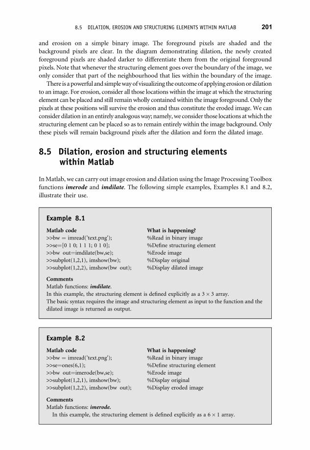
and erosion on a simple binary image. The foreground pixels are shaded and the

background pixels are clear. In the diagram demonstrating dilation, the newly created

foreground pixels are shaded darker to differentiate them from the original foreground

pixels. Note that whenever the structuring element goes over the boundary of the image, we

only consider that part of the neighbourhood that lies within the boundary of the image.

There is apowerful and simplewayof visualizing theoutcomeof applying erosionordilation

to an image. For erosion, consider all those locations within the image at which the structuring

element can be placed and still remainwholly containedwithin the image foreground.Only the

pixels at these positions will survive the erosion and thus constitute the eroded image. We can

consider dilation in an entirely analogousway; namely,we consider those locations atwhich the

structuring element can be placed so as to remain entirely within the image background. Only

these pixels will remain background pixels after the dilation and form the dilated image.

8.5 Dilation, erosion and structuring elementswithin Matlab

InMatlab, we can carry out image erosion and dilation using the Image Processing Toolbox

functions imerode and imdilate. The following simple examples, Examples 8.1 and 8.2,

illustrate their use.

Example 8.1


>>bw ¼ imread('text.png'); %Read in binary image

>>se¼[0 1 0; 1 1 1; 0 1 0]; %Define structuring element

>>bw out¼imdilate(bw,se); %Erode image

>>subplot(1,2,1), imshow(bw); %Display original

>>subplot(1,2,2), imshow(bw out); %Display dilated image

Comments

Matlab functions: imdilate.

In this example, the structuring element is defined explicitly as a 3� 3 array.

The basic syntax requires the image and structuring element as input to the function and the

dilated image is returned as output.

Example 8.2


>>bw ¼ imread('text.png'); %Read in binary image

>>se¼ones(6,1); %Define structuring element

>>bw out¼imerode(bw,se); %Erode image

>>subplot(1,2,1), imshow(bw); %Display original

>>subplot(1,2,2), imshow(bw out); %Display eroded image

Comments

Matlab functions: imerode.

In this example, the structuring element is defined explicitly as a 6� 1 array.

8.5 DILATION, EROSION AND STRUCTURING ELEMENTS WITHIN MATLAB 201

Explicitly defining the structuring element as in Examples 8.1 and 8.2 is a perfectly

acceptable way to operate. However, the best way to define the structuring element is to use

the Image Processing Toolbox function strel. The basic syntax is

� se ¼ strelð‘shape’; ‘parameters’Þ

where shape is a string that defines the required shape of the structuring element and

parameters is a list of parameters that determine various properties, including the size.

Example 8.3 shows how structuring elements generated using strel are then supplied along

with the target image as inputs to imdilate and imerode.

Example 8.3


bw ¼ imread('text.png'); %Read in binary image

se1 ¼ strel('square',4) %4 by 4 square

se2 ¼ strel('line',5,45) %line, length 5, angle 45 degrees

bw 1¼imdilate(bw,se1); %Dilate image

bw 2¼imerode(bw,se2); %Erode image

subplot(1,2,1), imshow(bw 1); %Display dilated image

subplot(1,2,2), imshow(bw 2); %Display eroded image

Comments

Matlab functions: strel.

This example illustrates the use of the Image Processing Toolbox function strel to define two

different types of structuring element and demonstrates their effects by dilating and eroding an

image.

Type doc strel at the Matlab prompt for full details of the structuring elements that can be

generated.

Use of the image processing toolbox function strel is recommended for two reasons.

First, all the most common types of structuring element can be specified directly as input

and it is rare that one will encounter an application requiring a structuring element that

cannot be specified directly in this way. Second, it also ensures that the actual computation

of the dilation or erosion is carried out in the most efficient way. This optimal efficiency

relies on the principle that dilation by large structuring elements can often actually be

achieved by successive dilation with a sequence of smaller structuring elements, a process

known as structuring element decomposition. Structuring element decomposition results in a

computationally more efficient process and is performed automatically whenever function

strel is called.

8.6 Structuring element decomposition and Matlab

It is important to note from these examples that the function strel does not return a normal

Matlab array, but rather an entity known as a strel object. The strel object is used to enable


the decomposition of the structuring element to be stored together with the desired

structuring element.

The example below illustrates how Matlab displays when a strel object is created:

>> se3 = strel(’disk,5’); % A disk of radius 5

se3 =

Flat STREL object containing 69 neighbors.

Decomposition: 6 STREL objects containing a total of 18

neighbors

Neighborhood:

0 0 1 1 1 1 1 0 0

0 1 1 1 1 1 1 1 0

1 1 1 1 1 1 1 1 1

1 1 1 1 1 1 1 1 1

1 1 1 1 1 1 1 1 1

1 1 1 1 1 1 1 1 1

1 1 1 1 1 1 1 1 1

0 1 1 1 1 1 1 1 0

0 0 1 1 1 1 1 0 0

This is basically telling us two things:

. The neighbourhood is the structuring element that you have created and will effectively

be applied; it has 69 nonzero elements (neighbours).

. The decomposition of this neighbourhood (to improve the computational efficiency of

dilation) results in six smaller structuring elements with a total of only 18 nonzero

elements.Thus, successive dilation by each of these smaller structuring elements will achieve

the same result with less computation. Since the computational load is proportional to the

number of nonzero elements in the structuring element, we expect the execution time to

be approximately 18/69 of that using the original form. This is the whole purpose of

structuring element decomposition.

If required, the function getsequence can be applied to find out what precisely these

smaller structuring elements are. Try

>> decomp=getsequence(se3); whos decomp

The structuring elements of the decomposition can be accessed by indexing into

decomp; e.g.:

>> decomp(1)

8.6 STRUCTURING ELEMENT DECOMPOSITION AND MATLAB 203

produces an output

ans =


Neighborhood:

1

1

1

>> decomp(2)

produces an output

ans =


Neighborhood:

1 0 0

0 1 0

and so on.

When you supply the strel object returned by the function strel to the functions imdilate

and imopen, the decomposition of the structuring element is automatically performed.

Thus, in the majority of cases, there is actually no practical need to concern oneself with the

details of the structuring element decomposition.

8.7 Effects and uses of erosion and dilation

It is apparent that erosion reduces the size of a binary object, whereas dilation increases it.

Erosion has the effect of removing small isolated features, of breaking apart thin, joining

regions in a feature and of reducing the size of solid objects by ‘eroding’ them at the

boundaries. Dilation has an approximately reverse effect, broadening and thickening

narrow regions and growing the feature around its edges. Dilation and erosion are the

reverse of each other, although they are not inverses in the strict mathematical sense. This is

because we cannot restore by dilation an object which has previously been completely

removed by erosion. Whether it is dilation or erosion (or both) that is of interest, we stress

that the appropriate choice of structuring element is often crucial and will depend strongly


on the application. In particular, we generally seek to contrive structuring elements which are

sensitive to specific shapes or structures and, therefore, identify, enhance or delete them.

One of the simplest applications of dilation is to join together broken lines which form a

contour delineating a region of interest. For example, the effects of noise, uneven

illumination and other uncontrollable effects often limit the effectiveness of basic segmen-

tation techniques (e.g. edge detection). In our chosen example, taken from the field of space

debris studies, a 3-D depth map of an impact crater caused by a high-velocity, micro-sized

aluminium particle has been obtained with a scanning electron microscope. This is

displayed at the top left in Figure 8.5. The binary image (top right in Figure 8.5) resulting

from edge detection using a Sobel kernel (Section 4.5.2) is reasonably good, but there are a

number of breaks in the contour defining the impact region. In this particular example, the

aimwas to define the impact region of such craters automatically in order to express the 3-D

depth map as an expansion over a chosen set of 2-D orthogonal functions. We can achieve

this task in three simple steps.

(1) Dilate the edge map until the contour is closed.

(2) Fill in the background pixels enclosed by the contour. This is achieved by a related

morphological method called region filling which is explained in Section 8.11.

(3) Erode the image (the same number of times as we originally dilated) to maintain the

overall size of the delineated region.

Our second example is illustrated in Figure 8.6 (which is produced by the Matlab code

produced in Example 8.4) and demonstrates the importance of choosing an appropriate

structuring element for the given task at hand. Figure 8.6a depicts the layout of a printed

Figure 8.5 Illustrating a simple use of dilation to join small breaks in a defining contour (image

courtesy of C.J. Solomon, M. Seeger, L. Kay and J. Curtis, ‘Automated compact parametric representa-

tion of impact craters’ Int. J. Impact Eng., vol. 21, no. 10, 895–904 (1998))

8.7 EFFECTS AND USES OF EROSION AND DILATION 205

Figure 8.6 Using dilation and erosion to identify features based on shape: (a) original; (b) result

after thresholding; (c) After erosion with horizontal line. (d) after erosion with vertical line;

(e) after dilation with same vertical and horizontal lines; (f) boundary of remaining objects super-

imposed on original

Example 8.4


>>length¼18; tlevel¼0.2; %Define SE and percent

threshold level

>>A¼imread('circuit.tif'); subplot(2,3,1), imshow(A) %Read image and display

>>B¼im2bw(A,tlevel); subplot(2,3,2), imshow(�B); %Threshold image and

display

>>SE¼ones(3,length); bw1¼imerode(�B,SE); %Erode vertical lines

>>subplot(2,3,3), imshow(bw1); %Display result

>>bw2¼imerode(bw1,SE'); subplot(2,3,4), imshow(bw2); %Erode horizontal lines

>>bw3¼imdilate(bw2,SE');bw4¼imdilate(bw3,SE); %Dilate back

>>subplot(2,3,5), imshow(bw4); %Display

>>boundary¼bwperim(bw4);[i,j]¼find(boundary); %Superimpose boundaries

>> subplot(2,3,6), imshow(A); hold on; plot(j,i,'r.');

Comments

Matlab functions: bwperim.

This function produces a binary image consisting of the boundary pixels in the input

binary image.


circuit in which there are two types of object: the rectangular chips and the horizontal and

vertical conduction tracks. The aim is to identify (i.e. segment) the chips automatically. The

microprocessor chips and the tracks are darker than the background and can be identified

reasonably well by simple intensity thresholding (see Figure 8.6b). The thin vertical tracks

can first be removed by eroding with a suitable long horizontal structuring element. As is

evident (see Figure 8.6c), the horizontal structuring element used here (a 3� 18 array of 1s)

tends to preserve horizontal lines but remove thin vertical ones. Analogously, we can

remove horizontal lines (see Figure 8.6d) using an appropriate vertical structuring element

(an 18� 3 array of 1s). These two erosions tend to remove most of the thin horizontal and

vertical lines. They leave intact the rectangular chips but have significantly reduced their

size. We can remedy this by now dilating twice with the same structuring elements

(Figure 8.6e). The boundaries of the structures identified in this way are finally super-

imposed on the original image for comparison (Figure 8.6f). The result is quite good

considering the simplicity of the approach (note the chip in the centre was not located

properly due to poor segmentation from thresholding).

8.7.1 Application of erosion to particle sizing

Another simple but effective use of erosion is in granulometry - the counting and sizing of

granules or small particles. This finds use in a number of automated inspection applications.

The typical scenario consists in having a large number of particles of different size but

approximately similar shape and the requirement is to rapidly estimate the probability

distribution of particle sizes. In automated inspection applications, the segmentation step in

which the individual objects are identified is often relatively straightforward as the image

background, camera view and illumination can all be controlled.

We begin the procedure by first counting the total number of objects present. The image

is then repeatedly eroded using the same structuring element until no objects remain. At

each step in this procedure, we record the total number of objects F which have been

removed from the image as a function of the number of erosions n. Now it is clear that the

number of erosions required tomake an object vanish is directly proportional to its size; thus,

if the object disappears at the kth erosion we can say that its size X � ak, where a is some

proportionality constant determined by the structuring element.2 This process thus

allows us to form an estimate of F(X) which is essentially a cumulative distribution

function (CDF) of particle size, albeit unnormalized.

Elementary probability theory tells us that the CDF and the probability density function

(PDF) are related as:

FðXÞ ¼ðX

1pðxÞ dx pðxÞ ¼ dF

dX

��x

2 This is not an exact relationship as we have not properly defined ‘size’. The astute reader will recognize that its

accuracy depends on the shape of the objects and of the structuring element. However, provided the structuring

element is of the same approximate shape as the particles (a normal condition in such applications), it is a good

approximation.

8.7 EFFECTS AND USES OF EROSION AND DILATION 207

Thus, by differentiating FðXÞ, wemay obtain an estimate of the particle size distribution.

As the structuring element is necessarily of finite size in a digital implementation, X is a

discrete variable. Therefore, it can be useful in certain instances to form a smooth

approximation to FðXÞ by a fitting technique before differentiating to estimate the PDF.

Morphological operations can be implemented very efficiently on specialist hardware,

andsooneof theprimaryattractionsof this simpleprocedure is its speed.Figure8.7 illustrates

the essential approach using a test image. The Matlab code which generates Figure 8.7 is

given in Example 8.5 (note that the estimated distribution and density functions remain

unnormalized in this code)

Figure 8.7 Using repeated erosion and object counting to estimate the distribution of particle sizes:

(a) original image; (b) binary image resulting from intensity thresholding; (c) estimated cumula-

tive distribution (unnormalized); (d) estimated size density function (unnormalized)

Example 8.5


A¼imread('enamel.tif'); subplot(1,3,1), imshow(A); %Read in image and display

bw¼�im2bw(A,0.5); bw ¼ imfill(bw,'holes'); %Threshold and fill in holes

subplot(1,3,2), imshow(bw); %Display resulting binary image

[L,num 0]¼bwlabel(bw); %Label and count number of

objects

%in binary image


8.8 Morphological opening and closing

Opening is the name given to the morphological operation of erosion followed by dilation

with the same structuring element. We denote the opening of A by structuring element B as

A B ¼ ðA� BÞ � B.

The general effect of opening is to remove small, isolated objects from the foreground of

an image, placing them in the background. It tends to smooth the contour of a binary object

and breaks narrow joining regions in an object.

Closing is the name given to the morphological operation of dilation followed by erosion

with the same structuring element. We denote the closing of A by structuring element B as

A .B ¼ ðA� BÞ � B.

Closing tends to remove small holes in the foreground, changing small regions of

background into foreground. It tends to join narrow isthmuses between objects.

On initial consideration of these operators, it is not easy to see how they can be useful or

indeed why they differ from one another in their effect on an image. After all, erosion and

dilation are logical opposites and superficial consideration would tempt us to conclude that

it will make little practical difference which one is used first? However, their different effects

stems from two simple facts.

se¼strel('disk',2); %Define structuring element,

radius¼2

count ¼0; %Set number of erosions ¼ 0

num¼num 0; %Initialise number of objects in

image

while num>0 %Begin iterative erosion

count¼countþ 1

bw¼imerode(bw,se); %Erode

[L,num]¼bwlabel(bw); %Count and label objects

P(count)¼num 0 num; %Build discrete distribution

figure(2); imshow(bw); drawnow; %Display eroded binary image

end

figure(2); subplot(1,2,1), plot(0:count,[0 P],'ro'); %Plot Cumulative distribution

axis square;axis([0 count 0 max(P)]); %Force square axis

xlabel('Size'); ylabel('Particles removed') %Label axes

subplot(1,2,2), plot(diff([0 P]),'k'); axis square; %Plot estimated size density

function

Comments

Matlab functions: bwlabel, imfill.

The function bwlabel analyses an input binary image so as to identify all the connected

components (i.e. objects) in the image. It returns a so called labelled image in which all the pixels

belonging to the first connected component are assigned a value 1, all the pixels belonging to the

second connected component are assigned a value 2 and so on. The function imfill identifies the

pixels constituting holes within connected components and fills them (ie. sets their value to 1).

8.8 MORPHOLOGICAL OPENING AND CLOSING 209

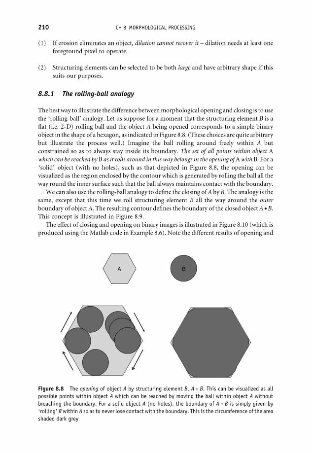
(1) If erosion eliminates an object, dilation cannot recover it – dilation needs at least one

foreground pixel to operate.

(2) Structuring elements can be selected to be both large and have arbitrary shape if this

suits our purposes.

8.8.1 The rolling-ball analogy

The bestway to illustrate the difference betweenmorphological opening and closing is to use

the ‘rolling-ball’ analogy. Let us suppose for a moment that the structuring element B is a

flat (i.e. 2-D) rolling ball and the object A being opened corresponds to a simple binary

object in the shape of a hexagon, as indicated in Figure 8.8. (These choices are quite arbitrary

but illustrate the process well.) Imagine the ball rolling around freely within A but

constrained so as to always stay inside its boundary. The set of all points within object A

which can be reached byB as it rolls around in this way belongs in the opening ofAwith B. For a

‘solid’ object (with no holes), such as that depicted in Figure 8.8, the opening can be

visualized as the region enclosed by the contour which is generated by rolling the ball all the

way round the inner surface such that the ball always maintains contact with the boundary.

We can also use the rolling-ball analogy to define the closing ofA by B. The analogy is the

same, except that this time we roll structuring element B all the way around the outer

boundary of objectA. The resulting contour defines the boundary of the closed objectA .B.

This concept is illustrated in Figure 8.9.

The effect of closing and opening on binary images is illustrated in Figure 8.10 (which is

produced using the Matlab code in Example 8.6). Note the different results of opening and

Figure 8.8 The opening of object A by structuring element B, A B. This can be visualized as all

possible points within object A which can be reached by moving the ball within object A without

breaching the boundary. For a solid object A (no holes), the boundary of A B is simply given by

‘rolling’ Bwithin A so as to never lose contact with the boundary. This is the circumference of the area

shaded dark grey


Figure 8.9 The closing of object A by structuring element B, A . B. This can be visualized as all

possible points contained within the boundary defined by the contour as B is rolled around the outer

boundary of object A. Strictly, this analogy holds only for a ‘solid’ object A (one containing no holes)

Figure 8.10 Illustrating the effects of opening and closing upon some example shapes. The original

image shown in the centre was opened using disk-shaped structuring elements of radii 3, 5 and 15

pixels, producing the images to the left. The images to the right were similarly produced by closing the

image using the same structuring elements. The differences become more pronounced the larger the

structuring element employed

8.8 MORPHOLOGICAL OPENING AND CLOSING 211

closing on the test objects and how this becomes more pronounced as the structuring

element increases in size.

Example 8.6


A¼imread('openclose shapes.png');

A¼�logical(A);

%Read in image and convert to binary

se¼strel('disk',3); bw1¼imopen(A,se);

bw2¼imclose(A,se);

%Define SEs then open and close

subplot(3,2,1), imshow(bw1); subplot(3,2,2),

imshow(bw2);

%Display results


bw2¼imclose(A,se);



imshow(bw2);

%Display results


bw2¼imclose(A,se);



imshow(bw2);

%Display results

Comments

Matlab functions: imopen, imclose.

The Image Processing Toolbox provides functions to carry outmorphological opening and

closing on both binary and grey scale images.

We have seen how the basic morphological operators of dilation and erosion can be

combined to define opening and closing. They can also be used together with simple logical

operations to define a number of practical and useful morphological transforms. In the

following sections we discuss some of the most important examples.

8.9 Boundary extraction

We can define the boundary of an object by first eroding the object with a suitable small

structuring element and then subtracting the result from the original image. Thus, for a

binary image A and a structuring element B, the boundary AP is defined as

AP ¼ A�A� B ð8:1Þ

The example in Figure 8.11 (the Matlab code for which is given in Example 8.7) illustrates

the process. Note that the thickness of the boundary can be controlled through the specific

choice of the structuring element B in Equation (8.1).


Example 8.7


A¼imread('circles.png'); %Read in binary image

bw¼bwperim(A); %Calculate perimeter

se¼strel('disk',5); bw1¼A imerode(A,se); %se allows thick perimeter extraction


subplot(1,3,2), imshow(bw);

subplot(1,3,3), imshow(bw)1; %Display results

Comments

Matlab functions: bwperim, imerode.

Boundary extraction which is a single pixel thick is implemented in the Matlab Image

Processing Toolbox through the function bwperim. Arbitrary thickness can be obtained by

specifying an appropriate structuring element.

8.10 Extracting connected components

Earlier in this chapter we discussed the 4-connection and 8-connection of pixels. The set of

all pixels which are connected to a given pixel is called the connected component of that pixel.

A group of pixels which are all connected to each other in this way is differentiated from

others by giving it a unique label. Typically, the process of extracting connected components

leads to a new image in which the connected groups of pixels (the objects) are given

sequential integer values: the background has value 0, the pixels in the first object have value

1, the pixels in the second object have value 2 and so on. To identify and label 8-connected

components in a binary image, we proceed as follows:

. Scan the entire image by moving sequentially along the rows from top to bottom.

. Whenever we arrive at a foreground pixel p we examine the four neighbours of p

which have already been encountered thus far in the scan. These are the neighbours (i)

to the left of p, (ii) above p, (iii) the upper left diagonal and (iv) the upper right

diagonal.

Figure 8.11 Boundary extraction. Left: original.; centre: single-pixel boundary; right: thick

boundary extracted through use of larger structuring element

8.10 EXTRACTING CONNECTED COMPONENTS 213

The labelling of p occurs as follows:

. if all four neighbours are background (i.e. have value 0), assign a new label to p; else

. if only one neighbour is foreground (i.e. has value 1), assign its label to p; else

. ifmore than one of the neighbours is foreground, assign one of the labels to p and resolve

the equivalences.

An alternative method exists for extracting connected components which is based on a

constrained region growing. The iterative procedure is as follows.

Let A denote our image, x0 be an arbitary foreground pixel identified at the beginning of

the procedure, xk the set of connected pixels existing at the kth iteration and B be a

structuring element. Apply the following iterative expression:

Do xk ¼ ðxk 1 � BÞ \ A k ¼ 1; 2; 3; . . .until xk ¼ xk 1

ð8:2Þ

The algorithm thus starts by dilating from a single pixel within the connected component

using the structuring element B. At each iteration, the intersection with A ensures that no

pixels are included which do not belong to the connected component. When we reach the

point at which a given iteration produces the same connected component as the previous

iteration (i.e. xk ¼ xk 1), all pixels belonging to the connected component have been found.

This is repeated for another foreground pixel which is again arbitrary except that it must

not belong to the connected components found this far. This procedure continues until all

foreground pixels have been assigned to a connected component.

Extracting connected components is a very common operation, particularly in auto-

mated inspection applications. Extracting connected components can be achieved with

the Matlab Image Processing Toolbox function bwlabel. A simple example is given in

Example 8.8 and Figure 8.12.

Example 8.8


bw¼imread('basic shapes.png'); %Read in image

[L,num]¼bwlabel(bw); %Get labelled image and number

%of objects

subplot(1,2,1), imagesc(bw); axis image; axis off; %Plot binary input image

colorbar('North'); subplot(1,2,2), imagesc(L); %Display labelled image

axis image; axis off; colormap(jet); colorbar('North')

Comments

The function bwlabel returns a so called labelled image inwhich all the pixels belonging to the

first connected component are assigned a value 1, the pixels belonging to the second connected

component are assigned a value 2 and so on.


8.11 Region filling

Binary images usually arise in image processing applications as the result of thresholding or

some other segmentation procedure on an input grey-scale or colour image. These

procedures are rarely perfect (often due to uncontrollable variations in illumination

intensity) and may leave ‘holes’, i.e. ‘background’ pixels within the binary objects that

emerge from the segmentation. Filling the holes within these objects is often desirable in

order that subsequent morphological processing can be carried out effectively.

Assume that we have a binary object A within which lies one or more background pixels

(a hole). Let B be a structuring element and let x0 be a ‘seed’ background pixel lying within

the hole (for the moment, we gloss over the question of how we find x0 in the first place).

Setting x0 to be foreground (value 1) to initialize the procedure, the hole may be filled by

applying the following iterative expression:

Do xk ¼ ðxk 1 � BÞ \ A where k ¼ 1; 2; 3; . . .until xk ¼ xk 1

ð8:3Þ

The filled region is then obtained as A [ xk.

The algorithm thusworks by identifying a point (x0)within the hole and then growing this

region by successive dilations. After each dilation, we take the intersection (logical AND)

with the logical complement of the object A. Without this latter step, the filled region would

simply grow and eventually occupy the entire image. Taking the intersection with the

complement ofA only allows the object to growwithin the confines of the internal boundary.

When the region has grown to the extent that it touches the boundary at all points, the next

iteration will grow the region into the boundary itself. However, the intersection with A will

produce the same pixel set as the previous iteration, atwhichpoint the algorithmstops.3 In the

final step, the union of A with the grown region gives the entire filled object.

Figure 8.12 Connected components labelling. The image displayed on the left is a binary image

containing five connected components or objects. The image displayed on the right is a ‘label matrix’

in which the first group of connected pixels is assigned a value of 1, the second group a value of 2 and

so on. The false-colour bar indicates the numerical values used

3 The astute reader will note that this is true provided the dilation only extends the growing region into and not

beyond the boundary. For this reason, the structuring element must not be larger than the boundary thickness.

8.11 REGION FILLING 215

Now, a hole is defined as a set of connected, background pixels that cannot be reached by

filling in the background from the edge of the image. So far, we have glossed over how we

formally identify the holes (and thus starting pixels x0 for Equation (8.3)) in the first place.

Starting from a background pixel x0 at the edge of the image, we apply exactly the same

iterative expression Equation (8.3):

Do xk ¼ ðxk 1 � BÞ \ A where k ¼ 1; 2; 3; . . .until xk ¼ xk 1

The complete set of pixels belonging to all holes is then obtained asH ¼ ðA [ xkÞ. The seedpixels x0 for the hole-filling procedure described by Equation (8.3) can thus be obtained by:

(i) sampling arbitrarily fromH; (ii) applying Equation (8.3) to fill in the hole; (iii) removing

the set of filled pixels resulting from step (ii) fromH; (iv) repeating (i)–(iii) untilH is empty.

Region filling is achieved in the Matlab Image Processing Toolbox through the function

imfill (see Example 8.2).

8.12 The hit-or-miss transformation

The hit-or-miss transform indicates the positions where a certain pattern (characterized by

a structuring element B) occurs in the input image. As such, it operates as a basic tool for

shape detection. This technique is best understood by an illustrative example. Consider

Figure 8.13, in which we depict a binary image A alongside a designated ‘target’ pixel

configuration B (foreground pixels are shaded). The aim is to identify all the locations

within the binary imageA at which the target pixel configuration defined by B can be found.

It is important to stress that we are seeking the correct combination of both foreground

(shaded) and background (white) pixels, not just the foreground, and will refer to this

combination of foreground and background as the target shape. The reader should note that

by this definition the target shape occurs at just one location within image A in Figure 8.13.

Recalling our earlier definitions, it is readily apparent that the erosion of image A by the

target shape B1 will preserve all those pixels in image A at which the foreground pixels of the

target B1 can be entirely contained within foreground pixels in the image. These points are

indicated in Figure 8.14 as asterisks and are designated as ‘hits’. In terms of our goal of

finding the precise target shape B1, the hits thus identify all locations at which the correct

Figure 8.13 The hit-or-miss transformation. The aim is to identify those locations within an image

(right) at which the specified target configuration of pixels or target shape (left) occurs


configuration of foreground pixels are found. However, this step does not test for the

required configuration of background pixels in B1.

Consider now Figure 8.15. This depicts the logical complement of image A together with

a target pixel configuration B2 which is the logical complement of B1 (i.e. B2 ¼ B1).

Consider now applying A� B2, namely erosion of the image complement A by the

complement of the target shape B2. By definition, this erosion will preserve all those pixels at

which the foreground pixels of the target complement B2 can be entirely contained within

the foreground pixels of the image complement A. These points are indicated in Figure 8.16

as crosses and are designated as ‘misses’. Note, however, that because we have carried out

the erosion using the complements of the target and image, this second step logically

translates to the identification of all those locations at which the background pixel configura-

tion of the target is entirely contained within the background of the image. The misses thus

identify all locations at which the correct configuration of background pixels are found but

does not test for the required configuration of foreground pixels.

The first step has identified all those points in the image foreground atwhich the required

configuration of foreground pixels in the target may be found (but has ignored the required

background configuration). By contrast, the second step has identified all those points in the

image background at which the required configuration of background pixels in the target

may be found (but has ignored the required foreground configuration). It follows,

therefore, that any point identified by both of these steps gives a location for the target

configuration. Accordingly, the third and final step in the process is to take a logical

intersection (AND) of the two images. Thus, the hit-or-miss transformation of A by B1 is

Figure 8.14 The hit-or-miss transformation. The first step is erosion of the image by the target

configuration. This produces the hits denoted by asterisks

Figure 8.15 The hit-or-miss transformation. For the second step where we locate the misses, we

consider the complement of the image A and the complement of the target shape B2 ¼ B1

8.12 THE HIT OR MISS TRANSFORMATION 217

formally defined as:

A� B ¼ ðA� BÞ \ ðA� BÞ ð8:4Þ

The result obtained for our example is indicated in Figure 8.17. The sole surviving pixel

(shaded) gives the only location of the target shape to be found in the image.

In summary then, the hit-or-miss transformation identifies those locations atwhich both

the defining foreground and background configurations for the target shape are to be

simultaneously found – in this sense, themethodmightmore properly be called the hit-and-

miss, but the former title is themost common. Example 8.9 and Figure 8.18 illustrate the use

of the hit-and-miss transform to identify the occurrences of a target letter ‘e’ in a string

of text.

Note that the two structuring elements B1 and B2 described in our account so far of the

hit-or-miss transform are logical complements. This means that only exact examples of the

target shape (including background and foreground pixel configurations) are identified. If

even one pixel of the configuration probed in the image differs from the target shape, then

the hit-or-miss transform we have used will not identify it (see Figure 8.19).

Figure 8.16 The hit-or-miss transformation. The second step consists of eroding the complement of

the image A by the complement of the target shape ðB2 ¼ B1Þ. This produces themisses denoted hereby crosses

Figure 8.17 The hit-or-miss transformation. The final step takes the intersection (logical AND) of

the two eroded images ðA� BÞ \ ðA� BÞ. Any surviving pixels give the location of the target shape inthe original image A


Example 8.9


imread('text.png'); %Read in text

B¼imcrop(A); %Read in target shape interactively

se1¼B; se2¼�B; %Define hit and miss structure elements

bw¼bwhitmiss(A,se1,se2); %Perform hit miss transformation

[i,j]¼find(bw¼¼1); %Get explicit coordinates of locations


subplot(1,3,2), imagesc(B); axis image;

axis off;

%Display target shape

subplot(1,3,3), imshow(A); hold on;

plot(j,i,'r');%Superimpose locations on image

Comments

Matlab functions: bwhitmiss.

TheMatlab Image Processing Toolbox has a purpose made function for carrying out the hit

or miss transformation: bwhitmiss. This example illustrates its use to identify the occurrences of

a target letter ‘e’ in a string of text.

8.12.1 Generalization of hit-or-miss

The hit-or-miss transformation given by Equation (8.4) and demonstrated in Example 8.9 was

chosen to be relatively straightforward to understand.However, it is important to stress that it is

actually a special case. The most general form of the hit-or-miss transformation is given by

A� B ¼ ðA� B1Þ \ ðA� B2Þ where B ¼ ðB1;B2Þ ð8:5Þ

B ¼ ðB1;B2Þ signifies a pair of structuring elements andB2 is a general structuring element that

is not necessarily the complement of B1 but which is mutually exclusive (i.e. B1 \ B2 ¼ ˘, the

empty set). By allowing the second structuring element B2 to take on forms other than the

complement of B1, we can effectively relax the constraint that the hit-or-miss operation only

identifies the exact target shape and widen the scope of the method. This relaxation of the

Figure 8.18 Application of the hit-or-miss transformation to detect a target shape in a string of

text. Note that the target includes the background and hit-or-miss is strictly sensitive to both the

scale and the orientation of the target shape (See colour plate section for colour version)

8.12 THE HIT OR MISS TRANSFORMATION 219

Figure 8.19 The fully constrained hit-or-miss transform is sensitive to noise and uncontrolled

variations in the target feature. In the example above, three instances of the target letter �e� on thesecond line were missed due to the presence of a small amount of random noise in the image

method can make it less sensitive to noise and small but insignificant variations in the shape.

Note that, in the limiting case where B2 is an empty structuring element, hit-or-miss transforma-

tion reduces to simple erosion by B1. We discuss this generalization of hit-or-miss next.

8.13 Relaxing constraints in hit-or-miss: ‘don’t care’ pixels

It is apparent that the application of the hit-or-miss transformation as carried out

in Figure 8.19 is ‘unforgiving’, since a discrepancy of even one pixel between the target

shape and the probed region in the image will result in the target shape being missed. In

many cases, it is desirable to be less constrained and allow a combination of foreground and

background pixels that is ‘sufficiently close’ to the target shape to be considered as a match.

We can achieve this relaxation of the exact match criterion through the use of ‘don’t care’

pixels (also known as wild-card pixels). In other words, the target shape now conceptually

comprises three types of pixel: strict foreground, strict background and ‘don’t care’. In the

simple example shown in Figure 8.20 (produced using theMatlab code in Example 8.10), we

consider the task of automatically locating the ‘upper right corners’ in a sample of shapes.

Example 8.10


A¼imread

Noisy Two Ls.png');

%CASE 1

se1¼[0 0 0; 1 1 0; 0 1 0]; %SE1 defines the hits

se2¼[1 1 1; 0 0 1; 0 0 1]; %SE2 defines the misses

bw¼bwhitmiss(A,se1,se2); %Apply hit or miss transform

subplot(2,2,1), imshow(A,[0 1]); %Display Image

subplot(2,2,2), imshow(bw,[0 1]); %Display located pixels

%NOTE ALTERNATIVE SYNTAX


interval¼[ 1 1 1; 1 1 1; 0 1 1]; %1s for hits, 1 for misses; 0s for don't

care

bw¼bwhitmiss(A,interval); %Apply hit or miss transform


%CASE 2

interval¼[0 1 1; 0 1 1; 0 0 0]; %1s for hits, 1 for misses; 0s for don't

care

bw¼bwhitmiss(A,interval); %Apply hit or miss transform


Comments

Note that bw2 ¼ bwhitmiss(bw,interval) performs the hit miss operation

defined in terms of a single array, called an ‘interval’. An interval is an array

whose elements can be 1, 0 or 1. The 1 valued elements specify the domain

of the first structuring element SE1 (hits); the 1 valued elements specify

the domain of the second structuring element SE2 (misses); the 0 valued

elements, which act as ‘don't care’ pixels, are ignored.

Figure 8.20 Generalizing the hit-or-miss transform. This illustrates the effect of relaxing con-

straints on the hit-or-miss transform. Top left: original image. Top right and bottom left (which uses

an alternative computation): the result of hit-or-miss for strict definition of upper right corner pixels –

only the upper right corner pixels of the solid L shapes are identified. Bottom right: in the second

(relaxed) case, the noisy pixels are also identified

8.13 RELAXING CONSTRAINTS IN HIT OR MISS: ‘DON’T CARE’ PIXELS 221

In the example shown in Figure 8.20, we consider two definitions for upper right corner

pixels:

(1) A strict definition which requires that an ‘upper right corner pixel’ must have no

neighbours to north, north-west, north-east or east (these are themisses) andmust have

neighbours to the south and west (these are the hits). The south-west neighbour is

neither hit nor miss and, thus, a don’t care pixel.

(2) A looser definition which only requires that an upper right corner pixel must have no

neighbours to north, north-west and north-east (the misses). All other neighbours are

‘don’t care’ pixels.

The differing effects of both definitions are shown in Figure 8.20 using the hit and miss

transform.

8.13.1 Morphological thinning

Closely related to the hit-or-miss transformation, the thinning of an image A by a

structuring element B is defined as

thinðA;BÞ ¼ A \ A� B

where A� B is the hit-or-miss transformation of A with B. The thinning of A with B is

calculated by successively translating the origin of the structuring element to each pixel in

the image and comparing it with the underlying image pixels. If both the foreground and

background pixels in the structuring element exactly match those in the underlying image,

then the image pixel underneath the origin of the structuring element is set to background

(zero). If no match occurs, then the pixel is left unchanged. Thinning is a key operation in

practical algorithms for calculating the skeleton of an image.

8.14 Skeletonization

Rather as its name implies, the skeleton of a binary object is a representation of the basic form

of that object which has been reduced down to its minimal level (i.e. a ‘bare bones’

representation). A very useful conceptualization of the morphological skeleton is provided

by the prairie-fire analogy: the boundary of an object is set on fire and spreads with uniform

velocity in all directions inwards; the skeleton of the object will be defined by the points at

which the fire fronts meet and quench (i.e. stop) each other.

Consider an arbitrary, binary object A. A point pwithin this binary object belongs to the

skeleton of A if and only if the two following conditions hold:

(1) A disk Dz may be constructed, with p at its centre, that lies entirely within A and

touches the boundary of A at two or more places.

(2) No other larger disk exists that lies entirely within A and yet contains Dz.


An equivalent geometric construction for producing the skeleton is to:

(1) Start at an arbitrary point on the boundary and consider themaximumpossible size of

disk which can touch the boundary at this point and at least one other point on the

boundary and yet remain within the object.

(2) Mark the centre of the disk.

(3) Repeat this process at all points along the entire boundary (moving in infinitesimal

steps) until you return to the original starting point. The trace or locus of all the disk

centre points is the skeleton of the object.

Figure 8.21 shows a variety of different shapes and their calculated skeletons. Consider-

ation of the calculated skeletons in Figure 8.21 should convince the reader that the circle is

actually slightly elliptical and that the pentagon and star are not regular.

The skeleton is a useful representation of the object morphology, as it provides both

topological information and numerical metrics which can be used for comparison and

categorization. The topology is essentially encapsulated in the number of nodes (where

branches meet) and number of end points and the metric information is provided by the

lengths of the branches and the angles between them.

Figure 8.21 Some shapes and their corresponding morphological skeletons

8.14 SKELETONIZATION 223

Aweakness of the skeleton as a representation of a shape is that it is sensitive (sometimes

highly) to small changes in the morphology. Slight irregularities in a boundary can lead to

spurious ‘spurs’ in the skeleton which can interfere with recognition processes based on

the topological properties of the skeleton. So-called pruning can be carried out to remove

spurs of less than a certain length, but this is not always effective as small perturbations in the

boundary of an image can sometimes lead to large spurs in the skeleton.

Actual computation of a skeleton can proceed in a number of ways. The preferred

method is based on an iterative thinning algorithm whose details we do not repeat here. As

well its use in a variety of image segmentation tasks, skeletonization has been usefully

applied in a number of medical applications, such as unravelling the colon and assessment

of laryngotracheal stenosis.

8.15 Opening by reconstruction

One simple but useful effect of morphological opening (erosion followed by dilation) is the

removal of small unwanted objects. By choosing a structuring element of a certain size,

erosion with this element guarantees the removal of any objects within which that

structuring element cannot be contained. The second step of dilation with the same

structuring element acts to restore the surviving objects to their original dimensions.

However, if we consider an arbitrary shape, opening will not exactlymaintain the shape of

the primary objects except in the simplest andmost fortuitous of cases. In general, the larger

the size of the structuring element and the greater the difference in shape between

structuring element and object, the larger the error in the restored shape will be. The

uneven effect on an object of erosion or dilation with a structuring element whose shape is

different from the object itself is referred to as the anisotropy effect. The examples in

Figure 8.22 (generated by Example 8.11) illustrate this effect.

In contrast to morphological opening, opening by reconstruction is a morphological

transformation which enables the objects which survive an initial erosion to be exactly

restored to their original shape. Themethod is conceptually simple and requires two images

which are called themarker and themask. Themask is the original binary image. Themarker

image is used as the starting point of the procedure and is, inmany cases, the image obtained

Figure 8.22 Effects of morphological opening. (a) Original binary image. (b) Result of opening

using a circular structuring element of radius 10. Note the rounding on the points of the star and the

corners of the rectangle. (c) Result of opening using a square structuring element of side length 25.

Only the rectangle is properly restored, the other shapes are significantly distorted


after an initial erosion of the original image. The marker image is then iteratively dilated

using an elementary 3� 3 structuring element with the condition that the output image at

each iteration is given by the intersection (logical AND) of themarker image with themask.

In this way, the mask constrains the marker, never allowing foreground pixels to appear

which were not present in the original image. When the output image which results from a

given iteration is the same as the image resulting from the previous iteration, this indicates

that the dilation is having no further effect and all objects which survived the initial erosion

have been restored to their original state. The procedure then terminates. Formally, we can

describe this procedure by the following simple algorithm:

. denote the marker image by A and the mask image by M;

. define a 3� 3 structuring element of 1s ¼ B;

. iteratively apply Anþ 1 ¼ ðAn � BÞ \M;

. when Anþ 1 ¼ An, stop.

Example 8.12 and Figure 8.23 illustrate the use of morphological reconstruction. We

preserve all alphabetic characters which have a long vertical stroke in a printed text sequence

whilst completely removing all others.

Example 8.12


mask¼�imread('shakespeare.pbm'); %Read in binary text

mask¼imclose(mask,ones(5)); %Close to bridge breaks in letters

se¼strel('line',40,90); %Define vertical se length 40

marker¼imerode(mask,se); %Erode to eliminate characters

im¼imreconstruct(marker,mask); %Reconstruct image

Example 8.11


A¼imread('open shapes.png'); %Read in image

se¼strel('disk',10); bw¼imopen(A,se); %Open with disk radius 10


title('Original Image');

%Display original


title('Opening disk radius¼10');

%Display opened image

se¼strel('square',25); bw¼imopen

(A,se);

%Open with square side 25


title('Opening square side¼25');

%Display opened image

8.15 OPENING BY RECONSTRUCTION 225

subplot(3,1,1), imshow(�mask);

title('Original mask Image');

subplot(3,1,2), imshow(�marker);

title('marker image');

subplot(3,1,3), imshow(�im);

title('Opening by reconstruction');

Comments

Opening by reconstruction is implemented in the Matlab Image Processing Toolbox through

the function imreconstruct.

Note that the �� operator in this example is the logical NOT (inversion) operator being

applied to binary images.

Figure 8.23 Opening by reconstruction. Top: the original text – the mask image. Middle: the text

after erosion by a long, vertical structuring element. This acts as the marker image. Bottom: the image

after opening by reconstruction. Only characters with long vertical strokes have been restored


8.16 Grey-scale erosion and dilation

To date, our discussion has only considered the application of morphology to binary

images. The same basic principles of morphological processing can, however, be extended

to intensity4 images. Just as in the binary case, the building blocks of grey-scale

morphology are the fundamental operations of erosion and dilation. For intensity images,

the definitions of these operators are subtly different and can, in principle, be defined in a

variety of ways. However, in practice, the following (informal) definitions aremore or less

universal.

Grey-scale erosion of image A by structuring element B is denoted A� B and the

operation may be described as follows:

. successively place the structuring element B over each location in the image A;

. for each location, select the minimum value of A�B occurring within the local

neighbourhood defined by the structuring element B.

Grey-scale dilation of image A by structuring element B is denoted A� B and the

operation may be described as follows:

. successively place the structuring element B over each location in the image;

. for each location, select the maximum value of A þ B occurring within the local

neighbourhood defined by the structuring element B.

8.17 Grey-scale structuring elements: general case

Where grey-scale morphology is being considered, structuring elements have, in the most

general case, two parts:

(1) An array of 0s and 1s, where the 1s indicate the domain or local neighbourhood

defined by the structuring element. We denote this by b.

(2) An array of identical size containing the actual numerical values of the structuring

element. We denote this by vb.

To illustrate this general form of grey-scale erosion and dilation, consider the simple

example in Example 8.13.

4 Colour images can also be morphologically processed. Since these simply comprise three 2 D intensity planes

(i.e. the three R,G and B colour channels), our discussion of grey scale morphology will apply to these images too.

8.17 GREY SCALE STRUCTURING ELEMENTS: GENERAL CASE 227

Example 8.13

A structuring element comprising a domain

b ¼0 1 01 1 10 1 0

and values

vb ¼0 3 03 1 30 3 0

is placed on a section of an image given by

A ¼12 13 117 14 810 9 10

Consider positioning the central pixel of the structuring element on the centre pixel of

the image segment (value ¼ 14). What is the value after erosion?

Solution

The value of this pixel after grey-scale erosion is theminimumof the valuesA�nb over

the domain defined by

b ¼ min� 13�3 �7�3 14�1 8�3� 9�3 �

8<:

9=; ¼ min

� 10 �4 13 5� 6 �

8<:

9=; ¼ 4

8.18 Grey-scale erosion and dilation with flatstructuring elements

Although grey-scale morphology can use structuring elements with two parts defining the

neighbourhood b and height values vb respectively, it is very common to use flat structuring

elements. Flat structuring elements have height values which are all zero and are thus

specified entirely by their neighbourhood.

When a flat structuring element is assumed, grey-scale erosion and dilation are

equivalent to local minimum and maximum filters respectively. In other words, erosion

with a flat element results in each grey-scale value being replaced by the minimum value

in the vicinity defined by the structuring element neighbourhood. Conversely, dilation

with a flat element results in each grey-scale value being replaced by the maximum.

Figure 8.24 shows how grey-scale erosion and dilation may be used to calculate a so-called


morphological image gradient. The Matlab code in Example 8.14 was used to produce

Figure 8.24.

Example 8.14


A¼imread('cameraman.tif'); %Read in image

se¼strel(ones(3)); %Define flat structuring element

Amax¼imdilate(A,se); %Grey scale dilate image

Amin¼imerode(A,se); %Grey scale erode image

Mgrad¼Amax Amin; %subtract the two

subplot(1,3,1), imagesc(Amax); axis image; axis off; %Display

subplot(1,3,2), imagesc(Amin); axis image; axis off;

subplot(1,3,3), imagesc(Mgrad); axis image; axis off;

colormap(gray);

It is easy to see why the morphological gradient works: replacing a given pixel by the

minimumormaximumvalue in the local neighbourhood defined by the structuring element

will effect little or no change in smooth regions of the image. However, when the structuring

element spans an edge, the response will be the difference between the maximum and

minimum-valued pixels in the defined region and, hence, large. The thickness of the edges

can be tailored by adjusting the size of the structuring elements if desired.

8.19 Grey-scale opening and closing

Grey-scale opening and closing are defined in exactly the same way as for binary images and

their effect on images is also complementary. Grey-scale opening (erosion followed by

dilation) tends to suppress small bright regions in the image whilst leaving the rest of the

image relatively unchanged, whereas closing (dilation followed by erosion) tends to suppress

small dark regions. We can exploit this property in the following example.

Figure 8.24 Calculating the morphological gradient: (a) grey-scale dilation with flat 3� 3

structuring element; (b) grey-scale erosion with flat 3� 3 structuring element; (c) difference of

(a) and (b) ¼ morphological gradient

8.19 GREY SCALE OPENING AND CLOSING 229

Example 8.15


I ¼ imread('rice.png'); %Read in image

background ¼ imopen(I,strel('disk',15)); %Opening to estimate

background

I2 ¼ imsubtract(I,background); %Subtract background

I3 ¼ imadjust(I2); %Improve contrast

subplot(1,4,1), imshow(I);subplot(1,4,2), imshow(background);

subplot(1,4,3), imshow(I2);subplot(1,4,4), imshow(I3);

Comments

imerode, imdilate, imclose and imopen may be used for both binary and grey scale images.

A relatively common problem in automated inspection and analysis applications is for

the field to be unevenly illuminated. This makes segmentation (the process of separating

objects of interest from their background)more difficult. In Figure 8.25 (producedusing the

Matlab code in Example 8.15), in which the objects/regions of interest are of similar size and

separated from one another, opening can be used quite effectively to estimate the

illumination function.

8.20 The top-hat transformation

The top-hat transformation is defined as the difference between the image and the image

after opening with structuring element b, namely I�I � b. Opening has the general effect of

removing small light details in the image whilst leaving darker regions undisturbed. The

difference of the original and the opened image thus tends to lift out the local details of

the image independently of the intensity variation of the image as a whole. For this reason, the

top-hat transformation is useful for uncovering detail which is rendered invisible by

Figure 8.25 Correction of nonuniform illumination through morphological opening. Left to right:

(a) original image; (b) estimate of illumination function by morphological opening of original;

(c) original with illumination subtracted; (d) contrast-enhanced version of image (c)


illumination or shading variation over the image as a whole. Figure 8.26 shows an example

in which the individual elements are enhanced. The Matlab code corresponding to

Figure 8.26 is given in Example 8.16.

Example 8.16


A ¼ imread('rice.png'); %Read in unevenly illuminated image

se ¼ strel('disk',12); %Define structuring element

Atophat ¼ imtophat(original,se); %Apply tophat filter

subplot(1,3,1), imshow(A); %Display original

subplot(1,3,2), imshow(Atophat); %Display raw filtered image

B ¼ imadjust(tophatFiltered); %Contrast adjust filtered image

subplot(1,3,3), imshow(B); %Display filtered and adjusted mage

Comments

imtophat is a general purpose function for top hat filtering and may be used for

both binary and grey scale images.

8.21 Summary

Notwithstanding the length of this chapter, we have presented here a relatively elementary

account of morphological processing aimed at conveying some of the core ideas and

methods. The interested reader canfind a large specialist literature on the use ofmorphology

in image processing. The key to successful application lies largely in the judicious combina-

tion of the standard morphological operators and transforms and intelligent choice of

structuring elements; detailed knowledge of how specific transforms work is often not

needed. To use an old analogy, it is possible to construct a variety of perfectly good houses

Figure 8.26 Morphological top-hat filtering to increase local image detail. Left to right: (a) original

image; (b) after application of top-hat filter (circular structuring element of diameter approximately

equal to dimension of grains); (c) after contrast enhancement

8.21 SUMMARY 231

Table 8.1 A summary of some important morphological operations and corresponding Matlab functions

Operation Matlab function Description

Definition

Image A

Structuring element B

Erosion imerode If any foreground pixels in neighbourhood of structuring

element are background, set pixel to background

A� B

Dilation imdilate If any background pixels in neighbourhood of structuring

element are foreground, set pixel to foreground

A� B

Opening imopen Erode image and then dilate the eroded image using the same

structuring element for both operations

A B ¼ ðA� BÞ � B

Closing imclose Dilate image and then erode the dilated image using the same

structuring element for both operations

A .B ¼ ðA� BÞ � B

Hit or miss bwhitmiss Logical AND between (i) the image eroded with one

structuring element and (ii) the image complement eroded

with a second structuring element

A� B ¼ ðA� B1Þ \ ðA� B2Þ

Top Hat imtophat Subtracts a morphologically opened image from the original

image

A ðA� BÞ � B

Bottom Hat imbothat Subtracts the original image from a morphologically closed

version of the image

½ðA� BÞ � B A

Boundary extraction bwperim Subtracts eroded version of the image from the original A ðA� BÞConnected components

labelling

bwlabel Finds all connected components and labels them distinctly See Section 8.10

Region filling imfill Fills in the holes in the image See Section 8.11

Thinning bwmorph Subtracts the hit or miss transform from the original image. thinðA;BÞ ¼ A \ A� B

Thickening bwmorph The original image plus additional foreground pixels

switched on by the hit and miss transform

thickenðA;BÞ ¼ A [ A� B

Skeletonization bwmorph See Section 8.14

232

CH8

MORPHOLOGICA

LPROCESSIN

G

without knowing how to manufacture bricks. With this in mind, we close this chapter with

Table 8.1, which gives a summary of the standardmorphological transforms and a reference

to the appropriate function in the Matlab Image Processing Toolbox.

Exercises

Exercise 8.1 Consider the original image in Figure 8.4 and the following structuring

element:1 0 00 1 00 0 1

Sketch the result of erosion with this structuring element.

Sketch the result of dilation with this structuring element.

Exercise 8.2 Consider the original image in Figure 8.4 and the following structuring

element:

1 1 11 1 11 1 1

What is the result of first eroding the image with this structuring element and then dilating

the eroded image with the same structuring element (an operation called closing)?

What is the result of first dilating the image with this structuring element and

then eroding the dilated image with the same structuring element (an operation called

opening)?

Exercise 8.3 Consider the following structuring element:

1 1 1 1

1 1 1 1

1 1 1 1

1 1 1 1

. Read in and display the Matlab image ‘blobs.png’.

. Carry out erosion using this structuring element directly on the image (do not use the

strel function). Display the result.

. Find the decomposition of this structuring element using strel. Explicitly demonstrate

that successive erosions using the decomposition produce the same result as erosion

with the original structuring element.

EXERCISES 233

Exercise 8.4 Based on the geometric definitions of the skeleton given, what form do the

skeletons of the following geometric figures take:

(1) A perfect circle?

(2) A perfect square?

(3) An equilateral triangle?

Exercise 8.5 Using the same structuring element and image segment as in Example 8.13,

show that

A� B ¼4 8 5

6 4 7

4 7 5

and that A� B ¼16 17 16

17 16 17

12 17 12

(Remember that, just as with binary images, if the structuring element goes outside the

bounds of the image we consider only those image pixels which intersect with the

structuring element.)



9Features

In this chapter we explore some techniques for the representation and extraction of image

features. Typically, the aim is to process the image in such away that the image, or properties

of it, can be adequately represented and extracted in a compact form amenable to

subsequent recognition and classification. Representations are typically of two basic kinds:

internal (which relates to the pixels comprising a region) or external (which relates to the

boundary of a region). We will discuss shape-based representations (external), features

based on texture and statistical moments (internal) and end the chapter with a detailed

look at principal component analysis (PCA), a statistical method which has been widely

applied to image processing problems.

9.1 Landmarks and shape vectors

A very basic representation of a shape simply requires the identification of a number N of

points along the boundary of the features. In two dimensions, this is simply

x ¼ ½x1 y1 x2 � � � xN yN �

Two basic points about the shape vector representation should be immediately stressed:

. In practice, we are restricted to a finite number of points. Therefore, we need to ensure

that a sufficient number of points are chosen to represent the shape to the accuracy

we require.

. Selection of the coordinate pairs which constitute the shape vector must be done in a

way that ensures (as far as possible) good agreement or correspondence. By correspon-

dence, we mean that the selected coordinates constituting the boundary/shape must be

chosen in such a way as to ensure close agreement across a group of observers. If this

were not satisfied, then different observers would define completely different shape

vectors for what is actually the same shape. Correspondence is achieved by defining

criteria for identifying appropriate and well-defined key points along the boundaries.

Such key points are called landmarks.




Landmarks essentially divide into three categories:

. Mathematical landmarks These correspond to points located on an object according

to somemathematical or geometric property (e.g. according to local gradient, curvature

or some extremum value). ‘Interest’ detectors, such as those devised by Harris and

Haralick (discussed in Chapter 10) combined with thresholding constitute a good

example of a mathematical criterion for the calculation of landmarks.

. Anatomical or true landmarks These are points assigned by an expert which are

identifiable in (andcorrespondbetween)differentmembersof a classofobjects.Examples

of anatomical landmarks are the corners of the mouth and eyes in human faces.1

. Pseudo-landmarks These are points which are neither mathematically nor anatomi-

cally completely well defined, though they may certainly be intuitively meaningful and/

or require some skilled judgment on the part of an operator. An example of a pseudo-

landmark might be the ‘centre of the cheek bones’ in a human face, because the visual

information is not definite enough to allow unerring placement. Despite their ‘second-

rank’ status, pseudo-landmarks are often very important in practice. This is because

true landmarks are often quite sparse and accurate geometric transformations (dis-

cussed in the geometry chapter) usually require correspondence between two similar

(but subtly different) objects at a large and well-distributed set of points over the region

of interest. In many cases, pseudo-landmarks are constructed as points between

mathematical or anatomical landmarks. Figure 9.1 depicts an image of a human face

in which examples of all three kinds of landmark have been placed.

Landmarks2 can also be defined in an analogous way for 3-D shapes or (in principle) even in

abstract higher dimensional ‘objects’.

Figure 9.1 Anatomical landmarks (indicated in red) are located at points which can be easily

identified visually. Mathematical landmarks (black crosses) are identified at points of zero gradient

and maximum corner content. The pseudo-landmarks are indicated by green circles (See colour plate

section for colour version)

1 ‘Anatomical’ landmarks can be defined for any pattern class of objects. The term is not confined to strictly

biological organisms.2 Labelling images with anatomical landmarks can become very tedious and is subject to a certain degree of

uncontrollable error. Accordingly, one of the big challenges of current image processing/computer vision research

is to develop methods which can automate the procedure of finding landmarks.

236 CH 9 FEATURES

9.2 Single-parameter shape descriptors

In certain applications, we do not require a shape analysis/recognition technique to provide

a precise, regenerative representation of the shape. The aim is simply to characterize a shape

as succinctly as possible in order that it can be differentiated fromother shapes and classified

accordingly. Ideally, a small number of descriptors or even a single parameter can be

sufficient to achieve this task. Differentiating between a boomerang and an apple, a cigar

and a cigarette can intuitively be achieved by quite simple methods, a fact reflected in our

everyday language (‘long and curved’, ‘roughly spherical’, ‘long, straight and thin’, etc).

Table 9.1 gives a number of common, single-parameter measures of approximate shape

which can be employed as shape features in basic tasks of discrimination and classification.

Note that many of these measures can be derived from knowledge of the perimeter length,

the extreme x and y values and the total area enclosed by the boundary – quantities which

can be calculated easily in practice. All such measures of shape are a dimensionless

combination of size parameters which, in many cases, exploit the variation in perimeter

length to surface area as shape changes. Meaningful reference values for such measures are

usually provided by the circle or square. Table 9.1 gives these measures for three basic

shapes: the circle, the square and the limiting case of a rectangle of length a and side bwhen

b=a!1.

Figure 9.2 (produced using the Matlab� code in Example 9.1) shows an image on the left

containing a number of metallic objects: a key, a drill bit and a collection of coins. The coins

are actually divisible into two basic shapes: those which are circular (1 and 2 pence coins) and

those which are heptagonal (the 20 pence and 50 pence coins). The centre image in Figure 9.2

shows the processed binary objects after thresholding and basic morphological processing

Table 9.1 Some common, single-parameter descriptors for approximate shape in 2-D

Measure Definition Circle Square Rectangle as b=a!1

Form factor4p� Area

Perimeter21 p=4 ! 0

Roundness4� Area

p�MaxDiameter21 2=p ! 0

Aspect ratioMaxDiameter

MinDiameter1 1 !1

SolidityArea

ConvexArea1 1 ! 0

ExtentTotalArea

Area Bounding Rectanglep=4 1 indeterminate

Compactnessð4� AreaÞ=pp

MaxDiameter1 2=p

p ! 0

ConvexityConvex Perimeter

Perimeter1 1 1

9.2 SINGLE PARAMETER SHAPE DESCRIPTORS 237

and the image on the right plots their associated areas and form factors. The key and drill bit

are easily distinguished from the coins by their form-factor values. However, the imperfect

result from thresholding means that the form factor is unable to distinguish between the

heptagonal coins and circular coins. These are, however, easily separated by area.

Example 9.1


A¼imread(‘coins and keys.png’);


%Read in image and display

bw¼�im2bw(rgb2gray(A),0.35); bw¼imfill(bw,‘holes'); %Threshold and fill in holes

bw¼imopen(bw,ones(5)); subplot(1,2,2), imshow(bw,[0 1]); %Morphological opening

[L,num]¼bwlabel(bw); %Create labelled image

s¼regionprops(L,‘area',‘perimeter'); %Calculate region properties

for i¼1:num %Object's area and perimeter

x(i)¼s(i).Area;

y(i)¼s(i).Perimeter;

form(i)¼4.�pi.�x(i)./(y(i).^2); %Calculate form factor

end

figure; plot(x./max(x),form,‘ro'); %Plot area against form factor

Comments

In this example, intensity thresholding produces a binary image containing a variety of objects of

different shapes. The regionprops function is then used to calculate the area and perimeter of each

of the objects in the binary object. regionprops is a powerful in built function called which can

calculate a number of basic and useful shape related measures. It requires as input a so called

labelled image (a matrix in which all pixels belonging to object 1 have value 1, all pixels belonging

to object 2 have value 2 and so on). This is generated through use of theMatlab function bwlabel.

The form factor is then calculated and plotted against the object area.

This example also uses the morphological functions imfill (to fill in the holes in the objects)

and imopen (to remove any small isolated objects), both of which result from imperfect

thresholding. These and other functions are discussed more fully in Chapter 8.

Figure 9.2 From left to right: (a) original image; (b) binary image after thresholding and

morphological processing; (c) the normalized area and the form factor of each object in (b) are

plotted in a 2-D feature space

238 CH 9 FEATURES

9.3 Signatures and the radial fourier expansion

A signature is the representation of a 2-D boundary as a 1-D function. Typically, this is

achieved by calculating the centroid of the given shape (as defined by the boundary

coordinates) and plotting the distance from the centroid to the boundary r as a function of

polar angle u. The signature then of a closed boundary is a periodic function, repeating itself

on an angular scale of 2p. Thus, one simple and neat way to encode and describe a closed

boundary to arbitrary accuracy is through a 1-D (radial) Fourier expansion. The signature

can be expressed in real or complex form as follows:

rðuÞ ¼ a02

þX1n¼1

ancosðnuÞþX1n¼1

bn sinðnuÞ ðreal formÞ

rðuÞ ¼X1

n¼ 1cn expðinuÞ ðcomplex formÞ

ð9:1Þ

and the shape can be parametrically encoded by the real Fourier expansion coefficients

fan; bng or by the complex coefficients fcng.3 These coefficients can easily be calculated

through use of the orthogonality relations for Fourier series (see Chapter 5). The real

coefficients for a radial signature are given by

an ¼ 1

p

ðpprðuÞcosðnuÞ du

bn ¼ 1

p

ðpprðuÞ sinðnuÞ du

ð9:2Þ

whereas the complex coefficients fcng are given by

cn ¼ 1

2p

ðp

p

rðuÞexpð� inuÞ du ð9:3Þ

Typically, a good approximation to the shape can be encoded using a relatively small

number of parameters, and more terms can be included if higher accuracy is required.

Figure 9.3 (produced using theMatlab code in Example 9.2) shows how a relatively complex

boundary (the Iberian Peninsula, comprising Spain and Portugal) can be increasingly well

approximated by a relatively modest number of terms in the Fourier expansion.

Example 9.2


A¼imread(‘spain.png’); iberia¼logical(A); %Read in image convert to binary

ibbig¼imdilate(iberia,ones(3));

bound¼ibbig iberia;

%Calculate boundary pixels

[i,j]¼find(bound>0); xcent¼mean(j);

ycent¼mean(i);

%Calculate centroid

hold on; plot(xcent,ycent,‘ro’);

3 Note that for a digital boundary specified by N points, the order of the expansion n cannot exceed N.

9.3 SIGNATURES AND THE RADIAL FOURIER EXPANSION 239

subplot(4,2,1),imagesc(bound); axis image;

axis on; colormap(gray);

%Plot perimeter

[th,r]¼cart2pol(j xcent,i ycent); %Convert to polar coordinates

subplot(4,2,2); plot(th,r,‘k.'); grid on; axis off; %Plot signature

%Calculate Fourier series boundary

N¼0;L¼2.�pi;f¼r;M¼length(f); %N ¼ 0 DC term only

[a,b,dc]¼fseries 1D(f,L,N); %Calculate expansion coeffs

fapprox¼fbuild 1D(a,b,dc,M,L); %Build function using the coeffs

[x,y]¼pol2cart(th,fapprox);

x¼xþ xcent; x¼x min(x)þ 1; y¼yþ ycent;

y¼y min(y)þ 1;

%Convert back to Cartesian coordinates

prm¼zeros(round(max(y)),round(max(x)));

i¼sub2ind(size(prm),round(y),round(x)); prm(i)¼1;

subplot(4,2,3); imagesc(prm); axis image;

axis ij; axis on; colormap(gray);

%Display 2 D boundary

subplot(4,2,4); plot(th,fapprox,‘k.'); axis off; %Display corresponding signature

s¼sprintf(‘Approximation %d terms',N); title(s);

N¼5;L¼2.�pi;f¼r;M¼length(f); %Repeat for N ¼ 5 terms



[x,y]¼pol2cart(th,fapprox);

x¼xþ xcent; x¼x min(x)þ 1; y¼yþ ycent;

y¼y min(y)þ 1;

prm¼zeros(round(max(y)),round(max(x)));



axis ij; axis off; colormap(gray);




N¼15;L¼2.�pi;f¼r;M¼length(f); %Repeat for N ¼ 15 terms



[x,y]¼pol2cart(th,fapprox); %Convert back to Cartesian coordinates

x¼xþ xcent; x¼x min(x)þ 1; y¼yþ ycent; y¼y min(y)þ 1;

prm¼zeros(round(max(y))þ 10,round(max(x))þ 10);



axis ij; axis off; colormap(gray);




Comments

Calculates the Fourier expansion of the radial signature of the Iberian landmass using DC only,

5 and 15 terms. This uses two user definedMatlab functions fbuild 1D and fseries 1D available

on the book's website http://www.fundipbook.com/materials/.

240 CH 9 FEATURES

The use of radial Fourier expansions can, however, become problematic on complicated

boundary shapes, particularly those in which the boundary ‘meanders back’ on itself (see

Figure 9.4). The signature function rðuÞmay not be single valued, there being two or more

possible radial values for a given value of u. In such cases, the choice of which value of rðuÞ toselect is somewhat arbitrary and the importance of these unavoidable ambiguities will

depend on the specific application. In general, however, strongly meandering boundaries,

such as the second example depicted in Figure 9.4, are not suitable for radial Fourier

expansion.

As discussed in Chapter 7 on geometry, a robust shape descriptor should be invariant

to translation, scaling and rotation. The Fourier descriptors calculated according to

Equations (9.2) and (9.3) are certainly translation invariant. This follows because the

radial distance in the signature is calculatedwith respect to an origin defined by the centroid

coordinates of the boundary.

Turning to the question of scale invariance, we note the linear nature of the expansion

given by Equation (9.1). Multiplication of the signature by an arbitrary scale factor is

reflected in the same scale factor multiplying each of the individual Fourier coefficients.

A form of scale invariance can thus be achievedmost simply by dividing the signature by its

maximum value (thus fixing its maximum value as one). Finally, rotational invariance can

Figure 9.3 An example of the use of the radial Fourier expansion technique to approximate the shape

of the Iberian Peninsula using N¼ 0, 5 and 15 terms

9.3 SIGNATURES AND THE RADIAL FOURIER EXPANSION 241

also be achieved relatively simply as follows. First, note that, for a radial signature, rotational

invariance is the same as start-point invariance. In other words, we need the same set of

descriptors for a shape irrespective of what point on the boundary we choose to define as

zero angle. Consider, then, a radial signature rðuÞ described by a set of complex Fourier

coefficients fcng according to Equation (9.3). Rotation of this shape by some positive,

arbitrary angle u0 results in a radial signature rðu� u0Þ. The complex Fourier coefficients for

this function, which we distinguish from the unrotated version as fc0ng, can be calculated

using Equation (9.3) as

c0n ¼1

2p

ðp

p

rðu� u0Þexpð� in uÞ du ð9:4Þ

Making the change of variable u00 ¼ u� u0 and substituting in Equation (9.4) gives

c0n ¼ expð� inu0Þ 1

2p

ðp

p

rðu00Þexpð� inu00Þ du00

¼ expð� inu0Þcn

ð9:5Þ

and we see that the coefficients of the rotated shape differ only by a multiplicative phase

factor expð� inu0Þ. A rotation-invariant set of descriptors can thus easily be obtained by

taking themodulus squared of the coefficients: fjcnj2 ¼ jc0nj2g. Such a parameterization can

form an effective way of comparing and distinguishing between different shapes for

purposes of recognition and classification. The shape itself, however, must clearly be

regenerated using the original complex values fc0ng.

Figure 9.4 The signature is given by the distance from the centroid to the boundary as a function of

polar angle. For complex, boundaries (second example) it will not, in general, be single-valued

242 CH 9 FEATURES

9.4 Statistical moments as region descriptors

The concept of moments forms an important part of elementary probability theory. If we

have a probability density function pðxÞ which describes the distribution of the random

variable x, then the nth moment is defined as

mn ¼ð1

1xnpðxÞdx ð9:6Þ

The zeroth moment m0 ¼Ð1

1 pðxÞdx gives the total area under the function pðxÞ, and is

always equal to unity if pðxÞ is a true probability density function. The first moment,

m ¼ m1 ¼Ð1

1 xpðxÞ dx, corresponds to the mean value of the random variable.

The centralmoments of the density function describe the variation about the mean and

are defined as

Mn ¼ð1

1ðx�mÞnpðxÞ dx ð9:7Þ

The most common central moment, M2 ¼Ð1

1 ðx�mÞ2pðxÞdx, is the well-known

variance and forms the most basic measure of how ‘spread out’ the density function is.

Higher order moments can yield other information on the shape of the density function,

such as the skewness (the tendency to shoot further on one side of themean than the other).

An important theorem of probability theory states that knowledge of all the moments

uniquely determines the density function. Thus, we can understand that the moments

collectively encode information on the shape of the density function.

Moments extend naturally to 2-D (and higher dimensional) functions. Thus, the pqth

moment of a 2-D density function pðx; yÞ is given by

mpq ¼ð1

1

ð11xpyqpðx; yÞdxdy ð9:8Þ

We calculate moments of images, however, by replacing the density function with the

intensity image Iðx; yÞ or, in some cases, a corresponding binary image bðx; yÞ. The intensityimage is thus viewed as an (unnormalized) probability density which provides the

likelihood of a particular intensity occurring at location Iðx; yÞ.Let us also note at this juncture that if the image in question is binary then the moments

directly encode information about the shape.

Thus, in a completely analogous way to the 1-D case, we can define the (p� q)th central

moment of our 2-D shape Iðx; yÞ as

Mpq ¼ð1

1

ð11ðx�mxÞpðy�myÞqIðx; yÞ dx dy ð9:9Þ

Since the central moments are measured with respect to the centroid of the shape, it

follows that they are necessarily translation invariant. In general, however, we require shape

descriptors which will not change when the shape is scaled and/or rotated, i.e. that are also

scale and rotation invariant. It is beyond the scope of our immediate discussion to offer a

proof, but it is possible to show that normalized central moments possess scale invariance.

9.4 STATISTICAL MOMENTS AS REGION DESCRIPTORS 243

The (p� q)th normalized central moment is defined as

hpq ¼Mpq

Mb00

where b ¼ pþ q

2þ 1 and pþ q � 2 ð9:10Þ

From these normalized central moments, it is possible to calculate seven derived

quantities attributed toHu (also referred to asmoments) which are invariant to translation,

scale and rotation:

L1 ¼ h20 þh02

L2 ¼ ðh20 �h02Þ2 þ 4h211

L3 ¼ ðh30 � 3h12Þ2 þð3h21 �h03Þ2L4 ¼ ðh30 þh12Þ2 þðh21 þh30Þ2L5 ¼ ðh30 � 3h12Þðh30 þh12Þ½ðh30 þh12Þ2 � 3ðh21 �h03Þ2� þ ð3h21 �h03Þðh03 þh21Þ

� ½3ðh30 þh12Þ2 �ðh03 þh21Þ2�L6 ¼ ðh20 �h02Þ½ðh12 þh30Þ2 �ðh21 þh03Þ2� þ 4h11ðh21 þh03Þðh12 þh30ÞL7 ¼ ð3h21 �h03Þðh30 þh12Þ½ðh30 þh12Þ2 � 3ðh03 þh21Þ2� þ ð3h21 �h30Þðh21 þh03Þ

� ½3ðh30 þh12Þ2 �ðh03 þh21Þ2�ð9:11Þ

Figure 9.5 (producedusing theMatlab code inExample 9.3) shows an object extracted from

an image along with identically shaped objects which have been translated, scaled and rotated

with respect to thefirst.The values of thefirst three invariantmoments are calculated according

to Equation (9.11) for all three shapes in code example 9.3. As is evident, they are equal to

within the computational precision allowed by a discrete, digital implementation of the

equations in Equation (9.11).

Figure 9.5 Example objects for Hu moment calculation in Example 9.3

244 CH 9 FEATURES

Example 9.3


A=rgb2gray(imread(‘spanners.png’)); %Read in image, convert to grey

bwin=�im2bw(A,0.5); %Threshold and display

[L, num]=bwlabel(bwin); %Create labelled image

subplot (2,2,1), imshow(A); %Display input image

for i=1:num %Loop through each labelled object

I=zeros(size(A)); %array for ith object

ind=find(L==i); I(ind)=1; %Find pixels belonging to ith object and set=1

subplot(2, 2, i+1), imshow(I); %Display identified object

%I=double(bw)./(sum(sum(bw)));

[rows,cols]=size(I); x=1:cols;y=1:rows; %get indices

[X,Y]=meshgrid(x,y); %Set up grid for calculation

%calculate required ordinary moments

M 00=sum(sum(I));

M 10=sum(sum(X.*I)); M 01=sum(sum(Y.*I));

xav=M 10./M 00; yav=M 01./M 00;

X=X xav; Y=Y yav; %mean subtract the X and Y coordinates

hold on; plot(M 10,M 01,‘ko’); drawnow

%calculate required central moments

M 11=sum(sum(X.*Y.*I));

M 20=sum(sum(X.^2.*I)); M 02=sum(sum(Y.^2.*I));

M 21=sum(sum(X.^2.*Y.*I)); M 12=sum(sum(X.*Y.^2.*I));

M 30=sum(sum(X.^3.*I)); M 03=sum(sum(Y.^3.*I));

%calculate normalised central moments

eta 11=M 11./M 00.^2;

eta 20=M 20./M 00.^2;

eta 02=M 02./M 00.^2;

eta 21=M 21./M 00.^(5./2);

eta 12=M 12./M 00.^(5./2);

eta 30=M 30./M 00.^(5./2);

eta 03=M 02./M 00.^(5./2);

%calculate Hu moments

Hu 1=eta 20 + eta 02;

Hu 2=(eta 20 eta 02).^2 + (2.*eta 11).^2;

Hu 3=(eta 30 3.*eta 12).^2 + (3.*eta 21 eta 03).^2;

s=sprintf(‘Object number is %d’, i)

s=sprintf(‘Hu invariant moments are %f %f %f ’,Hu 1,Hu 2,Hu 3)

pause;

end

Comments

This example takes an image containing three similar objects at different scale, location and

rotation and calculates the first three Hu invariant moments.

9.4 STATISTICAL MOMENTS AS REGION DESCRIPTORS 245

9.5 Texture features based on statistical measures

In the simplest terms, texture is loosely used to describe the ‘roughness’ of something.

Accordingly, texture measures the attempt to capture characteristics of the intensity

fluctuations between groups of neighbouring pixels, something to which the human eye

is very sensitive. Note that texture measures based on statistical measures must generally be

definedwith respect to a certain neighbourhoodWwhich defines the local region overwhich

the calculation is to be made. The simplest such measures are the range defined as

RW ¼ fmaxðIðx; yÞÞ�minðIðx; yÞÞgW ð9:12Þand the local variance defined as

VarW ¼ fhI2ðx; yÞi� hIðx; yÞi2gW ð9:13Þwhere the angle brackets denote averaging over the neighbourhood W. By first applying

a degree of smoothing and varying the size of W, we can attempt to extract multiscale

measures of texture.

Figure 9.6 (produced using the Matlab code in Example 9.4) shows an image with two

contrastingtexturesandtheresultsofapplyingthe localrange,entropyandvarianceoperators.

Example 9.4


A=imread(‘sunandsea.jpg’) ; %Read image

I=rgb2gray(A); %Convert to grey scale

J = stdfilt(I); %Apply local standard deviaton filter


subplot(1,4,2),imshow(J,[]); %Display original and processed

J = entropyfilt(I,ones(15)); %Apply entropy filter over 15x15 neighbourhood

subplot(1,4,3),imshow(J,[]); %Display processed result

J = rangefilt(I,ones(5)); %Apply range filter over 5x5 neighbourhood

subplot(1,4,4),imshow(J,[]); %Display processed result

Comments

This file shows the effect of three different texture filters based on calculating the variance

(standard devn), range and entropy over a locally defined neighbourhood

Figure 9.6 Some basic local texture operators: The response to the image is given by applying filters

extending over a certain neighbourhood region of the target pixel. Proceeding from left to right: The

original input image is followed by the output images resulting from a local operators calculating the

standard deviation, entropy and range

246 CH 9 FEATURES

9.6 Principal component analysis

The reader is probably familiar with the common saying that goes something along the

lines of ‘Why use a hundred words when ten will do?’ This idea of expressing

information in its most succinct and compact form embodies very accurately the central

idea behind Principal Component Analysis (PCA) a very important and powerful

statistical technique. Some of the more significant aspects of digital imaging in which

it has found useful application include the classification of photographic film, remote

sensing and data compression, and automated facial recognition and facial synthesis, an

application we will explore later in this chapter. It is also commonly used as a low-level

image processing tool for certain tasks, such as determination of the orientation of basic

shapes. Mathematically, PCA is closely related to eigenvector/eigenvalue analysis and, as

we shall see, can be conveniently understood in terms of the geometry of vectors in high-

dimensional spaces.

All the applications to which PCA is put have one very important thing in common:

they consider a sequence of images (or speaking more generally, data) which are

correlated. Whenever we have many examples of data/feature vectors which exhibit a

significant degree of correlation with each other, we may consider applying PCA as a

means of closely approximating the feature vectors, but using considerably fewer

parameters to describe them than the original data. This is termed dimensionality

reduction and can significantly aid interpretation and analysis of both the sample data

and new examples of feature vectors drawn from the same distribution. Performing PCA

often allows simple and effective classification and discrimination procedures to be

devised which would otherwise be difficult. In certain instances, PCA is also useful as a

convenient means to synthesize new data examples obeying the same statistical distribu-

tion as an original training sample.

9.7 Principal component analysis: anillustrative example

To grasp the essence of PCA, suppose we have a large sample ofM children and that we wish

to assess their physical development. For each child, we record exhaustive information onN

variables, such as age, height, weight, waist measurement, arm length, neck circumference,

finger lengths, etc. It is readily apparent that each of the variables considered here is not

independent of the others. An older child can generally be expected to be taller, a taller child

will generally weigh more, a heavier child will have a larger waist measurement and so on.

In other words, we expect that the value of a given variable in the set is, to some degree,

predictive of the values of the other variables. This example illustrates the primary and

essential requirement for PCA to be useful: theremust be some degree of correlation between

the data vectors. In fact, the more strongly correlated the original data, the more effective

PCA is likely to be.

To provide some concrete but simple data to work with, consider that we have just

M¼ 2 measurements on the height h and the weight w of a sample group of N¼ 12

people as given in Table 9.2. Figure 9.7 plots the mean-subtracted data in the 2-D

feature space ðw; hÞ and it is evident that the data shows considerable variance over both

9.7 PRINCIPAL COMPONENT ANALYSIS: AN ILLUSTRATIVE EXAMPLE 247

variables and that they are correlated. The sample covariance matrix for these two

variables is calculated as:

Cx ¼ 1

N � 1ðx� xÞðx� xÞT ð9:14Þ

where x ¼ ðh wÞT and x ¼ ðh wÞT is the sample mean and confirms this (see

Table 9.3).4

The basic aim of PCA is to effect a rotation of the coordinate system and thereby

express the data in terms of a new set of variables or equivalently axes which are

uncorrelated. How are these found? The first principal axis is chosen to satisfy the

following criterion:

The axis passing through the data points whichmaximizes the sum of the squared lengths of the

perpendicular projection of the data points onto that axis is the principal axis.

Table 9.2 A sample of 2-D feature vectors (height and weight)

Weight (kg) 65 75 53 54 61 88 70 78 52 95 70 72

Height (cm) 170 176 154 167 171 184 182 190 166 168 176 175

Figure 9.7 Distribution of weight and height values within a 2-D feature space. The mean value of

each variable has been subtracted from the data

4Note that the correlation matrix is effectively a normalized version of the covariance and given by

rij Cxði; jÞ=sij, where sij hðxi �xiÞðxj �xjÞi.

248 CH 9 FEATURES

Thus, the principal axis is oriented so as tomaximize the overall variance of the data with

respect to it (a variance-maximizing transform). We note in passing that an alternative but

entirely equivalent criterion for a principal axis is that it minimizes the sum of the squared

errors (differences) between the actual data points and their perpendicular projections onto

the said straight line.5 This concept is illustrated in Figure 9.8.

Let us suppose that the first principal axis has been found. To calculate the second

principal axis we proceed as follows:

. Calculate the projections of the data points onto the first principal axis.

. Subtract these projected values from the original data. The modified set of data points

is termed the residual data.

. The second principal axis is then calculated to satisfy an identical criterion to the first

(i.e. the variance of the residual data is maximized along this axis).

Table 9.3 Summary statistics for data in Table 9.2

Covariance matrix Correlation matrix

Weight Height Mean Weight Height

Weight 90.57 73.43 w ¼ 69:42 Weight 1 0.57

Height 73.43 182.99 h ¼ 173:25 Height 0.57 1

Figure 9.8 The principal axis minimizes the sum of the squared differences between the data and

their orthogonal projections onto that axis. Equivalently, this maximizes the variance of the data

along the principal axis

5 Note also that this is distinct from fitting a straight line by regression. In regression, x is an independent variable

and y the dependent variable andwe seek tominimize the sumof the squared errors between the actual y values and

their predicted values. In PCA, x and y are on an equal footing.

9.7 PRINCIPAL COMPONENT ANALYSIS: AN ILLUSTRATIVE EXAMPLE 249

For a 2-D space, we must stop here (there are no more dimensions left). Figure 9.9

shows our example height–weight data referred to both the original axes and to the

principal axes. However, for an N-dimensional feature space (i.e. when N variables

exist), this procedure is simply repeated N times to derive N principal axes each of

which successively maximizes the variance of the residual data along the given principal

axis.

Hopefully, the concept of PCA is clear, but how are these principal axes actually

calculated ? In the next two sections we will present the basic theory. There are in fact

two subtly different viewpoints and thus two different approaches to the calculation of

principal components. Both produce the same result, but, as wewill see, each offers a slightly

different viewpoint on PCA. As this subtlety is of direct relevance to the calculation of

principal-component images in image processing, we will present both.

9.8 Theory of principal component analysis: version 1

Assume we have N observations on M variables (N � M). Let us denote the mean-

subtracted observations on the ith variable by xi (i ¼ 1; 2; . . . ;N). The aim is to define

a set of new, uncorrelated variables yi which are some appropriate linear combination of

the xi. Thus:

yi ¼XMj¼1

aijxj ð9:14Þ

with the coefficients aij to be determined. The set of M linear equations expressed by

Equation (9.14) can be written compactly in matrix form as

~y ¼ R~x ð9:15Þ

Figure 9.9 The weight–height data of Example 9.5 referred to the original and principal axis

coordinate systems. Expressing the data with respect to the principal axes has increased the variance

of the data along one axis and (necessarily) reduced it with respect to the other

250 CH 9 FEATURES

where~y ¼ ½ y1; y2 � � � yM �T,~x ¼ ½x1; x2 � � � xM �T and R is a matrix of unknown coefficients.

Note that the variables xi have had their sample means subtracted and are zero-mean

variables, so that h~yi ¼ Rh~xi ¼ 0. By definition, the covariance matrix C~y on the new

variables represented by~y is then

C~y ¼ h~y~yTi ¼ Rh~x~xTiRT ¼ RC~xRT ð9:16Þ

where the angle brackets denote ensemble averaging over the observations on the data

vector. We demand that the new variables be uncorrelated. This is equivalent to requiring

that the covariance matrix C~y on the new variables is diagonal. Accordingly, we must form

the covariance matrix C~x ¼ h~x~xTi on our original data and find a diagonalizing matrix R

such that

C~y ¼ h~y~yTi ¼ RC~xRT ¼ L a diagonal matrix ð9:17Þ

Fortunately, finding such a matrix is easy. Equation (9.16) describes the classic

eigenvalue/eigenvector problem,6 which can be solved by standard numerical procedures.

The columns of R are the set of orthogonal eigenvectors which achieve the diagonalization

ofC~x and the diagonal elements ofL give the corresponding eigenvalues. Computationally,

the solution steps are as follows:

. Form the sample covariance matrix C~x ¼ h~x~xTi.

. Provide this as the input matrix to an eigenvector/eigenvalue decomposition routine

which will return the eigenvectors and eigenvalues in the matrices R and L respectively.

. The new variables (axes) are then readily calculable using Equation (9.15).

From this viewpoint, PCA has effected a rotation of the original coordinate system to

define new variables (or, equivalently, new axes) which are linear combinations of the

original variables. We have calculated the principal axes.

Note that the data itself can be expressed in terms of the new axes by exploiting the

orthonormality of the eigenvectormatrix (i.e. it consists of unit length,mutually orthogonal

vectors such thatRRT ¼ RTR ¼ I).Multiplying Equation (9.15) from the left byRT, we thus

have an expression for the data in the new system:

~x ¼ RT~y ð9:18Þ

9.9 Theory of principal component analysis: version 2

In this second approach to the PCA calculation, we take an alternative viewpoint. We

consider each sample of N observations on each of theM variables to form our basic data/

6More commonly written as RC~x LR with L a diagonal matrix

9.9 THEORY OF PRINCIPAL COMPONENT ANALYSIS: VERSION 2 251

observation vector. TheM data vectors f~x ig thus exist in anN-dimensional space and each

‘points to a particular location’ in this space. Themore strongly correlated the variables are,

it follows that the more similar will be the pointing directions of the data vectors. We

propose new vectors~v j which are linear combinations of the original vectors f~x ig. Thus,in tableau form, we may write

"~v1

#

"~v2

#

"� � � ~vM

#

24

35 ¼

"~x1

#

"~x2

#

"� � � ~xM

24

35

a11 a12 � � � a1M

a21. .. ..

.

..

. . .. ..

.

aM1 aM2 aMM

266664

377775 or V ¼ XR

ð9:19Þand demand that the~v j aremutually orthogonal. The task is to find thematrix of coefficients

R which will accomplish this task and, therefore, we require that the new vectors satisfy

VTV ¼ ½XR�T½XR� ¼ L a diagonal matrix

Multiplying both sides by the factor 1=ðN � 1Þ and rearranging we have

1

N � 1VTV ¼ RT ½XTX�

N � 1R ¼ L a diagonal matrix ð9:20Þ

Note that the insertion on both sides of the factor 1=ðN � 1Þ is not strictly required but is

undertaken as it enables us to identify terms on the left- and right-hand sides which are

sample covariance matrices on the data, i.e. CX ¼ ðN � 1Þ 1XTX. Thus, we require a

matrix R such that

RTCXR ¼ 1

N � 1VTV ¼ CV ¼ L a diagonal matrix ð9:21Þ

and we again arrive at a solution which requires the eigenvector/eigenvalue decomposition

of the data covariancematrixCX ¼ ðN � 1Þ 1XTX.7 Computationally, things are the same

as in the first case:

. Form the data covariance matrix CX ¼ ðN 1Þ� 1XTX.

. Perform an eigenvector/eigenvalue decomposition of CX, which will return the eigenvec

tors and eigenvalues in the matrices R and L respectively.

. Calculate the new data vectors inmatrixV using Equation (9.18). Note that the columns of

matrix V thus obtained are the principal components.

7 That this covariance is formally equivalent to that version given earlier is readily demonstrated by writing out the

terms explicitly.

252 CH 9 FEATURES

The data itself can be expressed in terms of the principal components by noting that the

eigenvectormatrix is orthonormal (i.e.RRT ¼ RTR ¼ I).Multiplying Equation (9.19) from

the left by RT then gives the original data as X ¼ VRT.

9.10 Principal axes and principal components

There is a subtle difference between the two alternative derivations we have offered. In

the first case we considered our variables to define the feature space and derived a set of

principal axes. The dimensionality of our feature space was determined by the number

of variables and the diagonalizing matrix of eigenvectors R is used in Equation (9.13) to

produce a new set of axes in that 2-D space. Our second formulation leads to essentially

the same procedure (i.e. to diagonalize the covariance matrix), but it nonetheless admits

an alternative viewpoint. In this instance, we view the observations on each of the

variables to define our (higher dimensional) feature vectors. The role of the diagonal-

izing matrix of eigenvectors R here is thus to multiply and transform these higher

dimensional vectors to produce a new orthogonal (principal) set. Thus, the dimension-

ality of the space here is determined by the number of observations made on each of the

variables.

Both points of view are legitimate. We prefer to reserve the term principal components

for the vectors which constitute the columns of the matrix V calculated according to

our second approach. Adopting this convention, the principal components are in fact

formally equivalent to the projections of the original data onto their corresponding

principal axes.

9.11 Summary of properties of principalcomponent analysis

It is worth summarizing the key points about the principal axes and principal

components.

. The principal axes are mutually orthogonal. This follows if we consider how they are

calculated. After the first principal axis has been calculated, each successive compo-

nent is calculated on the residual data (i.e. after subtraction of the projection onto

the previously calculated axis). It follows, therefore, that the next component can

have no component in the direction of the previous axis and must, therefore, be

orthogonal to it.

. The data expressed in the new (principal) axes system is uncorrelated. The new variables

do not co-vary and, thus, their covariance matrix has zero entries in the off-diagonal

terms.

9.11 SUMMARY OF PROPERTIES OF PRINCIPAL COMPONENT ANALYSIS 253

. The principal axes successively maximize the variance in the data with respect to

themselves.

. The eigenvalues in the diagonal matrixL directly specify the total amount of variance in

the data associated with each principal component.

Example 9.5 calculates the principal axes and principal components for the height and

weight measurements provided earlier. Figure 9.10 (in part shown in Figure 9.9) sum-

marizes the results.

Example 9.5


W¼[65 75 53 54 61 88 70 78 52 95 70 72]' %1. Form data vector on weight

H¼[170 176 154 167 171 184 182 190 166 168

176 175]'

%Form data vector on height

XM¼[mean(W).�ones(length(W),1)

mean(H).�ones(length(H),1)]

%matrix with mean values replicated

X¼[W H] XM; %Form mean subtracted data matrix

Cx¼cov(X) %Calculate covariance on data

[R,LAMBDA,Q]¼svd(Cx) %Get eigenvalues LAMBDA and

%eigenvectors R

V¼X�R; %Calculate principal components

subplot(1,2,1), plot(X(:,1),X(:,2),‘ko'); grid on; %2. Display data on original axes

subplot(1,2,2), plot(V(:,1),V(:,2),‘ro'); grid on; %Display PCs as data in rotated space

XR¼XMþV�R' %3. Reconstruct data in terms of PCs

XR [W H] %Confirm reconstruction (diff ¼ 0)

V'�V./(length(W) 1) %4. Confirm covariance terms on

%New axes ¼ LAMBDA

Comments

Matlab functions: cov, mean, svd.

This example (1) calculates the principal components of the data, (2) displays the data in

the new (principal) axes, (3) confirms that the original data can be ‘reconstructed' in terms of

the principal components and (4) confirms that the variance of the principal components is

equal to the eigenvalues contained in matrix LAMBDA.

Note that we have used the Matlab function svd (singular value decomposition) to

calculate the eigenvectors and eigenvalues rather than eig. The reason for this is that svd orders

the eigenvalues (and their associated eigenvectors) strictly according to size from largest to

smallest (eig does not). This is a desirable and natural ordering when calculating principal

components which are intended to successively describe the maximum possible amount of

variance in the data.

254 CH 9 FEATURES

Example 9.6 shows the basic use of PCA in the calculation of the principal axes of a 2-D

shape (the silhouette of an aeroplane). Identification of the principal axes, as shown in

Figure 9.11 of a 2-D or 3-D shape, can sometimes assist in applying processing operations

such that they are effectively invariant to image rotation.

Example 9.6


A¼imread(‘aeroplane silhouette.png'); %Read in image and convert to grey scale

bw¼�im2bw(A,0.5); %Threshold and invert

subplot(1,2,1), imshow(bw,[]); %Display image

[y,x]¼find(bw>0.5); %Get coordinates of non zero pixels

centroid¼mean([x y]); %Get (centroid) of data

hold on; plot(centroid(1),centroid(2),‘rd'); %Plot shape centroid

C¼cov([x y]); %Calculate covariance of coordinates

[U,S]¼eig(C) %Find principal axes and eigenvalues

%Plot the principal axes

m¼U(2,1)./U(1,1);

const¼centroid(2) m.�centroid(1);xl¼50:450; yl¼m.�xlþ const

subplot(1,2,2), imshow(bw,[]); h¼line(xl,yl); %Display image and axes

set(h,‘Color',[1 0 0],‘LineWidth',2.0)

m2¼U(2,2)./U(1,2);

const¼centroid(2) m2.�centroid(1);x2¼50:450; y2¼m2.�x2þ const

Figure 9.10 The weight–height data referred to the original axes x1 and x2 and to the principal axes

v1 and v2

9.11 SUMMARY OF PROPERTIES OF PRINCIPAL COMPONENT ANALYSIS 255

h¼line(x2,y2); set(h,‘Color',[1 0 0],

‘LineWidth',2.0)

Comments

This example calculates the principal axes of the foreground pixels in the binary image of the

aeroplane silhouette.

9.12 Dimensionality reduction: the purposeof principal component analysis

Depending on the precise context, there may be several closely related reasons for doing

PCA, but the aim central to most is dimensionality reduction. By identifying a dominant

subset of orthogonal directions in our feature space we can effectively discard those

components which contribute little variance to our sample and use only the significant

components to approximate accurately and describe our data in amuchmore compact way.

To take our 2-D height–weight problem as an example, the basic question we are really

asking is: ‘Do we really need two variables to describe a person’s basic physique or will just

one variable (what one might call a ‘size index’) do a reasonable job? We can answer this

question by calculating the principal components. In this particular example, a single index

(the value of the first principal component) accounts for 84 % of the variation in the data.

If we are willing to disregard the remaining 16% of the variance we would conclude that we

do, indeed, need just one variable. It should be readily apparent that the more closely our

height–weight data approximates to a straight line, the better we can describe our data using

just one variable. Ultimately, if the data lay exactly on a straight line, the first principal axis

then accounts for 100 % of the variance in the data.

Our height–weight example is, perhaps, a slightly uninspiring example, but it hopefully

makes the point. The real power of PCA becomes apparent in multidimensional problems,

where there may be tens, hundreds or even thousands of variables. Such, indeed, is often

the case when we are considering digital images. Here, a collection of primitive image

features, landmarks or even the pixel values themselves are treated as variables which vary

Figure 9.11 Calculation of the principal axes of a 2-D object (see Example 9.6 for calculation)

256 CH 9 FEATURES

over a sample of correlated images.We will shortly present such an example in Section 9.15.

In the next section, we first make an important note on how PCA on image ensembles is

carried out. This is important if we are to keep the computational problem to a manageable

size.

9.13 Principal components analysis on an ensembleof digital images

We can generally carry out PCA in two senses:

(1) by taking our statistical average over the ensemble of vectors;

(2) by taking our statistical average over the elements of the vectors themselves.

This point has rarely been made explicit in existing image-processing textbooks.

Consider Figure 9.12, in which we depict a stack of M images each of which contains

N pixels. In one possible approach to PCA the covariance is calculated on a pixel-to-

pixel basis. This is to say that the ijth element of our covariance matrix is calculated by

examining the values of the ith and jth pixels in each image, I(i, j), and averaging over

the whole sample of images. Unfortunately, such an approach will lead to the

calculation of a covariance matrix of quite unmanageable size (consider that even a

very modest image size of 2562 would then require calculation and diagonalization of a

covariance matrix of 2562 � 2562 � 4295� 106 elements). However, the second ap-

proach, in which the ensemble averaging takes place over the pixels of the images,

generally results in a much more tractable problem – the resulting covariance matrix

has a square dimension equal to the number of images in the ensemble and can be

diagonalized in a straightforward fashion.8

9.14 Representation of out-of-sample examplesusing principal component analysis

In the context of pattern recognition and classification applications, we speak of training

data (the data examples used to calculate the principal components) and test data (new

data examples from the same basic pattern class that we are interested in modelling). So

far, we have only explicitly discussed the capacity of PCA to produce a reduced-

dimension representation of training data. An even more important aspect of PCA is the

ability to model a certain class of object so that new (out-of-sample) examples of data

can be accurately and efficiently represented by the calculated components. For example,

if we calculate the principal components of a sample of human faces, a reasonable hope

8 The derivation and calculation of principal components for image ensembles is covered in full detail on the book’s

website at http://www.fundipbook.com/materials/.

9.14 REPRESENTATION OF OUT OF SAMPLE EXAMPLES 257

is that we might be able to represent new unseen faces using these principal components

as a basis.

Representing an out-of-sample data vector in terms of a set of precalculated principal

components is easily achieved by projection of the data onto the principal component axes.

Consider an arbitrary vector I having mean pixel value I. We wish to express this as a linear

combination of the principal components:

I� I ¼XNk¼1

akPk ð9:22Þ

Figure 9.12 Two ways of carrying out PCA on image ensembles. Only the second approach in which

the statistical averaging takes place over the image pixels is computationally viable.

258 CH 9 FEATURES

To do this we can simply exploit the orthogonality of the fPkg. Multiplying from the left

by PTi , since

~PTi~Pk ¼ lkdki, we have

PTi ðI� IÞ ¼

XNk¼1

akPTi Pk ¼

XNk¼1

aklkdki ð9:23Þ

And we thus obtain the required expansion coefficients as

ai ¼ PTi ðI� IÞli

ð9:24Þ

and the vector I is estimated as

I ¼ IþXNk¼1

akPk ð9:25Þ

Note that, in a really well-trained model, it should be possible to represent new test data

just as compactly and accurately as the training examples. This level of perfection is not often

achieved. However, a good model will allow a close approximation of all possible examples

of the given pattern class to be built using this basis.

9.15 Key example: eigenfaces and the human face

It is self-evident that the basic placement, size and shape of human facial features are similar.

Therefore, we can expect that an ensemble of suitably scaled and registered images of the

human face will exhibit fairly strong correlation. Figure 9.13 shows six such images from

a total sample of 290. Each image consisted of 21 054 grey-scale pixel values.

Figure 9.13 A sample of human faces scaled and registered such that each can be described by the

same number of pixels (21 054)

9.15 KEY EXAMPLE: EIGENFACES AND THE HUMAN FACE 259

Whenwe carry out a PCA on this ensemble of faces, we find that the eigenvalue spectrum

dies off quite rapidly. This suggests considerable potential for compression.

The first six facial principal components are displayed in Figure 9.14.

The potential use of PCA for face encoding and recognition has now been studied quite

extensively. The essence of the technique is that the face of any given individual may be

synthesized by adding or subtracting a multiple of each principal component. In general,

a linear combination of as few as 50–100 ‘eigenfaces’ is sufficient for human and machine

recognition of the synthesized face. This small code (the weights for the principal

components) can be readily stored as a very compact set of parameters occupying �50

bytes. Figure 9.16 shows the increasing accuracy of the reconstruction as more principal

Figure 9.14 The eigenvalue spectrum (on a log scale) after calculation of the principal components

of the sample of 290 faces, examples of which are shown in Figure 9.15

Figure 9.15 The first six facial principal components from a sample of 290 faces. The first principal

component is the average face. Note the strong male appearance coded by principal component no. 3

260 CH 9 FEATURES

Figure 9.16 Application of PCA to the compact encoding of out-of-sample human faces

Figure 9.17 Example of an EFIT-V. The facial likeness (right) was created by an evolutionary search

to find the dominant principal components in the real face (left) based on an eyewitness’smemory. The

image detail on the right has been slightly enhanced by use of a computer art package. (Image

courtesy of Visionmetric Ltd, www.visionmetric.com)

9.15 KEY EXAMPLE: EIGENFACES AND THE HUMAN FACE 261

components are used to approximate the face. Note that the original subject displayed was

not included in the ensemble used to form the covariance matrix.

The use of PCAmodelling of human faces has recently been extended to a new generation

of facial composite systems (commonly known as PhotoFIT systems)9 . These systems are

used by police forces in an attempt to create a recognisable likeness of a suspect in a crime

based on an eyewitnesss memory. It is hoped that subsequent exposure of the image to the

public might then result in positive identification. The basic idea behind these systems is

that the face can be synthesized by guiding thewitness to evolve an appropriate combination

of shape and texture principal components. As the witness is working from memory, this

forms a fundamental limitation on the accuracy of the constructed composite. Nonetheless,

the global nature of the principal components which carry information about thewhole face

appears to offer real advantages. Likenesses created in this way can be remarkably good and

are often achieved much more quickly than by traditional police methods. Figure 9.17

shows one such example in which a photo of the suspect is compared to the likeness created

using a PCA-based, evolutionary system. The image displayed shows the likeness after a

small degree of artistic enhancement which is commonplace in this application.


9 See for example the EFIT V system www.visionmetric.com.

262 CH 9 FEATURES

10Image segmentation

10.1 Image segmentation

Segmentation is the name given to the generic process by which an image is subdivided into

its constituent regions or objects. In general, completely autonomous segmentation is one

of the most difficult tasks in the design of computer vision systems and remains an active

field of image processing and machine vision research. Segmentation occupies a very

important role in image processing because it is so often the vital first step which must

be successfully taken before subsequent tasks such as feature extraction, classification,

description, etc. can be sensibly attempted. After all, if you cannot identify the objects in the

first place, how can you classify or describe them?

The basic goal of segmentation, then, is to partition the image into mutually exclusive

regions to which we can subsequently attach meaningful labels. The segmented objects are

often termed the foreground and the rest of the image is the background. Note that, for any

given image, we cannot generally speak of a single, ‘correct’ segmentation. Rather, the

correct segmentation of the image depends strongly on the types of object or region we are

interested in identifying. What relationship must a given pixel have with respect to its

neighbours and other pixels in the image in order that it be assigned to one region or another?

This really is the central question in image segmentation and is usually approached through

one of two basic routes:

. Edge/boundary methods This approach is based on the detection of edges as a means to

identifying the boundary between regions. As such, it looks for sharp differences

between groups of pixels.

. Region-based methods This approach assigns pixels to a given region based on their

degree of mutual similarity.

10.2 Use of image properties and features in segmentation

In the most basic of segmentation techniques (intensity thresholding), the segmentation is

used only on the absolute intensity of the individual pixels. However, more sophisticated

properties and features of the image are usually required for successful segmentation. Before




we begin our discussion of explicit techniques, it provides a useful (if somewhat simplified)

perspective to recognize that there are three basic properties/qualities in images which we

can exploit in our attempts to segment images.

(1) Colour is, in certain cases, the simplest and most obvious way of discriminating

between objects and background. Objects which are characterized by certain colour

properties (i.e. are confined to a certain region of a colour space) may be separated

from the background. For example, segmenting an orange from a background

comprising a blue tablecloth is a trivial task.

(2) Texture is a somewhat loose concept in image processing. It does not have a single

definition but, nonetheless, accords reasonably well with our everyday notions of a

‘rough’ or ‘smooth’ object. Thus, texture refers to the ‘typical’ spatial variation in

intensity or colour values in the image over a certain spatial scale. A number of texture

metrics are based on calculation of the variance or other statistical moments of the

intensity over a certain neighbourhood/spatial scale in the image. We use it in a very

general sense here.

(3) Motion of an object in a sequence of image frames can be a powerful cue.When it takes

place against a stationary background, simple frame-by-frame subtraction techniques

are often sufficient to yield an accurate outline of the moving object.

In summary, most segmentation procedures will use and combine information on one of

more of the properties colour, texture and motion.

Some simple conceptual examples and possible approaches to the segmentation problem

are summarized in Table 10.1.

What has led us to suggest the possible approaches in Table 10.1? Briefly: an aeroplane in

the sky is (we hope) in motion. Its colour is likely to be distinct from the sky. Texture is

unlikely to be a good approach because the aeroplane (being a man-made object) tends to

have a fairly smooth texture – so does the sky, at least in most weather conditions. Some

form of shape analysis or measurement could certainly be used, but in this particular case

would tend to be superfluous. Of course, these comments are highly provisional (and may

Table 10.1 Simple conceptual examples and possible approach to segmentation

Object(s) Image Purpose of segmentation Preferred

approach

Aeroplane Aeroplane in the sky Tracking Motion, colour

Human faces Crowded shopping mall Face recognition

surveillance system

Colour, shape

Man made

structures

Aerial satellite

photograph

Intelligence acquisition

from aircraft

Texture, colour

Cultivated regions Uncultivated regions LandSAT survey Texture, shape

Granny Smiths

apples, pears

Various fruits on

a conveyor belt

Automated fruit sorting Colour, shape

264 CH 10 IMAGE SEGMENTATION

actually be inaccurate in certain specific instances), but they are intended to illustrate the

importance of carefully considering the approach which is most likely to yield success.

We will begin our discussion of segmentation techniques with the simplest approach,

namely intensity thresholding.

10.3 Intensity thresholding

The basic idea of using intensity thresholding in segmentation is very simple. We choose

some threshold value such that pixels possessing values greater than the threshold are

assigned to one region whilst those that fall below the threshold are assigned to another

(adjoint) region. Thresholding creates a binary image bðx; yÞ from an intensity image Iðx; yÞaccording to the simple criterion

bðx; yÞ ¼1 if Iðx; yÞ>T0 otherwise

(ð10:1Þ

where T is the threshold.

In the very simplest of cases, this approach is quite satisfactory. Figure 10.1 (top right)

(produced using the Matlab� code in Example 10.1) shows the result of intensity thresh-

olding on an image of several coins lying on a dark background; all the coins are successfully

identified. In this case, the appropriate threshold was chosen manually by trial and error. In

a limited number of cases, this is an acceptable thing to do; for example, certain inspection

tasks may allow a human operator to set an appropriate threshold before automatically

processing a sequence of similar images. However, many image processing tasks require

full automation, and there is often a need for some criterion for selecting a threshold

automatically.

Figure 10.1 Top left: original image. Top right: result after manual selection of threshold. Bottom

left: result of automatic threshold selection by polynomial fitting to image histogram. Bottom right:

result of automatic threshold selection using Otsu’s method. The image on the right shows the

histogram and the result of fitting a sixth-order polynomial

10.3 INTENSITY THRESHOLDING 265

Example 10.1


I ¼ imread(‘coins.png’); %Read in original

subplot(2,2,1), imshow(I); %Display original

subplot(2,2,2),im2bw(I,0.35); %Result of manual threshold

[counts,X]¼imhist(I); %Calculate image hIstogram

P ¼ polyfit(X,counts,6); Y¼polyval(P,X); %Fit to histogram and evaluate

[V,ind]¼sort(abs(diff(Y))); thresh¼ind(3)./255; %Find minimum of polynomial

subplot(2,2,3), im2bw(I,thresh); %Result of Polynomial theshold

level ¼ graythresh(I); %Find threshold

subplot(2,2,4), im2bw(I,level); %Result of Otsu's method

figure; plot(X,counts); hold on, plot(X,Y,‘r ’); %Histogram and polynomial fit

Comments

Matlab functions: im2bw, imhist, polyfit, polyval, sort, graythresh.

Automated threshold selection is essentially based on a conceptual or actual consider-

ation of the image histogram. In those situations where thresholding can successfully

segment objects from the background, the 1-D histogram of the image will typically exhibit

two modes or peaks: one corresponding to the pixels of the objects and one to the pixels of

the background. This is, in fact, the case with our chosen example; see Figure 10.1 (image on

right). The threshold needs to be chosen so that these twomodes are clearly separated from

each other.

One simple approach is to calculate the image histogram and fit a polynomial function to

it. Provided the order of the polynomial function is chosen judiciously and the polynomial

adequately fits the basic shape of the histogram, a suitable threshold can be identified at the

minimum turning point of the curve.1

Amore principled approach to automatic threshold selection is given byOtsu’s method.

Otsu’s method is based on a relatively straightforward analysis which finds that threshold

whichminimizes the within-class variance of the thresholded black andwhite pixels. In other

words, this approach selects the threshold which results in the tightest clustering of the two

groups represented by the foreground and background pixels. Figure 10.1 shows the results

obtained using both a manually selected threshold and that calculated automatically by

Otsu’s method.

10.3.1 Problems with global thresholding

There are several serious limitations to simple global thresholding:

. there is no guarantee that the thresholded pixels will be contiguous (thresholding does

not consider the spatial relationships between pixels);

1 Twopeaks require aminimumof fourth order tomodel (twomaxima, oneminimum), but it is usually better to go

to fifth or sixth order to allow a bit more flexibility. If there is more than oneminimum turning point on the curve,

then it is usually straightforward to identify the appropriate one.


. it is sensitive to accidental and uncontrolled variations in the illumination field;

. it is only really applicable to those simple cases in which the entire image is divisible into

a foreground of objects of similar intensity and a background of distinct intensity to the

objects.

10.4 Region growing and region splitting

Region growing is an approach to segmentation in which pixels are grouped into larger

regions based on their similarity according to predefined similarity criteria. It should be

apparent that specifying similarity criteria alone is not an effective basis for segmentation

and it is necessary to consider the adjacency spatial relationships between pixels. In region

growing, we typically start from a number of seed pixels randomly distributed over the

image and append pixels in the neighbourhood to the same region if they satisfy similarity

criteria relating to their intensity, colour or related statistical properties of their own

neighbourhood. Simple examples of similarity criteria might be:

(1) the absolute intensity difference between a candidate pixel and the seed pixel must lie

within a specified range;

(2) the absolute intensity difference between a candidate pixel and the running average

intensity of the growing region must lie within a specified range;

(3) the difference between the standard deviation in intensity over a specified local

neighbourhood of the candidate pixel and that over a local neighbourhood of the

candidate pixel must (or must not) exceed a certain threshold – this is a basic

roughness/smoothness criterion.

Many other criteria can be specified according to the nature of the problem.

Region splitting essentially employs a similar philosophy, but is the reverse approach to

region growing. In this case we begin the segmentation procedure by treating the whole

image as a single region which is then successively broken down into smaller and smaller

regions until any further subdivision would result in the differences between adjacent

regions falling below some chosen threshold. One popular and straightforward approach to

this is the split-and-merge algorithm.

10.5 Split-and-merge algorithm

The algorithm divides into two successive stages. The aim of the region splitting is to break the

image into a set of disjoint regions each of which is regular within itself. The four basic steps are:

. consider the image as a whole to be the initial area of interest;

. look at the area of interest and decide if all pixels contained in the region satisfy some

similarity criterion;

10.5 SPLIT AND MERGE ALGORITHM 267

. if TRUE, then the area of interest (also called a block) corresponds to a region in the

image and is labelled;

. if FALSE, then split the area of interest (usually into four equal sub-areas) and consider

each of the sub-areas as the area of interest in turn.

This process continues until no further splitting occurs. In the worst-case scenario, this

might happen when some of the areas are just one pixel in size. The splitting procedure is an

example of what are sometimes referred to as divide-and-conquer or top-down methods.

The process by which each block is split into four equal sub-blocks is known as quadtree

decomposition.

However, if only splitting is carried out, then the final segmentation would probably

contain many neighbouring regions that have identical or similar properties. Thus,

a merging process is used after each split which compares adjacent regions and merges

them if necessary. When no further splitting or merging occurs, the segmentation is

complete. Figure 10.2 illustrates the basic process of splitting via quadtree decomposition

and merging.

Figure 10.3 (produced using theMatlab code in Example 10.2) shows the result of a split-

and-merge algorithm employing a similarity criterion based on local range (split the block if

the difference between the maximum andminimum values exceeds a certain fraction of the

image range).

Figure 10.2 The basic split-and-merge procedure. The initial image is split into four regions. In this

example, regions 1 and 3 satisfy the similarity criterion and are split no further. Regions 2 and 4 do not

satisfy the similarity criterion and are then each split into four sub-regions. Regions (2,1) and (2,3)

are then deemed sufficiently similar to merge them into a single region. The similarity criterion is

applied to the designated sub-regions until no further splitting or merging occurs


Example 10.2


I¼imread(‘trui.png’); %Read in image

S ¼ qtdecomp(I,.17); %Do quadtree decomposition

blocks ¼ repmat(uint8(0),size(S)); %Create empty blocks

for dim ¼ [512 256 128 64 32 16 8 4 2 1]; %Loop through successively

smaller blocks

numblocks ¼ length(find(S¼¼dim));

if (numblocks > 0)

values ¼ repmat(uint8(1),[dim dim numblocks]);

values(2:dim,2:dim,:) ¼ 0;

blocks ¼ qtsetblk(blocks,S,dim,values);

end

end

blocks(end,1:end) ¼1;

blocks(1:end,end) ¼ 1;


k¼find(blocks¼¼1); %Find border pixels of regions

A¼I; A(k)¼255; %Superimpose on original image

subplot(1,2,2), imshow(A); %Display

Comments

Matlab functions: qtdecomp, repmat, length, qsetblk, find.

The function qtdecomp performs a quadtree decomposition on the input intensity image and

returns a sparse array S. S contains the quadtree structure such that if Sðk;mÞ ¼ P 6¼ 0 then

ðk;mÞ is the upper left corner of a block in the decomposition, and the size of the block is given

by P pixels.

Figure 10.3 The image on the right delineates the regions obtained by carrying out a quadtree

decomposition on the image using a similarity criterion based on the range of the intensity values

within the blocks

10.5 SPLIT AND MERGE ALGORITHM 269

10.6 The challenge of edge detection

Edge detection is one of themost important andwidely studied aspects of image processing.

If we can find the boundary of an object by locating all its edges, then we have effectively

segmented it. Superficially, edge detection seems a relatively straightforward affair. After all,

edges are simply regions of intensity transition between one object and another. However,

despite its conceptual simplicity, edge detection remains an active field of research. Most

edge detectors are fundamentally based on the use of gradient differential filters. The most

important examples of these (the Prewitt and Sobel kernels) have already been discussed in

Chapter 4. However, these filters do not find edges per se, but rather only give some

indication of where they are most likely to occur. Trying to actually find an edge, several

factors may complicate the situation. The first relates to edge strength or, if you prefer, the

context – how large does the gradient have to be for the point to be designated part of an

edge? The second is the effect of noise – differential filters are very sensitive to noise and can

return a large response at noisy points which do not actually belong to the edge. Third,

where exactly does the edge occur? Most real edges are not discontinuous; they are smooth,

in the sense that the gradient gradually increases and then decreases over a finite region.

These are the issues and we will attempt to show how these are addressed in the techniques

discussed in the following sections.

10.7 The laplacian of Gaussian and difference ofGaussians filters

As we saw earlier in this book, second-order derivatives can be used as basic discontinuity

detectors. In Figure 10.4, we depict a (1-D) edge in which the transition from low to high

intensity takes place over a finite distance. In the ideal case (depicted on the left), the second-

order derivative d2f =dx2 depicts the precise onset of the edges (the point at which the

gradient suddenly increases giving a positive response and the point at which it suddenly

decreases giving a negative response). Thus, the location of edges is, in principle, predicted

well by using a second-order derivative. However, second-derivative filters do not give the

strength of the edge and they also tend to exaggerate the effects of noise (twice as much as

first-order derivatives). One approach to getting round the problem of noise amplification

is first to smooth the image with aGaussian filter (reducing the effects of the noise) and then

to apply the Laplacian operator. Since the Gaussian and Laplacian filtering operations are

linear, and thus interchangeable, this sequence of operations can actually be achieved more

efficiently by taking the Laplacian of a Gaussian (LoG) and then filtering the image with

a suitable discretized kernel. It is easy to show that the Laplacian of a radially symmetric

Gaussian is

r2 e r2=2s2n o

¼ r2�s2

s4e r2=2s2 ð10:2Þ

and a discrete approximation to this function over a local neighbourhood can then easily

be achieved with a filter kernel. The use of the LoG filter as a means of identifying

edge locations was first proposed byMarr andHildreth, who introduced the principle of the


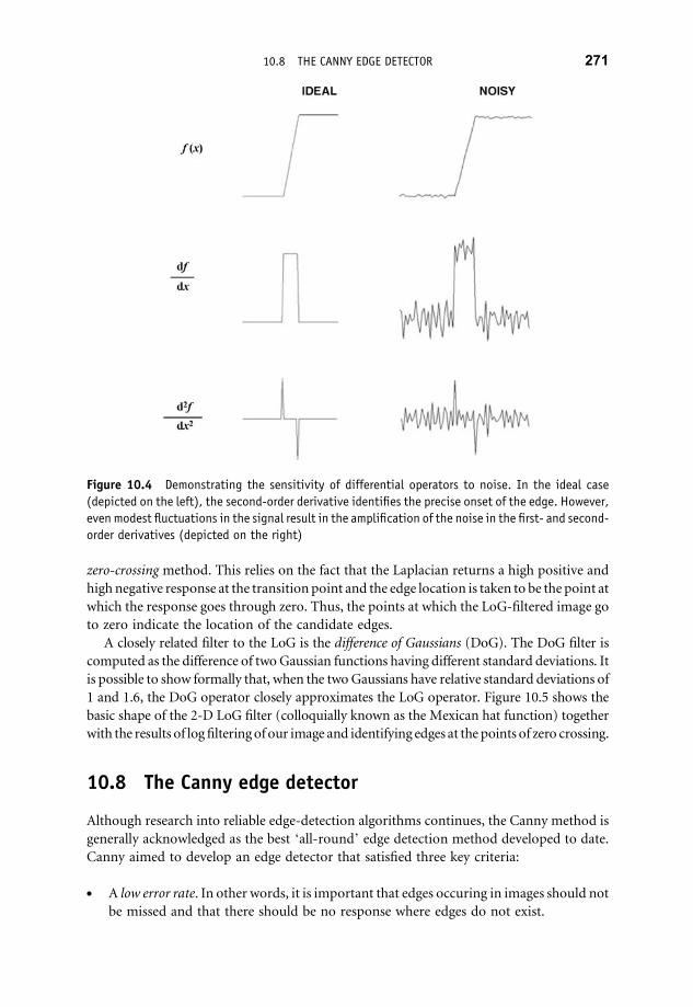
zero-crossing method. This relies on the fact that the Laplacian returns a high positive and

high negative response at the transition point and the edge location is taken to be the point at

which the response goes through zero. Thus, the points at which the LoG-filtered image go

to zero indicate the location of the candidate edges.

A closely related filter to the LoG is the difference of Gaussians (DoG). The DoG filter is

computed as the difference of twoGaussian functions having different standard deviations. It

is possible to show formally that, when the twoGaussians have relative standard deviations of

1 and 1.6, the DoG operator closely approximates the LoG operator. Figure 10.5 shows the

basic shape of the 2-D LoG filter (colloquially known as the Mexican hat function) together

with the results of logfilteringof our image and identifying edges at the points of zero crossing.

10.8 The Canny edge detector

Although research into reliable edge-detection algorithms continues, the Canny method is

generally acknowledged as the best ‘all-round’ edge detection method developed to date.

Canny aimed to develop an edge detector that satisfied three key criteria:

. A low error rate. In other words, it is important that edges occuring in images should not

be missed and that there should be no response where edges do not exist.

Figure 10.4 Demonstrating the sensitivity of differential operators to noise. In the ideal case

(depicted on the left), the second-order derivative identifies the precise onset of the edge. However,

even modest fluctuations in the signal result in the amplification of the noise in the first- and second-

order derivatives (depicted on the right)

10.8 THE CANNY EDGE DETECTOR 271

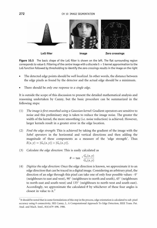
. The detected edge points should be well localized. In other words, the distance between

the edge pixels as found by the detector and the actual edge should be a minimum.

. There should be only one response to a single edge.

It is outside the scope of this discussion to present the detailed mathematical analysis and

reasoning undertaken by Canny, but the basic procedure can be summarized in the

following steps:

(1) The image is first smoothed using a Gaussian kernel: Gradient operators are sensitive to

noise and this preliminary step is taken to reduce the image noise. The greater the

width of the kernel, the more smoothing (i.e. noise reduction) is achieved. However,

larger kernels result in a greater error in the edge location.

(2) Find the edge strength: This is achieved by taking the gradient of the image with the

Sobel operators in the horizontal and vertical directions and then adding the

magnitude of these components as a measure of the ‘edge strength’. Thus

Eðx; yÞ ¼ jGxðx; yÞj þ jGyðx; yÞj.

(3) Calculate the edge direction: This is easily calculated as

u ¼ tan 1 Gyðx; yÞGxðx; yÞ

(4) Digitize the edge direction: Once the edge direction is known, we approximate it to an

edge direction that can be traced in a digital image. Considering an arbitrary pixel, the

direction of an edge through this pixel can take one of only four possible values - 0�

(neighbours to east and west), 90� (neighbours to north and south), 45� (neighboursto north-east and south-west) and 135� (neighbours to north-west and south-east).

Accordingly, we approximate the calculated u by whichever of these four angles is

closest in value to it.2

Figure 10.5 The basic shape of the LoG filter is shown on the left. The flat surrounding region

corresponds to value 0. Filtering of the centre image with a discrete 5� 5 kernel approximation to the

LoG function followed by thresholding to identify the zero crossings results in the image on the right

2 It should be noted that in some formulations of this step in the process, edge orientation is calculated to sub pixel

accuracy using 8 connectivity, SEE Canny, J., A Computational Approach To Edge Detection, IEEE Trans. Pat.

Anal. and Mach. Intel., 8(6):679 698, 1986.


(5) Nonmaximum suppression: After the edge directions are known, nonmaximum

suppression is applied. This works by tracing along the edge in the edge direction

and suppressing any pixel value (i.e. set it equal to zero) that is not considered to be an

edge. This will give a thin line in the output image.

(6) Hysteresis: After the first five steps have been completed, the final step is to track

along the remaining pixels that have not been suppressed and threshold the image to

identify the edge pixels. Critical to the Canny method, however, is the use of two

distinct thresholds – a higher value T2 and a lower value T1. The fate of each pixel is

then determined according to the following criteria:

. if jEðx; yÞj <T1, then the pixel is rejected and is not an edge pixel;

. if jEðx; yÞj>T2, then the pixel is accepted and is an edge pixel;

. if T1 < jEðx; yÞj <T2, the pixel is rejected except where a path consisting of edge

pixels connects it to an unconditional edge pixel with jEðx; yÞj>T2.

Two comments are pertinent to the practical application of the Canny edge detector.

First, we are, in general, interested in identifying edges on a particular scale. We can

introduce the idea of feature scale by filtering with Gaussian kernels of various widths.

Larger kernels introduce greater amounts of image smoothing and the gradient maxima

are accordingly reduced. It is normal, therefore, to specify the size of the smoothing kernel

in the Canny edge detection algorithm to reflect this aim. Second, we see that the Canny

detector identifies weak edges (T1 < jEðx; yÞj<T2) only if they are connected to strong

edges (jEðx; yÞj>T2).

Figure 10.6 demonstrates the use of the LoG and Canny edge detectors on an image

subjected to different degrees of Gaussian smoothing. The Matlab code corresponding to

Figure 10.6 is given in Example 10.3.

Example 10.3


A¼imread(‘trui.png’); %Read in image

subplot(3,3,1), imshow(A,[]); %Display original

h1¼fspecial(‘gaussian’,[15 15],6);

h2¼fspecial('gaussian',[30 30],12);

subplot(3,3,4), imshow(imfilter(A,h1),[]); %Display filtered version sigma¼6

subplot(3,3,7), imshow(imfilter(A,h2),[]); %Display filtered version sigma¼12

[bw,thresh]¼edge(A,‘log’); %Edge detection on original LoG filter

subplot(3,3,2), imshow(bw,[]);

[bw,thresh]¼edge(A,‘canny’); %Canny edge detection on original

subplot(3,3,3), imshow(bw,[]); %Display

[bw,thresh]¼edge(imfilter(A,h1),‘log’); %LoG edge detection on sigma¼6


10.8 THE CANNY EDGE DETECTOR 273

[bw,thresh]¼edge(imfilter(A,h1),‘canny’); %Canny edge detection on sigma¼6


[bw,thresh]¼edge(imfilter(A,h2),‘log’); %LoG edge detection on sigma¼12


[bw,thresh]¼edge(imfilter(A,h2),‘canny’); %Canny edge detection on sigma¼12


Comments

Matlab functions: edge.

The edge function can be called according to a variety of syntaxes. In the examples above,

appropriate thresholds are estimated automatically based on calculations on the input image.

See the Matlab documentation doc edge for full details of use.

10.9 Interest operators

In simple terms, a point is deemed interesting if it is distinct from all closely adjacent regions,

i.e. all those points in its surrounding neighbourhood. Interest operators are filters which

attempt to identify such points of interest automatically. Interest operators do not feature as

a ‘mainstream’ tool for segmentation but are, nonetheless, useful in certain special kinds of

problem. They also find application in problems concerned with image matching or

registration by geometric transformation, which presupposes the existence of so-called

tie points, i.e. known points of correspondence between two images. These are typically

points such as spots or corners which are easily distinguishable from their surroundings.

The identification of such points of interest is also desirable in other applications, such as

Figure 10.6 Edge detection using the zero-crossingmethod (LoG filter) and the Cannymethod for an

image at three different degrees of blur. In these examples, the LoG threshold and both the lower and

higher threshold for the Canny detector were calculated automatically on the basis of an estimated

signal/noise ratio. The superior performance of the Canny filter is evident


3-D stereographic imaging. The theoretical basis for identification of interesting points is

given below.

Consider the change in intensity in an image Iðx; yÞ by displacing from the point ðx; yÞ bysome small distanceðrx;ryÞ. A first-order Taylor series approximation gives

rI ¼ Iðxþrx; yþryÞ�Iðx; yÞ ¼ rxfx þryfy ð10:3Þ

where the image gradient at point ðx; yÞ is ½fx; fy�.We note from Equation (10.3) that the change in intensity is greatest when the

displacement is in the same direction as the gradient vector but is least when the

displacement is perpendicular to it. Haralick’s criterion deems a point to be interesting

when the quantity ðrIÞ2 (squared because negative changes are just as interesting as positiveand we do not want them to cancel) summed over a local neighbourhood is large for any

displacement direction. This condition then satisfies, in the general sense, our constraint that

the point be distinct from its surroundings. Using Equation (10.3), we may write a matrix

expression for rI2

ðrIÞ2 ¼ ðrxfx þryfyÞ2 ¼ ðrx ry Þ

XW

f 2xXW

fxfy

XW

fxfyXW

f 2y

0BB@

1CCA

rx

ry

!¼ vTFv ð10:4Þ

where we have denoted the displacement vector

v ¼ rx

ry

!; F ¼

XW

f 2xXW

fxfy

XW

fxfyXW

f 2y

0BBB@

1CCCA

and the elements inside the matrix F are summed over a local pixel neighbourhood W.

Summation over a local neighbourhood is desirable in practice to reduce the effects of noise and

measure the characteristics of the imageover a small ‘patch’with the givenpixel at its centre. For

convenience (andwithout imposing any restriction on our final result), we will assume that the

displacement vector we consider in Equation (10.4) has unit length, i.e. vTv ¼ 1.

Equation (10.4) is a quadratic form in the symmetric matrix F and it is straightforward to

show that the minimum and maximum values of a quadratic form are governed by the

eigenvaluesof thematrixwith theminimum value being givenbykvklmin ¼ lmin,withlmin the

smallest eigenvalue of the matrix F. Equation (10.4) is readily interpetable (in its 2-D form) as

the equation of an ellipse, the larger eigenvalue corresponding to the length of themajor axis of

the ellipse and the smaller eigenvalue to theminor axis. TheHaralickmethod designates a point

as interesting if the following two criteria are satisfied:

(1) that l1 þl22 is ‘large’. This is roughly interpretable as the ‘average radius’ of the ellipse

or average value of the quadratic over all directions.

10.9 INTEREST OPERATORS 275

(2) that 4det Fð ÞTr Ff g ¼ 1� l1 l2

l1 þ l2

� �2is ‘not too small’. This second criterion translates to the

requirement that the maximum and minimum values of the quadratic not be too

different from each other or, in geometric terms, that the ellipse not be too elongated.

It is apparent that a dominant eigenvalue such that l1 � l2 corresponds to a large

value in the direction of the first principal axis but a small value in the direction of the

second axis.

The question of what is ‘large’ and ‘not too small’ in the discussion above is, of course,

relative and must be placed in the direct context of the particular image being analysed.

‘Large’ usually relates to being a member of a selected top percentile, whereas ‘not too

small’ equates to an image-dependent cut-off value which can be systematically adjusted to

reduce or increase the number of detected points.

Harris developed a slightly different criterion. He independently defined an interest

function given by:

R ¼ l1l2�kðl1 þ l2Þ2 ð10:5Þ

which from the basic properties of the trace and determinant of a square matrix can be

written as:

R ¼ det½F��kðTrfFgÞ2 ¼ F11F22�F12F21�kðF11 þ F22Þ2 ð10:6Þ

or explicitly as:

Rðx; yÞ ¼ ð1�2kÞXW

f 2xXW

f 2y �kXW

f 2x

!2

þXW

f 2y

!2" #�ð fxfyÞ2 ð10:7Þ

and the constant k is set to 0.04.

One significant advantage of the Harris function is that it may be evaluated without

explicit calculation of the eigenvalues (which is computationally intensive). Note from

Equation (10.5), the following limiting forms of the Harris function:

. as l2 ! l1 ¼ lmax so R!ð1�2kÞl2max (its maximum possible value)

. as l2 ! l1 ! 0 so R! 0 (no response – a smooth region)

. if l1 � l2 then R!�kl2max.

Thus, a large positive value ofR indicates an ‘interesting’ point, whereas a negative response

suggests a dominant eigenvalue (a highly eccentric ellipse) and is ‘not interesting’. The basic

recipe for detection of interest points is as follows.


Detection of Interest Points

(1) Smooth the image by convolving the image with a Gaussian filter.

(2) For each pixel, compute the image gradient.

(3) For each pixel and its given neighbourhood W, compute the 2� 2 matrix F.

(4) For each pixel, evaluate the response function Rðx; yÞ.(5) Choose the interest points as localmaxima of the functionRðx; yÞ (e.g. by a nonmaximum

suppression algorithm).

For the final step, the non-maximum suppression of local minima, there are several

possible approaches. One simple but effective approach (employed in the Example 10.4)

is as follows:

. Let R be the interest response function.

. Let S be a filtered version of the interest function in which every pixel within a

specified (nonsparse) neighbourhood is replaced by the maximum value in that

neighbourhood.

. It follows that those pixels whose values are left unchanged in S correspond to the local

maxima.

We end our discussion with two comments of practical importance. First, image

smoothing reduces the size of the image gradients and, consequently, the number of

interest points detected (and vice versa). Second, if the size of the neighbourhood W (i.e.

the integrative scale) is too small, then there is a greater probability of rank deficiency in

matrix F.3 Larger integrative scale increases the probability of a full-rank matrix.

However, it also smoothes the response function Rðx; yÞ; thus, too large an integrative

scale can suppress the number of local maxima of Rðx; yÞ and, hence, the number of

interest points detected.

The example given in Figure 10.7 (produced using the Matlab code in Example 10.4)

illustrates the detection of interest points in two images on two different integrative

scales using the Harris function. Note in both examples the tendency of smooth regions

to have values close to zero and, in particular, of straight edges to return negative values.

Straight-edge pixels, by definition, have a significant gradient in one direction

(perpendicular to the dark–light boundary) but a zero (or at least very small) gradient

response parallel to the edge. This situation corresponds to a dominant eigenvalue in

the matrix F.

3 Rank deficient matrices have at least one zero eigenvalue.

10.9 INTEREST OPERATORS 277

Example 10.4


I¼imread(‘zener star.jpg’);

I¼double(rgb2gray(I));

%Read in image and convert to

%intensity

wdth¼5; sdvn¼2; %Fix smoothing parameters

k¼0.04; %Fix Harris constant

hsmall¼fspecial(‘gaussian’,[wdth wdth],sdvn); %Define Gaussian filter

[Fx,Fy]¼gradient(I); %Calculate gradient

Fx sq¼Fx.^2; Fy sq¼Fy.^2; Fx Fy¼Fx.�Fy; %Define terms in Harris function

Fx sq¼filter2(hsmall,Fx sq); %Perform neighbourhood smoothing

Fy sq¼filter2(hsmall,Fy sq); %on each term

Fx Fy¼filter2(hsmall,Fx Fy);

R¼(1 2.�k).�Fx sq.�Fy sq k.�(Fx sq.^2

þ Fy sq.^2) Fx Fy.^2;

%Calculate Harris function

S¼ordfilt2(R,wdth.^2,ones(wdth)); %Maximum filtering over

%neighbourhood

[j,k]¼find(R>max(R(:))./12 & R¼¼S); %Get subscript indices of local

%maxima

subplot(1,2,1), imagesc(R); axis image;

axis off; colormap(gray);

%Display Harris response

subplot(1,2,2), imshow(I,[]); %Display original image

hold on; plot(k,j,‘r�’); %Interest points superimposed

bw¼zeros(size(R)); bw([j,k])¼1;

bw¼logical(bw);

%Return logical array of interest

%locations

Figure 10.7 Left: the Harris response function to an image comprising a dark star on a plain

background. Right: the significant local maximum points are shown superimposed on the original

image


Comments

Matlab functions: ordfilt2, fspecial, find, logical.

The interest response is combined with a local maximum filter to ensure that only one local

maximum is identified. A subsequent hierarchical thresholding returns the points of

maximum interest.

10.10 Watershed segmentation

Watershed segmentation is a relatively recent approach which has come increasingly to the

fore in recent years and tends to be favoured in attempts to separate touching objects – one

of the more difficult image processing operations. In watershed segmentation, we envisage

the 2-D, grey-scale image as a topological surface or ‘landscape’ in which the location is

given by the x,y image coordinates and the height at that location corresponds to the image

intensity or grey-scale value.

Rain which falls on the landscape will naturally drain downwards, under the action of

gravity, to its nearest minimum point. A catchment basin defines that connected region or

area for which any rainfall drains to the same low point or minimum. In terms of a digital

image, the catchment basin thus consists of a group of connected pixels. Maintaining the

analogy with a physical landscape, we note that there will be points on the landscape (local

maxima) at which the rainfall is equally likely to fall into two adjacent catchment basins; this

is analogous to walking along the ridge of a mountain. Lines which divide one catchment

area from another are called watershed ridges, watershed lines or simply watersheds. An

alternative viewpoint is to imagine the landscape being gradually flooded from below with

thewater entering through the localminima. As the water level increases, we construct dams

which prevent the water from the catchment basins spilling or spreading into adjacent

catchment basins. When the water level reaches the height of the highest peak, the

construction process stops. The dams built in this way are the watersheds which partition

the landscape into distinct regions containing a catchment basin. The actual calculation of

watersheds in digital images can be performed in several ways, but all fundamentally hinge

on iterative morphological operations.

These basic concepts are illustrated for a 1-D landscape in Figure 10.8.

Figure 10.8 Watersheds and catchment basins. Basins are defined as connected regions with one

local minimum to which any incident rainfall will flow. The watersheds can be visualized as those

ridges fromwhich ‘water’would be equally likely to fall towards either of two ormore catchment basins

10.10 WATERSHED SEGMENTATION 279

Segmentation using watershedmethods has some advantages over the other methods we

have discussed in this chapter. A notable advantage is that watershedmethods, unlike edge-

detection-based methods, generally yield closed contours to delineate the boundary of the

objects. A number of different approaches can be taken to watershed segmentation, but

a central idea is thatwe try to transform the initial image (the onewewish to segment) into some

other image such that the catchment basins correspond to the objects we are trying to segment.

10.11 Segmentation functions

A segmentation function is basically a function of the original image (i.e. another image

derived from the original) whose properties are such that the catchment basins lie within

the objects we wish to segment. The computation of suitable segmentation functions is not

always straightforward but underpins successful watershed segmentation. The use of

gradient images is often the first preprocessing step in watershed segmentation for the

simple reason that the gradient magnitude is usually high along object edges and low

elsewhere. In an ideal scenario, the watershed ridges would lie along the object edges.

Figure 10.9 In the first, idealized example, the watershed yields a perfect segmentation. In the

second image of overlapping coins, morphological opening is required first on the thresholded image

prior to calculation of the watershed (See colour plate section for colour version)


However, noise and small-scale structures within the objects generally result in many local,

small catchment basins (broadly analogous to puddles on the landscape). These spoil

things and produce oversegmentation. Figure 10.9 (produced using the Matlab code in

Example 10.5) illustrates this.

Example 10.5


center1 ¼ 10; %Create image comprising two

%perfectly

center2 ¼ center1; %smooth overlapping circles

dist ¼ sqrt(2�(2�center1)^2);radius ¼ dist/2 � 1.4;lims ¼ [floor(center1 1.2�radius)eil(center2þ 1.2�radius)];[x,y] ¼ meshgrid(lims(1):lims(2));

bw1 ¼ sqrt((x center1).^2

þ (y center1).^2) <¼ radius;

bw2 ¼ sqrt((x center2).^2

þ (y center2).^2) <¼ radius;

bw ¼ bw1 | bw2;

D ¼ bwdist(�bw); %Calculate basic segmentation function

%(Euclidean distance transform

%of �bw)

subplot(2,2,1), imshow(bw,[]); %Display image

subplot(2,2,2), imshow(D,[]); %Display basic segmentation function

%Modify segmentation function

D ¼ D; %Invert and set background pixels

%lower

D(�bw) ¼ inf; %than all catchment basin minima

subplot(2,2,3), imshow(D,[]); %Display modified segmentation image

L ¼ watershed(D); subplot(2,2,4), Imagesc(L); %Calculate watershed of segmentation

%function

axis image; axis off; colormap(hot); colorbar %Display labelled image colour

%coded

A¼imread(‘overlapping euros1.png’); %Read in image

bw¼im2bw(A,graythresh(A)); %Threshold automatically

se¼strel(‘disk’,10); bwo¼imopen(bw,se); %Remove background by opening

D ¼ bwdist(�bwo); %Calculate basic segmentation function

D ¼ D; D(�bwo) ¼ 255; %Invert, set background lower than

%catchment basin minima

L ¼ watershed(D); %Calculate watershed

subplot(1,4,1), imshow(A); %Display original

subplot(1,4,2), imshow(bw) %Thresholded image

subplot(1,4,3), imshow(D,[]); %Display basic segmentation function

10.11 SEGMENTATION FUNCTIONS 281

ind¼find(L¼¼0); Ac¼A; Ac(ind)¼0; %Identify watersheds and set¼0 on

original

subplot(1,4,4), Imagesc(Ac); hold on %Segmentation superimposed on

original

Lrgb ¼ label2rgb(L, ‘jet’, ‘w’, ‘shuffle’); %Calculate label image

himage ¼ imshow(Lrgb); set(himage,

‘AlphaData’, 0.3);

%Superimpose transparently on original

Comments

Matlab functions: bwdist, watershed.

The Euclidean distance transform operates on a binary image and calculates the distance

from each point in the background to its nearest point in the foreground. This operation on the

(complement of) the input binary image produces the basic segmentation function. This is

modified to ensure the minima are at the bottom of the catchment basins. Computation of the

watershed then yields the segmentation. Note the watershed function labels each uniquely

segmented region with an integer and the watersheds are assigned a value of 0.

In Figure 10.9, the first (artificial) image is smooth and in this case, calculation of

a suitable segmentation function is achieved by the Euclidean distance transform.4 The

corresponding image of some real coins in the second example beneath it requires some

morphological pre-processing but essentially yields to the same method. However,

the segmentation is substantially achieved here (apart from the overlapping coins) by the

thresholding. In Figure 10.10 (produced using theMatlab code in Example 10.6) we attempt

a gradient-based segmentation function, but this results in the over-segmentation shown.

This outcome is typical in all but the most obliging cases.

An approach which can overcome the problem of over-segmentation in certain cases is

marker-controlled segmentation, the basic recipe for which is as follows:

(1) Select and calculate a suitable segmentation function. Recall that this is an image

whose catchments basins (dark regions) are the objects you are trying to segment. A

typical choice is the modulus of the image gradient.

Figure 10.10 Direct calculation of the watershed on gradient images typically results in

oversegmentation

4 The Euclidean distance transform codes each foreground pixel as the shortest distance to a background pixel.


(2) Process the original image to calculate so-called foreground markers. Foreground

markers are basically connected blobs of pixels lying within each of the objects. This is

usually achieved via grey-scale morphological operations of opening, closing and

reconstruction

(3) Repeat this process to calculate background markers. These are connected blobs of

pixels that are not part of any object.

(4) Process the segmentation function so that it only possesses minima at the foreground

and background marker locations.

(5) Calculate the watershed transform of the modified segmentation function.

Figure 10.11 shows a (largely) successful marker-controlled segmentation of a relatively

complex image.5 The rationale for this example is explained in Example 10.7.

Marker-controlled segmentation is an effective way of avoiding the problem

of over-segmentation. As is evident from the aforementioned example, it generally

needs and exploits a priori knowledge of the image and the methods required for

marker selection are strongly dependent on the specific nature of the image. Thus, its

strength is that it uses the specific context effectively. Conversely, its corresponding

weakness is that it does not generalize well and each problem must be treated

independently.

Example 10.6


A¼imread(‘overlapping euros.jpg’); %Read image

Agrad¼ordfilt2(A,25,ones(5)) ordfilt2(A,1,ones(5)); %Calculate basic

%segmentation function

figure, subplot(1,3,1), imshow(A,[]); %Display image

subplot(1,3,2), imshow(Agrad,[]); %Display basic segmentation

%function

L ¼ watershed(Agrad), rgb ¼ label2rgb(L,‘hot’,[.5 .5 .5]); %Calculate watershed

subplot(1,3,3), imshow(rgb,‘InitialMagnification’,‘fit’) %Display labelled image

Comments

Matlab functions: ordfilt2, watershed.

Watershed on the raw gradient image results in oversegmentation.

5 This example is substantially similar and wholly based on the watershed segmentation example provided by the

image processing demos inMatlab version 7.5. The authors offer grateful acknowledgments to TheMathWork Inc.

3 Apple Hill Dr. Natick, MA, USA.


Figure 10.11 Marker-controlled watershed segmentation (See colour plate section for colour version)

Example 10.7


rgb = imread(‘pears.png’); % Step 1. Read image and

I = rgb2gray(rgb); % use the Gradient Magnitude as

subplot(1,3,1), imshow(I) % the basic segmentation Function

hy = fspecial(‘sobel’);

hx = hy’;

Iy = imfilter(double(I), hy, ‘replicate’);

Ix = imfilter(double(I), hx, ‘replicate’);

gradmag = sqrt(Ix.^2 + Iy.^2);

se = strel(‘disk’, 20); % Step 2.Mark the Foreground Objects using

Ie = imerode(I, se); % morphological techniques called

Iobr = imreconstruct(Ie, I); % "opening by reconstruction" and

subplot(1,3,2), imshow(Iobr), % "closing by reconstruction" to "clean"

% up the image. These operations will

% create flat maxima inside each object

% that can be located using imregionalmax.

Iobrd = imdilate(Iobr, se); % Following the opening with a closing

Iobrcbr = imreconstruct(imcomplement(Iobrd),


imcomplement(Iobr));

Iobrcbr = imcomplement(Iobrcbr); % to remove the dark spots and stem marks.

subplot(1,3,3); imshow(Iobrcbr); % Notice you must complement the image

% inputs and output of imreconstruct.

fgm = imregionalmax(Iobrcbr); % Calculate the regional maxima of Iobrcbr

% to obtain good foreground markers.

I2 = I; I2(fgm) = 255; % To help interpret the result, superimpose

figure; subplot(1,3,1); imshow(I2); % these foreground marker image on the

% original image.

se2 = strel(ones(5,5)); % Some of the mostly occluded and shadowed

fgm2 = imclose(fgm, se2); % objects are not marked, which means that

fgm3 = imerode(fgm2, se2); % these objects will not be segmented

% properly in the end result. Also, the

% foreground markers in some objects go

% right up to the objects’ edge. That means

% we must clean the edges of the marker

% blobs and then shrink them a bit.

fgm4 = bwareaopen(fgm3, 20); % This procedure leaves some stray isolated

I3 = I; I3(fgm4) = 255; % pixels that must be removed. Do this

subplot(1,3,2), imshow(I3); % using bwareaopen, which removes all blobs

% that have fewer than a certain number of

% pixels.

bw = im2bw(Iobrcbr, %Step 3: Compute Background Markers

graythresh(Iobrcbr));

subplot(1,3,3), imshow(bw); % Now we need to mark the background. In

% the cleaned up image, Iobrcbr, the

% dark pixels belong to the background,

% so you could start with a thresholding

% operation.

D = bwdist(bw); % The background pixels are in black,

DL = watershed(D); % but ideally we don’t want the background

bgm = DL == 0; % markers to be too close to the edges of

figure; subplot(1,3,1);imshow(bgm); % the objects we are trying to segment.

% We’ll "thin" the background by computing

% the "skeleton by influence zones", or SKIZ,

% of the foreground of bw. This can be done

% by computing the watershed transform of the

% distance transform of bw, and

% then looking for the watershed ridge

% lines (DL == 0) of the result.

gradmag2 = imimposemin % Step 4: Compute the modified

(gradmag, bgm | fgm4);

% segmentation function.

% The function imimposemin is used to modify


10.12 Image segmentation with markov random fields

Except in the most obliging of situations, intensity thresholding alone is a crude approach

to segmentation. It rarely works satisfactorily because it does not take into account the

spatial relationships between pixels. Segmentation via region growing or splitting enables

pixels to be labelled based on their similarity with neighbouring pixels. The use ofMarkov

random field models is a more powerful technique which determines how well a pixel

belongs to a certain class by modelling both the variability of grey levels (or other pixel

attributes) within each class and its dependency upon the classification of the pixels in its

neighbourhood.

Segmentation using Markov random fields is not a simple technique. Our aim here will

be strictly limited to discussing the essence of the approach so that an interested reader is

then better equipped to go on to examine the literature on this subject. We shall start by

stating Bayes’ law of conditional probability:

pðxjyÞ ¼ pðyjxÞpðxÞpðyÞ ð10:8Þ

In our context of image segmentation, we shall supposewe are given an image containing

a range of grey levels denoted by y and a set of possible labels denoted by x. In the simplest

segmentation scenarios, there may, for example, be just two labels, referred to as object and

background.

Our basic task is to assign to each pixel the most probable label x given our set of

observations (i.e. our image) y. In other words, wewish tomaximize pðxjyÞwhich, by Bayes’

% an image so that it has regional minima

% only in certain desired locations.

% Here you can use imimposemin to modify

% the gradient magnitude image so that its

% regional minima occur at foreground and

% background marker pixels.

L = watershed(gradmag2); % Step 5: Now compute the Watershed

% Transform of modified function

Lrgb = label2 rgb(L, ‘jet’, % A useful visualization technique is to display the

‘w’, ‘shuffle’); % label matrix L as a color

subplot(1,3,2),imshow(Lrgb) % image using label2rgb. We can then superimpose this

subplot(1,3,3),imshow(I), %pseudo color label

hold on % matrix on top of the original intensity image.

himage = imshow(Lrgb);

set(himage, ‘AlphaData’, 0.3);


theorem, is equivalent to maximizing the right-hand side of Equation (10.8). Let us then

carefully consider each term in Equation 10.8.

. First, pðyÞ refers to the probability distribution of pixel grey levels (i.e. the distribution

whichwould be obtained froma grey-level histogram). For a given image, this quantity is

fixed. Therefore, if pðyÞ is a constant for a given image, then maximizing pðxjyÞ reducesto maximising pðyjxÞpðxÞ.

. Second, the conditional density pðyjxÞ refers to the probability distribution of pixel greylevels y for a given class x (e.g. background or object). In the ideal case, a background

would have one grey level and an object would have a second distinct grey level. In

reality, the grey levels for both classes will exhibit a spread. The densities are often

modelled as normal distributions:

pð yjxÞ ¼ 1

2pp

sx

exp �ð y�mxÞ22s2

x

" #ð10:9Þ

where mx and sx respectively refer to the mean and standard deviation of the pixel

intensity in the class x.

. Third, the term pðxÞ, known as the prior distribution, refers to the level of agreement

between the pixel’s current label and the label currently assigned to its neighbouring

pixels. This requires some elaboration. Intuitively, we would reason that pðxÞ shouldreturn a low value if the pixel’s label is different from all of its neighbours (since it is very

unlikely that an isolated pixel would be surrounded by pixels belonging to a different

class). By the same line of reasoning, pðxÞ should increase in value as the number of

identically labelled neighbouring pixels increases.

The whole approach thus hinges on the prior term in Bayes’ law, because it is this term

which must build in the spatial context (i.e. the correlation relations between a pixel and its

neighbours).

To the question ‘How exactly is the prior information built into our model?’, we cannot

give a full explanation here (this would require a long and complex detour into mathemati-

cal concepts traditionally associated with statistical physics), but the basic approach is to

model the relationship between a pixel and its neighbours as a Markov random field. A

Markov random field essentially models the probabilities of certain combination of

intensity values occurring at various pixel locations in a neighbourhood region. To specify

such probabilities directly is generally a difficult and even overwhelming task because there

are a huge number of possible combinations. Fortunately, a powerful mathematical result

exists which demonstrates that the right-hand side of Equation (10.8) can be written in the

form of an exponential which is known as a Gibbs distribution:

pðxjyÞ ¼ exp½�UðxjyÞ�Zy

ð10:10Þ

10.12 IMAGE SEGMENTATION WITH MARKOV RANDOM FIELDS 287

where Zy is a normalizing constant which is included to prevent the above equation from

returning a probability of greater than one. The exponential part of this equation turns out

to be:

UðxjyÞ ¼X

i

1

2lns2

xiþ ð y�mxi

Þ22s2

xi

þXNn¼1

un Jðxixiþ nÞ" #

ð10:11Þ

By analogy with arguments from statistical physics, UðxjyÞ can be loosely interpreted as

a ‘potential energy’ term and it is clear from Equation (10.10) that the maximization of

pðxjyÞ reduces to minimizing the energy term UðxjyÞ.In Equation (10.11), the outer summation covers all pixels in the image (i.e. the contents

are applied to every pixel in the image). The first two terms of the outer summation refer to

pðyjxÞ as given in Equation (10.9), which expresses how well the pixel’s grey level fits its

presumed class label. The third term represents pðxÞ and expresses the level of agreement

between the pixel’s label and those of its neighbours. This is itself expressed in the form of

a summation over the pixel’s immediate neighbours. The function Jðxi; xiþ nÞ returns avalue of �1 whenever the label for the nth neighbourhood pixel xiþ n is the same as the

label for the central pixel xi. The term un is included to adjust the relative weighting between

the pðxÞ and pðyjxÞ terms.

To complete our formulation of the problem, we need to resolve two questions:

(1) How do we model the class-conditional densities pðyjxÞ (the parameter estimation

problem)?

(2) How dowe select the neighbourhoodweighting parameters un to properly balance the

two contributions to the energy function?

10.12.1 Parameter estimation

Assuming the Gaussian distribution for the class-conditional densities pðyjxÞ given by

Equation (10.9), the two free parameters of the distribution (themean and variance) can be

foundby fittingGaussian curves to a representative (model) imagewhich has beenmanually

segmented into the desired classes. Where such a representative image is not available, the

parameters can be estimated by fitting such curves to the actual image histogram. For a two-

class segmentation problem (object and background), we would thus fit a Gaussianmixture

(sum of two Gaussian functions) to the image histogram hðyÞ, adjusting the free parameters

to achieve the best fit:


hðyÞ ¼X2i¼1

1

2pp

sxi

exp �ðy�mxiÞ2

2s2xi

24

35

¼ 1

2pp

sObj

exp �ðy�mObjÞ22s2

Obj

24

35þ 1

2pp

sBack

exp �ðy�mBackÞ22s2

Back

24

35

ð10:12Þ

The extension to more than two classes follows naturally.

10.12.2 Neighbourhood weighting parameter un

The parameter un represents the weighting which should be given to the local agreement

between pixel labels. For example, a pixel which is presently labelled as ‘object’ should have

a higher probability of being correct if, for example, six of its neighbouring pixels were

Figure 10.12 Segmentation of a noisy, underwater image of a cylindrical pipe structure. The

sequence from left to right and top to bottom shows the original image, the maximum likelihood

estimate and the results of segmentation using increasing numbers of iterations of the ICM algorithm.

(Image sequence courtesy of Dr Mark Hodgetts, Cambridge Research Systems Ltd.)

10.12 IMAGE SEGMENTATION WITH MARKOV RANDOM FIELDS 289

identically labelled as ‘object’ as opposed to three. The analytical approach to determining

un would involve initially labelling all pixels according to pixel attribute alone (i.e. in the

absence of any contextual information). Every labelled pixel in the image would then be

examined and a note would be made of the number of identically labelled neighbouring

pixels. Counts would be made for every combination of pixel label and number of agreeing

neighbouring pixel labels. These would be used to infer how the probability of the central

pixel label being correct varies with the number of consistent neighbouring labels, which

would in turn be used to generate estimates for un. In practice, most implementations treat

un as a constant u which is initially estimated at around unity and adjusted until optimal

results are obtained. Ahigher value of uwill tend to emphasize local agreement of pixel labels

over the class suitability according to pixel attribute and vice versa.

10.12.3 Minimizing U(x | y): the iterated conditional modes algorithm

Having formulated the problem and estimated the parameters of the class-conditional

densities and the neighbourhood weighting parameter, the final step in the segmentation is

to actually find a viable means to minimizeUðxjyÞ in Equation (10.11). We briefly describe

the iterated conditional modes (ICM) algorithm, as it is conceptually simple and compu-

tationally viable. The ICM algorithm is an example of a ‘greedy algorithm’, as it works on

a pixel-by-pixel basis, accepting only those changes (i.e. changes from background to

foreground or vice versa) which take us successively nearer to our goal of minimizing the

potential. This is in contrast to other approaches, such as simulated annealing (Geman and

Geman) which allow temporary increases in the potential function to achieve the overall

goal ofminimization. The ICMalgorithm decomposes Equation (10.11) so that it is applied

to single pixels in the image

UiðxjyÞ ¼ 1

2lns2

xiþ ðyi�mxi

Þ22s2

xi

þXNn¼1

un Jðxixiþ nÞ ð10:13Þ

. Step 1: label each pixel with its most probable class based on its pixel attribute only, i.e.

according to whichever of the class-conditional densities yields the maximum value.

This is termed the maximum-likelihood estimate.

. Step 2: for each pixel in the image, update it to the class which minimizes

Equation 10.13.

. Repeat Step 2 until stability occurs.

Figure 10.12 shows an example of Markov random field segmentation using the ICM

algorithm.



11Classification

11.1 The purpose of automated classification

The identification of cells in a histological slide as healthy or abnormal, the separation of

‘high-quality’ fruit from inferior specimens in a fruit-packing plant and the categorization

of remote-sensing images are just a few simple examples of classification tasks. The first two

examples are fairly typical of binary classification. In these cases, the purpose of the

classification is to assign a given cell or piece of fruit to either of just two possible classes.

In the first example above, the two classes might be ‘healthy’ and ‘abnormal’; in the second

example, these might be ‘top quality’ (expensive) or ‘market grade’ (cheap). The third

example typically permits a larger number of classes to be assigned (‘forest’, ‘urban’,

‘cultivated’, ‘unknown’, etc.).

Autonomous classification is a broad andwidely studied field thatmore properly belongs

within the discipline of pattern recognition than in image processing. However, these fields

are closely related and, indeed, classification is so important in the broader context and

applications of image processing that some basic discussion of classification seems essential.

In this chapter we will limit ourselves to some essential ideas and a discussion of some of the

best-known techniques.

Classification takes place in virtually all aspects of life and its basic role as a necessary first

step before selection or other basic forms of decision-making hardly needs elaboration. In

the context of image processing, the goal of classification is to identify characteristic

features, patterns or structures within an image and use these to assign them (or indeed the

image itself) to a particular class. As far as images and visual stimuli go, human observers will

often perform certain classification tasks very accurately. Why then should we attempt to

build automatic classification systems? The answer is that the specific demands or nature of

a classification task and the sheer volume of data that need to be processed often make

automated classification the only realistic and cost-effective approach to addressing a

problem. Nonetheless, expert human input into the design and training of automated

classifiers is invariably essential in two key areas:

(1) Task specification What exactly dowewant the classifier to achieve? The designer of a

classification systemwill need to decide what classes are going to be considered andwhat




variables or parameters are going to be important in achieving the classification.1 For

example, a simple classifier designed to make a preliminary medical diagnosis based

on image analysis of histological slides may only aim to classify cells as ‘abnormal’ or

‘normal’. If the classifier produces an ‘abnormal’ result, a medical expert is typically

called upon to investigate further. On the other hand, it may be that there is sufficient

information in the shape, density, size and colour of cells in typical slides to attempt a

more ambitious classification system. Such a systemmight assign the patient to one of

a number of categories, such as ‘normal’, ‘anaemic’, ‘type A viral infection’ and so on.

(2) Class labelling The process of training an automated classifier can often require

‘manual labelling’ in the initial stage, a process in which an expert human user assigns

examples to specific classes based on selected and salient properties. This forms part of

the process in generating so-called supervised classifiers.

11.2 Supervised and unsupervised classification

Classification techniques can be grouped into two main types: supervised and unsupervised.

Supervised classification relies on having example pattern or feature vectors which have

already been assigned to a defined class. Using a sample of such feature vectors as our

training data, we design a classification system with the intention and hope that new

examples of feature vectors which were not used in the design will subsequently be classified

accurately. In supervised classification then, the aim is to use training examples to design a

classifier which generalizes well to new examples. By contrast, unsupervised classification

does not rely on possession of existing examples from a known pattern class. The examples

are not labelled and we seek to identify groups directly within the overall body of data and

features which enables us to distinguish one group from another. Clustering techniques are

an example of unsupervised classification which we will briefly discuss later in the chapter.

11.3 Classification: a simple example

Consider the following illustrative problem. Images are taken at a food processing plant in

which three types of object occur: pine-nuts, lentils and pumpkin seeds.Wewish to design a

classifier that will enable us to identify the three types of object accurately. A typical image

frame is shown in Figure 11.1.

Let us assume that we can process these images to obtain reliable measurements on the

two quantities of circularity and line-fit error.2 This step (often the most difficult) is called

feature extraction. For each training example of a pine-nut, lentil or pumpkin seed we thus

obtain a 2-D feature vectorwhich we can plot as a point in a 2-D feature space. In Figure 11.2,

1 In a small number of specialist applications, it is possible even to attempt to identify identify appropriate patterns

and classes automatically; but generally, the expert input of the designer at this stage is absolutely vital.2 The details of these measures and how they are obtained from the image do not concern us here.

292 CH 11 CLASSIFICATION

training examples of pine-nuts, lentils and pumpkin seeds are respectively identified by

squares, triangles and circles.

We can see by direct inspection of Figure 11.2 that the three classes form more or less

distinct clusters in the feature space. This indicates that these two chosen features are

broadly adequate to discriminate between the different classes (i.e. to achieve satisfactory

classification). By contrast, note fromFigure 11.2what happens if we consider the use of just

one of these features in isolation. In this case, the feature space reduces to a single dimension

given by the orthogonal projection of the points either onto the vertical (line-fit error) or

horizontal (circularity) axis. In either case, there is considerable overlap or confusion of

classes, indicating that misclassification occurs in a certain fraction of cases.

Now, the real aim of any automatic classification system is to generalize to new examples,

performing accurate classification on objects or structures whose class is a priori unknown.

Figure 11.1 Three types of object exist in this image: pine-nuts, lentils and pumpkin seeds. The

image on the right has been processed to extract two: circularity and line-fit error

Figure 11.2 A simple 2-D feature space for discriminating between certain objects. The 1-D

bar plots in the horizontal x and vertical y directions show the projection of the data onto the

respective axes

11.3 CLASSIFICATION: A SIMPLE EXAMPLE 293

Consider, then, a previously unseen object having the feature vector indicated in Figure 11.2

by a star. How shouldwe assign this object to its appropriate class? As this object has features

which are closer to the lentils, common sense would suggest that it is more likely to be a

lentil, but where should we draw the boundary between classes and how sure can we be

about our decision? Most of the classification methods we will explore in the remainder of

this chapter are concerned with just such questions and finding rigorous mathematical

criteria to answer them. First, however, wemove fromour simple example to amore general

overview of the steps in the design of classifiers.

11.4 Design of classification systems

Figure 11.3 provides a summary flow chart for classifier design. We elaborate below on the

main steps indicated in Figure 11.3.

(1) Class definition Clearly, the definition of the classes is problem specific. For example,

an automated image-processing system that analysedmammogramsmight ultimately

aim to classify the images into just two categories of interest: normal and abnormal.

This would be a binary classifier or, as it is sometimes called, a dichotomizer. On the

other hand, a more ambitious system might attempt a more detailed diagnosis,

classifying the scans into several different classes according to the preliminary

diagnosis and the degree of confidence held.

(2) Data exploration In this step, a designer will explore the data to identify possible

attributeswhichwill allow discrimination between the classes. There is no fixed or best

way to approach this step, but it will generally rely on a degree of intuition and

common sense. The relevant attributes can relate to absolutely any property of an

image or image region that might be helpful in discriminating one class from another.

START

DEFINE THE CLASSES

EXAMINE THE DATA SAMPLE

DEFINE FEATURE SPACE

= WHAT CLASSES DO YOU NEED TOSOLVE THE PROBLEM ?

SATISFACTORY ?

TEST THE CLASSIFER

BUILD THE CLASSIFIER

= IS THE CLASSIFICATIONPERFORMANCE GOOD ENOUGH?

=FIND NEW EXAMPLES AND CLASSIFY THEM USING YOUR SYSTEM

=DEFINE DECISIONSURFACES IN FEATURE SPACE

= WHAT VARIABLES ALLOW DISCRMINATIONBETWEEN DATA EXAMPLES ?

= SELECT APPROPRIATE VARIABLES ANDFORM THE FEATURE VECTORS FOR DATA

STOP

NO

YES

Figure 11.3 Flow diagram representing the main steps in classifier design


Most commonmeasures or attributes will be broadly based on intensity, colour, shape,

texture or some mixture thereof.

(3) Feature selection and extraction Selection of the discriminating features defines the

feature space. This, of course, implicitly assumes that we have established reliable

image-processing procedures to perform the necessary feature extraction.3 In general,

it is crucial to select features that possess two key properties. The first is that the feature

set be as compact as possible and the second that they should possess what, forwant of a

more exact word, we will call discriminatory power. A compact set of features is

basically a small set and it is of paramount importance, as larger numbers of selected

features require an increasingly large number of training samples to train the classifier

effectively. Second, it obviously makes sense to select (i) attributes whose distribution

over the defined classes is as widely separated as possible and (ii) that the selected set of

attributes should be, as closely as possible, statistically independent of each other. A set

of attributes possessing these latter two properties would have maximum discrimi-

natory power.

A simple but concrete illustration of this idea might be the problem of trying to

discriminate between images of a lion and a leopard. Defining feature vectors which

give some measure of the boundary (e.g. a truncated radial Fourier series) or some

gross shapemeasure like form factor or elongation4 constitute one possible approach.

However, it is clearly not a very good one, since lions and leopards are both big cats of

similar physique. A better measure in this case will be one based on colour, since the

distribution in r–g chromatic space is simple to measure and is quite sufficient to

discriminate between them.

(4) Build the classifier using training data The training stage first requires us to find a

sample of examples which we can reliably assign to each of our selected classes. Let us

assume that we have selected N features which we anticipate will be sufficient to

achieve the task of discrimination and, hence, classification. For each training example

we thus record the measurements on the N features selected as the elements of an

N-dimensional feature vector x ¼ ½x1; x2; � � � ; xN �. All the training examples thus

provide feature vectors which may be considered to occupy a specific location in an

(abstract)N-dimensional feature space (the jth element xj specifying the length along

the jth axis of the space). If the feature selection has been performed judiciously, then

the feature vectors for each class of interest will form more or less distinct clusters or

groups of points in the feature space.

(5) Test the classifier The classifier performance should be assessed on a new sample of

feature vectors to see how well it can generalize to new examples. If the performance is

unsatisfactory (what constitutes an unsatisfactory performance is obviously applica-

tion dependent), the designer will return to the drawing board, considering whether

3 Something that is often very challenging but which, in the interest of staying focused, we will gloss over in this

chapter.4 The formal definitions of these particular measures are given in Chapter 9.

11.4 DESIGN OF CLASSIFICATION SYSTEMS 295

the selected classes are adequate, whether the feature selection needs to be recon-

sidered or whether the classification algorithm itself needs to be revised. The entire

procedure would then be repeated until a satisfactory performance was achieved.

Table 11.1 summarizes some of the main terms used in the field of pattern classification.

11.5 Simple classifiers: prototypes and minimumdistance criteria

A prototype is an instance of something serving as a typical example or standard for other

things of the same category. One of the simplest and most common methods of defining a

prototype for a particular class is to take a number of training examples for that class and

calculate their average. Figure 11.4 shows a set of 8 male faces and 8 female faces and their

calculated prototypes. In this particular example, the original images contain many tens of

thousands of pixels. By a procedure based on PCA, however, it is possible to represent these

faces as lower dimensional, feature vectors fxig whose components provide a compact

description of both the shape and texture of the face and fromwhich the original images can

be reconstructed with high accuracy. The prototypesM and F of the two classes are simply

calculated as

M ¼ 1

N

XNi¼1

xMi and F ¼ 1

N

XNi¼1

xFi ð11:1Þ

where fxMi g correspond to themale examples and fxFi g the female examples and there areN

examples of each. The reconstructed prototypes shown in Figure 11.4 are given by applying

Equation (11.1) and then reconstructing the original images from the feature vectors.

Minimumdistance classifiers are conceptually simple and generally easy to calculate. The

first step is to calculate the mean feature vector or class prototype for each class. When

Table 11.1 Some common pattern classification terms with summary descriptions

Term Description

Feature vector (pattern vector) AnN dimensional vector, each element of which specifies some

measurement on the object

Feature space The abstract (N dimensional) mathematical space spanned by

the feature vectors used in the classification problem

Training data A collection of feature vectors used to build a classifier

Test data A collection of feature vectors used to test the performance of a

classifier

Pattern class A generic term which encapsulates a group of pattern or feature

vectors which share a common statistical or conceptual origin

Discriminant function A functionwhose valuewill determine assignment to one class or

another; typically, a positive evaluation assigns to one class and

negative to another


presented with a previously unseen feature vector, the minimum distance classifier will

simply assign the new example to that class whose prototype lies closest to it. We note

immediately that the concept of ‘distance’ in a feature space is a flexible one and admits

of a number of other valid definitions apart from the familiar Euclideanmeasure. However,

the principle of a minimum distance classifier is the same irrespective of the precise metric

employed. Table 11.2 gives several such metrics which are sometimes used.

11.6 Linear discriminant functions

To apply a minimum distance classifier by calculating the Euclidean distance in the

feature space from a given point to the prototype of each class involves a quadratic

function of distance and is a straightforward enough procedure. However, it is

Figure 11.4 Facial prototypes: Left: 8 female faces with the prototype at the centre. Right: 8 male

faces with the calculated prototype at the centre. The prototypes are calculated by averaging the

shape coordinates of each example and then averaging the RGB colour values of each face after

warping to the average shape

Table 11.2 Some common distance measures ormetrics between two N-dimensional vectors x and y

Metric Definition

Euclidean distance (L2 norm) Lðx; yÞ ¼ PNi 1

ðxi yiÞ2� �1=2

City block� (L1 norm) Lðx; yÞ ¼ PNi 1

jxi yij

Minkowski metric (Lk norm) Lkðx; yÞ ¼PNi 1

jxi yijk� �1=k

Mahalanobis distance Lðx; yÞ ¼ ½ðx yÞTS�1ðx yÞ�1=2,where S ¼ hðx ~mxÞðy ~myÞTi

�Also known as the Manhattan Distance.

11.6 LINEAR DISCRIMINANT FUNCTIONS 297

possible to show that application of the minimum distance criterion reduces to a

formulation that is of greater utility when we extend our discussion to more complex

criteria. It is thus useful to introduce at this point the concept of a (linear) discriminant

function.

For simplicity, consider constructing a line in a 2-D feature space which orthogonally

bisects the line connecting a given pair of class prototypes (let us say from the ith prototype

possessing coordinates ðxi1; xi2Þ to the jth prototype ðxj1; xj2Þ) and passes through the exact

midpoint between them. This line divides the feature space into two regions, one of which is

closer to the ith prototype, the other to the jth prototype and any point lying on the line is

equidistant from the two prototypes. This line is the simplest example of a linear

discriminant function. It is easy to show that this function can be expressed in the

general form

gijðxÞ ¼ gijðx1; x2Þ ¼ ax1 þ bx2 þ c ¼ 0 ð11:2Þ

If we evaluate gijðxÞ at an arbitrary position within the feature space x ¼ ðx1; x2Þ, then a

positive value indicates that the point lies closer to the jth prototype, whereas a negative

value indicates greater proximity to the ith prototype.

In principle, wemay calculate a linear discriminant of this kind for every pair of classes.

Figure 11.5 depicts the data in the simple three-class problem described in Section 11.3;

therefore, we have32

� �¼ 3 linear discriminant functions. By calculating linear dis-

criminants for all pairs of prototypes and evaluating each discriminant function, it is

possible in principle to classify a feature vector simply by observing the signs of the

discriminants and applying basic logic (see table in Figure 11.5).

However, it is normal practice in N-class problems to define discriminant functions

(whether linear or otherwise) in the following way:

if gjðxÞ > gkðxÞ for all j 6¼ kthen assign x to class j

ð11:3Þ

It is evident, then, that the discriminant functions for each class consist of segments of such

linear functions and combine to define decision boundarieswhich partition the feature space

into distinct regions. Figure 11.5 (top right) shows the decision boundaries in the 2-D feature

space of our example.

Consider male and female faces; these differ in visual appearance, and human observers

are generally very adept at distinguishing between them. Could this be achieved through an

automatic classifier? In Example 11.1, we use a 2-D feature vector based on the sixth and

seventh component values extracted through a PCA on suitably normalized frontal images

of the human face. Ten of these subjects are male and ten female and the region of the face

subjected to the PCA is shown in Figure 11.6. It is apparent that use of just these two

components does a reasonably good job and a simple (Euclidean) minimum distance

classifier results in just two misclassifications.


Figure 11.5 Illustration of the minimum distance classifier, the construction of linear discriminant

functions and the resulting decision boundaries

Example 11.1

Matlab Example 11.1 What is happening?

load PCA data.mat; %Load PCA coefficients for males

%and females

f6=female(6,:)./1000; f7=female(7,:)./1000; %extract female coefficients on

%6 and 7

m6=male(6,:)./1000; m7=male(7,:)./1000; %extract male coefficients on 6 and 7

F proto=mean([f6’ f7’]);

M proto=mean([m6’ m7’]); %calculate Male and female

%prototypes

dely=M proto(2) F proto(2);

delx=M proto(1) F proto(1); %Difference between prototypes

mid pt=[F proto(1)+delx./2 F proto(2)+dely./2]; %Midpoint between prototypes

11.6 LINEAR DISCRIMINANT FUNCTIONS 299

grad= 1./(dely./delx); %Gradient of linear discriminant

a=1./(mid pt(2) grad.*mid pt(1)); %Coefficients of linear discriminant

b=grad./(mid pt(2) grad.*mid pt(1));

figure;

plot(f6,f7,’r*’); hold on; plot(m6,m7,’kd’); %Plot data

x=linspace( 5,5,100); y=(1+b.*x)./a; %Plot linear discriminant

plot(x,y,’b ’);

f indx=find(a.*f7 b.*f6 1>0) %Find index of misclassified females

m indx=find(a.*m7 b.*m6 1 %Find index of misclassified males

Figure 11.6 Thumbnail images of human faces and their respective positions in a 2-D feature space

based on the 6th and 7th principal components. Male faces are plotted as circles and female faces as

asterisks. A minimum distance classifier results in two misclassifications


Linear discriminants are important not just for simple minimum-distance

classifiers, but find much wider application. For this reason, the next section extends

the concept to a general N-dimensional feature space and looks at some of their key

properties.

11.7 Linear discriminant functions in N dimensions

Although a number of interesting classification problems are two-class problems, the

majority require the definition of multiple classes. The widespread popularity of linear

discriminants in classification problems originates from their simplicity, easy computa-

tion and the fact that they extend simply and naturally to higher dimensional feature

spaces.

The general form of the N-dimensional, linear discriminant gðxÞ is

gðxÞ ¼ gðx1; x2 � � � xNÞ ¼XNk¼0

wkxk ¼ w0 þw1x1 þw2x2 þ � � �wNxN ¼ 0

or expressed in compact, vector form

gðxÞ ¼ w � xþw0 ¼ 0 ð11:4Þ

For a 2-D feature space, the discriminant describes the equation of a straight line and divides

a plane into two partitions. For a 3-D feature space, the discriminant describes the equation

of a plane and divides a volume into two partitions. In themost generalN-dimensional case,

the discriminant describes the equation of a hyperplane and divides the N-dimensional

volume into two partitions.

We note two important properties. Let us consider two arbitrary but distinct vectors x1and x2 both lying on the hyperplane. Since gðxÞ ¼ 0 for any x that lies on the hyperplane, it

follows that

gðx1Þ�gðx2Þ ¼ 0 Y w � ðx1�x2Þ ¼ 0 ð11:5Þ

Since the arbitrary vector ðx1�x2Þ lies within the plane,5 we conclude that the vector w is

perpendicular to any vector lying in the hyperplane.

The discriminant function gðxÞ also gives an algebraic measure of the shortest

(i.e. perpendicular) distance s of the point x to the dividing hyperplane. It is possible to

show that this is:

s ¼ gðxÞkwk ð11:6Þ

5More precisely, the vector ðx1 x2Þ lies within the subspace defined by the hyperplane.

11.7 LINEAR DISCRIMINANT FUNCTIONS IN N DIMENSIONS 301

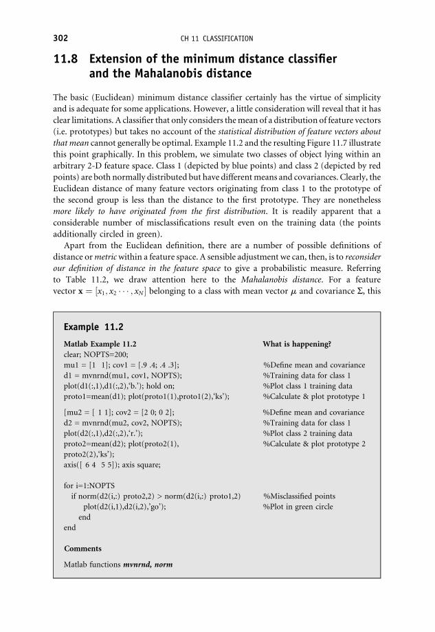
11.8 Extension of the minimum distance classifierand the Mahalanobis distance

The basic (Euclidean) minimum distance classifier certainly has the virtue of simplicity

and is adequate for some applications. However, a little consideration will reveal that it has

clear limitations. A classifier that only considers themean of a distribution of feature vectors

(i.e. prototypes) but takes no account of the statistical distribution of feature vectors about

that mean cannot generally be optimal. Example 11.2 and the resulting Figure 11.7 illustrate

this point graphically. In this problem, we simulate two classes of object lying within an

arbitrary 2-D feature space. Class 1 (depicted by blue points) and class 2 (depicted by red

points) are both normally distributed but have differentmeans and covariances. Clearly, the

Euclidean distance of many feature vectors originating from class 1 to the prototype of

the second group is less than the distance to the first prototype. They are nonetheless

more likely to have originated from the first distribution. It is readily apparent that a

considerable number of misclassifications result even on the training data (the points

additionally circled in green).

Apart from the Euclidean definition, there are a number of possible definitions of

distance ormetricwithin a feature space. A sensible adjustment we can, then, is to reconsider

our definition of distance in the feature space to give a probabilistic measure. Referring

to Table 11.2, we draw attention here to the Mahalanobis distance. For a feature

vector x ¼ ½x1; x2 � � � ; xN � belonging to a class with mean vector m and covariance S, this

Example 11.2


clear; NOPTS=200;

mu1 = [1 1]; cov1 = [.9 .4; .4 .3];

d1 = mvnrnd(mu1, cov1, NOPTS);

plot(d1(:,1),d1(:,2),‘b.’); hold on;

proto1=mean(d1); plot(proto1(1),proto1(2),‘ks’);

%Define mean and covariance

%Training data for class 1

%Plot class 1 training data

%Calculate & plot prototype 1

[mu2 = [ 1 1]; cov2 = [2 0; 0 2];

d2 = mvnrnd(mu2, cov2, NOPTS);

plot(d2(:,1),d2(:,2),‘r.’);

proto2=mean(d2); plot(proto2(1),

proto2(2),‘ks’);

axis([ 6 4 5 5]); axis square;

%Define mean and covariance

%Training data for class 1

%Plot class 2 training data

%Calculate & plot prototype 2

for i=1:NOPTS

if norm(d2(i,:) proto2,2) > norm(d2(i,:) proto1,2)

plot(d2(i,1),d2(i,2),’go’);

end

end

%Misclassified points

%Plot in green circle

Comments

Matlab functions mvnrnd, norm


is defined as

Dmh ¼ ðx�mÞTS 1ðx�mÞ ð11:7Þ

and the covariance matrix S in Equation (11.7) is defined by:

S ¼ hðx�mÞðx�mÞTi ¼

s21 s12 � � � s1N

s21 s22 s2N

..

. . .. ..

.

sN1 sN2 � � � s2N

26664

37775 ð11:8Þ

with sij ¼ hðxi�miÞðxj�mjÞi and h i denotes the expectation or ensemble average over the

sample.

TheMahalanobis distance effectively scales the absolute distances in the feature space by

their corresponding standard deviations and, thus, provides an intuitively more

‘probabilistic’ measure of distance. In the following section, we develop the basic ideas

behind classifiers that attempt tomake full use of any information we might possess about the

statistical distribution of the feature vectors within the space. This is the basic idea behind

Bayesian classifiers.

11.9 Bayesian classification: definitions

The Bayesian approach to optimizing classifier performance is probabilistic in nature. From

an operational perspective, a good classifier should obviously maximize the number of

correct classifications andminimize the number of incorrect classifications over a definitive

Figure 11.7 Feature vectors which are statistically more likely to have originated from one classmay

lie closer to the prototype of another class. This is a major weakness of a simple Euclidean minimum

distance classifier (See colour plate section for colour version)

11.9 BAYESIAN CLASSIFICATION: DEFINITIONS 303

number of trials. A little thought, however, will reveal that these are to some degree

conflicting requirements6 and cannot be used as a design principle. Bayesian classifiers are

actually designed to assign each feature vector to themost probable class. It is probably worth

saying at the outset that the Bayesian approach corresponds strictly to a rather idealized

situation (in which all relevant probabilities are known) and these conditions are not often

met in practice. Despite this, it forms an elegant framework, serving as both an adequate

approximation to many problems and as an excellent point of reference for practical

classifiers.

We begin by outlining some general definitions and notation. We will assume the

following:

. The patterns in whose classification we are interested may be represented as N-

dimensional feature vectors x ¼ ½x1; x2; � � � ; xN � whose components x1; x2; � � � ; xN are

the measurement parameters which describe the feature space.7

. There are a total ofC pattern classes,v1;v2 � � �vC to which a given feature vector xmay

be assigned.

. The probability of drawing a feature vector from each of the classes is known

and described by the probabilities pðv1Þ; pðv2Þ; � � � ; pðvCÞ. These are known as the

priors.

. There exists a set of M such examples of feature vectors fx1; x2; � � � ; xMgwhose corresponding pattern classes are known. These examples form the design or

training set.

11.10 The Bayes decision rule

Let the conditional probability pðvjjxÞ represent the probability density of belonging to

classvj given the occurrence of the feature vector x. Note that, in general, pðvjjxÞ should beinterpreted as a probability density (rather than a strict probability), since the feature vector

x is a continuous variable and, thus, pðvjjxÞ is a function conditional upon x. The Bayes

decision rule is an intuitive rule based on probabilities:

if pðvjjxÞ > pðvkjxÞ for all k 6¼ j

then assign x to vj

ð11:9Þ

6 For example, if I wish to ensure that patterns from class A are always correctly classified then I can ensure thismost

easily by always assigning to class A whatever the pattern. The consequences for patterns belonging to other classes

are obvious.7Naturally, themeasurement parameters should correspond directly or indirectly to those specific features thought

to be important for classification.


In other words, we simply assign x to the most probable class. This decision rule, however,

begs the question of how to find or estimate the probabilities pðvjjxÞ in Equation (11.9). Toresolve this, we invoke Bayes’ theorem, which for conditional probabilities extends

naturally to the notion of probability densities and says

pðvjjxÞ ¼ pðxjvjÞpðvjÞpðxÞ ð11:10Þ

On substitution into Equation (11.9), our decision rule then becomes

if pðxjvjÞpðvjÞ > pðxjvkÞpðvkÞ for all k 6¼ j

then assign x tovj

ð11:11Þ

It is important to interpret the terms occurring in Equations (11.10) and (11.11) clearly:

. pðxjvjÞ is known as the class-conditional probability density function. The term pðxjvjÞmay be interpreted as ‘the likelihood of the vector x occurringwhen the feature is known

to belong to class vj.

. The functions pðvjÞ are known as the prior probabilities. Their values are chosen to

reflect the fact that not all classes are equally likely to occur. Clearly, the values chosen for

the pðvjÞ should reflect one’s knowledge of the situation under which classification is

being attempted.

. pðxÞ is sometimes known as the ‘evidence’ and can be expressed using the partition

theorem or ‘law of total probability’ as pðxÞ ¼ PjpðxjvjÞpðvjÞ. Note that pðxÞ is

independent of the class label vj and does not enter into the decision rule described by

Equation (11.11).

The key thing to note here is that application of the Bayes decision rule given by

Equation (11.11) requires knowledge of all the class-conditional, probability density functions

and the priors.

It is rare that wewill know the functional forms and parameters of these density functions

exactly. The approach typically taken in practice is to assume (or estimate) suitable

functional forms for the distributions pðxjvjÞ and pðvjÞ for all values of j and estimate

their parameters from our training data. We then attempt to apply the rule given by

Equation (11.11).

In certain instances, the form of the distribution may actually be known or confidently

predicted. By far the most common is the multivariate normal (MVN) distribution. The

main reason for this is its analytical tractability and simple properties (other distributions in

N dimensions are much harder to deal with). However, real-life situations in which the

MVN distribution is a fairly good approximation are fortunately quite common.

Before we deal with the specific cases of Bayesian classifiers in which the underlying

distributions can be well approximated by the MVN, we will, therefore, dedicate the next

section to reviewing its properties.

11.10 THE BAYES DECISION RULE 305

11.11 The multivariate normal density

The one-dimensional Gaussian or normal density for the random variable x is given by

pðxÞ ¼ 1

2pp

sexp � 1

2

x�m

s

� �2� �

ð11:12Þ

where m is the mean of the distribution and s is the standard deviation. The 1-D normal

density is thus defined by just two parameters. For multivariate data x1; x2 � � � xN , repre-sented as a column vector x ¼ ½x1; x2 � � � xN �T, the normal distribution has themore general

form

pðxÞ ¼ 1

ð2pÞN=2jCj1=2exp � 1

2ðx�~mxÞTC 1

x ðx�~mxÞ� �

ð11:13Þ

where ~mx ¼ EðxÞ is the expectation or average value of x and Cx ¼ E½ðx�~mxÞðx�~mxÞT� isthe covariance matrix.

The covariance matrix contains the covariance between every pair of variables in the

vector x. Thus, the general, off-diagonal element is given by

Cxði; jÞ ¼ E½ðxi�miÞðxj�mjÞ� i 6¼ j ð11:14Þ

where mk ¼ EðxkÞ and the diagonal elements contain the variances

Cxði; iÞ ¼ E½ðxi�miÞ2� i ¼ 1; 2; � � � ;N ð11:15Þ

By definition, the covariance matrix is a symmetric matrix and there areNðN þ 1Þ=2 freeparameters. Combining these with the N free parameters for the average vector

~mx ¼ EðxÞ, a total of NðN þ 3Þ=2 parameters are required to completely specify the

MVN density.

We note in passing an important feature of theMVN density. The quadratic form which

appears in the exponential is actually the (squared) Mahalanobis distance which we

mentioned in Section 11.8:

L2 ¼ ðx�~mxÞTC 1x ðx�~mxÞ ð11:16Þ

Setting this term to a constant value, we obtain contours of constant probability

density. It is possible to show that this quadratic form defines an hyper-ellipsoid, which

reduces to an ellipsoid in three dimensions and to an ellipse in two dimensions and,

thus, determines the orientation and spread of the distribution of points within the

feature space.


11.12 Bayesian classifiers for multivariate normaldistributions

For an arbitrary class vj with features x distributed as an MVN distribution having mean

EðxÞ ¼ ~mi and covariance matrix Cj, the class-conditional density is given by

pðxjvjÞ ¼ 1

ð2pÞN=2jCj1=2exp � 1

2ðx�~miÞTC 1

j ðx�~miÞ� �

ð11:17Þ

The Bayes decision rule states that

if pðxjvjÞpðvjÞ > pðxjvkÞpðvkÞ for all k 6¼ j

then assign x tovj

ð11:18Þ

Taking logarithms on both sides of the Bayes decision rule and noting that log is a

monotonically increasing function, we obtain the equivalent rule

if gj xð Þ ¼ log pðxjvjÞþ log pðvjÞ > gkðxÞ ¼ log pðxjvkÞþ log pðvkÞ for all k 6¼ jthen assign x to vj

ð11:19Þ

Substituting the normal form for the class-conditional density function, it is easy to show

that the discriminant functions take the form

gjðxÞ ¼ log pðxjvjÞþ log pðvjÞ¼ � 1

2ðx�~mxÞTC 1

j ðx�~mxÞ�N

2log 2p� 1

2logjCjj þ log pðvjÞ ð11:20Þ

These discriminant functions take simpler forms when the covariance matrix Cj possesses

certain properties. First note, however, that the term ðN=2Þlog 2p is the same for all classes.

Since our task is to compare discriminants of the form given by Equation (11.20), it can thus

be removed from Equation (11.20).

Case I: Ci ¼ s2I If we have a situation in which the features in x are statistically

independent and all have the same variance, then the discriminant for MVN densities

reduces to the form

gjðxÞ ¼ log pðxjvjÞþ log pðvjÞ¼ �kx�~mxk2

2s2þ log pðvjÞ ð11:21Þ

Expanding the term kx�~mxk2 ¼ ðx�~mxÞTðx�~mxÞ and noting that xTx is the same for all

classes and can thus be ignored, we thereby obtain a linear discriminant of the standard form

gjðxÞ ¼ wTj xþ vj ð11:22Þ

11.12 BAYESIAN CLASSIFIERS FOR MULTIVARIATE NORMAL DISTRIBUTIONS 307

where

wj ¼~mj

s2and vj ¼ � 1

2s2~mT

j ~mj þ log pðvjÞ

Aclassifier that uses linear discriminant functions is called a linearmachine. The decision

surfaces for a linear machine are thus determined by the intersection of hyperplanes as

described by Equation (11.22). Note from Equation (11.22) that, in the case that all classes

have the same a priori likelihood of occurring (i.e. pðvjÞ is the same for all classes), the

expression reduces to the minimum distance criterion discussed in earlier sections.

Case II: Cj ¼ C When the covariance matrices may be assumed to be the same for all

classes (i.e. Cj ¼ C for all j), we again substitute Equation (11.20) into Equation (11.19),

simplify and obtain a linear discriminant:

gjðxÞ ¼ wTj xþ vj ð11:23Þ

where this time

wj ¼ C 1~mj and vj ¼ � 1

2~mT

j C~mj þ log pðvjÞ:

In Example 11.3 and the resulting Figure 11.8, we compare the results of these classifiers on

some test data for the two-class problem we presented in Section 11.8.

Example 11.3


NOPTS=200;

mu1 = [1 1]; cov1 = [.9 .4; .4 .3]; %Define mean and covariance

d1 = mvnrnd(mu1, cov1, NOPTS); %Training data for class 1

subplot(2,2,1), plot(d1(:,1),d1(:,2),‘b.’); hold on; %Plot class 1 training data

proto1=mean(d1); plot(proto1(1),proto1(2),’ks’); %Calculate and plot prototype 1

mu2 = [ 1 1]; cov2 = [2 0; 0 2]; %Define mean and covariance

d2 = mvnrnd(mu2, cov2, NOPTS); %Training data for class 1

plot(d2(:,1),d2(:,2),‘r.’); %Plot class 2 training data

proto2=mean(d2); plot(proto2(1),proto2(2),‘ks’); %Calculate and plot prototype 2

axis([ 6 4 5 5]); axis square;

title(‘TRAINING DATA’)

group=[ones(NOPTS,1); 2.*ones(NOPTS,1)]; %vector to specify actual classes of

%training points

%for i=1:NOPTS

% if norm(d2(i,:) proto2,2) > norm(d2(i,:) proto1,2) %Find misclassified points

% plot(d2(i,1),d2(i,2),‘go’); %Plot on top in green circles

% end

%end

%%%%%%%%%%%%%%%%%

%CLASS = CLASSIFY(SAMPLE,

TRAINING,GROUP,TYPE)


%generate TEST DATA

N1=50; N2=100; %Number of test points from classes

testgroup=[ones(N1,1); 2.*ones(N2,1)]; %vector to specify actual class of

%test points

sample=[mvnrnd(mu1, cov1, N1);

mvnrnd(mu2, cov2, N2)]; %generate test data points

subplot(2,2,2),

plot(proto1(1),proto1(2),‘ks’);

axis([ 6 4 5 5]); axis square; hold on;


plot(sample(1:N1,1),sample(1:N1,2),‘b*’);

plot(sample(N1+1:N1+N2,1),sample(N1+1:N1+N2,2),‘r*’);

title(’TEST DATA’);

[class,err]=classify(sample,[d1;d2],group,

‘DiagLinear’,[0.9 0.1]); %Classify using diagonal

%covariance estimate

subplot(2,2,3),






for i=1:size(class,1)

if class(i)~=testgroup(i)

plot(sample(i,1),sample(i,2),‘go’);

end

end

[class,err]=classify(sample,[d1;d2],group,‘DiagLinear’,[N1./(N1+N2) N2./(N1+N2)]);

%Classify using diagonal covariance estimate

subplot(2,2,4),






for i=1:size(class,1)

if class(i)~=testgroup(i)

plot(sample(i,1),sample(i,2),‘go’);

end

end

Comments

Matlab functions mvnrnd, norm: mvnrnd is a Matlab function that generates arrays of

normally distributed random variables


11.12.1 The Fisher linear discriminant

For simplicity, let us initially consider the case of a two-class problem in a feature space

where the training data are described by feature vectors fxig. The basic aim of the Fisher

linear discriminant (FLD) is to find that axis from among all the possible axes we could

choose within the feature space such that projection of the training data onto it will ensure

that the classes are maximally separated. The projection of the data fxig is given by some

linear combination wTx with w to be determined. This basic idea is demonstrated in

Figure 11.9 for a 2-D feature space. Note, however, that the concept extends naturally to

three dimensions and higher, since we can always project data of an arbitrary dimensionality

orthogonally onto a line.

The formal calculation of the FLD relies on maximizing the criterion function:

JðwÞ ¼ jmA�mBj2s2A þ s2B

wheremA andmB are themeans of the projected data and s2A and s2B are the sample variances

of the projected data. Note how this criterion tries to maximize the separation of the

projected means but scales them by the total variance of the data.

Figure 11.8 A comparison of Bayesian classifiers under different assumptions about the covariance

matrix and prior distributions. The class-conditional densities of the training data are both normal.

(a) Training data: 200 samples from each class (class 1: blue; class 2: red). (b) Test data: 50 originate

from class 1, 100 originate from class 2 (indicated in red). (c) Classification using a Bayesian classifier

with a diagonal estimate of the covariance and an erroneous prior distribution of pðw1Þ ¼ 0:9 and

pðw2Þ ¼ 0:1. Misclassified test points are circled in green. (d) Classification using a Bayesian classifier

with a diagonal estimate of the covariance and correct prior distribution of pðw1Þ ¼ 1=3 and

pðw2Þ ¼ 2=3. Misclassified test points are circled in green (See colour plate section for colour version)


It is possible to show8 that the solution is

w ¼ S 1w ½Mx

A�MxB�

whereMxA andM

xB are the vectors giving themeans of the original (unprojected) data and the

total scatter matrix Sw is given by the sum of the individual scatter matrices Sw ¼ SA þ SBwhich, in general, are of the form

SK ¼Xall x

in class K

ðx�MxKÞðx�Mx

KÞT

Once the optimalw has been found, the classification is then simply amatter of deciding the

threshold value along the axis (subspace) defined by the discriminant.

The FLD for the two-class problem reduces the N-dimensional feature space to a single

dimension. Whilst such an approach naturally sacrifices the best possible performance for a

classifier, this can be acceptable if the advantages of working in just one dimension compensate.

11.12.2 Risk and cost functions

It is self-evident that a basic aim of classification is to assign the maximum number of

feature vectors to their correct class whilst making as few misclassifications as possible.

Figure 11.9 The FLD defines a direction within the feature space that maximizes the separation of

the projected feature vectors in each class. This method can achieve a substantial reduction in the

dimensionality of the problem (from N dimensions to 1). However, there is, of course, no guarantee

that the data will be separable when projected onto a single direction

8 See, for example, Duda et al. (2001), Pattern Classification, John Wiley & Sons, Inc., pp. 117 124.


However, we should recognize that real-life situations are invariably more subtle than this.

Depending on the specific situation, the relative importance of misclassifications can vary

significantly. For instance, a significant amount of research has been devoted to the

development of image processing software for automatic breast-screening. Regular screen-

ing of the female population was introduced because of the much improved prognosis

which generally results if breast cancer can be detected in its early stages. The huge workload

involved inmanual inspection of these mammograms has motivated the search for reliable,

automated methods of diagnosis. The purpose of the automated analysis is essentially to

classify to the classes of either ‘normal’ (in which case no further action is taken) or

‘abnormal’ (which generally results in further more careful inspection by a radiologist).

Abnormal scans are not always the result of abnormal pathology, but because the

consequences of classifying what is actually an abnormal mammogram as ‘normal’ (i.e.

missing a pathological condition) can be very serious, the classification tends towards a

‘play-safe strategy’. In other words, we associate a greater cost or riskwith amisclassification

in one direction. The cost of a false-negative event (in which an abnormal scan is assigned to

the normal class) is considerably greater than the other kind of misclassification (the false

positive event, in which a normal scan is assigned to the abnormal class). A reverse

philosophy operates in courts of law, hence the old saying ‘Better one hundred guilty

men go free than one innocent man be convicted’.

By contrast, somefinancial organizations are beginning to employ sophisticated software

to assess the normality of their customers spending patterns, the idea being that unusual

and/or excessive spending is a likely indicator of fraudulent use of a card. The prevailing

philosophy tends towards the idea that it is better to accept a certain modest amount of

fraudulent use than to generate many false-alarms in which the legitimate owner of the card

is refused the use of their card.

It is outside the scope of this text to discuss risk or cost function analysis in image

classification problems. The theory has been extensively developed and the interested reader

can refer to the literature.9

11.13 Ensemble classifiers

Ensemble classifiers are classification systems that combine a set of component classifiers in

the attempt to achieve an overall performance that is better than any of the individual,

components. The principle of consulting several ‘experts’ before making a final decision is

familiar to us in our everyday lives. Before we decide to purchase a particular model of car,

undergo a medical procedure or employ a particular job candidate, we typically solicit

opinions from a number of sources. Combining the information from our various sources,

and weighting them according to our innate level of confidence in each, we generally feel

more confident about the final decision we reach.

Automated ensemble classifiers try to achieve a similar goal according to strict mathe-

matical (or at least sound, empirical) principles. A detailed discussion of ensemble classifiers

is beyond the scope of this book andwewill only attempt here to describe one such ensemble

9A good starting place is Pattern classification, Duda et al, Wiley 2001


classifier, namely the AdaBoost method, which is rapidly emerging as the most important.

Central to this method is the requirement that the component classifiers be as diverse as

possible. It stands to reason that if we had a single classifier that had perfect generalization to

new examples, then we would have no need at all to consider ensemble systems. It is thus

implicit that the component classifiers in an ensemble system are imperfect and make

misclassifications. Intuitively, the hope would be that each imperfect component mis-

classifies different examples and that the combination of the components would reduce

the total error. The notion of diversity encapsulates the idea that each classifier be as unique

as possible.

11.13.1 Combining weak classifiers: the AdaBoost method

A so-called ‘weak classifier’ is basically a classifier that does not performwell. Indeed, aweak

classifier may perform only slightly better than chance.

Consider a set of n feature vectors to constitute our training sample. A subset of these n

vectors is first randomly selected to form the training sample for the first component

classifier. The probability of random selection for each vector is determined by its associated

weight. After the first component classifier has been trained on the data, we increase the

weights of those vectors which have been incorrectly classified but decrease the weights of

those vectors which have been correctly classified. In this way, we increase the probability

that the next component classifier will be trained on more ‘troublesome/difficult’ feature

vectors. The process is then repeated for the second (and subsequent) component classifiers,

adjusting the weights associated with each feature vector. Thus, in general, on the kth

iteration we train the kth component classifier.

Provided each component classifier performs better than chance (i.e. has an error of less

than 0.5 on a two-class problem), it is possible to show that AdaBoost can achieve an

arbitrarily small misclassification error. Moreover, there is no restriction placed on the

nature of the component classifiers used; thus, the AdaBoost method is generic in nature.

This powerful result is not, however, an instant panacea. The choice of component

classifiers which satisfy the ‘better than chance’ requirement cannot be guaranteed

beforehand. Even so, AdaBoost performswell inmany real problems and has been described

as ‘the best off-the-shelf classifier in the world’.

11.14 Unsupervised learning: k-means clustering

Unsupervised classifiers do not have the benefit of class-labelled examples to train on.

Rather, they simply explore the data and search for naturally occurring patterns or

clusters within it. Once these clusters have been found, we may then construct decision

boundaries to classify unseen data using broadly similar methods to those used for

supervised classifiers. One of the simplest unsupervised learning algorithms is the

k-means algorithm.

This procedure, summarized in Figure 11.10 (the figure is generated using the Matlab�

code in Example 11.4), outlines a conceptually simple way to partition a data set into a

specified number of clusters k. The algorithm aims to iteratively minimize a simple

11.14 UNSUPERVISED LEARNING: K MEANS CLUSTERING 313

squared error objective function of the form

J ¼Xk

j¼1

Xall i

in class j

jxji�cjj2;

where ck denotes the coordinate vector of the jth cluster and fxjig are the points assigned tothe jth cluster. Minimizing J equivalently means reaching that configuration at which

switching any point to a cluster other than its currently assigned one will only increase the

Figure 11.10 The k means algorithm assigns the data to k classes such that the sum of the squared

distances from each point to the centroid of the assigned class is as small as possible. This example is

for k¼2 classes (see example 11.4)


objective function. It is possible to show that the procedure outlined in Figure 11.10

generally achieves this goal, although it is somewhat sensitive to the initial choice of centroid

locations. Typically, the k-means algorithm is run multiple times with different starting

configurations to reduce this effect.

Arguably, the central weakness of the k-means algorithm is the need to fix the number of

clusters ‘a priori’. Clearly, increasing the number of clusters will guarantee that the

minimum value of the objective function reduces monotonically (ultimately, the objective

function will have value zero when there as many clusters as points), so that the algorithm is

not inherently sensitive to ‘natural clusters’ in the data. This last problem is troublesome,

since we often have no way of knowing how many clusters exist.

Unfortunately, there is no general theoretical solution to find the optimal number of

clusters for any given data set. A simple approach is to compare the results of multiple runs

with different values of k and choose the best one according to a given criterion; but we need

to exercise care, because increasing k increases the risk of overfitting.

For further examples and exercises see http://www.fundipbook.com.

Example 11.4

Matlab Example 11.4 %What is happening?

X = [randn(100,2)+ones(100,2); randn(100,2)

ones(100,2)];

%Generate random data array

opts = statset(‘Display’,‘final’); %Specify statistics options structure

[cidx, ctrs] = kmeans(X, 2, ‘Distance’,‘city’,‘Replicates’,5, ‘Options’,opts);

%Run 5 repeats, city block metric

plot(X(cidx==1,1),X(cidx==1,2),‘r.’); %Plot 1st class points ...

hold on; plot(X(cidx==2,1),X(cidx==2,2),‘ko’); %Plot 2nd class points ...

plot(ctrs(:,1),ctrs(:,2),‘rs’,‘MarkerSize’,18); %plot class centroids as squares

11.14 UNSUPERVISED LEARNING: K MEANS CLUSTERING 315

Further reading

For further more specialist reading on some of the topics covered within this text the

authors recommend the following specific texts:

Image processing (general)

. Digital Image Processing: Gonzalez, R. & Woods R. (Prentice Hall, 2002)

. Image Processing & Computer Vision: Morris, T. (Palgrave Macmillan, 2004)

Image processing(in other programming environments/languages)

. Learning OpenCV: Bradski, G. & Kaehler, A. (O’Reilly, 2008) (C/C++)

. Digital Image Processing-An Algorithmic Introduction using Java: Burger,W&Burge, M.

J. (Springer, 2008) (Java)

Computer vision

. Computer Vision – A Modern Approach: Forsyth, D. & Ponce, J. (Prentice-Hall, 2003)

. Machine Vision – Theory, Applications & Practicalities: Davies, E.R. (Morgan-

Kaufmann, 2005)

Machine learning and classification

. Machine Learning: Mitchell, T. (McGraw-Hill, 1997)

. Pattern Recognition & Machine Learning: Bishop, C. (Springer, 2006)





Index

Abnormal scans, 312

Actual measurement vector, 163

AdaBoost method, 313

Adaptive histogram equalization, 76 79

applied to sample image, 79, 80

multi region calculation approach, 78

Adaptive thresholding, 66

applied to sample image, 66

in Matlab, 66

Additive noise, 46

Affine transformation, 179

in homogeneous coordinates, 174 175

property, 175

Analogue to digital (A/D) converter, 41

Anatomical landmarks, 236

Approximate shape

single parameter measures of, 237

Automated classification, 293

purpose of, 291 292

class labelling, 292

task specification, 291 292

Basic bitmap format (BMP), 6

Basic local texture operators, 245

Bayes decision rule, 304 305, 307

Bayesian approach, 303, 304

Bayesian classifiers, 303, 305

classification, 310

comparison of, 310

Bayesian estimators, 165

Bayesian related reconstruction

techniques, 158

Bayes’ law, 286, 287

Best linear unbiased estimator

(BLUE ), 167

Bilinear transform, 190

Binary images, 6, 197, 198

after thresholding, 238

erosion and dilation of, 200

effects and uses of, 204 205

to identify features, 206

Bit plane slicing, 5, 7

Bit plane splicing, 4 5

Blind deconvolution, 156 158

maximum likelihood, 158

Blurring effect, 85

Boost filtering. See Unsharp mask filter

Boundary extraction, 212 213

Camera, 38 43, 47, 48, 53, 131, 142,

180, 207

projection models, 38, 39

Canny edge detectors, 102, 271 274

basic procedure, 272

edge direction, 272

hysteresis, 273

nonmaximum suppression, 273

use of Gaussian kernel for image, 272

zero crossing method, 274

practical application of, 273

use of LoG and, 273

Capture card based system, schematic, 42

Capture noise, 44

Catchment basins, 279

Class conditional density function, 305, 307

Classification systems

binary classifier, 294

design of, 294 296

class definition, 294

classifier performance, 295




Classification systems (Continued)

data exploration, 294 295

descriptions, 296

feature selection and extraction, 295

flow diagram, 294

minimum distance criteria, 296 297

pattern, 296

prototypes, 296 297

supervised and unsupervised, 292

terms, with summary descriptions, 296

Class prototype, 296

Colour slicing, 14

Complex function, 121, 132

Compression artefacts, 8, 45

Computed tomography (CT), 49

Computer peripheral interfaces, 43

Computer system, 42, 43, 50

Connectivity concept, 86

Constrained least squares deconvolution,

151, 153

Constrained least squares restoration, 163 164

Continuous function, parameters, 95

Continuous spatial signal, 1

Contrast stretching, 67 69, 83


Convolution, 30

blind, 157

constrained, 163

of 1 D functions, 29

digital, 34 37

discrete, 35

with Gaussian blur, 24

importance and meaning, 30 34

integral, 29

between kernel and image, 88

kernels, 200

linear filtering, 88, 95

multiple, 34

operator, 21

with PSF, 22

standard, 161

theorem, 30, 129 131, 143

Correspondence, 235, 236, 274

Cost function, 152

least squares, 177, 178

risk and, 311 312

scalar, 163, 164

Covariance matrix, 251, 303, 306, 307, 310

diagonalization of, 256

minimize error, 166

for two variables, 248

Cumulative distribution function (CDF), 70, 74,

75, 207

2 D affine transformation, 173 174

Dark light boundary, 277

2 D arrays, 6, 7, 9

3 D arrays, 7, 10

2 D cartesian coordinate space

of MxN digital image, 2

1 D convolution integral, 31

Decision boundaries, 298

Delta like detector, 32

Descriptors, rotation invariant set, 242

Desktop level multi processor systems, 44

2 D feature space, 292, 293

summary statistics for data, 248

weight/height values, distribution

of, 247

2 D feature vectors, 247, 292

Difference of Gaussians (DoG), 271

Digital imaging systems, 34, 40, 161, 247

noise effects in, 45

Digital video camera, CCD sensor, 43

Digitization process

digitization hardware, 42 43

quantization, 40 42

resolution vs. performance, 43 44

3 D imaging, 50

Dimensionality reduction, 246, 255

Dirac delta function, 25, 26

Discrete Fourier transform (DFT), 135 137, 139.

See also Fourier transform

centring of, 135

definition of, 136

inverse, 136

quadrants in, 137

Discrete images, mathematical analysis, 2

Discriminant functions, 298, 307

linear, 297 299, 308

in N dimensions, 301

Distortion, 38 40, 44, 169, 184, 185, 190

2 D object, 169

principal axes of

calculation of, 255

Domain specific format, 7

2 D projective transformation matrix, 181

1 D rectangle signal, repeated convolution, 37

320 INDEX

2 D rotation matrix, 156

2 D signal, 49

3 D space, 180

Edge detection

challenges, 270

filtering for (See Image enhancement process)

using the zero crossing method, 274

Edge detector kernel, 98

Edge direction. See also Canny edge detector

calculation, 272

digitization, 272

nonmaximum suppression, application, 273

Edge spread function (ESF), 155

EFIT V, 260

Eigenfaces

and human face, 258 261

linear combination, 260

Eigenvalue spectrum, 259, 260

Eigenvector/eigenvalue decomposition, 251

Eigenvectors R, 253, 254

diagonalizing matrix of, 253

Ensemble classifiers, 312

automated, 311

combining weak classifiers, 313

Entropy, 246

Error covariance matrix, 166, 167

Error function, 156

Euclidean definition, 302

Euclidean distance, 177, 282, 297, 302

classifier, 298, 302, 303

Exponential function, 60, 119

Exponential transform, 59, 60, 82

Extracting connected components,

213 215

Facial prototypes, 297

Facial recognition, automated, 246

Facial synthesis, 247

Fast Fourier transform (FFT), 125, 134, 138.

See also Fourier transform

Feature extraction, 97, 169, 263, 292, 295

Feature space, 296, 298, 306

decision boundaries which partition, 298

distinct clusters, 293

FLD define direction within, 311

Field programmable gate arrays

(FPGA), 44

Filter kernels, 35, 87, 98. See also Filter mask

Filter mask, 95, 100

Finite detector, 33

Finite pinhole aperture, 33

Fisher linear discriminant (FLD)

calculation of, 310

defining direction within feature space, 311

reducing N dimensional feature space to, 311

Floating point images, 7

Fourier coefficients, 241, 242

expansion coefficients, 119, 239

Fourier descriptors, 241

Fourier domain, 35, 114, 115, 148

Fourier hypothesis, 119

Fourier transforms, 113, 126 129, 143

centred discrete, 136 139

complex Fourier series, 118 119

convolution theorem, 129 131

1 D Fourier transform, 119 121

2 D Fourier transform, 123

central meaning, 125

properties, 124

digital Fourier transforms, 134

Fourier spectrum calculation, 118

frequency space, 113 118

functions, 123

inverse Fourier transform/reciprocity,

122 126

linear systems, 129

optical transfer function, 131 134

properties, 124

sampled data, 135 136

Frequency cut off, 118

Frequency domain, 23, 85, 154. See also Fourier

domain

analysis, 115

central feature of, 122

convolution, 143

filtering, 127, 128, 130

Fourier transform spreading out in, 122

image processing, 126

linear system in, 129

multiplication of OTFs in, 131

restoration, 154

sampling intervals in, 135

‘standard’ deconvolution problem, 154, 156

Frequency domain processing, 113

centred discrete Fourier transform, 136 139

complex Fourier series, 118 119

convolution theorem, 129 131

INDEX 321

Frequency domain processing (Continued)

1 D Fourier transform, 119 121

digital Fourier transforms, 134

Fourier spectrum calculation, 118

Fourier transform, understanding, 126 129

frequency space, 113 118

inverse Fourier transform/reciprocity,

122 126

linear systems, 129

optical transfer function, 131 134

sampled data, 135 136

Frequency plot, 63

Frequency space methods, 113, 114

Gamma correction

application, 62

based on grey scale, 83

power law transform, 62

on sample image, 63

Gaussian blur, 24, 145

Gaussian curves, 288

Gaussian distribution, 288

Gaussian filter, 47, 95 97, 109, 110, 158,

270, 277

Gaussian function, 95, 134, 271, 288

Gaussian kernel, 37, 103, 104, 107, 108,

272, 273

Gaussian noise, 21, 46, 90 95, 97, 109

Gaussian smoothing operator, 104

Gauss Markov estimator, 165 167

Geometric construction, for producing skeleton,

223

Geometric manipulation of images, 171

Gibbs distribution, 287

GIF images, 6

Gradient images

preprocessing step in, 280

watershed, direct calculation of, 282

Graphics processing unit (GPU) processing, 44

Grayscale/false colour image, 3

Grey scale closing, 229

Grey scale dilation, 227

with flat structuring elements, 228 229

Grey scale erosion, 227

with flat structuring elements, 228 229

Grey scale image, 11, 12, 63, 69

Grey scale intensity, 49

Grey scale opening, 229

correction of nonuniform illumination, 230

Grey scale pixel, 258

Grey scale sensor, 41

Grey scale structuring elements, 227 228

Grey scale values, 72

Haralick’s criterion, 275

Harmonic functions, 23, 114 116, 118, 120,

124, 129

Harmonic signals, 114

Harris function, 276, 277

Harris response function, 278

Histogram equalization theory, 69 70


discrete case, 70 71

in practice, 71 73

Histogram matching theory, 73 74


discrete case, 74 75

in practice, 75 76

Histograms, 63 73

pixel distributions, 63 64

adaptive thresholding, 66 67

contrast stretching, 67 69

for threshold selection, 65

using Otsu’s method, 265

Hit or miss transformation, 216 219

application to detect target shape, 219

fully constrained, 220

general form of, 219

generalization, 219 220

to identify locations, 216, 217

relaxing constraints in, 220 222

steps, to identify points in image,

217, 218

Homogeneous coordinates, 171 173

Hue, Saturation and Value (HSV) colour space,

11 13, 78, 80, 111

Human faces

components of sample of, 257

scaled and registered, 259

thumbnail images of, 300

use of PCA modelling of, 262

Human visual system, 3, 41, 42, 97

Image

colour, 2 3

colour spaces, 9 14

perceptual colour space, 12 14

RGB, 10 12

322 INDEX

compression method, 5, 7

3 D imaging, 50, 180

encoding noise, 45

formation (See Image formation process)

formats, 5 9

image compression, 7 9

image data types, 6 7

properties, 6

grey scale images, 49

infrared (IR), 49

layout, 1 2

in Matlab, 14 19

accessing pixel values, 16 17

basic display of images, 15 16

reading, writing and querying images, 14

medical imaging, 49

neighbourhood connectivity, 86

processing operation, 44, 50 (See also Image

processing)

radar/sonar imaging, 50

registration, 179

resolution and quantization, 3 5

bit plane splicing, 4 5

scientific imaging, 50

transformations, 184

warping, 186

Image enhancement process

edge detection, filtering for, 97 105

derivative filters, for discontinuities, 97 99

first order edge detection, 99 101

second order edge detection, 101 105

edge enhancement, 105 109

Laplacian edge sharpening, 105 107

unsharp mask filter, 107 109

filter kernels, 87 90

goal of, 85

linear filtering mechanics, 87 90

nonlinear spatial filtering, 90

noise removal, filtering for, 90 97

Gaussian filtering, 95 97

mean filtering, 91 92

median filtering, 93 94

rank filtering, 94 95

pixel neighbourhoods, 86 87

via image filtering, 85 86

Image formation process, 21

engineering of, 37 46

camera, 38 44

noise, 44 46

key elements, 21

mathematics of, 22 37

convolution, 30 34

digital convolution, 34 37

dirac delta/impulse function, 25 27

linear imaging systems, 23 24

linear shift invariant systems/convolution

integral, 29 30

linear superposition integral, 24 25

multiple convolution, 34

point spread function, 28

Image histogram, 266. See also Histograms

Image processing, 264, 265

techniques, 87

Image recognition

colour, 264

motion, 264

texture, 264

Image restoration process, 141

blind deconvolution, 156 158

constrained deconvolution, 151 154

constrained least squares restoration,

163 164

generalizedGauss Markov estimator, 165 167

imaging equation, solutions to, 151

imaging models, 141 142

inverse Fourier filter, restoration by, 143 146

iterative deconvolution, 158 161

Lucy Richardson algorithm, 158 161

matrix formulation, 161 162

point spread function and noise, nature of,

142 143

standard least squares solution, 162 163

stochastic input distributions/Bayesian

estimators, 165

unknown point spread function/optical

transfer function, 154 156

Wiener Helstrom filter, 146 147

origin of, 147 151

Image segmentation, 170, 263

automated methods, 170

Canny edge detector, 271 274

edge/boundary methods, 263

edge detection, challenge of, 270

features, 263 265

image properties, use of, 263 265

intensity thresholding

global thresholding, problems, 266 267

using, 265

INDEX 323

Image segmentation (Continued)

interest operators, 274 279

Laplacian of a Gaussian (LoG),

270 271

manual segmentation, 170

with Markov random fields

Bayes’ theorem, 287

Gibbs distribution, 287

iterated conditional modes (ICM)

algorithm, 290

neighbourhood weighting parameter,

289 290

parameter estimation, 288 289

pixel, 286

noisy, under water image, 289

purpose of, 264

region based methods, 263

region growing, 267

region splitting, 267

segmentation function, 280 286

split and merge algorithm, 267 269

watershed segmentation, 279 280

Imaging systems. See Digital imaging systems;

Linear imaging system

Impulse function, 25 27

Incident intensity, 33, 34

Intensity quantization effects, 41, 42

Intensity thresholding, 207, 208, 238, 263,

265 267, 286

Inverse filter. See Optical transfer function

(OTF)

Isoplanatism. See Shift invariance

Iterated conditional modes (ICM) algorithm,

290

Markov random field segmentation,

290

Jet colour map, 3

JPEG format, 6

k means algorithm, 313, 314

k means clustering, 313 315

Lagrange multipliers method, 164

Landmarks, 235

anatomical/true landmarks, 236

mathematical landmarks, 236

pseudo landmarks, 236

Laplacian edge detection, 101 102

Laplacian filter, 102

construction of, 102

Laplacian kernels, 103

Laplacian of Gaussian (LoG) filter, 103 104,

270, 274

basic shape of, 272

edge sharpening, 106, 107

Law of total probability, 305

Linear discriminant, 307

functions, 297 301

in N dimensions, 301

Linear functions, 298

Linear imaging system, 23, 28

action of, 130

2 D systems, 141

equation, 158

frequency domain perspective, 129

main elements, 143

Linearly separable filtering, 101

Linear machine, 308

Linear model, 162

Linear operator, 152

demonstration, 24

Linear shift invariant systems, 29

Linear superposition integral, 24

principle, 25

Linear transformations

and effects, 175

coefficient values, 174

Line fit error, 293

Logarithmic function

parameter, 58

Logarithmic transform effect, 58

Lossy compression technique, 8, 9

LR deconvolution, 161

LSI imaging equation, 143, 146

LSI system, 30

output of, 34

Lucy Richardson algorithm,

158 161

Magnetic resonance imaging (MRI), 49

Mahalanobis distance, 302, 303, 306

extension of, 302 303

Mapping function, 59

Marker controlled segmentation,

282, 283

watershed segmentation, 284

Markov random fields, 286, 287

324 INDEX

Matlab, 1, 3, 14 17, 19, 35, 52, 56, 59, 61, 62, 64,

182, 189, 190, 238 240, 244, 253 255,

266, 268, 269, 273 274, 277 279,

281 286, 315

adaptive histogram equalization, 78

contrast stretching in, 68

convention, 1

filtering effect, 108

functions, 150

Gaussian filter in, 96

histogram matching, 75

histogram operations, 80

HSV implementation, 13

image multiplication and division, 54

image processing toolbox, 158

image subtraction, 53

imfliter() function, 103

imnoise() function, 47, 91, 109

linear convolution filtering, 89

LoG operator in, 104

in lossy compression format, 9

LR deconvolution algorithm, 160

mean filter, 91

median filtering, 93

zero crossing detector with LoG filter,

104 105

Matrix formulation, 161

Matrix operator, 166

Mean filtering, 91

drawbacks of, 92

Median filtering, 92

Medical imaging, 49 50

Mexican hat function, 271

Minimum distance classifier

extension of, 302 303

Minimum mean square error (MMSE), 148

Misclassifications, 300

relative importance of, 312

Misclassified test, 310

Modulation transfer function (MTF), 132, 134

Moore’s law, 44

Morphological opening

and closing, 209 210

rolling ball analogy, 210 212

effects of, 224

Morphological operations, 197

corresponding Matlab� functions, 232

to grey scale and colour images, 198

Morphological operators, 200

dilation, 200 201

to join small breaks in defining

contour, 205

erosion, 200 201

application in particle sizing, 207 209

Morphological processing, 237, 238

Morphological skeletons, 223

Morphological structuring elements, 199

Multivariate normal density, 306

Multivariate normal (MVN) distribution, 305,

307

Bayesian classifiers for, 307 310

risk and cost functions, 311 312

Multivariate normal distributions

Bayesian classifiers for

Fisher linear discriminant (FLD),

310 311

N dimensional space, 251

N dimensional vectors, 297

Neighbourhood weighting parameter yn289 290

Neighbouring pixels, 289

Noise, 21, 271

differential filters

effect of, 270

effects of, 270

power, 152

power spectra, 147

Noise models, 151

nature of, 142 143

Noisy, segmentation of, 289

Nonlinear distortion, 184

Nonlinear transformations, 184 186

degrees of freedom, 184

Normalization. See Contrast stretching

Normalized central moments possess, 243

Nyquist sampling theorem, 40

Object function, 21

Off diagonal element, 306

Opening, by reconstruction, 224 226

Optical transfer function (OTF), 129, 131 134,

144, 153

effect of, 133

Optimal linear restoration filter, 147

Optimization criterion, 148

Orthogonal eigenvectors, 250. See also

Eigenvectors R

INDEX 325

Orthographic projection, 39

Otsu’s method, for threshold selection,

265, 266

Periodic square wave synthesis, 117

Perspective distortion, 38. See also Distortion

Perspective projection model, effects, 39

Photon limited system, 29

Picture element, 49

Piecewise warp, 191. See also Warping

first stage in, 192

Pin hole perspective projection model, 39

Pixels, 1, 40, 43, 49

distributions, histograms, 63 73

adaptive histogram equalization,

76 79

adaptive thresholding, 66 67

contrast stretching, 67 69

histogram equalization in practice,

71 73

histogram equalization theory, 69 71

histogram matching, 73 76

histogram operations on colour images,

79 80

for threshold selection, 65

2 D pixel, 3

information, type, 51

intensity, 72

labelling, analytical approach, 289

neighbourhoods, 86 87

operations upon pixels, 50 57

arithmetic operations, 51 54

logical operations, 54 55

thresholding, 55 57

point based operations on images,

57 63

exponential transform, 59 61

logarithmic transform, 57 59

power law (gamma) transform,

61 63

value, types, 86

PNG format, 6

images, 7

Point spread function (PSF), 21, 22, 131

1 D version, 155

effect of, 28

nature of, 142 143

Poisson density function, 159

Poisson noise, 159

Power law transform, 61, 62

imadjust function, 62

Prairie fire analogy, 222

Prewitt/Sobel kernels, 100

Principal component analysis (PCA), 235,

246 249

basic aim of, 247

compact encoding, 260

of digital images, 256

dimensionality reduction, 255 256

for face encoding and recognition, 259

modelling of human faces, 261

out of sample data vector, 257

out of sample examples, representation of,

256 258

pixel to pixel basis, 256

principal axes, 252

properties of, 252 255

real power of, 255

theory of, 249 252

Prior probabilities, 305

Probability density function (PDF), 63, 74, 165,

207, 243, 305

Probability theory, 70, 207, 243

Processing noise, 45

Procrustes alignment, 170, 176 180

Procrustes transformation, 175 176

Projective transformation, 180 184

coordinate mappings, 183

defined by mapping, 181

preserved quantities and, 184

Pruning, 224

Quadtree decomposition, 268, 269

Quantization, 3 5

Radar/sonar imaging, 50

Radial Fourier expansion, 239 242

Rank filtering, 94 95

Rdial Fourier expansions, 241

Rectangle function, 26, 134

Fourier transform of, 122

Red, green and blue (RGB) image, 7, 10, 12.

See also True colour images

colour channels, 17

colour space, 11

to grey scale image conversion, 11 12

values, 79

Region filling, 215 216

326 INDEX

Resolution, 3 5

bit resolution, 4

spatial resolution, 4

temporal resolution, 4

Roberts, Prewitt and Sobel filters, 100, 101

Roberts cross, 99, 100

Rolling ball analogy, 210 212

Salt and pepper noise, 46, 90, 91, 93

Sample covariance matrix, 247

Sampling noise, 44

Sampling theorem, 40

Scaling, 178

Scaling constant, 58

Scaling factor, 39, 57, 108

Scene occlusion, 45

Scientific imaging, 50

Segmentation function, 280 286

Segmentation techniques. See Image

segmentation

Shannon’s sampling theorem, 40

Shape, description, 169 170

treatment of boundaries and

shape, 170

Shape descriptors, 169

Shape preserving transformations, 170

under linear operations of, 171

Shape transformation, 171 173

Shape vector, 169

Shift invariance, 29

Sifting theorem, 27

Signatures, 239 242

arbitrary scale factor, multiplication

of, 241

of closed boundary, 239

distance from, 242

Simple square root transform, 59

Single parameter measure, 169

Singularity, properties of, 27

Singular value decomposition (SVD),

178, 179

Size density function, 208, 209

Skeletonization, 222 224

Sliding window approach, 77

Sobel and Prewitt operators, 100

Sobel operators, 272

Soft focus effect. See Blurring effect

Spatial domain filtering, 85, 86

Spatial domain image processing, 126

Spatial frequency regime, 145

Spatial functions synthesis, 121

Spatial quantization effects, 41

Spatial transformation

of image, 186 189

overdetermined, 189 190

Split and merge algorithm, 267, 268

Spurs, in skeleton, 224

Standard least squares solution, 162 163

Statistical moments

over neighbourhood/spatial scale in image,

264

as region descriptors, 243 245

Statistical noise distribution, 21

Structuring element, 198

decomposition and Matlab, 202 204

function getsequence, 203

functions imdilate and imopen, 204

strel object, 202 203

local neighbourhood defined by, 199

within Matlab, 201 202

Sum of squared errors

principal axis minimizes, 248

Supervised classifiers, 292

System matrix, 164, 165

Texture features, 246

Three channel RGB images, 54

Thresholding, 55 57

of complex image, 56

for object identification, 56

variations on, 57

TIFF image format, 7

Tile based approach. See Sliding window

approach

Top hat transformation, 230 231

Translation, 170, 171, 173, 176, 177,

179, 189

invariant, 241, 243

parameters, 174

vector, 174

True colour images, 7

components, 10

Unsharp mask filter, 107 109

edge sharpening, 109

Unsupervised classifiers

k means clustering, 313 315

Unsupervised learning algorithms, 313

INDEX 327

Video frame, 4

Voxels, 2

Warping, 186

applications, 186

central concept, 187

forward and reverse mapping, 194 195

piecewise affine, 191 194

piecewise wrap, 191

transformation, basic steps, 188

using global polynomial transformation, 190

Watershed. See also Image segmentation

calculation, 282

methods, 280

segmentation, 279 280

marker controlled, 284

yields, 279, 280

Weak classifier, 313

Weighting factor, 159

Wiener Helstrom filter, 146 147

historical importance, 149

origin of, 147 151

Zero crossing detector, 104

Zero crossing method, 271

edge detection, 274

328 INDEX

Figure 1.2 Example of grayscale (left) and false colour (right) image display

Figure 1.5 Example image compressed using lossless and varying levels of lossy compression

Figure 1.6 Colour RGB image separated into its red (R), green (G) and blue (B) colour channels

Figure 1.7 An illustration of RGB colour space as a 3-D cube

Figure 1.8 An example of RGB colour image (left) to grey-scale image (right) conversion

Figure 1.9 HSV colour space as a 3-D cone

Figure 1.10 Image transformed and displayed in HSV colour space

Figure 3.21 Adaptive histogram equalization applied to a sample colour image

Figure 5.8 An application of frequency-domain filtering. Proceeding from left to right and top to

bottom, we have: (a) the original image with striping effect apparent; (b) the Fourier modulus of the

image (displayed on log scale); (c) the Fourier modulus of the image after filtering (displayed on log

scale); (d) the filtered image resulting from recombination with the original phase; (e) the

difference between the original and filtered images

Figure 8.18 Application of the hit-or-miss transformation to detect a target shape in a string of

text. Note that the target includes the background and hit-or-miss is strictly sensitive to both the

scale and the orientation of the target shape

Figure 9.1 Anatomical landmarks (indicated in red) are located at points which can be easily

identified visually. Mathematical landmarks (black crosses) are identified at points of zero gradient

and maximum corner content. The pseudo-landmarks are indicated by green circles

Figure 10.9 In the first, idealized example, the watershed yields a perfect segmentation. In the

second image of overlapping coins, morphological opening is required first on the thresholded image

prior to calculation of the watershed

Figure 10.11 Marker-controlled watershed segmentation

Figure 11.7 Feature vectors which are statistically more likely to have originated from one classmay

lie closer to the prototype of another class. This is a major weakness of a simple Euclidean minimum

distance classifier

Figure 11.8 A comparison of Bayesian classifiers under different assumptions about the covariance

matrix and prior distributions. The class-conditional densities of the training data are both normal.

(a) Training data: 200 samples from each class (class 1: blue; class 2: red). (b) Test data: 50 originate

from class 1, 100 originate from class 2 (indicated in red). (c) Classification using a Bayesian classifier

with a diagonal estimate of the covariance and an erroneous prior distribution of pðw1Þ ¼ 0:9 and

pðw2Þ ¼ 0:1. Misclassified test points are circled in green. (d) Classification using a Bayesian classifier

with a diagonal estimate of the covariance and correct prior distribution of pðw1Þ ¼ 1=3 and

pðw2Þ ¼ 2=3. Misclassified test points are circled in green

fundamentals of digital image processing - r-5.org · image processing and pattern recognition...

Documents